Embed Size (px)
Citation preview
Gross-Pitaevskii Dynamics of Bose-Einstein
Condensates and Superfluid Turbulence
M. E. Brachet a M. Abid b C. Huepe c S. Metens d C. Nore e
C. T. Pham a L. S. Tuckerman e
aLaboratoire de Physique Statistique de l’Ecole Normale Superieure,associe au CNRS et aux Universites Paris VI et VII, 24 Rue Lhomond, 75231
Paris, FrancebInstitut de Recherche sur les Phenomenes Hors Equilibre,U M R 6594 associe au
CNRS et aux Universites d’Aix-Marseille I et II,49 rue Joliot Curie,13384Marseille, France
cJames Franck Institute, University of Chicago,5640 S. Ellis Ave., Chicago IL 60637, USA
dLaboratoire de Physique Theorique de la Matiere Condensee,Universite Paris VII, 75005 Paris, France
eLaboratoire d’Informatique pour la Mecanique et les Sciences del’Ingenieur, BP133, 91403 Orsay, France
Abstract
The Gross-Pitaevskii equation, also called the nonlinear Schrodinger equation (NLSE),describes the dynamics of low-temperature superflows and Bose-Einstein Conden-sates (BEC). We review some of our recent NLSE-based numerical studies of super-fluid turbulence and BEC stability. The relations with experiments are discussed.
Key words:
Contents
1 Introduction 2
2 Hydrodynamics using the NLSE 4
2.1 Madelung’s transformation 4
2.2 Sound waves 6
2.3 Vortices in 2 and 3D 7
Preprint submitted to Elsevier Preprint 31 July 2003
3 Superfluid turbulence 8
3.1 Tools for vortex dynamics 9
3.2 Numerical results 14
3.3 Experimental results 15
4 Stability of stationary solutions 18
4.1 Exact solution in 1D 18
4.2 General formulation 21
4.3 Branch following methods 23
4.4 Stability of a superflow around a cylinder 25
4.5 Stability of attractive Bose-Einstein condensates 35
5 Conclusion 41
6 Acknowledgments 41
References 41
1 Introduction
The present paper is a review of results, obtained by our group during the last10 years, by numerically studying the nonlinear Schrodinger equation (NLSE).Direct numerical simulations (DNS) and branch-following methods were ex-tensively used to investigate the dynamics and stability of NLSE solutions in2 and 3 space dimensions.
Much work has been devoted to the determination of the critical velocity atwhich superfluidity breaks into a turbulent regime [1]. A mathematical modelof superfluid 4He, valid at temperatures low enough for the normal fluid tobe negligible, is the nonlinear Schrodinger equation (NLSE), also called theGross-Pitaevskii equation [2–4]. In a related context, dilute Bose-Einstein con-densates (BEC) have been recently produced experimentally [5–7]. The dy-namics of these compressible nonlinear quantum fluids is accurately describedby the NLSE allowing direct quantitative comparison between theory and ex-periment [8].
Excitations of superfluid 4He are described by the famous Landau spectrumwhich includes phonons in the low wave number range, and maxons and rotons
2
in the high (atomic-scale) wave number range. In contrast, the standard NLSE(the equation used in the present paper) used only phonon excitations. Ittherefore incompletely represents the atomic-scale excitations in superfluid4He. However, note that there exist generalizations of the NLSE [9,10] thatdo reproduce the correct excitation spectrum, at the cost of introducing aspatially non-local interaction potential.
Several problems pertaining to superfluidity and BEC can thus be studiedin the framework of the NLSE. In this review, we concentrate on two suchproblems: (i) low-temperature superfluid turbulence [11–13] and (ii) stabilityof BEC in the presence of a moving obstacle [14–16] or an attractive interaction[17,18].
The authors recognize that this paper relates for the most part to their ownwork and does not include important and relevant contributions by other au-thors. However, we now give a short (and partial) list of references to providea starting point to the reader motivated to undertake a deeper explorationof the field. A recent review of superfluid turbulence can be found in [19]and a proceeding devoted to the same subject is [20]. Alternate simulations(by Biot-Savart vortex methods) of low-temperature superfluid turbulence canbe found in [21]. Reconnection and acoustic emission are studied in [22]. Astandard reference on the subject of vortex reconnection is [23]. Cascade pro-cesses and Kelvin waves are investigated in [24–27] and [28]. Recent (very)low-temperature experiments in Helium are described in [29]. The experimen-tal field of Bose-Einstein condensation is in rapid evolution. Recent resultsinclude the observation of an isolated quantum vortex [30,31] and the nucle-ation of several vortices [32]. Details of vortex dynamics [33] and even Kelvinwaves [34] are now being observed.
The present paper is organized as follows: in section 2 the basic definitionsand properties of the model of superflow are given. A short presentation ofthe hydrodynamic form, through Madelung’s transformation, of NLSE withan arbitrary nonlinearity is derived. Simple solutions are discussed.
Section 3 is devoted to superfluid turbulence. The basic tools that are neededto numerically study 3D turbulence using NLSE are developed and validated inSection 3.1. The NLSE numerical results are given in section 3.2. Experimentalresults are given in section 3.3.
The stability of BEC is studied in section 4. Exact 1D results are given insection 4.1 and a general formulation of stability is given in section 4.2. Nu-merical branch-following methods are explained in section 4.3. The stabilityof a superflow around a cylinder is studied in section 4.4. The stability of anattractive Bose-Einstein condensate is studied in section 4.5. Finally, section5 is our conclusion.
3
2 Hydrodynamics using the NLSE
The hydrodynamical form of NLSE with an arbitrary nonlinearity, correspond-ing to a barotropic fluid with an arbitrary equation of state, is introduced inthis section. Basic hydrodynamical features such as acoustic propagation andstationary vortex solutions are also discussed.
2.1 Madelung’s transformation
The connection between the NLSE and fluid dynamics can be obtained directlyusing the following action [35]:
A = 2α∫
dt
∫d3x
(i
2
(ψ
∂ψ
∂t− ψ
∂ψ
∂t
))−F
(1)
with
F =∫
d3x(α|∇ψ|2 + f(|ψ|2)
), (2)
where ψ(~x, t) is a complex wave field and ψ its complex conjugate, α is apositive real constant and f is a polynomial in |ψ|2 ≡ ψψ with real coefficients:
f(|ψ|2) = −Ω|ψ|2 +β
2|ψ|4 + f3|ψ|6 + . . . + fn|ψ|2n. (3)
The NLSE is the Euler-Lagrange equation of motion for ψ corresponding to(1). It reads
∂ψ
∂t= −i
δFδψ
,
or
∂ψ
∂t= i(α∇2ψ − ψf ′(|ψ|2)). (4)
Madelung’s transformation [1,35]
ψ =√
ρ exp(i
ϕ
2α
)(5)
maps the nonlinear wave dynamics of ψ into equations of motion for a fluid ofdensity ρ and velocity ~v = ∇ϕ. Indeed, using equation (5), equation (1) can
4
be written as:
A = −∫
dtd3x
(ρ∂ϕ
∂t+
1
2ρ(∇ϕ)2 + 2αf(ρ) +
1
2(2α∇(
√ρ))2
)(6)
and the corresponding Euler-Lagrange equations of motion become:
∂ρ
∂t+∇ · (ρ~v) = 0, (7)
∂ϕ
∂t+
1
2(∇ϕ)2 + 2αf ′(ρ)− 2α2 ∆
√ρ√
ρ= 0. (8)
These equations are the continuity and Bernoulli equation [4] for an isentropic,compressible and irrotational fluid if one drops the last term of (8). This termis called the “quantum pressure”.
Using this identification, one can define the following “thermodynamical func-tions” 1 . First, by inspecting the Bernoulli equation, the fluid’s enthalpy perunit mass is given by:
h = 2αf ′(ρ). (9)
Second, noting that 12ρ(∇ϕ)2 corresponds to kinetic energy in equation (6),
the fluid’s internal energy per unit mass reads:
e =2αf(ρ)
ρ. (10)
The general thermodynamic relation
h = e + p/ρ, (11)
gives the expression
p = 2α(ρf ′(ρ)− f(ρ)) (12)
for the fluid’s pressure.
The units of the variables used in (2) and (3) can be recovered as follows:Madelung’s transformation (5) leads to [|ψ|2] = [ρ] = M L−3 and [α] =L2 T−1.Using (10), one gets [f(ρ)/ρ] = T−1 and thus, from (3), [Ω] = T−1, [β] =T−1 ρ−1 and [fi] = T−1 ρ1−i. Note that, in the case of a Bose condensate ofparticles of mass m, α has the value ~/2m [36].
1 Being isentropic (S = 0), the fluid is barotropic, and only one independent ther-modynamic variable is needed.
5
2.2 Sound waves
2.2.1 Dispersion relation
The effect of the quantum pressure term in (8) can be found, at least tolinear order, by means of the dispersion relation of acoustic (density) wavespropagating in a constant density background ρ0. Writing ρ = ρ0 + δρ (withf ′(ρ0) = 0), ∇ϕ = δu in (7) and in the gradient of (8), one obtains (keepingonly the linear terms):
∂tδρ + ρ0∇δu = 0
∂tδu + 2αf ′′(ρ0)∇δρ− 2α2∆∇δρ
2ρ0
= 0
or
∂t2δρ = 2αρ0f
′′(ρ0)∆δρ− α2∆2δρ.
The dispersion relation for an acoustic wave δρ = ε(exp(i(ωt − ~k · ~x)) + c.c.)(with ε ¿ 1) is thus
ω =√
2αρ0f ′′(ρ0)~k2 + α2~k4. (13)
It is clear from this relation that the quantum pressure has a noticeable dis-persive effect for large wave numbers. For small wave numbers, the usualpropagation, with a constant speed of sound given by:
c =
(∂p
∂ρ
) 12
=√
2αρ0f ′′(ρ0),
is recovered. The length scale ξ =√
α/(ρ0f ′′(ρ0)) at which dispersion becomesnoticeable is known as the coherence length.
2.2.2 Nonlinear acoustics
The description given by linear acoustics can be somewhat improved by in-cluding the dominant nonlinear effects. Such an equation was derived in [37].
Numerical simulations of NLSE in one space dimension using a standardFourier pseudo-spectral method [38] can be used to study the acoustic regime
6
triggered by an initial disturbance of the form :
ψ(x) = 1 + ae−x2
l2 .
Such simulations were performed in ref. [37] where it was found that the shockswhich would have appeared under compressible Euler dynamics (i.e. followingequation (8) without the last term in l.h.s.) are regularized by the dispersion.There was no evidence of finite-time singularity in our numerics: the spectrumof the solution was well resolved, with a conspicuous exponential tail.
2.3 Vortices in 2 and 3D
Stationary solutions of the equations of motion can give more insight into theconnection between the NLSE and fluid dynamics. Indeed, stationary solutionsof NLSE (4) are also solutions of the Real Ginzburg-Landau Equation (RGLE)
∂ψ
∂t= −δF
δψ= (α∇2ψ − ψf ′(|ψ|2)). (14)
They are thus extrema of the free energy F .
The simplest solution of this type corresponds to a constant density fluid atrest. Therefore, ψ is constant in space and (14) reads:
f ′(|ψ|2) = −Ω + β|ψ|2 + 3f3|ψ|4 + . . . + nfn|ψ|2n−2 = 0. (15)
This equation, for given values of the coefficients β and fi, i = 3, . . . , n, fixesthe Ω term of f by the fluid’s density |ψ|2. However, Ω could be removedfrom the Bernoulli equation (8) by the change of variable ϕ → ϕ + 2αΩtthat corresponds to a change of phase ψ → ψeiΩt in NLSE (4). Thus, Ω doesnot play an important role in the NLSE dynamics. It is however a matter ofconvention not to perform these changes of variable in order that stationarysolutions of (14) coincide with those of (4).
Vortex solutions are another important kind of stationary solutions of NLSE.They are topological defects, or singularities, of Madelung’s transformationwhen ρ = 0 (i.e. when both <(ψ) = 0 and =(ψ) = 0). These two condi-tions localize singularities into points in two dimensions and lines in threedimensions. The circulation of ~v around such a generic singularity is ±4πα.Therefore, they are known in the framework of superfluidity as quantum vor-tices [1]. Solutions of (14) with cylindrical symmetry are obtained numericallyin [39]. It is found that the density profile of a vortex admits a horizontal
7
tangent near the core while the velocity diverges as the inverse of the core dis-tance. The momentum density ρ~v is thus a regular quantity. It is importantto realize that such vortex solutions are regular solutions of the NLSE (4), thesingularity stemming only from Madelung’s transformation (5).
3 Superfluid turbulence
The mathematical description of superfluid flows (i.e. laboratory 4He flows)is based on Landau’s two-fluid model [4]. The interaction of normal fluid andsuperfluid vortices is called mutual friction and must be taken into accountas pioneered by Schwarz [40]. At sufficiently low temperatures, one can ne-glect the normal fluid (below T = 1K for helium at normal pressure) andanother mathematical description is given by the Nonlinear Schrodinger Equa-tion NLSE (or Gross-Pitaevskii equation [2,3]). Note that it is difficult to es-timate the precise temperature below which the normal component can beneglected. There remains an urgent need for more experiments at much lowertemperatures such as those reported in [29].
In this section, we will use the simplest form for f , corresponding to a cubicnonlinearity in the NLSE (4). The NLSE, with convenient normalization, thenreads:
∂tψ = (ic/√
2ξ)(ψ − |ψ|2ψ + ξ2∇2ψ). (16)
Madelung’s transformation (5) takes the form
ρ = |ψ|2 (17)
ρvj = (icξ/√
2)(ψ∂jψ − ψ∂jψ) (18)
where ξ and c are the coherence length defined above and speed of sound (whenρ0 = 1 [1]) respectively. The superflow is irrotational everywhere but nearthe lines ψ = 0 (topological defects). There, the flow evolves under Euleriandynamics [41,42]. The topological defect lines are the superfluid vortices, whosevelocity circulation is automatically correct in this model [36].
The present section is devoted to the analogy between turbulence in low–temperature superfluids and classical turbulence in incompressible viscous flu-ids. This is done numerically by conducting numerical simulations of NLSEfor the Taylor-Green (TG) vortex [43] and comparing the results with priorNavier-Stokes simulations for the same vortex. The well-documented TG vor-tex [44–46] is the solution of the Navier-Stokes equations with initial velocityfield:
8
vTG =(
sin(x) cos(y) cos(z),− cos(x) sin(y) cos(z), 0). (19)
It admits symmetries that are used to speed up computations: rotation by πabout the axis (x = z = π/2), (y = z = π/2) and (x = y = π/2) and reflectionsymmetry with respect to the planes x = 0, π, y = 0, π, z = 0, π. The velocityis parallel to these planes which form the sides of the impermeable box whichconfines the flow.
3.1 Tools for vortex dynamics
It is well known that compressible fluid dynamics, with an arbitrary choseninitial condition, leads to a flow dominated by acoustic radiation. We mustthus generate an initial data with as small acoustic emission as possible if weare to use NLSE to study vortex dynamics.
3.1.1 Preparation method
We now present a method for generating a vortex array whose NLSE dynamicsis similar to the classical vortex dynamics of the large scale flow vTG. Ourmethod has two steps. In the first, we exhibit a global Clebsch representationof vTG. The acoustic wave emission is minimized in the second step [47].
The Clebsch potentials:
λ(x, y, z) = cos(x)√
2 | cos(z)| (20)
µ(x, y, z) = cos(y)√
2 | cos(z)| sgn(cos(z)) (21)
(where sgn gives the sign of its argument) correspond to the TG flow in thesense that ∇×vTG = ∇λ×∇µ and λ and µ are periodic functions of (x, y, z).These Clebsch potentials map the physical space (x, y, z) into the (λ, µ) plane.The complex field ψc , corresponding to the large scale TG flow circulation,is given by ψc(x, y, z) = (ψ4(λ, µ))[γd/4] with γd = 2
√2/(πcξ) ([ ] denotes the
integer part of a real) and
ψ4(λ, µ) = ψe(λ− 1/√
2, µ)ψe(λ, µ− 1/√
2)×ψe(λ + 1/
√2, µ)ψe(λ, µ + 1/
√2) (22)
where ψe(λ, µ) = (λ + iµ)tanh(√
λ2 + µ2/√
2ξ)/√
λ2 + µ2.
9
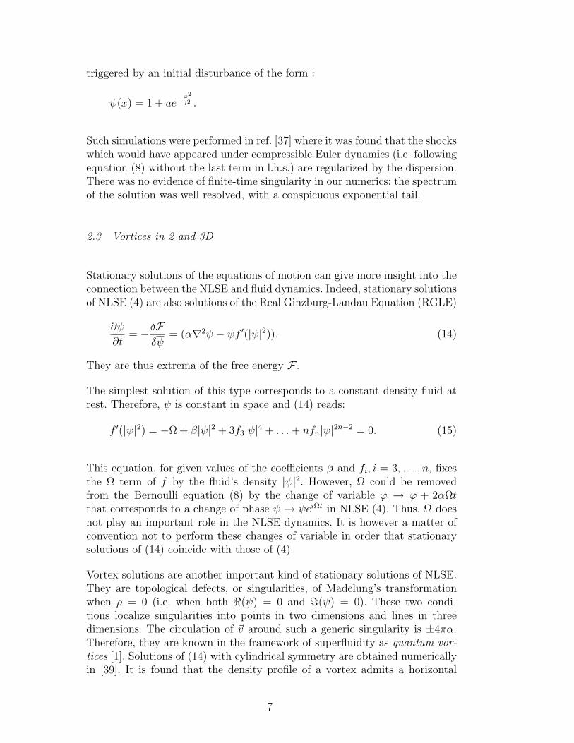
Fig. 1. Three-dimensional visualization of the vector field ∇ × (ρ~v) for the Tay-lor-Green flow at time t = 0 with coherence length ξ = 0.1/(8
√2), sound velocity
c = 2 and N = 512 in the impermeable box [0, π]× [0, π]× [0, π].
The second step of our procedure consists of integrating, to convergence, theAdvective Real Ginzburg-Landau Equation (ARGLE):
∂tψ = c/(√
2ξ)(ψ − |ψ|2ψ + ξ2∇2ψ)− ivTG · ∇ψ −(vTG)2/(2
√2cξ)ψ (23)
with initial data ψ = ψc.
Using the TG symmetries we expand ψ(x, y, z, t), solution of the ARGLE andNLSE equations, as [11]:
ψ(x, y, z, t) =N/2∑
m=0
N/2∑
n=0
N/2∑
p=0
ψ(m,n, p, t) cos mx cos ny cos pz (24)
where N is the resolution and ψ(m,n, p, t) = 0, unless m,n, p are either all evenor all odd integers. Furthermore ψ(m,n, p, t) satisfies the additional conditionsψ(m,n, p, t) = (−1)r+1ψ(n,m, p, t) where r = 1 when m,n, p are all even andr = 2 when m,n, p are all odd. Implementing this expansion in a pseudo–spectral code yields a saving of a factor 64 in computational time and memorysize when compared to general Fourier expansions.
The ARGLE converged periodic vortex array obtained in this manner is dis-played on Fig. 1. with coherence length ξ = 0.1/(8
√2), sound velocity c = 2
and resolution N = 512.
10
10 0
10 1
10 2
10 3
k
10-6
10-5
10-4
10-3
10-2
10-1
100
Eki
ni
(a)
(b)
kbump
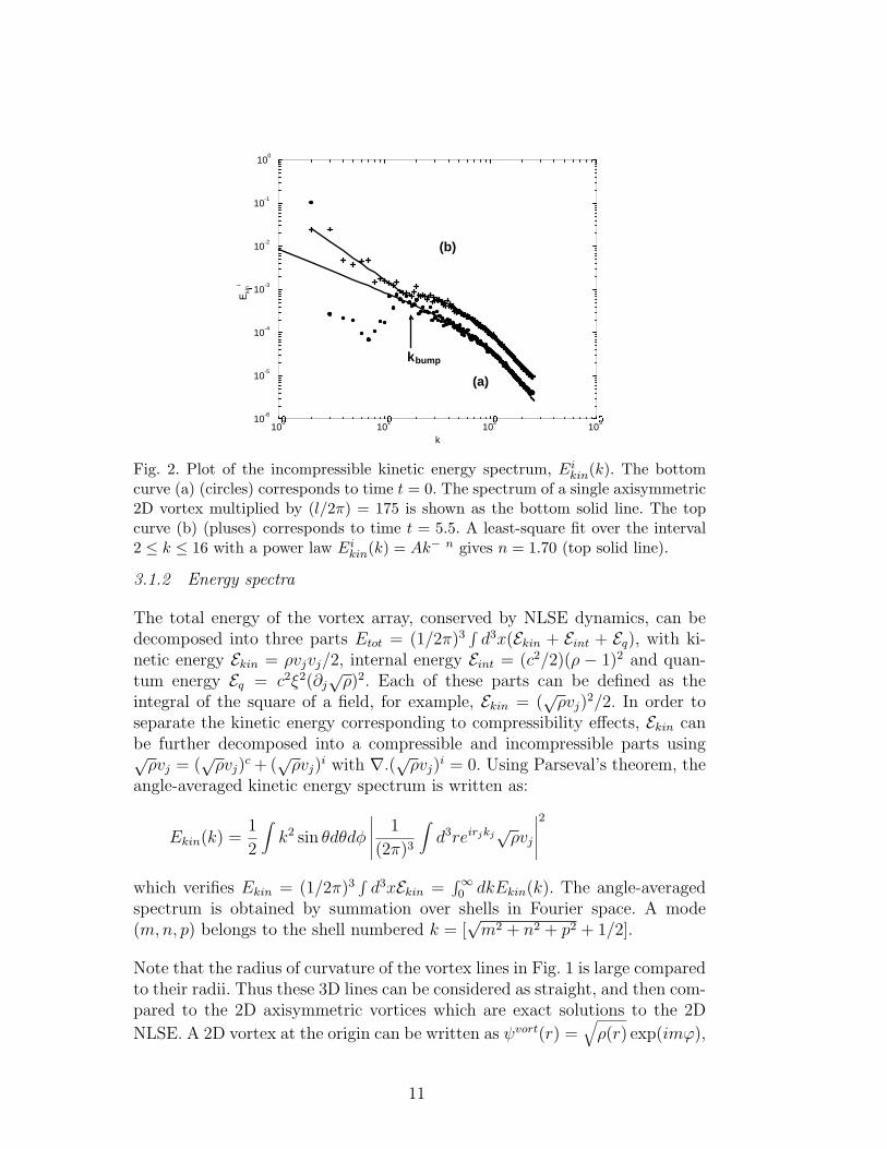
Fig. 2. Plot of the incompressible kinetic energy spectrum, Eikin(k). The bottom
curve (a) (circles) corresponds to time t = 0. The spectrum of a single axisymmetric2D vortex multiplied by (l/2π) = 175 is shown as the bottom solid line. The topcurve (b) (pluses) corresponds to time t = 5.5. A least-square fit over the interval2 ≤ k ≤ 16 with a power law Ei
kin(k) = Ak− n gives n = 1.70 (top solid line).
3.1.2 Energy spectra
The total energy of the vortex array, conserved by NLSE dynamics, can bedecomposed into three parts Etot = (1/2π)3
∫d3x(Ekin + Eint + Eq), with ki-
netic energy Ekin = ρvjvj/2, internal energy Eint = (c2/2)(ρ − 1)2 and quan-tum energy Eq = c2ξ2(∂j
√ρ)2. Each of these parts can be defined as the
integral of the square of a field, for example, Ekin = (√
ρvj)2/2. In order to
separate the kinetic energy corresponding to compressibility effects, Ekin canbe further decomposed into a compressible and incompressible parts using√
ρvj = (√
ρvj)c + (
√ρvj)
i with ∇.(√
ρvj)i = 0. Using Parseval’s theorem, the
angle-averaged kinetic energy spectrum is written as:
Ekin(k) =1
2
∫k2 sin θdθdφ
∣∣∣∣∣1
(2π)3
∫d3reirjkj
√ρvj
∣∣∣∣∣2
which verifies Ekin = (1/2π)3∫
d3xEkin =∫∞0 dkEkin(k). The angle-averaged
spectrum is obtained by summation over shells in Fourier space. A mode(m,n, p) belongs to the shell numbered k = [
√m2 + n2 + p2 + 1/2].
Note that the radius of curvature of the vortex lines in Fig. 1 is large comparedto their radii. Thus these 3D lines can be considered as straight, and then com-pared to the 2D axisymmetric vortices which are exact solutions to the 2D
NLSE. A 2D vortex at the origin can be written as ψvort(r) =√
ρ(r) exp(imϕ),
11

0
100
200
300
400
500
600
700
800
l/2π
0
2
4
6
8
10 12 14t
0.04
0.06
0.08
0.10
0.12
0.14
0.16
Eki
n i
Fig. 3. Total incompressible kinetic energy, Eikin, plotted versus time for
ξ = 0.1/(2√
2), N = 128 (long–dash line); ξ = 0.1/(4√
2), N = 256 (dash);ξ = 0.1/(6.25
√2), N = 400 (dot) and ξ = 0.1/(8
√2), N = 512 (solid line). All
runs are realized with c = 2. The evolution of the total vortex filament length di-vided by 2π (crosses) for the N = 512 run is also shown (scale given on the righty-axis).
Fig. 4. Same visualization as in Fig. 1 but at time t = 4.
12
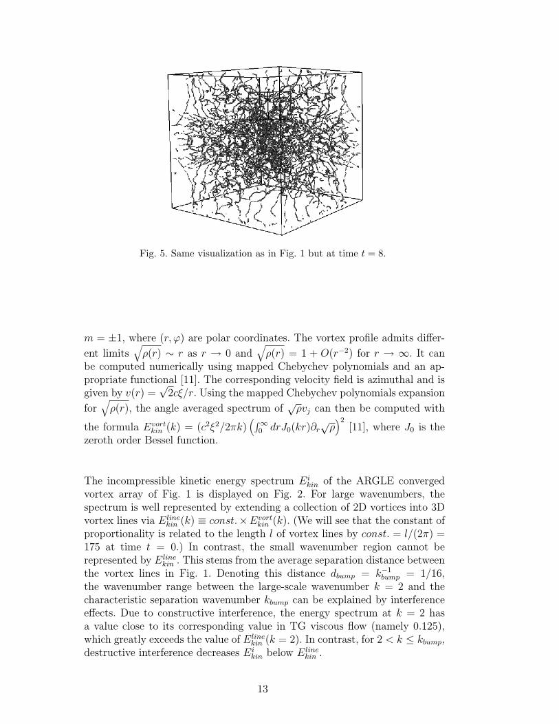
Fig. 5. Same visualization as in Fig. 1 but at time t = 8.
m = ±1, where (r, ϕ) are polar coordinates. The vortex profile admits differ-
ent limits√
ρ(r) ∼ r as r → 0 and√
ρ(r) = 1 + O(r−2) for r → ∞. It canbe computed numerically using mapped Chebychev polynomials and an ap-propriate functional [11]. The corresponding velocity field is azimuthal and isgiven by v(r) =
√2cξ/r. Using the mapped Chebychev polynomials expansion
for√
ρ(r), the angle averaged spectrum of√
ρvj can then be computed with
the formula Evortkin (k) = (c2ξ2/2πk)
(∫∞0 drJ0(kr)∂r
√ρ)2
[11], where J0 is thezeroth order Bessel function.
The incompressible kinetic energy spectrum Eikin of the ARGLE converged
vortex array of Fig. 1 is displayed on Fig. 2. For large wavenumbers, thespectrum is well represented by extending a collection of 2D vortices into 3Dvortex lines via Eline
kin (k) ≡ const.×Evortkin (k). (We will see that the constant of
proportionality is related to the length l of vortex lines by const. = l/(2π) =175 at time t = 0.) In contrast, the small wavenumber region cannot berepresented by Eline
kin . This stems from the average separation distance betweenthe vortex lines in Fig. 1. Denoting this distance dbump = k−1
bump = 1/16,the wavenumber range between the large-scale wavenumber k = 2 and thecharacteristic separation wavenumber kbump can be explained by interferenceeffects. Due to constructive interference, the energy spectrum at k = 2 hasa value close to its corresponding value in TG viscous flow (namely 0.125),which greatly exceeds the value of Eline
kin (k = 2). In contrast, for 2 < k ≤ kbump,destructive interference decreases Ei
kin below Elinekin .
13

3.2 Numerical results
The evolution in time via NLSE (16) of the incompressible kinetic energy isshown in Fig. 3. The main quantitative result is the excellent agreement ofthe energy dissipation rate, −dEi
kin/dt, with the corresponding data in theincompressible viscous TG flow (see reference [44], and reference [48], figure5.12). Both the moment tmax ∼ 5 − 10 of maximum energy dissipation (theinflection point of Fig. 3) and its value ε(tmax) ∼ 10−2 at that moment are inquantitative agreement. Furthermore, both tmax and ε(tmax) depend weaklyon ξ.
Another important quantity studied in viscous decaying turbulence is the scal-ing of the kinetic energy spectrum during time evolution and, especially, atthe moment of maximum energy dissipation, where a k−5/3 range can be ob-served (see reference [44]). Fig. 2 (b) shows the energy spectrum at t = 5.5. Aleast-square fit over the interval 2 ≤ k ≤ 16 with a power law Ei
kin(k) = Ak− n
gives n = 1.70 (solid line). For 5 < t < 8, a similar fit gives n = 1.6±0.2 (datanot shown). Note that recent numerical simulations [49] using incompressibleEulerian dynamics of vortex filaments also show evidence of a k−5/3 energyspectrum range.
The full Kolmogorov law is given by E(k) = Cε2/3k−5/3 with E(k) the energyspectrum (per unit mass), C the Kolmogorov constant and ε the energy dissi-pation rate (per unit mass). The viscous energy spectrum E(k) is comparable(see ref. [44]), in the inertial range, to the superfluid incompressible kinetic en-ergy Ei
kin(k). As stated above, the superfluid dissipation rate −dEikin/dt is also
comparable to the viscous dissipation rate ε. Therefore, the Kolmogorov con-stant C is of the same order of magnitude in both viscous and superfluid flows.Note that the viscous Taylor-Green vortex, because of the non-homogenouscharacter of the flow, has a Kolmogorov constant that is larger (by a factor' 1.5) [44] than that of homogeneous turbulence.
Fitting Eikin(k) in the interval 30 ≤ k ≤ 170 with l/(2π) × Evort
kin (k) leads tol/2π = 452, roughly three times the t = 0 length of the vortex lines. The timeevolution of l/2π obtained by this procedure is displayed in Fig. 3, showingthat the length continues to increase beyond tmax. The computations wereperformed with c = 2 corresponding to a root-mean-square Mach numberMrms ≡ |vTG
rms|/c = 0.25. As it is very costly to decrease Mrms, we checked [11]that compressible effects were non-dominant at this value of Mrms.
The vortex lines are visualized in physical space in Figs. 4 and 5 at timet = 4 and t = 8. At t = 4, no reconnection has yet taken place while acomplex vortex tangle is present at t = 8. Detailed visualizations (data notshown) demonstrate that reconnections occur for t > 5. Note that the viscous
14

TG vortex also undergoes a qualitative (and quantitative) change in vortexdynamics around t ∼ 5.
3.3 Experimental results
The TG flow is related to an experimentally studied swirling flow [50–52]. Therelation between the experimental flow and the TG vortex is a similarity inoverall geometry [50]: a shear layer between two counter–rotating eddies. TheTG vortex, however, is periodic with free-slip boundaries while the experi-mental flow is contained inside a tank between two counter–rotating disks.
The spectral behavior of NLSE can be compared to standard (viscous) turbu-lence only for k ≤ kbump. It is thus of interest to estimate the scaling of kbump
in terms of the characteristic parameters of the large scale flow and of thefluid. As seen above, kbump ∼ d−1
bump, where dbump is the average distance be-tween neighboring vortices. Consider a flow with characteristic integral scalel0 and large scale velocity u0 (in the case of the TG flow, l0 ∼ 1 and u0 ∼ 1).The fluid characteristics are the velocity of sound c and the coherence lengthξ (with corresponding wavenumber kξ ∼ ξ−1). The number nd of vortex linescrossing a typical large–scale l20 area is given by the ratio of the large–scale flowcirculation l0u0 to the quantum of circulation Γ = 4πcξ/
√2, i.e nd ∼ l0u0/cξ.
On the other hand, the assumption that the vortices are uniformly spreadover the large scale area gives nd ∼ l20/d
2bump. Equating these two evaluations
of nd yields the relation dbump ∼ l0√
(cξ)/(l0u0). Note that this argument as-sumes that the large-scale vorticity is coherent. It therefore yields a maximumpossible value of dbump, and thus a minimum for kbump.
In the case of helium, the viscosity at the critical point ( T = 5.174K, P =2.2 105 Pa) is νcp = 0.27 × 10⁻⁷m2s−1 while the quantum of circulation,Γ = h/mHe has the value 0.99× 10⁻⁷m2s−1. Thus, νcp ∼ 0.25Γ. The order of
magnitude for dbump is thus dbump ' l0/√
Rcp ∼ lλ where Rcp is the integralscale Reynolds number at the critical point and lλ the Taylor micro-scale. Inother words, the value of dbump in a superfluid helium experiment at T = 1Kis of the same order as the Taylor micro-scale in the same experimental set-uprun with viscous helium at the critical point.
The experimental set-up is similar to that described in [51]. To work withT ∼ 1.2K some modifications are, however, necessary. A cylinder, 8 cm indiameter and 12 cm high, limited axially by two counter-rotating disks limitsthe flow. One disk is flat and 8 radial blades, forming an angle of 45o betweeneach other, are fixed on the other one. To stabilize the turbulent shear region astator is mounted halfway the height of the container. The two disks are drivenby two DC motors rotating from 1 to 30 Hz. The whole system is enclosed
15

in a liquid Helium bath used as the experimental fluid and this is the maindifference with the set-up described in [51]. The pressure above the liquid bathis adjusted by a pumping system and this fixes the temperature of the fluid.
Local pressure fluctuations are measured by using small total-head pressuretubes, immersed in the flow. The pressure sensors are hollow metallic tubes,connected to a quartz pressure transducer WHM 112 A22 from PCB. Detailsare given in [13].
In normal fluids, the pressure measured at the tip of the total-head tube can berelated to the upstream flow U(t) and the local pressure P (t) using Bernoullitheorem:
Pmeas(t) = P (t) + ρU2(t)/2 (25)
In the flow region where the probe is immersed, a well established axial meanflow U exists so that, after removing the mean parts of equation (25), onegets:
pmeas(t) = p(t) + ρUu(t) (26)
where pmeas, p and u are the fluctuations of the measured pressure, the actualpressure, and the local velocity respectively. It is currently admitted that, inordinary turbulent situations, and at low fluctuation rates, equation (26) isdominated by the dynamic term, so that, by measuring the pressure fluctua-tions at the total head tube, one has a direct access to the velocity fluctuationsu(t).
The situation is less clear when the probe is immersed in the superfluid. It is,however, possible to write an equation similar to (26). Details can be foundin [13].
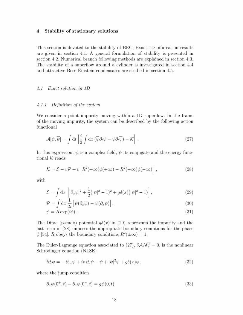
The analysis of the pressure fluctuations obtained with the total head tubeplaced at 2 cm above the mid plane and 2 cm from the cylinder axis, yieldsinteresting conclusions. Figures 6 and 7 show the spectra of the pressure fluc-tuations above and below Tλ (i.e respectively at 2.3K and 1.4K). Fig. 6 clearlyshows, as expected, that such fluctuations follow a Kolmogorov regime betweenthe injection scale (signaled by the peak at 25 Hz) and the largest resolvedfrequency, i.e 900 Hz. The spectrum obtained at 1.4K is similar to that ob-tained at T = 2.3K (see Fig. 7). A clear Kolmogorov like regime exists for thesame range of frequencies. The corresponding Kolmogorov constant turns outalso to be indistinguishable from the classical value. We have further analyzedthe deviations from Kolmogorov in the superfluid regime. The striking resultis that they have the same magnitude as in classical turbulence. More detailsare given in [53].
16
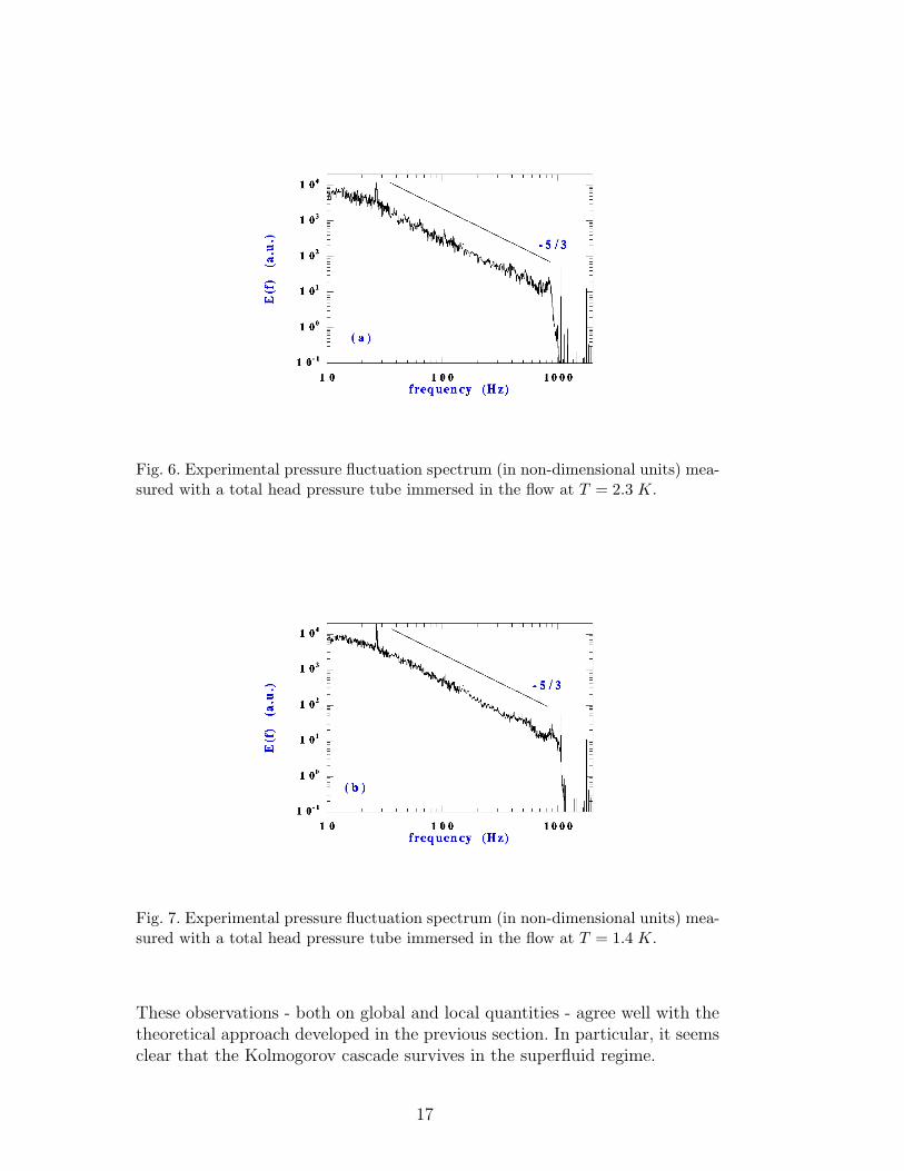
Fig. 6. Experimental pressure fluctuation spectrum (in non-dimensional units) mea-sured with a total head pressure tube immersed in the flow at T = 2.3 K.
Fig. 7. Experimental pressure fluctuation spectrum (in non-dimensional units) mea-sured with a total head pressure tube immersed in the flow at T = 1.4 K.
These observations - both on global and local quantities - agree well with thetheoretical approach developed in the previous section. In particular, it seemsclear that the Kolmogorov cascade survives in the superfluid regime.
17
4 Stability of stationary solutions
This section is devoted to the stability of BEC. Exact 1D bifurcation resultsare given in section 4.1. A general formulation of stability is presented insection 4.2. Numerical branch following methods are explained in section 4.3.The stability of a superflow around a cylinder is investigated in section 4.4and attractive Bose-Einstein condensates are studied in section 4.5.
4.1 Exact solution in 1D
4.1.1 Definition of the system
We consider a point impurity moving within a 1D superflow. In the frameof the moving impurity, the system can be described by the following actionfunctional
A[ψ, ψ] =∫
dt[i
2
∫dx (ψ∂tψ − ψ∂tψ)−K
]. (27)
In this expression, ψ is a complex field, ψ its conjugate and the energy func-tional K reads
K = E − vP + v[R2(+∞)φ(+∞)−R2(−∞)φ(−∞)
], (28)
with
E =∫
dx[|∂xψ|2 +
1
2(|ψ|2 − 1)2 + gδ(x)(|ψ|2 − 1)
], (29)
P =∫
dx1
2i
[ψ(∂xψ)− ψ(∂xψ)
], (30)
ψ = R exp(iφ) . (31)
The Dirac (pseudo) potential gδ(x) in (29) represents the impurity and thelast term in (28) imposes the appropriate boundary conditions for the phaseφ [54]. R obeys the boundary conditions R2(±∞) = 1.
The Euler-Lagrange equation associated to (27), δA/δψ = 0, is the nonlinearSchrodinger equation (NLSE)
i∂tψ = − ∂xxψ + iv ∂xψ − ψ + |ψ|2ψ + gδ(x)ψ , (32)
where the jump condition
∂xψ(0+, t)− ∂xψ(0−, t) = gψ(0, t) (33)
18
is imposed in order to balance the gδ(x)ψ singularity with the −∂xxψ termfor all times t.
4.1.2 Stationary solutions
Time-independent solutions of the NLSE (32) are best studied by performingthe change of variables defined above in (31): ψ = R exp(iφ). Using thesevariables, the NLSE reads
∂tR = v∂xR−R∂xxφ− 2∂xR∂xφ , (34)
∂tφ = v∂xφ− (∂xφ)2 + 1−R2 − gδ(x) +∂xxR
R, (35)
and the jump condition (33) reads
∂xR(0+, t)− ∂xR(0−, t) = gR(0, t) , (36)
∂xφ(0+, t)− ∂xφ(0−, t) = 0 . (37)
Note that equations (34) and (35) can be respectively interpreted as the con-tinuity and Bernoulli equations for a fluid of density ρ = R2(x) and velocityu = 2∂xφ (as done in section 2).
Explicit time-independent solutions of equations (34) and (35) were found byHakim[54], using what are called gray solitons in the nonlinear optics termi-nology. Gray solitons [55,56] are stationary solutions of equations (34) and(35), without the potential term gδ(x). They are localized density depletionof the form
R2GS(x) = v2/2 + (1− v2/2) tanh2[
√1/2− v2/4 x] , (38)
φGS(x) = arctan
(v√
2− v2
exp[√
2− v2 x] + v2 − 1
). (39)
Patching together pieces of gray solitons, Hakim found the following ξ-indexedstationary solutions of equations (34) and (35), including the potential termgδ(x)
Rξ(x) = RGS(x± ξ) , x ≷ 0 (40)
φξ(x) = φGS(x± ξ)− φGS(±ξ) , x ≷ 0 (41)
where the jump conditions (36) and (37) impose the relation
g(ξ) =√
2(1− v2/2)3/2tanh[
√1/2− v2/4 ξ]
v2/2 + sinh2[√
1/2− v2/4 ξ]. (42)
19
The function g(ξ) reaches a maximum [57] gc = g(ξc) at ξc =argcosh
(1+√
1+4v2
2
)√
2−v2
with
gc = 4(1− v2/2)[√
1 + 4v2 − (1 + v2)]1/2
2v2 − 1 +√
1 + 4v2. (43)
1
0.8
0.6
0.4
0.2
-15 -10 -5 0 5 10 15
-0.5
0
0.5
0 0.5 1 1.5
-0.8
-0.6
-0.4
-0.2
0
0.2
0.4
0.6
0.8
-15 -10 -5 0 5 10 15
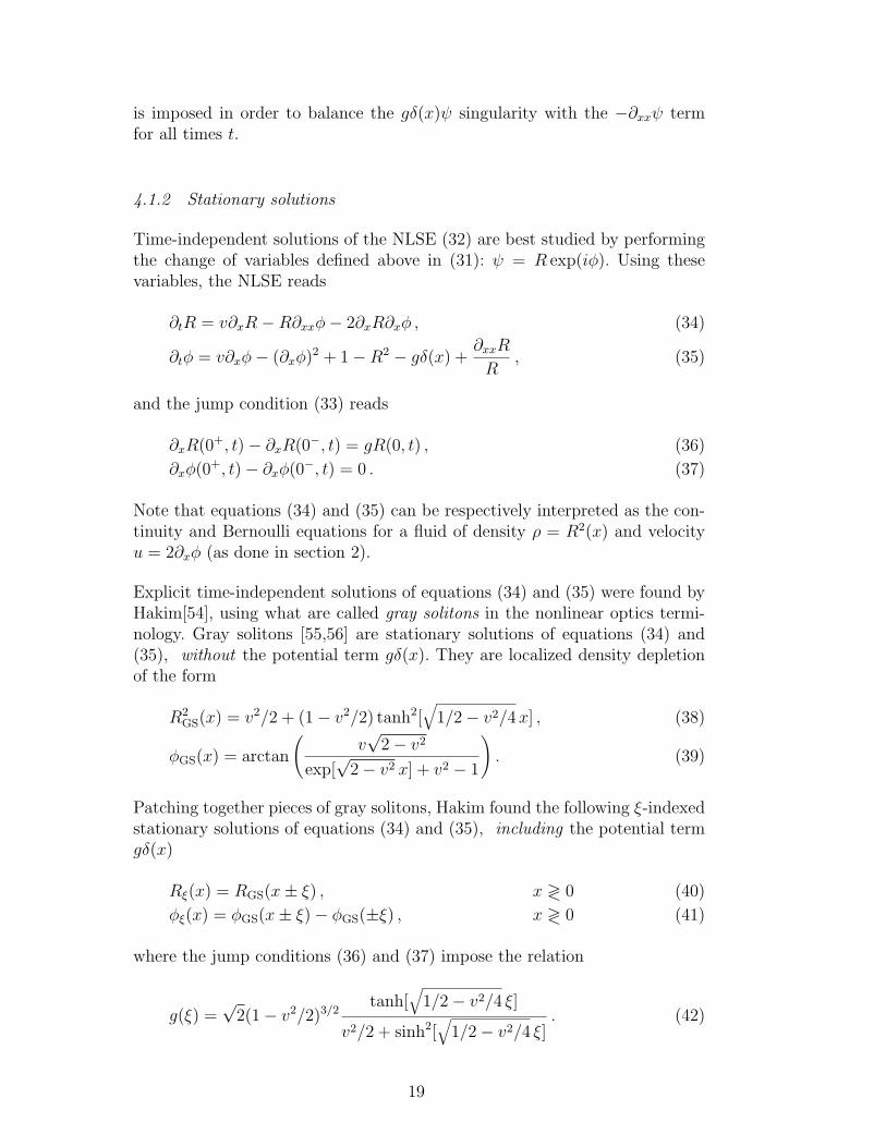
Fig. 8. (a) Modulus R of the stable (—) and unstable (- - -) stationary solutionsof equation (32) (see equation (40)) for g = 1.250 and v = 0.5; insert, energyfunctionalK of the stationary solutions versus g for v = 0.5 (see equation (28)); lowerbranch: energetically stable branch, upper branch: energetically unstable branch.The bifurcation occurs at g = 1.5514 (b) Phase φ of the stable (—) and unstable(- - -) stationary solutions (see equation (41)), same conditions as in (a).
The two stationary solutions of (32) corresponding to ξ+(g) > ξc and ξ−(g) <ξc obtained by inverting (42) for g < gc thus disappear, merging in a saddle-node bifurcation at a critical strength gc. Note that the bifurcation can also beobtained by varying v and keeping g constant. In the following, the strengthg of the delta function is used as the control parameter of our system, keepingv constant.
Fig. 8a shows the energetically unstable and stable solutions (K(ξ−(g)) >K(ξ+(g))) . The bifurcation diagram corresponding to the energy K (see equa-tion (28)) is also displayed on the figure as an insert. In fig. 8b, note that thephase φξ(x), as defined in equation (41), differs from that considered in [54]by an (x-independent) constant. The phase in [54] is set to 0 at x = +∞,whereas (41) is antisymmetric in x. This difference is unimportant becauseequations (34) and (35) are invariant under the constant phase shift
φ(x) 7→ φ(x) + ϕ . (44)
20
4.2 General formulation
In this section we define and test the numerical tools needed to obtain thestationary solutions of the NLSE.
Consider the following action functional associated with the NLSE
A =∫
dt
∫dx
i
2
(ψ
∂ψ
∂t− ψ
∂ψ
∂t
)−F
, (45)
where ψ is a complex field, ψ its conjugate and F is the energy of the system.Here, x and t correspond to nondimensionalized space and time variablesrespectively.
The Euler-Lagrange equation corresponding to (45) leads to the NLSE interms of the functional F
∂ψ
∂t= −i
δFδψ
. (46)
This equation obviously has stationary solution ψS if δF/δψ|ψ=ψS= 0. Thus,
stationary solutions of (46) are extrema of F . In general, we are looking for anextremum of an energy functional E under some constraint Q[ψ] = cst. Theusual Lagrange multiplier trick consists in introducing a control parameter νand, rather than solving for extrema of E [ψ], searching for extrema of the newfunctional F [ψ] = E [ψ]− νQ[ψ]. We thus solve for
δFδψ
∣∣∣∣∣ν=cst.
= 0. (47)
We now turn to the precise definitions, corresponding to the two systemsconsidered in this section : superflows and Bose-Einstein condensates.
4.2.1 Superflows
In the problem of a superflow past an obstacle, E is the hydrodynamic energyand ν ≡ ~U is the flow velocity with respect to the obstacle [14,16]. This implies
that Q ≡ ~P is the flow momentum. Functionals F , E and ~P are given by theexpressions
F = E − ~P · ~U (48)
E = c2∫
d3x([−1 + V (~x)]|ψ|2 +
1
2|ψ|4 + ξ2|∇ψ|2
)(49)
~P =√
2cξ∫
d3xi
2
(ψ∇ψ − ψ∇ψ
). (50)
21
Here, c and ξ are the physical parameters characterizing the superfluid. Theycorrespond to the speed of sound (c) for a fluid with mean density ρ0 = 1,and to the coherence length (ξ). The potential V (~x) = (Vo/2)(tanh[4(r −D/2)/∆] − 1) is used to represent a cylindrical obstacle of diameter D. Thecomputations are performed with Vo = 10 and ∆ = ξ for which the density|ψ| ∼ 0 in the disk. The NLSE reads
∂ψ
∂t= − i√
2cξ
δFδψ
= ic√2ξ
([1− V (~x)]ψ − |ψ|2ψ + ξ2∇2ψ
)+ ~U · ∇ψ. (51)
We will be interested in the solutions of δF/δψ = 0, for a given value of~U . According to equation (47), these solutions are extrema of E at constant
momentum ~P .
4.2.2 Bose-Einstein condensates
We consider a condensate of N particles of mass m and effective scatteringlength a in a radial confining harmonic potential V (r) = mω2r2/2 [17]. Quan-tities are rescaled by the natural quantum harmonic oscillator units of time
τ0 = 1/ω and length L0 =√~/mω, thus obtaining the nondimensionalized
variables t = t/τ0, x = x/L0 and a = 4πa/L0. The control parameter ν be-comes in this context the chemical potential µ. The total number of particlesin the condensate is therefore given by Q ≡ N . Functionals F , E and N aregiven, in terms of rescaled variables, by
F = E − µN (52)
E =∫
d3x(
1
2|∇xψ|2 + V (x)|ψ|2 +
a
2|ψ|4
)(53)
N =∫
d3x|ψ|2. (54)
Two different situations are possible, depending on the sign of the (rescaled)effective scattering length a. When a is positive the particles interact repul-sively. A negative a corresponds to an attractive interaction. The dynamicalequation is
∂ψ
∂t= −i
δFδψ
= i[1
2∇2
xψ −1
2|x|2ψ −
(a|ψ|2 − µ
)ψ
]. (55)
We will be interested in the solutions of δF/δψ = 0, for a given value ofµ. According to equation (47), these solutions are extrema of E at constantparticle number N .
22
4.3 Branch following methods
When the extremum of F is a local minimum, the stationary solution ψS
of (51) can be reached by a relaxation method. If the extremum is not aminimum, Newton’s iterative method is used to solve for ψS.
4.3.1 Relaxation method
In what remains of this section, we will write the NLSE under the followinggeneric form, which is valid for both the Bose-Einstein condensates and thesuperflow past an obstacle:
∂ψ
∂t= −i
δFδψ
= i(α∇2ψ + [Ω− V (~x)] ψ − β|ψ|2ψ
)+ ~U · ∇ψ. (56)
When the extremum of F is a local minimum, the stationary solution ψS of(56) can be reached by integrating to relaxation the associated real Ginzburg-Landau equation (RGLE)
∂ψ
∂t= −δF
δψ= α∇2ψ + [Ω− V (~x)] ψ − β|ψ|2ψ − i~U · ∇ψ. (57)
Indeed, (56) and (57) have the same stationary solutions.
In our numerical computations, equation (57) is integrated to convergence byusing the Forward-Euler/Backwards-Euler time stepping scheme
ψ(t + σ) = Θ−1[(
1− i σ ~U · ∇)
+ σ([Ω− V (~x)]− β|ψ(t)|2
)]ψ(t) (58)
with
Θ =[1− σ α∇2
]. (59)
The advantage of this method is that it converges to the stationary solutionof (56) independently of the time step σ.
4.3.2 Newton’s method
We use Newton’s method [58] to find unstable stationary solutions of theRGLE.
In order to work with a well-conditioned system [59], we search for the fixedpoints of (58). These can be found as the roots of
f(ψ) = Θ−1[(
1− i σ ~U · ∇)
+ σ([Ω− V (~x)]− β|ψ(t)|2
)]ψ(t)−ψ(t), (60)
23
0
5
10Iteration
10−30
10−20
10−10
100
Err
or
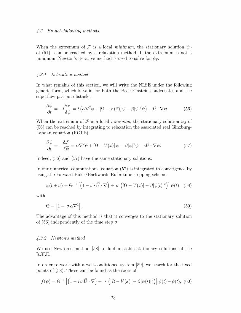
Fig. 9. Two typical examples of the Newton method convergence towards the solu-tion of equation (60) for the problem of a superflow past a cylinder with ξ/D = 1/10and a field ψ(j) discretized into n = 128 × 64 = 8190 collocation points. The errormeasure is given by
∑nj=1 f2
(j)(ψ)/n. The convergence is faster than exponential, asexpected for a Newton method.
0
20 40 60BCGM Iteration
10−5
10−3
10−1
101
103
|Ax−
b|/|b
|
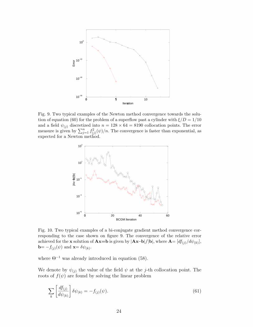
Fig. 10. Two typical examples of a bi-conjugate gradient method convergence cor-responding to the case shown on figure 9. The convergence of the relative errorachieved for the x solution of Ax=b is given by |Ax–b|/|b|, where A= [df(j)/dψ(k)],b= −f(j)(ψ) and x= δψ(k).
where Θ−1 was already introduced in equation (58).
We denote by ψ(j) the value of the field ψ at the j-th collocation point. Theroots of f(ψ) are found by solving the linear problem
∑
k
[df(j)
dψ(k)
]δψ(k) = −f(j)(ψ). (61)
24
for δψ and then incrementing ψ by
ψ(j) = ψ(j) + δψ(j) (62)
and iterating the Newton process (61)-(62) to convergence.
The solution to (61) is obtained by an iterative bi-conjugate gradient methodeither BCGM [60] or BiCGSTAB [61]. These methods require only the abilityto act repeatedly with [df(j)/dψ(k)] on an arbitrary field ϕ to obtain an approx-imative solution of (61). Note that since the convergence of the time step (58)does not depend on σ, the roots found through this Newton iteration are alsoindependent of σ. Therefore, σ becomes a free parameter that can be used toadjust the pre-conditioning of the system in order to optimize the convergenceof the BCGM [59].
4.3.3 Implementation
We use standard Fourier pseudo spectral methods [38]. Typical convergencesof the Newton and bi-conjugate gradient iterations are shown in figures 9 and10.
In the case of the radially symmetric Bose condensate, ψ(r, t) is expanded
as ψ(r, t) =∑NR/2
n=0 ψ2n(t)T2n(r/R), where Tn is the n-th order Chebychevpolynomial and ψNR
is fixed to satisfy the boundary condition ψ(R, t) = 0.
The NLSE is integrated in time by a fractional step (operator-splitting) method[62].
4.4 Stability of a superflow around a cylinder
In this section, following references [14–16], we investigate the stationary sta-ble and unstable (nucleation) solutions of the NLSE describing the superflowaround a cylinder, using the numerical methods developed in section 4.3. Westudy a disc of diameter D, moving at speed ~U in a two-dimensional (2D)superfluid at rest. The NLSE (51) can be mapped into two hydrodynamicalequations by applying Madelung’s transformation [1,35]:
ψ =√
ρ exp
(iφ√2cξ
). (63)
The real and imaginary parts of the NLSE produce for a fluid of density ρ andvelocity
~v = ∇φ− ~U, (64)
25
the following equations of motion
∂ρ
∂t+∇ (ρ~v) = 0 (65)
[∂φ
∂t− ~U · ∇φ
]+
1
2(∇φ)2 + c2[ρ− (1− V (~x))]− c2ξ2∇2√ρ√
ρ= 0. (66)
In the coordinate system ~x that follows the obstacle, these equations corre-spond to the continuity equation and to the Bernoulli equation [4] (with asupplementary quantum pressure term c2ξ2∇2√ρ/
√ρ) for an isentropic, com-
pressible and irrotational flow. Note that, in the limit where ξ/D → 0, thequantum pressure term vanishes and we recover the system of equations de-scribing an Eulerian flow.
4.4.1 Bifurcation diagram and scaling in 2D
In this section, varying the ratio of the coherence length ξ to the cylinderdiameter D, we obtain scaling laws in the ξ/D → 0 limit.
Bifurcation diagram
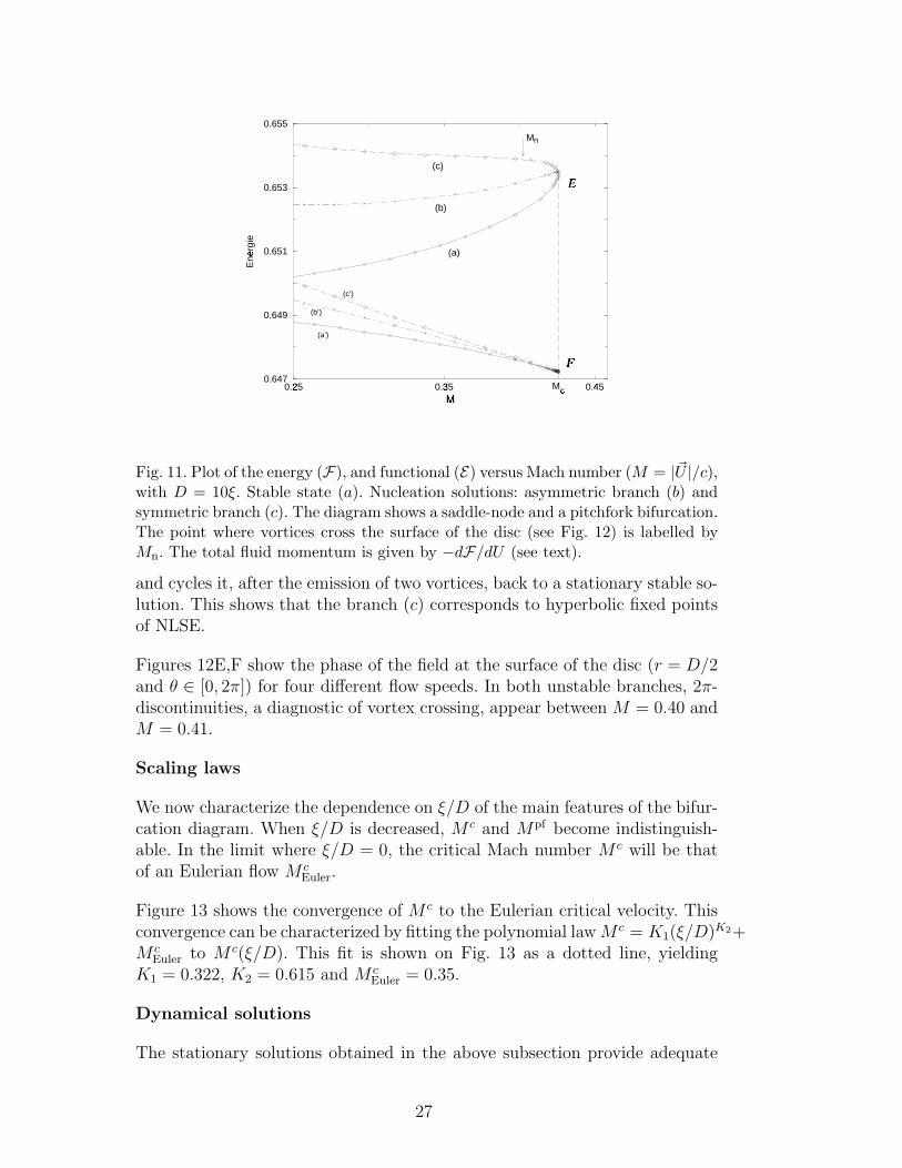
We present results for ξ/D = 1/10 which are representative of all ratios wecomputed. The functional E and energy F of the stationary solutions areshown in Fig. 11 as a function of the Mach number (M = |~U |/c). The stablebranch (a) disappears with the unstable solution (c) at a saddle-node bifur-cation when M = M c ≈ 0.4286. The energy F has a cusp at the bifurcationpoint, which is the generic behavior for a Hamiltonian saddle-node bifurcation,as described in section 4.5.1. There are no stationary solutions beyond thispoint. When Mpf ≈ 0.4282, the unstable symmetric branch (c) bifurcates at apitchfork to a pair of asymmetric branches (b). Their nucleation energy barrieris given by (Fb′ − Fa′) which is roughly half of the barrier for the symmetricbranch (Fc′ −Fa′).
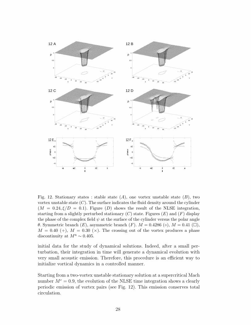
We can relate branches in Fig. 11 to the presence of vortices in the solution.When Mn ≤ M ≤ M c, solutions are irrotational (Mn ∼ 0.405 as indicated inFig. 11). For M ≤ Mn the stable branch (a) remains irrotational (Fig. 12A)while the unstable branch (b) corresponds to a one vortex solution (Fig. 12B)and the unstable branch (c), to a two vortex solution (Fig. 12C). The dis-tance between the vortices and the obstacle in branches (b) and (c) increaseswhen M is decreased. Branch (c) is precisely the situation described in [63].
Furthermore, the value M c ≈ 0.4286 is close to the predicted value√
2/11.Figure 12D shows the result of integrating the NLSE forward in time with,as initial condition, a slightly perturbed unstable symmetric stationary state(Fig. 12C). The perturbation drives the system over the nucleation barrier
26
0.25
0.35 0.45M
0.647
0.649
0.651
0.653
0.655
Ene
rgie
(a)
(b)
(c)
(a’)
(b’)
(c’)
E
Mn
Mc
F
Fig. 11. Plot of the energy (F), and functional (E) versus Mach number (M = |~U |/c),with D = 10ξ. Stable state (a). Nucleation solutions: asymmetric branch (b) andsymmetric branch (c). The diagram shows a saddle-node and a pitchfork bifurcation.The point where vortices cross the surface of the disc (see Fig. 12) is labelled byMn. The total fluid momentum is given by −dF/dU (see text).
and cycles it, after the emission of two vortices, back to a stationary stable so-lution. This shows that the branch (c) corresponds to hyperbolic fixed pointsof NLSE.
Figures 12E,F show the phase of the field at the surface of the disc (r = D/2and θ ∈ [0, 2π]) for four different flow speeds. In both unstable branches, 2π-discontinuities, a diagnostic of vortex crossing, appear between M = 0.40 andM = 0.41.
Scaling laws
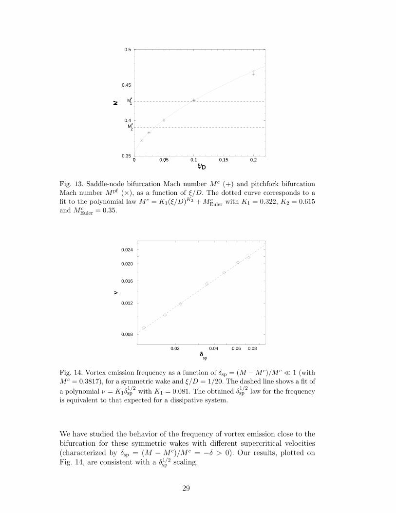
We now characterize the dependence on ξ/D of the main features of the bifur-cation diagram. When ξ/D is decreased, M c and Mpf become indistinguish-able. In the limit where ξ/D = 0, the critical Mach number M c will be thatof an Eulerian flow M c
Euler.
Figure 13 shows the convergence of M c to the Eulerian critical velocity. Thisconvergence can be characterized by fitting the polynomial law M c = K1(ξ/D)K2+M c
Euler to M c(ξ/D). This fit is shown on Fig. 13 as a dotted line, yieldingK1 = 0.322, K2 = 0.615 and M c
Euler = 0.35.
Dynamical solutions
The stationary solutions obtained in the above subsection provide adequate
27
U
-30-20
-100
1020
30-15
-10-5
05
1015
0
0.5
1
X
Y
12 A
ρ
U
-30-20
-100
1020
30-15
-10-5
05
1015
0
0.5
1
X
Y
12 B
ρ
U
-30-20
-100
1020
30-15
-10-5
05
1015
0
0.5
1
X
Y
12 C
ρ
U
-30-20
-100
1020
30-15
-10-5
05
1015
0
0.5
1
X
Y
12 D
ρ
12 E
0
π/2 π−π/2−π
θ
0
π/2
π
−π/2
−π
ph
ase
12 F
0
π/2 π−π/2−π
θ
0
π/2
π
−π/2
−π
ph
ase
Fig. 12. Stationary states : stable state (A), one vortex unstable state (B), twovortex unstable state (C). The surface indicates the fluid density around the cylinder(M = 0.24, ξ/D = 0.1). Figure (D) shows the result of the NLSE integration,starting from a slightly perturbed stationary (C) state. Figures (E) and (F ) displaythe phase of the complex field ψ at the surface of the cylinder versus the polar angleθ. Symmetric branch (E), asymmetric branch (F ). M = 0.4286 (), M = 0.41 (¤),M = 0.40 (+), M = 0.30 (×). The crossing out of the vortex produces a phasediscontinuity at Mn ∼ 0.405.
initial data for the study of dynamical solutions. Indeed, after a small per-turbation, their integration in time will generate a dynamical evolution withvery small acoustic emission. Therefore, this procedure is an efficient way toinitialize vortical dynamics in a controlled manner.
Starting from a two-vortex unstable stationary solution at a supercritical Machnumber M c = 0.9, the evolution of the NLSE time integration shows a clearlyperiodic emission of vortex pairs (see Fig. 12). This emission conserves totalcirculation.
28
0
0.05
0.1 0.15 0.2ξ/
0.35
0.4
0.45
0.5
M
D
M
M
*
*
1
2
Fig. 13. Saddle-node bifurcation Mach number M c (+) and pitchfork bifurcationMach number Mpf (×), as a function of ξ/D. The dotted curve corresponds to afit to the polynomial law M c = K1(ξ/D)K2 + M c
Euler with K1 = 0.322, K2 = 0.615and M c
Euler = 0.35.
0.02 0.04 0.06 0.08 δ
0.008
0.012
0.016
0.020
0.024
ν
sp
Fig. 14. Vortex emission frequency as a function of δsp = (M −M c)/M c ¿ 1 (withM c = 0.3817), for a symmetric wake and ξ/D = 1/20. The dashed line shows a fit ofa polynomial ν = K1δ
1/2sp with K1 = 0.081. The obtained δ
1/2sp law for the frequency
is equivalent to that expected for a dissipative system.
We have studied the behavior of the frequency of vortex emission close to thebifurcation for these symmetric wakes with different supercritical velocities(characterized by δsp = (M − M c)/M c = −δ > 0). Our results, plotted onFig. 14, are consistent with a δ1/2
sp scaling.
29
U
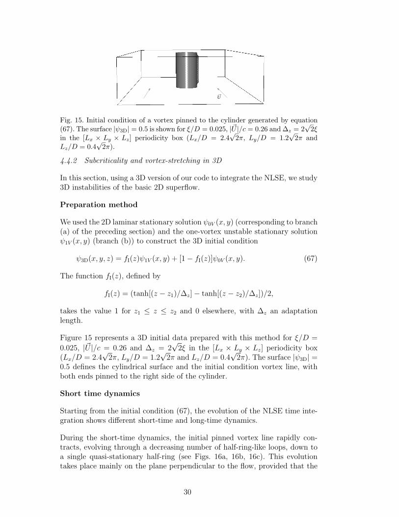
Fig. 15. Initial condition of a vortex pinned to the cylinder generated by equation(67). The surface |ψ3D| = 0.5 is shown for ξ/D = 0.025, |~U |/c = 0.26 and ∆z = 2
√2ξ
in the [Lx × Ly × Lz] periodicity box (Lx/D = 2.4√
2π, Ly/D = 1.2√
2π andLz/D = 0.4
√2π).
4.4.2 Subcriticality and vortex-stretching in 3D
In this section, using a 3D version of our code to integrate the NLSE, we study3D instabilities of the basic 2D superflow.
Preparation method
We used the 2D laminar stationary solution ψ0V (x, y) (corresponding to branch(a) of the preceding section) and the one-vortex unstable stationary solutionψ1V (x, y) (branch (b)) to construct the 3D initial condition
ψ3D(x, y, z) = fI(z)ψ1V (x, y) + [1− fI(z)]ψ0V (x, y). (67)
The function fI(z), defined by
fI(z) = (tanh[(z − z1)/∆z]− tanh[(z − z2)/∆z])/2,
takes the value 1 for z1 ≤ z ≤ z2 and 0 elsewhere, with ∆z an adaptationlength.
Figure 15 represents a 3D initial data prepared with this method for ξ/D =
0.025, |~U |/c = 0.26 and ∆z = 2√
2ξ in the [Lx × Ly × Lz] periodicity box(Lx/D = 2.4
√2π, Ly/D = 1.2
√2π and Lz/D = 0.4
√2π). The surface |ψ3D| =
0.5 defines the cylindrical surface and the initial condition vortex line, withboth ends pinned to the right side of the cylinder.
Short time dynamics
Starting from the initial condition (67), the evolution of the NLSE time inte-gration shows different short-time and long-time dynamics.
During the short-time dynamics, the initial pinned vortex line rapidly con-tracts, evolving through a decreasing number of half-ring-like loops, down toa single quasi-stationary half-ring (see Figs. 16a, 16b, 16c). This evolutiontakes place mainly on the plane perpendicular to the flow, provided that the
30
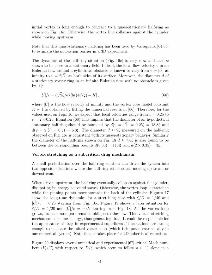
initial vortex is long enough to contract to a quasi-stationary half-ring asshown on Fig. 16c. Otherwise, the vortex line collapses against the cylinderwhile moving upstream.
Note that this quasi-stationary half-ring has been used by Varoquaux [64,65]to estimate the nucleation barrier in a 3D experiment.
The dynamics of the half-ring situation (Fig. 16c) is very slow and can beshown to be close to a stationary field. Indeed, the local flow velocity v in anEulerian flow around a cylindrical obstacle is known to vary from v = |~U | at
infinity to v = 2|~U | at both sides of its surface. Moreover, the diameter d ofa stationary vortex ring in an infinite Eulerian flow with no obstacle is givenby [1]:
|~U |/c = (√
2ξ/d) [ln (4d/ξ)−K] , (68)
where |~U | is the flow velocity at infinity and the vortex core model constantK ∼ 1 is obtained by fitting the numerical results in [66]. Therefore, for thevalues used on Figs. 16, we expect that local velocities range from v = 0.25 tov = 2× 0.25. Equation (68) thus implies that the diameter of an hypothetical
stationary half-ring should be bounded by d(v = |~U | = 0.25) = 18.8ξ and
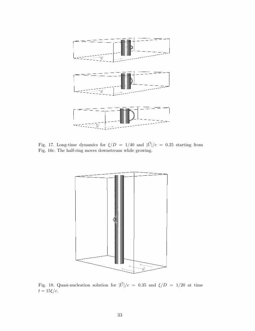
d(v = 2|~U | = 0.5) = 6.3ξ. The diameter d ≈ 9ξ measured on the half-ringobserved on Fig. 16c is consistent with its quasi-stationary behavior. Similarlythe diameter of the half-ring shown on Fig. 18 d ≈ 7.6ξ is also found to bebetween the corresponding bounds d(0.35) = 11.4ξ and d(2× 0.35) = 3ξ.
Vortex stretching as a subcritical drag mechanism
A small perturbation over the half-ring solution can drive the system intotwo opposite situations where the half-ring either starts moving upstream ordownstream.
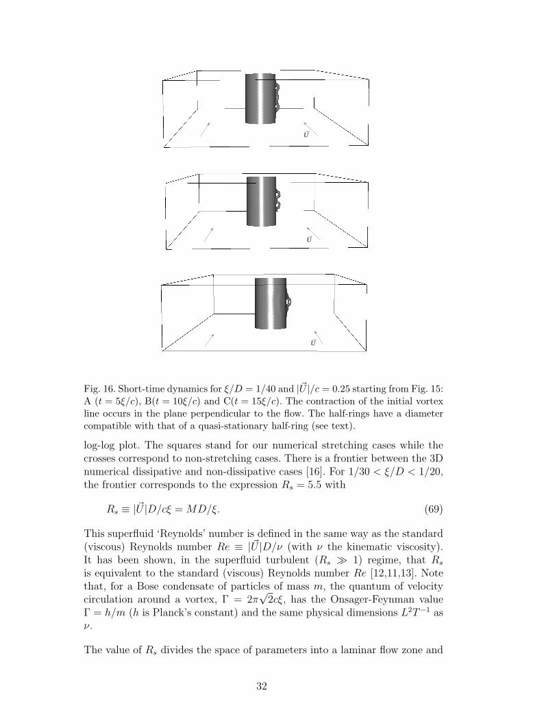
When driven upstream, the half-ring eventually collapses against the cylinder,dissipating its energy as sound waves. Otherwise, the vortex loop is stretchedwhile the pinning points move towards the back of the cylinder. Figures 17show the long-time dynamics for a stretching case with ξ/D = 1/40 and
|~U |/c = 0.25 starting from Fig. 16c. Figure 19 shows a later situation for
ξ/D = 1/20 and |~U |/c = 0.35 starting from Fig. 18. As the vortex loopgrows, its backmost part remains oblique to the flow. This vortex stretchingmechanism consumes energy, thus generating drag. It could be responsible forthe appearance of drag in experimental superflows if fluctuations are strongenough to nucleate the initial vortex loop (which is imposed extrinsically inour numerical system). Note that it takes place for 2D subcritical velocities.
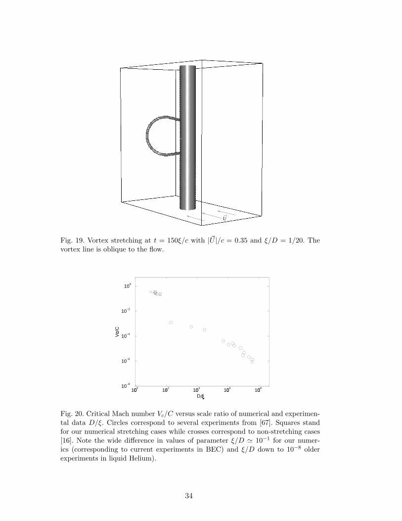
Figure 20 displays several numerical and experimental [67] critical Mach num-bers (Vc/C) with respect to D/ξ, which seem to follow a (−1) slope in a
31
U
U
U
Fig. 16. Short-time dynamics for ξ/D = 1/40 and |~U |/c = 0.25 starting from Fig. 15:A (t = 5ξ/c), B(t = 10ξ/c) and C(t = 15ξ/c). The contraction of the initial vortexline occurs in the plane perpendicular to the flow. The half-rings have a diametercompatible with that of a quasi-stationary half-ring (see text).
log-log plot. The squares stand for our numerical stretching cases while thecrosses correspond to non-stretching cases. There is a frontier between the 3Dnumerical dissipative and non-dissipative cases [16]. For 1/30 < ξ/D < 1/20,the frontier corresponds to the expression Rs = 5.5 with
Rs ≡ |~U |D/cξ = MD/ξ. (69)
This superfluid ‘Reynolds’ number is defined in the same way as the standard(viscous) Reynolds number Re ≡ |~U |D/ν (with ν the kinematic viscosity).It has been shown, in the superfluid turbulent (Rs À 1) regime, that Rs
is equivalent to the standard (viscous) Reynolds number Re [12,11,13]. Notethat, for a Bose condensate of particles of mass m, the quantum of velocitycirculation around a vortex, Γ = 2π
√2cξ, has the Onsager-Feynman value
Γ = h/m (h is Planck’s constant) and the same physical dimensions L2T−1 asν.
The value of Rs divides the space of parameters into a laminar flow zone and
32
U
U
U
Fig. 17. Long-time dynamics for ξ/D = 1/40 and |~U |/c = 0.25 starting fromFig. 16c. The half-ring moves downstream while growing.
U
Fig. 18. Quasi-nucleation solution for |~U |/c = 0.35 and ξ/D = 1/20 at timet = 15ξ/c.
33
U
Fig. 19. Vortex stretching at t = 150ξ/c with |~U |/c = 0.35 and ξ/D = 1/20. Thevortex line is oblique to the flow.
10 0
10 2
10 4
10 6
10 8
/ξ10
−8
10−6
10−4
10−2
100
Vc/
C
D
Fig. 20. Critical Mach number Vc/C versus scale ratio of numerical and experimen-tal data D/ξ. Circles correspond to several experiments from [67]. Squares standfor our numerical stretching cases while crosses correspond to non-stretching cases[16]. Note the wide difference in values of parameter ξ/D ' 10−1 for our numer-ics (corresponding to current experiments in BEC) and ξ/D down to 10−8 olderexperiments in liquid Helium).
34
a recirculating flow zone, very much like in the problem of a circular disc in aviscous fluid in which this frontier is also found to be around Re ∼ 5. Thus,there seems to exist some degree of universality between viscous normal fluidsand superfluids modeled by NLSE as discussed in [12,11,13]. In the contextof superfluid 4He flow, the experimental critical velocity is known to dependstrongly on the system’s characteristic size D. It is often found to be wellbelow the Landau value (based on the velocity of roton excitation) except forexperiments in which ions are dragged in liquid helium. Feynman’s alternativecritical velocity criterion Rs ∼ log(D/ξ) is based on the energy needed to formvortex lines. It produces better estimates for various experimental settings, butdoes not describe the vortex nucleation mechanism [1].
In a recent experiment, Raman et al. have studied dissipation in a Bose-Einstein condensed gas by moving a blue detuned laser beam through thecondensate at different velocities [68]. In their inhomogeneous condensate,they observed a critical Mach number for the onset of dissipation M c
2D/1.6.
Our computations were performed for values of ξ/D comparable to those inBose-Einstein condensed gas experiments. They demonstrate the possibility ofa subcritical drag mechanism, based on 3D vortex stretching. It would be veryinteresting to determine experimentally the dependence of the critical Machnumber on the parameter ξ/D and the nature (2D or 3D) of the excitations[16].
4.5 Stability of attractive Bose-Einstein condensates
In this section, following reference [17], we study condensates with attractiveinteractions which are known to be metastable in spatially localized systems,provided that the number of condensed particles is below a critical value Nc
[7]. Various physical processes compete to determine the lifetime of attractivecondensates. Among them one can distinguish macroscopic quantum tunnel-ing (MQT) [69,70], inelastic two and three body collisions (ICO) [71,72] andthermally induced collapse (TIC) [70,73]. We compute the life-times, usingboth a variational Gaussian approximation and the exact numerical solutionfor the condensate wave-function.
4.5.1 Computations of stationary states
Gaussian approximation
A Gaussian approximation for the condensate density can be obtained ana-lytically through the following procedure.
35
Inserting
ψ(r, t) = A(t) exp(−r2/2r2
G(t) + ib(t)r2)
(70)
into the action (45), where F is given by (52), yields a set of Euler-Lagrangeequations for rG(t), b(t) and the (complex) amplitude A(t). The stationarysolutions of the Euler-Lagrange equations produce the following values [74]:
N (µ) =4√
2π3(−8µ + 3
√7 + 4µ2
)
7|a|(−2µ +
√7 + 4µ2
)3/2, (71)
E = N (µ)(−µ + 3
√7 + 4µ2
)/7. (72)
N is found to be maximal at NGc = 8
√2π3/|55/4a|. The corresponding value
of the chemical potential is µ = µGc = 1/2
√5.
Linearizing the Euler-Lagrange equations around the stationary solutions,yields the following expression for the eigenvalues [74]:
λ2(µ) = 8µ2 − 4µ√
7 + 4µ2 + 2 (73)
This qualitative behavior is the generic signature of a Hamiltonian saddle-node(HSN) bifurcation defined, at lowest order, by the normal form [75]
meffQ = δ − βQ2, (74)
where δ = (1−N /Nc) is the bifurcation parameter. The critical amplitude Qis related to the radius of the condensate [74]. We can relate the parametersβ and meff to critical scaling laws, by defining the appropriate energy
E = E0 + meffQ2/2− δ Q + βQ3/3− γδ. (75)
From (74) it is straightforward to derive, close to the critical point δ = 0, theuniversal scaling laws
E± = Ec − Elδ ± E∆δ3/2, (76)
λ2± = ±λ2
∆δ1/2, (77)
where Ec = E0, El = γ, E∆ = 2/3√
β and λ2∆ = 2
√β/meff .
Numerical branch following
Using the branch-following method described in section 4.3, we have computedthe exact stationary solutions of the NLSE. We use the following value a =
36
600
800
1000 1200 1400 1600500
1000
1500
2000
2500
3000
cE
cGN
+ε
-ε
ε
N
N
600 800 1000 1200 1400 1600N
−20.0
−10.0
0.0
10.0
20.0
30.0
40.0
λ 2
λ
λ
N Nc c
+
−E E
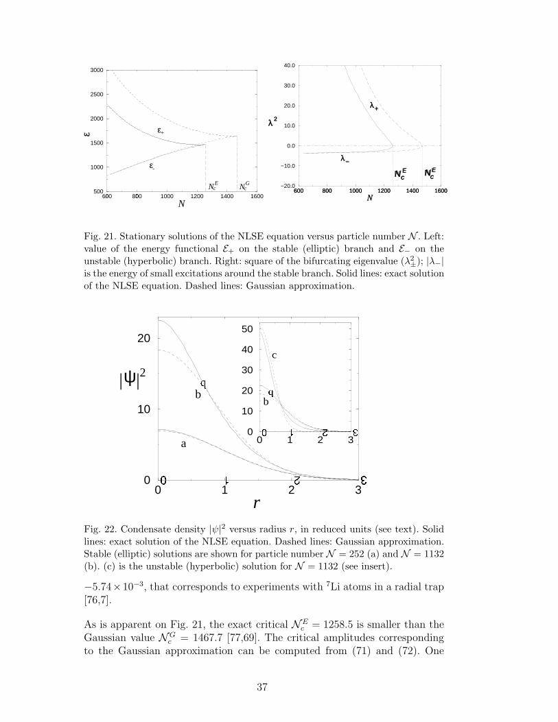
Fig. 21. Stationary solutions of the NLSE equation versus particle number N . Left:value of the energy functional E+ on the stable (elliptic) branch and E− on theunstable (hyperbolic) branch. Right: square of the bifurcating eigenvalue (λ2±); |λ−|is the energy of small excitations around the stable branch. Solid lines: exact solutionof the NLSE equation. Dashed lines: Gaussian approximation.
0
1
2
30
10
20
a
b
0
1
2
30
10
20
30
40
50
c
b
ψ| |2
rFig. 22. Condensate density |ψ|2 versus radius r, in reduced units (see text). Solidlines: exact solution of the NLSE equation. Dashed lines: Gaussian approximation.Stable (elliptic) solutions are shown for particle number N = 252 (a) and N = 1132(b). (c) is the unstable (hyperbolic) solution for N = 1132 (see insert).
−5.74×10⁻³, that corresponds to experiments with 7Li atoms in a radial trap[76,7].
As is apparent on Fig. 21, the exact critical NEc = 1258.5 is smaller than the
Gaussian value NGc = 1467.7 [77,69]. The critical amplitudes corresponding
to the Gaussian approximation can be computed from (71) and (72). One
37
finds Ec = 4√
2π3/|53/4a|, E∆ = 64√
π3/|59/4a| and λ2∆ = 4
√10. For the exact
solutions, we obtain the critical amplitudes by performing fits on the data.One finds E∆ = 1340 and λ2
∆ = 14.68. Thus, the Gaussian approximationcaptures the bifurcation qualitatively, but with quantitative 17% error on Nc
[77], 24% error on E∆ and 14% error on λ2∆. Fig. 22 shows the physical origin
of the quantitative errors in the Gaussian approximation. By inspection it isapparent that the exact solution is well approximated by a Gaussian only forsmall N on the stable (elliptic) branch.
4.5.2 Estimation of life-times
In this section, we estimate the decay rates due to thermally induced collapse,macroscopic quantum tunneling and inelastic collisions.
Thermally induced collapse
The thermally induced collapse (TIC) rate ΓT is estimated using the formula[78]
ΓT
ω=|λ+|2π
exp
[−~ω (E+ − E−)
kBT
](78)
where ~ω(E+−E−) is the (dimensionalized) height of the nucleation energy bar-rier, T is the temperature of the condensate and kB is the Boltzmann constant.Note that the prefactor characterizes the typical decay time which is controlledby the slowest part of the nucleation dynamics: the top-of-the-barrier saddlepoint eigenvalue λ+. The behavior of ΓT can be obtained directly from theuniversal saddle-node scaling laws (76) and (77). Thus the exponential factorand the prefactor vanish respectively as δ3/2 and δ1/4.
Macroscopic quantum tunneling
We estimate the MQT decay rate using an instanton technique that takes intoaccount the semi classical trajectory giving the dominant contribution to thequantum action path integral [70,69]. This trajectory is approximated as thesolution of
d2q(t)
dt2= − dΦ(q)
dq. (79)
Φ(q) is a polynomial such that −Φ(q) reconstructs the Hamiltonian dynamics,and is determined by the relations
38
qm
qf
qmqbqf
~
~
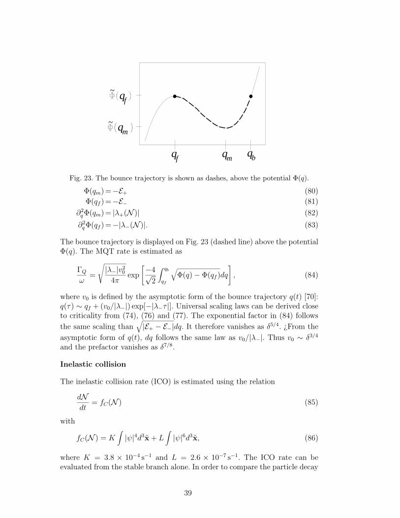
Fig. 23. The bounce trajectory is shown as dashes, above the potential Φ(q).
Φ(qm) =−E+ (80)
Φ(qf ) =−E− (81)
∂2qΦ(qm) = |λ+(N )| (82)
∂2qΦ(qf ) =−|λ−(N )|. (83)
The bounce trajectory is displayed on Fig. 23 (dashed line) above the potentialΦ(q). The MQT rate is estimated as
ΓQ
ω=
√|λ−|v2
0
4πexp
[−4√2
∫ qb
qf
√Φ(q)− Φ(qf )dq
], (84)
where v0 is defined by the asymptotic form of the bounce trajectory q(t) [70]:q(τ) ∼ qf + (v0/|λ−|) exp[−|λ−τ |]. Universal scaling laws can be derived closeto criticality from (74), (76) and (77). The exponential factor in (84) follows
the same scaling than√|E+ − E−|dq. It therefore vanishes as δ5/4. ¿From the
asymptotic form of q(t), dq follows the same law as v0/|λ−|. Thus v0 ∼ δ3/4
and the prefactor vanishes as δ7/8.
Inelastic collision
The inelastic collision rate (ICO) is estimated using the relation
dNdt
= fC(N ) (85)
with
fC(N ) = K∫|ψ|4d3x + L
∫|ψ|6d3x, (86)
where K = 3.8 × 10⁻⁴ s−1 and L = 2.6 × 10⁻⁷ s−1. The ICO rate can beevaluated from the stable branch alone. In order to compare the particle decay
39
1245 1250 125510
10
102
0
MQT
ICO
1
2
3
-2
600
800
1000 1200 140010
10
10
10
Con
dens
ate
Dec
ay R
ate
[s ]
1
0
-1
-2
ICO
MQT MQT
TIC: 4 7
-1
6 5 4 37 6 5 3
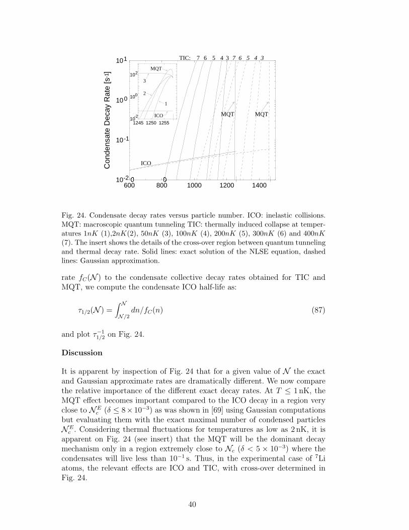
Fig. 24. Condensate decay rates versus particle number. ICO: inelastic collisions.MQT: macroscopic quantum tunneling TIC: thermally induced collapse at temper-atures 1nK (1),2nK(2), 50nK (3), 100nK (4), 200nK (5), 300nK (6) and 400nK(7). The insert shows the details of the cross-over region between quantum tunnelingand thermal decay rate. Solid lines: exact solution of the NLSE equation, dashedlines: Gaussian approximation.
rate fC(N ) to the condensate collective decay rates obtained for TIC andMQT, we compute the condensate ICO half-life as:
τ1/2(N ) =∫ N
N/2dn/fC(n) (87)
and plot τ−11/2 on Fig. 24.
Discussion
It is apparent by inspection of Fig. 24 that for a given value of N the exactand Gaussian approximate rates are dramatically different. We now comparethe relative importance of the different exact decay rates. At T ≤ 1 nK, theMQT effect becomes important compared to the ICO decay in a region veryclose to NE
c (δ ≤ 8× 10⁻³) as was shown in [69] using Gaussian computationsbut evaluating them with the exact maximal number of condensed particlesNE
c . Considering thermal fluctuations for temperatures as low as 2 nK, it isapparent on Fig. 24 (see insert) that the MQT will be the dominant decaymechanism only in a region extremely close to Nc (δ < 5 × 10⁻³) where thecondensates will live less than 10−1 s. Thus, in the experimental case of 7Liatoms, the relevant effects are ICO and TIC, with cross-over determined inFig. 24.
40
Calculations similar to those described here have also been generalized toan attractive Bose-Einstein condensate confined by a cylindrically symmetricpotential V (r) = m(ω2
rr2 + ω2
zz2)/2, which lead to cigar-shaped or pancake-
shaped condensates. Newton’s method was used to calculated stationary states,as described above. The inverse Arnoldi method was used to calculate the lead-ing eigenvalues λ2
±, yielding decay rates that are similar to those computedfor the spherically symmetric case. This was found to be due to spontaneousisotropization of the condensates. See [18] for more details.
5 Conclusion
The main result of the NLSE simulations presented in section 3.2 is thattwo diagnostics of Kolmogorov’s regime in decaying turbulence are satisfied.These diagnostics are, at the time of the maximum of energy dissipation: (i) aparameter-independent kinetic energy dissipation rate and (ii) a k−5/3 spectralscaling in the inertial range. Thus, the NLSE simulations were shown to bevery similar, as far as energetics is concerned, with the viscous simulations.The experimental results presented in section 3.3 prove that the Kolmogorovcascade survives in the superfluid regime.
We have seen that the numerical tools developed in section 4.3 can be used inpractice to obtain the stationary solutions of the NLSE. These methods haveallowed us to find the full bifurcation diagrams of Bose-Einstein condensateswith attractive interactions and superflows past a cylinder. Furthermore, thestationary solutions have given us efficient way to start vortical dynamics (in2D and 3D) in a controlled manner.
6 Acknowledgments
The work reviewed in this paper was performed in collaboration with G. Dewel,J. Maurer and P. Tabeling. It was supported by ECOS-CONICYT programno. C01E08 and by the NSF DMR 0094569. Computations were performed atthe Institut du Developpement et des Ressources en Informatique Scientifique.
References
[1] R. J. Donnelly. Quantized Vortices in Helium II. Cambridge Univ. Press,Cambridge, 1991.
41
[2] E.P. Gross. Structure of a quantized vortex in boson systems. Nuovo Cimento,20(3), 1961.
[3] L.P. Pitaevskii. Vortex lines in an imperfect Bose gas. Sov. Phys.-JETP, 13(2),1961.
[4] L. Landau and E. Lifchitz. Fluid Mechanics. Pergamon Press, Oxford, 1980.
[5] M. H. Anderson, J. R. Ensher, M. R. Matthews, C. E. Wieman, and E. A.Cornell. Observation of Bose-Einstein condensation in a dilute atomic vapor.Science, 269:198, 1995.
[6] K. B. Davis, M. O. Mewes, M. R. Adrews, N. J. van Druten, D. S. Durfee,D. M. Kurn, and W. Ketterle. Bose-Einstein condensation in a gas of sodiumatoms. Phys. Rev. Lett., 75:3969, 1995.
[7] C. C. Bradley, C. A. Sackett, and R. G. Hulet. Bose-Einstein condensation oflithium: Observation of limited condensate number. Phys. Rev. Lett., 78(6):985,1997.
[8] F. Dalfovo, S. Giorgini, L. P. Pitaevskii, and S. Stringari. Theory of Bose-Einstein condensation in trapped gases. Rev. Mod. Physics, 71(3), 1999.
[9] Y. Pomeau and S. Rica. Model of superflow with rotons. Phys. Rev. Lett.,71,2:247, 1993.
[10] P.H. Roberts and N.G. Berloff. The nonlinear Schrodinger equation as a modelof superfluidity. In C. F. Barenghi, R. J. Donnelly, and W. F. Vinen, editors,Quantized vortex dynamics and superfluid turbulence, pages 235–256. LectureNotes in Physics, 2001.
[11] C. Nore, M. Abid, and M. Brachet. Decaying kolmogorov turbulence in a modelof superflow. Phys. Fluids, 9(9):2644, 1997.
[12] C. Nore, M. Abid, and M. E. Brachet. Kolmogorov turbulence in low-temperature superflows. Phys. Rev. Lett., 78(20):3896–3899, 1997.
[13] M. Abid, M. Brachet, J. Maurer, C. Nore, and P. Tabeling. Experimentaland numerical investigations of low–temperature superfluid turbulence. Eur. J.Mech. B Fluids, 17(4):665–675, 1998.
[14] C. Huepe and M.-E. Brachet. Solutions de nucleation tourbillonnaires dansun modele d’ecoulement superfluide. C. R. Acad. Sci. Paris, 325(II):195–202,1997.
[15] C. Huepe and M. E. Brachet. Scaling laws for vortical nucleation solutions ina model of superflow. Physica D, 140:126–140, 2000.
[16] C. Nore, C. Huepe, and M. E. Brachet. Subcritical dissipation in three-dimensional superflows. Phys. Rev. Lett., 84(10):2191, 2000.
[17] C. Huepe, S. Metens, G. Dewel, P. Borckmans, and M.-E. Brachet. Decay ratesin attractive Bose-Einstein condensates. Phys. Rev. Lett., 82(2):1616, 1999.
42

[18] C. Huepe, L.S. Tuckerman, S. Metens, and M.-E. Brachet. Stability and decayrates of non-isotropic attractive Bose-Einstein condensates. Phys. Rev. A, inpress.
[19] W.F. Vinen and J.J. Niemela. Quantum turbulence. Jour. Low Temp. Phys.,128:167–231, 2002.
[20] C. F. Barenghi, R. J. Donnelly, and W. F. Vinen, editors. Quantized vortexdynamics and superfluid turbulence. Lecture Notes in Physics, 2001.
[21] T. Araki, M. Tsubota, and S. K. Nemirovskii. Energy spectrum of superfluidturbulence with no normal-fluid component. Phys. Rev. Lett., 89,14:1–4, 2002.
[22] S.I. Ogawa, M. Tsubota, and Y. Hattori. Study of reconnection and acousticemission of quantized vortices in superfluid by the numerical analysis of theGross-Pitaevskii equation. J. Phys. Soc. Jpn, 71:813, 2002.
[23] J. Koplik and H. Levine. Vortex reconnection in superfluid Helium. Phys. Rev.Lett., 71:1375–1378, 1993.
[24] T. Araki and M. Tsubota. Cascade process of vortex tangle dynamics insuperfluid 4He without mutual friction. J. Low Temp. Phys., 121:405, 2000.
[25] M. Leadbeater, D.C. Samuels, C.F. Barenghi, and C.S. Adams. Decay ofsuperfluid turbulence via Kelvin-wave radiation. Phys. Rev. A, 67:015601–1,2003.
[26] D. Kivotides, J.C.Vassilicos, D.C. Samuels, and C.F. Barenghi. Kelvin wavescascade in superfluid turbulence. Phys. Rev. Lett., 86:3080–3083, 2001.
[27] B. V. Svistunov. Superfluid turbulence in the low-temperature limit. Phys.Rev. B, 52:3647, 1995.
[28] W.F. Vinen. Decay of turbulence at a very low temperature: the radiation ofsound from a Kelvin wave on a quantized vortex. Phys. Rev. B, 64:134520–1,2001.
[29] S.I. Davis, P.C. Hendry, and P.V.E. McClintock. Decay of quantized vorticityin superfluid 4He at mK temperature. Physica B, 280:43–44, 2000.
[30] M. R. Matthews, B. P. Anderson, P. C. Haljan, D. S. Hall, C. E. Wieman,and E. A. Cornell. Vortices in a Bose-Einstein condensate. Phys. Rev. Lett.,83:2498–2501, 1999.
[31] S. Inouye, S. Gupta, T. Rosenband, A.P. Chikkatur, A. Gorlitz, T.L. Gustavson,A.E. Leanhardt, D.E. Pritchard, and W. Ketterle. Observation of vortex phasesingularities in Bose-Einstein condensates. Phys. Rev. Lett., 87:080402, 2001.
[32] K. W. Madison, F. Chevy, W. Wohlleben, and J. Dalibard. Vortex formationin a stirred Bose-Einstein condensate. Phys. Rev. Lett., 84:806–809, 2000.
[33] P. Rosenbush, V. Bretin, and J. Dalibard. Dynamics of a single vortex line ina Bose-Einstein condensate. Phys. Rev. Lett., 89:200403–1, 2002.
43
[34] V. Bretin, P. Rosenbush, F. Chevy, G.V. Shlyapnikov, and J. Dalibard.Quadrupole oscillation of a single-vortex condensate: evidence for Kelvin modes.condmat, page 0211101, 2003.
[35] E. A. Spiegel. Fluid dynamical form of the linear and nonlinear Schrodingerequations. Physica D, 1:236, 1980.
[36] P. Nozieres and D. Pines. The Theory of Quantum Liquids. Addison Wesley,New York, 1990.
[37] C. Nore, M. Brachet, and S. Fauve. Numerical study of hydrodynamics usingthe nonlinear Schrodinger equation. Physica D, 65:154–162, 1993.
[38] D. Gottlieb and S. A. Orszag. Numerical Analysis of Spectral Methods. SIAM,Philadelphia, 1977.
[39] M. P. Kawatra and R. K. Pathria. Quantized vortices in imperfect Bose gas.Phys.Rev., 151:1, 1966.
[40] K. W. Schwarz. Three-dimensional vortex dynamics in superfluid 4He: line-lineand line-boundary interactions. Phys. Rev. B, 31:5782, 1985.
[41] J. C. Neu. Vortices in complex scalar fields. Physica D, 43:385, 1990.
[42] F. Lund. Defect dynamics for the nonlinear Schrodinger equation derived froma variational principle. Phys.Rev.Lett., A 159:245, 1991.
[43] G. I. Taylor and A. E. Green. Mechanism of the production of small eddiesfrom large ones. Proc. Soc. Lond. A, 158:499, 1937.
[44] M. E. Brachet, D. I. Meiron, S. A. Orszag, B. G. Nickel, R. H. Morf, andU. Frisch. Small-scale structure of the Taylor-Green vortex. J. Fluid Mech.,130:411–452, 1983.
[45] M. Brachet. Geometrie des structures a petite echelle dans le vortex de Taylor-Green. C.R.A.S II, 311:775, 1990.
[46] J. Domaradzki, W. Liu, and M. Brachet. An analysis of sugrid-scale interactionsin numerically simulated isotropic turbulence. Phys. Fluids A, 5:1747, 1993.
[47] C. Nore, M. Abid, and M. Brachet. Simulation numerique d’ecoulementscisailles tridimensionnels a l’aide de l’equation de Schrodinger non lineaire.C.R.A.S, 319 II(7):733, 1994.
[48] U. Frisch. Turbulence, the legacy of A. N. Kolmogorov. Cambridge Univ. Press,Cambridge, 1995.
[49] T. Araki, M. Tsubota, and S. K. Nemirovskii. Energy spectrum of superfluidturbulence with no normal-fluid component. Phys. Rev. Lett., 89,14:1–4, 2002.
[50] S. Douady, Y. Couder, and M. E. Brachet. Direct observation of theintermittency of intense vorticity filaments in turbulence. Phys. Rev. Lett.,67:983, 1991.
44
[51] G. Zocchi, P. Tabeling, J. Maurer, and H. Willaime. Measurement of the scalingof the dissipation at high Reynolds numbers. Phys. Rev. E, 50:3693, 1994.
[52] S. Fauve, C. Laroche, and B. Castaing. Pressure fluctuations in swirlingturbulent flows. J. Phys. II, 3:271, 1993.
[53] J. Maurer and P. Tabeling. Local investigation of superfluid turbulence.Europhys. Lett., 43(1):29–34, 1998.
[54] V. Hakim. Nonlinear Schrodinger flow past an obstacle in one dimension. Phys.Rev. E, 55(3):2835–2845, 1997.
[55] T. Tsuzuki. Nonlinear waves in the Pitaevskii-Gross equation. J. Low Temp.Phys., 4(4), 1971.
[56] V.E. Zakharov and A.B. Shabat. Interaction between solitons in a stablemedium. Sov. Phys.-JETP, 37(5):823–828, 1973.
[57] C.-T. Pham and M. Brachet. Dynamical scaling laws in two types of extendedhamiltonian systems at dissipation onset. Physica D, 163:129–147, 2002.
[58] R. Seydel. From Equilibrium to Chaos: Practical Bifurcation and StabilityAnalysis. Elsevier, New York, 1988.
[59] C. Mamun and L. Tuckerman. Asymmetry and Hopf bifurcation in sphericalCouette flow. Phys. Fluids, 7(1):80, 1995.
[60] W. Press, S. Teukolsky, W. Vetterling, and B.Flannery. Numerical Recipees inFortran. Cambridge Univ. Press, Cambridge, 1994.
[61] H. van der Vorst. Bi-cgstab: A fast and smoothly converging variant of bi-cgfor the solution of nonsymmetric linear systems. SIAM J. Sci. Stat. Comput.,13:631, 1992.
[62] R. Klein and A. J. Majda. Self-stretching of perturbed vortex filaments. PhysicaD, 53:267, 1991.
[63] T. Frisch, Y. Pomeau, and S. Rica. Transition to dissipation in a model ofsuperflow. Phys.Rev.Lett., 69:1644, 1992.
[64] O. Avenel, G.G. Ihas, and E. Varoquaux. The nucleation of vortices in superfluid4He: Answers and questions. J. Low Temp.Phys., 93:1031–1057, 1993.
[65] G.G. Ihas, O. Avenel, R. Aarts, R Salmelin, and E. Varoquaux. Quantumnucleation of vortices in the flow of superfluid He-4 through an orifice. Phys.Rev. Lett., 69(2):327, 1992.
[66] C. A. Jones and P. H. Roberts. Motions in a bose condensate: Iv. axisymmetricsolitary waves. J. Phys. A, 15:2599, 1982.
[67] J. Wilks. The properties of liquid and solid helium. Clarendon Press, Oxford,1967.
45
[68] C. Raman, M. Kohl, R. Onofrio, D.S. Durfee, C.E. Kuklewicz, Z. Hadzibabic,and W. Ketterle. Evidence for a critical velocity in a Bose-Einstein condensedgas. Phys. Rev. Lett., 83(13):2502, 1999.
[69] M. Ueda and A. J. Leggett. Macroscopic quantum tunneling of a Bose-Einsteincondensate with attractive interaction. Phys. Rev. Lett., 80(8):1576, 1998.
[70] H. T. C. Stoof. Macroscopic quantum tunneling of a Bose condensate. J. Stat.Phys., 87:1353, 1997.
[71] H. Shi and W.-M. Zheng. Bose-Einstein condensation in an atomic gas withattractive interactions. Phys. Rev. A, 55(4):2930, 1997.
[72] R. J. Dodd, M. Edwards, C. J. Williams, C. W. Clark, M. J. Holland, P. A.Ruprecht, and K. Burnett. Role of attractive interactions on Bose-Einsteincondensation. Phys. Rev. A, 54(1):661, 1996.
[73] C. A. Sackett, H. T. C. Stoof, and R. G. Hulet. Growth and collapse of a Bose-Einstein condensate with attractive interactions. Phys. Rev. Lett., 80(10):2031,1998.
[74] C. Huepe. Bifurcations et instabilites dans les condensats de Bose-Einstein etles ecoulements superfluides. PhD thesis, Ecole Normale Superieure, 1999.
[75] J. Guckenheimer and P. Holmes. Nonlinear Oscillations, Dynamical Systemsand Bifurcations of Vector Fields. Springer-Verlag, Berlin, 1983.
[76] C. C. Bradley, C. A. Sackett, J. J. Tollett, and R. G. Hulet. Evidence of Bose-Einstein condensation in an atomic gas with attractive interactions. Phys. Rev.Lett., 75(9):1687, 1995.
[77] P. A. Ruprecht, M. J. Holland, K. Burnett, and M. Edwards. Time-dependentsolution of the nonlinear Schrodinger equation for Bose-condensed trappedneutral atoms. Phys. Rev. A, 51(6):4704, 1995.
[78] C.W. Gardiner. Handbook of Stochastic Methods. Springer-Verlag, Berlin, 1985.
46