Embed Size (px)
Citation preview
Advances in Intelligent Systems and Computing 248
ICT and Critical Infrastructure:Proceedings of the 48th Annual Convention of Computer Societyof India - Volume I
Suresh Chandra SatapathyP. S. AvadhaniSiba K. UdgataSadasivuni Lakshminarayana Editors
Hosted by CSI Vishakapatnam Chapter

Advances in Intelligent Systems and Computing
Volume 248
Series Editor
Janusz Kacprzyk, Warsaw, Poland
For further volumes:
http://www.springer.com/series/11156
Suresh Chandra Satapathy · P.S. AvadhaniSiba K. Udgata · Sadasivuni LakshminarayanaEditors
ICT and Critical Infrastructure:Proceedings of the 48th AnnualConvention of ComputerSociety of India - Volume I
Hosted by CSI Vishakapatnam Chapter
ABC

EditorsSuresh Chandra SatapathyAnil Neerukonda Institute of Technology
and Sciences, Sangivalasa(Affilated to Andhra University)VishakapatnamAndhra PradeshIndia
P.S. AvadhaniCollege of Engineering (A)Andhra UniversityVishakapatnamIndia
Siba K. UdgataUniversity of HyderabadHyderabadAndhra PradeshIndia
Sadasivuni LakshminarayanaCSIR-National Institute of OceanographyVishakapatnamIndia
ISSN 2194-5357 ISSN 2194-5365 (electronic)ISBN 978-3-319-03106-4 ISBN 978-3-319-03107-1 (eBook)DOI 10.1007/978-3-319-03107-1Springer Cham Heidelberg New York Dordrecht London
c© Springer International Publishing Switzerland 2014This work is subject to copyright. All rights are reserved by the Publisher, whether the whole or part of thematerial is concerned, specifically the rights of translation, reprinting, reuse of illustrations, recitation, broad-casting, reproduction on microfilms or in any other physical way, and transmission or information storageand retrieval, electronic adaptation, computer software, or by similar or dissimilar methodology now knownor hereafter developed. Exempted from this legal reservation are brief excerpts in connection with reviewsor scholarly analysis or material supplied specifically for the purpose of being entered and executed on acomputer system, for exclusive use by the purchaser of the work. Duplication of this publication or partsthereof is permitted only under the provisions of the Copyright Law of the Publisher’s location, in its cur-rent version, and permission for use must always be obtained from Springer. Permissions for use may beobtained through RightsLink at the Copyright Clearance Center. Violations are liable to prosecution underthe respective Copyright Law.The use of general descriptive names, registered names, trademarks, service marks, etc. in this publicationdoes not imply, even in the absence of a specific statement, that such names are exempt from the relevantprotective laws and regulations and therefore free for general use.While the advice and information in this book are believed to be true and accurate at the date of publication,neither the authors nor the editors nor the publisher can accept any legal responsibility for any errors oromissions that may be made. The publisher makes no warranty, express or implied, with respect to the materialcontained herein.
Printed on acid-free paper
Springer is part of Springer Science+Business Media (www.springer.com)
Preface
This AISC volume contains the papers presented at the 48th Annual Convention ofComputer Society of India (CSI 2013) with theme ‘ICT and Critical Infrastructure’held during 13th –15th December 2013 at Hotel Novotel Varun Beach, Visakhapatnamand hosted by Computer Society of India, Vishakhapatnam Chapter in association withVishakhapatnam Steel Plant, the flagship company of RINL, India.
Computer society of India (CSI) was established in 1965 with a view to increaseinformation and technological awareness among Indian society, and to make forumto exchange and share the IT- related issues. The headquarters of the CSI is situatedin Mumbai with a full-fledged office setup and is coordinating the individual chapteractivities. It has 70 chapters and 418 students’ branches operating in different cities ofIndia. The total strength of CSI is above 90000 members.
CSI Vishakhapatnam Chapter deems it a big pride to host this prestigious 48th Anu-ual Convention after successfully organizing various events like INDIA-2012, eCOG-2011, 28th National Student convention, and AP State Student Convention in the past.
CSI 2013 is targeted to bring researchers and practitioners from academia and in-dustry to report, deliberate and review the latest progresses in the cutting-edge researchpertaining to emerging technologies.
Research submissions in various advanced technology areas were received and aftera rigorous peer-review process with the help of program committee members and exter-nal reviewer, 173 ( Vol-I: 88, Vol-II: 85) papers were accepted with an acceptance ratioof 0.43.
The conference featured many distinguished personalities like Dr. V.K.Saraswat, Former Director General, DRDO, Prof. Rajeev Sangal, Director, IIT-BHU,Mr. Ajit Balakrishnan, Founder & CEO Rediff.com, Prof. L.M. Patnaik, Former ViceChancellor, IISc, Bangalore, Prof. Kesav Nori, IIIT-H & IIT-H, Mr. Rajesh Uppal, Ex-ecutive Director & CIO, Maruti Suzuki-India, Prof. D. Krishna Sundar, IISc, Bangalore,Dr. Dejan Milojicic, Senior Researcher and Director of the. Open Cirrus Cloud Comput-ing, HP Labs, USA & President Elect 2013, IEEE Computer Society, Dr. San Muruge-san, Director, BRITE Professional Services, Sydney, Australia, Dr. Gautam Shroff, VPand Chief Scientist, Tata Consultancy Services, Mr. P. Krishna Sastry, TCS, Ms. AngelaR. Burgess Executive Director, IEEE Computer Society, USA, Mr. Sriram Raghavan,

VI Preface
Security & Digital Forensics Consultant, Secure Cyber Space, and Dr. P. Bhanu Prasad,Vision Specialist, Matrix Vision GmbH, Germany among many others.
Four special sessions were offered respectively by Dr. Vipin Tyagi, Jaypee Universityof Engg. & Tech., Prof. J.K. Mandal, University of Kalyani, Dr. Dharam Singh, CTAE,Udaipur, Dr. Suma V., Dean, Research, Dayananda Sagar Institutions, Bengaluru. Sep-arate Invited talks were organized in industrial and academia tracks in both days. Theconference also hosted few tutorials and workshops for the benefit of participants.
We are indebted to Andhra University, JNTU-Kakinada and Visakhapatnam Steelplant for their immense support to make this convention possible in such a grand scale.CSI 2013 is proud to be hosted by Visakhapatnam Steel Plant (VSP), which is a Govt.of India Undertaking under the corporate entity of Rashtriya Ispat Nigam Ltd. It is thefirst shore-based integrated steel plant in India. The plant with a capacity of 3 mtpa wasestablished in the early nineties and is a market leader in long steel products. The Plantis almost doubling its capacity to a level of 6.3 mtpa of liquid steel at a cost of around2500 million USD. RINL-VSP is the first integrated steel plant in India to be accreditedwith all four international standards, viz. ISO 9001, ISO 14001, ISO 50001 and OHSAS18001. It is also the first Steel Plant to be certified with CMMI level-3 certificate andBS EN 16001 standard.
Our special thanks to Fellows, President, Vice President, Secretary, Treasurer, Re-gional VPs and Chairmen of Different Divisions, Heads of SIG Groups, National Stu-dent Coordinator, Regional and State Student Coordinators, OBs of different Chaptersand Administration staff of CSI-India. Thanks to all CSI Student Branch coordinators,Administration & Management of Engineering Colleges under Visakhapatnam chap-ter for their continuous support to our chapter activities. Sincere thanks to CSI-Vizagmembers and other Chapter Members across India those who have supported CSI-Vizagactivities directly or indirectly.
We take this opportunity to thank authors of all submitted papers for their hard work,adherence to the deadlines and patience with the review process. We express our thanksto all reviewers from India and abroad who have taken enormous pain to review thepapers on time.
Our sincere thanks to all the chairs who have guided and supported us from the begin-ning. Our sincere thanks to senior life members, life members, associate life membersand student members of CSI-India for their cooperation and support for all activities.
Our sincere thanks to all Sponsors, press, print & electronic media for their excellentcoverage of this convention.
December 2013 Dr. Suresh Chandra SatapathyDr. P.S. Avadhani
Dr. Siba K. UdgataDr. Sadasivuni Lakshminarayana

Organization
Chief Patrons
Shri A.P. Choudhary, CMD, RINLProf. G.S.N. Raju, VC, Andhra UniversityProf. G. Tulasi Ram Das, VC, JNTU-Kakinada
Patrons
Sri Umesh Chandra, Director (Operations), RINLSri P. Madhusudan, Director (Finance), RINLSri Y.R. Reddy, Director (Personnel), RINLSri N.S. Rao, Director (Projects), RINL
Apex (CSI) Committee
Prof. S.V. Raghavan, PresidentShri H.R. Mohan, Vice PresidentDr S. Ramanathan, Hon. SecretaryShri Ranga Rajagopal, Hon. TreasurerSri Satish Babu, Immd. Past PresidentShri Raju L. Kanchibhotla, RVP, Region-V
Chief Advisor
Prof D.B.V. Sarma, Fellow, CSI
Advisory Committee
Sri Anil Srivastav, IAS, Jt. Director General of Civil Aviation, GOISri G.V.L. Satya Kumar, IRTS, Chairman I/C, VPT, Visakhapatnam

VIII Organization
Sri N.K. Mishra, Rear Admiral IN (Retd), CMD, HSL, VisakhapatnamCapt.D.K. Mohanty, CMD, DCIL, VisakhapatnamSri S.V. Ranga Rajan, Outstanding Scientist, NSTL, VisakhapatnamSri Balaji Iyengar, GM I/C, NTPC-Simhadri, VisakhapatnamProf P. Trimurthy, Past President, CSISri M.D. Agarwal, Past President, CSIProf D.D. Sharma, Fellow, CSISri Saurabh Sonawala, Hindtron, MumbaiSri R.V.S. Raju, President, RHI Clasil Ltd.Prof. Gollapudi S.R., GITAM University & Convener, Advisory Board, CSI-2013
International Technical Advisory Committee:
Dr. L.M. Patnaik, IISc, India Dr. D. Janikiram, IIT-MDr. C. Krishna Mohan, IIT-H, India Dr. H.R. Vishwakarma, VIT, IndiaDr. K. RajaSekhar Rao, Dean, KLU,
India Dr. Deepak Garg, TU, PatialaDr. Chaoyang Zhang, USM, USA Dr. Hamid Arabnia, USADr. Wei Ding, USA Dr. Azah Kamilah Muda, MalaysiaDr. Cheng-Chi Lee, Taiwan Dr. Yun-Huoy Choo, MalaysiaDr. Pramod Kumar Singh,
ABV-IIITM, India Dr. Hongbo Liu, Dalian MaritimeDr. B. Biswal, GMRIT, India Dr. B.N. Biswal, BEC, IndiaDr. G. Pradhan, BBSR, India Dr. Saihanuman, GRIET, IndiaDr. B.K. Panigrahi, IITD, India Dr. L. Perkin, USADr. S. Yenduri, USA Dr. V. Shenbagraman, SRM, India
and many others
Organizing Committee
ChairSri T.K. Chand, Director (Commercial), RINL & Chairman, CSI-Vizag
Co-ChairmenSri P.C. Mohapatra, ED (Projects), Vizag SteelSri P. Ramudu, ED (Auto & IT), Vizag Steel
Vice-ChairmanSri K.V.S.S. Rajeswara Rao, GM (IT), Vizag Steel
Addl. Vice-Chairman:Sri Suman Das, DGM (IT) & Secretary, CSI-Vizag
ConvenerSri Paramata Satyanarayana, Sr. Manager (IT), Vizag Steel

Organization IX
Co-ConvenerSri C.K. Padhi, AGM (IT), Vizag Steel
Web Portal ConvenerSri S.S. Choudhary, AGM(IT)
Advisor (Press & Publicity)Sri B.S. Satyendra, AGM (CC)
Convener (Press & Publicity)Sri Dwaram Swamy, AGM (Con)
Co-Convener (Press & Publicity)Sri A.P. Sahu, AGM (IT)
Program Committee
Chairman:Prof P.S. Avadhani, Vice Principal, AUCE (A)
Co ChairmenProf D.V.L.N. Somayajulu, NIT-WDr S. Lakshmi Narayana, Scientist E, NIO-Vizag
Conveners:Sri Pulle Chandra Sekhar, DGM (IT), Vizag Steel – IndustryProf. S.C. Satapathy, HOD (CSE), ANITS – AcademicsDr. S.K. Udgata, UoH, Hyderabad
Finance Committee
ChairmanSri G.N. Murthy, ED (F&A), Vizag Steel
Co-ChairmenSri G.J. Rao, GM (Marketing)-Project SalesSri Y. Sudhakar Rao, GM (Marketing)-Retail Sales
ConvenerSri J.V. Rao, AGM (Con)
Co-ConvenersSri P. Srinivasulu, DGM (RMD)Sri D.V.G.A.R.G. Varma, AGM (Con)

X Organization
Sri T.N. Sanyasi Rao,Sr.Mgr (IT)
Members Sri V.R. Sanyasi, RaoSri P. Sesha Srinivas
Convention Committee
Chair Sri D.N. Rao, ED(Operations), Vizag Steel
Vice-Chairs
Sri Y. Arjun KumarSri S. RajaDr. B. Govardhana Reddy
Sri ThyagaRaju GuturuSri Bulusu Gopi KumarSri Narla Anand
Conveners
Sri S.K. MishraSri V.D. AwasthiSri M. Srinivasa BabuSri G.V. RameshSri A. BapujiSri B. Ranganath
Sri D. SatayanarayanaSri P.M. DivechaSri Y.N. ReddySri J.P. DashSri K. Muralikrishna
Co-Conveners
Sri Y. Madhusudan RaoSri S. GopalSri Phani GopalSri M.K. ChakravartySri P. Krishna RaoSri P. Balaramu
Sri B.V. Vijay KumarMrs M. Madhu BinduSri P. JanardhanaSri G.V. Saradhi
Members:
Sri Y. SatyanarayanaSri Shailendra KumarSri V.H. Sundara RaoMrs K. SaralaSri V. SrinivasSri G. Vijay KumarMrs. V.V. Vijaya Lakshmi
Sri D. RameshShri K. PratapSri P. Srinivasa RaoSri S. AdinarayanaSri B. GaneshSri Hanumantha NaikSri D.G.V. Saya

Organization XI
Sri V.L.P. LalSri U.V.V. JanardhanaSri S. Arun KumarSri K. RaviramSri N. Prabhakar RamSri BH.B.V.K. RajuSri K. Srinivasa RaoMrs T. Kalavathi
Mrs A. LakshmiSri N. PradeepSri K. DilipSri K.S.S. Chandra RaoSri Vamshee RamMs Sriya BasumallikSri Kunche SatyanarayanaSri Shrirama Murthy
Contents
Session 1: Computational Intelligence and Its Applications
Homogeneity Separateness: A New Validity Measure for ClusteringProblems . . . . . . . . . . . . . . . . . . . . . . . . . . . . . . . . . . . . . . . . . . . . . . . . . . . . . . . . 1M. Ramakrishna Murty, J.V.R. Murthy, P.V.G.D. Prasad Reddy, Anima Naik,Suresh C. Satapathy
Authenticating Grid Using Graph Isomorphism Based Zero KnowledgeProof . . . . . . . . . . . . . . . . . . . . . . . . . . . . . . . . . . . . . . . . . . . . . . . . . . . . . . . . . . . . 11Worku B. Gebeyehu, Lubak M. Ambaw, M.A. Eswar Reddy, P.S. Avadhani
Recognition of Marathi Isolated Spoken Words Using Interpolationand DTW Techniques . . . . . . . . . . . . . . . . . . . . . . . . . . . . . . . . . . . . . . . . . . . . . . 21Ganesh B. Janvale, Vishal Waghmare, Vijay Kale, Ajit Ghodke
An Automatic Process to Convert Documents into Abstracts by UsingNatural Language Processing Techniques . . . . . . . . . . . . . . . . . . . . . . . . . . . . . 31Ch. Jayaraju, Zareena Noor Basha, E. Madhavarao, M. Kalyani
A Novel Method for CBIR Using Texture Spectrum in Wavelet Domain . . . . 41G. Rosline Nesa Kumari, M. Sudheer, R. Tamilkodi
Identification of Abdominal Aorta Aneurysm Using Ant ColonyOptimization Algorithm . . . . . . . . . . . . . . . . . . . . . . . . . . . . . . . . . . . . . . . . . . . . 49A. Dinesh Kumar, R. Nidhya, V. Hanah Ayisha, Vigneshwar Manokar,Nandhini Vigneshwar Manokar
Color Image Watermarking Using Wavelet Transform Based on HVSChannel . . . . . . . . . . . . . . . . . . . . . . . . . . . . . . . . . . . . . . . . . . . . . . . . . . . . . . . . . 59G. Rosline Nesa Kumari, Syama Sundar Jeeru, S. Maruthuperumal
Automatic Vehicle Number Plate Localization Using SymmetricWavelets . . . . . . . . . . . . . . . . . . . . . . . . . . . . . . . . . . . . . . . . . . . . . . . . . . . . . . . . . 69V. HimaDeepthi, B. BalvinderSingh, V. SrinivasaRao
XIV Contents
Response Time Comparison in Multi Protocol Label Switching NetworkUsing Ant Colony Optimization Algorithm . . . . . . . . . . . . . . . . . . . . . . . . . . . . 77E.R. Naganathan, S. Rajagopalan, S. Narayanan
Software Effort Estimation Using Data Mining Techniques . . . . . . . . . . . . . . . 85Tirimula Rao Benala, Rajib Mall, P. Srikavya, M. Vani HariPriya
Infrared and Visible Image Fusion Using Entropy and Neuro-FuzzyConcepts . . . . . . . . . . . . . . . . . . . . . . . . . . . . . . . . . . . . . . . . . . . . . . . . . . . . . . . . . 93S. Rajkumar, P.V.S.S.R. Chandra Mouli
Hybrid Non-dominated Sorting Simulated Annealing Algorithmfor Flexible Job Shop Scheduling Problems . . . . . . . . . . . . . . . . . . . . . . . . . . . . 101N. Shivasankaran, P. Senthilkumar, K. Venkatesh Raja
DICOM Image Retrieval Using Geometric Moments and FuzzyConnectedness Image Segmentation Algorithm . . . . . . . . . . . . . . . . . . . . . . . . 109Amol Bhagat, Mohammad Atique
Soft Computing Based Partial-Retuning of Decentralised PI Controllerof Nonlinear Multivariable Process . . . . . . . . . . . . . . . . . . . . . . . . . . . . . . . . . . . 117L. Sivakumar, R. Kotteeswaran
Multi Objective Particle Swarm Optimization for Software CostEstimation . . . . . . . . . . . . . . . . . . . . . . . . . . . . . . . . . . . . . . . . . . . . . . . . . . . . . . . 125G. Sivanageswara Rao, Ch.V. Phani Krishna, K. Rajasekhara Rao
An Axiomatic Fuzzy Set Theory Based Feature Selection Methodologyfor Handwritten Numeral Recognition . . . . . . . . . . . . . . . . . . . . . . . . . . . . . . . . 133Abhinaba Roy, Nibaran Das, Ram Sarkar, Subhadip Basu,Mahantapas Kundu, Mita Nasipuri
Brownian Distribution Guided Bacterial Foraging Algorithmfor Controller Design Problem . . . . . . . . . . . . . . . . . . . . . . . . . . . . . . . . . . . . . . 141N. Sri Madhava Raja, V. Rajinikanth
Trapezoidal Fuzzy Shortest Path (TFSP) Selection for Green Routingand Scheduling Problems . . . . . . . . . . . . . . . . . . . . . . . . . . . . . . . . . . . . . . . . . . . 149P.K. Srimani, G. Vakula Rani, Suja Bennet
A Fused Feature Extraction Approach to OCR: MLP vs. RBF . . . . . . . . . . . . 159Amit Choudhary, Rahul Rishi
Fusion of Dual-Tree Complex Wavelets and Local Binary Patternsfor Iris Recognition . . . . . . . . . . . . . . . . . . . . . . . . . . . . . . . . . . . . . . . . . . . . . . . . 167N.L. Manasa, A. Govardhan, Ch. Satyanarayana
Contents XV
Evaluation of Feature Selection Method for Classification of Data UsingSupport Vector Machine Algorithm . . . . . . . . . . . . . . . . . . . . . . . . . . . . . . . . . . 179A. Veeraswamy, S. Appavu Alias Balamurugan, E. Kannan
Electrocardiogram Beat Classification Using Support Vector Machineand Extreme Learning Machine . . . . . . . . . . . . . . . . . . . . . . . . . . . . . . . . . . . . . 187C.V. Banupriya, S. Karpagavalli
Genetic Algorithm Based Approaches to Install Different Typesof Facilities . . . . . . . . . . . . . . . . . . . . . . . . . . . . . . . . . . . . . . . . . . . . . . . . . . . . . . . 195Soumen Atta, Priya Ranjan Sinha Mahapatra
A Trilevel Programming Approach to Solve Reactive Power DispatchProblem Using Genetic Algorithm Based Fuzzy Goal Programming . . . . . . . 205Papun Biswas, Bijay Baran Pal
An Iterative Fuzzy Goal Programming Method to Solve FuzzifiedMultiobjective Fractional Programming Problems . . . . . . . . . . . . . . . . . . . . . . 219Mousumi Kumar, Shyamal Sen, Bijay Baran Pal
An Efficient Ant Colony Based Routing Algorithm for Better Qualityof Services in MANET . . . . . . . . . . . . . . . . . . . . . . . . . . . . . . . . . . . . . . . . . . . . . 233Abdur Rahaman Sardar, Moutushi Singh, Rashi Ranjan Sahoo,Koushik Majumder, Jamuna Kanta Sing, Subir Kumar Sarkar
An Enhanced MapReduce Framework for Solving Protein FoldingProblem Using a Parallel Genetic Algorithm . . . . . . . . . . . . . . . . . . . . . . . . . . . 241A.G. Hari Narayanan, U. Krishnakumar, M.V. Judy
A Wavelet Transform Based Image Authentication Approach UsingGenetic Algorithm (AWTIAGA) . . . . . . . . . . . . . . . . . . . . . . . . . . . . . . . . . . . . . 251Amrita Khamrui, J.K. Mandal
Session 2: Mobile Communications and Social Netwroking
A New Approach to Monitor Network . . . . . . . . . . . . . . . . . . . . . . . . . . . . . . . . 259Hemant Kumar Saini, Anurag Jagetiya, Kailash Kumar,Satpal Singh Kushwaha
Detection and Mitigation of Misbehaving Vehicles from VANET . . . . . . . . . . 267Megha Kadam, Suresh Limkar
Comparative Study of Hierarchical Based Routing Protocols: WirelessSensor Networks . . . . . . . . . . . . . . . . . . . . . . . . . . . . . . . . . . . . . . . . . . . . . . . . . . 277Pritee Parwekar
Privacy Based Optimal Routing in Wireless Mesh Networks . . . . . . . . . . . . . . 287T.M. Navamani, P. Yogesh
XVI Contents
Security Issues and Its Counter Measures in Mobile Ad Hoc Networks . . . . . 301Pritee Parwekar, Sparsh Arora
Finding a Trusted and Shortest Path Mechanism of Routing Protocolfor Mobile Ad Hoc Network . . . . . . . . . . . . . . . . . . . . . . . . . . . . . . . . . . . . . . . . . 311Rabindra Kumar Shial, K. Hemant Kumar Reddy, Bhabani Sankar Gouda
Fusion Centric Decision Making for Node Level Congestion in WirelessSensor Networks . . . . . . . . . . . . . . . . . . . . . . . . . . . . . . . . . . . . . . . . . . . . . . . . . . 321N. Prabakaran, K. Naresh, R. Jagadeesh Kannan
An Intelligent Vertical Handoff Decision Algorithm for HeterogeneousWireless Networks . . . . . . . . . . . . . . . . . . . . . . . . . . . . . . . . . . . . . . . . . . . . . . . . . 331K.S.S. Anupama, S. Sri Gowri, B. Prabakara Rao, T. Satya Murali
Energy Efficient and Reliable Transmission of Data in Wireless SensorNetworks . . . . . . . . . . . . . . . . . . . . . . . . . . . . . . . . . . . . . . . . . . . . . . . . . . . . . . . . 341Chilukuri Shanti, Anirudha Sahoo
Inter-actor Connectivity Restoration in Wireless Sensor ActorNetworks : An Overview . . . . . . . . . . . . . . . . . . . . . . . . . . . . . . . . . . . . . . . . . . . 351Sasmita Acharya, C.R. Tripathy
MANFIS Approach for Path Planning and Obstacle Avoidancefor Mobile Robot Navigation . . . . . . . . . . . . . . . . . . . . . . . . . . . . . . . . . . . . . . . . 361Prases Kumar Mohanty, Krishna K. Pandey, Dayal R. Parhi
The Effect of Velocity and Unresponsive Traffic Volume on Performanceof Routing Protocols in MANET . . . . . . . . . . . . . . . . . . . . . . . . . . . . . . . . . . . . . 371Sukant Kishoro Bisoy, Prasant Kumar Patnaik, Tanmaya Kumar Swain
Improving the QOS in MANET by Enhancing the Routing Techniqueof AOMDV Protocol . . . . . . . . . . . . . . . . . . . . . . . . . . . . . . . . . . . . . . . . . . . . . . . 381Ankita Sharma, Sumit Vashistha
PRMACA: A Promoter Region Identification Using Multiple AttractorCellular Automata (MACA) . . . . . . . . . . . . . . . . . . . . . . . . . . . . . . . . . . . . . . . . . 393Pokkuluri Kiran Sree, Inampudi Ramesh Babu, S.S.S.N. Usha Devi Nedunuri
Analyzing Statistical Effect of Sampling on Network Traffic Dataset . . . . . . . 401Raman Singh, Harish Kumar, R.K. Singla
Localization of Information Dissemination in Agriculture Using MobileNetworks . . . . . . . . . . . . . . . . . . . . . . . . . . . . . . . . . . . . . . . . . . . . . . . . . . . . . . . . 409Lokesh Jain, Harish Kumar, R.K. Singla
Video Traffic in Wireless Sensor Networks . . . . . . . . . . . . . . . . . . . . . . . . . . . . 417Shilpa Pandey, Dharm Singh, Naveen Choudhary, Neha Mehta

Contents XVII
A Novel Pairwise Key Establishment and Management in HierarchicalWireless Sensor Networks (HWSN) Using Matrix . . . . . . . . . . . . . . . . . . . . . . 425B. Premamayudu, K. Venkata Rao, P. Suresh Varma
An Agent-Based Negotiating System with Multiple Trust ParameterEvaluation across Networks . . . . . . . . . . . . . . . . . . . . . . . . . . . . . . . . . . . . . . . . . 433Mohammed Tajuddin, C. Nandini
Enabling Self-organizing Behavior in MANETs: An Experimental Study . . . 441Annapurna P. Patil, K. Rajanikant, Sabarish, Madan, Surabi
Secure Hybrid Routing for MANET Resilient to Internal and ExternalAttacks . . . . . . . . . . . . . . . . . . . . . . . . . . . . . . . . . . . . . . . . . . . . . . . . . . . . . . . . . . 449Niroj Kumar Pani, Sarojananda Mishra
Compact UWB/BLUETOOTH Integrated Uniplanar Antennawith WLAN Notch Property . . . . . . . . . . . . . . . . . . . . . . . . . . . . . . . . . . . . . . . . 459Yashwant Kumar Soni, Navneet Kumar Agrawal
Session 3: Grid Computing, Cloud Computing, Virtual andScalable Applications
Open Security System for Cloud Architecture . . . . . . . . . . . . . . . . . . . . . . . . . . 467S. Koushik, Annapurna P. Patil
Client-Side Encryption in Cloud Storage Using Lagrange Interpolationand Pairing Based Cryptography . . . . . . . . . . . . . . . . . . . . . . . . . . . . . . . . . . . . 473R. Siva Ranjani, D. Lalitha Bhaskari, P.S. Avadhani
Analysis of Multilevel Framework for Cloud Security . . . . . . . . . . . . . . . . . . . 481Vadlamani Nagalakshmi, Vijeyta Devi
Agent Based Negotiation Using Cloud – An Approach in E-Commerce . . . . . 489Amruta More, Sheetal Vij, Debajyoti Mukhopadhyay
Improve Security with RSA and Cloud Oracle 10g . . . . . . . . . . . . . . . . . . . . . . 497Vadlamani Nagalakshmi, Vijeyta Devi
Negotiation Life Cycle: An Approach in E-Negotiation with Prediction . . . . . 505Mohammad Irfan Bala, Sheetal Vij, Debajyoti Mukhopadhyay
Dynamic Scheduling of Requests Based on Impacting Parametersin Cloud Based Architectures . . . . . . . . . . . . . . . . . . . . . . . . . . . . . . . . . . . . . . . 513R. Arokia Paul Rajan, F. Sagayaraj Francis
A Generic Agent Based Cloud Computing Architecture for E-Learning . . . . 523Samitha R. Babu, Krutika G. Kulkarni, K. Chandra Sekaran

XVIII Contents
Cache Based Cloud Architecture for Optimization of Resource Allocationand Data Distribution . . . . . . . . . . . . . . . . . . . . . . . . . . . . . . . . . . . . . . . . . . . . . . 535Salim Raza Qureshi
Implementing a Publish-Subscribe Distributed Notification Systemon Hadoop . . . . . . . . . . . . . . . . . . . . . . . . . . . . . . . . . . . . . . . . . . . . . . . . . . . . . . . 543Jyotiska Nath Khasnabish, Ananda Prakash Verma, Shrisha Rao
Securing Public Data Storage in Cloud Environment . . . . . . . . . . . . . . . . . . . . 555D. Boopathy, M. Sundaresan
An Enhanced Strategy to Minimize the Energy Utilization in CloudEnvironment to Accelerate the Performance . . . . . . . . . . . . . . . . . . . . . . . . . . . 563M. Vaidehi, V. Suma, T.R. Gopalakrishnan Nair
An Efficient Approach to Enhance Data Security in Cloud UsingRecursive Blowfish Algorithm . . . . . . . . . . . . . . . . . . . . . . . . . . . . . . . . . . . . . . . 575Naziya Balkish, A.M. Prasad, V. Suma
Effective Disaster Management to Enhance the Cloud Stability . . . . . . . . . . . 583O. Mahitha, V. Suma
An Efficient Job Classification Technique to Enhance Schedulingin Cloud to Accelerate the Performance . . . . . . . . . . . . . . . . . . . . . . . . . . . . . . . 593M. Vaidehi, T.R. Gopalakrishnan Nair, V. Suma
A Study on Cloud Computing Testing Tools . . . . . . . . . . . . . . . . . . . . . . . . . . . 605M.S. Narasimha Murthy, V. Suma
Session 4: Project Management and Quality Systems
Co-operative Junction Control System . . . . . . . . . . . . . . . . . . . . . . . . . . . . . . . . 613Sanjana Chandrashekar, V.S. Adarsh, P. Shashikanth Rangan, G.B. Akshatha
Identifying Best Products Based on Multiple Criteria Using DescisionMaking System . . . . . . . . . . . . . . . . . . . . . . . . . . . . . . . . . . . . . . . . . . . . . . . . . . . 621Swetha Reddy Donala, M. Archana, P.V.S. Srinivas
Design and Performance Analysis of File Replication Strategyon Distributed File System Using GridSim . . . . . . . . . . . . . . . . . . . . . . . . . . . . 629Nirmal Singh, Sarbjeet Singh
Extended Goal Programming Approach with Interval Data Uncertaintyfor Resource Allocation in Farm Planning: A Case Study . . . . . . . . . . . . . . . . 639Bijay Baran Pal, Mousumi Kumar
Design and Performance Analysis of Distributed Implementationof Apriori Algorithm in Grid Environment . . . . . . . . . . . . . . . . . . . . . . . . . . . . 653Priyanka Arora, Sarbjeet Singh
Contents XIX
Criticality Analyzer and Tester – An Effective Approach for CriticalComponents Identification and Verification . . . . . . . . . . . . . . . . . . . . . . . . . . . . 663Jeya Mala Dharmalingam, Balamurugan, Sabari Nathan
Real Time Collision Detection and Fleet Management System . . . . . . . . . . . . 671Anusha Pai, Vishal Vernekar, Gaurav Kudchadkar, Shubharaj Arsekar,Keval Tanna, Ross Rebello, Madhav Desai
An Effective Method for the Identification of Potential Failure Modesof a System by Integrating FTA and FMEA . . . . . . . . . . . . . . . . . . . . . . . . . . . . 679Samitha Khaiyum, Y.S. Kumaraswamy
Impact of Resources on Success of Software Project . . . . . . . . . . . . . . . . . . . . . 687N.R. Shashi Kumar, T.R. Gopalakrishnan Nair, V. Suma
Session 5: Emerging Technologies in Hardware and Software
An Optimized Approach for Density Based Spatial Clustering Applicationwith Noise . . . . . . . . . . . . . . . . . . . . . . . . . . . . . . . . . . . . . . . . . . . . . . . . . . . . . . . . 695Rakshit Arya, Geeta Sikka
A Kernel Space Solution for the Detection of Android Bootkit . . . . . . . . . . . . 703Harsha Rao, S. Selvakumar
Optimizing CPU Scheduling for Real Time Applications UsingMean-Difference Round Robin (MDRR) Algorithm . . . . . . . . . . . . . . . . . . . . . 713R.N.D.S.S. Kiran, Polinati Vinod Babu, B.B. Murali Krishna
A Study on Vectorization Methods for Multicore SIMD ArchitectureProvided by Compilers . . . . . . . . . . . . . . . . . . . . . . . . . . . . . . . . . . . . . . . . . . . . . 723Davendar Kumar Ojha, Geeta Sikka
A Clustering Analysis for Heart Failure Alert System Using RFIDand GPS . . . . . . . . . . . . . . . . . . . . . . . . . . . . . . . . . . . . . . . . . . . . . . . . . . . . . . . . . 729Gudikandhula Narasimha Rao, P. Jagdeeswar Rao
Globally Asynchronous Locally Synchronous Design BasedHeterogeneous Multi-core System . . . . . . . . . . . . . . . . . . . . . . . . . . . . . . . . . . . . 739Rashmi A. Jain, Dinesh V. Padole
Recognition of Smart Transportation through Randomizationand Prioritization . . . . . . . . . . . . . . . . . . . . . . . . . . . . . . . . . . . . . . . . . . . . . . . . . 749Bhavya Boggavarapu, Pabita Allada, SaiManasa Mamillapalli,V.P. Krishna Anne
Prioritized Traffic Management and Transport Security Using RFID . . . . . . 757V. Kishore, L. Britto Anthony, P. Jesu Jayarin
XX Contents
A Novel Multi Secret Sharing Scheme Based on Bitplane Flipsand Boolean Operations . . . . . . . . . . . . . . . . . . . . . . . . . . . . . . . . . . . . . . . . . . . . 765Gyan Singh Yadav, Aparajita Ojha
Large-Scale Propagation Analysis and Coverage Area Evaluation of 3GWCDMA in Urban Environments Based on BS Antenna Heights . . . . . . . . . 773Ramarakula Madhu, Gottapu Sasi Bhushana Rao
Inclination and Pressure Based Authentication for Touch Devices . . . . . . . . . 781K. Rajasekhara Rao, V.P. Krishna Anne, U. Sai Chand, V. Alakananda,K. Navya Rachana
Anticipated Velocity Based Guidance Strategy for Wheeled MobileEvaders Amidst Moving Obstacles in Bounded Environment . . . . . . . . . . . . . 789Amit Kumar, Aparajita Ojha
Reconfigurable Multichannel Down Convertor for on Chip Networkin MRI . . . . . . . . . . . . . . . . . . . . . . . . . . . . . . . . . . . . . . . . . . . . . . . . . . . . . . . . . . 799Vivek Jain, Navneet Kumar Agrawal
Author Index . . . . . . . . . . . . . . . . . . . . . . . . . . . . . . . . . . . . . . . . . . . . . . . . . . . . . . . . 807

S.C. Satapathy et al. (eds.), ICT and Critical Infrastructure: Proceedings of the 48th Annual Convention of CSI - Volume I, Advances in Intelligent Systems and Computing 248,
1
DOI: 10.1007/978-3-319-03107-1_1, © Springer International Publishing Switzerland 2014
Homogeneity Separateness: A New Validity Measure for Clustering Problems
M. Ramakrishna Murty1, J.V.R. Murthy2, P.V.G.D. Prasad Reddy3, Anima Naik4, and Suresh C. Satapathy5
1 Dept. of CSE, GMR Institute of Technology, Rajam, Srikakulam (Dist) A.P., India [email protected]
2 Dept. of CSE, JNTUK-Kakinada, A.P., India [email protected]
3 Dept. of CS&SE, Andhra University, Visakhapatnam, A.P., India [email protected]
4 Majhighariani Institute of Technology and Sciences, Rayagada, India [email protected]
5 Dept. of CSE, ANITS, Visakhapatna, A.P., India [email protected]
Abstract. Several validity indices have been designed to evaluate solutions obtained by clustering algorithms. Traditional indices are generally designed to evaluate center-based clustering, where clusters are assumed to be of globular shapes with defined centers or representatives. Therefore they are not suitable to evaluate clusters of arbitrary shapes, sizes and densities, where clusters have no defined centers or representatives. In this work, HS (Homogeneity Separateness) validity measure based on a different shape is proposed. It is suitable for clusters of any shapes, sizes and/or of different densities. The main concepts of the proposed measure are explained and experimental results on both synthetic and real life data set that support the proposed measure are given.
Keywords: Cluster validity index, homogeneity, separateness, spanning tree, CS Measure.
1 Introduction
The purpose of cluster analysis has been playing an important role in solving many problems in medicine, psychology, biology, sociology, pattern recognition and image processing. Clustering algorithms are used to assess the interaction among patterns by organizing patterns into clusters such that patterns within a cluster are more similar to each other than are patterns belonging to different clusters.
Cluster validity indexes correspond to the statistical–mathematical functions used to evaluate the results of a clustering algorithm on a quantitative basis. Generally, a cluster validity index serves two purposes. First, it can be used to determine the number of clusters, and second, it finds out the corresponding best partition. Validity
2 M. Ramakrishna Murty et al.
indices are used to evaluate a clustering solution according to specified measures that depend on measuring the proximity between patterns. The basic assumption in building a validity index is that patterns should be more similar to patterns in their cluster compared to other patterns outside the cluster. This concept has lead to the foundation of homogeneity and separateness measures, where homogeneity refers to the similarity between patterns of the same cluster, and separateness refers to the dissimilarity between patterns of different clusters. However, each of homogeneity and separateness measures could have different forms depending on the clustering assumptions; some clustering methods assume that patterns of the same cluster will group around a centroid or a representative, others will drop this assumption to the more general one that there are no specific centroids or representatives, and that patterns connect together to form a cluster. In the more popular methods of clustering as K-Means, average and complete linkage clustering [1], the clustering preserves the common assumption about a globular shape of a cluster, where in this case a cluster representative can be easily defined. Since validity indices were built for the most common used algorithms, the resulting indices defined homogeneity and separateness in the presence of centroids, examples are Dunn’s[15], Davies Bouldin indices[16]. However, moving from the traditional assumption of the globular shaped clusters, into the more general problem of having undefined geometrical cluster shapes, those algorithms are able to find clusters of arbitrary shapes, and where it is difficult to use cluster representatives as the case in globular-shaped clusters. In order to develop a validity measure for the more general problem of undefined cluster shapes other considerations for measuring homogeneity and separateness should follow. In this work, a validity measure that considers the general problem of arbitrary shapes, sizes and arbitrary densities clusters are proposed. It is based on minimizing the minimum spanning tree (MST) distances of the cluster, as a homogeneity measure, as the distance between two clusters have to be maximized, we have consider the average set distance between pairs of subsets in the data as a separateness measure.
The rest of the paper is organized as follows: we have discussed popular CS validity measures and introduce propose HS measure in II, Detailed simulation and results are presented in section 3. We conclude with a summary of the contributions of this paper in section 4.
2 Cluster Validity Measures
A comparative examination of thirty validity measures is presented in [2] and an overview of the various measures can be found in [3]. In [4] the performance of the CS measure is compared with five popular measures on several data sets. It has been shown that, CS measure is more effective than those measures for dealing with cluster of different densities and/or sizes. Since it is not feasible to attempt a comprehensive comparison of our proposed validity measure with each of these thirty measures we have compared only with CS measure. In this paper, the proposed HS Measure evaluates clustering results when the variance of the densities and/or sizes of clusters may be large and/or small and/or of different shapes. The performance of the
Homogeneity Separateness: A New Validity Measure for Clustering Problems 3
proposed measure is compared with popular CS measures on several both synthetic and real data sets.
Before going to discuss about the properties of each validity measures, the common characteristics have been defined in the following manner. Let ={ , , , … … … , } be a set of patterns or data points, each having D features. These patterns can also be represented by a data matrix × with N D-dimensional row vectors. The ℎ row vector characterizes the ℎ object from the set , and each element , in corresponds to the ℎ real-value feature ( = 1,2, … . . , ) of the ℎ partition ( = 1,2, … . . , ). given such an × matrix, a partitonal clustering algorithm tries to find a partition C={ , , … … , }of classes. In the following, we use to denote cluster center of cluster . Let ( = 1,2, … … … . . , ; =1,2, … … … , ) be the membership of data point j in cluster i. The K × N matrix U = [ ] is called a membership matrix. The membership matrix U is allowed to have elements with values between 0 and 1. The computation of depends on which clustering algorithm is adopted to cluster the data set rather than which validity measure is used to validate the clustering results. In addition, only fuzzy clustering algorithms (such as the FCM algorithm[5] and the Gustafson– Kessel (GK) algorithm [6]) will result in the membership matrix U=[ ]. Crisp clustering algorithms (e.g. the K-means algorithm), do not produce the membership matrix U=[ ]. However, if one insists on having the information of the membership matrix U=[ ] then the value of is assigned to be 1 if the ℎ data point is partitioned to the ℎ cluster; otherwise it is 0. For example, the FCM algorithm or the GK algorithm uses the following equation to compute :
=∑ ( )
Where represents the distance between the data point to the cluster center and is the fuzzifier parameter.
1) CS Measure The CS Measure is defined as ( ) = ∑ [ ∑ ∈∈ , ]∑ [ ∈ , , ]
= ∑ [ ∑ ∈∈ , ]∑ [ ∈ , , ] = ∑ ∈ , i=1,2,……,K
Where distance metric between any two data points and is denoted by
d( , ). Where is the cluster center of , and is the set whose elements are the data
points assigned to the ℎ cluster, and is the number of elements in , denotes a distance function. This measure is a function of the ratio of the sum of within-cluster scatter to between-cluster separation.

4 M. Ramakrishna Murty et al.
2) The Proposed Validity Measure The proposed measure is based on human’s visual cognition of clusters, where
clusters are distinguished if they are separated by distances larger than the internal distances of each cluster. Here the view of a cluster, as a group of patterns surrounding a center, should be altered; algorithms that considered arbitrary shapes. The measure, proposed here, is formulated based on:
a. Distance homogeneity between distances of the patterns of cluster b. Density separateness between different clusters.
Distance Homogeneity To be able to discover clusters of different density distributions, the distances between patterns of the cluster are used to reflect its density distribution. In this case relatively small distances reflect relatively high densities and vice versa. Thus, if internal distances of the cluster are homogenous, then the density distribution is consistent overall the cluster. This homogeneity will also guarantee that there is no merging of a different density region to a cluster, and thus the possibility of merging two natural clusters (naturally separated by low dense regions) is lowered.
To preserve distance homogeneity, the differences between the cluster’s internal distances should be minimized. This can be done by minimizing the MST (Minimum spanning tree) of a cluster. The MST generalizes the method of selecting the internal distances for any clustering solution, and considers, only, the minimal set of the smallest distances that make up the cluster. How so, for that follow below some lines.
Given a connected, undirected graph = ( , ),where is the set of nodes, is the set of edges between pairs of nodes, and a weight ( , ) specifying weight of the edge (u, v) for each edge ( , ) ∈ . A spanning tree is an acyclic subgraph of a graph , which contain all vertices from G. The Minimum Spanning Tree (MST) of a weighted graph is minimum weight spanning tree of that graph. Several well established MST algorithms exist to solve minimum spanning tree problem [9], [10], [11]. The cost of constructing a minimum spanning tree is ( ), where is the number of edges in the graph and is the number of vertices. A Euclidean minimum spanning tree (EMST) is a spanning tree of a set of points in a metric space ( ), where the length of an edge is the Euclidean distance between a pair of points in the point set.
Clustering algorithms using minimal spanning tree takes the advantage of MST. The MST ignores many possible connections between the data patterns, so the cost of clustering can be decreased. The MST based clustering algorithm is known to be capable of detecting clusters with various shapes and size [12]. Unlike traditional clustering algorithms, the MST clustering algorithm does not assume a spherical shapes structure of the underlying data. The EMST clustering algorithm [13], [12] uses the Euclidean minimum spanning tree of a graph to produce the structure of point clusters in the dimensional Euclidean space. Clusters are detected to achieve some measures of optimality, such as minimum intra-cluster distance or maximum inter-cluster distance [14]. The EMST algorithm has been widely used in practice.
Homogeneity Separateness: A New Validity Measure for Clustering Problems 5
All existing clustering Algorithm require a number of parameters as their inputs and these parameters can significantly affect the cluster quality. In this paper we want to avoid experimental methods and advocate the idea of need-specific as opposed to care-specific because users always know the needs of their applications. We believe it is a good idea to allow users to define their desired similarity within a cluster and allow them to have some flexibility to adjust the similarity if the adjustment is needed. Our Algorithm produces clusters of −dimensional points with a given cluster number and a naturally approximate intra-cluster distance. Density Separateness As the distance between two clusters has to be maximized, we have considered the average set distance between pairs of subsets in the data as separation. Similarity of two clusters is based on the two most similar (closest) points in the different clusters.
Hence validity measure is defined as ( ) = ∑ { }∑ ∈ , { ∈ , ∈ , }
Where = 1,2, … … . , , ′ are clusters and denotes a distance function, is the weight of minimum spanning tree of cluster .
3 Experimental Results
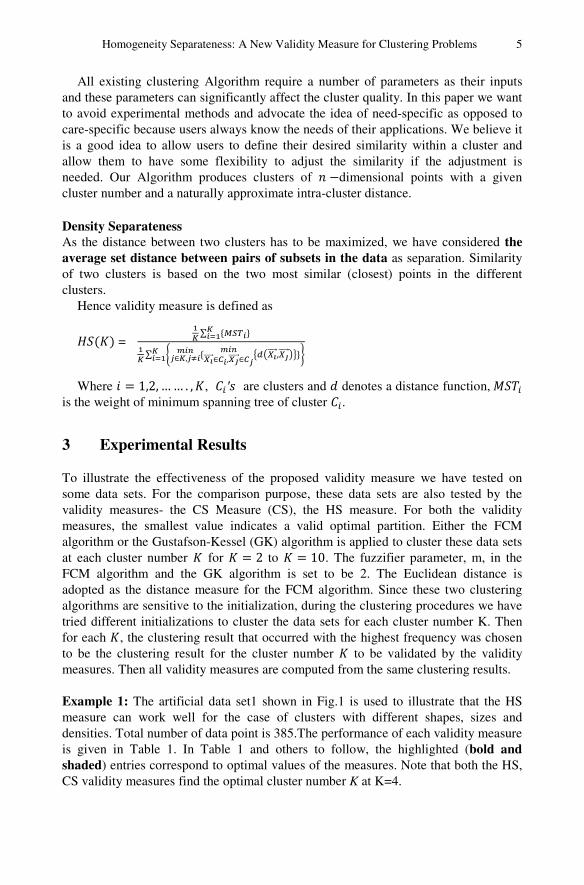
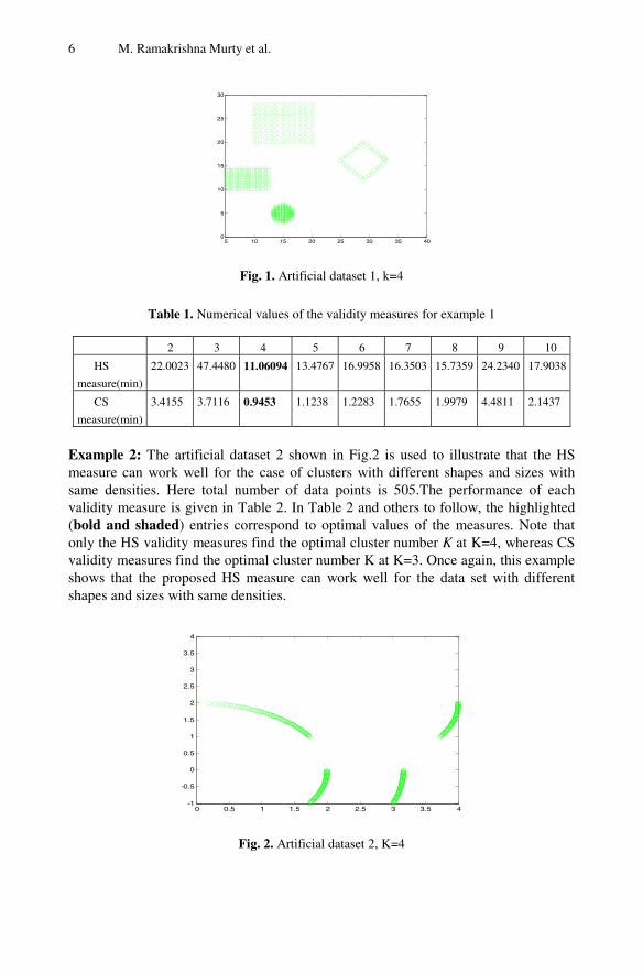
To illustrate the effectiveness of the proposed validity measure we have tested on some data sets. For the comparison purpose, these data sets are also tested by the validity measures- the CS Measure (CS), the HS measure. For both the validity measures, the smallest value indicates a valid optimal partition. Either the FCM algorithm or the Gustafson-Kessel (GK) algorithm is applied to cluster these data sets at each cluster number for = 2 to = 10. The fuzzifier parameter, m, in the FCM algorithm and the GK algorithm is set to be 2. The Euclidean distance is adopted as the distance measure for the FCM algorithm. Since these two clustering algorithms are sensitive to the initialization, during the clustering procedures we have tried different initializations to cluster the data sets for each cluster number K. Then for each , the clustering result that occurred with the highest frequency was chosen to be the clustering result for the cluster number to be validated by the validity measures. Then all validity measures are computed from the same clustering results. Example 1: The artificial data set1 shown in Fig.1 is used to illustrate that the HS measure can work well for the case of clusters with different shapes, sizes and densities. Total number of data point is 385.The performance of each validity measure is given in Table 1. In Table 1 and others to follow, the highlighted (bold and shaded) entries correspond to optimal values of the measures. Note that both the HS, CS validity measures find the optimal cluster number K at K=4.
6 M. Ramakrishna Murty et al.
Fig. 1. Artificial dataset 1, k=4
Table 1. Numerical values of the validity measures for example 1
2 3 4 5 6 7 8 9 10
HS
measure(min)
22.0023 47.4480 11.06094 13.4767 16.9958 16.3503 15.7359 24.2340 17.9038
CS
measure(min)
3.4155 3.7116 0.9453 1.1238 1.2283 1.7655 1.9979 4.4811 2.1437
Example 2: The artificial dataset 2 shown in Fig.2 is used to illustrate that the HS measure can work well for the case of clusters with different shapes and sizes with same densities. Here total number of data points is 505.The performance of each validity measure is given in Table 2. In Table 2 and others to follow, the highlighted (bold and shaded) entries correspond to optimal values of the measures. Note that only the HS validity measures find the optimal cluster number K at K=4, whereas CS validity measures find the optimal cluster number K at K=3. Once again, this example shows that the proposed HS measure can work well for the data set with different shapes and sizes with same densities.
Fig. 2. Artificial dataset 2, K=4
0 0.5 1 1.5 2 2.5 3 3.5 4-1
-0.5
0
0.5
1
1.5
2
2.5
3
3.5
4
5 10 15 20 25 30 35 400
5
10
15
20
25
30
Homogeneity Separateness: A New Validity Measure for Clustering Problems 7
Table 2. Numerical values of the validity measures for example 2
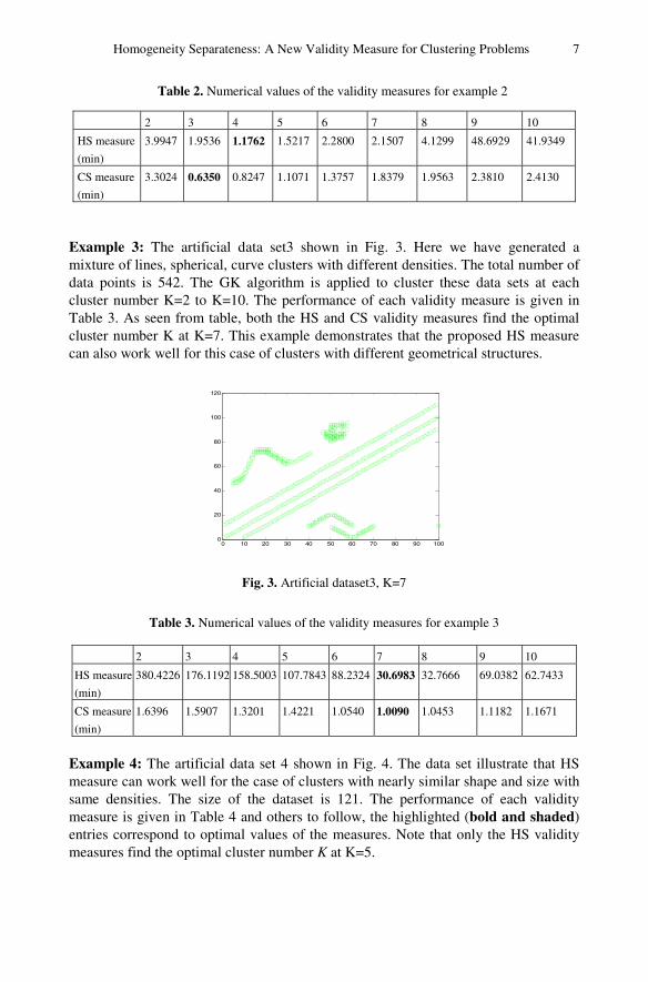
Example 3: The artificial data set3 shown in Fig. 3. Here we have generated a mixture of lines, spherical, curve clusters with different densities. The total number of data points is 542. The GK algorithm is applied to cluster these data sets at each cluster number K=2 to K=10. The performance of each validity measure is given in Table 3. As seen from table, both the HS and CS validity measures find the optimal cluster number K at K=7. This example demonstrates that the proposed HS measure can also work well for this case of clusters with different geometrical structures.
Fig. 3. Artificial dataset3, K=7
Table 3. Numerical values of the validity measures for example 3
2 3 4 5 6 7 8 9 10
HS measure
(min)
380.4226 176.1192 158.5003 107.7843 88.2324 30.6983 32.7666 69.0382 62.7433
CS measure
(min)
1.6396 1.5907 1.3201 1.4221 1.0540 1.0090 1.0453 1.1182 1.1671
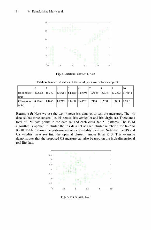
Example 4: The artificial data set 4 shown in Fig. 4. The data set illustrate that HS measure can work well for the case of clusters with nearly similar shape and size with same densities. The size of the dataset is 121. The performance of each validity measure is given in Table 4 and others to follow, the highlighted (bold and shaded) entries correspond to optimal values of the measures. Note that only the HS validity measures find the optimal cluster number K at K=5.
2 3 4 5 6 7 8 9 10
HS measure
(min)
3.9947 1.9536 1.1762 1.5217 2.2800 2.1507 4.1299 48.6929 41.9349
CS measure
(min)
3.3024 0.6350 0.8247 1.1071 1.3757 1.8379 1.9563 2.3810 2.4130
0 10 20 30 40 50 60 70 80 90 1000
20
40
60
80
100
120
8 M. Ramakrishna Murty et al.
Fig. 4. Artificial dataset 4, K=5
Table 4. Numerical values of the validity measures for example 4
Example 5: Here we use the well-known iris data set to test the measures. The iris data set has three subsets (i.e. iris setosa, iris versicolor and iris virginica). There are a total of 150 data points in the data set and each class had 50 patterns. The FCM algorithm is applied to cluster the iris data set at each cluster number c for K=2 to K=10. Table 5 shows the performance of each validity measure. Note that the HS and CS validity measures find the optimal cluster number K at K=3. This example demonstrates that the proposed CS measure can also be used on the high-dimensional real life data.
Fig. 5. Iris dataset, K=3
-5 0 5 10 15 205
10
15
20
25
30
2 3 4 5 6 7 8 9 10
HS measure
(min)
69.5208 15.3391 13.5281 8.5638 12.3394 10.8566 15.0347 13.2593 11.6142
CS measure
(min)
4.1669 1.1655 1.0223 1.0698 1.4352 1.2124 1.2931 1.3414 1.6383
2 2.5 3 3.5 4 4.54
4.5
5
5.5
6
6.5
7
7.5
8
Homogeneity Separateness: A New Validity Measure for Clustering Problems 9
Table 5. Numerical values of the validity measures for example 5
2 3 4 5 6 7 8 9 10
HS measure
(min)
60.5260 19.2111 57.7374 50.0703 30.4849 24.6778 21.0893 20.4061 19.3700
CS measure
(min)
0.7029 0.6683 0.7589 0.7375 1.5693 1.7164 1.0297 1.1593 1.8513
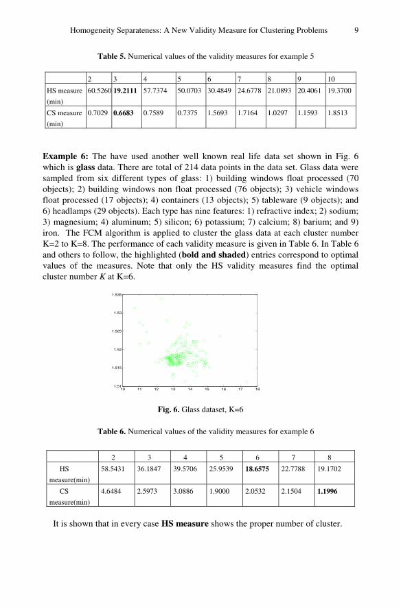
Example 6: The have used another well known real life data set shown in Fig. 6 which is glass data. There are total of 214 data points in the data set. Glass data were sampled from six different types of glass: 1) building windows float processed (70 objects); 2) building windows non float processed (76 objects); 3) vehicle windows float processed (17 objects); 4) containers (13 objects); 5) tableware (9 objects); and 6) headlamps (29 objects). Each type has nine features: 1) refractive index; 2) sodium; 3) magnesium; 4) aluminum; 5) silicon; 6) potassium; 7) calcium; 8) barium; and 9) iron. The FCM algorithm is applied to cluster the glass data at each cluster number K=2 to K=8. The performance of each validity measure is given in Table 6. In Table 6 and others to follow, the highlighted (bold and shaded) entries correspond to optimal values of the measures. Note that only the HS validity measures find the optimal cluster number K at K=6.
Fig. 6. Glass dataset, K=6
Table 6. Numerical values of the validity measures for example 6
It is shown that in every case HS measure shows the proper number of cluster.
10 11 12 13 14 15 16 17 181.51
1.515
1.52
1.525
1.53
1.535
2 3 4 5 6 7 8
HS
measure(min)
58.5431 36.1847 39.5706 25.9539 18.6575 22.7788 19.1702
CS
measure(min)
4.6484 2.5973 3.0886 1.9000 2.0532 2.1504 1.1996
10 M. Ramakrishna Murty et al.
4 Conclusion
In this paper, we first propose the HS measure to evaluate clustering results. The performance of the proposed HS measure is compared with popular CS measure on several data sets of both synthesis and real data sets. When HS index was compared with CS index, it always obtained better results. We hope that the procedure discussed here stimulates further investigation into development of better procedures for problems of clustering for data sets.
References
1. Hartigan, J.A.: Clustering Algorithms. Wiley Series in Probability and Mathematical statistics (1975)
2. Milligan, G.W., Cooper, M.C.: An examination of procedures for determining the number of clusters in a data set. Psychimetrika 50, 159–179 (1985)
3. Dubes, R., Jain, A.K.: Validity studies in clustering methodologies. Pattern Recognition 11, 235–253 (1979)
4. Chou, C.-H., Su, M.-C., Lai, E.: A new cluster validity measure and its application to image compression. Pattern Anal. Applic. 7, 205–220 (2004), doi:10.1007/s10044-004-0218-1
5. Gath, I., Geva, A.B.: Unsupervised optimal fuzzy clustering. IEEE Trans. Pattern Anal. Machine Intell. 11, 773–781 (1989)
6. Gustafson, D.E., Kessel, W.C.: Fuzzy clustering with a fuzzy covariance matrix. In: Proceedings of the IEEE Conference on Decision and Control, San Diego, pp. 761–766 (January 1979)
7. Halkidi, M., Vazirgiannis, M.: Clustering validity assessment: Finding the optimal partitioning of a data set. In: Proc. IEEE ICDM, San Jose, CA, pp. 187–194 (2001)
8. Babuška, R., van der Veen, P.J., Kaymak, U.: Improved Covariance Estimation for Gustafson-Kessel Clustering, 0-7803-7280-8/02/$10.00 ©2002. IEEE (2002)
9. Prim, R.: Shortest connection networks and some generalization. Bell Systems Technical Journal 36, 1389–1401 (1957)
10. Kruskal, J.: On the shortest spanning subtree and the travelling salesman problem. In: Proceedings of the American Mathematical Society, pp. 48–50 (1956)
11. Nesetril, J., Milkova, E., Nesetrilova, H.: Otakar boruvka on minimum spanning tree problem: Translation of both the 1926 papers, comments, history. DMATH: Discrete Mathematics 233 (2001)
12. Zahn, C.: Graph-theoretical methods for detecting and describing gestalt clusters. IEEE Transactions on Computers C-20, 68–86 (1971)
13. Preparata, F., Shamos, M.: Computational Geometry: An Introduction. Springer, Newyork (1985)
14. Asano, T., Bhattacharya, B., Keil, M., Yao, F.: Clustering Algorithms based on minimum and maximum spanning trees. In: Proceedings of the 4th Annual Symposium on Computational Geometry, pp. 252–257 (1988)
15. Dunn, J.C.: A Fuzzy Relative of the ISODATA Process and its Use in Detecting Compact Well-Separated Clusters. Journal Cybern. 3(3), 32–57 (1973)
16. Davies, D.L., Bouldin, D.W.: A cluster separation measure. IEEE Trans. Pattern Analysis and Machine Intelligence 1(4), 224–227 (1979)
S.C. Satapathy et al. (eds.), ICT and Critical Infrastructure: Proceedings of the 48th Annual Convention of CSI - Volume I, Advances in Intelligent Systems and Computing 248,
11
DOI: 10.1007/978-3-319-03107-1_2, © Springer International Publishing Switzerland 2014
Authenticating Grid Using Graph Isomorphism Based Zero Knowledge Proof
Worku B. Gebeyehu*, Lubak M. Ambaw*, M.A. Eswar Reddy, and P.S. Avadhani
Dept. of Computer Science & Systems Engineering, Andhra University, India {workubrhn,eswarreddy143}@gmail.com, {rosert2007,psavadhani}@yahoo.com
Abstract. A zero-Knowledge proof is a method by which the prover can prove to the verifier that the given statement is valid, without revealing any additional information apart from the veracity of the statement. Zero knowledge protocols have numerous applications in the domain of cryptography; they are commonly used in identification schemes by forcing adversaries to behave according to a predetermined protocol. In this paper, we propose an approach using graph isomorphism based zero knowledge proof to construct an efficient grid authentication mechanism. We demonstrate that using graph isomorphism based zero knowledge proof provide a much higher level of security when compared to other authentication schemes. The betterment of security arises from the fact that the proposed method hides the secret during the entire authentication process. Moreover, it enables one identity to be used for various accounts.
Keywords: Zero Knowledge proof, zero knowledge protocol, graph isomorphism, grid authentication, grid security, graph, prover, verifier.
1 Introduction
The intention of authentication and authorization is to deploy the policies which organizations have devised to administer the utilization of computing resources in the grid environment. According to Foster in grid technology is described as a “resource-sharing technology with software and services that let people access computing power, databases, and other tools securely online across corporate, institutional, and geographic boundaries without sacrificing local autonomy”[1]. For example a scientist in research institute might need to use regional, national, or international resources within grid-based projects in addition to using the major network of the campus. Each grid-project mainly requires its own authentication mechanisms, commonly in the form of GSI based or kerberos based certificates so as to authenticate the scientist to access and utilize grid based resources.
* Corresponding authors.
12 W.B. Gebeyehu et al.
These days, computer scientists are exerting lots of efforts to develop different kinds of authentication mechanisms that provide strong Grid security. The currently existing grid authentication mechanisms are usually bound with only one, in most cases based on public key infrastructure (PKI). Such system unnecessarily limits users since they are required to use only the one mechanism, which may not be flexible or convenient.
Moreover, regardless of particular type of certificates or PKI, one of the key drawbacks of the PKI is that current tools and producers for certificate management are too complicated for users. This leads either to rejection of the PKI or to insecure private-key management, which dis-empowers all the Grid infrastructure [2]. This paper proposes a novel methodology to overcome the aforementioned limitations by implementing ZKP based grid authentication.
2 Basic Concepts
2.1 What Is Zero-Knowledge Proof?
A zero-knowledge proof (ZKP) is a proof of some statement which reveals nothing other than the veracity of the statement. Zero-Knowledge proof is a much popular concept used in many cryptography systems. In this concept, two parties are involved, the prover A and the verifier B. Using this technique, it allows prover A to show that he has a credential, without having to give B the exact number.
The reason for the use of a Zero-Knowledge Proof in this situation for an authentication system is because it has the following properties:
Completeness: If an honest verifier will always be convinced of a true
statement by an honest prover Soundness: If a cheating prover can convince an honest verifier that some
false statement is actually true with only a small probability. Zero-knowledge: if the statement is true, the verifier will not know anything
other than that the statement is true.
Information about the details of the statement will not be revealed. [3]. A common application for zero-knowledge protocols is in identification schemes, due to Feige, Fiat, and Shamir[4].
2.2 Graph
A graph is a set of nodes or vertices V, connected by a set of edges E. The sets of vertices and edges are finite. A graph with n vertices will have: V = {1, 2, 3,..., n} and E a 2-element subsets of V. Let u and v be two vertices of a graph. If (u,v)ЄE, then u and v are said to be adjacent or neighbors.
Authenticating Grid Using Graph Isomorphism Based Zero Knowledge Proof 13
A graph is represented by its adjacency matrix. For instance, a graph with n vertices, is represented by a nxn matrix M=[m i,j] , where the entry is “1” if there is an edge linking the vertex i to the vertex j, and is “0” otherwise. For undirected graphs, the adjacency matrix is symmetric around the diagonal.
2.3 Graph Isomorphism
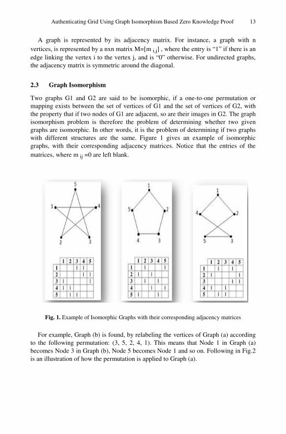
Two graphs G1 and G2 are said to be isomorphic, if a one-to-one permutation or mapping exists between the set of vertices of G1 and the set of vertices of G2, with the property that if two nodes of G1 are adjacent, so are their images in G2. The graph isomorphism problem is therefore the problem of determining whether two given graphs are isomorphic. In other words, it is the problem of determining if two graphs with different structures are the same. Figure 1 gives an example of isomorphic graphs, with their corresponding adjacency matrices. Notice that the entries of the matrices, where m ij =0 are left blank.
Fig. 1. Example of Isomorphic Graphs with their corresponding adjacency matrices
For example, Graph (b) is found, by relabeling the vertices of Graph (a) according to the following permutation: (3, 5, 2, 4, 1). This means that Node 1 in Graph (a) becomes Node 3 in Graph (b), Node 5 becomes Node 1 and so on. Following in Fig.2 is an illustration of how the permutation is applied to Graph (a).

14 W.B. Gebeyehu et al.
Fig. 2. Relabeling the vertices of Graph (a) using the permutation (3,5,2,4,1)
3 Proposed Method
3.1 Graph Isomorphism Based Zero-Knowledge Proofs
The purpose of Zero-Knowledge Proof (ZKP) protocols is to enable the prover to prove an assertion to the verifier that he holds some secret knowledge ,without leaking any information about the knowledge during the verification process (zero-knowledge).To demonstrate this concept ,we chose to implement ZKP protocol based on Graph Isomorphism (GI).In this protocol the input to the prover and the verifier is a pair of graphs G0 , G1 , and the goal of the prover is to convince the verifier that the graphs are isomorphic, but without revealing any information. If G0 and G1 are isomorphic, then the prover also has a permutation π such that π(G0 ) = G1 (i.e., π is an isomorphism).
Suppose we have two graphs G1 and G2 where G2 is generated from G1 using a secret permutation named π. G2 is obtained by relabeling the vertices of G1 according to secret permutation π by preserving the edges. The pair of graphs G1 and G2 forms the public key pair, and the permutation π serves as the private key. A third graph Q is either obtained from G1 or G2 using another random permutation ρ. Once the graph Q is found, the prover (represents the new node seeking entrance to the grid)sends it to the verifier who will challenge him to provide the permutation σ which can map Q to either G1 or G2.
For example, if Q is found from G1 and the verifier puts a challenge to the prover to map Q to G1, then σ = ρ-1. In the same fashion, if Q is obtained from G2 and the verifier challenges the prover to map Q to G2, then σ = ρ-1. Otherwise, if Q is obtained from G1 and the verifier puts a challenge to the prover to provide the permutation that maps Q to G2, then σ = ρ -1 ○ π, which is a combination of ρ-1and π. Indeed, ρ-1will be applied to Q to obtain G1 then the vertices of G1 will be modified according to the secret permutation π to get G2. Eventually, if Q is obtained from G2 and the verifier challenges the prover to map Q to G1, then σ = ρ-1○ π-1.
Authenticating Grid Using Graph Isomorphism Based Zero Knowledge Proof 15
One can observe that in the first two cases, the secret permutation π is not even used. Thus, a verifier could only be certain of a node’s identity after many interactions. Moreover, we can also observe that during the whole interaction process, no clue was given about the secret itself this makes it strong grid authentication mechanism.
3.2 Pseudo Code
Given G1 and G2 such that G2 = π (G1), the interactions constituting iterations of the graph isomorphism based ZKP protocol are demonstrated below:
Step 1: Prover randomly selects x Є {1,2} Step 2: Prover selects a random permutation ρ, and generates Q=ρ(Gx) Step 3: Prover communicates the adjacency matrix of Q to the verifier Step 4: Verifier communicates y Є {1,2}to prover and challenges for σ that maps
Q to Gy Step 5: If x=y the prover sends σ = ρ-1 to the verifier
Step 6: If x=1 and y=2 the prover sends σ = ρ-1 о π to the verifier Step 7: If x=2 and y=1 the prover sends σ = ρ-1 о π-1 to the verifier Step 8: Verifier checks if σ (Q)=Gy and access is granted to the prover accordingly
A number of iterations of these interactions are needed for the verifier to be totally convinced of the prover’s identity, as the prover can be lucky and guess the value of y before sending Q.
3.3 Prototype
The researchers have implemented a prototype version of graph isomorphism based ZKP protocol for authenticating a grid. Graph isomorphism has been chosen because of its ease of implementation. The JAVA-implementation of the ZKP protocol in authentication of the grid is presented below. The advantage of this implementation is that it allows us to verify the adjacency matrices at each level of the simulation and to evaluate the correctness of the algorithm. The JAVA implementations are mainly based on the pseudo-code provided in Pseudo code section above. So as to demonstrate the logic used in the program, we considered a simple graph with 4(four) nodes. In reality, however, the graphs need to be very large, consisting of several hundreds of nodes (in our case the number of users requesting for grid resources), and present a GI complexity in the order of NP-complete.
There are three functions that are used in the implementation, namely, “Generate_Isomorphic”, “Permutuate”, and “Compare_Graphs” also one main function.
a) “Generate_Isomorphic” function Generate_Isomorphic function enables us to apply a random permutation (π or ρ)
to a specific graph and to get another graph that is isomorphic to the first graph. For example, the declaration G2=Generate_Isomorphic(G1,pi,n)” is used to apply π to the
16 W.B. Gebeyehu et al.
graph G1 so as to get the graph G2; where the variable „n‟ represents the number of nodes in the graph( the number of users requesting for grid resources).
b) “Permutuate” function This function is used after receiving the challenge response from the prover.
Indeed, once the verifier receives σ from the prover, his objective is to apply that permutation to the graph Q to check if he will get the expected response G1 or G2. This function is declared as follows, “Permutuate (Q,sigma,n)” where σ is being applied to a graph Q.
c) “Compare_Graphs” function Once the verifier receives the response σ and applies it to Q to get another graph
that we will refer it as R for explanation purpose, the “Compare_Graphs” function is used to check whether or not R = G1 or R = G2 depending on the case.
The function is declared as “Compare_Graphs(G2,R,n).” Here, for instance, the function is used to compare both graphs G2 and R.
4 Simulations and Results
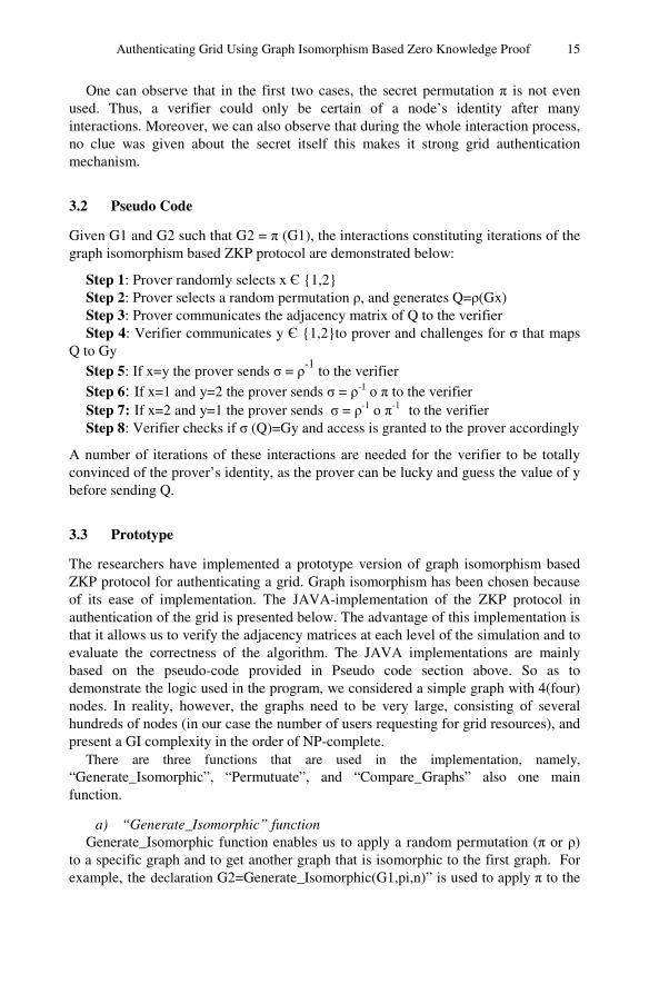
In this section we will depict how the implemented algorithm works through simulation. At first, the simulator requests for the value of “n” which represents the size of the graphs (In practise the number of grid users requesting for resource at one point of time). Once the size is set(the value of „n‟ is known), the user has the choice to either launch the interaction or to stop the simulation. The user is then prompted to provide the values of the graph G1. After all the values are entered, the user is asked for the value of the secret π and then for the value of the random permutation ρ. The user is then requested to choose the graph from which to create the graph Q and the graph that the verifier could ask the prover to generate when challenged. After these graphs are specified, the user is eventually asked for the value of σ. Once the value of σ entered, the simulator verifies all the inputs and declares if the prover is correct or incorrect. In other words, the simulator verifies if the prover knows the secret or not. In the real environment it is similar to proving the veracity of the grid user before allowing access to the grid. At last, the user is requested to repeat the process if he/she is willing. In order to test the correctness of the algorithm we simulate the code with some input examples and validate the results. In fact, the simulations were ran with the values of n, π, ρ and the graph G1 illustrated below.
Fig. 3. Graph G1 and its Adjacency Matrix representation
Authenticating Grid Using Graph Isomorphism Based Zero Knowledge Proof 17
If Q is obtained from G1 (Q = G1* ρ) and the verifier challenges for G1, we will have the equation:
σ = ρ-1 (1)
From equation 1 we have σ = ρ-1 = {1, 4, 2, 3} and to get the inverse of ρ = {1, 3, 4, 2}, we assign indices running from 1 to 4 to its vertices, and then process as follows. The first index “1” is at position 1, so its position remains the same. Index 2 is at the position 4; so the second vertex of ρ-1 is 4. Index 3 is at the second position; therefore the next vertex in ρ-1 is 2. Finally, index 4 is at the third position; therefore, the last element of ρ-1 is 3. Following this logic, the vertices of ρ-1 are obtained. If Q is obtained from G2 (Q = G2* ρ) and the verifier challenges for G2, we will have σ = ρ = {1, 4, 2, 3}.If Q is obtained from G1 (Q = G1* ρ) and the verifier challenges for G2, we will get the equation
σ = ρ-1○ π (2)
From equation 2 we have σ = ρ-1 ○ π = {1, 4, 2, 3} ○ {2, 3, 1, 4} = {2, 4, 3, 1}.To
equate and get the value of σ, we consider the vertices of ρ-1 as indices in π and observe which values they are associated with. The whole process consists of the following steps namely the first vertex of π is 2, the fourth vertex of π is 4. and the second vertex of π is 3 and the third vertex of π is 1. If Q is obtained from G2 (Q = G2* ρ) and the verifier challenges for G1, we will have the equation:
σ = ρ-1○ π-1 (3)
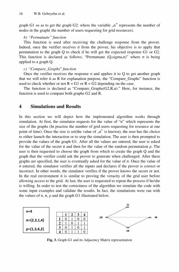
From equation 3 we have σ = ρ-1 ○ π-1 = {1, 4, 2,3} ○ {3, 1, 2, 4} = {3, 4, 1, 2}.Now that all the parameters are set, we can run the actual simulation. One can note that the permutations are applied to the rows as well as the columns of the adjacency matrix in the above process. Simulation results will be depicted in the following section so as to demonstrate the three different cases (i.e. σ ρ-1, σ = ρ-1 ○ π, and σ = ρ-
1 ○ π-1).
Fig. 4. Demonstration of the case in which Q = G1 *ρ and when the verifier challenges the prover to map Q to G1
18 W.B. Gebeyehu et al.
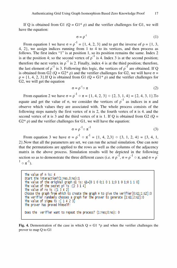
After the first simulations is over we obtained G2 = G1*π and Q = G1* ρ as depicted in figure 3 and figure 4 below respectively.
Fig. 5. Graph G2 in two distinct forms and its adjacency matrix
Fig. 6. Demonstration of graph Q = G1 * and its adjacency matrix
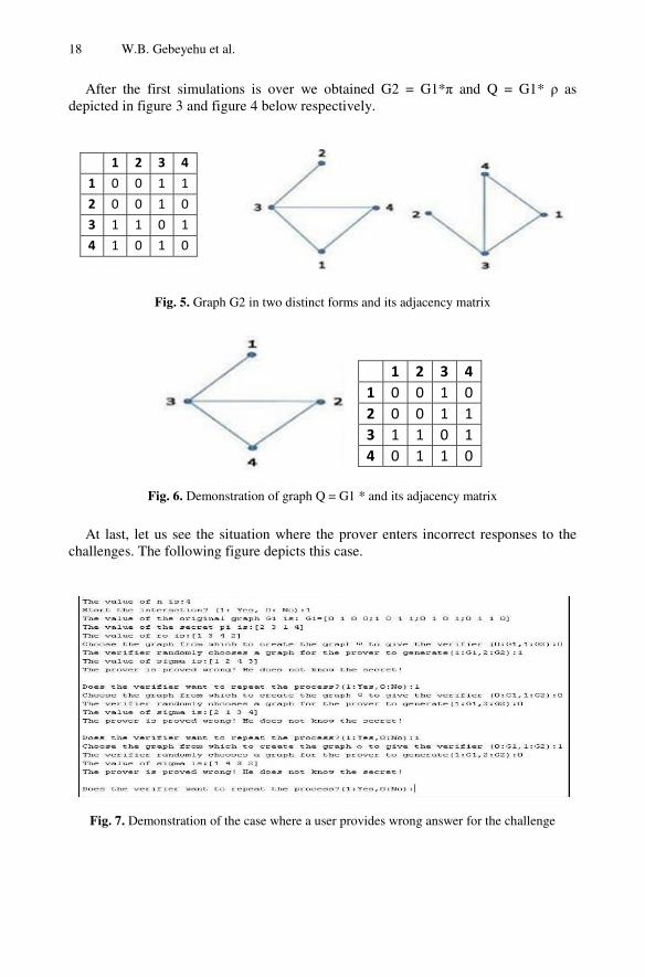
At last, let us see the situation where the prover enters incorrect responses to the challenges. The following figure depicts this case.
Fig. 7. Demonstration of the case where a user provides wrong answer for the challenge
Authenticating Grid Using Graph Isomorphism Based Zero Knowledge Proof 19
5 Conclusion and Future Work
A new approach for authenticating grid using ZKP protocol based on Graph Isomorphism (GI) is proposed. Our simulation results show that the proposed method provides a much higher level of security for authenticating users in the grid by hiding the secret during the entire authentication process. Besides, it enables one identity to be used for various accounts. The implementation could be modified further so that the system is interactive and user friendly. Moreover, one can integrate the implementation of graph isomorphism based zero knowledge proof within a grid portal.
References
[1] Foster, I.: The Physiology of the Grid: An Open Grid Services Architecture for Distributed Systems Integration. Wiley, Argonne Illinois (2002)
[2] Daniel, K., Ludek, M., Michal, P.: Survey of Authentication Mechanisms for Grids. In: CESNET Conference, pp. 200–204. Czech Academy of Science Press, Prague (2008)
[3] Lum, J.: Implementing Zero Knowledge Authentications with Zero Knowledge. In: The Python Papers Monograph Proceedings of PyCon Asia-Pacific, Melbourne (2010)
[4] Lior, M.: A Study of Perfect Zero-Knowledge Proofs, PhD Dissertation, University of Victoria, British Colombia, Victoria (2008)
S.C. Satapathy et al. (eds.), ICT and Critical Infrastructure: Proceedings of the 48th Annual Convention of CSI - Volume I, Advances in Intelligent Systems and Computing 248,
21
DOI: 10.1007/978-3-319-03107-1_3, © Springer International Publishing Switzerland 2014
Recognition of Marathi Isolated Spoken Words Using Interpolation and DTW Techniques
Ganesh B. Janvale1, Vishal Waghmare2, Vijay Kale3, and Ajit Ghodke4
1 Symbiosis International University, Symbiosis Centre for Information Technology, Pune-411 057(MS), India
2,3 Dept. of CS&IT, Dr. Babasaheb Ambedkar Marathwada University, Aurangabad-411004, India
4 Sinhgad Institute of Business Administration & Computer Application (SIBACA), Lonavala, India
[email protected], {vishal.pri12,vijaykale1685}@gmail.com, [email protected]
Abstract. This paper contains a Marathi speech database and isolated Marathi spoken words recognition system based on Mel-frequency cepstral coefficient (MFCC), optimal alignment using interpolation and dynamic time warping. Initially, Marathi speech database was designed and developed though Computerized Speech Laboratory. The database contained Marathi isolated words spoken by the 50 speakers including males and females. Mel-frequency Cepstral Coefficients were extracted and used for the recognition purpose. The 100% recognition rate for the isolated words have been achieved for both interpolation and dynamic time warping techniques.
Keywords: Speech Data base, CSL, MFCC, Speech Recognition and statistical method formatting.
1 Introduction
Currently, a lot of research is going on speech recognition and synthesis. The speech recognition understands basically what some speak to computer, asking a computer to translate speech into corresponding textual message, where as in speech synthesis, a computer generate artificial spoken dialogs. The speech is one of the natural forms of communication among the humans. The Marathi is an Indo-Aryan language, spoken in western and central India. There are 90 million of fluent speakers all over world [1][2]. The amount of work in Indian regional languages has not yet reached to a critical level to be used it as real communication tool, as already done in other languages in developed countries. Thus, this work was taken to focus on Marathi language. It is important to see that whether Speech Recognition System for Marathi can be carried out similar pathways of research as carried out in English [3]. Present work consists of the Marathi speech database and speech recognition system. The first part describes technical details of the database and second words recognition system. This paper is also split into four parts i.e. Introduction, Database, Words recognition System and Result and Conclusion.
22 G.B. Janvale et al.
2 Spoken Marathi Isolated Works Database
2.1 Features of Prosody in Marathi Words
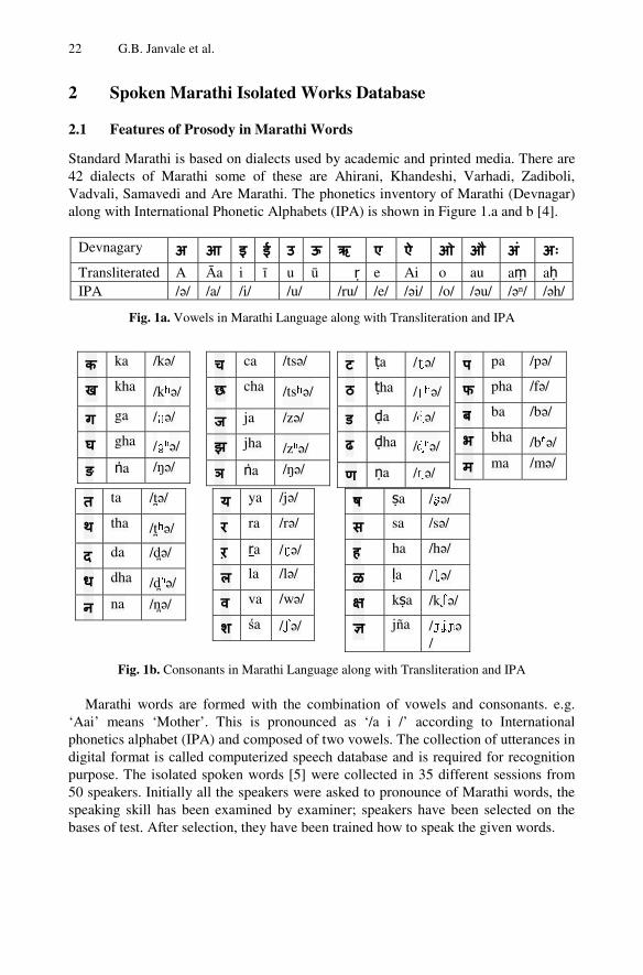
Standard Marathi is based on dialects used by academic and printed media. There are 42 dialects of Marathi some of these are Ahirani, Khandeshi, Varhadi, Zadiboli, Vadvali, Samavedi and Are Marathi. The phonetics inventory of Marathi (Devnagar) along with International Phonetic Alphabets (IPA) is shown in Figure 1.a and b [4].
Devnagary अ आ इ ई उ ऊ ऋ ए ऐ ओ औ अं अः Transliterated A Āa i ī u ū ṛ e Ai o au aṃ aḥ IPA /ə/ /a/ /i/ /u/ /ru/ /e/ /əi/ /o/ /əu/ /əⁿ/ /əh/
Fig. 1a. Vowels in Marathi Language along with Transliteration and IPA
Fig. 1b. Consonants in Marathi Language along with Transliteration and IPA
Marathi words are formed with the combination of vowels and consonants. e.g. ‘Aai’ means ‘Mother’. This is pronounced as ‘/a i /’ according to International phonetics alphabet (IPA) and composed of two vowels. The collection of utterances in digital format is called computerized speech database and is required for recognition purpose. The isolated spoken words [5] were collected in 35 different sessions from 50 speakers. Initially all the speakers were asked to pronounce of Marathi words, the speaking skill has been examined by examiner; speakers have been selected on the bases of test. After selection, they have been trained how to speak the given words.
क ka /kə/
ख kha /kʰə/
ग ga /ɡə/
घ gha /ɡʱə/
ङ ṅa /ŋə/
च ca /tsə/
छ cha /tsʰə/
ज ja /zə/
झ jha /zʱə/
ञ ṅa /ŋə/
ट ṭa /ʈə/
ठ ṭha /ʈʰə/
ड ḍa /ɖə/
ढ ḍha /ɖʱə/
ण ṇa /ɳə/
प pa /pə/
फ pha /fə/
ब ba /bə/
भ bha /bʱə/
म ma /mə/
त ta /t̪ə/
थ tha /t̪ʰə/
द da /d ̪ə/ ध dha /d ̪ʱə/ न na /n ̪ə/
य ya /jə/
र ra /rə/
ऱ ṟa /ɽə/
ल la /lə/
व va /wə/
श śa /ʃə/
ष ṣa /ʂə/
स sa /sə/
ह ha /hə/
ळ ḷa /ɭə/
kṣa /kʃə/
jña /ɟʝɲə/
Recognition of Marathi Isolated Spoken Words Using Interpolation 23
2.2 Acquisition Setup
The samples were recorded in 15 X 15 X 15 feet room with sampling frequency 11 KHz in normal temperature and humidity. The microphone was kept 5 – 7 cm from speakers. Whole speech database was collected with the help of Computerized Speech Laboratory (CSL). It is an input/output recording device for a PC, which has special features for reliable acoustic measurements. CSL offers input signal-to-noise performance typically 20-30dB. Analog Inputs with 4 channels two XLR and two phono-type, 5mV-10.5V peak-to-peak, channels 3 and 4, switchable AC or DC coupling, calibrated input, adjustable gain range >38dB, 24-bit A/D, Sampling rates::<-90dB F.S., 8000-200,000Hz, THD + NFrequency Response (AC coupled): 20 to 22kHz +.05dB at 44.1kHz [6][7].
2.3 Isolated Marathi Words Corpus
There are 12 vowels and 36 consonants in Marathi alphabets. Spoken words from the selected speakers were recorded and stored in different files and folders with respective to speakers’ initial names in the ‘wav’ format. The database was included mostly the words starting from each vowels, some of the words with phonetics.
3 Words Recognition System
The recognition system was developed using Mel – Frequency Cepstral Coefficient (MFCC) [8]. The following are the step to find the MFCC features.
3.1 Speech Signal
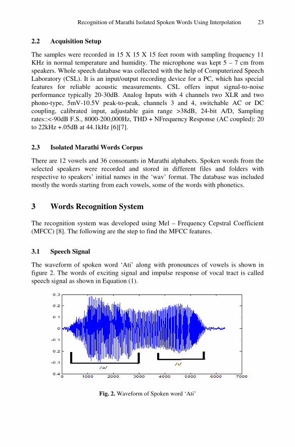
The waveform of spoken word ‘Ati’ along with pronounces of vowels is shown in figure 2. The words of exciting signal and impulse response of vocal tract is called speech signal as shown in Equation (1).
Fig. 2. Waveform of Spoken word ‘Ati’
24 G.B. Janvale et al.
][*][][ nnenS θ= (1)
Where, S[n], e[n] and θ[n] are speech signal, exciting signals and impulse response of vocal tract respectively.
3.2 Pre-emphasizing
Speech is emphasized with filter 1-az-1 where, “a” is between 0.9 and 1. In the time domain, the relationship between the output S’n and input Sn of the pre-emphasis by the default value of a ia 0.97 as shown in equation (2).
aSSS nnn 1
'*
−= (2)
3.3 Framing and Windowing
The signal is remained stationary at 20ms. Calculation of number of frame is done by multiplying the signal, consisting of N samples, with a rectangular window function of a finite length as shown in Equations (3), (4) and (5).
[ ] [ ] [ ]nWnSnS frames.= (3)
[ ] {12=nW (4)
1 - N ·r ≤ n < N ·(r+1), r = 0,1,2,3, ....., M−1 0- otherwise
tframefsN .= (5)
Where ‘M’ is the number of frames, ‘fs’ is the sampling frequency and tframe length of frame measured in time. The frame is shifted 10 ms so that the overlapping between two adjacent frames is to avoid the risk of losing the information from the speech signal. Each frame that contains nearly stationary signal blocks the windowing function is applied. There are a number of different windows functions to minimize the discontinuities. The Hamming window has a very good relative side lobe amplitude and good frequency resolution compared to the rectangular window. The window function is described by Equation (6).
−⋅⋅−=1
246.054.0][
N
nnx
π (6)
3.4 Fourier Transform
A 512 point Fast Fourier Transform was applied and calculated using equation 7, for good frequency resolution. The resolution of the frequency spectrum is primarily
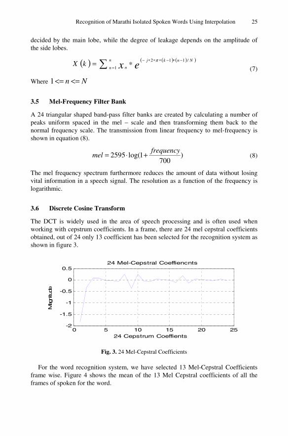
Recognition of Marathi Isolated Spoken Words Using Interpolation 25
decided by the main lobe, while the degree of leakage depends on the amplitude of the side lobes.
( ) ( ) ( )( ) =
−∗−∗∗∗−∗= n
n
Nnkj
n exkX1
/112 π
Where Nn <=<=1
(7)
3.5 Mel-Frequency Filter Bank
A 24 triangular shaped band-pass filter banks are created by calculating a number of peaks uniform spaced in the mel – scale and then transforming them back to the normal frequency scale. The transmission from linear frequency to mel-frequency is shown in equation (8).
)700
1log(2595frequency
mel +⋅= (8)
The mel frequency spectrum furthermore reduces the amount of data without losing vital information in a speech signal. The resolution as a function of the frequency is logarithmic.
3.6 Discrete Cosine Transform
The DCT is widely used in the area of speech processing and is often used when working with cepstrum coefficients. In a frame, there are 24 mel cepstral coefficients obtained, out of 24 only 13 coefficient has been selected for the recognition system as shown in figure 3.
Fig. 3. 24 Mel-Cepstral Coefficients
For the word recognition system, we have selected 13 Mel-Cepstral Coefficients frame wise. Figure 4 shows the mean of the 13 Mel Cepstral coefficients of all the frames of spoken for the word.
0 5 10 15 20 25-2
-1.5
-1
-0.5
0
0.5
24 Cepstrum Coeffients
Mag
nitu
de
24 Mel-Cepstral Coeffiencnts
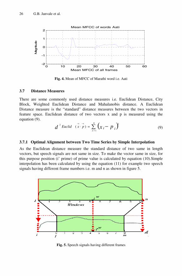
26 G.B. Janvale et al.
Fig. 4. Mean of MFCC of Marathi word i.e. Aati
3.7 Distance Measures
There are some commonly used distance measures i.e. Euclidean Distance, City Block, Weighted Euclidean Distance and Mahalanobis distance. A Euclidean Distance measure is the “standard” distance measures between the two vectors in feature space. Euclidean distance of two vectors x and p is measured using the equation (9).
( ) −=
→→=⋅
N
n
pxd iipxEuclid1
22)(
(9)
3.7.1 Optimal Alignment between Two Time Series by Simple Interpolation
As the Euclidean distance measure the standard distance of two same in length vectors, but speech signals are not same in size. To make the vector same in size, for this purpose position (i’ prime) of prime value is calculated by equation (10).Simple interpolation has been calculated by using the equation (11) for example two speech signals having different frame numbers i.e. m and n as shown in figure 5.
Fig. 5. Speech signals having different frames
0 10 20 30 40 50 60-2
-1
0
1
2
Mean MFCC of all frames
Mag
nitu
de
Mean MFCC of words Aati
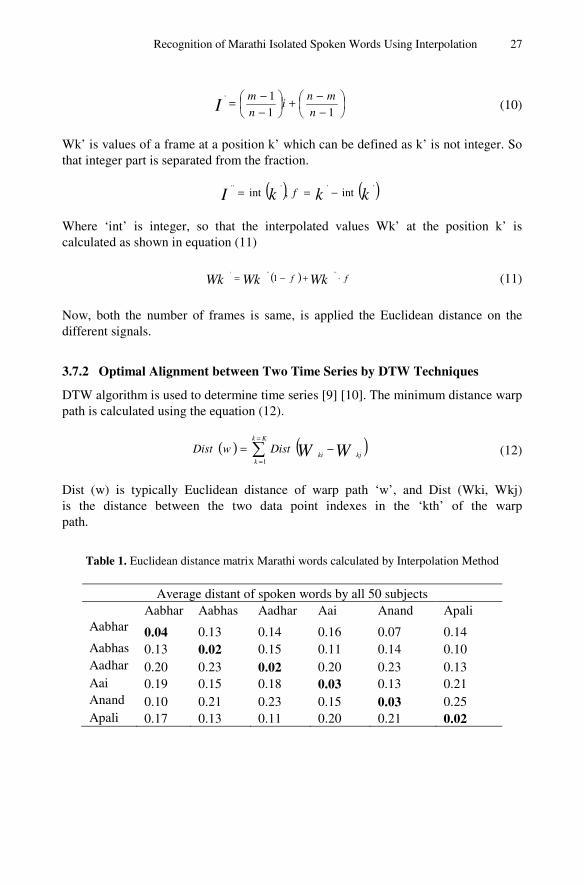
Recognition of Marathi Isolated Spoken Words Using Interpolation 27
−−+
−−=
11
1'
n
mni
n
mI (10)
Wk’ is values of a frame at a position k’ which can be defined as k’ is not integer. So that integer part is separated from the fraction.
( ) ( )kkkI f'''''
int,int −==
Where ‘int’ is integer, so that the interpolated values Wk’ at the position k’ is calculated as shown in equation (11)
( ) ff WkWkWk ⋅+−= '''''1 (11)
Now, both the number of frames is same, is applied the Euclidean distance on the different signals.
3.7.2 Optimal Alignment between Two Time Series by DTW Techniques
DTW algorithm is used to determine time series [9] [10]. The minimum distance warp path is calculated using the equation (12).
( ) ( )=
=
−=Kk
kkjki WWDistwDist
1
(12)
Dist (w) is typically Euclidean distance of warp path ‘w’, and Dist (Wki, Wkj) is the distance between the two data point indexes in the ‘kth’ of the warp path.
Table 1. Euclidean distance matrix Marathi words calculated by Interpolation Method
Average distant of spoken words by all 50 subjects Aabhar Aabhas Aadhar Aai Anand Apali Aabhar 0.04 0.13 0.14 0.16 0.07 0.14 Aabhas 0.13 0.02 0.15 0.11 0.14 0.10 Aadhar 0.20 0.23 0.02 0.20 0.23 0.13 Aai 0.19 0.15 0.18 0.03 0.13 0.21 Anand 0.10 0.21 0.23 0.15 0.03 0.25 Apali 0.17 0.13 0.11 0.20 0.21 0.02
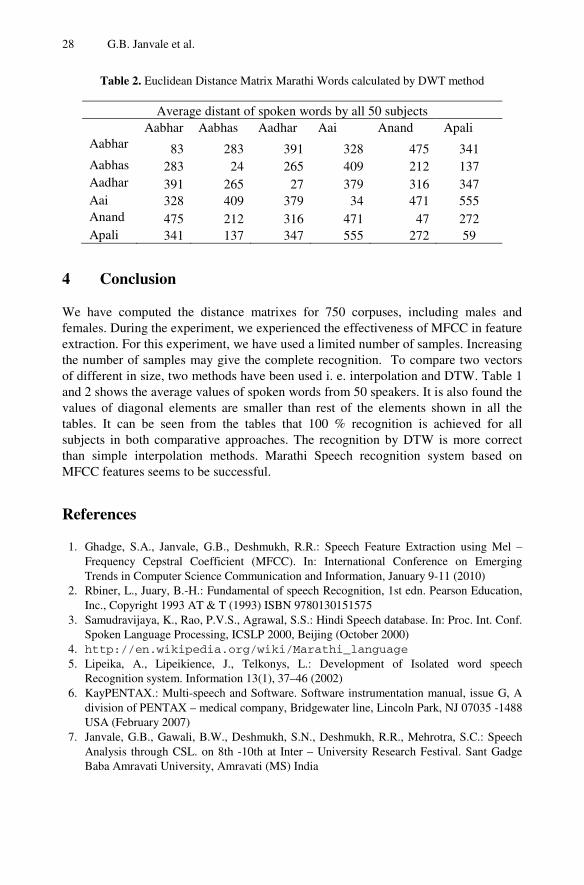
28 G.B. Janvale et al.
Table 2. Euclidean Distance Matrix Marathi Words calculated by DWT method
Average distant of spoken words by all 50 subjects Aabhar Aabhas Aadhar Aai Anand Apali Aabhar 83 283 391 328 475 341 Aabhas 283 24 265 409 212 137 Aadhar 391 265 27 379 316 347 Aai 328 409 379 34 471 555 Anand 475 212 316 471 47 272 Apali 341 137 347 555 272 59
4 Conclusion
We have computed the distance matrixes for 750 corpuses, including males and females. During the experiment, we experienced the effectiveness of MFCC in feature extraction. For this experiment, we have used a limited number of samples. Increasing the number of samples may give the complete recognition. To compare two vectors of different in size, two methods have been used i. e. interpolation and DTW. Table 1 and 2 shows the average values of spoken words from 50 speakers. It is also found the values of diagonal elements are smaller than rest of the elements shown in all the tables. It can be seen from the tables that 100 % recognition is achieved for all subjects in both comparative approaches. The recognition by DTW is more correct than simple interpolation methods. Marathi Speech recognition system based on MFCC features seems to be successful.
References
1. Ghadge, S.A., Janvale, G.B., Deshmukh, R.R.: Speech Feature Extraction using Mel – Frequency Cepstral Coefficient (MFCC). In: International Conference on Emerging Trends in Computer Science Communication and Information, January 9-11 (2010)
2. Rbiner, L., Juary, B.-H.: Fundamental of speech Recognition, 1st edn. Pearson Education, Inc., Copyright 1993 AT & T (1993) ISBN 9780130151575
3. Samudravijaya, K., Rao, P.V.S., Agrawal, S.S.: Hindi Speech database. In: Proc. Int. Conf. Spoken Language Processing, ICSLP 2000, Beijing (October 2000)
4. http://en.wikipedia.org/wiki/Marathi_language 5. Lipeika, A., Lipeikience, J., Telkonys, L.: Development of Isolated word speech
Recognition system. Information 13(1), 37–46 (2002) 6. KayPENTAX.: Multi-speech and Software. Software instrumentation manual, issue G, A
division of PENTAX – medical company, Bridgewater line, Lincoln Park, NJ 07035 -1488 USA (February 2007)
7. Janvale, G.B., Gawali, B.W., Deshmukh, S.N., Deshmukh, R.R., Mehrotra, S.C.: Speech Analysis through CSL. on 8th -10th at Inter – University Research Festival. Sant Gadge Baba Amravati University, Amravati (MS) India

Recognition of Marathi Isolated Spoken Words Using Interpolation 29
8. Sato, N., Obuchi, Y.: Emotion Recognition using Mel – Frequency Cepstral Coefficients. Journal of Natural Language processing 14(4), 83–96 (2007)
9. Keogh, E., Pazzani, M.: Derivative Dynamic Time Warping. In: International Processing of First Intl SIAM International Conference on Data Mining, Chicago, Illinoisi (2001)
10. Kruskall, J., Liberman, M.: The Symmetric Time Warping Problem: From continuous to Discrete. In: Time Warps String Edits and Macromolecules. The Theory and Practice of Sequence Comparison, pp. 125–161. Addison – Wesley Publication Co., Reading Massuchusetts (1983)
S.C. Satapathy et al. (eds.), ICT and Critical Infrastructure: Proceedings of the 48th Annual Convention of CSI - Volume I, Advances in Intelligent Systems and Computing 248,
31
DOI: 10.1007/978-3-319-03107-1_4, © Springer International Publishing Switzerland 2014
An Automatic Process to Convert Documents into Abstracts by Using Natural Language Processing
Techniques
Ch. Jayaraju, Zareena Noor Basha, E. Madhavarao, and M. Kalyani
Department of Computer Science & Engineering, Vignan’s Lara Institute of Technology and Science, Guntur, A.P., India
Abstract. Now a days each and every people using internet and collects the information. At the same time the internet is growing exponentially, huge amount of information is available online. That’s why the information overload problem is faced by every end user. So Automatic Process of Document Abstracts is recognized as an important task. For this intention we used various approaches these are Anaphora resolution, mining methods and TFxIDF. However these techniques have some limitations and mainly the drawback is from the end user’s perspective, the requestor may not be aware of all the knowledge that constitutes the methods. That’s why in this paper we focussed on developing Abstracts, that is Summarization method based on Natural Language Processing Techniques. At the same time it is also useful to multi-documents summarization. We explore some of the metrics and evaluation strategies, features in document abstracts or summarization.
Keywords: Information overload, TFxIDF, Natural Language Processing Techniques, Summarization.
1 Introduction
The Process of Documents to Abstracts has been a well-known field of computational linguists for many decades, but only recently has it been possible to advertise, these concepts. Abstract document is basically a short version or more purely we can state that it is a division of the original set. Text summarization is one of the segments of data preprocessing [1]. Abstracts or Summarization is also referred to as characterization [2]. The major design goal of summarization is to convey the same amount of information available in the original source text in a much smaller document. The study on Automatic Process of Documents to Abstracts has been initiated 40 years before. This area is highly interdisciplinary and related with artificial intelligence, Machine learning, natural language processing, information retrieval, information extraction. The abstract summaries are broadly categorized based on purpose, input and output. There are number of summaries be present [3].In that one of most important is Abstractive vs Extractive Summaries. Abstractive summaries or abstracts, involve identifying important parts of the source document
32 Ch. Jayaraju et al.
and reformulating it in original terms. The phrase "important parts" here refer to the parts which contain significant information content related to the source document. Extractive summaries or extracts, involve selecting sentences, words, phrases and combining them together in a cohesive and coherent manner. Abstracts are a much harder problem because the second phase in the problem of generating grammatically correct memories using a natural language generator is hard. On this much of the research has been concentrated in finding effective algorithms and building up efficient systems, such as SMART, SUMMARIST, MEAD [4], and NEATS, which provided precious experience for future research. This paper has proposed a new viable summarizer using Natural Language Processing (NLP) techniques. The aim is to design a summarizer that not only processes traditional "smooth" documents, which are primarily textual documents with no structure, but also to process complex structured documents by retaining the structure. The paper is organized as follows. Section 2 says about the related work in this area. The proposed architecture is discussed in Section 3.
2 Related Work
Till now the researchers considered the rate of recurrence of the word combining the mining and document frequency. Semi-supervised learning (SSL) is one of the major learning techniques in Machine learning. It makes use of both labeled and unlabeled data for training. It assumes that amount of labeled data is very little compared to unlabeled data, which makes it a very practical alternative to supervised learning which uses only labeled data, which is very expensive. Does not consider the performance of the effective documents. Based on an iterative graph based ranking algorithm, Rada Mihalcea and Paul Tarau explained an approach for language autonomous extractive summarization. They presented that in spite of the language, their algorithm works efficiently. They did so by means of appraisal applied on single document summarization task. Those tasks were in Portuguese and as well as in English [5].
Inderjit S. Dhillon [6], worked on Theoretic Feature Clustering Algorithm for text classification, it tells about feature clustering, feature selection of word clusters. But have not considered the meaningful documents and text summarization for better search.
Finley Lacatusu et. al. elucidates a novel clustering based text summarization system that uses manifold sequence Alignment in order to enhance the arrangement of sentences contained by theme clusters .
Youngjoong KO, JinwooPark et al. explores improving text categorization using the importance of sentences. They discuss the importance of sentences using text summarization techniques. Four kinds of classifiers are used in this experiment. Naive bayes, Rocchio, KNN, and SVM. A supervised learning algorithm has been applied to this area using a training data set of categorized documents. The aim of this paper presented a new indexing method for text categorization using two kinds of text summarization techniques; one uses the TITLE and the other uses the IMPORTANCE of TERMS. And don’t considered the how important the document is and the
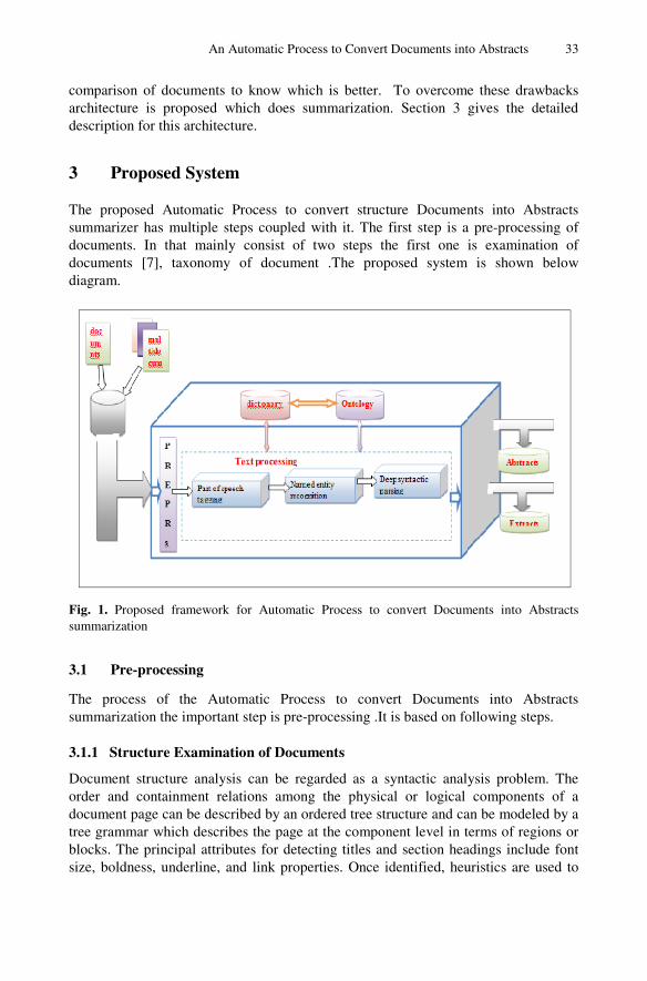
An Automatic Process to Convert Documents into Abstracts 33
comparison of documents to know which is better. To overcome these drawbacks architecture is proposed which does summarization. Section 3 gives the detailed description for this architecture.
3 Proposed System
The proposed Automatic Process to convert structure Documents into Abstracts summarizer has multiple steps coupled with it. The first step is a pre-processing of documents. In that mainly consist of two steps the first one is examination of documents [7], taxonomy of document .The proposed system is shown below diagram.
Fig. 1. Proposed framework for Automatic Process to convert Documents into Abstracts summarization
3.1 Pre-processing
The process of the Automatic Process to convert Documents into Abstracts summarization the important step is pre-processing .It is based on following steps.
3.1.1 Structure Examination of Documents
Document structure analysis can be regarded as a syntactic analysis problem. The order and containment relations among the physical or logical components of a document page can be described by an ordered tree structure and can be modeled by a tree grammar which describes the page at the component level in terms of regions or blocks. The principal attributes for detecting titles and section headings include font size, boldness, underline, and link properties. Once identified, heuristics are used to
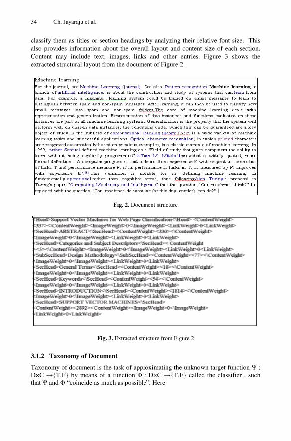
34 Ch. Jayaraju et al.
classify them as titles or section headings by analyzing their relative font size. This also provides information about the overall layout and content size of each section. Content may include text, images, links and other entries. Figure 3 shows the extracted structural layout from the document of Figure 2.
Fig. 2. Document structure
Fig. 3. Extracted structure from Figure 2
3.1.2 Taxonomy of Document
Taxonomy of document is the task of approximating the unknown target function Ψ : D×C →{T,F} by means of a function Φ : D×C →{T,F} called the classifier , such that Ψ and Φ “coincide as much as possible”. Here
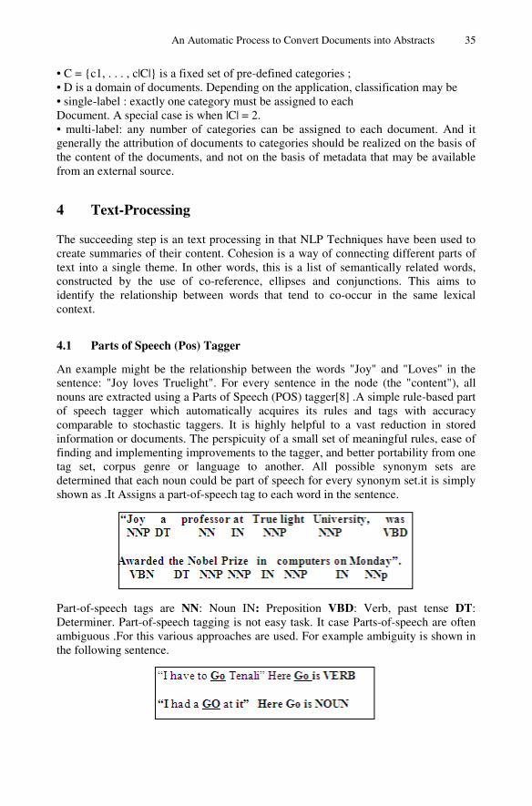
An Automatic Process to Convert Documents into Abstracts 35
• C = {c1, . . . , c|C|} is a fixed set of pre-defined categories ; • D is a domain of documents. Depending on the application, classification may be • single-label : exactly one category must be assigned to each Document. A special case is when |C| = 2. • multi-label: any number of categories can be assigned to each document. And it generally the attribution of documents to categories should be realized on the basis of the content of the documents, and not on the basis of metadata that may be available from an external source.
4 Text-Processing
The succeeding step is an text processing in that NLP Techniques have been used to create summaries of their content. Cohesion is a way of connecting different parts of text into a single theme. In other words, this is a list of semantically related words, constructed by the use of co-reference, ellipses and conjunctions. This aims to identify the relationship between words that tend to co-occur in the same lexical context.
4.1 Parts of Speech (Pos) Tagger An example might be the relationship between the words "Joy" and "Loves" in the sentence: "Joy loves Truelight". For every sentence in the node (the "content"), all nouns are extracted using a Parts of Speech (POS) tagger[8] .A simple rule-based part of speech tagger which automatically acquires its rules and tags with accuracy comparable to stochastic taggers. It is highly helpful to a vast reduction in stored information or documents. The perspicuity of a small set of meaningful rules, ease of finding and implementing improvements to the tagger, and better portability from one tag set, corpus genre or language to another. All possible synonym sets are determined that each noun could be part of speech for every synonym set.it is simply shown as .It Assigns a part-of-speech tag to each word in the sentence.
Part-of-speech tags are NN: Noun IN: Preposition VBD: Verb, past tense DT: Determiner. Part-of-speech tagging is not easy task. It case Parts-of-speech are often ambiguous .For this various approaches are used. For example ambiguity is shown in the following sentence.
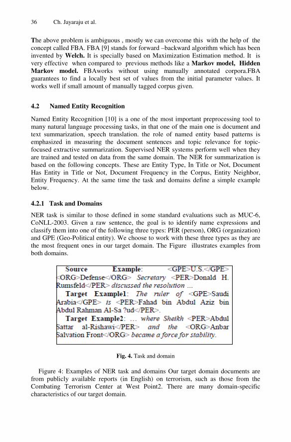
36 Ch. Jayaraju et al.
The above problem is ambiguous , mostly we can overcome this with the help of the concept called FBA. FBA [9] stands for forward –backward algorithm which has been invented by Welch. It is specially based on Maximization Estimation method. It is very effective when compared to previous methods like a Markov model, Hidden Markov model. FBAworks without using manually annotated corpora.FBA guarantees to find a locally best set of values from the initial parameter values. It works well if small amount of manually tagged corpus given.
4.2 Named Entity Recognition
Named Entity Recognition [10] is a one of the most important preprocessing tool to many natural language processing tasks, in that one of the main one is document and text summarization, speech translation. the role of named entity based patterns is emphasized in measuring the document sentences and topic relevance for topic-focused extractive summarization. Supervised NER systems perform well when they are trained and tested on data from the same domain. The NER for summarization is based on the following concepts. These are Entity Type, In Title or Not, Document Has Entity in Title or Not, Document Frequency in the Corpus, Entity Neighbor, Entity Frequency. At the same time the task and domains define a simple example below.
4.2.1 Task and Domains
NER task is similar to those defined in some standard evaluations such as MUC-6, CoNLL-2003. Given a raw sentence, the goal is to identify name expressions and classify them into one of the following three types: PER (person), ORG (organization) and GPE (Geo-Political entity). We choose to work with these three types as they are the most frequent ones in our target domain. The Figure illustrates examples from both domains.
Fig. 4. Task and domain
Figure 4: Examples of NER task and domains Our target domain documents are from publicly available reports (in English) on terrorism, such as those from the Combating Terrorism Center at West Point2. There are many domain-specific characteristics of our target domain.
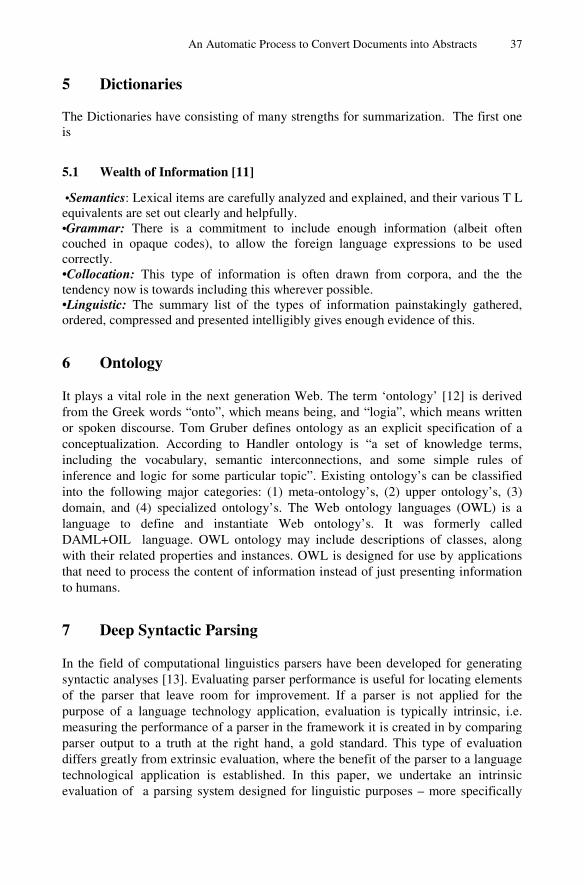
An Automatic Process to Convert Documents into Abstracts 37
5 Dictionaries
The Dictionaries have consisting of many strengths for summarization. The first one is
5.1 Wealth of Information [11]
•Semantics: Lexical items are carefully analyzed and explained, and their various T L equivalents are set out clearly and helpfully. •Grammar: There is a commitment to include enough information (albeit often couched in opaque codes), to allow the foreign language expressions to be used correctly. •Collocation: This type of information is often drawn from corpora, and the the tendency now is towards including this wherever possible. •Linguistic: The summary list of the types of information painstakingly gathered, ordered, compressed and presented intelligibly gives enough evidence of this.
6 Ontology
It plays a vital role in the next generation Web. The term ‘ontology’ [12] is derived from the Greek words “onto”, which means being, and “logia”, which means written or spoken discourse. Tom Gruber defines ontology as an explicit specification of a conceptualization. According to Handler ontology is “a set of knowledge terms, including the vocabulary, semantic interconnections, and some simple rules of inference and logic for some particular topic”. Existing ontology’s can be classified into the following major categories: (1) meta-ontology’s, (2) upper ontology’s, (3) domain, and (4) specialized ontology’s. The Web ontology languages (OWL) is a language to define and instantiate Web ontology’s. It was formerly called DAML+OIL language. OWL ontology may include descriptions of classes, along with their related properties and instances. OWL is designed for use by applications that need to process the content of information instead of just presenting information to humans.
7 Deep Syntactic Parsing
In the field of computational linguistics parsers have been developed for generating syntactic analyses [13]. Evaluating parser performance is useful for locating elements of the parser that leave room for improvement. If a parser is not applied for the purpose of a language technology application, evaluation is typically intrinsic, i.e. measuring the performance of a parser in the framework it is created in by comparing parser output to a truth at the right hand, a gold standard. This type of evaluation differs greatly from extrinsic evaluation, where the benefit of the parser to a language technological application is established. In this paper, we undertake an intrinsic evaluation of a parsing system designed for linguistic purposes – more specifically
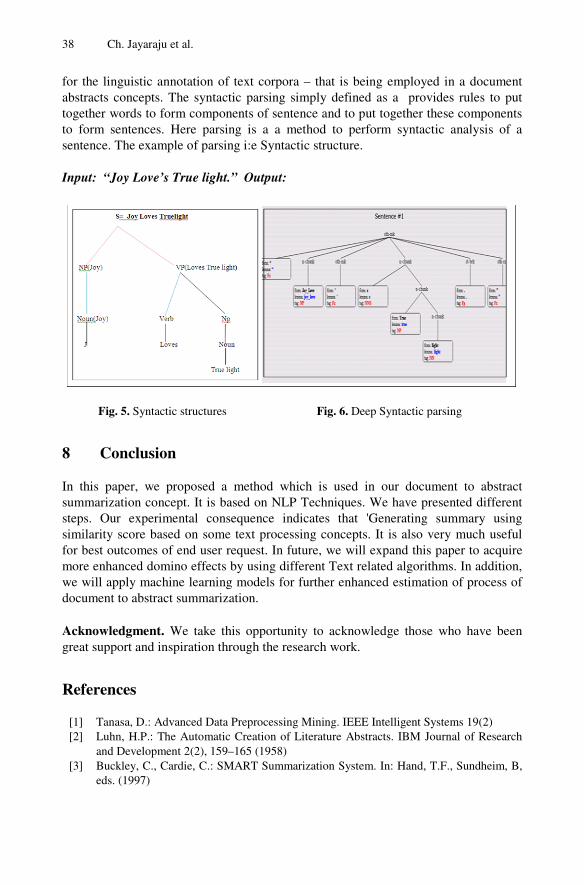
38 Ch. Jayaraju et al.
for the linguistic annotation of text corpora – that is being employed in a document abstracts concepts. The syntactic parsing simply defined as a provides rules to put together words to form components of sentence and to put together these components to form sentences. Here parsing is a a method to perform syntactic analysis of a sentence. The example of parsing i:e Syntactic structure. Input: “Joy Love’s True light.” Output:
Fig. 5. Syntactic structures Fig. 6. Deep Syntactic parsing
8 Conclusion
In this paper, we proposed a method which is used in our document to abstract summarization concept. It is based on NLP Techniques. We have presented different steps. Our experimental consequence indicates that 'Generating summary using similarity score based on some text processing concepts. It is also very much useful for best outcomes of end user request. In future, we will expand this paper to acquire more enhanced domino effects by using different Text related algorithms. In addition, we will apply machine learning models for further enhanced estimation of process of document to abstract summarization. Acknowledgment. We take this opportunity to acknowledge those who have been great support and inspiration through the research work.
References
[1] Tanasa, D.: Advanced Data Preprocessing Mining. IEEE Intelligent Systems 19(2) [2] Luhn, H.P.: The Automatic Creation of Literature Abstracts. IBM Journal of Research
and Development 2(2), 159–165 (1958) [3] Buckley, C., Cardie, C.: SMART Summarization System. In: Hand, T.F., Sundheim, B,
eds. (1997)
An Automatic Process to Convert Documents into Abstracts 39
[4] Radev, D.R., Jing, H., Budzikowska, M.: Summarization of multiple documents: clustering, sentence extraction, and evaluation. In: ANLP/NAACL Workshop on Summarization, Seattle, WA (April 2000)
[5] Dhillon, I.S.: A divisive information theoretic feature clustering algorithm for text classification. Journal of Machine Learning Research 3 (2003)
[6] Mihalcea, R., Tarau, P.: A Language Independent Algorithm for Single and Multiple Document Summarization. University of North Texas
[7] Alam, H., Kumar, A., Nakamura, M.: Structured and Unstructured Document Summarization: Design of a Commercial Summarizer using Lexical Chains
[8] Santorini, B.: Part-of-Speech Tagging Guidelines for the Penn Treebank Project [9] World of computing.net/pos-tagging/markov-models.html
[10] A survey of named entity recognition and classification David Nadeau. Satoshi Sekine National Research Council Canada / New York University
[11] dictionary generation for low-resourced language pairs Varga István Yamagata uNIVERSITY, Graduate School of Science and Engineering, [email protected]
[12] Ontology’s, Web 2.0 and Beyond. Keynote presentation at the Ontology Summit 2007 – Ontology, Taxonomy, Folksonomy: Understanding the Distinctions (March 1, 2007)
[13] Detecting Opinions Using Deep Syntactic Analysis Caroline Brun Xerox Research Centre Europe Meylan, France
S.C. Satapathy et al. (eds.), ICT and Critical Infrastructure: Proceedings of the 48th Annual Convention of CSI - Volume I, Advances in Intelligent Systems and Computing 248,
41
DOI: 10.1007/978-3-319-03107-1_5, © Springer International Publishing Switzerland 2014
A Novel Method for CBIR Using Texture Spectrum in Wavelet Domain
G. Rosline Nesa Kumari, M. Sudheer, and R. Tamilkodi
Godavari Institute of Engineering & Technology, Rajahmundry {rosemaruthu,maridisudheer}@gmail.com, [email protected]
Abstract. This paper presents an effective color image retrieval scheme by contrast based texture features, which achieves higher retrieval efficiency. The proposed method Texture Spectrum in Wavelet (TSW) domain is very fast to compute and enable to speed up the wavelet computation phase for thousands of sliding windows of varying sizes in an image. Proposed TSW provides a robust contrast features for image retrieval from a lot of objects in an image can be distinguished solely by their textures without any other information. The proposed system divides the lower resolution approximation image into four sections, where each section extracts 12 contrast features and stores the features of the query image and also all images in the database and extracts the features of each image. The proposed TSW method reduces the computation of possible patterns as well as fast and retrieving accurate images. Experimental results show that the proposed method for image retrieval is more accurate, efficient and quite understandable in spite of the availability of the existing retrieving algorithms.
Keywords: Image retrieval, Texture, Robust Feature, Query image, DWT.
1 Introduction
Multimedia data including images and videos have been dramatically increased in our life due to the popularity of digital devices and personal computers. Image searching is one of the most important services that need to be supported by such systems Content-Based Image Retrieval (CBIR) systems are used to extract feature vectors that represent image properties such as color, texture, and shape [1]. CBIR is originated with the work of Kato [2] for the automatic retrieval of the images from a database, based on the color and shape. Since CBIR has widely used to describe the process of retrieving desired images from a large collection of database. The CBIR system extracts and stores the features of the query image then it go through all images in the database and extract the features of each image.
In the decade, many image retrieval systems have been successfully developed, such as the IBM QBIC system[3], developed at the IBM Almaden Research Center, the VIRAGE System [6], developed by the Virage Incorporation, the Photo book System[8], developed by the MIT Media Lab, the Visual Seek System [7], developed at Columbia University, the WBIIS System [9], developed Stanford University, and the Blob world System[5], developed at U.C.Berkeley and SIMPLIcity System[4].
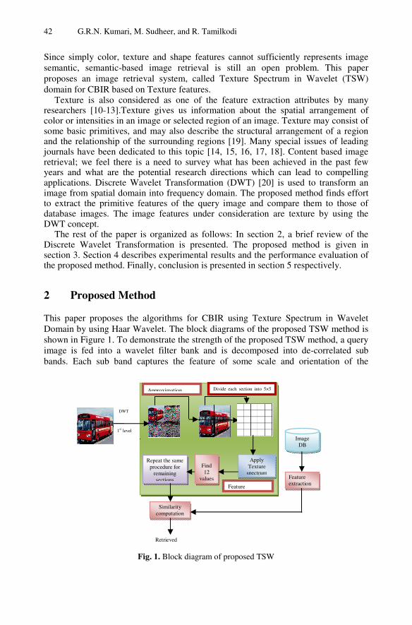
42 G.R.N. Kumari, M. Sudheer, and R. Tamilkodi
Since simply color, texture and shape features cannot sufficiently represents image semantic, semantic-based image retrieval is still an open problem. This paper proposes an image retrieval system, called Texture Spectrum in Wavelet (TSW) domain for CBIR based on Texture features.
Texture is also considered as one of the feature extraction attributes by many researchers [10-13].Texture gives us information about the spatial arrangement of color or intensities in an image or selected region of an image. Texture may consist of some basic primitives, and may also describe the structural arrangement of a region and the relationship of the surrounding regions [19]. Many special issues of leading journals have been dedicated to this topic [14, 15, 16, 17, 18]. Content based image retrieval; we feel there is a need to survey what has been achieved in the past few years and what are the potential research directions which can lead to compelling applications. Discrete Wavelet Transformation (DWT) [20] is used to transform an image from spatial domain into frequency domain. The proposed method finds effort to extract the primitive features of the query image and compare them to those of database images. The image features under consideration are texture by using the DWT concept.
The rest of the paper is organized as follows: In section 2, a brief review of the Discrete Wavelet Transformation is presented. The proposed method is given in section 3. Section 4 describes experimental results and the performance evaluation of the proposed method. Finally, conclusion is presented in section 5 respectively.
2 Proposed Method
This paper proposes the algorithms for CBIR using Texture Spectrum in Wavelet Domain by using Haar Wavelet. The block diagrams of the proposed TSW method is shown in Figure 1. To demonstrate the strength of the proposed TSW method, a query image is fed into a wavelet filter bank and is decomposed into de-correlated sub bands. Each sub band captures the feature of some scale and orientation of the
Fig. 1. Block diagram of proposed TSW
Apply Texture
spectrumFind 12
values
Repeat the same procedure for
remaining sections
Similarity computation
Image DB
Feature extraction
Divide each section into 5×5
DWT
1st level
Feature
Retrieved
Approximation
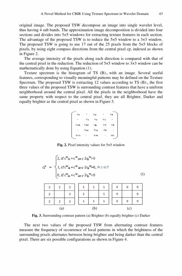
A Novel Method for CBIR Using Texture Spectrum in Wavelet Domain 43
original image. The proposed TSW decompose an image into single wavelet level, thus having 4 sub bands. The approximation image decomposition is divided into four sections and divides into 5×5 windows for extracting texture features in each section. The advantage of the proposed TSW is to reduce the 5×5 window to a 3×3 window. The proposed TSW is going to use 17 out of the 25 pixels from the 5×5 blocks of pixels, by using eight compass directions from the central pixel cp, indexed as shown in Figure 2.
The average intensity of the pixels along each direction is compared with that of the central pixel in the reduction. The reduction of 5×5 window to 3×3 window can be mathematically done by using Equation (1).
Texture spectrum is the histogram of TS (B)’s with an image. Several useful features, corresponding to visually meaningful patterns may be defined on the Texture Spectrum. The proposed TSW is extracting 12 values according to TS (B)’s. the first three values of the proposed TSW is surrounding contrast features that have a uniform neighborhood around the central pixel. All the pixels in the neighborhood have the same property with respect to the central pixel, they are all Brighter, Darker and equally brighter as the central pixel as shown in Figure 3.
Fig. 2. Pixel intensity values for 5×5 window
(a) (b) (c)
Fig. 3. Surrounding contrast pattern (a) Brighter (b) equally brighter (c) Darker
The next two values of the proposed TSW from alternating contrast features measure the frequency of occurrence of local patterns in which the brightness of the surrounding pixels alternates between being brighter and being darker than the central pixel. There are six possible configurations as shown in Figure 4.
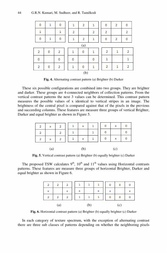
44 G.R.N. Kumari, M. Sudheer, and R. Tamilkodi
(a)
(b)
Fig. 4. Alternating contrast pattern (a) Brighter (b) Darker
These six possible configurations are combined into two groups. They are brighter and darker. These groups are 4-connected neighbors of collection patterns. From the vertical contrast patterns the next 3 values can be determined. This contrast pattern measures the possible values of x identical to vertical stripes in an image. The brightness of the central pixel is compared against that of the pixels in the previous and succeeding columns. These features are measure three groups of vertical Brighter, Darker and equal brighter as shown in Figure 5.
(a) (b) (c)
Fig. 5. Vertical contrast pattern (a) Brighter (b) equally brighter (c) Darker
The proposed TSW calculates 9th, 10th and 11th values using Horizontal contrasts patterns. These features are measure three groups of horizontal Brighter, Darker and equal brighter as shown in Figure 6.
(a) (b) (c)
Fig. 6. Horizontal contrast pattern (a) Brighter (b) equally brighter (c) Darker
In each category of texture spectrum, with the exception of alternating contrast there are three sub classes of patterns depending on whether the neighboring pixels
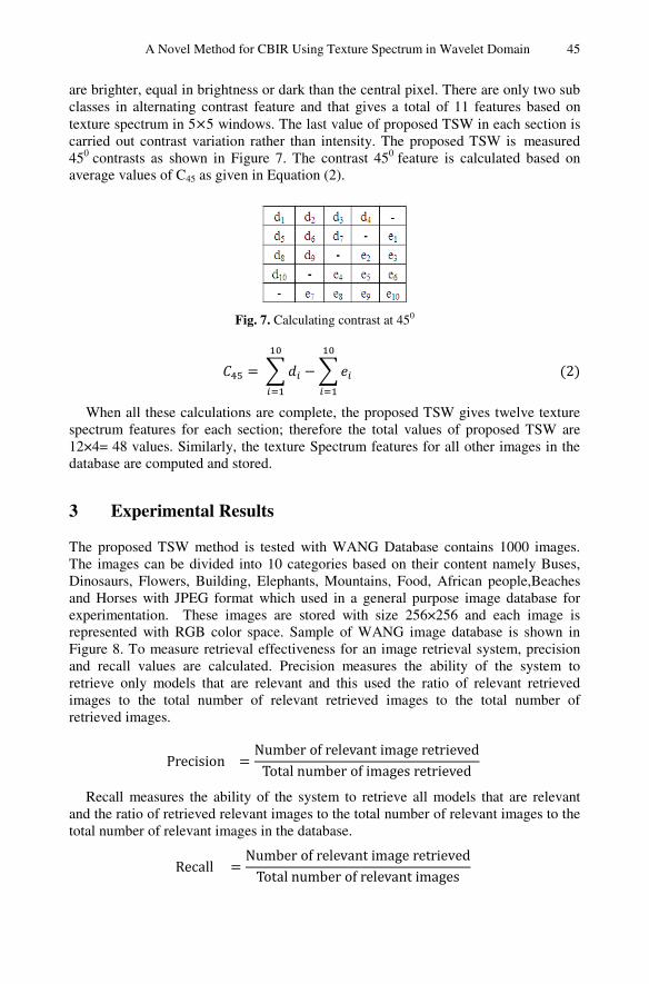
A Novel Method for CBIR Using Texture Spectrum in Wavelet Domain 45
are brighter, equal in brightness or dark than the central pixel. There are only two sub classes in alternating contrast feature and that gives a total of 11 features based on texture spectrum in 5×5 windows. The last value of proposed TSW in each section is carried out contrast variation rather than intensity. The proposed TSW is measured 450 contrasts as shown in Figure 7. The contrast 450 feature is calculated based on average values of C45 as given in Equation (2).
Fig. 7. Calculating contrast at 450
= − (2)
When all these calculations are complete, the proposed TSW gives twelve texture spectrum features for each section; therefore the total values of proposed TSW are 12×4= 48 values. Similarly, the texture Spectrum features for all other images in the database are computed and stored.
3 Experimental Results
The proposed TSW method is tested with WANG Database contains 1000 images. The images can be divided into 10 categories based on their content namely Buses, Dinosaurs, Flowers, Building, Elephants, Mountains, Food, African people,Beaches and Horses with JPEG format which used in a general purpose image database for experimentation. These images are stored with size 256×256 and each image is represented with RGB color space. Sample of WANG image database is shown in Figure 8. To measure retrieval effectiveness for an image retrieval system, precision and recall values are calculated. Precision measures the ability of the system to retrieve only models that are relevant and this used the ratio of relevant retrieved images to the total number of relevant retrieved images to the total number of retrieved images.
Precision = Number of relevant image retrievedTotal number of images retrieved Recall measures the ability of the system to retrieve all models that are relevant
and the ratio of retrieved relevant images to the total number of relevant images to the total number of relevant images in the database. Recall = Number of relevant image retrievedTotal number of relevant images
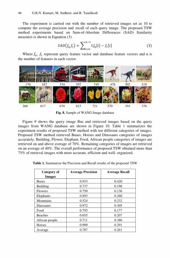
46 G.R.N. Kumari, M. Sudheer, and R. Tamilkodi
The experiment is carried out with the number of retrieved images set as 10 to compute the average precision and recall of each query image. The proposed TSW method experiments based on Sum-of-Absolute Differences (SAD) Similarity measures is shown in Equation (3). , = 1 [ ] − [ ] (3)
Where , represent query feature vector and database feature vectors and n is the number of features in each vector.
176 187 334 397 745 476 502 519
366 617 670 623 721 570 391 376
Fig. 8. Sample of WANG Image database
Figure 9 shows the query image Bus and retrieved images based on the query images from WANG database are shown in Figure 10. Table 1 summarizes the experiment results of proposed TSW method with ten different categories of images. Proposed TSW method retrieved Buses, Horses and Dinosaurs categories of images accurately. Building, Flower, Elephant, Food, African people categories of images are retrieved on and above average of 70%. Remaining categories of images are retrieved on an average of 40%. The overall performance of proposed TSW obtained more than 75% of retrieval images with more accurate, efficient and well- organized.
Table 1. Summarize the Precision and Recall results of the proposed TSW
Category of Images
Average Precision Average Recall
Buses 0.933 0.420 Building 0.737 0.198 Flowers 0.750 0.136 Elephants 0.893 0.260
Mountains 0.524 0.232 Dinosaurs 0.972 0.305 Food 0.793 0.177 Beaches 0.655 0.207 African people 0.711 0.386 Horses 0.909 0.291
Average 0.787 0.261
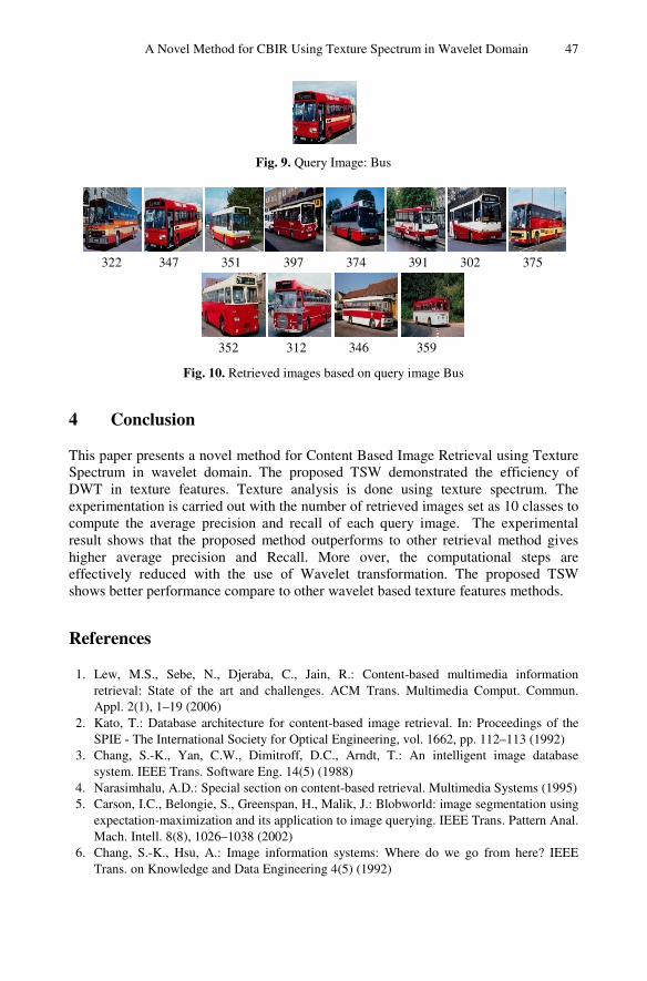
A Novel Method for CBIR Using Texture Spectrum in Wavelet Domain 47
Fig. 9. Query Image: Bus
322 347 351 397 374 391 302 375
352 312 346 359
Fig. 10. Retrieved images based on query image Bus
4 Conclusion
This paper presents a novel method for Content Based Image Retrieval using Texture Spectrum in wavelet domain. The proposed TSW demonstrated the efficiency of DWT in texture features. Texture analysis is done using texture spectrum. The experimentation is carried out with the number of retrieved images set as 10 classes to compute the average precision and recall of each query image. The experimental result shows that the proposed method outperforms to other retrieval method gives higher average precision and Recall. More over, the computational steps are effectively reduced with the use of Wavelet transformation. The proposed TSW shows better performance compare to other wavelet based texture features methods.
References
1. Lew, M.S., Sebe, N., Djeraba, C., Jain, R.: Content-based multimedia information retrieval: State of the art and challenges. ACM Trans. Multimedia Comput. Commun. Appl. 2(1), 1–19 (2006)
2. Kato, T.: Database architecture for content-based image retrieval. In: Proceedings of the SPIE - The International Society for Optical Engineering, vol. 1662, pp. 112–113 (1992)
3. Chang, S.-K., Yan, C.W., Dimitroff, D.C., Arndt, T.: An intelligent image database system. IEEE Trans. Software Eng. 14(5) (1988)
4. Narasimhalu, A.D.: Special section on content-based retrieval. Multimedia Systems (1995) 5. Carson, I.C., Belongie, S., Greenspan, H., Malik, J.: Blobworld: image segmentation using
expectation-maximization and its application to image querying. IEEE Trans. Pattern Anal. Mach. Intell. 8(8), 1026–1038 (2002)
6. Chang, S.-K., Hsu, A.: Image information systems: Where do we go from here? IEEE Trans. on Knowledge and Data Engineering 4(5) (1992)
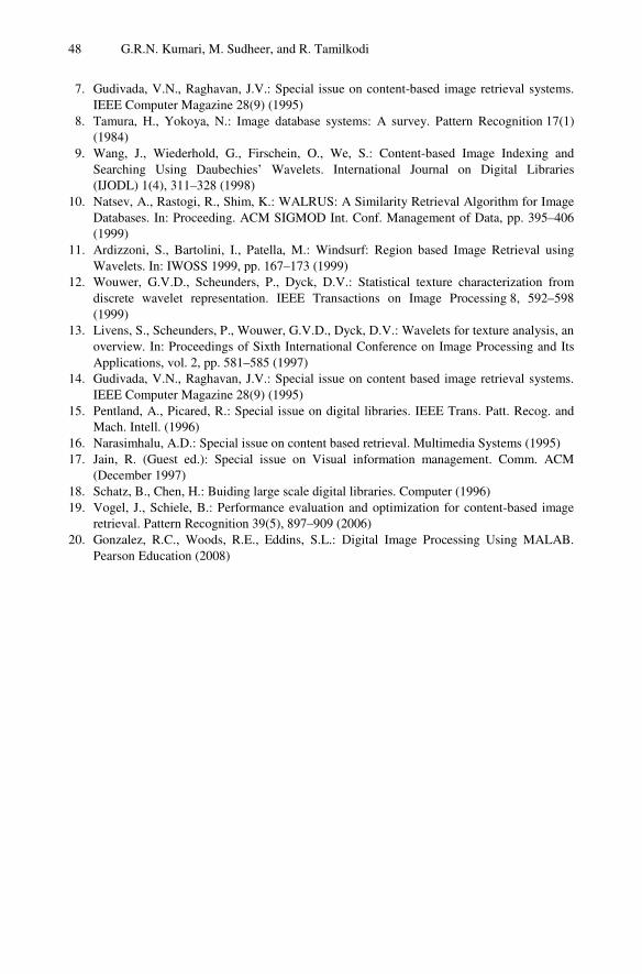
48 G.R.N. Kumari, M. Sudheer, and R. Tamilkodi
7. Gudivada, V.N., Raghavan, J.V.: Special issue on content-based image retrieval systems. IEEE Computer Magazine 28(9) (1995)
8. Tamura, H., Yokoya, N.: Image database systems: A survey. Pattern Recognition 17(1) (1984)
9. Wang, J., Wiederhold, G., Firschein, O., We, S.: Content-based Image Indexing and Searching Using Daubechies’ Wavelets. International Journal on Digital Libraries (IJODL) 1(4), 311–328 (1998)
10. Natsev, A., Rastogi, R., Shim, K.: WALRUS: A Similarity Retrieval Algorithm for Image Databases. In: Proceeding. ACM SIGMOD Int. Conf. Management of Data, pp. 395–406 (1999)
11. Ardizzoni, S., Bartolini, I., Patella, M.: Windsurf: Region based Image Retrieval using Wavelets. In: IWOSS 1999, pp. 167–173 (1999)
12. Wouwer, G.V.D., Scheunders, P., Dyck, D.V.: Statistical texture characterization from discrete wavelet representation. IEEE Transactions on Image Processing 8, 592–598 (1999)
13. Livens, S., Scheunders, P., Wouwer, G.V.D., Dyck, D.V.: Wavelets for texture analysis, an overview. In: Proceedings of Sixth International Conference on Image Processing and Its Applications, vol. 2, pp. 581–585 (1997)
14. Gudivada, V.N., Raghavan, J.V.: Special issue on content based image retrieval systems. IEEE Computer Magazine 28(9) (1995)
15. Pentland, A., Picared, R.: Special issue on digital libraries. IEEE Trans. Patt. Recog. and Mach. Intell. (1996)
16. Narasimhalu, A.D.: Special issue on content based retrieval. Multimedia Systems (1995) 17. Jain, R. (Guest ed.): Special issue on Visual information management. Comm. ACM
(December 1997) 18. Schatz, B., Chen, H.: Buiding large scale digital libraries. Computer (1996) 19. Vogel, J., Schiele, B.: Performance evaluation and optimization for content-based image
retrieval. Pattern Recognition 39(5), 897–909 (2006) 20. Gonzalez, R.C., Woods, R.E., Eddins, S.L.: Digital Image Processing Using MALAB.
Pearson Education (2008)
S.C. Satapathy et al. (eds.), ICT and Critical Infrastructure: Proceedings of the 48th Annual Convention of CSI - Volume I, Advances in Intelligent Systems and Computing 248,
49
DOI: 10.1007/978-3-319-03107-1_6, © Springer International Publishing Switzerland 2014
Identification of Abdominal Aorta Aneurysm Using Ant Colony Optimization Algorithm
A. Dinesh Kumar1, R. Nidhya2, V. Hanah Ayisha3, Vigneshwar Manokar4, and Nandhini Vigneshwar Manokar5
1,2 Department of Computer Science and Engineering, Dr. N.G.P. Institute of Technology, Coimbatore, Tamil Nadu, India
{dineshngpit,nidhuraji88}@gmail.com 3 Department of Computer Science and Engineering,
MEA College of Engineering, Kerala, India 4 Department of Computer Science and Engineering,
Faculty of Engineering, Karpagam University, Coimbatore, Tamil Nadu, India [email protected]
5 Applied Research – Modeling and Simulation, Technologies Division, Bharath Corporate, India
Abstract. Abdominal aortic aneurysm (AAA) is a localized dilatation of the abdominal aorta. It occurs when there is a increase in the normal diameter of the blood vessels by more than 50 percent. Approximately 90 percent of abdominal aortic aneurysms occur infrarenally, but they can also occur pararenally or suprarenally. This is because of some catastrophic outcome. Due to this, the blood flow is exaggerated so the blood hemodynamic interaction forces are affected. Therefore this will tends to wall rupture. To identify the AAA, it is important to identify the blood flow interaction and the wall shear stress. The blood and wall interaction is the wall shear stress. Computational fluid dynamics (CFD) is used to get the results for the mechanical conditions within the blood vessels with and without Aneurysms. CFD contains vast computations with Navier Stroke Equations so this will be very time consuming. So to make these CFD computations very efficient, Data mining algorithms are to be used. And also DM algorithms will be a best method to predict the shear stress at the AAA. This will estimate the wall shear stress. There is in need of thousands of CFD runs in a single computer for creating machine learning data so grid computing can be used.
Keywords: Computational fluid dynamics (CFD), data mining (DM), grid computing, hemodynamic parameters, predictive modeling, Ant Colony Optimization (ACO) algorithm.
1 Introduction
Cardiovascular disease is a class of diseases that involve the heart or blood vessels. Cardiovascular disease refers to any disease that affects the cardiovascular system. Cardiovascular diseases remain the biggest cause of deaths worldwide. Age is
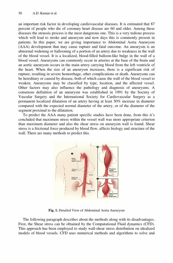
50 A.D. Kumar et al.
an important risk factor in developing cardiovascular diseases. It is estimated that 87 percent of people who die of coronary heart disease are 60 and older. Among these diseases the stenosis process is the most dangerous one. This is a very tedious process which will lead to stroke and aneurysm and now days this is commonly present in patients. In this paper, we are giving importance to Abdominal Aorta Aneurysm (AAA) development that may cause rupture and fatal outcome. An aneurysm is an abnormal widening or ballooning of a portion of an artery due to weakness in the wall of the blood vessel. It is a localized, blood-filled balloon-like bulge in the wall of a blood vessel. Aneurysms can commonly occur in arteries at the base of the brain and an aortic aneurysm occurs in the main artery carrying blood from the left ventricle of the heart. When the size of an aneurysm increases, there is a significant risk of rupture, resulting in severe hemorrhage, other complications or death. Aneurysms can be hereditary or caused by disease, both of which cause the wall of the blood vessel to weaken. Aneurysms may be classified by type, location, and the affected vessel. Other factors may also influence the pathology and diagnosis of aneurysms. A consensus definition of an aneurysm was established in 1991 by the Society of Vascular Surgery and the International Society for Cardiovascular Surgery as a permanent localized dilatation of an artery having at least 50% increase in diameter compared with the expected normal diameter of the artery, or of the diameter of the segment proximal to the dilatation.
To predict the AAA many patient specific studies have been done, from this it’s concluded that maximum stress within the vessel wall was more appropriate criterion than maximum diameter and also the shear stress on aneurysm wall is found. Shear stress is a frictional force produced by blood flow, affects biology and structure of the wall. There are many methods to predict this.
Fig. 1. Detailed View of Abdominal Aorta Aneurysm
The following paragraph describes about the methods along with its disadvantages. First, the Shear stress can be obtained by the Computational Fluid dynamics (CFD). This approach has been employed to study wall-shear stress distribution on idealized models of blood vessels. CFD uses numerical methods and algorithms to solve and
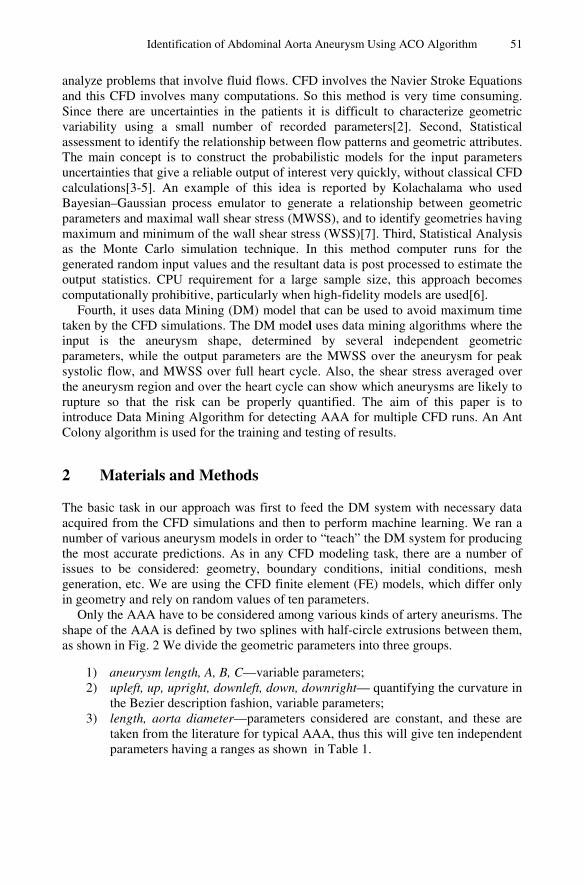
Identification of Abdominal Aorta Aneurysm Using ACO Algorithm 51
analyze problems that involve fluid flows. CFD involves the Navier Stroke Equations and this CFD involves many computations. So this method is very time consuming. Since there are uncertainties in the patients it is difficult to characterize geometric variability using a small number of recorded parameters[2]. Second, Statistical assessment to identify the relationship between flow patterns and geometric attributes. The main concept is to construct the probabilistic models for the input parameters uncertainties that give a reliable output of interest very quickly, without classical CFD calculations[3-5]. An example of this idea is reported by Kolachalama who used Bayesian–Gaussian process emulator to generate a relationship between geometric parameters and maximal wall shear stress (MWSS), and to identify geometries having maximum and minimum of the wall shear stress (WSS)[7]. Third, Statistical Analysis as the Monte Carlo simulation technique. In this method computer runs for the generated random input values and the resultant data is post processed to estimate the output statistics. CPU requirement for a large sample size, this approach becomes computationally prohibitive, particularly when high-fidelity models are used[6].
Fourth, it uses data Mining (DM) model that can be used to avoid maximum time taken by the CFD simulations. The DM model uses data mining algorithms where the input is the aneurysm shape, determined by several independent geometric parameters, while the output parameters are the MWSS over the aneurysm for peak systolic flow, and MWSS over full heart cycle. Also, the shear stress averaged over the aneurysm region and over the heart cycle can show which aneurysms are likely to rupture so that the risk can be properly quantified. The aim of this paper is to introduce Data Mining Algorithm for detecting AAA for multiple CFD runs. An Ant Colony algorithm is used for the training and testing of results.
2 Materials and Methods
The basic task in our approach was first to feed the DM system with necessary data acquired from the CFD simulations and then to perform machine learning. We ran a number of various aneurysm models in order to “teach” the DM system for producing the most accurate predictions. As in any CFD modeling task, there are a number of issues to be considered: geometry, boundary conditions, initial conditions, mesh generation, etc. We are using the CFD finite element (FE) models, which differ only in geometry and rely on random values of ten parameters.
Only the AAA have to be considered among various kinds of artery aneurisms. The shape of the AAA is defined by two splines with half-circle extrusions between them, as shown in Fig. 2 We divide the geometric parameters into three groups.
1) aneurysm length, A, B, C—variable parameters; 2) upleft, up, upright, downleft, down, downright— quantifying the curvature in
the Bezier description fashion, variable parameters; 3) length, aorta diameter—parameters considered are constant, and these are
taken from the literature for typical AAA, thus this will give ten independent parameters having a ranges as shown in Table 1.
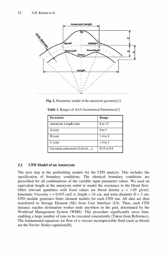
52 A.D. Kumar et al.
Fig. 2. Parametric model of the aneurysm geometry[1]
Table 1. Ranges of AAA Geometrical Parameters[1]
2.1 CFD Model of an Aneurysm
The next step in the prebuilding models for the CFD analysis. This includes the specification of boundary conditions. The identical boundary conditions are prescribed for all combinations of the variable input parameter values. We used an equivalent length at the aneurysm outlet to model the resistance to the blood flow. Other relevant quantities with fixed values are blood density ρ = 1.05 g/cm3, kinematic Viscosity ν = 0.035 cm2 /s, length = 24 cm, and aorta diameter D = 2 cm. CFD module generates finite element models for each CFD run. All data are then transferred to Storage Element (SE) from User Interface (UI). Then, each CFD instance reaches destination worker node anywhere in the grid, determined by the Workload Management System (WMS). This procedure significantly saves time, enabling a large number of runs to be executed concurrently (Taken from Reference). The fundamental equations for flow of a viscous incompressible fluid (such as blood) are the Navier–Stokes equations[8].
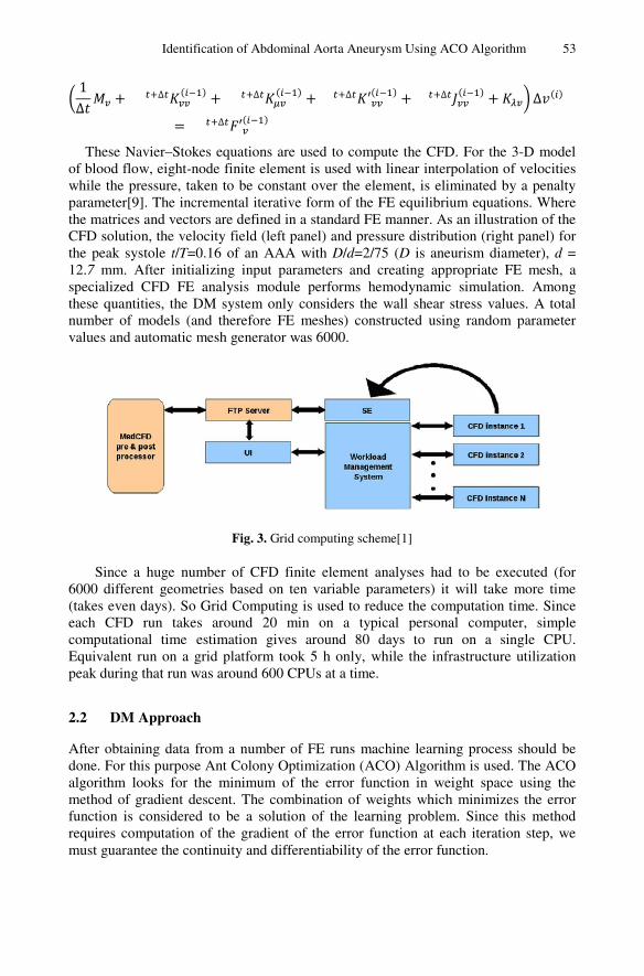
Identification of Abdominal Aorta Aneurysm Using ACO Algorithm 53
1∆ + ∆ ( ) + ∆ ( ) + ∆ ′( ) + ∆ ( ) + ∆ ( )= ∆ ′( ) These Navier–Stokes equations are used to compute the CFD. For the 3-D model
of blood flow, eight-node finite element is used with linear interpolation of velocities while the pressure, taken to be constant over the element, is eliminated by a penalty parameter[9]. The incremental iterative form of the FE equilibrium equations. Where the matrices and vectors are defined in a standard FE manner. As an illustration of the CFD solution, the velocity field (left panel) and pressure distribution (right panel) for the peak systole t/T=0.16 of an AAA with D/d=2/75 (D is aneurism diameter), d = 12.7 mm. After initializing input parameters and creating appropriate FE mesh, a specialized CFD FE analysis module performs hemodynamic simulation. Among these quantities, the DM system only considers the wall shear stress values. A total number of models (and therefore FE meshes) constructed using random parameter values and automatic mesh generator was 6000.
Fig. 3. Grid computing scheme[1]
Since a huge number of CFD finite element analyses had to be executed (for 6000 different geometries based on ten variable parameters) it will take more time (takes even days). So Grid Computing is used to reduce the computation time. Since each CFD run takes around 20 min on a typical personal computer, simple computational time estimation gives around 80 days to run on a single CPU. Equivalent run on a grid platform took 5 h only, while the infrastructure utilization peak during that run was around 600 CPUs at a time.
2.2 DM Approach
After obtaining data from a number of FE runs machine learning process should be done. For this purpose Ant Colony Optimization (ACO) Algorithm is used. The ACO algorithm looks for the minimum of the error function in weight space using the method of gradient descent. The combination of weights which minimizes the error function is considered to be a solution of the learning problem. Since this method requires computation of the gradient of the error function at each iteration step, we must guarantee the continuity and differentiability of the error function.
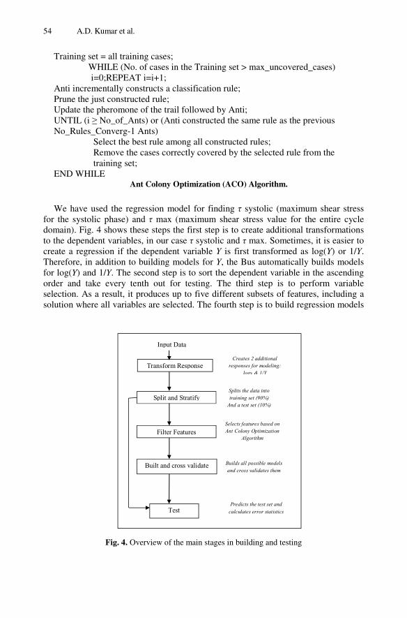
54 A.D. Kumar et al.
Training set = all training cases; WHILE (No. of cases in the Training set > max_uncovered_cases)
i=0;REPEAT i=i+1; Anti incrementally constructs a classification rule; Prune the just constructed rule; Update the pheromone of the trail followed by Anti; UNTIL (i ≥ No_of_Ants) or (Anti constructed the same rule as the previous No_Rules_Converg-1 Ants) Select the best rule among all constructed rules; Remove the cases correctly covered by the selected rule from the training set; END WHILE
Ant Colony Optimization (ACO) Algorithm.
We have used the regression model for finding τ systolic (maximum shear stress
for the systolic phase) and τ max (maximum shear stress value for the entire cycle domain). Fig. 4 shows these steps the first step is to create additional transformations to the dependent variables, in our case τ systolic and τ max. Sometimes, it is easier to create a regression if the dependent variable Y is first transformed as log(Y) or 1/Y. Therefore, in addition to building models for Y, the Bus automatically builds models for log(Y) and 1/Y. The second step is to sort the dependent variable in the ascending order and take every tenth out for testing. The third step is to perform variable selection. As a result, it produces up to five different subsets of features, including a solution where all variables are selected. The fourth step is to build regression models
Fig. 4. Overview of the main stages in building and testing
Split and Stratify
Transform Response
Input Data
Filter Features
Built and cross validate
Test Predicts the test set and
calculates error statistics
Builds all possible models and cross validates them
Selects features based on Ant Colony Optimization
Algorithm
Splits the data into training set (90%)
And a test set (10%)
Creates 2 additional responses for modeling:
logy & 1/Y
Identification of Abdominal Aorta Aneurysm Using ACO Algorithm 55
and to cross validate them. All regression models are at the end cross-validated (tenfold) and the following statistics is calculated.
1) Tenfold cross-validated RMSE—root mean square error after tenfold cross validation.
2) Tenfold cross-validated Q2—coefficient of determination after tenfold cross validation.
3) Tenfold cross-validated RelSE—relative squared error after tenfold cross validation.
4) Size of the training dataset (Ntr ) The last step is to apply all regression models to the test set and following statistics
are calculated.
1) RMSE—root means square error. RMSE = 1N (y − y′ ) RMSE = 1N (y − y′ )
2. R2—coefficient of determination. R = 1 − ∑(y − y′ )∑(y − y′ ) y ith observed value in the training dataset; y′ ith predicted value in the training dataset; y′ mean of the observed values in the testing dataset; Ntrain number of compounds in the training dataset; Ntest number of compounds in the training dataset From these values we have to produce a performance metrics in which the error
rate should be a minimum. RMSE can have an error of 0.001 and R2 as 0.9.
3 Results and Discussion
From 85 models for property τ systolic and the best model was found for τ −1 systolic. It is a feed forward neural network model that uses all ten input variables. From 82 models for property τmax and the best model was found for τ−1max. It is a feed forward neural network model that uses all ten input variables. The models show a very low error statistics on the test and training sets. In order to better quantify the DM method, we also analyzed an AAA model based on the patient-specific clinical data. The best model among 85 models produced by ACO algorithm (feed forward neural network that uses all ten input variables) has been chosen in order to obtain the best approximation for τ systolic and τ max. As expected, the most realistic model from the first approach consumes the most computing time. The values of τmax and τ systolic were taken as reference values for the parametric and DM models. It can be observed that all relative errors are below 10%, with significant computing time reduction in favor of the DM model.
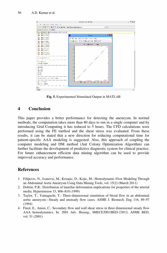
56 A.D. Kumar et al.
Fig. 5. Experimented Stimulated Output in MATLAB
4 Conclusion
This paper provides a better performance for detecting the aneurysm. In normal methods, the computation takes more than 80 days to run in a single computer and by introducing Grid Computing it has reduced to 5 hours. The CFD calculations were performed using the FE method and the shear stress was evaluated. From these results, it can be stated that a new direction for reducing computational time for patient-specific AAA modeling is suggested. Also, this approach of coupling the computer modeling and DM method (Ant Colony Optimization Algorithm) can further facilitate the development of predictive diagnostic system for clinical practice. For future enhancement efficient data mining algorithm can be used to provide improved accuracy and performance.
References
1. Filipovic, N., Ivanovic, M., Krstajic, D., Kojic, M.: Hemodynamic Flow Modeling Through an Abdominal Aorta Aneurysm Using Data Mining Tools, vol. 15(2) (March 2011)
2. Dobrin, P.B.: Distribution of lamellar deformation implications for properties of the arterial media. Hypertension 33, 806–810 (1999)
3. Taylor, T., Yamaguchi, T.: Three-dimensional simulation of blood flow in an abdominal aortic aneurysm—Steady and unsteady flow cases. ASME J. Biomech. Eng. 116, 89–97 (1994)
4. Finol, E., Amon, C.: Secondary flow and wall shear stress in three dimensional steady flow AAA hemodynamics. In: 2001 Adv. Bioeng., IMECE2001/BED-23013, ASME BED, vol. 51 (2001)

Identification of Abdominal Aorta Aneurysm Using ACO Algorithm 57
5. Kumar, R., Yamaguchi, T., Liu, H., Himeno, R.: Numerical simulation of 3D unsteady flow dynamics in a blood vessel with Multiple aneurysms. In: 2001 Adv. Bioeng., ASME BED, vol. 50, pp. 475–476 (2001)
6. Rubinstein, R.Y.: Simulation and the Monte Carlo Method. Wiley, Hoboken (1981) 7. Kolachalama, V.B., Bressloff, N.W., Nair, P.B.: Mining data from hemodynamic
simulations via Bayesian emulation. BioMed. Eng. Online 6, 47 (2007) 1475-925X-6-47.J 8. Kojić, M., Filipović, N., Stojanović, B., Kojić, N.: Computer Modeling in Bioengineering.
Wiley, Hoboken (2008) 9. Filipovic, N., Mijailovic, S., Tsuda, A., Kojic, M.: An implicit algorithm within the
arbitrary lagrangian-eulerian formulation for solving incompressible fluid flow with large boundary motions. Comput. Methods Appl. Mech. Eng. 195, 6347–6361 (2006)

S.C. Satapathy et al. (eds.), ICT and Critical Infrastructure: Proceedings of the 48th Annual Convention of CSI - Volume I, Advances in Intelligent Systems and Computing 248,
59
DOI: 10.1007/978-3-319-03107-1_7, © Springer International Publishing Switzerland 2014
Color Image Watermarking Using Wavelet Transform Based on HVS Channel
G. Rosline Nesa Kumari, Syama Sundar Jeeru, and S. Maruthuperumal
Godavari Institute of Engineering & Technology, Rajahmundry, India {rosemaruthu,jeerusyam,maruthumail}@gmail.com
Abstract. Digital image watermarking is a copyright protection technology expected at asserting intellectual property rights of digital images by embedding a copyright identifier in the contents of the image, without disturbing its quality. In this paper, a new robust and secure color watermarking scheme based on Discrete Wavelet domain is proposed. The RGB color space is converted into HSV color space and the H component is decomposition with ‘Haar’ which is simple, symmetric and orthogonal wavelet. The proposed embedding process, the scrambled watermark is embedded in the modification of the extraordinary value of LL band and LH band of H component to the watermarking scheme which excellent preserves the quality. The supplementary improvement of the proposed technique is taking advantage of HVS which can adaptively regulate the watermark embedding strength. Experimental results show that the method not only has better transparency, but also has good robustness such as noise, compression, filtering, cropping.
1 Introduction
In modern year’s Copyright protection and authentication of digital data using watermarking is a powerful issue of research. The basic principle of digital watermarking technique [5] is to embed an amount of secret information in the functional part of the cover data. This data may be an image, an audio or video. Since mid 1990s this technique has attracted much attention from academic and industrial sector. After the pioneering contribution by I. J. Cox [5], digital watermarking techniques have been widely developed as an effective tool against piracy, illegal alteration of contents or improper use of image. Digital watermarking is a method that inserts some information into a multimedia object and generates a watermarked multimedia object [6, 7]. The object may be an image, audio, video or text. Watermarking has many different applications [8, 9, 10, 11, 12], such as ownership evidence, fingerprinting, authentication and integrity verification, content labeling and protection, and usage control.
Watermarking techniques can be divided into spatial [13], [14], and frequency [15], [16], [17] based methods. Watermarking algorithms that rely on spatial domains, hide the watermark by modifying the pixel values of the host image. In transform domain technique [1,2,3,4], the host image is first converted into frequency domain by transformation method such as the discrete cosine transform (DCT), discrete
60 G.R.N. Kumari, S.S. Jeeru, and S. Maruthuperumal
Fourier transform (DFT) or discreet wavelet transform (DWT) ,etc. then, transform domain coefficients are modified by the watermark. Watermarking the process of embedding data into multimedia element can primarily for copyright protection. Because of its growing popularity, the Discrete Wavelet Transform (DWT) is commonly used in the proposed watermarking scheme increase, area increases so power consumption [18 ].
Human Visual System (HVS) plays important role in watermarking of images to maintain the perceptual similarity between original and watermarked image. HVS has been characterized with several phenomena that permit to adjust the pixel values to yield perception. These phenomena are luminance sensitivity, frequency sensitivity and texture sensitivity. Human visual model is based on the characteristics such as edges and textures, which are incorporated to determine the gain factor in watermarking. The distortion visibility is very low if the back ground contains texture. In a high texture block, energy is more distributed among the pixels. Therefore, the block having a stronger texture can have a high embedding gain factor. The paper also utilizes Torus automorphism (TA) permutation [19,20,21] to scramble the watermark before embedding and to reassemble it after extraction. This helps increase robustness to intentional attacks while preserving blindness. The paper also proposes an extended version of this technique to increase the robustness against intentional attacks even further. The algorithm is discussed in the rest of the paper.
This paper describes the efficient and robust color watermarking schemes in an attempt to improve watermark robustness to attacks. The proposed scheme embeds a scrambled watermark image by using Torus automorphism into a 2nd level wavelet color image of H components. Select a LL and LH subband having high energy and then embed scrambled the watermark. The proposed method is directly embedded into cover image using a transform before embedding. Experimental results demonstrate that there is high degree of perceptual similarity between original image and watermarked image. Further, the proposed method resists different types of attacks. The rest of the paper is organized as follows. Section 2 briefly reviews about DWT and Torus automorphism Section 3 describes the proposed color watermarking method and in section 4, the experimental results are discussed. Finally, some conclusions are drawn in section 5.
2 Discrete Wavelet Transformation
The Discrete Wavelet Transform (DWT) [22] is currently used in a wide variety of signal processing applications, such as in audio and video compression, removal of noise in audio, and the simulation of wireless antenna distribution. Discrete Wavelet decomposition of image produces the multi-resolution representation of image. A multi-resolution representation provides a simple hierarchical framework for interpreting the image information. At different resolutions, the details of an image generally characterize different physical structures of the image. At a coarse resolution, these details correspond to the larger structures which provide the image
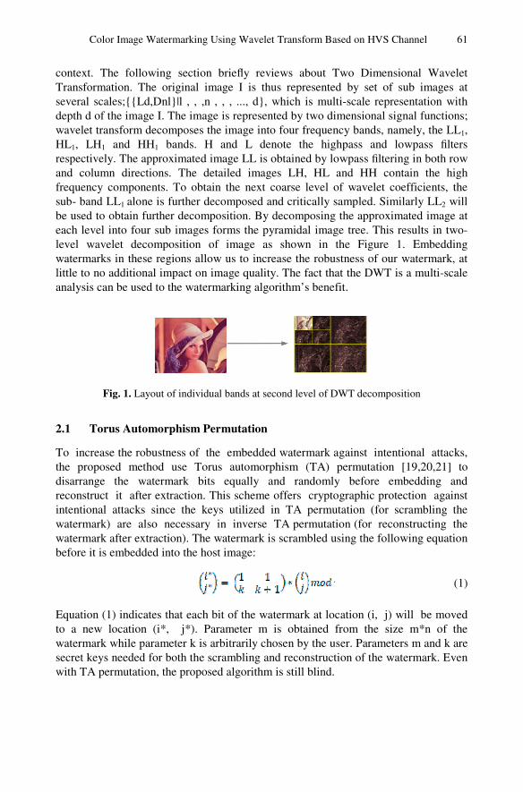
Color Image Watermarking Using Wavelet Transform Based on HVS Channel 61
context. The following section briefly reviews about Two Dimensional Wavelet Transformation. The original image I is thus represented by set of sub images at several scales;{{Ld,Dnl}|l , , ,n , , , ..., d}, which is multi-scale representation with depth d of the image I. The image is represented by two dimensional signal functions; wavelet transform decomposes the image into four frequency bands, namely, the LL1, HL1, LH1 and HH1 bands. H and L denote the highpass and lowpass filters respectively. The approximated image LL is obtained by lowpass filtering in both row and column directions. The detailed images LH, HL and HH contain the high frequency components. To obtain the next coarse level of wavelet coefficients, the sub- band LL1 alone is further decomposed and critically sampled. Similarly LL2 will be used to obtain further decomposition. By decomposing the approximated image at each level into four sub images forms the pyramidal image tree. This results in two-level wavelet decomposition of image as shown in the Figure 1. Embedding watermarks in these regions allow us to increase the robustness of our watermark, at little to no additional impact on image quality. The fact that the DWT is a multi-scale analysis can be used to the watermarking algorithm’s benefit.
Fig. 1. Layout of individual bands at second level of DWT decomposition
2.1 Torus Automorphism Permutation
To increase the robustness of the embedded watermark against intentional attacks, the proposed method use Torus automorphism (TA) permutation [19,20,21] to disarrange the watermark bits equally and randomly before embedding and reconstruct it after extraction. This scheme offers cryptographic protection against intentional attacks since the keys utilized in TA permutation (for scrambling the watermark) are also necessary in inverse TA permutation (for reconstructing the watermark after extraction). The watermark is scrambled using the following equation before it is embedded into the host image:
(1)
Equation (1) indicates that each bit of the watermark at location (i, j) will be moved to a new location (i*, j*). Parameter m is obtained from the size m*n of the watermark while parameter k is arbitrarily chosen by the user. Parameters m and k are secret keys needed for both the scrambling and reconstruction of the watermark. Even with TA permutation, the proposed algorithm is still blind.
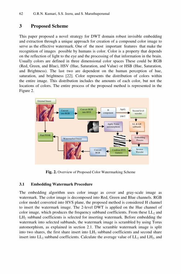
62 G.R.N. Kumari, S.S. Jeeru, and S. Maruthuperumal
3 Proposed Scheme
This paper proposed a novel strategy for DWT domain robust invisible embedding and extraction through a unique approach for creation of a compound color image to serve as the effective watermark. One of the most important features that make the recognition of images possible by humans is color. Color is a property that depends on the reflection of light to the eye and the processing of that information in the brain. Usually colors are defined in three dimensional color spaces These could be RGB (Red, Green, and Blue), HSV (Hue, Saturation, and Value) or HSB (Hue, Saturation, and Brightness). The last two are dependent on the human perception of hue, saturation, and brightness [22]. Color represents the distribution of colors within the entire image. This distribution includes the amounts of each color, but not the locations of colors. The entire process of the proposed method is represented in the Figure 2.
Fig. 2. Overview of Proposed Color Watermarking Scheme
3.1 Embedding Watermark Procedure
The embedding algorithm uses color image as cover and gray-scale image as watermark. The color image is decomposed into Red, Green and Blue channels. RGB color model converted into HVS plane, the proposed method is considered H channel to insert the watermark image. The 2-level DWT is applied on the Hue channel of color image, which produces the frequency subband coefficients. From these LL2 and LH2 subband coefficients is selected for inserting watermark. Before embedding the watermark into selected subbands, the watermark image is scrambled by using Torus automorphism, as explained in section 2.1. The scramble watermark image is split into two shares, the first share insert into LH2 subband coefficients and second share insert into LL2 subband coefficients. Calculate the average value of LL2 and LH2, and
Original Image
Convert into RGB
Convert RGB into HVS
Apply
DWT
H component
Second level wavelet
LL & LH subbands
Apply Torus automorphism
Embedding Process
Inverse Wavelet
Combine HVS features
Convert RGB
Watermarked Image
Find PSNR
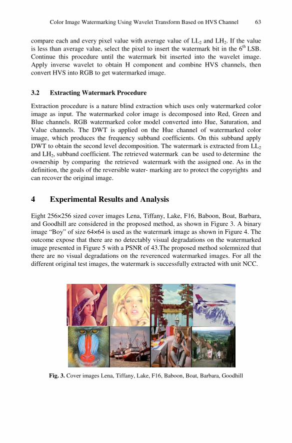
Color Image Watermarking Using Wavelet Transform Based on HVS Channel 63
compare each and every pixel value with average value of LL2 and LH2. If the value is less than average value, select the pixel to insert the watermark bit in the 6th LSB. Continue this procedure until the watermark bit inserted into the wavelet image. Apply inverse wavelet to obtain H component and combine HVS channels, then convert HVS into RGB to get watermarked image.
3.2 Extracting Watermark Procedure
Extraction procedure is a nature blind extraction which uses only watermarked color image as input. The watermarked color image is decomposed into Red, Green and Blue channels. RGB watermarked color model converted into Hue, Saturation, and Value channels. The DWT is applied on the Hue channel of watermarked color image, which produces the frequency subband coefficients. On this subband apply DWT to obtain the second level decomposition. The watermark is extracted from LL2 and LH2, subband coefficient. The retrieved watermark can be used to determine the ownership by comparing the retrieved watermark with the assigned one. As in the definition, the goals of the reversible water- marking are to protect the copyrights and can recover the original image.
4 Experimental Results and Analysis
Eight 256×256 sized cover images Lena, Tiffany, Lake, F16, Baboon, Boat, Barbara, and Goodhill are considered in the proposed method, as shown in Figure 3. A binary image “Boy” of size 64×64 is used as the watermark image as shown in Figure 4. The outcome expose that there are no detectably visual degradations on the watermarked image presented in Figure 5 with a PSNR of 43.The proposed method solemnized that there are no visual degradations on the reverenced watermarked images. For all the different original test images, the watermark is successfully extracted with unit NCC.
Fig. 3. Cover images Lena, Tiffany, Lake, F16, Baboon, Boat, Barbara, Goodhill
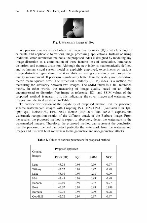
64 G.R.N. Kumari, S.S. Jeeru, and S. Maruthuperumal
Fig. 4. Watermark images (a) Boy
We propose a new universal objective image quality index (IQI), which is easy to calculate and applicable to various image processing applications. Instead of using traditional error summation methods, the proposed index is designed by modeling any image distortion as a combination of three factors: loss of correlation, luminance distortion, and contrast distortion. Although the new index is mathematically defined and no human visual system model is explicitly employed, experiments on various image distortion types show that it exhibits surprising consistency with subjective quality measurement. It performs significantly better than the widely used distortion metric mean squared error. The structural similarity (SSIM) index is a method for measuring the similarity between two images. The SSIM index is a full reference metric, in other words, the measuring of image quality based on an initial uncompressed or distortion-free image as reference. IQI and SSIM values of the proposed method is nearer to 1, this indicating the cover images and watermarked images are identical as shown in Table 1.
To provide verification of the capability of proposed method, test the proposed scheme watermarked images with Cropping (5%, 10%,15%) , (Gaussian Blur 1px, 2px, 3px), Noise(10%, 15%, 20%), Rotate (20,40,60). The Table 2 exposes the watermark recognition results of the different attack of the Barbara image. From the results, the proposed method is expert to absolutely detect the watermark in the watermarked images. Therefore, the proposed method can represent the conclusion that the proposed method can detect perfectly the watermark from the watermarked images and it is well built robustness to the geometric and non-geometric attacks.
Table 1. Values of various parameters for proposed method
Original images
Proposed approach
PSNR(dB) IQI SSIM NCC
Lena 43.24 0.98 0.99 0.97
Tiffany 42.57 0.99 0.97 0.98
Lake 43.98 0.97 0.98 0.99
F16 42.45 0.98 0.99 0.98
Baboon 42.10 0.97 0.97 0.97
Boat 43.07 0.99 0.98 0.998
Barbara 42.76 0.98 0.99 0.98
Goodhill 42.72 0.99 0.97 0.97
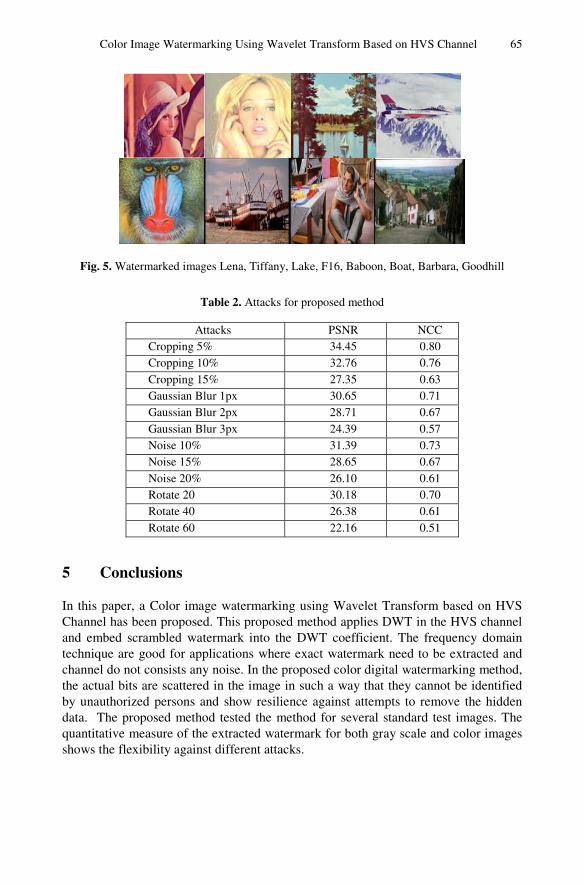
Color Image Watermarking Using Wavelet Transform Based on HVS Channel 65
Fig. 5. Watermarked images Lena, Tiffany, Lake, F16, Baboon, Boat, Barbara, Goodhill
Table 2. Attacks for proposed method
Attacks PSNR NCC Cropping 5% 34.45 0.80 Cropping 10% 32.76 0.76 Cropping 15% 27.35 0.63 Gaussian Blur 1px 30.65 0.71 Gaussian Blur 2px 28.71 0.67 Gaussian Blur 3px 24.39 0.57 Noise 10% 31.39 0.73 Noise 15% 28.65 0.67 Noise 20% 26.10 0.61 Rotate 20 30.18 0.70 Rotate 40 26.38 0.61 Rotate 60 22.16 0.51
5 Conclusions
In this paper, a Color image watermarking using Wavelet Transform based on HVS Channel has been proposed. This proposed method applies DWT in the HVS channel and embed scrambled watermark into the DWT coefficient. The frequency domain technique are good for applications where exact watermark need to be extracted and channel do not consists any noise. In the proposed color digital watermarking method, the actual bits are scattered in the image in such a way that they cannot be identified by unauthorized persons and show resilience against attempts to remove the hidden data. The proposed method tested the method for several standard test images. The quantitative measure of the extracted watermark for both gray scale and color images shows the flexibility against different attacks.