Embed Size (px)
Citation preview
No d’ordre: 10939
THÈSE
Présentée pour obtenir
LE GRADE DE DOCTEUR EN SCIENCESDES UNIVERSITÉS PARIS-SUD XI ET
YAOUNDE I
Spécialité : Mathématiques
par
Cyprien Mbogning Tchinda
Inférence dans les modèles conjoints etde mélange non-linéaires à effets
mixtes.Soutenue le 19 Décembre 2012 devant la Commission d’examen:
Mme. Hélène Jacqmin-Gadda (Professeur INSERM U897, Examinatrice)M. Marc Lavielle (Professeur Inria Saclay, Directeur de thèse)M. Jean-Michel Poggi (Professeur U-Paris Decartes, Président)M. Henri Gwet (Professeur ENSP Yaoundé, Co-Directeur)M. Jean-Marc Bardet (Professeur U-Paris 1, Rapporteur)Mme. Elisabeth Gassiat (Professeur U-Paris sud, Examinatrice)
Rapporteurs:M. Jean-Marc BardetM. Fabrice Gamboa

Thèse préparée dans les institutions suivantes :
Département de Mathématiques d’OrsayLaboratoire de Mathématiques (UMR 8628), Bât. 425Université Paris-Sud 1191 405 Orsay CEDEX
École Nationale Supérieure Polytechnique (ENSP)LIMSSUniversité de Yaoundé ICameroun
Thèse financée par :
Contrat doctoral attribué parInria-Saclay Île de France

To my Mom & my Dad

Remerciements
Cette Thèse a été réalisée dans le cadre d’une Co-tutelle internationale entrel’Université de Paris 11 Orsay (France) via le laboratoire de Mathématiques etl’université de Yaoundé I (Cameroun) via l’École Nationale Supérieure Polytech-nique. Elle s’inscrit aussi dans le cadre du projet STAFAV (Statistiques pourl’Afrique Francophone et Applications au Vivant) et est l’aboutissement d’un longet laborieux travail ayant nécessité l’assistance et le soutien de plusieurs personnes.
Je remercie mon directeur de thèse, le Professeur Marc Lavielle pour tout cequi m’est arrivé de bien pendant cette Thèse. Il est le principal initiateur des ques-tions traitées dans ce document et a été déterminant pour le financement. J’ai étébluffé par sa capacité à switcher de la théorie aux applications, avec comme prin-cipale philosophie que les méthodologies développées doivent être implémentées etmises à la disposition des utilisateurs dans un logiciel convivial. Merci encore pourta patience et ta disponibilité.
Je remercie le Professeur Henri Gwet, Co-encadreur de ce travail et respon-sable du master STAFAV de Yaoundé dont je suis un récipiendaire. Merci pour tadisponibilité et tes multiples conseils.
Merci aux Professeurs Jean-Marc Bardet et Fabrice Gamboa d’avoir gra-cieusement accepté de rapporter cette Thèse.
Merci au Professeur Jean-Michel Poggi pour avoir accepté de présider le juryde ma soutenance de thèse.
Je suis honoré de compter les Professeurs Elisabeth Gassiat et HélèneJaqmin-Gadda parmi les membres de mon jury de thèse en qualité d’exami-natrices.
J’exprime toute ma gratitude à Kevin Bleakley pour sa fructueuse collabo-ration lors de cette dernière année de thèse.
Je remercie tous les membres du projet STAFAV, particulièrement le principalinitiateur, le Professeur Didier Dacuhna-Castelle qui avec Elisabeth Gassiatm’ont mis en contact avec Marc Lavielle.
Je remercie tous les membres du LMO. Je pense notamment aux doctorantsou ex-doctorants : Emmanuel, Hatem, Jean-Patrick, Jairo, Maud, Wilson et tousles autres pour leur accueil et les multiples discussions. Je remercie aussi tousles membres de l’équipe POPIX de l’Inria, particulièrement les ingénieurs Hec-tor, Jean-François et Kaelig pour toutes les discussions, pour la plupart liées à laprogrammation.
Je tiens à remercier tous les membres du laboratoire LIMSS de l’ENSP deYaoundé pour toute leur collaboration. Je pense particulièrement au DocteurEugène-Patrice Ndong Nguema.

Je remercie Valérie Lavigne de l’école doctorale qui a effectué la quasi totalitédes procédures administratives me concernant à Orsay en mon absence. Je remercieaussi Katia Evrat de l’INRIA qui s’occupait de l’organisation de mes voyages enFrance.
Merci à tous mes ami(e)s pour leur soutien et surtout la patience dont ils ontfait preuve pendant toute la durée de cette thèse.
Je remercie enfin toute ma famille pour tout leur soutient, les sacrifices consen-tis et leur patience. J’ai une pensée particulière pour ma mère qui souhaitait avoirun docteur dans sa famille. J’espère que cette réalisation t’offrira un immensesourire quelques mètres sous terre...

Principales abréviations
BSMM : Between-Subject Model Mixtures
EM : Expectation Maximization.
SAEM : Stochastic Approximation EM.
MSAEM : Mixture SAEM.
SEM : Stochastic EM.
MLE : Maximum Likelihood Estimate.
MNLEM : Modèles Non Linéaires à Effets Mixtes.
NLMEM : Non Linear Mixed Effects Models.
MCMC : Markov Chain Monte Carlo.
PKPD : PharmacoKinetic-PharmacoDynamic.
REE : Relative Estmation Error.
RRMSE : Relative Root Mean Square Errors.
RTTE : Repeated Time-To-Event.
WSMM : Within-Subject Model Mixtures.
Résumé
Cette Thèse est consacrée au développement de nouvelles méthodologies pour l’ana-lyse des modèles non-linéaires à effets mixtes, à leur implémentation dans un logicielaccessible et leur application à des problèmes réels. Nous considérons particulièrementdes extensions des modèles non-linéaires à effets mixtes aux modèles de mélange et auxmodèles conjoints. L’étude de ces deux extensions constitue l’essentiel du travail réalisédans ce document qui peut donc être subdivisé en deux grandes parties.
Dans la première partie, nous proposons, dans le but d’avoir une meilleure maîtrise del’hétérogénéité liée aux données sur des patients issus de plusieurs clusters, des extensionsdes MNLEM aux modèles de mélange. Les modèles de mélanges de distributions, utiles pour caractériser des distributions
de population qui ne sont pas suffisamment bien décrites par les seules covariablesobservées. Certaines covariables catégorielles non observées définissent alors lescomposantes du mélange.
Les mélanges de modèles inter-sujets supposent également qu’il existe des sous-populations de patients. Ici, différents modèles structurels décrivent la réponse dechaque sous-population et chaque patient appartient à une sous-population.
Les mélanges de modèles intra-sujets supposent qu’il existe des sous-populations(de cellules, de virus ,...) au sein du patient. Différents modèles structurels dé-crivent la réponse de chaque sous-population mais la proportion de chaque sous-population dépend du patient.
Les algorithmes d’estimation dans les modèles de mélange tels que l’EM ne peuvent pasêtre appliqués de manière directe dans ce contexte. En effet, en plus de la structure delatence induite par les labels non observés des individus, on a aussi des paramètres in-dividuels expliquant une partie de la variabilité non-observée qui ne sont pas observés.Les algorithmes populaires pour l’estimation des paramètres dans les MNLEM tels queSAEM sont confrontés dans certains cas à des difficultés pratiques dues particulièrementà la propriété de "Label-switching" inhérente aux modèles de mélange. Nous proposonsdans cette thèse de combiner l’algorithme EM, utilisé traditionnellement pour les mo-dèles de mélange lorsque les variables étudiées sont observées, et l’algorithme SAEM,utilisé pour l’estimation de paramètres par maximum de vraisemblance lorsque ces va-riables ne sont pas observées. La procédure résultante, dénommée MSAEM, permet ainsid’éviter l’introduction d’une étape de simulation des covariables catégorielles latentesdans l’algorithme d’estimation. Cet algorithme est extrêmement rapide, très peu sensibleà l’initialisation des paramètres et converge vers un maximum (local) de la vraisem-blance. Cette méthodologie est désormais disponible sous Monolix , l’un des logicielsles plus populaires dans l’industrie pharmacologique, qui est libre pour les étudiants etla recherche académique. Nous avons ensuite effectué une classification non superviséedes données longitudinales réelles de charges virales sur des patients ayant le VIH, enconsidérant des mélanges de modèles structurels.
La seconde partie de cette thèse traite de la modélisation conjointe de l’évolutiond’un marqueur biologique au cours du temps et les délais entre les apparitions succes-sives censurées d’un évènement d’intérêt. Nous considérons entre autres, les censures àdroite, les multiples censures par intervalle d’évènements répétés. Nous proposons d’uti-liser un MNLEM pour l’évolution temporelle du marqueur et un modèle de risque mixte,permettant de prendre en compte l’hétérogénéité due aux évènements répétés ainsi que larelation entre le processus longitudinal et le processus à risque, pour une utilisation effi-

ciente des informations disponibles dans les données. Les paramètres du modèle conjointrésultant sont estimés en maximisant la vraisemblance jointe exacte par un algorithme detype MCMC-SAEM. La matrice de Fisher est estimée par approximations stochastiques.La méthodologie proposée est générale et s’étend facilement aux modèles conjoints usuels(modèle linéaire mixte pour la variable longitudinale et modèle de risque pour un uniqueévènement ne pouvant se manifester qu’une seule fois au cours de l’étude) et aux mo-dèles d’évènements récurrents ou encore les modèles de fragilité. L’application de cetteméthodologie aux jeux de données simulées montre que l’algorithme converge rapidementvers la cible avec une bonne précision. La méthode est ensuite illustrée sur des jeux dedonnées réelles des patients ayant des cirrhoses biliaires primitives ainsi que des patientsépileptiques. Cette méthodologie est désormais disponible sous Monolix.Mots-clefs : Algorithme MSAEM, Algorithme SAEM, Censures par intervalle, Évè-nements répétés, Maximum de vraisemblance, Modèles conjoints, Modèles de mélange,Modèles mixtes, Monolix..
Inference in non-linear mixed effects joints and mixtures models.
Abstract
The main goal of this thesis is to develop new methodologies for the analysis of nonlinear mixed-effects models, along with their implementation in an accessible softwareand their application to real problems. We consider particularly extensions of non-linear mixed effects model to mixture models and joint models. The study of these twoextensions is the essence of the work done in this document, which can be divided intotwo major parts.
In the first part, we propose, in order to have a better control of heterogeneity linkedto data of patient issued from several clusters , extensions of NLMEM to mixture models. Mixture models of distributions are useful to characterize distributions of popula-
tion that are not adequately described by only observed covariates. Some unob-served categorical covariates then define components of the mixture.
Between-subject model mixtures also assume the existence of subpopulations ofpatients. Here, different structural models describe the response of each subpop-ulation and each patient belongs to a sub-population.
Within-subject model mixtures assume that there exist subpopulations (Of cells,viruses, ...) within the patient. Different structural models describe the responseof each sub-population, but the proportion of each subpopulation depends on thepatient.
The standard estimation algorithms in mixture models such as EM can not be applieddirectly in this context. Indeed, in addition to the latency structure induced by unob-served individual labels, we also have individual parameters explaining part of the un-observed variability that are not observed. Popular algorithms for parameter estimationin NLMEM, such as SAEM, face in some practical cases several difficulties particularlydue to the well-known "Label-switching" phenomenon, inherent to mixture models. Wesuggest in this Thesis to combine the EM algorithm, traditionally used for mixturesmodels when the variables studied are observed, and the SAEM algorithm, used to es-timate the maximum likelihood parameters when these variables are not observed. Theresulting procedure, referred MSAEM, allows to avoid the introduction of a simulationstep of the latent categorical covariates in the estimation algorithm. This algorithm ap-pears to be extremely fast, very little sensitive to parameters initialization and convergesto a (local) maximum of the likelihood. This methodology is now available under theMonolix software, one of the most popular in the pharmacological industry, which isfree for students and academic research. We then performed a classification of a longi-tudinal real data on viral loads for patients with HIV, by considering mixtures of threestructural models.
The second part of this thesis deals with the joint modeling of the evolution of abiomarker over time and the time between successive appearances of a possibly censoredevent of interest. We consider among other, the right censoring and interval censorship ofmultiple events. We propose to use a NLMEM for the evolution of the marker and a riskmixed model, in order to take into account the heterogeneity due to repeated events andthe relationship between the longitudinal process and the risk process. The parameters ofthe resulting joint model are estimated by maximizing the exact joint likelihood by using aMCMC-SAEM algorithm. The Fisher matrix is estimated by stochastic approximations.The proposed methodology is general and can easily be extended to the usual joint models(Linear mixed model for longitudinal and risk model for a single event that can occur only

once during the study) and models of recurring events or frailty models. The applicationof this methodology to the simulated data sets shows that the algorithm converges quicklyto the target with high accuracy. As an illustration, such an approach is applied on realdata sets on primary biliary cirrhosis and epileptic seizures. The proposed methodologyis now available under Monolix.Keywords : Interval censoring, Maximum likelihood, MSAEM algorithm, Joint models,SAEM algorithm, Mixed-effects models, Mixture models, Monolix, Repeated time-to-events.

Table des matières
1 Introduction Générale 15
1.1 contexte et problématique . . . . . . . . . . . . . . . . . . . . . . . 16
1.2 Organisation de la thèse . . . . . . . . . . . . . . . . . . . . . . . . 18
2 État de l’art 21
2.1 Modèles non-linéaires à effets mixtes . . . . . . . . . . . . . . . . . 22
2.1.1 Modèles et notations . . . . . . . . . . . . . . . . . . . . . . 23
2.1.2 Méthodes d’estimation pour les MNLEM . . . . . . . . . . . 24
2.2 Modèles de mélanges finis . . . . . . . . . . . . . . . . . . . . . . . 33
2.2.1 Modèle de mélanges de distributions . . . . . . . . . . . . . 33
2.2.2 Mélanges fini de modèles de régression . . . . . . . . . . . . 39
2.3 Modèles conjoints . . . . . . . . . . . . . . . . . . . . . . . . . . . . 42
2.3.1 Motivations . . . . . . . . . . . . . . . . . . . . . . . . . . . 42
2.3.2 Formalisation des modèles conjoints . . . . . . . . . . . . . . 44
3 Inference in mixtures of non-linear mixed effects models 47
3.1 Introduction . . . . . . . . . . . . . . . . . . . . . . . . . . . . . . . 49
3.2 Mixtures in non linear mixed-effects models . . . . . . . . . . . . . 50
3.2.1 Non linear mixed-effects model . . . . . . . . . . . . . . . . 50
3.2.2 Mixtures of mixed effects models . . . . . . . . . . . . . . . 52
3.2.3 Log-likelihood of mixture models . . . . . . . . . . . . . . . 54
3.3 Algorithms proposed for maximum likelihood estimation . . . . . . 55
3.3.1 The EM algorithm . . . . . . . . . . . . . . . . . . . . . . . 55
3.3.2 The SAEM algorithm . . . . . . . . . . . . . . . . . . . . . . 56
12
3.3.3 The MSAEM algorithm . . . . . . . . . . . . . . . . . . . . 57
3.3.4 Some examples . . . . . . . . . . . . . . . . . . . . . . . . . 59
3.3.5 Estimation of the individual parameters . . . . . . . . . . . 62
3.4 Numerical experiments . . . . . . . . . . . . . . . . . . . . . . . . . 63
3.4.1 Mixtures of distributions . . . . . . . . . . . . . . . . . . . . 64
3.4.2 Mixtures of error models . . . . . . . . . . . . . . . . . . . . 70
3.5 An application to PK data . . . . . . . . . . . . . . . . . . . . . . . 71
3.6 Discussion . . . . . . . . . . . . . . . . . . . . . . . . . . . . . . . . 72
3.7 Appendix: Some important results . . . . . . . . . . . . . . . . . . 75
3..1 Estimation of several quantities of interest . . . . . . . . . . 75
3..2 Convergence result on MSAEM . . . . . . . . . . . . . . . . 77
3..3 Asymptotic properties of the MLE in Mixture of NLMEM . 81
4 Between-subject and within-subject model mixtures for classi-fying HIV treatment response 90
4.1 Introduction . . . . . . . . . . . . . . . . . . . . . . . . . . . . . . . 92
4.2 Models and methods . . . . . . . . . . . . . . . . . . . . . . . . . . 94
4.2.1 Between-subject model mixtures . . . . . . . . . . . . . . . . 94
4.2.2 Log-likelihood of between-subject model mixtures . . . . . . 95
4.2.3 Within-subject model mixtures . . . . . . . . . . . . . . . . 96
4.3 Maximum likelihood estimation algorithms for between-subject mo-del mixtures . . . . . . . . . . . . . . . . . . . . . . . . . . . . . . . 96
4.3.1 Estimation of individual parameters . . . . . . . . . . . . . . 98
4.4 Simulated Data Example . . . . . . . . . . . . . . . . . . . . . . . . 99
4.4.1 Modeling with between-subject model mixtures . . . . . . . 99
4.4.2 Modeling with within-subject mixture models . . . . . . . . 102
4.5 Application to real data . . . . . . . . . . . . . . . . . . . . . . . . 103
4.5.1 Description of the data . . . . . . . . . . . . . . . . . . . . . 103
4.5.2 Class prediction using between-subject model mixtures . . . 105
4.5.3 Class prediction using within-subject mixture models . . . . 106
4.6 Discussion . . . . . . . . . . . . . . . . . . . . . . . . . . . . . . . . 109
5 Joint modeling of longitudinal and repeated time-to-event datawith maximum likelihood estimation via the SAEM algorithm. 110
5.1 Introduction . . . . . . . . . . . . . . . . . . . . . . . . . . . . . . . 113
5.2 Models . . . . . . . . . . . . . . . . . . . . . . . . . . . . . . . . . 115
5.2.1 Nonlinear mixed-effects models for the population approach 115
5.2.2 Repeated time-to-event model . . . . . . . . . . . . . . . . . 116
5.2.3 Joint models . . . . . . . . . . . . . . . . . . . . . . . . . . . 118
5.3 Tasks and methods . . . . . . . . . . . . . . . . . . . . . . . . . . . 119
5.3.1 Maximum likelihood estimation of the population parameters 119
5.4 Computing the probability distribution for repeated time-to-events . 121
5.4.1 Exactly observed events . . . . . . . . . . . . . . . . . . . . 122
5.4.2 Single interval-censored events . . . . . . . . . . . . . . . . . 122
5.4.3 Multiple events per interval . . . . . . . . . . . . . . . . . . 123
5.5 Numerical experiments . . . . . . . . . . . . . . . . . . . . . . . . 125
5.5.1 Simulations . . . . . . . . . . . . . . . . . . . . . . . . . . . 125
5.5.2 Applications . . . . . . . . . . . . . . . . . . . . . . . . . . . 132
5.6 Discussion . . . . . . . . . . . . . . . . . . . . . . . . . . . . . . . . 134
5.7 Appendix: Several examples on the computation of the likelihoodof a RTTE model . . . . . . . . . . . . . . . . . . . . . . . . . . . . 136
6 Conclusion et perspectives 139
Table des figures 144
Liste des tableaux 146
Références 155
Chapitre 1
Introduction Générale
Contents1.1 contexte et problématique . . . . . . . . . . . . . . . . . 161.2 Organisation de la thèse . . . . . . . . . . . . . . . . . . 18
15
16 contexte et problématique
1.1 contexte et problématique
Pour étudier des phénomènes biologiques complexes comme la pharmacociné-tique d’un médicament, la dynamique d’un virus ou encore l’effet d’un traitement,l’industrie pharmaceutique fait de plus en plus appel à des approches de modéli-sation et de simulation. La modélisation de ces phénomènes complexes nécessite ledéveloppement et la mise en oeuvre de méthodologies de plus en plus performantes.En particulier, les approches de population ont pour objectif de modéliser la varia-bilité inter-sujet des données recueillies dans un essai clinique. L’outil statistique deréférence pour la modélisation PKPD (pharmacocinétique-pharmacodynamique)est les modèles à effets mixtes.
Il existe néanmoins des situations d’hétérogénéité où la variabilité ne pourraêtre complètement expliquée par la seule variabilité inter-sujet. Une population depatients est généralement hétérogène par rapport à la réponse à un même trai-tement. Dans un essai clinique, les patients qui répondent, ceux qui répondenten partie et ceux qui ne répondent pas présentent des profils très différents. Parconséquent, la variabilité des cinétiques observées ne peut pas être uniquement ex-pliquée de façon satisfaisante par la variabilité inter-patient de certains paramètreset les mélanges constituent une alternative pertinente dans de telles situations
Il existe à ce jour très peu de méthodes statistiques permettant d’estimerles paramètres dans les mélanges de modèles non-linéaires à effets mixtes par lemaximum de vraisemblance.
Les méthodes implémentées dans le package nlme du logiciel R et dans lelogiciel NONMEM sont basées sur la linéarisation de la vraisemblance. Ces mé-thodes présentent néanmoins des problèmes pratiques réels dans plusieurs situa-tions (biais, forte influence des valeurs initiales, mauvaise convergence,...). Plusgénéralement, les propriétés théoriques des estimateurs obtenus par ces méthodessont inexistantes dans plusieurs situations.
Des méthodes de type EM ont été proposées, utilisant des intégrations Monte-Carlo pour l’approximation de l’étape E. L’algorithme MCEM utilise ces inté-grations Monte-Carlo pour déterminer la distribution des données non-observéesconditionnellement aux observations, tandis que (De la Cruz-Mesia et al., 2008)proposent d’intégrer la distribution des données complètes pour déterminer ladistribution marginale des observations dans chaque cluster. Néanmoins, ces mé-thodes peuvent s’avérer extrêmement lentes et pénibles à mettre en pratique quandle modèle structurel est complexe, ce qui est généralement le cas des modèles PKPDdont les modèles structurels sont généralement des solutions d’équations différen-tielles ordinaires ou stochastiques.
La première partie de cette thèse a pour principal but de developer une métho-dologie d’estimation par maximum de vraisemblance, constituant une alternativeefficace aux méthodes précédemment citées, et ayant de bonnes propriétés théo-riques, dans le cadre des modèles de mélange non-linéaires à effets mixtes.
Manuscrit de thèse de C. Mbogning
CHAPITRE 1. INTRODUCTION GÉNÉRALE 17
Dans la plupart des études biomédicales (essais cliniques), on observe souventde manière simultanée une variable longitudinale (progression d’un marqueur) ainsiqu’un délai jusqu’à la survenue d’un évènement terminal d’intérêt. La questionscientifique la plus fréquente émanant de telles données est l’étude de la relationentre les deux variables, plus précisément, l’impact de l’une sur l’autre. A ce jour,plusieurs chercheurs ont manifesté un intérêt pour ce problème et il apparaît que laméthode optimale d’un point de vu modélisation est la modélisation conjointe desdeux processus. On peut citer entre autre (Dafny and Tsiatsis, 1998; Tsiatis andDavidian, 2004; Hsieh et al., 2006) ou plus récemment encore (Rizopoulos, 2012b).La plupart des auteurs utilisent des modèles linéaires mixtes pour modéliser lavariable longitudinale, ce qui constitue tout de même une importante restrictionau niveau des applications, principalement en pharmacologie.
Dans plusieurs situations médicales, on rencontre des sujets pouvant expéri-menter des évènements récurrents, tels que les crises d’épilepsie, les crises d’asthme,les tumeurs récurrentes, les hémorragies récurrentes, ... Les premiers travaux sur cetype de données considéraient juste le délai jusqu’à la première occurrence (igno-rant la multiplicité) en utilisant un modèle de Cox (Cox, 1972). Cette approchen’utilise néanmoins pas toute l’information disponible dans les données, telles quela variation du temps entre les divers évènements, la durée du traitement, etc., etconduit donc à des conclusions très peu fiables. C’est ainsi que, (Kelly and Jim,2000; Nelson, 2003) ont montré que le modèle de Cox est biaisé et inefficace dansle contexte typique des évènements répétés. Il est donc apparu une nécessité deconsidérer toutes les sources de variabilité dans le modèle pour des évènementsrécurrents. Par exemple, à cause du style de vie ou des traits génétiques, certainsindividus sont plus prédisposés à manifester leur première, deuxième,troisième,(etc) recurrence plus rapidement que les autres. Cette caractéristique introduit dece fait une hétérogénéité entre les individus et produit une corrélation entre lessujets dans l’occurrence des évènements récurrents. Dans le but de modéliser cettehétérogénéité, des chercheurs ont proposé des modèles de fragilité, en ajoutant unparamètre aléatoire à la fonction de risque, jouant un role de covariable latentedans le modèle de risque. Parmi eux, (Liu et al., 2004; Huang and Liu, 2007; Ron-deau et al., 2007) adoptent une fragilité de Gamma. Ce type de modèle est présentéen détail dans (Duchateau and Janssen, 2008).
Il existe aussi des situations médicales où on observe simultanément une va-riable longitudinale et des délais jusqu’aux observations répétées d’un évènementrécurrent. Une question scientifique émanent de ce type de données pourrait êtrede modéliser l’impact de la variable longitudinale sur les occurrences répétées del’évènement d’intérêt. On dénote cependant une absence de travaux liés à cettequestion.
Dans la deuxième partie de cette thèse, nous proposons une modélisationconjointe de l’évolution d’un marqueur biologique via un modèle non linéaire àeffets mixtes et les délais successifs des évènements répétés éventuellement cen-surés à droite ou par intervalle via un modèle de risque mixte. La méthodologie
Manuscrit de thèse de C. Mbogning
18 Organisation de la thèse
d’estimation prend aussi en compte les modèles conjoints ayant un évènement nepouvant se réaliser q’une seule fois lors de l’étude (évènement terminal), et lesmodèles constitués uniquement de données récurrentes.
1.2 Organisation de la thèse
Chapitre 2 : État de l’art
Le Chapitre 2 de cette thèse présente un état de l’art global sur les mo-dèles mixtes, les modèles de mélange et les modèles conjoints. Il est introductifet contient les outils utilisés ainsi qu’ une présentation détaillée des problèmesabordés dans la suite de cette thèse. Il contient entre autres – une présentation gé-nérale des modèles mixtes ainsi que les diverses méthodes utilisées à ce jour pourl’estimation des paramètres – une présentation des modèles de mélange "clas-siques" et quelques extensions ainsi que les méthodes d’estimation paramétrique –une présentation des modèles conjoints disponibles dans la littérature ainsi qu’uneprésentation détaillée de la problématique traitée par la suite.
Chapitre 3 : Inference in mixtures of non-linear mixed effectsmodels
Le Chapitre 3 de cette thèse est une version modifiée de l’article ayant le mêmetitre, effectué en collaboration avec Marc Lavielle 1 2, et soumis pour publication àStatistics and Computing.
Nous proposons dans ce Chapitre un modèle général de mélange incluant aussibien les modèles de mélanges de distributions non linéaires à effets mixtes queles mélanges de modèles non linéaires à effets mixtes, constituant des extensionsde MNLEM aux modèles de mélanges, ou encore des extensions de modèles demélange aux MNLEM : Les modèles de mélanges de distributions peuvent être utiles pour caractéri-
ser des distributions de population qui ne sont pas suffisamment bien décritespar les seules covariables observées. Certaines covariables catégorielles nonobservées définissent alors les composantes du mélange. Les mélanges de modèles inter-sujets supposent également qu’il existe des
sous-populations de patients. Ici, différents modèles structurels décrivent laréponse de chaque sous-population et chaque patient appartient à une sous-population. Les mélanges de modèles intra-sujets supposent qu’il existe des sous-
populations (de cellules, de virus ,...) au sein du patient. Différents modèlesstructurels décrivent la réponse de chaque sous-population mais la propor-tion de chaque sous-population dépend du patient.
Manuscrit de thèse de C. Mbogning
CHAPITRE 1. INTRODUCTION GÉNÉRALE 19
Nous proposons de combiner l’algorithme EM, utilisé traditionnellement pourles modèles de mélanges lorsque les variables étudiées sont observées, et l’algo-rithme SAEM, utilisé pour l’estimation de paramètres par maximum de vraisem-blance lorsque ces variables ne sont pas observées. La procédure résultante, dénotéeMSAEM, permet ainsi d’éviter l’introduction d’une étape de simulation des cova-riables catégorielles latentes dans l’algorithme d’estimation. Cet algorithme estextrêmement rapide, très peu sensible à l’initialisation des paramètres et convergevers un maximum (local) de la vraisemblance. Cette méthodologie est désormaisdisponible sous Monolix , l’un des logiciels les plus populaires dans l’industriepharmacologique, qui est libre pour les étudiants et la recherche académique.
Chapitre 4 : Between-subject and within-subject model mix-tures for classifying HIV treatment response
Le chapitre 4 de cette thèse est un article ayant le même titre, effectué encollaboration avec Kevin Bleakley 1 2 et Marc Lavielle 1 2 et publié dans le journalProgress in Applied Mathematics.
Nous présentons dans ce chapitre une classification des données longitudinalesréelles de charges virales sur des patients ayant le VIH. Nous considérons un mé-lange de modèles structurels pour classer les patients en 3 groupes : Ceux quirépondent totalement au traitement (caractérisés par une décroissance continuede la charge virale), ceux qui répondent partiellement (ou rebondissent) au traite-ment (caractérisés par une décroissance de la charge virale suivie d’une phase derebond), et ceux qui ne répondent pas au traitement (aucune décroissante signifi-cative de la charge virale). Les paramètres du modèle sont estimés par l’algorithmeSAEM et les patients sont ensuite classifiés par la règle du maximum à posteriori(MAP). Nous proposons aussi un mélange de modèle intra-sujet,qui suppose quechaque patient a une probabilité non nulle d’appartenir à chacune des 3 classes.Les 3 classes utilisées précédemment sont désormais internes à chaque patient. Cedernier modèle est meilleur que le précédent en terme d’estimation de densité, maisne permet néanmoins pas de classifier les patients. Cependant, il permet une étudeapprofondie des patients ayant des réponses atypiques (relativement aux 3 classesconsidérées).
Chapitre 5 : Joint modeling of longitudinal and repeatedtime-to-event data with maximum likelihood estimation viathe SAEM algorithm.
Le Chapitre 5 de cette thèse constitue la deuxième partie des travaux de Thèseet est issu d’une collaboration avec Kevin Bleakley 1 2 et Marc Lavielle 1 2.
Nous proposons dans ce chapitre de modéliser de manière conjointe une ré-
Manuscrit de thèse de C. Mbogning
20 Organisation de la thèse
ponse longitudinale en utilisant un modèle non linéaire à effets mixtes, et unesuite de délais successifs jusqu’à un évènement récurrent en utilisant un modèlede risque mixte. Nous admettons des censures à droite et par intervalle pour lesévènements successifs. Les paramètres du modèle conjoint résultant sont estimésen maximisant la vraisemblance jointe par un algorithme de type MCMC-SAEM.Cette méthodologie est générale et s’étend facilement aux modèles conjoints usuelset aux modèles d’évènements récurrents ou encore les modèles de fragilité. L’appli-cation de cette méthodologie aux jeux de données simulées montre que l’algorithmeconverge rapidement vers la cible avec une bonne précision. Une application à deuxjeux de données réelles est proposée. Le premier jeu de données est constitué depatients atteints de cirrhoses biliaires primitives ; le second de patients épilep-tiques. Ce Chapitre constitue une avancée importante dans l’état de l’art sur lesmodèles conjoints et la méthodologie résultante est désormais disponible via lelogiciel Monolix .
1. Laboratoire de Mathématiques d’Orsay (LMO), Bat 425, 91405 Orsay cedex, France.2. Inria Saclay, POPIX team.
Manuscrit de thèse de C. Mbogning
Chapitre 2
État de l’art
Contents2.1 Modèles non-linéaires à effets mixtes . . . . . . . . . . . 22
2.1.1 Modèles et notations . . . . . . . . . . . . . . . . . . . . 232.1.2 Méthodes d’estimation pour les MNLEM . . . . . . . . 24
Méthodes basées sur une approximation du modèle . . . 25Méthodes MCMC de Simulation suivant la loi à posteriori 26Estimation par maximum de vraisemblance . . . . . . . 28
2.2 Modèles de mélanges finis . . . . . . . . . . . . . . . . . 332.2.1 Modèle de mélanges de distributions . . . . . . . . . . . 33
Modèle . . . . . . . . . . . . . . . . . . . . . . . . . . . 33Identifiabilité . . . . . . . . . . . . . . . . . . . . . . . . 35Estimation des paramètres . . . . . . . . . . . . . . . . . 36Sélection de modèles . . . . . . . . . . . . . . . . . . . . 39
2.2.2 Mélanges fini de modèles de régression . . . . . . . . . . 392.3 Modèles conjoints . . . . . . . . . . . . . . . . . . . . . . 42
2.3.1 Motivations . . . . . . . . . . . . . . . . . . . . . . . . . 422.3.2 Formalisation des modèles conjoints . . . . . . . . . . . 44
Modèle des données longitudinales . . . . . . . . . . . . 44Modèle de survie . . . . . . . . . . . . . . . . . . . . . . 44Vraisemblance conjointe . . . . . . . . . . . . . . . . . . 45
21
22 Modèles non-linéaires à effets mixtes
Dans ce chapitre, nous dressons un état de l’art général sur les modèles mixtes,les modèles de mélange et les modèles conjoints. La plupart des outils abordés danscette thèse sont présentés dans ce Chapitre. La première section est consacrée àune présentation générale des modèles non-linéaires à effets mixtes ainsi que lesméthodologies utilisées à ce jour pour l’estimation des paramètres. La secondetraite des modèles de mélange (mélanges classiques ainsi que des extensions) etprésente les limites des approches usuelles, constituant la principale problématiquede la première partie de cette thèse. La dernière section traite des modèles conjointset aboutit à la problématique traitée dans la deuxième partie de cette thèse.
2.1 Modèles non-linéaires à effets mixtes
Durant la dernière décennie, on a observé une explosion de travaux relatifs auxmodèles mixtes et leur applications. Ces modèles se sont avérés être très efficacesdans le cadre des données répétées (longitudinales) et dans plusieurs domainesd’application tels que la biologie, la pharmacologie, l’agronomie, les sciences so-ciales. Les données répétées sont des données dans lesquelles plusieurs individussont soumis à de multiples mesures temporelles ou spatiales. L’analyse de ce typede données requiert des méthodes statistiques adaptées dans la mesure où, les don-nées de chaque patient sont supposées indépendantes les unes des autres, autorisanttout de même une corrélation dans le temps sur les observations d’un même sujet.Ainsi, une méthode d’analyse de ce type de données nécessite de reconnaître etd’estimer divers types de variabilité : une variabilité entre les individus, dite inter-individuelle, une variabilité des paramètres d’un même sujet au cours du temps,dite intra-individuelle et une variabilité résiduelle représentant l’écart par rapportau modèle utilisé. En général, les variabilités intra-individuelle et résiduelle sontconfondues. Ces modèles mixtes permettent de plus d’évaluer la distribution desparamètres du système biologique au sein de l’ensemble de la population en consi-dérant dans le modèle statistique les paramètres individuels comme des variablesaléatoires (effets aléatoires) définies à travers des paramètres de population. Ainsi,en tenant compte de la nature des relations entre la variable réponse et les va-riables explicatives, on distingue comme dans le cadre classique, trois catégoriesde modèles mixtes : Le modèle linéaire mixte qui fut introduit par (Laird andWare, 1982) est l’un
des plus utilisé pour étudier l’évolution d’un critère quantitatif continu aucours du temps en considérant une relation linéaire en les paramètres entredes variables explicatives et la variable réponse. Nous ne développerons pasd’avantage ces modèles par la suite et les lecteurs pourront se référer auxmultiples ouvrages disponibles parmi lesquels (Verbeke and Molenberghs,2000; Vonesh and Chinchilli, 1997; Jiang, 2007) Lorsque la linéarité est définie via une fonction de lien, on parle de modèle
linéaire mixte généralisé, utilisé pour des réponses quantitatives, qualitativesou discrètes (Gilmour et al., 1985; Breslow and Clayton, 1993; Jiang, 2007).
Manuscrit de thèse de C. Mbogning
2.1.1 - Modèles et notations 23
Il n’est pas rare de trouver une relation non-linéaire en les paramètres entredes variables explicatives (le temps en général) et une variable expliquée(concentration d’un médicament). On parle alors de modèle non-linéaire àeffets mixtes (MNLEM). Ces derniers représentent un outil pour l’analysedes données répétées dans lesquelles la relation entre les variables explica-tives et la variable réponse peut être modélisée comme une unique fonctionnon-linéaire, permettant aux paramètres de différer entre les individus. Cesmodèles sont généralement utilisés en pharmacologie où des statisticienssont impliqués à tous les niveaux pour l’évaluation des données collectéesau cours des essais thérapeutiques et pour aider à planifier les études sui-vantes en fonction des résultats obtenus. Ceci passe par une analyse minu-tieuse de l’ensemble des données physiologiques (concentrations, marqueursbiologiques, effets pharmacologiques, effets indésirables) ainsi que leur évo-lution au cours du temps et leur variabilité entre les patients afin de mieuxcomprendre l’ensemble de la relation dose réponse, nécessaire pour la plani-fication des essais cliniques suivants prenant mieux en compte les sources devariabilité et d’incertitude, ceci via des simulations. Ces modèles sont utiliséspour une grande variété de données parmi lesquelles les données continues,de comptage, catégorielles ou encore de survie.
La suite de cette section sera consacrée au formalisme mathématique des MN-LEM ainsi que les diverses méthodes d’estimation de paramètres présentes dansla littérature.
2.1.1 Modèles et notations
Les MNLEM peuvent être définis comme des modèles hiérarchiques. A unpremier niveau, les observations de chaque individu peuvent être décrites par unmodèle de régression paramétrique propre à l’individu, appelé généralement mo-dèle structurel, défini de manière identique moyennant un ensemble de paramètresindividuels inconnus fluctuant entre les individus. Au second niveau hiérarchique,chaque ensemble de paramètres individuels est considéré comme provenant d’unedistribution paramétrique inconnue.
Le modèle se présente donc de la manière suivante dans le cadre des observa-tions continues :
yij = f (xij, ϕi) + g (xij, ϕi, θy) εij, 1 ≤ i ≤ N, 1 ≤ j ≤ ni (2.1)
avec yij ∈ R la jème observation faite sur le sujet i. N le nombre d’individus présents dans l’étude, et ni le nombre d’observations
faites sur l’individu i. xij un vecteur de variables de régressions (contenant en général les temps
d’observation tij dans le cadre des données longitudinales). ϕi un vecteur d-dimensionnel de paramètres individuels liés à l’individu i.
On suppose que les ϕi sont générés par une même distribution de population
Manuscrit de thèse de C. Mbogning
24 Modèles non-linéaires à effets mixtes
définie comme des transformations de gaussiennes :
ϕi = h (µ, ci, ηi) (2.2)
? h une fonction décrivant le modèle de covariable,? ci = (cik ; 1 ≤ k ≤ K) un vecteur de K covariables connues,? ηi ∼i.i.d N (0,Σ) un vecteur inconnu d’effets aléatoires, Σ étant la matrice
de variance-covariance inter-individuelle.? µ un vecteur inconnu d’effets fixes εij ∼ N (0, 1) représentant les erreurs résiduelles qui sont considérées indé-
pendantes des paramètres individuels ϕi, f(·) et/ou g(·), des fonctions non-linéaires des ϕi, la fonction f définissant
le modèle structurel et la fonction g le modèle résiduel. θ = (θy, µ,Σ) ∈ Θ ⊂ Rp le vecteur de paramètres du modèle appelés para-
mètres de population.Pour les autres types de données, la présentation est semblable à la précédenteavec tout de même une définition adéquate pour le modèle des observations. Onconsidère alors que la loi des observations yi conditionnellement aux paramètresindividuels ϕi est connue, et la densité de probabilité donnée par l (yi|ϕi; θy).
La vraisemblance des observations sur un individu i est donnée par :
l (yi; θ) =
∫Rd
p (yi, ϕi; θ) dϕi, (2.3)
p (yi, ϕi; θ) étant la vraisemblance des données complètes sur l’individu i. Les fonc-tions de régression f et ou g étant non-linéaires, la vraisemblance des donnéesobservées n’a pas d’expression analytique. L’estimation des paramètres par maxi-misation de la vraisemblance des observations ne pourrait donc pas s’effectuer demanière directe. On dénote ainsi plusieurs problèmes liés à l’utilisation des MN-LEM : l’estimation des paramètres de population θ avec une mesure de l’erreurcommise, le calcul de la vraisemblance des observations l (y; θ) pour des besoinséventuels de sélection de modèles ou encore de tests d’hypothèses, l’estimation desparamètres individuels,...La section suivante sera consacrée aux méthodes d’estimations des paramètres desMNLEM présentes dans la littérature
2.1.2 Méthodes d’estimation pour les MNLEM
Comme nous le signalions dans la section précédente, la vraisemblance desobservations l (yi; θ) n’a pas d’expression analytique dans les MNLEM. Par consé-quent, dans le cadre des MNLEM, on rencontre des méthodes d’estimations desparamètres basées sur des approximations du modèle initial (via des linéarisationsou encore des approximations de la vraisemblance par des techniques Monte Carloou des algorithmes numériques), les méthodes d’estimation bayésiennes et les mé-thodes basées sur le maximum de vraisemblance du modèle original. Les premièresmaximisent plutôt un modèle approché.
Manuscrit de thèse de C. Mbogning
2.1.2 - Méthodes d’estimation pour les MNLEM 25
Méthodes basées sur une approximation du modèle
Plusieurs algorithmes basés sur des approximations du modèle ont été propo-sés, présentant des estimateurs minimisant un critère sur le modèle approché. Lesplus utilisés sont les algorithmes itératifs First Order (FO) et la plus générale, FirstOrder Conditional Estimate (FOCE), développés par (Beal and Sheiner, 1982) et(Lindstrom and Bates, 1990) respectivement. Ce dernier s’effectue en deux étapes.La première étape consiste à une estimation des paramètres individuels ϕi par uneméthode de maximum à posteriori maximisant la loi conditionnelle p (·|y; θ) enutilisant la Formule de Bayes. (Pinheiro and Bates, 1995) montreront plus tardque cette étape correspond à la minimisation d’un critère pénalisé non-linéairede moindres carrés via quelques itérations de l’algorithme de Newton-Raphson. Laseconde étape consiste en un développement de Taylor d’ordre 1 de la fonction défi-nissant le modèle structurel au voisinage des paramètres individuels précédemmentestimés. Cette opération permet d’avoir une expression analytique de la vraisem-blance des observations du modèle approché. Les paramètres de populations sontensuite actualisés en maximisant la pseudo-vraisemblance obtenue par un algo-rithme de Newton-Raphson. Les méthodes FO et FOCE sont implémentées dansla fonction nlme de Splus et R, et dans le logiciel NONMEM. On distingue aussientre autres, les méthodes numériques basées sur une approximation de Laplace ouune quadrature de Gauss de la vraisemblance des observations (Wolfinger, 1993;Vonesh, 1996). Les paramètres de populations sont ensuite obtenus en maximisantla vraisemblance approchée. Ces méthodes sont mises en oeuvre dans la procédureNLMIXED du logiciel SAS.
On note cependant que, pour toutes les méthodes sus-citées, aucun résultatthéorique sur la convergence vers un maximum de vraisemblance n’est établi àce jour. (Vonesh, 1996) donne un exemple pour lequel les estimateurs issus desalgorithmes de linéarisation FO et FOCE sont inconsistants dès que le nombred’observation par sujet ni croît moins vite que le nombre de sujet N (cette hypo-thèse est la plus rencontrée dans la pratique des modèles mixtes où on considèregénéralement le nombre d’observations par sujet borné). Des comportements si-milaires sont présentés par (Ge et al., 2004) dans des cas d’approximation de lavraisemblance par des fonctions splines, lorsque la variance des effets aléatoires esttrop grande. Les méthodes basées sur l’approximation de Laplace ou la quadraturede Gauss quant à elles souffrent, comme toutes les méthodes d’approximation nu-mériques d’intégrales, d’un problème lié à la dimension de l’espace d’intégration,et donc dans le cas présent de la dimension des effets aléatoires.
Il est donc apparu un besoin réel de développer des méthodes effectuant lemaximum de vraisemblance du modèle original, et non pas celui d’un modèle ap-proché, et qui possèdent des propriétés de convergence ou de consistence sous deshypothèses réalistes. Comme alternative aux précédentes méthodes, les méthodesbayésiennes présentent un cadre rigoureux et flexible pour l’estimation des para-mètres dans les MNLEM. Ces dernières se heurtent tout de même au fait que ladistribution à posteriori (proportionnelle au produit d’une distribution à prioriintroduite sur les paramètres de populations notée π (θ) avec la vraisemblance des
Manuscrit de thèse de C. Mbogning

26 Modèles non-linéaires à effets mixtes
observations l (y; θ)) est difficile à calculer dans le cadre des MNLEM. Cette dif-ficulté étant engendrée par l’absence d’expression analytique de la vraisemblancedes observations et des constantes de normalisation difficiles à calculer. Néan-moins, les méthodes Monte Carlo par Chaînes de Markov (MCMC) permettentde contourner ces difficultés. Le lecteur intéressés par des méthodes d’estimationBayésiennes dans le cadre des MNLEM pourront se référer entre autres aux ar-ticles de (Racine-Poon, 1985; Wakefield et al., 1994; Wakefield, 1996). Les mé-thodes MCMC, à l’origine développées dans un contexte bayésien, sont de plus enplus utilisées dans des approches fréquentistes. Avant de présenter les approchesfréquentistes de maximisation de la vraisemblance exacte du modèle, nous expose-rons dans la section suivante les méthodes MCMC les plus populaires permettantde réaliser des simulations suivant la loi à posteriori.
Méthodes MCMC de Simulation suivant la loi à posteriori
Les algorithmes tels que ceux de Metropolis-Hastings ou encore ceux du Gibbs-sampling sont les algorithmes de calcul d’inférence les plus efficaces fondés surles méthodes MCMC. Ils ont à cet effet provoqués des développements spectacu-laires récents de la statistique bayésienne. On appelle algorithme Monte Carlo parChaînes de Markov (MCMC) pour une loi de probabilité donnée toute méthodeproduisant une chaîne de Markov ergodique de loi stationnaire la dite loi (Ro-bert, 1996). Les possibilités d’application des méthodes MCMC pour l’estimationdans des modèles à données manquantes sont nombreuses. Dans le cadre précisdes modèles non-linéaires à effets mixtes, la distribution a posteriori est en généralinconnue et la simulation suivant cette distribution ne peut se faire de manièredirecte. On peut donc envisager de générer une chaîne de Markov ergodique dontla loi stationnaire serait celle du posterior. Nous décrirons dans la suite, de manièresuccincte les deux méthodes MCMC les plus populaires, à savoir l’algorithme deMetropolis-Hastings et l’échantillonneur de Gibbs, pour la simulation de la loi aposteriori.
Échantillonneur de Metropolis-Hastings
En général, la loi cible π est une loi a posteriori obtenue suite à l’application dela formule de Bayes si bien qu’elle n’est connue qu’à une constante multiplicativeprès. La méthode de Metropolis-Hastings étant historiquement la première desméthodes MCMC, se fonde sur le choix d’une distribution de transition instru-mentale conditionnelle q
(ϕ|ϕ(k−1)
)qui est une généralisation de la distribution
indépendante q (ϕ) de l’algorithme d’acceptation-rejet. Elle jouit de la propriétéremarquable de n’imposer que peu de limitations théoriques au choix de la fonc-tion d’exploration q. Cependant, les comportements pratiques et notamment larapidité d’atteinte de l’état limite ergodique doivent être considérés avec attentioncar ils dépendent fortement du choix de la loi instrumentale q. Il existe donc deslois instrumentales de transition pour lesquelles la convergence est extrêmement
Manuscrit de thèse de C. Mbogning
2.1.2 - Méthodes d’estimation pour les MNLEM 27
lente et donc inutilisable en pratique. Le choix de cette loi instrumentale est doncfondamental pour l’atteinte de la loi cible en un temps "raisonnable". C’est ainsique diverses formes de lois instrumentales ont été utilisées dans la littérature pourdes situations précises et pour lesquelles la probabilité d’acceptation du candidatϕ
α(ϕ(k−1), ϕ
)= min
(1,
p (ϕ|y) q(ϕ(k−1)|ϕ
)p (ϕ(k−1)|y) q (ϕ|ϕ(k−1))
)se présente sous diverses formes spécifiques. les lois instrumentales les plus cou-ramment utilisées sont les suivantes :• q
(ϕ|ϕ(k−1)
)= q (ϕ). Le tirage du candidat se fait indépendamment du point
de départ (ou précédent) ϕ(k−1)(comme dans le cas de l’algorithme d’accep-tation rejet). La probabilité d’acceptation du candidat se réduit en quelquesorte en un rapport de marginales et s’exprime comme suit dans le cas où ona par exemple comme loi instrumentale la loi à priori, q
(ϕ|ϕ(k−1)
)= p (ϕ)
α(ϕ(k−1), ϕ
)= min
(1,
p (y|ϕ)
p (y|ϕ(k−1))
)(2.4)
Dans ce cas, lorsque la loi instrumentale q est proche de la loi cible π, laconvergence est rapide. Cet algorithme est néanmoins sensible dans certaincas aux valeurs initiales et aux états absorbants de la chaîne. Il est doncrecommandé de ne pas l’utiliser seul.• q
(ϕ|ϕ(k−1)
)= q
(ϕ− ϕ(k−1)
)c’est-à-dire une marche aléatoire homogène
(ϕ = ϕ(k−1) + ε, ε étant généré par des tirages indépendants d’une loi fixéefacile à simuler). Le choix d’une fonction q symétrique dans ce cas à pourconséquence une définition plus simple de la probabilité d’acceptation quise réduit en un rapport de densité de données complètes (généralementconnues). Les marches aléatoires les plus utilisées dans la littérature sontles marches aléatoires gaussiennes et les marches aléatoires uniformes. Dansle cas précis des marches aléatoires gaussiennes, une grande attention doitêtre portée à la valeur de la variance car dans le cas d’une loi cible bi-modalepar exemple, les valeurs trop faibles de variance ne permettent pas de visitertous les modes et avec une variance trop forte, il y a systématiquement unrisque de rejet. De manière générale, on considère pour les marches aléatoiresun paramètre d’échelle κ qui doit être calibré de manière convenable. Si κest trop grand, la plupart des candidats seront rejetés. Si par contre κ esttrès petit, la fenêtre d’exploration des éventuels candidats est fine et induità un lent déplacement de la chaîne paramétrique. Lorsque la dimension de lachaîne est petite, différents auteurs (Gilks et al., 1996; Roberts and Rosen-thal, 2001) recommandent d’adapter ce paramètre d’échelle afin d’assurerun taux d’acceptation de 30%. La probabilité d’acceptation est réduite àune expression simple et donnée par :
α(ϕ(k−1), ϕ
)= min
(1,
p (y, ϕ)
p (y, ϕ(k−1))
)(2.5)
Manuscrit de thèse de C. Mbogning
28 Modèles non-linéaires à effets mixtes
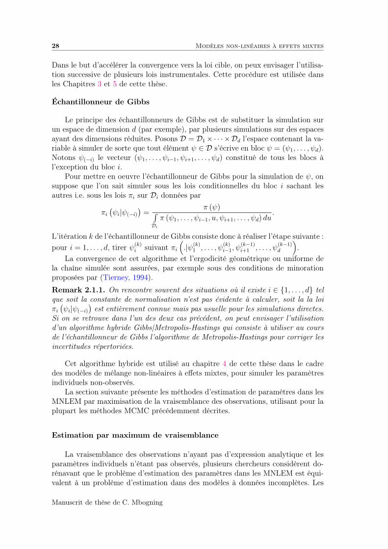
Dans le but d’accélérer la convergence vers la loi cible, on peux envisager l’utilisa-tion successive de plusieurs lois instrumentales. Cette procédure est utilisée dansles Chapitres 3 et 5 de cette thèse.
Échantillonneur de Gibbs
Le principe des échantillonneurs de Gibbs est de substituer la simulation surun espace de dimension d (par exemple), par plusieurs simulations sur des espacesayant des dimensions réduites. Posons D = D1×· · ·×Dd l’espace contenant la va-riable à simuler de sorte que tout élément ψ ∈ D s’écrive en bloc ψ = (ψ1, . . . , ψd).Notons ψ(−i) le vecteur (ψ1, . . . , ψi−1, ψi+1, . . . , ψd) constitué de tous les blocs àl’exception du bloc i.
Pour mettre en oeuvre l’échantillonneur de Gibbs pour la simulation de ψ, onsuppose que l’on sait simuler sous les lois conditionnelles du bloc i sachant lesautres i.e. sous les lois πi sur Di données par
πi(ψi|ψ(−i)
)=
π (ψ)∫Di
π (ψ1, . . . , ψi−1, u, ψi+1, . . . , ψd) du.
L’itération k de l’échantillonneur de Gibbs consiste donc à réaliser l’étape suivante :pour i = 1, . . . , d, tirer ψ(k)
i suivant πi(.|ψ(k)
1 , . . . , ψ(k)i−1, ψ
(k−1)i+1 , . . . , ψ
(k−1)d
).
La convergence de cet algorithme et l’ergodicité géométrique ou uniforme dela chaîne simulée sont assurées, par exemple sous des conditions de minorationproposées par (Tierney, 1994).
Remark 2.1.1. On rencontre souvent des situations où il existe i ∈ 1, . . . , d telque soit la constante de normalisation n’est pas évidente à calculer, soit la la loiπi(ψi|ψ(−i)
)est entièrement connue mais pas usuelle pour les simulations directes.
Si on se retrouve dans l’un des deux cas précédent, on peut envisager l’utilisationd’un algorithme hybride Gibbs|Metropolis-Hastings qui consiste à utiliser au coursde l’échantillonneur de Gibbs l’algorithme de Metropolis-Hastings pour corriger lesincertitudes répertoriées.
Cet algorithme hybride est utilisé au chapitre 4 de cette thèse dans le cadredes modèles de mélange non-linéaires à effets mixtes, pour simuler les paramètresindividuels non-observés.
La section suivante présente les méthodes d’estimation de paramètres dans lesMNLEM par maximisation de la vraisemblance des observations, utilisant pour laplupart les méthodes MCMC précédemment décrites.
Estimation par maximum de vraisemblance
La vraisemblance des observations n’ayant pas d’expression analytique et lesparamètres individuels n’étant pas observés, plusieurs chercheurs considèrent do-rénavant que le problème d’estimation des paramètres dans les MNLEM est équi-valent à un problème d’estimation dans des modèles à données incomplètes. Les
Manuscrit de thèse de C. Mbogning
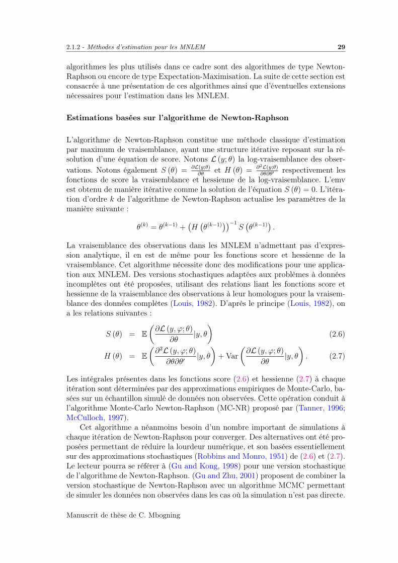
2.1.2 - Méthodes d’estimation pour les MNLEM 29
algorithmes les plus utilisés dans ce cadre sont des algorithmes de type Newton-Raphson ou encore de type Expectation-Maximisation. La suite de cette section estconsacrée à une présentation de ces algorithmes ainsi que d’éventuelles extensionsnécessaires pour l’estimation dans les MNLEM.
Estimations basées sur l’algorithme de Newton-Raphson
L’algorithme de Newton-Raphson constitue une méthode classique d’estimationpar maximum de vraisemblance, ayant une structure itérative reposant sur la ré-solution d’une équation de score. Notons L (y; θ) la log-vraisemblance des obser-vations. Notons également S (θ) = ∂L(y;θ)
∂θet H (θ) = ∂2L(y;θ)
∂θ∂θ′respectivement les
fonctions de score la vraisemblance et hessienne de la log-vraisemblance. L’emvest obtenu de manière itérative comme la solution de l’équation S (θ) = 0. L’itéra-tion d’ordre k de l’algorithme de Newton-Raphson actualise les paramètres de lamanière suivante :
θ(k) = θ(k−1) +(H(θ(k−1)
))−1S(θ(k−1)
).
La vraisemblance des observations dans les MNLEM n’admettant pas d’expres-sion analytique, il en est de même pour les fonctions score et hessienne de lavraisemblance. Cet algorithme nécessite donc des modifications pour une applica-tion aux MNLEM. Des versions stochastiques adaptées aux problèmes à donnéesincomplètes ont été proposées, utilisant des relations liant les fonctions score ethessienne de la vraisemblance des observations à leur homologues pour la vraisem-blance des données complètes (Louis, 1982). D’après le principe (Louis, 1982), ona les relations suivantes :
S (θ) = E(∂L (y, ϕ; θ)
∂θ|y, θ
)(2.6)
H (θ) = E(∂2L (y, ϕ; θ)
∂θ∂θ′|y, θ
)+ Var
(∂L (y, ϕ; θ)
∂θ|y, θ
). (2.7)
Les intégrales présentes dans les fonctions score (2.6) et hessienne (2.7) à chaqueitération sont déterminées par des approximations empiriques de Monte-Carlo, ba-sées sur un échantillon simulé de données non observées. Cette opération conduit àl’algorithme Monte-Carlo Newton-Raphson (MC-NR) proposé par (Tanner, 1996;McCulloch, 1997).
Cet algorithme a néanmoins besoin d’un nombre important de simulations àchaque itération de Newton-Raphson pour converger. Des alternatives ont été pro-posées permettant de réduire la lourdeur numérique, et son basées essentiellementsur des approximations stochastiques (Robbins and Monro, 1951) de (2.6) et (2.7).Le lecteur pourra se référer à (Gu and Kong, 1998) pour une version stochastiquede l’algorithme de Newton-Raphson. (Gu and Zhu, 2001) proposent de combiner laversion stochastique de Newton-Raphson avec un algorithme MCMC permettantde simuler les données non observées dans les cas où la simulation n’est pas directe.
Manuscrit de thèse de C. Mbogning
30 Modèles non-linéaires à effets mixtes
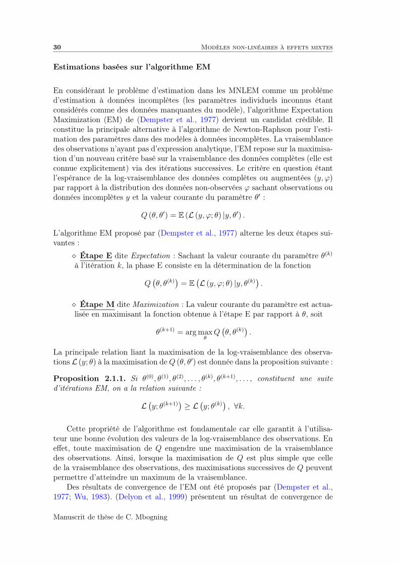
Estimations basées sur l’algorithme EM
En considérant le problème d’estimation dans les MNLEM comme un problèmed’estimation à données incomplètes (les paramètres individuels inconnus étantconsidérés comme des données manquantes du modèle), l’algorithme ExpectationMaximization (EM) de (Dempster et al., 1977) devient un candidat crédible. Ilconstitue la principale alternative à l’algorithme de Newton-Raphson pour l’esti-mation des paramètres dans des modèles à données incomplètes. La vraisemblancedes observations n’ayant pas d’expression analytique, l’EM repose sur la maximisa-tion d’un nouveau critère basé sur la vraisemblance des données complètes (elle estconnue explicitement) via des itérations successives. Le critère en question étantl’espérance de la log-vraisemblance des données complètes ou augmentées (y, ϕ)par rapport à la distribution des données non-observées ϕ sachant observations oudonnées incomplètes y et la valeur courante du paramètre θ′ :
Q (θ, θ′) = E (L (y, ϕ; θ) |y, θ′) .
L’algorithme EM proposé par (Dempster et al., 1977) alterne les deux étapes sui-vantes :
Étape E dite Expectation : Sachant la valeur courante du paramètre θ(k)
à l’itération k, la phase E consiste en la détermination de la fonction
Q(θ, θ(k)
)= E
(L (y, ϕ; θ) |y, θ(k)
).
Étape M dite Maximization : La valeur courante du paramètre est actua-lisée en maximisant la fonction obtenue à l’étape E par rapport à θ, soit
θ(k+1) = arg maxθQ(θ, θ(k)
).
La principale relation liant la maximisation de la log-vraisemblance des observa-tions L (y; θ) à la maximisation deQ (θ, θ′) est donnée dans la proposition suivante :
Proposition 2.1.1. Si θ(0), θ(1), θ(2), . . . , θ(k), θ(k+1), . . . , constituent une suited’itérations EM, on a la relation suivante :
L(y; θ(k+1)
)≥ L
(y; θ(k)
), ∀k.
Cette propriété de l’algorithme est fondamentale car elle garantit à l’utilisa-teur une bonne évolution des valeurs de la log-vraisemblance des observations. Eneffet, toute maximisation de Q engendre une maximisation de la vraisemblancedes observations. Ainsi, lorsque la maximisation de Q est plus simple que cellede la vraisemblance des observations, des maximisations successives de Q peuventpermettre d’atteindre un maximum de la vraisemblance.
Des résultats de convergence de l’EM ont été proposés par (Dempster et al.,1977; Wu, 1983). (Delyon et al., 1999) présentent un résultat de convergence de
Manuscrit de thèse de C. Mbogning

2.1.2 - Méthodes d’estimation pour les MNLEM 31
l’EM avec des hypothèses plus simples, dans le cadre des modèles appartenantà la famille exponentielle des modèles. En dépit de son caractère intuitif et desbonnes propriétés liées à l’algorithme EM, il est néanmoins sujet à plusieurs dif-ficultés d’ordre pratique. Il existe ainsi des situations où la quantité Q (θ, θ′) nepossède pas d’expression analytique, la maximisation de Q (θ, θ′) est extrêmementcomplexe, la convergence de l’algorithme est assez lente. Néanmoins, les problèmespersistants sont liés à la détermination de Q (θ, θ′). C’est d’ailleurs le cas dans lesMNLEM où la loi a posteriori l (ϕ|y, θ′) des paramètres individuels est inconnue,rendant impossible le calcul direct de Q (θ, θ′). Des extensions stochastiques del’EM ont été proposées pour remédier au problème.
L’Algorithme MCEM
(Wei and Tanner, 1990) proposent un algorithme MCEM (Monte-Carlo EM) per-mettant d’approcher la quantité Q (θ, θ′) par une méthode Monte-Carlo. A chaqueitération, un nombre L de variables aléatoires ϕ(k) est généré à partir de la loia posteriori l
(ϕ|y, θ(k)
), la fonction Q est ensuite approchée par une moyenne
empirique
Q(θ, θ(k)
)≈ 1
L
L∑k=1
L(y, ϕ(k); θ
).
On dénote cependant à ce jour une quasi-absence de résultats théoriques de conver-gence de cet algorithme. Il peut avoir des problèmes numériques tels qu’une conver-gence lente ou inexistante. Le nombre L de réplications joue un role importantpour la convergence, mais son choix reste un problème ouvert. En général, cetalgorithme nécessite un nombre de réplications assez important à chaque itérationet principalement lors des dernières itérations, ce qui rend la méthode assez lourdenumériquement avec des temps d’exécution très élevés.
La simulation de ϕ suivant la loi à posteriori l (ϕ|y, θ) n’étant pas directe dansles MNLEM, (Walker, 1996; Wu, 2004) proposent de combiner l’algorithme MCEMavec une procédure MCMC permettant de simuler les paramètres individuels ϕ. Ilsrapportent les mêmes problèmes de convergence numérique et ne proposent aucunrésultat théorique.
L’Algorithme SAEM
Une solution aussi bien théorique que numérique aux problèmes sus-cités repose surune approximation stochastique de l’étape E et a été proposée par (Delyon et al.,1999). L’algorithme SAEM (Stochastic Approximation EM) proposé par (Delyonet al., 1999) incorpore une étape de simulation et une étape d’approximation àl’algorithme EM. Partant d’une position initiale θ(0), une itération de l’algorithmeSAEM qui à θ(k) associe θ(k+1) est donnée par :
Étape S : Simuler les paramètres individuels inconnus ϕ(k) suivant la dis-tribution conditionnelle l
(ϕ|y, θ(k)
).
Manuscrit de thèse de C. Mbogning
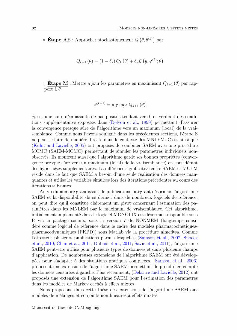
32 Modèles non-linéaires à effets mixtes
Étape AE : Approcher stochastiquement Q(θ, θ(k)
)par
Qk+1 (θ) = (1− δk)Qk (θ) + δkL(y, ϕ(k); θ
).
Étape M : Mettre à jour les paramètres en maximisant Qk+1 (θ) par rap-port à θ
θ(k+1) = arg maxθQk+1 (θ) .
δk est une suite décroissante de pas positifs tendant vers 0 et vérifiant des condi-tions supplémentaires exposées dans (Delyon et al., 1999) permettant d’assurerla convergence presque sûre de l’algorithme vers un maximum (local) de la vrai-semblance. Comme nous l’avons souligné dans les précédentes sections, l’étape Sne peut se faire de manière directe dans le contexte des MNLEM. C’est ainsi que(Kuhn and Lavielle, 2005) ont proposés de combiner SAEM avec une procédureMCMC (SAEM-MCMC) permettant de simuler les paramètres individuels non-observés. Ils montrent aussi que l’algorithme garde ses bonnes propriétés (conver-gence presque sûre vers un maximum (local) de la vraisemblance) en considérantdes hypothèses supplémentaires. La différence significative entre SAEM et MCEMréside dans le fait que SAEM a besoin d’une seule réalisation des données man-quantes et utilise les variables simulées lors des itérations précédentes au cours desitérations suivantes.
Au vu du nombre grandissant de publications intégrant désormais l’algorithmeSAEM et la disponibilité de ce dernier dans de nombreux logiciels de référence,on peut dire qu’il constitue clairement un pivot concernant l’estimation des pa-ramètres dans les MNLEM par le maximum de vraisemblance. Cet algorithme,initialement implementé dans le logiciel MONOLIX est désormais disponible sousR via la package saemix, sous la version 7 de NONMEM (longtemps consi-déré comme logiciel de référence dans le cadre des modèles pharmacocinétiques-pharmacodynamiques (PKPD)) sous Matlab via la procédure nlmefitsa. Commel’attestent plusieurs publications parmis lesquelles (Samson et al., 2007; Snoecket al., 2010; Chan et al., 2011; Dubois et al., 2011; Savic et al., 2011), l’algorithmeSAEM peut-être utilisé pour plusieurs types de données et dans plusieurs champsd’application. De nombreuses extensions de l’algorithme SAEM ont été dévelop-pées pour s’adapter à des situations pratiques complexes. (Samson et al., 2006)proposent une extension de l’algorithme SAEM permettant de prendre en compteles données censurées à gauche. Plus récemment, (Delattre and Lavielle, 2012) ontproposés une extension de l’algorithme SAEM pour l’estimation des paramètresdans les modèles de Markov cachés à effets mixtes.
Nous proposons dans cette thèse des extensions de l’algorithme SAEM auxmodèles de mélanges et conjoints non linéaires à effets mixtes.
Manuscrit de thèse de C. Mbogning
2.2.1 - Modèle de mélanges de distributions 33
2.2 Modèles de mélanges finis
2.2.1 Modèle de mélanges de distributions
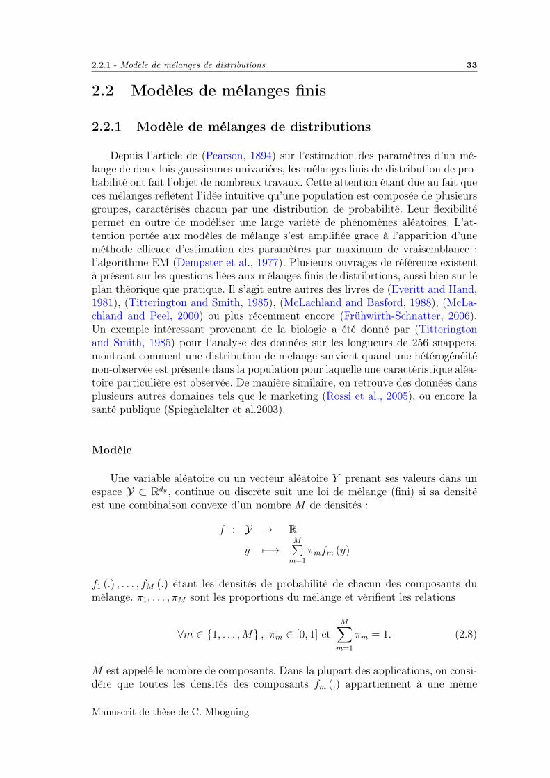
Depuis l’article de (Pearson, 1894) sur l’estimation des paramètres d’un mé-lange de deux lois gaussiennes univariées, les mélanges finis de distribution de pro-babilité ont fait l’objet de nombreux travaux. Cette attention étant due au fait queces mélanges reflètent l’idée intuitive qu’une population est composée de plusieursgroupes, caractérisés chacun par une distribution de probabilité. Leur flexibilitépermet en outre de modéliser une large variété de phénomènes aléatoires. L’at-tention portée aux modèles de mélange s’est amplifiée grace à l’apparition d’uneméthode efficace d’estimation des paramètres par maximum de vraisemblance :l’algorithme EM (Dempster et al., 1977). Plusieurs ouvrages de référence existentà présent sur les questions liées aux mélanges finis de distribrtions, aussi bien sur leplan théorique que pratique. Il s’agit entre autres des livres de (Everitt and Hand,1981), (Titterington and Smith, 1985), (McLachland and Basford, 1988), (McLa-chland and Peel, 2000) ou plus récemment encore (Frühwirth-Schnatter, 2006).Un exemple intéressant provenant de la biologie a été donné par (Titteringtonand Smith, 1985) pour l’analyse des données sur les longueurs de 256 snappers,montrant comment une distribution de melange survient quand une hétérogénéiténon-observée est présente dans la population pour laquelle une caractéristique aléa-toire particulière est observée. De manière similaire, on retrouve des données dansplusieurs autres domaines tels que le marketing (Rossi et al., 2005), ou encore lasanté publique (Spieghelalter et al.2003).
Modèle
Une variable aléatoire ou un vecteur aléatoire Y prenant ses valeurs dans unespace Y ⊂ Rdy , continue ou discrète suit une loi de mélange (fini) si sa densitéest une combinaison convexe d’un nombre M de densités :
f : Y → R
y 7−→M∑m=1
πmfm (y)
f1 (.) , . . . , fM (.) étant les densités de probabilité de chacun des composants dumélange. π1, . . . , πM sont les proportions du mélange et vérifient les relations
∀m ∈ 1, . . . ,M , πm ∈ [0, 1] etM∑m=1
πm = 1. (2.8)
M est appelé le nombre de composants. Dans la plupart des applications, on consi-dère que toutes les densités des composants fm (.) appartiennent à une même
Manuscrit de thèse de C. Mbogning

34 Modèles de mélanges finis
famille de distribution paramétrique P (ϑ) de densité f(y|ϑ), indexée par le para-mètre ϑ ∈ Θ :
f(y|ϑ) =M∑m=1
πmfm (y|θm) . (2.9)
La densité de probabilité du melange de distribution f(y|ϑ) est indexée par leparamètre ϑ = (π1, . . . , πM , θ1, . . . , θM) prenant ses valeurs dans l’espace paramé-trique ΘM = ΠM ×ΘM , ΠM étant l’ensemble des M-uplets π1, . . . , πM vérifiant lacondition (2.8).
Il existe dans la littérature plusieurs types de mélanges de lois (mélange delois uniformes, binomiales, exponentielles, gaussiennes,...). D’un point de vue his-torique, le mélange de deux distributions gaussiennes univariées de moyennes diffé-rentes et de variance différentes est la plus ancienne application connue du modèlede mélange de distribution (Pearson, 1894). On rencontre par la suite des modèlesde mélange de distributions de Poisson (Feller, 1943), modèles de mélange de dis-tributions exponentielles (Teicher, 1963). Ces exemples sont des cas spéciaux desmodèles de mélange de distributions issues de la famille exponentielle traités par(Barndoff-Nielsen, 1978). (Shaked, 1980) présente un traitement mathématique gé-néral sur les mélanges de la famille exponentielle. le mélange de gaussiennes restenéanmoins le plus populaire dans la littérature statistique. Dans le cas particu-lier d’un mélange de gaussiennes, les fm sont remplacées par les densités d’unegaussienne de moyenne µm et de matrice de variance Σm. On aura donc
∀y ∈ Rdy , f(y|θ) =M∑m=1
πmΦdy (y;µm,Σm) ,
Φd (.;µ,Σ) étant la densité d’une gaussienne d-dimensionnelle de moyenne µ etde matrice de variance Σ. Le vecteur des paramètres est donné ici par ϑ =(π1, . . . , πM , µ1, . . . , µM ,Σ1, . . . ,ΣM). Pour des nécessités de modélisation, les ma-trices de variances covariance des composantes Σm peuvent être restreintes à desstructures particulières. (Banfield and Raftery, 1993) et par la suite (Celeux andGovaert, 1995) ont proposé de manière analogue, la décomposition suivante de Σm
dans chaque composante :
Σm = λmHmAmH′m,
où λm représente la plus grande valeur propre de Σm dans (Banfield and Raftery,
1993) et λm =
∣∣∣∣Σ 1dym
∣∣∣∣ dans (Celeux and Govaert, 1995). Suivant cette dernière
convention, λm est le volume de Σm. λmAm est une matrice diagonale contenantles valeurs propres de Σm rangées par ordre décroissant sur la diagonale : cettequantité représente la forme des composantes. Hm est la matrice des vecteurspropres de Σm et représente l’orientation des composantes. En faisant varier ounon les proportions du mélange, les volumes, les formes et les orientations, onobtient une collection de 28 modèles présentés dans (Celeux and Govaert, 1995).
Manuscrit de thèse de C. Mbogning
2.2.1 - Modèle de mélanges de distributions 35
Identifiabilité
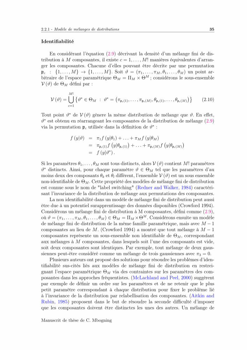
En considérant l’équation (2.9) décrivant la densité d’un mélange fini de dis-tribution à M composantes, il existe c = 1, . . . ,M ! manières équivalentes d’arran-ger les composantes. Chacune d’elles pouvant être décrite par une permutationpc : 1, . . . ,M → 1, . . . ,M. Soit ϑ = (π1, . . . , πM , θ1, . . . , θM) un point ar-bitraire de l’espace paramétrique ΘM = ΠM × ΘM ; considérons le sous-ensembleV (ϑ) de ΘM défini par :
V (ϑ) =M !⋃c=1
ϑ∗ ∈ ΘM : ϑ∗ =
(πpc(1), . . . , πpc(M), θpc(1), . . . , θpc(M)
)(2.10)
Tout point ϑ∗ de V (ϑ) génere la même distribution de mélange que ϑ. En effet,ϑ∗ est obtenu en réarrangeant les composantes de la distribution de mélange (2.9)via la permutation pc utilisée dans la définition de ϑ∗ :
f (y|ϑ) = π1f (y|θ1) + . . .+ πMf (y|θM)
= πpc(1)f(y|θpc(1)
)+ . . .+ πpc(M)f
(y|θpc(M)
)= f (y|ϑ∗) .
Si les paramètres θ1, . . . , θM sont tous distincts, alors V (ϑ) contientM ! paramètresϑ∗ distincts. Ainsi, pour chaque paramètre ϑ ∈ ΘM tel que les paramètres d’aumoins deux des composants θk et θl diffèrent, l’ensemble V (ϑ) est un sous ensemblenon-identifiable de ΘM . Cette propriété des modèles de mélange fini de distributionest connue sous le nom de "label switching" (Redner and Walker, 1984) caractéri-sant l’invariance de la distribution de mélange aux permutations des composantes.
La non identifiabilité dans un modèle de mélange fini de distribution peut aussiêtre due à un potentiel surapprentissage des données disponibles (Crowford 1994).Considérons un mélange fini de distribution à M composantes, défini comme (2.9),où ϑ = (π1, . . . , πM , θ1, . . . , θM) ∈ ΘM = ΠM×ΘM . Considérons ensuite un modèlede mélange fini de distribution de la même famille paramétrique, mais avec M − 1composantes au lieu de M . (Crowford 1994) a montré que tout mélange à M − 1composantes représente un sous-ensemble non identifiable de ΘM , correspondantaux mélanges à M composantes, dans lesquels soit l’une des composants est vide,soit deux composantes sont identiques. Par exemple, tout mélange de deux gaus-siennes peut-être considéré comme un mélange de trois gaussiennes avec π3 = 0.
Plusieurs auteurs ont proposé des solutions pour résoudre les problèmes d’iden-tifiabilité sus-cités liés aux modèles de mélange fini de distribution en restrei-gnant l’espace paramétrique ΘM via des contraintes sur les paramètres des com-posantes dans les approches fréquentistes. (McLachland and Peel, 2000) suggèrentpar exemple de définir un ordre sur les paramètres et de ne retenir que le pluspetit paramètre correspondant à chaque distribution pour fixer le problème liéà l’invariance de la distribution par relabellisation des composantes. (Aitkin andRubin, 1985) proposent dans le but de résoudre la seconde difficulté d’imposerque les composantes doivent être distinctes les unes des autres. Un mélange de
Manuscrit de thèse de C. Mbogning
36 Modèles de mélanges finis
distribution à M composantes sera considéré comme un mélange de distributionà M − 1 composantes dès que deux de ses composantes seront identiques. Dans lemême esprit, les proportions de mélange nulles ne sont pas acceptées. (Yakowitzand Spragins, 1968) définissent une notion faible d’identifiabilité qui accepte le"label switching". Cette définition est suffisante lorsque les grandeurs d’intérêt nedépendent pas de l’ordre des composantes. Dans le but de construire un test derapport de vraisemblance pour les modèles de mélange de distribution, (Dacunha-Castelle and Gassiat, 1999) ont défini une paramétrisation appelées "locally conicparametrization" permettant de séparer la partie identifiable des paramètres et lapartie non-identifiable. Dans un cadre bayésien, le phénomène de "label switching"a attiré l’attention de plusieurs auteurs. On peut citer entre autres (Celeux, 1998;Yao and Lindsay, 2009; Papastamoulis and Iliopoulos, 2010; Yao, 2012).
Nous proposons, dans le Chapitre 3, une procédure qui permet entre autred’éviter le "label switching" lors de l’estimation des paramètres du modèle.
Estimation des paramètres
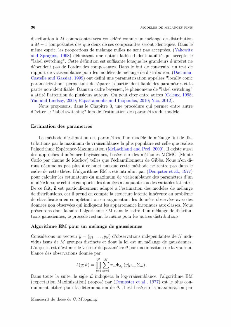
La méthode d’estimation des paramètres d’un modèle de mélange fini de dis-tributions par le maximum de vraisemblance la plus populaire est celle que réalisel’algorithme Espérance-Maximisation (McLachland and Peel, 2000). Il existe aussides approches d’inférence bayésiennes, basées sur des méthodes MCMC (MonteCarlo par chaîne de Markov) telles que l’échantillonneur de Gibbs. Nous n’en di-rons néanmoins pas plus à ce sujet puisque cette méthode ne rentre pas dans lecadre de cette thèse. L’algorithme EM a été introduit par (Dempster et al., 1977)pour calculer les estimateurs du maximum de vraisemblance des paramètres d’unmodèle lorsque celui-ci comporte des données manquantes ou des variables latentes.De ce fait, il est particulièrement adapté à l’estimation des modèles de mélangede distributions, car il prend en compte la structure latente inhérente au problèmede classification en complétant ou en augmentant les données observées avec desdonnées non observées qui indiquent les appartenance inconnues aux classes. Nousprésentons dans la suite l’algorithme EM dans le cadre d’un mélange de distribu-tions gaussiennes, le procédé restant le même pour les autres distributions.
Algorithme EM pour un mélange de gaussiennes
Considérons un vecteur y = (y1, . . . , yN) d’observations indépendantes de N indi-vidus issus de M groupes distincts et dont la loi est un mélange de gaussiennes.L’objectif est d’estimer le vecteur de paramètre ϑ par maximisation de la vraisem-blance des observations donnée par
l (y;ϑ) =N∏i=1
M∑m=1
πmΦdy (y|µm,Σm) .
Dans toute la suite, le sigle L indiquera la log-vraisemblance. l’algorithme EM(expectation Maximization) proposé par (Dempster et al., 1977) est le plus cou-ramment utilisé pour la détermination de ϑ. Il est basé sur la maximisation par
Manuscrit de thèse de C. Mbogning
2.2.1 - Modèle de mélanges de distributions 37
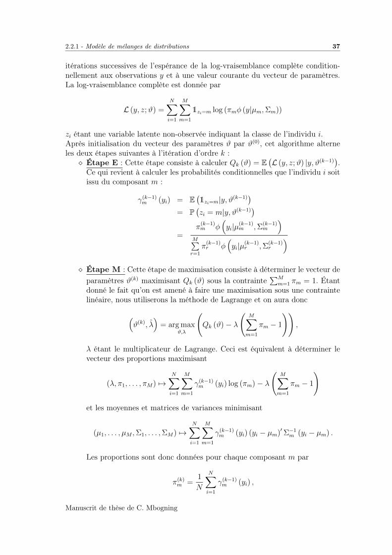
itérations successives de l’espérance de la log-vraisemblance complète condition-nellement aux observations y et à une valeur courante du vecteur de paramètres.La log-vraisemblance complète est donnée par
L (y, z;ϑ) =N∑i=1
M∑m=1
1zi=m log (πmφ (y|µm,Σm))
zi étant une variable latente non-observée indiquant la classe de l’individu i.Après initialisation du vecteur des paramètres ϑ par ϑ(0), cet algorithme alterneles deux étapes suivantes à l’itération d’ordre k : Étape E : Cette étape consiste à calculer Qk (ϑ) = E
(L (y, z;ϑ) |y, ϑ(k−1)
).
Ce qui revient à calculer les probabilités conditionnelles que l’individu i soitissu du composant m :
γ(k−1)m (yi) = E
(1zi=m|y, ϑ(k−1)
)= P
(zi = m|y, ϑ(k−1)
)=
π(k−1)m φ
(yi|µ(k−1)
m ,Σ(k−1)m
)M∑r=1
π(k−1)r φ
(yi|µ(k−1)
r ,Σ(k−1)r
) Étape M : Cette étape de maximisation consiste à déterminer le vecteur de
paramètres ϑ(k) maximisant Qk (ϑ) sous la contrainte∑M
m=1 πm = 1. Étantdonné le fait qu’on est amené à faire une maximisation sous une contraintelinéaire, nous utiliserons la méthode de Lagrange et on aura donc
(ϑ(k), λ
)= arg max
ϑ,λ
(Qk (ϑ)− λ
(M∑m=1
πm − 1
)),
λ étant le multiplicateur de Lagrange. Ceci est équivalent à déterminer levecteur des proportions maximisant
(λ, π1, . . . , πM) 7→N∑i=1
M∑m=1
γ(k−1)m (yi) log (πm)− λ
(M∑m=1
πm − 1
)
et les moyennes et matrices de variances minimisant
(µ1, . . . , µM ,Σ1, . . . ,ΣM) 7→N∑i=1
M∑m=1
γ(k−1)m (yi) (yi − µm)′Σ−1
m (yi − µm) .
Les proportions sont donc données pour chaque composant m par
π(k)m =
1
N
N∑i=1
γ(k−1)m (yi) ,
Manuscrit de thèse de C. Mbogning
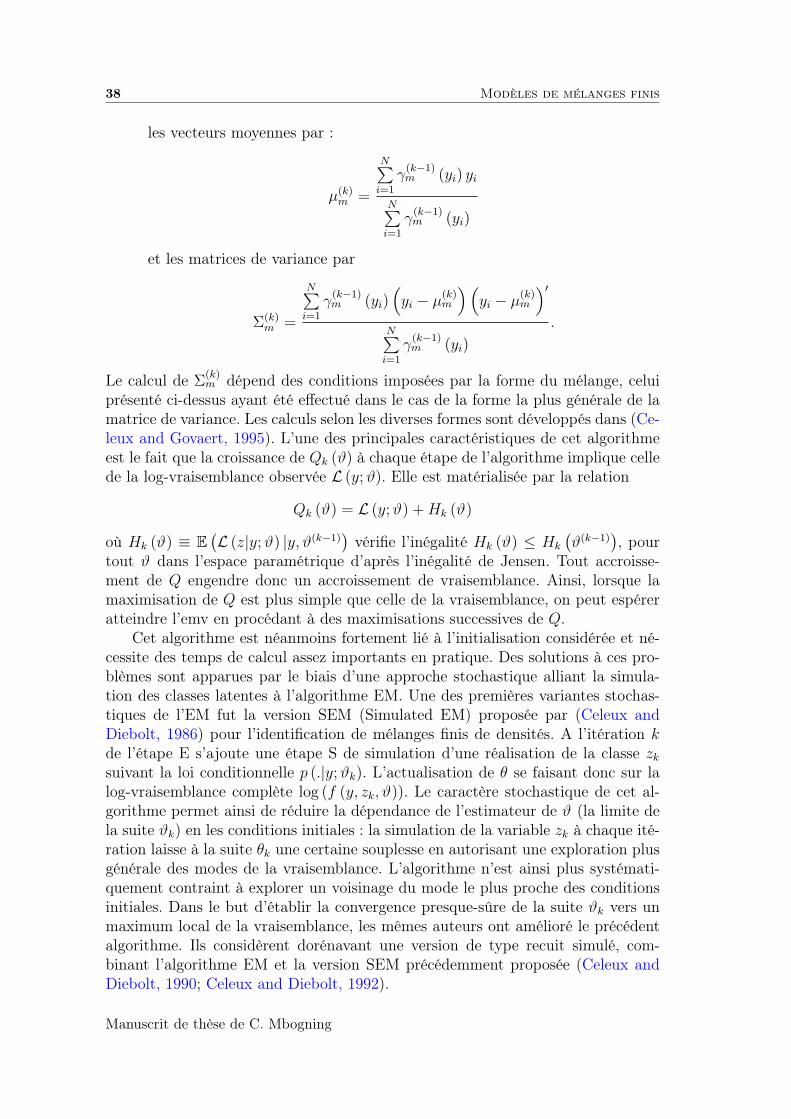
38 Modèles de mélanges finis
les vecteurs moyennes par :
µ(k)m =
N∑i=1
γ(k−1)m (yi) yi
N∑i=1
γ(k−1)m (yi)
et les matrices de variance par
Σ(k)m =
N∑i=1
γ(k−1)m (yi)
(yi − µ(k)
m
)(yi − µ(k)
m
)′N∑i=1
γ(k−1)m (yi)
.
Le calcul de Σ(k)m dépend des conditions imposées par la forme du mélange, celui
présenté ci-dessus ayant été effectué dans le cas de la forme la plus générale de lamatrice de variance. Les calculs selon les diverses formes sont développés dans (Ce-leux and Govaert, 1995). L’une des principales caractéristiques de cet algorithmeest le fait que la croissance de Qk (ϑ) à chaque étape de l’algorithme implique cellede la log-vraisemblance observée L (y;ϑ). Elle est matérialisée par la relation
Qk (ϑ) = L (y;ϑ) +Hk (ϑ)
où Hk (ϑ) ≡ E(L (z|y;ϑ) |y, ϑ(k−1)
)vérifie l’inégalité Hk (ϑ) ≤ Hk
(ϑ(k−1)
), pour
tout ϑ dans l’espace paramétrique d’après l’inégalité de Jensen. Tout accroisse-ment de Q engendre donc un accroissement de vraisemblance. Ainsi, lorsque lamaximisation de Q est plus simple que celle de la vraisemblance, on peut espéreratteindre l’emv en procédant à des maximisations successives de Q.
Cet algorithme est néanmoins fortement lié à l’initialisation considérée et né-cessite des temps de calcul assez importants en pratique. Des solutions à ces pro-blèmes sont apparues par le biais d’une approche stochastique alliant la simula-tion des classes latentes à l’algorithme EM. Une des premières variantes stochas-tiques de l’EM fut la version SEM (Simulated EM) proposée par (Celeux andDiebolt, 1986) pour l’identification de mélanges finis de densités. A l’itération kde l’étape E s’ajoute une étape S de simulation d’une réalisation de la classe zksuivant la loi conditionnelle p (.|y;ϑk). L’actualisation de θ se faisant donc sur lalog-vraisemblance complète log (f (y, zk, ϑ)). Le caractère stochastique de cet al-gorithme permet ainsi de réduire la dépendance de l’estimateur de ϑ (la limite dela suite ϑk) en les conditions initiales : la simulation de la variable zk à chaque ité-ration laisse à la suite θk une certaine souplesse en autorisant une exploration plusgénérale des modes de la vraisemblance. L’algorithme n’est ainsi plus systémati-quement contraint à explorer un voisinage du mode le plus proche des conditionsinitiales. Dans le but d’établir la convergence presque-sûre de la suite ϑk vers unmaximum local de la vraisemblance, les mêmes auteurs ont amélioré le précédentalgorithme. Ils considèrent dorénavant une version de type recuit simulé, com-binant l’algorithme EM et la version SEM précédemment proposée (Celeux andDiebolt, 1990; Celeux and Diebolt, 1992).
Manuscrit de thèse de C. Mbogning
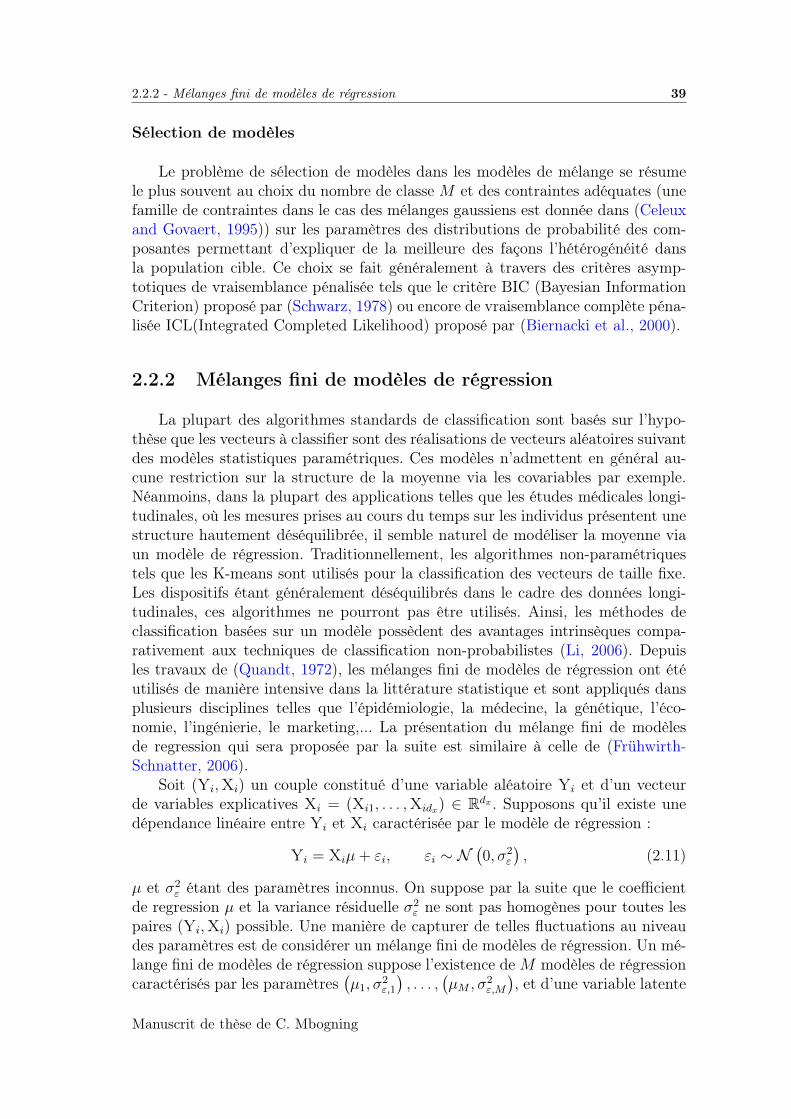
2.2.2 - Mélanges fini de modèles de régression 39
Sélection de modèles
Le problème de sélection de modèles dans les modèles de mélange se résumele plus souvent au choix du nombre de classe M et des contraintes adéquates (unefamille de contraintes dans le cas des mélanges gaussiens est donnée dans (Celeuxand Govaert, 1995)) sur les paramètres des distributions de probabilité des com-posantes permettant d’expliquer de la meilleure des façons l’hétérogénéité dansla population cible. Ce choix se fait généralement à travers des critères asymp-totiques de vraisemblance pénalisée tels que le critère BIC (Bayesian InformationCriterion) proposé par (Schwarz, 1978) ou encore de vraisemblance complète péna-lisée ICL(Integrated Completed Likelihood) proposé par (Biernacki et al., 2000).
2.2.2 Mélanges fini de modèles de régression
La plupart des algorithmes standards de classification sont basés sur l’hypo-thèse que les vecteurs à classifier sont des réalisations de vecteurs aléatoires suivantdes modèles statistiques paramétriques. Ces modèles n’admettent en général au-cune restriction sur la structure de la moyenne via les covariables par exemple.Néanmoins, dans la plupart des applications telles que les études médicales longi-tudinales, où les mesures prises au cours du temps sur les individus présentent unestructure hautement déséquilibrée, il semble naturel de modéliser la moyenne viaun modèle de régression. Traditionnellement, les algorithmes non-paramétriquestels que les K-means sont utilisés pour la classification des vecteurs de taille fixe.Les dispositifs étant généralement déséquilibrés dans le cadre des données longi-tudinales, ces algorithmes ne pourront pas être utilisés. Ainsi, les méthodes declassification basées sur un modèle possèdent des avantages intrinsèques compa-rativement aux techniques de classification non-probabilistes (Li, 2006). Depuisles travaux de (Quandt, 1972), les mélanges fini de modèles de régression ont étéutilisés de manière intensive dans la littérature statistique et sont appliqués dansplusieurs disciplines telles que l’épidémiologie, la médecine, la génétique, l’éco-nomie, l’ingénierie, le marketing,... La présentation du mélange fini de modèlesde regression qui sera proposée par la suite est similaire à celle de (Frühwirth-Schnatter, 2006).
Soit (Yi,Xi) un couple constitué d’une variable aléatoire Yi et d’un vecteurde variables explicatives Xi = (Xi1, . . . ,Xidx) ∈ Rdx . Supposons qu’il existe unedépendance linéaire entre Yi et Xi caractérisée par le modèle de régression :
Yi = Xiµ+ εi, εi ∼ N(0, σ2
ε
), (2.11)
µ et σ2ε étant des paramètres inconnus. On suppose par la suite que le coefficient
de regression µ et la variance résiduelle σ2ε ne sont pas homogènes pour toutes les
paires (Yi,Xi) possible. Une manière de capturer de telles fluctuations au niveaudes paramètres est de considérer un mélange fini de modèles de régression. Un mé-lange fini de modèles de régression suppose l’existence deM modèles de régressioncaractérisés par les paramètres
(µ1, σ
2ε,1
), . . . ,
(µM , σ
2ε,M
), et d’une variable latente
Manuscrit de thèse de C. Mbogning
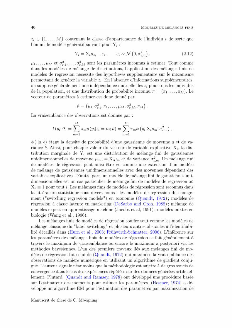
40 Modèles de mélanges finis
zi ∈ 1, . . . ,M contenant la classe d’appartenance de l’individu i de sorte quel’on ait le modèle génératif suivant pour Yi :
Yi = Xiµzi + εi, εi ∼ N(0, σ2
ε,zi
). (2.12)
µ1, . . . , µM et σ2ε,1, . . . , σ
2ε,M sont les paramètres inconnus à estimer. Tout comme
dans les modèles de mélange de distributions, l’application des mélanges finis demodèles de regression nécessite des hypothèses supplémentaire sur le mécanismepermettant de générer la variable zi. En l’absence d’informations supplémentaires,on suppose généralement une indépendance mutuelle des zi pour tous les individusde la population, et une distribution de probabilité inconnu π = (π1, . . . , πM). Levecteur de paramètres à estimer est donc donné par
ϑ =(µ1, σ
2ε,1, π1, . . . , µM , σ
2ε,M , πM
).
La vraisemblance des observations est donnée par :
l (yi;ϑ) =M∑m=1
πmp (yi|zi = m;ϑ) =M∑m=1
πmφ(yi|Xiµm;σ2
ε,m
),
φ (·|a, b) étant la densité de probabilité d’une gaussienne de moyenne a et de va-riance b. Ainsi, pour chaque valeur du vecteur de variable explicative Xi, la dis-tribution marginale de Yi est une distribution de mélange fini de gaussiennesunidimensionnelles de moyenne µm,i = Xiµm et de variance σ2
ε,m. Un melange finide modèles de régression peut ainsi être vu comme une extension d’un modèlede mélange de gaussiennes unidimensionnelles avec des moyennes dépendant desvariables explicatives. D’autre part, un modèle de mélange fini de gaussiennes uni-dimensionnelles est un cas particulier de mélange fini de modèles de regression oùXi ≡ 1 pour tout i. Les mélanges finis de modèles de régression sont reconnus dansla littérature statistique sous divers noms : les modèles de regression du change-ment ("switching regression models") en économie (Quandt, 1972) ; modèles derégression à classe latente en marketing (DeSarbo and Cron, 1988) ; mélange demodèles expert en apprentissage machine (Jacobs et al, 1991) ; modèles mixtes enbiologie (Wang et al., 1996).
Les mélanges finis de modèles de régression souffre tout comme les modèles demélange classique du "label switching" et plusieurs autres obstacles à l’identifiabi-lité détaillés dans (Hurn et al., 2003; Frühwirth-Schnatter, 2006). L’inférence surles paramètres des mélanges finis de modèles de régression se fait généralement àtravers le maximum de vraisemblance ou encore le maximum a posteriori via lesméthodes bayesiennes. L’un des premiers travaux liés aux mélanges fini de mo-dèles de régression fut celui de (Quandt, 1972) qui maximise la vraisemblance desobservations de manière numérique en utilisant un algorithme de gradient conju-gué. L’auteur signale néanmoins que la méthodologie est sujette à de gros soucis deconvergence dans le cas des expériences répétées sur des données générées artificiel-lement. Plutard, (Quandt and Ramsey, 1978) ont développé une procédure baséesur l’estimateur des moments pour estimer les paramètres. (Hosmer, 1974) a dé-veloppé un algorithme EM pour l’estimation des paramètres par maximization de
Manuscrit de thèse de C. Mbogning
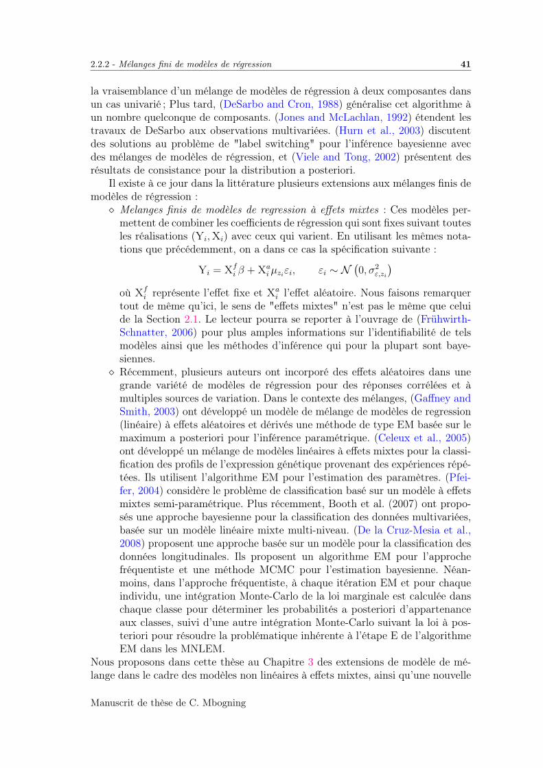
2.2.2 - Mélanges fini de modèles de régression 41
la vraisemblance d’un mélange de modèles de régression à deux composantes dansun cas univarié ; Plus tard, (DeSarbo and Cron, 1988) généralise cet algorithme àun nombre quelconque de composants. (Jones and McLachlan, 1992) étendent lestravaux de DeSarbo aux observations multivariées. (Hurn et al., 2003) discutentdes solutions au problème de "label switching" pour l’inférence bayesienne avecdes mélanges de modèles de régression, et (Viele and Tong, 2002) présentent desrésultats de consistance pour la distribution a posteriori.
Il existe à ce jour dans la littérature plusieurs extensions aux mélanges finis demodèles de régression : Melanges finis de modèles de regression à effets mixtes : Ces modèles per-
mettent de combiner les coefficients de régression qui sont fixes suivant toutesles réalisations (Yi,Xi) avec ceux qui varient. En utilisant les mêmes nota-tions que précédemment, on a dans ce cas la spécification suivante :
Yi = Xfi β + Xa
i µziεi, εi ∼ N(0, σ2
ε,zi
)où Xf
i représente l’effet fixe et Xai l’effet aléatoire. Nous faisons remarquer
tout de même qu’ici, le sens de "effets mixtes" n’est pas le même que celuide la Section 2.1. Le lecteur pourra se reporter à l’ouvrage de (Frühwirth-Schnatter, 2006) pour plus amples informations sur l’identifiabilité de telsmodèles ainsi que les méthodes d’inférence qui pour la plupart sont baye-siennes. Récemment, plusieurs auteurs ont incorporé des effets aléatoires dans une
grande variété de modèles de régression pour des réponses corrélées et àmultiples sources de variation. Dans le contexte des mélanges, (Gaffney andSmith, 2003) ont développé un modèle de mélange de modèles de regression(linéaire) à effets aléatoires et dérivés une méthode de type EM basée sur lemaximum a posteriori pour l’inférence paramétrique. (Celeux et al., 2005)ont développé un mélange de modèles linéaires à effets mixtes pour la classi-fication des profils de l’expression génétique provenant des expériences répé-tées. Ils utilisent l’algorithme EM pour l’estimation des paramètres. (Pfei-fer, 2004) considère le problème de classification basé sur un modèle à effetsmixtes semi-paramétrique. Plus récemment, Booth et al. (2007) ont propo-sés une approche bayesienne pour la classification des données multivariées,basée sur un modèle linéaire mixte multi-niveau. (De la Cruz-Mesia et al.,2008) proposent une approche basée sur un modèle pour la classification desdonnées longitudinales. Ils proposent un algorithme EM pour l’approchefréquentiste et une méthode MCMC pour l’estimation bayesienne. Néan-moins, dans l’approche fréquentiste, à chaque itération EM et pour chaqueindividu, une intégration Monte-Carlo de la loi marginale est calculée danschaque classe pour déterminer les probabilités a posteriori d’appartenanceaux classes, suivi d’une autre intégration Monte-Carlo suivant la loi à pos-teriori pour résoudre la problématique inhérente à l’étape E de l’algorithmeEM dans les MNLEM.
Nous proposons dans cette thèse au Chapitre 3 des extensions de modèle de mé-lange dans le cadre des modèles non linéaires à effets mixtes, ainsi qu’une nouvelle
Manuscrit de thèse de C. Mbogning
42 Modèles conjoints
méthodologie d’estimation des paramètres basée sur l’estimation par le maximumde vraisemblance. Le Chapitre 4 constitue une application à un jeu de donnéesréelles sur le VIH.
2.3 Modèles conjoints
2.3.1 Motivations
Lors des études médicales, plusieurs types de données sont généralement collec-tées sur chaque individu. 0n peut citer entre autres, des réponses de type longitudi-nal et le temps d’attente jusqu’à l’apparition d’un événement d’intérêt particulier.Les questions de recherche inhérentes à ce type de données sont diverses et variées.L’une d’entre elles consisterait en une analyse séparée des diverses réponses. Néan-moins, dans plusieurs situations, l’intérêt principal de l’étude consiste à étudier lastructure associative des diverses réponses. Un exemple fréquemment rencontrépour ce type de problème pourrait se trouver dans la recherche sur les marqueursbiologiques, où la plupart des études cliniques consistent en l’identification desbiomarqueurs ayant de fortes capacités pronostiques pour l’événement d’intérêt.Parmi les exemples standards, on peut citer entre autres, les recherches sur le VIHoù l’intérêt est généralement lié à l’association entre le nombre de CD4 ou la chargevirale et le temps d’attente jusqu’à l’apparition du SIDA, les études sur les cir-rhoses, destinées à évaluer la relation entre le sérum bilirubin et le temps jusqu’audécès. Une caractéristique inhérente importante de ces conditions médicales estleur nature dynamique. Ainsi, le taux de progression vers l’évènement d’intérêt estnon seulement différent d’un patient à l’autre, mais change aussi dynamiquementdans le temps pour un même patient. Ainsi, le vrai potentiel d’un biomarqueurdans la description de la progression d’une maladie et son association avec la surviene peut-être révélée qu’en considérant des évaluations répétées du marqueur dansl’analyse.
Plusieurs auteurs se sont penchés sur la question de modélisation de la relationentre une variable longitudinale et le temps jusqu’à l’apparition d’un événementd’intérêt. La première approche fut celle de (Kalbfleisch and Prentice, 2002) quiproposent de considérer un modèle de survie à risque proportionnel pour le délaijusqu’à l’évènement d’intérêt, en considérant la variable longitudinale comme unecovariable dépendant du temps. notons Ti la variable aléatoire contenant le délaijusqu’à l’évènement d’intérêt sur le sujet i, Yi(t), t > 0 le processus longitudinal surle sujet i, et Zi un vecteur de covariables mesurées sur l’individu i. L’associationentre le processus longitudinal, le délai à l’évènement et les covariables est carac-térisée par la relation entre Ti, Yi(t), et Zi via le modèle de risque proportionnel
λi (t) = limdt→0
P(t ≤ Ti < t+ dt|Ti ≥ t, Y H
i (t), Zi)
dt= λ0 (t) exp (γYi(t) + β′Zi) (2.13)
Manuscrit de thèse de C. Mbogning

2.3.1 - Motivations 43
Y Hi (t) = Yi(u), 0 ≤ u ≤ t étant l’historique du processus longitudinal jusqu’au
temps t. Ainsi, la fonction de risque dépend linéairement de l’historique du pro-cessus longitudinal via la valeur courante Yi(t). Ce modèle, très intuitif et simpleà appréhender théoriquement, s’avère néanmoins compliqué à mettre en oeuvre enpratique car les données idéales ne sont généralement pas disponibles. En dépitdu fait que le modèle de risque donné par 2.13 nécessite les valeurs de la réponselongitudinale à tout instant t, cette dernière n’est mesurée que de manière in-termittente à des instants tij ≤ Ti, i = 1, . . . , ni. De plus, les valeurs observéesYi (tij) pourraient différer des vraies valeurs de la variable longitudinale à causedes erreurs de mesure et au lieu de Yi (tij), on observerait plutôt Yi (tij) + εij, oùεij représente une erreur intra-individuelle. Le temps d’évènement pouvant êtrecensuré, la valeur de la variable longitudinale aux instants de censure est consi-dérée comme manquante. Dans l’idéal des cas où Yi(t) est observable pour toutt ≤ Ti, la seul difficulté inhérente au modèle (2.13) est la présence des censures.Soit Ci la variable aléatoire contenant l’instant de censure de l’évènement d’inté-rêt. Ainsi, on l’observation sur l’évènement d’intérêt est constituée des variablesBi = min (Ti, Ci) et ∆i = 1(Ti≤Ci). Suivant (Cox, 1972) et sous les conditionsdiscutées dans (Kalbfleisch and Prentice, 2002), l’inférence sur β et γ se fait enmaximisant la vraisemblance partielle
N∏i=1
exp (γYi(Bi) + β′Zi)∑Nk=1 exp (γYk(Bi) + β′Zk)1(Bk≥Bi)
. (2.14)
Il apparaît donc clairement à travers (2.14) que l’inférence nécessite les valeursdu processus longitudinal Yi(t) pour tous les individus i = 1, . . . , N et à tousles instants observés d’évènement. Comme nous l’avons mentionné précédemment,l’implémentation de ce modèle en pratique est compliquée de par le fait qu’on n’apas toutes les valeurs nécessaires de Yi(t).
Les premières approches qu’on pourrait considérer comme naïves consistaientgénéralement à imputer la valeur manquante Yi(t) par la valeur observée la plusproche pour l’individu i. Cette propriété est connue dans littérature sous le nomLOCF (Last Observation Carried Forward). Néanmoins, cette approche résulte endes estimations biaisées (Prentice, 1982), particulièrement quand le délai entre lesdiverses mesures est long ou les erreurs de mesure sont importantes. Des auteursproposent dans le but de s’affranchir des erreurs de mesures et d’obtenir les valeursde la variable longitudinale à tout instant, d’estimer les paramètres d’un modèlemixte sur la variable longitudinale, et d’ensuite utiliser les prédictions aux instantsnon observés dans le modèle de survie. D’après (Dafny and Tsiatsis, 1998), cetteapproche permet de réduire le biais par rapport à la méthode précédente sanstoutefois l’éradiquer. Ainsi, pour répondre aux questions de recherche concernantl’association entre des mesures répétées et le temps jusqu’à l’apparition d’un évé-nement d’intérêt de manière optimale, une nouvelle classe de modèles statistiquesa vu le jour : modèles conjoints de données longitudinales et de survie.
De nombreux auteurs se sont intéressés aux modèles conjoints, parmi lesquels(Tsiatis and Davidian, 2004) qui donnent un apercu global des modèles conjoints
Manuscrit de thèse de C. Mbogning
44 Modèles conjoints
et montre que l’estimation simultanée des paramètres d’un modèle linéaire mixtepour l’évolution de la variable longitudinale et d’un modèle de survie pour le dé-lai d’attente jusqu’à l’apparition de l’évènement, en maximisant la vraisemblanceconjointe permet d’obtenir des estimations sans biais des paramètres. Ces modèlessont désormais largement utilisés dans plusieurs domaines et ont fait l’objet deplusieurs ouvrages, l’un des plus récents étant celui de (Rizopoulos, 2012b).
2.3.2 Formalisation des modèles conjoints
Nous considérons ici la description faite par (Tsiatis and Davidian, 2004).Comme dans la section précédente, notons pour i = 1, . . . , N , Ti et Ci respec-tivement le délai à l’évènement et la censure ; Yi (t) le processus longitudinal à uninstant t, Zi un vecteur de covariables, Bi = min (Ti, Ci) et ∆i = 1(Ti≤Ci).
Un modèle conjoint est constitué de deux sous-modèles liés entre eux. L’unmodélisant le processus longitudinal Yi (t) et l’autre pour le délai à l’évènementTi, avec des hypothèses et des spécifications supplémentaires permettant une re-présentation complète de la distribution jointe des données observées Yi, Vi,∆i.
Modèle des données longitudinales
Un modèle linéaire mixte (Laird and Ware, 1982) est généralement utilisé pourles données longitudinales :
Yij = f (ϕi, tij) + εij, (2.15)
où Yij = Yi (tij), f est une fonction linéaire en les paramètres individuels ϕi etεij ∼ N (0, σ2) représente l’erreur intra-individuelle.
Modèle de survie
Le modèle de survie considéré est généralement de la forme (2.13) en rempla-çant Yi(t) par des valeurs dépourvues d’erreurs de mesure :
λi (t) = λ0 (t) exp (γf (ϕi, t) + β′Zi) . (2.16)
(Schluchter, 1992) et (Pawitan and Self, 1993) proposent des modèles conjointsde la forme (2.15) et (2.16) avec un modèle de risque paramétrique. (Self andPawitan, 1992) proposent un modèle longitudinal de la forme (2.15) et un modèlede risque similaire à (2.13) en remplaçant le terme exp (γYi(t)) par 1+γYi (t) pouravoir un modèle de risque linéaire en ϕi. Ils utilisent une stratégie inférentielleà deux étapes où l’estimateur des moindres carrés des paramètres individuels ϕiest utilisé pour imputer les valeurs manquantes de Yi (t). (Tsiatis et al., 1995)proposent un modèle conjoint de la forme conjoint de la forme (2.15) et (2.16)
Manuscrit de thèse de C. Mbogning
2.3.2 - Formalisation des modèles conjoints 45
pour effectuer l’inférence sur la relation entre le taux de CD4 Yi(t) et la mortalitéTi dans une étude sur le VIH. Ils proposent de linéariser la fonction de risqueet d’utiliser les estimations des paramètres individuels pour prédire les valeursnon-observées de la variable longitudinale dans la vraisemblance partielle (2.14).(Dafny and Tsiatsis, 1998) montre que cette approche résulte en une estimationbiaisée des paramètres, mais réduit néanmoins le biais par rapport aux méthodesnaïves d’imputation.
Vraisemblance conjointe
La vraisemblance conjointe issue des modèles (2.15) et (2.16) est donnée par :
l(λ0(·), γ, β, σ2, θϕ
)=
N∏i=1
∫[λ0 (Bi) exp γf (ϕi, Bi) + β′Zi]∆i
exp
[−∫ Bi
0
λ0 (u) exp γf (ϕi, u) + β′Zi du]
(2.17)
1
(2πσ2)ni/2exp
[−
ni∑j=1
(Yij − f (ϕi, tij))2
2σ2
]p (ϕi; θϕ) dϕi.
(DeGruttola and Tu, 1994) proposent un modèle longitudinal de la forme (2.15)et un modèle paramétrique (lognormal) pour Ti et proposent un algorithme EMpour l’estimation des paramètres. Plus récemment, (Rizopoulos, 2012a) a proposéune méthode d’estimation basée sur quadrature de Gauss pour la détermination del’intégrale présente dans l’expression de la vraisemblance conjointe (2.17). Cetteméthode est désormais implémentée dans le package JM (Rizopoulos, 2010) dulogiciel R.
Nous proposons dans le cadre de cette Thèse, principalement au Chapitre5, plusieurs extensions des modèles conjoints ainsi que des méthodes d’inférenceoptimales.
comme on l’a vu dans le précédent argumentaire, les modèles linéaires mixtessont considérés pour modéliser la variable longitudinale. Cette hypothèseest néanmoins rarement vérifiée dans les modèles de pharmacologie qui sontgénéralement issus des solutions d’équations différentielles ordinaires ou sto-chastiques. Nous proposons donc à la place des modèles mixtes linéaires,des modèles non-linéaires permettant d’expliquer un très grande variété dephénomènes biologiques, incluant ceux définis par une relation linéaire. On remarque aussi que toutes les méthodologies évoquées précédemment
sont valables dans le cas de la modélisation jointe d’un marqueur longitu-dinal avec le délai jusqu’à l’apparition d’un unique évènement ou encoreun évènement terminal, pouvant se produire une seule fois durant l’étude.Nous proposons de modéliser de manière conjointe les données longitudinaleset les délais successifs d’apparition répétée des évènements en considérant
Manuscrit de thèse de C. Mbogning

46 Modèles conjoints
en plus des censures à droite, des censures par intervalle. Un modèle non-linéaire à effets mixtes est proposé pour modéliser l’évolution du marqueuret un modèle mixte paramétrique de risque est proposé pour modéliser lesévènements répétés. Une procédure d’inférence basée sur l’algorithme SAEM est proposée per-
mettant de maximiser la vraisemblance conjointe exacte et non pas des ap-proximations.
Manuscrit de thèse de C. Mbogning
Chapitre 3
Inference in mixtures of non-linearmixed effects models
Contents3.1 Introduction . . . . . . . . . . . . . . . . . . . . . . . . . 493.2 Mixtures in non linear mixed-effects models . . . . . . 50
3.2.1 Non linear mixed-effects model . . . . . . . . . . . . . . 503.2.2 Mixtures of mixed effects models . . . . . . . . . . . . . 523.2.3 Log-likelihood of mixture models . . . . . . . . . . . . . 54
3.3 Algorithms proposed for maximum likelihood estima-tion . . . . . . . . . . . . . . . . . . . . . . . . . . . . . . . 55
3.3.1 The EM algorithm . . . . . . . . . . . . . . . . . . . . . 553.3.2 The SAEM algorithm . . . . . . . . . . . . . . . . . . . 563.3.3 The MSAEM algorithm . . . . . . . . . . . . . . . . . . 573.3.4 Some examples . . . . . . . . . . . . . . . . . . . . . . . 59
Mixtures of Gaussian distributions . . . . . . . . . . . . 59Mixtures of residual error models . . . . . . . . . . . . . 61
3.3.5 Estimation of the individual parameters . . . . . . . . . 623.4 Numerical experiments . . . . . . . . . . . . . . . . . . . 63
3.4.1 Mixtures of distributions . . . . . . . . . . . . . . . . . . 643.4.2 Mixtures of error models . . . . . . . . . . . . . . . . . . 70
3.5 An application to PK data . . . . . . . . . . . . . . . . . 713.6 Discussion . . . . . . . . . . . . . . . . . . . . . . . . . . . 723.7 Appendix : Some important results . . . . . . . . . . . . 75
3..1 Estimation of several quantities of interest . . . . . . . . 753..2 Convergence result on MSAEM . . . . . . . . . . . . . . 773..3 Asymptotic properties of the MLE in Mixture of NLMEM 81
47
48
Abstract
We propose several extensions of non linear mixed-effects models (NLMEM)for dealing with mixture models. These extensions include among others, mix-tures of distributions, mixtures of structural models and mixtures of residual errormodels. A new methodology is proposed to carry out estimation of parametersof these mixture models by maximizing the likelihood of the observations. Sincethe individual parameters inside the NLMEM are not observed, we propose tocombine the EM algorithm usually used for mixtures models when the mixturestructure concerns an observed variable, with the SAEM (Stochastic Approxima-tion EM) algorithm, which is known to be suitable for estimating parameters inNLMEM and also has nice theoretical properties. The main advantage of thishybrid procedure is to avoid a simulation step of unknown labels required by a“full” version of SAEM. Indeed, such a simulation step may introduce numericalinstability into the algorithm. The resulting MSAEM (Mixture SAEM) algorithmis now implemented in the Monolix software. Several criteria for classificationof subjects and estimation of individual parameters are also proposed. Numericalexperiments on simulated data showed that MSAEM performs well in a generalframework of mixtures of NLMEM. Indeed, MSAEM provides an estimator closeto the maximum likelihood estimator in very few iterations and is robust withregard to initialization.
Keywords: SAEM algorithm - Maximum likelihood estimation - Mixture mod-els - Non linear mixed effects model - Monolix .
Manuscrit de thèse de C. Mbogning
CHAPITRE 3. INFERENCE IN MIXTURES OF NON-LINEAR MIXED EFFECTSMODELS 49
3.1 Introduction
Mixed model are statistical models containing both fixed effects and randomeffects. They are well suited for the analysis of the wide variety of data for whichobservations come from a population of differing individuals. Here, there are twosources of variability: intra-subject and inter-subject. Part of the inter-subjectvariability can be explained by known covariates (age, weight, sex, etc.). Therandom effects are used for modelling the non-explained part of the inter-subjectvariability of the individual parameters.
Mixed effects models are useful in a wide variety of disciplines such as for ex-ample agronomy, biology and pharmacology. The use of nonlinear mixed-effectsfor quantifying both within and between-subject variability in a drug’s pharma-cokinetics (PK) was first proposed in (Sheiner et al., 1972). Following this work,the population approach had a significant impact on the quantification of the vari-ability of pharmacokinetics and pharmacodynamics data to better understand thevariability of responses in a given population to the same treatment.
A set of patients is usually heterogeneous with respect to response to a drugtherapy. In any clinical efficacy trial, patients who respond, partially respond ordo not respond present quite different profiles. Thus, diversity of the observedkinetics cannot be explained adequately only by inter-patient variability of certainparameters.
It was recognized as well in (Evans and Relling, 1999) that genetic polymor-phisms in drug metabolism and in the molecular targets of drug therapy can alsohave a significant influence on the efficacy and toxicity of medications. There istherefore a need for population modeling approaches that allow taking into accountthe existence of sub-populations, with the aim of helping to identify, for example,unknown genetic determinants of observed pharmacokinetic/pharmacodynamic(PK/PD) phenotypes.
Introducing a categorical covariate (sex, genotype, treatment, etc.) in themodel assumes that the whole population can be decomposed into several sub-populations. Mixture models usually refer to such models when the categoricalcovariate is unknown. They are relevant to model heterogenous populations whenobserved data is treated as outcomes from different populations. Mixture modelsare well studied; we refer the reader to (Redner and Walker, 1984; McLachlandand Basford, 1988; Bryant, 1991; Roeder and Wasserman, 1997; McLachland andPeel, 2000; Frühwirth-Schnatter, 2006) and references therein for more details.
There exist several types of mixture models in the context of mixed effectsmodels: Mixtures of distributions assume that non-observed individual parameterscome from different sub-populations Such models are considered for instance in(Frühwirth-Schnatter, 2006; De la Cruz-Mesia et al., 2008). Between-subject modelmixtures (BSMM) also assume that there exist sub-populations of patients. Here,various structural models describe the response of each sub-population, and each
Manuscrit de thèse de C. Mbogning
50 Mixtures in non linear mixed-effects models
patient belongs to one sub-population. Within-subject model mixtures (WSMM)assume that there exist sub-populations (of cells, viruses, etc.) within each patient.Differing structural models describe the response of each sub-population, and theproportions of each sub-population depend on the patient.
Our goal is to propose new methods for maximum likelihood estimation (MLE)of population parameters in the context of a mixture of NLMEM. Since the in-dividual parameters and the latent variables, which contain individual labels, arenot observed, we can suppose that we are in a classical framework of incompletedata, and EM-type algorithms can be envisaged. The EM algorithm (Dempsteret al., 1977; Wu, 1983) and several EM-based algorithms have been used in “clas-sical” mixture models for different goals (density estimation, clustering). (Celeuxand Diebolt, 1986) proposed a stochastic EM (SEM) algorithm which incorpo-rated a stochastic step (S step) between the E and the M steps to deal with somelimitations of the EM algorithm (limiting position strongly dependent on startingposition, extremely slow rate of convergence in some cases, etc.). (Celeux and Go-vaert, 1992) proposed a Classification EM (CEM) algorithm for clustering whichincorporated a classification step (C step) between the E and M steps. (Wanget al., 2007; Wang et al., 2009) used a Monte Carlo EM (MCEM) algorithm withimportance sampling to deal with the intractable E step of the EM algorithm innon-linear mixtures. In the NLMEM framework, (Kuhn and Lavielle, 2005) pro-posed the SAEM (Stochastic Approximation EM) algorithm which incorporates asimulation step of the unobserved individual parameters and an approximation ofseveral statistics between the E and M steps. SAEM is a very powerful tool forNLMEM, known to accurately estimate population parameters and also to havegood theoretical properties.
In this paper, we propose to combine the EM algorithm typically used for mix-tures models when the mixture structure concerns some observed variable, withthe SAEM algorithm used in NLMEM. The use of the resulting Mixed SAEM(MSAEM) instead of the SAEM itself avoid a simulation step of the unobservedcategorical covariates and significantly improves results. Section 2 of this paperdescribes NLMEM and mixtures of NLMEM, and Section 3 is devoted to a descrip-tion of the proposed methods. Several numerical examples in Section 4 illustratethe performance of MSAEM. A discussion is provided in section 5.
3.2 Mixtures in non linear mixed-effects models
3.2.1 Non linear mixed-effects model
Mixed-effects models are used in a wide variety of applications, including pop-ulation pharmacology (see for example (Wakefield et al., 1998)). Data in thisparticular field consist of repeated measurements on a number of individuals withspecific individual parameters. In the population approach, mixed effects mod-
Manuscrit de thèse de C. Mbogning
3.2.1 - Non linear mixed-effects model 51
els are commonly used for modelling inter-subject variability of these individualparameters.
Mixed-effects models can address a wide class of data including continuous,count, categorical and time-to-event data. Modelling such data leads to usingNLMEM as hierarchical models. At a first level, each individual has their ownparametric regression model, known as the structural model, each identically de-fined up to a set of unknown individual parameters. At a second level, each setof individual parameters is assumed to be randomly drawn from some unknownpopulation distribution.
We will focus here on continuous data models which can be described as follows:
yij = f (xij;ϕi) + g (xij;ϕi, θy) εij, (3.1)
where• yij ∈ R denotes the j-th observation for the i-th individual, 1 ≤ i ≤ N and
1 ≤ j ≤ ni. yi = (yij) is the vector of observations for the i-th individual.• N is the number of individuals and ni the number of observations for thei-th individual.• xij denotes a vector of regression variables (for longitudinal data, x will
generally be time).• ϕi is the d-vector of individual parameters of individual i. We assume that all
the ϕi are drawn from the same population distribution. We limit ourselvesto Gaussian models of the form:
ϕi = h(µ, ci) + Σ−1/2ηi, (3.2)
where h is a function which describes the covariate model: µ a vector offixed-effects and ci a vector of known covariates, ηi ∼i.i.d N (0, Id) a vector ofstandardized random effects and Σ the inter-individual variance-covariancematrix.• εij ∼ N (0, 1) denote the residual errors and are independent of individual
parameters ϕi.• f is a function defining the structural model and g a function defining the
(possibly heteroscedastic) residual error model.• θ = (µ,Σ, θy) denotes the complete set of population parameters.
The model is therefore completely defined by the joint probability distribution ofthe observations y = (yi) and the individual parameters ϕ = (ϕi) which admitsthis hierarchical decomposition:
p(y, ϕ; θ) = p(y|ϕ; θ)p(ϕ; θ) (3.3)
Many problems are related with the use of these models: estimation of the pop-ulation parameters θ with their standard errors, calculation of the likelihood of theobservations p(y; θ) for model selection or hypothesis testing purpose, estimationof the individual parameters (ϕi),...
Manuscrit de thèse de C. Mbogning
52 Mixtures in non linear mixed-effects models
When the model is linear, i.e. when the observations (yij) are Normally dis-tributed, then the likelihood of the observations can be computed in a closed formand the EM algorithm can be used for maximizing this likelihood. On the otherhand, when the structural model is not a linear function of the random effectsand/or when the residual error model is not a linear Gaussian model, then themodel of the observations is not linear anymore and the likelihood cannot be max-imized using EM. A complete methodology for NLMEM is implemented in theMonolix software, including the Stochastic Approximation of EM (SAEM) pro-posed in (Delyon et al., 1999). This algorithm is becoming a reference methodfor maximum likelihood estimation in NLMEM. Indeed, it is now implemented inNONMEM (software widely used for PKPD applications), Matlab (nlmefitsa.m)and R (saemix package).
3.2.2 Mixtures of mixed effects models
Mixture models can be useful for representing the presence of sub-populationswithin an overall population. The simplest way to model a finite mixture model isto introduce a label sequence (zi; 1 ≤ zi ≤ N) that takes its values in 1, 2, . . . ,Mand is such that zi = m if subject i belongs to sub-population m.
In some situations, the label sequence (zi) is known and can then be used asa categorical covariate in the model. We will address in the following the morechallenging situation where this sequence is unknown. We therefore consider that(zi) is a sequence of independent random variables taking values in 1, 2, . . . ,M.A simple model might assume that the (zi) are identically distributed: for m =1, . . . ,M ,
P (zi = m) = πm. (3.4)
But more complex models deserve to be considered for practical applications, forinstance, the introduction of covariates for defining each individual’s probabilities.
In its most general form, a mixture of mixed effects models assumes that thereexist M joint distributions p1,. . . , pM and M vector of parameters θ1, . . . θM suchthat the joint distribution defined in (3.3) now decomposes into
p(yi, ϕi; θ) =M∑m=1
P (zi = m) pm(yi, ϕi, θm) (3.5)
The mixture can then concern the distribution of the individual parametersp(ϕi; θ) and/or the conditional distribution of the observations p(yi|ϕi; θ) . Let ussee some examples of such mixtures models:
i) A latency structure can be introduced at the level of the individual parame-ters assuming a Gaussian mixture model. This mixture model assumes that there
Manuscrit de thèse de C. Mbogning
3.2.2 - Mixtures of mixed effects models 53
exist µ1,Σ1, . . . , µM ,ΣM such that
ϕi =M∑m=1
1zi=mh(µm, ci) + Σ−1/2m ηi. (3.6)
The shape of the mixture depends on the structure of the variance-covariancematrices Σm. In the standard case of Gaussian mixture models, h(µm, ci) = µm.Then, p (ϕi; θ) =
∑Mm=1 πmΦ (ϕi;µm,Σm), where Φ denotes the d-dimensional
Gaussian probability distribution function (pdf). We refer to (Banfield andRaftery, 1993) or (Celeux and Govaert, 1995) for a detailed presentation of suchmodels. Gaussian mixture models are widely used for supervised and unsupervisedclassification in many applications. But even if the model itself is standard, itsuse in the context in NLMEM requires particular attention since the individualparameters are not observed. In other words, we aim to create clusters of nonobserved parameters.
ii) A latency structure can also be introduced at the level of the conditionaldistribution of the observations (yij):
yij = f (xij;ϕi, zi) + g (xij;ϕi, zi, θy) εij. (3.7)
A mixture of conditional distributions therefore reduces to a mixture of residualerrors and/or a mixture of structural models.
A mixture of residual error models has the general form:
g (xij;ϕi, zi, ξ) =M∑m=1
1zi=mgm (xij;ϕi, ξm) . (3.8)
As an example, a mixture of constant error models assumes that
yij = f (xij;ϕi) +M∑m=1
1zi=mξmεij. (3.9)
Between subject model mixtures (BSMM) assume that the structural modelis a mixture of M different structural models:
f ( · ;ϕi, zi) =M∑m=1
1zi=mfm ( · ;ϕi) . (3.10)
This model is relevant for example to distinguish different types of response tothe same treatment. See the next chapter for an application to HIV where dif-ferent viral kinetics models are used to classify treated patients into responders,non-responders and rebounders on the basis of their viral load profiles.
Manuscrit de thèse de C. Mbogning
54 Mixtures in non linear mixed-effects models
Remark 3.2.1. Within subject model mixtures (WSMM) assume a mixture ofstructural models for each individual, but with differing weights πi = (πi1, . . . πiM):
f (·;ϕi, pi) =M∑m=1
πimfm (·;ϕi) . (3.11)
Here, πi is an additional vector of individual parameters. This model is a classicalNLMEM since there is no latent categorical covariate, so no specific methodologyneeds to be developed for WSMM.
3.2.3 Log-likelihood of mixture models
The completed data is (y, ϕ, z), where y and (ϕ, z) are respectively the observedand unobserved data. The log-likelihood of the complete data of subject i is
L (yi, ϕi, zi; θ) =M∑m=1
1zi=m (Lm (yi, ϕi; θm) + logP (zi = m)) , (3.12)
Lm (yi, ϕi; θm) being the log-likelihood of the pair of variables (yi, ϕi) in groupGm defined by
Gm = i, 1 ≤ i ≤ N such that zi = m .
In the case of a mixture of Gaussian distributions as described in (3.6), θm =(ξ, µm,Σm) and the complete log-likelihood becomes
Lm (yi, ϕi; θm) = L (yi|ϕi; ξ) + Lm (ϕi;µm,Σm) .
For the mixture of structural models (BSMM) defined in (3.10), θm = (ξ, µ,Σ)and
Lm (yi, ϕi; θm) = Lm (yi|ϕi; ξ) + L (ϕi;µ,Σ) ,
while for the mixture or error models defined in (3.8), θm = (ξm, µ,Σ) and
Lm (yi, ϕi; θm) = L (yi|ϕi; ξm) + L (ϕi;µ,Σ) .
The likelihood of any combination of these different mixture models is straightfor-ward to derive.
In the following, for the sake of clarity, we will make the assumption that thelikelihood Lm belongs to the exponential family: there exists a function ψ of θmand a minimal sufficient statistic T (yi, ϕi) such that
Lm (yi, ϕi; θm) = 〈T (yi, ϕi) , θm〉 − ψ (θm) . (3.13)
According to (3.4), if we assume that πm = P (zi = m), then
L (yi, ϕi, zi; θ) =M∑m=1
1zi=m (〈T (yi, ϕi) , θm〉+ log(πm)− ψ (θm)) . (3.14)
Manuscrit de thèse de C. Mbogning
3.3.1 - The EM algorithm 55
Then, the likelihood of the complete model (y, ϕ, z) also belongs to the exponentialfamily:
L (y, ϕ, z; θ) = 〈S (y, ϕ, z) , θ〉 − ψ (θ) , (3.15)
where
S (y, ϕ, z) =
(n∑i=1
1zi=m,
n∑i=1
1zi=mT (yi, ϕi) ; 1 ≤ m ≤M
). (3.16)
We will take advantage of this representation of the log-likelihood for our de-scription of the proposed stochastic EM-like algorithms. Indeed, computing any(conditional) expectation of L (y, ϕ, z; θ) reduces to computing the (conditional)expectation of S (y, ϕ, z).
Some statistical properties of the MLE for NLMEM can be derived Section3.6.
3.3 Algorithms proposed for maximum likelihoodestimation
We aim to estimate θ by maximizing the likelihood of the observations (yi).As mentioned above, we are in the general framework of incomplete data whereEM-type algorithms are known to be efficient.
First of all, we assume that the complete likelihood L(y, ϕ, z; θ) can be maxi-mized when the complete data is observed. In other words, there exists a functionθ such that for any (y, ϕ, z),
θ(S(y, ϕ, z)) = arg max 〈S (y, ϕ, z) , θ〉 − ψ (θ) . (3.17)
3.3.1 The EM algorithm
Since ϕ and z are not observed, the EM algorithm replaces S(y, ϕ, z) by itsconditional expectation (Dempster et al., 1977; Wu, 1983). Then, given someinitial value θ(0), iteration k of the EM algorithm updates θ(k−1) into θ(k) with thetwo following steps:• E-step : evaluate the quantity
sk = E(S (y, ϕ, z) |y; θ(k−1)
).
• M-step: with respect to (3.17), compute
θ(k) = θ(sk).
Manuscrit de thèse de C. Mbogning
56 Algorithms proposed for maximum likelihood estimation
Each EM iteration increases the likelihood of observations and the EM sequenceθ(k+1) converges to a stationary point of the observed likelihood under mild regu-larity conditions (Wu, 1983).
Unfortunately, in the framework of non linear mixed-effects models, there is noexplicit expression for the E-step since the relationship between observations y andindividual parameters ϕ is non linear. Several authors have proposed stochasticversions of the EM algorithm which attempt to solve the problem. (Wei andTanner, 1990) proposed the Monte Carlo EM (MCEM) algorithm in which theE-step is replaced by a Monte Carlo approximation based on a large number ofindependent simulations of the missing data. In recent work, (Wang et al., 2007;Wang et al., 2009) also proposed an MCEM algorithm with importance sampling.
Another EM type algorithm for mixtures of mixed effects models was proposedin (De la Cruz-Mesia et al., 2008). They use an extensive Monte-Carlo integrationprocedure during the E step for computing the marginal distribution of the obser-vations in each cluster. Unfortunately, the computational effort required by thismethod is prohibitive for most practical application since the structural model fneeds to be evaluated T times (here T is the Monte-Carlo size), at each iterationof the algorithm and for each patient. Furthermore, the authors claim that theirprocedure converges if conditions that ensure the convergence of EM are fulfilled.This is true in “theory”, with an infinite Monte-Carlo size, but nothing can be saidin realistic conditions.
We will see in the next sections that the proposed modified SAEM algorithmoffers appealing practical and theoretical properties. Indeed, convergence of thealgorithm is demonstrated under general conditions. Moreover it is extremely fastand can be used for complex problems.
3.3.2 The SAEM algorithm
The stochastic approximation version of the EM algorithm, proposed by (De-lyon et al., 1999), consists of replacing the E-step by a stochastic approximationobtained using simulated data. Given some initial value θ(0), iteration k of SAEMconsists of the three following steps:• S-step: draw
(z(k), ϕ(k)
)with the conditional distribution p
(z, ϕ|y, θ(k−1)
).
• AE-step: update sk according to
sk = sk−1 + δk(S(y, ϕ(k), z(k)
)− sk−1
). (3.18)
• M-step: compute θ(k) = θ(sk).Here, (δk) is a decreasing sequence. In the case of NLMEM, the simulation stepcannot be directly performed, and a MCMC procedure can be used (Kuhn andLavielle, 2004). Convergence of the parameter sequence (θ(k)) toward a (local)maximum of the likelihood is ensured under general conditions (see (Delyon et al.,1999; Kuhn and Lavielle, 2004; Allassonnière et al., 2010)).
Manuscrit de thèse de C. Mbogning
3.3.3 - The MSAEM algorithm 57
This version of SAEM for mixtures of NLMEM was first implemented in theMonolix software. We have noticed that the algorithm tends to become unstableand produces poor estimations when the problem becomes difficult: small samplesizes, heteroscedastic models, overlap between mixture components, etc. This poorbehavior is mainly due to the fact that the S-step of SAEM requires simulation ofthe categorical variable (zi), which then impacts the M-step, leading to inferenceproblems. Due to the well known label-switching phenomenon, as pointed outby (Celeux et al., 2000), uniform ergodicity of the Markov chain
(ϕ(k), z(k)
)is no
longer guaranteed and convergence of SAEM can not be ensured. We also havenoticed that some components of the mixture can disappear during iterations,mainly when these components are not well separated. In the next section, wepropose a methodology that avoids simulation of these latent categorical covariatesand exhibits improved practical behavior.
3.3.3 The MSAEM algorithm
We have seen that the E-step of the EM algorithm requires evaluatingE(S (y, ϕ, z) |y; θ(k−1)
). We have the following relation:
E (S (y, ϕ, z) |y; θ) = E (E (S (y, ϕ, z) |y, ϕ, θ) |y; θ) .
Then, by settingH (y, ϕ, θ) = E (S (y, ϕ, z) |y, ϕ, θ) , (3.19)
the E-step of the EM algorithm at iteration k reduces to calculating
E(H(y, ϕ, θ(k−1)
)|y; θ(k−1)
).
The underlying idea in this operation is to use a conditional distribution that onlydepends on ϕ and y but not the latent categorical covariates z. Then, ϕ becomesthe only unobserved variable of the model. Nevertheless, introduction of the latentcategorical variable remains very useful since it allows one to derive a manageableexpression of the complete likelihood. Then, iteration k of MSAEM requires us tocalculate H
(y, ϕ; θ(k−1)
):
• S-step: draw ϕ(k) with the conditional distribution p(.|y, θ(k−1)
).
• E-step: compute H(y, ϕ(k); θ(k−1)
)using (3.19).
• AE-step: update sk according to
sk = sk−1 + δk(H(y, ϕ(k), θ(k−1)
)− sk−1
). (3.20)
• M-step : compute θ(k) = θ(sk).The simulation step of the MSAEM algorithm at iteration k consists of a few
MCMC iterations with p(φ|y; θ(k)) as the stationary distribution. More precisely,we propose to use the Hasting-Metropolis algorithm, with various proposal kernels.Here, the N subjects are assumed to be independent and the same procedure isused for the N subjects, i.e., for i = 1, 2, . . . , N .
Manuscrit de thèse de C. Mbogning
58 Algorithms proposed for maximum likelihood estimation
A first kernel consists in using the marginal distribution p(ϕi) for generatinga candidate ϕci . Then, the probability of acceptance, i.e., the probability to movefrom ϕi to ϕci , reduces to
α (ϕi, ϕci) = min
(1,p(y|ϕci ; θ(k)
)p (y|ϕi; θ(k))
).
Another possible kernel is the random walk: ϕci ∼ N(ϕ(k−1),Ω
), where Ω is a
diagonal matrix which is adaptively adjusted in order to reach a given acceptancerate (typically 0.3). Different directions can be used by setting different elementsof the diagonal of Ω to 0 during iteration. Here, the probability of acceptance is
α (ϕi, ϕci) = min
(1,p(y, ϕci ; θ
(k))
p (y, ϕi; θ(k))
).
Practical implementation of this algorithm requires computing p(ϕi) and p(y|ϕi).Depending on the type of mixture model considered (mixture of distributions,mixture of structural models, mixture of residual error models,etc.), these twoterms can easily be computed in a closed form.
Certain parameters need to be well chosen to improve the convergence of thealgorithm, such as the total number of iterationsK, the number of iterations of theMCMC procedure during the S-step, and the step-size sequence (δk). We remarkthat selection of the various settings of the algorithm is not a problem relatedto the particular extension of SAEM to mixture models considered here, but ageneral issue for practical implementation of SAEM. We will give some leads, butan in-depth discussion of the choice of these settings is beyond the scope of thepaper.
Sequence (δk) has a strong impact on the speed of convergence of the algorithm.Fast convergence towards a neighborhood of the solution is obtained with a con-stant sequence δk = 1 during the first K1 iterations of SAEM. Then, the M-stepof SAEM reduces to maximizing the complete log-likelihood: for k = 1, . . . , K1,
θ(k) = arg maxL(y, ϕ(k); θ
).
Thus, if we consider a mixture model, the M-step consists of estimating the com-ponents of the mixtures using the observations y and the simulated individualparameters ϕ(k). An EM can be used at iteration k for computing θ(k). Afterconverging to a neighborhood of the MLE, a decreasing step-size sequence (δk)will permit almost sure convergence of the algorithm to a maximum of the ob-served likelihood (Section 3..2). For the numerical experiments presented below,(δk) decreases as 1/k.
When the number of subjects N is small, convergence of the algorithm can beimproved by combining the stochastic approximation with Monte-Carlo, i.e., by
Manuscrit de thèse de C. Mbogning
3.3.4 - Some examples 59
running R Markov chains in parallel instead of only one chain. The S-step nowconsists of generating R sequences ϕ(k,1), . . . , ϕ(k,R), and (3.20) becomes
sk = sk−1 + δk
(1
R
R∑r=1
H(y, ϕ(k,r), θ(k−1)
)− sk−1
).
For the numerical experiments, we have set R = 5 with N = 100.
3.3.4 Some examples
Mixtures of Gaussian distributions
We consider here that the distributions of the individual parameters is a mix-ture of Gaussian distributions
ϕi ∼iid
M∑m=1
πmN (µm,Σm)
Let π = (π1, . . . , πM), µ = (µ1, . . . , µM) and Σ = (Σ1, . . . ,ΣM). Then, the condi-tional log-likelihood of the individual parameters ϕ is given by
L (ϕ|z;µ,Σ) = −1
2
N∑i=1
M∑m=1
1zi=m (d log(2π) + log |Σm|)
− 1
2
N∑i=1
M∑m=1
1zi=m(ϕi − µm)′Σ−1m (ϕi − µm),
and the log-likelihood of the labels z is:
L (z; π) =N∑i=1
M∑m=1
1zi=m log(πm). (3.21)
On the other hand, we consider a proportional residual model:
yij = f (xij, ϕi) + ξf (xij, ϕi) εij.
Then, the conditional log-likelihood of the observations y is given by
L (y|ϕ, z; ξ) = −∑i,j
log (ξf (xij, ϕi))−Ntot
2log (2π)
− 1
2ξ2
∑i,j
(yij − f (xij, ϕi)
f (xij, ϕi)
)2
, (3.22)
where Ntot =∑N
i=1 ni is the total number of observations. Sufficient statistics ofthe complete model are:
S = (S1,m, S2,m, S3,m, S4; 1 ≤ m ≤M),
Manuscrit de thèse de C. Mbogning
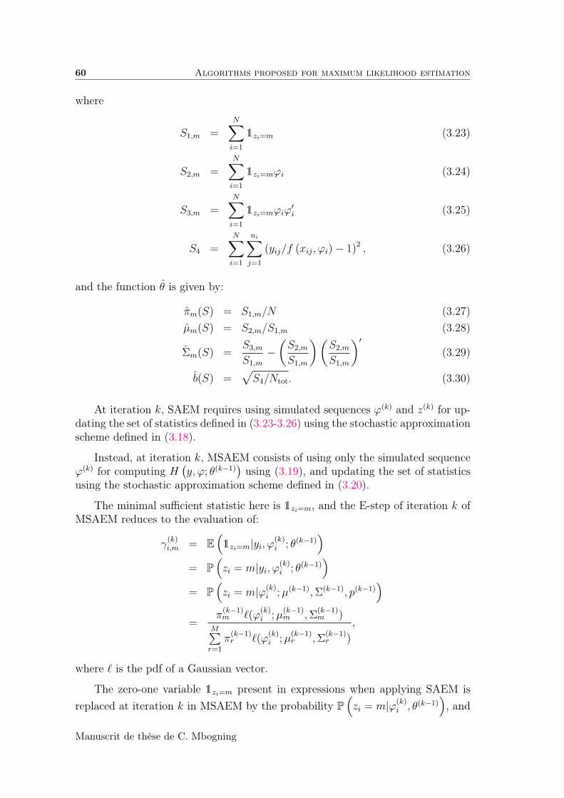
60 Algorithms proposed for maximum likelihood estimation
where
S1,m =N∑i=1
1zi=m (3.23)
S2,m =N∑i=1
1zi=mϕi (3.24)
S3,m =N∑i=1
1zi=mϕiϕ′i (3.25)
S4 =N∑i=1
ni∑j=1
(yij/f (xij, ϕi)− 1)2 , (3.26)
and the function θ is given by:
πm(S) = S1,m/N (3.27)µm(S) = S2,m/S1,m (3.28)
Σm(S) =S3,m
S1,m
−(S2,m
S1,m
)(S2,m
S1,m
)′(3.29)
b(S) =√S4/Ntot. (3.30)
At iteration k, SAEM requires using simulated sequences ϕ(k) and z(k) for up-dating the set of statistics defined in (3.23-3.26) using the stochastic approximationscheme defined in (3.18).
Instead, at iteration k, MSAEM consists of using only the simulated sequenceϕ(k) for computing H
(y, ϕ; θ(k−1)
)using (3.19), and updating the set of statistics
using the stochastic approximation scheme defined in (3.20).
The minimal sufficient statistic here is 1zi=m, and the E-step of iteration k ofMSAEM reduces to the evaluation of:
γ(k)i,m = E
(1zi=m|yi, ϕ
(k)i ; θ(k−1)
)= P
(zi = m|yi, ϕ(k)
i ; θ(k−1))
= P(zi = m|ϕ(k)
i ;µ(k−1),Σ(k−1), p(k−1))
=π
(k−1)m `(ϕ
(k)i ;µ
(k−1)m ,Σ
(k−1)m )
M∑r=1
π(k−1)r `(ϕ
(k)i ;µ
(k−1)r ,Σ
(k−1)r )
,
where ` is the pdf of a Gaussian vector.
The zero-one variable 1zi=m present in expressions when applying SAEM isreplaced at iteration k in MSAEM by the probability P
(zi = m|ϕ(k)
i , θ(k−1)), and
Manuscrit de thèse de C. Mbogning
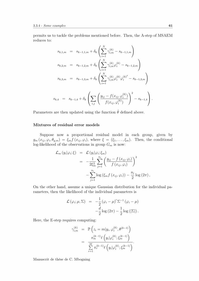
3.3.4 - Some examples 61
permits us to tackle the problems mentioned before. Then, the A-step of MSAEMreduces to:
sk,1,m = sk−1,1,m + δk
(N∑i=1
γ(k)i,m − sk−1,1,m
)
sk,2,m = sk−1,2,m + δk
(N∑i=1
γ(k)i,mϕ
(k)i − sk−1,2,m
)
sk,3,m = sk−1,3,m + δk
(N∑i=1
γ(k)i,mϕ
(k)i ϕ
(k)i
′− sk−1,3,m
)
sk,4 = sk−1,4 + δk
∑i,j
(yij − f(xij, ϕ
(k)i )
f(xij, ϕ(k)i )
)2
− sk−1,4
.
Parameters are then updated using the function θ defined above.
Mixtures of residual error models
Suppose now a proportional residual model in each group, given bygm (xij, ϕi, θy,m) = ξmf (xij, ϕi), where ξ = (ξ1, . . . , ξm). Then, the conditionallog-likelihood of the observations in group Gm is now:
Lm (yi|ϕi; ξ) = L (yi|ϕi; ξm)
= − 1
2ξ2m
ni∑j=1
(yij − f (xij, ϕi)
f (xij, ϕi)
)2
−ni∑j=1
log (ξmf (xij, ϕi))−ni2
log (2π) ,
On the other hand, assume a unique Gaussian distribution for the individual pa-rameters, then the likelihood of the individual parameters is
L (ϕi;µ,Σ) = −1
2(ϕi − µ)′Σ−1 (ϕi − µ)
−d2
log (2π)− 1
2log (|Σ|) .
Here, the E-step requires computing:
γ(k)i,m = P
(zi = m|yi, ϕ(k)
i , θ(k−1))
=π
(k−1)m `
(yi|ϕ(k)
i ; ξ(k−1)m
)M∑r=1
π(k−1)r `
(yi|ϕ(k)
i ; ξ(k−1)m
) .Manuscrit de thèse de C. Mbogning
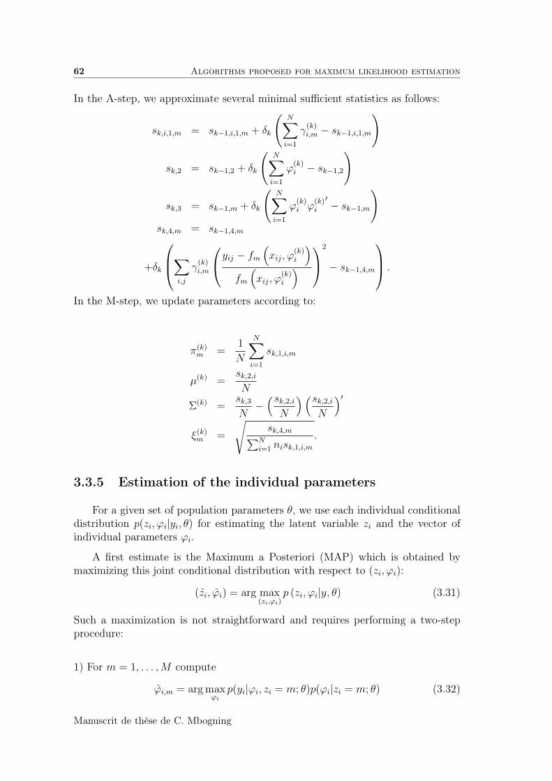
62 Algorithms proposed for maximum likelihood estimation
In the A-step, we approximate several minimal sufficient statistics as follows:
sk,i,1,m = sk−1,i,1,m + δk
(N∑i=1
γ(k)i,m − sk−1,i,1,m
)
sk,2 = sk−1,2 + δk
(N∑i=1
ϕ(k)i − sk−1,2
)
sk,3 = sk−1,m + δk
(N∑i=1
ϕ(k)i ϕ
(k)i
′− sk−1,m
)sk,4,m = sk−1,4,m
+δk
∑i,j
γ(k)i,m
yij − fm(xij, ϕ
(k)i
)fm
(xij, ϕ
(k)i
)2
− sk−1,4,m
.
In the M-step, we update parameters according to:
π(k)m =
1
N
N∑i=1
sk,1,i,m
µ(k) =sk,2,iN
Σ(k) =sk,3N−(sk,2,iN
)(sk,2,iN
)′ξ(k)m =
√sk,4,m∑N
i=1 nisk,1,i,m.
3.3.5 Estimation of the individual parameters
For a given set of population parameters θ, we use each individual conditionaldistribution p(zi, ϕi|yi, θ) for estimating the latent variable zi and the vector ofindividual parameters ϕi.
A first estimate is the Maximum a Posteriori (MAP) which is obtained bymaximizing this joint conditional distribution with respect to (zi, ϕi):
(zi, ϕi) = arg max(zi,ϕi)
p (zi, ϕi|y, θ) (3.31)
Such a maximization is not straightforward and requires performing a two-stepprocedure:
1) For m = 1, . . . ,M compute
ϕi,m = arg maxϕi
p(yi|ϕi, zi = m; θ)p(ϕi|zi = m; θ) (3.32)
Manuscrit de thèse de C. Mbogning
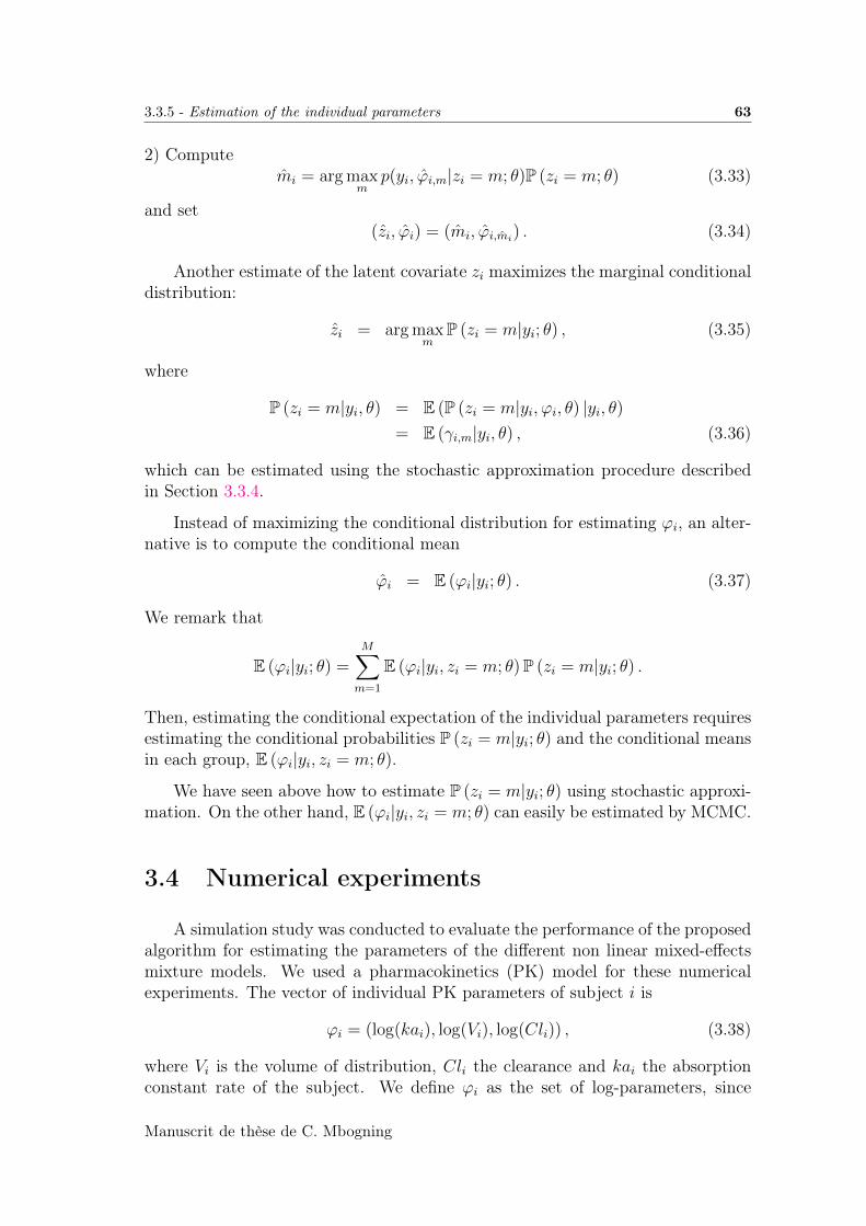
3.3.5 - Estimation of the individual parameters 63
2) Computemi = arg max
mp(yi, ϕi,m|zi = m; θ)P (zi = m; θ) (3.33)
and set(zi, ϕi) = (mi, ϕi,mi
) . (3.34)
Another estimate of the latent covariate zi maximizes the marginal conditionaldistribution:
zi = arg maxm
P (zi = m|yi; θ) , (3.35)
where
P (zi = m|yi, θ) = E (P (zi = m|yi, ϕi, θ) |yi, θ)= E (γi,m|yi, θ) , (3.36)
which can be estimated using the stochastic approximation procedure describedin Section 3.3.4.
Instead of maximizing the conditional distribution for estimating ϕi, an alter-native is to compute the conditional mean
ϕi = E (ϕi|yi; θ) . (3.37)
We remark that
E (ϕi|yi; θ) =M∑m=1
E (ϕi|yi, zi = m; θ)P (zi = m|yi; θ) .
Then, estimating the conditional expectation of the individual parameters requiresestimating the conditional probabilities P (zi = m|yi; θ) and the conditional meansin each group, E (ϕi|yi, zi = m; θ).
We have seen above how to estimate P (zi = m|yi; θ) using stochastic approxi-mation. On the other hand, E (ϕi|yi, zi = m; θ) can easily be estimated by MCMC.
3.4 Numerical experiments
A simulation study was conducted to evaluate the performance of the proposedalgorithm for estimating the parameters of the different non linear mixed-effectsmixture models. We used a pharmacokinetics (PK) model for these numericalexperiments. The vector of individual PK parameters of subject i is
ϕi = (log(kai), log(Vi), log(Cli)) , (3.38)
where Vi is the volume of distribution, Cli the clearance and kai the absorptionconstant rate of the subject. We define ϕi as the set of log-parameters, since
Manuscrit de thèse de C. Mbogning
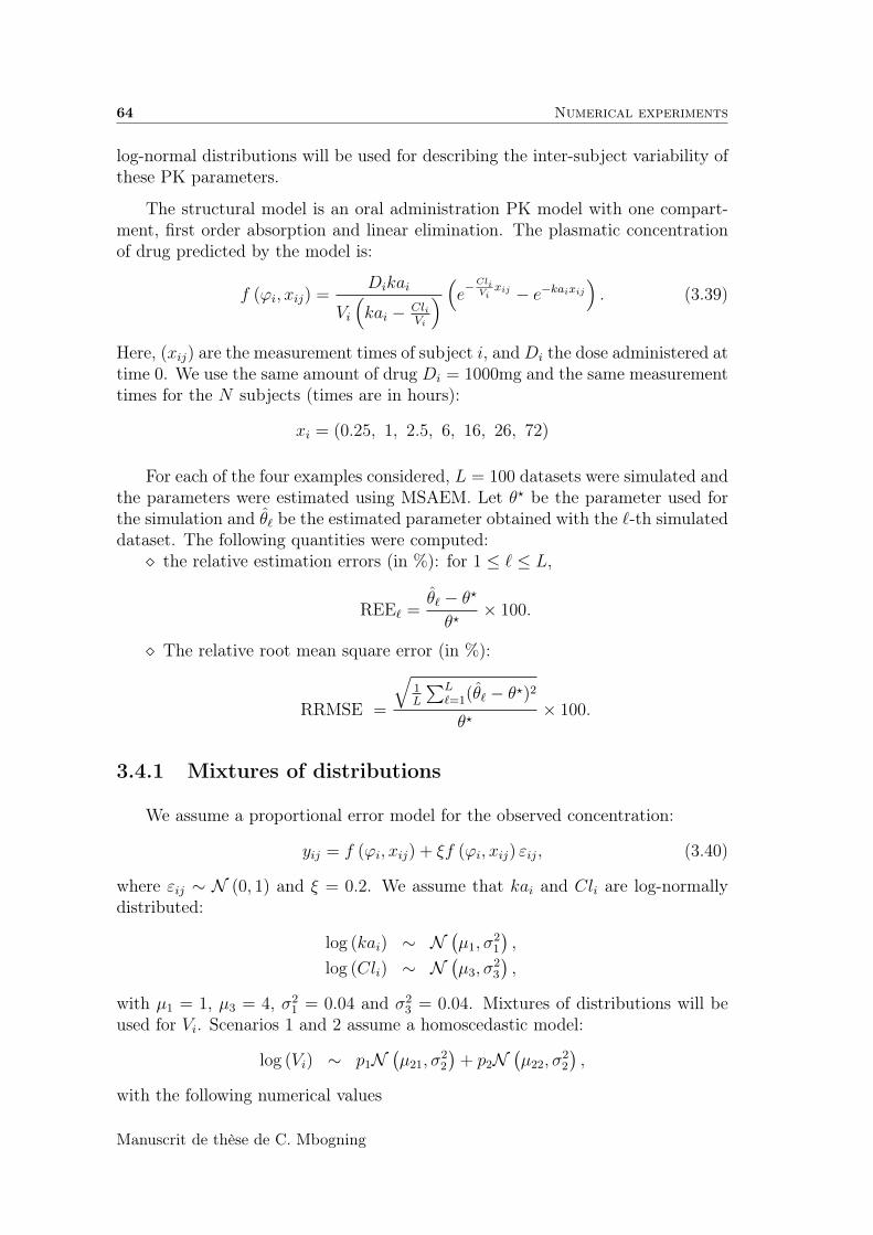
64 Numerical experiments
log-normal distributions will be used for describing the inter-subject variability ofthese PK parameters.
The structural model is an oral administration PK model with one compart-ment, first order absorption and linear elimination. The plasmatic concentrationof drug predicted by the model is:
f (ϕi, xij) =Dikai
Vi
(kai − Cli
Vi
) (e−CliVixij − e−kaixij
). (3.39)
Here, (xij) are the measurement times of subject i, andDi the dose administered attime 0. We use the same amount of drug Di = 1000mg and the same measurementtimes for the N subjects (times are in hours):
xi = (0.25, 1, 2.5, 6, 16, 26, 72)
For each of the four examples considered, L = 100 datasets were simulated andthe parameters were estimated using MSAEM. Let θ? be the parameter used forthe simulation and θ` be the estimated parameter obtained with the `-th simulateddataset. The following quantities were computed: the relative estimation errors (in %): for 1 ≤ ` ≤ L,
REE` =θ` − θ?
θ?× 100.
The relative root mean square error (in %):
RRMSE =
√1L
∑L`=1(θ` − θ?)2
θ?× 100.
3.4.1 Mixtures of distributions
We assume a proportional error model for the observed concentration:
yij = f (ϕi, xij) + ξf (ϕi, xij) εij, (3.40)
where εij ∼ N (0, 1) and ξ = 0.2. We assume that kai and Cli are log-normallydistributed:
log (kai) ∼ N(µ1, σ
21
),
log (Cli) ∼ N(µ3, σ
23
),
with µ1 = 1, µ3 = 4, σ21 = 0.04 and σ2
3 = 0.04. Mixtures of distributions will beused for Vi. Scenarios 1 and 2 assume a homoscedastic model:
log (Vi) ∼ p1N(µ21, σ
22
)+ p2N
(µ22, σ
22
),
with the following numerical values
Manuscrit de thèse de C. Mbogning
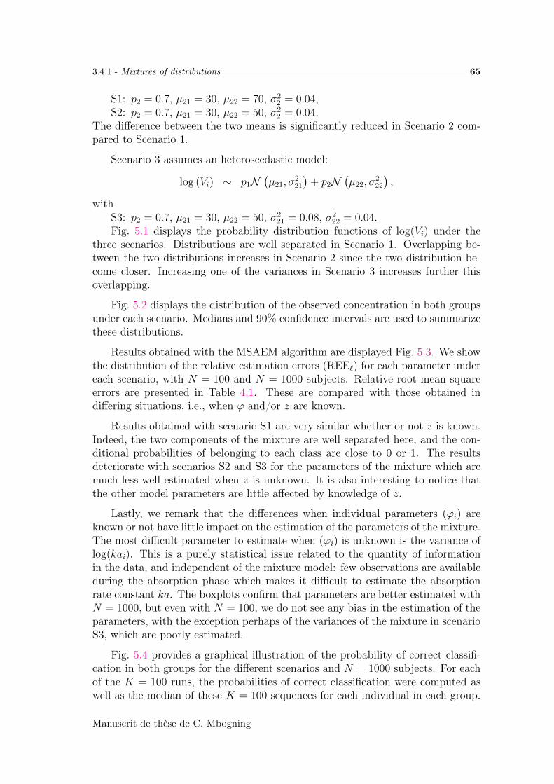
3.4.1 - Mixtures of distributions 65
S1: p2 = 0.7, µ21 = 30, µ22 = 70, σ22 = 0.04,
S2: p2 = 0.7, µ21 = 30, µ22 = 50, σ22 = 0.04.
The difference between the two means is significantly reduced in Scenario 2 com-pared to Scenario 1.
Scenario 3 assumes an heteroscedastic model:
log (Vi) ∼ p1N(µ21, σ
221
)+ p2N
(µ22, σ
222
),
withS3: p2 = 0.7, µ21 = 30, µ22 = 50, σ2
21 = 0.08, σ222 = 0.04.
Fig. 5.1 displays the probability distribution functions of log(Vi) under thethree scenarios. Distributions are well separated in Scenario 1. Overlapping be-tween the two distributions increases in Scenario 2 since the two distribution be-come closer. Increasing one of the variances in Scenario 3 increases further thisoverlapping.
Fig. 5.2 displays the distribution of the observed concentration in both groupsunder each scenario. Medians and 90% confidence intervals are used to summarizethese distributions.
Results obtained with the MSAEM algorithm are displayed Fig. 5.3. We showthe distribution of the relative estimation errors (REE`) for each parameter undereach scenario, with N = 100 and N = 1000 subjects. Relative root mean squareerrors are presented in Table 4.1. These are compared with those obtained indiffering situations, i.e., when ϕ and/or z are known.
Results obtained with scenario S1 are very similar whether or not z is known.Indeed, the two components of the mixture are well separated here, and the con-ditional probabilities of belonging to each class are close to 0 or 1. The resultsdeteriorate with scenarios S2 and S3 for the parameters of the mixture which aremuch less-well estimated when z is unknown. It is also interesting to notice thatthe other model parameters are little affected by knowledge of z.
Lastly, we remark that the differences when individual parameters (ϕi) areknown or not have little impact on the estimation of the parameters of the mixture.The most difficult parameter to estimate when (ϕi) is unknown is the variance oflog(kai). This is a purely statistical issue related to the quantity of informationin the data, and independent of the mixture model: few observations are availableduring the absorption phase which makes it difficult to estimate the absorptionrate constant ka. The boxplots confirm that parameters are better estimated withN = 1000, but even with N = 100, we do not see any bias in the estimation of theparameters, with the exception perhaps of the variances of the mixture in scenarioS3, which are poorly estimated.
Fig. 5.4 provides a graphical illustration of the probability of correct classifi-cation in both groups for the different scenarios and N = 1000 subjects. For eachof the K = 100 runs, the probabilities of correct classification were computed aswell as the median of these K = 100 sequences for each individual in each group.
Manuscrit de thèse de C. Mbogning
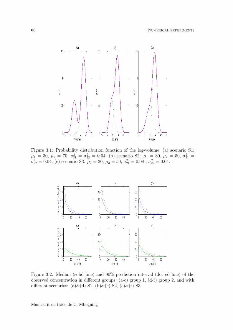
66 Numerical experiments
Figure 3.1: Probability distribution function of the log-volume, (a) scenario S1:µ1 = 30, µ2 = 70, σ2
21 = σ222 = 0.04; (b) scenario S2: µ1 = 30, µ2 = 50, σ2
21 =σ2
22 = 0.04; (c) scenario S3: µ1 = 30, µ2 = 50, σ221 = 0.08 , σ2
22 = 0.04.
Figure 3.2: Median (solid line) and 90% prediction interval (dotted line) of theobserved concentration in different groups: (a-c) group 1, (d-f) group 2, and withdifferent scenarios: (a)&(d) S1, (b)&(e) S2, (c)&(f) S3.
Manuscrit de thèse de C. Mbogning
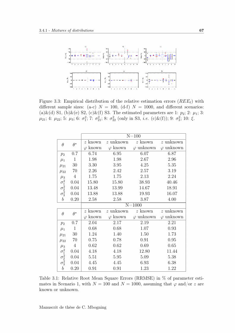
3.4.1 - Mixtures of distributions 67
Figure 3.3: Empirical distribution of the relative estimation errors (REE`) withdifferent sample sizes: (a-c) N = 100, (d-f) N = 1000, and different scenarios:(a)&(d) S1, (b)&(e) S2, (c)&(f) S3. The estimated parameters are 1: p2; 2: µ1; 3:µ21; 4: µ22; 5: µ3; 6: σ2
1; 7: σ221; 8: σ2
22 (only in S3, i.e. (c)&(f)); 9: σ23; 10: ξ.
N=100
θ θ∗z known z unknown z known z unknownϕ known ϕ known ϕ unknown ϕ unknown
p2 0.7 6.74 6.95 6.07 6.87µ1 1 1.98 1.98 2.67 2.96µ21 30 3.30 3.95 4.25 5.35µ22 70 2.26 2.42 2.57 3.19µ3 4 1.75 1.75 2.13 2.24σ2
1 0.04 15.80 15.80 38.93 40.46σ2
2 0.04 13.48 13.99 14.67 18.91σ2
3 0.04 13.88 13.88 19.93 16.07b 0.20 2.58 2.58 3.87 4.00
N=1000
θ θ∗z known z unknown z known z unknownϕ known ϕ known ϕ unknown ϕ unknown
p2 0.7 2.04 2.17 2.19 2.21µ1 1 0.68 0.68 1.07 0.93µ21 30 1.24 1.40 1.50 1.73µ22 70 0.75 0.78 0.91 0.95µ3 4 0.62 0.62 0.69 0.65σ2
1 0.04 4.18 4.18 12.80 11.44σ2
2 0.04 5.51 5.95 5.09 5.38σ2
3 0.04 4.45 4.45 6.93 6.38b 0.20 0.91 0.91 1.23 1.22
Table 3.1: Relative Root Mean Square Errors (RRMSE) in % of parameter esti-mates in Scenario 1, with N = 100 and N = 1000, assuming that ϕ and/or z areknown or unknown.
Manuscrit de thèse de C. Mbogning
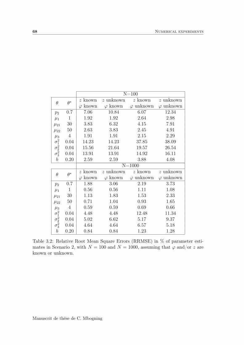
68 Numerical experiments
N=100
θ θ∗z known z unknown z known z unknownϕ known ϕ known ϕ unknown ϕ unknown
p2 0.7 7.06 10.84 6.07 12.34µ1 1 1.92 1.92 2.64 2.98µ21 30 3.83 6.32 4.15 7.91µ22 50 2.63 3.83 2.45 4.91µ3 4 1.91 1.91 2.15 2.29σ2
1 0.04 14.23 14.23 37.85 38.09σ2
2 0.04 15.56 21.64 19.57 26.54σ2
3 0.04 13.91 13.91 14.92 16.11b 0.20 2.59 2.59 3.88 4.08
N=1000
θ θ∗z known z unknown z known z unknownϕ known ϕ known ϕ unknown ϕ unknown
p2 0.7 1.88 3.06 2.19 3.73µ1 1 0.56 0.56 1.11 1.08µ21 30 1.13 1.83 1.53 2.33µ22 50 0.71 1.04 0.93 1.65µ3 4 0.59 0.59 0.69 0.66σ2
1 0.04 4.48 4.48 12.48 11.34σ2
2 0.04 5.02 6.62 5.17 9.37σ2
3 0.04 4.64 4.64 6.57 5.18b 0.20 0.84 0.84 1.23 1.28
Table 3.2: Relative Root Mean Square Errors (RRMSE) in % of parameter esti-mates in Scenario 2, with N = 100 and N = 1000, assuming that ϕ and/or z areknown or unknown.
Manuscrit de thèse de C. Mbogning
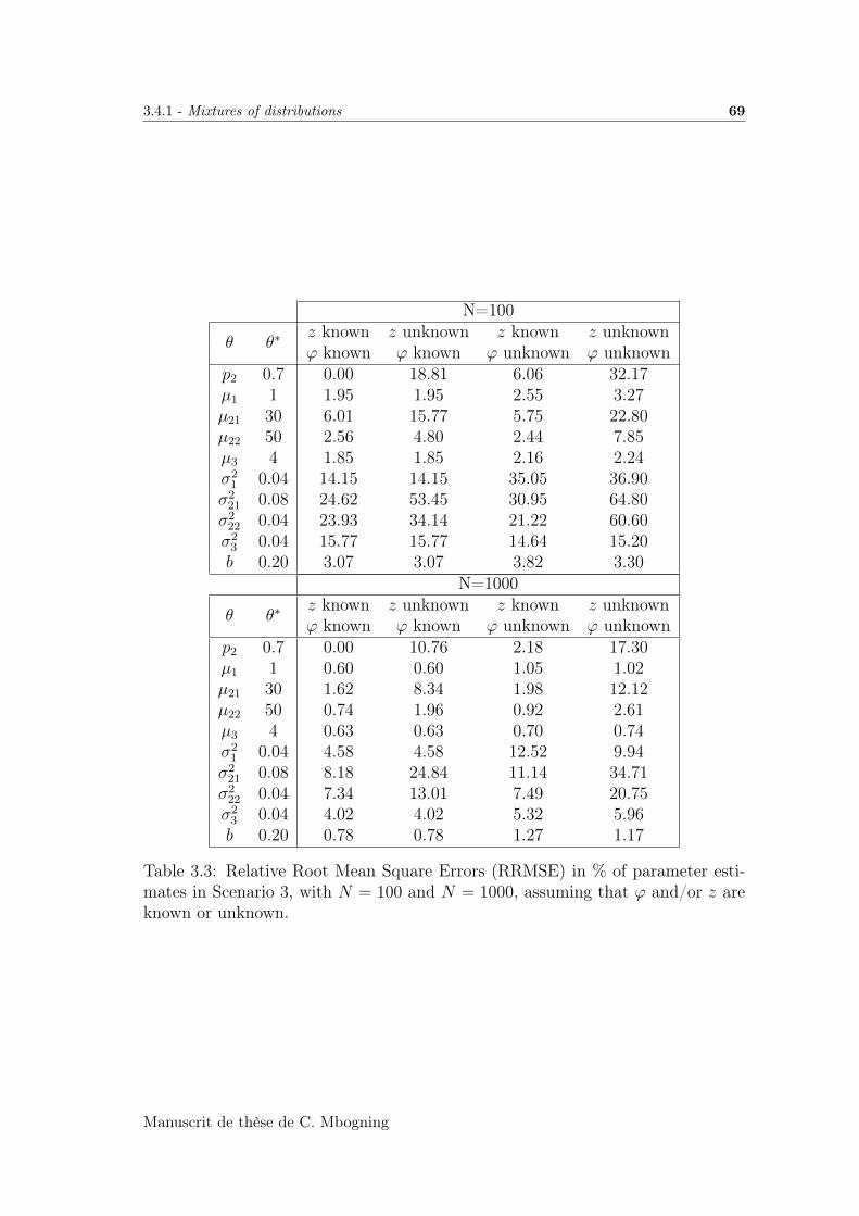
3.4.1 - Mixtures of distributions 69
N=100
θ θ∗z known z unknown z known z unknownϕ known ϕ known ϕ unknown ϕ unknown
p2 0.7 0.00 18.81 6.06 32.17µ1 1 1.95 1.95 2.55 3.27µ21 30 6.01 15.77 5.75 22.80µ22 50 2.56 4.80 2.44 7.85µ3 4 1.85 1.85 2.16 2.24σ2
1 0.04 14.15 14.15 35.05 36.90σ2
21 0.08 24.62 53.45 30.95 64.80σ2
22 0.04 23.93 34.14 21.22 60.60σ2
3 0.04 15.77 15.77 14.64 15.20b 0.20 3.07 3.07 3.82 3.30
N=1000
θ θ∗z known z unknown z known z unknownϕ known ϕ known ϕ unknown ϕ unknown
p2 0.7 0.00 10.76 2.18 17.30µ1 1 0.60 0.60 1.05 1.02µ21 30 1.62 8.34 1.98 12.12µ22 50 0.74 1.96 0.92 2.61µ3 4 0.63 0.63 0.70 0.74σ2
1 0.04 4.58 4.58 12.52 9.94σ2
21 0.08 8.18 24.84 11.14 34.71σ2
22 0.04 7.34 13.01 7.49 20.75σ2
3 0.04 4.02 4.02 5.32 5.96b 0.20 0.78 0.78 1.27 1.17
Table 3.3: Relative Root Mean Square Errors (RRMSE) in % of parameter esti-mates in Scenario 3, with N = 100 and N = 1000, assuming that ϕ and/or z areknown or unknown.
Manuscrit de thèse de C. Mbogning

70 Numerical experiments
These medians were then ranked in increasing order in each group. We repeatedthen the same procedure, but assuming that the individual parameters (ϕi) wereknown. Fig.5.4 compares these two medians. The y-axis of Fig. 5.4 representsthe Monte Carlo median probability of correct classification ranked in increasingorder. As expected, for each scenario, the probabilities of correct classification aregreater when (ϕi) is known, but it is interesting to notice that the difference isrelatively small. As already mentioned, the difficulty of the estimation problemincreases from Scenario 1 to Scenario 3. We see that the difficulty of the classifica-tion problem also increases: it is obviously much more difficult to correctly classifythe subjects under Scenario 3, where there is a lot of overlap, than under Scenario1, where the two distributions are well separated.
Figure 3.4: Medians of the probabilities of correct classification ranked in increas-ing order in both groups for the different scenarios and N = 1000 subjects. Blue:group 1 ; green: group 2. Solid line: the individual parameters (ϕi) are unknown; dotted line: the individual parameters (ϕi) are known.
3.4.2 Mixtures of error models
We still use the same PK model, but assuming now a mixture of residual errormodels:
if zi = 1 , yij = f (ϕi, xij) + ξ1f (ϕi, xij) εij,
if zi = 2 , yij = f (ϕi, xij) + ξ2f (ϕi, xij) εij,
with P (zi = 1) = 0.3 and ξ1 = 0.1, ξ2 = 0.2.
We assume that kai, Vi and Cli are log-normally distributed:
log (kai) ∼ N(µ1, σ
21
)log (Vi) ∼ N
(µ2, σ
22
)log (Cli) ∼ N
(µ3, σ
23
).
Manuscrit de thèse de C. Mbogning
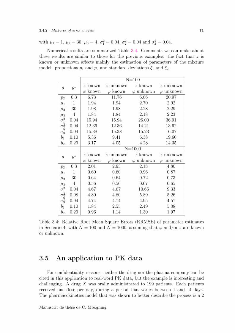
3.4.2 - Mixtures of error models 71
with µ1 = 1, µ2 = 30, µ3 = 4, σ21 = 0.04, σ2
2 = 0.04 and σ23 = 0.04.
Numerical results are summarized Table 3.4. Comments we can make aboutthese results are similar to those for the previous examples: the fact that z isknown or unknown affects mainly the estimation of parameters of the mixturemodel: proportions p1 and p2 and standard deviations ξ1 and ξ2.
N=100
θ θ∗z known z unknown z known z unknownϕ known ϕ known ϕ unknown ϕ unknown
p2 0.3 6.73 11.76 6.06 20.97µ1 1 1.94 1.94 2.70 2.92µ2 30 1.98 1.98 2.28 2.29µ3 4 1.84 1.84 2.18 2.23σ2
1 0.04 15.94 15.94 26.00 36.91σ2
2 0.04 12.36 12.36 14.21 13.62σ2
3 0.04 15.38 15.38 15.23 16.07b1 0.10 5.36 9.41 6.38 19.60b2 0.20 3.17 4.05 4.28 14.35
N=1000
θ θ∗z known z unknown z known z unknownϕ known ϕ known ϕ unknown ϕ unknown
p2 0.3 2.01 2.93 2.18 4.80µ1 1 0.60 0.60 0.96 0.87µ2 30 0.64 0.64 0.72 0.73µ3 4 0.56 0.56 0.67 0.65σ2
1 0.04 4.67 4.67 10.66 9.33σ2
2 0.08 4.80 4.80 5.89 5.26σ2
3 0.04 4.74 4.74 4.95 4.57b1 0.10 1.84 2.55 2.49 5.08b2 0.20 0.96 1.14 1.30 1.97
Table 3.4: Relative Root Mean Square Errors (RRMSE) of parameter estimatesin Scenario 4, with N = 100 and N = 1000, assuming that ϕ and/or z are knownor unknown.
3.5 An application to PK data
For confidentiality reasons, neither the drug nor the pharma company can becited in this application to real-word PK data, but the example is interesting andchallenging. A drug X was orally administrated to 199 patients. Each patientsreceived one dose per day, during a period that varies between 1 and 14 days.The pharmacokinetics model that was shown to better describe the process is a 2
Manuscrit de thèse de C. Mbogning
72 Discussion
compartment models with linear absorption and linear elimination:
Ad(t) = −kaAd(t)Ac(t) = kaAd(t)− keAc(t)− k12Ac(t) + k21Ap(t)
Ap(t) = k12Ac(t)− k21Ap(t)
where Ad is the amount of drug in the depot compartment, Ac the amount in thecentral compartment and Ap the amount in the peripheral compartment. There isno drug in any compartment before the administration of the drug: for any t < 0,Ad(t) = Ac(t) = Ap(t) = 0. If an amount D of drug is administrated at time τ ,then Ad(τ+) = Ad(τ
−) +D.
The concentration of drug Cc = Ac/V is measured in the central compartment,where V is the volume of the central compartment.
Here, the individual PK parameters (ka, V, ke, k12, k21) are log-normally dis-tributed. Then, the Gaussian vector ϕi is the vector of log-parameters. Thevariance-covariance matrix of ϕi is assumed to be diagonal.
The measured log-concentration is assumed to be normally distributed with aconstant error model:
log(yij) = log(Cc(tij;φi)) + aεij.
We first used Monolix to fit this NLMEM to the PK data. Observed con-centration data from 4 patients with their concentrations predicted by the modelare displayed Figure 3.5.
We then used a mixture of two log-normal distributions for modelling thedistribution of the PK parameters. We used a forward strategy for selecting thebest mixture model: we first assumed that only one of the five PK parameterdistributions was a mixture of two distributions and we compared the five possiblemodels with only one component modelled as a mixture. The model with thehighest likelihood value was selected (ke was selected). We then looked for asecond parameter among the four remaining ones (k12 was selected), then a thirdparameter among the three remaining ones (V was selected), and lastly the bestcombination of four mixtures (ka was selected). We then used the BIC criteriafor comparing the six selected models, including the model without any mixturecomponent and that with all the parameters modelled with mixtures. All theresults are summarized Table 3.5. The final model was a model assuming that thedistributions of V , ke and k12 are mixtures of log-normal distributions. The fiveestimated distributions of the five PK parameters are displayed Figure 3.6.
3.6 Discussion
There exist very few methods available for maximum likelihood estimation inmixtures of mixed effects models. Methods implemented in the nlme R package
Manuscrit de thèse de C. Mbogning
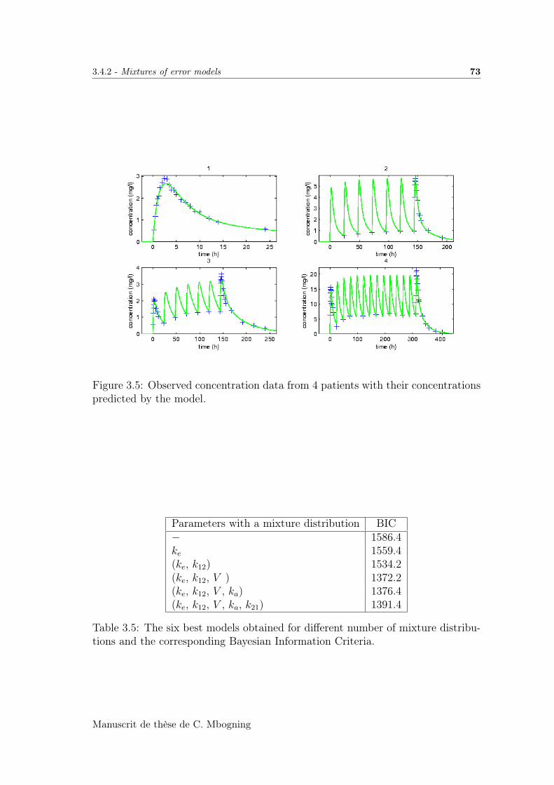
3.4.2 - Mixtures of error models 73
Figure 3.5: Observed concentration data from 4 patients with their concentrationspredicted by the model.
Parameters with a mixture distribution BIC− 1586.4ke 1559.4(ke, k12) 1534.2(ke, k12, V ) 1372.2(ke, k12, V , ka) 1376.4(ke, k12, V , ka, k21) 1391.4
Table 3.5: The six best models obtained for different number of mixture distribu-tions and the corresponding Bayesian Information Criteria.
Manuscrit de thèse de C. Mbogning
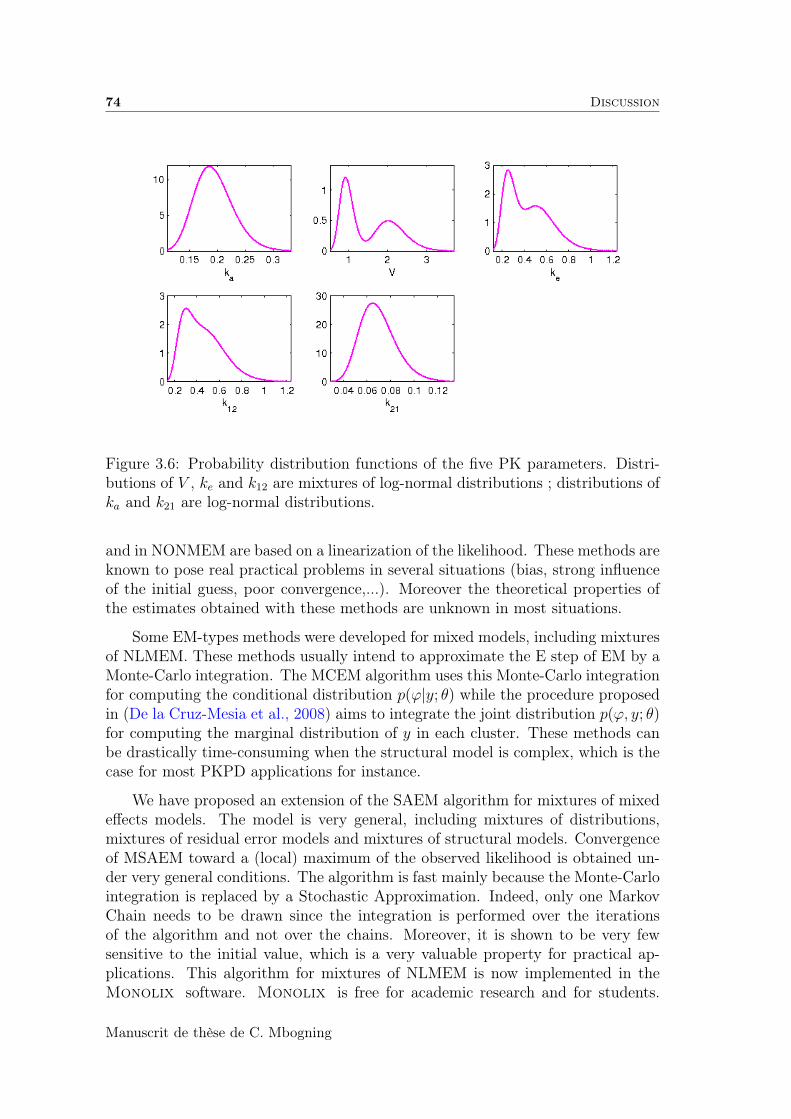
74 Discussion
Figure 3.6: Probability distribution functions of the five PK parameters. Distri-butions of V , ke and k12 are mixtures of log-normal distributions ; distributions ofka and k21 are log-normal distributions.
and in NONMEM are based on a linearization of the likelihood. These methods areknown to pose real practical problems in several situations (bias, strong influenceof the initial guess, poor convergence,...). Moreover the theoretical properties ofthe estimates obtained with these methods are unknown in most situations.
Some EM-types methods were developed for mixed models, including mixturesof NLMEM. These methods usually intend to approximate the E step of EM by aMonte-Carlo integration. The MCEM algorithm uses this Monte-Carlo integrationfor computing the conditional distribution p(ϕ|y; θ) while the procedure proposedin (De la Cruz-Mesia et al., 2008) aims to integrate the joint distribution p(ϕ, y; θ)for computing the marginal distribution of y in each cluster. These methods canbe drastically time-consuming when the structural model is complex, which is thecase for most PKPD applications for instance.
We have proposed an extension of the SAEM algorithm for mixtures of mixedeffects models. The model is very general, including mixtures of distributions,mixtures of residual error models and mixtures of structural models. Convergenceof MSAEM toward a (local) maximum of the observed likelihood is obtained un-der very general conditions. The algorithm is fast mainly because the Monte-Carlointegration is replaced by a Stochastic Approximation. Indeed, only one MarkovChain needs to be drawn since the integration is performed over the iterationsof the algorithm and not over the chains. Moreover, it is shown to be very fewsensitive to the initial value, which is a very valuable property for practical ap-plications. This algorithm for mixtures of NLMEM is now implemented in theMonolix software. Monolix is free for academic research and for students.
Manuscrit de thèse de C. Mbogning
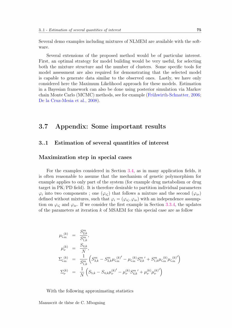
3..1 - Estimation of several quantities of interest 75
Several demo examples including mixtures of NLMEM are available with the soft-ware.
Several extensions of the proposed method would be of particular interest.First, an optimal strategy for model building would be very useful, for selectingboth the mixture structure and the number of clusters. Some specific tools formodel assessment are also required for demonstrating that the selected modelis capable to generate data similar to the observed ones. Lastly, we have onlyconsidered here the Maximum Likelihood approach for these models. Estimationin a Bayesian framework can also be done using posterior simulation via Markovchain Monte Carlo (MCMC) methods, see for example (Frühwirth-Schnatter, 2006;De la Cruz-Mesia et al., 2008).
3.7 Appendix: Some important results
3..1 Estimation of several quantities of interest
Maximization step in special cases
For the examples considered in Section 3.4, as in many application fields, itis often reasonable to assume that the mechanism of genetic polymorphism forexample applies to only part of the system (for example drug metabolism or drugtarget in PK/PD field). It is therefore desirable to partition individual parametersϕi into two components ; one (ϕiζ) that follows a mixture and the second (ϕiν)defined without mixtures, such that ϕi = (ϕiζ , ϕiν) with an independence assump-tion on ϕiζ and ϕiν . If we consider the first example in Section 3.3.4, the updatesof the parameters at iteration k of MSAEM for this special case are as follow
µζ(k)m =
Sm2,kSm1,k
,
µ(k)ν =
S4,k
N,
Σζ(k)m =
1
Sm1,k
(Sm3,k − Sm2,kµζ (k)
m
′ − µζ (k)m Sm2,k
′ + Sm1,kµζ(k)m µζ
(k)m
′)
Σ(k)ν =
1
N
(S5,k − S4,kµ
(k)ν
′ − µ(k)ν Sm4,k
′ + µ(k)ν µ(k)
ν
′)
With the following approximating statistics
Manuscrit de thèse de C. Mbogning
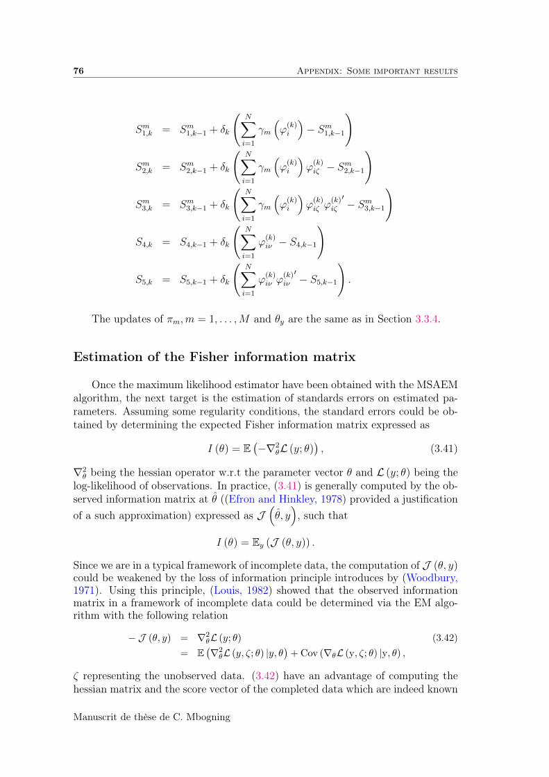
76 Appendix: Some important results
Sm1,k = Sm1,k−1 + δk
(N∑i=1
γm
(ϕ
(k)i
)− Sm1,k−1
)
Sm2,k = Sm2,k−1 + δk
(N∑i=1
γm
(ϕ
(k)i
)ϕ
(k)iζ − S
m2,k−1
)
Sm3,k = Sm3,k−1 + δk
(N∑i=1
γm
(ϕ
(k)i
)ϕ
(k)iζ ϕ
(k)iζ
′− Sm3,k−1
)
S4,k = S4,k−1 + δk
(N∑i=1
ϕ(k)iν − S4,k−1
)
S5,k = S5,k−1 + δk
(N∑i=1
ϕ(k)iν ϕ
(k)iν
′− S5,k−1
).
The updates of πm,m = 1, . . . ,M and θy are the same as in Section 3.3.4.
Estimation of the Fisher information matrix
Once the maximum likelihood estimator have been obtained with the MSAEMalgorithm, the next target is the estimation of standards errors on estimated pa-rameters. Assuming some regularity conditions, the standard errors could be ob-tained by determining the expected Fisher information matrix expressed as
I (θ) = E(−∇2
θL (y; θ)), (3.41)
∇2θ being the hessian operator w.r.t the parameter vector θ and L (y; θ) being the
log-likelihood of observations. In practice, (3.41) is generally computed by the ob-served information matrix at θ ((Efron and Hinkley, 1978) provided a justificationof a such approximation) expressed as J
(θ, y), such that
I (θ) = Ey (J (θ, y)) .
Since we are in a typical framework of incomplete data, the computation of J (θ, y)could be weakened by the loss of information principle introduces by (Woodbury,1971). Using this principle, (Louis, 1982) showed that the observed informationmatrix in a framework of incomplete data could be determined via the EM algo-rithm with the following relation
− J (θ, y) = ∇2θL (y; θ) (3.42)
= E(∇2θL (y, ζ; θ) |y, θ
)+Cov (∇θL (y, ζ; θ) |y, θ) ,
ζ representing the unobserved data. (3.42) have an advantage of computing thehessian matrix and the score vector of the completed data which are indeed known
Manuscrit de thèse de C. Mbogning
3..2 - Convergence result on MSAEM 77
explicitly. In our model, the unobserved vector ζ is given by (ϕ, z) and (3.42) thenbecomes
− J (θ, y) = E(∇2θL (y, ϕ, z; θ) |y, θ
)+ Cov (∇θL (y, ϕ, z; θ) |y, θ) . (3.43)
Remark 3..1. We have to notice that the introduction of the latent covariates zis really fundamental in order to have a manageable expression of the completedlikelihood.
We will use the same scheme used to carry out parameters estimation hereto approximate the observed fisher information matrix. We have the followingrelation
E(∇2θL (y, ϕ, z; θ) |y, θ
)= E
(E(∇2θL (y, ϕ, z; θ) |y, ϕ; θ
)|y, θ
).
By the same way, we have
E (∇θL (y, ϕ, z; θ) |y, θ) = E (E (∇θL (y, ϕ, z; θ) |y, ϕ; θ) |y, θ)
By settingH (y, ϕ, θ) = E
(∇2θL (y, ϕ, z; θ) |y, ϕ; θ
)and
∆ (y, ϕ, θ) = E (∇θL (y, ϕ, z; θ) |y, ϕ; θ) .
The observed information matrix is obtained using the following approximationscheme
∆k+1 = ∆k + δk(∆(y, ϕ(k+1), θ
)−∆k
)Hk+1 = δk
(H(y, ϕ(k+1), θ
)+ ∆
(y, ϕ(k+1), θ
)∆t(y, ϕ(k+1), θ
))+Hk (1− δk) .
Finally, the observed information matrix is approximated by
Jk+1 = −Hk+1 + ∆k+1∆tk+1. (3.44)
3..2 Convergence result on MSAEM
We shall make the following assumptions on the model:(C1) The parameter space Θ is an open subset of Rp. The complete data
log-likelihood function for a given unit i is given by:
L (yi, ϕi, zi; θ) =M∑m=1
1zi=m (Lm (yi, ϕi; θm) + log πm) , (3.45)
with
Lm (yi, ϕi; θm) = 〈T (yi, ϕi) , φ (θm)〉 − ψ (θm) , m = 1, . . . ,M (3.46)
Manuscrit de thèse de C. Mbogning
78 Appendix: Some important results
where 〈·, ·〉 denotes the scalar product, T is a Borel function on Rd in thesecond variable taking its values in an open subset T of Rn. According to(3.45) and (3.46), it appears that the complete data belongs to the expo-nential family and the log-likelihood of the complete data is given by
L (y, ϕ, z; θ) = 〈S (y, ϕ, z) , φ (θ)〉 − ψ (θ) , (3.47)
whereS (y, ϕ, z) = (Sm (y, ϕ, z))m=1,...,M
with
Sm (y, ϕ, z) =
(n∑i=1
1zi=m,
n∑i=1
1zi=mT (yi, ϕi)
).
By setting γm (yi, ϕi) = P (zi = m|yi, ϕi, θ), with θ considered here asfix or known, we define an intermediate set of statistic H (y, ϕ) =(Hm (y, ϕ))m=1,...,M with
Hm (y, ϕ) =
(∑i
γm (yi, ϕi) ,∑i
γm (yi, ϕi)T (yi, ϕi)
).
Since γm (yi, ϕi) is bounded between 0 and 1, H is indeed a Borel functionon Rd in the second variable taking its values in an open subset H of R2nM .
(C2) Define CL : H×Θ→ R as:
CL (h; θ) , 〈h, φ (θ)〉 − ψ (θ) .
The functions φ and ψ are twice continuously differentiable on Θ.(C3) The function h : Θ→ H defined as
h (θ) , E (H (y, ϕ) |y; θ)
is continuously differentiable on Θ.(C4) The function l : Θ→ R defined as the observed-data log-likelihood
l (θ) , log
∫Rd
f (y, ϕ, θ) dϕ
is continuously differentiable on Θ and
∂θ
∫Rd
f (y, ϕ, θ) dϕ =
∫Rd
∂θf (y, ϕ, θ) dϕ.
(C5) There exists a function θ : H → Θ, such that:
∀h ∈ H,∀θ ∈ Θ, CL(h, θ (h)
)≥ CL (h; θ) .
Furthermore, θ ∈ C1 (H).
Manuscrit de thèse de C. Mbogning
3..2 - Convergence result on MSAEM 79
Let us define
Q (θ|θ′) =
∫Rd×1,...,M
L (y, ϕ, z; θ) p (ϕ, z|y; θ′)µ (dϕ, dz) . (3.48)
According to (3.47), in order to compute (3.48), it is sufficient to computeE (S (y, ϕ, z) |y; θ′) which is same as computing E (H (y, ϕ) |y; θ′).
At iteration k of the MSAEM algorithm, the S-step consists in generating arealization of the missing data vector ϕ(k) instead of
(z(k), ϕ(k)
)under the con-
ditional distribution p(·|y; θ(k−1)
)by approaching it with a transition probability
pθ(k−1)
(ϕ, ϕ(k−1)
)and the integration step in a stochastic averaging procedure
hk = hk−1 + δk(H(y, ϕ(k)
)− hk−1
).
The maximization step is then given by θ(k) = θ (hk). We consider here severaladditional conditions on the stochastic approximation procedure, which are similarto those displayed in (Kuhn and Lavielle, 2004) : It is assumed that the randomvariables h0, ϕ
(1), ϕ(2), . . . are defined on the same probability space (Ω,A, P ). Wedenote F = Fk≥0 the increasing family of σ-algebras generated by the randomvariables h0, ϕ
(1), ϕ(2), . . . , ϕ(k). We also assume that:(SAEM1) For all k ∈ N, γk ∈ [0, 1],
∑∞k=1 γk =∞ and
∑∞k=1 γ
2k <∞.
(SAEM2) l : Θ→ R and θ : H → Θ are v times differentiable, where v is theinteger such that H is an open subset of Rv.
(SAEM3) ? The chain(ϕ(k)
)k≥0
takes its value in a compact subset E of Rd.? For any compact subset U of Θ, there exists a real constant L such that
for any (θ, θ′) in U2
sup(α,β)∈E2
|pθ (α, β)− pθ′ (α, β) | ≤ L|θ − θ′|.
? The transition probability pθ generates a uniformly ergodic chain whoseinvariant probability is the conditional distribution p (·|y; θ):
∃Kθ ∈ R+ ∃ρθ ∈]0, 1[ ∀ϕ ∈ E ∀k ∈ N∥∥pkθ (ϕ, ·)− p (·|y; θ)
∥∥TV≤ Kθρ
kθ ,
where ‖‖TV denotes the total variation norm. We suppose also that:
K , supθKθ <∞ and ρ , sup
θρθ < 1.
? The function H is bounded on E.We obtain the following convergence result:
Theorem 3..1. Assume that assumptions (C1 - C5), (SAEM1 - SAEM3) hold.Assume in addition the assumption (D): The sequence (hk)k≥0 takes its values ina compact subset of A. Then, we have with probability 1 that ,
limk→∞
d(θ(k),L
)= 0
where d(v,B) denotes the distance of v to the closed subset B and L =θ ∈ Θ, ∂θl (y; θ) = 0 is the set of stationary points of the observed likelihood l.
Manuscrit de thèse de C. Mbogning
80 Appendix: Some important results
Remark 3..2. We have considered θ as fixed in γm (yi, ϕi) to be able to considerH (y, ϕ) as a statistics. In fact, during the E-step of the algorithm, γm (yi, ϕi)depends on the previous value of the parameter which is known and indeed doesn’taffect the current maximization step.
Proof. First of all, we have to check that under assumptions (C1 - C5),assumptions (M1 - M5) of (Kuhn and Lavielle, 2004) are fulfilled by consideringthat the model involves the completed data (y, ϕ, z). According to (C1), thecomplete data likelihood belongs to the curved exponential family and the completedata log-likelihood is given by
L (y, ϕ, z; θ) = 〈S (y, ϕ, z) ,Φ (θ)〉 −Ψ (θ)
whereS (y, ϕ, z) = (Sm (y, ϕ, z))m=1,...,M
with
Sm (y, ϕ, z) =
(n∑i=1
1zi=m,n∑i=1
1zi=mT (yi, ϕi)
),
Φ (θ) = (log pm − ψ (θm) ;φ (θm))m=1,...,M and Ψ (θ) ≡ 0. The assumption (M1) istherefore fulfilled.By construction and according to assumption (C2), the functions ψ and φ aretwice continuously differentiable on Θ. The assumption (M2) is now fulfilled.According to the relation
E (S (y, ϕ, z) |y; θ) = E (H (y, ϕ) |y; θ) ,
assumption (M3) is fulfilled under assumption (C3).Assumption (C4) is similar as assumption (M4).Assumption (M5) is fulfilled under assumption (C5) by construction. Assumptions(M1-M5) are now fulfilled. According to (Kuhn and Lavielle, 2004), under addi-tional assumptions (SAEM1 - SAEM3), the convergence result is straightforward.The proof of Theorem 3..1 is now complete.
Remark 3..3. The convergence of this algorithm has been proved in the particularcase of non observed individual parameters living in a compact subset. However, aswe use mixtures of Gaussian distributions, we cannot assume that their support iscompact. In order to provide an algorithm whose convergence can be proved in thismore general framework, we can use a more general setting originally introducedin (Andrieu et al., 2005) which involves truncation on random boundaries. Anaplication of this technique for SAEM was proposed in (Allassonnière et al., 2010)and can easily be extended for MSAEM.
Manuscrit de thèse de C. Mbogning
3..3 - Asymptotic properties of the MLE in Mixture of NLMEM 81
3..3 Asymptotic properties of the MLE in Mixture ofNLMEM
The Maximum Likelihood, a popular method proposed as a general estima-tion method by Fisher(1912) has become a standard tool for making inferenceon unknown parameters in mixed effects models. Nevertheless, obtaining MLE’sinvolves tremendous computational difficulty because of the integrated likelihood,which does not have a close form. The asymptotic properties of MLE have beenwidely investigated. (Chanda, 1954) generalizes a result by (Cramer, 1946) andproves, under some regularity conditions, that there exists a unique solution of thelikelihood equations which is consistent and asymptotically normally distributed.Using the same conditions (Peters and Walker, 1978) show that there is a uniquestrongly consistent solution of the likelihood equations, which locally maximizesthe log-likelihood functions. (Redner, 1981) gives an extension of a previous workby (Wald, 1949)) on the strong consistency of MLE in the non-identifiable case,using some integrability conditions. (Bradley and Gart, 1962) and (Hoadley, 1971)proved weak consistency when the observations are sampled from independent as-sociated populations, i.e., random samples are independent but not identicallydistributed (it’s generally the case in mixed-effects models). A compendium of allthese previous results are given in (Redner and Walker, 1984). We can also referto Kaufmann and Fahrmeir () for standard tools on proof on MLE consistency.However, it is usually assumed that the MLE is consistent in mixed-effects models,without providing a proof. A rigorous proof of the consistency by verifying con-ditions from existing results can be very difficult due to the integrated likelihoodwhich doesn’t have a close form. There are very few works dedicated for that pur-pose in literature. (Nie and Yang, 2005) has established the strong consistency ofMLE in nonlinear mixed-effects models with large cluster size. The same author(Nie, 2006) presents some easily verifiable conditions for the strong consistencyof the MLE in generalized linear and nonlinear mixed-effects models. (Nie, 2007)once again, investigates in another paper the rate of convergence depending of thesize of the population and the number of observation per subject. This can besummarized as three different type of asymptotic as follow: The number of observation tends to infinity while the number of observation
per individual is bounded (N →∞, supni <∞, i = 1, . . . , N). The number of observation is finite while the number of observation per
individual is allowed to grow (N <∞, inf ni →∞, i = 1, . . . , N). Both the number of observation and the number of observation per individ-
ual are allowed to grow (N →∞, inf ni →∞, i = 1, . . . , N).In this section, we will focus on the first type of asymptotic and will investigatedthe asymptotic properties of the MLE in the special case of mixture of NLMEM.
Manuscrit de thèse de C. Mbogning
82 Appendix: Some important results
Consistency of the MLE
The study of the consistency of the MLE is important for two reasons. Thefirst one is obvious – in order to apply the MLE, we need to specify conditionsunder which its asymptotic properties hold. The second reason is more subtle inthe sense that for models like mixture in NLMEM, the likelihood is obtained onlyas an integral over the random effects. Hence, computation of the MLE is generallydifficult. As a result, parameters are estimated using alternative estimators suchas those provided by the MSAEM algorithm, which has been proved to provide anestimator close to the MLE in the previous section 3..2. First of all, we have torecall the main result of (Nie, 2006) on the consistency of the MLE in generalizedand nonlinear mixed-effects models.
Consider the data partitioned into N clusters (or subjects), where the ithcluster consists of ni observations, yi = (yi1, . . . , yini
)′. Let πi (yi, ϕi, θy) denotethe conditional probability density function of yi given a random variable ϕi =(ϕi1, . . . , ϕip). We assume that y1, . . . , yN are conditionally independent. Theunobservable random effects vectors ϕ1, . . . , ϕN are assumed to be a random samplefrom a distribution with probability density function Φ (ϕi, θϕ). Let Θ denote theparameter space for θ = (θy, θϕ). The marginal likelihood l (y; θ) of θ based on theobservations y1, . . . , yN is a product of the individual marginal likelihood,
l (y; θ) =N∏i=1
li (yi; θ) ,
where li (yi; θ) is the marginal likelihood based on yi,
li (yi; θ) =
∫πi (yi, ϕi, θy) Φ (ϕi, θϕ) dϕi. (3.49)
Theorem 3..2. The maximum likelihood estimating equation∂
∂θl (y; θ) = 0
has a root θn such that,P(
limn→∞
θn = θ0)
= 1,
if there is C > 0 and an open subset ω of Θ which contains the true parameter θ0
such that the following conditions are true for all i = 1, . . . , N .
N1- For almost all yi, the density πi (yi, bi, θy) and Φ (ϕi, θϕ) admits all first,second and third derivatives on θ ∈ ω.N2- There are functions Kγ (ϕi) for |γ| ≤ 3 and Ψ (ϕi), such that
supθ∈ω|DγΦ (ϕi, θϕ)| ≤ Kγ (ϕi)
infθ∈ω|Φ (ϕi, θϕ)| ≥ Ψ (ϕi) > 0
Eϕi|θ0ϕ
[(Φ−1
(ϕi, θ
0ϕ
)Kγ (ϕi)
)32]≤ C
Eϕi|θ0ϕ
[(Ψ−1 (ϕi) Φ
(ϕi, θ
0ϕ
))32]≤ C.
Manuscrit de thèse de C. Mbogning
3..3 - Asymptotic properties of the MLE in Mixture of NLMEM 83
N3- There are functions Fα for |α| ≤ 3 and Ri, such that
supθ∈ω|Dαπi (yi, ϕi, θy)| ≤ Fα (yi, ϕi)
infθ∈ω|πi (yi, ϕi, θy)| ≥ Ri (yi, ϕi) > 0
Eϕi|θ0ϕEyi|ϕi,θ0y
[(π−1i
(yi, ϕi, θ
0y
)Fα (yi, ϕi)
)32]≤ C
Eϕi|θ0ϕEyi|ϕi,τ0
[(R−1i (yi, ϕi)πi
(yi, ϕi, θ
0y
))32]≤ C.
N4- lim infN→∞ λN = λ > 0, where λN is the smallest eigenvalue of
FN(θ0)
= − 1
N
N∑i=1
Eyi|θ0(∂2 ln li (yi; θ)
∂θ∂θ′
).
In order to proof this result, Nie shows that under assumptions (N1-N4),assumptions of the following lemma are fulfilled. Those assumptions constituteconditions in a typical study of asymptotic properties of MLE. We can refer to(Chanda, 1954; Bradley and Gart, 1962; Hoadley, 1971; Lehmann, 1983) for similarconditions.
Lemma 3..1. The maximum likelihood estimating equation
∂
∂θl (y; θ) = 0
has a root θn such that,P(
limn→∞
θn = θ0)
= 1,
if there exists an open convex subset ω of Θ containing the true parameter pointθ0 and L > 0 such that
for almost all yi, the density li (yi; θ) admits all first, second and thirdderivatives.
Eyi|θ0
[∂ ln li (yi; θ)
θk|θ=θ0
]2
≤ L, ∀1 ≤ k ≤ r = u+ w.
Eyi|θ0[∂2 ln li (yi; θ)
θkθl|θ=θ0
]2
≤ L, ∀1 ≤ k, l ≤ r.
There is a sequence of functions G1 (y1) , . . . , GN (yN) such that,
|∂3 ln li (yi; θ)
θkθlθh| ≤ Gi (yi) , ∀θ ∈ ω, ∀1 ≤ k, l, h ≤ r
andEyi|θ0
[G2i (yi)
]≤ L, ∀1 ≤ i ≤ N.
Manuscrit de thèse de C. Mbogning
84 Appendix: Some important results
lim infN→∞
λN = λ > 0.
Theorem 3..2 is thus obtained by weakening assumptions of Lemma 3..1 whichis quite general, but difficult to check in mixed-effects models framework.
In order to prove the consistency result on mixture in nonlinear mixed-effectsmodels, we have to check that assumptions (N1-N4) of Theorem3..2 are fulfilled.Since the theorem involves the factorization of the probability density function ofthe complete data as the conditional probability density function of observationsgiven the random effects and the probability density function of the random effects,we can not apply the Theorem on our global mixture of NLMEM. There is indeeda need to use particular models of our global mixture of NLMEM.Let us consider first of all a mixture of distribution model defined as:
yij|ϕi, σ2 ∼ N(fij (ϕi) , σ
2f 2ij (ϕi)
)ϕi|θϕ ∼
M∑m=1
πmN (µm,Σm)
ϕi ∈ RP and∑M
m=1 pm = 1
(3.50)
According to notations in Theorem 3..2, the marginal likelihood based on yi isgiven by (3.49) with
π(yi, ϕi, σ
2)
= exp
−1
2
ni∑j=1
[(yij − fij (ϕi))
2
σ2f 2ij (ϕi)
+ ln f 2ij (ϕi) + ln
(2πσ2
)],
(3.51)and
Φ (ϕi, µ,Σ, p) =M∑m=1
pm exp
−1
2
[(ϕi − µm)′Σ−1
m (ϕi − µm) + ln |2πΣm|]
.
By identification, the parameters are defined as follow:∣∣∣∣∣∣∣∣∣θy = σ2
θϕ =(p, µ1, . . . , µp, θ1, . . . , θ p(p+1)
2
)µk = (µk,m)m=1,...,M , ∀k = 1, . . . , p and θj = (θj,m)m=1,...,M ∀j = 1, . . . , p(p+1)
2
p = (p1, . . . , pM)
Let w =
p(p+3)+42∏i=1
wi containing the true value of the parameters, in which
w1 = ]σ21, σ
22[
w2 = ]κ1, κ2[M , κ1 > 0, κ2 < 1
wi = ]− t, t[M , i = 3, . . . , p+ 2, 0 < t <∞
wi =M∏m=1
]θmi−p−2,1, θmi−p−2,2[ i = p+ 3, . . . ,
p (p+ 3) + 4
2
Manuscrit de thèse de C. Mbogning
3..3 - Asymptotic properties of the MLE in Mixture of NLMEM 85
Assumption (N1) is fulfilled since π (yi, ϕi, σ2) and Φ (ϕi, µ,Σ, p) are smooth func-
tions.Let uij =
yij−fij(ϕi)
fij(ϕi). (3.51) becomes
π(yi, ϕi, σ
2)
= exp
−1
2
ni∑j=1
[u2ij
σ2+ ln f 2
ij (ϕi) + ln(2πσ2
)].
We have the following inequality:
π(yi, ϕi, σ
2)≤ exp
−1
2
ni∑j=1
[u2ij
σ22
+ ln f 2ij (ϕi) + ln
(2πσ2
1
)].
The first derivative of π (yi, ϕi, σ2) w.r.t σ2 is given by
∂π
∂σ2= π
(yi, ϕi, σ
2)(1
2
ni∑j=1
u2ij
σ4− niπ
σ2
).
By taking the absolute value, we have the following majoration∣∣∣∣ ∂π∂σ2
∣∣∣∣ ≤ π(yi, ϕi, σ
2)(1
2
ni∑j=1
u2ij
σ4+niπ
σ2
).
Similarly, we obtain the following majoration for the absolute value of the secondderivative of π (yi, ϕi, σ
2) w.r.t σ2
∣∣∣∣ ∂2π
∂ (σ2)2
∣∣∣∣ ≤ π(yi, ϕi, σ
2) 1
4σ6
(ni∑j=1
u2ij
)2
+niπ
2σ6
ni∑j=1
u2ij +
niπ
2σ4
ni∑j=1
u2ij +
(niπσ2
)2
.
The third derivative w.r.t σ2 is given by
∂3π
∂ (σ2)3 = π(yi, ϕi, σ
2) 1
8σ10
(ni∑j=1
u2ij
)3
− niπ
4σ10
(ni∑j=1
u2ij
)2
− niπ
4σ8
(ni∑j=1
u2ij
)2
+(niπ)2
σ8
ni∑j=1
u2ij −
niπ
4σ8
(ni∑j=1
u2ij
)2
+(niπ)2
2σ6
ni∑j=1
u2ij −
(niπ)3
σ6
− 3
4σ6
(ni∑j=1
u2ij
)2
+3πni2σ8
ni∑j=1
u2ij +
niπ
σ6
ni∑j=1
u2ij −
2 (niπ)2
σ6
.
Finally, we obtained the following result:
∀α/ |α| ≤ 3,∣∣Dαπ
(yi, ϕi, σ
2)∣∣ ≤ π
(yi, ϕi, σ
2)Q(ui, σ
2)
Manuscrit de thèse de C. Mbogning
86 Appendix: Some important results
with
ui = (ui,j)j=1,...,niand Q
(ui, σ
2)
=3∑l=1
5∑k=1
clk
(∑ni
j=1 u2ij
)lσ2k
,
where clk are positive constants. We thus have
supσ2∈ω1
∣∣Dαπ(yi, ϕi, σ
2)∣∣ ≤ exp
−1
2
ni∑j=1
[u2ij
σ22
+ ln f 2ij (ϕi) + ln
(2πσ2
1
)]Q(ui, σ
21
)(3.52)
Let
Fαi(yi, ϕi) = exp
−1
2
ni∑j=1
[u2ijσ22
+ ln f 2ij (ϕi) + ln (2πσ2
1)]
Q (ui, σ21)
Then,
(π−1
(yi, ϕi, σ
20
)Fαi
(yi, ϕi))32
= exp
[−1
2
(32
σ22
− 32
σ20
) ni∑j=1
u2ij − 16ni ln
σ21
σ20
]Q32
(ui, σ
21
)Thus, the 32nd moment is given by
Eyi|ϕi,σ20
(π−1
(yi, ϕi, σ
20
)Fαi
(yi, ϕi))32
= Eui|ϕi,σ20
exp
[−1
2
(32
σ22
− 32
σ20
) ni∑j=1
u2ij − 16ni ln
σ21
σ20
]Q32
(ui, σ
21
)(3.53)
We have to notice that uij|ϕi, σ20 ∼ N (0, σ2
0) ; thus,Given the random variablesϕi, uij are i.i.d and an immediate consequence is that (3.53) doesn’t depends onϕi. Hence,
Eϕi|θ0Eyi|ϕi,σ20
(π−1
(yi, ϕi, σ
20
)Fαi
(yi, ϕi))32
= Eyi|ϕi,σ20
(π−1
(yi, ϕi, σ
20
)Fαi
(yi, ϕi))32
.
The uij being centered, the evaluation of the previous operation involves an in-tegration of the form
∫∞0e−ax
2dx with a = 1
2
(1σ20− 32
(1σ20− 1
σ22
)). This type of
integral is finite if and only if a > 0. We thus obtained an constraint on σ2 for thedefinition of the open subset ω1. The condition is as follow:
1
σ20
− 32
(1
σ20
− 1
σ22
)> 0. (3.54)
Over these condition, (3.53) is finite.In the other hand, we have that
infσ2∈ω1
π(yi, ϕi, σ
2)≥ exp
−1
2
ni∑j=1
[u2ij
σ21
+ ln f 2ij (ϕi) + ln
(2πσ2
2
)].
Manuscrit de thèse de C. Mbogning
3..3 - Asymptotic properties of the MLE in Mixture of NLMEM 87
Let
Ri (yi, ϕi) = exp
−1
2
ni∑j=1
[u2ijσ21
+ ln f 2ij (ϕi) + ln (2πσ2
2)]
By using a similar procedure as before, we obtain that
Eyi|ϕi,σ20
(π(yi, ϕi, σ
20
)R−1i (yi, ϕi)
)32
doesn’t depends on ϕi and is finite if
1
σ20
− 32
(1
σ21
− 1
σ20
)> 0. (3.55)
We therefore verified Condition (N3) in Theorem 3..2.Assuming that ϕi is a mixture of M gaussian distributions, we obtained the
following result derived from the partial derivative of order 1, 2 and 3 of Φ (ϕi, θϕ)w.r.t θϕ:
∀α/ |α| ≤ 3, DαΦ (ϕi, θϕ) <M∑m=1
Km1 (ϕi) exp
−1
2(ϕi − µm)′Σ−1
m (ϕi − µm)
, θ ∈ ω,
where Km1 (ϕi) is a polynomial function of ϕi with order less than 6. Coefficients ofthis polynomial are finite values depending on the boundaries of ω ; more preciselyt and θmk,j, k = 1, . . . , p(p+1)/2; j = 1, 2. With the aim of providing a majorationof exp
−1
2(ϕi − µm)′Σ−1
m (ϕi − µm)
which doesn’t depends on θϕ, we supposethat there exists a set of real constant γ1 = (γ1,m)m=1,...,M such that
infθ∈ω
Σ−1m − γ1,mΣ−1
m0 is positive definite ∀m = 1, . . . ,M (3.56)
Σm0 is the true value of the parameter Σm. Let ϕim = Σ−1m0ϕi, µ∗m = Σ−1
m0µm. Inaddition with (3.58), we have the following inequality
exp
−1
2(ϕi − µm)′Σ−1
m (ϕi − µm)
≤ exp
−1
2γ1mϕ
′imϕim + γ1m
p∑j=1
|ϕjim||µ∗jm |
,
where ϕjim is the jth component of the vector ϕim and µ∗jm the jth component ofthe vector µ∗m. Define
Km2 (ϕi) = exp
−1
2γ1mϕ
′imϕim + γ1m
p∑j=1
|ϕjim| supθ∈ω|µ∗jm |
.
Thus, we have
supθ∈ω
DαΦ (ϕi, θϕ) ≤M∑m=1
Km1 (ϕi)Km2 (ϕi) .
Manuscrit de thèse de C. Mbogning

88 Appendix: Some important results
Let
Φα (ϕi) =M∑m=1
Km1 (ϕi) exp
−1
2γ1mϕ
′imϕim + γ1m
∑pj=1 |ϕ
jim| sup
θ∈ω|µ∗jm |
.
After using the relation(M∑m=1
am
)n
≤Mn−1
M∑m=1
anm, am ≥ 0∀m = 1, . . . ,M ; n ∈ N∗,
obtained after using the Hölder inequality, we obtain the following result:
(Φ−1
(ϕi, θ
0ϕ
)Φα (ϕi)
)32 ≤ csteκ32
1
M∑m=1
Hm (ϕi) exp(−16 (γ1m − 1)ϕ′iΣ
−1l0 ϕi
),
where l ∈ 1, . . . ,M and Hm (ϕi) is a product of a polynomial function of ϕi andan exponential of a polynomial function of |ϕjim| with order 1. Using similar argu-ments as before, the 32nd moment of Φ−1
(ϕi, θ
0ϕ
)Φα (ϕi) is finite if the following
condition holds:
1− 32 (1− γ1m) > 0, for all m = 1, . . . ,M. (3.57)
By using an analogue procedure, we suppose that there exists a set of real constantγ2 = (γ2,m)m=1,...,M such that the following condition holds:
− supθ∈ω
Σ−1m + γ2,mΣ−1
m0 is positive definite for all m = 1, . . . ,M. (3.58)
Then, Let
Ψ (ϕi) =M∑m=1
√γp1,m|2πΣm0| exp
−12γ2,m
ϕ′imϕim +
(γ1,m
p∑j=1
supθ∈ω|µ∗jm |
)2+ γ2,m
p∑j=1
|ϕjim| infθ∈ω|µ∗jm |
By the same manner, we can show that the 32nd moment of Ψ−1 (ϕi) Φ
(ϕi, θ
0ϕ
)is finite if the following condition holds:
1− 32 (γ2,m − 1) > 0, for all m = 1, . . . ,M. (3.59)
We therefore verified Condition (N2) in Theorem 3..2.In order to show Condition (N4), it suffices to show that each Fi (θ0) is positive
definite, where,
Fi(θ0)
= Eyi|θ0(∂2 ln li (yi; θ)
∂θ∂θ′
).
Manuscrit de thèse de C. Mbogning
3..3 - Asymptotic properties of the MLE in Mixture of NLMEM 89
Fi (θ0) is positive definite if and only if the components of the score vector obtained
at θ0 are linearly independent, that is, there do not exist constants (λ1, . . . , λr),such that
∑rk=1 λk
∂ ln li(yi;θ)∂θk
|θ=θ0 = 0 with yi|θ0-probability one ; r being an integersuch that Θ is an open subset of Rr. We have the following relation:
∀k ∈ 1, . . . , r , ∂ ln li (yi; θ)
∂θk|θ=θ0 = Eϕi|yi,θ
(∂ (lnπ (yi; θy) + ln Φ (ϕi; θϕ))
∂θk
)|θ=θ0 .
Thus,∂ ln li (yi; θ)
∂σ2|θ=θ0 = Eϕi|yi,θ
(∂ (ln π (yi;σ
2))
∂σ2
)|θ=θ0
and∂ ln li (yi; θ)
∂θϕ|θ=θ0 = Eϕi|yi,θ
(∂ (ln Φ (ϕi; θϕ))
∂θϕ
)|θ=θ0 .
In addition, we have that
∀k ∈ 1, . . . , r s.t. θk 6= σ2,∂ ln li (yi; θ)
∂θk6= b
∂ ln li (yi; θ)
∂σ2for any constant b.
Using the regularity conditions on Φ (ϕi, θϕ) it is clear that, there do not existconstants a2, . . . , ar, such that,
∑rk=2 ak
∂ ln li(yi;θ)∂θk
|θ=θ0 = 0, with θ1 = σ2.
We have therefore verified condition (N4) of Theorem3..2. As a consequence,the MLE of θ is consistent. Thus, the
√N -consistency is straightforward here and
is obtained by considering a Taylor expansion of the score function in a neighbor-hood of the true parameter.
Manuscrit de thèse de C. Mbogning
Chapter 4
Between-subject and within-subjectmodel mixtures for classifying HIVtreatment response
Contents4.1 Introduction . . . . . . . . . . . . . . . . . . . . . . . . . 924.2 Models and methods . . . . . . . . . . . . . . . . . . . . 94
4.2.1 Between-subject model mixtures . . . . . . . . . . . . . 944.2.2 Log-likelihood of between-subject model mixtures . . . . 954.2.3 Within-subject model mixtures . . . . . . . . . . . . . . 96
4.3 Maximum likelihood estimation algorithms forbetween-subject model mixtures . . . . . . . . . . . . . 96
4.3.1 Estimation of individual parameters . . . . . . . . . . . 984.4 Simulated Data Example . . . . . . . . . . . . . . . . . . 99
4.4.1 Modeling with between-subject model mixtures . . . . . 994.4.2 Modeling with within-subject mixture models . . . . . . 102
4.5 Application to real data . . . . . . . . . . . . . . . . . . 1034.5.1 Description of the data . . . . . . . . . . . . . . . . . . . 1034.5.2 Class prediction using between-subject model mixtures . 1054.5.3 Class prediction using within-subject mixture models . . 106
4.6 Discussion . . . . . . . . . . . . . . . . . . . . . . . . . . . 109
90

CHAPTER 4. BETWEEN-SUBJECT AND WITHIN-SUBJECT MODEL MIXTURES FORCLASSIFYING HIV TREATMENT RESPONSE 91
Abstract
We present a method for using longitudinal data to classify individuals intoclinically-relevant population subgroups. This is achieved by treating “subgroup”as a categorical covariate whose value is unknown for each individual, and predict-ing its value using mixtures of models that represent “typical” longitudinal datafrom each subgroup. Under a nonlinear mixed effects model framework, two typesof model mixtures are presented, both of which have their advantages. Followingillustrative simulations, longitudinal viral load data for HIV-positive patients isused to predict whether they are responding – completely, partially or not at all –to a new drug treatment.
Keywords: Mixture models, HIV, SAEM, Classification.
Manuscrit de thèse de C. Mbogning
92 Introduction
4.1 Introduction
For a variety of reasons – some known, some not – different patients responddifferently to the same drug treatment. For certain patients, a drug does what itwas prescribed to do: kill bacteria, reduce blood pressure, decrease viral load, etc.,but for others, the drug may be toxic or ineffective. When we collect response dataon patients undergoing a treatment, it is useful to try to find patients for whichthe treatment is ineffective, and thus suggest modifications. We are particularlyinterested here in longitudinal response data in a population; the methods wepresent are generally applicable to this type of data.
The real-world example that motivates the approach is longitudinal HIV viralload data. For HIV-positive patients on a given drug regime, the evolution ofthe viral load in the blood can be measured over time. For some patients, thedrug regime is ineffective and the viral load does not consistently drop; we callthese non-responders, and it is of interest to detect them and provide alternative– hopefully more effective – treatments. Other patients react favourably to thetreatment and the viral load drops to undetectable levels and stays there for along period of time; these are called responders. Yet another group – rebounders –show an initial drop in viral load followed by an increase back towards the initialhigh viral load. They too will eventually require an alternative treatment.
Our goal is to use longitudinal data to infer the efficacy of the treatment, i.e.,infer whether each patient is a non-responder, responder, rebounder or, as we willexplain, some mixture of the above. In order to do this, we first model longi-tudinal HIV viral load data using recent additions to the nonlinear mixed-effectsmodel (NLMEM) framework. Then, we extract relevant posterior probabilitiesor individual parameters to infer patient status. We now briefly introduce theNLMEM framework and model mixtures. To avoid potential confusion, note thatmixed-effects models and model mixtures are not the same thing.
NLMEM – a special case of mixed-effects models – are statistical models whichuse both fixed and random effects in their construction (see (Sheiner and Beal,1985; Lindstrom and Bates, 1990; Davidian and Giltinan, 1995; Vonesh and Chin-chilli, 1997) for more details). The model structure is hierarchical. At a first level,each individual has their own parametric regression model, known as the struc-tural model, each identically defined up to a set of unknown individual parameters.At a second level, each set of individual parameters is assumed to be randomlydrawn from some unknown population distribution. These models are particularlyuseful in population studies (e.g., population pharmacology – see (Wakefield et al.,1998)) where data is available for many individuals. Two types of variability areinvolved: intra- and inter -subject. We attempt to explain the latter using knownfixed-effects (covariates) such as weight, blood type, etc. The non-explained partof the inter-subject variability is then modeled using random effects.
The introduction of a categorical covariate (e.g., sex, blood type, etc.) into
Manuscrit de thèse de C. Mbogning
CHAPTER 4. BETWEEN-SUBJECT AND WITHIN-SUBJECT MODEL MIXTURES FORCLASSIFYING HIV TREATMENT RESPONSE 93
such a model supposes that the population can be divided into subpopulationswith respect to that covariate. However, there may be a categorical covariatewhich interests us but whose value is unknown for all individuals, such as thecovariate “patient status” which interests us here. In this case, part of the goalbecomes to infer the value of this covariate for each individual as part of themodeling process. One way to do this is to introduce model mixtures. There existseveral types of model mixture which are useful in the context of mixed effectsmodels; we will focus on two here:
Between-Subject Model Mixtures (BSMM) assume that each individual’s lon-gitudinal data follows one of M “base” models, but we do not necessarilyknow a priori which one. Individual i thus has a label zi = m ∈ 1, . . . ,Mreferring to the model that is supposed to have generated it. If the zi areknown, they can be treated as categorical covariates. We will show how todeal with the more challenging case of when they are unknown. Furthermore,for this zi unknown case, we will show how to extract a posteriori estimatesof the probability that each individual was generated by each of the basemodels; this will be used to predict which type of patient we have: non-responder, responder or rebounder. We note that BSMM were introducedas an example of a more general framework in (Mbogning and Lavielle, )but were not developed further there.
Within-Subject Model Mixtures (WSMM) make the hypothesis that themodel mixture occurs within each individual. In the HIV example, thismeans that we consider that each patient is partially a non-responder, par-tially a responder and partially a rebounder. This is perhaps more bio-logically plausible than BSMMs in the sense that each individual’s responsemay be due to their own particular combination of virus strains, cell popula-tions, etc. Within the NLMEM framework, this means including individual“model proportion” parameters into the model and having to estimate themalong with the other parameters of the NLMEM. It turns out that this doesnot require any mathematical extensions to a typical NLMEM. But as willbe seen in the HIV example, we can use the estimated proportions to helpcategorize patients, especially those who do not naturally fall into one of thethree “typical” categories.
BSMM and WSMM are new approaches in the context of NLMEM. We refer thereader to (Redner and Walker, 1984; McLachland and Basford, 1988; Bryant, 1991;Roeder and Wasserman, 1997; McLachland and Peel, 2000) for general details onmixture models in a standard context. We note also that there are fully Bayesianapproaches to similar types of problems, in particular Bayesian nonparametricones, see (Hjort et al., 2010) for more details.
The paper is structured as follows. We introduce BSMMs in the NLMEMframework and calculate their log-likelihood, before briefly presenting WSMMs;they require no new mathematical framework. We then describe how to per-
Manuscrit de thèse de C. Mbogning
94 Models and methods
form maximum likelihood estimation (MLE) for BSMMs using the Stochastic Ap-proximation Expectation Maximization (SAEM) algorithm (Delyon et al., 1999).SAEM is implemented in the Monolix software and can be widely applied tovarious data types and real-life scenarios (Samson et al., 2007; Snoeck et al., 2010;Chan et al., 2011; Dubois et al., 2011; Lavielle et al., 2011). Next, we present an ex-ample for a simple BSMM case, and then a simulated example for mixtures of twomodels in the both the BSMM and WSMM cases. The simulations illustrate thequality of the parameter estimation of both methods and also their classificationperformance, i.e., how well they “predict” which model was used to generate eachindividual’s data (in the BSMM case) and which model represented the biggestproportion (in the WSMM case). This is followed by a comprehensive modelingof HIV treatment response longitudinal data from a cohort of 578 patients usingboth BSMM and WSMM and a comparison of the quality and practical usefulnessof each method. A discussion follows.
4.2 Models and methods
4.2.1 Between-subject model mixtures
Between-subject model mixtures (BSMMs) are a special case of NLMEMs thatassume that the structural model is a mixture of M different structural modelsand can be written, in the case of a continuous response, as:
yij =M∑m=1
1zi=m
(fm (xij;ψi) + gm (xij;ψi, θy) εij
), (4.1)
where• yij ∈ R denotes the jth observation of the ith individual, 1 ≤ i ≤ N and
1 ≤ j ≤ ni.• N is the number of individuals and ni the number of observations of the ith
individual.• xijis a vector of regression variables (for longitudinal data, xij will generally
be time tij).• ψi is the d-vector of individual parameters of individual i. We assume that
all the ψi are drawn from the same population distribution and are definedas Gaussian transformations:
ψi = h(µ, ci, ηi), (4.2)
where h is a function which describes the covariate model, µ a vector offixed-effects, ci a vector of known covariates, ηi ∼i.i.d N (0,Σ) a vector ofrandom effects and Σ the inter-individual variance-covariance matrix.• zi ∈ 1, . . . ,M represents the (un)known group to which belongs the in-
dividual i. The proportion of individuals in group m is given by πm =P (zi = m) with
∑Mm=1 πm = 1.
Manuscrit de thèse de C. Mbogning
4.2.2 - Log-likelihood of between-subject model mixtures 95
• εij ∼ N (0, 1) are the residual errors, and are independent of individualparameters ψi.• fm for m = 1, . . . ,M are functions defining structural models in each group.• gm for m = 1, . . . ,M are functions defining the (possibly heteroscedastic)
residual error model. We will consider here error models of the form gm =a+ b fm.
Furthermore, let θ = (µ,Σ, θy, π1, . . . , πM) represent the complete set of populationparameters.
BSMMs are particularly relevant in the domain of population pharmacologyif we are aiming to distinguish between different classes of response to the sametreatment. For example, if we can effectively model each class of longitudinalresponse data (specific mathematical function with parameters, etc.), a posterioriestimation of the label zi for each individual leads to being able to assign each toa given “typical” response. We shall see later in the real HIV data that classessuch as “non-responder”, “responder”, and “rebounder” could be used to categorizeindividuals’ responses in this application.
4.2.2 Log-likelihood of between-subject model mixtures
In this section, we briefly recall the initial exposition and notation in Chapter3 for the log-likelihood of mixture models in general; it will be useful in the fol-lowing. The complete data is noted (y, ψ, z) with y the observed data and (ψ, z)the unobserved data. For subject i, the log-likelihood of the complete data is
L (yi, ψi, zi; θ) =M∑m=1
1zi=m (Lm (yi, ψi; θ) + logP (zi = m)) , (4.3)
where Lm (yi, ψi; θ), the log-likelihood of pairs of variables (yi, ψi) in group Gm :=i, 1 ≤ i ≤ N such that zi = m , is given by Lm (yi, ψi; θ) = LY,m (yi|ψi; ξ) +Lψ (ψi;µ,Σ). The right-hand side terms are simple to calculate. Lm is assumedto belong to the exponential family, i.e., there exists a function ψ of θ and a mini-mal sufficient statistic T (yi, ψi) such that Lm (yi, ψi; θ) = 〈T (yi, ψi) , θ〉−ψ (θ) . Inwhat follows, we will note P (zi = m) as πm or πim for “proportion” for respectivelyBSMM or WSMM. We have that
L (yi, ψi, zi; θ) =M∑m=1
1zi=m (〈T (yi, ψi) , θ〉+ log πm − ψ (θ)) .
The likelihood of the complete data also belongs to the exponential family as itcan be written L (y, ψ, z; θ) = 〈S (y, ψ, z) , θ〉 − ψ (θ) , where the mth row of S isgiven by (
n∑i=1
1zi=m ,n∑i=1
1zi=mT (yi, ψi)
).
We will show later that this representation of the log-likelihood is helpful forimplementing stochastic EM-like algorithms for the BSMM case.
Manuscrit de thèse de C. Mbogning
96 Models and methods
4.2.3 Within-subject model mixtures
It may be too simplistic to assume that each individual is represented byonly one well-defined model from the mixture. For instance, in a pharmacologicalsetting there may be subpopulations of cells, viruses (etc.) within each patient thatreact differently to a drug treatment. In this case, it makes sense to consider thatthe mixture of models happens within each individual. Such within-subject modelmixtures (WSMMs) therefore require additional vectors of individual parametersπi = (πi1, . . . πiM) representing proportions of theM models within each individuali. These vectors are supposed independent of ψ, and naturally sum to 1 for eachindividual. Using the same notation as Section 4.2.1, observations are modeled by:
yij =M∑m=1
πim (fm (xij;ψi) + gm (xij;ψi, θy) εij) . (4.4)
Since there are no latent categorical covariates, WSMMs actually fall under theframework of classical NLMEMs. Thus, no further specific methodology needs tobe developed, and we refer to (Delyon et al., 1999; Kuhn and Lavielle, 2005) forthe standard treatment.
4.3 Maximum likelihood estimation algorithms forbetween-subject model mixtures
A method such as the Stochastic Approximation EM (SAEM) algorithm (De-lyon et al., 1999) needs to be used to replace the E-step of the EM algorithm in theNLMEM framework. The stochastic step of SAEM is performed in practice usingan MCMC procedure. SAEM has been successfully applied to a wide number ofdata types and real-life situations including bioequivalence crossover trials (Duboiset al., 2011), estimation of population pharmacokinetic-pharmacodynamic viraldynamics parameters (Chan et al., 2011), longitudinal ordered categorical data(Savic et al., 2011), population models for count data (Savic and Lavielle, 2009)and group comparison tests in longitudinal data analysis (Samson et al., 2007).
We now develop this technique in the case of BSMMs. Iteration k consists ofa number of MCMC iterations with p(ψ, z|y; θ(k)) as the stationary distribution.More precisely, the Gibbs algorithm is combined with the Metropolis-Hastingsalgorithm, with various proposal kernels. Here, the N subjects are assumed tobe independent and the same procedure is used for each of the N subjects. Forsubject i, draw z
(k)i ∈ 1, . . . ,M from the multinomial distribution
MM
π(k−1)m pm
(yi, ψ
(k−1)i ; θ(k−1)
)M∑r=1
π(k−1)r pr
(yi, ψ
(k−1)i ; θ(k−1)
)m=1,...,M
.
Manuscrit de thèse de C. Mbogning
4.2.3 - Within-subject model mixtures 97
A first possible kernel uses the marginal distribution p(ψi; ci, θ(k)) for generating acandidate ψci ; more precisely, ηi ∼ N
(0,Σ(k)
)and ψci is as in (4.2). The probability
of acceptance, i.e., the probability to move from ψi to ψci , becomes
α (ψi, ψci ) = min
1,p(y|ψci , z
(k)i ; θ(k)
)p(y|ψi, z(k)
i ; θ(k)) .
A random walk can also be used as a possible kernel: ψci ∼ N(ψ(k−1),Ω
). The
diagonal matrix Ω can be adaptively adjusted to get a chosen acceptance rate.Setting different elements of the diagonal of Ω to 0 during iterations can be doneto use different directions. The probability of acceptance is
α (ψi, ψci ) = min
1,p(y, ψci , z
(k)i ; θ(k)
)p(y, ψi, z
(k)i ; θ(k)
) .
For details on how to choose parameters such as the number of iterations of theMCMC procedure during the simulation step, the step-size sequence (δk), etc., werefer the reader to (Mbogning and Lavielle, ). We remark that this version ofSAEM for BSMMs is now implemented in the Monolix software.
BSMM Example. In order to illustrate MLE for the BSMM model, let usconsider a simple example. Suppose first that we have a constant residual modelgm (xij;ψi, θy) = a. Then, the conditional log-likelihood of the observations in thegroup Gm is:
LY,m (yi|ψi; θy) = − 1
2a2
ni∑j=1
(yij − fm (xij, ψi))2 − ni log (a)− ni
2log (2π) .
Furthermore, assuming a Gaussian distribution without covariates (i.e., ψi = µ+ηi)for individual parameters, the likelihood of the individual parameters is
Lψ (ψi;µ,Σ) = −1
2(ψi − µ)′Σ−1 (ψi − µ)− d
2log (2π)− 1
2log (|Σ|) .
In the first step of iteration k, we must approximate the following minimal sufficientstatistics:
sk,1,m = sk−1,1,m + δk
(N∑i=1
1z(k)i =m
− sk−1,1,m
)
sk,2 = sk−1,2 + δk
(N∑i=1
ψ(k)i − sk−1,2
)
sk,3 = sk−1,3 + δk
(N∑i=1
ψ(k)i ψ
(k)i
′− sk−1,3
)
sk,4 = sk−1,4 + δk
(∑i,j,m
1z(k)i =m
(yij − fm
(xij, ψ
(k)i
))2
− sk−1,4
).
Manuscrit de thèse de C. Mbogning
98Maximum likelihood estimation algorithms for between-subject model mixtures
Then, in the M-step, we update parameters according to:
π(k)m =
sk,1,mN
µ(k) =sk,2N
Σ(k) =sk,3N−(sk,2N
)(sk,2N
)′a(k) =
√sk,4∑Ni=1 ni
.
4.3.1 Estimation of individual parameters
The overall goal of this paper is not to provide complicated viral dynamicsmodels (ordinary differential equations, etc.) but rather to show how the modelmixture framework can be used to predict classes of individuals. For our real-life application, this means being able to decide whether HIV patients are non-responders, responders, rebounders or some mixture of the above. For BSMM, thelatent categorical covariate z contains the unknown “class” labels that need to beestimated. For a given set of population parameters θ, we can use each individual’sconditional distribution p(zi, ψi|yi, θ) to estimate the latent variable zi and thevector of individual parameters ψi. A first estimate is the Maximum a Posteriori(MAP) which is obtained by maximizing this joint conditional distribution withrespect to (zi, ψi): (
zi, ψi
)= arg max
(zi,ψi)p (zi, ψi|yi, θ) .
This maximization is not straightforward and we refer the reader to Chapter 3for a complete methodology. Another way to estimate the latent covariate zi is tomaximize the marginal conditional distribution:
zi = arg maxm
P (zi = m|yi; θ) . (4.5)
The value of (4.5) can be estimated using a stochastic approximation during theSAEM iterations.
As for WSMM, since there are no latent categorical covariates z, estimation ofindividual proportions πi as well as individual parameters ψi is straightforwardlyobtained by maximizing the joint conditional distribution p (πi, ψi|yi, θ) with re-spect to (πi, ψi): (
πi, ψi
)= arg max
(πi,ψi)p (πi, ψi|yi, θ) .
Once we have estimates of individual parameters, individual predictions for BSMMare obtained using yij = fzi
(xij, ψi
). Similarly, for WSMM, the individual pre-
Manuscrit de thèse de C. Mbogning
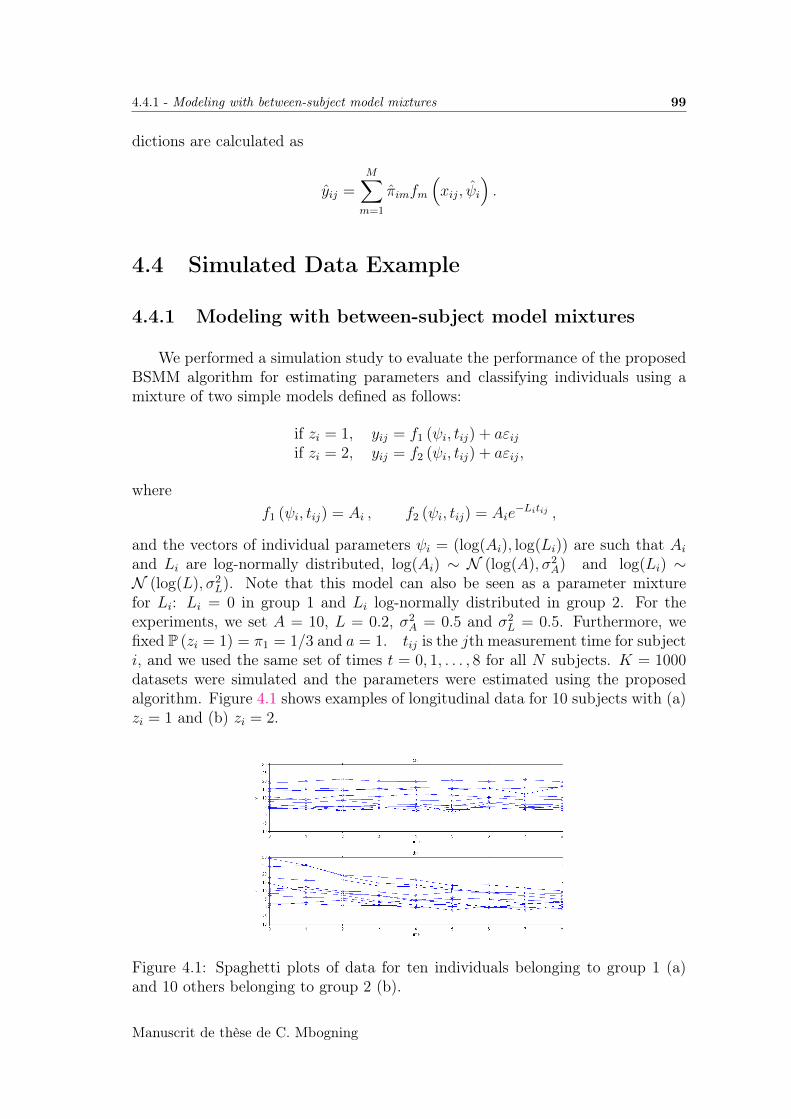
4.4.1 - Modeling with between-subject model mixtures 99
dictions are calculated as
yij =M∑m=1
πimfm
(xij, ψi
).
4.4 Simulated Data Example
4.4.1 Modeling with between-subject model mixtures
We performed a simulation study to evaluate the performance of the proposedBSMM algorithm for estimating parameters and classifying individuals using amixture of two simple models defined as follows:
if zi = 1, yij = f1 (ψi, tij) + aεijif zi = 2, yij = f2 (ψi, tij) + aεij,
wheref1 (ψi, tij) = Ai , f2 (ψi, tij) = Aie
−Litij ,
and the vectors of individual parameters ψi = (log(Ai), log(Li)) are such that Aiand Li are log-normally distributed, log(Ai) ∼ N (log(A), σ2
A) and log(Li) ∼N (log(L), σ2
L). Note that this model can also be seen as a parameter mixturefor Li: Li = 0 in group 1 and Li log-normally distributed in group 2. For theexperiments, we set A = 10, L = 0.2, σ2
A = 0.5 and σ2L = 0.5. Furthermore, we
fixed P (zi = 1) = π1 = 1/3 and a = 1. tij is the jth measurement time for subjecti, and we used the same set of times t = 0, 1, . . . , 8 for all N subjects. K = 1000datasets were simulated and the parameters were estimated using the proposedalgorithm. Figure 4.1 shows examples of longitudinal data for 10 subjects with (a)zi = 1 and (b) zi = 2.
Figure 4.1: Spaghetti plots of data for ten individuals belonging to group 1 (a)and 10 others belonging to group 2 (b).
Manuscrit de thèse de C. Mbogning
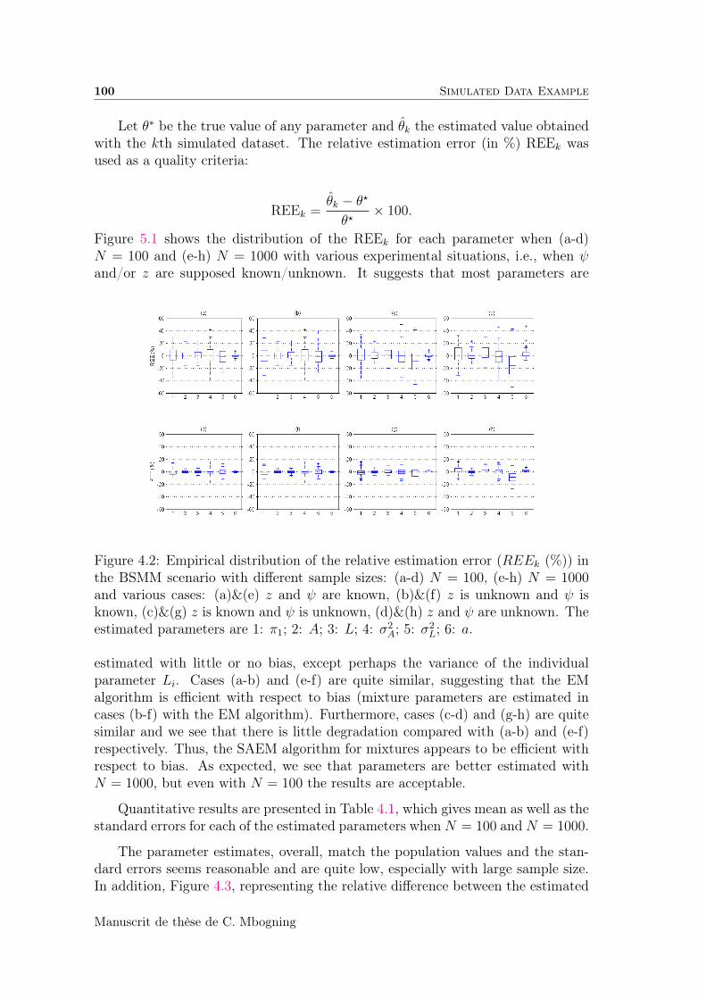
100 Simulated Data Example
Let θ∗ be the true value of any parameter and θk the estimated value obtainedwith the kth simulated dataset. The relative estimation error (in %) REEk wasused as a quality criteria:
REEk =θk − θ?
θ?× 100.
Figure 5.1 shows the distribution of the REEk for each parameter when (a-d)N = 100 and (e-h) N = 1000 with various experimental situations, i.e., when ψand/or z are supposed known/unknown. It suggests that most parameters are
Figure 4.2: Empirical distribution of the relative estimation error (REEk (%)) inthe BSMM scenario with different sample sizes: (a-d) N = 100, (e-h) N = 1000and various cases: (a)&(e) z and ψ are known, (b)&(f) z is unknown and ψ isknown, (c)&(g) z is known and ψ is unknown, (d)&(h) z and ψ are unknown. Theestimated parameters are 1: π1; 2: A; 3: L; 4: σ2
A; 5: σ2L; 6: a.
estimated with little or no bias, except perhaps the variance of the individualparameter Li. Cases (a-b) and (e-f) are quite similar, suggesting that the EMalgorithm is efficient with respect to bias (mixture parameters are estimated incases (b-f) with the EM algorithm). Furthermore, cases (c-d) and (g-h) are quitesimilar and we see that there is little degradation compared with (a-b) and (e-f)respectively. Thus, the SAEM algorithm for mixtures appears to be efficient withrespect to bias. As expected, we see that parameters are better estimated withN = 1000, but even with N = 100 the results are acceptable.
Quantitative results are presented in Table 4.1, which gives mean as well as thestandard errors for each of the estimated parameters when N = 100 and N = 1000.
The parameter estimates, overall, match the population values and the stan-dard errors seems reasonable and are quite low, especially with large sample size.In addition, Figure 4.3, representing the relative difference between the estimated
Manuscrit de thèse de C. Mbogning
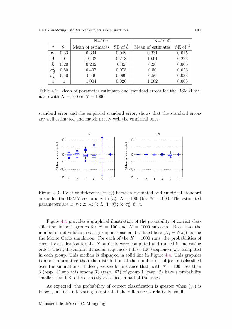
4.4.1 - Modeling with between-subject model mixtures 101
N=100 N=1000θ θ∗ Mean of estimates SE of θ Mean of estimates SE of θπ1 0.33 0.334 0.049 0.331 0.015A 10 10.03 0.713 10.01 0.226L 0.20 0.202 0.02 0.20 0.006σ2A 0.50 0.497 0.075 0.50 0.023σ2L 0.50 0.49 0.099 0.50 0.033a 1 1.004 0.026 1.002 0.008
Table 4.1: Mean of parameter estimates and standard errors for the BSMM sce-nario with N = 100 or N = 1000.
standard error and the empirical standard error, shows that the standard errorsare well estimated and match pretty well the empirical ones.
Figure 4.3: Relative difference (in %) between estimated and empirical standarderrors for the BSMM scenario with (a): N = 100, (b): N = 1000. The estimatedparameters are 1: π1; 2: A; 3: L; 4: σ2
A; 5: σ2L; 6: a.
Figure 4.4 provides a graphical illustration of the probability of correct clas-sification in both groups for N = 100 and N = 1000 subjects. Note that thenumber of individuals in each group is considered as fixed here (N1 = Nπ1) duringthe Monte Carlo simulation. For each of the K = 1000 runs, the probabilities ofcorrect classification for the N subjects were computed and ranked in increasingorder. Then, the empirical median sequence of these 1000 sequences was computedin each group. This median is displayed in solid line in Figure 4.4. This graphicsis more informative than the distribution of the number of subject misclassifiedover the simulations. Indeed, we see for instance that, with N = 100, less than3 (resp. 4) subjects among 33 (resp. 67) of group 1 (resp. 2) have a probabilitysmaller than 0.8 to be correctly classified in half of the cases.
As expected, the probability of correct classification is greater when (ψi) isknown, but it is interesting to note that the difference is relatively small.
Manuscrit de thèse de C. Mbogning
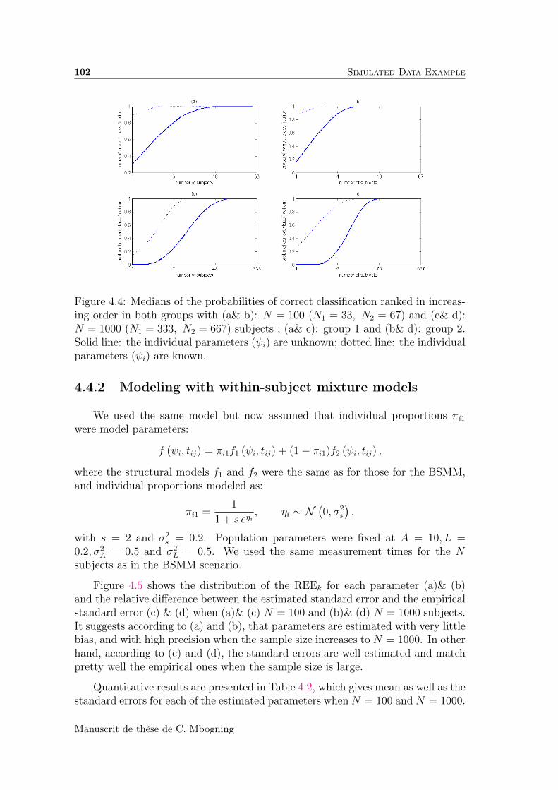
102 Simulated Data Example
Figure 4.4: Medians of the probabilities of correct classification ranked in increas-ing order in both groups with (a& b): N = 100 (N1 = 33, N2 = 67) and (c& d):N = 1000 (N1 = 333, N2 = 667) subjects ; (a& c): group 1 and (b& d): group 2.Solid line: the individual parameters (ψi) are unknown; dotted line: the individualparameters (ψi) are known.
4.4.2 Modeling with within-subject mixture models
We used the same model but now assumed that individual proportions πi1were model parameters:
f (ψi, tij) = πi1f1 (ψi, tij) + (1− πi1)f2 (ψi, tij) ,
where the structural models f1 and f2 were the same as for those for the BSMM,and individual proportions modeled as:
πi1 =1
1 + s eηi, ηi ∼ N
(0, σ2
s
),
with s = 2 and σ2s = 0.2. Population parameters were fixed at A = 10, L =
0.2, σ2A = 0.5 and σ2
L = 0.5. We used the same measurement times for the Nsubjects as in the BSMM scenario.
Figure 4.5 shows the distribution of the REEk for each parameter (a)& (b)and the relative difference between the estimated standard error and the empiricalstandard error (c) & (d) when (a)& (c) N = 100 and (b)& (d) N = 1000 subjects.It suggests according to (a) and (b), that parameters are estimated with very littlebias, and with high precision when the sample size increases to N = 1000. In otherhand, according to (c) and (d), the standard errors are well estimated and matchpretty well the empirical ones when the sample size is large.
Quantitative results are presented in Table 4.2, which gives mean as well as thestandard errors for each of the estimated parameters when N = 100 and N = 1000.
Manuscrit de thèse de C. Mbogning
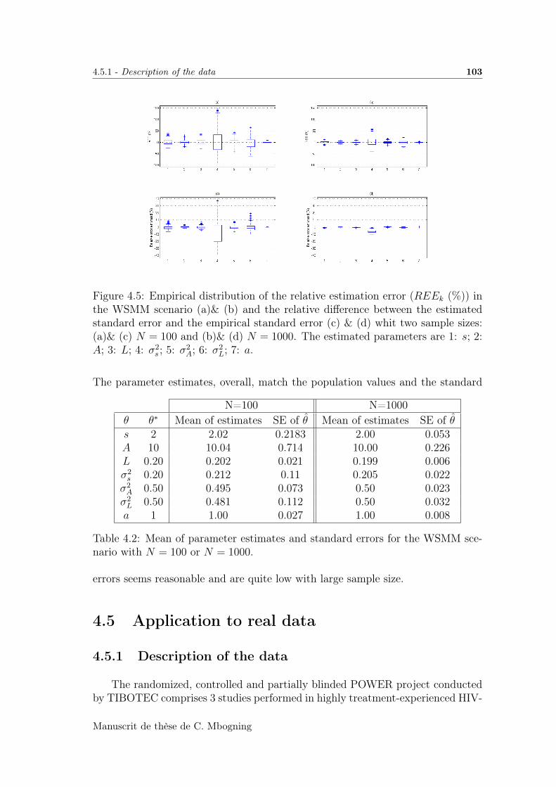
4.5.1 - Description of the data 103
Figure 4.5: Empirical distribution of the relative estimation error (REEk (%)) inthe WSMM scenario (a)& (b) and the relative difference between the estimatedstandard error and the empirical standard error (c) & (d) whit two sample sizes:(a)& (c) N = 100 and (b)& (d) N = 1000. The estimated parameters are 1: s; 2:A; 3: L; 4: σ2
s ; 5: σ2A; 6: σ2
L; 7: a.
The parameter estimates, overall, match the population values and the standard
N=100 N=1000θ θ∗ Mean of estimates SE of θ Mean of estimates SE of θs 2 2.02 0.2183 2.00 0.053A 10 10.04 0.714 10.00 0.226L 0.20 0.202 0.021 0.199 0.006σ2s 0.20 0.212 0.11 0.205 0.022σ2A 0.50 0.495 0.073 0.50 0.023σ2L 0.50 0.481 0.112 0.50 0.032a 1 1.00 0.027 1.00 0.008
Table 4.2: Mean of parameter estimates and standard errors for the WSMM sce-nario with N = 100 or N = 1000.
errors seems reasonable and are quite low with large sample size.
4.5 Application to real data
4.5.1 Description of the data
The randomized, controlled and partially blinded POWER project conductedby TIBOTEC comprises 3 studies performed in highly treatment-experienced HIV-
Manuscrit de thèse de C. Mbogning
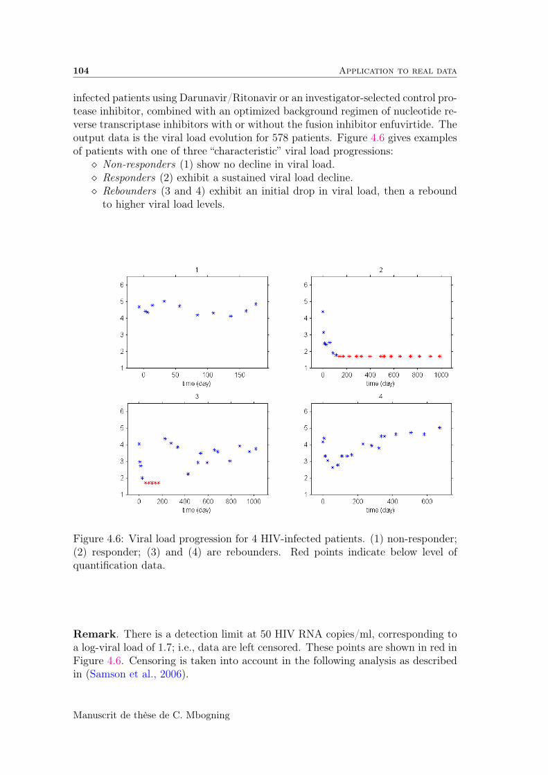
104 Application to real data
infected patients using Darunavir/Ritonavir or an investigator-selected control pro-tease inhibitor, combined with an optimized background regimen of nucleotide re-verse transcriptase inhibitors with or without the fusion inhibitor enfuvirtide. Theoutput data is the viral load evolution for 578 patients. Figure 4.6 gives examplesof patients with one of three “characteristic” viral load progressions: Non-responders (1) show no decline in viral load. Responders (2) exhibit a sustained viral load decline. Rebounders (3 and 4) exhibit an initial drop in viral load, then a rebound
to higher viral load levels.
Figure 4.6: Viral load progression for 4 HIV-infected patients. (1) non-responder;(2) responder; (3) and (4) are rebounders. Red points indicate below level ofquantification data.
Remark. There is a detection limit at 50 HIV RNA copies/ml, corresponding toa log-viral load of 1.7; i.e., data are left censored. These points are shown in red inFigure 4.6. Censoring is taken into account in the following analysis as describedin (Samson et al., 2006).
Manuscrit de thèse de C. Mbogning
4.5.2 - Class prediction using between-subject model mixtures 105
4.5.2 Class prediction using between-subject model mix-tures
Within a few months of HIV infection, patients typically enter a steady state ofchronic infection and show their concentration of HIV-1 in blood plasma stabilized.When the anti-retroviral treatment starts, the viral load of patients who respondshows an initial rapid exponential decay, usually followed by a slower second phaseof exponential decay, see (Perelson et al., 1997). It is shown in (Ding and Wu,2001) that the biphasic decay in viral load can be approximated by a bi-exponentialmodel A1e
−λ1t + A2e−λ2t.
After the decrease in viral load levels, some subjects show a rebound whichcan be due to several factors (non adherence to the therapy, emergence of drug-resistant virus strains, . . . ). We propose to extend the bi-exponential model forthese patients by adding a third phase described by a logistic growth processA3/(1 + e−λ3(t−τ)) where τ is the inflection point of this growth process.
We then propose to describe the log-transformed viral load with a BSMMwith three simple models, corresponding to each of three characteristic viral loadprogressions: Non-responder-like data can be described using a simple horizontal line. The
structural model is given by:
zi = 1, f1 (ψi, tij) = A1i + A2i .
As described above, the drop in viral load in responder-like data can bedescribed using a bi-exponential mixed-effects model:
zi = 2, f2 (ψi, tij) = A1ie−λ1itij + A2ie
−λ2itij ,
where λ1i and λ2i describe the rate of exponential decay and A1i and A2i areintercept parameters for individual i. As in (Davidian and Giltinan, 1995),these parameters are considered to be strictly positive. Rebounder-like data show a rebound after a biphasic decrease in viral load
levels:
zi = 3, f3 (ψi, tij) = A1ie−λ1itij + A2ie
−λ2itij +A3i
1 + e−λ3i(tij−τi).
The log-transform viral load is then modeled by:
log (yij) =3∑
m=1
1zi=m log (fm (ψi, tij)) + εij, (4.6)
where yij is the viral load for subject i at time tij and ψi =(A1i, A2i, A3i, λ1i, λ2i, λ3i, τi) the vector of individual parameters.
Manuscrit de thèse de C. Mbogning
106 Application to real data
These parameters are positive and distributed according to log-normal distri-butions. Thus,
logAli = logAl + ηli, ηli ∼ N(0, σ2
Al
), l = 1, 2, 3
log λmi = log λm + η(m+3) i, η(m+3) i ∼ N(0, σ2
λm
), m = 1, 2, 3
log τi = log τ + η7i, η7i ∼ N(0, σ2
τ
).
By setting π1 = P (zi = 1) , π2 = P (zi = 2) and π3 = P (zi = 3) with∑3m=1 πm = 1, the complete set of population parameters to be estimated is given
by θ = (A1, A2, A3, λ1, λ2, λ3, τ, π1, π2, π3).
Parameter estimation was performed using the SAEM algorithm for BSMMimplemented in Monolix . This algorithm combined with a previous version(Samson et al., 2006)(which is an extension of the SAEM algorithm (Kuhn andLavielle, 2005) to left censored data) takes properly into account the censoredviral load data below the limit of quantification. Figure 4.7 shows the individualfits for the 4 patients, the vector of estimated posterior probabilities pi wherepim = P
(zi = m|yi; θ
), i.e., the probabilities for each subject to belong to each of
the three classes, and the class zi to which they are assigned (1 = non-responder,2 = responder, 3 = rebounder) corresponding to the maximum of the estimatedposterior probabilities. We see that in all four cases, there is little ambiguity inthe results, i.e., the correct class has a posterior probability very close to 1.
4.5.3 Class prediction using within-subject mixture models
Not all observed viral load progressions fall so easily into one of the threeclasses, as for example the patients shown in Figure 4.8. In these cases, it doesnot seem quite so reasonable to model the data under the BSMM assumption thateach patient must belong uniquely to one class; instead, it is perhaps more naturalto suppose that each patient is partially responding, partially non-responding andpartially rebounding with respect to the given drug treatment. The goal becomesto find the relative strength of each process in each patient, and a WSMM isan ideal tool to do this. The proportions πi are now individual parameters inthe model and the problem is transformed into a standard NLMEM. Since theseproportions are assumed to be positive and summing to 1 for each patient, weassumed a logit-normal distribution on the πim,m = 1, 2, 3 as follows:
πi1 =γ1i
1 + γ1i + γ2i
πi2 =γ2i
1 + γ1i + γ2i
πi3 =1
1 + γ1i + γ2i
,
withlog γki = log γk + ηki, ηki ∼ N
(0, σ2
γk
)for k = 1, 2.
We performed parameter estimation for WSMM using the SAEM algorithmin Monolix , taking properly into account the censored viral load data below
Manuscrit de thèse de C. Mbogning
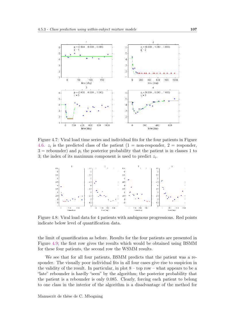
4.5.3 - Class prediction using within-subject mixture models 107
Figure 4.7: Viral load time series and individual fits for the four patients in Figure4.6. zi is the predicted class of the patient (1 = non-responder, 2 = responder,3 = rebounder) and pi the posterior probability that the patient is in classes 1 to3; the index of its maximum component is used to predict zi.
Figure 4.8: Viral load data for 4 patients with ambiguous progressions. Red pointsindicate below level of quantification data.
the limit of quantification as before. Results for the four patients are presented inFigure 4.9; the first row gives the results which would be obtained using BSMMfor these four patients, the second row the WSMM results.
We see that for all four patients, BSMM predicts that the patient was a re-sponder. The visually poor individual fits in all four cases give rise to suspicion inthe validity of the result. In particular, in plot 8 – top row – what appears to be a“late” rebounder is hardly “seen” by the algorithm; the posterior probability thatthe patient is a rebounder is only 0.085. Clearly, forcing each patient to belongto one class in the interior of the algorithm is a disadvantage of the method for
Manuscrit de thèse de C. Mbogning
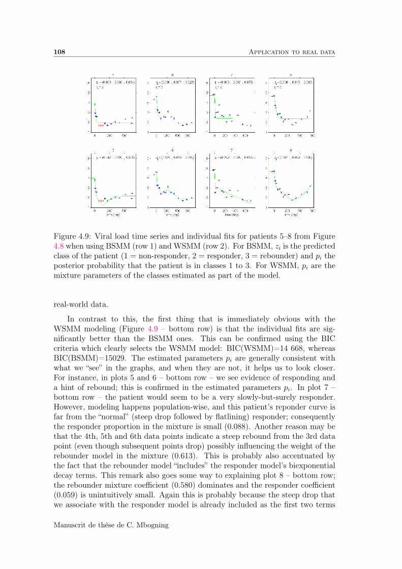
108 Application to real data
Figure 4.9: Viral load time series and individual fits for patients 5–8 from Figure4.8 when using BSMM (row 1) and WSMM (row 2). For BSMM, zi is the predictedclass of the patient (1 = non-responder, 2 = responder, 3 = rebounder) and pi theposterior probability that the patient is in classes 1 to 3. For WSMM, pi are themixture parameters of the classes estimated as part of the model.
real-world data.
In contrast to this, the first thing that is immediately obvious with theWSMM modeling (Figure 4.9 – bottom row) is that the individual fits are sig-nificantly better than the BSMM ones. This can be confirmed using the BICcriteria which clearly selects the WSMM model: BIC(WSMM)=14 668, whereasBIC(BSMM)=15029. The estimated parameters pi are generally consistent withwhat we “see” in the graphs, and when they are not, it helps us to look closer.For instance, in plots 5 and 6 – bottom row – we see evidence of responding anda hint of rebound; this is confirmed in the estimated parameters pi. In plot 7 –bottom row – the patient would seem to be a very slowly-but-surely responder.However, modeling happens population-wise, and this patient’s reponder curve isfar from the “normal” (steep drop followed by flatlining) responder; consequentlythe responder proportion in the mixture is small (0.088). Another reason may bethat the 4th, 5th and 6th data points indicate a steep rebound from the 3rd datapoint (even though subsequent points drop) possibly influencing the weight of therebounder model in the mixture (0.613). This is probably also accentuated bythe fact that the rebounder model “includes” the responder model’s biexponentialdecay terms. This remark also goes some way to explaining plot 8 – bottom row;the rebounder mixture coefficient (0.580) dominates and the responder coefficient(0.059) is unintuitively small. Again this is probably because the steep drop thatwe associate with the responder model is already included as the first two terms
Manuscrit de thèse de C. Mbogning

4.5.3 - Class prediction using within-subject mixture models 109
in the rebounder model; hence the small responder coefficient.
4.6 Discussion
We have presented a classification methodology to interpret longitudinal datain a population context using model mixtures in the NLMEM framework. Twoclasses of model mixtures were introduced: between-subject and within-subject(BSMM and WSMM), and it was shown how to perform maximum likelihoodestimation in the BSMM case. These algorithms are now available in the softwareMonolix . In simulations with mixtures of two models, we saw generally goodparameter estimation performance and prediction performance, i.e., prediction ofwhich model had been used to generate each individual’s longitudinal data. Inreal longitudinal HIV viral load data, we found that BSMMs were very efficientboth in modeling and predicting the type of patient (non-responder, responder,rebounder) whenever the patient’s viral load evolution was a “model case” of oneof the three classes. However, when the viral load evolution was not so “typical”,the fact that BSMMs force the allocation of once class to each patient lead to poorindividual model fits and what’s more, dubious class prediction.
On the other hand, WSMMs allow for more flexibility in modeling and are con-sistent with the biologically plausible hypothesis that each individual may be onlypartially responding/non-responding/rebounding due to their own unique virusstrains, cell populations, etc. Allowing a mixture of biologically relevant modelsinternally to each patient clearly improved the individual model fits and permit-ted a more nuanced reply to the classification question of whether the patient wasresponding adequately to the treatment or not. Based on these results, we wouldhave more confidence in suggesting a modification to HIV drug regimes based onWSMM modeling than BSMM.
Manuscrit de thèse de C. Mbogning
Chapter 5
Joint modeling of longitudinal andrepeated time-to-event data withmaximum likelihood estimation viathe SAEM algorithm.
Contents5.1 Introduction . . . . . . . . . . . . . . . . . . . . . . . . . 1135.2 Models . . . . . . . . . . . . . . . . . . . . . . . . . . . . 115
5.2.1 Nonlinear mixed-effects models for the population ap-proach . . . . . . . . . . . . . . . . . . . . . . . . . . . . 115
5.2.2 Repeated time-to-event model . . . . . . . . . . . . . . . 1165.2.3 Joint models . . . . . . . . . . . . . . . . . . . . . . . . 118
5.3 Tasks and methods . . . . . . . . . . . . . . . . . . . . . 1195.3.1 Maximum likelihood estimation of the population pa-
rameters . . . . . . . . . . . . . . . . . . . . . . . . . . . 119General description of the SAEM algorithm . . . . . . . 120
5.4 Computing the probability distribution for repeatedtime-to-events . . . . . . . . . . . . . . . . . . . . . . . . 121
5.4.1 Exactly observed events . . . . . . . . . . . . . . . . . . 1225.4.2 Single interval-censored events . . . . . . . . . . . . . . 1225.4.3 Multiple events per interval . . . . . . . . . . . . . . . . 123
5.5 Numerical experiments . . . . . . . . . . . . . . . . . . . 1255.5.1 Simulations . . . . . . . . . . . . . . . . . . . . . . . . . 125
Example 1 . . . . . . . . . . . . . . . . . . . . . . . . . . 126Example 2 . . . . . . . . . . . . . . . . . . . . . . . . . . 128Example 3 . . . . . . . . . . . . . . . . . . . . . . . . . . 129Example 4 . . . . . . . . . . . . . . . . . . . . . . . . . . 129
5.5.2 Applications . . . . . . . . . . . . . . . . . . . . . . . . . 132
110

CHAPTER 5. JOINT MODELING OF LONGITUDINAL AND REPEATEDTIME-TO-EVENT DATA WITH MAXIMUM LIKELIHOOD ESTIMATION VIA THESAEM ALGORITHM. 111
Primary Biliary Cirrhosis Data . . . . . . . . . . . . . . 132Epileptic seizure counts . . . . . . . . . . . . . . . . . . 134
5.6 Discussion . . . . . . . . . . . . . . . . . . . . . . . . . . . 1345.7 Appendix: Several examples on the computation of
the likelihood of a RTTE model . . . . . . . . . . . . . . 136
Manuscrit de thèse de C. Mbogning
112
Abstract
We propose a nonlinear mixed-effects framework to jointly model longitudinaland repeated time-to-event data. A parametric nonlinear mixed-effects model isused for the longitudinal observations and a parametric mixed-effects hazard modelfor repeated event times. We show the importance for parameter estimation ofproperly calculating the conditional density of the observations (given the individ-ual parameters) in the presence of interval and/or right censoring. Parameters areestimated by maximizing the exact joint likelihood with the Stochastic Approxi-mation Expectation-Maximization algorithm. The simulation study demonstratesthat our methodology yields satisfactory results in this complex setting. As an il-lustration, such an approach is applied on two real word data sets. The first one isa primary biliary cirrhosis data, with longitudinal serum bilirubin measurements,jointly modelled with death. The second one is an epileptic seizure counts data,with seizures considered as interval censored. This workflow for joint models isnow implemented in the Monolix software.
Keywords: Interval censoring; Joint models; Maximum likelihood; Mixed-effects models; SAEM algorithm; Repeated time-to-events.
Manuscrit de thèse de C. Mbogning
CHAPTER 5. JOINT MODELING OF LONGITUDINAL AND REPEATEDTIME-TO-EVENT DATA WITH MAXIMUM LIKELIHOOD ESTIMATION VIA THESAEM ALGORITHM. 113
5.1 Introduction
Joint models are a class of statistical methods for bringing together longitudi-nal data and time-to-event data into a unified framework. In the medical setting(the most common application of joint models), we often have, for a set of pa-tients, time-to-event data of interest, e.g. tumor recurrences, epileptic seizures,asthma attacks, migraines, infectious episodes, heart attacks, injuries, hospital ad-missions, or even death. One may be interested in modeling the process inducingthe event(s), using for example a suitable chosen (time-dependent or not) hazardfunction to describe the instantaneous chance of an event occurrence.
Simultaneously, for each patient we may be able to measure a longitudinal out-come (called biomarker in the following) and model its progression. Joint modelscome into the picture when there is a distinct possibility that a given longitudinalbiomarker has a real influence on the time-to-event process. In such cases and inthe most general way possible, the joint model strategy is to suggest a relation-ship between the biomarker and the hazard function, i.e., have its predicted valueinfluence the instantaneous probability of the event of interest.
Early attempts to create joint models and apply them to biological settingswere introduced by (Self and Pawitan, 1992) and (DeGruttola and Tu, 1994) withapplications in AIDS research. What goes today as the standard joint modelwas introduced by (Faucett and Thomas, 1996) and (Wulfsohn and Tsiatis, 1997)and since that time, developments in the field have continued apace. We nowbriefly present the joint modeling framework as it currently stands, then explainthe contribution of the present article to the state of the art. For a more thoroughintroduction, we point the reader to the monograph by (Rizopoulos, 2012b).
Joint modeling tries to characterize the relationship between a longitudinalbiomarker’s evolution and the risk of a given event, while also providing an ac-ceptable model of the biomarker’s evolution itself. First, let us concentrate onthe longitudinal biomarker. Its evolution is often modeled under a linear mixed-effects framework (Laird and Ware, 1982; Harville, 1977; Verbeke and Molen-berghs, 2000) using for instance splines (Ruppert et al., 2003) or B-splines withrandom effects (Rizopoulos et al., 2009; Brown et al., 2005). This frameworktakes into account the correlated nature of the measures for a given individual,while also allowing inter-individual random variability in key model parameters(e.g. slope, intercept). We can thus estimate the mean values of these parame-ters, as well as model/plot the evolution of the biomarker for each individual usingtheir own estimated parameter values. Parameter estimation is often performedusing a maximum likelihood strategy. However, linearity and the associated sup-position of normally distributed parameters are strong hypotheses which are notnecessarily representative of what is seen in real-life situations. For instance, inpharmacometrics and in particular pharmacokinetic-pharmacodynamic (PKPD)applications, linear models are usually not sufficient to satisfactorily model data.Consequently, nonlinear mixed-effects models have been largely adopted (Sheiner
Manuscrit de thèse de C. Mbogning
114 Introduction
and Beal, 1985; Lindstrom and Bates, 1990; Davidian and Giltinan, 1995; Voneshand Chinchilli, 1997) even though they involve computationally taxing calculationswhen performing maximum likelihood, a stumbling block until recently. However,strategies such as the Stochastic Approximation EM (SAEM) algorithm (Kuhnand Lavielle, 2005), implemented in the Monolix software and R (R Develop-ment Core Team, 2008), have recently led to significantly faster methods for notonly linear mixed-effects but also nonlinear mixed-effects models.
Next let us consider the event risk itself, modeled by a hazard function λ,which characterizes the distribution of the time-to-event process. The hazardfunction may be constant or vary as a function of time. Joint modeling is achievedby allowing the hazard function λ at time t to also depend on the value of thelongitudinal biomarker predicted at t. In this framework, the baseline value ofλ can be supposed constant or randomly varying across the population. Jointmodeling then involves the simultaneous estimation of all the parameters fromboth parts of the model, again often by a maximum-likelihood strategy.
Due to significant complexity in the calculation of likelihoods for these models,initial approaches to fit them focused on two-stage methods (Self and Pawitan,1992; Tsiatis et al., 1995), with the downside of often producing biased results(Dafny and Tsiatsis, 1998) in simulation studies. Full likelihood approaches havetherefore been introduced to try to eliminate this bias (Wulfsohn and Tsiatis, 1997;Henderson et al., 2000; Hsieh et al., 2006). Maximization of the log-likelihoodfunction is then often attempted using the EM algorithm (Dempster et al., 1977),treating random effects as missing data. However, the integrals that must beapproximated for joint models are a big computational problem, especially theintegral with respect to the random effects. Indeed, this is perhaps the mainbottleneck blocking the more frequent everyday use of joint models. The R packageJM (Rizopoulos, 2012b) provides a set of procedures for solving these problems inthe linear mixed-models framework. We will show in this article that the SAEMalgorithm (Kuhn and Lavielle, 2005) can be extended to efficiently perform jointmodeling in the more general nonlinear framework and in the presence of censoreddata, as described in the following.
Censoring is a defining characteristic of time-to-event data and poses problemsfor using many typical statistical tools (sample average and standard deviation,t-tests, linear regression) because these suppose we have complete information.Censoring takes several forms: left censoring (event time is before the individualenters the study), right censoring (event happens after the last recorded time) andinterval censoring (event is known to happen between two time-points, but theexact event time is not known). If censoring is not correctly taken into accountwhen calculating likelihoods, bias will be introduced into parameter estimation.
The current article therefore advances the state of the art in several ways.First, it presents time-to-events models for repeated events, including for censoredevents (interval-censored, right-censored) where there may be 0, 1 or many eventsin each interval. Second, it develops a framework for joint models combining non-
Manuscrit de thèse de C. Mbogning
5.2.1 - Nonlinear mixed-effects models for the population approach 115
linear mixed effects models for continuous covariates/biomarkers with (perhapsrepeated) time-to-events data. Third, for likelihood calculations it presents a rig-orous calculation of the conditional density of the observations given the individualparameters in a wide variety of situations, and shows that bias is introduced if weapproximate by replacing a censoring interval by its mean, or do not take into ac-count when it is known that there is a maximum number of events. Fifth, it showsthat the Stochastic Approximation Expectation Maximization (SAEM) algorithm(Kuhn and Lavielle, 2005) is not only capable, but also extremely fast, when itcomes to performing maximum likelihood estimation for joint models. And last,it shows that we can also estimate the Fisher information matrix, the observedlikelihood and the individual parameters under the same framework.
The article is structured as follows. In section 5.2 we first recall nonlinearmixed-effects models for the population approach and then repeated time-to-eventsmodels, and show how they can be combined as joint models. In section 5.3 weintroduce the SAEM algorithm (Kuhn and Lavielle, 2005), proven to be efficient formaximum likelihood estimation of parameters in mixed-effects models in general,and nonlinear models in particular. We then describe how to estimate standarderrors and individual parameters, and how to approximate the log-likelihood usingimportance sampling in order to calculate model selection criteria such as BIC.
For all of these calculations, we require an expression for the conditional den-sity of the observations given the individual parameters, and furthermore, thisexpression depends on the situation we are interested in, whether it be repeatedevents with interval censoring, right-censored time-to-events, multiple events perinterval, joint models, etc. Therefore, in section 5.4 we derive these expressionsacross a wide range of situations. In section 5.5, a series of simulated examples areprovided to illustrate the methods in action and to show that the SAEM algorithmis accurate and extremely fast for the joint modeling of longitudinal and time-to-events data. Finally, in section 5.5.2, the methodology is applied on two real worddata sets. The first one is a primary biliary cirrhosis data, and the second one isan epileptic seizure counts data, with seizures considered as interval censored.
5.2 Models
5.2.1 Nonlinear mixed-effects models for the population ap-proach
Consider first a single subject i of the population. Let yi = (yij, 1 ≤ j ≤ni) be the vector of observations for this subject. The model that describes theobservations yi is assumed to be a parametric probabilistic model: let p(yi|ψi) bethe probability distribution of yi, where ψi is a vector of parameters.
In the population framework, the vector of parameters ψi is assumed to be
Manuscrit de thèse de C. Mbogning
116 Models
drawn from a population distribution p(ψi; θ). Then, the probabilistic model isthe joint probability distribution
p(yi, ψi; θ) = p(yi|ψi)p(ψi; θ). (5.1)
To define a model for the data thus consists in defining precisely these two terms.
First, let us present ψi in its most general form:
ψi = H(ψpop, β, ci, ηi),
where ψpop is a “typical” value of the parameters in the population, β a set ofcoefficients (usually called fixed effects), ci a vector of individual covariates and ηithe random component (usually called random effects). For example, in a linearmodel we assume that, up to some transformation, ψi is a linear function of thecovariates and the normally distributed random effects:
h(ψi) = h(ψpop) + βci + ηi, (5.2)
where h is some monotonic function (log, logit, probit, etc.) and ηi ∼ N (0,Ω).The set of population parameters that define the population distribution p(ψi; θ)of the individual parameters ψi is thus θ = (ψpop, β,Ω).
The conditional distribution p(yi|ψi) of the observations depends on the typeof observations (continuous, categorical, count, time-to-event, etc.). We considerhere two situations: observations are time-to-events, perhaps repeated (several events per indi-
vidual are observed) and perhaps interval or right censored (times of eventsare not precisely known). observations are a combination of continuous values (some biomarker) and
time-to-events. They are thus characterized by a joint model which describesthe relationship between the two types of data.
5.2.2 Repeated time-to-event model
For several reasons, time-to-event data are not amenable to standard statis-tical procedures. One is that they are generally not symmetrically distributed.Typically, a histogram constructed from the times-to-events of a group of similarindividuals will tend to be positively skewed. As a consequence, it is not reason-able to assume that data of this type have a normal distribution. This difficultycould be resolved by first transforming the data to give a more symmetric distribu-tion, for example by taking logarithms, which results in the well know AcceleratedFailure Time (AFT) model (Klein and Moeschberger, 1997). However, a moresatisfactory approach is to adopt an alternative model for the distribution of theoriginal data.
The main feature of time-to-event data that renders standard methods inap-propriate is that times-to-event are frequently censored (Klein and Moeschberger,
Manuscrit de thèse de C. Mbogning
5.2.2 - Repeated time-to-event model 117
1997), i.e., the time-points of interest may not be observed for some individuals.This may be because the study data are analyzed at a point in time where someindividuals have not yet experienced the event of interest. Alternatively, the sta-tus of an individual at the time of the analysis might not be known because thatindividual has been lost to follow-up.
More precisely, suppose an individual who enters a study at time t0 experiencesa relevant event at time t0 + t. However, t may be unknown, either because theindividual has not experienced the event yet, or because they have been lost tofollow-up. If they were last known to be alive at time t0 + c, then c is called acensored event time. This censoring occurs to the right of (i.e., after) the lastrecorded time, and is therefore known as right censoring. Similarly, left censoringis encountered when the actual event time is early than the entry of the individualinto the study. Left censoring occurs less than right censoring.
Another type of censoring is interval censoring. Here, individuals are knownto have experienced the event within a given interval of time, but the exact eventtime is not known. Interval-censored data commonly arise in studies where thereis a non-lethal end-point, such as the recurrence of a disease or condition. Severalauthors have focused on a single interval-censored event. For instance, (Kongerudand Samuelsen, 1991) and (Samuelsen and Kongerud, 1993) studied respiratoryand asthmatic symptoms among Norwegian aluminum workers in which the timeto the development of symptoms was only known to be between consecutive healthexaminations.
In summarizing time-to-event data, there are two main functions of interest,namely the survival function and the hazard function. The actual event time t canbe regarded as the value taken by a non-negative random variable T . For the caseof a single event process, the survival function S (t) is defined as
S (t) = P(T ≥ t) = 1− F (t) ,
where F is the cumulative distribution function of T . The hazard function λ(t)is the instantaneous risk of experiencing an event at some time t; therefore S canalso be written:
S(t) = e−∫ t0 λ(u)du.
In the case of a repeated events process we have instead a sequence of event times(Tj) and are now interested in the probability of an event after tj given the previousevent at tj−1:
P(Tj > tj|Tj−1 = tj−1) = e−
∫ tjtj−1
λ(u)du.
Under a population framework, we suppose a hazard function λi for each individuali:
λi(t) = λ(ψi, t).
As an example, consider the model with constant hazard (Karlsson et al., 2011)given by λi(t) = λi. Then, the duration between successive events has an expo-nential distribution with parameter λi, and the number of events in any interval
Manuscrit de thèse de C. Mbogning
118 Models
of length ∆ has a Poisson distribution with parameter ∆λi. Here, the vector ofindividual parameters reduces to ψi = λi.
In the most simple case, yi is a vector of known event times: yi =(ti1, ti2, . . . , ti ni
). But if we only know that events occur within certain intervals,then observations are the number of events per interval. Let (Ii1, . . . , Ii ni
) be a setof disjoint time intervals for individual i relevant to the experimental design. Wethen can write yi = (ki1, . . . , ki ni
), where ki` is the number of events for individuali that have occurred in interval Ii`. Note that this includes the interval censoredcase with finite intervals Ii`, as well as the right censored case with Ii ni
= [tend ,∞).
5.2.3 Joint models
Besides the parametric form of the model, an essential point of joint modelingis the type of dependency between the longitudinal data model and the events.Suppose that we have a continuous biomarker of the form
bij = f(tij, ψ
(1)i
)+ g
(tij, ψ
(1)i
)εij, 1 ≤ i ≤ N, 1 ≤ j ≤ n1,i. (5.3)
Next, we connect this with RTTE via the hazard function given in general form:
λi(t) = λ(f(t, ψ
(1)i ), ψ
(2)i
).
Observations are therefore a combination of the n1,i continuous-valued biomarkermeasurements with the n2,i event times (if observed):
yi = ((bij, 1 ≤ j ≤ n1,i), (ti`, 1 ≤ ` ≤ n2,i),
or with the number of events per interval in the case of censoring:
yi = ((bij, 1 ≤ j ≤ n1,i), (ki`, 1 ≤ ` ≤ n2,i).
The vector of individual parameters ψi = (ψ(1)i , ψ
(2)i ) combines the individual
parameters from the two parts of the joint model.
Example. Suppose that the biomarker measurements can be modeled by
bij = γi + δitij + aiεij, 1 ≤ i ≤ N, 1 ≤ j ≤ n1,i, (5.4)
and are related to an event process with hazard function
λi(t) = λ0,ieαi(γi+δit). (5.5)
Here, ψi = (γi, δi, ai, λ0,i, αi). Formulas 5.4 and 5.5 thus characterize the proba-bility model p(yi|ψi) of the observations. In the following, we will suppose certainparameters to be constants (i.e., without inter-individual variability), essentially
Manuscrit de thèse de C. Mbogning
5.3.1 - Maximum likelihood estimation of the population parameters 119
for reasons of identifiability. This is not to do with the distribution of the obser-vations, but rather with the distributions of the individual parameters. In effect,building the statistical model for the individual parameters relies in part on de-ciding which components of ψi vary or not within the population. In the presentexample, we are unable to estimate all the parameters and their variability. Innumerical trials in Section 5.5, we will therefore investigate this example furtherwhen supposing λ0,i = λ0, αi = α and ai = a to be population constants.
5.3 Tasks and methods
There are a variety of tasks that we are interested in performing here, whetherit be estimating population parameters and their variation, estimating individualparameters or estimating the likelihood, the latter useful for performing likelihoodratio tests and calculating information criteria such as BIC.
In the following sections, we propose methodology for each of these tasks.We show that each requires calculation of the joint pdf (5.1) and in particularthe conditional density p(yi|ψi) since under (5.2), p(ψi; θ) is straightforward tocompute since it is derived from a Gaussian density.
5.3.1 Maximum likelihood estimation of the population pa-rameters
Estimation in mixed-effects models consists of estimating the probability dis-tribution of the ψi’s in the population from the observations of the N subjects, i.e.,in evaluating both the typical values in the population and the variability betweensubjects. More precisely, we aim to compute the maximum likelihood estimate of θin (nonlinear) mixed-effects models by maximizing the observed likelihood p(y; θ).Estimation is complex because the N random vectors of parameters ψi are notobserved and because there is a nonlinear relationship between the observationsand the random effects defined in (5.2). For these reasons the likelihood functioncan not be explicitly given and its maximization is far from straightforward.
In a general way, linear and nonlinear mixed-effects models, including mixed-effects diffusion models, can be seen as incomplete data models in which the in-dividual parameters π = (ψ1, . . . , ψN) are the non-observed data and the pop-ulation parameters are the parameters of the model that need to be estimatedfrom the N individual observations vectors y = (y1, . . . , yN). The EM algorithm(Dempster et al., 1977) iteratively performs parameter estimation in such models.The algorithm requires computing at each iteration the conditional expectationE(log p(y, ψ; θ)|y, θ(k−1)
), where θ(k−1) represents the current estimation of θ. In
many situations, especially when dealing with nonlinear mixed-effects models, thisconditional expectation has no closed form. Some variants of the algorithm get
Manuscrit de thèse de C. Mbogning
120 Tasks and methods
around this difficulty. For instance, in the SAEM algorithm (Delyon et al., 1999),the E-step is evaluated by a stochastic approximation procedure.
General description of the SAEM algorithm
Let θ(k−1) denote the current estimate for the population parameters. Iterationk of the SAEM algorithm involves three steps (Delyon et al., 1999; Kuhn andLavielle, 2005): In the simulation step, θ(k−1) is used to simulate the missing data ψ(k)
i underthe conditional distribution p(ψi|yi, θ(k−1)), i = 1, . . . , N . In the stochastic approximation step, the simulated data ψ(k) and the obser-
vations y are used together to update the stochastic approximation Qk(θ)of the conditional expectation E
(log p(y, ψ; θ)|y, θ(k−1)
)according to:
Qk(θ) = Qk−1(θ) + νk(log p(y, φ(k); θ)−Qk−1(θ)
), (5.6)
where (νk)k>0 is a sequence of positive step sizes decreasing to 0 and startingwith ν1 = 1. In the maximization step, an updated value of the estimate θ(k) is obtained
by maximization of Qk(θ) with respect to θ:
θ(k) = argmaxθ
Qk(θ).
This procedure is iterated until numerical convergence of the sequence(θ(k))k>0
tosome estimate θ is achieved. Convergence results can be found in (Delyon et al.,1999).
When an estimate θ has been obtained, estimates of the standard errorsof its components can be derived by estimating the Fisher information matrixI(θ) = −∂2 log(p(y; θ))/∂θ∂θ′|θ=θ following the stochastic approximation proce-dure suggested in (Kuhn and Lavielle, 2005), which requires simulation of the ψi’sunder p(·|y, θ) via a Metropolis-Hastings algorithm.
Estimates of the ψi’s can also be derived from the conditional distributionp(ψi|yi, θ) such as the conditional mode or the conditional mean. Whatever theestimate chosen, simulating this conditional distribution via Metropolis-Hastings,or maximizing it, requires computing the conditional distribution of the observa-tions p(yi|ψi).
Standard model selection criteria such as BIC require calculation of the ob-served log-likelihood log(p(y; θ)). As the log-likelihood cannot be computed ina closed form here, it is approximated using an importance sampling procedure.This consists of drawing ψ(1), ψ(2), . . . , ψ(M) under a given sampling distributionπ, and approximating the likelihood with:
p(y; θ) ≈ 1
M
M∑k=1
p(y|ψ(k))π(ψ(k), θ)
π(ψ(k)).
Manuscrit de thèse de C. Mbogning
5.3.1 - Maximum likelihood estimation of the population parameters 121
Here also, we see that computation of p(yi|ψi) is required. In summary, calculationof p(yi|ψi) for the various cases (repeated events with interval censoring, right-censored time-to-events, joint models, etc.) is a critical step in the modelingprocess. In the following section, we therefore explicitly calculate this pdf for awide range of cases.
5.4 Computing the probability distribution for re-peated time-to-events
The aim of this section is to compute precisely the conditional distributionp(yi|ψi) for any subject i, when the vector of observations yi only consists of(possibly repeated and possibly censored) time-to-events. For the sake of simplicitywe only consider a single subject, and therefore omit the subscript i in notation.Also for simplicity we denote λ(t) the hazard function at time t and omit thedependence with respect to the parameter ψ. We assume that the trial starts attime t0 and ends at time tend. Both t0 and tend are known. Let T = (T1, T2, . . .)be the (random) event times after t0, and Λ be the cumulative hazard function:
Λ(a, b) :=
∫ b
a
λ(t) dt
= Λ(t0, b)− Λ(t0, a).
By definition, recall that
P(Tj > tj|Tj−1 = tj−1) = e−Λ(tj−1,tj). (5.7)
We now distinguish between the three following situations:
exactly observed events: the sequence of event times (Tj) is exactly known;
single interval-censored events: we only know that the j-th event occurredbetween aj and bj, where ([aj, bj]) is a sequence of intervals such that aj ≥bj−1;
multiple interval-censored events: a sequence (Kj; j ≥ 1) is observed,where Kj is the number of events in interval [bj−1, bj]. Here, ([bj−1, bj])is a sequence of successive intervals with b0 = t0 < b1 < b2 < . . .
We remark that the exactly observed event situation is the limiting case of the sin-gle interval-censored events one as aj → bj. Similarly, the single interval-censoredcase is a special case of the multiple interval-censored case, where the number ofevents in each interval is 0 or 1.
Now suppose n is the number of observed events between t0 and tend. Wefurther distinguish between two situations:
Manuscrit de thèse de C. Mbogning
122 Computing the probability distribution for repeated time-to-events
(i) the sequence of event times (Tj) is finite and all events are known to occurbetween t0 and tend, i.e., t0 < T1 < T2 < . . . < Tn ≤ tend;
(ii) the sequence of event times (Tj) is not bounded above by tend and at leastone event is known to occur after tend. It is very important to realise thateven if the (n+1)-th event is not observed, the information that Tn+1 > tend ispertinent and contributes to the probability distribution of the observations.It should therefore always be taken into account.
5.4.1 Exactly observed events
i) the last event is observed. Assume that we observe n events at timest1, t2, . . . , tn and that no event occurs after tend. The vector of observations isy = (t1, t2, . . . , tn) and
p(y|ψ) = p(t1, t2, . . . , tn)
= p(t1|t0)p(t2|t1)p(t3|t2) . . . p(tn|tn−1).
By definition, p(tj|tj−1) = λ(tj)e−Λ(tj−1,tj). Thus,
p(y|ψ) =n∏j=1
p(tj|tj−1) (5.8)
=n∏j=1
λ(tj)e−Λ(tj−1,tj) . (5.9)
ii) the last event is not observed. Assume that we observe n events at timest1, t2, . . . , tn and that an event is known to occur at time Tn+1 > tend. Here, thevector of observations is y = (t1, t2, . . . , tn, tn+1 > tend) and
p(y|ψ) = p(t1, t2, . . . , tn)P(Tn+1 > tend|Tn = tn)
= p(t1|t0)p(t2|t1)p(t3|t2) . . . p(tn|tn−1)P(Tn+1 > tend|Tn = tn)
=
(n∏j=1
λ(tj)e−Λ(tj−1,tj)
)e−Λ(tn,tend) .
5.4.2 Single interval-censored events
Assume that n events occur between t0 and tend but that we only know thatt1 ∈ [a1, b1], t2 ∈ [a2, b2], . . . , tn ∈ [an, bn].
i) the last event is observed. Here, no event occurs after tend. The vectorof observations is y = (t1 ∈ [a1, b1], t2 ∈ [a2, b2], . . . , tn ∈ [an, bn]) and its joint
Manuscrit de thèse de C. Mbogning
5.4.3 - Multiple events per interval 123
probability distribution is:
p(y|ψ) = P(T1 ∈ [a1, b1], T2 ∈ [a2, b2], . . . , Tn ∈ [an, bn])
=
∫ b1
a1
∫ b2
a2
. . .
∫ bn
an
p(t1, t2, . . . , tn) dt1 dt2, . . . , dtn.
Using equations 5.8-5.9,
p(t1, t2, . . . , tn) =n∏j=1
λ(tj)e−Λ(tj−1,tj)
=
(n∏j=1
λ(tj)
)e−
∑nj=1 Λ(tj−1,tj)
=
(n−1∏j=1
λ(tj)
)λ(tn)e−Λ(t0,tn)
=
(n−1∏j=1
λ(tj)
)p(tn|t0).
Thus, the multiple integral can be computed:
p(y|ψ) =
(n−1∏j=1
Λ(aj, bj)
)P(Tn ∈ [an, bn]|Tn−1 = t0)
=
(n−1∏j=1
Λ(aj, bj)
)(e−Λ(t0,an) − e−Λ(t0,bn)
). (5.10)
ii) the last event is not observed. Here, at least one event is known to occurafter tend. Thus, y = (t1 ∈ [a1, b1], t2 ∈ [a2, b2], . . . , tn ∈ [an, bn], tn+1 > tend). Theprevious result (see equation 5.10) holds with an+1 = tend and bn+1 = +∞:
p(y|ψ) = P(T1 ∈ [a1, b1], T2 ∈ [a2, b2], . . . , Tn ∈ [an, bn], Tn+1 > tend)
=
(n∏j=1
Λ(aj, bj)
)e−Λ(t0,tend). (5.11)
5.4.3 Multiple events per interval
Consider first a single interval [0, b] and let kmax (kmax ≤ +∞) be the maximumnumber of events. Let K be the number of events in [0, b].
For any k < kmax, K = k implies that the (k+ 1)-th event occurs after time b.
Manuscrit de thèse de C. Mbogning
124 Computing the probability distribution for repeated time-to-events
Then, for any k < kmax,
P(K = k) = P(T1 ∈ [0, b], . . . , Tk ∈ [0, b], Tk+1 > b; T1 < . . . < Tk < Tk+1)
=
∫ b
0
∫ b
t1
. . .
∫ b
tk−1
∫ +∞
b
p(t1, t2, . . . , tk, tk+1) dt1 dt2 . . . dtk dtk+1
=
∫ b
0
∫ b
t1
. . .
∫ b
tk−1
∫ +∞
b
(k∏j=1
λ(tj)
)p(tk+1|t0) dt1 dt2 . . . dtk dtk+1
=Λ(0, b)k
k!e−Λ(0,b). (5.12)
Remark. In the case of a constant hazard function λ(t) = λ, the inter-eventtimes follow the exponential distribution with parameter λ. Then, the number ofevents in any interval of length b follows a Poisson distribution with parameterΛ(0, b) = λb. For any k < kmax,
P(K = k) =(λb)k
k!e−λb. (5.13)
Equation 5.12 thus shows that this type of property still holds for non-constanthazard functions λ(t).
So, for a bounded number of events (kmax < +∞),
P(K = kmax) = 1−kmax−1∑k=0
P(K = k)
= 1−kmax−1∑k=0
Λ(0, b)k
k!e−Λ(0,b). (5.14)
Consider now n contiguous intervals ([bj−1, bj]; 1 ≤ j ≤ n), where b0 = t0 andbn = tend. Let Kj be the number of events in interval [bj−1, bj].
i) the last event is observed.. Let sn−1 =∑n−1
j=1 kj. Using equations 5.12 and5.14, we can show that
p(y|ψ) = P(K1 = k1, K2 = k2, . . . , Kn = kmax − sn−1)
=
(n−1∏j=1
P(Kj = kj)
)(1−
kmax−sn−1∑k=0
P(Kn = k)
)(5.15)
=
(n−1∏j=1
Λ(bj−1, bj)kj
kj!e−Λ(bj−1,bj)
)(5.16)
×
(1−
kmax−sn−1∑k=0
Λ(bn−1, bn)k
k!e−Λ(bn−1,bn)
). (5.17)
Manuscrit de thèse de C. Mbogning
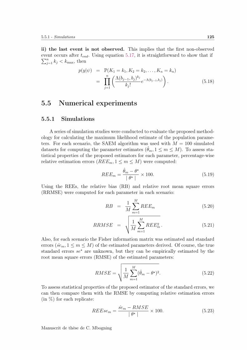
5.5.1 - Simulations 125
ii) the last event is not observed. This implies that the first non-observedevent occurs after tend. Using equation 5.17, it is straightforward to show that if∑n
j=1 kj < kmax, then
p(y|ψ) = P(K1 = k1, K2 = k2, . . . , Kn = kn)
=n∏j=1
(Λ(bj−1, bj)
kj
kj!e−Λ(bj−1,bj)
). (5.18)
5.5 Numerical experiments
5.5.1 Simulations
A series of simulation studies were conducted to evaluate the proposed method-ology for calculating the maximum likelihood estimate of the population parame-ters. For each scenario, the SAEM algorithm was used with M = 100 simulateddatasets for computing the parameter estimates (θm, 1 ≤ m ≤ M). To assess sta-tistical properties of the proposed estimators for each parameter, percentage-wiserelative estimation errors (REEm, 1 ≤ m ≤M) were computed:
REEm =θm − θ?
| θ? |× 100. (5.19)
Using the REEs, the relative bias (RB) and relative root mean square errors(RRMSE) were computed for each parameter in each scenario:
RB =1
M
M∑m=1
REEm (5.20)
RRMSE =
√√√√ 1
M
M∑m=1
REE2m . (5.21)
Also, for each scenario the Fisher information matrix was estimated and standarderrors (sem, 1 ≤ m ≤M) of the estimated parameters derived. Of course, the truestandard errors se? are unknown, but they can be empirically estimated by theroot mean square errors (RMSE) of the estimated parameters:
RMSE =
√√√√ 1
M
M∑m=1
(θm − θ?)2. (5.22)
To assess statistical properties of the proposed estimator of the standard errors, wecan then compare them with the RMSE by computing relative estimation errors(in %) for each replicate:
REEsem =sem −RMSE
| θ? |× 100. (5.23)
Manuscrit de thèse de C. Mbogning
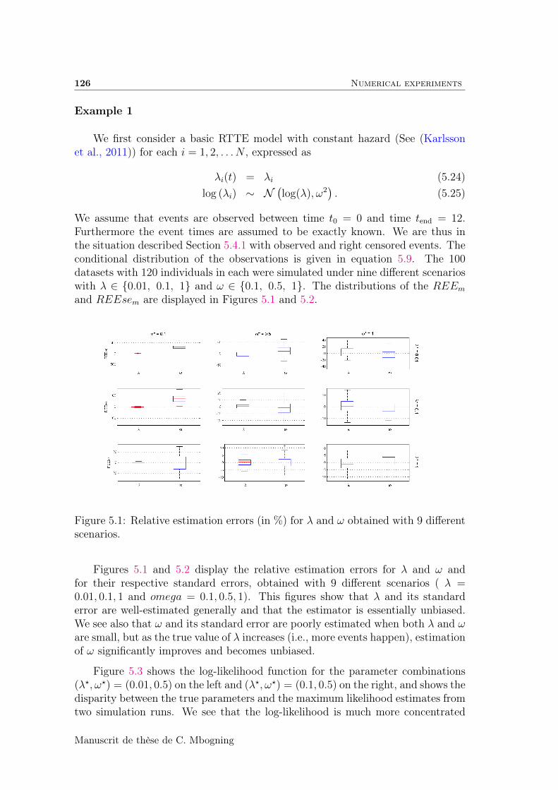
126 Numerical experiments
Example 1
We first consider a basic RTTE model with constant hazard (See (Karlssonet al., 2011)) for each i = 1, 2, . . . N , expressed as
λi(t) = λi (5.24)log (λi) ∼ N
(log(λ), ω2
). (5.25)
We assume that events are observed between time t0 = 0 and time tend = 12.Furthermore the event times are assumed to be exactly known. We are thus inthe situation described Section 5.4.1 with observed and right censored events. Theconditional distribution of the observations is given in equation 5.9. The 100datasets with 120 individuals in each were simulated under nine different scenarioswith λ ∈ 0.01, 0.1, 1 and ω ∈ 0.1, 0.5, 1. The distributions of the REEmand REEsem are displayed in Figures 5.1 and 5.2.
Figure 5.1: Relative estimation errors (in %) for λ and ω obtained with 9 differentscenarios.
Figures 5.1 and 5.2 display the relative estimation errors for λ and ω andfor their respective standard errors, obtained with 9 different scenarios ( λ =0.01, 0.1, 1 and omega = 0.1, 0.5, 1). This figures show that λ and its standarderror are well-estimated generally and that the estimator is essentially unbiased.We see also that ω and its standard error are poorly estimated when both λ and ωare small, but as the true value of λ increases (i.e., more events happen), estimationof ω significantly improves and becomes unbiased.
Figure 5.3 shows the log-likelihood function for the parameter combinations(λ?, ω?) = (0.01, 0.5) on the left and (λ?, ω?) = (0.1, 0.5) on the right, and shows thedisparity between the true parameters and the maximum likelihood estimates fromtwo simulation runs. We see that the log-likelihood is much more concentrated
Manuscrit de thèse de C. Mbogning

5.5.1 - Simulations 127
Figure 5.2: Relative estimation errors (in %) for the standard errors of λ and ωobtained with 9 different scenarios.
around its global maximum when λ = 0.1. On the other hand, maximizationof the log-likelihood cannot provide an accurate estimation of ω if λ = 0.1, ı.e.if the number of events is too small. Note that Gaussian quadrature, efficient
Figure 5.3: Observed log-likelihood as a function of λ and ω obtained with 2different scenarios. Left: (λ?, ω?) = (0.01, 0.5), right: (λ?, ω?) = (0.1, 0.5).
for low-dimensional numerical integration, was used to compute the log-likelihoodcolormap. We can see why parameter estimation improves as we increase the truevalue of λ from 0.01 to 0.1 (and thus increase number of events per subject),keeping ω = 0.5 fixed. In effect, the region of likelihood with a value close tothe maximum is much more concentrated around the true value when λ increases
Manuscrit de thèse de C. Mbogning
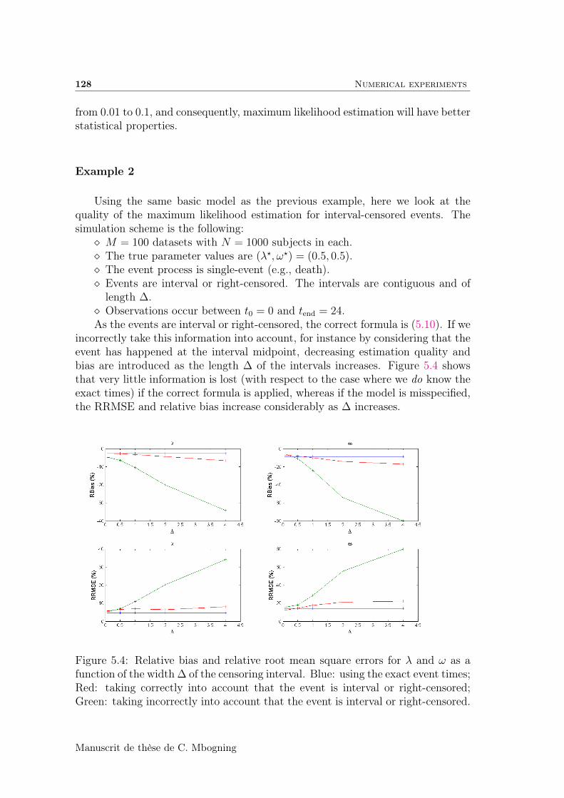
128 Numerical experiments
from 0.01 to 0.1, and consequently, maximum likelihood estimation will have betterstatistical properties.
Example 2
Using the same basic model as the previous example, here we look at thequality of the maximum likelihood estimation for interval-censored events. Thesimulation scheme is the following: M = 100 datasets with N = 1000 subjects in each. The true parameter values are (λ?, ω?) = (0.5, 0.5). The event process is single-event (e.g., death). Events are interval or right-censored. The intervals are contiguous and of
length ∆. Observations occur between t0 = 0 and tend = 24.As the events are interval or right-censored, the correct formula is (5.10). If we
incorrectly take this information into account, for instance by considering that theevent has happened at the interval midpoint, decreasing estimation quality andbias are introduced as the length ∆ of the intervals increases. Figure 5.4 showsthat very little information is lost (with respect to the case where we do know theexact times) if the correct formula is applied, whereas if the model is misspecified,the RRMSE and relative bias increase considerably as ∆ increases.
Figure 5.4: Relative bias and relative root mean square errors for λ and ω as afunction of the width ∆ of the censoring interval. Blue: using the exact event times;Red: taking correctly into account that the event is interval or right-censored;Green: taking incorrectly into account that the event is interval or right-censored.
Manuscrit de thèse de C. Mbogning
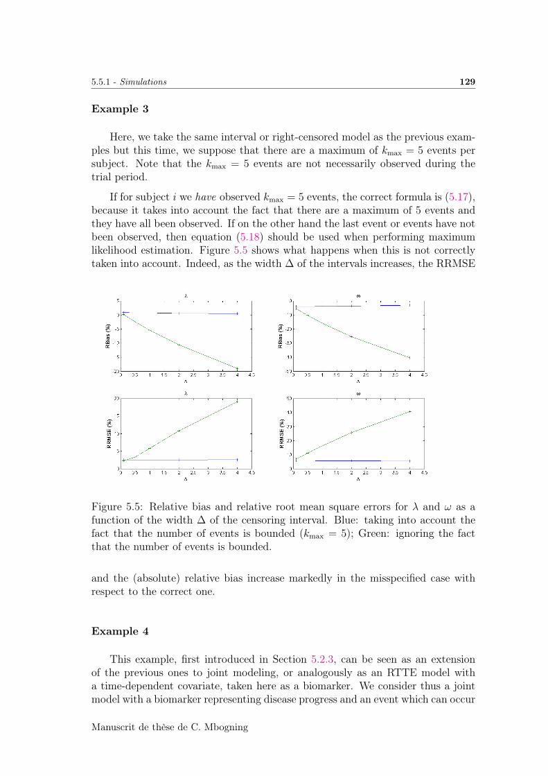
5.5.1 - Simulations 129
Example 3
Here, we take the same interval or right-censored model as the previous exam-ples but this time, we suppose that there are a maximum of kmax = 5 events persubject. Note that the kmax = 5 events are not necessarily observed during thetrial period.
If for subject i we have observed kmax = 5 events, the correct formula is (5.17),because it takes into account the fact that there are a maximum of 5 events andthey have all been observed. If on the other hand the last event or events have notbeen observed, then equation (5.18) should be used when performing maximumlikelihood estimation. Figure 5.5 shows what happens when this is not correctlytaken into account. Indeed, as the width ∆ of the intervals increases, the RRMSE
Figure 5.5: Relative bias and relative root mean square errors for λ and ω as afunction of the width ∆ of the censoring interval. Blue: taking into account thefact that the number of events is bounded (kmax = 5); Green: ignoring the factthat the number of events is bounded.
and the (absolute) relative bias increase markedly in the misspecified case withrespect to the correct one.
Example 4
This example, first introduced in Section 5.2.3, can be seen as an extensionof the previous ones to joint modeling, or analogously as an RTTE model witha time-dependent covariate, taken here as a biomarker. We consider thus a jointmodel with a biomarker representing disease progress and an event which can occur
Manuscrit de thèse de C. Mbogning
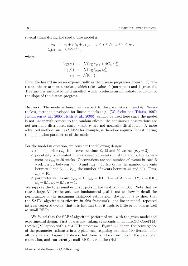
130 Numerical experiments
several times during the study. The model is:
bij = γi + δitij + aεij, 1 ≤ i ≤ N, 1 ≤ j ≤ n1,i
λi(t) = λeα(γi+δit),
where
log(γi) ∼ N (log γpop + βCi, ω2γ)
log(δi) ∼ N (log δpop, ω2δ )
εij ∼ N (0, 1).
Here, the hazard increases exponentially as the disease progresses linearly. Ci rep-resents the treatment covariate, which takes values 0 (untreated) and 1 (treated).Treatment is associated with an effect which produces an immediate reduction ofthe slope of the disease progress.
Remark. The model is linear with respect to the parameters γi and δi. Never-theless, methods developed for linear models (e.g. (Wulfsohn and Tsiatis, 1997;Henderson et al., 2000; Hsieh et al., 2006)) cannot be used here since the modelis not linear with respect to the random effects: the continuous observations arenot normally distributed since γi and δi are not normally distributed. A moreadvanced method, such as SAEM for example, is therefore required for estimatingthe population parameters of the model.
For the model in question, we consider the following design: the biomarker (bij) is observed at times 0, 25 and 50 weeks: (ni,1 = 3). possibility of repeated interval-censored events until the end of the experi-
ment at tend = 50 weeks. Observations are the number of events in each 5week period between t0 = 0 and tend = 50 (so ki,1 is the number of eventsbetween 0 and 5,. . . , ki,10 the number of events between 45 and 50). Thus,ni,2 = 10. parameter values are γpop = 1, δpop = 100, β = −0.3, α = 0.02, λ = 0.01,ωγ = 0.1, ωλ = 0.1, a = 1.
We suppose the total number of subjects in the trial is N = 1000. Note that wetake a large N here because our fundamental goal is not to show in detail theperformance of the maximum likelihood estimation. Rather, it is to show thatthe SAEM algorithm is effective in this framework: non-linear model, repeatedinterval-censored events, that it is fast and that it leads to little or no bias as wellas small REEs.
We found that the SAEM algorithm performed well with the given model andexperimental design. First, it was fast, taking 82 seconds on an Intel(R) Core(TM)i7-2760QM laptop with a 2.4 GHz processor. Figure 5.6 shows the convergenceof the parameter estimates in a typical run, requiring less than 100 iterations forall parameters. Figure 5.7 shows that there is little or no bias in the parameterestimation, and consistently small REEs across the trials.
Manuscrit de thèse de C. Mbogning

5.5.1 - Simulations 131
Figure 5.6: Convergence of the SAEM algorithm
Figure 5.7: Relative estimation errors (in %) for the joint model.
Manuscrit de thèse de C. Mbogning
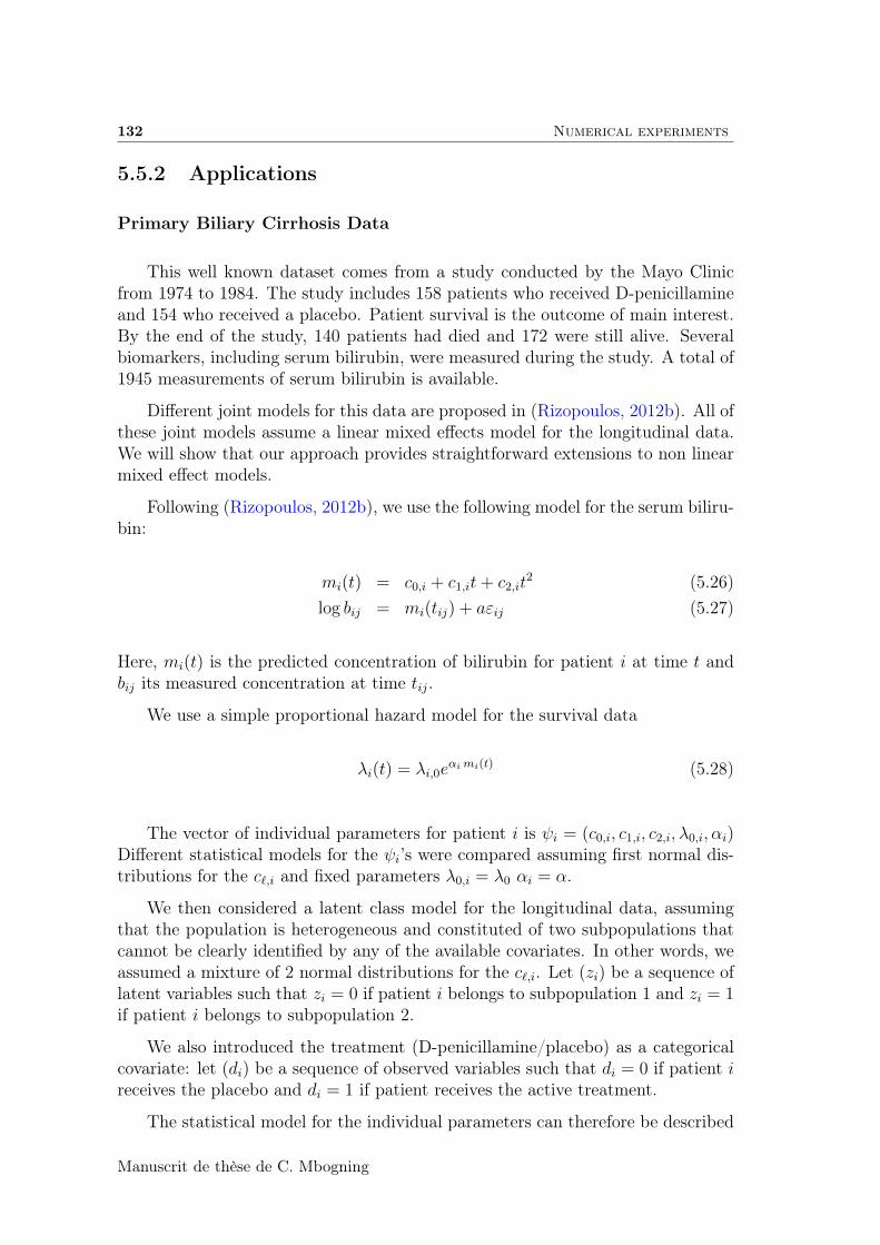
132 Numerical experiments
5.5.2 Applications
Primary Biliary Cirrhosis Data
This well known dataset comes from a study conducted by the Mayo Clinicfrom 1974 to 1984. The study includes 158 patients who received D-penicillamineand 154 who received a placebo. Patient survival is the outcome of main interest.By the end of the study, 140 patients had died and 172 were still alive. Severalbiomarkers, including serum bilirubin, were measured during the study. A total of1945 measurements of serum bilirubin is available.
Different joint models for this data are proposed in (Rizopoulos, 2012b). All ofthese joint models assume a linear mixed effects model for the longitudinal data.We will show that our approach provides straightforward extensions to non linearmixed effect models.
Following (Rizopoulos, 2012b), we use the following model for the serum biliru-bin:
mi(t) = c0,i + c1,it+ c2,it2 (5.26)
log bij = mi(tij) + aεij (5.27)
Here, mi(t) is the predicted concentration of bilirubin for patient i at time t andbij its measured concentration at time tij.
We use a simple proportional hazard model for the survival data
λi(t) = λi,0eαimi(t) (5.28)
The vector of individual parameters for patient i is ψi = (c0,i, c1,i, c2,i, λ0,i, αi)Different statistical models for the ψi’s were compared assuming first normal dis-tributions for the c`,i and fixed parameters λ0,i = λ0 αi = α.
We then considered a latent class model for the longitudinal data, assumingthat the population is heterogeneous and constituted of two subpopulations thatcannot be clearly identified by any of the available covariates. In other words, weassumed a mixture of 2 normal distributions for the c`,i. Let (zi) be a sequence oflatent variables such that zi = 0 if patient i belongs to subpopulation 1 and zi = 1if patient i belongs to subpopulation 2.
We also introduced the treatment (D-penicillamine/placebo) as a categoricalcovariate: let (di) be a sequence of observed variables such that di = 0 if patient ireceives the placebo and di = 1 if patient receives the active treatment.
The statistical model for the individual parameters can therefore be described
Manuscrit de thèse de C. Mbogning
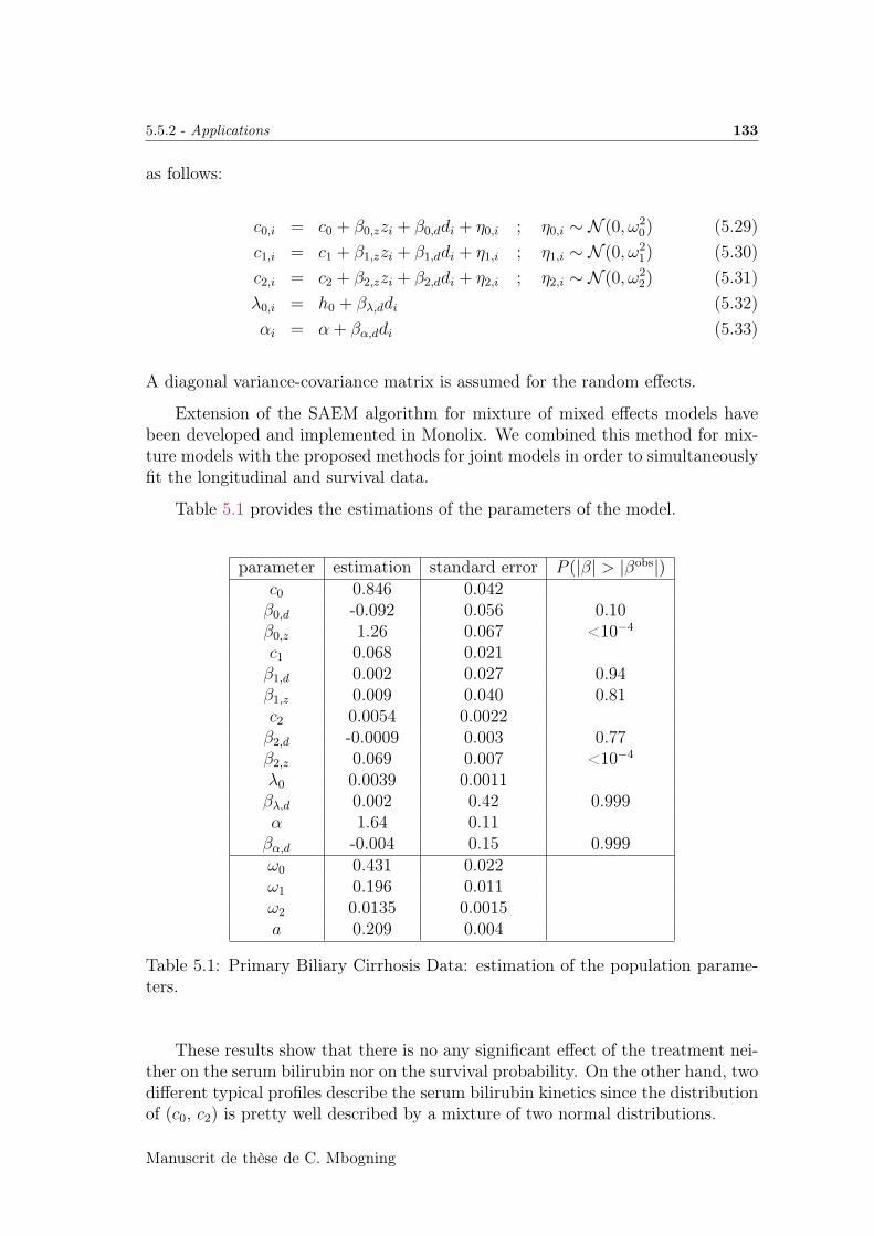
5.5.2 - Applications 133
as follows:
c0,i = c0 + β0,zzi + β0,ddi + η0,i ; η0,i ∼ N (0, ω20) (5.29)
c1,i = c1 + β1,zzi + β1,ddi + η1,i ; η1,i ∼ N (0, ω21) (5.30)
c2,i = c2 + β2,zzi + β2,ddi + η2,i ; η2,i ∼ N (0, ω22) (5.31)
λ0,i = h0 + βλ,ddi (5.32)αi = α + βα,ddi (5.33)
A diagonal variance-covariance matrix is assumed for the random effects.
Extension of the SAEM algorithm for mixture of mixed effects models havebeen developed and implemented in Monolix. We combined this method for mix-ture models with the proposed methods for joint models in order to simultaneouslyfit the longitudinal and survival data.
Table 5.1 provides the estimations of the parameters of the model.
parameter estimation standard error P (|β| > |βobs|)c0 0.846 0.042β0,d -0.092 0.056 0.10β0,z 1.26 0.067 <10−4
c1 0.068 0.021β1,d 0.002 0.027 0.94β1,z 0.009 0.040 0.81c2 0.0054 0.0022β2,d -0.0009 0.003 0.77β2,z 0.069 0.007 <10−4
λ0 0.0039 0.0011βλ,d 0.002 0.42 0.999α 1.64 0.11βα,d -0.004 0.15 0.999ω0 0.431 0.022ω1 0.196 0.011ω2 0.0135 0.0015a 0.209 0.004
Table 5.1: Primary Biliary Cirrhosis Data: estimation of the population parame-ters.
These results show that there is no any significant effect of the treatment nei-ther on the serum bilirubin nor on the survival probability. On the other hand, twodifferent typical profiles describe the serum bilirubin kinetics since the distributionof (c0, c2) is pretty well described by a mixture of two normal distributions.
Manuscrit de thèse de C. Mbogning
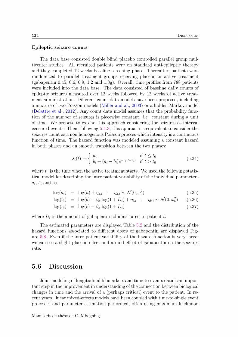
134 Discussion
Epileptic seizure counts
The data base consisted double blind placebo controlled parallel group mul-ticenter studies. All recruited patients were on standard anti-epileptic therapyand they completed 12 weeks baseline screening phase. Thereafter, patients wererandomized to parallel treatment groups receiving placebo or active treatment(gabapentin 0.45, 0.6, 0.9, 1.2 and 1.8g). Overall, time profiles from 788 patientswere included into the data base. The data consisted of baseline daily counts ofepileptic seizures measured over 12 weeks followed by 12 weeks of active treat-ment administration. Different count data models have been proposed, includinga mixture of two Poisson models (Miller and al., 2003) or a hidden Markov model(Delattre et al., 2012). Any count data model assumes that the probability func-tion of the number of seizures is piecewise constant, i.e. constant during a unitof time. We propose to extend this approach considering the seizures as intervalcensored events. Then, following 5.4.3, this approach is equivalent to consider theseizures count as a non homogenous Poisson process which intensity is a continuousfunction of time. The hazard function was modeled assuming a constant hazardin both phases and an smooth transition between the two phases:
λi(t) =
ai if t ≤ t0bi + (ai − bi)e−ci(t−t0) if t > t0
(5.34)
where t0 is the time when the active treatment starts. We used the following statis-tical model for describing the inter patient variability of the individual parametersai, bi and ci:
log(ai) = log(a) + ηa,i ; ηa,i ∼ N (0, ω2a) (5.35)
log(bi) = log(b) + βb log(1 +Di) + ηb,i ; ηb,i ∼ N (0, ω2b ) (5.36)
log(ci) = log(c) + βc log(1 +Di) (5.37)
where Di is the amount of gabapentin administrated to patient i.
The estimated parameters are displayed Table 5.2 and the distribution of thehazard functions associated to different doses of gabapentin are displayed Fig-ure 5.8. Even if the inter patient variability of the hazard function is very large,we can see a slight placebo effect and a mild effect of gabapentin on the seizuresrate.
5.6 Discussion
Joint modeling of longitudinal biomarkers and time-to-events data is an impor-tant step in the improvement in understanding of the connection between biologicalchanges in time and the arrival of a (perhaps critical) event to the patient. In re-cent years, linear mixed-effects models have been coupled with time-to-single eventprocesses and parameter estimation performed, often using maximum likelihood
Manuscrit de thèse de C. Mbogning
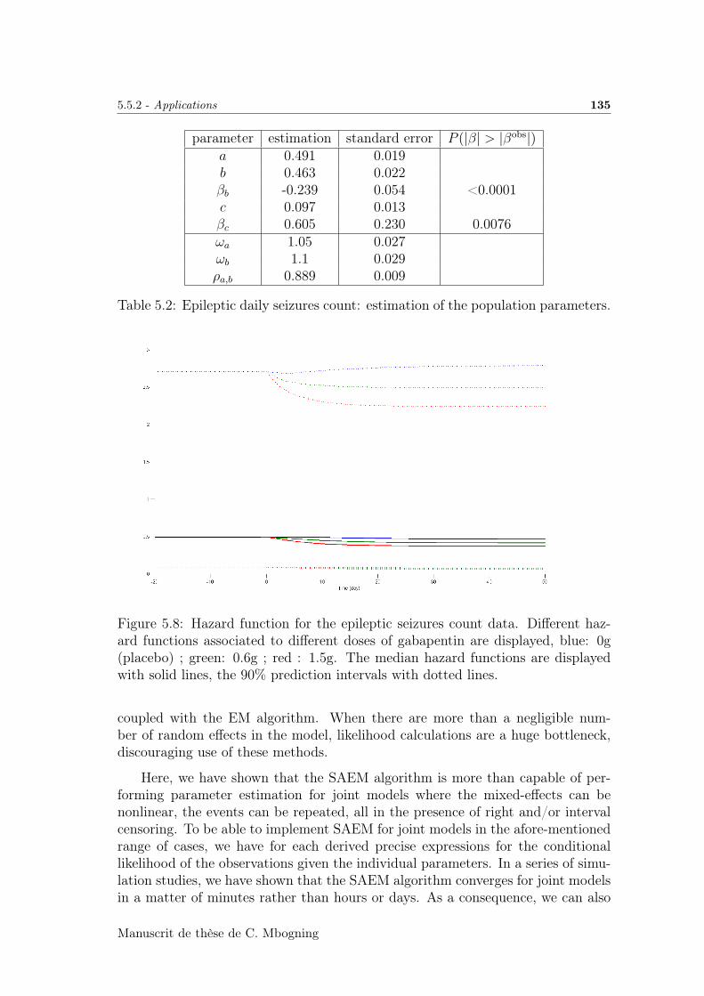
5.5.2 - Applications 135
parameter estimation standard error P (|β| > |βobs|)a 0.491 0.019b 0.463 0.022βb -0.239 0.054 <0.0001c 0.097 0.013βc 0.605 0.230 0.0076ωa 1.05 0.027ωb 1.1 0.029ρa,b 0.889 0.009
Table 5.2: Epileptic daily seizures count: estimation of the population parameters.
Figure 5.8: Hazard function for the epileptic seizures count data. Different haz-ard functions associated to different doses of gabapentin are displayed, blue: 0g(placebo) ; green: 0.6g ; red : 1.5g. The median hazard functions are displayedwith solid lines, the 90% prediction intervals with dotted lines.
coupled with the EM algorithm. When there are more than a negligible num-ber of random effects in the model, likelihood calculations are a huge bottleneck,discouraging use of these methods.
Here, we have shown that the SAEM algorithm is more than capable of per-forming parameter estimation for joint models where the mixed-effects can benonlinear, the events can be repeated, all in the presence of right and/or intervalcensoring. To be able to implement SAEM for joint models in the afore-mentionedrange of cases, we have for each derived precise expressions for the conditionallikelihood of the observations given the individual parameters. In a series of simu-lation studies, we have shown that the SAEM algorithm converges for joint modelsin a matter of minutes rather than hours or days. As a consequence, we can also
Manuscrit de thèse de C. Mbogning
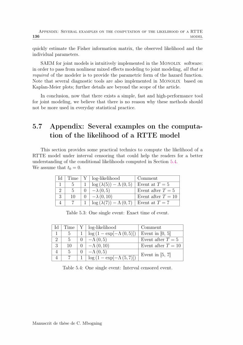
136Appendix: Several examples on the computation of the likelihood of a RTTE
model
quickly estimate the Fisher information matrix, the observed likelihood and theindividual parameters.
SAEM for joint models is intuitively implemented in the Monolix software:in order to pass from nonlinear mixed effects modeling to joint modeling, all that isrequired of the modeler is to provide the parametric form of the hazard function.Note that several diagnostic tools are also implemented in Monolix based onKaplan-Meier plots; further details are beyond the scope of the article.
In conclusion, now that there exists a simple, fast and high-performance toolfor joint modeling, we believe that there is no reason why these methods shouldnot be more used in everyday statistical practice.
5.7 Appendix: Several examples on the computa-tion of the likelihood of a RTTE model
This section provides some practical technics to compute the likelihood of aRTTE model under interval censoring that could help the readers for a betterunderstanding of the conditional likelihoods computed in Section 5.4.We assume that t0 = 0.
Id Time Y log-likelihood Comment1 5 1 log (λ(5))− Λ (0, 5) Event at T = 52 5 0 −λ (0, 5) Event after T = 53 10 0 −λ (0, 10) Event after T = 104 7 1 log (λ(7))− Λ (0, 7) Event at T = 7
Table 5.3: One single event: Exact time of event.
Id Time Y log-likelihood Comment1 5 1 log (1− exp[−Λ (0, 5)]) Event in [0, 5]2 5 0 −Λ (0, 5) Event after T = 53 10 0 −Λ (0, 10) Event after T = 104 5 0 −Λ (0, 5) Event in [5, 7]4 7 1 log (1− exp[−Λ (5, 7)])
Table 5.4: One single event: Interval censored event.
Manuscrit de thèse de C. Mbogning
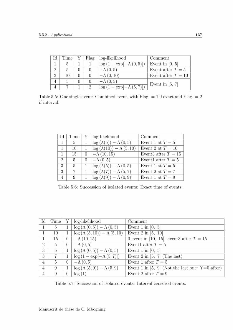
5.5.2 - Applications 137
Id Time Y Flag log-likelihood Comment1 5 1 1 log (1− exp[−Λ (0, 5)]) Event in [0, 5]2 5 0 0 −Λ (0, 5) Event after T = 53 10 0 0 −Λ (0, 10) Event after T = 104 5 0 0 −Λ (0, 5) Event in [5, 7]4 7 1 2 log (1− exp[−Λ (5, 7)])
Table 5.5: One single event: Combined event, with Flag = 1 if exact and Flag = 2if interval.
Id Time Y log-likelihood Comment1 5 1 log (λ(5))− Λ (0, 5) Event 1 at T = 51 10 1 log (λ(10))− Λ (5, 10) Event 2 at T = 101 15 0 −Λ (10, 15) Event3 after T = 152 5 0 −Λ (0, 5) Event1 after T = 53 5 1 log (λ(5))− Λ (0, 5) Event 1 at T = 53 7 1 log (λ(7))− Λ (5, 7) Event 2 at T = 74 9 1 log (λ(9))− Λ (0, 9) Event 1 at T = 9
Table 5.6: Succession of isolated events: Exact time of events.
Id Time Y log-likelihood Comment1 5 1 log (Λ (0, 5))− Λ (0, 5) Event 1 in [0, 5]1 10 1 log (Λ (5, 10))− Λ (5, 10) Event 2 in [5, 10]1 15 0 −Λ (10, 15) 0 event in [10, 15]: event3 after T = 152 5 0 −Λ (0, 5) Event1 after T = 53 5 1 log (Λ (0, 5))− Λ (0, 5) Event 1 in [0, 5]3 7 1 log (1− exp[−Λ (5, 7)]) Event 2 in [5, 7] (The last)4 5 0 −Λ (0, 5) Event 1 after T = 54 9 1 log (Λ (5, 9))− Λ (5, 9) Event 1 in [5, 9] (Not the last one: Y=0 after)4 9 0 log (1) Event 2 after T = 9
Table 5.7: Succession of isolated events: Interval censored events.
Manuscrit de thèse de C. Mbogning

138Appendix: Several examples on the computation of the likelihood of a RTTE
model
Id Time Y Flag log-likelihood Comment1 5 1 1 log (λ (5))− Λ (0, 5) Event 1 at T = 51 10 1 2 log (Λ (5, 10))− Λ (5, 10) Event 2 in [5, 10]1 15 0 0 −Λ (10, 15) event3 after T = 152 5 0 0 −Λ (0, 5) Event1 after T = 53 5 1 2 log (Λ (0, 5))− Λ (0, 5) Event 1 in [0, 5]3 7 1 1 log (λ(7))− Λ (5, 7) Event 2 at T = 74 5 0 0 −Λ (0, 5) Event 1 after T = 54 9 1 2 log (Λ (5, 9))− Λ (5, 9) Event 1 in [5, 9] (Not the last one: Y=0 after)4 9 0 0 log (1) Event 2 after T = 9
Table 5.8: Succession of isolated events: Combined events, with Flag = 1 if exact,Flag = 2 if interval and Flag = 0 if right censored.
Manuscrit de thèse de C. Mbogning

Chapter 6
Conclusion et perspectives
139
140
Nos travaux de Thèse portent sur des développements méthodologiques dansle cadre de l’estimation des paramètres des MNLEM. Ils permettent de répondreà l’une des préoccupations de l’industrie pharmacologique, qui est le développe-ment et la mise en oeuvre de méthodologies de plus en plus performantes pour lamodélisation de phénomènes complexes.
Il existe à ce jour très peu de méthodes disponibles pour l’estimation parmaximum de vraisemblance dans les modèles de mélange à effets mixtes. Les mé-thodes mises en oeuvre dans le package R nlme et dans le logiciel NONMEM sontbasées sur une linéarisation de la vraisemblance. Il est néanmoins reconnu queces méthodes posent des problèmes pratiques réels dans plusieurs situations (lebiais, forte influence des valeurs initiales, mauvaise convergence...). De plus lespropriétés théoriques des estimateurs obtenus par ces méthodes restent inconnuesdans la plupart des situations. Des méthodes de type EM ont été développéesdans le cadre des modèles mixtes incluant des mélanges. Ces méthodes effectuegénéralement une approximation de l’étape E par des intégrations Monte-Carlo.(De la Cruz-Mesia et al., 2008) proposent d’intégrer la vraisemblance p (y, ϕ; θ)des données complètes, pour déterminer la vraisemblance marginale p (y; θ) desobservations dans chaque cluster. Les algorithmes du type MCEM utilisent lesintégration Monte-Carlo pour déterminer la distribution conditionnelle p (ϕ|y; θ).Ces méthodes peuvent nécessiter un temps d’exécution rédhibitoire en pratique,notamment lorsque le modèle structurel est complexe, ce qui est généralement lecas dans plusieurs applications aux modèles PKPD.
Nous proposons une extension de l’algorithme SAEM pour les mélanges de mo-dèles non linéaires à effets mixtes. Le modèle considéré est très général et inclutdes mélanges de distributions, des mélanges de modèles structurels et des mélangesde modèles résiduels. La convergence de l’algorithme MSAEM vers un maximum(local) de la vraisemblance des observations est obtenue sous des hypothèses gé-nérales. L’algorithme s’avère être extrêmement rapide, principalement par le faitque les intégrations Monte-Carlo sont remplacées par des approximations stochas-tiques. Il a en effet besoin de la simulation d’une unique Chaîne de Markov àchaque itération. De plus, l’algorithme MSAEM reste très peu sensible aux valeursinitiales, constituant de ce fait une très bonne propriété pour des applications pra-tiques. Cette méthode d’estimation est donc extrêmement prometteuse, tant auniveau des résultats théoriques de convergence qu’au niveau algorithmique. Cetalgorithme, destiné aux mélanges de MNLEM est désormais disponible sous le lo-giciel Monolix , un des leaders dans l’industrie pharmacologique. Monolix estgratuit pour les étudiants et pour des recherches académiques, et contient quelquesexamples de démos sur les mélanges de MNLEM.
Nous proposons, dans le but de stratifier les patients ayant le VIH sur la basedes mesures réelles longitudinales de charges virales, deux types de modèles. Unmélange de 3 modèles structurels a été utilisé pour classifier les patients en 3groupes distincts : le groupe des "répondant", caractérisé par une décroissancecontinue de la charge virale ; le groupe des "rebondissant", caractérisé par une
Manuscrit de thèse de C. Mbogning
CHAPTER 6. CONCLUSION ET PERSPECTIVES 141
décroissance de la charge virale suivie d’une phase de rebond ; le groupe des "non-répondant" caractérisé par une non-décroissance de la charge virale. Les résultatsobtenus par ce modèle montrent une bonne précision aussi bien sur l’estimationdes paramètre du mélange que sur la classification des patients, du moment quel’évolution des charges virales des individus considérés est effectivement décritepar l’un des modèles structurels considérés. Néanmoins, quand l’évolution de lacharge virale ne peut-être décrite convenablement par l’un des trois modèles struc-turels, les fits individuels deviennent mauvais et les prédictions des classes dou-teuses. Nous avons ensuite considéré que chaque patient contenait des virus quirépondent, ceux qui répondent partiellement et ceux qui ne réponde pas du toutau traitement. Chaque patient est désormais partiellement "répondant", partielle-ment "rebondissant" et partiellement "non-répondant". Cette approche amélioreclairement les fits individuels et permet une réponse plus nuancée à la questionde savoir si un individu répond de manière adéquate au traitement ou pas. Surla base de ces résultats, la deuxième approche semble la plus indiquée pour deséventuels changements de régime thérapeutique chez les patients.
Nous envisageons des extensions de l’algorithme MSAEM pour s’affranchirde plusieurs problèmes d’ordre pratique. Une stratégie optimale de constructiondu modèle pourrait s’avérer utile à cet effet, pour sélectionner simultanément laforme du modèle adéquat ainsi que le nombre de classes. Nous avons considérédans cette Thèse uniquement la méthode du maximum de vraisemblance pourles mélanges considérés. Les méthodes Bayésiennes peuvent être considérées enutilisant les simulations de la loi à posteriori via des méthodes MCMC telles quecelles proposées par (Frühwirth-Schnatter, 2006; De la Cruz-Mesia et al., 2008).
Nous avons également proposé dans cette Thèse de modéliser de manièreconjointe une réponse longitudinale en utilisant un modèle non linéaire à effetsmixtes, et une suite de délais successifs jusqu’à un évènement récurrent (censuréà droite ou par intervalle) en utilisant un modèle de risque mixte. L’inférencestatistique s’est faite via un algorithme de type SAEM convergent rapidementvers la cible. Il existe plusieurs logiciels traitant de l’estimation dans les modèlesconjoints d’une variable longitudinale et d’un unique évènement terminal. On peutciter, entre autres, le plus récent qui est un package R dénommé JM, proposé par(Rizopoulos, 2010). Ce package ne considère néanmoins que des modèles linéairesmixtes pour la variable longitudinale. Ceci pourrait être considéré comme une im-portante restriction, spécialement dans le cadre des modèles PKPD, où les modèlesstructurels sont généralement des solutions d’équations différentielles ordinaires oustochastiques. Notre méthode offre ainsi une grande flexibilité au niveau de la va-riable longitudinale, permettant ainsi d’expliquer une très grande variété de phé-nomènes biologiques. La plupart des méthodes utilisées dans le cadre des modèlesconjoints classiques (modèle linéaire mixte pour la variable longitudinale et mo-dèle de risque pour l’unique évènement terminal) utilisent des approximations dumodèle conjoints. JM par exemple, utilise une méthode de Gauss-Hermite ou uneméthode pseudo-adaptative de Gauss-Hermite d’intégration (Rizopoulos, 2012a)pour approcher la vraisemblance du modèle conjoint. Nous proposons de maxi-
Manuscrit de thèse de C. Mbogning
142
miser la vraisemblance conjointe exacte, sans approximations. Au vu de toutesces observations, on peut considérer que le modèle que nous proposons dans cetteThèse est une avancée importante dans l’état de l’art des modèles conjoints caren plus de la flexibilité utilisée pour le modèle de la variable longitudinale, nousproposons aussi un modèle permettant de considérer les évènements répétés etéventuellement censurés à droite ou par intervalles lors de l’étude. La méthodolo-gie générale SAEM proposée pour les modèles conjoints s’appliquent aisément auxmodèles conjoints "classiques" rencontrés dans diverses publications, et aux mo-dèles d’évènements récurrents. Cette méthodologie est désormais disponible sousMonolix. Son application à des données réelles de patients atteints d’une cirrhosebiliaire primitive met en exergue la relation entre l’évolution du sérum bilirubin etla survie des patients.
Nous envisageons, de considérer dans de futurs travaux, des situations où onaurait plusieurs évènements de type distinct lors de l’étude. Une idée serait alorsde stratifier la fonction de risque (en fonction des différents types d’évènements)via la fonction de risque de base ou des covariables, constituant ainsi une extensiondes risques compétitifs aux évènements récurrents.
Manuscrit de thèse de C. Mbogning
Table des figures
3.1 Probability distribution function of the log-volume . . . . . . . . . . 66
3.2 Median (solid line) and 90% prediction interval (dotted line) of theobserved concentration in different groups . . . . . . . . . . . . . . 66
3.3 Empirical distribution of the relative estimation errors (REEk) withdifferent sample sizes: (a-c) N = 100, (d-f) N = 1000, and differentscenarios . . . . . . . . . . . . . . . . . . . . . . . . . . . . . . . . . 67
3.4 Monte-Carlo median probability of correct classification for the dif-ferent scenarios and N = 1000 subjects . . . . . . . . . . . . . . . . 70
3.5 Observed concentration data from 4 patients with their concentra-tions predicted by the model. . . . . . . . . . . . . . . . . . . . . . 73
3.6 Probability distribution functions of the five PK parameters . . . . 74
4.1 Spaghetti plots of data for ten individuals belonging to group 1 (a)and 10 others belonging to group 2 (b). . . . . . . . . . . . . . . . 99
4.2 Empirical distribution of the relative estimation error (REEk (%))in the BSMM scenario with different sample sizes . . . . . . . . . . 100
4.3 Relative difference (in %) between estimated and empirical standarderrors for the BSMM scenario . . . . . . . . . . . . . . . . . . . . . 101
4.4 Medians of the probabilities of correct classification ranked in in-creasing order in both groups . . . . . . . . . . . . . . . . . . . . . 102
4.5 Empirical distribution of the relative estimation error (REEk (%))in the WSMM scenario . . . . . . . . . . . . . . . . . . . . . . . . . 103
4.6 Viral load progression for 4 HIV-infected patients. . . . . . . . . . . 104
4.7 Viral load time series and individual fits for the four patients inFigure 4.6 . . . . . . . . . . . . . . . . . . . . . . . . . . . . . . . . 107
4.8 Viral load data for 4 patients with ambiguous progressions. Redpoints indicate below level of quantification data. . . . . . . . . . . 107
143
144 TABLE DES FIGURES
4.9 Viral load time series and individual fits for patients 5–8 from Figure4.8 when using BSMM (row 1) and WSMM (row 2). . . . . . . . . . 108
5.1 Relative estimation errors (in %) for λ and ω obtained with 9 dif-ferent scenarios. . . . . . . . . . . . . . . . . . . . . . . . . . . . . . 126
5.2 Relative estimation errors (in %) for the standard errors of λ and ωobtained with 9 different scenarios. . . . . . . . . . . . . . . . . . . 127
5.3 Observed log-likelihood as a function of λ and ω obtained with 2different scenarios. . . . . . . . . . . . . . . . . . . . . . . . . . . . 127
5.4 Relative bias and relative root mean square errors for λ and ω as afunction of the width ∆ of the censoring interval. . . . . . . . . . . 128
5.5 Relative bias and relative root mean square errors for λ and ω as afunction of the width ∆ of the censoring interval. . . . . . . . . . . 129
5.6 Convergence of the SAEM algorithm . . . . . . . . . . . . . . . . . 131
5.7 Relative estimation errors (in %) for the joint model. . . . . . . . . 131
5.8 Hazard function for the epileptic seizures count data. Different ha-zard functions associated to different doses of gabapentin are dis-played. . . . . . . . . . . . . . . . . . . . . . . . . . . . . . . . . . . 135
Manuscrit de thèse de C. Mbogning
Liste des tableaux
3.1 RRMSE in % of parameter estimates in Scenario 1, with N = 100and N = 1000 . . . . . . . . . . . . . . . . . . . . . . . . . . . . . . 67
3.2 RRMSE in % of parameter estimates in Scenario 2, with N = 100and N = 1000 . . . . . . . . . . . . . . . . . . . . . . . . . . . . . . 68
3.3 RRMSE in % of parameter estimates in Scenario 3, with N = 100and N = 1000 . . . . . . . . . . . . . . . . . . . . . . . . . . . . . . 69
3.4 RRMSE of parameter estimates in Scenario 4, with N = 100 andN = 1000. . . . . . . . . . . . . . . . . . . . . . . . . . . . . . . . . 71
3.5 The six best models obtained for different number of mixture dis-tributions and the corresponding Bayesian Information Criteria. . . 73
4.1 Mean of parameter estimates and standard errors for the BSMMscenario with N = 100 or N = 1000. . . . . . . . . . . . . . . . . . 101
4.2 Mean of parameter estimates and standard errors for the WSMMscenario with N = 100 or N = 1000. . . . . . . . . . . . . . . . . . 103
5.1 Primary Biliary Cirrhosis Data: estimation of the population para-meters. . . . . . . . . . . . . . . . . . . . . . . . . . . . . . . . . . . 133
5.2 Epileptic daily seizures count: estimation of the population para-meters. . . . . . . . . . . . . . . . . . . . . . . . . . . . . . . . . . . 135
5.3 One single event: Exact time of event. . . . . . . . . . . . . . . . . 136
5.4 One single event: Interval censored event. . . . . . . . . . . . . . . . 136
5.5 One single event: Combined event, with Flag = 1 if exact andFlag = 2 if interval. . . . . . . . . . . . . . . . . . . . . . . . . . . 137
5.6 Succession of isolated events: Exact time of events. . . . . . . . . . 137
5.7 Succession of isolated events: Interval censored events. . . . . . . . 137
145

146 LISTE DES TABLEAUX
5.8 Succession of isolated events: Combined events, with Flag = 1 ifexact, Flag = 2 if interval and Flag = 0 if right censored. . . . . . 138
Manuscrit de thèse de C. Mbogning
Références
Aitkin, M. and Rubin, D. B. (1985). Estimation and Hypothesis testing in FiniteMixture Models. Journal of the Royal Statistical Society, 47 :67–75.
Allassonnière, S., Kuhn, E., and Trouvé, A. (2010). Construction of Bayesiandeformable models via a stochastic approximation algorithm : A convergencestudy. Bernoulli, 16 :641–678.
Andrieu, C., Moulines, E., and Priouret, P. (2005). Stability of stochas-tic approximation under verifiable conditions. SIAM J. Control Optim.,44(1) :283–312.
Banfield, J. D. and Raftery, A. E. (1993). Model-based Gaussian and non Gaus-sian clustering. Biometrics, 49 :803–821.
Barndoff-Nielsen, O. (1978). Information and Exponential Families in StatisticalTheory. Wiley., Chichester.
Beal, S. L. and Sheiner, L. B. (1982). Estimating population kinetics. Crit. Rev.Biomed. Eng., 8 :195–222.
Biernacki, C., Celeux, G., and Govaert, G. (2000). Assessing a mixture modelfor clustering with the integrated completed likelihood. IEEE Transactionson Pattern Analysis and Machine Intelligence, 22 :719–725.
Bradley, R. and Gart, J. (1962). The asymptotic properties of ml estimatorswhen sampling from associated populations. Biometrika, 49(1-2) :205–214.
Breslow, N. E. and Clayton, D. G. (1993). Approximate inference in generalizedlinear mixed models. J. Amer. Statist. Assoc., 88 :9–25.
Brown, E., Ibrahim, J., and DeGruttola, V. (2005). A flexible B-spline modelfor multiple longitudinal biomarkers and survival. Biometrics, 61 :64–73.
Bryant, P. G. (1991). Large Sample Results for Optimization Based ClusteringMethods. Journal of Classification, 8 :31–44.
Celeux, G. (1998). Bayesian inference for mixtures : The label switching problem.Compstat 98-Proc. in Computational Statistics, Physica, Heidelberg, in :payne, r., green, p.j. edition.
Celeux, G. and Diebolt, J. (1986). L’algorithme SEM : Un algorithme d’ap-prentissage probabiliste pour la reconnaissance de mélange de densités. (TheSEM algorithm : An algoritm of probabilistic learning for the determinationof mixtures of densities). Rev. Stat. Appl., 34 :35–52.
Celeux, G. and Diebolt, J. (1990). Une version de type recuit simulé de l’algo-rithme EM. C. R. Acad. Sci. Paris Sér. I Math, 310 :119–124.
147
148 RÉFÉRENCES
Celeux, G. and Diebolt, J. (1992). A stochastic approximation type EM algo-rithm for the mixture problem. Stochastics Stochastics Rep, 41 :119–134.
Celeux, G. and Govaert, G. (1992). A Classification EM Algorithm and twoStochastic Versions. Computational Statistics and Data Analysis, 14(3) :315–322.
Celeux, G. and Govaert, G. (1995). Gaussian parsimonious clustering models.Pattern Recoguition, 28 :781–793.
Celeux, G., Hurn, M., and Robert, C. (2000). Computational and inferentialdifficulties with mixtures posterior distribution. J. American Statist. Assoc.,95(3) :957–979.
Celeux, G., Lavergne, C., and Martin, O. (2005). Mixture of linear mixed modelsfor clustering gene expression profiles from repeated microarray experiments.Statist. Model., 5 :243–267.
Chan, P., Jacqmin, P., Lavielle, M., McFadyen, L., and Weatherley, B. (2011).The Use of the SAEM Algorithm in MONOLIX Software for Estimation ofPopulation Pharmacokinetic-Pharmacodynamic-Viral Dynamics Parametersof Maraviroc in Asymptomatic HIV Subjects. Journal of Pharmacokineticsand Pharmacodynamics, 38 :41–61.
Chanda, S. (1954). A note on the consistency and maxima of the roots of thelikelihood equations. Biometrika, 41 :56–61.
Cox, D. R. (1972). Regression models and life-tables (with discussion). J. Royal.Stat. Soc., 34(B) :187–220.
Cramer, S. (1946). Mathematical Methods of Statistics. Princeton UniversityPress, Princeton, New York.
Dacunha-Castelle, D. and Gassiat, E. (1999). Testing the order of a model usinglocally conic parametrization : Population mixtures and stationary armaprocesses. Annals of Statistics, 27(4) :1178–1209.
Dafny, U. G. and Tsiatsis, A. A. (1998). Evaluating Surrogate markers of clinicaloutcome measured with error. Biometrics, 54 :1445–1462.
Davidian, M. and Giltinan, D. M. (1995). Nonlinear Models for Repeated Mea-surements Data. Chapman & Hall., London.
De la Cruz-Mesia, R., Fernando, A. Q., and Guillermo, M. (2008). Model-based clustering for longitudinal data. Comput. Statist. and Data Analysis,52 :1441–1457.
DeGruttola, V. and Tu, X. M. (1994). Modeling progression of CD-4 lymphocytecount and its relationship to survival time. Biometrics, 50 :1003–1014.
Delattre, M. and Lavielle, M. (2012). Maximum likelihood estimation in discretemixed hidden Markov models using the SAEM algorithm. ComputationalStatistics & Data Analysis, 56(6) :2073–2085.
Delattre, M., Savic, R., Miller, R., Karlsson, M., and Lavielle, M. (2012). Ana-lysis of exposure-response of CI-945 in patients with epilepsy : applicationof novel mixed hidden Markov modeling methodology. J. Pharmacokinet.Pharmacodyn., 39 :263–271.
Manuscrit de thèse de C. Mbogning
RÉFÉRENCES 149
Delyon, B., Lavielle, M., and Moulines, E. (1999). Convergence Of A StochasticApproximation Version Of The EM Algorithm. The Annals Of Statistics,27 :94–128.
Dempster, A. P., Laird, N. M., and Rubin, D. B. (1977). Maximum Likelihoodfrom Incomplete Data via the EM Algorithm. JRSS, 39(B) :1–38.
DeSarbo, W. S. and Cron, W. L. (1988). A maximum likelihood methodologyfor clusterwise linear regression. J. Classification, 5 :249–282.
Ding, A. A. andWu, H. (2001). Assessing antiviral potency of anti-HIV therapiesin vivo by comparing viral decay rates in viral dynamic models. Biostatistics,2 :13–29.
Dubois, A., Lavielle, M., Gsteiger, S., Pigeolet, E., and Mentré, F. (2011). Model-Based Analyses of Bioequivalence Crossover Trials Using the SAEM Algo-rithm. Statistics in Medicine, 30 :582–600.
Duchateau, L. and Janssen, P. (2008). The Frailty Model. Statistics for Biologyand Health. Springer., New York.
Efron, B. and Hinkley, D. (1978). Assessing the accuracy of the maximum like-lihood estimator : observed versus expected Fisher information. Biometrica,65 :457–487.
Evans, W. E. and Relling, M. V. (1999). Pharmacogenomics : Translating func-tional genomics into rational therapeutics. Science, 286 :487–491.
Everitt, B. S. and Hand, D. J. (1981). Finite Mixture Distributions. Chapman& Hall., London.
Faucett, C. and Thomas, D. (1996). Simultaneously modelling censored survivaldata and repeatedly measured covariates : A Gibbs sampling approach. Stat.Med., 15 :1663–1685.
Feller, W. (1943). On a General Class of Contagious Distributions. Annals ofMathematical Statistics, 14 :389–400.
Frühwirth-Schnatter, S. (2006). Finite Mixture and Markov Switching Models.Springer, New York.
Gaffney, S. J. and Smith, P. (2003). Curve clustering with random effects re-gression mixtures. In : Bishop, C.M., Frey, B.J. (Eds.), Proceedings of theNinth International Workshop on Artificial Intelligence and Statistics, Key-West, FL.
Ge, Z., Bickel, P. J., and Rice, J. A. (2004). An approximate likelihood approachto nonlinear mixed effects models via spline approximation. Comput. Statist.Data. Anal., 46 :747–776.
Gilks, W. R., Richardson, S., and Spiegelhalter, D. J. (1996). Markov chainMonte Carlo in practice. Interdisciplinary Statistics. Chapman & Hall, Lon-don.
Gilmour, A. R., Anderson, R. D., and Rae, A. L. (1985). The analysis of binomialdata by a generalized linear mixed model. Biometrika, 72 :593–599.
Gu, M. G. and Kong, F. H. (1998). A stochastic approximation algorithm withmarkov chain monte-carlo method for incomplete data estimation problems.Proc. Natl. Acad. Sci. U. S. A., 95 :7270–7274.
Manuscrit de thèse de C. Mbogning
150 RÉFÉRENCES
Gu, M. G. and Zhu, H. T. (2001). Maximum likelihood estimation for spatialmodels by markov chain monte carlo stochastic approximation. J. R. Stat.Soc. B, 63 :339–355.
Harville, D. (1977). Maximum likelihood approaches to variance component es-timation and to related problems. Biometrika, 61 :383–385.
Henderson, R., Diggle, P., and Dobson, A. (2000). Joint modelling of longitudinalmeasurements and event time data. Biostatistics, 1 :465–480.
Hjort, N. L., Holmes, C., Müller, P., and Walker, S. G. (2010). (eds). BayesianNonparametrics. Cambridge University Press., Cambridge.
Hoadley, B. (1971). Asymptotic properties of maximum likelihood estimators forindependent not identically distributed case. Ann. Math. Stat, 42(6) :1977–1991.
Hosmer, D. (1974). Maximum likelihood estimates of the parameters of a mix-ture of two regression lines. Comm. Statist., 3(10) :995–1010.
Hsieh, F., Tseng, Y., andWang, J. (2006). Joint modeling of survival and longitu-dinal data : Likelihood approach revisited. Biometrics, 62(1037–1043) :995–1010.
Huang, X. and Liu, L. (2007). A joint frailty model for survival and gap timesbetween recurrent events. Biometrics, 63 :389–397.
Hurn, M., Justel, A., and Robert, C. P. (2003). Estimating mixtures of regres-sions. J. Comput. and Graphical Statist., 12(1) :55–79.
Jiang, J. (2007). Linear and Generalized Linear Mixed Models and Their Appli-cations. Springer Series in Statistics, New York.
Jones, P. N. and McLachlan, G. J. (1992). Fitting finite mixture models in aregression context. Austral. J. Statist, 34(2) :233–240.
Kalbfleisch, J. D. and Prentice, R. L. (2002). The Statistical Analysis of FailureTime Data. 2nd edition John Wiley, New York.
Karlsson, K. E., Plan, E. L., and Karlsson, M. O. K. (2011). Performance ofthree estimation methods in repeated time-to-event modeling. The AAPSJournal, 13(1) :83–91.
Kelly, P. J. and Jim, L. L. (2000). Survival analysis for recurrent event data : anapplication to childhood infectious disease. Statistics in Medicine, 19(1) :13–33.
Klein, J. P. and Moeschberger, M. L. (1997). Survival Analysis - Techniques forCensored and Truncated Data. Springer-Verlag, New York.
Kongerud, J. and Samuelsen, S. O. (1991). A longitudinal study of respiratorysymptoms in aluminum potroom workers. American Review of RespiratoryDiseases, 144 :10–16.
Kuhn, E. and Lavielle, M. (2004). Coupling a stochastic approximation versionof em with a mcmc procedure. ESAIM P& S, 8 :115–131.
Kuhn, E. and Lavielle, M. (2005). Maximum likelihood estimation in nonlinearmixed effects models. Comput. Statist. Data Anal., 49 :1020–1038.
Manuscrit de thèse de C. Mbogning
RÉFÉRENCES 151
Laird, N. M. and Ware, J. H. (1982). Random-Effects Models for LongitudinalData. Biometrics, 38(4) :963–974.
Lavielle, M., Samson, A., Fermin, A. K., and Mentré, F. (2011). Maximum like-lihood estimation of long term HIV dynamic models and antiviral response.Biometrics, 67 :250–259.
Lehmann, E. (1983). Theory of point estimation. John Wiley, New York.Li, B. (2006). A new approach to cluster analysis : the clustering-function-based
method. J. Roy. Statist. Soc. Ser. B, 68 :457–476.Lindstrom, M. J. and Bates, D. M. (1990). Nonlinear mixed-effects models for
repeated measures. Biometrics, 46 :673–687.Liu, L., Wolfe, R., and Huang, X. (2004). Shared frailty models for recurrent
events and a terminal event. Biometrics, 60 :747–756.Louis, T. A. (1982). Finding the Observed Information Matrix when Using the
EM Algorithm. J. Royal. Statist. Soc., 44 :226–233.Mbogning, C. and Lavielle, M. Inference in mixtures of non linear mixed effects
models. Submitted.McCulloch, C. (1997). Maximum likelihood algorithms for generalized linear
mixed models. J. Am. Stat. Assoc., 92 :162–170.McLachland, G. J. and Basford, K. E. (1988). Mixture models : Inference and
Applications to clustering. Marcel Dekker Inc., New York.McLachland, G. J. and Peel, D. (2000). Finite Mixture models. Wiley-
Interscience, New York.Miller, R. and al. (2003). Exposure response analysis of pregabalin add-on
treatment of patients with refractory partial seizures. Clin Pharmacol Ther,73 :491–505.
Nelson, W. B. (2003). Recurrent Events Data Analysis for Product Repairs,Disease Recurrences, and Other Applications. ASA-SIAM Series on Statisticsand Applied Probability, Philadelphia.
Nie, L. (2006). Strong consistency of the maximum likelihood estimator in ge-neralized linear and nonlinear mixed-effects models. Metrika, 63 :123–143.
Nie, L. (2007). Convergence rate of the mle in generalized linear and nonli-near mixed-effects models : Theory and applications. Journal of StatisticalPlanning and Inference, 137 :1787–1804.
Nie, L. and Yang, M. (2005). Strong Consistency of MLE in Nonlinear Mixed-effects Models with large cluster size. Sankya : The Indian Journal of Sta-tistics, 67 :736–763.
Papastamoulis, P. and Iliopoulos, G. (2010). An artificial allocations based so-lution to the label switching problem in bayesian analysis of mixtures ofdistributions. J. Comput. Graph. Stat., 19 :313–331.
Pawitan, Y. and Self, S. (1993). Modeling disease marker processes in AIDS. J.Amer. Statist. Assoc., 83 :719–726.
Pearson, K. (1894). Contribution to the mathematical theory of evolution. Phi-losophical Transactions of the Royal Society of London, 185 :71–110.
Manuscrit de thèse de C. Mbogning
152 RÉFÉRENCES
Perelson, A., Essunger, P., Cao, Y., Vesanen, M., Hurley, A., Saksela, K., Mar-kowitz, M., and Ho, D. (1997). Decay characteristics of HIV-1 infected com-partments during combination therapy. Nature, 387 :188–191.
Peters, B. C. and Walker, H. F. (1978). An iterative procedure for obtainingmaximum-likelihood estimates of the parameters for a mixture of normaldistributions. SIAM J. Appl. Math., 35 :362–378.
Pfeifer, C. (2004). Classification of longitudinal profiles based on semi-parametric regression with mixed effects. Statist. Model., 4 :314–323.
Pinheiro, J. and Bates, D. (1995). Approximation to the log-likelihood functionin the non-linear mixed-effect models. J. Comput. Graph. Statist., 4 :12–35.
Prentice, R. L. (1982). Covariate measurement errors and parameter estimationin a failure time regression model. Biometrika, 69 :339–342.
Quandt, R. E. (1972). A new approach to estimating switching regressions. J.Amer. Statist. Assoc., 57 :306–310.
Quandt, R. E. and Ramsey, J. B. (1978). Estimating mixtures of normal distri-butions and switching regressions. J. Amer. Statist. Assoc., 73 :730–738.
R Development Core Team (2008). R : A Language and Environment for Statis-tical Computing. R Foundation for Statistical Computing, Vienna, Austria.ISBN 3-900051-07-0.
Racine-Poon, A. (1985). A Bayesian approach to nonlinear random effects mo-dels . Biometrics, 41 :1015–1023.
Redner, R. A. (1981). Note on the consistency of the maximum-likelihood esti-mate for non-indentifiable distributions. Ann. Statist., 9 :225–228.
Redner, R. A. and Walker, H. F. (1984). Mixture densities, maximum likelihoodand the EM algorithm. SIAM Review, 26 :195–239.
Rizopoulos, D. (2010). JM : An R package for the joint modelling of longitudinaland time-to-event data. Journal of Statistical Software, 35(9) :1–33.
Rizopoulos, D. (2012a). Fast fitting of joint models for longitudinal and eventtime data using a pseudo-adaptive gaussian quadrature rule. ComputationalStatistics and Data Analysis, 56(3) :491–501.
Rizopoulos, D. (2012b). Joint Models for Longitudinal and Time-to-Event Data :With Applications in R. Chapman & Hall/CRC Biostatistics, Boca Raton.
Rizopoulos, D., Verbeke, G., and Molenberghs, G. (2009). Fully exponentialLaplace approximations for the joint modelling of survival and longitudinaldata. J. Roy. Stat. Soc. B, 71 :637–654.
Robbins, H. and Monro, S. (1951). A stochastic approximation method. Ann.Math. Statist., 22 :400–407.
Robert, C. (1996). Methode de Monte Carlo par chaînes de Markov. Economica,Paris.
Roberts, G. O. and Rosenthal, J. S. (2001). Optimal scaling for variousMetropolis-Hastings algorithms. Stat. Sci., 16 :351–367.
Roeder, K. and Wasserman, L. (1997). Practical Bayesian Density EstimationUsing Mixtures of Normals. Journal of the American Statistician Associa-tion, 92 :894–902.
Manuscrit de thèse de C. Mbogning
RÉFÉRENCES 153
Rondeau, V., Mathoulin-Pelissier, S., Jacqmin-Gadda, H., Brouste, V., and Sou-beyran, P. (2007). Joint frailty models for recurring events and death usingmaximum penalized likelihood estimation : application on cancer events.Biostatistics, 8 :708–721.
Rossi, P., Allenby, G., and McCulloch, R. (2005). Bayesian Statistics and Mar-keting. John Wiley & Sons, New York.
Ruppert, D., Wand, M., and Carroll, R. (2003). Semiparametric Regression.Cambridge University Press, Cambridge.
Samson, A., Lavielle, M., and Mentré, F. (2006). Extension of the SAEM algo-rithm to left-censored data in nonlinear mixed-effects model : Application toHIV dynamics model. Comput. Statist. Data Anal., 51 :1562–1574.
Samson, A., Lavielle, M., and Mentré, F. (2007). The SAEM algorithm for groupcomparison tests in longitudinal data analysis based on nonlinear mixed-effects model. Statistics in Medicine, 26 :4860–4875.
Samuelsen, S. O. and Kongerud, J. (1993). Evaluation of applying interval cen-soring on longitudinal data on asthmatic symptoms. Statistical ResearchReport 2, Institute of Mathematics, University of Oslo.
Savic, R. and Lavielle, M. (2009). A new SAEM algorithm : Performance inPopulation Models for Count Data. Journal of Pharmacokinetics and Phar-macodynamics, 36 :367–379.
Savic, R., Mentré, F., and Lavielle, M. (2011). Implementation and evaluationof an SAEM algorithm for longitudinal ordered categorical data with anillustration in pharmacometrics. The AAPS Journal, 13(1) :44–53.
Schluchter, M. D. (1992). Methods for the analysis of informatively censoredlongitudinal data. Statist. Medicine, 11 :1861–1870.
Schwarz, G. (1978). Estimating the dimension of a model. The Annals of Sta-tistics, 6 :461–464.
Self, S. and Pawitan, Y. (1992). Modeling a marker of disease progression andonset of disease. In AIDS Epidemiology : Methodological Issues. Birkhaüser,Boston.
Shaked, M. (1980). On mixtures from exponential families. J. R. Statist. Soc.B, 42 :192–198.
Sheiner, L. B. and Beal, S. L. (1985). Pharmacokinetic parameter estimates fromseveral least squares procedures : superiority of extended least squares. J.Pharmacokinet. Biop., 13 :185–201.
Sheiner, L. B., Rosenberg, B., and Melmon, K. L. (1972). Modelling of individualpharmacokinetics for computer-aided drug dosage. Comput. Biomed. Res.,5 :441–459.
Snoeck, E., Chan, P., Lavielle, M., Jacqmin, P., Jonsson, N., Jorga, K., Goggin,T., Jumbe, S., and Frey, N. (2010). Hepatitis C Viral Dynamics ExplainingBreakthrough, Relapse or Response after Chronic Treatment. Clinical Phar-macology and Therapeutics, 87(6) :706–713.
Tanner, M. (1996). Tools for statistical inference, methods for the exploration of
Manuscrit de thèse de C. Mbogning
154 RÉFÉRENCES
posterior distributions and likelihood functions., volume 34. Springer-Verlag,New York.
Teicher, H. (1963). Identifiability of finite mixtures. The Annals of MathematicalStatistics, 34 :1265–1269.
Tierney, L. (1994). Markov chains for exploring posterior distributions. Ann.Statist., 22 :1701–1762.
Titterington, D. M. and Smith, A. F. M. (1985). Finite Mixture Distributions.John Wiley & Sons., Chichester.
Tsiatis, A. A. and Davidian, M. (2004). Joint modelling of longitudinal andtime-to-event data : An overview. Statistica Sinica, 14 :809–834.
Tsiatis, A. A., DeGruttola, V., and Wulfsohn, M. S. (1995). Modeling the rela-tionship of survival to longitudinal data measured with error : applicationsto survival and CD4 counts in patients with AIDS. J. Amer. Statist. Assoc.,90 :27–37.
Verbeke, G. and Molenberghs, G. (2000). Linear Mixed Models for LongitudinalData. Springer-Verlag, New York.
Viele, K. and Tong, B. (2002). Modeling with mixtures of linear regressions.Ann. Statist., 27 :439–460.
Vonesh, E. F. (1996). A note on the use of Laplace’s approximation for non-linearmixed effects models . Biometrika, 83 :447–452.
Vonesh, E. G. and Chinchilli, V. M. (1997). Linear and nonlinear models for theanalysis of repeated measurments. Marcel Dekker, New York.
Wakefield, J. (1996). The Bayesian analysis of population pharmacokinetic mo-dels. J. Am. Stat. Assoc., 91 :62–75.
Wakefield, J., Smith, A., Racine-Poon, A., and Gelfand, A. (1994). Bayesiananalysis of linear and non-linear population models by using the gibbs sam-pler. J. Roy. Stat. Soc., Ser. C, Appl. Stat., 43 :201–221.
Wakefield, J. C., Aaron, L., and Racine-Poon, A. (1998). The Bayesian approachto population pharmacokinetic/pharmacodynamic modelling. In case studiesin Bayesian Statistics. Springer, New York.
Wald, A. (1949). Note on the consistency of the maximum-likelihood estimate.Ann. Math. Statist., 20 :595–600.
Walker, S. (1996). An EM algorithm for non-linear random effects models. Bio-metrics, 52 :934–944.
Wang, X., Schumitzky, A., and D’Argenio, D. Z. (2007). Non linear random ef-fects mixture models : Maximum likelihood estimation via the EM algorithm.Comput. Stat. Data Anal., 51 :6614–6623.
Wang, X., Schumitzky, A., and D’Argenio, D. Z. (2009). Population pharma-cokinetic/pharmacodynamic mixture models via maximum a posteriori esti-mation. Comput. Stat. Data Anal., 53 :3907–3915.
Wei, G. and Tanner, M. (1990). A Monte Carlo implementation of the EMalgorithm and the poor man’s data augmentation algorithms. Journal of theAmerican Statistician Association, 85 :699–704.
Manuscrit de thèse de C. Mbogning
RÉFÉRENCES 155
Wolfinger, R. (1993). Laplace approximation for non-linear mixed effects models.Biometrica, 80 :791–795.
Woodbury, M. (1971). Discussion of paper by Hartley and Hocking. Biometrics,27 :808–817.
Wu, C. (1983). On the convergence property of the EM algorithm. Ann. Statist.,11 :95–103.
Wu, L. (2004). Exact and approximate inferences for nonlinear mixed-effectsmodels with missing covariates. J. Am. Stat. Assoc., 99 :700–709.
Wulfsohn, M. and Tsiatis, A. (1997). A joint model for survival and longitudinaldata measured with error. Biometrics, 53 :330–339.
Yakowitz, S. and Spragins, J. (1968). On the identifiability of finite mixtures.Annals of Mathematical Statistics, 39 :209–214.
Yao, W. (2012). Model based labeling for mixture models. Stat Comput, 22 :337–347.
Yao, W. and Lindsay, B. G. (2009). Bayesian mixture labeling by highest pos-terior density. J. Am. Stat. Assoc, 104 :758–767.
Manuscrit de thèse de C. Mbogning