Journal de la Société Française de Statistique

Journal de la Société Française de StatistiqueVol. 155 No. 3 (2014)

Crossed Linear Gaussian Bayesian Networks,parsimonious models

Titre: Réseaux Bayésiens Gaussiens Linéaires Croisés, des modèles parcimonieux

Simiao Tian1 , Marco Scutari2 and Jean-Baptiste Denis1

Abstract: Linear Gaussian Bayesian networks can dramatically reduce the parametric dimension of the covariancematrices in the framework of multivariate multiple regression models. This idea is developed using structured, crosseddirected acyclic graphs (DAGs) when node sets can be interpreted as the cartesian product of two sets. Some interestingproperties of these DAGs are shown as well as the probability distributions of the associated Bayesian networks.A numerical experiment on simulated data was performed to check that the idea could be applied in practice. Thismodelling is applied to the prediction of body composition from easily measurable covariates and compared with theresults of a saturated regression prediction.

Résumé : Dans cet article, nous proposons de substituer aux régressions linéaires multivariées classiques des sousmodélisations plus parcimonieuses construites à l’aide de réseaux bayésiens gaussiens. L’idée est d’améliorer laprédiction de variables par des covariables, grâce à une réduction sensible de la dimension paramétrique de la matricede variance-covariance. Une mise en œuvre est développée par l’utilisation de DAG (graphe orienté sans circuit)structurés lorsque l’ensemble des nœuds à modéliser est un produit cartésien de deux ensembles. Un certain nombre depropriétés intéressantes de ces DAG et des réseaux bayésiens associés en découle. Une expérimentation numériquebasée sur des données simulées est réalisée pour vérifier la faisabilité de la proposition à partir de données lorsque lastructure du DAG n’est pas connue. Enfin, la proposition est appliquée à la prédiction de la composition corporelle àpartir de covariables faciles à obtenir. Les résultats obtenus par une recherche systématique de cette classe de réseauxbayésiens sont comparés avec la prédiction du modèle saturé de regression multiple multivariée.

Keywords: Bayesian network, crossed DAG, multivariate multiple regression, predictionMots-clés : réseau bayésien, DAG croisé, régression multiple multivariée, prédictionAMS 2000 subject classifications: 62J05, 62P10, 62M20

1. Introduction

1.1. Starting from Multiple Regression

A very standard statistical model is the multivariate multiple regression model (Anderson, 2003,Chapter 8). Let us suppose that we have n observations with p variables to predict with the helpof q covariates. The model reads

Y = XΘ+EV (vec(E)) = In⊗Σ

(1)

1 Mathématiques et Informatique Appliquées, INRA, France.E-mail: [email protected]

2 Genetics Institute, UCL, United Kingdom.

Journal de la Société Française de Statistique, Vol. 155 No. 3 1-21http://www.sfds.asso.fr/journal

© Société Française de Statistique et Société Mathématique de France (2014) ISSN: 2102-6238

mailto:[email protected]

2 S. Tian, M. Scutari & J.-B. Denis

where Y is the variable matrix [n× p], X is the covariate matrix augmented with a 1 vector[n× (1+q)], Θ is the expectation parameter matrix [(1+q)× p], E is the error matrix [n× p]and Σ is the covariance matrix [p× p]. The number of parameters is p(1+q) for the expectationand p(p+ 1)/2 for the covariance matrix. When p and q are large, n must be large as well toobtain estimates with desirable statistical properties. Of course, variances and covariances aremore demanding in terms of sample size.

Many proposals have been made in the literature to offer more sophisticated and convenientstatistical tools for multivariate regression problems. Some examples are the undirected graphicalmodels used in Whittaker (1990), the multivariate analysis of variance (MANOVA) and seeminglyunrelated regression (SUR) models in Timm (2002), the multivariate generalised linear models inFahrmeir and Tutz (1994), and more recently the graphical lasso in Friedman et al. (2007).

The idea we develop in this paper is to use linear models in a more parsimonious frameworkbased on linear Gaussian Bayesian networks (GBNs). Moreover when the structure of the set ofthe variables is crossed to use what we call crossed GBNs to decrease even more the number ofparameters.

1.2. Linear Gaussian Bayesian Networks

1.2.1. Definition

Bayesian networks (BNs) are a class of probabilistic models used more and more in many fieldsof applications; at first they were developped for discrete variables but can be applied to any typeof random variables. General presentations can be found in many books, for instance Naïm et al.(2004), Koller and Friedman (2009), Nagarajan et al. (2013) and Scutari and Denis (2014). AGBN is a BN (Neapolitan, 2003, sections 4.1.3 and 7.2.3; Korb and Nicholson, 2011, section8.2) where every variable (or node) follows a Normal distribution. For each node, conditionallyto its ascendants, the variance is constant and the expectation depends only on the direct parentsthrough an affine transformation of the parent values. As a consequence, the joint probabilitydistribution of the set of variables is multinormal with a free expectation and a constrainedcovariance matrix. In addition the acyclicity constraint of BNs induces a partial ordering on thenodes, and their relationships can be represented with a directed acyclic graph (DAG) (Pearl,1988; Pearl, 2009; Leray, 2006, chapter 1; Koller and Friedman, 2009). More precisely, it exists atleast one topological order on the node set, say ([1], [2], ..., [p]) such that the distributions can bedefined by the following p equations:

Y[i] | Y[1], ...,Y[i−1] ∼ N

(µ[i]+

i−1

∑u=1

ρ[u],[i]Y[u],σ2[i]

)for i = 1, ..., p (2)

where the summation term vanishes if node Y[i] has no parent. When the p(p−1)/2 regressioncoefficients ρ[u],[i] are all unknown and unconstrained, the GBN is saturated and there is norestriction on the form of the covariance matrix of the implied multinormal distribution. In thatcase, the model has p(p+3)/2 free parameters. If we denote the number of parents of the ithnode with p(i), there are p free parameters for the µs, p for the σs and m = ∑

pi=1 p(i) for the ρs. It

is easy to see that the µs and σs are respectively associated with the location and scale parameters



Prediction with Bayesian Networks 3

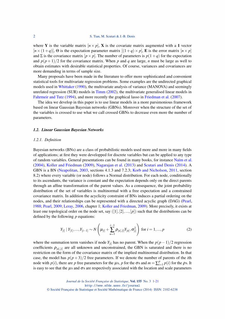
FIGURE 1. A serial DAG with three nodes supporting the Bayesian network defined in (3).

of the variables, so we can assume that all variables have marginal zero expectations and unityvariances without altering the intrinsic properties of the model. As a result, the maximum numberof parameters is m = p(p−1)/2, corresponding to the conveniently modified ρs and related tothe p(p−1)/2 correlation parameters of the multinormal distributions.

1.2.2. Example

Just to give a small example, let us consider a GBN, based on the DAG drawn in Figure 1, withthree marginally centred and normalised nodes with the following local distributions:

Y1 ∼ N (0,1) ,

Y2 | Y1 ∼ N(ρ12Y1,

(1−ρ

212))

, (3)

Y3 | Y1,Y2 ∼ Y3 | Y2 ∼ N(ρ23Y2,

(1−ρ

223))

;

which imply the following joint distribution: Y1Y2Y3

= N

000

,

1 ρ12 ρ12ρ23ρ12 1 ρ23

ρ12ρ23 ρ23 1

.

Compared to an unconstrained distribution on Y1, Y2 and Y3, there is one less free parameter (ρ13),due to the following constraint on the correlation matrix:

Cor(Y1,Y3) =Cor(Y1,Y2).Cor(Y2,Y3).

For any GBN, the number of free parameters in the correlation matrix is simply given by thenumber of arcs in the associated DAG, which is equal to m. It is important to note that this way toimpose constraints on the correlation matrix is quite efficient and intuitive. However, expressingthe induced constraints is not always as straightforward as in this small example, even thoughthe rules to get the correlation coefficients from the regression coefficients can be expressed in amatricial closed form.

1.2.3. Matrix Formulation

To define the DAG associated with a GBN, it is convenient to use a p× p adjacency matrix(Nagarajan et al., 2013; Jungnickel, 2013), say A. Each row and each column of A is associatedwith one of the nodes in the DAG, and when Yi is a parent of Yi′ , then Ai,i′ is equal to one, and zero




otherwise. Since it is equivalent to the DAG, the adjacency matrix shares all its properties; forinstance, the number of arcs in the DAG is given by the sum of all the elements of A. Another moreinteresting property is that Au provides the number of paths of length u joining any ordered pairof nodes built with successive arcs of the DAG (Bang-Jensen and Gutin, 2009). It is convenient toassume that the order of the rows and columns of the A matrix is a topological order of the nodes,that is one of the orders compatible with all arcs of the associated DAG; this implies that the Amatrix is upper triangular with a null diagonal.

Any GBN can be defined with (i) the vector of the constants, say µ , (ii) the vector of thestandard deviations, say σ and (iii) the matrix of the regression coefficients, say R, which hasthe same dimension and the same zeros as the adjacency matrix, but the regression coefficientsinstead of ones. Here are those matrices for Model (3):

A =

0 1 00 0 10 0 0

; µ =

000

;σ =

1√

1−ρ212√

1−ρ223

; R =

0 ρ12 00 0 ρ230 0 0

.

1.2.4. Joint Distribution

A basic problem is the computation of the joint distribution of the set of nodes, say Y , from thedefinition of the BN. Indeed, the definition of a GBN, with the marginal distributions of the rootnodes and the conditional distributions for the others, provides only the local behavior of everynode. For interpretative purposes, it is important to know the marginal distribution of non-rootnodes, and the strength of the dependencies between indirectly related nodes. This is achievedwith the joint distribution. In the multinormal framework, the point is to obtain the expectationvector and covariance matrix which is not always an easy task even for such tractable distributions.Two ways are reported in the following. The first relies on the topological order and is relatedto the algorithm illustrated in Korb and Nicholson (2011) section 2.4.1 for discrete BNs; also ofinterest are the proposals made by Neapolitan (2003) (section 4.1.3).

1. Affine transformation of white noise (a vector of independent centred and normalisednormal variables), denoted by E, that is the identification of the vector M and matrix Gsuch that Y = M+G ·E. This is obtained by (i) express the first node as M1 +G1,1E1 and(ii) from the second node until the last node express Mi +∑

iu=1 Gi,uEu. Note that the matrix

G is lower triangular and that all its diagonal components can be imposed to be strictlypositive.

2. Use of the matrix R defined above by computing the matrix R∗ = Ip +∑p−1u=1 Ru. There are

algorithms to compute it for a specific DAG (Bang-Jensen and Gutin, 2009; Sedgewick,2011) which can be of interest when the number of nodes is large. Then, it can be checkedthat

E [Y] = R∗′ ·µ and V [Y] = R∗

′ ·diag(σ)2 ·R∗. (4)

where diag(σ) is the diagonal matrix built with vector σ .




2. Crossed Gaussian Bayesian Networks

2.1. Definition

In some situations, the set of variables has a crossed structure, that is the variables can be indexedby a couple of indexes, all couples being present. In the following we will denominate theseindexes: series of items. The most widely-known case is dynamic BNs (Ghahramani, 1997;Friedman et al., 1998), in which the same set of variables is observed at different successivetimes, but other situations are possible as shown in the examples below (§2.2). In order to obtaina parsimonious model, requiring only a small number of parameters, it can be profitable to usea crossed structure. To do so, we propose to use crossed DAGs, which are the product of oneDAG on the first series of items by another DAG on the second series of items. In fact a crossedDAG is the Cartesian product of DAGs associated with each series of items (Bang-Jensen andGutin, 2009). More formally, let us denote each variable with a pair of indices associated withthe two series of items: Y(i1,i2) with i1 = 1, ..., p1, i2 = 1, ..., p2 and p = p1 p2; also be A(1) (A(2))the adjacency matrices associated onto the p1 (p2) items. The adjacency matrix of the resultingcrossed DAG is given by the simple rule:

A(i1,i2),( j1, j2) = 1 when

i1 = j1 and A(2)

i2, j2 = 1or

i2 = j2 and A(1)i1, j1 = 1

= 0 otherwise.

(5)

That is, for each set of nodes having a common item of series 1, the DAG for series 2 is applied;and conversely for each set of nodes having a common item of series 2, the DAG for series 1 isapplied. Equation (5) is equivalent to the matrix formula

A = Ip1⊗A(2)+A(1)⊗ Ip2 .

From this formula, one can see that the number of ρ coefficients for a crossed BN is p1m2 + p2m1where m1 and m2 are the number of ρs of the two elementary DAGs.

2.2. Examples

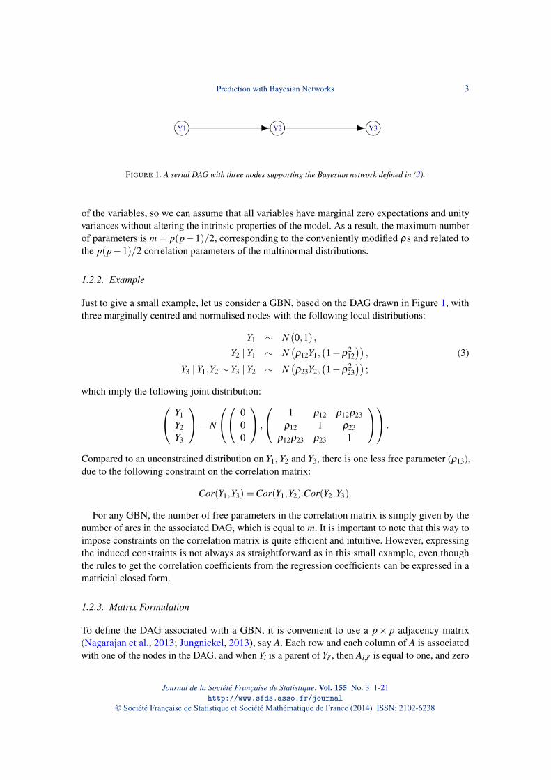
Crossing the DAG defined by (3) and shown in Figure 1 with itself produces the crossed DAG ofFigure 2. This DAG can be used to propose a GBN, and the number of parameters is reduced froma maximum of 36 to 12. This situation occurs each time a multivariate observation is repeated indifferent correlated places. A reduced example can be that of different properties measured to thetwo eyes of an individual; the application on body composition, developped in §4, belongs to thiscategory.

Now the DAG drawn in Figure 2 could as well be representing a dynamic BN with three slicesof time (from one column to another) and a direct link for each variable of the system (associatedwith the rows). Notice that if dynamic BN nodes are described as the Cartesian product of twosets, crossed BNs apply only when temporal arcs are placed to each variable.

Other fields of application are two crossed random factor effects when the levels are notexchangeable: for instance a set of more or less related genotypes cultivated within different typesof environments structured according to the year and soil categories.




FIGURE 2. Crossed DAG obtained by crossing the serial DAG shown in Figure (1) by itself.

TABLE 1. Different restrictions on the regression coefficients of a crossed DAG. p1 and p2 are the node numbers ofthe elementary DAGs generating the crossed DAG, and m1 and m2 are their respective parametric dimensions.

type constraints parametric dimension

F.F no one p2m1 + p1m2C.F identical for each item of series 1 p2m1 +m2F.C identical for each item of series 2 m1 + p1m2C.C identical for both series m1 +m2

2.3. Additional Constraints

In order to decrease even more the parametric dimension, some constraints linked to the crossedstructure can be added on the regression coefficients. Particularly, some equalities can be imposed,like those implied by:

R = Ip1⊗R(2)+R(1)⊗ Ip2

where R(1) (R(2)) is some regression matrix associated with the DAG of the first (second) seriesof items. In that case, the number of ρ coefficients is just m1 +m2, which can be a drastic drop.Intermediate proposals can be made, examples are given in Table 1.

2.4. Introducing Covariates

2.4.1. Introduction

When discussing GBNs in the previous sections, we focused only on the variables, Y . We willnow incorporate covariates, X , to match the regression model described in Equation (1). The basicidea is to add the covariates as ancestors of the variables in the crossed DAG and then retain thesub BN conditionally to the covariates. Starting from the simple example in Figure 2, an example




is shown in Figure 3-ii. The presence of the conditioning covariates alters the properties of GBNspreviously indicated. For instance, the expectations cannot be further supposed to be null sincethey depend on the covariates’ values; in addition, the covariance matrix loses the simplicity ofEquation (4).

2.4.2. Example

As an example of the increased complexity introduced by the covariates, consider a toy example ofone covariate intervening in two nodes of a 2×2 crossed DAG. Suppose that the joint distributionbetween variables and covariates can be described with a centred and normalised GBN as proposedin Figure 3-i, that is:

C ∼ N (0,1)Y1,1 |C ∼ N

(eC,1− e2

)Y1,2 | Y1,1 ∼ N

(aY1,1,1−a2

)Y2,1 | Y1,1 ∼ N

(cY1,1,1− c2

)Y2,2 |C,Y1,2,Y2,1 ∼ N

(fC+dY1,2 +bY2,1,σ

22,2

)where

σ22,2 = 1−

(f 2 +d2 +b2 +2(e f ad + e f cb+adcb)

).

In the equations above, the main difficulty lies in defining the conditional variances to achieve allthe marginal variances to be one. The structure of the covariance (here correlation) matrix is moreevident, giving only the upper part:

V

C

Y1,1Y2,1Y1,2Y2,2

=

1 e ce ae f +ade+bce− 1 c a e f +ad +bc− − 1 ac ce f +acd +b− − − 1 ae f +d +abc− − − − 1

.

It can be checked that every correlation is the sum of the products of the regression coefficientsfollowing every possible path linking the two considered nodes. This is a consequence of Equation4.

The induced regression formulas can be computed from the equations above as follows:

E

Y1,1Y2,1Y1,2Y2,2

|C =

eceae

f +ade+bce

·C,

V

Y1,1Y2,1Y1,2Y2,2

|C =

1− e2 c(1− e2) a(1− e2) (ad +bc)(1− e2)− 1− c2e2 ac(1− e2) acd(1− e2)+b(1− c2e2)− − 1−a2e2 abc(1− e2)+d(1−a2e2)− − − 1− ( f +ade+bce)2

.

Some of these expressions can be interpreted in terms of paths over the DAG from Figure 3-i, butothers are more complicated and have no obvious graphical interpretation. The presence of two




FIGURE 3. (i) Toy 2× 2 crossed DAG with one covariate (C); regression coefficients of the centred normaliseddistribution are indicated on each arc of the DAG. (ii) Crossed DAG from Figure 2 completed with two covariates (C1and C2). The covariates intervene only on some of the variables for parsimony.

or more covariates (Figure 3-ii) makes the algebraic computations intractable, only numericalcomputations are possible in general.

2.5. Parametric Dimension

Previous considerations showed that the parametric dimension of a GBN is 2p+m where pis the number of nodes and m the number of arcs. They are respectively associated with theconstant terms of the expectations, the conditional variances and the regression coefficients. Whenconsidering a GBN comprising p variables and q covariates with the restriction of no variablebeing parent of some covariate, the parametric dimension is 2(q+ p)+mXX +mXY +mYY wheremXX , mXY and mYY are respectively the number of arcs within the variables, between a covariateand a variable, and within the covariates. Let us write down the joint density of this BN [X ,Y ], wehave that

[X ,Y ] = [X ] [Y | X ]

pd ([X ,Y ]) = pd ([X ])+ pd ([Y | X ])

2(q+ p)+mXX +mXY +mYY = (2q+mXX)+ pd ([Y | X ])

where pd([Z]) is the parametric dimension of the density [Z]. It follows that the parametricdimension of the conditional GBN is 2p+mXY +mYY .

The decomposition of the joint distribution into [X ] and [Y |X ] has two interesting consequences.First when one is interested in the variables, there is no need to introduce arcs between covariatenodes when drawing the DAG. Second, the distributions of the covariates need not to be of the




same type that the distributions of the variables as we supposed here; even the nature of covariatescould be different.

2.6. Parameter Estimation

When a GBN is free with respect to its DAG, that is the parameters of each Equation (2) arenot constrained, maximum likelihood (ML) estimates can be computed with the standard MLestimators of each equation.

When some simple additional equalities are assumed like those in Table 1, things are moredifficult. ML estimators cannot be simply obtained from data by stacking the variables and thecorresponding parents since the same regression coefficient can be involved in different setsof regression coefficients. The situation is similar to that of dynamic GBNs, but without theadditional complication of handling hidden variables (Murphy, 2002, Chapters 3 and 4). We didnot find reference to estimate parameters in these circumstances for GBNs, only for discrete BNs(see for instance Section 17.5 Learning Models with Shared Parameters in Koller and Friedman,2009). To overcome the difficulty, we adapted the following heuristic alternating least squares(for instance described in Lütkepohl, 2005) procedure:

– Define as score for the difference between two GBNs sharing the same DAG, the sum ofsquared discrepancies of all the parameters, including the standard deviation.

– Initialise all the parameter values with the unconstrained fit.– Iterate until the decrease of the score be less that some predefined threshold. Each iteration

is a cycle over all expectation parameters. Each expectation along with the parametersand the standard deviations of the involved nodes is updated in turn, while keeping all theothers fixed. Estimation is performed by weighted least squares since each elementary fit isassociated with the fit of a linear model.

For all the examples we considered, convergence was very fast, typically after less than teniterations. The implementation of this algorithm is included within the RBMN R package (Denis,2013) available on CRAN but further research on estimation is required.

3. Numerical Experiment

In order to check that the models we proposed could be efficiently tackled, a small numericalexperiment was performed. Indeed, using GBNs seems a bright idea to decrease the modelcomplexity of multivariate multiple regressions but the challenge of discovering the true structureof the DAG could compromise the quality of the prediction and the remedy could be worst thanthe disease. Numerically checking the quality of such a general process is a huge task due to thenumerous causes involved and we had to make some choices. After describing which simulationswere performed, how predictions were made and how they have been assessed, the results areproposed in four tables and commented in a last subsection.

All calculations have been done with R (R Core Team, 2013) with the help of the three packagesBNLEARN (Scutari, 2010), RBMN (Denis, 2013) and GLMNET (Friedman et al., 2010).




XC1

XR1

XR2

XR3

Y11 Y12 Y13 Y14

Y21 Y22 Y23 Y24

Y31 Y32 Y33 Y34

Y41 Y42 Y43 Y44

Y51 Y52 Y53 Y54

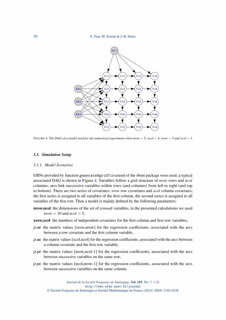
FIGURE 4. The DAG of a model used for the numerical experiment when nrow = 5, ncol = 4, xrow = 3 and xcol = 1.

3.1. Simulation Setup

3.1.1. Model Scenarios

GBNs provided by function generate8grid7crossed of the rbmn package were used; a typicalassociated DAG is shown in Figure 4. Variables follow a grid structure of nrow rows and ncolcolumns; arcs link successive variables within rows (and columns) from left to right (and topto bottom). There are two series of covariates: xrow row covariates and xcol column covariates;the first series is assigned to all variables of the first column, the second series is assigned to allvariables of the first row. Then a model is mainly defined by the following parameters:

nrow,ncol the dimensions of the set of crossed variables, in the presented calculations we usednrow = 10 and ncol = 5,

xrow,xcol the numbers of independent covariates for the first column and first row variables,

ρ .xr the matrix values [xrow,nrow] for the regression coefficients, associated with the arcsbetween a row covariate and the first column variable,

ρ .xc the matrix values [xcol,ncol] for the regression coefficients, associated with the arcs betweena column covariate and the first row variable,

ρ .yr the matrix values [nrow,ncol-1] for the regression coefficients, associated with the arcsbetween successive variables on the same row,

ρ .yc the matrix values [ncol,nrow-1] for the regression coefficients, associated with the arcsbetween successive variables on the same column.




All local (marginal or conditional) distributions are given a null expectation and unit variance. Toreduce the computation, all ρ coefficients were used with the same unique value.

3.1.2. Ten Different Strategies for Prediction

The aim is to check whether using a GBN whose structure and parameters are learned from a dataset can perform better than a standard multivariate multiple regression for prediction. To be fairerto the standard regression, we implemented three estimations to build the predictor: the standardleast squares, the lasso and the elastic net, respectively coded as S-ls, S-la and S-en with the helpof the GLMNET package (Friedman et al., 2010). The known true model was also implementedbeing the target to tend to (denoted as G-true), in fact only the DAG was used, the parametersbeing estimated from the data sets. Finally, six GBN predictions were attempted, differing in theamount of information provided to the model structure; also with two different ways of indicatingthat some nodes of the DAG are covariates and cannot be children of the variables. They are:

1. Learning the DAG constraining (i) every covariate to be a parent of every variable and (ii)preventing arcs between covariates [G-c],

2. Like (1) and preventing Y (i′, j′) to be a parent of Y (i, j) when j < j′ [G-cc],

3. Like (2) and preventing Y (i′, j′) to be a parent of Y (i, j) when (i < i′) [G-ccr],

4. Learning the DAG constraining (i) covariates not to be children of any variable and (ii)preventing arcs between covariates [G-n],

5. Like (4) and preventing Y (i′, j′) to be a parent of Y (i, j) when j < j′ [G-nc],

6. Like (5) and preventing Y (i′, j′) to be a parent of Y (i, j) when (i < i′) [G-ncr].

All results presented below were obtained with the tabu search of the tabu function ofBNLEARN R package (Scutari, 2010) using the default parameter values.

3.1.3. Simulation Design

Any simulation is a two-levels simulation of data sets of N observations comprising the variablesand covariates, according to the two repetition numbers: S and T .

A data set is a triplet of related matrices(X ,Y T R,YVA

)of respective sizes (N×C), (N×V )

and (N×V ) where N is the sample size, C the number of covariates and V the number of variables.Y T R is used for the TRaining, YVA being reserved for the VAlidation. Such triplets of matrices aregenerated ST times and denoted

(Xs,Y T R

st ,YVAst)

for s = 1, ...,S and t = 1, ...,T evidencing the factthat covariates, Xs, are generated only S times and are identical for the training and validating datasets, while 2T repetitions for each covariate configuration is done for the variables. This design isnecessary (i) to get a fair assessment of the error of prediction and (ii) to distinguish the bias fromthe standard deviation.

For such a simulation, a predictor (of the variables using the covariates) is obtained indepen-dently from

(Xs,Y T R

st)

on each st simulation and applied for a prediction to the associated data set(Xs,YVA

st). Let us denote it by Pst , it is a (N×V ) matrix.

As the model is known, the true target values are known, It is the matrix of conditionalexpectations of size (N×V ), different for each draw of the covariates. Let us denote it by Λs.




To assess a prediction we will use the following ST matrices of the discrepancies between theprediction and the conditional expectation:

Dst = Pst −Λs.

3.1.4. Criteria for comparison

Bias Let Ds. be the mean over t on matrices Dst , it can be interpreted as the estimated bias forthe sth draw of the covariates. And we will use

B2v =

∑Ss=1 ∑

Nn=1 ((Ds.)nv)

2

SN

B2 =∑

Vv=1 B2

v

V

as squared bias for each variable and global squared bias.

Standard Deviation In the same way, the dispersion around the average predicted values willbe assessed with

SD2v =

∑Ss=1 ∑

Tt=1 ∑

Nn=1 ((Dst −Ds.)nv)

2

ST N

SD2 =∑

Vv=1 S2

v

V

S.E.P. Finally, the standard error of prediction can be written as

SEP2v =

∑Ss=1 ∑

Tt=1 ∑

Nn=1 ((Dst)nv)

2

ST N

SEP2 =∑

Vv=1 SEP2

v

V

3.2. Simulation Sizes

These simulations are quite time consuming and a first study was conducted to determine adaptedvalues for S and T . Table 2 presents the three criteria for N = 100, xrow = 2, xcol = 1 and ρ = 0.5.Even for the smallest combination (S = 10,T = 20) results are similar to the most expansive one(S = 30,T = 80). Therefore, for computational reasons, all further calculations were made withthe intermediate combination (S = 20,T = 30).

Another important parameter is the sample size of individual data sets, that is N. The S.E.P.was computed for the ten predictions with different values varying from 50 to 500 (see Table 3).It appears that there is a strong effect of N within each prediction while the comparisons betweenpredictions remain similar for a fixed sample size. Again for computational reasons, we retainedthe intermediate value of N = 100.




TABLE 2. Effect of the repetition numbers, S and T , on the calculations of the criteria. The other parameters are fixedto nrow = 10, ncol = 5, xrow = 2, xcol = 1, N = 100 and ρ = 0.5.

S-ls G-true

T = 20 30 80 20 30 80

S = 10bias 0.069 0.054 0.032 0.032 0.028 0.018SD 0.289 0.293 0.295 0.144 0.148 0.148SEP 0.297 0.298 0.297 0.147 0.151 0.149

S = 20bias 0.069 0.055 0.032 0.031 0.027 0.017SD 0.290 0.293 0.296 0.144 0.148 0.148SEP 0.298 0.298 0.297 0.147 0.151 0.149

S = 40bias 0.065 0.055 0.032 0.031 0.027 0.017SD 0.291 0.294 0.296 0.145 0.148 0.148SEP 0.298 0.299 0.298 0.149 0.150 0.149

TABLE 3. Looking for the sample size, N, effect on the S.E.P.. The other parameters are fixed to nrow = 10, ncol = 5,xrow = 2, xcol = 1, S = 20, T = 30 and ρ = 0.5.

N S-ls S-la S-en G-c G-n G-cc G-nc G-ccr G-ncr G-true

50 0.422 0.420 0.420 0.338 0.412 0.319 0.390 0.295 0.364 0.21360 0.384 0.382 0.382 0.308 0.362 0.283 0.338 0.264 0.312 0.19570 0.359 0.357 0.357 0.283 0.337 0.256 0.303 0.239 0.280 0.17980 0.333 0.332 0.332 0.261 0.311 0.236 0.278 0.220 0.253 0.16890 0.314 0.312 0.312 0.249 0.295 0.220 0.254 0.297 0.232 0.162100 0.298 0.297 0.297 0.234 0.272 0.204 0.234 0.192 0.214 0.151200 0.210 0.209 0.209 0.171 0.183 0.132 0.140 0.127 0.132 0.105300 0.172 0.171 0.171 0.144 0.141 0.106 0.107 0.102 0.103 0.086400 0.149 0.148 0.148 0.132 0.122 0.089 0.090 0.087 0.087 0.074500 0.134 0.133 0.133 0.121 0.108 0.080 0.080 0.078 0.077 0.068

3.3. Effect of the Arc Strength

Once the numbers of repetitions have been fixed, we first varied the dependence between directlyrelated nodes changing the ρ value from 0 to 1: resulting S.E.P.s are presented in Table 4. Noticethat when the regression coefficients are all zero, variables are independent from the covariates(also mutually independent) with null expectation and variance unity; this explains the nullS.E.P. for the true model since it does not depend anymore on the pseudo-randomly generatedconditioning covariates. It is amazing to see how the S.E.P. increases with ρ for all the predictions.This is the simple consequence of the increase of the marginal variances of nodes in the last rowsand last columns due the multiplicative effect of the variation transmission as shown in the lastline of Table 4.

3.4. Effect of the Covariate Numbers

The S.E.P values obtained for the ten predictions for different numbers of covariates have beencollected in Table 5.

3.5. Conclusions

From the performed numerical experiments (see Tables 4 and 5) some conclusions appear:




TABLE 4. ρ effect on the S.E.P. for the ten predictions (first 10 lines); marginal standard deviation of four variablesaccording to the same variation of parameter ρ (last 4 lines). The other parameters are fixed to nrow = 10, ncol = 5,xrow = 2, xcol = 1, S = 20, T = 30 and N = 100.

(SEP) 0 0.25 0.5 0.75 1

S-ls 0.200 0.212 0.298 2.119 40.589S-la 0.194 0.208 0.297 2.118 40.592S-en 0.194 0.209 0.297 2.117 40.592

G-c 0.115 0.131 0.234 2.278 35.552G-n 0.090 0.157 0.272 2.228 39.351G-c.cc 0.111 0.129 0.204 1.852 34.803G-nc 0.086 0.160 0.234 2.255 36.596G-c.ccr 0.110 0.125 0.192 1.685 33.674G-ncr 0.083 0.158 0.214 1.804 34.744

G-true 0.000 0.080 0.151 1.562 33.093

St.Dev.(Y.1.2) 1 1.031 1.118 1.250 1.414St.Dev.(Y.1.5) 1 1.033 1.154 1.469 2.236St.Dev.(Y.3.5) 1 1.074 1.599 5.184 20.761St.Dev.(Y.10.5) 1 1.075 1.856 36.861 1020.685

– As expected, the true DAG [G-true] always gives the best prediction.– Sophisticated estimations (lasso and elastic net) are not decisively better than the standard

least-squares estimations for the multivariate multiple regression model.– Predicting with the considered GBN models always gives better prediction than using the

saturated regression model.– Among the six GBN models, there are differences which depend on the circumstances:

– The strongest difference is between the two ways used to indicate the covariate nodes, butthe difference depends on the strength of the relationships. When the strength is low it isworth imposing all covariates as parents of all variables, even if most of them does notexist. The explanation seems that when the strength is high, the learning algorithm maybe able to recover the structure and not too many arcs are missed.

– Adding information about the ordering of the columns and rows improved predictions butnot as much as using a GBN instead of the saturated model. This is encouraging becauseit means that the strongest point is to use a GBN approach for predicting.

– When the number of covariates increase in the model, surprisingly the prediction areworst. This could be the effect of different marginal variances due to more randomness?The reassuring point is that the main differences between the different predictions are notmodified.

This is positive but it must be indicated that, from results not shown, not all learning algorithmsprovided good results. Other attempts with constraint-based algorithms like grow-shrink gavebad results, much worse than the saturated regression. Detailed examination of the resultingDAG showed that in a non negligible proportion of simulations, arcs were not discovered, thusintroducing bias that was obviously absent from saturated models. Increasing the α parameter toretain more arcs was not the solution since it implied graphs not reducible to DAGs. The presentpositive results were obtained with the score-based algorithm more precisely the tabu algorithmimplemented in the BNLEARN R package (Scutari, 2010) and used with the default parameters ofits tabu function.




TABLE 5. Effect of the number of row/column covariates on the S.E.P. for the ten predictions. The other parametersare fixed to nrow = 10, ncol = 5, S = 20, T = 30, N = 100 and ρ = 0.5.

xrow xcol S-ls S-la S-en G-c G-n G-cc G-nc G-ccr G-ncr G-true

1 0 0.212 0.211 0.211 0.157 0.172 0.133 0.139 0.124 0.130 0.1051 1 0.258 0.257 0.257 0.202 0.224 0.176 0.183 0.161 0.164 0.1231 2 0.298 0.297 0.297 0.229 0.256 0.202 0.210 0.184 0.189 0.1341 3 0.335 0.333 0.333 0.252 0.280 0.225 0.235 0.206 0.217 0.1463 0 0.298 0.297 0.297 0.216 0.176 0.199 0.268 0.196 0.258 0.1613 1 0.335 0.334 0.334 0.255 0.325 0.230 0.304 0.220 0.284 0.1733 2 0.366 0.364 0.364 0.281 0.343 0.250 0.317 0.237 0.297 0.1813 3 0.396 0.394 0.394 0.296 0.368 0.268 0.337 0.255 0.317 0.1905 0 0.366 0.365 0.365 0.259 0.405 0.248 0.400 0.243 0.395 0.1985 1 0.396 0.394 0.394 0.293 0.435 0.270 0.429 0.263 0.412 0.2065 2 0.422 0.420 0.420 0.317 0.445 0.287 0.444 0.278 0.422 0.2165 3 0.449 0.447 0.447 0.333 0.478 0.305 0.466 0.294 0.441 0.2257 0 0.422 0.421 0.421 0.292 0.532 0.286 0.520 0.281 0.518 0.2297 1 0.449 0.447 0.447 0.325 0.561 0.308 0.565 0.302 0.547 0.2387 2 0.471 0.469 0.469 0.346 0.588 0.322 0.592 0.313 0.559 0.2437 3 0.494 0.492 0.492 0.362 0.596 0.336 0.608 0.327 0.565 0.250

4. Application

4.1. Presentation

The human body composition is the allocation of body weight among three components: (L)ean,(F)at and (B)one. In detailed analyses, the body composition is investigated for each of the mainsegments of the body: (T)runk, (L)egs and (A)rms; so nine variables crossing the three componentswith the three segments are available. Body composition is an important diagnostic indicator sinceratios of these masses can reveal regional physiological disorders. In the following, we will try topredict it from easily accessible covariates: the (A)ge in years, the (H)eight in cm, the (W)eight inkg and the waist (C)ircumference in cm; more details can be found in Tian et al. (2013) wherea saturated model was used. For this purpose, we retained a data set of one hundred white menavailable in the RBMN R package (Denis, 2013). For each individual the variables to predict aswell as the covariates have been recorded. Below are the first four individuals.

A H W C TF LF AF TL LL AL TB LB AB1 83 182 92.6 117 17.1 8.9 3.0 31.2 18.5 6.6 0.6 1.1 0.52 68 169 74.7 93 8.3 5.4 2.0 28.0 16.2 7.5 0.7 1.0 0.53 28 182 112.2 112 17.7 11.3 3.1 36.7 24.5 10.1 0.8 1.1 0.54 41 171 82.6 96 10.6 6.5 1.8 29.2 19.6 7.8 0.8 1.1 0.5

Here, (LF) stands for the (L)eg (F)at, and so on; all variables are given in kg. An additionalcovariate, the body mass index (B) has been calculated; it is a very popular score normalising theweight by the height. Overall we have q = 5 covariates and p = 9 = 3×3 variables for n = 100individuals.

All calculations have been done with R (R Core Team, 2013) with the help of the three packagesBNLEARN (Scutari, 2010), RBMN (Denis, 2013) and GLMNET (Friedman et al., 2010). DAGs havebeen drawn using the IGRAPH (Csardi and Nepusz, 2006) package as all other DAGs of the paper.




4.2. Predicting with a crossed BN

Using the crossed structure of the nine variables to perform the prediction, we tried to improve onthat given by the standard multivariate multiple regression model from Equation (1). We are thenin a model selection perspective (Claeskens and Hjort, 2008 and Burnham and Anderson, 2010).To do so, following Hastie et al. (2009), we randomly splitted our data set into two subsets of sizen = 50, one for estimating models and the second one to assess their predictive power, the samesplitting was used for all models. The validation of the models over an independent subsampleexempted us from considering model selection criteria like AIC. In the framework of linearregression, the prediction of a new individual is made with a Normal distribution with expectationobtained from the regression formula and with standard deviation given by the estimation of thestandard error. The difference between the observed value and the expectation is the bias (Bv

i , forthe individual i and variable v); the squared standard deviation is the variance of the prediction((σ v)2). To obtain a global score, we computed a global bias, a global standard deviation and aglobal standard error of prediction by summing them up as follows:

|Bias| =p

∑v=1

(1n

n

∑i=1|Bv

i |),

Sd.Dev. =p

∑v=1

σv, (6)

SEP =p

∑v=1

(1n

n

∑i=1

√|Bv

i |2 +(σ v)2

).

In addition to these global quality scores, we measured the parametric dimensions with thenumber of arcs linking the covariates to the variables (mXY : the number of retained regressioncoefficients) and the number of arcs between pairs of variables (mYY : related to the complexity ofthe correlation structure within the variables). Also, we introduced m̃YY , the parametric dimensionof the covariance matrix, which is smaller in case of equality constraints on the regressionparameters.

A systematic series of non degenerated crossed BNs were attempted among all possible 25DAGs within the three compartments (F, L, B) crossed with all possible 25 DAGs within the threesegments (T, L, A), and for each one the four constraint types proposed in Table 1. Table 6 showsthe results for the best twelve, together with the corresponding results for the saturated model.Some interesting features can be noticed from this table:

– The selected crossed BNs perform better than the saturated model globally (SEP) and forboth the bias and the variance, the improvement being greater for the variance.

– The reduction in the number of parameters with respect to the saturated model is striking,especially for the variance parameters.

– None of the selected models is without constraints (type F.F).– For all the selected models, constraints on the three segments (Trunk, Legs, Arms) are

present.– For the segments, only two generating BNs (numbers 14 and 6) are present among the

possible 25 ones. These two generating BNs are nested since 14 is (A→ T→ L) and 6 is




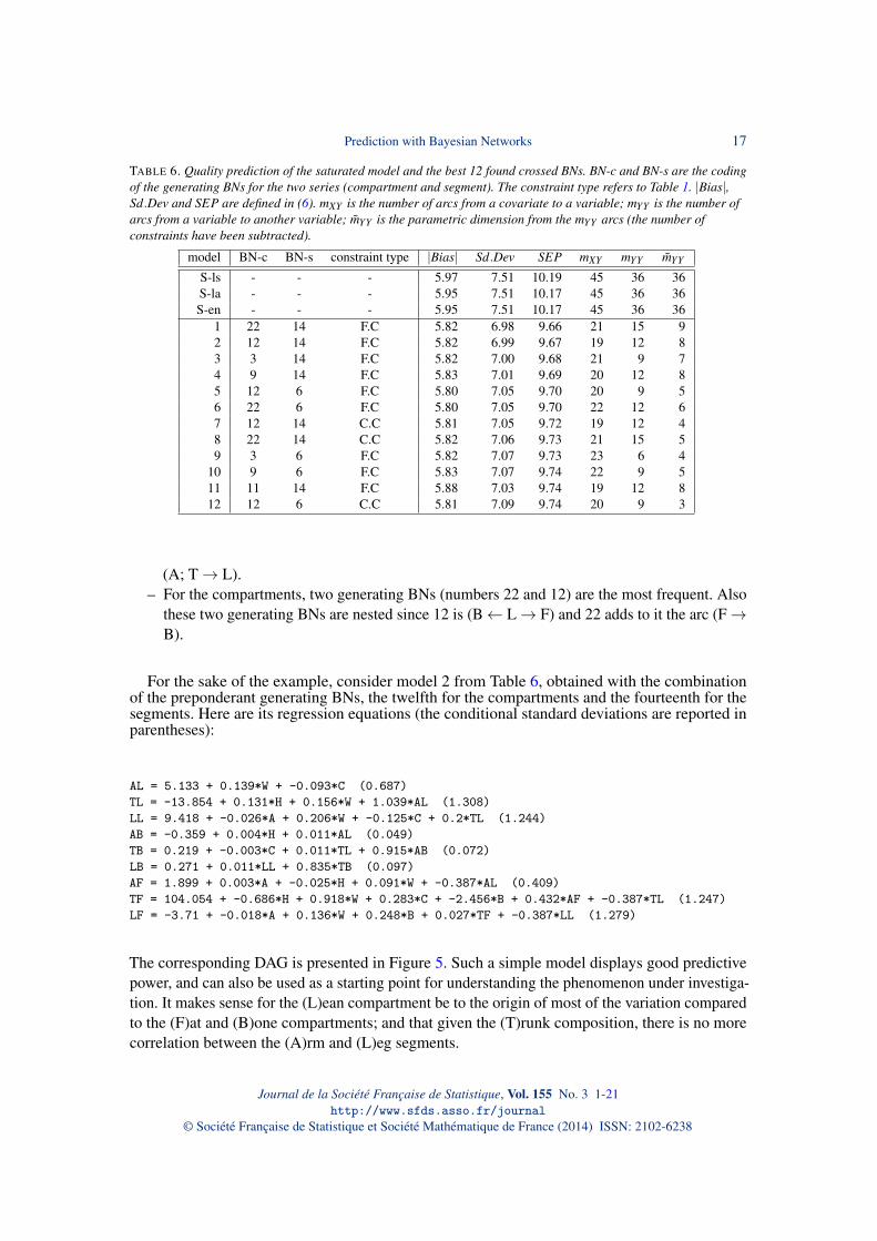
TABLE 6. Quality prediction of the saturated model and the best 12 found crossed BNs. BN-c and BN-s are the codingof the generating BNs for the two series (compartment and segment). The constraint type refers to Table 1. |Bias|,Sd.Dev and SEP are defined in (6). mXY is the number of arcs from a covariate to a variable; mYY is the number ofarcs from a variable to another variable; m̃YY is the parametric dimension from the mYY arcs (the number ofconstraints have been subtracted).

model BN-c BN-s constraint type |Bias| Sd.Dev SEP mXY mYY m̃YY

S-ls - - - 5.97 7.51 10.19 45 36 36S-la - - - 5.95 7.51 10.17 45 36 36S-en - - - 5.95 7.51 10.17 45 36 36

1 22 14 F.C 5.82 6.98 9.66 21 15 92 12 14 F.C 5.82 6.99 9.67 19 12 83 3 14 F.C 5.82 7.00 9.68 21 9 74 9 14 F.C 5.83 7.01 9.69 20 12 85 12 6 F.C 5.80 7.05 9.70 20 9 56 22 6 F.C 5.80 7.05 9.70 22 12 67 12 14 C.C 5.81 7.05 9.72 19 12 48 22 14 C.C 5.82 7.06 9.73 21 15 59 3 6 F.C 5.82 7.07 9.73 23 6 4

10 9 6 F.C 5.83 7.07 9.74 22 9 511 11 14 F.C 5.88 7.03 9.74 19 12 812 12 6 C.C 5.81 7.09 9.74 20 9 3

(A; T→ L).– For the compartments, two generating BNs (numbers 22 and 12) are the most frequent. Also

these two generating BNs are nested since 12 is (B← L→ F) and 22 adds to it the arc (F→B).

For the sake of the example, consider model 2 from Table 6, obtained with the combinationof the preponderant generating BNs, the twelfth for the compartments and the fourteenth for thesegments. Here are its regression equations (the conditional standard deviations are reported inparentheses):

AL = 5.133 + 0.139*W + -0.093*C (0.687)TL = -13.854 + 0.131*H + 0.156*W + 1.039*AL (1.308)LL = 9.418 + -0.026*A + 0.206*W + -0.125*C + 0.2*TL (1.244)AB = -0.359 + 0.004*H + 0.011*AL (0.049)TB = 0.219 + -0.003*C + 0.011*TL + 0.915*AB (0.072)LB = 0.271 + 0.011*LL + 0.835*TB (0.097)AF = 1.899 + 0.003*A + -0.025*H + 0.091*W + -0.387*AL (0.409)TF = 104.054 + -0.686*H + 0.918*W + 0.283*C + -2.456*B + 0.432*AF + -0.387*TL (1.247)LF = -3.71 + -0.018*A + 0.136*W + 0.248*B + 0.027*TF + -0.387*LL (1.279)

The corresponding DAG is presented in Figure 5. Such a simple model displays good predictivepower, and can also be used as a starting point for understanding the phenomenon under investiga-tion. It makes sense for the (L)ean compartment be to the origin of most of the variation comparedto the (F)at and (B)one compartments; and that given the (T)runk composition, there is no morecorrelation between the (A)rm and (L)eg segments.




AHW CB

AF

TF

LF

AL

TL

LL

AB

TB

LB

FIGURE 5. DAG associated with Model 2 of Table 6. Arcs within covariates were not drawn for the sake of clarity;they are of no importance when conditioning by the covariates.

5. Discussion

ANOVA models, regression models and their combinations presented in the framework of linearmodels are versatile tools for analysing complex data sets at the level of big trends, that is atthe level of modelling the expectations of random variables (Graybill, 1976). To achieve betterpredictions, in this framework the common way is to reduce the number of used covariateslooking for a small and efficient subset (see Miller, 2002 and Celeux et al., 2006 for a review).The next step is the modelling of variances and covariances. Random models are the naturalextensions and many developments have been proposed in that direction, such as the introductionof variance components in hierarchical models and extensions. For instance, linear models havebeen developed to fit the logarithm of the variances (Foulley et al., 2004) in the univariate case. Inthe multivariate case, we think that BNs, not only GBNs, are appropriate candidates for furtherproposals. Recent publications appear in that perspective and we can cite Scutari et al. (2014) asan example. In this study, we showed that two-way structures can be introduced. Of course, thereis no limitation to two ways, similar multi-factor approaches can be devised as well. The work byMurphy (1998) also uses BNs with constraints on the variances (so-called tied variances); buthis focus is different from ours since he proposed equalities between conditional variances whilewe use the DAG structure itself to constraint the joint variance matrix on the set of nodes; theadditional constraints defined of Table 1 are put on the conditional expectations.




The need for modelling variance structure is all the more urgent now, that statisticians arefacing more and more situations where p, the number of variables, is great while n, the numberof statistical units to afford them, is small. BNs modelling seems a good way to take up thechallenge.

We showed that, at least for GBN modelling, it was possible to introduce a known structure onthe set of variables of interest, and that can lead to very effective results to obtain interpretablepredictive formulae. The numerical experiments based on simulated data sets with a knownstructure showed that at least in some situations, some learning algorithms were sufficientlyefficient to give our proposal a practical impact on data analysis. One of the advantages of the BNformulation is to allow non-statisticians, typically experts in some field, to contribute to modelspecification through the easy to understand DAG presentations. In our mind, such BNs mustand can serve as thinking material for non-experts in BNs. In that respect, the availability ofuser-friendly and performing software is a prerequisite and we are happy to see that more andmore R packages playing this role, are proposed: the most complete and versatile is BNLEARN

(Scutari, 2010), but PCALG (Kalisch et al., 2012), DEAL (Bottcher and Dethlefsen., 2012) andIGRAPH (Csardi and Nepusz, 2006) are also worth mentioning.

Besides the introduction of structures on the set of the variables of interest, our study underlinesthe distinction between variables and covariates. One could think that the ideal model would be amodel such that the targeted variables be conditionally independent to the covariates. That is allthe covariation between them could be explained by external variables. With this respect some ofthe exhibited models, having a very small parametric dimension (for instance Model 12 of Table6 with 3 instead of 36) are appealing.

Many more ideas could be proposed to achieve the goals we were interested in. Among them,the use of distributions other than Normal ones. Probably mathematical properties will be muchmore difficult to obtain, but the advantage would be to achieve a more realistic model specification.Advanced numerical tools already exist to undertake such an investigation. Among them, evenif not originally devised for this purpose, are the BUGS software packages (Plummer, 2003and Lunn et al., 2013). But also simpler approaches could also be worthwhile, like the use oftransformations of the initial variables. More sophisticated constraints than the equalities couldalso be implemented. For instance, following again a two-way structure, some bilinear modellingcould be thought about like those proposed to generalise additive models (Denis and Gower,1996).

We do think that not only BNs are beautiful for mathematical aspects, they are also useful forplenty of applied questions within a classic statistics point of view. In particular, they allow toincorporate, in the statistical models used to the data sets to interpret, more prior knowledge aboutthe phenomenon under study leading to more precise inferences and predictions. The proposalswe made are going this way.

Acknowledgments

The authors acknowledge the relevant comments made by the reviewers and editors of the journalon a first version of the manuscript which lead to an improvement of the paper.




References

Anderson, T. W. (2003). An introduction to multivariate statistical analysis. Wiley, 3rd edition.Bang-Jensen, J. and Gutin, G. (2009). Digraphs: Theory, Algorithms and Applications. Springer, 2nd edition.Bottcher, S. G. and Dethlefsen., C. (2012). deal: Learning Bayesian Networks with Mixed Variables. R package

version 1.2-35.Burnham, K. P. and Anderson, D. R. (2010). Model Selection and Multimodel Inference: A Practical Information-

Theoretic Approach. Springer.Celeux, G., Marin, J.-M., and Robert, C. P. (2006). Sélection bayésienne de variables en régression linéaire. Journal

de la Société Française de Statistique, 147(1):59–79.Claeskens, G. and Hjort, N. L. (2008). Model Selection and Model Averaging. Cambridge University Press.Csardi, G. and Nepusz, T. (2006). The igraph software package for complex network research. InterJournal, Complex

Systems:1695.Denis, J.-B. (2013). rbmn: Handling Linear Gaussian Bayesian Networks. R package version 0.9-2.Denis, J.-B. and Gower, J. C. (1996). Asymptotic confidence regions for biadditive models: interpreting genotype-

environment interactions. Applied Statistics, 45(4):479–493.Fahrmeir, L. and Tutz, G. (1994). Multivariate Statistical Modelling based on Generalized Linear Models. Springer-

Verlag.Foulley, J.-L., Sorensen, D., Robert-Granié, C., and Bonaïti, B. (2004). Heteroskedasticity and structural models for

variances. Jour. Ind. Soc. Ag. Slatistics, 57:64–70.Friedman, J., Hastie, T., and Tibshirani, R. (2007). Sparse Inverse Covariance Estimation With the Graphical Lasso.

Biostatistics, 9:432–441.Friedman, J., Hastie, T., and Tibshirani, R. (2010). Regularization paths for generalized linear models via coordinate

descent. Journal of Statistical Software, 33(1):1–22.Friedman, N., Murphy, K., and Russell, S. (1998). Learning the structure of dynamic probabilistic networks. In

Proceeding of the 14th Conference on Uncertainty and Artificial Intelligence (UAI’98), pages 139–147. MorganKaufmann.

Ghahramani, Z. (1997). Learning Dynamic Bayesian Networks. Number 1387 in Lecture Notes In Computer Science.Springer.

Graybill, F. A. (1976). Theory and application of the linear model. Duxbury Press.Hastie, T., Tibshirani, R., and Friedman, J. (2009). The Elements of Statistical Learning: Data Mining, Inference and

Prediction. Springer, 2nd edition.Jungnickel, D. (2013). Graphs, Networks and Algorithms. Springer, 4rth edition.Kalisch, M., Mächler, M., Colombo, D., Maathuis, M. H., and Bühlmann, P. (2012). Causal inference using graphical

models with the R package pcalg. Journal of Statistical Software, 47(11):1–26.Koller, D. and Friedman, N. (2009). Probabilistic Graphical Models: Principles and Techniques. MIT Press.Korb, K. B. and Nicholson, A. E. (2011). Bayesian Artificial Intelligence. CRC press, 2nd edition.Leray, P. (2006). Réseaux bayésiens : apprentissage et modélisation de systèmes complexes. PhD thesis, Université de

Rouen. Habilitation à Diriger des Recherches.Lütkepohl, H. (2005). New Introduction to Multiple Time Series Analysis. Springer.Lunn, D., Jackson, C., Best, N., Thomas, A., and Spiegelhalter, D. (2013). The BUGS Book. A practical introduction to

Bayesian analysis. CRC press.Miller, A. J. (2002). Subset selection in regression. Boca Raton: Chapman & Hall / CRC, 2d edition.Murphy, K. P. (1998). Fitting a conditional gaussian distribution. Technical report.Murphy, K. P. (2002). Dynamic Bayesian Networks: Representation, Inference and Learning. PhD thesis, University

of California, Berkeley. PhD dissertation.Nagarajan, R., Scutari, M., and Lèbre, S. (2013). Bayesian Networks in R with Applications in Systems Biology.

Springer.Naïm, P., Wuillemin, P.-H., Leray, P., Pourret, O., and Becker, A. (2004). Réseaux bayésiens. Eyrolles, 2nd edition.Neapolitan, R. E. (2003). Learning Bayesian Networks. Prentice Hall.Pearl, J. (1988). Probabilistic Reasoning in Intelligent Systems: Networks of Plausible Inference. Morgan Kaufmann.Pearl, J. (2009). Causality: Models, Reasoning and Inference. Cambridge University Press, 2nd edition.Plummer, M. (2003). Jags: A program for analysis of bayesian graphical models using gibbs sampling. In Proceedings

of the 3rd International Workshop on Distributed Statistical Computing (DSC 2003).




R Core Team (2013). R: A Language and Environment for Statistical Computing. R Foundation for StatisticalComputing, Vienna, Austria.

Scutari, M. (2010). Learning bayesian networks with the bnlearn R package. Journal of Statistical Software, 35(3):1–22.Scutari, M. and Denis, J.-B. (2014). Bayesian Networks with Examples in R. Chapman & Hall. in print.Scutari, M., Howell, P., Balding, D. J., and Mackay, I. (2014). Multiple quantitative trait analysis using bayesian

networks. Genetics. in print.Sedgewick, R. (2011). Algorithms. Addison-Wesley, 4th edition.Tian, S., Mioche, L., Denis, J.-B., and Morio, B. (2013). A multivariate model for predicting segmental body

composition. British Journal of Nutrition, 110(12):2260–70.Timm, N. (2002). Applied Multivariate Analysis. Springer.Whittaker, J. (1990). Graphical Models in Applied Multivariate Statistics. Wiley.



Documents

Journal de la Société Française de Statistique