Embed Size (px)
Citation preview
Laboratoire Kastler Brossel
Collège de France, ENS, UPMC, CNRS
Ultracold quantum gases in optical latticessolid-state physics with atoms in crystals made of light
Fabrice Gerbier ([email protected])
International school on phase transitions, Bavaria
March 21, 2016
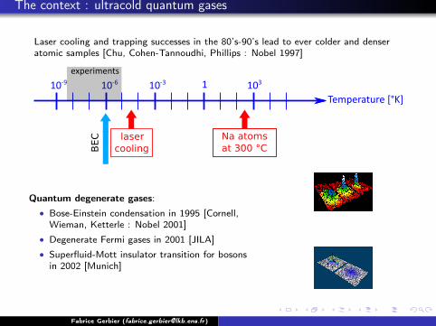
The context : ultracold quantum gases
Laser cooling and trapping successes in the 80’s-90’s lead to ever colder and denseratomic samples [Chu, Cohen-Tannoudhi, Phillips : Nobel 1997]
Quantum degenerate gases:• Bose-Einstein condensation in 1995 [Cornell,Wieman, Ketterle : Nobel 2001]
• Degenerate Fermi gases in 2001 [JILA]• Superfluid-Mott insulator transition for bosonsin 2002 [Munich]
Fabrice Gerbier ([email protected])
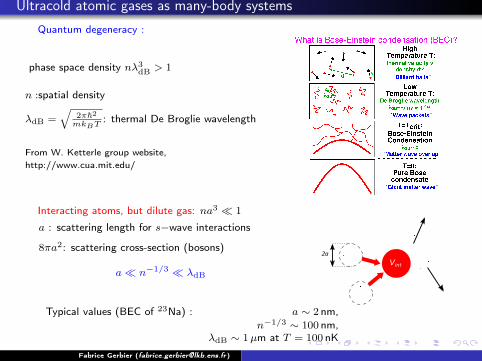
Ultracold atomic gases as many-body systems
Quantum degeneracy :
phase space density nλ3dB > 1
n :spatial density
λdB =√
2π~2mkBT
: thermal De Broglie wavelength
From W. Ketterle group website,http://www.cua.mit.edu/
Interacting atoms, but dilute gas: na3 � 1
a : scattering length for s−wave interactions
8πa2: scattering cross-section (bosons)
a� n−1/3 � λdB
Typical values (BEC of 23Na) : a ∼ 2 nm,n−1/3 ∼ 100 nm,
λdB ∼ 1µm at T = 100 nK
Fabrice Gerbier ([email protected])
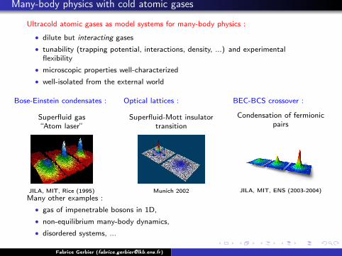
Many-body physics with cold atomic gases
Ultracold atomic gases as model systems for many-body physics :
• dilute but interacting gases• tunability (trapping potential, interactions, density, ...) and experimentalflexibility
• microscopic properties well-characterized• well-isolated from the external world
Bose-Einstein condensates :
Superfluid gas“Atom laser”
JILA, MIT, Rice (1995)
Optical lattices :
Superfluid-Mott insulatortransition
Munich 2002
BEC-BCS crossover :
Condensation of fermionicpairs
JILA, MIT, ENS (2003-2004)Many other examples :
• gas of impenetrable bosons in 1D,• non-equilibrium many-body dynamics,• disordered systems, ...
Fabrice Gerbier ([email protected])
From one to three-dimensional optical lattices
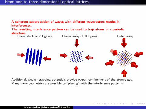
A coherent superposition of waves with different wavevectors results ininterferences.The resulting interference pattern can be used to trap atoms in a periodicstructure.
Linear stack of 2D gases Planar array of 1D gases Cubic array
Additional, weaker trapping potentials provide overall confinement of the atomic gas.Many more geometries are possible by “playing” with the interference patterns.
Fabrice Gerbier ([email protected])
Scope of the lectures
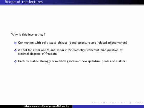
Why is this interesting ?
1 Connection with solid-state physics (band structure and related phenomenon)
2 A tool for atom optics and atom interferometry: coherent manipulation ofexternal degrees of freedom
3 Path to realize strongly correlated gases and new quantum phases of matter
Fabrice Gerbier ([email protected])
1 Introduction
2 Band structure in one dimension
3 Thermodynamics of Bose gases in optical lattices
4 Dynamics of Bose-Einstein condensates in optical lattices
5 Bloch oscillations
Fabrice Gerbier ([email protected])
Optical dipole traps
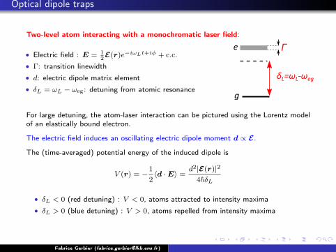
Two-level atom interacting with a monochromatic laser field:
• Electric field : E = 12E(r)e−iωLt+iφ + c.c.
• Γ: transition linewidth• d: electric dipole matrix element• δL = ωL − ωeg: detuning from atomic resonance
For large detuning, the atom-laser interaction can be pictured using the Lorentz modelof an elastically bound electron.
The electric field induces an oscillating electric dipole moment d ∝ E.
The (time-averaged) potential energy of the induced dipole is
V (r) = −1
2〈d ·E〉 =
d2|E(r)|2
4~δL
• δL < 0 (red detuning) : V < 0, atoms attracted to intensity maxima• δL > 0 (blue detuning) : V > 0, atoms repelled from intensity maxima
Fabrice Gerbier ([email protected])
Some numbers
Potential energy :
V (r) =d2
4~δL|E(r)|2
Take 87Rb atoms for definiteness :• Γ/2π ≈ 6MHz,• λeg ≈ 780 nm [ωL/2π ≈ 4× 10¹⁴ Hz]• λ0 ≈ 1064 nm, δL/2π ≈ −3× 10¹³ Hz,• Laser parameters : power P = 200mW, beam size 100µm]
One finds a potential depth |V | ∼ h× 20 kHz ∼ kB × 1µK.
Trapping atoms in such a potential requires sub-µK temperatures, or equivalentlydegenerate (or almost degenerate) gases.
NB : trap depths up to mK are possible using tightly focused lasers.
Fabrice Gerbier ([email protected])
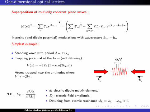
One-dimensional optical lattices
Superposition of mutually coherent plane waves :
|E(r)|2 =
∣∣∣∣∣∑n
Eneikn·r
∣∣∣∣∣2
=
∑n
|En|2 +∑n 6=n′
E∗n · En′ei(kn′−kn)·r
Intensity (and dipole potential) modulations with wavevectors kn′ − kn
Simplest example :
• Standing wave with period d = π/kL
• Trapping potential of the form (red detuning):
V (x) = −2V0 (1 + cos(2kLx))
Atoms trapped near the antinodes whereV ≈ −2V0.
N.B. : V0 =d2E2
0
4|~δL|
• d: electric dipole matrix element,• E0: electric field amplitude,• Detuning from atomic resonance :δL = ωL − ωeg < 0.
Fabrice Gerbier ([email protected])
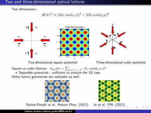
Two and three-dimensional optical lattices
Two dimensions :
|E(r)|2 ≈ |2E0 cos(kLx)|2 + |2E0 cos(kLy)|2
Two-dimensional square potential Three-dimensional cubic potential
Square or cubic lattices : Vlat(r) =∑ν=1,··· ,d−Vν cos(kνxν)2
• Separable potentials : sufficient to analyze the 1D caseOther lattice geometries are realizable as well:
Soltan-Panahi et al., Nature Phys. (2011) Jo et al., PRL (2012)
Fabrice Gerbier ([email protected])
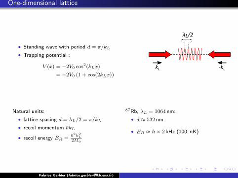
One-dimensional lattice
• Standing wave with period d = π/kL
• Trapping potential :
V (x) = −2V0 cos2(kLx)
= −2V0 (1 + cos(2kLx))
Natural units:• lattice spacing d = λL/2 = π/kL
• recoil momentum ~kL
• recoil energy ER =~2k2L2Ma
87Rb, λL = 1064 nm:• d ≈ 532 nm
• ER ≈ h× 2 kHz (100 nK)
Fabrice Gerbier ([email protected])
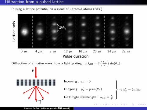
Diffraction from a pulsed lattice
Pulsing a lattice potential on a cloud of ultracold atoms (BEC) :
Pulse duration
Latt
ice a
xis
0 µs 4 µs 8 µs
2 kL
12 µs 16 µs 20 µs 24 µs 28 µs
Diffraction of a matter wave from a light grating : nλdB = 2(λL2
)sin(θn)
p
θ
Incoming : px = 0
Outgoing : p′x = p sin(θn)
De Broglie wavelength : λdB = hp
→ p′x = 2n~kL
Fabrice Gerbier ([email protected])
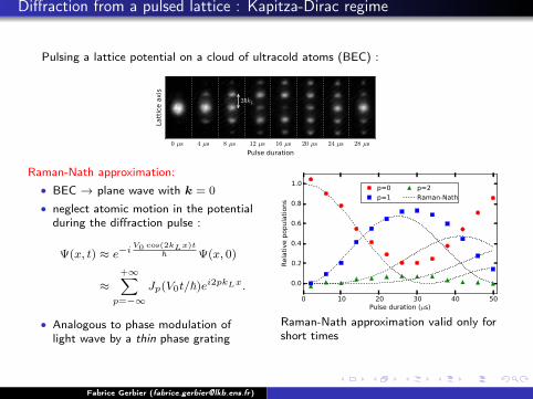
Diffraction from a pulsed lattice : Kapitza-Dirac regime
Pulsing a lattice potential on a cloud of ultracold atoms (BEC) :
Pulse durationLa
ttic
e a
xis
0 µs 4 µs 8 µs
2 kL
12 µs 16 µs 20 µs 24 µs 28 µs
Raman-Nath approximation:• BEC → plane wave with k = 0
• neglect atomic motion in the potentialduring the diffraction pulse :
Ψ(x, t) ≈ e−iV0 cos(2kLx)t
~ Ψ(x, 0)
≈+∞∑p=−∞
Jp(V0t/~)ei2pkLx.
• Analogous to phase modulation oflight wave by a thin phase grating
0 10 20 30 40 50Pulse duration (µs)
0.0
0.2
0.4
0.6
0.8
1.0
Rela
tive p
opula
tions
p=0
p=1
p=2
Raman-Nath
Raman-Nath approximation valid only forshort times
Fabrice Gerbier ([email protected])

1 Introduction
2 Band structure in one dimension
3 Thermodynamics of Bose gases in optical lattices
4 Dynamics of Bose-Einstein condensates in optical lattices
5 Bloch oscillations
Fabrice Gerbier ([email protected])
Bloch theorem
Hamiltonian :
H =p2
2M+ Vlat(x), Vlat(x) = −V0 sin2 (kLx)
Lattice translation operator :• definition : Td = exp (ipd/~)
• 〈x|Td|φ〉 = φ (x+ d) for any |φ〉• [Td, H] = 0.
Bloch theorem : Simultaneous eigenstates of H and Td (Bloch waves) are of the form
φn,q (x) = eiqxun,q (x) ,
where the un,q ’s (Bloch functions) are periodic in space with period d.
• q : quasi-momentum• n : band index
Fabrice Gerbier ([email protected])
Bloch theorem
Bloch waves :
φn,q (x) = eiqxun,q (x) ,
where the un,q ’s (Bloch functions) are periodic in space with period d.
• q : quasi-momentum• n : band index
Quasi-momentum is defined from the eigenvalue of Td :
Tdφn,q (x) = eiqdφn,q (x) .
For Qp = 2pkL with p integer (a vector of the reciprocal lattice),
Tdφn,q+Qp (x) = ei(q+Qp)dφn,q+Qp (x) = eiqdφn,q+Qp (x) .
To avoid double-counting, restrict q to the
first Brillouin zone: BZ1 = [−kL, kL].
Fabrice Gerbier ([email protected])
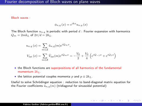
Fourier decomposition of Bloch waves on plane waves
Bloch waves :
φn,q (x) = eikxun,q (x)
The Bloch function un,q is periodic with period d : Fourier expansion with harmonicsQm = 2mkL of 2π/d = 2kL.
un,q (x) =∑m∈Z
un,q(m)eiQmx,
Vlat (x) =∑m∈Z
Vlat(m)eiQmx = −V0
2+V0
4
(eiQ−1x + eiQ1x
)
• the Bloch functions are superpositions of all harmonics of the fundamentalmomentum 2kL.
• the lattice potential couples momenta p and p± 2kL.
Useful to solve Schrödinger equation : reduction to band-diagonal matrix equation forthe Fourier coefficients un,q(m) (tridiagonal for sinusoidal potential)
Fabrice Gerbier ([email protected])
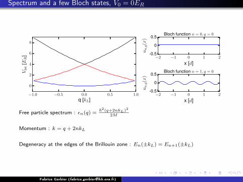
Spectrum and a few Bloch states, V0 = 0ER
−1.0 −0.5 0.0 0.5 1.0
q [kL]
0
2
4
6
8
Vla
t[E
R] −2 −1 0 1 2
x [d]
-0.5
0
0.5
un,q
(x)
Bloch function n = 0, q = 0
−2 −1 0 1 2
x [d]
-0.5
0
0.5
un,q
(x)
Bloch function n = 1, q = 0
Free particle spectrum : εn(q) =~2(q+2nkL)2
2M
Momentum : k = q + 2nkL
Degeneracy at the edges of the Brillouin zone : En(±kL) = En+1(±kL)
Fabrice Gerbier ([email protected])
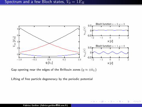
Spectrum and a few Bloch states, V0 = 1ER
−1.0 −0.5 0.0 0.5 1.0
q [kL]
0
2
4
6
8
Vla
t[E
R] −2 −1 0 1 2
x [d]
-0.5
0
0.5
un,q
(x)
Bloch function n = 0, q = 0
−2 −1 0 1 2
x [d]
-0.5
0
0.5
un,q
(x)
Bloch function n = 1, q = 0
Gap opening near the edges of the Brillouin zones (q ≈ ±kL)
Lifting of free particle degeneracy by the periodic potential
Fabrice Gerbier ([email protected])
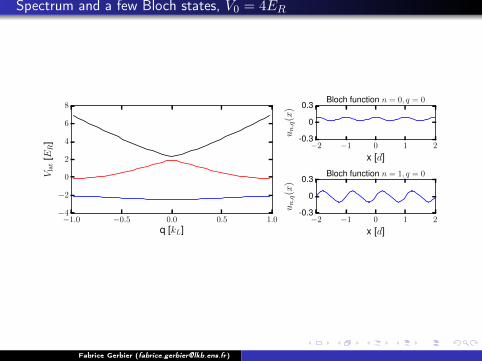
Spectrum and a few Bloch states, V0 = 4ER
−1.0 −0.5 0.0 0.5 1.0
q [kL]
−4
−2
0
2
4
6
8
Vla
t[E
R] −2 −1 0 1 2
x [d]
-0.3
0
0.3
un,q
(x)
Bloch function n = 0, q = 0
−2 −1 0 1 2
x [d]
-0.3
0
0.3
un,q
(x)
Bloch function n = 1, q = 0
Fabrice Gerbier ([email protected])
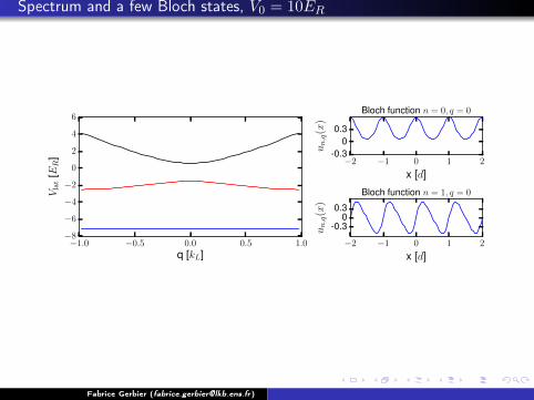
Spectrum and a few Bloch states, V0 = 10ER
−1.0 −0.5 0.0 0.5 1.0
q [kL]
−8
−6
−4
−2
0
2
4
6
Vla
t[E
R] −2 −1 0 1 2
x [d]
-0.30
0.3
un,q
(x)
Bloch function n = 0, q = 0
−2 −1 0 1 2
x [d]
-0.30
0.3
un,q
(x)
Bloch function n = 1, q = 0
Fabrice Gerbier ([email protected])
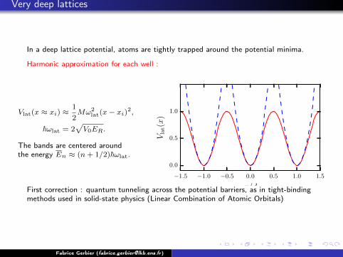
Very deep lattices
In a deep lattice potential, atoms are tightly trapped around the potential minima.
Harmonic approximation for each well :
Vlat(x ≈ xi) ≈1
2Mω2
lat(x− xi)2,
~ωlat = 2√V0ER.
The bands are centered aroundthe energy En ≈ (n+ 1/2)~ωlat.
−1.5 −1.0 −0.5 0.0 0.5 1.0 1.5
x/d
0.0
0.5
1.0
Vla
t(x
)
First correction : quantum tunneling across the potential barriers, as in tight-bindingmethods used in solid-state physics (Linear Combination of Atomic Orbitals)
Fabrice Gerbier ([email protected])
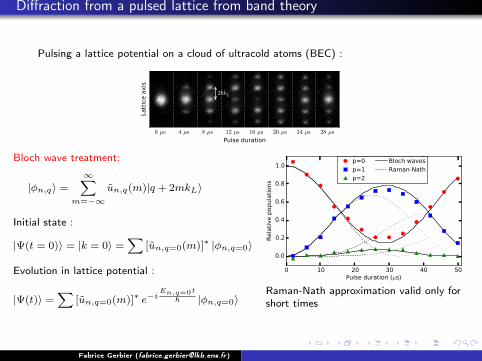
Diffraction from a pulsed lattice from band theory
Pulsing a lattice potential on a cloud of ultracold atoms (BEC) :
Pulse durationLa
ttic
e a
xis
0 µs 4 µs 8 µs
2 kL
12 µs 16 µs 20 µs 24 µs 28 µs
Bloch wave treatment:
|φn,q〉 =
∞∑m=−∞
un,q(m)|q + 2mkL〉
Initial state :
|Ψ(t = 0)〉 = |k = 0〉 =∑
[un,q=0(m)]∗ |φn,q=0〉
Evolution in lattice potential :
|Ψ(t)〉 =∑
[un,q=0(m)]∗ e−iEn,q=0t
~ |φn,q=0〉
0 10 20 30 40 50Pulse duration (µs)
0.0
0.2
0.4
0.6
0.8
1.0
Rela
tive p
opula
tions
p=0
p=1
p=2
Bloch waves
Raman-Nath
Raman-Nath approximation valid only forshort times
Fabrice Gerbier ([email protected])

1 Introduction
2 Band structure in one dimension
3 Thermodynamics of Bose gases in optical lattices
4 Dynamics of Bose-Einstein condensates in optical lattices
5 Bloch oscillations
Fabrice Gerbier ([email protected])
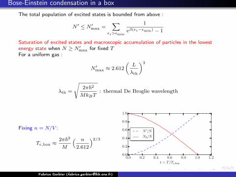
Bose-Einstein condensation in a box
The total population of excited states is bounded from above :
N ′ ≤ N ′max =∑
εi>εmin
1
eβ(εi−εmin) − 1
Saturation of excited states and macroscopic accumulation of particles in the lowestenergy state when N ≥ N ′max for fixed TFor a uniform gas :
N ′max ≈ 2.612
(L
λth
)3
λth =
√2π~2
MkBT: thermal De Broglie wavelength
Fixing n = N/V :
Tc,box ≈2π~2
M
( n
2.612
)2/3
0.0 0.2 0.4 0.6 0.8 1.0 1.2t = T/Tc,box
0.0
0.2
0.4
0.6
0.8
1.0
N ′/N
N0/N
Fabrice Gerbier ([email protected])
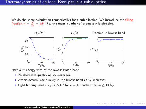
Thermodynamics of an ideal Bose gas in a cubic lattice
We do the same calculation (numerically) for a cubic lattice. We introduce the fillingfraction n = N
Ns= ρd3, i.e. the mean number of atoms per lattice site.
Tc/ER Tc/J Fraction in lowest band
0 10 200
0.2
0.4
0.6
V0/ER
T c/ER
0 10 200
2
4
6
V0/ER
T c/J
0 10 200
0.5
1
V0/ER
f 0
Here J ≡ energy with of the lowest Bloch band.• Tc decreases quickly as V0 increases,• Atoms accumulate quickly in the lowest band as V0 increases.• tight-binding limit : kBTc ≈ 6J for n = 1, reached for V0 ≥ 10ER,
Fabrice Gerbier ([email protected])
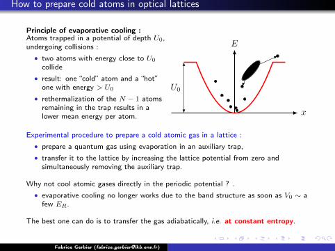
How to prepare cold atoms in optical lattices
Principle of evaporative cooling :Atoms trapped in a potential of depth U0,undergoing collisions :
• two atoms with energy close to U0
collide• result: one “cold” atom and a “hot”one with energy > U0
• rethermalization of the N − 1 atomsremaining in the trap results in alower mean energy per atom. x
E
U0
Experimental procedure to prepare a cold atomic gas in a lattice :• prepare a quantum gas using evaporation in an auxiliary trap,• transfer it to the lattice by increasing the lattice potential from zero andsimultaneously removing the auxiliary trap.
Why not cool atomic gases directly in the periodic potential ? .• evaporative cooling no longer works due to the band structure as soon as V0 ∼ afew ER.
The best one can do is to transfer the gas adiabatically, i.e. at constant entropy.
Fabrice Gerbier ([email protected])
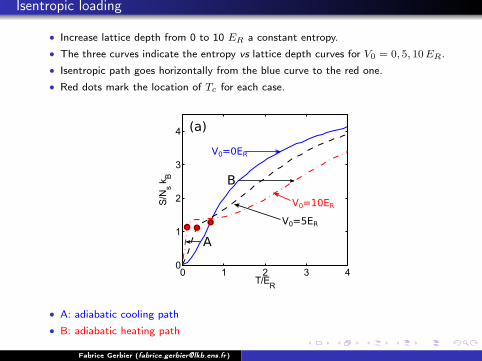
Isentropic loading
• Increase lattice depth from 0 to 10 ER a constant entropy.• The three curves indicate the entropy vs lattice depth curves for V0 = 0, 5, 10ER.• Isentropic path goes horizontally from the blue curve to the red one.• Red dots mark the location of Tc for each case.
• A: adiabatic cooling path• B: adiabatic heating path
Fabrice Gerbier ([email protected])
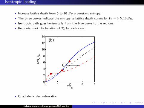
Isentropic loading
• Increase lattice depth from 0 to 10 ER a constant entropy.• The three curves indicate the entropy vs lattice depth curves for V0 = 0, 5, 10ER.• Isentropic path goes horizontally from the blue curve to the red one.• Red dots mark the location of Tc for each case.
• C: adiabatic decondensation
Fabrice Gerbier ([email protected])

1 Introduction
2 Band structure in one dimension
3 Thermodynamics of Bose gases in optical lattices
4 Dynamics of Bose-Einstein condensates in optical lattices
5 Bloch oscillations
Fabrice Gerbier ([email protected])
Adiabatic theorem
Quantum adiabatic theorem :
Slowly evolving quantum system, with Hamiltonian H(t).
Instantaneous eigenbasis of H: H(t)|φn(t)〉 = εn(t)|φn(t)〉.
Time-dependent wave function in the {|φn(t)〉} basis:
|Ψ(t)〉 =∑n
an(t)e−i~
∫ t0 εn(t′)dt′ |φn(t)〉,
From Schrödinger equation, one gets [ωmn = εm − εn] :
an = −〈φn|φn〉an(t)−∑m 6=n
e−i~
∫ t0 ωmn(t′)dt′ 〈φn|φm〉am(t),
• Berry phase : 〈φn|φn〉 = −iγB is a pure phase. Wavefunction unchanged up to aphase evolution after a cyclic change.
• The adiabatic theorem : for arbitrarily slow evolution starting from a particularstate n0 (an(0) = δn,n0 ), and in the absence of level crossings, an(t)→ δn,n0
(up to a global phase).
Fabrice Gerbier ([email protected])
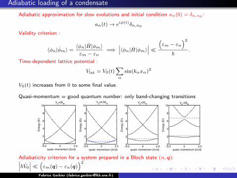
Adiabatic loading of a condensate
Adiabatic approximation for slow evolutions and initial condition an(0) = δn,n0 :
an(t)→ eiφ(t)δn,n0
Validity criterion :
〈φn|φm〉 =〈φn|H|φm〉εm − εn
=⇒∣∣∣〈φn|H|φm〉∣∣∣�
(εm − εn
)2
~.
Time-dependent lattice potential :
Vlat = V0(t)∑α
sin(kαxα)2
V0(t) increases from 0 to some final value.
Quasi-momentum = good quantum number: only band-changing transitions
−0.5 0 0.50
2
4
6
8
10
quasi−momentum (2//d)
Ener
gy (E
r)
V0=0.5ER
−0.5 0 0.50
2
4
6
8
10
quasi−momentum (2//d)
Ener
gy (E
r)
V0=0ER
−0.5 0 0.50
2
4
6
8
10
quasi−momentum (2//d)
Ener
gy (E
r)
V0=2ER
−0.5 0 0.50
2
4
6
8
10
quasi−momentum (2//d)
Ener
gy (E
r)
V0=5ER
Adiabaticity criterion for a system prepared in a Bloch state (n, q):∣∣∣~V0
∣∣∣� (εm(q)− εn(q)
)2
Fabrice Gerbier ([email protected])
Adiabatic loading of a condensate
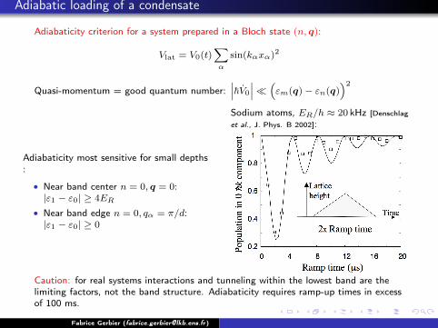
Adiabaticity criterion for a system prepared in a Bloch state (n, q):
Vlat = V0(t)∑α
sin(kαxα)2
Quasi-momentum = good quantum number:∣∣∣~V0
∣∣∣� (εm(q)− εn(q)
)2
Adiabaticity most sensitive for small depths:
• Near band center n = 0, q = 0:|ε1 − ε0| ≥ 4ER
• Near band edge n = 0, qα = π/d:|ε1 − ε0| ≥ 0
Sodium atoms, ER/h ≈ 20 kHz [Denschlaget al., J. Phys. B 2002]:
Caution: for real systems interactions and tunneling within the lowest band are thelimiting factors, not the band structure. Adiabaticity requires ramp-up times in excessof 100 ms.
Fabrice Gerbier ([email protected])
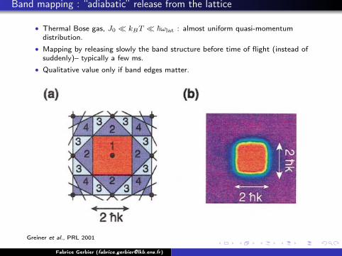
Band mapping : “adiabatic” release from the lattice
• Thermal Bose gas, J0 � kBT � ~ωlat : almost uniform quasi-momentumdistribution.
• Mapping by releasing slowly the band structure before time of flight (instead ofsuddenly)– typically a few ms.
• Qualitative value only if band edges matter.
Greiner et al., PRL 2001
Fabrice Gerbier ([email protected])
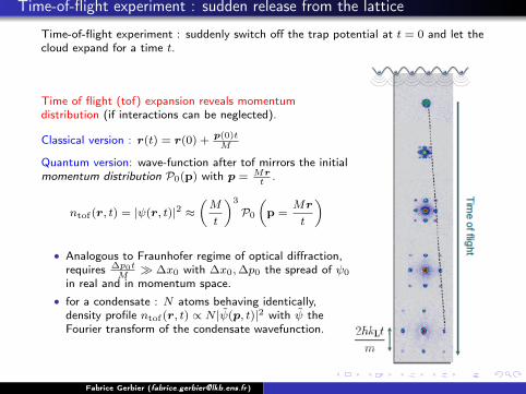
Time-of-flight experiment : sudden release from the lattice
Time-of-flight experiment : suddenly switch off the trap potential at t = 0 and let thecloud expand for a time t.
Time of flight (tof) expansion reveals momentumdistribution (if interactions can be neglected).
Classical version : r(t) = r(0) +p(0)tM
Quantum version: wave-function after tof mirrors the initialmomentum distribution P0(p) with p = Mr
t.
ntof(r, t) = |ψ(r, t)|2 ≈(M
t
)3
P0
(p =
Mr
t
)
• Analogous to Fraunhofer regime of optical diffraction,requires ∆p0t
M� ∆x0 with ∆x0,∆p0 the spread of ψ0
in real and in momentum space.• for a condensate : N atoms behaving identically,density profile ntof(r, t) ∝ N |ψ(p, t)|2 with ψ theFourier transform of the condensate wavefunction.
Fabrice Gerbier ([email protected])
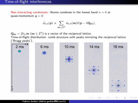
Time-of-flight interferences
Non-interacting condensate: Atoms condense in the lowest band n = 0 atquasi-momentum q = 0:
φ0,0(p) ∝∑
m∈Z3
u0,0(m)δ(p− ~Qm),
Qm = 2kLm (m ∈ Z3) is a vector of the reciprocal lattice.Time-of-flight distribution: comb structure with peaks mirroring the reciprocal lattice(“Bragg peaks”).
Fabrice Gerbier ([email protected])

1 Introduction
2 Band structure in one dimension
3 Thermodynamics of Bose gases in optical lattices
4 Dynamics of Bose-Einstein condensates in optical lattices
5 Bloch oscillations
Fabrice Gerbier ([email protected])
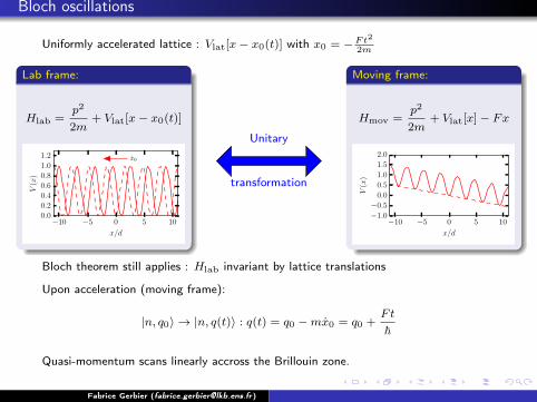
Bloch oscillations
Uniformly accelerated lattice : Vlat[x− x0(t)] with x0 = −Ft2
2m
Lab frame:
Hlab =p2
2m+ Vlat[x− x0(t)]
−10 −5 0 5 10
x/d
0.00.20.40.60.81.01.2
V(x
)
x0
Unitary
transformation
Moving frame:
Hmov =p2
2m+ Vlat[x]− Fx
−10 −5 0 5 10
x/d
−1.0
−0.5
0.0
0.5
1.0
1.5
2.0
V(x
)
Bloch theorem still applies : Hlab invariant by lattice translations
Upon acceleration (moving frame):
|n, q0〉 → |n, q(t)〉 : q(t) = q0 −mx0 = q0 +Ft
~
Quasi-momentum scans linearly accross the Brillouin zone.
Fabrice Gerbier ([email protected])
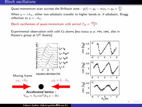
Bloch oscillations
Quasi-momentum scan accross the Brillouin zone : q(t) = q0 −mx0 = q0 + Ft~
When q = +kL, either non-adiabatic transfer to higher bands or, if adiabatic, Braggreflection to q = −kL.
Bloch oscillations of quasi-momentum with period TB = 2~kLF
Experimental observation with cold Cs atoms [Ben Dahan et al., PRL 1995, also inRaizen’s group at UT Austin]:
Moving frameωL,+kL ωL + δ,−kL
Accelerated lattice :Vlat = V0 cos2(kLx− δt)
Fabrice Gerbier ([email protected])
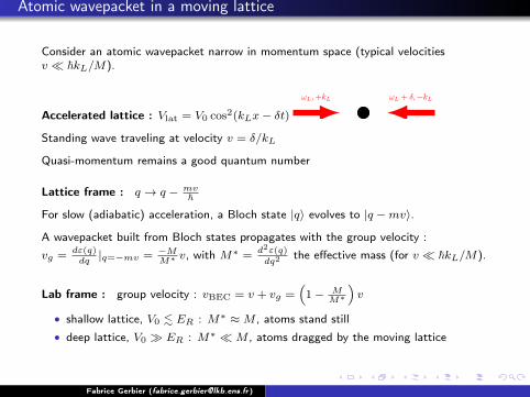
Atomic wavepacket in a moving lattice
Consider an atomic wavepacket narrow in momentum space (typical velocitiesv � ~kL/M).
Accelerated lattice : Vlat = V0 cos2(kLx− δt)ωL,+kL ωL + δ,−kL
Standing wave traveling at velocity v = δ/kL
Quasi-momentum remains a good quantum number
Lattice frame : q → q − mv~
For slow (adiabatic) acceleration, a Bloch state |q〉 evolves to |q −mv〉.
A wavepacket built from Bloch states propagates with the group velocity :
vg =dε(q)dq|q=−mv = −M
M∗ v, with M∗ =
d2ε(q)
dq2the effective mass (for v � ~kL/M).
Lab frame : group velocity : vBEC = v + vg =(
1− MM∗
)v
• shallow lattice, V0 . ER : M∗ ≈M , atoms stand still• deep lattice, V0 � ER : M∗ �M , atoms dragged by the moving lattice
Fabrice Gerbier ([email protected])
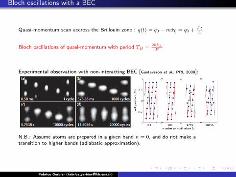
Bloch oscillations with a BEC
Quasi-momentum scan accross the Brillouin zone : q(t) = q0 −mx0 = q0 + Ft~
Bloch oscillations of quasi-momentum with period TB = 2~kLF
Experimental observation with non-interacting BEC [Gustavsson et al., PRL 2008]:
N.B.: Assume atoms are prepared in a given band n = 0, and do not make atransition to higher bands (adiabatic approximation).
Fabrice Gerbier ([email protected])
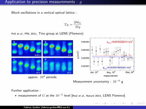
Application to precision measurements : g
Bloch oscillations in a vertical optical lattice :
TB =2~kLMg
Poli et al., PRL 2011, Tino group at LENS (Florence)
approx. 104 periodsMeasurement uncertainty : 10−6 g
Further application :• measurement of G at the 10−5 level [Rosi et al., Nature 2014, LENS Florence]
Fabrice Gerbier ([email protected])
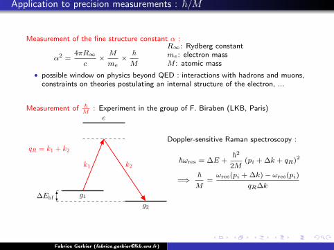
Application to precision measurements : ~/M
Measurement of the fine structure constant α :
α2 =4πR∞
c×M
me×
~M
R∞: Rydberg constantme: electron massM : atomic mass
• possible window on physics beyond QED : interactions with hadrons and muons,constraints on theories postulating an internal structure of the electron, ...
Measurement of ~M
: Experiment in the group of F. Biraben (LKB, Paris)
g1
g2
e
k1 k2
∆Ehf
qR = k1 + k2
Doppler-sensitive Raman spectroscopy :
~ωres = ∆E +~2
2M(pi + ∆k + qR)2
=⇒~M
=ωres(pi + ∆k)− ωres(pi)
qR∆k
Fabrice Gerbier ([email protected])
Application to precision measurements : ~/M
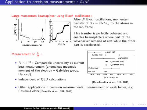
Large momentum beamsplitter using Bloch oscillations :After N Bloch oscillations, momentumtransfer of ∆k = 2N~kL to the atoms inthe lab frame.
This transfer is perfectly coherent andenables beamsplitters where part of thewavepacket remains at rest while the otherpart is accelerated.
Measurement of ~M
:
• N ∼ 103 : Comparable uncertainty as currentbest measurement (anomalous magneticmoment of the electron – Gabrielse group,Harvard).
• Independent of QED calculations[Bouchendira et al., PRL 2011]
• Other applications in precision measurements: measurement of weak forces, e.g.Casimir-Polder [Beaufils et al., PRL 2011].
Fabrice Gerbier ([email protected])