On the minimum dilatation of pseudo-Anosov homeromorphisms ... · SYSTOLE IN SMALL GENUS 107 that realize δ 2, in the mapping class group of genus 2 surfaces, Mod(2) (see Theorem

AN

NALESDE

L’INSTIT

UTFOUR

IER

ANNALESDE

L’INSTITUTFOURIER

Erwan LANNEAU & Jean-Luc THIFFEAULT

On the minimum dilatation of pseudo-Anosov homeromorphisms onsurfaces of small genusTome 61, no 1 (2011), p. 105-144.

<http://aif.cedram.org/item?id=AIF_2011__61_1_105_0>

© Association des Annales de l’institut Fourier, 2011, tous droitsréservés.

L’accès aux articles de la revue « Annales de l’institut Fourier »(http://aif.cedram.org/), implique l’accord avec les conditionsgénérales d’utilisation (http://aif.cedram.org/legal/). Toute re-production en tout ou partie cet article sous quelque forme quece soit pour tout usage autre que l’utilisation à fin strictementpersonnelle du copiste est constitutive d’une infraction pénale.Toute copie ou impression de ce fichier doit contenir la présentemention de copyright.

cedramArticle mis en ligne dans le cadre du

Centre de diffusion des revues académiques de mathématiqueshttp://www.cedram.org/

http://aif.cedram.org/item?id=AIF_2011__61_1_105_0

http://aif.cedram.org/

http://aif.cedram.org/legal/

http://www.cedram.org/

http://www.cedram.org/

Ann. Inst. Fourier, Grenoble61, 1 (2011) 105-144

ON THE MINIMUM DILATATIONOF PSEUDO-ANOSOV HOMEROMORPHISMS

ON SURFACES OF SMALL GENUS

by Erwan LANNEAU & Jean-Luc THIFFEAULT

Abstract. — We find the minimum dilatation of pseudo-Anosov homeo-morphisms that stabilize an orientable foliation on surfaces of genus three, four,or five, and provide a lower bound for genus six to eight. Our technique alsosimplifies Cho and Ham’s proof of the least dilatation of pseudo-Anosov homeo-morphisms on a genus two surface. For genus g = 2 to 5, the minimum dilatationis the smallest Salem number for polynomials of degree 2g.

Résumé. — Nous calculons la plus petite dilatation d’un homéomorphismede type pseudo-Anosov laissant invariant un feuilletage mesuré orientable surune surface de genre g pour g = 3, 4, 5. Nous donnons aussi une borne inférieurepour les genres 6, 7 et 8. Nos techniques simplifient la preuve de Cho et Hamsur le calcul de la plus petite dilatation d’un homéomorphisme de type pseudo-Anosov sur une surface de genre 2. Pour g = 2 à 5, la plus petite dilatation estle plus petit nombre de Salem pour les polynomes à degré fixé 2g.

1. Introduction

This paper concerns homeomorphisms of a compact oriented surface Mto itself. There are natural equivalence classes of such homeomorphismsunder isotopy, called isotopy classes or mapping classes. An irreduciblemapping class is such that no power of its members preserves a nontriv-ial subsurface. By the Thurston–Nielsen classification [28], irreducible

Keywords: Pseudo-Anosov homeomorphism, small dilatation, flat surface.Math. classification: 37D40, 37E30.

106 Erwan LANNEAU & Jean-Luc THIFFEAULT

mapping classes are either finite-order or are of a type called pseudo-Anosov. The class of pseudo-Anosov homeomorphisms is by far the rich-est. One can think of such a homeomorphism φ as an Anosov (or hyper-bolic) homeomorphism on M\ {singularities}. In particular, as for stan-dard Anosov on the two dimensional torus, there exists a local Euclideanstructure (with singularities) and two linear foliations (Fs and Fu, calledstable and unstable) such that φ expands the leaves of one foliation witha coefficient λ, and shrinks those of the other foliation with the samecoefficient. The number λ is a topological invariant called the dilatationof φ; the number log(λ) is the topological entropy of φ.

Thurston proved that λ + λ−1 is an algebraic integer (in fact, it is aPerron number) over Q of degree bounded by 4g− 3. In particular New-ton’s formulas imply that for each g > 2 the set of dilatations boundedfrom above by a constant is finite. Hence the minimum value δg of the di-latation of pseudo-Anosov homeomorphisms on M is well defined [2, 13].It can be shown that the logarithm of δg is the length of the shortestgeodesics on the moduli space of complex curves of genus g,Mg (for theTeichmüller metric).

Two natural questions arise. The first is how to compute δg explicitlyfor small g > 2. The second question asks if there is a unique (up to con-jugacy) pseudo-Anosov homeomorphism with minimum dilatation in themodular group Mod(g). It is well known that δ1 = 1

2 (3+√

5) and this di-latation is uniquely realized by the conjugacy class in Mod(1) = PSL2(Z)of the matrix ( 2 1

1 1 ). In principle these dilatations can be computed forany given g using train tracks. Of course actually carrying out this pro-cedure, even for small values of g, seems impractical.

We know very little about the value of the constants δg. Using acomputer and train tracks techniques for the punctured disc, Cho andHam [7] proved that δ2 is equal to the largest root of the polynomialX4−X3−X2−X+1, δ2 ' 1.72208 [7]. One of the results of the presentpaper is an independent and elementary proof of this fact.

One can also ask about the uniqueness (up to conjugacy) of pseudo-Anosov homeomorphisms that realize δg. In genus 2, δ2 is not unique dueto the existence of the hyperelliptic involution and covering transforma-tions (see Section 4 and Remark 4.1 for a precise definition). But, upto hyperelliptic involution and covering transformations, we prove theuniqueness of the conjugacy class of pseudo-Anosov homeomorphisms

ANNALES DE L’INSTITUT FOURIER

SYSTOLE IN SMALL GENUS 107

that realize δ2, in the mapping class group of genus 2 surfaces, Mod(2)(see Theorem 1.1).

For g > 1 the estimate 21/(12g−12) 6 δg 6 (2 +√

3)1/g holds [25, 12].We will denote by δ+

g the minimum value of the dilatation of pseudo-Anosov homeomorphisms on a genus g surface with orientable invariantfoliations. We shall prove:

Theorem 1.1. — The minimum dilatation of a pseudo-Anosov ho-meomorphism on a genus two surface is equal to the largest root of thepolynomial X4 −X3 −X2 −X + 1,

δ2 = δ+2 = 1

4 +√

134 + 1

2

√√132 −

12 ' 1.72208.

Moreover there exists a unique (up to conjugacy, hyperelliptic involu-tion, and covering transformations) pseudo-Anosov homeomorphism ona genus two surface with dilatation δ2.

Remark. — This answers Problem 7.3 and Question 7.4 of Farb [8]in genus two.

Theorem 1.2. — The minimum value of the dilatation of pseudo-Anosov homeomorphisms on a genus g surface, 3 6 g 6 5, with orientableinvariant foliations is equal to the largest root of the polynomials inTable 1.1.

g polynomial δ+g '

3 X6 −X4 −X3 −X2 + 1 1.401274 X8 −X5 −X4 −X3 + 1 1.280645 X10 +X9 −X7 −X6 −X5 −X4 −X3 +X + 1 1.17628

Table 1.1

All of the minimum dilatations for 2 6 g 6 5 are Salem numbers [26].In fact, their polynomials have the smallest Mahler measure over poly-nomials of their degree [4]. For g = 5, the dilatation is realized by thepseudo-Anosov homeomorphism described by Leininger [19] as a compo-sition of Dehn twists about two multicurves. Its characteristic polynomialis the irreducible one having Lehmer’s number as a root: this is the small-est known Salem number. The polynomial has the smallest known Mahlermeasure over all integral polynomials.

TOME 61 (2011), FASCICULE 1


For g = 3 and 4, we have constructed explicit examples. We present twoindependent constructions in this paper: The first is given in term of Dehntwists on a surface; The second involves the Rauzy–Veech construction(see Appendix B).

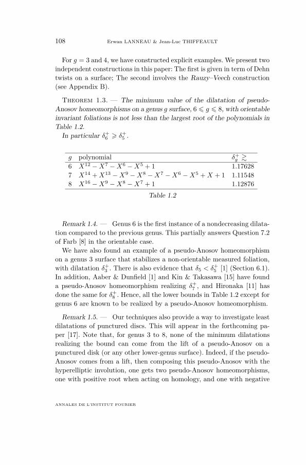
Theorem 1.3. — The minimum value of the dilatation of pseudo-Anosov homeomorphisms on a genus g surface, 6 6 g 6 8, with orientableinvariant foliations is not less than the largest root of the polynomials inTable 1.2.

In particular δ+6 > δ+

5 .

g polynomial δ+g &

6 X12 −X7 −X6 −X5 + 1 1.176287 X14 +X13 −X9 −X8 −X7 −X6 −X5 +X + 1 1.115488 X16 −X9 −X8 −X7 + 1 1.12876

Table 1.2

Remark 1.4. — Genus 6 is the first instance of a nondecreasing dilata-tion compared to the previous genus. This partially answers Question 7.2of Farb [8] in the orientable case.

We have also found an example of a pseudo-Anosov homeomorphismon a genus 3 surface that stabilizes a non-orientable measured foliation,with dilatation δ+

3 . There is also evidence that δ5 < δ+5 [1] (Section 6.1).

In addition, Aaber & Dunfield [1] and Kin & Takasawa [15] have founda pseudo-Anosov homeomorphism realizing δ+

7 , and Hironaka [11] hasdone the same for δ+

8 . Hence, all the lower bounds in Table 1.2 except forgenus 6 are known to be realized by a pseudo-Anosov homeomorphism.

Remark 1.5. — Our techniques also provide a way to investigate leastdilatations of punctured discs. This will appear in the forthcoming pa-per [17]. Note that, for genus 3 to 8, none of the minimum dilatationsrealizing the bound can come from the lift of a pseudo-Anosov on apunctured disk (or any other lower-genus surface). Indeed, if the pseudo-Anosov comes from a lift, then composing this pseudo-Anosov with thehyperelliptic involution, one gets two pseudo-Anosov homeomorphisms,one with positive root when acting on homology, and one with negative



root. Since the polynomials we find have only one sign of the dominantroot when acting on homology, a lift is always ruled out. This is in con-trast to the Hironaka & Kin [12] examples, which come from punctureddisks.

Acknowledgments. The authors thank Christopher Leininger, FrédéricLe Roux, Jérôme Los, Sarah Matz, and Rupert Venzke for helpful conver-sations, and are grateful to Matthew D. Finn for help in finding pseudo-Anosov homeomorphisms in terms of Dehn twists. J-LT thanks the Cen-tre de Physique Théorique de Marseille, where this work began, for itshospitality. J-LT was also supported by the Division of Mathematical Sci-ences of the US National Science Foundation, under grant DMS-0806821.

2. Background and tools

In this section we recall some general properties of dilatations andpseudo-Anosov homeomorphisms, namely algebraic and spectral radiusproperties. We also summarizes basic tools for proving our results (forexample see [28, 9, 22, 23]).

To guide the reader, we will first outline the general method used tofind the least dilatation δ+

g :Summary: to find the least dilatation δ+

g on a surface M of genus g.(1) Start with a known pseudo-Anosov homeomorphism on M , with

dilatation α, that stabilizes orientable foliations (we use the fam-ily in [12]).

(2) Enumerate all reciprocal polynomials with Perron root less that α(see Section 2.2 for definitions, and Appendix A for an explicitalgorithm). For genus g > 2, this requires a computer, but is astandard calculation.

(3) Of these polynomials, eliminate the ones that are incompatiblewith the Lefschetz theorem (see Section 2.3). The remaining poly-nomial with the smallest root gives a lower bound on the leastdilatation δ+

g . For genus g > 4, this step requires a computer.(4) If possible, construct an explicit pseudo-Anosov homeomorphism

on M having the lower bound in the previous step as a dilatation.We do this by either exhibiting a sequence of Dehn twists, or by



the Rauzy–Veech construction (see Appendix B). This confirmsthat we have found δ+

g .

2.1. Affine structures and affine homeomorphisms

To each pseudo-Anosov homeomorphism φ one can associate an affinestructure on M for which φ is affine.

2.1.1. Affine structures

A surface of genus g > 1 is called a flat surface if it can be obtainedby edge-to-edge gluing of polygons in the plane using translations ortranslations composed with − id. We will call such a surface (M, q) whereq is the form dz2 defined locally. The metric on M has zero curvatureexcept at the zeroes of q where the metric has conical singularities of angle(k + 2)π (with k > −1). The integer k is called the degree of the zeroof q. A point that is not singular is regular. We will use the conventionthat a singular point of degree 0 is regular. A measured foliation M is alinear flow on this flat surface M for an affine structure.

The Gauss–Bonnet formula applied to the singularities reads∑i ki =

4g−4. We will call the integer vector (or simply the stratum) (k1, . . . , kn)with ki > −1 the singularity data of the measured foliation.

If one restricts gluing to translations only then the surface is called atranslation surface; otherwise it is called a half-translation surface. For atranslation surface the degree of all singularities is even; the converse isfalse in general.

There is a standard construction, the orientating cover, that producea translation surface from a half-translation surface.

Construction 2.1. — Let N be a half-translation surface with sin-gularity data (k1, . . . , kn). Then there exists a translation surface M anda double branched cover π : M → N , branched precisely over the singu-lar points of odd degree. In addition π is the minimal double branchedcover in this class.



2.1.2. Affine homeomorphisms

A homeomorphism f is affine with respect to (M, q) if f permutes thesingularities, f is a diffeomorphism on the complement of the singulari-ties, and the derivative map Df of f is a constant matrix in PSL2(R).

There is a standard classification of the elements of PSL2(R) into threetypes: elliptic, parabolic and hyperbolic. This induces a classification ofaffine homeomorphisms. An affine homeomorphism is parabolic, ellip-tic, or pseudo-Anosov, respectively, if |Tr(Df)| = 2, Tr(Df)| < 2, or|Tr(Df)| > 2, respectively (where Tr is the trace).

2.1.3. Pseudo-Anosov homeomorphisms

Since we are interested in pseudo-Anosov homeomorphisms we willassume that |Tr(Df)| > 2. Then there exists an eigenvalue λ of Df suchthat |λ| > 1 and Tr(Df) = λ + λ−1. The two eigenvectors associatedto λ and λ−1 determine two directions on the flat surface M , invariantby φ. Of course φ expends leaves of the stable foliation by the factor|λ| and shrinks leaves of the unstable foliation by the same factor. Wecan assume that these directions are horizontal and vertical. In thesecoordinates (M, q), the pair of associated measured foliations (stable andunstable) of φ are given by the horizontal and vertical measured foliationsIm(q) and Re(q) and the derivative of φ is the matrix A =

(±λ−1 0

0 ±λ

).

By construction the dilatation λ(φ) of φ equals |λ|. The singularity dataof a pseudo-Anosov φ is the singularity data of its invariant measuredfoliation.

The group PSL2(R) naturally acts on the set of flat surfaces. Withabove notations the matrix A fixes the surface (M, q), that is, (M, q)can be obtained from A · (M, q) by “cutting” and “gluing” (i.e., the twosurfaces represent the same point in the moduli space). The converseis true: if A stabilizes a flat surface (M, q), then there exists an affinediffeomorphism f : M →M such that Df = A.

Masur and Smillie [21] proved the following result:

Theorem 2.1 (Masur, Smillie). — For each integer partition (k1, . . . ,

kn) of 4g−4 with ki > 0 even, there is a pseudo-Anosov homeomorphism



φ with singularity data (k1, . . . , kn) that fixes an orientable measuredfoliation.

For each integer partition (k1, . . . , kn) of 4g−4 with ki > −1, there is apseudo-Anosov homeomorphism φ with singularity data (k1, . . . , kn) thatfixes a non-orientable measured foliation, with the following exceptions:

(1,−1), (1, 3), and (4).

Convention. — For the remainder of this paper, unless explicitlystated (in particular in Section 4), we shall assume that pseudo-Anosovhomeomorphisms preserve orientable measured foliations.

For instance, if g = 3 and φ preserves an orientable measured foliation,then there are 5 possible strata for the singularity data of φ:

(8), (2, 6), (4, 4), (2, 2, 4), and (2, 2, 2, 2).

2.2. Algebraic properties of dilatations

The next theorem follows from basic results in the theory of pseudo-Anosov homeomorphisms (see for example [28]).

Theorem 2.2 (Thurston). — Let φ be a pseudo-Anosov homeomor-phism on a genus g surface that leaves invariant an orientable measuredfoliation. Then

(1) The linear map φ∗ defined on H1(M,R) has a simple eigenvalueρ(φ∗) ∈ R such that |ρ(φ∗)| > |x| for all other eigenvalues x;

(2) φ is affine, for the affine structure determined by the measuredfoliations, and the eigenvalues of the derivative Dφ are ρ(φ∗)±1;

(3) |ρ(φ∗)| > 1 is the dilatation λ of φ.

A Perron root is an algebraic integer λ > 1 all whose other conjugatessatisfy |λ′| < λ. Observe that these are exactly the numbers that arise asthe leading eigenvalues of Perron–Frobenius matrices. Since φ∗ preservesa symplectic form, the characteristic polynomial χφ∗ is a reciprocal degree2g polynomial.

Remark 2.3. — The dilatation of a pseudo-Anosov homeomorphismφ is the Perron root of a reciprocal degree 2g polynomial, namely χφ∗(X)if ρ(φ∗) > 0 and χφ∗(−X) otherwise.



There is a converse to Theorem 2.2, but the proof does not seem aswell-known, so we include a proof here (see [3] Lemma 4.3).

Theorem 2.4. — Let φ be a pseudo-Anosov homeomorphism on asurface M with dilatation λ. Then the following are equivalent:

(1) λ is an eigenvalue of the linear map φ∗ defined on H1(M,R).(2) The invariant measured foliations of φ are orientable.

Proof. — Suppose the stable measured foliation on (M, q) is non-orien-table. There exists a double branched cover π : N → M which orientsthe foliation (we denote by τ the involution of the covering). Let [w]be an eigenvector of φ∗ in H1(M,R) with eigenvalue λ. The vector [w]pulls back to an eigenvector [w′] of the adjoint φ∗ in H1(N,R) for theeigenvalue λ.

The stable foliation on N now also defines a cohomology class [Re(ω)]where ω2 = π∗q. By construction [Re(ω)] is an eigenvector for the eigen-value λ. By Theorem 2.2 λ is simple so that the two classes [Re(ω)]and [w′] must be linearly dependent. But since [w′] is invariant by thedeck transformation τ , while [Re(ω)] is sent to −[Re(ω)] by τ , we get acontradiction. �

Combining this theorem with two classical results of Casson–Bleiler [6]and Thurston [9] we get

Theorem 2.5. — Let f be a homeomorphism on a surface M and letP (X) be the characteristic polynomial of the linear map f∗ defined onH1(M,R). Then one has

(1) If P (X) is irreducible over Z, has no roots of unity as zeroes,and is not a polynomial in Xk for k > 1, then f is isotopic to apseudo-Anosov homeomorphism φ;

(2) In addition, if the maximal eigenvalue (in absolute value) of theaction of f on the fundamental group is λ > 1, then the dilatationof φ is λ;

(3) In addition, if λ is the Perron root of P (X), then φ leaves invariantorientable measured foliations.

Proof. — The first point asserts that f is isotopic to a pseudo-Anosovhomeomorphism φ [6, Lemma 5.1]. The second point asserts that φ hasdilatation λ [9, Exposé 10]. Finally by the previous theorem, the last



assumption implies that the invariant measured foliations of φ are ori-entable. �

We will need a more precise statement. The following has been re-marked by Bestvina:

Proposition 2.6. — The statement “P is irreducible over Z” in part(1) of Theorem 2.5 can be replaced by “P is symplectically irreducibleover Z”, meaning that P is not the product of two nontrivial reciprocalpolynomials.

2.3. Pseudo-Anosov homeomorphismsand the Lefschetz theorem

In this section, we recall the well-known Lefschetz theorem for homeo-morphisms on compact surfaces (see for example [5]). If p is a fixed pointof a homeomorphism f , we define the index of f at p to be the algebraicnumber Ind(f, p) of turns of the vector (x, f(x)) when x describes a smallloop around p.

Theorem (Lefschetz theorem). — Let f be a homeomorphism on acompact surface M . Denote by Tr(f∗) the trace of the linear map f∗ de-fined on the first homology group H1(M,R). Then the Lefschetz numberL(f) is 2− Tr(f∗). Moreover the following equality holds:

L(f) =∑p=f(p)

Ind(f, p).

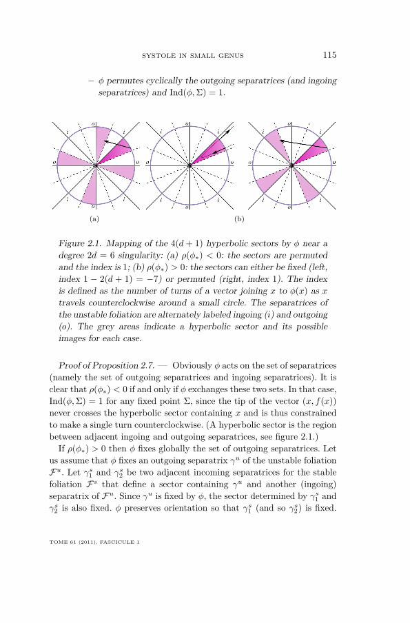
For a pseudo-Anosov homeomorphism φ, if Σ ∈ M is a singularity ofthe stable foliation of φ (of degree 2d) then there are 2(d+ 1) emanatingrays. The orientation of the foliation defines d+ 1 outgoing separatricesand d+ 1 ingoing separatrices.

Proposition 2.7. — Let Σ be a fixed singularity of φ of degree 2dand let ρ(φ∗) be the leading eigenvalue of φ∗. Then

• If ρ(φ∗) < 0 then φ exchanges the set of outgoing separatricesand the set of ingoing separatrices. Moreover Ind(φ,Σ) = 1.• If ρ(φ∗) > 0 then either

– φ fixes each separatrix and Ind(φ,Σ) = 1− 2(d+ 1) < 0, or



– φ permutes cyclically the outgoing separatrices (and ingoingseparatrices) and Ind(φ,Σ) = 1.

(a) (b)

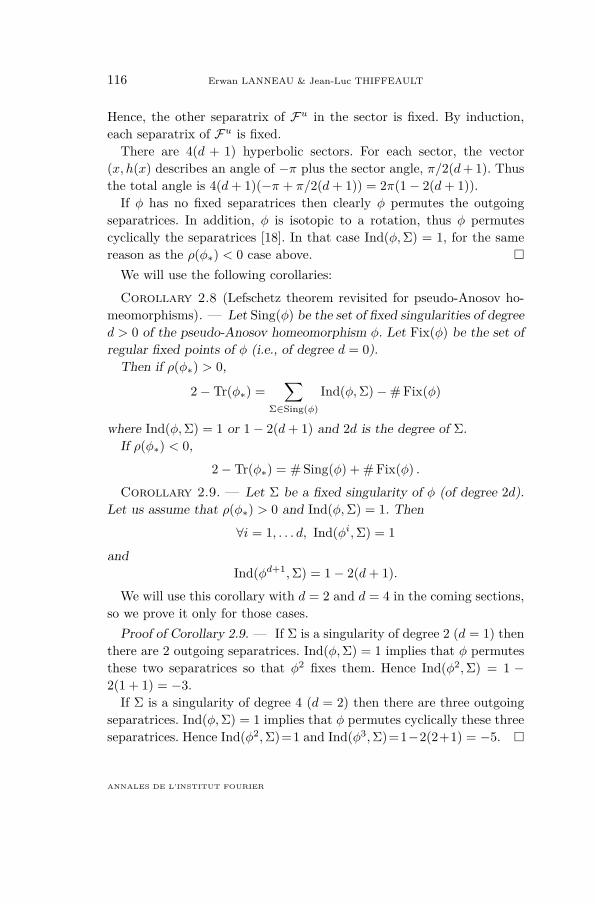
Figure 2.1. Mapping of the 4(d+ 1) hyperbolic sectors by φ near adegree 2d = 6 singularity: (a) ρ(φ∗) < 0: the sectors are permutedand the index is 1; (b) ρ(φ∗) > 0: the sectors can either be fixed (left,index 1 − 2(d + 1) = −7) or permuted (right, index 1). The indexis defined as the number of turns of a vector joining x to φ(x) as xtravels counterclockwise around a small circle. The separatrices ofthe unstable foliation are alternately labeled ingoing (i) and outgoing(o). The grey areas indicate a hyperbolic sector and its possibleimages for each case.

Proof of Proposition 2.7. — Obviously φ acts on the set of separatrices(namely the set of outgoing separatrices and ingoing separatrices). It isclear that ρ(φ∗) < 0 if and only if φ exchanges these two sets. In that case,Ind(φ,Σ) = 1 for any fixed point Σ, since the tip of the vector (x, f(x))never crosses the hyperbolic sector containing x and is thus constrainedto make a single turn counterclockwise. (A hyperbolic sector is the regionbetween adjacent ingoing and outgoing separatrices, see figure 2.1.)

If ρ(φ∗) > 0 then φ fixes globally the set of outgoing separatrices. Letus assume that φ fixes an outgoing separatrix γu of the unstable foliationFu. Let γs1 and γs2 be two adjacent incoming separatrices for the stablefoliation Fs that define a sector containing γu and another (ingoing)separatrix of Fu. Since γu is fixed by φ, the sector determined by γs1 andγs2 is also fixed. φ preserves orientation so that γs1 (and so γs2) is fixed.



Hence, the other separatrix of Fu in the sector is fixed. By induction,each separatrix of Fu is fixed.

There are 4(d + 1) hyperbolic sectors. For each sector, the vector(x, h(x) describes an angle of −π plus the sector angle, π/2(d+ 1). Thusthe total angle is 4(d+ 1)(−π + π/2(d+ 1)) = 2π(1− 2(d+ 1)).

If φ has no fixed separatrices then clearly φ permutes the outgoingseparatrices. In addition, φ is isotopic to a rotation, thus φ permutescyclically the separatrices [18]. In that case Ind(φ,Σ) = 1, for the samereason as the ρ(φ∗) < 0 case above. �

We will use the following corollaries:

Corollary 2.8 (Lefschetz theorem revisited for pseudo-Anosov ho-meomorphisms). — Let Sing(φ) be the set of fixed singularities of degreed > 0 of the pseudo-Anosov homeomorphism φ. Let Fix(φ) be the set ofregular fixed points of φ (i.e., of degree d = 0).

Then if ρ(φ∗) > 0,

2− Tr(φ∗) =∑

Σ∈Sing(φ)

Ind(φ,Σ)−# Fix(φ)

where Ind(φ,Σ) = 1 or 1− 2(d+ 1) and 2d is the degree of Σ.If ρ(φ∗) < 0,

2− Tr(φ∗) = # Sing(φ) + # Fix(φ) .

Corollary 2.9. — Let Σ be a fixed singularity of φ (of degree 2d).Let us assume that ρ(φ∗) > 0 and Ind(φ,Σ) = 1. Then

∀i = 1, . . . d, Ind(φi,Σ) = 1

andInd(φd+1,Σ) = 1− 2(d+ 1).

We will use this corollary with d = 2 and d = 4 in the coming sections,so we prove it only for those cases.

Proof of Corollary 2.9. — If Σ is a singularity of degree 2 (d = 1) thenthere are 2 outgoing separatrices. Ind(φ,Σ) = 1 implies that φ permutesthese two separatrices so that φ2 fixes them. Hence Ind(φ2,Σ) = 1 −2(1 + 1) = −3.

If Σ is a singularity of degree 4 (d = 2) then there are three outgoingseparatrices. Ind(φ,Σ) = 1 implies that φ permutes cyclically these threeseparatrices. Hence Ind(φ2,Σ)=1 and Ind(φ3,Σ)=1−2(2+1) = −5. �



3. Genus three: A proof of Theorem 1.2 for g = 3

We write ρ(P ) for the largest root (in absolute value) of a polyno-mial P ; for the polynomials we consider this is always real and withstrictly larger absolute value than all the other roots, though it couldhave either sign. If ρ(P ) > 0 then it is a Perron root; otherwise ρ(P (−X))is a Perron root.

We find all reciprocal polynomials with a Perron root less than our can-didate and then we test whether a polynomial is compatible with a givenstratum. This is straightforward: we simply try all possible permutationsof the singularities and separatrices, and calculate the contribution to theLefschetz numbers for each iterate of φ. Then we see whether the deficitin the Lefschetz numbers can be exactly compensated by regular peri-odic orbits. If not, the polynomial cannot correspond to a pseudo-Anosovhomeomorphism on that stratum.

We prove the theorems out of order since genus 3 is simplest. We knowthat δ+

3 6 ρ(X3 −X2 − 1) ' 1.46557 (for instance see [12] or [17]). Wewill construct a pseudo-Anosov homeomorphism with a smaller dilatationthan 1.46557 and prove that this dilatation is actually the least dilatation.

Recall that δ+3 is the Perron root of some reciprocal polynomial P

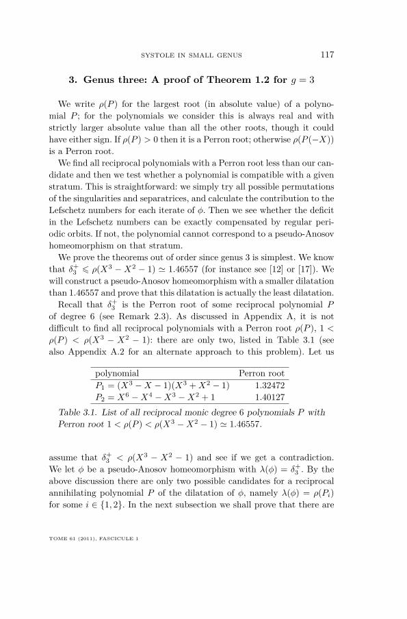
of degree 6 (see Remark 2.3). As discussed in Appendix A, it is notdifficult to find all reciprocal polynomials with a Perron root ρ(P ), 1 <ρ(P ) < ρ(X3 − X2 − 1): there are only two, listed in Table 3.1 (seealso Appendix A.2 for an alternate approach to this problem). Let us

polynomial Perron rootP1 = (X3 −X − 1)(X3 +X2 − 1) 1.32472P2 = X6 −X4 −X3 −X2 + 1 1.40127

Table 3.1. List of all reciprocal monic degree 6 polynomials P withPerron root 1 < ρ(P ) < ρ(X3 −X2 − 1) ' 1.46557.

assume that δ+3 < ρ(X3 − X2 − 1) and see if we get a contradiction.

We let φ be a pseudo-Anosov homeomorphism with λ(φ) = δ+3 . By the

above discussion there are only two possible candidates for a reciprocalannihilating polynomial P of the dilatation of φ, namely λ(φ) = ρ(Pi)for some i ∈ {1, 2}. In the next subsection we shall prove that there are



no pseudo-Anosov homeomorphisms on a genus three surface (stabilizingorientable foliations) with a dilatation ρ(P1). We shall then show thata pseudo-Anosov homeomorphism with dilatation ρ(P2) exists on thissurface.

3.1. First polynomial: λ(φ) = ρ(P1)

Let φ∗ be the linear map defined on H1(X,R) and let χφ∗ be its char-acteristic polynomial. By Theorem 2.2 the leading eigenvalue ρ(φ∗) of φ∗is ±ρ(P1). The minimal polynomial of the dilatation of φ is X3−X − 1;thus if ρ(φ∗) > 0 then X3 − X − 1 divides χφ∗ , otherwise X3 − X + 1divides χφ∗ . Requiring the polynomial to be reciprocal leads to χφ∗ = P1for the the first case and χφ∗ = P1(−X) = (X3 −X + 1)(X3 −X2 + 1)for the second.

The trace of φn∗ (and so the Lefschetz number of φn) is easy to computein terms of its characteristic polynomial. Let us analyze carefully the twocases depending on the sign of ρ(φ∗).

(1) If ρ(φ∗) < 0 then χφ∗(X) = P1(−X) = (X3−X+1)(X3−X2+1).Let ψ = φ2. Observe that ψ is a pseudo-Anosov homeomorphismand ρ(ψ∗) > 0 is a Perron root. >From Newton’s formulas (seeAppendix A), we have Tr(φ∗) = −1, Tr(ψ∗) = 3, Tr(ψ2

∗) = −1,and Tr(ψ3

∗) = 3, so that L(φ) = 3, L(ψ) = −1, L(ψ2) = 3,and L(ψ3) = −1.

As we have seen in Section 2, there are 5 possible strata for thesingularity data of φ, and so for ψ, namely,

(8), (2, 6), (4, 4), (2, 2, 4), and (2, 2, 2, 2).

Since L(ψ2) = 3 there are at least 3 singularities (of index +1)fixed by ψ2; thus we need only consider strata (2, 2, 4) and(2, 2, 2, 2). (From Corollary 2.8 regular fixed points can only givenegative index since ρ(ψ2

∗) > 0).For stratum (2, 2, 4), the single degree-4 singularity must be

fixed, and its three outgoing separatrices must be fixed by ψ3. Thecontribution to the index is then −5, which contradicts L(ψ3) =−1 since there is no way to make up the deficit.



For stratum (2, 2, 2, 2), since ψ2 fixes at least three singulari-ties they account for +3 of the Lefschetz number L(ψ2) = 3. Butthe fourth singularity must also be fixed by ψ2, so it adds +1or −3 to the Lefschetz number, depending on the permutationof its two separatrices. The only compatible scenario is that itadds +1, with the difference accounted by a single regular fixedpoint that contributes −1. Since all four singularities are thusfixed by ψ2 = φ4, this means that their permutation σ ∈ S4 mustsatisfy σ4 = id. There are three cases: either the singularitiesare all fixed by φ, they are permuted in groups of two, or theyare cyclically permuted. For the first two cases, the singularitiesare also fixed by ψ = φ2, so by Corollary 2.9 they cannot con-tribute positively to ψ2, which they must as we saw above. If thefour singularities are all cyclically permuted, then they contributenothing to L(φ) = 3 and there is only one regular fixed point, sowe get a contradiction here as well.

(2) If ρ(φ∗) > 0 then χφ∗(X) = P1(X). We have Tr(φ∗) = −1 andTr(φ2

∗) = 3, so that L(φ) = 3 and L(φ2) = −1. Since L(φ) = 3there are at least 3 fixed singularities; thus we need only considerstrata (2, 2, 4) and (2, 2, 2, 2).L(φ) = 3 implies that all the singularities are necessarily fixed,

with positive index. Let us denote by Σ1, Σ2 two degree-2 singu-larities. Since Ind(φ,Σi) = 1, by Corollary 2.9 one has Ind(φ2,Σi)= −3, leading to L(φ2) 6 −6 + 2 = −4; but L(φ2) = −1, whichis a contradiction.

3.2. Second polynomial: λ(φ) = ρ(P2)

As in the previous section, we can rule out most strata associatedwith P2 both for positive (P2(X)) or negative (P2(−X)) dominant root.For P2(−X), however, there remain three strata that cannot be elimi-nated:

(8), (2, 6), and (2, 2, 2, 2).

We single out the last stratum, (2, 2, 2, 2), to illustrate that this is a candi-date. Indeed, assume that three of the degree 2 singularities are cyclically



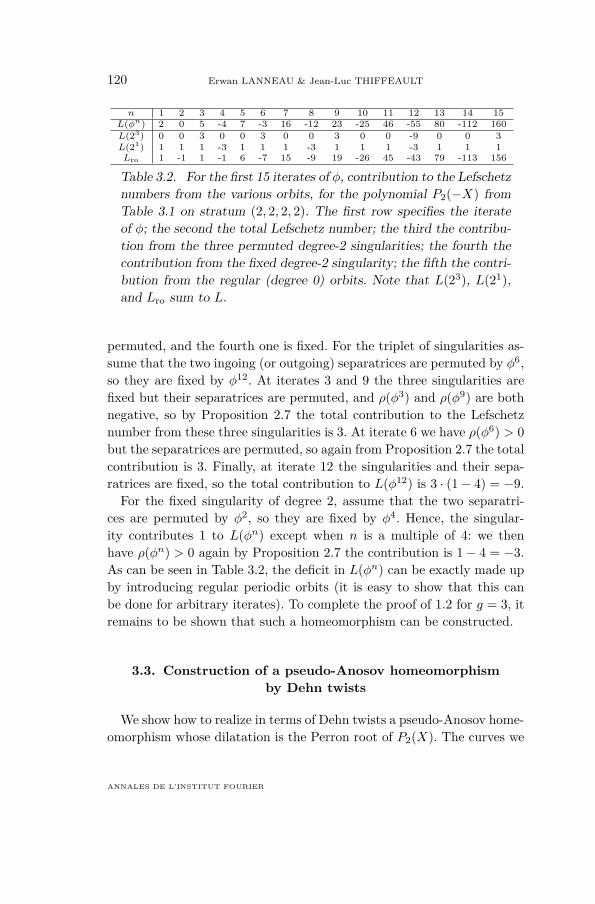
n 1 2 3 4 5 6 7 8 9 10 11 12 13 14 15L(φn) 2 0 5 -4 7 -3 16 -12 23 -25 46 -55 80 -112 160L(23) 0 0 3 0 0 3 0 0 3 0 0 -9 0 0 3L(21) 1 1 1 -3 1 1 1 -3 1 1 1 -3 1 1 1Lro 1 -1 1 -1 6 -7 15 -9 19 -26 45 -43 79 -113 156

Table 3.2. For the first 15 iterates of φ, contribution to the Lefschetznumbers from the various orbits, for the polynomial P2(−X) fromTable 3.1 on stratum (2, 2, 2, 2). The first row specifies the iterateof φ; the second the total Lefschetz number; the third the contribu-tion from the three permuted degree-2 singularities; the fourth thecontribution from the fixed degree-2 singularity; the fifth the contri-bution from the regular (degree 0) orbits. Note that L(23), L(21),and Lro sum to L.

permuted, and the fourth one is fixed. For the triplet of singularities as-sume that the two ingoing (or outgoing) separatrices are permuted by φ6,so they are fixed by φ12. At iterates 3 and 9 the three singularities arefixed but their separatrices are permuted, and ρ(φ3) and ρ(φ9) are bothnegative, so by Proposition 2.7 the total contribution to the Lefschetznumber from these three singularities is 3. At iterate 6 we have ρ(φ6) > 0but the separatrices are permuted, so again from Proposition 2.7 the totalcontribution is 3. Finally, at iterate 12 the singularities and their sepa-ratrices are fixed, so the total contribution to L(φ12) is 3 · (1− 4) = −9.

For the fixed singularity of degree 2, assume that the two separatri-ces are permuted by φ2, so they are fixed by φ4. Hence, the singular-ity contributes 1 to L(φn) except when n is a multiple of 4: we thenhave ρ(φn) > 0 again by Proposition 2.7 the contribution is 1− 4 = −3.As can be seen in Table 3.2, the deficit in L(φn) can be exactly made upby introducing regular periodic orbits (it is easy to show that this canbe done for arbitrary iterates). To complete the proof of 1.2 for g = 3, itremains to be shown that such a homeomorphism can be constructed.

3.3. Construction of a pseudo-Anosov homeomorphismby Dehn twists

We show how to realize in terms of Dehn twists a pseudo-Anosov home-omorphism whose dilatation is the Perron root of P2(X). The curves we



c1

a1

b1c2

a2

b2

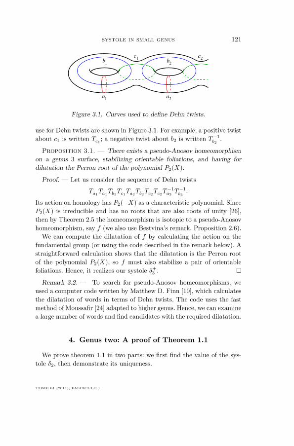
Figure 3.1. Curves used to define Dehn twists.

use for Dehn twists are shown in Figure 3.1. For example, a positive twistabout c1 is written Tc1 ; a negative twist about b2 is written T−1

b2.

Proposition 3.1. — There exists a pseudo-Anosov homeomorphismon a genus 3 surface, stabilizing orientable foliations, and having fordilatation the Perron root of the polynomial P2(X).

Proof. — Let us consider the sequence of Dehn twists

Ta1Ta1

Tb1Tc1Ta2Tb2Tc2Tc2T

−1a3T−1b3.

Its action on homology has P2(−X) as a characteristic polynomial. SinceP2(X) is irreducible and has no roots that are also roots of unity [26],then by Theorem 2.5 the homeomorphism is isotopic to a pseudo-Anosovhomeomorphism, say f (we also use Bestvina’s remark, Proposition 2.6).

We can compute the dilatation of f by calculating the action on thefundamental group (or using the code described in the remark below). Astraightforward calculation shows that the dilatation is the Perron rootof the polynomial P2(X), so f must also stabilize a pair of orientablefoliations. Hence, it realizes our systole δ+

3 . �

Remark 3.2. — To search for pseudo-Anosov homeomorphisms, weused a computer code written by Matthew D. Finn [10], which calculatesthe dilatation of words in terms of Dehn twists. The code uses the fastmethod of Moussafir [24] adapted to higher genus. Hence, we can examinea large number of words and find candidates with the required dilatation.

4. Genus two: A proof of Theorem 1.1

We prove theorem 1.1 in two parts: we first find the value of the sys-tole δ2, then demonstrate its uniqueness.



Recall that a surface M of genus g is called hyperelliptic if there existsan involution τ (called the hyperelliptic involution) with 2g + 2 fixedpoints. It is a classical fact that each genus two surface is hyperelliptic.The fixed points are also called the Weierstrass points. We now makemore precise the qualification “up to hyperelliptic involution and coveringtransformation” of Theorem 1.1.

Remark 4.1. — If (M, q) is a hyperelliptic surface, then for each con-jugacy class of a pseudo Anosov homeomorphism φ on M there existsanother conjugacy class, namely τ ◦ φ, having the same dilatation. Forinstance in genus 1 the two Anosov homeomorphisms φ = ( 2 1

1 1 ) andτ ◦ φ =

(−2 −1−1 −1

)have the same dilatation.

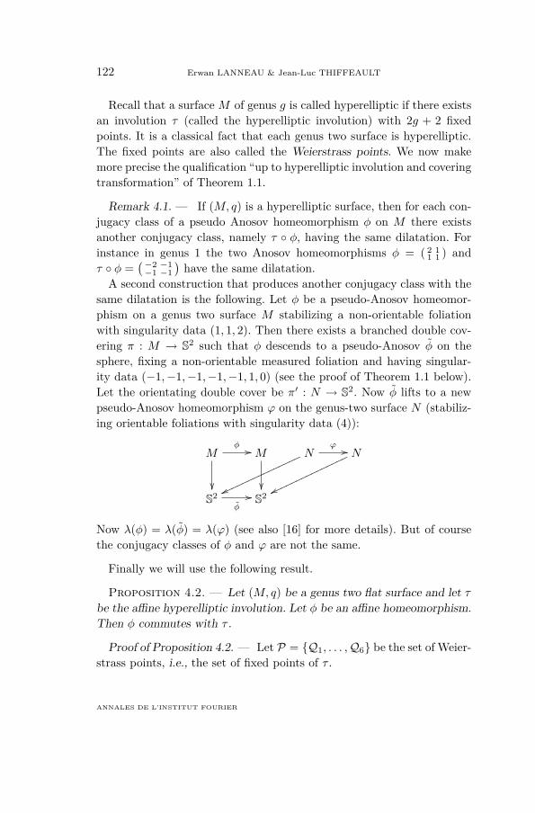
A second construction that produces another conjugacy class with thesame dilatation is the following. Let φ be a pseudo-Anosov homeomor-phism on a genus two surface M stabilizing a non-orientable foliationwith singularity data (1, 1, 2). Then there exists a branched double cov-ering π : M → S2 such that φ descends to a pseudo-Anosov φ̃ on thesphere, fixing a non-orientable measured foliation and having singular-ity data (−1,−1,−1,−1,−1, 1, 0) (see the proof of Theorem 1.1 below).Let the orientating double cover be π′ : N → S2. Now φ̃ lifts to a newpseudo-Anosov homeomorphism ϕ on the genus-two surface N (stabiliz-ing orientable foliations with singularity data (4)):

Mφ //

��

M

��

N

vvnnnnnnnnnnnnnnnϕ // N

wwnnnnnnnnnnnnnnn

S2φ̃

// S2

Now λ(φ) = λ(φ̃) = λ(ϕ) (see also [16] for more details). But of coursethe conjugacy classes of φ and ϕ are not the same.

Finally we will use the following result.

Proposition 4.2. — Let (M, q) be a genus two flat surface and let τbe the affine hyperelliptic involution. Let φ be an affine homeomorphism.Then φ commutes with τ .

Proof of Proposition 4.2. — Let P = {Q1, . . . ,Q6} be the set of Weier-strass points, i.e., the set of fixed points of τ .



Firstly let us show that φ preserves the set of Weierstrass points. Sinceφ−1◦τ ◦φ is a non-trivial involution, it is an automorphism of the complexsurface, thus the fixed points of φ−1 ◦ τ ◦ φ are also Weierstrass points.Let p be a Weierstrass point. Then φ−1 ◦ τ ◦ φ(p) = p or τ ◦ φ(p) = φ(p).Hence φ(p) is a fixed point of τ , and thus φ(p) is a Weierstrass point.

Now let ψ = [φ, τ ] = φ◦τ ◦φ−1◦τ be the commutator of φ and τ . Sinceτ and φ are affine homeomorphisms, ψ is also an affine homeomorphism.The derivative of ψ is equal to the identity so that ψ is a translation.Since φ−1 ◦τ(Q1) = φ−1(Q1) ∈ P one has τ ◦φ−1 ◦τ(Q1) = φ−1(Q1) andψ(Q1) = φ◦φ−1(Q1) = Q1. The translation ψ fixes a regular point. Thusit also fixes the separatrix issued from this point, and therefore ψ = idand φ commutes with τ . �

Proof of Theorem 1.1 (systole). — Let φ be a pseudo-Anosov home-omorphism with λ(φ) = δ2. We know that δ+

2 is the Perron root ofX4−X3−X2−X + 1 (see Zhirov [30]; see also Appendix C for a differ-ent construction). Let us assume that δ2 < δ+

2 . Thus φ preserves a pairof non-orientable measured foliations. The allowable singularity data forthese foliations are (2, 2), (1, 1, 2) or (1, 1, 1, 1). (Masur and Smillie [21]showed that (4) and (1, 3) cannot occur for non-orientable measured fo-liations.)

It is well known that each genus two surface is a branched doublecovering of the standard sphere. Let π : M → S2 be the covering and τ

the associated involution. It can be shown that τ is affine for the metricdetermined by φ (see [16]). Thus Proposition 4.2 applies and φ commuteswith τ . Hence φ induces a pseudo-Anosov homeomorphism φ̃ on thesphere S2 with the same dilatation. Of course φ̃ leaves invariant a non-orientable pair of measured foliations. The singularity data for φ are(2, 2), (1, 1, 2), or (1, 1, 1, 1); The singularity data for φ̃ are respectively(−1,−1,−1,−1, 0, 0), (−1,−1,−1,−1,−1, 1, 0), or (−1,−1,−1,−1,−1,−1, 1, 1). (For the first case, the singularity data cannot be (−1,−1,−1,−1,−1,−1, 2), otherwise the cover π would be the orientating cover —the branched points are precisely the singular points of odd degree, seeRemark 2.1 — thus the foliations of φ would be orientable.)

There exists an (orientating) double covering π′ : N → S2 such thatφ̃ lifts to a pseudo-Anosov homeomorphism f on N that stabilizes anorientable measured foliation. Actually, since the deck group is Z/2Z,



there are two lifts: f and τ ◦f , where τ denote the hyperelliptic involutionon N . Since Tr((τ ◦f)∗)=−Tr(f), there is one lift, say f , with ρ(χf∗) > 0.By construction λ(f) = δ2 = ρ(χf∗). Let us compute the genus ofN usingthe singularity data of f as follows.

(1) If the singularities of φ are (2, 2) then the singularities of f are(0); thus N is a torus.

(2) If the singularities of φ are (1, 1, 2) then the singularities of f are(0, 4); thus N is a genus two surface.

(3) If the singularities of φ are (1, 1, 1, 1) then the singularities of fare (4, 4); thus N is a genus three surface.

In the first case one has δ2 > δ1, but since δ1 > δ+2 this contradicts

the assumption δ2 < δ+2 . In the second case δ2 > δ+

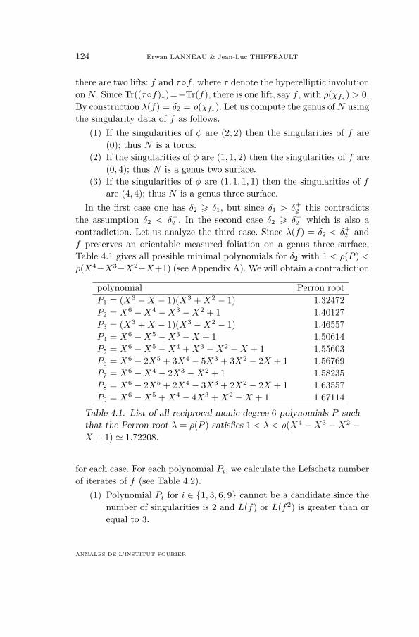
2 which is also acontradiction. Let us analyze the third case. Since λ(f) = δ2 < δ+

2 andf preserves an orientable measured foliation on a genus three surface,Table 4.1 gives all possible minimal polynomials for δ2 with 1 < ρ(P ) <ρ(X4−X3−X2−X+1) (see Appendix A). We will obtain a contradiction

polynomial Perron rootP1 = (X3 −X − 1)(X3 +X2 − 1) 1.32472P2 = X6 −X4 −X3 −X2 + 1 1.40127P3 = (X3 +X − 1)(X3 −X2 − 1) 1.46557P4 = X6 −X5 −X3 −X + 1 1.50614P5 = X6 −X5 −X4 +X3 −X2 −X + 1 1.55603P6 = X6 − 2X5 + 3X4 − 5X3 + 3X2 − 2X + 1 1.56769P7 = X6 −X4 − 2X3 −X2 + 1 1.58235P8 = X6 − 2X5 + 2X4 − 3X3 + 2X2 − 2X + 1 1.63557P9 = X6 −X5 +X4 − 4X3 +X2 −X + 1 1.67114

Table 4.1. List of all reciprocal monic degree 6 polynomials P suchthat the Perron root λ = ρ(P ) satisfies 1 < λ < ρ(X4 −X3 −X2 −X + 1) ' 1.72208.

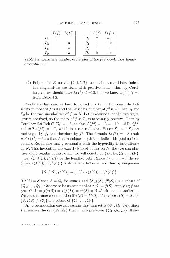
for each case. For each polynomial Pi, we calculate the Lefschetz numberof iterates of f (see Table 4.2).

(1) Polynomial Pi for i ∈ {1, 3, 6, 9} cannot be a candidate since thenumber of singularities is 2 and L(f) or L(f2) is greater than orequal to 3.



L(f) L(f2)P1 3P3 3P6 4P9 3

L(f) L(f3)P2 2 −1P4 1 −2P5 1 1P7 2 −4

Table 4.2. Lefschetz number of iterates of the pseudo-Anosov home-omorphism f .

(2) Polynomial Pi for i ∈ {2, 4, 5, 7} cannot be a candidate. Indeedthe singularities are fixed with positive index, thus by Corol-lary 2.9 we should have L(f3) 6 −10, but we know L(f3) > −4from Table 4.2.

Finally the last case we have to consider is P8. In that case, the Lef-schetz number of f is 0 and the Lefschetz number of f3 is −3. Let Σ1 andΣ2 be the two singularities of f on N . Let us assume that the two singu-larities are fixed, so the index of f at Σi is necessarily positive. Then byCorollary 2.9 Ind(f3,Σi) = −5, so that L(f3) = −3 = −10 −# Fix(f3)and # Fix(f3) = −7, which is a contradiction. Hence Σ1 and Σ2 areexchanged by f , and therefore by f3. The formula L(f3) = −3 reads# Fix(f3) = 3, so that f has a unique length 3 periodic orbit (and no fixedpoints). Recall also that f commutes with the hyperelliptic involution τ

on N . This involution has exactly 8 fixed points on N : the two singular-ities and 6 regular points, which we will denote by {Σ1,Σ2,Q1, . . . ,Q6}.

Let {S, f(S), f2(S)} be the length-3 orbit. Since f ◦ τ = τ ◦ f the set{τ(S), τ(f(S)), τ(f2(S))} is also a length-3 orbit and thus by uniqueness{

S, f(S), f2(S)}

={τ(S), τ(f(S)), τ(f2(S))

}.

If τ(S) = S then S = Qi for some i and {S, f(S), f2(S)} is a subset of{Q1, . . . ,Q6}. Otherwise let us assume that τ(S) = f(S). Applying f onegets f2(S) = f(τ(S)) = τ(f(S)) = τ2(S) = S which is a contradiction.We get the same contradiction if τ(S) = f2(S). Therefore τ(S) = S and{S, f(S), f2(S)} is a subset of {Q1, . . . ,Q6}.

Up to permutation one can assume that this set is {Q1,Q2,Q3}. Sincef preserves the set {Σ1,Σ2} then f also preserves {Q4,Q5,Q6}. Hence



f has a fixed point or another length-3 periodic orbit, which is a contra-diction. This ends the proof of the first part of Theorem 1.1. �

We now prove the uniqueness of the pseudo-Anosov homeomorphismrealizing the systole in genus two, up to conjugacy, hyperelliptic involu-tion, and covering transformations (see Remark 4.1).

Proof of Theorem 1.1 (uniqueness). — We will prove that there is noother construction that realizes the systole in genus two. The proof usesessentially McMullen’s work [23]. Let φ and φ′ be two pseudo-Anosovhomeomorphisms on M with λ(φ) = δ2 and let (M, q), (M ′, q′) be thetwo associated flat surfaces.

The proof decomposes into 4 steps. We first show that one can assumethat φ and φ′ leave invariant an orientable measured foliation with sin-gularity data (4). Then we show that we can assume, up to conjugacy,that the two surfaces (M, q) and (M ′, q′) are isometric. Finally we showthat the derivatives Dφ and Dφ′ of the affine homeomorphism on M areconjugate. We then conclude that φ and φ are conjugated in the mappingclass group Mod(2).

Step 4.3. — If the foliation is non-orientable then we have seen (proofof Theorem 1.1) that the singularity data of φ is (1, 1, 2). By Remark 4.1there exists a branched double covering π : M → P1 such that φ descendsto a pseudo-Anosov on the sphere P1 with singularity (−1,−1,−1,−1,−1, 1, 0). Now the orientating cover π̃ : M̃ → P1 gives a pseudo-Anosovhomeomorphism φ̃ on the genus 2 surface M̃ , with orientable foliation andsingularity data (4). In addition λ(φ) = λ(φ̃). Hence, from this discussionone can assume that φ stabilizes an orientable measured foliation. Thesingularity data of the measured foliation is either (4) or (2, 2). Using theLefschetz theorem, one shows that (2, 2) is impossible.

Step 4.4. — Up to the hyperelliptic involution, we can assume thatTr(φ) > 0 and Tr(φ′) > 0. There is natural invariant we can associate toa flat surface with a pseudo-Anosov homeomorphism ϕ: this is the tracefield (see [14]), the number field generated by λ(ϕ) + 1

λ(ϕ) . In our caseof course the trace field of the surfaces (M, q) and (M ′, q′) is the samesince the dilatation of φ and φ′ is the same. More precisely the trace fieldis Q[t], where t = δ2 + δ−1

2 . A straightforward calculation gives that theminimal polynomial of t is X2 −X − 3, so the trace field is Q(

√13).



Since the discriminant ∆ = 13 6≡ 1 mod 8, Theorem 1.1 of [23] impliesthat there exists a A ∈ SL2(R) such that A(M, q) = (M ′, q′). (We canalways assume that the area of the flat surfaces (M, q) and (M ′, q′) is 1.)In particular there exists an affine homeomorphism f : M → M ′ suchthat Df = A. Hence f−1φ′f is a pseudo-Anosov homeomorphism on thesame affine surface (M, q).

Step 4.5. — Now the derivatives of the two affine maps φ and φ′ (onthe same flat surface (M, q)) belong to the Veech group of the surface(M, q). (This group has 3 cusps and genus zero — see [23], Theorem 9.8.)Using the Rauzy–Veech induction, we can check that Dφ and A−1Dφ′A

are conjugated in this group.

Step 4.6. — Thus there exists B ∈ SL2(R) such thatDφ = B−1Dφ′B.Now let h : M → M be such that Dh = B; hence one has Dφ =Dh−1Dφ′Dh. Finally h−1φ′hφ−1 is an affine diffeomorphism with de-rivative map equal to the identity, and so it is a translation. Since themetric has a unique singularity (of type (4)), h−1φ′hφ−1 = id. We con-clude that φ and φ′ are conjugate in the mapping class group Mod(2),and the theorem is proved.

�

5. Genus four: A proof of Theorem 1.2 for g = 4

5.1. Polynomials

The techniques of the previous sections can also be applied to thegenus 4 case. The only difference is that for genus four and higher werely on a set of Mathematica scripts to test whether a polynomial iscompatible with a given stratum. This is straightforward: we simply tryall possible permutations of the singularities and separatrices, and cal-culate the contribution to the Lefschetz numbers for each iterate of φ.Then we see whether the deficit in the Lefschetz numbers can be exactlycompensated by regular periodic orbits. If not, the polynomial cannotcorrespond to a pseudo-Anosov homeomorphism on that stratum.



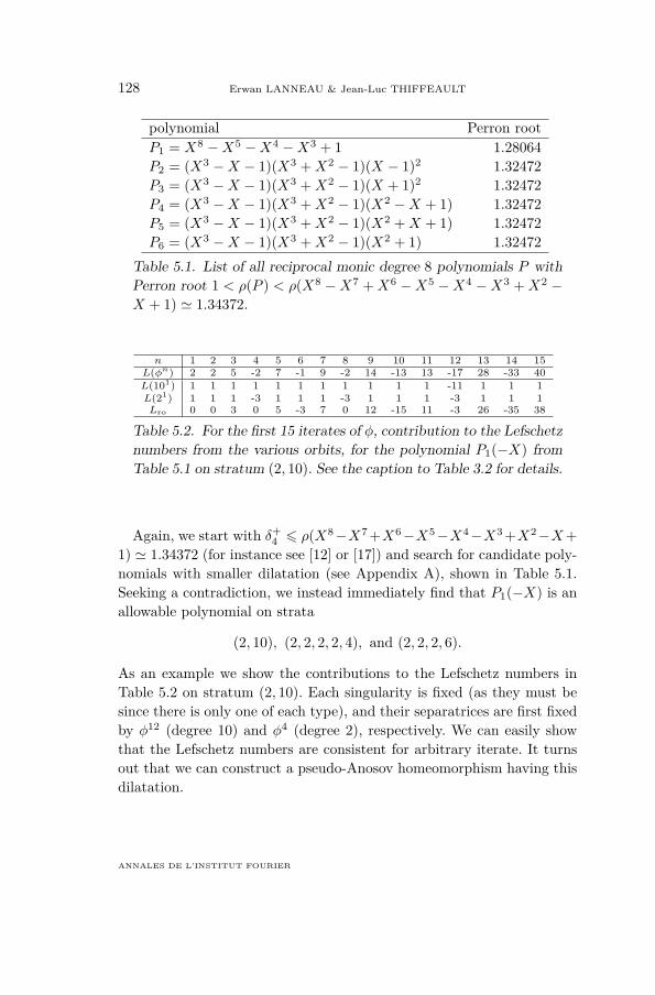
polynomial Perron rootP1 = X8 −X5 −X4 −X3 + 1 1.28064P2 = (X3 −X − 1)(X3 +X2 − 1)(X − 1)2 1.32472P3 = (X3 −X − 1)(X3 +X2 − 1)(X + 1)2 1.32472P4 = (X3 −X − 1)(X3 +X2 − 1)(X2 −X + 1) 1.32472P5 = (X3 −X − 1)(X3 +X2 − 1)(X2 +X + 1) 1.32472P6 = (X3 −X − 1)(X3 +X2 − 1)(X2 + 1) 1.32472

Table 5.1. List of all reciprocal monic degree 8 polynomials P withPerron root 1 < ρ(P ) < ρ(X8 −X7 +X6 −X5 −X4 −X3 +X2 −X + 1) ' 1.34372.

n 1 2 3 4 5 6 7 8 9 10 11 12 13 14 15L(φn) 2 2 5 -2 7 -1 9 -2 14 -13 13 -17 28 -33 40L(101) 1 1 1 1 1 1 1 1 1 1 1 -11 1 1 1L(21) 1 1 1 -3 1 1 1 -3 1 1 1 -3 1 1 1Lro 0 0 3 0 5 -3 7 0 12 -15 11 -3 26 -35 38

Table 5.2. For the first 15 iterates of φ, contribution to the Lefschetznumbers from the various orbits, for the polynomial P1(−X) fromTable 5.1 on stratum (2, 10). See the caption to Table 3.2 for details.

Again, we start with δ+4 6 ρ(X8−X7 +X6−X5−X4−X3 +X2−X+

1) ' 1.34372 (for instance see [12] or [17]) and search for candidate poly-nomials with smaller dilatation (see Appendix A), shown in Table 5.1.Seeking a contradiction, we instead immediately find that P1(−X) is anallowable polynomial on strata

(2, 10), (2, 2, 2, 2, 4), and (2, 2, 2, 6).

As an example we show the contributions to the Lefschetz numbers inTable 5.2 on stratum (2, 10). Each singularity is fixed (as they must besince there is only one of each type), and their separatrices are first fixedby φ12 (degree 10) and φ4 (degree 2), respectively. We can easily showthat the Lefschetz numbers are consistent for arbitrary iterate. It turnsout that we can construct a pseudo-Anosov homeomorphism having thisdilatation.



5.2. Construction of a pseudo-Anosov homeomorphismby Dehn twists

We use the same approach as in Section 3.3 to find the candidate word.

Proposition 5.1. — There exists a pseudo-Anosov homeomorphismon a genus 4 surface, stabilizing orientable foliations, and having fordilatation the Perron root of the polynomial P1(X).

Proof. — Let us consider the sequence of Dehn twists

Ta1Tb1Tc1Ta2

Tb2Tc2Tb3Tc3Tb4 .

Its action on homology has P1(−X) as a characteristic polynomial. SinceP1(X) is irreducible and has no roots that are also roots of unity [26],then by Theorem 2.5 the homeomorphism is isotopic to a pseudo-Anosovhomeomorphism, say f .

We compute the dilatation of f by calculating the action on the fun-damental group, which shows that the dilatation is the Perron root ofthe polynomial P1(X). Hence, f must also stabilize a pair of orientablefoliations, and it realizes our systole δ+

4 . �

6. Higher genus

6.1. Genus five: A proof of Theorem 1.2 for g = 5

This time there is a known candidate with a lower dilatation thanHironaka & Kin’s [12]: Leininger’s pseudo-Anosov homeomorphism [19]having Lehmer’s number ' 1.17628 as a dilatation. This pseudo-Anosovhomeomorphism has invariant foliations corresponding to stratum (16).(The Lefschetz numbers are also compatible with stratum (4, 4, 4, 4).)The polynomial associated with its action on homology has ρ(P ) < 0.An exhaustive search (see Appendix A) leads us to conclude that thereis no allowable polynomial with a lower dilatation, so there is nothingelse to check.

As we finished this paper we learned that Aaber & Dunfield [1] havefound a pseudo-Anosov homeomorphism with dilatation lower than δ+

5(stabilizing a non-orientable foliation), implying that δ5 < δ+

5 .



6.2. Genus six: A proof of Theorem 1.3 for g = 6(computer-assisted)

For genus 6, we have demonstrated that the Lefschetz numbers asso-ciated with P (−X), with P the polynomial in Table 1.2, are compatiblewith stratum (16, 4), with Lehmer’s number as a root (Lehmer’s polyno-mial is a factor). (There is another polynomial with the same dilatationthat is compatible with the stratum (20).) We have not yet constructedan explicit pseudo-Anosov homeomorphism with this dilatation for genus6, so Theorem 1.3 is a weaker form than 1.2: it only asserts that δ+

6 isnot less than this dilatation. Note, however, that whether or not thispseudo-Anosov homeomorphism exists this is the first instance wherethe minimum dilatation is not lower than for smaller genus.

6.3. Genus seven: A proof of Theorem 1.3 for g = 7(computer-assisted)

Again, we have not constructed the pseudo-Anosov homeomorphismexplicitly, but the Lefschetz numbers for the polynomial P (−X), with Pas in Table 1.2, are compatible with stratum (2, 2, 2, 2, 2, 14).

As we finished this paper we learned that Aaber & Dunfield [1] andKin & Takasawa [15] have found a pseudo-Anosov homeomorphism withdilatation equal to the systole δ+

7 .

6.4. Genus eight: A proof of Theorem 1.3 for g = 8(computer-assisted)

Genus eight is roughly the limit of this brute-force approach: it takesour computer program about five days to ensure that we have the mini-mizing polynomial. The bound described in Appendix A yields 5× 1012

cases for the traces, most of which do not correspond to integer-coefficientpolynomials.

Yet again, we have not constructed the pseudo-Anosov homeomor-phism explicitly, but the Lefschetz numbers for the polynomial P (−X),with P as in Table 1.2, are compatible with stratum (6, 22).



As we finished this paper we learned that Hironaka [11] has found apseudo-Anosov homeomorphism with dilatation equal to the systole δ+

8 .Examining the cases with even g leads to a natural question:

Question 6.1. — Is the minimum value of the dilatation of pseudo-Anosov homeomorphisms on a genus g surface, for g even, with orientableinvariant foliations, equal to the largest root of the polynomial X2g −Xg+1 −Xg −Xg−1 + 1?

Appendix A. Searching for polynomialswith small Perron root

A.1. Newton’s formulas

The crucial task in our proofs is to find all reciprocal polynomials witha largest real root bounded by a given value α (typically the candidateminimum dilatation). Moreover, these must be allowable polynomials fora pseudo-Anosov homeomorphism: the largest root (in absolute value)must be real and strictly larger than all other roots, and it must beoutside the unit circle in the complex plane.

The simplest way to find all such polynomials is to bound the coeffi-cients directly. For example, in genus 3, If we denote an arbitrary recip-rocal polynomial by P (X) = X6 + aX5 + bX4 + cX3 + bX2 + aX + 1,we want to find all polynomials with Perron root smaller than α =ρ(X3 − X2 − 1) ' 1.46557 (the candidate minimum dilatation at thebeginning of Section 3). Let t = α + α−1; a straightforward calculationassuming that half the roots of P (X) are equal to α shows

|a| 6 3t, |b| 6 3(t2 + 1), |c| 6 t(t2 + 6).

Plugging in numbers, this means |a| 6 6, |b| 6 18, and |c| 6 26. Allowingfor X → −X since we only care about the absolute value of the largestroot, we have a total of 12, 765 cases to examine. Out of these, onlytwo polynomials actually have a root small enough and satisfy the otherconstraints (reality, uniqueness of largest root), as given in Section 3.

The problem with this straightforward approach (also employed byCho and Ham for genus 2, see [7]) is that it scales very poorly with in-creasing genus. For genus 4, the number of cases is 9, 889, 930; for genus 5,



we have 63, 523, 102, 800 cases (we use for α the dilatation of Hironaka& Kin’s pseudo-Anosov homeomorphism [12], currently the best generalupper bound on δg). As g increases, the target dilatation α decreases,which should limit the number of cases, but the quantity t = α + α−1

converges to unity, and the bound depends only weakly on α− 1.An improved approach is to start from Newton’s formulas relating the

traces to the coefficients: for a polynomial P (X) = Xn + a1Xn−1 +

a2Xn−2 + . . . + an−1X + an which is the characteristic polynomial of a

matrix M , we have

Tr(Mk) =

{−kak −

∑k−1m=1 am Tr(Mk−m), 1 6 k 6 n;

−∑nm=1 am Tr(Mk−m), k > n.

For a reciprocal polynomial, we have an−k = ak. We can use these for-mulas to solve for the ak given the first few traces Tr(Mk), 1 6 k 6 g

(g = n/2, n is even in this paper). We also have

Lemma A.1. — If the characteristic polynomial P (X) of a matrix Mhas a largest eigenvalue with absolute value r, then

|Tr(Mk)| 6 n rk;

Furthermore, if P (X) is reciprocal and of even degree, then

|Tr(Mk)| 6 12n(rk + r−k).

Proof. — Obviously,

|Tr(Mk)| =

∣∣∣∣∣n∑m=1

skm

∣∣∣∣∣ 6n∑m=1|sm|k 6 n rk

where sk are the eigenvalues of M . If the polynomial is reciprocal and nis even, then

|Tr(Mk)| =

∣∣∣∣∣∣n/2∑m=1

(skm + s−km )

∣∣∣∣∣∣ 6 12n(rk + r−k).

�

We now have the following prescription for enumerating allowable poly-nomials, given n and a largest root α:

(1) Use Lemma A.1 to bound the traces Tr(Mk) ∈ Z, k = 1, . . . , n/2;



(2) For each possible set of n/2 traces, solve for the coefficients of thepolynomial;

(3) If these coefficients are not all integers, move on to the next pos-sible set of traces;

(4) If the coefficients are integers, check if the polynomial is allowable:largest eigenvalue real and with absolute value less than α, outsidethe unit circle, and nondegenerate;

(5) Repeat step 2 until we run out of possible values for the traces.

Let’s compare with the earlier numbers for g = 5: assuming Tr(M) > 0,we have 7, 254, 775 cases to try, which is already a factor of 104 fewerthan with the coefficient bound. Moreover, of these 7, 194, 541 lead tofractional coefficients, and so are discarded in step 3 above. This onlyleaves 60, 234 cases, roughly a factor of 106 fewer than with the coefficientbound. Hence, with this simple approach we can tackle polynomials upto degree 16 (g = 8). More refined approaches will certainly allow higherdegrees to be reached.

A final note on the numerical technique: we use Newton’s iterativemethod to check the dominant root of candidate polynomials. A nicefeature of polynomials with a dominant real root is that their graph isstrictly convex upwards for x greater than the root (when that root ispositive, otherwise for x less than the root). Hence, Newton’s methodis guaranteed to converge rapidly and uniquely for appropriate initialguess (typically, 5 iterates is enough for about 6 significant figures). Ifthe method does not converge quickly, then the polynomial is ruled out.

A.2. Mahler measures

Another approach is to use the Mahler measure of a polynomial. If Pis a degree 2g monic polynomial that admits a Perron root, say α, thenthe Mahler measure of P satisfies M(P ) 6 αg. Thus to list all possiblepolynomials with a Perron root less than a constant α, we just have tolist all possible polynomials with a Mahler measure less than αg. Suchlists already exist in the literature (for example in [4]).



Appendix B. Rauzy–Veech inductionand pseudo-Anosov homeomorphisms

In this section we recall very briefly the basic construction of pseudo-Anosov homeomorphisms using the Rauzy–Veech induction (for detailssee [29], §8, and [27, 20]). We will use this to construct the minimizingpseudo-Anosov homeomorphisms in genus 3 and 4.

B.1. Interval exchange map

Let I ⊂ R be an open interval and let us choose a finite partition ofI into d > 2 open subintervals {Ij , j = 1, . . . , d}. An interval exchangemap is a one-to-one map T from I to itself that permutes, by translation,the subintervals Ij . It is easy to see that T is precisely determined bya permutation π that encodes how the intervals are exchanged, and avector λ = {λj}j=1,...,d with positive entries that encodes the lengths ofthe intervals.

B.2. Suspension data

A suspension datum for T is a collection of vectors {ζj}j=1,...,d suchthat

(1) ∀j ∈ {1, . . . , d}, Re(ζj) = λj ;(2) ∀k, 1 6 k 6 d− 1, Im(

∑kj=1 ζj) > 0;

(3) ∀k, 1 6 k 6 d− 1, Im(∑kj=1 ζπ−1(j)) < 0.

To each suspension datum ζ, we can associate a translation surface(M, q) = M(π, ζ) in the following way. Consider the broken line L0 onC = R2 defined by concatenation of the vectors ζj (in this order) forj = 1, . . . , d with starting point at the origin (see Figure B.1). Similarly,we consider the broken line L1 defined by concatenation of the vectorsζπ−1(j) (in this order) for j = 1, . . . , d with starting point at the origin.If the lines L0 and L1 have no intersections other than the endpoints,we can construct a translation surface S by identifying each side ζj onL0 with the side ζj on L1 by a translation. The resulting surface is atranslation surface endowed with the form dz2.



Let I ⊂M be the horizontal interval defined by I = (0,∑dj=1 λj)×{0}.

Then the interval exchange map T is precisely the one defined by the firstreturn map to I of the vertical flow on M .

B.3. Rauzy–Veech induction

The Rauzy–Veech induction R(T ) of T is defined as the first returnmap of T to a certain subinterval J of I (see [27, 20] for details).

We recall very briefly the construction. The type ε of T is defined by0 if λd > λπ−1(d) and 1 otherwise. We define a subinterval J of I by

J ={I\T (Iπ−1(d)) if T is of type 0;I\Id if T is of type 1.

The Rauzy–Veech induction R(T ) of T is defined as the first return mapof T to the subinterval J . This is again an interval exchange transforma-tion, defined on d letters (see e.g., [27]). Moreover, we can compute thedata of the new map (permutation and length vector) by a combinatorialmap and a matrix. We can also define the Rauzy–Veech induction on thespace of suspensions. For a permutation π, we call the Rauzy class thegraph of all permutations that we can obtain by the Rauzy–Veech induc-tion. Each vertex of this graph corresponds to a permutation, and fromeach permutation there are two edges labelled 0 and 1 (the type). To eachedge, one can associate a transition matrix that gives the correspondingvector of lengths.

B.4. Closed loops and pseudo-Anosov homeomorphisms

We now recall a theorem of Veech:

Theorem (Veech). — Let γ be a closed loop, based at π, in a Rauzyclass and R = R(γ) be the product of the associated transition matrices.Let us assume that R is irreducible. Let λ be an eigenvector for thePerron eigenvalue α of R and τ be an eigenvector for the eigenvalue 1

α ofR. Then

(1) ζ = (λ, τ) is a suspension data for T = (π, λ);



(2) The matrixA =(α−1 0

0 α

)is the derivative map of an affine pseudo-

Anosov diffeomorphism φ on the suspension M(π, ζ) over (π, λ);(3) The dilatation of φ is α;(4) All pseudo-Anosov homeomorphisms that fix a separatrix are con-

structed in this way.

Since genus 4 is simpler to construct than genus 3, we present thegenus 4 case first in detail, and briefly outline the construction of theother case.

B.5. Construction of an example for g = 4

We shall prove

Theorem B.1. — There exists a pseudo-Anosov homeomorphism ona genus four surface, stabilizing orientable measured foliations, and hav-ing for dilatation the maximal real root of the polynomial X8 − X5 −X4 −X3 + 1 (namely 1.28064...).

B.5.1. Construction of the translation surface for g = 4

Let |α| > 1 be the maximal real root of the polynomial P1(X) =X8−X5−X4−X3 + 1 with α < −1, so that α8 +α5−α4 +α3 + 1 = 0.In the following, we will present elements of Q[α] in the basis {αi}i=0,...,7.Thus the octuplet (a0, . . . , a7) stands for

∑7i=0 aiα

i.We start with the permutation π = (5, 3, 9, 8, 6, 2, 7, 1, 4) and the closed

Rauzy path

0− 1− 0− 0− 1− 1− 1− 0− 1− 0− 0− 1− 0− 0.

The associated Rauzy–Veech matrix is

R =

1 1 0 0 0 0 0 0 00 0 1 1 1 1 1 1 00 0 0 0 0 1 0 1 11 0 0 1 0 0 1 0 00 0 1 0 1 0 0 0 00 0 0 1 1 0 0 0 00 0 0 0 0 1 1 0 01 0 0 0 0 1 1 1 01 1 0 1 0 0 1 0 0

.One checks that the characteristic polynomial of R is Q(X) with theproperty that Q(X) factors into Q(X4) = P1(−X)S(X), where S(X)



is a polynomial. Let λ and τ be the corresponding eigenvectors for thePerron root α4 of Q, expressed in the α-basis:

λ1 = (0, 1,−2, 1,−1, 0, 1,−1)λ2 = (0,−1, 1, 0, 1, 0,−1, 0)λ3 = (−1, 0,−1, 0, 0,−1, 0, 0)λ4 = (−1, 2,−1, 1, 0,−1, 1, 0)λ5 = (1,−1, 1, 0, 0, 1, 0, 0)λ6 = (−1, 1,−1, 1,−1,−1, 0,−1)λ7 = (1,−2, 2,−2, 1, 1,−1, 1)λ8 = (0, 0, 1,−1, 1, 0, 0, 1)λ9 = (1, 0, 0, 0, 0, 0, 0, 0)

τ1 = (−1, 0, 0, 0, 0,−1, 0, 0)τ2 = (0, 0,−1, 1, 0, 1, 0,−1)τ3 = (0, 0,−1, 0,−1, 0, 0,−1)τ4 = (0, 1, 0, 0, 0, 0, 1, 0)τ5 = (0, 0, 0, 1, 0, 0, 0, 0)τ6 = (0, 0,−1, 0, 0, 0, 1, 0)τ7 = (0, 0, 0, 0, 0, 0,−1, 0)τ8 = (0, 1, 0, 0, 0, 0, 0, 0)τ9 = (−1, 0, 0, 0, 0, 0, 0, 0).

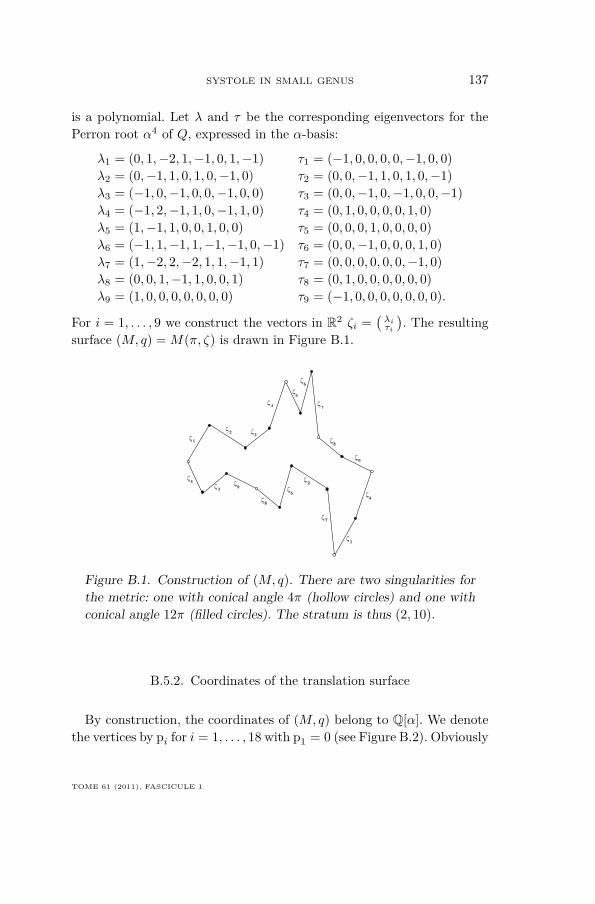
For i = 1, . . . , 9 we construct the vectors in R2 ζi =(λiτi

). The resulting

surface (M, q) = M(π, ζ) is drawn in Figure B.1.

5

6

7

8

9

1

23

4

5

3 9

8

6

2

7

1

4

z

�

�

�

�

�

��

��

�

��

�

�

�

�

�

Figure B.1. Construction of (M, q). There are two singularities forthe metric: one with conical angle 4π (hollow circles) and one withconical angle 12π (filled circles). The stratum is thus (2, 10).

B.5.2. Coordinates of the translation surface

By construction, the coordinates of (M, q) belong to Q[α]. We denotethe vertices by pi for i = 1, . . . , 18 with p1 = 0 (see Figure B.2). Obviously



for i 6 9, pi =∑ij=1 ζj , and for i > 10, pi =

∑9j=1 ζj −

∑i−9j=1 ζπ−1(j). A

direct calculation givesp1 = ((0, 0, 0, 0, 0, 0, 0, 0), (0, 0, 0, 0, 0, 0, 0, 0))p2 = ((0, 1,−2, 1,−1, 0, 1,−1), (−1, 0, 0, 0, 0,−1, 0, 0))p3 = ((0, 0,−1, 1, 0, 0, 0,−1), (−1, 0,−1, 1, 0, 0, 0,−1))p4 = ((−1, 0,−2, 1, 0,−1, 0,−1), (−1, 0,−2, 1,−1, 0, 0,−2))p5 = ((−2, 2,−3, 2, 0,−2, 1,−1), (−1, 1,−2, 1,−1, 0, 1,−2))p6 = ((−1, 1,−2, 2, 0,−1, 1,−1), (−1, 1,−2, 2,−1, 0, 1,−2))p7 = ((−2, 2,−3, 3,−1,−2, 1,−2), (−1, 1,−3, 2,−1, 0, 2,−2))p8 = ((−1, 0,−1, 1, 0,−1, 0,−1), (−1, 1,−3, 2,−1, 0, 1,−2))p9 = ((−1, 0, 0, 0, 1,−1, 0, 0), (−1, 2,−3, 2,−1, 0, 1,−2))p10 = ((0, 0, 0, 0, 1,−1, 0, 0), (−2, 2,−3, 2,−1, 0, 1,−2))p11 = ((1,−2, 1,−1, 1, 0,−1, 0), (−2, 1,−3, 2,−1, 0, 0,−2))p12 = ((1,−3, 3,−2, 2, 0,−2, 1), (−1, 1,−3, 2,−1, 1, 0,−2))p13 = ((0,−1, 1, 0, 1,−1,−1, 0), (−1, 1,−3, 2,−1, 1, 1,−2))p14 = ((0, 0, 0, 0, 0,−1, 0, 0), (−1, 1,−2, 1,−1, 0, 1,−1))p15 = ((1,−1, 1,−1, 1, 0, 0, 1), (−1, 1,−1, 1,−1, 0, 0,−1))p16 = ((1,−1, 0, 0, 0, 0, 0, 0), (−1, 0,−1, 1,−1, 0, 0,−1))p17 = ((0,−1, 0, 0, 0, 0, 0, 0), (0, 0,−1, 1,−1, 0, 0,−1))p18 = ((1,−1, 1, 0, 0, 1, 0, 0), (0, 0, 0, 1, 0, 0, 0, 0))

B.5.3. Construction of the pseudo-Anosov diffeomorphism

Let A be the hyperbolic matrix(α−1 0

0 α

). Of course by construction A4

stabilizes the translation surface (M, q) and hence there exists a pseudo-Anosov homeomorphism on M with dilatation α4. We shall prove thatthis homeomorphism admits a root.

Let (M ′, q′) be the image of (M, q) by the matrix A. We only need toprove that (M ′, q′) and (M, q) defines the same translation surface, i.e.,one can cut and glue (M ′, q′) in order to recover (M, q). This is

Theorem B.2. — The surfaces (M ′, q′) and (M, q) are isometric.

Corollary B.3. — There exists a pseudo-Anosov diffeomorphismf : X → X such that Df = A. In particular the dilatation of f is |α|.

Proof of Theorem B.2. — Using the two relations α8 = −1 − α3 +α4 −α5 and α−1 = α2 −α3 +α4 +α7 and the relations that give the pi,



one gets by a straightforward calculation the coordinates p’i = Api ofthe surface (M ′, q′):

p’1 = ((0, 0, 0, 0, 0, 0, 0, 0), (0, 0, 0, 0, 0, 0, 0, 0))p’2 = ((1,−2, 1,−1, 0, 1,−1, 0), (0,−1, 0, 0, 0, 0,−1, 0))p’3 = ((0,−1, 1, 0, 0, 0,−1, 0), (1,−1, 0, 0, 0, 1, 0, 0))p’4 = ((0,−2, 2,−1, 0, 0,−1, 1), (2,−1, 0, 0,−1, 1, 0, 0))p’5 = ((2,−3, 4,−2, 0, 1,−1, 2), (2,−1, 1, 0,−1, 1, 0, 1))p’6 = ((1,−2, 3,−1, 0, 1,−1, 1), (2,−1, 1, 0, 0, 1, 0, 1))p’7 = ((2,−3, 5,−3, 0, 1,−2, 2), (2,−1, 1,−1, 0, 1, 0, 2))p’8 = ((0,−1, 2,−1, 0, 0,−1, 1), (2,−1, 1,−1, 0, 1, 0, 1))p’9 = ((0, 0, 1, 0, 0, 0, 0, 1), (2,−1, 2,−1, 0, 1, 0, 1))p’10 = ((0, 0, 0, 1,−1, 0, 0, 0), (2,−2, 2,−1, 0, 1, 0, 1))p’11 = ((−2, 1,−2, 2,−1,−1, 0,−1), (2,−2, 1,−1, 0, 1, 0, 0))p’12 = ((−3, 3,−3, 3,−1,−2, 1,−1), (2,−1, 1,−1, 0, 1, 1, 0))p’13 = ((−1, 1, 0, 1,−1,−1, 0, 0), (2,−1, 1,−1, 0, 1, 1, 1))p’14 = ((0, 0, 0, 0,−1, 0, 0, 0), (1,−1, 1,−1, 0, 0, 0, 1))p’15 = ((−1, 1,−2, 2,−1, 0, 1,−1), (1,−1, 1, 0, 0, 0, 0, 0))p’16 = ((−1, 0,−1, 1,−1, 0, 0,−1), (1,−1, 0, 0, 0, 0, 0, 0))p’17 = ((−1, 0, 0, 0, 0, 0, 0, 0), (1, 0, 0, 0, 0, 0, 0, 0))p’18 = ((−1, 1,−1, 1, 0, 0, 0,−1), (0, 0, 0, 0, 1, 0, 0, 0))

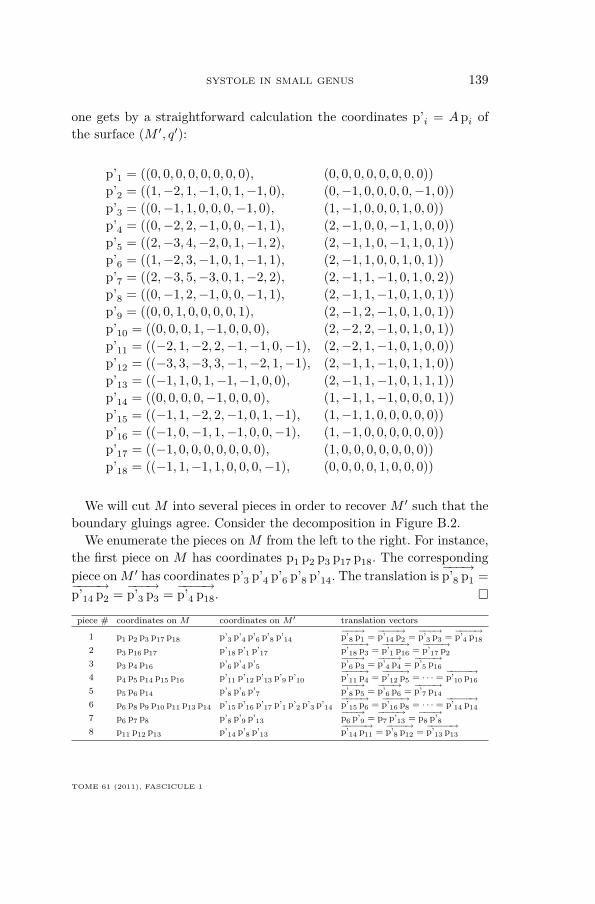
We will cut M into several pieces in order to recover M ′ such that theboundary gluings agree. Consider the decomposition in Figure B.2.

We enumerate the pieces on M from the left to the right. For instance,the first piece on M has coordinates p1 p2 p3 p17 p18. The correspondingpiece onM ′ has coordinates p’3 p’4 p’6 p’8 p’14. The translation is−−−→p’8 p1 =−−−−→p’14 p2 = −−−→p’3 p3 = −−−−→p’4 p18. �

piece # coordinates on M coordinates on M ′ translation vectors

1 p1 p2 p3 p17 p18 p’3 p’4 p’6 p’8 p’14−−−→p’8 p1 =

−−−−→p’14 p2 =

−−−→p’3 p3 =

−−−−→p’4 p18

2 p3 p16 p17 p’18 p’1 p’17−−−−→p’18 p3 =

−−−−→p’1 p16 =

−−−−→p’17 p2

3 p3 p4 p16 p’6 p’4 p’5−−−→p’6 p3 =

−−−→p’4 p4 =

−−−−→p’5 p16

4 p4 p5 p14 p15 p16 p’11 p’12 p’13 p’9 p’10−−−−→p’11 p4 =

−−−−→p’12 p5 = · · · =

−−−−−→p’10 p16

5 p5 p6 p14 p’8 p’6 p’7−−−→p’8 p5 =

−−−→p’6 p6 =

−−−−→p’7 p14

6 p6 p8 p9 p10 p11 p13 p14 p’15 p’16 p’17 p’1 p’2 p’3 p’14−−−−→p’15 p6 =

−−−−→p’16 p8 = · · · =

−−−−−→p’14 p14

7 p6 p7 p8 p’8 p’9 p’13−−−→p6 p’9 =

−−−−→p7 p’13 =

−−−→p8 p’8

8 p11 p12 p13 p’14 p’8 p’13−−−−−→p’14 p11 =

−−−−→p’8 p12 =

−−−−−→p’13 p13



p

18

17

16

15

14

13

12

11

10

9

8

7

6

5

1

24

3

p

p

p

p

p

p

p

p

p

p

p

p

p

p

p

p

p

18

17

16

15

14

13

12

11

10

9

8

7

6

5

4

3

2

1p'

p'

p'

p'

p'

p'

p'

p'

p'

p'

p'

p'

p'

p'

p'

p'

p'

p'

Figure B.2. Partition of (M, q) and (M ′, q′) = A(M, q).

B.6. Construction of an example for g = 3

We shall prove

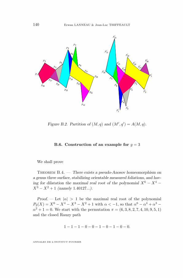
Theorem B.4. — There exists a pseudo-Anosov homeomorphism ona genus three surface, stabilizing orientable measured foliations, and hav-ing for dilatation the maximal real root of the polynomial X6 − X4 −X3 −X2 + 1 (namely 1.40127...).

Proof. — Let |α| > 1 be the maximal real root of the polynomialP2(X) = X6 −X4 −X3 −X2 + 1 with α < −1, so that α6 − α4 + α3 −α2 + 1 = 0. We start with the permutation π = (6, 3, 8, 2, 7, 4, 10, 9, 5, 1)and the closed Rauzy path

1− 1− 1− 0− 0− 1− 0− 1− 0− 0.



The associated Rauzy–Veech matrix is

R =

1 1 1 1 1 1 0 0 0 00 0 0 0 0 0 1 0 0 00 0 0 0 0 0 0 1 0 00 0 0 0 0 0 0 0 1 00 0 0 0 1 0 0 0 1 10 0 1 0 0 1 0 0 0 01 0 0 1 1 0 0 0 1 10 1 0 0 0 0 0 0 0 00 0 1 1 0 0 0 0 0 00 0 0 0 1 1 0 0 0 0

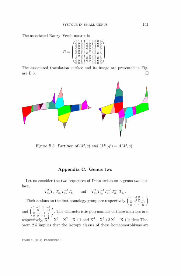
.The associated translation surface and its image are presented in Fig-ure B.3. �

Figure B.3. Partition of (M, q) and (M ′, q′) = A(M, q).

Appendix C. Genus two

Let us consider the two sequences of Dehn twists on a genus two sur-face,

T 2a1Tc1Tb2T

−1a2Tb1 and T 2

a1T−1b2T−1c1 T−1

a2Tb1 .

Their actions on the first homology group are respectively( 1 −3 0 1

1 −2 0 10 2 2 −10 1 1 0

)and( 1 −1 1 −1

1 0 1 −10 −1 −1 20 0 −1 1

). The characteristic polynomials of these matrices are,

respectively, X4−X3−X2−X +1 and X4−X3 +3 X2−X +1; thus The-orem 2.5 implies that the isotopy classes of these homeomorphisms are



pseudo-Anosov. Let φ1 and φ2 be the corresponding maps. One can cal-culate their dilatations from their action on the fundamental group [9].We check that the dilatations, λ, are the same, namely the Perron rootof the polynomial X4−X3−X2−X +1 (λ ' 1.72208).

Theorem 2.4 thus implies that φ1 fixes an orientable measured foliation,and hence δ+

2 = λ(φ1) and φ2 fixes a non-orientable measured foliation.We conclude that δ−2 = λ(φ2).

These two homeomorphisms are related by covering transformations(see Remark 4.1).

BIBLIOGRAPHY

[1] J. W. Aaber & N. M. Dunfield, “Closed surface bundles of least volume”, 2010,arXiv:1002.3423.

[2] P. Arnoux & J.-C. Yoccoz, “Construction de difféomorphismes pseudo-Anosov”, C. R. Acad. Sci. Paris Sér. I Math. 292 (1981), no. 1, p. 75-78.

[3] G. Band & P. Boyland, “The Burau estimate for the entropy of a braid”,Algebr. Geom. Topol. 7 (2007), p. 1345-1378.

[4] D. W. Boyd, “Reciprocal polynomials having small measure”, Math. Comp. 35(1980), no. 152, p. 1361-1377.

[5] R. F. Brown, The Lefschetz fixed point theorem, Scott, Foresman and Co.,Glenview, Ill.-London, 1971, vi+186 pages.

[6] A. J. Casson & S. A. Bleiler, Automorphisms of surfaces after Nielsen andThurston, London Mathematical Society Student Texts, vol. 9, Cambridge Uni-versity Press, Cambridge, 1988, iv+105 pages.

[7] J.-H. Cho & J.-Y. Ham, “The minimal dilatation of a genus-two surface”, Ex-periment. Math. 17 (2008), no. 3, p. 257-267.

[8] B. Farb, “Some problems on mapping class groups and moduli space”, in Prob-lems on mapping class groups and related topics, Proc. Sympos. Pure Math.,vol. 74, Amer. Math. Soc., Providence, RI, 2006, p. 11-55.

[9] A. Fathi, F. Laudenbach & V. Poénaru, “Travaux de Thurston sur les sur-faces”, in Astérisque, vol. 66–67, Société Mathématique de France, 1979.

[10] M. D. Finn, J.-L. Thiffeault & N. Jewell, “Topological entropy of braids onarbitrary surfaces”, 2010, preprint.

[11] E. Hironaka, “Small dilatation pseudo-Anosov mapping classes coming from thesimplest hyperbolic braid”, 2009, arXiv:0909.4517.



[12] E. Hironaka & E. Kin, “A family of pseudo-Anosov braids with small dilata-tion”, Algebr. Geom. Topol. 6 (2006), p. 699-738 (electronic).

[13] N. V. Ivanov, “Coefficients of expansion of pseudo-Anosov homeomorphisms”,Zap. Nauchn. Sem. Leningrad. Otdel. Mat. Inst. Steklov. (LOMI) 167 (1988),no. Issled. Topol. 6, p. 111-116, 191, translation in J. Soviet Math., 52, (1990),pp. 2819–2822.

[14] R. Kenyon & J. Smillie, “Billiards in rational-angled triangles”, Comment.Math. Helv. 75 (2000), p. 65-108.

[15] E. Kin & M. Takasawa, “Pseudo-Anosovs on closed surfaces having small en-tropy and the Whitehead sister link exterior”, 2010, arXiv:1003.0545.

[16] E. Lanneau, “Hyperelliptic components of the moduli spaces of quadratic differ-entials with prescribed singularities”, Comment. Math. Helv. 79 (2004), no. 3,p. 471-501.

[17] E. Lanneau & J.-L. Thiffeault, “Enumerating Pseudo-Anosov Homeomor-phisms of the Punctured Disc”, 2010, preprint, arXiv:1004.5344.

[18] F. Le Roux, “Homéomorphismes de surfaces: théorèmes de la fleur de Leau-Fatou et de la variété stable”, Astérisque (2004), no. 292, p. vi+210.

[19] C. J. Leininger, “On groups generated by two positive multi-twists: Teichmüllercurves and Lehmer’s number”, Geom. Topol. 8 (2004), p. 1301-1359 (electronic).

[20] S. Marmi, P. Moussa & J.-C. Yoccoz, “The cohomological equation for Roth-type interval exchange maps”, J. Amer. Math. Soc. 18 (2005), no. 4, p. 823-872(electronic).

[21] H. Masur & J. Smillie, “Quadratic differentials with prescribed singularitiesand pseudo-Anosov diffeomorphisms”, Comment. Math. Helv. 68 (1993), no. 2,p. 289-307.

[22] H. Masur & S. Tabachnikov, “Rational billiards and flat structures”, in Hand-book of dynamical systems, Vol. 1A, North-Holland, Amsterdam, 2002, p. 1015-1089.

[23] C. T. McMullen, “Teichmüller curves in genus two: discriminant and spin”,Math. Ann. 333 (2005), no. 1, p. 87-130.

[24] J.-O. Moussafir, “On the Entropy of Braids”, Func. Anal. and Other Math. 1(2006), p. 43-54.

[25] R. C. Penner, “Bounds on least dilatations”, Proc. Amer. Math. Soc. 113(1991), no. 2, p. 443-450.

[26] C. Pisot & R. Salem, “Distribution modulo 1 of the powers of real numberslarger than 1”, Compositio Math. 16 (1964), p. 164-168 (1964).



[27] G. Rauzy, “Échanges d’intervalles et transformations induites”, Acta Arith. 34(1979), no. 4, p. 315-328.

[28] W. P. Thurston, “On the geometry and dynamics of diffeomorphisms of sur-faces”, Bull. Amer. Math. Soc. (N.S.) 19 (1988), no. 2, p. 417-431.

[29] W. A. Veech, “Gauss measures for transformations on the space of intervalexchange maps”, Ann. of Math. (2) 115 (1982), no. 1, p. 201-242.

[30] A. Y. Zhirov, “On the minimum dilation of pseudo-Anosov diffeomorphisms ofa double torus”, Uspekhi Mat. Nauk 50 (1995), no. 1(301), p. 197-198.

Manuscrit reçu le 21 mai 2009,révisé le 21 janvier 2010,accepté le 5 mars 2010.

Erwan LANNEAUUniversité du Sud Toulon-Varand Fédération de Recherchesdes Unités de Mathématiques de MarseilleCentre de Physique Théorique (CPT)UMR CNRS 6207,Luminy, Case 90713288 Marseille Cedex 9 (France)[email protected] THIFFEAULTUniversity of WisconsinDepartment of MathematicsVan Vleck Hall, 480 Lincoln DriveMadison, WI 53706 (USA)[email protected]


mailto:[email protected]

mailto:[email protected]

Documents

On the minimum dilatation of pseudo-Anosov homeromorphisms ... · SYSTOLE IN SMALL GENUS 107 that realize δ 2, in the mapping class group of genus 2 surfaces, Mod(2) (see Theorem