Article D

« Retrieving vertical foliagedistribution using high resolution

airborne scatterometer data »

J.M. Martinez, T. Le Toan, E. Mushinzimana, M. Deshayes,

soumis à Tree Physiology.

1

RETRIEVING VERTICAL FOLIAGE DISTRIBUTION USING HIGH

RESOLUTION AIRBORNE SCATTEROMETER DATA

J.M. MARTINEZ 1 2, T. LE TOAN 1, E. MUSHINZIMANA 2, M. DESHAYES2

1 CESBIO, 18 Ave Edouard Belin, 31055 Toulouse, France

tel: (33) 5.61.55.85.08 fax: (33) 5.61.55.85.00 e-mail: martinez@cesbio.cnes.fr

2 Laboratoires des Systèmes et Structures Spatiaux Cemagref-ENGREF (L3S),

500 rue J.F. Breton, 34093 Montpellier Cedex 05, France

2

ABSTRACT

This paper presents the comparison between vertical backscatter profiles of forest measured by an

airborne ranging scatterometer radar and in-situ measurements of foliar biomass in a pine forest.

Radar ranging scatterometer allows to study, with a vertical resolution inferior to the meter, the

radar backscatter vertical distribution into the canopy which is known to be physically related to the

vegetation biophysical properties. The objective is to explore a new method to assess the vertical

distribution of foliar biomass inside tree canopy using remotely sensed data.

In a recent work, simulations of the backscatter profiles using a multi-layer radiative transfer (RT)

model have shown that the needles are by far the main scatters at short wavelength (2.1 cm) and

that the microwave interacts with all the canopy allowing to retrieve the tree foliar characteristics.

Based on these results, a simple relation between the measured backscatter and the foliar biomass is

derived using the RT model. Experimental backscatter profiles are then inverted into the vertical

foliar biomass distribution. For validation, 7 and 9 trees have been destructively sampled in

respectively 40 and 100-year old Austrian pine stands. Good agreement is found for different ages,

both qualitatively and quantitatively, between the retrieved and measured vertical distribution of the

foliar biomass as well as the total foliar biomass. Finally, advantages and limitations of the method

are discussed.

3

I. INTRODUCTION

Vertical distribution of forest foliar biomass is an important structural characteristic for quantifying

energy and mass exchange inside forest canopies. A better characterisation of the foliar biomass

distribution would allow a better modelling of the light transmittance inside tree canopies, which is

an important regulator of canopy carbon gain (Russel et al. 1989). Several studies have shown that

foliar vertical distribution plays a major role in different vegetation processes such as trunk cross

sectional increment (Kershaw et al. 1999), partitioning of nutrient resources and photosynthetic

activity (Ellsworth and Reich 1993), and that the nature of the leaf area profile as well as the canopy

geometry control the amount and pattern of the light at the forest floor (Cowan 1968). It has interest

for process-based forest growth models in which canopy characteristics are often required.

Vegetation distribution is also an indication of the growth competition between trees (Vose et al.

1995) and of the impact of the sylvicultural practices.

Some studies have provided information on the vertical distribution (Aber 1979, Ellsworth and

Reich 1993, Hollinger 1989, Hutchison et al. 1986, Kruijt 1989, Parker et al. 1989, Vose et al.

1995, Yang et al. 1999). However, in comparison to other forestry research subjects, the

architecture of forest canopies is not much studied, in particular due to the difficulty to work

throughout forest canopies. In particular, it is difficult to extend the experimental results due to the

diversity in ground measurements techniques and the specificity of the forest type under study

(monospecific/mixed stands, even aged/uneven aged forests).

The objective of this paper is to present a new method to assess foliar vegetation distribution using

remotely sensed data from a ranging radar scatterometer. Radar data are well known to be

physically related to the vegetation characteristics allowing to retrieved forest biomass and other

4

correlated parameters (Dobson et al. 1992, Le Toan et al. 1992, Beaudoin et al. 1994). For forestry

radar airborne scatterometers combines three interesting properties: a) the possibility to vertically

sound tree canopies with a high resolution (< 1 m); b) the possibility to retrieve the biophysical

characteristics of the vegetation from the radar backscatter coefficient; c) the potentiality to cover

large areas with an aircraft instead of in situ measurements located on reduce sets of sample plots.

Several studies dealt with ranging scatterometer applications for forestry concerning tree height

retrieval, stem volume or species discrimination (Bernard et al. 1987, Hallikainen et al. 1993,

Martinez et al. 2000a) giving excellent results. In this paper, we propose to explore another

potentiality of vertical backscatter profiles within tree canopies, by assessing the foliar biomass

vertical distribution inside a pine forest.

The study is driven by past experimental and theoretical results (Martinez et al. 2000a, Martinez et

al. 2000b) based on an experiment performed in November 1997 (Martinez et al. 1998), using the

helicopter-borne scatterometer HUTSCAT (Helsinki University of Technology SCATterometer),

over the Lozère forest in France.

In the first part of the paper, we present the test-site, the radar data and the ground data used for

validation which consist in destructive sampling of 16 trees in two stands of 40 and 100 years old.

In the second part, a short summary of the previous theoretical work introduces the foliar

distribution retrieval algorithm. Then, comparisons between radar derived foliar biomass

distribution and ground based measurements are presented. Finally, a discussion on the results and

on the potential of the method is presented.

5

TEST-SITE AND DATA

Test-site

The Lozère forest is located in the South of France over limestone plateaus at an altitude of about

1000 m above sea level. The plateaus are intersected by deep gorges of about 300 m depth. This

forest is a plantation made of even-aged and relatively homogeneous stands of Austrian Pine (Pinus

nigra Arnold ssp Nigricans Host.) with age from 0 to 130 years old, covering 5400 ha. The first

seedlings date from the last century in the framework of a program aiming at limiting the erosion of

the plateaus. The forest was not managed until the 1960’s when the forest began to be also used for

wood production. Nowadays the majority of the stands are aged of 100 to 130 years old but a part of

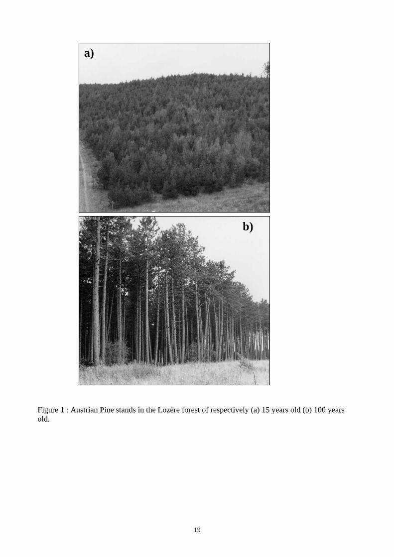
the forest has been renewed and a new generation between 0 and 40 years old is present. Figure 1

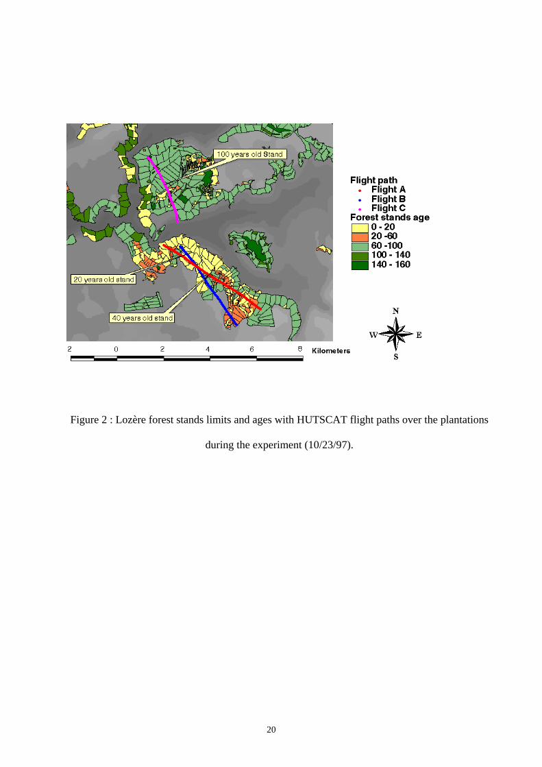
presents examples of 15 and 100 year-old stands. The stands are of about 10 ha each and are

managed by the French Forestry Board. The stands limits and ages are included in a Geographic

Information System (GIS) (Figure 2).

Radar data

HUTSCAT is a helicopter-borne non-imaging FM-CW scatterometer (Hallikainen et al. 1993)

designed and constructed by the Laboratory of Space Technology of the Helsinki University of

Technology (HUT). The system provides the vertical distribution of backscatter within the tree

canopy with a 68-cm vertical resolution. In this paper we will focus on profiles obtained at X band

(wavelength of 2,1 cm) and at 3° of incidence (near normal to the ground).

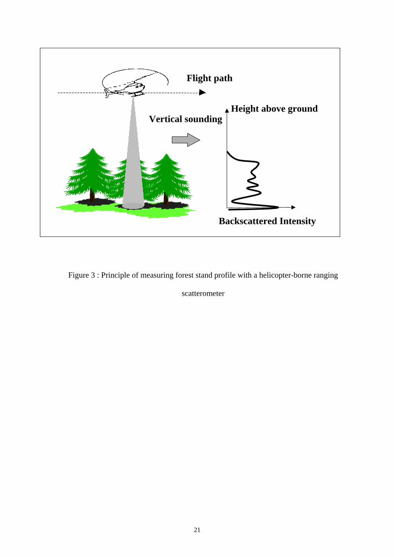
Fig. 3 shows the basic principle of an HUTSCAT acquisition. An antenna, located under the

helicopter flying at an altitude of 100 m above the ground, emits pulses with a regular frequency

6

toward the ground and measures the backscattered echoes. The system gives the backscatter

coefficient which represents the ratio of the backscattered energy to the emitted energy, normalised

by the backscattering area (circular area of 7 to 9 meters depending on the flight altitude which is

the intersection of the beam with the ground). The signal is frequency modulated, which allows by

measuring the frequency shifts, to assess the different distances between the targets and the antenna

in the frequency spectrum. It is then possible to obtain the backscatter variation as a function of the

height. The height of a resolution cell in the radar return spectrum is estimated relatively to the

ground echo, meaning that the height measurements are independent to the local topography.

Data were collected during a campaign in November 1997. A total of 6 flights of 4 km long, aligned

along 3 transects (see figure 2), acquired at 3° incidence was used. The calibrated data provide the

ground and tree canopy backscattering coefficients along each measurement transect. The forest

backscattering profile was calculated only when returns from ground and tree canopy were

reasonably well separated from each other.

At near vertical incidence, the understory layer and other vegetation elements above the ground

(dead branches) contribute significantly to the total backscatter. We selected profiles in which 90 %

of the total above ground backscattered energy comes from the canopy layer. The bottom limits of

the canopy were determined with in situ measurements of the canopy depth (Martinez et al. 1998).

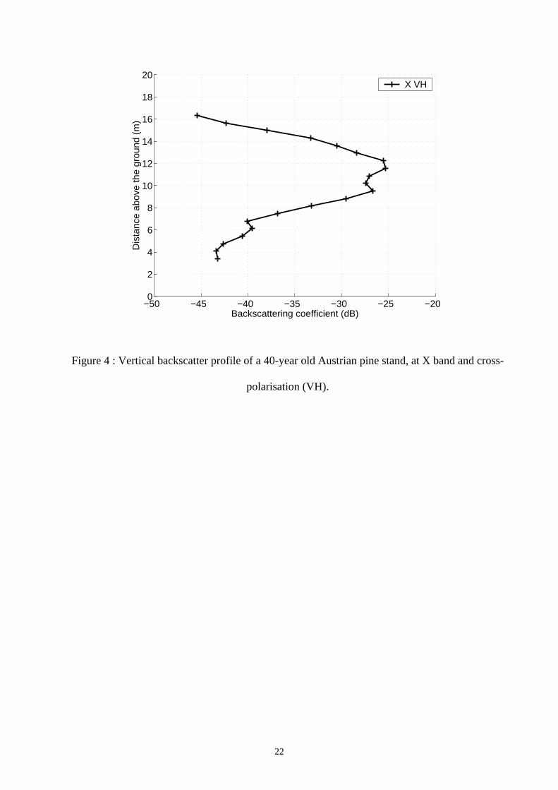
One example of vertical backscatter profiles is shown in Fig. 4, for a 40-year old Austrian pine

stand at X band and for cross-polarisation. The backscatter distribution seems clearly correlated

with the canopy characteristic, suggesting that the microwave interacts with all the canopy layers.

7

Foliar biomass in-situ measurements

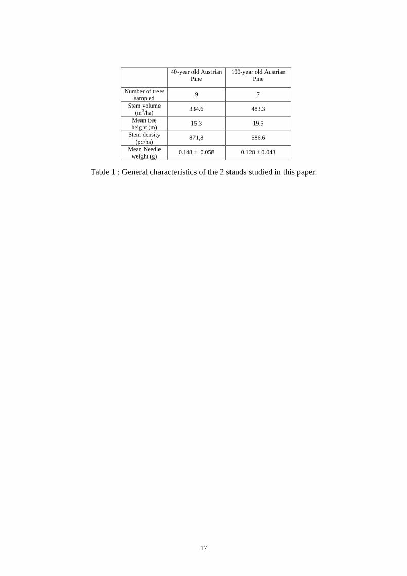
Two stands of 40 and 100-year old were chosen for biomass measurements, in which respectively 9

and 7 trees were cut down for destructive sampling (Deshayes et al. 1999). The trees were chosen

with respect to the class frequency of DBH and the social status (dominant, codominant and

dominated) in the stands. The stand characteristics are summarised in Table 1.

Measurements were first performed for 40 years old trees for protocol validation. For all the

primary branches of 2 trees, total needle biomass (fresh and dry weight), branch length and

diameter were measured. For the other 7 trees, all the primary branches diameter were measured but

needle biomass (fresh weight) simply measured every 2 whorls. To interpolate the missing foliar

biomass in between the measured whorls, we used relations linking the diameter of the primary

branches to their foliar biomass weight (Deshayes et al. 1999). This undersampling method was

validated on the two firsts 40-year old pines sampled. By comparing the measurements and the

interpolated results, the error introduced on the estimation of the tree foliar biomass by the under-

sampling was found to be less than 10%. The same protocol was used for the 100 years old stand,

except that only one tree was fully sampled for foliar biomass measurements.

Needle samples were ovendried (at 105°C during 72 hours). These samples were in majority

collected on the fully sampled trees (the two 40 year old pines and the one 100 year old pine). Some

other samples were collected on the others trees. The total projected area of a sample is then

measured with a planimeter and weighted in order to establish the specific area (area per unit of

weight). In the results section we will use needle number density and total foliar area instead of

needle biomass for the comparisons with the scatterometer data. Needle density and foliar area were

determined from mean needle weight and mean needle specific area.

8

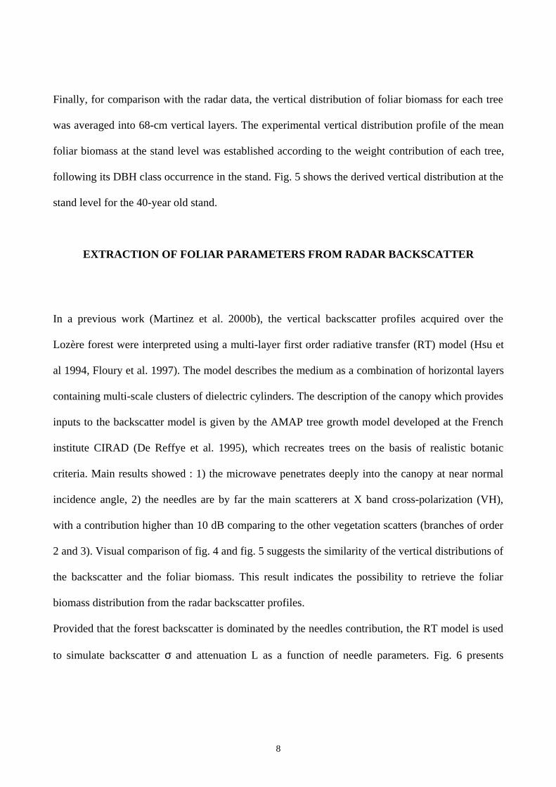
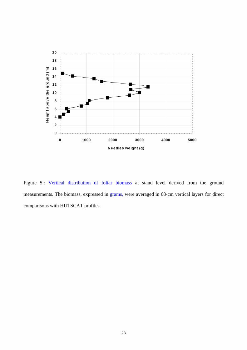
Finally, for comparison with the radar data, the vertical distribution of foliar biomass for each tree

was averaged into 68-cm vertical layers. The experimental vertical distribution profile of the mean

foliar biomass at the stand level was established according to the weight contribution of each tree,

following its DBH class occurrence in the stand. Fig. 5 shows the derived vertical distribution at the

stand level for the 40-year old stand.

EXTRACTION OF FOLIAR PARAMETERS FROM RADAR BACKSCATTER

In a previous work (Martinez et al. 2000b), the vertical backscatter profiles acquired over the

Lozère forest were interpreted using a multi-layer first order radiative transfer (RT) model (Hsu et

al 1994, Floury et al. 1997). The model describes the medium as a combination of horizontal layers

containing multi-scale clusters of dielectric cylinders. The description of the canopy which provides

inputs to the backscatter model is given by the AMAP tree growth model developed at the French

institute CIRAD (De Reffye et al. 1995), which recreates trees on the basis of realistic botanic

criteria. Main results showed : 1) the microwave penetrates deeply into the canopy at near normal

incidence angle, 2) the needles are by far the main scatterers at X band cross-polarization (VH),

with a contribution higher than 10 dB comparing to the other vegetation scatters (branches of order

2 and 3). Visual comparison of fig. 4 and fig. 5 suggests the similarity of the vertical distributions of

the backscatter and the foliar biomass. This result indicates the possibility to retrieve the foliar

biomass distribution from the radar backscatter profiles.

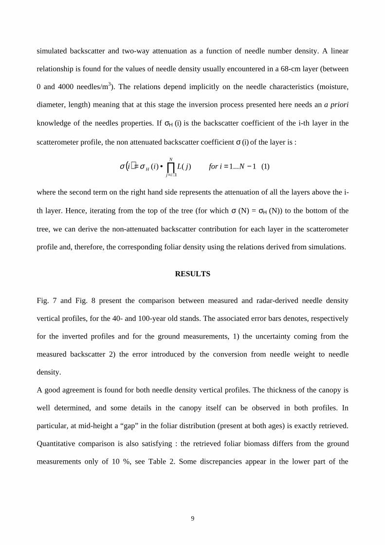
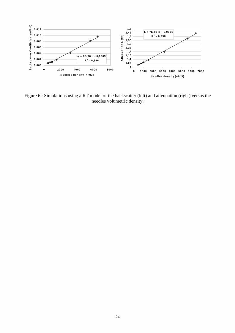
Provided that the forest backscatter is dominated by the needles contribution, the RT model is used

to simulate backscatter σ and attenuation L as a function of needle parameters. Fig. 6 presents

9

simulated backscatter and two-way attenuation as a function of needle number density. A linear

relationship is found for the values of needle density usually encountered in a 68-cm layer (between

0 and 4000 needles/m3). The relations depend implicitly on the needle characteristics (moisture,

diameter, length) meaning that at this stage the inversion process presented here needs an a priori

knowledge of the needles properties. If σΗ (i) is the backscatter coefficient of the i-th layer in the

scatterometer profile, the non attenuated backscatter coefficient σ (i) of the layer is :

( ) )1(1...1)()(1

−=•= ∏+=

NiforjLiiN

ijHσσ

where the second term on the right hand side represents the attenuation of all the layers above the i-

th layer. Hence, iterating from the top of the tree (for which σ (N) = σΗ (N)) to the bottom of the

tree, we can derive the non-attenuated backscatter contribution for each layer in the scatterometer

profile and, therefore, the corresponding foliar density using the relations derived from simulations.

RESULTS

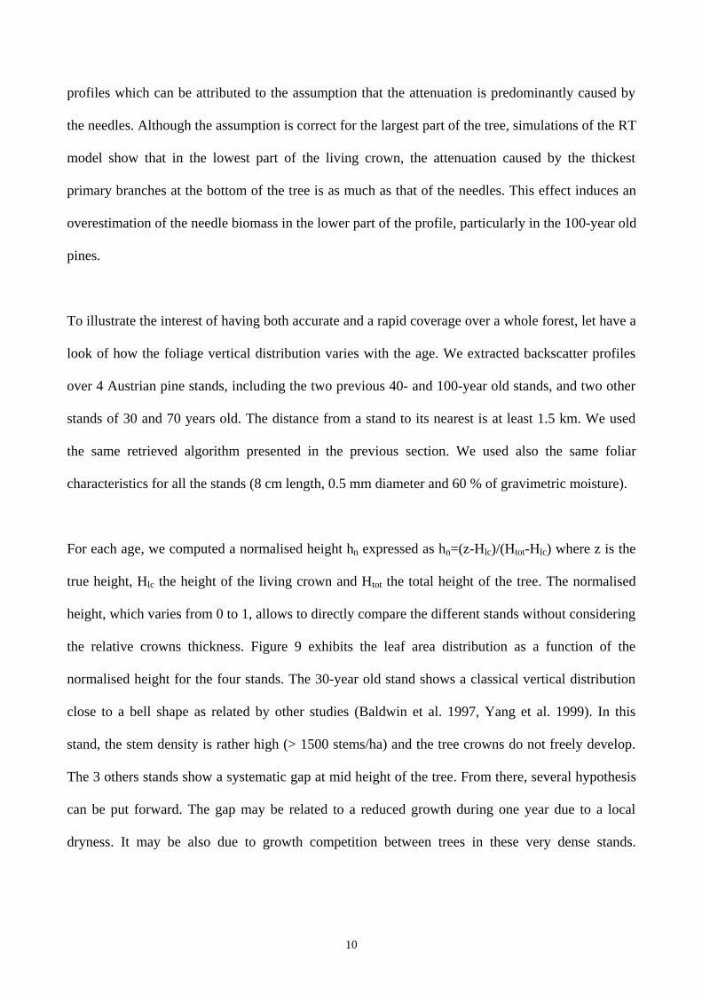
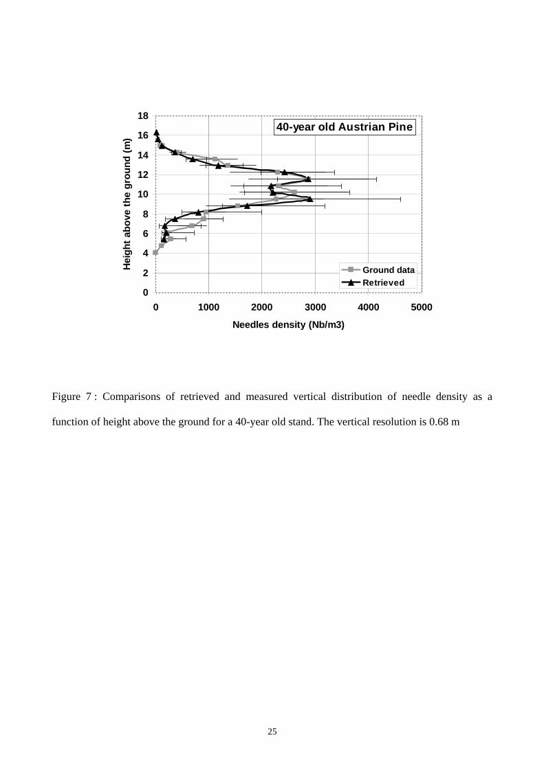
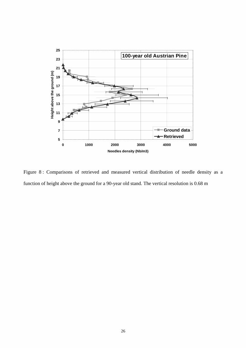
Fig. 7 and Fig. 8 present the comparison between measured and radar-derived needle density

vertical profiles, for the 40- and 100-year old stands. The associated error bars denotes, respectively

for the inverted profiles and for the ground measurements, 1) the uncertainty coming from the

measured backscatter 2) the error introduced by the conversion from needle weight to needle

density.

A good agreement is found for both needle density vertical profiles. The thickness of the canopy is

well determined, and some details in the canopy itself can be observed in both profiles. In

particular, at mid-height a “gap” in the foliar distribution (present at both ages) is exactly retrieved.

Quantitative comparison is also satisfying : the retrieved foliar biomass differs from the ground

measurements only of 10 %, see Table 2. Some discrepancies appear in the lower part of the

10

profiles which can be attributed to the assumption that the attenuation is predominantly caused by

the needles. Although the assumption is correct for the largest part of the tree, simulations of the RT

model show that in the lowest part of the living crown, the attenuation caused by the thickest

primary branches at the bottom of the tree is as much as that of the needles. This effect induces an

overestimation of the needle biomass in the lower part of the profile, particularly in the 100-year old

pines.

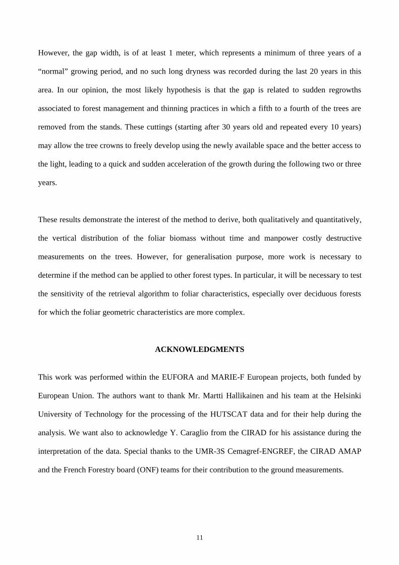
To illustrate the interest of having both accurate and a rapid coverage over a whole forest, let have a

look of how the foliage vertical distribution varies with the age. We extracted backscatter profiles

over 4 Austrian pine stands, including the two previous 40- and 100-year old stands, and two other

stands of 30 and 70 years old. The distance from a stand to its nearest is at least 1.5 km. We used

the same retrieved algorithm presented in the previous section. We used also the same foliar

characteristics for all the stands (8 cm length, 0.5 mm diameter and 60 % of gravimetric moisture).

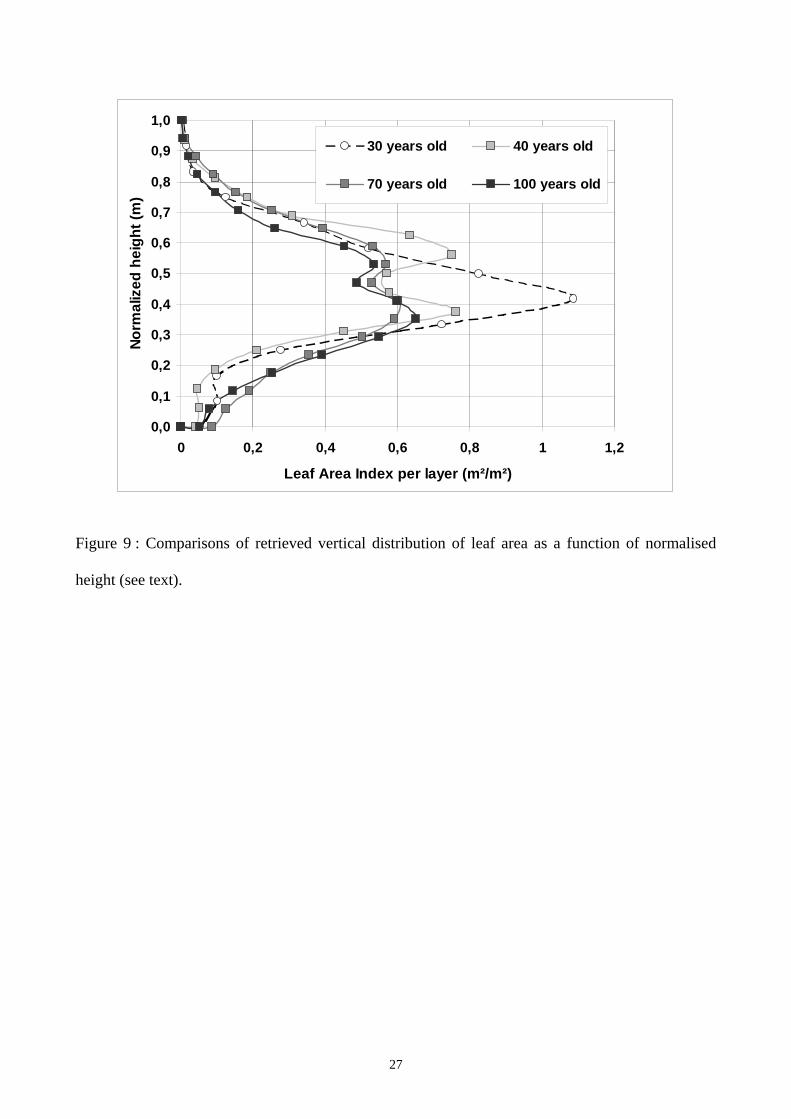
For each age, we computed a normalised height hn expressed as hn=(z-Hlc)/(Htot-Hlc) where z is the

true height, Hlc the height of the living crown and Htot the total height of the tree. The normalised

height, which varies from 0 to 1, allows to directly compare the different stands without considering

the relative crowns thickness. Figure 9 exhibits the leaf area distribution as a function of the

normalised height for the four stands. The 30-year old stand shows a classical vertical distribution

close to a bell shape as related by other studies (Baldwin et al. 1997, Yang et al. 1999). In this

stand, the stem density is rather high (> 1500 stems/ha) and the tree crowns do not freely develop.

The 3 others stands show a systematic gap at mid height of the tree. From there, several hypothesis

can be put forward. The gap may be related to a reduced growth during one year due to a local

dryness. It may be also due to growth competition between trees in these very dense stands.

11

However, the gap width, is of at least 1 meter, which represents a minimum of three years of a

“normal” growing period, and no such long dryness was recorded during the last 20 years in this

area. In our opinion, the most likely hypothesis is that the gap is related to sudden regrowths

associated to forest management and thinning practices in which a fifth to a fourth of the trees are

removed from the stands. These cuttings (starting after 30 years old and repeated every 10 years)

may allow the tree crowns to freely develop using the newly available space and the better access to

the light, leading to a quick and sudden acceleration of the growth during the following two or three

years.

These results demonstrate the interest of the method to derive, both qualitatively and quantitatively,

the vertical distribution of the foliar biomass without time and manpower costly destructive

measurements on the trees. However, for generalisation purpose, more work is necessary to

determine if the method can be applied to other forest types. In particular, it will be necessary to test

the sensitivity of the retrieval algorithm to foliar characteristics, especially over deciduous forests

for which the foliar geometric characteristics are more complex.

ACKNOWLEDGMENTS

This work was performed within the EUFORA and MARIE-F European projects, both funded by

European Union. The authors want to thank Mr. Martti Hallikainen and his team at the Helsinki

University of Technology for the processing of the HUTSCAT data and for their help during the

analysis. We want also to acknowledge Y. Caraglio from the CIRAD for his assistance during the

interpretation of the data. Special thanks to the UMR-3S Cemagref-ENGREF, the CIRAD AMAP

and the French Forestry board (ONF) teams for their contribution to the ground measurements.

12

REFERENCES

Aber, J.D. 1979. A method for estimating foliage-height profiles in broad-leaved forests. Journal of

Ecology 67:35-40.

Baldwin V.C., Jr., K.D. Peterson, H.E. Burkhart, R.L. Amateis and P.M. Dougherty. 1997.

Equations for estimating loblolly pine branch and foliage weight and surface area distributions.

Canadian Journal of Forest Research 27:918-927.

Beaudoin A., T. Le Toan, S. Goze, E. Nezry, A. Lopes, E. Mougin, C.C. Hsu, H.C. Han, J.A. Kong,

and R.T. Shin. 1994. Retrieval of forest biomass from SAR data. International Journal of Remote

Sensing 15(14):2777-2796.

Bernard, R., M.E. Frezal, D. Vidal-Madjar, D. Guyon, J. Riom. 1987. Nadir looking Airborne

Radar and Possible Applications to Forestry. Remote Sensing of Environment 21:297-309.

Cowan I.R. 1968. The interception and absorption of radiation in plant stands. Journal of Applied

Ecology 8:367-379.

De Reffye, P., F. Houllier, F. Blaise, D. Barthelemy, J. Dauzat, and D. Auclair 1995. A model

simulating above- and below-ground tree architecture with agroforestry applications, Agroforestry

Systems 30:175-197.

Deshayes, M., E. Mushinzima and N. Stach 1999. Assessment of FLIM reflectance model : case

study Lozère, France. In, MARIE-F (Monitoring and Assesment of Resources in Europe – Forest)

project final report, contract ENV4-CT96-0316, 5.1-5.56.

Dobson, M. C., F.T. Ulaby, T. Le Toan, A. Beaudoin, E.S. Kasischke, and N.L. Christensen Jr.

1992. Dependence of radar backscatter on coniferous forest biomass. IEEE Transactions on

Geoscience and Remote Sensing 30(2):412-415.

Ellsworth, D.S., P.B. Reich. 1993. Canopy structure and vertical patterns of photosynthesis and

related leaf straits in a deciduous forest. Oecologia 96:169-178.

13

Floury, N., G. Picard, T. Le Toan, J. A. Kong, T. Castel, A. Beaudoin, J. F. Barczi. 1997. On the

coupling of backscatter models with tree growth models: 2) RT modelling of forest backscatter.

Proceedings of IGARSS’97 Symposium, Singapore 2:787-789.

Hallikainen, M., J. Hyyppä, J. Haapanen, T. Tares, P. Ahola, J. Pulliainen, and M. Toikka. 1993. A

helicopter-borne eight-channel ranging scatterometer for remote sensing - Part I: system

description, IEEE Transactions on Geoscience and Remote Sensing 31(1):161-169.

Hollinger, D.Y. 1989. Canopy organization and foliage photo-synthetic capacity in a broad-leaved

evergreen montane forest. Funct. Ecol. 3:53-62.

Hsu C.C., H.C. Han, R.T. Shin, J.A. Kong, A. Beaudoin, T. Le Toan. 1994. Radiative Transfer

theory for polarimetric remote sensing of forest at P band. Int. Journal of Remote Sensing

15(14):2943-2954.

Hutchison, B.A. et al. 1986. The architecture of a deciduous forest canopy in eastern Tennessee.

Journal of ecology 74:635-646.

Kershaw, J.A. Jr and D.A. Maguire 2000. Influence of vertical foliage structure on the distribution

of stem cross-sectionnal area increment area increment in western hemlock and balsam fir. Forest

Science 46(1):86-94.

Kruijt, B. 1989. Estimating canopy structure of an oak forest at several scales. Forestry 62:269-284.

Martinez, J.M., A. Beaudoin, N. Floury, M. Makynen T. Le Toan, M. Hallikainen, and J. Uusitalo

1998. First results and analysis of HUTSCAT data over Austrian Pine plantations. Proceedings of

the 2nd International Workshop on Retrieval of Bio- & Geo-physical parameters from SAR data,

ESTEC, 317-324.

Martinez, J.M., A. Beaudoin, P. Durand, T. Le Toan, N. Stach 2000a. Une nouvelle méthode pour

l’estimation de la hauteur des peuplements, Canadian Journal of Forest Research, p 1983-1991,

Décembre 2000.

14

Martinez, J.M., N. Floury, T. Le Toan, A. Beaudoin, M. Hallikainen, M. Makinen 2000b.

Understanding of backscatter mechanisms inside tree canopy for penetration depth estimation, IEEE

Trans. Geosci. Remote Sensing 38(2):710-719.

Le Toan T., A. Beaudoin, J.Riom, D. Guyon. 1992. Relating forest biomass to SAR data. IEEE

Transactions on Geoscience and Remote Sensing 30(2):403-411.

Parker, G.G., J.P. O’Neill, and D. Higman. 1989. Vertical profile and canopy organization in a

mixed deciduous forest. Vegetatio 89:1-12.

Vose, J.M., N.H. Sullivan, B.D. Clinton and P.V. Bolstad. 1995. Vertical leaf area distribution, light

transmittance, and application of the Beer-Lambert law in four mature hardwood stands in the

southern Appalachians. Canadian Journal of Forest Research 25:1036-1043.

Yang, X., J.J. Witcosky, and D.R. Miller. 1999. Vertical overstory canopy architecture of temperate

deciduous hardwood forests in the eastern United States. Forest Science 45(3):349-358.

15

List of the figures

Fig. 1 : Lozère forest stands limits and ages with HUTSCAT flight paths over the plantations

during the experiment (10/23/97).

Fig. 2 : Principle of measuring forest stand profile with a helicopter-borne ranging scatterometer

Fig. 3 : Austrian Pine stands in the Lozère forest of respectively (a) 15 years old (b) 100 years old.

Fig. 4 : Vertical backscatter profile of a 40-year old Austrian pine stand, at X band and cross-

polarisation (VH).

Fig. 5 : Foliar biomass vertical distribution derived from the ground measurements. The biomass,

expressed in grammes, were averaged in 68-cm vertical layers for direct comparisons with

HUTSCAT profiles.

Fig. 6 : Simulations using a RT model of the backscatter (left) and attenuation (right) versus the

needles volumetric density.

Fig. 7 : Comparisons of retrieved and measured vertical distribution of needle density as a function

of height above the ground for a 40-year old stand. The vertical resolution is 0.68 m.

Fig. 8 : Comparisons of retrieved and measured vertical distribution of needle density as a function

of height above the ground for a 90-year old stand. The vertical resolution is 0.68 m.

16

List of the tables

Table 1 : General characteristics of the 2 stands studied in this paper.

Table 2 : Comparisons of measured and retrieved total foliar biomass.

17

40-year old AustrianPine

100-year old AustrianPine

Number of treessampled

9 7

Stem volume(m3/ha)

334.6 483.3

Mean treeheight (m)

15.3 19.5

Stem density(pc/ha)

871,8 586.6

Mean Needleweight (g)

0.148 ± 0.058 0.128 ± 0.043

Table 1 : General characteristics of the 2 stands studied in this paper.

18

40 years old pine 100 years old pineMeasured Retrieved Relative

errorMeasured Retrieved Relative

error

Total density of

needles (Nb/m3)13638 12525 8.2 % 12305 14241 13.6 %

Total LAI(m2/m2)

5.3 4.8 7.7 % 4.1 4.7 12.8 %

Table 2 : Comparisons of measured and retrieved total foliar biomass.

19

Figure 1 : Austrian Pine stands in the Lozère forest of respectively (a) 15 years old (b) 100 yearsold.

b)

a)

20

Figure 2 : Lozère forest stands limits and ages with HUTSCAT flight paths over the plantations

during the experiment (10/23/97).

21

Figure 3 : Principle of measuring forest stand profile with a helicopter-borne ranging

scatterometer

Flight path

Height above ground

Backscattered Intensity

Vertical sounding

22

−50 −45 −40 −35 −30 −25 −200

2

4

6

8

10

12

14

16

18

20

Backscattering coefficient (dB)

Dis

tanc

e ab

ove

the

grou

nd (

m)

X VH

Figure 4 : Vertical backscatter profile of a 40-year old Austrian pine stand, at X band and cross-

polarisation (VH).

23

Figure 5 : Vertical distribution of foliar biomass at stand level derived from the ground

measurements. The biomass, expressed in grams, were averaged in 68-cm vertical layers for direct

comparisons with HUTSCAT profiles.

0

2

4

6

8

10

12

14

16

18

20

0 1000 2000 3000 4000 5000

Needles we ight (g)

He

igh

t a

bo

ve

th

e g

rou

nd

(m

)

24

Figure 6 : Simulations using a RT model of the backscatter (left) and attenuation (right) versus theneedles volumetric density.

σσσσ = 2E-06 n - 0 ,0003

R 2 = 0 ,996

0,000

0,002

0,004

0,006

0,008

0,010

0,012

0 2000 4000 6000 8000

N eedles den s ity (n /m3)

Ba

ck

sc

att

er

Co

eff

icie

nt

(m²/

m²)

L = 7E-05 n + 0 ,9931

R 2 = 0 ,998

11,05

1,11 ,15

1,21 ,25

1,31 ,35

1,41 ,45

1,5

0 1000 2000 3000 4000 5000 6000 7000

N eedles den s ity (n /m3)

Att

en

ua

tio

n L

(/m

)

25

0

2

4

6

8

10

12

14

16

18

0 1000 2000 3000 4000 5000

Needles density (Nb/m3)

Hei

ght a

bove

the

gro

und

(m)

Ground dataRetrieved

40-year old Austrian Pine

Figure 7 : Comparisons of retrieved and measured vertical distribution of needle density as a

function of height above the ground for a 40-year old stand. The vertical resolution is 0.68 m

26

5

7

9

11

13

15

17

19

21

23

25

0 1000 2000 3000 4000 5000

Needles density (Nb/m3)

Hei

ght a

bove

the

grou

nd (m

)

Ground dataRetrieved

100-year old Austrian Pine

Figure 8 : Comparisons of retrieved and measured vertical distribution of needle density as a

function of height above the ground for a 90-year old stand. The vertical resolution is 0.68 m

27

0,0

0,1

0,2

0,3

0,4

0,5

0,6

0,7

0,8

0,9

1,0

0 0,2 0,4 0,6 0,8 1 1,2

Leaf Area Index per layer (m²/m²)

Nor

mal

ized

hei

ght (

m)

30 years old 40 years old

70 years old 100 years old

Figure 9 : Comparisons of retrieved vertical distribution of leaf area as a function of normalised

height (see text).