Embed Size (px)
Citation preview
Les rapports internes du LaMSID sont publiés sous la seule responsabilité de leurs auteurs
Rapports internes du LaMSID
P. TESTUD – P. MOUSSOU – A. HIRSCHBERG* – Y. AUREGAN**
Noise generated by cavitating single-hole and multi-hole
orifices in a water pipe RI-B3-N°005 Avril 2007
*Fluid Dynamics Laboratory, Technische Universiteit Eindhoven, The Netherlands **Laboratoire Acoustique de l’Université du Maine, UMR CNRS 6613
Laboratoire de Mécanique des Structures Industrielles Durables UMR EDF-CNRS 2832 EDF R&D 1, Avenue du Général de Gaulle - 92141 CLAMART CEDEX FRANCE
Noise generated by cavitating single-hole and
multi-hole orifices in a water pipe
P. Testuda , P. Moussou a, A. Hirschberg b, Y. Auregan c
aLaboratoire de Mecanique des Structures Industrielles Durables, UMR
CNRS-EDF 2832, 1 Avenue du General De Gaulle, F-92141 Clamart, France
bFluid Dynamics Laboratory, Department of Applied Physics, Technische
Universiteit Eindhoven, P.O. Box 513, 5600 MB Eindhoven, The Netherlands
cLaboratoire d’Acoustique de l’Universite du Maine, UMR CNRS 6613, Avenue
Olivier Messiaen, F-72085 Le Mans Cedex 9, France
Abstract
This paper presents an experimental study of the acoustical effects of cavitation
caused by a water flow through an orifice. A circular-centered single-hole orifice and
a multi-hole orifice are tested. Experiments are performed under industrial condi-
tions: the pressure drop across the orifice varies from 3 bars to 30 bars, corresponding
to cavitation numbers from 0.74 to 0.03.
Two regimes of cavitation are discerned. In each regime, the broadband noise
spectra obtained far downstream of the orifice are presented. A non-dimensional
representation is proposed: in the intermediate ’developed cavitation’ regime, spec-
tra collapse reasonably well; in the more intense ’super cavitation’ regime, spectra
depend strongly on the quantity of air remaining in the water downstream of the
orifice, which is revealed by the measure of the speed of sound at the downstream
transducers.
In the ’developed cavitation’ regime, whistling associated with periodic vortex
shedding is observed. The corresponding Strouhal number agrees reasonably well
with literature for single-phase flows. In the ’super cavitation’ regime, the whistling
disappears.
Key words: Confined flow, Orifice, Cavitation, Broadband noise, Whistling
1 Introduction
1.1 Motivations
In industrial processes, cavitating flows are known to sometimes generate
significant levels of noise and high vibrations of structures. Some papers have
been published in the last years on this topic: Au-Yang (2001); Weaver et al.
(2000); Moussou et al. (2004).
In particular, fatigue issues have been reported recently the configurations
of a cavitating valve (Moussou et al. 2001) and a cavitating orifice (Moussou
et al. 2003). The examination of the noise generated by a cavitating device,
in this study a cavitating orifice, is typically an industrial issue. It provides
information which is a basis for a safer design in terms of pipe vibrations.
1.2 Literature
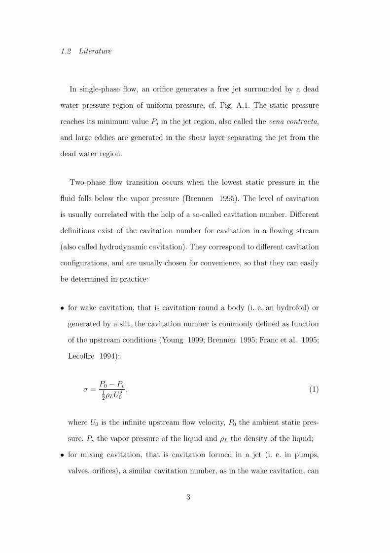
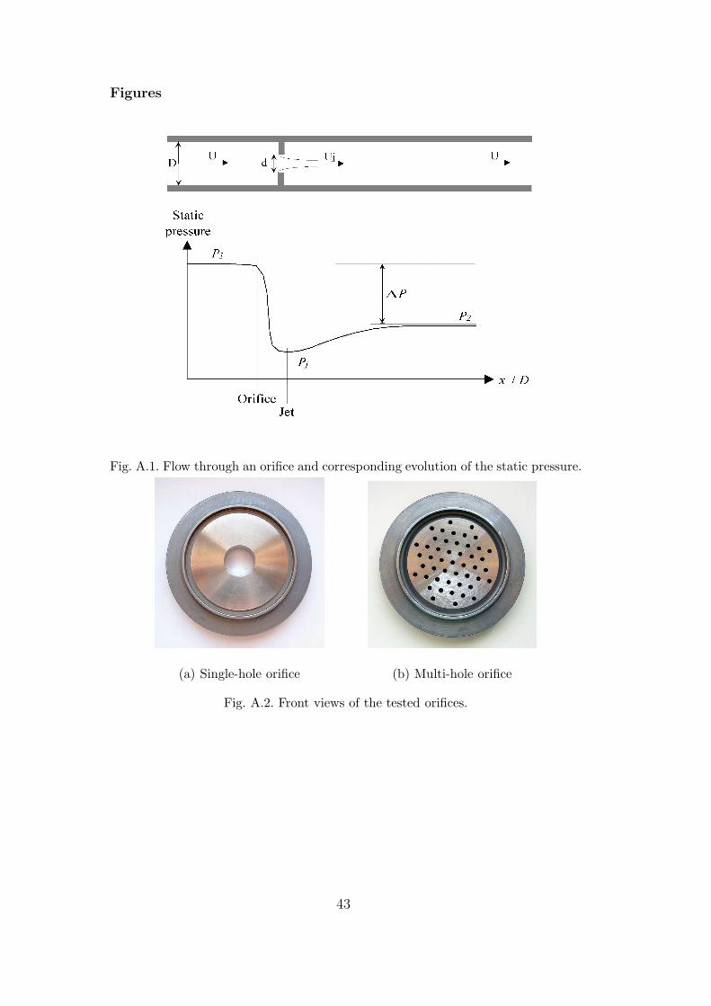
In single-phase flow, an orifice generates a free jet surrounded by a dead
water pressure region of uniform pressure, cf. Fig. A.1. The static pressure
reaches its minimum value Pj in the jet region, also called the vena contracta,
and large eddies are generated in the shear layer separating the jet from the
dead water region.
Two-phase flow transition occurs when the lowest static pressure in the
fluid falls below the vapor pressure (Brennen 1995). The level of cavitation
is usually correlated with the help of a so-called cavitation number. Different
definitions exist of the cavitation number for cavitation in a flowing stream
(also called hydrodynamic cavitation). They correspond to different cavitation
configurations, and are usually chosen for convenience, so that they can easily
be determined in practice:
• for wake cavitation, that is cavitation round a body (i. e. an hydrofoil) or
generated by a slit, the cavitation number is commonly defined as function
of the upstream conditions (Young 1999; Brennen 1995; Franc et al. 1995;
Lecoffre 1994):
σ =P0 − Pv12ρLU2
0
, (1)
where U0 is the infinite upstream flow velocity, P0 the ambient static pres-
sure, Pv the vapor pressure of the liquid and ρL the density of the liquid;
• for mixing cavitation, that is cavitation formed in a jet (i. e. in pumps,
valves, orifices), a similar cavitation number, as in the wake cavitation, can
3
be used (Young 1999; Brennen 1995):
σ =Pref − Pv
12ρLU2
0
, (2)
where Pref is very often defined as the downstream static pressure.
We prefer to use the cavitation number, based on the pressure drop across
the singularity generating the jet:
σ =P2 − Pv
∆P, (3)
where ∆P = P1−P2 is the pressure drop across the orifice, with P1 the static
pressure upstream of the orifice and P2 the downstream static pressure far
away from the orifice. In this choice, we follow common practice in industry
(Tullis 1989; Franc et al. 1995; Lecoffre 1994).
One should note that those both cavitation numbers lead to very similar
classifications as they are related each other by the pressure drop coefficient
of the singularity.
When the pressure Pj has a sufficiently low value, intermittent tiny cavita-
tion bubbles are produced in the heart of the turbulent eddies along the shear
layer of the jet. This flow regime transition is called cavitation inception, and
it appears at a cavitation number of the order of 1 (when d/D = 0.30) accord-
ing to the data of Tullis (1989). Other references (Numachi et al. 1960; Tullis
et al. 1973; Ball et al. 1989; Yan and Thorpe 1990; Kugou et al. 1996; Sato
and Saito 2001; Pan et al. 2001) are in good agreement with the values and
scale effects given by Tullis (1989). Some differences result from the influence
of the variation in the dissolved gas content and in the viscosity (Keller 1994).
As the jet pressure decreases further, more bubbles with larger radii are
generated, forming a white cloud. The pressure fluctuations increase and a
4
characteristic shot noise can be heard. A further decrease in jet pressure in-
duces the formation of a large vapor pocket just downstream of the orifice,
surrounding the liquid jet. The regime occurring after this transition is called
super cavitation and it exhibits the largest noise and vibration levels. In the
super cavitation regime, noise is known [see for example VanWijngaarden
(1972)] to be mainly generated in a shock transition between the cavitation
region and the pipe flow, at some distance downstream of the orifice. Down-
stream of the shock, some residual gas (air) bubbles can persist but pure vapor
bubbles have disappeared.
Cavitation indicators are used to predict the occurrence of cavitation regimes.
The use of two of them have seemed relevant in view of our experimental re-
sults. First, a so-called incipient cavitation indicator, noted σi, which predicts
the transition from a non cavitating flow to a moderately cavitating flow, that
is called developed cavitation regime. Second, a so-called choked cavitation in-
dicator, noted σch, which predicts the transition from a moderately cavitating
flow to a super cavitating flow, with the formation and continuous presence
of a vapor pocket downstream of the orifice around the liquid jet.
To calculate both those incipient and the choked cavitation indicators, scaling
laws are given by Tullis (1989). They take into account the various pressure
effects and size scale effects, by means of extensive experiments on single-hole
orifices in water pipe-flow. For multi-hole orifices, as mentioned in the same
work, less data are available but identical values are expected to hold.
Only a few studies provide downstream noise spectra generated by cavitat-
ing orifices (Yan et al. 1988; Bistafa et al. 1989; Kim et al. 1997; Pan et
al. 2001). Some few complementary studies give the noise spectra created by
cavitating valves (Hassis 1999; Martin et al. 1981). In fact, it appears that
5
far more research has been developed on submerged water jets (Jorgensen
1961; Esipov and Naugol’nykh 1975; Franklin and McMillan 1984; Brennen
1995; Latorre 1997). A comprehensive overview of the state of the art in this
domain is given in Brennen (1995).
6
Nomenclature
c speed of sound measured
downstream of the orifice (in
m s−1 )
Sj cross section of the jet (in m2)
cw speed of sound in pure water
(in m s−1 )
St Strouhal number for the
whistling frequency
cmin minimum speed of sound (in
m s−1 )
t orifice thickness (t = 14 10−3
m)
d diameter of the single-hole ori-
fice (d = 2.2 10−2 m)
tp pipe wall thickness (tp =
8 10−3 m)
deq single-hole equivalent diameter
of the multi-hole orifice (deq =
2.1 10−2 m)
U volume flux divided by pipe
cross-sectional area (in m s−1 )
dmulti diameter of the holes of the
multi-hole orifice (dmulti =
3 10−3 m)
Ud volume flux divided by orifice
cross-sectional area (in m s−1 )
f0 whistling frequency (in Hz) Uj volume flux divided by ori-
fice jet cross-sectional area (in
m s−1 )
D pipe diameter (D = 7.4 10−2
m)
β volume fraction of gas in the
water
7
Gpp Power Spectrum Density of the
pressure (in Pa2/Hz)
∆P static pressure difference
across the orifice (in Pa)
Nholes number of holes for the multi-
hole orifice (Nholes = 47)
νwatercinematic viscosity of water
[νwater(310 K) = 7.2 10−7
m2 s−1 (Idel’cik 1969)]
p+,
p−
forward, backward propagat-
ing plane wave spectra (in
Pa/√
Hz)
ρw density of water (ρw(310 K) =
994 kg m−3)
P1,
P2
static pressure respectively up-
stream and far downstream of
the orifice
σ cavitation number
Pj static pressure at the jet (vena
contracta)
σi incipient cavitation number
Pv vapor pressure
(Pv(310 K) =5.65 103 Pa
(Tullis 1989))
σch choked cavitation number
S cross section of the pipe (in
m2)
8
2 Experimental setup
2.1 Tested orifices
In a piping system of French nuclear power plants, a basic configuration
to obtain a pressure discharge can be realized with a single-hole orifice. The
maximum flow velocity can reach about 10 m s−1 and the pressure drop 100
bar across the orifice. This can induce high vibration levels. The orifices used
are chosen in order to reduce the pipe vibration to acceptable levels (Caillaud
et al. 2006).
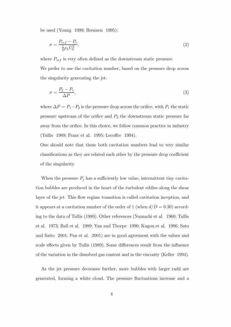
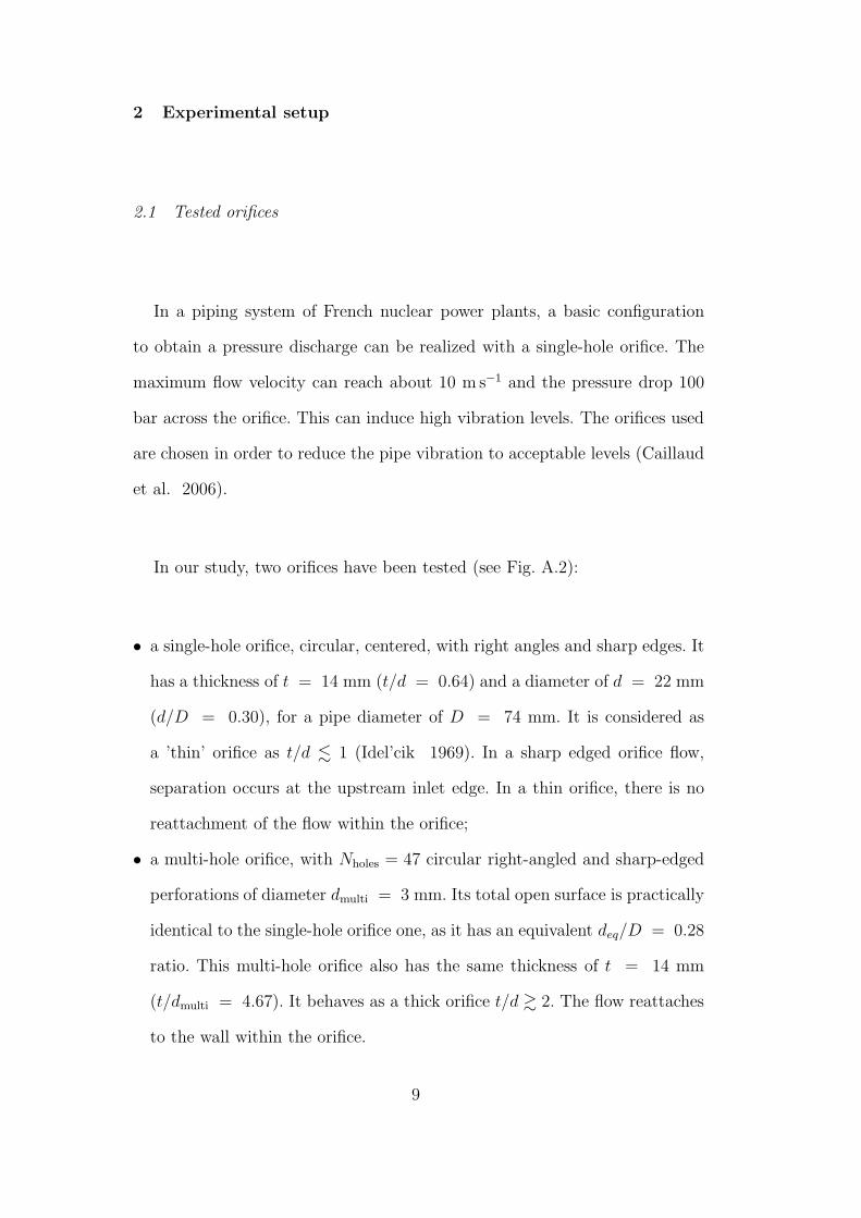
In our study, two orifices have been tested (see Fig. A.2):
• a single-hole orifice, circular, centered, with right angles and sharp edges. It
has a thickness of t = 14 mm (t/d = 0.64) and a diameter of d = 22 mm
(d/D = 0.30), for a pipe diameter of D = 74 mm. It is considered as
a ’thin’ orifice as t/d . 1 (Idel’cik 1969). In a sharp edged orifice flow,
separation occurs at the upstream inlet edge. In a thin orifice, there is no
reattachment of the flow within the orifice;
• a multi-hole orifice, with Nholes = 47 circular right-angled and sharp-edged
perforations of diameter dmulti = 3 mm. Its total open surface is practically
identical to the single-hole orifice one, as it has an equivalent deq/D = 0.28
ratio. This multi-hole orifice also has the same thickness of t = 14 mm
(t/dmulti = 4.67). It behaves as a thick orifice t/d & 2. The flow reattaches
to the wall within the orifice.
9
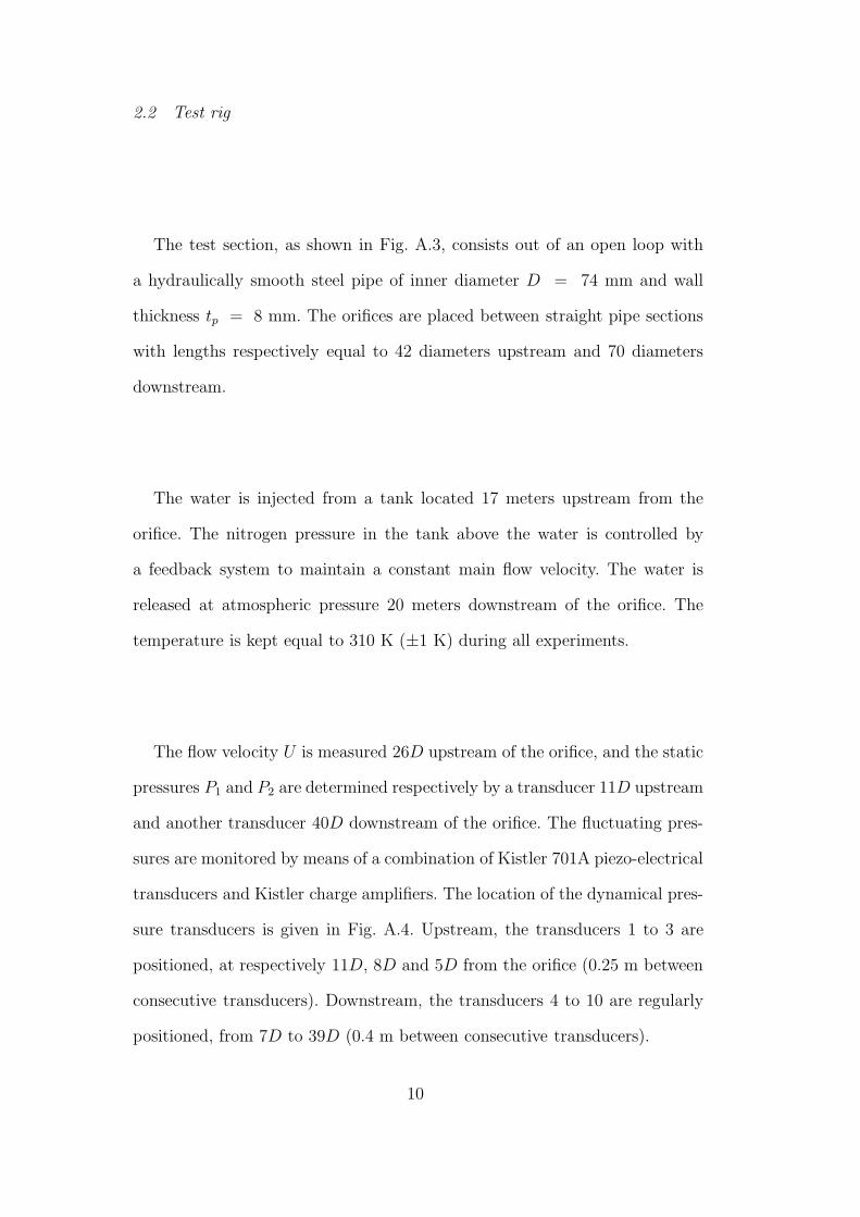
2.2 Test rig
The test section, as shown in Fig. A.3, consists out of an open loop with
a hydraulically smooth steel pipe of inner diameter D = 74 mm and wall
thickness tp = 8 mm. The orifices are placed between straight pipe sections
with lengths respectively equal to 42 diameters upstream and 70 diameters
downstream.
The water is injected from a tank located 17 meters upstream from the
orifice. The nitrogen pressure in the tank above the water is controlled by
a feedback system to maintain a constant main flow velocity. The water is
released at atmospheric pressure 20 meters downstream of the orifice. The
temperature is kept equal to 310 K (±1 K) during all experiments.
The flow velocity U is measured 26D upstream of the orifice, and the static
pressures P1 and P2 are determined respectively by a transducer 11D upstream
and another transducer 40D downstream of the orifice. The fluctuating pres-
sures are monitored by means of a combination of Kistler 701A piezo-electrical
transducers and Kistler charge amplifiers. The location of the dynamical pres-
sure transducers is given in Fig. A.4. Upstream, the transducers 1 to 3 are
positioned, at respectively 11D, 8D and 5D from the orifice (0.25 m between
consecutive transducers). Downstream, the transducers 4 to 10 are regularly
positioned, from 7D to 39D (0.4 m between consecutive transducers).
10
2.3 Experimental conditions
2.3.1 Water quality
The water used is tap water, demineralized, with pH 9 and weak conduc-
tivity. It is not degassed hence it is expected to be saturated with dissolved
air. The volume fraction of dissolved gas (noted β) is high compared to other
cavitation studies. This gas content has not been measured, but an estima-
tion assuming saturation condition under a temperature of T = 310 K or
T = 273 K, gives for the volume fraction an order of magnitude around re-
spectively 10−2 or 10−3.
It should be pointed out that the presence of dissolved gas in the water
does not mean a presence of gas bubbles in the water. Thus, the measured
upstream speed of sound does not reveal any presence of gas bubbles as it is
close to the one in pure water flow.
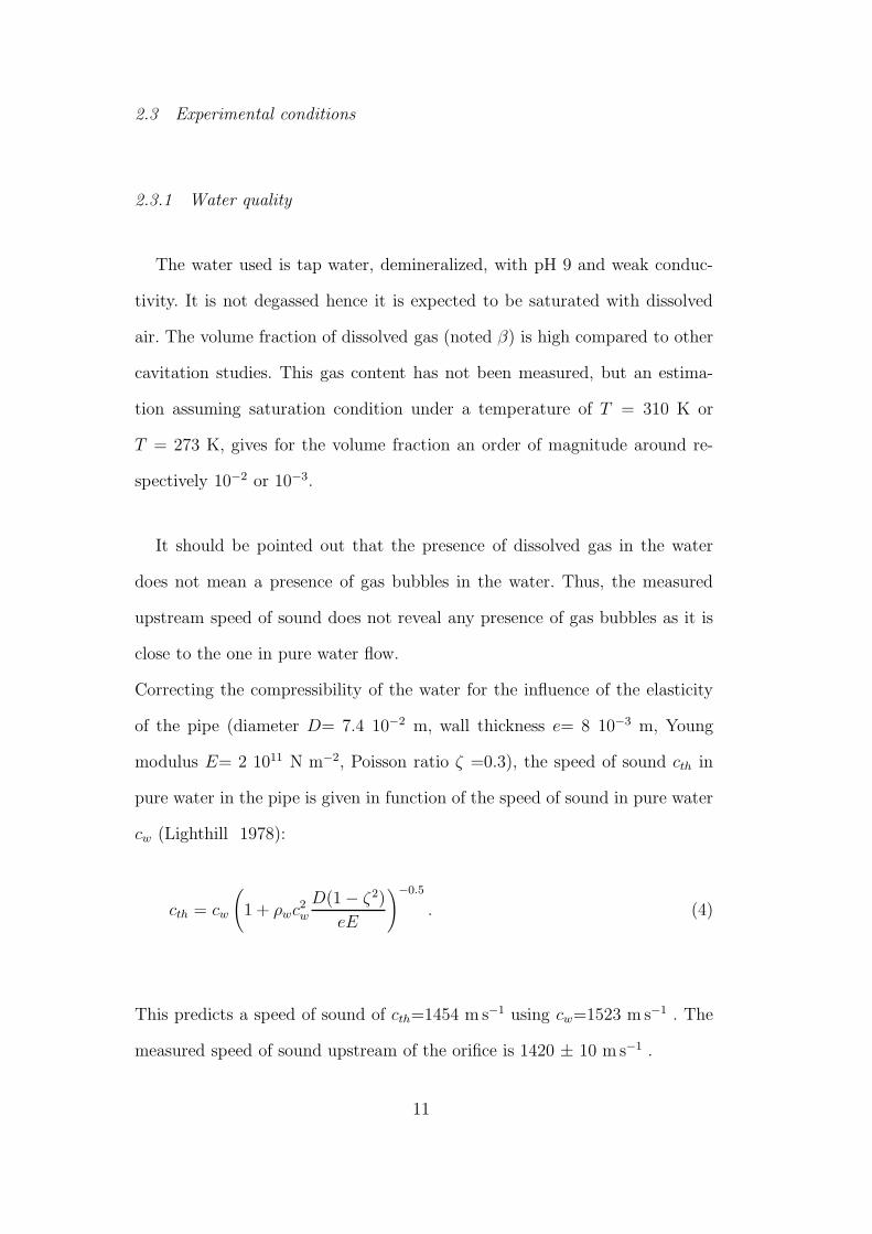
Correcting the compressibility of the water for the influence of the elasticity
of the pipe (diameter D= 7.4 10−2 m, wall thickness e= 8 10−3 m, Young
modulus E= 2 1011 N m−2, Poisson ratio ζ =0.3), the speed of sound cth in
pure water in the pipe is given in function of the speed of sound in pure water
cw (Lighthill 1978):
cth = cw
(
1 + ρwc2w
D(1 − ζ2)
eE
)−0.5
. (4)
This predicts a speed of sound of cth=1454 m s−1 using cw=1523 m s−1 . The
measured speed of sound upstream of the orifice is 1420 ± 10 m s−1 .
11
2.3.2 Experimental flow conditions
Experiments are carried out at a constant flow by controlling the static
pressure upstream of the orifice. The downstream pressure P2 is imposed by
the hydraulic static head of the 17.2 meters. high vertical pipe downstream
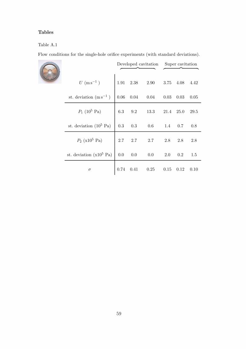
of the orifice. Each experiment lasts about 90 seconds. Pressures and volume
flows are provided in Tab. A.1 for the six experiments on the single-hole orifice,
and in Tab. A.2 for the six experiments on the multi-hole orifice.
The Reynolds number Re = UD/νwater based on the pipe diameter and the
water viscosity varies from 2 105 to 5 105: turbulence is fully developed, as
usual in industrial pipes.
Higher flow regimes have been tested, but the pressure transducers down-
stream delivered no signal, as they were located in a vapor pocket character-
istic of the super cavitation regime. As a consequence, no acoustic data are
available in these conditions, and the corresponding hydraulic conditions are
not reported in Tab. A.1 & Tab. A.2.
2.4 Distinction of two cavitation regimes
The application of Tullis’ formulas to our experiments gives the cavitation
indicators: σi for the developed cavitation and σch for the super cavitation.
Compared to our observations, those cavitation regime indicators are in good
accordance:
• for the single-hole orifice: σi ≥ 0.93, σch = 0.25.
The observations, based on listening and on the measured downstream speed
12
of sound, indicate that all experiments (i.e., σ < 0.74) are cavitating. Fur-
thermore, the downstream acoustic properties and particularly the shape of
the downstream noise spectra indicate that the last three experiments (i.e.,
σ < 0.25) are in super cavitation regime.
• for the multi-hole orifice: σi ≥ 0.87, σch = 0.20.
The observations in this case indicate that all experiments (i.e., σ < 0.74)
are cavitating. The super cavitation regime is observed for the last two ex-
periments (i.e., σ < 0.17).
2.5 Acoustic analysis method
In the frequency range of the study, only acoustic plane waves propagate.
The issue is to determine the spectra p+ and p− representing respectively the
upstream and downstream traveling plane waves and for which Fourier-like
analysis holds.
From each experiment, time fluctuating-pressure signals are obtained. These
data are truncated to a time interval where the acoustic properties do not
evolve significantly, i.e., on a duration of about 10 seconds. With the help of
a reference pressure pref , we compute the cross-spectral densities Gppref(f),
which are defined as the Fourier Transform of the time correlation (Bendat
and Piersol 1986). It is worth recalling that, for a small frequency bandwidth
∆f , the mean square value of the pressure in the frequency range [f, f + ∆f ]
is given by Gpp (f) ∆f . These cross-spectra are expressed in Pa2/Hz. In order
to get a spectral expression linear with the pressure, we choose to use the
13
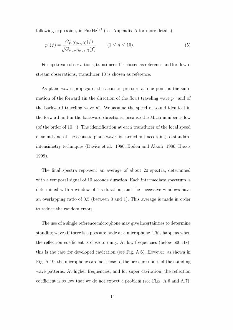
following expression, in Pa/Hz1/2 (see Appendix A for more details):
pn(f) =Gpn(t)pref (t)(f)
√
Gpref (t)pref (t)(f)(1 ≤ n ≤ 10). (5)
For upstream observations, transducer 1 is chosen as reference and for down-
stream observations, transducer 10 is chosen as reference.
As plane waves propagate, the acoustic pressure at one point is the sum-
mation of the forward (in the direction of the flow) traveling wave p+ and of
the backward traveling wave p−. We assume the speed of sound identical in
the forward and in the backward directions, because the Mach number is low
(of the order of 10−3). The identification at each transducer of the local speed
of sound and of the acoustic plane waves is carried out according to standard
intensimetry techniques (Davies et al. 1980; Boden and Abom 1986; Hassis
1999).
The final spectra represent an average of about 20 spectra, determined
with a temporal signal of 10 seconds duration. Each intermediate spectrum is
determined with a window of 1 s duration, and the successive windows have
an overlapping ratio of 0.5 (between 0 and 1). This average is made in order
to reduce the random errors.
The use of a single reference microphone may give incertainties to determine
standing waves if there is a pressure node at a microphone. This happens when
the reflection coefficient is close to unity. At low frequencies (below 500 Hz),
this is the case for developed cavitation (see Fig. A.6). However, as shown in
Fig. A.19, the microphones are not close to the pressure nodes of the standing
wave patterns. At higher frequencies, and for super cavitation, the reflection
coefficient is so low that we do not expect a problem (see Figs. A.6 and A.7).
14
2.6 Acoustic boundary conditions on both sides of the orifice
2.6.1 Acoustic boundary conditions upstream of the orifice
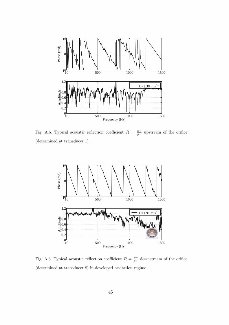
The acoustic conditions imposed by the test rig upstream of the orifice are
quite reflecting, as illustrated in Fig. A.5 by the upstream reflection coefficient
R = p−/p+, defined as the ratio between the forward and the backward propa-
gating plane waves. These reflecting characteristics are due to multiple partial
reflections of the acoustic waves on various elements present on the upstream
part of the test rig as an open valve, a few bends and section restrictions.
Those elements have not been modified in the course of the experiments, so
that these reflecting conditions do not to vary much from one experiment to
another.
2.6.2 Acoustic boundary conditions downstream of the orifice
The downstream acoustic boundary condition depends on the cavitation
regime, developed cavitation regime or super cavitation regime.
In developed cavitation regime (see Fig. A.6), the downstream reflection
coefficient has a magnitude close to 1 up to 600 Hz, which indicates strong
reflecting condition. As the phase is a linear function of the frequency, the
reflection point is determined: it corresponds with the location of an open
valve (at 53 D downstream of the orifice). The cavity of this valve is hence
filled with a very compressible fluid, i. e. air, imposing an acoustic pressure
node p′ = 0.
The reflection coefficient shows values above the unity in Fig. A.5 and A.6.
This may be due to measurement inaccuracies. Also the presence of a noise
15
source outside the main source region is possible and would give values above
the unity.
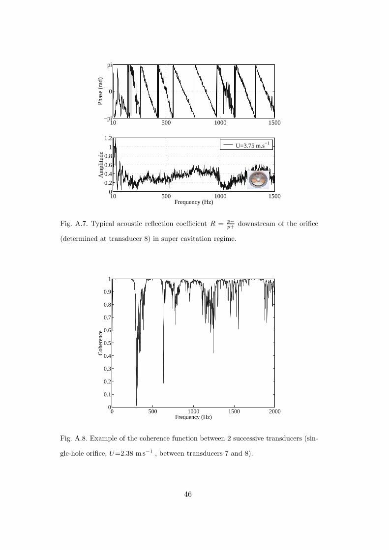
In super cavitation regime (see Fig. A.7), the downstream reflection co-
efficient falls down below the value of 0.5. In first approximation, the pipe
termination is then almost anechoic. This difference of behavior between the
developed cavitation regime is not analysed in the frame of the present study.
This variation of the downstream acoustic boundary conditions is specific
of the test rig. It has some impact on the levels of the downstream spectra.
This will be taken into account further in the study of the downstream noise
spectra.
It should be pointed out that, for some frequencies, the determination of the
acoustical spectra is inaccurate. But coherence values are still good enough,
as illustrated in Fig A.8, to allow a satisfying fit of the spectra to determine
the speed of sound, as illustrated in Fig A.9.
3 Cavitation regimes
3.1 Hydraulic model for the pressure drop ∆P across the single-hole orifice
A simple model of the hydraulics of the single-hole orifice is proposed. The
hydraulic conditions (pressure and Mach number) at the jet of the orifice
are estimated, hence giving some insight for a physical interpretation of the
different cavitation regimes.
This hydraulic model is a simple classical Borda-Carnot model [see for
16
example Durrieu et al. (2001)]. It assumes an incompressible stationary single-
phase flow, that is, no effect of cavitation on the hydraulics. Also, the ratio
Sj/S of the free jet cross-section and the pipe cross-section S is considered as
fixed.
Firstly, mass conservation demands:
Sj Uj = S U. (6)
Secondly, the flow upstream of the jet is assumed to be an inviscid steady
potential flow, so that:
P1 +1
2ρw U2 = Pj +
1
2ρw U2
j . (7)
Downstream of the jet, a turbulent mixing region is followed by a uniform flow
of velocity U . Neglecting friction at the walls, and assuming a thin (t/d . 2)
orifice (with no re-attachment of the flow inside the hole of the orifice), one
obtains (Sd is the cross-section of the orifice):
S Pj + ρw U2j Sj = S P2 + ρw U2S. (8)
The pressure Pj and the velocity Uj at the jet are deduced from Eq. 6, Eq. 7
and Eq. 8. The measured pressure drop, noted ∆Pmeasured, is in this case equal
to the pressure drop across the orifice: ∆Pmeasured = P1 −P2. Hence, noting α
the contraction coefficient (α = Sj/Sd), this developed cavitation model gives:
∆Pmeasured12ρwU2
=
(
S
Sj
)2
− 1
+
[
2 − 2S
Sj
]
. (9)
The first part representing the dissipation from upstream to the jet, and the
second part the dissipation from the jet to downstream.
17
Finally, after simplifications, we find:
∆Pmeasured12ρwU2
=
[(D
d
)2 1
α− 1
]2
. (10)
In super cavitation, the downstream static sensor is in the jet region, mea-
suring Pj. The pressure drop measured represents the dissipation from up-
stream to the jet (the first part of the preceding expression):
∆Pmeasured12ρwU2
=1
α2
(D
d
)4
− 1. (11)
Figure A.10 compare those two models using a contraction coefficient α =
0.65 with experimental results (additional experimental results in super cavi-
tation, not shown in Tab. A.1, are plotted).
• in developed cavitation regime (U < 3.5 m s−1 ), theory agrees qualitatively
well with experiments, predicting ∆P within 15 %;
• in super cavitation regime (U > 3.5 m s−1 ), experimental data agree re-
markably well with the model, predicting ∆P within 1 %. Incidentally, we
observe that super cavitation does not induce a strong slope variation in
the ∆P vs. U curve. This is mentioned in Tullis (1989) for orifices of low
d/D ratio (approximately under 0.5, which is the case here).
As a result, the model is validated as a satisfying broad estimation of the
hydraulics, taking a contraction coefficient of 0.65. This value is reasonable,
as it is close to 0.61 which is the theoretical value for sharp-edged orifices
with a jet from a gas to a free space exit (Gilbarg 1960) and it is less than
0.70, which indicates (Blevins 1984) that the real radius of curvature of the
upstream edge of the orifice is less than 1% of the pipe diameter (this confirms
that this edge is a neat sharp angle edge).
18
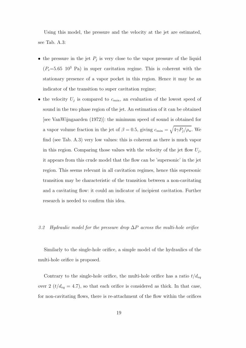
Using this model, the pressure and the velocity at the jet are estimated,
see Tab. A.3:
• the pressure in the jet Pj is very close to the vapor pressure of the liquid
(Pv=5.65 103 Pa) in super cavitation regime. This is coherent with the
stationary presence of a vapor pocket in this region. Hence it may be an
indicator of the transition to super cavitation regime;
• the velocity Uj is compared to cmin, an evaluation of the lowest speed of
sound in the two phase region of the jet. An estimation of it can be obtained
[see VanWijngaarden (1972)]: the minimum speed of sound is obtained for
a vapor volume fraction in the jet of β = 0.5, giving cmin =√
4γPj/ρw. We
find (see Tab. A.3) very low values: this is coherent as there is much vapor
in this region. Comparing those values with the velocity of the jet flow Uj ,
it appears from this crude model that the flow can be ’supersonic’ in the jet
region. This seems relevant in all cavitation regimes, hence this supersonic
transition may be characteristic of the transition between a non-cavitating
and a cavitating flow: it could an indicator of incipient cavitation. Further
research is needed to confirm this idea.
3.2 Hydraulic model for the pressure drop ∆P across the multi-hole orifice
Similarly to the single-hole orifice, a simple model of the hydraulics of the
multi-hole orifice is proposed.
Contrary to the single-hole orifice, the multi-hole orifice has a ratio t/deq
over 2 (t/deq = 4.7), so that each orifice is considered as thick. In that case,
for non-cavitating flows, there is re-attachment of the flow within the orifices
19
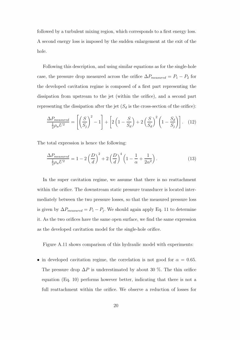
followed by a turbulent mixing region, which corresponds to a first energy loss.
A second energy loss is imposed by the sudden enlargement at the exit of the
hole.
Following this description, and using similar equations as for the single-hole
case, the pressure drop measured across the orifice ∆Pmeasured = P1 − P2 for
the developed cavitation regime is composed of a first part representing the
dissipation from upstream to the jet (within the orifice), and a second part
representing the dissipation after the jet (Sd is the cross-section of the orifice):
∆Pmeasured12ρwU2
=
(
S
Sj
)2
− 1
+
[
2(
1 − S
Sd
)
+ 2(
S
Sd
)2(
1 − Sd
Sj
)]
. (12)
The total expression is hence the following:
∆Pmeasured12ρwU2
= 1 − 2(
D
d
)2
+ 2(
D
d
)4 (
1 − 1
α+
1
2α2
)
. (13)
In the super cavitation regime, we assume that there is no reattachment
within the orifice. The downstream static pressure transducer is located inter-
mediately between the two pressure losses, so that the measured pressure loss
is given by ∆Pmeasured = P1 −Pj. We should again apply Eq. 11 to determine
it. As the two orifices have the same open surface, we find the same expression
as the developed cavitation model for the single-hole orifice.
Figure A.11 shows comparison of this hydraulic model with experiments:
• in developed cavitation regime, the correlation is not good for α = 0.65.
The pressure drop ∆P is underestimated by about 30 %. The thin orifice
equation (Eq. 10) performs however better, indicating that there is not a
full reattachment within the orifice. We observe a reduction of losses for
20
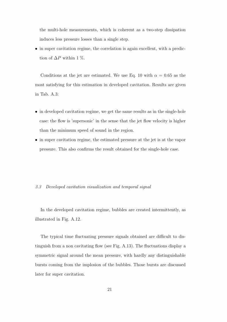
the multi-hole measurements, which is coherent as a two-step dissipation
induces less pressure losses than a single step.
• in super cavitation regime, the correlation is again excellent, with a predic-
tion of ∆P within 1 %.
Conditions at the jet are estimated. We use Eq. 10 with α = 0.65 as the
most satisfying for this estimation in developed cavitation. Results are given
in Tab. A.3:
• in developed cavitation regime, we get the same results as in the single-hole
case: the flow is ’supersonic’ in the sense that the jet flow velocity is higher
than the minimum speed of sound in the region.
• in super cavitation regime, the estimated pressure at the jet is at the vapor
pressure. This also confirms the result obtained for the single-hole case.
3.3 Developed cavitation visualization and temporal signal
In the developed cavitation regime, bubbles are created intermittently, as
illustrated in Fig. A.12.
The typical time fluctuating pressure signals obtained are difficult to dis-
tinguish from a non cavitating flow (see Fig. A.13). The fluctuations display a
symmetric signal around the mean pressure, with hardly any distinguishable
bursts coming from the implosion of the bubbles. Those bursts are discussed
later for super cavitation.
21
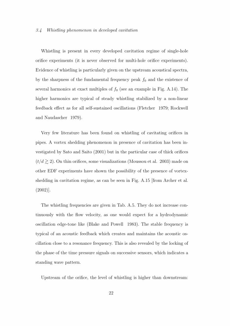
3.4 Whistling phenomenon in developed cavitation
Whistling is present in every developed cavitation regime of single-hole
orifice experiments (it is never observed for multi-hole orifice experiments).
Evidence of whistling is particularly given on the upstream acoustical spectra,
by the sharpness of the fundamental frequency peak f0 and the existence of
several harmonics at exact multiples of f0 (see an example in Fig. A.14). The
higher harmonics are typical of steady whistling stabilized by a non-linear
feedback effect as for all self-sustained oscillations (Fletcher 1979; Rockwell
and Naudascher 1979).
Very few literature has been found on whistling of cavitating orifices in
pipes. A vortex shedding phenomenon in presence of cavitation has been in-
vestigated by Sato and Saito (2001) but in the particular case of thick orifices
(t/d & 2). On thin orifices, some visualizations (Moussou et al. 2003) made on
other EDF experiments have shown the possibility of the presence of vortex-
shedding in cavitation regime, as can be seen in Fig. A.15 [from Archer et al.
(2002)].
The whistling frequencies are given in Tab. A.5. They do not increase con-
tinuously with the flow velocity, as one would expect for a hydrodynamic
oscillation edge-tone like (Blake and Powell 1983). The stable frequency is
typical of an acoustic feedback which creates and maintains the acoustic os-
cillation close to a resonance frequency. This is also revealed by the locking of
the phase of the time pressure signals on successive sensors, which indicates a
standing wave pattern.
Upstream of the orifice, the level of whistling is higher than downstream:
22
hence the acoustic feedback is suspected to happen predominantly upstream.
The upstream reflection coefficient, see Fig. A.5, is reflecting but irregular: no
clear acoustic reflection point can be identified (as it can be for the cavity of a
valve downstream, see section 2.6.2). This irregular shape is due to the intri-
cacy of the upstream rig design, with a succession of elbows, slight restrictions
of sections and some open valves.
It is also worth mentioning that the whistling frequency does not coincide
with any downstream natural acoustic frequency. This is coherent with the
acoustic uncoupling observed from both sides of the orifice.
The single-hole orifice has a ratio t/d = 0.6, inferior to 2, so that it is
considered as a thin orifice. We assume that the whistling phenomenon is
influenced by the thickness of the orifice t, rather than its diameter. It is also
natural to use the velocity at the orifice Ud as a relevant scaling velocity. Hence
the Strouhal number is defined as:
St =f0 t
Ud, (14)
and values are reported in Tab. A.5.
The Strouhal number is obtained in the range 0.18-0.26. These values are
close to data on orifices: Anderson (1953) finds a Strouhal number around 0.2
on whistling orifices in air with a free air exit. In Anderson’s experiments, the
orifices were a bit thinner (with 0.2 ≤ t/D ≤ 0.5 whereas here t/D = 0.19)
and the Reynolds numbers smaller (Ud t/νair v 103 with νair the cinematic
viscosity of air, whereas here Ud t/νwater v 105).
The multi-hole orifice is a thick one, as t/dmulti = 4.7. Hence it is no surprise
23
that it does not whistle. The flow re-attaches itself inside of each hole, which
stabilizes the shear layers of the jet and hence prevents from whistling in the
same manner as it is observed for the single-hole orifice.
3.5 Super cavitation visualization and typical temporal signal
In the super cavitation regime, a vapor pocket is created in the jet region,
as illustrated in Fig. A.16.
When the vapor pocket expand and reach the downstream transducers,
those transducers do no more deliver any acoustical signal. This constitues an
evidence for the existence of the vapor pocket.
It appears that the length of the vapor pocket increases quickly with the
flow velocity. The length of the vapor pocket increases from about 7D at
U0 = 3.8 m s−1 to 18D at U0 = 4.4 m s−1 and is larger than 38D at U0 = 4.7
m s−1 for the single-hole orifice. For the multi-hole orifice, the length of the
vapor pocket increases from around 7D at U0 = 4.2 m s−1 to larger than 38D
at U0 = 4.5 m s−1 .
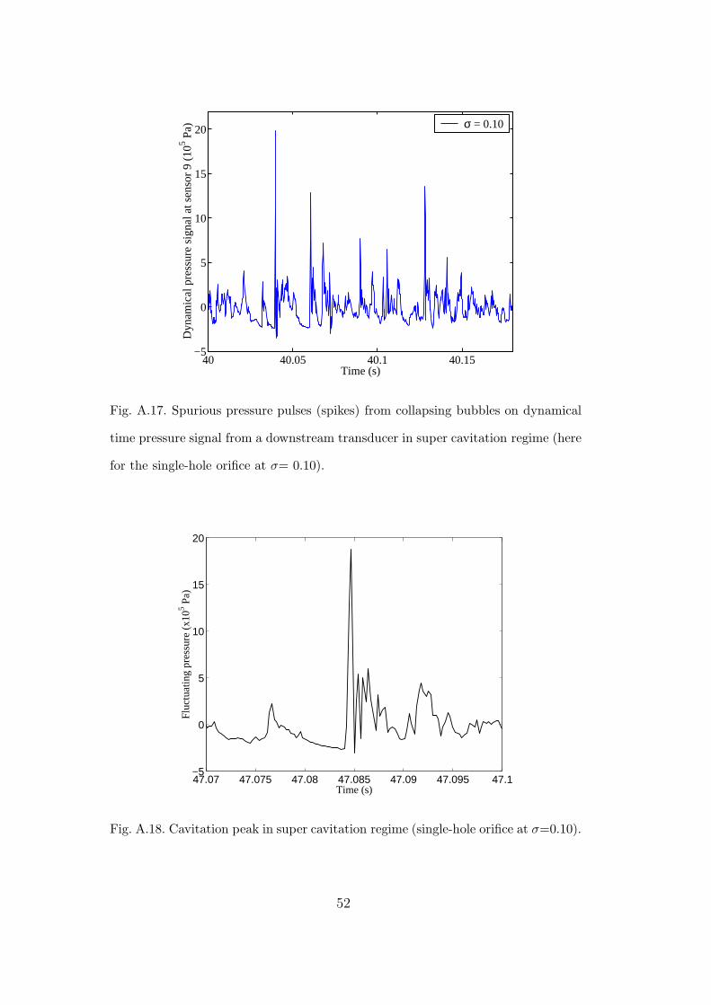
The typical time fluctuating pressure signals obtained are very different
from developed cavitation regime (see Fig. A.17). They are asymmetric around
the mean pressure, exhibiting very large positive spikes, up to 20 bars, linked
to the collapse of bubbles.
Focuses on time signals (see an illustration in Fig. A.18) show that the phe-
nomenon of bubble implosion is characterized by a first decrease in negative
values of the fluctuating pressure with a characteristic duration of a tens of
milliseconds, followed by an abrupt increase of the pressure, a ’spike’, with a
24
characteristic duration of one millisecond. By assimilating this volume bubble
evolution with a monopole source [which is a common and satisfying simple
model, see for instance Brennen (1995)], the first decrease is linked with a de-
crease of the bubble size from its initial size to a value close to zero; the second
part of the signal is linked with a pressure shock wave originating from the
abrupt collision of the water particles. However, extremely high amplitudes
are observed in comparison to Brennen (1995) (cf. Fig 3.19). This can either
be due to the large size of our bubbles or to the effect of confinement.
4 Results in the developed cavitation regime
The single-hole and the multi-hole orifice developed cavitation regimes are
presented together as they show similar acoustical behavior. Firstly, results
on the acoustic features of this cavitation regime are introduced: the observed
variations of the downstream speed of sound and the presence of resonance
frequencies on downstream spectra. Then the downstream spectra, depending
on those acoustical features, are presented and discussed.
4.1 Acoustic features
4.1.1 Spontaneous variations of the downstream speed of sound
For a fixed set of hydraulic conditions in developed cavitation regime, the
downstream speed of sound may spontaneously evolve. For instance, the single-
hole orifice experiment at U = 2.38 m s−1 shows the downstream speed of
sound evolving from 660 m s−1 (during the first 20 seconds) to 1420 m s−1 (till
the end of the experiment: 90 seconds).
25
This variation of the speed of sound indicates that air bubbles are present,
in varying quantity, in the water far downstream of the orifice. For instance, a
value of 660 m s−1 indicates a volume gas fraction in the water between 10−3
and 10−4, assuming the static pressure being between Pj and P2 [we use a
classic formula, see for example VanWijngaarden (1972)]. On the contrary, a
value of 1420 m s−1 indicates a negligible content of air in the water, as it is
close to the speed of sound in pure water (which equals to 1454 m s−1 when
correcting for pipe elasticity, see Pierce (1981)).
Cavitation bubbles, when they are formed, are originally mainly constituted
out of vapor. During their lifetime, they are gradually filled with air, due to
the diffusion of the dissolved gas present in the water surrounding them. As
they drift downstream, moving away from their region of creation, they reach
regions where the pressure recovers higher levels. Pure vapor bubbles can not
persist, those bubbles remaining far downstream of the orifice are mainly filled
with air (see for example Fig. A.12). Consequently, the observed variation of
the quantity of air bubbles is suspected to be due to a non homogeneity of
the dissolved gas content in the injected water. This non homogeneity may
be related to temperature variations in the experimental installations. This
hypothesis is all the more plausible as the water used has not received any
degassing treatment, hence having a fluctuating and high dissolved gas con-
tent, not measured but estimated around 10−2 or 10−3 (values at saturation
conditions for T = 273 K and T = 310 K respectively). In some experiments,
the change in residual air bubbles content occurs after that the water from the
pipe segment between the orifice and the tank has been evacuated and that
’fresh’ tank water start to flow through the orifice.
These variations of the downstream speed of sound during each experiment
26
have some influence on the acoustical behavior downstream of the orifice: the
values of the natural frequencies, appearing downstream, are altered propor-
tionally with the speed of sound.
The propagating waves are subjected to two-phase flow damping, as already
mentioned by Hassis (1999). As regards this last effect, no significant variation
of the propagating waves amplitude could be measured along the downstream
sensors, but the downstream acoustical reflection coefficient appears to vary
significantly with the downstream speed of sound.
4.1.2 Acoustical uncoupling from both sides of the orifice
An acoustical uncoupling is observed between acoustical spectra upstream
and downstream of the orifice: the natural frequencies present downstream
are strongly attenuated on upstream spectra, the whistling, when present, is
visible on upstream spectra, but hardly on downstream spectra, and further-
more, the background noise on downstream spectra is higher than the one on
upstream spectra, approximately from a factor 2 (for U = 1.91 m s−1 ) up to
7 (for U = 2.90 m s−1 ) for the single-hole orifice, and much more significantly
for the multi-hole orifice, with an approximately constant factor of about 10.
This acoustical uncoupling is an effect of cavitation as there is choking [
indicated in Tab. A.3].
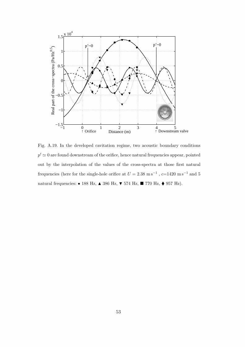
4.1.3 Presence of natural modes downstream
In this developed cavitation regime, resonance frequencies are systemati-
cally observed in acoustical spectra downstream of the orifice (both for the
single-hole and the multi-hole).
27
The acoustic boundary conditions are of a similar type, as the frequencies
are of the form: fn = nf1, f1 being the first resonance frequency. More pre-
cisely, these acoustic boundary conditions can be identified by extrapolating
the standing wave patterns at those resonance frequencies. This extrapolation
is made possible as a series of transducers (7 in number) is present down-
stream of the orifice. As a result, we find two acoustic pressure nodes p′ = 0
(see Fig. A.19):
• one is found far downstream of the orifice, at 52D (±1D). It is the result
of the influence of a cavity of an open valve filled with air. The reflection
coefficient imposed by such a cavity has been presented in Fig A.6. The
magnitude of the reflection coefficient |R| is close to 1 , which confirms the
acoustic influence of this cavity;
• another is found just downstream of the orifice, at 4D (±1D). It is likely to
be caused by a cavitation cloud.
4.2 Noise spectra generated downstream
Noise spectra generated in the pipe downstream of the orifice for the de-
veloped cavitation regime are presented in this section.
The downstream transducers give a far-field measurement, as they are not
located in the source region mainly constituted of bubbles implosions located
just downstream of the orifice. The acoustical power measured at downstream
transducers represents the noise generated in the pipe. Under the assumptions
of plane-wave propagation and no influence of the flow (the Mach number is
around 10−3), the acoustical power takes the expression: S (p+2 − p−2) /(ρwcw)
28
(Morfey 1971).
It is furthermore assumed that the backward propagating wave spectra p− is
small enough to be neglected. Even if acoustical reflection is observed to occur
downstream, this estimation of the source of noise is considered satisfying
enough as an order of magnitude (this is all the more relevant as logarithmic
representation is used). Thus it comes that the source power is represented by
the quantity Sp+2/(ρwcw).
Of course, this representation is no more valid for the discrete frequencies
which are whistling harmonics and resonance frequencies, as the backward
propagating wave has great influence in those cases.
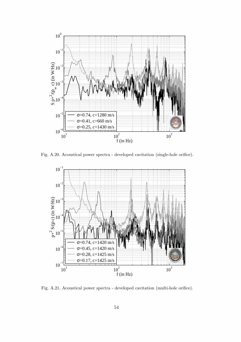
The acoustical power spectra obtained downstream of the orifice for the de-
veloped cavitation regime are given in Fig. A.20 for the single-hole orifice and
in Fig. A.21 for the multi-hole orifice. The rejection frequency corresponding
to a wavelength of half of the distance between two successive transducers
and depending on the measured speed of sound has been excluded from those
results. The following observations are made on those spectra:
• spectra exhibit a hump form in the upper frequency range (above 200 Hz).
This hump form is typical of cavitational noise (Martin et al. 1981; Brennen
1995);
• the single-hole orifice generates remarkably much more noise (with a factor
of about 102 on the acoustical power) than the multi-hole orifice.
29
4.3 Non-dimensional analysis and representation
4.3.1 Choice of the scaling variables for the noise spectra
Scaling is proposed in order to obtain a dimensionless representation of the
acoustical source power.
Cavitation noise from the implosions of bubbles is assumed to be predom-
inant in order to scale the noise spectra. Hence, broadband turbulence noise
from the mixing region downstream, whistling and resonance frequencies are
not taken into account to choose the scaling variables. This assumption of
predominance of cavitation noise is globally valid, but seems to fail at low fre-
quencies (in this work, below 200-300 Hz approximately). Also, it is assumed
that whistling does not alter cavitation noise, generalizing the hypothesis that
broadband noise is not affected by whistling [as shown in Verge (1995) for a
flue organ pipe].
Following Blake (1986), the amplitude of noise produced by cavitation
should be made dimensionless by dividing with the downstream pressure, and
not the pressure drop, when using a Rayleigh-Plesset bubble dynamic model
for a spherical isolated free bubble. However, ring vortices generated by an
orifice are not isolated bubbles in free space, so that this scaling should not
hold in the case of the present study, as it also does not for sheet cavitation
on airfoils (Keller 1994).
As we lack a precise model, the scaling data are chosen in the sake of
simplicity: the basic idea, as shown in Fig. A.22, relies on the fact that, in
developed cavitation regime, the bubbles are created in the mixing high-shear
30
region of the jet.
For the single-hole orifice experiments, the velocity Ud and the orifice diam-
eter d are representative of the conditions in this region, hence those quantities
are used in order to scale the noise spectra in this regime. Furthermore, the
scaling pressure is defined as the pressure drop ∆P across the orifice, which
is a measure of the kinetic energy density in the jet. Hence for the single-hole
orifice in developed cavitation:
• fd/Ud is the non-dimensional frequency;
• p+2 Ud/(∆P 2 d) is the non-dimensional magnitude.
For the multi-hole orifice experiments, we assume the noise issuing from
incoherent Nholes sources.
Each source represents the radiation of one hole. It radiates on a char-
acteristic surface of S/Nholes. The strength of each source is assumed to be
independent of the environment of the source. This assumption is natural, as
we have previously supposed (see previous section) that the noise generated by
the single-hole orifice does not depend on the diameter of the pipe. However,
it should be pointed out that this assumption is wrong when whistling occurs.
In this model, the total acoustic power P measured downstream is a summa-
tion of the acoustic power Peach source emitted by each source [the key element
is that sources are supposed incoherent between each other, see Pierce (1981)]:
P = Nholes Peach source. (15)
The acoustic power of each source Peach source is, by definition, the total acoustic
31
intensity flux I multiplied the surface of this source:
Peach source = I S/Nholes. (16)
Hence the total acoustic power is:
P = S I. (17)
The total acoustic power is consequently independent of the number of holes.
As previously, we ignore any downstream reflections so that I = p+2/(ρc).
This argumentation based on energy considerations can be also be lead in
terms of forces: is the source is represented as a force acting on the orifice,
taking the form Sp+, the total force imposed on the multi-hole orifice is due to
the contribution of the forces imposed by Nholes equivalent single-hole orifices
with open surface S/Nholes. Those forces are supposed uncorrelated with each
other. Thus the total square force equals Nholes times the square force due to
one hole. As the square force of one hole is (p+S/Nholes)2, the total square force
takes the expression: Nholes(p+S/Nholes)
2, or by simplifying: (p+S)2/Nholes.
The scaling of the acoustic power is based on each source of surface S/Nholes.
The scaling velocity is the velocity at the orifice, which is taken equal to the
velocity of the single-hole orifice Ud, as the open surface of the two orifices
are very similar, and the scaling length is the diameter of one hole dmulti. In
conclusion for the multi-hole orifice in developed cavitation:
• fdmulti/Ud is the non-dimensional frequency;
• p+2 Ud/(∆P 2 dmulti) is the non-dimensional magnitude.
32
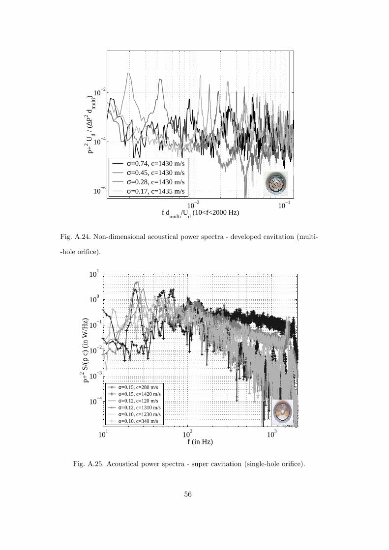
4.3.2 Non-dimensional noise spectra generated downstream
The dimensionless acoustical power spectra obtained downstream of the
orifice for the developed cavitation regime are given in Fig. A.23 for the
single-hole orifice and in Fig. A.24 for the multi-hole orifice. The following
observations are worth to be noted:
• the scaling for the single-hole orifice and the multi-hole orifice is efficient as
the non-dimensional noise spectra collapse for each orifice. This is illustrated
in Fig. A.23 for the single-hole orifice and Fig. A.24 for the multi-hole orifice.
Hence it is found that these spectra do not depend significantly on the
cavitation number neither on the downstream speed of sound. However, the
dispersion of the scaling variables is weak, so that additional data should
be added to confirm this result;
• the different scaling used for the single-hole and the multi-hole orifice is
rather efficient as it makes the levels of the two types of orifices closer to
each other. However, the non-dimensional level of noise of the single-hole
orifice is still higher, with a ratio of 10, than the one of the multi-hole orifice
experiments: see Fig. A.23 & A.24;
• we compare the cavitation noise with a standard turbulence noise from a
non-cavitating orifice in the low frequency range. Indeed, in this range of
frequency, the level of noise is expected to be mainly determined by turbu-
lence noise (Martin et al. 1981). We use a non-dimensional turbulence noise
level proposed by Moussou (2005). In this model, the scaling is based on
empirical data obtained with simple singularities (single-hole orifice, valve)
in water-pipe flow: the level of noise is assumed to depend only on a Strouhal
number using the pipe diameter and the pipe flow velocity. We apply this
model with the values of the pipe diameter D and a pipe flow velocity of
33
2.20 m s−1 and compare it to the single-hole orifice non-dimensional noise,
see Fig. A.23. As expected, the turbulence level fits rather well the cav-
itation noise in the low frequencies, with a good estimation of the slope;
the cavitation noise is much stronger than the turbulence noise above the
low-frequency range, which is a well-known result (Brennen 1995).
5 Results in the super cavitation regime
5.1 Acoustic features
The super cavitation experiments exhibit two main differences compared
to the developed cavitation experiments:
• the downstream speed of sound appears to be quite constant during each
experiment;
• no resonance frequencies are found on downstream spectra. The downstream
reflection coefficient is much lower than in the developed cavitation case (as
previously shown in Fig. A.7). In this case, the cavity of the downstream
valve does not reflect the acoustic waves.
As for the developed cavitation case, strong acoustic uncoupling is observed
from both sides of the orifice. The effect is much more obvious here, with an
average ratio between downstream and upstream spectra of about 2 to 30 for
the single-hole orifice case, and about 10 to 50 for the multi-hole orifice case.
34
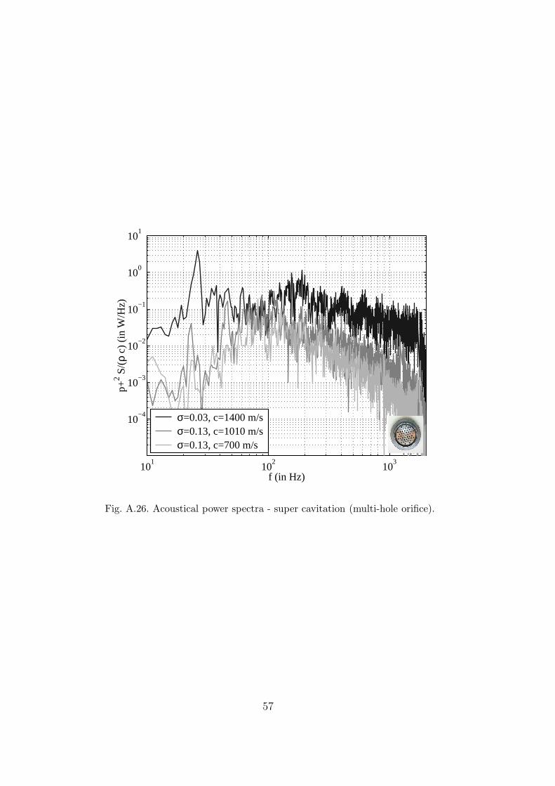
5.2 Noise spectra generated downstream
Noise spectra obtained downstream are given in Fig. A.25 for the single-hole
orifice and in Fig. A.26 for the multi-hole orifice (as previously, the rejection
frequencies being excluded). We note the following points:
• the typical cavitational hump form is observed, as in the developed cavita-
tion case, but with much more evidence. The level of the hump is higher
than for the developed cavitation regime; also, the frequency peak is smaller:
those tendencies when cavitation number increases confirm literature data
(Brennen 1995);
• also, as in the developed cavitation case, the single-hole orifice is clearly
more noisy (with an approximate factor of 10 on acoustical power spectra)
than the multi-hole orifice, .
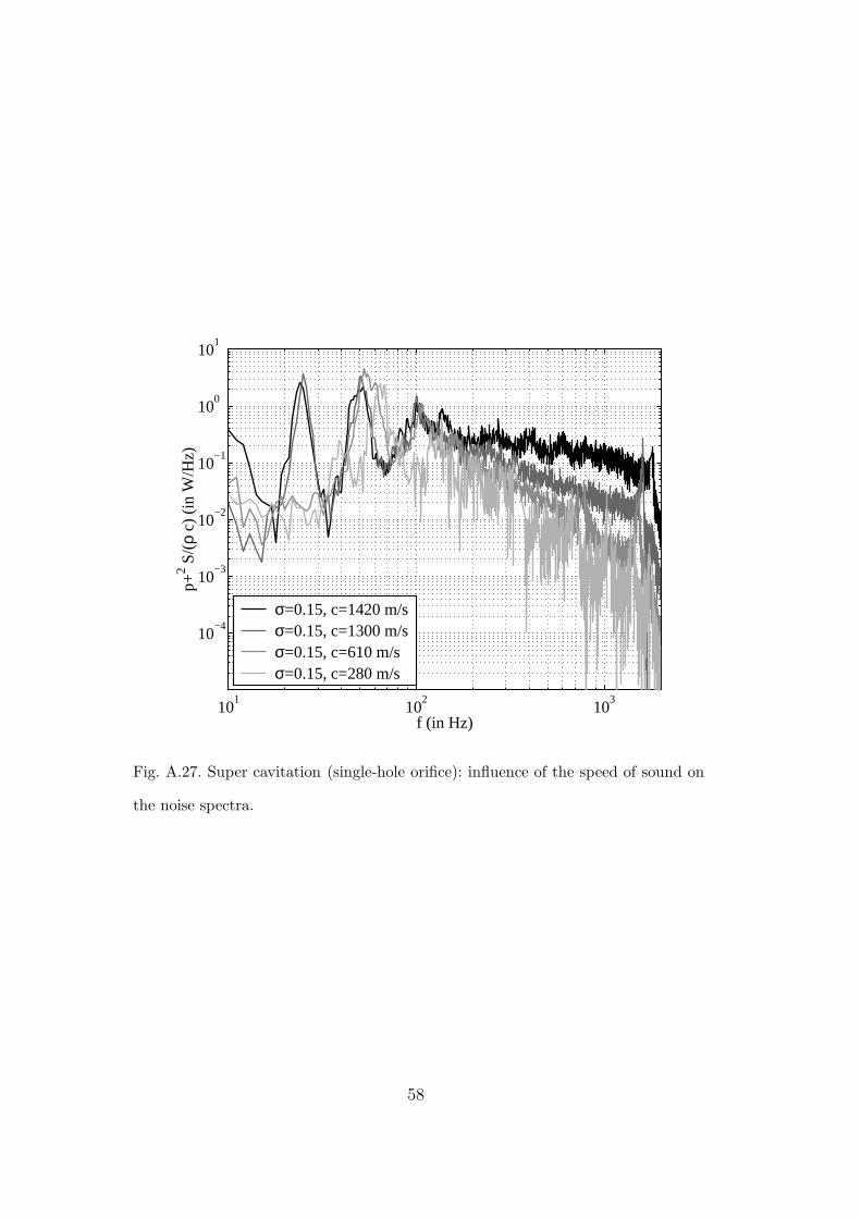
An important result is illustrated in Fig. A.27 & Fig. A.26: the part of the
spectra succeeding the hump peak frequency depend strongly on the down-
stream speed of sound. Two-phase flow attenuations phenomena are supposed
to be the cause of this observation.
6 Conclusion
A single hole cavitating orifice in a water pipe has been studied experimen-
tally under industrial conditions, i.e., with a pressure drop varying from 3 to
30 bars and a cavitation number in the range 0.10 ≤ σ ≤ 0.77.
In the regime of developed cavitation, whistling is observed. This occurs at
a Strouhal number based on the orifice thickness with a value close to 0.2.
35
Our results indicate that in the developed cavitation regime, a multi-hole
orifice is much more silent than a single-hole orifice with the same total cross-
sectional opening. This might be partially explained by the absence of correla-
tion between the sound produced by different holes in absence of whistling. No
such difference is found in super cavitation. This is explained by the fact that,
in super cavitation regime, sound is produced far downstream of the orifice
rather than in a near region downstream of the orifice.
A non-dimensional noise source is proposed for the developed cavitation
regime (cf. section 4.3). The source model seems satisfying for the developed
cavitation case.
The results presented are certainly limited and call for further research. In
particular, it can be interesting to vary the shape of the orifices and repeat
the experiments with degassed water.
Acknowledgements
The experiments have been designed and realized by MM. S. Caillaud, Ch.
Martin and L. Paulhiac.
A Appendice: Acoustic analysis
We assume that only plane waves propagate in the pipe.
First, cross-spectral density functions Gpprefare used. They are well suited
to acoustic analysis, because they eliminate non-propagating noise present in
time measurements. Indeed, if we decompose time pressure measurements p(t)
36
into a non-propagating signal pnon prop(t) and a propagating one, we have:
p(t) = p+(t) + p−(t) + pnon prop(t). (A.1)
Having defined and fixed a reference sensor and applying the cross-spectral
density functions, we get an expression where the non-propagating pressure is
removed because it is not correlated to the propagating pressure:
Gp(t)pref (t)(ω) = Gp+(t)pref (t)(ω) + Gp−(t)pref (t)(ω). (A.2)
Second, we define quantities Gppref/√
Gprefprefwhich can be handled like
Fourier Transforms, and which are almost independent of the reference pres-
sure. Indeed, if we assume a perfect coherence between the point of observation
and the reference sensor, we have:
|Gppref|2
Gpp Gprefpref
= 1. (A.3)
In this case the quantity Gppref/√
Gprefprefdoes not depend on the reference
sensor. In practice, the reference sensor is taken all the closer to the points of
observation.
Finally, we calculate plane waves. Considering two consecutive sensors, de-
noted n and n + 1, plane waves propagation and the linearity characteristics
of the cross-spectral density function give:
Gp+
n+1pref
(ω) = Gp+n pref
(ω) e−iωτ , (A.4)
Gp−n+1pref
(ω) = Gp−n pref(ω) e+iωτ , (A.5)
37
with τ being the time of flight of the wave between the two sensors. For the
sake of ease, we note pn for Gpnpref/√
Gprefpref. By means of Eq. A.2, Eq. A.4
and Eq. A.5, we get the plane wave spectra:
p+n (ω) =
pn(ω) e+iωτ + pn+1(ω)
2 i sin(ωτ), (A.6)
p−n (ω) =pn(ω) e−iωτ + pn+1(ω)
−2 i sin(ωτ), (A.7)
for upstream measurements (1 ≤ n ≤ 2) and downstream measurements
(4 ≤ n ≤ 9). These spectra are expressed in Pa/√
Hz.
The reflection coefficient is defined as p−
p+ downstream of the orifice, and
by p+p−
upstream, because we assume the source of sound to be located in the
region of the orifice. For example, if a zero pressure condition is located far
downstream of the orifice, and if T is the time of flight toward this pressure
node, the reflection coefficient at this current point is −e−2iωT .
References
1 Anderson, A. B. C., 1953. A circular-orifice number describing dependency of
primary Pfeifenton frequency on differential pressure, gas density and orifice
geometry. J. Acoust. Soc. Am. 25, 626-631.
2 Archer, A., Boyer, A., Nimanbeg, N., L’Exact, C., Lemercier, S., 2002.
Resultats des essais hydrauliques et hydroacoustiques du troncon PTR
900 sur la boucle EPOCA (in French). EDF R&D, Technical Note HI-
85/02/023/A, France.
3 Au-Yang, M. K., 2001. Flow-Induced Vibration of Power and Process Plant
Components: a Practical Workbook. ASME Press.
38
4 Ball, J. W., Tullis, J. P., Stripling, T., 1975. Predicting cavitation in sudden
enlargements. J. Hydrau. Div. ASCE 101, 857-870.
5 Bendat, J. S., Piersol, A. G., 1986. Random Data - Analysis and Measurement
Procedures (2nd Edition). Wiley-Interscience Ed., ISBN 0-471-04000-2.
6 Bistafa, S. R., Lauchle, G. C., Reethof, G., 1989. Noise generated by cavitation
orifice plates. Journal of Fluids Engineering 111, 278-289.
7 Blake, W. K., 1986. Mechanics of Flow-Induced Sound and Vibration (Vol.
II). Academic Press.
8 Blake, W. K., Powell, A., 1983. The development of contemporary views
of flow-tone generation. In Recent Advances in Aeroacoustics, New York,
Springer-Verlag.
9 Blevins, R., 1984. Applied Fluid dynamics handbook. Krieger Ed., ISBN 0-
89464-717-2.
10 Boden, H., Abom, M, 1986. Influence of errors on the two-microphone method
for acoustic properties in ducts. J. Acoust. Soc. Am 79 (2).
11 Brennen, C. E., 1995. Cavitation and bubble dynamics. Oxford University
Press.
12 Caillaud, S., Gibert, J. R., Moussou, P., Cohen, J., Millet, F., 2006. Effect on
pipe vibrations of cavitation in an orifice and in globe-style valves. In ASME
Pressure Vessels and Piping Division Conference, Proceeding PVP2006-
ICPVT11-93882, Vancouver, CANADA.
13 Davies, P. O. A. L., Bhattacharva, M., Bento Coelho, J. L., 1980. Measurement
of plane wave acoustic fields in flow ducts. Journal of Sound and Vibration
72 (4), 539-542.
14 Durrieu, P., Hofmans, G., Ajello, G., Boot, R., Auregan, Y., Hirschberg, A.,
Peters, M. C. A. M., 2001. Quasisteady aero-acoustic response of orifices.
J. Acoust. Soc. Am 110 (4).
39
15 Esipov, I. B., Naugol’nykh, K. A., 1975. Cavitation noise in submerged jets.
Sov. Phys. Acoust. 21 (4).
16 Franklin, R. E. and McMillan, J., 1984. Noise generation in cavitating flows,
the submerged jet. Journal of Fluids Engineering 106, 336-341.
17 Franc, J. P., Avellan, F., Belahadji, B., Billard, J. Y., Briancon-Marjollet,
L., Frechou, D., Fruman, D. H., Karimi, A., Kueny, J. L., Michel, J. M.,
1999. La cavitation (in French). ISBN 2.7061.0605.0, Presses Universitaires
de Grenoble.
18 Fletcher, N. H., 1979. Excitation Mechanisms in Woodwind and Brass Instru-
ments, Acustica 43 (1), 63-72.
19 Gilbarg, G., 1960. Jets and cavities. In Handbuch der Physik (Vol. 9), Flfugge,
S. (Ed.), Springer, 311-445.
20 Hassis, H., 1999. Noise caused by cavitating butterfly and monovar valves.
Journal of Sound and Vibration 225.
21 Idel’cik, I. E., 1969. Memento des pertes de charge (in French). Eyrolles Ed.,
Paris.
22 Jorgensen, D. W., 1961. Noise from cavitating submerged water jets. J. Acoust.
Soc. Am. 33 (10), 1334-1338.
23 Keller, A. P., 1994. New Scaling Laws for Hydrodynamic Cavitation Inception.
In 2nd Inter. Symp. On Cavitation (2), Tokyo, Japan, 327-334.
24 Kim, B. C., Pak, B. C., Cho, C. H., Chi, D. S., Choi, H. M., Choi, Y. M.,
Park, K. A., Effects of cavitation and plate thickness on small diameter
ratio orifice meters. Flow Meas. Instrum. 8, 85-92.
25 Kugou, N., Matsuda, H., Izuchi, H., Miyamoto, H., Yamazaki, A., Ogasawara,
M., 1996. Cavitation characteristics of restriction orifices, Fluids Engineer-
ing Division Conference, ASME.
26 Latorre, R., 1997. Bubble cavitation noise and the cavitation noise spectrum.
40
Acta Acustica 83, 424-429.
27 Lecoffre, Y., 1994. La cavitation, traqueurs de bulles (in French). ISBN 2-
86601-409-X, Hermes Ed., Paris.
28 Lighthill, J., 1978. Waves in Fluids. Cambridge University Press.
29 Martin, C. S., Medlarz, H., Wiggert, D. C., Brennen, C. E., 1981. Cavitation
inception in spool valves. Journal of Fluids Engineering 103, 564-576.
30 Morfey, C. L., 1971. Acoustic energy in non-uniform flows. J. Sound Vib. 14
(2), 159-170.
31 Moussou, P., Cambier, C., Lachene, D., Longarini, S., Paulhiac, L., Villouvier,
V., 2001. Vibration investigation of a French PWR power plant piping sys-
tem caused by cavitating butterfly valves. In PVP-Vol. 420-2, Flow-Induced
Vibration: Axial Flow, Piping Systems, Other Topics, pp. 99-106, ASME
Press.
32 Moussou, P., Caillaud, L., Villouvier, V., Archer, A., Boyer, A., Rechu, B.,
Benazet, S., 2003. Vortex-shedding of a multi-hole orifice synchronized to
an acoustic cavity in a PWR piping system. In PVP-Vol. 465, Flow-Induced
Vibration PVP2003-2086, pp. 161-168, ASME Press.
33 Moussou, P., Lafon, Ph., Potapov, S., Paulhiac, L., Tijsseling, A., 2004. Indus-
trial cases of FSI due to internal flows. In 9th International conference on
pressure surges, Chester (UK), Volume 1, pp. 167-184, BHR Group Limited.
34 Moussou, P., 2005. An attempt to scale the vibration of water pipes. Proceed-
ing 71217 of PVP, ASME, Denver, Colorado USA.
35 Numachi, F., Yamabe, M., Oba, R., 1960. Cavitation effect on the discharge
coefficient of the sharp-edged orifice plate. Journal of Basic Engineering.
36 Pan, S. S., Xiang, T., Wu, B., 2001. Investigating to Cavitation Behavior of
Orifice Tunnel. In CAV2001 - 4th Symposium on Cavitation.
37 Pierce, A. D., 1981. Acoustics: an introduction to its physical principles and
41
applications. McGraw-Hill Book Company, Inc., New York.
38 Rockwell, D., naudascher, E., 1979. Self-sustained oscillations of impinging
free shear layers. Ann. Rev. Fluid Mech. 11, 67-94.
39 Sato, K., Saito, Y., 2001. Unstable Cavitation Behavior in a Circular-
Cylindrical Orifice Flow. In CAV2001 - 4th Symposium on Cavitation.
40 Tullis, J. P., Asce, M., Govindajaran, R., 1973. Cavitation and size scale effects
for orifices. J. of the Hydraulics Division, 417-430.
41 Tullis, J. P., 1989. Hydraulics of pipelines: pumps, valves, cavitation, tran-
sients. Wiley Interscience Ed., New York.
42 Verge, M. P., 1995. Aeroacoustics of confined jets. Thesis, Technische Univer-
siteit Eindhoven, the Netherlands, ISBN-90-386-0306-1.
43 Van Wijngaarden, L., 1972. One-dimensional flow of liquids containing small
gas bubbles. Journal of Fluid Mechanics 16, 369-396.
44 Weaver, D. S., Ziada, S., Au-Yang, M. K., Chen S. S., Padoussis, M. P., Pe-
titgrew, M. J., 2000. Flow-Induced Vibration of Power and Process Plant
Components: Progress and Prospects. ASME Journal of Pressure Vessel
Technology, 122, pp. 3339-348.
45 Yan, Y., Thorpe, R. B., Pandit, A. B., 1988. Cavitation noise and its suppres-
sion by air in orifice flow. In Symposium on Flow-Induced Noise, Chicago,
Ill., ASME, 6 25-39.
46 Yan, Y., and Thorpe, R. B., 1990. Flow regime transitions due to cavitation
in the flow through an orifice. Int. J. Multiphase Flow, 16 (6), 1023-1045.
47 Young, F. R., 1999. Cavitation. ISBN 1-86094-198-2, Imperial College Press.
42
Figures
Fig. A.1. Flow through an orifice and corresponding evolution of the static pressure.
(a) Single-hole orifice (b) Multi-hole orifice
Fig. A.2. Front views of the tested orifices.
43
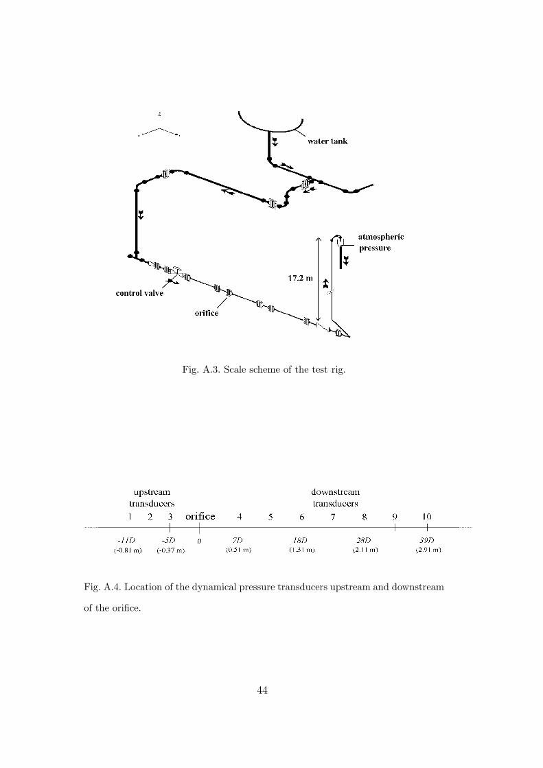
Fig. A.3. Scale scheme of the test rig.
Fig. A.4. Location of the dynamical pressure transducers upstream and downstream
of the orifice.
44
10 500 1000 1500−pi
0
pi
Pha
se (
rad)
10 500 1000 15000
0.2
0.4
0.6
0.8
1
1.2
Frequency (Hz)
Am
plitu
de
U=2.38 m.s−1
Fig. A.5. Typical acoustic reflection coefficient R = p+p− upstream of the orifice
(determined at transducer 1).
10 500 1000 1500−pi
0
pi
Pha
se (
rad)
10 500 1000 15000
0.2
0.4
0.6
0.8
1
1.2
Frequency (Hz)
Am
plitu
de
U=1.91 m.s−1
Fig. A.6. Typical acoustic reflection coefficient R = p−p+ downstream of the orifice
(determined at transducer 8) in developed cavitation regime.
45
10 500 1000 1500−pi
0
pi
Pha
se (
rad)
10 500 1000 15000
0.2
0.4
0.6
0.8
1
1.2
Frequency (Hz)
Am
plitu
de
U=3.75 m.s−1
Fig. A.7. Typical acoustic reflection coefficient R = p−p+ downstream of the orifice
(determined at transducer 8) in super cavitation regime.
0 500 1000 1500 20000
0.1
0.2
0.3
0.4
0.5
0.6
0.7
0.8
0.9
1
Frequency (Hz)
Coh
eren
ce
Fig. A.8. Example of the coherence function between 2 successive transducers (sin-
gle-hole orifice, U=2.38 m s−1 , between transducers 7 and 8).
46
0 500 1000 1500 2000
−1
−0.8
−0.6
−0.4
−0.2
0
0.2
0.4
0.6
0.8
1
Frequency (Hz)
cos(
ω∆l
/c)
(p6(ω)+p
8(ω)) / p
7(ω)
fit with c=1425 m/s
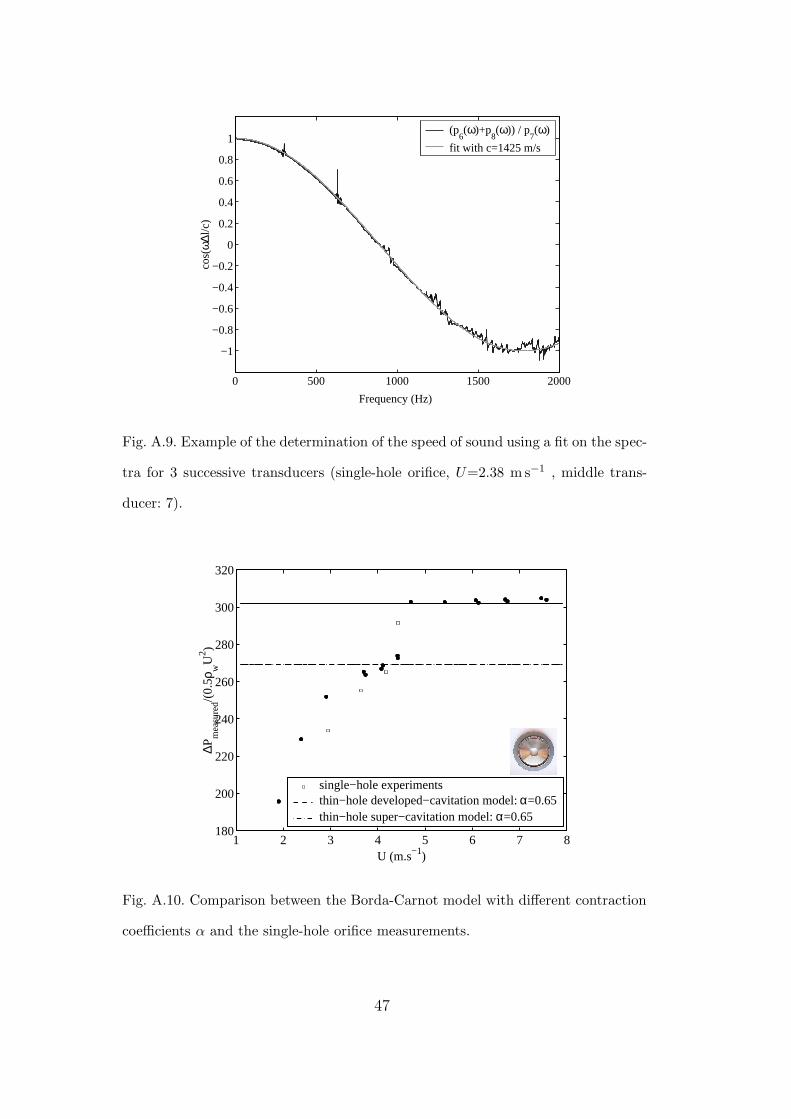
Fig. A.9. Example of the determination of the speed of sound using a fit on the spec-
tra for 3 successive transducers (single-hole orifice, U=2.38 m s−1 , middle trans-
ducer: 7).
1 2 3 4 5 6 7 8180
200
220
240
260
280
300
320
U (m.s−1)
∆Pm
easu
red/(
0.5ρ
wU
2 )
single−hole experimentsthin−hole developed−cavitation model: α=0.65thin−hole super−cavitation model: α=0.65
Fig. A.10. Comparison between the Borda-Carnot model with different contraction
coefficients α and the single-hole orifice measurements.
47
1 2 3 4 5 6 7 8140
160
180
200
220
240
260
280
300
320
U (m.s−1)
∆Pm
easu
red/(
0.5ρ
wU
2 )
multi−hole experimentsthick−hole developed−cavitation model: α=0.65thin−hole developed−cavitation model: α=0.65thick−hole super−cavitation model: α=0.65single−hole experiments
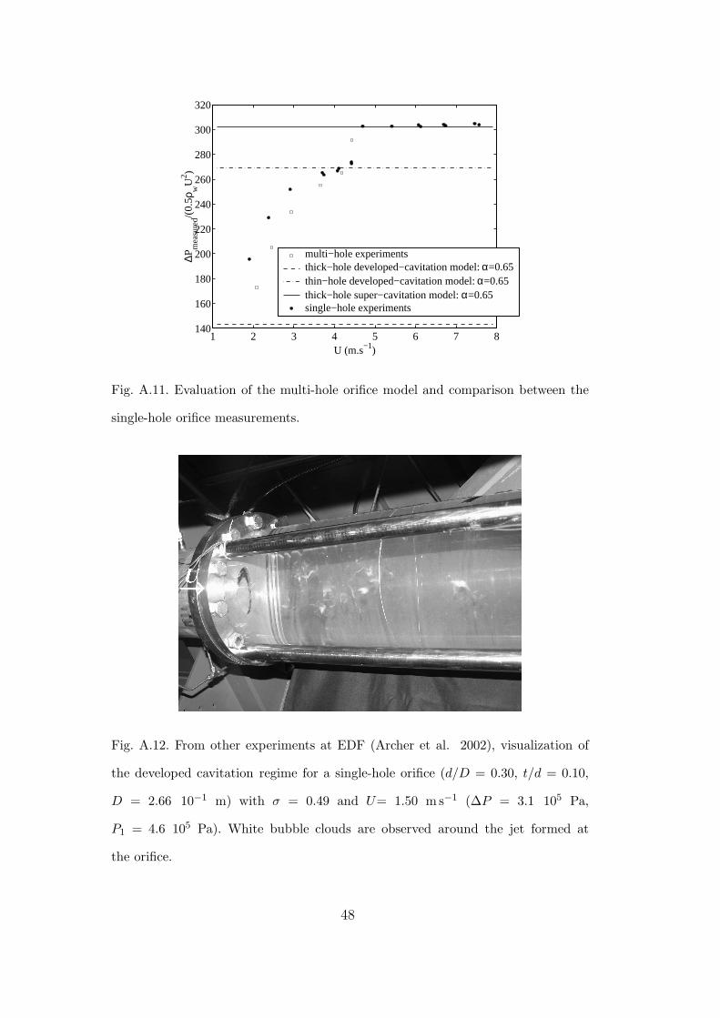
Fig. A.11. Evaluation of the multi-hole orifice model and comparison between the
single-hole orifice measurements.
Fig. A.12. From other experiments at EDF (Archer et al. 2002), visualization of
the developed cavitation regime for a single-hole orifice (d/D = 0.30, t/d = 0.10,
D = 2.66 10−1 m) with σ = 0.49 and U= 1.50 m s−1 (∆P = 3.1 105 Pa,
P1 = 4.6 105 Pa). White bubble clouds are observed around the jet formed at
the orifice.
48
40 40.05 40.1 40.15−2.5
−2
−1.5
−1
−0.5
0
0.5
1
1.5
2
2.5
Time (s)
Dyn
amic
al p
ress
ure
sign
al a
t sen
sor
9 (1
05 P
a) σ = 0.41
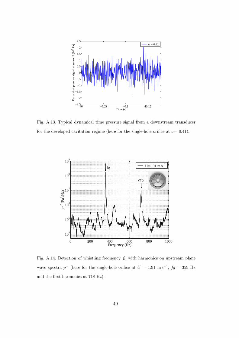
Fig. A.13. Typical dynamical time pressure signal from a downstream transducer
for the developed cavitation regime (here for the single-hole orifice at σ= 0.41).
0 200 400 600 800 1000
104
105
106
107
108
109
Frequency (Hz)
p−2 (
Pa2 /H
z)
U=1.91 m.s−1f 0
0 f 2
Fig. A.14. Detection of whistling frequency f0 with harmonics on upstream plane
wave spectra p− (here for the single-hole orifice at U = 1.91 m s−1, f0 = 359 Hz
and the first harmonics at 718 Hz).
49
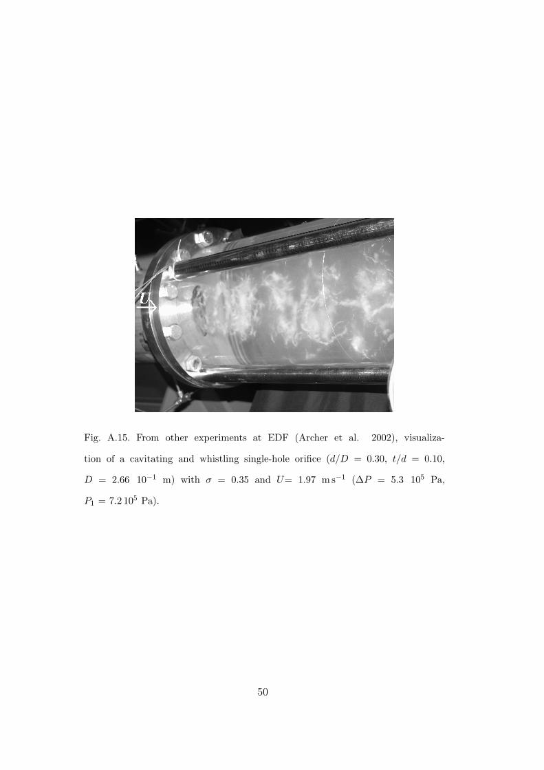
Fig. A.15. From other experiments at EDF (Archer et al. 2002), visualiza-
tion of a cavitating and whistling single-hole orifice (d/D = 0.30, t/d = 0.10,
D = 2.66 10−1 m) with σ = 0.35 and U= 1.97 m s−1 (∆P = 5.3 105 Pa,
P1 = 7.2 105 Pa).
50
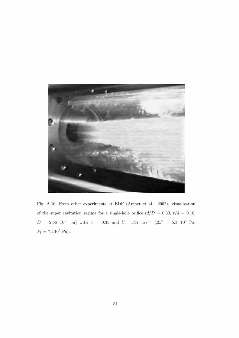
Fig. A.16. From other experiments at EDF (Archer et al. 2002), visualization
of the super cavitation regime for a single-hole orifice (d/D = 0.30, t/d = 0.10,
D = 2.66 10−1 m) with σ = 0.35 and U= 1.97 m s−1 (∆P = 5.3 105 Pa,
P1 = 7.2 105 Pa).
51
40 40.05 40.1 40.15−5
0
5
10
15
20
Time (s)
Dyn
amic
al p
ress
ure
sign
al a
t sen
sor
9 (1
05 P
a) σ = 0.10
Fig. A.17. Spurious pressure pulses (spikes) from collapsing bubbles on dynamical
time pressure signal from a downstream transducer in super cavitation regime (here
for the single-hole orifice at σ= 0.10).
47.07 47.075 47.08 47.085 47.09 47.095 47.1−5
0
5
10
15
20
Time (s)
Flu
ctua
ting
pres
sure
(x1
05 P
a)
Fig. A.18. Cavitation peak in super cavitation regime (single-hole orifice at σ=0.10).
52
−1 0 1 2 3 4 5−1.5
−1
−0.5
0
0.5
1
1.5x 10
4
Distance (m)
Rea
l par
t of t
he c
ross
−sp
ectr
a (P
a/H
z0.
5 )
↑ Orifice ↑ Downstream valve
p’~0 p’~0
Fig. A.19. In the developed cavitation regime, two acoustic boundary conditions
p′ ' 0 are found downstream of the orifice, hence natural frequencies appear, pointed
out by the interpolation of the values of the cross-spectra at those first natural
frequencies (here for the single-hole orifice at U = 2.38 m s−1 , c=1420 m s−1 and 5
natural frequencies: • 188 Hz, N 386 Hz, H 574 Hz, � 770 Hz, � 957 Hz).
53
101
102
103
10−6
10−5
10−4
10−3
10−2
10−1
100
f (in Hz)
S p
+2 /(ρ w
c)
(in W
/Hz)
σ=0.74, c=1280 m/sσ=0.41, c=660 m/sσ=0.25, c=1430 m/s
Fig. A.20. Acoustical power spectra - developed cavitation (single-hole orifice).
101
102
103
10−7
10−6
10−5
10−4
10−3
10−2
10−1
f (in Hz)
p+2 S
/(ρ c
) (in
W/H
z)
σ=0.74, c=1420 m/sσ=0.45, c=1420 m/sσ=0.28, c=1425 m/sσ=0.17, c=1425 m/s
Fig. A.21. Acoustical power spectra - developed cavitation (multi-hole orifice).
54
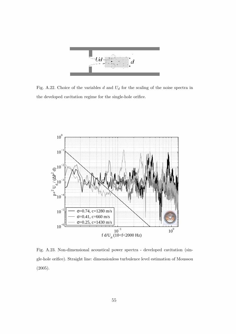
Fig. A.22. Choice of the variables d and Ud for the scaling of the noise spectra in
the developed cavitation regime for the single-hole orifice.
10−1
100
10−6
10−5
10−4
10−3
10−2
10−1
100
f d/Ud (10<f<2000 Hz)
p+2 U
d / (∆
P2 d)
σ=0.74, c=1280 m/sσ=0.41, c=660 m/sσ=0.25, c=1430 m/s
Fig. A.23. Non-dimensional acoustical power spectra - developed cavitation (sin-
gle-hole orifice). Straight line: dimensionless turbulence level estimation of Moussou
(2005).
55
10−2
10−1
10−6
10−4
10−2
f dmulti
/Ud (10<f<2000 Hz)
p+2 U
d / (∆
P2 dm
ulti)
σ=0.74, c=1430 m/sσ=0.45, c=1430 m/sσ=0.28, c=1430 m/sσ=0.17, c=1435 m/s
Fig. A.24. Non-dimensional acoustical power spectra - developed cavitation (multi-
-hole orifice).
101
102
103
10−4
10−3
10−2
10−1
100
101
f (in Hz)
p+2 S
/(ρ c
) (in
W/H
z)
σ=0.15, c=280 m/sσ=0.15, c=1420 m/sσ=0.12, c=120 m/sσ=0.12, c=1310 m/sσ=0.10, c=1230 m/sσ=0.10, c=340 m/s
Fig. A.25. Acoustical power spectra - super cavitation (single-hole orifice).
56
101
102
103
10−4
10−3
10−2
10−1
100
101
f (in Hz)
p+2 S
/(ρ c
) (in
W/H
z)
σ=0.03, c=1400 m/sσ=0.13, c=1010 m/sσ=0.13, c=700 m/s
Fig. A.26. Acoustical power spectra - super cavitation (multi-hole orifice).
57
101
102
103
10−4
10−3
10−2
10−1
100
101
f (in Hz)
p+2 S
/(ρ c
) (in
W/H
z)
σ=0.15, c=1420 m/sσ=0.15, c=1300 m/sσ=0.15, c=610 m/sσ=0.15, c=280 m/s
Fig. A.27. Super cavitation (single-hole orifice): influence of the speed of sound on
the noise spectra.
58
Tables
Table A.1
Flow conditions for the single-hole orifice experiments (with standard deviations).
Developed cavitation︷ ︸︸ ︷
Super cavitation︷ ︸︸ ︷
U (m s−1 ) 1.91 2.38 2.90 3.75 4.08 4.42
st. deviation (m s−1 ) 0.06 0.04 0.04 0.03 0.03 0.05
P1 (105 Pa) 6.3 9.2 13.3 21.4 25.0 29.5
st. deviation (105 Pa) 0.3 0.3 0.6 1.4 0.7 0.8
P2 (x105 Pa) 2.7 2.7 2.7 2.8 2.8 2.8
st. deviation (x105 Pa) 0.0 0.0 0.0 2.0 0.2 1.5
σ 0.74 0.41 0.25 0.15 0.12 0.10
59
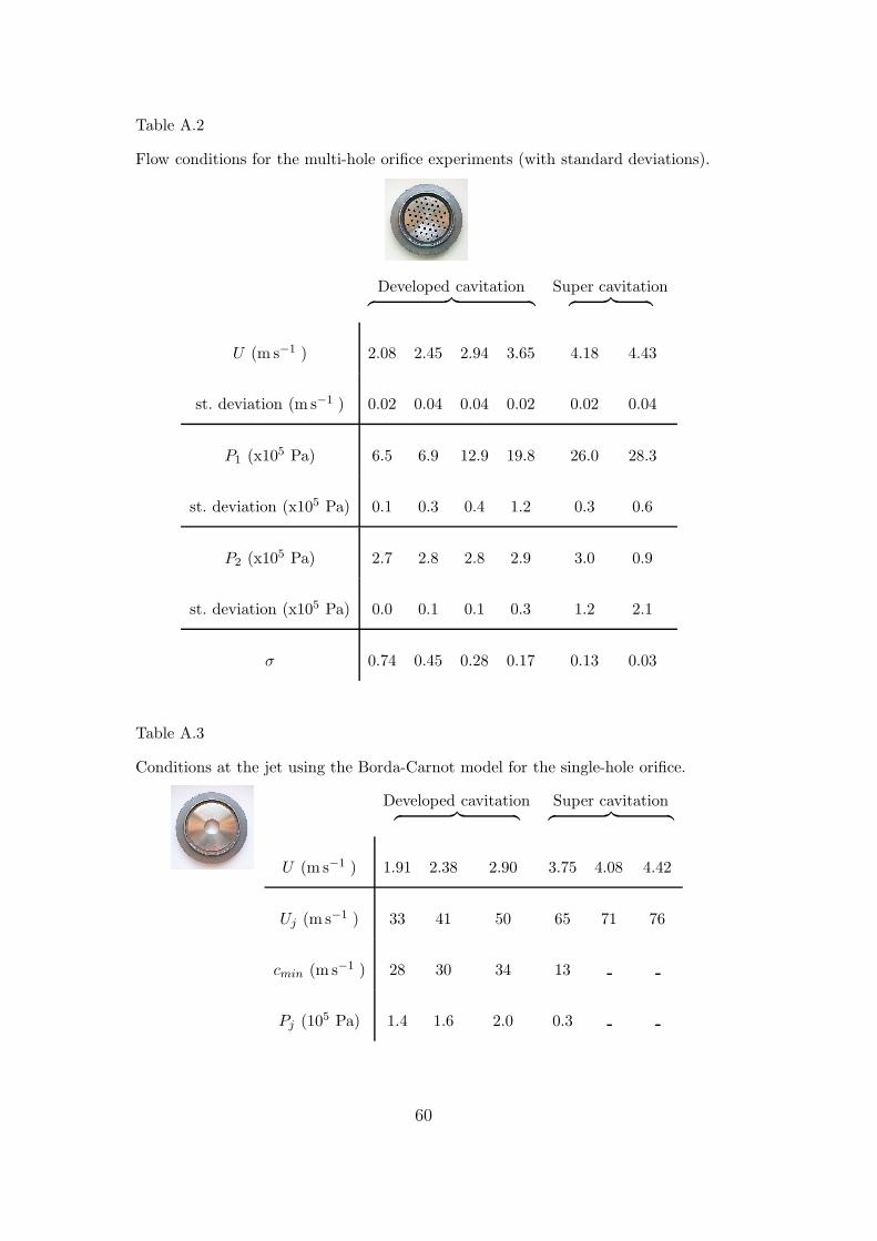
Table A.2
Flow conditions for the multi-hole orifice experiments (with standard deviations).
Developed cavitation︷ ︸︸ ︷
Super cavitation︷ ︸︸ ︷
U (m s−1 ) 2.08 2.45 2.94 3.65 4.18 4.43
st. deviation (m s−1 ) 0.02 0.04 0.04 0.02 0.02 0.04
P1 (x105 Pa) 6.5 6.9 12.9 19.8 26.0 28.3
st. deviation (x105 Pa) 0.1 0.3 0.4 1.2 0.3 0.6
P2 (x105 Pa) 2.7 2.8 2.8 2.9 3.0 0.9
st. deviation (x105 Pa) 0.0 0.1 0.1 0.3 1.2 2.1
σ 0.74 0.45 0.28 0.17 0.13 0.03
Table A.3
Conditions at the jet using the Borda-Carnot model for the single-hole orifice.
Developed cavitation︷ ︸︸ ︷
Super cavitation︷ ︸︸ ︷
U (m s−1 ) 1.91 2.38 2.90 3.75 4.08 4.42
Uj (m s−1 ) 33 41 50 65 71 76
cmin (m s−1 ) 28 30 34 13
Pj (105 Pa) 1.4 1.6 2.0 0.3
60
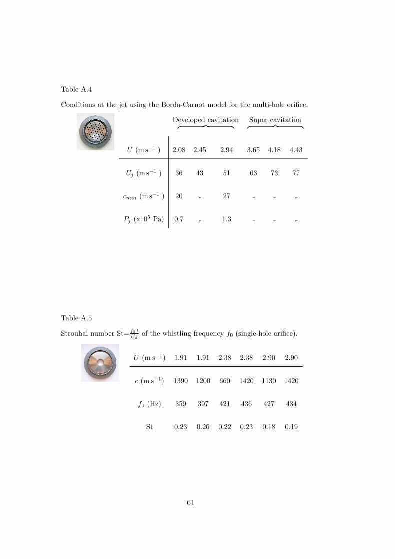
Table A.4
Conditions at the jet using the Borda-Carnot model for the multi-hole orifice.
Developed cavitation︷ ︸︸ ︷
Super cavitation︷ ︸︸ ︷
U (m s−1 ) 2.08 2.45 2.94 3.65 4.18 4.43
Uj (m s−1 ) 36 43 51 63 73 77
cmin (m s−1 ) 20 27
Pj (x105 Pa) 0.7 1.3
Table A.5
Strouhal number St=f0 tUd
of the whistling frequency f0 (single-hole orifice).
U (m s−1) 1.91 1.91 2.38 2.38 2.90 2.90
c (m s−1) 1390 1200 660 1420 1130 1420
f0 (Hz) 359 397 421 436 427 434
St 0.23 0.26 0.22 0.23 0.18 0.19
61