Embed Size (px)
Citation preview
Module I3.5GE
Signaux - Systemes et AutomatiqueLineaire
Yassine Ariba
Dpt GEI - Icam, Toulouse.
version 4.0
Y. Ariba - Icam, Toulouse. GE-SSAL 1 / 99

Informations pratiques
Contact
Tel : 05 34 50 50 38
Email : [email protected]
Forum : Moodle. Favorise le partage, l’auto-formation, la capitalisation
d’informations...
Organisation du cours
Pre-requis : cours de l’an dernier, mathematiques depuis le CP !
8h en amphi et 2h de TD : cours + exercices. Presentation sur transparents.
4h de TP.
utilisation de MATLABR© et SimulinkR©
evaluation sur QCM.
1 examen final (1h).
Sur Moodle
Documents : transparent cours + support redige + exercices + sujets TP.
Forum.
Y. Ariba - Icam, Toulouse. GE-SSAL 2 / 99

Contents
1 Introduction
Introductory example
What is automatic control ?2 Quick review
Modelisation
Time response
Frequency response
Notion of stability
Summary
Back to our example3 Performances
Precision
Responsiveness
Stability margins
4 Control design
Introduction
Synthese directe : modele impose
Action proportionnelle
Action integrale
Action derivee
Combinaisons d’actions
Proportionnel-Integral-Derive (PID)
Y. Ariba - Icam, Toulouse. GE-SSAL 3 / 99
Introduction Introductory example
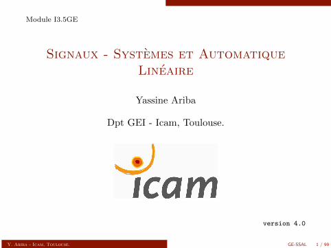
Introductory example
We want to control the angular position of a robotic arm.
What do we do ? What do we need ?
Y. Ariba - Icam, Toulouse. GE-SSAL 4 / 99
Introduction Introductory example
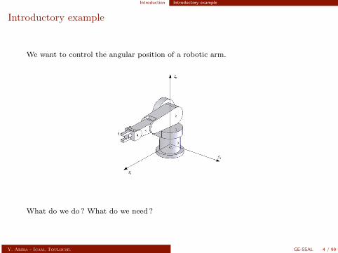
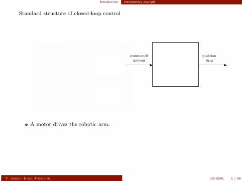
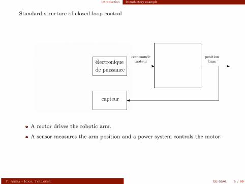
Standard structure of closed-loop control
A motor drives the robotic arm.
A sensor measures the arm position and a power system controls the motor.
An “intelligent” system provides a control strategy.
The control system may be implemented on an electronic board, a computer,a microcontroller...
Y. Ariba - Icam, Toulouse. GE-SSAL 5 / 99
Introduction Introductory example
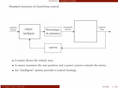
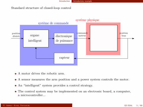
Standard structure of closed-loop control
A motor drives the robotic arm.
A sensor measures the arm position and a power system controls the motor.
An “intelligent” system provides a control strategy.
The control system may be implemented on an electronic board, a computer,a microcontroller...
Y. Ariba - Icam, Toulouse. GE-SSAL 5 / 99
Introduction What is automatic control ?
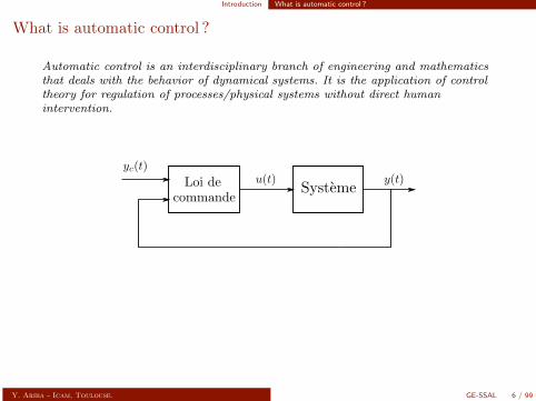
What is automatic control ?
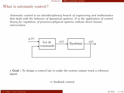
Automatic control is an interdisciplinary branch of engineering and mathematicsthat deals with the behavior of dynamical systems. It is the application of controltheory for regulation of processes/physical systems without direct humanintervention.
? Goal : To design a control law to make the system output track a referencesignal.
⇒ feedback control
Y. Ariba - Icam, Toulouse. GE-SSAL 6 / 99
Introduction What is automatic control ?
What is automatic control ?
Automatic control is an interdisciplinary branch of engineering and mathematicsthat deals with the behavior of dynamical systems. It is the application of controltheory for regulation of processes/physical systems without direct humanintervention.
? Goal : To design a control law to make the system output track a referencesignal.
⇒ feedback control
Y. Ariba - Icam, Toulouse. GE-SSAL 6 / 99
Introduction What is automatic control ?
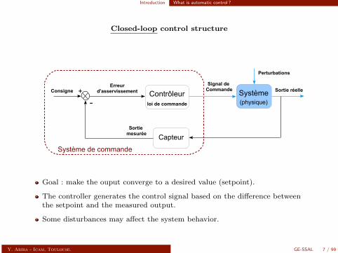
Closed-loop control structure
Système(physique)
Signal de CommandeConsigne Sortie réelle
CapteurSortie
mesurée
+
-
Erreurd'asservissement Contrôleur
loi de commande
Système de commande
Perturbations
Goal : make the ouput converge to a desired value (setpoint).
The controller generates the control signal based on the difference betweenthe setpoint and the measured output.
Some disturbances may affect the system behavior.
Y. Ariba - Icam, Toulouse. GE-SSAL 7 / 99
Introduction What is automatic control ?
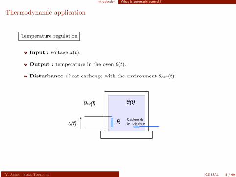
Thermodynamic application
Temperature regulation
Input : voltage u(t).
Output : temperature in the oven θ(t).
Disturbance : heat exchange with the environment θair(t).
u(t)
θ(t)
R Capteur de température
θair(t)
Y. Ariba - Icam, Toulouse. GE-SSAL 8 / 99
Introduction What is automatic control ?
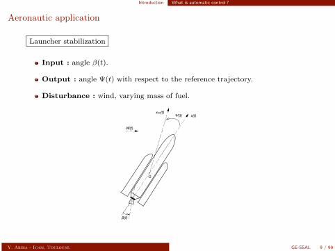
Aeronautic application
Launcher stabilization
Input : angle β(t).
Output : angle Ψ(t) with respect to the reference trajectory.
Disturbance : wind, varying mass of fuel.
G
β(t)
W(t)
x(t)xref(t)
Ψ(t)
Y. Ariba - Icam, Toulouse. GE-SSAL 9 / 99
Introduction What is automatic control ?
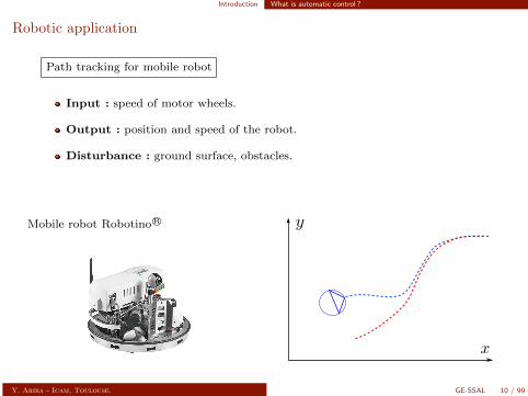
Robotic application
Path tracking for mobile robot
Input : speed of motor wheels.
Output : position and speed of the robot.
Disturbance : ground surface, obstacles.
Mobile robot Robotino R©
Y. Ariba - Icam, Toulouse. GE-SSAL 10 / 99

Introduction What is automatic control ?
Academic applications
Stabilization of a ball on a surface and an inverted pendulum
c© Quanser
Y. Ariba - Icam, Toulouse. GE-SSAL 11 / 99

Quick review
Contents
1 Introduction
Introductory example
What is automatic control ?2 Quick review
Modelisation
Time response
Frequency response
Notion of stability
Summary
Back to our example3 Performances
Precision
Responsiveness
Stability margins
4 Control design
Introduction
Synthese directe : modele impose
Action proportionnelle
Action integrale
Action derivee
Combinaisons d’actions
Proportionnel-Integral-Derive (PID)
Y. Ariba - Icam, Toulouse. GE-SSAL 12 / 99
Quick review Modelisation
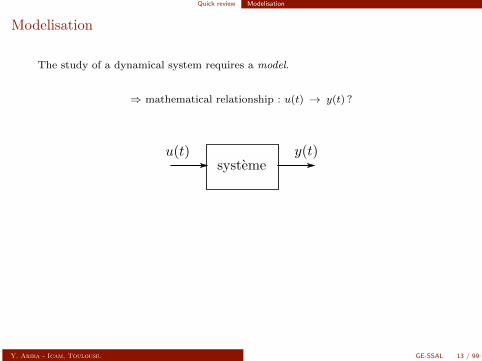
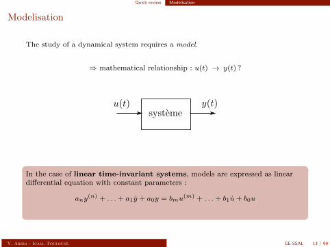
Modelisation
The study of a dynamical system requires a model.
⇒ mathematical relationship : u(t) → y(t) ?
In the case of linear time-invariant systems, models are expressed as lineardifferential equation with constant parameters :
any(n) + . . .+ a1y + a0y = bmu
(m) + . . .+ b1u+ b0u
Y. Ariba - Icam, Toulouse. GE-SSAL 13 / 99
Quick review Modelisation
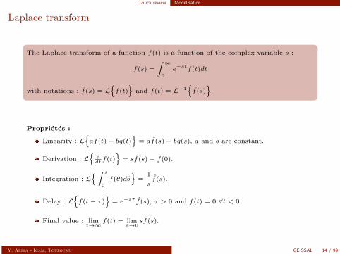
Laplace transform
The Laplace transform of a function f(t) is a function of the complex variable s :
f(s) =
∫ ∞0
e−st
f(t)dt
with notations : f(s) = Lf(t)
and f(t) = L−1
f(s)
.
Proprietes :
Linearity : Laf(t) + bg(t)
= af(s) + bg(s), a and b are constant.
Derivation : Lddt f(t)
= sf(s)− f(0).
Integration : L∫ t
0
f(θ)dθ
=1
sf(s).
Delay : Lf(t− τ)
= e−sτ f(s), τ > 0 and f(t) = 0 ∀t < 0.
Final value : limt→∞
f(t) = lims→0
sf(s).
Y. Ariba - Icam, Toulouse. GE-SSAL 14 / 99
Quick review Modelisation
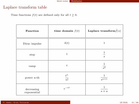
Laplace transform table
Time functions f(t) are defined only for all t ≥ 0.
Function time domain f(t) Laplace transformf(s)
Dirac impulse δ(t) 1
step 11
s
ramp t1
s2
power n-thtn
n!
1
sn+1
decreasingexponential
e−at 1
s+ a
Y. Ariba - Icam, Toulouse. GE-SSAL 15 / 99
Quick review Modelisation
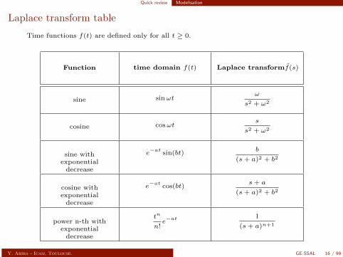
Laplace transform table
Time functions f(t) are defined only for all t ≥ 0.
Function time domain f(t) Laplace transformf(s)
sine sinωtω
s2 + ω2
cosine cosωts
s2 + ω2
sine withexponential
decrease
e−at
sin(bt)b
(s+ a)2 + b2
cosine withexponential
decrease
e−at
cos(bt)s+ a
(s+ a)2 + b2
power n-th withexponential
decrease
tn
n!e−at 1
(s+ a)n+1
Y. Ariba - Icam, Toulouse. GE-SSAL 16 / 99
Quick review Modelisation
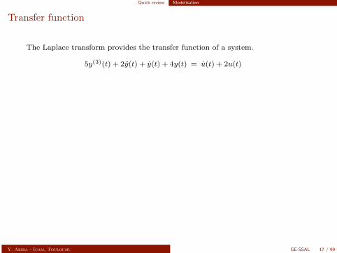
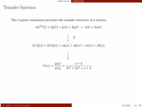
Transfer function
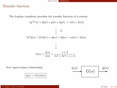
The Laplace transform provides the transfer function of a system.
5y(3)(t) + 2y(t) + y(t) + 4y(t) = u(t) + 2u(t)
y L
5s3y(s) + 2s2y(s) + sy(s) + 4y(s) = su(s) + 2u(s)yG(s) =
y(s)
u(s)=
s+ 2
5s3 + 2s2 + s+ 4
New input-output relationship
y(s) = G(s)u(s)
Y. Ariba - Icam, Toulouse. GE-SSAL 17 / 99
Quick review Modelisation
Transfer function
The Laplace transform provides the transfer function of a system.
5y(3)(t) + 2y(t) + y(t) + 4y(t) = u(t) + 2u(t)y L
5s3y(s) + 2s2y(s) + sy(s) + 4y(s) = su(s) + 2u(s)yG(s) =
y(s)
u(s)=
s+ 2
5s3 + 2s2 + s+ 4
New input-output relationship
y(s) = G(s)u(s)
Y. Ariba - Icam, Toulouse. GE-SSAL 17 / 99
Quick review Modelisation
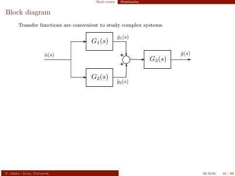
Block diagram
Transfer functions are convenient to study complex systems
+
+
we have : y1(s) = G1(s)u(s)y2(s) = G2(s)u(s)
y(s) = G3(s)(y1(s) + y2(s)
)equivalent transfer :
y(s) = G3(s)(G1(s) +G2(s)
)︸ ︷︷ ︸
F (s)
u(s)
Y. Ariba - Icam, Toulouse. GE-SSAL 18 / 99

Quick review Modelisation
Block diagram
Transfer functions are convenient to study complex systems
+
+
we have : y1(s) = G1(s)u(s)y2(s) = G2(s)u(s)
y(s) = G3(s)(y1(s) + y2(s)
)equivalent transfer :
y(s) = G3(s)(G1(s) +G2(s)
)︸ ︷︷ ︸
F (s)
u(s)
Y. Ariba - Icam, Toulouse. GE-SSAL 18 / 99
Quick review Time response
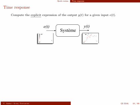
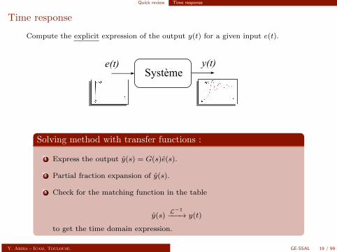
Time response
Compute the explicit expression of the output y(t) for a given input e(t).
Systèmey(t)e(t)
Solving method with transfer functions :
1 Express the output y(s) = G(s)e(s).
2 Partial fraction expansion of y(s).
3 Check for the matching function in the table
y(s)L−1
−−−→ y(t)
to get the time domain expression.
Y. Ariba - Icam, Toulouse. GE-SSAL 19 / 99
Quick review Time response
Time response
Compute the explicit expression of the output y(t) for a given input e(t).
Systèmey(t)e(t)
Solving method with transfer functions :
1 Express the output y(s) = G(s)e(s).
2 Partial fraction expansion of y(s).
3 Check for the matching function in the table
y(s)L−1
−−−→ y(t)
to get the time domain expression.
Y. Ariba - Icam, Toulouse. GE-SSAL 19 / 99

Quick review Time response
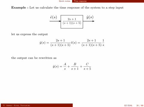
Example : Let us calculate the time response of the system to a step input
let us express the output
y(s) =2s+ 1
(s+ 1)(s+ 5)e(s) =
2s+ 1
(s+ 1)(s+ 5)
1
s
the output can be rewritten as
y(s) =A
s+
B
s+ 1+
C
s+ 5
with : A = sy(s)
∣∣s=0
= 15
B = (s+ 1)y(s)∣∣s=−1
= 14
C = (s+ 5)y(s)∣∣s=−5
= − 920
Y. Ariba - Icam, Toulouse. GE-SSAL 20 / 99

Quick review Time response
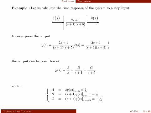
Example : Let us calculate the time response of the system to a step input
let us express the output
y(s) =2s+ 1
(s+ 1)(s+ 5)e(s) =
2s+ 1
(s+ 1)(s+ 5)
1
s
the output can be rewritten as
y(s) =A
s+
B
s+ 1+
C
s+ 5
with : A = sy(s)
∣∣s=0
= 15
B = (s+ 1)y(s)∣∣s=−1
= 14
C = (s+ 5)y(s)∣∣s=−5
= − 920
Y. Ariba - Icam, Toulouse. GE-SSAL 20 / 99
Quick review Time response
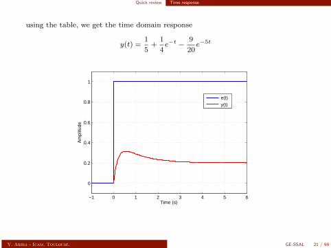
using the table, we get the time domain response
y(t) =1
5+
1
4e−t −
9
20e−5t
−1 0 1 2 3 4 5 6
0
0.2
0.4
0.6
0.8
1
Time (s)
Am
plitu
de
e(t)
y(t)
Y. Ariba - Icam, Toulouse. GE-SSAL 21 / 99
Quick review Time response
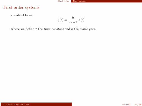
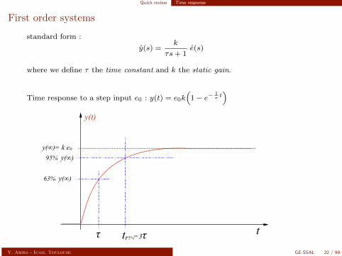
First order systems
standard form :
y(s) =k
τs+ 1e(s)
where we define τ the time constant and k the static gain.
Time response to a step input e0 : y(t) = e0k(
1− e−1τt)
t
y(t)
y(∞)= k e0
95% y(∞)
tr5%=3ττ
63% y(∞)
Y. Ariba - Icam, Toulouse. GE-SSAL 22 / 99
Quick review Time response
First order systems
standard form :
y(s) =k
τs+ 1e(s)
where we define τ the time constant and k the static gain.
Time response to a step input e0 : y(t) = e0k(
1− e−1τt)
t
y(t)
y(∞)= k e0
95% y(∞)
tr5%=3ττ
63% y(∞)
Y. Ariba - Icam, Toulouse. GE-SSAL 22 / 99
Quick review Time response
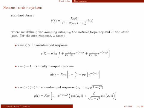
Second order system
standard form :
y(s) =Kω2
n
s2 + 2ζωns+ ω2n
e(s)
where we define ζ the damping ratio, ωn the natural frequency and K the staticgain. For the step response, 3 cases :
case ζ > 1 : overdamped response
y(t) = Ke0
[1 + p2
p1−p2e−ζωnt + p1
p2−p1e−ζωnt
]
cas ζ = 1 : critically damped response
y(t) = Ke0
[1−
(1− p1t
)e−ζωnt
]
cas 0 < ζ < 1 : underdamped response (ωp = ωn√
1− ζ2)
y(t) = Ke0
[1− e−ζωnt
(cos(ωpt) +
ζ√1− ζ2
sin(ωpt))]
Y. Ariba - Icam, Toulouse. GE-SSAL 23 / 99
Quick review Time response
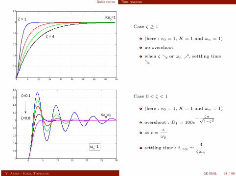
0 5 10 15 20 25 30 35 40 450
0.2
0.4
0.6
0.8
1
1.2
ζ = 4
Ke0=1ζ = 1
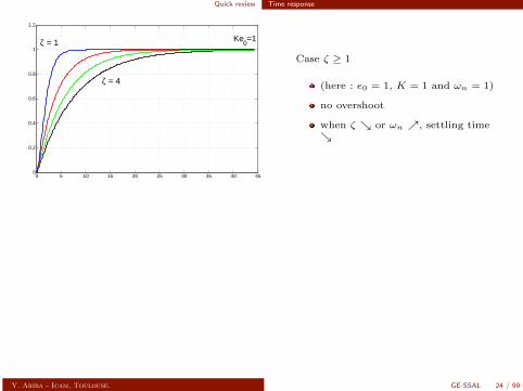
Case ζ ≥ 1
(here : e0 = 1, K = 1 and ωn = 1)
no overshoot
when ζ or ωn , settling time
0 5 10 15 20 25 300
0.2
0.4
0.6
0.8
1
1.2
1.4
1.6
1.8
ζ=0.1
ζ=0.8Ke
0=1
ωn=1
Case 0 < ζ < 1
(here : e0 = 1, K = 1 and ωn = 1)
overshoot : D1 = 100e− ζπ√
1−ζ2
at t =π
ωp
settling time : tr5% '3
ζωn
Y. Ariba - Icam, Toulouse. GE-SSAL 24 / 99
Quick review Time response
0 5 10 15 20 25 30 35 40 450
0.2
0.4
0.6
0.8
1
1.2
ζ = 4
Ke0=1ζ = 1
Case ζ ≥ 1
(here : e0 = 1, K = 1 and ωn = 1)
no overshoot
when ζ or ωn , settling time
0 5 10 15 20 25 300
0.2
0.4
0.6
0.8
1
1.2
1.4
1.6
1.8
ζ=0.1
ζ=0.8Ke
0=1
ωn=1
Case 0 < ζ < 1
(here : e0 = 1, K = 1 and ωn = 1)
overshoot : D1 = 100e− ζπ√
1−ζ2
at t =π
ωp
settling time : tr5% '3
ζωn
Y. Ariba - Icam, Toulouse. GE-SSAL 24 / 99
Quick review Frequency response
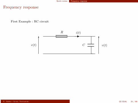
Frequency response
First Example : RC circuit
Sinusoidal steady state : e(t) = em cos(ωt+ φe)
v(t) = vm cos(ωt+ φv)⇒
e = emejφe
v = vmejφv
Y. Ariba - Icam, Toulouse. GE-SSAL 25 / 99
Quick review Frequency response
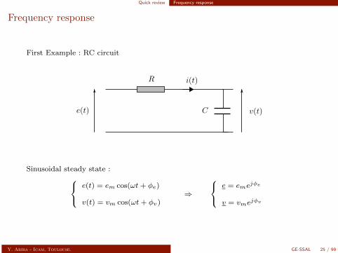
Frequency response
First Example : RC circuit
Sinusoidal steady state : e(t) = em cos(ωt+ φe)
v(t) = vm cos(ωt+ φv)⇒
e = emejφe
v = vmejφv
Y. Ariba - Icam, Toulouse. GE-SSAL 25 / 99
Quick review Frequency response
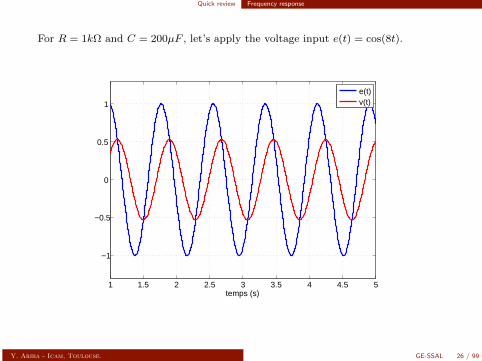
For R = 1kΩ and C = 200µF , let’s apply the voltage input e(t) = cos(8t).
1 1.5 2 2.5 3 3.5 4 4.5 5
−1
−0.5
0
0.5
1
temps (s)
e(t)v(t)
Y. Ariba - Icam, Toulouse. GE-SSAL 26 / 99
Quick review Frequency response
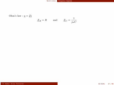
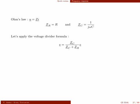
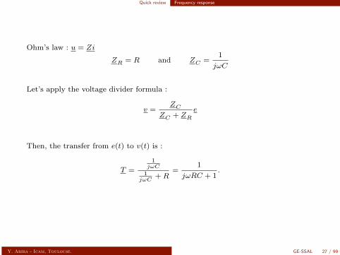
Ohm’s law : u = Zi
ZR = R and ZC =1
jωC
Let’s apply the voltage divider formula :
v =ZC
ZC + ZRe
Then, the transfer from e(t) to v(t) is :
T =
1jωC
1jωC
+R=
1
jωRC + 1.
Y. Ariba - Icam, Toulouse. GE-SSAL 27 / 99
Quick review Frequency response
Ohm’s law : u = Zi
ZR = R and ZC =1
jωC
Let’s apply the voltage divider formula :
v =ZC
ZC + ZRe
Then, the transfer from e(t) to v(t) is :
T =
1jωC
1jωC
+R=
1
jωRC + 1.
Y. Ariba - Icam, Toulouse. GE-SSAL 27 / 99
Quick review Frequency response
Ohm’s law : u = Zi
ZR = R and ZC =1
jωC
Let’s apply the voltage divider formula :
v =ZC
ZC + ZRe
Then, the transfer from e(t) to v(t) is :
T =
1jωC
1jωC
+R=
1
jωRC + 1.
Y. Ariba - Icam, Toulouse. GE-SSAL 27 / 99
Quick review Frequency response
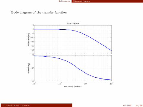
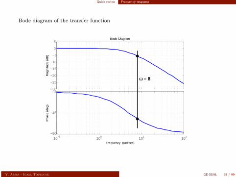
Bode diagram of the transfer function
−30
−25
−20
−15
−10
−5
0
5M
agni
tude
(dB
)
10−1 100 101 102−90
−45
0
Pha
se (
deg)
Bode Diagram
Frequency (rad/sec)
Y. Ariba - Icam, Toulouse. GE-SSAL 28 / 99
Quick review Frequency response
Bode diagram of the transfer function
−30
−25
−20
−15
−10
−5
0
5M
agni
tude
(dB
)
10−1 100 101 102−90
−45
0
Pha
se (
deg)
Bode Diagram
Frequency (rad/sec)
ω = 8
Y. Ariba - Icam, Toulouse. GE-SSAL 28 / 99
Quick review Frequency response
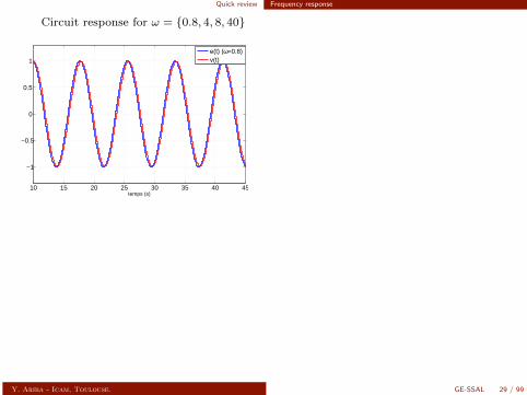
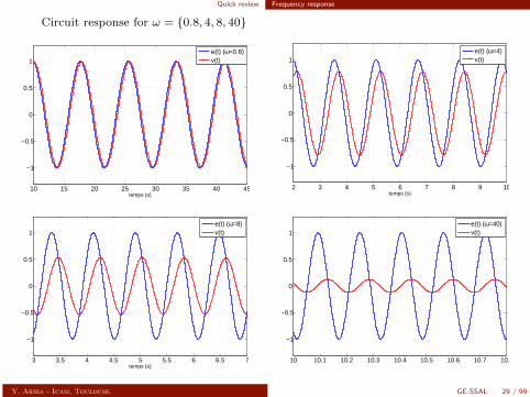
Circuit response for ω = 0.8, 4, 8, 40
10 15 20 25 30 35 40 45
−1
−0.5
0
0.5
1
temps (s)
e(t) (ω=0.8)v(t)
2 3 4 5 6 7 8 9 10
−1
−0.5
0
0.5
1
temps (s)
e(t) (ω=4)v(t)
3 3.5 4 4.5 5 5.5 6 6.5 7
−1
−0.5
0
0.5
1
temps (s)
e(t) (ω=8)v(t)
10 10.1 10.2 10.3 10.4 10.5 10.6 10.7 10.8
−1
−0.5
0
0.5
1
e(t) (ω=40)v(t)
Y. Ariba - Icam, Toulouse. GE-SSAL 29 / 99
Quick review Frequency response
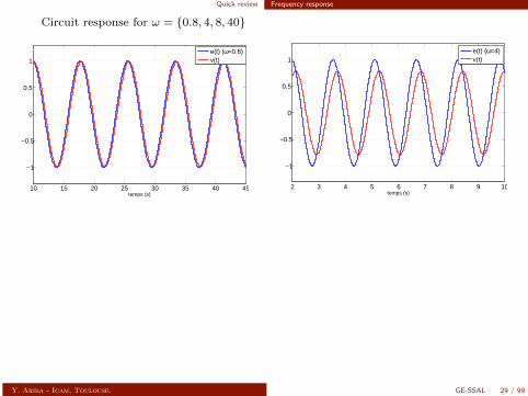
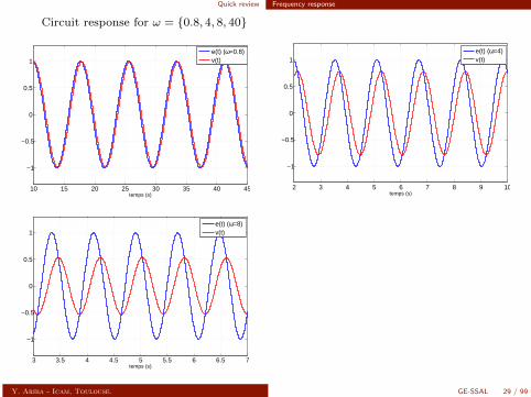
Circuit response for ω = 0.8, 4, 8, 40
10 15 20 25 30 35 40 45
−1
−0.5
0
0.5
1
temps (s)
e(t) (ω=0.8)v(t)
2 3 4 5 6 7 8 9 10
−1
−0.5
0
0.5
1
temps (s)
e(t) (ω=4)v(t)
3 3.5 4 4.5 5 5.5 6 6.5 7
−1
−0.5
0
0.5
1
temps (s)
e(t) (ω=8)v(t)
10 10.1 10.2 10.3 10.4 10.5 10.6 10.7 10.8
−1
−0.5
0
0.5
1
e(t) (ω=40)v(t)
Y. Ariba - Icam, Toulouse. GE-SSAL 29 / 99
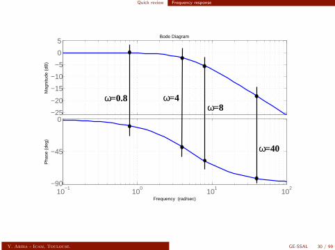
Quick review Frequency response
−25
−20
−15
−10
−5
0
5M
agni
tude
(dB
)
10−1
100
101
102
−90
−45
0
Pha
se (
deg)
Bode Diagram
Frequency (rad/sec)
ω=8ω=4ω=0.8
ω=40
Y. Ariba - Icam, Toulouse. GE-SSAL 30 / 99
Quick review Frequency response
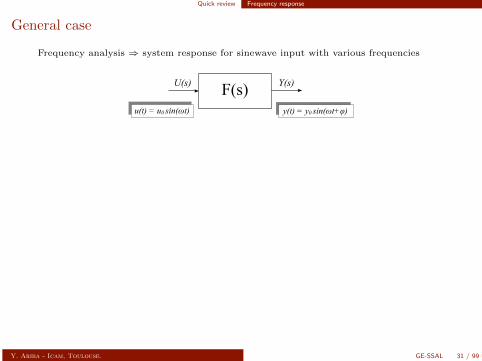
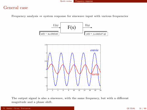
General case
Frequency analysis ⇒ system response for sinewave input with various frequencies
F(s) Y(s)U(s)
u(t) = u0 sin(ωt) u(t) = u0 sin(ωt) y(t) = y0 sin(ωt+φ) y(t) = y0 sin(ωt+φ)
0 2 4 6 8 10 12 14 16 18 20
−1
−0.5
0
0.5
1
1.5
entrée
sortie
The output signal is also a sinewave, with the same frequency, but with a different
magnitude and a phase shift.
Y. Ariba - Icam, Toulouse. GE-SSAL 31 / 99
Quick review Frequency response
General case
Frequency analysis ⇒ system response for sinewave input with various frequencies
F(s) Y(s)U(s)
u(t) = u0 sin(ωt) u(t) = u0 sin(ωt) y(t) = y0 sin(ωt+φ) y(t) = y0 sin(ωt+φ)
0 2 4 6 8 10 12 14 16 18 20
−1
−0.5
0
0.5
1
1.5
entrée
sortie
The output signal is also a sinewave, with the same frequency, but with a different
magnitude and a phase shift.
Y. Ariba - Icam, Toulouse. GE-SSAL 31 / 99

Quick review Frequency response
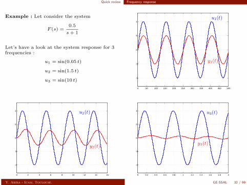
Example : Let consider the system
F (s) =0.5
s+ 1
Let’s have a look at the system response for 3frequencies :
u1 = sin(0.05 t)
u2 = sin(1.5 t)
u3 = sin(10 t)
0 50 100 150 200 250 300 350 400 450 500
−1
−0.5
0
0.5
1
u1(t)
y1(t)
0 2 4 6 8 10 12 14 16
−1
−0.5
0
0.5
1 u2(t)
y2(t)
0 0.2 0.4 0.6 0.8 1 1.2 1.4 1.6 1.8 2
−1
−0.5
0
0.5
1 u3(t)
y3(t)
Y. Ariba - Icam, Toulouse. GE-SSAL 32 / 99
Quick review Frequency response
A system can be characterized by its
gain = |F (jω)| phase shift= arg(F (jω)
)
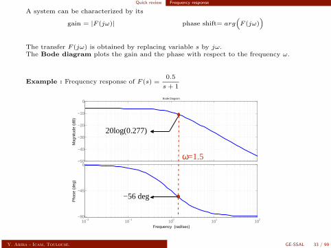
The transfer F (jω) is obtained by replacing variable s by jω.The Bode diagram plots the gain and the phase with respect to the frequency ω.
Example : Frequency response of F (s) =0.5
s+ 1
Bode Diagram
Frequency (rad/sec)
−50
−40
−30
−20
−10
0
Mag
nitu
de (
dB)
10−2 10−1 100 101 102−90
−45
0
Pha
se (
deg)
20log(0.277)
−56 deg
ω=1.5
Y. Ariba - Icam, Toulouse. GE-SSAL 33 / 99
Quick review Frequency response
A system can be characterized by its
gain = |F (jω)| phase shift= arg(F (jω)
)
The transfer F (jω) is obtained by replacing variable s by jω.The Bode diagram plots the gain and the phase with respect to the frequency ω.
Example : Frequency response of F (s) =0.5
s+ 1
Bode Diagram
Frequency (rad/sec)
−50
−40
−30
−20
−10
0
Mag
nitu
de (
dB)
10−2 10−1 100 101 102−90
−45
0
Pha
se (
deg)
20log(0.277)
−56 deg
ω=1.5
Y. Ariba - Icam, Toulouse. GE-SSAL 33 / 99
Quick review Frequency response
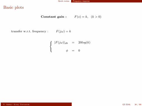
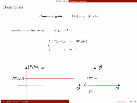
Basic plots
Constant gain : F (s) = k, (k > 0)
transfer w.r.t. frequency : F (jω) = k
|F (jω)|db = 20log(k)
φ = 0
|F(jω)|dB
ω0+90
-90
φ20log|k|
ω
Y. Ariba - Icam, Toulouse. GE-SSAL 34 / 99
Quick review Frequency response
Basic plots
Constant gain : F (s) = k, (k > 0)
transfer w.r.t. frequency : F (jω) = k
|F (jω)|db = 20log(k)
φ = 0
|F(jω)|dB
ω0+90
-90
φ20log|k|
ω
Y. Ariba - Icam, Toulouse. GE-SSAL 34 / 99
Quick review Frequency response
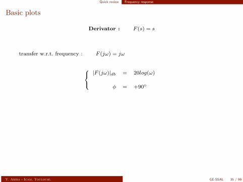
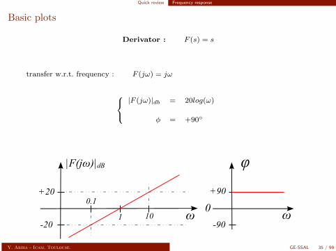
Basic plots
Derivator : F (s) = s
transfer w.r.t. frequency : F (jω) = jω
|F (jω)|db = 20log(ω)
φ = +90
|F(jω)|dB
ω0+90
-90
φ+20
-201 10
0.1
ω
Y. Ariba - Icam, Toulouse. GE-SSAL 35 / 99
Quick review Frequency response
Basic plots
Derivator : F (s) = s
transfer w.r.t. frequency : F (jω) = jω
|F (jω)|db = 20log(ω)
φ = +90
|F(jω)|dB
ω0+90
-90
φ+20
-201 10
0.1
ω
Y. Ariba - Icam, Toulouse. GE-SSAL 35 / 99
Quick review Frequency response
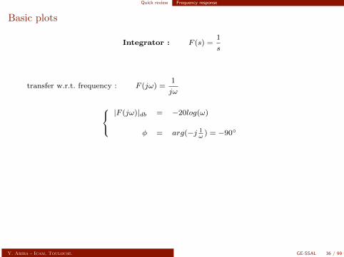
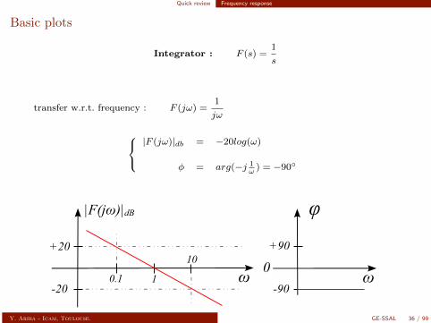
Basic plots
Integrator : F (s) =1
s
transfer w.r.t. frequency : F (jω) =1
jω
|F (jω)|db = −20log(ω)
φ = arg(−j 1ω
) = −90
|F(jω)|dB
ω0+90
-90
φ+20
-201
10
0.1 ω
Y. Ariba - Icam, Toulouse. GE-SSAL 36 / 99
Quick review Frequency response
Basic plots
Integrator : F (s) =1
s
transfer w.r.t. frequency : F (jω) =1
jω
|F (jω)|db = −20log(ω)
φ = arg(−j 1ω
) = −90
|F(jω)|dB
ω0+90
-90
φ+20
-201
10
0.1 ω
Y. Ariba - Icam, Toulouse. GE-SSAL 36 / 99
Quick review Frequency response
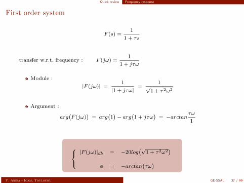
First order system
F (s) =1
1 + τs
transfer w.r.t. frequency : F (jω) =1
1 + jτω
Module :
|F (jω)| =1
|1 + jτω|=
1√
1 + τ2ω2
Argument :
arg(F (jω)
)= arg
(1)− arg
(1 + jτω
)= −arctan
τω
1
|F (jω)|db = −20log
(√1 + τ2ω2
)φ = −arctan
(τω)
Y. Ariba - Icam, Toulouse. GE-SSAL 37 / 99
Quick review Frequency response
First order system
F (s) =1
1 + τs
|F(jω)|dBω
0-45
-90
φ
-3
1/τ ω0
-20db/decade
1/τ
Y. Ariba - Icam, Toulouse. GE-SSAL 38 / 99
Quick review Frequency response
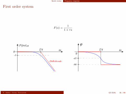
First order system
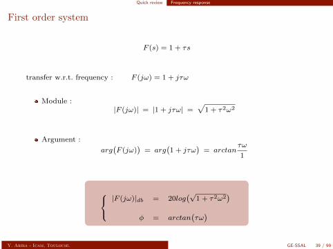
F (s) = 1 + τs
transfer w.r.t. frequency : F (jω) = 1 + jτω
Module :|F (jω)| = |1 + jτω| =
√1 + τ2ω2
Argument :
arg(F (jω)
)= arg
(1 + jτω
)= arctan
τω
1
|F (jω)|db = 20log
(√1 + τ2ω2
)φ = arctan
(τω)
Y. Ariba - Icam, Toulouse. GE-SSAL 39 / 99
Quick review Frequency response
First order system
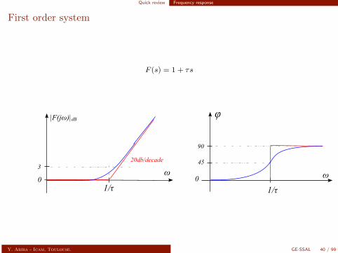
F (s) = 1 + τs
|F(jω)|dB
ω0
45
90
φ
3
1/τ
ω0
20db/decade
1/τ
Y. Ariba - Icam, Toulouse. GE-SSAL 40 / 99

Quick review Frequency response
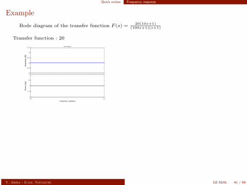
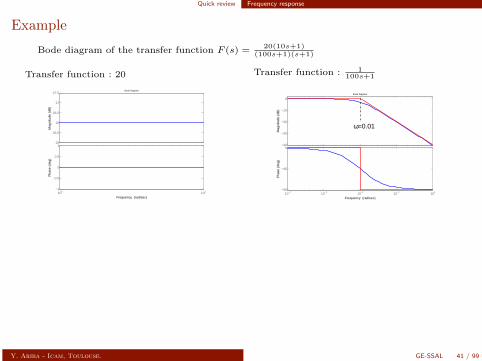
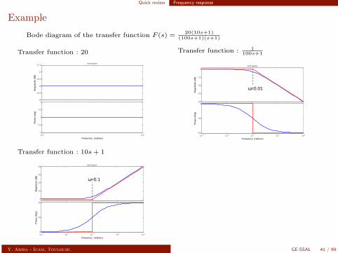
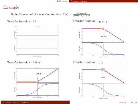
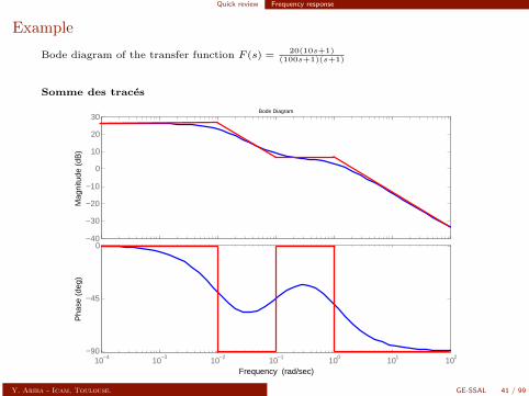
Example
Bode diagram of the transfer function F (s) =20(10s+1)
(100s+1)(s+1)
Transfer function : 20
25
25.5
26
26.5
27
27.5
Mag
nitu
de (
dB)
100 101−1
−0.5
0
0.5
1
Pha
se (
deg)
Bode Diagram
Frequency (rad/sec)
Transfer function : 1100s+1
−40
−30
−20
−10
0
Mag
nitu
de (
dB)
10−4 10−3 10−2 10−1 100−90
−45
0
Pha
se (
deg)
Bode Diagram
Frequency (rad/sec)
ω=0.01
Transfer function : 10s+ 1
0
10
20
30
40
Mag
nitu
de (
dB)
10−3 10−2 10−1 100 1010
45
90
Pha
se (
deg)
Bode Diagram
Frequency (rad/sec)
ω=0.1
Transfer function : 1s+1
−40
−30
−20
−10
0
Mag
nitu
de (
dB)
10−2 10−1 100 101 102−90
−45
0
Pha
se (
deg)
Bode Diagram
Frequency (rad/sec)
ω=1
Y. Ariba - Icam, Toulouse. GE-SSAL 41 / 99
Quick review Frequency response
Example
Bode diagram of the transfer function F (s) =20(10s+1)
(100s+1)(s+1)
Somme des traces
−40
−30
−20
−10
0
10
20
30
Mag
nitu
de (
dB)
10−4 10−3 10−2 10−1 100 101 102−90
−45
0
Pha
se (
deg)
Bode Diagram
Frequency (rad/sec)
Y. Ariba - Icam, Toulouse. GE-SSAL 41 / 99
Quick review Frequency response
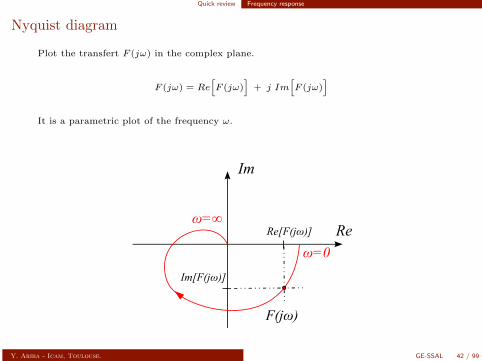
Nyquist diagram
Plot the transfert F (jω) in the complex plane.
F (jω) = Re[F (jω)
]+ j Im
[F (jω)
]
It is a parametric plot of the frequency ω.
Im
Re
F(jω)
Re[F(jω)]
Im[F(jω)]
ω=0
ω=∞
Y. Ariba - Icam, Toulouse. GE-SSAL 42 / 99
Quick review Frequency response
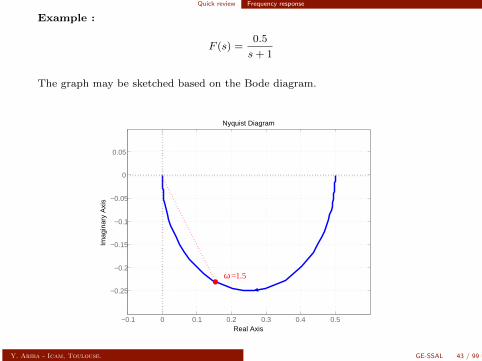
Example :
F (s) =0.5
s+ 1
The graph may be sketched based on the Bode diagram.
Nyquist Diagram
Real Axis
Imag
inar
y A
xis
−0.1 0 0.1 0.2 0.3 0.4 0.5
−0.25
−0.2
−0.15
−0.1
−0.05
0
0.05
ω =1.5
Y. Ariba - Icam, Toulouse. GE-SSAL 43 / 99
Quick review Notion of stability
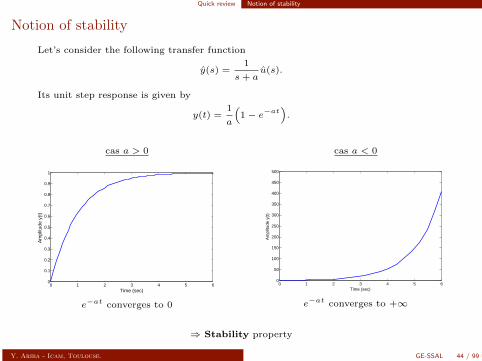
Notion of stability
Let’s consider the following transfer function
y(s) =1
s+ au(s).
Its unit step response is given by
y(t) =1
a
(1− e−at
).
cas a > 0
0 1 2 3 4 5 60
0.1
0.2
0.3
0.4
0.5
0.6
0.7
0.8
0.9
1
Time (sec)
Am
plitu
de y
(t)
e−at converges to 0
cas a < 0
0 1 2 3 4 5 60
50
100
150
200
250
300
350
400
450
500
Time (sec)
Am
plitu
de y
(t)
e−at converges to +∞
⇒ Stability property
Y. Ariba - Icam, Toulouse. GE-SSAL 44 / 99
Quick review Notion of stability
Notion of stability
Let’s consider the following transfer function
y(s) =1
s+ au(s).
Its unit step response is given by
y(t) =1
a
(1− e−at
).
cas a > 0
0 1 2 3 4 5 60
0.1
0.2
0.3
0.4
0.5
0.6
0.7
0.8
0.9
1
Time (sec)
Am
plitu
de y
(t)
e−at converges to 0
cas a < 0
0 1 2 3 4 5 60
50
100
150
200
250
300
350
400
450
500
Time (sec)
Am
plitu
de y
(t)
e−at converges to +∞
⇒ Stability property
Y. Ariba - Icam, Toulouse. GE-SSAL 44 / 99

Quick review Notion of stability
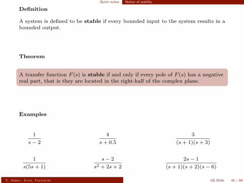
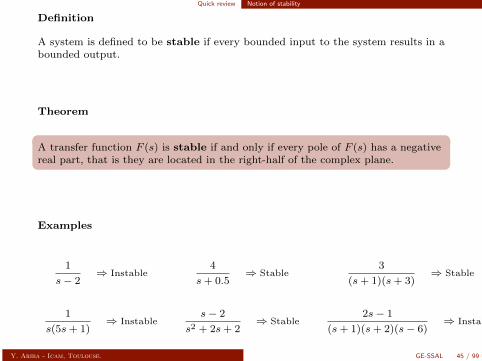
Definition
A system is defined to be stable if every bounded input to the system results in abounded output.
Theorem
A transfer function F (s) is stable if and only if every pole of F (s) has a negativereal part, that is they are located in the right-half of the complex plane.
Examples
1
s− 2
⇒ Instable
4
s+ 0.5
⇒ Stable
3
(s+ 1)(s+ 3)
⇒ Stable
1
s(5s+ 1)
⇒ Instable
s− 2
s2 + 2s+ 2
⇒ Stable
2s− 1
(s+ 1)(s+ 2)(s− 6)
⇒ Instable
Y. Ariba - Icam, Toulouse. GE-SSAL 45 / 99
Quick review Notion of stability
Definition
A system is defined to be stable if every bounded input to the system results in abounded output.
Theorem
A transfer function F (s) is stable if and only if every pole of F (s) has a negativereal part, that is they are located in the right-half of the complex plane.
Examples
1
s− 2⇒ Instable
4
s+ 0.5⇒ Stable
3
(s+ 1)(s+ 3)⇒ Stable
1
s(5s+ 1)⇒ Instable
s− 2
s2 + 2s+ 2⇒ Stable
2s− 1
(s+ 1)(s+ 2)(s− 6)⇒ Instable
Y. Ariba - Icam, Toulouse. GE-SSAL 45 / 99
Quick review Notion of stability
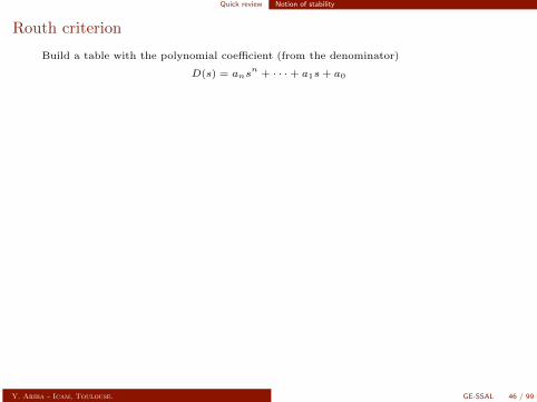
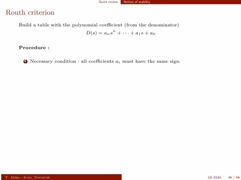
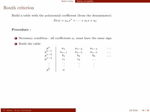
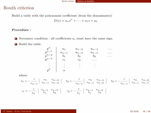
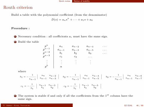
Routh criterion
Build a table with the polynomial coefficient (from the denominator)
D(s) = ansn
+ · · ·+ a1s+ a0
Procedure :
1 Necessary condition : all coefficients ai must have the same sign.
2 Build the table
pn an an−2 an−4 . . .
pn−1 an−1 an−3 an−5 . . .
pn−2 b1 b2 b3 . . .
pn−3 c1 c2 . . .
.
.
....
.
.
....
p0 α
where
b1 = −1
an−1
∣∣∣∣ an an−2an−1 an−3
∣∣∣∣ b2 = −1
an−1
∣∣∣∣ an an−4an−1 an−5
∣∣∣∣ b3 = −1
an−1
∣∣∣∣ an an−6an−1 an−7
∣∣∣∣c1 = −
1
b1
∣∣∣∣ an−1 an−3b1 b2
∣∣∣∣ c2 = −1
b1
∣∣∣∣ an−1 an−5b1 b3
∣∣∣∣
3 The system is stable if and only if all the coefficients from the 1st column have thesame sign.
Y. Ariba - Icam, Toulouse. GE-SSAL 46 / 99
Quick review Notion of stability
Routh criterion
Build a table with the polynomial coefficient (from the denominator)
D(s) = ansn
+ · · ·+ a1s+ a0
Procedure :
1 Necessary condition : all coefficients ai must have the same sign.
2 Build the table
pn an an−2 an−4 . . .
pn−1 an−1 an−3 an−5 . . .
pn−2 b1 b2 b3 . . .
pn−3 c1 c2 . . .
.
.
....
.
.
....
p0 α
where
b1 = −1
an−1
∣∣∣∣ an an−2an−1 an−3
∣∣∣∣ b2 = −1
an−1
∣∣∣∣ an an−4an−1 an−5
∣∣∣∣ b3 = −1
an−1
∣∣∣∣ an an−6an−1 an−7
∣∣∣∣c1 = −
1
b1
∣∣∣∣ an−1 an−3b1 b2
∣∣∣∣ c2 = −1
b1
∣∣∣∣ an−1 an−5b1 b3
∣∣∣∣3 The system is stable if and only if all the coefficients from the 1st column have the
same sign.
Y. Ariba - Icam, Toulouse. GE-SSAL 46 / 99
Quick review Notion of stability
Routh criterion
Build a table with the polynomial coefficient (from the denominator)
D(s) = ansn
+ · · ·+ a1s+ a0
Procedure :
1 Necessary condition : all coefficients ai must have the same sign.
2 Build the table
pn an an−2 an−4 . . .
pn−1 an−1 an−3 an−5 . . .
pn−2 b1 b2 b3 . . .
pn−3 c1 c2 . . .
.
.
....
.
.
....
p0 α
where
b1 = −1
an−1
∣∣∣∣ an an−2an−1 an−3
∣∣∣∣ b2 = −1
an−1
∣∣∣∣ an an−4an−1 an−5
∣∣∣∣ b3 = −1
an−1
∣∣∣∣ an an−6an−1 an−7
∣∣∣∣c1 = −
1
b1
∣∣∣∣ an−1 an−3b1 b2
∣∣∣∣ c2 = −1
b1
∣∣∣∣ an−1 an−5b1 b3
∣∣∣∣
3 The system is stable if and only if all the coefficients from the 1st column have thesame sign.
Y. Ariba - Icam, Toulouse. GE-SSAL 46 / 99
Quick review Notion of stability
Routh criterion
Build a table with the polynomial coefficient (from the denominator)
D(s) = ansn
+ · · ·+ a1s+ a0
Procedure :
1 Necessary condition : all coefficients ai must have the same sign.
2 Build the table
pn an an−2 an−4 . . .
pn−1 an−1 an−3 an−5 . . .
pn−2 b1 b2 b3 . . .
pn−3 c1 c2 . . .
.
.
....
.
.
....
p0 α
where
b1 = −1
an−1
∣∣∣∣ an an−2an−1 an−3
∣∣∣∣ b2 = −1
an−1
∣∣∣∣ an an−4an−1 an−5
∣∣∣∣ b3 = −1
an−1
∣∣∣∣ an an−6an−1 an−7
∣∣∣∣c1 = −
1
b1
∣∣∣∣ an−1 an−3b1 b2
∣∣∣∣ c2 = −1
b1
∣∣∣∣ an−1 an−5b1 b3
∣∣∣∣3 The system is stable if and only if all the coefficients from the 1st column have the
same sign.
Y. Ariba - Icam, Toulouse. GE-SSAL 46 / 99
Quick review Notion of stability
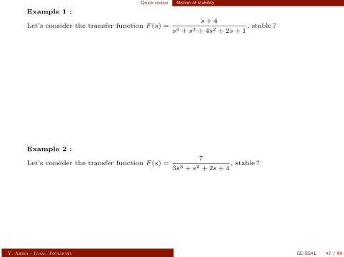
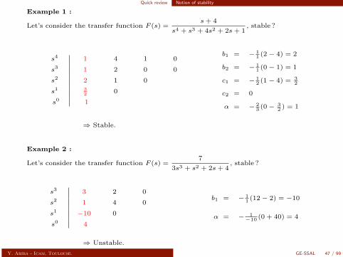
Example 1 :
Let’s consider the transfer function F (s) =s+ 4
s4 + s3 + 4s2 + 2s+ 1, stable ?
s4 1 4 1 0
s3 1 2 0 0
s2 2 1 0
s1 32 0
s0 1
b1 = − 11 (2− 4) = 2
b2 = − 11 (0− 1) = 1
c1 = − 12 (1− 4) = 3
2
c2 = 0
α = − 23 (0− 3
2 ) = 1
⇒ Stable.
Example 2 :
Let’s consider the transfer function F (s) =7
3s3 + s2 + 2s+ 4, stable ?
s3 3 2 0
s2 1 4 0
s1 −10 0
s0 4
b1 = − 11 (12− 2) = −10
α = − 1−10 (0 + 40) = 4
⇒ Unstable.
Y. Ariba - Icam, Toulouse. GE-SSAL 47 / 99
Quick review Notion of stability
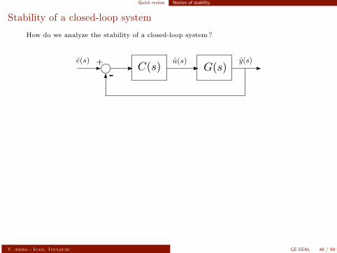
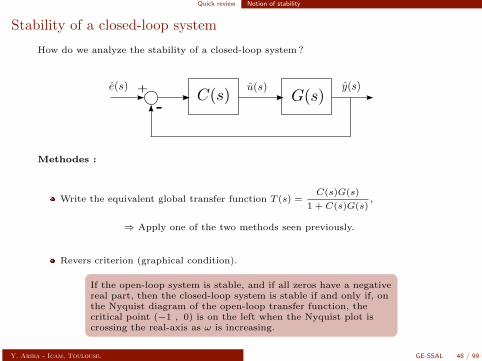
Stability of a closed-loop system
How do we analyze the stability of a closed-loop system ?
Methodes :
Write the equivalent global transfer function T (s) =C(s)G(s)
1 + C(s)G(s),
⇒ Apply one of the two methods seen previously.
Revers criterion (graphical condition).
If the open-loop system is stable, and if all zeros have a negativereal part, then the closed-loop system is stable if and only if, onthe Nyquist diagram of the open-loop transfer function, thecritical point (−1 , 0) is on the left when the Nyquist plot iscrossing the real-axis as ω is increasing.
Y. Ariba - Icam, Toulouse. GE-SSAL 48 / 99
Quick review Notion of stability
Stability of a closed-loop system
How do we analyze the stability of a closed-loop system ?
Methodes :
Write the equivalent global transfer function T (s) =C(s)G(s)
1 + C(s)G(s),
⇒ Apply one of the two methods seen previously.
Revers criterion (graphical condition).
If the open-loop system is stable, and if all zeros have a negativereal part, then the closed-loop system is stable if and only if, onthe Nyquist diagram of the open-loop transfer function, thecritical point (−1 , 0) is on the left when the Nyquist plot iscrossing the real-axis as ω is increasing.
Y. Ariba - Icam, Toulouse. GE-SSAL 48 / 99

Quick review Notion of stability
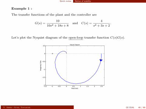
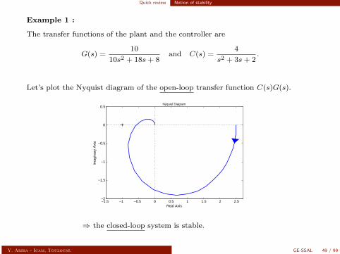
Example 1 :
The transfer functions of the plant and the controller are
G(s) =10
10s2 + 18s+ 8and C(s) =
4
s2 + 3s+ 2.
Let’s plot the Nyquist diagram of the open-loop transfer function C(s)G(s).
−1.5 −1 −0.5 0 0.5 1 1.5 2 2.5−2
−1.5
−1
−0.5
0
0.5Nyquist Diagram
Real Axis
Imag
inar
y A
xis
⇒ the closed-loop system is stable.
Y. Ariba - Icam, Toulouse. GE-SSAL 49 / 99
Quick review Notion of stability
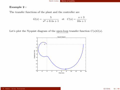
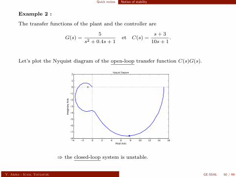
Example 2 :
The transfer functions of the plant and the controller are
G(s) =5
s2 + 0.4s+ 1et C(s) =
s+ 3
10s+ 1.
Let’s plot the Nyquist diagram of the open-loop transfer function C(s)G(s).
−4 −2 0 2 4 6 8 10 12 14 16−8
−7
−6
−5
−4
−3
−2
−1
0
1
2Nyquist Diagram
Real Axis
Imag
inar
y A
xis
⇒ the closed-loop system is unstable.
Y. Ariba - Icam, Toulouse. GE-SSAL 50 / 99
Quick review Notion of stability
Example 2 :
The transfer functions of the plant and the controller are
G(s) =5
s2 + 0.4s+ 1et C(s) =
s+ 3
10s+ 1.
Let’s plot the Nyquist diagram of the open-loop transfer function C(s)G(s).
−4 −2 0 2 4 6 8 10 12 14 16−8
−7
−6
−5
−4
−3
−2
−1
0
1
2Nyquist Diagram
Real Axis
Imag
inar
y A
xis
⇒ the closed-loop system is unstable.
Y. Ariba - Icam, Toulouse. GE-SSAL 50 / 99
Quick review Summary
Summary
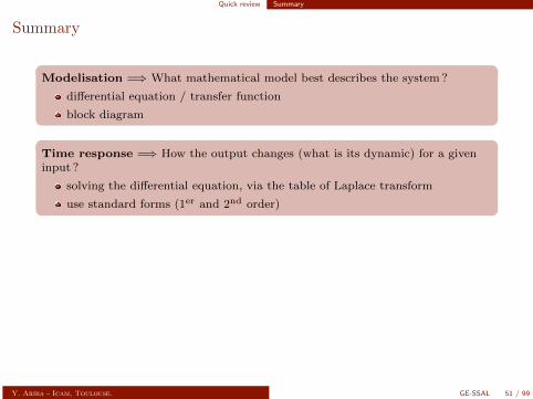
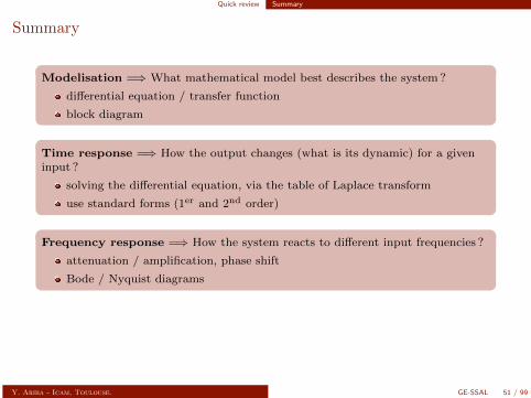
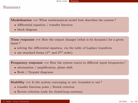
Modelisation =⇒ What mathematical model best describes the system ?
differential equation / transfer function
block diagram
Time response =⇒ How the output changes (what is its dynamic) for a giveninput ?
solving the differential equation, via the table of Laplace transform
use standard forms (1er and 2nd order)
Frequency response =⇒ How the system reacts to different input frequencies ?
attenuation / amplification, phase shift
Bode / Nyquist diagrams
Stability =⇒ Is the system converging or not, bounded or not ?
transfer function poles / Routh criterion
Revers criterion (only for closed-loop systems)
Y. Ariba - Icam, Toulouse. GE-SSAL 51 / 99
Quick review Summary
Summary
Modelisation =⇒ What mathematical model best describes the system ?
differential equation / transfer function
block diagram
Time response =⇒ How the output changes (what is its dynamic) for a giveninput ?
solving the differential equation, via the table of Laplace transform
use standard forms (1er and 2nd order)
Frequency response =⇒ How the system reacts to different input frequencies ?
attenuation / amplification, phase shift
Bode / Nyquist diagrams
Stability =⇒ Is the system converging or not, bounded or not ?
transfer function poles / Routh criterion
Revers criterion (only for closed-loop systems)
Y. Ariba - Icam, Toulouse. GE-SSAL 51 / 99
Quick review Back to our example
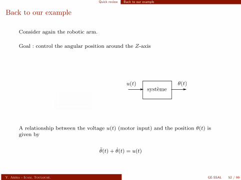
Back to our example
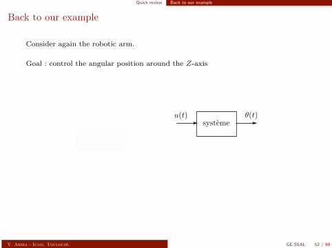
Consider again the robotic arm.
Goal : control the angular position around the Z-axis
A relationship between the voltage u(t) (motor input) and the position θ(t) isgiven by
θ(t) + θ(t) = u(t)
Y. Ariba - Icam, Toulouse. GE-SSAL 52 / 99
Quick review Back to our example
Back to our example
Consider again the robotic arm.
Goal : control the angular position around the Z-axis
A relationship between the voltage u(t) (motor input) and the position θ(t) isgiven by
θ(t) + θ(t) = u(t)
Y. Ariba - Icam, Toulouse. GE-SSAL 52 / 99

Quick review Back to our example
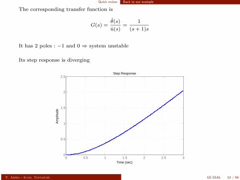
The corresponding transfer function is
G(s) =θ(s)
u(s)=
1
(s+ 1)s
It has 2 poles : −1 and 0 ⇒ system unstable
Its step response is diverging
0 0.5 1 1.5 2 2.5 30
0.5
1
1.5
2
2.5Step Response
Time (sec)
Am
plitu
de
Y. Ariba - Icam, Toulouse. GE-SSAL 53 / 99
Quick review Back to our example
The corresponding transfer function is
G(s) =θ(s)
u(s)=
1
(s+ 1)s
It has 2 poles : −1 and 0 ⇒ system unstable
Its step response is diverging
0 0.5 1 1.5 2 2.5 30
0.5
1
1.5
2
2.5Step Response
Time (sec)
Am
plitu
de
Y. Ariba - Icam, Toulouse. GE-SSAL 53 / 99
Quick review Back to our example
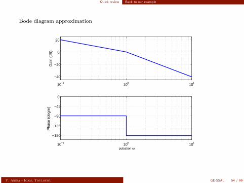
Bode diagram approximation
10−1 100 101
−40
−20
0
20
Gai
n (d
B)
10−1 100 101
−180
−135
−90
−45
0
Pha
se (
degr
e)
pulsation ω
Y. Ariba - Icam, Toulouse. GE-SSAL 54 / 99
Quick review Back to our example
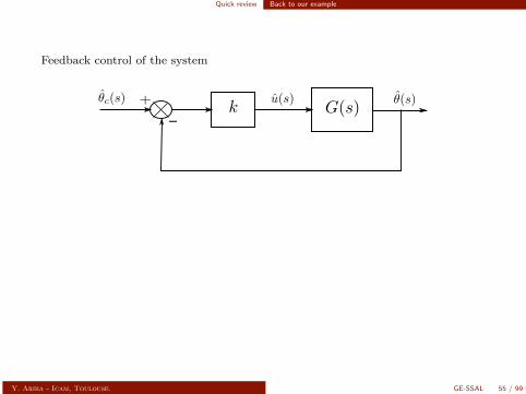
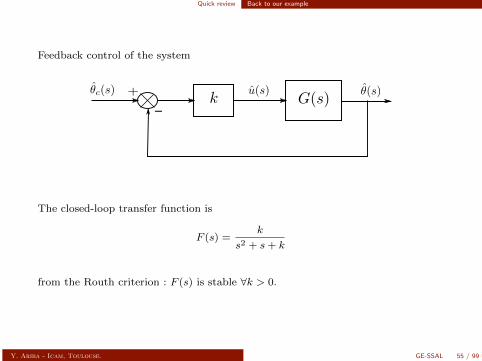
Feedback control of the system
The closed-loop transfer function is
F (s) =k
s2 + s+ k
from the Routh criterion : F (s) is stable ∀k > 0.
Y. Ariba - Icam, Toulouse. GE-SSAL 55 / 99
Quick review Back to our example
Feedback control of the system
The closed-loop transfer function is
F (s) =k
s2 + s+ k
from the Routh criterion : F (s) is stable ∀k > 0.
Y. Ariba - Icam, Toulouse. GE-SSAL 55 / 99
Quick review Back to our example
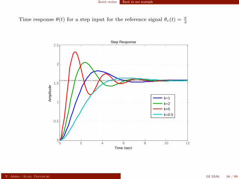
Time response θ(t) for a step input for the reference signal θc(t) = π2
0 2 4 6 8 10 120
0.5
1
1.5
2
2.5
Step Response
Time (sec)
Am
plitu
de
k=1
k=2k=5
k=0.5
Y. Ariba - Icam, Toulouse. GE-SSAL 56 / 99

Quick review Back to our example
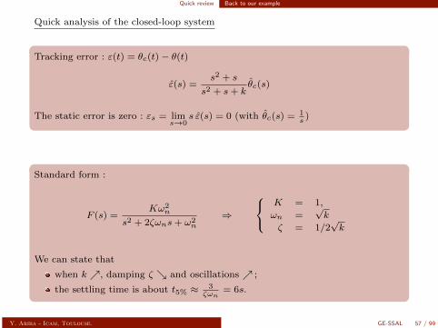
Quick analysis of the closed-loop system
Tracking error : ε(t) = θc(t)− θ(t)
ε(s) =s2 + s
s2 + s+ kθc(s)
The static error is zero : εs = lims→0
s ε(s) = 0 (with θc(s) = 1s
)
Standard form :
F (s) =Kω2
n
s2 + 2ζωns+ ω2n
⇒
K = 1,
ωn =√k
ζ = 1/2√k
We can state that
when k , damping ζ and oscillations ;
the settling time is about t5% ≈ 3ζωn
= 6s.
Y. Ariba - Icam, Toulouse. GE-SSAL 57 / 99
Quick review Back to our example
Quick analysis of the closed-loop system
Tracking error : ε(t) = θc(t)− θ(t)
ε(s) =s2 + s
s2 + s+ kθc(s)
The static error is zero : εs = lims→0
s ε(s) = 0 (with θc(s) = 1s
)
Standard form :
F (s) =Kω2
n
s2 + 2ζωns+ ω2n
⇒
K = 1,
ωn =√k
ζ = 1/2√k
We can state that
when k , damping ζ and oscillations ;
the settling time is about t5% ≈ 3ζωn
= 6s.
Y. Ariba - Icam, Toulouse. GE-SSAL 57 / 99
Performances
Contents
1 Introduction
Introductory example
What is automatic control ?2 Quick review
Modelisation
Time response
Frequency response
Notion of stability
Summary
Back to our example3 Performances
Precision
Responsiveness
Stability margins
4 Control design
Introduction
Synthese directe : modele impose
Action proportionnelle
Action integrale
Action derivee
Combinaisons d’actions
Proportionnel-Integral-Derive (PID)
Y. Ariba - Icam, Toulouse. GE-SSAL 58 / 99
Performances
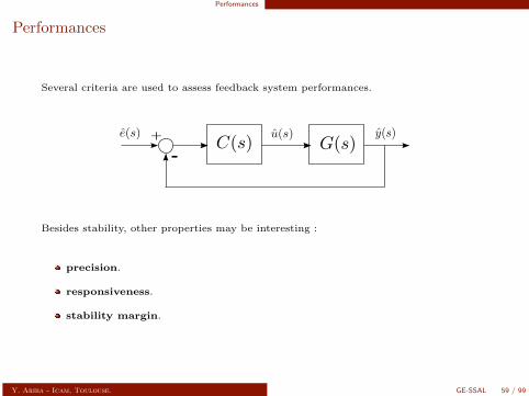
Performances
Several criteria are used to assess feedback system performances.
Besides stability, other properties may be interesting :
precision.
responsiveness.
stability margin.
Y. Ariba - Icam, Toulouse. GE-SSAL 59 / 99

Performances Precision
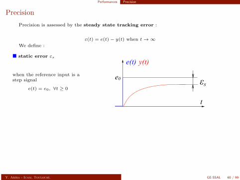
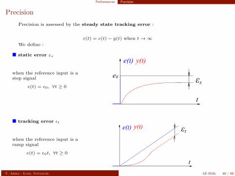
Precision
Precision is assessed by the steady state tracking error :
ε(t) = e(t)− y(t) when t→∞
We define :
static error εs
when the reference input is astep signal
e(t) = e0, ∀t ≥ 0
t
e(t)
0
e0
y(t)
εs
tracking error εt
when the reference input is aramp signal
e(t) = e0t, ∀t ≥ 0
t0
εte(t) y(t)
Y. Ariba - Icam, Toulouse. GE-SSAL 60 / 99
Performances Precision
Precision
Precision is assessed by the steady state tracking error :
ε(t) = e(t)− y(t) when t→∞We define :
static error εs
when the reference input is astep signal
e(t) = e0, ∀t ≥ 0
t
e(t)
0
e0
y(t)
εs
tracking error εt
when the reference input is aramp signal
e(t) = e0t, ∀t ≥ 0
t0
εte(t) y(t)
Y. Ariba - Icam, Toulouse. GE-SSAL 60 / 99
Performances Precision
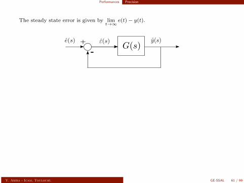
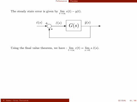
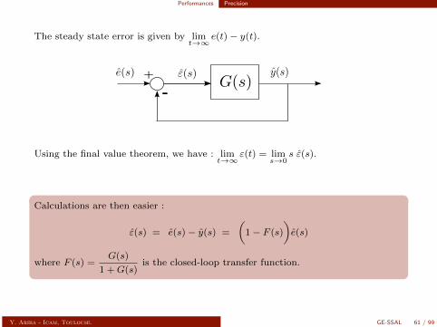
The steady state error is given by limt→∞
e(t)− y(t).
Using the final value theorem, we have : limt→∞
ε(t) = lims→0
s ε(s).
Calculations are then easier :
ε(s) = e(s)− y(s) =
(1− F (s)
)e(s)
where F (s) =G(s)
1 +G(s)is the closed-loop transfer function.
Y. Ariba - Icam, Toulouse. GE-SSAL 61 / 99
Performances Precision
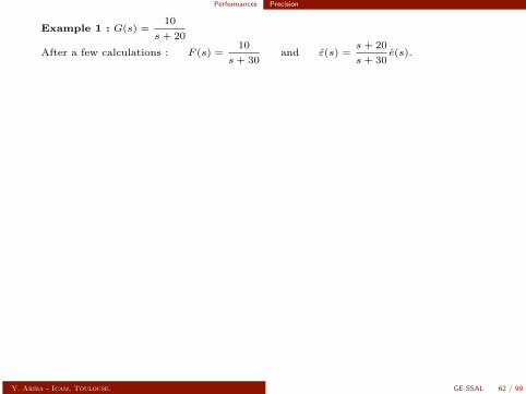
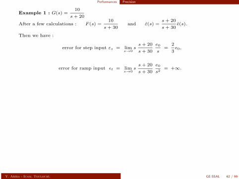
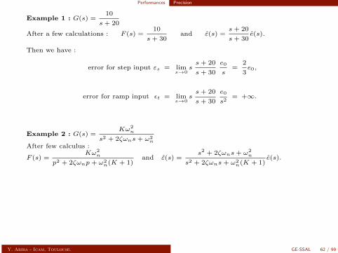
Example 1 : G(s) =10
s+ 20
After a few calculations : F (s) =10
s+ 30and ε(s) =
s+ 20
s+ 30e(s).
Then we have :
error for step input εs = lims→0
ss+ 20
s+ 30
e0
s=
2
3e0,
error for ramp input εt = lims→0
ss+ 20
s+ 30
e0
s2= +∞.
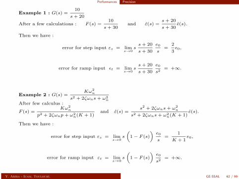
Example 2 : G(s) =Kω2
n
s2 + 2ζωns+ ω2n
After few calculus :
F (s) =Kω2
n
p2 + 2ζωnp+ ω2n(K + 1)
and ε(s) =s2 + 2ζωns+ ω2
n
s2 + 2ζωns+ ω2n(K + 1)
e(s).
Then we have :
error for step input εs = lims→0
s
(1− F (s)
)e0
s=
1
K + 1e0,
error for ramp input εt = lims→0
s
(1− F (s)
)e0
s2= +∞.
Y. Ariba - Icam, Toulouse. GE-SSAL 62 / 99
Performances Precision
Example 1 : G(s) =10
s+ 20
After a few calculations : F (s) =10
s+ 30and ε(s) =
s+ 20
s+ 30e(s).
Then we have :
error for step input εs = lims→0
ss+ 20
s+ 30
e0
s=
2
3e0,
error for ramp input εt = lims→0
ss+ 20
s+ 30
e0
s2= +∞.
Example 2 : G(s) =Kω2
n
s2 + 2ζωns+ ω2n
After few calculus :
F (s) =Kω2
n
p2 + 2ζωnp+ ω2n(K + 1)
and ε(s) =s2 + 2ζωns+ ω2
n
s2 + 2ζωns+ ω2n(K + 1)
e(s).
Then we have :
error for step input εs = lims→0
s
(1− F (s)
)e0
s=
1
K + 1e0,
error for ramp input εt = lims→0
s
(1− F (s)
)e0
s2= +∞.
Y. Ariba - Icam, Toulouse. GE-SSAL 62 / 99
Performances Precision
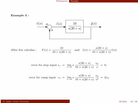
Example 3 :
After few calculus : F (s) =10
10 + s(20 + s)and ε(s) =
s(20 + s)
10 + s(20 + s)e(s).
error for step input εs = lims→0
ss(20 + s)
10 + s(20 + s)
e0
s= 0,
error for ramp input εt = lims→0
ss(20 + s)
10 + s(20 + s)
e0
s2= 2e0.
Y. Ariba - Icam, Toulouse. GE-SSAL 63 / 99
Performances Responsiveness
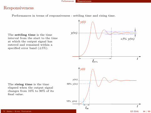
Responsiveness
Performances in terms of responsiveness : settling time and rising time.
The settling time is the timeinterval from the start to the timeat which the output signal hasentered and remained within aspecified error band (±5%).
t
y(t)
y(∞)
±5% y(∞)
tr5%
The rising time is the timeelapsed when the output signalchanges from 10% to 90% of itsfinal value.
t
y(t)
y(∞)90% y(∞)
10% y(∞)
tmY. Ariba - Icam, Toulouse. GE-SSAL 64 / 99

Performances Stability margins
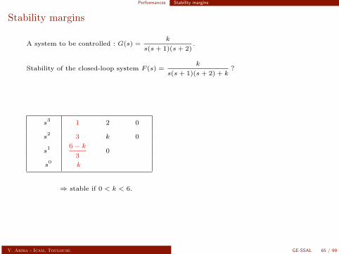
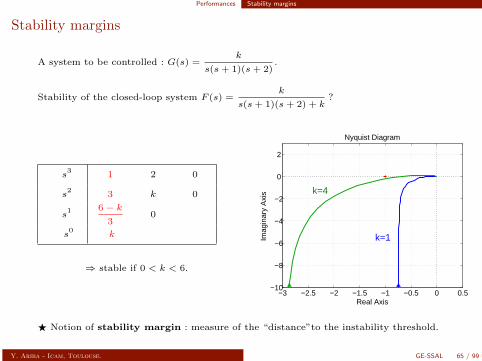
Stability margins
A system to be controlled : G(s) =k
s(s+ 1)(s+ 2).
Stability of the closed-loop system F (s) =k
s(s+ 1)(s+ 2) + k?
s3
1 2 0
s2
3 k 0
s1 6− k
30
s0
k
⇒ stable if 0 < k < 6.
−3 −2.5 −2 −1.5 −1 −0.5 0 0.5−10
−8
−6
−4
−2
0
2
Nyquist Diagram
Real Axis
Imag
inar
y A
xis
k=1
k=4
F Notion of stability margin : measure of the “distance”to the instability threshold.
Y. Ariba - Icam, Toulouse. GE-SSAL 65 / 99
Performances Stability margins
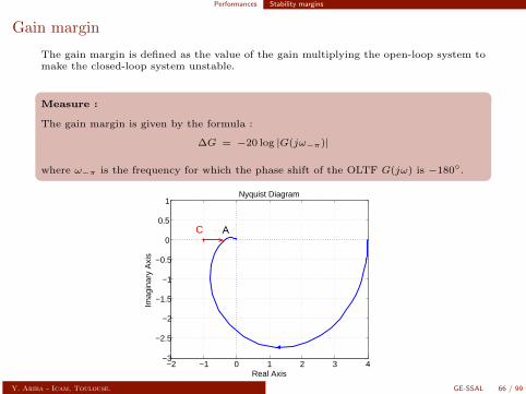
Gain margin
The gain margin is defined as the value of the gain multiplying the open-loop system tomake the closed-loop system unstable.
Measure :
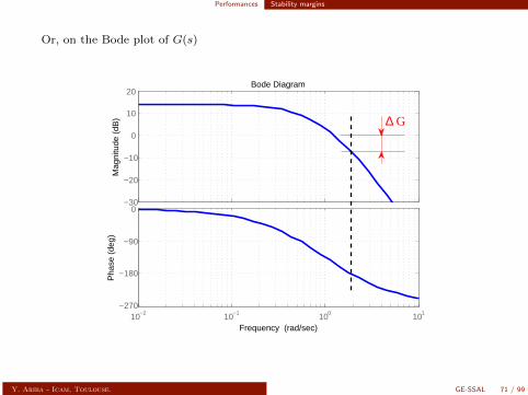
The gain margin is given by the formula :
∆G = −20 log |G(jω−π)|
where ω−π is the frequency for which the phase shift of the OLTF G(jω) is −180.
−2 −1 0 1 2 3 4−3
−2.5
−2
−1.5
−1
−0.5
0
0.5
1Nyquist Diagram
Real Axis
Imag
inar
y A
xis
AC
Y. Ariba - Icam, Toulouse. GE-SSAL 66 / 99
Performances Stability margins
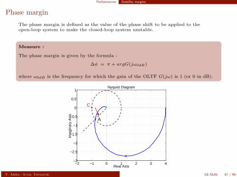
Phase margin
The phase margin is defined as the value of the phase shift to be applied to theopen-loop system to make the closed-loop system unstable.
Measure :
The phase margin is given by the formula :
∆φ = π + argG(jω0dB)
where ω0dB is the frequency for which the gain of the OLTF G(jω) is 1 (or 0 in dB).
−2 −1 0 1 2 3 4−3
−2.5
−2
−1.5
−1
−0.5
0
0.5
1Nyquist Diagram
Real Axis
Imag
inar
y A
xis
C
A
Y. Ariba - Icam, Toulouse. GE-SSAL 67 / 99
Performances Stability margins
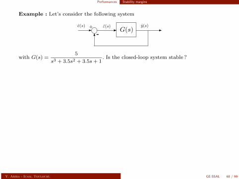
Example : Let’s consider the following system
with G(s) =5
s3 + 3.5s2 + 3.5s+ 1. Is the closed-loop system stable ?
−2 −1 0 1 2 3 4 5 6−4
−3.5
−3
−2.5
−2
−1.5
−1
−0.5
0
0.5
1
1.5Nyquist Diagram
Real Axis
Imag
inar
y A
xis
⇒ Invoking the Revers criteria : the feedback system is stable
Y. Ariba - Icam, Toulouse. GE-SSAL 68 / 99
Performances Stability margins
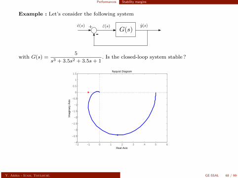
Example : Let’s consider the following system
with G(s) =5
s3 + 3.5s2 + 3.5s+ 1. Is the closed-loop system stable ?
−2 −1 0 1 2 3 4 5 6−4
−3.5
−3
−2.5
−2
−1.5
−1
−0.5
0
0.5
1
1.5Nyquist Diagram
Real Axis
Imag
inar
y A
xis
⇒ Invoking the Revers criteria : the feedback system is stable
Y. Ariba - Icam, Toulouse. GE-SSAL 68 / 99
Performances Stability margins
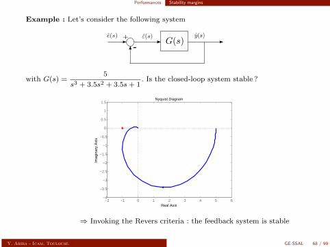
Example : Let’s consider the following system
with G(s) =5
s3 + 3.5s2 + 3.5s+ 1. Is the closed-loop system stable ?
−2 −1 0 1 2 3 4 5 6−4
−3.5
−3
−2.5
−2
−1.5
−1
−0.5
0
0.5
1
1.5Nyquist Diagram
Real Axis
Imag
inar
y A
xis
⇒ Invoking the Revers criteria : the feedback system is stable
Y. Ariba - Icam, Toulouse. GE-SSAL 68 / 99

Performances Stability margins
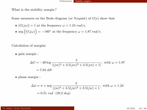
What is the stability margin ?
Some measures on the Bode diagram (or Nyquist) of G(s) show that
|G(jω)| = 1 at the frequency ω = 1.24 rad/s,
arg(G(jω)
)= −180 at the frequency ω = 1.87 rad/s.
Calculation of margins
gain margin :
∆G = −20 log5
|(jw)3 + 3.5(jw)2 + 3.5(jw) + 1|, with ω = 1.87
= 7.04 dB
phase margin :
∆φ = π + arg5
(jw)3 + 3.5(jw)2 + 3.5(jw) + 1, with ω = 1.24
= 0.51 rad (29.2 deg)
Y. Ariba - Icam, Toulouse. GE-SSAL 69 / 99
Performances Stability margins
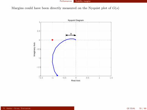
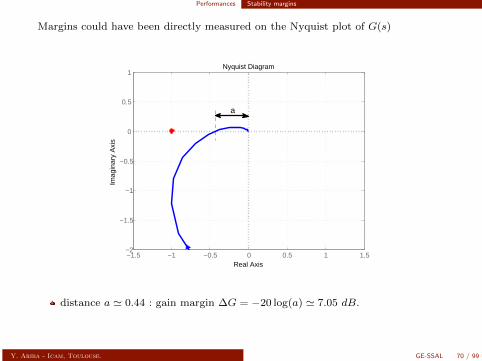
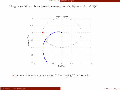
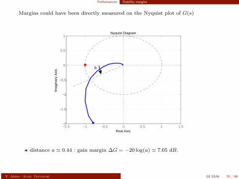
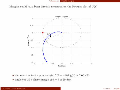
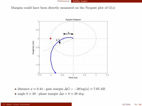
Margins could have been directly measured on the Nyquist plot of G(s)
−1.5 −1 −0.5 0 0.5 1 1.5−2
−1.5
−1
−0.5
0
0.5
1Nyquist Diagram
Real Axis
Imag
inar
y A
xis
a
distance a ' 0.44 : gain margin ∆G = −20 log(a) ' 7.05 dB.
angle b ' 29 : phase margin ∆φ = b ' 29 deg.
Y. Ariba - Icam, Toulouse. GE-SSAL 70 / 99
Performances Stability margins
Margins could have been directly measured on the Nyquist plot of G(s)
−1.5 −1 −0.5 0 0.5 1 1.5−2
−1.5
−1
−0.5
0
0.5
1Nyquist Diagram
Real Axis
Imag
inar
y A
xis
distance a ' 0.44 : gain margin ∆G = −20 log(a) ' 7.05 dB.
angle b ' 29 : phase margin ∆φ = b ' 29 deg.
Y. Ariba - Icam, Toulouse. GE-SSAL 70 / 99
Performances Stability margins
Margins could have been directly measured on the Nyquist plot of G(s)
−1.5 −1 −0.5 0 0.5 1 1.5−2
−1.5
−1
−0.5
0
0.5
1Nyquist Diagram
Real Axis
Imag
inar
y A
xis b
distance a ' 0.44 : gain margin ∆G = −20 log(a) ' 7.05 dB.
angle b ' 29 : phase margin ∆φ = b ' 29 deg.
Y. Ariba - Icam, Toulouse. GE-SSAL 70 / 99
Performances Stability margins
Margins could have been directly measured on the Nyquist plot of G(s)
−1.5 −1 −0.5 0 0.5 1 1.5−2
−1.5
−1
−0.5
0
0.5
1Nyquist Diagram
Real Axis
Imag
inar
y A
xis
a
b
distance a ' 0.44 : gain margin ∆G = −20 log(a) ' 7.05 dB.
angle b ' 29 : phase margin ∆φ = b ' 29 deg.
Y. Ariba - Icam, Toulouse. GE-SSAL 70 / 99
Performances Stability margins
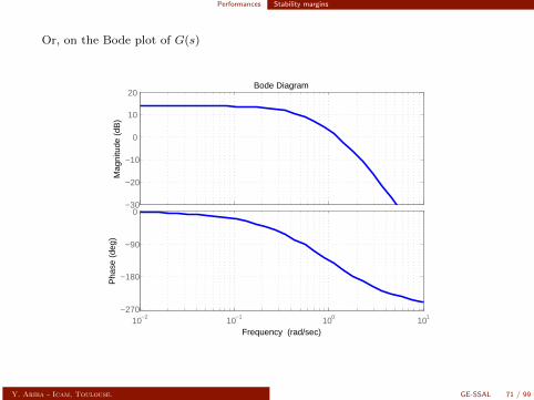
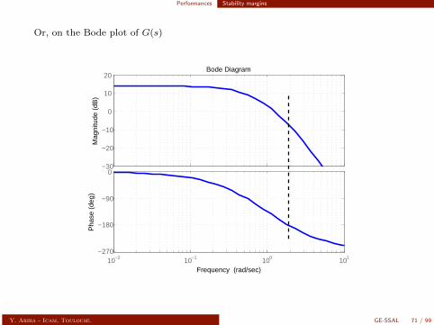
Or, on the Bode plot of G(s)
−30
−20
−10
0
10
20
Mag
nitu
de (
dB)
10−2 10−1 100 101−270
−180
−90
0
Pha
se (
deg)
Bode Diagram
Frequency (rad/sec)
Y. Ariba - Icam, Toulouse. GE-SSAL 71 / 99
Performances Stability margins
Or, on the Bode plot of G(s)
−30
−20
−10
0
10
20
Mag
nitu
de (
dB)
10−2 10−1 100 101−270
−180
−90
0
Pha
se (
deg)
Bode Diagram
Frequency (rad/sec)
Y. Ariba - Icam, Toulouse. GE-SSAL 71 / 99
Performances Stability margins
Or, on the Bode plot of G(s)
−30
−20
−10
0
10
20
Mag
nitu
de (
dB)
10−2 10−1 100 101−270
−180
−90
0
Pha
se (
deg)
Bode Diagram
Frequency (rad/sec)
∆ G
Y. Ariba - Icam, Toulouse. GE-SSAL 71 / 99

Performances Stability margins
Or, on the Bode plot of G(s)
−30
−20
−10
0
10
20
Mag
nitu
de (
dB)
10−2 10−1 100 101−270
−180
−90
0
Pha
se (
deg)
Bode Diagram
Frequency (rad/sec)
Y. Ariba - Icam, Toulouse. GE-SSAL 71 / 99
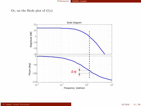
Performances Stability margins
Or, on the Bode plot of G(s)
−30
−20
−10
0
10
20
Mag
nitu
de (
dB)
10−2 10−1 100 101−270
−180
−90
0
Pha
se (
deg)
Bode Diagram
Frequency (rad/sec)
∆ φ
Y. Ariba - Icam, Toulouse. GE-SSAL 71 / 99
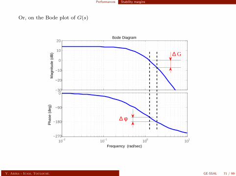
Performances Stability margins
Or, on the Bode plot of G(s)
−30
−20
−10
0
10
20
Mag
nitu
de (
dB)
10−2 10−1 100 101−270
−180
−90
0
Pha
se (
deg)
Bode Diagram
Frequency (rad/sec)
∆ φ
∆ G
Y. Ariba - Icam, Toulouse. GE-SSAL 71 / 99

Control design
Contents
1 Introduction
Introductory example
What is automatic control ?2 Quick review
Modelisation
Time response
Frequency response
Notion of stability
Summary
Back to our example3 Performances
Precision
Responsiveness
Stability margins
4 Control design
Introduction
Synthese directe : modele impose
Action proportionnelle
Action integrale
Action derivee
Combinaisons d’actions
Proportionnel-Integral-Derive (PID)
Y. Ariba - Icam, Toulouse. GE-SSAL 72 / 99
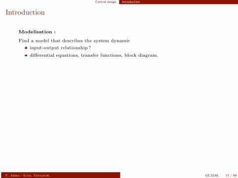
Control design Introduction
Introduction
Modelisation :
Find a model that describes the system dynamic
input-output relationship ?
differential equations, transfer functions, block diagram.
Analysis :
Analyze the properties of the model and performances (open or closed loop).
time and frequency responses
stability
performance analysis of a feedback system for a given controller
⇒ what you have seen so far.
Y. Ariba - Icam, Toulouse. GE-SSAL 73 / 99
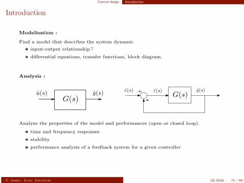
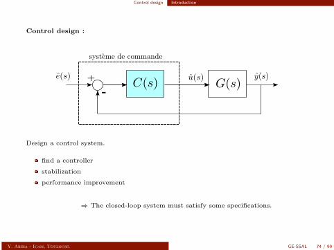
Control design Introduction
Control design :
Design a control system.
find a controller
stabilization
performance improvement
⇒ The closed-loop system must satisfy some specifications.
Y. Ariba - Icam, Toulouse. GE-SSAL 74 / 99

Control design Introduction
A control system is designed to control/improve/ensure :
the feedback system stability,
the responsiveness (transient regime),
precision at the steady state,
robustness (stability margin, disturbance sensitivity).
In this class, only classical frequency based methods will be considered. Widely used inindustries because of
their practical aspect,
easy to design and often based on experience,
sometimes parameters can be tuned in an intuitive way.
Y. Ariba - Icam, Toulouse. GE-SSAL 75 / 99
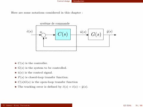
Control design Introduction
Here are some notations considered in this chapter :
C(s) is the controller.
G(s) is the system to be controlled.
u(s) is the control signal.
F (s) is closed-loop transfer function.
C(s)G(s) is the open-loop transfer function
The tracking error is defined by ε(s) = e(s)− y(s).
Y. Ariba - Icam, Toulouse. GE-SSAL 76 / 99
Control design Synthese directe : modele impose
Synthese directe : modele impose
Une 1iere methode directe et pratique consiste a imposer un modele pour la FTBF.
Qu’est-ce qu’un modele “ideal” ?
pour un premier ordre : Fd(s) =1
τs+ 1
0
0.2
0.4
0.6
0.8
1
Step Response
Time (sec)
Am
plitu
de
τ
63%
la constante de temps τ definit la rapidite : tr5% = 3τ
Y. Ariba - Icam, Toulouse. GE-SSAL 77 / 99
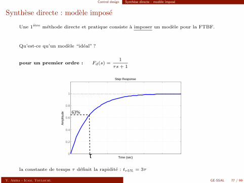
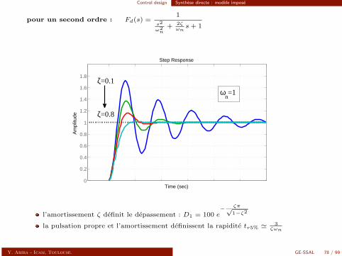
Control design Synthese directe : modele impose
pour un second ordre : Fd(s) =1
s2
ω2n
+ 2ζωns+ 1
0
0.2
0.4
0.6
0.8
1
1.2
1.4
1.6
1.8
Step Response
Time (sec)
Am
plitu
de ζ=0.8
ζ=0.1
ωn=1
l’amortissement ζ definit le depassement : D1 = 100 e− ζπ√
1−ζ2
la pulsation propre et l’amortissement definissent la rapidite tr5% ' 3ζωn
Y. Ariba - Icam, Toulouse. GE-SSAL 78 / 99
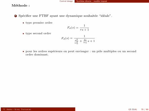
Control design Synthese directe : modele impose
Methode :
1 Specifier une FTBF ayant une dynamique souhaitee “ideale”.
type premier ordre
Fd(s) =1
τs+ 1
type second ordre
Fd(s) =1
s2
ω2n
+ 2ζωns+ 1
pour les ordres superieurs on peut envisager : un pole multiples ou un secondordre dominant.
2 En identifiant la FTBF avec la fonction desiree, calculer le correcteur :
Fd(p) = F (p) ⇒ Fd(p) =C(p)G(p)
1 + C(p)G(p)
⇒ C(p) =Fd(p)
G(p)(
1− Fd(p))
Y. Ariba - Icam, Toulouse. GE-SSAL 79 / 99
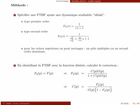
Control design Synthese directe : modele impose
3 Le correcteur doit etre propre pour etre realisable.(ordre numerateur ≤ ordre denominateur)
4 Une phase de simulation est necessaire pour valider le fonctionnement(comportement attendu, pas de saturation...).
Remarques :
L’approche est valide seulement si le modele du systeme est bien connu.
Le systeme a commander doit posseder des poles et zeros stables.
L’approche est adaptee plutot pour des systemes d’ordre faible.
Y. Ariba - Icam, Toulouse. GE-SSAL 80 / 99
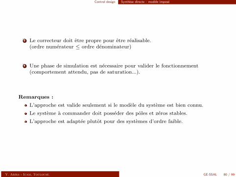
Control design Synthese directe : modele impose
ExempleSoit le systeme a commander de fonction de transfert :
G(s) =6
s2 + 2s+ 8.
Simulons sa reponse indicielle :
Step Response
Time (sec)
Am
plitu
de
0 1 2 3 4 5 60
0.2
0.4
0.6
0.8
1
1.2
Depassement = 30% ; temps de reponse a 5% = 2.78s ; erreur de position = 25%.
Y. Ariba - Icam, Toulouse. GE-SSAL 81 / 99
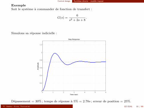
Control design Synthese directe : modele impose
Choisissons un modele de reference du second ordre :
Fd(s) =1
s2
ω2n
+ 2ζωns+ 1
.
L’amortissement ζ est fixe a 0.8 de sorte que le depassement soit inferieur a2%.
La pulsation propre ωn est fixee a 1.87 de sorte que le temps de reponse soitde l’ordre de 2s.(formule approximative : tr5% ' 3
ζωn)
La FTBF desiree s’ecrit donc :
Fd(s) =1
0.284s2 + 0.853s+ 1.
Enfin, nous pouvons en deduire le correcteur :
C(s) =s2 + 2s+ 86ω2ns2 + 12ζ
ωns
=s2 + 2s+ 8
1.707s2 + 5.12s
Y. Ariba - Icam, Toulouse. GE-SSAL 82 / 99
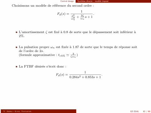
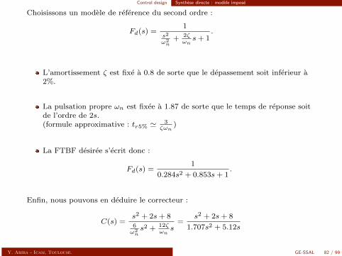
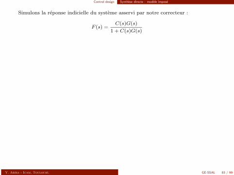
Control design Synthese directe : modele impose
Simulons la reponse indicielle du systeme asservi par notre correcteur :
F (s) =C(s)G(s)
1 + C(s)G(s)
Step Response
Time (sec)
Am
plitu
de
0 1 2 3 4 5 60
0.2
0.4
0.6
0.8
1
1.2
Depassement = 1.51% ; temps de reponse a 5% = 1.81s ; erreur de position = 0%.
Y. Ariba - Icam, Toulouse. GE-SSAL 83 / 99
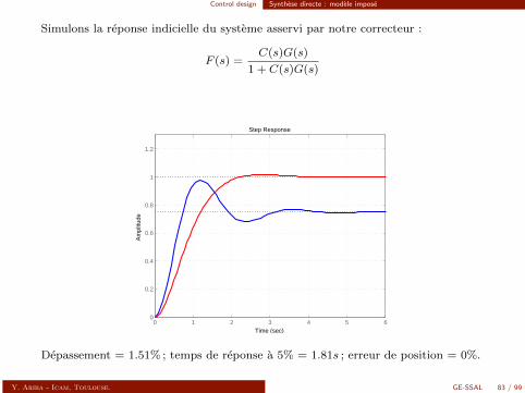
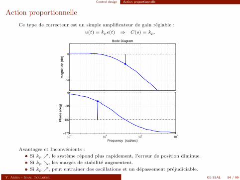
Control design Action proportionnelle
Action proportionnelle
Ce type de correcteur est un simple amplificateur de gain reglable :
u(t) = kpε(t) ⇒ C(s) = kp.
10−1
100
101
102
−270
−180
−90
0
Pha
se (
deg)
Bode Diagram
Frequency (rad/sec)
−50
0
Mag
nitu
de (
dB)
Avantages et Inconvenients :
Si kp , le systeme repond plus rapidement, l’erreur de position diminue.
Si kp , les marges de stabilite augmentent.
Si kp , peut entrainer des oscillations et un depassement prejudiciable.
Y. Ariba - Icam, Toulouse. GE-SSAL 84 / 99
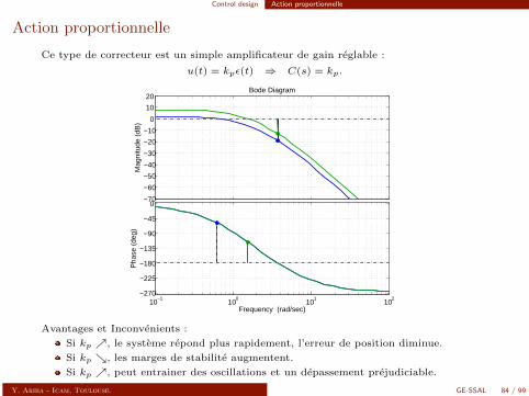
Control design Action proportionnelle
Action proportionnelle
Ce type de correcteur est un simple amplificateur de gain reglable :
u(t) = kpε(t) ⇒ C(s) = kp.
10−1
100
101
102
−270
−225
−180
−135
−90
−45
0
Pha
se (
deg)
Bode Diagram
Frequency (rad/sec)
−70
−60
−50
−40
−30
−20
−10
0
10
20
Mag
nitu
de (
dB)
Avantages et Inconvenients :
Si kp , le systeme repond plus rapidement, l’erreur de position diminue.
Si kp , les marges de stabilite augmentent.
Si kp , peut entrainer des oscillations et un depassement prejudiciable.
Y. Ariba - Icam, Toulouse. GE-SSAL 84 / 99
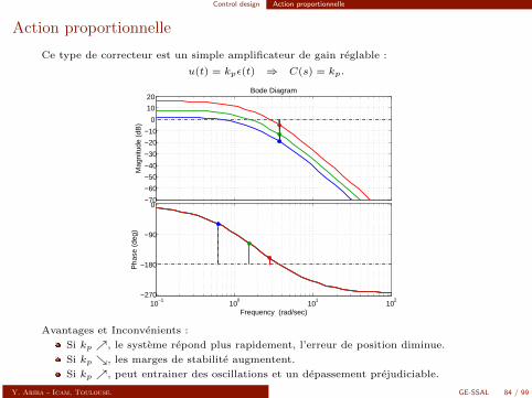
Control design Action proportionnelle
Action proportionnelle
Ce type de correcteur est un simple amplificateur de gain reglable :
u(t) = kpε(t) ⇒ C(s) = kp.
Bode Diagram
Frequency (rad/sec)
−70
−60
−50
−40
−30
−20
−10
0
10
20
Mag
nitu
de (
dB)
10−1
100
101
102
−270
−180
−90
0
Pha
se (
deg)
Avantages et Inconvenients :
Si kp , le systeme repond plus rapidement, l’erreur de position diminue.
Si kp , les marges de stabilite augmentent.
Si kp , peut entrainer des oscillations et un depassement prejudiciable.
Y. Ariba - Icam, Toulouse. GE-SSAL 84 / 99
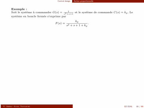
Control design Action proportionnelle
Exemple :Soit le systeme a commander G(s) = 1
s2+s+1et le systeme de commande C(s) = kp. Le
systeme en boucle fermee s’exprime par
F (s) =kp
s2 + s+ 1 + kp.
schema de gauche : bode de la BO ; schema de droite : reponse indicielle de la BF.
−80
−60
−40
−20
0
20
Mag
nitu
de (
dB)
Bode Diagram
Frequency (rad/sec)10−2
10−1
100
101
102
−180
−135
−90
−45
0
Pha
se (
deg)
kp=0.5
0 2 4 6 8 10 120
0.2
0.4
0.6
0.8
1
1.2
Step Response
Time (sec)
Am
plitu
de
kp=0.5
Y. Ariba - Icam, Toulouse. GE-SSAL 85 / 99
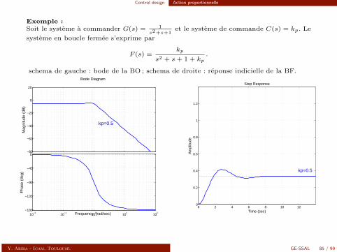
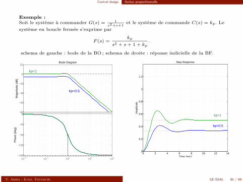
Control design Action proportionnelle
Exemple :Soit le systeme a commander G(s) = 1
s2+s+1et le systeme de commande C(s) = kp. Le
systeme en boucle fermee s’exprime par
F (s) =kp
s2 + s+ 1 + kp.
schema de gauche : bode de la BO ; schema de droite : reponse indicielle de la BF.
−80
−60
−40
−20
0
20
Mag
nitu
de (
dB)
10−2
10−1
100
101
102
−180
−135
−90
−45
0
Pha
se (
deg)
Bode Diagram
Frequency (rad/sec)
kp=1
kp=0.5
0 2 4 6 8 10 12 140
0.2
0.4
0.6
0.8
1
1.2
Step Response
Time (sec)
Am
plitu
de
kp=0.5
kp=1
Y. Ariba - Icam, Toulouse. GE-SSAL 85 / 99
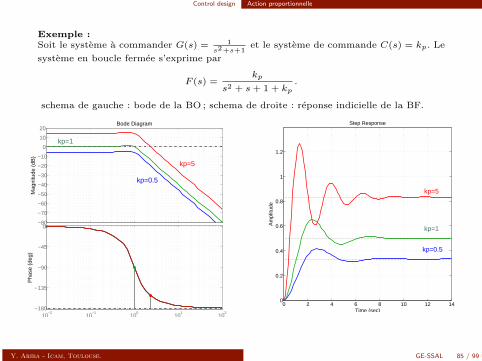
Control design Action proportionnelle
Exemple :Soit le systeme a commander G(s) = 1
s2+s+1et le systeme de commande C(s) = kp. Le
systeme en boucle fermee s’exprime par
F (s) =kp
s2 + s+ 1 + kp.
schema de gauche : bode de la BO ; schema de droite : reponse indicielle de la BF.
−80
−70
−60
−50
−40
−30
−20
−10
0
10
20
Mag
nitu
de (
dB)
Bode Diagram
Frequency (rad/sec)10
−210
−110
010
110
2−180
−135
−90
−45
0
Pha
se (
deg)
kp=1
kp=0.5
kp=5
0 2 4 6 8 10 12 140
0.2
0.4
0.6
0.8
1
1.2
Step Response
Time (sec)
Am
plitu
de
kp=1
kp=0.5
kp=5
Y. Ariba - Icam, Toulouse. GE-SSAL 85 / 99
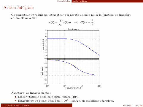
Control design Action integrale
Action integrale
Ce correcteur introduit un integrateur qui ajoute un pole nul a la fonction de transferten boucle ouverte :
u(t) =
∫ t
0
ε(t)dt ⇒ C(s) =1
s.
−60
−50
−40
−30
−20
−10
0
10
20
30
Mag
nitu
de (
dB)
Bode Diagram
Frequency (rad/sec)10
−110
010
110
2−270
−225
−180
−135
−90
−45
0
Pha
se (
deg)
Avantages et Inconvenients :
Erreur statique nulle en boucle fermee (BF),
Diagramme de phase decale de −90 : marges de stabilites degradees,
Peut provoquer des oscillations et du depassement.Y. Ariba - Icam, Toulouse. GE-SSAL 86 / 99
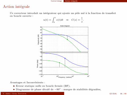
Control design Action integrale
Exemple :Soit le systeme a commander G(s) = 0.8
s2+s+1et le systeme de commande C(s) = 1/s.
Le systeme en boucle fermee s’exprime par
F (p) =0.8
s3 + s2 + s+ 0.8.
F est un ordre 3 : la marge de gain est finie,Courbe plus proche du point critique : marges degradees, oscillations et depassement,Pas d’erreur statique. schema de gauche : bode de la BO ; schema de droite : reponseindicielle de la BF.
−80
−60
−40
−20
0
20
40
Mag
nitu
de (
dB)
10−2
10−1
100
101
102
−270
−225
−180
−135
−90
−45
0
Pha
se (
deg)
Bode Diagram
Frequency (rad/sec)0 10 20 30 40 50 60 70
0
0.2
0.4
0.6
0.8
1
1.2
1.4
1.6Step Response
Time (sec)
Am
plitu
de
Y. Ariba - Icam, Toulouse. GE-SSAL 87 / 99
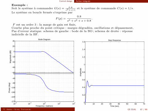
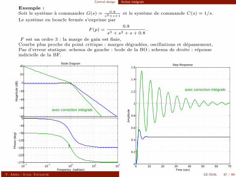
Control design Action integrale
Exemple :Soit le systeme a commander G(s) = 0.8
s2+s+1et le systeme de commande C(s) = 1/s.
Le systeme en boucle fermee s’exprime par
F (p) =0.8
s3 + s2 + s+ 0.8.
F est un ordre 3 : la marge de gain est finie,Courbe plus proche du point critique : marges degradees, oscillations et depassement,Pas d’erreur statique. schema de gauche : bode de la BO ; schema de droite : reponseindicielle de la BF.
−80
−60
−40
−20
0
20
40
Mag
nitu
de (
dB)
10−2
10−1
100
101
102
−270
−225
−180
−135
−90
−45
0
Pha
se (
deg)
Bode Diagram
Frequency (rad/sec)
avec correction intégrale
0 10 20 30 40 50 60 700
0.2
0.4
0.6
0.8
1
1.2
1.4
1.6Step Response
Time (sec)
Am
plitu
de
avec correction intégrale
Y. Ariba - Icam, Toulouse. GE-SSAL 87 / 99
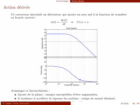
Control design Action derivee
Action derivee
Ce correcteur introduit un derivateur qui ajoute un zero nul a la fonction de transferten boucle ouverte :
u(t) =dε(t)
dt⇒ C(s) = s.
−50
−40
−30
−20
−10
0
10
20
30
40
Mag
nitu
de (
dB)
10−2
10−1
100
101
102
−180
−135
−90
−45
0
45
90
Pha
se (
deg)
Bode Diagram
Frequency (rad/sec)
Avantages et Inconvenients :
Ajoute de la phase : marges susceptibles d’etre augmentees,
A tendance a accelerer la reponse du systeme : temps de monte diminue,
Le gain statique est diminue : precision degradee.Y. Ariba - Icam, Toulouse. GE-SSAL 88 / 99
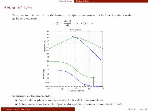
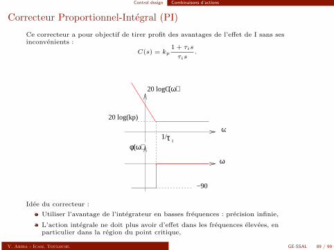
Control design Combinaisons d’actions
Correcteur Proportionnel-Integral (PI)
Ce correcteur a pour objectif de tirer profit des avantages de l’effet de I sans sesinconvenients :
C(s) = kp1 + τis
τis.
1/ω
ω
φ(ω)
20 log(kp)
τ i
20 logC(ω)
−90
Idee du correcteur :
Utiliser l’avantage de l’integrateur en basses frequences : precision infinie,
L’action integrale ne doit plus avoir d’effet dans les frequences elevees, enparticulier dans la region du point critique,
Y. Ariba - Icam, Toulouse. GE-SSAL 89 / 99
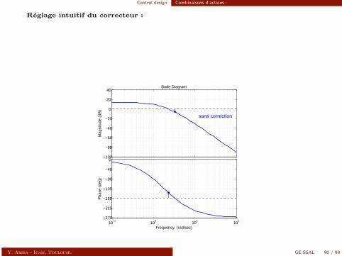
Control design Combinaisons d’actions
Reglage intuitif du correcteur :
Ajuster le gain proportionnel en fonction de l’objectif et des caracteristiques dusysteme avant correction :
le diminuer pour augmenter les marges de stabilite,l’augmenter pour ameliorer la rapidite du systeme.
Ensuite, la partie I est ajoutee en reglant le zero 1/τi de facon a ce que lacorrection ne se fasse qu’en basses frequences.
−100
−80
−60
−40
−20
0
20
40
Mag
nitu
de (
dB)
10−1
100
101
102
−270
−225
−180
−135
−90
−45
0
Pha
se (
deg)
Bode Diagram
Frequency (rad/sec)
sans correction
Y. Ariba - Icam, Toulouse. GE-SSAL 90 / 99
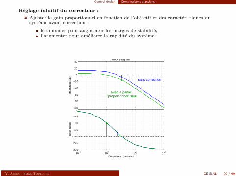
Control design Combinaisons d’actions
Reglage intuitif du correcteur :
Ajuster le gain proportionnel en fonction de l’objectif et des caracteristiques dusysteme avant correction :
le diminuer pour augmenter les marges de stabilite,l’augmenter pour ameliorer la rapidite du systeme.
Ensuite, la partie I est ajoutee en reglant le zero 1/τi de facon a ce que lacorrection ne se fasse qu’en basses frequences.
−100
−80
−60
−40
−20
0
20
40
Mag
nitu
de (
dB)
Bode Diagram
Frequency (rad/sec)10
−110
010
110
2−270
−225
−180
−135
−90
−45
0
Pha
se (
deg)
sans correction
avec la partie"proportionnel" seul
Y. Ariba - Icam, Toulouse. GE-SSAL 90 / 99
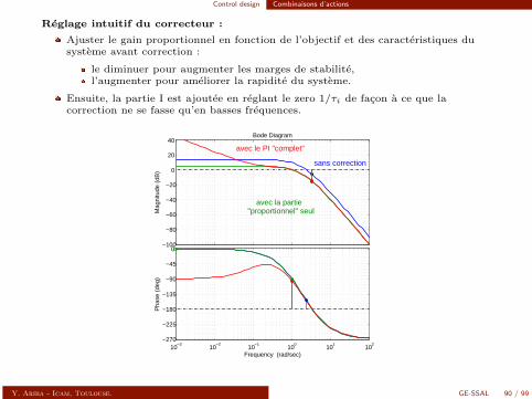
Control design Combinaisons d’actions
Reglage intuitif du correcteur :
Ajuster le gain proportionnel en fonction de l’objectif et des caracteristiques dusysteme avant correction :
le diminuer pour augmenter les marges de stabilite,l’augmenter pour ameliorer la rapidite du systeme.
Ensuite, la partie I est ajoutee en reglant le zero 1/τi de facon a ce que lacorrection ne se fasse qu’en basses frequences.
−100
−80
−60
−40
−20
0
20
40
Mag
nitu
de (
dB)
Bode Diagram
Frequency (rad/sec)10
−310
−210
−110
010
110
2−270
−225
−180
−135
−90
−45
0
Pha
se (
deg)
avec le PI "complet"
sans correction
avec la partie"proportionnel" seul
Y. Ariba - Icam, Toulouse. GE-SSAL 90 / 99
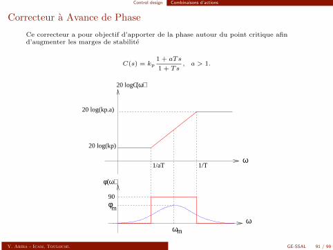
Control design Combinaisons d’actions
Correcteur a Avance de Phase
Ce correcteur a pour objectif d’apporter de la phase autour du point critique afind’augmenter les marges de stabilite
C(s) = kp1 + aTs
1 + Ts, a > 1.
ω
φ(ω)
20 logC(ω)
1/aT 1/T
20 log(kp)
20 log(kp.a)
90
mφ
ωm
ω
Y. Ariba - Icam, Toulouse. GE-SSAL 91 / 99

Control design Combinaisons d’actions
Le principe repose sur le reglage de a et T tels que le correcteur apporte de la phase(plage [ 1
aT ,1T ]) autour du point critique.
Methode de reglage du correcteur :
Regler le gain kp pour ajuster la precision ou la rapidite ou les marges.
Mesurer la marge de phase (apres la correction prop. kp) et en deduire la quantitede phase necessaire
φm = ∆φdesiree −∆φ.
A partir de φm, a peut etre calcule
a =1 + sinφm
1− sinφm
Enfin, nous avons la relation
ωm =1
T√a,
il s’agit alors de calculer T tel que ωm coıncide avec ω0db (apres correction prop.) :
T =1
ω0db√a.
Y. Ariba - Icam, Toulouse. GE-SSAL 92 / 99
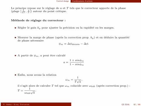
Control design Combinaisons d’actions
Exemple :
Soit la fonction de transfert
G(s) =100
(1 + s)2
On souhaite que le systeme en boucle fermee ait une marge de phase Mφ = 45 :
Calculons la marge de phase avant correction
G(ω) = 100
(1+ω20db
)= 1 ⇒ ω0db = 9.95rad/s
Mφ = π − 2arctanω0db = 11
La marge est insuffisante, il faut donc remonter la phase de φm = 34 a lapulsation ω0db
a =1 + sinφm
1− sinφm=
1 + sin34
1− sin34= 3.54
Puis, on regle T afin d’ajouter la quantite φm au bon endroit
1
T√a
= ω0db ⇒ T = 0.053
Souvent, on choisit φm = 1.2φnecessaire pour compenser le decalage de ω0db aprescorrection.
Y. Ariba - Icam, Toulouse. GE-SSAL 93 / 99
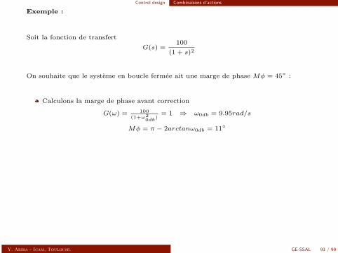
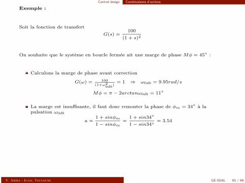
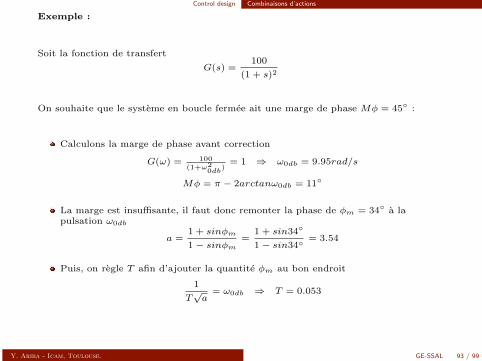
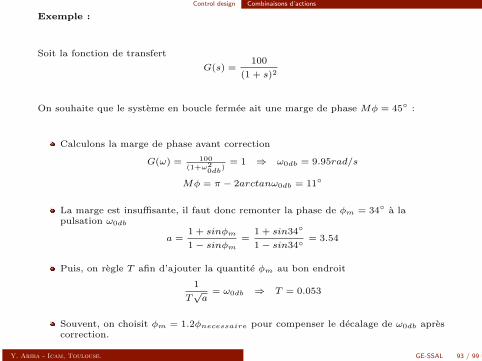
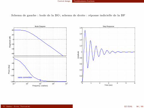
Control design Combinaisons d’actions
Schema de gauche : bode de la BO ; schema de droite : reponse indicielle de la BF
−60
−40
−20
0
20
40
Mag
nitu
de (
dB)
10−1
100
101
102
103
−180
−135
−90
−45
0
Pha
se (
deg)
Bode Diagram
Frequency (rad/sec)
sans correction
0 1 2 3 4 5 60
0.2
0.4
0.6
0.8
1
1.2
1.4
1.6
1.8Step Response
Time (sec)
Am
plitu
de
Y. Ariba - Icam, Toulouse. GE-SSAL 94 / 99
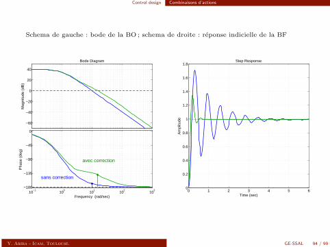
Control design Combinaisons d’actions
Schema de gauche : bode de la BO ; schema de droite : reponse indicielle de la BF
−60
−40
−20
0
20
40
Mag
nitu
de (
dB)
10−1
100
101
102
103
−180
−135
−90
−45
0
Pha
se (
deg)
Bode Diagram
Frequency (rad/sec)
sans correction
avec correction
0 1 2 3 4 5 60
0.2
0.4
0.6
0.8
1
1.2
1.4
1.6
1.8Step Response
Time (sec)
Am
plitu
de
Y. Ariba - Icam, Toulouse. GE-SSAL 94 / 99
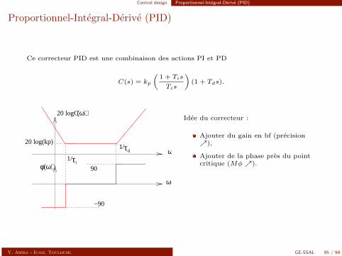
Control design Proportionnel-Integral-Derive (PID)
Proportionnel-Integral-Derive (PID)
Ce correcteur PID est une combinaison des actions PI et PD
C(s) = kp
(1 + Tis
Tis
)(1 + Tds).
ω
ω
20 log(kp)
20 logC(ω)
φ(ω)
−90
1/τi
90
1/τd
Idee du correcteur :
Ajouter du gain en bf (precision),
Ajouter de la phase pres du pointcritique (Mφ).
Le correcteur est propre,
Attenuer l’effet du bruit (moins degain en hf).
Y. Ariba - Icam, Toulouse. GE-SSAL 95 / 99
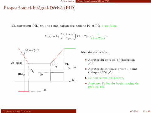
Control design Proportionnel-Integral-Derive (PID)
Proportionnel-Integral-Derive (PID)
Ce correcteur PID est une combinaison des actions PI et PD + un filtre
C(s) = kp
(1 + Tis
Tis
)(1 + Tds)
1
(1 + Tfs).
ω20 log(kp)
20 logC(ω)
φ(ω)
−90
1/τi
90
1/τd
ω
1/τf
Idee du correcteur :
Ajouter du gain en bf (precision),
Ajouter de la phase pres du pointcritique (Mφ).
Le correcteur est propre,
Attenuer l’effet du bruit (moins degain en hf).
Y. Ariba - Icam, Toulouse. GE-SSAL 95 / 99
Control design Proportionnel-Integral-Derive (PID)
Proportionnel-Integral-Derive (PID)
Methode de reglage du correcteur :
Etudier le systeme en BO et ses caracteristiques
(marges, precision, rapidite...).
Regler le gain proportionnel kp afin d’obtenir un premier asservissementsatisfaisant
(en termes de marges, depassement, oscillations, rapidite).
Regler la constante de temps de l’action integrale de sorte qu’elle n’agisse qu’en bf
(pour ne pas penaliser les marges).
Regler la constante de temps de l’action derivee de sorte qu’elle n’agisse qu’autourdu point critique
(pour ne pas penaliser la precision).
Regler la constante de temps du filtre de sorte qu’il n’enleve pas de phase pres dupoint critique,
L’ordre du filtre peut etre augmente afin de mieux attenuer le bruit en hf.
Y. Ariba - Icam, Toulouse. GE-SSAL 96 / 99
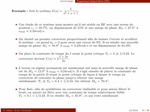
Control design Proportionnel-Integral-Derive (PID)
Exemple : Soit le systeme G(s) =5
s2 + s+ 1.
Une etude de ce systeme nous montre qu’il est stable en BF avec une erreur deposition εs = 16.7%, un depassement de 51% et une marge de phase Mφ = 27.8 aω0db = 2.33rad/s.
On choisit un premier correcteur proportionnel afin de baisser l’erreur et accelererle systeme : on prend kp = 2 pour avoir une erreur de 9%. Il en resulte une nouvellemarge de phase Mφ = 18.9 a ω0db = 3.23rad/s et un depassement de 61.9%.
On place la constante de temps du I avant le point critique Ti = 3 1/3.23. Le
correcteur devient C(s) = 21 + 3s
3s.
L’erreur en regime permanent est maintenant nul mais la nouvelle marge de phaseest de Mφ = 12.9 a ω0db = 3.24rad/s. Il s’agit ensuite de placer la constante detemps de la partie D avant le point critique de facon a laisser le temps aucorrecteur de remonter la phase jusqu’a obtenir une margesatisfaisante :Ti Td = 0.4 > 1/3.24. On obtient Mφ = 70.4.
Pour finir, afin de synthetiser un correcteur realisable et pour mieux filtrer lebruit, on ajoute un filtre avec une constante de temps relativement faibleTf = 0.1 < 1/3.24. Il en resulte Mφ = 45.9, ce qui reste satisfaisant.
Y. Ariba - Icam, Toulouse. GE-SSAL 97 / 99
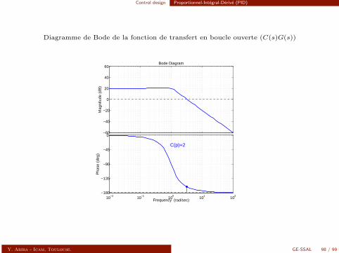
Control design Proportionnel-Integral-Derive (PID)
Diagramme de Bode de la fonction de transfert en boucle ouverte (C(s)G(s))
−60
−40
−20
0
20
40
60
Mag
nitu
de (
dB)
10−2
10−1
100
101
102
−180
−135
−90
−45
0
Pha
se (
deg)
Bode Diagram
Frequency (rad/sec)
C(p)=2
Y. Ariba - Icam, Toulouse. GE-SSAL 98 / 99
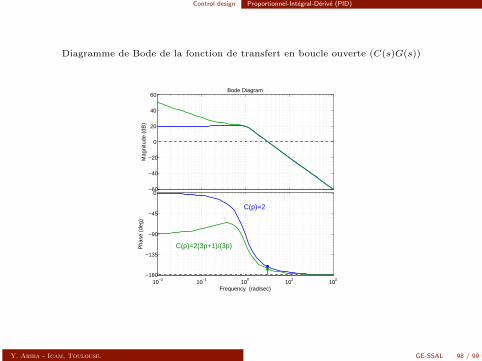
Control design Proportionnel-Integral-Derive (PID)
Diagramme de Bode de la fonction de transfert en boucle ouverte (C(s)G(s))
−60
−40
−20
0
20
40
60
Mag
nitu
de (
dB)
Bode Diagram
Frequency (rad/sec)10
−210
−110
010
110
2−180
−135
−90
−45
0
Pha
se (
deg)
C(p)=2
C(p)=2(3p+1)/(3p)
Y. Ariba - Icam, Toulouse. GE-SSAL 98 / 99
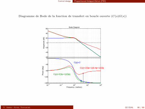
Control design Proportionnel-Integral-Derive (PID)
Diagramme de Bode de la fonction de transfert en boucle ouverte (C(s)G(s))
−60
−40
−20
0
20
40
60
Mag
nitu
de (
dB)
Bode Diagram
Frequency (rad/sec)10
−210
−110
010
110
2−180
−135
−90
−45
0
Pha
se (
deg)
C(p)=2
C(p)=2(3p+1)/(3p)
C(p)=2(3p+1)(0.4p+1)/(3p)
Y. Ariba - Icam, Toulouse. GE-SSAL 98 / 99
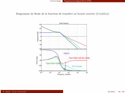
Control design Proportionnel-Integral-Derive (PID)
Diagramme de Bode de la fonction de transfert en boucle ouverte (C(s)G(s))
−60
−40
−20
0
20
40
60
Mag
nitu
de (
dB)
Bode Diagram
Frequency (rad/sec)10
−210
−110
010
110
210
3−180
−135
−90
−45
0
Pha
se (
deg)
C(p)=2
C(p)=2(3p+1)/(3p)
C(p)=2(3p+1)(0.4p+1)/(3p)
PID complet
Y. Ariba - Icam, Toulouse. GE-SSAL 98 / 99
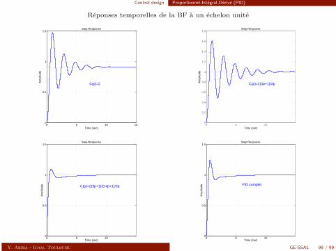
Control design Proportionnel-Integral-Derive (PID)
Reponses temporelles de la BF a un echelon unite
0 5 10 150
0.5
1
1.5Step Response
Time (sec)
Am
plitu
de
C(p)=2
0 5 100
0.2
0.4
0.6
0.8
1
1.2
1.4
1.6
1.8Step Response
Time (sec)
Am
plitu
de
C(p)=2(3p+1)/3p
0 5 100
0.5
1
1.5Step Response
Time (sec)
Am
plitu
de C(p)=2(3p+1)(0.4p+1)/3p
0 5 100
0.5
1
1.5Step Response
Time (sec)
Am
plitu
de PID complet
Y. Ariba - Icam, Toulouse. GE-SSAL 99 / 99


![[R5.06.01] Réduction de modèle en dynamique linéaire et non-linéaire](https://img.pdfslide.fr/doc/110x75/586e1f941a28ab69708c2587/r50601-reduction-de-modele-en-dynamique-lineaire-et-non-lineaire.jpg)