Smukler et al. 2010

8/6/2019 Smukler et al. 2010

http://slidepdf.com/reader/full/smukler-et-al-2010 1/18

Agriculture, Ecosystems and Environment 139 (2010) 80–97

Contents lists available at ScienceDirect

Agriculture, Ecosystems and Environment

j o u r n a l h o m e p a g e : w w w . e l s e v i e r . c o m / l o c a t e / a g e e

Biodiversity and multiple ecosystem functions in an organic farmscape

S.M. Smukler a, S. Sánchez-Moreno c, S.J. Fonte d, H. Ferris e, K. Klonsky f , A.T. O’Geen b,K.M. Scow b, K.L. Steenwerth g, L.E. Jackson b,∗

a Tropical Agriculture Program, The Earth Institute at Columbia University, 61 Route 9W, Lamont Hall, Room 2H, Palisades, NY 10964-8000, USAb Department of Land, Air and Water Resources, University of California, Davis, CA 95616, USAc Unidad de Productos Fitosanitarios, Instituto Nacional de Investigación y Tecnología Agraria y Alimentaria, Crta. Coru na km 7.5, Madrid 28040, Spaind Department of Plant Sciences, University of California, Davis, CA 95616, USAe Department of Nematology, University of California, Davis, CA 95616, USAf Department of Agriculture and Resource Economics, University of California, Davis, CA 95616, USAg USDA/ARS, Crops Pathology and Genetics Research Unit, Davis, CA 95616, USA

a r t i c l e i n f o

Article history:

Received 11 January 2010

Received in revised form 4 June 2010

Accepted 8 July 2010

Available online 19 August 2010

Keywords:

Agrobiodiversity

Ecosystem services

Landscape ecology

Multifunctionality

Organic farming

Partial canonical correspondence analysis

Tradeoff analysis

a b s t r a c t

To increase ecosystem services provided by their lands, farmers in the United States are managing

non-production areas to create a more biodiverse set of habitats and greater landscape heterogene-

ity. Relatively little is known, however, of the actual environmental outcomes of this practice, termed

‘farmscaping’. We inventoried communities of plant and soil organisms and monitored indicators of

ecosystem functions in six distinct habitats of an organic farm in California’s Central Valley to better

understand the ecological costs and benefits of farmscaping. A riparian corridor, hedgerows, a system of

drainage ditches, and tailwater pondssupporteddifferent plantlife history/functionalgroups and greater

native plant diversitythan the twoproduction fields. Differences were less pronounced for belowground

organisms, i.e., nematode functional groups, microbial communities (based on phospholipid fatty acid

(PLFA) analysis) and earthworm taxa. Partial ordination analysis showed that environmental variables,

ratherthan spatiallocation, explainedmuchof thedistribution ofsoil andplanttaxaacrossthe farmscape.

Riparian and hedgerow habitats with woody vegetation stored 18% of the farmscape’s total carbon (C),

despite occupying only 6% of the total area. Infiltration rates in the riparian corridor were >230% higher

than those observed in the production fields, and concentrations of dissolved organic carbon (DOC) in

soilsolution were as much as 65%higher. Thetailwater pond reduced total suspended solids in irrigation

runoff by 97%. Drainage ditches had the highest N 2O-N emissions (mean values of 16.7g m−2 h−1) and

nitrate(NO3−-N)leaching(12.1g m−2 year−1 at 75cm depth). Emissions ofN 2O-Nand leaching ofNO3

−-N

were, however, quite low for all the habitats. Non-production habitats increased biodiversity (particu-

larly plants) and specific ecosystem functions (e.g. water regulation and carbon storage). Extrapolating

relative tradeoffs to the entirefarmscape showed that greater habitatenhancement through farmscaping

could increase both biodiversity and multiple ecosystem functions of agricultural lands with minor loss

of production area.

© 2010 Elsevier B.V. All rights reserved.

1. Introduction

Management to provide multiple ecosystem services (e.g., food

and fiber production, water and soil quality, and pest control)

in agricultural landscapes requires an understanding of ecologi-

cal functions (i.e., the processes that result in ecosystem services)

(Adleret al., 2007; Bennett and Balvanera, 2007;Jordanet al., 2007).

Ecological theory suggests that managing for biological diversity

couldimproveecological functions related to bothagriculturalpro-

duction and environmental quality in agricultural landscapes, such

∗ Corresponding author. Tel.: +1 530 754 9116; fax: +1 530 752 9659.

E-mail address: [email protected] (L.E. Jackson).

as through a wider set of cultivars or crops (Bullock et al., 2001;

Smukler et al., 2008),natural enemies of pests (Zehnder et al.,2007;

Letourneau and Bothwell, 2008), more complex soil food webs to

regulate nutrient cycling (Brussaard et al., 2007; Minoshima et al.,

2007), and vegetated buffer zones to increase retention of C and

other nutrients (Young-Mathews et al., 2010). In addition to man-

agement at the field level, more complex agricultural landscapes

support higher biodiversity, resulting in increased ecosystem func-

tions for pollination, pest control, or water quality ( Gabriel et al.,

2006; Tscharntke et al., 2008).

Moststudies on biodiversity andecosystemfunctions havebeen

done at the plot level, often only considering a single ecosystem

function and/or a single taxonomic unit of biodiversity (Balvanera

et al., 2006). To understand multifunctionality, consideration of

0167-8809/$ – see front matter © 2010 Elsevier B.V. All rights reserved.

doi:10.1016/j.agee.2010.07.004

8/6/2019 Smukler et al. 2010


S.M. Smukler et al. / Agriculture, Ecosystems and Environment 139 (2010) 80–97 81

species in a diversity of functional guilds is required (Hector and

Bagchi, 2007; Gamfeldt et al., 2008), but few studies have occurred

at scales broad enough to test this hypothesis ( Bengtsson et al.,

2003; Culman et al., in press). A mechanistic understanding of bio-

diversity and multifunctional relationships (Swift et al., 2004; Diaz

et al., 2007) requires multi-scale, long-term research. As an initial

approach, however, the focus can be placed on the associationsand relationships of biodiversity inventories to ecological func-

tions, which given sampling constraints, are often assessed by an

indicator parameter rather than a quantitative flux (e.g. spot vs.

continuous sampling of soil greenhouse gas emissions).

The farmscape, the land use system of a single farm, is an

intermediate scale for studying biodiversity and ecosystem func-

tions at the landscape level (Asteraki et al., 2004; Feehan et al.,

2005). The farmscape unit allows for replicate plot level observa-

tions of some functions while serving as an indicator of ecological

processes at larger scales (Herzog, 2005). Local experiences and

farmer experimentation with biodiversity-based production sys-

tems exist in many farmscapes (Cardoso et al., 2001; Pacini et al.,

2003; Harvey et al., 2005; Méndez et al., 2007; Henry et al., 2009).

These approaches provide opportunities to analyze the relation-shipbetween the biodiversity of differentsets of taxa, management

and multiple ecosystem functions and show the tradeoffs that

occur when some functions are provided at the expense of oth-

ers. Understanding these tradeoffs will help prioritize biodiversity

management options that are most likely to ensure long-term sus-

tainability ( Jackson et al., 2007).

In theUnited States, the term“farmscaping” hasbeen adopted to

refer to managing the farmed landscape for positive environmen-

taloutcomes (Imhoff, 2003). Farmscaping can enhance biodiversity

and improve specific ecosystem functions. Hedgerows conserve

plant biodiversity (Le Coeur et al., 2002), improve climate regu-

latingservices such as decreasing carbondioxide (CO2) and nitrous

oxide (N2O) emissions (Robertson et al., 2000; Falloon et al., 2004),

increase carbon(C) storage (Follain et al., 2007), andincrease water

infiltration and quality (Caubel et al., 2003). Grassed waterways

and tailwater ponds or wetlands can improve the water quality

of effluent from agricultural lands (Braskerud, 2002; Jordan et al.,

2003; Blanco-Canqui et al., 2004; O’Geen et al., 2007). Vegetated

field margins can harbor insects that regulate pests or increase

pollination (Olson and Wackers, 2007).

Farmscaping often involves planned biodiversity-based prac-

tices such as woody perennial plantings to increase associated

diversity of birds (Vickery et al., 2002), mammals (Michel et al.,2007), and pollinators (Kremen et al., 2004). For belowground

organisms, the relationship between farm habitats and biodiver-

sity is more complex, because soil organisms are rarely planned

components of biodiversity. Also, they perceive scale in different

ways, depending on their size, movement, and mode of disper-

sal (Brussaard et al., 2007). The composition of soil microbial and

faunal communities can be affected by management, particular

plant functional groups (e.g. legumes, grasses, or woody perenni-

als), or plant life history (e.g. native perennial vs. non-native annual

species) (Hooper et al., 2000; Steenwerth et al., 2003; Broz et al.,

2007; Sánchez-Moreno et al., 2008). Alternatively, there maybe no

link if restoration activities are recent, or if the setting is in a sim-

plified landscape with little overall biodiversity (Wardle and van

der Putten, 2002; Tscharntke et al., 2005; Wardle et al., 2006).This case study examines how farmscaping may increase biodi-

versity and ecosystem functions related to soil and water quality in

the various production and non-production habitats of an organic

farm. Participatory research provided a way to focus on man-

agement practices that were considered important by the farmer

and local agencies involved in biodiversity and natural resource

conservation (Robins et al., 2002), i.e., riparian forest conserva-

tion, hedgerows of native shrubs, and vegetated tailwater ponds.

Farmscaping practices with native perennial plant species were

expected to result in greater biodiversity of plants, nematodes, and

microbes (based on phospholipid fatty acid (PLFA) analysis which

provides a profile or ‘fingerprint’ of specific groups and activities

(Bossioet al., 1998;Ferriset al., 2004;Brussaard etal.,2007).In turn,

higher biodiversity was expected to be associated with increased

ecosystemfunctions related to crop production and environmental

quality. Indicators of ecosystem functions were chosen that were

Fig. 1. Sampling map and location of the organic farm. The farm is located 5 km north of Winters, California, on the edge of the Central Valley. 42 plots were randomly

stratified within six habitats across the 44 ha farmscape.

8/6/2019 Smukler et al. 2010


8/6/2019 Smukler et al. 2010



the Shannon-Wiener diversity index (Shannon, 1948). It should be

noted that the PLFA biomarkers are not directly equivalent to taxa,

although some are characteristic of specific groups. The diversity

across habitats was calculated as the number of unique taxa (or

PLFA biomarkers) for each habitat (i.e. found only in that habitat)

(Koleff et al., 2003).

Within 24 h, soil was analyzed for gravimetric moisture, andKCl-extractable ammonium (NH4

+-N) and nitrate (NO3−-N) col-

orimetrically (Foster, 1995; Miranda et al., 2001), or incubated

anaerobically for 7 days to determine potentially mineraliz-

able nitrogen (PMN) (Waring and Bremner, 1964). Microbial

biomass carbon (MBC) was measured by fumigation extrac-

tion according to Vance et al. (1987), but with C analysis on

a Dohrmann Phoenix 8000 UV-persulfate oxidation analyzer

(Tekmar-Dohrmann, Cincinnati, OH).

Air-dried subsamples were analyzed for electrical conductiv-

ity (EC) (Rhoades, 1982), pH using a 1:1 ratio of soil to deionized

water (USSL, 1954). Olsen phosphorus (P) was determined using

the methods outlined by Olsen and Sommers (1982) and total C

and N using a dynamic flash combustion system coupled with a

gas chromatograph at the University of California Agriculture andNatural Resources(ANR) Analytical Laboratory. Vegetationsamples

were analyzed similarly for total C and N.

Intact soil monoliths were passed through an 8-mm sieve by

gently breaking the soil clods by hand along natural fracture

lines, then air dried. This soil was wet sieved into four fractions

(Elliott, 1986): large aggregates (>2000m), small macroaggre-

gates (250–2000m), microaggregates (53–250m), and the silt

and clay fraction (<53m). A weighted average for the oven-

dried soil mass of each fraction was calculated to obtain mean

aggregate diameter, an indicator of aggregate stability (van Bavel,

1949).

2.5. Two-year assessment of indicators of ecological functions

Monitoring of indicators of ecological functions began immedi-

atelyafter the biodiversityinventory in March, 2005, and continued

until April, 2007. Sampling took place in the same 16m2 plots for

each habitat described above.

Gas emissions (CO2-C and N2O-N) from the soil surface were

monitored on the ∼13th day (+/− 2 days) of each month for the

entire two-year period using closed chambers consisting of PVC

collars that were pounded into the soil surface between 6 to 24h

before samplingand thenremoved to avoid disturbance by farming

operations (Hutchinson and Livingston, 1993). Soil emissions were

sampled fromthe production fieldson thebeds betweenplants,and

in the ditches and tailwater ponds randomly within the plot when

water was not present, or if present, within 6 cm of water’s edge

using a LI-COR8100 fittedwith a portable surveychamber10 cm in

diameter (LI-COR Biosciences, Lincoln, NE) and static closed cham-bers (Livingston and Hutchinson, 1995). The CO2 samples taken by

the LI-COR 8100 were analyzed in the field at 3-min intervals. One

sample was taken from the closed chamber at 0 and 30 min with

glass syringes and stored in over-pressurized vacutainers for <2

week. Concentrations of CO2-C were determined using a gas chro-

matograph (GC) with a thermal conductivity detector (HP 5890,

Hewlett Packard, Palo Alto, CA). Samples of CO2-C from the two

methods were treated as duplicates and reported as means. Analy-

sis of N2O was on a HP 6890 gas chromatograph (Hewlett Packard,

Palo Alto, CA).

For sampling C stocks in woody plants, the 2.5ha riparian corri-

dor was stratifiedequallyinto six sampling areas, basedon distance

from the eastern edge of the farm. All hedgerow areas were sam-

pled. Within each sampling area, all woody plants were sampled.Carbon stocks were categorized into six pools: standing live tree

aboveground biomass, standing live tree belowground biomass,

shrub and herbaceous understory aboveground biomass, stand-

ing dead trees, litter and duff, and soil (California Climate Action

Registry,2009). Biomass determinations for woody plants included

stems, branches, leaves, and both live and dead roots in the case

of trees, and coarse roots for shrubs (Cairns et al., 1997; California

ClimateActionRegistry, 2009). Biomass foreach treewas calculated

using the allometric equations provided for C inventories of Cali-fornia forests (California Climate Action Registry, 2009) based on

measuring the diameter at breast height (DBH) at 1.3 m above the

ground. Belowground live tree root biomass was estimated using

the equation developed by Cairns et al. (1997). Carbon was calcu-

lated as 50% of tree dry biomass (IPCC, 2006). For the one dead

standing tree found on the farm, C was determined using the same

methodology as live trees.

For C stored in all understory and hedgerow shrubs, biomass

was calculated based on the shrub volume, which was estimated

using the length of the longest diameter, its perpendicular length,

and the shrub height (Appendix B). Allometric equations that

relate shrub volume to total measured above- and below-ground

biomass followed Cleary et al. (2008), but were based on sam-

pled C content of leaves, wood, and roots for shrub species in theregion.

In each subplot, litter (<2.5cm) and duff was collected within a

30cm diameter PVCring. Dead downedbranches up to15 cmdiam-

eter were collected for the entire subplot. These materials were

dried, weighed, chipped, ground, and analyzed for total C to deter-

mine surface litter and duff C pools. Soil C (g m−2) was calculated

for 0–15 cm depth using observed C concentrations and the mean

of the bulk density measurements taken at 0–6 cm and 9–15 cm.

For the 15–30cm depth, bulk density taken at 18–24cm depth was

used.

Surface runoff was monitored for summer irrigation and win-

ter storm events with ISCO 6700 (Teledyne Isco, Inc., Lincoln, NE)

automated water samplers fitted with low-profile area flow veloc-

ity meters, and with targeted grab samples. Samplers were placed

in four strategic locations on ditches and tailwater ponds to deter-

mine the influx and discharge of water and sediment into the

tailwater pond, and the effectiveness of the tailwater pond to

reduce sediment losses to the adjacent riparian habitat. During

irrigation, 250 mL samples were taken every 4 h and composited

daily. During storm events, autosamplers were programmed to

capture initial flush of sediments accurately. Autosamplers ini-

tially were set to sample every 5 min for 30 min, then switched

to sampling after every 1000L of discharge. A total of 583 runoff

samples were collected. Water samples were immediately put on

ice, transported back to the laboratory and frozen. For thorough

mixing of solids, a 50 mL subsample was pipetted while vortexed,

then was suction-filtered through a 0.7m pore size glass fiber fil-

ter (GF75; Advantec, Tokyo, Japan). Total suspended solids (TSS)

were calculated from differences in pre-filter and post-filter dryweights (Clesceri et al., 1998). Volatile suspended solids (VSS)

were calculated from the difference in pre- and post-ignition filter

weights. A separate subsample was analyzed for EC, pH, NH4+-N,

NO3−-N, (see above), dissolved reactive phosphate (DRP) colori-

metrically (Murphy and Riley, 1958), anddissolved organic C (DOC)

using a using a Dohrman DC-190 total organic C analyzer (Tekmar-

Dohrmann, Cincinnati, OH).

Soil solute leachingwas assessed in two ways: ceramic cup suc-

tionlysimeters (SoilMoisture Corp., Santa Barbara, CA) which were

deployed in each randomized plot (Fig. 1) at a depth of 30 and

60cm ( Jackson, 2000), and anion exchange resin bags for cumu-

lative NO3−-N losses (Wyland and Jackson, 1993). Lysimeters were

sampled weekly during periods when the soil was saturated (e.g.

summer irrigation and the winter rainy season). Resin bags wereset within a 7.62 cm diameter PVC ring, packed into a shelf duginto

the side of the pit at 75 cm under an undisturbed soil profile. Bags

8/6/2019 Smukler et al. 2010


84 S.M. Smukler et al. / Agriculture, Ecosystems and Environment 139 (2010) 80–97

were collected in the springand fall of the two years, and extracted

with 2M KCl for NO3−-N analysis.

Cumulative infiltration rates were determined in single ring

infiltrometers (25cm dia.) that were pounded evenly into the soil

to 20cm depth. One reading was made per plot. Water was contin-

uously added, and the rate of falling head was recorded for at least

30 min (Bouwer, 1986).Tomato yields were sampled within 3 days before the farmer’s

harvest. To capture yield variability across the field, transects were

oriented north-south of each main sampling plot (393 m in the

North Field or 250m in the South Field). Along each transect, a

1 m × 3 m sub-plot was established at 30-m intervals (five or nine

sub-plots depending on the width of the field). At each sampling

point, individual tomato plants were cut at the base and the fruit

separated by hand. Biomass of fruits, tomato vegetative material,

and weed biomass were weighed in the field (fresh weight) then

subsampled and dried at 60 ◦C for 2 week, before grinding and

analyzing for total C and N (see above).

2.6. Sampling design and statistical analysis

Due to the differences in relative size of the habitats, random-

ization inevitably resulted in some plots being closer together in

particular habitatsthan in others (e.g., the largest distance between

plots was 775 m, while the smallest distance was 22 m) creating a

situation where pairs of locations could be more (positively auto-

correlated) or less similar (negatively autocorrelated) than others.

Specific statistical approaches were used to address this poten-

tial spatial autocorrelation due to the uneven distribution of

sampling units, which implies that standard assumptions of inde-

pendence of random pairs could not be upheld (Legendre, 1993).

When testing for differences in biodiversity or ecosystem function

among habitats a mixed model ANOVA was employed that incor-

porated a spatial covariance structure. The proc mixed statement in

SAS(SAS, 2003) combined with a power correlation function(POW )

model enables spatial location to be used as a covariate. The POW

model uses a one dimensional (1-D) isotropic power covariance

term based on using the Universal Transverse Mercator (UTM) X , Y

coordinates for each plot (Self and Liang, 1987; Wolfinger, 1993).

This methodology has been tested against other spatial and non-

spatial models in agricultural systems and is an effective way to

deal with spatial covariance (Casanoves et al., 2005; Bajwa and

Mozaffari, 2007). The proc mixed models were first run with all

42 sampling points (two years of data together) including habitat ,

year ,and year × habitat , afterchecking for homogeneity of variance,

and conducting log transformations if necessary. Graphs illus-

trate untransformed data. If there were no significant interactions

between year and habitat, the two-year mean was reported. Oth-

erwise, each year was analyzed separately and results are reportedas year 1 (March 1, 2005–March 31, 2006) and year 2 (April 1,

2006–April 1, 2007).

To further explore theenvironmental variablesthat wereimpor-

tant for species/taxa assemblages across the farmscape, Partial

Canonical Correspondence Analysis(CCA), a method of partial (con-

strained) ordination analysis was employed (Legendre, 1993). The

partial CCA concurrently uses ordination and regression to assess

the relationship between variables, but also accounts for poten-

tial spatial autocorrelation by removing, through multiple linear

regression, the effects of known or undesirable variables, called

covariables, which in this case are spatial coordinates of each

sampling point. A matrix of spatial covariables was developed as

suggested by Borcard et al. (1992) using x and y (the difference

of UTM coordinates of each plot from the UTM coordinate at thesoutheast corner of the farmscape) as variables for a cubic surface

regression, that then is used to generate a best-fit equation foreach

type of biota (see Section 3):

f ( x,y) = b1 x + b2 y + b3 x2

+ b4 xy + b5 y2

+ b6 x3

+ b7 x2 y

+b8 xy2

+ b9 y3.

For each species/taxa dataset, a CCA was run four times: withenvironmental variables only (‘environmental’); with spatial vari-

ables based on the regression of UTM coordinates only (‘spatial’);

with environmental variables constrained by spatial covariables

(‘environmental variables partial’); and with spatial covariables

constrained by environment (‘spatial partial’). In the first two types

of CCA runs, a forward selection process was used to identify those

variables that were significant (P < 0.05) using a Monte Carlo per-

mutations test run 499 times. Constraining each analysis by one

set of explanatory variables (i.e. environmental or spatial) enabled

the partitioning of the variation in species/taxa distribution into

four classifications: environmental only, spatial and environmen-

tal, spatial only and unexplained variation. These partitions were

calculated as follows, where the variation for each component is

the sumof allcanonical eigenvalues andthe total inertia is thetotalvariation of the model:

1. Environmental

variation only

‘environmental variable partial’ × 100 total inertia

2. Spatially

structured

environmental

variation

‘environmental’−‘environmentalvar iablepartial’×100totalinertia

=

‘spatial’−‘spatialpar tial’×100total inertia

3. Spatial variation

only

‘spatialpart ial’×100total inertia

4. Unexplained

variation

1 − (the sum of the variation of 1–3)

The total inertia is measured by the chi-square statistic of the

sample-by-taxa table divided by the table’s total (ter Braak and

Smilauer, 1998). The overall measure of the CCA fit is determined

by dividing the sum of all canonical eigenvalues by the total iner-tia thus giving the percentage of total variance in the species/taxa

dataset thatis explainedby theexplanatoryvariables (terBraak and

Smilauer, 1998). This method was also used to calculate the pro-

portion of thetotalinertia in thespecies/taxadata that is explained

by each canonical axis. To test the significance of canonical axes an

unrestricted Monte Carlo permutation was used. As these tests are

not dependent on parametric distributional assumptions (Palmer,

1993), species/taxa data were not transformed, and environmental

and spatial variables were simply standardized.

3. Results

3.1. Plant and soil biodiversity

Only 61 species of plants were observed across the entire farm-

scape. Each habitat had an average of only 11 plant species, with

on average, more non-natives (8 species) than natives (3 species)

(Table 1; Appendix B). The largest number of unique species was in

the riparian corridor. The perennial habitats (i.e., the riparian cor-

ridor and hedgerow) had higher diversity of native plant species

than the production fields, with the irrigation habitats interme-

diate. The Shannon-Wiener diversity index for native vegetation

differed between years and by habitat. For native species richness,

there was a year × habitat interaction. Non-native plant species

were generally more abundant in the irrigation habitats, especially

the tailwater pond, than elsewhere. Most of these species areannu-

als. The Shannon-Wiener diversity index for non-natives differed

by habitat depending on year (Table 1). High cover of non-nativesin the South Field was largely due to volunteer oats from previous

crops (Fig. 2).

8/6/2019 Smukler et al. 2010



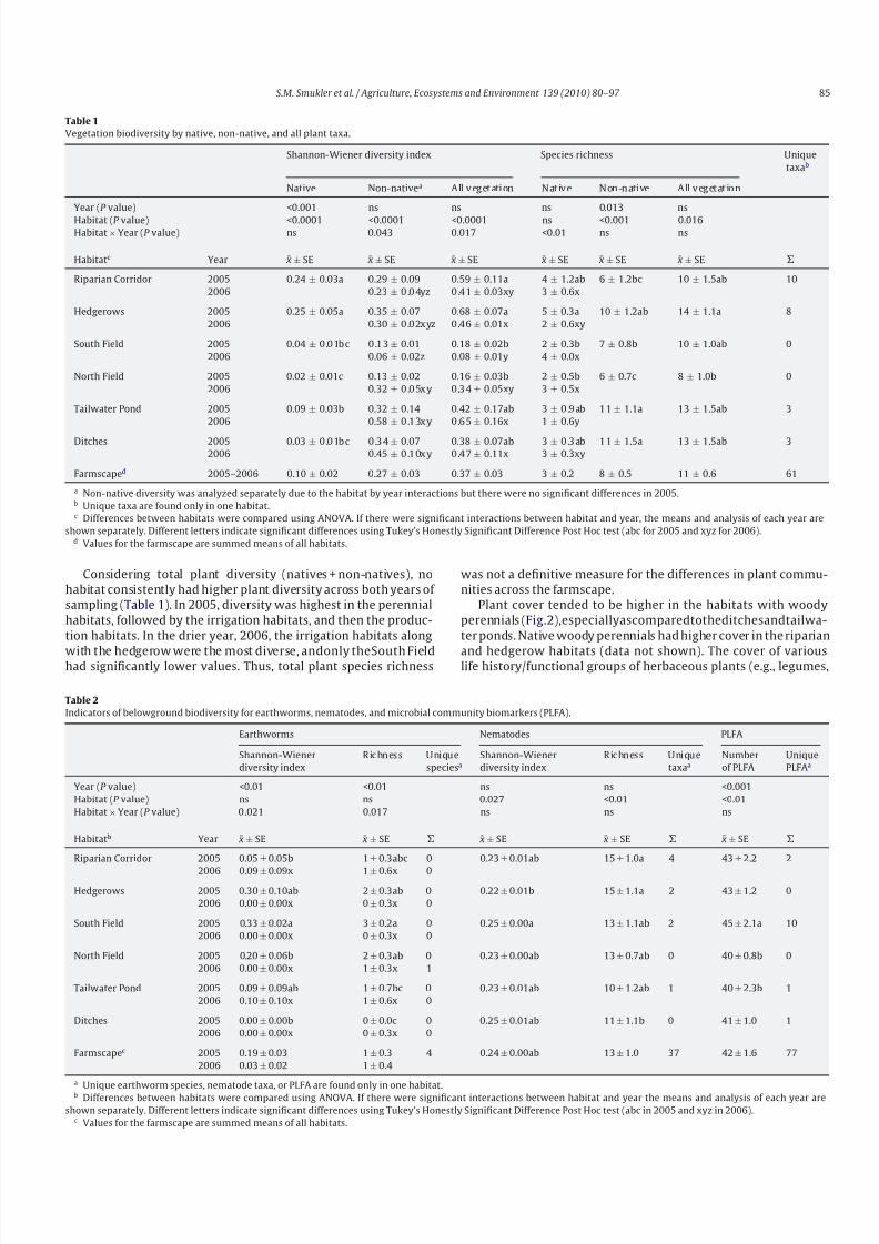
Table 1

Vegetation biodiversity by native, non-native, and all plant taxa.

Shannon-Wiener diversity index Species richness Unique

taxab

Native Non-nativea All veget ation Nat ive Non -n ative All veget at io n

Year (P value) <0.001 ns ns ns 0.013 ns

Habitat (P value) <0.0001 <0.0001 <0.0001 ns <0.001 0.016Habitat × Year (P value) ns 0.043 0.017 <0.01 ns ns

Habitatc Year ¯ x ± SE ¯ x ± SE ¯ x ± SE ¯ x ± SE ¯ x ± SE ¯ x ± SE

Riparian Corridor 2005 0.24 ± 0.03a 0.29 ± 0.09 0.59 ± 0.11a 4 ± 1.2ab 6 ± 1.2bc 10 ± 1.5ab 10

2006 0.23 ± 0.04yz 0.41 ± 0.03xy 3 ± 0.6x

Hedgerows 2005 0.25 ± 0.05a 0.35 ± 0.07 0.68 ± 0.07a 5 ± 0.3a 10 ± 1.2ab 14 ± 1.1a 8

2006 0.30 ± 0.02xyz 0.46 ± 0.01x 2 ± 0.6xy

South Field 2005 0.04 ± 0.01bc 0.13 ± 0.01 0.18 ± 0.02b 2 ± 0.3b 7 ± 0.8b 10 ± 1.0ab 0

2006 0.06 ± 0.02z 0.08 ± 0.01y 4 ± 0.0x

North Field 2005 0.02 ± 0.01c 0.13 ± 0.02 0.16 ± 0.03b 2 ± 0.5b 6 ± 0.7c 8 ± 1.0b 0

2006 0.32 ± 0.05xy 0.34 ± 0.05xy 3 ± 0.5x

Tailwater Pond 2005 0.09 ± 0.03b 0.32 ± 0.14 0.42 ± 0.17ab 3 ± 0.9ab 11 ± 1.1a 13 ± 1.5ab 3

2006 0.58 ± 0.13xy 0.65 ± 0.16x 1 ± 0.6y

Ditches 2005 0.03 ± 0.01bc 0.34 ± 0.07 0.38 ± 0.07ab 3 ± 0.3ab 11 ± 1.5a 13 ± 1.5ab 3

2006 0.45 ± 0.10xy 0.47 ± 0.11x 3 ± 0.3xy

Farmscaped 2005–2006 0.10 ± 0.02 0.27 ± 0.03 0.37 ± 0.03 3 ± 0.2 8 ± 0.5 11 ± 0.6 61

a Non-native diversity was analyzed separately due to the habitat by year interactions but there were no significant differences in 2005.b Unique taxa are found only in one habitat.c Differences between habitats were compared using ANOVA. If there were significant interactions between habitat and year, the means and analysis of each year are

shown separately. Different letters indicate significant differences using Tukey’s Honestly Significant Difference Post Hoc test (abc for 2005 and xyz for 2006).d Values for the farmscape are summed means of all habitats.

Considering total plant diversity (natives + non-natives), no

habitat consistently had higher plant diversity across both years of

sampling (Table 1). In 2005, diversity was highest in the perennial

habitats, followed by the irrigation habitats, and then the produc-

tion habitats. In the drier year, 2006, the irrigation habitats along

with the hedgerow were the most diverse, andonly theSouth Fieldhad significantly lower values. Thus, total plant species richness

was not a definitive measure for the differences in plant commu-

nities across the farmscape.

Plant cover tended to be higher in the habitats with woody

perennials (Fig.2),especiallyascomparedtotheditchesandtailwa-

ter ponds. Native woody perennials had higher cover in the riparian

and hedgerow habitats (data not shown). The cover of variouslife history/functional groups of herbaceous plants (e.g., legumes,

Table 2

Indicators of belowground biodiversity for earthworms, nematodes, and microbial community biomarkers (PLFA).

Earthworms Nematodes PLFA

Shannon-Wiener

diversity index

Richness Unique

speciesa

Shannon-Wiener

diversity index

Richness Unique

taxaa

Number

of PLFA

Unique

PLFAa

Year (P value) <0.01 <0.01 ns ns <0.001

Habitat (P value) ns ns 0.027 <0.01 <0.01

Habitat × Year (P value) 0.021 0.017 ns ns ns

Habitatb Year ¯ x ± SE ¯ x ± SE ¯ x ± SE ¯ x ± SE ¯ x ± SE

Riparian Corridor 2005 0.05 ± 0.05b 1 ± 0.3abc 0 0.23 ± 0.01ab 15 ± 1.0a 4 43 ± 2.2 2

2006 0.09 ± 0.09x 1 ± 0.6x 0

Hedgerows 2005 0.30 ± 0.10ab 2 ± 0.3ab 0 0.22 ± 0.01b 15 ± 1.1a 2 43 ± 1.2 0

2006 0.00 ± 0.00x 0 ± 0.3x 0

South Field 2005 0.33 ± 0.02a 3 ± 0.2a 0 0.25 ± 0.00a 13 ± 1.1ab 2 45 ± 2.1a 10

2006 0.00 ± 0.00x 0 ± 0.3x 0

North Field 2005 0.20 ± 0.06b 2 ± 0.3ab 0 0.23 ± 0.00ab 13 ± 0.7ab 0 40 ± 0.8b 0

2006 0.00 ± 0.00x 1 ± 0.3x 1

Tailwater Pond 2005 0.09 ± 0.09ab 1 ± 0.7bc 0 0.23 ± 0.01ab 10 ± 1.2ab 1 40 ± 2.3b 1

2006 0.10 ± 0.10x 1 ± 0.6x 0

Ditches 2005 0.00 ± 0.00b 0 ± 0.0c 0 0.25 ± 0.01ab 11 ± 1.1b 0 41 ± 1.0 1

2006 0.00 ± 0.00x 0 ± 0.3x 0

Farmscapec 2005 0.19 ± 0.03 1 ± 0.3 4 0.24 ± 0.00ab 13 ± 1.0 37 42 ± 1.6 77

2006 0.03 ± 0.02 1 ± 0.4

a

Unique earthworm species, nematode taxa, or PLFA are found only in one habitat.b Differences between habitats were compared using ANOVA. If there were significant interactions between habitat and year the means and analysis of each year are

shown separately. Different letters indicate significant differences using Tukey’s Honestly Significant Difference Post Hoc test (abc in 2005 and xyz in 2006).c Values for the farmscape are summed means of all habitats.

8/6/2019 Smukler et al. 2010



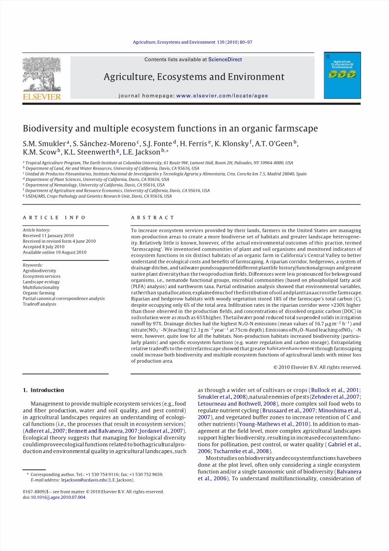
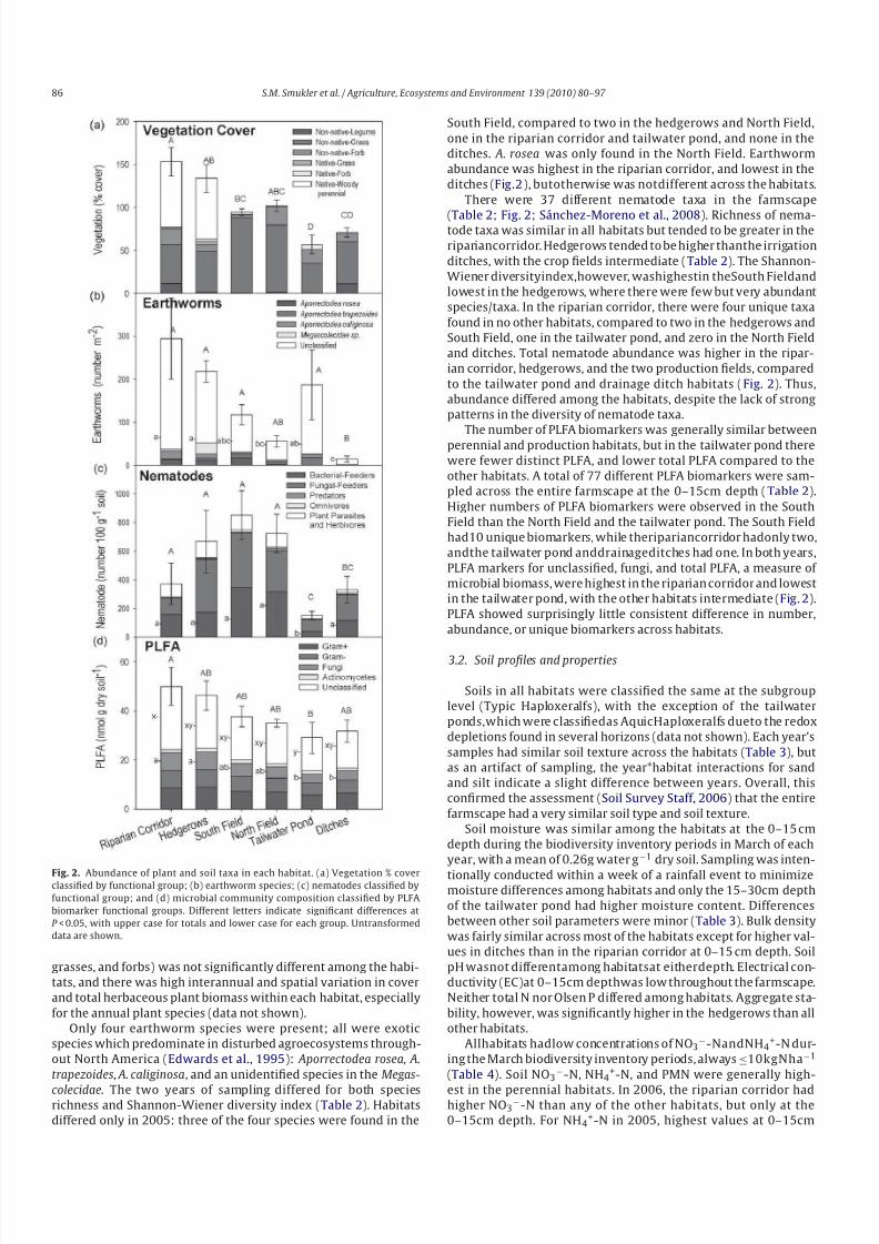
Fig. 2. Abundance of plant and soil taxa in each habitat. (a) Vegetation % coverclassified by functional group; (b) earthworm species; (c) nematodes classified by

functional group; and (d) microbial community composition classified by PLFA

biomarker functional groups. Different letters indicate significant differences at

P < 0.05, with upper case for totals and lower case for each group. Untransformed

data are shown.

grasses, and forbs) was not significantly different among the habi-

tats, and there was high interannual and spatial variation in cover

and total herbaceous plant biomass within each habitat, especially

for the annual plant species (data not shown).

Only four earthworm species were present; all were exotic

species which predominate in disturbed agroecosystems through-

out North America (Edwards et al., 1995): Aporrectodea rosea, A.

trapezoides, A. caliginosa, and an unidentified species in the Megas-

colecidae. The two years of sampling differed for both speciesrichness and Shannon-Wiener diversity index (Table 2). Habitats

differed only in 2005: three of the four species were found in the

South Field, compared to two in the hedgerows and North Field,

one in the riparian corridor and tailwater pond, and none in the

ditches. A. rosea was only found in the North Field. Earthworm

abundance was highest in the riparian corridor, and lowest in the

ditches (Fig.2), butotherwise was notdifferent across the habitats.

There were 37 different nematode taxa in the farmscape

(Table 2; Fig. 2; Sánchez-Moreno et al., 2008). Richness of nema-tode taxa was similar in all habitats but tended to be greater in the

ripariancorridor. Hedgerows tended to be higher thanthe irrigation

ditches, with the crop fields intermediate (Table 2). The Shannon-

Wiener diversityindex,however, washighestin theSouth Fieldand

lowest in the hedgerows, where there were few but very abundant

species/taxa. In the riparian corridor, there were four unique taxa

found in no other habitats, compared to two in the hedgerows and

South Field, one in the tailwater pond, and zero in the North Field

and ditches. Total nematode abundance was higher in the ripar-

ian corridor, hedgerows, and the two production fields, compared

to the tailwater pond and drainage ditch habitats (Fig. 2). Thus,

abundance differed among the habitats, despite the lack of strong

patterns in the diversity of nematode taxa.

The number of PLFA biomarkers was generally similar betweenperennial and production habitats, but in the tailwater pond there

were fewer distinct PLFA, and lower total PLFA compared to the

other habitats. A total of 77 different PLFA biomarkers were sam-

pled across the entire farmscape at the 0–15cm depth (Table 2).

Higher numbers of PLFA biomarkers were observed in the South

Field than the North Field and the tailwater pond. The South Field

had10 unique biomarkers, while theripariancorridor hadonly two,

andthe tailwater pond anddrainageditches had one. In both years,

PLFA markers for unclassified, fungi, and total PLFA, a measure of

microbial biomass, were highest in the riparian corridor and lowest

in the tailwater pond, with the other habitats intermediate (Fig. 2).

PLFA showed surprisingly little consistent difference in number,

abundance, or unique biomarkers across habitats.

3.2. Soil profiles and properties

Soils in all habitats were classified the same at the subgroup

level (Typic Haploxeralfs), with the exception of the tailwater

ponds,which were classifiedas AquicHaploxeralfs dueto the redox

depletions found in several horizons (data not shown). Each year’s

samples had similar soil texture across the habitats (Table 3), but

as an artifact of sampling, the year*habitat interactions for sand

and silt indicate a slight difference between years. Overall, this

confirmed the assessment (Soil Survey Staff, 2006) that the entire

farmscape had a very similar soil type and soil texture.

Soil moisture was similar among the habitats at the 0–15 cm

depth during the biodiversity inventory periods in March of each

year, with a mean of 0.26g water g−1 dry soil. Sampling was inten-

tionally conducted within a week of a rainfall event to minimizemoisture differences among habitats and only the 15–30cm depth

of the tailwater pond had higher moisture content. Differences

between other soil parameters were minor (Table 3). Bulk density

was fairly similar across most of the habitats except for higher val-

ues in ditches than in the riparian corridor at 0–15 cm depth. Soil

pH wasnot differentamong habitatsat eitherdepth. Electrical con-

ductivity (EC)at 0–15cm depthwas low throughout the farmscape.

Neither total N nor Olsen P differed among habitats. Aggregate sta-

bility, however, was significantly higher in the hedgerows than all

other habitats.

Allhabitats hadlow concentrations of NO3−-NandNH4

+-N dur-

ing the March biodiversity inventory periods, always ≤10kgNha−1

(Table 4). Soil NO3−-N, NH4

+-N, and PMN were generally high-

est in the perennial habitats. In 2006, the riparian corridor hadhigher NO3

−-N than any of the other habitats, but only at the

0–15cm depth. For NH4+-N in 2005, highest values at 0–15cm

8/6/2019 Smukler et al. 2010


S .M . S m u k l e r e t a l . / A g r i c u l t ur e ,E c o s y s t e m s a n d

E nv i r o n m e n t 1 3 9

( 2 0 1 0 ) 8 0 – 9 7

8 7

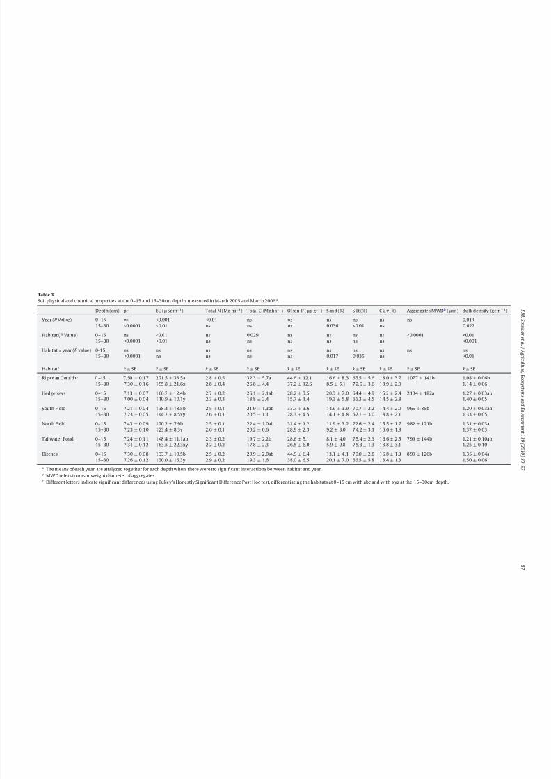
Table 3

Soil physical and chemical properties at the 0–15 and 15–30cm depths measured in March 2005 and March 2006a.

Depth (cm) pH EC (Sc m−1) Total N (Mg ha−1) Total C (Mgha−1) Olsen-P (g g−1) S and ( %) S ilt ( %) C la y ( %) Agg re ga te s M WDb (m) Bulk density (gcm −3)

Year (P Value) 0–15 ns <0.001 <0.01 ns ns ns ns ns ns 0.013

15–30 <0.0001 <0.01 ns ns ns 0.036 <0.01 ns 0.022

Habitat (P Value) 0–15 ns <0.01 ns 0.029 ns ns ns ns <0.0001 <0.01

15–30 <0.0001 <0.01 ns ns ns ns ns ns <0.001

Habitat × year (P value) 0-15 ns ns ns ns ns ns ns ns ns ns

15–30 <0.0001 ns ns ns ns 0.017 0.035 ns <0.01

Habitatc ¯ x ± SE ¯ x ± SE ¯ x ± SE ¯ x ± SE ¯ x ± SE ¯ x ± SE ¯ x ± SE ¯ x ± SE ¯ x ± SE ¯ x ± SE

Ri pa ri an C or ri dor 0 –15 7. 50 ± 0 .17 271.5 ± 33.5a 2.8 ± 0.5 32.3 ± 5.7a 44.6 ± 12.1 16.6 ± 8.3 65.5 ± 5.6 18.0 ± 3.7 1077 ± 141b 1.08 ± 0.06b

15–30 7.30 ± 0 .16 195.8 ± 21.6x 2.8 ± 0.4 26.8 ± 4.4 37.2 ± 12.6 8.5 ± 5.1 72. 6 ± 3.6 18.9 ± 2.9 1.14 ± 0.06

Hedgerows 0–15 7.13 ± 0 .0 7 166.7 ± 12.4b 2.7 ± 0.2 26.1 ± 2.1ab 28.2 ± 3.5 20.3 ± 7.0 64.4 ± 4.9 15.2 ± 2.4 2104 ± 182a 1.27 ± 0.03ab

15–30 7.00 ± 0 .0 4 110 .9 ± 10.1y 2.3 ± 0.3 18.8 ± 2.4 15.7 ± 1.4 19.3 ± 5.8 66.3 ± 4.5 14.5 ± 2.8 1.40 ± 0.05

South Field 0–15 7.21 ± 0 .0 4 138.4 ± 18.5b 2.5 ± 0.1 21.9 ± 1.3ab 33.7 ± 3.6 14.9 ± 3.9 70.7 ± 2.2 14.4 ± 2.0 965 ± 85b 1.20 ± 0.03ab15–30 7.23 ± 0 .0 5 144.7 ± 8.5xy 2.6 ± 0.1 20.5 ± 1.1 28.3 ± 4.5 14.1 ± 4.8 67.1 ± 3.0 18.8 ± 2.1 1.33 ± 0.05

North Field 0–15 7.43 ± 0 .0 9 120 .2 ± 7.9b 2.5 ± 0.1 22.4 ± 1.0ab 31.4 ± 1.2 11.9 ± 3.2 72.6 ± 2.4 15.5 ± 1.7 982 ± 121b 1.31 ± 0.03a

15–30 7.23 ± 0 .10 123.4 ± 8.3y 2.6 ± 0.1 20.2 ± 0.6 28.9 ± 2.3 9.2 ± 3.0 74. 2 ± 3.1 16.6 ± 1.8 1.37 ± 0.03

Tailwater Pond 0–15 7.24 ± 0 .11 148.4 ± 11.1ab 2.3 ± 0.2 19.7 ± 2.2b 28.6 ± 5.1 8.1 ± 4.0 75. 4 ± 2.3 16.6 ± 2.5 799 ± 144b 1.21 ± 0.10ab

15–30 7.31 ± 0 .12 163.5 ± 22.3xy 2.2 ± 0.2 17.8 ± 2.3 26.5 ± 6.0 5.9 ± 2.8 75. 3 ± 1.3 18.8 ± 3.1 1.25 ± 0.10

Ditches 0–15 7.30 ± 0 .0 8 133.7 ± 10.5b 2.5 ± 0.2 20.9 ± 2.0ab 44.9 ± 6.4 13.1 ± 4.1 70.0 ± 2.8 16.8 ± 1.3 899 ± 126b 1.35 ± 0.04a

15–30 7.26 ± 0 .12 130 .0 ± 16.3y 2.9 ± 0.2 19.3 ± 1.6 38.0 ± 6.5 20.1 ± 7.0 66.5 ± 5.8 13.4 ± 1.3 1.50 ± 0.06

a The means of each year are analyzed together for each depth when there were no significant interactions between habitat and year.b MWD refers to mean weight diameter of aggregates.c Different letters indicate significant differences using Tukey’s Honestly Significant Difference Post Hoc test, differentiating the habitats at 0–15 cm with abc and with xyz at the 15–30cm depth.

8/6/2019 Smukler et al. 2010



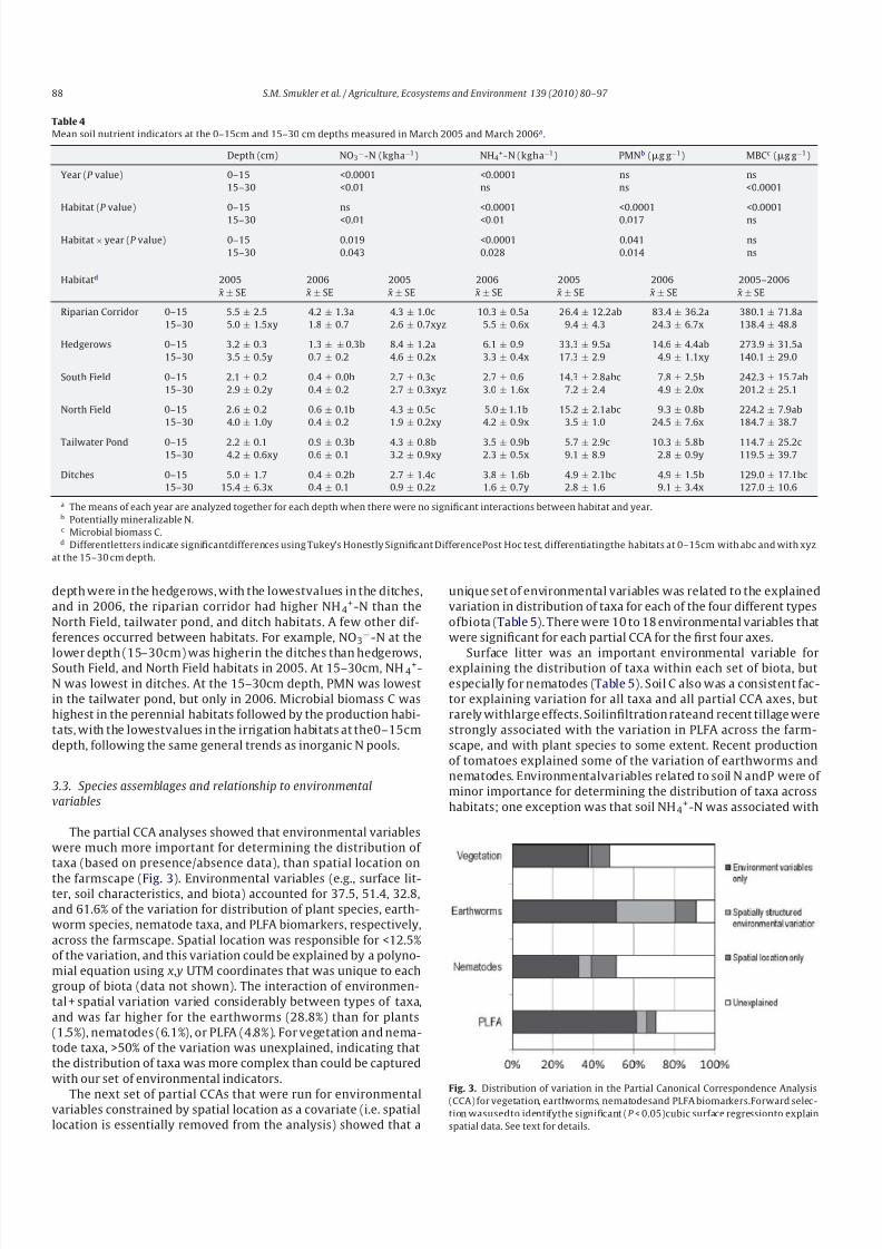
Table 4

Mean soil nutrient indicators at the 0–15cm and 15–30 cm depths measured in March 2005 and March 2006a .

Depth (cm) NO3−-N (kgha−1) NH4

+-N (kgha−1) PMNb (g g−1) MBCc (g g−1)

Year (P value) 0–15 <0.0001 <0.0001 ns ns

15–30 <0.01 ns ns <0.0001

Habitat (P value) 0–15 ns <0.0001 <0.0001 <0.0001

15–30 <0.01 <0.01 0.017 ns

Habitat × year (P value) 0–15 0.019 <0.0001 0.041 ns

15–30 0.043 0.028 0.014 ns

Habitatd 2005 2006 2005 2006 2005 2006 2005–2006

¯ x ± SE ¯ x ± SE ¯ x ± SE ¯ x ± SE ¯ x ± SE ¯ x ± SE ¯ x ± SE

Riparian Corridor 0–15 5.5 ± 2.5 4.2 ± 1.3a 4.3 ± 1.0c 10.3 ± 0.5a 26.4 ± 12.2ab 83.4 ± 36.2a 380.1 ± 71.8a

15–30 5.0 ± 1.5xy 1.8 ± 0.7 2.6 ± 0.7xyz 5.5 ± 0.6x 9.4 ± 4.3 24.3 ± 6.7x 138.4 ± 48.8

Hedgerows 0–15 3.2 ± 0.3 1.3 ± ± 0.3b 8.4 ± 1.2a 6.1 ± 0.9 33.3 ± 9.5a 14.6 ± 4.4ab 273.9 ± 31.5a

15–30 3.5 ± 0.5y 0.7 ± 0.2 4.6 ± 0.2x 3.3 ± 0.4x 17.3 ± 2.9 4.9 ± 1.1xy 140.1 ± 29.0

South Field 0–15 2.1 ± 0.2 0.4 ± 0.0b 2.7 ± 0.3c 2.7 ± 0.6 14.3 ± 2.8abc 7.8 ± 2.5b 242.3 ± 15.7ab

15–30 2.9 ± 0.2y 0.4 ± 0.2 2.7 ± 0.3xyz 3.0 ± 1.6x 7.2 ± 2.4 4.9 ± 2.0x 201.2 ± 25.1

North Field 0–15 2.6 ± 0.2 0.6 ± 0.1b 4.3 ± 0.5c 5.0 ± 1.1b 15.2 ± 2.1abc 9.3 ± 0.8b 224.2 ± 7.9ab

15–30 4.0 ± 1.0y 0.4 ± 0.2 1.9 ± 0.2xy 4.2 ± 0.9x 3.5 ± 1.0 24.5 ± 7.6x 184.7 ± 38.7

Tailwater Pond 0–15 2.2 ± 0.1 0.9 ± 0.3b 4.3 ± 0.8b 3.5 ± 0.9b 5.7 ± 2.9c 10.3 ± 5.8b 114.7 ± 25.2c

15–30 4.2 ± 0.6xy 0.6 ± 0.1 3.2 ± 0.9xy 2.3 ± 0.5x 9.1 ± 8.9 2.8 ± 0.9y 119.5 ± 39.7

Ditches 0–15 5.0 ± 1.7 0.4 ± 0.2b 2.7 ± 1.4c 3.8 ± 1.6b 4.9 ± 2.1bc 4.9 ± 1.5b 129.0 ± 17.1bc

15–30 15.4 ± 6.3x 0.4 ± 0.1 0.9 ± 0.2z 1.6 ± 0.7y 2.8 ± 1.6 9.1 ± 3.4x 127.0 ± 10.6

a The means of each year are analyzed together for each depth when there were no significant interactions between habitat and year.b Potentially mineralizable N.c Microbial biomass C.d Differentletters indicate significantdifferences using Tukey’s Honestly Significant DifferencePost Hoc test, differentiatingthe habitats at 0–15cm with abc and with xyz

at the 15–30 cm depth.

depth were in the hedgerows, with the lowestvalues in the ditches,

and in 2006, the riparian corridor had higher NH4+-N than the

North Field, tailwater pond, and ditch habitats. A few other dif-

ferences occurred between habitats. For example, NO3−-N at the

lower depth (15–30cm) was higherin the ditches than hedgerows,South Field, and North Field habitats in 2005. At 15–30cm, NH4+-

N was lowest in ditches. At the 15–30cm depth, PMN was lowest

in the tailwater pond, but only in 2006. Microbial biomass C was

highest in the perennial habitats followed by the production habi-

tats, with the lowestvalues in the irrigation habitats at the0–15cm

depth, following the same general trends as inorganic N pools.

3.3. Species assemblages and relationship to environmental

variables

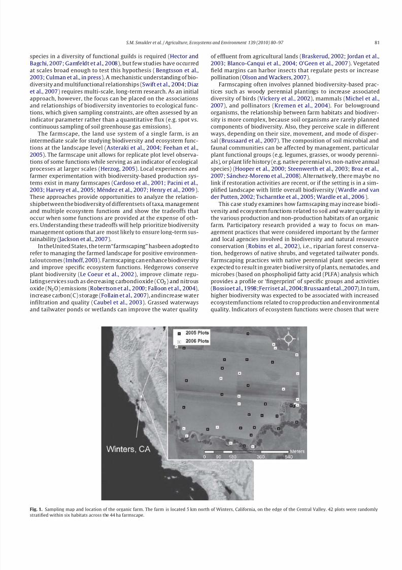
The partial CCA analyses showed that environmental variables

were much more important for determining the distribution of

taxa (based on presence/absence data), than spatial location on

the farmscape (Fig. 3). Environmental variables (e.g., surface lit-ter, soil characteristics, and biota) accounted for 37.5, 51.4, 32.8,

and 61.6% of the variation for distribution of plant species, earth-

worm species, nematode taxa, and PLFA biomarkers, respectively,

across the farmscape. Spatial location was responsible for <12.5%

of the variation, and this variation could be explained by a polyno-

mial equation using x, y UTM coordinates that was unique to each

group of biota (data not shown). The interaction of environmen-

tal + spatial variation varied considerably between types of taxa,

and was far higher for the earthworms (28.8%) than for plants

(1.5%), nematodes (6.1%), or PLFA (4.8%). For vegetation and nema-

tode taxa, >50% of the variation was unexplained, indicating that

the distribution of taxa was more complex than could be captured

with our set of environmental indicators.

The next set of partial CCAs that were run for environmentalvariables constrained by spatial location as a covariate (i.e. spatial

location is essentially removed from the analysis) showed that a

unique set of environmental variables was related to the explained

variation in distribution of taxa for each of the four different types

ofbiota (Table 5). There were 10 to 18 environmental variables that

were significant for each partial CCA for the first four axes.

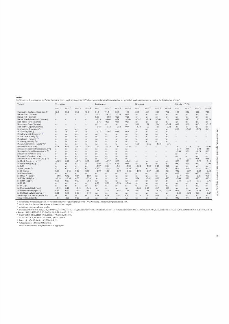
Surface litter was an important environmental variable forexplaining the distribution of taxa within each set of biota, but

especially for nematodes (Table 5). Soil C also was a consistent fac-

tor explaining variation for all taxa and all partial CCA axes, but

rarely withlarge effects. Soilinfiltration rateand recent tillage were

strongly associated with the variation in PLFA across the farm-

scape, and with plant species to some extent. Recent production

of tomatoes explained some of the variation of earthworms and

nematodes. Environmentalvariables related to soil N andP were of

minor importance for determining the distribution of taxa across

habitats; one exception was that soil NH4+-N was associated with

Fig. 3. Distribution of variation in the Partial Canonical Correspondence Analysis

(CCA) for vegetation, earthworms, nematodesand PLFA biomarkers.Forward selec-

tion wasusedto identifythe significant (P < 0.05)cubic surface regressionto explain

spatial data. See text for details.

8/6/2019 Smukler et al. 2010


S .M . S m u k l e r e t a l . / A g r i c u l t ur e ,E c o s y s t e m s a n d

E nv i r o n m e n t 1 3 9

( 2 0 1 0 ) 8 0 – 9 7

8 9

Table 5

Coefficients of determination for Partial Canonical Correspondence Analysis (CCA) of environmental variables controlled for by spatial location covariates to explain the distribution of taxaa .

Variable Vegetation Earthworms Nematodes Microbes (PLFA)

Axis 1 Axis 2 Axis 3 Axis 4 Axis 1 Axis 2 Axis 3 Axis 4 Axis 1 Axis 2 Axis 3 Axis 4 Axis 1 Axis 2 Axis 3 Axis 4

Cumulative Explained Variation (%) 32.0 50.3 63.3 72.6 51.1 71.5 86.7 100 25.1 46.1 63.0 76.2 30.0 52.2 64.2 73.8

Native Grass (% cover) b – – – −0.31 −1.31 −0.24 0.19 nsc ns ns ns ns ns ns ns

Native Forb (% cover) – – – – 0.59 −0.02 0.23 0.36 ns ns ns ns ns ns ns ns

Native Woody Perennials (% cover) – – – – −0.29 −1.04 0.84 −0.63 −0.87 −3.16 −0.63 1.61 0.80 0.97 1.02 −1.74

Non-native Forbs (% cover) – – – – −0.16 0.00 0.81 0.31 ns ns ns ns ns ns ns ns

Non-native Grass (% cover) – – – – nsc ns ns ns 3.11 1.98 5.64 −0.45 0.02 0.19 0.13 −0.17

Non-native Legume (% cover) – – – – −0.43 −0.42 −0.52 0.44 −4.38 1.23 1.01 −0.24 ns ns ns ns

Earthworms (biomass m2) ns ns ns ns – – – – ns ns ns ns 0.16 −0.02 −0.70 0.41

PLFA Total (nmol g−1) ns ns ns ns −0.12 −0.97 0.16 0.08 ns ns ns ns – – – –

PLFA Unclassified (nmol g−1)d ns ns ns ns ns ns ns ns ns ns ns ns – – – –

PLFA Gram+ (nmol g−1)e ns ns ns ns ns ns ns ns ns ns ns ns – – – –

PLFA Gram− (nmolg−1)f ns ns ns ns ns ns ns ns ns ns ns ns – – – –

PLFA Fungi (nmolg−1)g ns ns ns ns ns ns ns ns ns ns ns ns – – – –

PLFA Actinomycetes (nmol g−1)h ns ns ns ns ns ns ns ns 5.08 −0.66 −1.58 −0.75 – – – –

Nematodes Total (no. g−1) 0.01 0.66 −0.13 −0.02 1.37 −0.19 1.11 −0.58 – – – – 1.47 −0.74 1.59 −2.61

Nematodes Bacterial Feeders (no. g−1) ns ns ns ns ns ns ns ns – – – – −0.17 0.16 −0.04 1.86

Nematodes Fungal Feeders (no. g−1) ns ns ns ns ns ns ns ns – – – – −0.66 0.79 −1.76 0.97

Nematodes Predators (no. g−1) ns ns ns ns ns ns ns ns – – – – ns ns ns ns

Nematodes Omnivores (no. g−1) ns ns ns ns ns ns ns ns – – – – ns ns ns ns

Nematodes Plant Parasites (no. g−1) n s ns ns ns ns ns ns ns – – – – −0.52 −0.21 0.18 0.06

Soil Bulk Density (g cm−3)a −0.03 0.42 −0.13 0.07 0.21 −0.37 0.03 −1.41 ns ns ns ns 0.29 0.61 −0.72 −0.19

Soil Moisture (g H2Og −1) ns ns ns ns −0.46 −0.35 0 .59 0.64 ns ns ns ns 0.62 0.35 0.43 −0.03

Soil pH ns ns ns ns −0.37 0.44 −0.41 −0.98 −4.04 −3.90 0 .28 0.20 ns ns ns ns

Soil EC (Sc m−1) ns ns ns ns 0 .77 −0.57 1.30 −2.39 ns ns ns ns 0.75 0.59 −0.71 0.22

Soil C (Mgha−1) 0.07 −0.12 0.10 0.56 −0.70 1.10 −0.79 −0.46 −1.08 −0.67 4.00 0.74 0.02 −0.97 −0.23 −0.50Soil Olsen-P (pg g) ns ns ns ns ns ns ns ns ns ns ns ns 0.12 0.21 0.77 0.09

Soil NCV-N (kgha−1) −0.08 0.42 0.14 −1.00 ns ns ns ns ns ns ns ns −0.17 0.13 −0.41 0.70

Soil NH4+-N (kgha−1) −0.18 −0.56 0.08 −0.38 ns ns ns ns 0.94 −0.82 0.60 4.93 −0.04 0.29 0.23 0.05

Soil PMN (gg −1) 0.05 0.37 0.09 −0.64 ns ns ns ns ns ns ns ns −0.38 −0.11 −0.16 −0.75

Soil % Silt ns ns ns ns 0.33 0.66 −0.59 −0.94 ns ns ns ns ns ns ns ns

Soil % Clay ns ns ns ns ns ns ns ns ns ns ns ns ns ns ns ns

Soil Aggregate MWD (m)i −0.12 0.12 −0.15 −0.43 ns ns ns ns −3.60 0 .19 0.45 0.19 ns ns ns ns

Soil Surface Litter (kgm−2) 0.97 0.42 −0.51 2.19 1.59 1.01 −1.97 1.69 0.42 3.18 −1.23 −0.46 0.14 −0.91 −1.60 2.18

Soil Infiltration Rate (cmmin−1) 0.21 0.01 0.90 −0.10 ns ns ns ns ns ns ns ns −0.32 −0.03 0.23 −0.67

Previous year in tomato production ns ns ns ns 0.22 0.02 −0.07 0.67 −0.78 2.62 0.39 1.47 ns ns ns ns

Tilled within 6 months −0.11 0.35 0.36 1.59 ns ns ns ns ns ns ns ns 0.92 0.41 −1.07 0.49

a Coefficients are only illustrated for variables that were significantly selected ( P <0.05) using a Monte Carlo permutation test.b - indicates that the variable was not included in the analysis.c ns indicates non-significant results.d Unclassified 10:010:0 2OH, 12:0, i13:0,14:0, i15:1@5, i15:1f, i15:1g, unknown 14#503,15:0, i16:1h, 16:1w11c, 16:0, unknown 16#295, i17:1w5c, 15:0 3OH, 17:0, unknown i17:1,16:1 2OH, 10Me17:0,16:0 3OH, 18:0, i18:1h,

unknown 18#715,10Me19:0, 20:2 w6,9c, 20:0, 20:4 co6,9,12,15c.e Gram+i14:0, i15:0, a15:0, i16:0, a16:0, i17:0, a17:0,18:1w7t.f Gram -16:1 w7t, 16:1 w7c, 17:1 w9c, cy17:0, cy19:0.

g Fungi 16:1w5c, 18:1w9c, 18:3 006c (6,9,12).h Actinomycetes 10Me16:0,10me18:0.i MWD refers to mean weight diameter of aggregates.

8/6/2019 Smukler et al. 2010



nematode diversity. Other soil properties were important for spe-

cific types of biota, e.g., a strong negative association with high pH

for nematodes (e.g. Psilenchus). Soil moisture did not have a major

effect on thedistributionof anyof thetypes of biota, confirming that

the goal of sampling in the spring under fairly uniform moisture

conditions had been achieved.

Furthermore, other biota were often more important than soilphysical and chemical properties in explaining the distribution

of taxa in the partial CCAs for environmental variables (Table 5).

For earthworm variation, total nematodes were important along

axis 1, and native grasses, woody perennials, and total PLFA

along axis 2. Plant life history/functional groups present in the

perennial habitats (e.g., native grasses and woody species) were

associated with the earthworms, A. caliginosa and the unidentified

species in the Megascolecidae . For thenematodepartialCCA, trophic

relationships were important in explaining variation (see Sánchez-

Moreno et al.(2008) for details). Several fungal-feeding nematodes

were associated strongly with the actinomycetes PLFA biomark-

ers (e.g., 10Me16:0, 10me18:0). Some plant-parasitic nematodes

were associated with native forbs and previous tomato production

(Sánchez-Moreno et al., 2008). Microbial communities, based onthe PLFA partial CCA, were strongly explained by intertrophic rela-

tionships, such as total nematode biomass and presence/absence

of native woody perennials.

The CCA of the life history/functional groups of plants, nema-

todes, and PLFA, and earthworm species (as function could not

be determined), that was run concurrently with 17 soil and man-

agement variables, showed distinct separation between perennial,

production, and irrigation habitats (data not shown). The first axis

represented this sequential disturbance gradient and explained

37% of the variation. The second and third axes together accounted

for 25% of the variation and were less useful in discerning pat-

terns. This confirms that unexplained variation was high, as was

observed for the partial CCAs (Fig. 3), indicating that unmeasured

factors were important for the distribution of taxa for each group

of biota across the farmscape.

3.4. Indicators of ecosystem functions

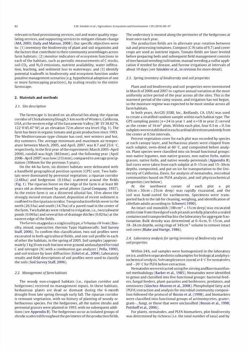
Total C storage (MgC ha−1) in soil and wood was greatest in

the riparian corridor, largely due to woody biomass; it was twice

that found in hedgerows, and more than three times that of the

other habitats (Fig. 4). Total soil C at the 0–15cm depth was

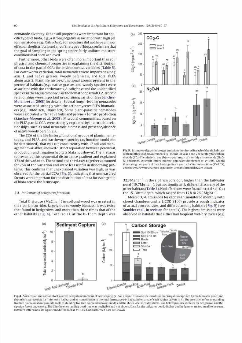
Fig. 5. Estimates of greenhouse gas emissions monitored in each of the six habitats

with monthly spot measurements. (a) means for year 1 and 2 separately for carbon

dioxide (CO2 -C) emissions; and (b) two-year mean of monthly nitrous oxide (N2O-

N) emissions. Different letters indicate significant differences at P < 0.05. Graphs

illustrating two years of data had significant year × habitat interactions (P <0.05),

and thus years were analyzed separately. Untransformed data are shown.

32.3 Mgha−1 in the riparian corridor, higher than the tailwaterpond (19.7Mg ha−1), but not significantly different from any of the

other habitats (Table 3). No differences were found in total soil C at

the 15–30cm depth, which ranged from 17.8 to 26.9Mg ha−1.

Mean CO2-C emissions for each year (monitored monthly with

closed chambers and a LICOR 8100) provide a rough indicator

of actual process rates, and differed among habitats (Fig. 5) (see

Smukler et al., in revision for details). The highest emissions were

observed in habitats that either had frequent wet-dry cycles (e.g.

Fig. 4. Soil erosion and carbon stocks as two ecosystem functions of farmscaping. (a) Soil erosion from one season of summer irrigation captured by the tailwater pond; and

(b) carbon storage (Mg ha−1

) for each habitat and its contribution to the total farmscape (44 ha) based on area of each habitat (given in %). The tree label refers to standinglive tree biomass (aboveground), roots to standing live tree biomass (belowground), and the shrub label includes above- and belowground estimates for hedgerows and the

riparian forest understory. The C in the one standing dead tree was negligible and not shown. Data for the tailwater pond, ditches and hedgerow are too small to be seen.

Different letters indicate significant differences at P < 0.05. Untransformed data are shown.

8/6/2019 Smukler et al. 2010



ditches, and after irrigation in year 1 in the South Field and year

2 the North Field), or high C stocks (e.g. the riparian corridor).

The highest mean value observed for any month was in ditches

in the spring of 2006, after the extremely wet winter (559mg

CO2-C m−2 h−1). In the spring of both years, CO2-C emissions were

>200mgCO2-C m−2 h−1 in the riparian corridor, andcontributed to

the high annual means, which were otherwise low for much of theyear. The lowest average CO2-C emissions were observed in the

rainfed oats of the North Field.

Mean annual N2O-N emissions monitored with closed cham-

bers,againservingas a rough indicatorof actual rates, weregreatest

in the irrigation habitats, but overall were very low for all the habi-

tats (Fig. 5). For example, annual means from the ditches were two

times greater than the production and perennial habitats, butwere

only 16.7g N2O-Nm−2 h−1 (data not shown). Emissions some-

timesspiked considerably,and the highest observed monthly mean

was in the tailwater pond in the fall, after production had ceased

and the pond began to dry (92.8g N2O-Nm−2 h−1). Mean annual

N2O-N emissions from the production fields and perennial habi-

tats did not differ, and were consistently in the range of 4.8 to

8.6g N2O-Nm

−2

h

−1

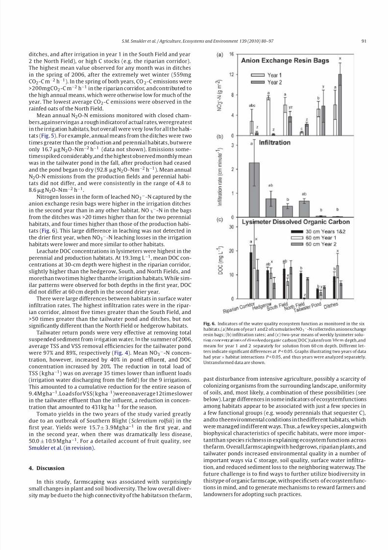
.Nitrogen losses in the form of leached NO3−-N captured by the

anion exchange resin bags were higher in the irrigation ditches

in the second year than in any other habitat. NO 3−-N in the bags

from the ditches was >20 times higher than for the two perennial

habitats, and four times higher than those of the production habi-

tats (Fig. 6). This large difference in leaching was not detected in

the drier first year, when NO3−-N leaching losses in the irrigation

habitats were lower and more similar to other habitats.

Leachate DOC concentrations in lysimeters were highest in the

perennial and production habitats. At 19.3mg L−1, mean DOC con-

centrations at 30-cm depth were highest in the riparian corridor,

slightly higher than the hedgerow, South, and North Fields, and

morethan two times higher thanthe irrigation habitats. While sim-

ilar patterns were observed for both depths in the first year, DOC

did not differ at 60 cm depth in the second drier year.

There were large differences between habitats in surface water

infiltration rates. The highest infiltration rates were in the ripar-

ian corridor, almost five times greater than the South Field, and

>50 times greater than the tailwater pond and ditches, but not

significantly different than the North Field or hedgerow habitats.

Tailwater return ponds were very effective at removing total

suspended sediment from irrigation water. In the summer of 2006,

average TSS and VSS removal efficiencies for the tailwater pond

were 97% and 89%, respectively (Fig. 4). Mean NO3−-N concen-

tration, however, increased by 40% in pond effluent, and DOC

concentration increased by 20%. The reduction in total load of

TSS (kgha−1) was on average 35 times lower than influent loads

(irrigation water discharging from the field) for the 9 irrigations.

This amounted to a cumulative reduction for the entire season of 9.4Mgha−1.LoadsforVSS(kgha−1)wereonaverage12timeslower

in the tailwater effluent than the influent, a reduction in concen-

tration that amounted to 431kg ha−1 for the season.

Tomato yields in the two years of the study varied greatly

due to an outbreak of Southern Blight (Sclerotium rolfsii) in the

first year. Yields were 15.7± 3.9Mgha−1 in the first year, and

in the second year, when there was dramatically less disease,

50.0 ± 10.9 Mgha−1. For a detailed account of fruit quality, see

Smukler et al. (in revision).

4. Discussion

In this study, farmscaping was associated with surprisinglysmall changes in plant and soil biodiversity. The low overall diver-

sity may be dueto the high connectivity of the habitatson thefarm,

Fig. 6. Indicators of the water quality ecosystem function as monitored in the six

habitats.(a)Means ofyear1 and2 ofcumulativeNO3−-N collectedin anionexchange

resin bags; (b) infiltration rates; and (c) two-year means of weekly lysimeter solu-

tion concentrations of dissolvedorganic carbon(DOC)takenfrom 30cm depth,and

means for year 1 and 2 separately for solution from 60 cm depth. Different let-

ters indicate significant differences at P < 0.05. Graphs illustrating two years of data

had year × habitat interactions P < 0.05, and thus years were analyzed separately.

Untransformed data are shown.

past disturbance from intensive agriculture, possibly a scarcity of

colonizing organisms from the surrounding landscape, uniformityof soils, and, most likely, a combination of these possibilities (see

below). Large differences in some indicators of ecosystemfunctions

among habitats appear to be associated with just a few species in

a few functional groups (e.g. woody perennials that sequester C),

andto theenvironmental conditions in thedifferent habitats, which

were managed indifferent ways. Thus, a fewkey species, alongwith

biophysical characteristics of specific habitats, were more impor-

tantthan species richness in explaining ecosystem functions across

thefarm. Overall,farmscapingwith hedgerows, riparian plants, and

tailwater ponds increased environmental quality in a number of

important ways via C storage, soil quality, surface water infiltra-

tion, and reduced sediment loss to the neighboring waterway. The

future challenge is to find ways to further utilize biodiversity in

thistype of organic farmscape, withspecificsets of ecosystem func-tions in mind, and to generate mechanisms to reward farmers and

landowners for adopting such practices.

8/6/2019 Smukler et al. 2010



4.1. Research design

The farmscape in this study was selected for a number of rea-

sons. It is a working farm which, of necessity, implements adaptive

management practices. It is an organic farm, which is likely the

best-case scenario for maximizing biodiversity (Drinkwater et al.,

1995;Bossioet al., 1998;Holeet al., 2005).The farmscapealsohad amature riparian forest, hedgerows, tailwater ponds, and was oper-

ated by an innovative farmer-cooperator, who plays a leadership

role for farmers in the area. Finally, like many farms in California’s

Central Valley, the native woodlands at thissite had beenconverted

to highly intensive grain and vegetable production at the beginning

of the last century.

Stratified random sampling was used to evaluate the contribu-

tions of the six habitats to the biodiversity and ecosystem function

within this farmscape. Selecting a farmscape on a single soil type

was an effort to increase statistical robustness. Effort was made to

replicate and randomize, but a more robust design (e.g. a random-

ized complete block design) was not possible given the different

configurationand size of the habitattypes. For example, interspers-

ing or randomizing mature riparian forests and tomato productionareas was impossible within the same area. No other similar farms

exist to serve as replications, but the results are still broadly rele-

vant to other agricultural situations.

4.2. Plant biodiversity

We expected that farmscaping practices designed to increase

biotic habitat along field margins would increase both landscape-

and plot-level plant and soil biodiversity. In particular, we thought

that an increase in plant diversity would increase belowground

biodiversity (Hooper et al., 2000). However, comparison of undis-

turbed habitats dominated by woody perennial vegetation vs. the

large fields under organic agricultural production and their con-

nected irrigation habitats revealed surprisingly subtle differences

in plant, and especially soil biodiversity.

Riparian habitat has elsewhere been shown to be important

zone for maintaining landscape biodiversity (Naiman et al., 1993).

Here, plots in the riparian habitat had an average of only 10 plant

species, whichis extremelylow compared to the numberof species

(between 254 and 684) found in some wildland riparian zones

in the mountains of nearby Oregon (Planty-Tabacchi et al., 1996).

Published plant species lists of riparian forests in the Sacramento

Valley are not complete inventories (e.g ., Harris, 1987), but undis-

turbed riparian vegetation is described as having some of the

highest productivity and diversity of any California ecosystem due

to the year-round water supply in this Mediterranean-type climate

(Holstein, 1984; Barbour et al.,1993).In a floodplainabove a contin-

uously flooded zone (2–6 m above the water), undisturbed forests

canhave a complex architecture with typically five species of over-story trees, five species of shrubs, several vine species, and many

annual and perennial herbs. Most (>90%) of the Central Valley’s

riparian forests, however, have been cleared and the soil has been

disturbed; they are now relegated to narrow bands at the edge

of stream channels (Barbour et al., 1993; Seavy et al., 2009), as

observed here. The low number of plant species in the relatively

small patches of perennial plant habitats in this farmscape may

also be in part due to the simplicity of the surrounding landscape

(Culman et al., in press). There may be a minimum threshold of

complexity and connectivity required for a surrounding landscape

to provide the colonization potential to maintain the biodiversity

of these riparian forests (Tscharntke et al., 2005; Concepcion et al.,

2008).

With fewer species present in an ecosystemor farmscape, smallincreases in biodiversity may become more important for ecosys-

temfunction than in higherdiversitysystems,as redundancy is less

likely to occur (Naeem et al., 1994; Tilman and Downing, 1994). In

fact, one of the major differences in ecosystem function between

the habitatswasC storage,due toa fewspeciesof woodyperennials.

Thesefew species, found onlyin theripariancorridor andhedgerow

habitats, were associated with higher soil infiltration rates, likely

due to higher soil organic matter inputs, increased aggregate sta-

bility and absence of heavy traffic.

4.3. Soil biodiversity

Soil biodiversity, as indicated by the few groups of organisms

studied, may be explained by a combination of environmental and

intertrophic interactions. Earthworm diversity was consistently

low across this farmscape, as is found for other nearby agricul-

tural sites, including other organic farms (Fonte et al., 2009). Lack

of tillage, less compaction, and high inputs of organic matter likely

contribute to the higher abundance of earthworms in the perennial

habitats (Curry et al., 2002; Chan and Barchia, 2007). Moreover,

these habitats would be expected to provide both an abundant

food source and a distinct litter layer that would help to conserve

soil moisture and lessen temperature fluctuations, which promoteearthworm growth and survival. Although ANOVA showed no dif-

ferences among habitats, multivariate statistics indicated thatboth

A. caliginosa and the Megascolecid spp. tended to be associated

withthe less-disturbed perennial habitats, while A. trapezoides was

more prevalent in production habitats, possibly because it is more

tolerant across a broader range of environmental stresses (Mele

and Carter, 1999; Chan and Barchia, 2007). Earthworm taxa were

more affected by spatial/environmental correlation than other soil

organisms corroborating evidence for strong spatial aggregation in

earthwormpopulations (Poier andRichter, 1992; Rossi and Lavelle,

1998). Thus more intensive sampling may be necessary to better

assess the environmental and trophic factors controlling earth-

worm differences among habitats.

Multivariate analysis suggested that the abundance of earth-

worms is associated with other trophic groups, particularly

nematodes. Low nematode survival rates due to earthworm gut

transit have been reported (Monroy et al., 2008), and nematode

populations have been drastically reduced by earthworms in a

microcosm experiments (Räty and Huhta, 2003). In this study,

the abundance of nematode functional groups were negatively

associated with the earthworm, A. caliginosa, but were not signifi-

cantly correlated with earthworm abundance in general (Table 5).

Nematode functional groups instead were more correlated with

actinomycete PLFA biomarkers and plant functional groups. One

possible explanation for this relationship is that the nematode

fungal feeders consumedfungi, opening a niche for competing acti-

nomycetes. Alternatively, fewer bacterial feeding nematodes may

be associated with higher actinomycete abundance (Wardle et al.,

2006).Thelack of differences in nematodeabundance andlow diversity

at the plot level among the perennial and crop production habitats

was unexpected given the divergent forms of habitat management

(Freckman and Ettema, 1993; Neher, 2001; Ou et al., 2005). Tillage

was not a significant explanatory variable in the nematode partial

CCA, but surface litter and pH correlations were large, suggesting

that organic matter management may be more important than

disturbance. A nearby study on a similar soil type showed that

organic matter additions can increase the nematode abundance

morerapidlythan conversion to no-tillage (Minoshimaet al.,2007).

Many decades of prior intensive agriculture may have selected for

nematodes that are resistant and resilient to tillage and intermit-

tent moisture, and this may explain the very low species richness,

i.e.,15 taxain thecultivated fields. Across theentire farmscape, only37 taxa were observed. Including the perennial plant habitats only

slightly increased diversity. By contrast, in an extensive review, 15

8/6/2019 Smukler et al. 2010



to 82 taxa were reported for temperate cultivated ecosystems, and

13 to as many as 175 species for temperate broadleaved forests

(Boag and Yeates, 1998).

Total PLFA in the production field plots were similar

(∼40nmolg−1 soil) to those reported in a study across the State

of California (Drenovsky et al., 2010). But, the mean number of

PLFA observed per habitat (40–45) was in the middle of the rangereported in the same study, from 30in deserts to 55 in rice produc-

tionsystems.Overall, the77 PLFAfound across theentire farmscape

is low,consideringthe potentialdiversity thatexists in forested and

agricultural ecosystems in California.

The low soil biodiversity within and among habitats may be a

result of past or recurring disturbance, as well as lack of coloniza-

tion potential from neighboring ecosystems. The production fields

experience tillage, fluctuating water regimes, sporadic plant cover,

and nutrient inputs, which constitute frequent and intensive dis-

turbance. In the perennialhabitats, disturbances consist of flooding

in the ripariancorridor, erosion from crop fields,or tramplingof the

hedgerows (i.e. farm workers often use the hedgerows for shade

during the hot summers). It is also possible that the soil ecosystem

is still recovering from the disturbance initiated by European set-tlers who arrived in the1880s. At some point shortly thereafter, the

alluvial valley was leveled for farming operations, the slough was

deepened and bermed, and the undulating hills nearby were tilled

andgrazed,which inevitably resulted in the loss of topsoil (Vaught,

2007). Since these types of disturbance were nearly ubiquitous in

the landscape with the widespread adoption of intensive agricul-

ture, colonization may be limited by lack of nearby habitats with

richer biodiversity.

4.4. Soil properties

Despite the apparent differences in habitat vegetation and man-

agement,soil propertieswere quite similar among all habitats. Even

though higher plant biomass occurred in the riparian corridor, soil

C wasnot significantlygreater than in theproduction habitats. This

may be related to the high inputs of organic material applied every

year (> 15Mgha−1 of compost) to produce organic crops. Soil C

(21.8 and 22.4 Mg C ha−1 at 0–15 cm depth in the South and North

Field, respectively)was similar to fields under organicmanagement

at a nearbyresearchstation(22.8 MgC ha−1) (Kong et al., 2005). The

long-term research station study reported much higher concentra-

tions of soil C than conventional plots (16.1 Mg C ha−1) indicating

that substantial C can accumulate under organic management in a

period of only 10–15 years.

Soil aggregate stability demonstrated the most pronounced

differences for soil properties among habitats. Mean weight

of diameter (MWD) values for the farm’s production fields

(0.9–1.0mm) were similar to values for organic production at the

nearby research station (0.3–1.2mm, respectively, for conventionaland organic fields) (Kong et al., 2005). Aggregate stability in the

hedgerows (2.1mm) was more than double that observed for the

other farmscape habitats. These high values likely result from a

combination of low disturbance, diverse types of plant litter, and

the absence of mineral N fertilizers (Bronick and Lal, 2005). Curi-

ously, despite a longer period of such conditions, the soils of the

riparian corridor had lower aggregate stability than the hedgerow

soils. This might be explained by more erosion on steeper slopes

and deeper rooting systems than the hedgerow shrubs.

Some habitats were more homogenous in their soil properties

than others (e.g. the high SE of Olsen P in the riparian corridor

vs. other habitats). Variability in the riparian corridor is likely

due to the interactions between topography, the influence of the

ephemeral stream flow (deposition and erosion), and patchy plantcommunity composition. The diversity of substrates from different

life formsof plants, withdifferent functional traits, in theory should

result in a diversity of belowground soil organisms (Hooper et al.,

2000; Wardle, 2006). But as mentioned above, the differences in

plant species composition among habitatswere notassociated with

concomitant difference in the belowground communities (Hooper

et al., 2005).

4.5. Ecosystem functions

The C stocks in the mature riparian forest tree biomass far

exceeded the storage of soil C (0–30cm depth) in the produc-

tion fields on a per ha basis. It should be noted, however, that

these data for soil C at 0–30cm depth underestimate the pool

of soil C at 0–100cm depth by about half, based on a survey of

cropland and riparian corridor soils surrounding this project site

(Young-Mathews et al., 2010).The estimated 70.8Mg C ha−1 stored

in aboveground woody biomass was lower than a pristine ripar-

ian forest in South Carolina Coastal plains (98.2 Mg C ha−1) (Giese

et al., 2003). It was, however, greater than the estimated poten-

tial 50MgCha−1 for afforestation of marginal agricultural lands

in the Midwest USA (Niu and Duiker, 2006). Including the esti-

mates for soil, roots, litter and understory shrubs, the C stocks(157.7MgCha−1) in the small area of riparian forest (6%) repre-

sents a disproportionate amount of thetotal C stock (18%) measured

within the farmscape (Fig. 4b). Hedgerowsstored1% of the totalC in

the farmscape. If soil data had been collected at 30–100 cm depth,

these percentages would decrease, as would excluding C in leaves

and in fine roots. Even so, woody perennials are an important pool

of C storage in the farmscape.

Higher rates of CO2-C emissions occurred during the rainy sea-

sonin thelatefall,winter,and early springin the perennialhabitats,

while highest summer emissions occurred in the production habi-

tats during the irrigated growing season. Despite the different

seasonal emissions patterns, annual means were similar. N2O-N

emissions, however, were much larger in irrigation habitats. The

highest fluxobservedon this farmscape(in thetailwater pond) was

still an order of magnitude lower than what others have found in

agricultural soils (Matson et al., 1998; Burger et al., 2005), proba-

bly due to the low level of mineral N in the production system (see

Smukler et al., in revision). Higher rates of gas emissions found in

ditches were likely a combination of two factors: (1) high influx of

mineral N via the accumulation of water with high levels of dis-

solved N and deposition of N-rich eroded soil; and (2) frequent

wetting cycles that saturated the soil during the warmest time of

the year.

Althoughlarge quantities of sedimentwere lostin surface runoff

from the production fields (see Smukler et al., in revision for

details), most was captured by the tailwater pond (Fig. 4a). With

no tailwater pond, this sediment would have discharged directly

into the adjacent riparian corridor. And without a pump to return

irrigation water to the field, DOC that accumulated in the pondwould have discharged into the riparian zone.

The higher DOC concentrations in the soil solution in the peren-

nial habitats compared to the fields were similar in range to

concentrations found in a prairie vs. agriculture production study

in Wisconsin (5 to 20 mg DOCL−1) (Brye et al., 2001). Pore water

NO3−-N, measured in lysimeters and resin bags, was low relative

to other studies. Infiltration rates were also high in the riparian

corridor, similar to a study showing rates that were 6 times higher

in the riparian buffer compared to corn and pasture ( Bharati et al.,

2002). High infiltration rates are an indicatorof regulating services,

as they prevent surface erosion and promote aquifer recharge, but

are also likely to increase the loss of DOC by leaching and transport

into the adjacent waterway, which is a concern for downstream

water quality (Fujii et al., 1998).The non-production habitats have little impact on the farm’s

food provisioning functions. Some local farmers are reluctant to

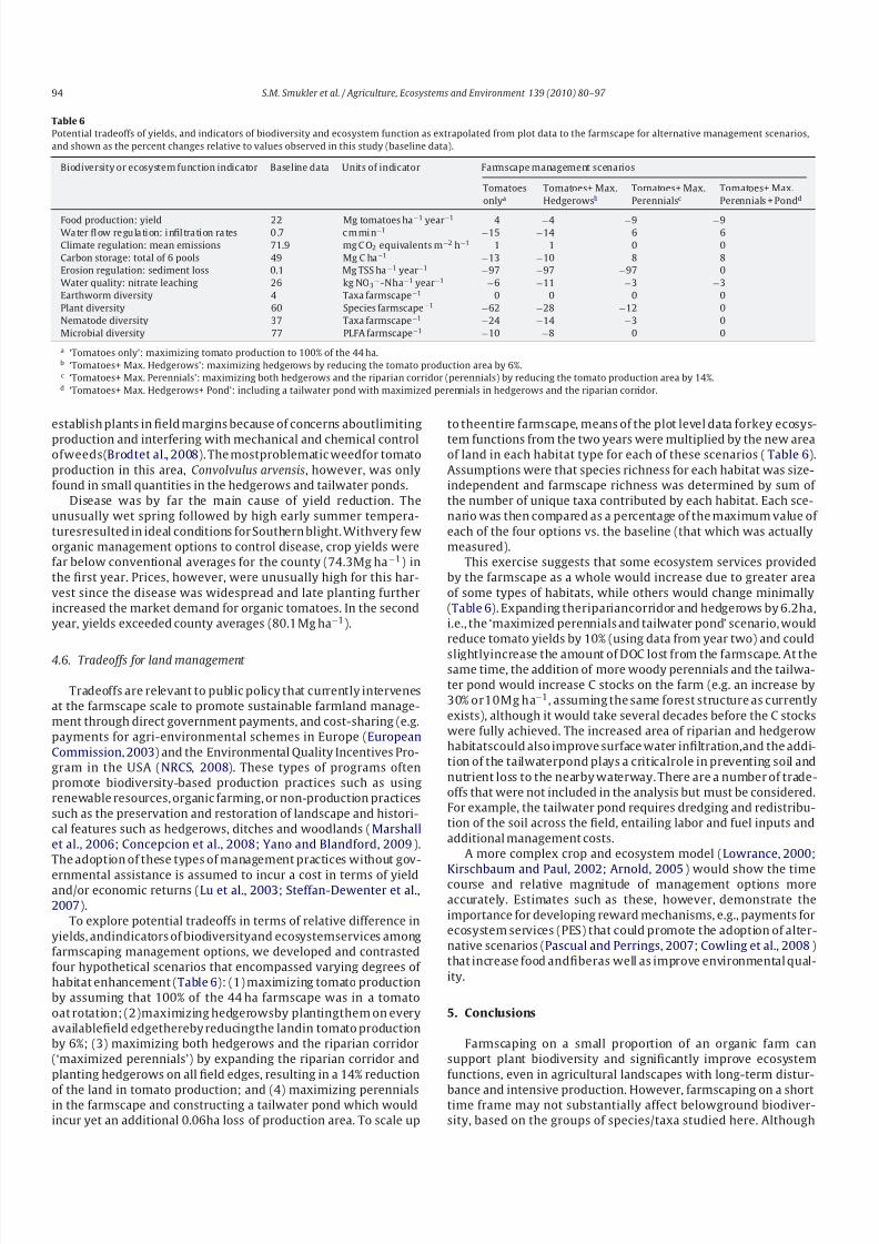
8/6/2019 Smukler et al. 2010



Table 6

Potential tradeoffs of yields, and indicators of biodiversity and ecosystem function as extrapolated from plot data to the farmscape for alternative management scenarios,

and shown as the percent changes relative to values observed in this study (baseline data).

Biodiversity or ecosystem function indicator Baseline data Units of indicator Farmscape management scenarios

Tomatoes

onlya

Tomatoes+ Max.

Hedgerowsb

Tomatoes+ Max.

Perennialsc

Tomatoes+ Max.

Perennials + Pondd

Food production: yield 22 Mg tomatoes ha−1 year−1 4 −4 −9 −9Water flow re gulation: infiltration rates 0.7 cm min−1 −15 −14 6 6

Climate regulation: mean emissions 71.9 mg C O2 equivalents m−2 h−1 1 1 0 0

Carbon storage: total of 6 pools 49 Mg C ha−1 −13 −10 8 8

Erosion regulation: sediment loss 0.1 Mg TSS ha−1 year−1 −97 −97 −97 0

Water quality: nitrate leaching 26 kg NO3−-Nha−1 year−1 −6 −11 −3 −3

Earthworm diversity 4 Taxa farmscape−1 0 0 0 0

Plant diversity 60 Species farmscape−1 −62 −28 −12 0

Nematode diversity 37 Taxa farmscape−1 −24 −14 −3 0

Microbial diversity 77 PLFA farmscape−1 −10 −8 0 0

a ‘Tomatoes only’: maximizing tomato production to 100% of the 44 ha.b ‘Tomatoes+ Max. Hedgerows’: maximizing hedgerows by reducing the tomato production area by 6%.c ‘Tomatoes+ Max. Perennials’: maximizing both hedgerows and the riparian corridor (perennials) by reducing the tomato production area by 14%.d ‘Tomatoes+ Max. Hedgerows+ Pond’: including a tailwater pond with maximized perennials in hedgerows and the riparian corridor.

establish plants in field margins because of concerns aboutlimiting

production and interfering with mechanical and chemical controlofweeds(Brodtet al., 2008). The mostproblematic weedfor tomato

production in this area, Convolvulus arvensis, however, was only

found in small quantities in the hedgerows and tailwater ponds.

Disease was by far the main cause of yield reduction. The

unusually wet spring followed by high early summer tempera-

turesresulted in ideal conditions for Southern blight. Withvery few

organic management options to control disease, crop yields were

far below conventional averages for the county (74.3Mg ha−1) in

the first year. Prices, however, were unusually high for this har-

vest since the disease was widespread and late planting further

increased the market demand for organic tomatoes. In the second

year, yields exceeded county averages (80.1Mg ha−1).

4.6. Tradeoffs for land management

Tradeoffs are relevant to public policy that currently intervenes

at the farmscape scale to promote sustainable farmland manage-

ment through direct government payments, and cost-sharing (e.g.

payments for agri-environmental schemes in Europe (European

Commission, 2003) and the Environmental Quality Incentives Pro-

gram in the USA (NRCS, 2008). These types of programs often

promote biodiversity-based production practices such as using

renewable resources, organic farming, or non-production practices

such as the preservation and restoration of landscape and histori-

cal features such as hedgerows, ditches and woodlands (Marshall

et al., 2006; Concepcion et al., 2008; Yano and Blandford, 2009).

The adoption of these types of management practices without gov-

ernmental assistance is assumed to incur a cost in terms of yieldand/or economic returns (Lu et al., 2003; Steffan-Dewenter et al.,

2007).

To explore potential tradeoffs in terms of relative difference in

yields, andindicators of biodiversityand ecosystemservices among

farmscaping management options, we developed and contrasted

four hypothetical scenarios that encompassed varying degrees of

habitat enhancement (Table 6): (1) maximizing tomato production

by assuming that 100% of the 44 ha farmscape was in a tomato

oat rotation; (2)maximizing hedgerowsby plantingthem on every

availablefield edgethereby reducingthe landin tomato production

by 6%; (3) maximizing both hedgerows and the riparian corridor

(‘maximized perennials’) by expanding the riparian corridor and

planting hedgerows on all field edges, resulting in a 14% reduction

of the land in tomato production; and (4) maximizing perennialsin the farmscape and constructing a tailwater pond which would

incur yet an additional 0.06ha loss of production area. To scale up

to theentire farmscape, means of the plot level data forkey ecosys-

tem functions from the two years were multiplied by the new areaof land in each habitat type for each of these scenarios ( Table 6).

Assumptions were that species richness for each habitat was size-

independent and farmscape richness was determined by sum of

the number of unique taxa contributed by each habitat. Each sce-

nario was then compared as a percentage of the maximum value of

each of the four options vs. the baseline (that which was actually

measured).

This exercise suggests that some ecosystem services provided

by the farmscape as a whole would increase due to greater area

of some types of habitats, while others would change minimally

(Table 6). Expanding theripariancorridor and hedgerows by 6.2ha,

i.e., the ‘maximized perennials and tailwater pond’ scenario, would

reduce tomato yields by 10% (using data from year two) and could

slightlyincrease the amount of DOC lost from the farmscape. At thesame time, the addition of more woody perennials and the tailwa-

ter pond would increase C stocks on the farm (e.g. an increase by

30% or10Mg ha−1, assuming the same forest structure as currently

exists), although it would take several decades before the C stocks

were fully achieved. The increased area of riparian and hedgerow

habitatscould also improve surface water infiltration,and the addi-

tion of the tailwaterpond plays a criticalrole in preventing soil and

nutrient loss to the nearby waterway. There are a number of trade-

offs that were not included in the analysis but must be considered.

For example, the tailwater pond requires dredging and redistribu-

tion of the soil across the field, entailing labor and fuel inputs and

additional management costs.

A more complex crop and ecosystem model (Lowrance, 2000;

Kirschbaum and Paul, 2002; Arnold, 2005) would show the timecourse and relative magnitude of management options more

accurately. Estimates such as these, however, demonstrate the

importance for developing reward mechanisms, e.g., payments for

ecosystem services (PES) that could promote the adoption of alter-

native scenarios (Pascual and Perrings, 2007; Cowling et al., 2008)

that increase food andfiberas well as improve environmental qual-

ity.

5. Conclusions

Farmscaping on a small proportion of an organic farm can

support plant biodiversity and significantly improve ecosystem

functions, even in agricultural landscapes with long-term distur-

bance and intensive production. However, farmscaping on a shorttime frame may not substantially affect belowground biodiver-

sity, based on the groups of species/taxa studied here. Although

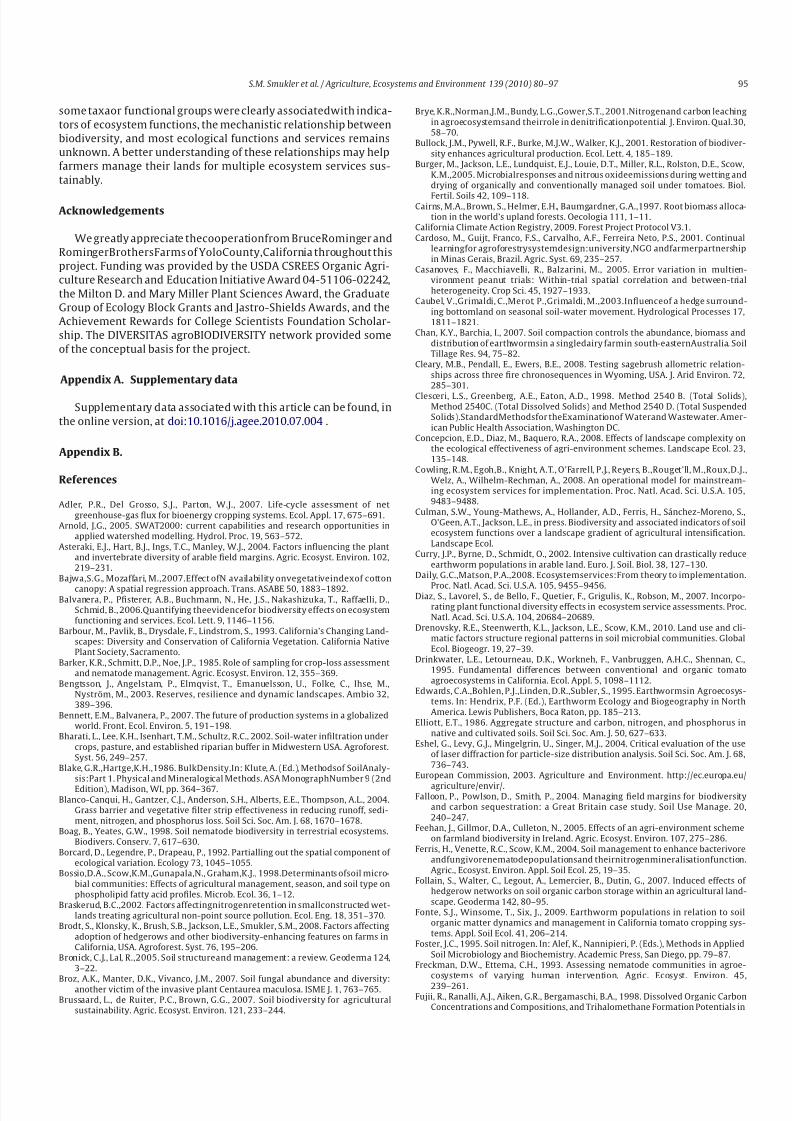
8/6/2019 Smukler et al. 2010



some taxaor functional groups were clearly associatedwith indica-

tors of ecosystem functions, the mechanistic relationship between

biodiversity, and most ecological functions and services remains

unknown. A better understanding of these relationships may help

farmers manage their lands for multiple ecosystem services sus-

tainably.

Acknowledgements

We greatly appreciate thecooperationfrom BruceRominger and

RomingerBrothersFarms of YoloCounty,California throughout this

project. Funding was provided by the USDA CSREES Organic Agri-

culture Research and Education Initiative Award 04-51106-02242,

the Milton D. and Mary Miller Plant Sciences Award, the Graduate

Group of Ecology Block Grants and Jastro-Shields Awards, and the

Achievement Rewards for College Scientists Foundation Scholar-

ship. The DIVERSITAS agroBIODIVERSITY network provided some

of the conceptual basis for the project.

Appendix A. Supplementary data

Supplementary data associated with this article can be found, in

the online version, at doi:10.1016/j.agee.2010.07.004 .

Appendix B.

References

Adler, P.R., Del Grosso, S.J., Parton, W.J., 2007. Life-cycle assessment of netgreenhouse-gas flux for bioenergy cropping systems. Ecol. Appl. 17, 675–691.

Arnold, J.G., 2005. SWAT2000: current capabilities and research opportunities inapplied watershed modelling. Hydrol. Proc. 19, 563–572.

Asteraki, E.J., Hart, B.J., Ings, T.C., Manley, W.J., 2004. Factors influencing the plantand invertebrate diversity of arable field margins. Agric. Ecosyst. Environ. 102,219–231.

Bajwa,S.G., Mozaffari, M.,2007.Effect ofN availability onvegetativeindexof cotton

canopy: A spatial regression approach. Trans. ASABE 50, 1883–1892.Balvanera, P., Pfisterer, A.B., Buchmann, N., He, J.S., Nakashizuka, T., Raffaelli, D.,

Schmid, B., 2006.Quantifying theevidencefor biodiversity effects on ecosystemfunctioning and services. Ecol. Lett. 9, 1146–1156.

Barbour, M., Pavlik, B., Drysdale, F., Lindstrom, S., 1993. California’s Changing Land-scapes: Diversity and Conservation of California Vegetation. California NativePlant Society, Sacramento.

Barker, K.R., Schmitt, D.P., Noe, J.P., 1985. Role of sampling for crop-loss assessmentand nematode management. Agric. Ecosyst. Environ. 12, 355–369.

Bengtsson, J., Angelstam, P., Elmqvist, T., Emanuelsson, U., Folke, C., Ihse, M.,Nyström, M., 2003. Reserves, resilience and dynamic landscapes. Ambio 32,389–396.

Bennett, E.M., Balvanera, P., 2007. The future of production systems in a globalizedworld. Front. Ecol. Environ. 5, 191–198.

Bharati, L., Lee, K.H., Isenhart, T.M., Schultz, R.C., 2002. Soil-water infiltration undercrops, pasture, and established riparian buffer in Midwestern USA. Agroforest.Syst. 56, 249–257.

Blake, G.R.,Hartge,K.H.,1986. BulkDensity.In: Klute, A. (Ed.), Methodsof SoilAnaly-sis:Part 1. Physical and Mineralogical Methods. ASA MonographNumber 9 (2nd

Edition), Madison, WI, pp. 364–367.Blanco-Canqui, H., Gantzer, C.J., Anderson, S.H., Alberts, E.E., Thompson, A.L., 2004.

Grass barrier and vegetative filter strip effectiveness in reducing runoff, sedi-ment, nitrogen, and phosphorus loss. Soil Sci. Soc. Am. J. 68, 1670–1678.

Boag, B., Yeates, G.W., 1998. Soil nematode biodiversity in terrestrial ecosystems.Biodivers. Conserv. 7, 617–630.

Borcard, D., Legendre, P., Drapeau, P., 1992. Partialling out the spatial component of ecological variation. Ecology 73, 1045–1055.

Bossio,D.A., Scow,K.M.,Gunapala,N., Graham,K.J., 1998.Determinants ofsoil micro-bial communities: Effects of agricultural management, season, and soil type onphospholipid fatty acid profiles. Microb. Ecol. 36, 1–12.

Braskerud, B.C.,2002. Factors affectingnitrogenretention in smallconstructed wet-lands treating agricultural non-point source pollution. Ecol. Eng. 18, 351–370.

Brodt, S., Klonsky, K., Brush, S.B., Jackson, L.E., Smukler, S.M., 2008. Factors affectingadoption of hedgerows and other biodiversity-enhancing features on farms inCalifornia, USA. Agroforest. Syst. 76, 195–206.

Bronick, C.J., Lal, R.,2005. Soil structureand management: a review. Geoderma 124,3–22.

Broz, A.K., Manter, D.K., Vivanco, J.M., 2007. Soil fungal abundance and diversity:another victim of the invasive plant Centaurea maculosa. ISME J. 1, 763–765.Brussaard, L., de Ruiter, P.C., Brown, G.G., 2007. Soil biodiversity for agricultural

sustainability. Agric. Ecosyst. Environ. 121, 233–244.

Brye, K.R.,Norman,J.M., Bundy, L.G.,Gower,S.T., 2001.Nitrogenand carbon leachingin agroecosystemsand theirrole in denitrificationpotential. J. Environ. Qual.30,58–70.

Bullock, J.M., Pywell, R.F., Burke, M.J.W., Walker, K.J., 2001. Restoration of biodiver-sity enhances agricultural production. Ecol. Lett. 4, 185–189.

Burger, M., Jackson, L.E., Lundquist, E.J., Louie, D.T., Miller, R.L., Rolston, D.E., Scow,K.M.,2005. Microbialresponses and nitrous oxideemissions during wetting anddrying of organically and conventionally managed soil under tomatoes. Biol.

Fertil. Soils 42, 109–118.Cairns, M.A., Brown, S., Helmer, E.H., Baumgardner, G.A.,1997. Root biomass alloca-

tion in the world’s upland forests. Oecologia 111, 1–11.California Climate Action Registry, 2009. Forest Project Protocol V3.1.Cardoso, M., Guijt, Franco, F.S., Carvalho, A.F., Ferreira Neto, P.S., 2001. Continual

learningfor agroforestrysystemdesign:university,NGO andfarmerpartnershipin Minas Gerais, Brazil. Agric. Syst. 69, 235–257.

Casanoves, F., Macchiavelli, R., Balzarini, M., 2005. Error variation in multien-vironment peanut trials: Within-trial spatial correlation and between-trialheterogeneity. Crop Sci. 45, 1927–1933.

Caubel, V.,Grimaldi, C.,Merot, P.,Grimaldi, M.,2003.Influenceof a hedge surround-ing bottomland on seasonal soil-water movement. Hydrological Processes 17,1811–1821.

Chan, K.Y., Barchia, I., 2007. Soil compaction controls the abundance, biomass anddistribution of earthwormsin a singledairy farmin south-easternAustralia. SoilTillage Res. 94, 75–82.

Cleary, M.B., Pendall, E., Ewers, B.E., 2008. Testing sagebrush allometric relation-ships across three fire chronosequences in Wyoming, USA. J. Arid Environ. 72,285–301.

Clesceri, L.S., Greenberg, A.E., Eaton, A.D., 1998. Method 2540 B. (Total Solids),Method 2540C. (Total Dissolved Solids) and Method 2540 D. (Total SuspendedSolids).StandardMethodsfor theExaminationof Waterand Wastewater. Amer-ican Public Health Association, Washington DC.

Concepcion, E.D., Diaz, M., Baquero, R.A., 2008. Effects of landscape complexity onthe ecological effectiveness of agri-environment schemes. Landscape Ecol. 23,135–148.

Cowling, R.M., Egoh,B., Knight, A.T., O’Farrell, P.J., Reyers, B.,Rouget’ll, M.,Roux,D.J.,Welz, A., Wilhelm-Rechman, A., 2008. An operational model for mainstream-ing ecosystem services for implementation. Proc. Natl. Acad. Sci. U.S.A. 105,9483–9488.

Culman, S.W., Young-Mathews, A., Hollander, A.D., Ferris, H., Sánchez-Moreno, S.,O’Geen, A.T., Jackson, L.E., in press. Biodiversity and associated indicators of soilecosystem functions over a landscape gradient of agricultural intensification.Landscape Ecol.

Curry, J.P., Byrne, D., Schmidt, O., 2002. Intensive cultivation can drastically reduceearthworm populations in arable land. Euro. J. Soil. Biol. 38, 127–130.

Daily, G.C.,Matson, P.A.,2008. Ecosystemservices:From theory to implementation.

Proc. Natl. Acad. Sci. U.S.A. 105, 9455–9456.Diaz, S., Lavorel, S., de Bello, F., Quetier, F., Grigulis, K., Robson, M., 2007. Incorpo-rating plant functional diversity effects in ecosystem service assessments. Proc.Natl. Acad. Sci. U.S.A. 104, 20684–20689.

Drenovsky, R.E., Steenwerth, K.L., Jackson, L.E., Scow, K.M., 2010. Land use and cli-matic factors structure regional patterns in soil microbial communities. GlobalEcol. Biogeogr. 19, 27–39.

Drinkwater, L.E., Letourneau, D.K., Workneh, F., Vanbruggen, A.H.C., Shennan, C.,1995. Fundamental differences between conventional and organic tomatoagroecosystems in California. Ecol. Appl. 5, 1098–1112.

Edwards, C.A.,Bohlen, P.J.,Linden, D.R.,Subler, S., 1995. Earthwormsin Agroecosys-tems. In: Hendrix, P.F. (Ed.), Earthworm Ecology and Biogeography in NorthAmerica. Lewis Publishers, Boca Raton, pp. 185–213.

Elliott, E.T., 1986. Aggregate structure and carbon, nitrogen, and phosphorus innative and cultivated soils. Soil Sci. Soc. Am. J. 50, 627–633.

Eshel, G., Levy, G.J., Mingelgrin, U., Singer, M.J., 2004. Critical evaluation of the useof laser diffraction for particle-size distribution analysis. Soil Sci. Soc. Am. J. 68,736–743.

European Commission, 2003. Agriculture and Environment. http://ec.europa.eu/

agriculture/envir/.Falloon, P., Powlson, D., Smith, P., 2004. Managing field margins for biodiversity

and carbon sequestration: a Great Britain case study. Soil Use Manage. 20,240–247.

Feehan, J., Gillmor, D.A., Culleton, N., 2005. Effects of an agri-environment schemeon farmland biodiversity in Ireland. Agric. Ecosyst. Environ. 107, 275–286.

Ferris, H., Venette, R.C., Scow, K.M., 2004. Soil management to enhance bacterivoreandfungivorenematodepopulationsand theirnitrogenmineralisationfunction.Agric., Ecosyst. Environ. Appl. Soil Ecol. 25, 19–35.

Follain, S., Walter, C., Legout, A., Lemercier, B., Dutin, G., 2007. Induced effects of hedgerow networks on soil organic carbon storage within an agricultural land-scape. Geoderma 142, 80–95.

Fonte, S.J., Winsome, T., Six, J., 2009. Earthworm populations in relation to soilorganic matter dynamics and management in California tomato cropping sys-tems. Appl. Soil Ecol. 41, 206–214.

Foster, J.C., 1995. Soil nitrogen. In: Alef, K., Nannipieri, P. (Eds.), Methods in AppliedSoil Microbiology and Biochemistry. Academic Press, San Diego, pp. 79–87.

Freckman, D.W., Ettema, C.H., 1993. Assessing nematode communities in agroe-cosystems of varying human intervention. Agric. Ecosyst. Environ. 45,239–261.

Fujii, R., Ranalli, A.J., Aiken, G.R., Bergamaschi, B.A., 1998. Dissolved Organic CarbonConcentrations and Compositions, and Trihalomethane Formation Potentials in

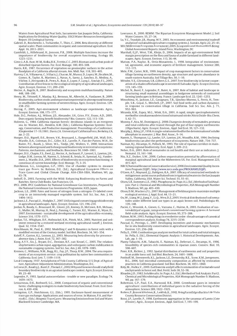
8/6/2019 Smukler et al. 2010



Waters from Agricultural Peat Soils, Sacramento-San Joaquin Delta, California:Implications for Drinking-Water Quality. USGS Water-Resources InvestigationsReport. US Geological Survey.

Gabriel, D., Roschewitz, I., Tscharntke, T., Thies, C., 2006. Beta diversity at differentspatial scales: Plant communities in organic and conventional agriculture. Ecol.Appl. 16, 2011–2021.

Gamfeldt, L., Hillebrand, H., Jonsson, P.R., 2008. Multiple functions increase theimportance of biodiversity for overall ecosystem functioning. Ecology 89,

1223–1231.Giese,L.A.B., Aust, W.M., Kolka,R.K.,Trettin,C.C.,2003.Biomass andcarbon pools of

disturbed riparian forests. For. Ecol. Manage. 180, 493–508.Harris, R.R., 1987. Occurrence of vegetation on geomorphic surfaces in the active

floodplain of a California alluvial stream. Am. Midl. Nat. 118, 393–405.Harvey, C.A., Villanueva, C.,Villacis, J.,Chacon, M.,Munoz, D.,Lopez, M.,Ibrahim,M.,

Gomez, R., Taylor, R., Martinez, J., Navas, A., Saenz, J., Sanchez, D., Medina, A.,Vilchez, S.,Hernandez,B., Perez,A., Ruiz, E.,Lopez, F.,Lang,I., Sinclair,F.L.,2005.Contribution of live fences to the ecological integrity of agricultural landscapes.Agric. Ecosyst. Environ. 111, 200–230.

Hector, A., Bagchi, R., 2007. Biodiversity and ecosystem multifunctionality. Nature448, 188–190.

Henry, M., Tittonell, P., Manlay, R.J., Bernoux, M., Albrecht, A., Vanlauwe, B., 2009.Biodiversity,carbon stocks andsequestrationpotential in aboveground biomassin smallholder farming systems of western Kenya. Agric. Ecosyst. Environ. 129,238–252.

Herzog, F., 2005. Agri-environment schemes as landscape experiments. Agric.,Ecosyst. Environ. 108, 175–177.

Hole, D.G., Perkins, A.J., Wilson, J.D., Alexander, I.H., Grice, P.V., Evans, A.D., 2005.

Does organic farming benefit biodiversity? Bio. Conserv. 122, 113–130.Holstein, G., 1984. California riparian forests: deciduous islands in an evergreen

sea. In: Warner, R.E., Hendrix, K.M. (Eds.), California Riparian Systems: Ecol-ogy, Conservation, and Productive management: Proceedings of a Conference;XSeptember 17-19,1981; Davis,CA. Universityof CaliforniaPress, Berkeley,CA,pp. 2–22.

Hooper, D.U., Bignell, D.E., Brown, V.K., Brussaard, L., Dangerfield, J.M., Wall, D.H.,Wardle, D.A., Coleman, D.C., Giller, K.E., Lavelle, P., Van der Putten, W.H., DeRuiter, P.C., Rusek, J., Silver, W.L., Tiedje, J.M., Wolters, V., 2000. Interactionsbetween aboveground and b elowground biodiversity in terrestrial ecosystems:Patterns, mechanisms, and feedbacks. Bioscience 50, 1049–1061.

Hooper, D.U., Chapin, F.S., Ewel, J.J., Hector, A., Inchausti, P., Lavorel, S., Lawton, J.H.,Lodge, D.M., Loreau, M., Naeem, S., Schmid, B., Setala, H., Symstad, A.J., Vander-meer, J., Wardle, D.A., 2005. Effects of biodiversity on ecosystem functioning: Aconsensus of current knowledge. Ecol. Monogr. 75, 3–35.

Hutchinson, G.L., Livingston, G.P., 1993. Use of chamber systems to measuretrace gas fluxes. In: Rolston, D.E. (Ed.), Agricultural Ecosystem Effects onTrace Gases and Global Climate Change. ASA-CSSA-SSSA, Madison, WI, pp.

63–78.Imhoff, D., 2003. Farming with the Wild: Enhancing Biodiversity on Farms andRanches. Sierra Club Books, San Francisco, CA.

IPCC, 2006. IPCC Guidelines for National Greenhouse Gas Inventories, Prepared bythe National Greenhouse Gas Inventories Programme. IGES, Japan.

Jackson, L.E., 2000. Fates and losses of nitrogen from a nitrogen-15-labeled covercrop in an intensively managed vegetable system. Soil Sci. Soc. Am. J. 64,1404–1412.

Jackson,L.E., Pascual,U., Hodgkin,T., 2007.Utilizingand conservingagrobiodiversityin agricultural landscapes. Agric. Ecosyst. Environ. 121, 196–210.

Jordan, N., Boody, G., Broussard, W., Glover, J.D., Keeney, D., McCown, B.H., McIsaac,G., Muller, M., Murray, H., Neal, J., Pansing, C., Turner, R.E., Warner, K., Wyse, D.,2007. Environment - sustainable development of the agriculturalbio-economy.Science 316, 1570–1571.

Jordan, T.E., Whigham, D.F., Hofmockel, K.H., Pittek, M.A., 2003. Nutrient and sed-iment removal by a restored wetland receiving agricultural runoff. J. Environ.Qual. 32, 1534–1547.

Kirschbaum, M., Paul, K., 2002. Modelling C and N dynamics in forest soils with amodified version of the Century model. Soil Biol. Biochem. 34, 341–354.

Koleff, P., Gaston, K.J., Lennon, J.J., 2003. Measuring beta diversity for presence-absence data. J. Anim. Ecol. 72, 367–382.

Kong, A.Y.Y., Six, J., Bryant, D.C., Denison, R.F., van Kessel, C., 2005. The relation-ship between carbon input, aggregation, and soilorganic carbon stabilization insustainable cropping systems. Soil Sci. Soc. Am. J. 69, 1078–1085.

Kremen, C., Williams, N.M., Bugg, R.L., Fay, J.P., Thorp, R.W., 2004. The area require-ments of an ecosystem service: crop pollination by native bee communities inCalifornia. Ecol. Lett. 7, 1109–1119.

Laval Company, 1937. Aerialphotos of Yolo County, California. U.S. Dept. of Agricul-ture, Agriculture Adjustment Administration, Washington, D.C.

LeCoeur,D., Baudry,J., Burel,F.,Thenail, C.,2002.Whyand howweshould studyfieldboundary biodiversity in an agrarian landscape context. Agric.Ecosyst.Environ.89, 23–40.

Legendre, P., 1993. Spatial autocorrelation - trouble or new paradigm. Ecology 74,1659–1673.

Letourneau, D.K., Bothwell, S.G., 2008. Comparison of organic and conventionalfarms: challenging ecologists to make biodiversity functional. Front. Ecol. Envi-ron. 6, 430–438.

Livingston, G.P., Hutchinson, G.L. (Eds.), 1995. Enclosure-based measurement of trace gas exchange: Applications and sources of error. In Matson, P.A. and Har-rissR.C. (Eds.). Biogenic TraceGases: Measuring Emissionsfrom Soil and Water.Blackwell Science Cambridge, MA.

Lowrance, R., 2000. REMM: The Riparian Ecosystem Management Model. J. SoilWater Conserv. 55, 27–34.

Lu, Y.C., Teasdale, J.R., Huang, W.Y., 2003. An economic and environmental tradeoff analysisof sustainableagriculture cropping systems.J. Sustain. Agric.22, 25–41.

MA (Millennium Ecosystem Assessment),2005. Ecosystemsand HumanWell-Being:Global Assessment Reports. Island Press, Washington, DC.

Marshall, E.J.P., West, T.M., Kleijn, D., 2006. Impacts of an agri-environment fieldmargin prescription on the flora and fauna of arable farmland in different land-

scapes. Agric. Ecosyst. Environ. 113, 36–44.Matson, P.A., Naylor, R., Ortiz-Monasterio, I., 1998. Integration of environmen-

tal, agronomic, and economic aspects of fertilizer management. Science 280,112–115.

Mele, P.M., Carter, M.R., 1999. Impact of crop management factors in conservationtillage farming on earthworm density, age structure and species abundance insouth-eastern Australia. Soil Tillage Res. 50, 1–10.

Méndez, V.E., Gliessman, S.R.,Gilbert,G.S., 2007.Tree biodiversity in farmer cooper-atives of a shadecoffeelandscape in western El Salvador.Agric. Ecosyst.Environ.119, 145–159.

Michel, N., Burel, F., Legendre, P., Butet, A., 2007. Role of habitat and landscape instructuring small mammal assemblages in hedgerow networks of contrastedfarming landscapes in Brittany. France. Landscape Ecol. 22, 1241–1253.

Minoshima, H., Jackson, L.E., Cavagnaro, T.R., Sánchez-Moreno, S., Ferris, H., Tem-ple, S.R., Goyal, S., Mitchell, J.P., 2007. Soil food webs and carbon dynamicsin response to conservation tillage in California. Soil Sci. Soc. Am. J. 71,952–963.

Miranda, K.M., Espey, M.G., Wink, D.A., 2001. A rapid, simple spectrophotometricmethodfor simultaneousdetectionof nitrateand nitrite.NitricOxide-Bio. Chem.

5, 62–71.Monroy, F.,Aira, M., Dominguez,J., 2008.Changesin density of nematodes, protozoa

and total coliforms after transit through the gut of four epigeic earthworms(Oligochaeta). Agric. Ecosyst. Environ., Appl. Soil Ecol. 39, 127–132.

Murphy,J., Riley, J.P., 1958.A single-solutionmethodforthe determinationof solublephosphate in seawater. J. Mar. Biol. Assoc., 9–14.

Naeem, S., Thompson, L.J., Lawler, S.P., Lawton, J.H., Woodfin, R.M., 1994. Decliningbiodiversity can alter the performance of ecosystems. Nature 368:, 734–737.

Naiman, R.J., Decamps, H., Pollock, M., 1993. The role of riparian corridors in main-taining regional biodiversity. Ecol. Appl. 3, 209–212.

Neher, D.A., 2001. Role of nematodes in soil health and their use as indicators. J.Nematol. 33, 161–168.

Niu, X.Z., Duiker, S.W., 2006. Carbon sequestration potential by afforestation of marginal agricultural land in the Midwestern US. For. Ecol. Management 223,415–427.

NRCS(National ResourceConservationService), 2008.Environmental Quality Incen-tives Program (EQIP). http://www.nrcs.usda.gov/PROGRAMS/EQIP/.

O’Geen, A.T., Maynard, J.J., Dahlgren, R.A., 2007. Efficacy of constructed wetlands to

mitigatenon-point source pollutionfrom irrigationtailwatersin theSan JoaquinValley, California, USA. Water Sci. Technol. 55, 55–61.Olsen, S.R.,Sommers,L.E.,1982. Phosphorus.In: Page,A.L.(Ed.),Methodsof SoilAnal-

ysis: Part 2. Chemical and Microbiological Properties, ASA Monograph Number9. Madison, WI, pp. 403–430.

Olson, D.M.,Wackers,F.L., 2007.Management of fieldmarginsto maximize multipleecological services. J. Appl. Ecol. 44, 13–21.

Ou,W., Liang,W.J., Jiang,Y., Li,Q., Wen, D.Z.,2005.Vertical distributionof soil nema-todes under different land use types in an aquic brown soil. Pedobiologia 49,139–148.

Pacini, C., Wossink, A., Giesen, G., Vazzana, C., Huirne, R., 2003. Evaluation of sus-tainabilityof organic, integratedand conventional farming systems:A farmandfield-scale analysis. Agric. Ecosyst. Environ. 95, 273–288.

Palmer, M.W.,1993. Putting things in evenbetter order–theadvantages of canonicalcorrespondence-analysis. Ecology 74, 2215–2230.

Pascual, U., Perrings, C., 2007. Developing incentives and economic mechanismsfor in situ biodiversity conservation in agricultural landscapes. Agric. Ecosyst.Environ. 121, 256–268.

Pella, E., 1990. Combustion gas analyzer method for total carbon and total nitrogen.

In: Pella, E. (Ed.), Elemental Organic Analysis 1. Historical Developments. Am.Lab., pp. 1–16.

Planty-Tabacchi, A.M., Tabacchi, E., Naiman, R.J., Deferrari, C., Decamps, H., 1996.Invasibility of species-rich communities in riparian zones. Conserv. Biol. 10,598–607.

Poier, K.R., Richter, J., 1992. Spatial distribution of earthworms and soil propertiesin an arable loess soil. Soil Biol. Biochem. 24, 1601–1608.

Potthoff, M., Steenwerth, K.L., Jackson, L.E., Drenovsky, R.E., Scow, K.M., Joergensen,R.G., 2006. Soil microbial community composition as affected by restorationpractices in California grassland. Soil Biol. Biochem. 38, 1851–1860.

Räty,M., Huhta,V., 2003. Earthworms andpH affectcommunities of nematodesandenchytraeids in forest soil. Biol. Fertil. Soils 38, 52–58.

Rhoades,J.D.,1982.Solublesalts. In:Page, A.L. (Ed.),Methodsof Soil Analysis:Part2.Chemical and Microbiological Properties, ASA Monograph Number 9. Madison,WI, pp. 167–179.

Robertson, G.P., Paul, E.A., Harwood, R.R., 2000. Greenhouse gases in intensiveagriculture: contributions of individual gases to the radiative forcing of theatmosphere. Science 289, 1922–1925.

Robins, P.,BresnickHolmes,R., Laddish,K., 2002. BringFarmEdgesBackto Life!YoloCounty Resource Conservation District.

Rossi, J.P., Lavelle, P., 1998. Earthworm aggregation in the savannas of Lamto (Coted’Ivoire). Agric., Ecosyst. Environ., Appl. Soil Ecol. 7, 195–199.

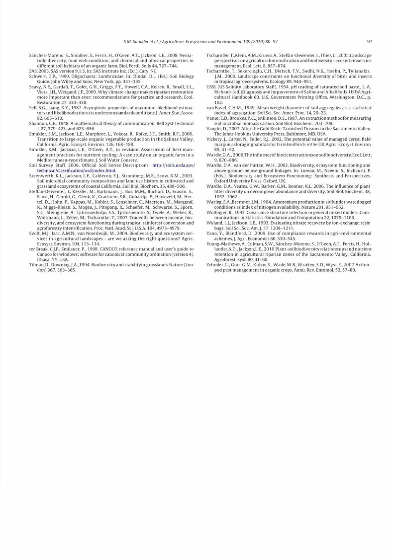
8/6/2019 Smukler et al. 2010



Sánchez-Moreno, S., Smukler, S., Ferris, H., O’Geen, A.T., Jackson, L.E., 2008. Nema-tode diversity, food web condition, and chemical and physical properties indifferent soil habitats of an organic farm. Biol. Fertil. Soils 44, 727–744.

SAS, 2003. SAS version 9.1.3. In: SAS Institute Inc. (Ed.), Cary, NC.Schwert, D.P., 1990. Oligochaeta: Lumbricidae. In: Dindal, D.L. (Ed.), Soil Biology

Guide. John Wiley and Sons, New York, pp. 341–355.Seavy, N.E., Gardali, T., Golet, G.H., Griggs, F.T., Howell, C.A., Kelsey, R., Small, S.L.,

Viers, J.H., Weigand, J.F., 2009. Why climate change makes riparian restoration

more important than ever: recommendations for practice and research. Ecol.Restoration 27, 330–338.

Self, S.G., Liang, K.Y., 1987. Asymptotic properties of maximum-likelihood estima-torsand likelihoodratiotests undernonstandardconditions.J. Amer.Stat.Assoc.82, 605–610.

Shannon, C.E., 1948. A mathematical theory of communication. Bell Syst Technical J. 27, 379–423, and 623–656.

Smukler, S.M., Jackson, L.E., Murphree, L., Yokota, R., Koike, S.T., Smith, R.F., 2008.Transition to large-scale organic vegetable production in the Salinas Valley,California. Agric. Ecosyst. Environ. 126, 168–188.

Smukler, S.M., Jackson, L.E., O’Geen, A.T., in revision. Assessment of best man-agement practices for nutrient cycling: A case study on an organic farm in aMediterranean-type climate. J. Soil Water Conserv.

Soil Survey Staff, 2006. Official Soil Series Descriptions. http://soils.usda.gov/technical/classification/osd/index.html.

Steenwerth, K.L., Jackson, L.E., Calderon, F.J., Stromberg, M.R., Scow, K.M., 2003.Soil microbial community composition and land use history in cultivated andgrassland ecosystems of coastal California. Soil Biol. Biochem. 35, 489–500.

Steffan-Dewenter, I., Kessler, M., Barkmann, J., Bos, M.M., Buchori, D., Erasmi, S.,

Faust, H., Gerold, G., Glenk, K., Gradstein, S.R., Guhardja, E., Harteveld, M., Her-tel, D., Hohn, P., Kappas, M., Kohler, S., Leuschner, C., Maertens, M., Marggraf,R., Migge-Kleian, S., Mogea, J., Pitopang, R., Schaefer, M., Schwarze, S., Sporn,S.G., Steingrebe, A., Tjitrosoedirdjo, S.S., Tjitrosoemito, S., Twele, A., Weber, R.,Woltmann, L., Zeller, M., Tscharntke, T., 2007. Tradeoffs between income, bio-diversity, and ecosystem functioning during tropical rainforest conversion andagroforestry intensification. Proc. Natl. Acad. Sci. U.S.A. 104, 4973–4978.

Swift, M.J., Izac, A.M.N., van Noordwijk, M., 2004. Biodiversity and ecosystem ser-vices in agricultural landscapes - are we asking the right questions? Agric.Ecosyst. Environ. 104, 113–134.

ter Braak, C.J.F., Smilauer, P., 1998. CANOCO reference manual and user’s guide toCanoco for windows: software for canonical community ordination (version 4).Ithaca, NY, USA.

Tilman, D., Downing, J.A.,1994. Biodiversity and stabilityin grasslands. Nature (Lon-don) 367, 363–365.

Tscharntke, T.,Klein, A.M.,Kruess,A., Steffan-Dewenter, I., Thies, C., 2005.Landscapeperspectives on agriculturalintensification and biodiversity - ecosystemservicemanagement. Ecol. Lett. 8, 857–874.

Tscharntke, T., Sekercioglu, C.H., Dietsch, T.V., Sodhi, N.S., Hoehn, P., Tylianakis, J.M., 2008. Landscape constraints on functional diversity of birds and insectsin tropical agroecosystems. Ecology 89, 944–951.

USSL (US Salinity Laboratory Staff), 1954. pH reading of saturated soil paste., L. A.Richards (ed.)Diagnosis and Improvement of Saline and AlkaliSoils. USDA Agri-

cultural Handbook 60. U.S. Government Printing Office, Washington, D.C., p.102.

van Bavel, C.H.M., 1949. Mean weight diameter of soil aggregates as a statisticalindex of aggregation. Soil Sci. Soc. Amer. Proc. 14, 20–23.

Vance, E.D.,Brookes, P.C.,Jenkinson, D.S.,1987. An extractionmethodfor measuringsoil microbial biomass carbon. Soil Biol. Biochem., 703–708.

Vaught, D., 2007. After the Gold Rush: Tarnished Dreams in the Sacramento Valley.The Johns Hopkins University Press, Baltimore, MD, USA.

Vickery, J., Carter, N., Fuller, R.J., 2002. The potential value of managed cereal fieldmargins asforaginghabitatsfor farmlandbirds inthe UK.Agric. Ecosyst.Environ.89, 41–52.

Wardle,D.A., 2006.The influenceof bioticinteractionson soilbiodiversity.Ecol. Lett.9, 870–886.

Wardle, D.A., van der Putten, W.H., 2002. Biodiversity, ecosystem functioning andabove-ground-below-ground linkages. In: Loreau, M., Naeem, S., Inchausti, P.(Eds.), Biodiversity and Ecosystem Functioning: Synthesis and Perspectives.Oxford University Press, Oxford, UK.

Wardle, D.A., Yeates, G.W., Barker, G.M., Bonner, K.I., 2006. The influence of plantlitter diversity on decomposer abundance and diversity. Soil Biol. Biochem. 38,

1052–1062.Waring, S.A.,Bremner, J.M.,1964. Ammonium productionin soilunder waterlogged

conditions as index of nitrogen availability. Nature 201, 951–952.Wolfinger, R., 1993. Covariance structure selection in general mixed models. Com-

munications in Statistics-Simulation and Computation 22, 1079–1106.Wyland, L.J., Jackson, L.E., 1993. Evaluating nitrate recovery by ion-exchange resin

bags. Soil Sci. Soc. Am. J. 57, 1208–1211.Yano, Y., Blandford, D., 2009. Use of compliance rewards in agri-environmental

achemes. J. Agri. Economics 60, 530–545.Young-Mathews, A., Culman, S.W., Sánchez-Moreno, S., O’Geen, A.T., Ferris, H., Hol-

lander,A.D., Jackson,L.E., 2010.Plant-soilbiodiversityrelationshipsand nutrientretention in agricultural riparian zones of the Sacramento Valley, California.Agroforest. Syst. 80, 41–60.

Zehnder,G., Gurr, G.M., Kuhne,S., Wade, M.R., Wratten, S.D., Wyss, E.,2007.Arthro-pod pest management in organic crops. Annu. Rev. Entomol. 52, 57–80.

Documents

Smukler et al. 2010