16.810 (16.682)16.810 (16.682)

Engineering Design and Rapid PrototypingEngineering Design and Rapid Prototyping

Instructor(s)

Structural Testing

January 21, 2004

Prof. Olivier de WeckProf. Olivier de Weckdeweck@mit.edudeweck@mit.edu

Lecture 7

16.810 (16.682) 2

Outline

! Structural Testing! Why testing is important! Types of Sensors, Procedures .! Mass, Static Displacement, Dynamics

! Test Protocol for 16.810! Explain protocol! Sign up for time slots

16.810 (16.682) 3

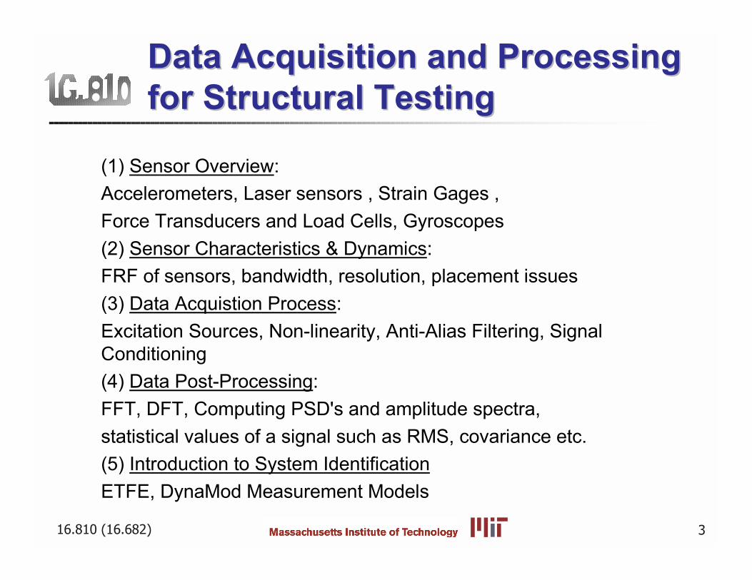
(1) Sensor Overview:Accelerometers, Laser sensors , Strain Gages ,Force Transducers and Load Cells, Gyroscopes(2) Sensor Characteristics & Dynamics:FRF of sensors, bandwidth, resolution, placement issues(3) Data Acquistion Process:Excitation Sources, Non-linearity, Anti-Alias Filtering, SignalConditioning(4) Data Post-Processing:FFT, DFT, Computing PSD's and amplitude spectra,statistical values of a signal such as RMS, covariance etc.(5) Introduction to System IdentificationETFE, DynaMod Measurement Models

Data Acquisition and ProcessingData Acquisition and Processingfor Structural Testingfor Structural Testing

16.810 (16.682) 4

Why is Structural Testing Important?

! Product Qualification Testing! Performance Assessment! System Identification! Design Verification! Damage Assessment! Aerodynamic Flutter Testing! Operational Monitoring! Material Fatigue Testing

F-22 Raptor #01 during ground F-22 Raptor #01 during ground vibration tests at Edwards Air vibration tests at Edwards Air

Force Base, Calif., in April 1999Force Base, Calif., in April 1999

Ref: http://www.af.mil/photos/May1999/19990518f2235.html

Example: Ground Vibration TestingExample: Ground Vibration Testing

StructuralSystem

stimulusu(t)

DAQ DSP

response

DAQ = data acquisitionDSP = digital signal processing

x(t)

16.810 (16.682) 5

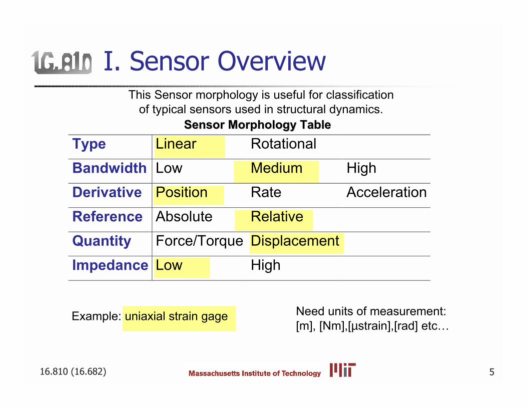
Type Linear Rotational

Bandwidth Low Medium High Derivative Position Rate Acceleration

Reference Absolute Relative

Quantity Force/Torque Displacement

Impedance Low High

I. Sensor OverviewThis Sensor morphology is useful for classification

of typical sensors used in structural dynamics.

Example: uniaxial strain gage Need units of measurement: [m], [Nm],[µstrain],[rad] etc

Sensor Morphology TableSensor Morphology Table

16.810 (16.682) 6

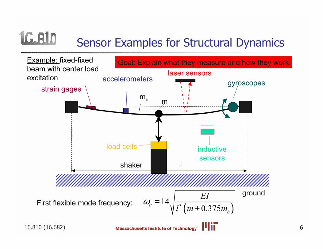
Sensor Examples for Structural Dynamics

strain gages

shaker

laser sensorsaccelerometers gyroscopes

load cells

ground

inductivesensors

Example: fixed-fixedbeam with center loadexcitation

First flexible mode frequency: ( )3140.375n

b

EIl m m

ω =+

mb m

l

Goal: Explain what they measure and how they work

16.810 (16.682) 7

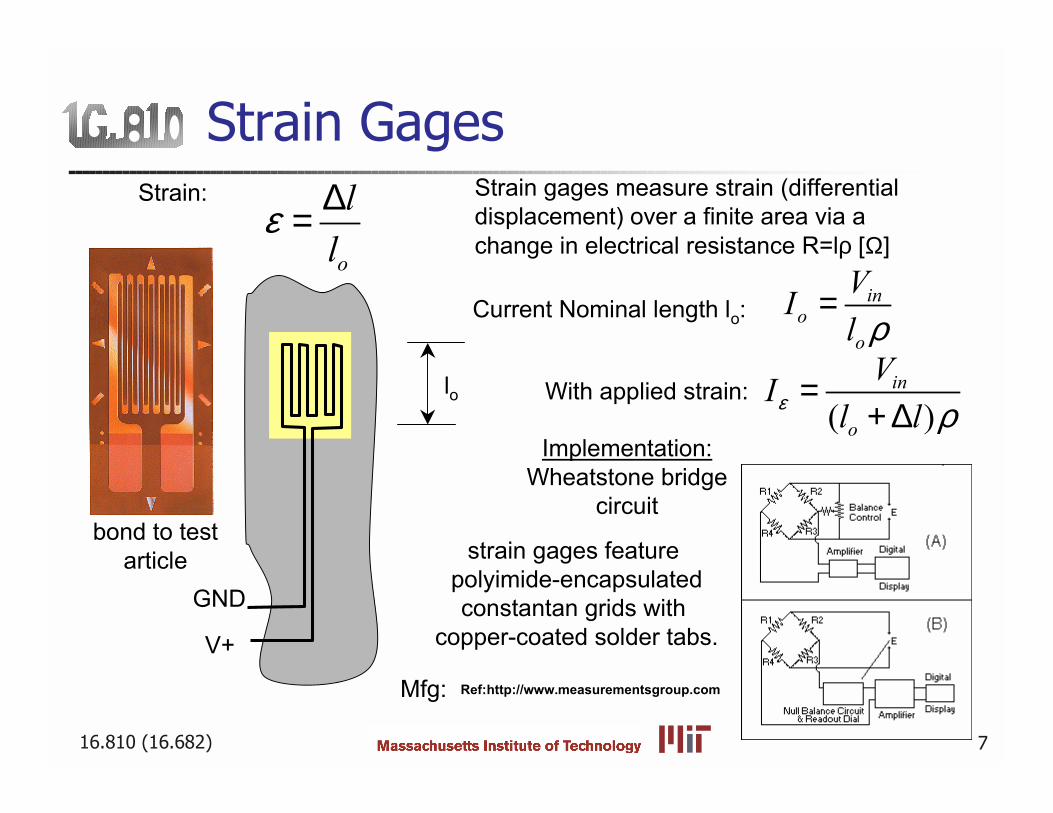
Strain Gages

Current Nominal length lo:in

oo

VIl ρ

=

Strain:

o

ll

ε ∆=

GND

V+

lo With applied strain:( )

in

o

VIl lε ρ

=+ ∆

Strain gages measure strain (differentialdisplacement) over a finite area via achange in electrical resistance R=lρ [Ω]

strain gages feature polyimide-encapsulatedconstantan grids with

copper-coated solder tabs.

bond to testarticle

Ref:http://www.measurementsgroup.com

Implementation:Wheatstone bridge

circuit

Mfg:

16.810 (16.682) 8

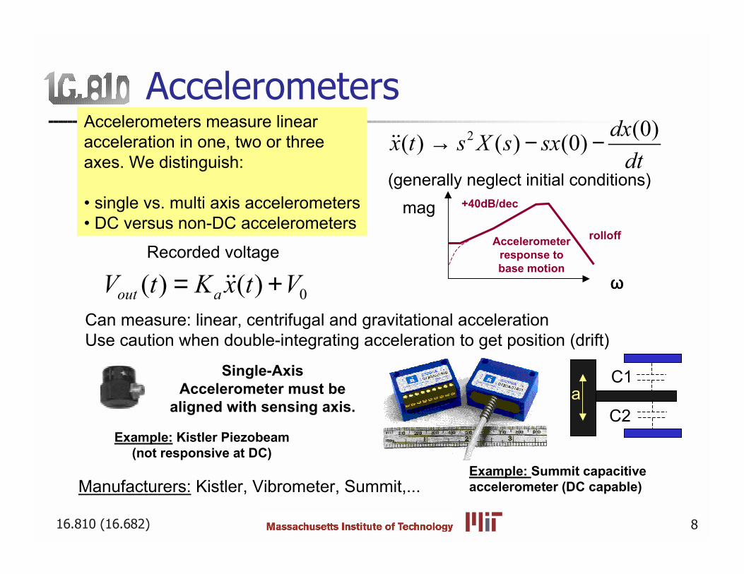
Accelerometers

Single-AxisAccelerometer must be

aligned with sensing axis.

Accelerometers measure linearacceleration in one, two or threeaxes. We distinguish:

single vs. multi axis accelerometers DC versus non-DC accelerometers

Example: Kistler Piezobeam(not responsive at DC)

2 (0)( ) ( ) (0) dxx t s X s sxdt

→ − −!!

Recorded voltage

0( ) ( )out aV t K x t V= +!!Can measure: linear, centrifugal and gravitational accelerationUse caution when double-integrating acceleration to get position (drift)

(generally neglect initial conditions)

Manufacturers: Kistler, Vibrometer, Summit,...

mag

ωωωω

Accelerometerresponse tobase motion

+40dB/dec

rolloff

Example: Summit capacitiveaccelerometer (DC capable)

C1

C2a

16.810 (16.682) 9

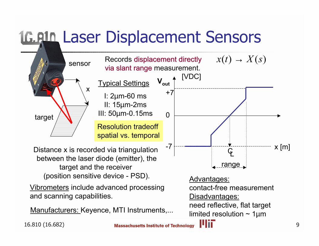
Laser Displacement SensorsRecords displacement directlydisplacement directlyvia slant rangevia slant range measurement.

Advantages:contact-free measurementDisadvantages:need reflective, flat targetlimited resolution ~ 1µm

target

( ) ( )x t X s→

Vout

x [m]

[VDC]

Distance x is recorded via triangulation between the laser diode (emitter), the

target and the receiver (position sensitive device - PSD).

x

sensor

0

-7

+7

CLrange

Manufacturers: Keyence, MTI Instruments,...

Vibrometers include advanced processing and scanning capabilities.

Typical Settings

I: 2µm-60 msII: 15µm-2ms

III: 50µm-0.15ms

Resolution tradeoffspatial vs. temporal

16.810 (16.682) 10

Force Transducers / Load Cells

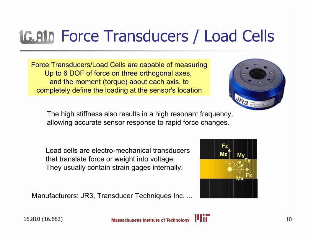
Force Transducers/Load Cells are capable of measuringUp to 6 DOF of force on three orthogonal axes,

and the moment (torque) about each axis, tocompletely define the loading at the sensor's location

Manufacturers: JR3, Transducer Techniques Inc. ...

The high stiffness also results in a high resonant frequency, allowing accurate sensor response to rapid force changes.

Fx

Fz

Fy

Mx

Mz MyLoad cells are electro-mechanical transducers that translate force or weight into voltage. They usually contain strain gages internally.

16.810 (16.682) 11

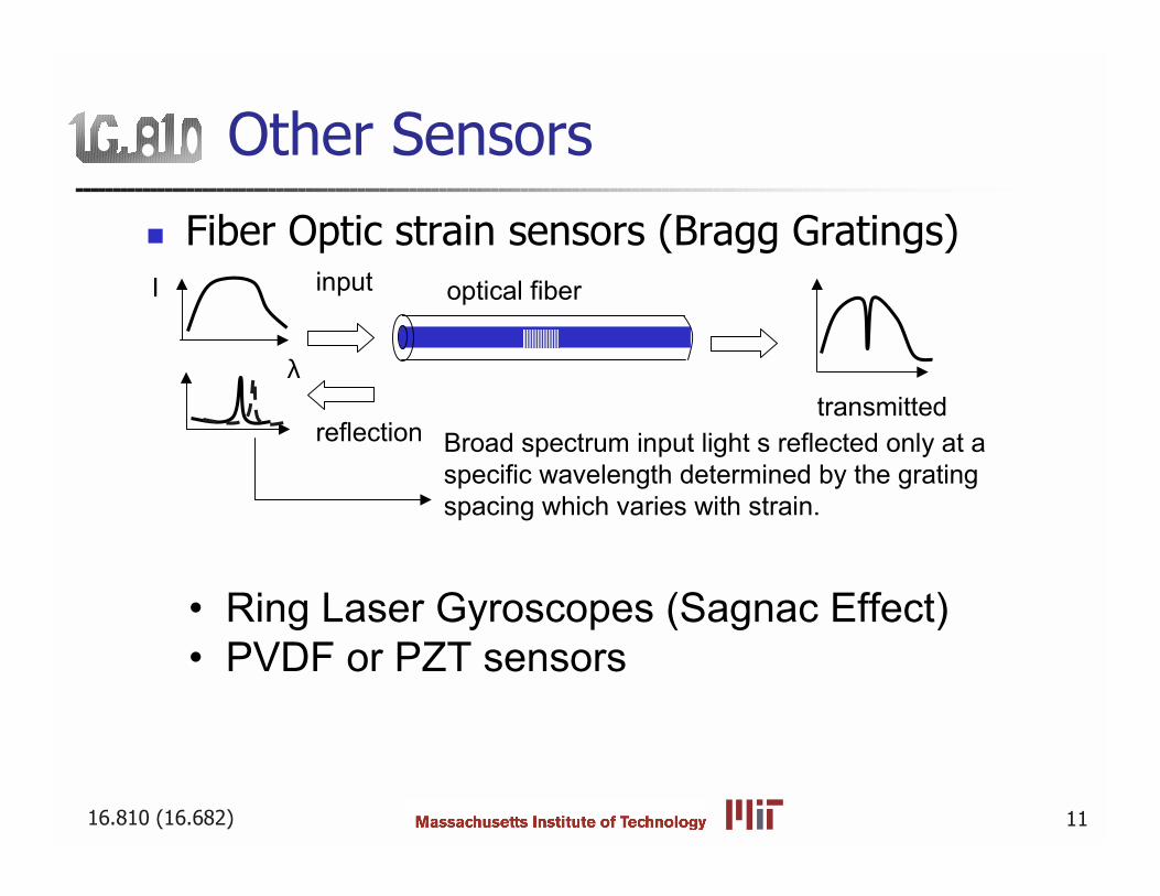
Other Sensors! Fiber Optic strain sensors (Bragg Gratings)

Ring Laser Gyroscopes (Sagnac Effect) PVDF or PZT sensors

I

λ

input

reflectiontransmitted

optical fiber

Broad spectrum input light s reflected only at aspecific wavelength determined by the grating spacing which varies with strain.

16.810 (16.682) 12

II. Sensor Characteristics & Dynamics

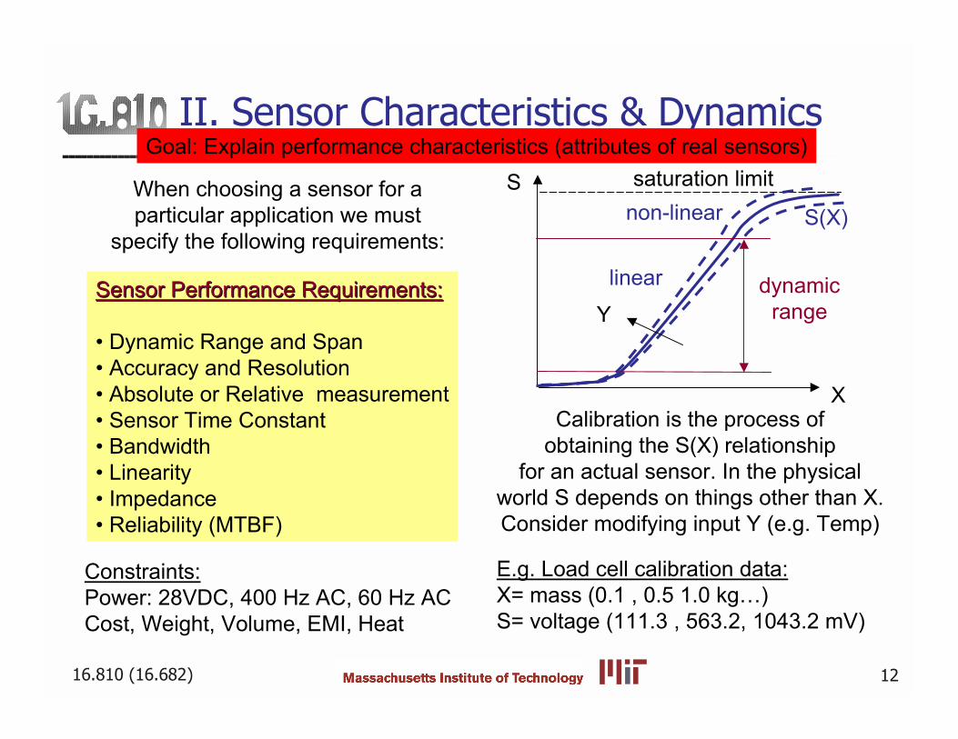
When choosing a sensor for aparticular application we must

specify the following requirements:

Sensor Performance Requirements:Sensor Performance Requirements:

Dynamic Range and Span Accuracy and Resolution Absolute or Relative measurement Sensor Time Constant Bandwidth Linearity Impedance Reliability (MTBF)

Constraints:Power: 28VDC, 400 Hz AC, 60 Hz ACCost, Weight, Volume, EMI, Heat

X

S saturation limit

dynamicrange

linear

non-linear

Calibration is the process ofobtaining the S(X) relationship

for an actual sensor. In the physicalworld S depends on things other than X.Consider modifying input Y (e.g. Temp)

E.g. Load cell calibration data:X= mass (0.1 , 0.5 1.0 kg)S= voltage (111.3 , 563.2, 1043.2 mV)

Goal: Explain performance characteristics (attributes of real sensors)

S(X)

Y

16.810 (16.682) 13

Sensor Frequency Response Function

m

ck

x(t)

xb(t)

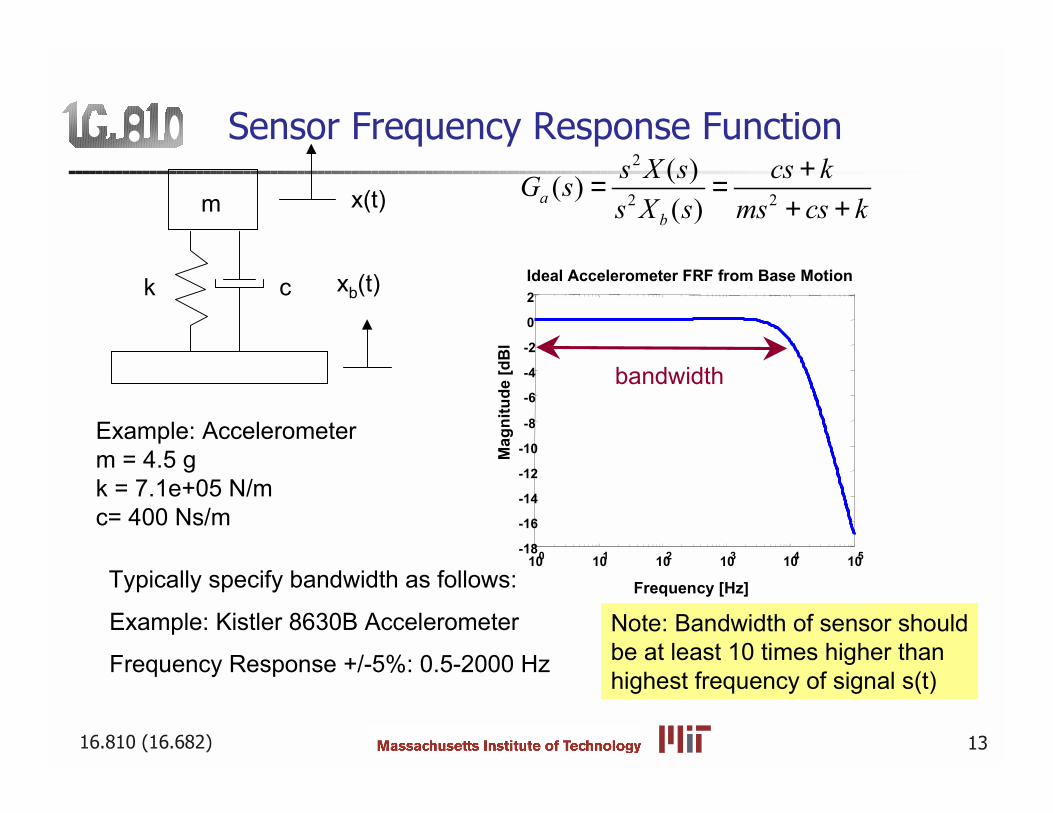
Example: Accelerometerm = 4.5 gk = 7.1e+05 N/mc= 400 Ns/m

2

2 2

( )( )( )ab

s X s cs kG ss X s ms cs k

+= =+ +

100 101 102 103 104 105-18

-16

-14

-12

-10

-8

-6

-4

-2

0

2

Frequency [Hz]

Mag

nitu

de [d

Bl

Ideal Accelerometer FRF from Base Motion

Typically specify bandwidth as follows:

Frequency Response +/-5%: 0.5-2000 Hz

bandwidth

Note: Bandwidth of sensor shouldbe at least 10 times higher thanhighest frequency of signal s(t)

Example: Kistler 8630B Accelerometer

16.810 (16.682) 14

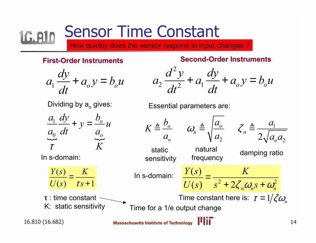
Sensor Time Constant

First-Order InstrumentsFirst-Order Instruments

1 o odya a y b udt

+ =

Dividing by ao gives:

" "1

0

o

o

ba dy y ua dt a

Kτ

+ =

In s-domain:

( )( ) 1Y s KU s sτ

=+

ττττ : time constantK: static sensitivity

Second-Order InstrumentsSecond-Order Instruments

How quickly does the sensor respond to input changes ?

2

2 12 o od y dya a a y b udt dt

+ + =

Essential parameters are:

1

2 2

2

o on n

o o

b a aKa a a a

ω ζ# # #

static sensitivity

natural frequency

damping ratio

In s-domain:2 2

( )( ) 2 n n n

Y s KU s s sζ ω ω

=+ +

Time for a 1/e output changeTime constant here is: 1 nτ ζω=

16.810 (16.682) 15

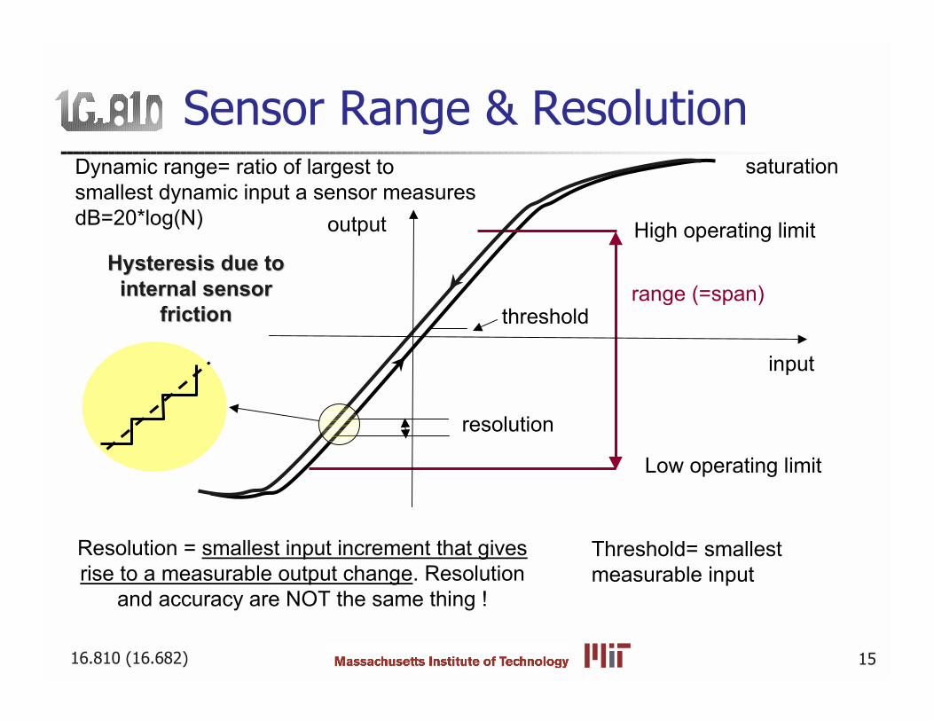
Sensor Range & Resolution

Resolution = smallest input increment that givesrise to a measurable output change. Resolution

and accuracy are NOT the same thing !

range (=span)

resolution

Dynamic range= ratio of largest tosmallest dynamic input a sensor measuresdB=20*log(N)

Low operating limit

High operating limit

saturation

Hysteresis due toHysteresis due tointernal sensorinternal sensor

frictionfriction

input

output

threshold

Threshold= smallest measurable input

16.810 (16.682) 16

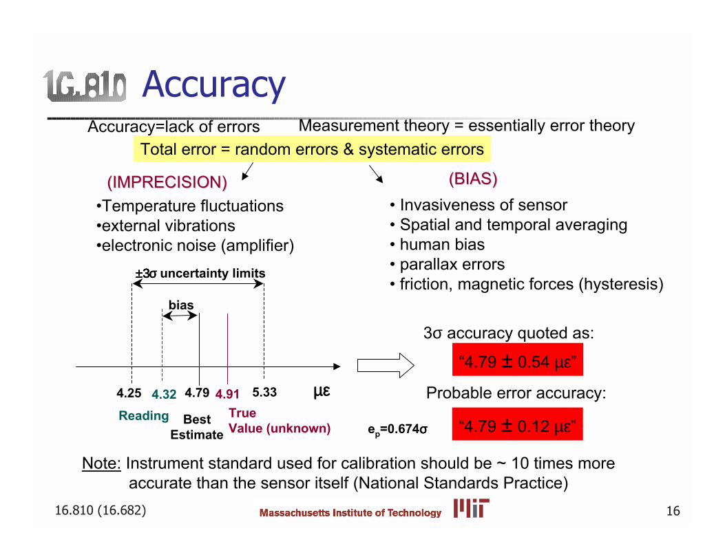
AccuracyMeasurement theory = essentially error theory

Total error = random errors & systematic errors

Invasiveness of sensor Spatial and temporal averaging human bias parallax errors friction, magnetic forces (hysteresis)

Note: Instrument standard used for calibration should be ~ 10 times moreaccurate than the sensor itself (National Standards Practice)

Temperature fluctuationsexternal vibrationselectronic noise (amplifier)

Accuracy=lack of errors

(BIAS)(BIAS)(IMPRECISION)(IMPRECISION)

±3σ ±3σ ±3σ ±3σ uncertainty limits

bias

4.25 4.794.32 5.334.91Reading Best

EstimateTrueValue (unknown)

3σ accuracy quoted as:

µεµεµεµε Probable error accuracy:

ep=0.674σσσσ

4.79 ± 0.54 µε

4.79 ± 0.12 µε

16.810 (16.682) 17

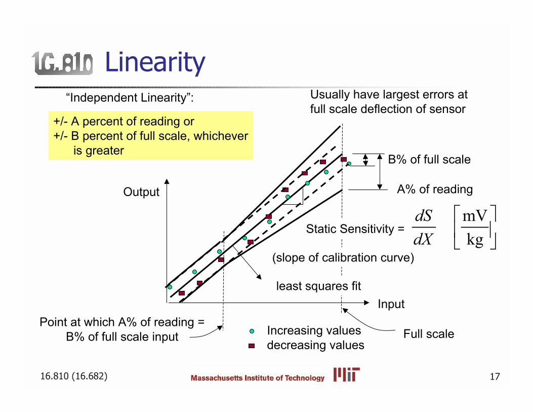
Linearity

Static Sensitivity =

(slope of calibration curve)

Usually have largest errors atfull scale deflection of sensor

Independent Linearity:

Increasing valuesdecreasing values

least squares fit

+/- A percent of reading or+/- B percent of full scale, whichever is greater

Input

Output

B% of full scale

A% of reading

Point at which A% of reading =B% of full scale input Full scale

mV kg

dSdX

16.810 (16.682) 18

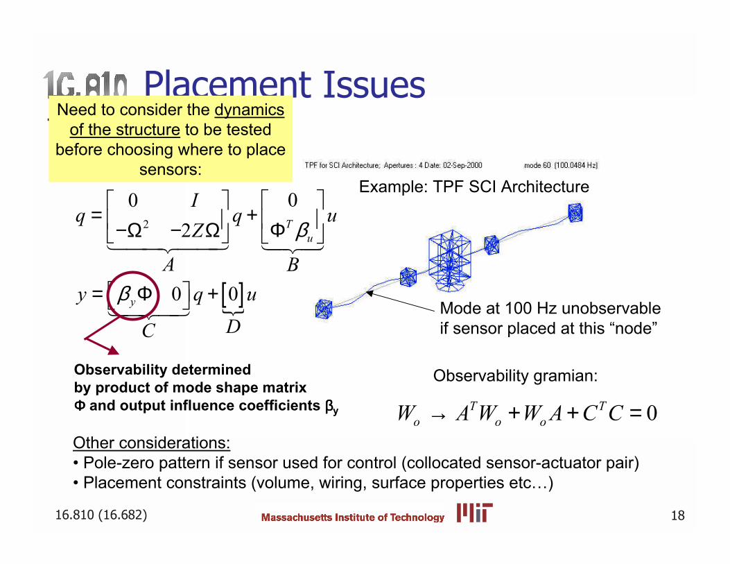
Placement IssuesNeed to consider the dynamics

of the structure to be testedbefore choosing where to place

sensors:

Mode at 100 Hz unobservable if sensor placed at this node

Observability determinedby product of mode shape matrixΦΦΦΦ and output influence coefficients ββββy

Other considerations: Pole-zero pattern if sensor used for control (collocated sensor-actuator pair) Placement constraints (volume, wiring, surface properties etc)

Example: TPF SCI Architecture

[ ]"

2

002

0 0

Tu

y

Iq q u

Z

A By q u

DC

β

β

= + Φ−Ω − Ω

= Φ +

$%%&%%' $%&%'

$%&%'

Observability gramian:

0T To o oW A W W A C C→ + + =

16.810 (16.682) 19

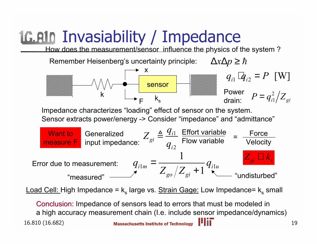
Invasiability / ImpedanceHow does the measurement/sensor influence the physics of the system ?

Remember Heisenbergs uncertainty principle: x p∆ ∆ ≥ (

Impedance characterizes loading effect of sensor on the system.Sensor extracts power/energy -> Consider impedance and admittance

Generalized input impedance:

1

2

igi

i

qZq# Effort variable

Flow variable = ForceVelocity

Load Cell: High Impedance = ks large vs. Strain Gage: Low Impedance= ks small

Conclusion: Conclusion: Impedance of sensors lead to errors that must be modeled in a high accuracy measurement chain (I.e. include sensor impedance/dynamics)

sensor

ksk

x

F

Want tomeasure F

1 2 [W]i iq q P⋅ =

Error due to measurement: 1 11

1i m i ugo gi

q qZ Z

=+

Power drain:

21i giP q Z=

measured undisturbed

gi sZ k∝

16.810 (16.682) 20

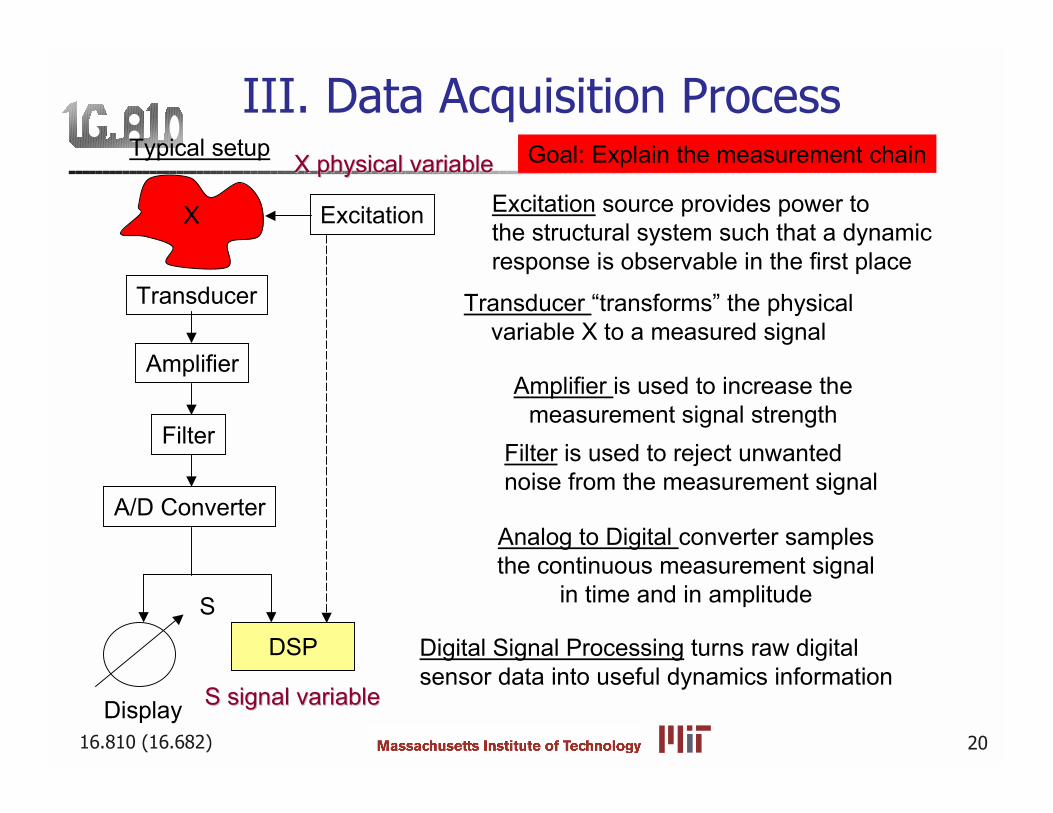
III. Data Acquisition ProcessTypical setup

X

Transducer

Amplifier

Filter

A/D Converter

Display

DSP

S

Transducer transforms the physicalvariable X to a measured signal

Amplifier is used to increase themeasurement signal strength

Filter is used to reject unwantednoise from the measurement signal

Analog to Digital converter samplesthe continuous measurement signal

in time and in amplitude

Goal: Explain the measurement chain

Excitation Excitation source provides power to the structural system such that a dynamicresponse is observable in the first place

Digital Signal Processing turns raw digitalsensor data into useful dynamics information

X physical variableX physical variable

S signal variableS signal variable

16.810 (16.682) 21

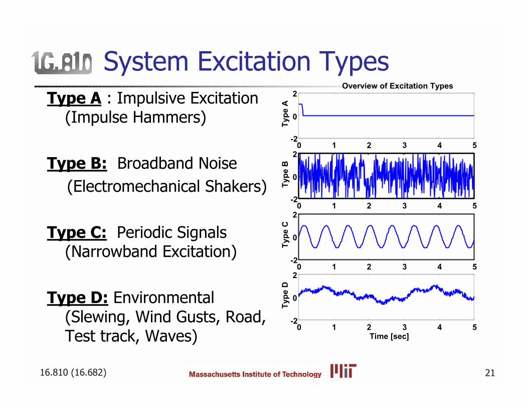
System Excitation TypesType A : Impulsive Excitation

(Impulse Hammers)

Type B: Broadband Noise (Electromechanical Shakers)

Type C: Periodic Signals(Narrowband Excitation)

Type D: Environmental(Slewing, Wind Gusts, Road,Test track, Waves)

0 1 2 3 4 5-2

0

2Overview of Excitation Types

Type

A

0 1 2 3 4 5-2

0

2

Type

B

0 1 2 3 4 5-2

0

2

Type

C

0 1 2 3 4 5-2

0

2Ty

pe D

Time [sec]

16.810 (16.682) 22

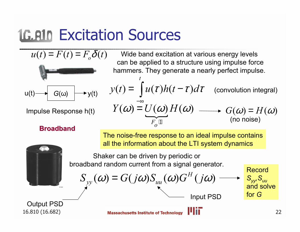
Excitation SourcesWide band excitation at various energy levels

can be applied to a structure using impulse forcehammers. They generate a nearly perfect impulse.

Shaker can be driven by periodic orbroadband random current from a signal generator.

Impulse Response h(t)

( ) ( ) ( )t

y t u h t dτ τ τ−∞

= −∫ (convolution integral)

( ) ( ) ( )ou t F t F tδ= =

( ) ( ) ( ) ( )Hyy uuS G j S G jω ω ω ω=

G(ω)u(t) y(t)

"1

( ) ( ) ( )Fo

Y U Hω ω ω⋅

= ( ) ( )G Hω ω=(no noise)

The noise-free response to an ideal impulse containsall the information about the LTI system dynamics

Input PSDOutput PSD

RecordSyy,Suuand solvefor G

BroadbandBroadband

16.810 (16.682) 23

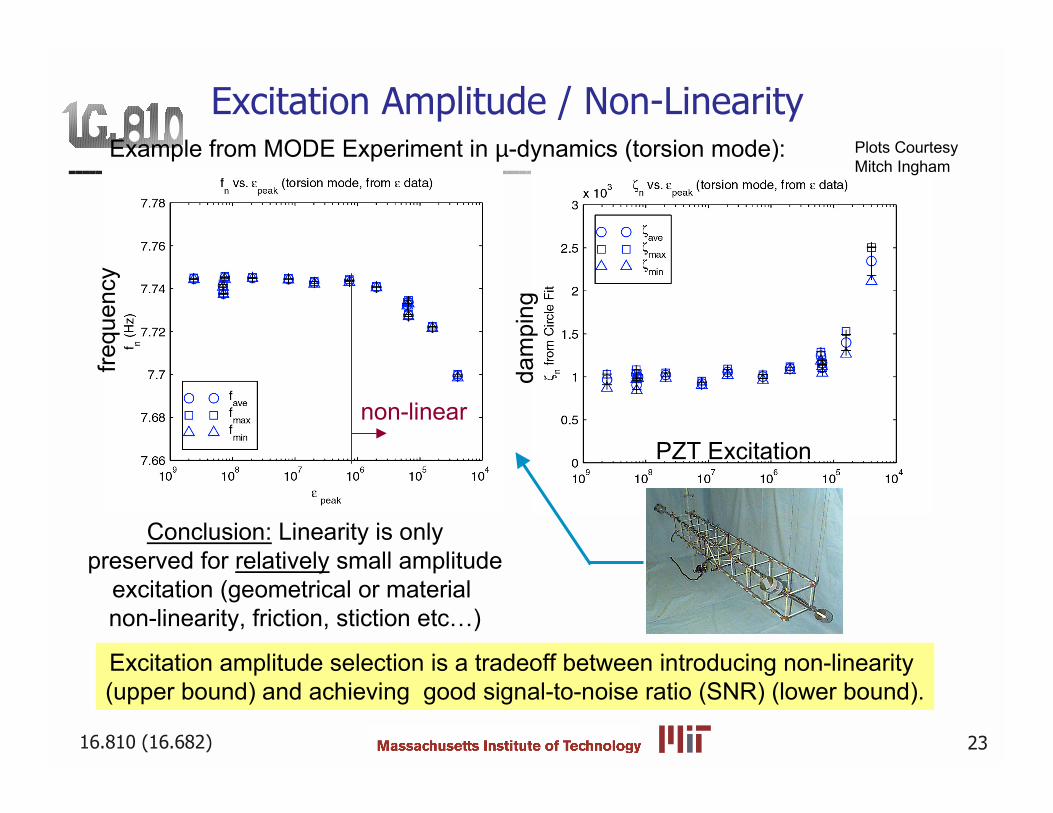
Excitation Amplitude / Non-LinearityExample from MODE Experiment in µ-dynamics (torsion mode):

Conclusion: Linearity is only preserved for relatively small amplitude

excitation (geometrical or material non-linearity, friction, stiction etc)

non-linear

frequ

ency

dam

ping

PZT Excitation

Excitation amplitude selection is a tradeoff between introducing non-linearity (upper bound) and achieving good signal-to-noise ratio (SNR) (lower bound).

Plots CourtesyMitch Ingham

16.810 (16.682) 24

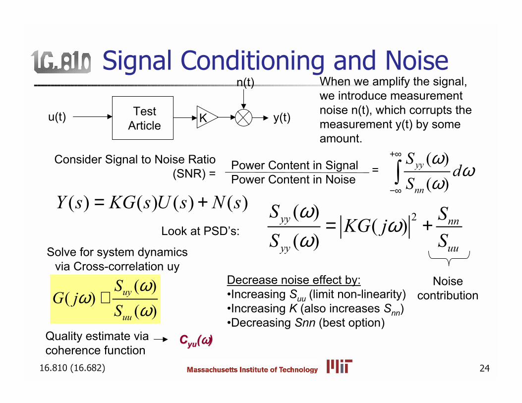
Signal Conditioning and Noise

u(t) KTestArticle

n(t)

y(t)

When we amplify the signal,we introduce measurementnoise n(t), which corrupts themeasurement y(t) by someamount.

Consider Signal to Noise Ratio (SNR) =

Power Content in SignalPower Content in Noise

( ) ( ) ( ) ( )Y s KG s U s N s= +Look at PSDs:

2( )( )

( )yy nn

yy uu

S SKG jS S

ωω

ω= +

Noisecontribution

Solve for system dynamicsvia Cross-correlation uy

Decrease noise effect by:Increasing Suu (limit non-linearity)Increasing K (also increases Snn)Decreasing Snn (best option)

( )( )

( )uy

uu

SG j

Sω

ωω

≅

( )( )

yy

nn

Sd

Sω

ωω

+∞

−∞∫=

Quality estimate viacoherence function

CCyuyu((ωωωωωωωω))

16.810 (16.682) 25

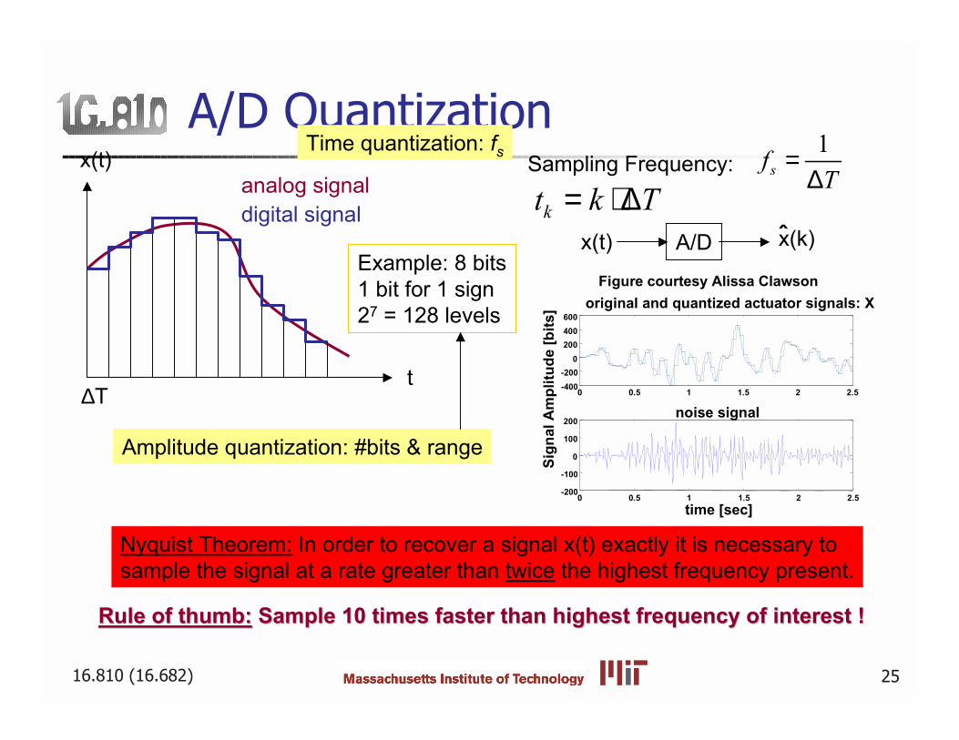
A/D QuantizationSampling Frequency:

1sf T

=∆analog signal

digital signal

Nyquist Theorem: In order to recover a signal x(t) exactly it is necessary tosample the signal at a rate greater than twice the highest frequency present.

Amplitude quantization: #bits & range

∆Tt

x(t)

x(t) A/D x(k)

Rule of thumb:Rule of thumb: Sample 10 times faster than highest frequency of interest ! Sample 10 times faster than highest frequency of interest !

0 0.5 1 1.5 2 2.5-400-200

0200400600

original and quantized actuator signals: X

0 0.5 1 1.5 2 2.5-200

-100

0

100

200noise signal

time [sec]

Sign

al A

mpl

itude

[bits

]

Figure courtesy Alissa ClawsonExample: 8 bits1 bit for 1 sign27 = 128 levels

kt k T= ⋅∆

Time quantization: fs

16.810 (16.682) 26

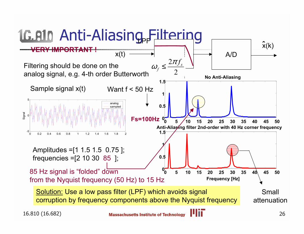
Anti-Aliasing FilteringVERY IMPORTANT !

Solution: Use a low pass filter (LPF) which avoids signal corruption by frequency components above the Nyquist frequency

A/D2

2s

ffπω ≤

x(t)x(k)

Filtering should be done on theanalog signal, e.g. 4-th order Butterworth

Sample signal x(t)

Amplitudes =[1 1.5 1.5 0.75 ];frequencies =[2 10 30 85 ];

LPF

0 0.2 0.4 0.6 0.8 1 1.2 1.4 1.6 1.8 2-5

0

5

Sig

nal

analog sampled

Want f < 50 Hz

Fs=100Hz 0 5 10 15 20 25 30 35 40 45 500

0.5

1

1.5No Anti-Aliasing

0 5 10 15 20 25 30 35 40 45 500

0.5

1

1.5

Frequency [Hz]

Anti-Aliasing filter 2nd-order with 40 Hz corner frequency

85 Hz signal is folded downfrom the Nyquist frequency (50 Hz) to 15 Hz

Smallattenuation

16.810 (16.682) 27

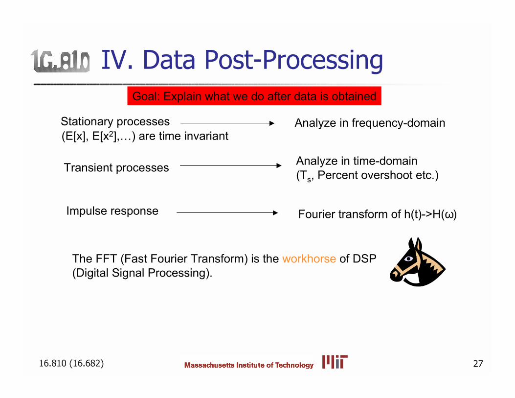
IV. Data Post-Processing

Transient processes Analyze in time-domain(Ts, Percent overshoot etc.)

Stationary processes Analyze in frequency-domain

The FFT (Fast Fourier Transform) is the workhorse of DSP(Digital Signal Processing).

Goal: Explain what we do after data is obtained

Impulse response Fourier transform of h(t)->H(ω)

(E[x], E[x2],) are time invariant

16.810 (16.682) 28

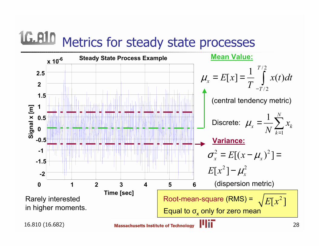
Metrics for steady state processes

0 1 2 3 4 5 6

-2

-1.5

-1

-0.5

0

0.5

1

1.5

2

2.5

x 10-6

Time [sec]

Sign

al x

[m]

Steady State Process Example Mean Value:/ 2

/ 2

1[ ] ( )T

xT

E x x t dtT

µ−

= = ∫(central tendency metric)

2 2

2 2

[( ) ]

[ ]x x

x

E xE xσ µ

µ= − =

−

Variance:

Root-mean-square (RMS) = 2[ ]E x

Discrete:1

1 N

x kkx

Nµ

=

= ∑

Rarely interestedin higher moments.

(dispersion metric)

Equal to σx only for zero mean

16.810 (16.682) 29

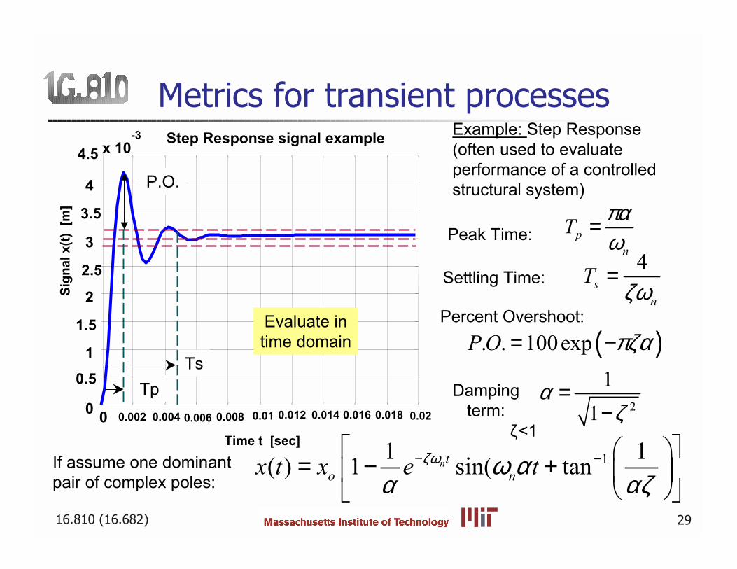
Metrics for transient processes

0 0.002 0.004 0.006 0.008 0.01 0.012 0.014 0.016 0.018 0.020

0.5

1

1.5

2

2.5

3

3.5

4

4.5 x 10-3

Time t [sec]

Sign

al x

(t) [

m]

Step Response signal example

Peak Time:

Settling Time:

Percent Overshoot:

Example: Step Response(often used to evaluateperformance of a controlledstructural system)

If assume one dominantpair of complex poles:

P.O.

11 1( ) 1 sin( tannto nx t x e tζω ω α

α αζ− −

= − +

2

11

αζ

=−

Dampingterm:

TsTp

4s

n

Tζω

=

pn

T παω

=

Evaluate intime domain ( ). . 100expPO πζα= −

ζ<1

16.810 (16.682) 30

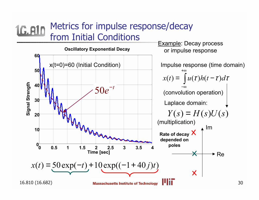
Metrics for impulse response/decayfrom Initial Conditions

Example: Decay processor impulse response

0 0.5 1 1.5 2 2.5 3 3.5 40

10

20

30

40

50

60

Time [sec]

Sign

al S

tren

gth

Oscillatory Exponential Decay

( ) 50exp( ) 10exp(( 1 40 ) )x t t j t= − + − +

Rate of decaydepended on

poles

Re

Im

x(t=0)=60 (Initial Condition) Impulse response (time domain)

( ) ( ) ( )x t u h t dτ τ τ+∞

−∞

= −∫(convolution operation)

( ) ( ) ( )Y s H s U s=Laplace domain:

(multiplication)

50 te−

16.810 (16.682) 31

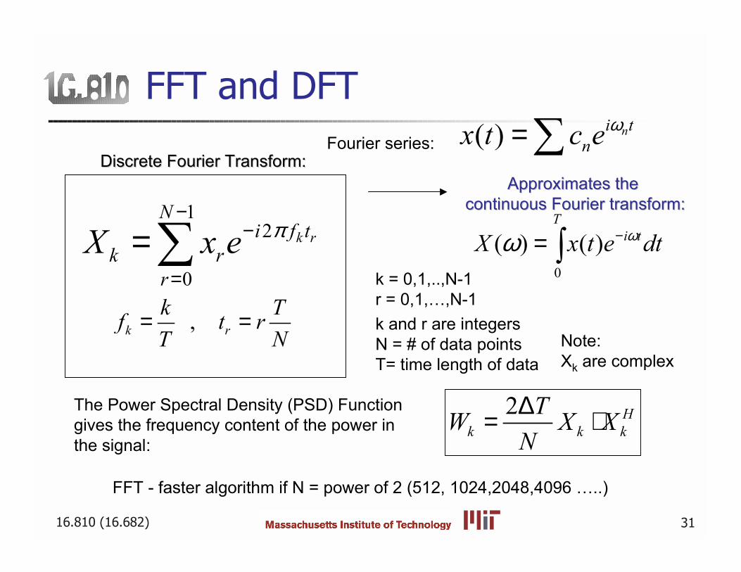
FFT and DFT

Discrete Fourier Transform:Discrete Fourier Transform:( ) ni t

nx t c e ω=∑Fourier series:

12

0

k r

Ni f t

k rr

X x e π−

−

=

=∑ , k r

k Tf t rT N

= = k and r are integersN = # of data pointsT= time length of data

Approximates the Approximates the continuous Fourier transform:continuous Fourier transform:

0

( ) ( )T

i tX x t e dtωω −= ∫

Note:Xk are complex

k = 0,1,..,N-1r = 0,1,,N-1

The Power Spectral Density (PSD) Functiongives the frequency content of the power inthe signal:

2 Hk k k

TW X XN∆= ⋅

FFT - faster algorithm if N = power of 2 (512, 1024,2048,4096 ..)

16.810 (16.682) 32

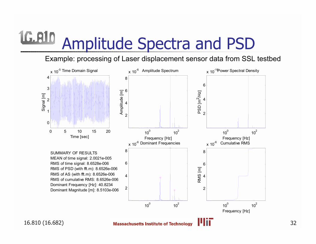
Amplitude Spectra and PSD

0 5 10 15 20

0

1

2

3

4x 10-5

Time [sec]

Sig

nal [

m]

Time Domain Signal

100 102

2

4

6

8x 10-6

Frequency [Hz]

Am

plitu

de [m

]

Amplitude Spectrum

100 102

2

4

6

8x 10-6 Dominant Frequencies

100 102

2

4

6

x 10-10

Frequency [Hz]

PS

D [m

2 /Hz]

Power Spectral Density

100 102

2

4

6

8

x 10-6

Frequency [Hz]

RM

S [m

]

Cumulative RMS

SUMMARY OF RESULTSMEAN of time signal: 2.0021e-005RMS of time signal: 8.6528e-006RMS of PSD (with fft.m): 8.6526e-006RMS of AS (with fft.m): 8.6526e-006RMS of cumulative RMS: 8.6526e-006Dominant Frequency [Hz]: 40.8234Dominant Magnitude [m]: 8.5103e-006

Example: processing of Laser displacement sensor data from SSL testbed

16.810 (16.682) 33

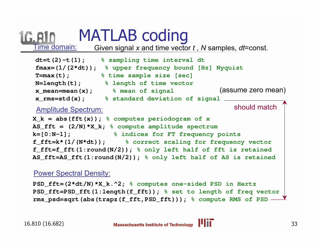
MATLAB coding

Amplitude Spectrum:X_k = abs(fft(x)); % computes periodogram of xAS_fft = (2/N)*X_k; % compute amplitude spectrumk=[0:N-1]; % indices for FT frequency pointsf_fft=k*(1/(N*dt)); % correct scaling for frequency vectorf_fft=f_fft(1:round(N/2)); % only left half of fft is retainedAS_fft=AS_fft(1:round(N/2)); % only left half of AS is retained

Power Spectral Density:PSD_fft=(2*dt/N)*X_k.^2; % computes one-sided PSD in Hertz PSD_fft=PSD_fft(1:length(f_fft)); % set to length of freq vectorrms_psd=sqrt(abs(trapz(f_fft,PSD_fft))); % compute RMS of PSD

Time domain:

dt=t(2)-t(1); % sampling time interval dt fmax=(1/(2*dt)); % upper frequency bound [Hz] NyquistT=max(t); % time sample size [sec]N=length(t); % length of time vectorx_mean=mean(x); % mean of signalx_rms=std(x); % standard deviation of signal

Given signal x and time vector t , N samples, dt=const.

should match

(assume zero mean)

16.810 (16.682) 34

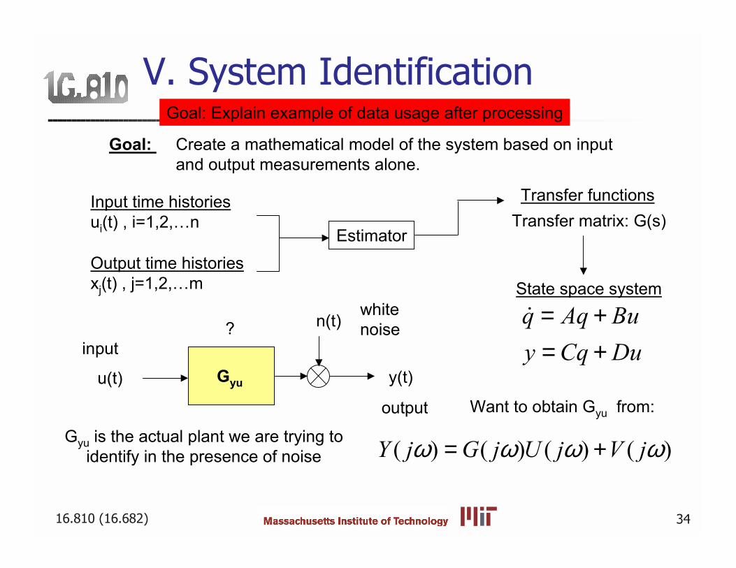
V. System Identification

Estimator

Input time historiesui(t) , i=1,2,n

Output time historiesxj(t) , j=1,2,m

Transfer functions

State space system

Goal: Create a mathematical model of the system based on inputand output measurements alone.

Transfer matrix: G(s)

q Aq Buy Cq Du

= += +!

Goal: Explain example of data usage after processing

Gyuu(t)

n(t)

y(t)

Gyu is the actual plant we are trying toidentify in the presence of noise

?white noise

input

output Want to obtain Gyu from:

( ) ( ) ( ) ( )Y j G j U j V jω ω ω ω= +

16.810 (16.682) 35

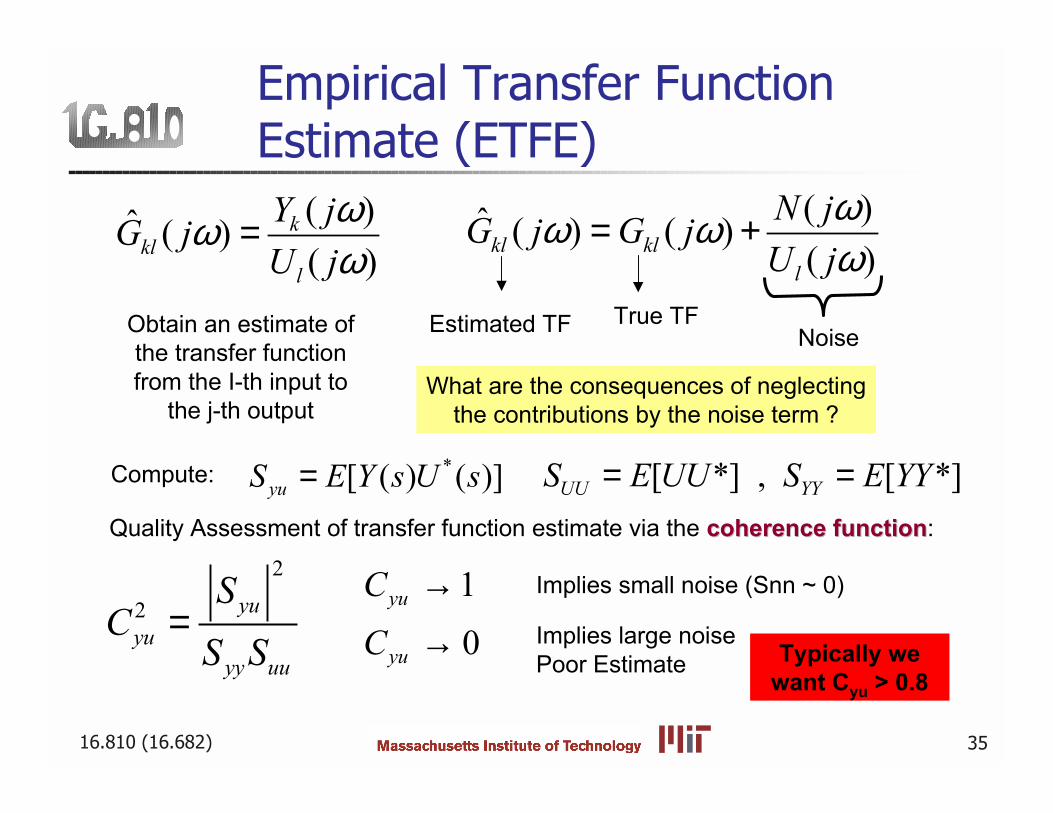
Empirical Transfer FunctionEstimate (ETFE)

Obtain an estimate ofthe transfer functionfrom the I-th input to

the j-th output

( ) ( )( )

kkl

l

Y jG jU j

ωωω

=

Quality Assessment of transfer function estimate via the coherence functioncoherence function:

( ) ( ) ( )( )kl kll

N jG j G jU j

ωω ωω

= +

What are the consequences of neglectingthe contributions by the noise term ?

2

2 yuyu

yy uu

SC

S S=

10

yu

yu

CC

→

→

Implies small noise (Snn ~ 0)

Implies large noisePoor Estimate Typically we

want Cyu > 0.8

True TFEstimated TF Noise

*[ ( ) ( )]yuS E Y s U s=Compute: [ *] , [ *]UU YYS E UU S E YY= =

16.810 (16.682) 36

Averaging

Y(t)

T1 T2 T3 ...

data subdivided in Nd parts

1

2

1

1 ( ) ( ) ( ) 1 ( )

d

d

Ni ii

d

Nii

d

Y s U sNG s

U sN

=

=

−=

∑

∑

10-2 10-1 100 101 102-80

-70

-60

-50

-40

-30

-20

-10

0

10

20

30

Frequency [Hz]

Mag

nitu

de [d

B]

ETFE with no averaging

ETFE True System

10-2 10-1 100 101 102-80

-70

-60

-50

-40

-30

-20

-10

0

10

20

30

Frequency [Hz]

Mag

nitu

de [d

B]

ETFE with 10 averages

ETFE 10 avgTrue System

TNd

Error improves with:

Bias [ ] 1 dE G G N− ∝12-state system

16.810 (16.682) 37

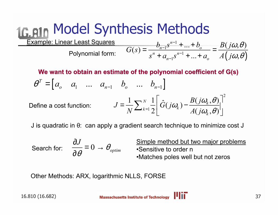
Model Synthesis MethodsExample: Linear Least Squares

Other Methods: ARX, logarithmic NLLS, FORSE

Polynomial form: ( )1

11

1

... ( , )( )... ,

nn o

n nn o

b s b B jG ss a s a A j

ω θω θ

−−

−−

+ += =+ + +

We want to obtain an estimate of the polynomial coefficient of G(s) We want to obtain an estimate of the polynomial coefficient of G(s)

[ ]1 1 1... ...To n o na a a b bθ − −=

Define a cost function:

2

1

( , )1 1 ( )2 ( , )

N kkk

k

B jJ G jN A j

ω θωω θ=

= −

∑

J is quadratic in θ: can apply a gradient search technique to minimize cost J

Search for: 0 optimJ θθ

∂ = →∂

Simple method but two major problemsSensitive to order nMatches poles well but not zeros

16.810 (16.682) 38

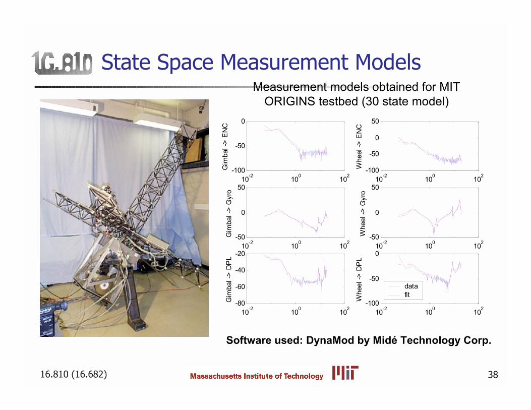
State Space Measurement Models

10-2 100 102-100

-50

0

Gim

bal -

> E

NC

10-2 100 102-100

-50

0

50

Whe

el ->

EN

C

10-2 100 102-50

0

50

Gim

bal -

> G

yro

10-2 100 102-50

0

50

Whe

el ->

Gyr

o

10-2 100 102-80

-60

-40

-20

Gim

bal -

> D

PL

10-2 100 102-100

-50

0

Whe

el ->

DP

L

datafit

Measurement models obtained for MITORIGINS testbed (30 state model)

Software used: DynaMod by Midé Technology Corp.

16.810 (16.682) 39

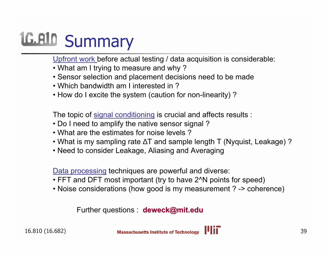
SummaryUpfront work before actual testing / data acquisition is considerable: What am I trying to measure and why ? Sensor selection and placement decisions need to be made Which bandwidth am I interested in ? How do I excite the system (caution for non-linearity) ?

The topic of signal conditioning is crucial and affects results : Do I need to amplify the native sensor signal ? What are the estimates for noise levels ? What is my sampling rate ∆T and sample length T (Nyquist, Leakage) ? Need to consider Leakage, Aliasing and Averaging

Data processing techniques are powerful and diverse: FFT and DFT most important (try to have 2^N points for speed) Noise considerations (how good is my measurement ? -> coherence)

Further questions : deweck@mit.edudeweck@mit.edu

16.810 (16.682) 40

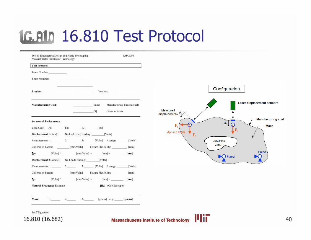
16.810 Test Protocol16.810 Engineering Design and Rapid Prototyping IAP 2004 Massachusetts Institute of Technology Test Protocol Team Number _____________ Team Members __________________________ __________________________ Product: __________________________ Version: ________________ Manufacturing Cost: ______________ [min] Manufacturing Time (actual)

______________ [$] Omax estimate Structural Performance: Load Case: F1:_______ F2:________ F3:________ [lbs] Displacement 1 (fork): No load (zero) reading: _________[Volts] Measurements 1:_______ 2:______ 3:_______ [Volts] Average ________ [Volts] Calibration Factor: _________ [mm/Volts] Fixture Flexibility: ___________ [mm] δδδδ1= ________ [Volts] * __________ [mm/Volts] + ______ [mm] = _________ [mm] Displacement 2 (saddle): No Loads reading: _________[Volts] Measurements 1:_______ 2:______ 3:_______ [Volts] Average ________ [Volts] Calibration Factor: _________ [mm/Volts] Fixture Flexibility: ___________ [mm] δδδδ2= ________ [Volts] * __________ [mm/Volts] + ______ [mm] = _________ [mm] Natural Frequency Estimate: ________________________ [Hz] (Oscilloscope) Mass: 1:_______ 2:______ 3:_______ [grams] avg: ______ [grams] Staff Signature __________________________