Universite Paris–Sud — U.F.R. des Sciences — Orsay

These de doctorat

discipline: Physique

presentee par David Papoular

pour obtenir le grade de docteur de l’Universite Paris–Sud

Manipulation des Interactions dans les Gaz Quantiques:

Approche theorique

soutenue le 11 juillet 2011 devant le Jury compose de

MM. J. Dalibard

O. Dulieu

R. KaiserG. Shlyapnikov Directeur de theseS. Stringari RapporteurE. Trizac

J. Walraven Rapporteur

tel-0

0624

682,

ver

sion

1 -

22 S

ep 2

011

tel-0

0624

682,

ver

sion

1 -

22 S

ep 2

011

Abstract

The interparticle interactions in ultracold atomic gases can be tuned using Fano–Feshbachscattering resonances, which occur in low–energy collisions between two atoms. These reso-nances are usually obtained using an external static magnetic field. They turn ultracold atomicgases into an experimental playground for the investigation of novel phases in which QuantumPhysics plays a key role. The work presented in this memoir is part of the theoretical efforttowards the search for yet unexplored quantum phases.

This manuscript is organised in two parts. The first one is devoted to composite bosonsformed in a 2D heteronuclear Fermi gas. We characterise the zero–temperature phase diagramand show the gas–crystal phase transition in this system. Our results are promising in view offuture experiments with the 6Li–40K mixture.

In the second part, we propose an alternative to static–field Fano–Feshbach resonances.The idea is to achieve the coupling by using a resonant microwave magnetic field. Our schemeapplies to any atomic species whose ground state is split by the hyperfine interaction. It doesnot require the use of a static magnetic field. First, these resonances are presented using asimple two–channel model. We then characterise them numerically using our own full–fledgedimplementation of the coupled–channel approach. Our results yield optimistic prospects forthe observation of microwave–induced Fano–Feshbach resonances with the bosonic alkali atoms23Na, 41K, 87Rb, and 133Cs.

Keywords: cold atoms, quantum gases, Feshbach resonance, cold molecules, quantum phase

transition, microwave–dressed atoms, cold collisions, coupled–channel method.

Resume

Les interactions entre particules dans les gaz quantiques ultrafroids peuvent etre controleesa l’aide de resonances de Fano–Feshbach. Ces resonances de diffusion se produisent lors decollisions a basse energie entre deux atomes et sont generalement obtenues a l’aide d’un champmagnetique statique externe. Elles font des gaz atomiques ultrafroids un terrain d’explorationpour la recherche de nouvelles phases dans lesquelles la physique quantique joue un role clef.Le travail presente dans ce memoire s’inscrit dans le cadre de la recherche de telles phases.

Ce manuscrit comporte deux parties. La premiere est consacree a l’etude de bosons compo-sites obtenus dans des gaz de Fermi heteronucleaires 2D. Nous etudions le diagramme de phasede ce systeme a T = 0 et nous mettons en evidence une transition de phase gaz–cristal. Nosresultats sont prometteurs en vue d’experiences futures avec le melange 6Li–40K.

Dans la seconde partie, nous proposons un nouveau type de resonance de Fano–Feshbach. Lecouplage a l’origine de cette resonance est obtenu a l’aide d’un champ magnetique micro–onde.Notre methode s’applique a n’importe quelle espece atomique dont l’etat fondamental est clivepar l’interaction hyperfine. Elle ne necessite pas l’utilisation d’un champ magnetique statique.Nous decrivons d’abord ces resonances a l’aide d’un modele simple a deux niveaux. Ensuite,nous les caracterisons numeriquement a l’aide de notre propre programme implementant l’ap-proche multi–canaux des collisions atomiques. Nos resultats ouvrent des perspectives optimistesen vue de l’observation des resonances de Feshbach induites par un champ micro–onde avecles atomes alcalins bosoniques suivants : 23Na, 41K, 87Rb et 133Cs.

Mots–clefs : atomes froids, gaz quantiques, resonance de Feshbach, molecules froides, transi-

tion de phase quantique, collisions froides, description multi–canaux des collisions atomiques.

tel-0

0624

682,

ver

sion

1 -

22 S

ep 2

011

tel-0

0624

682,

ver

sion

1 -

22 S

ep 2

011

How much better it is to get wisdom than gold,and to get understanding rather to be chosen than silver.

Proverbs 16:16

In loving memoryof my grandfather Jules Salfati.

tel-0

0624

682,

ver

sion

1 -

22 S

ep 2

011

tel-0

0624

682,

ver

sion

1 -

22 S

ep 2

011

Contents

Foreword 1

I. A two–dimensional crystal of composite bosons 5

1. Introduction 71.1. Bosonic dimers obtained in a bipartite Fermi gas . . . . . . . . . . . . . . 71.2. Effective interaction between heteronuclear composite bosons . . . . . . . 91.3. Zero–temperature phase diagram of a 2D system of composite bosons . . 101.4. Outline of the following chapters . . . . . . . . . . . . . . . . . . . . . . 11

2. Simple approaches to the crystal–gas phase diagram 132.1. The phase diagram in the harmonic approximation . . . . . . . . . . . . 132.2. Hard–core boson approximation for low densities . . . . . . . . . . . . . . 20

3. Born–Oppenheimer potentials for the interaction between composite bosons 23

4. Decay processes for composite bosons 294.1. Collisional relaxation into deeply bound states . . . . . . . . . . . . . . . 294.2. Formation of trimer bound states . . . . . . . . . . . . . . . . . . . . . . 30

5. Suggestion for a new experiment 33

6. Article 1: Crystalline Phase of Strongly Interacting Fermi Mixtures 35

7. Conclusion and outlook 41

Bibliography 43

II. Microwave–induced Fano–Feshbach resonances 47

8. Introduction 498.1. Static–field Fano–Feshbach resonances . . . . . . . . . . . . . . . . . . . 518.2. Previous work on alternative Feshbach resonances . . . . . . . . . . . . . 528.3. Outline of the following chapters . . . . . . . . . . . . . . . . . . . . . . 53

iii

tel-0

0624

682,

ver

sion

1 -

22 S

ep 2

011

Contents

9. An overview of microwave–induced Feshbach resonances 559.1. One single square well . . . . . . . . . . . . . . . . . . . . . . . . . . . . 559.2. The two–square–well model for microwave–induced Feshbach resonances 58

10. The Two–Atom Hamiltonian 6710.1. A single atom in a magnetic field . . . . . . . . . . . . . . . . . . . . . . 6710.2. Two atoms in a magnetic field . . . . . . . . . . . . . . . . . . . . . . . 6910.3. Block–matrix structure of the two–atom Hamiltonian . . . . . . . . . . . 73

11.Characterising the resonances 8111.1. The two–subspace approach . . . . . . . . . . . . . . . . . . . . . . . . . 8211.2. The coupled–channel approach . . . . . . . . . . . . . . . . . . . . . . . 8911.3. Experimental prospects . . . . . . . . . . . . . . . . . . . . . . . . . . . . 9811.4. Comparison with RF–induced Feshbach resonances . . . . . . . . . . . . 99

12.The numerical calculation of two–atom wavefunctions 11112.1. The multi–channel scattering state wavefunction . . . . . . . . . . . . . 11212.2. The Accumulated–Phase approach . . . . . . . . . . . . . . . . . . . . . 11512.3. The relaxation method . . . . . . . . . . . . . . . . . . . . . . . . . . . . 11912.4. An approach based on the shooting method . . . . . . . . . . . . . . . . 12112.5. Summary . . . . . . . . . . . . . . . . . . . . . . . . . . . . . . . . . . . 126

13.Article 2: Microwave–Induced Fano–Feshbach resonances 129

14.Static–Field Feshbach resonances 13514.1. Two atoms in a static magnetic field . . . . . . . . . . . . . . . . . . . . 13514.2. Recovering known Feshbach resonance results . . . . . . . . . . . . . . . 13614.3. Low static–field resonances in Cesium . . . . . . . . . . . . . . . . . . . . 138

15.Towards an experimental observation of our predictions 14515.1. Two atoms in a linearly–polarised magnetic field . . . . . . . . . . . . . . 14515.2. In the absence of a static magnetic field . . . . . . . . . . . . . . . . . . . 14715.3. In the presence of a static magnetic field . . . . . . . . . . . . . . . . . . 154

16.Conclusion and outlook 157

Bibliography 161

Acknowledgements 167

iv

tel-0

0624

682,

ver

sion

1 -

22 S

ep 2

011

Foreword

The achievement of Bose–Einstein condensation [1–3] has stimulated considerable de-velopments in atomic Physics. Ultracold atoms have found applications in metrology[4]. They are used in high–precision experiments with the aim of determining physicalconstants [5] or testing the validity of fundamental theories [6]. Ultracold gases providepromising building blocks for quantum information processing [7]. They can be cooleddown to quantum degeneracy and used to simulate condensed–matter systems [8] or tomodel systems for the investigation of problems arising in astrophysics [9]. Collateralwork [10] has even lead to improved medical imaging methods.

A fundamental feature of ultracold atomic gases is that the interparticle interactions inthe gas can be tailored at will. The manipulation of the interactions is performed usingscattering resonances that occur in low–energy collisions between two atoms [11]. TheseFano–Feshbach resonances are usually obtained using an external static magnetic field[12]. They have turned ultracold atomic gases into an experimental playground for theinvestigation of novel phases of matter in which Quantum Physics plays a key role. Bose–Einstein condensation stands among these new phases, and so do spinor condensates [13]and the Mott–insulating phase [14]. Furthermore, effective dimensionality can also betuned by using a tight optical confinement of the gas in one or two directions. This hasallowed the investigation of the 1D Tonks–Girardeau gas [15, 16] and the 2D Berezinskii–Kousterlitz–Thouless transition [17].

The work presented in this memoir is part of the theoretical effort underlying thesearch for yet unexplored quantum phases. It is organised in two parts:

• The shorter first part illustrates how the manipulation of atomic interactions canbe applied to the search for new quantum phases. We focus on the crystallinephase of a two–dimensional assembly of composite bosons formed in an ultracoldheteronuclear Fermi gas [18] and characterise the zero–temperature crystal–gasphase diagram of this system [19]. Our results are promising in view of a possibleobservation of this crystalline phase in a mixture of 6Li and 40K atoms.

• In the longer second part, the object of our analysis is the actual manipulationof interactions in ultracold gases. We propose an alternative to static–field Fano–Feshbach resonances. In our case, the coupling is achieved using a resonant mi-crowave magnetic field [20]. This scheme is reminiscent of optical Feshbach res-onances [21]. It applies to any atomic species whose ground state is split by thehyperfine interaction. The microwave–induced resonances that we discuss in this

1

tel-0

0624

682,

ver

sion

1 -

22 S

ep 2

011

Foreword

manuscript are present even when no static–field Feshbach resonances are accessi-ble. They do not require the presence of a static magnetic field component, whichwill be an asset in the investigation of new phases in spinor Bose–Einstein conden-sates [22]. Our results yield optimistic prospects for experiments with 23Na, 41K,87Rb, and 133Cs.

References

[1] M. H. Anderson et al. “Observation of Bose-Einstein Condensation in a DiluteAtomic Vapor”. In: Science 269.5221 (1995), pp. 198–201. doi: 10.1126/science.269.5221.198.

[2] C. C. Bradley et al. “Evidence of Bose-Einstein Condensation in an Atomic Gaswith Attractive Interactions”. In: Phys. Rev. Lett. 75.9 (Aug. 1995), pp. 1687–1690. doi: 10.1103/PhysRevLett.75.1687.

[3] Kendall B. Davis et al. “Evaporative Cooling of Sodium Atoms”. In: Phys. Rev.Lett. 74.26 (June 1995), pp. 5202–5205. doi: 10.1103/PhysRevLett.74.5202.

[4] S. Bize et al. “Cold atom clocks and applications”. In: Journal of Physics B:Atomic, Molecular and Optical Physics 38.9 (2005), S449. doi: 10.1088/0953-4075/38/9/002.

[5] F. Biraben. “Spectroscopy of atomic hydrogen”. In: The European Physical Journal-Special Topics 172.1 (2009), pp. 109–119. doi: 10.1140/epjst/e2009-01045-3.

[6] Keng-Yeow Chung et al. “Atom interferometry tests of local Lorentz invariance ingravity and electrodynamics”. In: Phys. Rev. D 80.1 (July 2009), p. 016002. doi:10.1103/PhysRevD.80.016002.

[7] J.J. Garcıa-Ripoll, P. Zoller, and J.I. Cirac. “Quantum information processing withcold atoms and trapped ions”. In: Journal of Physics B: Atomic, Molecular andOptical Physics 38 (2005), S567. doi: 10.1088/0953-4075/38/9/008.

[8] A. Georges. “Condensed-matter Physics with light and atoms”. In: Proceedingsof the International School of Physics “Enrico Fermi,” Course CLXIV, Varenna,2006. IOS Press, 2008.

[9] Andrew G. Truscott et al. “Observation of Fermi Pressure in a Gas of TrappedAtoms”. In: Science 291.5513 (2001), pp. 2570–2572. doi: 10.1126/science.1059318.

[10] Michele Leduc and Pierre Jean Nacher. “Polarized Helium to Image the Lung”. In:AIP Conference Proceedings 770.1 (2005). Ed. by Luis Gustavo Marcassa, KristianHelmerson, and Vanderlei Salvador Bagnato, pp. 381–389. doi: 10.1063/1.1928872.

[11] Cheng Chin et al. “Feshbach resonances in ultracold gases”. In: Rev. Mod. Phys.82.2 (Apr. 2010), pp. 1225–1286. doi: 10.1103/RevModPhys.82.1225.

2

tel-0

0624

682,

ver

sion

1 -

22 S

ep 2

011

0.0. References

[12] S. Inouye et al. “Observation of Feshbach resonances in a Bose–Einstein conden-sate”. In: Nature 392.6672 (1998), pp. 151–154. issn: 0028-0836. doi: 10.1038/32354.

[13] J. Stenger et al. “Spin domains in ground-state Bose-Einstein condensates”. In:Nature 396 (1998), p. 345. doi: 10.1038/24567.

[14] M. Greiner et al. “Quantum phase transition from a superfluid to a Mott insulatorin a gas of ultracold atoms”. In: Nature 415 (2002), p. 39. doi: 10.1038/415039a.

[15] Toshiya Kinoshita, Trevor Wenger, and David S. Weiss. “Observation of a One-Dimensional Tonks-Girardeau Gas”. In: Science 305.5687 (2004), pp. 1125–1128.doi: 10.1126/science.1100700.

[16] B. Paredes et al. “Tonks-Girardeau gas of ultracold atoms in an optical lattice”.In: Nature 429 (2004), p. 277. doi: 10.1038/nature02530.

[17] Z. Hadzibabic et al. “Berezinskii-Kosterlitz-Thouless crossover in a trapped atomicgas”. In: Nature 441 (2006), p. 1118. doi: 10.1038/nature04851.

[18] D. S. Petrov, C. Salomon, and G. V. Shlyapnikov. “Molecular regimes in ultracoldFermi gases”. In: Cold Molecules: Theory, Experiment, Applications. CRC Press,2009. Chap. 9. isbn: 978-1-4200-5903-8.

[19] D. S. Petrov et al. “Crystalline Phase of Strongly Interacting Fermi Mixtures”. In:Phys. Rev. Lett. 99.13 (Sept. 2007), p. 130407. doi: 10.1103/PhysRevLett.99.130407.

[20] D. J. Papoular, G. V. Shlyapnikov, and J. Dalibard. “Microwave-induced Fano-Feshbach resonances”. In: Phys. Rev. A 81.4 (Apr. 2010), p. 041603. doi: 10.1103/PhysRevA.81.041603.

[21] P. O. Fedichev et al. “Influence of Nearly Resonant Light on the Scattering Lengthin Low-Temperature Atomic Gases”. In: Phys. Rev. Lett. 77.14 (Sept. 1996), pp. 2913–2916. doi: 10.1103/PhysRevLett.77.2913.

[22] Tin-Lun Ho. “Spinor Bose Condensates in Optical Traps”. In: Phys. Rev. Lett.81.4 (July 1998), pp. 742–745. doi: 10.1103/PhysRevLett.81.742.

3

tel-0

0624

682,

ver

sion

1 -

22 S

ep 2

011

tel-0

0624

682,

ver

sion

1 -

22 S

ep 2

011

Part I.

A two–dimensional crystal ofcomposite bosons

5

tel-0

0624

682,

ver

sion

1 -

22 S

ep 2

011

tel-0

0624

682,

ver

sion

1 -

22 S

ep 2

011

1. Introduction

The first part of the present manuscript focuses on the zero–temperature phase diagramof a two–dimensional system of composite bosons formed in a heteronuclear fermionicmixture with equal densities of the two species.

We consider an ultracold gas of fermionic atoms. In order to avoid a suppressionof the atomic interactions due to the Pauli principle, we consider a bipartite mixture,i.e. a gas in which two types of atoms are present. These atoms may all belong to thesame atomic species, part of them being in a different internal state than the others.Alternately, two different species of fermions, such as Lithium 6 and Potassium 40, maybe present in the mixture.

Assuming that the gas is cold enough for s–wave collisions to be dominant [1], the na-ture (repulsive or attractive) and strength of the interaction between two distinguishableatoms are encoded in a single real parameter, the scattering length a. This interactionis represented by the following pseudopotential [2]:

Upseudo(r) =4π~2

maδ(r) , (1.1)

where r is the interactomic distance.

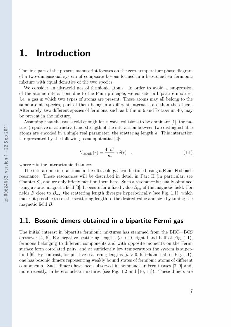
The interatomic interactions in the ultracold gas can be tuned using a Fano–Feshbachresonance. These resonances will be described in detail in Part II (in particular, seeChapter 8), and we only briefly mention them here. Such a resonance is usually obtainedusing a static magnetic field [3]. It occurs for a fixed value Bres of the magnetic field. Forfields B close to Bres, the scattering length diverges hyperbolically (see Fig. 1.1), whichmakes it possible to set the scattering length to the desired value and sign by tuning themagnetic field B.

1.1. Bosonic dimers obtained in a bipartite Fermi gas

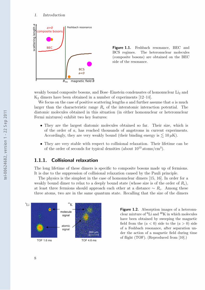
The initial interest in bipartite fermionic mixtures has stemmed from the BEC—BCScrossover [4, 5]. For negative scattering lengths (a < 0, right–hand half of Fig. 1.1),fermions belonging to different components and with opposite momenta on the Fermisurface form correlated pairs, and at sufficiently low temperatures the system is super-fluid [6]. By contrast, for positive scattering lengths (a > 0, left–hand half of Fig. 1.1),one has bosonic dimers representing weakly bound states of fermionic atoms of differentcomponents. Such dimers have been observed in homonuclear Fermi gases [7–9] and,more recently, in heteronuclear mixtures (see Fig. 1.2 and [10, 11]). These dimers are

7

tel-0

0624

682,

ver

sion

1 -

22 S

ep 2

011

1. Introduction

magnetic field B

scatt

eri

ng

len

gth

a

a>0composite bosons

a<0BCS

BEC

Feshbach resonance

Bres

Figure 1.1. Feshbach resonance, BEC andBCS regimes. The heteronuclear molecules(composite bosons) are obtained on the BECside of the resonance.

weakly bound composite bosons, and Bose–Einstein condensates of homonuclear Li2 andK2 dimers have been obtained in a number of experiments [12–14].

We focus on the case of positive scattering lengths a and further assume that a is muchlarger than the characteristic range Re of the interatomic interaction potential. Thediatomic molecules obtained in this situation (in either homonuclear or heteronuclearFermi mixtures) exhibit two key features:

• They are the largest diatomic molecules obtained so far. Their size, which isof the order of a, has reached thousands of angstroms in current experiments.Accordingly, they are very weakly bound (their binding energy is . 10µK).

• They are very stable with respect to collisional relaxation. Their lifetime can beof the order of seconds for typical densities (about 1013 atoms/cm3).

1.1.1. Collisional relaxation

The long lifetime of these dimers is specific to composite bosons made up of fermions.It is due to the suppression of collisional relaxation caused by the Pauli principle.

The physics is the simplest in the case of homonuclear dimers [15, 16]. In order for aweakly bound dimer to relax to a deeply bound state (whose size is of the order of Re),at least three fermions should approach each other at a distance ∼ Re. Among thesethree atoms, two are in the same quantum state. Recalling that the size of the dimers

Figure 1.2. Absorption images of a heteronu-clear mixture of 6Li and 40K in which moleculeshave been obtained by sweeping the magneticfield from the (a < 0) side to the (a > 0) sideof a Feshbach resonance, after separation un-der the action of a magnetic field during timeof flight (TOF). (Reproduced from [10].)

8

tel-0

0624

682,

ver

sion

1 -

22 S

ep 2

011

1.2. Effective interaction between heteronuclear composite bosons

is ∼ a, the typical momentum of the atoms is k ∼ 1/a, and this three–body encounteris Pauli–supressed by a factor of (k Re)

s ∼ (Re/a)s 1, where s is of the order of 2.In the case of heteronuclear dimers, the situation is more involved. The weakly bound

heteronuclear molecules can decay towards lower–energy states through two main chan-nels [17]: (i) the relaxation into deeply bound dimer states and (ii) the formation oftrimer states.

The relaxation into deeply bound dimer states can occur in dimer–dimer collisionswhen one heavy and two light fermions1 are within a distance ∼ Re from each other.The relaxation rate acquires a dependence on the ratio M/m of the heavy to lightfermionic masses [18], but the suppression of collisional relaxation still holds.

The formation of a trimer state requires two heavy and one light atoms to come at adistance R . a from each other. At such distances the light fermion mediates an effectiveinteraction between the two dimers which is attractive [17]. This attractive interactionis proportional to −1/(mR2), and it competes with the Pauli repulsion, which manifestsitself through a centrifugal barrier which is proportional to 1/(MR2). The physics thusdepends on the value of the mass ratio M/m. For mass ratios M/m ∼ 1, the Paulirepulsion is dominant and the trimer states do not exist. For mass ratios M/m > 13.6,the attractive interaction dominates, and Efimov trimers can appear [19]. These trimerscannot be described using the scattering length alone, and an additional three–bodyparameter must be introduced.

Besides the Efimov trimers, one light and two heavy atoms may form “universal”trimer states, which are well described in the zero–range approximation without intro-ducing the three–body parameter [20]. They exist for the orbital angular momentum` = 1 and mass ratios below the critical value M/m < 13.6, where the Efimov effect isabsent. One such state emerges for M/m ≈ 8.1. These universal trimer states also existabove the critical mass ratio, but the trimer formation at such mass ratios is dominatedby the formation of smaller–` Efimov trimers.

1.2. Effective interaction between heteronuclearcomposite bosons

We now concentrate on the case of bosonic dimers obtained in a Fermi mixture containingtwo types of atoms, chosen such that the ratio M/m of the heavy to light fermion massesis large. These dimers interact with one another via an exchange interaction mediatedby the light fermions [18, 19]. This interaction has been studied theoretically in twosituations:

1. The motion of the heavy atoms is two–dimensional, whereas that of the light atomsis three–dimensional (abbreviated to 2× 3 in [17]).

1Experiments involving composite bosons are likely to be performed in the presence of an opticallattice (see Section 5). The relaxation process involving one light and two heavy fermions is heavilysuppressed due to the presence of the lattice, as it requires the heavy fermions to occupy the samelattice site.

9

tel-0

0624

682,

ver

sion

1 -

22 S

ep 2

011

1. Introduction

2. The motion of both the heavy and light atoms is two–dimensional(abbreviated to 2× 2 in [17]).

In dilute systems (i.e. if the mean intermolecular spacing R exceeds the scattering lengtha of the interatomic interaction), this interaction can be modelled by an effective pairpotential. The detailed expression for the effective potential depends on the consideredsituation (2 × 3 or 2 × 2), but in both cases the interaction between the dimers isrepulsive2.

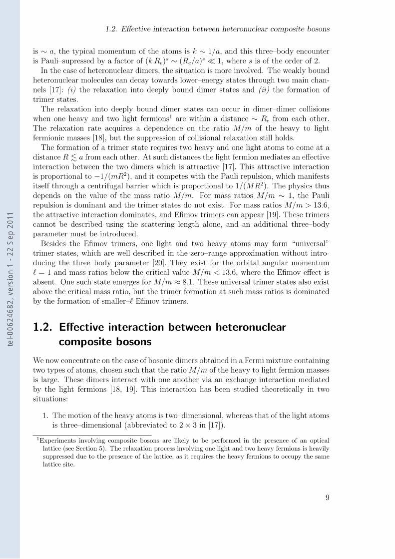
Analytical expressions for this effective potential have been obtained in both situations[17, 18] using the Born–Oppenheimer approximation. A detailed derivation of theseexpressions is given in Chapter 3. In the 2 × 3 case, the effective potential U3D(R) isgiven by:

U3D(R) = 4 |ε0| (1− (2κ0R)−1)exp(−2κ0R)

κ0R, (1.2)

where the composite–boson molecular size κ−10 is related to the binding energy |ε0| of a

single dimer:

|ε0| =~2κ2

0

2m, (1.3)

with m being the mass of the light fermion. In the 2×3 case the molecular size κ−10 = a.

In the 2× 2 case the effective potential U2D(R) reads:

U2D(R) = 4 |ε0|[κ0RK0(κ0R)K1(κ0R) − K2

0(κ0R)]

, (1.4)

where K0 and K1 are modified Bessel functions [21]. In this regime, achieved by confiningthe light–atom motion to zero–point oscillations with amplitude l0, the weakly–boundmolecular states exist at a negative a. For |a| l0, the molecular size is given byκ−1

0 =√πl0 exp(−

√π/2 l0/a) [17, 22].

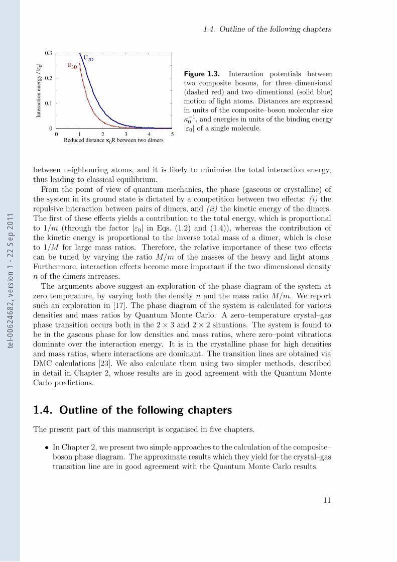
The potentials U3D(r) and U2D(r) are shown on Fig. 1.3. The range of these potentialsis given by the molecular size κ−1

0 . Therefore, the dimer–dimer interaction can be maderelatively long–ranged by selecting a value for a which does not greatly exceed the meanintermolecular separation.

1.3. Zero–temperature phase diagram of a 2D systemof composite bosons

The interaction between the dimers described above is repulsive, and it can be madelong–range3. These are two indications that the 2D system of composite bosons mayexhibit a crystalline phase. Indeed, a triangular crystalline lattice maximises distances

2This is in contrast to the attractive effective interaction mediated by one light atom between twoheavy atoms at a distance R . a: see Section 1.1.1.

3The crystalline phase is also predicted to exist for very low two–dimensional densities n. In thislimit, the mean distance between molecules greatly exceeds the size of the molecule, and the systembehaves like a set of 2D hard–core bosons: see Section 2.2.

10

tel-0

0624

682,

ver

sion

1 -

22 S

ep 2

011

1.4. Outline of the following chapters

0

0.1

0.2

0.3

0 1 2 3 4 5

Inte

ract

ion e

ner

gy /

|ε0|

Reduced distance κ0R between two dimers

U3D

U2D

Figure 1.3. Interaction potentials betweentwo composite bosons, for three–dimensional(dashed red) and two–dimentional (solid blue)motion of light atoms. Distances are expressedin units of the composite–boson molecular sizeκ−1

0 , and energies in units of the binding energy|ε0| of a single molecule.

between neighbouring atoms, and it is likely to minimise the total interaction energy,thus leading to classical equilibrium.

From the point of view of quantum mechanics, the phase (gaseous or crystalline) ofthe system in its ground state is dictated by a competition between two effects: (i) therepulsive interaction between pairs of dimers, and (ii) the kinetic energy of the dimers.The first of these effects yields a contribution to the total energy, which is proportionalto 1/m (through the factor |ε0| in Eqs. (1.2) and (1.4)), whereas the contribution ofthe kinetic energy is proportional to the inverse total mass of a dimer, which is closeto 1/M for large mass ratios. Therefore, the relative importance of these two effectscan be tuned by varying the ratio M/m of the masses of the heavy and light atoms.Furthermore, interaction effects become more important if the two–dimensional densityn of the dimers increases.

The arguments above suggest an exploration of the phase diagram of the system atzero temperature, by varying both the density n and the mass ratio M/m. We reportsuch an exploration in [17]. The phase diagram of the system is calculated for variousdensities and mass ratios by Quantum Monte Carlo. A zero–temperature crystal–gasphase transition occurs both in the 2 × 3 and 2 × 2 situations. The system is found tobe in the gaseous phase for low densities and mass ratios, where zero–point vibrationsdominate over the interaction energy. It is in the crystalline phase for high densitiesand mass ratios, where interactions are dominant. The transition lines are obtained viaDMC calculations [23]. We also calculate them using two simpler methods, describedin detail in Chapter 2, whose results are in good agreement with the Quantum MonteCarlo predictions.

1.4. Outline of the following chapters

The present part of this manuscript is organised in five chapters.

• In Chapter 2, we present two simple approaches to the calculation of the composite–boson phase diagram. The approximate results which they yield for the crystal–gastransition line are in good agreement with the Quantum Monte Carlo results.

11

tel-0

0624

682,

ver

sion

1 -

22 S

ep 2

011

1. Introduction

• Chapter 3 is devoted to the derivation of the analytical expressions (1.2) and (1.4)for the effective interaction between composite bosons.

• In Chapter 4, we evaluate the decay rates of weakly bound composite bosons intodeeply bound states and trimer states.

• Chapter 5 briefly sketches an experimental proposal for the observation of thecrystalline phase of composite bosons.

• Chapter 6 reproduces our published article [17].

12

tel-0

0624

682,

ver

sion

1 -

22 S

ep 2

011

2. Simple approaches to thecrystal–gas phase diagram

We consider a two–dimensional assembly of composite bosons obtained in an ultracoldmixture of two different fermionic atoms. Throughout this chapter, we assume that the2D density is sufficiently low for these composite bosons to be considered as basic entitiesinteracting via an effective pair potential which is repulsive (see Chapter 1 and [17]).

The nature of the ground state of such a system results from the competition betweentwo effects: (i) the zero–point kinetic energy, and (ii) the repulsive interaction betweencomposite bosons. If the zero–point vibrations are dominant, the ground state is gaseous.On the other hand, if the interaction energy dominates, the ground state is crystalline.The numerical analysis of the system, using Diffusion Monte Carlo [23], has revealed [17]that the system should undergo a crystal–gas phase transition. The stable phase atT = 0 K depends on two parameters:

• the 2D density n, and

• the ratio M/m of the heavy (M) to light (m) fermion masses in the mixture.

In this chapter, we present two approximate methods which allow for simple calcula-tions of the phase diagram of the system, with little or no input from the QMC resultsfor this diagram. The first approach is based on a harmonic approximation to the crys-tal Hamiltonian, and it relies on the Lindemann criterion to predict the critical massratio as a function of the density. This approach is valid for all values of the parametersM/m and n for which the composite nature of the molecules does not come into play.The second method, which does not involve the Lindemann criterion, is only applicablefor very low densities. In this limit, the composite bosons are modelled by hard disks,and for a given mass ratio the critical density can be deduced from accurate numericalanalyses of the fluid–crystal phase transition in hard–disk systems.

Both approximate approaches are in good agreement with the more accurate QuantumMonte Carlo results.

2.1. The phase diagram in the harmonic approximation

2.1.1. Hamiltonian of the crystal

We consider a two–dimensional assembly of N composite bosons at an ultracold tem-perature. More precisely, we assume that T = 0.

13

tel-0

0624

682,

ver

sion

1 -

22 S

ep 2

011

2. Simple approaches to the crystal–gas phase diagram

d

a1

a2

2π/3

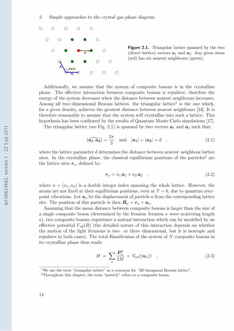
Figure 2.1. Triangular lattice spanned by the two(direct–lattice) vectors a1 and a2. Any given atom(red) has six nearest neighbours (green).

Additionally, we assume that the system of composite bosons is in the crystallinephase. The effective interaction between composite bosons is repulsive, therefore theenergy of the system decreases when the distance between nearest neighbours increases.Among all two–dimensional Bravais lattices, the triangular lattice1 is the one which,for a given density, achieves the greatest distance between nearest neighbours [24]. It istherefore reasonable to assume that the system will crystallise into such a lattice. Thishypothesis has been confirmed by the results of Quantum Monte Carlo simulations [17].

The triangular lattice (see Fig. 2.1) is spanned by two vectors a1 and a2 such that:

(a1,a2) =2π

3and |a1| = |a2| = d , (2.1)

where the lattice parameter d determines the distance between nearest–neighbour latticesites. In the crystalline phase, the classical equilibrium positions of the particles2 arethe lattice sites rn, defined by:

rn = n1 a1 + n2 a2 , (2.2)

where n = (n1, n2) is a double integer index spanning the whole lattice. However, theatoms are not fixed at their equilibrium positions, even at T = 0, due to quantum zero–point vibrations. Let un be the displacement of particle n from the corresponding latticesite. The position of this particle is then Rn = rn + un.

Assuming that the mean distance between composite bosons is larger than the size ofa single composite boson (determined by the fermion–fermion s–wave scattering lengtha), two composite bosons experience a mutual interaction which can be modelled by aneffective potential Ueff(R) (the detailed nature of this interaction depends on whetherthe motion of the light fermions is two– or three–dimensional, but it is isotropic andrepulsive in both cases). The total Hamiltonian of the system of N composite bosons inits crystalline phase then reads:

H =∑n

P 2n

2M+ Vint((un)) , (2.3)

1We use the term “triangular lattice” as a synonym for “2D hexagonal Bravais lattice”.2Throughout this chapter, the term “particle” refers to a composite boson.

14

tel-0

0624

682,

ver

sion

1 -

22 S

ep 2

011

2.1. The phase diagram in the harmonic approximation

where M is the mass of the heavier atomic species3, and the total interaction energyVint((un)) is given by:

Vint((un)) =1

2

∑i 6=j

Ueff (|(ri − rj) + (ui − uj)|) . (2.4)

2.1.2. Harmonic crystal dynamics

We are interested in the ground state properties of the N–particle system described bythe Hamiltonian (2.3). This ground state has been numerically studied by QuantumMonte Carlo methods [17]. In this Section, we introduce a harmonic approximation tothe N–particle Hamiltonian, which will be used to derive an approximate phase diagramof the system (see Section 2.1.4) with minimal input from the Monte Carlo results.

If the system is in its crystalline phase, the amplitude of the displacement un of particlen from the corresponding lattice site n is characterised by the root–mean–square (RMS)displacement ln:

l2n = 〈Ω |u2n|Ω 〉 , (2.5)

where |Ω 〉 is the exact N–particle ground state of the Hamiltonian H. The discretetranslational invariance of the crystal lattice implies that the RMS displacement is thesame for all particles in the crystal, i.e. ln = l. Deeply in the crystalline domain ofthe phase diagram, the RMS displacement l is small compared to the characteristiclengthscale Reff of the effective interaction Ueff(R) (i.e. l/Reff 1), and we expand thetotal interaction energy Vint as:

Vint = V(0)

int + V(1)

int ((un)) + V(2)

int ((un)) + . . . . (2.6)

In Eq. (2.6) we have the following terms:

• The term V(0)

int is the value of the interaction energy for all particles fixed at theirclassical equilibrium positions rn. It is a constant number and has no incidenceon the dynamics of the crystal. It will be dropped in subsequent calculations.

• The term V(1)

int ((un)) is the contribution to Vint which is linear in the displacements(un). The expansion is performed around the classical equilibrium state of thesystem, which minimises the total interaction energy Vint((un)). Therefore, thisterm vanishes.

• The term V(2)

int ((un)) is the contribution to Vint which is quadratic in the displace-ments (un).

3The total mass of a composite boson is (M +m), where M and m are the masses of the heavier andlighter atoms, respectively. However, the phase transition occurs for mass ratios M/m > 100 (seeFig. 2.3), and the lighter mass m can thus be neglected in the kinetic energy part of Eq. (2.3).

15

tel-0

0624

682,

ver

sion

1 -

22 S

ep 2

011

2. Simple approaches to the crystal–gas phase diagram

The harmonic approximation, used throughout this section, consists in neglecting allterms containing products of three or more displacement operators. We have thus re-placed the original Hamiltonian H by the approximate Hamiltonian Hharm given by:

Hharm =∑n

P 2n

2M+ V

(2)int ((un)) . (2.7)

The Hamiltonian Hharm can be diagonalised in terms of phonons, each of which is thequantum equivalent of a classical vibrational mode of the system.

Classical crystal vibrations

We first briefly introduce classical vibrational modes of the crystal [24, 25].Each classical vibrational mode is characterised by (i) its wavevector k, and (ii) its

polarisation index p = 1 or 2. These two attributes can be condensed into a singlemulti–index κ = (k, p). The classical vibrational mode κ corresponds to the followinglattice wave:

un = A eκ exp(i(k · rn − ωκt)) , (2.8)

where A is an arbitrary amplitude, the unit vector eκ gives the polarisation, and ωκ isthe frequency of the mode.

For a crystal which comprises N particles, there are 2N independent vibrationalmodes. In order to characterise these modes, we write the quadratic part of the in-teraction energy as:

V(2)

int =1

2

∑pq

tup Λpq uq , (2.9)

where tup is the (real) transpose of up, and the (Λpq)’s are 2×2 real symmetric matricesgiven by:

Λijpq =

∂2U tot((un))

∂uip ∂ujq

∣∣∣∣∣(un=0)

. (2.10)

The discrete translational invariance of the crystal lattice implies that Λpq = Λ(rp−rq).We now introduce the momentum–space dynamical matrix Λ(k) defined as [24]:

Λ(k) =∑p

Λ(rp) e−ik·rp = −2

∑p

Λ0p sin2

(1

2k · rp

), (2.11)

where the second equality follows from the invariance of the crystal lattice under spatialinversion. The classical vibrational modes of the crystal lattice are completely deter-mined by the eigenelements of the dynamical matrices ˜Λ(k) [24]. For a given wavevectork, Λ(k) is a 2 × 2 real symmetric matrix whose eigenvalues are Mω2

k,1 and Mω2k,2,

where ωk,1 and ωk,2 are the frequencies of the two vibrational modes with wavevector k.The corresponding (unit–normalised and orthogonal) eigenvectors ek,1 and ek,2 are thepolarisations of these vibrational modes.

16

tel-0

0624

682,

ver

sion

1 -

22 S

ep 2

011

2.1. The phase diagram in the harmonic approximation

Quantum crystal vibrations

We now return to quantum mechanics and introduce the phonon annihilation (aκ) andcreation (a†κ) operators defined by the following relations [26]:

un = 1√2N

∑κ

(~

Mωκ

)1/2 (aκeκe

ik·rn + a†κe∗κe−ik·rn

)Pn = i√

2N

∑κ

(M~ωκ)1/2 (−aκeκeik·rn + a†κe∗κe−ik·rn

) (2.12)

The operators a†κ and aκ are the creation and annihilation operators for a phonon in themode related to the lattice wave of Eq. (2.8). They satisfy the bosonic commutationrules [aκ, a

†κ′ ] = δκ,κ′ and [aκ, aκ′ ] = [a†κ, a

†κ′ ] = 0, where δκ,κ′ is the Kronecker symbol.

In terms of these operators, the Hamiltonian (2.7) reduces to that of 2N independentharmonic oscillators indexed by κ:

Hharm =∑κ

~ωκ(a†κaκ +

1

2

), (2.13)

The ground state | 0 〉 of the Hamiltonian Hharm, corresponding to the absence ofany phonon excitation, is an approximation to the N–particle ground state |Ω 〉 of thecomplete Hamiltonian H of Eq. (2.3). This approximate ground state can be used toevaluate the RMS displacement l0 of a particle in the crystal around its lattice site:

l20 =1

2N

∑κ

~Mωκ

. (2.14)

As expected from the discrete translational invariance of the system, the RMS displace-ment l0 is the same for all particles in the crystal. It depends both on the distanced between neighbouring lattice sites and on the mass ratio M/m. The dependence onthe mass ratio can be made explicit. Recalling that the effective potential Ueff(R) isproportional to4 1/m and that the Mω2

κ are the eigenvalues of the matrix Λ(k), we findthat the frequency ωκ is proportional to (Mm)−1/2. Equation (2.14) then shows that l0is proportional to (M/m)−1/4.

2.1.3. The specific case of the triangular lattice

In this Section, we apply the general formalism summarised in Section 2.1.4 to thespecific case of the 2D triangular lattice. We obtain an analytical expression for thetwo branches of the phonon dispersion relation in the nearest–neighbour approximationand compare these analytical results to numerical calculations including five rings ofneighbours.

4The effective interaction Ueff(R) between two composite bosons is mediated by the lighter fermions:see Chapter 1.

17

tel-0

0624

682,

ver

sion

1 -

22 S

ep 2

011

2. Simple approaches to the crystal–gas phase diagram

We express the displacement vectors (un) in an orthonormal basis (ex, ey) with ex =a1/d. Equation (2.10) yields the following expression for Λ0p, where p = (p1, p2) is adouble integer index:

Λ0p = −1

4

d2

r2p

[(2p1 − p2)2 U ′′(rp) + 3p2

2U ′(rp)

rp

√3 p2(2p1 − p2) (U ′′(rp)− U ′(rp)

rp)√

3 p2(2p1 − p2) (U ′′(rp)− U ′(rp)

rp) 3p2

2 U′′(rp) + (2p1 − p2)2U

′(rp)

rp

].

(2.15)We assume that the range Reff of the effective potential Ueff(R) is significantly smaller

than the distance d between nearest–neighbour lattice sites. Therefore, we calculatethe dynamical matrices Λ(k) in the nearest–neighbour approximation. Equation (2.16)yields:

Λ(k) =

[4U ′′(d)s2

1 + (U ′′(d) + 3U′(d)d

)(s22 + s2

3)√

3(U ′′(d)− U ′(d)d

)(s23 − s2

2)√3(U ′′(d)− U ′(d)

d)(s2

3 − s22) 4U

′(d)d

+ (3U ′′(d) + U ′(d)d

)(s22 + s2

3)

],

(2.16)where s1 = sin

(12k · a1

), s2 = sin

(12k · a2

), and s3 = sin

(12k · (a1 + a2)

). Equa-

tion (2.16) yields the following analytical expression for the two branches of the dis-persion relation, which are obtained as the two eigenvalues of Λ(k):

mω21,2(k) = 2

(U ′′(d) +

U ′(d)

d

)(s2

1 + s22 + s2

3)± 2

(U ′′(d)− U ′(d)

d

)s2

0 , (2.17)

where s20 =

√(s2

1 + s22 + s2

3)2 − 3(s21s

22 + s2

2s33 + s2

3s21). Equation 2.17 is symmetrical in

s1, s2, and s3, and is thus compatible with the six–fold symmetry of the two–dimensionalhexagonal lattice.

The wavevectors k are conveniently described in the reciprocal lattice basis (a∗1,a∗2)

defined by a∗i · aj = 2π · δij. The reciprocal lattice of a hexagonal lattice is also ahexagonal lattice (see Fig. 2.2(right)):

|a∗1| = |a∗2| =2π

d

2√3

and (a∗1,a∗2) =

π

3. (2.18)

The two branches ω21,2(k) of the dispersion relation are represented in Figure 2.2(right)

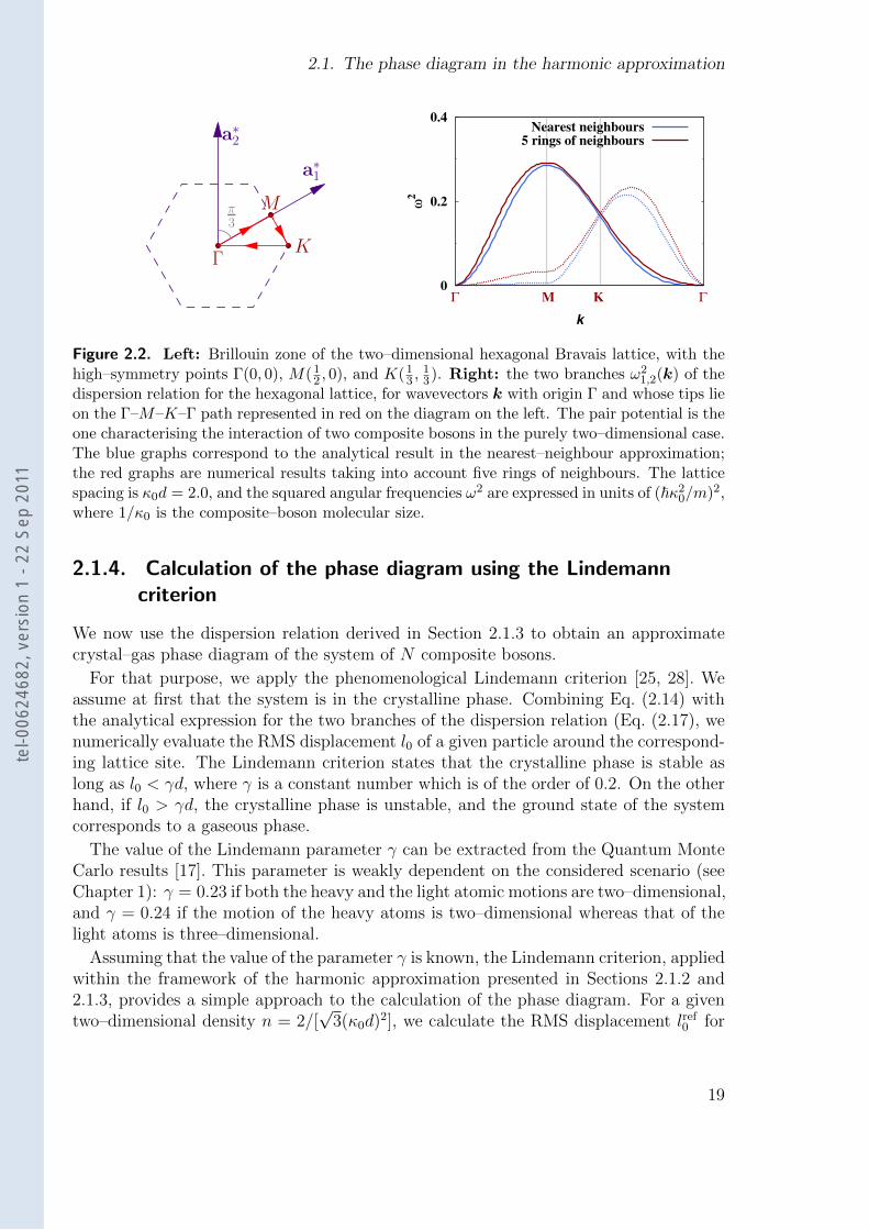
in the case of the pair potential characterising the interaction between two compos-ite bosons in the fully two–dimensional situation (see Chapter 1), for wavevectors kwhose tips lie on the high–symmetry axes of the Brillouin zone[27]. The analytical re-sults obtained in the nearest–neighbour approximation (Equation 2.17) are comparedto numerical calculations taking into account five rings of neighbours on a finite–sizedhexagonal lattice with 100 independent particles in both the a1 and a2 directions. Bothcalculations have been performed for the lattice parameter κ0d = 2.0 (1/κ0 being thecomposite–boson molecular size). For this lattice parameter, the two branches ω2

1,2(k)of the dispersion relation are positive for all wavevectors in the Brillouin zone, whichensures that the triangular lattice of composite bosons is stable with respect to harmoniclattice vibrations.

18

tel-0

0624

682,

ver

sion

1 -

22 S

ep 2

011

2.1. The phase diagram in the harmonic approximation

π3

a∗1

a∗2

ΓK

M

0

0.2

0.4

ω2

k

Γ M K Γ

Nearest neighbours5 rings of neighbours

Figure 2.2. Left: Brillouin zone of the two–dimensional hexagonal Bravais lattice, with thehigh–symmetry points Γ(0, 0), M(1

2 , 0), and K(13 ,

13). Right: the two branches ω2

1,2(k) of thedispersion relation for the hexagonal lattice, for wavevectors k with origin Γ and whose tips lieon the Γ–M–K–Γ path represented in red on the diagram on the left. The pair potential is theone characterising the interaction of two composite bosons in the purely two–dimensional case.The blue graphs correspond to the analytical result in the nearest–neighbour approximation;the red graphs are numerical results taking into account five rings of neighbours. The latticespacing is κ0d = 2.0, and the squared angular frequencies ω2 are expressed in units of (~κ2

0/m)2,where 1/κ0 is the composite–boson molecular size.

2.1.4. Calculation of the phase diagram using the Lindemanncriterion

We now use the dispersion relation derived in Section 2.1.3 to obtain an approximatecrystal–gas phase diagram of the system of N composite bosons.

For that purpose, we apply the phenomenological Lindemann criterion [25, 28]. Weassume at first that the system is in the crystalline phase. Combining Eq. (2.14) withthe analytical expression for the two branches of the dispersion relation (Eq. (2.17), wenumerically evaluate the RMS displacement l0 of a given particle around the correspond-ing lattice site. The Lindemann criterion states that the crystalline phase is stable aslong as l0 < γd, where γ is a constant number which is of the order of 0.2. On the otherhand, if l0 > γd, the crystalline phase is unstable, and the ground state of the systemcorresponds to a gaseous phase.

The value of the Lindemann parameter γ can be extracted from the Quantum MonteCarlo results [17]. This parameter is weakly dependent on the considered scenario (seeChapter 1): γ = 0.23 if both the heavy and the light atomic motions are two–dimensional,and γ = 0.24 if the motion of the heavy atoms is two–dimensional whereas that of thelight atoms is three–dimensional.

Assuming that the value of the parameter γ is known, the Lindemann criterion, appliedwithin the framework of the harmonic approximation presented in Sections 2.1.2 and2.1.3, provides a simple approach to the calculation of the phase diagram. For a giventwo–dimensional density n = 2/[

√3(κ0d)2], we calculate the RMS displacement lref

0 for

19

tel-0

0624

682,

ver

sion

1 -

22 S

ep 2

011

2. Simple approaches to the crystal–gas phase diagram

Up to a normalization constant, G!0is the wave function of

a bound state of a single molecule with energy "0 !"@2!2

0=2m and molecular size !"10 . From Eqs. (1) and

(2) one gets a set of N equations:P

jAijCj ! 0, whereAij ! ##!$$ij %G!#Rij$#1" $ij$, Rij ! jRi "Rjj, and##!$ ! limr!0&G!#r$ "G!0

#r$'. The single-particle en-ergy levels are determined by the equation

det&Aij#!; fRg$' ! 0: (3)

For Rij ! 1, Eq. (3) gives an N-fold degenerate groundstate with ! ! !0. At finite large Rij, the levels split into anarrow band. Given a small parameter

% ! G!0# ~R$=!0j#0

!#!0$j ( 1; (4)

where ~R is a characteristic distance at which heavy atomscan approach each other, the bandwidth is !" ) 4j"0j% (j"0j. It is important for the adiabatic approximation that alllowest N eigenstates have negative energies and are sepa-rated from the continuum by a gap *j"0j.

We now calculate the single-particle energies up tosecond order in %. To this order we write !##$ ) !0 %!0##% !00

###2=2 and turn from Aij#!$ to Aij##$:

Aij ! #$ij % &G!0#Rij$ % !0

##@G!0#Rij$=@!'#1" $ij$;

(5)

where all derivatives are taken at # ! 0. Using Aij (5) inEq. (3) gives a polynomial of degree N in #. Its roots #igive the light-atom energy spectrum "i ! "@2!2##i$=2m.The total energy E ! PN

i!1 "i is then given by

E!"#@2=2m$!N!2

0%2!0!0#

XN

i!1

#i%#!!0#$0#

XN

i!1

#2i

": (6)

Keeping only the terms up to second order in % and usingbasic properties of determinants and polynomial roots wefind that the first order terms vanish, and the energy readsE ! N"0 % 1

2

Pi!jU#Rij$, where

U#R$ ! " @2m

!!0#!0

#$2@G2

!0#R$

@!% #!!0

#$0#G2!0#R$

": (7)

Thus, up to second order in % the interaction in the systemof N molecules is the sum of binary potentials (7).

If the motion of light atoms is 3D, the Green function isG!#R$ ! #1=4&R$ exp#"!R$, and ##!$ ! #!0 " !$=4&,with the molecular size !"1

0 equal to the 3D scatteringlength a. Equation (7) then gives a repulsive potential

U3D#R$ ! 4j"0j!1" #2!0R$"1" exp#"2!0R$=!0R; (8)

and the criterion (4) reads #1=!0R$ exp#"!0R$ ( 1. Forthe 2D motion of light atoms we have G!#R$ !#1=2&$K0#!R$ and ##!$ ! "#1=2&$ ln#!=!0$, where K0is the decaying Bessel function, and !"1

0 follows from [6].This leads to a repulsive intermolecular potential

U2D#R$ ! 4j"0j&!0RK0#!0R$K1#!0R$ " K20#!0R$'; (9)

with the validity criterion K0#!0R$ ( 1. In both cases,which we denote 2+ 3 and 2+ 2 for brevity, the validitycriteria are well satisfied already for !0R ) 2.

The Hamiltonian of the many-body system reads

H ! "#@2=2M$Xi!Ri

% 1

2

Xi!j

U#Rij$; (10)

and the state of the system is determined by two parame-ters: the mass ratio M=m and the rescaled 2D density n!"2

0 .At a large M=m, the potential repulsion dominates over thekinetic energy and one expects a crystalline ground state.For separations Rij < !"1

0 the adiabatic approximationbreaks down. However, the interaction potential U#R$ isstrongly repulsive at larger distances. Hence, even for anaverage separation between heavy atoms "R close to 2=!0,they approach each other at distances smaller than !"1

0

with a small tunneling probability P / exp#"'###########M=m

p$ (

1, where '* 1. We extended U#R$ to R & !"10 in a way

providing a proper molecule-molecule scattering phaseshift in vacuum and checked that the phase diagram forthe many-body system is not sensitive to the choice of thisextension.

Using the DMC method [11] we solved the many-bodyproblem at zero temperature. For each phase, gaseous andsolid, the state with a minimum energy was obtained in astatistically exact way. The lowest of the two energiescorresponds to the ground state, the other phase beingmetastable. The phase diagram is displayed in Fig. 1.The guiding wave function was taken in the Nosanow-Jastrow form [12]. Simulations were performed with 30particles and showed that the solid phase is a 2D triangularlattice. For the largest density we checked that using moreparticles has little effect on the results.

For both 2+ 3 and 2+ 2 cases the (Lindemann) ratio (of the rms displacement of molecules to "R on the transition

FIG. 1 (color online). DMC gas-crystal transition lines for 3D(triangles) and 2D (circles) motion of light atoms. Solid curvesshow the low-density hard-disk limit, and dashed curves theresults of the harmonic approach (see text).

PRL 99, 130407 (2007) P H Y S I C A L R E V I E W L E T T E R S week ending28 SEPTEMBER 2007

130407-2

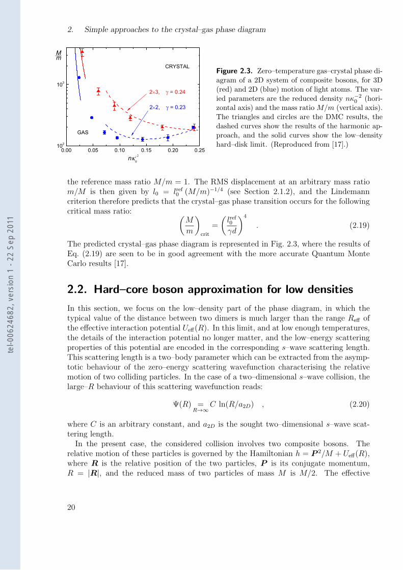
Figure 2.3. Zero–temperature gas–crystal phase di-agram of a 2D system of composite bosons, for 3D(red) and 2D (blue) motion of light atoms. The var-ied parameters are the reduced density nκ−2

0 (hori-zontal axis) and the mass ratio M/m (vertical axis).The triangles and circles are the DMC results, thedashed curves show the results of the harmonic ap-proach, and the solid curves show the low–densityhard–disk limit. (Reproduced from [17].)

the reference mass ratio M/m = 1. The RMS displacement at an arbitrary mass ratiom/M is then given by l0 = lref

0 (M/m)−1/4 (see Section 2.1.2), and the Lindemanncriterion therefore predicts that the crystal–gas phase transition occurs for the followingcritical mass ratio: (

M

m

)crit

=

(lref0

γd

)4

. (2.19)

The predicted crystal–gas phase diagram is represented in Fig. 2.3, where the results ofEq. (2.19) are seen to be in good agreement with the more accurate Quantum MonteCarlo results [17].

2.2. Hard–core boson approximation for low densities

In this section, we focus on the low–density part of the phase diagram, in which thetypical value of the distance between two dimers is much larger than the range Reff ofthe effective interaction potential Ueff(R). In this limit, and at low enough temperatures,the details of the interaction potential no longer matter, and the low–energy scatteringproperties of this potential are encoded in the corresponding s–wave scattering length.This scattering length is a two–body parameter which can be extracted from the asymp-totic behaviour of the zero–energy scattering wavefunction characterising the relativemotion of two colliding particles. In the case of a two–dimensional s–wave collision, thelarge–R behaviour of this scattering wavefunction reads:

Ψ(R) =R→∞

C ln(R/a2D) , (2.20)

where C is an arbitrary constant, and a2D is the sought two–dimensional s–wave scat-tering length.

In the present case, the considered collision involves two composite bosons. Therelative motion of these particles is governed by the Hamiltonian h = P 2/M + Ueff(R),where R is the relative position of the two particles, P is its conjugate momentum,R = |R|, and the reduced mass of two particles of mass M is M/2. The effective

20

tel-0

0624

682,

ver

sion

1 -

22 S

ep 2

011

2.2. Hard–core boson approximation for low densities

interaction Ueff(R) is proportional to 1/m, whereas the kinetic term is proportional to1/M , therefore a2D is a function of the mass ratio M/m.

In the low–density limit, the potential may be replaced by any other potential whichhas the same two–dimensional scattering length. The crystal–fluid phase diagram of atwo–dimensional assembly of hard disks at zero temperature has been studied numer-ically using Quantum Monte Carlo methods [29]. Therefore, we replace the effectivepotential Ueff(R) by a hard–disk potential UHD(R), characterised by the hard–disk di-ameter D:

UHD(R) =

+∞ for R < D/2,

0 for R > D/2.(2.21)

The scattering length characterising the s–wave collision between two hard disks ofradius D is given by5 aHD = D. Therefore, for a given mass ratio M/m, the hard–diskradius is chosen to be equal to the ‘physical’ scattering length a2D(M/m).

The Quantum Monte Carlo analysis reported in [29] shows that a two–dimensionalsystem of N bosonic hard disks of radius D undergoes a crystal–fluid phase transitionat the critical density ncrit

HD = 0.33/D2. For densities nHD < ncritHD, the ground state of

the system exhibits no crystalline order, whereas for nHD < ncritHD the ground state is a

crystal (even though in the classical picture separated hard disks do not interact at all).The numerical results for bosonic hard–disk systems yield a simple way to evaluate

the low–density part of the phase diagram of our system of composite bosons. For agiven mass ratio M/m (chosen large, so that the phase transtion occurs at low den-sity: see Fig. 2.3), we calculate the scattering length a2D(M/m) characterising the low–density and low–temperature scattering by the effective potential Ueff(R). Replacingthis effective potential by the hard–disk potential UHD(R), and choosing the radiusD = a2D(M/m) so as to leave the scattering length unchanged, the critical density forthe crystal–gas phase transition is thus close to ncrit(M/m) = 0.33/a2

2D(M/m).The results of this approximate low–density approach are compared in Fig. 2.3 to the

more accurate Quantum Monte Carlo results, and a good agreement can be observedbetween the two approaches for densities nκ−2

0 < 0.25.

5The centres of the two hard disks can never come any closer than 2 × D/2 = D. Combining theasymptotic behaviour of Eq. (2.20), which is exact for R ≥ D, with the hard–disk condition Ψ(D) =0, one obtains aHD = D.

21

tel-0

0624

682,

ver

sion

1 -

22 S

ep 2

011

tel-0

0624

682,

ver

sion

1 -

22 S

ep 2

011

3. Born–Oppenheimer potentials forthe interaction between compositebosons

The object of this chapter is the derivation of the analytical expressions (1.2) and (1.4)for the potentials characterising the effective interaction between two composite bosonsin the 2 × 3 and 2 × 2 situations, respectively [17]. This derivation hinges on two ap-proximations: (i) the zero–range approximation for the interatomic interaction, and (ii)the Born–Oppenheimer approach, assuming that the motion of the heavy atoms is muchslower than that of the light atoms.

The zero–range approximation

As a first step, we consider the interaction between one heavy atom and one light atom.We assume that the scattering length a characterising this interaction is much larger thanthe range Re of the interaction potential. Under this assumption, the detailed nature ofthe atomic interaction is no longer important, and it can be taken into account throughthe boundary condition for the wavefunction at vanishing interparticle distances. In thecase of a 3D s–wave interaction between two atoms, this boundary condition reads [30]:

limr→0

(rψ3D)′

rψ3D

= − 1

a3D

, (3.1)

where a = a3D is the 3D scattering length, r is the interatomic distance, the (s–wave)wavefunction ψ(r) describes the relative motion of the two atoms, and C is an unknownconstant. This boundary condition can be rewritten as:

ψ3D(r) = C

(1

r− 1

a3D

)for Re r , (3.2)

which is the familiar condition that the radial wavefunction be proportional to (r−a3D)for Re r. In the 2D case, the corresponding condition reads:

ψ2D(r) = C ln

(r

a2D

)for Re r , (3.3)

where ψ2D is the wavefunction describing the 2D relative motion and a2D is the 2Danalog of the scattering length.

23

tel-0

0624

682,

ver

sion

1 -

22 S

ep 2

011

3. Born–Oppenheimer potentials for the interaction between composite bosons

We now state the Bethe–Peierls boundary conditions (Eqs. 3.2 and 3.3) in a waythat does not depend on dimensionality (3D or 2D). For that purpose, we introduce thefree–particle Green’s function Gκ(r) for the bound–state energy1 ε = −~2κ2/2m, whichsatisfies the following differential equation:

(−4+ κ2)Gκ(r) = δ(r) . (3.4)

In the 3D case, it is given by:

G3Dκ (r) =

e−κr

4πr, (3.5)

whereas in the 2D case it reads:

G2Dκ (r) =

K0(κr)

2π, (3.6)

where K0(x) is the modified Bessel’s function which decays exponentially for large x[21]. Introducing κ0 = 1/a, where a = a3D or a2D depending on the considered case, Eqs.3.2 and (3.3) both reduce to the condition:

ψ(r) = C Gκ0(r) for Re r . (3.7)

The Born–Oppenheimer wavefunction

We now consider a system of N heavy atoms and N light atoms. We use the Born–Oppenheimer approach [31], taking advantage of the motion of the N heavy atomsbeing much slower than that of the N light atoms. We thus wish to describe the systemassuming that the heavy atoms are fixed at their positions Ri1≤i≤N .

Furthermore, we neglect the interaction between the identical light fermions (whichis zero in the zero–range approximation because of the Pauli principle). Hence, we wishto calculate the wavefunction Ψ(Ri, r) of a single light fermion in the presence of Nfixed heavy atoms. Note that the vectors Ri belong to the 2D plane of the heavyatoms, whereas the vector r, giving the position of the light fermion, can be 3D or 2Ddepending on the considered situation (2× 3 or 2× 2: see Chapter 1).

More precisely, we wish to calculate the N lowest eigenvalues of the Hamiltonian fora single light fermion whose motion is free everywhere except at the positions of theheavy atoms, where the Bethe–Peierls condition (3.7) is applied. The sum of these Nenergies will provide the Born–Oppenheimer potential describing the effective interactionbetween the molecules.

We seek the wavefunction of a single light fermion in the form

Ψ(Ri, r) =N∑i=1

CiGκ(r −Ri) , (3.8)

1The mass m of a light atom is very close the reduced mass Mm/(M +m) of one light atom and oneheavy atom.

24

tel-0

0624

682,

ver

sion

1 -

22 S

ep 2

011

which describes free motion everywhere except at the singular points Ri. The energy ofthe state Ψ(Ri, r) is ε = −~2κ2/2m. The Green’s functions Gκ are given by Eq. (3.5)or by Eq. (3.6) depending on whether the motion of the light atoms is 3D or 2D, andare calculated for the energy ε.

The coefficients Ci appearing in Eq. (3.8) are determined by applying the Bethe–Peierls boundary condition at the N heavy atom positions Ri:

Ψ(Ri, r) =r→Ri

CiGκ0(r −Ri) . (3.9)

The coefficient of Gκ0 on the right–hand side of Eq. (3.9) is Ci in order to ensure thatboth sides of the equality have the same irregular parts. These N boundary conditionsyield a system of N linear equations for the coefficients Ci1≤i≤N , which we write as

AC = 0 . (3.10)

In Eq. (3.10), C is the N–component vector (C1, . . . , CN), and A is an N × N realsymmetric matrix depending on κ and Ri, whose coefficients Aij are given by:

Aij = λ(κ) δij + Gκ(Rij) (1− δij) , (3.11)

where Rij = |Ri −Rj| and

λ(κ) = limr→0

[Gκ(r) − Gκ0(r)] . (3.12)

The linear system (3.10) has non–zero solutions if

det (A(κ, Ri) = 0 , (3.13)

which is a polynomial equation whose N roots (κi)1≤i≤N yield the sought N energiesεi = −~2κ2

i /2m.

Calculation of the total energy

For infinitely large separations Rij between heavy atoms, all off–diagonal elements inA vanish, and Eq. (3.13) yields an N–fold degenerate ground state whose energy is−~2κ2

0/2m. We now consider finite, albeit large, values of Rij. More precisely, weassume that the following parameter remains small:

ξ =Gκ0(R)

κ0λ′κ(κ0) 1 , (3.14)

where R is a typical value for the Rij and λ′κ(κ0) = dλ/dκ, taken at κ = κ0.

25

tel-0

0624

682,

ver

sion

1 -

22 S

ep 2

011

3. Born–Oppenheimer potentials for the interaction between composite bosons

Calculation of the determinant

We now calculate the determinant appearing in Eq. (3.13) to second order in ξ. Theparameter ξ being small entails that λ′κ(κ0) is large and, hence, that κ(λ) is a slowly–varying function for small values of λ. We expand κ(λ) to second order in λ:

κ(λ) = κ0 + κ′λ λ+1

2κ′′λλ λ

2 , (3.15)

where κ′λ = ∂κ/∂λ and κ′′λλ = ∂2κ/∂λ2, all derivatives being taken at λ = 0. We alsoexpand Gκ(Rij) to first order in λ:

Gκ(Rij) = Gκ0(Rij) + κ′λ λ∂Gκ0(Rij)

∂κ. (3.16)

We introduce the N ×N symmetric matrix K such that:

A = λ (1 + K) , (3.17)

The matrix elements Kij depend on λ and are all of order ξ:

Kij(λ) =1

λ

[Gκ0(Rij) + κ′λ λ

∂Gκ0(Rij)

∂κ

∣∣∣∣κ=κ0

](1− δij) . (3.18)

We calculate the determinant det(A) through the identity2:

det(A) = exp[Tr(lnA)] , (3.19)

where Tr(M) denotes the trace of the square matrix M . Noting that Tr(K) = 0,Eqs. (3.17), (3.18), and (3.19) yield the following expansion for det(A) up to secondorder in ξ:

det(A) = λN

(1− 1

2κ′2λ∑i 6=j

[∂Gκ0(Rij)

∂κ

]2)

− λN−1 1

2κ′λ∑i 6=j

∂G2κ0

(Rij)

∂κ− λN−2 1

2

∑i 6=j

G2κ0

(Rij) + . . . (3.20)

Calculation of the total energy

The N roots λi of the polynomial (3.20) yield the N sought bound–state energies εi.The total energy of N light fermions in the presence of the N fixed heavy fermions isE =

∑Ni=1 εi, which, using Eq. (3.15), is given by:

E = − ~2

2m

[Nκ2

0 + 2κ0κ′λ

N∑i=1

λi + (κκ′λ)′λ

N∑i=1

λ2i

], (3.21)

2Equation (3.19) holds for any positive–definite symmetric matrix.

26

tel-0

0624

682,

ver

sion

1 -

22 S

ep 2

011

where (κκ′λ)′λ = κ0κ

′′λλ+κ′2λ . The quantities

∑Ni=1 λi and

∑Ni=1 λ

2i are symmetric functions

of the roots λi of the polynomial (3.20). Hence, they can be expressed in terms of thecoefficients of this polynomial. Up to second order in ξ, we find:

N∑i=1

λi =1

2κ′λ∑i 6=j

∂G2κ0

(Rij)

∂κ, (3.22)

N∑i=1

λ2i =

∑i 6=j

G2κ0

(Rij) . (3.23)

Finally, substituting Eqs. (3.22) and (3.23) into Eq. (3.21), the total energy E reducesto:

E(Ri) = −N ε0 +1

2

∑i 6=j

U(Rij) , (3.24)

where ε0 = −~2κ20/2m and the function U(R) is given by:

U(R) = −~2

m

[κ0(κ′λ)

2∂G2κ0

(R)

∂κ+ (κκ′λ)

′λG

2κ0

(R)

]. (3.25)

Analytical expressions for the effective potentials

We have calculated the total energy E(Ri) of N light atoms as a function of thepositions Ri of the heavy atoms. In the Born–Oppenheimer approach [31], the to-tal energy of the light atoms gives the effective potential energy for the heavy atoms.Therefore, Eq. (3.25) gives the total effective potential for a system of N compositebosons. Dropping the constant energy offset (−N ε0), the structure of this equationshows that the composite bosons interact via the effective pair potential U(R). We nowderive analytical expressions for this effective potential in the 2× 3 and 2× 2 situations.

If the motion of the light atoms is 3D (2 × 3 situation), the Green’s function G3Dκ is

given by Eq. (3.5). Equation (3.12) then leads to λ3D(κ) = (κ0 − κ)/4π. The effectivepotential reads:

U3D(R) = 4 |ε0| (1− (2κ0R)−1)exp(−2κ0R)

κ0R, (1.2)

and the corresponding validity criterion, given by Eq. (3.14), is exp(−κ0R)/(κ0R) 1.If the motion of the light atoms is 2D (2 × 2 situation), the Green’s function G2D

κ isgiven by Eq. (3.6). In this case, λ2D(κ) = ln(κ0/κ)/2π. The effective potential is givenby:

U2D(R) = 4 |ε0|[κ0RK0(κ0R)K1(κ0R) − K2

0(κ0R)]

, (1.4)

and the validity criterion is K(κ0r) 1.Both criteria are well satisfied for κ0R ≥ 2.

27

tel-0

0624

682,

ver

sion

1 -

22 S

ep 2

011

tel-0

0624

682,

ver

sion

1 -

22 S

ep 2

011

4. Decay processes for compositebosons

The gaseous and solid phases of weakly bound molecules are actually metastable. Themain decay channels are the relaxation of molecules into deep bound states and theformation of trimer states by one light and two heavy atoms (see Section 1.1.1 and [17]).

In order to achieve the large mass ratios M/m > 100 required for the realisation ofthe crystalline phase, one should put heavy atoms in an optical lattice, where for a smallfilling factor they acquire a large effective mass M∗. The crystalline phase then emergesas a superlattice.

In this chapter, we focus on the stability of the dimers in an optical lattice, and weevaluate the relaxation rates for the two main decay processes.

4.1. Collisional relaxation into deeply bound states

Let m be the mass of the light atoms, and M∗ the effective mass of the heavy fermions inan optical lattice. For a large effective mass ratioM∗/m, the relaxation into deeply boundstates occurs when a molecule is approached by another light atom1 and both light-heavyseparations are of the order of the size of a deep bound state. This size is determinedby the range Re of the interatomic interaction, which satisfies Re κ−1

0 , where κ−10

is the molecular size (see Section 1.2) and R is a typical value for the distances Rijbetween the heavy atoms. The released binding energy is taken by outgoing particleswhich escape from the sample. The rate of this process is not influenced by the opticallattice.

We estimate this rate in the solid phase and near the gas-solid transition to the leadingorder in (κ0R)−1. At light–heavy separations r1,2 κ−1

0 the initial-state wavefunctionfor a single heavy atom (position R) and two light atoms (positions r1 and r2) reads:

Ψ(R, r1, r2) = B(κ−10 , R)ψ(r1, r2) . (4.1)

We write the wavefunction (4.1) as an antisymmetrized product of wavefunctions of theform CiGκ(ri −R), where Gκ is the free–particle Green’s function, given by Eq. (3.5)or by Eq. (3.6) depending on whether the motion of the light atoms is 3D (2 × 3 case)or 2D (2× 2 case). For the 2× 3 case (κ−1

0 = a), we find

B ≈ (1/Ra2) exp(−R/a) . (4.2)

1The relaxation involving one light and two heavy atoms is strongly suppressed, as it requires theheavy atoms to approach each other and get to the same lattice site.

29

tel-0

0624

682,

ver

sion

1 -

22 S

ep 2

011

4. Decay processes for composite bosons

The quantity W = B2R6e is the probability of having both light atoms at distances ∼ Re

from a heavy atom, and the relaxation rate is ν3D ∝ W . As the short-range physics ischaracterised by the energy scale ~2/mR2

e, we restore the dimensions and write:

ν3D = C(~/m)(Re/a)4(1/R2) exp(−2R/a), (4.3)

where the typical distance R is linked to the 2D density by R−2 ≈ n. The coefficient Cdepends on a particular system and is ∼ 1 within an order of magnitude. The relaxationrate ν3D is generally rather low. For the 40K–6Li mixture, where Re ≈ 50 A, even atna2 = 0.24 (see Fig. 1) the relaxation time exceeds 10 s for the density n = 109 cm−2

and the scattering length a = 1600 A. In the 2 × 2 case, for the same n and κ−10 the

probability W is smaller and the relaxation is slower.

4.2. Formation of trimer bound states

The formation of trimer bound states by one light and two heavy atoms occurs whentwo molecules approach each other at distances R . κ−1

0 . It is accompanied by a releaseof the second light atom.

4.2.1. Born–Oppenheimer wavefunction for a trimer

The existence of the trimer states is seen considering a light atom (position r) inter-acting with two heavy ones (positions R1 and R2). We use the Born–Oppenheimerapproximation, assuming as a first step that the heavy atoms are fixed. We seek thewavefunction of this system in the form:

Ψtrimer(R1,R2, r) = C1Gκ(r −R1) + C2Gκ(r −R2) , (4.4)

where Gκ(r) is the (3D or 2D) free–particle Green’s function. Applying the Bethe–Peierls boundary condition (3.7) at each of the two heavy–atom positions, we obtain asecond–order polynomial condition on κ (see Eq. (3.13)), whose roots yield the energies−~2κ2/2m of the possible states Ψtrimer. The lowest–energy solution is the gerade state(C1 = C2). In the Born–Oppenheimer approach, its energy ε+(R) introduces an effectiveattractive potential acting on the heavy atoms, and the trimer states are bound statesof two heavy atoms in this potential.

4.2.2. Trimer formation in an optical lattice

In an optical lattice, the trimers are eigenstates of the Hamiltonian

H0 = − ~2

2M∗

∑i=1,2

∆Ri+ ε+(R12) . (4.5)

In a deep lattice, one can neglect all higher bands and regard Ri as discrete latticecoordinates and ∆ as the lattice Laplacian. Then, the fermionic nature of the heavyatoms prohibits them to be in the same lattice site.

30

tel-0

0624

682,

ver

sion

1 -

22 S

ep 2

011

4.2. Formation of trimer bound states

For a very large effective mass ratio M∗/m, the kinetic energy term in H0 can beneglected, and the lowest trimer state has the energy

εtr ≈ ε+(L) , (4.6)

where L is the spatial period of the lattice. It consists of a pair of heavy atoms localizedat neighbouring sites and a light atom in the gerade state. Higher trimer states areformed by heavy atoms localized in sites separated by distances R > L. This picturebreaks down at large R, where the spacing between trimer levels is comparable with thetunneling energy ~2/M∗L

2 and the heavy atoms are delocalized.The scale of energies in a many–body system of composite bosons is much smaller than|ε0|. Thus, the formation of trimers in molecule-molecule “collisions” is energeticallyallowed only if the trimer binding energy is εtr < 2ε0. Since the lowest trimer energyin the optical lattice is ε+(L), the trimer formation requires the condition ε+(L) . 2ε0,which is equivalent to κ−1

0 & 1.6L in the 2× 3 case and κ−10 & 1.25L in the 2× 2 case.

This means that for a sufficiently small molecular size κ−10 , or for a sufficiently large

lattice period L, the formation of trimers is forbidden. At a larger molecular size orsmaller L the trimer formation is possible.

4.2.3. Rate of formation of trimers in an optical lattice

We now assume that κ−10 /L is large enough for the formation of trimers to be energeti-

cally allowed, and we calculate the rate of trimer formation.For that purpose, we consider the interaction between two molecules as a reduced

three–body problem, accounting for the fact that one of the light atoms is in the geradestate and the other one in the ungerade state (C1 = −C2). The gerade light atom isintegrated out and is substituted by the effective potential ε+(R). For the ungerade statethe adiabaticity breaks down at inter-heavy separations R . κ−1

0 , and the ungerade lightatom is treated explicitly.

The wavefunction of the reduced 3-body problem satisfies the Schrodinger equation[H0 −

~2∇2r

2m− E

]ψ(R, r) = 0 , (4.7)

where the energy E is close to 2ε0, R denotes the set R1,R2, and r is the coordinateof the ungerade light atom. The interaction between this atom and the heavy ones isreplaced by the Bethe–Peierls boundary condition (3.7) on ψ. The three–body problemcan then be solved by encoding the information on the wavefunction ψ in an auxiliaryfunction f(R) [32] and representing the solution of Eq. (4.7) in the form:

ψ =∑R,ν

χν(R)χ∗ν(R)f(R)Fκν (r, R) , (4.8)

where χν(R) is an eigenfunction of H0 with energy εν ,Fκν (r, R) = Gκν (r−R1)−Gκν (r−R2), and κν =

√2m(εν − E)/~2. For εν < E, the

31

tel-0

0624

682,

ver

sion

1 -

22 S

ep 2

011

4. Decay processes for composite bosons

trimer formation in the state ν is possible. This is consistent with an imaginary valuefor κν and the Green function Gκν describing an outgoing wave of the light atom andtrimer.

We derive an equation for the function f in a deep lattice, where the tunneling energy~2/M∗L

2 |ε0|. Then the main contribution to the sum in Eq. (4.8) comes from thestates ν for which |εν − ε+(R12)| . ~2/M∗L

2. The sum is calculated by expanding κνaround κ(R12) =

√2m(ε+(R12)− E)/~2 up to first order in (εν−ε+(R12))/ε0 and using

the equation (H0 − εν)χν = 0. The equation for f is then obtained by taking the limitr → R1 in the resulting expression for ψ and comparing it with the boundary condition(3.7). This yields [

− ~2

2M∗

∑i=1,2

∆Ri+ Ueff(R12)

]f(R1,R2) = 0 , (4.9)

where the effective potential Ueff(R12) is given by

Ueff(R) =~2κ(R)

m

λ(κ(R))−Gκ(R)(R)

(∂/∂κ)[λ(κ(R))−Gκ(R)(R)], (4.10)

andλ(κ) = lim

r→0[Gκ(r) − Gκ0(r)] . (3.12)

At large distances one has Ueff ≈ U(R)+2ε0−E, and for smaller R where ε+(R) < E,the potential Ueff acquires an imaginary part accounting for the decay of molecules intotrimers. The number of trimer states that can be formed grows with the molecular size.It eventually becomes independent of L, and so does the loss rate.

In this limit, we solve Eq. (4.9) for two molecules with zero total momentum under thecondition that f(R1,R2) is maximal for |R1−R2| = R ≈ n−1/2. We thus obtain E as afunction of the density and mass ratio, and its imaginary part gives the loss rate ν for themany body system. Numerical analysis for 0.06 < nκ−2

0 < 0.4 and 50 < M∗/m < 2000is well fitted by

ν ≈ (D~n/M∗)(nκ−20 ) exp(−J

√M∗/m) , (4.11)

withD = 7 and J = 0.95−1.4(nκ−20 ) for the 2×3 case, andD = 102, J = 1.45−2.8(nκ−2

0 )in the 2 × 2 case. One can suppress ν by increasing M∗/m, whereas for M∗/m . 100the trimers can be formed on a time scale τ . 1 s.

32

tel-0

0624

682,

ver

sion

1 -

22 S

ep 2

011

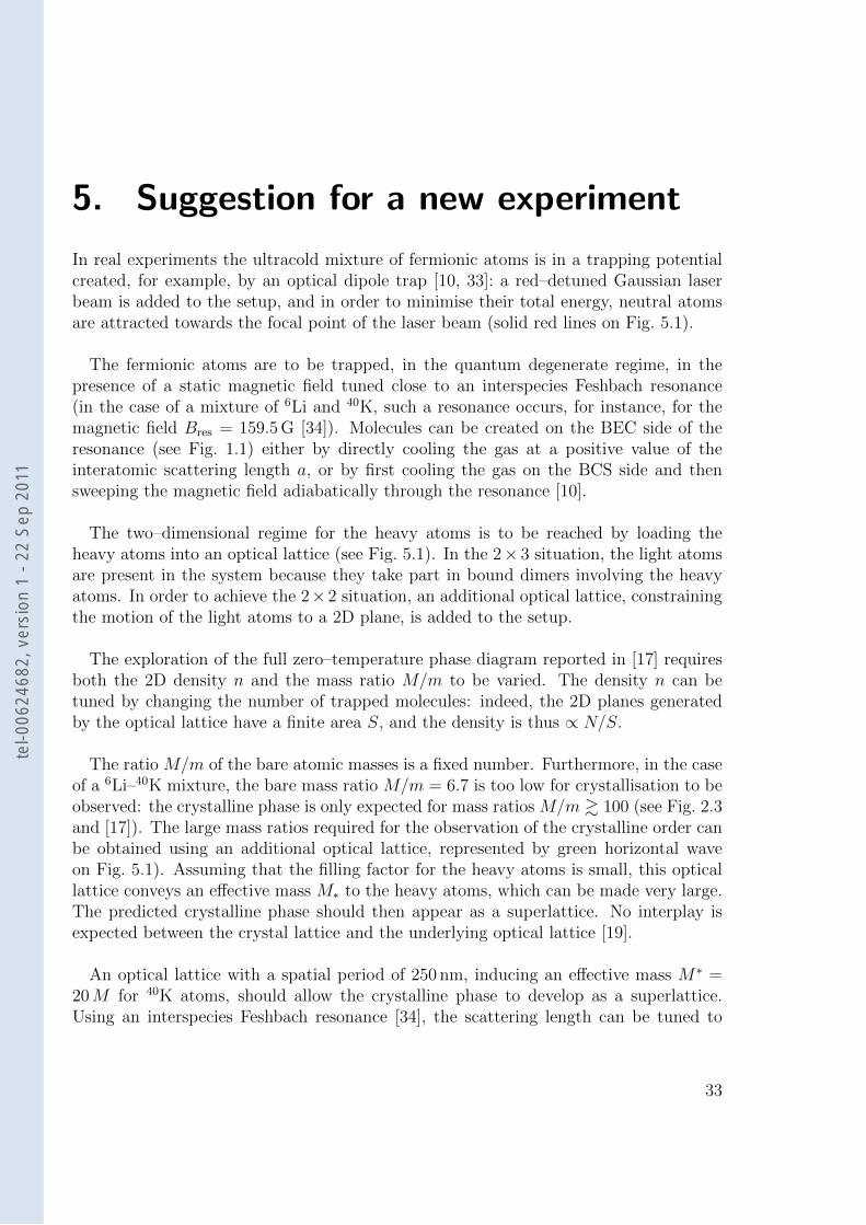
5. Suggestion for a new experiment

In real experiments the ultracold mixture of fermionic atoms is in a trapping potentialcreated, for example, by an optical dipole trap [10, 33]: a red–detuned Gaussian laserbeam is added to the setup, and in order to minimise their total energy, neutral atomsare attracted towards the focal point of the laser beam (solid red lines on Fig. 5.1).

The fermionic atoms are to be trapped, in the quantum degenerate regime, in thepresence of a static magnetic field tuned close to an interspecies Feshbach resonance(in the case of a mixture of 6Li and 40K, such a resonance occurs, for instance, for themagnetic field Bres = 159.5 G [34]). Molecules can be created on the BEC side of theresonance (see Fig. 1.1) either by directly cooling the gas at a positive value of theinteratomic scattering length a, or by first cooling the gas on the BCS side and thensweeping the magnetic field adiabatically through the resonance [10].

The two–dimensional regime for the heavy atoms is to be reached by loading theheavy atoms into an optical lattice (see Fig. 5.1). In the 2× 3 situation, the light atomsare present in the system because they take part in bound dimers involving the heavyatoms. In order to achieve the 2×2 situation, an additional optical lattice, constrainingthe motion of the light atoms to a 2D plane, is added to the setup.

The exploration of the full zero–temperature phase diagram reported in [17] requiresboth the 2D density n and the mass ratio M/m to be varied. The density n can betuned by changing the number of trapped molecules: indeed, the 2D planes generatedby the optical lattice have a finite area S, and the density is thus ∝ N/S.

The ratio M/m of the bare atomic masses is a fixed number. Furthermore, in the caseof a 6Li–40K mixture, the bare mass ratio M/m = 6.7 is too low for crystallisation to beobserved: the crystalline phase is only expected for mass ratios M/m & 100 (see Fig. 2.3and [17]). The large mass ratios required for the observation of the crystalline order canbe obtained using an additional optical lattice, represented by green horizontal waveon Fig. 5.1). Assuming that the filling factor for the heavy atoms is small, this opticallattice conveys an effective mass M∗ to the heavy atoms, which can be made very large.The predicted crystalline phase should then appear as a superlattice. No interplay isexpected between the crystal lattice and the underlying optical lattice [19].

An optical lattice with a spatial period of 250 nm, inducing an effective mass M∗ =20M for 40K atoms, should allow the crystalline phase to develop as a superlattice.Using an interspecies Feshbach resonance [34], the scattering length can be tuned to

33

tel-0

0624

682,

ver

sion

1 -

22 S

ep 2

011

5. Suggestion for a new experiment

waistw

Iheavy

Ilight

IM

Heavy atomsin 2D plane

Figure 5.1. Projected experimentalsetup. The heavy atoms (purple) aretrapped within a 2D plane by an opticallattice (Iheavy, blue wave). In order toachieve the 2 × 2 situation, an additionaloptical lattice is added to the setup inorder to constrain the motion of thelight atoms to a 2D plane (Ilight, dashedred wave) The horizontal optical lattice(green) conveys a tunable effective massto the heavy atoms.

a = 500 nm, corresponding to the binding energy ~2/(ma2) = 300 nK, and lower tem-peratures are experimentally accessible in heteronuclear Fermi gases. With these param-eters, crystallisation is predicted to occur for densities of the order of 107 atoms/cm2,which are experimentally accessible as well.

The lifetime of composite bosons is determined by the rates of decay through therelaxation to deeply bound states and the formation of trimers (see Section 1.1.1). Forthe values of the experimental parameters chosen above, this lifetime is expected to beof the order of a few seconds [17].

34

tel-0

0624

682,

ver

sion

1 -

22 S

ep 2

011

6. Article 1: Crystalline Phase ofStrongly Interacting Fermi Mixtures

35

tel-0

0624

682,

ver

sion

1 -

22 S

ep 2

011

Crystalline Phase of Strongly Interacting Fermi Mixtures

D. S. Petrov,1,2 G. E. Astrakharchik,3 D. J. Papoular,1 C. Salomon,4 and G. V. Shlyapnikov1,5

1Laboratoire de Physique Theorique et Modeles Statistiques, CNRS, Universite Paris Sud, 91405 Orsay, France2Russian Research Center Kurchatov Institute, Kurchatov Square, 123182 Moscow, Russia

3Departament de Fısica i Enginyeria Nuclear, Campus Nord B4-B5, Universitat Politecnica de Catalunya, E-08034 Barcelona, Spain4Laboratoire Kastler Brossel, CNRS, Ecole Normale Superieure, 24 rue Lhomond, 75231 Paris, France

5Van der Waals-Zeeman Institute, University of Amsterdam, Valckenierstraat 65/67, 1018 XE Amsterdam, The Netherlands(Received 24 June 2007; published 28 September 2007)

We show that the system of weakly bound molecules of heavy and light fermionic atoms is char-acterized by a long-range intermolecular repulsion and can undergo a gas-crystal quantum transition if themass ratio exceeds a critical value. For the critical mass ratio above 100 obtained in our calculations, thiscrystalline order can be observed as a superlattice in an optical lattice for heavy atoms with a small fillingfactor. We also find that this novel system is sufficiently stable with respect to molecular relaxation intodeep bound states and to the process of trimer formation.

DOI: 10.1103/PhysRevLett.99.130407 PACS numbers: 05.30.Fk, 03.75.Ss

The use of Feshbach resonances for tuning the interac-tion in two-component ultracold Fermi gases of 6Li or 40Khas led to remarkable developments, such as the observa-tion of superfluid behavior in the strongly interacting re-gime through vortex formation [1], and Bose-Einsteincondensation of weakly bound molecules of fermionicatoms on the positive side of the resonance (the atom-atom scattering length a > 0) [2]. Being highly excited,these extremely large diatomic molecules are remarkablystable with respect to collisional relaxation into deepbound states, which is a consequence of the Pauli exclusionprinciple for identical fermionic atoms [3].

Currently, a new generation of experiments is being setup for studying mixtures of different fermionic atoms, withthe idea of revealing the influence of the mass difference onsuperfluid properties and finding novel types of superfluidpairing. Weakly bound heteronuclear molecules on thepositive side of the resonance are unique objects [4,5],which should manifest collisional stability and can pavea way to creating ultracold dipolar gases.

So far it was believed that dilute Fermi mixtures shouldbe in the gas phase, like Fermi gases of atoms in twodifferent internal states. In this Letter we find that thesystem of molecules of heavy (mass M) and light (massm) fermions can undergo a phase transition to a crystallinephase. This is due to a repulsive intermolecular potentialoriginating from the exchange of light fermions and in-versely proportional to m. As the kinetic energy of themolecules has a prefactor 1=M, above a certain mass ratioM=m the system can crystallize.

We show that the interaction potential in a sufficientlydilute system of molecules is equal to the sum of their pairinteractions and then analyze the case where the motion ofheavy atoms is confined to two dimensions, whereas thelight fermions can be either 2D or 3D [6]. We calculate thezero-temperature gas-crystal transition line using the dif-fusion Monte Carlo (DMC) method and draw the phase

diagram in terms of the mass ratio and density. This phasetransition resembles the one for the flux lattice melting insuperconductors, where the flux lines are mapped onto asystem of bosons interacting via a 2D Yukawa potential [7].In this case the Monte Carlo studies [8,9] identified the firstorder liquid-crystal transition at zero and finite tempera-tures. Aside from the difference in the interaction poten-tials, a distinguished feature of our system is related to itsstability. The molecules can undergo collisional relaxationinto deep bound states, or form weakly bound trimers. Weanalyze resulting limitations on the lifetime of the system.

We first derive the Born-Oppenheimer interaction po-tential in the system of N molecules. In this approach thestate of light atoms adiabatically adjusts itself to the set ofheavy-atom coordinates fRg fR1; . . . ;RNg and one cal-culates the wave function and energy of light fermions inthe field of fixed heavy atoms. Omitting the interactionbetween light (identical) fermions, it is sufficient to find Nlowest single-particle eigenstates, and the sum of theirenergies will give the interaction potential for the mole-cules. For the interaction between light and heavy atomswe use the Bethe-Peierls approach [10] assuming that themotion of light atoms is free everywhere except for theirvanishing distances from heavy atoms.

The wave function of a single light atom then reads

fRg; r XNi1

CiGrRi; (1)

where r is its coordinate, and the Green function Gsatisfies the equation r2

r 2Gr r. The en-

ergy of the state (1) equals @22=2m, and here weonly search for negative single-particle energies (see be-low). The dependence of the coefficients Ci and on fRg isobtained using the Bethe-Peierls boundary condition:

fRg; r / G0rRi; r! Ri: (2)

PRL 99, 130407 (2007) P H Y S I C A L R E V I E W L E T T E R S week ending28 SEPTEMBER 2007

0031-9007=07=99(13)=130407(4) 130407-1 © 2007 The American Physical Society

tel-0

0624

682,

ver

sion

1 -

22 S

ep 2

011

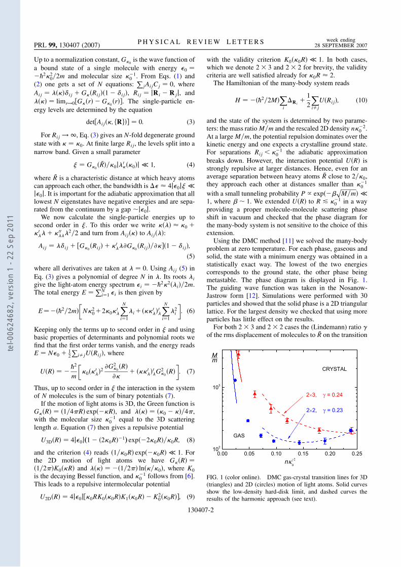
Up to a normalization constant, G0is the wave function of

a bound state of a single molecule with energy 0 @22

0=2m and molecular size 10 . From Eqs. (1) and

(2) one gets a set of N equations:PjAijCj 0, where

Aij ij GRij1 ij, Rij jRi Rjj, and limr!0Gr G0

r. The single-particle en-ergy levels are determined by the equation

detAij; fRg 0: (3)

For Rij ! 1, Eq. (3) gives an N-fold degenerate groundstate with 0. At finite large Rij, the levels split into anarrow band. Given a small parameter

G0 ~R=0j

00j 1; (4)

where ~R is a characteristic distance at which heavy atomscan approach each other, the bandwidth is 4j0jj0j. It is important for the adiabatic approximation that alllowest N eigenstates have negative energies and are sepa-rated from the continuum by a gap j0j.

We now calculate the single-particle energies up tosecond order in . To this order we write 0 0

00

2=2 and turn from Aij to Aij:

Aij ij G0Rij 0@G0

Rij=@1 ij;

(5)

where all derivatives are taken at 0. Using Aij (5) inEq. (3) gives a polynomial of degree N in . Its roots igive the light-atom energy spectrum i @22i=2m.The total energy E

PNi1 i is then given by

E@2=2mN2

0200

XNi1

i00

XNi1

2i

: (6)

Keeping only the terms up to second order in and usingbasic properties of determinants and polynomial roots wefind that the first order terms vanish, and the energy readsE N0

12

PijURij, where

UR @

2

m

00

2@G2

0R

@ 0

0G

20R

: (7)

Thus, up to second order in the interaction in the systemof N molecules is the sum of binary potentials (7).

If the motion of light atoms is 3D, the Green function isGR 1=4R expR, and 0 =4,with the molecular size 1

0 equal to the 3D scatteringlength a. Equation (7) then gives a repulsive potential

U3DR 4j0j1 20R1 exp20R=0R; (8)

and the criterion (4) reads 1=0R exp0R 1. Forthe 2D motion of light atoms we have GR 1=2K0R and 1=2 ln=0, where K0

is the decaying Bessel function, and 10 follows from [6].

This leads to a repulsive intermolecular potential

U2DR 4j0j0RK00RK10R K200R; (9)

with the validity criterion K00R 1. In both cases,which we denote 2 3 and 2 2 for brevity, the validitycriteria are well satisfied already for 0R 2.

The Hamiltonian of the many-body system reads

H @2=2MXi

Ri

1

2

Xij

URij; (10)

and the state of the system is determined by two parame-ters: the mass ratioM=m and the rescaled 2D density n2

0 .At a largeM=m, the potential repulsion dominates over thekinetic energy and one expects a crystalline ground state.For separations Rij < 1

0 the adiabatic approximationbreaks down. However, the interaction potential UR isstrongly repulsive at larger distances. Hence, even for anaverage separation between heavy atoms R close to 2=0,they approach each other at distances smaller than 1

0

with a small tunneling probability P / expM=m

p

1, where 1. We extended UR to R & 10 in a way

providing a proper molecule-molecule scattering phaseshift in vacuum and checked that the phase diagram forthe many-body system is not sensitive to the choice of thisextension.

Using the DMC method [11] we solved the many-bodyproblem at zero temperature. For each phase, gaseous andsolid, the state with a minimum energy was obtained in astatistically exact way. The lowest of the two energiescorresponds to the ground state, the other phase beingmetastable. The phase diagram is displayed in Fig. 1.The guiding wave function was taken in the Nosanow-Jastrow form [12]. Simulations were performed with 30particles and showed that the solid phase is a 2D triangularlattice. For the largest density we checked that using moreparticles has little effect on the results.

For both 2 3 and 2 2 cases the (Lindemann) ratio of the rms displacement of molecules to R on the transition

FIG. 1 (color online). DMC gas-crystal transition lines for 3D(triangles) and 2D (circles) motion of light atoms. Solid curvesshow the low-density hard-disk limit, and dashed curves theresults of the harmonic approach (see text).

PRL 99, 130407 (2007) P H Y S I C A L R E V I E W L E T T E R S week ending28 SEPTEMBER 2007

130407-2

tel-0

0624

682,

ver

sion

1 -

22 S

ep 2

011

lines ranges from 0.23 to 0.27. At low densities n thede Broglie wavelength of molecules is R 1

0 ,and UR can be approximated by a hard-disk potentialwith the diameter equal to the 2D scattering length. Then,using the DMC results for hard-disk bosons [13], we obtainthe transition lines shown by solid curves in Fig. 1. Atlarger n, we have < 1

0 and use the harmonic expansionof UR around equilibrium positions in the crystal, calcu-late the Lindemann ratio, and select for the best fit to theDMC data points (dashed curves in Fig. 1).

The mass ratio above 100, required for the observationof the crystalline order (see Fig. 1), can be achieved in anoptical lattice with a small filling factor for heavy atoms.Their effective mass in the lattice M can be made verylarge, and the discussed solid phase should appear as asuperlattice. There is no interplay between the superlatticeorder and the shape of the underlying optical lattice, incontrast to the recently studied solid and supersolid phasesin a triangular lattice with the filling factor of order one[14]. Our superlattice remains compressible and supportstwo branches of phonons.

The gaseous and solid phases of weakly bound mole-cules are actually metastable. The main decay channels arethe relaxation of molecules into deep bound states and theformation of trimer states by one light and two heavyatoms. A detailed analysis of scattering properties of thesemolecules will be given elsewhere, and here we focus ontheir stability in an optical lattice.

For a large effective mass ratio M =m, the relaxationinto deep states occurs when a molecule is approached byanother light atom and both light-heavy separations are ofthe order of the size of a deep state, Re 1

0 [15]. Thereleased binding energy is taken by outgoing particleswhich escape from the sample. The rate of this process isnot influenced by the optical lattice.

We estimate this rate in the solid phase and near the gas-solid transition to the leading order in 0

R1. At light-heavy separations r1;2 1

0 the initial-state wave func-tion reads ~ B1

0 ; R r1; r2. Writing it as an anti-symmetrized product of wave functions (1), for the 2 3case (1

0 a) we find B 1= Ra2 exp R=a. Thequantity W B2R6

e is the probability of having both lightatoms at distances Re from a heavy atom, and the re-laxation rate is 3D / W. As the short-range physics ischaracterized by the energy scale @

2=mR2e, we restore the

dimensions and write

3D C@=mRe=a41= R2 exp2 R=a; (11)

where R2 n. The coefficient C depends on a particularsystem and is 1 within an order of magnitude. Therelaxation rate 3D is generally rather low. For the K-Limixture where Re 50 A, even at na2 0:24 (see Fig. 1)the relaxation time exceeds 10 s for n 109 cm2 anda 1600 A. In the 2 2 case, for the same n and 1

0 theprobability W is smaller and the relaxation is slower.

The formation of trimer bound states by one light andtwo heavy atoms occurs when two molecules approacheach other at distances R & 1

0 . It is accompanied by arelease of the second light atom. The existence of thetrimer states is seen considering a light atom interactingwith two heavy ones. The lowest energy solution of Eq. (3)for N 2 is the gerade state (C1 C2). Its energy Rintroduces an effective attractive potential acting on theheavy atoms, and the trimer states are bound states of twoheavy atoms in this potential.

In an optical lattice the trimers are eigenstates of theHamiltonian H0 @

2=2M Pi1;2Ri

R12. In adeep lattice one can neglect all higher bands and regard Rias discrete lattice coordinates and as the latticeLaplacian. Then, the fermionic nature of the heavy atomsprohibits them to be in the same lattice site. For a very largemass ratio M =m the kinetic energy term in H0 can beneglected, and the lowest trimer state has energy tr L, where L is the lattice period. It consists of a pairof heavy atoms localized at neighboring sites and a lightatom in the gerade state. Higher trimer states are formed byheavy atoms localized in sites separated by distances R>L. This picture breaks down at large R, where the spacingbetween trimer levels is comparable with the tunnelingenergy @

2=M L2 and the heavy atoms are delocalized.In the many-body molecular system the scale of energies

in Eq. (10) is much smaller than j0j. Thus, the formationof trimers in molecule-molecule ‘‘collisions’’ is energeti-cally allowed only if the trimer binding energy is tr < 20.Since the lowest trimer energy in the optical lattice isL, the trimer formation requires the conditionL & 20, which is equivalent to 1

0 * 1:6L in the2 3 case and 1

0 * 1:25L in the 2 2 case. This meansthat for a sufficiently small molecular size or large latticeperiod L the formation of trimers is forbidden.

At a larger molecular size or smaller L the trimer for-mation is possible. For finding the rate we consider theinteraction between two molecules as a reduced 3-bodyproblem, accounting for the fact that one of the light atomsis in the gerade and the other one in the ungerade state(C1 C2). The gerade light atom is integrated out and issubstituted by the effective potential R. For the unger-ade state the adiabaticity breaks down at interheavy sepa-rations R & 1

0 , and the ungerade light atom is treatedexplicitly. The wave function of the reduced 3-body prob-lem satisfies the Schrodinger equation

H0 @2r2

r=2m E fRg; r 0; (12)

where the energy E is close to 20, fRg denotes the setfR1;R2g, and r is the coordinate of the ungerade atom. Theinteraction between this atom and the heavy ones is re-placed by the boundary condition (2) on . The 3-bodyproblem can then be solved by encoding the information onthe wave function in an auxiliary function ff ~Rg [16]and representing the solution of Eq. (12) in the form

PRL 99, 130407 (2007) P H Y S I C A L R E V I E W L E T T E R S week ending28 SEPTEMBER 2007

130407-3

tel-0

0624

682,

ver

sion

1 -

22 S

ep 2

011

Xf ~Rg;

fRg f ~Rgff ~RgFr; f ~Rg; (13)

where fRg is an eigenfunction of H0 with energy ,and Fr; f ~Rg Gr ~R1 Gr ~R2 with

2m E=@2

p. For < E the trimer formation

in the state is possible. This is consistent with imaginary and the Green function G describing an outgoingwave of the light atom and trimer.

We derive an equation for the function f in a deeplattice, where the tunneling energy @

2=M L2 j0j.Then the main contribution to the sum in Eq. (13) comesfrom the states for which j R12j & @

2=M L2.

The sum is calculated by expanding around R12 2mR12 E=@

2p

up to first order in R12=0 and using the equation H0 0.The equation for f is then obtained by taking the limit r!R1 in the resulting expression for and comparing it withthe boundary condition (2). This yields

@2=2M

Xi1;2

RiUeffR12

fR1;R2 0; (14)

where the effective potential UeffR12 is given by

UeffR @

2Rm

RGRR

@=@RGRR: (15)

At large distances one has Ueff UR 20 E, andfor smaller R where R<E, the potential Ueff acquiresan imaginary part accounting for the decay of moleculesinto trimers. The number of trimer states that can beformed grows with the molecular size. Eventually it be-comes independent of L and so does the loss rate.

In this limit, we solve Eq. (14) for two molecules withzero total momentum under the condition that fR1;R2 ismaximal for jR1 R2j R n1=2. We thus obtain E asa function of the density and mass ratio, and its imaginarypart gives the loss rate for the many-body system.Numerical analysis for 0:06< n2

0 < 0:4 and 50<M =m< 2000 is well fitted by D@n=M n2

0

expJM =m

p, withD 7 and J 0:95–1:4n2

0 forthe 2 3 case, and D 102, J 1:45–2:8n2

0 in the2 2 case. One can suppress by increasing M =m,whereas for M =m & 100 the trimers can be formed on atime scale & 1 s.

In conclusion, we have shown that the system of weaklybound molecules of heavy and light fermionic atoms canundergo a gas-crystal quantum transition. The necessarymass ratio is above 100 and the observation of such crys-talline order requires an optical lattice for heavy atoms,where it appears as a superlattice. A promising candidate isthe 6Li-40K mixture as the Li atom may tunnel freely in alattice while localizing the heavy K atoms to reach high

mass ratios. A lattice with period 250 nm and K effectivemass M 20M provide a tunneling rate 103 s1 suffi-ciently fast to let the crystal form. Near a Feshbach reso-nance, a value a 500 nm gives a binding energy 300 nK,and lower temperatures should be reached in the gas. Theparameters n2

0 of Fig. 1 are then obtained at 2D densitiesin the range 107–108 cm2 easily reachable in experi-ments. For n 108 cm2 the rate of the trimer formationis of the order of seconds, and these peculiar bound statescan be detected optically.

This work was supported by the IFRAF Institute, byANR (Grants No. 05-BLAN-0205, No. 05-NANO-008-02,and No. 06-NANO-014), by the Dutch Foundation FOM,by the Russian Foundation for Fundamental Research, andby the National Science Foundation (Grant No. PHY05-51164). LKB is a research unit No. 8552 of CNRS, ENS,and University of Pierre et Marie Curie. LPTMS is aresearch unit No. 8626 of CNRS and University Paris-Sud.

[1] M. W. Zwierlein et al., Nature (London) 435, 1047 (2005).[2] M. Greiner et al., Nature (London) 426, 537 (2003);

S. Jochim et al., Science 302, 2101 (2003); M. W.Zwierlein et al., Phys. Rev. Lett. 91, 250401 (2003);T. Bourdel et al., ibid. 93, 050401 (2004); G. B.Partridge et al., ibid. 95, 020404 (2005).

[3] D. S. Petrov, C. Salomon, and G. V. Shlyapnikov, Phys.Rev. Lett. 93, 090404 (2004); Phys. Rev. A 71, 012708(2005).

[4] D. S. Petrov, C. Salomon, and G. V. Shlyapnikov,J. Phys. B 38, S645 (2005).

[5] C. Ospelkaus et al., Phys. Rev. Lett. 97, 120402 (2006).[6] In the 2D regime achieved by confining the light-atom

motion to zero point oscillations with amplitude l0, theweakly bound molecular states exist at a negative asatisfying the condition jaj l0. See D. S. Petrov andG. V. Shlyapnikov, Phys. Rev. A 64, 012706 (2001).

[7] D. R. Nelson and H. S. Seung, Phys. Rev. B 39, 9153(1989).

[8] W. R. Magro and D. M. Ceperley, Phys. Rev. B 48, 411(1993).

[9] H. Nordborg and G. Blatter, Phys. Rev. Lett. 79, 1925(1997).

[10] H. Bethe and R. Peierls, Proc. R. Soc. A 148, 146 (1935).[11] For a general reference on the DMC method, see, e.g.,

J. Boronat and J. Casulleras, Phys. Rev. B 49, 8920 (1994).[12] G. E. Astrakharchik et al., Phys. Rev. Lett. 98, 060405

(2007).[13] L. Xing, Phys. Rev. B 42, 8426 (1990).[14] S. Wessel and M. Troyer, Phys. Rev. Lett. 95, 127205

(2005); D. Heidarian and K. Damle, ibid. 95, 127206(2005); R. G. Melko et al., ibid. 95, 127207 (2005).

[15] The relaxation involving one light and two heavy atoms isstrongly suppressed as it requires the heavy atoms toapproach each other and get to the same lattice site.

[16] D. S. Petrov, Phys. Rev. A 67, 010703(R) (2003).

PRL 99, 130407 (2007) P H Y S I C A L R E V I E W L E T T E R S week ending28 SEPTEMBER 2007

130407-4

tel-0

0624

682,

ver

sion

1 -

22 S

ep 2

011

tel-0

0624

682,

ver

sion

1 -

22 S

ep 2

011

7. Conclusion and outlook

The subject of the first part of the present manuscript has been the calculation ofthe zero–temperature phase diagram of a two–dimensional system of composite bosonsformed in an ultracold mixture containing two different types of fermionic atoms. Thissystem has been predicted to undergo a zero–temperature crystal–gas phase transition[17], due to the competition between the zero–point kinetic energy of the molecules andthe repulsive interaction between them due to an exchange of light fermions.

The phase diagram of the system has been accurately calculated using the DiffusionMonte Carlo method. We have presented two simple approaches which allow an ap-proximate calculation of this phase diagram (see Chapter 2). The results of these twoapproaches are in good agreement with the accurate DMC results reported in [17]. Ourfirst approach relies on a harmonic approximation for the total interaction energy in thecrystal phase, and the crystal–gas transition line is determined using the phenomenolog-ical Lindemann criterion. Our second approach, which does not rely on the Lindemanncriterion, is applicable for very low densities. In this limit, the system behaves like a setof 2D hard–core bosons, and the existing prediction [29] for the phase transition in thissimpler system can be used.

Prospects for theoretical extensions of this work include the development of a con-venient method to distinguish between the crystal and gas phases in experiments. Forexample, low–energy vibrational modes of the system can be excited using a rotatinganisotropic potential. The calculation of the low–energy spectrum for the crystal phase,and its comparison to the corresponding spectrum for molecular Bose–Einstein conden-sates in the usual gaseous phase, may yield such a method.

Another planned extension on the theory side deals with the behaviour of the systemat high densities. The increasing high–density part of the dashed blue line in the crystal–gas phase diagram (Fig. 2.3) suggests that the crystal of composite bosons will melt forhigher densities in the 2 × 2 case. This quantum melting has yet to be confirmed andunderstood. The beginning of an explanation, in terms of a classical harmonic stabilityanalysis of the 2D triangular lattice, is presented in [35].

The study of heteronuclear fermionic mixtures presented in this part of the manuscriptalso yields interesting experimental prospects.

First, the phase diagram that we discussed is promising for the observation of thezero–temperature crystal–gas phase transition (see Chapter 5). Such an experimentcould be performed, for instance, using heteronuclear Fermi mixture containing equalnumbers of 6Li and 40K atoms. In order to achieve the large mass ratios required toobserve crystallisation, an optical lattice can be used to endow the 40K atoms with a

41

tel-0

0624

682,

ver

sion

1 -

22 S

ep 2

011

7. Conclusion and outlook

heavier effective mass, while the 6Li atoms tunnel freely through the lattice. An opti-cal lattice with a spatial period of 250 nm, inducing an effective mass M∗ = 20M for40K atoms, should allow the crystalline phase to develop as a superlattice. Using aninterspecies Feshbach resonance [34], the scattering length can be tuned to a = 500 nm,corresponding to the binding energy ~2/(ma2) = 300 nK, and lower temperatures areexperimentally accessible in heteronuclear Fermi gases. With these parameters, crys-tallisation is predicted to occur for densities of the order of 107 atoms/cm2, which areexperimentally accessible as well.

Another interesting prospect is the transfer of the (highly excited) composite bosonsobtained on the BEC side of the Feshbach resonance to their ground state. Similarexperiments have already been performed with molecules consisting of bosonic atoms(85Rb133Cs [36, 37], 87Rb2 [38], and 7Li133Cs [39, 40]) and with fermionic 40K87Rbmolecules [41, 42]. Heteronuclear molecules in their ground state have a large elec-tric dipole moment (0.6 Debye for 40K87Rb). The dipolar gases thus obtained exhibitanisotropic long–range dipole–dipole interactions [43]. These long–range interactions willstrongly affect the physics of Bose–Einstein condensation. The realisation of ground–state composite bosons in the quantum degenerate regime will allow for an experimentalexploration of the predicted novel phases [44].

Finally, the collisional stability of weakly–bound heteronuclear molecules (see Section1.1.1 and [18, 45]) involves few–body effects such as the formation of Efimov trimers.(see e.g. [46] for evidence of the Efimov effect through the measurement of the rate ofthree–body recombination in an ultracold atomic gas). Heteronuclear Fermi mixturesoffer a promising alternative system for the experimental investigation of these few–bodyeffects.

42

tel-0

0624

682,

ver

sion

1 -

22 S

ep 2

011

Bibliography

[1] J. Dalibard. “Collisional dynamics of ultracold atomic gases”. In: Proceedings ofthe International School of Physics Enrico Fermi, Course CXL: Bose – Einsteincondensation in gases. Societa Italiana di Fisica, 1998. Chap. Collisional dynamicsof ultracold atomic gases.

[2] C. Pethick and H. Smith. Bose-Einstein condensation in dilute gases. CambridgeUniversity Press, 2002. isbn: 0521665809.

[3] Cheng Chin et al. “Feshbach resonances in ultracold gases”. In: Rev. Mod. Phys.82.2 (Apr. 2010), pp. 1225–1286. doi: 10.1103/RevModPhys.82.1225.

[4] Stefano Giorgini, Lev P. Pitaevskii, and Sandro Stringari. “Theory of ultracoldatomic Fermi gases”. In: Rev. Mod. Phys. 80.4 (Oct. 2008), pp. 1215–1274. doi:10.1103/RevModPhys.80.1215.

[5] Immanuel Bloch, Jean Dalibard, and Wilhelm Zwerger. “Many-body physics withultracold gases”. In: Rev. Mod. Phys. 80.3 (July 2008), pp. 885–964. doi: 10.1103/RevModPhys.80.885.

[6] E.M. Lifshitz and L.P. Pitaevskii. Statistical Physics, Part II. Pergamon Press,1980.

[7] C. A. Regal et al. “Creation of ultracold molecules from a Fermi gas of atoms”.In: Nature 424 (2003), p. 47. doi: 10.1038/nature01738.

[8] J. Cubizolles et al. “Production of Long-Lived Ultracold Li2 Molecules from aFermi Gas”. In: Phys. Rev. Lett. 91.24 (Dec. 2003), p. 240401. doi: 10.1103/PhysRevLett.91.240401.

[9] S. Jochim et al. “Pure Gas of Optically Trapped Molecules Created from FermionicAtoms”. In: Phys. Rev. Lett. 91.24 (Dec. 2003), p. 240402. doi: 10.1103/PhysRevLett.91.240402.

[10] A.-C. Voigt et al. “Ultracold Heteronuclear Fermi-Fermi Molecules”. In: Phys. Rev.Lett. 102.2 (Jan. 2009), p. 020405. doi: 10.1103/PhysRevLett.102.020405.

[11] F. M. Spiegelhalder et al. “All-optical production of a degenerate mixture of 6Liand 40K and creation of heteronuclear molecules”. In: Phys. Rev. A 81.4 (Apr.2010), p. 043637. doi: 10.1103/PhysRevA.81.043637.

[12] M. Greiner, C. Regal, and D. S. Jin. “Emergence of a molecular Bose-Einsteincondensate from a Fermi gas”. In: Nature 426 (2003). doi: 10.1038/nature02199.

[13] S. Jochim et al. “Bose-Einstein Condensation of Molecules”. In: Science 302.5653(2003), pp. 2101–2103. doi: 10.1126/science.1093280.

43

tel-0

0624

682,

ver

sion

1 -

22 S

ep 2

011

Bibliography

[14] M. W. Zwierlein et al. “Observation of Bose-Einstein Condensation of Molecules”.In: Phys. Rev. Lett. 91.25 (Dec. 2003), p. 250401. doi: 10.1103/PhysRevLett.91.250401.

[15] D. S. Petrov, C. Salomon, and G. V. Shlyapnikov. “Weakly Bound Dimers ofFermionic Atoms”. In: Phys. Rev. Lett. 93.9 (Aug. 2004), p. 090404. doi: 10.1103/PhysRevLett.93.090404.

[16] D. S. Petrov, C. Salomon, and G. V. Shlyapnikov. “Scattering properties of weaklybound dimers of fermionic atoms”. In: Phys. Rev. A 71.1 (Jan. 2005), p. 012708.doi: 10.1103/PhysRevA.71.012708.

[17] D. S. Petrov et al. “Crystalline Phase of Strongly Interacting Fermi Mixtures”. In:Phys. Rev. Lett. 99.13 (Sept. 2007), p. 130407. doi: 10.1103/PhysRevLett.99.130407.

[18] D. S. Petrov, C. Salomon, and G. V. Shlyapnikov. “Diatomic Molecules in Ul-tracold Fermi Gases — Novel Composite Bosons”. In: Journal of Physics B 38(2005). doi: 10.1088/0953-4075/38/9/014.

[19] D. S. Petrov, C. Salomon, and G. V. Shlyapnikov. “Molecular regimes in ultracoldFermi gases”. In: Cold Molecules: Theory, Experiment, Applications. CRC Press,2009. Chap. 9. isbn: 978-1-4200-5903-8.

[20] O I Kartavtsev and A V Malykh. “Low-energy three-body dynamics in binaryquantum gases”. In: Journal of Physics B: Atomic, Molecular and Optical Physics40.7 (2007), p. 1429. doi: 10.1088/0953-4075/40/7/011.

[21] M. Abramowitz and I.A. Stegun. Handbook of mathematical functions with formu-las, graphs, and mathematical tables. Dover publications, 1964.

[22] D. S. Petrov and G. V. Shlyapnikov. “Interatomic collisions in a tightly confinedBose gas”. In: Phys. Rev. A 64.1 (June 2001), p. 012706. doi: 10.1103/PhysRevA.64.012706.

[23] J. Boronat and J. Casulleras. “Monte Carlo analysis of an interatomic potential forHe”. In: Phys. Rev. B 49.13 (Apr. 1994), pp. 8920–8930. doi: 10.1103/PhysRevB.49.8920.

[24] N. W. Ashcroft and N. D. Mermin. Solid State Physics. Holt, Rinehart, and Win-ston, 1976.

[25] J. M. Ziman. Principles of the Theory of Solids. 2nd ed. Cambridge UniversityPress, 1972.

[26] L. D. Landau and E. M. Lifshitz. Statistical Physics, Part I. 3rd ed. PergamonPress, 1980.

[27] C. Kittel and C. Fong. Quantum theory of solids. Vol. 316. Wiley New York, 1987.isbn: 0471624128.

[28] F. A. Lindemann. “The calculation of molecular vibration frequencies”. In: Physik.Z 11 (1910), pp. 609–612.

44

tel-0

0624

682,

ver

sion

1 -

22 S

ep 2

011

Bibliography

[29] Lei Xing. “Monte Carlo simulations of a two-dimensional hard-disk boson system”.In: Phys. Rev. B 42.13 (Nov. 1990), pp. 8426–8430. doi: 10.1103/PhysRevB.42.8426.

[30] H. Bethe and R. Peierls. “Quantum theory of the diplon”. In: Proceedings of theRoyal Society of London. Series A-Mathematical and Physical Sciences 148.863(1935), p. 146.

[31] C. Cohen-Tannoudji et al. Quantum Mechanics. Vols. 1 and 2. Wiley Interscience,1977.

[32] D. S. Petrov. “Three-body problem in Fermi gases with short-range interparticleinteraction”. In: Phys. Rev. A 67.1 (Jan. 2003), p. 010703. doi: 10.1103/PhysRevA.67.010703.

[33] Steven Chu et al. “Experimental Observation of Optically Trapped Atoms”. In:Phys. Rev. Lett. 57.3 (July 1986), pp. 314–317. doi: 10.1103/PhysRevLett.57.314.

[34] E. Wille et al. “Exploring an Ultracold Fermi-Fermi Mixture: Interspecies FeshbachResonances and Scattering Properties of 6Li and 40K”. In: Phys. Rev. Lett. 100.5(Feb. 2008), p. 053201. doi: 10.1103/PhysRevLett.100.053201.

[35] D. J. Papoular. “Harmonic Stability Analysis of the 2D Square and HexagonalBravais Lattices for a Finite–Ranged Repulsive Pair Potential. Consequence fora 2D System of Ultracold Composite Bosons”. In: ArXiv e-prints (June 2008).arXiv:0806.4325.

[36] Andrew J. Kerman et al. “Production and State-Selective Detection of UltracoldRbCs Molecules”. In: Phys. Rev. Lett. 92.15 (Apr. 2004), p. 153001. doi: 10.1103/PhysRevLett.92.153001.

[37] Jeremy M. Sage et al. “Optical Production of Ultracold Polar Molecules”. In: Phys.Rev. Lett. 94.20 (May 2005), p. 203001. doi: 10.1103/PhysRevLett.94.203001.

[38] K. Winkler et al. “Coherent Optical Transfer of Feshbach Molecules to a LowerVibrational State”. In: Phys. Rev. Lett. 98.4 (Jan. 2007), p. 043201. doi: 10.1103/PhysRevLett.98.043201.

[39] J. Deiglmayr et al. “Formation of Ultracold Polar Molecules in the RovibrationalGround State”. In: Phys. Rev. Lett. 101.13 (Sept. 2008), p. 133004. doi: 10.1103/PhysRevLett.101.133004.

[40] J. Deiglmayr et al. “Permanent dipole moment of LiCs in the ground state”. In:Phys. Rev. A 82.3 (Sept. 2010), p. 032503. doi: 10.1103/PhysRevA.82.032503.

[41] K.-K. Ni et al. “A High Phase-Space-Density Gas of Polar Molecules”. In: Science322.5899 (2008), pp. 231–235. doi: 10.1126/science.1163861.

[42] S. Ospelkaus et al. “Controlling the Hyperfine State of Rovibronic Ground-StatePolar Molecules”. In: Phys. Rev. Lett. 104.3 (Jan. 2010), p. 030402. doi: 10.1103/PhysRevLett.104.030402.

45

tel-0

0624

682,

ver

sion

1 -

22 S

ep 2

011

Bibliography

[43] K.-K. Ni et al. “Dipolar collisions of polar molecules in the quantum regime”. In:Nature 464 (2010), p. 1324. doi: 10.1038/nature08953.

[44] L. Santos and T. Pfau. “Spin-3 Chromium Bose-Einstein Condensates”. In: Phys.Rev. Lett. 96.19 (May 2006), p. 190404. doi: 10.1103/PhysRevLett.96.190404.

[45] B. Marcelis et al. “Collisional properties of weakly bound heteronuclear dimers”.In: Phys. Rev. A 77.3 (Mar. 2008), p. 032707. doi: 10.1103/PhysRevA.77.032707.

[46] T. Kraemer et al. “Evidence for Efimov quantum states in an ultracold gas ofcaesium atoms”. In: Nature 440 (2006), p. 315. doi: 10.1038/nature04626.

46

tel-0

0624

682,

ver

sion

1 -

22 S

ep 2

011

Part II.

Microwave–InducedFano–Feshbach Resonances

47

tel-0

0624

682,

ver

sion

1 -

22 S

ep 2

011

tel-0

0624

682,

ver

sion

1 -

22 S

ep 2

011

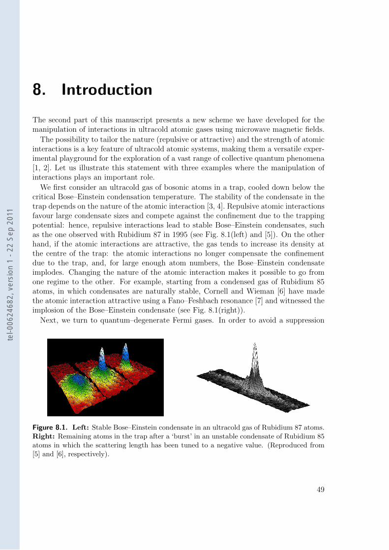
8. Introduction

The second part of this manuscript presents a new scheme we have developed for themanipulation of interactions in ultracold atomic gases using microwave magnetic fields.

The possibility to tailor the nature (repulsive or attractive) and the strength of atomicinteractions is a key feature of ultracold atomic systems, making them a versatile exper-imental playground for the exploration of a vast range of collective quantum phenomena[1, 2]. Let us illustrate this statement with three examples where the manipulation ofinteractions plays an important role.

We first consider an ultracold gas of bosonic atoms in a trap, cooled down below thecritical Bose–Einstein condensation temperature. The stability of the condensate in thetrap depends on the nature of the atomic interaction [3, 4]. Repulsive atomic interactionsfavour large condensate sizes and compete against the confinement due to the trappingpotential: hence, repulsive interactions lead to stable Bose–Einstein condensates, suchas the one observed with Rubidium 87 in 1995 (see Fig. 8.1(left) and [5]). On the otherhand, if the atomic interactions are attractive, the gas tends to increase its density atthe centre of the trap: the atomic interactions no longer compensate the confinementdue to the trap, and, for large enough atom numbers, the Bose–Einstein condensateimplodes. Changing the nature of the atomic interaction makes it possible to go fromone regime to the other. For example, starting from a condensed gas of Rubidium 85atoms, in which condensates are naturally stable, Cornell and Wieman [6] have madethe atomic interaction attractive using a Fano–Feshbach resonance [7] and witnessed theimplosion of the Bose–Einstein condensate (see Fig. 8.1(right)).

Next, we turn to quantum–degenerate Fermi gases. In order to avoid a suppression

Figure 8.1. Left: Stable Bose–Einstein condensate in an ultracold gas of Rubidium 87 atoms.Right: Remaining atoms in the trap after a ‘burst’ in an unstable condensate of Rubidium 85atoms in which the scattering length has been tuned to a negative value. (Reproduced from[5] and [6], respectively).

49

tel-0

0624

682,

ver

sion

1 -

22 S

ep 2

011

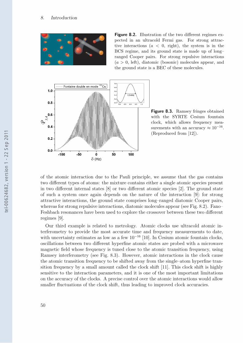
8. Introduction

Figure 8.2. Illustration of the two different regimes ex-pected in an ultracold Fermi gas. For strong attrac-tive interactions (a < 0, right), the system is in theBCS regime, and its ground state is made up of long–ranged Cooper pairs. For strong repulsive interactions(a > 0, left), diatomic (bosonic) molecules appear, andthe ground state is a BEC of these molecules.

Figure 8.3. Ramsey fringes obtainedwith the SYRTE Cesium fountainclock, which allows frequency mea-surements with an accuracy ≈ 10−16.(Reproduced from [12]).

of the atomic interaction due to the Pauli principle, we assume that the gas containstwo different types of atoms: the mixture contains either a single atomic species presentin two different internal states [8] or two different atomic species [2]. The ground stateof such a system once again depends on the nature of the interaction [9]: for strongattractive interactions, the ground state comprises long–ranged diatomic Cooper pairs,whereas for strong repulsive interactions, diatomic molecules appear (see Fig. 8.2). Fano–Feshbach resonances have been used to explore the crossover between these two differentregimes [9].

Our third example is related to metrology. Atomic clocks use ultracold atomic in-terferometry to provide the most accurate time and frequency measurements to date,with uncertainty estimates as low as a few 10−16 [10]. In Cesium atomic fountain clocks,oscillations between two different hyperfine atomic states are probed with a microwavemagnetic field whose frequency is tuned close to the atomic transition frequency, usingRamsey interferometry (see Fig. 8.3). However, atomic interactions in the clock causethe atomic transition frequency to be shifted away from the single–atom hyperfine tran-sition frequency by a small amount called the clock shift [11]. This clock shift is highlysensitive to the interaction parameters, and it is one of the most important limitationson the accuracy of the clocks. A precise control over the atomic interactions would allowsmaller fluctuations of the clock shift, thus leading to improved clock accuracies.

50

tel-0

0624

682,

ver

sion

1 -

22 S

ep 2

011

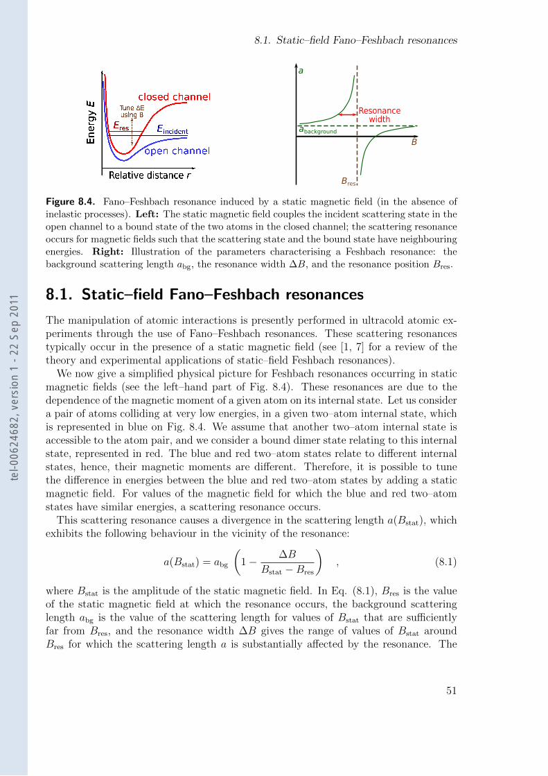
8.1. Static–field Fano–Feshbach resonances

Figure 8.4. Fano–Feshbach resonance induced by a static magnetic field (in the absence ofinelastic processes). Left: The static magnetic field couples the incident scattering state in theopen channel to a bound state of the two atoms in the closed channel; the scattering resonanceoccurs for magnetic fields such that the scattering state and the bound state have neighbouringenergies. Right: Illustration of the parameters characterising a Feshbach resonance: thebackground scattering length abg, the resonance width ∆B, and the resonance position Bres.

8.1. Static–field Fano–Feshbach resonances

The manipulation of atomic interactions is presently performed in ultracold atomic ex-periments through the use of Fano–Feshbach resonances. These scattering resonancestypically occur in the presence of a static magnetic field (see [1, 7] for a review of thetheory and experimental applications of static–field Feshbach resonances).

We now give a simplified physical picture for Feshbach resonances occurring in staticmagnetic fields (see the left–hand part of Fig. 8.4). These resonances are due to thedependence of the magnetic moment of a given atom on its internal state. Let us considera pair of atoms colliding at very low energies, in a given two–atom internal state, whichis represented in blue on Fig. 8.4. We assume that another two–atom internal state isaccessible to the atom pair, and we consider a bound dimer state relating to this internalstate, represented in red. The blue and red two–atom states relate to different internalstates, hence, their magnetic moments are different. Therefore, it is possible to tunethe difference in energies between the blue and red two–atom states by adding a staticmagnetic field. For values of the magnetic field for which the blue and red two–atomstates have similar energies, a scattering resonance occurs.

This scattering resonance causes a divergence in the scattering length a(Bstat), whichexhibits the following behaviour in the vicinity of the resonance:

a(Bstat) = abg

(1− ∆B

Bstat −Bres

), (8.1)

where Bstat is the amplitude of the static magnetic field. In Eq. (8.1), Bres is the valueof the static magnetic field at which the resonance occurs, the background scatteringlength abg is the value of the scattering length for values of Bstat that are sufficientlyfar from Bres, and the resonance width ∆B gives the range of values of Bstat aroundBres for which the scattering length a is substantially affected by the resonance. The

51

tel-0

0624

682,

ver

sion

1 -

22 S

ep 2

011

8. Introduction

resonance parameters Bres, abg and ∆B are illustrated on the right–hand part of Fig. 8.4.Tuning the static magnetic field close to the resonant value Bres therefore makes itpossible to set the scattering length to an arbitrary value and sign. Positive scatteringlengths correspond to an effective atomic interaction which is repulsive, whereas negativescattering lengths correspond to attractive interactions [13].

Fano–Feshbach resonances in static magnetic fields have proved to be an invaluabletool [1, 2, 9] to manipulate the interaction properties of a number of atomic species, suchas Lithium, Potassium, or Cesium. In order for a Feshbach resonance to be a convenientexperimental tool, it has to be broad enough (∆B & 10G), so that the scattering lengthcan be tuned to the desired value with sufficient accuracy despite the presence of smallstray magnetic fields. Broad Feshbach resonances are available for all three atoms listedabove (see [7] for a list of available Feshbach resonances: all three atoms listed aboveexhibit resonances whoses widths satisfy |∆B| > 50 G).

However, broad static–field resonances are not available for all atomic species. Fur-thermore, these resonances often occur for large magnetic fields. For example, all knownFeshbach resonances in 23Na occur for magnetic fields larger than 850 G and their widthsare smaller than 1.5 G [14]. The observation of resonances in 87Rb is even more involved,as the broadest available resonance is less than 200 mG wide and occurs for a magneticfield larger than 1000 G [15]. These resonances in Sodium and Rubidium have been ob-served; however, their observation requires elaborate experimental setups involving largecoils and highly stabilised currents, and they are thus more difficult to use as a tool inmore complex experiments. The manipulation of interactions in atoms such as 87Rb and23Na thus calls for other experimental schemes.

8.2. Previous work on alternative Feshbach resonances

Alternative schemes causing Feshbach resonances have already been considered, basedon the use of electromagnetic fields that are not pure static magnetic fields:

• Marinescu and You ([16], November 1998) have suggested usingDC electric fields ;

• Our scheme is especially reminiscent of the optically–induced Feshbach resonances,first proposed by Fedichev, Kagan, Shlyapnikov and Walraven ([17], Septem-ber 1996). These resonances are due to a coupling between the scattering state andthe resonant bound state caused by an oscillating electric field whose frequencyis in the optical range. They have been experimentally demonstrated in [18, 19].However, the lifetimes of the atomic samples undergoing optically–induced Fes-hbach resonances are severely limited by the losses due to spontaneous emissionthrough the resonant bound state, which is an electronically–excited dimer.

• Moerdijk, Verhaar, and Nagtegaal ([20], June 1996) have considered Sodiumatoms in the lower hyperfine manifold (f1 = 1, f2 = 1), trapped in a static mag-

52

tel-0

0624

682,

ver

sion

1 -

22 S

ep 2

011

8.3. Outline of the following chapters

netic field, and suggested using a radio–frequency magnetic field whose frequencyis tuned close to the single–atom Zeeman splitting to induce scattering resonances.A detailed analysis of their scheme is presented in Section 11.4, where we empha-size the similarities and differences between their RF–induced resonances and themicrowave-induced resonances that we describe in our own published work [21].

8.3. Outline of the following chapters

In the present part of this manuscript, we describe an alternative to static–field Fano–Feshbach resonances where the incident scattering state is resonantly coupled by a mi-crowave magnetic field to a bound state corresponding to a different two–atom internalstate. All states taking part in the resonance belong to the electronic ground level ofthe atoms. The microwave magnetic field amplitude is kept fixed, and the resonance isreached by tuning the microwave frequency.

These microwave–induced resonances occur even in the absence of a static magneticfield. Their characteristics are not directly related to those of the resonances induced bystatic fields. Their widths are proportional to the squared amplitude of the oscillatingmagnetic field.

For the sake of simplicity, we focus on the case of bosonic alkali atoms, but neither ofthese assumptions is essential. We study the microwave–induced resonances occurringwith 7Li, 23Na, 41K, 87Rb, and 133Cs. Except for 7Li (for which a broad static–fieldresonance is already available [22]), our results yield optimistic prospects for experimentswith all of these atoms.

The present part of this manuscript is organised in seven chapters.

• Chapter 9 is introductory. It provides an overview of our analysis of the microwave–induced Feshbach resonances, based on a simple model involving two coupledsquare wells. It briefly presents many of the concepts used and described in depthin later chapters.

• Chapter 10 introduces the Hamiltonian we have used to describe collisions betweentwo alkali atoms in the presence of an oscillating magnetic field. We analyse itssimple block structure, exploited in all subsequent chapters.

• Chapter 11 contains a detailed description of the approaches we have used tocharacterise the microwave–induced Feshbach resonances, based on the resonanceswe have analysed in [21].

• In Chapter 12, we present our own implementations of the numerical methodswe have used to calculate the multi–channel wavefunctions characterising the twoatoms in the presence of static and oscillating magnetic fields.

• Chapter 13 reproduces our published article [21].

53

tel-0

0624

682,

ver

sion

1 -

22 S

ep 2

011

8. Introduction

• Chapter 14 is devoted to static–field Feshbach resonances. We have numericallyreproduced Feshbach resonances observed in 133Cs for very small magnetic fields(SYRTE–Observatoire de Paris), which to our knowledge had remained unex-plained. We interpret these measurements as s–wave resonances involving theweakest–bound triplet dimer state in 133Cs.

• In Chapter 15, we present numerical results for microwave–induced Feshbach res-onances involving experimental parameters accessible in a Cesium fountain clock.These realistic parameters lead to calculations involving a larger number of coupledchannels, and inelastic processes are accounted for.

54

tel-0

0624

682,

ver

sion

1 -

22 S

ep 2

011

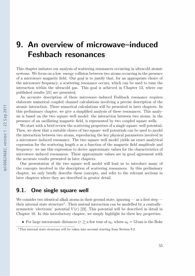
9. An overview of microwave–inducedFeshbach resonances

This chapter initiates our analysis of scattering resonances occurring in ultracold atomicsystems. We focus on a low–energy collision between two atoms occurring in the presenceof a microwave magnetic field. Our goal is to justify that, for an appropriate choice ofthe microwave frequency, a scattering resonance occurs, which can be used to tune theinteraction within the ultracold gas. This goal is achieved in Chapter 13, where ourpublished results [21] are presented.

An accurate description of these microwave–induced Feshbach resonance requireselaborate numerical coupled–channel calculations involving a precise description of theatomic interaction. These numerical calculations will be presented in later chapters. Inthis preliminary chapter, we give a simplified analysis of these resonances. This analy-sis is based on the two–square–well model: the interaction between two atoms, in thepresence of an oscillating magnetic field, is represented by two coupled square wells.

We start with a brief review the scattering properties of a single square–well potential.Then, we show that a suitable choice of two square–well potentials can be used to modelthe interaction between two atoms, reproducing the key physical parameters involved ina microwave–induced resonance. The two–square–well model yields an exact analyticalexpression for the scattering length a as a function of the magnetic field amplitude andfrequency: we use this expression to derive approximate values for the characteristics ofmicrowave–induced resonances. These approximate values are in good agreement withthe accurate results presented in later chapters.

Our presentation of the two–square–well model will lead us to introduce many ofthe concepts involved in the description of scattering resonances. In this preliminarychapter, we only briefly describe these concepts, and refer to the relevant sections inlater chapters where they are described in greater detail.

9.1. One single square well

We consider two identical alkali atoms in their ground state, ignoring — as a first step —their internal state structure1. Their mutual interaction can be modelled by a centrally–symmetric ‘electronic’ potential V (r) [23]. This potential will be described in detail inChapter 10. In this introductory chapter, we simply highlight its three key properties:

• For large interatomic distances (r & a few tens of a0, where a0 = 53 nm is the Bohr

1This internal state structure will be taken into account starting from Section 9.2

55

tel-0

0624

682,

ver

sion

1 -

22 S

ep 2

011

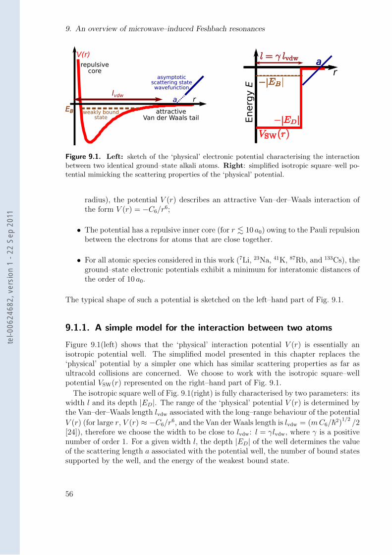
9. An overview of microwave–induced Feshbach resonances

rlvdw

repulsivecore

attractiveVan der Waals tail

EB

V(r)

weakly boundstate

asymptoticscattering statewavefunction

a

r

Energ

y E

a

Figure 9.1. Left: sketch of the ‘physical’ electronic potential characterising the interactionbetween two identical ground–state alkali atoms. Right: simplified isotropic square–well po-tential mimicking the scattering properties of the ‘physical’ potential.

radius), the potential V (r) describes an attractive Van–der–Waals interaction ofthe form V (r) = −C6/r

6;

• The potential has a repulsive inner core (for r . 10 a0) owing to the Pauli repulsionbetween the electrons for atoms that are close together.

• For all atomic species considered in this work (7Li, 23Na, 41K, 87Rb, and 133Cs), theground–state electronic potentials exhibit a minimum for interatomic distances ofthe order of 10 a0.

The typical shape of such a potential is sketched on the left–hand part of Fig. 9.1.

9.1.1. A simple model for the interaction between two atoms

Figure 9.1(left) shows that the ‘physical’ interaction potential V (r) is essentially anisotropic potential well. The simplified model presented in this chapter replaces the‘physical’ potential by a simpler one which has similar scattering properties as far asultracold collisions are concerned. We choose to work with the isotropic square–wellpotential VSW(r) represented on the right–hand part of Fig. 9.1.

The isotropic square well of Fig. 9.1(right) is fully characterised by two parameters: itswidth l and its depth |ED|. The range of the ‘physical’ potential V (r) is determined bythe Van–der–Waals length lvdw associated with the long–range behaviour of the potential

V (r) (for large r, V (r) ≈ −C6/r6, and the Van der Waals length is lvdw = (mC6/~2)

1/2/2

[24]), therefore we choose the width to be close to lvdw: l = γlvdw, where γ is a positivenumber of order 1. For a given width l, the depth |ED| of the well determines the valueof the scattering length a associated with the potential well, the number of bound statessupported by the well, and the energy of the weakest bound state.

56

tel-0

0624

682,

ver

sion

1 -

22 S

ep 2

011

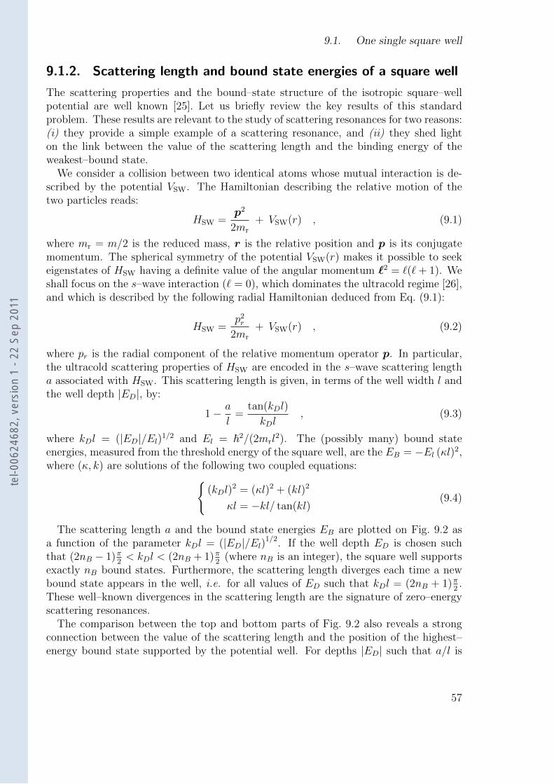
9.1. One single square well

9.1.2. Scattering length and bound state energies of a square well

The scattering properties and the bound–state structure of the isotropic square–wellpotential are well known [25]. Let us briefly review the key results of this standardproblem. These results are relevant to the study of scattering resonances for two reasons:(i) they provide a simple example of a scattering resonance, and (ii) they shed lighton the link between the value of the scattering length and the binding energy of theweakest–bound state.

We consider a collision between two identical atoms whose mutual interaction is de-scribed by the potential VSW. The Hamiltonian describing the relative motion of thetwo particles reads:

HSW =p2

2mr

+ VSW(r) , (9.1)

where mr = m/2 is the reduced mass, r is the relative position and p is its conjugatemomentum. The spherical symmetry of the potential VSW(r) makes it possible to seekeigenstates of HSW having a definite value of the angular momentum `2 = `(`+ 1). Weshall focus on the s–wave interaction (` = 0), which dominates the ultracold regime [26],and which is described by the following radial Hamiltonian deduced from Eq. (9.1):

HSW =p2r

2mr

+ VSW(r) , (9.2)

where pr is the radial component of the relative momentum operator p. In particular,the ultracold scattering properties of HSW are encoded in the s–wave scattering lengtha associated with HSW. This scattering length is given, in terms of the well width l andthe well depth |ED|, by:

1− a

l=

tan(kDl)

kDl, (9.3)

where kDl = (|ED|/El)1/2 and El = ~2/(2mrl2). The (possibly many) bound state

energies, measured from the threshold energy of the square well, are the EB = −El (κl)2,where (κ, k) are solutions of the following two coupled equations:

(kDl)2 = (κl)2 + (kl)2

κl = −kl/ tan(kl)(9.4)

The scattering length a and the bound state energies EB are plotted on Fig. 9.2 asa function of the parameter kDl = (|ED|/El)1/2. If the well depth ED is chosen suchthat (2nB − 1)π

2< kDl < (2nB + 1)π

2(where nB is an integer), the square well supports

exactly nB bound states. Furthermore, the scattering length diverges each time a newbound state appears in the well, i.e. for all values of ED such that kDl = (2nB + 1)π

2.

These well–known divergences in the scattering length are the signature of zero–energyscattering resonances.

The comparison between the top and bottom parts of Fig. 9.2 also reveals a strongconnection between the value of the scattering length and the position of the highest–energy bound state supported by the potential well. For depths |ED| such that a/l is

57

tel-0

0624

682,

ver

sion

1 -

22 S

ep 2

011

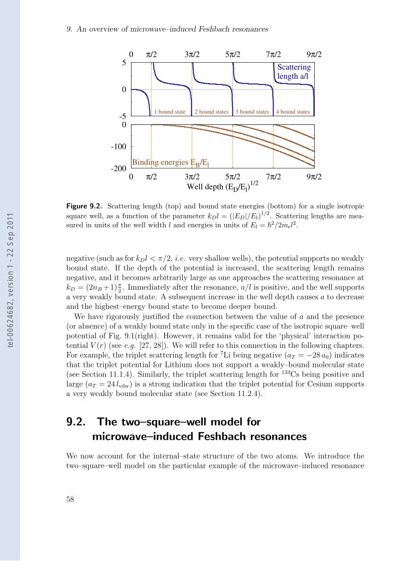
9. An overview of microwave–induced Feshbach resonances

-5

0

50 π/2 3π/2 5π/2 7π/2 9π/2

1 bound state 2 bound states 3 bound states 4 bound states

Scatteringlength a/l

-200

-100

0

0 π/2 3π/2 5π/2 7π/2 9π/2

Well depth (ED/El)1/2

Binding energies EB/El

Figure 9.2. Scattering length (top) and bound state energies (bottom) for a single isotropic

square well, as a function of the parameter kDl = (|ED|/El)1/2. Scattering lengths are mea-sured in units of the well width l and energies in units of El = ~2/2mrl

2.

negative (such as for kDl < π/2, i.e. very shallow wells), the potential supports no weaklybound state. If the depth of the potential is increased, the scattering length remainsnegative, and it becomes arbitrarily large as one approaches the scattering resonance atkD = (2nB+1)π

2. Immediately after the resonance, a/l is positive, and the well supports

a very weakly bound state. A subsequent increase in the well depth causes a to decreaseand the highest–energy bound state to become deeper bound.

We have rigorously justified the connection between the value of a and the presence(or absence) of a weakly bound state only in the specific case of the isotropic square–wellpotential of Fig. 9.1(right). However, it remains valid for the ‘physical’ interaction po-tential V (r) (see e.g. [27, 28]). We will refer to this connection in the following chapters.For example, the triplet scattering length for 7Li being negative (aT = −28 a0) indicatesthat the triplet potential for Lithium does not support a weakly–bound molecular state(see Section 11.1.4). Similarly, the triplet scattering length for 133Cs being positive andlarge (aT = 24 lvdw) is a strong indication that the triplet potential for Cesium supportsa very weakly bound molecular state (see Section 11.2.4).

9.2. The two–square–well model formicrowave–induced Feshbach resonances

We now account for the internal–state structure of the two atoms. We introduce thetwo–square–well model on the particular example of the microwave–induced resonance

58

tel-0

0624

682,

ver

sion

1 -

22 S

ep 2

011

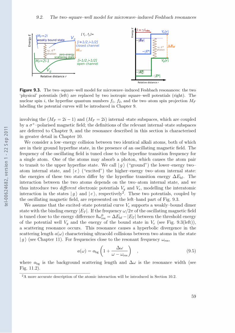
9.2. The two–square–well model for microwave–induced Feshbach resonances

Relative distance r

En

erg

y E

[i-1/2,i-1/2]open channel

[i+1/2,i-1/2]closed channel

zero-energyscattering state

weakly bound state

ω, σ+photon

ΔEhf

MF=2i-1

MF=2i [ f1 , f2 ]=

Vg

Ve

Relative distance r

ω, σ+photon

Energ

y E

Figure 9.3. The two–square–well model for microwave–induced Feshbach resonances: the two‘physical’ potentials (left) are replaced by two isotropic square–well potentials (right). Thenuclear spin i, the hyperfine quantum numbers f1, f2, and the two–atom spin projection MF

labelling the potential curves will be introduced in Chapter 9.

involving the (MF = 2i− 1) and (MF = 2i) internal–state subspaces, which are coupledby a σ+–polarised magnetic field; the definitions of the relevant internal–state subspacesare deferred to Chapter 9, and the resonance described in this section is characterisedin greater detail in Chapter 10.

We consider a low–energy collision between two identical alkali atoms, both of whichare in their ground hyperfine state, in the presence of an oscillating magnetic field. Thefrequency of the oscillating field is tuned close to the hyperfine transition frequency fora single atom. One of the atoms may absorb a photon, which causes the atom pairto transit to the upper hyperfine state. We call | g 〉 (“ground”) the lower–energy two–atom internal state, and | e 〉 (“excited”) the higher–energy two–atom internal state:the energies of these two states differ by the hyperfine transition energy ∆Ehf . Theinteraction between the two atoms depends on the two–atom internal state, and wethus introduce two different electronic potentials Vg and Ve, modelling the interatomicinteraction in the states | g 〉 and | e 〉, respectively2. These two potentials, coupled bythe oscillating magnetic field, are represented on the left–hand part of Fig. 9.3.

We assume that the excited–state potential curve Ve supports a weakly–bound dimerstate with the binding energy |ET |. If the frequency ω/2π of the oscillating magnetic fieldis tuned close to the energy difference ~ω0

res = ∆Ehf−|ET | between the threshold energyof the potential well Vg and the energy of the bound state in Ve (see Fig. 9.3(left)),a scattering resonance occurs. This resonance causes a hyperbolic divergence in thescattering length a(ω) characterising ultracold collisions between two atoms in the state| g 〉 (see Chapter 11). For frequencies close to the resonant frequency ωres,

a(ω) = abg

(1 +

∆ω

ω − ωres

), (9.5)

where abg is the background scattering length and ∆ω is the resonance width (seeFig. 11.2).

2A more accurate description of the atomic interaction will be introduced in Section 10.2.

59

tel-0

0624

682,

ver

sion

1 -

22 S

ep 2

011

9. An overview of microwave–induced Feshbach resonances

We will show in Section 11.1.2 that the resonance width ∆ω is proportional to B2osc,

where Bosc is the amplitude of the oscillating magnetic field. The coupling between thetwo channels | g 〉 and | e 〉 causes the resonance frequency ωres to be slightly shifted awayfrom ω0

res (see [1] and Section 11.1):

ωres = ω0res + αB2

osc . (9.6)

The main goal of the present work is to characterise the microwave–induced Feshbachresonances described by Eqs. (9.5) and (9.6), i.e. to evaluate the resonance width ∆ωand the resonance shift α for given choices of the two–atom states | g 〉 and | e 〉 andof the resonant bound state |ET |. An accurate characterisation of these resonanceswill be presented in Chapter 11. These accurate results are obtained through complexnumerical calculations based on the coupled–channel approach (see Chapter 12). In thissection, we present a simplified approach based on the square–well potentials introducedin Section 9.1. This simple model can be solved analytically (see Section 9.2.5) and yieldsnumerical results for the resonance characteristics (see Section 9.2.6) which are in goodagreement with the full–fledged coupled–channel results of Chapter 11 (see Table 11.2).

Analyses of Feshbach resonances in terms of two coupled square wells have previouslybeen reported [29]. The two–square–well model presented in this chapter has been devel-opped independently, within the context of microwave–induced resonances (rather thanresonances induced by static fields [7]); it is not equivalent3 to the one presented in [29].

9.2.1. Choice of the square wells modelling the atomic interaction

Our simple model is based on replacing each of the potential well Vg and Ve of the left–hand side of Fig. 9.3 by the isotropic square–well potentials shown on the right–hand sideof this figure. In order to define these two wells, four parameters have to be specified:the two well widths lg and le, and the two well depths |Eg| and |Ee|.

The ‘physical’ electronic potentials Vg and Ve have the same spatial range, determinedby the Van–der–Waals length lvdw which is the same for | g 〉 and | e 〉 [24]. Consequently,we choose the two square wells to have the same width l = lg = le = γ lvdw, where γ isa positive number of order 1.

The resonance we are describing occurs in the ultracold regime, where the scatteringproperties of the potentials Vg and Ve are encapsulated in the corresponding scatteringlengths ag and ae. Therefore, we require the two square wells of Fig. 9.3(right) to havethe same scattering lengths as the corresponding original potentials.

The strength of the coupling between the incoming scattering state in the potential Vgand the resonant bound state in the potential Ve is determined by the overlap betweenthe two corresponding wavefunctions (see Section 11.1.2). This overlap depends on the

3For instance, the model described in [29] uses a closed–channel square well which is infinite for r > l,whereas both of our wells are finite for all values of r > 0. Furthermore, they choose the widthof both square wells to be equal to the Van–der–Waals length lvdw, whereas our square–well widthis an adjustable parameter which we tune to reproduce the binding energy of the closed–channelbound state: see Section 9.2.1.

60

tel-0

0624

682,

ver

sion

1 -

22 S

ep 2

011

9.2. The two–square–well model for microwave–induced Feshbach resonances

binding energy of the resonant bound state: a weakly bound state has a large spatialextent, leading to a large overlap and a strong coupling to the scattering state; a deeplybound state has a small spatial extent, and its coupling to the scattering state is thusmuch smaller (see Section 11.1.4). Hence, we wish the square–well potential representingVe to support a bound state which has the same binding energy |ET | as the resonantbound state in Ve.

We call |ϕscatg 〉 the threshold–energy scattering state wavefunction in the square–

well potential representing Vg, and |ϕbounde 〉 the wavefunction of the bound state hav-

ing the energy −|ET | in the square–well potential representing Ve. The overlap F =〈ϕbound

e |ϕscatg 〉 between these two wavefunctions is the sum of two contributions: F =

F< + F>, where F< corresponds to the inner r < l region in which the square wellsare non–zero, and F> corresponds to the outer region (r > l) where both square wellpotentials vanish. Let us assume at first that one of the two well depths is much largerthan the other: we take |Eg| |Ee| (but the argument also holds in the opposite limit).In this case, the kinetic energy available in the r < l region is much larger for an atompair in the state | g 〉 than it is for an atom pair in the state | e 〉. Therefore, in theregion r < l, the wavefunction ϕg(r) oscillates much faster than ϕe(r) does: these fastoscillations average F< to zero. This is not the expected behaviour for the inner partof the overlap, where the oscillations occur in phase and build up a non–vanishing con-tribution to the total overlap (see the multi–channel numerical results for the overlaps,represented on Figs. 11.5). In order to avoid this non–physical averaging, the depths |Eg|and |Ee| should have the same orders of magnitude, i.e. the two square–well potentialsshould support the same number of bound states4 nB = ngB = neB.

To sum up, the four square well parameters lg, le, Eg and Ee are chosen to satisfy thefollowing four conditions:

1. The two square–well potentials have the same width l, which is of the order of,but not equal to, the Van–der–Waals length of the original potentials;

2. The square–well potentials have the same scattering lengths ag and ae as theoriginal potentials Vg and Ve;

3. The highest–energy bound state of the square–well potential representing Ve hasthe same binding energy as the resonant bound state in Ve;

4. The two square–well potentials support the same number of bound states.

The parameters ag, ae, l, and nB defining the two square–well potentials of our sim-plified model are collected in Table 9.1 for all considered alkali atoms. For the sake ofsimplicity, we choose the smallest number of bound states nB for which the four condi-tions stated above can be simultaneously satisfied (nB = 1 or 2 for all considered atomicspecies). We have checked that using a larger number of bound states ngB = neB does notsubstantially modify the results obtained with this model. On the contrary, choosing a

4Figure 9.2 shows that the depth of a square–well potential supporting nB bound states roughlybehaves as |ED| ≈ El π2n2

B .

61

tel-0

0624

682,

ver

sion

1 -

22 S

ep 2

011

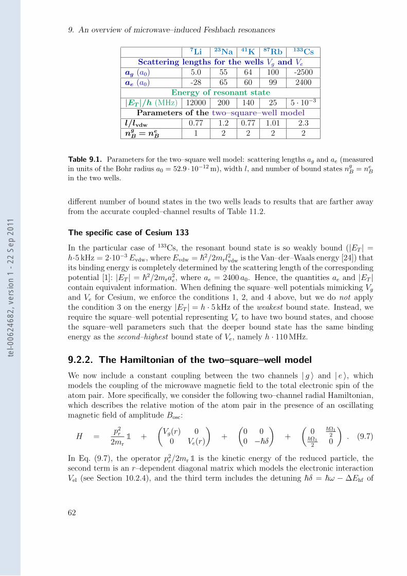
9. An overview of microwave–induced Feshbach resonances

7Li 23Na 41K 87Rb 133CsScattering lengths for the wells Vg and Ve

ag (a0) 5.0 55 64 100 -2500ae (a0) -28 65 60 99 2400

Energy of resonant state|ET |/h (MHz) 12000 200 140 25 5 · 10−3

Parameters of the two–square–well modell/lvdw 0.77 1.2 0.77 1.01 2.3ng

B = neB 1 2 2 2 2

Table 9.1. Parameters for the two–square well model: scattering lengths ag and ae (measuredin units of the Bohr radius a0 = 52.9 · 10−12 m), width l, and number of bound states ngB = neBin the two wells.

different number of bound states in the two wells leads to results that are farther awayfrom the accurate coupled–channel results of Table 11.2.

The specific case of Cesium 133

In the particular case of 133Cs, the resonant bound state is so weakly bound (|ET | =h·5 kHz = 2·10−3Evdw, where Evdw = ~2/2mrl

2vdw is the Van–der–Waals energy [24]) that

its binding energy is completely determined by the scattering length of the correspondingpotential [1]: |ET | = ~2/2mra

2e, where ae = 2400 a0. Hence, the quantities ae and |ET |

contain equivalent information. When defining the square–well potentials mimicking Vgand Ve for Cesium, we enforce the conditions 1, 2, and 4 above, but we do not applythe condition 3 on the energy |ET | = h · 5 kHz of the weakest bound state. Instead, werequire the square–well potential representing Ve to have two bound states, and choosethe square–well parameters such that the deeper bound state has the same bindingenergy as the second–highest bound state of Ve, namely h · 110 MHz.

9.2.2. The Hamiltonian of the two–square–well model

We now include a constant coupling between the two channels | g 〉 and | e 〉, whichmodels the coupling of the microwave magnetic field to the total electronic spin of theatom pair. More specifically, we consider the following two–channel radial Hamiltonian,which describes the relative motion of the atom pair in the presence of an oscillatingmagnetic field of amplitude Bosc:

H =p2r

2mr

1 +

(Vg(r) 0

0 Ve(r)

)+

(0 00 −~δ

)+

(0 ~Ω1

2~Ω1

20

). (9.7)

In Eq. (9.7), the operator p2r/2mr 1 is the kinetic energy of the reduced particle, the

second term is an r–dependent diagonal matrix which models the electronic interactionVel (see Section 10.2.4), and the third term includes the detuning ~δ = ~ω − ∆Ehf of

62

tel-0

0624

682,

ver

sion

1 -

22 S

ep 2

011

9.2. The two–square–well model for microwave–induced Feshbach resonances

the microwave frequency ω/2π with respect to the single–atom hyperfine splitting ∆Ehf .The last term is a constant symmetric matrix which only has off–diagonal elements andmodels the coupling of the two channels due to the magnetic dipole coupling betweenthe microwave magnetic field and the total electronic spin S. The strength Ω1 of thecoupling between the channels | g 〉 and | e 〉 relates to the amplitude Bosc of the oscillatingmagnetic field through:

~Ω1

2= µBBosc , (9.8)

where we have assumed that the g–factor of the resonant bound state is g = 1.The Hamiltonian (9.7) is the simplified version, within the framework of the two–

square–well model, of the two–atom Hamiltonian (10.13) presented in Chapter 10 andused in all subsequent chapters. The two Hamiltonians have a similar structure, and theterms appearing in them are discussed in greater detail in Section 10.2.2.

9.2.3. The microwave–dressed two–atom states

In this section, we briefly present the microwave–dressed two–atom states. These dressedstates are the stationary states of a pair of atoms that are infinitely far away from eachother.

We first introduce the total potential Vtot(r), which is the 2× 2 operator defined by:

Vtot(r) =

(Vg(r) 0

0 Ve(r)

)+

(0 00 −~δ

)+

(0 ~Ω1

2~Ω1

20

), (9.9)

so that the Hamiltonian (9.7) reads H = p2

2mr1 + Vtot(r).

For r > l, both of the square–well potentials Vg(r) and Ve(r) vanish. The matrixVtot(r) does not vanish, but it reduces to a constant matrix V∞:

V∞ = Vtot(r > l) =

(0 ~Ω1

2~Ω1

2−δ

). (9.10)

The matrix V∞ is real and symmetric, therefore it has two orthogonal eigenvectors | g 〉and | e 〉, which are the microwave–dressed (two–atom) internal states [30]. The couplingterms ~Ω1/2, modelling the magnetic dipole interaction between the atom pair and theoscillating magnetic field, do not depend on r: their presence causes the dressed statesto differ from the ‘bare’ two–atom states | g 〉 and | e 〉.

Note that the dressed states | g 〉 and | e 〉, as well as the corresponding dressed energiesEg and Ee, depend both on the coupling strength Ω1 and on the detuning δ.

We assume Eg < Ee. The dressed–state energy splitting ~Ω = Ee − Eg is given by(see Fig. 11.7):

Ω =(Ω2

1 + δ2)1/2

. (9.11)

A more detailed presentation of the microwave–dressed two–atom states will be givenin Section 11.2.2.

63

tel-0

0624

682,

ver

sion

1 -

22 S

ep 2

011

9. An overview of microwave–induced Feshbach resonances

9.2.4. The two–channel scattering state

We are interested in the scattering length a(δ,Ω1), associated with collisions betweenatoms which are asymptotically all in the lowest–energy dressed state | g 〉, for givenvalues of the detuning δ and the coupling strength Ω1. We thus solve for the zero–energystationary scattering state |Ψ0 〉 of the Hamiltonian (9.7). The state |Ψ0 〉 is a two–channel wavefunction, in the sense that it has two r–dependent components 〈 g |Ψ0(r) 〉and 〈 e |Ψ0(r) 〉. It depends on the detuning δ and on the coupling strength Ω1. It isdefined by the stationary Schrodinger equation:

H|Ψ0 〉 = Eg|Ψ0 〉 , (9.12)

along with the asymptotic behaviour (exact for r > l):

|Ψ0 〉 =r>l

(1− a

r

)| g 〉 + feg

e−κr

r| e 〉 . (9.13)

Note that the asymptotic behaviour of Eq. (9.13) is expressed in the dressed–state basis| g 〉, | e 〉 (rather than in the bare–state basis | g 〉, | e 〉). The constant κ characterisesthe decay of the closed–channel component 〈 g |Ψ0(r) 〉:

κl = (~Ω/El)1/2 . (9.14)

A lengthier discussion of multi–channel wavefunctions, open and closed channels, andboundary conditions will be given in Section 12.1.3.

9.2.5. Analytical expression for the scattering length

The scattering length a and the scattering amplitude feg appearing in Eq. (9.13) areunknown a priori : they are determined from the large–r behaviour of the wavefunctioncomponents 〈 g |Ψ0(r) 〉 and 〈 e |Ψ0(r) 〉, respectively.

The two–square–well model allows for an exact calculation of the scattering length a.It can be expressed analytically in terms of the well depths |Eg| and |Ee|, the couplingstrength Ω1, and the detuning δ:

a

l= 1 − (κl)u1u2 + sin2 Ψu1 + cos2 Ψu2

1 + (κl) (cos2 Ψu1 + sin2 Ψu2). (9.15)

The auxiliary parameters appearing in Eq. (9.15) are defined below:

u1 =tan(k1l)

k1land u2 =

tan(k2l)

k2l, (9.16)

cos(2Ψ) =δ

Ω

~δ + |Ee| − |Eg|~χ

+Ω1

Ω

Ω1

χ, (9.17)

~χ =((|Ee| − |Eg|+ ~δ)2 + (~Ω1)2

)1/2, (9.18)

k1l =

( |Ee|+ |Eg| − ~Ω− ~χ2El

)1/2

and k2l =

( |Ee|+ |Eg| − ~Ω + ~χ2El

)1/2

. (9.19)

64

tel-0

0624

682,

ver

sion

1 -

22 S

ep 2

011

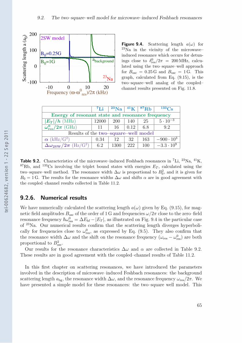
9.2. The two–square–well model for microwave–induced Feshbach resonances

-100

0

100

200

-10 0 10 20

Sca

tter

ing l

ength

a (

a 0)

Frequency (ω-ω0res)/2π (kHz)

abackgroundB0=1G

B0=0.25G

23Na

2SW model

Figure 9.4. Scattering length a(ω) for23Na in the vicinity of the microwave–induced resonance which occurs for detun-ings close to δ0

res/2π = 200 MHz, calcu-lated using the two–square–well approachfor Bosc = 0.25 G and Bosc = 1 G. Thisgraph, calculated from Eq. (9.15), is thetwo–square–well analog of the coupled–channel results presented on Fig. 11.8.

7Li 23Na 41K 87Rb 133CsEnergy of resonant state and resonance frequency

|ET |/h (MHz) 12000 200 140 25 5 · 10−3

ω0res/2π (GHz) 11 16 0.12 6.8 9.2

Results of the two–square–well modelα (kHz/G2) 0.34 12 32 163 −900 · 103

∆ω2SW/2π (Hz/G2) 6.2 1300 222 100 −3.3 · 109

Table 9.2. Characteristics of the microwave–induced Feshbach resonances in 7Li, 23Na, 41K,87Rb, and 133Cs involving the triplet bound states with energies ET , calculated using thetwo–square–well method. The resonance width ∆ω is proportional to B2

0 , and it is given forB0 = 1 G. The results for the resonance widths ∆ω and shifts α are in good agreement withthe coupled–channel results collected in Table 11.2.

9.2.6. Numerical results

We have numerically calculated the scattering length a(ω) given by Eq. (9.15), for mag-netic field amplitudes Bosc of the order of 1 G and frequencies ω/2π close to the zero–fieldresonance frequency ~ω0

res = ∆Ehf−|ET |, as illustrated on Fig. 9.4 in the particular caseof 23Na. Our numerical results confirm that the scattering length diverges hyperboli-cally for frequencies close to ω0

res, as expressed by Eq. (9.5). They also confirm thatthe resonance width ∆ω and the shift on the resonance frequency (ωres − ω0

res) are bothproportional to B2

osc.

Our results for the resonance characteristics ∆ω and α are collected in Table 9.2.These results are in good agreement with the coupled–channel results of Table 11.2.

In this first chapter on scattering resonances, we have introduced the parametersinvolved in the description of microwave–induced Feshbach resonances: the backgroundscattering length abg, the resonance width ∆ω, and the resonance frequency ωres/2π. Wehave presented a simple model for these resonances: the two–square well model. This

65

tel-0

0624

682,

ver

sion

1 -

22 S

ep 2

011

9. An overview of microwave–induced Feshbach resonances

model leads to an exact analytical expression of the scattering length a. We have used itto derive orders of magnitude of the resonance positions and shifts for the bosonic alkaliatoms 7Li, 23Na, 41K, 87Rb, and 133Cs.

We have also briefly presented the key concepts involved in the analysis of ultra-cold scattering resonances, among which the electronic interaction between two atoms,dressed two–atom states, and multi–channel scattering wavefunctions. All of these con-cepts will be described in greater detail in Chapters 10 and 11.

Starting from Chapter 10, we relinquish the two–square–well model of the presentchapter and turn towards more accurate approaches. These approaches are more in-volved as they require numerical coupled–channel calculations. Our accurate coupled–channel results are given at the end of Chapter 11 (in particular, see Table 11.2), andthe numerical methods we have used to obtain them are presented in Chapter 12.

66

tel-0

0624

682,

ver

sion

1 -

22 S

ep 2

011

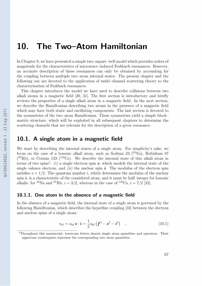
10. The Two–Atom Hamiltonian

In Chapter 9, we have presented a simple two–square–well model which provides orders ofmagnitude for the characteristics of microwave–induced Feshbach resonances. However,an accurate description of these resonances can only be obtained by accounting forthe coupling between multiple two–atom internal states. The present chapter and thefollowing one are devoted to the application of multi–channel scattering theory to thecharacterisation of Feshbach resonances.

This chapter introduces the model we have used to describe collisions between twoalkali atoms in a magnetic field [20, 31]. The first section is introductory and brieflyreviews the properties of a single alkali atom in a magnetic field. In the next section,we describe the Hamiltonian describing two atoms in the presence of a magnetic fieldwhich may have both static and oscillating components. The last section is devoted tothe symmetries of the two–atom Hamiltonian. These symmetries yield a simple block–matrix structure, which will be exploited in all subsequent chapters to determine thescattering channels that are relevant for the description of a given resonance.

10.1. A single atom in a magnetic field

We start by describing the internal states of a single atom. For simplicity’s sake, wefocus on the case of a bosonic alkali atom, such as Sodium 23 (23Na), Rubidium 87(87Rb), or Cesium 133 (133Cs). We describe the internal state of this alkali atom interms of two spins1: (i) a single electron spin s, which models the internal state of thesingle valence electron, and (ii) the nuclear spin i. The modulus of the electron spinsatisfies s = 1/2. The quantum number i, which determines the modulus of the nuclearspin i, is a characteristic of the considered atom, and it must be half–integer for bosonicalkalis: for 23Na and 87Rb, i = 3/2, whereas in the case of 133Cs, i = 7/2 [32].

10.1.1. One atom in the absence of a magnetic field

In the absence of a magnetic field, the internal state of a single atom is governed by thefollowing Hamiltonian, which describes the hyperfine coupling [33] between the electronand nuclear spins of a single atom:

vhf = ahf s · i =1

2ahf

(f 2 − s2 − i2

), (10.1)

1Throughout this manuscript, lowercase letters denote single–atom quantities and operators. Theiruppercase counterparts represent the corresponding two–atom quantities.

67

tel-0

0624

682,

ver

sion

1 -

22 S

ep 2

011

10. The Two–Atom Hamiltonian

Figure 10.1. Single–atom hyperfine states for an alkali atom with nuclear spin i = 3/2, suchas 23Na or 87Rb: there are 3 states with f = f− = 1 and 5 states with f = f+ = 2.

where the operator f is the total single–atom spin: f = s+ i.Equation (10.1) shows that the Hamiltonian vhf conserves both hyperfine quantum

numbers f and mf , where mf characterises the total spin projection fz. Therefore, itis convenient to describe the internal states of a single atom using the hyperfine basisstates | f,mf 〉. For an alkali atom, f can take two values: f− = i−1/2 and f+ = i+1/2.The internal–state subspace thus has dimension (2f− + 1) + (2f+ + 1) = 4i + 2. Thesingle–atom hyperfine states are represented on Fig. 10.1 in the case of an atom withnuclear spin i = 3/2, for which the internal–state subspace has dimension 8. In the caseof an atom with nuclear spin i = 7/2, the internal–state subspace has dimension 16.In the absence of a magnetic field, all hyperfine states | f,mf 〉 with the same quantumnumber f are degenerate.

10.1.2. One atom in a static magnetic field

If a static magnetic fieldBstat is added to the system, the Hamiltonian acquires a Zeemanterm vZ. Choosing the direction ez of the static magnetic field as the quantisation axis,the total single–atom Hamiltonian reads [33]

hstat = vhf + vZ , (10.2)

where

vZ = 2µBBstat

~sz , (10.3)

µB is the Bohr magneton, and sz is the projection along ez of the electron–spin operator.The Hamiltonian hstat conserves the spin projection mf , but it no longer conserves f .

10.1.3. One atom in an oscillating magnetic field

We now add to the system an oscillating magnetic field Bosc, whose frequency ω/2π istuned close to the hyperfine transition frequency of the considered atoms, i.e. in themicrowave range. We still assume the presence of a static magnetic field Bstat, whosedirection determines the quantisation axis ez.

We use a quantum description for the oscillating field, and we assume that all of itsphotons are in the same mode. We call a† the creation operator for a photon in the

68

tel-0

0624

682,

ver

sion

1 -

22 S

ep 2

011

10.2. Two atoms in a magnetic field

relevant mode, and ε its polarisation. The magnetic field operator is then given by [30]:

Bosc =b0√

2(εa+ ε∗a†) , (10.4)

where b0 is related to the magnetic field amplitude Bosc = b0

√N , and N is the total

number of photons, which we assume to be 1.The magnetic field and the atom are coupled via the magnetic dipole coupling term:

w = −m ·Bosc , (10.5)

where m = −2µB s/~ is the total magnetic dipole operator for the atom [33], assumingthat the valence electron has zero orbital angular momentum (l = 0).

We focus on the case of a σ+–polarised magnetic field about the quantisation axis ez:ε = ex+iey√

2. Equations (10.4) and (10.5) then yield2:

w = w1 (s+a+ s−a†) , (10.6)

where

w1 =µBb0

~, (10.7)

and s± = sx ± isy are the ladder operators for the electron spin.Including both the static fieldBstat and the oscillating fieldBosc, the total single–atom

internal–state Hamiltonian reads:

h = vhf + vZ + ~ω a†a+ w . (10.8)

The Hamiltonian h conserves none of the quantum numbers f , mf , and N (only thesum (mf +N) of the atomic spin and the photon number is conserved). The stationarystates of the Hamiltonian h are thus dressed states of the joint system “single atom andoscillating magnetic field”, which can be expressed as linear combinations of basis statesof the form | f,mf , N 〉.

10.2. Two atoms in a magnetic field

In Section 10.1, we described the internal–state subspace for a single atom in the pres-ence of a magnetic field. However, the resonances we wish to describe involve a collisionbetween two atoms. In this section, we introduce the complete two–atom Hamiltonian,which takes into account both the internal–state and magnetic terms described in Sec-tion 10.1, and the coupling between the spatial dynamics and the internal degrees offreedom of the atoms.

2Strictly speaking, the magnetic field also couples to the nuclear spin i. However, this coupling is veryweak, as the nuclear gyromagnetic ratios gi are about 1000 times smaller than that of the electron(gs = 2). This coupling is included in our numerical calculations, but we omit it in Eqs. (10.3) and(10.5) for the sake of clarity.

69

tel-0

0624

682,

ver

sion

1 -

22 S

ep 2

011

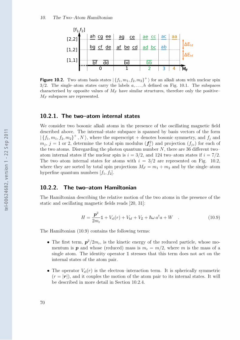
10. The Two–Atom Hamiltonian

Figure 10.2. Two–atom basis states | f1,m1, f2,m2+ 〉 for an alkali atom with nuclear spin3/2. The single–atom states carry the labels a, . . . , h defined on Fig. 10.1. The subspacescharacterised by opposite values of MF have similar structures, therefore only the positive–MF subspaces are represented.

10.2.1. The two–atom internal states

We consider two bosonic alkali atoms in the presence of the oscillating magnetic fielddescribed above. The internal–state subspace is spanned by basis vectors of the form| f1,m1, f2,m2+ , N 〉, where the superscript + denotes bosonic symmetry, and fj andmj, j = 1 or 2, determine the total spin modulus (f 2

j ) and projection (fjz) for each ofthe two atoms. Disregarding the photon quantum number N , there are 36 different two–atom internal states if the nuclear spin is i = 3/2, and 124 two–atom states if i = 7/2.The two–atom internal states for atoms with i = 3/2 are represented on Fig. 10.2,where they are sorted by total spin projections MF = m1 +m2 and by the single–atomhyperfine quantum numbers [f1, f2].

10.2.2. The two–atom Hamiltonian

The Hamiltonian describing the relative motion of the two atoms in the presence of thestatic and oscillating magnetic fields reads [20, 31]:

H =p2

2mr

1 + Vel(r) + Vhf + VZ + ~ω a†a+W . (10.9)

The Hamiltonian (10.9) contains the following terms:

• The first term, p2/2mr, is the kinetic energy of the reduced particle, whose mo-mentum is p and whose (reduced) mass is mr = m/2, where m is the mass of asingle atom. The identity operator 1 stresses that this term does not act on theinternal states of the atom pair.

• The operator Vel(r) is the electron–interaction term. It is spherically symmetric(r = |r|), and it couples the motion of the atom pair to its internal states. It willbe described in more detail in Section 10.2.4.

70

tel-0

0624

682,

ver

sion

1 -

22 S

ep 2

011

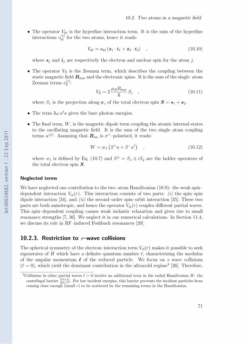
10.2. Two atoms in a magnetic field

• The operator Vhf is the hyperfine interaction term. It is the sum of the hyperfineinteractions v

(j)hf for the two atoms, hence it reads:

Vhf = ahf (s1 · i1 + s2 · i2) , (10.10)

where sj and ij are respectively the electron and nuclear spin for the atom j.

• The operator VZ is the Zeeman term, which describes the coupling between thestatic magnetic fieldBstat and the electronic spins. It is the sum of the single–atomZeeman terms v

(j)Z :

VZ = 2µBBstat

~Sz , (10.11)

where Sz is the projection along ez of the total electron spin S = s1 + s2.

• The term ~ω a†a gives the bare photon energies.

• The final term, W , is the magnetic dipole term coupling the atomic internal statesto the oscillating magnetic field. It is the sum of the two single–atom couplingterms w(j). Assuming that Bosc is σ+–polarised, it reads:

W = w1

(S+a+ S−a†

), (10.12)

where w1 is defined by Eq. (10.7) and S± = Sx ± iSy are the ladder operators ofthe total electron spin S.

Neglected terms

We have neglected one contribution to the two–atom Hamiltonian (10.9): the weak spin–dependent interaction Vss(r). This interaction consists of two parts: (i) the spin–spindipole interaction [34], and (ii) the second–order spin–orbit interaction [35]. These twoparts are both anisotropic, and hence the operator Vss(r) couples different partial waves.This spin–dependent coupling causes weak inelastic relaxation and gives rise to smallresonance strengths [7, 36]. We neglect it in our numerical calculations. In Section 11.4,we discuss its role in RF–induced Feshbach resonances [20].

10.2.3. Restriction to s–wave collisions

The spherical symmetry of the electron–interaction term Vel(r) makes it possible to seekeigenstates of H which have a definite quantum number `, characterising the modulusof the angular momentum ` of the reduced particle. We focus on s–wave collisions(` = 0), which yield the dominant contribution in the ultracold regime3 [26]. Therefore,

3Collisions in other partial waves ` > 0 involve an additional term in the radial Hamiltonian H: the

centrifugal barrier `(`+1)2mr r2

. For low incident energies, this barrier prevents the incident particles fromcoming close enough (small r) to be scattered by the remaining terms in the Hamiltonian.

71

tel-0

0624

682,

ver

sion

1 -

22 S

ep 2

011

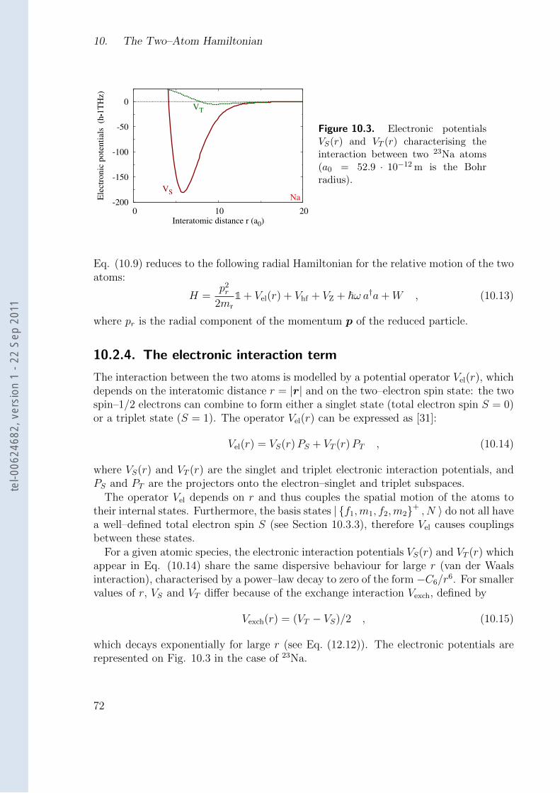
10. The Two–Atom Hamiltonian

-200

-150

-100

-50

0

0 10 20

Ele

ctro

nic

pote

nti

als

(h

•1T

Hz)

Interatomic distance r (a0)

NaVS

VT

Figure 10.3. Electronic potentialsVS(r) and VT (r) characterising theinteraction between two 23Na atoms(a0 = 52.9 · 10−12 m is the Bohrradius).

Eq. (10.9) reduces to the following radial Hamiltonian for the relative motion of the twoatoms:

H =p2r

2mr

1 + Vel(r) + Vhf + VZ + ~ω a†a+W , (10.13)

where pr is the radial component of the momentum p of the reduced particle.

10.2.4. The electronic interaction term

The interaction between the two atoms is modelled by a potential operator Vel(r), whichdepends on the interatomic distance r = |r| and on the two–electron spin state: the twospin–1/2 electrons can combine to form either a singlet state (total electron spin S = 0)or a triplet state (S = 1). The operator Vel(r) can be expressed as [31]:

Vel(r) = VS(r)PS + VT (r)PT , (10.14)

where VS(r) and VT (r) are the singlet and triplet electronic interaction potentials, andPS and PT are the projectors onto the electron–singlet and triplet subspaces.

The operator Vel depends on r and thus couples the spatial motion of the atoms totheir internal states. Furthermore, the basis states | f1,m1, f2,m2+ , N 〉 do not all havea well–defined total electron spin S (see Section 10.3.3), therefore Vel causes couplingsbetween these states.

For a given atomic species, the electronic interaction potentials VS(r) and VT (r) whichappear in Eq. (10.14) share the same dispersive behaviour for large r (van der Waalsinteraction), characterised by a power–law decay to zero of the form −C6/r

6. For smallervalues of r, VS and VT differ because of the exchange interaction Vexch, defined by

Vexch(r) = (VT − VS)/2 , (10.15)

which decays exponentially for large r (see Eq. (12.12)). The electronic potentials arerepresented on Fig. 10.3 in the case of 23Na.

72

tel-0

0624

682,

ver

sion

1 -

22 S

ep 2

011

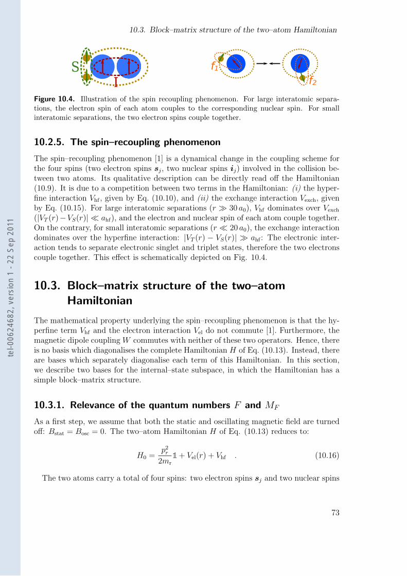
10.3. Block–matrix structure of the two–atom Hamiltonian

SI

Figure 10.4. Illustration of the spin recoupling phenomenon. For large interatomic separa-tions, the electron spin of each atom couples to the corresponding nuclear spin. For smallinteratomic separations, the two electron spins couple together.

10.2.5. The spin–recoupling phenomenon

The spin–recoupling phenomenon [1] is a dynamical change in the coupling scheme forthe four spins (two electron spins sj, two nuclear spins ij) involved in the collision be-tween two atoms. Its qualitative description can be directly read off the Hamiltonian(10.9). It is due to a competition between two terms in the Hamiltonian: (i) the hyper-fine interaction Vhf , given by Eq. (10.10), and (ii) the exchange interaction Vexch, givenby Eq. (10.15). For large interatomic separations (r 30 a0), Vhf dominates over Vexch

(|VT (r)−VS(r)| ahf), and the electron and nuclear spin of each atom couple together.On the contrary, for small interatomic separations (r 20 a0), the exchange interactiondominates over the hyperfine interaction: |VT (r) − VS(r)| ahf : The electronic inter-action tends to separate electronic singlet and triplet states, therefore the two electronscouple together. This effect is schematically depicted on Fig. 10.4.

10.3. Block–matrix structure of the two–atomHamiltonian

The mathematical property underlying the spin–recoupling phenomenon is that the hy-perfine term Vhf and the electron interaction Vel do not commute [1]. Furthermore, themagnetic dipole coupling W commutes with neither of these two operators. Hence, thereis no basis which diagonalises the complete Hamiltonian H of Eq. (10.13). Instead, thereare bases which separately diagonalise each term of this Hamiltonian. In this section,we describe two bases for the internal–state subspace, in which the Hamiltonian has asimple block–matrix structure.

10.3.1. Relevance of the quantum numbers F and MF

As a first step, we assume that both the static and oscillating magnetic field are turnedoff: Bstat = Bosc = 0. The two–atom Hamiltonian H of Eq. (10.13) reduces to:

H0 =p2r

2mr

1 + Vel(r) + Vhf . (10.16)

The two atoms carry a total of four spins: two electron spins sj and two nuclear spins

73

tel-0

0624

682,

ver

sion

1 -

22 S

ep 2

011

10. The Two–Atom Hamiltonian

ij. The addition of these four spins yields the total two–atom spin F :

F = s1 + i1 + s2 + i2 . (10.17)

The Hamiltonian H0 commutes with the total spin F 2 and its projection Fz along thequantisation axis ez:

• The kinetic energy term is rotationally invariant.

• The single–atom spins sj and ij are vector operators4, and the scalar productssj · ij are thus scalar operators, hence they commute with F 2 and Fz. Therefore,so does Vhf .

• The electron interaction can be rewritten as [37]:

Vel(r) =

(1

4VS(r) +

3

4VT (r)

)+ (VT (r)− VS(r))

s1 · s2

~2. (10.18)

The operator s1 · s2 is a scalar operator, and VS(r) and VT (r) depend only on r,therefore Vel is rotationally invariant.

It is therefore relevant to use internal–state basis vectors which have well–defined quan-tum number F and MF , which characterise the modulus of F and its projection Fz,respectively.

In the presence of static and oscillating magnetic fields, the quantum numbers F andMF are no longer conserved. However, we show below that the Hamiltonian H doeshave a simple block–matrix structure in bases involving these quantum numbers.

10.3.2. Two bases for two spin–coupling modes

We focus on the subspace characterised by given values of the quantum numbers F andMF . There are two distinct bases5 spanning this subspace, corresponding to the twocoupling modes represented on Fig. 10.4:

1. The two electron spins couple together (S = s1 + s2) and the two nuclear spinscouple together (I = i1 + i2), then F results from the addition of S and I. Thiscoupling mode results in the ‘molecular’ basis :

eM = (|S, I, F,MF 〉) , (10.19)

and corresponds to the left–hand part of Fig. 10.4.

2. The two spins on each atom couple together (fj = sj + ij), then F results fromthe addition of f1 and f2. This coupling mode results in the ‘atomic’ basis :

eA = (| f1, f2εf , F,MF 〉) , (10.20)

and corresponds to the right–hand part of Fig. 10.4.

4Each of these four operators V satisfies the characteristic commutation relations [Fi, Vj ] =i∑k εijk Vk, where εijk is the antisymmetric unit tensor.

5For a given (F,MF ) subspace, the ‘frame transformation’ linking the basis states in eA to those ineM is conveniently expressed in terms of Wigner 9j coefficients.

74

tel-0

0624

682,

ver

sion

1 -

22 S

ep 2

011

10.3. Block–matrix structure of the two–atom Hamiltonian

Consequences of bosonic symmetry The basis states in eM and eA are all eithersymmetric or antisymmetric under the exchange of the two atoms. In order to enforcebosonic symmetry, the ‘molecular’ basis eM only contains states with (S + I) even. Inthe case of the ‘atomic’ basis eA, the (anti–)symmetric two–atom states of Eq. (10.20)are defined by:

| f1, f2εf , F,MF 〉 =1√

2(1 + δf1,f2)(| f1, f2, F,MF 〉+ εf | f2, f1, F,MF 〉) . (10.21)

Bosonic symmetry requires that eA only contain states such that εf = (−1)f1+f2−F .

10.3.3. Analysis of the subspaces characterised by (F,MF )

Let us consider an internal–state subspace characterised by given quantum numbers(F,MF ). The addition rules for angular momenta and the symmetry properties describedin Section 10.3.2 constrain the dimension and electron–spin properties of this subspace.

If F is odd (F = 2i, 2i− 2, . . ., or 1):The (F,MF ) subspace has dimension 1. It is spanned by the single internal–state vector| f+, f−+, F,MF 〉 = |S = 1, I = F, F,MF 〉, which is electronic–triplet.

If F is even (F = 2i+ 1, 2i− 1, . . ., or 0):The (F,MF ) subspace has dimension 3. It is spanned by three ‘atomic’ basis states:| f+, f+, F,MF 〉, | f+, f−−, F,MF 〉, and | f−, f−, F,MF 〉,or, equivalently, by three ‘molecular’ basis states:|S = 1, I = F + 1, F,MF 〉, |S = 0, I = F, F,MF 〉, and |S = 1, I = F − 1, F,MF 〉.It has no well–defined total electronic spin S.

The (F even ,MF ) block is affected by a finite–size effect for F = 2i+ 1. In this case,the first two ‘molecular–basis’ states do not exist: the (F = 2i + 1,MF ) subspace hasdimension 1 and is electronic–triplet.

Other finite–size effects affect other (F even ,MF ) blocks, but for simplicity’s sake weshall not describe them here6.

10.3.4. Ordering of the basis states in eA and eM

Bringing together the ‘molecular’ basis states spanning the (F,MF ) subspaces as de-scribed above, we obtain the complete ‘molecular’ basis eM, which spans all internalstates accessible to the atom pair. We order these basis states by values of MF , decreas-ing from MF = 2i + 1 to MF = −(2i + 1). Within each subspace characterised by agiven value of MF , we order the states as shown in Table 10.1:

6However, they are accounted for in all of our results.

75

tel-0

0624

682,

ver

sion

1 -

22 S

ep 2

011

10. The Two–Atom Hamiltonian

• we sort the states by decreasing values of F , from F = 2i+ 1 to |MF |;

• Within each (F,MF ) subspace that is not one–dimensional, we sort them by de-creasing values of I.

Similarly, we construct the complete ‘atomic’ basis eA by collecting the basis statesfor all (F,MF ) subspaces. We order them by decreasing values of MF ; within a givenMF subspace, we order them as shown in Table 10.2:

• We sort the states by decreasing values of F .

• Within each (F,MF ) subspace that is not one–dimensional, we sort them by de-creasing values of (f1 + f2).

10.3.5. Block–matrix structure in the ‘molecular’ basis eM

Restriction of the Hamiltonian to a stable (MF +N) subspace

The operators Vel, Vhf and VZ all commute with Fz, and do not act on the photon number.The photon energy term ~ω a†a commutes with the photon number operator a†a, anddoes not act on the atomic spins. In the case of a σ+–polarised oscillating magnetic fieldBosc, the coupling term W σ+

commutes neither with Fz nor with a†a. However, a directcalculation yields [

W σ+

,Fz~

+ a†a

]= 0 , (10.22)

which can be seen as a consequence of the conservation of angular momentum for thesystem “two atoms in the presence of the magnetic field”. Therefore, for a given value ofN0, the subspace spanned by all states |S, I, F,MF , N 〉, where N is the photon numberand MF + N = N0, is stable under H. We choose N0 1, its exact value beingarbitrary: the physically meaningful parameter is the average magnetic field amplitudeBosc = b0

√N0, where b0 has been introduced in Eq. (10.4).

We write H = p2r2mr

+ Vtot(r), where the total matrix potential Vtot(r) reads:

Vtot(r) = Vel(r) + Vhf + VZ + ~ω a†a+W . (10.23)

We are interested in a matrix representation of the restriction of Vtot(r) to the stablesubspace described above.

We find that this matrix has a simple ‘block’ structure in the ‘molecular’ basis eM

described in Section 10.3.4. This block structure is represented on Fig. 10.5. The nextfew paragraphs focus on its derivation.

76

tel-0

0624

682,

ver

sion

1 -

22 S

ep 2

011

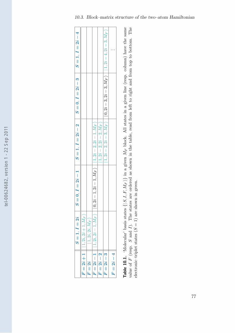
10.3. Block–matrix structure of the two–atom Hamiltonian

S=

1,I=

2i

S=

0,I=

2i−

1S

=1

,I=

2i−

2S

=0

,I=

2i−

3S

=1

,I=

2i−

4

F=

2i+

1|1,2i,

2i+

1,M

F〉

F=

2i

|1,2i,

2i,MF〉

F=

2i−

1|1,2i,

2i−

1,MF〉|0,2i−

1,2i−

1,M

F〉|1,2i−

2,2i−

1,M

F〉

F=

2i−

2|1,2i−

2,2i−

2,M

F〉

F=

2i−

3|1,2i−

2,2i−

3,M

F〉|0,2i−

3,2i−

3,MF〉|1,2i−

4,2i−

3,MF〉

F=

2i−

4. . .

Ta

ble

10

.1.

‘Mol

ecu

lar’

basi

sst

ates|S,I,F,M

F〉

ina

give

nMF

blo

ck.

All

stat

esin

agi

ven

lin

e(r

esp

.co

lum

n)

hav

eth

esa

me

valu

eofF

(res

p.S

an

dI).

Th

est

ates

are

ord

ered

assh

own

inth

eta

ble

,re

adfr

om

left

tori

ght

and

from

top

tob

otto

m.

Th

eel

ectr

onic

–tri

ple

tst

ate

s(S

=1)

are

show

nin

gree

n.

77

tel-0

0624

682,

ver

sion

1 -

22 S

ep 2

011

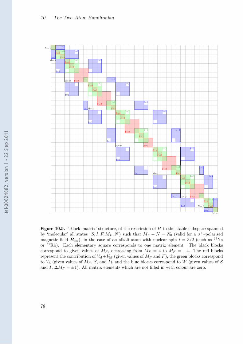
10. The Two–Atom Hamiltonian

M= 4

M= 3

M= 2

M= 1

M= 0

M=-1

M=-2

M=-3

M=-4

F=4

F=3

F=4

F=3

F=2

F=4

F=3

F=2

F=1

F=4

F=3

F=2

F=1

F=0

F=4

F=3

F=2

F=1

F=4

F=3

F=2

F=4

F=3

I=3

I=3

I=1

I=3

I=1

I=3

I=1

I=3

I=1

I=3

I=1

I=3

I=3

I=3

I=3

I=1

I=3

I=1

I=3

I=1

I=3

I=1

I=3

I=3

I=3

I=3

I=3

I=1

I=3

I=1

I=3

I=1

I=3

I=1

I=3

I=3

Figure 10.5. ‘Block–matrix’ structure, of the restriction of H to the stable subspace spannedby ‘molecular’ all states |S, I, F,MF , N 〉 such that MF + N = N0 (valid for a σ+–polarisedmagnetic field Bosc), in the case of an alkali atom with nuclear spin i = 3/2 (such as 23Naor 87Rb). Each elementary square corresponds to one matrix element. The black blockscorrespond to given values of MF , decreasing from MF = 4 to MF = −4. The red blocksrepresent the contribution of Vel +Vhf (given values of MF and F ), the green blocks correspondto VZ (given values of MF , S, and I), and the blue blocks correspond to W (given values of Sand I, ∆MF = ±1). All matrix elements which are not filled in with colour are zero.

78

tel-0

0624

682,

ver

sion

1 -

22 S

ep 2

011

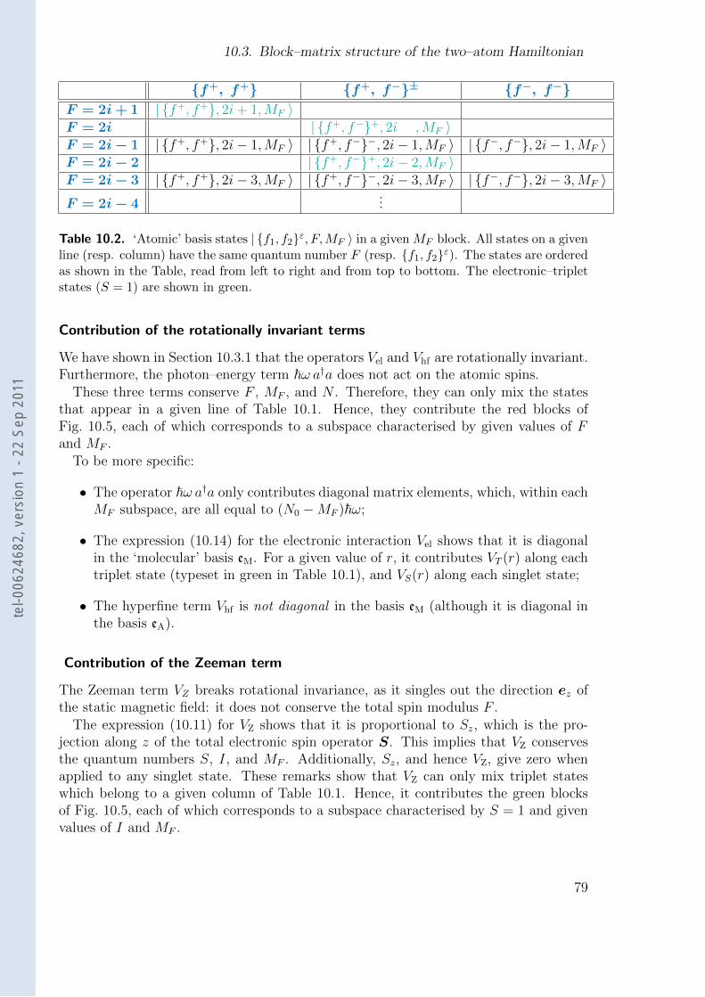
10.3. Block–matrix structure of the two–atom Hamiltonian

f+, f+ f+, f−± f−, f−F = 2i+ 1 | f+, f+, 2i+ 1,MF 〉F = 2i | f+, f−+, 2i ,MF 〉F = 2i− 1 | f+, f+, 2i− 1,MF 〉 | f+, f−−, 2i− 1,MF 〉 | f−, f−, 2i− 1,MF 〉F = 2i− 2 | f+, f−+, 2i− 2,MF 〉F = 2i− 3 | f+, f+, 2i− 3,MF 〉 | f+, f−−, 2i− 3,MF 〉 | f−, f−, 2i− 3,MF 〉F = 2i− 4

...

Table 10.2. ‘Atomic’ basis states | f1, f2ε, F,MF 〉 in a given MF block. All states on a givenline (resp. column) have the same quantum number F (resp. f1, f2ε). The states are orderedas shown in the Table, read from left to right and from top to bottom. The electronic–tripletstates (S = 1) are shown in green.

Contribution of the rotationally invariant terms

We have shown in Section 10.3.1 that the operators Vel and Vhf are rotationally invariant.Furthermore, the photon–energy term ~ω a†a does not act on the atomic spins.

These three terms conserve F , MF , and N . Therefore, they can only mix the statesthat appear in a given line of Table 10.1. Hence, they contribute the red blocks ofFig. 10.5, each of which corresponds to a subspace characterised by given values of Fand MF .

To be more specific:

• The operator ~ω a†a only contributes diagonal matrix elements, which, within eachMF subspace, are all equal to (N0 −MF )~ω;

• The expression (10.14) for the electronic interaction Vel shows that it is diagonalin the ‘molecular’ basis eM. For a given value of r, it contributes VT (r) along eachtriplet state (typeset in green in Table 10.1), and VS(r) along each singlet state;

• The hyperfine term Vhf is not diagonal in the basis eM (although it is diagonal inthe basis eA).

Contribution of the Zeeman term

The Zeeman term VZ breaks rotational invariance, as it singles out the direction ez ofthe static magnetic field: it does not conserve the total spin modulus F .

The expression (10.11) for VZ shows that it is proportional to Sz, which is the pro-jection along z of the total electronic spin operator S. This implies that VZ conservesthe quantum numbers S, I, and MF . Additionally, Sz, and hence VZ, give zero whenapplied to any singlet state. These remarks show that VZ can only mix triplet stateswhich belong to a given column of Table 10.1. Hence, it contributes the green blocksof Fig. 10.5, each of which corresponds to a subspace characterised by S = 1 and givenvalues of I and MF .

79

tel-0

0624

682,

ver

sion

1 -

22 S

ep 2

011

10. The Two–Atom Hamiltonian

Furthermore, S is a vector operator, therefore VZ obeys the vector selection rule [37]on the quantum number F : it can have non–zero matrix elements only in betweenstates whose quantum numbers F1 and F2 satisfy |F1−F2| ≤ 1. The green–block matrixelements which do not satisfy this criterion are zero, and are shown in white on Fig.10.5.

Contribution of the magnetic dipole coupling term

The magnetic dipole coupling term W does not conserve F , MF , or N .As pointed out in Section 10.3.5, W conserves the sum (MF +N). Furthermore, it is

a sum of two terms which involve S+ and S− (see Eq. (10.12). Hence, it conserves thequantum numbers S and I, and it gives zero when acting on any singlet state.

The operators S± have non–zero matrix elements only in between states whose quan-tum numbers MF1 and MF2 satisfy |MF1 −MF2| = 1. Therefore, W connects a giventriplet column of Table 10.1, belonging to a subspace with given MF , to the correspond-ing column of Table 10.1 in the subspaces having the total spin projections MF + 1 andMF − 1. It contributes the blue blocks on Fig. 10.5.

Finally, the S± are the ladder operators for the vector operator S, therefore W obeysthe vector selection rule on F . The blue–block matrix elements which do not satisfy thiscriterion are zero, and are shown in white on Fig. 10.5.

80

tel-0

0624

682,

ver

sion

1 -

22 S

ep 2

011

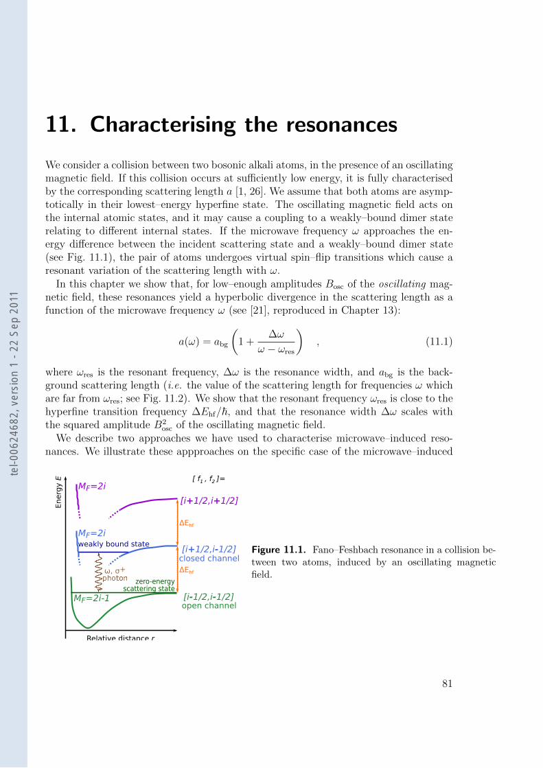
11. Characterising the resonances

We consider a collision between two bosonic alkali atoms, in the presence of an oscillatingmagnetic field. If this collision occurs at sufficiently low energy, it is fully characterisedby the corresponding scattering length a [1, 26]. We assume that both atoms are asymp-totically in their lowest–energy hyperfine state. The oscillating magnetic field acts onthe internal atomic states, and it may cause a coupling to a weakly–bound dimer staterelating to different internal states. If the microwave frequency ω approaches the en-ergy difference between the incident scattering state and a weakly–bound dimer state(see Fig. 11.1), the pair of atoms undergoes virtual spin–flip transitions which cause aresonant variation of the scattering length with ω.

In this chapter we show that, for low–enough amplitudes Bosc of the oscillating mag-netic field, these resonances yield a hyperbolic divergence in the scattering length as afunction of the microwave frequency ω (see [21], reproduced in Chapter 13):

a(ω) = abg

(1 +

∆ω

ω − ωres

), (11.1)

where ωres is the resonant frequency, ∆ω is the resonance width, and abg is the back-ground scattering length (i.e. the value of the scattering length for frequencies ω whichare far from ωres; see Fig. 11.2). We show that the resonant frequency ωres is close to thehyperfine transition frequency ∆Ehf/~, and that the resonance width ∆ω scales withthe squared amplitude B2

osc of the oscillating magnetic field.We describe two approaches we have used to characterise microwave–induced reso-

nances. We illustrate these appproaches on the specific case of the microwave–induced

Relative distance r

Energ

y E

[i-1/2,i-1/2]open channel

[i+1/2,i-1/2]closed channel

zero-energyscattering state

weakly bound state

ω, σ+ ΔEhf

[i+1/2,i+1/2]

ΔEhf

MF=2i-1

MF=2i

MF=2i[ f1 , f2 ]=

Figure 11.1. Fano–Feshbach resonance in a collision be-tween two atoms, induced by an oscillating magneticfield.

81

tel-0

0624

682,

ver

sion

1 -

22 S

ep 2

011

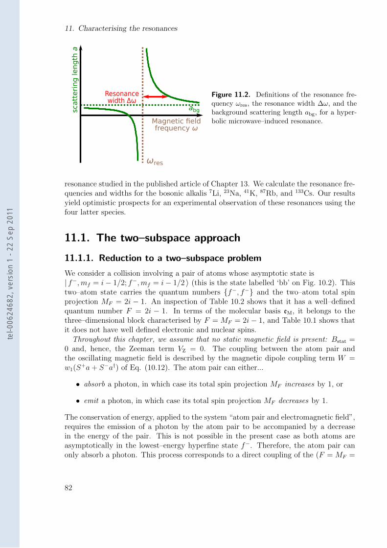
11. Characterising the resonances

ωres

abg

Magnetic fieldfrequency ω

scatt

eri

ng

len

gth

a

Resonancewidth Δω

Figure 11.2. Definitions of the resonance fre-quency ωres, the resonance width ∆ω, and thebackground scattering length abg, for a hyper-bolic microwave–induced resonance.

resonance studied in the published article of Chapter 13. We calculate the resonance fre-quencies and widths for the bosonic alkalis 7Li, 23Na, 41K, 87Rb, and 133Cs. Our resultsyield optimistic prospects for an experimental observation of these resonances using thefour latter species.

11.1. The two–subspace approach

11.1.1. Reduction to a two–subspace problem

We consider a collision involving a pair of atoms whose asymptotic state is| f−,mf = i− 1/2; f−,mf = i− 1/2 〉 (this is the state labelled ‘bb’ on Fig. 10.2). Thistwo–atom state carries the quantum numbers f−, f− and the two–atom total spinprojection MF = 2i − 1. An inspection of Table 10.2 shows that it has a well–definedquantum number F = 2i − 1. In terms of the molecular basis eM, it belongs to thethree–dimensional block characterised by F = MF = 2i− 1, and Table 10.1 shows thatit does not have well defined electronic and nuclear spins.

Throughout this chapter, we assume that no static magnetic field is present: Bstat =0 and, hence, the Zeeman term VZ = 0. The coupling between the atom pair andthe oscillating magnetic field is described by the magnetic dipole coupling term W =w1(S+a+ S−a†) of Eq. (10.12). The atom pair can either...

• absorb a photon, in which case its total spin projection MF increases by 1, or

• emit a photon, in which case its total spin projection MF decreases by 1.

The conservation of energy, applied to the system “atom pair and electromagnetic field”,requires the emission of a photon by the atom pair to be accompanied by a decreasein the energy of the pair. This is not possible in the present case as both atoms areasymptotically in the lowest–energy hyperfine state f−. Therefore, the atom pair canonly absorb a photon. This process corresponds to a direct coupling of the (F = MF =

82

tel-0

0624

682,

ver

sion

1 -

22 S

ep 2

011

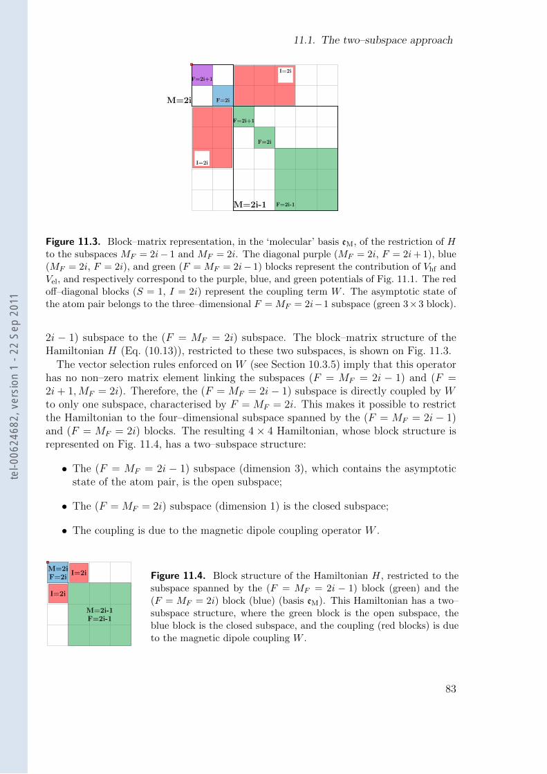
11.1. The two–subspace approach

M=2i

M=2i-1

F=2i+1

F=2i

F=2i+1

F=2i

F=2i-1

I=2i

I=2i

Figure 11.3. Block–matrix representation, in the ‘molecular’ basis eM, of the restriction of Hto the subspaces MF = 2i− 1 and MF = 2i. The diagonal purple (MF = 2i, F = 2i+ 1), blue(MF = 2i, F = 2i), and green (F = MF = 2i− 1) blocks represent the contribution of Vhf andVel, and respectively correspond to the purple, blue, and green potentials of Fig. 11.1. The redoff–diagonal blocks (S = 1, I = 2i) represent the coupling term W . The asymptotic state ofthe atom pair belongs to the three–dimensional F = MF = 2i−1 subspace (green 3×3 block).

2i − 1) subspace to the (F = MF = 2i) subspace. The block–matrix structure of theHamiltonian H (Eq. (10.13)), restricted to these two subspaces, is shown on Fig. 11.3.

The vector selection rules enforced on W (see Section 10.3.5) imply that this operatorhas no non–zero matrix element linking the subspaces (F = MF = 2i − 1) and (F =2i+ 1,MF = 2i). Therefore, the (F = MF = 2i− 1) subspace is directly coupled by Wto only one subspace, characterised by F = MF = 2i. This makes it possible to restrictthe Hamiltonian to the four–dimensional subspace spanned by the (F = MF = 2i − 1)and (F = MF = 2i) blocks. The resulting 4 × 4 Hamiltonian, whose block structure isrepresented on Fig. 11.4, has a two–subspace structure:

• The (F = MF = 2i − 1) subspace (dimension 3), which contains the asymptoticstate of the atom pair, is the open subspace;

• The (F = MF = 2i) subspace (dimension 1) is the closed subspace;

• The coupling is due to the magnetic dipole coupling operator W .

M=2iF=2i

M=2i-1F=2i-1

I=2i

I=2i Figure 11.4. Block structure of the Hamiltonian H, restricted to thesubspace spanned by the (F = MF = 2i − 1) block (green) and the(F = MF = 2i) block (blue) (basis eM). This Hamiltonian has a two–subspace structure, where the green block is the open subspace, theblue block is the closed subspace, and the coupling (red blocks) is dueto the magnetic dipole coupling W .

83

tel-0

0624

682,

ver

sion

1 -

22 S

ep 2

011

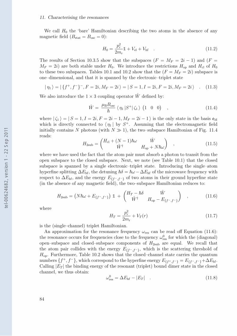
11. Characterising the resonances

We call H0 the ‘bare’ Hamiltonian describing the two atoms in the absence of anymagnetic field (Bstat = Bosc = 0):

H0 =p2r

2mr

1 + Vel + Vhf . (11.2)

The results of Section 10.3.5 show that the subspaces (F = MF = 2i − 1) and (F =MF = 2i) are both stable under H0. We introduce the restrictions Hop and Hcl of H0

to these two subspaces. Tables 10.1 and 10.2 show that the (F = MF = 2i) subspace isone–dimensional, and that it is spanned by the electronic–triplet state

| η1 〉 = | f+, f−−, F = 2i,MF = 2i 〉 = |S = 1, I = 2i, F = 2i,MF = 2i 〉 . (11.3)

We also introduce the 1× 3 coupling operator W defined by:

W =µBBosc

~〈 η1 |S+| ζ1 〉

(1 0 0

), (11.4)

where | ζ1 〉 = |S = 1, I = 2i, F = 2i− 1,MF = 2i− 1 〉 is the only state in the basis eM

which is directly connected to 〈 η1 | by S+. Assuming that the electromagnetic fieldinitially contains N photons (with N 1), the two–subspace Hamiltonian of Fig. 11.4reads:

H2sub =

(Hcl + (N − 1)~ω W

W † Hop +N~ω

), (11.5)

where we have used the fact that the atom pair must absorb a photon to transit from theopen subspace to the closed subspace. Next, we note (see Table 10.1) that the closedsubspace is spanned by a single electronic–triplet state. Introducing the single–atomhyperfine splitting ∆Ehf , the detuning ~δ = ~ω−∆Ehf of the microwave frequency withrespect to ∆Ehf , and the energy Ef−,f− of two atoms in their ground hyperfine state(in the absence of any magnetic field), the two–subspace Hamiltonian reduces to:

H2sub =(N~ω + Ef−,f−

)1 +

(HT − ~δ W

W † Hop − Ef−,f−

), (11.6)

where

HT =p2r

2mr

+ VT (r) (11.7)

is the (single–channel) triplet Hamiltonian.An approximation for the resonance frequency ωres can be read off Equation (11.6):

the resonance occurs for frequencies close to the frequency ω0res for which the (diagonal)

open–subspace and closed–subspace components of H2sub are equal. We recall thatthe atom pair collides with the energy Ef−,f−, which is the scattering threshold ofHop. Furthermore, Table 10.2 shows that the closed–channel state carries the quantumnumbers f+, f−, which correspond to the hyperfine energy Ef+,f− = Ef−,f−+∆Ehf .Calling |ET | the binding energy of the resonant (triplet) bound dimer state in the closedchannel, we thus obtain:

ω0res = ∆Ehf − |ET | . (11.8)

84

tel-0

0624

682,

ver

sion

1 -

22 S

ep 2

011

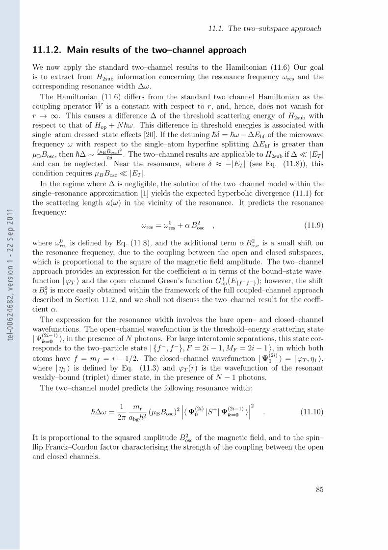
11.1. The two–subspace approach

11.1.2. Main results of the two–channel approach

We now apply the standard two–channel results to the Hamiltonian (11.6) Our goalis to extract from H2sub information concerning the resonance frequency ωres and thecorresponding resonance width ∆ω.

The Hamiltonian (11.6) differs from the standard two–channel Hamiltonian as thecoupling operator W is a constant with respect to r, and, hence, does not vanish forr → ∞. This causes a difference ∆ of the threshold scattering energy of H2sub withrespect to that of Hop + N~ω. This difference in threshold energies is associated withsingle–atom dressed–state effects [20]. If the detuning ~δ = ~ω−∆Ehf of the microwavefrequency ω with respect to the single–atom hyperfine splitting ∆Ehf is greater than

µBBosc, then ~∆ ∼ (µBBosc)2

~δ . The two–channel results are applicable to H2sub if ∆ |ET |and can be neglected. Near the resonance, where δ ≈ −|ET | (see Eq. (11.8)), thiscondition requires µBBosc |ET |.

In the regime where ∆ is negligible, the solution of the two–channel model within thesingle–resonance approximation [1] yields the expected hyperbolic divergence (11.1) forthe scattering length a(ω) in the vicinity of the resonance. It predicts the resonancefrequency:

ωres = ω0res + αB2

osc , (11.9)

where ω0res is defined by Eq. (11.8), and the additional term αB2

osc is a small shift onthe resonance frequency, due to the coupling between the open and closed subspaces,which is proportional to the square of the magnetic field amplitude. The two–channelapproach provides an expression for the coefficient α in terms of the bound–state wave-function |ϕT 〉 and the open–channel Green’s function G+

op(Ef−f−); however, the shiftαB2

0 is more easily obtained within the framework of the full coupled–channel approachdescribed in Section 11.2, and we shall not discuss the two–channel result for the coeffi-cient α.

The expression for the resonance width involves the bare open– and closed–channelwavefunctions. The open–channel wavefunction is the threshold–energy scattering state|Ψ(2i−1)

k=0 〉, in the presence of N photons. For large interatomic separations, this state cor-responds to the two–particle state | f−, f−, F = 2i− 1,MF = 2i− 1 〉, in which both

atoms have f = mf = i − 1/2. The closed–channel wavefunction |Ψ(2i)0 〉 = |ϕT , η1 〉,

where | η1 〉 is defined by Eq. (11.3) and ϕT (r) is the wavefunction of the resonantweakly–bound (triplet) dimer state, in the presence of N − 1 photons.

The two–channel model predicts the following resonance width:

~∆ω =1

2π

mr

abg~2(µBBosc)

2∣∣∣〈Ψ(2i)

0 |S+|Ψ(2i−1)k=0 〉

∣∣∣2 . (11.10)

It is proportional to the squared amplitude B2osc of the magnetic field, and to the spin–

flip Franck–Condon factor characterising the strength of the coupling between the openand closed channels.

85

tel-0

0624

682,

ver

sion

1 -

22 S

ep 2

011

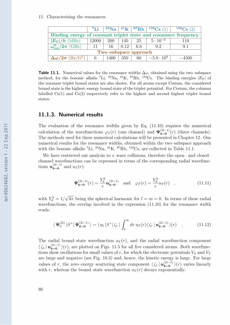
11. Characterising the resonances

7Li 23Na 41K 87Rb 133Cs (1) 133Cs (2)Binding energy of resonant triplet state and resonance frequency|ET |/h (MHz) 12000 200 140 25 5 · 10−3 110ω0

res/2π (GHz) 11 16 0.12 6.8 9.2 9.1Two–subspace approach

∆ω/2π (Hz/G2) 6 1400 350 60 −5.8 · 109 −4500

Table 11.1. Numerical values for the resonance widths ∆ω, obtained using the two–subspacemethod, for the bosonic alkalis 7Li, 23Na, 41K, 87Rb, 133Cs. The binding energies |ET | ofthe resonant triplet bound states are also shown. For all atoms except Cesium, the consideredbound state is the highest–energy bound state of the triplet potential. For Cesium, the columnslabelled Cs(1) and Cs(2) respectively refer to the highest and second–highest triplet boundstates.

11.1.3. Numerical results

The evaluation of the resonance widths given by Eq. (11.10) requires the numerical

calculation of the wavefunctions ϕT (r) (one channel) and Ψ(2i−1)k=0 (r) (three channels).

The methods used for these numerical calculations will be presented in Chapter 12. Ournumerical results for the resonance widths, obtained within the two–subspace approachwith the bosonic alkalis 7Li, 23Na, 41K, 87Rb, 133Cs, are collected in Table 11.1.

We have restricted our analysis to s–wave collisions, therefore the open– and closed–channel wavefunctions can be expressed in terms of the corresponding radial wavefunc-tions u

(2i−1)k=0 and uT (r):

Ψ(2i−1)k=0 (r) =

Y 00

ru

(2i−1)k=0 and ϕT (r) =

Y 00

ruT (r) , (11.11)

with Y 00 = 1/

√4π being the spherical harmonic for l = m = 0. In terms of these radial

wavefunctions, the overlap involved in the expression (11.10) for the resonance widthreads:

〈Ψ(2i)0 |S+|Ψ(2i−1)

k=0 〉 = 〈 η1 |S+| ζ1 〉∫ ∞

0

dr uT (r)〈 ζ1 |u(2i−1)k=0 〉(r) . (11.12)

The radial bound–state wavefunction uT (r), and the radial wavefunction component

〈 ζ1 |u(2i−1)k=0 〉(r), are plotted on Figs. 11.5 for all five considered atoms. Both wavefunc-

tions show oscillations for small values of r, for which the electronic potentials VS and VTare large and negative (see Fig. 10.3) and, hence, the kinetic energy is large. For large

values of r, the zero–energy scattering state component 〈 ζ1 |u(2i−1)k=0 〉(r) varies linearly

with r, whereas the bound–state wavefunction uT (r) decays exponentially.

86

tel-0

0624

682,

ver

sion

1 -

22 S

ep 2

011

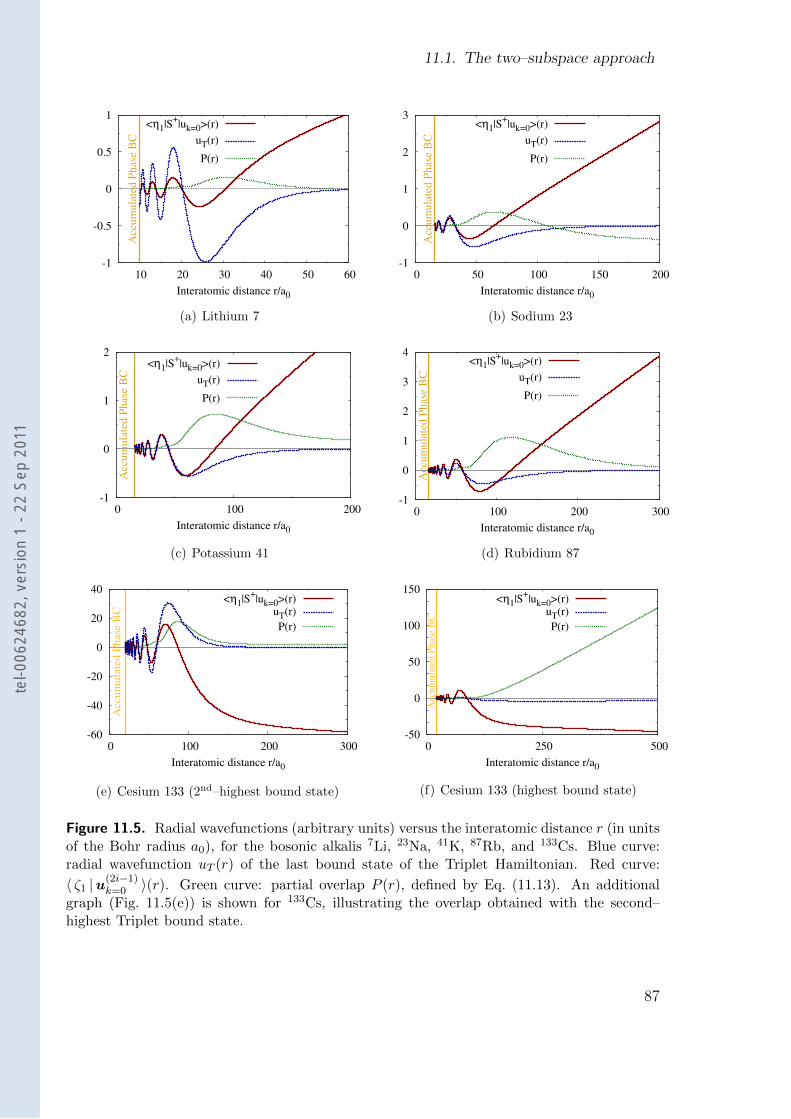
11.1. The two–subspace approach

-1

-0.5

0

0.5

1

10 20 30 40 50 60

Interatomic distance r/a0

Accum

ula

ted P

hase

BC

<η1|S+|uk=0>(r)

uT(r)

P(r)

(a) Lithium 7

-1

0

1

2

3

0 50 100 150 200

Interatomic distance r/a0

Accum

ula

ted P

hase

BC

<η1|S+|uk=0>(r)

uT(r)

P(r)

(b) Sodium 23

-1

0

1

2

0 100 200

Interatomic distance r/a0

Accum

ula

ted P

hase

BC

<η1|S+|uk=0>(r)

uT(r)

P(r)

(c) Potassium 41

-1

0

1

2

3

4

0 100 200 300

Interatomic distance r/a0

Accum

ula

ted P

hase

BC

<η1|S+|uk=0>(r)

uT(r)

P(r)

(d) Rubidium 87

-60

-40

-20

0

20

40

0 100 200 300

Interatomic distance r/a0

Accum

ula

ted P

hase

BC

<η1|S+|uk=0>(r)

uT(r)

P(r)

(e) Cesium 133 (2nd–highest bound state)

-50

0

50

100

150

0 250 500

Interatomic distance r/a0

Accu

mu

late

d P

hase

BC

<η1|S+|uk=0>(r)

uT(r)

P(r)

(f) Cesium 133 (highest bound state)

Figure 11.5. Radial wavefunctions (arbitrary units) versus the interatomic distance r (in unitsof the Bohr radius a0), for the bosonic alkalis 7Li, 23Na, 41K, 87Rb, and 133Cs. Blue curve:radial wavefunction uT (r) of the last bound state of the Triplet Hamiltonian. Red curve:

〈 ζ1 |u(2i−1)k=0 〉(r). Green curve: partial overlap P (r), defined by Eq. (11.13). An additional

graph (Fig. 11.5(e)) is shown for 133Cs, illustrating the overlap obtained with the second–highest Triplet bound state.

87

tel-0

0624

682,

ver

sion

1 -

22 S

ep 2

011

11. Characterising the resonances

Figures 11.5 also show the dependence on r of the ‘partial’ overlap P (r), defined by1

P (r) =

∫ r

r0

dρ uT (ρ)〈 ζ1 |u(2i−1)k=0 〉(ρ) , (11.13)

so that 〈Ψ(2i0 |S+|Ψ(2i−1

k=0 〉 = 〈 η1 |S+| ζ1 〉P (r → ∞). The plots of P (r) show that, forall considered cases except the resonance in 133Cs involving the highest triplet boundstate of (Fig. 11.5(f)), the contribution to the overlap of the small–r region (where thewavefunctions oscillate) and the large–r region (where the wavefunctions reach theirasymptotic behaviour) have opposite signs and comparable magnitudes: this leads to areduction of the total overlap and, hence, to smaller resonance widths than could havebeen expected by neglecting the large–r wavefunction ‘tails’.

The resonance in 133Cs involving the highest triplet bound state (see Fig. 11.5(f) andthe column labelled 133Cs(1) in Table 11.1) is particularly large. In this specific case, theresonant bound state is very weakly bound (|ET |/Evdw ≈ 2 · 10−3, where the van–der–Waals energy Evdw [24] is an energy scale associated with the large–r behaviour of theelectron potentials) and thus has a very large spatial extent, determined by the scatteringlength aT = 2500 a0: in this particular case, the large–r contribution dominates, whichleads to a very large resonance width compared to the results obtained with all otheratoms (see Table 11.1). However, the two–channel result for this giant resonance is onlyapplicable for magnetic fields which satisfy µBBosc . |ET | (i.e. Bosc . 4 mG), abovewhich dressed–state effects affect the shape of the resonance, as explained in Section11.2.

To our knowledge, no experimental measurement of the weakly–bound state in 133Cshas yet been published. The large value of the triplet scattering length (aT = 2500 a0)is a strong indication that it does exist (see Section 9.1.2). Furthermore, we interpretthe Feshbach resonances occurring in 133Cs for small static magnetic fields, analysed inChapter 14, as experimental evidence of its existence.

11.1.4. Narrow resonances for Lithium and Rubidium

The numerical results for the resonance widths, collected in Table 11.1, show thatmicrowave–induced Feshbach resonances are particularly narrow for 7Li (∆ω = 6 Hz/G2)and 87Rb (∆ω = 60 Hz/G2). The reasons behind such narrow resonances are differentfor the two atoms.

In the case of 7Li, the triplet scattering length aT , characterising collisions in theclosed channel, is negative: aT = −28 a0 [38]. Thinking along the lines of bound statesin a square–well potential (see Section 9.1.2), a negative scattering length is a goodindication that the highest bound state is deeply bound. Indeed, the binding energyof the last triplet bound state is |ET | = h · 12 GHz, whereas the corresponding binding

1 In Eq. (11.13), the lower bound r0 is the small non–zero value of r at which the accumulated–phaseboundary condition is applied: see Chapter 12. The contribution to the overlap of the 0 < r < r0

region is neglected in the two–subspace approach; it is taken into account in the coupled–channelapproach presented in Section 11.2.

88

tel-0

0624

682,

ver

sion

1 -

22 S

ep 2

011

11.2. The coupled–channel approach

energies for all other considered atoms are of the order of 100 MHz. The wavefunctionΨ

(2i)0 (r) of this deeply–bound state has a very small spatial extent, hence its overlap with

the open–channel wavefunction Ψ(2i−1)k=0 is also small. In accordance with Eq. (11.10),

this leads to a narrow resonance width.In the case of 87Rb, the narrowness of the resonance stems from the near–degeneracy

of the singlet and triplet scattering lengths: aS = 90 a0 and aT = 99 a0 [39] differby less than 10%. Therefore, the singlet and triplet Hamiltonians have very similarproperties as far as ultracold collisions are concerned. In particular, the scattering–statewavefunction Ψ

(2i−1)k=0 and the bound–state wavefunction Ψ

(2i)0 are almost eigenstates of

the same Hamiltonian, and are therefore almost orthogonal. This leads to a small overlapfor these two wavefunctions and, hence, to a narrow resonance width.

11.1.5. Limitations of the two–subspace approach

The two–subspace approach provides simple expressions for the resonance frequency(Eq. (11.9)) and width (Eq. (11.10)). It exhibits a simple scaling with B2

osc for both ofthese parameters.

However, this approach has one main limitation: it does not account for W not goingto zero for large values of r. The effect of such a ‘long–ranged’ coupling term can beneglected for small Bosc, but it affects the shape of the resonance for larger magneticfield amplitudes.

Furthermore, the two–subspace approach neglects a small contribution to the Franck–Condon factor of Eq. (11.10), coming from the small–r region (see footnote 1).

In the next section, we present a more elaborate approach which properly accountsfor W not vanishing for large interatomic separations, and which does not require thesmall–r part of the wavefunctions to be neglected. This new approach confirms our two–channel results for small values of Bosc. It also allows for a straightforward calculationof the shift αB2

osc. Finally, it enables us to explore the behaviour of the resonance in133Cs involving the highest triplet bound state for magnetic fields larger than 5 mG.

11.2. The coupled–channel approach

In this section, we give up the simple scaling laws obtained with the two–subspaceapproach of Section 11.1.1, in favour of a more accurate and more general coupled–channel approach. We assume, as in the previous section, that the magnetic field hasno static component: Bstat = 0 and VZ = 0.

11.2.1. Hamiltonian for the coupled–channel approach

Within the framework of the two–subspace method of Section 11.1, we were only in-terested in internal states which were connected to each other, by the magnetic dipolecoupling term W , via the absorption or emission of a single photon. However, the systemwe are considering actually contains two atoms, each of which can absorb a photon.

89

tel-0

0624

682,

ver

sion

1 -

22 S

ep 2

011

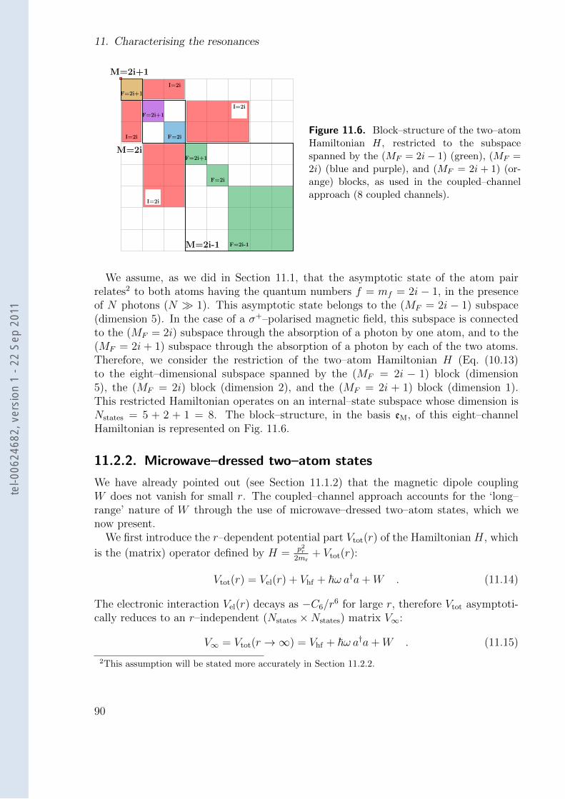
11. Characterising the resonances

M=2i+1

M=2i

M=2i-1

F=2i+1

F=2i+1

F=2i

F=2i+1

F=2i

F=2i-1

I=2i

I=2i

I=2i

I=2i

Figure 11.6. Block–structure of the two–atomHamiltonian H, restricted to the subspacespanned by the (MF = 2i− 1) (green), (MF =2i) (blue and purple), and (MF = 2i + 1) (or-ange) blocks, as used in the coupled–channelapproach (8 coupled channels).

We assume, as we did in Section 11.1, that the asymptotic state of the atom pairrelates2 to both atoms having the quantum numbers f = mf = 2i − 1, in the presenceof N photons (N 1). This asymptotic state belongs to the (MF = 2i − 1) subspace(dimension 5). In the case of a σ+–polarised magnetic field, this subspace is connectedto the (MF = 2i) subspace through the absorption of a photon by one atom, and to the(MF = 2i + 1) subspace through the absorption of a photon by each of the two atoms.Therefore, we consider the restriction of the two–atom Hamiltonian H (Eq. (10.13)to the eight–dimensional subspace spanned by the (MF = 2i − 1) block (dimension5), the (MF = 2i) block (dimension 2), and the (MF = 2i + 1) block (dimension 1).This restricted Hamiltonian operates on an internal–state subspace whose dimension isNstates = 5 + 2 + 1 = 8. The block–structure, in the basis eM, of this eight–channelHamiltonian is represented on Fig. 11.6.

11.2.2. Microwave–dressed two–atom states

We have already pointed out (see Section 11.1.2) that the magnetic dipole couplingW does not vanish for small r. The coupled–channel approach accounts for the ‘long–range’ nature of W through the use of microwave–dressed two–atom states, which wenow present.

We first introduce the r–dependent potential part Vtot(r) of the Hamiltonian H, which

is the (matrix) operator defined by H = p2r2mr

+ Vtot(r):

Vtot(r) = Vel(r) + Vhf + ~ω a†a+W . (11.14)

The electronic interaction Vel(r) decays as −C6/r6 for large r, therefore Vtot asymptoti-

cally reduces to an r–independent (Nstates ×Nstates) matrix V∞:

V∞ = Vtot(r →∞) = Vhf + ~ω a†a+W . (11.15)

2This assumption will be stated more accurately in Section 11.2.2.

90

tel-0

0624

682,

ver

sion

1 -

22 S

ep 2

011

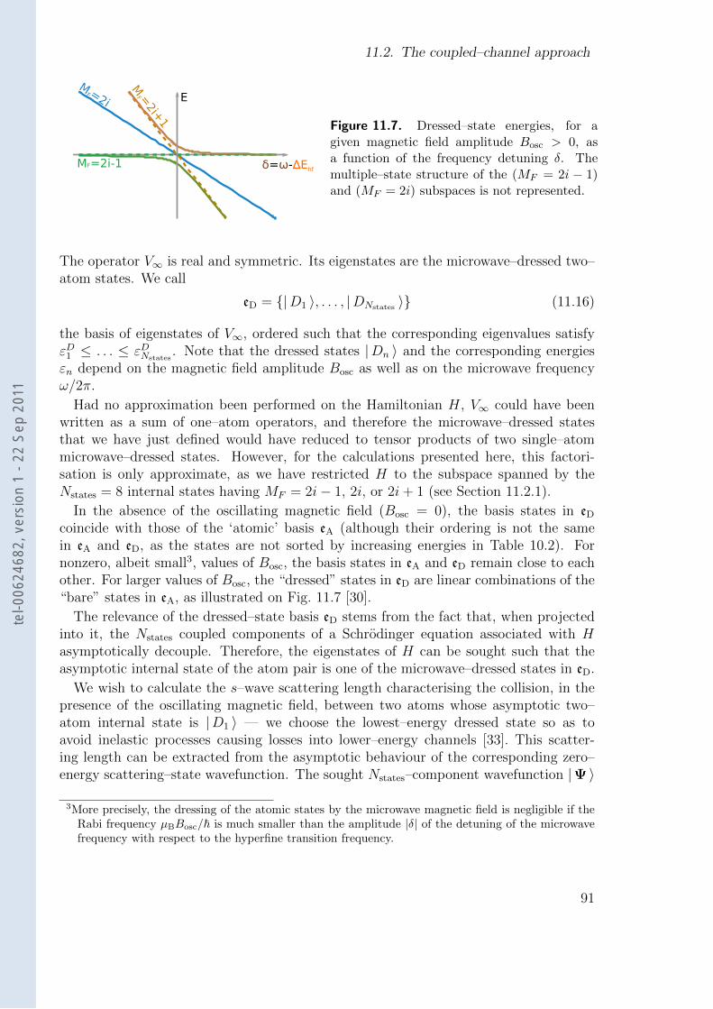
11.2. The coupled–channel approach

δ=ω-ΔEhf

E

MF=2i+

1

MF=2i

MF=2i-1

Figure 11.7. Dressed–state energies, for agiven magnetic field amplitude Bosc > 0, asa function of the frequency detuning δ. Themultiple–state structure of the (MF = 2i − 1)and (MF = 2i) subspaces is not represented.

The operator V∞ is real and symmetric. Its eigenstates are the microwave–dressed two–atom states. We call

eD = |D1 〉, . . . , |DNstates 〉 (11.16)

the basis of eigenstates of V∞, ordered such that the corresponding eigenvalues satisfyεD1 ≤ . . . ≤ εDNstates

. Note that the dressed states |Dn 〉 and the corresponding energiesεn depend on the magnetic field amplitude Bosc as well as on the microwave frequencyω/2π.

Had no approximation been performed on the Hamiltonian H, V∞ could have beenwritten as a sum of one–atom operators, and therefore the microwave–dressed statesthat we have just defined would have reduced to tensor products of two single–atommicrowave–dressed states. However, for the calculations presented here, this factori-sation is only approximate, as we have restricted H to the subspace spanned by theNstates = 8 internal states having MF = 2i− 1, 2i, or 2i+ 1 (see Section 11.2.1).

In the absence of the oscillating magnetic field (Bosc = 0), the basis states in eD

coincide with those of the ‘atomic’ basis eA (although their ordering is not the samein eA and eD, as the states are not sorted by increasing energies in Table 10.2). Fornonzero, albeit small3, values of Bosc, the basis states in eA and eD remain close to eachother. For larger values of Bosc, the “dressed” states in eD are linear combinations of the“bare” states in eA, as illustrated on Fig. 11.7 [30].

The relevance of the dressed–state basis eD stems from the fact that, when projectedinto it, the Nstates coupled components of a Schrodinger equation associated with Hasymptotically decouple. Therefore, the eigenstates of H can be sought such that theasymptotic internal state of the atom pair is one of the microwave–dressed states in eD.

We wish to calculate the s–wave scattering length characterising the collision, in thepresence of the oscillating magnetic field, between two atoms whose asymptotic two–atom internal state is |D1 〉 — we choose the lowest–energy dressed state so as toavoid inelastic processes causing losses into lower–energy channels [33]. This scatter-ing length can be extracted from the asymptotic behaviour of the corresponding zero–energy scattering–state wavefunction. The sought Nstates–component wavefunction |Ψ 〉

3More precisely, the dressing of the atomic states by the microwave magnetic field is negligible if theRabi frequency µBBosc/~ is much smaller than the amplitude |δ| of the detuning of the microwavefrequency with respect to the hyperfine transition frequency.

91

tel-0

0624

682,

ver

sion

1 -

22 S

ep 2

011

11. Characterising the resonances

satisfies both the stationary Schrodinger equation:

H|Ψ 〉 = εD1 |Ψ 〉 (11.17)

and the large–r boundary conditions [37]:

〈D1 |Ψ(r) 〉 =r − ar

(entrance channel) (11.18a)

〈Dp |Ψ(r) 〉 = Apexp(−κpr)

rfor 2 ≤ p ≤ Nstates (closed channels), (11.18b)

where ~κp = (2mr(εDN − εD1 ))1/2 for all closed channels p > 1. In other words, for large

interatomic separations r, the radial wavefunction reduces to the usual linear form (r−a)in the entrance channel (where, asymptotically, no kinetic energy is present) and decaysexponentially in all closed channels. In Eqs. (11.18), the real numbers Ap and the realscattering length a are initially unknown: their values are extracted from the asymptoticbehaviour of the wavefunction Ψ(r) after its numerical calculation.

In order to fully define the wavefunction |Ψ 〉, an additional condition must be speci-fied, which enforces that Ψ(r) be regular at r = 0 [25]:

limr→0

(rΨ(r)) = 0 . (11.19)

Technical difficulties, arising from the electronic potentials VT and VT being less well–known for small values of r, lead us to replace the condition (11.19) by the “accumulated–phase” boundary condition [31], applied at a non–zero minimal radius r0 (see Chap-ter 12), but this more elaborate condition has a similar interpretation.

The Schrodinger equation (11.17), along with the boundary conditions for large r(Eqs. (11.18)) and small r (Eq. (11.19), defines a two–point boundary–value problemwhich we solve numerically using the methods described in Chapter 12.

11.2.3. Results for small oscillating magnetic fields

For a given atomic species and a given value of the magnetic field amplitude Bosc, wesolve the Schrodinger equation of Section 11.2.2 for various values of the microwavefrequency ω close to the zero–field resonance frequency ω0

res. Figure 11.8 shows plotsof the scattering length a(ω), calculated using this method, with 23Na and the twomagnetic field amplitudes Bosc = 0.25 G and Bosc = 1 G. These plots confirm that thescattering length diverges hyperbolically near the resonance. They also confirm thatthe effect of increasing the magnetic field amplitude is two–fold, as predicted by thetwo–subspace approach in the small–Bosc regime: (i) the resonance width increases, and(ii) the resonance frequency is shifted away from ω0

res.For each considered atomic species, we have checked that, in the small–Bosc regime,

the resonance width ∆ω and the frequency shift (ωres − ω0res) are proportional to B2

osc

(see Figs. 11.9), as predicted by the two–subspace approach (Eqs. (11.9) and (11.10)).The numerical results for this approach are summarised in Table 11.2. The results

for the resonance widths are in very good agreement with the two–subspace results ofTable 11.1. Furthermore, the results for the resonance widths and shifts are of the sameorder as those obtained with the two–square–well model of Chapter 9.

92

tel-0

0624

682,

ver

sion

1 -

22 S

ep 2

011

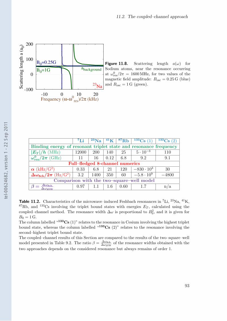
11.2. The coupled–channel approach

Figure 11.8. Scattering length a(ω) forSodium atoms, near the resonance occurringat ω0

res/2π = 1600 MHz, for two values of themagnetic field amplitude: Bosc = 0.25 G (blue)and Bosc = 1 G (green).

7Li 23Na 41K 87Rb 133Cs (1) 133Cs (2)Binding energy of resonant triplet state and resonance frequency|ET |/h (MHz) 12000 200 140 25 5 · 10−3 110ω0

res/2π (GHz) 11 16 0.12 6.8 9.2 9.1Full–fledged 8-channel numerics

α (kHz/G2) 0.33 6.8 21 120 −830 · 103 30∆ω8ch/2π (Hz/G2) 3.2 1400 350 60 −5.8 · 109 −4800

Comparison with the two–square–well model

β = ∆ω8ch

∆ω2SW0.97 1.1 1.6 0.60 1.7 n/a

Table 11.2. Characteristics of the microwave–induced Feshbach resonances in 7Li, 23Na, 41K,87Rb, and 133Cs involving the triplet bound states with energies ET , calculated using thecoupled–channel method. The resonance width ∆ω is proportional to B2

0 , and it is given forB0 = 1 G.The column labelled “133Cs (1)” relates to the resonance in Cesium involving the highest tripletbound state, whereas the column labelled “133Cs (2)” relates to the resonance involving thesecond–highest triplet bound state.The coupled–channel results of this Section are compared to the results of the two–square–wellmodel presented in Table 9.2. The ratio β = ∆ω8ch

∆ω2SWof the resonance widths obtained with the

two approaches depends on the considered resonance but always remains of order 1.

93

tel-0

0624

682,

ver

sion

1 -

22 S

ep 2

011

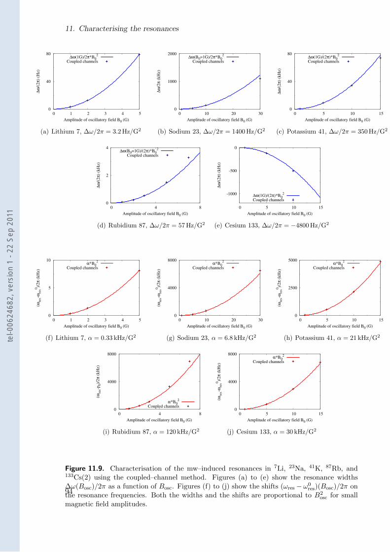
11. Characterising the resonances

0

40

80

0 1 2 3 4 5

∆ω

/(2

π)

(Hz)

Amplitude of oscillatory field B0 (G)

∆ω(1G)/2π*B02

Coupled channels

(a) Lithium 7, ∆ω/2π = 3.2 Hz/G2

0

1000

2000

0 10 20 30

∆ω

/2π

(k

Hz)

Amplitude of oscillatory field B0 (G)

∆ω(B0=1G)/2π*B02

Coupled channels

(b) Sodium 23, ∆ω/2π = 1400 Hz/G2

0

40

80

0 5 10 15

∆ω

/(2

π)

(kH

z)

Amplitude of oscillatory field B0 (G)

∆ω(1G)/(2π)*B02

Coupled channels

(c) Potassium 41, ∆ω/2π = 350 Hz/G2

0

2

4

0 4 8

∆ω

/(2

π)

(kH

z)

Amplitude of oscillatory field B0 (G)

∆ω(B0=1G)/(2π)*B02

Coupled channels

(d) Rubidium 87, ∆ω/2π = 57 Hz/G2

-1000

-500

0

0 5 10 15

∆ω

/(2

π)

(kH

z)Amplitude of oscillatory field B0 (G)

∆ω(1G)/(2π)*B02

Coupled channels

(e) Cesium 133, ∆ω/2π = −4800 Hz/G2

0

5

10

0 1 2 3 4 5

(ωre

s-ω

res0

)/2

π (

kH

z)

Amplitude of oscillatory field B0 (G)

α*B02

Coupled channels

(f) Lithium 7, α = 0.33 kHz/G2

0

4000

8000

0 10 20 30

(ωre

s-ω

res0

)/2

π (

kH

z)

Amplitude of oscillatory field B0 (G)

α*B02

Coupled channels

(g) Sodium 23, α = 6.8 kHz/G2

0

2500

5000

0 5 10 15

(ωre

s-ω

res0

)/2

π (

kH

z)

Amplitude of oscillatory field B0 (G)

α*B02

Coupled channels

(h) Potassium 41, α = 21 kHz/G2

0

4000

8000

0 4 8

(ωre

s-p

0)/

2π

(k

Hz)

Amplitude of oscillatory field B0 (G)

α*B02

Coupled channels

(i) Rubidium 87, α = 120 kHz/G2

0

4000

8000

0 5 10 15

(ωre

s-ω

res0

)/2

π (

kH

z)

Amplitude of oscillatory field B0 (G)

α*B02

Coupled channels

(j) Cesium 133, α = 30 kHz/G2

Figure 11.9. Characterisation of the mw–induced resonances in 7Li, 23Na, 41K, 87Rb, and133Cs(2) using the coupled–channel method. Figures (a) to (e) show the resonance widths∆ω(Bosc)/2π as a function of Bosc. Figures (f) to (j) show the shifts (ωres − ω0

res)(Bosc)/2π onthe resonance frequencies. Both the widths and the shifts are proportional to B2

osc for smallmagnetic field amplitudes.

94

tel-0

0624

682,

ver

sion

1 -

22 S

ep 2

011

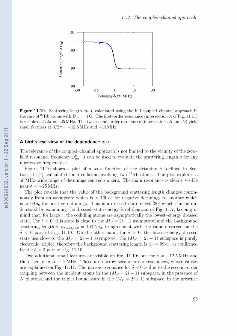
11.2. The coupled–channel approach

98

99

100

101

-30 -15 0 15 30

Sca

tter

ing

len

gth

a (

a 0)

Detuning δ/2π (MHz)

Figure 11.10. Scattering length a(ω), calculated using the full coupled–channel approach inthe case of 87Rb atoms with Bosc = 1 G. The first–order resonance (intersection A of Fig. 11.11)is visible at δ/2π = −25 MHz. The two second–order resonances (intersections B and D) yieldsmall features at δ/2π = −12.5 MHz and +13 MHz.

A bird’s–eye view of the dependence a(ω)

The relevance of the coupled–channel approach is not limited to the vicinity of the zero–field resonance frequency ω0

res: it can be used to evaluate the scattering length a for anymicrowave frequency ω.

Figure 11.10 shows a plot of a as a function of the detuning δ (defined in Sec-tion 11.1.2), calculated for a collision involving two 87Rb atoms. The plot explores a50 MHz–wide range of detunings centred on zero. The main resonance is clearly visiblenear δ = −25 MHz.

The plot reveals that the value of the background scattering length changes contin-uously from an asymptote which is > 100 a0 for negative detunings to another whichis ≈ 99 a0 for positive detunings. This is a dressed–state effect [30] which can be un-derstood by examining the dressed–state energy–level diagram of Fig. 11.7, keeping inmind that, for large r, the colliding atoms are asymptotically the lowest–energy dressedstate. For δ < 0, this state is close to the MF = 2i− 1 asymptote, and the backgroundscattering length is aF=MF=2 = 100.5 a0, in agreement with the value observed on theδ < 0 part of Fig. 11.10. On the other hand, for δ > 0, the lowest–energy dressedstate lies close to the MF = 2i + 1 asymptote: the (MF = 2i + 1) subspace is purelyelectronic–triplet, therefore the background scattering length is aT = 99 a0, as confirmedby the δ > 0 part of Fig. 11.10.

Two additional small features are visible on Fig. 11.10: one for δ ≈ −12.5 MHz andthe other for δ ≈ +12 MHz. These are narrow second–order resonances, whose causesare explained on Fig. 11.11. The narrow resonance for δ < 0 is due to the second–ordercoupling between the incident atoms in the (MF = 2i− 1) subspace, in the presence ofN photons, and the triplet bound state in the (MF = 2i+ 1) subspace, in the presence

95

tel-0

0624

682,

ver

sion

1 -

22 S

ep 2

011

11. Characterising the resonances

of (N − 2) photons: it corresponds to the intersection B on Fig. 11.11. The narrowresonance for δ > 0 is due to the second–order coupling between the incident atoms inthe (MF = 2i + 1) subspace, in the presence of (N − 2) photons, and the bound statein the (MF = 2i − 1) subspace, in the presence of N photons: it corresponds to theintersection D.

The intersection C does not yield a first–order resonance for positive detunings, be-cause it corresponds to a coupling between the subspaces (MF = 2i) and (MF = 2i+ 1).Both of these subspaces are purely electronic–triplet, therefore the spin–flip Franck–Condon factor involves an overlap between two wavefunctions which are eigenstates ofthe same Hamiltonian: these two wavefunctions are orthogonal, leading to a Franck–Condon factor which is zero and thus to a vanishing resonance width.

11.2.4. A giant resonance in Cesium

The coupled–channel channel allows us to explore the large–Bosc behaviour of the res-onance in 133Cs involving the highest triplet bound state (|ET | = h · 5 kHz, columnslabelled “Cs(1)” in Tables 11.1 and 11.2). In this particular case, Eqs. (11.9) and (11.10)are inapplicable for magnetic field amplitudes larger than |ET |/µB = 4 mG.

Graphs of the scattering length a(δ), calculated using the coupled–channel methodfor various values of Bosc, are shown on Fig. 11.12. For small amplitudes (Bosc = 0.1 mGand 1 mG), the behaviour of a(δ) is similar to the one shown on Fig. 11.10 for 87Rb: themain resonance at δ = h·(−5) kHz, the ‘step’ corresponding to the change in backgroundscattering lengths near δ = 0, and the two narrow second–order resonances are all visibleon the plot for Bosc = 1 mG. For larger magnetic field amplitudes (Bosc ≥ 5 mG), thescattering length becomes very large for ~ω ≈ ∆Ehf , but the resonance is no longerhyperbolic: the δ < 0 asymptote corresponds to aF=MF=6 = −2500 a0, whereas forlarge δ > 0 the scattering length goes to aT = +2500 a0. This ‘giant’ resonance hasan approximate width of the order of 1 MHz for Bosc = 1 G. Its non–standard shaperesults from the interplay between (i) the two–atom resonance and (ii) the (single–atom) dressed–state effect leading to different background scattering lengths for δ < 0and δ > 0.

11.2.5. Applicability in more general situations

The coupled–channel approach has a wide applicability. We have used it to characterisethe resonance involving the highest–energy triplet bound state in 133Cs for more realis-tic experimental parameters, which lead to a greater number of coupled channels andrequire inelastic collisions to be accounted for: see Chapter 15. We have also used it tocharacterise static–field Feshbach resonances occurring in 133Cs for very small magneticfield amplitudes: these static–field resonances are described in Chapter 14.

96

tel-0

0624

682,

ver

sion

1 -

22 S

ep 2

011

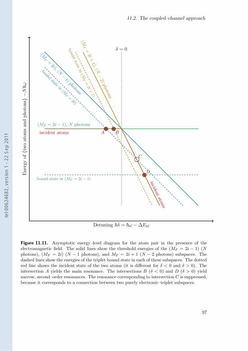
11.2. The coupled–channel approach

δ = 0

(MF = 2i− 1), N photons

(MF

=2i), (N

−1)

photons

(MF

=2i

+1),

(N−

2)photons

incident atoms

incidentatom

s

bound state in (MF = 2i− 1)

boundstate

in(MF

=2i)

bound

statein

(MF

=2i

+1)

A B

C

D

Detuning ~δ = ~ω −∆Ehf

Ener

gyoft

wo

atom

san

dphot

ons−N~ω

Figure 11.11. Asymptotic energy–level diagram for the atom pair in the presence of theelectromagnetic field. The solid lines show the threshold energies of the (MF = 2i − 1) (Nphotons), (MF = 2i) (N − 1 photons), and MF = 2i + 1 (N − 2 photons) subspaces. Thedashed lines show the energies of the triplet bound state in each of these subspaces. The dottedred line shows the incident state of the two atoms (it is different for δ < 0 and δ > 0). Theintersection A yields the main resonance. The intersections B (δ < 0) and D (δ > 0) yieldnarrow, second–order resonances. The resonance corresponding to intersection C is suppressed,because it corresponds to a connection between two purely electronic–triplet subspaces.

97

tel-0

0624

682,

ver

sion

1 -

22 S

ep 2

011

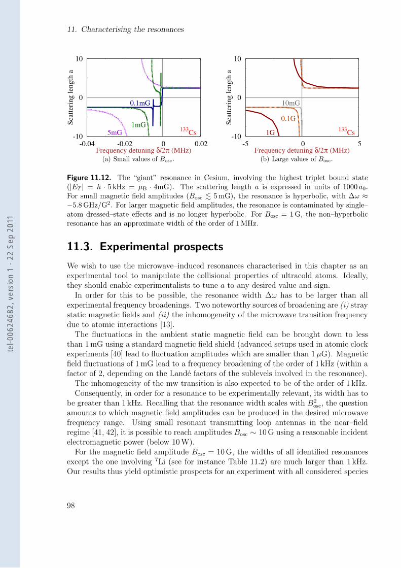
11. Characterising the resonances

-10

0

10

-0.04 -0.02 0 0.02

Sca

tter

ing l

ength

a

Frequency detuning δ/2π (MHz)

0.1mG

1mG5mG

133Cs

(a) Small values of Bosc.

-10

0

10

-5 0 5

Sca

tter

ing l

ength

a

Frequency detuning δ/2π (MHz)

10mG

0.1G

1G133

Cs

(b) Large values of Bosc.

Figure 11.12. The “giant” resonance in Cesium, involving the highest triplet bound state(|ET | = h · 5 kHz = µB · 4mG). The scattering length a is expressed in units of 1000 a0.For small magnetic field amplitudes (Bosc . 5 mG), the resonance is hyperbolic, with ∆ω ≈−5.8 GHz/G2. For larger magnetic field amplitudes, the resonance is contaminated by single–atom dressed–state effects and is no longer hyperbolic. For Bosc = 1 G, the non–hyperbolicresonance has an approximate width of the order of 1 MHz.

11.3. Experimental prospects

We wish to use the microwave–induced resonances characterised in this chapter as anexperimental tool to manipulate the collisional properties of ultracold atoms. Ideally,they should enable experimentalists to tune a to any desired value and sign.

In order for this to be possible, the resonance width ∆ω has to be larger than allexperimental frequency broadenings. Two noteworthy sources of broadening are (i) straystatic magnetic fields and (ii) the inhomogeneity of the microwave transition frequencydue to atomic interactions [13].

The fluctuations in the ambient static magnetic field can be brought down to lessthan 1 mG using a standard magnetic field shield (advanced setups used in atomic clockexperiments [40] lead to fluctuation amplitudes which are smaller than 1µG). Magneticfield fluctuations of 1 mG lead to a frequency broadening of the order of 1 kHz (within afactor of 2, depending on the Lande factors of the sublevels involved in the resonance).

The inhomogeneity of the mw transition is also expected to be of the order of 1 kHz.Consequently, in order for a resonance to be experimentally relevant, its width has to

be greater than 1 kHz. Recalling that the resonance width scales with B2osc, the question

amounts to which magnetic field amplitudes can be produced in the desired microwavefrequency range. Using small resonant transmitting loop antennas in the near–fieldregime [41, 42], it is possible to reach amplitudes Bosc ∼ 10 G using a reasonable incidentelectromagnetic power (below 10 W).

For the magnetic field amplitude Bosc = 10 G, the widths of all identified resonancesexcept the one involving 7Li (see for instance Table 11.2) are much larger than 1 kHz.Our results thus yield optimistic prospects for an experiment with all considered species

98

tel-0

0624

682,

ver

sion

1 -

22 S

ep 2

011

11.4. Comparison with RF–induced Feshbach resonances

except 7Li. The absence of a broad microwave–induced resonance for 7Li is not a drasticissue, as a broad static–field Feshbach resonance is available for this atom [22].

Other experimental schemes are being considered for the observation of microwave–induced resonances. For example, the microwave magnetic field could also be ‘sprayed’onto the atoms from the end of a waveguide connected to a powerful mw amplifier[43]. Alternatively, the experiment could be performed in a cavity which is reflectivefor mw fields but transparent in the optical domain [44]. The most promising schemepresently seems to be the observation of the large resonance in 133Cs using an atomicfountain clock. The experimental parameters relevant for such an observation lead to amore involved theoretical description: a greater number of coupled channels is involved,and inelastic collisions must be taken into account. The results of this more elaboratecalculation are presented in Chapter 15.

11.4. Comparison with RF–induced Feshbach resonances

To our present knowledge, the first published proposals for the manipulation of ultracoldscattering properties using oscillating electromagnetic fields date back to 1996: (i) Mo-erdijk, Verhaar, and Nagtegaal reported a theoretical analysis of resonances induced byradio–frequency magnetic fields [20], and (ii) Fedichev et al. proposed using optically–induced Feshbach resonances [17].

In this section, we focus on the work reported in [20] by Moerdijk et al.. In the fourthsection of that paper, the authors consider 23Na atoms in a static magnetic trap. Theyassume that all of the atoms are in the ground hyperfine manifold (f = i−1/2 = 1), andthat the static magnetic field amplitude at the centre of the trap is zero. They studythe effect of an additional radio–frequency magnetic field on atoms at the centre of thetrap, and they focus on the RF frequency4 ω/2π = 7 MHz. They perform coupled–channel calculations of the scattering matrix characterising a cold collision between twoSodium atoms which are asymptotically both in the state | f = 1,mf = −1 〉, for thefixed RF frequency ω/2π = 7 MHz and for Rabi frequencies ωr/2π ranging from 0 to700 MHz. They report a series of narrow scattering resonances (whose widths ∆ωr/2πare of the order of 100 Hz for temperatures of the order of T = 3µK) occurring forωr/2π ≈ 60 MHz, 200 MHz, . . . , and a broader resonance occurring for ωr/2π = 255 MHz(whose width is ∆ωr/2π ≈ 40 kHz at the same temperature). Their plot of the S–matrixelement characterising collisions in the presence of the RF field is shown on Fig. 11.13.

To our knowledge, these resonances have not yet been observed experimentally. Thebroad resonance occurs for a Rabi frequency ωr/2π which is 36 times larger than the RFfrequency ω/2π = 7 MHz. Its observation will require the use of RF amplitudes of theorder of 500 G. In contrast, the microwave–induced resonance involving Sodium whichwe have characterised in Sections 11.1 and 11.2 have comparable widths for magnetic fieldamplitudes of the order of Bosc = 5 G, and it can be made even broader by increasing theoscillating magnetic field amplitude as its width is proportional to B2

osc (see Fig. 11.9(b)).

4The static magnetic field is zero, hence the detuning δ from the Zeeman splitting is equal to ω.

99

tel-0

0624

682,

ver

sion

1 -

22 S

ep 2

011

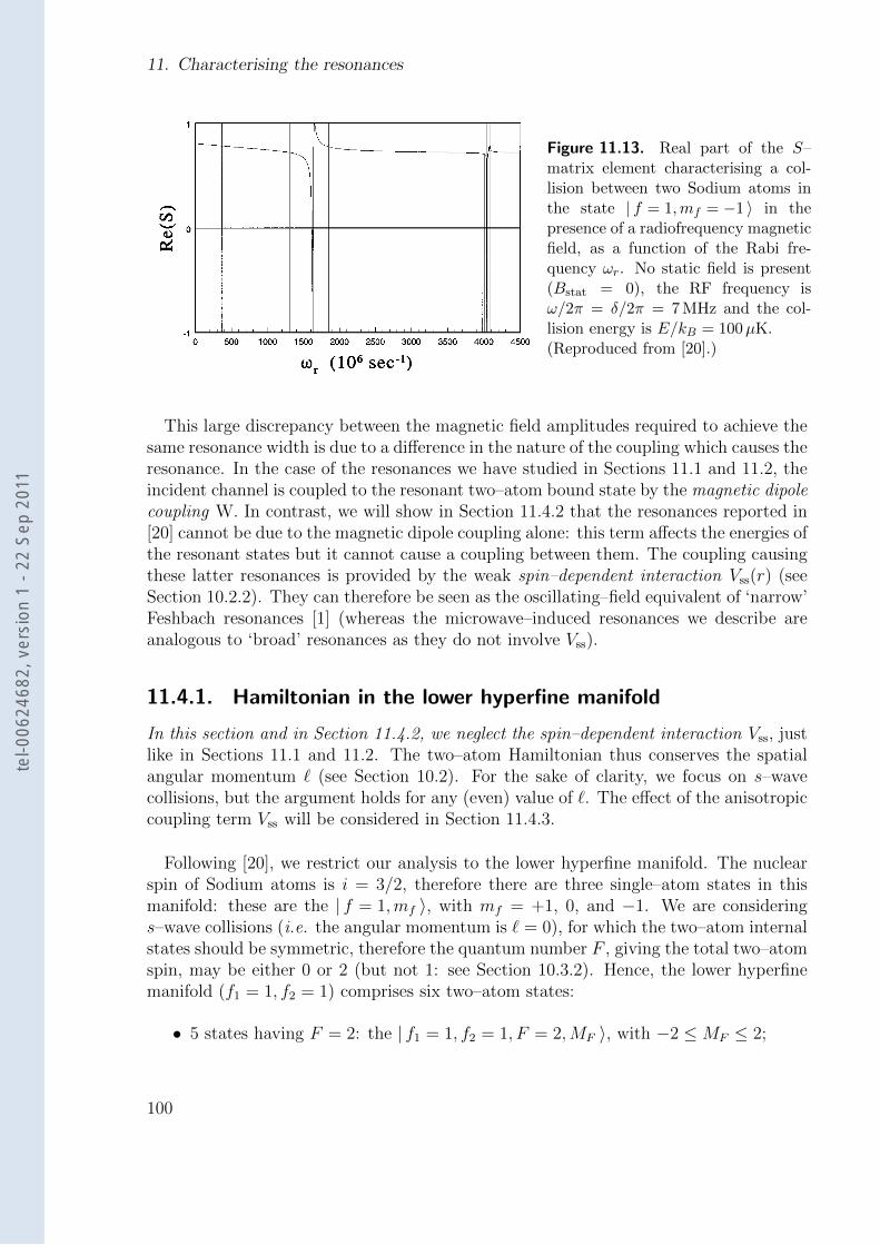
11. Characterising the resonances

Figure 11.13. Real part of the S–matrix element characterising a col-lision between two Sodium atoms inthe state | f = 1,mf = −1 〉 in thepresence of a radiofrequency magneticfield, as a function of the Rabi fre-quency ωr. No static field is present(Bstat = 0), the RF frequency isω/2π = δ/2π = 7 MHz and the col-lision energy is E/kB = 100µK.(Reproduced from [20].)

This large discrepancy between the magnetic field amplitudes required to achieve thesame resonance width is due to a difference in the nature of the coupling which causes theresonance. In the case of the resonances we have studied in Sections 11.1 and 11.2, theincident channel is coupled to the resonant two–atom bound state by the magnetic dipolecoupling W. In contrast, we will show in Section 11.4.2 that the resonances reported in[20] cannot be due to the magnetic dipole coupling alone: this term affects the energies ofthe resonant states but it cannot cause a coupling between them. The coupling causingthese latter resonances is provided by the weak spin–dependent interaction Vss(r) (seeSection 10.2.2). They can therefore be seen as the oscillating–field equivalent of ‘narrow’Feshbach resonances [1] (whereas the microwave–induced resonances we describe areanalogous to ‘broad’ resonances as they do not involve Vss).

11.4.1. Hamiltonian in the lower hyperfine manifold

In this section and in Section 11.4.2, we neglect the spin–dependent interaction Vss, justlike in Sections 11.1 and 11.2. The two–atom Hamiltonian thus conserves the spatialangular momentum ` (see Section 10.2). For the sake of clarity, we focus on s–wavecollisions, but the argument holds for any (even) value of `. The effect of the anisotropiccoupling term Vss will be considered in Section 11.4.3.

Following [20], we restrict our analysis to the lower hyperfine manifold. The nuclearspin of Sodium atoms is i = 3/2, therefore there are three single–atom states in thismanifold: these are the | f = 1,mf 〉, with mf = +1, 0, and −1. We are considerings–wave collisions (i.e. the angular momentum is ` = 0), for which the two–atom internalstates should be symmetric, therefore the quantum number F , giving the total two–atomspin, may be either 0 or 2 (but not 1: see Section 10.3.2). Hence, the lower hyperfinemanifold (f1 = 1, f2 = 1) comprises six two–atom states:

• 5 states having F = 2: the | f1 = 1, f2 = 1, F = 2,MF 〉, with −2 ≤MF ≤ 2;

100

tel-0

0624

682,

ver

sion

1 -

22 S

ep 2

011

11.4. Comparison with RF–induced Feshbach resonances

• 1 state having F = 0: | f1 = 1, f2 = 1, F = 0,MF = 0 〉.In order to determine the state of the system “two atoms in the presence of the radio–

frequency magnetic field” completely, the quantum number N , giving the number ofphotons, has to be specified as well. For the sake of simplicity, we assume that theradio–frequency magnetic field is σ−–polarised56. In this context, the magnetic dipolecoupling term is W = W σ− and reads:

W σ− = w1 (S+a† + S−a) , (11.20)

where w1 is defined by Eq. (10.7). The conservation of angular momentum implies thatthe quantum number N0 = −MF + N is conserved (see Section 10.3.5). Therefore, wechoose a value7 for N0 and we restrict the Hamiltonian H of Eq. (10.13) to the six–dimensional stable subspace spanned by the states| f1 = 1, f2 = 1, F = 2,MF , N = N0 +MF 〉 (−2 ≤MF ≤ 2) and| f1 = 1, f2 = 1, F = 0,MF = 0, N = N0 〉.

Just like in Section 10.3.5, we write H = p2r2mr

+ Vtot(r), where the total potentialmatrix Vtot(r) reads:

Vtot(r) = Vel(r) + Vhf + VZ + ~ω a†a+W . (10.23)

We are interested in the block structure of the matrix representation of Vtot(r) restrictedto the stable subspace defined above.

• The electronic–interaction term Vel conserves both F and MF , and it thus onlycontributes diagonal matrix elements.

• All of the six relevant states bear the hyperfine quantum numbers f1 = f2 = 1,therefore the hyperfine term Vhf only contributes a constant to the Hamiltonian(Vhf = −5

2ahf 1).

• The photon–energy term ~ω a†a contributes the usual diagonal matrix elements.

• The Zeeman term VZ obeys the vector selection rule on F (see Section 10.3.5),therefore it does not couple the (F = 2) subspace to the F = 0 state. Furthermore,it conserves the total spin projection MF , therefore it only contributes diagonalmatrix elements.

• The magnetic dipole coupling term W also obeys vector selection rules, hence, itdoes not couple the (F = 2) and (F = 0) subspaces. It contributes off–diagonalcoupling terms within the (F = 2) subspace (represented in blue on Fig. 11.14).

5This assumption is not a requirement: any polarisation which is perpendicular to the quantisationaxis can be seen as a linear combination of σ+ and σ− polarisations. In the context of the evaporativecooling of Sodium atoms mentioned in [20], the resonant term is the second one, because the low–field–seeking single–atom state | f = 1,mf = −1 〉 has a higher energy than the untrapped states| f = 1,mf = 0 〉 and | f = 1,mf = +1 〉 [45].

6This polarisation is defined by the vector eσ− = (ex − iey)/√

2: see also Fig. 15.1.7We choose N0 1, its exact value being arbitrary: see Section 10.3.5.

101

tel-0

0624

682,

ver

sion

1 -

22 S

ep 2

011

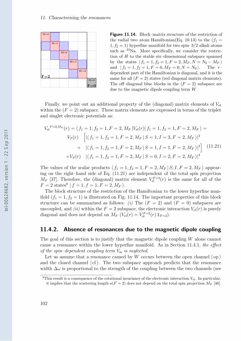
11. Characterising the resonances

F=2

F=0

M=2

M=1

M=0

M=-1

M=-2

M=0

Figure 11.14. Block–matrix structure of the restriction ofthe radial two–atom Hamiltonian(Eq. 10.13) to the (f1 =1, f2 = 1) hyperfine manifold for two spin–3/2 alkali atomssuch as 23Na. More specifically, we consider the restric-tion of H to the stable six–dimensional subspace spannedby the states | f1 = 1, f2 = 1, F = 2,MF , N = N0 −MF 〉and | f1 = 1, f2 = 1, F = 0,MF = 0, N = N0 〉. The r–dependent part of the Hamiltonian is diagonal, and it is thesame for all (F = 2) states (red diagonal matrix elements).The off–diagonal blue blocks in the (F = 2) subspace aredue to the magnetic dipole coupling term W .

Finally, we point out an additional property of the (diagonal) matrix elements of Vel

within the (F = 2) subspace. These matrix elements are expressed in terms of the tripletand singlet electronic potentials as:

VelF=2,MF (r) = 〈 f1 = 1, f2 = 1, F = 2,MF |Vel(r)| f1 = 1, f2 = 1, F = 2,MF 〉 =

VT (r)[|〈 f1 = 1, f2 = 1, F = 2,MF |S = 1, I = 3, F = 2,MF 〉|2

+ |〈 f1 = 1, f2 = 1, F = 2,MF |S = 1, I = 1, F = 2,MF 〉|2]

+VS(r) |〈 f1 = 1, f2 = 1, F = 2,MF |S = 0, I = 2, F = 2,MF 〉|2(11.21)

The values of the scalar products 〈 f1 = 1, f2 = 1, F = 2,MF |S, I, F = 2,MF 〉 appear-ing on the right–hand side of Eq. (11.21) are independent of the total spin projectionMF [37]. Therefore, the (diagonal) matrix element V F=2

el (r) is the same for all of theF = 2 states8 | f = 1, f = 1, F = 2,MF 〉.

The block structure of the restriction of the Hamiltonian to the lower hyperfine man-ifold (f1 = 1, f2 = 1) is illustrated on Fig. 11.14. The important properties of this blockstructure can be summarised as follows: (i) The (F = 2) and (F = 0) subspaces areuncoupled, and (ii) within the F = 2 subspace, the electronic interaction Vel(r) is purelydiagonal and does not depend on MF (Vel(r) = V F=2

el (r) 1F=2).

11.4.2. Absence of resonances due to the magnetic dipole coupling

The goal of this section is to justify that the magnetic dipole coupling W alone cannotcause a resonance within the lower hyperfine manifold. As in Section 11.4.1, the effectof the spin–dependent coupling term Vss is neglected.

Let us assume that a resonance caused by W occurs between the open channel | op 〉and the closed channel | cl 〉. The two–subspace approach predicts that the resonancewidth ∆ω is proportional to the strength of the coupling between the two channels (see

8This result is a consequence of the rotational invariance of the electronic interaction Vel. In particular,it implies that the scattering length a(F = 2) does not depend on the total spin projection MF [46].

102

tel-0

0624

682,

ver

sion

1 -

22 S

ep 2

011

11.4. Comparison with RF–induced Feshbach resonances

Eq. (11.10) and [1]):∆ω ∝ |〈Ψcl |W |Ψop 〉|2 , (11.22)

where |Ψop 〉 and |Ψcl 〉 are the wavefunctions in the open and closed channels, re-spectively. The decoupling between the (F = 0) and (F = 2) subspaces, describedin Section 11.4.1, makes it possible to choose open– and closed–channel wavefunctionswhich have a well–defined quantum number F .

If the wavefunctions |Ψop 〉 and |Ψcl 〉 correspond to different values of F (i.e. one ofthem has F = 2 and the other has F = 0), the matrix element on the right–hand sideof Eq. (11.22) is zero because W does not connect the (F = 2) and (F = 0) subspaces.

We now assume that |Ψop 〉 and |Ψcl 〉 bear the same quantum number F . For the sakeof definiteness, we take F = 2 (but the argument also holds for F = 0). The operatorV F=2

el (r) not depending on the spin projection MF makes it possible to choose open–and closed–channel wavefunctions of the form:

|Ψop(r) 〉 = ϕF=2op (r)|χF=2

op 〉 and |Ψcl(r) 〉 = ϕF=2cl (r)|χF=2

cl 〉 , (11.23)

where |χF=2op 〉 and |χF=2

cl 〉 are two (RF–dressed) two–atom internal states belongingto the (F = 2) subspace, and the (single–channel) spatial wavefunctions ϕF=2

op (r) andϕF=2

cl (r) are both eigenfunctions of the spatial Hamiltonian

HF=2spatial = p2

r/2mr + V F=2el (r) . (11.24)

The open–channel wavefunction is a scattering state of HF=2spatial, and the closed–channel

wavefunction is a bound state of the same Hamiltonian. Two different eigenfunctionsof the same (Hermitian) Hamiltonian are always orthogonal, hence 〈ϕF=2

op |ϕF=2cl 〉 = 0.

Thus, the resonance width is zero:

∆ω ∝∣∣〈χF=2

op |W |χF=2cl 〉

∣∣2 ∣∣〈ϕF=2op |ϕF=2

cl 〉∣∣2 = 0 , (11.25)

which finishes the proof that the magnetic dipole coupling term W alone cannot causeany resonance within the (f = 1, f = 1) hyperfine manifold.

11.4.3. Resonances due to the spin–dependent interaction Vss

We have justified in Section 11.4.2 that the magnetic dipole coupling W alone cannotcause resonances within the lower hyperfine manifold (f1 = 1, f2 = 1). We now justifythat the resonances reported by Moerdijk et al. [20] are due to the spin–dependent inter-action Vss(r) (see Section 10.2), and we identify the resonant two–atom states yieldingthe resonances visible on Fig. 11.13.

The complete two–atom Hamiltonian

The complete two–atom Hamiltonian, including Vss(r), reads:

Hcomplete =p2r

2µ+

`2

2µr2+ Vtot(r) + Vss(r) = H + Vss(r) , (11.26)

103

tel-0

0624

682,

ver

sion

1 -

22 S

ep 2

011

11. Characterising the resonances

where ` is the angular momentum of the reduced particle, the operator Vtot(r) is definedby Eq. (10.23), and H is the Hamiltonian introduced in Section 11.4.1. The spin–dependent interaction Vss(r) can be expressed as [47]:

Vss(r) = f(r) [s1 · s2 − 3(s1 · r)(s2 · r)] . (11.27)

It is anisotropic and, hence, couples partial waves with different angular momenta ` [7];therefore, the centrifugal term `2/2µr2 is included in Eq. (11.26) and in H.

We apply the two–channel model to the Hamiltonian Hcomplete (see also Section 11.1and [1]), considering H as the bare Hamiltonian and Vss as the coupling operator.

Choice of the open– and closed–channel wavefunctions

The symmetry considerations presented in Sections 11.4.1 and 11.4.2 fully apply to thebare Hamiltonian H. Thus, the bare open– and closed–channel wavefunctions can bechosen within specific (f1 = f2 = 1, F,N0, `) subspaces, where the quantum numberF gives the total (electronic and nuclear) two–atom spin, the integer N0 specifies theRF–dressed manifold, and the partial–wave index ` determines the angular momentumof the reduced particle.

The incident state used in [20] describes a collision of two atoms which, for largeseparations, are both in an RF–dressed state relating to | f = 1,mf = −1 〉, with theincident energy Einc = kB · 100µK. This two–atom wavefunction has components withangular momenta ` = 0, 2, . . . We choose the open channel to be the component havingthe angular momentum `op, which is of the form:

|Ψ(F=2,Nop0 ,`op)

op (r) 〉 = ϕ(F=2,`op)op (r)|χ(F=2,Nop

0 )op 〉 , (11.28)

where |χ(F=2,Nop0 )

op 〉 is an RF–dressed two–atom state belonging to the (f1 = f2 = 1, F =

2, Nop0 ) subspace and the (single–channel) spatial wavefunction ϕ

(F=2,`op)op (r) is the scat-

tering state of HF=2,`op

spatial with the energy Einc, the spatial Hamiltonian H(F=2,`)spatial being

defined by:

H(F=2,`)spatial =

p2r

2mr

+`(`+ 1)

2mrr2+ V

(F=2)el (r) . (11.29)

The closed–channel wavefunction may belong to any subspace (f1 = f2 = 1, F,N cl0 , `

cl)which is coupled to the open–channel state by Vss. In particular, the quantum numberF must be 2 or 0, and the partial wave `cl must be even. According to [48], the twohighest bound states of two Sodium atoms satisfying these conditions are F = 2 states:

• The state | ν = 15, ` = 0, SI = (13), F = 2 〉 has the binding energy h · 90 MHz;

• The state | ν = 14, ` = 4, SI = (13), F = 2 〉 has the binding energy h · 900 MHz.

Our aim is to show that the RF–induced resonances visible on Fig. 11.13 are due to thesetwo weakly–bound states. For that purpose, we consider a closed–channel wavefunctionof the form:

|Ψ(F=2,Ncl0 ,`

cl)cl (r) 〉 = ϕ

(F=2,`cl)cl (r)|χ(F=2,Ncl

0 )cl 〉 , (11.30)

104

tel-0

0624

682,

ver

sion

1 -

22 S

ep 2

011

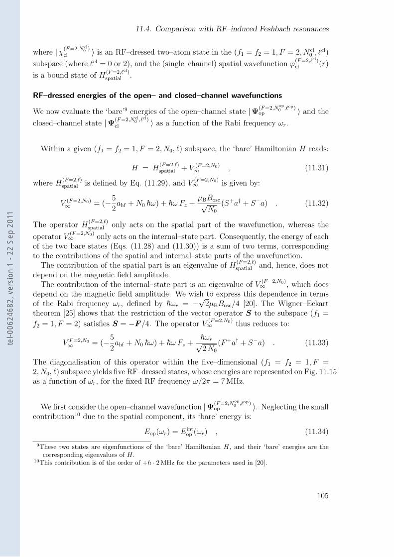
11.4. Comparison with RF–induced Feshbach resonances

where |χ(F=2,Ncl0 )

cl 〉 is an RF–dressed two–atom state in the (f1 = f2 = 1, F = 2, N cl0 , `

cl)

subspace (where `cl = 0 or 2), and the (single–channel) spatial wavefunction ϕ(F=2,`cl)cl (r)

is a bound state of H(F=2,`cl)spatial .

RF–dressed energies of the open– and closed–channel wavefunctions

We now evaluate the ‘bare’9 energies of the open–channel state |Ψ(F=2,Nop0 ,`op)

op 〉 and the

closed–channel state |Ψ(F=2,Ncl0 ,`

cl)cl 〉 as a function of the Rabi frequency ωr.

Within a given (f1 = f2 = 1, F = 2, N0, `) subspace, the ‘bare’ Hamiltonian H reads:

H = H(F=2,`)spatial + V (F=2,N0)

∞ , (11.31)

where H(F=2,`)spatial is defined by Eq. (11.29), and V

(F=2,N0)∞ is given by:

V (F=2,N0)∞ = (−5

2ahf +N0 ~ω) + ~ω Fz +

µBBosc√N0

(S+a† + S−a) . (11.32)

The operator H(F=2,`)spatial only acts on the spatial part of the wavefunction, whereas the

operator V(F=2,N0)∞ only acts on the internal–state part. Consequently, the energy of each

of the two bare states (Eqs. (11.28) and (11.30)) is a sum of two terms, correspondingto the contributions of the spatial and internal–state parts of the wavefunction.

The contribution of the spatial part is an eigenvalue of H(F=2,`)spatial and, hence, does not

depend on the magnetic field amplitude.The contribution of the internal–state part is an eigenvalue of V

(F=2,N0)∞ , which does

depend on the magnetic field amplitude. We wish to express this dependence in termsof the Rabi frequency ωr, defined by ~ωr = −

√2µBBosc/4 [20]. The Wigner–Eckart

theorem [25] shows that the restriction of the vector operator S to the subspace (f1 =

f2 = 1, F = 2) satisfies S = −F /4. The operator V(F=2,N0)∞ thus reduces to:

V F=2,N0∞ = (−5

2ahf +N0 ~ω) + ~ω Fz +

~ωr√2N0

(F+a† + S−a) . (11.33)

The diagonalisation of this operator within the five–dimensional (f1 = f2 = 1, F =2, N0, `) subspace yields five RF–dressed states, whose energies are represented on Fig. 11.15as a function of ωr, for the fixed RF frequency ω/2π = 7 MHz.

We first consider the open–channel wavefunction |Ψ(F=2,Nop0 ,`op)

op 〉. Neglecting the smallcontribution10 due to the spatial component, its ‘bare’ energy is:

Eop(ωr) = Eintop (ωr) , (11.34)

9These two states are eigenfunctions of the ‘bare’ Hamiltonian H, and their ‘bare’ energies are thecorresponding eigenvalues of H.

10This contribution is of the order of +h · 2 MHz for the parameters used in [20].

105

tel-0

0624

682,

ver

sion

1 -

22 S

ep 2

011

11. Characterising the resonances

-0.083

-0.077

-0.071

-0.065

0 200 400 600

Dre

ssed

ener

gie

s (h

c • 1cm

-1)

Rabi frequency ωr (rad/s)

Dressed states in (f1=f2=1,F=2,N0,l)

Na MF=-2

MF=-1

MF= 0

MF= 1

MF= 2

Figure 11.15. Energies of the five RF–dressedtwo–atom states in the (f1 = f2 = 1, F =2, N0, `) subspace, calculated for the RF fre-quency ω/2π = 7 MHz.

where the internal–state energy Eintop (ωr) is the eigenvalue of V

(F=2,Nop0 )

∞ corresponding

to the eigenstate |χ(F=2,Nop0 )

op 〉.

We now turn to the bare energy of the closed–channel wavefunction |Ψ(F=2,Ncl0 ,`

cl)cl (r) 〉:

Ecl(ωr) = −|Eb|+ Eintcl (ωr) , (11.35)

where |Eb| is the binding energy of the bound state ϕ(F=2,`cl)cl (r) of the spatial Hamiltonian

H(F=2,`cl)spatial , and Eint

cl (ωr) is the eigenvalue of V(F=2,Ncl

0 )∞ corresponding to the eigenstate

|χ(F=2,Ncl0 )

cl 〉. In Eq. (11.35), the separation between the spatial–state and internal–statecontributions to the energy (Eb and Eint

cl (ωr), respectively) is not a perturbative result:it stems from our restricting the analysis to a given (f1 = f2 = 1, F = 2, `) subspace,within which the electronic interaction Vel does not couple the spatial motion of theatoms to their internal states (see Section 11.4.1).

Identification of the RF–induced resonances reported in [20]

A divergence on Fig. 11.13, occurring for a given Rabi frequency ωresr , can be explained

in terms of a resonance between two ‘bare’ states |Ψop 〉 and |Ψcl 〉 if the corresponding‘bare’ energies are equal for a Rabi frequency ωr which is close to ωres

r .

The entrance channel used in [20] is an RF–dressed scattering state relating, for smallωr, to the bare two–atom state | f1 = f2 = 1, F = 2,MF = −2, Nop

0 − 2 〉. The corre-sponding threshold energy is represented by the dashed red line on Figs. 11.15 and11.16.

We first consider the bound state | ν = 15, ` = 0, SI = (13), F = 2 〉, which has thebinding energy h · 90 MHz [48]. Within each (f1 = f2 = 1, F = 2, ` = 0, N0) subspace,this level is split into five RF–dressed bound states. The left–hand part of Fig. 11.16 rep-resents the dependence on ωr of the energies of the five dressed bound states relating, for

106

tel-0

0624

682,

ver

sion

1 -

22 S

ep 2

011

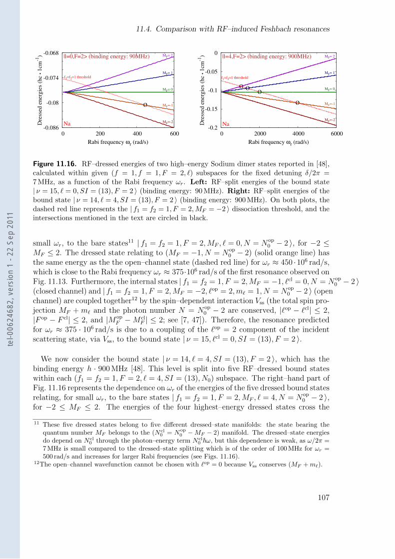
11.4. Comparison with RF–induced Feshbach resonances

-0.086

-0.08

-0.074

-0.068

0 200 400 600

Dre

ssed

ener

gie

s (h

c • 1cm

-1)

Rabi frequency ωr (rad/s)

|l=0,F=2> (binding energy: 90MHz)

Na MF=-2

MF=-1

MF= 0

MF= 1

MF= 2

f1=f2=1 threshold

o

-0.2

-0.15

-0.1

-0.05

0

0 2000 4000 6000

Dre

ssed

ener

gie

s (h

c • 1cm

-1)

Rabi frequency ωr (rad/s)

|l=4,F=2> (binding energy: 900MHz)

NaMF=-2

MF=-1

MF= 0

MF= 1

MF= 2

f1=f2=1 threshold

o

ooo

Figure 11.16. RF–dressed energies of two high–energy Sodium dimer states reported in [48],calculated within given (f = 1, f = 1, F = 2, `) subspaces for the fixed detuning δ/2π =7 MHz, as a function of the Rabi frequency ωr. Left: RF–split energies of the bound state| ν = 15, ` = 0, SI = (13), F = 2 〉 (binding energy: 90 MHz). Right: RF–split energies of thebound state | ν = 14, ` = 4, SI = (13), F = 2 〉 (binding energy: 900 MHz). On both plots, thedashed red line represents the | f1 = f2 = 1, F = 2,MF = −2 〉 dissociation threshold, and theintersections mentioned in the text are circled in black.

small ωr, to the bare states11 | f1 = f2 = 1, F = 2,MF , ` = 0, N = Nop0 − 2 〉, for −2 ≤

MF ≤ 2. The dressed state relating to (MF = −1, N = Nop0 − 2) (solid orange line) has

the same energy as the the open–channel state (dashed red line) for ωr ≈ 450 ·106 rad/s,which is close to the Rabi frequency ωr ≈ 375·106 rad/s of the first resonance observed onFig. 11.13. Furthermore, the internal states | f1 = f2 = 1, F = 2,MF = −1, `cl = 0, N = Nop

0 − 2 〉(closed channel) and | f1 = f2 = 1, F = 2,MF = −2, `op = 2,m` = 1, N = Nop

0 − 2 〉 (openchannel) are coupled together12 by the spin–dependent interaction Vss (the total spin pro-jection MF + m` and the photon number N = Nop

0 − 2 are conserved, |`op − `cl| ≤ 2,|F op − F cl| ≤ 2, and |Mop

F −M clF | ≤ 2; see [7, 47]). Therefore, the resonance predicted

for ωr ≈ 375 · 106 rad/s is due to a coupling of the `op = 2 component of the incidentscattering state, via Vss, to the bound state | ν = 15, `cl = 0, SI = (13), F = 2 〉.

We now consider the bound state | ν = 14, ` = 4, SI = (13), F = 2 〉, which has thebinding energy h · 900 MHz [48]. This level is split into five RF–dressed bound stateswithin each (f1 = f2 = 1, F = 2, ` = 4, SI = (13), N0) subspace. The right–hand part ofFig. 11.16 represents the dependence on ωr of the energies of the five dressed bound statesrelating, for small ωr, to the bare states | f1 = f2 = 1, F = 2,MF , ` = 4, N = Nop

0 − 2 〉,for −2 ≤ MF ≤ 2. The energies of the four highest–energy dressed states cross the

11 These five dressed states belong to five different dressed–state manifolds: the state bearing thequantum number MF belongs to the (N cl

0 = Nop0 −MF − 2) manifold. The dressed–state energies

do depend on N cl0 through the photon–energy term N cl

0 ~ω, but this dependence is weak, as ω/2π =7 MHz is small compared to the dressed–state splitting which is of the order of 100 MHz for ωr =500 rad/s and increases for larger Rabi frequencies (see Figs. 11.16).

12The open–channel wavefunction cannot be chosen with `op = 0 because Vss conserves (MF +m`).

107

tel-0

0624

682,

ver

sion

1 -

22 S

ep 2

011

11. Characterising the resonances

threshold energy once, for Rabi frequencies which are close to the resonant Rabi fre-quencies ωres

r ≈ 1300 · 106 rad/s, 1600 · 106 rad/s, 1850 · 106 rad/s, and 4000 · 106 rad/sobserved on Fig. 11.13.

The closed–channel internal states | f1 = f2 = 1, F = 2,M clF , `

cl = 4,mcl` , N = Nop

0 − 2 〉are coupled to the s–wave open–channel states| f1 = f2 = 1, F = 2,MF = −2, `op = 0, N = Nop

0 − 2 〉 (choose M clF + mcl

` = −2 in or-der to conserve the total angular momentum) to second order in Vss. Thus, the fourresonances mentioned above can be explained in terms of a second–order couplingvia Vss of the s–wave component of the incident scattering state to the bound state| ν = 14, ` = 4, SI = (13), F = 2 〉 to second order in Vss.

The resonance occurring for ωresr ≈ 4000 · 106 rad/s has a multi–peaked structure, at

least seven peaks being visible on Fig. 11.15. This structure can be explained in termsof two effects:

1. For large Rabi frequencies ωr, the open–channel wavefunction |Ψ(F=2,Nop0 ,`=0

op 〉 and

the closed–chanel wavefunction |Ψ(F=2,Nop0 −1,`=4

cl 〉 both have non–vanishing com-ponents for all −2 ≤ MF ≤ 2. For each MF ≤ 1, the open–channel componentbearing the quantum numbers (MF , ` = 0, N = Nop

0 + MF ) resonates with theclosed–channel component whose quantum numbers are (MF + 1, ` = 4,m` =−1, N = Nop

0 +MF ). This accounts for four of the observed peaks.

2. The closed–channel state | f1 = f2 = 1, F = 2,MF = −1, `cl = 4,mcl` , N = Nop

0 − 2 〉is also coupled, to first order in Vss, to the d–wave open–channel state| f1 = f2 = 1, F = 2,MF = −2, `op = 2,mop

` , N = Nop0 − 2 〉. This coupling, and the

corresponding ones for the dressed–state components along MF = −1, 0, and +1,account for the remaining peaks observed on Fig. 11.15.

11.4.4. Differences between RF–induced and MW–inducedFeshbach resonances.

We have shown that the RF–induced Feshbach resonances within the lower hyperfinemanifold, presented in [20], cannot be due to the magnetic dipole coupling term alone(see Section 11.4.2). These resonances thus involve the weak spin–dependent interac-tion Vss(r). By contrast, the microwave–induced Feshbach resonances which we havedescribed in Sections 11.1 and 11.2 do not involve Vss(r): they are due solely to themagnetic dipole interaction W between the two electron spins and the magnetic field.

This is the main difference between the work reported in [20] and the one we presentin our published article [21]. Radio–frequency induced resonances can be seen as theoscillating–field equivalent of ‘narrow’ Feshbach resonances, whereas microwave–inducedresonances, which do not involve Vss, are analogous to ‘broad’ Feshbach resonances[1]. In this sense, microwave–induced Feshbach resonances are more closely related tooptically–induced Feshbach resonances [17], where the incident two–atom state is coupledto an electronically–excited dimer state using a resonant oscillating electric field: these

108

tel-0

0624

682,

ver

sion

1 -

22 S

ep 2

011

11.4. Comparison with RF–induced Feshbach resonances

latter resonances are due to the electric–dipole coupling and, like microwave–inducedresonances, they do not rely on Vss.

The couplings involved being different also has an impact on the partial waves tak-ing part in the resonances. The isotropic magnetic dipole coupling W conserves theangular momentum `, and the microwave–induced resonances we have described onlyinvolve s–wave Physics (see Section 10.2). On the other hand, the spin–dependentinteraction Vss(r) is not isotropic, and it does not cause resonances between s–wavestates; therefore, at least one of the two resonant states has a spatial angular momen-tum ` ≥ 2. We have identified the bound states causing the RF–induced resonances re-ported in [20] to be the s–wave level | ν = 15, ` = 0, SI = (13), F = 2 〉 and the ` = 4 level| ν = 14, ` = 4, SI = (13), F = 2 〉, whose binding energies are h·90 MHz and h·900 MHz,respectively [48]. The s–wave level is resonant with the d–wave component of the inci-dent scattering state, and the ` = 4 level is resonant with both the s–wave and d–wavecomponents of the incident scattering state.

Microwave–induced Feshbach resonances exploit a stronger coupling mechanism, there-fore they allow for the use of weaker magnetic fields. We focus on the small magneticfield regime, where the Rabi frequency associated with the oscillating field amplitudeBosc is much smaller than the detuning δ of the frequency from the hyperfine transitionfrequency. In the specific case of Sodium, the microwave–induced resonance occurs forthe detuning δ/2π = −200 MHz, and the amplitude Bosc = 1 G, corresponding to a Rabifrequency of the order of 1 MHz, yields a resonance which is broad enough to be observedexperimentally (∆ω/2π > 1 kHz: see Table 11.2 and Section 11.3).

In this regime (Rabi frequency much smaller than detuning), the dressing of a singleatom due to the microwave is negligible, and the dominant effect is the two–atom reso-nance between the incident scattering state and a well–defined bound state. Our weakmicrowave magnetic fields not affecting the single–atom Physics could turn out to be animportant asset, for example in the context of experiments involving atomic clocks.

109

tel-0

0624

682,

ver

sion

1 -

22 S

ep 2

011

tel-0

0624

682,

ver

sion

1 -

22 S

ep 2

011

12. The numerical calculation oftwo–atom wavefunctions

This chapter describes the challenges presented by the numerical calculation of multi–channel scattering wavefunctions, and the approaches that we have used to meet them.

We have written our own, fully independent implementations of all of the programs de-scribed in this chapter. The data used as input (the large–r singlet and triplet electronicpotentials, the corresponding scattering lengths, and the hyperfine atomic structure) areavailable1 in the published litterature (see [21] and references therein).

The difficulties associated with the calculation of two–atom wavefunctions can besummarised as follows:

1. The wavefunctions are solutions of a differential system involving boundary con-ditions at both ends of the integration interval.

2. The electronic potentials are not known with sufficient accuracy for small inter-atomic separations.

3. The physically acceptable solution is the one for which all closed–channel compo-nents asymptotically decay to zero, but other solutions of the same Schrodingerequation asymptotically involve growing exponentials.

4. The two–atom wavefunction may involve many coupled channels.

5. The two–atom wavefunction may be non–real.

We start with a precise statement of the differential system we wish to solve and of theboundary conditions involved (Section 12.1). Then, we introduce the accumulated–phaseapproach [31], which circumvents the need for accurate information on the inner parts ofthe electronic potentials (Section 12.2). Next, we present the two numerical approacheswe have used to calculate two–atom wavefunctions. Our first approach, presented inSection 12.3, is based on the relaxation method. This approach addresses points 1, 2,and 3 above. This is the approach we have used to perform the calculations presentedin the published article of Chapter 13. However, this method is not readily extended toaddress points 4 and 5. Our second approach, presented in Section 12.4, is based on theshooting method. This more elaborate approach addresses all five difficulties mentionedabove.

1We thank Prof. S. Kokkelmans for providing up–to–date electronic potentials for 87Rb.

111

tel-0

0624

682,

ver

sion

1 -

22 S

ep 2

011

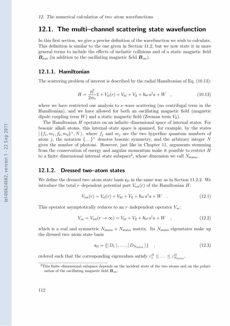
12. The numerical calculation of two–atom wavefunctions

12.1. The multi–channel scattering state wavefunction

In this first section, we give a precise definition of the wavefunction we wish to calculate.This definition is similar to the one given in Section 11.2, but we now state it in moregeneral terms to include the effects of inelastic collisions and of a static magnetic fieldBstat (in addition to the oscillating magnetic field Bosc).

12.1.1. Hamiltonian

The scattering problem of interest is described by the radial Hamiltonian of Eq. (10.13):

H =p2r

2mr

1 + Vel(r) + Vhf + VZ + ~ω a†a+W , (10.13)

where we have restricted our analysis to s–wave scattering (no centrifugal term in theHamiltonian), and we have allowed for both an oscillating magnetic field (magneticdipole coupling term W ) and a static magnetic field (Zeeman term VZ).

The Hamiltonian H operates on an infinite–dimensional space of internal states. Forbosonic alkali atoms, this internal–state space is spanned, for example, by the states| f1,m1, f2,m2+, N 〉, where fj and mj are the two hyperfine quantum numbers ofatom j, the notation . . .+ denotes bosonic symmetry, and the arbitrary integer Ngives the number of photons. However, just like in Chapter 11, arguments stemmingfrom the conservation of energy and angular momentum make it possible to restrict Hto a finite–dimensional internal–state subspace2, whose dimension we call Nstates.

12.1.2. Dressed two–atom states

We define the dressed two–atom state basis eD in the same way as in Section 11.2.2. Weintroduce the total r–dependent potential part Vtot(r) of the Hamiltonian H:

Vtot(r) = Vel(r) + Vhf + VZ + ~ω a†a+W . (12.1)

This operator asymptotically reduces to an r–independent operator V∞:

V∞ = Vtot(r →∞) = Vhf + VZ + ~ω a†a+W , (12.2)

which is a real and symmetric Nstates × Nstates matrix. Its Nstates eigenstates make upthe dressed two–atom state basis

eD = |D1 〉, . . . , |DNstates 〉 , (12.3)

ordered such that the corresponding eigenvalues satisfy εD1 ≤ . . . ≤ εDNstates.

2This finite–dimensional subspace depends on the incident state of the two atoms and on the polari-sation of the oscillating magnetic field Bosc.

112

tel-0

0624

682,

ver

sion

1 -

22 S

ep 2

011

12.1. The multi–channel scattering state wavefunction

incidentatomsentrance

closed

openthre

shold

energ

ies

Figure 12.1. Threshold energies of the open(εm < E), entrance (εn0 = E) and closed(εp > E) channels. For large r, the radial wave-function oscillates in all open channels, behaveslike (r− a) in the entrance channel, and decaysexponentially in all closed channels.

12.1.3. Schrodinger equation and boundary conditions

We wish to calculate the scattering length a = an0 characterising the collision betweentwo atoms whose incident internal state is a given microwave–dressed two–atom state|Dn0 〉. The scattering length can be extracted from the asymptotic behaviour of theoutgoing stationary scattering state [37] of H for the energy E = εDn0

. This scatteringstate |Ψn0 〉, which is an Nstates–component wavefunction, is defined by the Schrodingerequation:

H|Ψn0 〉 = εDn0|Ψn0 〉 , (12.4)

along with the large–r boundary conditions

〈Dm |Ψn0(r) 〉 = Bm1

rexp(ikmr) for m < n0 (open channel) (12.5a)

〈Dn0 |Ψn0(r) 〉 =r − an0

r(entrance channel) (12.5b)

〈Dp |Ψn0(r) 〉 = Ap1

rexp(−κpr) for p > n0 (closed channel) (12.5c)

where ~km = (2mr(εn0 − εm))1/2 for all open channels m < n0 (εm < εn0) and ~κp =(2mr(εp−εn0))

1/2 for all closed channels p > n0 (εp > εn0). In Eqs. (12.5), the (complex)coefficients Ap and Bm, as well as the (complex) scattering length an0 , are not known apriori ; they can be extracted from the asymptotic behaviour of Ψn0(r) after it has beencalculated. In other words, for large interatomic separations, the radial wavefunctionr|Ψn0(r) 〉 reduces to a pure outgoing wave in all open channels, has the usual linear formin the entrance channel, and decays exponentially in all closed channels. The definitionsof the open, entrance, and closed channels, as well as the asymptotic behaviours of theradial wavefunction components in these channels, are illustrated on Fig. 12.1.

Note that our choice of the incident state of the atom pair as an eigenstate of V∞implies that the microwave dressing of the internal states and the AC Zeeman shifton their energies are taken into account in our calculations. Also note the absence ofkinetic energy in the channel |Dn0 〉 for large values of r, which causes the boundaryconditions (12.5) to be spherically symmetric and thus ensures compatibility with ourassumption of pure s–wave scattering.

113

tel-0

0624

682,

ver

sion

1 -

22 S

ep 2

011

12. The numerical calculation of two–atom wavefunctions

The Schrodinger equation (12.4) is a system of Nstates coupled differential equations.In order for its solution to be uniquely determined, Nstates conditions have to be appliedin addition to Eqs. (12.5). These conditions have already been stated in Section 11.2.2;they enforce that the radial solution be regular [25] at r = 0:

limr→0

(rΨ(r)) = 0 . ( (11.19))

12.1.4. In terms of radial wavefunctions

Exploiting the rotational symmetry in real space, we introduce the s–wave radial wave-function |U 〉 defined, as in Eqs. (11.11), by [25]:

Ψn0(r) =Y 0

0

rUn0(r) , (12.6)

where Y 00 = 1/

√4π is the spherical harmonic for l = m = 0. In terms of |Un0 〉, the

Schrodinger equation (12.4) reduces to a standard system of Nstates coupled second–orderdifferential equations:

d2

dr2Un0 =

2mr

~2(Vtot(r)− εn0) Un0 . (12.7)

The large–r boundary conditions (12.5) become:

〈Dm |Un0(r) 〉 =√

4π Bm exp(ikmr) for m < n0 (open channel) (12.8a)

〈Dn0 |Un0(r) 〉 =√

4π (r − an0) (entrance channel) (12.8b)

〈Dp |Un0(r) 〉 =√

4π Ap exp(−κpr) for p > n0 (closed channel), (12.8c)

and the regularity condition reads:

Un0(r = 0) = 0 . (12.9)

12.1.5. Real and non–real scattering lengths

An imaginary part Im(an0) 6= 0 in the scattering length an0 is the signature of thepresence of inelastic processes [33]. If the incident internal state of the atom pair is thelowest–energy internal state |D1 〉, the conservation of energy forbids inelastic processes,therefore a1 is a real number. On the other hand, if the incident internal state is ahigher–energy dressed state |Dn0 〉 (n0 > 1), the atoms may undergo an inelastic decayinto lower–energy channels (the conservation of energy being ensured by an increase intheir kinetic energy): thus, an0 is not real.

From a mathematical point of view, the potential term Vtot(r) appearing in the dif-ferential system (12.7) is real. Any solution of this system which is specified by realboundary conditions will be real; if the boundary conditions are not real, the solutionmay no longer be real. If the incident two–atom state is |D1 〉, the only open channel is

114

tel-0

0624

682,

ver

sion

1 -

22 S

ep 2

011

12.2. The Accumulated–Phase approach

the entrance channel, and Eqs. (12.4) show that all boundary conditions involve only realnumbers: this leads to a real wavefunction |Ψ1 〉 and, hence, to a real scattering lengtha1. If the incident two–atom state is |Dn0 〉 with n0 > 1, other open channels are presentbesides the entrance channel; the wavefunction asymptotically behaves as an outgoingspherical wave in each of these channels: such spherical waves have non–zero imaginaryparts, therefore the wavefunction |Ψn0 〉 is not real, which leads to a scattering lengthan0 which is not real.

12.2. The Accumulated–Phase approach

12.2.1. Description of the electronic interaction potentials

The only r–dependent term in the two–atom Hamiltonian (10.13) is the electronic in-teraction operator Vel(r), expressed by Eq. (10.14) in terms of the singlet and tripletpotentials VS and VT . These latter potentials can, in turn, be written in terms of a‘dispersive’ part Vdisp and an ‘exchange’ part Vexch [31]:

VS,T (r) = Vdisp(r)∓ Vexch(r) , (12.10)

The dispersive part is a power series in 1/r2 whose leading term is the van–der–Waalsinteraction −C6/r

6:

Vdisp(r) = −(C6

r6+C8

r8+C10

r10+ . . .

). (12.11)

An analytical description of the exchange term is available only for large values of r(r & 20 a0) [49]:

Vexch =1

2Jr[7/(2αa0)−1] exp(−2αr) , (12.12)

where α is related to the atomic ionisation energy EI by EI = Eh · (α a0)2 [39] andEh = 4.36 · 10−18 J is the Hartree energy.

Equations (12.11) and (12.12) show that, for r & 20 a0, the electronic potentials VSand VT are characterised by a small number of parameters (the dispersion coefficientsCj, the energy J , and the coefficient α). These few parameters can readily be extractedfrom the available experimental high–precision measurements and are thus known withvery good accuracy. The description of the electronic potentials for smaller interatomicdistances is more involved and less accurate. However, the scattering properties of thesepotentials are very sensitive to their short–range details.

Our two–atom wavefunction calculations have been performed using the AccumulatedPhase approach, developped by Verhaar and coworkers [31, 50]. This approach encap-sulates all of the short–range Physics into a boundary condition applied at a minimumnon–zero radius r0, of the order of 20 a0. This boundary condition is formulated in termsof four parameters which can be tuned to reproduce available results, such as the valuesof the singlet and triplet scattering lengths aS and aT .

115

tel-0

0624

682,

ver

sion

1 -

22 S

ep 2

011

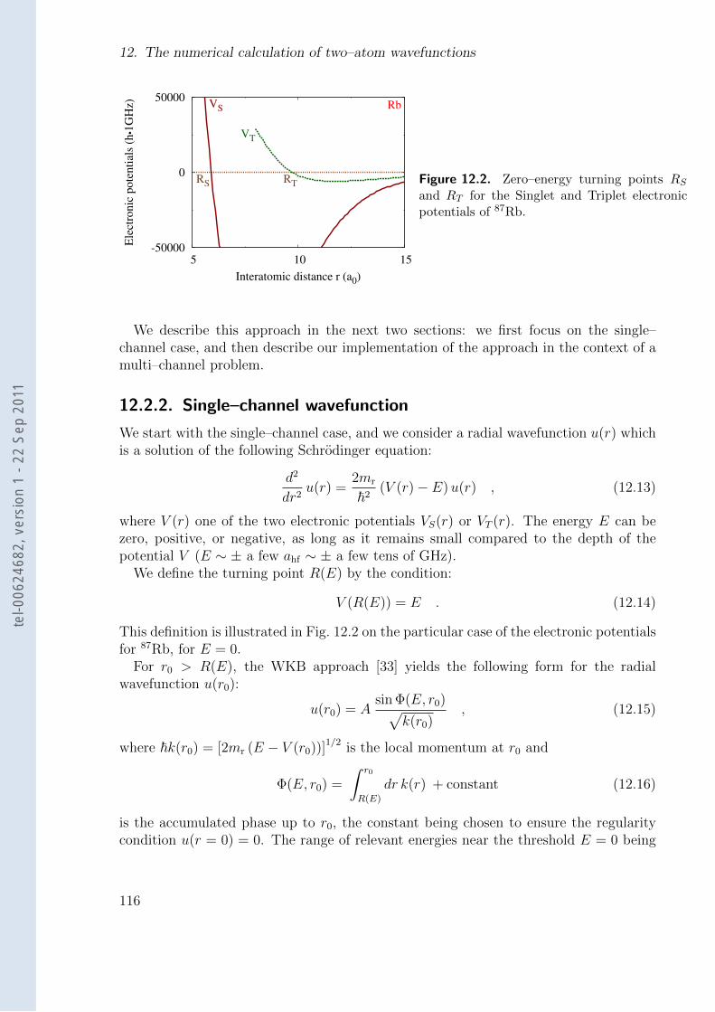
12. The numerical calculation of two–atom wavefunctions

-50000

0

50000

5 10 15

Ele

ctro

nic

pote

nti

als

(h•1

GH

z)

Interatomic distance r (a0)

VS

VT

RS RT

Rb

Figure 12.2. Zero–energy turning points RSand RT for the Singlet and Triplet electronicpotentials of 87Rb.

We describe this approach in the next two sections: we first focus on the single–channel case, and then describe our implementation of the approach in the context of amulti–channel problem.

12.2.2. Single–channel wavefunction

We start with the single–channel case, and we consider a radial wavefunction u(r) whichis a solution of the following Schrodinger equation:

d2

dr2u(r) =

2mr

~2(V (r)− E)u(r) , (12.13)

where V (r) one of the two electronic potentials VS(r) or VT (r). The energy E can bezero, positive, or negative, as long as it remains small compared to the depth of thepotential V (E ∼ ± a few ahf ∼ ± a few tens of GHz).

We define the turning point R(E) by the condition:

V (R(E)) = E . (12.14)

This definition is illustrated in Fig. 12.2 on the particular case of the electronic potentialsfor 87Rb, for E = 0.

For r0 > R(E), the WKB approach [33] yields the following form for the radialwavefunction u(r0):

u(r0) = Asin Φ(E, r0)√

k(r0), (12.15)

where ~k(r0) = [2mr (E − V (r0))]1/2 is the local momentum at r0 and

Φ(E, r0) =

∫ r0

R(E)

dr k(r) + constant (12.16)

is the accumulated phase up to r0, the constant being chosen to ensure the regularitycondition u(r = 0) = 0. The range of relevant energies near the threshold E = 0 being

116

tel-0

0624

682,

ver

sion

1 -

22 S

ep 2

011

12.2. The Accumulated–Phase approach

small, we use a linear approximation to the accumulated phase at r0:

Φ(E, r0) = Φ0 + E ΦE0 + . . . , (12.17)

where Φ0 = Φ(E = 0, r0) and ΦE0 = ∂Φ

∂E

∣∣E=0,r0

.

Choosing r0 > R to be as small as possible (in our calculations, r0 ranges from 10 a0

to 20 a0), while maintaining the validity of the WKB approach, Eqs. (12.15) and (12.17)yield a boundary condition on the logarithmic derivative of u, which is applied at thenon–zero minimal radius r0 but still enforces the regularity condition at r = 0:

u′(r0)

u(r0)=

1

~[2mr (E − V (r0))]1/2

tan(Φ0 + E ΦE0 )

+1

4

V ′(r0)

E − V (r0), (12.18)

where the prime denotes derivation with respect to r.

Calculating the accumulated–phase parameters

For each electronic potential VS or VT , the boundary condition defined by Eq. (12.18)encapsulates all of the short–range Physics into the two real numbers Φ0 and ΦE

0 .The parameter Φ0 is the accumulated phase for E = 0. We adjust it such that the

zero–energy scattering state wavefunction, which behaves like u(r) =√

4π(r − a) forlarge values of r, has the correct scattering length a = aS or aT .

The coefficient ΦE0 has a simple integral expression in terms of the potential V (r) for

R < r < r0. First, we note that both electronic potentials VS and VT are very steepfor energies close to the dissociation threshold (see Fig. 12.2): RT and RS only varysignicantly on a scale of a few hundreds of GHz, whereas the energies relevant to us areof the order of tens of GHz. Therefore we take R(E) ≈ R(E = 0), both for the singletfor the triplet potentials. Now, the energy–derivative of Eq. (12.16) yields [51]:

ΦE0 = ~mr

∫ r0

R(E=0)

dr

[2mr (E − V (r))]1/2, (12.19)

The denominator of the integrand being the local momentum ~k(r). An approximationfor ΦE

0 can be calculated from Eq. (12.19) using the ‘inner parts’ of the electronic poten-tials. For all of the atoms we have considered, this approximation has been sufficientlyaccurate to reproduce the positions of known static–field Feshbach resonances.

12.2.3. Multiple channels

We now move on to the implementation of the accumulated–phase approach in themultiple–channel case.

The scattering problems we are interested in are described by the two–atom Hamil-tonian H and involve multiple scattering channels which are coupled to each other (seeFig. 10.5 for a block–matrix representation of H which illustrates the channel couplingsin the ‘molecular’ basis eM). There is no basis in which these channels uncouple for allvalues of r.

117

tel-0

0624

682,

ver

sion

1 -

22 S

ep 2

011

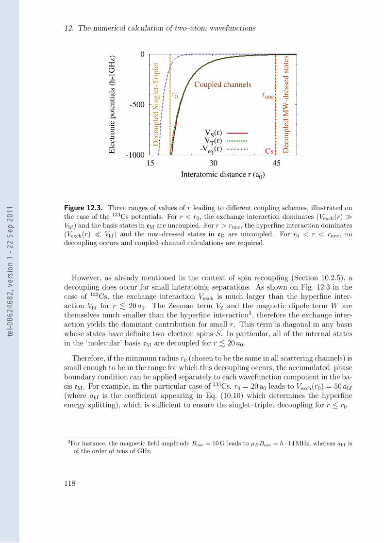
12. The numerical calculation of two–atom wavefunctions

-1000

-500

0

15 30 45

Ele

ctro

nic

pote

nti

als

(h•1

GH

z)

Interatomic distance r (a0)

Dec

ouple

d S

ingle

t-T

riple

t

r0

Dec

ouple

d M

W-d

ress

ed s

tate

s

runc

Coupled channels

Cs

VS(r)VT(r)

-Vex(r)

Figure 12.3. Three ranges of values of r leading to different coupling schemes, illustrated onthe case of the 133Cs potentials. For r < r0, the exchange interaction dominates (Vexch(r) Vhf) and the basis states in eM are uncoupled. For r > runc, the hyperfine interaction dominates(Vexch(r) Vhf) and the mw–dressed states in eD are uncoupled. For r0 < r < runc, nodecoupling occurs and coupled–channel calculations are required.

However, as already mentioned in the context of spin recoupling (Section 10.2.5), adecoupling does occur for small interatomic separations. As shown on Fig. 12.3 in thecase of 133Cs, the exchange interaction Vexch is much larger than the hyperfine inter-action Vhf for r . 20 a0. The Zeeman term VZ and the magnetic dipole term W arethemselves much smaller than the hyperfine interaction3, therefore the exchange inter-action yields the dominant contribution for small r. This term is diagonal in any basiswhose states have definite two–electron spins S. In particular, all of the internal statesin the ‘molecular’ basis eM are decoupled for r . 20 a0.

Therefore, if the minimum radius r0 (chosen to be the same in all scattering channels) issmall enough to be in the range for which this decoupling occurs, the accumulated–phaseboundary condition can be applied separately to each wavefunction component in the ba-sis eM. For example, in the particular case of 133Cs, r0 = 20 a0 leads to Vexch(r0) = 50 ahf

(where ahf is the coefficient appearing in Eq. (10.10) which determines the hyperfineenergy splitting), which is sufficient to ensure the singlet–triplet decoupling for r ≤ r0.

3For instance, the magnetic field amplitude Bosc = 10 G leads to µBBosc = h · 14 MHz, whereas ahf isof the order of tens of GHz.

118

tel-0

0624

682,

ver

sion

1 -

22 S

ep 2

011

12.3. The relaxation method

The adiabatic accumulated phase approach

The accuracy of the accumulated–phase approach can be improved [31] by accountingfor the ‘adiabatic’ mixing between states in eM caused by the hyperfine term for r smallerthan, but close to, r0.

For that purpose, we apply the accumulated–phase approach, not in the basis eM, butin the basis eM which diagonalises Vtot(r0) = (Vtot(r0)−VS(r0)1), keeping in mind that allterms in this matrix other than the exchange interaction Vexch(r0) = (VT (r0) − VS(r0))are small corrections. In particular, this matrix contains Vhf , therefore the use of abasis in which it is diagonal accounts for the contamination due to Vhf . The ‘adiabatic’approximation resides in the fact that, although the basis states in eM no longer havedefinite values of the quantum number S, we still assume that the corresponding spatialcomponents are pure singlet and triplet waves.

In order to identify the ‘singlet’ and ‘triplet’ channels in eM, we note that Vtot(r0)

acting on an electronic–triplet state contains Vexch(r0) > 0, whereas Vtot(r0) acting on anelectronic–singlet state does not. Furthermore, we recall that Vexch(r0) is the dominant

contribution to Vtot(r0). Therefore, introducing NSstates, the number of accessible internal

states which are electronic–singlet, we approximate the spatial parts corresponding tothe NS lowest–energy eigenstates of eM to pure singlet waves, and the spatial partscorresponding to the remaining (N −NS) eigenstates to pure triplet waves.

12.3. The relaxation method

In this section and the next one, we present the two numerical approaches we have usedto calculate two–atom wavefunctions.

As mentioned in the introduction of this chapter, the differential system to be solvedis a two–point boundary–value problem, as it involves boundary conditions at both endsof the integration interval. Two types of approaches are available for the numericalsolution of such problems [52]: (i) relaxation methods and (ii) shooting methods. Wehave experimented with both approaches. We first briefly present an approach based onthe relaxation method.

12.3.1. From a second–order differential system to a first–order one

The Schrodinger equation (12.7) is a system of Nstates coupled second–order differentialequations. Our first step is to rewrite it as a system of 2Nstates coupled first–orderdifferential equations:

Y ′(r) =

(0 1

2mr

~2 (Vtot(r)− εn0) 0

)Y (r) = G(r,Y (r)) with Y (r) =

(Un0(r)U ′n0

(r)

),

(12.20)where the vectors Y (r) andG(r,Y (r)) have 2Nstates–components, and the prime denotesderivation with respect to the variable r.

119

tel-0

0624

682,

ver

sion

1 -

22 S

ep 2

011

12. The numerical calculation of two–atom wavefunctions

12.3.2. Discretisation of the differential system

We choose the integration interval to be [r0, rmax]. The lower bound r0 > 0 is the radiusat which the accumulated phase boundary condition is applied: we choose r0 = 10 a0 for7Li, r0 = 16 a0 for 23Na, 41K, and 87Rb, and r0 = 20 a0 for 133Cs. The upper bound rmax

is chosen to be sufficiently large for the total potential matrix Vtot(rmax) (Eq. (12.1) tohave reached its asymptotic value V∞, given by Eq. (12.2): we choose rmax = 1000 a0 forall considered atoms.

The relaxation method is based on the use of a mesh representing the integrationinterval. Following [52], we use an evenly–spaced mesh. The density of mesh pointsmust be sufficiently large to accomodate for the oscillating behaviour of the wavefunc-tion for small values of r (see Figs. 11.5): our implementation uses Mpoints = 4 · 105

mesh points evenly spaced from r0 to rmax. The sought solution Y (r) is represented by(2NstatesMpoints) numbers, giving the values of the 2Nstates components Yj(rk) at each ofthe Mpoints mesh points rk (0 ≤ k ≤Mpoints − 1).

The relaxation method replaces the 2Nstates coupled equations (12.20) by finite–differenceequations at each mesh point. The finite–difference at the mesh point xk (1 ≤ k ≤M−1)reads:

Yk − Yk−1 − (rk − rk−1)G

(rk−1 + rk

2,Yk−1 + Yk

2

)= 0 , (12.21)

where the vectors Yk−1 and Yk have 2Nstates components and give the numerical valuesfor the 2Nstates coupled waves at the mesh points rk−1 and rk. There are 2Nstates(Mpoints−1) such finite–difference equations; the boundary conditions provide 2Nstates additionalequations. Therefore, the discretisation process leads to 2NstatesMpoints coupled equationsfor an equal number of unknowns.

We solve these coupled equations using an iterative ‘relaxation’ procedure based onthe multidimensional Newton method [52], exploiting the strong sparsity and the specificblock structure of the linear systems involved.

12.3.3. Stability of the relaxation method

This first approach is the approach we have used for all of the numerical results presentedin the published article of Chapter 13. Our choice of this method was due to the followingremark (point 3 in the introduction of this chapter). The solutions of the Schrodingerequation (12.7) may asymptotically involve both growing exponentials exp(+κpr) ordecaying exponentials exp(−κpr), in all closed channels p > n0. The only physically–acceptable solution is the one which can be normalised, i.e. the one which involves onlydecaying exponentials. However, the existence of the unacceptable ‘growing’ solutionsmay contaminate the numerical calculation of the ‘decaying’ one. The use of relaxationmethods helps to avoid such a contamination, because of its enforcing conditions at eachmesh point (rather than only at the two ends of the integration interval).

120

tel-0

0624

682,

ver

sion

1 -

22 S

ep 2

011

12.4. An approach based on the shooting method

12.3.4. Limitations of our implementation

The use of an evenly–spaced mesh, in conjunction with the oscillatory nature of thewavefunction components for small values of r, causes our implementation to requirea large number of mesh points. Most of these mesh points are located in the large–rregion, where a comparable accuracy could be obtained with a much smaller mesh pointdensity. This issue could be solved by using a mesh with variable step sizes.

The present implementation (using evenly–spaced meshes) leads to long relaxationtimes. For example, each graph represented on Fig. 11.12, which results from calculationsinvolving 8 coupled internal states (see Section 11.2), took several days to obtain. Such aslow convergence prohibits the use of this method for problems involving larger numbersof coupled internal states, such as the static–field resonances of Chapter 14 (up to 14coupled states) or the microwave–induced resonances involving the (MF = 0) subspacepresented in Chapter 15 (48 coupled states).

Finally, this approach does not make use of the uncoupling which occurs for relativelylarge r: as shown on Fig. 12.3 for 133Cs, the exchange interaction is negligible comparedto the hyperfine energy term for distances greater than runc ≈ 45 a0 (in the case of133Cs, the choice of runc = 45 a0 yields Vexch(rmax) = 10−8 ahf). Therefore, even thoughthe electronic potentials have not yet completely vanished, the electronic term Vel isdiagonal in any basis, and the channels all decouple in the dressed–state basis eD.

Our second approach, described in the next section, is not affected by any of theselimitations.

12.4. An approach based on the shooting method

In this last section, we describe the second approach we have used for the numericalcalculation of two–atom wavefunctions. This second approach has been implemented tocircumvent the limitations of the relaxation method described in Section 12.3: it doesnot use a mesh with a fixed step, it exploits the linearity of the differential system definedby Eq. (12.20) and the uncoupling that occurs for r > runc, and it runs considerablyfaster than our relaxation codes.

For this second approach, we abandon the ‘relaxation’ method of Section 12.3 andturn towards a ‘shooting’ scheme. We also relinquish the first–order differential systemof Eq. (12.20), and go back to the original radial Schrodinger equation (12.7).

We operate on the integration interval [r0, rmax], defined in Section 12.3.2. We do notmanually discretise this interval.

12.4.1. Two standard ‘shooting’ methods

We first briefly describe two standard methods involving ‘shooting’: the basic ‘shooting’method and ‘shooting towards a fitting point’ [52].

In its basic implementation, the ‘shooting’ method consists in choosing ‘guess’ valuesfor the Nstates components of the wavefunction U(r0) and those of its derivative U ′(r0)such that the boundary conditions at the lower bound r0 are satisfied. The solution

121

tel-0

0624

682,

ver

sion

1 -

22 S

ep 2

011

12. The numerical calculation of two–atom wavefunctions

is then ‘propagated’, using any initial–value differential equation solver, through theintegration interval towards the upper bound rmax. This ‘shot’ is successful if the com-ponents of U(rmax) and U ′(rmax) satisfy the boundary conditions at rmax. If the ‘shot’is not successful, the initial ‘guess’ values are improved (for example, using Newton’smethod for finding the zeros of a multi–variable function), and the whole procedure isiterated until a successful ‘shot’ is fired.

A more elaborate approach, called ‘shooting towards a fitting point’, involves thechoice of an intermediate ‘fitting point’ rfit within the integration interval [r0, rmax].‘Guesses’ are made for the wavefunction components and derivatives at the lower boundr0, chosen such that the boundary conditions at r0 are satisfied; the solution is ‘prop-agated’, in the increasing–r direction, up to rfit. Similarly, ‘guesses’ are made for thewavefunction components at rmax satisfying the boundary conditions at that point; thesolution is ‘propagated’, in the decreasing–r direction, down to rfit. The ‘double–shot’ issuccessful if the wavefunction components and derivatives obtained at rfit through theforward and backward propagations are equal. If it is not successful, the ‘guess’ valuesat r0 and rmax are improved, and the whole procedure is iterated until the backward–and forward–propagated solutions match at rfit.

12.4.2. Shooting and fitting for a linear problem

The ‘shooting’ approach implemented in our program is a variant of ‘shooting towardsa fitting point’, which we have adapted to the case of a linear problem in order tocircumvent the need for iterations.

The radial Schrodinger equation (12.7) is a system of Nstates coupled second–orderSchrodinger equations. We call En0 its set of solutions, which is a 2Nstates–dimensionalvector space.

Calculating basis solutions

As in the standard ‘shooting to a fitting point’ method, we introduce a ‘fitting radius’ rfit

within the integration interval [r0, rmax]. The choice of the value of rfit will be discussedin Section 12.4.3.

The Nstates accumulated–phase boundary conditions applied at r0 (see Section 12.2)define an Nstates–dimensional subspace of En0 . We calculate a basis of Nstates indepen-dent functions (Xi(r)), each of which satisfies the Nstates accumulated–phase boundaryconditions. These functions are determined, for r0 ≤ r ≤ rfit, by integrating in theincreasing–r direction starting from initial values at r0.

We now turn to the boundary conditions at the upper bound rmax. The number of openchannels (including the zero–energy entrance channel) is n0; we call Ncl = Nstates − n0

the number of closed channels. We first focus on the closed–channel components. The

122

tel-0

0624

682,

ver

sion

1 -

22 S

ep 2

011

12.4. An approach based on the shooting method

large–r boundary condition:

〈Dm |Y (r) 〉 = 0 for m < n0 (open channel) (12.22a)

〈Dn0 |Y (r) 〉 = 0 (entrance channel) (12.22b)

〈Dp |Y (r) 〉 =√

4π Ap exp(−κpr) for p > n0 (closed channel), (12.22c)

where the (Ap)’s are arbitrary numbers and the (κp)’s are defined as in Section 12.1.3,define an Ncl–dimensional subspace of En0 , for which we calculate a basis (Yj(r))1≤j≤Ncl

.Next, we focus on the open–channel components (including the zero–energy entrance

channel n0). The large–r boundary conditions

〈Dm |Z(r) 〉 =√

4π Bm exp(ikmr) for m < n0 (open channel) (12.23a)

〈Dn0 |Z(r) 〉 =√

4π Bn0 (entrance channel) (12.23b)

〈Dp |Z(r) 〉 = 0 for p > n0 (closed channel), (12.23c)

where the (Bm)’s are arbitrary numbers and the (km)’s are defined as in Section 12.1.3,define an n0–dimensional subspace of En0 , for which we calculate a basis (Zl(r))1≤l≤Ncl

.Finally, we calculate the single function T (r), defined by the large–r boundary con-

dition:

〈Dm |T (r) 〉 = 0 for m < n0 (open channel) (12.24a)

〈Dn0 |T (r) 〉 =√

4π r (entrance channel) (12.24b)

〈Dp |T (r) 〉 = 0 for p > n0 (closed channel). (12.24c)

The functions (Yj(r)), (Zl(r)) and T (r) are determined, for rfit ≤ r ≤ rmax, by integrat-ing in the decreasing–r direction starting from initial values at rmax.

Note that the numerical calculation of the functions (Xi), (Yj), (Zl), and T onlyinvolves boundary conditions at one end of the integration interval (i.e. they are nottwo–point boundary value problems). Therefore, it can be performed using any of thestandard numerical solvers for differential equations. We use an algorithm, based onStoermer’s rule [52], which is optimised for second–order systems of the form y′′ = f(r,y)(where the first–order derivative y′ does not appear). Our implementation includesadaptive stepsize control: the discretisation of the intervals [r0, rfit] and [rfit, rmax] isdone automatically, with an r–dependent step size that is chosen to improve accuracyand efficiency.

Calculating the physical wavefunction

The ‘physical’ wavefunction U(r), defined for r0 ≤ r ≤ rmax, is the function in En0 whichsatisfies both the accumulated–phase boundary conditions of Section 12.2 and the large–r behaviour of Eqs. (12.8). For values of r smaller than rfit, it is a linear combination ofthe (Xi)’s:

U(r) =Nstates∑i=1

xiXi(r) for r0 ≤ r ≤ rfit. (12.25)

123

tel-0

0624

682,

ver

sion

1 -

22 S

ep 2

011

12. The numerical calculation of two–atom wavefunctions

For r ≥ rfit, it can be expressed in terms of the (Yj)’s, (Zl)’s and T :

U(r) =

Ncl∑j=1

yj Yj(r) +

n0∑k=1

zkZl(r) + T (r) for r0 ≥ r ≤ rfit. (12.26)

The requirement that both U(r) and U ′(r) be continuous at the fitting point r =rfit yields a linear system of 2Nstates equations which determines the 2Nstates complexcoefficients (xi)1≤i≤Nstates , (yj)1≤j≤Ncl

, and (zk)1≤k≤n0 .

12.4.3. Exploiting the large–r uncoupling of the dressed two–atomstates

We have already mentioned (see Section 12.3.4) that the fast decay of the exchangeinteraction Vexch(r) (see Eq. (12.12)) and Fig. 12.3) causes the electronic interactionterm Vel(r) to become spin–independent for r ≥ runc, where runc is of the order of afew tens of a0 (we take runc = 45 a0 for 133Cs). This causes the channels defined by thedressed two–atom states (|Dn 〉) to become uncoupled for r ≥ runc.

In order to take advantage of this uncoupling, we choose the fitting point rfit to be equalto the uncoupling radius runc. Suitable choices of the values at rmax for the functions(Yj), (Zl), T , and their derivatives, thus reduces their calculation, for rfit ≤ r ≤ rmax,to single–channel calculations. The large–r boundary conditions for T are specified byEqs. (12.24). We choose the following values at rmax for the functions (Yj)1≤j≤Ncl

and(Zl)1≤l≤n0 :

〈Dn |Yj(rmax) 〉 = δn,(n0+j) and 〈Dn |Y ′j (rmax) 〉 = −κ(n0+j) δn,(n0+j) (12.27a)

〈Dn |Zl(rmax) 〉 = δn,l and 〈Dn |Z ′l(rmax) 〉 = ikl δn,l (12.27b)

In Equation (12.27b), we use the convention kn0 = 0 for the entrance channel, so that|Yn0(r) 〉 is asymptotically equal to |∆n0 〉 for large values of r. The scattering length ais directly related to the corresponding (complex) coefficient zn0 :

zn0 = −√

4π a , (12.28)

as can be obtained from the asymptotic behaviour of Eq. (12.26).

12.4.4. Accounting for the fast exponential decay in closed channels

When projected in the dressed–state basis, the closed channel components asymptoti-cally behave like decaying exponentials exp(−κpr) (see for instance Eqs. (12.22)). If κpis large (i.e. if the channel energy εp is large), the integration in the decreasing–r direc-tion starting from the boundary condition of Eq. (12.27a) will quickly yield very largenumerical values for Yj(r), which may cause numerical instabilities. We now explainhow to avoid these instabilities.

124

tel-0

0624

682,

ver

sion

1 -

22 S

ep 2

011

12.4. An approach based on the shooting method

We focus on a closed channel |Dp 〉 with a large channel energy εp. More specifically,we assume that

VS,T (rfit) + εp > εn0 . (12.29)

We consider the function Yj(r), defined for rfit ≤ r ≤ rmax by the boundary condition ofEq. (12.27a) and the single–channel Schrodinger equation:

Y ′′j (r) =2mr

~2(V p

tot(r)− εn0)Yj(r) , (12.30)

where j = p − n0, Yj(r) = 〈Dp |Yj(r) 〉, and V ptot(r) = 〈Dp |Vtot(r)|Dp 〉. The condi-

tion (12.29) ensures that the potential term (V ptot(r) − εn0) appearing in Eq. (12.30)

never goes to zero. It is then readily seen4 that Yj(r) never goes to 0 for rfit ≤ r ≤ rmax.Therefore, we introduce the logarithmic derivative Wj(r) of the function Yj(r), definedby:

Wj(r) =Y ′j (r)

Yj(r). (12.31)

The Schrodinger equation (12.30) translates onto Wj(r) as the following first–orderequation:

W ′j(r) +W 2

j (r) = (V ptot(r)− εn0) , (12.32)

and the boundary condition at rmax (Eq. 12.27a) reduces to Wj(rmax) = −κp. Thefunction Wj(r), being related to the logarithm of Yj(r), is no longer very large for valuesof r close to rfit.

When solving the linear system of Section 12.4.2 giving the values of the coefficients(xi), (yj), and (zk), the values of Yj(rfit) and Y ′j (rfit) can be replaced by 1 and Wj(rfit),respectively: this amounts to changing the boundary conditions (12.27a) to include theadditional condition Yj(rfit) = 1.

12.4.5. Calculating complex wavefunctions using real basisfunctions

We have already pointed out in Section 12.1.5 that the ‘physical’ wavefunction U(r)is real in the absence of inelastic processes, but that it becomes non–real as soon asinelastic processes are present, i.e. as soon one of open the open channels |Dm 〉 satisfiesεm < E, where E is the energy of the colliding atom pair.

We now show that such a complex wavefunction may be calculated from functions(Xi(r)), (Yj(r)), T (r), and functions related to the (Zl(r)) which are all real.

We recall that the total potential operator Vtot(r) is a real matrix for all values of r.Additionally, the boundary conditions (12.24) and (12.27a), respectively defining T (r)and the functions (Yj(r)), are real, therefore the functions T (r) and (Yj(r)) are real for

4The value Yj(rmax) > 0. Integrating from rmax back towards rfit, Eq. (12.30) shows that, as long asYj(r) does not change signs, its second derivative Y ′′j (r) is positive. This entails that Y ′j (r) < 0 and,hence, that the function goes farther away from zero when r decreases towards rfit.

125

tel-0

0624

682,

ver

sion

1 -

22 S

ep 2

011

12. The numerical calculation of two–atom wavefunctions

rfit ≤ r ≤ rmax. Similarly, the boundary conditions at r0 defining the functions (Xi(r))can be chosen to be real, which leads to the (Xi(r))’s being real for r0 ≤ r ≤ rmax.

The boundary condition (12.27b), defining the functions (Zl(r)) for 1 ≤ l < n0, arenon–real, and thus lead to non–real solutions. However, each of the complex (Zl(r))’sis a linear combination of two real functions in En0 :

For 1 ≤ l < n0, Zl(r) = Zcl (r) + iZs

l (r) , (12.33)

where Zcl (r) and Zc

l (r) are defined by the following real boundary conditions at rmax:

〈Dn |Zcl (rmax) 〉 = cos(kl rmax) δn,l and 〈Dn |Zc ′

l (rmax) 〉 = − sin(kl rmax) δn,l ,(12.34a)

〈Dn |Zsl (rmax) 〉 = sin(kl rmax) δn,l and 〈Dn |Zs ′

l (rmax) 〉 = cos(kl rmax) δn,l .(12.34b)

This remark allows the calculation of the (n0− 1) complex functions (Zl)1≤l<n0 in termsof the 2(n0 − 1) real functions (Zc

l )1≤l<n0 and (Zsl )1≤l<n0 .

12.5. Summary

In this chapter, we have presented the two approaches we have used for the numeri-cal calculation of two–atom wavefunctions. Both of them use the accumulated–phaseapproach (Section 12.2) to encapsulate the short–range physics into a boundary condi-tion applied at a non–zero radius r0 for which the singlet and triplet potentials are wellknown.

Our first approach (Section 12.3) is based on the relaxation method for the solutionof two–point boundary–value problems (first challenge mentioned in the Introduction).This method is stable and accurate, but it requires a very fine mesh to accomodatefor the short–range oscillations of the wavefunction. It is thus ill–suited for problemsinvolving many coupled channels, such as the ones involved in Chapters 14 and 15.

Our second approach (Section 12.4) is based on the shooting method. It is much fasterthan our relaxation approach. It exploits the linearity of the Schrodinger equationas well as the large–r uncoupling of the dressed two–atom states. It allows for thedescription of inelastic processes through the calculation of complex wavefunctions. Ityields an accurate evaluation of the exponentially–decaying closed–channel components.It requires no iteration: the physical wavefunction is determined as a linear combinationof (Nstates+Ncl+2n0) real solutions of the Schrodinger equation, among which (Ncl+2n0)involve a single channel.

Our first method has been used for all numerical calculations presented in the pub-lished paper of Chapter 13. These calculations involved at most eight coupled channels.

Chapter 14 is devoted to the characterisation of Feshbach resonances in 133Cs inducedby small static magnetic fields: this characterisation requires coupled–channel calcu-lations involving up to fourteen coupled channels. Chapter 15 focuses on microwave–induced Feshbach resonances involving two 133Cs atoms whose incident state asymptot-ically belongs to the (MF = 0) subspace. These resonances involve inelastic processes

126

tel-0

0624

682,

ver

sion

1 -

22 S

ep 2

011

12.5. Summary

(and hence non–real wavefunctions), and the corresponding calculations include up toforty–eight coupled channels. Our second method has been used for all numerical cal-culations presented in both of these chapters.

127

tel-0

0624

682,

ver

sion

1 -

22 S

ep 2

011

tel-0

0624

682,

ver

sion

1 -

22 S

ep 2

011

13. Article 2: Microwave–InducedFano–Feshbach resonances

129

tel-0

0624

682,

ver

sion

1 -

22 S

ep 2

011

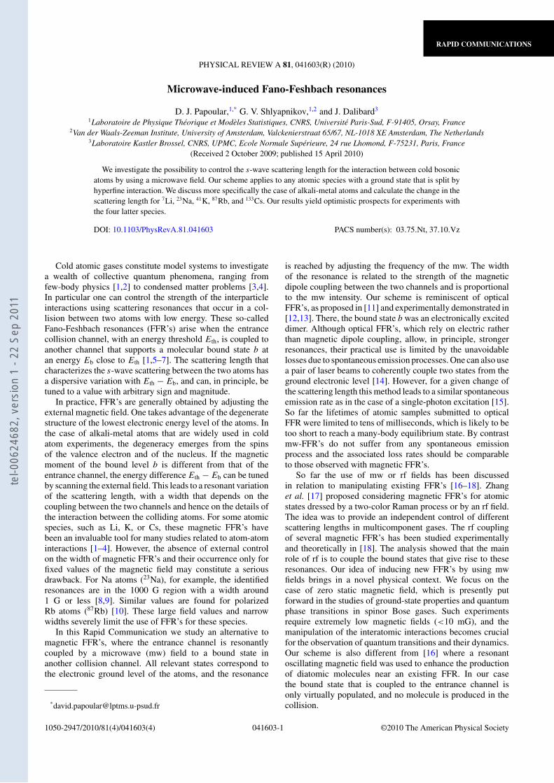
RAPID COMMUNICATIONS

PHYSICAL REVIEW A 81, 041603(R) (2010)

Microwave-induced Fano-Feshbach resonances

D. J. Papoular,1,* G. V. Shlyapnikov,1,2 and J. Dalibard3

1Laboratoire de Physique Theorique et Modeles Statistiques, CNRS, Universite Paris-Sud, F-91405, Orsay, France2Van der Waals-Zeeman Institute, University of Amsterdam, Valckenierstraat 65/67, NL-1018 XE Amsterdam, The Netherlands

3Laboratoire Kastler Brossel, CNRS, UPMC, Ecole Normale Superieure, 24 rue Lhomond, F-75231, Paris, France(Received 2 October 2009; published 15 April 2010)

We investigate the possibility to control the s-wave scattering length for the interaction between cold bosonicatoms by using a microwave field. Our scheme applies to any atomic species with a ground state that is split byhyperfine interaction. We discuss more specifically the case of alkali-metal atoms and calculate the change in thescattering length for 7Li, 23Na, 41K, 87Rb, and 133Cs. Our results yield optimistic prospects for experiments withthe four latter species.

DOI: 10.1103/PhysRevA.81.041603 PACS number(s): 03.75.Nt, 37.10.Vz

Cold atomic gases constitute model systems to investigatea wealth of collective quantum phenomena, ranging fromfew-body physics [1,2] to condensed matter problems [3,4].In particular one can control the strength of the interparticleinteractions using scattering resonances that occur in a col-lision between two atoms with low energy. These so-calledFano-Feshbach resonances (FFR’s) arise when the entrancecollision channel, with an energy threshold Eth, is coupled toanother channel that supports a molecular bound state b atan energy Eb close to Eth [1,5–7]. The scattering length thatcharacterizes the s-wave scattering between the two atoms hasa dispersive variation with Eth − Eb, and can, in principle, betuned to a value with arbitrary sign and magnitude.

In practice, FFR’s are generally obtained by adjusting theexternal magnetic field. One takes advantage of the degeneratestructure of the lowest electronic energy level of the atoms. Inthe case of alkali-metal atoms that are widely used in coldatom experiments, the degeneracy emerges from the spinsof the valence electron and of the nucleus. If the magneticmoment of the bound level b is different from that of theentrance channel, the energy difference Eth − Eb can be tunedby scanning the external field. This leads to a resonant variationof the scattering length, with a width that depends on thecoupling between the two channels and hence on the details ofthe interaction between the colliding atoms. For some atomicspecies, such as Li, K, or Cs, these magnetic FFR’s havebeen an invaluable tool for many studies related to atom-atominteractions [1–4]. However, the absence of external controlon the width of magnetic FFR’s and their occurrence only forfixed values of the magnetic field may constitute a seriousdrawback. For Na atoms (23Na), for example, the identifiedresonances are in the 1000 G region with a width around1 G or less [8,9]. Similar values are found for polarizedRb atoms (87Rb) [10]. These large field values and narrowwidths severely limit the use of FFR’s for these species.

In this Rapid Communication we study an alternative tomagnetic FFR’s, where the entrance channel is resonantlycoupled by a microwave (mw) field to a bound state inanother collision channel. All relevant states correspond tothe electronic ground level of the atoms, and the resonance

*david.papoular@lptms.u-psud.fr

is reached by adjusting the frequency of the mw. The widthof the resonance is related to the strength of the magneticdipole coupling between the two channels and is proportionalto the mw intensity. Our scheme is reminiscent of opticalFFR’s, as proposed in [11] and experimentally demonstrated in[12,13]. There, the bound state b was an electronically exciteddimer. Although optical FFR’s, which rely on electric ratherthan magnetic dipole coupling, allow, in principle, strongerresonances, their practical use is limited by the unavoidablelosses due to spontaneous emission processes. One can also usea pair of laser beams to coherently couple two states from theground electronic level [14]. However, for a given change ofthe scattering length this method leads to a similar spontaneousemission rate as in the case of a single-photon excitation [15].So far the lifetimes of atomic samples submitted to opticalFFR were limited to tens of milliseconds, which is likely to betoo short to reach a many-body equilibrium state. By contrastmw-FFR’s do not suffer from any spontaneous emissionprocess and the associated loss rates should be comparableto those observed with magnetic FFR’s.

So far the use of mw or rf fields has been discussedin relation to manipulating existing FFR’s [16–18]. Zhanget al. [17] proposed considering magnetic FFR’s for atomicstates dressed by a two-color Raman process or by an rf field.The idea was to provide an independent control of differentscattering lengths in multicomponent gases. The rf couplingof several magnetic FFR’s has been studied experimentallyand theoretically in [18]. The analysis showed that the mainrole of rf is to couple the bound states that give rise to theseresonances. Our idea of inducing new FFR’s by using mwfields brings in a novel physical context. We focus on thecase of zero static magnetic field, which is presently putforward in the studies of ground-state properties and quantumphase transitions in spinor Bose gases. Such experimentsrequire extremely low magnetic fields (<10 mG), and themanipulation of the interatomic interactions becomes crucialfor the observation of quantum transitions and their dynamics.Our scheme is also different from [16] where a resonantoscillating magnetic field was used to enhance the productionof diatomic molecules near an existing FFR. In our casethe bound state that is coupled to the entrance channel isonly virtually populated, and no molecule is produced in thecollision.

1050-2947/2010/81(4)/041603(4) 041603-1 ©2010 The American Physical Society

tel-0

0624

682,

ver

sion

1 -

22 S

ep 2

011

RAPID COMMUNICATIONS

D. J. PAPOULAR, G. V. SHLYAPNIKOV, AND J. DALIBARD PHYSICAL REVIEW A 81, 041603(R) (2010)

FIG. 1. (Color online) Fano-Feshbach resonance in a collisionbetween two atoms, induced by an oscillatory magnetic field. Ifthe mw frequency ω approaches the energy difference between theincident scattering state and a weakly bound dimer state, the pair ofatoms undergoes virtual spin-flip transitions which cause a resonantvariation of the scattering length with ω.

For simplicity we study in the following a collision betweentwo identical bosonic atoms prepared in the same internal state.Our treatment can be straightforwardly extended to fermionicparticles and to mixtures of atoms in different internal states.More specifically, we consider alkali-metal atoms whoseground level is split by the hyperfine interaction into twosublevels with total spins f+ = i + 1/2 and f− = i − 1/2,where i is the nuclear spin. The frequency ω of the mw field ischosen close to the hyperfine splitting Ehf between these twosublevels (see Fig. 1). The various collision channels can thenbe grouped into three categories corresponding to asymptoticstates with (i) both atoms in f+, (ii) one atom in f+ and one inf−, and (iii) both atoms in f−. We consider in the following thecase of a f−f− collision and the mw induces a quasiresonanttransition to a bound state in a potential from the f+f− groupas shown in Fig. 1.

We describe the system in the center-of-mass frame of theatom pair. Neglecting the weak coupling between the atomicspins, the atom-atom interaction is spatially isotropic. Welimit our analysis to s-wave collisions governed by the radialHamiltonian (see [19] and references therein)

H = p2

2µ+ Vc(r) + Vhf + hω a†a + W = H0 + W, (1)

where r is the interatomic distance, p is its conjugatemomentum, and µ = m/2 is the reduced mass of the atom pair.The central part Vc(r) of the interaction is given by Vc(r) =VS(r)PS + VT (r)PT , where PS and PT are the projectionoperators onto the electronic-singlet and triplet subspaces. Theterm Vhf = ahf(s1i1 + s2i2) is the hyperfine interaction, wheresj and ij stand for the spin operators of the electron and nucleusof atom j . We use a quantum description for the mw field anda† is the creation operator for an mw photon in the relevantmode. The magnetic dipole interaction between the atoms andthe mw is W = −MB, where M is the total magnetic dipoleoperator of the atom pair and B = b0(εa + ε∗a†)/

√2 is the

magnetic field operator for the mode of polarization ε. As usual

in the dressed-atom approach [20], the amplitude b0 and thenumber of photons N in the mw mode are arbitrary. The onlyrelevant physical quantity is the amplitude of the applied mwfield B0 = b0

√N (with N 1). We assume that the magnetic

field is σ+ polarized with respect to the quantization axis ez.1

The valence electron in each atom has zero angular momentumand W reduces to2

W = W1 (S+ a + S− a†), (2)

where W1 =µBb0/h, µB is the Bohr magneton and S± =Sx ±iSy , with S= s1+s2 being the total electron spin.

We study the scattering properties of H using two differentmethods: (i) if the mw Rabi frequency µBB0 is much smallerthan the binding energy |ET | of the dimer and the level spacingin the closed channel, the scattering is well described by asingle-resonance two-channel model; (ii) for µBB0 |ET |, amore general description is obtained through a full coupled-channel calculation.

We first describe method (i). We consider H as a two-channel model [1] where H0 is the bare Hamiltonian andW is the coupling operator. The symmetries of H0 allowthe choice of bare open- and closed-channel wave functionswhich have well-defined photon numbers N , total spin F ,and total spin projection MF along the quantization axis (F =s1 + i1 + s2 + i2), whereas W directly couples subspaces withMF = −N = ±1. The coupling term W does not vanishin the limit of infinitely separated atoms. Hence, there is adifference in the scattering threshold energy of H comparedto that of H0. If the detuning δ of the mw with respect to thesingle-atom hyperfine splitting Ehf is greater than µBB0, then ∼ (µBB0)2/δ. Method (i) is applicable when |ET |and can be neglected. Near resonance, where |δ| ∼ |ET |, thiscondition requires µBB0 |ET |.

We start by stating a selection rule associated withW . All internal states in the MF = 2i + 1 and MF =2i subspaces are electronic-triplet states. More precisely,the MF = 2i + 1 subspace has dimension one, with|S = 1, I = 2i, F = 2i + 1,MF = 2i + 1〉 as a basis vector(I determines the modulus of the total nuclear spin I =i1 + i2). The MF = 2i subspace has dimension two,3 andit is spanned by |η1〉 = |S = 1, I = 2i, F = 2i,MF = 2i〉and |η2〉 = |S = 1, I = 2i, F = 2i + 1,MF = 2i〉. The spa-tial components of the eigenfunctions of H0 in these subspacesdecouple from the internal states and are all eigenfunctions ofthe triplet Hamiltonian HT = p2/2µ + VT (r). The bare open-and closed-channel spatial wave functions are thus orthogonal.The operator W does not act on the spatial parts of the wavefunctions. Hence, its matrix element between an open-channelstate with MF = 2i and a bound state with MF = 2i + 1 is

1This restriction leads to simpler algebra, but is not essential: anypolarization can be decomposed into σ± components and, for a givenω, only one of the components will induce the desired resonantcoupling to a bound state.

2In Eq. (2) we omit a small coupling of the mw to the nuclear spinswhich does not affect the results.

3For s-wave collisions between bosons, only symmetric internalstates are relevant.

041603-2

tel-0

0624

682,

ver

sion

1 -

22 S

ep 2

011

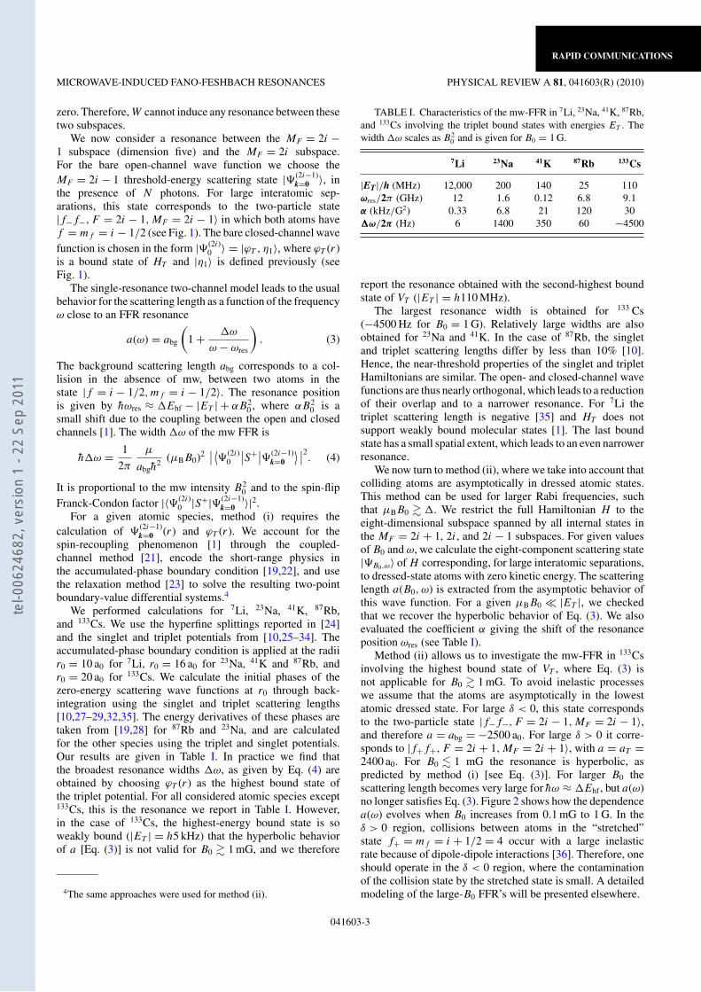
RAPID COMMUNICATIONS

MICROWAVE-INDUCED FANO-FESHBACH RESONANCES PHYSICAL REVIEW A 81, 041603(R) (2010)

zero. Therefore, W cannot induce any resonance between thesetwo subspaces.

We now consider a resonance between the MF = 2i −1 subspace (dimension five) and the MF = 2i subspace.For the bare open-channel wave function we choose theMF = 2i − 1 threshold-energy scattering state |(2i−1)

k=0 〉, inthe presence of N photons. For large interatomic sep-arations, this state corresponds to the two-particle state|f−f−, F = 2i − 1,MF = 2i − 1〉 in which both atoms havef = mf = i − 1/2 (see Fig. 1). The bare closed-channel wavefunction is chosen in the form |(2i)

0 〉 = |ϕT , η1〉, where ϕT (r)is a bound state of HT and |η1〉 is defined previously (seeFig. 1).

The single-resonance two-channel model leads to the usualbehavior for the scattering length as a function of the frequencyω close to an FFR resonance

a(ω) = abg

(1 + ω

ω − ωres

). (3)

The background scattering length abg corresponds to a col-lision in the absence of mw, between two atoms in thestate |f = i − 1/2,mf = i − 1/2〉. The resonance positionis given by hωres ≈ Ehf − |ET | + αB2

0 , where αB20 is a

small shift due to the coupling between the open and closedchannels [1]. The width ω of the mw FFR is

hω = 1

2π

µ

abgh2 (µBB0)2

∣∣ ⟨(2i)0

∣∣S+∣∣(2i−1)k=0

⟩ ∣∣2. (4)

It is proportional to the mw intensity B20 and to the spin-flip

Franck-Condon factor |〈(2i)0 |S+|(2i−1)

k=0 〉|2.For a given atomic species, method (i) requires the

calculation of (2i−1)k=0 (r) and ϕT (r). We account for the

spin-recoupling phenomenon [1] through the coupled-channel method [21], encode the short-range physics inthe accumulated-phase boundary condition [19,22], and usethe relaxation method [23] to solve the resulting two-pointboundary-value differential systems.4

We performed calculations for 7Li, 23Na, 41K, 87Rb,and 133Cs. We use the hyperfine splittings reported in [24]and the singlet and triplet potentials from [10,25–34]. Theaccumulated-phase boundary condition is applied at the radiir0 = 10 a0 for 7Li, r0 = 16 a0 for 23Na, 41K and 87Rb, andr0 = 20 a0 for 133Cs. We calculate the initial phases of thezero-energy scattering wave functions at r0 through back-integration using the singlet and triplet scattering lengths[10,27–29,32,35]. The energy derivatives of these phases aretaken from [19,28] for 87Rb and 23Na, and are calculatedfor the other species using the triplet and singlet potentials.Our results are given in Table I. In practice we find thatthe broadest resonance widths ω, as given by Eq. (4) areobtained by choosing ϕT (r) as the highest bound state ofthe triplet potential. For all considered atomic species except133Cs, this is the resonance we report in Table I. However,in the case of 133Cs, the highest-energy bound state is soweakly bound (|ET | = h5 kHz) that the hyperbolic behaviorof a [Eq. (3)] is not valid for B0 1 mG, and we therefore

4The same approaches were used for method (ii).

TABLE I. Characteristics of the mw-FFR in 7Li, 23Na, 41K, 87Rb,and 133Cs involving the triplet bound states with energies ET . Thewidth ω scales as B2

0 and is given for B0 = 1 G.

7Li 23Na 41K 87Rb 133Cs

|ET|/h (MHz) 12,000 200 140 25 110ωres/2π (GHz) 12 1.6 0.12 6.8 9.1α (kHz/G2) 0.33 6.8 21 120 30ω/2π (Hz) 6 1400 350 60 −4500

report the resonance obtained with the second-highest boundstate of VT (|ET | = h110 MHz).

The largest resonance width is obtained for 133 Cs(−4500 Hz for B0 = 1 G). Relatively large widths are alsoobtained for 23Na and 41K. In the case of 87Rb, the singletand triplet scattering lengths differ by less than 10% [10].Hence, the near-threshold properties of the singlet and tripletHamiltonians are similar. The open- and closed-channel wavefunctions are thus nearly orthogonal, which leads to a reductionof their overlap and to a narrower resonance. For 7Li thetriplet scattering length is negative [35] and HT does notsupport weakly bound molecular states [1]. The last boundstate has a small spatial extent, which leads to an even narrowerresonance.

We now turn to method (ii), where we take into account thatcolliding atoms are asymptotically in dressed atomic states.This method can be used for larger Rabi frequencies, suchthat µBB0 . We restrict the full Hamiltonian H to theeight-dimensional subspace spanned by all internal states inthe MF = 2i + 1, 2i, and 2i − 1 subspaces. For given valuesof B0 and ω, we calculate the eight-component scattering state|B0,ω〉 of H corresponding, for large interatomic separations,to dressed-state atoms with zero kinetic energy. The scatteringlength a(B0, ω) is extracted from the asymptotic behavior ofthis wave function. For a given µBB0 |ET |, we checkedthat we recover the hyperbolic behavior of Eq. (3). We alsoevaluated the coefficient α giving the shift of the resonanceposition ωres (see Table I).

Method (ii) allows us to investigate the mw-FFR in 133Csinvolving the highest bound state of VT , where Eq. (3) isnot applicable for B0 1 mG. To avoid inelastic processeswe assume that the atoms are asymptotically in the lowestatomic dressed state. For large δ < 0, this state correspondsto the two-particle state |f−f−, F = 2i − 1,MF = 2i − 1〉,and therefore a = abg = −2500 a0. For large δ > 0 it corre-sponds to |f+f+, F = 2i + 1,MF = 2i + 1〉, with a = aT =2400 a0. For B0 1 mG the resonance is hyperbolic, aspredicted by method (i) [see Eq. (3)]. For larger B0 thescattering length becomes very large for hω ≈ Ehf , but a(ω)no longer satisfies Eq. (3). Figure 2 shows how the dependencea(ω) evolves when B0 increases from 0.1 mG to 1 G. In theδ > 0 region, collisions between atoms in the “stretched”state f+ = mf = i + 1/2 = 4 occur with a large inelasticrate because of dipole-dipole interactions [36]. Therefore, oneshould operate in the δ < 0 region, where the contaminationof the collision state by the stretched state is small. A detailedmodeling of the large-B0 FFR’s will be presented elsewhere.

041603-3

tel-0

0624

682,

ver

sion

1 -

22 S

ep 2

011

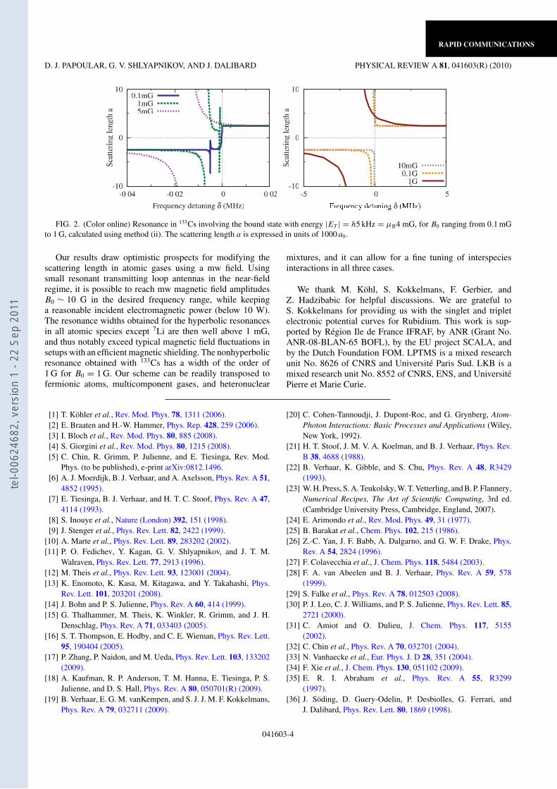
RAPID COMMUNICATIONS

D. J. PAPOULAR, G. V. SHLYAPNIKOV, AND J. DALIBARD PHYSICAL REVIEW A 81, 041603(R) (2010)

FIG. 2. (Color online) Resonance in 133Cs involving the bound state with energy |ET | = h5 kHz = µB4 mG, for B0 ranging from 0.1 mGto 1 G, calculated using method (ii). The scattering length a is expressed in units of 1000 a0.

Our results draw optimistic prospects for modifying thescattering length in atomic gases using a mw field. Usingsmall resonant transmitting loop antennas in the near-fieldregime, it is possible to reach mw magnetic field amplitudesB0 ∼ 10 G in the desired frequency range, while keepinga reasonable incident electromagnetic power (below 10 W).The resonance widths obtained for the hyperbolic resonancesin all atomic species except 7Li are then well above 1 mG,and thus notably exceed typical magnetic field fluctuations insetups with an efficient magnetic shielding. The nonhyperbolicresonance obtained with 133Cs has a width of the order of1 G for B0 = 1 G. Our scheme can be readily transposed tofermionic atoms, multicomponent gases, and heteronuclear

mixtures, and it can allow for a fine tuning of interspeciesinteractions in all three cases.

We thank M. Kohl, S. Kokkelmans, F. Gerbier, andZ. Hadzibabic for helpful discussions. We are grateful toS. Kokkelmans for providing us with the singlet and tripletelectronic potential curves for Rubidium. This work is sup-ported by Region Ile de France IFRAF, by ANR (Grant No.ANR-08-BLAN-65 BOFL), by the EU project SCALA, andby the Dutch Foundation FOM. LPTMS is a mixed researchunit No. 8626 of CNRS and Universite Paris Sud. LKB is amixed research unit No. 8552 of CNRS, ENS, and UniversitePierre et Marie Curie.

[1] T. Kohler et al., Rev. Mod. Phys. 78, 1311 (2006).[2] E. Braaten and H.-W. Hammer, Phys. Rep. 428, 259 (2006).[3] I. Bloch et al., Rev. Mod. Phys. 80, 885 (2008).[4] S. Giorgini et al., Rev. Mod. Phys. 80, 1215 (2008).[5] C. Chin, R. Grimm, P. Julienne, and E. Tiesinga, Rev. Mod.

Phys. (to be published), e-print arXiv:0812.1496.[6] A. J. Moerdijk, B. J. Verhaar, and A. Axelsson, Phys. Rev. A 51,

4852 (1995).[7] E. Tiesinga, B. J. Verhaar, and H. T. C. Stoof, Phys. Rev. A 47,

4114 (1993).[8] S. Inouye et al., Nature (London) 392, 151 (1998).[9] J. Stenger et al., Phys. Rev. Lett. 82, 2422 (1999).

[10] A. Marte et al., Phys. Rev. Lett. 89, 283202 (2002).[11] P. O. Fedichev, Y. Kagan, G. V. Shlyapnikov, and J. T. M.

Walraven, Phys. Rev. Lett. 77, 2913 (1996).[12] M. Theis et al., Phys. Rev. Lett. 93, 123001 (2004).[13] K. Enomoto, K. Kasa, M. Kitagawa, and Y. Takahashi, Phys.

Rev. Lett. 101, 203201 (2008).[14] J. Bohn and P. S. Julienne, Phys. Rev. A 60, 414 (1999).[15] G. Thalhammer, M. Theis, K. Winkler, R. Grimm, and J. H.

Denschlag, Phys. Rev. A 71, 033403 (2005).[16] S. T. Thompson, E. Hodby, and C. E. Wieman, Phys. Rev. Lett.

95, 190404 (2005).[17] P. Zhang, P. Naidon, and M. Ueda, Phys. Rev. Lett. 103, 133202

(2009).[18] A. Kaufman, R. P. Anderson, T. M. Hanna, E. Tiesinga, P. S.

Julienne, and D. S. Hall, Phys. Rev. A 80, 050701(R) (2009).[19] B. Verhaar, E. G. M. vanKempen, and S. J. J. M. F. Kokkelmans,

Phys. Rev. A 79, 032711 (2009).

[20] C. Cohen-Tannoudji, J. Dupont-Roc, and G. Grynberg, Atom-Photon Interactions: Basic Processes and Applications (Wiley,New York, 1992).

[21] H. T. Stoof, J. M. V. A. Koelman, and B. J. Verhaar, Phys. Rev.B 38, 4688 (1988).

[22] B. Verhaar, K. Gibble, and S. Chu, Phys. Rev. A 48, R3429(1993).

[23] W. H. Press, S. A. Teukolsky, W. T. Vetterling, and B. P. Flannery,Numerical Recipes, The Art of Scientific Computing, 3rd ed.(Cambridge University Press, Cambridge, England, 2007).

[24] E. Arimondo et al., Rev. Mod. Phys. 49, 31 (1977).[25] B. Barakat et al., Chem. Phys. 102, 215 (1986).[26] Z.-C. Yan, J. F. Babb, A. Dalgarno, and G. W. F. Drake, Phys.

Rev. A 54, 2824 (1996).[27] F. Colavecchia et al., J. Chem. Phys. 118, 5484 (2003).[28] F. A. van Abeelen and B. J. Verhaar, Phys. Rev. A 59, 578

(1999).[29] S. Falke et al., Phys. Rev. A 78, 012503 (2008).[30] P. J. Leo, C. J. Williams, and P. S. Julienne, Phys. Rev. Lett. 85,

2721 (2000).[31] C. Amiot and O. Dulieu, J. Chem. Phys. 117, 5155

(2002).[32] C. Chin et al., Phys. Rev. A 70, 032701 (2004).[33] N. Vanhaecke et al., Eur. Phys. J. D 28, 351 (2004).[34] F. Xie et al., J. Chem. Phys. 130, 051102 (2009).[35] E. R. I. Abraham et al., Phys. Rev. A 55, R3299

(1997).[36] J. Soding, D. Guery-Odelin, P. Desbiolles, G. Ferrari, and

J. Dalibard, Phys. Rev. Lett. 80, 1869 (1998).

041603-4

tel-0

0624

682,

ver

sion

1 -

22 S

ep 2

011

tel-0

0624

682,

ver

sion

1 -

22 S

ep 2

011

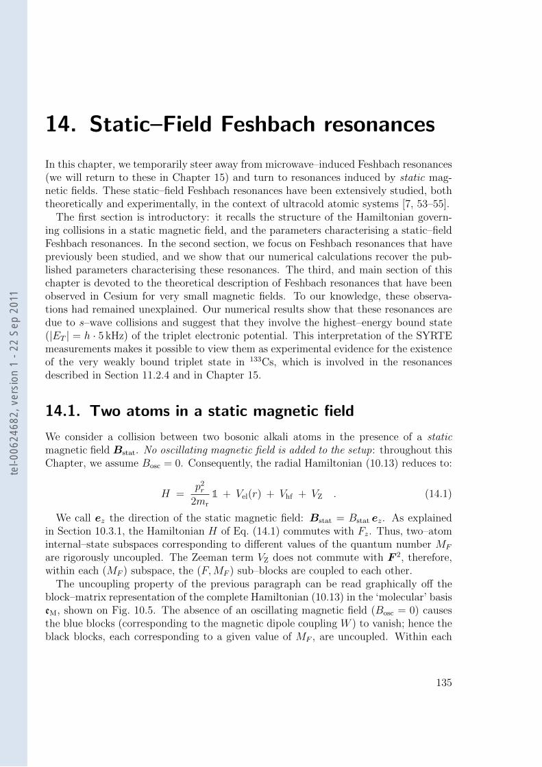
14. Static–Field Feshbach resonances

In this chapter, we temporarily steer away from microwave–induced Feshbach resonances(we will return to these in Chapter 15) and turn to resonances induced by static mag-netic fields. These static–field Feshbach resonances have been extensively studied, boththeoretically and experimentally, in the context of ultracold atomic systems [7, 53–55].

The first section is introductory: it recalls the structure of the Hamiltonian govern-ing collisions in a static magnetic field, and the parameters characterising a static–fieldFeshbach resonances. In the second section, we focus on Feshbach resonances that havepreviously been studied, and we show that our numerical calculations recover the pub-lished parameters characterising these resonances. The third, and main section of thischapter is devoted to the theoretical description of Feshbach resonances that have beenobserved in Cesium for very small magnetic fields. To our knowledge, these observa-tions had remained unexplained. Our numerical results show that these resonances aredue to s–wave collisions and suggest that they involve the highest–energy bound state(|ET | = h · 5 kHz) of the triplet electronic potential. This interpretation of the SYRTEmeasurements makes it possible to view them as experimental evidence for the existenceof the very weakly bound triplet state in 133Cs, which is involved in the resonancesdescribed in Section 11.2.4 and in Chapter 15.

14.1. Two atoms in a static magnetic field

We consider a collision between two bosonic alkali atoms in the presence of a staticmagnetic field Bstat. No oscillating magnetic field is added to the setup: throughout thisChapter, we assume Bosc = 0. Consequently, the radial Hamiltonian (10.13) reduces to:

H =p2r

2mr

1 + Vel(r) + Vhf + VZ . (14.1)

We call ez the direction of the static magnetic field: Bstat = Bstat ez. As explainedin Section 10.3.1, the Hamiltonian H of Eq. (14.1) commutes with Fz. Thus, two–atominternal–state subspaces corresponding to different values of the quantum number MF

are rigorously uncoupled. The Zeeman term VZ does not commute with F 2, therefore,within each (MF ) subspace, the (F,MF ) sub–blocks are coupled to each other.

The uncoupling property of the previous paragraph can be read graphically off theblock–matrix representation of the complete Hamiltonian (10.13) in the ‘molecular’ basiseM, shown on Fig. 10.5. The absence of an oscillating magnetic field (Bosc = 0) causesthe blue blocks (corresponding to the magnetic dipole coupling W ) to vanish; hence theblack blocks, each corresponding to a given value of MF , are uncoupled. Within each

135

tel-0

0624

682,

ver

sion

1 -

22 S

ep 2

011

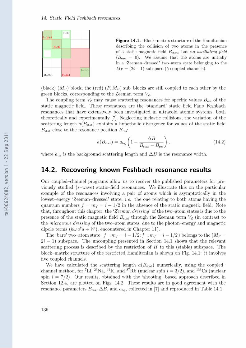
14. Static–Field Feshbach resonances

M=2i-1

F=2i+1

F=2i

F=2i-1

I=2i

I=2i-2

Figure 14.1. Block–matrix structure of the Hamiltoniandescribing the collision of two atoms in the presenceof a static magnetic field Bstat, but no oscillating field(Bosc = 0). We assume that the atoms are initiallyin a ‘Zeeman–dressed’ two–atom state belonging to theMF = (2i− 1) subspace (5 coupled channels).

(black) (MF ) block, the (red) (F,MF ) sub–blocks are still coupled to each other by thegreen blocks, corresponding to the Zeeman term VZ.

The coupling term VZ may cause scattering resonances for specific values Bres of thestatic magnetic field. These resonances are the ‘standard’ static–field Fano–Feshbachresonances that have extensively been investigated in ultracold atomic systems, boththeoretically and experimentally [7]. Neglecting inelastic collisions, the variation of thescattering length a(Bstat) exhibits a hyperbolic divergence for values of the static fieldBstat close to the resonance position Bres:

a(Bstat) = abg

(1− ∆B

Bstat −Bres

), (14.2)

where abg is the background scattering length and ∆B is the resonance width.

14.2. Recovering known Feshbach resonance results

Our coupled–channel programs allow us to recover the published parameters for pre-viously studied (s–wave) static–field resonances. We illustrate this on the particularexample of the resonances involving a pair of atoms which is asymptotically in thelowest–energy ‘Zeeman–dressed’ state, i.e. the one relating to both atoms having thequantum numbers f = mf = i − 1/2 in the absence of the static magnetic field. Notethat, throughout this chapter, the ‘Zeeman dressing ’ of the two–atom states is due to thepresence of the static magnetic field Bstat through the Zeeman term VZ (in contrast tothe microwave dressing of the two–atom states, due to the photon–energy and magneticdipole terms (~ω a†a+W ), encountered in Chapter 11).

The ‘bare’ two–atom state | f−,mf = i− 1/2; f−,mf = i− 1/2 〉 belongs to the (MF =2i − 1) subspace. The uncoupling presented in Section 14.1 shows that the relevantscattering process is described by the restriction of H to this (stable) subspace. Theblock–matrix structure of the restricted Hamiltonian is shown on Fig. 14.1: it involvesfive coupled channels.

We have calculated the scattering length a(Bstat) numerically, using the coupled–channel method, for 7Li, 23Na, 41K, and 87Rb (nuclear spin i = 3/2), and 133Cs (nuclearspin i = 7/2). Our results, obtained with the ‘shooting’–based approach described inSection 12.4, are plotted on Figs. 14.2. These results are in good agreement with theresonance parameters Bres, ∆B, and abg, collected in [7] and reproduced in Table 14.1.

136

tel-0

0624

682,

ver

sion

1 -

22 S

ep 2

011

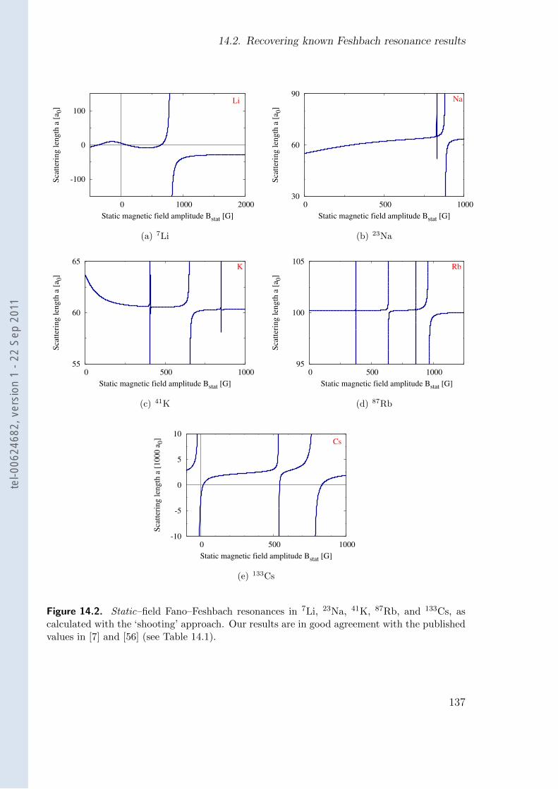
14.2. Recovering known Feshbach resonance results

-100

0

100

0 1000 2000

Sca

tter

ing l

ength

a [

a 0]

Static magnetic field amplitude Bstat [G]

Li

(a) 7Li

30

60

90

0 500 1000

Sca

tter

ing l

ength

a [

a 0]

Static magnetic field amplitude Bstat [G]

Na

(b) 23Na

55

60

65

0 500 1000

Sca

tter

ing l

ength

a [

a 0]

Static magnetic field amplitude Bstat [G]

K

(c) 41K

95

100

105

0 500 1000

Sca

tter

ing l

ength

a [

a 0]

Static magnetic field amplitude Bstat [G]

Rb

(d) 87Rb

-10

-5

0

5

10

0 500 1000

Sca

tter

ing l

ength

a [

1000 a

0]

Static magnetic field amplitude Bstat [G]

Cs

(e) 133Cs

Figure 14.2. Static–field Fano–Feshbach resonances in 7Li, 23Na, 41K, 87Rb, and 133Cs, ascalculated with the ‘shooting’ approach. Our results are in good agreement with the publishedvalues in [7] and [56] (see Table 14.1).

137

tel-0

0624

682,

ver

sion

1 -

22 S

ep 2

011

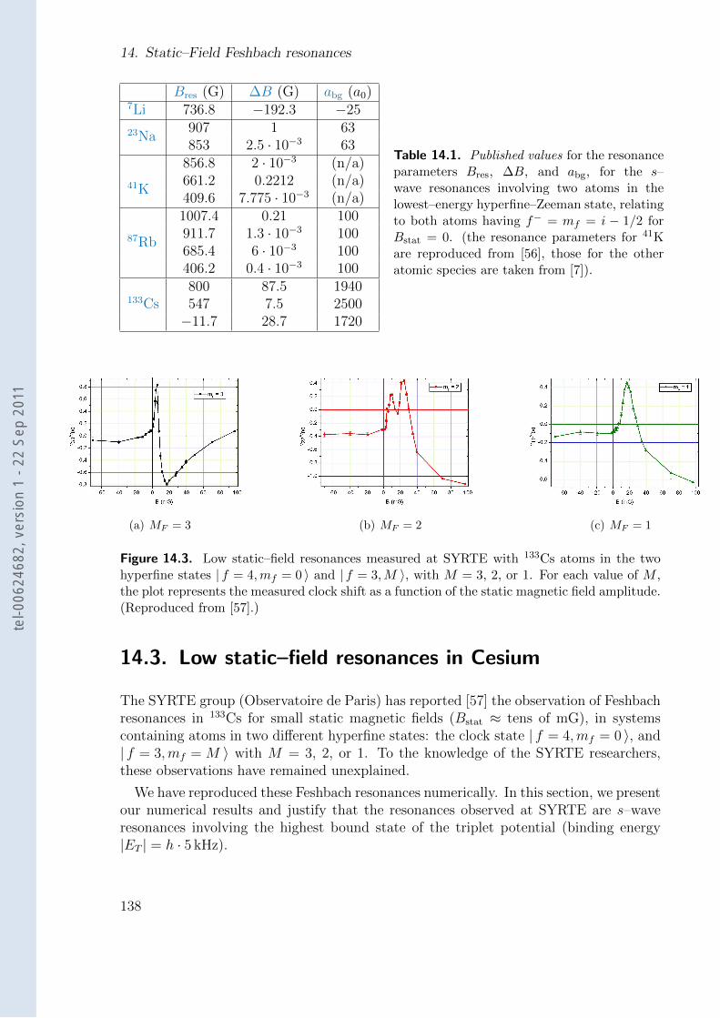
14. Static–Field Feshbach resonances

Bres (G) ∆B (G) abg (a0)7Li 736.8 −192.3 −25

23Na907 1 63853 2.5 · 10−3 63

41K

856.8 2 · 10−3 (n/a)661.2 0.2212 (n/a)409.6 7.775 · 10−3 (n/a)

87Rb

1007.4 0.21 100911.7 1.3 · 10−3 100685.4 6 · 10−3 100406.2 0.4 · 10−3 100

133Cs800 87.5 1940547 7.5 2500−11.7 28.7 1720

Table 14.1. Published values for the resonanceparameters Bres, ∆B, and abg, for the s–wave resonances involving two atoms in thelowest–energy hyperfine–Zeeman state, relatingto both atoms having f− = mf = i − 1/2 forBstat = 0. (the resonance parameters for 41Kare reproduced from [56], those for the otheratomic species are taken from [7]).

(a) MF = 3 (b) MF = 2 (c) MF = 1

Figure 14.3. Low static–field resonances measured at SYRTE with 133Cs atoms in the twohyperfine states | f = 4,mf = 0 〉 and | f = 3,M 〉, with M = 3, 2, or 1. For each value of M ,the plot represents the measured clock shift as a function of the static magnetic field amplitude.(Reproduced from [57].)

14.3. Low static–field resonances in Cesium

The SYRTE group (Observatoire de Paris) has reported [57] the observation of Feshbachresonances in 133Cs for small static magnetic fields (Bstat ≈ tens of mG), in systemscontaining atoms in two different hyperfine states: the clock state | f = 4,mf = 0 〉, and| f = 3,mf = M 〉 with M = 3, 2, or 1. To the knowledge of the SYRTE researchers,these observations have remained unexplained.

We have reproduced these Feshbach resonances numerically. In this section, we presentour numerical results and justify that the resonances observed at SYRTE are s–waveresonances involving the highest bound state of the triplet potential (binding energy|ET | = h · 5 kHz).

138

tel-0

0624

682,

ver

sion

1 -

22 S

ep 2

011

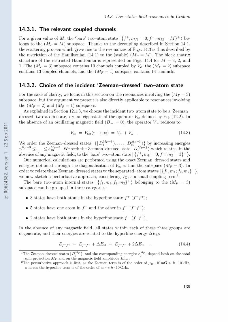
14.3. Low static–field resonances in Cesium

14.3.1. The relevant coupled channels

For a given value of M , the ‘bare’ two–atom state | f+,mf1 = 0; f−,mf2 = M+ 〉 be-longs to the (MF = M) subspace. Thanks to the decoupling described in Section 14.1,the scattering process which gives rise to the resonances of Figs. 14.3 is thus described bythe restriction of the Hamiltonian (14.1) to the (stable) (MF = M). The block–matrixstructure of the restricted Hamiltonian is represented on Figs. 14.4 for M = 3, 2, and1. The (MF = 3) subspace contains 10 channels coupled by VZ, the (MF = 2) subspacecontains 13 coupled channels, and the (MF = 1) subspace contains 14 channels.

14.3.2. Choice of the incident ‘Zeeman–dressed’ two–atom state

For the sake of clarity, we focus in this section on the resonances involving the (MF = 3)subspace, but the argument we present is also directly applicable to resonances involvingthe (MF = 2) and (MF = 1) subspaces.

As explained in Section 12.1.3, we choose the incident two–atom state to be a ‘Zeeman–dressed’ two–atom state, i.e. an eigenstate of the operator V∞ defined by Eq. (12.2). Inthe absence of an oscillating magnetic field (Bosc = 0), the operator V∞ reduces to:

V∞ = Vtot(r →∞) = Vhf + VZ . (14.3)

We order the Zeeman–dressed states1 |DMF=31 〉, . . . , |DMF=3

10 〉 by increasing energiesεMF=3

1 ≤ . . . ≤ εMF=310 . We seek the Zeeman–dressed state |DMF=3

n 〉 which relates, in theabsence of any magnetic field, to the ‘bare’ two–atom state | f+,m1 = 0; f−,m2 = 3+ 〉.

Our numerical calculations are performed using the exact Zeeman–dressed states andenergies obtained through the diagonalisation of V∞ within the subspace (MF = 3). Inorder to relate these Zeeman–dressed states to the separated–atom states | f1,m1; f2,m2+ 〉,we now sketch a perturbative approach, considering VZ as a small coupling term2.

The bare two–atom internal states | f1,m1; f2,m2+ 〉 belonging to the (MF = 3)subspace can be grouped in three categories:

• 3 states have both atoms in the hyperfine state f+ (f+f+);

• 5 states have one atom in f+ and the other in f− (f+f−);

• 2 states have both atoms in the hyperfine state f− (f−f−).

In the absence of any magnetic field, all states within each of these three groups aredegenerate, and their energies are related to the hyperfine energy ∆Ehf :

Ef+f+ = Ef+f− + ∆Ehf = Ef−f− + 2∆Ehf . (14.4)

1The Zeeman–dressed states |DMFj 〉, and the corresponding energies εMF

j , depend both on the totalspin projection MF and on the magnetic field amplitude Bstat.

2The perturbative approach is licit, as the Zeeman term is of the order of µB · 10 mG ≈ h · 10 kHz,whereas the hyperfine term is of the order of ahf ≈ h · 10 GHz.

139

tel-0

0624

682,

ver

sion

1 -

22 S

ep 2

011

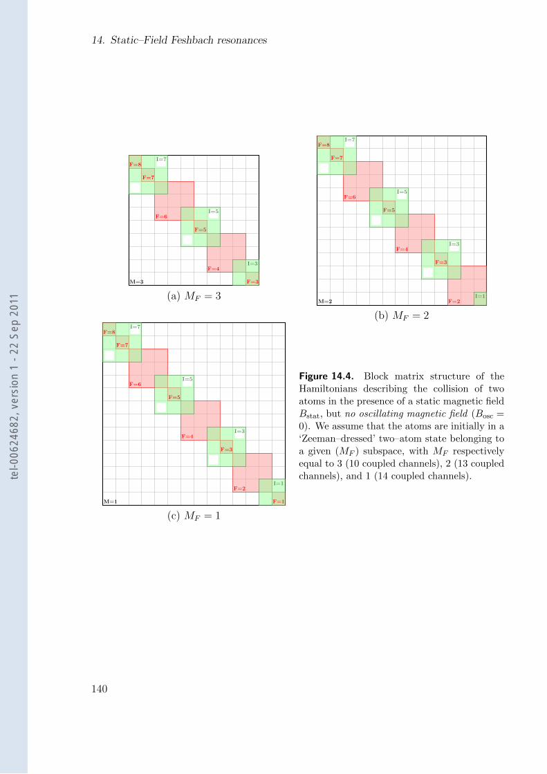
14. Static–Field Feshbach resonances

M=3

F=8

F=7

F=6

F=5

F=4

F=3

I=7

I=5

I=3

(a) MF = 3M=2

F=8

F=7

F=6

F=5

F=4

F=3

F=2

I=7

I=5

I=3

I=1

(b) MF = 2

M=1

F=8

F=7

F=6

F=5

F=4

F=3

F=2

F=1

I=7

I=5

I=3

I=1

(c) MF = 1

Figure 14.4. Block matrix structure of theHamiltonians describing the collision of twoatoms in the presence of a static magnetic fieldBstat, but no oscillating magnetic field (Bosc =0). We assume that the atoms are initially in a‘Zeeman–dressed’ two–atom state belonging toa given (MF ) subspace, with MF respectivelyequal to 3 (10 coupled channels), 2 (13 coupledchannels), and 1 (14 coupled channels).

140

tel-0

0624

682,

ver

sion

1 -

22 S

ep 2

011

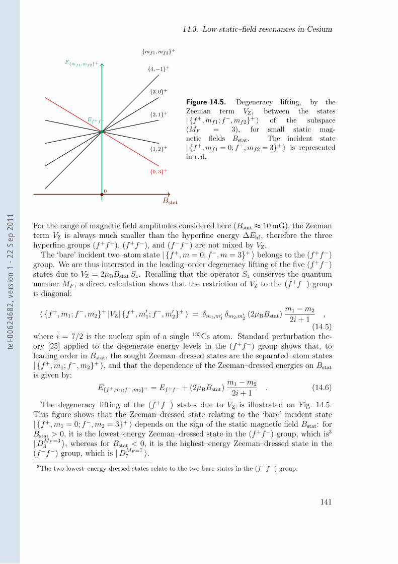
14.3. Low static–field resonances in Cesium

Bstat

Emf1,mf2+

mf1,mf2+

4,−1+

3, 0+

2, 1+

1, 2+

0, 3+

Ef+f−

0

Figure 14.5. Degeneracy lifting, by theZeeman term VZ, between the states| f+,mf1; f−,mf2+ 〉 of the subspace(MF = 3), for small static mag-netic fields Bstat. The incident state| f+,mf1 = 0; f−,mf2 = 3+ 〉 is representedin red.

For the range of magnetic field amplitudes considered here (Bstat ≈ 10 mG), the Zeemanterm VZ is always much smaller than the hyperfine energy ∆Ehf , therefore the threehyperfine groups (f+f+), (f+f−), and (f−f−) are not mixed by VZ.

The ‘bare’ incident two–atom state | f+,m = 0; f−,m = 3+ 〉 belongs to the (f+f−)group. We are thus interested in the leading–order degeneracy lifting of the five (f+f−)states due to VZ = 2µBBstat Sz. Recalling that the operator Sz conserves the quantumnumber MF , a direct calculation shows that the restriction of VZ to the (f+f−) groupis diagonal:

〈 f+,m1; f−,m2+ |VZ| f+,m′1; f−,m′2+ 〉 = δm1,m′1δm2,m′2

(2µBBstat)m1 −m2

2i+ 1,

(14.5)where i = 7/2 is the nuclear spin of a single 133Cs atom. Standard perturbation the-ory [25] applied to the degenerate energy levels in the (f+f−) group shows that, toleading order in Bstat, the sought Zeeman–dressed states are the separated–atom states| f+,m1; f−,m2+ 〉, and that the dependence of the Zeeman–dressed energies on Bstat

is given by:

Ef+,m1;f−,m2+ = Ef+f− + (2µBBstat)m1 −m2

2i+ 1. (14.6)

The degeneracy lifting of the (f+f−) states due to VZ is illustrated on Fig. 14.5.This figure shows that the Zeeman–dressed state relating to the ‘bare’ incident state| f+,m1 = 0; f−,m2 = 3+ 〉 depends on the sign of the static magnetic field Bstat: forBstat > 0, it is the lowest–energy Zeeman–dressed state in the (f+f−) group, which is3

|DMF=33 〉, whereas for Bstat < 0, it is the highest–energy Zeeman–dressed state in the

(f+f−) group, which is |DMF=77 〉.

3The two lowest–energy dressed states relate to the two bare states in the (f−f−) group.

141

tel-0

0624

682,

ver

sion

1 -

22 S

ep 2

011

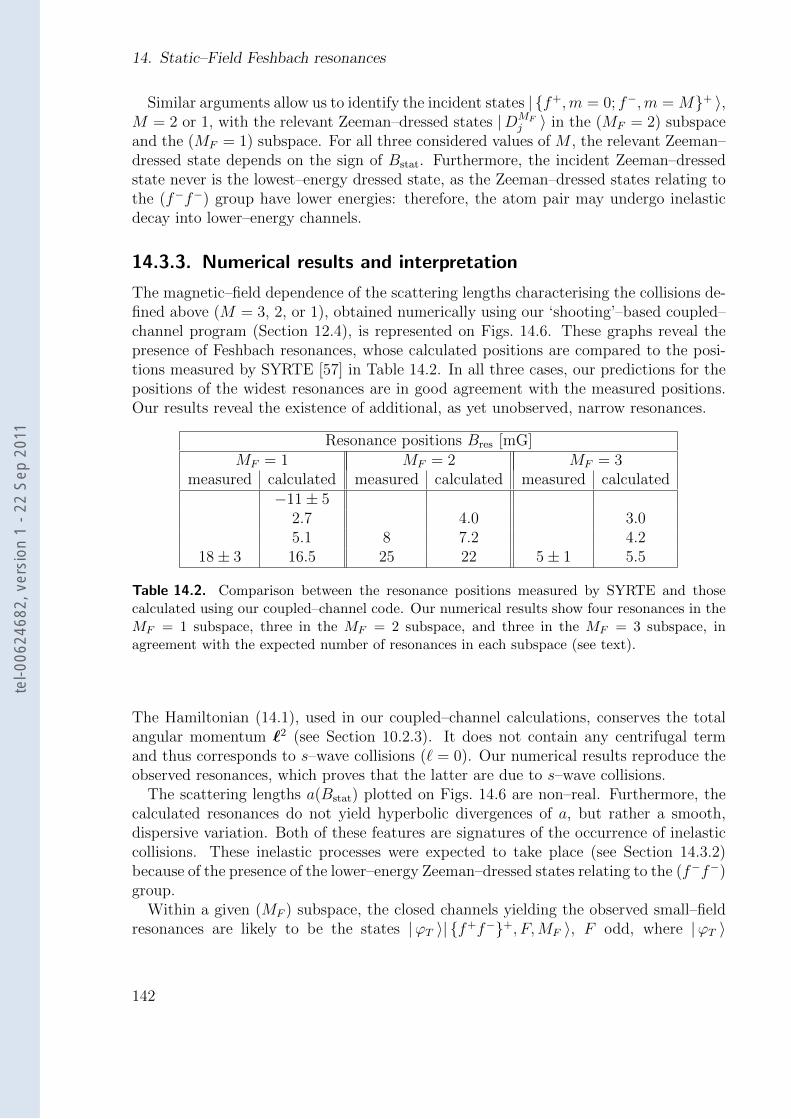
14. Static–Field Feshbach resonances

Similar arguments allow us to identify the incident states | f+,m = 0; f−,m = M+ 〉,M = 2 or 1, with the relevant Zeeman–dressed states |DMF

j 〉 in the (MF = 2) subspaceand the (MF = 1) subspace. For all three considered values of M , the relevant Zeeman–dressed state depends on the sign of Bstat. Furthermore, the incident Zeeman–dressedstate never is the lowest–energy dressed state, as the Zeeman–dressed states relating tothe (f−f−) group have lower energies: therefore, the atom pair may undergo inelasticdecay into lower–energy channels.

14.3.3. Numerical results and interpretation

The magnetic–field dependence of the scattering lengths characterising the collisions de-fined above (M = 3, 2, or 1), obtained numerically using our ‘shooting’–based coupled–channel program (Section 12.4), is represented on Figs. 14.6. These graphs reveal thepresence of Feshbach resonances, whose calculated positions are compared to the posi-tions measured by SYRTE [57] in Table 14.2. In all three cases, our predictions for thepositions of the widest resonances are in good agreement with the measured positions.Our results reveal the existence of additional, as yet unobserved, narrow resonances.

Resonance positions Bres [mG]MF = 1 MF = 2 MF = 3

measured calculated measured calculated measured calculated−11± 5

2.7 4.0 3.05.1 8 7.2 4.2

18± 3 16.5 25 22 5± 1 5.5

Table 14.2. Comparison between the resonance positions measured by SYRTE and thosecalculated using our coupled–channel code. Our numerical results show four resonances in theMF = 1 subspace, three in the MF = 2 subspace, and three in the MF = 3 subspace, inagreement with the expected number of resonances in each subspace (see text).

The Hamiltonian (14.1), used in our coupled–channel calculations, conserves the totalangular momentum `2 (see Section 10.2.3). It does not contain any centrifugal termand thus corresponds to s–wave collisions (` = 0). Our numerical results reproduce theobserved resonances, which proves that the latter are due to s–wave collisions.

The scattering lengths a(Bstat) plotted on Figs. 14.6 are non–real. Furthermore, thecalculated resonances do not yield hyperbolic divergences of a, but rather a smooth,dispersive variation. Both of these features are signatures of the occurrence of inelasticcollisions. These inelastic processes were expected to take place (see Section 14.3.2)because of the presence of the lower–energy Zeeman–dressed states relating to the (f−f−)group.

Within a given (MF ) subspace, the closed channels yielding the observed small–fieldresonances are likely to be the states |ϕT 〉| f+f−+, F,MF 〉, F odd, where |ϕT 〉

142

tel-0

0624

682,

ver

sion

1 -

22 S

ep 2

011

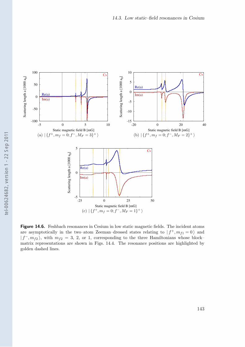
14.3. Low static–field resonances in Cesium

-100

-50

0

50

100

-5 0 5 10

Sca

tter

ing l

ength

a [

1000 a

0]

Static magnetic field B [mG]

Cs

Re(a)

Im(a)

(a) | f+,mf = 0; f−,MF = 3+ 〉

-15

-10

-5

0

5

10

-20 0 20 40

Sca

tter

ing l

ength

a [

1000 a

0]

Static magnetic field B [mG]

Cs

Re(a)

Im(a)

(b) | f+,mf = 0; f−,MF = 2+ 〉

-5

0

5

-25 0 25 50

Sca

tter

ing l

ength

a [

1000 a

0]

Static magnetic field B [mG]

Cs

Re(a)

Im(a)

(c) | f+,mf = 0; f−,MF = 1+ 〉

Figure 14.6. Feshbach resonances in Cesium in low static magnetic fields. The incident atomsare asymptotically in the two–atom Zeeman–dressed states relating to | f+,mf1 = 0 〉 and| f−,mf2 〉, with mf2 = 3, 2, or 1, corresponding to the three Hamiltonians whose block–matrix representations are shown in Figs. 14.4. The resonance positions are highlighted bygolden dashed lines.

143

tel-0

0624

682,

ver

sion

1 -

22 S

ep 2

011

14. Static–Field Feshbach resonances

is the spatial wavefunction of the highest-energy triplet bound state (binding energy|ET | = h · 5 kHz) and the internal–state ket describes a two–atom state which is purelyelectronic–triplet (see Section 10.3.3). This statement is supported by the following twoobservations:

• Our calculations show no similar resonances in 87Rb, which does not have a veryweakly–bound triplet state (for 87Rb, the binding energy of the highest tripletbound state is |ET | = h · 25 MHz [58]);

• The observed resonance positions are of the order of |ET |/µB = 4 mG.

For a given value of MF , there are as many resonances as there are different internalstates of the form | f+, f−+, F,MF 〉, F odd. The total spin F results from the couplingof two atomic spins f1 and f2 having the quantum numbers f+ = i+ 1/2 = 4 and f− =i− 1/2 = 3 respectively, and it must therefore satisfy MF ≤ F ≤ 2i = 7. Furthermore,F must be odd in order to ensure the bosonic symmetry of the two–atom internal states.Consequently, four resonances are expected for MF = 1 (F = 7, 5, 3, 1), whereas thereare only three resonances for MF = 2 and MF = 3 (F = 7, 5, 3). The variation a(Bstat)of the scattering length a as a function of the magnetic field Bstat, shown on Figs. 14.6,exhibits the expected number of resonances in all three MF subspaces.

144

tel-0

0624

682,

ver

sion

1 -

22 S

ep 2

011

15. Towards an experimentalobservation of our predictions

The microwave–induced resonances characterised in Chapter 11 are those whose theo-retical description is the simplest: they can be modelled in terms of a small number ofcoupled channels, and they do not involve inelastic processes. However, these are notthe resonances which are the most readily accessible experimentally.

An experimental study of the microwave–induced resonances in 133Cs is likely to beperformed soon using the Cesium fountain clocks set up at SYRTE—Observatoire deParis. The experimental parameters in these fountain clocks differ from the conditionsconsidered in Chapter 11 in three respects:

1. A small homogeneous static magnetic field is present in the experimental setup;

2. The microwave source is π–polarised (rather than circularly polarised);

3. The atoms are most easily prepared in the lowest–energy hyperfine state havingzero spin projection along the axis defined by the static field.

In this chapter, we characterise the microwave–induced resonances occurring in 133Csdue to the very weakly–bound triplet dimer state in the experimental conditions listedabove. The description of these resonances requires a larger number of coupled channels,and inelastic processes must be accounted for.

We start by recalling the dependence of the magnetic dipole coupling on the polari-sation of the oscillating magnetic field. Then, assuming that no static magnetic field ispresent, we determine the microwave–dressed two–atom state which relates to the baretwo–atom state mentioned above. We present a plot of the dependence of the (complex)scattering length a(ω) in the frequency range for which the weakly–bound triplet stateis expected to be resonant, and we qualitatively explain many of the features of thisplot. Finally, we include the effect of an additional small static magnetic field along thequantisation axis, and we show that this static field only has a small qualitative impacton the microwave–induced resonances.

15.1. Two atoms in a linearly–polarised magnetic field

Up to Chapter 13, we had only considered microwave–induced resonances caused bycircularly–polarised magnetic fields. In the present chapter, we abandon circularly–polarised fields and turn to a linearly–polarised magnetic field, whose direction is par-

145

tel-0

0624

682,

ver

sion

1 -

22 S

ep 2

011

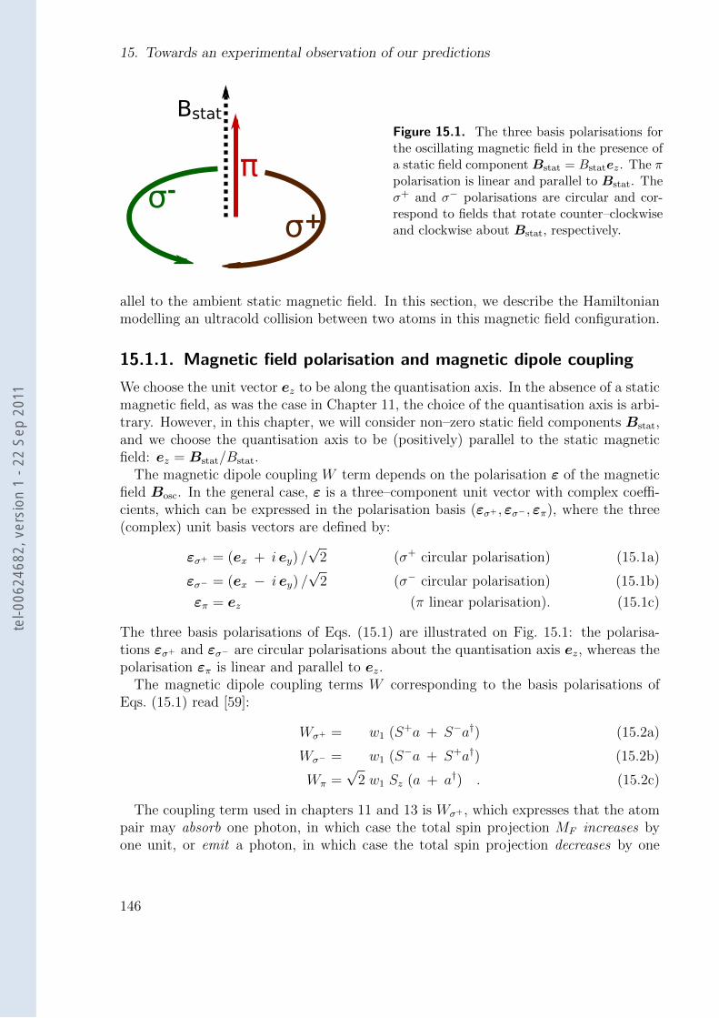
15. Towards an experimental observation of our predictions

Bstat

σ+σ-

πFigure 15.1. The three basis polarisations forthe oscillating magnetic field in the presence ofa static field componentBstat = Bstatez. The πpolarisation is linear and parallel to Bstat. Theσ+ and σ− polarisations are circular and cor-respond to fields that rotate counter–clockwiseand clockwise about Bstat, respectively.

allel to the ambient static magnetic field. In this section, we describe the Hamiltonianmodelling an ultracold collision between two atoms in this magnetic field configuration.

15.1.1. Magnetic field polarisation and magnetic dipole coupling

We choose the unit vector ez to be along the quantisation axis. In the absence of a staticmagnetic field, as was the case in Chapter 11, the choice of the quantisation axis is arbi-trary. However, in this chapter, we will consider non–zero static field components Bstat,and we choose the quantisation axis to be (positively) parallel to the static magneticfield: ez = Bstat/Bstat.

The magnetic dipole coupling W term depends on the polarisation ε of the magneticfield Bosc. In the general case, ε is a three–component unit vector with complex coeffi-cients, which can be expressed in the polarisation basis (εσ+ , εσ− , επ), where the three(complex) unit basis vectors are defined by:

εσ+ = (ex + i ey) /√

2 (σ+ circular polarisation) (15.1a)

εσ− = (ex − i ey) /√

2 (σ− circular polarisation) (15.1b)

επ = ez (π linear polarisation). (15.1c)

The three basis polarisations of Eqs. (15.1) are illustrated on Fig. 15.1: the polarisa-tions εσ+ and εσ− are circular polarisations about the quantisation axis ez, whereas thepolarisation επ is linear and parallel to ez.

The magnetic dipole coupling terms W corresponding to the basis polarisations ofEqs. (15.1) read [59]:

Wσ+ = w1 (S+a + S−a†) (15.2a)

Wσ− = w1 (S−a + S+a†) (15.2b)

Wπ =√

2 w1 Sz (a + a†) . (15.2c)

The coupling term used in chapters 11 and 13 is Wσ+ , which expresses that the atompair may absorb one photon, in which case the total spin projection MF increases byone unit, or emit a photon, in which case the total spin projection decreases by one

146

tel-0

0624

682,

ver

sion

1 -

22 S

ep 2

011

15.2. In the absence of a static magnetic field

unit. These processes enforce the conservation of angular momentum, as σ+–polarisedphotons carry one unit of angular momentum along ez.

In this chapter, we focus on the π–polarised case: the coupling term Wπ expresses thatthe atom pair may absorb or emit a photon, and that neither of these processes causesa change in the total spin projection. These two latter processes are also compatiblewith the conservation of angular momentum, as π–polarised photons carry no angularmomentum.

15.1.2. Hamiltonian and relevant coupled channels

The Hamiltonian describing two atoms in the presence of a π–polarised magnetic fieldis similar to Eq. (10.9), where the coupling operator W is replaced by Wπ. In its radials–wave form, it reads:

H =p2r

2mr

1 + Vel(r) + Vhf + VZ + ~ω a†a + Wπ . (15.3)

We assume that the two incident atoms are in the (dressed state relating to the)‘bare’ two–atom state | f−,mf = 0; f−,mf = 0 〉, in the presence of N photons whosefrequency is close to the hyperfine energy ∆Ehf . This ‘bare’ incident state belongs tothe (MF = 0, N photons) subspace. Being in their lowest-energy hyperfine state f−,each of the two atoms may absorb one photon, but neither may emit a photon. Hence,the coupling term W connects the ‘incident’ subspace (MF = 0, N photons) subspaceto the (MF = 0, N − 1 photons) and (MF = 0, N − 2 photons) subspaces, through theabsorption of a single photon, and of a photon by each atom, respectively. The block–matrix structure, in the ‘molecular’ basis eM, of the restriction of the Hamiltonian tothese three subspaces is represented on Fig. 15.2. The (MF = 0) blocks correspondingto different photon numbers are distinct, therefore the restricted Hamiltonian operateson Nstates = 3× 16 = 48 coupled channels.

15.2. In the absence of a static magnetic field

In this section, we assume that the magnetic field has no static component (Bstat = 0).The effect of an additional static component will be presented in Section 15.3.

In the absence of a static magnetic field, the quantisation axis ez is defined by thedirection of the linearly–polarised oscillating magnetic field Bosc.

15.2.1. Choice of the incident dressed two–atom state

As explained in Section 12.1.3, we choose the incident state of the two atoms, in thepresence of the magnetic field, to be a ‘dressed’ two–atom state, i.e. one of the Nstates =48 eigenstates of the symmetric matrix V∞, defined by Eq. (12.2):

V∞ = Vtot(r →∞) = Vhf + VZ + ~ω a†a+Wπ . (12.2)

147

tel-0

0624

682,

ver

sion

1 -

22 S

ep 2

011

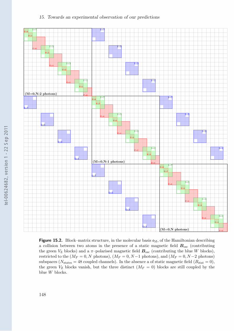
15. Towards an experimental observation of our predictions

(M=0,N-2 photons)

(M=0,N-1 photons)

(M=0,N photons)

F=8

F=7

F=6

F=5

F=4

F=3

F=2

F=1

F=0

F=8

F=7

F=6

F=5

F=4

F=3

F=2

F=1

F=0

F=8

F=7

F=6

F=5

F=4

F=3

F=2

F=1

F=0

I=7

I=5

I=3

I=1

I=7

I=5

I=3

I=1

I=7

I=5

I=3

I=1

I=7

I=5

I=3

I=1

I=7

I=5

I=3

I=1

I=7

I=5

I=3

I=1

I=7

I=5

I=3

I=1

Figure 15.2. Block–matrix structure, in the molecular basis eM, of the Hamiltonian describinga collision between two atoms in the presence of a static magnetic field Bosc (contributingthe green VZ blocks) and a π–polarised magnetic field Bosc (contributing the blue W blocks),restricted to the (MF = 0, N photons), (MF = 0, N−1 photons), and (MF = 0, N−2 photons)subspaces (Nstates = 48 coupled channels). In the absence a of static magnetic field (Bstat = 0),the green VZ blocks vanish, but the three distinct (MF = 0) blocks are still coupled by theblue W blocks.

148

tel-0

0624

682,

ver

sion

1 -

22 S

ep 2

011

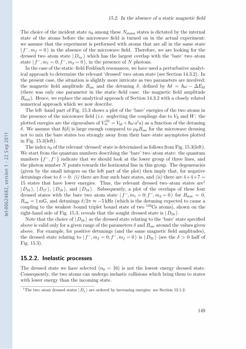
15.2. In the absence of a static magnetic field

The choice of the incident state n0 among these Nstates states is dictated by the internalstate of the atoms before the microwave field is turned on in the actual experiment:we assume that the experiment is performed with atoms that are all in the same state| f−,mf = 0 〉 in the absence of the microwave field. Therefore, we are looking for thedressed two–atom state |Dn0 〉 which has the largest overlap with the ‘bare’ two–atomstate | f−,m1 = 0; f−,m2 = 0 〉, in the presence of N photons.

In the case of the static–field Feshbach resonances, we have used a perturbative analyt-ical approach to determine the relevant ‘dressed’ two–atom state (see Section 14.3.2). Inthe present case, the situation is slightly more intricate as two parameters are involved:the magnetic field amplitude Bosc and the detuning δ, defined by ~δ = ~ω − ∆Ehf

(there was only one parameter in the static–field case: the magnetic field amplitudeBstat). Hence, we replace the analytical approach of Section 14.3.2 with a closely relatednumerical approach which we now describe.

The left–hand part of Fig. 15.3 shows a plot of the ‘bare’ energies of the two atoms inthe presence of the microwave field (i.e. neglecting the couplings due to VZ and W : the

plotted energies are the eigenvalues of V(0)∞ = Vhf +~ω a†a) as a function of the detuning

δ. We assume that ~|δ| is large enough compared to µBBosc for the microwave dressingnot to mix the bare states too strongly away from their bare–state asymptotes plottedin Fig. 15.3(left).

The index n0 of the relevant ‘dressed’ state is determined as follows from Fig. 15.3(left).We start from the quantum numbers describing the ‘bare’ two–atom state: the quantumnumbers f−, f− indicate that we should look at the lower group of three lines, andthe photon number N points towards the horizontal line in this group. The degeneracies(given by the small integers on the left part of the plot) then imply that, for negativedetunings close to δ = 0: (i) there are four such bare states, and (ii) there are 4+4+7 =15 states that have lower energies. Thus, the relevant dressed two–atom states are1

|D16 〉, |D17 〉, |D18 〉, and |D19 〉. Subsequently, a plot of the overlaps of these fourdressed states with the bare two–atom state | f−,m1 = 0; f−,m2 = 0 〉 for Bstat = 0,Bosc = 1 mG, and detunings δ/2π ≈ −5 kHz (which is the detuning expected to cause acoupling to the weakest–bound triplet bound state of two 133Cs atoms), shown on theright-hand side of Fig. 15.3, reveals that the sought dressed state is |D16 〉.

Note that the choice of |D16 〉 as the dressed state relating to the ‘bare’ state specifiedabove is valid only for a given range of the parameters δ and Bosc around the values givenabove. For example, for positive detunings (and the same magnetic field amplitudes),the dressed state relating to | f−,mf = 0; f−,mf = 0 〉 is |D31 〉 (see the δ > 0 half ofFig. 15.3).

15.2.2. Inelastic processes

The dressed state we have selected (n0 = 16) is not the lowest–energy dressed state.Consequently, the two atoms can undergo inelastic collisions which bring them to stateswith lower energy than the incoming state.

1The two–atom dressed states |Dj 〉 are ordered by increasing energies: see Section 12.1.2.

149

tel-0

0624

682,

ver

sion

1 -

22 S

ep 2

011

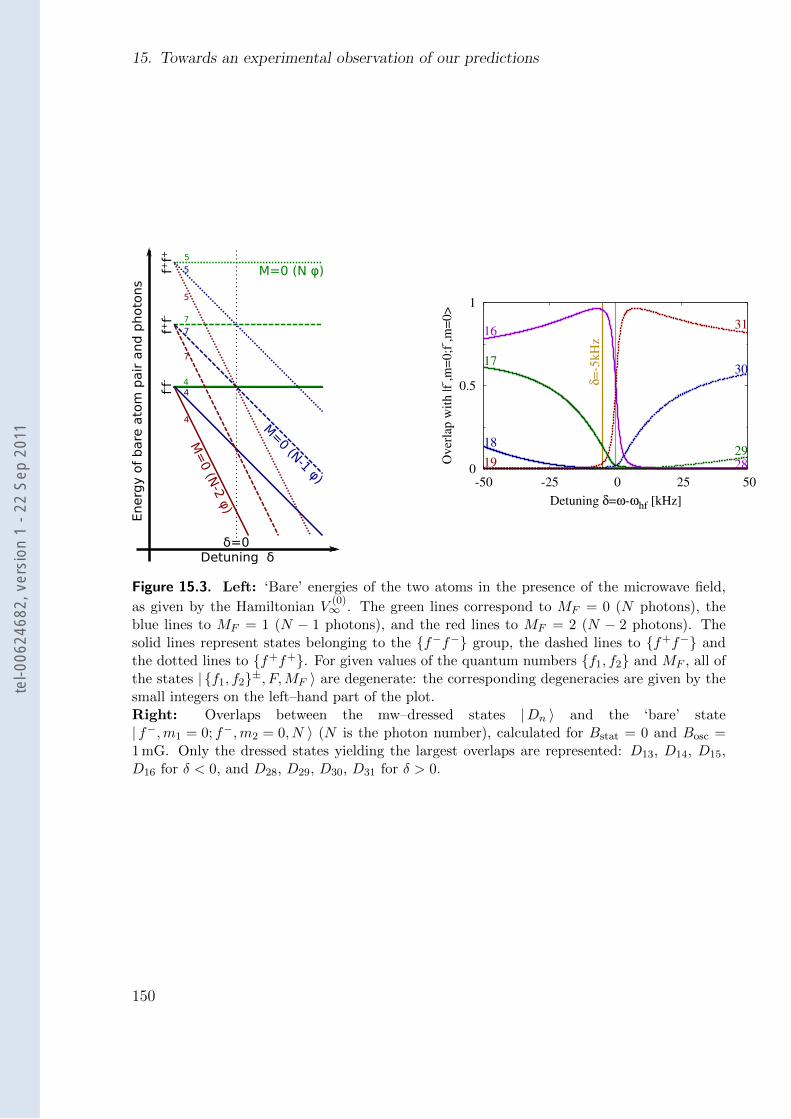
15. Towards an experimental observation of our predictions

4

7

5

5

7

4

5

7

4

f+f+

f+f-

f-f-

M=0 (N φ)

M=0 (N-1 φ)

M=

0 (N-2 φ

)Detuning δ

En

erg

y o

f b

are

ato

m p

air

an

d p

hoto

ns

δ=0

0

0.5

1

-50 -25 0 25 50

Over

lap w

ith |f

- ,m=

0;f

- ,m=

0>

Detuning δ=ω-ωhf [kHz]

16

17

18

19

31

30

2928

δ=

-5kH

zFigure 15.3. Left: ‘Bare’ energies of the two atoms in the presence of the microwave field,

as given by the Hamiltonian V(0)∞ . The green lines correspond to MF = 0 (N photons), the

blue lines to MF = 1 (N − 1 photons), and the red lines to MF = 2 (N − 2 photons). Thesolid lines represent states belonging to the f−f− group, the dashed lines to f+f− andthe dotted lines to f+f+. For given values of the quantum numbers f1, f2 and MF , all ofthe states | f1, f2±, F,MF 〉 are degenerate: the corresponding degeneracies are given by thesmall integers on the left–hand part of the plot.Right: Overlaps between the mw–dressed states |Dn 〉 and the ‘bare’ state| f−,m1 = 0; f−,m2 = 0, N 〉 (N is the photon number), calculated for Bstat = 0 and Bosc =1 mG. Only the dressed states yielding the largest overlaps are represented: D13, D14, D15,D16 for δ < 0, and D28, D29, D30, D31 for δ > 0.

150

tel-0

0624

682,

ver

sion

1 -

22 S

ep 2

011

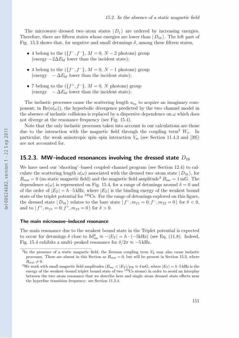
15.2. In the absence of a static magnetic field

The microwave–dressed two–atom states |Dj 〉 are ordered by increasing energies.Therefore, there are fifteen states whose energies are lower than |D16 〉. The left part ofFig. 15.3 shows that, for negative and small detunings δ, among these fifteen states,

• 4 belong to the (f−, f−, M = 0, N − 2 photons) group(energy −2∆Ehf lower than the incident state);

• 4 belong to the (f−, f−, M = 0, N − 1 photons) group(energy −∆Ehf lower than the incident state);

• 7 belong to the (f+, f−, M = 0, N photons) group(energy −∆Ehf lower than the incident state);

The inelastic processes cause the scattering length an0 to acquire an imaginary com-ponent; in Re(a(ω)), the hyperbolic divergence predicted by the two–channel model inthe absence of inelastic collisions is replaced by a dispersive dependence on ω which doesnot diverge at the resonance frequency (see Fig. 15.4).

Note that the only inelastic processes taken into account in our calculations are thosedue to the interaction with the magnetic field through the coupling term2 Wπ. Inparticular, the weak anisotropic spin–spin interaction Vss (see Section 11.4.3 and [39])are not accounted for.

15.2.3. MW–induced resonances involving the dressed state D16

We have used our ‘shooting’–based coupled–channel program (see Section 12.4) to cal-culate the scattering length a(ω) associated with the dressed two–atom state |D16 〉, forBstat = 0 (no static magnetic field) and the magnetic field amplitude3 Bosc = 1 mG. Thedependence a(ω) is represented on Fig. 15.4, for a range of detunings around δ = 0 andof the order of |ET | = h · 5 kHz, where |ET | is the binding energy of the weakest boundstate of the triplet potential for 133Cs. For the range of detunings explored on this figure,the dressed state |D16 〉 relates to the bare state | f−,mf1 = 0; f−,mf2 = 0 〉 for δ < 0,and to | f+,mf1 = 0; f+,mf2 = 0 〉 for δ > 0.

The main microwave–induced resonance

The main resonance due to the weakest bound state in the Triplet potential is expectedto occur for detunings δ close to ~δ0

res ≈ −|ET | = h · (−5kHz) (see Eq. (11.8). Indeed,Fig. 15.4 exhibits a multi–peaked resonance for δ/2π ≈ −5 kHz.

2In the presence of a static magnetic field, the Zeeman coupling term VZ may also cause inelasticprocesses. These are absent in this Section as Bstat = 0, but will be present in Section 15.3, whereBstat 6= 0.

3We work with small magnetic field amplitudes (Bosc < |ET |/µB ≈ 4 mG, where |ET | = h ·5 kHz is theenergy of the weakest–bound triplet bound state of two 133Cs atoms) in order to avoid an interplaybetween the two–atom resonance that we describe here and single–atom dressed–state effects nearthe hyperfine transition frequency: see Section 11.2.4.

151

tel-0

0624

682,

ver

sion

1 -

22 S

ep 2

011

15. Towards an experimental observation of our predictions

-50

0

50

-10 -5 0 5

Sca

tter

ing l

ength

a [

1000 a

0]

Detuning δ/2π=(ω−ωhf)/2π [kHz]

Re(a)

Im(a)

Figure 15.4. Frequency dependence a(ω) of the (complex) scattering length a(ω) associ-ated with the dressed two–atom state |D16 〉, calculated for Bosc = 1 mG, Bstat = 0, and−10 kHz ≤ δ

2π ≤ 6kHz. The dressed state relates to | f−,mf1 = 0; f−,mf2 = 0 〉 for δ < 0 andto | f+,mf1 = 0; f+,mf2 = 0 〉 for δ > 0.

This resonance is analogous to the one that we have identified with 133Cs atoms thatare asymptotically all in the state | f−,mf = i− 1/2 〉 (see Chapter 11: it is analogousto the resonance due to the intersection A on Fig. 11.11). The present resonance differsfrom the previous one in two respects:

1. Because of inelastic processes, a(ω) has a non–zero imaginary part which becomesimportant near the resonance;

2. The multi–peaked structure is a signature of the presence of multiple resonantclosed–channel states.

These features are new in the context of microwave–induced resonance, but they havealready been encountered in our analysis of the small static–field Feshbach resonancesmeasured at SYRTE (see Chapter 14).

Let us focus on the second new feature. The choice of |D16 〉 as the incident two–atom ‘dressed’ state determines the open–channel block to be (MF = 0, N photons).The absorption of a single π–polarised photon connects this block to the (MF = 0, N −1 photons) block, which therefore contains the closed channels. The resonance we arediscussing occurs for ~δ ≈ −|ET | and is therefore due to the triplet bound states in(MF = 0, N − 1 photons) which have odd F : F = 7, 5, 3, 1. These multiple closed–channel states yield the multi–peaked structure observed on Fig. 15.2.

152

tel-0

0624

682,

ver

sion

1 -

22 S

ep 2

011

15.2. In the absence of a static magnetic field

The second–order resonance occurring for negative detunings

The resonance occurring at δ/2π ≈ −12

5 kHz is a two–photon resonance involving the(MF = 0, N photons) and (MF = 0, N − 2 photons) blocks. It is analogous to thesecond–order mw–FFR resonance involving the MF = 2i − 1 (open) and MF = 2i + 1(closed) subspaces which we have previously encountered (see Section 11.2.4 and theintersection B on Fig. 11.11).

Its single–peak character can be understood in terms of an energy–conservation argu-ment. The incident atoms are in a (dressed) state which relates to a bare two-atom statebelonging to the f−f− group within the (MF = 0, N photons) block. The absorptionof two photons, each of which has a frequency tuned close to the hyperfine transitionenergy, will therefore lead to a state belonging to the f+f+ group (conservation ofenergy) within the (MF = 0, N−2 photons) block. There is only one purely triplet statewhich satisfies these two conditions, namely | f+f+, F = 2i+ 1 = 8,MF = 0, N − 2 photons 〉.Therefore, the two–photon resonance involving the MF = 0 (open) and MF = 2 (closed)subspaces should only have one peak.

No second–order resonance occurs at4 δ/2π ≈ +12

5 kHz. This is due to the absenceof a triplet two–atom state satisfying the required energy–conservation condition. In-deed, on the δ > 0 side of the anticrossing, the incident two–atom state belongs to the(f+, f+,MF = 0, N − 2 photons) block. The emission of two photons would connectthe incident state with one in the (f−, f−,MF = 0, N photons) block, which containsno triplet internal state, and thus does not support a weakly–bound state whose bindingenergy would be ≈ h · 5 kHz.

A narrower first–order resonance for positive detunings

Figure 15.4 shows that a resonance occurs for detunings δ/2π ≈ +5 kHz. This is afirst–order resonance involving the (MF = 0, N − 2 photons) block (open subspace) andthe (MF = 0, N − 1 photons) block (which contains the closed triplet channels).

This first–order resonance corresponds to the intersection C on Fig. 11.11. Unlike inSection 11.2.3, this resonance is not suppressed. Indeed, in the present situation, theincident two–atom internal state for δ > 0 has non–zero components along the states| f+, f+, F,MF = 0 〉 with F = 6, 4, 2, and 0: these four internal states are not purelyelectronic–triplet and may thus take part in resonances involving triplet closed channels.

However, this first–order resonance on the δ > 0 side of the graph is much narrowerthan its δ < 0 counterpart, as |D16 〉 has a large overlap with the purely–triplet state5

| f+, f+, F = 8,MF = 0 〉.4The resonance corresponding to the intersection D on Fig. 11.11 is not suppressed, but it occurs

for detunings ~δ ≈ + 12 |Eb|, where |Eb| is the binding energy of a bound state supported by an

(F even,MF ) block and is expected to be of the order of a few tens of MHz.5For δ > 0, the incident dressed two–atom state is close to the bare state | f+,mf = 0; f+,mf = 0 〉,

whose squared overlap with | f+, f+, F = 8,MF = 0 〉 is 0.38. Only the F = 6, 4, 2, and 0components cause a resonance; their total squared overlap with the incident state is only ≈ 0.62,which explains the narrowness of the calculated resonance.

153

tel-0

0624

682,

ver

sion

1 -

22 S

ep 2

011

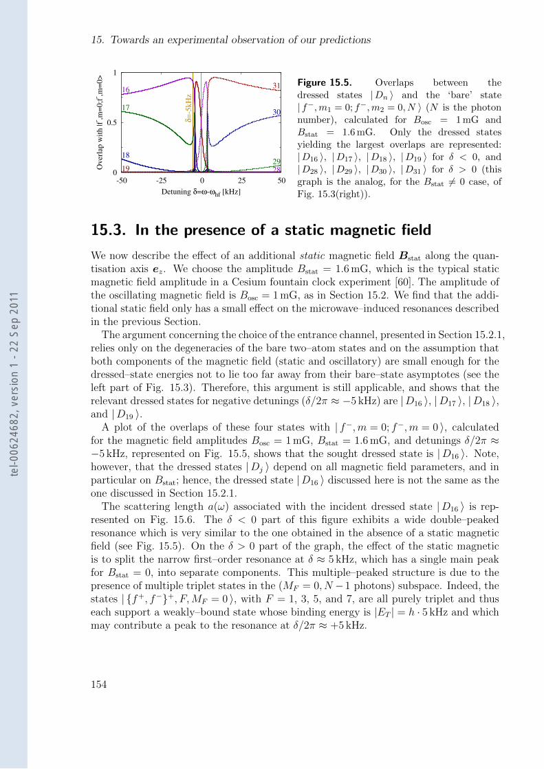
15. Towards an experimental observation of our predictions

0

0.5

1

-50 -25 0 25 50

Over

lap w

ith |f

- ,m=

0;f

- ,m=

0>

Detuning δ=ω-ωhf [kHz]

16

17

18

19

31

30

2928

δ=

-5kH

z

Figure 15.5. Overlaps between thedressed states |Dn 〉 and the ‘bare’ state| f−,m1 = 0; f−,m2 = 0, N 〉 (N is the photonnumber), calculated for Bosc = 1 mG andBstat = 1.6 mG. Only the dressed statesyielding the largest overlaps are represented:|D16 〉, |D17 〉, |D18 〉, |D19 〉 for δ < 0, and|D28 〉, |D29 〉, |D30 〉, |D31 〉 for δ > 0 (thisgraph is the analog, for the Bstat 6= 0 case, ofFig. 15.3(right)).

15.3. In the presence of a static magnetic field

We now describe the effect of an additional static magnetic field Bstat along the quan-tisation axis ez. We choose the amplitude Bstat = 1.6 mG, which is the typical staticmagnetic field amplitude in a Cesium fountain clock experiment [60]. The amplitude ofthe oscillating magnetic field is Bosc = 1 mG, as in Section 15.2. We find that the addi-tional static field only has a small effect on the microwave–induced resonances describedin the previous Section.

The argument concerning the choice of the entrance channel, presented in Section 15.2.1,relies only on the degeneracies of the bare two–atom states and on the assumption thatboth components of the magnetic field (static and oscillatory) are small enough for thedressed–state energies not to lie too far away from their bare–state asymptotes (see theleft part of Fig. 15.3). Therefore, this argument is still applicable, and shows that therelevant dressed states for negative detunings (δ/2π ≈ −5 kHz) are |D16 〉, |D17 〉, |D18 〉,and |D19 〉.

A plot of the overlaps of these four states with | f−,m = 0; f−,m = 0 〉, calculatedfor the magnetic field amplitudes Bosc = 1 mG, Bstat = 1.6 mG, and detunings δ/2π ≈−5 kHz, represented on Fig. 15.5, shows that the sought dressed state is |D16 〉. Note,however, that the dressed states |Dj 〉 depend on all magnetic field parameters, and inparticular on Bstat; hence, the dressed state |D16 〉 discussed here is not the same as theone discussed in Section 15.2.1.

The scattering length a(ω) associated with the incident dressed state |D16 〉 is rep-resented on Fig. 15.6. The δ < 0 part of this figure exhibits a wide double–peakedresonance which is very similar to the one obtained in the absence of a static magneticfield (see Fig. 15.5). On the δ > 0 part of the graph, the effect of the static magneticis to split the narrow first–order resonance at δ ≈ 5 kHz, which has a single main peakfor Bstat = 0, into separate components. This multiple–peaked structure is due to thepresence of multiple triplet states in the (MF = 0, N −1 photons) subspace. Indeed, thestates | f+, f−+, F,MF = 0 〉, with F = 1, 3, 5, and 7, are all purely triplet and thuseach support a weakly–bound state whose binding energy is |ET | = h · 5 kHz and whichmay contribute a peak to the resonance at δ/2π ≈ +5 kHz.

154

tel-0

0624

682,

ver

sion

1 -

22 S

ep 2

011

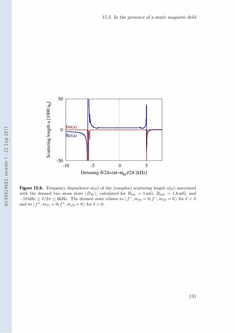
15.3. In the presence of a static magnetic field

-50

0

50

-10 -5 0 5

Sca

tter

ing l

ength

a [

1000 a

0]

Detuning δ/2π=(ω−ωhf)/2π [kHz]

Re(a)

Im(a)

Figure 15.6. Frequency dependence a(ω) of the (complex) scattering length a(ω) associatedwith the dressed two–atom state |D16 〉, calculated for Bosc = 1 mG, Bstat = 1.6 mG, and−10 kHz ≤ δ/2π ≤ 6kHz. The dressed state relates to | f−,mf1 = 0; f−,mf2 = 0 〉 for δ < 0and to | f+,mf1 = 0; f+,mf2 = 0 〉 for δ > 0.

155

tel-0

0624

682,

ver

sion

1 -

22 S

ep 2

011

tel-0

0624

682,

ver

sion

1 -

22 S

ep 2

011

16. Conclusion and outlook

The object of the work presented in the second part of this manuscript has been todescribe a new type of scattering resonance occurring in ultracold atomic systems: themicrowave–induced Fano–Feshbach resonances. Scattering resonances occur when a low–energy scattering state of a pair of colliding atoms, in given internal states, is coupledto a bound state of the two atoms in a different two–atom internal state. In the caseof the “standard” Feshbach resonances, the coupling between the scattering state andthe resonant bound state is obtained using a static magnetic field. Microwave–inducedFeshbach resonances are caused by couplings generated by oscillating magnetic fieldswhose frequencies are tuned close to the atomic hyperfine splitting.

Just like their static–field counterparts, microwave–induced Feshbach resonances causea hyperbolic divergence in the scattering length (see Eq. (11.1)). Therefore, they canbe used to set the value of the scattering length to any desired value and sign, and thusto tailor the nature (attractive or repulsive) and strength (strongly–interacting regime,ideal gas, . . . ) of the interactions within the ultracold atomic sample. They also allowthe scattering length to be adiabatically scanned through the resonance (e.g., in viewof an experimental study of a BEC—BCS crossover): such a scan can be performed,for example, by working at a fixed magnetic field amplitude and slowly ramping themagnetic field frequency from one side of the resonance to the next.

Despite their kinship, microwave–induced Feshbach resonances differ from static–fieldresonances in quite a few respects. Microwave–induced Feshbach resonances occur evenin the absence of any static magnetic field. The resonance frequencies and widths ofmicrowave–induced resonances are not directly related to the characteristics of static–field resonances. Furthermore, the widths of microwave–induced resonances are propor-tional to the squared amplitude of the magnetic field, and these resonances can thereforebe made very broad if a powerful microwave source is available.

We have focused on the case of bosonic alkali atoms, although neither of these twoassumptions is essential. We have characterised the microwave–induced resonances oc-curring in 7Li, 23Na, 41K, 87Rb, and 133Cs using three different approaches: (i) thetwo–square–well approach (Section 9.2), (ii) the two–channel approach (Section 11.1),and (iii) the coupled–channel approach (Section 11.2). The first approach involves asimple model from which orders of magnitude for the resonance positions, widths, andshifts can be extracted without resorting to elaborate numerical methods. The sec-ond approach yields simple scaling laws for the resonance width and the shift on theresonance position due to the interchannel coupling. The third approach is the most

157

tel-0

0624

682,

ver

sion

1 -

22 S

ep 2

011

16. Conclusion and outlook

accurate and general: it remains applicable in the presence of larger oscillating fields(Section 11.2.4), it accounts for inelastic processes, and for the presence of both staticand oscillating fields (Chapter 15). The results of all three approaches (Tables 9.2, 11.1,and 11.2) are in good agreement with each other.

Our numerical results for the resonance widths lead to optimistic experimental prospectswith all atoms except 7Li (for the oscillating field amplitude Bosc = 10 G, all predictedresonance widths are much larger than 1 kHz, except for 7Li; see the discussion in Sec-tion 11.3). In the case of 7Li, the absence of a microwave–induced resonance is not ahindrance, as a very broad static–field Feshbach resonance is already available [22].

The divergence associated with a microwave–induced resonance is actually hyperboliconly for magnetic field amplitudes that are small enough. For all atoms except 133Cs,the resonance remains hyperbolic for magnetic field amplitudes of the order of 10 G (seeFig. 11.9). In the specific case of 133Cs, the resonance involving the weakly bound tripletdimer state (binding energy |ET | = h·5 kHz) becomes non–hyperbolic for magnetic fieldsas small as 5 mG (see Fig. 11.12). We have analysed the large–field behaviour of thisresonance in terms of a competition between the two–atom resonance and single–atomdressed–state effects (Section 11.2.4).

Small static–field resonances have been observed in Cesium fountain clocks at SYRTE–Observatoire de Paris [57]. To our knowledge, these resonances had since remained un-explained. We have shown (Section 14.3) that they are s–wave resonances involving thesame weakly bound dimer state discussed in the previous paragraph.

Finally, we have characterised microwave–induced Feshbach resonances in Cesium in-volving experimental parameters that are relevant for a prospective observation in aCesium fountain clock experiment (Chapter 15). The description of the resonances oc-curring in these situations involves numerous coupled channels; inelastic collisions, aswell as the effect of a small additional static magnetic field, have been accounted for.

All of the numerical calculations presented in this manuscript have been performedwith our own implementations of the coupled–channel method, using the accumulatedphase approach. These implementations are described in Chapter 14.

Throughout the present part of this manuscript, we have characterised the collisionalproperties of ultracold atoms using scattering lengths only. Scattering lengths are zero–temperature quantities; in most cases, the scattering properties at non–zero, albeit small,temperatures may be deduced from the zero–temperature case [1]. However, in the par-ticular case of Cesium, the very large value of the triplet scattering length (aT = 2500 a0)causes atomic interactions to be strongly affected by thermal effects [61]. An experimentperformed in a Cesium fountain clock will be sensitive to these thermal effects, even for

158

tel-0

0624

682,

ver

sion

1 -

22 S

ep 2

011

temperatures as low as T = 1µK. We are currently working on the inclusion of thesethermal effects in our theoretical description.

Our method can be extended to the case of heteronuclear mixtures. Microwave–induced resonances may thus be used to tune the interaction in such systems (e.g inexperiments related to the work presented in the first part of this manuscript) in situa-tions where static–field Feshbach resonances are not easily accessible.

Microwave–induced Feshbach resonances are present even in the absence of a staticmagnetic field. This situation is actively studied in the context of spinor Bose gases.Microwave–induced resonances could be used to tune the sign of the interaction betweenvarious hyperfine states, possibly leading to novel accessible quantum states.

159

tel-0

0624

682,

ver

sion

1 -

22 S

ep 2

011

tel-0

0624

682,

ver

sion

1 -

22 S

ep 2

011

Bibliography

[1] Thorsten Kohler, Krzysztof Goral, and Paul S. Julienne. “Production of coldmolecules via magnetically tunable Feshbach resonances”. In: Rev. Mod. Phys.78.4 (Dec. 2006), pp. 1311–1361. doi: 10.1103/RevModPhys.78.1311.

[2] Stefano Giorgini, Lev P. Pitaevskii, and Sandro Stringari. “Theory of ultracoldatomic Fermi gases”. In: Rev. Mod. Phys. 80.4 (Oct. 2008), pp. 1215–1274. doi:10.1103/RevModPhys.80.1215.

[3] L. Pitaevskii and S. Stringari. Bose-Einstein condensation. Clarendon Press, 2003.isbn: 0198507194.

[4] Franco Dalfovo et al. “Theory of Bose-Einstein condensation in trapped gases”.In: Rev. Mod. Phys. 71.3 (Apr. 1999), pp. 463–512. doi: 10.1103/RevModPhys.71.463.

[5] M. H. Anderson et al. “Observation of Bose-Einstein Condensation in a DiluteAtomic Vapor”. In: Science 269.5221 (1995), pp. 198–201. doi: 10.1126/science.269.5221.198.

[6] E.A. Donley et al. “Dynamics of collapsing and exploding Bose–Einstein conden-sates”. In: Nature 412.6844 (2001), pp. 295–299. issn: 0028-0836. doi: doi:10.1038/35085500.

[7] Cheng Chin et al. “Feshbach resonances in ultracold gases”. In: Rev. Mod. Phys.82.2 (Apr. 2010), pp. 1225–1286. doi: 10.1103/RevModPhys.82.1225.

[8] T. Bourdel et al. “Experimental Study of the BEC-BCS Crossover Region inLithium 6”. In: Phys. Rev. Lett. 93.5 (July 2004), p. 050401. doi: 10 . 1103 /

PhysRevLett.93.050401.

[9] Immanuel Bloch, Jean Dalibard, and Wilhelm Zwerger. “Many-body physics withultracold gases”. In: Rev. Mod. Phys. 80.3 (July 2008), pp. 885–964. doi: 10.1103/RevModPhys.80.885.

[10] Jocelyne Guena et al. “Evaluation of Doppler Shifts to Improve the Accuracyof Primary Atomic Fountain Clocks”. In: Phys. Rev. Lett. 106.13 (Apr. 2011),p. 130801. doi: 10.1103/PhysRevLett.106.130801.

[11] Kurt Gibble. “Decoherence and Collisional Frequency Shifts of Trapped Bosonsand Fermions”. In: Phys. Rev. Lett. 103.11 (Sept. 2009), p. 113202. doi: 10.1103/PhysRevLett.103.113202.

[12] H Marion. “Controle des collisions froides du Cesium 133. Tests de la variation dela constante de structure fine a l’aide d’une fontaine atomique double Rubidium-Cesium”. PhD thesis. Universite Paris VI, 2005.

161

tel-0

0624

682,

ver

sion

1 -

22 S

ep 2

011

Bibliography

[13] C. Pethick and H. Smith. Bose-Einstein condensation in dilute gases. CambridgeUniversity Press, 2002. isbn: 0521665809.

[14] J. Stenger et al. “Strongly Enhanced Inelastic Collisions in a Bose-Einstein Con-densate near Feshbach Resonances”. In: Phys. Rev. Lett. 82.12 (Mar. 1999), pp. 2422–2425. doi: 10.1103/PhysRevLett.82.2422.

[15] A. Marte et al. “Feshbach Resonances in Rubidium 87: Precision Measurementand Analysis”. In: Phys. Rev. Lett. 89.28 (Dec. 2002), p. 283202. doi: 10.1103/PhysRevLett.89.283202.

[16] M. Marinescu and L. You. “Controlling Atom-Atom Interaction at Ultralow Tem-peratures by dc Electric Fields”. In: Phys. Rev. Lett. 81.21 (Nov. 1998), pp. 4596–4599. doi: 10.1103/PhysRevLett.81.4596.

[17] P. O. Fedichev et al. “Influence of Nearly Resonant Light on the Scattering Lengthin Low-Temperature Atomic Gases”. In: Phys. Rev. Lett. 77.14 (Sept. 1996), pp. 2913–2916. doi: 10.1103/PhysRevLett.77.2913.

[18] M. Theis et al. “Tuning the Scattering Length with an Optically Induced FeshbachResonance”. In: Phys. Rev. Lett. 93.12 (Sept. 2004), p. 123001. doi: 10.1103/PhysRevLett.93.123001.

[19] K. Enomoto et al. “Optical Feshbach Resonance Using the Intercombination Tran-sition”. In: Phys. Rev. Lett. 101.20 (Nov. 2008), p. 203201. doi: 10.1103/PhysRevLett.101.203201.

[20] A. J. Moerdijk, B. J. Verhaar, and T. M. Nagtegaal. “Collisions of dressed ground-state atoms”. In: Phys. Rev. A 53.6 (June 1996), pp. 4343–4351. doi: 10.110

3/PhysRevA.53.4343.

[21] D. J. Papoular, G. V. Shlyapnikov, and J. Dalibard. “Microwave-induced Fano-Feshbach resonances”. In: Phys. Rev. A 81.4 (Apr. 2010), p. 041603. doi: 10.1103/PhysRevA.81.041603.

[22] K.E. Strecker et al. “Formation and propagation of matter-wave soliton trains”. In:Nature 417.6885 (2002), pp. 150–153. issn: 0028-0836. doi: 10.1038/nature747.

[23] G. Herzberg. Molecular Spectra and Molecular Structure. I. Spectra of DiatomicMolecules. D. Van Nostrand, 1950.

[24] Kevin M. Jones et al. “Ultracold photoassociation spectroscopy: Long-range moleculesand atomic scattering”. In: Rev. Mod. Phys. 78.2 (May 2006), pp. 483–535. doi:10.1103/RevModPhys.78.483.

[25] C. Cohen-Tannoudji et al. Quantum Mechanics. Vols. 1 and 2. Wiley Interscience,1977.

[26] J. Dalibard. “Collisional dynamics of ultracold atomic gases”. In: Proceedings ofthe International School of Physics Enrico Fermi, Course CXL: Bose – Einsteincondensation in gases. Societa Italiana di Fisica, 1998. Chap. Collisional dynamicsof ultracold atomic gases.

162

tel-0

0624

682,

ver

sion

1 -

22 S

ep 2

011

Bibliography

[27] G. F. Gribakin and V. V. Flambaum. “Calculation of the scattering length inatomic collisions using the semiclassical approximation”. In: Phys. Rev. A 48.1(July 1993), pp. 546–553. doi: 10.1103/PhysRevA.48.546.

[28] GV Shlyapnikov, J.T.M. Walraven, and E.L. Surkov. “Antihydrogen at sub-Kelvintemperatures”. In: Hyperfine Interactions 76.1 (1993), pp. 31–46. issn: 0304-3843.doi: 10.1007/BF02316704.

[29] A. D. Lange et al. “Determination of atomic scattering lengths from measurementsof molecular binding energies near Feshbach resonances”. In: Phys. Rev. A 79.1(Jan. 2009), p. 013622. doi: 10.1103/PhysRevA.79.013622.

[30] C. Cohen-Tannoudji, J. Dupont-Roc, and G. Grynberg. Atom-Photon Interactions:Basic Processes and Applications. Wiley, 1998.

[31] B. J. Verhaar, E. G. M. van Kempen, and S. J. J. M. F. Kokkelmans. “Predictingscattering properties of ultracold atoms: Adiabatic accumulated phase methodand mass scaling”. In: Phys. Rev. A 79.3 (Mar. 2009), p. 032711. doi: 10.1103/PhysRevA.79.032711.

[32] E. Arimondo, M. Inguscio, and P. Violino. “Experimental determinations of thehyperfine structure in the alkali atoms”. In: Rev. Mod. Phys. 49.1 (Jan. 1977),pp. 31–75. doi: 10.1103/RevModPhys.49.31.

[33] L.D. Landau and L.M. Lifshitz. Quantum Mechanics: Non-Relativistic Theory.3rd ed. Butterworth-Heinemann, 2003.

[34] H. T. C. Stoof, J. M. V. A. Koelman, and B. J. Verhaar. “Spin-exchange and dipolerelaxation rates in atomic hydrogen: Rigorous and simplified calculations”. In:Phys. Rev. B 38.7 (Sept. 1988), pp. 4688–4697. doi: 10.1103/PhysRevB.38.4688.

[35] F. H. Mies et al. “Estimating Bounds on Collisional Relaxation Rates of Spin-Polarized 87Rb Atoms at Ultracold Temperatures”. In: J. Res. Natl. Inst. Stand.Technol. 101 (July 1996), pp. 521–535. url: http://nvl.nist.gov/pub/nistpubs/jres/101/4/cnt101-4.htm.

[36] A. J. Moerdijk, B. J. Verhaar, and A. Axelsson. “Resonances in ultracold collisionsof 6Li, 7Li, and 23Na”. In: Phys. Rev. A 51.6 (June 1995), pp. 4852–4861. doi:10.1103/PhysRevA.51.4852.

[37] A. Messiah. Quantum Mechanics. Vol. II. North Holland Publishing Company,1966.

[38] F. D. Colavecchia et al. “The potential energy surface for spin-aligned Li3(14A′)and the potential energy curve for spin-aligned Li2(a3Σ+

u )”. In: The Journal ofChemical Physics 118.12 (2003), pp. 5484–5495. doi: 10.1063/1.1555124.

[39] E. G. M. van Kempen et al. “Interisotope Determination of Ultracold RubidiumInteractions from Three High-Precision Experiments”. In: Phys. Rev. Lett. 88.9(Feb. 2002), p. 093201. doi: 10.1103/PhysRevLett.88.093201.

[40] S. Bize. “Tests fondamentaux a l’aide d’horloges a atomes froids de rubidium etde cesium”. PhD thesis. Universite Pierre et Marie Curie, 2001.

163

tel-0

0624

682,

ver

sion

1 -

22 S

ep 2

011

Bibliography

[41] M. Kohl. private communication. 2009.

[42] Magnetic loop antenna calculator. url: http://www.66pacific.com/calculators/small_tx_loop_calc.aspx.

[43] I. Spielman. private communication. 2009.

[44] L. Turner. private communication. 2010.

[45] Kendall B. Davis et al. “Evaporative Cooling of Sodium Atoms”. In: Phys. Rev.Lett. 74.26 (June 1995), pp. 5202–5205. doi: 10.1103/PhysRevLett.74.5202.

[46] Tin-Lun Ho. “Spinor Bose Condensates in Optical Traps”. In: Phys. Rev. Lett.81.4 (July 1998), pp. 742–745. doi: 10.1103/PhysRevLett.81.742.

[47] E. G. M. van Kempen. “Feshbach Resonances in Cold Atomic Gases”. PhD thesis.Technische Universiteit Eindhoven, 2001.

[48] A. J. Moerdijk and B. J. Verhaar. “Laser cooling and the highest bound states ofthe Na diatom system”. In: Phys. Rev. A 51.6 (June 1995), R4333–R4336. doi:10.1103/PhysRevA.51.R4333.

[49] B.M. Smirnov and M.I. Chibisov. “Electron exchange and changes in the hyperfinestate of colliding alkaline earth atoms”. In: Soviet Physics JETP 21 (1965), p. 624.

[50] Boudewijn Verhaar, Kurt Gibble, and Steven Chu. “Cold-collision properties de-rived from frequency shifts in a cesium fountain”. In: Phys. Rev. A 48.5 (Nov.1993), R3429–R3432. doi: 10.1103/PhysRevA.48.R3429.

[51] J. M. Vogels et al. “Coupled singlet-triplet analysis of two-color cold-atom pho-toassociation spectra”. In: Phys. Rev. A 61.4 (Mar. 2000), p. 043407. doi: 10.1103/PhysRevA.61.043407.

[52] W.H. Press et al. Numerical Recipes: the Art of Scientific Programming. 3rd ed.Cambridge University Press, 2007.

[53] E. Tiesinga et al. “Conditions for Bose-Einstein condensation in magneticallytrapped atomic cesium”. In: Phys. Rev. A 46.3 (Aug. 1992), R1167–R1170. doi:10.1103/PhysRevA.46.R1167.

[54] E. Tiesinga, B. J. Verhaar, and H. T. C. Stoof. “Threshold and resonance phe-nomena in ultracold ground-state collisions”. In: Phys. Rev. A 47.5 (May 1993),pp. 4114–4122. doi: 10.1103/PhysRevA.47.4114.

[55] S. Inouye et al. “Observation of Feshbach resonances in a Bose–Einstein conden-sate”. In: Nature 392.6672 (1998), pp. 151–154. issn: 0028-0836. doi: 10.1038/32354.

[56] Chiara D’Errico et al. “Feshbach resonances in ultracold 39 K”. In: New Journalof Physics 9.7 (2007), p. 223. url: http://stacks.iop.org/1367-2630/9/i=7/a=223.

[57] S. Bize et al. Feshbach resonances at very low magnetic field in a Cesium 133fountain and other results. Presentation at ICAP 2004.

164

tel-0

0624

682,

ver

sion

1 -

22 S

ep 2

011

Bibliography

[58] R. S. Freeland. “Photoassociation Spectroscopy of Ultracold and Bose-condensedAtomic Gases”. PhD thesis. The University of Texas at Austin, 2001.

[59] S. Haroche. “Etude theorique et experimentale des proprietes d’atomes habillespar des photons de radiofrequence”. PhD thesis. LKB - Universite Paris VI, 1971.

[60] P. Rosenbusch. private communication. 2011.

[61] Paul J. Leo et al. “Collisional Frequency Shifts in 133Cs Fountain Clocks”. In: Phys.Rev. Lett. 86.17 (Apr. 2001), pp. 3743–3746. doi: 10.1103/PhysRevLett.86.3743.

165

tel-0

0624

682,

ver

sion

1 -

22 S

ep 2

011

tel-0

0624

682,

ver

sion

1 -

22 S

ep 2

011

Acknowledgements

This memoir describes the research work I have performed towards the preparation of myPh.D. at Laboratoire de Physique Theorique et Modeles Statisiques (CNRS — Univer-site Paris–Sud) from 2007 to 2011. I am very grateful to Profs. S. Ouvry and M. Mezard,who directed LPTMS during that time, for their very warm welcome.

My Ph.D. work has been supervised by Prof. G. Shlyapnikov. Every encounter withGora has been inspirational. His drive for research and his benevolence seem to haveno bounds. It has been a great privilege to benefit from his clear explanations andhis well–thought–out advice. Gora’s interests extend far beyond Physics, his sense ofhumour is outstanding, and it has been a great pleasure to learn a little about Russianhistory and culture from him. I would like to convey my very sincere thanks to him forall of his help and involvement in this work.

I am hugely indebted to Prof. J. Dalibard (LKB, ENS–Paris) for his luminous ex-planations and his constant optimism. I am very grateful for his availability and hiswillingness to help. I have also learnt a lot about pedagogy from him.

I am very much beholden to Profs. S. Stringari (Univ. Trento) and J. Walraven(Univ. Amsterdam) for the interest they have shown for this work, and for readily ac-cepting to act as Referees for my defence. My special thanks also go to Profs. O. Dulieu(LAC), R. Kaiser (INLN), and E. Trizac for accepting to take part in the Jury.

Many thanks are due to Drs. P. Rosenbusch and S. Bize (SYRTE–Observatoire deParis), who have patiently explained the experimental issues associated with atomicclocks. The interest they have expressed for our work on microwave–induced resonanceshas been instrumental in seeing it through. I warmly thank S. Bize for inviting me togive a seminar at SYRTE.

Dr. D. Petrov has kindly guided my first steps at LPTMS. I thank him for his helpand explanations concerning our theoretical work on composite bosons.

I wish to thank Prof. C. Salomon (LKB, ENS–Paris) for his enthusiastic presentationof the experimental challenges of the study of heteronuclear Fermi mixtures.

I am very grateful to Prof. M. Leduc (LKB, ENS–Paris and IFRAF), who, alongwith J. Dalibard, suggested that I contact G. Shlyapnikov in the first place. Moreover,IFRAF’s generous financial support has enabled me to attend ICAP 2010 in Australia.

167

tel-0

0624

682,

ver

sion

1 -

22 S

ep 2

011

Acknowledgements

I thank Profs. J. Robert, P. Mendels, N. Pavloff, and Dr. F. Caetano for giving methe chance to take part in the teaching effort at Univ. Paris–Sud, and for sharing theirinvaluable experience. I am very much obliged towards Dr. L. Caperan (Lycee Louis–le–Grand), who has transmitted his enthusiasm for teaching Physics to me, and whoprovided me with early teaching opportunities.

I am happy to acknowledge help from two friends and colleagues. Dr. P. Clade(LKB Jussieu) has proofread the greater part of this manuscript. Dr. E. Lepage (Univ.Paris VI) has explained away many mathematical mysteries, in amazingly clear andsimple terms. I thank them both for very fruitful discussions.

Last but not least, I am extremely grateful to all my family for their unfailing support.I thank my grandparents for their wisdom, my younger sister for her constant goodhumour, my mother for her infinite patience, and my father, who first showed me howrewarding scientific research can be.

168

tel-0

0624

682,

ver

sion

1 -

22 S

ep 2

011