THESE DE DOCTORAT DE - Hydrologiehydrologie.org/THE/SALEH.pdf · THESE DE DOCTORAT DE L UNIVERSITE PIERRE ET MARIE CURIE Spécialité ... between the gauging stations of Dissangis

THESE DE DOCTORAT DE L’UNIVERSITE PIERRE ET MARIE CURIE

Spécialité

Hydrologie et Hydrogéologie Quantitative

Ecole Doctorale Géosciences et Ressources Naturelles 398 Paris

Présentée par

M. Firas S. M. SALEH

Pour obtenir le grade de

DOCTEUR de l’UNIVERSITÉ PIERRE ET MARIE CURIE

Sujet de la thèse : Apport de la modélisation hydraulique pour une meilleure simulation des tirants d'eau et des échanges nappe-rivière à l'échelle régionale soutenue le 15 décembre 2010

devant le jury composé de :

M. Jean-Marie MOUCHEL : Président Mme. Isabelle BRAUD : Rapporteur

M. Julio GONCALVES : Rapporteur

M. Philippe BELLEUDY : Examinateur

M. Emmanuel LEDOUX : Directeur de thèse

Mme. Agnès DUCHARNE : Co-directeur de thèse

M. Nicolas FLIPO : Co-directeur de thèse Université Pierre & Marie Curie - Paris 6 Bureau d’accueil, inscription des doctorants Esc G, 2ème étage 15 rue de l’école de médecine 75270-PARIS CEDEX 06

Tél. Secrétariat : 01 44 27 28 10 Fax : 01 44 27 23 95

Tél. pour les étudiants de A à EL : 01 44 27 28 07 Tél. pour les étudiants de EM à MON : 01 44 27 28 05

Tél. pour les étudiants de MOO à Z : 01 44 27 28 02 E-mail : [email protected]

tel-0

0582

551,

ver

sion

1 -

1 Ap

r 201

1

http://tel.archives-ouvertes.fr/tel-00582551/fr/

http://hal.archives-ouvertes.fr

II

tel-0

0582

551,

ver

sion

1 -

1 Ap

r 201

1

III

Contribution of 1D local hydraulic modeling to improve simulations of river stages and stream-aquifer interactions at regional scale

Abstract

This thesis contributes to the development of the integrated model EauDyssée of regional

scale river systems, in the pilot case study of the Seine River basin. The main objective is to

provide a realistic simulation of river stage and discharge at the regional scale, in order to

improve the simulation of stream-aquifer interactions and better assess piezometric heads.

The first part of the thesis aims at establishing whether a reliable hydrodynamic routing model

can be developed based on limited river bed morphological data. A wide variety of "what if"

river geometry scenarios are explored to determine the most appropriate river representation

geometry in areas where cross sections surveys are not always accessible. This study is

carried out in the Serein River (tributary of the Yonne River), between the gauging stations of

Dissangis et Beaumont, in a well surveyed reach (20 cross sections over 89 km). River

discharge and stage are simulated by the hydraulic model HEC-RAS (1D Saint-Venant

equations), while lateral inflows are simulated by the regional hydrogeological model

EauDyssée. The results of this study show that a 1D Saint-Venant model is not suitable for

simulating water levels in areas where river geomorphologic date is not available. Based on

these conclusions, we developed an original upscaling strategy, which allows for benefiting

from high resolution hydraulic modeling outputs to describe fluctuating river stage and

improve the regional scale simulation of stream-aquifer interactions in the integrated model

EauDyssée.

The validity of this approach has been illustrated in a 4500 km2 sub-basin of the Oise River,

for the period 1990-1995. We used the HEC-RAS to achieve a hydrodynamic simulation of a

188-km reach, where 420 surveyed cross sections are available. This model is used to

interpolate rating curves (river stage vs. discharge) with a mean resolution of 200 m. The

tel-0

0582

551,

ver

sion

1 -

1 Ap

r 201

1

IV

latter are then projected onto the river grid cells of the regional model EauDyssée (1-km

resolution), where they allow for fluctuating river stage, as a function of the discharge routed

at the regional scale by EauDyssée. The altitude of the river surface defining its hydraulic

head, these fluctuations influence the exchanges between the river and aquifer cells, which

depend on the related vertical hydraulic gradient (Darcy’s law).

This work outlines the efficiency of the approach to better simulate river stages and stream-

aquifer interactions at regional scale with low computing cost. Furthermore, this framework

coupling strategy have several perspectives: for example simulating the hydrodynamic

behavior of alluvial wetlands, modeling more accurately the impact of climate change on

hydrosystems, especially concerning pollutants removal or release by biogeochemical

processes, or better assessing the risk of inundations at the regional scale.

Keywords: Stream-aquifer interactions, Hydrology, Hydrogeology, Upscaling, Regional scale, Local scale, EauDyssée platform, river morphology

Résumé court en français

Cette thèse s’inscrit dans le développement de la plateforme EauDyssée de modélisation

intégrée des hydrosystèmes régionaux, au sein du bassin pilote de la Seine. L’objectif

principal est de contribuer à une meilleure simulation des tirants d'eau à l’échelle régionale

afin d'améliorer la simulation des interactions nappe-rivière et de mieux quantifier les niveaux

piézométriques dans les aquifères.

La première partie de la thèse vise à évaluer la sensibilité d'un modèle hydraulique à la

précision de la description géomorphologique des lits pour identifier le meilleur compromis

entre parcimonie et réalisme et identifier les facteurs morphologiques les plus importants pour

obtenir une simulation satisfaisante des tirants d'eau à l’échelle régionale. Cette étude est

menée sur le Serein (affluent de l'Yonne), entre les stations limnimétriques de Dissangis et

tel-0

0582

551,

ver

sion

1 -

1 Ap

r 201

1

V

Beaumont, dans un bief bien renseigné (20 sections transversales sur 89 kms). Débits et

tirants d’eau sont simulés par le modèle hydraulique HEC-RAS (équations de Saint-Venant

1D), en fonction des apports latéraux simulés par le modèle régional EauDyssée.

Les résultats de cette étude montrent qu’un modèle 1D type Saint-Venant n’est pas adapté à la

simulation des écoulements à l’échelle régionale. Nous avons donc développé une méthode de

changement d’échelle originale, dans laquelle la modélisation fine des processus hydrauliques

à haute résolution permet d'améliorer la représentation des profils d’eau en rivière et les

interactions nappe-rivière simulées à l'échelle régionale par le modèle intégré EauDyssée.

Cette méthodologie de changement d’échelle a été validée dans un sous bassin versant de

l’Oise d’une superficie de 4500 km2, pour la période 1990-1995. Nous avons utilisé HEC-

RAS pour la modélisation hydraulique d’un tronçon de l’Oise de 188 km, où 420 sections

transversales sont disponibles. Le modèle permet d’interpoler des courbes de tarage simulées

tous les 200m en moyenne. Ces courbes de tarage sont ensuite projetées sur les mailles

rivière du modèle régional EauDyssée (résolution de 1 km), où elles permettent de simuler la

fluctuation du niveau d'eau en fonction du débit à l’échelle régionale par EauDyssée. La cote

de la surface libre de la rivière définissant sa charge hydraulique, ces fluctuations influencent

alors les échanges entre les mailles rivière et les nappes, qui dépendent des gradients de

charge verticaux entre rivière et nappe (loi de Darcy).

Ce travail montre l'intérêt de l'approche pour mieux évaluer les interactions nappes-rivières à

l'échelle régionale avec un faible coût de calcul. Il offre des perspectives intéressantes pour

simuler des processus jusque là négligés par le modèle EauDyssée : élimination de nitrate

dans les zones humides qui sont souvent situées à la zone de contact entre les nappes

souterraines et la rivière, ou l’impact du changement climatique sur le fonctionnement des

hydrosystèmes et plus particulièrement sur l’élimination ou le relarguage de polluants par des

tel-0

0582

551,

ver

sion

1 -

1 Ap

r 201

1

VI

processus biogéochimiques, ainsi que de mieux estimer les risques d’inondation à l’échelle

régionale.

Un résumé long en français de la thèse se trouve dans l'appendice B.

Mots clés: Interactions nappe-rivière, hydrologie, hydrogéologie, Changement d’échelle, Plateforme EauDyssée, morphologie des rivières

tel-0

0582

551,

ver

sion

1 -

1 Ap

r 201

1

VII

DEDICATION

This thesis is dedicated to the memory of my mother,

Layla S. Khalil (1952-2009)

tel-0

0582

551,

ver

sion

1 -

1 Ap

r 201

1

VIII

ACKNOWLEDGMENTS

This thesis owes its existence to the help, support, and inspiration of many people. It is a

pleasure to convey my deep appreciation and gratitude to them all in my humble

acknowledgment.

First, I am proud to record that I had the opportunity to work with exceptionally experienced

scientists in France.

I would like to express my sincere appreciation and gratitude to my supervisor Dr. Emmanuel

Ledoux for his advice and guidance as well as giving me extraordinary experiences through

out the work. Above all and the most needed, he provided me unflinching encouragement and

support in various ways.

I gratefully acknowledge Dr. Nicolas Flipo for his advice, supervision, and crucial

contribution to this work. He always granted me his time even for answering some of my

unintelligent questions in the science of hydrology. Nicolas, I am grateful in every possible

way and hope to keep up our collaboration in the future.

I am grateful to Dr. Agnès Ducharne for her supervision, patience, enthusiasm as well as her

help whenever I was in need during more than three years. I am indebted to her more than she

knows.

Many thanks go in particular to Dr. Ludovic Oudin. I am much indebted to Ludovic for his

valuable advice in science discussion, supervision and furthermore, using his precious time to

read my scientific reports and gave his critical comments about them.

I would like to express my sincere appreciation and gratitude to Dr. Isabelle Braud and Dr.

Julio Goncalves for accepting to review my thesis and participate in my thesis jury, I am

confident that their review and constructive feedback will enrich this study.

tel-0

0582

551,

ver

sion

1 -

1 Ap

r 201

1

IX

I am indebted to Dr. Jean-Marie Mouchel and Dr. Philippe Belleudy for accepting to be

examiners in my thesis jury.

I am indebted to Dr. Florence Habets and Pascal Viennot, who have been a source of support

and encouragement over many years. Thank you Florence for supporting me through the

modelization phase and helping me better understand the EauDyssée platform.

I am grateful for the data provided by Yan Lacaze and the Direction Régionale de

l'Environnement Ile de France (DIREN).

I am also grateful to the members of the UMR Sisyphe and the members of the SHR team of

the Center of Geosciences of MINES ParisTech for their support and their comradeship,

especially Céline Monteil for her motivating discussions and ideas.

I am thankful for the financial support provided by the PIREN-Seine research program on the

Seine basin and the Centre National des Oeuvres Universitaires et Scolaires (CNOUS).

Finally, I would like to express my deepest gratitude for the constant support, understanding

and love that I received from my wife and my family during the past years.

tel-0

0582

551,

ver

sion

1 -

1 Ap

r 201

1

X

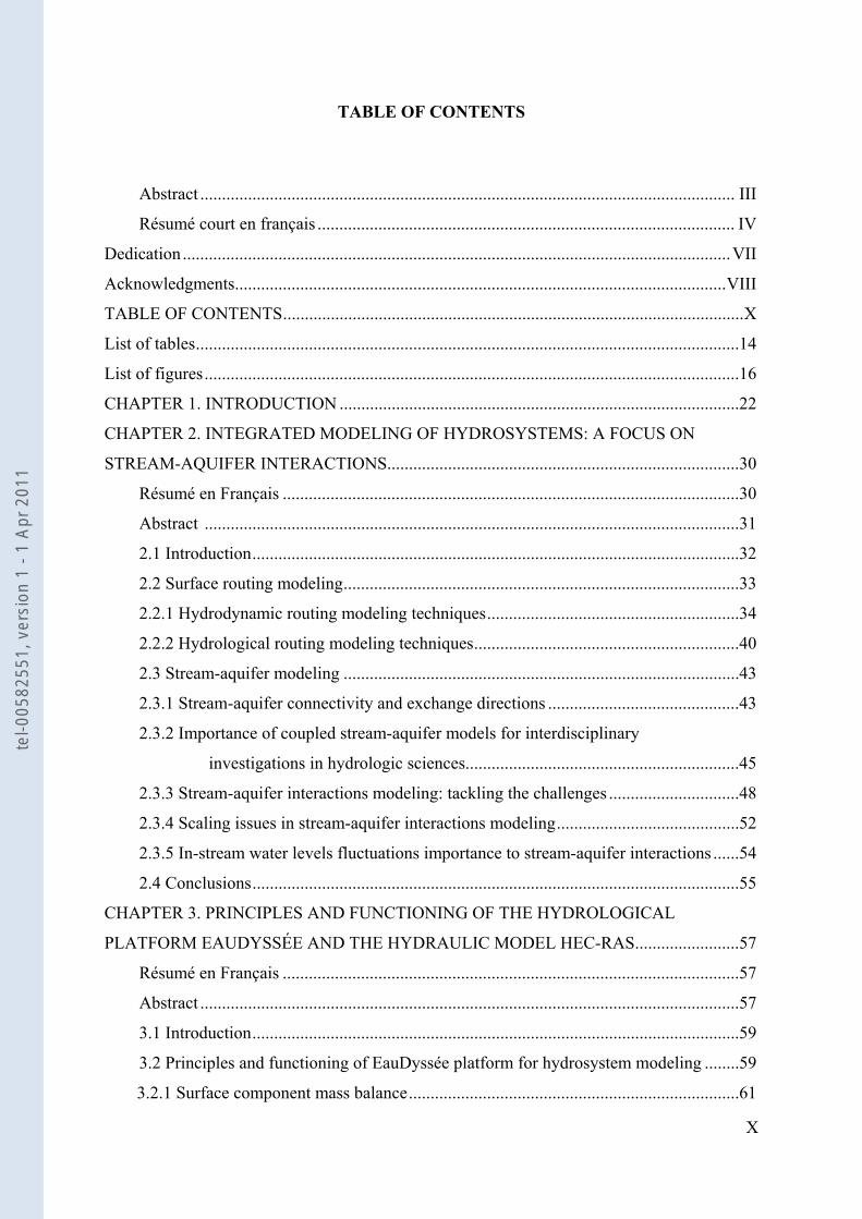
TABLE OF CONTENTS

Abstract ........................................................................................................................... III

Résumé court en français ................................................................................................ IV

Dedication..............................................................................................................................VII

Acknowledgments.................................................................................................................VIII

TABLE OF CONTENTS..........................................................................................................X

List of tables.............................................................................................................................14

List of figures...........................................................................................................................16

CHAPTER 1. INTRODUCTION ............................................................................................22

CHAPTER 2. INTEGRATED MODELING OF HYDROSYSTEMS: A FOCUS ON

STREAM-AQUIFER INTERACTIONS.................................................................................30

Résumé en Français .........................................................................................................30

Abstract. ...........................................................................................................................31

2.1 Introduction................................................................................................................32

2.2 Surface routing modeling...........................................................................................33

2.2.1 Hydrodynamic routing modeling techniques..........................................................34

2.2.2 Hydrological routing modeling techniques.............................................................40

2.3 Stream-aquifer modeling ...........................................................................................43

2.3.1 Stream-aquifer connectivity and exchange directions ............................................43

2.3.2 Importance of coupled stream-aquifer models for interdisciplinary

investigations in hydrologic sciences...............................................................45

2.3.3 Stream-aquifer interactions modeling: tackling the challenges ..............................48

2.3.4 Scaling issues in stream-aquifer interactions modeling..........................................52

2.3.5 In-stream water levels fluctuations importance to stream-aquifer interactions ......54

2.4 Conclusions................................................................................................................55

CHAPTER 3. PRINCIPLES AND FUNCTIONING OF THE HYDROLOGICAL

PLATFORM EAUDYSSÉE AND THE HYDRAULIC MODEL HEC-RAS........................57


Abstract ............................................................................................................................57

3.1 Introduction................................................................................................................59

3.2 Principles and functioning of EauDyssée platform for hydrosystem modeling ........59

3.2.1 Surface component mass balance............................................................................61

tel-0

0582

551,

ver

sion

1 -

1 Ap

r 201

1

XI

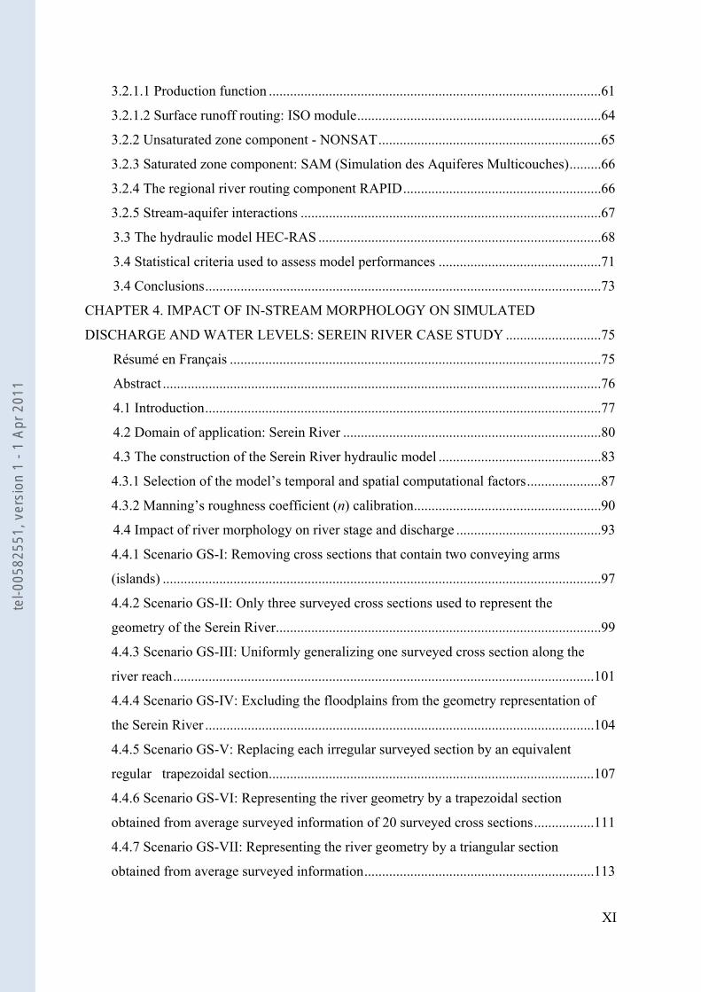
3.2.1.1 Production function ..............................................................................................61

3.2.1.2 Surface runoff routing: ISO module.....................................................................64

3.2.2 Unsaturated zone component - NONSAT...............................................................65

3.2.3 Saturated zone component: SAM (Simulation des Aquiferes Multicouches).........66

3.2.4 The regional river routing component RAPID........................................................66

3.2.5 Stream-aquifer interactions .....................................................................................67

3.3 The hydraulic model HEC-RAS ................................................................................68

3.4 Statistical criteria used to assess model performances ..............................................71

3.4 Conclusions................................................................................................................73

CHAPTER 4. IMPACT OF IN-STREAM MORPHOLOGY ON SIMULATED

DISCHARGE AND WATER LEVELS: SEREIN RIVER CASE STUDY ...........................75


Abstract ............................................................................................................................76

4.1 Introduction................................................................................................................77

4.2 Domain of application: Serein River .........................................................................80

4.3 The construction of the Serein River hydraulic model ..............................................83

4.3.1 Selection of the model’s temporal and spatial computational factors.....................87

4.3.2 Manning’s roughness coefficient (n) calibration.....................................................90

4.4 Impact of river morphology on river stage and discharge .........................................93

4.4.1 Scenario GS-I: Removing cross sections that contain two conveying arms

(islands) ............................................................................................................................97

4.4.2 Scenario GS-II: Only three surveyed cross sections used to represent the

geometry of the Serein River............................................................................................99

4.4.3 Scenario GS-III: Uniformly generalizing one surveyed cross section along the

river reach.......................................................................................................................101

4.4.4 Scenario GS-IV: Excluding the floodplains from the geometry representation of

the Serein River ..............................................................................................................104

4.4.5 Scenario GS-V: Replacing each irregular surveyed section by an equivalent

regular trapezoidal section............................................................................................107

4.4.6 Scenario GS-VI: Representing the river geometry by a trapezoidal section

obtained from average surveyed information of 20 surveyed cross sections.................111

4.4.7 Scenario GS-VII: Representing the river geometry by a triangular section

obtained from average surveyed information.................................................................113

tel-0

0582

551,

ver

sion

1 -

1 Ap

r 201

1

XII

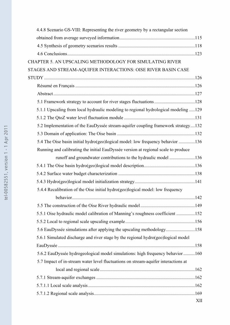
4.4.8 Scenario GS-VIII: Representing the river geometry by a rectangular section

obtained from average surveyed information.................................................................115

4.5 Synthesis of geometry scenarios results ..................................................................118

4.6 Conclusions..............................................................................................................123

CHAPTER 5. AN UPSCALING METHODOLOGY FOR SIMULATING RIVER

STAGES AND STREAM-AQUIFER INTERACTIONS: OISE RIVER BASIN CASE

STUDY ..................................................................................................................................126

Résumé en Français .......................................................................................................126

Abstract ..........................................................................................................................127

5.1 Framework strategy to account for river stages fluctuations ...................................128

5.1.1 Upscaling from local hydraulic modeling to regional hydrological modeling .....129

5.1.2 The QtoZ water level fluctuation module .............................................................131

5.2 Implementation of the EauDyssée stream-aquifer coupling framework strategy....132

5.3 Domain of application: The Oise basin ...................................................................132

5.4 The Oise basin initial hydro(geo)logical model: low frequency behavior ..............136

Running and calibrating the initial EauDyssée version at regional scale to produce

runoff and groundwater contributions to the hydraulic model ......................136

5.4.1 The Oise basin hydro(geo)logical model description............................................136

5.4.2 Surface water budget characterization ..................................................................138

5.4.3 Hydro(geo)logical model initialization strategy....................................................141

5.4.4 Recalibration of the Oise initial hydro(geo)logical model: low frequency

behavior..........................................................................................................142

5.5 The construction of the Oise River hydraulic model ...............................................149

5.5.1 Oise hydraulic model calibration of Manning’s roughness coefficient ................152

5.5.2 Local to regional scale upscaling example............................................................156

5.6 EauDyssée simulations after applying the upscaling methodology.........................158

5.6.1 Simulated discharge and river stage by the regional hydro(geo)logical model

EauDyssée ......................................................................................................................158

5.6.2 EauDyssée hydrogeological model simulations: high frequency behavior ..........160

5.7 Impact of in-stream water level fluctuations on stream-aquifer interactions at

local and regional scale..................................................................................162

5.7.1 Stream-aquifer exchanges .....................................................................................162

5.7.1.1 Local scale analysis ............................................................................................162

5.7.1.2 Regional scale analysis.......................................................................................169

tel-0

0582

551,

ver

sion

1 -

1 Ap

r 201

1

XIII

5.8 Quantification of stream-aquifer exchange..............................................................172

5.9 Conclusions..............................................................................................................175

CHAPTER 6. CONCLUSIONS AND FUTURE WORK.....................................................178

ANNEXE A: SEREIN RIVER MORPHOLOGICAL DATA VS. SIMULATED

RATING CURVES................................................................................................................185

ANNEXE B: RESUME LONG DE LA THESE EN FRANÇAIS........................................190

REFERENCES ......................................................................................................................197

tel-0

0582

551,

ver

sion

1 -

1 Ap

r 201

1

14

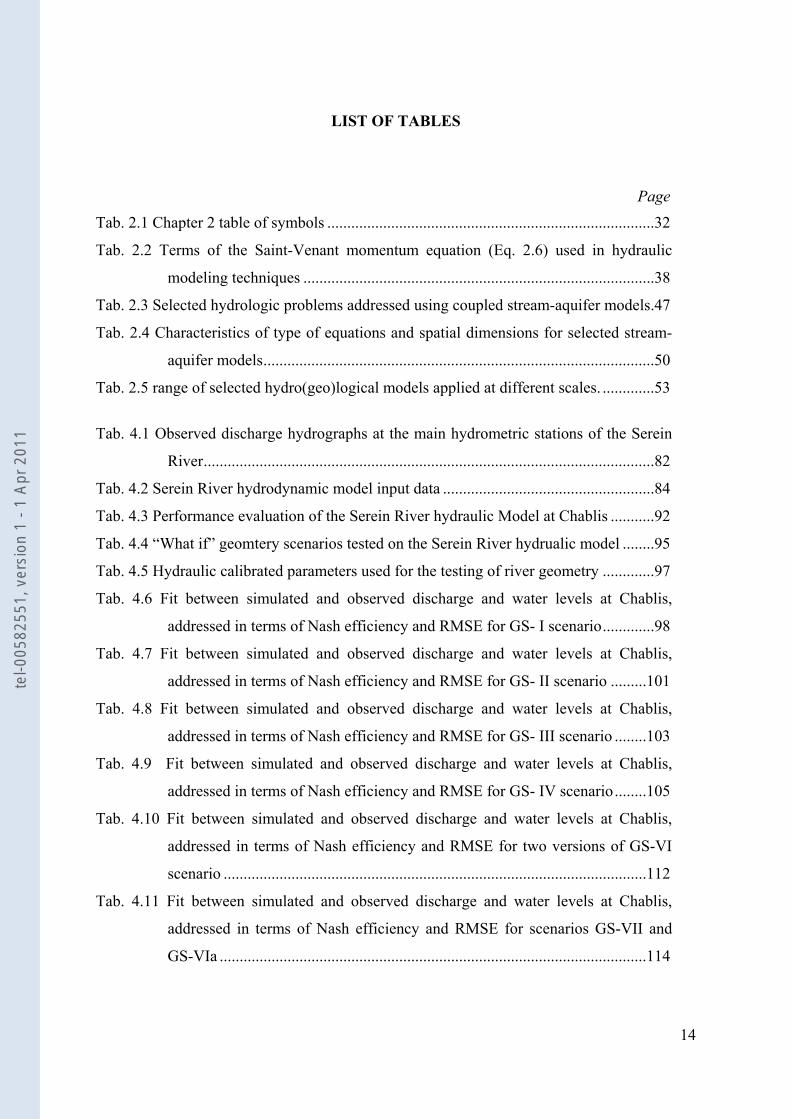
LIST OF TABLES

Page

Tab. 2.1 Chapter 2 table of symbols ..................................................................................32

Tab. 2.2 Terms of the Saint-Venant momentum equation (Eq. 2.6) used in hydraulic

modeling techniques ........................................................................................38

Tab. 2.3 Selected hydrologic problems addressed using coupled stream-aquifer models.47

Tab. 2.4 Characteristics of type of equations and spatial dimensions for selected stream-

aquifer models..................................................................................................50

Tab. 2.5 range of selected hydro(geo)logical models applied at different scales. .............53

Tab. 4.1 Observed discharge hydrographs at the main hydrometric stations of the Serein

River.................................................................................................................82

Tab. 4.2 Serein River hydrodynamic model input data .....................................................84

Tab. 4.3 Performance evaluation of the Serein River hydraulic Model at Chablis ...........92

Tab. 4.4 “What if” geomtery scenarios tested on the Serein River hydrualic model ........95

Tab. 4.5 Hydraulic calibrated parameters used for the testing of river geometry .............97

Tab. 4.6 Fit between simulated and observed discharge and water levels at Chablis,

addressed in terms of Nash efficiency and RMSE for GS- I scenario.............98


addressed in terms of Nash efficiency and RMSE for GS- II scenario .........101


addressed in terms of Nash efficiency and RMSE for GS- III scenario ........103


addressed in terms of Nash efficiency and RMSE for GS- IV scenario........105


addressed in terms of Nash efficiency and RMSE for two versions of GS-VI

scenario ..........................................................................................................112


addressed in terms of Nash efficiency and RMSE for scenarios GS-VII and

GS-VIa ...........................................................................................................114

tel-0

0582

551,

ver

sion

1 -

1 Ap

r 201

1

15


addressed in terms of Nash efficiency and RMSE for scenarios GS-VIII, GS-

VII, GS-VIa and the reference simulation .....................................................116

Tab. 4.13 Model performance at Chablis vs. Manning’s roughness coefficients (scenario

GS-VIII).........................................................................................................117

Tab. 4.14 Fit between simulated and observed water levels and discharge at Chablis,

addressed in terms of Nash efficiency, RMSE, Bias and average for all

geometry scenarios.........................................................................................120

Tab. 5.1 Water mass balance terms definition.................................................................139

Tab. 5.2 Hydrodynamic Characteristics of the Seine hydrogeological model ................142

Tab. 5.3 Comparison of statistical criteria between EauDyssée recalibrated piezometric

heads and piezometric heads obtained in the Seine regional model..............146

Tab. 5.4 Summary of HEC-RAS performances at the four available hydrometric stations.

The statistical criteria are computed at the daily time step............................156

Tab. 5.5 Summary of EauDyssée performances at the four available hydrometric stations.

The statistical criteria are computed at the daily time step............................159

Tab. 5.6 Overview of the main EauDyssée simulations to characterize the impact of in-

stream water level fluctuations on stream-aquifer interactions .....................162

Tab. 5.7 Local impact of Qmax on simulated aquifer piezometric heads compared with

measurements at Precy piezometer................................................................165

Tab. 5.8 Local impact of river conductance on simulated aquifer piezometric heads

compared with measurements at Precy piezometer. ......................................167

tel-0

0582

551,

ver

sion

1 -

1 Ap

r 201

1

16

LIST OF FIGURES

Number Page

Fig. 2.1 (a) a contiguous fluctuating stream, with stream gaining during low-stage period

and losing during high-stage period, (b) a gaining stream where in-stream

water levels are lower than the surrounding watertable, (c) a contiguous losing

stream, (d) a perched losing stream (graphics from Winter et al, 1998). ........44

Fig. 2.2 Stream-aquifer categories of connectivity............................................................44

Fig. 3.1 Principle of the multi-layer schematization of EauDyssée...................................60

Fig. 3.2 EauDyssée platform components and simulated hydro(geo)logical layers..........61

Fig. 3.3 Production function schematization (Ledoux, 1984) ...........................................62

Fig. 3.4 Principle of the Nash model .................................................................................65

Fig. 3.5 Two-dimensional characteristics of the interaction between the channel and

floodplain flows (USACE, 2002) ....................................................................69

Fig. 4.1 Topography of the Serein watershed between Dissangis and Beaumont

hydrometric stations, and location of Chablis hydrometric station where

calibration was carried out ...............................................................................81

Fig. 4.2 Mean annual discharge in the three major hydrometric stations of the Serein

River.................................................................................................................82

Fig. 4.3 Maximum observed discharges for a given hydrological year.............................83

Fig. 4.4 Required input data to construct a hydraulic model .............................................83

Fig. 4.5 Locations of the Serein River cross sections and main hydrometric stations ......84

Fig. 4.6 Serein River observed discharge hydrograph at Dissangis used as an upstream

boundary condition for the hydraulic model HEC-RAS..................................85

Fig. 4.7 Serein River observed rating curve at Beaumont used as upstream boundary

condition ..........................................................................................................85

Fig. 4.8 Serein River sub-catchments and EauDyssée river cells between Dissangis and

Beaumont .........................................................................................................86

tel-0

0582

551,

ver

sion

1 -

1 Ap

r 201

1

17

Fig. 4.9 Observed time of wave transfer and river rise of a) The April 1998 flood peak

from Dissangis to Beaumont (flood attenuation), b) The March 2001 flood

peak from Dissangis to Beaumont (flood amplification).................................88

Fig. 4.10 Sensitivity of simulated rating curves at Chablis to the variation of a selected

range of Manning’s roughness coefficients (n) in the main channel (legend left

values) and floodplain (legend right values)....................................................91

Fig. 4.11 Observed vs. simulated discharge hydrographs at Chablis hydrometric station

(nchannel = 0.28, nfloodplain = 0.04) .............................................................92

Fig. 4.12 Observed vs. simulated stage hydrographs at Chablis hydrometric station .......93

Fig. 4.13 Comparison between surveyed and interpolated bed levels of the Serein River94

Fig. 4.14 The change in the river surveyed bed levels generated from the linear

interpolation between the three major hydrometric stations bed levels located

at Dissangis, Chablis and Beaumont................................................................94

Fig. 4.15 Cross sections containing two conveying arms are removed from the

morphological representation of the Serein River ...........................................98

Fig. 4.16 Longitudinal comparison of maximum water depths between the simulation of

reference and the obtained simulation using scenario GS-I river morphological

representation...................................................................................................99

Fig. 4.17 Surveyed cross sections at Dissangis, Chablis and Beaumont .........................100


reference and the obtained simulation using scenario GS-II river

morphological representation.........................................................................101

Fig. 4.19 Comparison between Dissangis, Chablis and Beaumont a) Cross sectional

wetted area; b) Cross sectional wetted perimeter ..........................................102

Fig. 4.20 Comparison of simulated water level hydrographs at Chablis using three

geometry representation scenarios generalize along the river (Dissangis,

Chablis and Beaumont)..................................................................................104

Fig. 4.21 Longitudinal comparison of maximum water depths using one surveyed section

generalized along the Serein River (GS-III) ..................................................104

Fig. 4.22Comparison of maximum water depths between the simulation of reference and

scenario GS-IV in cross section 18 during the 2001 flood ............................106

Fig. 4.23 Comparison of peak simulated water levels between the simulation of reference

and GS-IV at section 18 (Fig. 4.22): a) April 1998 flood; b) March 2001 flood

........................................................................................................................106

tel-0

0582

551,

ver

sion

1 -

1 Ap

r 201

1

18

Fig. 4.24 Longitudinal comparison of maximum water depths along the Serein River

(scenario GS-IV vs. simulation of reference) ................................................107

Fig. 4.25 River geometry scenario GS-V: example of main channel modification from

irregular to regular shape in a cross-section located at 74 km downstream of

Dissangis ........................................................................................................108

Fig. 4.26 Nash statistical index compared at each cross section between discharge and

water level hydrographs obtained from the simulation of reference and ones

obtained from using GS-V geometry.............................................................109

Fig. 4.27 Comparison of water levels obtained from regular and irregular geometrical

shape of the cross-section located at 74 km downstream of Dissangis .........110

Fig. 4.28 Comparison of wetted area characteristics between surveyed irregular and

modified regular cross section representation of the cross-section located at 74

km downstream of Dissangis (water levels are above sea level)...................110

Fig. 4.29 Trapezoidal cross section obtained from average information on top width,

wetted area and depth of 20 surveyed cross section (Scenario GS-VI).........111


(scenario GS-VIa and GS-VIb)......................................................................113

Fig. 4.31 Triangular cross section obtained from average information on top width and

depth of 20 surveyed cross section (scenario GS-VII), and rectangular cross

section obtained from average information on depth and wetted area (scenario

GS-VIII).........................................................................................................114


between scenarios GS-VIa, GS-VII, GS-VIII and the reference simulation .115

Fig. 4.33 Sensitivity of simulated water levels (scenario GS-VIII) to the variation of

Manning’s roughness coefficient...................................................................117


using different values of Manning’s roughness coefficients (Scenario GS-VIII)

........................................................................................................................118

Fig. 4.35 Fit between simulated and observed discharge at Chablis, addressed in terms of

Nash efficiency, RMSE, Bias and average for all geometry scenarios .........119

Fig. 4.36 Fit between simulated and observed water levels at Chablis, addressed in terms

of Nash efficiency, RMSE, Bias and average for all geometry scenarios .....120

tel-0

0582

551,

ver

sion

1 -

1 Ap

r 201

1

19

Fig. 5.1 Framework strategy for coupling results of local scale hydraulic modeling with

regional hydrological modeling .....................................................................129

Fig. 5.2 Example of spatial projection of EauDyssée river cells discharge over a given

river reach ......................................................................................................130

Fig. 5.3 Example of water level calculated at the center of the river grid-cell using the

inverse distance weighted method .................................................................131

Fig. 5.4 a) Main cities of the Oise River basin, b) Oise River basin main tributaries and

topography .....................................................................................................133

Fig. 5.5 Oise basin stream flow measurements at Sarron hydrometric station (14 200

km2), average monthly discharge of 49 years (1960-2008)...........................134

Fig. 5.6 Oise River basin hydrometric stations (in red), main navigational barrages (in

green) and maximum observed discharges and water levels at selected

hydrometric stations since 1900 ....................................................................135

Fig. 5.7 Hydrogeological formations of the Oise basin ...................................................136

Fig. 5.8 Oise basin surface cells intersected with meteo France (SAFRAN) cells..........137

Fig. 5.9 Oise basin average annual precipitation and potential evaporation (1990-1995)

rates obtained from SAFRAN database and used as input data for the Oise

basin hydrological model...............................................................................137

Fig. 5.10 Oise basin Eocene and Chalk aquifer unit cells (1 km2 – 16 km2)...................138

Fig. 5.11 Average yearly water mass balance for the Oise basin calculated over five years

(1990-1995)....................................................................................................139

Fig. 5.12 Annual distribution of precipitation by the water balance component to actual

evapotranspiration, infiltration and runoff for the period 1990-1995............140

Fig. 5.13 Temporal evolution of water distribution percentage to actual

evapotranspiration, infiltration and runoff for the period 1990-1995. AET+R+I

= 100%...........................................................................................................140

Fig. 5.14 Chalk and Eocene aquifer units initial piezometric heads obtained from the spin-

up method.......................................................................................................141

Fig. 5.15 Regional hydrological routing model (RAPID) initial conditions for the Oise

stream network...............................................................................................142

Fig. 5.16 Oise basin measured piezometric heads and local zones for calibration..........143

Fig. 5.17 Oise Chalk aquifer initial and recalibrated transmissivity................................144

Fig. 5.18 Oise Chalk aquifer initial and recalibrated storage coefficients.......................145

Fig. 5.19 Oise Eocene aquifer initial and recalibrated storage coefficients.....................145

tel-0

0582

551,

ver

sion

1 -

1 Ap

r 201

1

20

Fig. 5.20 Comparison between EauDyssée recalibrated piezometric heads of the Oise

basin (in green), piezometric heads obtained in the Seine basin regional model

(in blue) developed by Gomez (2002) and observations (in red) ..................147

Fig. 5.21 Average simulated piezometric heads for the period 1990-1995 a) Eocene

aquifer units, b) Chalk aquifer units ..............................................................148

Fig. 5.22 The k parameter of RAPID along the Oise stream network a) SIM-France model

(David et al., 2010), b) Determined using the relative transfer time

methodology ..................................................................................................149

Fig. 5.23 Surveyed cross sections along the Oise River network....................................150

Fig. 5.24 Location of the Oise basin boundary conditions and observed sub-catchments

flow used to construct the Oise hydrodynamic model...................................151

Fig. 5.25 Oise River observed discharge hydrographs at Sempigny, Herant and Beauvais

used as upstream boundary conditions for the hydraulic model HEC-RAS..151

Fig. 5.26 Oise stream network and EauDyssée river cells (1 km * 1 km).......................152

Fig. 5.27 Oise hydraulic model calibration stations ........................................................153

Fig. 5.28 Comparison of observations and simulations at the Sarron hydrometric station

over 5 years, obtained from the high resolution hydraulic model HEC-RAS: a)

river discharge, b) river stage.........................................................................154

Fig. 5.29 HEC-RAS simulated discharge hydrographs compared to observations at a)

Auvers sur Oise, b) Maysel hydrometric stations with and without runoff and

groundwater contributions from EauDyssée..................................................155

Fig. 5.30 local to regional scale uspcaling example in a given river grid-cell ................157

Fig. 5.31 Comparison between observations, EauDyssée simulations using observed

boundary conditions imposed at the upstream and simulations using boundary

conditions given by EauDyssée applied over the whole Seine basin: a) river

discharge, b) river stage at the Sarron hydrometric station over 5 years.......159

Fig. 5.32 Measured piezometric heads located at Precy sur Oise....................................160

Fig. 5.33 Constant and variable in-stream water level located in the river cell draining the

aquifer cell containing the Precy piezometer (Fig. 5.32)...............................161

Fig. 5.34 Comparison between the simulations of the recalibrated version of EauDyssée

(high frequency behavior) and the initial version (low frequency behavior) at

Precy ..............................................................................................................161

tel-0

0582

551,

ver

sion

1 -

1 Ap

r 201

1

21

Fig. 5.35 Simulated ground-water levels in the Chalk aquifer cell containing the Precy

piezometer using: a) variable and constant in-stream water levels for Qmax

values varying between 0 and 100 l.s-1 (Tab. 5.7)..........................................163

Fig. 5.36 Simulated Chalk aquifer unit piezometric heads located at three distances from

the in-stream grid-cell: 1) underlying the river cell, 2) at 1.5 km from the

center of the main stream (Precy piezometer) , 3) at 3.5 km from the main

stream, using: a) Constant in-stream water levels (C100), b) Variable in-

stream water levels (V100) ............................................................................164

Fig. 5.37 Comparison of exchanged stream-aquifer flux for constant and variable in-

stream water levels (C100 vs. V100) (Negative when stream recharges the

aquifer, and positive when water flows from the aquifer towards the stream)

........................................................................................................................166

Fig. 5.38 Impact of Kriv on average exfiltration rates in the river cell adjacent to Precy

piezometer......................................................................................................168


piezometer using variable in-stream water levels for Kriv values varying

between 0.05 and 1 m2.s-1 (Tab. 5.8) .............................................................168

Fig. 5.40 : Mean absolute difference between piezometric heads of two simulations based

on constant and variable in-stream water levels (1/Aug/1990 – 31/Jul/1995)

........................................................................................................................170

Fig. 5.41 Standard deviation between piezometric heads of two simulations based on

constant and variable in-stream water levels (1/Aug/1990 – 31/Jul/1995)....170

Fig. 5.42 Comparison of aquifer piezometric heads simulated by EauDyssée with variable

river stage (using two values of Qmax) to observations in 6 piezometers

(located in Fig. 5.16)......................................................................................171

Fig. 5.43: Comparison of the net river-aquifer flux and its components between the four

simulations of Tab. 5.6. The fluxes are expressed in cumulated volume over

the 4-year simulation period (mm.yr-1) and the mean linear stream-aquifer

exchanged flux for each 1 km of stream network (l.s-1.km-1). .......................175

Fig. 5.44 Average monthly linear exchanged flux (mm.month-1) and the mean linear

stream-aquifer exchanged flux (l.s-1.km-1) for each 1 km for scenario V100175

tel-0

0582

551,

ver

sion

1 -

1 Ap

r 201

1

22

CHAPTER 1. INTRODUCTION

Accurate simulation of river stage is important for numerous water resources applications

such as floodplain management, flood control operations, overtopping frequency, wave time

of transfer, average river velocity, water quality and stream-aquifer interactions. In this thesis,

we will focus on the importance of accurately simulating river stage for simulating stream-

aquifer interactions.

Streams and aquifer units are connected components of the hydrosystem (Winter, 1998), they

interact in a variety of physiographic and climatic landscapes. Thus, contamination of one of

them commonly affects the other one. Therefore, an understanding of the basic principles of

interactions between streams and aquifer units is important for effective management of

water resources.

In low flow periods, river flow is usually controlled by stream-aquifer exchange. The

magnitude of exchange is governed by the hydraulic properties of aquifer and bed level

material as well as the water stage in the river. The accurate determination of water depth

during low river flow has an important impact on ecology and biochemical processes.

Interactions between groundwater and streams have been studied since the 1960s (Cooper

and Rorabaugh, 1963; Meyboom, 1961; Pinder and Jones, 1969). The increasing concerns in

the past few decades over in-stream flows, riparian conditions, Total Maximum Daily Load

(TMDL) limits and nitrate contamination have motivated researches to expand the stream

aquifer interactions scope to include studies of headwater streams, wetlands, nutrient

discharge, climate change, lakes and estuaries (Anderson, 2003; Henderson et al., 2009; Hunt

et al., 2008; Smith and Townley, 2002; Smith and Turner, 2001; Walker et al., 2008; Winter,

1995).

tel-0

0582

551,

ver

sion

1 -

1 Ap

r 201

1

23

The interaction between streams and aquifers is a complex process and depends on many

physical factors that are directly related to topography, geology, and climate (Sophocleous,

2002; Winter, 2002). Due to the level of complexity, many modelers have considered limited

or no interactions between stream and aquifer units. Therefore, even though specific models

provide good results for simulating the water flows, deviations occur when the interactions

between these domains become important (Gunduz and Aral, 2005). Furthermore,

fluctuations of in-stream water levels are acknowledged to influence the aquifer system to

which it is connected and the hydraulic gradients in areas surrounding the stream (Ataie-

Ashtianti et al., 1999; Cooper, 1959; Glover, 1959; Reilly and Goodman, 1985; Winter,

1998).

The recognition of those interactions motivated researchers to focus on coupled models

(Abbott et al., 1986b; Cunningham and Sinclair, 1979; Freeze, 1971; Graham and Refsgaard,

2001; Gunduz and Aral, 2005; Harbaugh and McDonald, 1996; Ledoux et al., 1984;

Markstrom et al., 2008; Morita and Yen, 2002; Pinder and Sauer, 1971; Swain and Wexler,

1996; VanderKwaak, 1999). The aforementioned coupled models simulate stream-aquifer

interactions with different levels of complexity. The levels of complexity are based on the

type of equations and the spatial dimension (1-D, 2-D or 3-D) used to describe surface water

and groundwater flows and on the coupling method of the stream and the aquifer units.

Nevertheless, these fully stream-aquifer coupling approaches, endemic to distributed physics-

based models, face a number of challenges, such as spatial and temporal scale issues (Kollet

and Maxwell, 2006; Loague and Corwin, 2007; Loague and VanderKwaak, 2004; Sudicky et

al., 2005; Werner et al., 2006), initial conditions (Noto et al., 2008), absence or inadequacy of

measured data to calibrate/control model outputs (Beven and Binley, 1992; Lefebvre et al.,

2010; Uhlenbrook et al., 1999), equifinality (Beven, 2006; Beven and Freer, 2001a; Ebel and

tel-0

0582

551,

ver

sion

1 -

1 Ap

r 201

1

24

Loague, 2006), insufficient computational power and conceptual and numerical difficulties

(Jolly and Rassam, 2009).

The main objective of this thesis is to provide a realistic simulation of river stage and

discharge in regional scale river networks in order to improve stream-aquifer interactions and

potentially better assess piezometric heads as well as exchanged fluxes at this scale. To

achieve the aforementioned objectives, the present research focuses on improving coupling

methods for stream-aquifer interactions at regional scale basins.

The objectives of this thesis are attained through addressing the following sets of research

questions:

- Can a hydrodynamic model provide reliable in-stream discharge and water level

simulations with limited morphological data at regional scale?

- Which framework strategy should be implemented to improve stream-aquifer

interactions at regional scale?

- What is the local and regional impact of river stage fluctuations on stream-aquifer

interactions, the distribution of simulated piezometric heads and the stream-aquifer

exchanged flux?

The present work is motivated by the need to perform reliable simulations of river stage and

discharge in the Seine regional scale hydro(geo)logical1 model (Gomez, 2002; Gomez et al.,

1 Hydro(geo)logical modeling: It is a hydrosystem modeling tool that explicitly simulates the

hydrogeological behavior of the aquifer system. The simulation of the aquifer system is

physically based. We thus exclude from the hydro(geo)logical model models that simulate

aquifer system with a conceptual model such as SWAT (Arnold et al., 1993).

tel-0

0582

551,

ver

sion

1 -

1 Ap

r 201

1

25

2003; Ledoux et al., 2007) in order to improve stream-aquifer interactions and better assess

piezometric head distributions over time as well as exchanged fluxes between the river

network and the aquifer units. In the initial version of the Seine model, in-stream water

levels, that are obtained from a Digital Elevation Model (DEM), are imposed as constant

boundary conditions along the Seine River network. In consequence, these in-stream water

levels do not fluctuate as function of the hydrological event or the discharge routed by the

river network. But as exchanged fluxes are controlled by in-stream water levels, these in-

stream water levels are of primary importance for simulating stream-aquifer interactions.

Additionally, in-stream water levels are of importance on river average velocity, inundations,

low flows and water quality. In this study we focus on stream-aquifer interactions, with the

objective to improve the Seine model for better taking into account stream-aquifer

interactions. (Arnold et al., 1993)

This thesis consists of six chapters in addition to this introductory chapter. In chapter two, a

synopsis of surface routing and stream-aquifer modeling techniques at multiple scales is

presented. In particular, this chapter provides an overview of available hydrologic and

hydraulic routing techniques at multi scales as well as an overview of selected hydrologic

problems investigated using models that fully couple stream-aquifer interactions.

Furthermore, the mechanisms of stream-aquifer interactions as they affect infiltration and

exfiltration processes are presented.

Chapter three is devoted to presenting the different models composing the initial version of

the hydrological modeling platform EauDyssée

Chapter four of this thesis aims at establishing whether a reliable hydraulic routing model can

be developed based on limited morphological data at regional scale. A wide variety of "what

if" river geometry scenarios are explored to determine the most appropriate river

representation geometry in areas where cross sections surveys are not available.

tel-0

0582

551,

ver

sion

1 -

1 Ap

r 201

1

26

Chapter five is devoted to present the strategy we developed to improve modeling of stream-

aquifer interactions in the regional hydrological model EauDyssée. The developed strategy is

validated in the Oise River basin, sub basin of the Seine River. The impacts of resulting river

stage fluctuations on stream-aquifer interactions, exfiltration-infiltration rates and

piezometric head distribution are demonstrated.

Finally, chapter six represents the summary of the work and some suggestions for further

research.

Introduction en Français

La simulation de niveau d’eau en rivière est importante pour les applications des ressources

en eau, telles que la gestion des plaines inondables, la prévention contre les inondations, les

fréquences de débordements, la vitesse moyenne de la rivière, la qualité de l'eau et les

interactions nappe-rivière. Dans cette thèse, nous nous focalisons sur l'importance de la

précision de niveau d’eau en rivière pour simuler les interactions nappe-rivière.

Les nappes et les rivières sont des composantes connectées de l’hydrosystème. Elles

interagissent de manière variée selon les conditions hydrologiques et climatiques (Winter,

1998). En conséquence, la contamination de l'une des deux a un impact important sur le

système hydro(géo)logique. Pour cela, une meilleure compréhension des principes des

interactions nappe-rivière est nécessaire pour une gestion efficace des ressources en eau.

Les interactions nappe-rivière ont été étudiées depuis les années 1960 (Cooper et Rorabaugh,

1963; Meyboom, 1961; Pinder et Jones, 1969).

L’importance croissante de caractériser ou quantifier la qualité des eaux et l’impact de la

contamination de surface ou souterraine par des polluants comme les nitrates a conduit les

chercheurs à développer des modèles couplés (Anderson, 2003; Henderson et al., 2009; Hunt

tel-0

0582

551,

ver

sion

1 -

1 Ap

r 201

1

27

et al., 2008; Smith et Townley, 2002; Smith et Turner, 2001; Walker et al., 2008; d'hiver,

1995).

Les interactions nappe-rivière sont un processus complexe et elles dépendent de nombreux

facteurs physiques qui sont directement liés à la topographie, à la géologie et au climat

(Sophocleous, 2002; Winter, 2002). En raison du niveau de complexité, de nombreux

modèles considèrent peu ou pas d'interactions entre les écoulements surface et souterrains.

Par conséquent, même si certains modèles donnent de bons résultats pour la simulation de

l'écoulement de l'eau, des écarts se produisent lorsque les interactions entre les domaines de

surface et souterrain deviennent importantes (Gunduz et Aral, 2005).

La reconnaissance de ces interactions a motivé les chercheurs à se focaliser sur les modèles

couplés (Abbott et al., 1986; Cunningham et Sinclair, 1979; Freeze, 1971; Graham et

Refsgaard, 2001; Gunduz et Aral, 2005; Harbaugh et McDonald, 1996; Ledoux et al., 1984;

Markstrom et al., 2008; Morita et Yen, 2002; Pinder et Sauer, 1971; Swain et Wexler, 1996;

VanderKwaak, 1999). Ces modèles couplés simulent les interactions nappe-rivière avec

différents niveaux de complexité. En général, les niveaux de complexité sont basés sur le type

d'équations et la discrétisation spatiale (1-D, 2-D ou 3-D) utilisée pour décrire les

écoulements ainsi que la méthode de couplage.

Toutefois, les modélisation nappe-rivière font face à un certain nombre de défis : l'échelle

(Kollet and Maxwell, 2006; Loague and Corwin, 2007; Loague and VanderKwaak, 2004;

Sudicky et al., 2005; Werner et al., 2006), les conditions initiales (Noto et al., 2008),

l'absence ou l'insuffisance des données de mesure pour valider le modèle (Beven and Binley,

1992; Lefebvre et al., 2010; Uhlenbrook et al., 1999), l’équifinalité (Beven, 2006; Beven and

Freer, 2001a; Ebel and Loague, 2006) et les problèmes conceptuels ou numériques (Jolly and

Rassam, 2009).

tel-0

0582

551,

ver

sion

1 -

1 Ap

r 201

1

28

Le présent travail a pour but d'effectuer des simulations précises et fiables de tirants d'eau et

de débit à l’échelle régionale du réseau hydrographique de la Seine (Gomez, 2002; Gomez et

al., 2003; Ledoux et al., 2007) afin d'améliorer la simulation des interactions nappe-rivière et

de mieux quantifier les niveaux piézométriques dans les aquifères.

Cette étude est motivée par la version initiale du modèle Seine dans laquelle les échanges

nappe-rivière sont simulés avec une cote d’eau imposée en rivière obtenue à partir d'un

Modèle Numérique de Terrain (MNT). En conséquence ces cotes d'eau ne fluctuent pas en

fonction de l'événement hydrologique ou du débit en rivière. En revanche, les dynamiques

des fluctuations des cotes en rivière ont des impacts important sur les écoulements en rivière,

la vitesse moyenne d’écoulement, les fréquences de débordements et la simulation des

interactions nappe-rivière.

Pour attendre les objectifs de cette thèse, nous cherchons à répondre aux questions

scientifiques suivantes :

- Quelle est la capacité d'un modèle hydraulique à géométrie simplifiée pour simuler les

niveaux d’eau et les débits à l’échelle régionale ?

- Comment faire le lien entre un modèle hydraulique local et un modèle hydrologique

régional ?

- Quel est l’impact local et régional de la fluctuation des niveaux d’eau en rivière sur

les niveaux piézométriques et les échanges nappe-rivière ?

Le présent mémoire est structuré en six chapitres:

Le Chapitre 1 présente les objectifs généraux dans lesquels s'inscrit cette étude ainsi que la

problématique qui motive cette étude.

Le Chapitre 2 est consacré à la révision des différents modèles de routage de surface

hydraulique et hydrologique, ainsi qu’un nombre de problèmes hydro(géo)logiques qui ont

tel-0

0582

551,

ver

sion

1 -

1 Ap

r 201

1

29

été abordés en utilisant des modèles nappe-rivière couplés. Les mécanismes des interactions

nappe-rivière, que ce soit les processus d'infiltration ou d’alimentation de la rivière par la

nappe, sont également décrits.

Le chapitre 3 décrit les différents composants qui composent la version initiale de la

plateforme de modélisation intégrée des hydrosystèmes EauDyssée.

Le Chapitre 4 vise à évaluer la sensibilité d'un modèle hydraulique type Saint-Venant à la

précision de la description géomorphologique des lits et à la géométrie réduite afin

d’identifier le meilleur compromis entre parcimonie et réalisme et d'identifier les facteurs

morphologiques les plus importants pour obtenir une simulation satisfaisante des hauteurs

d'eau. Les tests de sensibilités ont été réalisés sur les biefs du Serein (affluent de l'Yonne)

entre Dissangis et Beaumont.

Dans chapitre 5 nous avons développé une méthode de changement d’échelle dans laquelle la

modélisation fine des processus hydrauliques à haute résolution permet d'améliorer la

représentation des profils d’eau en rivière et les interactions nappe-rivière simulées à l'échelle

régionale. Cette méthode a été validée dans le bassin versant de l'Oise. L’impact de la

fluctuation des niveaux en rivière sur les isopièzes a été analysé par rapport à un état de

référence pour lequel les niveaux en rivière sont fixes.

Le dernier chapitre présente les conclusions et les recommandations qui ont été tirées des

cette étude.

tel-0

0582

551,

ver

sion

1 -

1 Ap

r 201

1

30

CHAPTER 2. INTEGRATED MODELING OF HYDROSYSTEMS: A FOCUS ON

STREAM-AQUIFER INTERACTIONS

Résumé en Français

Dans ce chapitre, nous avons réalisé une revue des différentes techniques de modélisation

hydrologiques, hydrauliques et hydro(geo)logique à des échelles multiples, ainsi qu’un

nombre de problèmes hydro(géo)logiques qui ont été abordés en utilisant des modèles nappe-

rivière couplés. Les mécanismes des interactions nappe-rivière, que ce soit les processus

d'infiltration ou d’alimentation de la rivière par la nappe, sont également décrits.

L'objectif principal de cette revue est d'identifier les avantages et les limites de chaque modèle

ainsi que les principaux défis à relever dans la discipline de la modélisation nappe-rivière afin

d'avoir une vision claire sur les besoins et de compléter la gamme d'applicabilité des modèles

nappe-rivière à l'échelle locale et régionale.

Les différentes techniques qui ont été revues montrent que le choix final d'un modèle est un

compromis entre un certain nombre de facteurs tels que la précision requise, le type et la

disponibilité des données, le coût de calcul, l’importance de simuler les niveaux d'eau dans la

rivière, l’échelle spatiale et temporelle. Nous pouvons conclure qu’il n'y a pas de modèle

supérieur et que le choix d’une méthodologie dépend du problème hydrologique en question.

L'étude illustre également l'importance de modèles hydrologiques capables de simuler les

échanges nappe-rivière pour mener des études interdisciplinaires en sciences hydrologiques.

Le choix d’une technique de modélisation nappe-rivière est fonction de l'objectif de

l'application et de la capacité du modèle pour simuler certains aspects du problème

scientifique.

tel-0

0582

551,

ver

sion

1 -

1 Ap

r 201

1

31

Abstract.

This chapter provides first an overview and background information of available

hydrodynamic and hydrological surface routing techniques, followed by the review of

different hydr(geo)logical models that integrate stream and aquifer models at multi scale with

their advantages and limitations. This chapter also provides an overview of selected

hydrologic problems investigated using models that fully couple stream-aquifer flow.

Furthermore, the mechanisms of interactions between streams and aquifer units as they affect

infiltration and exfiltration processes are outlined.

The main objective of this review is to identify the capabilities and limitations of each

modeling methodolgy as well as the main challenges faced in the discipline of stream-aquifer

modeling in order to come up with a clear vision on major necessities required to complement

stream-aquifer model’s range of applicability at local and regional scale. This clear vision will

eventually lead to identifying an optimal framework strategy to improve stream-aquifer and

basin hydrological behavior at different scales as well as expanding the domains of

application.

The modeling techniques reviewed herein demonstrate that the final choice of a routing model

is a trade off between a number of factors such as required accuracy, type and availability of

data, available computational facilities, extent of required information on water levels,

temporal and spatial scale. Having reached this conclusion, there is no universal routing

model, as choosing the appropriate routing approach depends to a great extent on the

questioned hydrological problem. The review also illustrates the importance of hydrologic

models capable of simulating coupled stream-aquifer water flow for conducting

interdisciplinary investigations in hydrologic sciences. The rational for selecting a particular

stream-aquifer modeling technique is function of the application’s objective and of the

model’s suitability for modeling key aspects of the problem at hand.

tel-0

0582

551,

ver

sion

1 -

1 Ap

r 201

1

32

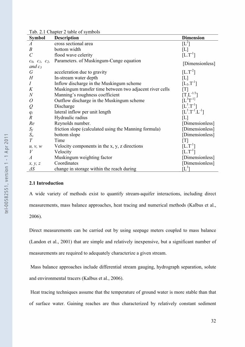
Tab. 2.1 Chapter 2 table of symbols Symbol Description Dimension A cross sectional area [L2] B bottom width [L] C flood wave celerity [L.T-1] c0, c1, c2, and c3

Parameters. of Muskingum-Cunge equation [Dimensionless]

G acceleration due to gravity [L.T-2] H In-stream water depth [L] I Inflow discharge in the Muskingum scheme [L3.T-1] K Muskingum transfer time between two adjacent river cells [T] N Manning’s roughness coefficient [T.L-1/3] O Outflow discharge in the Muskingum scheme [L3T-1] Q Discharge [L3.T-1] ql lateral inflow per unit length [L3.T-1.L-1] R Hydraulic radius [L] Re Reynolds number. [Dimensionless] Sf friction slope (calculated using the Manning formula) [Dimensionless] So bottom slope [Dimensionless] T Time [T] u, v, w Velocity components in the x, y, z directions [L.T-1] V Velocity [L.T-1] Α Muskingum weighting factor [Dimensionless] x, y, z Coordinates [Dimensionless] ΔS change in storage within the reach during [L3]

2.1 Introduction

A wide variety of methods exist to quantify stream-aquifer interactions, including direct

measurements, mass balance approaches, heat tracing and numerical methods (Kalbus et al.,

2006).

Direct measurements can be carried out by using seepage meters coupled to mass balance

(Landon et al., 2001) that are simple and relatively inexpensive, but a significant number of

measurements are required to adequately characterize a given stream.

Mass balance approaches include differential stream gauging, hydrograph separation, solute

and environmental tracers (Kalbus et al., 2006).

Heat tracing techniques assume that the temperature of ground water is more stable than that

of surface water. Gaining reaches are thus characterized by relatively constant sediment

tel-0

0582

551,

ver

sion

1 -

1 Ap

r 201

1

33

temperatures, where as losing reaches tend to present significant variability over short periods

of time (Constantz et al., 2001).

A recent geophysical method for quantifying stream-aquifer exchanged fluxes at the local

scale uses Fiber-optic distributed temperature sensing (FO-DTS) (Day-Lewis and Lane, 2006;

Selker et al., 2006; Vogt et al., 2010).

At the regional scale, the aforementioned methods are not feasible to apply because they

require the availability of consistent data along the river which is not always accessible at this

scale.

This review will be focused on stream-aquifer interactions modeling based on numerical

methods in order to identify the capabilities and limitations of each modeling methodology as

well as the necessities required to complement stream-aquifer model’s range of applicability

at local and regional scale. The stream-aquifer interactions review follows a review on surface

routing models which are of primary importance for simulating stream-aquifer interactions.

2.2 Surface routing modeling

Surface routing methodologies can be classified into two categories: (1) hydrodynamic

routing methodologies; (2) hydrological routing methodologies (Arora et al., 2001).

In general, hydrodynamic routing methodologies are based on the 1D Saint-Venant equations

(Barré de Saint-Venant, 1871). The Saint-Venant formulation includes a continuity equation

(Eq. 2.5) which describes the balance between input, storage and output in a section of river,

and a momentum equation (Eq. 2.6) which relates the change in momentum to the applied

forces (Bathurst, 1988; Becker and Serban, 1990; Liggett, 1975).

The hydrological routing approaches are based on the continuity equation while empirical

relationships are used to replace the momentum equation (Carter, 1960; Cunge, 1969; Dooge

tel-0

0582

551,

ver

sion

1 -

1 Ap

r 201

1

34

et al., 1982; Sherman, 1932; Wilson, 1990). Examples of hydrological routing approaches

include the Muskingum, Muskinum-Cunge and Unit Hydrograph methods.

A number of routing methodologies are reviewed in the following sections. These routing

methodologies vary from fine scale to large scale applications.

2.2.1 Hydrodynamic routing modeling techniques

Navier-Stokes equations

The Navier-Stokes equations (Navier, 1822) of fluid are a formulation of Newton's law of

motion for a continuous distribution of matter in the fluid state, they are central to applied

research (Doering and Gibbon, 1995). The Navier-Stokes equations are a set of nonlinear

partial differential equations that describe the flow of fluids. These equations are used to

model the movement of air in the atmosphere, river hydraulics, ocean currents, water flow in

pipes, as well as many other fluid flow phenomena.

The Navier-Stokes equations are based on the continuity equation (Eq. 2.1) and the

momentum equation in the three dimensions x, y, z (Eq. 2.2, Eq. 2.3, Eq. 2.4)

( ) ( ) ( ) 0=∂

∂+

∂∂

+∂

∂+

∂∂

zw

yv

xu

tρρρρ Eq. 2.1

( ) ( ) ( ) ( )⎥⎦

⎤⎢⎣

⎡∂∂

+∂

∂+

∂∂

+∂∂

−=∂

∂+

∂∂

+∂

∂+

∂∂

zyxRexp

zuw

yuv

xu

tu xzxyxx

r

τττρρρρ 12

Eq. 2.2

( ) ( ) ( ) ( )⎥⎦

⎤⎢⎣

⎡∂

∂+

∂

∂+

∂

∂+

∂∂

−=∂

∂+

∂∂

+∂

∂+

∂∂

zyxReyp

zvw

yv

xuv

tv yzyyxy

r

τττρρρρ 12

Eq. 2.3

( ) ( ) ( ) ( )⎥⎦

⎤⎢⎣

⎡∂∂

+∂

∂+

∂∂

+∂∂

−=∂

∂+

∂∂

+∂

∂+

∂∂

zyxRezp

zw

yvw

xuw

tw zzyzxz

r

τττρρρρ 12

Eq. 2.4

Where x, y, z are the coordinates, t is time, p is pressure, u, v, w are velocity components, ρ is

density, τ is stress and Re is the Reynolds number.

tel-0

0582

551,

ver

sion

1 -

1 Ap

r 201

1

35

A number of complex models to simulate river flow using the Navier-Stokes equations may

be found in literature (Abbott, 1979; Bradford and Katopodes, 1998; Naot and Rodi, 1982;

Spanoudaki et al., 2009). However, these models that use the complete set of 3D Navier-

Stokes equations are very complex and thus require a substantial amount of data and

computer memory in order to obtain accurate solutions (Ma and Sikorski, 1993). The

aforementioned raisons lead hydrodynamic modelers to use the 1D Saint-Venant equations or

it’s approximations in river flow modeling.

Saint-Venant equations

In 1843 Barré de Saint-Venant published a derivation of the incompressible Navier-Stokes

equations that applies to both laminar and turbulent flows. The 1D Saint-Venant equations

based on the continuity (Eq. 2.5) and momentum (Eq. 2.6) equations formalize the main

concepts of river hydrodynamic modeling.

The basic derivation assumptions of the Saint Venant Equations (Abbott, 1979; Chow, 1959)

are the following:

• The flow is one-dimensional, i.e. the velocity is uniform over the cross-section and the water

level across the section is represented by a horizontal line.

• The streamline curvature is small and the vertical accelerations are negligible, so pressure

can be considered as hydrostatic.

• The effects of boundary friction and turbulence can be accounted for through resistance laws

analogous to those used for steady state flow.

• The average channel bed slope is small so that the cosine of the angle it makes with the

horizontal may be replaced by unity.

tel-0

0582

551,

ver

sion

1 -

1 Ap

r 201

1

36

The aforementioned hypotheses do not impose any restriction on the shape of the cross-

section of the channel and on its variation along the channel axis.

The full derivation of the basic Saint-Venant equations can be found in a number of reviews

(Chow, 1959; Cunge et al., 1980; Graff and Altinakar, 1996; Strelkoff, 1970).

0=−∂∂

+∂∂

lqtA

xQ Eq. 2.5

( ) 0=−−∂

∂+

∂∂

+∂∂

of SSgxh

gxVV

tV Eq. 2.6

Where Q is discharge [L3.T-1], A is cross sectional area [L2], x is distance along the

longitudinal axes of the channel or floodplain [L], t is Time [T], ql is lateral inflow per unit

length [L3.T-1.L-1], V is velocity [L.T-1], hr is flow depth [L] and g is acceleration due to

gravity [L.T-2], So is bottom slope (dimensionless), Sf is friction slope (dimensionless).

Sf is calculated using the Manning formula:

2

32 ⎥⎦⎤

⎢⎣⎡= /f AR

nQS Eq. 2.7

Where n is Manning’s roughness coefficient [TL-1/3], R is Hydraulic radius [L].

Term I represents the local inertia and reflects unsteady flow, term II represents the

convective inertia and reflects both spatial variation of the flow (∂Q/∂x) and longitudinal

change in the cross-section area, term III represents the pressure differential and reflects the

change in depth in the longitudinal direction and term IV accounts for friction and bed slopes.

Hydrodynamic models that include all the momentum terms of the Saint-Venant equation are

called dynamic wave models.

I II III IV

tel-0

0582

551,

ver

sion

1 -

1 Ap

r 201

1

37

Many numerical schemes have been used to solve the 1D Saint-Venant equations, these

methods include explicit finite difference (Stoker, 1957b), method of characteristics (Abbott,

1966), finite differences methods (Cunge et al., 1980), and finite element schemes (Fread,

1985; Richard, 1976). Examples of widely used Saint-Venant models include Mike-11 (DHI,

2001), ISIS (Wallingford, 1997), FLDWAV (Fread and Lewis, 1998) and HEC-RAS (HEC,

2002).

Hydrodynamic models based on the complete Saint-Venant equations have the capability of

accurately simulating the widest spectrum of waterway characteristics. Moreover, the

calibration process is quite evident since the Saint-Venant hydraulic model contains only one

parameter (Manning’s roughness coefficient). Other advantages for using the full Saint-

Venant formula are when downstream backwater effects are present, significant tributary

inflows, or when upstream propagation of wave can occur from large tides and storm surges.

At large scale applications, one of the major challenges in hydrodynamic routing models

based on the Saint-Venant equations is the lack of accurate data in the channel network such

as channel geometry, slope, length, etc. That being said, only one reference was found with

regards to the impact of degradation or simplification of channel geometry on the

performance of the model (Hicks, 1996). This particular aspect will be addressed in chapters 3

of this thesis. Other limitations of the Saint-Venant equations include sharp discontinuities,

such as the transition from subcritical flow to critical flow that can only be solved with a few

numerical methods (Flipo, 2005).

The computational cost and scale factors motivated researchers to use simplified forms of the

momentum equation (Eq. 2.6). Depending on which terms of the momentum equation terms

are neglected, hydraulic models can be classified in Tab. 2.2 (Ponce and Simons, 1977). The

most commonly simplified representations of the Saint-Venant equations are the kinematic

tel-0

0582

551,

ver

sion

1 -

1 Ap

r 201

1

38

wave and the diffusive wave approximations. Hereafter only these two formulations are

presented.

Tab. 2.2 Terms of the Saint-Venant momentum equation (Eq. 2.6) used in hydraulic modeling techniques Hydraulic Considered momentum equation References

Dynamic wave I, II, III, IV (Fread and Lewis, 1998; HEC, 2002; Stoker, 1957a)

Diffusive wave III, IV

(Dooge, 1973; Hayami, 1951; Lighthill and Whitham, 1955; Todini and Bossi, 1986)

Kinematic wave IV

(Beven et al., 1987; Graham and Refsgaard, 2001; Hussein and Schwartz, 2003; Leavesley et al., 1983; Linsley, 1971; Wooding, 1965; Woolhiser and Liggett, 1967; Woolhiser et al., 1990b)

Steady dynamic wave II, III, IV (Tsai, 2003)

Gravity waves I, II, III (Gregory et al., 1998)

Diffusion wave equation

A simplified approximation of the Saint-Venant formulation combines the spatial derivative

from the momentum equation with the continuity equation, which results in a second

derivative term in the continuity equation (Dooge, 1973; Hayami, 1951; Lighthill and

Whitham, 1955; Todini and Bossi, 1986). The second derivative term in the continuity

equation causes the flood wave to spread upstream slightly and is commonly referred to as a

diffusion analogy for the dynamic component of the momentum equation. The simplified

form of the momentum equation (Eq. 2.6) is:

0=∂

∂−

xh

s f Eq. 2.8

The diffusion wave equations are efficiently solved with a four point centered implicit finite

difference solution techniques (Brankensiek, 1965) or explicit finite difference solution

techniques (Harder and Armacost, 1966). The slope of water surface allows the diffusion

tel-0

0582

551,

ver

sion

1 -

1 Ap

r 201

1

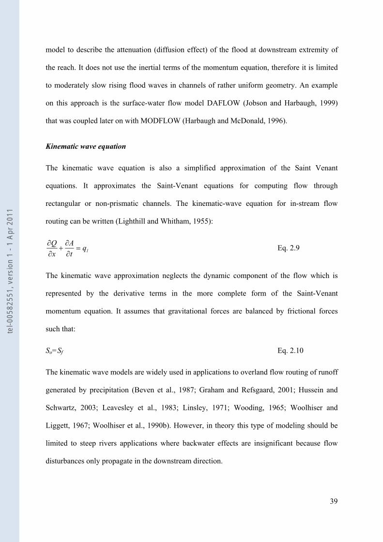
39

model to describe the attenuation (diffusion effect) of the flood at downstream extremity of

the reach. It does not use the inertial terms of the momentum equation, therefore it is limited

to moderately slow rising flood waves in channels of rather uniform geometry. An example

on this approach is the surface-water flow model DAFLOW (Jobson and Harbaugh, 1999)

that was coupled later on with MODFLOW (Harbaugh and McDonald, 1996).

Kinematic wave equation

The kinematic wave equation is also a simplified approximation of the Saint Venant

equations. It approximates the Saint-Venant equations for computing flow through

rectangular or non-prismatic channels. The kinematic-wave equation for in-stream flow

routing can be written (Lighthill and Whitham, 1955):

lqtA

xQ

=∂∂

+∂∂ Eq. 2.9

The kinematic wave approximation neglects the dynamic component of the flow which is

represented by the derivative terms in the more complete form of the Saint-Venant

momentum equation. It assumes that gravitational forces are balanced by frictional forces

such that:

So=Sf Eq. 2.10

The kinematic wave models are widely used in applications to overland flow routing of runoff

generated by precipitation (Beven et al., 1987; Graham and Refsgaard, 2001; Hussein and

Schwartz, 2003; Leavesley et al., 1983; Linsley, 1971; Wooding, 1965; Woolhiser and

Liggett, 1967; Woolhiser et al., 1990b). However, in theory this type of modeling should be

limited to steep rivers applications where backwater effects are insignificant because flow

disturbances only propagate in the downstream direction.

tel-0

0582

551,

ver

sion

1 -

1 Ap

r 201

1

40

2.2.2 Hydrological routing modeling techniques

Hydrological routing techniques have been and continue to be an important tool to better

understand the dynamical interactions within the water cycle. It is an essential component of

integrated water resources management involving environment and ecology.

Regional scale hydrological modeling routing techniques have been used in a number of

applications, for instance:

1- Integrated basin hydrology: Runoff Routing provides a basis for comparing and validating

estimates of streamflow with observed hydrograph data. As most variables describing the

state of the surface are not directly observable, river discharge is an appropriate measurement

to assess model qualities (Nijssen et al., 2001).

2- Export from continental surface to the sea: The simulated fresh water flux into the oceans

alters their salinity and may affect the thermohaline circulation (Wang et al., 1999; Wijffels et

al., 1992).

3- Climate changes scenarios: Estimates of river discharge from climate change simulations

can also be used to assess the impact of climate change on water resources and the hydrology

of the major river basins (Arora et al., 2001; Milly et al., 2005; Oki and Kanae, 2006).

4- Influence of river discharge on freshwater ecosystems (Azevedo et al., 2010; Carpenter et

al., 1992).

In general, hydrological routing approaches are based on the conservation of mass (Eq. 2.11)

coupled with empirical relationships replacing the momentum equation.

Additionally, all the geomorphological characteristics and the hydraulic properties of river

reaches are lumped into a number of more or less conceptual model parameters.

tSOIΔΔ

=− Eq. 2.11

tel-0

0582

551,

ver

sion

1 -

1 Ap

r 201

1

41

Where I and O are the upstream and downstream discharge respectively [L3.T-1], and ΔS [L3]

is the change in storage within the reach during a Δt time increment [T].

At the regional scale, the majority of hydrological models uses simplified hydrological

techniques for flow routing that are generally based on linear/non-linear reservoir or

Muskingum type routing methods (McCarthy, 1938), which is considered as one of the most

popular hydrological routing approaches. Other examples include the cascade of linear

reservoirs (Nash, 1958) and the Muskingum-Cunge (MC) approach (Cunge, 1969).

Hydrological storage routing models offer the advantages of simplicity when backwater

effects are insignificant. These hydrological models however do not simulate the

corresponding in-stream water levels which are essential to accurately simulate the stream-

aquifer interactions based on Darcy’s equation.

The majority of regional scale hydrological models either assume a constant and uniform

velocity (Coe, 1998; Miller et al., 1994; Oki and Sud, 1998) or constant flow velocities

parameterized to the topographic gradient (Ducharne et al., 2003; Hagemann and Dumenil,

1998).

Muskingum method

The Muskingum channel routing method is based on two equations (Linsley et al., 1982).

The first is the continuity equation or conservation of mass.

122121

22SSt

OOt

II−=Δ

+−Δ

+ Eq. 2.12

Where I1 and I2 are inflow discharges at time 1 and time 2, O1 and O2 are outflow discharges

at time 1 and time 2, Δt is time difference between time 1 and time 2, S1 and S2 are values of

reach storage at time 1 and time 2.

The second equation is a relationship between storage, inflow, and outflow of the reach.

tel-0

0582

551,

ver

sion

1 -

1 Ap

r 201

1

42

( )O)I(IkS αα −+= Eq. 2.13 where S is the reach storage, I = inflow discharge, O = outflow discharge, k is storage

coefficient, α is weighting factor.

Combining equations 2.12 and 2.13 and simplifying results (Ponce and Yevjevich, 1978):

O2 = C1I1 + C2I2 + C3O1 Eq. 2.14

Where: C1 = (Δt / k) + 2 α) /C0 Eq. 2.15

C2 = (Δt / k) – 2 α) /C0 Eq. 2.16

C3 = (2(1 – α) - Δt /k)/C0 Eq. 2.17

C0 = Δt/k + 2(1 – α) Eq. 2.18

C0, C1, C2, and C3 are dimensionless parameters.

The Muskingum models are widely used for river routing applications because of the modest

data requirement (Aldama, 1990; Birkhead and James, 2002; David et al., 2010; Drobot and

Corbus, 1998; Gill, 1992; Tang et al., 1999).

The application of the Muskingum model to river and channel flood routing may have some

limitations because of its inherent assumption of a linear relationship between channel storage

and weighted flow (Mohan, 1997). Additionally it does not compute in-stream water levels

associated with simulated discharge.

Muskingum-Cunge method

Cunge (1969) developed equations to estimate k and α from hydraulic properties of the reach.

The mathematical derivation is condensed and presented by Ponce (1981). The equations for

k and α Muskingum parameters are:

tel-0

0582

551,

ver

sion

1 -

1 Ap

r 201

1

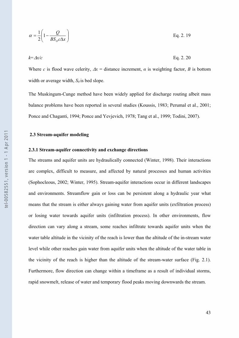
43

⎟⎟⎠

⎞⎜⎜⎝

⎛Δ

−=xcBS

Q

O

121α Eq. 2. 19

k=Δx/c Eq. 2. 20 Where c is flood wave celerity, Δx = distance increment, α is weighting factor, B is bottom

width or average width, S0 is bed slope.

The Muskingum-Cunge method have been widely applied for discharge routing albeit mass

balance problems have been reported in several studies (Koussis, 1983; Perumal et al., 2001;

Ponce and Chaganti, 1994; Ponce and Yevjevich, 1978; Tang et al., 1999; Todini, 2007).

2.3 Stream-aquifer modeling

2.3.1 Stream-aquifer connectivity and exchange directions

The streams and aquifer units are hydraulically connected (Winter, 1998). Their interactions

are complex, difficult to measure, and affected by natural processes and human activities

(Sophocleous, 2002; Winter, 1995). Stream-aquifer interactions occur in different landscapes

and environments. Streamflow gain or loss can be persistent along a hydraulic year what

means that the stream is either always gaining water from aquifer units (exfiltration process)

or losing water towards aquifer units (infiltration process). In other environments, flow

direction can vary along a stream, some reaches infiltrate towards aquifer units when the

water table altitude in the vicinity of the reach is lower than the altitude of the in-stream water

level while other reaches gain water from aquifer units when the altitude of the water table in

the vicinity of the reach is higher than the altitude of the stream-water surface (Fig. 2.1).

Furthermore, flow direction can change within a timeframe as a result of individual storms,

rapid snowmelt, release of water and temporary flood peaks moving downwards the stream.

tel-0

0582

551,

ver

sion

1 -

1 Ap

r 201

1

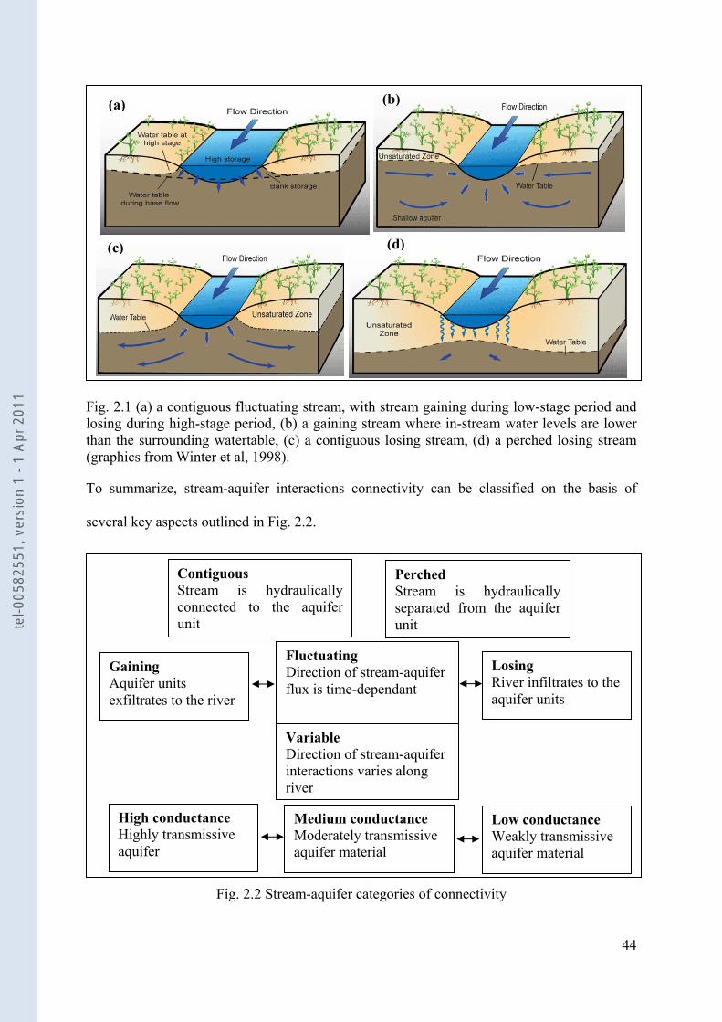
44

Fig. 2.1 (a) a contiguous fluctuating stream, with stream gaining during low-stage period and losing during high-stage period, (b) a gaining stream where in-stream water levels are lower than the surrounding watertable, (c) a contiguous losing stream, (d) a perched losing stream (graphics from Winter et al, 1998).

To summarize, stream-aquifer interactions connectivity can be classified on the basis of

several key aspects outlined in Fig. 2.2.

Fig. 2.2 Stream-aquifer categories of connectivity

(a)

(d)(c)

(b)

Contiguous Stream is hydraulically connected to the aquifer unit

Perched Stream is hydraulically separated from the aquifer unit

Gaining Aquifer units exfiltrates to the river

Losing River infiltrates to the aquifer units

Fluctuating Direction of stream-aquifer flux is time-dependant

High conductance Highly transmissive aquifer

Variable Direction of stream-aquifer interactions varies along river

Medium conductance Moderately transmissive aquifer material

Low conductance Weakly transmissive aquifer material

tel-0

0582

551,

ver

sion

1 -

1 Ap

r 201

1

45

In this framework, stream-aquifer interactions have been the focus of a number of studies,

many of which have focused on 1D vertical river-aquifer exchange: either as groundwater

sustaining base flow in gaining streams or as streamflow recharging groundwater in losing

streams (Baillie et al., 2007; Cox and Stephens, 1988; Flipo et al., 2005; Gillespie and Perry,

1988; Goodrich et al., 1997; Harrington et al., 2002; Korkmaz et al., 2009; Ledoux et al.,

1984; McDonnell et al., 1991; Pearce et al., 1986; Peters and Ratcliffe, 1998; Plummer et al.,

2004; Ponce et al., 1999; Stephens, 1988; Waichler and Wigmosta, 2004).

Few other studies have shown that two-way exchanges have substantial implications for both

water quantity and quality, including nitrate concentrations (Squillace, 1996; Whitaker, 2000).

This two-way exchange process might occur in different sections of the river network and

more importantly, a given river reach may be losing during high flow then suddenly

becoming gaining as flow declines and the hydraulic gradient shifts towards the channel

(Rushton, 2007; Saleh et al., 2010).

2.3.2 Importance of coupled stream-aquifer models for interdisciplinary investigations in hydrologic sciences

Stream-aquifer modeling tools have evolved rapidly in recent years (Jones et al., 2006;

Panday and Huyakorn, 2004; Werner et al., 2006). Coupled hydro(geo)logical models capable

of simulating stream-aquifer interactions are increasingly used to examine problems in

hydrologic sciences (Ebel et al., 2009). Stream-aquifer coupling have enlarged visions on

interdisciplinary investigations in hydrologic sciences (Loague et al., 2006).

It permitted to address scientific problems that were difficult to measure or observe, such as

the quantification of flood recharge along river networks and how this compares to

tel-0

0582

551,

ver

sion

1 -

1 Ap

r 201

1

46

phreatophyte2 transpiration and groundwater exfiltration to the river (Morin et al., 2009),

agricultural practices and scenarios related to nitrate contamination (Flipo et al., 2007a;

Ledoux et al., 2007). A number of selected hydrologic problems addressed using models that

fully couple stream-aquifer flow are listed in Tab. 2.3.

It also permitted to better understand where flood recharge is spatially highest along the river,

and to characterize the temporal change after floods.

In these coupling techniques hydrodynamic surface routing models using the Saint-Venant

equations require high resolution input data to parameterize the hydraulic model, which is

usually not available in large scale applications.

To overcome this limitation, modelers use simplified hydraulic or hydrological routing

techniques, where convective and local acceleration terms are neglected. This reduces the

accuracy of in-stream water levels estimations when compared to methods that use the 1D

Saint-Venant equations and eventually impacts the accuracy of stream-aquifer interactions.

2 Phreatophyte is a deep-rooted plant that obtains a significant portion of the water that it needs from the phreatic zone (zone of saturation) or the capillary fringe above the phreatic zone.

tel-0

0582

551,

ver

sion

1 -

1 Ap

r 201

1

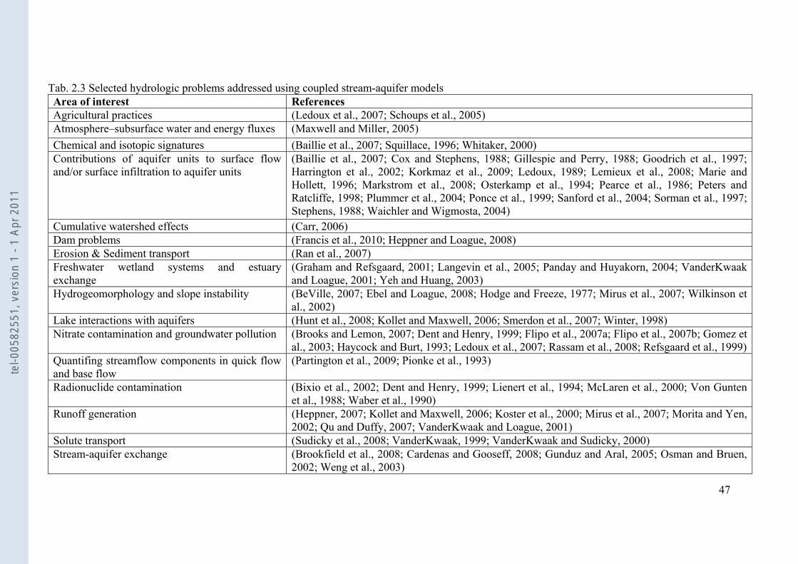
47

Tab. 2.3 Selected hydrologic problems addressed using coupled stream-aquifer models Area of interest References Agricultural practices (Ledoux et al., 2007; Schoups et al., 2005) Atmosphere–subsurface water and energy fluxes (Maxwell and Miller, 2005) Chemical and isotopic signatures (Baillie et al., 2007; Squillace, 1996; Whitaker, 2000) Contributions of aquifer units to surface flow and/or surface infiltration to aquifer units

(Baillie et al., 2007; Cox and Stephens, 1988; Gillespie and Perry, 1988; Goodrich et al., 1997; Harrington et al., 2002; Korkmaz et al., 2009; Ledoux, 1989; Lemieux et al., 2008; Marie and Hollett, 1996; Markstrom et al., 2008; Osterkamp et al., 1994; Pearce et al., 1986; Peters and Ratcliffe, 1998; Plummer et al., 2004; Ponce et al., 1999; Sanford et al., 2004; Sorman et al., 1997; Stephens, 1988; Waichler and Wigmosta, 2004)

Cumulative watershed effects (Carr, 2006) Dam problems (Francis et al., 2010; Heppner and Loague, 2008) Erosion & Sediment transport (Ran et al., 2007) Freshwater wetland systems and estuary exchange

(Graham and Refsgaard, 2001; Langevin et al., 2005; Panday and Huyakorn, 2004; VanderKwaak and Loague, 2001; Yeh and Huang, 2003)

Hydrogeomorphology and slope instability (BeVille, 2007; Ebel and Loague, 2008; Hodge and Freeze, 1977; Mirus et al., 2007; Wilkinson et al., 2002)

Lake interactions with aquifers (Hunt et al., 2008; Kollet and Maxwell, 2006; Smerdon et al., 2007; Winter, 1998) Nitrate contamination and groundwater pollution (Brooks and Lemon, 2007; Dent and Henry, 1999; Flipo et al., 2007a; Flipo et al., 2007b; Gomez et

al., 2003; Haycock and Burt, 1993; Ledoux et al., 2007; Rassam et al., 2008; Refsgaard et al., 1999) Quantifing streamflow components in quick flow and base flow

(Partington et al., 2009; Pionke et al., 1993)

Radionuclide contamination (Bixio et al., 2002; Dent and Henry, 1999; Lienert et al., 1994; McLaren et al., 2000; Von Gunten et al., 1988; Waber et al., 1990)

Runoff generation (Heppner, 2007; Kollet and Maxwell, 2006; Koster et al., 2000; Mirus et al., 2007; Morita and Yen, 2002; Qu and Duffy, 2007; VanderKwaak and Loague, 2001)

Solute transport (Sudicky et al., 2008; VanderKwaak, 1999; VanderKwaak and Sudicky, 2000) Stream-aquifer exchange (Brookfield et al., 2008; Cardenas and Gooseff, 2008; Gunduz and Aral, 2005; Osman and Bruen,

2002; Weng et al., 2003)

tel-0

0582

551,

ver

sion

1 -

1 Ap

r 201

1

48

2.3.3 Stream-aquifer interactions modeling: tackling the challenges

In spite of the evolution of the stream-aquifer modeling discipline in the last few years, many

challenges still remain unsolved. Notable challenges in stream-aquifer modeling include

spatial and temporal scale issues (Kollet and Maxwell, 2006; Loague and Corwin, 2007;

Loague and VanderKwaak, 2004; Sudicky et al., 2005; Werner et al., 2006), initial conditions

(Noto et al., 2008), absence or inadequacy of measured data to calibrate/control model outputs

(Beven and Binley, 1992; Lefebvre et al., 2010; Uhlenbrook et al., 1999), equifinality3

(Beven, 2006; Beven and Freer, 2001a; Ebel and Loague, 2006), insufficient computational

power and conceptual and numerical difficulties (Jolly and Rassam, 2009).

Tab. 2.4 illustrates the diversity of equations and spatial dimension characteristics of selected

coupled models employed for stream-aquifer modeling. The levels of complexity in these

models are based on the type of equations and the spatial dimension (1D, 2D or 3D) used to

describe surface water and groundwater flows (Tab. 2.4). Based on the discussion of Aral and

Gunduz (2003) with regards to spatial scale issues, an approximate formulation of coupled

stream and aquifer units may be successfully achieved using a multi-layer 2D horizontal

model for the subsurface flow, preceeding a 1D model for stream flow, as in CASC2D (Julien

et al., 1995), LISFLOOD (De Roo et al., 2000), MIKE-SHE (Refsgaard and Storm, 1995;

Thompson et al., 2004), HEC-HMS/HEC-RAS (Knebl et al., 2005b), CAWAQS (Flipo et al.,

2007a) and EauDyssée (Ledoux et al., 1984; Ledoux et al., 2007) . Other studies further

encourage ground water modelers to start simple and to add complexity carefully as

warranted by the complexity supported by the available data (Hill, 2006). The conclusion of

3 Equifinality is a key concept to assess how uncertain hydrological predictions. In hydrological modeling, two models are equifinal if they lead to an equally acceptable or behavioral representation of the observed natural processes (Beven and Freer, 2001a).

tel-0

0582

551,

ver

sion

1 -

1 Ap

r 201

1

49

Hill’s study is that neither very simple nor very complex models are likely to provide the most

accurate predictions.

Another significant conceptual obstacle is to determine the most effective technique for

coupling the stream and aquifer continuum. According to Panday and Huyakorn (2004),

several options for coupling stream and aquifer models are available including a fully coupled

approach, in which the interaction flux is applied as a boundary condition to each model or a

sequentially coupled approach in which the head for one system acts as a general-head

boundary for the other system.

With regards to numerical difficulties, several techniques have been adapted to overcome this

problem, including adaptive time steps (D' Haese et al., 2007; Park et al., 2008), non linear

solvers (Hammond et al., 2005; Jones and Woodward, 2001; Knoll and Keyes, 2004) and

parallel algorithms for solution (Kollet and Maxwell, 2006).

tel-0

0582

551,

ver

sion

1 -

1 Ap

r 201

1

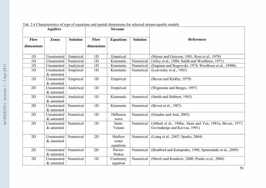
50

Tab. 2.4 Characteristics of type of equations and spatial dimensions for selected stream-aquifer models Aquifers Streams

Flow

dimensions

Zones Solution Flow

dimensions

Equations Solution

References

1D Unsaturated Empirical 1D Empirical (Moore and Grayson, 1991; Ross et al., 1979) 1D Unsaturated Numerical 1D Kinematic Numerical (Alley et al., 1980; Smith and Woolhiser, 1971) 1D Unsaturated Analytical 1D Kinematic Numerical (Engman and Rogowski, 1974; Woolhiser et al., 1990b) 1D Unsaturated

& saturated Empirical 1D Kinematic Numerical (Leavesley et al., 1983)

1D Unsaturated & saturated

Empirical 1D Empirical (Beven and Kirkby, 1979)


Analytical 1D Empirical (Wigmosta and Burges, 1997)


Analytical 1D Kinematic Numerical (Smith and Hebbert, 1983)


Numerical 1D Kinematic Numerical (Beven et al., 1987)


Numerical 1D Diffusion wave

Numerical (Gunduz and Aral, 2005)


Numerical 1D Saint-Venant

Numerical (Abbott et al., 1986a; Akan and Yen, 1981a; Beven, 1977; Govindaraju and Kavvas, 1991)


Numerical 2D Shallow water

equations

Numerical (Liang et al., 2007; Sparks, 2004)


Numerical 2D Navier-Stokes

Numerical (Bradford and Katopodes, 1998; Spanoudaki et al., 2009)


Numerical 1D Continuity equation

Numerical (Merrit and Konikow, 2000; Prudic et al., 2004)

tel-0

0582

551,

ver

sion

1 -

1 Ap

r 201

1

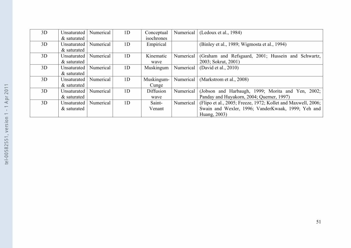
51


Numerical 1D Conceptual isochrones

Numerical (Ledoux et al., 1984)


Numerical 1D Empirical (Binley et al., 1989; Wigmosta et al., 1994)


Numerical 1D Kinematic wave

Numerical (Graham and Refsgaard, 2001; Hussein and Schwartz, 2003; Sokrut, 2001)


Numerical 1D Muskingum Numerical (David et al., 2010)

3D

Unsaturated & saturated

Numerical

1D

Muskingum-Cunge

Numerical (Markstrom et al., 2008)


Numerical 1D Diffusion wave

Numerical (Jobson and Harbaugh, 1999; Morita and Yen, 2002; Panday and Huyakorn, 2004; Querner, 1997)


Numerical 1D Saint-Venant

Numerical (Flipo et al., 2005; Freeze, 1972; Kollet and Maxwell, 2006; Swain and Wexler, 1996; VanderKwaak, 1999; Yeh and Huang, 2003)

tel-0

0582

551,

ver

sion

1 -

1 Ap

r 201

1

52

2.3.4 Scaling issues in stream-aquifer interactions modeling

Spatial scale is defined as the dimension at which entities, patterns, and processes can be

observed and characterized to capture the important details of a hydrological or

hydro(geo)logical process (Aral and Gunduz, 2003). It is an important issue in the assessment

and management of stream-aquifer interactions.

In general, there are three main scales relating to stream-aquifer interactions modeling:

- Regional scale, where the stream is placed in context with the overall

hydro(geo)logical setting of the catchment (> 100 km2).

- Local scale, at the level of individual surface water features such as a lake or a stream

reach (10 - 100 km).

- Site scale, where site specific studies provide insights into processes particularly at

the stream-aquifer interface (1 m - 1 km).

Tab. 2.5 illustrates a range of selected hydro(geo)logical models applied at site scale, local

scale and regional scale.

Each model has different levels of complexity and simulation capabilities ranging from

models which simulate the complete land phase of hydrologic cycle at regional scale (e.g.

MODHMS, MIKE SHE, MODCOU) to models that focus on local stream-aquifer water

interactions (e.g. InHM). At regional scale applications, the majority of regional

hydr(geo)logical models have limited capacity to simulate small-scale processes (e.g., near-

stream groundwater pumping, bank storage effects, in-stream water level fluctuations)

because these processes require a very fine discretization of the considered domain. The fine

discretization required to capture such processes influences the computational efficiency. It is

why alternative approaches are required to complement model’s range of applicability

(Werner et al., 2006). When large scale models are used to predict small scale events or when

tel-0

0582

551,

ver

sion

1 -

1 Ap

r 201

1

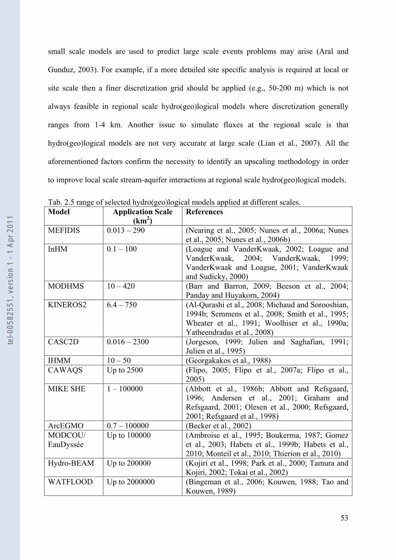
53

small scale models are used to predict large scale events problems may arise (Aral and

Gunduz, 2003). For example, if a more detailed site specific analysis is required at local or

site scale then a finer discretization grid should be applied (e.g., 50-200 m) which is not

always feasible in regional scale hydro(geo)logical models where discretization generally

ranges from 1-4 km. Another issue to simulate fluxes at the regional scale is that

hydro(geo)logical models are not very accurate at large scale (Lian et al., 2007). All the

aforementioned factors confirm the necessity to identify an upscaling methodology in order

to improve local scale stream-aquifer interactions at regional scale hydro(geo)logical models.

Tab. 2.5 range of selected hydro(geo)logical models applied at different scales. Model Application Scale

(km2) References

MEFIDIS 0.013 – 290 (Nearing et al., 2005; Nunes et al., 2006a; Nunes et al., 2005; Nunes et al., 2006b)

InHM 0.1 – 100 (Loague and VanderKwaak, 2002; Loague and VanderKwaak, 2004; VanderKwaak, 1999; VanderKwaak and Loague, 2001; VanderKwaak and Sudicky, 2000)

MODHMS 10 – 420 (Barr and Barron, 2009; Beeson et al., 2004; Panday and Huyakorn, 2004)

KINEROS2 6.4 – 750 (Al-Qurashi et al., 2008; Michaud and Sorooshian, 1994b; Semmens et al., 2008; Smith et al., 1995; Wheater et al., 1991; Woolhiser et al., 1990a; Yatheendradas et al., 2008)

CASC2D 0.016 – 2300 (Jorgeson, 1999; Julien and Saghafian, 1991; Julien et al., 1995)

IHMM 10 – 50 (Georgakakos et al., 1988) CAWAQS Up to 2500 (Flipo, 2005; Flipo et al., 2007a; Flipo et al.,

2005) MIKE SHE 1 – 100000 (Abbott et al., 1986b; Abbott and Refsgaard,

1996; Andersen et al., 2001; Graham and Refsgaard, 2001; Olesen et al., 2000; Refsgaard, 2001; Refsgaard et al., 1998)

ArcEGMO 0.7 – 100000 (Becker et al., 2002) MODCOU/ EauDyssée

Up to 100000 (Ambroise et al., 1995; Boukerma, 1987; Gomez et al., 2003; Habets et al., 1999b; Habets et al., 2010; Monteil et al., 2010; Thierion et al., 2010)

Hydro-BEAM Up to 200000 (Kojiri et al., 1998; Park et al., 2000; Tamura and Kojiri, 2002; Tokai et al., 2002)

WATFLOOD Up to 2000000 (Bingeman et al., 2006; Kouwen, 1988; Tao and Kouwen, 1989)

tel-0

0582

551,

ver

sion

1 -

1 Ap

r 201

1

54

2.3.5 In-stream water levels fluctuations importance to stream-aquifer interactions

Time-dependent in-stream water levels fluctuations are acknowledged to influence the

groundwater system and hydraulic gradients in regions surrounding the stream (Ataie-

Ashtianti et al., 1999; Cooper, 1959; Glover, 1959; Reilly and Goodman, 1985; Winter,

1998).

In-stream water level fluctuations can arise from many natural and anthropogenic sources

such as flood events, intense precipitation episodes, tidal oscillations, wave induced

displacement, dam releases and associated reservoir drawdown. The increase in in-stream

water levels due to one of the aforementioned factors frequently results in reversal stream

aquifer units exchange, leading to losing water conditions for the stream network

(Friesz, 1996; Squillace, 1996).

In a study developed to simulate mass transport from a contaminant plume to a tidal estuary,

comparison of models with and without tidal fluctuation (Yim and Mohsen, 1992)

demonstrates that concentrations near the interface are less than ones obtained in simulations

with tidal fluctuations enabled, velocity gradients are much greater, and more mass exchange

from the aquifer to the estuary occurs.

In-stream water level variations have been also used to study large-scale hydraulic properties

of fluvial aquifers (Bolster et al., 2001; Carrera and Neuman, 1986a; Loeltz and Leake, 1983;

Pinder and Jones, 1969; Reynolds, 1987; Sophocleous, 1991). Moreover, Aquifer reaction to

tidal fluctuations has been employed to calculate aquifer parameters (Erskine, 1991; Jha et

al., 2003). In other studies, time varying surface water stage is frequently used to estimate

aquifer hydraulic diffusivity (Ferris, 1951; Pinder and Jones, 1969; Reynolds, 1987; Swamee

and Singh, 2003).

tel-0

0582

551,

ver

sion

1 -

1 Ap

r 201

1

55

2.4 Conclusions

In this chapter an overview of available hydrosystems modeling with a specific focus on

surface routing and stream-aquifer modeling techniques is presented with their relative

advantages and limitations.

The routing techniques reviewed show that the final choice of a routing model is a trade off

between a number of factors such as the temporal and spatial scale, the required accuracy, the

type and availability of data, the available computational facilities and the extent of required

information on water levels. Taking all the aforementioned factors into consideration, there is

no universal superior routing model and choosing the appropriate routing approach depends

to a great extent on the hydrological problem in question.

The review of stream-aquifer modeling techniques show that the rationale for selecting an

appropriate stream-aquifer modeling technique is function of the application’s objective and

the model’s suitability for modeling key aspects of the problem at hand. A more complex

model does not necessarily make a better model, additional complexity is only justified if

sufficient data are available for characterization of parameters, and if the problem will profit

of the final resolution provided by additional complexity.

The review also illustrates the importance of regional hydro(geo)logic models capable of

simulating coupled stream-aquifer interactions for conducting interdisciplinary investigations

in hydrologic sciences. However, the majority of these regional models have limited capacity

to simulate small-scale processes (e.g., near-stream groundwater pumping, bank storage

effects, in-stream water level fluctuations, hyporheic exchange) because modeling these

processes require a very fine discretization of the considered domain which is not always

applicable in regional scale hydrological models.

The aforementioned factors addresse the necessity of identifying a methodology to improve

the modeling of local scale stream-aquifer interactions in regional hydro(geo)logical models.

tel-0

0582

551,

ver

sion

1 -

1 Ap

r 201

1

56

The following chapters will focus on identifying a methodology to compromise between local

and regional scale modeling in order to complement regional hydrological models range of

applicability. The regional hydrological model selected for this purpose is EauDyssée.

tel-0

0582

551,

ver

sion

1 -

1 Ap

r 201

1

57

CHAPTER 3. PRINCIPLES AND FUNCTIONING OF THE HYDROLOGICAL

PLATFORM EAUDYSSÉE AND THE HYDRAULIC MODEL HEC-RAS


Dans ce chapitre, nous présentons la version initiale de la plateforme de modélisation intégrée

des hydrosystèmes EauDyssée, le modèle hydraulique HEC-RAS, ainsi que les critères

statistiques que nous avons utilisé pour évaluer les résultantes obtenus dans cette thèse.

Nous nous focalisons sur la plateforme EauDyssée qui repose sur le couplage de modèles

experts simulant le bilan hydrique, les écoulements de surface et souterrain, le transfert en

zone non saturée, et les interactions nappe-rivière. Dans la version initiale d’EauDyssée, les

échanges entre la nappe et la rivière sont simulés avec une cote d’eau imposée en rivière

obtenue à partir d'un Modèle Numérique de Terrain (MNT). En conséquence ces cotes d'eau

ne fluctuent pas en fonction de l'événement hydrologique ou du débit en rivière.

Abstract

In this chapter, the principles and functioning of the initial version of the hydrological

platform EauDyssée and the hydraulic model HEC-RAS are presented. Additionally, we

illustrate the statistical criteria used to evaluate the results of this thesis.

We particularly focus on the initial version of the platform EauDyssée which couples existing

specialized models to address water resources and quality in regional scale river basins. It

simulates the surface runoff, groundwater flow and stream-aquifer interactions using constant

in-stream water levels that are obtained from a Digital Elevation Model (DEM) and imposed

as constant boundary conditions along river networks. Hence, these in-stream water levels do

not fluctuate as function of the simulated river discharge or the hydrological event.

tel-0

0582

551,

ver

sion

1 -

1 Ap

r 201

1

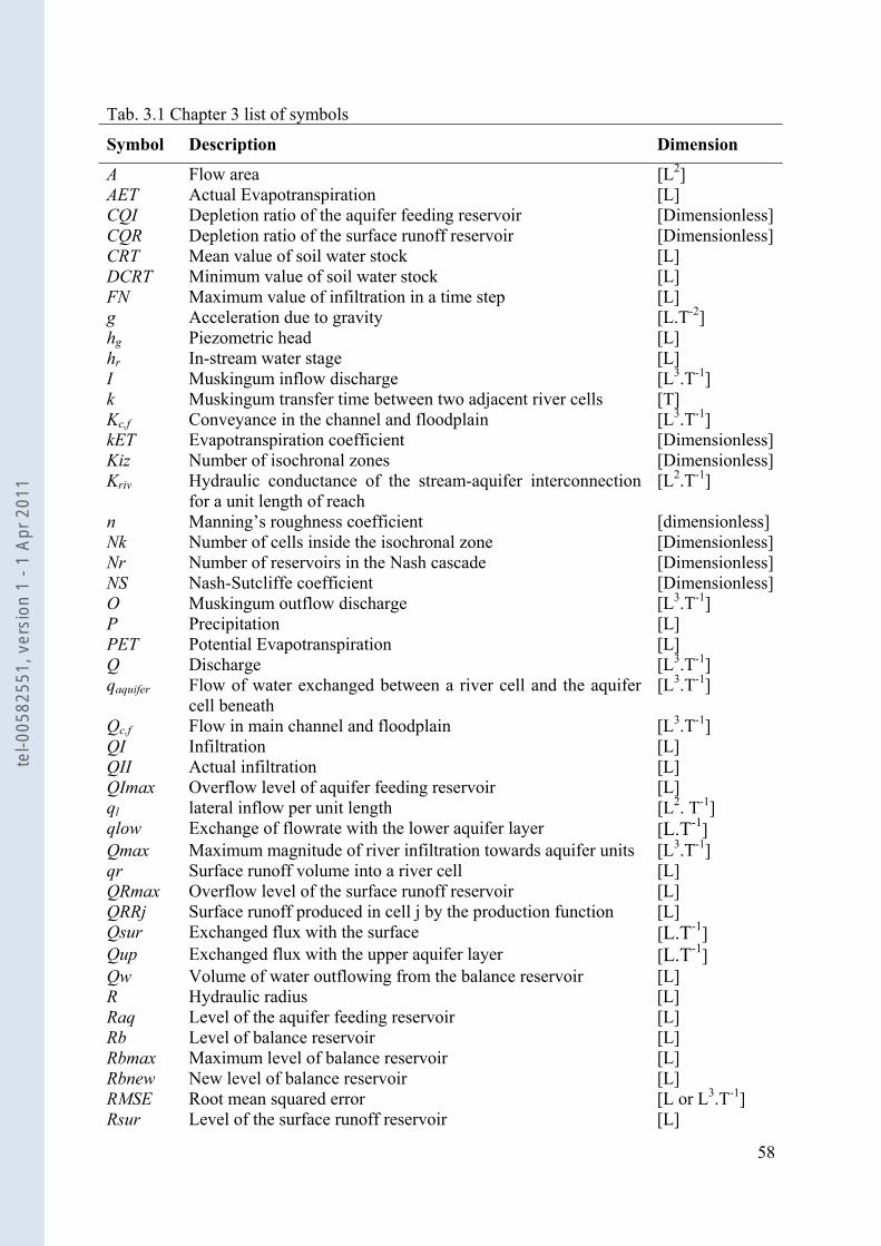
58

Tab. 3.1 Chapter 3 list of symbols

Symbol Description Dimension

A Flow area [L2] AET Actual Evapotranspiration [L] CQI Depletion ratio of the aquifer feeding reservoir [Dimensionless] CQR Depletion ratio of the surface runoff reservoir [Dimensionless] CRT Mean value of soil water stock [L] DCRT Minimum value of soil water stock [L] FN Maximum value of infiltration in a time step [L] g Acceleration due to gravity [L.T-2] hg Piezometric head [L] hr In-stream water stage [L] I Muskingum inflow discharge [L3.T-1] k Muskingum transfer time between two adjacent river cells [T] Kc,f Conveyance in the channel and floodplain [L3.T-1] kET Evapotranspiration coefficient [Dimensionless] Kiz Number of isochronal zones [Dimensionless] Kriv Hydraulic conductance of the stream-aquifer interconnection

for a unit length of reach [L2.T-1]

n Manning’s roughness coefficient [dimensionless] Nk Number of cells inside the isochronal zone [Dimensionless] Nr Number of reservoirs in the Nash cascade [Dimensionless] NS Nash-Sutcliffe coefficient [Dimensionless] O Muskingum outflow discharge [L3.T-1] P Precipitation [L] PET Potential Evapotranspiration [L] Q Discharge [L3.T-1] qaquifer Flow of water exchanged between a river cell and the aquifer

cell beneath [L3.T-1]

Qc,f Flow in main channel and floodplain [L3.T-1] QI Infiltration [L] QII Actual infiltration [L] QImax Overflow level of aquifer feeding reservoir [L] ql lateral inflow per unit length [L2. T-1] qlow Exchange of flowrate with the lower aquifer layer [L.T-1] Qmax Maximum magnitude of river infiltration towards aquifer units [L3.T-1] qr Surface runoff volume into a river cell [L] QRmax Overflow level of the surface runoff reservoir [L] QRRj Surface runoff produced in cell j by the production function [L] Qsur Exchanged flux with the surface [L.T-1] Qup Exchanged flux with the upper aquifer layer [L.T-1] Qw Volume of water outflowing from the balance reservoir [L] R Hydraulic radius [L] Raq Level of the aquifer feeding reservoir [L] Rb Level of balance reservoir [L] Rbmax Maximum level of balance reservoir [L] Rbnew New level of balance reservoir [L] RMSE Root mean squared error [L or L3.T-1] Rsur Level of the surface runoff reservoir [L]

tel-0

0582

551,

ver

sion

1 -

1 Ap

r 201

1

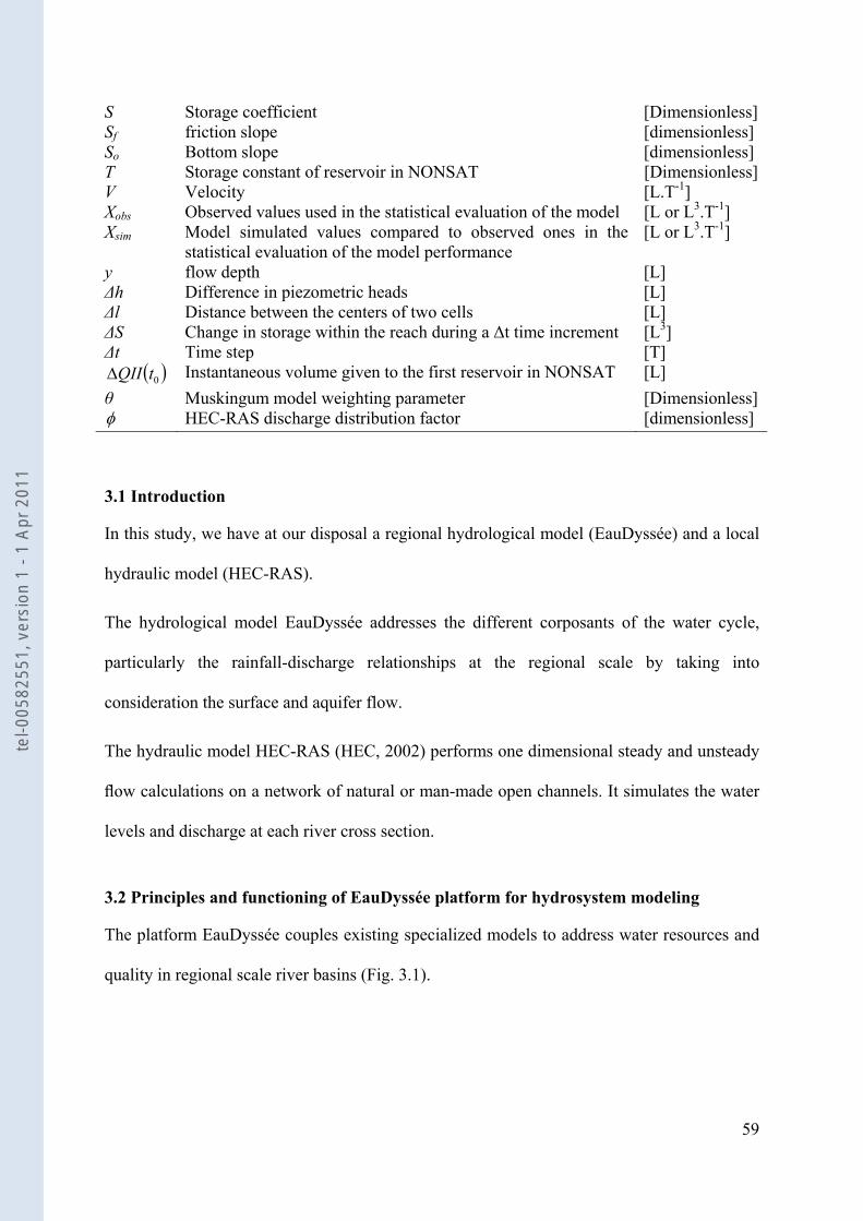
59

S Storage coefficient [Dimensionless] Sf friction slope [dimensionless] So Bottom slope [dimensionless] Τ Storage constant of reservoir in NONSAT [Dimensionless] V Velocity [L.T-1] Xobs Observed values used in the statistical evaluation of the model [L or L3.T-1] Xsim Model simulated values compared to observed ones in the

statistical evaluation of the model performance [L or L3.T-1]

y flow depth [L] Δh Difference in piezometric heads [L] Δl Distance between the centers of two cells [L] ΔS Change in storage within the reach during a Δt time increment [L3] Δt Time step [T]

( )0tQIIΔ Instantaneous volume given to the first reservoir in NONSAT [L] θ Muskingum model weighting parameter [Dimensionless] φ HEC-RAS discharge distribution factor [dimensionless]

3.1 Introduction

In this study, we have at our disposal a regional hydrological model (EauDyssée) and a local

hydraulic model (HEC-RAS).

The hydrological model EauDyssée addresses the different corposants of the water cycle,

particularly the rainfall-discharge relationships at the regional scale by taking into

consideration the surface and aquifer flow.

The hydraulic model HEC-RAS (HEC, 2002) performs one dimensional steady and unsteady

flow calculations on a network of natural or man-made open channels. It simulates the water

levels and discharge at each river cross section.

3.2 Principles and functioning of EauDyssée platform for hydrosystem modeling

The platform EauDyssée couples existing specialized models to address water resources and

quality in regional scale river basins (Fig. 3.1).

tel-0

0582

551,

ver

sion

1 -

1 Ap

r 201

1

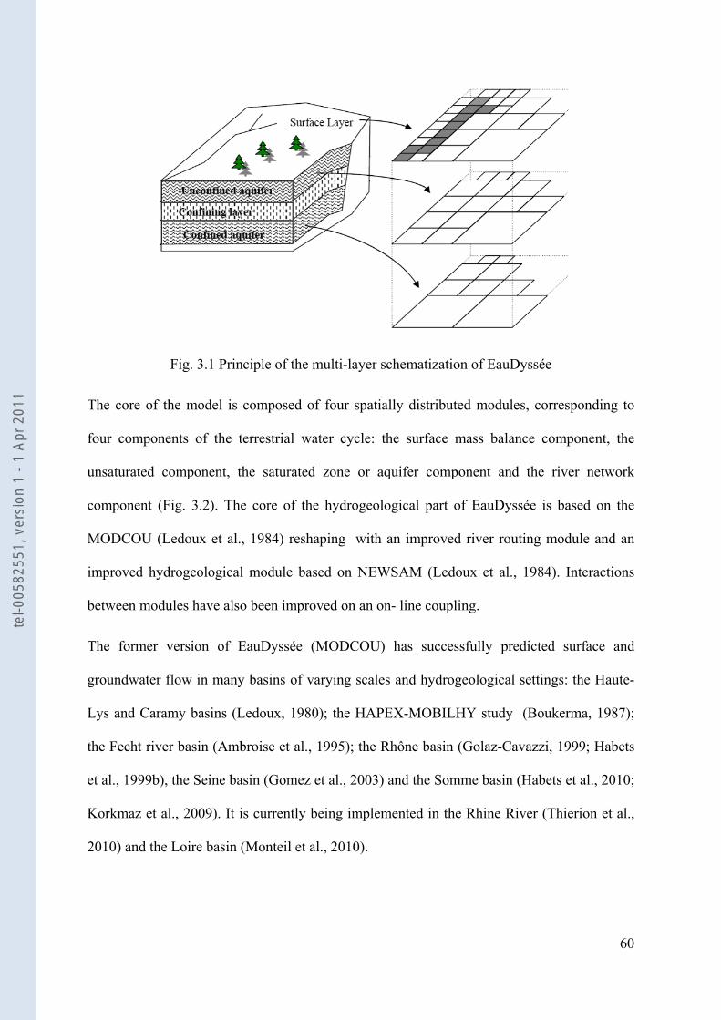
60

Fig. 3.1 Principle of the multi-layer schematization of EauDyssée

The core of the model is composed of four spatially distributed modules, corresponding to

four components of the terrestrial water cycle: the surface mass balance component, the

unsaturated component, the saturated zone or aquifer component and the river network

component (Fig. 3.2). The core of the hydrogeological part of EauDyssée is based on the

MODCOU (Ledoux et al., 1984) reshaping with an improved river routing module and an

improved hydrogeological module based on NEWSAM (Ledoux et al., 1984). Interactions

between modules have also been improved on an on- line coupling.

The former version of EauDyssée (MODCOU) has successfully predicted surface and

groundwater flow in many basins of varying scales and hydrogeological settings: the Haute-

Lys and Caramy basins (Ledoux, 1980); the HAPEX-MOBILHY study (Boukerma, 1987);

the Fecht river basin (Ambroise et al., 1995); the Rhône basin (Golaz-Cavazzi, 1999; Habets

et al., 1999b), the Seine basin (Gomez et al., 2003) and the Somme basin (Habets et al., 2010;

Korkmaz et al., 2009). It is currently being implemented in the Rhine River (Thierion et al.,

2010) and the Loire basin (Monteil et al., 2010).

tel-0

0582

551,

ver

sion

1 -

1 Ap

r 201

1

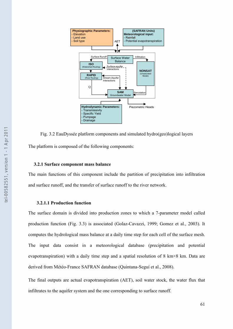
61

Fig. 3.2 EauDyssée platform components and simulated hydro(geo)logical layers

The platform is composed of the following components:

3.2.1 Surface component mass balance

The main functions of this component include the partition of precipitation into infiltration

and surface runoff, and the transfer of surface runoff to the river network.

3.2.1.1 Production function

The surface domain is divided into production zones to which a 7-parameter model called

production function (Fig. 3.3) is associated (Golaz-Cavazzi, 1999; Gomez et al., 2003). It

computes the hydrological mass balance at a daily time step for each cell of the surface mesh.

The input data consist in a meteorological database (precipitation and potential

evapotranspiration) with a daily time step and a spatial resolution of 8 km×8 km. Data are

derived from Météo-France SAFRAN database (Quintana-Seguí et al., 2008).

The final outputs are actual evapotranspiration (AET), soil water stock, the water flux that

infiltrates to the aquifer system and the one corresponding to surface runoff.

(SAFRAN Units)Meteorological input: - Rainfall - Potential evapotranspiration

SAMGroundwater Model

Surface Water Balance

Infiltration Surface Runoff

Q

Z

Stream-Aquifer Interactions

Percolation

NONSAT (Unsaturated

Model)

RAPID (River Routing)

Piezometric Heads

ISO (Watershed Routing)

AET

Surface-aquifer interactions

Physiographic Parameters:- Elevation - Land use - Soil type

Hydrodynamic Parameters:- Transmissivity - Specific Yield - Pumpage - Drainage

Q

tel-0

0582

551,

ver

sion

1 -

1 Ap

r 201

1

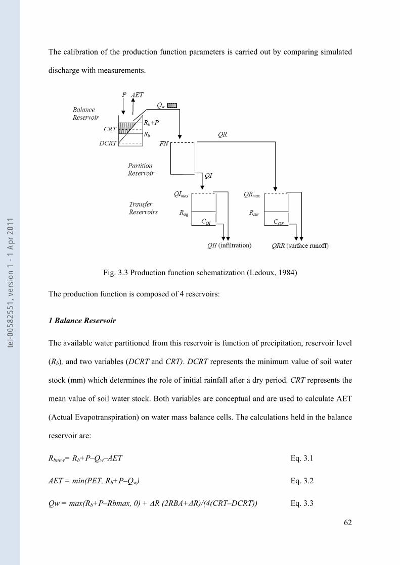
62

The calibration of the production function parameters is carried out by comparing simulated

discharge with measurements.

Fig. 3.3 Production function schematization (Ledoux, 1984)

The production function is composed of 4 reservoirs:

1 Balance Reservoir

The available water partitioned from this reservoir is function of precipitation, reservoir level

(Rb), and two variables (DCRT and CRT). DCRT represents the minimum value of soil water

stock (mm) which determines the role of initial rainfall after a dry period. CRT represents the

mean value of soil water stock. Both variables are conceptual and are used to calculate AET

(Actual Evapotranspiration) on water mass balance cells. The calculations held in the balance

reservoir are:

Rbnew= Rb+P–Qw–AET Eq. 3.1

AET = min(PET, Rb+P–Qw) Eq. 3.2

Qw = max(Rb+P–Rbmax, 0) + ΔR (2RBA+ΔR)/(4(CRT–DCRT)) Eq. 3.3

tel-0

0582

551,

ver

sion

1 -

1 Ap

r 201

1

63

ΔR = max(0, RHA–RBA) Eq. 3.4

RHA = min(Rb+P, Rbmax) – DCRT Eq. 3.5

RBA = max(DCRT, Rb) – DCRT Eq. 3.6

Rbmax = 2(CRT–DCRT) + DCRT Eq. 3. 7

Where Rbnew is the new level of balance reservoir [L], Qw is the volume of water outflowing

from the balance reservoir [L] and the other variables are temporary ones simplifying the

writing of equations.

2 Partition Reservoir

This reservoir partitions the output received from the balance reservoir between the potential

infiltration reservoir and the surface runoff reservoir. The distribution between potential

infiltrating water (QI, [L]) and potential surface runoff (QR, [L]) is controlled by the

parameter (FN, [L]) which stands for the maximum value of infiltration in a time step. These

are expressed as follows:

QI = min(Qw, FN) Eq. 3.8

QR = max(0, Qw – QI) Eq. 3.9

Water joins surface runoff when the infiltration capacity of soil is overtopped. If the level of

available water is not high enough to overtop the partitioning reservoir, then there will be no

surface runoff and all the water will infiltrate.

3 Transfer Reservoirs

The transfer reservoirs include the infiltration reservoir that feeds the unsaturated zone or

directly the aquifer units, and the surface runoff reservoir. The infiltration reservoir

tel-0

0582

551,

ver

sion

1 -

1 Ap

r 201

1

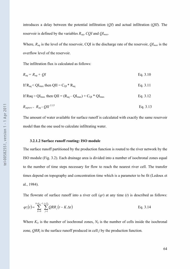
64

introduces a delay between the potential infiltration (QI) and actual infiltration (QII). The

reservoir is defined by the variables Raq, CQI and QImax.

Where, Raq is the level of the reservoir, CQI is the discharge rate of the reservoir, QImax is the

overflow level of the reservoir.

The infiltration flux is calculated as follows:

Raq = Raq + QI Eq. 3.10

If Raq < QImax then QII = CQI * Raq Eq. 3.11

If Raq > QImax then QII = (Raq – QImax) + CQI * QImax Eq. 3.12

Raqnew = Raq - QII 3.13 Eq. 3.13

The amount of water available for surface runoff is calculated with exactly the same reservoir

model than the one used to calculate infiltrating water.

3.2.1.2 Surface runoff routing: ISO module

The surface runoff partitioned by the production function is routed to the river network by the

ISO module (Fig. 3.2). Each drainage area is divided into a number of isochronal zones equal

to the number of time steps necessary for flow to reach the nearest river cell. The transfer

times depend on topography and concentration time which is a parameter to be fit (Ledoux et

al., 1984).

The flowrate of surface runoff into a river cell (qr) at any time (t) is described as follows:

( ) ( )t.KtQRRtqriz kkk

k

Nj

jji Δ−= ∑ ∑

−=

=

=

=

1

0 1 Eq. 3.14

Where Kiz is the number of isochronal zones, Nk is the number of cells inside the isochronal

zone, QRRj is the surface runoff produced in cell j by the production function.

tel-0

0582

551,

ver

sion

1 -

1 Ap

r 201

1

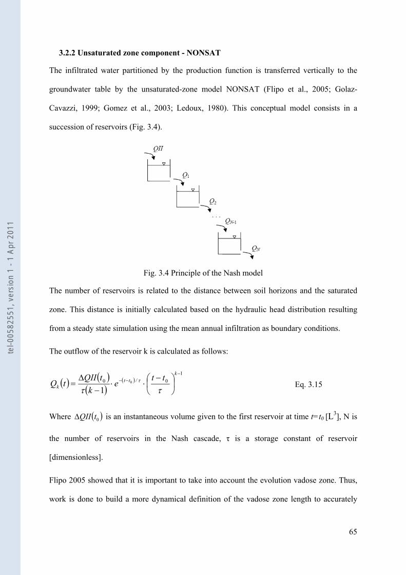
65

3.2.2 Unsaturated zone component - NONSAT

The infiltrated water partitioned by the production function is transferred vertically to the

groundwater table by the unsaturated-zone model NONSAT (Flipo et al., 2005; Golaz-

Cavazzi, 1999; Gomez et al., 2003; Ledoux, 1980). This conceptual model consists in a

succession of reservoirs (Fig. 3.4).

Fig. 3.4 Principle of the Nash model

The number of reservoirs is related to the distance between soil horizons and the saturated

zone. This distance is initially calculated based on the hydraulic head distribution resulting

from a steady state simulation using the mean annual infiltration as boundary conditions.

The outflow of the reservoir k is calculated as follows:

( ) ( )( )

( )1

00 0

1

−−− ⎟

⎠⎞

⎜⎝⎛ −⋅⋅

−Δ

=k

/ttk

tte

ktQII

tQττ

τ Eq. 3.15

Where ( )0tQIIΔ is an instantaneous volume given to the first reservoir at time t=t0 [L3], N is

the number of reservoirs in the Nash cascade, τ is a storage constant of reservoir

[dimensionless].

Flipo 2005 showed that it is important to take into account the evolution vadose zone. Thus,

work is done to build a more dynamical definition of the vadose zone length to accurately

tel-0

0582

551,

ver

sion

1 -

1 Ap

r 201

1

66

simulate water reaching the top of the aquifer units. Otherwise, transfer time in the vadose

zone can be overestimated up to one order of magnitude (Philippe et al., 2010).

3.2.3 Saturated zone component: SAM (Simulation des Aquiferes Multicouches)

The SAM model (Ledoux et al., 1984, 1989) is a regional spatially distributed model that

computes the temporal distribution of the piezometric heads of a multilayer aquifer system,

using the diffusivity equation (de Marsily, 1986).

lowupsurgg

yg

x QQQt

hs

yh

Tyx

hT

x+++

∂

∂=⎟⎟

⎠

⎞⎜⎜⎝

⎛∂

∂

∂∂

+⎟⎟⎠

⎞⎜⎜⎝

⎛∂

∂

∂∂ Eq. 3.16

Where hg is the piezometric head [L], T is the transmissivity [L2.T-1], S is the storage

coefficient [dimensionless], Qsur is the exchanged flux with the surface [L.T-1], Qup is the

exchange flux with the upper aquifer unit [L.T-1] and Qlow is the exchanged of flowrate with

the lower aquifer unit [L.T-1].

In each aquifer, flows are bidimensionnal whereas they are vertically monodimensionnal in

the aquitard between two horizontal layers. The multilayer model simulates confined and

unconfined aquifer units. The variation through time of the head is modeled by nonlinear

Boussinesq equaiton. It also computes exchange between aquifer units and rivers.

3.2.4 The regional river routing component RAPID

The in-stream discharge routing within the platform EauDyssée is conducted by a parallel

computing-based river routing model called RAPID (David et al., 2010), Routing Application

for Parallel Computation of Discharge, which is based on the Muskingum routing scheme

(Eq. 2.12).

tel-0

0582

551,

ver

sion

1 -

1 Ap

r 201

1

67

3.2.5 Stream-aquifer interactions

Stream-aquifer interactions are calculated in each river grid cell from the difference between

hydraulic heads in the river cell and the underlying aquifer cell. Depending on the sign of this

difference, surface water either infiltrates towards aquifer units, or groundwater exfiltrates

towards the river network.

For large river basins such as the Seine River and the Loire River, cells representing the river

have a length of 1 km and are thus usually greater than the dimensions of the stream.

Therefore, the stream-aquifer interactions are simplified and controlled by a coefficient called

river conductance that relates stream-aquifer flow to the difference between the in-stream

water level and the groundwater head:

( )grrivaquifer hhKq −= Eq. 3.17

Where aquiferq is the flow between stream and aquifer [L3.T-1], rh is the in-stream water stage

[L], gh is the piezometric head in the aquifer unit [L] and rivK is the hydraulic conductance

of the stream-aquifer interconnection for a unit length of reach [L2.T-1].

In the current EauDyssée version, in-stream water levels are obtained from a Digital

Elevation Model (DEM) and imposed as constant boundary conditions along the river

network. Thus stream-aquifer interactions are only controlled by the fluctuation of the

piezometric head in the aquifer units.

The magnitude of river infiltration towards aquifer units is controlled by a maximal value

called Qmax [L3.T-1. L-2]. If Qmax is equal to zero, infiltration from stream to aquifer unit is not

authorized even if the in-stream water level is higher than the water table level. Qmax can be

estimated either from field measurements based on local mass balance or through available

literature on river’s bed permeability (Lange, 2005). Typically Qmax varies from 0 l.s-1km-2 for

tel-0

0582

551,

ver

sion

1 -

1 Ap

r 201

1

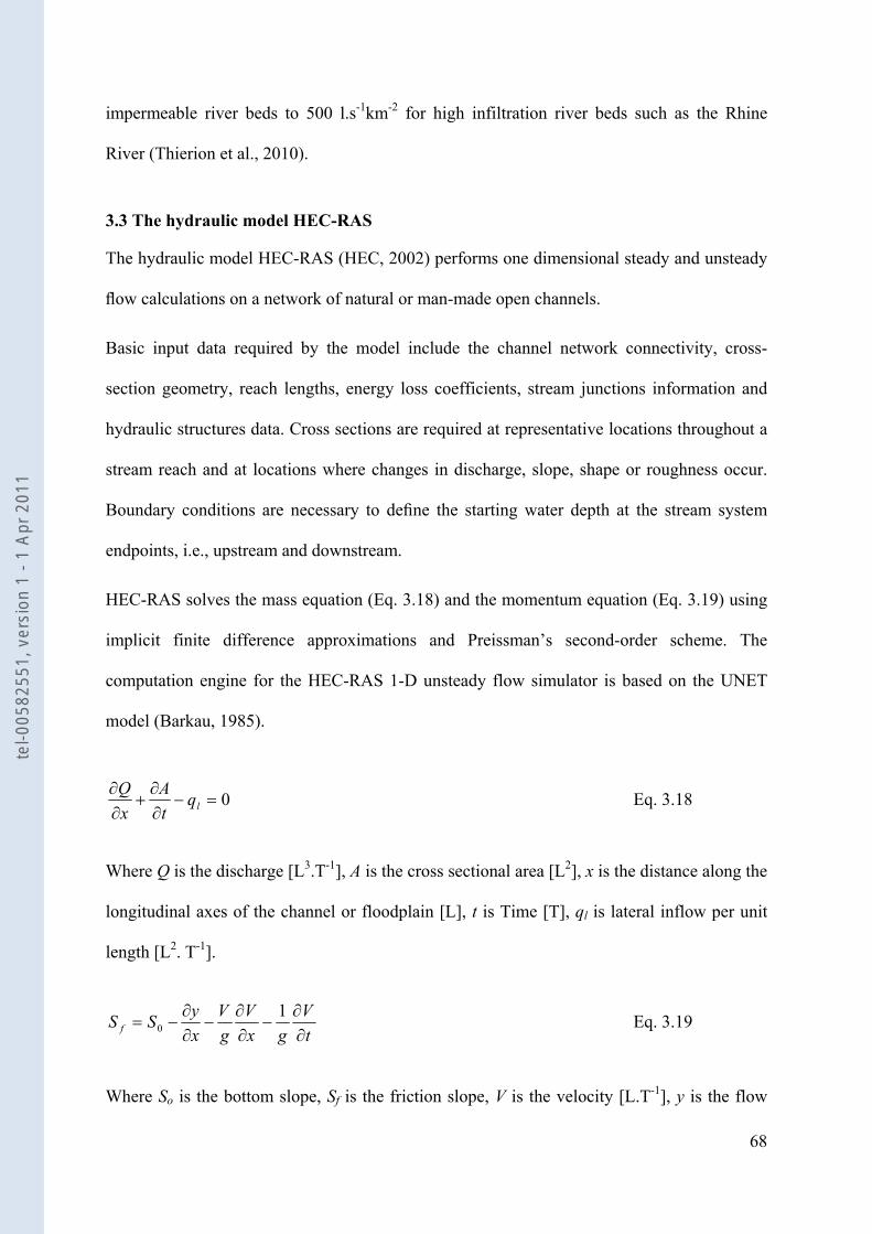
68

impermeable river beds to 500 l.s-1km-2 for high infiltration river beds such as the Rhine

River (Thierion et al., 2010).

3.3 The hydraulic model HEC-RAS

The hydraulic model HEC-RAS (HEC, 2002) performs one dimensional steady and unsteady

flow calculations on a network of natural or man-made open channels.

Basic input data required by the model include the channel network connectivity, cross-

section geometry, reach lengths, energy loss coefficients, stream junctions information and

hydraulic structures data. Cross sections are required at representative locations throughout a

stream reach and at locations where changes in discharge, slope, shape or roughness occur.

Boundary conditions are necessary to define the starting water depth at the stream system

endpoints, i.e., upstream and downstream.

HEC-RAS solves the mass equation (Eq. 3.18) and the momentum equation (Eq. 3.19) using

implicit finite difference approximations and Preissman’s second-order scheme. The

computation engine for the HEC-RAS 1-D unsteady flow simulator is based on the UNET

model (Barkau, 1985).

0=−∂∂

+∂∂

lqtA

xQ Eq. 3.18

Where Q is the discharge [L3.T-1], A is the cross sectional area [L2], x is the distance along the

longitudinal axes of the channel or floodplain [L], t is Time [T], ql is lateral inflow per unit

length [L2. T-1].

tV

gxV

gV

xySS f ∂

∂−

∂∂

−∂∂

−=1

0 Eq. 3.19

Where So is the bottom slope, Sf is the friction slope, V is the velocity [L.T-1], y is the flow

tel-0

0582

551,

ver

sion

1 -

1 Ap

r 201

1

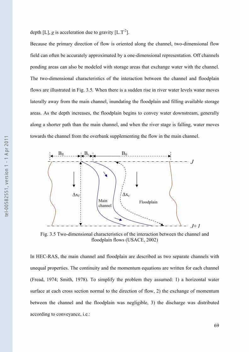
69

depth [L], g is acceleration due to gravity [L.T-2].

Because the primary direction of flow is oriented along the channel, two-dimensional flow

field can often be accurately approximated by a one-dimensional representation. Off channels

ponding areas can also be modeled with storage areas that exchange water with the channel.

The two-dimensional characteristics of the interaction between the channel and floodplain

flows are illustrated in Fig. 3.5. When there is a sudden rise in river water levels water moves

laterally away from the main channel, inundating the floodplain and filling available storage

areas. As the depth increases, the floodplain begins to convey water downstream, generally

along a shorter path than the main channel, and when the river stage is falling, water moves

towards the channel from the overbank supplementing the flow in the main channel.

Fig. 3.5 Two-dimensional characteristics of the interaction between the channel and

floodplain flows (USACE, 2002)

In HEC-RAS, the main channel and floodplain are described as two separate channels with

unequal properties. The continuity and the momentum equations are written for each channel

(Fread, 1974; Smith, 1978). To simplify the problem they assumed: 1) a horizontal water

surface at each cross section normal to the direction of flow, 2) the exchange of momentum

between the channel and the floodplain was negligible, 3) the discharge was distributed

according to conveyance, i.e.:

Δxc Δxf

J

Bfr Bc Bfl

J+1

Main channel

Floodplain

tel-0

0582

551,

ver

sion

1 -

1 Ap

r 201

1

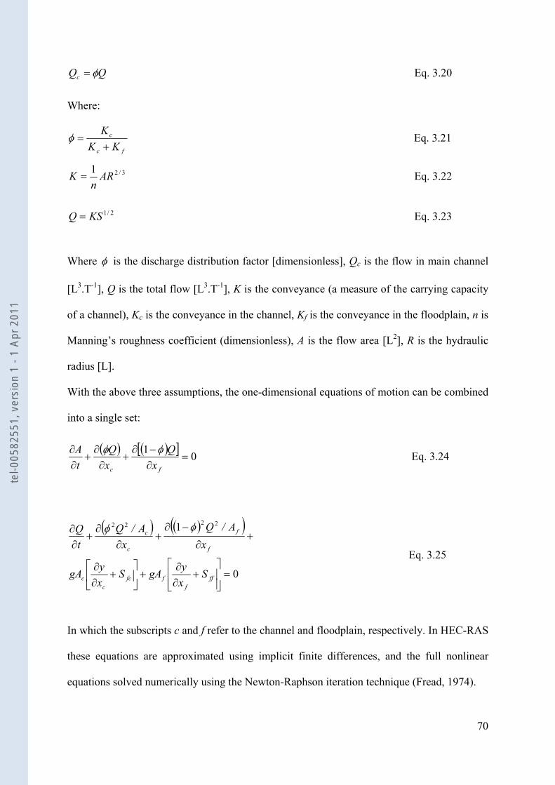
70

QQc φ= Eq. 3.20

Where:

fc

c

KKK+

=φ Eq. 3.21

3/21 ARn

K = Eq. 3.22

2/1KSQ = Eq. 3.23

Where φ is the discharge distribution factor [dimensionless], Qc is the flow in main channel

[L3.T-1], Q is the total flow [L3.T-1], K is the conveyance (a measure of the carrying capacity

of a channel), Kc is the conveyance in the channel, Kf is the conveyance in the floodplain, n is

Manning’s roughness coefficient (dimensionless), A is the flow area [L2], R is the hydraulic

radius [L].

With the above three assumptions, the one-dimensional equations of motion can be combined

into a single set:

( ) ( )[ ] 01=

∂−∂

+∂∂

+∂∂

fc xQ

xQ

tA φφ

Eq. 3.24

( ) ( )( )

0

1 2222

=⎥⎥⎦

⎤

⎢⎢⎣

⎡+

∂∂

+⎥⎦

⎤⎢⎣

⎡+

∂∂

+∂

−∂+

∂∂

+∂∂

fff

ffcc

c

f

f

c

c

SxygAS

xygA

xA/Q

xA/Q

tQ φφ

Eq. 3.25

In which the subscripts c and f refer to the channel and floodplain, respectively. In HEC-RAS

these equations are approximated using implicit finite differences, and the full nonlinear

equations solved numerically using the Newton-Raphson iteration technique (Fread, 1974).

tel-0

0582

551,

ver

sion

1 -

1 Ap

r 201

1

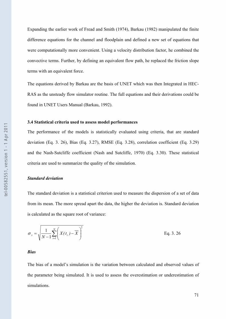
71

Expanding the earlier work of Fread and Smith (1974), Barkau (1982) manipulated the finite

difference equations for the channel and floodplain and defined a new set of equations that

were computationally more convenient. Using a velocity distribution factor, he combined the

convective terms. Further, by defining an equivalent flow path, he replaced the friction slope

terms with an equivalent force.

The equations derived by Barkau are the basis of UNET which was then Integrated in HEC-

RAS as the unsteady flow simulator routine. The full equations and their derivations could be

found in UNET Users Manual (Barkau, 1992).

3.4 Statistical criteria used to assess model performances

The performance of the models is statistically evaluated using criteria, that are standard

deviation (Eq. 3. 26), Bias (Eq. 3.27), RMSE (Eq. 3.28), correlation coefficient (Eq. 3.29)

and the Nash-Sutcliffe coefficient (Nash and Sutcliffe, 1970) (Eq. 3.30). These statistical

criteria are used to summarize the quality of the simulation.

Standard deviation

The standard deviation is a statistical criterion used to measure the dispersion of a set of data

from its mean. The more spread apart the data, the higher the deviation is. Standard deviation

is calculated as the square root of variance:

∑=

⎟⎟⎠

⎞⎜⎜⎝

⎛−

−=

N

iix X)t(X

N 1

2

11σ Eq. 3. 26

Bias

The bias of a model’s simulation is the variation between calculated and observed values of

the parameter being simulated. It is used to assess the overestimation or underestimation of

simulations.

tel-0

0582

551,

ver

sion

1 -

1 Ap

r 201

1

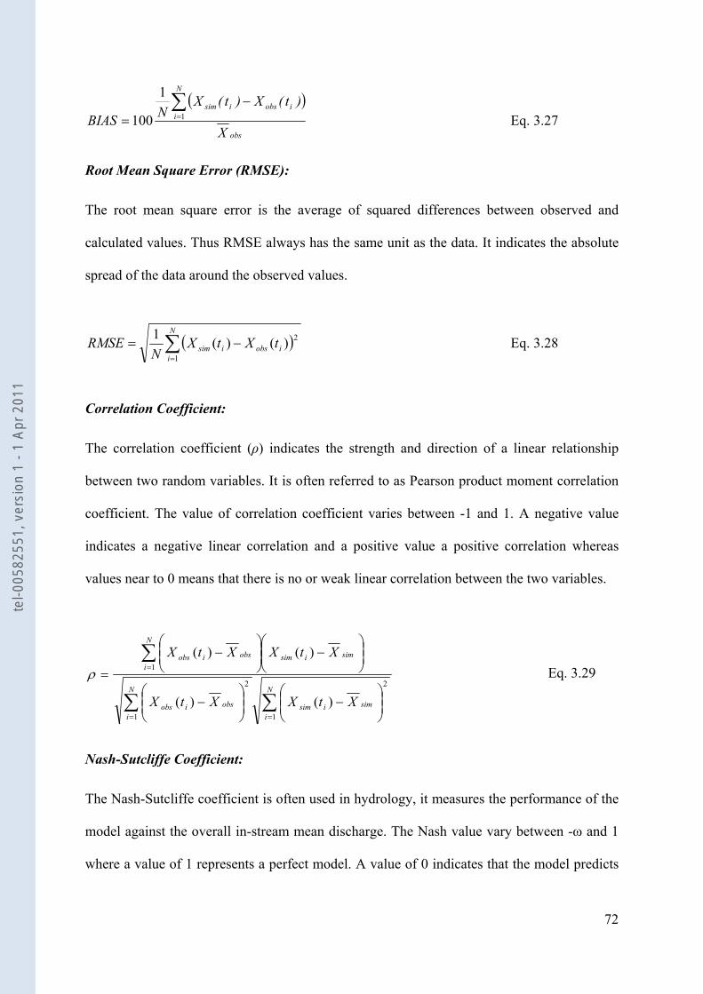
72

( )

obs

N

iiobsisim

X

)t(X)t(XNBIAS∑=

−= 1

1

100 Eq. 3.27

Root Mean Square Error (RMSE):

The root mean square error is the average of squared differences between observed and

calculated values. Thus RMSE always has the same unit as the data. It indicates the absolute

spread of the data around the observed values.

( )∑=

−=N

iiobsisim tXtX

NRMSE

1

2)()(1 Eq. 3.28

Correlation Coefficient:

The correlation coefficient (ρ) indicates the strength and direction of a linear relationship

between two random variables. It is often referred to as Pearson product moment correlation

coefficient. The value of correlation coefficient varies between -1 and 1. A negative value

indicates a negative linear correlation and a positive value a positive correlation whereas

values near to 0 means that there is no or weak linear correlation between the two variables.

∑∑

∑

==

=

⎟⎟⎠

⎞⎜⎜⎝

⎛−⎟⎟

⎠

⎞⎜⎜⎝

⎛−

⎟⎟⎠

⎞⎜⎜⎝

⎛−⎟⎟

⎠

⎞⎜⎜⎝

⎛−

=N

isimisim

N

iobsiobs

N

isimisimobsiobs

XtXXtX

XtXXtX

1

2

1

2

1

)()(

)()(ρ Eq. 3.29

Nash-Sutcliffe Coefficient:

The Nash-Sutcliffe coefficient is often used in hydrology, it measures the performance of the

model against the overall in-stream mean discharge. The Nash value vary between -ω and 1

where a value of 1 represents a perfect model. A value of 0 indicates that the model predicts

tel-0

0582

551,

ver

sion

1 -

1 Ap

r 201

1

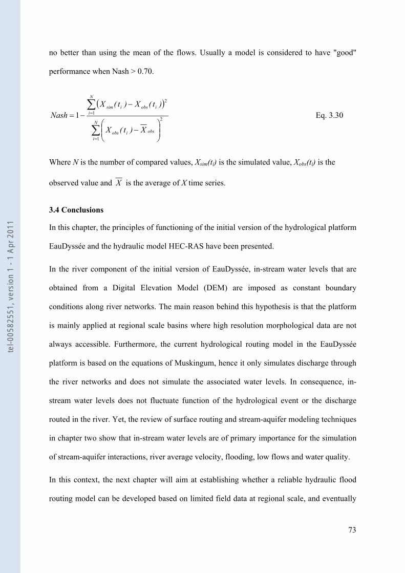
73

no better than using the mean of the flows. Usually a model is considered to have "good"

performance when Nash > 0.70.

( )

∑

∑

=

=

⎟⎟⎠

⎞⎜⎜⎝

⎛−

−−=

N

iobsiobs

N

iiobsisim

X)t(X

)t(X)t(XNash

1

21

2

1 Eq. 3.30

Where N is the number of compared values, Xsim(ti) is the simulated value, Xobs(ti) is the

observed value and X is the average of X time series.

3.4 Conclusions

In this chapter, the principles of functioning of the initial version of the hydrological platform

EauDyssée and the hydraulic model HEC-RAS have been presented.

In the river component of the initial version of EauDyssée, in-stream water levels that are

obtained from a Digital Elevation Model (DEM) are imposed as constant boundary

conditions along river networks. The main reason behind this hypothesis is that the platform

is mainly applied at regional scale basins where high resolution morphological data are not

always accessible. Furthermore, the current hydrological routing model in the EauDyssée

platform is based on the equations of Muskingum, hence it only simulates discharge through

the river networks and does not simulate the associated water levels. In consequence, in-

stream water levels does not fluctuate function of the hydrological event or the discharge

routed in the river. Yet, the review of surface routing and stream-aquifer modeling techniques

in chapter two show that in-stream water levels are of primary importance for the simulation

of stream-aquifer interactions, river average velocity, flooding, low flows and water quality.

In this context, the next chapter will aim at establishing whether a reliable hydraulic flood

routing model can be developed based on limited field data at regional scale, and eventually

tel-0

0582

551,

ver

sion

1 -

1 Ap

r 201

1

74

identifying a methodology to improve the simulations of in-stream water levels and stream-

aquifer interactions in EauDyssée.

tel-0

0582

551,

ver

sion

1 -

1 Ap

r 201

1

75

CHAPTER 4. IMPACT OF IN-STREAM MORPHOLOGY ON SIMULATED

DISCHARGE AND WATER LEVELS: SEREIN RIVER CASE STUDY


Les modèles de routage hydrologiques de débit continuent d'être les outils principaux pour le

routage des débits à l’échelle des bassins versants. Cependant, la simulation des hauteurs

d’eau nécessite des modèles (hydrauliques) déterministes. Un avantage fondamental des

modèles de routage hydrauliques par rapport aux modèles hydrologique, en terme

d'événements dynamiques, est que des données décrivant les hydrogrammes de débit et la

hauteur d’eau entre des sites de jaugeage sont exploitées. De telles données sont importantes

pour la simulation des interactions nappe-rivière (cf. chapitre 2).

A ce jour, les modèles hydrauliques à l’échelle régionale de bassin versant ne sont pas

toujours utilisés pour deux raisons clés. Premièrement, ils peuvent être difficiles d’emploi

d’un point de vue numérique. Deuxièmement, ils sont exigeants en données géométriques sur

l'entière étendue du domaine modélisé.

Le premier problème n'est plus la préoccupation principale, puisque des recherches récentes

ont abouti au développement de configurations de calcul robustes.

La nécessité d’utiliser de nombreuses données par les modèles hydrauliques est beaucoup

plus limitante d'un point de vue pratique, puisque le routage de débit couvre de très longues

étendues et que le coût d'obtention des données suffisantes sur la section peut être prohibitif.

Dans cette étude, la sensibilité d'un modèle hydraulique à la précision de la description

géomorphologique des lits et à la géométrie réduite est évaluée pour identifier le meilleur

compromis entre parcimonie et réalisme et identifier les facteurs morphologiques les plus

importants pour obtenir une simulation satisfaisante des hauteurs d'eau.

tel-0

0582

551,

ver

sion

1 -

1 Ap

r 201

1

76

Le principe des simulations est basé sur l’association entre un modèle hydraulique et un

modèle hydrologique. Le modèle hydraulique utilisé est le modèle HEC-RAS, et les variables

évaluées sont les débits et les hauteurs d'eau. Les apports latéraux sont simulés par la

plateforme EauDyssée sous forme de lames d'eau écoulées depuis le bassin versant

directement contributif. Les résultats ont été obtenus sur les biefs du Serein (affluent de

l'Yonne) bien renseignés entre Dissangis et Beaumont (89 km).

A partir des résultats de ces tests, nous pouvons conclure qu’une simplification de la

géométrie ne modifie pas significativement la simulation des débits. En revanche, une

géométrie précise est nécessaire pour bien simuler les hauteurs d’eau, notamment dans les

simulations nappe-rivière et la simulation des inondations.

Abstract

Hydrological routing models are the main tool for discharge routing at regional scale, while

the simulation of river water levels require hydraulic models that are capable of simulating

hydrodynamic events such as floods and overtopping frequency.

To date, hydrodynamic models are not widely used at the regional scale because they require

high resolution morphological data that are not always accessible at regional scale, in

addition to insufficient computational power and numerical difficulties when applied at

regional scale.

The numerical difficulties are no longer the main concern, especially with the recent

advances in the domain of numerical research.

In hydrodynamic models it is recognized that river flow characteristics are influenced by

several morphological factors, amongst which, the channel slope and morphology. However,

literature does not show to what extent these morphological factors influence the quality of

the hydraulic model in predicting water levels and discharge hydrographs.

tel-0

0582

551,

ver

sion

1 -

1 Ap

r 201

1

77

This chapter aims at establishing whether a reliable hydraulic model can be developed based

on limited field data. A wide variety of "what if" river geometry scenarios are explored to

determine the most appropriate simplified river representation geometry in areas where cross

sections surveys are not available.

The validity of this approach has been illustrated by developing the Serein River hydraulic

model (tributary of the Yonne River). The modelization methodology is based on the

association between a hydraulic and hydrological model. The hydraulic model used is HEC-

RAS (HEC, 2002) which is based on the Saint Venant equations solved using the four point

implicit finite difference scheme. The calibration parameter involved in the development of

the hydraulic model is the Manning's roughness coefficient (n). The hydrogeological model

EauDyssée (explained in chapter 5) is used to simulate the lateral inflows of the Serein River

subcatchments.

The results of this study show that hydraulic routing models based on the Saint Venant

equations could be successfully used to determine discharge hydrographs in reaches where

little channel geometry data are available, by approximating the modeled reach with

simplified geometry. However, a hydraulic model based on approximate channel geometry

does not always predict the associated water levels with possible consequences on stream-

aquifer interactions and inundation zones. The results show that the accuracy of predicted

water levels, maximum water depths rely on an accurate representation of channel geometry

and bed level slopes along the river reach.

4.1 Introduction

The morphology of natural streams has attracted the attention of researchers since early

1900s (Lindley, 1919). Natural streams are characterized by variations in cross sections and

bed slopes that occur over a range of spatial scales as result of several systematic and

tel-0

0582

551,

ver

sion

1 -

1 Ap

r 201

1

78

statistical analysis of the river system such as discharge characteristics, quantity and

characteristics of sediment load, and perimeter (bed and bank) sediments (Leopold et al.,

1964).

The irregularities in bed slopes and cross-sectional shapes usually lead to rising irregularities

of pressure and gravity forces in the flow direction, thus producing irregular driving forces

(Chiu, 1972). Furthermore, irregularities of in-stream channel cross-section and channel slope

are important in streams where the hydraulic behavior at low flow is dominated by backwater

effects due to pool-riffle streams (Hey and Thorne, 1986; Miller and Wenzel, 1984). This

effect is significant for low Froude numbers (which usually occur during low flows) and less

important for high Froude numbers (Li et al., 1992). Moreover, the channel irregularities

increase the range of flow velocities and water depths which occur in a stream reach

(Western et al., 1994) thereby increasing the diversity of the physical habitats in the stream

(Gubala et al., 1996; Rabeni and Jacobson, 1993). A recent study showed that irregularities in

channel geometry throughout river networks are important to effectively manage flood

propagation, sediment and nutrient transport, and river habitats at regional scale (Stewardson,

2005). Nevertheless, spatial and temporal variation in channel geometry is often difficult and

expensive to measure at regional scale. This regional variation in the size and shape of river

channels has been the core concern of fluvial geomorphologists and hydrologists for decades

(Gordon, 1996; Snell and Sivapalan, 1995).

A number of techniques have been developed to estimate channel geometry indirectly, using

catchment characteristics, hydrological information and climatic variables, which are easily

measured and commonly available (Stewardson, 2005). In these techniques, regression

relationships are developed between channel geometry and catchment characteristics (area,

slope, vegetations etc), hydrology information (annual mean flow, two-year recurrence

intervals) and climatic variables. These relationships are known as hydrologic geometry

tel-0

0582

551,

ver

sion

1 -

1 Ap

r 201

1

79

models or regional geometry curves (Leopold and Maddock, 1953). Others have since used

the bankfull discharge, instead of the mean discharge, as the independent variable in these

downstream hydraulic geometry relations (Harman et al., 2008). Yet, there is no theoretical

argument for the use of power functions (Rhoads, 1992), and this choice is rather based on

empirical analysis (Leopold and Maddock, 1953). Recently, there have been efforts to

develop hydraulic geometry relations for the distribution of cross-sectional hydraulic

parameters within a reach based on surveys of multiple cross-sections. Some studies have

examined the variability of channel geometry for studies of fluvial processes (Buhman et al.,

2002; Western et al., 1997), others have developed hydraulic geometry relations for reach-

averaged hydraulic parameters to assist stream habitat assessment (Jowett, 1998; Lamouroux

and Capra, 2002; Lamouroux and Suchon, 2002; Singh and McConkey, 1989). This

determination of hydraulic geometry relationships through river network analysis provides

important inputs to regional scale hydrological models for predicting flood frequency and

extent, pollutant transport as nutrient or sediment load e.g., (DeRose et al., 2005; Lu et al.,

2004; McKergow et al., 2004; Prosser et al., 2001a).

A major advancement has been achieved in the late 1980’s when geographic information

extracted from Digital Elevation Models (DEM) were used to delineate watershed boundaries

and stream networks (Jenson and Dominique, 1988). Although DEMs provide sufficient data

for watershed delineation purposes and floodplain representation, they usually lack the

accuracy required to represent stream channel cross-sectional morphology which is important

for modeling in-stream hydrodynamic.

River morphological data are required to parameterize hydrodynamic models (Hateley et al.,

2006). An important geomorphological factor for river hydrodynamic modeling is the correct

identification of the bankfull stage and discharge. Bankfull stage corresponds with the

discharge that fills a channel to the elevation of the active floodplain. Numerous methods

tel-0

0582

551,

ver

sion

1 -

1 Ap

r 201

1

80

exist for bankfull stage identification including significant breaks in slope, changes in

vegetation, and river top bank (Kilpatrick and Barnes, 1964; Leopold and Wolman, 1957;

Nixon, 1959; Schumm, 1960; Williams, 1978) but this remains difficult and subjective

(Johnson and Heil, 1996; Knighton, 1984; Williams, 1978).

In hydrodynamic models based on the Saint Venant equations, river flow is influenced by the

aforementioned morphological factors. However, literature does not show to what extent

these morphological factors impact the quality of the hydraulic model in predicting water

levels and discharge hydrographs.

To investigate the influence of minimum field data available for the hydraulic model, the

objective of this section is to examine the sensitivity of a hydraulic model to different river

morphological data. In particular, the validity of using simplified geometry when surveyed

cross sections are not available is explored, since one of the principal objectives of this thesis

is to simulate water level and discharge hydrographs at regional scale, where surveyed cross

sections are not always available.

4.2 Domain of application: Serein River

The Serein River is a sub tributary of the Seine River, its total length is 186 km. The source

of the Serein is located in Saulieu (near to Morvan), and it meets the right bank of the Yonne

at Bassou (Fig. 4.1). Within the studied reach, the Serein runs about 89 km starting from

Dissangis and ending at Beaumont (confluence with the Yonne River). The control point

where calibration is held is Chablis located in the middle of the reach, 55 km downstream

from Dissangis (Fig. 4.1). The selection of this reach was based on the availability of

unsteady flow simulations and high resolution morphological data.

tel-0

0582

551,

ver

sion

1 -

1 Ap

r 201

1

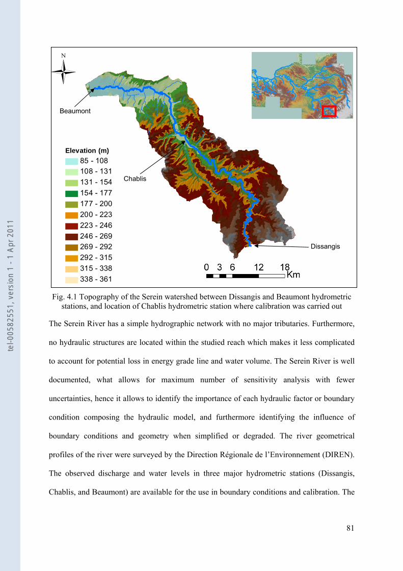
81

Fig. 4.1 Topography of the Serein watershed between Dissangis and Beaumont hydrometric stations, and location of Chablis hydrometric station where calibration was carried out

The Serein River has a simple hydrographic network with no major tributaries. Furthermore,

no hydraulic structures are located within the studied reach which makes it less complicated

to account for potential loss in energy grade line and water volume. The Serein River is well

documented, what allows for maximum number of sensitivity analysis with fewer

uncertainties, hence it allows to identify the importance of each hydraulic factor or boundary

condition composing the hydraulic model, and furthermore identifying the influence of

boundary conditions and geometry when simplified or degraded. The river geometrical

profiles of the river were surveyed by the Direction Régionale de l’Environnement (DIREN).

The observed discharge and water levels in three major hydrometric stations (Dissangis,

Chablis, and Beaumont) are available for the use in boundary conditions and calibration. The

85 - 108108 - 131131 - 154154 - 177177 - 200200 - 223223 - 246246 - 269269 - 292292 - 315315 - 338338 - 361

Elevation (m)

Chablis

Dissangis

Beaumont

Ü

tel-0

0582

551,

ver

sion

1 -

1 Ap

r 201

1

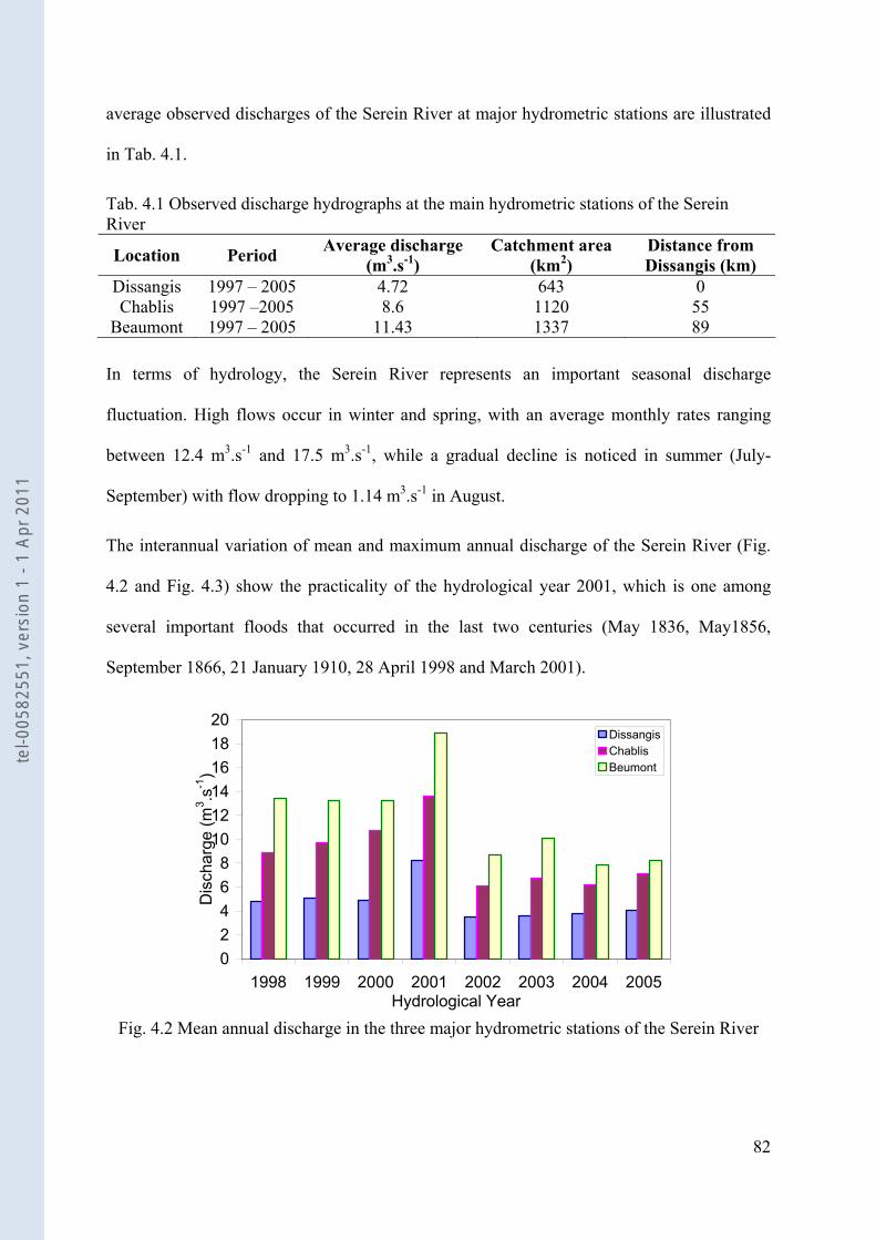
82

average observed discharges of the Serein River at major hydrometric stations are illustrated

in Tab. 4.1.

Tab. 4.1 Observed discharge hydrographs at the main hydrometric stations of the Serein River

Location Period Average discharge (m3.s-1)

Catchment area (km2)

Distance from Dissangis (km)

Dissangis 1997 – 2005 4.72 643 0 Chablis 1997 –2005 8.6 1120 55

Beaumont 1997 – 2005 11.43 1337 89

In terms of hydrology, the Serein River represents an important seasonal discharge

fluctuation. High flows occur in winter and spring, with an average monthly rates ranging

between 12.4 m3.s-1 and 17.5 m3.s-1, while a gradual decline is noticed in summer (July-

September) with flow dropping to 1.14 m3.s-1 in August.

The interannual variation of mean and maximum annual discharge of the Serein River (Fig.

4.2 and Fig. 4.3) show the practicality of the hydrological year 2001, which is one among

several important floods that occurred in the last two centuries (May 1836, May1856,

September 1866, 21 January 1910, 28 April 1998 and March 2001).

02468

101214161820

1998 1999 2000 2001 2002 2003 2004 2005Hydrological Year

Dis

char

ge (m

3 .s-1

)

DissangisChablisBeumont

Fig. 4.2 Mean annual discharge in the three major hydrometric stations of the Serein River

tel-0

0582

551,

ver

sion

1 -

1 Ap

r 201

1

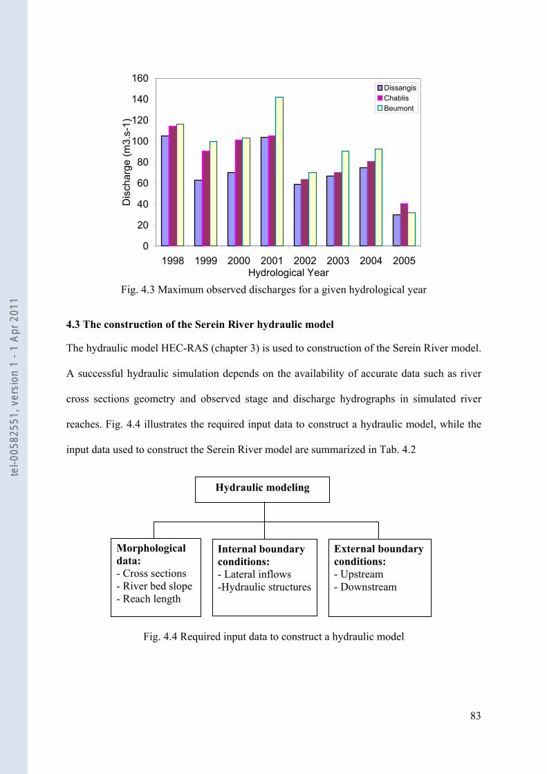
83

0

20

40

60

80

100

120

140

160

1998 1999 2000 2001 2002 2003 2004 2005Hydrological Year

Dis

char

ge (m

3.s-

1)

DissangisChablisBeumont

Fig. 4.3 Maximum observed discharges for a given hydrological year

4.3 The construction of the Serein River hydraulic model

The hydraulic model HEC-RAS (chapter 3) is used to construction of the Serein River model.

A successful hydraulic simulation depends on the availability of accurate data such as river

cross sections geometry and observed stage and discharge hydrographs in simulated river

reaches. Fig. 4.4 illustrates the required input data to construct a hydraulic model, while the

input data used to construct the Serein River model are summarized in Tab. 4.2

Fig. 4.4 Required input data to construct a hydraulic model

Morphological data: - Cross sections - River bed slope - Reach length

External boundary conditions: - Upstream - Downstream

Internal boundary conditions: - Lateral inflows -Hydraulic structures

Hydraulic modeling

tel-0

0582

551,

ver

sion

1 -

1 Ap

r 201

1

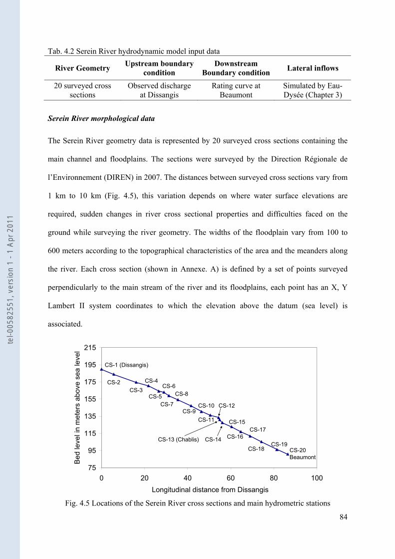
84

Tab. 4.2 Serein River hydrodynamic model input data

River Geometry Upstream boundary condition

Downstream Boundary condition Lateral inflows

20 surveyed cross sections

Observed discharge at Dissangis

Rating curve at Beaumont

Simulated by Eau-Dysée (Chapter 3)

Serein River morphological data

The Serein River geometry data is represented by 20 surveyed cross sections containing the

main channel and floodplains. The sections were surveyed by the Direction Régionale de

l’Environnement (DIREN) in 2007. The distances between surveyed cross sections vary from

1 km to 10 km (Fig. 4.5), this variation depends on where water surface elevations are

required, sudden changes in river cross sectional properties and difficulties faced on the

ground while surveying the river geometry. The widths of the floodplain vary from 100 to

600 meters according to the topographical characteristics of the area and the meanders along

the river. Each cross section (shown in Annexe. A) is defined by a set of points surveyed

perpendicularly to the main stream of the river and its floodplains, each point has an X, Y

Lambert II system coordinates to which the elevation above the datum (sea level) is

associated.

75

95

115

135

155

175

195

215

0 20 40 60 80 100 Longitudinal distance from Dissangis

Bed

leve

l in

met

ers

abov

e se

a le

vel

CS-2CS-3

CS-4

CS-5

CS-6

CS-7

CS-8

CS-9CS-10

CS-11

CS-12

CS-13 (Chablis)

CS-15CS-17

CS-18CS-19

CS-20Beaumont

CS-14 CS-16

CS-1 (Dissangis)

Fig. 4.5 Locations of the Serein River cross sections and main hydrometric stations

tel-0

0582

551,

ver

sion

1 -

1 Ap

r 201

1

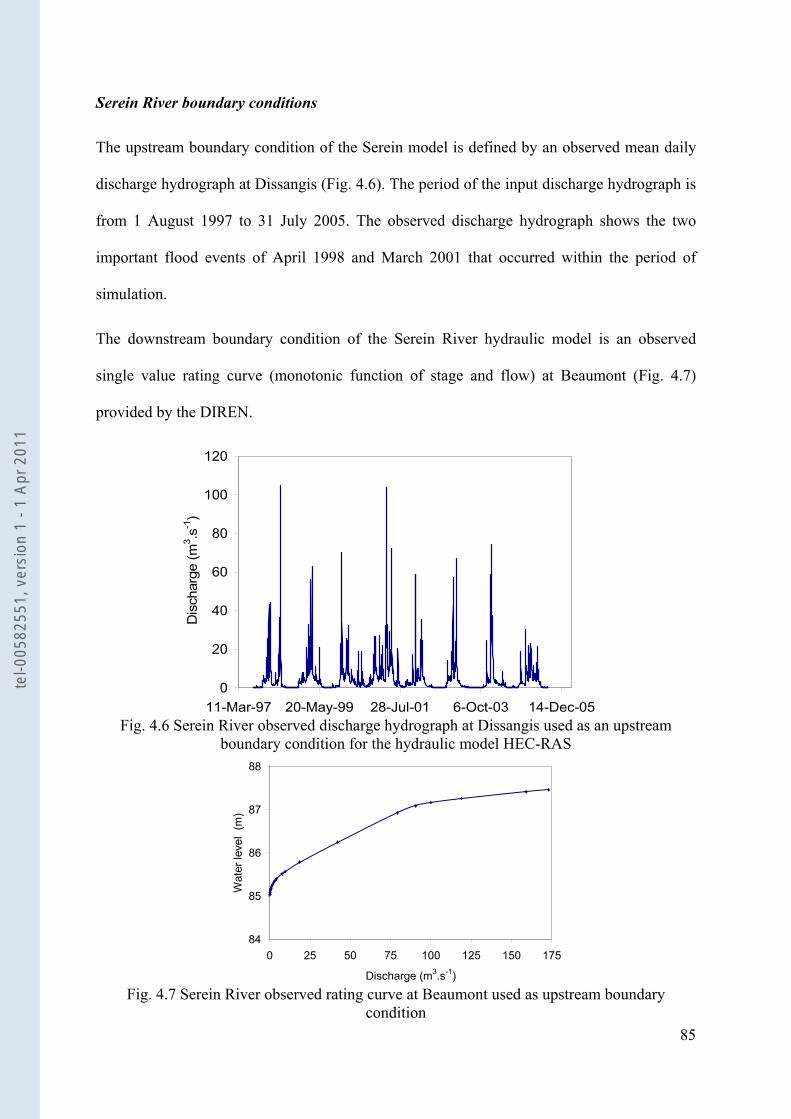
85

Serein River boundary conditions

The upstream boundary condition of the Serein model is defined by an observed mean daily

discharge hydrograph at Dissangis (Fig. 4.6). The period of the input discharge hydrograph is

from 1 August 1997 to 31 July 2005. The observed discharge hydrograph shows the two

important flood events of April 1998 and March 2001 that occurred within the period of

simulation.

The downstream boundary condition of the Serein River hydraulic model is an observed

single value rating curve (monotonic function of stage and flow) at Beaumont (Fig. 4.7)

provided by the DIREN.

0

20

40

60

80

100

120

11-Mar-97 20-May-99 28-Jul-01 6-Oct-03 14-Dec-05

Dis

char

ge (m

3 .s-1

)

Fig. 4.6 Serein River observed discharge hydrograph at Dissangis used as an upstream

boundary condition for the hydraulic model HEC-RAS

84

85

86

87

88

0 25 50 75 100 125 150 175

Discharge (m3.s-1)

Wat

er le

vel

(m)

Fig. 4.7 Serein River observed rating curve at Beaumont used as upstream boundary

condition

tel-0

0582

551,

ver

sion

1 -

1 Ap

r 201

1

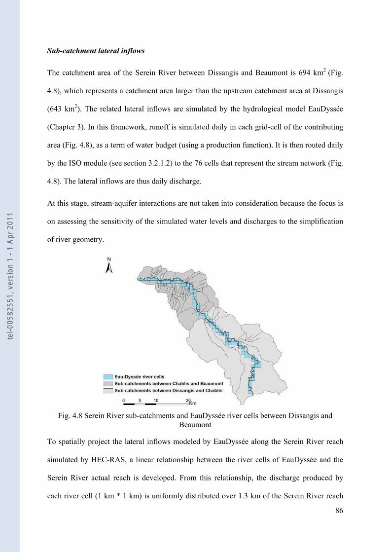
86

Sub-catchment lateral inflows

The catchment area of the Serein River between Dissangis and Beaumont is 694 km2 (Fig.

4.8), which represents a catchment area larger than the upstream catchment area at Dissangis

(643 km2). The related lateral inflows are simulated by the hydrological model EauDyssée

(Chapter 3). In this framework, runoff is simulated daily in each grid-cell of the contributing

area (Fig. 4.8), as a term of water budget (using a production function). It is then routed daily

by the ISO module (see section 3.2.1.2) to the 76 cells that represent the stream network (Fig.

4.8). The lateral inflows are thus daily discharge.

At this stage, stream-aquifer interactions are not taken into consideration because the focus is

on assessing the sensitivity of the simulated water levels and discharges to the simplification

of river geometry.

Fig. 4.8 Serein River sub-catchments and EauDyssée river cells between Dissangis and

Beaumont

To spatially project the lateral inflows modeled by EauDyssée along the Serein River reach

simulated by HEC-RAS, a linear relationship between the river cells of EauDyssée and the

Serein River actual reach is developed. From this relationship, the discharge produced by

each river cell (1 km * 1 km) is uniformly distributed over 1.3 km of the Serein River reach

tel-0

0582

551,

ver

sion

1 -

1 Ap

r 201

1

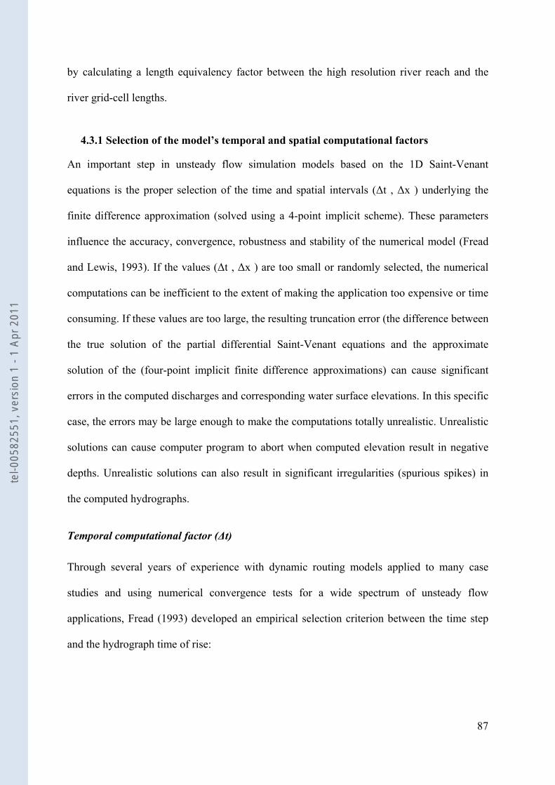
87

by calculating a length equivalency factor between the high resolution river reach and the

river grid-cell lengths.

4.3.1 Selection of the model’s temporal and spatial computational factors

An important step in unsteady flow simulation models based on the 1D Saint-Venant

equations is the proper selection of the time and spatial intervals (Δt , Δx ) underlying the

finite difference approximation (solved using a 4-point implicit scheme). These parameters

influence the accuracy, convergence, robustness and stability of the numerical model (Fread

and Lewis, 1993). If the values (Δt , Δx ) are too small or randomly selected, the numerical

computations can be inefficient to the extent of making the application too expensive or time

consuming. If these values are too large, the resulting truncation error (the difference between

the true solution of the partial differential Saint-Venant equations and the approximate

solution of the (four-point implicit finite difference approximations) can cause significant

errors in the computed discharges and corresponding water surface elevations. In this specific

case, the errors may be large enough to make the computations totally unrealistic. Unrealistic

solutions can cause computer program to abort when computed elevation result in negative

depths. Unrealistic solutions can also result in significant irregularities (spurious spikes) in

the computed hydrographs.

Temporal computational factor (Δt)

Through several years of experience with dynamic routing models applied to many case

studies and using numerical convergence tests for a wide spectrum of unsteady flow

applications, Fread (1993) developed an empirical selection criterion between the time step

and the hydrograph time of rise:

tel-0

0582

551,

ver

sion

1 -

1 Ap

r 201

1

88

20rTt ≈Δ Eq. 4.1

Where Tr is the hydrographs time of rise (time from the significant beginning of increased

discharge to the peak of the discharge hydrograph), in hours.

Fig. 4.9 illustrates the observed waves time of rise of the two major peaks (April 1998 &

March 2001) occurring at the three gauging stations of the Serein River. The peak of April

1998 has a rising time of 19 hrs while the peak of March 2001 has a rising time of 21 hrs.

According to the aforementioned equations, the computational time step was set to ~1hr in

HEC-RAS simulations.

Other time step increments (0.5, 3, 4, 6, 12, 18, 24 hrs) were also tested for Δx set to 100 m.

The comparison between the different time steps showed that the simulated water level and

discharge hydrographs are not sensitive to the variation of Δt between 0.5 to 3 hours.

However, the time of simulation was influenced, as smaller time steps required more time to

complete the simulation. A time step larger than 4 hrs led to a slight numerical oscillation,

while time steps larger than 5 hrs (6, 8, 12, 18 and 24 hrs) caused larger numerical

oscillations and hence failure in the matrix solving.

Fig. 4.9 Observed time of wave transfer and river rise of a) The April 1998 flood peak from Dissangis to Beaumont (flood attenuation), b) The March 2001 flood peak from Dissangis to

Beaumont (flood amplification)

0

25

50

75

100

125

150

175

1 16 31 46 61 76 91 106Time of wave transfer (hrs)

Dis

char

ge (m

3 .s-1

)

DissangisChablisBeaumont

0

25

50

75

100

125

150

175

1 21 41 61 81 101 121 141 161Time of wave transfer (hrs)

Dis

char

ge (m

3/s)


(a) (b)

tel-0

0582

551,

ver

sion

1 -

1 Ap

r 201

1

89

Spatial computational factor (Δx)

Cross sections are usually located along the river to describe the changes in geometry,

discharge, slope, velocity, and roughness. There is no hard and fast guidance concerning the

appropriate distance between cross sections. In the author's experience, large rivers (rivers

with several thousand square kilometers of watershed) with mild slopes (less than 1.0 m.km-

1) can have a maximum cross-section spacing of approximately 750 m. On smaller streams

with steeper slopes, closer spacing should be the rule. For urban situations, a section every

100 m or less is often needed (Dyhouse et al., 2003).

An empirical selection criterion between the time step and the hydrograph time of rise was

developed by Fread (1993):

20rcTx ≤Δ Eq. 4.2

Where Tr is the hydrographs time of rise in hours [T], c is the bulk wave speed or the celerity

associated with an essential characteristic of the unsteady flow such as the peak or the center

of the hydrograph [L.T-1].

In most applications the bulk wave speed is approximated as the kinematic wave speed. The

kinematic wave celerity is approximated as:

kvc = Eq. 4.3

Where k is the kinematic wave ratio having values ranging from 35

34 ≤≤ k ( 5.1≈k for

most natural channels), v is flow velocity.

The peak flow velocity between Dissangis and Beaumont during the 1998 peak is 0.48 m.s-1

and 0.6 m.s-1 for the 2001 peak (Fig. 4.9).

tel-0

0582

551,

ver

sion

1 -

1 Ap

r 201

1

90

Because the period of simulation (1997-2005) is too long when compared to classic hydraulic

simulations and input hydrographs contain several peaks with wave transfer time fluctuating

as function of the intensity and hydrological properties of the flood (Fig. 4.9), it was not

evident to obtain numerical convergence depending on the above Δx, Δt selection criteria. To

overcome that, a wide spectrum of convergence tests was conducted to select the most

appropriate Δx. Large distance steps ( m1000≥ ) created numerical oscillations and failure in

matrix solution for high flow periods. The Δx of 250 m was found to be stable for both high

and low flow simulations. However numerical oscillations occurred when conducting

sensitivity analysis on Manning’s roughness coefficient. The Δx of 100m was found to be the

most stable spatial step and therefore adopted for all model simulations and sensitivity

analysis.

4.3.2 Manning’s roughness coefficient (n) calibration

Manning's n normally carries the most uncertainty in hydraulic modeling. In this study a wide

range of possible Manning’s roughness coefficients values for both the main channel and

floodplain are investigated to calibrate the model.

The calibration of Manning’s roughness coefficient (n) was investigated at Chablis

hydrometric station where observed water levels and discharge hydrographs are available.

The roughness coefficient was supposed to be uniform along the 89 km of the river.

Sensitivity analysis was performed with n of the main channel ranging from 0.01 to 0.05 with

an increment Δn = 0.002, and from 0.05 to 0.1 with Δn = 0.01 while the one of the floodplain

ranged from 0.02 to 0.2 with Δn = 0.01.

The influence of Manning’s n in the main channel is well illustrated when looking at the

simulated rating curves (discharge vs. water levels) (Fig. 4.10). The increase of Manning’s

roughness coefficient in the main channel increases the simulated stage and attenuates the

tel-0

0582

551,

ver

sion

1 -

1 Ap

r 201

1

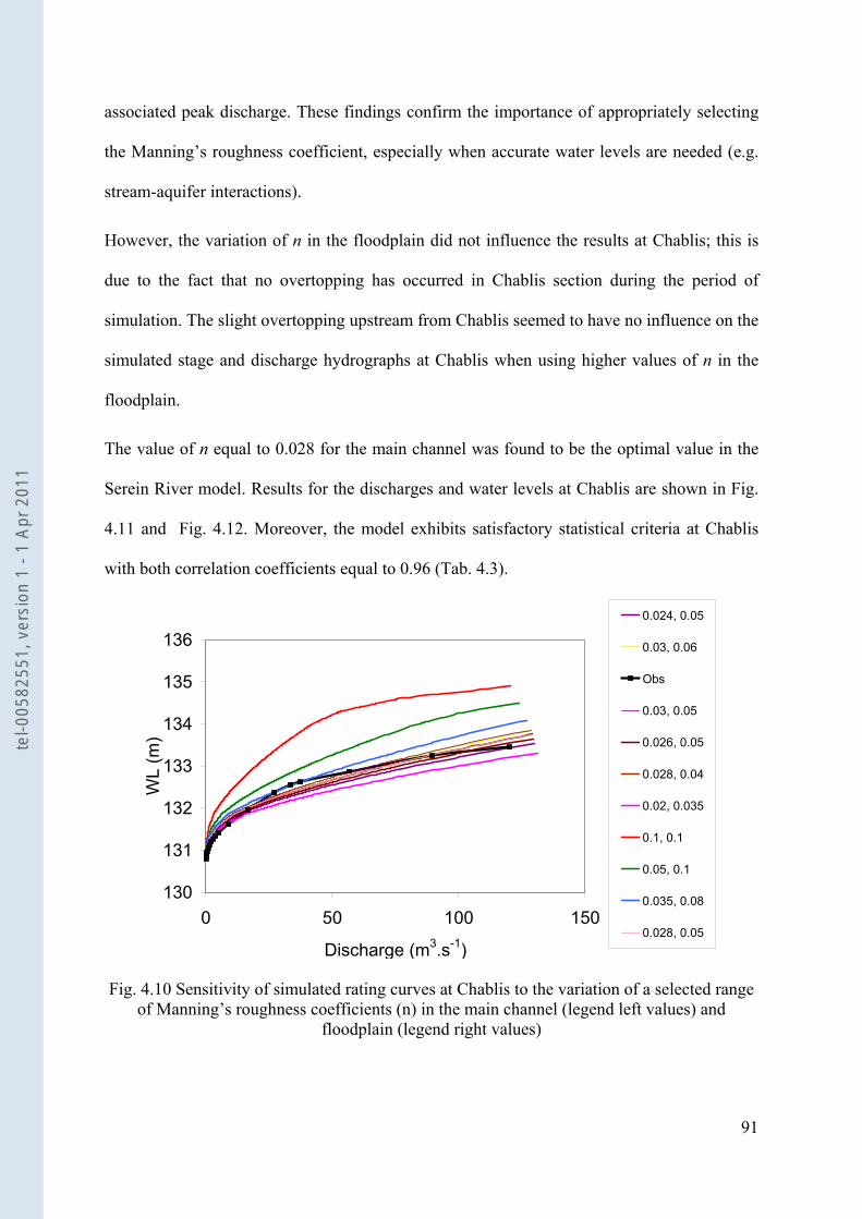
91

associated peak discharge. These findings confirm the importance of appropriately selecting

the Manning’s roughness coefficient, especially when accurate water levels are needed (e.g.

stream-aquifer interactions).

However, the variation of n in the floodplain did not influence the results at Chablis; this is

due to the fact that no overtopping has occurred in Chablis section during the period of

simulation. The slight overtopping upstream from Chablis seemed to have no influence on the

simulated stage and discharge hydrographs at Chablis when using higher values of n in the

floodplain.

The value of n equal to 0.028 for the main channel was found to be the optimal value in the

Serein River model. Results for the discharges and water levels at Chablis are shown in Fig.

4.11 and Fig. 4.12. Moreover, the model exhibits satisfactory statistical criteria at Chablis

with both correlation coefficients equal to 0.96 (Tab. 4.3).

130

131

132

133

134

135

136

0 50 100 150

Discharge (m3.s-1)

WL

(m)

0.024, 0.05

0.03, 0.06

Obs

0.03, 0.05

0.026, 0.05

0.028, 0.04

0.02, 0.035

0.1, 0.1

0.05, 0.1

0.035, 0.08

0.028, 0.05

Fig. 4.10 Sensitivity of simulated rating curves at Chablis to the variation of a selected range

of Manning’s roughness coefficients (n) in the main channel (legend left values) and floodplain (legend right values)

tel-0

0582

551,

ver

sion

1 -

1 Ap

r 201

1

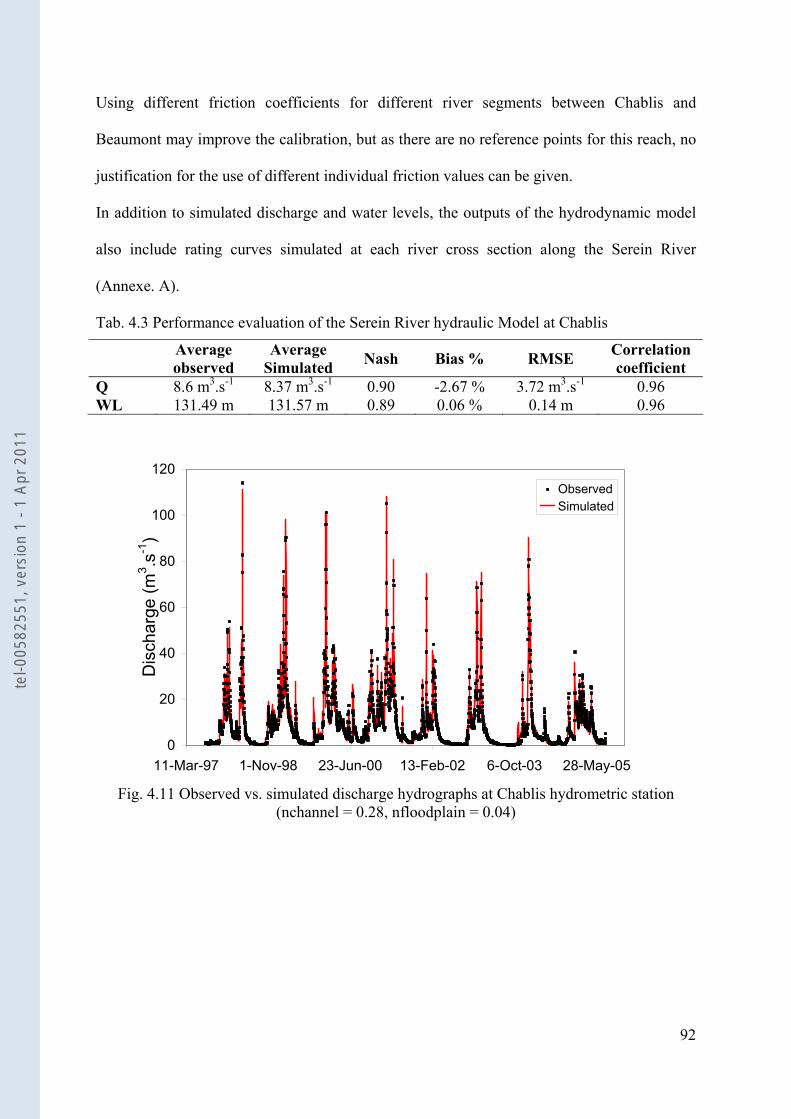
92

Using different friction coefficients for different river segments between Chablis and

Beaumont may improve the calibration, but as there are no reference points for this reach, no

justification for the use of different individual friction values can be given.

In addition to simulated discharge and water levels, the outputs of the hydrodynamic model

also include rating curves simulated at each river cross section along the Serein River

(Annexe. A).

Tab. 4.3 Performance evaluation of the Serein River hydraulic Model at Chablis

0

20

40

60

80

100

120

11-Mar-97 1-Nov-98 23-Jun-00 13-Feb-02 6-Oct-03 28-May-05

Dis

char

ge (m

3 .s-1

)

ObservedSimulated

Fig. 4.11 Observed vs. simulated discharge hydrographs at Chablis hydrometric station

(nchannel = 0.28, nfloodplain = 0.04)

Average observed

Average Simulated Nash Bias % RMSE Correlation

coefficient Q 8.6 m3.s-1 8.37 m3.s-1 0.90 -2.67 % 3.72 m3.s-1 0.96 WL 131.49 m 131.57 m 0.89 0.06 % 0.14 m 0.96

tel-0

0582

551,

ver

sion

1 -

1 Ap

r 201

1

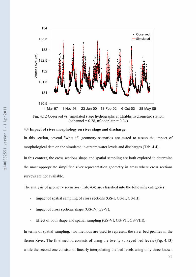
93

130.5

131

131.5

132

132.5

133

133.5

134


Wat

er L

evel

(m)

ObservedSimulated

Fig. 4.12 Observed vs. simulated stage hydrographs at Chablis hydrometric station

(nchannel = 0.28, nfloodplain = 0.04)

4.4 Impact of river morphology on river stage and discharge

In this section, several "what if" geometry scenarios are tested to assess the impact of

morphological data on the simulated in-stream water levels and discharges (Tab. 4.4).

In this context, the cross sections shape and spatial sampling are both explored to determine

the most appropriate simplified river representation geometry in areas where cross sections

surveys are not available.

The analysis of geometry scenarios (Tab. 4.4) are classified into the following categories:

- Impact of spatial sampling of cross sections (GS-I, GS-II, GS-III).

- Impact of cross sections shape (GS-IV, GS-V).

- Effect of both shape and spatial sampling (GS-VI, GS-VII, GS-VIII).

In terms of spatial sampling, two methods are used to represent the river bed profiles in the

Serein River. The first method consists of using the twenty surveyed bed levels (Fig. 4.13)

while the second one consists of linearly interpolating the bed levels using only three known

tel-0

0582

551,

ver

sion

1 -

1 Ap

r 201

1

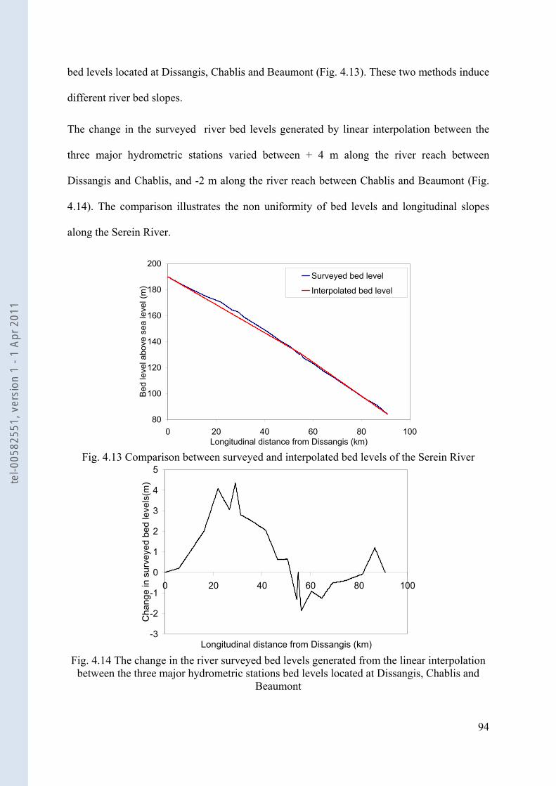
94

bed levels located at Dissangis, Chablis and Beaumont (Fig. 4.13). These two methods induce

different river bed slopes.

The change in the surveyed river bed levels generated by linear interpolation between the

three major hydrometric stations varied between + 4 m along the river reach between

Dissangis and Chablis, and -2 m along the river reach between Chablis and Beaumont (Fig.

4.14). The comparison illustrates the non uniformity of bed levels and longitudinal slopes

along the Serein River.

80

100

120

140

160

180

200

0 20 40 60 80 100Longitudinal distance from Dissangis (km)

Bed

leve

l abo

ve s

ea le

vel (

m)

Surveyed bed level

Interpolated bed level

Fig. 4.13 Comparison between surveyed and interpolated bed levels of the Serein River

-3

-2

-1

0

1

2

3

4

5

0 20 40 60 80 100

Longitudinal distance from Dissangis (km)

Cha

nge

in s

urve

yed

bed

leve

ls(m

)

Fig. 4.14 The change in the river surveyed bed levels generated from the linear interpolation

between the three major hydrometric stations bed levels located at Dissangis, Chablis and Beaumont

tel-0

0582

551,

ver

sion

1 -

1 Ap

r 201

1

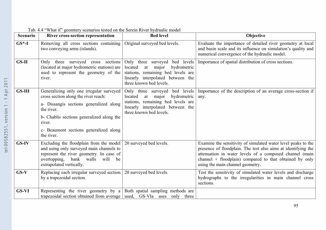
95

Tab. 4.4 “What if” geomtery scenarios tested on the Serein River hydrualic model Scenario River cross-section representation Bed level Objective

GS*-I Removing all cross sections containing two conveying arms (islands).

Original surveyed bed levels. Evaluate the importance of detailed river geometry at local and basin scale and its influence on simulation’s quality and numerical convergence of the hydraulic model.

GS-II Only three surveyed cross sections (located at major hydrometric stations) are used to represent the geometry of the river.

Only three surveyed bed levels located at major hydrometric stations, remaining bed levels are linearly interpolated between the three known bed levels.

Importance of spatial distribution of cross sections.

GS-III Generalizing only one irregular surveyed cross section along the river reach:

a- Dissangis sections generalized along the river.

b- Chablis sections generalized along the river.

c- Beaumont sections generalized along the river.


Importance of the description of an average cross-section if any.

GS-IV Excluding the floodplain from the model and using only surveyed main channels to represent the river geometry. In case of overtopping, bank walls will be extrapolated vertically.

20 surveyed bed levels. Examine the sensitivity of simulated water level peaks to the presence of floodplain. The test also aims at identifying the attenuation in water levels of a composed channel (main channel + floodplain) compared to that obtained by only using the main channel geometry.

GS-V Replacing each irregular surveyed section by a trapezoidal section.

20 surveyed bed levels. Test the sensitivity of simulated water levels and discharge hydrographs to the irregularities in main channel cross sections.

GS-VI Representing the river geometry by a trapezoidal section obtained from average

Both spatial sampling methods are used, GS-VIa uses only three

tel-0

0582

551,

ver

sion

1 -

1 Ap

r 201

1

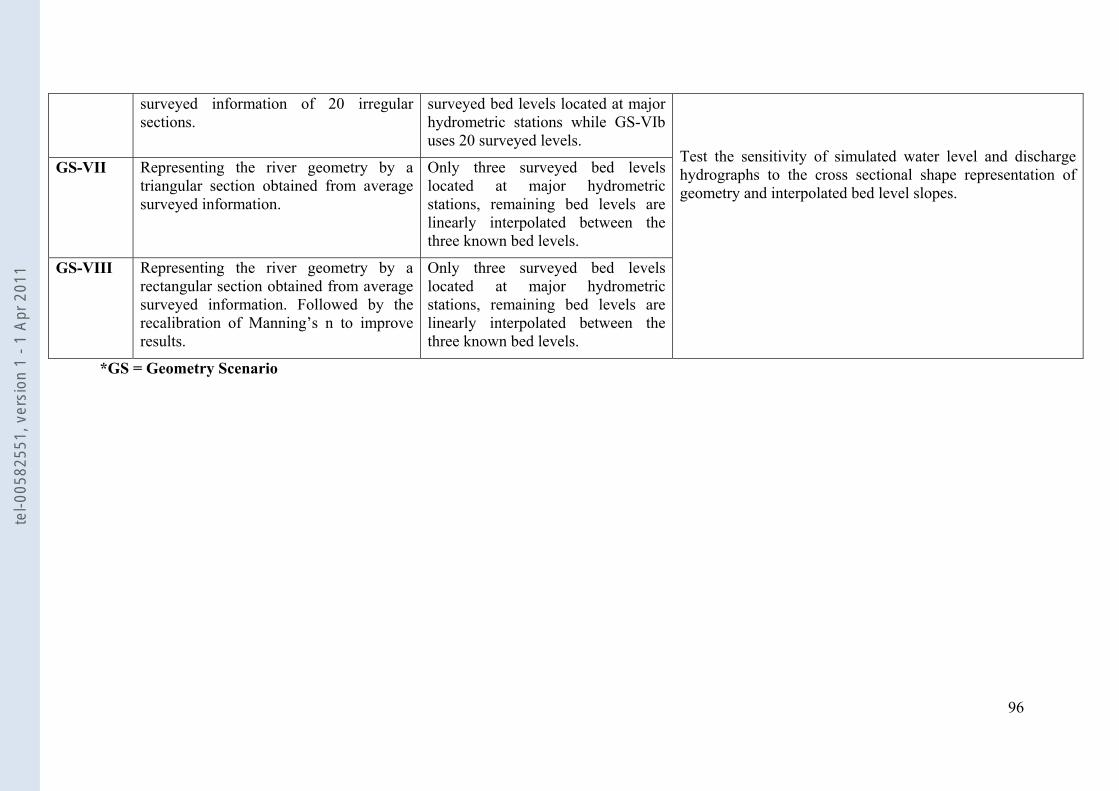
96

surveyed information of 20 irregular sections.

surveyed bed levels located at major hydrometric stations while GS-VIb uses 20 surveyed levels.

GS-VII Representing the river geometry by a triangular section obtained from average surveyed information.


GS-VIII Representing the river geometry by a rectangular section obtained from average surveyed information. Followed by the recalibration of Manning’s n to improve results.


Test the sensitivity of simulated water level and discharge hydrographs to the cross sectional shape representation of geometry and interpolated bed level slopes.

*GS = Geometry Scenario

tel-0

0582

551,

ver

sion

1 -

1 Ap

r 201

1

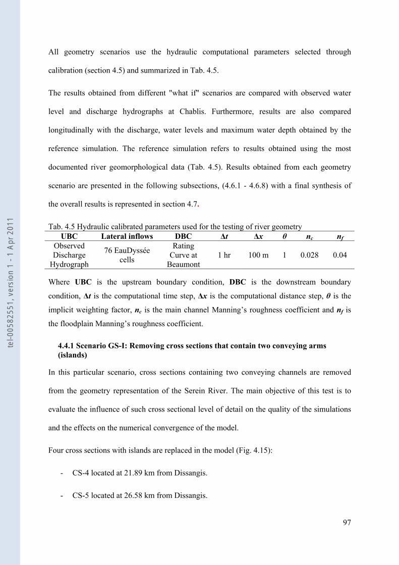
97

All geometry scenarios use the hydraulic computational parameters selected through

calibration (section 4.5) and summarized in Tab. 4.5.

The results obtained from different "what if" scenarios are compared with observed water

level and discharge hydrographs at Chablis. Furthermore, results are also compared

longitudinally with the discharge, water levels and maximum water depth obtained by the

reference simulation. The reference simulation refers to results obtained using the most

documented river geomorphological data (Tab. 4.5). Results obtained from each geometry

scenario are presented in the following subsections, (4.6.1 - 4.6.8) with a final synthesis of

the overall results is represented in section 4.7.

Tab. 4.5 Hydraulic calibrated parameters used for the testing of river geometry UBC Lateral inflows DBC Δt Δx θ nc nf

Observed Discharge

Hydrograph

76 EauDyssée cells

Rating Curve at

Beaumont 1 hr 100 m 1 0.028 0.04

Where UBC is the upstream boundary condition, DBC is the downstream boundary

condition, Δt is the computational time step, Δx is the computational distance step, θ is the

implicit weighting factor, nc is the main channel Manning’s roughness coefficient and nf is

the floodplain Manning’s roughness coefficient.

4.4.1 Scenario GS-I: Removing cross sections that contain two conveying arms (islands)

In this particular scenario, cross sections containing two conveying channels are removed

from the geometry representation of the Serein River. The main objective of this test is to

evaluate the influence of such cross sectional level of detail on the quality of the simulations

and the effects on the numerical convergence of the model.

Four cross sections with islands are replaced in the model (Fig. 4.15):

- CS-4 located at 21.89 km from Dissangis.


tel-0

0582

551,

ver

sion

1 -

1 Ap

r 201

1

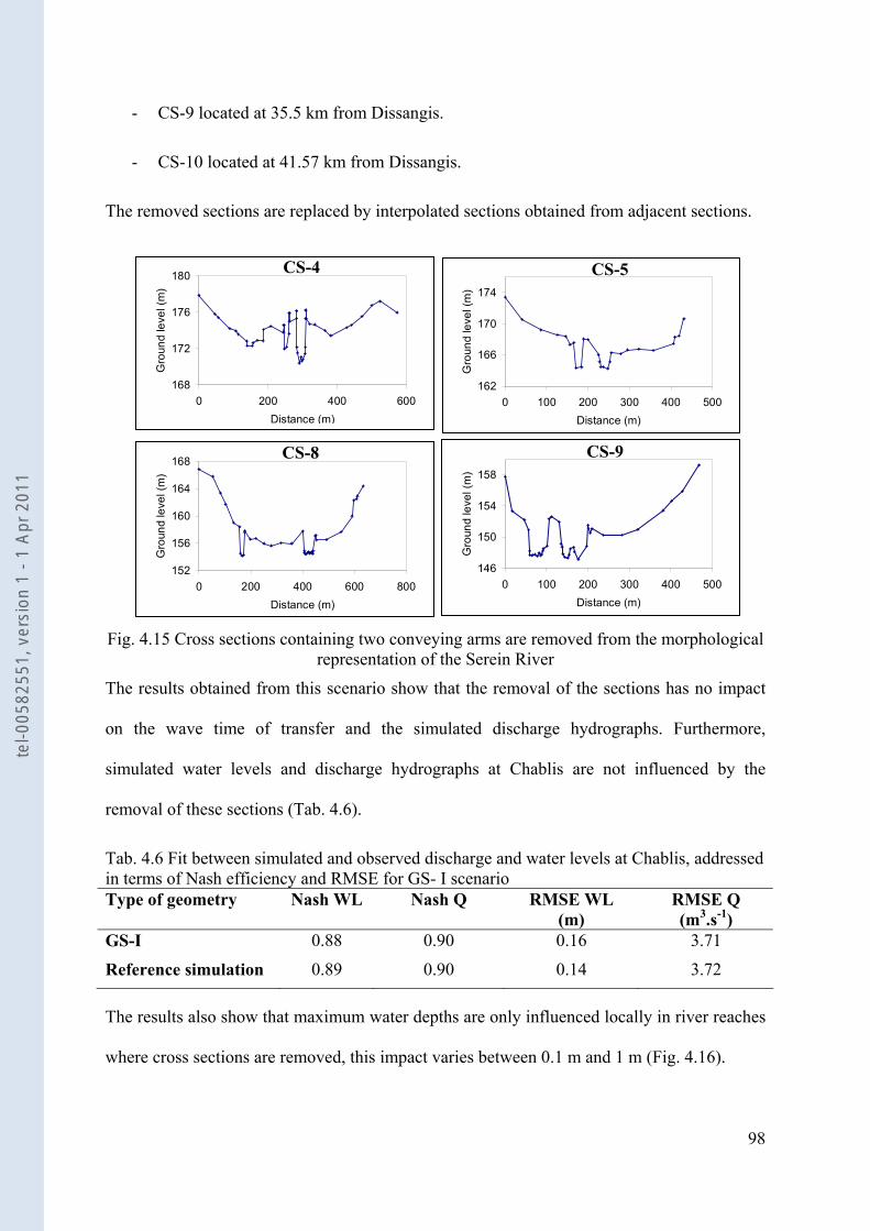
98



The removed sections are replaced by interpolated sections obtained from adjacent sections.

Fig. 4.15 Cross sections containing two conveying arms are removed from the morphological

representation of the Serein River

The results obtained from this scenario show that the removal of the sections has no impact

on the wave time of transfer and the simulated discharge hydrographs. Furthermore,

simulated water levels and discharge hydrographs at Chablis are not influenced by the

removal of these sections (Tab. 4.6).

Tab. 4.6 Fit between simulated and observed discharge and water levels at Chablis, addressed in terms of Nash efficiency and RMSE for GS- I scenario Type of geometry Nash WL

Nash Q

RMSE WL

(m) RMSE Q (m3.s-1)

GS-I 0.88 0.90 0.16 3.71

Reference simulation 0.89 0.90 0.14 3.72

The results also show that maximum water depths are only influenced locally in river reaches

where cross sections are removed, this impact varies between 0.1 m and 1 m (Fig. 4.16).

152

156

160

164

168

0 200 400 600 800Distance (m)

Gro

und

leve

l (m

)

146

150

154

158

0 100 200 300 400 500Distance (m)

Gro

und

leve

l (m

)

162

166

170

174

0 100 200 300 400 500Distance (m)

Gro

und

leve

l (m

)

168

172

176

180

0 200 400 600Distance (m)

Gro

und

leve

l (m

)

CS-5

CS-9 CS-8

CS-4

tel-0

0582

551,

ver

sion

1 -

1 Ap

r 201

1

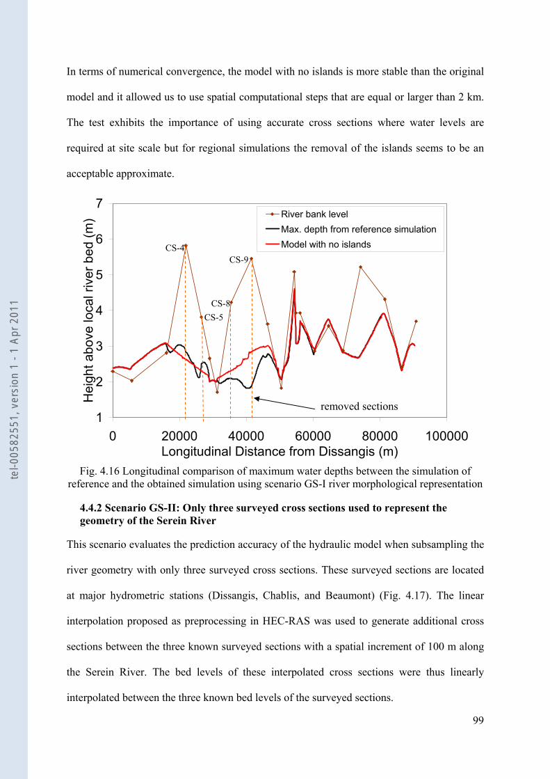
99

In terms of numerical convergence, the model with no islands is more stable than the original

model and it allowed us to use spatial computational steps that are equal or larger than 2 km.

The test exhibits the importance of using accurate cross sections where water levels are

required at site scale but for regional simulations the removal of the islands seems to be an

acceptable approximate.

1

2

3

4

5

6

7

0 20000 40000 60000 80000 100000Longitudinal Distance from Dissangis (m)

Hei

ght a

bove

loca

l riv

er b

ed (m

) River bank levelMax. depth from reference simulationModel with no islands


reference and the obtained simulation using scenario GS-I river morphological representation

4.4.2 Scenario GS-II: Only three surveyed cross sections used to represent the geometry of the Serein River

This scenario evaluates the prediction accuracy of the hydraulic model when subsampling the

river geometry with only three surveyed cross sections. These surveyed sections are located

at major hydrometric stations (Dissangis, Chablis, and Beaumont) (Fig. 4.17). The linear

interpolation proposed as preprocessing in HEC-RAS was used to generate additional cross

sections between the three known surveyed sections with a spatial increment of 100 m along

the Serein River. The bed levels of these interpolated cross sections were thus linearly

interpolated between the three known bed levels of the surveyed sections.

removed sections

CS-4

CS-5 CS-8

CS-9

tel-0

0582

551,

ver

sion

1 -

1 Ap

r 201

1

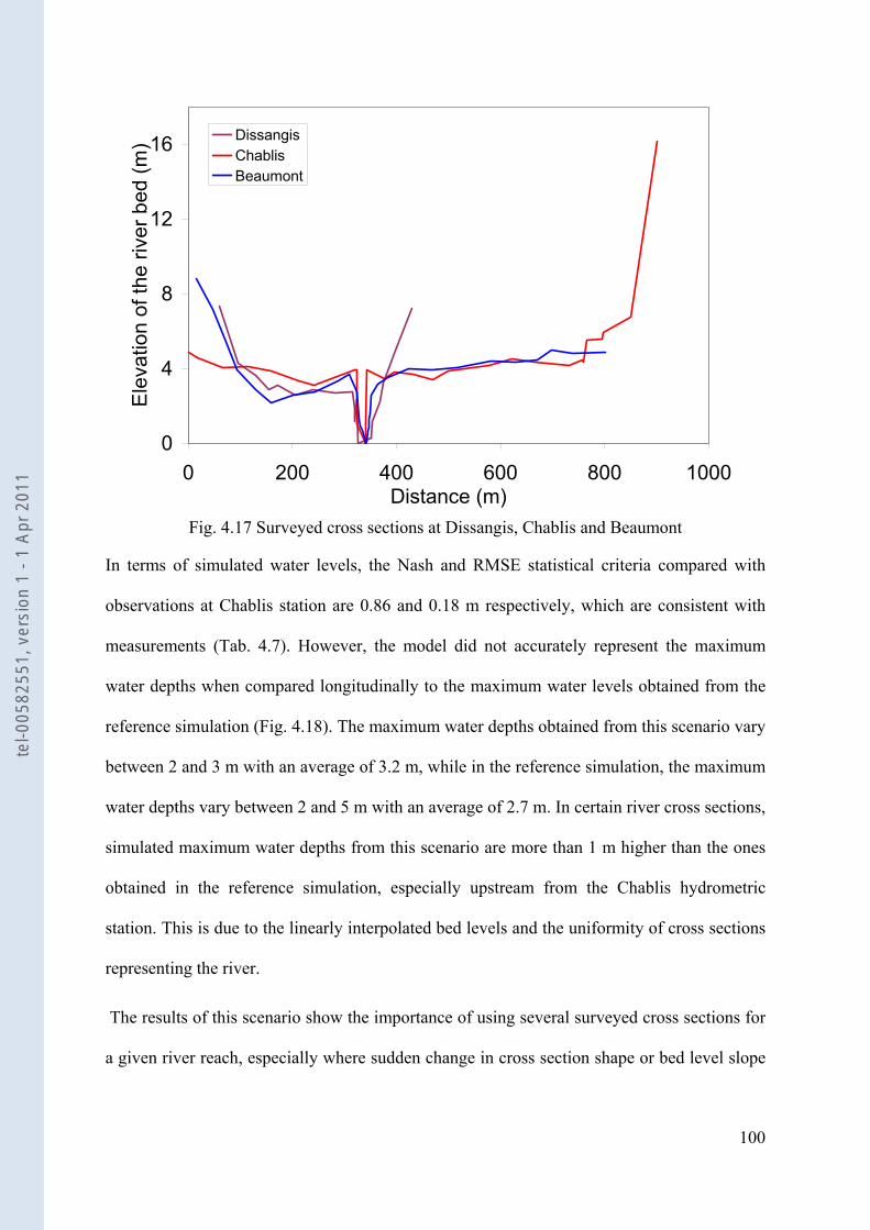
100

0

4

8

12

16

0 200 400 600 800 1000Distance (m)

Ele

vatio

n of

the

river

bed

(m) Dissangis

ChablisBeaumont

Fig. 4.17 Surveyed cross sections at Dissangis, Chablis and Beaumont

In terms of simulated water levels, the Nash and RMSE statistical criteria compared with

observations at Chablis station are 0.86 and 0.18 m respectively, which are consistent with

measurements (Tab. 4.7). However, the model did not accurately represent the maximum

water depths when compared longitudinally to the maximum water levels obtained from the

reference simulation (Fig. 4.18). The maximum water depths obtained from this scenario vary

between 2 and 3 m with an average of 3.2 m, while in the reference simulation, the maximum

water depths vary between 2 and 5 m with an average of 2.7 m. In certain river cross sections,

simulated maximum water depths from this scenario are more than 1 m higher than the ones

obtained in the reference simulation, especially upstream from the Chablis hydrometric

station. This is due to the linearly interpolated bed levels and the uniformity of cross sections

representing the river.

The results of this scenario show the importance of using several surveyed cross sections for

a given river reach, especially where sudden change in cross section shape or bed level slope

tel-0

0582

551,

ver

sion

1 -

1 Ap

r 201

1

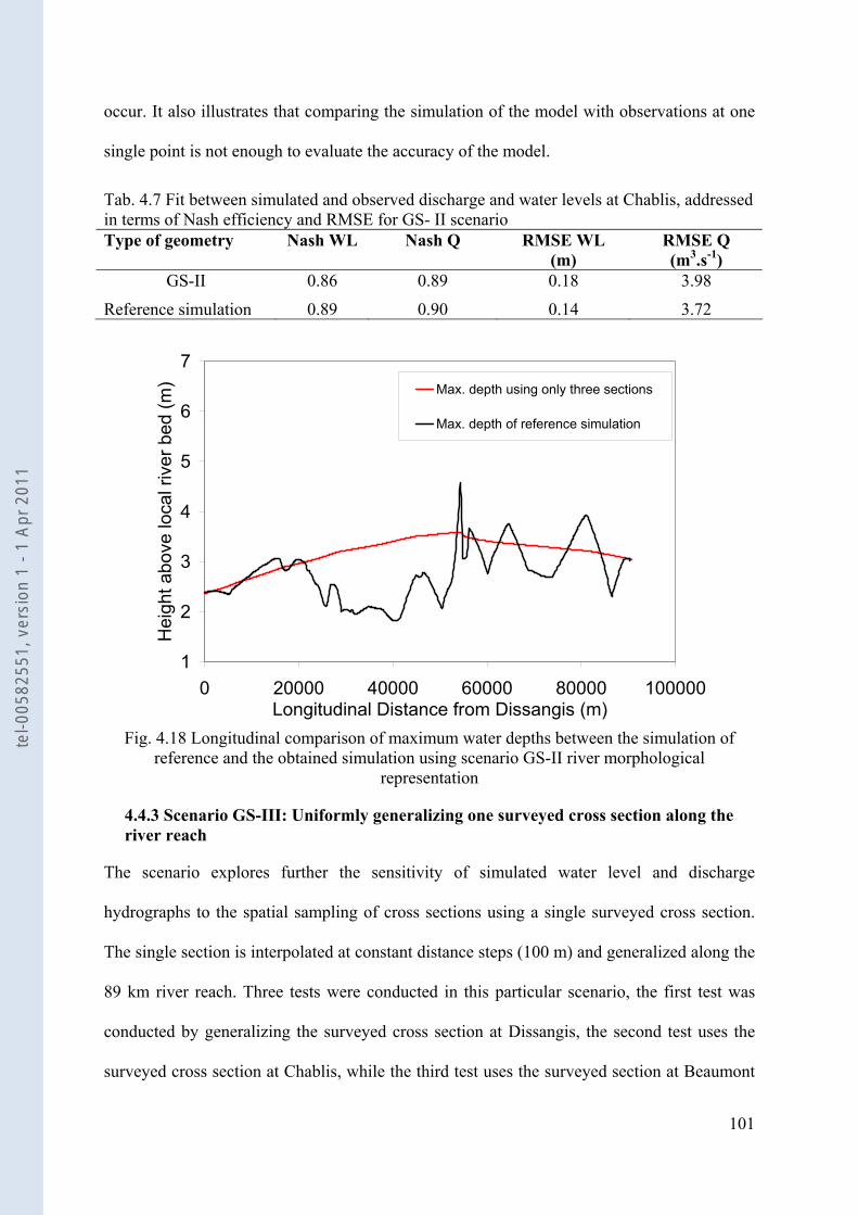
101

occur. It also illustrates that comparing the simulation of the model with observations at one

single point is not enough to evaluate the accuracy of the model.

Tab. 4.7 Fit between simulated and observed discharge and water levels at Chablis, addressed in terms of Nash efficiency and RMSE for GS- II scenario Type of geometry Nash WL

Nash Q

RMSE WL

(m) RMSE Q (m3.s-1)

GS-II 0.86 0.89 0.18 3.98


1

2

3

4

5

6

7


Hei

ght a

bove

loca

l riv

er b

ed (m

) Max. depth using only three sections

Max. depth of reference simulation


reference and the obtained simulation using scenario GS-II river morphological representation

4.4.3 Scenario GS-III: Uniformly generalizing one surveyed cross section along the river reach

The scenario explores further the sensitivity of simulated water level and discharge

hydrographs to the spatial sampling of cross sections using a single surveyed cross section.

The single section is interpolated at constant distance steps (100 m) and generalized along the

89 km river reach. Three tests were conducted in this particular scenario, the first test was

conducted by generalizing the surveyed cross section at Dissangis, the second test uses the

surveyed cross section at Chablis, while the third test uses the surveyed section at Beaumont

tel-0

0582

551,

ver

sion

1 -

1 Ap

r 201

1

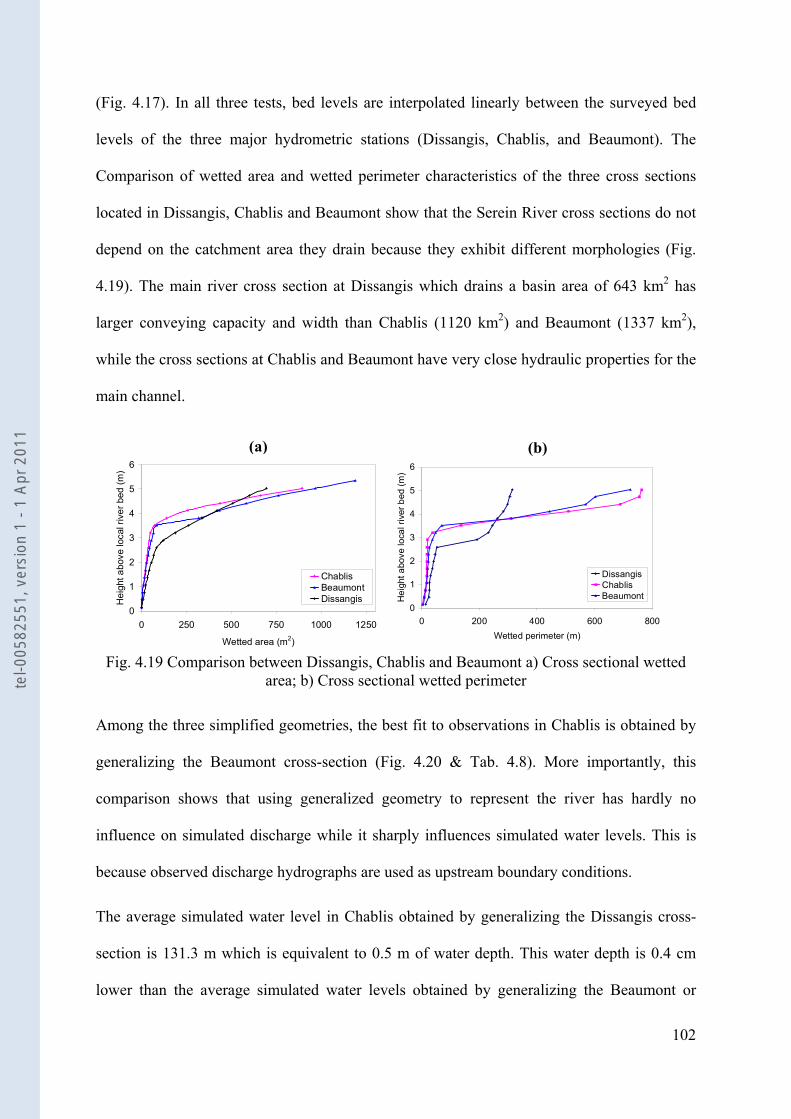
102

(Fig. 4.17). In all three tests, bed levels are interpolated linearly between the surveyed bed

levels of the three major hydrometric stations (Dissangis, Chablis, and Beaumont). The

Comparison of wetted area and wetted perimeter characteristics of the three cross sections

located in Dissangis, Chablis and Beaumont show that the Serein River cross sections do not

depend on the catchment area they drain because they exhibit different morphologies (Fig.

4.19). The main river cross section at Dissangis which drains a basin area of 643 km2 has

larger conveying capacity and width than Chablis (1120 km2) and Beaumont (1337 km2),

while the cross sections at Chablis and Beaumont have very close hydraulic properties for the

main channel.

Fig. 4.19 Comparison between Dissangis, Chablis and Beaumont a) Cross sectional wetted

area; b) Cross sectional wetted perimeter

Among the three simplified geometries, the best fit to observations in Chablis is obtained by

generalizing the Beaumont cross-section (Fig. 4.20 & Tab. 4.8). More importantly, this

comparison shows that using generalized geometry to represent the river has hardly no

influence on simulated discharge while it sharply influences simulated water levels. This is

because observed discharge hydrographs are used as upstream boundary conditions.

The average simulated water level in Chablis obtained by generalizing the Dissangis cross-

section is 131.3 m which is equivalent to 0.5 m of water depth. This water depth is 0.4 cm

lower than the average simulated water levels obtained by generalizing the Beaumont or

0

1

2

3

4

5

6

0 250 500 750 1000 1250

Wetted area (m2)

Hei

ght a

bove

loca

l riv

er b

ed (m

)

ChablisBeaumontDissangis

0

1

2

3

4

5

6

0 200 400 600 800Wetted perimeter (m)

Hei

ght a

bove

loca

l riv

er b

ed (m

)


(a) (b)

tel-0

0582

551,

ver

sion

1 -

1 Ap

r 201

1

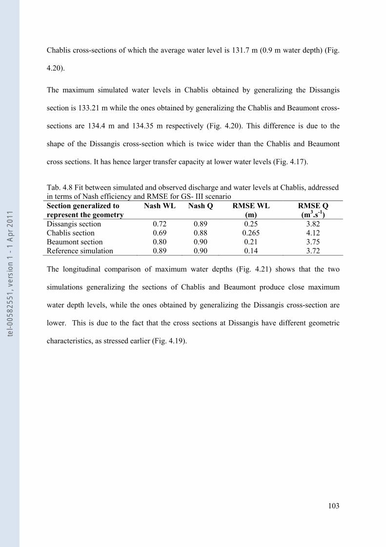
103

Chablis cross-sections of which the average water level is 131.7 m (0.9 m water depth) (Fig.

4.20).

The maximum simulated water levels in Chablis obtained by generalizing the Dissangis

section is 133.21 m while the ones obtained by generalizing the Chablis and Beaumont cross-

sections are 134.4 m and 134.35 m respectively (Fig. 4.20). This difference is due to the

shape of the Dissangis cross-section which is twice wider than the Chablis and Beaumont

cross sections. It has hence larger transfer capacity at lower water levels (Fig. 4.17).

Tab. 4.8 Fit between simulated and observed discharge and water levels at Chablis, addressed in terms of Nash efficiency and RMSE for GS- III scenario Section generalized to represent the geometry

Nash WL Nash Q RMSE WL (m)

RMSE Q (m3.s-1)

Dissangis section 0.72 0.89 0.25 3.82 Chablis section 0.69 0.88 0.265 4.12 Beaumont section 0.80 0.90 0.21 3.75 Reference simulation 0.89 0.90 0.14 3.72 The longitudinal comparison of maximum water depths (Fig. 4.21) shows that the two

simulations generalizing the sections of Chablis and Beaumont produce close maximum

water depth levels, while the ones obtained by generalizing the Dissangis cross-section are

lower. This is due to the fact that the cross sections at Dissangis have different geometric

characteristics, as stressed earlier (Fig. 4.19).

tel-0

0582

551,

ver

sion

1 -

1 Ap

r 201

1

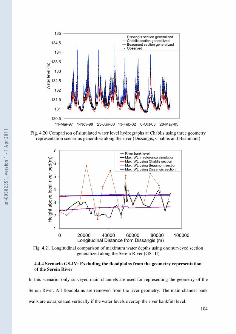
104

130.5

131

131.5

132

132.5

133

133.5

134

134.5

135


Wat

er le

vel (

m)

Dissangis section generalizedChablis section generalizedBeaumont section generalizedObserved

Fig. 4.20 Comparison of simulated water level hydrographs at Chablis using three geometry

representation scenarios generalize along the river (Dissangis, Chablis and Beaumont)

1

2

3

4

5

6

7


Hei

ght a

bove

loca

l riv

er b

ed(m

)

River bank levelMax. WL in reference simulationMax. WL using Chablis sectionMax. WL using Beaumont sectionMax. WL using Dissangis section

Fig. 4.21 Longitudinal comparison of maximum water depths using one surveyed section

generalized along the Serein River (GS-III)

4.4.4 Scenario GS-IV: Excluding the floodplains from the geometry representation of the Serein River

In this scenario, only surveyed main channels are used for representing the geometry of the

Serein River. All floodplains are removed from the river geometry. The main channel bank

walls are extrapolated vertically if the water levels overtop the river bankfull level.

tel-0

0582

551,

ver

sion

1 -

1 Ap

r 201

1

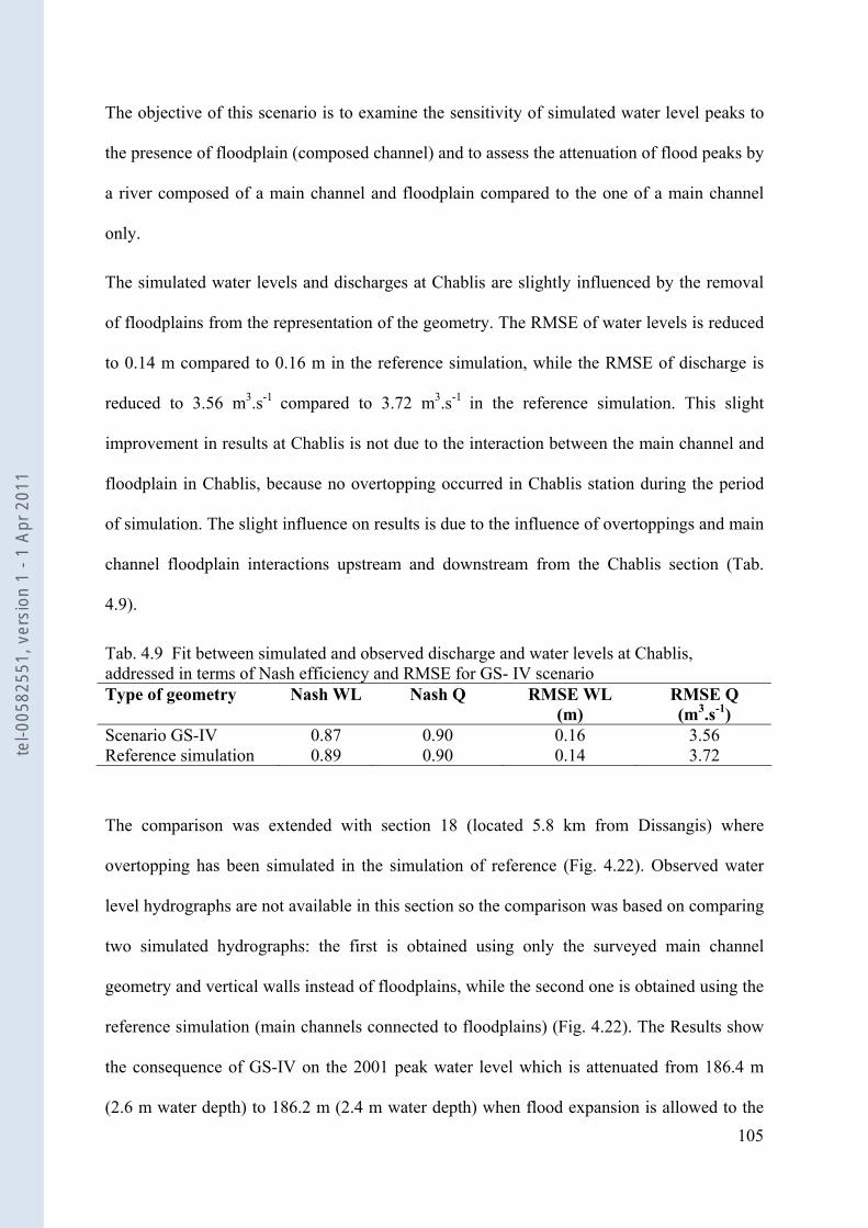
105

The objective of this scenario is to examine the sensitivity of simulated water level peaks to

the presence of floodplain (composed channel) and to assess the attenuation of flood peaks by

a river composed of a main channel and floodplain compared to the one of a main channel

only.

The simulated water levels and discharges at Chablis are slightly influenced by the removal

of floodplains from the representation of the geometry. The RMSE of water levels is reduced

to 0.14 m compared to 0.16 m in the reference simulation, while the RMSE of discharge is

reduced to 3.56 m3.s-1 compared to 3.72 m3.s-1 in the reference simulation. This slight

improvement in results at Chablis is not due to the interaction between the main channel and

floodplain in Chablis, because no overtopping occurred in Chablis station during the period

of simulation. The slight influence on results is due to the influence of overtoppings and main

channel floodplain interactions upstream and downstream from the Chablis section (Tab.

4.9).

Tab. 4.9 Fit between simulated and observed discharge and water levels at Chablis, addressed in terms of Nash efficiency and RMSE for GS- IV scenario Type of geometry Nash WL

Nash Q

RMSE WL

(m) RMSE Q (m3.s-1)

Scenario GS-IV 0.87 0.90 0.16 3.56 Reference simulation 0.89 0.90 0.14 3.72

The comparison was extended with section 18 (located 5.8 km from Dissangis) where

overtopping has been simulated in the simulation of reference (Fig. 4.22). Observed water

level hydrographs are not available in this section so the comparison was based on comparing

two simulated hydrographs: the first is obtained using only the surveyed main channel

geometry and vertical walls instead of floodplains, while the second one is obtained using the

reference simulation (main channels connected to floodplains) (Fig. 4.22). The Results show

the consequence of GS-IV on the 2001 peak water level which is attenuated from 186.4 m

(2.6 m water depth) to 186.2 m (2.4 m water depth) when flood expansion is allowed to the

tel-0

0582

551,

ver

sion

1 -

1 Ap

r 201

1

106

floodplain in this cross-section (Fig. 4.22 and Fig. 4.23 b). The 1998 peak water level is also

attenuated by 12 cm in this particular cross-section (Fig. 4.23 a), which shows the influence

of floodplain expansion in attenuating the peak water levels.

183.5

184

184.5

185

185.5

186

186.5

187

200 220 240 260 280 300 320Distance

Leve

l (m

)

Main channel

Max. water depth mainchannel onlyLeft extrapolated bank

Right extrapolated bank

Max. water depth with mainchannel + floodplainFloodplain extension

Fig. 4.22Comparison of maximum water depths between the simulation of reference and

scenario GS-IV in cross section 18 during the 2001 flood

Fig. 4.23 Comparison of peak simulated water levels between the simulation of reference and

GS-IV at section 18 (Fig. 4.22): a) April 1998 flood; b) March 2001 flood Finally, the maximum water depths along the river reach were longitudinally compared in

order to assess the influence of floodplains on the whole river reach (Fig. 4.24).

The influence of floodplain expansion in attenuating the peak water levels varies between 10

cm and 20 cm, particularly in the first 15 km reach nearby Dissangis and the 8 km reach

upstream of Chablis where the main channel is not so deep (< 2.5 m) and where overtopping

184.8

185

185.2

185.4

185.6

185.8

186

186.2

186.4

186.6

7-Mar-01 11-Mar-01 15-Mar-01 19-Mar-01 23-Mar-01Date

Wat

er le

vel (

m)

Only main channel

Main channel + Floodplain

(a) (b)

184

184.5

185

185.5

186

186.5

187

24-Apr-98 28-Apr-98 2-May-98 6-May-98Date

Wat

er le

vel (

m)

Only main channel

Main channel +Floodplain

tel-0

0582

551,

ver

sion

1 -

1 Ap

r 201

1

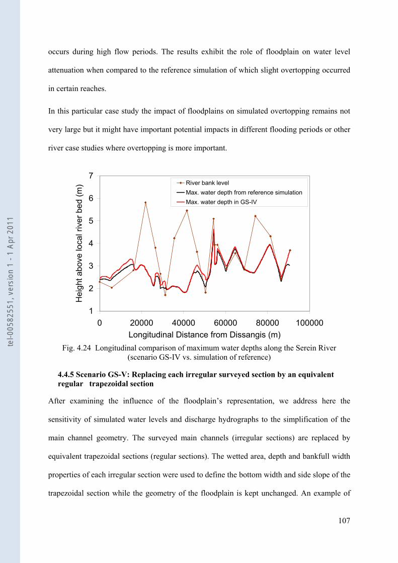
107

occurs during high flow periods. The results exhibit the role of floodplain on water level

attenuation when compared to the reference simulation of which slight overtopping occurred

in certain reaches.

In this particular case study the impact of floodplains on simulated overtopping remains not

very large but it might have important potential impacts in different flooding periods or other

river case studies where overtopping is more important.

1

2

3

4

5

6

7


Hei

ght a

bove

loca

l riv

er b

ed (m

) River bank levelMax. water depth from reference simulationMax. water depth in GS-IV


(scenario GS-IV vs. simulation of reference)

4.4.5 Scenario GS-V: Replacing each irregular surveyed section by an equivalent regular trapezoidal section

After examining the influence of the floodplain’s representation, we address here the

sensitivity of simulated water levels and discharge hydrographs to the simplification of the

main channel geometry. The surveyed main channels (irregular sections) are replaced by

equivalent trapezoidal sections (regular sections). The wetted area, depth and bankfull width

properties of each irregular section were used to define the bottom width and side slope of the

trapezoidal section while the geometry of the floodplain is kept unchanged. An example of

tel-0

0582

551,

ver

sion

1 -

1 Ap

r 201

1

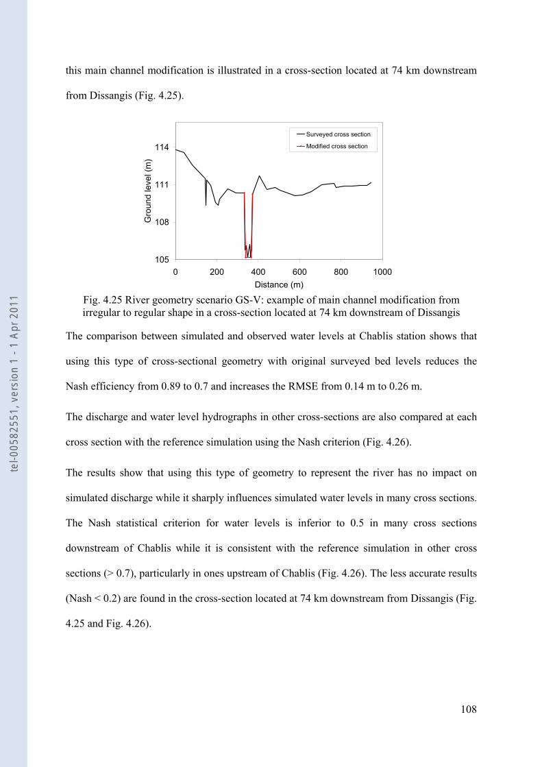
108

this main channel modification is illustrated in a cross-section located at 74 km downstream

from Dissangis (Fig. 4.25).

105

108

111

114

0 200 400 600 800 1000Distance (m)

Gro

und

leve

l (m

)Surveyed cross section

Modified cross section

Fig. 4.25 River geometry scenario GS-V: example of main channel modification from irregular to regular shape in a cross-section located at 74 km downstream of Dissangis

The comparison between simulated and observed water levels at Chablis station shows that

using this type of cross-sectional geometry with original surveyed bed levels reduces the

Nash efficiency from 0.89 to 0.7 and increases the RMSE from 0.14 m to 0.26 m.

The discharge and water level hydrographs in other cross-sections are also compared at each

cross section with the reference simulation using the Nash criterion (Fig. 4.26).

The results show that using this type of geometry to represent the river has no impact on

simulated discharge while it sharply influences simulated water levels in many cross sections.

The Nash statistical criterion for water levels is inferior to 0.5 in many cross sections

downstream of Chablis while it is consistent with the reference simulation in other cross

sections (> 0.7), particularly in ones upstream of Chablis (Fig. 4.26). The less accurate results

(Nash < 0.2) are found in the cross-section located at 74 km downstream from Dissangis (Fig.

4.25 and Fig. 4.26).

tel-0

0582

551,

ver

sion

1 -

1 Ap

r 201

1

109

0

0.2

0.4

0.6

0.8

1

1.2

0 20 40 60 80 100Distance from Dissangis (km)

Nas

h

Nash WLNash Q

Fig. 4.26 Nash statistical index compared at each cross section between discharge and water level hydrographs obtained from the simulation of reference and ones obtained from using

GS-V geometry

In this particular cross-section, the comparison of the simulated water levels hydrograph with

the reference simulation (Fig. 4.27) shows the impact of cross sectional morphological

modification on simulated water levels, especially during low flow periods where the water

levels are, on average, 20 cm lower than the ones in the reference simulation. This is due to

the fact that the lower the water level, the more important the friction is. Thus the description

of the cross section geometry is crucial for low flow modeling. These cross-section bottom

irregularities are neglected by the trapezoidal section which considers a plain bottom width.

The difference between the two simulations becomes less important when the water level

rises towards the bank level (Fig. 4.27) because the difference between the two wetted areas

characteristics decreases as the water level rises towards the bank level (Fig. 4.28).

The comparison of the wetted area characteristics between the original and modified sections

(Fig. 4.28) shows that as the water level of the regular section approaches the bankfull level,

the hydraulic characteristics of the regular section becomes equal to the hydraulic

characteristics of the irregular sections:

tel-0

0582

551,

ver

sion

1 -

1 Ap

r 201

1

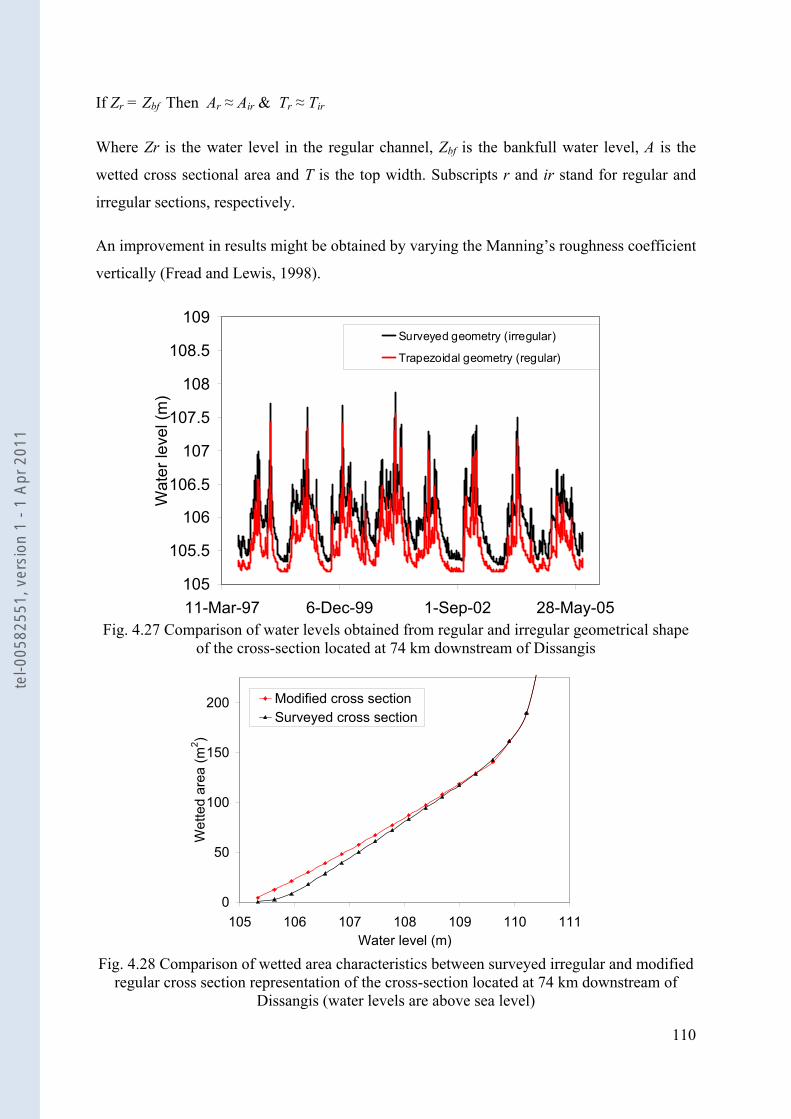
110

If Zr = Zbf Then Ar ≈ Air & Tr ≈ Tir

Where Zr is the water level in the regular channel, Zbf is the bankfull water level, A is the

wetted cross sectional area and T is the top width. Subscripts r and ir stand for regular and

irregular sections, respectively.

An improvement in results might be obtained by varying the Manning’s roughness coefficient

vertically (Fread and Lewis, 1998).

105

105.5

106

106.5

107

107.5

108

108.5

109

11-Mar-97 6-Dec-99 1-Sep-02 28-May-05

Wat

er le

vel (

m)

Surveyed geometry (irregular)

Trapezoidal geometry (regular)

Fig. 4.27 Comparison of water levels obtained from regular and irregular geometrical shape

of the cross-section located at 74 km downstream of Dissangis

0

50

100

150

200

105 106 107 108 109 110 111Water level (m)

Wet

ted

area

(m2 )

Modified cross sectionSurveyed cross section

Fig. 4.28 Comparison of wetted area characteristics between surveyed irregular and modified

regular cross section representation of the cross-section located at 74 km downstream of Dissangis (water levels are above sea level)

tel-0

0582

551,

ver

sion

1 -

1 Ap

r 201

1

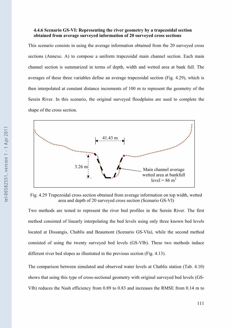
111

4.4.6 Scenario GS-VI: Representing the river geometry by a trapezoidal section obtained from average surveyed information of 20 surveyed cross sections

This scenario consists in using the average information obtained from the 20 surveyed cross

sections (Annexe. A) to compose a uniform trapezoidal main channel section. Each main

channel section is summarized in terms of depth, width and wetted area at bank full. The

averages of these three variables define an average trapezoidal section (Fig. 4.29), which is

then interpolated at constant distance increments of 100 m to represent the geometry of the

Serein River. In this scenario, the original surveyed floodplains are used to complete the

shape of the cross section.

Fig. 4.29 Trapezoidal cross section obtained from average information on top width, wetted area and depth of 20 surveyed cross section (Scenario GS-VI)

Two methods are tested to represent the river bed profiles in the Serein River. The first

method consisted of linearly interpolating the bed levels using only three known bed levels

located at Dissangis, Chablis and Beaumont (Scenario GS-VIa), while the second method

consisted of using the twenty surveyed bed levels (GS-VIb). These two methods induce

different river bed slopes as illustrated in the previous section (Fig. 4.13).

The comparison between simulated and observed water levels at Chablis station (Tab. 4.10)

shows that using this type of cross-sectional geometry with original surveyed bed levels (GS-

VIb) reduces the Nash efficiency from 0.89 to 0.83 and increases the RMSE from 0.14 m to

41.43 m

Main channel average wetted area at bankfull

level = 86 m2

3.26 m

tel-0

0582

551,

ver

sion

1 -

1 Ap

r 201

1

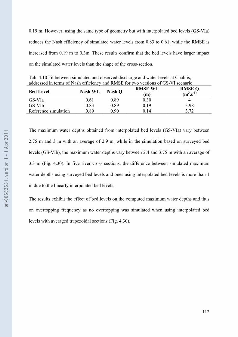
112

0.19 m. However, using the same type of geometry but with interpolated bed levels (GS-VIa)

reduces the Nash efficiency of simulated water levels from 0.83 to 0.61, while the RMSE is

increased from 0.19 m to 0.3m. These results confirm that the bed levels have larger impact

on the simulated water levels than the shape of the cross-section.

Tab. 4.10 Fit between simulated and observed discharge and water levels at Chablis, addressed in terms of Nash efficiency and RMSE for two versions of GS-VI scenario

Bed Level Nash WL Nash Q RMSE WL (m)

RMSE Q (m3.s-1)

GS-VIa 0.61 0.89 0.30 4 GS-VIb 0.83 0.89 0.19 3.98 Reference simulation 0.89 0.90 0.14 3.72

The maximum water depths obtained from interpolated bed levels (GS-VIa) vary between

2.75 m and 3 m with an average of 2.9 m, while in the simulation based on surveyed bed

levels (GS-VIb), the maximum water depths vary between 2.4 and 3.75 m with an average of

3.3 m (Fig. 4.30). In five river cross sections, the difference between simulated maximum

water depths using surveyed bed levels and ones using interpolated bed levels is more than 1

m due to the linearly interpolated bed levels.

The results exhibit the effect of bed levels on the computed maximum water depths and thus

on overtopping frequency as no overtopping was simulated when using interpolated bed

levels with averaged trapezoidal sections (Fig. 4.30).

tel-0

0582

551,

ver

sion

1 -

1 Ap

r 201

1

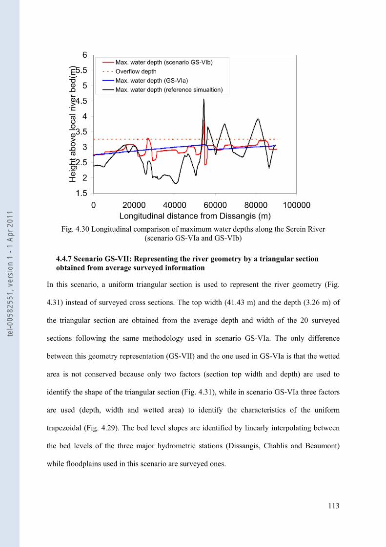
113

1.5

2

2.5

3

3.5

4

4.5

5

5.5

6

0 20000 40000 60000 80000 100000Longitudinal distance from Dissangis (m)

Hei

ght a

bove

loca

l riv

er b

ed(m

) Max. water depth (scenario GS-VIb)Overflow depthMax. water depth (GS-VIa)Max. water depth (reference simualtion)


(scenario GS-VIa and GS-VIb)

4.4.7 Scenario GS-VII: Representing the river geometry by a triangular section obtained from average surveyed information

In this scenario, a uniform triangular section is used to represent the river geometry (Fig.

4.31) instead of surveyed cross sections. The top width (41.43 m) and the depth (3.26 m) of

the triangular section are obtained from the average depth and width of the 20 surveyed

sections following the same methodology used in scenario GS-VIa. The only difference

between this geometry representation (GS-VII) and the one used in GS-VIa is that the wetted

area is not conserved because only two factors (section top width and depth) are used to

identify the shape of the triangular section (Fig. 4.31), while in scenario GS-VIa three factors

are used (depth, width and wetted area) to identify the characteristics of the uniform

trapezoidal (Fig. 4.29). The bed level slopes are identified by linearly interpolating between

the bed levels of the three major hydrometric stations (Dissangis, Chablis and Beaumont)

while floodplains used in this scenario are surveyed ones.

tel-0

0582

551,

ver

sion

1 -

1 Ap

r 201

1

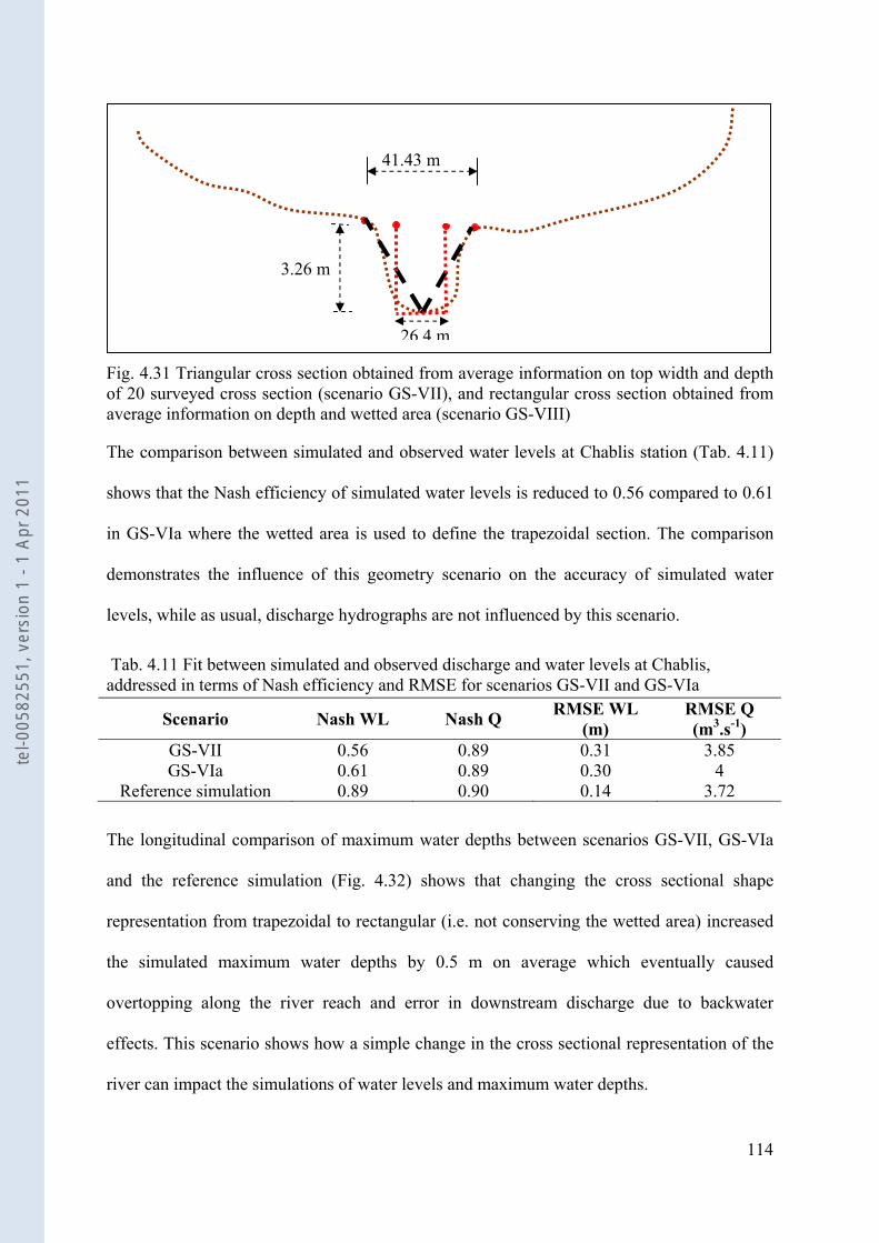
114

Fig. 4.31 Triangular cross section obtained from average information on top width and depth of 20 surveyed cross section (scenario GS-VII), and rectangular cross section obtained from average information on depth and wetted area (scenario GS-VIII)


shows that the Nash efficiency of simulated water levels is reduced to 0.56 compared to 0.61

in GS-VIa where the wetted area is used to define the trapezoidal section. The comparison

demonstrates the influence of this geometry scenario on the accuracy of simulated water

levels, while as usual, discharge hydrographs are not influenced by this scenario.

Tab. 4.11 Fit between simulated and observed discharge and water levels at Chablis, addressed in terms of Nash efficiency and RMSE for scenarios GS-VII and GS-VIa

The longitudinal comparison of maximum water depths between scenarios GS-VII, GS-VIa

and the reference simulation (Fig. 4.32) shows that changing the cross sectional shape

representation from trapezoidal to rectangular (i.e. not conserving the wetted area) increased

the simulated maximum water depths by 0.5 m on average which eventually caused

overtopping along the river reach and error in downstream discharge due to backwater

effects. This scenario shows how a simple change in the cross sectional representation of the

river can impact the simulations of water levels and maximum water depths.

Scenario Nash WL Nash Q RMSE WL (m)

RMSE Q (m3.s-1)

GS-VII 0.56 0.89 0.31 3.85 GS-VIa 0.61 0.89 0.30 4


41.43 m

3.26 m

26.4 m

tel-0

0582

551,

ver

sion

1 -

1 Ap

r 201

1

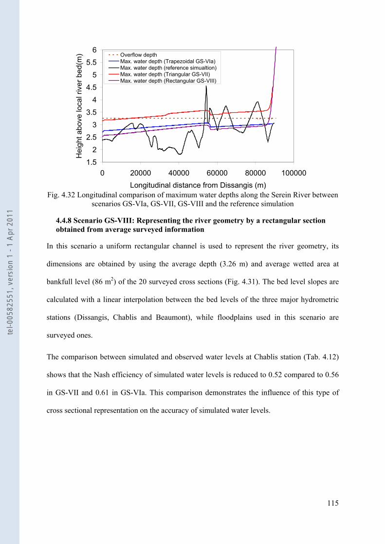
115

1.52

2.53

3.54

4.55

5.56

0 20000 40000 60000 80000 100000Longitudinal distance from Dissangis (m)

Hei

ght a

bove

loca

l riv

er b

ed(m

) Overflow depthMax. water depth (Trapezoidal GS-VIa)Max. water depth (reference simualtion)Max. water depth (Triangular GS-VII)Max. water depth (Rectangular GS-VIII)

Fig. 4.32 Longitudinal comparison of maximum water depths along the Serein River between

scenarios GS-VIa, GS-VII, GS-VIII and the reference simulation

4.4.8 Scenario GS-VIII: Representing the river geometry by a rectangular section obtained from average surveyed information

In this scenario a uniform rectangular channel is used to represent the river geometry, its

dimensions are obtained by using the average depth (3.26 m) and average wetted area at

bankfull level (86 m2) of the 20 surveyed cross sections (Fig. 4.31). The bed level slopes are

calculated with a linear interpolation between the bed levels of the three major hydrometric

stations (Dissangis, Chablis and Beaumont), while floodplains used in this scenario are

surveyed ones.


shows that the Nash efficiency of simulated water levels is reduced to 0.52 compared to 0.56

in GS-VII and 0.61 in GS-VIa. This comparison demonstrates the influence of this type of

cross sectional representation on the accuracy of simulated water levels.

tel-0

0582

551,

ver

sion

1 -

1 Ap

r 201

1

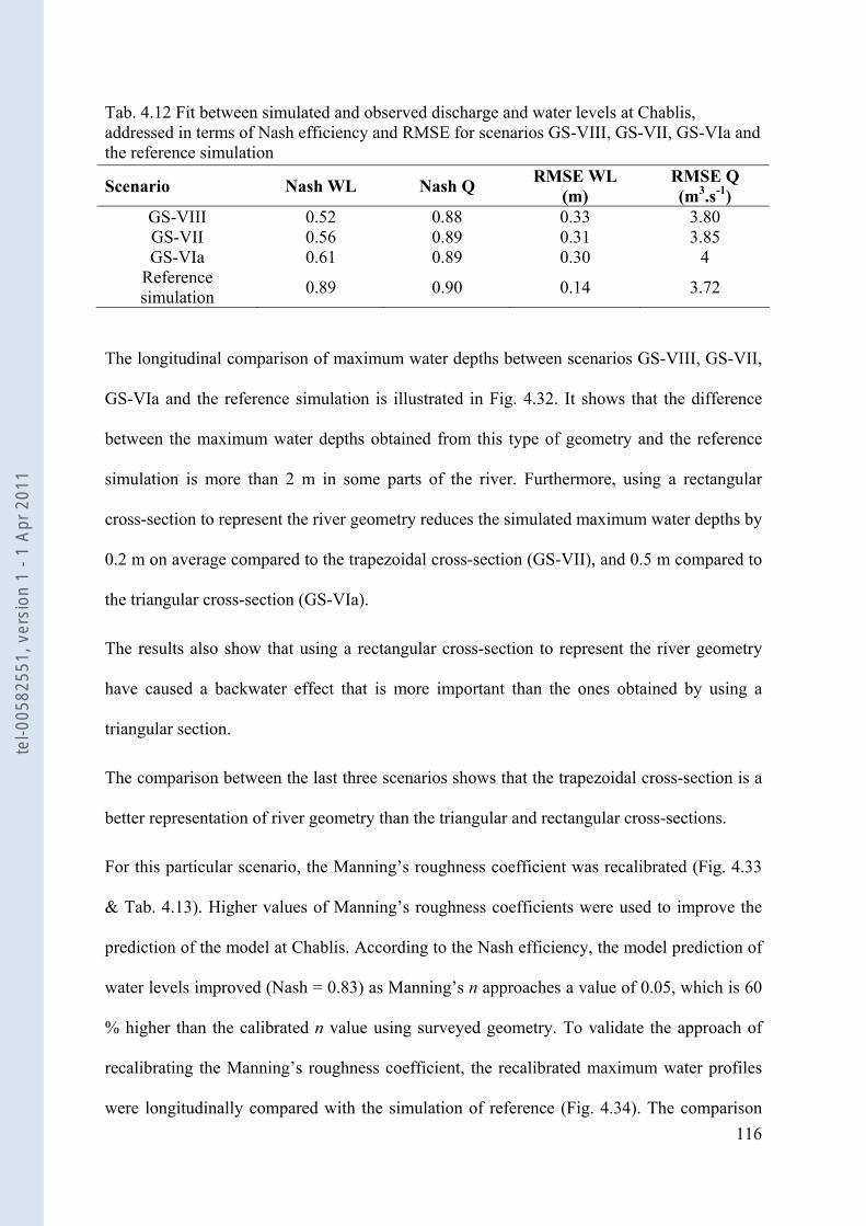
116

Tab. 4.12 Fit between simulated and observed discharge and water levels at Chablis, addressed in terms of Nash efficiency and RMSE for scenarios GS-VIII, GS-VII, GS-VIa and the reference simulation

The longitudinal comparison of maximum water depths between scenarios GS-VIII, GS-VII,

GS-VIa and the reference simulation is illustrated in Fig. 4.32. It shows that the difference

between the maximum water depths obtained from this type of geometry and the reference

simulation is more than 2 m in some parts of the river. Furthermore, using a rectangular

cross-section to represent the river geometry reduces the simulated maximum water depths by

0.2 m on average compared to the trapezoidal cross-section (GS-VII), and 0.5 m compared to

the triangular cross-section (GS-VIa).

The results also show that using a rectangular cross-section to represent the river geometry

have caused a backwater effect that is more important than the ones obtained by using a

triangular section.

The comparison between the last three scenarios shows that the trapezoidal cross-section is a

better representation of river geometry than the triangular and rectangular cross-sections.

For this particular scenario, the Manning’s roughness coefficient was recalibrated (Fig. 4.33

& Tab. 4.13). Higher values of Manning’s roughness coefficients were used to improve the

prediction of the model at Chablis. According to the Nash efficiency, the model prediction of

water levels improved (Nash = 0.83) as Manning’s n approaches a value of 0.05, which is 60

% higher than the calibrated n value using surveyed geometry. To validate the approach of

recalibrating the Manning’s roughness coefficient, the recalibrated maximum water profiles

were longitudinally compared with the simulation of reference (Fig. 4.34). The comparison

Scenario Nash WL Nash Q RMSE WL (m)

RMSE Q (m3.s-1)

GS-VIII 0.52 0.88 0.33 3.80 GS-VII 0.56 0.89 0.31 3.85 GS-VIa 0.61 0.89 0.30 4


tel-0

0582

551,

ver

sion

1 -

1 Ap

r 201

1

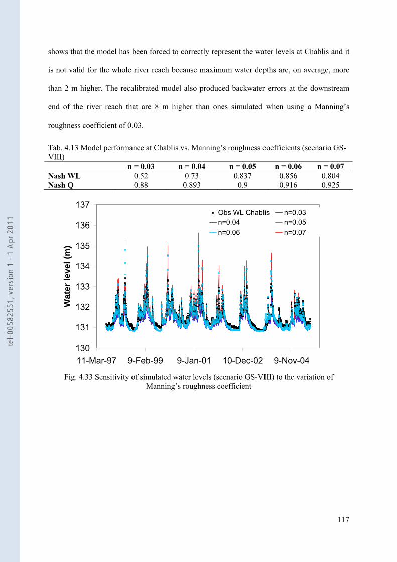
117

shows that the model has been forced to correctly represent the water levels at Chablis and it

is not valid for the whole river reach because maximum water depths are, on average, more

than 2 m higher. The recalibrated model also produced backwater errors at the downstream

end of the river reach that are 8 m higher than ones simulated when using a Manning’s

roughness coefficient of 0.03.

Tab. 4.13 Model performance at Chablis vs. Manning’s roughness coefficients (scenario GS-VIII)

n = 0.03 n = 0.04 n = 0.05 n = 0.06 n = 0.07 Nash WL 0.52 0.73 0.837 0.856 0.804 Nash Q 0.88 0.893 0.9 0.916 0.925

130

131

132

133

134

135

136

137

11-Mar-97 9-Feb-99 9-Jan-01 10-Dec-02 9-Nov-04

Wat

er le

vel (

m)

Obs WL Chablis n=0.03n=0.04 n=0.05n=0.06 n=0.07

Fig. 4.33 Sensitivity of simulated water levels (scenario GS-VIII) to the variation of

Manning’s roughness coefficient

tel-0

0582

551,

ver

sion

1 -

1 Ap

r 201

1

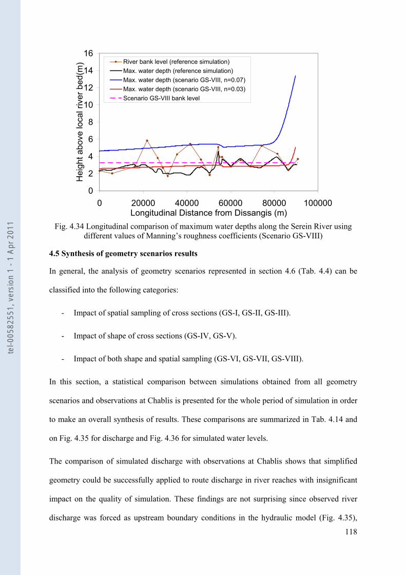
118

0

2

4

6

8

10

12

14

16


Hei

ght a

bove

loca

l riv

er b

ed(m

) River bank level (reference simulation)Max. water depth (reference simulation)Max. water depth (scenario GS-VIII, n=0.07)Max. water depth (scenario GS-VIII, n=0.03)Scenario GS-VIII bank level

Fig. 4.34 Longitudinal comparison of maximum water depths along the Serein River using

different values of Manning’s roughness coefficients (Scenario GS-VIII)

4.5 Synthesis of geometry scenarios results

In general, the analysis of geometry scenarios represented in section 4.6 (Tab. 4.4) can be

classified into the following categories:

- Impact of spatial sampling of cross sections (GS-I, GS-II, GS-III).

- Impact of shape of cross sections (GS-IV, GS-V).

- Impact of both shape and spatial sampling (GS-VI, GS-VII, GS-VIII).

In this section, a statistical comparison between simulations obtained from all geometry

scenarios and observations at Chablis is presented for the whole period of simulation in order

to make an overall synthesis of results. These comparisons are summarized in Tab. 4.14 and

on Fig. 4.35 for discharge and Fig. 4.36 for simulated water levels.

The comparison of simulated discharge with observations at Chablis shows that simplified

geometry could be successfully applied to route discharge in river reaches with insignificant

impact on the quality of simulation. These findings are not surprising since observed river

discharge was forced as upstream boundary conditions in the hydraulic model (Fig. 4.35),

tel-0

0582

551,

ver

sion

1 -

1 Ap

r 201

1

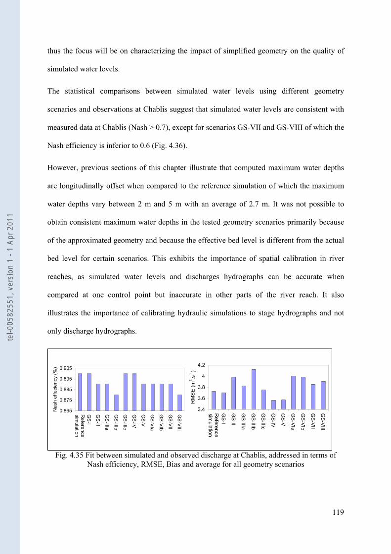
119

thus the focus will be on characterizing the impact of simplified geometry on the quality of

simulated water levels.

The statistical comparisons between simulated water levels using different geometry

scenarios and observations at Chablis suggest that simulated water levels are consistent with

measured data at Chablis (Nash > 0.7), except for scenarios GS-VII and GS-VIII of which the

Nash efficiency is inferior to 0.6 (Fig. 4.36).

However, previous sections of this chapter illustrate that computed maximum water depths

are longitudinally offset when compared to the reference simulation of which the maximum

water depths vary between 2 m and 5 m with an average of 2.7 m. It was not possible to

obtain consistent maximum water depths in the tested geometry scenarios primarily because

of the approximated geometry and because the effective bed level is different from the actual

bed level for certain scenarios. This exhibits the importance of spatial calibration in river

reaches, as simulated water levels and discharges hydrographs can be accurate when

compared at one control point but inaccurate in other parts of the river reach. It also

illustrates the importance of calibrating hydraulic simulations to stage hydrographs and not

only discharge hydrographs.

Fig. 4.35 Fit between simulated and observed discharge at Chablis, addressed in terms of

Nash efficiency, RMSE, Bias and average for all geometry scenarios

3.4

3.6

3.8

4

4.2

Reference

simulation

GS

-I

GS

-II

GS

-IIIa

GS

-IIIb

GS

-IIIc

GS

-IV

GS

-V

GS

-VIa

GS

-VIb

GS

-VII

GS

-VIII

RM

SE

(m3 .s

-1)

0.865

0.875

0.885

0.895

0.905

Reference

simulation

GS

-I

GS

-II

GS-IIIa

GS-IIIb

GS-IIIc

GS

-IV

GS

-V

GS

-VIa

GS

-VIb

GS

-VII

GS

-VIII

Nas

h ef

feci

ency

(%)

tel-0

0582

551,

ver

sion

1 -

1 Ap

r 201

1

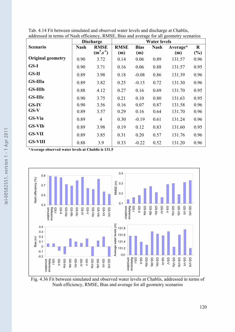
120

Tab. 4.14 Fit between simulated and observed water levels and discharge at Chablis, addressed in terms of Nash efficiency, RMSE, Bias and average for all geometry scenarios

Discharge Water levels Scenario Nash

RMSE (m3.s-1)

RMSE (m)

Bias (m)

Nash

Average* (m)

R (%)

Original geometry 0.90 3.72 0.14 0.06 0.89 131.57 0.96 GS-I 0.90 3.71 0.16 0.06 0.88 131.57 0.95 GS-II 0.89 3.98 0.18 -0.08 0.86 131.39 0.96 GS-IIIa 0.89 3.82 0.25 -0.15 0.72 131.30 0.96 GS-IIIb 0.88 4.12 0.27 0.16 0.69 131.70 0.95 GS-IIIc 0.90 3.75 0.21 0.10 0.80 131.63 0.95 GS-IV 0.90 3.56 0.16 0.07 0.87 131.58 0.96 GS-V 0.89 3.57 0.29 0.16 0.64 131.70 0.96 GS-Via 0.89 4 0.30 -0.19 0.61 131.24 0.96 GS-VIb 0.89 3.98 0.19 0.12 0.83 131.60 0.95 GS-VII 0.89 3.85 0.31 0.20 0.57 131.76 0.96 GS-VIII 0.88 3.9 0.33 -0.22 0.52 131.20 0.96 *Average observed water levels at Chablis is 131.5

Fig. 4.36 Fit between simulated and observed water levels at Chablis, addressed in terms of

Nash efficiency, RMSE, Bias and average for all geometry scenarios

0.1

0.2

0.3

0.4

Reference

simulation

GS

-I

GS

-II

GS-IIIa

GS-IIIb

GS-IIIc

GS-IV

GS-V

GS-V

Ia

GS

-VIb

GS

-VII

GS

-VIII

RM

SE

(m)

0.3

0.5

0.7

0.9

Reference

simulation

GS-I

GS

-II

GS-IIIa

GS

-IIIb

GS-IIIc

GS

-IV

GS-V

GS

-VIa

GS-V

Ib

GS-VII

GS

-VIII

Nas

h ef

feci

ency

(%)

131

131.2

131.4

131.6

131.8

Reference

simulation

GS-I

GS

-II

GS-IIIa

GS

-IIIb

GS-IIIc

GS

-IV

GS-V

GS

-VIa

GS-V

Ib

GS-VII

GS

-VIII

Aver

age

wat

er le

vels

(m)

-0.2

-0.1

0

0.1

0.2

0.3

0.4

Reference

simulation

GS-I

GS-II

GS-IIIa

GS

-IIIb

GS

-IIIc

GS

-IV

GS-V

GS-V

Ia

GS-V

Ib

GS

-VII

GS

-VIII

Bias

(m)

tel-0

0582

551,

ver

sion

1 -

1 Ap

r 201

1

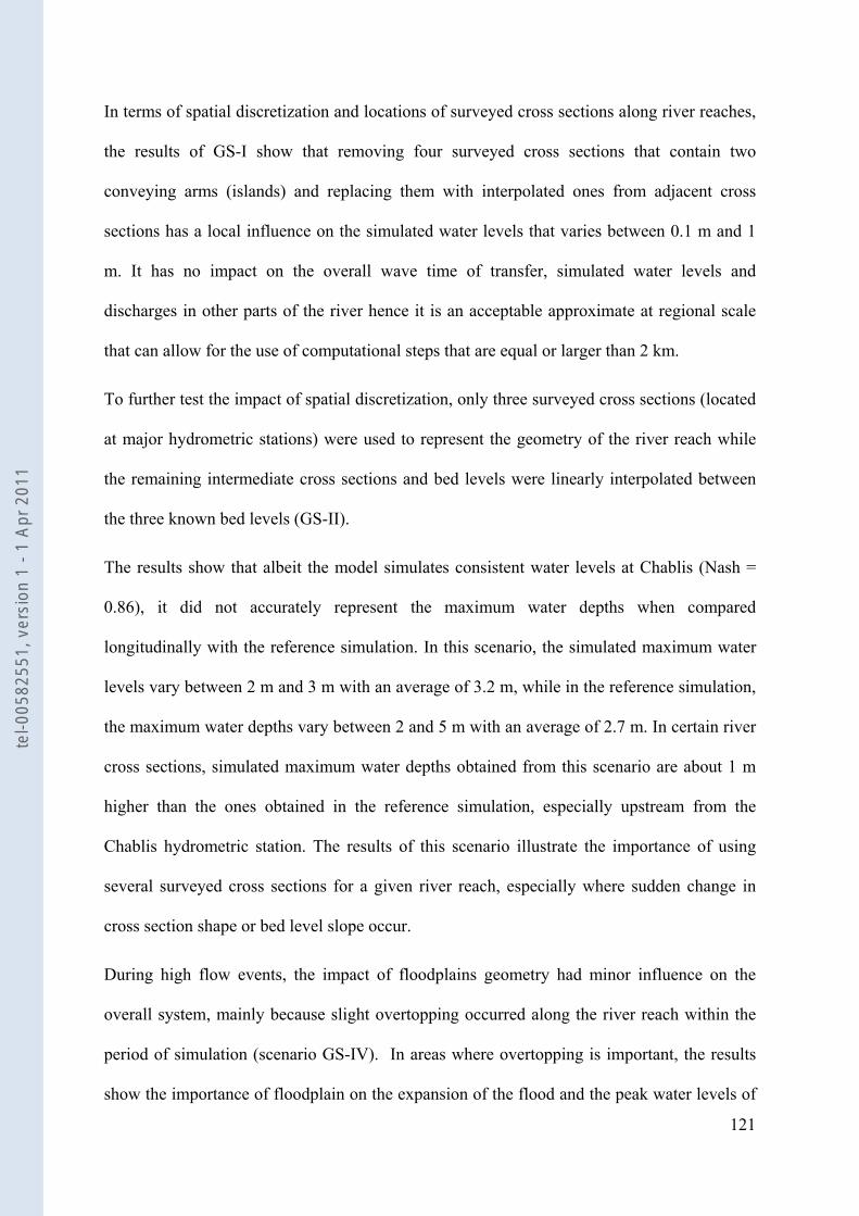
121

In terms of spatial discretization and locations of surveyed cross sections along river reaches,

the results of GS-I show that removing four surveyed cross sections that contain two

conveying arms (islands) and replacing them with interpolated ones from adjacent cross

sections has a local influence on the simulated water levels that varies between 0.1 m and 1

m. It has no impact on the overall wave time of transfer, simulated water levels and

discharges in other parts of the river hence it is an acceptable approximate at regional scale

that can allow for the use of computational steps that are equal or larger than 2 km.

To further test the impact of spatial discretization, only three surveyed cross sections (located

at major hydrometric stations) were used to represent the geometry of the river reach while

the remaining intermediate cross sections and bed levels were linearly interpolated between

the three known bed levels (GS-II).

The results show that albeit the model simulates consistent water levels at Chablis (Nash =

0.86), it did not accurately represent the maximum water depths when compared

longitudinally with the reference simulation. In this scenario, the simulated maximum water

levels vary between 2 m and 3 m with an average of 3.2 m, while in the reference simulation,

the maximum water depths vary between 2 and 5 m with an average of 2.7 m. In certain river

cross sections, simulated maximum water depths obtained from this scenario are about 1 m

higher than the ones obtained in the reference simulation, especially upstream from the

Chablis hydrometric station. The results of this scenario illustrate the importance of using

several surveyed cross sections for a given river reach, especially where sudden change in

cross section shape or bed level slope occur.

During high flow events, the impact of floodplains geometry had minor influence on the

overall system, mainly because slight overtopping occurred along the river reach within the

period of simulation (scenario GS-IV). In areas where overtopping is important, the results

show the importance of floodplain on the expansion of the flood and the peak water levels of

tel-0

0582

551,

ver

sion

1 -

1 Ap

r 201

1

122

which attenuation levels varied between 10cm and 20 cm. This scenario offers interesting

perspectives for flood mitigation and river channelization management.

During low flow events, irregularities in the river bed bottom have an important impact on

simulated river stages, as simplifying the irregular river bed bottom to plain have, on average,

attenuated the low flow water levels by 20 cm compared to ones in the reference simulation.

This is because the lower the water level is, the more important is the friction and thus the

description of the cross section geometry. This finding is important, especially in the

simulations of stream-aquifer interactions where the river is sustained by aquifer units during

low flow periods.

In terms of river bed levels, the results show how natural variations in bed levels and cross

sections characteristics are large and, consequently, the effective bed used in limited

geometry scenarios (interpolated bed levels) can be several meters different from the

surveyed bed at a given point. This difference is not significant in terms of discharge routing

over tens of kilometers. However, in the context of determining water levels at specific local

scale, these differences are important. For instance, in GS-VIa using interpolated bed levels

instead of surveyed ones for the same cross sectional representation have reduced the Nash

efficiency of simulated water levels from 0.83 to 0.61, while the RMSE was increased from

0.19 m to 0.3 m. The maximum water depths obtained from interpolated bed levels vary

between 2.75 m and 3 m with an average of 2.9 m, while in the simulation based on surveyed

bed levels, the maximum water depths vary between 2.4 and 3.75 m with an average of 3.3 m

for the same type of section. In certain river cross sections, the difference between simulated

maximum water depths using surveyed bed levels and ones using interpolated bed levels is

more than 1 m due to the linearly interpolated bed levels. The results exhibit the effect of bed

levels on the computed maximum water depths and thus on overtopping frequency.

tel-0

0582

551,

ver

sion

1 -

1 Ap

r 201

1

123

Finally, the cross sections shape impact on simulated water levels was characterized by

comparing between water levels simulations based on using trapezoidal (GS-VI), triangular

(GS-VII) and rectangular (GS-VIII) cross sections. The comparison of water levels with

observed ones at Chablis station shows that the Nash efficiency of simulated water levels in

GS-VIII is dropped to 0.52 compared to 0.56 in GS-VII and 0.61 in GS-VI.

The longitudinal comparison of maximum water depths between scenarios GS-VIII, GS-VII,

GS-VI and the reference simulation shows that using a rectangular cross-section to represent

the river geometry reduces the simulated maximum water depths by 0.2 m on average

compared to the trapezoidal cross-section (GS-VII), and 0.5 m compared to the triangular

cross-section (GS-VIa). Furthermore, using a simple rectangular or triangular cross-section to

represent the river geometry has caused a backwater effect.

Trapezoidal cross sections are found to give more accurate results than triangular and

rectangular ones, additionally, no backwater problems have occurred when using this

particular shape of cross section.

4.6 Conclusions

The primary objective of this study was to establish whether a reliable hydraulic routing

model could be developed based on limited field data. This study was carried out in the

Serein River (tributary of the Yonne River), between the gauging stations of Dissangis et

Beaumont, in a well surveyed reach (20 cross sections over 89 kms).

River discharge and stage are simulated by the hydraulic model HEC-RAS (1D Saint-Venant

equations) solved using the four point implicit finite difference scheme while lateral inflows

are simulated by the regional hydrogeological model EauDyssée.

The calibration parameter involved in the development of the hydraulic model was the

Manning's roughness coefficient (n) which was first calibrated for a real channel morphology.

tel-0

0582

551,

ver

sion

1 -

1 Ap

r 201

1

124

The results of the different geometry scenarios indicate that hydrodynamic models based on

the Saint-Venant equations could be successfully used to determine discharge hydrographs in

reaches where little channel geometry data are available, by approximating the modeled reach

with simplified geometry. This result is not surprising since river discharge is mostly

controlled by the upstream and lateral boundary conditions. However, a hydraulic model

based on approximate morphological data does not accurately predict the associated water

levels. For instance, in GS-VIa using interpolated bed levels instead of surveyed ones for the

same cross sectional representation have reduced the Nash efficiency of simulated water

levels at Chablis hydrometric station from 0.83 to 0.61, while the RMSE was increased from

0.19 m to 0.3 m. The maximum water depths obtained from interpolated bed levels vary



for the same type of section. In five river cross sections, the difference between simulated


more than 1 m due to the linearly interpolated bed levels. This exhibits the effect of bed

levels on the simulated water levels, especially at the regional scale where DEM is used to

identify the river geometry hence it is difficult to obtain an accurate river bed level

representation.

In terms of river shape, the results show that irregularities in the river bed bottom have an

important impact on simulated river stages, especially during low flow as simplifying the

irregular river bed bottom to plain have, on average, attenuated the low flow water levels by

20 cm compared to ones in the reference simulation. This is because the lower the water level

is, the more important is the friction and thus the description of the cross section geometry.

This finding is important, especially in the simulations of stream-aquifer interactions where

the river is sustained by aquifer units during low flow periods.

tel-0

0582

551,

ver

sion

1 -

1 Ap

r 201

1

125

The study confirms that the accuracy of predicted water levels and maximum water depths

simulated by a Saint-Venant model rely on an accurate representation of channel geometry


That being said, a 1D Saint-Venant model is not suitable for simulating flow at regional scale

where river morphology is not accessible. In spite of the aforementioned limitations, this type

of hydrodynamic modeling remains crucial to accurately simulate in-stream water levels. To

compromise between the scale issue, morphological data limitation and the importance to

accurately simulate in-stream water levels, an original upscaling strategy will be developed.

This strategy will allow for benefiting from high resolution hydraulic modeling outputs (e.g.

Annexe. A) to describe fluctuating river stage function of routed discharge and potentially

improve the regional scale simulation of stream-aquifer interactions in the integrated model

EauDyssée.

tel-0

0582

551,

ver

sion

1 -

1 Ap

r 201

1

126

CHAPTER 5. AN UPSCALING METHODOLOGY FOR SIMULATING RIVER

STAGES AND STREAM-AQUIFER INTERACTIONS: OISE RIVER BASIN CASE

STUDY


Dans ce chapitre, nous proposons une méthode de changement d’échelle dans laquelle la

modélisation fine des processus hydrauliques à haute résolution permet d'améliorer la

représentation des profils d’eau en rivière et les interactions nappe-rivière simulent à l'échelle

régionale par la plateforme de modélisation intégrée des hydrosystèmes EauDyssée.

La méthodologie de changement d’échelle a été testée pour le bassin versant de l’Oise (sous

bassin de le Seine) d’une superficie de 17000 Km2, pour la période 1990-1995. Le modèle

HEC-RAS a été utilisé pour la modélisation hydraulique basée sur les équations de Saint-

Venant 1D pour un tronçon de l’Oise de 188 km. Le calage de ce modèle a été effectué en

faisant varier le coefficient de Manning n (1/K) avec pour objectif de reproduire les courbes

de tarage observées. L'efficacité du modèle hydraulique est évaluée par les critères

statistiques classiques de Nash, RMSE, biais à 4 stations hydrométriques. Une courbe de

tarage est définie à partir de la simulation hydraulique à la résolution du modèle HEC, tous

les 200m en moyenne.

Ces courbes de tarage sont ensuite projetées comme conditions aux limites sur les mailles

rivière du modèle régional EauDyssée (résolution de 1 km) afin de simuler la fluctuation du

niveau d'eau en fonction du débit routé par le module de routage (RAPID). Les échanges

entre les mailles rivière et les mailles aquifères (modèle SAM) sont ensuite estimés à partir

d’une relation de type loi de Darcy se basant sur les gradients de charge verticaux entre la

rivière et la nappe.

tel-0

0582

551,

ver

sion

1 -

1 Ap

r 201

1

127

L’impact de la fluctuation des niveaux en rivière sur les isopièzes a été analysé par rapport à

un état de référence pour lequel les niveaux en rivière sont fixes. L’analyse des résultats sur

la période de simulation montre un écart moyen des niveaux piézométriques pouvant

atteindre 1.9 m pour les mailles souterraines situées sous les mailles rivière.

Cet écart se réduit si l’on considère des mailles souterraines plus éloignées de la rivière.

L’extension spatiale de cet écart moyen est plus importante dans la nappe de la Craie qui est

confinée (jusqu’à 20 km de la rivière) que dans celle de l’Éocène qui est libre (3 km de la

rivière).

Abstract

In this chapter, a coupling framework strategy is proposed to simulate stream-aquifer

interactions. The methodology is based on an upscaling approach, which allows for

benefiting from high resolution hydraulic modeling outputs to improve the simulation of

fluctuating river stage in a regional scale hydro(geo)logical platfrom EauDyssée.

The hydro(geo)logical platfrom EauDyssée computes runoff and groundwater flows that are

lateral inflow inputs of the hydraulic model. At the regional scale, the coupling between

streams and aquifer units is ensured using rating curves calculated with the hydraulic model

and discharges routed by the regional model. Then, during an Eau-Syssée simulation,

differences between in-stream water stages and piezometric heads are used to calculate and

quantify the exchanges between aquifer units and rivers.

This coupling framework strategy is applied on the Oise River basin, a 17 000 km2 sub-basin

of the Seine River basin, in Northern France.

The hydraulic model HEC-RAS (chapter 4) was used for simulating 188 km of the Oise

stream network. Manning's roughness coefficient (n) was calibrated against discharges and

water stages hydrographs measured at 4 hydrometric stations.

tel-0

0582

551,

ver

sion

1 -

1 Ap

r 201

1

128

Upon calibrating the Oise River hydraulic model, the rating curves (discharge vs. water

levels) derived at each cross-section by HEC-RAS are linearly projected along the river cells,

and an equivalent rating curve at the center of this river grid-cell is calculated by inverse

distance weight averaging with respect to the cell’s center. Then, the resulting equivalent

rating curve is sent as input boundary conditions for the QtoZ module which calculates the

water level as function of the discharge routed by RAPID and sends it to the groundwater

model (SAM) in order to simulate stream aquifer interactions.

Once the methodology is validated at the regional scale, the simulated regional river stages

were almost as realistic as the ones from the local 1D hydraulic model.

The impacts of in-stream water level fluctuations on the aquifer system are characterized at

local and regional scale by comparing with EauDyssée results obtained using constant in-

stream water levels.

The variation in simulated piezometric heads caused by the in-stream water level fluctuations

reach up to 1.9 m in aquifer units directly connected to the river cells, the impact decreases

with distance to the stream.

The area influenced by fluctuating river stages extends across 3 to 20 km around the streams,

depending on the hydrogeological setting (confined/unconfined) of the aquifer unit.

Substantial portions of this chapter are submitted for publishing in Journal of hydrology: Saleh, F., et al. 2010. (ref: HYDROL-S-10-01053)

5.1 Framework strategy to account for river stages fluctuations

To compromise between the spatial scale issue, morphological data limitation and the

importance to accurately simulate in-stream water levels (stressed in previous chapters), a

strategy is proposed to benefit from the results of the high resolution 1D channel flow model

HEC-RAS (Fig. 5.1). Runoff and groundwater contribution to stream flow are first simulated

tel-0

0582

551,

ver

sion

1 -

1 Ap

r 201

1

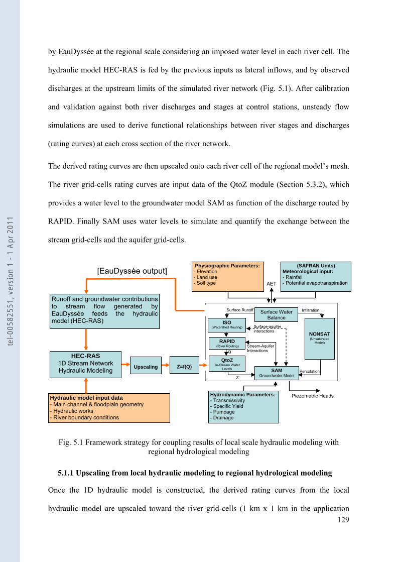
129

by EauDyssée at the regional scale considering an imposed water level in each river cell. The

hydraulic model HEC-RAS is fed by the previous inputs as lateral inflows, and by observed

discharges at the upstream limits of the simulated river network (Fig. 5.1). After calibration

and validation against both river discharges and stages at control stations, unsteady flow

simulations are used to derive functional relationships between river stages and discharges

(rating curves) at each cross section of the river network.

The derived rating curves are then upscaled onto each river cell of the regional model’s mesh.

The river grid-cells rating curves are input data of the QtoZ module (Section 5.3.2), which

provides a water level to the groundwater model SAM as function of the discharge routed by

RAPID. Finally SAM uses water levels to simulate and quantify the exchange between the

stream grid-cells and the aquifer grid-cells.

Fig. 5.1 Framework strategy for coupling results of local scale hydraulic modeling with regional hydrological modeling

5.1.1 Upscaling from local hydraulic modeling to regional hydrological modeling

Once the 1D hydraulic model is constructed, the derived rating curves from the local

hydraulic model are upscaled toward the river grid-cells (1 km x 1 km in the application

(SAFRAN Units)Meteorological input: - Rainfall - Potential evapotranspiration

SAM Groundwater Model

Surface Water Balance

Infiltration Surface Runoff

Q

Z

Stream-Aquifer Interactions

Percolation

NONSAT (Unsaturated

Model)


Piezometric Heads

ISO (Watershed Routing)

QtoZ In-Stream Water

Levels

AET

Surface-aquifer interactions

Hydraulic model input data- Main channel & floodplain geometry - Hydraulic works - River boundary conditions

[EauDyssée output] Physiographic Parameters:

- Elevation - Land use - Soil type

Hydrodynamic Parameters:- Transmissivity - Specific Yield - Pumpage - Drainage

Z=f(Q)

Upscaling

Runoff and groundwater contributions to stream flow generated by EauDyssée feeds the hydraulic model (HEC-RAS)

HEC-RAS 1D Stream Network Hydraulic Modeling

tel-0

0582

551,

ver

sion

1 -

1 Ap

r 201

1

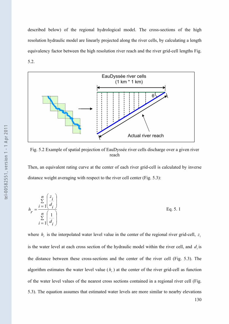
130

described below) of the regional hydrological model. The cross-sections of the high

resolution hydraulic model are linearly projected along the river cells, by calculating a length

equivalency factor between the high resolution river reach and the river grid-cell lengths Fig.

5.2.

Fig. 5.2 Example of spatial projection of EauDyssée river cells discharge over a given river reach

Then, an equivalent rating curve at the center of each river grid-cell is calculated by inverse

distance weight averaging with respect to the river cell center (Fig. 5.3):

∑= ⎟

⎟

⎠

⎞

⎜⎜

⎝

⎛

∑= ⎟

⎟

⎠

⎞

⎜⎜

⎝

⎛

=n

i id

n

i idiz

rh

1

1

1 Eq. 5. 1

where rh is the interpolated water level value in the center of the regional river grid-cell, iz

is the water level at each cross section of the hydraulic model within the river cell, and id is

the distance between these cross-sections and the center of the river cell (Fig. 5.3). The

algorithm estimates the water level value ( rh ) at the center of the river grid-cell as function

of the water level values of the nearest cross sections contained in a regional river cell (Fig.

5.3). The equation assumes that estimated water levels are more similar to nearby elevations

EauDyssée river cells

(1 km * 1 km)

θ

Actual river reach

tel-0

0582

551,

ver

sion

1 -

1 Ap

r 201

1

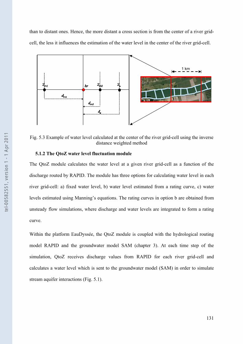
131

than to distant ones. Hence, the more distant a cross section is from the center of a river grid-

cell, the less it influences the estimation of the water level in the center of the river grid-cell.

Fig. 5.3 Example of water level calculated at the center of the river grid-cell using the inverse

distance weighted method

5.1.2 The QtoZ water level fluctuation module

The QtoZ module calculates the water level at a given river grid-cell as a function of the

discharge routed by RAPID. The module has three options for calculating water level in each

river grid-cell: a) fixed water level, b) water level estimated from a rating curve, c) water

levels estimated using Manning’s equations. The rating curves in option b are obtained from

unsteady flow simulations, where discharge and water levels are integrated to form a rating

curve.

Within the platform EauDyssée, the QtoZ module is coupled with the hydrological routing

model RAPID and the groundwater model SAM (chapter 3). At each time step of the

simulation, QtoZ receives discharge values from RAPID for each river grid-cell and

calculates a water level which is sent to the groundwater model (SAM) in order to simulate

stream aquifer interactions (Fig. 5.1).

1 km

tel-0

0582

551,

ver

sion

1 -

1 Ap

r 201

1

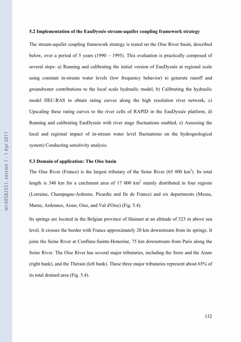
132

5.2 Implementation of the EauDyssée stream-aquifer coupling framework strategy

The stream-aquifer coupling framework strategy is tested on the Oise River basin, described

below, over a period of 5 years (1990 – 1995). This evaluation is practically composed of

several steps: a) Running and calibrating the initial version of EauDyssée at regional scale

using constant in-stream water levels (low frequency behavior) to generate runoff and

groundwater contributions to the local scale hydraulic model, b) Calibrating the hydraulic

model HEC-RAS to obtain rating curves along the high resolution river network, c)

Upscaling these rating curves to the river cells of RAPID in the EauDyssée platform, d)

Running and calibrating EauDyssée with river stage fluctuations enabled, e) Assessing the

local and regional impact of in-stream water level fluctuations on the hydrogeological

system) Conducting sensitivity analysis.

5.3 Domain of application: The Oise basin

The Oise River (France) is the largest tributary of the Seine River (65 000 km2). Its total

length is 340 km for a catchment area of 17 000 km2 mainly distributed in four regions

(Lorraine, Champagne-Ardenne, Picardie and Ile de France) and six departments (Meuse,

Marne, Ardennes, Aisne, Oise, and Val d'Oise) (Fig. 5.4).

Its springs are located in the Belgian province of Hainaut at an altitude of 323 m above sea

level. It crosses the border with France approximately 20 km downstream from its springs. It

joins the Seine River at Conflans-Sainte-Honorine, 75 km downstream from Paris along the

Seine River. The Oise River has several major tributaries, including the Serre and the Aisne

(right bank), and the Thérain (left bank). These three major tributaries represent about 65% of

its total drained area (Fig. 5.4).

tel-0

0582

551,

ver

sion

1 -

1 Ap

r 201

1

133

Fig. 5.4 a) Main cities of the Oise River basin, b) Oise River basin main tributaries and topography

The simulated part of the Oise River covers 131 km downstream from Sempigny to the

confluence with the Seine River at Conflans-Sainte-Honorine (Fig. 5.4). It also includes part

of the Oise’s major tributaries, namely the Aisne downstream from Herant and the Thérain

downstream from Beauvais. The total length of the simulated river network is 188 km. The

hydrological regime of the Oise basin is pluvial, thus, floods are mainly caused by heavy

rainfall events that lead to soil saturation. The average monthly precipitation is 60 mm.month-

1 while the average annual precipitation is 735 mm.yr-1. The dispersion of average monthly

(b)

(a)

tel-0

0582

551,

ver

sion

1 -

1 Ap

r 201

1

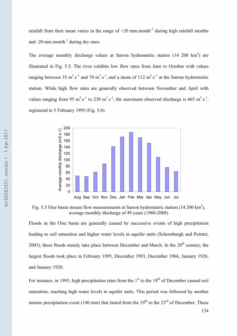
134

rainfall from their mean varies in the range of +20 mm.month-1 during high rainfall months

and -20 mm.month-1 during dry ones.

The average monthly discharge values at Sarron hydrometric station (14 200 km2) are

illustrated in Fig. 5.5. The river exhibits low flow rates from June to October with values

ranging between 35 m3.s-1 and 70 m3.s-1, and a mean of 112 m3.s-1 at the Sarron hydrometric

station. While high flow rates are generally observed between November and April with

values ranging from 95 m3.s-1 to 230 m3.s-1, the maximum observed discharge is 665 m3.s-1,

registered in 5 February 1995 (Fig. 5.6).

020406080

100120140160180200

Aug Sep Oct Nov Dec Jan Feb Mar Apr May Jun Jul

Ave

rage

mon

thly

dis

char

ge (m

3.s-

1)

Fig. 5.5 Oise basin stream flow measurements at Sarron hydrometric station (14 200 km2),

average monthly discharge of 49 years (1960-2008)

Floods in the Oise basin are generally caused by successive events of high precipitation

leading to soil saturation and higher water levels in aquifer units (Schornburgk and Pointet,

2003), these floods mainly take place between December and March. In the 20th century, the

largest floods took place in February 1995, December 1993, December 1966, January 1926,

and January 1920.

For instance, in 1993, high precipitation rates from the 1st to the 18th of December caused soil

saturation, reaching high water levels in aquifer units. This period was followed by another

intense precipitation event (140 mm) that lasted from the 19th to the 23rd of December. These

tel-0

0582

551,

ver

sion

1 -

1 Ap

r 201

1

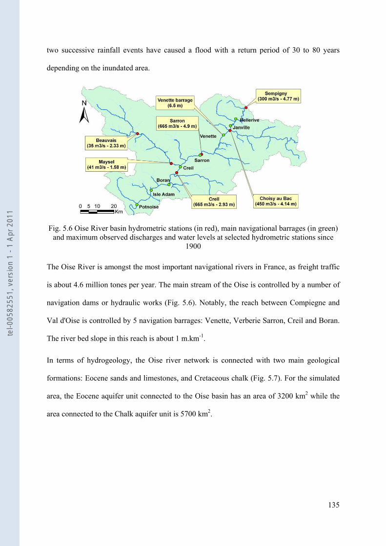
135

two successive rainfall events have caused a flood with a return period of 30 to 80 years

depending on the inundated area.

Fig. 5.6 Oise River basin hydrometric stations (in red), main navigational barrages (in green)

and maximum observed discharges and water levels at selected hydrometric stations since 1900

The Oise River is amongst the most important navigational rivers in France, as freight traffic

is about 4.6 million tones per year. The main stream of the Oise is controlled by a number of

navigation dams or hydraulic works (Fig. 5.6). Notably, the reach between Compiegne and

Val d'Oise is controlled by 5 navigation barrages: Venette, Verberie Sarron, Creil and Boran.

The river bed slope in this reach is about 1 m.km-1.

In terms of hydrogeology, the Oise river network is connected with two main geological

formations: Eocene sands and limestones, and Cretaceous chalk (Fig. 5.7). For the simulated

area, the Eocene aquifer unit connected to the Oise basin has an area of 3200 km2 while the

area connected to the Chalk aquifer unit is 5700 km2.

tel-0

0582

551,

ver

sion

1 -

1 Ap

r 201

1

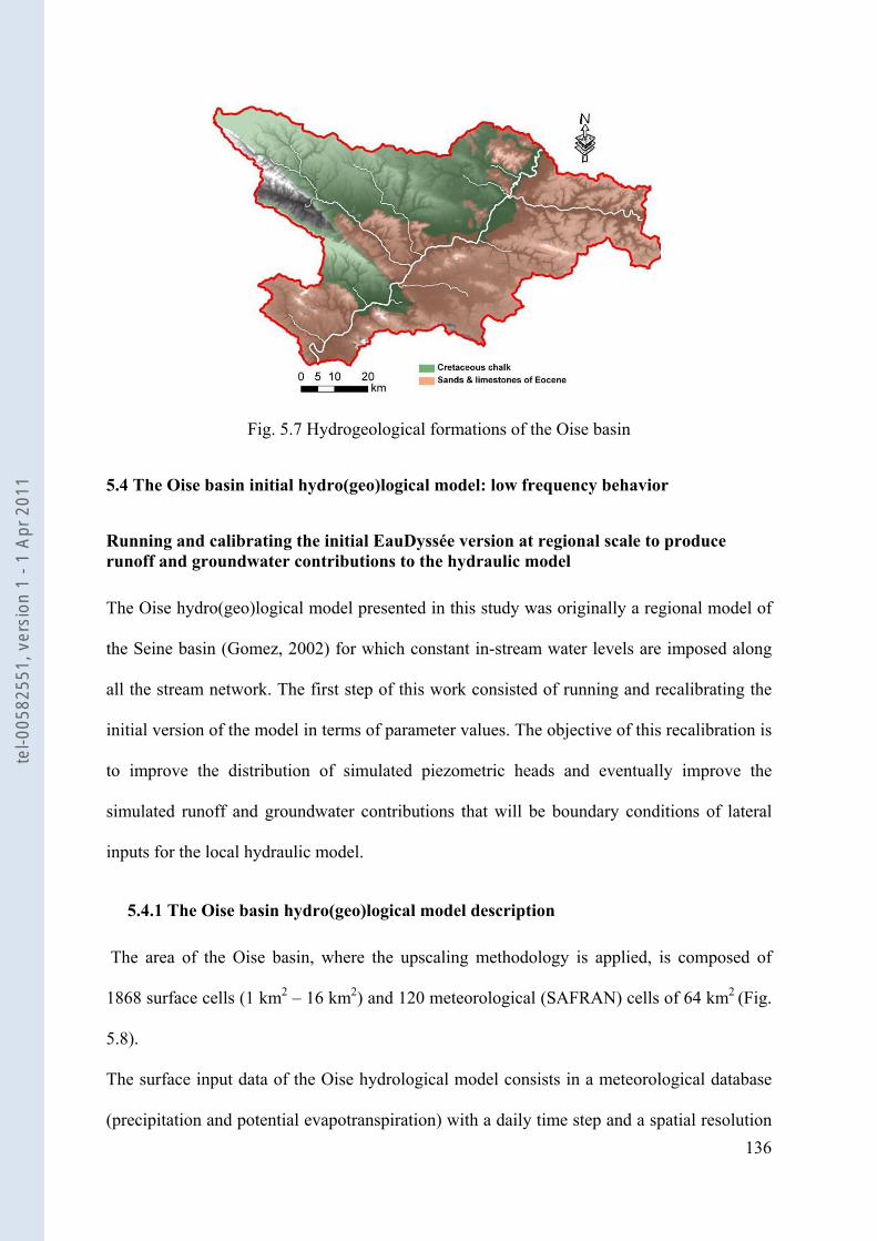
136

Fig. 5.7 Hydrogeological formations of the Oise basin

5.4 The Oise basin initial hydro(geo)logical model: low frequency behavior

Running and calibrating the initial EauDyssée version at regional scale to produce runoff and groundwater contributions to the hydraulic model

The Oise hydro(geo)logical model presented in this study was originally a regional model of

the Seine basin (Gomez, 2002) for which constant in-stream water levels are imposed along

all the stream network. The first step of this work consisted of running and recalibrating the

initial version of the model in terms of parameter values. The objective of this recalibration is

to improve the distribution of simulated piezometric heads and eventually improve the

simulated runoff and groundwater contributions that will be boundary conditions of lateral

inputs for the local hydraulic model.

5.4.1 The Oise basin hydro(geo)logical model description

The area of the Oise basin, where the upscaling methodology is applied, is composed of

1868 surface cells (1 km2 – 16 km2) and 120 meteorological (SAFRAN) cells of 64 km2 (Fig.

5.8).

The surface input data of the Oise hydrological model consists in a meteorological database

(precipitation and potential evapotranspiration) with a daily time step and a spatial resolution

tel-0

0582

551,

ver

sion

1 -

1 Ap

r 201

1

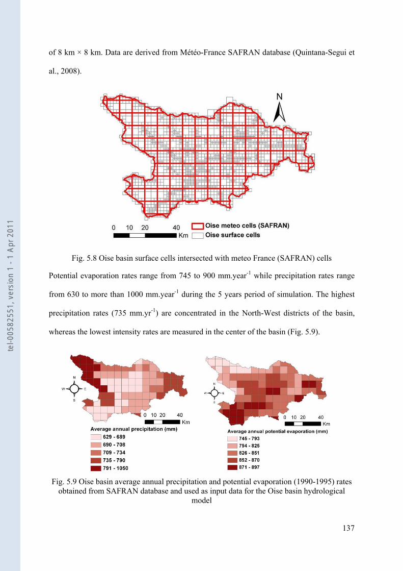
137

of 8 km × 8 km. Data are derived from Météo-France SAFRAN database (Quintana-Segui et

al., 2008).

Fig. 5.8 Oise basin surface cells intersected with meteo France (SAFRAN) cells

Potential evaporation rates range from 745 to 900 mm.year-1 while precipitation rates range

from 630 to more than 1000 mm.year-1 during the 5 years period of simulation. The highest

precipitation rates (735 mm.yr-1) are concentrated in the North-West districts of the basin,

whereas the lowest intensity rates are measured in the center of the basin (Fig. 5.9).

Fig. 5.9 Oise basin average annual precipitation and potential evaporation (1990-1995) rates

obtained from SAFRAN database and used as input data for the Oise basin hydrological model

tel-0

0582

551,

ver

sion

1 -

1 Ap

r 201

1

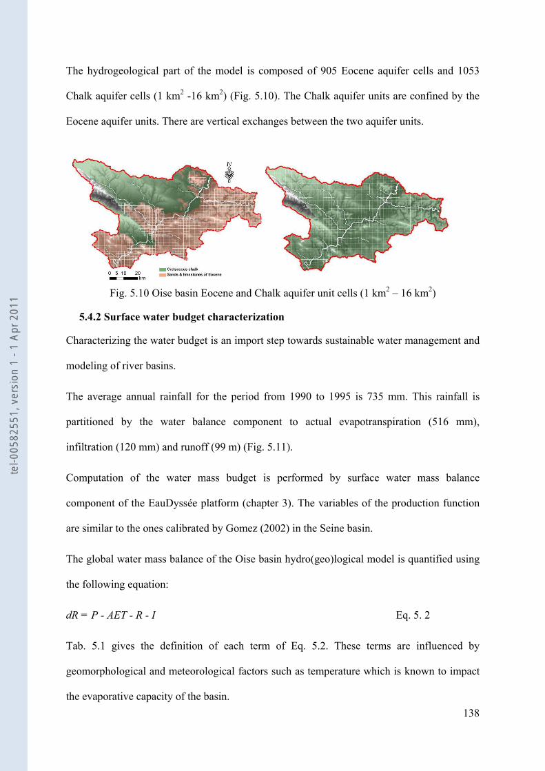
138

The hydrogeological part of the model is composed of 905 Eocene aquifer cells and 1053

Chalk aquifer cells (1 km2 -16 km2) (Fig. 5.10). The Chalk aquifer units are confined by the

Eocene aquifer units. There are vertical exchanges between the two aquifer units.

Fig. 5.10 Oise basin Eocene and Chalk aquifer unit cells (1 km2 – 16 km2)

5.4.2 Surface water budget characterization

Characterizing the water budget is an import step towards sustainable water management and

modeling of river basins.

The average annual rainfall for the period from 1990 to 1995 is 735 mm. This rainfall is

partitioned by the water balance component to actual evapotranspiration (516 mm),

infiltration (120 mm) and runoff (99 m) (Fig. 5.11).

Computation of the water mass budget is performed by surface water mass balance

component of the EauDyssée platform (chapter 3). The variables of the production function

are similar to the ones calibrated by Gomez (2002) in the Seine basin.

The global water mass balance of the Oise basin hydro(geo)logical model is quantified using

the following equation:

dR = P - AET - R - I Eq. 5. 2

Tab. 5.1 gives the definition of each term of Eq. 5.2. These terms are influenced by

geomorphological and meteorological factors such as temperature which is known to impact

the evaporative capacity of the basin.

tel-0

0582

551,

ver

sion

1 -

1 Ap

r 201

1

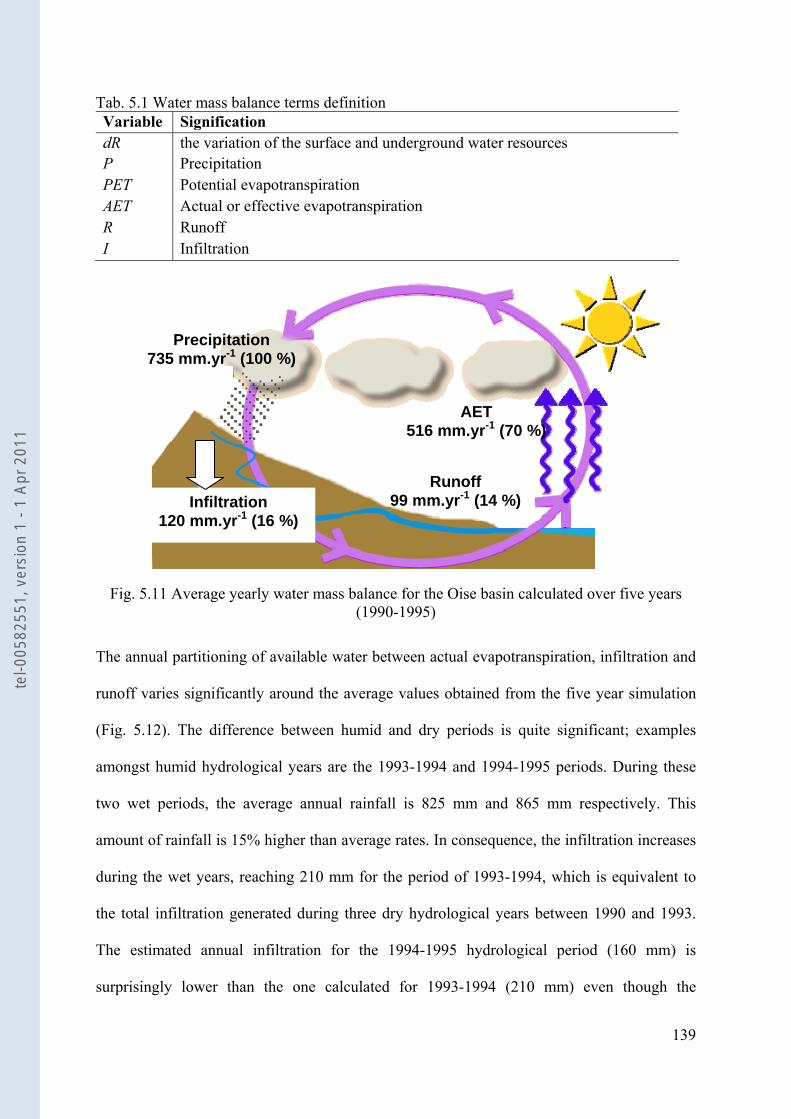
139

Tab. 5.1 Water mass balance terms definition Variable Signification dR the variation of the surface and underground water resources P Precipitation PET Potential evapotranspiration AET Actual or effective evapotranspiration R Runoff I Infiltration

Fig. 5.11 Average yearly water mass balance for the Oise basin calculated over five years

(1990-1995)

The annual partitioning of available water between actual evapotranspiration, infiltration and

runoff varies significantly around the average values obtained from the five year simulation

(Fig. 5.12). The difference between humid and dry periods is quite significant; examples

amongst humid hydrological years are the 1993-1994 and 1994-1995 periods. During these

two wet periods, the average annual rainfall is 825 mm and 865 mm respectively. This

amount of rainfall is 15% higher than average rates. In consequence, the infiltration increases

during the wet years, reaching 210 mm for the period of 1993-1994, which is equivalent to

the total infiltration generated during three dry hydrological years between 1990 and 1993.

The estimated annual infiltration for the 1994-1995 hydrological period (160 mm) is

surprisingly lower than the one calculated for 1993-1994 (210 mm) even though the

Infiltration 120 mm.yr-1 (16 %)

Runoff 99 mm.yr-1 (14 %)

AET 516 mm.yr-1 (70 %)

Precipitation 735 mm.yr-1 (100 %)

tel-0

0582

551,

ver

sion

1 -

1 Ap

r 201

1

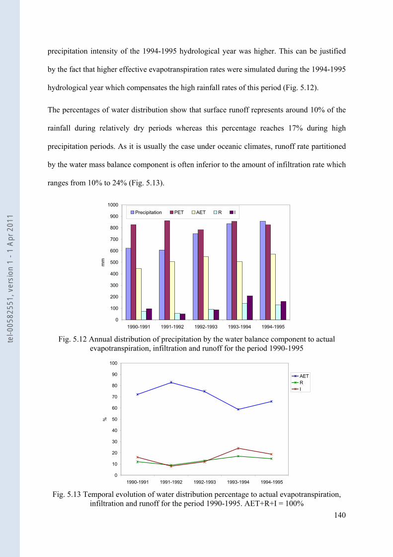
140

precipitation intensity of the 1994-1995 hydrological year was higher. This can be justified

by the fact that higher effective evapotranspiration rates were simulated during the 1994-1995

hydrological year which compensates the high rainfall rates of this period (Fig. 5.12).

The percentages of water distribution show that surface runoff represents around 10% of the

rainfall during relatively dry periods whereas this percentage reaches 17% during high

precipitation periods. As it is usually the case under oceanic climates, runoff rate partitioned

by the water mass balance component is often inferior to the amount of infiltration rate which

ranges from 10% to 24% (Fig. 5.13).

0

100

200

300

400

500

600

700

800

900

1000

1990-1991 1991-1992 1992-1993 1993-1994 1994-1995

mm

Precipitation PET AET R I

Fig. 5.12 Annual distribution of precipitation by the water balance component to actual

evapotranspiration, infiltration and runoff for the period 1990-1995

0

10

20

30

40

50

60

70

80

90

100

1990-1991 1991-1992 1992-1993 1993-1994 1994-1995

%

AETRI

Fig. 5.13 Temporal evolution of water distribution percentage to actual evapotranspiration,

infiltration and runoff for the period 1990-1995. AET+R+I = 100%

tel-0

0582

551,

ver

sion

1 -

1 Ap

r 201

1

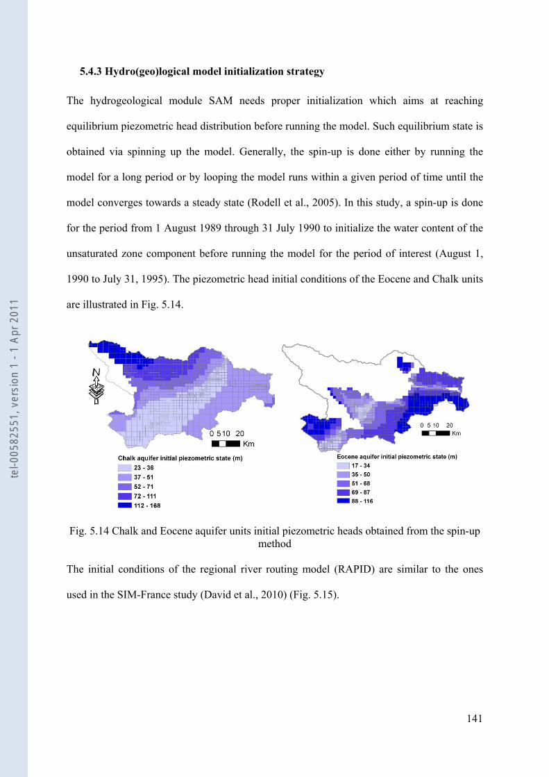
141

5.4.3 Hydro(geo)logical model initialization strategy

The hydrogeological module SAM needs proper initialization which aims at reaching

equilibrium piezometric head distribution before running the model. Such equilibrium state is

obtained via spinning up the model. Generally, the spin-up is done either by running the

model for a long period or by looping the model runs within a given period of time until the

model converges towards a steady state (Rodell et al., 2005). In this study, a spin-up is done

for the period from 1 August 1989 through 31 July 1990 to initialize the water content of the

unsaturated zone component before running the model for the period of interest (August 1,

1990 to July 31, 1995). The piezometric head initial conditions of the Eocene and Chalk units

are illustrated in Fig. 5.14.

Fig. 5.14 Chalk and Eocene aquifer units initial piezometric heads obtained from the spin-up method

The initial conditions of the regional river routing model (RAPID) are similar to the ones

used in the SIM-France study (David et al., 2010) (Fig. 5.15).

tel-0

0582

551,

ver

sion

1 -

1 Ap

r 201

1

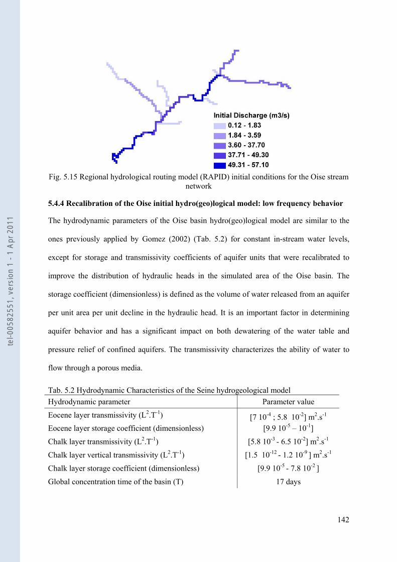
142

Fig. 5.15 Regional hydrological routing model (RAPID) initial conditions for the Oise stream

network

5.4.4 Recalibration of the Oise initial hydro(geo)logical model: low frequency behavior

The hydrodynamic parameters of the Oise basin hydro(geo)logical model are similar to the

ones previously applied by Gomez (2002) (Tab. 5.2) for constant in-stream water levels,

except for storage and transmissivity coefficients of aquifer units that were recalibrated to

improve the distribution of hydraulic heads in the simulated area of the Oise basin. The

storage coefficient (dimensionless) is defined as the volume of water released from an aquifer

per unit area per unit decline in the hydraulic head. It is an important factor in determining

aquifer behavior and has a significant impact on both dewatering of the water table and

pressure relief of confined aquifers. The transmissivity characterizes the ability of water to

flow through a porous media.

Tab. 5.2 Hydrodynamic Characteristics of the Seine hydrogeological model Hydrodynamic parameter Parameter value

Eocene layer transmissivity (L2.T-1) [7 10-4 ; 5.8 10-2] m2.s-1 Eocene layer storage coefficient (dimensionless) [9.9 10-5 – 10-1]

Chalk layer transmissivity (L2.T-1) [5.8 10-3 - 6.5 10-2] m2.s-1

Chalk layer vertical transmissivity (L2.T-1) [1.5 10-12 - 1.2 10-9 ] m2.s-1

Chalk layer storage coefficient (dimensionless) [9.9 10-5 - 7.8 10-2 ]

Global concentration time of the basin (T) 17 days

tel-0

0582

551,

ver

sion

1 -

1 Ap

r 201

1

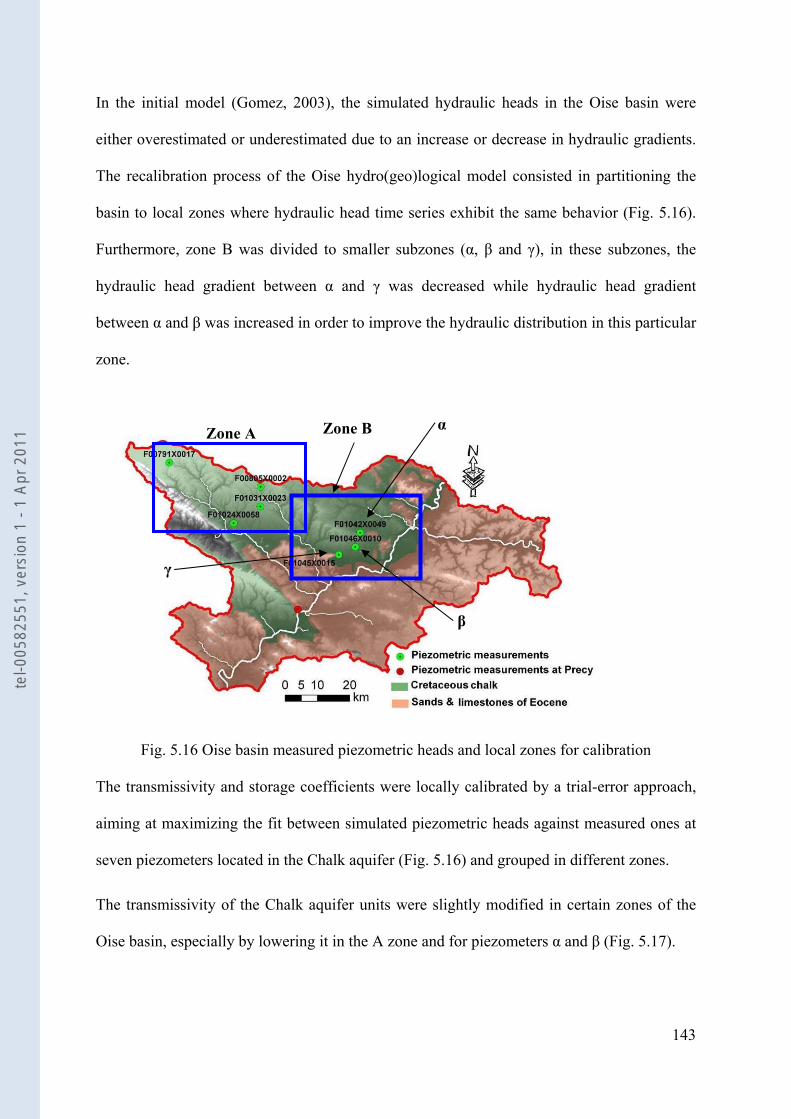
143

In the initial model (Gomez, 2003), the simulated hydraulic heads in the Oise basin were

either overestimated or underestimated due to an increase or decrease in hydraulic gradients.

The recalibration process of the Oise hydro(geo)logical model consisted in partitioning the

basin to local zones where hydraulic head time series exhibit the same behavior (Fig. 5.16).

Furthermore, zone B was divided to smaller subzones (α, β and γ), in these subzones, the

hydraulic head gradient between α and γ was decreased while hydraulic head gradient

between α and β was increased in order to improve the hydraulic distribution in this particular

zone.

Fig. 5.16 Oise basin measured piezometric heads and local zones for calibration The transmissivity and storage coefficients were locally calibrated by a trial-error approach,

aiming at maximizing the fit between simulated piezometric heads against measured ones at

seven piezometers located in the Chalk aquifer (Fig. 5.16) and grouped in different zones.

The transmissivity of the Chalk aquifer units were slightly modified in certain zones of the

Oise basin, especially by lowering it in the A zone and for piezometers α and β (Fig. 5.17).

Zone B Zone A α

β

γ

tel-0

0582

551,

ver

sion

1 -

1 Ap

r 201

1

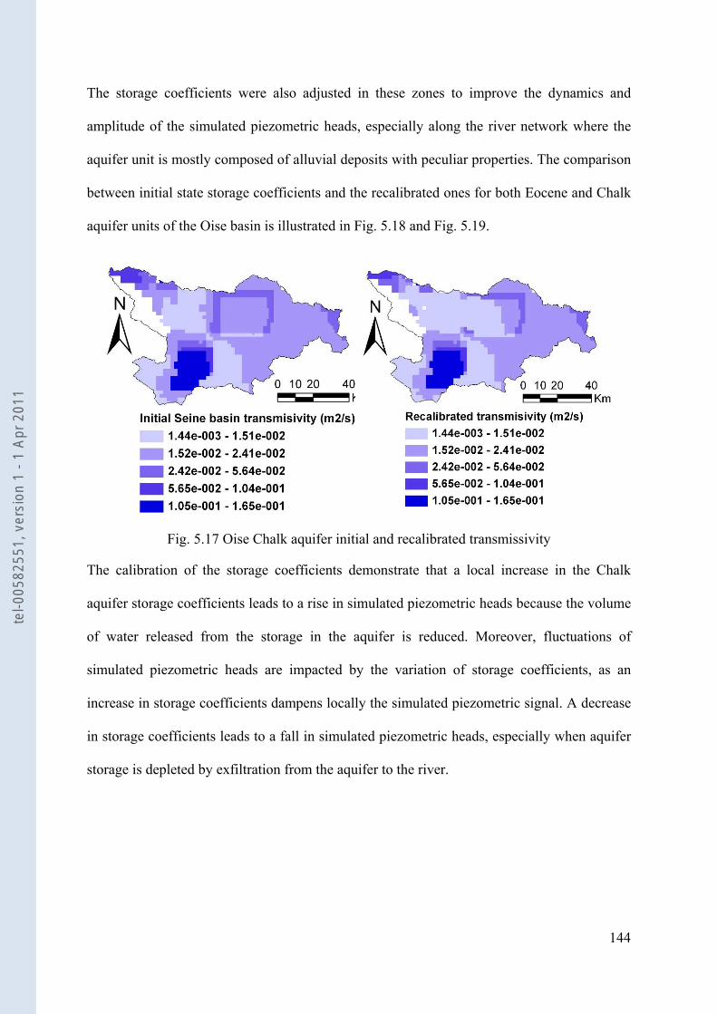
144

The storage coefficients were also adjusted in these zones to improve the dynamics and

amplitude of the simulated piezometric heads, especially along the river network where the

aquifer unit is mostly composed of alluvial deposits with peculiar properties. The comparison

between initial state storage coefficients and the recalibrated ones for both Eocene and Chalk

aquifer units of the Oise basin is illustrated in Fig. 5.18 and Fig. 5.19.

Fig. 5.17 Oise Chalk aquifer initial and recalibrated transmissivity

The calibration of the storage coefficients demonstrate that a local increase in the Chalk

aquifer storage coefficients leads to a rise in simulated piezometric heads because the volume

of water released from the storage in the aquifer is reduced. Moreover, fluctuations of

simulated piezometric heads are impacted by the variation of storage coefficients, as an

increase in storage coefficients dampens locally the simulated piezometric signal. A decrease

in storage coefficients leads to a fall in simulated piezometric heads, especially when aquifer

storage is depleted by exfiltration from the aquifer to the river.

tel-0

0582

551,

ver

sion

1 -

1 Ap

r 201

1

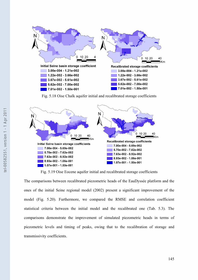
145

Fig. 5.18 Oise Chalk aquifer initial and recalibrated storage coefficients

Fig. 5.19 Oise Eocene aquifer initial and recalibrated storage coefficients

The comparisons between recalibrated piezometric heads of the EauDyssée platform and the

ones of the initial Seine regional model (2002) present a significant improvement of the

model (Fig. 5.20). Furthermore, we compared the RMSE and correlation coefficient

statistical criteria between the initial model and the recalibrated one (Tab. 5.3). The

comparisons demonstrate the improvement of simulated piezometric heads in terms of

piezometric levels and timing of peaks, owing that to the recalibration of storage and

transmissivity coefficients.

tel-0

0582

551,

ver

sion

1 -

1 Ap

r 201

1

146

Tab. 5.3 Comparison of statistical criteria between EauDyssée recalibrated piezometric heads and piezometric heads obtained in the Seine regional model Initial model Recalibrated model Station code Number of

observations (days)

Average observed

(m)

Average simulated

(m)

RMSE (m)

R (%)

Average simulated

(m)

RMSE (m)

R (%)

F00791X0017 1576 162.11 157.54 4.9 0.81 161.611 1.794 0.86 F00805X0002 1592 119.39 113.36 6.4 0.481 120.2 1.473 0.918 F01042X0049 1408 60.15 57.76 2.5 0.922 60.02 0.67 0.93 F01045X0015 225 38.5 49.36 10.9 NA 38.53 1.5 NA F01024X0058 1576 77.35 73.88 4 0.941 75.1 3.042 0.813 F01046X0010 1606 51.46 47.25 4.5 0.779 50.9 1.82 0.716

Finally, the average aquifer piezometric heads were calculated for the whole period of

simulation (Fig. 5.21). The steep piezometric gradients of both Chalk and Eocene aquifer

units near to the main stream suggest that the movement of water is directed towards the Oise

river and eventually the output of the basin. The figures also show that piezometric heads are

generally correlated with topography for surface aquifer units.

tel-0

0582

551,

ver

sion

1 -

1 Ap

r 201

1

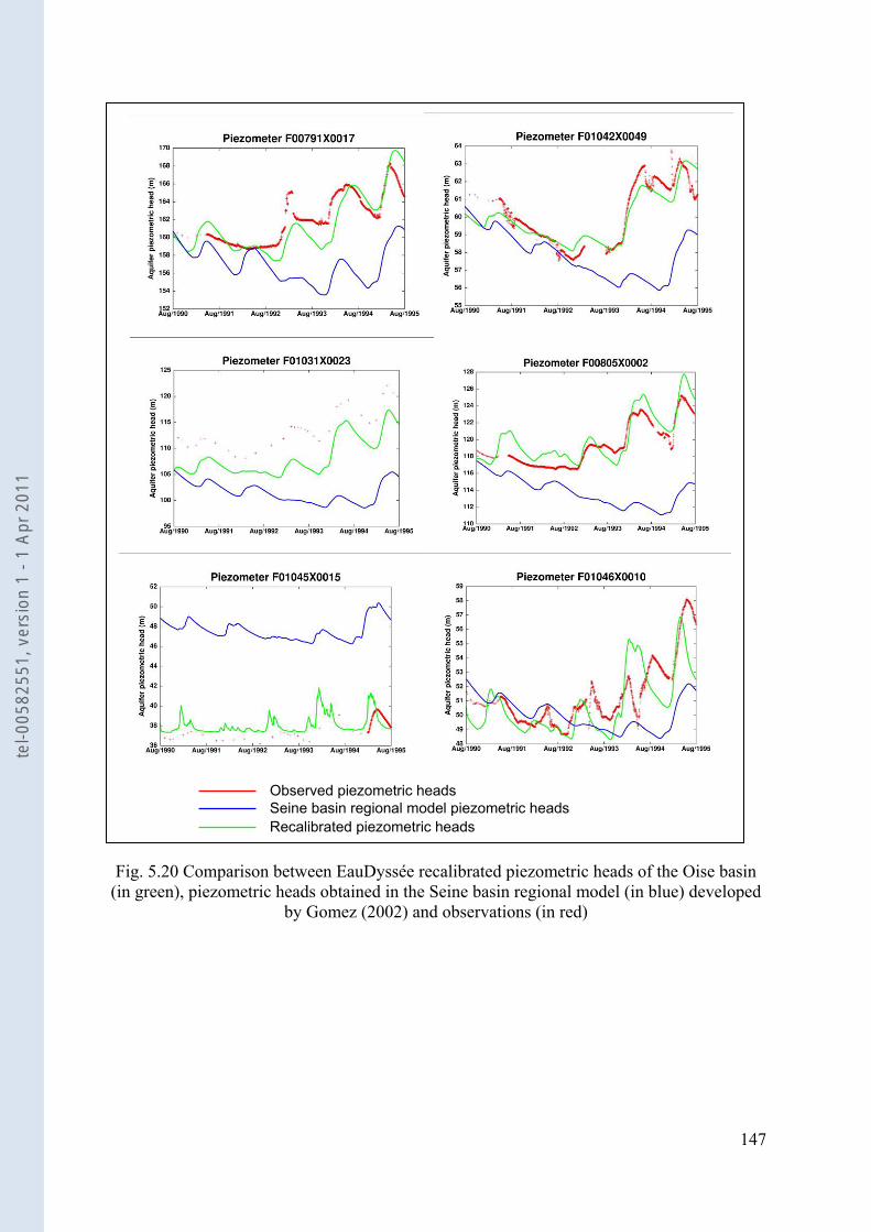
147

Fig. 5.20 Comparison between EauDyssée recalibrated piezometric heads of the Oise basin (in green), piezometric heads obtained in the Seine basin regional model (in blue) developed

by Gomez (2002) and observations (in red)

Observed piezometric heads Seine basin regional model piezometric heads Recalibrated piezometric heads

tel-0

0582

551,

ver

sion

1 -

1 Ap

r 201

1

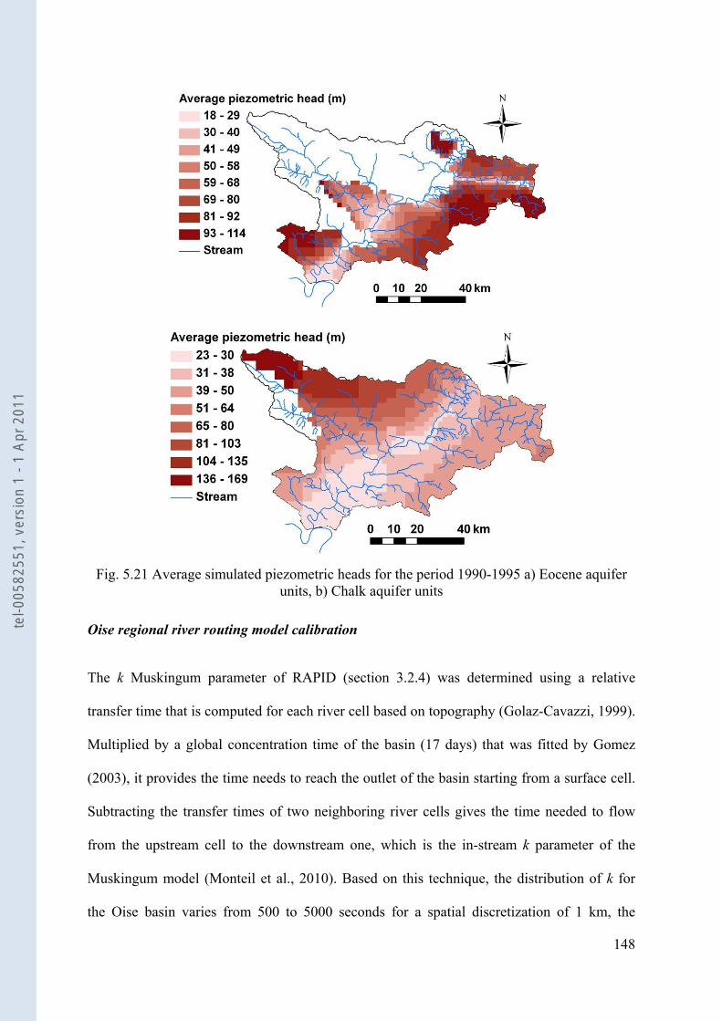
148

Fig. 5.21 Average simulated piezometric heads for the period 1990-1995 a) Eocene aquifer

units, b) Chalk aquifer units

Oise regional river routing model calibration

The k Muskingum parameter of RAPID (section 3.2.4) was determined using a relative

transfer time that is computed for each river cell based on topography (Golaz-Cavazzi, 1999).

Multiplied by a global concentration time of the basin (17 days) that was fitted by Gomez

(2003), it provides the time needs to reach the outlet of the basin starting from a surface cell.

Subtracting the transfer times of two neighboring river cells gives the time needed to flow

from the upstream cell to the downstream one, which is the in-stream k parameter of the

Muskingum model (Monteil et al., 2010). Based on this technique, the distribution of k for

the Oise basin varies from 500 to 5000 seconds for a spatial discretization of 1 km, the

tel-0

0582

551,

ver

sion

1 -

1 Ap

r 201

1

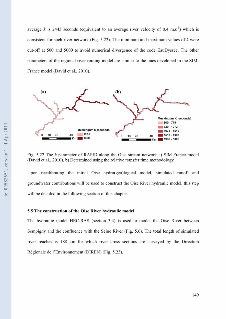
149

average k is 2443 seconds (equivalent to an average river velocity of 0.4 m.s-1) which is

consistent for such river network (Fig. 5.22). The minimum and maximum values of k were

cut-off at 500 and 5000 to avoid numerical divergence of the code EauDyssée. The other

parameters of the regional river routing model are similar to the ones developed in the SIM-

France model (David et al., 2010).

Fig. 5.22 The k parameter of RAPID along the Oise stream network a) SIM-France model (David et al., 2010), b) Determined using the relative transfer time methodology

Upon recalibrating the initial Oise hydro(geo)logical model, simulated runoff and

groundwater contributions will be used to construct the Oise River hydraulic model, this step

will be detailed in the following section of this chapter.

5.5 The construction of the Oise River hydraulic model

The hydraulic model HEC-RAS (section 3.4) is used to model the Oise River between

Sempigny and the confluence with the Seine River (Fig. 5.6). The total length of simulated

river reaches is 188 km for which river cross sections are surveyed by the Direction

Régionale de l’Environnement (DIREN) (Fig. 5.23).

(a) (b)

tel-0

0582

551,

ver

sion

1 -

1 Ap

r 201

1

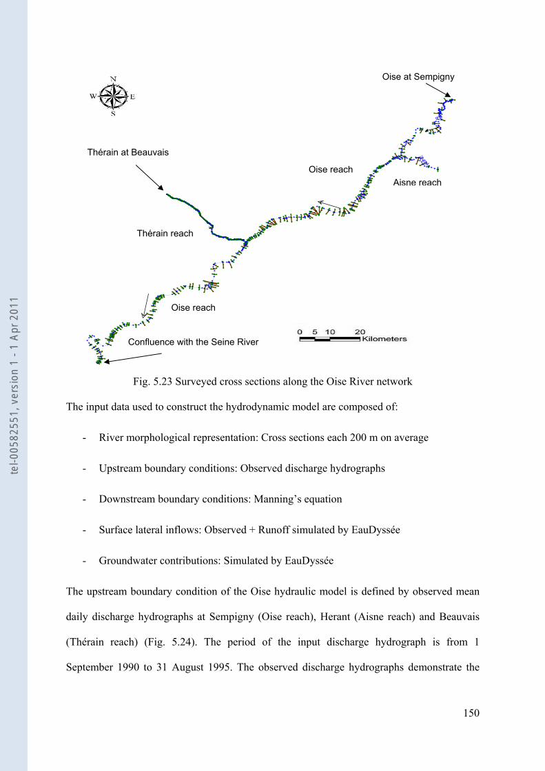
150

Fig. 5.23 Surveyed cross sections along the Oise River network

The input data used to construct the hydrodynamic model are composed of:

- River morphological representation: Cross sections each 200 m on average

- Upstream boundary conditions: Observed discharge hydrographs

- Downstream boundary conditions: Manning’s equation

- Surface lateral inflows: Observed + Runoff simulated by EauDyssée

- Groundwater contributions: Simulated by EauDyssée

The upstream boundary condition of the Oise hydraulic model is defined by observed mean

daily discharge hydrographs at Sempigny (Oise reach), Herant (Aisne reach) and Beauvais

(Thérain reach) (Fig. 5.24). The period of the input discharge hydrograph is from 1

September 1990 to 31 August 1995. The observed discharge hydrographs demonstrate the

AISNE_OISE

AISNE

OISE_AISNE

O IS

E

OISE_SEINEOISE

OISE_Seine2

Oi se

Therain_Oise

Ther ai n

Oise reach

Oise reach

Oise at Sempigny

Aisne reach

Thérain at Beauvais

Confluence with the Seine River

Thérain reach

tel-0

0582

551,

ver

sion

1 -

1 Ap

r 201

1

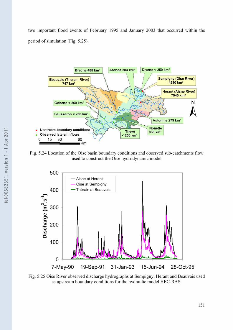
151

two important flood events of February 1995 and January 2003 that occurred within the

period of simulation (Fig. 5.25).

Fig. 5.24 Location of the Oise basin boundary conditions and observed sub-catchments flow used to construct the Oise hydrodynamic model

0

100

200

300

400

500

7-May-90 19-Sep-91 31-Jan-93 15-Jun-94 28-Oct-95

Dis

char

ge (m

3 .s-1

)

Aisne at HerantOise at SempignyThérain at Beauvais

Fig. 5.25 Oise River observed discharge hydrographs at Sempigny, Herant and Beauvais used

as upstream boundary conditions for the hydraulic model HEC-RAS.

tel-0

0582

551,

ver

sion

1 -

1 Ap

r 201

1

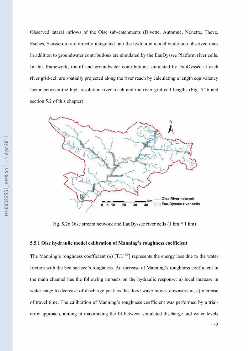
152

Observed lateral inflows of the Oise sub-catchments (Divette, Automne, Nonette, Theve,

Esches, Sausseron) are directly integrated into the hydraulic model while non observed ones

in addition to groundwater contributions are simulated by the EauDyssée Platform river cells.

In this framework, runoff and groundwater contributions simulated by EauDyssée at each

river grid-cell are spatially projected along the river reach by calculating a length equivalency

factor between the high resolution river reach and the river grid-cell lengths (Fig. 5.26 and

section 5.2 of this chapter).

Fig. 5.26 Oise stream network and EauDyssée river cells (1 km * 1 km)

5.5.1 Oise hydraulic model calibration of Manning’s roughness coefficient

The Manning’s roughness coefficient (n) [T.L-1/3] represents the energy loss due to the water

friction with the bed surface’s roughness. An increase of Manning’s roughness coefficient in

the main channel has the following impacts on the hydraulic response: a) local increase in

water stage b) decrease of discharge peak as the flood wave moves downstream, c) increase

of travel time. The calibration of Manning’s roughness coefficient was performed by a trial-

error approach, aiming at maximizing the fit between simulated discharge and water levels

tel-0

0582

551,

ver

sion

1 -

1 Ap

r 201

1

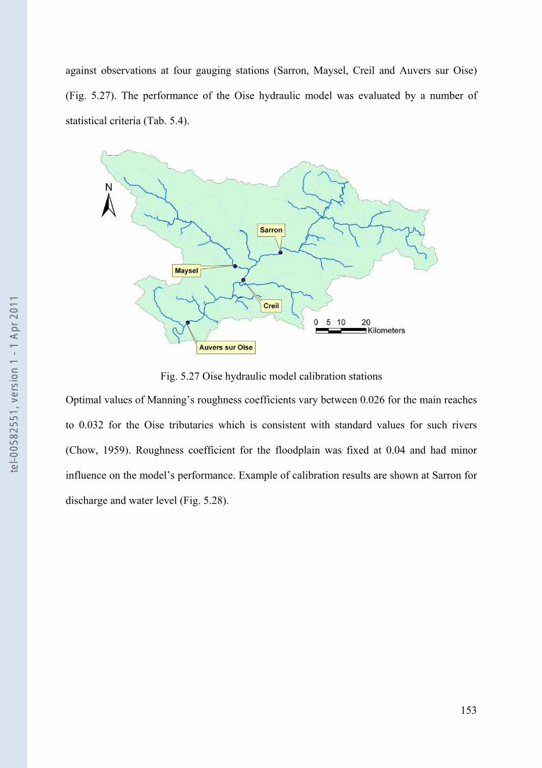
153

against observations at four gauging stations (Sarron, Maysel, Creil and Auvers sur Oise)

(Fig. 5.27). The performance of the Oise hydraulic model was evaluated by a number of

statistical criteria (Tab. 5.4).

Fig. 5.27 Oise hydraulic model calibration stations

Optimal values of Manning’s roughness coefficients vary between 0.026 for the main reaches

to 0.032 for the Oise tributaries which is consistent with standard values for such rivers

(Chow, 1959). Roughness coefficient for the floodplain was fixed at 0.04 and had minor

influence on the model’s performance. Example of calibration results are shown at Sarron for

discharge and water level (Fig. 5.28).

tel-0

0582

551,

ver

sion

1 -

1 Ap

r 201

1

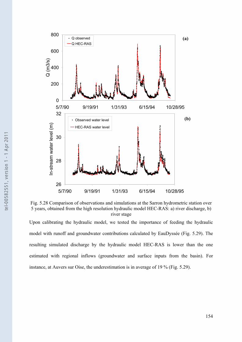
154

Fig. 5.28 Comparison of observations and simulations at the Sarron hydrometric station over 5 years, obtained from the high resolution hydraulic model HEC-RAS: a) river discharge, b)

river stage

Upon calibrating the hydraulic model, we tested the importance of feeding the hydraulic

model with runoff and groundwater contributions calculated by EauDyssée (Fig. 5.29). The

resulting simulated discharge by the hydraulic model HEC-RAS is lower than the one

estimated with regional inflows (groundwater and surface inputs from the basin). For

instance, at Auvers sur Oise, the underestimation is in average of 19 % (Fig. 5.29).

0

200

400

600

800

5/7/90 9/19/91 1/31/93 6/15/94 10/28/95

Q (m

3/s)

Q observedQ HEC-RAS

26

28

30

32

5/7/90 9/19/91 1/31/93 6/15/94 10/28/95

In-s

tream

wat

er le

vel (

m) Observed water level

HEC-RAS water level

(a)

(b)

tel-0

0582

551,

ver

sion

1 -

1 Ap

r 201

1

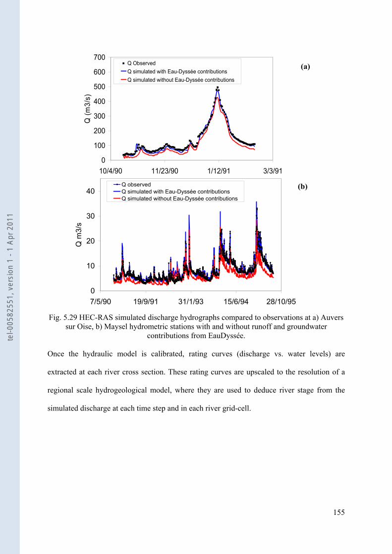
155

Fig. 5.29 HEC-RAS simulated discharge hydrographs compared to observations at a) Auvers sur Oise, b) Maysel hydrometric stations with and without runoff and groundwater

contributions from EauDyssée. Once the hydraulic model is calibrated, rating curves (discharge vs. water levels) are

extracted at each river cross section. These rating curves are upscaled to the resolution of a

regional scale hydrogeological model, where they are used to deduce river stage from the

simulated discharge at each time step and in each river grid-cell.

0

100

200

300

400

500

600

700

10/4/90 11/23/90 1/12/91 3/3/91

Q (m

3/s)

Q ObservedQ simulated with Eau-Dyssée contributionsQ simulated without Eau-Dyssée contributions

(a)

(b)

0

10

20

30

40

7/5/90 19/9/91 31/1/93 15/6/94 28/10/95

Q m

3/s

Q observedQ simulated with Eau-Dyssée contributionsQ simulated without Eau-Dyssée contributions

tel-0

0582

551,

ver

sion

1 -

1 Ap

r 201

1

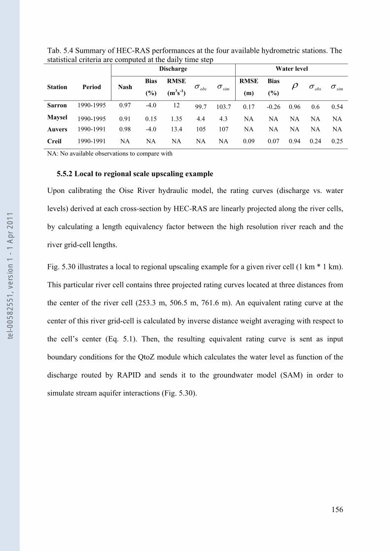
156

Tab. 5.4 Summary of HEC-RAS performances at the four available hydrometric stations. The statistical criteria are computed at the daily time step

Discharge Water level

Station Period Nash Bias

(%)

RMSE

(m3s-1) obsσ simσ

RMSE

(m)

Bias

(%) ρ obsσ simσ

Sarron 1990-1995 0.97 -4.0 12 99.7 103.7 0.17 -0.26 0.96 0.6 0.54 Maysel 1990-1995 0.91 0.15 1.35 4.4 4.3 NA NA NA NA NA Auvers 1990-1991 0.98 -4.0 13.4 105 107 NA NA NA NA NA

Creil 1990-1991 NA NA NA NA NA 0.09 0.07 0.94 0.24 0.25

NA: No available observations to compare with

5.5.2 Local to regional scale upscaling example

Upon calibrating the Oise River hydraulic model, the rating curves (discharge vs. water

levels) derived at each cross-section by HEC-RAS are linearly projected along the river cells,

by calculating a length equivalency factor between the high resolution river reach and the

river grid-cell lengths.

Fig. 5.30 illustrates a local to regional upscaling example for a given river cell (1 km * 1 km).

This particular river cell contains three projected rating curves located at three distances from

the center of the river cell (253.3 m, 506.5 m, 761.6 m). An equivalent rating curve at the

center of this river grid-cell is calculated by inverse distance weight averaging with respect to

the cell’s center (Eq. 5.1). Then, the resulting equivalent rating curve is sent as input

boundary conditions for the QtoZ module which calculates the water level as function of the

discharge routed by RAPID and sends it to the groundwater model (SAM) in order to

simulate stream aquifer interactions (Fig. 5.30).

tel-0

0582

551,

ver

sion

1 -

1 Ap

r 201

1

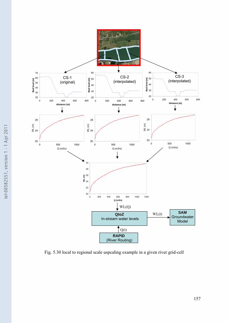
157

Fig. 5.30 local to regional scale uspcaling example in a given river grid-cell

20

30

40

50

60

0 200 400 600 800distance (m)

Bed

leve

l (m

)

20

30

40

50

60

0 200 400 600 800distance (m)

Bed

leve

l (m

)

20

30

40

50

60

70

0 200 400 600 800distance (m)

Bed

leve

l (m

)

20

24

28

0 500 1000Q (m3/s)

WL

(m)

20

24

28

0 500 1000Q (m3/s)

WL

(m)

20

24

28

0 500 1000Q (m3/s)

WL

(m)

20

22

24

26

28

30

0 200 400 600 800 1000 1200Q (m3/s)

WL

(m)

CS-2 (interpolated)

SAM Groundwater

Model


QtoZ In-stream water levels

Q(t)

WL(t)

CS-3 (interpolated)

CS-1 (original)

WL(Q)

tel-0

0582

551,

ver

sion

1 -

1 Ap

r 201

1

158

5.6 EauDyssée simulations after applying the upscaling methodology

5.6.1 Simulated discharge and river stage by the regional hydro(geo)logical model EauDyssée

Discharge and water level hydrographs are simulated by the regional model EauDyssée after

implementing the new methodology of in-stream water level fluctuations.

In-stream discharges and water levels simulated by EauDyssée are visually in agreement with

observations in terms of hydrograph shape and timing of peaks albeit the model tends to

overestimate discharge peaks due to overestimation produced by the Seine regional model

upstream of the simulated area (e.g. at Sarron, Fig. 5.31). Indeed in-stream boundary

conditions for the Oise and its tributaries are given by EauDyssée applied over the whole

Seine basin (Gomez et al., 2003), whereas we used observed hydrographs for the HEC-RAS

simulation. To prove that overestimation is due to upstream boundary condition discharge,

we have imposed observed discharge hydrographs similar to the ones used to construct the

hydraulic model (HEC-RAS) upstream boundary conditions instead of discharge hydrographs

produced by the regional Seine model (Fig. 5.25). The comparison between the two

simulations demonstrates the impact of upstream boundary conditions on the quality of

simulated discharge and water levels, especially during high flow periods (Fig. 5.31).

Nevertheless, the Nash and bias criteria of the simulated discharge at Sarron station remain

satisfactory when using boundary conditions given by EauDyssée applied over the whole

Seine basin, equal to 0.85 and 6%, respectively (Tab. 5.5).

The overestimation in the Seine regional model upstream of the simulated area is most likely

due to a not optimal calibration of the upstream production units.

tel-0

0582

551,

ver

sion

1 -

1 Ap

r 201

1

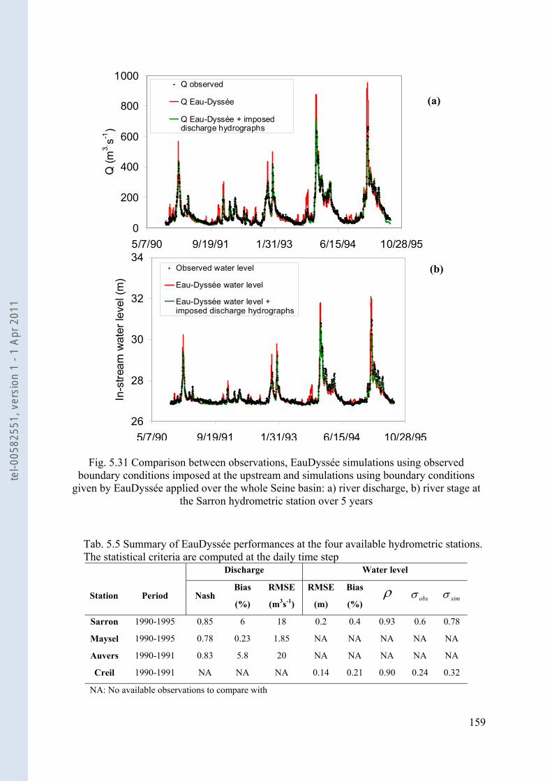
159

Fig. 5.31 Comparison between observations, EauDyssée simulations using observed boundary conditions imposed at the upstream and simulations using boundary conditions

given by EauDyssée applied over the whole Seine basin: a) river discharge, b) river stage at the Sarron hydrometric station over 5 years

Tab. 5.5 Summary of EauDyssée performances at the four available hydrometric stations. The statistical criteria are computed at the daily time step

Discharge Water level

Station Period Nash Bias

(%)

RMSE

(m3s-1)

RMSE

(m)

Bias

(%) ρ obsσ simσ

Sarron 1990-1995 0.85 6 18 0.2 0.4 0.93 0.6 0.78

Maysel 1990-1995 0.78 0.23 1.85 NA NA NA NA NA

Auvers 1990-1991 0.83 5.8 20 NA NA NA NA NA

Creil 1990-1991 NA NA NA 0.14 0.21 0.90 0.24 0.32

NA: No available observations to compare with

26

28

30

32

34

5/7/90 9/19/91 1/31/93 6/15/94 10/28/95

In-s

tream

wat

er le

vel (

m)

Observed water level

Eau-Dyssée water level

Eau-Dyssée water level +imposed discharge hydrographs

0

200

400

600

800

1000

5/7/90 9/19/91 1/31/93 6/15/94 10/28/95

Q (m

3.s-1

)

Q observed

Q Eau-Dyssée

Q Eau-Dyssée + imposeddischarge hydrographs

(a)

(b)

tel-0

0582

551,

ver

sion

1 -

1 Ap

r 201

1

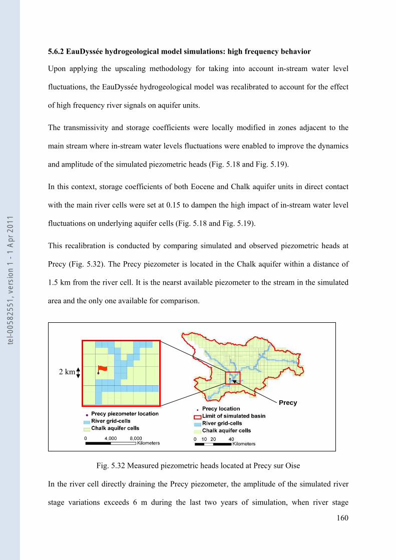
160

5.6.2 EauDyssée hydrogeological model simulations: high frequency behavior

Upon applying the upscaling methodology for taking into account in-stream water level

fluctuations, the EauDyssée hydrogeological model was recalibrated to account for the effect

of high frequency river signals on aquifer units.

The transmissivity and storage coefficients were locally modified in zones adjacent to the

main stream where in-stream water levels fluctuations were enabled to improve the dynamics

and amplitude of the simulated piezometric heads (Fig. 5.18 and Fig. 5.19).

In this context, storage coefficients of both Eocene and Chalk aquifer units in direct contact

with the main river cells were set at 0.15 to dampen the high impact of in-stream water level

fluctuations on underlying aquifer cells (Fig. 5.18 and Fig. 5.19).

This recalibration is conducted by comparing simulated and observed piezometric heads at

Precy (Fig. 5.32). The Precy piezometer is located in the Chalk aquifer within a distance of

1.5 km from the river cell. It is the nearst available piezometer to the stream in the simulated

area and the only one available for comparison.

Fig. 5.32 Measured piezometric heads located at Precy sur Oise

In the river cell directly draining the Precy piezometer, the amplitude of the simulated river

stage variations exceeds 6 m during the last two years of simulation, when river stage

2 km

Precy

tel-0

0582

551,

ver

sion

1 -

1 Ap

r 201

1

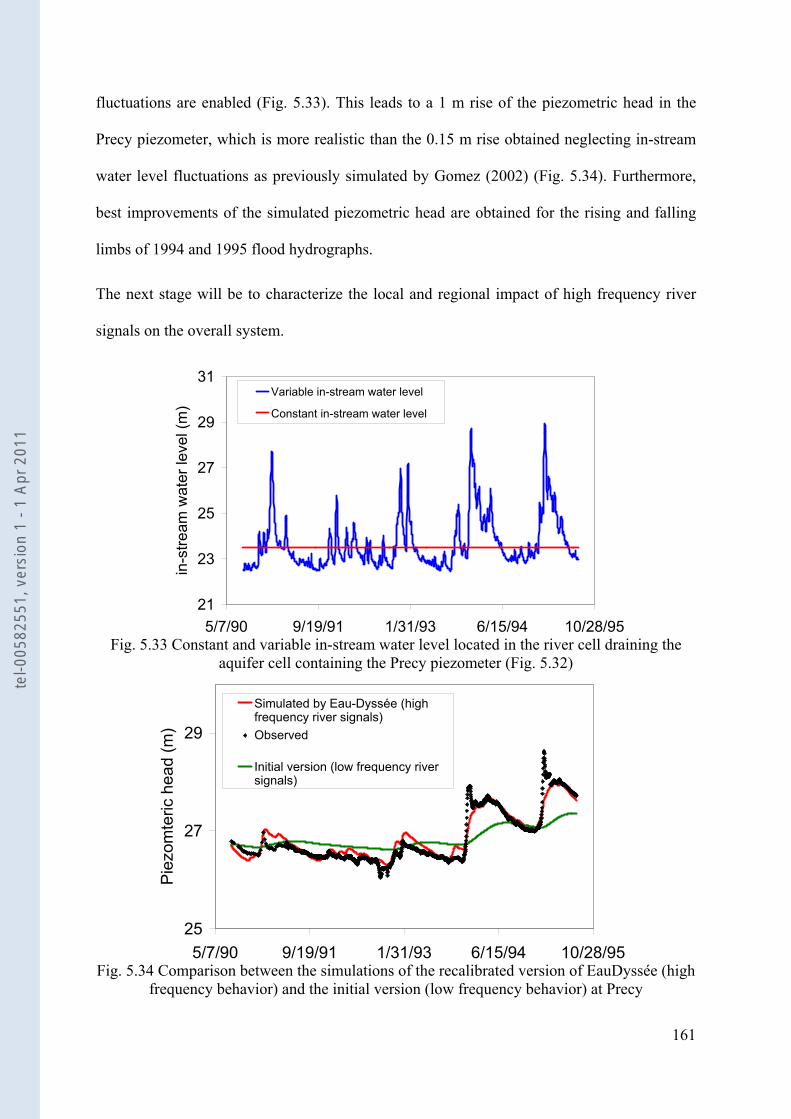
161

fluctuations are enabled (Fig. 5.33). This leads to a 1 m rise of the piezometric head in the

Precy piezometer, which is more realistic than the 0.15 m rise obtained neglecting in-stream

water level fluctuations as previously simulated by Gomez (2002) (Fig. 5.34). Furthermore,

best improvements of the simulated piezometric head are obtained for the rising and falling

limbs of 1994 and 1995 flood hydrographs.

The next stage will be to characterize the local and regional impact of high frequency river

signals on the overall system.

21

23

25

27

29

31

5/7/90 9/19/91 1/31/93 6/15/94 10/28/95

in-s

tream

wat

er le

vel (

m)

Variable in-stream water level

Constant in-stream water level

Fig. 5.33 Constant and variable in-stream water level located in the river cell draining the

aquifer cell containing the Precy piezometer (Fig. 5.32)

25

27

29

5/7/90 9/19/91 1/31/93 6/15/94 10/28/95

Pie

zom

teric

hea

d (m

)

Simulated by Eau-Dyssée (highfrequency river signals)Observed

Initial version (low frequency riversignals)

Fig. 5.34 Comparison between the simulations of the recalibrated version of EauDyssée (high

frequency behavior) and the initial version (low frequency behavior) at Precy

tel-0

0582

551,

ver

sion

1 -

1 Ap

r 201

1

162

5.7 Impact of in-stream water level fluctuations on stream-aquifer interactions at local and regional scale

In this part of the study, the impacts of in-stream water level fluctuations and Qmax (section

3.2.5) on the aquifer system are characterized at local and regional scale comparing four

EauDyssée simulations summarized in Tab. 5.6.

Tab. 5.6 Overview of the main EauDyssée simulations to characterize the impact of in-stream water level fluctuations on stream-aquifer interactions Simulation name C0 C100 V0 V100

In-stream water level Constant Constant Variable Variable

Qmax (l s-1) 0 100 0 100

5.7.1 Stream-aquifer exchanges

5.7.1.1 Local scale analysis

Impact of water level fluctuations. This analysis is conducted by comparing simulated and

observed piezometric heads at Precy that are impacted by in-stream water levels.

The results of comparing V0 with C0 and V100 with C100 show that each flood wave

initiates an infiltration process from streams to aquifer units, leading to a significant increase

in the piezometric head at Precy (Fig. 5.35). Taking into account water level fluctuations

allows for simulating this aquifer unit recharge processes by the stream network.

tel-0

0582

551,

ver

sion

1 -

1 Ap

r 201

1

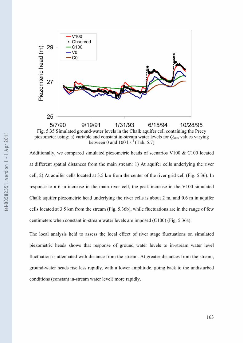
163

25

27

29

5/7/90 9/19/91 1/31/93 6/15/94 10/28/95

Pie

zom

teric

hea

d (m

)V100ObservedC100V0C0


piezometer using: a) variable and constant in-stream water levels for Qmax values varying between 0 and 100 l.s-1 (Tab. 5.7)

Additionally, we compared simulated piezometric heads of scenarios V100 & C100 located

at different spatial distances from the main stream: 1) At aquifer cells underlying the river

cell, 2) At aquifer cells located at 3.5 km from the center of the river grid-cell (Fig. 5.36). In

response to a 6 m increase in the main river cell, the peak increase in the V100 simulated

Chalk aquifer piezometric head underlying the river cells is about 2 m, and 0.6 m in aquifer

cells located at 3.5 km from the stream (Fig. 5.36b), while fluctuations are in the range of few

centimeters when constant in-stream water levels are imposed (C100) (Fig. 5.36a).

The local analysis held to assess the local effect of river stage fluctuations on simulated

piezometric heads shows that response of ground water levels to in-stream water level

fluctuation is attenuated with distance from the stream. At greater distances from the stream,

ground-water heads rise less rapidly, with a lower amplitude, going back to the undisturbed

conditions (constant in-stream water level) more rapidly.

tel-0

0582

551,

ver

sion

1 -

1 Ap

r 201

1

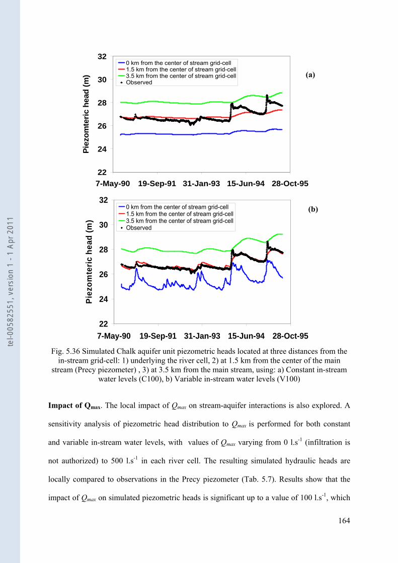
164

Fig. 5.36 Simulated Chalk aquifer unit piezometric heads located at three distances from the

in-stream grid-cell: 1) underlying the river cell, 2) at 1.5 km from the center of the main stream (Precy piezometer) , 3) at 3.5 km from the main stream, using: a) Constant in-stream

water levels (C100), b) Variable in-stream water levels (V100)

Impact of Qmax. The local impact of Qmax on stream-aquifer interactions is also explored. A

sensitivity analysis of piezometric head distribution to Qmax is performed for both constant

and variable in-stream water levels, with values of Qmax varying from 0 l.s-1 (infiltration is

not authorized) to 500 l.s-1 in each river cell. The resulting simulated hydraulic heads are

locally compared to observations in the Precy piezometer (Tab. 5.7). Results show that the

impact of Qmax on simulated piezometric heads is significant up to a value of 100 l.s-1, which

22

24

26

28

30

32


Piez

omte

ric h

ead

(m)

0 km from the center of stream grid-cell1.5 km from the center of stream grid-cell3.5 km from the center of stream grid-cellObserved

(a)

(b)

22

24

26

28

30

32


Piez

omte

ric h

ead

(m)

0 km from the center of stream grid-cell1.5 km from the center of stream grid-cell3.5 km from the center of stream grid-cellObserved

(b)

tel-0

0582

551,

ver

sion

1 -

1 Ap

r 201

1

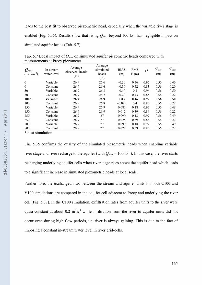
165

leads to the best fit to observed piezometric head, especially when the variable river stage is

enabled (Fig. 5.35). Results show that rising Qmax beyond 100 l.s-1 has negligible impact on

simulated aquifer heads (Tab. 5.7)

Tab. 5.7 Local impact of Qmax on simulated aquifer piezometric heads compared with measurements at Precy piezometer

Qmax (l.s-1km-2)

In-stream water level

Average observed heads

(m)

Average simulated

heads (m)

BIAS (m)

RMSE (m)

ρ obsσ (m)

simσ (m)

0 Variable 26.9 26.6 -0.30 0.36 0.95 0.56 0.46 0 Constant 26.9 26.6 -0.30 0.52 0.83 0.56 0.20 50 Variable 26.9 26.8 -0.10 0.2 0.96 0.56 0.50 50 Constant 26.9 26.7 -0.20 0.43 0.85 0.56 0.22 100* Variable 26.9 26.9 0.03 0.16 0.97 0.56 0.50 100 Constant 26.9 26.8 -0.025 0.4 0.86 0.56 0.22 150 Variable 26.9 26.9 0.081 0.18 0.97 0.56 0.48 150 Constant 26.9 26.9 0.012 0.39 0.86 0.56 0.22 250 Variable 26.9 27 0.099 0.18 0.97 0.56 0.49 250 Constant 26.9 27 0.028 0.39 0.86 0.56 0.22 500 Variable 26.9 27 0.099 0.18 0.97 0.56 0.49 500 Constant 26.9 27 0.028 0.39 0.86 0.56 0.22 * best simulation

Fig. 5.35 confirms the quality of the simulated piezometric heads when enabling variable

river stage and river recharge to the aquifer (with Qmax = 100 l.s-1). In this case, the river starts

recharging underlying aquifer cells when river stage rises above the aquifer head which leads

to a significant increase in simulated piezometric heads at local scale.

Furthermore, the exchanged flux between the stream and aquifer units for both C100 and

V100 simulations are compared in the aquifer cell adjacent to Precy and underlying the river

cell (Fig. 5.37). In the C100 simulation, exfiltration rates from aquifer units to the river were

quasi-constant at about 0.2 m3.s-1 while infiltration from the river to aquifer units did not

occur even during high flow periods, i.e. river is always gaining. This is due to the fact of

imposing a constant in-stream water level in river grid-cells.

tel-0

0582

551,

ver

sion

1 -

1 Ap

r 201

1

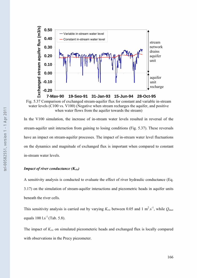
166

Fig. 5.37 Comparison of exchanged stream-aquifer flux for constant and variable in-stream

water levels (C100 vs. V100) (Negative when stream recharges the aquifer, and positive when water flows from the aquifer towards the stream)

In the V100 simulation, the increase of in-stream water levels resulted in reversal of the

stream-aquifer unit interaction from gaining to losing conditions (Fig. 5.37). These reversals

have an impact on stream-aquifer processes. The impact of in-stream water level fluctuations

on the dynamics and magnitude of exchanged flux is important when compared to constant

in-stream water levels.

Impact of river conductance (Kriv)

A sensitivity analysis is conducted to evaluate the effect of river hydraulic conductance (Eq.

3.17) on the simulation of stream-aquifer interactions and piezometric heads in aquifer units

beneath the river cells.

This sensitivity analysis is carried out by varying Kriv between 0.05 and 1 m2.s-1, while Qmax

equals 100 l.s-1 (Tab. 5.8).

The impact of Kriv on simulated piezometeric heads and exchanged flux is locally compared

with observations in the Precy piezometer.

-0.20

-0.10

0.00

0.10

0.20

0.30

0.40

0.50

7-May-90 19-Sep-91 31-Jan-93 15-Jun-94 28-Oct-95Exch

ange

d st

ream

aqu

ifer f

lux

(m3/

s)Variable in-stream water level

Constant in-stream water levelstream network drains aquifer unit

aquifer unit recharge

tel-0

0582

551,

ver

sion

1 -

1 Ap

r 201

1

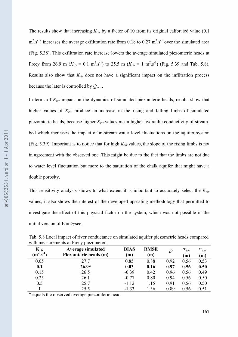
167

The results show that increasing Kriv by a factor of 10 from its original calibrated value (0.1

m2.s-1) increases the average exfiltration rate from 0.18 to 0.27 m3.s-1 over the simulated area

(Fig. 5.38). This exfiltration rate increase lowers the average simulated piezomteric heads at

Precy from 26.9 m (Kriv = 0.1 m2.s-1) to 25.5 m (Kriv = 1 m2.s-1) (Fig. 5.39 and Tab. 5.8).

Results also show that Kriv does not have a significant impact on the infiltration process

because the later is controlled by Qmax.

In terms of Kriv impact on the dynamics of simulated piezomteric heads, results show that

higher values of Kriv produce an increase in the rising and falling limbs of simulated

piezomteric heads, because higher Kriv values mean higher hydraulic conductivity of stream-

bed which increases the impact of in-stream water level fluctuations on the aquifer system

(Fig. 5.39). Important is to notice that for high Kriv values, the slope of the rising limbs is not

in agreement with the observed one. This might be due to the fact that the limbs are not due

to water level fluctuation but more to the saturation of the chalk aquifer that might have a

double porosity.

This sensitivity analysis shows to what extent it is important to accurately select the Kriv

values, it also shows the interest of the developed upscaling methodology that permitted to

investigate the effect of this physical factor on the system, which was not possible in the

initial version of EauDysée.

Tab. 5.8 Local impact of river conductance on simulated aquifer piezometric heads compared with measurements at Precy piezometer.

Kriv (m2.s-1)

Average simulated Piezomteric heads (m)

BIAS (m)

RMSE (m)

ρ obsσ (m)

simσ (m)

0.05 27.7 0.85 0.88 0.92 0.56 0.53 0.1 26.9* 0.03 0.16 0.97 0.56 0.50 0.15 26.5 -0.39 0.42 0.96 0.56 0.49 0.25 26.1 -0.77 0.80 0.94 0.56 0.50 0.5 25.7 -1.12 1.15 0.91 0.56 0.50 1 25.5 -1.33 1.36 0.89 0.56 0.51

* equals the observed average piezomteric head

tel-0

0582

551,

ver

sion

1 -

1 Ap

r 201

1

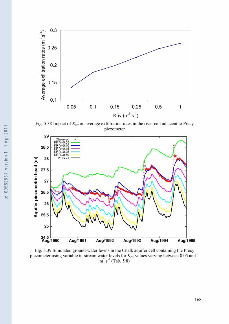
168

0.1

0.15

0.2

0.25

0.3

0.05 0.1 0.15 0.25 0.5 1

Kriv (m2.s-1)

Ave

rage

exf

iltra

tion

rate

s (m

3 .s-1

)

Fig. 5.38 Impact of Kriv on average exfiltration rates in the river cell adjacent to Precy

piezometer


piezometer using variable in-stream water levels for Kriv values varying between 0.05 and 1 m2.s-1 (Tab. 5.8)

tel-0

0582

551,

ver

sion

1 -

1 Ap

r 201

1

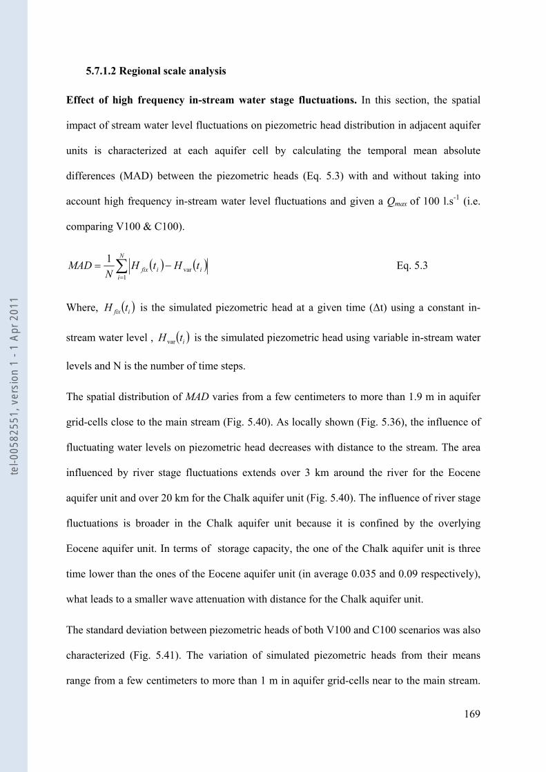
169

5.7.1.2 Regional scale analysis

Effect of high frequency in-stream water stage fluctuations. In this section, the spatial

impact of stream water level fluctuations on piezometric head distribution in adjacent aquifer

units is characterized at each aquifer cell by calculating the temporal mean absolute

differences (MAD) between the piezometric heads (Eq. 5.3) with and without taking into

account high frequency in-stream water level fluctuations and given a Qmax of 100 l.s-1 (i.e.

comparing V100 & C100).

( ) ( )∑=

−=N

iiifix tHtH

NMAD

1var

1 Eq. 5.3

Where, ( )ifix tH is the simulated piezometric head at a given time (Δt) using a constant in-

stream water level , ( )itHvar is the simulated piezometric head using variable in-stream water

levels and N is the number of time steps.

The spatial distribution of MAD varies from a few centimeters to more than 1.9 m in aquifer

grid-cells close to the main stream (Fig. 5.40). As locally shown (Fig. 5.36), the influence of

fluctuating water levels on piezometric head decreases with distance to the stream. The area

influenced by river stage fluctuations extends over 3 km around the river for the Eocene

aquifer unit and over 20 km for the Chalk aquifer unit (Fig. 5.40). The influence of river stage

fluctuations is broader in the Chalk aquifer unit because it is confined by the overlying

Eocene aquifer unit. In terms of storage capacity, the one of the Chalk aquifer unit is three

time lower than the ones of the Eocene aquifer unit (in average 0.035 and 0.09 respectively),

what leads to a smaller wave attenuation with distance for the Chalk aquifer unit.

The standard deviation between piezometric heads of both V100 and C100 scenarios was also

characterized (Fig. 5.41). The variation of simulated piezometric heads from their means

range from a few centimeters to more than 1 m in aquifer grid-cells near to the main stream.

tel-0

0582

551,

ver

sion

1 -

1 Ap

r 201

1

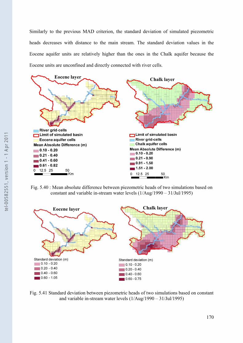
170

Similarly to the previous MAD criterion, the standard deviation of simulated piezometric

heads decreases with distance to the main stream. The standard deviation values in the

Eocene aquifer units are relatively higher than the ones in the Chalk aquifer because the

Eocene units are unconfined and directly connected with river cells.

Fig. 5.40 : Mean absolute difference between piezometric heads of two simulations based on

constant and variable in-stream water levels (1/Aug/1990 – 31/Jul/1995)

Fig. 5.41 Standard deviation between piezometric heads of two simulations based on constant and variable in-stream water levels (1/Aug/1990 – 31/Jul/1995)

Chalk layer Eocene layer

Eocene layer Chalk layer

tel-0

0582

551,

ver

sion

1 -

1 Ap

r 201

1

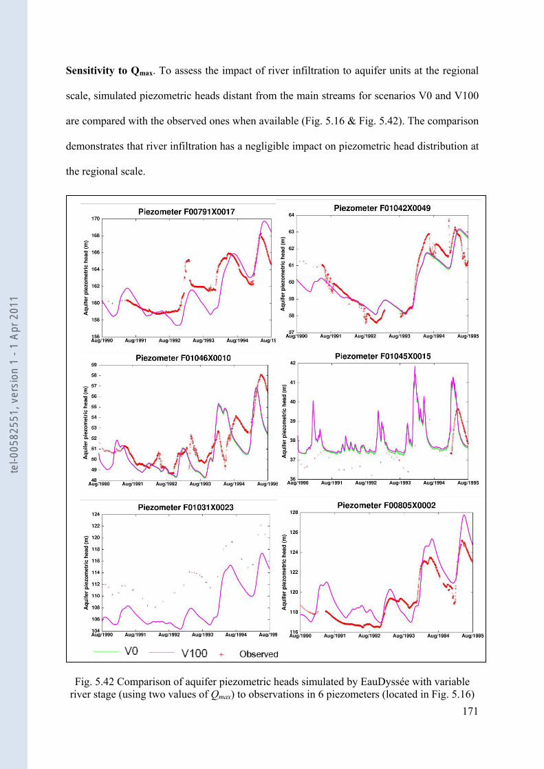
171

Sensitivity to Qmax. To assess the impact of river infiltration to aquifer units at the regional

scale, simulated piezometric heads distant from the main streams for scenarios V0 and V100

are compared with the observed ones when available (Fig. 5.16 & Fig. 5.42). The comparison

demonstrates that river infiltration has a negligible impact on piezometric head distribution at

the regional scale.

Fig. 5.42 Comparison of aquifer piezometric heads simulated by EauDyssée with variable river stage (using two values of Qmax) to observations in 6 piezometers (located in Fig. 5.16)

tel-0

0582

551,

ver

sion

1 -

1 Ap

r 201

1

172

5.8 Quantification of stream-aquifer exchange

A wide variety of methods exist to quantify stream-aquifer exchange, including mass balance

approaches, heat tracing, direct measurements and numerical methods (Kalbus et al., 2006;

Lange, 2005).

Mass balance approaches, include a variety of procedures that range from differential stream

gauging and hydrograph separation methods to solute and environmental tracers (Kalbus et

al., 2006).

Heat tracing techniques assume that the temperature of ground water is more stable than that

of surface water. Gaining reaches are thus characterized by relatively constant sediment

temperatures, where as losing reaches tend to present significant variability over short periods

of time (Constantz et al., 2001).

A recent geophysical method for quantifying stream-aquifer exchanged fluxes at the local

scale includes Fiber-optic distributed temperature sensing (FO-DTS) (Day-Lewis and Lane,

2006; Selker et al., 2006; Vogt et al., 2010).

Direct measurements can be carried out by using seepage meters (Landon et al., 2001) that

are simple and relatively inexpensive, but a significant number of measurements are required

to adequately characterize a given stream. Other approaches use observed hydraulic head

fluctuations within piezometers close by the stream to assess increase or decrease of the

aquifer water storage, from which the infiltration/exfiltration rate of water is derived (Blasch

et al., 2004; Sanford, 2002). These methods are widely used in flood-water infiltration

studies. However, they require the availability of consistent data along the river which is not

always the case at the regional scale.

tel-0

0582

551,

ver

sion

1 -

1 Ap

r 201

1

173

For the Oise River, exchanged fluxes between streams and aquifer units are assessed based

on simulations for four different scenarios (Tab. 5.6) during the period of simulation

(1/Aug/1990 – 31/Jul/1995) (Eq. 5.4):

Net exchanged flux = Aquifer exfiltration – River infiltration Eq. 5.4

Therefore, a positive net exchanged flux means that the overall exfiltrated volume of water

by the aquifer units is higher than river infiltration, and vice versa.

The net exchange is positive for all simulations, which means that overall, the aquifer system

sustains the river network.

To assess the impact of Qmax on the exchanges between streams and aquifer units, scenarios

V0 & V100 are compared (Fig. 5.43). The comparison shows that the infiltration flux from

the rivers to the aquifer units has almost no impact on the net stream-aquifer exchanges. The

main impact is a dynamical one due to the volume of the infiltrated flux from river to aquifer

unit during in-stream high flow periods which eventually involves a longer transfer time in

aquifer units near to the river network that corresponds to an increase of the stored water in

the aquifer system.

To globally assess the impact of in-stream water level fluctuations on exchanged stream-

aquifer flux, scenarios V100 & C100 are compared. The comparison (Fig. 5.43) shows that

fluctuations of in-stream water level slightly modifies the net stream-aquifer exchanges (from

37.8 mm.yr-1 to 37.7 mm.yr-1). The exchanged flux from aquifer units to streams slightly

increases, while the exchanged one from stream to aquifer units also increases leading to a

net exchange of 37.7 mm.yr-1, which remains almost unchanged for the two scenarios. But

the intensity of exchanges is 2 times higher for V100 than C100 showing the importance of

taking into account water levels fluctuations for simulating high frequency aquifer system

response.

tel-0

0582

551,

ver

sion

1 -

1 Ap

r 201

1

174

Finally, the mean monthly stream-aquifer exchange dynamics is analyzed based on scenario

V100 (Fig. 5.44). The minimum of net exchanges occurs in October (2.6 mm.month-1) which

corresponds to low water piezometric level and to the beginning of the hydrological year.

From October to January infiltrated water from rivers towards aquifer units increases from

0.18 mm.month-1 to 0.31 mm.month-1. While January corresponds to the maximum of

infiltration (3.2 l.s-1.km-1 of river stretch), it appears on Fig. 10b that the recharge of the

aquifer system is not only due to infiltration from the river network but to the recharge from

the impluvium so that high water piezometric level is only reached in March when the flux

from aquifer units to rivers is maximum (3.8 mm.month-1). During the rising of piezometric

level in aquifer units, the infiltrated flux from rivers to aquifer units decreases, reaching a

minimum of 0.1 mm.month-1 in March. During spring, the net exchanges are maximum and

the exfiltration from the aquifer system prevails. During summer the river network mostly

drains the aquifer system which leads to the low water piezometric level in late August.

Interesting is that the later in the summer, the more the summer storms impact the water

content of the aquifer system because infiltrated water from rivers to aquifer units increases

from 0.1 mm. month-1 in May to 0.15 mm. month-1 in September. This is important for

pollutant transfer at the basin scale because late summer is the warmest period when bacterial

activity is maximal. Hence, doubling the exchange flux can have an impact on nitrate

elimination for instance.

tel-0

0582

551,

ver

sion

1 -

1 Ap

r 201

1

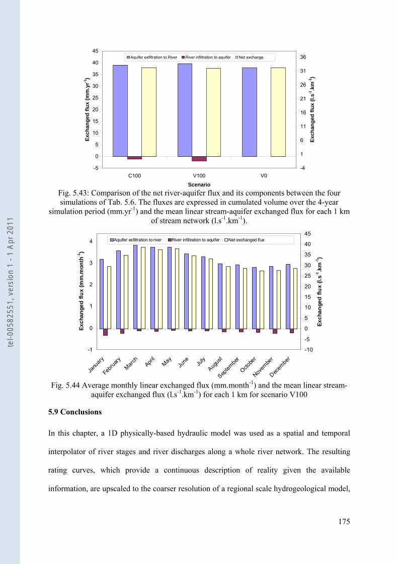
175

-5

0

5

10

15

20

25

30

35

40

45

C100 V100 V0

Scenario

Exch

ange

d flu

x (m

m.y

r-1)

-4

1

6

11

16

21

26

31

36

Exch

ange

d flu

x (l.

s-1.k

m-1

)

Aquifer exfiltration to River River infiltration to aquifer Net exchange

Fig. 5.43: Comparison of the net river-aquifer flux and its components between the four simulations of Tab. 5.6. The fluxes are expressed in cumulated volume over the 4-year

simulation period (mm.yr-1) and the mean linear stream-aquifer exchanged flux for each 1 km of stream network (l.s-1.km-1).

-1

0

1

2

3

4

Janu

ary

Febru

aryMarc

hApri

lMay

June Ju

ly

Augus

t

Septem

ber

Octobe

r

Novem

ber

Decem

ber

Exch

ange

d flu

x (m

m.m

onth

-1)

-10

-5

0

5

10

15

20

25

30

35

40

45

Exch

ange

d flu

x (l.

s-1.k

m-1

)

Aquifer exfiltration to river River infiltration to aquifer Net exchanged flux

Fig. 5.44 Average monthly linear exchanged flux (mm.month-1) and the mean linear stream-

aquifer exchanged flux (l.s-1.km-1) for each 1 km for scenario V100

5.9 Conclusions

In this chapter, a 1D physically-based hydraulic model was used as a spatial and temporal

interpolator of river stages and river discharges along a whole river network. The resulting

rating curves, which provide a continuous description of reality given the available

information, are upscaled to the coarser resolution of a regional scale hydrogeological model,

tel-0

0582

551,

ver

sion

1 -

1 Ap

r 201

1

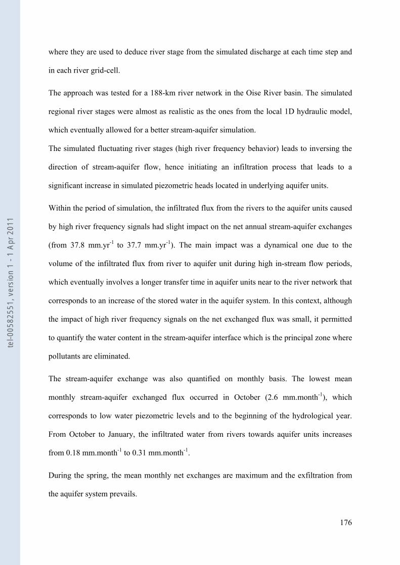
176

where they are used to deduce river stage from the simulated discharge at each time step and

in each river grid-cell.

The approach was tested for a 188-km river network in the Oise River basin. The simulated

regional river stages were almost as realistic as the ones from the local 1D hydraulic model,

which eventually allowed for a better stream-aquifer simulation.

The simulated fluctuating river stages (high river frequency behavior) leads to inversing the

direction of stream-aquifer flow, hence initiating an infiltration process that leads to a

significant increase in simulated piezometric heads located in underlying aquifer units.

Within the period of simulation, the infiltrated flux from the rivers to the aquifer units caused

by high river frequency signals had slight impact on the net annual stream-aquifer exchanges

(from 37.8 mm.yr-1 to 37.7 mm.yr-1). The main impact was a dynamical one due to the

volume of the infiltrated flux from river to aquifer unit during high in-stream flow periods,

which eventually involves a longer transfer time in aquifer units near to the river network that

corresponds to an increase of the stored water in the aquifer system. In this context, although

the impact of high river frequency signals on the net exchanged flux was small, it permitted

to quantify the water content in the stream-aquifer interface which is the principal zone where

pollutants are eliminated.

The stream-aquifer exchange was also quantified on monthly basis. The lowest mean

monthly stream-aquifer exchanged flux occurred in October (2.6 mm.month-1), which

corresponds to low water piezometric levels and to the beginning of the hydrological year.

From October to January, the infiltrated water from rivers towards aquifer units increases

from 0.18 mm.month-1 to 0.31 mm.month-1.

During the spring, the mean monthly net exchanges are maximum and the exfiltration from

the aquifer system prevails.

tel-0

0582

551,

ver

sion

1 -

1 Ap

r 201

1

177

During the summer the river network mostly drains the aquifer system which leads to low

water piezometric levels in late August. Interesting is that the later in the summer, the more

the summer storms impact the water content of the aquifer system because infiltrated water

from rivers to aquifer units increases from 0.1 mm.month-1 in May to 0.15 mm.month-1 in

September. This is particularly important for pollutant transfer at the basin scale because late

summer is the warmest period when bacterial activity is maximal. Hence, doubling the

exchange flux can have an impact on nitrate elimination for instance.

In terms of spatial impact, the area influenced by high frequency river signals extends across

3 to 20 km around the streams, depending on the hydrogeological setting

(confined/unconfined) of the aquifer unit. The fluctuations of simulated piezometric heads

from their means range from a few centimeters to more than 1 m in aquifer grid-cells near to

the main stream. The impact of these high frequency river signals on simulated piezometric

heads decreases with distance to the stream.

This study confirms that surface and groundwater models should not be treated separately

because they are connected components of the hydrosystem, especially in large sedimentary

basins as the one of the Oise River. The upscaling method offers an efficient way to improve

the physics of the stream-aquifer interactions at the regional scale, with a limited

computational burden owing to the pre-computation of the rating curves.

tel-0

0582

551,

ver

sion

1 -

1 Ap

r 201

1

178

CHAPTER 6. CONCLUSIONS AND FUTURE WORK

The present work contributes to the development of the integrated hydrosystem model

EauDyssée applied to the Seine River basin. The main objective was to provide a realistic

simulation of river stage and discharge at the regional scale, in order to improve the

simulation of stream-aquifer interactions and better assess piezometric heads.

Two operating regimes for hydraulic heads are considered. The first one is a low frequency

behavior of hydraulic heads at large scale. At this scale, the basin filters the rainfall signal for

which the temporal variability is highly reduced by the signal filtering effect of the flow

through the soil, the unsaturated zone and the aquifer unit. The second regime is a temporal

frequency behavior of hydraulic heads due to fast in-stream water levels fluctuation. This

regime impacts the stream-aquifer interactions and the aquifer system at local scale near the

river with a high frequency response.

The initial version of EauDyssée was a low frequency behavior, while this study is focused

on high frequency behavior that was taken into consideration through developing an

upscaling framework under unsteady-state conditions. The outputs from this framework were

compared to the initial version in order to quantify the improvements carried out by

considering this physical process in the model.

This work started with an overview of available surface routing and integrated hydrosystem

models with a special focus on stream-aquifer interactions modeling techniques. The review

of the surface routing techniques shows that the final choice of a surface routing model is a

trade off between a number of factors such as the temporal and spatial scale, the required

accuracy, the type and availability of data, the available computational facilities and the

extent of required information on water levels. This shows that there is no universal superior

tel-0

0582

551,

ver

sion

1 -

1 Ap

r 201

1

179

routing model and choosing the appropriate routing approach depends to a great extent on the

hydrological problem in question.

On the other hand, the review of stream-aquifer modeling techniques shows the importance

of regional hydro(geo)logical models that are capable of simulating coupled stream-aquifer

interactions and conducting interdisciplinary investigations in hydrological sciences.

However, the majority of these regional models has limited capacity to simulate small-scale

processes (e.g., near-stream groundwater pumping, bank storage effects, in-stream water

level fluctuations, hyporheic exchange) because modeling these processes require a very fine

discretization of the considered domain which is not always applicable in regional scale

hydrological models. This particular limitation addresses the necessity of identifying a

methodology to improve the modeling of local scale stream-aquifer interactions within

regional hydrogeological models. The review also shows that in-stream water levels are of

primary importance for the simulation of stream-aquifer interactions, the estimation of low

flow discharge and the water quality.

Upon reviewing the integrated models of the hydrosystems, the regional hydrological model

EauDyssée was selected to simulate the hydrosystem with a special focus on the surface

routing and stream-aquifer interaction component. The later is simulated with imposed

constant in-stream water levels because river morphological data are not always accessible in

regional scale applications. To quantify the impact of morphological data on in-stream water

levels and discharge simulations, an investigation using different simplified geometry

scenarios was carried out in the Serein River (tributary of the Yonne River), between the

gauging stations of Dissangis and Beaumont, in a well surveyed reach (20 cross sections over

89 kms).

tel-0

0582

551,

ver

sion

1 -

1 Ap

r 201

1

180

River discharge and stage are simulated by the hydraulic model HEC-RAS (1D Saint-Venant

equations) solved using the four point implicit finite difference scheme while lateral inflows

are simulated by the regional hydrological model EauDyssée.

The results of the different geometry scenarios show that certain cross sectional

representation (e.g. trapezoidal shape) produces water levels that are consistent with

measured data in certain locations of the river reach. However, the maximum water depths

are longitudinally offset, primarily because of the approximated geometry and because the

simplified bed levels are different from the actual bed levels. During low flow, the results

show that irregularities in the river bed bottom have an important impact on simulated river

stages, as simplifying the irregular river bed bottom to plain have, on average, attenuated the

low flow water levels by 20 cm compared to ones in the reference simulation. This is because

the lower the water level is, the more important is the friction and thus the description of the

cross section geometry. This finding is important, especially in the simulations of stream-

aquifer interactions where the river is sustained by aquifer units during low flow periods.

In terms of river bed level, the results show that using interpolated bed levels instead of

surveyed ones for a trapezoidal cross-section have reduced the Nash efficiency of simulated

water levels at Chablis hydrometric station from 0.83 to 0.61, while the RMSE was increased

from 0.19 m to 0.3 m. The maximum water depths obtained from interpolated bed levels vary



for the same type of section. In five river cross sections, the difference between simulated


more than 1 m due to the linearly interpolated bed levels. This exhibits the effect of bed

levels on the simulated water levels, especially at the regional scale where DEM is usually

tel-0

0582

551,

ver

sion

1 -

1 Ap

r 201

1

181

used to identify the river geometry hence it is difficult to obtain an accurate river bed level

representation.

This confirms that the accuracy of predicted water levels and maximum water depths

simulated by a Saint-Venant model rely on an accurate representation of channel geometry


That being said, a 1D Saint-Venant model is not suitable for simulating flow in areas where

river morphology is not accessible. In spite of these limitations, this type of hydrodynamic

modeling remains crucial to accurately simulate in-stream water levels. To compromise

between the spatial scale issue, morphological data limitation and the importance to

accurately simulate in-stream water levels, an original upscaling strategy is developed, with

which a 1D Saint-Venant hydraulic model is used as a spatial and temporal interpolator of

river stages and river discharges along a whole river network. The resulting rating curves are

upscaled to the coarser resolution of a regional scale hydrogeological model, where they are

used to deduce river stage from the simulated discharge routed with a simple Muskingum

model at each time step and in each river grid-cell.

The approach was validated in a 188-km river network in the Oise River basin. The simulated

regional river stages were almost as realistic as the ones from the local 1D hydraulic model.

The simulated fluctuating river stages (high frequency behavior) leads to inversing the

direction of stream-aquifer flow, hence initiating an infiltration process that leads to a

significant increase in simulated piezometric heads located in underlying aquifer units.

Within the period of simulation, the infiltrated flux from the rivers to the aquifer units caused

by high river frequency signals had slight impact on the net annual stream-aquifer exchanges

(from 37.8 mm.yr-1 to 37.7 mm.yr-1). The main impact was a dynamical one due to the

volume of the infiltrated flux from river to aquifer unit during high in-stream flow periods,

tel-0

0582

551,

ver

sion

1 -

1 Ap

r 201

1

182

which eventually involves a longer transfer time in aquifer units near to the river network that

corresponds to an increase of the stored water in the aquifer system. In this context, although

the impact of high river frequency signals on the net exchanged flux was small, it permitted

to quantify the water content in the stream-aquifer interface which is the principal zone where

pollutants are eliminated.

The stream-aquifer exchange was also quantified on monthly basis. The lowest mean

monthly stream-aquifer exchanged flux occurred in October (2.6 mm.month-1), which

corresponds to low water piezometric levels and to the beginning of the hydrological year.

From October to January, the amount of infiltrated water from rivers towards aquifer units

increases from 0.18 mm.month-1 to 0.31 mm.month-1. During spring, the mean monthly net

exchanges are maximum and the exfiltration from the aquifer system prevails. In summer the

river network mostly drains the aquifer system which leads to low water piezometric levels in

late August. Interesting is that the later in the summer, the more the summer storms impact

the water content of the aquifer system because infiltrated water from rivers to aquifer units

increases from 0.1 mm.month-1 in May to 0.15 mm.month-1 in September. This is particularly

important for pollutant transfer at the basin scale because late summer is the warmest period

when bacterial activity can be maximal. Hence, doubling the exchange flux can have an

impact on nitrate elimination for instance.

In terms of spatial impact, the area influenced by high frequency river signals extends across

3 to 20 km around the streams, depending on the hydrogeological setting

(confined/unconfined) of the aquifer unit. The fluctuations of simulated piezometric heads

from their means range from a few centimeters to more than 1 m in aquifer grid-cells near the

main stream. The impact of these high frequency river signals on simulated piezometric

heads decreases with distance to the stream.

tel-0

0582

551,

ver

sion

1 -

1 Ap

r 201

1

183

This study confirms that surface and groundwater models should not be treated separately

because they are connected components of the hydrosystem, especially in large sedimentary

basins as the one of the Oise River. The upscaling method offers an efficient way to improve

the physics of the stream-aquifer interactions and better assess soil water content at the

regional scale, with a limited computational burden owing to the pre-computation of the

rating curves. Thus, it offers interesting perspectives to better address the impacts of

environmental changes on hydrosystems, such as climate change (Ducharne et al., 2007;

Ducharne et al., 2010), irrigation, or nitrate contamination from agricultural practices (Flipo

et al., 2007a; Gomez et al., 2003; Ledoux et al., 2007) and wetlands which are often located

at the contact zone between groundwater and in-stream waters (Curie et al., 2009; Devito et

al., 1996; Kehew et al., 1998).

The functional curves approach could also be generalized to account for variable river

velocity in regional scale hydrological models (Lucas-Picher et al., 2003). The advantage of

the proposed method would be to benefit from the complete physics offered by the hydraulic

model (Saint-Venant equations) and from high resolution morphological data, but with a

significant spare of computational time in the regional model, owing to the pre-computation

of the functional curves. The approach could even be further generalized to account for

floods and inundations assessment in regional hydrological models (Knebl et al., 2005a), by

defining functional curves derived from 2D hydraulic modeling.

The proposed approach also offers an interesting way to benefit from river stage remote-

sensing measurements (Alsdorf et al., 2007; Biancamaria et al., 2010; Neal et al., 2009) to

constrain hydrological modeling, with increasing coverage, precision, and temporal

resolution.

This methodology also offers interesting perspectives for coastal aquifers applications, where

tidal fluctuation is an important driving force for groundwater flow, and dynamic interactions

tel-0

0582

551,

ver

sion

1 -

1 Ap

r 201

1

184

between groundwater and seawater are important (Guo et al., 2010; Sun et al., 2008). In this

context, Aquifer reaction to tidal fluctuations has been employed to calculate aquifer

parameters (Erskine, 1991; Jha et al., 2003).

Other coastal applications include the impact of coastal land reclamation on ground water

level and the sea water interface (Guo and Jiao, 2007).

The in-stream water level variations can also be used to study hydraulic properties of fluvial

aquifers at large scale (Bolster et al., 2001; Carrera and Neuman, 1986a; Loeltz and Leake,

1983; Pinder and Jones, 1969; Reynolds, 1987; Sophocleous, 1991).

In other studies, time varying surface water stage is frequently used to estimate aquifer

hydraulic diffusivity (Ferris, 1951; Pinder and Jones, 1969; Reynolds, 1987; Swamee and

Singh, 2003).

Furthermore, this methodology allows to account for smaller scale processes, such as

simulating the mixing in the hyporheic zone (Arntzen et al., 2006; Ryan et al., 2004),

biogeochemical processing (Cardenas, 2009) nutrient cycling (Kim et al., 1992; Kim et al.,

2000) and nutrient release from sediment pore fluids during low flow conditions, especially

in estuarine environments (Linderfelt and Turner, 2001; Westbrook et al., 2005).tel-0

0582

551,

ver

sion

1 -

1 Ap

r 201

1

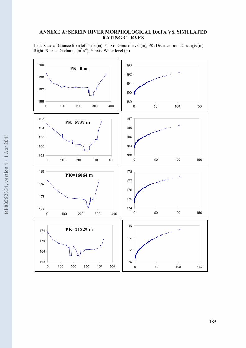
185

ANNEXE A: SEREIN RIVER MORPHOLOGICAL DATA VS. SIMULATED RATING CURVES

Left: X-axis: Distance from left bank (m), Y-axis: Ground level (m), PK: Distance from Dissangis (m) Right: X-axis: Discharge (m3.s-1), Y-axis: Water level (m)

188

192

196

200

0 100 200 300 400189

190

191

192

193

0 50 100 150

174

178

182

186

0 100 200 300 400

174

175

176

177

178

0 50 100 150

PK=0 m

PK=16064 m

183

184

185

186

187

0 50 100 150182

186

190

194

198

0 100 200 300 400

164

165

166

167

0 50 100 150162

166

170

174

0 100 200 300 400 500

PK=21829 m

PK=5737 m

tel-0

0582

551,

ver

sion

1 -

1 Ap

r 201

1

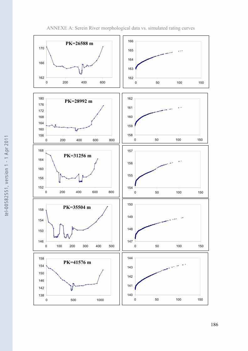
186

154

155

156

157

0 50 100 150

147

148

149

150

0 50 100 150

152

156

160

164

168

0 200 400 600 800

PK=31256 m

158

159

160

161

162

0 50 100 150156

160

164

168

172

176

180

0 200 400 600 800

162

166

170

0 200 400 600162

163

164

165

166

0 50 100 150

146

150

154

158

0 100 200 300 400 500

PK=28992 m

PK=35504 m

138

142

146

150

154

158

0 500 1000

PK=41576 m

140

141

142

143

144

0 50 100 150

PK=26588 m

ANNEXE A: Serein River morphological data vs. simulated rating curves

tel-0

0582

551,

ver

sion

1 -

1 Ap

r 201

1

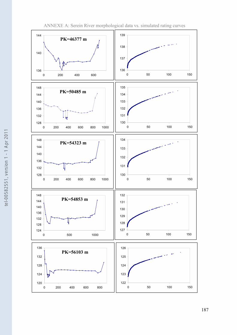
187

136

140

144

0 200 400 600

PK=46377 m

128

132

136

140

144

148

0 200 400 600 800 1000

PK=50485 m

136

137

138

139

0 50 100 150

130

131

132

133

134

135

0 50 100 150

128

132

136

140

144

148

0 200 400 600 800 1000 130

131

132

133

134

0 50 100 150

PK=54323 m

124

128

132

136

140

144

148

0 500 1000

PK=54853 m

120

124

128

132

136

0 200 400 600 800

PK=56103 m

127

128

129

130

131

132

0 50 100 150

122

123

124

125

126

0 50 100 150


tel-0

0582

551,

ver

sion

1 -

1 Ap

r 201

1

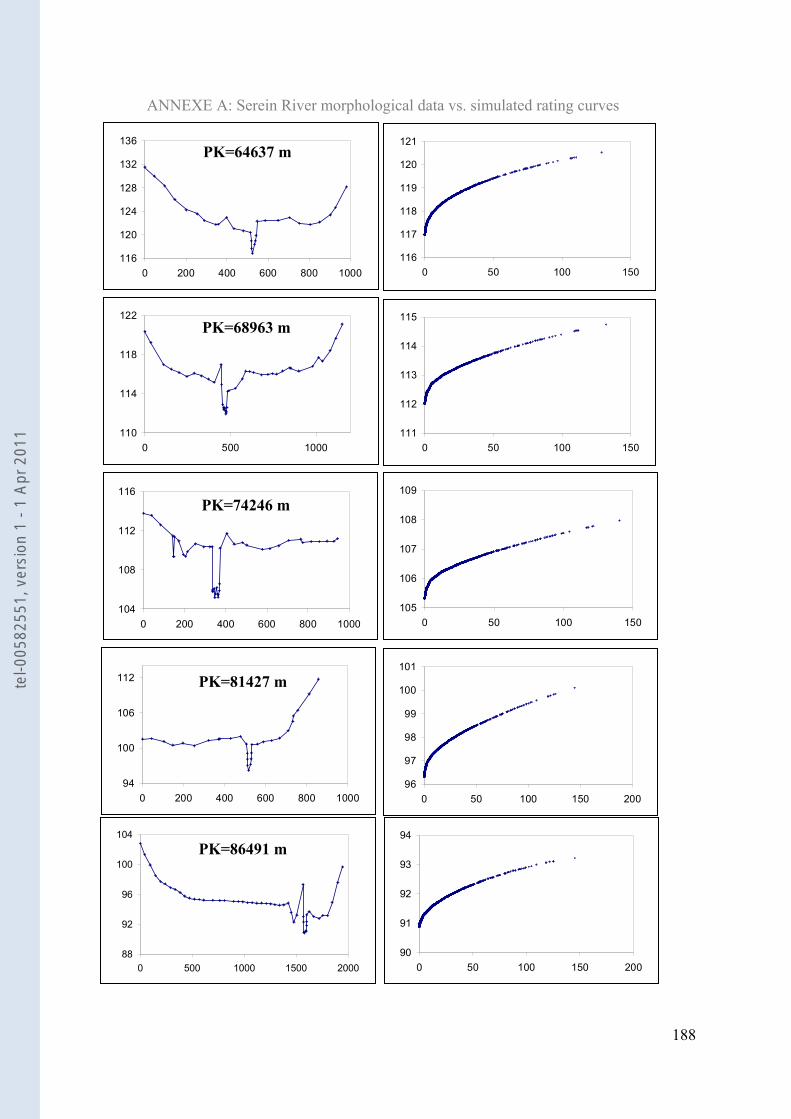
188

116

120

124

128

132

136

0 200 400 600 800 1000

PK=64637 m

110

114

118

122

0 500 1000

PK=68963 m

116

117

118

119

120

121

0 50 100 150

111

112

113

114

115

0 50 100 150

104

108

112

116

0 200 400 600 800 1000

PK=74246 m

94

100

106

112

0 200 400 600 800 1000

PK=81427 m

105

106

107

108

109

0 50 100 150

96

97

98

99

100

101

0 50 100 150 200

88

92

96

100

104

0 500 1000 1500 2000

PK=86491 m

90

91

92

93

94

0 50 100 150 200


tel-0

0582

551,

ver

sion

1 -

1 Ap

r 201

1

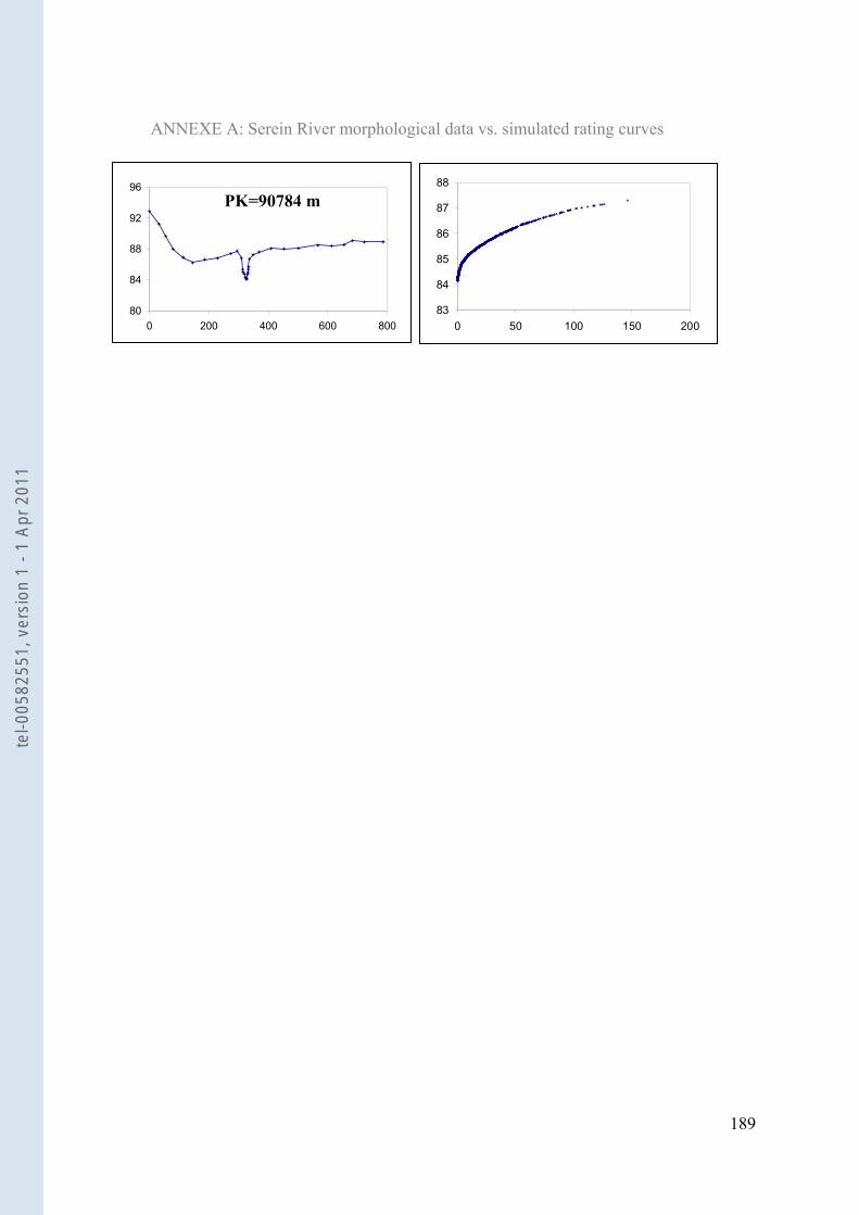
189

80

84

88

92

96

0 200 400 600 800

PK=90784 m

83

84

85

86

87

88

0 50 100 150 200


tel-0

0582

551,

ver

sion

1 -

1 Ap

r 201

1

190

ANNEXE B: RESUME LONG DE LA THESE EN FRANÇAIS

Apport de la modélisation hydraulique pour une meilleure simulation des tirants d'eau et des échanges nappe-rivière à l'échelle régionale

Cette thèse s’inscrit dans le développement de la plateforme EauDyssée de modélisation

intégrée des hydrosystèmes régionaux, au sein du bassin pilote de la Seine. L’objectif

principal est de contribuer à une meilleure simulation des niveaux des cours d’eau à l’échelle

régionale afin d'améliorer la simulation des interactions nappe-rivière et de mieux quantifier

les niveaux piézométriques dans les aquifères. Il s’agit donc de construire le lien entre débits

et niveaux d’eau dans une modélisation des écoulements en rivière à l’échelle régionale.

Comme détaillé dans le Chapitre 2, la modélisation des écoulements en rivière peut être

classifiée en deux catégories : la modélisation hydrologique et la modélisation hydraulique. A

l’échelle régionale, les principaux outils sont les modèles hydrologiques, qui propagent le

débit dans le réseau hydrographique sur des bases simples (ex. Muskingum, Muskingum-

Cunge). Ces modèles sont généralement ciblés sur le routage du débit, sans tenir compte des

niveaux d’eau, du fait de l’intérêt prioritaire pour les ressources en eau à l’échelle régionale

ou globale. Au contraire, les modèles hydrauliques déterministes (ex. Navier–Stokes 3D,

Saint-Venant) sont couramment utilisés pour simuler les relations entre débit et niveau d’eau

à l’échelle locale. L’intérêt principal est alors de caractériser les événements dynamiques ou

les phénomènes d’inondation.

L’avantage fondamental des modèles de routage hydraulique par rapport aux modèles

hydrologiques vient de leur résolution physique des processus, qui rend compte des liens

débit/niveau d’eau, et implique une haute résolution le long du réseau de drainage, ce qui

permet d’exploiter les données intermédiaires (sections transversales et/ou courbes de tarage).

A ce jour, les modèles hydrauliques restent cependant peu utilisés à l’échelle régionale du

tel-0

0582

551,

ver

sion

1 -

1 Ap

r 201

1

191

bassin versant. En effet, ils requièrent des données géométriques sur l'intégralité du réseau

hydrographique modélisé, si bien que le coût d'obtention de données suffisantes peut être

prohibitif ; ils peuvent aussi poser des problèmes de stabilité numérique, potentiellement plus

fréquents dans un grand domaine avec de nombreuses confluences et points singuliers ; ils

sont enfin plus exigeants en puissance de calcul que les modèles hydrologiques.

En conséquence de cette analyse, la démarche de cette thèse fut de combiner les capacités de

deux types de modèles d’écoulement ci-dessus, ce qui amène à répondre aux questions

scientifiques suivantes :

- Quelle est la capacité d'un modèle hydraulique à géométrie simplifiée pour simuler les

niveaux d’eau et les débits à l’échelle régionale ?

- Comment faire le lien entre un modèle hydraulique local et un modèle hydrologique

régional ?

- Quel est l’impact local et régional de la fluctuation des niveaux d’eau en rivière sur

les niveaux piézométriques et les échanges nappe-rivière ?

Dans ce contexte, nous nous somme appuyés sur deux modèles représentatifs :

1- Le modèle hydrologique régional EauDyssée (Chapitre 3) permet de modéliser les

principales composantes du cycle continental de l’eau, en particulier le rôle des écoulements

de surface et souterrain sur les relations pluies-débit à l’échelle. Ce modèle s’articule autour

d’une plateforme qui permet le couplage de modèles experts simulant le bilan hydrique, les

écoulements de surface et souterrain, le transfert en zone non saturée, et les interactions

nappe-rivière, qui sont estimées à partir d’une relation de type loi de Darcy, en fonction des

gradients de charge verticaux entre la rivière et la nappe

Dans la version initiale d’EauDyssée, les échanges entre la nappe et la rivière sont simulés

avec une cote d’eau fixe, obtenue à partir d'un Modèle Numérique de Terrain (MNT). Ces

tel-0

0582

551,

ver

sion

1 -

1 Ap

r 201

1

192

cotes ne fluctuent donc pas en fonction du débit, alors que la dynamique des niveaux des

cours d’eau a des impacts reconnus sur la vitesse des écoulements, la dynamique des

débordements, et les interactions nappe-rivière.

2- Le modèle hydraulique HEC-RAS (Hydrologic Engineering Centers River Analysis

System, USACE, 2002 ; Chapitre 3.3) est un logiciel de modélisation hydraulique

monodimensionnelle à surface libre. Il permet de simuler les écoulements permanents et non

permanents, le transport de sédiments et certaines fonctions facilitant la conception

d'ouvrages hydrauliques. Il permet également d'analyser les débits et les niveaux d’eau dans

le lit des rivières et de déterminer les zones inondables. Ce modèle résout l'ensemble

dynamique des équations de Saint-Venant par la méthode des différences finies, à partir de

données morphologiques de rivière, notamment les sections transversales et la pente de fond

des cours d’eau. La rugosité du lit de la rivière est représentée par le coefficient de Manning

n, sur lequel porte le calage hydrodynamique du modèle.

Dans les deux applications décrites ci-dessous, le modèle hydraulique est forcé par le débit

observé à l’amont, par une courbe de tarage observée à l’aval, et par les apports latéraux

simulés par le modèle hydrologique EauDyssée. Le calage est effectué manuellement, en

sélectionnant les valeurs de n qui permettent la meilleure reproduction des niveaux d’eau

observés. La qualité des simulations est évaluée par les critères statistiques classiques de

Nash, RMSE et biais aux stations hydrométriques de contrôle.

Pour répondre à la première question scientifique de cette thèse, le Chapitre 4 vise à évaluer

la sensibilité du modèle hydraulique HEC-RAS à la précision de la description

géomorphologique du lit mineurs et de la pente du fond de rivière. Le but est de définir le

meilleur compromis entre parcimonie et réalisme, en d'identifiant les facteurs

morphologiques les plus importants pour obtenir une simulation satisfaisante des tirants d'eau

à l’échelle régionale.

tel-0

0582

551,

ver

sion

1 -

1 Ap

r 201

1

193

Cette étude est menée sur le Serein (affluent de l'Yonne), dans un bief bien renseigné (20

sections transversales sur 89 km) entre les stations hydrométriques de Dissangis et Beaumont.

Le principe consiste à comparer différents scénarios de géométrie simplifiée, portant sur le

nombre (de 20 à 3) et la forme (irrégulière, trapézoïdale, rectangulaire ou triangulaire) des

sections transversales. Cette analyse montre que ces simplifications de la géométrie n’altèrent

pas significativement la simulation des débits, mais qu’une géométrie précise est nécessaire

pour simuler précisément les niveaux d’eau. En conclusion, si un modèle hydraulique Saint-

venant 1D est indispensable pour effectuer des simulations fiables des niveaux d'eau en

fonction de données géométriques précises, ce type de modélisation hydrodynamique ne

permet pas une simulation précise des niveaux d’eau à partir d’une géométrie simplifiée.

Pour trouver un bon compromis entre l’échelle d’application, l’importance d’effectuer des

simulations précises et fiables des niveaux d'eau, et la disponibilité des données

morphologiques, une méthode de changement d’échelle est proposée en Chapitre 5. Le

principe est d’utiliser la modélisation des processus hydrauliques à haute résolution par le

modèle HEC-RAS, pour améliorer la représentation des niveaux d’eau et des interactions

nappe-rivière à l'échelle régionale dans la plateforme de modélisation EauDyssée.

Cette méthodologie a été validée dans un sous-bassin versant de l’Oise, d’une superficie de

4500 km2, sur la période 1990-1995. Le domaine de surface est constitué de 1868 mailles (de

1 km2 à 16 km2), dont 202 mailles rivière de 1 km2 qui représentent le réseau hydrographique.

Le domaine souterrain comprend deux couches souterraines qui représentent les nappes de

l'Éocène et de la Craie, avec des mailles de 1 km2 à 16 km2. La couche de la Craie est

confinée par l'Éocène et il y a des échanges verticaux entre ces deux couches. Le modèle

hydrogéologique développé par Gomez (2002) dans l’application régionale du bassin de la

Seine a d’abord été recalé, en séparant deux régimes de fonctionnement. Nous avons

commencé par recaler les coefficients d'emmagasinement et les transmissivités qui contrôlent

tel-0

0582

551,

ver

sion

1 -

1 Ap

r 201

1

194

le comportement à basse fréquence des charges hydrauliques, dans lequel la variabilité des

niveaux piézométriques de la nappe est due aux fluctuations climatiques. Le deuxième

régime se caractérise par un comportement à haute fréquence temporelle des niveaux

piézométriques, qui est dû aux fluctuations des niveaux d’eau en rivière. Nous avons pu

améliorer la restitution de ce régime en recalant les coefficients d'emmagasinement dans les

mailles souterraines situées sous les mailles rivière, ainsi qu’un coefficient de transfert nappe-

rivière (Qmax).

Une fois le modèle hydrogéologique recalé, il a permis de simuler les apports latéraux pour la

modélisation hydraulique par HEC-RAS d’un tronçon de l’Oise de 188 km, où 420 sections

transversales sont disponibles. Le calage du modèle HEC-RAS a été validé en 4 stations

hydrométriques de contrôle, ce qui a permis de simuler des courbes de tarage (reliant débit et

niveau d’eau) a priori réalistes à la résolution de ce modèle, c'est-à-dire tous les 200m en

moyenne. Ces courbes de tarage ont ensuite été moyennées à la résolution des mailles rivières

du modèle hydrologique régional (1 km²) afin de pouvoir en déduire la fluctuation du niveau

d'eau en fonction du débit simulé par le module de routage régional. Les échanges entre les

mailles rivière et les mailles aquifères peuvent alors être estimés en fonction des gradients de

charge verticaux entre la nappe et la rivière, dont le niveau, représentatif de la charge, n’est

plus fixe.

L’impact de la fluctuation des niveaux en rivière sur les isopièzes a été analysé par rapport à

un état de référence pour lequel les niveaux en rivière sont constants, ce qui correspond donc

à la version originale de la plateforme EauDyssée. À l’échelle locale, nous avons comparé les

niveaux piézométriques simulés avec les observations d’un unique piézomètre suffisamment

proche de la rivière (Précy sur Oise). L’analyse des résultats montre que ces fluctuations en

rivière ont des impacts importants sur les dynamiques des niveaux piézométriques. Par

exemple, une fluctuation des niveaux d’eau en rivière de 5 mètres produit une modification

tel-0

0582

551,

ver

sion

1 -

1 Ap

r 201

1

195

des niveaux piézométriques qui peut atteindre 1.5 m, alors que la variation piézométrique

correspondante n’est que de 15 cm dans la version de référence où la cote des cours d’eau est

fixe. A l’échelle régionale, l’analyse des résultats sur la période de simulation montre un écart

moyen des niveaux piézométriques pouvant atteindre 1,9 m pour les mailles souterraines

situées sous les mailles rivière. Cet écart se réduit si l’on considère des mailles souterraines

plus éloignées de la rivière. L’extension spatiale de cet écart moyen est plus importante dans

la nappe de la Craie qui est confinée (jusqu’à 25 km de la rivière) que dans celle de l’Éocène

qui est libre (6 km de la rivière).

Ces résultats démontrent l’efficacité de la méthode de changement d’échelle proposée pour

simuler les niveaux d’eau et mieux évaluer les interactions nappe-rivière à l'échelle régionale

avec un faible coût de calcul pour le modèle régional. En revanche, le problème crucial du

manque de données à l’échelle régionale n'est pas levé par cette démarche, dont le principal

avantage est la finalement d’exploiter au mieux l'information disponible, que ce soient des

courbes de tarage observées, des modèles hydrauliques existants, ou même une cote fixe en

absence de meilleure information, ce qui permet d’enrichir graduellement le modèle

hydrologique régional et traiter les zones de manière flexible et de mieux exploiter

La suite de ce travail consistera donc à généraliser cette méthodologie à l'échelle du bassin

de la Seine, en exploitant les sorties de modèles hydrauliques existants, ou par interpolation

de courbes de tarage observées. En parallèle, cette méthode pourrait aussi être étendue pour

relier d’autres paramètres hydrauliques au débit, notamment la vitesse des écoulements et le

volume d’eau débordé pendant les crues, qui peuvent tous deux rétroagir sur le débit.

En conclusion, ce travail offre des perspectives intéressantes dans différent domaines

(Chapitre 6):

- simulation de processus jusque là négligés par le modèle EauDyssée : risques d’inondation à

l’échelle régionale (Knebl et al., 2005) ; fonctionnement de la zone hyporhéique, où l'eau du

tel-0

0582

551,

ver

sion

1 -

1 Ap

r 201

1

196

cours d'eau s'infiltre et se mélange à l'eau interstitielle des sédiments (Arntzen et al., 2006;

Ryan et al., 2004) ; élimination des nitrates dans les zones humides, qui sont souvent situées à

la zone de contact entre les nappes souterraines et la rivière (Curie et al., 2009; Devito et al.,

1996; Kehew et al., 1998) ; relargage de polluants comme les nitrates par des processus

biogéochimiques (Cardenas, 2009; Flipo et al., 2007a; Gomez et al., 2003; Ledoux et al.,

2007),

- estimation de l'’impact du changement climatique sur le fonctionnement des

hydrosystèmes : risques de crue et étiage, évolution des niveaux piézométriques et des

processus hydrodynamique et bioégochimiques associés (Ducharne et al., 2007; Ducharne et

al., 2010),

- simulation des aquifères côtiers, où la fluctuation des marées est importante pour

l'écoulement des eaux souterraines, et où les interactions dynamiques entre les eaux

souterraines et l'eau de mer sont importantes (Guo et al., 2010; Sun et al., 2008).

Mots clés: Interactions nappe-rivière, hydrologie, hydrogéologie, Changement d’échelle,

Plateforme EauDyssée, morphologie des rivières

tel-0

0582

551,

ver

sion

1 -

1 Ap

r 201

1

197

REFERENCES

Abbott, M.B., 1966. An introduction to the method of characteristics. Elsevier, New York. Abbott, M.B., 1979. Computational hydraulics: Elements of the theory of free surface flows.

Pitman, London. Abbott, M.B., Bathurst, J.C., Cunge, J.A., E., O.C.P. and J., R., 1986a. An introduction to the

European Hydrological System -Système Hydrologique Européen, SHE. 2. Structure of a physically-based, distributed modeling system. Journal of Hydrology, 87: 61-77.

Abbott, M.B., Bathurst, J.C., Cunge, J.A., O'Connell, P.E. and Rasmussen, J., 1986b. An introduction to the European Hydrological System -Système Hydrologique Européen, SHE. 2. Structure of a physically-based, distributed modeling system. Journal of Hydrology, 87: 61-77.

Abbott, M.B. and Refsgaard, J.C., 1996. Distributed Hydrological Modelling. Kluwer Academic, Dordrecht.

Akan, A.O. and Yen, B.C., 1981a. Mathematical model of shallow water flow over porous media. Journal of the Hydraulics Division, ASCE, 107(HY4): 479–494.

Al-Qurashi, A., McIntyre, N., Wheater, H. and Unkrich, C.L., 2008. Application of the Kineros2 rainfall-runoff model to an arid catchment in Oman. Journal of Hydrology, 355(1-4): 91.

Aldama, A.A., 1990. Least-squares parameter estimation for Muskingum flood routing. Journal of Hydraulic Engineering, 116(4): 580.

Alley, W.M., Dawdy, D.R. and Schaake, J.C., 1980. Parametric-deterministic urban watershed model. Journal of Hydraulics Division, American Society of Civil Engineers, 106: 679–690.

Alsdorf, D., Rodriguez, E. and Lettenmaier, D., 2007. Measuring surface water from space. Reviews of Geophysics, 45(2): RG2002.

Ambroise, B., Perrin, J.L. and Reutenauer, D., 1995. Multi-criterion validation of a semi-distributed conceptual model of the water cycle in the Fecht catchment (Vosges Massif, France). Water Resources Research, 31(6): 1467–1481.

Andersen, J., Refsgaard, J.C. and Jensen, K.H., 2001. Distributed hydrological modelling of the Senegal River Basin -- model construction and validation. Journal of Hydrology, 247(3-4): 200.

Anderson, E.I., 2003. An analytical solution representing groundwater–surface water interaction. Water Resources Research, 39(3): 1071.

Aral, M.M. and Gunduz, O., 2003. Scale effects in large scale watershed modeling. In: V.P. Singh and R.N. Yadava (Editors), International Conference on Water and Environment. WE, Allied Publishers, India, pp. 37–51.

Arnold, J.G., Allen, P.M. and Bernhardt, G., 1993. A comprehensive surface-groundwater flow model. Journal of Hydrology, 142: 47–69.

Arntzen, E., Geist, D. and Dresel, E., 2006. Effects of fluctuating river flow on ground¬water/surface water mixing in the hyporheic zone of a regulated, large cobble bed river. River Research and Applications, 22: 937–946.

Arora, V.K., Seglenieks, F., Kouwen, N. and Soulis, E., 2001. Scaling aspects of river flow routing. Hydrological Processes, 15(3): 461-477.

Ataie-Ashtianti, B., Volker, R. and Lockington, D., 1999. Tidal effects on sea water intrusion in unconfined aquifers. Journal of Hydrology, 216: 17–31.

Azevedo, I.C., Bordalo, A.A. and Duarte P, M., 2010. Influence of river discharge patterns on the hydrodynamics and potential contaminant dispersion in the Douro estuary

tel-0

0582

551,

ver

sion

1 -

1 Ap

r 201

1

198

(Portugal). Water Research, 2010, vol. 44, no10, pp. 3133-3146 [14 page(s) (article)] (1 p.1/4).

Baillie, M.N., Hogan, J.F., Ekwurzel, B., Wahi, A.K. and Eastoe, C.J., 2007. Quantifying water sources to a semiarid riparian ecosystem, San Pedro River, Arizona. Journal of Geophysical Research, 112: G03S02.

Barkau, R.L., 1985. A Mathematical Model of Unsteady Flow Through a Dendritic Network, Colorado State University, Collins, CO.

Barkau, R.L., 1992. UNET, One-Dimensional Unsteady Flow Through a Full Network of Open Channels. Computer Program, St. Louis, MO.

Barr, A. and Barron, O., 2009. Application of a coupled surface water-groundwater model to evaluate environmental conditions in the Southern River catchment. CSIRO: Water for a Healthy Country National Research Flagship.

Barré de Saint-Venant, 1871. Théorie du mouvement non permanent des eaux, avec application aux crues des rivières et à l'introduction des marées dans leur lit. C.R. [Comptes Rendus des Séances de l'Académie des Sciences. Paris.] 73, 147-154, 237-240.

Bathurst, J.C., 1988. Flow processes and data provision for channel flow models. Modelling Geomorphological Systems. John Wiley and Sons New York.

Becker, A., Klocking, B., Lahmer, W. and Pfutzner, B., 2002. The Hydrological Modelling System ArcEGMO In Mathematical Models of Watershed Hydrology. In: V.P. Singh and D.K. Frevert (Editors), Water Resources Publications, Littleton, Colorado, pp. 891.

Becker, A. and Serban, P., 1990. Hydrological models for water-resources systems design and operation. WMO Operational Hydrology Report No. 34.

Beeson, P., Duffy, C., Springer, E. and Panday, S., 2004. Integrated hydrologic models for closing the water budget. Whitewater River Basin, Kansas. Eos Trans. AGU, 85(47), Fall Meeting Supplement, Abstract H34B-05.

Beven, K., 1977. Hillslope hydrographs by the finite element method. Earth Surface Processes and Landforms, 2: 13–28.

Beven, K., 2006. A manifesto for the equifinality thesis. Journal of Hydrology, 320(1-2): 18. Beven, K. and Kirkby, M.J., 1979. A physically-based variable contributing area model of

basin hydrology. Hydrological Sciences Bulletin. 24: 43–69. Beven, K.J. and Binley, A.M., 1992. The future of distributed models: model calibration and

uncertainty prediction. Hydrological Processes, 6: 279-298. Beven, K.J., Calver, A. and Morris, E.M., 1987. The Institute of Hydrology distributed

model. Report 98, Institute of Hydrology, Wallingford. Beven, K.J. and Freer, J., 2001a. Equifinality, data assimilation, and uncertainty estimation in

mechanistic modelling of complex environmental systems. Journal of Hydrology, 249: 11–29.

BeVille, S.H., 2007. Physics-based simulation of near-surface hydrologic response for the Lerida Court landslide in Portola Valley, California, Stanford University, Stanford.

Biancamaria, S. et al., 2010. Preliminary characterization of SWOT hydrology error budget and global capabilities. Journal of Selected Topics in Earth Observations and Remote Sensing, 3(1): 6-19.

Bingeman, A.K., Kouwen, N., ASCE, M. and Soulis, E.D., 2006. Validation of the hydrological processes in a hydrological model. Journal of Hydrologic Engineering, ASCE, 11(5): 451-463.

Binley, A.M., Beven, K. and Elgy, J., 1989. A physically-based model of heterogeneous hillslopes. II. Effective hydraulic conductivities. Water Resources Research, 25: 1227–1233.

tel-0

0582

551,

ver

sion

1 -

1 Ap

r 201

1

199

Birkhead, A.L. and James, C.S., 2002. Muskingum river routing with dynamic bank storage. Journal of Hydrology, 264(1-4): 113.

Bixio, A. et al., 2002. Modeling groundwater-surface water interactions including effects of morphogenetic depressions in the Chernobyl exclusion zone. Environmental Geology, 42(2-3): 162-177.

Blasch, K. et al., 2004. Processes controlling recharge beneath ephemeral streams in southern Arizona. In: J.F. Hogan, F.M. Phillips and B.R. Scanlon (Editors), Ground-water Recharge in Desert Environments. American Geophysical Union, Washington, DC, pp. 69–76.

Bolster, C.H., Genereux, D.P. and Saiers, J.E., 2001. Determination of specific yield for the Biscayne Aquifer with a canal-drawdown test. Ground Water, 39(5): 768–777.

Boukerma, B., 1987. Modélisation des écoulements superficiels et souterrains dans le sud Ouest de la France: Approche du bilan hydrique., Ecole Nationale Supérieure des Mines de Paris.

Bradford, S.F. and Katopodes, N.D., 1998. Nonhydrostatic model for surface irrigation. Journal of Irrigation and Drainage Engineering, 124 (4): 200–212.

Brankensiek, D.L., 1965. An Implicit Flood Routing Method. Hydraulics Division Speciality Conference, American Society of Civil Engineers, Tucson, Arizona.

Brookfield, A.E., Sudicky, E.A. and Park, Y.-J., 2008. Analysis of Thermal Stream Loadings In A Fully-Integrated Surface/Subsurface Modelling Framework. IAHS-AISH Publication, 321: 117–123.

Brooks, P.D. and Lemon, M.M., 2007. Spatial variability in dissolved organic matter and inorganic nitrogen concentrations in a semiarid stream, San Pedro River, Arizona. Journal of Geophysical Research - Biogeosciences, 112: G03S05.

Buhman, D.L., Gates, T.K. and Watson, C.C., 2002. Stochastic variability of fluvial hydraulic geometry: Mississippi and Red Rivers. Journal of Hydraulic Engineering, ASCE, 128(4): 426–437.

Cardenas, M.B., 2009. Stream-aquifer interactions and hyporheic exchange in gaining and losing sinuous streams. WATER RESOURCES RESEARCH, 45(W06429): 13.

Cardenas, M.B. and Gooseff, M.N., 2008. Comparison of hyporheic flow under uncovered and covered channels based on linked surfaceground-water simulations. Water Resources Research, 44: W03418.

Carpenter, S.R., Fisher, S.G., Grimm, N.B. and Kitchell, J.F., 1992. Global Change and Freshwater Ecosystems. Annual Review of Ecology and Systematics, 23(1): 119-139.

Carr, A.E., 2006. Physics-based simulations of hydrologic response and cumulative watershed effects, Stanford University, Stanford.

Carrera, J. and Neuman, S.P., 1986a. Estimation of aquifer parameters under steady-state and transient conditions: I. Background and statistical framework. Water Resources Research, 22(2): 199–210.

Carter, R.W., and R. G. Godfrey, 1960. Storage and flood routing. US Geological Survey Water Supply Paper, 1543-B:93.

Chiu, C.-L., 1972. Stochastic methods in hydraulics and hydrology of streamflow. 1(1): 61-84.

Chow, V.T., 1959. Open Channel Hydraulics. McGraw Hill Company Inc., New York. Coe, M., 1998. A linked global model of terrestrial hydrologic processes: Simulation of

modern rivers, lakes and wetlands. Journal of Geophysical Research, 103: 8885-8899. Constantz, J., Stonestrom, D., Stewart, A., Niswonger, R. and Smith, T.R., 2001. Analysis of

streambed temperatures in ephemeral channels to determine streamflow frequency and duration. Water Resources Research, 37(2): 317–328.

tel-0

0582

551,

ver

sion

1 -

1 Ap

r 201

1

200

Cooper, H., 1959. A hypothesis concerning the dynamic balance of fresh water and salt water in a coastal aquifer. Journal of Geophysics, 64: 461–467.

Cooper, H.H. and Rorabaugh, M.I., 1963. Groundwater movements and bank storage due to flood stages in surface streams. USGS Water Supply Paper, 1536-J: 343-366.

Cox, W.B. and Stephens, D.B., 1988. Field study of ephemeral stream-aquifer interaction., Proceedings of the FOCUS Conference on Southwestern Ground Water Issues. National Water Well Association, Dublin OH, pp. 337-358.

Cunge, J.A., 1969. On the Subject of a Flood Propagation Computation Method, (Muskingum Method). Journal of Hydraulic Research, 7(2): 205-230.

Cunge, J.A., Holly, F.M. and Verwey, A., 1980. Practical aspects of computational river hydraulics. Pitman Publishing Ltd. London, (17 CUN).

Cunningham, A.B. and Sinclair, P.J., 1979. Application and analysis of a coupled surface and groundwater model. Journal of Hydrology, 43: 129-148.

Curie, F., Ducharne, A., Sebilo, M. and Bendjoudi, H., 2009. Denitrification in a hyporheic riparian zone controlled by river regulation in the Seine River basin (France). Hydrological Processes, 23: 655-664.

D' Haese, C.M.F., Putti, M., Paniconi, C. and Verhoest, N.E.C., 2007. Assessment of adaptive and heuristic time stepping for variably saturated flow. International Journal for Numerical Methods in Fluids, 53(7): 1173-1193.

David, C., Habets, F. and Maidment, D.R., 2010. Rapid applied to the SIM-France model. Submitted to Journal of Hydrological Processes (revision phase).

Day-Lewis, F.D. and Lane, J.W., 2006. Using a Fiber-Optic Distributed Temperature Sensor to Understand Ground-Water/Surface-Water Interaction. U.S. Geological Survey Water Resources Discipline - Wester Region Research Seminar Series, November 30, 2006.

de Marsily, G., 1986. Groundwater Hydrology for Engineers. Academic Press, New-York. De Roo, A.P.J., Wesseling, C.G. and Van Deursen, W.P.A., 2000. Physically based river

basin modelling within a GIS: the LISFLOOD model. Hydrological Processes(14): 1981-1992.

Dent, C.L. and Henry, J.C., 1999. Modelling nutrient-periphyton dynamics in streams with surface-subsurface exchange. Ecological Modelling, 122(1-2): 97.

DeRose, R.C. et al., 2005. Regional patterns of riparian vegetation, erosion and sediment transport in the Ovens River Basin. CSIRO Land and Water Client Report, Canberra.: 26.

Devito, K.J., Hill, A.R. and Roulet, N., 1996. Groundwater-surface water interactions in headwater forested wetlands of the Canadian Shield. Journal of Hydrology, 181(1-4): 127.

DHI, 2001. MIKE11 Hydrodynamic Reference Manual, DHI Water & Environment, Horshølm, Denmark.

Doering, C.R. and Gibbon, J.D., 1995. Applied Analysis of the Navier-Stokes Equations. Cambridge University Press, 232 pp.

Dooge, J.C.I., 1973. Linear Theory of Hydrologic Systems, USDA, Tech. Bull.1468, U.S. Department of Agriculture, Washington, D.C.

Dooge, J.C.I., Strupczewski, W.G. and Napiórkowski, J.J., 1982. Hydrodynamic derivation of storage parameters of the Muskingum model. Journal of Hydrology, 54(4): 371.

Drobot, R. and Corbus, C., 1998. Muskingum Model for Large Major Beds Rivers, XIXth Conference of the Danube Countries on Hydrological Forecasting and Hydrological Bases of Water Management, Osijek, Croatia, pp. 59-66.

tel-0

0582

551,

ver

sion

1 -

1 Ap

r 201

1

201

Ducharne, A. et al., 2007. Long term prospective of the Seine river system: Confronting climatic and direct anthropogenic changes. Science of the Total Environment, 375: 292-311.

Ducharne, A. et al., 2003. Development of a High Resolution Runoff Routing Model, Calibration and Application to Assess Runoff from the LMD GCM. Journal of Hydrology, 280: 207-228.

Ducharne, A. et al., 2010. Climate change impacts on Water Resources and Hydrological Extremes in Northern France, proceedings of XVIII International Conference on Water Resources, Barcelona.

Dyhouse, G., Hatchett, J. and Benn, J., 2003. Floodplain Modeling using HEC-RAS. Haestad Press, Waterbury, CT. USA.

Ebel, B.A. and Loague, K., 2006. Physics-based hydrologic-response simulation: Seeing through the fog of equifinality. Hydrological Processes, 20: 2887–2900.

Ebel, B.A. and Loague, K., 2008. Rapid simulated hydrologic response within the variably saturated near surface. Hydrological Processes, 22: 464–471.

Ebel, B.A., Mirus, B.B., Heppner, C.S., VanderKwaak, J.E. and Loague, K., 2009. First-order exchange coefficient coupling for simulating surface water-groundwater interactions: parameter sensitivity and consistency with a physics-based approach. Hydrological Processes, 23(13): 1949-1959.

Engman, E.T. and Rogowski, A.S., 1974. A partial area model for storm flow synthesis. Water Resources Research, 10: 464–472.

Erskine, A.D., 1991. The effect of tidal fluctuation on a coastal aquifer in the UK. Ground Water, 29(4): 556–562.

Ferris, J.G., 1951. Cyclic fluctuations of water level as a basis for determining aquifer transmissibility. In: IAHS (Editor), Proceedings of the International Union of Geodesy and Geophysics, pp. 148–155.

Flipo, N., 2005. Modélisation intégrée des transferts d'azote dans les aquifères et les rivières: Application au bassin du Grand Morin. Doctorat Hydrologie et Hydrogéologie Quantitatives, CIG- Centre d'informatique géologique, ENSMP.

Flipo, N., Even, S., Poulin, M., Théry, S. and Ledoux, E., 2007a. Modeling nitrate fluxes at the catchment scale using the integrated tool CAWAQS. Science of the Total Environment, 375: 69-79.

Flipo, N., Jeannée, N., Poulin, M., Even, S. and Ledoux, E., 2007b. Assessment of nitrate pollution in the Grand Morin aquifers (France): combined use of geostatistics and physically-based modelling. Environmental Pollution, 146(1): 241-256.

Flipo, N., Poulin, M., Even, S. and Ledoux, E., 2005. Hydrological part of CAWAQS (CAtchment WAter Quality Simulator): fitting on a small sedimentary basin., Proceedings of the SIL, Lahti. Verh. Internat. Verein. Limnol., pp. 768-772.

Francis, B.A., Francis, L.K. and Cardenas, M.B., 2010. Water table dynamics and groundwater–surface water interaction during filling and draining of a large fluvial island due to dam-induced river stage fluctuations. Water Resources Research, 46: W07513.

Fread, D.L., 1974. Numerical Properties of Implicit Four-Point Finite Difference Equations of Unsteady Flow, U.S. Department of Commerce, NWS, NOAA.

Fread, D.L., 1985. Channel Routing’, Hydrological Forecasting. Edit by M.G.Anderson and T.P.Burt, 437-503.

Fread, D.L. and Lewis, J.M., 1993. Selection of DX and DT computational Steps for Four-Point Implicit Nonlinear Dynamic Routing Models, San Francisco.

Fread, D.L. and Lewis, J.M., 1998. NWS FLDWAY MODEL, Hydrologic Research Laboratory, Office of Hydrology, National Weather Service, NOAA.

tel-0

0582

551,

ver

sion

1 -

1 Ap

r 201

1

202

Freeze, R.A., 1971. Three-dimensional, transient, saturated–unsaturated flow in a groundwater basin. Water Resources Research, 7(347–366).

Freeze, R.A., 1972. Role of subsurface flow in generating surface runoff: 1. Base flow contributions to channel flow. Water Resources Research, 8(3): 609-623.

Friesz, P., 1996. Geohydrology of stratified drift and stream flow in the deerfield river basin, northwestern massachusetts. Water Resources Investigations, 96(4115): 1–17.

Georgakakos, K.P., Rajaram, H. and Li, S.G., 1988. On Improved Operational Hydrologic Forecasting of Streamflows," IIHR Report No. 325, Iowa Institute of Hydraulic Research, The University of Iowa, Iowa City, Iowa, 162.

Gill, M.A., 1992. Numerical solution of Muskingum equation. Journal of Hydraulic Engineering - ASCE, 118(5): 804.

Gillespie, J.B. and Perry, C.A., 1988. Channel infiltration from floodflows along the Pawnee River and its tributaries, west-central Kansas. U.S. Geological Survey Water-Resources Investigations Report 88-4055, 30 p.

Glover, R., 1959. The pattern of fresh-water flow in a coastal aquifer. Journal of Geophysical Research, 64: 457–459.

Golaz-Cavazzi, C., 1999. Modélisation hydrologique à l'échelle régionale appliquée au bassin du Rhône Comparaison de deux modes de calcul des bilans hydriques de surface et étude de sensibilité à une perturbation des forçages climatiques, Ecole Nationale Supérieur des Mines de Paris.

Gomez, E., 2002. Modélisation intégrée du transfert de nitrate à l'échelle régionale dans un système hydrologique. Application au bassin de la Seine., Ecole Nationale Supérieure des Mines de Paris.

Gomez, E. et al., 2003. Un outil de modélisation intégrée du transfert des nitrates sur un système hydrologique: application au bassin de la Seine. La Houille Blanche, No. 3/2003.

Goodrich, D.C. et al., 1997. Linearity of basin response as a function of scale in a semiarid watershed. Water Resources Research, 33(12): 2951-2965.

Gordon, N.D., 1996. The Hydraulic Geometry of the Acheron River, Victoria, Australia. Unpublished Report by the Centre for Environmental Applied Hydrology, The University of Melbourne, Australia.

Govindaraju, R.S. and Kavvas, M.L., 1991. Dynamics of moving boundary overland flows over infiltrating surfaces at hillslopes. Water Resources Research, 27: 1885–1898.

Graff, W. and Altinakar, M.S., 1996. Ecoulement non permanent et phenomenes de transport. Presse Polytechnique et Universitaires Romandes, Lausanne.

Graham, D.N. and Refsgaard, A., 2001. MIKE SHE: A Distributed, Physically based Modelling System for Surface Water/Groundwater Interactions, MODFLOW 2001 and other modelling Odysseys Conference, Colorado.

Gregory, D., Shutts, G.J. and Mitchell, J.R., 1998. A new gravity-wave-drag scheme incorporating anisotropic orography and low-level wave breaking: Impact upon the climate of the UK Meteorological Office Unified Model. Quarterly Journal of the Royal Meteorological Society, 124(546): 463.

Gubala, C.P., Eilers, J.M. and Bemert, J.A., 1996. The relationships between river channel morphology, complexity and aquatic habitat, Proceedings of 2nd IAHR Symp. Habitat Hydraulics, Ecohydraulics 2000, 1996, INRS-Eau with FQSA, IAHR, Québec, pp. B299-B306.

Gunduz, O. and Aral, M.M., 2005. River Networks and Groundwater Flow: Simultaneous Solution of a Coupled System. Journal of Hydrology, 301(1-4): 216-234.

Guo, H. and Jiao, J.J., 2007. Impact of coastal land reclamation on ground water level and the sea water interface. Ground Water, 45(3): 362.

tel-0

0582

551,

ver

sion

1 -

1 Ap

r 201

1

203

Guo, H., Jiao, J.J. and Li, H., 2010. Groundwater response to tidal fluctuation in a two-zone aquifer. Journal of Hydrology, 381(3-4): 364.

Habets, F. et al., 1999b. Simulation of the water budget and the river flows of the Rhone basin. Journal of Geophysical Research, 104(D24): 31145-31172.

Habets, F. et al., 2010. Multi-model simulation of a major flood in the groundwater-fed basin of the Somme River (France). Journal of Hydrology and Earth System Sciences, 4(1): 99-117.

Hagemann, S. and Dumenil, L., 1998. A parameterization of lateral water flow for the global scale. Journal of Climate Dynamics, 14: 17-41.

Hammond, G.E., Valocchi, A.J. and Lichtner, P.C., 2005. Application of Jacobianfree Newton-Krylov with physics-based preconditioning to biogeochemical transport. Advances in Water Resources, 28: 359–376.

Harbaugh, A.W. and McDonald, M.G., 1996. User’s Documentation for MODFLOW-96, an Update to the U.S. Geological Survey Modular Finite-Difference Ground-Water Flow Model. U.S. Geological Survey, Open-File Report 96-485.

Harder, J.A. and Armacost, L.V., 1966. Wave propogation in rivers. Hydraulic Engineering Laboratory, report No. 1, Serien 8, University of California, Berkeley.

Harman, C., Stewardson, M. and DeRose, R., 2008. Variablity and uncertainty in reach bankfull hydraulic geometry. Journal of hydrology, 351: 13-25.

Harrington, G.A., Cook, P.G. and Herczeg, A.L., 2002. Spatial and temporal variability of ground water recharge in central Australia: A tracer approach. Ground Water, 40(5): 518-528.

Hateley, L. et al., 2006. Sediment and nutrient modeling in the Far North Queensland NRM region. Volume 1. In: The use of SedNet and ANNEX models to guide GBR catchment sediment and nutrient target setting (Ed) A.L. Cogle, C. Carroll and B.S. Sherman. Department of Natural Resource and Water. QNRM06138.

Hayami, S., 1951. On the propagation of flood waves. Bulletin of the Disaster Prevention Research Institute, Kyoto Univ., Japan, 1, 1-16.

Haycock, N.E. and Burt, T.P., 1993. Role of floodplain sediments in reducing the nitrate concentration of subsurface run-off: a case study in the Cotswolds, UK. Hydrological Processes, 7: 287–295.

HEC, 2002. River analysis system (HEC-RAS) user's manual. Hydrologic Engineering Center (HEC), U.S. Army Corps of Engineers, Davis, California.

Henderson, R.D., Day-Lewis, F.D. and Harvey, C.F., 2009. Investigation of aquifer-estuary interaction using wavelet analysis of fiber-optic temperature data. Geophysical Research Letters, 36(6): L06403.

Heppner, C.S., 2007. A dam problem: characterizing the upstream hydrologic and geomorphologic impacts of dams, Stanford University, Stanford.

Heppner, C.S. and Loague, K., 2008. A dam problem: simulated upstream impacts for the Searsville Watershed. Journal of Ecohydrology, 1: 408-424.

Hey, R.D. and Thorne, C.R., 1986. Stable channels with mobile gravel beds. Journal of Hydraulic Engineering, ASCE, 112(8): 671–689.

Hicks, F.E., 1996. Hydraulic flood routing with minimal channel data: Peace River, Canada. Canadian Journal of Civil Engineering, 23: 525-535.

Hill, M.C., 2006. The practical use of simplicity in developing ground water models. Ground Water, 44(6): 775-781.

Hodge, R.A. and Freeze, R.A., 1977. Groundwater flow systems and slope stability. Canadian Geotechnical Journal, 14: 466-476.

Hunt, R.J., Walker, J.F., Westenbroek, S. and Doherty, J., 2008. Hydrologic climate change from a deterministic view: Using GSFLOW to simulate climate change in a northern

tel-0

0582

551,

ver

sion

1 -

1 Ap

r 201

1

204

temperate climate, 2nd USGS Modeling Conference. U.S. Geological Survey., Orange Beach, Ala.

Hussein, M. and Schwartz, F.W., 2003. Modelling of flow and contaminant transport in coupled stream–aquifer systems. Journal of Contaminant Hydrology, 65(1–2): 41–64.

Jenson, K. and Dominique, J.O., 1988. Extracting topographic structure from digital elevation data for geographical information system analysis. Photogram etric Engineering and Remote Sensing, 54(11): 1593-1600.

Jha, M.K., Kamii, Y. and Chikamori, K., 2003. On the estimation of phreatic aquifer parameters by the tidal response technique. Water Resources Management, 17(1): 69–88.

Jobson, H.E. and Harbaugh, A.W., 1999. Modifications to the diffusion analogy surface water flow model (Daflow) for coupling to the modular finite-difference groundwater flow model (Modflow). United States Geological Survey, Open File Report: 99-217.

Johnson, P.A. and Heil, T.M., 1996. Uncertainty in Estimating Bankfull Conditions. Water Resources Bulletin, Journal of the American Water Resources Association, 32(6): 1283-1292.

Jolly, I.D. and Rassam, D.W., 2009. A review of modelling of groundwater-surface water interactions in arid/semi-arid floodplains, 18th World IMACS / MODSIM Congress, Cairns, Australia.

Jones, J.E. and Woodward, C.S., 2001. Newton-Krylov-multigrid solvers for large-scale, highly heterogeneous, variably saturated flow problems. Advances in Water Resources, 24: 763–774.

Jones, J.P., Sudicky, E.A., Brookfield, A.E. and Park, Y.J., 2006. An assessment of the tracer-based approach to quantifying groundwater contributions to streamflow. Water Resources Research, 42(W02407.1-W02407).

Jorgeson, J.D., 1999. Peak flow analysis using a two dimensional watershed model with radar precipitation data, Colorado State University, Fort Collins, Colorado.

Jowett, I.G., 1998. Hydraulic geometry of New Zealand rivers and its use as a preliminary method of habitat assessment. Regulated Rivers. Research and Management, 14: 451-466.

Julien, P.Y. and Saghafian, B., 1991. CASC2D Users Manual, Civil Engineering report, Dept. of Civil Engineering, Colorado State University, Fort Collins, CO 80523.

Julien, P.Y., Saghafian, B. and Ogden, F.L., 1995. Raster-Based Hydrologic Modeling of Spatially-Varied Surface Runoff. Water Resources Bulletin, 31(3): 523-536.

Kalbus, E., Reinstorf, F. and Schirmer, M., 2006. Measuring methods for groundwater–surface water interactions: a review. Hydrol Earth Syst Sci, 10(6): 873–887.

Kehew, A.E. et al., 1998. Hydrogeochemical Interaction Between a Wetland and an Unconfined Glacial Drift Aquifer Southwestern Michigan. Ground Water, 36(5): 849.

Kilpatrick, F.A. and Barnes, H.H.J., 1964. Channel Geometry of Piedmont Streams as Related to Frequency of Floods. Professional Paper 422-E. US Geological Survey, Washington, DC.

Kim, B., Jackman, A. and Triska, F., 1992. Modeling biotic uptake by periphyton and transient hyporheic storage of nitrate in a natural stream. Water Resources Research, 28(10).

Kim, K., Anderson, M.P. and Bowser, C.J., 2000. Enhanced dispersion in groundwater caused by temporal changes in recharge rate and lake levels. Advances in Water Resources, 23(6): 625-635.

Knebl, M.R., Yang, Z.L., Hutchison, K. and Maidment, D.R., 2005a. Regional scale flood modeling using NEXRAD rainfall, GIS, and HEC-HMS/RAS: a case study for the

tel-0

0582

551,

ver

sion

1 -

1 Ap

r 201

1

205

San Antonio River Basin Summer 2002 storm event. Journal of Environmental Management, 75: 325-336.

Knebl, M.R., Yang, Z.L., Hutchison, K. and Maidment, D.R., 2005b. Regional scale flood modeling using NEXRAD rainfall, GIS, and HEC-HMS/RAS: a case study for the San Antonio River Basin Summer 2002 storm event. Journal of Environmental Management, 75(4): 325.

Knighton, D., 1984. Fluvial Forms and Process. Edward Arnold, London. Knoll, D.A. and Keyes, D.E., 2004. Jacobian-free Newton-Krylov methods: a survey of

approaches and applications. Journal of Computational Physics, 193: 357–397. Kojiri, T., Tokai, A. and Kinai, Y., 1998. Assessment of river basin environment through

simulation with water quality and quantity. Annuals of Disaster Preventation Research Institute, 41(2): 119-134.

Kollet, J. and Maxwell, R., 2006. Integrated surface–groundwater flow modeling: A free-surface overland flow boundary condition in a parallel groundwater flow model. Advances in Water Resources, 29: 945-958.

Korkmaz, S., Ledoux, E. and Önder, H., 2009. Application of the coupled model to the Somme river basin. Journal of Hydrology, 366(1-4): 21.

Koster, R.D., Suarez, M.J., Ducharne, A., Praveen, K. and Stieglitz, M., 2000. A catchment-based approach to modeling land surface processes in a GCM - Part 1: Model structure. Journal of Geophysical Research, 105(D20): 24809-24822.

Koussis, A.D., 1983. Accuracy criteria in diffusion routing: a discussion. Journal of hydraulic Division. ASCE, 109(5): 803–806.

Kouwen, N., 1988. WATFLOOD: A Micro-Computer based Flood Forecasting System based on Real-Time Weather Radar. Canadian Water Resources Journal, 13(1): 62-77.

Lamouroux, N. and Capra, H., 2002. Simple predictions of instream habitat model outputs for target fish populations. Journal of Freshwater Biology, 47(8): 1543–1556.

Lamouroux, N. and Suchon, Y., 2002. Simple predictions of instream habitat model outputs for habitat guilds in large streams. Journal of Freshwater Biology, 47(8): 1531–1542.

Landon, M.K., Rus, D.L. and Harvey, F.E., 2001. Comparison of Instream Methods for Measuring Hydraulic Conductivity in Sandy Streambeds. Ground Water, 39(6): 870.

Lange, J., 2005. Dynamics of transmission losses in a large arid stream channel. Journal of Hydrology, 306(1-4): 112-126.

Langevin, C.D., Swain, E.D. and Wolfert, M.A., 2005. Simulation of integrated surface-water/ground-water flow and salinity for a coastal wetland and adjacent estuary. Journal of Hydrology, 314(1-4): 212-234.

Leavesley, G.H., Lichty, R.W., Troutman, B.M. and Saindon, L.G., 1983. Precipitation-runoff modeling system user’s manual. Water Re-sources Investigation Report, US Geological Survey.

Ledoux, E., 1980. Modélisation intégrée des écoulements de surface et des écoulements souterrains sur un bassin hydrologique, Ecole Nationale Supérieure des Mines de Paris.

Ledoux, E., Girard, G. and Villeneuve, J.P., 1984. Proposition d'un modèle couplé pour la simulation conjointe des écoulements de surface et des écoulements souterrains sur un bassin hydrologique. La Houille Blanche: 101-110.

Ledoux, E., Girard, G., De Marsily, G., Villeneuve, JP., Deschenes, J., 1989. Spatially distributed modeling: conceptual approach, coupling surface water and groundwater. In: Morel-Seytoux HJ, editor. Unsaturated flow in hydrologic modeling, theory and practice. NATO ASI Ser. CNorwell, Massachussett: Kluwer Academic: 435-454.

tel-0

0582

551,

ver

sion

1 -

1 Ap

r 201

1

206

Ledoux, E. et al., 2007. Agriculture and Groundwater Nitrate Contamination in the Seine Basin. The STICS-MODCOU modelling chain. Science of the Total Environment, 375(33-47).

Lefebvre, E., Flipo, N., de Fouquet, C. and Poulin, M., 2010. Geostatistics for assessing the efficiency of distributed physically-based water quality model. Application to nitrates in the Seine River. Hydrological Processes (Accepted).

Lemieux, J.-M., Sudicky, E.A., Peltier, W.R. and Tarasov, L., 2008. Dynamics of groundwater recharge and seepage over the Canadian landscape during the Wisconsinian glaciation. Journal of Geophysical Research, 113: F01011.

Leopold, L.B. and Maddock, T., 1953. The hydraulic geometry of stream channels and some physiographic implications. U.S. Geological Survey Paper, 252: 1–57.

Leopold, L.B. and Wolman, M.G., 1957. River Channel Patterns: Braided, Meandering and Straight. U.S. Geological Survey Professional Paper 282-B, 51p.

Leopold, L.B., Wolman, M.G. and Miller, J.P., 1964. Fluvial Processes in Geomorphology. W.H. Freeman, San Francisco, California, USA.

Li, S.G., Venkataraman, L. and McLaughlin, D., 1992. Stochastic theory for irregular stream modelling. I: Flow resistance. Journal of Hydraulic Engineering, 118(8): 1079-1090.

Lian, Y. et al., 2007. Coupling of hydrologic and hydraulic models for the Illinois River Basin. Journal of Hydrology, 344(3-4): 210.

Liang, D., Falconer, R.A. and Lin, B., 2007. Coupling surface and subsurface flows in a depth averaged flood wave model. Journal of Hydrology, 337(1-2): 147.

Lienert, C., Short, S.A. and Gunten, H.R., 1994. Uranium infiltration from a river to shallow groundwater. Geochimica et Cosmochimica Acta, 58(24): 5455.

Liggett, J.A., 1975. Basic equations of unsteady flow, in Unsteady Flow in Open Channels, K. Mahmood, and V. Yevjevick (Eds.), Vol. I, Fort Collins, Colorado,Water Resources Publications, pp. 29-62.

Lighthill, M.J. and Whitham, G.B., 1955. On kinematic waves. I. Flood movement in long rivers, Proceedings of the Royal Society of London., Piccadilly, London. A229(1178):281–316.

Linderfelt, W. and Turner, J., 2001. Interactions between shallow groundwater, saline surface water and nutrient discharge in a seasonal estuary: the swan-canning system. Hydrological Processes, 15: 2631–2653.

Lindley, E.S., 1919. Regime channels, Proceedings of Punjab Engineering Congress. Linsley, R.K., 1971. A critical review of currently available hydrologic models for analysis of

urban stormwater runoff. Palo Alto, Calif.: Hydrocomp International. Linsley, R.K., Kohler, M.A. and Paulhus, J.L.H., 1982. Hydrology for Engineers, Third

Edition. McGraw-Hill, New York. Loague, K. and Corwin, D.L., 2007. Scale issues. In The Handbook of Groundwater

Engineering, Delleur JW (ed.). CRC Press; 25D1–25D21. Loague, K. et al., 2006. Physics-based hydrologic-response simulation: foundation for

hydroecology and hydrogeomorphology. Hydrological Processes, 20: 1231–1237. Loague, K. and VanderKwaak, J.E., 2002. Simulating hydrologic response for the R-5

catchment:comparison of two models and the impact of the roads. Hydrological Processes, 16: 1015–1032.

Loague, K. and VanderKwaak, J.E., 2004. Physics-based hydrologic response simulation: Platinum bridge, 1958 Edsel, or useful tool. Hydrological Processes, 18: 2949–2956.

Loeltz, O.J. and Leake, S.A., 1983. A method for estimating groundwater return flow to the lower Colorado river in the Yuma Area. USGS Water Resources Investigation Report 83-4220.

tel-0

0582

551,

ver

sion

1 -

1 Ap

r 201

1

207

Lu, H., Moran, C.J., Prosser, I.P. and DeRose, R., 2004. Investment prioritization based on broad scale spatial budgeting to meet downstream targets for suspended sediment loads. Water Resources Research, 40: W09501.

Lucas-Picher, P., Arora, V., Caya, D. and Laprise, R., 2003. Implementation of a large-scale variable velocity river flow routing algorithm in the Canadian Regional Climate Model (CRCM). Atmosphere - ocean, 41(2): 139-153.

Ma, K.L. and Sikorski, K., 1993. A distributed 3D Navier-Stokes solver in Express. Energy & Fuels, 7(6): 897.

Marie, J.R. and Hollett, K.J., 1996. Determination of hydraulic characteristics and yield of aquifers underlying Vekol Valley, Arizona, using several classical and current methods. U.S. Geological Survey Water-Supply Paper 2453.

Markstrom, S.L., Niswonger, R.G., Regan, R.S., Prudic, D.E. and Barlow, P.M., 2008. GSFLOW - Coupled ground-water and surface-water flow model based on the integration of the precipitation-runoff modeling system (PRMS) and the modular ground-water flow model (MODFLOW-2005). U.S. Geological Survey Techniques and Methods, 6(D1)(240).

Maxwell, R.M. and Miller, N.L., 2005. Development of a coupled land surface and groundwater model. Journal of Hydrometeorology, 6: 233–247.

McCarthy, G.T., 1938. The Unit Hydrograph and Flood Routing. Unpublished manuscript presented at a conference of the North Atlantic Division, U.S. Army Corps of Engineers.

McDonnell, J.J., Stewart, M.K. and Owens, I.F., 1991. Effect of catchment-scale subsurface mixing on stream isotopic response. Water Resources Research, 27(12): 3065–3073.

McKergow, L.A., Prosser, I.P., Hughes, A.O. and Brodie, J., 2004. Sources of sediment to the Great Barrier Reef World Heritage Area. Marine Pollution Bulletin, 51: 200–211.

McLaren, R.G. et al., 2000. Flow and transport in fractured tuff at Yucca Mountain: numerical experiments on fast preferential flow mechanisms. Journal of Contaminant Hydrology, 43: 211–238.

Merrit, L.M. and Konikow, L.F., 2000. Documentation of a computer program to simulate lake-aquifer interaction using the MODFLOW ground-water flow model and the MOC3D solute transport model. United States Geological Survey, Water-Resources Investigation Report 00-4167.

Meyboom, P., 1961. Estimating ground-water recharge from stream hydrographs. Journal of Geophysical Research, 66(4): 1203-1214.

Michaud, J.D. and Sorooshian, S., 1994b. Comparison of simple versus complex distributed runoff models on a midsized semi arid watershed. Water Resources Research, 30(3): 593–606.

Miller, B.A. and Wenzel, H.G., 1984. Low flow hydraulics in alluvial channels. Dept. of Civil Engineering, University of Illinois at Urbana-Champaign.

Miller, J.R., Russell, G.L. and Caliri, G., 1994. Continental-Scale river flow in climate models. Journal of Climatology, 7: 914-928.

Milly, P.C.D., Dunne, K.A. and Vecchia, A.V., 2005. Global pattern of trends in streamflow and water availability in a changing climate. Nature Geoscience, 438(7066): 347–350.

Mirus, B.B., Ebel, B.A., Loague, K. and Wemple, B.C., 2007. Simulated effect of a forest road on near-surface hydrologic response: redux. Earth Surface Processes and Landforms, 32: 126–142.

Mohan, S., 1997. Parameter estimation of nonlinear muskingum models using genetic algorithm. Journal of hydraulic engineering, 123(2): 137-142.

tel-0

0582

551,

ver

sion

1 -

1 Ap

r 201

1

208

Monteil, C. et al., 2010. Assessing the contribution of the main aquifer units of the Loire Basin to river discharge during low flow, Proceedings of XVIII International Conference on Water Resources, Barcelona.

Moore, I.D. and Grayson, R.B., 1991. Terrain-based catchment partitioning and runoff prediction using vector elevation data. Water Resources Research, 27: 1177–1191.

Morin, E. et al., 2009. Flood routing and alluvial aquifer recharge along the ephemeral arid Kuiseb River, Namibia. Journal of Hydrology, 368(1-4): 262.

Morita, M. and Yen, B.C., 2002. Modeling of conjunctive two dimensional surface-three dimensional subsurface flows. Journal of Hydraulic Engineering, ASCE, 128(2): 184-200.

Naot, D. and Rodi, W., 1982. Calculation of secondary currents in channel flow. Journal of Hydraulic Devision- ASCE, 108(HY8): 948-968.

Nash, J.E., 1958. IUGG General Assembly of Toronto, UGG General Assembly of Toronto, vol. III, IAHS Publ, pp. 114–121.

Nash, J.E. and Sutcliffe, J.V., 1970. River flow forecasting through conceptual models, 1-A discussion of principles. Journal of Hydrology, 10(3): 282–290.

Navier, C.L.M.H., 1822. Memoire sur les lois du mouvement des fluides. Mem. Acad. Sci. Inst. France, 6, 389-440.

Neal, J. et al., 2009. A data assimilation approach to discharge estimation from space. Hydrological Processes, 23 (25): 3641-3649.

Nearing, M.A. et al., 2005. Modeling response of soil erosion and runoff to changes in precipitation and cover. Catena, 61(2-3): 131-154.

Nijssen, B., O'Donnell, G.M., Lettenmaier, D.P., Lohmann, D. and Wood, E.F., 2001. Predicting the Discharge of Global Rivers. Journal of Climate, 14: 3307–3323.

Nixon, M., 1959. A Study of Bankfull Discharges of Rivers in England and Wales, Proceedings of the Institution of Civil Engineers, pp. 157-175.

Noto, L.V., Ivanov, V.Y., Bras, R.L. and Vivoni, E.R., 2008. Effects of initialization on response of a fully-distributed hydrologic model. Journal of Hydrology, 352(1-2): 107.

Nunes, J.P., de Lima, J.L.M.P., Singh, V.P., de Lima, M.I.P. and Vieira, G.N., 2006a. Numerical modelling of surface runoff and erosion due to moving rainstorms at the drainage basin scale. Journal of Hydrology, 330(3-4): 709-720.

Nunes, J.P., Vieira, G., Seixas, J., Gonçalves, P. and Carvalhais, N., 2005. Evaluating the MEFIDIS model for runoff and soil erosion prediction during rainfall events. Catena, 61(2-3): 210-228.

Nunes, J.P., Vieira, G.N. and Seixas, J., 2006b. MEFIDIS - A Physically-based, Spatially-Distributed Runoff and Erosion Model for Extreme Rainfall Events. In: Singh VP, Frevert DK (Eds.), Watershed Models. CRC press, Boca Raton. 291-314.

Oki, T. and Kanae, S., 2006. Global Hydrologic Cycle and World Water Resources. Science, 313(5790): 1068–1072.

Oki, T. and Sud, Y.C., 1998. Design of Total Runoff Integrating Pathways (TRIP) - A global river channel network. Earth Interactions 2., available at http://EarthInteractions.org.

Olesen, K.W., Refsgaard, A. and Havnø, K., 2000. Restoring River Ecology, A Complex Challenge, International Conference on New Trends in Water and Environmental Engineering for Safety and Life, Capri, Italy.

Osman, Y.Z. and Bruen, M.P., 2002. Modelling stream-aquifer seepage in an alluvial aquifer: an improved loosing-stream package for MODFLOW. Journal of Hydrology, 264(1-4): 69.

tel-0

0582

551,

ver

sion

1 -

1 Ap

r 201

1

209

Osterkamp, W.R., Lane, L.J. and Savard, C.S., 1994. Recharge estimates using a geomorphic/distributed-parameter simulation approach, Amargosa River basin. Water Resources Bulletin, 30(3): 493-507.

Panday, S. and Huyakorn, P.S., 2004. A fully coupled physically-based spatially-distributed model for evaluating surface/subsurface flow. Advances in Water Resources, 27(4): 361.

Park, J., Kojiri, T., Ikebuchi, S. and Oishi, S., 2000. GIS based hydrological comparison and run-off simulation of a river basin. Fresh Perspectives on Hydrology and Water Resources in Southeast Asia and the Pacific: 143-156.

Park, Y.J., Sudicky, E.A., Panday, S., Sykes, J.F. and Guvanasen, V., 2008. Application of implicit sub-time stepping to simulate flow and transport in fractured porous media. Advances in Water Resources, 31(7): 995.

Partington, D.J. et al., 2009. Using a fully coupled surface water - groundwater model to quantify streamflow components, Proceedings of the 18th World IMACS and MODSIM09 International Congress.

Pearce, A.J., Stewart, M.K. and Sklash, M.G., 1986. Storm runoff generation in humid headwater catchments: 1. where does the water come from? Water Resources Research, 22(8): 1263-1272.

Perumal, M., O’Connell, P.E. and Raju, R., 2001. Field Applications of a Variable-Parameter Muskingum Method. Journal of Hydraulic Devision- ASCE, 6(3): 196–207.

Peters, N.E. and Ratcliffe, E.B., 1998. Tracing Hydrologic Pathways Using Chloride at the Panola Mountain Research Watershed, Georgia, USA. Water, Air, & Soil Pollution, 105(1-2): 263-275.

Philippe, E. et al., 2010. Improvement of a conceptual unsaturated zone scheme: a case study of the Seine river basin. Hydrological Processes, in press.

Pinder, F.G. and Jones, J.F., 1969. Determination of the groundwater component of peak discharge from the chemistry of total runoff. Water Resources Research, 5(2): 438-445.

Pinder, G.F. and Sauer, S.P., 1971. Numerical simulation of flood wave modification due to bank storage effects. Water Resources Research, 7(1): 63-70.

Pionke, H.B., Gburek, W.J. and Folmar, G.J., 1993. Quantifying stormflow components in a Pennsylvania watershed when 18O input and storm conditions vary. Journal of Hydrology, 148(1-4): 169.

Plummer, L.N., Bexfield, L.M., Anderholm, S.K., Sanford, W.E. and Busenberg, E., 2004. Hydrochemical tracers in the Middle Rio Grande Basin, USA: 1. Conceptualization of groundwater flow. Hydrogeology Journal, 12(4): 359-388.

Ponce, V.M. and Chaganti, P.V., 1994. Variable-parameter Muskingum-Cunge revisited. Journal of Hydrology, 162(3-4): 433–439.

Ponce, V.M., Pandey, R.P. and Kumar, S., 1999. Groundwater recharge by channel infiltration in El Barbon Basin, Baja California, Mexico. Journal of Hydrology, 214(1-4): 1-7.

Ponce, V.M. and Simons, D.B., 1977. Shallow wave propagation in open channel flow. Journal of the Hydraulics Division. ASCE 103 HY12: 1461–1476.

Ponce, V.M. and Yevjevich, V., 1978. Muskingum-Cunge method with variable parameters. Journal of the Hydraulics Division. ASCE, 104(12): 1663–1667.

Prosser, I.P., Rustomji, P., Young, W., Moran, C.J. and Hughes, A.O., 2001a. Constructing river basin sediment budgets for the national land and water resources audit. CSIRO Land and Water Tech. Report no 15/01. CSIRO Land and Water, Canberra.

tel-0

0582

551,

ver

sion

1 -

1 Ap

r 201

1

210

Prudic, D.E., Konikow, L.F. and Banta, E.R., 2004. A new streamflow-routing (SFR1) package to simulate stream–aquifer interaction with Modflow 2000. United States Geological Survey, Open File Report 2004-1042.

Qu, Y. and Duffy, C.J., 2007. A semidiscrete finite volume formulation for multiprocess watershed simulation. Water Resources Research, 43(8, W08419.1-W08419).

Querner, E.P., 1997. Description and application of the combined surface and groundwater flow model MOGROW. Journal of Hydrology, 192(1-4): 158–188.

Quintana-Seguí, P. et al., 2008. The SAFRAN atmospheric analysis. Description and Validation. Journal of Applied Meteorology and Climatology, 47: 92-107.

Rabeni, C.F. and Jacobson, R.B., 1993. The importance of fluvial hydraulics for fish-habitat restoration in low-gradient alluvial streams. Freshwater Biolagy, 29: 211-220.

Ran, Q., Heppner, C.H., VanderKwaak, J.E. and Loague, K., 2007. Further testing of the Integrated Hydrology Model (InHM): Multiple-species sediment transport. Hydrological Processes, 21: 1522–1531.

Rassam, D.W., Pagendam, D.E. and Hunter, H.M., 2008. Conceptualisation and application of models for groundwater-surface water interactions and nitrate attenuation potential in riparian zones. Environmental Modelling & Software, 23(7): 859-875.

Refsgaard, J.C., 2001. Discussion of model validation in relation to the regional and global scale. In: Model Validation: Perspectives in Hydrological Science. eds. Anderson M.G. and Bates, P.D., John Wiley and Sons. 461-483.

Refsgaard, J.C. et al., 1998. An integrated model for the Danubian Lowland - methodology and applications. Water Resources Management, 12: 433-465.

Refsgaard, J.C. and Storm, B., 1995. MIKE SHE, in Computer Models of Watershed Hydrology, edited by V. P. Singh, pp. 809-846, Water Resources Publications, Highlands Ranch, CO, USA. 809-846.

Refsgaard, J.C., Thorsen, M., Jensen, J.B., Kleeschulte, S. and HANSEN, S., 1999. Large scale modelling of groundwater contamination from nitrate leaching. Journal of hydrology, 221(3-4): 117-140.

Reilly, T. and Goodman, D., 1985. Quantitative analysis of salt water-freshwater relationships in groundwater systems– a historical perspective. Journal of Hydrology, 80: 125–160.

Reynolds, R.J., 1987. Diffusivity of a glacial-outwash aquifer by the floodwave-response-technique. Ground Water, 25(3): 290–298.

Rhoads, B.L., 1992. Statistical models of fluvial systems. Journal of Geomorphology, 5: 433-455.

Richard, L.C., 1976. Finite Element Solution of Saint-Venant Equations. Journal of the Hydraulics Division, ASCE, 102(6): 759-775.

Rodell, M., Houser, P.R., Berg, A.A. and Famiglietti, J.S., 2005. Evaluation of 10 Methods for Initializing a Land Surface Model. Journal of Hydrometeorology, 6(2): 146-155.

Ross, B.B., N., C.D. and O., S.V., 1979. A finite element model of overland and channel flow for assessing the hydrological impact of land-use change. Journal of Hydrology, 41: 10–30.

Rushton, K., 2007. Representation in regional models of saturated river–aquifer interaction for gaining/losing rivers. Journal of Hydrology, 334(1-2): 262– 281.

Ryan, R., Packman, A. and Welty, C., 2004. Estimation of solute transport and storage parameters in a stream with anthropogenically produced unsteady flow and industrial bromide input. Water Resources Research, 40(1).

Saleh, F.S. et al., 2010. Contribution of 1D river flow modeling to the quantification of stream-aquifer interactions in a regional hydrological model, proceedings of XVIII International Conference on Water Resources, Barcelona.

tel-0

0582

551,

ver

sion

1 -

1 Ap

r 201

1

211

Sanford, W., 2002. Recharge and groundwater models: an overview. Hydrogeology Journal, 10(1): 110.

Sanford, W.E., Plummer, L.N., McAda, D.P., Bexfield, L.M. and Anderholm, S.K., 2004. Hydrochemical tracers in the Middle Rio Grande Basin, USA: 2. Calibration of a groundwater-flow model. 12(4): 389-407.

Schornburgk, S. and Pointet, T., 2003. Pré-étude des inter-relations Nappes - cours d’eau de l’Oise entre Compiègne et Pontoise. Rapport final. Étude réalisée dans le cadre des opérations de Service public du BRGM 2003- 02PIR327.

Schoups, G. et al., 2005. Sustainability of irrigated agriculture in the San Joaquin Valley, California., Proceedings of the National Academy of Sciences, USA, pp. 15352–15356.

Schumm, S.A., 1960. The shape of alluvial channels in relation to sediment type. U.S. Geological Survey Prof. Paper 352-B: 17-30.

Selker, J.S. et al., 2006. Distributed fiber-optic temperature sensing for hydrologic systems. Water Resources Research, 42, W12202.

Semmens, D.J. et al., 2008. KINEROS2 and the AGWA modeling framework. Hydrological modelling in arid and semi-arid areas, Cambridge University Press, Cambridge: 41–48.

Sherman, L.K., 1932. Stream-flow from rainfall by the unit-graph method. Eng. News-Rec., 108: 501-505.

Singh, K.P. and McConkey, S., 1989. Hydraulic geometry of streams and stream habitat assessment. Journal of Water Resources Planning and Management, 115(5): 583–597.

Smerdon, B.D., Medoza, C.A. and Devito, K.J., 2007. Simulations of fully coupled lake groundwater exchange in a subhumid climate with an integrated hydrologic model. Water Resources Research, 43: W01416.

Smith, A.J. and Townley, L.R., 2002. Influence of regional setting on the interaction between shallow lakes and aquifers. Water Resources Research, 38 (9): 1170.

Smith, A.J. and Turner, J.V., 2001. Density-dependent surface water-groundwater interaction and nutrient discharge in the Swan-Canning Estuary. Hydrological Processes, 15(13): 2595-2616.

Smith, R.E., Goodrich, D.C., Woolhiser, D.A. and Unkrich, C.L., 1995. KINEROS - a kinematic runoff and erosion model. Computer Models of Watershed Hydrology. Water Resources Publications, Highlands Ranch, Colorado: 697–732.

Smith, R.E. and Hebbert, R.H.B., 1983. Mathematical simulation of interdependent surface and subsurface hydrologic response. Water Resources Research, 19: 987–1001.

Smith, R.E. and Woolhiser, D.A., 1971. Overland flow on an infiltrating surface. Water Resources Research, 7(4): 899-913.

Smith, R.H., 1978. Development of a Flood Routing Model for Small Meandering Rivers, University of Missouri at Rolla, MO.

Snell, J.D. and Sivapalan, M., 1995. On the application of the meta-channel concept: Construction of the meta-channel hydraulic geometry for a natural catchment. Hydrological Processes, 9(5-6): 485-505.

Sokrut, N., 2001. A distributed coupled model of surface and subsurface dynamics as a tool for catchment management. Licentiate Thesis, Royal Institute of

Technology, Department of Land and Water Resources Engineering, Stockholm, Sweden. Sophocleous, M., 2002. Interactions between groundwater and surface water: the state of the

science. Hydrogeology Journal, 10: 52-67. Sophocleous, M.A., 1991. Stream-floodwave propagation through the Great Bend alluvial

aquifer, Kansas: Field measurements and numerical simulations. Journal of Hydrology, 124(3-4): 207-228.

tel-0

0582

551,

ver

sion

1 -

1 Ap

r 201

1

212

Sorman, A.U., Abdulrazzak, M.J. and Morel-Seytoux, H.J., 1997. Groundwater recharge estimation from ephemeral streams. Case study: Wadi Tabalah, Saudi Arabia. Hydrological Processes, 11(12): 1607-1619.

Spanoudaki, K., Stamou, A.I. and Nanou-Giannarou, A., 2009. Development and verification of a 3-D integrated surface water-groundwater model. Journal of Hydrology, 375(3-4): 410.

Sparks, T., 2004. Integrated modelling of 2-D surface water and groundwater flow with contaminant transport, Proceedings of XXXI IAHR Congress, Seoul, Korea.

Squillace, P.J., 1996. Observed and simulated movement of bank-storage water. Ground Water, 34(1): 121-134.

Stephens, D.B., 1988. Field study of ephemeral stream infiltration and recharge. National Technical Information Service, Springfield VA. 22161.

Stewardson, M., 2005. Hydraulic geometry of stream reaches. Journal of Hydrology, 306: 97–111.

Stoker, J.J., 1957a. Water Waves, The Mathematical Theory with Applications. Interscience Publishers, New York.

Stoker, J.J., 1957b. Water waves: The mathematical theory with applications. Pure and Appl. Math., vol. 4, Interscience, New York.

Strelkoff, T., 1970. Numerical solution of Saint-Venant equations. Journal of hydraulic Division. ASCE, 96.

Sudicky, E.A., Jones, J.P., Park, Y.-J., Brookfield, A.E. and Colautti, D., 2008. Simulating complex flow and transport dynamics in an integrated surfacesubsurface modeling framework. Geosciences Journal, 12: 107–122.

Sudicky, E.A. et al., 2005. On the challenge of integrated surface-subsurface flow and transport modelling at multiple catchment scales, Salt Lake City Annual Meeting, Salt Lake City, pp. 28.

Sun, P., Li, H., Boufadel, M.C., Geng, X. and Chen, S., 2008. An analytical solution and case study of groundwater head response to dual tide in an island leaky confined aquifer. Water Resources Research, 44(12).

Swain, E.D. and Wexler, E.J., 1996. A Coupled Surface-Water and Ground-Water flow Model (MODBRANCH) for Simulation of Stream-Aquifer Interaction: U.S. Geological Survey Techniques of Water-Resources Investigations, book 6, chap. A6.

Swamee, P.K. and Singh, S.K., 2003. Estimation of aquifer diffusivity from stream stage variation. Journal of Hydrologic Engineering, 8(1): 20–24.

Tamura, N. and Kojiri, T., 2002. Water quantity and turbidity simulation with distributed runoff model in the Yellow River basin. Flood Defence. Science press, New York, 2: 1699-1705.

Tang, X., Knight, D.W. and Samuels, P.G., 1999. Volume conservation in Variable Parameter Muskingum-Cunge Method. Journal of Hydraulic Engineering-ASCE, 125(6): 610–620.

Tao, T. and Kouwen, N., 1989. Remote Sensing and Fully Distributed Modeling for Flood Forecasting. Journal of Water Resources Planning and Management, ASCE, 115(6): 809-823.

Thierion, C. et al., 2010. Modelling the coupled surface water and ground water system of the upper Rhine graben, proceedings of XVIII International Conference on Water Resources, Barcelona.

Thompson, J.R., Sørenson, H.R., Gavin, H. and Refsgaard, A., 2004. Application of the coupled MIKE SHE/MIKE 11 modelling system to a lowland wet grassland in southeast England. Journal of Hydrology, 293(1-4): 151.

tel-0

0582

551,

ver

sion

1 -

1 Ap

r 201

1

213

Todini, E., 2007. A mass conservative and water storage consistent variable parameter Muskingum-Cunge approach. Hydrol. Earth Syst. Sci. Discuss., 4: 1549–1592.

Todini, E. and Bossi, A., 1986. PAB (Parabolic and Backwater) an unconditionally stable flood routing 15 scheme particularly suitedfor real timeforecasting and control. Journal of Hydraulic Research, 24(5): 405-424.

Tokai, A., Kojiri, T. and Yoshikawa, H., 2002. Case study of basin wide environmental quality assessment based on the distributed runoff model., 6th Water Resources Symposium, Japan, pp. 229-234.

Tsai, C.W., 2003. Applicability of Kinematic, Noninertia, and Quasi-Steady Dynamic Wave Models to Unsteady Flow Routing. Journal of Hydraulic Engineering, 129(8): 613-627.

Uhlenbrook, S., Seibert, J., Rodhe, A. and Leibundgut, C., 1999. Prediction uncertainty of conceptual rainfall-runoff models caused by problems to identify model parameters and structure. Journal of Hydrological Science, 44(5): 279–299.

VanderKwaak, J.E., 1999. Numerical Simulation of Flow and Chemical Transport in Integrated Surface-Subsurface Hydrologic Systems, University of Waterloo, Ontario, Canada.

VanderKwaak, J.E. and Loague, K., 2001. Hydrologic-response simulations for the R-5 catchment with a comprehensive physics-based model. Water Resources Research, 37(4): 999-1013.

VanderKwaak, J.E. and Sudicky, E.A., 2000. Application of a physically-based numerical model of surface and subsurface water flow and solute transport., Calibration and Reliability in Groundwater Modelling, IAHS Publication No. 265, ModelCARE 99. IAHS, Zurich, pp. 515–523.

Vogt, T., Schneider, P., Hahn-Woernle, L. and Cirpka, O.A., 2010. Estimation of seepage rates in a losing stream by means of fiber-optic high-resolution vertical temperature profiling. Journal of Hydrology, 380.: 154-164.

Von Gunten, H.R., Waber, U.E. and Krähenbühl, U., 1988. The reactor accident at chernobyl: A possibility to test colloid-controlled transport of radionuclides in a shallow aquifer. Journal of Contaminant Hydrology, 2(3): 237.

Waber, U.E., Lienert, C. and Von G, H.R., 1990. Colloid-related infiltration of trace metals from a river to shallow groundwater. Journal of Contaminant Hydrology, 6(3): 251.

Waichler, S.R. and Wigmosta, M.S., 2004. Application of hydrograph shape and channel infiltration models to an arid watershed. Journal of Hydrological Engineering, 9(5): 433-439.

Walker, J.F., Hunt, R.J., Markstrom, S.L., Hay, L.E. and Doherty, J., 2008. Using a Coupled Groundwater/Surface-Water Model to Predict Climate-Change Impacts to Lakes in the Trout Lake Watershed, Northern Wisconsin, The third Interagency Conference on Research in the Watersheds, Estes Park, CO.

Wallingford, H.R., 1997. SIS user reference manual, HR Wallingford, Wallingford, OXON. Wang, X., Stone, P.H. and Marotzke, J., 1999. Global thermohaline circulation. Part I –

Sensitivity to atmospheric moisture transport. Journal of Climatology, 12: 71-82. Weng, P.h., Giraud, F., Fleury, P. and Chevallier, C., 2003. Characterising and modeling

groundwater discharge in an agricultural wetland on the French Atlantic coast. Hydrology and Earth System Sciences, 7: 33–42.

Werner, A.D., Gallagher, M.R. and Weeks, S.W., 2006. Regional-scale, fully coupled modelling of stream-aquifer interaction in a tropical catchment. Journal of Hydrology, 328(3-4): 497.

tel-0

0582

551,

ver

sion

1 -

1 Ap

r 201

1

214

Westbrook, S. et al., 2005. Interaction between shallow groundwater, saline surface water and contaminant discharge at a seasonally and tidally forced estuarine boundary. Journal of Hydrology, 302: 255-269.

Western, A.W., Finlayson, B.L., Mcmahon, T.A. and Oneill, I.C., 1997. A method for characterising longitudinal irregularity in river channels. Journal of Geomorphology, 21: 39–51.

Western, A.W., O'Neill, I.C. and McMahon, T.A., 1994. Sophisticated Stream Modelling: Some Practical Limitations, Water Down Under 94: Groundwater/Surface Hydrology Common Interest Papers; Preprints of Papers. Barton, ACT: Institution of Engineers, Australia, pp. 513-518.

Wheater, H.S., Butler, A.P., Stewart, E.J. and Hamilton, G.S., 1991. A multivariate spatial - temporal model of rainfall in south west Saudi Arabia. I. Spacial rainfall characteristics and model formulations. Journal of Hydrology, 125: 175–199.

Whitaker, M.P.L., 2000. Estimating bank storage and evapotranspiration using soil physical and hydrological techniques in a gaining reach of the San Pedro River, Arizona., University of Arizona.

Wigmosta, M.S. and Burges, S.J., 1997. An adaptive modeling and monitoring approach to describe the hydrologic behavior of small catchments. Journal of Hydrology, 202: 48–77.

Wigmosta, M.S., Vail, L.W. and Lettenmaier, D.P., 1994. A distributed hydrology–vegetation model for complex terrain. Water Resources Research, 30: 1665–1679.

Wijffels, S.E., Scimtt, R.W., Bryden, H.L. and Stigebrandt, A., 1992. On the transport of freshwater by the oceans. J. Phys. Oceanogr., 22: 155-162.

Wilkinson, P.L., Anderson, M.G. and Lloyd, D.M., 2002. An integrated hydrological model for rain-induced landslide prediction. Earth Surface Processes and Landforms, 27(1285–1297).

Williams, G.P., 1978. Bank-full discharge of rivers. Water Resource Research, 14(6): 1141-1154.

Wilson, E.M., 1990. Engineering Hydrology, pp. 110, 196, and 301, Macmillan, Indianapolis, Indiana.

Winter, T.C., 1995. Recent advances in understanding the interaction of groundwater and surface water. Reviews of Geophysics, 33(S1): 985–994.

Winter, T.C., 1998. Relation of streams, lakes, and wetlands to Research groundwater flow systems. Hydrogeology Journal, 7(1): 28-45.

Winter, T.C., 2002. Subaqueous capping and natural recovery: Understanding the hydro-geologic setting at contaminated sites: Dredging Operations and Environmental Research (DOER) Technical Notes Collection (TN DOER-C26, U.S. Army Engineer Research and Development Center, Vicksburg, MS.: 1-16.

Wooding, R.A., 1965. A hydraulic model for the catchment-stream problem: I. Kinematic-wave theory. Journal of Hydrology, 3(3-4): 254-267.

Woolhiser, D.A. and Liggett, J.A., 1967. Unsteady, one-dimensional flow over a plane-The rising hydrograph. Water Resources Research, 3(3): 753-771.

Woolhiser, D.A., Smith, R.E. and Goodrich, D.C., 1990a. KINEROS, A Kinematic Runoff and Erosion Model: Documentation and User Manual. US Department of Agriculture, Agricultural Research Service, ARS-77: 130.

Woolhiser, D.A., Smith, R.E. and Goodrich, D.C., 1990b. KINEROS, a kinematic runoff and erosion model: documentation and user manual. US Department of Agriculture, Agricultural Research Service, ARS-77.

tel-0

0582

551,

ver

sion

1 -

1 Ap

r 201

1

215

Yatheendradas, S. et al., 2008. Understanding uncertainty in distributed flash flood forecasting for semi arid regions. Water Resources Research, in press, doi:10.1029/2007WR005940.

Yeh, G.T. and Huang, G.B., 2003. A Numerical Model to Simulate Water Flow in Watershed Systems of 1-D Stream-River Network, 2-D Overland Regime, and 3-D Subsurface Media (WASH123D: Version 1.5), Technical Report. Dept. of Civil and Environmental Engineering, University of Central Florida, Orlando, Florida.

Yim, C. and Mohsen, M., 1992. Simulation of tidal effects on contaminant transport in porous media. Ground Water, 30(1): 78–86.

tel-0

0582

551,

ver

sion

1 -

1 Ap

r 201

1

Documents

THESE DE DOCTORAT DE - Hydrologiehydrologie.org/THE/SALEH.pdf · THESE DE DOCTORAT DE L UNIVERSITE PIERRE ET MARIE CURIE Spécialité ... between the gauging stations of Dissangis