TP 3 - Régression linéaireCharlotte Baey

18 novembre 2016

knitr::opts_chunk$set(echo = TRUE)

Lorsqu’un forestier évalue la vigeur d’une forêt, il considère souvent la haureur des arbres qui la composent.Plus les arbres sont hauts, plus la forêt ou la plantation produit. Si l’on cherche à quantifier la production parle volume de bois, il est nécessaire d’avoir la hauteur de l’arbre pour calculer le volume du bois grâce à uneformule du type ‘’tronc-cône”. Cependant la mesure de la hauteur d’un arbre d’une vingtaine de mètres n’estpas aisée. Il est alors nécessaire d’estimer la hauteur grâce à une mesure simple, la mesure de la circonférenceà 1 mètre 30 du sol.

Les données sont consituées de n = 1429 mesures couples circonférences-hauteur, mesures obtenues surune parcelle d’dlyptus agés de 6 ans (âge de rotation avant la coupe). Ces données sont dans un fichierdlyptus.txt. Nous souhaitons donc trouver la relation qui lie la circonférence à la hauteur de façon à prédirela hauteur d’un arbre à partir de sa circonférence.

1. Importer les données à l’aide de la commande read.table.

# question 1d <- read.table("eucalyptus.txt", header=TRUE)summary(d)

## id ht circ## Min. : 1.0 Min. :11.25 Min. :26.00## 1st Qu.: 449.0 1st Qu.:19.75 1st Qu.:42.00## Median : 893.0 Median :21.75 Median :48.00## Mean : 883.2 Mean :21.21 Mean :47.35## 3rd Qu.:1318.0 3rd Qu.:23.00 3rd Qu.:54.00## Max. :1737.0 Max. :27.75 Max. :77.00

2. Préciser la variable ‘’expliquée”, la variable explicative ainsi que leur type (qualitative, quantitative,. . . .).

3. Tracer le nuage de point de la hauteur en fonction de la circonférence.

# question 3plot(d$ht ~ d$circ, pch=20,

xlab="Circonférence à 1m30",ylab="Hauteur",main="Hauteur en fonction de la circonférence")

1

30 40 50 60 70

1520

25

Hauteur en fonction de la circonférence

Circonférence à 1m30

Hau

teur

4. On propose dans un premier temps de modéliser la relation entre hauteur et circonférence par unmodèle de régression linéaire simple. Rappeler le modèle et les hypothèses associées.

5. En utilisant R, calculer les estimateurs des coefficients de la droite.

# question 5modLIN <- lm(ht ~ circ, data=d)summary(modLIN)

#### Call:## lm(formula = ht ~ circ, data = d)#### Residuals:## Min 1Q Median 3Q Max## -4.7659 -0.7802 0.0557 0.8271 3.6913#### Coefficients:## Estimate Std. Error t value Pr(>|t|)## (Intercept) 9.037476 0.179802 50.26 <2e-16 ***## circ 0.257138 0.003738 68.79 <2e-16 ***## ---## Signif. codes: 0 '***' 0.001 '**' 0.01 '*' 0.05 '.' 0.1 ' ' 1#### Residual standard error: 1.199 on 1427 degrees of freedom## Multiple R-squared: 0.7683, Adjusted R-squared: 0.7682## F-statistic: 4732 on 1 and 1427 DF, p-value: < 2.2e-16

# Pour afficher les estimateurs des coefficients du modèlemodLIN$coefficients

## (Intercept) circ## 9.0374757 0.2571379

2

# Pour obtenir les intervalles de confiance de ces estimateursconfint(modLIN)

## 2.5 % 97.5 %## (Intercept) 8.6847719 9.3901795## circ 0.2498055 0.2644702

6. Quels sont les tests mis en oeuvre par le logiciel R ?

# question 6# Tests mis en oeuvre : tests de Student pour tester si chaque coefficient individuellement est nul, et test de Fisher pour tester si tous les coefficients sont nuls simultanément

7. Tracer sur un même graphe les valeurs prédites par le modèle linéaire et les valeurs observées. Commenter.

# question 7x <- seq(min(d$circ),max(d$circ),1)plot(d$circ, d$ht, pch=20)predLIN <- modLIN$coefficients[1] + modLIN$coefficients[2] * xpoints(x, predLIN, type="l", col="red", lwd=2)

30 40 50 60 70

1520

25

d$circ

d$ht

8. On cherche maintenant à modéliser la relation par un modèle linéaire reliant la racine carrée de lacirconférence à la hauteur. Expliciter le modèle et le mettre en oeuvre avec R.

# question 8modSQRT <- lm(ht ~ sqrt(circ), data=d)summary(modSQRT)

#### Call:## lm(formula = ht ~ sqrt(circ), data = d)#### Residuals:## Min 1Q Median 3Q Max## -4.5360 -0.7249 0.0265 0.7813 3.6904##

3

## Coefficients:## Estimate Std. Error t value Pr(>|t|)## (Intercept) -2.73036 0.33600 -8.126 9.51e-16 ***## sqrt(circ) 3.49424 0.04883 71.560 < 2e-16 ***## ---## Signif. codes: 0 '***' 0.001 '**' 0.01 '*' 0.05 '.' 0.1 ' ' 1#### Residual standard error: 1.163 on 1427 degrees of freedom## Multiple R-squared: 0.7821, Adjusted R-squared: 0.7819## F-statistic: 5121 on 1 and 1427 DF, p-value: < 2.2e-16

predSQRT <- modSQRT$coefficients[1] + modSQRT$coefficients[2] * sqrt(x)plot(d$circ, d$ht, pch=20)points(x, predSQRT, col="red", type="l", lwd=2)

30 40 50 60 70

1520

25

d$circ

d$ht

9. On considère maintenant un modèle linéaire faisant intervenir deux variables, la racine carrée de lacirconférence à la hauteur et la circonférence elle même. Expliciter le modèle et le mettre en oeuvreavec R.

# question 9modLINSQRT <- lm(ht ~ circ + sqrt(circ), data=d)summary(modLINSQRT)

#### Call:## lm(formula = ht ~ circ + sqrt(circ), data = d)#### Residuals:## Min 1Q Median 3Q Max## -4.1881 -0.6881 0.0427 0.7927 3.7481#### Coefficients:## Estimate Std. Error t value Pr(>|t|)## (Intercept) -24.35200 2.61444 -9.314 <2e-16 ***## circ -0.48295 0.05793 -8.336 <2e-16 ***## sqrt(circ) 9.98689 0.78033 12.798 <2e-16 ***

4

## ---## Signif. codes: 0 '***' 0.001 '**' 0.01 '*' 0.05 '.' 0.1 ' ' 1#### Residual standard error: 1.136 on 1426 degrees of freedom## Multiple R-squared: 0.7922, Adjusted R-squared: 0.7919## F-statistic: 2718 on 2 and 1426 DF, p-value: < 2.2e-16

predLINSQRT <- modLINSQRT$coefficients[1] + modLINSQRT$coefficients[2] * x + modLINSQRT$coefficients[3] * sqrt(x)plot(d$circ, d$ht, pch=20)points(x, predLINSQRT, col="red", type="l", lwd=2)

30 40 50 60 70

1520

25

d$circ

d$ht

10. Considérons maintenant un modèle de régression linéaire multiple faisant intervenir des puissancesentières de la circonférence. Ecrire les modèles associés et les mettre en oeuvre avec R.

# question 10# Modele de regression lineaire simple (carre) M2_2modPOW2<-lm(ht~I(circ^2), data=d)summary(modPOW2)

#### Call:## lm(formula = ht ~ I(circ^2), data = d)#### Residuals:## Min 1Q Median 3Q Max## -5.5942 -0.8184 0.0551 0.8449 3.8080#### Coefficients:## Estimate Std. Error t value Pr(>|t|)## (Intercept) 1.504e+01 1.056e-01 142.46 <2e-16 ***## I(circ^2) 2.667e-03 4.315e-05 61.82 <2e-16 ***## ---## Signif. codes: 0 '***' 0.001 '**' 0.01 '*' 0.05 '.' 0.1 ' ' 1#### Residual standard error: 1.299 on 1427 degrees of freedom## Multiple R-squared: 0.7281, Adjusted R-squared: 0.7279## F-statistic: 3821 on 1 and 1427 DF, p-value: < 2.2e-16

5

predPOW2 <- modPOW2$coefficients[1] + modPOW2$coefficients[2] * x^2plot(d$circ, d$ht, pch=20)points(x, predPOW2, col="red", type="l", lwd=2)

30 40 50 60 70

1520

25

d$circ

d$ht

## Modele de regression lineaire simple (cube) M2_3modPOW3<-lm(ht~I(circ^3), data=d)summary(modPOW3)

#### Call:## lm(formula = ht ~ I(circ^3), data = d)#### Residuals:## Min 1Q Median 3Q Max## -6.5067 -0.8320 0.1243 0.9734 3.9180#### Coefficients:## Estimate Std. Error t value Pr(>|t|)## (Intercept) 1.714e+01 8.353e-02 205.20 <2e-16 ***## I(circ^3) 3.501e-05 6.419e-07 54.55 <2e-16 ***## ---## Signif. codes: 0 '***' 0.001 '**' 0.01 '*' 0.05 '.' 0.1 ' ' 1#### Residual standard error: 1.418 on 1427 degrees of freedom## Multiple R-squared: 0.6759, Adjusted R-squared: 0.6756## F-statistic: 2975 on 1 and 1427 DF, p-value: < 2.2e-16

predPOW3 <- modPOW3$coefficients[1] + modPOW3$coefficients[2] * x^3plot(d$circ, d$ht, pch=20)points(x, predPOW3, col="red", type="l", lwd=2)

6

30 40 50 60 7015

2025

d$circ

d$ht

## Modele de regression lineaire multiple (circ+I(circ^2)) M3_1modPOW12<-lm(ht~circ+I(circ^2),data=d)summary(modPOW12)

#### Call:## lm(formula = ht ~ circ + I(circ^2), data = d)#### Residuals:## Min 1Q Median 3Q Max## -4.2140 -0.6947 0.0360 0.7732 3.6970#### Coefficients:## Estimate Std. Error t value Pr(>|t|)## (Intercept) 0.8028038 0.7012035 1.145 0.252## circ 0.6227415 0.0303984 20.486 <2e-16 ***## I(circ^2) -0.0039224 0.0003239 -12.110 <2e-16 ***## ---## Signif. codes: 0 '***' 0.001 '**' 0.01 '*' 0.05 '.' 0.1 ' ' 1#### Residual standard error: 1.142 on 1426 degrees of freedom## Multiple R-squared: 0.7899, Adjusted R-squared: 0.7896## F-statistic: 2681 on 2 and 1426 DF, p-value: < 2.2e-16

predPOW12 <- modPOW12$coefficients[1] + modPOW12$coefficients[2] * x + modPOW12$coefficients[3] * x^2plot(d$circ, d$ht, pch=20)points(x, predPOW12, col="red", type="l", lwd=2)

7

30 40 50 60 7015

2025

d$circ

d$ht

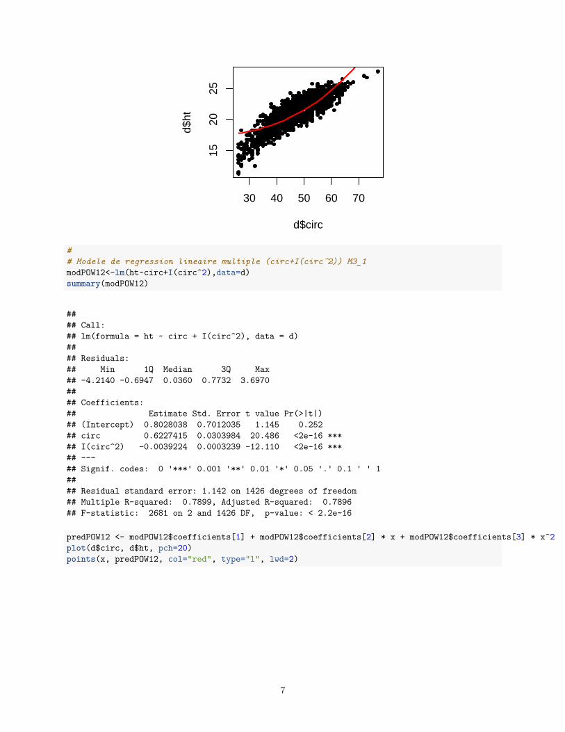
## Modele de regression lineaire multiple (circ+I(circ^3)) M3_2modPOW13<-lm(ht~circ+I(circ^3),data=d)summary(modPOW13)

#### Call:## lm(formula = ht ~ circ + I(circ^3), data = d)#### Residuals:## Min 1Q Median 3Q Max## -4.2514 -0.7127 0.0322 0.7463 3.7262#### Coefficients:## Estimate Std. Error t value Pr(>|t|)## (Intercept) 3.716e+00 4.935e-01 7.531 8.89e-14 ***## circ 4.344e-01 1.582e-02 27.464 < 2e-16 ***## I(circ^3) -2.642e-05 2.296e-06 -11.505 < 2e-16 ***## ---## Signif. codes: 0 '***' 0.001 '**' 0.01 '*' 0.05 '.' 0.1 ' ' 1#### Residual standard error: 1.148 on 1426 degrees of freedom## Multiple R-squared: 0.788, Adjusted R-squared: 0.7877## F-statistic: 2650 on 2 and 1426 DF, p-value: < 2.2e-16

predPOW13 <- modPOW13$coefficients[1] + modPOW13$coefficients[2] * x + modPOW13$coefficients[3] * x^3plot(d$circ, d$ht, pch=20)points(x, predPOW13, col="red", type="l", lwd=2)

8

30 40 50 60 7015

2025

d$circ

d$ht

## Modele de regression lineaire multiple (I(circ^2)+I(circ^3)) M3_3modPOW23<-lm(ht~I(circ^2)+I(circ^3),data=d)summary(modPOW23)

#### Call:## lm(formula = ht ~ I(circ^2) + I(circ^3), data = d)#### Residuals:## Min 1Q Median 3Q Max## -4.3362 -0.7261 0.0012 0.7781 3.7883#### Coefficients:## Estimate Std. Error t value Pr(>|t|)## (Intercept) 1.039e+01 2.653e-01 39.16 <2e-16 ***## I(circ^2) 9.128e-03 3.467e-04 26.33 <2e-16 ***## I(circ^3) -8.859e-05 4.724e-06 -18.75 <2e-16 ***## ---## Signif. codes: 0 '***' 0.001 '**' 0.01 '*' 0.05 '.' 0.1 ' ' 1#### Residual standard error: 1.164 on 1426 degrees of freedom## Multiple R-squared: 0.7819, Adjusted R-squared: 0.7816## F-statistic: 2556 on 2 and 1426 DF, p-value: < 2.2e-16

predPOW23 <- modPOW23$coefficients[1] + modPOW23$coefficients[2] * x^2 + modPOW23$coefficients[3] * x^3plot(d$circ, d$ht, pch=20)points(x, predPOW23, col="red", type="l", lwd=2)

9

30 40 50 60 7015

2025

d$circ

d$ht

# Modele de regression lineaire multiple (puissances) M4modPOW123<-lm(ht~circ+I(I(circ^2))+I(I(circ^3)),data=d)summary(modPOW123)

#### Call:## lm(formula = ht ~ circ + I(I(circ^2)) + I(I(circ^3)), data = d)#### Residuals:## Min 1Q Median 3Q Max## -4.1632 -0.6981 0.0395 0.7895 4.0358#### Coefficients:## Estimate Std. Error t value Pr(>|t|)## (Intercept) -1.192e+01 2.424e+00 -4.916 9.86e-07 ***## circ 1.487e+00 1.606e-01 9.256 < 2e-16 ***## I(I(circ^2)) -2.285e-02 3.471e-03 -6.583 6.46e-11 ***## I(I(circ^3)) 1.342e-04 2.450e-05 5.477 5.12e-08 ***## ---## Signif. codes: 0 '***' 0.001 '**' 0.01 '*' 0.05 '.' 0.1 ' ' 1#### Residual standard error: 1.131 on 1425 degrees of freedom## Multiple R-squared: 0.7943, Adjusted R-squared: 0.7938## F-statistic: 1834 on 3 and 1425 DF, p-value: < 2.2e-16

predPOW123 <- modPOW123$coefficients[1] + modPOW123$coefficients[2] * x + modPOW123$coefficients[3] * x^2 + modPOW123$coefficients[4] * x^3plot(d$circ, d$ht, pch=20)points(x, predPOW123, col="red", type="l", lwd=2)

10

30 40 50 60 7015

2025

d$circ

d$ht

## Modele de regression lineaire multiple (puissances) M5modPOW1234<-lm(ht~circ+I(circ^2)+I(circ^3)+I(circ^4),data=d)summary(modPOW1234)

#### Call:## lm(formula = ht ~ circ + I(circ^2) + I(circ^3) + I(circ^4), data = d)#### Residuals:## Min 1Q Median 3Q Max## -4.1696 -0.6951 0.0307 0.7807 4.0564#### Coefficients:## Estimate Std. Error t value Pr(>|t|)## (Intercept) -1.378e+01 8.170e+00 -1.686 0.0920 .## circ 1.655e+00 7.212e-01 2.294 0.0219 *## I(circ^2) -2.834e-02 2.327e-02 -1.218 0.2235## I(circ^3) 2.116e-04 3.258e-04 0.650 0.5161## I(circ^4) -3.992e-07 1.675e-06 -0.238 0.8116## ---## Signif. codes: 0 '***' 0.001 '**' 0.01 '*' 0.05 '.' 0.1 ' ' 1#### Residual standard error: 1.131 on 1424 degrees of freedom## Multiple R-squared: 0.7943, Adjusted R-squared: 0.7937## F-statistic: 1374 on 4 and 1424 DF, p-value: < 2.2e-16

predPOW1234 <- modPOW1234$coefficients[1] + modPOW1234$coefficients[2] * x + modPOW1234$coefficients[3] * x^2 + modPOW1234$coefficients[4] * x^3 + modPOW1234$coefficients[5] * x^4plot(d$circ, d$ht, pch=20)points(x, predPOW1234, col="red", type="l", lwd=2)

11

30 40 50 60 7015

2025

d$circ

d$ht

11. Tracer pour chacun des modèles proposés ci-dessus les valeurs prédites par le modèle et les valeursobservées. Commenter.

# Tracé des droites de régression sur le même graphecouleurs <- rainbow(10)

# on ajoute des marges autour du graphe pour pouvoir ajouter la légende# la fonction par permet d'ajuster les paramètres graphiques, et l'option "mar" concerne les margespar(mar=c(5,4,3,11), xpd=FALSE)plot(d$circ, d$ht, pch=20, xlab="Circonférence", ylab="Hauteur")points(x, predLIN, col=couleurs[1], type="l", lwd=2)points(x, predSQRT, col=couleurs[2], type="l", lwd=2)points(x, predLINSQRT, col=couleurs[3], type="l", lwd=2)points(x, predPOW2, col=couleurs[4], type="l", lwd=2)points(x, predPOW3, col=couleurs[5], type="l", lwd=2)points(x, predPOW12, col=couleurs[6], type="l", lwd=2)points(x, predPOW13, col=couleurs[7], type="l", lwd=2)points(x, predPOW23, col=couleurs[8], type="l", lwd=2)points(x, predPOW123, col=couleurs[9], type="l", lwd=2)points(x, predPOW1234, col=couleurs[10], type="l", lwd=2)par(xpd=TRUE)legend("topright", inset=c(-0.65,0), legend=c("Linéaire","Racine","Linéaire + racine","Carré","Cube","Degrés 1 et 2","Degrés 1 et 3","Degrés 2 et 3","Degrés 1,2 et 3","Degrés 1, 2, 3 et 4"), col=couleurs, lwd=2)

12

30 40 50 60 70

1520

25

Circonférence

Hau

teur

LinéaireRacineLinéaire + racineCarréCubeDegrés 1 et 2Degrés 1 et 3Degrés 2 et 3Degrés 1,2 et 3Degrés 1, 2, 3 et 4

12. Comparer ces différents modèles à l’aide de la fonction anova de R. Proposer le meilleur modèle parmitous les modèles testés selon cette procédure.

# question 12# modèle constantmodCST <- lm(ht ~ 1, data=d)

# modele M1 contre modele M2anova(modCST,modLIN)

## Analysis of Variance Table#### Model 1: ht ~ 1## Model 2: ht ~ circ## Res.Df RSS Df Sum of Sq F Pr(>F)## 1 1428 8857.4## 2 1427 2052.1 1 6805.3 4732.4 < 2.2e-16 ***## ---## Signif. codes: 0 '***' 0.001 '**' 0.01 '*' 0.05 '.' 0.1 ' ' 1

# modele M1 contre modele regression lineaire simple (carre) M2_2anova(modCST,modPOW2)

## Analysis of Variance Table#### Model 1: ht ~ 1## Model 2: ht ~ I(circ^2)## Res.Df RSS Df Sum of Sq F Pr(>F)## 1 1428 8857.4## 2 1427 2408.3 1 6449.1 3821.3 < 2.2e-16 ***## ---## Signif. codes: 0 '***' 0.001 '**' 0.01 '*' 0.05 '.' 0.1 ' ' 1

13

# modele M1 contre modele de regression lineaire simple (cube) M2_3anova(modCST,modPOW3)

## Analysis of Variance Table#### Model 1: ht ~ 1## Model 2: ht ~ I(circ^3)## Res.Df RSS Df Sum of Sq F Pr(>F)## 1 1428 8857.4## 2 1427 2871.0 1 5986.4 2975.4 < 2.2e-16 ***## ---## Signif. codes: 0 '***' 0.001 '**' 0.01 '*' 0.05 '.' 0.1 ' ' 1

# modele M1 contre modele de regression lineaire simple (racine carree) M2bisanova(modCST,modSQRT)

## Analysis of Variance Table#### Model 1: ht ~ 1## Model 2: ht ~ sqrt(circ)## Res.Df RSS Df Sum of Sq F Pr(>F)## 1 1428 8857.4## 2 1427 1930.4 1 6927.1 5120.8 < 2.2e-16 ***## ---## Signif. codes: 0 '***' 0.001 '**' 0.01 '*' 0.05 '.' 0.1 ' ' 1

# modele M1 contre modele de regression lineaire multiple (circ+circ^2) M3_1anova(modCST,modPOW12)

## Analysis of Variance Table#### Model 1: ht ~ 1## Model 2: ht ~ circ + I(circ^2)## Res.Df RSS Df Sum of Sq F Pr(>F)## 1 1428 8857.4## 2 1426 1860.7 2 6996.7 2681 < 2.2e-16 ***## ---## Signif. codes: 0 '***' 0.001 '**' 0.01 '*' 0.05 '.' 0.1 ' ' 1

# modele M2 contre modele de regression lineaire multiple (circ+circ^2) M3_1anova(modLIN,modPOW12)

## Analysis of Variance Table#### Model 1: ht ~ circ## Model 2: ht ~ circ + I(circ^2)## Res.Df RSS Df Sum of Sq F Pr(>F)## 1 1427 2052.1## 2 1426 1860.7 1 191.37 146.66 < 2.2e-16 ***## ---## Signif. codes: 0 '***' 0.001 '**' 0.01 '*' 0.05 '.' 0.1 ' ' 1

14

# modele M2 contre modele de regression lineaire multiple (circ+circ^3) M3_2anova(modLIN,modPOW13)

## Analysis of Variance Table#### Model 1: ht ~ circ## Model 2: ht ~ circ + I(circ^3)## Res.Df RSS Df Sum of Sq F Pr(>F)## 1 1427 2052.1## 2 1426 1877.8 1 174.31 132.37 < 2.2e-16 ***## ---## Signif. codes: 0 '***' 0.001 '**' 0.01 '*' 0.05 '.' 0.1 ' ' 1

# modele M2 contre modele de reg lin multiple (circ + sqrt(circ)) M3bisanova(modLIN,modLINSQRT)

## Analysis of Variance Table#### Model 1: ht ~ circ## Model 2: ht ~ circ + sqrt(circ)## Res.Df RSS Df Sum of Sq F Pr(>F)## 1 1427 2052.1## 2 1426 1840.7 1 211.43 163.8 < 2.2e-16 ***## ---## Signif. codes: 0 '***' 0.001 '**' 0.01 '*' 0.05 '.' 0.1 ' ' 1

# modele reg lin simple (carre) M2_2 contre reg lin multiple (circ+circ^2) M3_1anova(modPOW2,modPOW12)

## Analysis of Variance Table#### Model 1: ht ~ I(circ^2)## Model 2: ht ~ circ + I(circ^2)## Res.Df RSS Df Sum of Sq F Pr(>F)## 1 1427 2408.3## 2 1426 1860.7 1 547.61 419.68 < 2.2e-16 ***## ---## Signif. codes: 0 '***' 0.001 '**' 0.01 '*' 0.05 '.' 0.1 ' ' 1

# reg lin simple (racine carree) M2bis contre reg lin multiple (circ + sqrt(circ)) M3bisanova(modSQRT,modLINSQRT)

## Analysis of Variance Table#### Model 1: ht ~ sqrt(circ)## Model 2: ht ~ circ + sqrt(circ)## Res.Df RSS Df Sum of Sq F Pr(>F)## 1 1427 1930.3## 2 1426 1840.7 1 89.696 69.489 < 2.2e-16 ***## ---## Signif. codes: 0 '***' 0.001 '**' 0.01 '*' 0.05 '.' 0.1 ' ' 1

15

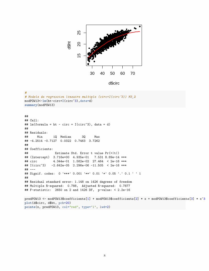
# modele de reg lin mult (circ+circ^2) M3_1 contre modele de reg lin mult (puissances) M4anova(modPOW12,modPOW123)

## Analysis of Variance Table#### Model 1: ht ~ circ + I(circ^2)## Model 2: ht ~ circ + I(I(circ^2)) + I(I(circ^3))## Res.Df RSS Df Sum of Sq F Pr(>F)## 1 1426 1860.7## 2 1425 1822.3 1 38.357 29.993 5.118e-08 ***## ---## Signif. codes: 0 '***' 0.001 '**' 0.01 '*' 0.05 '.' 0.1 ' ' 1

# modele de reg lin mult (circ+circ^3) M3_2 contre modele de reg lin mult (puissances) M4anova(modPOW13,modPOW123)

## Analysis of Variance Table#### Model 1: ht ~ circ + I(circ^3)## Model 2: ht ~ circ + I(I(circ^2)) + I(I(circ^3))## Res.Df RSS Df Sum of Sq F Pr(>F)## 1 1426 1877.8## 2 1425 1822.3 1 55.422 43.337 6.459e-11 ***## ---## Signif. codes: 0 '***' 0.001 '**' 0.01 '*' 0.05 '.' 0.1 ' ' 1

# reg lin mult (circ^2+circ^3) M3_3 contre modele de reg lin mult (puissances) M4anova(modPOW23,modPOW123)

## Analysis of Variance Table#### Model 1: ht ~ I(circ^2) + I(circ^3)## Model 2: ht ~ circ + I(I(circ^2)) + I(I(circ^3))## Res.Df RSS Df Sum of Sq F Pr(>F)## 1 1426 1931.9## 2 1425 1822.3 1 109.57 85.676 < 2.2e-16 ***## ---## Signif. codes: 0 '***' 0.001 '**' 0.01 '*' 0.05 '.' 0.1 ' ' 1

# reg lin mult (puissances) M4 contre reg lin mult (puissances) M5anova(modPOW123,modPOW1234)

## Analysis of Variance Table#### Model 1: ht ~ circ + I(I(circ^2)) + I(I(circ^3))## Model 2: ht ~ circ + I(circ^2) + I(circ^3) + I(circ^4)## Res.Df RSS Df Sum of Sq F Pr(>F)## 1 1425 1822.3## 2 1424 1822.3 1 0.072734 0.0568 0.8116

13. Calculer le critère AIC pour chacun des modèles. Qu’en concluez-vous ?

16

# question 13#Selection AICAIC(modCST)

## [1] 6666.223

AIC(modLIN)

## [1] 4578.454

AIC(modPOW2)

## [1] 4807.202

AIC(modPOW3)

## [1] 5058.335

AIC(modPOW12)

## [1] 4440.56

AIC(modPOW13)

## [1] 4453.605

AIC(modPOW23)

## [1] 4494.227

AIC(modPOW123)

## [1] 4412.794

AIC(modPOW1234)

## [1] 4414.737

AIC(modSQRT)

## [1] 4491.066

AIC(modLINSQRT)

## [1] 4425.074

14. Utiliser la commande step pour sélectionner le meilleur modèle pas à pas au sens du critère AIC.

17

# question 14# sélection "backward" -> on part du modèle complet et on supprime des variablesstep(modPOW1234,direction="backward",trace="True")

## Start: AIC=357.41## ht ~ circ + I(circ^2) + I(circ^3) + I(circ^4)#### Df Sum of Sq RSS AIC## - I(circ^4) 1 0.0727 1822.3 355.47## - I(circ^3) 1 0.5399 1822.8 355.83## - I(circ^2) 1 1.8980 1824.2 356.90## <none> 1822.3 357.41## - circ 1 6.7353 1829.0 360.68#### Step: AIC=355.47## ht ~ circ + I(circ^2) + I(circ^3)#### Df Sum of Sq RSS AIC## <none> 1822.3 355.47## - I(circ^3) 1 38.357 1860.7 383.23## - I(circ^2) 1 55.422 1877.8 396.28## - circ 1 109.566 1931.9 436.90

#### Call:## lm(formula = ht ~ circ + I(circ^2) + I(circ^3), data = d)#### Coefficients:## (Intercept) circ I(circ^2) I(circ^3)## -1.192e+01 1.487e+00 -2.285e-02 1.342e-04

# sélection "forward" -> on part du modèle constant et on ajoute des variablesstep(modCST,scope=list(upper=~circ+I(circ^2)+I(circ^3)+I(circ^4)),direction="forward",trace="True")

## Start: AIC=2608.9## ht ~ 1#### Df Sum of Sq RSS AIC## + circ 1 6805.3 2052.1 521.13## + I(circ^2) 1 6449.1 2408.3 749.88## + I(circ^3) 1 5986.4 2871.0 1001.01## + I(circ^4) 1 5460.0 3397.5 1241.59## <none> 8857.4 2608.90#### Step: AIC=521.13## ht ~ circ#### Df Sum of Sq RSS AIC## + I(circ^2) 1 191.37 1860.7 383.23## + I(circ^3) 1 174.31 1877.8 396.28## + I(circ^4) 1 155.46 1896.6 410.55## <none> 2052.1 521.13

18

#### Step: AIC=383.23## ht ~ circ + I(circ^2)#### Df Sum of Sq RSS AIC## + I(circ^3) 1 38.357 1822.3 355.47## + I(circ^4) 1 37.889 1822.8 355.83## <none> 1860.7 383.23#### Step: AIC=355.47## ht ~ circ + I(circ^2) + I(circ^3)#### Df Sum of Sq RSS AIC## <none> 1822.3 355.47## + I(circ^4) 1 0.072734 1822.3 357.41

#### Call:## lm(formula = ht ~ circ + I(circ^2) + I(circ^3), data = d)#### Coefficients:## (Intercept) circ I(circ^2) I(circ^3)## -1.192e+01 1.487e+00 -2.285e-02 1.342e-04

# sélection à la fois backward et forward, on part du modèle constant et on ajoute des variables tout en vérifiants à chaque ajout que cela ne modifie pas la significativité des autres variablesstep(modCST,scope=list(upper=~circ+I(circ^2)+I(circ^3)+I(circ^4)),direction="both",trace="True")

## Start: AIC=2608.9## ht ~ 1#### Df Sum of Sq RSS AIC## + circ 1 6805.3 2052.1 521.13## + I(circ^2) 1 6449.1 2408.3 749.88## + I(circ^3) 1 5986.4 2871.0 1001.01## + I(circ^4) 1 5460.0 3397.5 1241.59## <none> 8857.4 2608.90#### Step: AIC=521.13## ht ~ circ#### Df Sum of Sq RSS AIC## + I(circ^2) 1 191.4 1860.7 383.23## + I(circ^3) 1 174.3 1877.8 396.28## + I(circ^4) 1 155.5 1896.6 410.55## <none> 2052.1 521.13## - circ 1 6805.3 8857.4 2608.90#### Step: AIC=383.23## ht ~ circ + I(circ^2)#### Df Sum of Sq RSS AIC## + I(circ^3) 1 38.36 1822.3 355.47## + I(circ^4) 1 37.89 1822.8 355.83

19

## <none> 1860.7 383.23## - I(circ^2) 1 191.37 2052.1 521.13## - circ 1 547.61 2408.3 749.88#### Step: AIC=355.47## ht ~ circ + I(circ^2) + I(circ^3)#### Df Sum of Sq RSS AIC## <none> 1822.3 355.47## + I(circ^4) 1 0.073 1822.3 357.41## - I(circ^3) 1 38.357 1860.7 383.23## - I(circ^2) 1 55.422 1877.8 396.28## - circ 1 109.566 1931.9 436.90

#### Call:## lm(formula = ht ~ circ + I(circ^2) + I(circ^3), data = d)#### Coefficients:## (Intercept) circ I(circ^2) I(circ^3)## -1.192e+01 1.487e+00 -2.285e-02 1.342e-04

15. Répondre au deux questions précédentes en utilisant à présent le critère BIC.

# question 15BIC(modCST)

## [1] 6676.752

BIC(modLIN)

## [1] 4594.248

BIC(modPOW2)

## [1] 4822.997

BIC(modPOW3)

## [1] 5074.129

BIC(modPOW12)

## [1] 4461.619

BIC(modPOW13)

## [1] 4474.664

20

BIC(modPOW23)

## [1] 4515.286

BIC(modPOW123)

## [1] 4439.118

BIC(modPOW1234)

## [1] 4446.326

BIC(modSQRT)

## [1] 4506.86

BIC(modLINSQRT)

## [1] 4446.133

# pour obtenir une sélection à partir du critère BIC, il faut modifier la constante de pénalisation# dans la fonction step, cela se fait en précisant k=log(n), où n est la taille de l'échantillonn = nrow(d)step(modPOW1234,direction="backward",trace="True", k=log(n))

## Start: AIC=383.73## ht ~ circ + I(circ^2) + I(circ^3) + I(circ^4)#### Df Sum of Sq RSS AIC## - I(circ^4) 1 0.0727 1822.3 376.53## - I(circ^3) 1 0.5399 1822.8 376.89## - I(circ^2) 1 1.8980 1824.2 377.96## - circ 1 6.7353 1829.0 381.74## <none> 1822.3 383.73#### Step: AIC=376.53## ht ~ circ + I(circ^2) + I(circ^3)#### Df Sum of Sq RSS AIC## <none> 1822.3 376.53## - I(circ^3) 1 38.357 1860.7 399.03## - I(circ^2) 1 55.422 1877.8 412.07## - circ 1 109.566 1931.9 452.69

#### Call:## lm(formula = ht ~ circ + I(circ^2) + I(circ^3), data = d)#### Coefficients:## (Intercept) circ I(circ^2) I(circ^3)## -1.192e+01 1.487e+00 -2.285e-02 1.342e-04

21

step(modCST,scope=list(upper=~circ+I(circ^2)+I(circ^3)+I(circ^4)),direction="forward",trace="True", k=log(n))

## Start: AIC=2614.16## ht ~ 1#### Df Sum of Sq RSS AIC## + circ 1 6805.3 2052.1 531.66## + I(circ^2) 1 6449.1 2408.3 760.41## + I(circ^3) 1 5986.4 2871.0 1011.54## + I(circ^4) 1 5460.0 3397.5 1252.12## <none> 8857.4 2614.16#### Step: AIC=531.66## ht ~ circ#### Df Sum of Sq RSS AIC## + I(circ^2) 1 191.37 1860.7 399.03## + I(circ^3) 1 174.31 1877.8 412.07## + I(circ^4) 1 155.46 1896.6 426.34## <none> 2052.1 531.66#### Step: AIC=399.03## ht ~ circ + I(circ^2)#### Df Sum of Sq RSS AIC## + I(circ^3) 1 38.357 1822.3 376.53## + I(circ^4) 1 37.889 1822.8 376.89## <none> 1860.7 399.03#### Step: AIC=376.53## ht ~ circ + I(circ^2) + I(circ^3)#### Df Sum of Sq RSS AIC## <none> 1822.3 376.53## + I(circ^4) 1 0.072734 1822.3 383.73

#### Call:## lm(formula = ht ~ circ + I(circ^2) + I(circ^3), data = d)#### Coefficients:## (Intercept) circ I(circ^2) I(circ^3)## -1.192e+01 1.487e+00 -2.285e-02 1.342e-04

step(modCST,scope=list(upper=~circ+I(circ^2)+I(circ^3)+I(circ^4)),direction="both",trace="True", k=log(n))

## Start: AIC=2614.16## ht ~ 1#### Df Sum of Sq RSS AIC## + circ 1 6805.3 2052.1 531.66## + I(circ^2) 1 6449.1 2408.3 760.41

22

## + I(circ^3) 1 5986.4 2871.0 1011.54## + I(circ^4) 1 5460.0 3397.5 1252.12## <none> 8857.4 2614.16#### Step: AIC=531.66## ht ~ circ#### Df Sum of Sq RSS AIC## + I(circ^2) 1 191.4 1860.7 399.03## + I(circ^3) 1 174.3 1877.8 412.07## + I(circ^4) 1 155.5 1896.6 426.34## <none> 2052.1 531.66## - circ 1 6805.3 8857.4 2614.16#### Step: AIC=399.03## ht ~ circ + I(circ^2)#### Df Sum of Sq RSS AIC## + I(circ^3) 1 38.36 1822.3 376.53## + I(circ^4) 1 37.89 1822.8 376.89## <none> 1860.7 399.03## - I(circ^2) 1 191.37 2052.1 531.66## - circ 1 547.61 2408.3 760.41#### Step: AIC=376.53## ht ~ circ + I(circ^2) + I(circ^3)#### Df Sum of Sq RSS AIC## <none> 1822.3 376.53## + I(circ^4) 1 0.073 1822.3 383.73## - I(circ^3) 1 38.357 1860.7 399.03## - I(circ^2) 1 55.422 1877.8 412.07## - circ 1 109.566 1931.9 452.69

#### Call:## lm(formula = ht ~ circ + I(circ^2) + I(circ^3), data = d)#### Coefficients:## (Intercept) circ I(circ^2) I(circ^3)## -1.192e+01 1.487e+00 -2.285e-02 1.342e-04

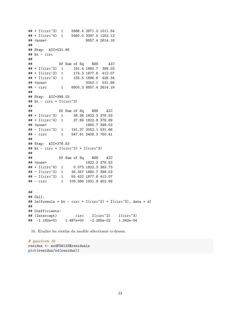
16. Etudier les résidus du modèle sélectionné ci-dessus.

# question 16residus <- modPOW123$residualsplot(residus/sd(residus))

23

0 400 800 1200−

20

2Index

resi

dus/

sd(r

esid

us)

# histogrammehist(residus/sd(residus))

Histogram of residus/sd(residus)

residus/sd(residus)

Fre

quen

cy

−4 −2 0 2 4

010

020

0

# qq-plotqqnorm(residus/sd(residus))qqline(residus/sd(residus))

24

−3 −1 0 1 2 3−

20

2

Normal Q−Q Plot

Theoretical Quantiles

Sam

ple

Qua

ntile

s

# test de normalitéshapiro.test(residus/sd(residus))

#### Shapiro-Wilk normality test#### data: residus/sd(residus)## W = 0.99807, p-value = 0.09493

# comparason avec les résidus du modèle constantresidusCST <- modCST$residualsplot(residusCST/sd(residusCST))

0 400 800 1200

−4

−2

01

2

Index

resi

dusC

ST

/sd(

resi

dusC

ST

)

hist(residusCST/sd(residusCST))

25

Histogram of residusCST/sd(residusCST)

residusCST/sd(residusCST)

Fre

quen

cy

−4 −2 0 2

010

020

030

0

qqnorm(residusCST/sd(residusCST))qqline(residusCST/sd(residusCST))

−3 −1 0 1 2 3

−4

−2

01

2

Normal Q−Q Plot

Theoretical Quantiles

Sam

ple

Qua

ntile

s

shapiro.test(residusCST)

#### Shapiro-Wilk normality test#### data: residusCST## W = 0.96403, p-value < 2.2e-16

17. Dans ce modèle, donner les intervalles de confiance observés pour les paramètres d’espérance.

26