Transport spectroscopy of a Kondo quantum dot coupled to a finite size grain

Pascal Simon,1 Julien Salomez,1 and Denis Feinberg2

1Laboratoire de Physique et Modélisation des Milieux Condensés, CNRS et Université Joseph Fourier, 38042 Grenoble, France2Laboratoire d’Etudes des Propriétés Electroniques des Solides, CNRS, associated with Université Joseph Fourier, BP 166, 38042

Grenoble, France�Received 17 November 2005; revised manuscript received 7 February 2006; published 11 May 2006�

We analyze a simple setup in which a quantum dot is strongly connected to a metallic grain or finite sizewire and weakly connected to two normal leads. The Kondo screening cloud essentially develops in thestrongly coupled grain whereas the two weakly connected reservoirs can be used as transport probes. Since thetransport channels and the screening channels are almost decoupled, such a setup allows an easier access to themeasure of finite-size Kondo effects.

DOI: 10.1103/PhysRevB.73.205325 PACS number�s�: 73.23.�b, 72.15.Qm, 73.63.Kv, 72.10.Fk

I. INTRODUCTION

One of the most remarkable achievements of recentprogress in nanoelectronics has been the observation of theKondo effect in a single semiconductor quantum dot.1–3

When the number of electrons in the dot is odd, it can behaveas an S=1/2 magnetic impurity interacting via magnetic ex-change with the conduction electrons. One of the main sig-natures of the Kondo effect is a zero-bias anomaly and theconductance reaching the unitary limit 2e2 /h at low enoughtemperature T�TK

0 . TK0 stands for the Kondo temperature and

is the main energy scale of the problem. At low temperature,the impurity spin is screened and forms a singlet with a con-duction electron belonging to a very extended many-bodywave-function known as the Kondo screening cloud. Thesize of this screening cloud may be evaluated as �K

0

��vF /TK0 where vF is the Fermi velocity. In a quantum dot,

the typical Kondo temperature is of order 1 K which leads to�K

0 �1 micron in semiconducting heterostructures. Finite sizeeffects �FSE� related to the actual extent of this length scalehave been predicted recently in different geometries: an im-purity embedded in a finite size box,4 a quantum dot embed-ded in a ring threaded by a magnetic flux,5–8 and a quantumdot embedded between two open finite size wires �OFSW��by open we mean connected to at least one external infinitelead�.9,10 In the ring geometry, it was shown that the persis-tent current induced by a magnetic flux is particularly sensi-tive to screening cloud effects and is drastically reducedwhen the circumference of the ring becomes smaller than�K

0 .5 In the wire geometry, a signature of the finite size ex-tension of the Kondo cloud was found in the temperaturedependence of the conductance through the whole system.9,10

To be more precise, in a one-dimensional geometry wherethe finite size l is associated to a level spacing �, the Kondocloud fully develops if �K

0 � l, a condition equivalent to TK0

��. On the contrary, FSE effects appear if �K0 � l or TK

0

��.Nevertheless, in such a two-terminal geometry, the

screening of the artificial spin impurity is done in the OF-SWs which are also used to probe transport propertiesthrough the whole system. This brings at least two maindrawbacks: first, the analysis of FSE relies on the indepen-

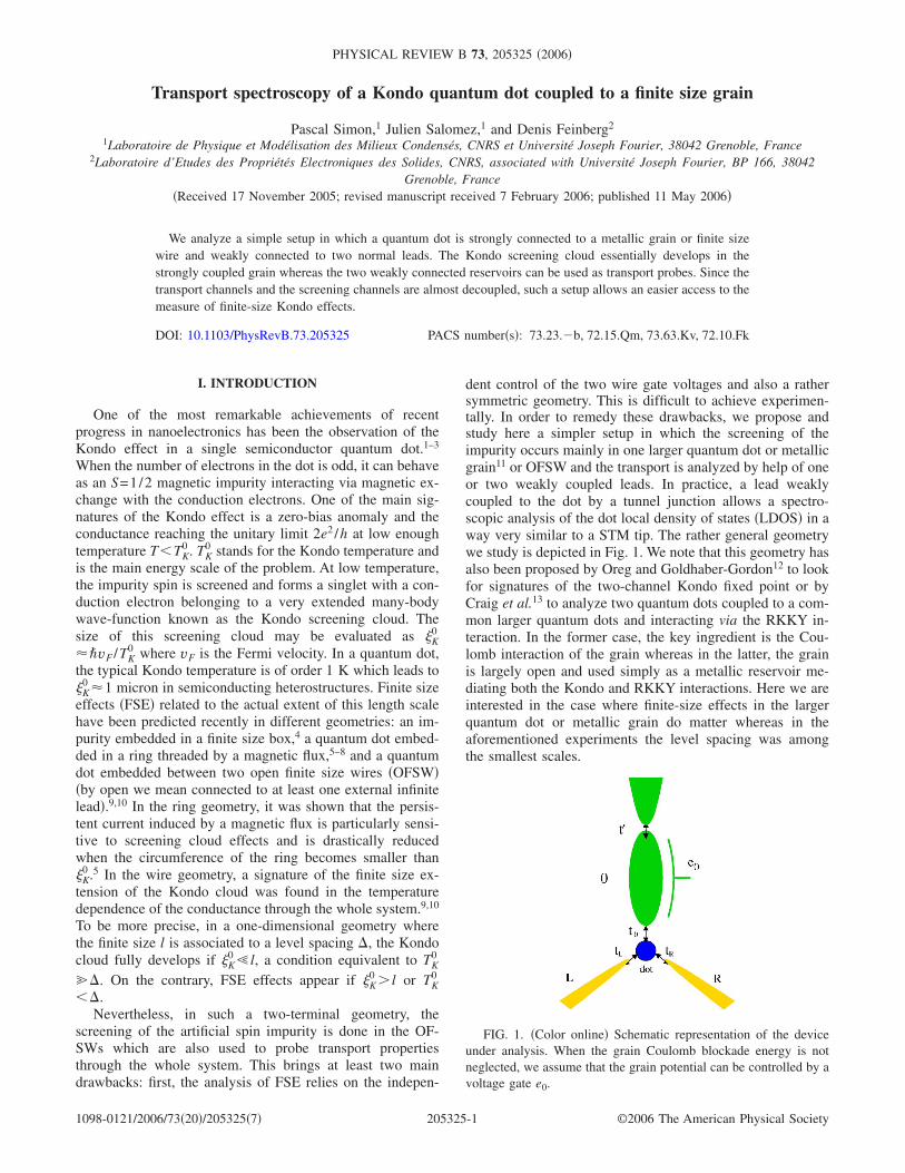
dent control of the two wire gate voltages and also a rathersymmetric geometry. This is difficult to achieve experimen-tally. In order to remedy these drawbacks, we propose andstudy here a simpler setup in which the screening of theimpurity occurs mainly in one larger quantum dot or metallicgrain11 or OFSW and the transport is analyzed by help of oneor two weakly coupled leads. In practice, a lead weaklycoupled to the dot by a tunnel junction allows a spectro-scopic analysis of the dot local density of states �LDOS� in away very similar to a STM tip. The rather general geometrywe study is depicted in Fig. 1. We note that this geometry hasalso been proposed by Oreg and Goldhaber-Gordon12 to lookfor signatures of the two-channel Kondo fixed point or byCraig et al.13 to analyze two quantum dots coupled to a com-mon larger quantum dots and interacting via the RKKY in-teraction. In the former case, the key ingredient is the Cou-lomb interaction of the grain whereas in the latter, the grainis largely open and used simply as a metallic reservoir me-diating both the Kondo and RKKY interactions. Here we areinterested in the case where finite-size effects in the largerquantum dot or metallic grain do matter whereas in theaforementioned experiments the level spacing was amongthe smallest scales.

FIG. 1. �Color online� Schematic representation of the deviceunder analysis. When the grain Coulomb blockade energy is notneglected, we assume that the grain potential can be controlled by avoltage gate e0.

PHYSICAL REVIEW B 73, 205325 �2006�

1098-0121/2006/73�20�/205325�7� ©2006 The American Physical Society205325-1

The plan of the paper is the following: in Sec. II, wepresent the model Hamiltonian and derive how the FSErenormalizes the Kondo temperature in our geometry. In Sec.III, we show how FSE affect the transport properties of thequantum dot and perform a detailed spectroscopic analysis.The effect of a finite Coulomb energy in the grain is alsodiscussed. Finally Sec. IV summarizes our results.

II. PRESENTATION OF THE MODEL

A. Model Hamiltonian

The geometry we analyze is depicted in Fig. 1. In thissection we assume that the large dot is connected to a thirdlead. We neglect the Coulomb interaction in the grain. As wewill see in the next section, the Coulomb interaction does notaffect the main results we discuss here. In order to model thefinite-size grain connected to a normal reservoir, we choosefor convenience a finite-size wire characterized by its lengthl or equivalently by its level spacing ���vF / l. In fact, theprecise shape of the finite-size grain is not important for ourpurpose as soon as it is characterized by a mean level spac-ing � separating peaks in the electronic density of states. Weassume that the small quantum dot is weakly coupled to oneor two adjacent leads �L and R�. On the Hamiltonian level,we use the following tight-binding description, and for sim-plicity model the leads as one-dimensional wires �this is byno means restrictive�: H=HL+HR+H0+Hdot+Htun with

HL = − t �j=1,s

�cj,s,L† cj+1,s,L + H.c.� − Lnj,s,L, �1�

H0 = − t �j=1,s

�cj,s,0† cj+1,s,0 + H.c.� − 0nj,s,0

+ �t − t���s

�cl,s,0† cl+1,s,0 + H.c.� , �2�

Hdot = �s

�dnd,s + Und↑nd↓, �3�

Htun = �s

��=L,R,0

�t�cds† c1,s,� + H.c.� . �4�

HR is obtained from HL by changing L→R. Here cj,s,� de-stroys an electron of spin s at site j in lead �=0,L ,R; cd,sdestroys an electron with spin s in the dot, nj,s,�=cj,s,�

† cj,s,�and nds=cds

† cds. The quantum dot is described by an Ander-son impurity model, �d ,U are, respectively, the energy leveland the Coulomb repulsion energy in the dot. The tunnelingamplitudes between the dot and the left lead, right lead andgrain are, respectively, denoted as tL , tR , t0 �see Fig. 1�. Thetunneling amplitude between the grain and the third lead isdenoted as t� �see Fig. 1�. Finally t denotes the tight bindingamplitude for conduction electrons implying that the elec-tronic bandwidth 0=4t. Since we want to use the left andright leads just as transport probes, we assume in the rest ofthe paper that tL , tR� t0.

We are particularly interested in the Kondo regime where�nd��1. In this regime, we can map Htun+Hdot to a Kondo

Hamiltonian by help of a Schrieffer-Wolff transformation,

HK = Htun + Hdot = ��,�=L,R,0

J��c1,s,�†

�� ss�

2· S�c1,s�,�, �5�

where J��=2t�t��1/ �d +1/ ��d+U�. It is clear that J00

�J0L ,J0R�JLL ,JRR ,JLR. In Eq. �5�, we have neglected directpotential scattering terms which do not renormalize and canbe omitted in the low energy limit.

B. Kondo temperatures

The Kondo temperature is a crossover scale separating thehigh temperature perturbative regime from the low tempera-ture one where the impurity is screened. There are manyways to define such scale. We choose the “perturbativescale” which is defined as the scale at which the second ordercorrections to the Kondo couplings become of the same or-der of the bare Kondo coupling. Note that all various defini-tions of Kondo scales differ by a constant multiplicative fa-cor �see, for example, Ref. 8 for a comparison of theperturbative Kondo scale with the one coming from the slaveBoson mean field theory�.

The renormalization group equations relate the Kondocouplings defined at scales 0 and . They simply read

J��� � � J��� 0� +1

2��

J��� 0�

�J��� 0���

0

+ �− 0

− ������

d� , �6�

where �� is the LDOS in lead � seen by the quantum dot.When the density of states �� are uniform, the RG equations

can be rewritten by introducing �̂, the matrix of the dimen-sionless Kondo couplings, ���=�����J��.9,14 The Kondotemperature TK may be therefore defined as

1

2��TK

0

+ �− 0

−TK Tr��̂����

d� = 1. �7�

Since J00�JLL ,JRR, the Kondo temperature essentiallydepends on the LDOS in the lead 0 and the Kondo tempera-ture definition can be well approximated by

J00

2 ��TK

0

+ �− 0

−TK �0����

d� = 1. �8�

When the lead 0 becomes infinite �i.e., when t�= t�, �0���=�0=const and we recover TK=TK

0 the usual Kondo tempera-ture where a constant density of states is assumed. It is worthnoting that including the Coulomb interaction in the graindoes not affect much the Kondo temperature. The grain Cou-lomb energy EG slightly renormalizes J00 in the Schrieffer-Wolff transformation12 since EG�U , �d.

The LDOS �0 can be easily computed and corresponds inthe limit t�2� t2 to a sum of peaks at positions �n=−2t cos k0,n−0 of width �n��2�t��2sin3�k0,n� / tl wherek0,n��n / �l+1�+O�t�2 / t2l� �Ref. 9�. The LDOS �0 is verywell approximated by a sum of Lorentzian functions9 in thelimit t�� t,

SIMON, SALOMEZ, AND FEINBERG PHYSICAL REVIEW B 73, 205325 �2006�

205325-2

��0��� �2

l + 1�n

sin2�k0,n��n

�� − �n�2 + �n2 . �9�

This approximation is quite convenient in order to estimatethe Kondo temperature TK through �8�. Note that the positionof the resonance peaks may be controlled by the chemicalpotential 0. Another possibility is to fix 0 and to add asmall transverse magnetic field which modifies the orbitalpart of the electronic wave function in the grain and thereforeshift the resonance peak positions. When the level spacing�n�2�t sin k0,n / l is much smaller than the Kondo tempera-ture TK

0 , no finite-size effects are expected. Indeed, the inte-gral in �8� averages out over many peaks and the genuineKondo temperature is TK�TK

0 . On the other hand, when TK0

��n, the Kondo temperature begins to depend on the finestructure of the LDOS �0 and a careful calculation of theintegral in �8� is required. Two cases may be distinguished:either �0 is tuned such that a resonance �n sits at the Fermienergy EF=0 �labeled by the index R� or in a nonresonantsituation �labeled by the index NR�.

In the former case, we can estimate

TKR =

�n�n

���n2 + �n

2�exp� 2

J00��n��0R�0�

� − �n2

� �n exp�−1

J00��n��0R�0�

� � �n�TK0

�n���n/�n

, �10�

where we approximate the on-resonance LDOS at EF=0 by��0

R�0��2 sin2k0,n / l�n. In the latter case, we obtain,

TKNR = �n exp�−

�l�n2

16J00��n�sin2�k0,n��n�

� �n exp�−1

J00��n��0NR�0�

� � �n�TK0

�n���n/8�n

,

�11�

where ��0NR�0��16�n sin2k0,n / l�n

2. These two scales arevery different when t�2� t2. By controlling �0, we can con-trol the Kondo temperature �only when TK���. The mainfeature of such geometry is that the screening of the artificialspin impurity is essentially performed in the open finite-sizewire corresponding to lead 0. Now we want to study whatare the consequences of FSE on transport when one or twoleads are weakly coupled to the dot. This is the purpose ofthe next section.

III. TRANSPORT SPECTROSCOPY OF A QUANTUM DOTCOUPLED TO AN OPEN GRAIN

In this section, we consider a standard three-terminal ge-ometry as depicted in Fig. 1 and analyze the conductancematrix of the system. There are several approaches we maycombine to obtain such quantity for the whole temperaturerange. Nonetheless, before going into these details, let usanalyze the dot density of states in presence of FSE in thegrain.

A. Density of states

We have used the slave Boson mean field theory�SBMFT�15 in order to calculate the dot density of states.This approximation describes qualitatively well the behaviorof the Kondo impurity at low temperature T�TK when theimpurity is screened. This method has been proved to beefficient to capture finite size effects in Ref. 9. The mainadvantage of the SBMFT relies on its ability to qualitativelyreproduce the energy scales of the problem �here the Kondotemperature�.

An interesting quantity to look at is the dot density ofstates �d���. The density of states can be read from the dif-ferential conductance as follows: The current in the left elec-trode IL reads16

IL =4e

h�L�

−

�2�f�� − L��d��� − Gd����d� , �12�

where �d is the dot LDOS, Gd����=�ei�t�d†d�t�� the lesser

Green function for the dot and �L/R=�tL/R2 �L/R. The standard

procedure is to get rid of the lesser dot Green function usingthe current conservation �here IL+ IR+ I0=0�. Nevertheless,such procedure is useful only when the leads density ofstates can be assumed constant on the typical scale we areinterested in. This is not the case here because of the varia-tions of �0���=�t0

2�0���. Nevertheless, one can makeprogress by assuming �L/R��0��� such that for low bias thedot Green functions weakly depend on the chemical potentialin the left and right leads. Therefore

edI

dL�

2e2

h4�L�

−

�− df���d�

���d�� + L�d� , �13�

which allows an experimental access to �d�L�. Note that asimilar approximation is used for STM theory with magneticadatoms.17 We have plotted �d��� in Fig. 2 for both the non-resonant case and the on-resonance case for three differentvalues of �K

0 / l. We took the following parameters in units oft=1: t0=0.5, tL= tR=0.1 �therefore tL

2 � t02�, t�=0.5, and l

�1000a �a the lattice constant� or equivalently ��0.006.The Kondo energy scale �K

0 can be varied using the dot en-ergy level �d which is controlled by the dot gate voltage.When TK

0 ��, no finite-size effect is to be expected. In thiscase, �d��� mimics the density of state in the lead 0 but isshifted such that an off-resonance peak in the lead 0 corre-sponds to a dot resonance peak. The various peaks appearingin �d are included in an envelope of width O�TK

0 ��� �whichis a broader range than Fig. 2 actually covers for �K

0 / l=� /TK

0 �0.15�. This can be simply understood from a non-interacting picture valid at T=0. The noninteracting dotGreen function reads

Gdd��� �1

� − �d − ����� + i�0���, �14�

where �� is the real part of the dot self-energy and �0 itsimaginary part. The minima’s of �0 thus correspond to themaxima of −Im�Gdd�. We also note that the resonance peak isslightly shifted from �=0 in this limit. Therefore the2-terminal conductance does not reach its unitary limit �i.e.,

TRANSPORT SPECTROSCOPY OF A KONDO QUANTUM¼ PHYSICAL REVIEW B 73, 205325 �2006�

205325-3

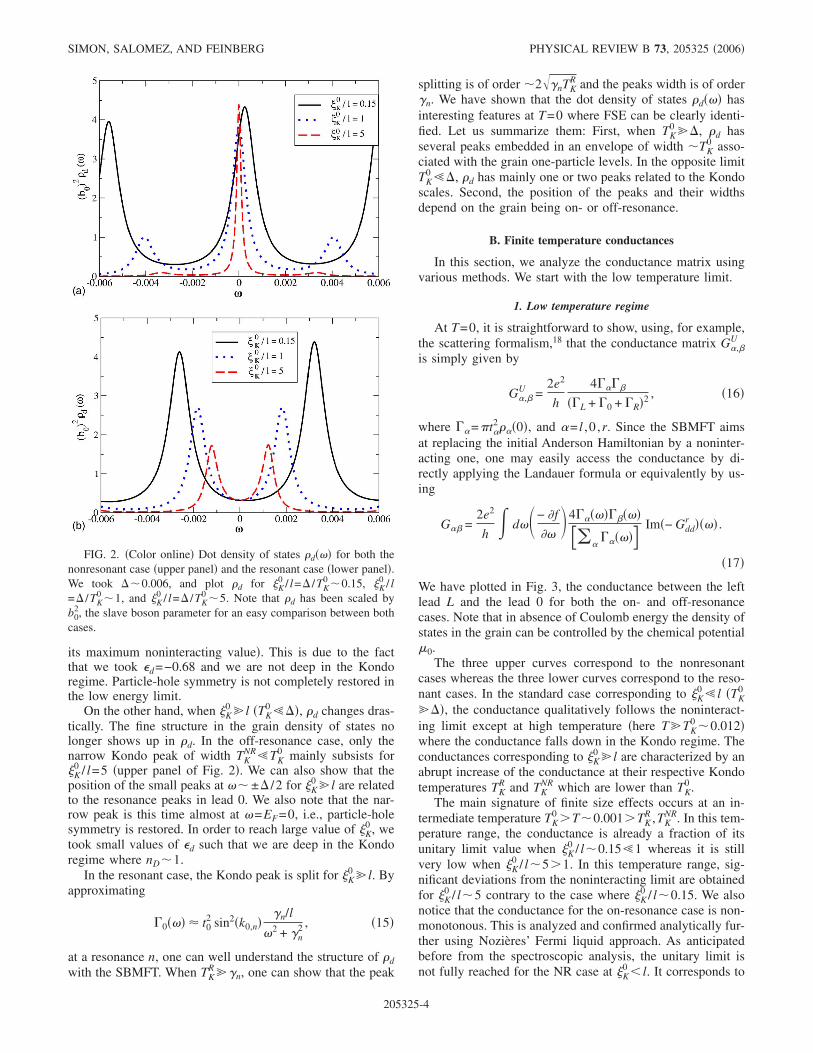
its maximum noninteracting value�. This is due to the factthat we took �d=−0.68 and we are not deep in the Kondoregime. Particle-hole symmetry is not completely restored inthe low energy limit.

On the other hand, when �K0 � l �TK

0 ���, �d changes dras-tically. The fine structure in the grain density of states nolonger shows up in �d. In the off-resonance case, only thenarrow Kondo peak of width TK

NR�TK0 mainly subsists for

�K0 / l=5 �upper panel of Fig. 2�. We can also show that the

position of the small peaks at �� ±� /2 for �K0 � l are related

to the resonance peaks in lead 0. We also note that the nar-row peak is this time almost at �=EF=0, i.e., particle-holesymmetry is restored. In order to reach large value of �K

0 , wetook small values of �d such that we are deep in the Kondoregime where nD�1.

In the resonant case, the Kondo peak is split for �K0 � l. By

approximating

�0��� � t02 sin2�k0,n�

�n/l

�2 + �n2 , �15�

at a resonance n, one can well understand the structure of �dwith the SBMFT. When TK

R ��n, one can show that the peak

splitting is of order �2��nTKR and the peaks width is of order

�n. We have shown that the dot density of states �d��� hasinteresting features at T=0 where FSE can be clearly identi-fied. Let us summarize them: First, when TK

0 ��, �d hasseveral peaks embedded in an envelope of width �TK

0 asso-ciated with the grain one-particle levels. In the opposite limitTK

0 ��, �d has mainly one or two peaks related to the Kondoscales. Second, the position of the peaks and their widthsdepend on the grain being on- or off-resonance.

B. Finite temperature conductances

In this section, we analyze the conductance matrix usingvarious methods. We start with the low temperature limit.

1. Low temperature regime

At T=0, it is straightforward to show, using, for example,the scattering formalism,18 that the conductance matrix G�,�

U

is simply given by

G�,�U =

2e2

h

4����

��L + �0 + �R�2 , �16�

where ��=�t�2���0�, and �= l ,0 ,r. Since the SBMFT aims

at replacing the initial Anderson Hamiltonian by a noninter-acting one, one may easily access the conductance by di-rectly applying the Landauer formula or equivalently by us-ing

G�� =2e2

h� d��− �f

���4����������

��������

Im�− Gddr ���� .

�17�

We have plotted in Fig. 3, the conductance between the leftlead L and the lead 0 for both the on- and off-resonancecases. Note that in absence of Coulomb energy the density ofstates in the grain can be controlled by the chemical potential0.

The three upper curves correspond to the nonresonantcases whereas the three lower curves correspond to the reso-nant cases. In the standard case corresponding to �K

0 � l �TK0

���, the conductance qualitatively follows the noninteract-ing limit except at high temperature �here T�TK

0 �0.012�where the conductance falls down in the Kondo regime. Theconductances corresponding to �K

0 � l are characterized by anabrupt increase of the conductance at their respective Kondotemperatures TK

R and TKNR which are lower than TK

0 .The main signature of finite size effects occurs at an in-

termediate temperature TK0 �T�0.001�TK

R ,TKNR. In this tem-

perature range, the conductance is already a fraction of itsunitary limit value when �K

0 / l�0.15�1 whereas it is stillvery low when �K

0 / l�5�1. In this temperature range, sig-nificant deviations from the noninteracting limit are obtainedfor �K

0 / l�5 contrary to the case where �K0 / l�0.15. We also

notice that the conductance for the on-resonance case is non-monotonous. This is analyzed and confirmed analytically fur-ther using Nozières’ Fermi liquid approach. As anticipatedbefore from the spectroscopic analysis, the unitary limit isnot fully reached for the NR case at �K

0 � l. It corresponds to

FIG. 2. �Color online� Dot density of states �d��� for both thenonresonant case �upper panel� and the resonant case �lower panel�.We took ��0.006, and plot �d for �K

0 / l=� /TK0 �0.15, �K

0 / l=� /TK

0 �1, and �K0 / l=� /TK

0 �5. Note that �d has been scaled byb0

2, the slave boson parameter for an easy comparison between bothcases.

SIMON, SALOMEZ, AND FEINBERG PHYSICAL REVIEW B 73, 205325 �2006�

205325-4

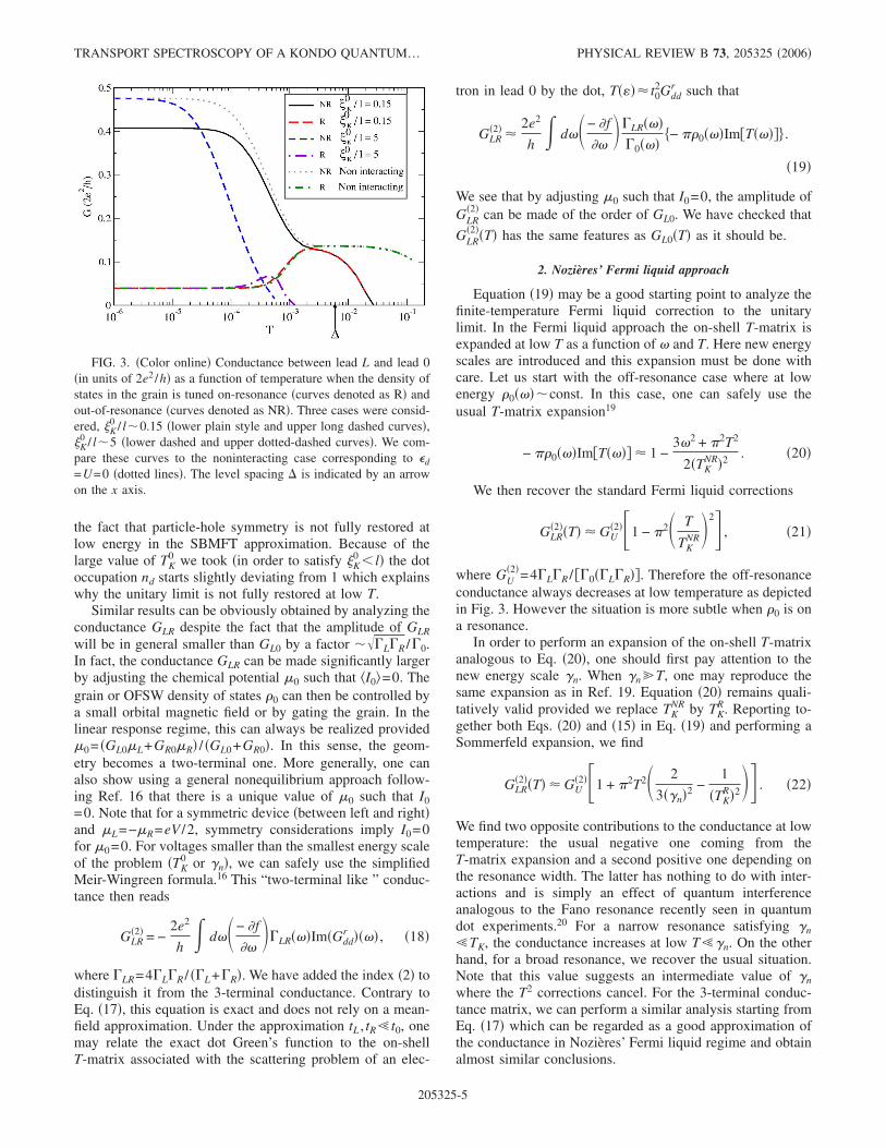
the fact that particle-hole symmetry is not fully restored atlow energy in the SBMFT approximation. Because of thelarge value of TK

0 we took �in order to satisfy �K0 � l� the dot

occupation nd starts slightly deviating from 1 which explainswhy the unitary limit is not fully restored at low T.

Similar results can be obviously obtained by analyzing theconductance GLR despite the fact that the amplitude of GLR

will be in general smaller than GL0 by a factor ���L�R /�0.In fact, the conductance GLR can be made significantly largerby adjusting the chemical potential 0 such that �I0�=0. Thegrain or OFSW density of states �0 can then be controlled bya small orbital magnetic field or by gating the grain. In thelinear response regime, this can always be realized provided0= �GL0L+GR0R� / �GL0+GR0�. In this sense, the geom-etry becomes a two-terminal one. More generally, one canalso show using a general nonequilibrium approach follow-ing Ref. 16 that there is a unique value of 0 such that I0=0. Note that for a symmetric device �between left and right�and L=−R=eV /2, symmetry considerations imply I0=0for 0=0. For voltages smaller than the smallest energy scaleof the problem �TK

0 or �n�, we can safely use the simplifiedMeir-Wingreen formula.16 This “two-terminal like ” conduc-tance then reads

GLR�2� = −

2e2

h� d��− �f

����LR���Im�Gdd

r ���� , �18�

where �LR=4�L�R / ��L+�R�. We have added the index �2� todistinguish it from the 3-terminal conductance. Contrary toEq. �17�, this equation is exact and does not rely on a mean-field approximation. Under the approximation tL , tR� t0, onemay relate the exact dot Green’s function to the on-shellT-matrix associated with the scattering problem of an elec-

tron in lead 0 by the dot, T���� t02Gdd

r such that

GLR�2� �

2e2

h� d��− �f

����LR���

�0����− ��0���Im�T���� .

�19�

We see that by adjusting 0 such that I0=0, the amplitude ofGLR

�2� can be made of the order of GL0. We have checked that

GLR�2��T� has the same features as GL0�T� as it should be.

2. Nozières’ Fermi liquid approach

Equation �19� may be a good starting point to analyze thefinite-temperature Fermi liquid correction to the unitarylimit. In the Fermi liquid approach the on-shell T-matrix isexpanded at low T as a function of � and T. Here new energyscales are introduced and this expansion must be done withcare. Let us start with the off-resonance case where at lowenergy �0����const. In this case, one can safely use theusual T-matrix expansion19

− ��0���Im�T��� � 1 −3�2 + �2T2

2�TKNR�2 . �20�

We then recover the standard Fermi liquid corrections

GLR�2��T� � GU

�2��1 − �2� T

TKNR�2 , �21�

where GU�2�=4�L�R / ��0��L�R�. Therefore the off-resonance

conductance always decreases at low temperature as depictedin Fig. 3. However the situation is more subtle when �0 is ona resonance.

In order to perform an expansion of the on-shell T-matrixanalogous to Eq. �20�, one should first pay attention to thenew energy scale �n. When �n�T, one may reproduce thesame expansion as in Ref. 19. Equation �20� remains quali-tatively valid provided we replace TK

NR by TKR. Reporting to-

gether both Eqs. �20� and �15� in Eq. �19� and performing aSommerfeld expansion, we find

GLR�2��T� � GU

�2��1 + �2T2� 2

3��n�2 −1

�TKR�2� . �22�

We find two opposite contributions to the conductance at lowtemperature: the usual negative one coming from theT-matrix expansion and a second positive one depending onthe resonance width. The latter has nothing to do with inter-actions and is simply an effect of quantum interferenceanalogous to the Fano resonance recently seen in quantumdot experiments.20 For a narrow resonance satisfying �n�TK, the conductance increases at low T��n. On the otherhand, for a broad resonance, we recover the usual situation.Note that this value suggests an intermediate value of �nwhere the T2 corrections cancel. For the 3-terminal conduc-tance matrix, we can perform a similar analysis starting fromEq. �17� which can be regarded as a good approximation ofthe conductance in Nozières’ Fermi liquid regime and obtainalmost similar conclusions.

FIG. 3. �Color online� Conductance between lead L and lead 0�in units of 2e2 /h� as a function of temperature when the density ofstates in the grain is tuned on-resonance �curves denoted as R� andout-of-resonance �curves denoted as NR�. Three cases were consid-ered, �K

0 / l�0.15 �lower plain style and upper long dashed curves�,�K

0 / l�5 �lower dashed and upper dotted-dashed curves�. We com-pare these curves to the noninteracting case corresponding to �d

=U=0 �dotted lines�. The level spacing � is indicated by an arrowon the x axis.

TRANSPORT SPECTROSCOPY OF A KONDO QUANTUM¼ PHYSICAL REVIEW B 73, 205325 �2006�

205325-5

3. High temperature

At temperature higher than the Kondo temperature T�TK

0 , perturbation theory in the Kondo couplings can a pri-ori be used. We therefore start directly from the KondoHamiltonian written in Eq. �5�. In order to compute the con-ductance between the left lead and lead 0, we use the renor-malized perturbation theory. At lowest order, the conduc-tance reads

GL0 =2e2

h

3�2

4JL0

2 � d��− �f

����L�0��� . �23�

When TK0 ��, one may replace �0 by its average value and

JL0 by its renormalized coupling and the high temperatureconductance takes its standard scaling form21

GL0 = GL0U 3�2/16

ln2�T/TK0 �

, T � TK0 � � = GL0

U f� T

TK0 � , �24�

where f�x� is a universal scaling function such that f�x�1��3�2 /16 ln2 x and GL0

U has been defined in Eq. �16�.Let us consider the more interesting situation where TK

0

��. Suppose the bandwidth is reduced from ± 0 �where�0=4t here� to ± , the renormalization of the Kondo cou-pling is well approximated by

JL0� � = JL0� 0� +1

2JL0J00��

− 0

−

+ �

0 �d��0���

�.

�25�

When ��, the integral in Eq. �25� averages over manypeaks in the LDOS �0 and we obtain the usual result for theKondo model with a constant density of states. It implies thatin the limit T��, the result in Eq. �24� remains valid inde-pendently of �0��� being tuned on or off a resonance.

On the other hand, when ��, the integral in Eq. �25�becomes strongly dependent on �0. When �0 is tuned off aresonance and for ��T�TK

NR, the result in Eq. �24� remainsapproximately valid provided we replace TK

0 by TKNR defined

in Eq. �11� such that GL0�T�=GUf�T /TKNR�. When �0 is tuned

on a resonance that we assume for convenience to be at �=EF=0, only the variation of the LDOS in the vicinity of EFmatters such that we further approximate the LDOS usingEq. �15�. The renormalization group equation in Eq. �25�may be integrated in two steps, first between 0 and � wherethe variations of the LDOS average out and then between �and where

JL0� � � JL0��� + 12JL0���J00����0�0�ln�1 + ��n

2/ 2� ,

�26�

where we assumed �n��. At ��, the Kondo couplingsrenormalize following the RG equations given in Eq. �6�. Atthe scale �, the Kondo couplings have been weakly renor-malized and one may use the RG equations given in Eq. �6�that imply JL0���� tlt0 / t0

2J00���. Using this approximationand the definition of the on-resonance Kondo temperature inEq. �10�, the conductance at ��T��n reads

GL0 � GU3�2

16

1

ln2�1 +�n

2

�TKR�2�

�n

T �1 +

ln�1 +�n

2

T2�ln�1 +

�n2

�TKR�2��

2

.

�27�

The high temperature on-resonance conductance takes amore complicated form than the one given in Eq. �24�. No-tice nonetheless that the multiplicative factor �1+ ¯ � ap-pearing in Eq. �27� is O�1� since T�TK

R =O���.

C. Scaling analysis

From the low and high temperature analysis, we haveseen than the conductance matrix elements cannot be in gen-eral simply written as a simple universal scaling function ofT /TK

0 both at high and low temperature. This is particularlystriking when �0 was tuned on a resonance characterized bythe width �n �see Eqs. �22� and �27�.

In general, one would expect

G�� = G��U g� T

TK0 ,

�

TK0 ,

�n

T� . �28�

In the high temperature regime, this scaling function takesa simple form and simply reads f�T /TK� where TK eitherequates TK

0 when ��TK0 or can be simply expressed as a

function of TK0 ,� ,�n �see Eqs �10� and �11�. Nevertheless, at

intermediate or low temperature, the conductance in Eq. �28�takes a complicated scaling form which depends on �n /T andis in this sense nonuniversal. It depends on the geometricdetails of the sample, at least for bare Kondo temperature TK

0

of the order or smaller than the level spacing �. A similarconclusion has been reached by Kaul et al.22 by assuming achaotic large quantum grain and explicitly calculating thefluctuations and deviations from the universal behavior tak-ing into account mesoscopic fluctuations.

D. Finite grain Coulomb energy

In this section, we discuss whether a finite grain Coulombenergy modifies or not the results presented in this work. Aswe already mentioned in Sec. II, the Kondo coupling J00, isalmost not affected by the grain Coulomb energy EG �sinceEG�U� and therefore the Kondo temperature remains al-most unchanged. As shown in, Refs. 12, 23, and 24, a smallenergy scale EG changes the renormalization group equationin Eq. �6�. The off-diagonal couplings J0L� � ,J0R� � tend to0 for �EG. At energy �EG the problem therefore re-duces to an anisotropic 2-channel Kondo problem. Thestrongly coupled channel is the grain 0, the weakly coupledone is the even combination of the conduction electron in theleft/right leads. At very low energy, the fixed point of theanisotropic 2-channel Kondo model is a Fermi liquid. It ischaracterized by the strongly coupled lead �here the grain�screening the impurity whereas the weakly coupled one com-pletely decouples from the impurity. The dot density of states

SIMON, SALOMEZ, AND FEINBERG PHYSICAL REVIEW B 73, 205325 �2006�

205325-6

depicted in Fig. 2 remains therefore almost unaffected. Theon- and off-resonance Kondo temperatures TK

R and TKNR given

in Eqs. �10� and �11� remain valid too. The problem is toread the dot LDOS with the weakly coupled leads since theydecouple at T=0. Nevertheless, for a typical experimentdone at low temperature T, such a decoupling is not completeand the dot density of state should be still accessible usingthe weakly coupled leads but with a very small amplitude.

In this paper we analyze the situation in which a grain ora finite size wire is also used as a third terminal. In somesituations, like the theoretical one presented in Ref. 12, noterminal lead is attached to the grain and the geometry is agenuine 2-terminal one. Taking into account both a finitelevel spacing and a finite grain Coulomb energy is quite in-volved �with several different regimes� and goes beyond thescope of the present paper. A step into this direction wasrecently achieved in Ref. 25.

IV. CONCLUSIONS

In this paper, we have studied a geometry in which asmall quantum dot in the Kondo regime is strongly coupledto a large open quantum dot or open finite size wire andweakly coupled to other normal leads which are simply usedas transport probes. The artificial impurity is mainly screenedis the large quantum dot. Such a geometry thus allows toprobe the dot spectroscopic properties without perturbing it.We have shown combining several techniques how finite sizeeffects show up in the dot density of states and in the con-ductance matrix. We hope the predictions presented here arerobust enough to be checked experimentally.

ACKNOWLEDGMENTS

This research was partly supported by the Institut de laPhysique de la Matière Condensée �IPMC, Grenoble�.

1 D. Goldhaber-Gordon, H. Shtrikman, D. Mahalu, D. Abusch-Magder, U. Meirav, and M. A. Kaster, Nature �London� 391,156 �1998�.

2 S. M. Cronenwett, T. H. Oosterkamp, and L. P. Kouwenhoven,Science 281, 540 �1998�; F. Simmel, R. H. Blick, J. P. Kotthaus,W. Wegscheider, and M. Bichler, Phys. Rev. Lett. 83, 804�1999�.

3 W. G. van der Wiel, S. De Franceschi, T. Fujisawa, J. M. Elzer-man, S. Tarucha, and L. P. Kouwenhoven, Science 289, 2105�2000�.

4 W. B. Thimm, J. Kroha, and J. von Delft, Phys. Rev. Lett. 82,2143 �1999�.

5 I. Affleck and P. Simon, Phys. Rev. Lett. 86, 2854 �2001�; P.Simon and I. Affleck, Phys. Rev. B 64, 085308 �2001�.

6 H. Hu, G.-M. Zhang, and L. Yu, Phys. Rev. Lett. 86, 5558�2001�.

7 E. S. Sorensen and I. Affleck, Phys. Rev. Lett. 94, 086601�2005�.

8 P. Simon, O. Entin-Wohlman, and A. Aharony, Phys. Rev. B 72,245313 �2005�.

9 P. Simon and I. Affleck, Phys. Rev. B 68, 115304 �2003�; P.Simon and I. Affleck, Phys. Rev. Lett. 89, 206602 �2002�.

10 P. S. Cornaglia and C. A. Balseiro, Phys. Rev. Lett. 90, 216801�2003�.

11 Note that for a 2D or 3D metallic grain, the level spacing � is notsimply related to the Fermi velocity and the length scale of thegrain. In this case, we shall compare directly TK

0 to �.

12 Y. Oreg and D. Goldhaber-Gordon, Phys. Rev. Lett. 90, 136602�2003�.

13 N. J. Craig, J. M. Taylor, E. A. Lester, C. M. Marcus, M. P.Hanson, and A. C. Gossard, Science 304, 565 �2004�.

14 This matrix has only one nonzero eigenvalue, Tr��̂���00 whichflows to strong coupling. It follows that the dimensionless

Kondo coupling ���� �= t�t� /��t�2Tr��̂�� �.9

15 A. C. Hewson, The Kondo Problem to Heavy Fermions �Cam-bridge University Press, Cambridge, UK, 1997�, Chap. 7.

16 Y. Meir and N. S. Wingreen, Phys. Rev. Lett. 68, 2512 �1992�.17 A. Schiller and S. Hershfield, Phys. Rev. B 61, 9036 �2000�.18 T. K. Ng and P. A. Lee, Phys. Rev. Lett. 61, 1768 �1988�.19 P. Nozières, J. Low Temp. Phys. 17, 31 �1974�.20 M. Sato, H. Aikawa, K. Kobayashi, S. Katsumoto, and Y. Iye,

Phys. Rev. Lett. 95, 066801 �2005� and references therein.21 M. Pustilnik and L. I. Glazman, “Nanophysics: Coherence and

Transport,” edited by H. Bouchiat et al. �Elsevier, 2005� pp.427–478, cond-mat/0501007.

22 R. K. Kaul, D. Ullmo, S. Chandrasekharan, and H. U. Baranger,Europhys. Lett. 71, 973 �2005�.

23 M. Pustilnik, L. Borda, L. I. Glazman, and J. von Delft, Phys.Rev. B 69, 115316 �2004�.

24 S. Florens and A. Rosch, Phys. Rev. Lett. 92, 216601 �2004�.25 R. K. Kaul, G. Zarand, S. Chandrasekharan, D. Ullmo, and H. U.

Baranger, Phys. Rev. Lett. 96, 176802 �2006�.

TRANSPORT SPECTROSCOPY OF A KONDO QUANTUM¼ PHYSICAL REVIEW B 73, 205325 �2006�

205325-7