UNIVERSITÉ DE BOURGOGNE

UFR des Sciences et des TechniquesInstitut de mathématiques de Bourgogne

THÈSEPour obtenir le grade de

Docteur de l'Université de BourgogneDiscipline : mathématiques

parGautier Picot

le 29 novembre 2010

Contrôle optimal géométrique et numériqueappliqué au problème de transfert Terre-Lune

Directeur de thèseBernard Bonnard

Rapporteurs :

Bergounioux Maïtine Université d'Orléans RapportriceChyba Monique Université de Hawaii RapportricePomet Jean-Baptiste INRIA Rapporteur

Membres du jury :

Bergounioux Maïtine Université d'Orléans ExaminatriceBonnard Bernard Université de Bourgogne ExaminateurCaillau Jean-Baptiste Université de Bourgogne ExaminateurGergaud Joseph ENSEEIHT-INP ExaminateurJauslin Hans Rudolf Université de Bourgogne PrésidentPomet Jean-Baptiste INRIA Examinateur

ii

Table des matières

Introduction 1

1 Le problème restreint des 3 corps 5

1.1 Le problème des N corps . . . . . . . . . . . . . . . . . . . . . . 51.2 Le problème restreint des 3 corps plan . . . . . . . . . . . . . . . 7

1.2.1 Equations du mouvement . . . . . . . . . . . . . . . . . . 71.2.2 Formalisme hamiltonien et régions de Hill . . . . . . . . . 71.2.3 Points d'équilibre . . . . . . . . . . . . . . . . . . . . . . . 91.2.4 Linéarisation au voisinage des points d'équilibre . . . . . 111.2.5 Dynamique autour des points L1 et L2 . . . . . . . . . . . 131.2.6 Construction d'orbites à itinéraires prédénis . . . . . . . 171.2.7 le problème restreint des 3-corps plan contrôlé . . . . . . 18

1.3 Le problème restreint des 3 corps spatial . . . . . . . . . . . . . . 191.3.1 Equations du mouvement et points d'équilibre . . . . . . 201.3.2 Dynamique au voisinage des points colinéaires . . . . . . 211.3.3 Le problème spatial contrôlé au voisinage de L1 . . . . . . 26

2 Outils géométriques et numériques en contrôle optimal. 27

2.1 Dénition du problème . . . . . . . . . . . . . . . . . . . . . . . . 272.2 Le principe du maximum . . . . . . . . . . . . . . . . . . . . . . 282.3 Temps conjugués géométriques et conditions d'optimalité du se-

cond ordre . . . . . . . . . . . . . . . . . . . . . . . . . . . . . . 312.4 Problème de temps minimal . . . . . . . . . . . . . . . . . . . . 33

2.4.1 Le cas normal . . . . . . . . . . . . . . . . . . . . . . . . . 332.4.2 Le cas anormal . . . . . . . . . . . . . . . . . . . . . . . . 34

2.5 Problème de minimisation de l'énergie . . . . . . . . . . . . . . . 362.6 Méthode de tir simple . . . . . . . . . . . . . . . . . . . . . . . . 372.7 Méthode de continuation . . . . . . . . . . . . . . . . . . . . . . . 372.8 Implémentation Numérique . . . . . . . . . . . . . . . . . . . . . 39

3 Contribution scientique 41

3.1 Transferts Terre-Lune à temps minimal et énergie minimale . . . 413.2 Transferts à énergie minimale au voisinage du point L1 . . . . . . 44

Geometric and numerical techniques in optimal control of two and

three-body problems 47

Note complémentaire : trajectoires Terre-Lune à énergie minimale

et technique de recollement 87

iii

Shooting and numerical continuation methods for computing time-

minimal and energy-minimal trajectories in Earth-Moon trans-

fer using low propulsion. 93

Energy-minimal transfers in the vicinity of the Lagrangian point

L1 121

Conclusion 133

Bibliographie 135

iv

Remerciements

Je tiens à remercier profondément Bernard Bonnard de la conance qu'ilm'a accordée en me proposant d'eectuer cette thèse sous sa direction et de larigueur avec laquelle il l'a encadrée. Sa présence, son exigence, sa grande culturemathématique et l'importance qu'il attache aux relations humaines ont été deformidables moteurs pour la poursuite de mes recherches. Je mesure maintenantà quel point je lui suis redevable et combien son enseignement sera bénéque àmes activités futures. Je remercie au même titre Jean-Baptiste Caillau d'avoirporté autant d'intérêt à mon travail. Sa disponibilité, sa bienveillance et sesnombreux conseils ont été essentiels à ma bonne progression. Qu'il sache à quelpoint je lui suis reconnaissant. Je remercie sincèrement Maïtine Bergounioux,professeur à l'Université d'Orléans, d'avoir non seulement accepté de rappor-ter cette thèse, mais aussi encouragé, de concert avec ses collègues EmmanuelTrélat et Sandrine Grellier, mes premiers pas de chercheur au sortir de mondiplôme de Master. Je remercie également Monique Chyba, professeur à l'Uni-versité d'Hawaii et Jean-Baptiste Pomet, Chargé de recherches à l'INRIA deSophia Antipolis, pour leur lecture critique de mon manuscrit, leurs précieusesremarques et leurs encouragements. Joseph Gergaud, maître de conférences àl'ENSEEIHT de Toulouse, a oeuvré avec Nicolas Delong pour que je puisse pré-senter en juin 2010 mes résultats lors du séminaire du CNES sur les points deLagrange. Je l'en remercie et suis heureux de le compter parmi mes examina-teurs. Et je suis bien sûr très honoré qu'un homme de science tel que Hans RudolfJauslin, professeur à l'Université de Bourgogne, ait accepté de présider mon jury.

J'adresse une pensée particulière à Gabriel Janin et Bilel Daoud avec lesquelsj'ai partagé ces trois dernières années la condition de doctorant en contrôle op-timal et qui ont si souvent consacré du temps à me venir en aide, pour quelquequestion que ce soit. Je leur témoigne toute ma gratitude et leur souhaite lameilleure continuation possible sur les chemins qu'ils emprunteront. Je remer-cie chaleureusement au passage tous mes collègues et amis de l'association desDoctorants en Mathématiques de Dijon sans lesquels Calamity Janet, repue degoulash, ivre de noni et victorieuse du quatre à la suite, n'eût jamais danséle rock'n'roll sur la piste enammée du dancing club de Ganat. Parmi eux, jevoudrais saluer ceux qui, ayant traversé les frontières de leur pays natal pourvenir étudier dans le mien, m'ont instruit de leur regard sur le monde, depuisles bureaux 213 et 217 de l'aile A du batiment Mirande. Leur culture est désor-mais aussi mon patrimoine. Merci de même à tous les membres de l'Institut deMathématiques de Bourgogne qui ont su, d'une quelconque manière, faciliter ouenrichir ma tâche de thésard depuis mon arrivée à Dijon. A Lucy Moser Jauslin,qui m'accorda toute l'attention qu'elle put en tant que directrice du laboratoire,

v

Rosane Ushirobira, qui me cona mes premières responsabilités d'enseignement,Anissa, Caroline, Gladys, Muriel, Véronique et Béatrice qui comblèrent si ami-calement et avec ecacité toutes mes lacunes organisationnelles et administra-tives, Sylvie, qui résolut avec humour mes problèmes informatiques et Aziz dontle sourire quotidien contraste si agréablement avec la grisaille des mornes matinsbourguignons.

Je rends évidemment hommage à mes parents, Catherine et Michel, qui, enencourageant chacun de mes choix personnels, m'ont appris à être libre. C'estavec patience et conviction qu'ils m'ont inculqué que le savoir et l'esprit critiquesont les plus grandes des richesses. J'espère aujourd'hui les rendre ers de moi.Je remercie avec tendresse mes soeurs Marie et Hélène pour les exemples qu'ellessont depuis toujours à mes yeux et n'oublie aucun des membres de ma famillequi m'entourent indéfectiblement avec toute l'aection que je peux souhaiter.

Je prote enn de ces quelques lignes de liberté pour remercier mes amisd'hier et d'aujourd'hui, anciens, médiocres, gazelles et autres, d'avoir coloré lessouvenirs de toutes ces années d'école qui se terminent aujourd'hui. Leurs éclatsde rires me sont précieux.

vi

A Oliviaet à Mochère

dont l'absence est une joie et une sourance.

Il est quasiment impossible de diérencier le nordique primitifinférieur autenthique du nordique primitif inférieur inventé.

L'épopée du buveur d'eau, J. Irving

vii

viii

Introduction

La conception de missions à faibles coûts énergétiques représente un enjeumajeur pour l'avenir de l'exploration spatiale. De la diminution des besoins encarburant dépendent les possibilités futures de missions spatiales à très longuedurée, telles que d'hypothétiques voyages vers Mars ou les lunes de Jupiter.En eet, les approches classiques, qui au milieu du XXe siècle permirent lespremiers pas de la conquête spatiale, sont beaucoup trop nécessiteuses en éner-gie pour être exploitées lors de missions à longue distance. Par exemple, lestransferts de Hohmann dans le problème des 2 corps, utilisés avec ecacité ausein du programme Apollo, requièrent une quantité de fuel bien trop iportantepour que l'on puisse envisager leur utilisation sur de longs intervalles de temps.Les nouvelles technologies ont d'ores et déjà apporté certaines solutions. Lasonde SMART-1 de l'Agence Spatiale Européenne [57, 58], équipée de moteurshélio-électriques, a ainsi eectué entre les mois de septembre 2003 et septembre2006 un transfert à faible propulsion entre deux orbites Kepleriennes autour dela Terre et de la Lune suivi d'une mission d'observation. Cette mission a enparticulier inspiré divers travaux dédiés à la minimisation de la consommationénergétique au cours des transferts Terre-Lune [6, 9].

Au cours des vingt dernières années, l'application de la théorie des systèmesdynamiques hamiltoniens au problème restreint des 3 corps a mis en lumièredes classes d'orbites naturelles permettant de concevoir des missions spatialestrès économiques en énergie. Ces travaux sont dus à la collaboration des équipesaméricaines et espagnoles respectivement composées de W. S. Koon, M. W. Lo,J. E. Marsden, S. D. Ross [41] et G. Gómez, A. Jorba, J. Llibre, J. Masdemont,C. Simó [26, 27, 30, 31]. Leur principe fondamental repose sur le recours à lastructure de variétés invariantes autour de certains points d'équilibre du pro-blème restreint des trois corps an qu'un engin spatial puisse relier à moindrecoût les zones d'inuence gravitationnelle de deux planètes. Ces variétés inva-riantes contiennent les orbites évoluant asymptotiquement, en temps croissantou décroissant, vers des orbites périodiques autour des points d'équilibre. Ellesagissent par conséquent comme des chemins dynamiques dont les connectionspermettent de joindre naturellement diérentes régions de l'espace. La missionGENESIS, notamment, fournit une brillante illustration de l'utilisation des va-riétés invariantes pour le problème de réduction du coût énergétique.

C'est l'objet de cette thèse que de proposer une approche complémentairede calcul numérique de trajectoires spatiales à poussée faible dans le problèmerestreint des 3 corps. On se base pour ce faire sur l'application de résultatsfondamentaux de la théorie du contrôle optimal géométrique. Plus précisément,

1

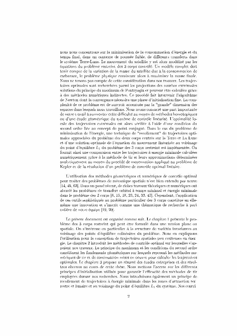
nous nous concentrons sur la minimisation de la consommation d'énergie et dutemps nal, dans un contexte de poussée faible, de diérents transferts dansle système Terre-Lune. Le mouvement du satellite y est alors modélisé par leséquations du problème restreint des 3 corps contrôlé. Un modèle complet doittenir compte de la variation de la masse du satellite due à la consommation decarburant, le problème physique consistant alors à maximiser la masse nale.Nous ne tenons pas compte de cette considération dans nos travaux. Les trajec-toires optimales sont recherchées parmi les projections des courbes extrémalessolutions du principe du maximum de Pontryagin et peuvent être calculées grâceà des méthodes numériques indirectes. Ce procédé fait intervenir l'algorithmede Newton dont la convergence nécessite une phase d'initialisation ne. La com-plexité de ce problème est de surcroît accentuée par la "grande" dimension desespaces dans lesquels nous travaillons. Nous avons consacré une part importantede notre travail à surmonter cette diculté au moyen de méthodes homotopiquesou d'une étude géométrique du système de contrôle linéarisé. L'optimalité lo-cale des trajectoires extrémales est alors vériée à l'aide d'une condition dusecond ordre liée au concept de point conjugué. Dans le cas du problème deminimisation de l'énergie, une technique de "recollement" de trajectoires opti-males approchées du problème des deux corps centrés sur la Terre et La Luneet d'une solution optimale de l'équation du mouvement linéarisée au voisinagedu point d'équilibre L1 du problème des 3 corps restreint est implémentée. Onfournit ainsi une comparaison entre les trajectoires à energie minimale calculéesnumériquement grâce à la méthode de tir et leurs approximations déterminéesanalytiquement au moyen du procédé de moyennation appliqué au problème deKepler et de la résolution d'un problème de contrôle optimal linéaire.

L'utilisation des méthodes géométriques et numériques de contrôle optimalpour traiter des problèmes de mécanique spatiale n'est bien entendu pas neuve[14, 45, 63]. Dans un passé récent, de riches travaux théoriques et numériques ontabordé les problèmes de transfert orbital à temps minimal et énergie minimaledans le problème des 2 corps [8, 15, 18, 23, 24, 33, 47]. Cependant, l'applicationde ces outils sophistiqués au problème particulier des 3 corps constitue en elle-même une innovation et s'inscrit comme une thématique de recherche à partentière de notre équipe [19, 20].

Le présent document est organisé comme suit. Le chapitre 1 présente le pro-blème des 3 corps restreint qui peut être formulé dans une version plane ouspatiale. On s'intéresse en particulier à la structure de variétés invariantes auvoisinage des points d'équilibre colinéaires du problème. Nous en expliquonsl'utilisation pour la conception de trajectoires spatiales peu coûteuses en éner-gie. Le chapitre 2 introduit les méthodes de contrôle optimal sur lesquelles s'ap-puient nos travaux. Le principe du maximum et les conditions du second ordreconstituent les fondements géométriques sur lesquels reposent les méthodes nu-mériques de tir et de continuation mises en oeuvre pour calculer les trajectoiresoptimales. Le chapitre 3 propose un résumé des études entreprises et des résul-tats obtenus au cours de cette thèse. Nous mettons l'accent sur les diérentsprincipes d'initialisation utilisés pour garantir l'ecacité des méthodes de tiremployées durant nos recherches. Nous introduisons également un principe derecollement de trajectoires à énergie minimale dans les zones d'attraction ter-restre et lunaire et au voisinage du point d'équilibre L1 du système. Nos contri-

2

−1 −0.5 0 0.5 1

−0.8

−0.6

−0.4

−0.2

0

0.2

0.4

0.6

0.8

(a)

−1 −0.5 0 0.5 1−1

−0.8

−0.6

−0.4

−0.2

0

0.2

0.4

0.6

0.8

(b)

Figure 1 Comparaison, dans le repère xe, entre une trajectoire Terre-Lune àénergie minimale du problème restreint des trois corps plan calculée numérique-ment, représentée en (a), et un recollement de trajectoires à énergie minimaledu problème à deux corps, en (b).

butions scientiques sont présentées en détails au sein des trois articles cosignésou entièrement rédigés et soumis ces trois dernières années. Nous fournissonsune collection de transferts Terre-Lune à énergie minimale dans Geometric andnumerical techniques in optimal orbital transfer using low propulsion [10] encomplément de travaux géométriques de Bernard Bonnard et Jean-BaptisteCaillau sur le problème de minimisation du coût énergétique et de la tech-nique de moyennation dans le problème des 2 corps. La note complémentaireTrajectoires Terre-Lune à énergie minimale et technique de recollement, rédi-gée en français et non soumise à publication, explique comment la technique demoyennation peut être utilisée pour approximer les trajectoires énergies mini-males obtenus grâce à la méthode de tir. Nous complétons ces résultats par uneétude considérable des trajectoires à temps minimal dans le système Terre-Lunedans Shooting and numerical continuation methods for computing time-minimalor energy-minimal trajectories in Earth-Moon transfer using low propulsion [51].On s'intéresse enn à l'inuence de la structure de variétés invariantes sur la mi-nimisation du coût énergétique des transferts au voisinage du point d'équilibreL1 dans Energy-minimal transfers in the vicinity of the Lagrangian point L1 [52].

Cette thèse a été conancée, sous forme d'une Bourse Docteur Ingénieur,par le Centre National de la Recherche Scientique (contrat no. 37244) et laRégion Bourgogne (contrat no. 079201PP02454515). Elle a été eectuée au seinde l'équipe Equations diérentielles et contrôle de l'Institut de Mathématiquesde Bourgogne, de l'Université de Bourgogne.

3

4

Chapitre 1

Le problème restreint des 3

corps

1.1 Le problème des N corps

Présentons brièvement le problème dit des N corps où N désigne un entiernaturel supérieur ou égal à 2 [54]. Il s'agit d'étudier le mouvement de N parti-cules de masses m1, . . . ,mN évoluant dans le référentiel Galiléen R3 et soumisesà la seule inuence de leur attraction gravitationnelle mutuelle. Notons qi ∈ R3

le vecteur position de la ième particule. Le vecteur q = (q1, . . . , qN ) ∈ R3N estappelé vecteur d'état et selon la loi fondamentale de la dynamique, les équationsdu mouvement s'écrivent

Mq = −∂U∂q

(1.1)

où U est le potentiel mécanique déni par

U = −∑

1≤i<j≤N

Gmimj

|qj − qi|

et M est la matrice diagonale

M =

m1 0. . .

0 mN

.

Dénissons le Lagrangien L = T − U où T = 12

∑Ni=1miq

2i représente l'énergie

cinétique du système. L'équation du mouvement 1.1 peut alors s'écrire sousforme d'une équation d'Euler-Lagrange

d

dt

∂L

∂q− ∂L

∂q= 0 (1.2)

dont les solutions minimisent localement, en vertu du principe de moindre ac-tion, la quantité

S(q(.)) =∫L(q, q)dt.

5

En posant pi = miqi ∈ R3, i = 1, . . . , N , les systèmes 1.1 et 1.2 deviennentéquivalents au système hamiltonien

q =∂H

∂p, p = −∂H

∂q(1.3)

où la fonction hamiltonienne H est donnée par

H = T + U =

N∑i=1

‖ pi ‖2

2mi+ U

et le vecteur p = (p1, . . . , pN ) ∈ R3N est appelé vecteur moment. Le problèmedes N corps est ainsi formalisé par un système de 6N équations du premierordre dont on peut montrer qu'il admet 10 intégrales premières non triviales,voir par exemple [14]. Une simplication de ce problème consiste à supposer queles N points massiques appartiennent au plan R2. Le référentiel Galiléen utilisépeut alors être remplacé par un repère en rotation. En eet, en posant

K =

(0 1−1 0

), exp(ωtK) =

(cosωt sinωt− sinωt cosωt

),

on introduit l'ensemble des coordonnées en rotation uniforme dénies grâce à latransformation

ui = exp(ωtK)qi, vi = exp(ωtK)pi.

Un calcul classique [49] fournit alors l' expression du Hamiltonien du problèmedes N corps dans les coordonnées en rotation

H =N∑i=1

‖ v ‖2

2mi−

N∑i=1

ωuTi Kvi −N∑

1≤i<j≤N

Gmimj

‖ qi − qj ‖.

En 1687, Issac Newton énonçait dans ses célèbres Principes mathématiquesde philosophie naturelle [50] l'intégrabilité du problème des 2 corps, dont onpeut montrer que les trajectoires satisfont les équations de coniques particu-lières. La première loi de Kepler, stipulant que les planètes décrivent des ellipsesdont le soleil est un foyer, était ainsi justiée. Il fallut attendre la n du XIXesiècle et les travaux de Poincaré [53] pour savoir que le problème des N corpsn'est pas intégrable pour N ≥ 3. Les solutions du problème des 3 corps sontpar conséquent relativement méconnues, bien que certaines trajectoires remar-quables fussent mises en lumières par Euler et Lagrange dès le XVIIe siècle.Dans la suite de ce chapitre, on présente le célèbre problème restreint des 3corps, simplication du problème des 3 corps dans lequel la masse de la troi-sième particule est supposée négligeable en comparaison des deux autres. Cemodèle est notamment pertinent pour décrire le mouvement d'un satellite sou-mis aux forces gravitationnelles de deux planètes. Il peut être formulé de deuxmanières diérentes :

dans le problème restreint des 3 corps plan, on suppose que la particulede masse négligeable évolue dans le plan déni par la rotation des deuxparticules principales autour de leur centre de masse,

dans le problème restreint des trois corps spatial, on tient compte de ladirection verticale de sorte que la particule de masse négligeable évoluedans R3.

6

1.2 Le problème restreint des 3 corps plan

On introduit dans cette section le problème restreint des 3 corps plan. Cemodèle mathématique a été largement étudié et les ouvrages de Szebehely [60] etMarchal [44] en orent tous eux une description exhaustive. Il présente l'intérêtde fournir un cadre adéquat à l'étude d'approximations de transfert orbitauxentre deux planètes, ce qui explique son recours dans de très nombreux travauxde mécanique spatiale. L'objet des pages qui suivent est de résumer les propriétéset caractéristiques du problème restreint des trois corps plan dont il s'avère quel'utilisation permet la conception de missions spatiales à faible coût énergétique.

1.2.1 Equations du mouvement

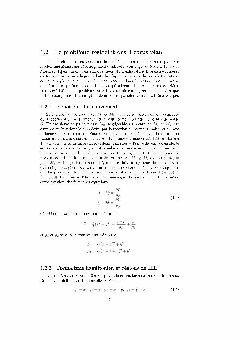
Soient deux corps de masses M1 et M2, appelés primaires, dont on supposequ'ils décrivent un mouvement circulaire uniforme autour de leur centre de masseG. Un troisième corps de masse M3, négligeable au regard de M1 et M2, estsupposé évoluer dans le plan déni par la rotation des deux primaires et ce sansinuencer leur mouvement. Pour se ramener à un problème sans dimension, onconsidère les normalisations suivantes : la somme des massesM1+M2 est xée à1, de même que la distance entre les deux primaires et l'unité de temps considéréeest telle que la constante gravitationnelle vaut également 1. Par conséquent,la vitesse angulaire des primaires est constante égale à 1 et leur période derévolution autour de G est égale à 2π. Supposons M1 ≥ M2 et notons M2 =µ et M1 = 1 − µ. Par commodité, on introduit un système de coordonnéesdynamiques (x, y) en rotation uniforme autour deG et de même vitesse angulaireque les primaires, dont les positions dans le plan sont ainsi xées à (−µ, 0) et(1 − µ, 0). On a ainsi déni le repère synodique. Le mouvement du troisièmecorps est alors décrit par les équations

x− 2y =∂Ω

∂x

y + 2x =∂Ω

∂y

(1.4)

où −Ω est le potentiel du système déni par

Ω =1

2(x2 + y2) +

1− µ

ρ1+µ

ρ2

et ρ1 et ρ2 sont les distances aux primaires

ρ1 =√(x+ µ)2 + y2

ρ2 =√(x− 1 + µ)2 + y2.

1.2.2 Formalisme hamiltonien et régions de Hill

Le problème restreint des 3 corps plan admet une formulation hamiltonienne.En eet, en dénissant les nouvelles variables

q1 = x, q2 = y, p1 = x− y, q2 = y + x (1.5)

7

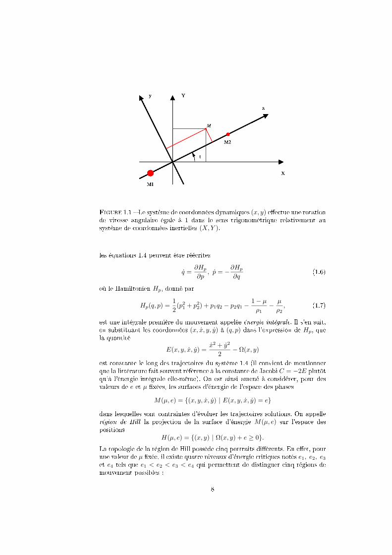
Figure 1.1 Le système de coordonnées dynamiques (x, y) eectue une rotationde vitesse angulaire égale à 1 dans le sens trigonométrique relativement ausystème de coordonnées inertielles (X,Y ).

les équations 1.4 peuvent être réécrites

q =∂Hp

∂p, p = −∂Hp

∂q(1.6)

où le Hamiltonien Hp, donné par

Hp(q, p) =1

2(p21 + p22) + p1q2 − p2q1 −

1− µ

ρ1− µ

ρ2, (1.7)

est une intégrale première du mouvement appelée énergie intégrale. Il s'en suit,en substituant les coordonnées (x, x, y, y) à (q, p) dans l'expression de Hp, quela quantité

E(x, y, x, y) =x2 + y2

2− Ω(x, y)

est constante le long des trajectoires du système 1.4 (il convient de mentionnerque la littérature fait souvent référence à la constante de Jacobi C = −2E plutôtqu'à l'énergie intégrale elle-même). On est ainsi amené à considérer, pour desvaleurs de e et µ xées, les surfaces d'énergie de l'espace des phases

M(µ, e) = (x, y, x, y) | E(x, y, x, y) = e

dans lesquelles sont contraintes d'évoluer les trajectoires solutions. On appellerégion de Hill la projection de la surface d'énergie M(µ, e) sur l'espace despositions

H(µ, e) = (x, y) | Ω(x, y) + e ≥ 0.

La topologie de la région de Hill possède cinq portraits diérents. En eet, pourune valeur de µ xée, il existe quatre niveaux d'énergie critiques notés e1, e2, e3et e4 tels que e1 < e2 < e3 < e4 qui permettent de distinguer cinq régions demouvement possibles :

8

si e < e1, le mouvement s'eectue soit dans un voisinage de la plus grossedes primaires appelé domaine intérieur, soit dans un voisinage de la pluspetite des primaires, appelé domaine extérieur,

si e1 < e < e2, une encolure entre le domaine intérieur et le domainelunaire se forme,

si e2 < e < e3, une seconde encolure entre le domaine lunaire et le domaineextérieur se crée ,

si e3 < e < e4, le passage direct du domaine intérieur vers le domaineextérieur est possible,

si e4 < e le mouvement n'a aucune restriction.

Les valeurs e1, . . . , e4 correspondent en fait à l'énergie intégrale calculée auxpoints d'équilibre du problème qui font l'objet de la section suivante.

1.2.3 Points d'équilibre

−2 −1.5 −1 −0.5 0 0.5 1 1.5 2

−2

−1.5

−1

−0.5

0

0.5

1

1.5

2

(a) e=1.7

−2 −1.5 −1 −0.5 0 0.5 1 1.5 2

−2

−1.5

−1

−0.5

0

0.5

1

1.5

2

(b) e=1.594

−2 −1.5 −1 −0.5 0 0.5 1 1.5 2

−2

−1.5

−1

−0.5

0

0.5

1

1.5

2

(c) e=1.58

−2 −1.5 −1 −0.5 0 0.5 1 1.5 2

−2

−1.5

−1

−0.5

0

0.5

1

1.5

2

(d) e=1.5

Figure 1.2 Les diérents portraits de la région de Hill en fonction de e. Lavaleur du paramètre µ est xé à 1.2153e−2 pour correspondre au cas du systèmeTerre-Lune. Les deux croix rouges représentent la position des primaires. Larégion du mouvement autorisé est dessinée en gris.

Les points d'équilibre du problème restreint des 3 corps plan sont bienconnus. Leur positions respectives dans le repère en rotation restent xes et

9

ils représentent donc les localisations où les inuences des deux primaires secompensent. Ils vérient par dénition les égalités

x = y = x = y = 0,

et, au regard de l'équation 1.4, sont donc les solutions du système

− x+ (1− µ)x+ µ

ρ31+ µ

x− 1 + µ

ρ32= 0

− y + (1− µ)y

ρ31+ µ

y

ρ32= 0

(1.8)

On distingue tout d'abord trois points colinéaires, également appelés pointsd'Euler, notés L1, L2 et L3 et situés sur l'axe y = 0. Leur position respective estcalculée en divisant l'axe des x en trois parties, voir [60]. Illustrons cette méthodeen recherchant les points d'équilibre colinéaires dont l'abscisse appartient ausegment S1 =]µ− 1, µ[. Puisque leur ordonnée est nulle, le problème consiste àdéterminer les solutions de l'équation

−x+1− µ

(x+ µ)2+

µ

(x− 1 + µ)2= 0 (1.9)

appartenant à S1. Notons γ1 la distance d'une solution x1 de cette équation àla plus petite des primaires. De l'égalité x1 = 1−µ−γ1, il vient, en substituantdans 1.9, que γ1 est solution de

1− γ1 − µ− 1− µ

(1− γ1)2− µ

γ21= 0 (1.10)

que l'on réécrit sous la forme de l'équation du cinquième ordre

γ51 − (3− µ)γ41 + (3− 2µ)γ31 + µγ21 − 2µγ1 + µ = 0. (1.11)

D'après la règle de Descartes, cette équation admet une unique solution positivesi 0 < µ ≤ 1

2 et une unique solution réelle pour µ = 0. On peut montrer [60]que la solution γ1 est donnée par le développement en série

γ1 = r1(1−1

3r1 −

1

9r21 − . . . ) (1.12)

où r1 = (µ3 )13 . On peut ainsi calculer numériquement une valeur approchée

de γ1 en utilisant une méthode de Newton initialisée avec r1 et en déduire lavaleur de l'unique point d'Euler L1 dont l'abscisse appartient au segment S1. Enremplaçant S1 par S2 =]µ,+∞[ ou S3 =]−∞, µ−1[ et en adaptant la méthodeprécédente, on localise les deux autres points d'Euler L2 et L3. Précisons quedans le système Terre-Lune, pour lequel µ = 1.2153e−2, les abscisses respectivesdes points d'Euler L1, L2 et L3 sont données par

x1 ' 0.8369, x2 ' 1.1557, x3 ' −1.0051.

On identie également deux points équilatéraux ou points de Lagrange dontl'ordonnée n'est pas nulle. Pour ce faire, il sut d'exprimer les coordonnées duvecteur

v =

(−x+ (1− µ)x+µ

ρ31

+ µx−1+µρ32

−y + (1− µ) yρ31+ µ y

ρ32

)

10

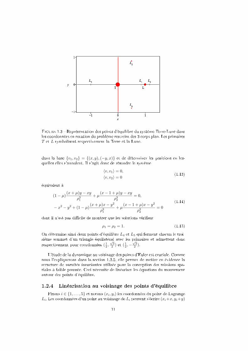
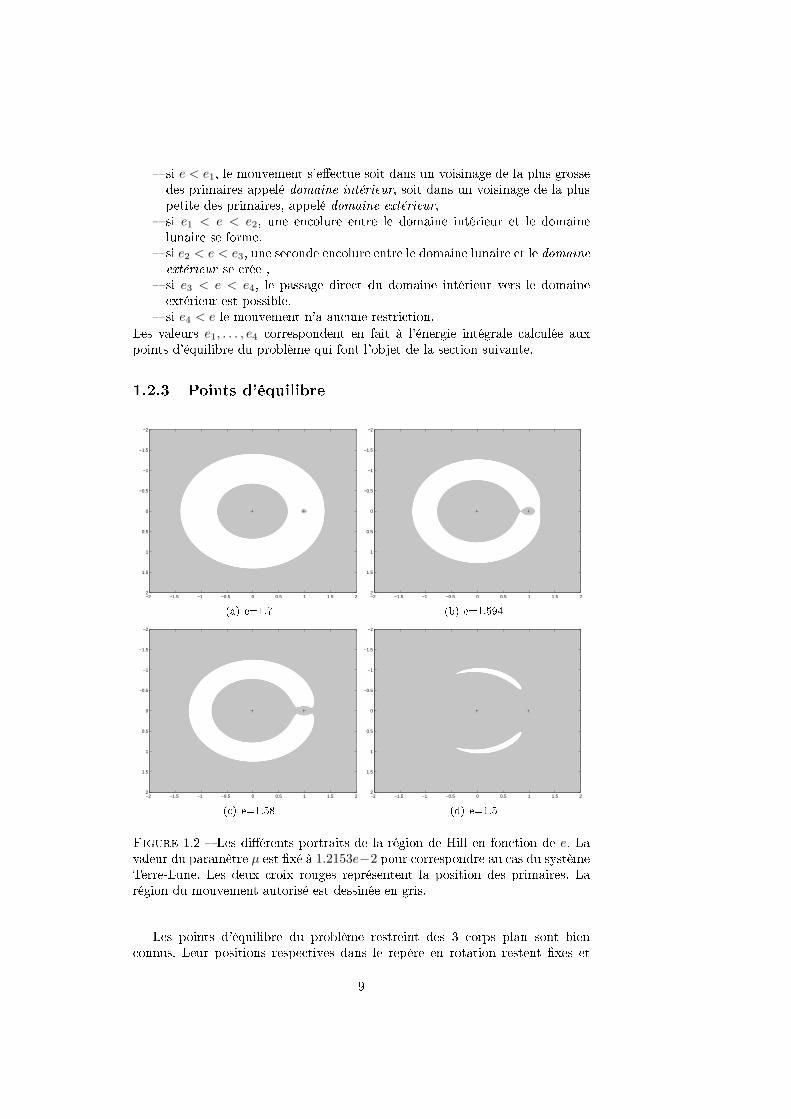
Figure 1.3 Représentation des points d'équilibre du système Terre-Lune dansles coordonnées en rotation du problème restreint des 3 corps plan. Les primairesT et L symbolisent respectivement la Terre et la Lune.

dans la base v1, v2 = (x, y), (−y, x) et de déterminer les positions en les-quelles elles s'annulent. Il s'agit donc de résoudre le système

〈v, v1〉 = 0,

〈v, v2〉 = 0(1.13)

équivalent à

(1− µ)(x+ µ)y − xy

ρ31+ µ

(x− 1 + µ)y − xy

ρ32= 0,

− x2 − y2 + (1− µ)(x+ µ)x− y2

ρ31+ µ

(x− 1 + µ)x− y2

ρ32= 0

(1.14)

dont il n'est pas dicile de montrer que les solutions vérient

ρ1 = ρ2 = 1. (1.15)

On détermine ainsi deux points d'équilibre L4 et L5 qui forment chacun le troi-sième sommet d'un triangle équilatéral avec les primaires et admettent donc

respectivement pour coordonnées ( 12 ,√32 ) et ( 12 ,−

√32 ).

L'étude de la dynamique au voisinage des points d'Euler est cruciale. Commenous l'expliquerons dans la section 1.2.5, elle permet de mettre en évidence lastructure de variétés invariantes utilisée pour la conception des missions spa-tiales à faible poussée. Ceci nécessite de linéariser les équations du mouvementautour des points d'équilibre.

1.2.4 Linéarisation au voisinage des points d'équilibre

Fixons i ∈ 1, . . . , 5 et notons (xi, yi) les coordonnées du point de LagrangeLi. Les coordonnées d'un point au voisinage de Li peuvent s'écrire (xi+x, yi+y)

11

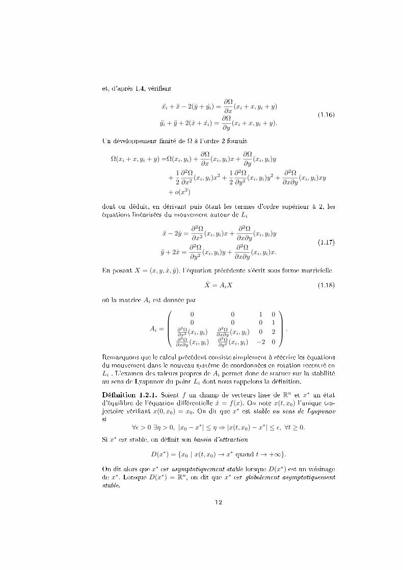
et, d'après 1.4, vérient

xi + x− 2(y + yi) =∂Ω

∂x(xi + x, yi + y)

yi + y + 2(x+ xi) =∂Ω

∂y(xi + x, yi + y).

(1.16)

Un développement limité de Ω à l'ordre 2 fournit

Ω(xi + x, yi + y) =Ω(xi, yi) +∂Ω

∂x(xi, yi)x+

∂Ω

∂y(xi, yi)y

+1

2

∂2Ω

∂x2(xi, yi)x

2 +1

2

∂2Ω

∂y2(xi, yi)y

2 +∂2Ω

∂x∂y(xi, yi)xy

+ o(x2)

dont on déduit, en dérivant puis ôtant les termes d'ordre supérieur à 2, leséquations linéarisées du mouvement autour de Li

x− 2y =∂2Ω

∂x2(xi, yi)x+

∂2Ω

∂x∂y(xi, yi)y

y + 2x =∂2Ω

∂y2(xi, yi)y +

∂2Ω

∂x∂y(xi, yi)x.

(1.17)

En posant X = (x, y, x, y), l'équation précédente s'écrit sous forme matricielle

X = AiX (1.18)

où la matrice Ai est donnée par

Ai =

0 0 1 00 0 0 1

∂2Ω∂x2 (xi, yi)

∂2Ω∂x∂y (xi, yi) 0 2

∂2Ω∂x∂y (xi, yi)

∂2Ω∂y2 (xi, yi) −2 0

.

Remarquons que le calcul précédent consiste simplement à réécrire les équationsdu mouvement dans le nouveau système de coordonnées en rotation recentré enLi . L'examen des valeurs propres de Ai permet donc de statuer sur la stabilitéau sens de Lyapunov du point Li dont nous rappelons la dénition.

Dénition 1.2.1. Soient f un champ de vecteurs lisse de Rn et x∗ un étatd'équilibre de l'équation diérentielle x = f(x). On note x(t, x0) l'unique tra-jectoire vériant x(0, x0) = x0. On dit que x∗ est stable au sens de Lyapunovsi

∀ε > 0 ∃η > 0, |x0 − x∗| ≤ η ⇒ |x(t, x0)− x∗| ≤ ε, ∀t ≥ 0.

Si x∗ est stable, on dénit son bassin d'attraction

D(x∗) = x0 | x(t, x0) → x∗ quand t→ +∞.

On dit alors que x∗ est asymptotiquement stable lorsque D(x∗) est un voisinagede x∗. Lorsque D(x∗) = Rn, on dit que x∗ est globalement asymptotiquementstable.

12

Le théorème suivant est classique, voir par exemple [4, 14] pour une démons-tration complète.

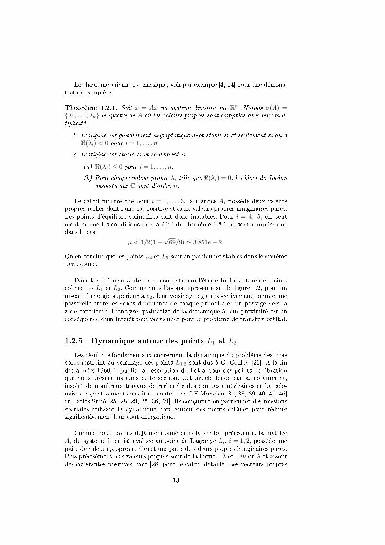
Théorème 1.2.1. Soit x = Ax un système linéaire sur Rn. Notons σ(A) =λ1, . . . , λn le spectre de A où les valeurs propres sont comptées avec leur mul-tiplicité.

1. L'origine est globalement asymptotiquement stable si et seulement si on a<(λi) < 0 pour i = 1, . . . , n.

2. L'origine est stable si et seulement si

(a) <(λi) ≤ 0 pour i = 1, . . . , n.

(b) Pour chaque valeur propre λi telle que <(λi) = 0, les blocs de Jordanassociés sur C sont d'ordre n.

Le calcul montre que pour i = 1, . . . , 3, la matrice Ai possède deux valeurspropres réelles dont l'une est positive et deux valeurs propres imaginaires pures.Les points d'équilibre colinéaires sont donc instables. Pour i = 4, 5, on peutmontrer que les conditions de stabilité du théorème 1.2.1 ne sont remplies quedans le cas

µ < 1/2(1−√69/9) ' 3.851e− 2.

On en conclut que les points L4 et L5 sont en particulier stables dans le systèmeTerre-Lune.

Dans la section suivante, on se concentre sur l'étude du ot autour des pointscolinéaires L1 et L2. Comme nous l'avons représenté sur la gure 1.2, pour unniveau d'énergie supérieur à e2, leur voisinage agit respectivement comme unepasserelle entre les zones d'inuence de chaque primaire et un passage vers lazone extérieure. L'analyse qualitative de la dynamique à leur proximité est enconséquence d'un intérêt tout particulier pour le problème de transfert orbital.

1.2.5 Dynamique autour des points L1 et L2

Les résultats fondamentaux concernant la dynamique du problème des troiscorps restreint au voisinage des points L1,2 sont dus à C. Conley [21]. A la ndes années 1960, il publia la description du ot autour des points de librationque nous présentons dans cette section. Cet article fondateur a, notamment,inspiré de nombreux travaux de recherche des équipes américaines et barcelo-naises respectivement constituées autour de J.E Marsden [37, 38, 39, 40, 41, 46]et Carles Simó [25, 28, 29, 35, 36, 59]. Ils conçurent en particulier des missionsspatiales utilisant la dynamique libre autour des points d'Euler pour réduiresignicativement leur coût énergétique.

Comme nous l'avons déjà mentionné dans la section précédente, la matriceAi du système linéarisé évaluée au point de Lagrange Li, i = 1, 2, possède unepaire de valeurs propres réelles et une paire de valeurs propres imaginaires pures.Plus précisément, ces valeurs propres sont de la forme ±λ et ±iν où λ et ν sontdes constantes positives, voir [28] pour le calcul détaillé. Les vecteurs propres

13

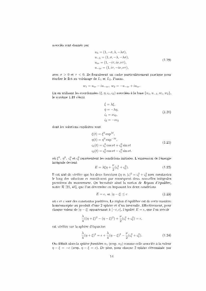
associés sont donnés par

uλ = (1,−σ, λ,−λσ),u−λ = (1, σ,−λ,−λσ),uiν = (1,−iτ, iν, ντ),u−iν = (1, iτ,−iν, ντ),

(1.19)

avec σ > 0 et τ < 0. Ils fournissent un cadre particulièrement pratique pourétudier le ot au voisinage de L1 et L2. Posons

w1 = uiν − iu−iν , w2 = −u−iν + iuiν .

En en utilisant les coordonnées (ξ, η, ς1, ς2) associées à la base uλ, u−λ, w1, w2,le système 1.18 s'écrit

ξ = λξ,

η = −λη,ς1 = νς2,

ς2 = −νς1

(1.20)

dont les solutions explicites sont

ξ(t) = ξ0 expλt,

η(t) = η0 exp−λt,

ς1(t) = ς01 cos νt+ ς02 sin νt

ς2(t) = ς02 cos νt− ς01 sin νt.

(1.21)

où ξ0, η0, ς01 et ς02 représentent les conditions initiales. L'expression de l'énergieintégrale devient

E = λξη +ν

2(ς21 + ς22 ). (1.22)

Il est aisé de vérier que les deux fonctions ξη et |ς|2 = ς21 + ς22 sont constantesle long des solutions et constituent par conséquent deux nouvelles intégralespremières du mouvement. On introduit ainsi la notion de Région d'équilibre,notée R [21, 41], que l'on détermine en imposant les deux conditions

E = ε, et |η − ξ| ≤ c (1.23)

où ε et c sont des constantes positives. La région d'équilibre est de cette manièrehoméomorphe au produit d'une 2-sphère et d'un intervalle. Eectivement, pourchaque valeur de |η − ξ| appartenant à [−c, c], l'égalité E = ε, que l'on réécrit

λ

4((η + ξ)2 − (η − ξ)2) +

ν

2(ς21 + ς22 ) = ε,

est vériée sur la sphère d'équation

λ

4(η + ξ)2 = ε+

λ

4(η − ξ)2 − ν

2(ς21 + ς22 ). (1.24)

On dénit alors la sphère frontière n1 (resp. n2) comme celle associée à la valeurη − ξ = −c (resp. η − ξ = c). De plus, pour chaque 2-sphère déterminée par

14

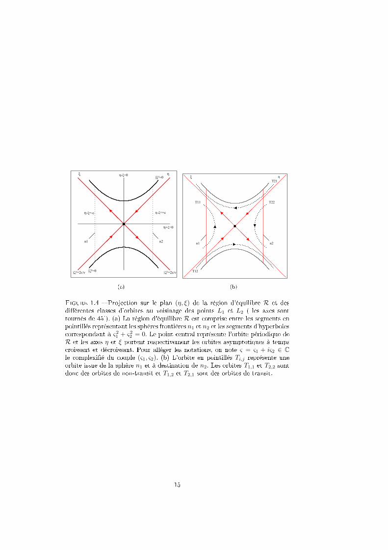
(a) (b)

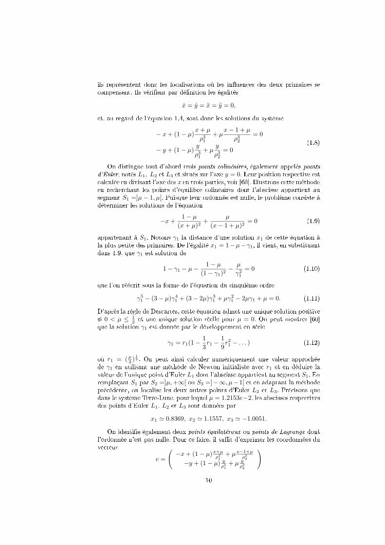
Figure 1.4 Projection sur le plan (η, ξ) de la région d'équilibre R et desdiérentes classes d'orbites au voisinage des points L1 et L2 ( les axes sonttournés de 45). (a) La région d'équilibre R est comprise entre les segments enpointillés représentant les sphères frontières n1 et n2 et les segments d'hyperbolescorrespondant à ς21 + ς22 = 0. Le point central représente l'orbite périodique deR et les axes η et ξ portent respectivement les orbites asymptotiques à tempscroissant et décroissant. Pour alléger les notations, on note ς = ς1 + iς2 ∈ Cle complexié du couple (ς1, ς2). (b) L'orbite en pointillés Ti,j représente uneorbite issue de la sphère n1 et à destination de n2. Les orbites T1,1 et T2,2 sontdonc des orbites de non-transit et T1,2 et T2,1 sont des orbites de transit.

15

l'équation 1.24, l'équateur désigne la région où η+ ξ = 0 et les hémisphère nordet sud sont respectivement décrits par les inégalités η + ξ > 0 et η + ξ < 0.

Le ot dans la région d'équilibre est alors schématisé en projetant les tra-jectoires solutions du système 1.20 sur le plan (η, ξ), ce qui fournit le portraitclassique d'un point critique, voir gure 1.4. La projection de R est compriseentre les hyperboles d'équation ηξ = ε

λ , correspondant à l'intégrale ς21+ς

22 = 0, et

les droites η−ξ = ±c qui ne sont autre que les projections des sphères frontièresn1 et n2. Les orbites de la région d'équilibre se projettent sur les branches d'hy-perboles d'équation ηξ = constante ∈ [−c, c], sauf évidemment lorsque ηξ = 0.Si ηξ > 0, les extrémités des projections des orbites joignent les deux droitesfrontières, ce qui n'est pas vrai lorsque ηξ < 0. Pour représenter globalement ladynamique au sein de la région d'équilibre, il faut enn associer à chaque pointde la projection sur le plan (η, ξ) le cercle correspondant à l'équation

ς21 + ς22 =2

ν(ε− ληξ) (1.25)

que doit vérier le couple de coordonnées (ς1, ς2) en vertu de 1.24. Il existe parconséquent à l'intérieur de la région d'équilibre R neuf classes d'orbites qui sontregroupées en quatre catégories :

1. le point η = ξ = 0 est la projection d'une orbite périodique autour de L1,2

appelée orbite de Lyapunov instable.

2. les deux demi-droites dénies par à ξ = 0, η 6= 0 (resp. η = 0, ξ 6= 0)correspondent à deux cylindres d'orbites asymptotiques qui convergentvers l'orbite de Lyapunov en +∞ (resp. −∞).

3. Chaque branche d'hyperbole donnée par ηξ > 0 est la projection d'uncylindre d'orbites parcourant la région d'équilibre d'une sphère frontièreà l'autre. Ces orbites restent dans le même hémisphère ; plus précisément,elles appartiennent à l'hémisphère nord si elles se dirigent de n2 vers n1 età l'hémisphère sud dans l'autre cas. En raison de la traversée de la régionR qu'elles eectuent, elles sont appelées orbites de transit.

4. Enn, les branches d'hyperboles correspondant à ηξ < 0 représentent descylindres d'orbites se déplaçant d'un hémisphère à l'autre mais dont lesextrémités appartiennent à la même sphère frontière. Si η > 0, les orbitessont issues de la sphère n1 et la rejoignent, passant de l'hémisphère sudà l'hémisphère nord. Dans le cas opposé où η < 0, les orbites partent den2 et y reviennent, évoluant de l'hémisphère nord à l'hémisphère sud. Cesorbites retournant à leur sphère d'origine sont appelées orbites de non-transit.

La gure 1.4 illustre bien le fait que les orbites asymptotiques séparent les deuxtypes de mouvements que sont les orbites de transit, qui passent d'une régionà l'autre, et les orbites de non-transit qui restent connées dans un certain do-maine. Ces orbites asymptotiques sont les approximations linéaires des variétésinvariantes de l'orbite de Lyapunov correspondant au niveau d'énergie ε. Ellessont dénies comme l'ensemble des conditions initiales de l'espace des phasesdesquelles les trajectoires issues convergent en temps inni vers l'orbite de Lya-punov.On parle de variété stable lorsque les trajectoires convergent en tempscroissant et de variété instable lorsqu'elles convergent en temps décroissant.

16

Ce rôle de séparatrice est essentiel pour le design de mission spatiale à faiblepropulsion. Par exemple, si l'on considère un niveau d'énergie très légèrementsupérieur à e1, la capture par la Lune d'un satellite en orbite autour de la Terren'est possible qu'en utilisant le tube invariant constitué par les orbites de transitévoluant du domaine intérieur vers le domaine lunaire et bordé par les branchesdes variétés stables et instables correspondantes. Dans la section suivante, nousproposons un bref aperçu de techniques basées sur la structure de variétés inva-riantes mises en oeuvre pour calculer numériquement des trajectoires spatialespeu coûteuses en énergie.

1.2.6 Construction d'orbites à itinéraires prédénis

A l'analyse qualitative du ot au voisinage des points L1,2 ont succédé deriches études de trajectoires particulières du problème restreint des trois corpsplan. En 1969, R. McGehee mettait en évidence au sein de sa thèse de doctorat[48] certaines orbites homoclines. Ces orbites appartiennent à l'intersection desvariétés stables et instables d'une orbite périodique autour d'un point d'équilibreet relient par conséquent asymptotiquement cette orbite périodique à elle-même.Au début des années 2000, l'équipe de J. Marsden conceptualisait des trajec-toires hétéroclines naturelles reliant les deux orbites de Lyapunov autour de L1

et L2 associées à la même constante de Jacobi. En concaténant ces trajectoireshétéroclines aux trajectoires homoclines déjà connues, ils déduisirent des tra-jectoires du problème des trois corps restreint suivant un itinéraire prédéni àtravers les diérentes régions possibles du mouvement. Ce résultat majeur peutêtre énoncé sous la forme simpliée suivante, voir par exemple [29, 38, 40].

Théorème 1.2.2. Soit une suite u = (ui)i∈Z dont les termes appartiennentà l'ensemble de symboles I, M, X où I désigne le domaine intérieur, Mle domaine lunaire et X le domaine extérieur. Considérons t = 0 comme letemps présent. Alors il existe une orbite dont les localisations passées et futuresrelativement aux trois régions correspondent à u.

Ils proposèrent en outre une procédure systématique permettant de calculernumériquement une orbite associée à un itinéraire donné. Cette procédure estdécrite précisément dans [3, 29, 40]. Leur méthode est basée sur la détermina-tion de points appartenant aux intersections de coupes de Poincaré de variétésinvariantes autour de L1 ou L2. Ces coupes de Poincaré sont déterminées en cal-culant l'intersection d'une variété invariante avec une section de Poincaré S, voir[34], convenablement choisie dans le domaine du mouvement. En sélectionnantcomme conditions initiales les points de l'intersection Λ des coupes de Poincarédes variétés stables et instables avec S puis en intégrant ces conditions à tempscroissant et décroissant, on construit les portions d'orbites évoluant naturel-lement d'une certaine région admissible du mouvement vers une autre. Pourgénérer une orbite respectant un itinéraire plus long, il faut "concaténer" dif-férentes portions d'orbites calculées comme précédemment. Subdivisons à titred'exemple une trajectoire admissible à itinéraire xé en trois portions distinctes.Notons Λi, i = 1, . . . , 3 l'intersection des deux coupes de Poincaré utilisées pourconstruire la ième partie de cette trajectoire. Il sut alors de déterminer l'in-tersection Λ2 ∩ P (Λ1) ∩ P−1(Λ3) où P est l'application de Poincaré associéeà Λ2. Les points de cette intersection correspondent ainsi aux conditions ini-tiales qui, intégrées à temps croissant et décroissant, fournissent les trajectoires

17

recherchées. Ces trajectoires étant naturelles, puisque directement déduites dela dynamique libre du problème des 3 corps restreint au voisinage des pointsL1,2, elles sont théoriquement gratuites du point de vue énergétique, c'est-à-direqu'elles ne nécessitent aucune manoeuvre spécique pour être réalisées.

Mentionnons également le calcul d'une trajectoire Terre-Lune à faible coût,proposée par l'équipe de J. Marsden dans [40]. Pour tenir compte des pertur-bations dues au Soleil, mais plutôt que de se placer dans le problème encorerelativement méconnu des quatre corps, on utilise le modèle de deux systèmesà trois corps couplés. La section terrestre désigne la section de Poincaré de laTerre x = 1− µST , µST étant le ratio des masses du système Terre-Lune, quirelie les deux environnements. L'idée est alors de calculer l'intersection entre lacoupe de Poincaré de la variété stable d'une orbite périodique autour du pointL2 du système Terre-Lune associée à la section terrestre et et la coupe de Poin-caré de la variété instable d'une orbite périodique autour du point L1 ou L2 dusystème Soleil-Terre et la même section. A nouveau, les points contenus danscette intersection constituent les conditions initiales d'orbites qui convergent en±∞ vers les régions souhaitées du mouvement. Outre la structure de variétésinvariantes, cette méthode utilise en particulier la propriété de twisting des or-bites, précisément décrite dans [39], an de déterminer une trajectoire qui soitde plus issue d'une orbite raisonnablement choisie autour de la Terre.

Les collections d'orbites naturelles que nous avons présentées dans cette sec-tion sont d'un grand intérêt pour l'élaboration de missions spatiales à faiblepropulsion. Leur découverte est le fruit de l'étude des caractéristiques des pointsd'équilibre du problème restreint des trois corps, qui relève de la théorie des sys-tèmes dynamiques. C'est pour proposer une approche complémentaire du pro-blème de réduction des coûts énergétiques des transferts Terre-Lune que nousavons orienté nos recherches vers la théorie du contrôle optimal dont l'objet estde déterminer les solutions d'un système commandé, satisfaisant des conditionsaux deux bouts et minimisant un certain coût. Les équations du mouvementque nous avons été amenés à considérer dépendent par conséquent d'un para-mètre dynamique appelé contrôle. Ce sont les équations du problème restreintdes 3-corps plan contrôlé et nous les introduisons maintenant.

1.2.7 le problème restreint des 3-corps plan contrôlé

Les équations du problème restreint des 3-corps plan contrôlé sont obtenuespar l'ajout d'un terme de contrôle à chaque ligne du système 1.4. Elles s'écriventdonc simplement

x− 2y =∂Ω

∂x+ u1

y + 2x =∂Ω

∂y+ u2

(1.26)

et, en appliquant le changement de variable 1.30, peuvent être formulées sousla forme hamiltonienne

q =∂H

∂p, p = −∂H

∂q(1.27)

18

où la fonction hamiltonienne H est donnée par

H(q, p) = Hp(q, p)− q1u1 − q2u2 (1.28)

et Hp est le Hamiltonien du mouvement libre déni en 1.7. Dans le but de déter-miner des transferts Terre-Lune à poussée faible, nous nous sommes intéressésaux trajectoires solutions du système 1.26 dont les conditions initiales et nalesdoivent respectivement caractériser des orbites terrestres et lunaires. La pous-sée appliquée au satellite à un instant t pouvant être modélisée par la normeL2(R2) du contrôle u(t) = (u1(t), u2(t)), nous avons focalisé notre étude sur laminimisation de deux coûts distincts. L'un est logiquement la minimisation ducoût énergétique le long d'une trajectoire,

minu(.)∈R2

∫ tf

t0

u21 + u22dt,

où t0 est le temps initial et tf est xé et désigne le temps de transfert. L'autreest la minimisation de ce temps de transfert

minu(.)∈BR2 (0,ε)

∫ tf

t0

dt

où ε désigne la poussée maximale autorisée, autrement dit le rayon du disque deR2 dans lequel on impose au contrôle u d'être contenu, qui doit être d'un ordre degrandeur comparable à une propulsion signicativement faible. Les principauxoutils géométriques et numériques de la théorie du contrôle optimal auxquelsnous avons eu recours pour traiter ces problèmes sont introduits dans le cha-pitre 2. Leurs applications au problème restreint des 3-corps plan et les résultatsque nous avons obtenus sont résumés dans la section 3.1 du chapitre 3 et sontprésentés avec précision dans les articles Geometric and numerical techniquesin optimal orbital transfer using low propulsion [10] et Shooting and numericalcontinuation methods for computing time-minimal and energy-minimal trajec-tories in the Earth-Moon system using low propulsion [51] qui gurent dans cemanuscrit.

1.3 Le problème restreint des 3 corps spatial

L'extension du problème plan au problème spatial permet de considérer ladynamique dans la troisième direction qui est importante quand le satellite ap-proche une des primaires. Cette prise en compte est en outre essentielle, commecela est souligné dans [41], pour le bon fonctionnement des relais de communica-tions spatiaux qui est conditionné par l'inclinaison de leur plan orbital. Citonségalement la nécessité d'étudier le problème spatial an de coupler plusieurssystèmes à trois corps non-coplanaires, comme le sont en particulier les sys-tème Soleil-Terre-satellite et Terre-Lune-satellite. L'augmentation des dégrés deliberté du modèle, plus précis et en ce sens davantage réaliste, induit certainescomplications géométriques [41]. Cependant, nous verrons que les résultats pré-sentés au long de la section 1.2 peuvent être généralisés au cas du problèmespatial. La structure de variétés invariantes étant préservée, il est intéressantd'étudier son inuence sur les transferts à énergie minimale au voisinage dupoint L1 qui joue le rôle crucial de passerelle de l'inuence terrestre vers l'in-uence lunaire.

19

1.3.1 Equations du mouvement et points d'équilibre

Le problème spatial dière du problème plan uniquement dans la mesureoù l'on suppose que la particule de masse négligeable n'évolue plus uniquementdans le plan P déni par le mouvement circulaire des primaires mais dans R3

tout entier. En considérant la dynamique dans la direction z orthogonale auplan P et telle que le repère synodique G, x, y, z soit positivement orienté, leséquations 1.26 deviennent

x− 2y =∂Ω

∂x

y + 2x =∂Ω

∂y

z =∂Ω

∂z

(1.29)

où le potentiel −Ω est déni identiquement à celui de la section 1.2.1 mais oùles distances aux primaires sont

ρ1 =√(x+ µ)2 + y2 + z2

ρ2 =√(x− 1 + µ)2 + y2 + z2.

Le changement de variable

q1 = x, q2 = y, q3 = z, p1 = x− y, p2 = y + x, p3 = z (1.30)

induit les équations hamiltoniennes

q =∂Hs

∂p, p = −∂Hs

∂q(1.31)

où la fonction hamiltonienne Hs décrivant le mouvement libre du problèmespatial s'écrit

Hs(q, p) =1

2(p21 + p22 + p23) + p1q2 − p2q1 −

1− µ

ρ1− µ

ρ2. (1.32)

On obtient ainsi, de la même manière que dans la section 1.2.2, l'expression del'énergie intégrale du mouvement

Es(x, y, z, x, y, z) =x2 + y2 + z2

2− Ω(x, y, z)

qui conduit à la dénition de la surface d'énergie

M(µ, e) = (x, y, z, x, y, z) | E(x, y, z, x, y, z) = e

comme sous-variété de R6 de dimension 5 contenant, pour une valeur xée deµ, les trajectoires correspondantes au niveau d'énergie e. L'intersection de larégion de Hill

H(µ, e) = (x, y, z) | Ω(x, y, z) + e ≥ 0.

avec le plan (x, y) fournit alors les mêmes portraits topologiques des régionspossibles du mouvement que ceux représentés sur la gure 1.2. Les niveaux

20

d'énergies critiques e1, . . . , e4 sont de mêmes valeurs que dans problème planet correspondent également aux niveaux d'énergie des points d'équilibre du pro-blème spatial. Ces points d'équilibre appartiennent au plan (x, y) ; on distingue,comme dans le problème plan, les trois points colinéaires L1, L2, L3 et les deuxpoints équilatéraux L4 et L5. Leur position, identique à celle calculée en section1.2.3, est déterminée en suivant la même méthode.

1.3.2 Dynamique au voisinage des points colinéaires

Pour étudier la dynamique du problème spatial au voisinage d'un point co-linéaire Li, i = 1, 2 où 3, on translate l'origine du repère synodique en Li eton normalise le système de coordonnées de telle sorte que la distance de Li àla plus proche des primaires soit égale à 1. Les nouvelles coordonnées x, y, zproviennent donc du changement de variables

x =x+ µ+ ai

γi

y =y

γi

z =z

γi

(1.33)

où les constantes ai sont dénies par a1 = −1 + γ1, a2 = −1 − γ2, a3 = γ3 etγi désigne la distance du point Li à la primaire la plus proche. Pour alléger lesnotations, nous conserverons dans les lignes qui suivent les symboles x, y et zpour désigner les variables du système normalisé. De cette façon, les équationsdu mouvement 1.29 peuvent être exprimées au moyen de séries formelles sousla forme

x− 2y − (1 + c2)x =∂

∂x

∑n≥3

cnρnPn(

x

ρ),

y + 2x+ (c2 − 1)y =∂

∂y

∑n≥3

cnρnPn(

x

ρ)

z + 2c2z =∂

∂z

∑n≥3

cnρnPn(

x

ρ)

(1.34)

où Pn représente le polynôme de Legendre d'ordre n, ρ = x2 + y2 + z2 et lescoecients cn sont donnés par

cn(µ) =1

γ3i

((±1)nµ+ (−1)n

(1− µ)γn+1i

(1∓ γi)n+1

)pour L1,2,

cn(µ) =(−1)n

γ3i

(1− µ+

µγn+13

(1 + γ3)n+1

)pour L3

où dans la première équation le signe du haut vaut pour L1 et celui du baspour L2. Le changement de variable 1.30 permet alors évidemment d'obtenirla formulation hamiltonienne des équations 1.34. Le Hamiltonien correspondants'écrit

HL(q, p) =1

2(p21 + p22 + p23) + p1q2 − p2q1 −

1− µ

ρ1−∑n≥2

cnρnPn(

q1ρ). (1.35)

21

En éliminant les termes non-linéaires gurant au sein du système 1.34, on obtientles équations linéarisées du problème spatial au voisinage du point Li

x− 2y − (1 + c2)x = 0

y + 2x+ (c2 − 1)y = 0

z + 2c2z = 0.

(1.36)

et le Hamiltonien 1.35 devient

H2L(q, p) =

1

2(p21 + p22 + p23) + q2p1 − q1p2 −

c22(2q21 − q22 − q23) (1.37)

On cherche alors à identier un changement de coordonnées canonique, c'est-à-dire qui préserve le formalisme hamiltonien des équations linéarisées 1.36. Il sutpour cela, voir [35], de déterminer un changement de variable symplectique descoordonnées (q1, q2, q3, p1, p2, p3), à savoir une matrice A ∈ M(R6) satisfaisantl'égalité

ATJA = J (1.38)

où J est la matrice

J =

(0 IdR2

−IdR2 0

).

Puisque la direction verticale est découplée des directions planaires dans le sys-tème 1.36, on se restreint dans un premier temps à calculer un changementsymplectique des coordonnées (q1, q2, p1, p2).On s'intéresse donc à la fonctionhamiltonienne

H2L(q, p) =

1

2(p21 + p22) + q2p1 − q1p2 −

c22(2q21 − q22) (1.39)

que l'on note comme 1.37 par souci de simplication. Les équations du mouve-ment associées s'écrivent sous la forme du système linéaire

xypxpy

=M

xypxpy

(1.40)

avec

M =

0 1 1 0−1 0 0 12c2 0 0 10 −c2 −1 0

.

Il est relativement simple, voir [36], de montrer que la matrice M possède deuxvaleurs propres réelles et deux valeurs propres imaginaires pures, notées ±λ1 et±iω1, associées aux vecteurs propres

uλ1 = (2λ1, λ21 − 2c2 − 1, λ21 + 2c2 + 1, λ31 + (1− 2c2)λ1),

u−λ1 = (−2λ1, λ21 − 2c2 − 1, λ21 + 2c2 + 1,−λ31 − (1− 2c2)λ1),

uiω1 = (0,−ω21 − 2c2 − 1,−ω2

1 + 2c2 + 1, 0),

u−iω1 = (2ω1, 0, 0,−ω31 + (1− 2c2)ω1).

(1.41)

22

Le changement de variables déni par la matrice C = (uλ1 , u−λ1 , uiω1 , u−iω1)vérie alors l'égalité

CTJC =

(0 D

−D 0

)où D est donnée par

D =

(dλ1 00 dω1

)et dλ1 et dω1 sont les deux constantes strictement positives pour 0 < µ < 1

2

dλ1 = 2λ1((4 + 3c2)λ21 + 4 + 5c2 − 6c22)),

dω1 = ω1((4 + 3c2)ω21 − 4− 5c2 + 6c22).

Pour que C dénisse une transformation symplectique, il sut donc de diviserses deux premières colonnes par s1 =

√dλ1 et ses deux dernières par s2 =

√dω1 .

Le changement de coordonnées nal doit alors tenir compte de la directionverticale. Puisque c2 > 1, on pose ω2 =

√c2. Ainsi la matrice

A =

2λ1

s10 0 −2λ1

s12ω1

s20

λ21−2c2−1

s1−ω2

1−2c2−1s2 0

λ21−2c2−1

s1 0 00 0 1√

ω20 0 0

λ21+2c2+1

s1−ω2

1+2c2+1s2 0

λ21+2c2+1

s1 0 0λ31+(1−c2)λ1

s1 0 0−λ3

1−(1−c2)λ1

s1−ω3

1+(1−c2)ω1

s1λ21+2c2+1

s10 0 0 0 0

√ω2

est un changement de variable symplectique qui, en conservant les symboles qet p pour désigner les nouvelles coordonnées, transforme l'expression du Hamil-tonien 1.35 en

H = λ1q1p1 +ω1

2(q22 + p22) +

ω2

2(q23 + p23). (1.42)

Les équations linéarisées 1.36 s'écrivent alors

q1 = λ1q1, p1 = −λ1p1,q2 = ω1p2, p2 = −ω1q2,q3 = ω2p3, p3 = −ω2q3,

(1.43)

et leurs solutions sont explicitement données par

q1(t) = q01 expλ1t,

p1(t) = p01 exp−λ1t,

q2(t) + ip2(t) = (q02 + ip02) exp−iω1t,

q3(t) + ip3(t) = (q03 + ip03) exp−iω2t .

(1.44)

où q01 , p01, q

02 + ip

02 et q

03 + ip

03 sont les conditions initiales. Les points colinéaires

du problème spatial sont par conséquent du type selle×centre×centre. En ob-servant que les fonctions q1p1, q

22 + p22 et q23 + p23 sont des intégrales premières

du mouvement, la dynamique dans leur voisinage peut être schématisée d'unemanière similaire au cas plan. La région d'équilibre R est déterminée par

H = h, et |p1 − q1| ≤ c (1.45)

23

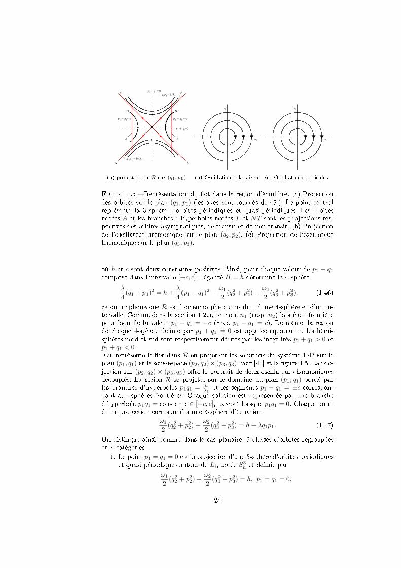
(a) projection de R sur (q1, p1) (b) Oscillations planaires (c) Oscillations verticales

Figure 1.5 Représentation du ot dans la région d'équilibre. (a) Projectiondes orbites sur le plan (q1, p1) (les axes sont tournés de 45). Le point centralreprésente la 3-sphère d'orbites périodiques et quasi-périodiques. Les droitesnotées A et les branches d'hyperboles notées T et NT sont les projections res-pectives des orbites asymptotiques, de transit et de non-transit. (b) Projectionde l'oscillateur harmonique sur le plan (q2, p2). (c) Projection de l'oscillateurharmonique sur le plan (q3, p3).

où h et c sont deux constantes positives. Ainsi, pour chaque valeur de p1 − q1comprise dans l'intervalle [−c, c], l'égalité H = h détermine la 4-sphère

λ

4(q1 + p1)

2 = h+λ

4(p1 − q1)

2 − ω1

2(q22 + p22)−

ω2

2(q23 + p23). (1.46)

ce qui implique que R est homéomorphe au produit d'une 4-sphère et d'un in-tervalle. Comme dans la section 1.2.5, on note n1 (resp. n2) la sphère frontièrepour laquelle la valeur p1 − q1 = −c (resp. p1 − q1 = c). De même, la régionde chaque 4-sphère dénie par p1 + q1 = 0 est appelée équateur et les hémi-sphères nord et sud sont respectivement décrits par les inégalités p1 + q1 > 0 etp1 + q1 < 0.On représente le ot dans R en projetant les solutions du système 1.43 sur leplan (p1, q1) et le sous-espace (p2, q2)× (p3, q3), voir [41] et la gure 1.5. La pro-jection sur (p2, q2) × (p3, q3) ore le portrait de deux oscillateurs harmoniquesdécouplés. La région R se projette sur le domaine du plan (p1, q1) bordé parles branches d'hyperboles p1q1 = h

λ1et les segments p1 − q1 = ±c correspon-

dant aux sphères frontières. Chaque solution est représentée par une branched'hyperbole p1q1 = constante ∈ [−c, c], excepté lorsque p1q1 = 0. Chaque pointd'une projection correspond à une 3-sphère d'équation

ω1

2(q22 + p22) +

ω2

2(q23 + p23) = h− λq1p1. (1.47)

On distingue ainsi, comme dans le cas planaire, 9 classes d'orbites regroupéesen 4 catégories :

1. Le point p1 = q1 = 0 est la projection d'une 3-sphère d'orbites périodiqueset quasi-périodiques autour de Li, notée S

3h et dénie par

ω1

2(q22 + p22) +

ω2

2(q23 + p23) = h, p1 = q1 = 0.

24

2. les couples de demi-droites q1 = 0, p1 6= 0 et p1 = 0, q1 6= 0 correspondentrespectivement aux branches de variété stable W s

±(S3h) et variété instable

Wu±(S

3h) de S

3h dénies par

W s±(S

3h) = ω1

2(q22 + p22) +

ω2

2(q23 + p23) = h, q1 = 0, p1 ≷ 0,

Wu±(S

3h) = ω1

2(q22 + p22) +

ω2

2(q23 + p23) = h, p1 = 0, q1 ≷ 0.

Ces variétés sont des cylindres contenant les orbites convergeant asymp-totiquement vers S3

h en temps croissant et décroissant.

3. Les branches d'hyperboles données par q1p1 > 0 sont les projections decylindres d'orbites parcourant la région d'équilibre d'une sphère frontièreà l'autre. Ces orbites appartiennent exclusivement à l'hémisphère nord sielles se dirigent de n2 vers n1 et à l'hémisphère sud sinon. Elles formentl'ensemble des orbites de transit.

4. Enn, les branches d'hyperboles correspondant à q1p1 < 0 représententdes cylindres d'orbites se déplaçant d'un hémisphère à l'autre mais dontles extrémités appartiennent à la même sphère frontière. Si q1 > 0, cettesphère est n1 et les orbites passent de l'hémisphère sud à l'hémisphèrenord. Si q1 < 0, la sphère est n2 et les orbites évoluent de l'hémisphèrenord à l'hémisphère sud. Ce sont les orbites de non-transit.

La structure de variétés invariantes peut donc être étendue à la description duot au voisinage des points colinéaires du problème spatial. Les variétés stableset instables jouent, tout comme dans le problème plan, un rôle de séparatriceentre orbites de transit et orbites de non-transit. Leur utilisation est en ce sensecace pour traiter du problème de calcul de trajectoires à faible coût éner-gétique. Il gure notamment dans [29] une généralisation au cas spatial de laméthode de construction d'orbites naturelles à itinéraires prédénis présentéeen section 1.2.6. Du point de vue géométrique, ces constructions sont plus com-plexes que dans le cas plan car les coupes de Poincaré à prendre en considérationsont des 3-sphères topologiques dont il est délicat de déterminer les intersections.

Il est important de préciser que la dynamique non-linéaire dans la région Rest qualitativement la même que la dynamique linéaire. Dans ce cas, la 3-sphèreS3h se généralise en la variété

M3h = (q, p) | ω1

2(q22 + p22) +

ω2

2(q23 + p23) + f(q2, p2, q3, p3) = h, p1 = q1 = 0

où f est au moins d'ordre 3. Elle admet alors les variétés stables et instables

W s±(M

3h) = ω1

2(q22 + p22) +

ω2

2(q23 + p23) + f(q2, p2, q3, p3) = h, q1 = 0, p1 ≷ 0,

Wu±(M3

h) = ω1

2(q22 + p22) +

ω2

2(q23 + p23) + f(q2, p2, q3, p3) = h, p1 = 0, q1 ≷ 0.

Ajoutons de plus que dans un petit voisinage de L1, les variétés invariantesde la dynamique linéaire sont de très acceptables approximations des variétésinvariantes de la dynamique non linéaire, les termes d'ordre non-linéaires étantnégligeables devant ceux linéaires.

25

1.3.3 Le problème spatial contrôlé au voisinage de L1

Comme nous l'avons mentionné au début de la section , notre troisième ob-jectif a été d'évaluer l'impact de la structure de variétés invariantes sur le cal-cul de trajectoires à poussée faible au voisinage de L1. Plus précisément, nousavons cherché à déterminer des trajectoires énergie-minimales entre la brancheW s

+(S3h) de la variété stable et la branche la branche Wu

+(S3h) de la variété in-

stable de ce point . Ces trajectoires peuvent en fait être considérées comme desportions de transferts Terre-Lune utilisant la structure de variétés invariantespour tenter de minimiser la consommation énergétique lors du passage du do-maine intérieur vers le domaine extérieur. Elles sont solutions des équations dumouvement contrôlé autour de L1

x− 2y − (1 + c2)x =∂

∂x

∑n≥3

cnρnPn(

x

ρ) + u1

y + 2x+ (c2 − 1)y =∂

∂y

∑n≥3

cnρnPn(

x

ρ) + u2

z + 2c2z =∂

∂z

∑n≥3

cnρnPn(

x

ρ) + u3

(1.48)

obtenues à partir du système 1.34 et minimisent le coût en énergie∫ tf

t0

u1(t)2 + u2(t)

2 + u3(t)2dt. (1.49)

L'article Energy-minimal transfers in the vicinity of the Lagrangian point L1

[52] fournit les développements et résultats de cette étude et la section 3.2 duchapitre 3 en ore un résumé. Les résultats fondamentaux de la théorie ducontrôle qui y sont utilisés sont les mêmes que ceux employés pour calculerles trajectoires Terre-Lune temps-minimales et énergie-minimales du problèmeplan. Le chapitre suivant leur est consacré.

26

Chapitre 2

Outils géométriques et

numériques en contrôle

optimal.

2.1 Dénition du problème

Considérons un problème général de contrôle optimal déni comme suit.Soient M et U deux variétés lisses de dimensions respectives n et m. On s'inté-resse au système de contrôle sur M

q(t) = f(q(t), u(t)) (2.1)

où f :M × U −→ TM est lisse et les contrôles u sont des fonctions mesurableset bornées dénies sur un intervalle [t0, t(u)[⊂ R+ à valeurs dans U . Rappelonstout d'abord trois dénitions fondamentales.

Dénition 2.1.1. Soit q0 ∈ M . L'ensemble accessible en temps tf pour lesystème 2.1 depuis q0, noté Acc(q0, tf ), est l'ensemble des valeurs au temps tfdes solutions du système 2.1 partant de q0 au temps t0 et associées à un contrôleu tel que t(u) > tf .

Dénition 2.1.2. Le système 2.1 est dit contrôlable en temps tf depuis q0 ∈Msi

M = Acc(q0, tf ).

Il est dit contrôlable depuis q0 si

M =⋃t≥0

Acc(q0, tf ).

Dénition 2.1.3. Soient M0 et M1 deux sous-ensembles de M et tf > t0.L'ensemble Utf des contrôles admissibles sur [t0, tf ] est déni comme l'ensembledes contrôles u tels que t(u) > tf dont les trajectoires associées relient un pointinitial dans M0 à un point nal de M1.

27

Dénissons par

C(tf , u) =

∫ tf

t0

f0(x(t), u(t))dt (2.2)

où f0 :M ×U −→ R est supposée lisse, le coût associé à un contrôle admissiblesur [t0, tf ]. Considérons alors le problème de contrôle optimal consistant à déter-miner une trajectoire q(.) solution de 2.1 et associée à un contrôle u admissiblesur [t0, tf ] telle que q(0) ∈ M0, q(tf ) ∈ M1 et le coût 2.2 soit minimisé. Intro-duisons la notion suivante qui nous sera utile dans la section 2.3 pour énoncerles conditions nécessaires et susante d'optimalité du second ordre.

Dénition 2.1.4. Soient q0 ∈ M et tf > t0. L'application entrée-sortie dusystème 2.1 est l'application

Eq0,tf : Utf −→M

u −→ q(q0, tf , u)(2.3)

où t −→ q(q0, t, u) est la trajectoire solution de 2.1 associée au contrôle u telleque q(q0, 0, u) = q0

Remarquons que, pour q0 ∈ M xé, l'image de l'application entrée-sortieau temps tf est égale à l'ensemble accessible en temps tf depuis q0. Si U estdoté de la topologie de L∞ alors l'application entrée-sortie est lisse. Soit q(.)une trajectoire du système 2.1 associée au contrôle lisse u sur [t0, tf ]. Alors lecontrôle u peut être prolongé de manière lisse à l'intervalle [t0, tf + ε] où ε > 0.

Dénition 2.1.5. On considère deux cas distincts. Si le temps nal tf est xé, q(.) est dite localement optimale pour latopologie L∞ (resp. localement optimale pour pour la topologie C0) si elleest optimale dans un voisinage de u pour la topologie L∞ (resp. dans unvoisinage de q(.) pour la topologie C0).

Si le temps nal tf n'est pas xé, q(.) est dite localement optimale pourla topologie L∞ si pour tout voisinage V de u dans L∞([t0, tf + ε], U),pour tout réel η tel que |η| ≤ ε et pour tout contrôle v ∈ V satisfaisantE(q0, tf + η, v) = E(q0, tf , u), on ait C(tf + η, v) ≥ C(tf , u) . De plus q(.)est dite localement optimale pour la topologie C0 si pour tout voisinageWde q(.) dans M , pour tout réel η tel que |η| ≤ ε et pour toute trajectoirey associée à un contrôle v sur [t0, tf + η] contenue dans W et satisfaisanty(0) = q0 et y(tf + η) = q(tf ), on ait C(tf + η, v) ≥ C(tf , u)

2.2 Le principe du maximum

Le principe du maximum de Pontryagin, qui fournit une condition néces-saire d'optimalité, est le résultat fondateur de la théorie moderne du contrôleoptimal. Nous l'énonçons ici sous une forme assez générale qui correspond auxproblèmes de contrôle optimal traités au cours de nos travaux de recherche. Iladmet néanmoins des extensions à de plus larges classes de dynamiques et decritères à minimiser, voir [55, 61].

Théorème 2.2.1 (Principe du maximum de Pontryagin). Considérons le sys-tème de contrôle 2.1 et le coût 2.2. Si le contrôle u est optimal alors il existe

28

un réel p0 ∈ R∗− et une application p(.) absolument continue sur [t0, tf ] vériant

p(t) ∈ T ∗x(t)M tels que le couple (p0, p) soit non trivial et presque partout sur

[t0, tf ] on ait

q(t) =∂H

∂p(q(t), p0, p(t), u(t))

p(t) = −∂H∂q

(q(t), p0, p(t), u(t))

(2.4)

où H est l'application dénie par

H : T ∗M × R∗− × U −→ R

(q(t), p(t), p0, u) −→ p0f0(q(t), u(t)) + 〈p(t), f(q(t), u(t))〉.

Le principe du maximum assure en outre la condition de maximisation

H(q(t), p(t), p0, u(t)) = maxv∈U

H(q(t), p(t), p0, v) (2.5)

presque partout sur l'intervalle [t0, tf ]. Si le temps de transfert tf n'est pas xé,l'égalité

maxv∈U

H(q(t), p(t), p0, v) = 0 (2.6)

est de plus vériée pour tout t ∈ [t0, tf ]. Enn, si M0 (resp. M1) est une sous-variété régulière de M , l'application p(.) vérie la condition de transversalité

p(0) ⊥ Tq(0)M0 (resp. p(tf ) ⊥ Tq(tf )M1). (2.7)

Dénition 2.2.1. L' application H est appelée pseudo-Hamiltonien et la formelinéaire p est appelée état adjoint. On appelle extrémale du problème de contrôleoptimal déni par 2.1 et 2.2 un quadruplet (q(.), p(.), p0, u(.)) solution des équa-tions 2.4, 2.5 et, le cas échéant, 2.6 . Si p0 = 0, on dit que l'extrémale estanormale. Sinon on elle dite normale. Si de plus les conditions de transversalitésont satisfaites, l'extrémale est appelée BC-extrémale.

Puisque U est une est une variété lisse de dimension m on peut supposer, enutilisant le système de coordonnées locales, que localement U = Rm. Ainsi, ilvient de la condition maximisation 2.5 l'égalité ∂H

∂u = 0. Formulons l'hypothèsesuivante.

(L)(condition stricte de Legendre) La forme quadratique ∂2H∂u2 est dénie né-

gative le long de l'extrémale (q(.), p(.), p0, u(.)).

Le théorème des fonctions implicites assure alors qu'il existe un voisinage deu dans lequel les contrôles extrémaux sont des fonctions lisses de la forme

ur(t) = ur(q(t), p(t)).

Ceci induit la dénition ci-dessous.

Dénition 2.2.2. On dénit le Hamiltonien vrai, également appelé Hamilto-nien réduit et noté Hr, par

Hr(q, p) = H(q, p, ur(q, p)).

29

Chaque extrémale est alors solution du système hamiltonien

q(t) =∂Hr

∂p(q(t), p(t)),

p(t) = −∂Hr

∂q(q(t), p(t))

(2.8)

lequel, en posant z = (q, p), s'écrit

z(t) =−→Hr(z(t)). (2.9)

Comme nous l'avons déjà souligné au début de cette section, il existe de nom-breuses formulations du principe du maximum, adaptées aux diérentes classesde systèmes contrôlés, coûts et contraintes sur les contrôles admissibles. Pourclore cette section, énonçons ce résultat dans le cas d'un système de contrôle li-néaire avec un coût quadratique, comme l'est en particulier le coût énergétique.Nous expliquerons dans la section 3.2 en quoi ce théorème nous a été utile pourinitialiser les méthodes numériques de calcul de trajectoires énergie-minimalesau voisinage du point L1.

Théorème 2.2.2 (Principe du maximum dans le cas linéaire quadratique).Considérons le système contrôlé

z = A(t)z +B(t)u

contrôlable sur Rn où A(t) et B(t) sont deux matrices continues sur l'intervalleborné [t0, tf ] appartenant respectivement à Mn,n(R) et Mn,m(R). Dénissonsle coût

C0(u) =

∫ tf

t0

z(s)TW (s)z(s) + u(s)TU(s)u(s)dt

où W (s) et U(s) sont deux matrices carrées continues et symétriques sur l'inter-valle [t0, tf ]. Supposons de plus que W (s) et U(s) soient respectivement semi-dénie positive et positive pour tout s ∈ [t0, tf ]. Soient G un sous-ensembleconvexe compact non-vide de Rn et z0 ∈ Rn. Alors il existe un unique contrôleu∗(t) telle que la trajectoire associée z∗(t) minimise le coût C et vérie z∗(0) =z0 et z∗(tf ) ∈ G . Plus précisément, il existe un état adjoint η∗ tel que z∗(t) etη∗(t) soient solutions de

z = A(t)z +B(t)U(t)−1B(t)T ηT

η = zTW (t)− ηA(t)(2.10)

où z∗(t0) = z0, z∗(tf ) ∈ ∂G et η∗(tf ) est intérieur et normal à G en z∗(tf ). Le

contrôle optimal u∗ est alors donné par

u∗(t) = U(t)−1B(t)T η∗(t)T . (2.11)

Le résultat suivant complète le principe du maximum dans le cas linéairequadratique et permet d'exprimer le contrôle optimal sous la forme d'une bouclefermée.

30

Théorème 2.2.3. Considérons le problème consistant à trouver une trajectoiresolution de

z = A(t)x+B(t)u(t)

z(0) = z0 ∈ Rn

minimisant le coût

C0(u) = x(tf )TQx(tf ) +

∫ tf

t0

z(s)TW (s)z(s) + u(s)TU(s)u(s)dt

où Q, W (s) et U(s) sont trois matrices carrées continues et symétriques surl'intervalle [t0, tf ]. Supposons de plus que W (s) est semi-dénie positive et queQ et U(s) soient positives pour tout s ∈ [t0, tf ]. Alors, pour tout z0 ∈ Rn ilexiste une unique trajectoire optimale z∗ associée au contrôle u∗. Ce contrôle semet sous forme de boucle fermée

u(t) = U(t)−1B(t)TE(T )x(t) (2.12)

où E ∈ Mn(R) est solution sur [t0, tf ] de l'équation matricielle de Riccati

E(t) =W (t)−A(t)TE(t)− E(t)A(t)− E(t)B(t)U−1(t)B(t)TE(T ),

E(tf ) = −Q.(2.13)

Le principe du maximum, puisse-t-il être formulé de la manière la plus géné-rale possible, ne fournit qu'une condition nécessaire d'optimalité. On introduitdonc la notion de temps conjugué géométrique qui est à la base d'une méthodedu second ordre orant une condition susante d'optimalité locale d'une extré-male.

2.3 Temps conjugués géométriques et conditions

d'optimalité du second ordre

Considérons une variété lisse M de dimension n et notons Πq : T ∗M −→M

la projection canonique du bré cotangent T ∗M sur M . Soient−→H un champ de

vecteurs hamiltonien sur T ∗M et z(t) = (q(t), p(t)) une trajectoire de−→H dénie

sur un intervalle [t0, tf ]. L'égalité z(t) =−→H (z(t)) est alors vériée pour tout

t ∈ [t0, tf ]. On note expt(−→H ) le ot du champ de vecteurs

−→H .

Dénition 2.3.1. L'équation variationnelle

δz(t) = d−→H (z(t))δz(t)

vériée sur [t0, tf ] est appelée équation de Jacobi le long de z(.). On appellechamp de Jacobi une solution J(t) non triviale de l'équation de jacobi le longde z(.) et on dit qu'il est vertical au temps t si dΠq(z(t)).J(t) = 0. Un temps tcest dit geométriquement conjugué si il existe un champ de Jacobi vertical en 0et en tc. Auquel cas, le point q(tc), est dit conjugué à q(0).

Remarquons qu'en coordonnées locales, un champ de Jacobi peut s'écrireJ(t) = (δq(t), δp(t)). La verticalité de J au temps t se traduit alors δq(t) = 0.La notion de temps conjugué admet la généralisation suivante.

31

Dénition 2.3.2. Soit M1 une sous-variété régulière de M . On note M⊥1 =

(q, p) | q ∈ M1, p ∈ TqM1. On dit que tfoc ∈ [t0, T ] est un temps focal siil existe un champ de Jacobi J = (δq, δp) tel que δq(tfoc) = 0 et J(tfoc) esttangent à M⊥

1 .

Dénition 2.3.3. Soit z0 ∈ T ∗M . Pour tout t ∈ [t0, tf ], on dénit l'applicationexponentielle par

expt : z0 −→ Πq(z(t, z0))

où z(t, z0) est la trajectoire de−→H satisfaisant z(0, z0) = z0.

Dans le système de coordonnées locales, puisque z0 = (q0, p0) ∈ T ∗M , onpeut écrire z(t, q0, p0) = (q(t, q0, p0), p(t, q0, p0)). Si la condition initiale q0 ∈Mest xée, l'application exponentielle s'écrit expq0,t(p0) = q(t, q0, p0). Rappelonsquelques notions classiques de géométrie.

Dénition 2.3.4. E un espace vectoriel sur R de dimension 2n. On appellestructure symplectique linéaire sur E la donnée d'une forme extérieure ω, i.emultilinéaire et antisymétrique, de degré 2 et non-dégénérée, i.e qui vérie l'éga-lité ω(x, y) = 0 ∀y ⇒ x = 0.

Dénition 2.3.5. Soit (N,ω) une variété symplectique de dimension 2n. Unesous-variété régulière L de N est dite isotrope si son espace tangent est en toutpoint isotrope, i.e la restriction de ω(x) à TxL× TxL est nulle pour tout x ∈ L.Si de plus L est de dimension n, alors L est dite Lagrangienne.

La proposition suivante résulte d'une interprétation géométrique de l'équa-tion de Jacobi.

Proposition 2.3.1. Soient q0 ∈ M , L0 = T ∗q0M = R4 et Lt = expt(

−→H )(L0).

Alors Lt est une sous-variété Lagrangienne de T ∗M dont l'espace tangent estengendré par les champs de Jacobi dont la condition initiale appartient à L0.De plus q(tc) est géométriquement conjugué à q0 si et seulement si l'applicationexpq0,tc n'est pas une immersion en p0.

An de formuler sans ambiguïté l'hypothèse de forte régularité nécessaireà l'obtention de la condition d'optimalité du second ordre dans le cas normal,nous énonçons la proposition suivante, voir [13].

Proposition 2.3.2. Soit q0 ∈ M . Un contrôle extrémal est une singularitéde l'application entrée-sortie quand l'ensemble des contrôles admissibles U estconsidéré muni de la topologie L∞. De plus, pour tout t ∈ [t0, tf ], le vecteuradjoint p(t) est orthogonal à l'image de la diérentielle DuEq0,t.

Supposons alors :

(S) (hypothèse de forte régularité) Soit q0 ∈ M . Sur chaque sous-intervallede[t0, tf ], le contrôle u est de codimension 1. Autrement dit, l'image de la dié-rentielle DuEq0,t est de dimension n− 1.

On peut alors énoncer le résultat fondamental qui relie l'optimalité des ex-trémales et la notion de temps conjugué [1, 16, 56].

32

Théorème 2.3.1. Soit t1c le premier temps conjugué géométrique le long de z.Sous les hypothèses (L) et (S), la trajectoire q(.) est localement optimale sur[t0, t

1c) pour la topologie de L∞ ( et C0 optimale dans le cas d'une extrémale

normale) ; si t > t1c alors la trajectoire q(.) n'est pas localement optimale sur[t0, t].

Dans les deux prochaines sections, nous présentons quelques résultats géné-raux relatifs à l'application du principe du maximum et des conditions du secondordre dans les problèmes de minimisation du temps de transfert et du coût éner-gétique, qui sont les deux critères auxquels nous nous sommes intéressés dansnos travaux.

2.4 Problème de temps minimal

2.4.1 Le cas normal

Pour coller au contexte spécique de notre étude, on se limite à considérerle système contrôlé bi-entrées sur Rn

q = F0(q) + ε2∑

i=1

uiFi(q), ε > 0, u21 + u22 ≤ 1 (2.14)

où les champs de vecteurs de Rn F0, F1 et F2 sont supposés lisses. Comme nousl'avons déjà évoqué en section 1.2.7, le réel ε représente la borne imposée sur lanorme du contrôle. On doit le choisir signicativement petit si l'on recherche destrajectoires à faible propulsion. On s'intéresse au problème du temps minimal

minu(.)∈BR2 (0,1)

∫ tf

t0

dt.

D'après le principe du maximum, les trajectoires optimales sont des projectionsd'extrémales (q(.), p(.), p0, u(.)) solutions du système

q(t) =∂H

∂p(q(t), p0, p(t), u(t)), p(t) = −∂H

∂q(q(t), p0, p(t), u(t))

où H est le pseudo-Hamiltonien

H(q, p, u) = −p0 +H0(q, p) + ε(u1H1(q, p) + u2H2(q, p))

etHi(q, p) =< p, Fi(q) >, i = 0, . . . , 2.

La condition de maximisation 2.5 implique que si (H1(q, p),H2(q, p)) 6= (0, 0),le contrôle extrémal u est donné par

ui =Hi√

H21 +H2

2

, i = 1, 2.

Plaçons-nous dans le cas normal où p0 6= 0. On peut eectuer la normalisationp0 = −1 et obtenir ainsi le Hamiltonien vrai

Hr(z) = −1 +H0(z) + ε√(H2

1 (z) +H22 (z)).

où z = (q, p). Le temps nal tf n'étant pas xé, on sait queHr est identiquementnul sur [t0, tf ] d'après l'égalité 2.6.

33

Dénition 2.4.1. On appelle surface de commutation l'ensemble

Σ = z ∈ T ∗Rn, H1(z) = H2(z) = 0.

On appelle point d'ordre 0 un élément z ∈ T ∗Rn\Σ et point d'ordre 1 un élémentz ∈ Σ tel que (H1(z), H2(z)) 6= 0.

En dehors de la surface de commutation, les contrôles extrémaux appar-tiennent donc au cercle unité S1 ⊂ R2 . Considérons le cas particulier où q ∈ R4.Pour mémoire, dénissons la notion fondamentale de crochet de Lie, voir [5, 14].

Dénition 2.4.2. Soient M une variété lisse de dimension n et X,Y deuxchamps de vecteurs lisses sur M . Le crochet de Lie de X et Y , noté [X,Y ], estle champ de vecteurs lisse sur M déni par convention par

[X,Y ] = Y X −XY,

soit, en coordonnées locales,

[X,Y ](q) =∂X

∂q(q)Y (q)− ∂Y

∂q(q)X(q).

Supposons que les champs de vecteurs F0, F1 et F2 sont tels que D =VectF1, F2 soit involutive, c'est-à-dire que [F1, F2] ⊂ D, et que, pour toutx ∈ R4 le rang de la famille F1, F2, [F0, F1], [F0, F2] soit égal à 4. On peutalors montrer le résultat suivant dont on trouvera une preuve complète dans[12].

Proposition 2.4.1. En un point d'ordre 1, le contrôle u tourne instantanémentd'un angle π. Autrement dit, on a l'égalité u(t+) = −u(t−).

On en déduit, sous forme de proposition, le corollaire suivant.

Proposition 2.4.2. Chaque trajectoire temps-minimale est une concaténationd'un nombre ni d'arcs d'ordre 0 avec des π-singularités aux points de jonction.

Nous expliquerons en section 3.1, que les équations du mouvement contrôlédu problème restreint des 3 corps plan peuvent être écrites sous la forme d'unsystème contrôlé bi-entrée sur R4 avec des champs de vecteurs F0, F1 et F2 lisses.La proposition 2.4.2 nous a ainsi fourni la justication théorique du principe dela continuation numérique que nous avons utilisée pour calculer des transfertsTerre-Lune à temps minimal d'ordre 0.

2.4.2 Le cas anormal

Les résultats relatifs au cas anormal du problème du temps minimal que nousprésentons dans cette section sont issus de [16] où gurent également leur dé-monstration détaillée . Rappelons tout d'abord la méthode classique qui permetd'exprimer un système contrôlé bi-entrée sous la forme équivalente d'un sys-tème mono-entrée via une transformation de Goh. Fixons ε > 0 et considéronsle système bi-entrée sur Rn

q = F0(q) + ε

2∑i=1

uiFi(q), q ∈ Rn, u21 + u22 = 1

34

dont le pseudo-Hamiltonien correspondant s'écrit

H(q, p, u) = H0(q, p) + u1H1(q, p) + u2H2(q, p)

comme nous l'avons déjà vu dans la section 2.4.1. En utilisant la paramétrisation

u1 = cosα, u2 = sinα,

le système devient

q = F0(q) + ε cosαF1(q) + ε sinαF2(q), α ∈ R

et en considérant la variable augmentée

q =

(qα

),

il se réécrit sous la forme du système mono-entrée

˙q = F0(q) + vF1(q) (2.15)

où

F0(q) =

(F0(q) + ε cosαF1(q) + ε sinαF2(q)

0

), F1(q) =

(0R4

1

), v = α.

Dénition 2.4.3. Soit M une variété lisse de dimension n. Le crochet de Pois-son de deux fonctions hamiltoniennes H1 et H2 sur M est déni par

H1,H2 = dH1(−→H2)

soit, en coordonnées canoniques (q, p),

H1,H2(q, p) =n∑

i=1

(∂H1

∂qi

∂H2

∂pi− ∂H1

∂pi

∂H2

∂qi

).

On peut alors énoncer le théorème suivant.

Théorème 2.4.1. Les extrémales singulières dy système (F0, F1) et le contrôle

u(z) = −HF1

,HF0,HF0

HF1

,HF0,HF1

sont les courbes intégrales du champ de vecteurs hamiltonien lisse Hr(z) del'espace des contraintes

HF1= HF1

, HF0 = 0,

oùHF0

=< p, F0 >,HF1=< p, F1 > .

Elles correspondent aux extrémales singulières du système d'origine.

La proposition suivante fournit une condition nécessaire et susante d'opti-malité locale d'une trajectoire dans le cas anormal.

35

Proposition 2.4.3. Sous des conditions génériques, une extrémale anormaleest localement temps-minimale jusqu'au premier temps conjugué noté t1cc.

Le calcul de t1cc le long d'une extrémale anormale prend en compte la condi-tion HF0

= 0 et dière par conséquent du calcul du premier temps conjugué t1ccorrespondant au cas normal. Le résultat suivant ore une comparaison entreces deux temps.

Théorème 2.4.2. Le long d'une extrémale anormale, on a t0 < t1cc < t1c.

Nous fournissons notamment une vérication numérique de ce résultat dansle contexte du problème de minimisation du temps de transfert Terre-L1, voirla section 3.1.

2.5 Problème de minimisation de l'énergie

Dans le problème de la minimisation du coût énergétique, la borne sur lanorme du contrôle peut être relaxée. Considérons donc le système de contrôlebi-entrée sur Rn

q = F0(q) +2∑

i=1

uiFi(q), u ∈ R2

et intéressons-nous à la minimisation du coût∫ tf

t0

u21 + u22dt

où le temps de transfert tf est supposé xé. Le pseudo-Hamiltonien donné parle principe du maximum s'écrit alors

H(z, u) = p0m∑i=1

u2i+ < p, F (x, u) > ,

où z = (x, p) ∈ T ∗Rn et p0 ≤ 0. Si p0 < 0 on peut, par homogénéité, eectuerla normalisation p0 =-1/2. Puisque le domaine du contrôle n'est pas borné, lacondition de maximisation s'écrit ∂H/∂u =0, de laquelle on déduit l'expressiondu contrôle extrémal

ui = Hi(z) =< p, Fi(q) >, i = 1, 2.

En substituant dans l'expression de H, on obtient le Hamiltonien vrai

Hr(z) = H0(z) +1

2

∑H2

i (z).

La suite de ce chapitre est dédiée à la présentation des méthodes de cal-cul numérique en contrôle optimal que nous avons employées au cours de nostravaux.

36

2.6 Méthode de tir simple

La méthode de tir simple est une méthode numérique dite indirecte quipermet de résoudre un problème aux valeurs limites issu de l'application duprincipe du maximum, voir [14]. Ce dernier implique que les solutions d'unproblème de contrôle optimal du type de celui déni par le système contrôlé2.1 et le coût 2.2, dont on suppose dans un premier temps que le temps naltf est xé, sont les projections d'extrémales (q(.), p(.), p0, u(.)). Il s'agit alorsd'utiliser la condition de maximisation, et au besoin certaines hypothèses tellesque par exemple la condition stricte de Legendre, pour exprimer localement lescontrôles extrémaux sous la forme de fonctions lisses ur(t) = ur(q(t), p(t)), lesystème extrémal se réécrivant alors

z(t) =−→Hr(z(t))

où z = (q, p). En exprimant les conditions initiales, nales et les conditionséventuelles de transversalité sous la forme R(z(0), z(tf )) = 0, le problème auxvaleurs limites que l'on doit résoudre devient

z(t) =−→Hr(z(t))

R(z(0), z(tf )) = 0.(2.16)

Supposons avoir xé une condition initiale q0. Nous sommes conduits à la dé-nition suivante.

Dénition 2.6.1. On appelle fonction de tir l'application E dénie par

E : p0 −→ R(z0, z(tf )).

La résolution du problème aux deux bouts est donc équivalente à la déter-mination d'un zéro de la fonction de tir E. On parle alors de résoudre l'équationde tir. Puisque ur(q, p) est lisse, la fonction de tir E l'est également. Le zérocherché peut donc être obtenu via la méthode de Newton, si tant est qu'on dis-pose d'une approximation assez précise de l'état adjoint initial p0 . Remarquonsque si le temps tf n'est pas xé mais libre, il sut de considérer tf commeune inconnue supplémentaire pour se ramener à un problème semblable de re-cherche de zéro d'une fonction de tir. On incorpore alors la condition nale denullité du Hamiltonien vrai Hr(z(tf )) = 0, déduite de l'égalité 2.6, à l'équationR(z(0), z(tf )) = 0 pour obtenir un problème bien posé.

Le problème de l'approximation de p0 est une des principales dicultés àsurmonter pour espérer faire converger la méthode de tir. Une importante partiede notre travail a consisté à déterminer de précises initialisations de cette mé-thode, permettant ainsi de calculer les trajectoires à temps minimal et énergieminimale dans les contextes des problèmes des trois corps plan et spatial. Pource faire, nous avons notamment utilisé diérentes méthodes de continuationnumérique, dont nous expliquons le principe général dans la section suivante.

2.7 Méthode de continuation

La méthode de continuation repose sur l'idée de considérer le Hamiltonienvrai Hr associé au problème de contrôle optimal auquel on s'intéresse, comme

37

l'élément H1 d'une famille de Hamiltoniens lisses (Hλ)λ∈[0,1] dont l'élément H0

induit une équation de tir facile à résoudre. La construction d'une telle familleest conditionnée par la pertinence du choix du paramètre λ. Celui-ci doit être unparamètre naturel du problème dont le choix est guidé par une bonne connais-sance de la physique du problème. On en déduit un algorithme homotopiquepermettant de calculer une solution de l'équation de tir correspondante à Hr.Son schéma est le suivant :

1. On détermine le point de départ p00 associé à λ = 0 de la méthode decontinuation. On peut ainsi calculer une extrémale de référence z0(t) sur[t0, tf ] partant de (q0, p0) et satisfaisant les conditions limites.

2. On construit le chemin des λ. On adopte une discrétisation judicieusementchoisie 0=λ0, λ1, . . . , λN = 1 telle que l'équation de tir est résolue itéra-tivement en λi+1 depuis λi. On remarque que l'utilisation de la méthodede Newton implique de générer au cours de l'algorithme la diérentiellede chaque fonction de tir Ei, i = 0, 1, . . . , N .

3. On construit ainsi une suite p00, . . . , pN0 de solutions des équations de tir

associées aux fonctions E0, . . . , EN . La condition initiale pN0 est celle quiétait recherchée.

La validité de cette méthode est garantie par le théorème suivant, voir [62].

Théorème 2.7.1. Soit B la boule unité de Rn et soit F : B → B une applicationde classe C2. Pour a ∈ B et λ ∈ [0, 1], on pose

ρa(λ, x) = λ(x− F (x)) + (1− λ)(x− a).

Supposons que pour chaque point xe de F , la matrice Jacobienne de l'applica-tion x → x − F (x) soit non singulière. Alors, pour presque tout point apparte-nant à l'intérieur de B, l'ensemble des zéros de ρa consiste en un nombre nide courbes C1, disjointes et de longueur nie, voir la gure 2.1, de la forme :

1. une courbe fermée de [0, 1]×B ;

2. un arc d'extrémités appartenant à 1 ×B ;

3. une courbe joignant (0, a) à (1, x), où x est un point xe de F .

L'algorithme consiste donc à suivre la courbe de zéros d'une fonction de laforme ρa en appliquant la méthode de Newton.

Mentionnons un résultat complémentaire fournissant une condition néces-saire et susante pour que les solutions des équations de tir associées à lafamille de Hamiltoniens (Hλ)λ∈[0,1] se présentent sous forme de courbes lisses.Sans perte de généralité, et par souci de simplicité, on peut supposer que letemps nal tf est xé et que la condition nale s'écrit qf = q1, le théorèmeénoncé par la suite s'adaptant parfaitement aux autres cas. La famille paramé-trée (Eλ)λ∈[0,1] des fonctions de tir est alors dénie par

Eλ(p0) = expλq0,tf (p0)− x1, ∀λ ∈ [0, 1].

Une simple application du théorème des fonctions implicites fournit alors lerésultat suivant.

38

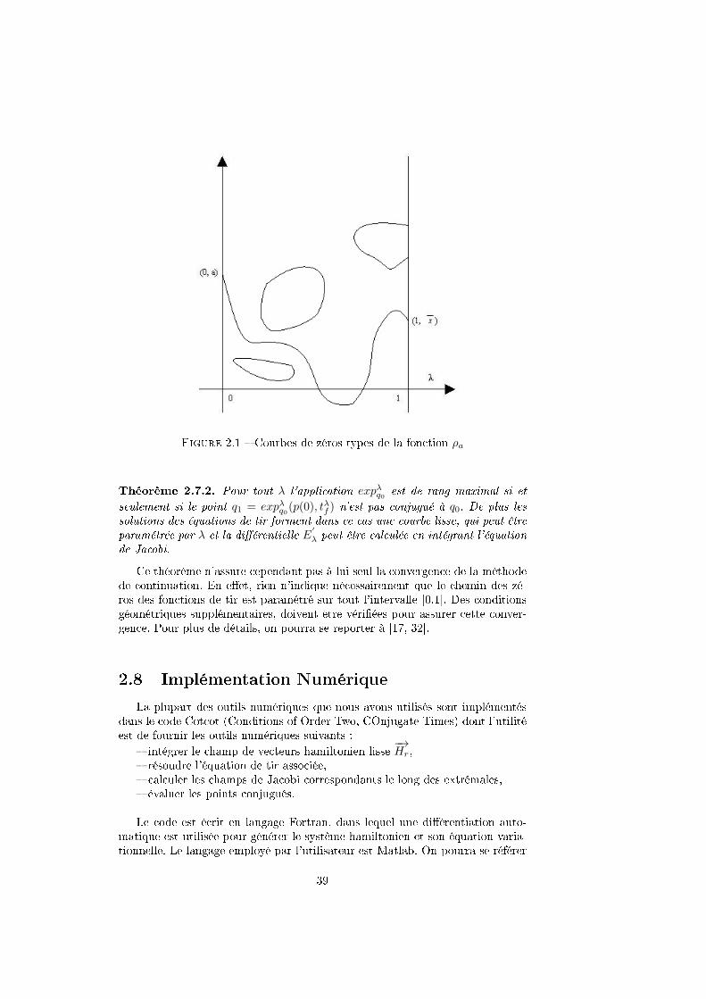
Figure 2.1 Courbes de zéros types de la fonction ρa

Théorème 2.7.2. Pour tout λ l'application expλq0 est de rang maximal si et

seulement si le point q1 = expλq0(p(0), tλf ) n'est pas conjugué à q0. De plus les

solutions des équations de tir forment dans ce cas une courbe lisse, qui peut êtreparamétrée par λ et la diérentielle E

′

λ peut être calculée en intégrant l'équationde Jacobi.

Ce théorème n'assure cependant pas à lui seul la convergence de la méthodede continuation. En eet, rien n'indique nécessairement que le chemin des zé-ros des fonctions de tir est paramétré sur tout l'intervalle [0,1]. Des conditionsgéométriques supplémentaires, doivent être vériées pour assurer cette conver-gence. Pour plus de détails, on pourra se reporter à [17, 32].

2.8 Implémentation Numérique

La plupart des outils numériques que nous avons utilisés sont implémentésdans le code Cotcot (Conditions of Order Two, COnjugate Times) dont l'utilitéest de fournir les outils numériques suivants :

intégrer le champ de vecteurs hamiltonien lisse−→Hr,

résoudre l'équation de tir associée, calculer les champs de Jacobi correspondants le long des extrémales, évaluer les points conjugués.

Le code est écrit en langage Fortran, dans lequel une diérentiation auto-matique est utilisée pour générer le système hamiltonien et son équation varia-tionnelle. Le langage employé par l'utilisateur est Matlab. On pourra se référer

39

à [6] pour une description précise du code qui s'appuie sur des algorithmes d'in-tégration d'équations diérentielles ordinaires et de résolution de la méthode deNewton. Le test des points conjugués consiste à vérier une condition de rangqui se base sur l'évaluation des zéros d'un déterminant ou une SVD ( SingularValue Decomposition). La méthode de continuation a été implémentée parallèle-ment en tant que simple discrétisation du chemin de l'homotopie où la méthodede Newton est employée à chaque pas. Une alternative à cette implémentationpeut consister en une continuation numérique du chemin, utilisant les équationsdiérentielles ordinaires implicites, où la méthode de Newton est utilisée aupremier pas pour initialiser la continuation et au dernier pas pour résoudre lafonction de tir nale avec une précision arbitraire.

Le chapitre suivant propose un résumé de l'ensemble des travaux eectuésau cours de cette thèse, lesquels sont détaillés dans les trois articles gurantdans ce manuscrit. On y décrit l'application des méthodes géométriques et nu-mériques de contrôle optimal présentées précédemment au problème de calculde trajectoires à poussée faible dans le modèle des trois corps restreint. L'enjeude nos recherches a principalement consisté en la détermination d'initialisationsecaces des méthodes de tir utilisées pour générer numériquement un large en-semble de trajectoires temps-minimales et énergie-minimales dans le systèmeTerre-Lune.

40

Chapitre 3

Contribution scientique

3.1 Transferts Terre-Lune à temps minimal et éner-

gie minimale

La première contribution de ce travail de thèse a été de calculer numéri-quement des transferts Terre-Lune à poussée faible dans le problème restreintdes 3 corps plan. De telles trajectoires sont solutions du système 1.26, lequel,en posant q = (q1, q2, q3, q4) = (x, y, x, y), peut être réécrit sous la forme dusystème contrôlé bi-entrée

q = F0(q) + F1(q)u1 + F2(q)u2, (3.1)

où F0, F1 et F2 sont les champs de vecteurs lisses de R4 donnés par

F0(q) =

q3q4

2q4 + q1 − (1− µ) q1+µ

((q1+µ)2+q22)32− µ q1−1+µ

((q1−1+µ)2+q22)32

−2q3 + q2 − (1− µ) q2

((q1+µ)2+q22)32− µ q2

((q1−1+µ)2+q22)32

,

F1(q) =

0010

, F2(q) =

0001

.

Les conditions initiales et nales des transferts doivent respectivement caracté-riser des orbites terrestres et lunaires. Par commodité, nous avons xé l'orbitegéostationnaire comme orbite initiale et l'orbite circulaire centrée sur la Lunecomme orbite cible. Nous avons alors déterminé des transferts à poussée faible enconsidérant les problèmes de minimisation du coût énergétique d'une trajectoire

minu(.)∈R2

∫ tf

t0

u21 + u22dt,

lorsque le temps de transfert tf est xé, et de minimisation du temps de transfert

minu(.)∈BR2 (0,ε)

∫ tf

t0

dt

41

où la borne ε imposée sur la norme du contrôle est choisie susament petite.La masse réduite µ dans le système Terre-Lune est égale 1.2153e − 2. En réfé-rence aux données pratiques de la mission spatiale Smart-1 [57, 58], nous avonsconsidéré un satellite de 350 kg et xé le seuil de poussée faible à 7.3e − 2N.Nos résultats sont présentés en détails dans les articles Geometric and nume-rical techniques in optimal orbital transfer using low propulsion [10], en com-plément de travaux géométriques de Bernard Bonnard et Jean-Baptiste Caillausur le problème de minimisation énergétique et Shooting and numerical conti-nuation methods for computing time-minimal and energy-minimal trajectoriesin the Earth-Moon system using low propulsion [51]. La méthode générale quenous avons employée pour calculer les diérentes trajectoires optimales peutêtre résumée de la manière suivante. En vertu du principe du maximum gé-néral de Pontryagin, les trajectoires optimales sont nécessairement des courbesextrémales solutions d'un certain système hamiltonien sur le bré cotangentde l'espace des phases. En intégrant numériquement ce système hamiltonien,on peut calculer les trajectoires extrémales dépendant de conditions initialesdonnées. En xant une condition initiale dans l'espace des phases, l'objectifest de déterminer les vecteurs adjoints initiaux tels que les extrémales corres-pondantes satisfassent à la fois des conditions nales imposées, en l'occurrenceappartiennent à l'orbite circulaire autour de la Lune, et les conditions de trans-versalité du principe du maximum. On utilise pour cela la méthode de tir simplebasée sur l'algorithme de Newton, qui requiert pour être ecace une initialisa-tion précise. Cette initialisation est une étape délicate lorsqu'il s'agit de calculerdes transferts à propulsion faible. En eet, plus le contrôle qu'on opère sur la dy-namique est petit, plus le temps de transfert est long et l'intégration numériqueimprécise, ce qui complique la convergence de l'algorithme de Newton. Pourpallier à cette diculté, on utilise une méthode de continuation qui permet derésoudre la question de l'initialisation grâce à un algorithme homotopique. Onpratique ainsi une continuation sur la poussée maximale autorisée dans le cas dela minimisation du temps de transfert. A poussée forte, le temps de transfert dela Terre à la Lune est court ce qui facilite l'initialisation et fournit un point dedépart à la méthode d'homotopie. Pour le problème de minimisation de l'éner-gie, on utilise une continuation sur la masse réduite µ de manière à relier leproblème intégrable des 2 corps et celui des 3 corps restreint. Dans les deux cas,on calcule tout d'abord des extrémales joignant l'orbite terrestre et le point L1.On simplie ainsi les conditions nales imposées, de sorte que la convergence del'algorithme de Newton soit favorisée. En outre, on fournit une collection d'or-bites pouvant être comparées aux premières parties des trajectoires Terre-Lunean d'évaluer le rôle du voisinage de L1 dans la minimisation des deux coûts, voirles gures 3.1 et 3.2. Mentionnons également les calculs d'extrémales Terre-L4 àtemps minimal, qui ont été menés pour juger des similitudes topologiques entreles orbites reliant le domaine intérieur et diérents points d'équilibre. L'optima-lité locale des trajectoires extrémales générées numériquement est déduite desconditions susantes du second ordre. La vérication de ces conditions est enoutre nécessaire pour la bonne convergence des méthodes de continuation.Nousproposons enn une vérication numérique du théorème 2.4.2, en comparant lestemps t1c et t1cc d'une extrémale anormale temps-minimale entre la Terre et lepoint L1.

La pertinence de nos résultats est en partie estimée en comparant les carac-

42

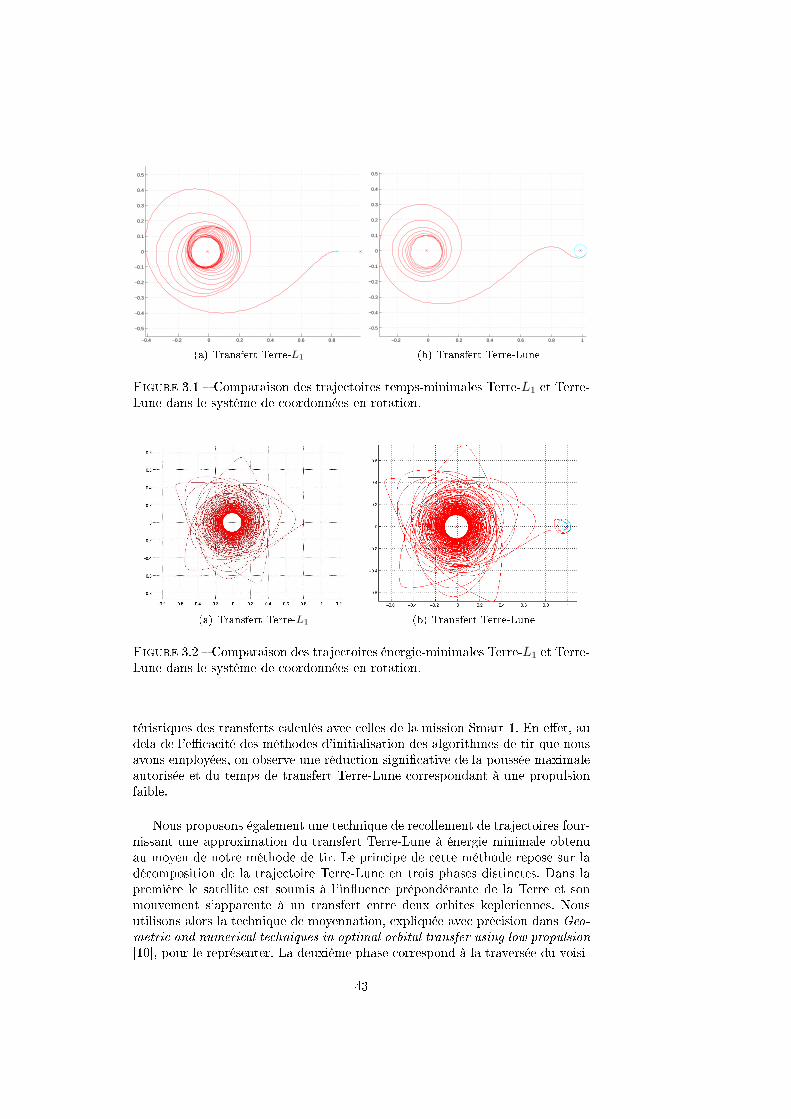
−0.4 −0.2 0 0.2 0.4 0.6 0.8

−0.5

−0.4

−0.3

−0.2

−0.1

0

0.1

0.2

0.3

0.4

0.5

(a) Transfert Terre-L1

−0.2 0 0.2 0.4 0.6 0.8 1

−0.5

−0.4

−0.3

−0.2

−0.1

0

0.1

0.2

0.3

0.4

0.5

(b) Transfert Terre-Lune

Figure 3.1 Comparaison des trajectoires temps-minimales Terre-L1 et Terre-Lune dans le système de coordonnées en rotation.

(a) Transfert Terre-L1 (b) Transfert Terre-Lune

Figure 3.2 Comparaison des trajectoires énergie-minimales Terre-L1 et Terre-Lune dans le système de coordonnées en rotation.

téristiques des transferts calculés avec celles de la mission Smart-1. En eet, audela de l'ecacité des méthodes d'initialisation des algorithmes de tir que nousavons employées, on observe une réduction signicative de la poussée maximaleautorisée et du temps de transfert Terre-Lune correspondant à une propulsionfaible.

Nous proposons également une technique de recollement de trajectoires four-nissant une approximation du transfert Terre-Lune à énergie minimale obtenuau moyen de notre méthode de tir. Le principe de cette méthode repose sur ladécomposition de la trajectoire Terre-Lune en trois phases distinctes. Dans lapremière le satellite est soumis à l'inuence prépondérante de la Terre et sonmouvement s'apparente à un transfert entre deux orbites kepleriennes. Nousutilisons alors la technique de moyennation, expliquée avec précision dans Geo-metric and numerical techniques in optimal orbital transfer using low propulsion[10], pour le représenter. La deuxième phase correspond à la traversée du voisi-

43

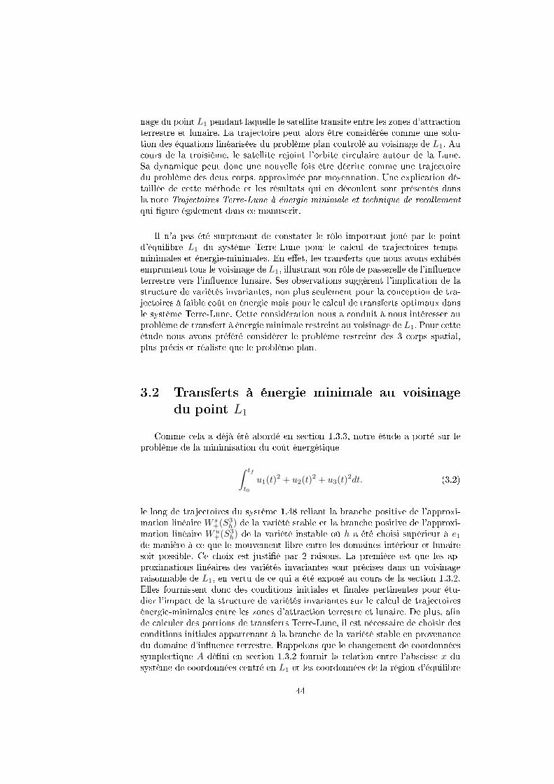
nage du point L1 pendant laquelle le satellite transite entre les zones d'attractionterrestre et lunaire. La trajectoire peut alors être considérée comme une solu-tion des équations linéarisées du problème plan controlé au voisinage de L1. Aucours de la troisième, le satellite rejoint l'orbite circulaire autour de la Lune.Sa dynamique peut donc une nouvelle fois être décrite comme une trajectoiredu problème des deux corps, approximée par moyennation. Une explication dé-taillée de cette méthode et les résultats qui en découlent sont présentés dansla note Trajectoires Terre-Lune à énergie minimale et technique de recollementqui gure également dans ce manuscrit.

Il n'a pas été surprenant de constater le rôle important joué par le pointd'équilibre L1 du système Terre-Lune pour le calcul de trajectoires temps-minimales et énergie-minimales. En eet, les transferts que nous avons exhibésempruntent tous le voisinage de L1, illustrant son rôle de passerelle de l'inuenceterrestre vers l'inuence lunaire. Ses observations suggèrent l'implication de lastructure de variétés invariantes, non plus seulement pour la conception de tra-jectoires à faible coût en énergie mais pour le calcul de transferts optimaux dansle système Terre-Lune. Cette considération nous a conduit à nous intéresser auproblème de transfert à énergie minimale restreint au voisinage de L1. Pour cetteétude nous avons préféré considérer le problème restreint des 3 corps spatial,plus précis et réaliste que le problème plan.

3.2 Transferts à énergie minimale au voisinage

du point L1

Comme cela a déjà été abordé en section 1.3.3, notre étude a porté sur leproblème de la minimisation du coût énergétique

∫ tf

t0

u1(t)2 + u2(t)

2 + u3(t)2dt. (3.2)

le long de trajectoires du système 1.48 reliant la branche positive de l'approxi-mation linéaire W s

+(S3h) de la variété stable et la branche positive de l'approxi-

mation linéaire Wu+(S

3h) de la variété instable où h a été choisi supérieur à e1

de manière à ce que le mouvement libre entre les domaines intérieur et lunairesoit possible. Ce choix est justié par 2 raisons. La première est que les ap-proximations linéaires des variétés invariantes sont précises dans un voisinageraisonnable de L1, en vertu de ce qui a été exposé au cours de la section 1.3.2.Elles fournissent donc des conditions initiales et nales pertinentes pour étu-dier l'impact de la structure de variétés invariantes sur le calcul de trajectoiresénergie-minimales entre les zones d'attraction terrestre et lunaire. De plus, ande calculer des portions de transferts Terre-Lune, il est nécessaire de choisir desconditions initiales appartenant à la branche de la variété stable en provenancedu domaine d'inuence terrestre. Rappelons que le changement de coordonnéessymplectique A déni en section 1.3.2 fournit la relation entre l'abscisse x dusystème de coordonnées centré en L1 et les coordonnées de la région d'équilibre

44

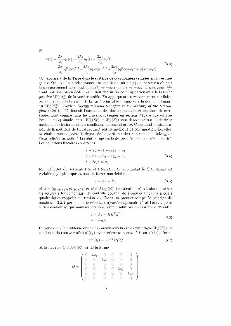
R

x(t) =2λ1s1

q1(t)−2λ1s1

p1(t) +2ω1

s2p2(t)

=2λ1s1

q01 expλ1t −2λ1

s1p01 exp

−λ1t +2ω1

s2(q02 cosω1t+ p02 sinω1t).

(3.3)

Or l'abcisse x de la Terre dans le système de coordonnées centrées en L1 est né-gative. On doit donc sélectionner une condition initiale p01 de manière à obtenirle comportement asymptotique x(t) → −∞ quand t → −∞. La constante 2λ1

s1étant positive, on en déduit qu'il faut choisir un point appartenant à la branchepositive W s

+(S3h) de la variété stable. En appliquant un raisonnement similaire,

on montre que la branche de la variété instable dirigée vers le domaine lunaireest Wu

+(S3h). L'article Energy-minimal transfers in the vicinity of the Lagran-

gian point L1 [52] fournit l'ensemble des développements et résultats de cetteétude. Tout comme dans les travaux présentés en section 3.1, des trajectoireslocalement optimales entre W s

+(S3h) et W

u+(S

3h) sont déterminées à l'aide de la

méthode de tir simple et des conditions du second ordre. Cependant, l'initialisa-tion de la méthode de tir ne requiert pas de méthode de continuation. En eet,on choisit comme point de départ de l'algorithme de tir la valeur initiale η∗0 del'état adjoint associée à la solution optimale du problème de contrôle linéarisé.Les équations linéaires contrôlées

x− 2y − (1 + c2)x = u1

y + 2x+ (c2 − 1)y = u2

z + 2c2z = u3

(3.4)

sont déduites du système 1.36 et s'écrivent, en appliquant le changement devariables symplectique A, sous la forme matricielle

z = Az +Bu (3.5)

où z = (q1, q2, q3, p1, p2, p3) et B ∈ M6,3(R). Le calcul de η∗0 est alors basé surles résultats fondamentaux de contrôle optimal de systèmes linéaires à coûtsquadratiques rappelés en section 2.2. Dans un premier temps, le principe dumaximum 2.2.2 permet de décrire la trajectoire optimale z∗ et l'état adjointcorrespondant η∗ que nous recherchons comme solutions du système diérentiel

z = Az +BBT ηT

η = −ηA.(3.6)

Puisque dans le problème que nous considérons la cible cylindrique Wu+(S

3h), la

condition de transversalité η∗(tf ) est intérieur et normal à G en z∗(tf ) s'écrit

η∗T (tf) = −z∗T (tf)Q (3.7)

où la matrice Q ∈ M6(R) est de la forme

Q =

0 kω1 0 0 0 00 0 kω2 0 0 00 0 0 0 0 00 0 0 0 kω1 00 0 0 0 0 kω2

0 0 0 0 0 0

45

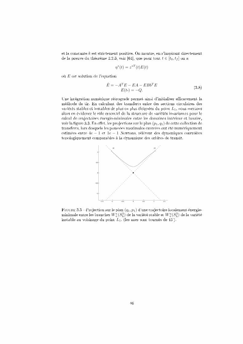
et la constante k est strictement positive. On montre, en s'inspirant directementde la preuve du théorème 2.2.3, voir [61], que pour tout t ∈ [t0, tf ] on a

η∗(t) = z∗T (t)E(t)

où E est solution de l'equation

E = −ATE − EA− EBbTEE(tf) = −Q. (3.8)

Une intégration numérique rétrograde permet ainsi d'initialiser ecacement laméthode de tir. En calculant des transferts entre des sections circulaires desvariétés stables et instables de plus en plus éloignées du point L1, nous mettonsalors en évidence le rôle essentiel de la structure de variétés invariantes pour lecalcul de trajectoires énergie-minimales entre les domaines intérieur et lunaire,voir la gure 3.3. En eet, les projections sur le plan (p1, q1) de cette collection detransferts, lors desquels les poussées maximales exercées ont été numériquementestimées entre 4e − 1 et 1e − 1 Newtons, rélèvent des dynamiques contrôléestopologiquement comparables à la dynamique des orbites de transit.

−1.5 −1 −0.5 0 0.5 1 1.5

−1

−0.5

0

0.5

1

p1q1

Figure 3.3 Projection sur le plan (q1, p1) d'une trajectoire localement énergie-minimale entre les branchesW s

+(S3h) de la variété stable etW

u+(S

3h) de la variété

instable au voisinage du point L1. (les axes sont tournés de 45).

46

Geometric and numerical

techniques in optimal control

of two and three-body problems

B. Bonnard,∗ J.-B. Caillau† and G. Picot‡

Dedicated to John Baillieul on the occasion of his 65th birthday

Abstract. The objective of this article is to present geometric and numeri-cal techniques developed to study the orbit transfer between Keplerian ellipticorbits in the two-body problem or between quasi-Keplerian orbits in the Earth-Moon transfer when low propulsion is used. We concentrate our study on theenergy minimization problem. From Pontryagin's maximum principle, the opti-mal solution can be found solving the shooting equation for smooth Hamiltoniandynamics. A rst step in the analysis is to nd in the Kepler case an analyti-cal solution for the averaged Hamiltonian, which corresponds to a Riemannianmetric. This will allow to compute the solution for the original Kepler problem,using a numerical continuation method where the smoothness of the path is re-lated to the conjugate point condition. Similarly, the solution of the Earth-Moontransfer is computed using geometric and numerical continuation techniques.

1 Introduction

In this article we consider the orbit transfer in the two and three-body problem,using low propulsion. In the rst case, the model is given by Kepler equation

q = − q

|q|3+u

m

where m represents the mass of the satellite, subject to

m = −δ|u|

modelling fuel consumption. The control satises the constraint |u| ≤ ε whereε is a small parameter.

The physical optimal control has to maximize the nal mass which leads to

minu(.)

∫ tf

0

|u|dt

∗Mathematics Institute, Bourgogne University & CNRS, 9 avenue Savary, F-21078 Dijon(bernard.bonnard@u-bourgogne.fr).

†Same address (jean-baptiste.caillau@u-bourgogne.fr), supported by Conseil Régionalde Bourgogne (contract no. 2009-160E-160-CE-160T).

‡Same address (gautier.picot@u-bourgogne.fr), supported by CNRS (contractno. 37244) and Conseil Régional de Bourgogne (contract no. 079201PP02454515).

47

where tf is the xed transfer time. From Pontryagin maximum principle [28],xing the boundary conditionse.g. a transfer from a low eccentric to a geo-stationary orbit, an optimal solution can be numerically computed using ashooting algorithm. This leads to a complicated numerical problem. In [20],the following numerical scheme is proposed. One computes the optimal solutionusing the convex homotopy

minu(.)

∫ tf

0

[λ|u|2 + (1− λ)|u|]dt, λ ∈ [0, 1],

which amounts to regularizing the L1-minimization problem into an L2-problem.This was the starting point of the use of continuation methods in orbital transfer,when low propulsion is appliedsee also [14] for the use of the continuationmethod in the time minimal control problem, where the homotopy parameteris the bound of the maximal amplitude of the thrust. From the mathematicalpoint of view, the original dynamics associated with the optimal ow is replacedby another Hamiltonian one, and a continuation is made to solve the shootingequation.

The rst motivation of this article is to present a neat geometric resultfrom [8]: Neglecting the mass variation, restricting to coplanar transfer (theinclination being considered as a homotopy parameter) and replacing the L1-problem by an averaged L2-problem, one can substitute the Hamiltonian vectoreld dened by the maximum principle with

H =1

2n5/3

[9n2p2n +

5

2(1− e2)p2e +

5− 4e2

2

p2θe2

],

where n is the mean motion, e the eccentricity, and θ the angle of the pericenter(the singularity e = 0 corresponds to circular orbits). Coordinates (n, e, θ) aremoreover orthogonal coordinates for the Riemannian metric associated with H,

g =dn2

9n13

+2n

53

5(1− e2)de2 +

2n53

5− 4e2dθ2.

Such a metric is isometric to

g = dr2 +r2

c2(dϕ2 +G(ϕ)dθ2)

where

r =2

5n5/6, ϕ = arcsin e

and

c =√2/5, G(ϕ) =

5 sin2(ϕ)

1 + 4 cos2(ϕ)·

The Hamiltonian ow−→H is Liouville integrable and the metric in the above nor-

mal form captures the main properties of the averaged orbital transfer. Indeed,one can extract from g the following two-dimensional Riemannian metrics:

g1 = dr2 + r2dψ2 which is associated with the orbital transfer where θ iskept xed (this encompasses the case of circular targets). Such a metricis at and geodesics are straight lines in suitable coordinates.

48

g2 = dϕ2 + G(ϕ)dθ2 which represents the restriction of the metric tor2 = c2 and describes by homogeneity the orbit transfer in the generalcase.

A generalization of the results of [31] will allow to compute for the metric g2 theconjugate and cut loci and to get a global optimality solution for the averagedoptimal control problem. This is the starting point to analyze the originaloptimal control problem using a continuation method.

A second motivation of this article is to present some results from geometriccontrol theory connected to our analysis with adapted numerical codes devel-oped to compute the solutions. First of all, the maximum principle is onlya necessary optimality condition. In order to get sucient optimality con-ditions under generic assumptions one must dene the concept of conjugatepoint, associated with the energy minimization problem. This concept was al-ready introduced in the standard litterature of calculus of variations [5]. If theHamiltonian optimal dynamics is described by a smooth Hamiltonian vector

eld−→H , conjugate points are the image of the singularities of the exponential

mapping: expx(0) : p(0) −→ Πx exp tf−→H (x(0), p(0)) where Πx : (x, p) −→ x is

the canonical projection. Such points can be numerically computed using thecode [12]. An important remark, in view of the use of the (smooth) continuationmethod in optimal control is to observe that the shooting equation is preciselyto nd p(0) such that expx(0)(p(0)) = x1 where x1 is the terminal condition and

the derivative is generated using the variational equation of−→H . This will lead

to convergence results for the smooth continuation method in optimal control,related to estimates of conjugate points.

The last section is devoted to the Earth-Moon transfer, using low propulsion.The model is the standard circular restricted model [25] where the two primariesare xed in a rotating frame. Up to a normalization the system can be writtenin Hamiltonian form,

x =−→H0(x) + u1

−→H1(x) + u2

−→H2(x)

where x = (q, p) ∈ R4 and the drift−→H0 is given by

H0(x) =1

2(p21 + p22) + p1q2 − p2q1 −

1− µ

ρ1− µ

ρ2,

q being the position of the spacecraft, ρ1 representing the distance to the Earthwith mass 1−µ located at (−µ, 0), and ρ2 the distance to the Moon with mass µlocated at (1−µ, 0), µ ' 1.2153e−2 being a small parameter. The Hamiltonianelds associated with the control are given by

Hi(x) = −qi, i = 1, 2,

and the control bound is |u| ≤ ε. The parameter µ is small and this remarkwas used by Poincaré to study the dynamics of the free motion described by−→H0 by making a deformation of the case µ = 0 which corresponds to Keplerequation in rotating coordinates [25]. Inspired by this approach and using ourpreliminary geometric analysis, we propose a simple solution to the Earth-Moontransfer using low propulsion for the energy minimization problem.

49

2 Geometric and numerical methods

2.1 Maximum principle

We consider the energy minimization problem minu(.)∫ tf0

|u|2dt, for a smoothcontrol system of the form

x = F0(x(t)) +m∑i=1

ui(t)Fi(x(t)) = F (x(t), u(t)), x ∈ X.

The set of admissible controls is the subset U of measurable bounded mappingsu(.) with corresponding trajectory x(.) dened on the whole interval [0, tf ].Pontryagin maximum principle [28] tells us that

Proposition 2.1. If (x, u) is an optimal pair on [0, tf ], there exists a non trivialpair (p0, p), p0 ≤ 0 and p an absolutely continuous adjoint vector valued in T ∗X,such that on [0, tf ] we have

x =∂H

∂p(x, p, u), p = −∂H

∂x(x, p, u), (1)

andH(x, p, u) = max

v∈RmH(x, p, v) (2)

where H(x, p, u) = p0∑m

i=1 u2i+ < p, F (x, u) >.

Denition 2.1. The mapping H from T ∗X ×Rm to R is called the pseudo-Hamiltonian. A triple (x, p, u) solution of (1-2) is called an extremal trajectory.

2.2 Computation of extremals

From the maximization condition (4), one deduces that ∂H/∂v = 0, and thereare two types of extremals:

Abnormal extremals. They correspond to the situation p0 = 0 and areimplicitely dened by the relations Hi = 0, i = 1, . . . ,m, where Hi =<p, Fi(x) > are the Hamiltonian lifts.

Normal extremals. If p0 < 0, it can be normalized to−1/2 by homogeneity.From ∂H/∂v = 0, one deduces ui = Hi for i = 1, . . . ,m, and pluggingsuch Hi into H denes a true smooth Hamiltonian

Hn = H0 +1

2

m∑i=1

H2i

whose solutions are the normal extremals.

2.3 The concept of conjugate point

Denition 2.2. Let z = (x, p) be a normal reference extremal dened on [0, tf ].The variational equation

δz(t) = d−→Hn(z(t))δz(t)

50

is called the Jacobi equation. A Jacobi eld is a non-trivial solution δz =(δx, δp). It is said to be vertical at time t if δx(t) = dΠx(z(t))δz(t) = 0 whereΠx is the projection (x, p) 7→ x.

The following standard geometric result is crucial.

Proposition 2.2. Let L0 be the ber T ∗x0X and Lt = expt(

−→Hn)(L0) be its

image by the one-parameter subgroup generated by−→Hn. Then Lt is a Lagrangian

submanifold whose tangent space at z(t) is generated by the Jacobi elds whichare vertical at t = 0.

Denition 2.3. We x x0 = x(0) and dene for t ∈ [0, tf ] the exponentialmapping

expx0,t(p0) = Πx(z(t, z0))

where z(t, z0), with z0 = (x0, p0), denotes the normal extremal departing fromz0 when t = 0.

Denition 2.4. Let z = (x, p) be the reference normal extremal. The timetc ∈ [0, tf ] is called conjugate if the mapping expx0,tc is not an immersion atp(0). The associated point x(tc) is said to be conjugate to x0. We denote byt1,c the rst conjugate point and by C(x0) the conjugate locus formed by theset of rst conjugate points occuring at time tf when we consider all normalextremals starting from x0.

The conjugate time notion admits the following generalization.

Denition 2.5. Let M1 be a regular submanifold of M , and let us deneM⊥

1 = (x, p) ∈ T ∗M | x ∈M1, p ⊥ TxM1. Then tfoc ∈ [0, tf ] is called a focaltime if there exists a Jacobi eld J = (δx, δp) such that δx(0) = 0 and J(tfoc)is tangent to M⊥

1 .

Remark 2.1. The concept of conjugate point is related to the necessary andsucient optimality conditions, under generic assumptions, see for instance [12].

2.4 Conjugate points and smooth continuation method

Smooth continuation is a general numerical method to solve a system of equa-tions F (x) = 0 where F : Rn −→ Rn is a smooth mapping, see [1]. Theprinciple is to construct a homotopy path h(x, λ) such that h(x, 0) = G(x) andh(x, 1) = F (x) where G(x) is a map having known zeros, or where the zeroscan be easily computed using a Newton type algorithm. The zeros along thepath can be calculated by dierent methods, the simplest being a discretization0 = λ0 < λ1 < · · · < λn = 1 of the homotopy parameter where, at step i+1, thezero computed at step i is used to initialize Newton algorithm. The approachhas to be adapted to optimal control problems: The shooting equation comesfrom the projection of a symplectic mapping, the Jacobian can be computedusing Jacobi elds and one must consider the central extremal elds associatedwith the problem (see [13]). A short description of the method is given belowin our case study.

51

2.4.1 Shooting equation

We consider a family Hλ, λ ∈ [0, 1], of smooth Hamiltonians on T ∗X associatedwith normal extremals of an energy minimization problem. We x the boundaryconditions x0, x1 and the transfer time tf . This leads to a family expλx0,tf

(p0) of

exponential mappings. Using the notation Eλ : p0 −→ expλx0,tf(p0), one must

solve the shooting equation Eλ(p0) = x1.

Proposition 2.3. For each λ, the shooting equation is of maximal rank if andonly if the point x1 is not conjugate to x0 for the corresponding λ. Moreover, inthis case, the solutions of the shooting equation contain a smooth branch, whichcan be parameterized by λ and the derivative E′λ can be generated integratingthe Jacobi equation.

From the above proposition, to ensure convergence of the method one mustcontrol

the distance to the conjugate loci,

that the branch has is dened on the whole interval [0, 1].

The second point is related to two standard problems in optimal control: Ex-istence of Lipschitzian minimizershence solutions of the maximum principle[22], and compactness of the domain of the exponential mapping. Next wepresent a nice geometric situation for which convergence of the method is en-sured.

Denition 2.6. Consider the normal extremal eld−→Hn of an energy mini-

mization problem with xed nal time tf . Given an initial condition x0, theseparating locus L(x0) is the set of points where two distinct normal extremalcurves intersect with same cost. The cut point along a normal extremal is therst point where it ceases to be optimal. The cut locus Cut(x0) is the set of suchpoints when we consider all extremals initiating from x0 and losing optimalityexactly at time tf .

2.4.2 Convergence of the continuation method in the Riemannian

case

We rst recall that the Riemannian problem can be, at least locally, reset in thefollowing framework.

Let F1, . . . , Fn be a set of smooth vector elds on a manifold X and assumethat they are linearly independent. One can dene a Riemannian metric onX by asserting that F1, . . . , Fn form an orthonormal frame. Introducing thecontrol system dx(t)/dt =

∑ni=1 ui(t)Fi(x(t)), the length of the curve x(·) is

l(x) =∫ T

0

∑ni=1(u

2i (t))

1/2dt. From Maupertuis principle, minimizing length is

equivalent to minimizing the energy∫ T

0

∑ni=1 u

2i (t)dt. There exists only normal

extremals and Hn is given by (1/2)∑n

i=1H2i . Fixing the level set Hn = 1/2

parameterizes trajectories by arc length. For the energy minimization problem,the transfer time can be arbitrarily prescribed.

Theorem 2.1. Let gλ, λ ∈ [0, 1], be a smooth family of complete Riemannianmetrics on X. Let us x the initial point x0. Denote iλ(x0) the distance fromx0 to the cut locus Cutλ(x0) and by iλ = infx0 iλ(x0) the injectivity radius ofthe corresponding metric. Then,

52

for length shorter than infλ iλ(x0), the continuation method with initialcondition of the shooting equation at x0 converges,

for length shorter than infλ iλ the continuation method converges for everyinitial condition of the shooting equation.

Remark 2.2. In the Riemannian case, the situation is neat. Completeness leadsto existence of smooth normal minimizers, the domain of the exponential map-ping is a sphere, and estimates of the injectivity radius are related to the curva-ture tensor. In general, such estimates are a dicult problem and a pragmaticpoint of view is to have numerical approximations [12].

3 The energy minimization problem in orbital

transfer with low thrust

3.1 Preliminaries

Neglecting the mass variation and restricting to the coplanar case, the systemis represented in Cartesian coordinates by

q = − q

|q|3+ u

where q = (q1, q2) is the position and x = (q, q) ∈ R4 is the state. We denoteby H0(q, q) = (1/2)q2 − 1/|q| the Hamiltonian of the free motion. We have thefollowing rst integrals:

C = q ∧ q (momentum),

L = −q/|q|+ q ∧ C (Laplace integral).

Proposition 3.1. The domain Σe = (q, q) | H < 0, C 6= 0, called the ellipticdomain, is lled by elliptic orbits and to each orbit (C,L) corresponds a unique(oriented) ellipse.

To represent the space of ellipses, one introduces the following geometriccoordinates:

the semi-major axis of the ellipse a, related to the semi-latus rectum Pby the relation a = P/

√1− e2,

the argument of the pericenter θ,

the eccentricity e, the eccentricity vector being (ex, ey) = (e cos θ, e sin θ).

To represent the position of the satellite we use the longitude l ∈ S1, while l ∈ Rtakes into account the rotation number and is called the cumulated longitude.Observe that e = 0 corresponds to circular orbits. The control u can be de-composed into moving frames attached to the satellite, the two standard framesbeing

the radial-orthoradial frame Fr, For where Fr = (q/|q|) ∂/∂q,

the tangential-normal frame Ft, Fn where Ft = (q/|q|) ∂/∂q.

53

3.2 Averaging of periodic sub-Riemannian problems

Let X be an n-dimensional smooth manifold and let Fi(l, x), i = 1, . . . ,m besmooth vector elds parameterized by l ∈ S1 that set up a constant rank mdistribution on X (see also Remark 3.2). Given a positive pulsation ω on S1×Xrelating the time t and the angle l according to

dl = ω(l, x)dt, (3)

one denes a periodic sub-Riemannian problem as follows: Given two pointsx0 and xf on the manifold, minimize the L2dt control norm of trajectoriesconnecting the two points and associated with the previous vector elds,

dx

dl=

m∑i=1

uiFi(l, x), u ∈ Rm,

minu(.)

∫ tf

0

|u|2dt =∫ lf

0

|u|2 dl

ω(l, x)(here |u|2 =

m∑i=1

|ui|2).

The total angular length, lf > 0 is xed, implicitly dening tf through (3).Pontryagin maximum principle asserts that minimizing trajectories are pro-

jection of Hamiltonian curves on the cotangent bundle (extremals), z = (x, p),such that

dx

dl=∂H

∂p(l, x, p, u),

dp

dl= −∂H

∂x(l, x, p, u),

where

H(l, x, p, u) = p0|u|2 +m∑i=1

uiHi(l, x, p), Hi = 〈p, Fi(l, x)〉, i = 1, . . . ,m,

is the Hamiltonian parameterized by l ∈ S1, u ∈ Rm, and a non-positive con-stant p0. We restrict the analysis to the normal case, p0 < 0, and pass to anecoordinates in (p0, p) setting p0 = −1/2. Pontryagin maximization conditionthat, almost everywhere along an extremal,

H(l, z(l), u(l)) = maxv∈Rm

H(l, z(l), v),

implies that the control is given by the dynamic feedback

u(l, z) = ω(l, x)(H1, . . . , Hm)(l, z), (4)

and that z is an integral curve of the maximized Hamiltonian

Hn(l, z) =ω(l, x)

2

m∑i=1

H2i (l, z).

We are interested in the behaviour of solutions for large angular length, so we setε = 1/lf as the small parameter and renormalize the problem in the followingmannertypical of systems with two time scales.

In contrast to l which is the fast time, dene the slow time s = εl in [0, 1],and renormalize variables on the cotangent bundle by

x = x, p = p/ε.

54

Lemma 3.1. In the renormalized variables,

dz

ds=

−→Hn(s/ε, z). (5)

Proof. Obvious since Hn(l, x, ·) is quadratic in the adjoint state p.

For xed z, Hn(·, z) is a smooth function on S1 and can be expanded intoits Fourier series. In particular, one can dene its rst coecient or average,

H(z) =1

2π

∫ 2π

0

Hn(l, z) dl.

Since taking symplectic vector eld and averaging readily commute, it is wellknown [2, 21] that H trajectories are good approximations of those of Hn as εgoes to zero.

Theorem 3.1. Given any initial condition, the solution zε of (5) convergesuniformly on [0, 1] towards the solution z of the averaged Hamiltonian.

Remark 3.1. The same rate of convergence holds for the cost which can beadded as a new state in the augmented system. But as the integrand dependson the fast variable l through the pulsation ω, there is a priori no higher orderapproximation of the performance index [4, 16].

As for Hn(s/ε, z) which converges to H in the large space of Schwartz distri-butions,1 one can only expect weak convergence on the control uε of the originalproblem on [0, 1/ε]. We address two questions: rst, can we describe the fastoscillating control by means of Fourier series with slowly varying coecientsand, secondly, what is the asymptotic behaviour of ‖uε‖∞ when ε → 0? Theimportance of such an estimate relies on the fact that one has in practice toestimate lf so as to meet a given requirement on the L∞-norm of the control.

We rst note that the average system provides a sub-Riemannian approxi-mation of the original one.

Proposition 3.2. The averaged Hamiltonian is a nonnegative quadratic formin the adjoint. If constant, its rank is not less than m, and H can locally bewritten as a sum of squares, thus dening a sub-Riemannian (Riemannian ifk = n) problem.

Proof. Clearly, H(x, ·) remains quadratic nonnegative in p by linearity and pos-itivity of the integral and

kerH(x, ·) =⋂l∈S1

kerHn(l, x, ·)

so that, if constant, the rank k is at least equal to m. In this case, the quadraticform can always be decomposed into a sum of k squares in a chart by takingthe square root of the associated symmetric nonnegative matrix.

Remark 3.2. (i) The increase in the rank is related to the generation of Liebrackets of the following system with drift: Set x = (l, x) and dene

F0(x) = ω(x)∂

∂l, Fi(x) = ω(x)Fi(x), i = 1, . . . ,m.

1Topological dual of the space of smooth compactly supported functions on the real line.

55

Th fast oscillations (with respect to l) of the control in

dx

dt= F0(x) +

m∑i=1

uiFi(x)

generate new directions, namely

(adjF0)Fi, j ≥ 0, i = 1, . . . ,m,

a natural requirement being that the distribution F0, F1, . . . , Fm on the aug-mented space S1 ×X be bracket generating. This is equivalent to the bracketcondition on S1 ×X for the distribution ∂/∂l, F1, . . . , Fm.(ii) The assumption of rank constancy is sucient to get a decomposition intoa smooth sum of squares [3]. That the assumption is crucial is illustrated bythe fact that it cannot be removed, even in the analytical category. Eigen-values (and associated projectors) are indeed analytic functions on the set ofmatrices in the neighbourhoud of a simple (hence diagonalizable) endomorphism[23, Theorem II.5.16]. Avoiding semi-simple eigenvalues is necessary as is clearconsidering [

x1 x2x2 −x1

]whose eigenvalues are not dierentiable at (0, 0). But even in the simple sym-metric nonnegative analytic case, existence of a dierentiable square root matrixmay fail as illustrated by [

x21 + x22 00 1

]. (6)

To get a positive result with non constant rank, one must actually restrict to thesymmetric nonnegative case with analytic dependence on one real variable only.Eigenvalues and eigenvectors are then analytic on the real line [Ibid., TheoremII.6.1 and II.6.2], and nonnegativeness ensures analyticity of square roots ofthe eigenvalues.(iii) In the case of periodic sub-Riemannian systems, the loss of regularity mayoriginate in averaging. The analytical distribution on S1 ×R2

F1(l, x) =√2(x1 cos l + x2 sin l)

∂

∂x1, F2(l, x) =

∂

∂x2

has quadratic form [2(x1 cos l + x2 sin l)

2 00 1

]whose averaged is (6) which does not even dene a dierentiable sub-Riemanniansystem on R2.(iv) A much stronger requirement is the existence of a change of coordinates onX (inducing a symplectic transformation on the cotangent) so that the averagedquadratic form be diagonal.

For a given z ∈ T ∗X, let

u(l, z) =∑k∈Z

ck(z)ek(l), ek(l) = eikl,

denote the Fourier series of the control (4). One has the following convergenceresult.

56

Proposition 3.3. For any positive ε, the normal optimal control is

uε(l) = ε∑k∈Z

ck zε(εl) ek(l)

and the series converges pointwisely. Moreover, for any k ∈ Z,

ck zε → ck z uniformly on [0, 1] as ε→ 0+

where the sub-Riemannian extremal z depends only on the boundary conditionsx0, xf on X.

Proof. For l ∈ [0, lf ],

uε(l) = u(l, xε(εl), εpε(εl))

= εu(l, xε(εl), pε(εl))

= ε∑k∈Z

ck(zε(εl)) ek(l)

thanks to the pointwise convergence of the Fourier series at l for z = zε(l). Forany k ∈ Z,

ck(z) =1

2π

∫ 2π

0

u(l, z)ek(l)dl

and the dependence on z is continuous since the integrand is bounded in acompact neighbourhood of the image of z.

Let us nally denote λ(l, x) the biggest (positive) eigenvalue of the nonneg-ative quadratic form in p

|u(l, x, p)|2 = ω2(l, x)m∑i=1

H2i (l, z) = 2ω(l, x)Hn(l, z),

and deneλ(x) = max

l∈S1λ(l, x).

As a supremum of continuous functions, x 7→ λ(x) is only lower semi-continousand we must assume the existence of a continous upper bound in the subsequentresult.

Proposition 3.4. Let σ be a continuous function such that σ2 dominates λ ina neighbourhood of x. Then

lim supε→0+

‖uε‖∞ε

≤ ‖σ x · |p|‖∞.

Proof. On [0, lf ], one has

|uε(l)|2 = ε2|u(l, zε(εl))|2

≤ ε2σ2 xε(εl) · |pε(εl)|2,

so the result holds since the square root of the right hand side converges uni-formly to σ x · |p| as ε goes to zero by continuity of σ.

57

3.3 Computations in Kepler case

Using the neat geometric coordinates of 3.1 on the three dimensional space ofellipses, we get

Hn(l, z) =ω(l, x)

2(H2

1 +H22 )(l, z), u(l, z) = ω(l, x)(H1, H2)(l, z),

|u(l, z)|2 = ω2(l, x)(H21 +H2

2 )(l, z), (7)

with

F1(l, x) =P 2

W 2

(sin l

∂

∂ex− cos l

∂

∂ey

),

F2(l, x) =P 2

W 2

(2P

W

∂

∂P

+(cos l +ex + cos l

W)∂

∂ex+ (sin l +

ey + sin l

W)∂

∂ey

),

and

ω(l, x) =W 2

P 3/2, W = 1 + ex cos l + ey sin l.

Introducing mean motion, n = a−3/2, and true anomaly, τ = l − θ, one gets

F1(l, x) =(1− e2)2

n4/3W 2

(−3ne sin τ

1− e2∂

∂n+ sin τ

∂

∂e− cos τ

1

e

∂

∂θ

), (8)

F2(l, x) =(1− e2)2

n4/3W 2

(− 3nW

1− e2∂

∂n+ (cos τ +

e+ cos τ

W)∂

∂e

+ (sin τ +sin τ

W)1

e

∂

∂θ

), (9)

withW = 1 + e cos τ.

As a result, the computation of Fourier series of Hn (or u) are performed withrespect to τ rather than l so, as θ only appears through τ ,

Hn(l, z) =∑k∈Z

ck(n, e, p)ek(l − θ) =∑k∈Z

ck(z)ek(l),

and coecients verifyck(z) = ck(n, e, p)ek(θ).

Proposition 3.5. The adjoint pθ is a linear rst integral of H.

Proof. According to the previous remark, θ is cyclic in the averaged Hamilto-nian.

The remarkable feature of the set (n, e, θ) of coordinates is the following[7, 18, 19].

Proposition 3.6. The averaged Hamiltonian is Riemannian and orthogonal in(n, e, θ) coordinates,

H(z) =1

2n5/3

[9n2p2n +

5

2(1− e2)p2e +

5− 4e2

2

p2θe2

].

58

Fourier coecients of the control are obviously obtained from (8-9), notingthat

Lemma 3.2. One has

e+ cos τ

W= −z − 2

√1− e2

e

∑k≥1

zk cos kτ,sin τ

W= −2

e

∑k≥1

zk sin kτ,

where z = −e/(1 +√1− e2) is the only pole in the open unit disk of W =

1 + e cos τ .

We nally provide a continuous upper bound of the eigenvalues of the qua-dratic form associated with the control norm, allowing us to estimate precisely‖uε‖∞ as ε→ 0+.

Proposition 3.7. Eigenvalues of the quadratic form (7) are uniformly domi-nated by

σ2(n, e) =4(1− e2)

n2/3

[(1 + e)2

n4/3+ 1

]+

e

n2/3

[e+

√1− e2

].

Proof. Since we have a rank two distribution (8-9) of vector elds (parameterizedby l ∈ S1) on the three-dimensional manifold X, a simple computation showsthat the maximum eigenvalue is

λ(l, x) =ω2(l, x)

2

[F 21 + F 2

2 +√(F 2

1 − F 22 )

2 + 4(F1|F2)2](l, x),

hence the result.

The resulting estimate provided by Proposition 3.4 depends only on thegeodesic connecting the two prescribed points on the manifold. Complete qua-drature for these geodesics are computed in the next section.

3.4 Analysis of the averaged system

The main step in the analysis is to use further normalizations to obtain a geo-metric interpretation.

Proposition 3.8. In the elliptic domain, we set

r =2

5n5/6, ϕ = arcsin e,

and the metric is isometric to

g = dr2 +r2

c2(dϕ2 +G(ϕ)dθ2)

with

c =√2/5 and G(ϕ) =

5 sin2 ϕ

1 + 4 cos2 ϕ·

59

Geometric interpretation. This normal form captures the main propertiesof the averaged orbital transfer. Indeed, we extract from g two Riemannianmetrics in dimension two

g1 = dr2 + r2dψ2

with ψ = ϕ/c which is associated with orbital transfer where θ is kept xed,and also

g2 = dϕ2 +G(ϕ)dθ2

which represents the restriction to r2 = c2.

3.4.1 Analysis of g1

When pθ vanishes, θ is constant. The corresponding extremals are geodesics ofthe Riemannian problem in dimension two dened by dθ = 0. We extend theelliptic domain to the meridian half-planes all isometric to

Σ0 = n > 0, e ∈]− 1,+1[.

In polar coordinates (r, ψ), Σ0 is dened by r > 0, ψ ∈]−π/(2c), π/(2c)[. Thisextension allows to go through the singularity corresponding to circular orbits.Geometrically, this describes transfers where the angle of the pericenter is keptxed and pθ = 0 corresponds to the transversality condition. Such a policy isclearly associated with steering the system towards circular orbits where theangle θ of the pericenter is not prescribed. An important physical subcase isthe geostationary nal orbit.

In the domain Σ0, the metric g1 = dr2 + r2dψ2 is a polar metric isometricto the at metric dx2 + dz2 if we set x = r sinψ and z = r cosψ.We deduce the following proposition.

Proposition 3.9. The extremals of the averaged coplanar transfer in Σ0 arestraight lines in suitable coordinates, namely

x =23/2

5n5/6 sin(c−1arcsin e), z =

23/2

5n5/6 cos(c−1arcsin e)

with c =√2/5. Since c < 1, the domain is not convex and the metric g1 is not

complete.

Proof. The axis ex = 0 corresponds to circular orbits. Among the extremals,we have two types (see Fig. 1): complete curves of type 1, and non-completecurves of type 2 that meet the boundary of the domain. The domain is notgeodesically convex and in subdomain II, the existence theorem fails. For eachinitial condition, there exists a separatrix S which corresponds to a segment linein the orbital coordinates which is meeting n = 0 in nite time. Its length givesthe bound for a sphere to be compact.

In order to complete the analysis of g and to understand the role of g2, wepresent now the integration algorithm.

60

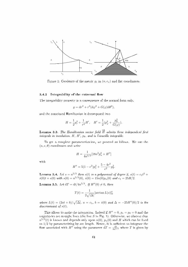
L1

L2

L3n

S

ex

1

2 3

Figure 1: Geodesics of the metric g1 in (n, ex) and at coordinates.

3.4.2 Integrability of the extremal ow

The integrability property is a consequence of the normal form only,

g = dr2 + r2(dϕ2 +G(ϕ)dθ2),

and the associated Hamiltonian is decomposed into

H =1

2p2r +

1

r2H ′, H ′ =

1

2(p2ϕ +

p2θG(ϕ)

).

Lemma 3.3. The Hamiltonian vector eld−→H admits three independent rst

integrals in involution, H, H ′, pθ, and is Liouville integrable.

To get a complete parameterization, we proceed as follows. We use the(n, e, θ) coordinates and write

H =1

4n5/3[18n2p2n +H ′′]

with

H ′′ = 5(1− e2)p2e +5− 4e2

e2p2θ.

Lemma 3.4. Let s = n5/3 then s(t) is a polynomial of degree 2, s(t) = c1t2 +

s(0)t+ s(0) with s(0) = n5/3(0), s(0) = 15n(0)pn(0) and c1 = 25H/2.

Lemma 3.5. Let dT = dt/4n5/3. If H ′′(0) 6= 0, then

T (t) =1

2√

|∆|[arctanL(s)]t0

where L(t) = (2at + b)/√

|∆|, a = c1, b = s(0) and ∆ = −25H ′′(0)/2 is thediscriminant of s(t).

This allows to make the integration. Indeed if H ′′ = 0, pe = pθ = 0 and thetrajectories are straight lines (the line S in Fig. 1). Otherwise, we observe thatn5/3(t) is known and depends only upon n(0), pn(0) and H which can be xedto 1/2 by parameterizing by arc length. Hence, it is sucient to integrate theow associated with H ′′ using the parameter dT = dt

4n5/3 where T is given by

61

the previous lemma. Let H ′′ = c23 and pθ = c2. Using pe = e/10(1 − e2), weobtain

e2 =20(1− e2)

e2[c3e

2 − (5− 4e2)c22].

To integrate, we set w = 1− e2 for e ∈]0, 1[, so the equation takes the form

dw

dT= Q(w)

whereQ(w) = 80w[(c23 − c22)− (c23 + 4c22)w]

with positive discriminant. Hence the solution is

w =1

2

c23 − c22c23 + 4c22

[1 + sin(

4√5

√c23 + 4c22 )T +K

],

K being a constant. We deduce that

θ(T ) = θ(0) + 2c2

∫ T

0

1 + 4w(s)

1− w(s)ds

where θ(0) can be set to 0 by symmetry. To conclude, we must integrate (1 +4w(s))/(1 − w(s)) with w = K1(1 + sinx) and x = (4s/

√5)√c23 + 4c22 + K.

Therefore, we must evaluate an integral of the form∫A+B sinx

C +D sinxdx·

More precisely, the formula is∫A+B sinx

C +D sinxdx =

B

Dx+AD −BC

∫dx

C +D sinx

with ∫dx

C +D sinx=

2√C2 −D2

arctan

(C tan(x/2) +D√

C2 −D2

)and C2 −D2 > 0. The previous lemmas and computations give

Proposition 3.10. For H ′′ 6= 0, the solutions of−→H can be computed using

elementary functions and

n(t) =

[25

2Ht2 + 15n(0)pn(0)t+ n5/3(0)

]3/5,

e(t) =√1−K1(1 + sinK2(t)),

θ(t) = θ(0) +pθ

2|pθ|K3

[−4x+

10

K3arctan

(1−K1) tan(x/2)−K1

K3

]K2(t)

K

,

with

K = arcsin

(1− e(0)2

K1− 1

), K1 =

1

2

H ′′(0)− p2θH ′′(0) + 4p2θ

,

K2(t) =4√5

(T (t)

√H ′′(0) + 4p2θ +K

), K3 =

√5p2θ

H ′′(0) + 4p2θ·

For H ′′ = 0, they are straight lines.

Remark 3.3. The above formulas give the complete solution of the associatedHamilton-Jacobi Equation.

62

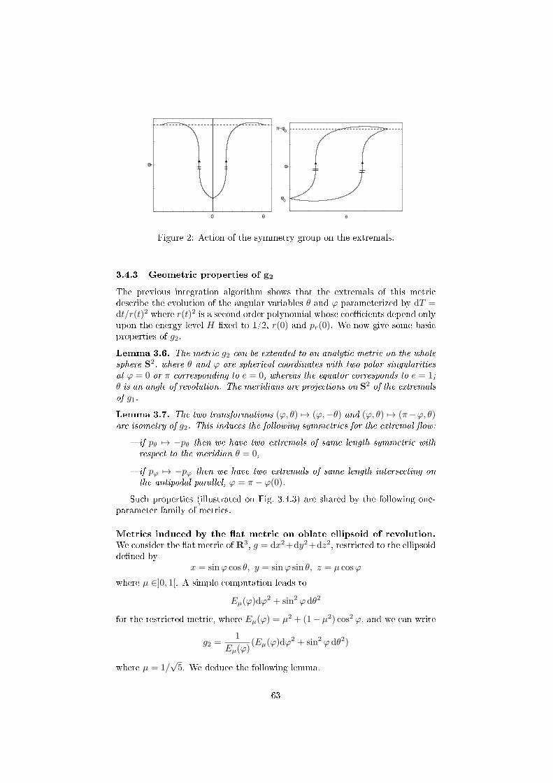
0 θ

φ

φ

θ

φ0

π−φ0

Figure 2: Action of the symmetry group on the extremals.

3.4.3 Geometric properties of g2

The previous integration algorithm shows that the extremals of this metricdescribe the evolution of the angular variables θ and ϕ parameterized by dT =dt/r(t)2 where r(t)2 is a second order polynomial whose coecients depend onlyupon the energy level H xed to 1/2, r(0) and pr(0). We now give some basicproperties of g2.

Lemma 3.6. The metric g2 can be extended to an analytic metric on the wholesphere S2, where θ and ϕ are spherical coordinates with two polar singularitiesat ϕ = 0 or π corresponding to e = 0, whereas the equator corresponds to e = 1;θ is an angle of revolution. The meridians are projections on S2 of the extremalsof g1.

Lemma 3.7. The two transformations (ϕ, θ) 7→ (ϕ,−θ) and (ϕ, θ) 7→ (π−ϕ, θ)are isometry of g2. This induces the following symmetries for the extremal ow:

if pθ 7→ −pθ then we have two extremals of same length symmetric withrespect to the meridian θ = 0,

if pϕ 7→ −pϕ then we have two extremals of same length intersecting onthe antipodal parallel, ϕ = π − ϕ(0).

Such properties (illustrated on Fig. 3.4.3) are shared by the following one-parameter family of metrics.

Metrics induced by the at metric on oblate ellipsoid of revolution.

We consider the at metric of R3, g = dx2+dy2+dz2, restricted to the ellipsoiddened by

x = sinϕ cos θ, y = sinϕ sin θ, z = µ cosϕ

where µ ∈]0, 1[. A simple computation leads to

Eµ(ϕ)dϕ2 + sin2 ϕ dθ2

for the restricted metric, where Eµ(ϕ) = µ2 + (1− µ2) cos2 ϕ, and we can write

g2 =1

Eµ(ϕ)(Eµ(ϕ)dϕ

2 + sin2 ϕ dθ2)

where µ = 1/√5. We deduce the following lemma.

63

Lemma 3.8. The metric g2 is conformal to the at metric restricted to anoblate ellipsoid of revolution with parameter µ = 1/

√5.

3.4.4 A global optimality result with application to orbital transfer

In this section, we consider an analytic metric on R+ × S2

g = dr2 + (dϕ2 +G(ϕ)dθ2)

and let H be the associated Hamiltonian. We x the parameterization to arclength by restricting to the level set H = 1/2. Let x1, x2 be two extremal curvesstarting from the same initial point x0 and intersecting at some positive t. Weget the relations

r1(t) = r2(t), ϕ1(t) = ϕ2(t), θ1(t) = θ2(t),

and from Lemma 3.4, we deduce that

Lemma 3.9. Both extremals x1 and x2 share the same pr(0) and for each t,r1(t) = r2(t).

If we consider now the integral curves of H ′ where H = (1/2)p2r + H ′/r2

on the xed induced level and parameterize these curves using dT = dt/r2, wededuce the following characterization.

Proposition 3.11. The following conditions are necessary and sucient tocharacterize extremals of H ′ 6= 0 intersecting with same length

ϕ1(T ) = ϕ2(T ) and θ1(T ) = θ2(T )

together with the compatibility condition

T =

∫ t

0

dt

r2(t)=

[2√∆

arctanL(t)

]tt=0

.

Theorem 3.2. A necessary global optimality condition for an analytic metricon R+ × S1 normalized to

g = dr2 + r2(dϕ2 +G(ϕ)dθ2)

is that the injectivity radius be greater than or equal to π on the sphere r = 1,the bound being reached by the at metric in spherical coordinates.

Proof. We observe that in the at case, the compatibility condition cannot besatised. Moreover, the injectivity radius on S2 is π corresponding to the half-length of a great circle. For the analytic metric on S2 under consideration, theinjectivity radius is the length of the conjugate point at minimum distance orthe half-length of a closed geodesic [17]. The conjugate point is, in addition,a limit point of the separating line. Hence, if the injectivity radius is smallerthan π, we have two minimizers for the restriction of the metric on S2 whichintersects with a length smaller than π. We shall show that it corresponds to aprojection of two extremals x1 and x2 which intersect with same length.

64

For such extremals r(0) = 1, we set pr(0) = ε, H = 1/2 and we get

2H ′ = p2ϕ(0) +p2θ(0)

G(ϕ(0))= λ2(ε), λ(ε) =

√1− ε2.

If t1 is the injectivity radius on the level set H ′ = 1/2, for H ′ = λ2(ε)/2 andpr(0) = ε, it is rescaled to T1 = t1/λ(ε). The compatibility relation for T = T1then gives

T1 = arctant+ ε

λ(ε)− arctan

ε

λ(ε)·

Clearly, the maximum of the right member is π, taking ε < 0, |ε| → 1. Hence,it can be satised since t1 < π. The at case shows that it is the sharpestbound.

By homogeneity, we deduce the following corollary.

Corollary 3.1. If the metric is normalized to dr2 + (r2/c2)(dϕ2 + G(ϕ)dθ2),then the bound for the injectivity radius on r2 = c2 is cπ.

3.4.5 Riemannian curvature and injectivity radius in orbital transfer

Using standard formulæ from Riemannian geometry [17], we have the followingproposition.

Proposition 3.12. Let g be a smooth metric of the form dr2 + r2(dϕ2 +G(ϕ)dθ2). The only non-zero component of the Riemann tensor is

R2323 = r2[−G

′′(ϕ)

2−G(ϕ) +

G′(ϕ)2

4G(ϕ)

]which takes the form R2323 = −r2F (F ′′ +F ) if we set G(ϕ) = F 2(ϕ). We havetherefore R2323 = 0 if and only if F (ϕ) = A sin(ϕ+ϕ0) which is induced by theat case in spherical coordinates.

Hence, the main non-zero sectional curvature of the metric is

K =R2323

| ∂∂θ ∧ ∂

∂ϕ |2

and computing this term in the case of orbital transfer, we get:

Lemma 3.10. The sectional curvature in the plane (ϕ, θ) is given by

K =(1− 24 cos2 ϕ− 16 cos4 ϕ)

r2(1 + 4 cos2 ϕ)2

and K → 0 as r → +∞.

Proposition 3.13. The Gauss curvature of the metric of g2 = dϕ2 +G(ϕ)dθ2

with G(ϕ) = (sin2 ϕ)/(1 + 4 cos2 ϕ) is

K =5(1− 8 cos2 ϕ)

(1 + 4 cos2 ϕ)2·

65

Theorem 3.3. The Gauss curvature of g2 is negative near the poles and max-imum at the equator. The injectivity radius is π/

√5 and is reached by the

shortest conjugate point along the equator.

Proof. Clearly K is maximum and equal to ve along the equator which is anextremal solution. Hence a direct computation gives that the shortest conjugatepoint is on the equator with length π/

√5. It corresponds to the injectivity

radius if the half-length of a shortest periodic extremal is greater than π/√5.

Simple closed extremals are computed in [8] using the integrability propertyand a simple reasoning gives that the shortest corresponds to meridians whoselength is 2π. Hence the result is proved.

Corollary 3.2. Since π/√5 < π

√2/5, the necessary optimality condition of

Theorem 3.3 is not satised in orbital transfer for the extension of the metricto R+ × S2.

3.4.6 Cut locus on S2 and global optimality results in orbital transfer

From the previous section, the computation of the injectivity radius for themetric on S2 is not sucient to conclude about global optimality. A morecomplete analysis is necessary to evaluate the cut locus. This analysis requiresnumerical simulations. The main results are [8, 11]:

Proposition 3.14. For the metric g2 on S2, they are exactly ve simple closedgeodesics modulo rotations around the poles, the shortest being meridians withlength 2π, the longest the equator with length 2π

√5.

Theorem 3.4. Except for poles, the conjugate locus is a deformation of a stan-dard astroid with axial symmetry and two cusps located on the antipodal parallel.With the exception of poles, the cut locus is a simple segment, located on theantipodal parallel, with axial symmetry, and whose extremities are cusps pointsof the conjugate locus. For a pole, the cut locus is reduced to the antipodal pole.

Proof. The proof is made by direct analysis of the extremal curves. The mainproblem is to prove that the separating line is given by points on the antipodalparallel where, because of the isometry ϕ → π − ϕ, two extremals curves withsame length intersect. This property cannot occur before. The results arerepresented Fig. 3.

Geometric interpretation and comments. The metric is conformal tothe restriction of the at metric to an oblate ellipsoid of revolution. For such ametric, the cut locus is known since Jacobi and is similar to the one representedon Fig. 3. It is a remarkable property that there is no bifurcation of the cutlocus when the metric is deformed by the factor Eµ(ϕ) In orbital transfer forinstance, the Gauss curvature is not positive. On S2, relations between theconjugate and cut loci allow to deduce the cut locus from the conjugate locus.2

The conjugate locus can also easily be computed using the code [12]. It can alsobe deduced by inspecting the extremal ow only, the conjugate locus being anenvelope.

2For instance, a domain bounded by two intersecting minimizing curves must contain aconjugate point.

66

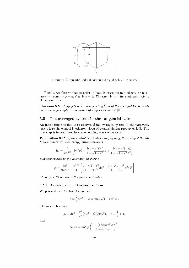
φθ

φ0

π−φ0

Figure 3: Conjugate and cut loci in averaged orbital transfer.

Finally, we observe that in order to have intersecting minimizers, we mustcross the equator ϕ = π, that is e = 1. The same is true for conjugate points.Hence we deduce

Theorem 3.5. Conjugate loci and separating lines of the averaged Kepler met-ric are always empty in the spaces of ellipses where e ∈ [0, 1[.

3.5 The averaged system in the tangential case

An interesting question is to analyze if the averaged system in the tangentialcase where the control is oriented along Ft retains similar properties [10]. Therst step is to compute the corresponding averaged system.

Proposition 3.15. If the control is oriented along Ft only, the averaged Hamil-tonian associated with energy minimization is

Ht =1

2n5/3

[9n2p2n +

4(1− e2)3/2

1 +√1− e2

p2e +4(1− e2)

1 +√1− e2

p2θe2

]and corresponds to the Riemannian metric

gt =dn2

9n1/3+n5/3

4

[1 +

√1− e2

(1− e2)3/2de2 +

1 +√1− e2

(1− e2)e2dθ2

]where (n, e, θ) remain orthogonal coordinates.

3.5.1 Construction of the normal form

We proceed as in Section 3.4 and set

r =2

5n5/6, e = sinϕ

√1 + cos2 ϕ .

The metric becomes

gt = dr2 +r2

c2(dϕ2 +G(ϕ)dθ2), c =

2

5< 1,

and

G(ϕ) = sin2 ϕ

(1− (1/2) sin2 ϕ

1− sin2 ϕ

)2

.

67

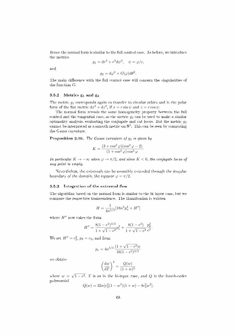
Hence the normal form is similar to the full control case. As before, we introducethe metrics

g1 = dr2 + r2dψ2, ψ = ϕ/c,

andg2 = dϕ2 +G(ϕ)dθ2.

The main dierence with the full control case will concern the singularities ofthe function G.

3.5.2 Metrics g1 and g2

The metric g1 corresponds again to transfer to circular orbits and is the polarform of the at metric dx2 + dz2, if x = r sinψ and z = r cosψ.

The normal form reveals the same homogeneity property between the fullcontrol and the tangential case, so the metric g2 can be used to make a similaroptimality analysis, evaluating the conjugate and cut locus. But the metric g2cannot be interpreted as a smooth metric on S2. This can be seen by computingthe Gauss curvature.

Proposition 3.16. The Gauss curvature of g2 is given by

K =(3 + cos2 ϕ)(cos2 ϕ− 2)

(1 + cos2 ϕ) cos2 ϕ·

In particular K → −∞ when ϕ→ π/2, and since K < 0, the conjugate locus ofany point is empty.

Nevertheless, the extremals can be smoothly extended through the singularboundary of the domain, the equator ϕ = π/2.

3.5.3 Integration of the extremal ow

The algorithm based on the normal form is similar to the bi-input case, but wecompare the respective transcendence. The Hamiltonian is written

H =1

4n5/3[18n2p2n +H ′′]

where H ′′ now takes the form

H ′′ =8(1− e2)3/2

1 +√1− e2

p2e +8(1− e2)

1 +√1− e2

p2θe2

·

We set H ′′ = c23, pθ = c2, and from

pe = 4n5/3(1 +

√1− e2)e

16(1− e2)3/2

we obtain (dw

dT

)2

=Q(w)

(1 + w)2

where w =√1− e2, T is as in the bi-input case, and Q is the fourth-order

polynomialQ(w) = 32w[c23(1− w2)(1 + w)− 8c22w

2].

68

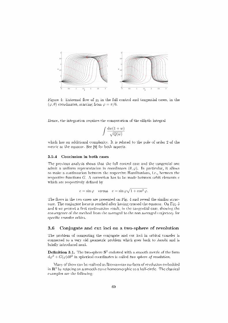
0 0.5 1 1.5 2 2.5 30

0.5

1

1.5

2

2.5

3

θ

φ

0 0.5 1 1.5 2 2.5 30

0.5

1

1.5

2

2.5

3

θ

φ

Figure 4: Extremal ow of g2 in the full control and tangential cases, in the(ϕ, θ) coordinates, starting from ϕ = π/6.

Hence, the integration requires the computation of the elliptic integral∫dw(1 + w)√

Q(w)

which has an additional complexity. It is related to the pole of order 2 of themetric at the equator. See [9] for both aspects.

3.5.4 Conclusion in both cases

The previous analysis shows that the full control case and the tangential oneadmit a uniform representation in coordinates (θ, ϕ). In particular, it allowsto make a continuation between the respective Hamiltonians, i.e., between therespective functions G. A correction has to be made between orbit elements ewhich are respectively dened by

e = sinϕ versus e = sinϕ√1 + cos2 ϕ.

The ows in the two cases are presented on Fig. 4 and reveal the similar struc-ture. The conjugate locus is reached after having crossed the equator. On Fig. 5and 6 we present a rst continuation result, in the tangential case, showing theconvergence of the method from the averaged to the non averaged trajectory forspecic transfer orbits.

3.6 Conjugate and cut loci on a two-sphere of revolution

The problem of computing the conjugate and cut loci in orbital transfer isconnected to a very old geometric problem which goes back to Jacobi and isbriey introduced next.

Denition 3.1. The two-sphere S2 endowed with a smooth metric of the formdϕ2 +G(ϕ)dθ2 in spherical coordinates is called two-sphere of revolution.

Many of them can be realized as Riemannian surfaces of revolution embeddedinR3 by rotating on a smooth curve homeomorphic to a half-circle. The classicalexamples are the following:

69

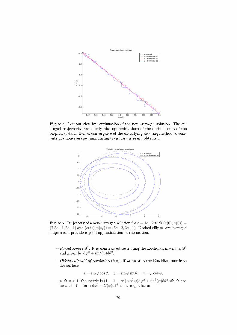
0.22 0.24 0.26 0.28 0.3 0.32 0.34 0.36 0.38 0.4

−0.6

−0.5

−0.4

−0.3

−0.2

−0.1

u cos(v)

u s

in(v

)

Trajectory in flat coordinates

Averaged

ε = 1.000000e−02

ε = 5.000000e−03

ε = 1.000000e−03

Figure 5: Computation by continuation of the non-averaged solution. The av-eraged trajectories are clearly nice approximations of the optimal ones of theoriginal system. Hence, convergence of the underlying shooting method to com-pute the non-averaged minimizing trajectory is easily obtained.

−3 −2 −1 0 1 2

−2.5

−2

−1.5

−1

−0.5

0

0.5

1

1.5

2

Trajectory in cartesian coordinates

Averaged

ε = 1.000000e−02

Figure 6: Trajectory of a non-averaged solution for ε = 1e−2 with (e(0), n(0)) =(7.5e−1, 5e−1) and (e(tf ), n(tf )) = (5e−2, 3e−1). Dashed ellipses are averagedellipses and provide a good approximation of the motion.

Round sphere S2. It is constructed restricting the Euclidian metric to S2

and given by dϕ2 + sin2(ϕ)dθ2.

Oblate ellipsoid of revolution O(µ). If we restrict the Euclidian metric tothe surface

x = sinϕ cos θ, y = sinϕ sin θ, z = µ cosϕ,

with µ < 1, the metric is (1− (1− µ2) sin2 ϕ)dϕ2 + sin2(ϕ)dθ2 which canbe set in the form dϕ2 +G(ϕ)dθ2 using a quadrature.

70

We recall some basic properties on the ellipsoid of revolution.

Proposition 3.17. On an oblate ellipsoid of revolution,

the Gauss curvature is monotone increasing from the North pole to theequator,

the cut locus of a point which is not a pole is a subarc of the antipodalparallel,

the conjugate locus of a point which is not a pole has a standard astroidshape with four cusps.

The simple structure of the cut locus is a consequence of [31].

Theorem 3.6. Let dϕ2 + G(ϕ)dθ2 be a metric on a two-sphere of revolution.We assume:

The transformation ϕ −→ π − ϕ is an isometry i.e. G(π − ϕ) = G(ϕ),

The Gauss curvature K is monotone non decreasing along a meridianfrom the North pole to the equator.

Then, the cut locus of a point not a pole is a simple branch located on theantipodal parallel.

Application. Let gλ be the family of analytic metrics on S2 dened by

gλ = dϕ2 +Gλ(ϕ)dθ2, Gλ(ϕ) =

(1 + λ)2 sin2 ϕ

(1 + λ cos2 ϕ), λ ≥ 0.

The Gauss curvature is given by

Kλ = − 1√G

∂2√G

∂2ϕ=

(1 + λ)(1− 2λ cos2 ϕ)

(1 + λ cos2 ϕ)2·

Hence if 0 < λ ≤ 2, then Kλ is monotone non decreasing from the North poleto the equator and the previous theorem asserts that the one parameter familyhas a cut locus reduced to a simple branch for λ ∈]0, 2].

If λ > 2 the Gaussian curvatureKλ is not monotone and the result cannot beapplied. In particular the orbit transfer with full control corresponds to λ = 4,while at the limit case λ = +∞ a singularity appears. The Riemannian metrichas a pole at the equator, the situation being similar to the one occuring whenthe thrust is only tangential. Hence Theorem 3.6 has to be rened to deal withsuch situations. The nal result is coming from [9].

We consider a metric of the form g = ϕ2 +G(ϕ)dθ2 where G′ is non zero on]0, π2 [ and G(π − ϕ) = G(ϕ).

Denition 3.2. The rst return mapping to the equator is the map

∆θ : pθ ∈]0,√G(π/2)[ 7→ ∆θ(pθ)

that is the θ-variation of the extremal parameterized by arc length and associ-ated with the adjoint vector component pθ. The extremal ow is called tame ifthe rst return mapping is monotone non-increasing for pθ ∈]0,

√G(π/2)[.

71

Theorem 3.7. In the tame case, the cut locus of a point dierent from a poleis a subset of the antipodal parallel. If moreover ∆θ′(pθ) < 0 < ∆θ′′(pθ) on]0,

√G(π/2)[, then the conjugate locus of such a point has exactly four cusps.

Remark 3.4. This result can be extended to the singular case where the metrichas poles at the equator.

4 Energy minimization in the Earth-Moon space

mission with low thrust

4.1 The N-body problem

In this section, we follow mainly [25] (see also [27] and [32]). Consider N pointmasses m1, . . . ,mN moving in a Galilean reference system R3 where the onlyforces acting are their mutual attractions. If q = (q1, . . . , qN ) ∈ R3N is the stateand p = (p1, . . . , pN ) is the momentum vector, the equations of motion are

q =∂H

∂p, p = −∂H

∂q

where the Hamiltonian is

H =N∑i=1

|pi|2

2mi− U, U(q) =

N∑1≤i<j≤N

Gmimj

|qi − qj |·

A subcase is the coplanar situation where the N masses are in a plane R2.In this case the Galilean reference frame can be replaced by a rotating framedened by

K =

[0 1−1 0

], exp(ωtK) =

[cosωt sinωt− sinωt cosωt

],

and introducing a set of coordinates which uniformly rotates with frequency ω,one denes the symplectic transformation

ui = exp(ωtK)qi, vi = exp(ωtK).

A standard computation gives the Hamiltonian of the N -body problem in ro-tating coordinates,

H =N∑i=1

|v|2

2mi−

N∑i=1

wtuiKvi −N∑

1≤i<j≤N

Gmimj

|qi − qj |·

In particular, the Kepler problem in rotating coordinates up to a normalizationhas the following Hamiltonian

H =|p|2

2− tqKp− 1

|q|·

72

4.2 The circular restricted 3-body problem in Jacobi co-

ordinates

The following representation of the Earth-Moon problem ts in the so-calledcircular restricted 3-body problem. In the rotating frame, the Earth which is thebiggest primary planet with mass 1 − µ is located at (−µ, 0) while the Moonwith mass µ is located at (1−µ, 0) (the small parameter being µ ' 1.2153e−2).We note z = x + iy the position of the spacecraft, and ρ1, ρ2 the distances tothe primaries,

ρ1 =√(x+ µ)2 + y2,

ρ2 =√(x− 1 + µ)2 + y2.

The equation of motion is

z + 2iz − z = −(1− µ)z + µ

ρ31− µ

z − 1 + µ

ρ32

that is

x− 2y − x =∂V

∂x, y + 2x− y =

∂V

∂y,

where −V is the potential of the system dened by

V =1− µ

ρ31+µ

ρ32·

The system can be written using Hamiltonian formalism setting

q1 = x, q2 = y, p1 = x− y, q2 = y + x,

and the Hamiltonian describing the motion writes

H0(q1, q2, p1, p2) =1

2(p21 + p22) + p1q2 − p2q1 −

1− µ

ρ1− µ

ρ2·

4.3 Jacobi integral, Hill regions and equilibrium points

The Jacobi integral using Hamiltonian formalism is simply the Hamiltonian H0

which gives

H(x, y, x− y, y + x) =x2 + y2

2− Ω(x, y)

where

Ω(x, y) =1

2(x2 + y2) +

1− µ

ρ1+µ

ρ2·

Solutions are conned on the level set

x2 + y2

2− Ω(x, y) = h, h constant.

The Hill domain for the value h is the region where the motion can occur, thatis (x, y) ∈ R2 | Ω(x, y) + h ≥ 0.

The equilibrium points of the problem are well known. They split into twodierent types:

73

Euler points. They are the collinear points denoted L1, L2 and L3 locatedon the line y = 0 dened by the primaries. For the Earth-Moon problemthey are given by

x1 ' −1.0051, x2 ' 8.369e− 1, x3 ' 1.1557.

Lagrange points. The two points L4 and L5 form with the two primariesan equilateral triangle.

Some important information about stability of the equilibrium points are pro-vided by the eigenvalues of the linearized system. The linearized matrix eval-uated at points L1, L2 or L3 admits two real eigenvalues, one being strictlypositive, and two imaginary ones. The collinear points are consequently notstable. In particular, the eigenvalues of the linearized matrix evaluated at L2

with µ = 1.2153e − 2 are approximately ±2.931837 and ±2.334248i. When itis evaluated at L4 or L5, the linearized matrix has two imaginary eigenvaluessince µ < µ1 = (1/2)(1−

√69/9) in the Earth-Moon system. Points L4 and L5

are thus stable according to Arnold stability theorem [25]. See also [24] for areview of mission design techniques using the equilibrium points.

4.4 The continuation method

The mathematical continuation method in the restricted circular problem isomnipresent in Poincaré's work, in particular for the continuation of circularorbits [26]. Geometrically, it is simply a continuation of trajectories of Keplerproblem into trajectories of the 3-body problem. It amounts to considering µ asa small parameterthe limit case µ = 0 being Kepler problem in the rotatingframewriting

H0 =|p|2

2− tqKp− 1

|q|+ o(µ).

The approximation for µ is valid, a neighbourhood of the primaries being ex-cluded. In the Earth-Moon problem, since µ is very small, the Kepler problemis a good approximation of the motion in a large neighbourhood of the Earth.

4.4.1 The control problem

The control system in the rotating frame is deduced from the previous modeland can be written in Hamiltonian form

dx

dt=

−→H 0(x) + u1

−→H 1(x) + u2

−→H 2(x)

where x = (q, p),−→H 0 is the free motion and

−→H 1,

−→H 2 are given by

−→H i = −qi,

i =1,2. As for the Kepler problem, the mass variation of the satellite can beintroduced in the model dividing ui bym(t) and adding the equation m = −δ|u|.Again, it will be not taken into account here. Moreover we still restrict ouranalysis to the energy minimization problem with xed nal time tf and controlvalued in R2. The physical problem which is to maximize the nal mass canbe analyzed using a continuation method. Preliminary results in the minimumtime case are given in [15].

74

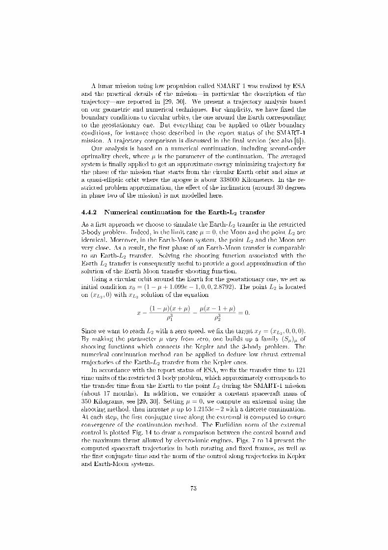
A lunar mission using low propulsion called SMART-1 was realized by ESAand the practical details of the missionin particular the description of thetrajectoryare reported in [29, 30]. We present a trajectory analysis basedon our geometric and numerical techniques. For simplicity, we have xed theboundary conditions to circular orbits, the one around the Earth correspondingto the geostationary one. But everything can be applied to other boundaryconditions, for instance those described in the report status of the SMART-1mission. A trajectory comparison is discussed in the nal section (see also [6]).

Our analysis is based on a numerical continuation, including second-orderoptimality check, where µ is the parameter of the continuation. The averagedsystem is nally applied to get an approximate energy minimizing trajectory forthe phase of the mission that starts from the circular Earth orbit and aims ata quasi-elliptic orbit where the apogee is about 338000 Kilometers. In the re-stricted problem approximation, the eect of the inclination (around 30 degreesin phase two of the mission) is not modelled here.

4.4.2 Numerical continuation for the Earth-L2 transfer

As a rst approach we choose to simulate the Earth-L2 transfer in the restricted3-body problem. Indeed, in the limit case µ = 0, the Moon and the point L2 areidentical. Moreover, in the Earth-Moon system, the point L2 and the Moon arevery close. As a result, the rst phase of an Earth-Moon transfer is comparableto an Earth-L2 transfer. Solving the shooting function associated with theEarth-L2 transfer is consequently useful to provide a good approximation of thesolution of the Earth-Moon transfer shooting function.

Using a circular orbit around the Earth for the geostationary one, we set asinitial condition x0 = (1− µ+ 1.099e− 1, 0, 0, 2.8792). The point L2 is locatedon (xL2 , 0) with xL2 solution of the equation

x− (1− µ)(x+ µ)

ρ31− µ(x− 1 + µ)

ρ32= 0.

Since we want to reach L2 with a zero speed, we x the target xf = (xL2 , 0, 0, 0).By making the parameter µ vary from zero, one builds up a family (Sµ)µ ofshooting functions which connects the Kepler and the 3-body problem. Thenumerical continuation method can be applied to deduce low thrust extremaltrajectories of the Earth-L2 transfer from the Kepler ones.

In accordance with the report status of ESA, we x the transfer time to 121time units of the restricted 3-body problem, which approximately corresponds tothe transfer time from the Earth to the point L2 during the SMART-1 mission(about 17 months). In addition, we consider a constant spacecraft mass of350 Kilograms, see [29, 30]. Setting µ = 0, we compute an extremal using theshooting method, then increase µ up to 1.2153e−2 with a discrete continuation.At each step, the rst conjugate time along the extremal is computed to ensureconvergence of the continuation method. The Euclidian norm of the extremalcontrol is plotted Fig. 14 to draw a comparison between the control bound andthe maximum thrust allowed by electro-ionic engines. Figs. 7 to 14 present thecomputed spacecraft trajectories in both rotating and xed frames, as well asthe rst conjugate time and the norm of the control along trajectories in Keplerand Earth-Moon systems.

75

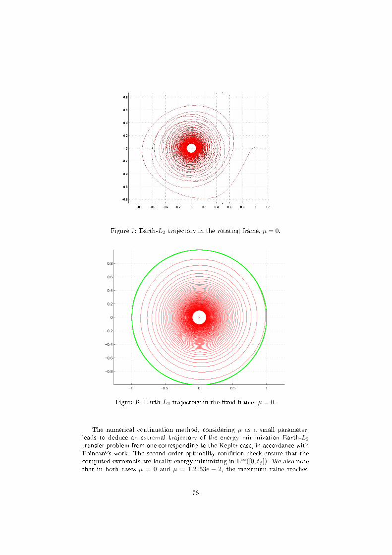
Figure 7: Earth-L2 trajectory in the rotating frame, µ = 0.

−1 −0.5 0 0.5 1

−0.8

−0.6

−0.4

−0.2

0

0.2

0.4

0.6

0.8

Figure 8: Earth-L2 trajectory in the xed frame, µ = 0.

The numerical continuation method, considering µ as a small parameter,leads to deduce an extremal trajectory of the energy minimization Earth-L2

transfer problem from one corresponding to the Kepler case, in accordance withPoincaré's work. The second order optimality condition check ensure that thecomputed extremals are locally energy minimizing in L∞([0, tf ]). We also notethat in both cases µ = 0 and µ = 1.2153e − 2, the maximum value reached

76

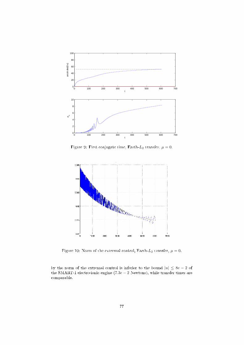
0 100 200 300 400 500 600 7000

20

40

60

80

100

t

arcs

h de

t(δ

x)

0 100 200 300 400 500 600 7000

2

4

6

8

10

t

σ n

Figure 9: First conjugate time, Earth-L2 transfer, µ = 0.

Figure 10: Norm of the extremal control, Earth-L2 transfer, µ = 0.

by the norm of the extremal control is inferior to the bound |u| ≤ 8e − 2 ofthe SMART-1 electro-ionic engine (7.3e− 2 Newtons), while transfer times arecomparable.

77

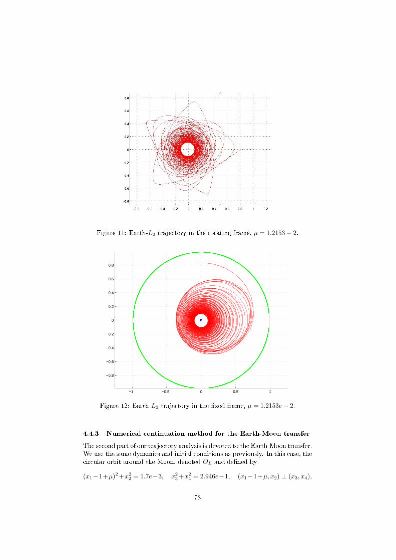
Figure 11: Earth-L2 trajectory in the rotating frame, µ = 1.2153− 2.

−1 −0.5 0 0.5 1

−0.8

−0.6

−0.4

−0.2

0

0.2

0.4

0.6

0.8

Figure 12: Earth-L2 trajectory in the xed frame, µ = 1.2153e− 2.

4.4.3 Numerical continuation method for the Earth-Moon transfer

The second part of our trajectory analysis is devoted to the Earth-Moon transfer.We use the same dynamics and initial conditions as previously. In this case, thecircular orbit around the Moon, denoted OL and dened by

(x1−1+µ)2+x22 = 1.7e−3, x23+x24 = 2.946e−1, (x1−1+µ, x2) ⊥ (x3, x4),

78

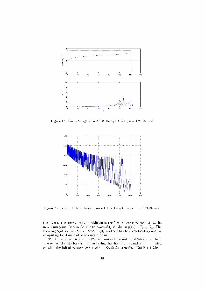
Figure 13: First conjugate time, Earth-L2 transfer, µ = 1.2153e− 2.

Figure 14: Norm of the extremal control, Earth-L2 transfer, µ = 1.2153e− 2.

is chosen as the target orbit. In addition to the former necessary conditions, themaximum principle provides the transversality condition p(tf ) ⊥ Tx(tf )OL. Theshooting equation is modied accordingly, and one has to check local optimalitycomputing focal instead of conjugate points.

The transfer time is xed to 124 time units of the restricted 3-body problem.The extremal trajectory is obtained using the shooting method and initializingp0 with the initial costate vector of the Earth-L2 transfer. The Earth-Moon

79

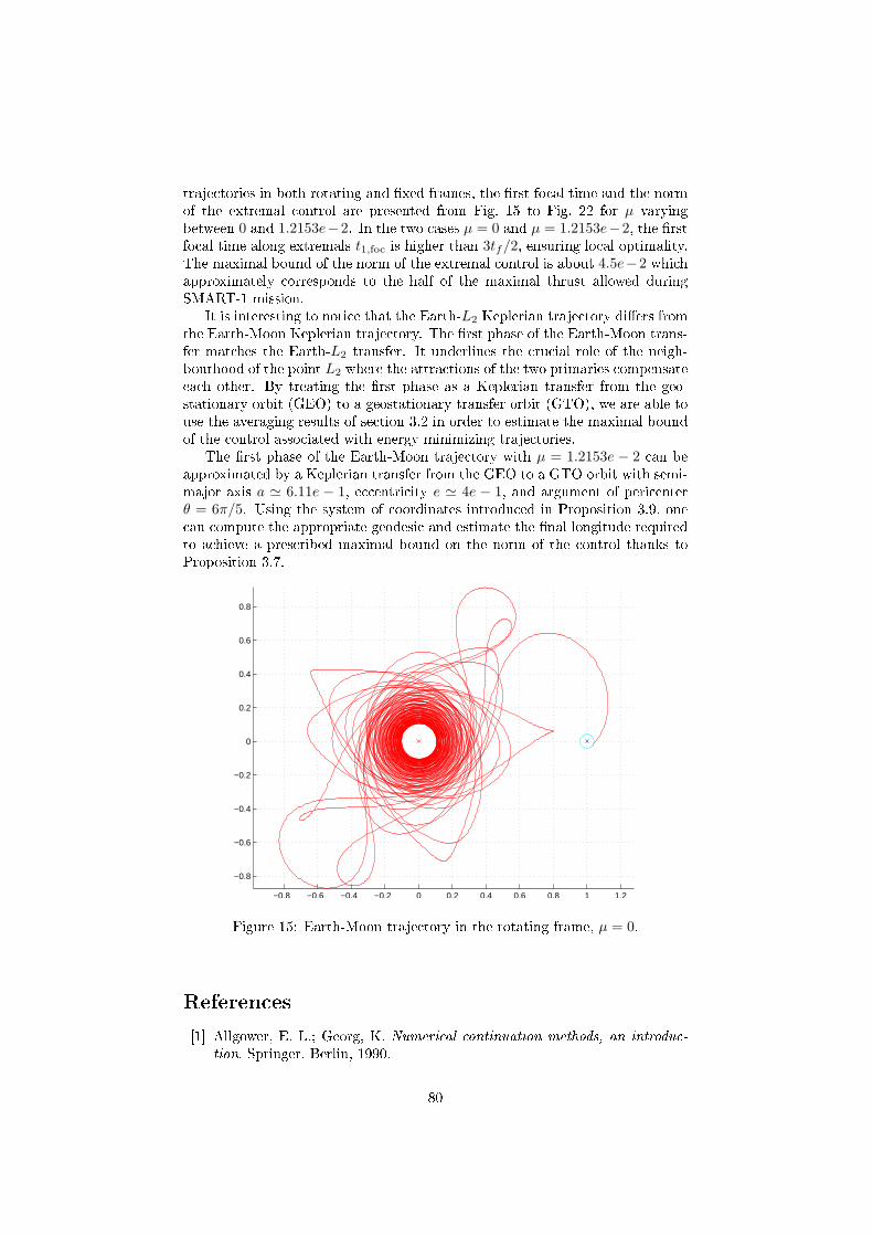
trajectories in both rotating and xed frames, the rst focal time and the normof the extremal control are presented from Fig. 15 to Fig. 22 for µ varyingbetween 0 and 1.2153e−2. In the two cases µ = 0 and µ = 1.2153e−2, the rstfocal time along extremals t1,foc is higher than 3tf/2, ensuring local optimality.The maximal bound of the norm of the extremal control is about 4.5e−2 whichapproximately corresponds to the half of the maximal thrust allowed duringSMART-1 mission.

It is interesting to notice that the Earth-L2 Keplerian trajectory diers fromthe Earth-Moon Keplerian trajectory. The rst phase of the Earth-Moon trans-fer matches the Earth-L2 transfer. It underlines the crucial role of the neigh-bourhood of the point L2 where the attractions of the two primaries compensateeach other. By treating the rst phase as a Keplerian transfer from the geo-stationary orbit (GEO) to a geostationary transfer orbit (GTO), we are able touse the averaging results of section 3.2 in order to estimate the maximal boundof the control associated with energy minimizing trajectories.

The rst phase of the Earth-Moon trajectory with µ = 1.2153e − 2 can beapproximated by a Keplerian transfer from the GEO to a GTO orbit with semi-major axis a ' 6.11e − 1, eccentricity e ' 4e − 1, and argument of pericenterθ = 6π/5. Using the system of coordinates introduced in Proposition 3.9, onecan compute the appropriate geodesic and estimate the nal longitude requiredto achieve a prescribed maximal bound on the norm of the control thanks toProposition 3.7.

−0.8 −0.6 −0.4 −0.2 0 0.2 0.4 0.6 0.8 1 1.2

−0.8

−0.6

−0.4

−0.2

0

0.2

0.4

0.6

0.8

Figure 15: Earth-Moon trajectory in the rotating frame, µ = 0.

References

[1] Allgower, E. L.; Georg, K. Numerical continuation methods, an introduc-tion. Springer, Berlin, 1990.

80

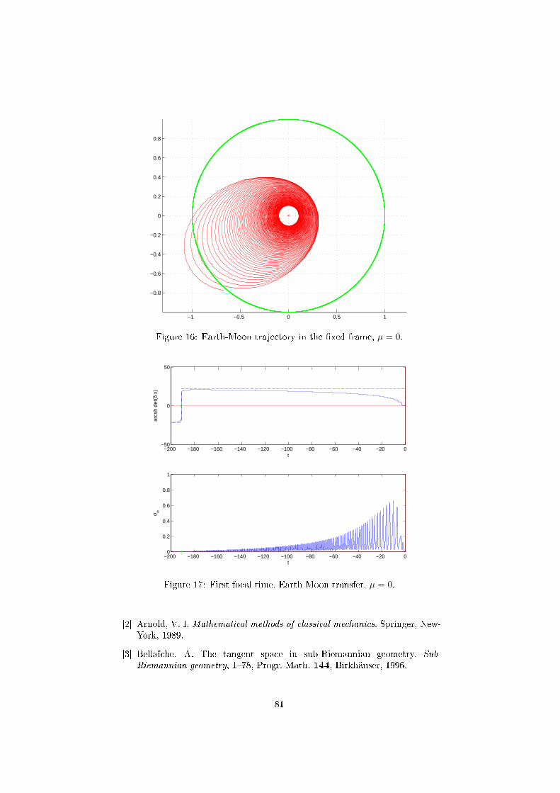
−1 −0.5 0 0.5 1

−0.8

−0.6

−0.4

−0.2

0

0.2

0.4

0.6

0.8

Figure 16: Earth-Moon trajectory in the xed frame, µ = 0.

−200 −180 −160 −140 −120 −100 −80 −60 −40 −20 0−50

0

50

t

arcs

h de

t(δ

x)

−200 −180 −160 −140 −120 −100 −80 −60 −40 −20 00

0.2

0.4

0.6

0.8

1

t

σ n

Figure 17: First focal time, Earth-Moon transfer, µ = 0.

[2] Arnold, V. I. Mathematical methods of classical mechanics. Springer, New-York, 1989.

[3] Bellaïche, A. The tangent space in sub-Riemannian geometry. Sub-Riemannian geometry, 178, Progr. Math. 144, Birkhäuser, 1996.

81

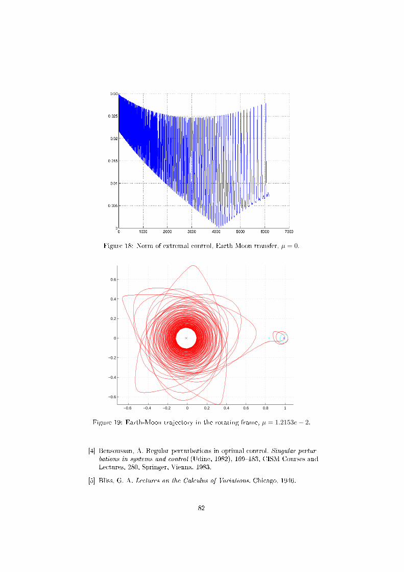
Figure 18: Norm of extremal control, Earth-Moon transfer, µ = 0.

−0.6 −0.4 −0.2 0 0.2 0.4 0.6 0.8 1

−0.6

−0.4

−0.2

0

0.2

0.4

0.6

Figure 19: Earth-Moon trajectory in the rotating frame, µ = 1.2153e− 2.

[4] Bensoussan, A. Regular perturbations in optimal control. Singular pertur-bations in systems and control (Udine, 1982), 169183, CISM Courses andLectures, 280, Springer, Vienna, 1983.

[5] Bliss, G. A. Lectures on the Calculus of Variations. Chicago, 1946.

82

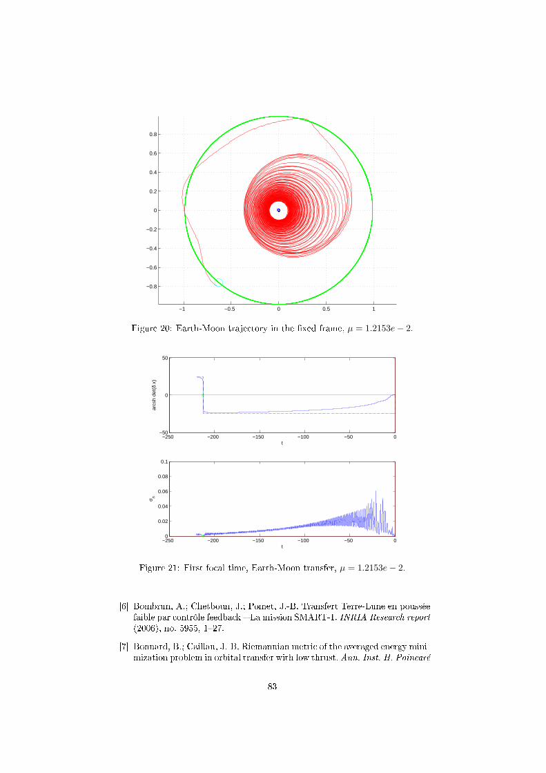
−1 −0.5 0 0.5 1

−0.8

−0.6

−0.4

−0.2

0

0.2

0.4

0.6

0.8

Figure 20: Earth-Moon trajectory in the xed frame, µ = 1.2153e− 2.

−250 −200 −150 −100 −50 0−50

0

50

t

arcs

h de

t(δ

x)

−250 −200 −150 −100 −50 00

0.02

0.04

0.06

0.08

0.1

t

σ n

Figure 21: First focal time, Earth-Moon transfer, µ = 1.2153e− 2.

[6] Bombrun, A.; Chetboun, J.; Pomet, J.-B. Transfert Terre-Lune en pousséefaible par contrôle feedback La mission SMART-1. INRIA Research report(2006), no. 5955, 127.

[7] Bonnard, B.; Caillau, J.-B. Riemannian metric of the averaged energy mini-mization problem in orbital transfer with low thrust. Ann. Inst. H. Poincaré

83

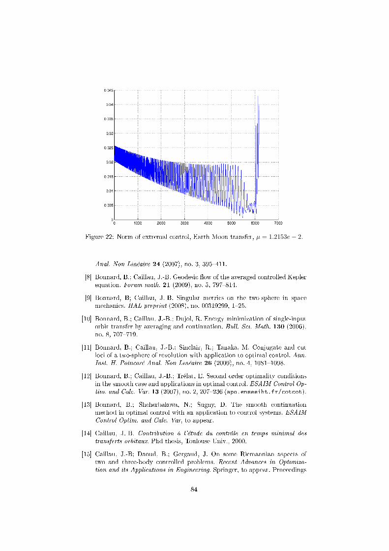
Figure 22: Norm of extremal control, Earth-Moon transfer, µ = 1.2153e− 2.

Anal. Non Linéaire 24 (2007), no. 3, 395411.

[8] Bonnard, B.; Caillau, J.-B. Geodesic ow of the averaged controlled Keplerequation. Forum math. 21 (2009), no. 5, 797814.

[9] Bonnard, B; Caillau, J.-B. Singular metrics on the two-sphere in spacemechanics. HAL preprint (2008), no. 00319299, 125.

[10] Bonnard, B.; Caillau, J.-B.; Dujol, R. Energy minimization of single-inputorbit transfer by averaging and continuation. Bull. Sci. Math. 130 (2006),no. 8, 707719.

[11] Bonnard, B.; Caillau, J.-B.; Sinclair, R.; Tanaka, M. Conjugate and cutloci of a two-sphere of revolution with application to optimal control. Ann.Inst. H. Poincaré Anal. Non Linéaire 26 (2009), no. 4, 10811098.

[12] Bonnard, B.; Caillau, J.-B.; Trélat, E. Second order optimality conditionsin the smooth case and applications in optimal control. ESAIM Control Op-tim. and Calc. Var. 13 (2007), no. 2, 207236 (apo.enseeiht.fr/cotcot).

[13] Bonnard, B.; Shcherbakova, N.; Sugny, D. The smooth continuationmethod in optimal control with an application to control systems. ESAIMControl Optim. and Calc. Var, to appear.

[14] Caillau, J.-B. Contribution à l'étude du contrôle en temps minimal destransferts orbitaux. Phd thesis, Toulouse Univ., 2000.

[15] Caillau, J.-B; Daoud, B.; Gergaud, J. On some Riemannian aspects oftwo and three-body controlled problems. Recent Advances in Optimiza-tion and its Applications in Engineering, Springer, to appear. Proceedings

84

of the 14th Belgian-French-German Conference on Optimization, Leuven,September 2009.

[16] Chaplais, F. Averaging and deterministic optimal control. SIAM J. ControlOptim. 25 (1987), no. 3, 767780.

[17] Do Carmo, M. P. Riemannian geometry. Birkhauser, Boston, 1992.

[18] Edelbaum, T. N. Optimal low-thrust rendez-vous and station keeping.AIAA J. 2 (1964), no. 7, 11961201.

[19] Geroy, S. Généralisation des techniques de moyennation en contrôle op-timal. Application aux problèmes de transfert et rendez-vous orbitaux àpoussée faible. Phd thesis, Toulouse Univ., 1997.

[20] Gergaud, J.; Haberkorn, T. Homotopy method for minimum consumptionorbit transfer problem. ESAIM Control Optim. Calc. Var. 12 (2006), no. 2,294310.

[21] Guckenheimer, J.; Holmes, P. Nonlinear oscillations, dynamical systemsand bifurcations of vector elds. Springer, 1993.

[22] Guerra, M.; Sarychev, A. Existence and Lipschitzian regularity for relaxedminimizers. Mathematical control theory and nance, 231250, Springer,Berlin, 2008.

[23] Kato, T. Perturbation theory for linear operators. Springer, 1980.

[24] Marsden, J. E.; Ross, S. D. New methods in celestial mechanics and missiondesign, Bull. Amer. Math. Soc. (N.S.) 43 (2006), no. 1, 4373.

[25] Meyer, K.; Hall, G. R. Introduction to Hamiltonian dynamical systems andthe N -body problem. Springer, New York, 1992.

[26] Poincaré, H. Oeuvres. Gauthier-Villars, Paris, 1934.

[27] Pollard, H.Mathematical introduction to celestial mechanics. Prentice-Hall,Englewood Clis, 1966.

[28] Pontryagin, L. S.; Boltyanskii, V. G.; Gamkrelidze, R. V.; Mishchenko, E.F. The mathematical theory of optimal processes. John Wiley & Sons, NewYork, 1962.

[29] Racca, G.; Foing, B. H.; Coradini, M. SMART-1: The rst time of Europeto the Moon. Earth, Moon and planets 85-86 (2001), 379390.

[30] Racca, G.; et al. SMART-1 mission description and development status.Planetary and space science 50 (2002), 13231337.

[31] Sinclair, R.; Tanaka, M. The cut locus of a two-sphere of revolution andToponogov's comparison theorem. Tohoku Math. J. 59 (2007), no. 2, 379399.

[32] Szebehely, V. Theory of orbits: The restricted problem of three bodies. Aca-demic Press, 1967.

85

86

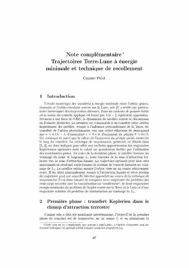
Note complémentaire ∗

Trajectoires Terre-Lune à énergie

minimale et technique de recollement

Gautier Picot

1 Introduction

L'étude numérique des transferts à énergie minimale entre l'orbite géosta-tionnaire et l'orbite circulaire centrée sur la Lune, voir [1] a révélé une particu-larité intéressante des trajectoires obtenues. Dans un contexte de poussée faibleoù la norme du contrôle appliqué est borné par 4.5e− 2, équivalent approxima-tivement à une force de 0.35N, la dynamique du satellite semble se décomposeren 3 phases distinctes. La première est comparable à un transfert entre orbiteskepleriennes. Le satellite, soumis à l'inuence prépondérante de la Terre, esttransféré de l'orbite géostationnaire vers une orbite elliptique de demi-grandaxe a ' 6.11e − 1, d'exentricité e ' 0.4 et d'argument du périgée θ ' 6π/5.On remarque en outre que la valeur de l'argument du périgée parait conservéele long du transfert. La technique de moyennation, présentée en détails dans[1, 2], est donc indiquée pour orir une exellente approximation des trajectoireskepleriennes optimales dont le calcul est grandement facilité par l'utilisationdes coordonnées plates. Au cours de la deuxième phase, le satellite traverse unvoisinage du point de Lagrange L1 pour basculer de la zone d'attraction ter-restre vers la zone d'attraction lunaire. La trajectoire optimale peut alors êtreapproximée en résolvant explicitement le système de contrôle linéarisé au voisi-nage de L1. Le satellite rejoint ensuite l'orbite visée en un temps relativementcourt. Il est alors principalement soumis à l'attraction lunaire et cette portionde trajectoire peut une nouvelle fois être approchée au moyen de la technique demoyennation Il est donc naturel de comparer cette trajectoire du problème destrois corps restreint avec la concaténation ou recollement, de deux trajectoiresenergie-minimales du problème de Kepler centré sur la Terre et la Lune et d'unetrajectoire solution du problème de minimisation au voisinage de L1.

2 Première phase : transfert Keplerien dans le

champ d'attraction terrestre

Comme cela a déjà été mentionné précédemment, l'objectif de la premièrephase du transfert est de transporter, en un temps t1f et en minimisant la

∗Cette note est un complément, non soumis à publication, à l'article Geometric and nu-

merical techniques in optimal orbital transfer using low propulsion [1].

87

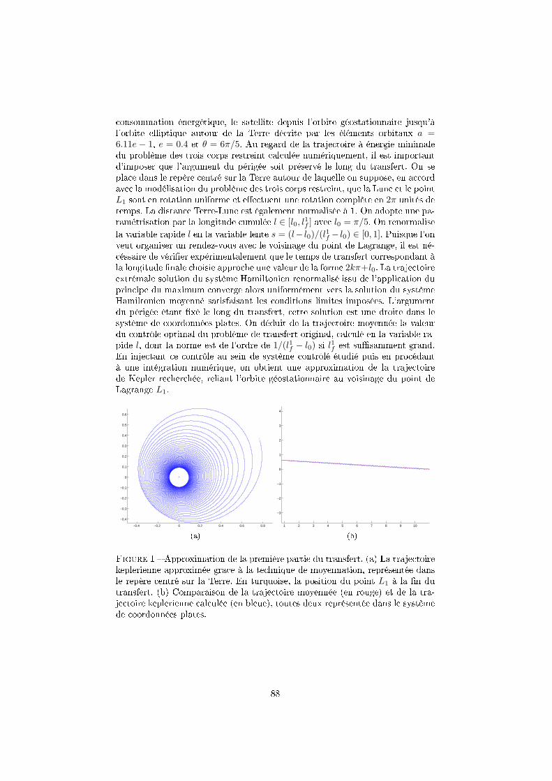
consommation énergétique, le satellite depuis l'orbite géostationnaire jusqu'àl'orbite elliptique autour de la Terre décrite par les éléments orbitaux a =6.11e − 1, e = 0.4 et θ = 6π/5. Au regard de la trajectoire à énergie minimaledu problème des trois corps restreint calculée numériquement, il est importantd'imposer que l'argument du périgée soit préservé le long du transfert. On seplace dans le repère centré sur la Terre autour de laquelle on suppose, en accordavec la modélisation du problème des trois corps restreint, que la Lune et le pointL1 sont en rotation uniforme et eectuent une rotation complète en 2π unités detemps. La distance Terre-Lune est également normalisée à 1. On adopte une pa-ramétrisation par la longitude cumulée l ∈ [l0, l

1f ] avec l0 = π/5. On renormalise

la variable rapide l en la variable lente s = (l− l0)/(l1f − l0) ∈ [0, 1]. Puisque l'onveut organiser un rendez-vous avec le voisinage du point de Lagrange, il est né-céssaire de vérier expérimentalement que le temps de transfert correspondant àla longitude nale choisie approche une valeur de la forme 2kπ+l0. La trajectoireextrémale solution du système Hamiltonien renormalisé issu de l'application duprincipe du maximum converge alors uniformément vers la solution du systèmeHamiltonien moyenné satisfaisant les conditions limites imposées. L'argumentdu périgée étant xé le long du transfert, cette solution est une droite dans lesystème de coordonnées plates. On déduit de la trajectoire moyennée la valeurdu contrôle optimal du problème de transfert original, calculé en la variable ra-pide l, dont la norme est de l'ordre de 1/(l1f − l0) si l

1f est susamment grand.

En injectant ce contrôle au sein de système contrôlé étudié puis en procédantà une intégration numérique, on obtient une approximation de la trajectoirede Kepler recherchée, reliant l'orbite géostationnaire au voisinage du point deLagrange L1.

−0.4 −0.2 0 0.2 0.4 0.6 0.8

−0.4

−0.3

−0.2

−0.1

0

0.1

0.2

0.3

0.4

0.5

0.6

(a)

1 2 3 4 5 6 7 8 9 10

−3

−2

−1

0

1

2

3

4

(b)

Figure 1 Approximation de la première partie du transfert. (a) La trajectoirekeplerienne approximée grâce à la technique de moyennation, représentée dansle repère centré sur la Terre. En turquoise, la position du point L1 à la n dutransfert. (b) Comparaison de la trajectoire moyennée (en rouge) et de la tra-jectoire keplerienne calculée (en bleue), toutes deux représentée dans le systèmede coordonnées plates.

88

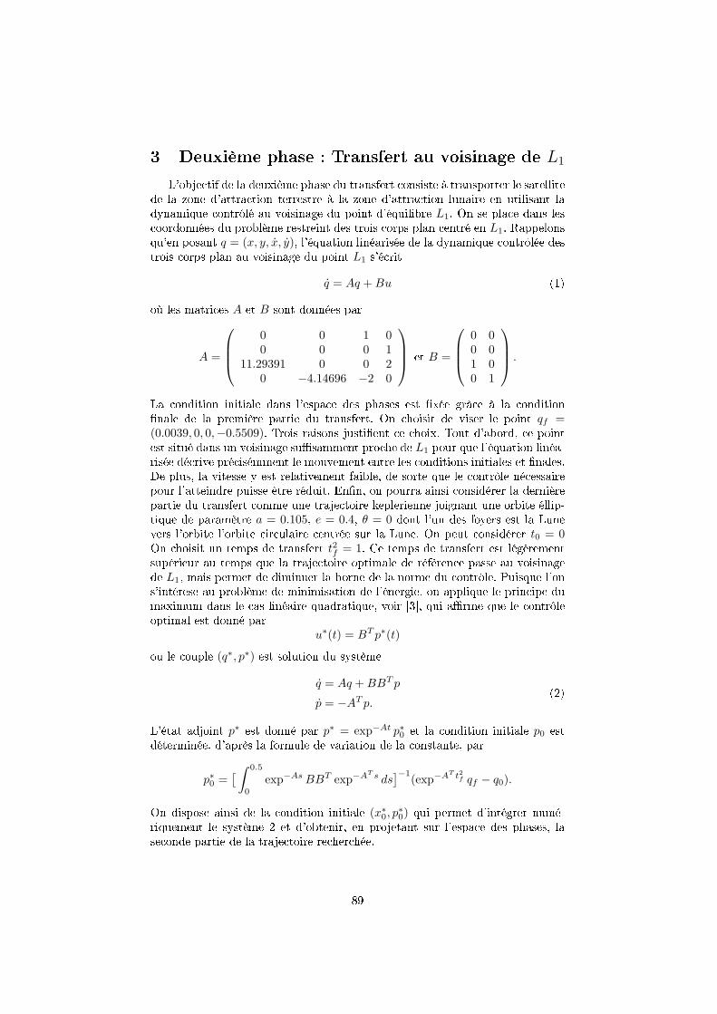
3 Deuxième phase : Transfert au voisinage de L1

L'objectif de la deuxième phase du transfert consiste à transporter le satellitede la zone d'attraction terrestre à la zone d'attraction lunaire en utilisant ladynamique contrôlé au voisinage du point d'équilibre L1. On se place dans lescoordonnées du problème restreint des trois corps plan centré en L1. Rappelonsqu'en posant q = (x, y, x, y), l'équation linéarisée de la dynamique contrôlée destrois corps plan au voisinage du point L1 s'écrit

q = Aq +Bu (1)

où les matrices A et B sont données par

A =

0 0 1 00 0 0 1

11.29391 0 0 20 −4.14696 −2 0

et B =

0 00 01 00 1

.

La condition initiale dans l'espace des phases est xée grâce à la conditionnale de la première partie du transfert. On choisit de viser le point qf =(0.0039, 0, 0,−0.5509). Trois raisons justient ce choix. Tout d'abord, ce pointest situé dans un voisinage susamment proche de L1 pour que l'équation linéa-risée décrive précisémment le mouvement entre les conditions initiales et nales.De plus, la vitesse y est relativement faible, de sorte que le contrôle nécessairepour l'atteindre puisse être réduit. Enn, on pourra ainsi considérer la dernièrepartie du transfert comme une trajectoire keplerienne joignant une orbite éllip-tique de paramètre a = 0.105, e = 0.4, θ = 0 dont l'un des foyers est la Lunevers l'orbite l'orbite circulaire centrée sur la Lune. On peut considérer t0 = 0On choisit un temps de transfert t2f = 1. Ce temps de transfert est légèrementsupérieur au temps que la trajectoire optimale de référence passe au voisinagede L1, mais permet de diminuer la borne de la norme du contrôle. Puisque l'ons'intérese au problème de minimisation de l'énergie, on applique le principe dumaximum dans le cas linéaire quadratique, voir [3], qui arme que le contrôleoptimal est donné par

u∗(t) = BT p∗(t)

ou le couple (q∗, p∗) est solution du système

q = Aq +BBT p

p = −AT p.(2)

L'état adjoint p∗ est donné par p∗ = exp−At p∗0 et la condition initiale p0 estdéterminée, d'après la formule de variation de la constante, par

p∗0 =[ ∫ 0.5

0

exp−AsBBT exp−AT s ds]−1

(exp−AT t2f qf − q0).

On dispose ainsi de la condition initiale (x∗0, p∗0) qui permet d'intégrer numé-

riquement le système 2 et d'obtenir, en projetant sur l'espace des phases, laseconde partie de la trajectoire recherchée.

89

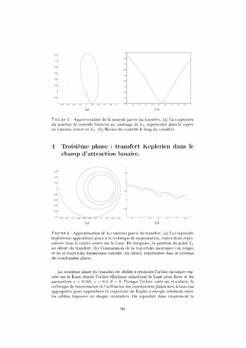
−0.08 −0.06 −0.04 −0.02 0 0.02 0.04 0.06 0.08 0.1

−0.02

0

0.02

0.04

0.06

0.08

0.1

0.12

(a)

0 0.1 0.2 0.3 0.4 0.5 0.6 0.7 0.8 0.9 10.05

0.1

0.15

0.2

0.25

0.3

0.35

0.4

0.45

0.5

(b)

Figure 2 Approximation de la seconde partie du transfert. (a) La trajectoiredu système de contrôle linéarisé au voisinage de L1, représentée dans le repèreen rotation centré en L1. (b) Norme du contrôle le long du transfert.

4 Troisième phase : transfert Keplerien dans le

champ d'attraction lunaire.

−0.14 −0.12 −0.1 −0.08 −0.06 −0.04 −0.02 0 0.02 0.04 0.06−0.1

−0.08

−0.06

−0.04

−0.02

0

0.02

0.04

0.06

(a)

1.5 2 2.5 3 3.5 4 4.5

−0.5

0

0.5

1

1.5

(b)

Figure 3 Approximation de la troisième partie du transfert. (a) La trajectoirekeplerienne approximée grace à la technique de moyennation, toutes deux repré-sentées dans le repère centré sur la Lune. En turquoise, la position du point L1

au début du transfert. (b) Comparaison de la trajectoire moyennée (en rouge)et de la trajectoire keplerienne calculée (en bleue), représentée dans le systèmede coordonnées plates.

La troisième phase du transfert est dédiée à rejoindre l'orbite circulaire cen-trée sur la Lune depuis l'orbite elliptique admettant la Lune pour foyer et lesparamètres a = 0.105, e = 0.4, θ = 0. Puisque l'orbite visée est circulaire, latechnique de moyennation et l'utilisation des coordonnées plates sont à nouveauappropriées pour approximer la trajectoire de Kepler à énergie minimale entreles orbites imposées en chaque extrémités. On reproduit donc exactement la

90

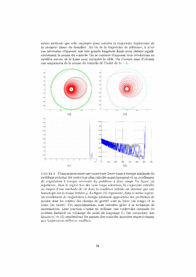
même méthode que celle employée pour calculer la trajectoire keplerienne dela première phase du transfert. Au vu de la trajectoire de référence, il n'estpas nécessaire d'imposer une très grande longitude nale pour réduire signi-cativement la norme du contrôle. On se contente d'imposer trois révolutions ausatellite autour de la Lune pour rejoindre la cible. On s'assure ainsi d'obtenirune majoration de la norme du contrôle de l'ordre de 1e− 1.

−1 −0.5 0 0.5 1

−0.8

−0.6

−0.4

−0.2

0

0.2

0.4

0.6

0.8

(a)

−1 −0.5 0 0.5 1−1

−0.8

−0.6

−0.4

−0.2

0

0.2

0.4

0.6

0.8

(b)

0 1 2 3 4 5 6 7 8 9

x 104

0

0.05

0.1

0.15

0.2

0.25

0.3

0.35

0.4

0.45

0.5

(c) (d)

Figure 4 Comparaison entre une trajectoire Terre-Lune à énergie minimale duproblème restreint des trois corps plan calculée numériquement et un recollementde trajectoires à énergie minimale du problème à deux corps. La gure (a)représente, dans le repère xe des trois corps restreints, la trajectoire calculéeau moyen d'une méthode de tir dont la condition initiale est obtenue par unehomotopie sur la masse réduite µ. La gure (b) représente, dans le même repère,un recollement de trajectoires à énergie minimale approchées des problèmes deKepler dont les centres des champs de gravité sont la Terre (en rouge) et laLune (en violet). Ces approximations sont calculées grâce à la technique demoyennation. Leur jonction s'opère en utilisant une trajectoire optimale dusystème linéarisé au voisinage du point de Lagrange L1 (en turquoise). Lesgures (c) et (d) représentent les normes des contrôles associées respectivementaux trajectoires réelles et recollées.

91

5 Conclusion

La méthode de recollement de trajectoires que nous présentons permet, grâceà des méthodes purement analytiques, la conception d'une approximation de tra-jectoire à énergie minimale du problème des trois corps restreint. Les similitudesphysiques des trajectoires obtenues numériquement au moyen de la méthode detir et par recollement, voir Fig. 4, attestent de la pertinence de cette techniquepour l'étude de la dynamique controlés du problème restreint des trois corps.Les coordonnées plates s'avèrent être un outil particulièrement ecace et élégantpour approximer les première et troisième phases d'une telle trajectoires, lorsquel'inuence d'une des deux primaires est prépondérante. On peut en outre, enchoisissant une longitude nale susamment élévée, xer l'ordre de grandeur ducontrôle appliqué de manière à imposer une poussée aussi faible que désirée. Lanorme du contrôle optimal le long de la deuxième phase du transfert, calculéeen résolvant le système controlé des trois corps plan linéarisé au voisinage depoint L1, est cependant signicativement plus élevée que celle du contrôle cal-culé par la méthode de tir, lors du passage entre les zones d'inuence de la Terreet de la Lune. Cette remarque illustre les limites de cette étude, qui fait gured'introduction à de nombreuses perspectives de travail et doit être notammentpoursuivie par une étude de l'optimalité globale des trajectoires obtenues parrecollement. L'utilisation du principe du maximum avec contraintes semble unoutil approprié pour traiter cette question. Les conditions géométriques assurantla continuité de l'état adjoint le long du transfert sont également à étudier.

Références

[1] B. Bonnard, J.B. Caillau and G. Picot Geometric and numerical techniques

in optimal control of the two and three body problems, Commun. Inf. Syst,10 (2010), to appear.

[2] Geroy, S. Généralisation des techniques de moyennation en contrôle opti-

mal. Application aux problèmes de transfert et rendez-vous orbitaux à pous-

sée faible. Phd thesis, Toulouse Univ., 1997.

[3] E.B. Lee and L. Markus. Fondations of optimal control theory Reprintedition, Krieger, 1986.

92

Shooting and numerical continuation

methods for computing time-minimal and

energy-minimal trajectories in

Earth-Moon transfer using low

propulsion.

G. Picot∗

Abstract. In this article we describe the principle of computations of opti-mal transfers between quasi-Keplerian orbits in the Earth-Moon system usinglow-propulsion. The spacecraft's motion is modelled by the equations of thecontrol restricted 3-body problem and we base our work on previous studiesconcerning the orbit transfer in the two-body problem where geometric and nu-meric methods were developped to compute optimal solutions. Using numericalsimple shooting and continuation methods connected with fundamental resultsfrom control theory, as the Pontryagin Maxium Principle and the second orderoptimality conditions related to the concept of conjugate points, we computetime-minimal and energy-minimal trajectories between the geostationary initialorbit and a nal circular one around the Moon, passing through the neigh-borhood of the libration point L1. Our computations give simple trajectories,obtained by referring to numerical values of the SMART-1 mission.

Key Words. Geometric control theory, numerical analysis method, 3-bodyproblem, Earth-Moon transfer, time minimization problem, energy minimiza-tion problem.

AMS subject classication. 49K15, 49M05, 70F07.

1 Introduction

The aim of this article is to study the optimal orbit transfer between quasi-Keplerian orbits in the Earth-Moon system when low propulsion is applied.This study is in particular motivated by the recent mission SMART-1 of theEuropean Space Agency, see [26, 27], which has already been investigated indepth, using for example simple feedback laws [7] or the transcription method[4]. Our model is the circular restricted 3-body problem [24] that has providedthe framework to numerous dynamical systems studies about space missiondesign in the solar system, see notably [19, 21]. The physical issue is to maximize

∗Mathematics Institute, Bourgogne University, 9 avenue Savary, F-21078 Dijon(gautier.picot@u-bourgogne.fr), supported by CNRS (contract no. 37244) and ConseilRégional de Bourgogne (contrat no. 079201PP02454515)

93

the nal mass of the spacecraft but, as a rst step, we restrict our analysis to thetime-minimal control problem and the so-called energy minimization problem,see also [13, 16, 17] for complementary results, for two reasons. First of all,the rst problem will provide an estimate about the time transfer. Second, theenergy minimization problem is a L2-regularization of the mass maximizationproblem which is a non smooth L1-problem. This regularization is known to bean important step in the analysis, see [18]. Our work is based on previous worksconcerning the orbit transfer between Keplerian orbit in the two-body problemwith low propulsion, see [15, 18], where geometric and numeric techniques weredeveloped to compute the optimal solutions. They are based on the so-calledindirect method in optimal control where optimal solutions are found among aset of extremal curves, solutions of the Pontryagin's Maximum Principle [25].This led to compute the solution using a shooting method where the solution iscomputed using a Newton method. In this framework, a continuation methodis used to solve the delicate problem of nding a precise enough initial solution,see [2].

The rst section of this article presents the main results from geometric con-trol theory connected to our analysis with adapted numerical codes developedto compute the solutions. First of all, the maximum principle is only a necessaryoptimality condition. In order to get necessary sucient optimality conditions(under generic assumptions) one must dene the concept of conjugate point,which was already introduced in the standard literature of calculus of variations[6] and can be generalized in optimal control, see for instance [1, 12]. If theHamiltonian optimal dynamics is described by a smooth Hamiltonian vector

eld−→H , conjugate points are the image of the singularities of the exponential

mapping : expq(0) : p(0) −→ Πq(exptf (−→H )(q(0), p(0))) where Πq : (q, p) −→ q

is the standard projection. Such a point can be numerically computed usingthe Cotcot code described in [8]. Besides, an important remark, in view ofthe use of the (smooth) continuation method in optimal control, is to observethat the shooting equation is precisely to nd p(0) such that expq(0)(p(0)) = q1where q1 is the terminal condition and the derivative can be generated using the

variational equation of−→H . This will lead to convergence results for the smooth

continuation method in optimal control, related to estimates of conjugate points[14].

The second section is devoted to present the system which is deduced fromthe standard circular restricted model where the two primaries are xed in arotating frame, see [24, 22, 30]. Up to a normalization the system can be writtenin the Hamiltonian form

z =−→H0(z) + u1

−→H1(z) + u2

−→H2(z)

where z = (q, p) ∈ R4 and−→H0 is the Hamiltonian vector eld corresponding to

the the drift

H0(z) =1

2(p21 + p22) + p1q2 − p2q1 −

1− µ

%1− µ

%2,

q being the position of the spacecraft, %1 representing the distance to the Earthwith mass 1− µ located at (−µ, 0) and %2 the distance to the Moon with massµ and located at (1 − µ, 0), while µ ' 0.012153 is a small parameter. The

94

Hamiltonian lifts associated with the control correspond to the functions

Hi(z) = −qi, for i = 1, 2

and ‖ u ‖ is bounded by ε.The third section deals with the time-minimal Earth-Moon transfer problem.

In that case, the norm of an extremal control is constant outside a set of measurezero, see [9]. A preliminary study will focus on the Earth-L1 transfer, whichprovides an approximation of the rst phase of the Earth-Moon transfer. Usingour geometric analysis, a locally minimizing extremal is numerically computedusing a continuation method on the control bound ε. Actually, the convergenceof the simple shooting method is easily obtained with large thrust, the transfertime being short, and provides a starting point to the continuation method, see[11]. This rst study naturally leads to the analysis of time-minimal Earth-Moontrajectories. In addition, we propose a time-minimal transfer strategy towardsthe Lagrange point L4, in order to compare, from the topological point of view,extremal trajectories associated with dierent targets. Finally, we proceed to anumerical verication of the relation of comparison between the rst conjugatetimes in the normal and abnormal cases, see [12]. .

The fourth section is devoted to the energy minimization of the Earth-Moontransfer. The parameter µ is small and this remark was used by Poincaré to

study the dynamics of the free motion described by−→H0, by making a deformation

of the case µ = 0 which corresponds to Kepler problem in rotating coordinates,see [23]. Inspired by this approach we propose a simple solution to the energy-minimal Earth-Moon transfer using low propulsion, after having investigatedthe Earth-L1 transfer case.

2 Numerical methods in optimal control.

2.1 Optimal control problem

Let M and U be two smooth manifolds of respective dimensions n and m.Consider the control system

q(t) = f(q(t), u(t)) (1)

where f : M × U −→ TM is smooth and u is a bounded measurable functiondened on [0, t(u)[⊂ R+ and valued in U . Let M0 and M1 be two subsets of M .

Denition 2.1. Let be q0 ∈M . One calls trajectory associated with the controlu the solution q(t, q0, u) of (1) starting from q0 at t = 0. For the sake ofsimplicity, such a trajectory can be denoted q(t). A control u is called anadmissible control on [0, tf ], with tf < t(u), if its associated trajectory satisesq0 ∈M0 and q(tf ) ∈M1. One denotes by Utf the set of these admissible controlsand denes the cost of q by

C(tf , u) =

∫ tf

0

f0(q(t), u(t))dt (2)

where f0 :M × U −→ R is smooth.

95

Solving the optimal control problem consists in determining an admissiblecontrol u such that C is minimized.

Denition 2.2. Let be q0 ∈M and tf > 0. The end-point mapping is denedby

Eq0,tf : Utf −→M

u −→ q(q0, tf , u).(3)

If Utf is endowed with the L∞ topology then the end-point mapping is smooth.Let us remark that, for every ε > 0, an admissible control u can be smoothlyextended to [0, tf + ε], provided the control is left continuous at tf .

Denition 2.3. Consider two distinct cases.

If the nal time is xed, q is said to be locally optimal in L∞ topology ifit is optimal in a neighborhood of u in L∞ topology.

If the nal time is not xed and the control is left continuous at tf , q(.) issaid to be locally optimal in L∞ topology if for each neighborhood V of uin L∞([0, tf+ε], U), for each η such that |η| ≤ ε and for each control v ∈ Vwhich satises E(q0, tf + η, v) = E(q0, tf , u) then C(tf + η, v) ≥ C(tf , u).

2.2 The Pontryagin's Maximum Principle

Consider the control system (1) and the cost (2). The Pontryagin's MaximumPrinciple [25] asserts that if the control u ∈ Utf is optimal then there exists p0

a nonpositive real and p an absolutely continuous mapping on [0, tf ] such thatp(t) ∈ T ∗

q(t)M , (p0, p) 6= (0, 0) and, almost everywhere on [0, tf ], there holds

q =∂H

∂p(q, p, p0, u), p = −∂H

∂q(q, p, p0, u), (4)

where H is dened by

H : T ∗M × R∗− × U −→ R

(q, p, p0, u) −→ p0f0(q, u)+ < p, f(q, u) > .

Moreover, the optimal control satises the maximization condition

H(q(t), p(t), p0, u(t)) = maxv∈U

H(q(t), p(t), p0, v) (5)

almost everywhere on [0, tf ]. If tf is not xed, there holds

maxv∈U

H(q(t), p(t), p0, v) = 0

for every t ∈ [0, tf ]. Finally, if M0 (resp. M1) is a regular submanifold of M ,the transversality condition is satised

p(0) ⊥ Tq(0)M0 (resp. p(tf ) ⊥ Tq(tf )M1).

Denition 2.4. One calls pseudo-Hamiltonian the mapping H and costate thefunction p. A solution (q, p, p0, u) of equations (4) and (5) is called an extremal.If p0 = 0, an extremal is said to be abnormal. Otherwise it is said to be normal.

96

Since the domain U is a manifold, restricting to a chart we may assume that,locally, U = Rm and the maximization condition leads to ∂H

∂u = 0. Express thefollowing assumption.

(L) (Strong Legendre condition) The quadratic form ∂2H∂u2 is negative denite

along the reference extremal.From the implicit function theorem, one deduces that extremal controls are

smooth functions ur(t) = ur(q(t), p(t)) in a neighborhood of u.

Denition 2.5. One denes the true Hamiltonian, denoted Hr, by

Hr(q, p) = H(q, p, ur(q, p)).

Then any extremal is solution of the Hamiltonian system

q =∂Hr

∂p(q, p), p = −∂Hr

∂q(q, p). (6)

Denoting z = (q, p), this system writes

z =−→Hr(z(t)). (7)

2.3 Second order optimality condition

Let us briey present the concept of geometric conjugate time which is relatedto a second order optimality condition, see [8] for the details. Consider a smoothmanifold M of dimension n and denote Πq : T ∗M −→ M the standard projec-

tion from the cotangent bundle T ∗M on M . Let−→H be an Hamiltonian vector

eld on T ∗M and z(t) = (q(t), p(t)) a trajectory of−→H dened on [0, tf ] so that

there holds z(t) =−→H (z(t)) for each t ∈ [0, tf ].

Denition 2.6. The variational equation on [0, tf ]

δz(t) = d−→H (z(t)).δz(t) (8)

is called the Jacobi equation along z(.). One calls a Jacobi eld a nontrivialsolution J(t) of the Jacobi equation along z(.) and it is said to be vertical atthe time t if dΠq(z(t)).J(t) = 0. A time tc is said to be geometrically conjugateif there exists a Jacobi eld vertical at 0 and tc. In which case, q(tc) is said tobe conjugate to q(0).

Let us point out that, in local coordinates, one can write a Jacobi eldJ(t) = (δq(t), δp(t)). Then J is vertical at the time t whenever δq(t) = 0. Whenthe nal target is a regular submanifold M1 ⊂M , the notion of conjugate timeis generalized as follows.

Denition 2.7. Denote M⊥1 = (q, p), q ∈ M1, p ⊥ TqM1. Then a time

tfoc ∈ [0, T ] is said to be a focal time if there exists a Jacobi eld J = (δq, δp)such that δq(tfoc) = 0 and J(tfoc) is tangent to M

⊥1 .

Denition 2.8. Let be z0 ∈ T ∗M . For each t ∈ [0, tf ], one denes the expo-nential mapping by

expt : z0 −→ Πq(z(t, z0))

where z(t, z0) is the trajectory of−→H satisfying z(0, z0) = z0.

97

Using local coordinates and setting z0 = (q0, p0) ∈ T ∗M , one can writez(t, q0, p0) = (q(t, q0, p0), p(t, q0, p0)). Setting q0 ∈ M as the initial condition,

the exponential mapping writes expq0,t(p0) = q(t, q0, p0). Let expt(−→H ) be the

ow of−→H . The following proposition results from a geometrical interpretation

of the Jacobi equation.

Proposition 2.1. Let be q0 ∈M , L0 = T ∗q0M and Lt = expt(

−→H )(L0). Then Lt

is a Lagrangian submanifold of T ∗M whose tangent space is spanned by Jacobields starting from L0. Moreover q(tc) is geometrically conjugate to q0 if andonly if expq0,tc is not an immersion at p0.

The following proposition, see [10], will be used to formulate the relevantgeneric assumptions.

Proposition 2.2. An extremal control is a singularity of the end-point map-ping when the set of admissible controls U is endowed with the L∞-topology.Moreover, the adjoint vector p(t) is orthogonal to the image of DuEq0,t.

The following assumptions is needed to derive second order optimality con-ditions in the normal case.

(S) (Strong regularity) On every subinterval of [0, tf ], the control u is ofcorank 1.

As a result, one can enunciate the following crucial theorem which connectsthe notion of conjugate time and the local optimality of extremals, see [1, 12, 28].

Theorem 2.1. Let t1c be the rst conjugate time along z. Under previous as-sumptions, the trajectory q(.) is locally optimal on [0, t1c) in L∞ topology; ift > t1c then q(.) is not locally optimal on [0, t].

2.4 Simple shooting method

We previously stated that the maximization and strong Legendre conditions en-able to write locally any extremal control as ur(t) = ur(q(t), p(t)), the extremal

system becoming z =−→Hr(z(t)) where z = (q, p). Expressing boundary and

transversality conditions by R(z(0), z(tf )) = 0, the boundary values problembecomes

z =−→Hr(z(t))

R(z(0), z(tf )) = 0.(9)

The initial condition q0 is xed which leads to the following denition.

Denition 2.9. Assume that the transfer time tf is xed. One calls shootingfunction the mapping E dened by

E : p0 −→ R(z0, ztf ).

It is important to notice that whenever one considers an optimal controlproblem with a non-xed transfer time, the corresponding shooting functionapplies on (tf , p0). Moreover, the conditionHr = 0 from the maximum principleprovides one additional equation.

Hence solving the boundary values system is equivalent to nding a zero of E,that is to say solving the so-called shooting equation. Since ur(q, p) is smooth,

98

E is smooth and such a zero can be found using a Newton type algorithm,providing that one has a precise initial guess of it. The continuation method isappropriate to overcome this diculty.

2.5 Smooth continuation method

Without loss of generality, one can assume that the nal time tf is xed andthe nal condition is written qf = q1, the following results being adaptableto other cases. The smooth continuation method consists in considering thereduced Hamiltonian Hr as the element H1 of a family (Hλ)λ∈[0,1] of smoothHamiltonians. One thus builds up a one-parameter family of shooting functions

Eλ(p0) = expλq0,tf (p0)− q1

Considering the normal case, the following theorem is deduced from the implicitfunction theorem, see [14].

Theorem 2.2. For each λ the exponential mapping expλq0 is of maximal rank

if and only if the point q1 = expλq0,tf (p(0)) is non-conjugate to q0. Moreover,solutions of the parametrized shooting equation contain a smooth curve, whichcan be parametrized by λ and the derivative E

′

λ can be computed integrating theJacobi equation.

For more details, in paticular about geometric considerations relative to thistheorem, one can refer to [20]. The scheme of the smooth continuation methodto compute solutions of the shooting equation is the following :

1. One determines the starting point p0 of the continuation method using asimple shooting. Setting λ = 0, one computes the extremal z(t) on [0, tf ]starting from (q0, p0).

2. One chooses a discretization 0=λ0, λ1,. . . , λN=1 such that the shootingfunction is solved iteratively at λi+1 from λi.

3. One builds up the nite sequence p0,. . . , pN with zeros of shooting func-tions Eλ0 ,. . . , EλN

.

From theorem 2.2, a crucial point to guarantee the convergence of the smoothcontinuation method is to check the lack of conjugate points along each extremalzλ on [0, tf ], which must be iteratively performed.

2.6 Numeric methods

They are implemented in the COTCOT (Conditions of Order Two, COnjugateTimes) whose aim is to provide the numerical tool :

• to integrate the smooth Hamiltonian vector eld−→Hn,

• to solve the associated shooting equation,

• to compute the corresponding Jacobi elds along the extremals,

• to evaluate the resulting conjugate points.

99

The code is written in Fortran language, while automatic dierentiation pro-vided by the software Adifor [5] is used to generate the Hamiltonian dierentialequation and the variational one. For the users the language is Matlab, see [9] fora precise description of the Cotcot code, with the underlying algorithms: NetlibRunge-Kutta one-step ODE integrator [29], Netlib HYBRD Newton solver. Theconjugate point test consists in checking a rank condition which is based on twomethods: evaluating zeros of a determinant or a SVD ( Singular Value Decom-position). The continuation method will be included in the code which can bea simple discretization of the homotopy path, with a Newton method at eachstep or a numeric continuation of the path, using the implicit ODE, where theNewton method is used only at the rst step to initialize the continuation andat the nal step, to solve the nal shooting equation with arbitrary accuracy.

3 The restricted 3-body problem

3.1 The circular restricted 3-body problem in Jacobi co-

ordinates

Recall the following representation of the Earth-Moon problem, see [24, 30]. Inthe rotating frame, the Earth which is the biggest primary planet with mass1− µ is located at (−µ, 0) while the Moon with mass µ, is located at (1− µ, 0)with the small parameter µ ' 0.012153. We note z = x+ iy the position of thespacecraft and %1, %2 are the distances to the primaries

%1 =√(

(x+ µ)2 + y2), %2 =

√((x− 1 + µ)2 + y2

).

The equation of motion takes the form

z + 2iz − z = −(1− µ)z + µ

%31− µ

z − 1 + µ

%32(10)

which can be written x− 2y − x = ∂V

∂x

y + 2x− y = ∂V∂y

(11)

where −V is the potential of the system dened by V = 1−µ%31

+ µ%32. The system

can be written using Hamiltonian formalism setting

q1 = x, q2 = y, p1 = x− y, p2 = y + x

and the Hamiltonian describing the motion takes the form

H0(q1, q2, p1, p2) =1

2(p21 + p22) + p1q2 − p2q1 −

1− µ

%1− µ

%2.

3.2 Equilibrium points

The equilibrium points of the problem are well known. They split in two dierenttypes :

100

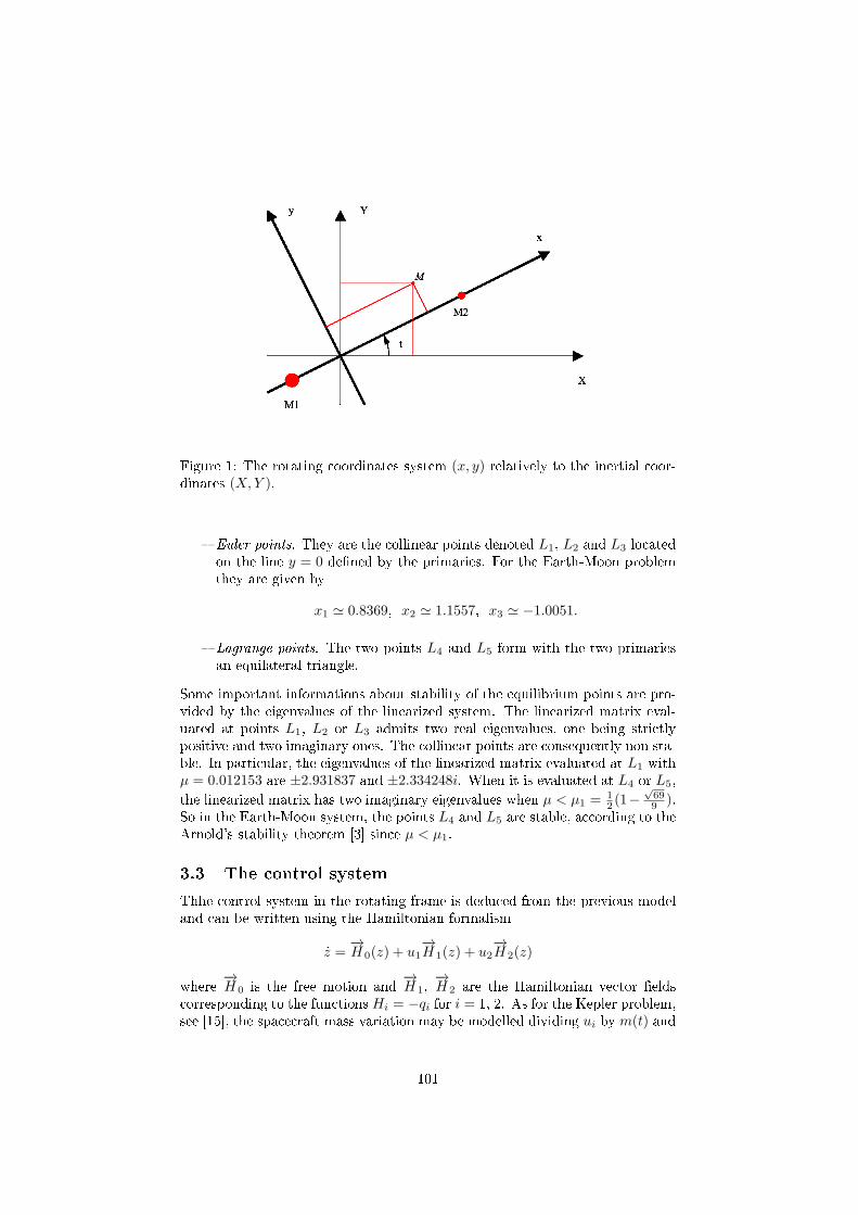
Figure 1: The rotating coordinates system (x, y) relatively to the inertial coor-dinates (X,Y ).

Euler points. They are the collinear points denoted L1, L2 and L3 locatedon the line y = 0 dened by the primaries. For the Earth-Moon problemthey are given by

x1 ' 0.8369, x2 ' 1.1557, x3 ' −1.0051.

Lagrange points. The two points L4 and L5 form with the two primariesan equilateral triangle.

Some important informations about stability of the equilibrium points are pro-vided by the eigenvalues of the linearized system. The linearized matrix eval-uated at points L1, L2 or L3 admits two real eigenvalues, one being strictlypositive and two imaginary ones. The collinear points are consequently non sta-ble. In particular, the eigenvalues of the linearized matrix evaluated at L1 withµ = 0.012153 are ±2.931837 and ±2.334248i. When it is evaluated at L4 or L5,

the linearized matrix has two imaginary eigenvalues when µ < µ1 = 12 (1−

√699 ).

So in the Earth-Moon system, the points L4 and L5 are stable, according to theArnold's stability theorem [3] since µ < µ1.

3.3 The control system

Thhe control system in the rotating frame is deduced from the previous modeland can be written using the Hamiltonian formalism

z =−→H 0(z) + u1

−→H 1(z) + u2

−→H 2(z)

where−→H 0 is the free motion and

−→H 1,

−→H 2 are the Hamiltonian vector elds

corresponding to the functions Hi = −qi for i = 1, 2. As for the Kepler problem,see [15], the spacecraft mass variation may be modelled dividing ui by m(t) and

101

considering the equation m = −δ|u|. This will not be taken into account andwe will focus on both time-minimal transfer problem

minu(.)∈BR2 (0,ε)

∫ tf

t0

dt (12)

where ε is the maximum thrust allowed by spacecraft's engines and energy-minimal transfer problem

minu(.)∈R2

∫ tf

t0

u21 + u22dt

when the transfer time tf is xed and the constraint on the control boundis relaxed. The rst problem will provide an estimation of the Earth-Moontransfer time when low thrust is used. The energy minimization problem willgive a starting point in order to perform a homotopy method relating the nalspacecraft mass maximization problem and the energy minimization problem

minu(.)

∫ tf

0

(λ|u|2 + (1− λ)|u|)dt, λ ∈ [0, 1].

4 Time-minimal transfers in the Earth-Moon sys-

tem

4.1 Normal case

4.1.1 Generalities on the normal case

Let us recall fundamental results about time-minimal control problems. Con-sider a bi-input control system on Rn

q = F0(q) + ε2∑

i=1

uiFi(q), ε > 0, u21 + u22 ≤ 1 (13)

and the time-minimal problem

minu(.)∈BR2 (0,1)

∫ tf

t0

dt.

Then the pseudo-Hamiltonian from the maximum principle is

H(z, u) = p0 +H0(z) + ε(u1H1(z) + u2H2(z))

where z = (q, p) ∈ T ∗Rn and

Hi(z) =< p, Fi(q) >, i = 0, . . . , 2.

The maximization condition implies that when (H1,H2) 6= (0, 0), the control uis given by

ui =Hi√

H21 +H2

2

, i = 1, 2.

In the normal case p0 6= 0, one can normalize p0 to -1 and so

Hr(z) = −1 +H0(z) + ε√(H2

1 (z) +H22 (z)).

Since the transfer time is not xed, Hr is identically zero on [0, tf ].

102

Denition 4.1. One calls switching surface the set

Σ = z ∈ T ∗Rn, H1(z) = H2(z) = 0.

One calls point of order 0 an element z ∈ T ∗Rn\Σ and point of order 1 anelement z ∈ Σ such that (H1(z), H2(z)) 6= 0.

In particular, an extremal control belongs to the unit circle S1 outside theswitching surface. Consider the specic case q ∈ R4. Under specic conditions,we have the following result, see [9] for the complete proof.

Proposition 4.1. At a point of order 1, the control u instantaneously rotatesof an angle π i.e. u(t+) = −u(t−).

The following proposition is a corollary of the above result.

Proposition 4.2. Each normal time-minimal trajectory is a concatenation ofa nite number of arcs of order 0 with π-singularities at junction points.

As we will see in the section 4.1.3, the second order system of controlledequations of motion in the circular 3-body problem can be expressed as a bi-input system in R4 with

F1 =∂

∂q3, F2 =

∂

∂q4.

Conditions of the proposition 4.2 are consequently fullled, see [9], that allowsto use a continuation method on the control bound to compute time-minimalEarth-Moon trajectories.

4.1.2 Continuation method on the control bound

Considering a bi-input control system on R4 satisfying some regularity proper-ties, proposition 4.2 asserts that the control corresponding to a time-minimaltrajectory has a constant norm outside a set of measure zero. Such regular-ity properties are satised regarding the orbital transfer control in the Keplerproblem, justifying the numerical continuation method on the control bound,see [15] and [18]. We statued that the same justication holds in the case ofthe restricted 3-body problem and we use the numerical continuation methodto compute time-minimal extremals with low-thrust.By choosing the parameterε corresponding to a large enough value, the time transfer is short and the sim-ple shooting method directly converges on a starting point of the continuationmethod. Mention that our numerical study results in computing only extremalsof order 0. Consequently, the time minimal extremal control vectors we de-termined are continuous along the transfer time. However, it is clear that thesimple shooting and the continuation method can be performed with extremalsof order one, providing the use of an adaptive integration step. As a preliminarystudy, we will focus on the Earth-L1 transfer which is a good representation ofthe rst phase of the Earth-Moon transfer. By simplifying the nal condition,we make the simple shooting and the numerical continuation easier. So we com-pute more precise approximations of time-minimal extremals of the Earth-Moontransfer.

103

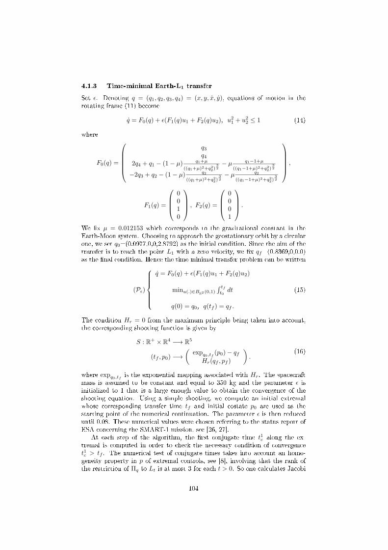
4.1.3 Time-minimal Earth-L1 transfer

Set ε. Denoting q = (q1, q2, q3, q4) = (x, y, x, y), equations of motion in therotating frame (11) become

q = F0(q) + ε(F1(q)u1 + F2(q)u2), u21 + u22 ≤ 1 (14)

where

F0(q) =

q3q4

2q4 + q1 − (1− µ) q1+µ

((q1+µ)2+q22)32− µ q1−1+µ

((q1−1+µ)2+q22)32

−2q3 + q2 − (1− µ) q2

((q1+µ)2+q22)32− µ q2

((q1−1+µ)2+q22)32

,

F1(q) =

0010

, F2(q) =

0001

.

We x µ = 0.012153 which corresponds to the gravitational constant in theEarth-Moon system. Choosing to approach the geostationary orbit by a circularone, we set q0=(0.0977,0,0,2.8792) as the initial condition. Since the aim of thetransfer is to reach the point L1 with a zero velocity, we x qf=(0.8369,0,0,0)as the nal condition. Hence the time-minimal transfer problem can be written

(Pε)

q = F0(q) + ε(F1(q)u1 + F2(q)u2)

minu(.)∈BR2 (0,1)

∫ tft0dt

q(0) = q0, q(tf ) = qf .

(15)

The condition Hr = 0 from the maximum principle being taken into account,the corresponding shooting function is given by

S : R+ × R4 −→ R5

(tf , p0) −→(

expq0,tf (p0)− qfHr(qf , pf )

).

(16)

where expq0,tf is the exponential mapping associated with Hr. The spacecraftmass is assumed to be constant and equal to 350 kg and the parameter ε isinitialized to 1 that is a large enough value to obtain the convergence of theshooting equation. Using a simple shooting, we compute an initial extremalwhose corresponding transfer time tf and initial costate p0 are used as thestarting point of the numerical continuation. The parameter ε is then reduceduntil 0.08. These numerical values were chosen referring to the status report ofESA concerning the SMART-1 mission, see [26, 27].

At each step of the algorithm, the rst conjugate time t1c along the ex-tremal is computed in order to check the necessary condition of convergencet1c > tf . The numerical test of conjugate times takes into account an homo-geneity property in p of extremal controls, see [8], involving that the rank ofthe restriction of Πq to Lt is at most 3 for each t > 0. So one calculates Jacobi

104

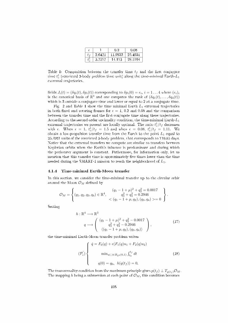
ε 1 0.2 0.08tf 2.6421 11.9533 25.4931t1c 3.7217 14.113 28.5194

Table 1: Comparision between the transfer time tf and the rst conjugatetime t1c (restricted 3-body problem time unit) along the time-minimal Earth-L1

extremal trajectories.

elds Ji(t) = (δqi(t), δpi(t)) corresponding to δpi(0) = ei, i = 1 . . . 4 where (ei)iis the canonical basis of R4 and one computes the rank of (δq1(t), . . . , δq4(t))which is 3 outside a conjugate time and lower or equal to 2 at a conjugate time.

Fig. 2 and Table 1 show the time-minimal Earth-L1 extremal trajectoriesin both xed and rotating frames for ε = 1, 0.2 and 0.08 and the comparisonbetween the transfer time and the rst conjugate time along these trajectories.According to the second order optimality condition, the time-minimal Earth-L1

extremal trajectories we present are locally optimal. The ratio t1c/tf decreaseswith ε. When ε = 1, t1c/tf = 1.5 and when ε = 0.08, t1c/tf = 1.11. Weobtain a low-propulsion transfer time from the Earth to the point L1 equal to25.4931 units of the restricted 3-body problem, that corresponds to 110.85 days.Notice that the extremal transfers we compute are similar to transfers betweenKeplerian orbits when the Earth's inluence is predominant and during whichthe pericenter argument is constant. Futhermore, for information only, let usmention that this transfer time is approximately ve times lower than the timeneeded during the SMART-1 mission to reach the neighborhood of L1.

4.1.4 Time-minimal Earth-Moon transfer

In this section, we consider the time-minimal transfer up to the circular orbitaround the Moon OM dened by

OM =

(q1, q2, q3, q4) ∈ R4,(q1 − 1 + µ)2 + q22 = 0.0017

q23 + q24 = 0.2946< (q1 − 1 + µ, q2), (q3, q4) >= 0

.

Setting

h : R4 −→ R3

q −→

(q1 − 1 + µ)2 + q22 − 0.0017q23 + q24 − 0.2946

〈(q1 − 1 + µ, q2), (q3, q4)〉

,(17)

the time-minimal Earth-Moon transfer problem writes

(P′

ε)

q = F0(q) + ε(F1(q)u1 + F2(q)u2)

minu(.)∈BR2 (0,1)

∫ tft0dt

q(0) = q0, h(q(tf )) = 0.

(18)

The transversality condition from the maximum principle gives p(tf ) ⊥ Tq(tf )OM .The mapping h being a submersion at each point of OM , this condition becomes

105

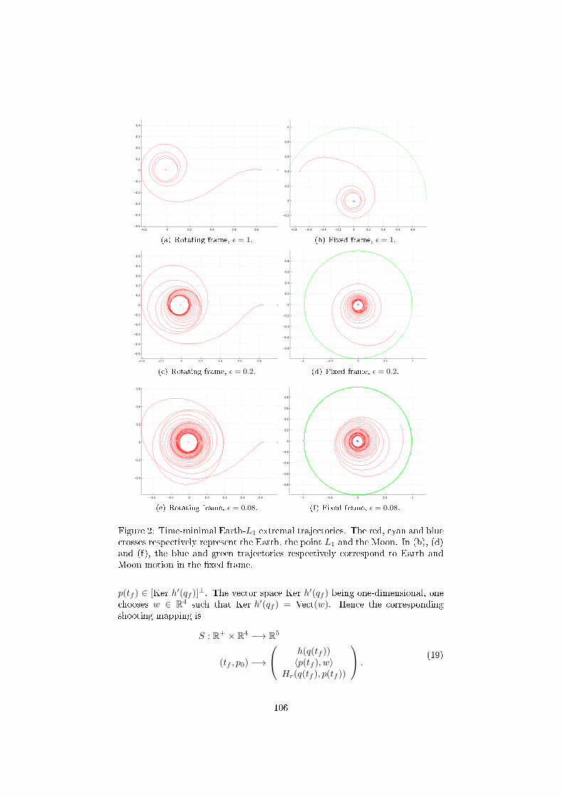
−0.2 0 0.2 0.4 0.6 0.8−0.5

−0.4

−0.3

−0.2

−0.1

0

0.1

0.2

0.3

0.4

(a) Rotating frame, ε = 1.

−0.8 −0.6 −0.4 −0.2 0 0.2 0.4 0.6 0.8

−0.2

0

0.2

0.4

0.6

0.8

1

(b) Fixed frame, ε = 1.

−0.4 −0.2 0 0.2 0.4 0.6 0.8

−0.5

−0.4

−0.3

−0.2

−0.1

0

0.1

0.2

0.3

0.4

0.5

(c) Rotating frame, ε = 0.2.

−1 −0.5 0 0.5 1

−0.8

−0.6

−0.4

−0.2

0

0.2

0.4

0.6

0.8

(d) Fixed frame, ε = 0.2.

−0.4 −0.2 0 0.2 0.4 0.6 0.8

−0.4

−0.2

0

0.2

0.4

0.6

(e) Rotating frame, ε = 0.08.

−1 −0.5 0 0.5 1

−0.8

−0.6

−0.4

−0.2

0

0.2

0.4

0.6

0.8

(f) Fixed frame, ε = 0.08.

Figure 2: Time-minimal Earth-L1 extremal trajectories. The red, cyan and bluecrosses respectively represent the Earth, the point L1 and the Moon. In (b), (d)and (f), the blue and green trajectories respectively correspond to Earth andMoon motion in the xed frame.

p(tf ) ∈ [Ker h′(qf )]⊥. The vector space Ker h′(qf ) being one-dimensional, one

chooses w ∈ R4 such that Ker h′(qf ) = Vect(w). Hence the correspondingshooting mapping is

S : R+ × R4 −→ R5

(tf , p0) −→

h(q(tf ))〈p(tf ), w〉

Hr(q(tf ), p(tf ))

.(19)

106

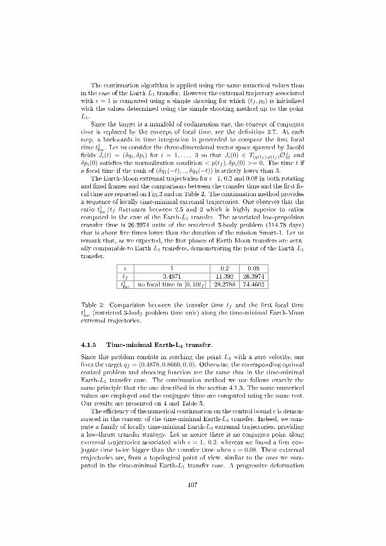
The continuation algorithm is applied using the same numerical values thanin the case of the Earth-L1 transfer. However the extremal trajectory associatedwith ε = 1 is computed using a simple shooting for which (tf , p0) is initializedwith the values determined using the simple shooting method up to the pointL1.

Since the target is a manifold of codimension one, the concept of conjugatetime is replaced by the concept of focal time, see the denition 2.7. At eachstep, a backwards in time integration is proceeded to compute the rst focaltime t1

foc. Let us consider the three-dimensional vector space spanned by Jacobi

elds Ji(t) = (δqi, δpi) for i = 1, . . . , 3 so that Ji(0) ∈ T(q(tf ),p(tf )O⊥M and

δpi(0) satises the normalization condition < p(tf ), δpi(0) >= 0. The time t ifa focal time if the rank of (δq1(−t), .., δq4(−t)) is strictly lower than 3.

The Earth-Moon extremal trajectories for ε=1, 0.2 and 0.08 in both rotatingand xed frames and the comparisons between the transfer time and the rst fo-cal time are reported on Fig.3 and on Table 2. The continuation method providesa sequence of locally time-minimal extremal trajectories. One observes that theratio t1

foc/tf uctuates between 2.5 and 3 which is highly superior to ratios

computed in the case of the Earth-L1 transfer. The associated low-propulsiontransfer time is 26.3974 units of the restricted 3-body problem (114.78 days)that is about ve times lower than the duration of the mission Smart-1. Let usremark that, as we expected, the rst phases of Earth-Moon transfers are actu-ally comparable to Earth-L1 transfers, demonstrating the point of the Earth-L1

transfer.

ε 1 0.2 0.08tf 3.4971 11.392 26.3974t1foc

no focal time in [0, 10tf ] 28.2788 74.4602

Table 2: Comparision between the transfer time tf and the rst focal timet1foc

(restricted 3-body problem time unit) along the time-minimal Earth-Moonextremal trajectories.

4.1.5 Time-minimal Earth-L4 transfer.

Since this problem consists in reaching the point L4 with a zero velocity, onexes the target qf = (0.4878, 0.8660, 0, 0). Otherwise, the corresponding optimalcontrol problem and shooting function are the same that in the time-minimalEarth-L1 transfer case. The continuation method we use follows exactly thesame principle that the one described in the section 4.1.3. The same numericalvalues are employed and the conjugate time are computed using the same test.Our results are presented on 4 and Table 3.

The eciency of the numerical continuation on the control bound ε is demon-strated in the context of the time-minimal Earth-L4 transfer. Indeed, we com-pute a family of locally time-minimal Earth-L4 extremal trajectories, providinga low-thrust transfer strategy. Let us notice there is no conjugate point alongextremal trajectories associated with ε = 1, 0.2, whereas we found a rst con-jugate time twice bigger than the transfer time when ε = 0.08. These extremaltrajectories are, from a topological point of view, similar to the ones we com-puted in the time-minimal Earth-L1 transfer case. A progressive deformation

107

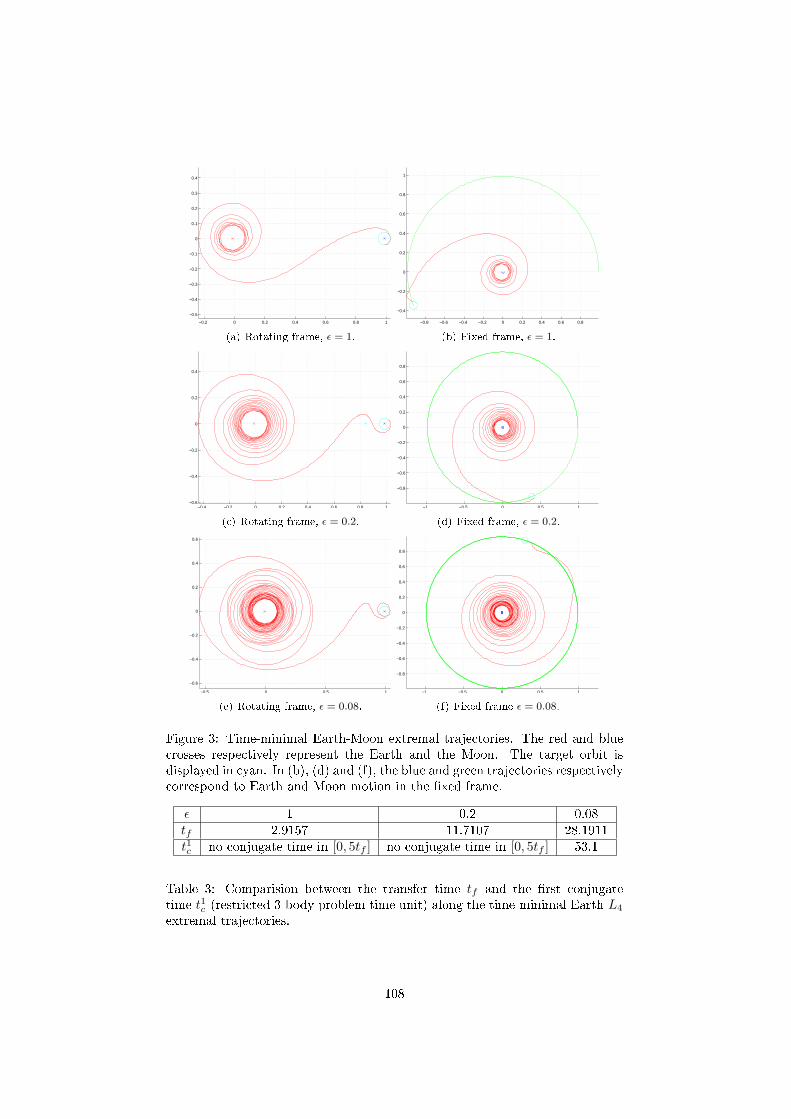
−0.2 0 0.2 0.4 0.6 0.8 1

−0.5

−0.4

−0.3

−0.2

−0.1

0

0.1

0.2

0.3

0.4

(a) Rotating frame, ε = 1.

−0.8 −0.6 −0.4 −0.2 0 0.2 0.4 0.6 0.8

−0.4

−0.2

0

0.2

0.4

0.6

0.8

1

(b) Fixed frame, ε = 1.

−0.4 −0.2 0 0.2 0.4 0.6 0.8 1−0.6

−0.4

−0.2

0

0.2

0.4

(c) Rotating frame, ε = 0.2.

−1 −0.5 0 0.5 1

−0.8

−0.6

−0.4

−0.2

0

0.2

0.4

0.6

0.8

(d) Fixed frame, ε = 0.2.

−0.5 0 0.5 1

−0.6

−0.4

−0.2

0

0.2

0.4

0.6

(e) Rotating frame, ε = 0.08.

−1 −0.5 0 0.5 1

−0.8

−0.6

−0.4

−0.2

0

0.2

0.4

0.6

0.8

(f) Fixed frame ε = 0.08.

Figure 3: Time-minimal Earth-Moon extremal trajectories. The red and bluecrosses respectively represent the Earth and the Moon. The target orbit isdisplayed in cyan. In (b), (d) and (f), the blue and green trajectories respectivelycorrespond to Earth and Moon motion in the xed frame.

ε 1 0.2 0.08tf 2.9157 11.7107 28.1911t1c no conjugate time in [0, 5tf ] no conjugate time in [0, 5tf ] 53.1

Table 3: Comparision between the transfer time tf and the rst conjugatetime t1c (restricted 3-body problem time unit) along the time-minimal Earth-L4

extremal trajectories.

108

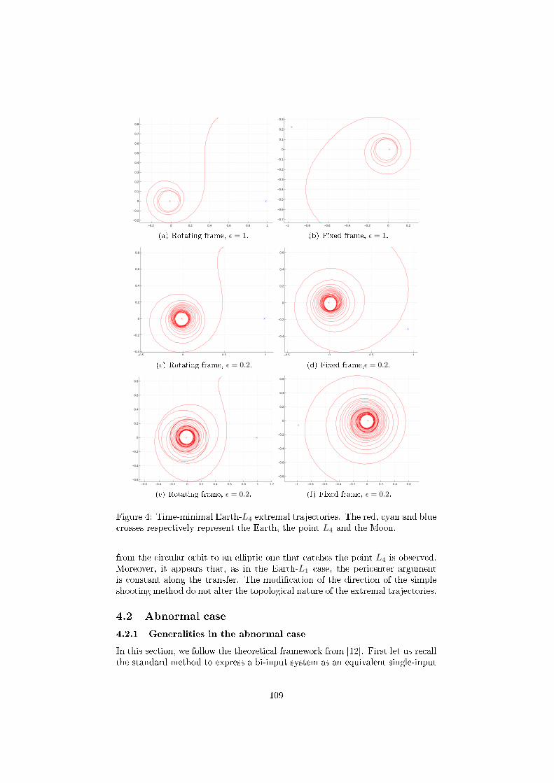
−0.2 0 0.2 0.4 0.6 0.8 1

−0.2

−0.1

0

0.1

0.2

0.3

0.4

0.5

0.6

0.7

0.8

(a) Rotating frame, ε = 1.

−1 −0.8 −0.6 −0.4 −0.2 0 0.2

−0.7

−0.6

−0.5

−0.4

−0.3

−0.2

−0.1

0

0.1

0.2

0.3

(b) Fixed frame, ε = 1.

−0.5 0 0.5 1−0.4

−0.2

0

0.2

0.4

0.6

0.8

(c) Rotating frame, ε = 0.2.

−0.5 0 0.5 1

−0.4

−0.2

0

0.2

0.4

0.6

(d) Fixed frame,ε = 0.2.

−0.6 −0.4 −0.2 0 0.2 0.4 0.6 0.8 1 1.2

−0.6

−0.4

−0.2

0

0.2

0.4

0.6

0.8

(e) Rotating frame, ε = 0.2.

−1 −0.8 −0.6 −0.4 −0.2 0 0.2 0.4 0.6

−0.8

−0.6

−0.4

−0.2

0

0.2

0.4

0.6

(f) Fixed frame, ε = 0.2.

Figure 4: Time-minimal Earth-L4 extremal trajectories. The red, cyan and bluecrosses respectively represent the Earth, the point L4 and the Moon.

from the circular orbit to an elliptic one that catches the point L4 is observed.Moreover, it appears that, as in the Earth-L1 case, the pericenter argumentis constant along the transfer. The modication of the direction of the simpleshooting method do not alter the topological nature of the extremal trajectories.

4.2 Abnormal case

4.2.1 Generalities in the abnormal case

In this section, we follow the theoretical framework from [12]. First let us recallthe standard method to express a bi-input system as an equivalent single-input

109

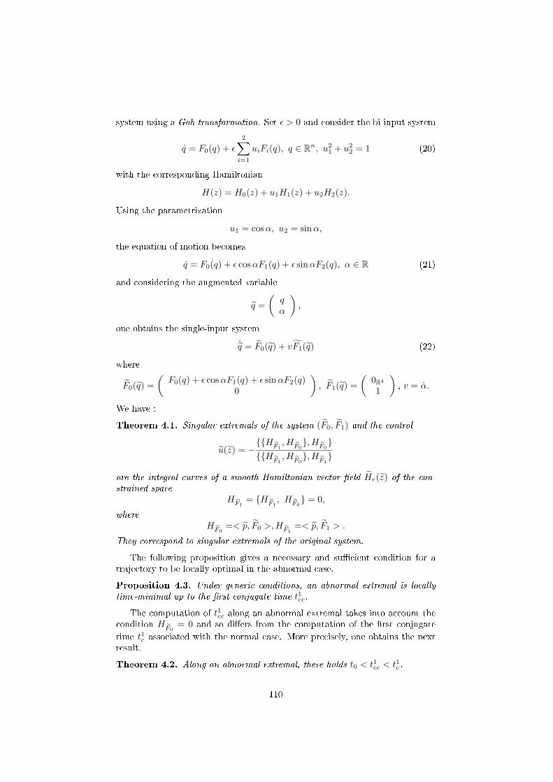
system using a Goh transformation. Set ε > 0 and consider the bi-input system

q = F0(q) + ε2∑

i=1

uiFi(q), q ∈ Rn, u21 + u22 = 1 (20)

with the corresponding Hamiltonian

H(z) = H0(z) + u1H1(z) + u2H2(z).

Using the parametrization

u1 = cosα, u2 = sinα,

the equation of motion becomes

q = F0(q) + ε cosαF1(q) + ε sinαF2(q), α ∈ R (21)

and considering the augmented variable

q =

(qα

),

one obtains the single-input system

˙q = F0(q) + vF1(q) (22)

where

F0(q) =

(F0(q) + ε cosαF1(q) + ε sinαF2(q)

0

), F1(q) =

(0R4

1

), v = α.

We have :

Theorem 4.1. Singular extremals of the system (F0, F1) and the control

u(z) = −HF1

,HF0,HF0

HF1

,HF0,HF1

are the integral curves of a smooth Hamiltonian vector eld Hr(z) of the con-strained space

HF1= HF1

, HF0 = 0,

whereHF0

=< p, F0 >,HF1=< p, F1 > .

They correspond to singular extremals of the original system.

The following proposition gives a necessary and sucient condition for atrajectory to be locally optimal in the abnormal case.

Proposition 4.3. Under generic conditions, an abnormal extremal is locallytime-minimal up to the rst conjugate time t1cc.

The computation of t1cc along an abnormal extremal takes into account thecondition HF0

= 0 and so diers from the computation of the rst conjugate

time t1c associated with the normal case. More precisely, one obtains the nextresult.

Theorem 4.2. Along an abnormal extremal, there holds t0 < t1cc < t1c.

110

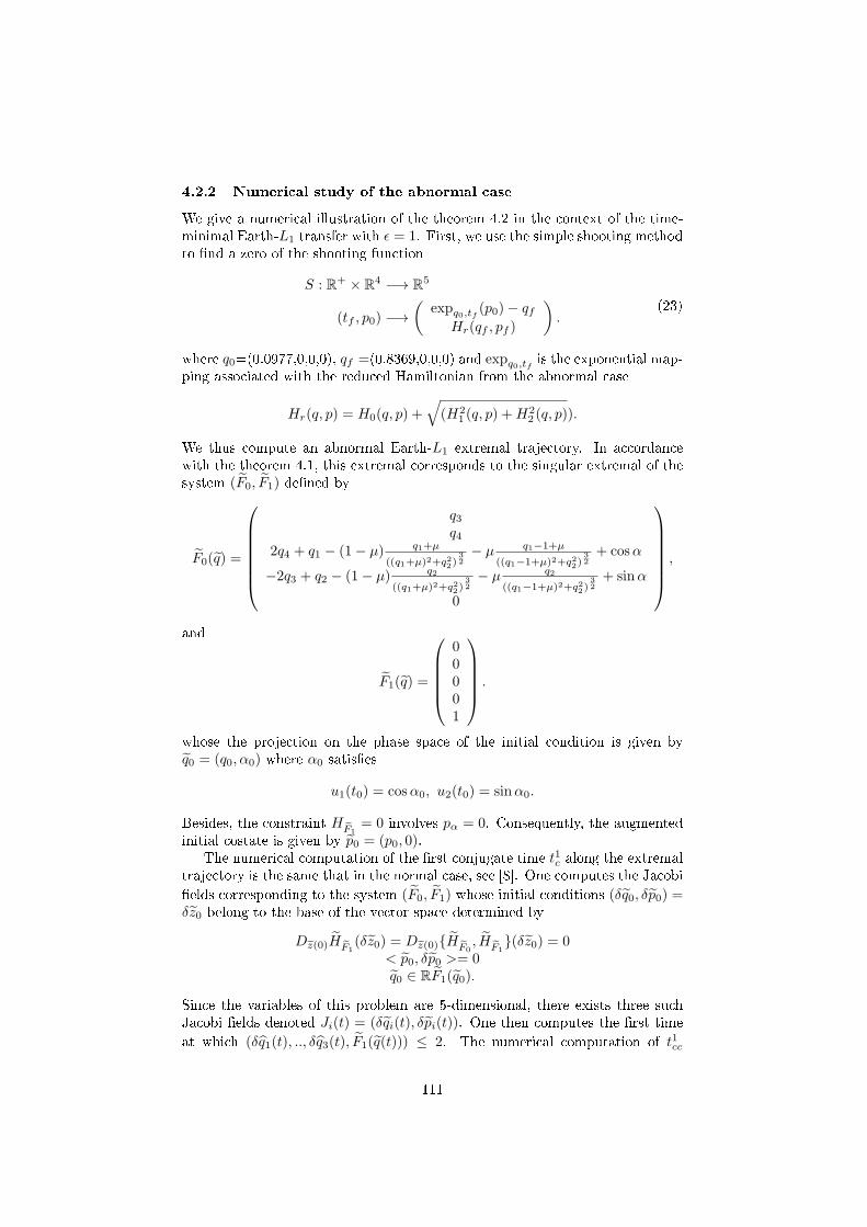
4.2.2 Numerical study of the abnormal case

We give a numerical illustration of the theorem 4.2 in the context of the time-minimal Earth-L1 transfer with ε = 1. First, we use the simple shooting methodto nd a zero of the shooting function

S : R+ × R4 −→ R5

(tf , p0) −→(

expq0,tf (p0)− qfHr(qf , pf )

).

(23)

where q0=(0.0977,0,0,0), qf =(0.8369,0,0,0) and expq0,tf is the exponential map-ping associated with the reduced Hamiltonian from the abnormal case

Hr(q, p) = H0(q, p) +√(H2

1 (q, p) +H22 (q, p)).

We thus compute an abnormal Earth-L1 extremal trajectory. In accordancewith the theorem 4.1, this extremal corresponds to the singular extremal of thesystem (F0, F1) dened by

F0(q) =

q3q4

2q4 + q1 − (1− µ) q1+µ

((q1+µ)2+q22)32− µ q1−1+µ

((q1−1+µ)2+q22)32+ cosα

−2q3 + q2 − (1− µ) q2

((q1+µ)2+q22)32− µ q2

((q1−1+µ)2+q22)32+ sinα

0

,

and

F1(q) =

00001

.

whose the projection on the phase space of the initial condition is given byq0 = (q0, α0) where α0 satises

u1(t0) = cosα0, u2(t0) = sinα0.

Besides, the constraint HF1= 0 involves pα = 0. Consequently, the augmented

initial costate is given by p0 = (p0, 0).The numerical computation of the rst conjugate time t1c along the extremal

trajectory is the same that in the normal case, see [8]. One computes the Jacobi

elds corresponding to the system (F0, F1) whose initial conditions (δq0, δp0) =δz0 belong to the base of the vector space determined by

Dz(0)HF1(δz0) = Dz(0)HF0

, HF1(δz0) = 0

< p0, δp0 >= 0q0 ∈ RF1(q0).

Since the variables of this problem are 5-dimensional, there exists three suchJacobi elds denoted Ji(t) = (δqi(t), δpi(t)). One then computes the rst time

at which (δq1(t), .., δq3(t), F1(q(t))) ≤ 2. The numerical computation of t1cc

111

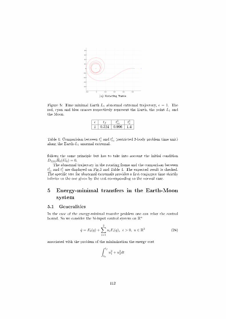
−0.2 0 0.2 0.4 0.6 0.8

−0.4

−0.3

−0.2

−0.1

0

0.1

0.2

0.3

0.4

(a) Rotating frame

Figure 5: Time-minimal Earth-L1 abnormal extremal trajectory, ε = 1. Thered, cyan and blue crosses respectively represent the Earth, the point L1 andthe Moon.

ε tf t1cc t1c1 0.524 0.996 1.4

Table 4: Comparision between t1c and t1cc (restricted 3-body problem time unit)

along the Earth-L1 anormal extremal.

follows the same principle but has to take into account the initial conditionDz(0)H0(δz0) = 0.

The abnormal trajectory in the rotating frame and the comparison betweent1cc and t1c are displayed on Fig.5 and Table 4. The expected result is checked.The specic test for abnormal extremals provides a rst conjugate time strictlyinferior to the one given by the test corresponding to the normal case.

5 Energy-minimal transfers in the Earth-Moon

system

5.1 Generalities

In the case of the energy-minimal transfer problem one can relax the controlbound. So we consider the bi-input control system on Rn

q = F0(q) +2∑

i=1

uiFi(q), ε > 0, u ∈ R2 (24)

associated with the problem of the minimization the energy cost∫ tf

t0

u21 + u22dt

112

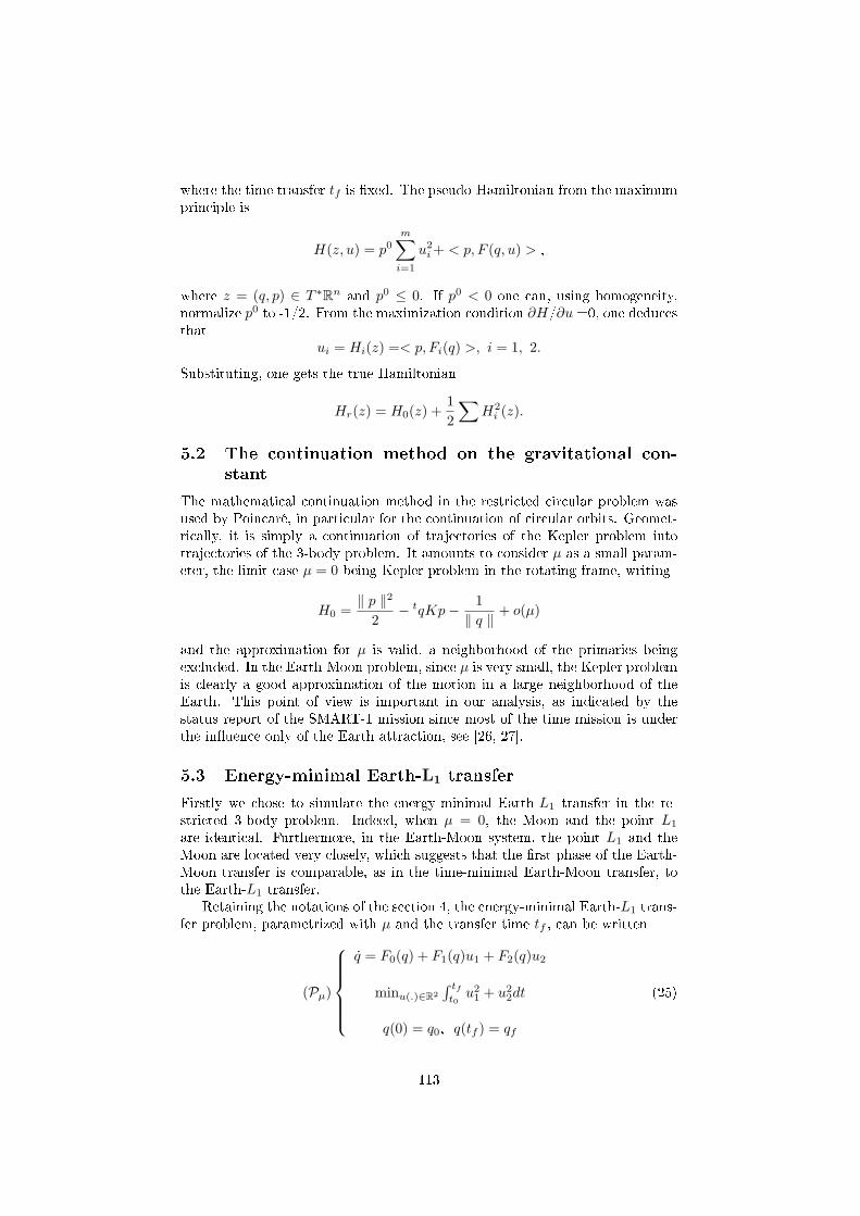
where the time transfer tf is xed. The pseudo-Hamiltonian from the maximumprinciple is

H(z, u) = p0m∑i=1

u2i+ < p, F (q, u) > ,

where z = (q, p) ∈ T ∗Rn and p0 ≤ 0. If p0 < 0 one can, using homogeneity,normalize p0 to -1/2. From the maximization condition ∂H/∂u =0, one deducesthat

ui = Hi(z) =< p, Fi(q) >, i = 1, 2.

Substituting, one gets the true Hamiltonian

Hr(z) = H0(z) +1

2

∑H2

i (z).

5.2 The continuation method on the gravitational con-

stant

The mathematical continuation method in the restricted circular problem wasused by Poincaré, in particular for the continuation of circular orbits. Geomet-rically, it is simply a continuation of trajectories of the Kepler problem intotrajectories of the 3-body problem. It amounts to consider µ as a small param-eter, the limit case µ = 0 being Kepler problem in the rotating frame, writing

H0 =‖ p ‖2

2− tqKp− 1

‖ q ‖+ o(µ)

and the approximation for µ is valid, a neighborhood of the primaries beingexcluded. In the Earth-Moon problem, since µ is very small, the Kepler problemis clearly a good approximation of the motion in a large neighborhood of theEarth. This point of view is important in our analysis, as indicated by thestatus report of the SMART-1 mission since most of the time mission is underthe inuence only of the Earth attraction, see [26, 27].

5.3 Energy-minimal Earth-L1 transfer

Firstly we chose to simulate the energy-minimal Earth-L1 transfer in the re-stricted 3-body problem. Indeed, when µ = 0, the Moon and the point L1

are identical. Furthermore, in the Earth-Moon system, the point L1 and theMoon are located very closely, which suggests that the rst phase of the Earth-Moon transfer is comparable, as in the time-minimal Earth-Moon transfer, tothe Earth-L1 transfer.

Retaining the notations of the section 4, the energy-minimal Earth-L1 trans-fer problem, parametrized with µ and the transfer time tf , can be written

(Pµ)

q = F0(q) + F1(q)u1 + F2(q)u2

minu(.)∈R2

∫ tft0u21 + u22dt

q(0) = q0, q(tf ) = qf

(25)

113

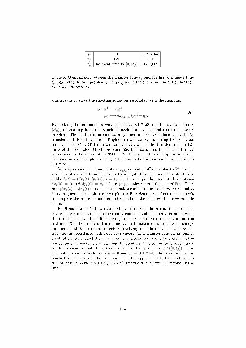
µ 0 0.012153tf 121 121t1c no focal time in [0, 5tf ] 121.932

Table 5: Comparision between the transfer time tf and the rst conjugate timet1c (restricted 3-body problem time unit) along the energy-minimal Earth-Moonextremal trajectories.

which leads to solve the shooting equation associated with the mapping

S : R4 −→ R4

p0 −→ expq0,tf (p0)− qf .(26)

By making the parameter µ vary from 0 to 0.012153, one builds up a family(Sµ)µ of shooting functions which connects both Kepler and restricted 3-bodyproblem. The continuation method may then be used to deduce an Earth-L1

transfer with low-thrust from Keplerian trajectories. Referring to the statusreport of the SMART-1 mission, see [26, 27], we x the transfer time to 121units of the restricted 3-body problem (526.1365 days) and the spacecraft massis assumed to be constant to 350kg. Setting µ = 0, we compute an initialextremal using a simple shooting. Then we make the parameter µ vary up to0.012153.

Since tf is xed, the domain of expx0,tc is locally dieomorphic to R4, see [8].Consequently one determines the rst conjugate time by computing the Jacobields Ji(t) = (δxi(t), δpi(t)), i = 1, . . . , 4, corresponding to initial conditionsδxi(0) = 0 and δpi(0) = ei, where (ei)i is the canonical basis of R4. Thenrank(δx1(t), .., δx4(t)) is equal to 4 outside a conjugate time and lower or equal to3 at a conjugate time. Moreover we plot the Euclidean norm of extremal controlsto compare the control bound and the maximal thrust allowed by electro-ionicengines.

Fig.6 and Table 5 show extremal trajectories in both rotating and xedframes, the Euclidean norm of extremal controls and the comparisons betweenthe transfer time and the rst conjugate time in the Kepler problem and therestricted 3-body problem. The numerical continuation on µ provides an energyminimal Earth-L1 extremal trajectory resulting from the distortion of a Keple-rian one, in accordance with Poincaré's theory. This transfer consists in joiningan elliptic orbit around the Earth from the geostationary one by preserving thepericenter argument, before reaching the point L1. The second order optimalitycondition ensures that the extremals are locally optimal in L∞([0, tf ]). Onecan notice that in both cases µ = 0 and µ = 0.012153, the maximum valuereached by the norm of the extremal control is approximately twice inferior tothe low-thrust bound ε ≤ 0.08 (0.073 N), but the transfer times are roughly thesame.

114

(a) Rotating frame, µ = 0.

−1 −0.5 0 0.5 1

−0.8

−0.6

−0.4

−0.2

0

0.2

0.4

0.6

0.8

(b) Fixed frame, µ = 0.

(c) Norm of the extremal control alongthe transfer, µ = 0.

(d) Rotating frame, µ = 0.012153.

−1 −0.5 0 0.5 1

−0.8

−0.6

−0.4

−0.2

0

0.2

0.4

0.6

0.8

(e) Fixed frame, µ = 0.012153.

(f) Norm of the extremal control alongthe transfer, µ = 0.012153.

Figure 6: Energy-minimal Earth-L1 extremal trajectories. The red cross repre-sents the Earth. In (b), the green trajectory correspond to motion of the pointL1 which is identical to the Moon. In (d) and (e), the point L1 and the Moonare dierent and respectively represented by cyan and blue crosses. The greentrajectory correspond to the Moon motion in the xed frame.

115

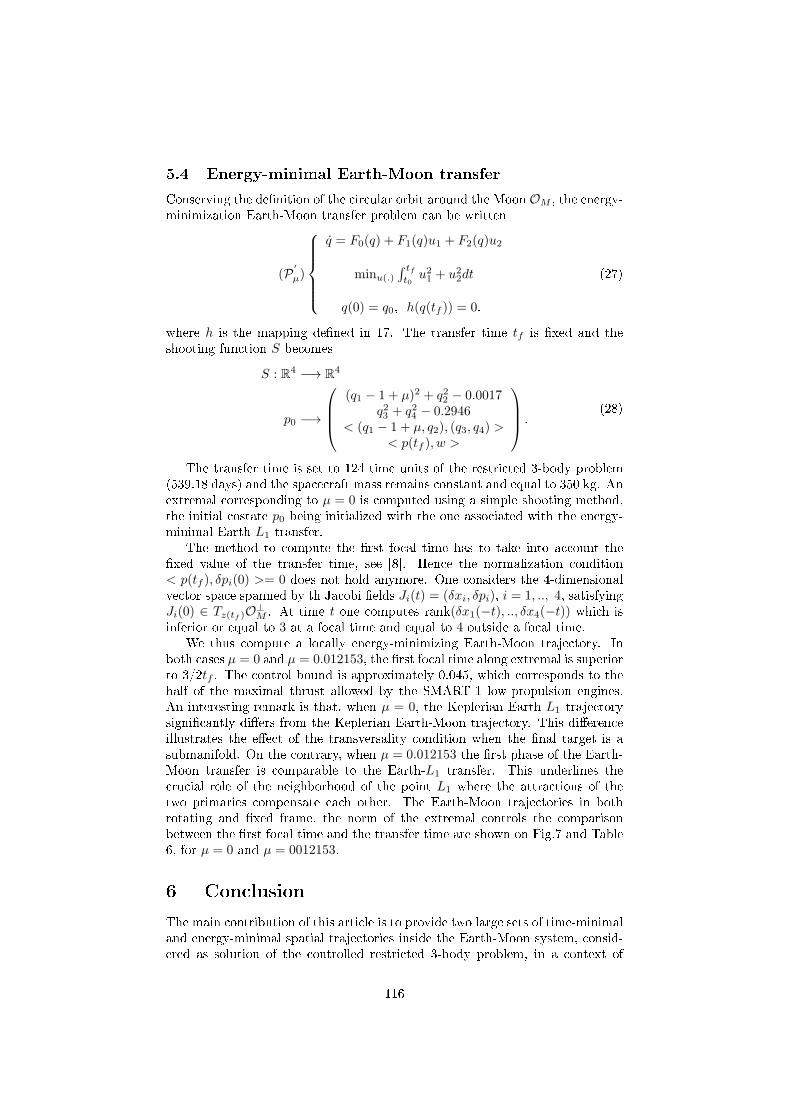
5.4 Energy-minimal Earth-Moon transfer

Conserving the denition of the circular orbit around the Moon OM , the energy-minimization Earth-Moon transfer problem can be written

(P′

µ)

q = F0(q) + F1(q)u1 + F2(q)u2

minu(.)∫ tft0u21 + u22dt

q(0) = q0, h(q(tf )) = 0.

(27)

where h is the mapping dened in 17. The transfer time tf is xed and theshooting function S becomes

S : R4 −→ R4

p0 −→

(q1 − 1 + µ)2 + q22 − 0.0017

q23 + q24 − 0.2946< (q1 − 1 + µ, q2), (q3, q4) >

< p(tf ), w >

.(28)

The transfer time is set to 124 time units of the restricted 3-body problem(539.18 days) and the spacecraft mass remains constant and equal to 350 kg. Anextremal corresponding to µ = 0 is computed using a simple shooting method,the initial costate p0 being initialized with the one associated with the energy-minimal Earth-L1 transfer.

The method to compute the rst focal time has to take into account thexed value of the transfer time, see [8]. Hence the normalization condition< p(tf ), δpi(0) >= 0 does not hold anymore. One considers the 4-dimensionalvector space spanned by th Jacobi elds Ji(t) = (δxi, δpi), i = 1, .., 4, satisfyingJi(0) ∈ Tz(tf )O⊥

M . At time t one computes rank(δx1(−t), .., δx4(−t)) which isinferior or equal to 3 at a focal time and equal to 4 outside a focal time.

We thus compute a locally energy-minimizing Earth-Moon trajectory. Inboth cases µ = 0 and µ = 0.012153, the rst focal time along extremal is superiorto 3/2tf . The control bound is approximately 0.045, which corresponds to thehalf of the maximal thrust allowed by the SMART-1 low-propulsion engines.An interesting remark is that, when µ = 0, the Keplerian Earth-L1 trajectorysignicantly diers from the Keplerian Earth-Moon trajectory. This dierenceillustrates the eect of the transversality condition when the nal target is asubmanifold. On the contrary, when µ = 0.012153 the rst phase of the Earth-Moon transfer is comparable to the Earth-L1 transfer. This underlines thecrucial role of the neighborhood of the point L1 where the attractions of thetwo primaries compensate each other. The Earth-Moon trajectories in bothrotating and xed frame, the norm of the extremal controls the comparisonbetween the rst focal time and the transfer time are shown on Fig.7 and Table6, for µ = 0 and µ = 0012153.

6 Conclusion

The main contribution of this article is to provide two large sets of time-minimaland energy-minimal spatial trajectories inside the Earth-Moon system, consid-ered as solution of the controlled restricted 3-body problem, in a context of

116

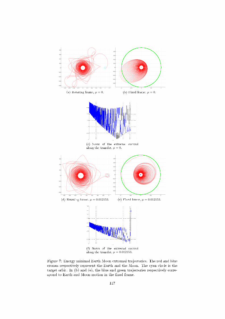
−0.8 −0.6 −0.4 −0.2 0 0.2 0.4 0.6 0.8 1 1.2

−0.8

−0.6

−0.4

−0.2

0

0.2

0.4

0.6

0.8

(a) Rotating frame, µ = 0.

−1 −0.5 0 0.5 1

−0.8

−0.6

−0.4

−0.2

0

0.2

0.4

0.6

0.8

(b) Fixed frame, µ = 0.

(c) Norm of the extremal controlalong the transfer, µ = 0.

−0.6 −0.4 −0.2 0 0.2 0.4 0.6 0.8 1

−0.6

−0.4

−0.2

0

0.2

0.4

0.6

(d) Rotating frame, µ = 0.012153.

−1 −0.5 0 0.5 1

−0.8

−0.6

−0.4

−0.2

0

0.2

0.4

0.6

0.8

(e) Fixed frame, µ = 0.012153.

(f) Norm of the extremal controlalong the transfer, µ = 0.012153.

Figure 7: Energy-minimal Earth-Moon extremal trajectories. The red and bluecrosses respectively represent the Earth and the Moon. The cyan circle is thetarget orbit. In (b) and (e), the blue and green trajectories respectively corre-spond to Earth and Moon motion in the xed frame.

117

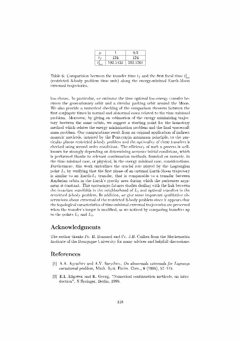
µ 1 0.2tf 124 124t1foc

192.5432 212.5761

Table 6: Comparision between the transfer time tf and the rst focal time t1foc

(restricted 3-body problem time unit) along the energy-minimal Earth-Moonextremal trajectories.

low-thrust. In particular, we estimate the time optimal low-energy transfer be-tween the geostationary orbit and a circular parking orbit around the Moon.We also provide a numerical checking of the comparison theorem between therst conjugate times in normal and abnormal cases related to the time-minimalproblem. Moreover, by giving an estimation of the energy minimizing trajec-tory beetwen the same orbits, we suggest a starting point for the homotopymethod which relates the energy minimization problem and the nal spacecraftmass problem. Our computations result from an original application of indirectnumeric methods, inspired by the Pontryagin maximum principle, to the par-ticular planar restricted 3-body problem and the optimality of these transfers ischecked using second order conditions. The eciency of such a process is well-known for strongly depending on determining accurate initial conditions, whichis performed thanks to relevant continuation methods, founded on numeric, inthe time-minimal case, or physical, in the energy-minimal case, considerations.Furthermore, this work underlines the crucial role played by the Lagrangianpoint L1 by verifying that the rst phase of an optimal Earth-Moon trajectoryis similar to an Earth-L1 transfer, that is comparable to a transfer betweenKeplerian orbits in the Earth's gravity area during which the pericenter argu-ment is constant. This encourages futures studies dealing with the link betweenthe invariant manifolds in the neighborhood of L1 and optimal transfers in therestricted 3-body problem. In addition, we give some important qualitative ob-servations about extremal of the restricted 3-body problem since it appears thatthe topological caracteristics of time-minimal extremal trajectories are preservedwhen the transfer's target is modied, as we noticed by comparing transfers upto the points L1 and L4.

Acknowledgments

The author thanks Pr. B. Bonnard and Pr. J.B. Caillau from the MathematicsInstitute of the Bourgogne University for many advices and helpfull discussions.

References

[1] A.A. Agrachev and A.V. Sarychev, On abnormals extremals for Lagrangevariational problem, Math. Syst. Estim. Cont., 8 (1998), 87118.

[2] E.L Allgower and K. Georg, Numerical continuation methods, an intro-duction", S Springer, Berlin, 1990.

118

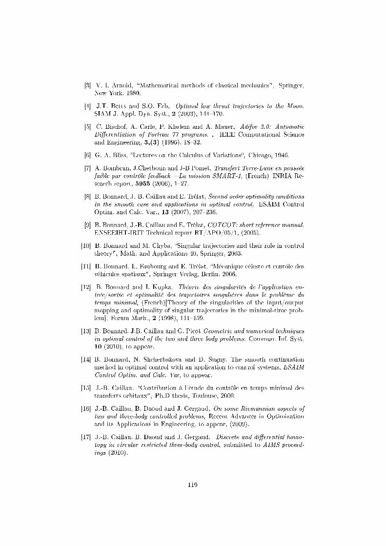
[3] V. I. Arnold, Mathematical methods of classical mechanics", Springer,New-York, 1989.

[4] J.T. Betts and S.O. Erb, Optimal low thrust trajectories to the Moon,SIAM J. Appl. Dyn. Syst., 2 (2003), 144170.

[5] C. Bischof, A. Carle, P. Kladem and A. Mauer, Adifor 2.0: AutomaticDierentiation of Fortran 77 programs. , IEEE Computational Scienceand Engineering, 3,(3) (1996), 1832.

[6] G. A. Bliss, Lectures on the Calculus of Variations, Chicago, 1946.

[7] A. Bombrun, J.Chetboun and J-B Pomet, Transfert Terre-Lune en pousséefaible par contrôle feedback La mission SMART-1, (French) INRIA Re-search report, 5955 (2006), 127.

[8] B. Bonnard, J.-B. Caillau and E. Trélat, Second order optimality conditionsin the smooth case and applications in optimal control, ESAIM ControlOptim. and Calc. Var., 13 (2007), 207236.

[9] B. Bonnard, J.-B. Caillau and E. Trélat, COTCOT: short reference manual,ENSEEIHT-IRIT Technical report RT/APO/05/1, (2005).

[10] B. Bonnard and M. Chyba, Singular trajectories and their role in controltheory", Math. and Applications 40, Springer, 2003.

[11] B. Bonnard, L. Faubourg and E. Trélat, Mécanique céleste et contôle desvéhicules spatiaux", Springer-Verlag, Berlin, 2006.

[12] B. Bonnard and I. Kupka, Théorie des singularités de l'application en-trée/sortie et optimalité des trajectoires singulières dans le problème dutemps minimal, (French)[Theory of the singularities of the input/outputmapping and optimality of singular trajectories in the minimal-time prob-lem], Forum Math., 2 (1998), 111159.

[13] B. Bonnard, J.B. Caillau and G. Picot Geometric and numerical techniquesin optimal control of the two and three body problems, Commun. Inf. Syst,10 (2010), to appear.

[14] B. Bonnard, N. Shcherbakova and D. Sugny, The smooth continuationmethod in optimal control with an application to control systems, ESAIMControl Optim. and Calc. Var, to appear.

[15] J.-B. Caillau, Contribution à l'étude du contrôle en temps minimal destransferts orbitaux", Ph.D thesis, Toulouse, 2000.

[16] J.-B. Caillau, B. Daoud and J. Gergaud, On some Riemannian aspects oftwo and three-body controlled problems, Recent Advances in Optimizationand its Applications in Engineering, to appear, (2009).

[17] J.-B. Caillau, B. Daoud and J. Gergaud, Discrete and dierential homo-topy in circular restricted three-body control, submitted to AIMS proceed-ings (2010).

119

[18] J. Gergaud and T. Haberkorn, Homotopy method for minimum consump-tion orbit transfer problem, ESAIM Control Optim. Calc. Var., 12 (2006),294310.

[19] G. Gómez, S.Koon, M. Lo, J.E Marsden, J. Madesmont and S.D. Ross, In-variant manifolds, the spatial three-body problem ans space mission design,Adv. Astronaut. Sci, 109 (2001), 322.

[20] M. Guerra and A. Sarychev, Existence and Lipschitzian regularity forrelaxed minimizers, Mathematical control theory and nance, 231250,Springer, Berlin 2008.

[21] J.E. Marsden and S.D. Ross, New methods in celestial mechanics andmission design, Bull. Amer. Math. Soc. (N.S), 43 (2006), 4373.

[22] K. Meyer and G. R. Hall, Introduction to Hamiltonian dynamical systemsand the N -body problem", Springer, New York, 1992.

[23] H. Poincaré, Oeuvres", Gauthier-Villars, Paris, 1934.

[24] H. Pollard, Mathematical introduction to celestial mechanics", Prentice-Hall, Englewood Clis, 1966.

[25] (MR1301779) L. S. Pontryagin, V. G. Boltyanskii, R. V. Gamkrelidze andE. F. Mishchenko, The mathematical theory of optimal processes", JohnWiley & Sons, New York, 1962.

[26] G. Racca, B. H. Foing and M. Coradini, SMART-1: The rst time ofEurope to the Moon, Earth, Moon and planets, 85-86 (2001), 379390.

[27] G. Racca et al., SMART-1 mission description and development status,Planetary and space science, 50 (2002), 13231337.

[28] A.V. Sarychev, The index of second variation of a control system, Matem.Sbornik, 113 (1980), 464486.

[29] L.F. Shampine, H.A. Watts and S. Davenport, Solving non-sti ordinarydierential equations-the state of the art., Technical report sand75-0182,Sandia Laboratories, Albuquerque, New Mexico (1975).

[30] V. Szebehely, Theory of orbits: The restricted problem of three bodies",Academic Press, 1967.

120

Energy-minimal transfers in the vicinity

of the Lagrangian point L1.

G. Picot∗

Abstract. This article deals with the problem of computing energy-minimaltrajectories between the invariant manifolds in the neighborhood of the equilib-rium point L1 of the restricted 3-body problem. Initializing a simple shootingmethod with solutions of the corresponding linear optimal control problem, wenumerically compute energy-minimal extremals from the Pontryagin's Maxi-mum principle, whose optimality is ensured thanks to the second order optimal-ity condition.Key Words. Optimal control, 3-body problem, numerical analysis methods.

AMS subject classication. 49K15, 49M05, 70F07.

1 Introduction

Computing energy-minimal orbit transfers is one of the crucial challenges to takeup to design space missions using low-propulsion. In particular, the SMART-1mission from the European Space Agency, see [11], has motivated numerousstudies dealing with low thrust trajectories from the Earth to the Moon, usingfor instance simple feedback laws [3] or the transcription method [2]. In [4],optimal transfers between quasi-Keplerian orbits in the Earth-Moon system arecomputed basing on numeric methods connected with fundamental results fromgeometric control theory. The free motion of the spacecraft is described bythe equations of the planar restricted 3-body problem, [13]: two primaries arecircularly revolving around their center of mass with a constant angular velocityunder the inuence of their mutual gravitational attraction and a third bodywith negligible mass is moving in the plane dened by the motion of the twoprimaries. Adding control terms in the equations of motion, extremal curvessolutions of the Pontryagin's Maximum Principle [10] are numerically computedusing simple shooting and smooth continuation methods. Their local optimalityis checked according with the second order optimality condition related with thenotion of conjugate points. In gure 1 is displayed an example of such an optimaltrajectory.

In this article, the above methods are used to compute energy-minimal trans-fers in the vicinity of the equilibrium point L1 of the spatial restricted 3-bodyproblem where the vertical dimension is taken into account. Indeed, the study of

∗Mathematics Institute, Bourgogne University, 9 avenue Savary, F-21078 Dijon(gautier.picot@u-bourgogne.fr), supported by CNRS (contract no. 37244) and ConseilRégional de Bourgogne (contrat no. 079201PP02454515)

121

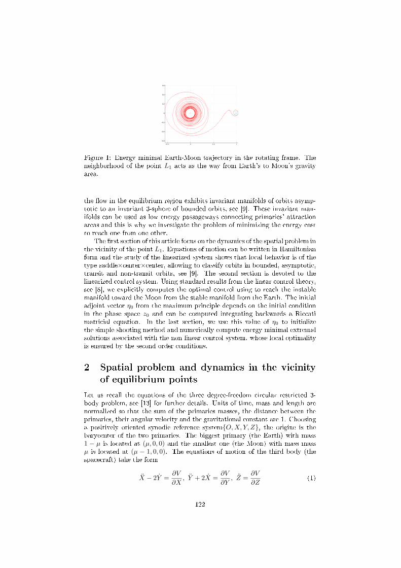
−0.5 0 0.5 1

−0.6

−0.4

−0.2

0

0.2

0.4

0.6

Figure 1: Energy minimal Earth-Moon trajectory in the rotating frame. Theneighborhood of the point L1 acts as the way from Earth's to Moon's gravityarea.

the ow in the equilibrium region exhibits invariant manifolds of orbits asymp-totic to an invariant 3-sphere of bounded orbits, see [9]. These invariant man-ifolds can be used as low energy passageways connecting primaries' attractionareas and this is why we investigate the problem of minimizing the energy costto reach one from one other.

The rst section of this article focus on the dynamics of the spatial problem inthe vicinity of the point L1. Equations of motion can be written in Hamiltonianform and the study of the linearized system shows that local behavior is of thetype saddle×center×center, allowing to classify orbits in bounded, asymptotic,transit and non-transit orbits, see [9]. The second section is devoted to thelinearized control system. Using standard results from the linear control theory,see [8], we explicitly computes the optimal control using to reach the instablemanifold toward the Moon from the stable manifold from the Earth. The initialadjoint vector η0 from the maximum principle depends on the initial conditionin the phase space z0 and can be computed integrating backwards a Riccatimatricial equation. In the last section, we use this value of η0 to initializethe simple shooting method and numerically compute energy-minimal extremalsolutions associated with the non-linear control system, whose local optimalityis ensured by the second order conditions.

2 Spatial problem and dynamics in the vicinity

of equilibrium points

Let us recall the equations of the three degree-freedom circular restricted 3-body problem, see [13] for further details. Units of time, mass and length arenormalized so that the sum of the primaries masses, the distance between theprimaries, their angular velocity and the gravitational constant are 1. Choosinga positively oriented synodic reference systemO,X, Y, Z, the origine is thebarycenter of the two primaries. The biggest primary (the Earth) with mass1 − µ is located at (µ, 0, 0) and the smallest one (the Moon) with mass massµ is located at (µ − 1, 0, 0). The equations of motion of the third body (thespacecraft) take the form

X − 2Y =∂V

∂X, Y + 2X =

∂V

∂Y, Z =

∂V

∂Z(1)

122

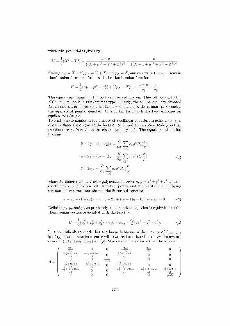
where the potential is given by

V =1

2(X2 + Y 2)− 1− µ

((X + µ)2 + Y 2 + Z2)32

+µ

((X − 1 + µ)2 + Y 2 + Z2)32

Setting pX = X − Y , pY = Y +X and pZ = Z, one can write the equations inHamiltonian form associated with the Hamiltonian function

H =1

2(p2X + p2Y + p2Z) + Y pX −XpY − 1− µ

ρ1− µ

ρ2.

The equilibrium points of the problem are well known. They all belong to theXY-plane and split in two dierent types. Firstly, the collinear points, denotedL1, L2 and L3, are located on the line y = 0 dened by the primaries. Secondly,the equilateral points, denoted, L4 and L5, form with the two primaries anequilateral triangle.To study the dynamics in the vicinity of a collinear equilibrium point Li=1, 2, 3,one translates the origine to the location of Li and applies some scaling so thatthe distance γj from Li to the closest primary is 1. The equations of motionbecome

x− 2y − (1 + c2)x =∂

∂x

∑n≥3

cnρnPn(

x

ρ),

y + 2x+ (c2 − 1)y =∂

∂y

∑n≥3

cnρnPn(

x

ρ)

z + 2c2z =∂

∂z

∑n≥3

cnρnPn(

x

ρ)

(2)

where Pn denotes the Legendre polynomial of order n, ρ = x2+ y2+ z2 and thecoecients cn depend on both libration points and the constant µ. Skippingthe non-linear terms, one obtains the linearized equation

x− 2y − (1 + c2)x = 0, y + 2x+ (c2 − 1)y = 0, z + 2c2z = 0. (3)

Dening px, py and pz as previously, the linearized equation is equivalent to theHamiltonian system associated with the function

H =1

2(p2x + p2y + p2z) + ypx − xpy −

c22(2x2 − y2 − z2). (4)

It is not dicult to check that the linear behavior in the vicinity of Li=1, 2, 3

is of type saddle×center×center with two real and four imaginary eigenvaluesdenoted (±λ1,±iω1,±iω2) see [9]. Moreover, one can show that the matrix

A =

2λ1s1

0 0 − 2λ1s1

2ω1s2

0λ21−2c2−1

s1

−ω21−2c2−1

s20

λ21−2c2−1

s10 0

0 0 1√ω2

0 0 0λ21+2c2+1

s1

−ω21+2c2+1

s20

λ21+2c2+1

s10 0

λ31+(1−c2)λ1

s10 0

−λ31−(1−c2)λ1

s1

−ω31+(1−c2)ω1

s1

λ21+2c2+1

s1

0 0 0 0 0√ω2

123

where

s1 = (2λ1((4+3c2)λ21+4+5c2−6c22))

12 , s2 = (ω1((4+3c2)ω

21 −4−5c2+6c22)

12 ,

denes a symplectic change of variables that, denoting z = (q1, q2, q3, p1, p2, p3)the new coordinates, casts the Hamiltonian 4 into

H = λ1q1p1 +ω1

2(q22 + p22) +

ω2

2(q23 + p23). (5)

The analysis of the ow of the linearized system in the equilibrium region R,determined for positive h and c by H = h and |q1 − p1| ≤ c, can be performednoting that, when q1p1 6= 0, the projections of the orbits in the q1p1-plane lieon the branches of hyperbolas q1p1=constant, since q1p1 is a rst integral ofthe linearized equation. One thus distinguishes four categories of orbits [9]:

• the point (q1, p1) = 0 corresponds to an invariant 3-sphere S3h of bounded

orbits,

• the asymptotic orbits gather the stable and unstable manifolds of S3h,

respectively denoted W s±(S

3h) and W

u±(S

3h) and given by

W s±(S

3h) = ω1

2(q22 + p22) +

ω2

2(q23 + p23) = h, q1 = 0, p10

Wu±(S

3h) = ω1

2(q22 + p22) +

ω2

2(q23 + p23) = h, p1 = 0, q10

• the hyperbolic segments q1p1 = constant > 0 correspond to transit orbits,

• the hyperbolic segments q1p1 = constant < 0 correspond to non-transitorbits.

Let us mention that the non-linear dynamics in the Region R is qualitativelythe same that the linear one, see [9]. In this case, there exists a normally perodicinvariant manifold Mh

3 which still has stable and instable manifolds which canbe approximated by the invariant manifolds W s

±(S3h) and Wu

±(S3h), the non-

linear terms being much smaller than the linear ones in a neighborhood of thecollinear point.

3 Linear control system with energy cost around

the point L1.

From now on, we focus on studying the controlled dynamics around the La-grangian point L1. Our aim is to compute energy-minimal transfers reachingthe positive branch of the instable manifolds Wu

+(S3h) from the positive branch

of the stable manifolds W s+(S

3h). Indeed, W

s+(S

3h) (resp. W

u+(S

3h)) is a dynam-

ical channel which connects the Earth's (resp. Moon's) attraction area and aclosed neighborhood of L1 as time increases (resp. decreases) that justies theinterest of such transfers for designing low-energy Earth-Moon trajectories. Letus start by investigating the linearized control system

x− 2y − (1 + c2)x = u1, y + 2x+ (c2 − 1)y = u2, z + 2c2z = u3. (6)

124

which is obtained adding control terms in the equations of motion 3. Thus, theHamiltonian function 4 becomes

H =1

2(p2x + p2y + p2z) + ypx − xpy + c2(x

2 +y

2+z

2)− u1x− u2y − u3z. (7)

Applying the symplectic change of variable A, equation 3 can be written

z = Az +Bu (8)

where

B =

2λ1

s1

λ21−2c2−1

s1 02ω1

s2

−ω21−2c2−1s2 0

0 0 02λ1

s1

λ21−2c2−1

s1 0

0 −ω21−2c2−1λ1

s1 00 0 1√

ω2

.

Considering no constraints on the control bound, the Kalman condition, see [8],asserts that the system 8 is controlable. Let us x a transfer time tf . Therefore,determining an energy-minimal transfer from W s

+(S3h) to Wu

+(S3h) consists in

solving the following linear optimal control problem with quadratic cost

z = Az +Bu

minu(.)∈R2

∫ tft0u21 + u22 + u23dt

z(0) ∈W s+(S

3h), z(tf ) ∈Wu

+(S3h).

(9)

Set z0 ∈ W s+(S

3h). From the standard linear quadratic maximum principle, see

[8], there exists an unique optimal control u∗ solving 9; the corresponding opti-mal response z∗ and adjoint vector η∗ ∈ T ∗

z∗W s+(S

3h) are found as any solutions

of the system

z = Az +BBT ηT , η = −ηAz(0) = z0, z(tf ) ∈ ∂Wu

+(S3h)

η(tf ) is interior normal to Wu+(S

3h) at z(tf ).

(10)

and u∗ is given byu∗(t) = BT ηT (t). (11)

Given an initial η0 ∈ T ∗z0W

s+(S

3h) such that (zf , ηf ) fullls the nal transversality

condition of the system 10, the solution of the linear dierential system 10 is

(z(t)η(t)

)= exp

t

A BBT

0 −AT

(z0η0

)(12)

and substituting in 11, the optimal control can be explicitly written

u∗(t) =

2λ1s1

(η0q1e

−λ1t + η0p1e

λ1t)− 2ω1s2

(η0q2 cos(ω1t) + η0

p2 sin(ω1t))λ21−2c2−1

s1(−η0

q1e−λ1t + η0

p1eλ1t)− ω2

1+2c2+1

s2(η0

p2 cos(ω1t)− η0q2 sin(ω1t))

1√ω2

(η0p3 cos(ω2t)− η0

q3 sin(ω2t))

.

125

Such an initial adjoint η0 can be determined integrating backwards a Riccatimatricial equation, see [8]. Indeed, since Wu

+(S3h) is a cylinder, the condition

η(tf ) is interior normal to Wu+(S

3h) at z(tf ) involves

η∗T (tf ) = −z∗T (tf )Q (13)

where the matrix Q is given by

Q =

0 0 0 0 0 00 kω1 0 0 0 00 0 kω2 0 0 00 0 0 0 0 00 0 0 0 kω1 00 0 0 0 0 kω2

and the constant k is stictly positive. Since the couple (z∗, η∗) satises

z = Az +BBT ηT , η = −ηA

one can show thatη∗(t) = z∗T (t)E(t)

where E is the solution of the Riccati matricial equation

E = −ATE − EA− EBBTEE(tf ) = −Q. (14)

The optimal control u∗ is consequently a feedback control given by

u∗(t) = BTE(t)z(t)

and integrating backwards the equation 14 allows to obtain the appropriateinitial condition

η∗(0) = z∗T0 E(0).

4 Energy-minimal transfers computations around

the point L1.

Let us now consider the non-linear control system in the vicinity of L1

x− 2y − (1 + c2)x =∂

∂x

∑n≥3

cnρnPn(

x

ρ) + u1

y + 2x+ (c2 − 1)y =∂

∂y

∑n≥3

cnρnPn(

x

ρ) + u2

z + 2c2z =∂

∂z

∑n≥3

cnρnPn(

x

ρ) + u3

(15)

which is derived from 2. As we mentionned previously, the invariant mani-folds of the linear dynamics near L1 are good approximations of the invariantmanifolds that exist in the non-linear dynamics case. This is why we keep the

126

denition of W s+(S

3h) and Wu

+(S3h) we gave in section 2. For the sake of sim-

plicity, we investigate the problem of computing energy-minimal transfers fromthe submanifold W s

α(S3h) where α is a stricly positive constant and p1 is set to

α, to Wuα (S

3h) where q1 is set to α. Once again, the transfer time tf is xed

and no constraints on the control bound are considered. Keeping the notationz = (q, p) = (x, y, z, px, py, pz), the optimal control problem we are investigatingwrites

z = F0(z) +∑3

i=1 uiFi(z)

minu(.)∈R2

∫ tft0u21 + u22 + u23dt

z(0) ∈W sα(S

3h), z(tf ) ∈Wu

α (S3h)

(16)

where

F0(z) =

px + yp− y − x

pz∂∂x

∑n≥2 cnρ

nPn(xρ ) + py − x

∂∂y

∑n≥2 cnρ

nPn(xρ )− x− y

∂∂y

∑n≥2 cnρ

nPn(xρ )

, Fi(z) =∂

∂pi, i = 1, 2, 3.

Control theory provides powerfull tools to study optimal solutions from thegeometric point of view. First, from the Pontryagin's Maximum Principle, see[10],optimal solutions are found among extremal curves (z, η) ∈ T ∗R6 solutionsof the system

z =∂H

∂η, η = −∂H

∂z(17)

where H is the pseudo-Hamiltonian function

H(x, p, u) =< η, F0(z) > +3∑

i=1

ui < η, Fi(z) > +η0(3∑

i=1

u2i )

= H0(z, η) +3∑

i=1

uiHi(z, η) + η0(3∑

i=1

u2i )

(18)

and η0 is a non-positive constant. Moreover, the optimal control u∗ satises themaximization condition

H(z, η, u∗) = maxv∈R3

H(z, η, v) (19)

that involves Hi = −2p0ui. In the normal case p0 6= 0, one can normalize p0

to -1/2 which gives Hi = ui so that, substituting in 18, H becomes the trueHamiltonian

Hr(z, η) = H0(z, η) +1

2(η24 + η25 + η26) (20)

and equation 17 can be written

(z, η) =−→Hr(z, η) (21)

where−→Hr is the Hamiltonian vectoreld associated with Hr. Finally, the fol-

lowing nal transversality condition

η(tf ) ⊥ Tz(tf )Wuα (S

3h). (22)

127

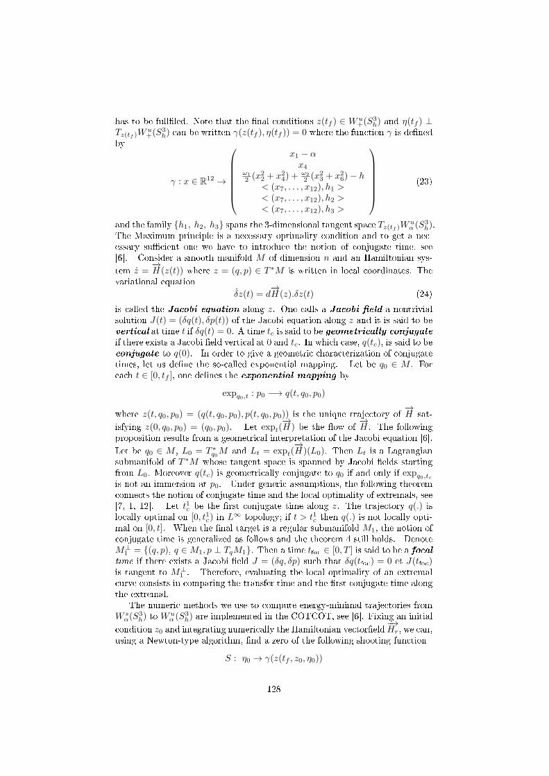
has to be fullled. Note that the nal conditions z(tf ) ∈ Wu+(S

3h) and η(tf ) ⊥

Tz(tf )Wu+(S

3h) can be written γ(z(tf ), η(tf )) = 0 where the function γ is dened

by

γ : x ∈ R12 →

x1 − αx4

ω1

2 (x22 + x24) +ω2

2 (x23 + x26)− h< (x7, . . . , x12), h1 >< (x7, . . . , x12), h2 >< (x7, . . . , x12), h3 >

(23)

and the family h1, h2, h3 spans the 3-dimensional tangent space Tz(tf )Wuα (S

3h).

The Maximum principle is a necessary optimality condition and to get a nec-essary sucient one we have to introduce the notion of conjugate time, see[6]. Consider a smooth manifold M of dimension n and an Hamiltonian sys-

tem z =−→H (z(t)) where z = (q, p) ∈ T ∗M is written in local coordinates. The

variational equation

δz(t) = d−→H (z).δz(t) (24)

is called the Jacobi equation along z. One calls a Jacobi eld a nontrivialsolution J(t) = (δq(t), δp(t)) of the Jacobi equation along z and it is said to bevertical at time t if δq(t) = 0. A time tc is said to be geometrically conjugate

if there exists a Jacobi eld vertical at 0 and tc. In which case, q(tc), is said to beconjugate to q(0). In order to give a geometric characterization of conjugatetimes, let us dene the so-called exponential mapping. Let be q0 ∈ M . Foreach t ∈ [0, tf ], one denes the exponential mapping by

expq0,t : p0 −→ q(t, q0, p0)

where z(t, q0, p0) = (q(t, q0, p0), p(t, q0, p0)) is the unique trajectory of−→H sat-

isfying z(0, q0, p0) = (q0, p0). Let expt(−→H ) be the ow of

−→H . The following

proposition results from a geometrical interpretation of the Jacobi equation [6].

Let be q0 ∈ M , L0 = T ∗q0M and Lt = expt(

−→H )(L0). Then Lt is a Lagrangian

submanifold of T ∗M whose tangent space is spanned by Jacobi elds startingfrom L0. Moreover q(tc) is geometrically conjugate to q0 if and only if expq0,tcis not an immersion at p0. Under generic assumptions, the following theoremconnects the notion of conjugate time and the local optimality of extremals, see[7, 1, 12]. Let t1c be the rst conjugate time along z. The trajectory q(.) islocally optimal on [0, t1c) in L

∞ topology; if t > t1c then q(.) is not locally opti-mal on [0, t]. When the nal target is a regular submanifold M1, the notion ofconjugate time is generalized as follows and the theorem 4 still holds. DenoteM⊥

1 = (q, p), q ∈M1, p ⊥ TqM1. Then a time tfoc ∈ [0, T ] is said to be a focaltime if there exists a Jacobi eld J = (δq, δp) such that δq(tfoc) = 0 et J(tfoc)is tangent to M⊥

1 . Therefore, evaluating the local optimality of an extremalcurve consists in comparing the transfer time and the rst conjugate time alongthe extremal.

The numeric methods we use to compute energy-minimal trajectories fromW s

α(S3h) to W

uα (S

3h) are implemented in the COTCOT, see [6]. Fixing an initial

condition z0 and integrating numerically the Hamiltonian vectoreld−→Hr, we can,

using a Newton-type algorithm, nd a zero of the following shooting function

S : η0 → γ(z(tf , z0, η0))

128

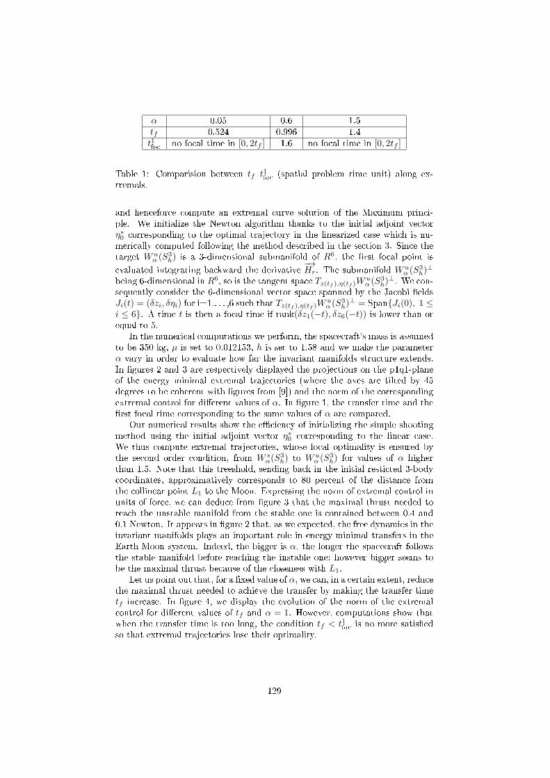
α 0.05 0.6 1.5tf 0.524 0.996 1.4t1foc

no focal time in [0, 2tf ] 1.6 no focal time in [0, 2tf ]

Table 1: Comparision between tf t1foc

(spatial problem time unit) along ex-tremals.

and henceforce compute an extremal curve solution of the Maximum princi-ple. We initialize the Newton algorithm thanks to the initial adjoint vectorη∗0 corresponding to the optimal trajectory in the linearized case which is nu-merically computed following the method described in the section 3. Since thetarget Wu

α (S3h) is a 3-dimensional submanifold of R6, the rst focal point is

evaluated integrating backward the derivative−→Hr. The submanifold Wu

α (S3h)

⊥

being 6-dimensional in R6, so is the tangent space Tz(tf ),η(tf )Wuα (S

3h)

⊥. We con-sequently consider the 6-dimensional vector space spanned by the Jacobi eldsJi(t) = (δzi, δηi) for i=1,. . . ,6 such that Tz(tf ),η(tf )W

uα (S

3h)

⊥ = SpanJi(0), 1 ≤i ≤ 6. A time t is then a focal time if rank(δz1(−t), δz6(−t)) is lower than orequal to 5.

In the numerical computations we perform, the spacecraft's mass is assumedto be 350 kg, µ is set to 0.012153, h is set to 1.58 and we make the parameterα vary in order to evaluate how far the invariant manifolds structure extends.In gures 2 and 3 are respectively displayed the projections on the p1q1-planeof the energy minimal extremal trajectories (where the axes are tilted by 45degrees to be coherent with gures from [9]) and the norm of the correspondingextremal control for dierent values of α. In gure 1, the transfer time and therst focal time corresponding to the same values of α are compared.

Our numerical results show the eciency of initializing the simple shootingmethod using the initial adjoint vector η∗0 corresponding to the linear case.We thus compute extremal trajectories, whose local optimality is ensured bythe second order condition, from W s

α(S3h) to Wu

α (S3h) for values of α higher

than 1.5. Note that this treeshold, sending back in the initial resticted 3-bodycoordinates, approximatively corresponds to 80 percent of the distance fromthe collinear point L1 to the Moon. Expressing the norm of extremal control inunits of force, we can deduce from gure 3 that the maximal thrust needed toreach the unstable manifold from the stable one is contained between 0.4 and0.1 Newton. It appears in gure 2 that, as we expected, the free dynamics in theinvariant manifolds plays an important role in energy-minimal transfers in theEarth-Moon system. Indeed, the bigger is α, the longer the spacecraft followsthe stable manifold before reaching the instable one; however bigger seems tobe the maximal thrust because of the closeness with L1.

Let us point out that, for a xed value of α, we can, in a certain extent, reducethe maximal thrust needed to achieve the transfer by making the transfer timetf increase. In gure 4, we display the evolution of the norm of the extremalcontrol for dierent values of tf and α = 1. However, computations show thatwhen the transfer time is too long, the condition tf < t1

focis no more satised

so that extremal trajectories lose their optimality.

129

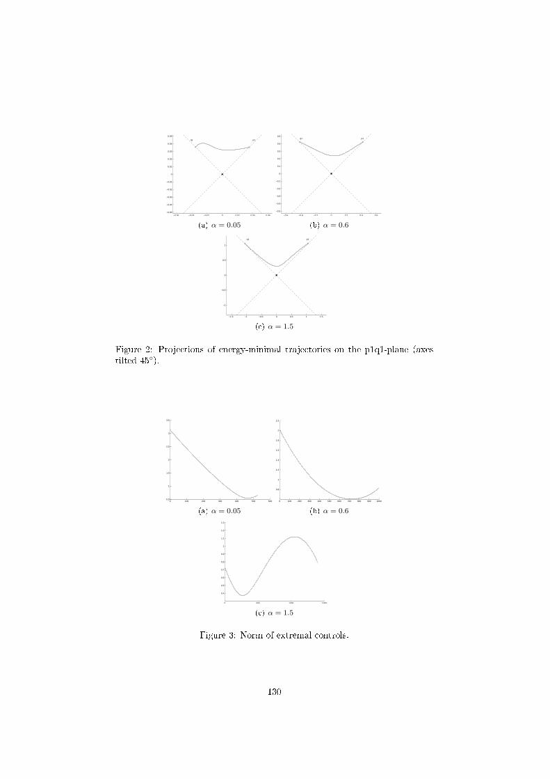
−0.06 −0.04 −0.02 0 0.02 0.04 0.06−0.05

−0.04

−0.03

−0.02

−0.01

0

0.01

0.02

0.03

0.04

0.05

p1q1

(a) α = 0.05

−0.6 −0.4 −0.2 0 0.2 0.4 0.6

−0.5

−0.4

−0.3

−0.2

−0.1

0

0.1

0.2

0.3

0.4

0.5p1q1

(b) α = 0.6

−1.5 −1 −0.5 0 0.5 1 1.5

−1

−0.5

0

0.5

1

p1q1

(c) α = 1.5

Figure 2: Projections of energy-minimal trajectories on the p1q1-plane (axestilted 45).

0 100 200 300 400 500 6000.5

1

1.5

2

2.5

3

3.5

(a) α = 0.05

0 100 200 300 400 500 600 700 800 900 1000

0.8

1

1.2

1.4

1.6

1.8

2

2.2

(b) α = 0.6

0 500 1000 1500

0.4

0.5

0.6

0.7

0.8

0.9

1

1.1

1.2

1.3

(c) α = 1.5

Figure 3: Norm of extremal controls.

130

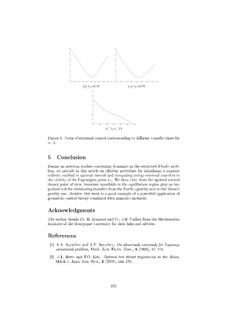
0 50 100 150 200 250 300 350 400 450 5000

2

4

6

8

10

12

(a) tf=0.45

0 100 200 300 400 500 600 700 8000.5

1

1.5

2

2.5

3

3.5

(b) tf=0.76

0 200 400 600 800 1000 12000.4

0.6

0.8

1

1.2

1.4

1.6

1.8

(c) tf=1.13

Figure 4: Norm of extremal control corresponding to dierent transfer times forα=1.

5 Conclusion

Basing on previous studies concerning dynamics in the restricted 3-body prob-lem, we provide in this article an ecient procedure for initializing a numericindirect method in optimal control and computing energy-minimal transfers inthe vicinity of the Lagrangian point L1. We show that, from the optimal controltheory point of view, invariant manifolds in the equilibrium region play an im-portant role for envisioning transfers from the Earth's gravity area to the Moon'sgravity one. Besides, this work is a good example of a powerfull application ofgeometric control theory combined with numerics methods.

Acknowledgments

The author thanks Pr. B. Bonnard and Pr. J.B. Caillau from the MathematicsInstitute of the Bourgogne University for their help and advices.

References

[1] A.A. Agrachev and A.V. Sarychev, On abnormals extremals for Lagrangevariational problem, Math. Syst. Estim. Cont., 8 (1998), 87118.

[2] J.T. Betts and S.O. Erb, Optimal low thrust trajectories to the Moon,SIAM J. Appl. Dyn. Syst., 2 (2003), 144170.

131

[3] A. Bombrun, J.Chetboun and J-B Pomet, Transfert Terre-Lune en pousséefaible par contrôle feedback La mission SMART-1, (French) INRIA Re-search report, 5955 (2006), 127.

[4] B. Bonnard, J.B. Caillau and G. Picot Geometric and numerical techniquesin optimal control of the two and three body problems, Commun. Inf. Syst,10 (2010), to appear.

[5] B. Bonnard, J.-B. Caillau and E. Trélat, Second order optimality conditionsin the smooth case and applications in optimal control, ESAIM ControlOptim. and Calc. Var., 13 (2007), 207236.

[6] B. Bonnard, J.-B. Caillau and E. Trélat, COTCOT: short reference manual,ENSEEIHT-IRIT Technical report RT/APO/05/1, (2005).

[7] B. Bonnard and I. Kupka, Théorie des singularités de l'application en-trée/sortie et optimalité des trajectoires singulières dans le problème dutemps minimal, (French)[Theory of the singularities of the input/outputmapping and optimality of singular trajectories in the minimal-time prob-lem], Forum Math., 2 (1998), 111159.

[8] (MR1301779) E.B. Lee and L. Markus, Fondations of optimal controltheory" Reprint edition, Krieger, 1986.

[9] G. Gomez, W.S. Koon, M.W. Lo, J.E. Marsden, J. Masdemont and S.D.Ross Connecting orbits and invariant manifolds in the spatial three-bodyproblem, Nonlinearity, 17 (2004), 15711606.

[10] (MR1301779) L. S. Pontryagin, V. G. Boltyanskii, R. V. Gamkrelidze andE. F. Mishchenko, The mathematical theory of optimal processes" JohnWiley & Sons, New York, 1962.

[11] G. Racca, B. H. Foing and M. Coradini, SMART-1: The rst time ofEurope to the Moon, Earth, Moon and planets, 85-86 (2001), 379390.

[12] A.V. Sarychev, The index of second variation of a control system, Matem.Sbornik, 113 (1980), 464486.

[13] V. Szebehely, Theory of orbits: The restricted problem of three bodies,"Academic Press, 1967.

132

Conclusion

La contribution principale de cette thèse est de fournir plusieurs collectionsde trajectoires à temps minimal et energie minimale au sein du système Terre-Lune, modélisé par le problème des trois corps restreint et ce dans un contextede poussée faible. Nous calculons ces trajectoires au moyen de méthodes nu-mériques sophistiquées, inspirées de la théorie du contrôle géométrique, dontl'ecacité depend de l'estimation précise des conditions initiales appropriées.La complexité de ce problème est en outre augmentée du fait des dimensionsimportantes des espaces dans lesquels nous avons été amenés à travailler, quisont respectivement R8 et R12 selon que l'on étudie le problème plan ou spatial.Nous surmontons ces dicultés en utilisant pertinemment des méthodes homo-topiques fondées sur une analyse de la géométrie de chaque problème. Cetteapproche permet de déterminer des transferts optimaux controlés par des pous-sées inférieures à 8e−2 Newton. Nous fournissons ainsi les premiers exemples detrajectoires optimales dans le problème, encore relativement méconnu, des troiscorps restreint, calculées à l'aide de méthodes indirectes fondées sur la notionde solutions extrémales issues du principe du maximum de Pontryagin. En cesens, nous proposons une approche complémentaire aux travaux de Marsden &al. et Simó & al. en étudiant numériquement la réduction du côut des transfertorbitaux dans le problème des trois corps restreint, non plus du point de vuede la théorie des systèmes dynamiques mais de celle du contrôle optimal. Nousillustrons d'ailleurs le rôle crucial joué par la structure de variété invariantepour minimiser le coût energétique lors des transferts autour du point L1. Dansle cas du problème de minimisation de l'énergie, les trajectoires peuvent êtrecomparées à celles obtenues par "recollement" des trajectoires optimales asso-ciées aux problème des deux corps dont les centres du champ de gravité sont laTerre puis la Lune, via une solution optimale du système linéarisé au voisinagedu point d'équilibre L1 que l'on peut calculer explicitement. La technique demoyennation ore, sur un long intervalle de temps, une exellente approxima-tion du transfert à énergie minimale entre deux orbites du problème de Kepler,lorsque l'une d'entre elle est circulaire. On obtient de cette manière une trajec-toire entre l'orbite géostationnaire et l'orbite circulaire centrée sur la Lune.

Le recours à la moyennation, dans le but de calculer analytiquement des tra-jectoires à energie minimale par le biais d'un recollement, est ici essentiellementintroduit en guise d'ouverture à un travail futur. Bien que nous ayons procédéà une implémentation numérique de cette méthode, une étude géométrique nedoit être menée pour juger de l'optimalité globale des transferts obtenus de lasorte. L'application du principe du maximum avec contrainte doit être envisa-gée pour cela. Les conditions assurant la continuité de l'état adjoint dans le

133

contexte d'un système de contrôle discontinu sont également dignes d'intérêt.De plus, cette comparaison n'est malheureusement pas encore possible dans lecas de la minimisation du temps de transfert. Une étude géométrique du Ha-miltonien moyenné associé au problème de temps minimal doit préalablementêtre réalisée pour permettre d'envisager une telle expérimentation numérique.Notons que la question de la contrôlabilité dans le modèle restreints des troiscorps n'a pas été abordée au cours de ce travail, bien qu'elle représente un enjeuconsidérable pour l'analyse de la dynamique controlée du problème. Elle s'érigepar conséquent comme l'une des principales contributions théoriques à apporter.De même, l'étude de la maximisation de la masse nale du satellite et de la mi-nimisation du cout L1 le long du transfert ont été volontairement éludées, dansla mesure où elle constitue un des socles de la thèse de Bilel Daoud, voir [22],menée à l'université de Bourgogne sous la direction de Jean-Baptiste Caillauen parallèle à ce travail. Enn, il serait intéressant de prendre en considérationl'utilisation d'une méthode de tir multiple inspirée de travaux d'applications desméthodes numériques pour la résolution de problèmes de contrôle optimal telsque [42].

134

Bibliographie

[1] A.A. Agrachev and A.V. Sarychev. On abnormals extremals for Lagrangevariational problem. J. Math. Syst. Estim. Cont. 8 (1998), 87-118.

[2] E.L Allgower and K. Georg. Numerical continuation methods, an introduc-tion. Springer, Berlin, 1990.

[3] G. Archambeau. Etude de la dynamique autour des points de Lagrange.Ph.D thesis, Université Paris-Sud XI, Paris, France, 2008.

[4] V. I. Arnold. Mathematical methods of classical mechanics. Springer, New-York, 1989.

[5] M. Audin. Les systèmes hamiltoniens et leur intégrabilité. Cours spécialisés,SMF et EDP-sciences, 2001.

[6] J.T. Betts and S.O Erb. Optimal low thrust trajectories to the Moon. SIAMJ. Appl. Dyn. Syst., 2 (2003), 144170.

[7] G. A. Bliss. Lectures on the Calculus of Variations. Chicago, 1946.

[8] A. Bombrun. Les transerts orbitaux à poussée faible-Optimalité et stabili-sation. PhD thesis, Ecole des mines de Paris, Paris, France, 2007.

[9] A. Bombrun, J. Chetboun and J.-B. Pomet. Transfert Terre-Lune en pous-sée faible par contrôle feedback La mission SMART-1. INRIA Researchreport (2006), no. 5955, 127.

[10] B. Bonnard, J.B. Caillau and G. Picot Geometric and numerical techniquesin optimal control of the two and three body problems, Commun. Inf. Syst,10 (2010), to appear.

[11] B. Bonnard, J.-B. Caillau and E. Trélat. Second order optimality conditionsin the smooth case and applications in optimal control. ESAIM Control Op-tim. and Calc. Var. 13 (2007), no. 2, 207-236 (apo.enseeiht.fr/cotcot).

[12] B. Bonnard, J.-B. Caillau and E. Trélat. Geometric optimal control of el-liptic Keplerian orbits. Discrete Contin. Dyn. Syst. Ser. B 5 (2005), no. 4,929-956.

[13] B. Bonnard and M. Chyba. Singular trajectories and their role in controltheory. Math. and Applications 40, Springer, 2003.

[14] B. Bonnard, L.Faubourg and E. Trélat. Méecanique céleste et contôle desvéhicules spatiaux. Springer-Verlag, Berlin, 2006.

[15] B. Bonnard and G. Janin. Geometric orbital transfer using averaging tech-niques. J. Dyn. Control Syst 14, 2 (2008), no. 2, 145-167.

[16] B. Bonnard and I. Kupka. Théorie des singularités de l'application en-trée/sortie et optimalité des trajectoires singulières dans le problème du

135

temps minimal. (French) [Theory of the singularities of the input/outputmapping and optimality of singular trajectories in the minimal-time pro-blem] Forum Math. 5 (1993), no. 2, 111-159.

[17] B. Bonnard, N. Shcherbakova and D. Sugny. The smooth continuation me-thod in optimal control with an application to control systems. ESAIMControl Optim. and Calc. Var, to appear.

[18] J.-B. Caillau. Contribution à l'étude du contrôle en temps minimal destransferts orbitaux. Phd thesis, Institut National Polytechnique de Tou-louse, Toulouse, France, 2000.

[19] J.-B. Caillau, B. Daoud and J. Gergaud. On some Riemannian aspectsof two and three-body controlled problems. Recent Advances in Optimiza-tion and its Applications in Engineering, Springer, to appear. Proceedingsof the 14th Belgian-French-German Conference on Optimization, Leuven,September 2009.

[20] J.-B. Caillau, B. Daoud and J. Gergaud, Discrete and dierential homo-topy in circular restricted three-body control, submitted to AIMS procee-dings Proceedings of the 8th AIMS Conference on Dynamical Systems,Dierential Equations and Applications, Dresden, May 2010.

[21] C. C. Conley. Low energy transit orbits in the restricted three-body pro-blem. SIAM J. Appl. Math. 16 (1968), 732746.

[22] B. Daoud. Contrôle L1 min du problème restreint des trois corps.ENSEEIHT-IRIT Tech. Report (20010), no. RT-APO-10-09.

[23] R. Dujol. Contribution à l'étude du contrôle optimal des transferts orbitauxmono-entrée. Phd thesis, Institut National Polytechnique de Toulouse, Tou-louse, France, 2006.

[24] J. Gergaud and J T. Haberkorn. Homotopy method for minimum consump-tion orbit transfer problem. ESAIM Control Optim. Calc. Var. 12 (2006),no. 2, 294310.

[25] G. Gomez, W.S. Koon, M.W. Lo, J.E. Marsden, J. Masdemont and S.D.Ross. Connecting orbits and invariant manifolds in the spatial three-bodyproblem. Nonlinearity, 17 (2004), 15711606.

[26] G. Gómez, A. Jorba , J. Madesmont and C. Simò. Dynamics and missiondesign near libration points. Vol III. Advanced methods or collinear points.World Scientic Publishing Co. Pte. Ltd., 2001.

[27] G. Gómez, A. Jorba , J. Madesmont and C. Simò. Dynamics and missiondesign near libration points. Vol VI. Advanced methods or triangular points.World Scientic Publishing Co. Pte. Ltd., 2001.

[28] G. Gómez, S.Koon, M. Lo, J.E Marsden, J. Madesmont and S.D. Ross.Invariants manifolds, the spatial three-body problem ans space mission de-sign. Adv. Astronaut. Sci 109 (2001), 3-22.

[29] G. Gómez, S.Koon, M. Lo, J.E Marsden, J. Madesmont and S.D. Ross.Connecting orbits ans invariant manifolds in the spatial restricted three-body problem. Nonlinearity 17 15711606.

[30] G. Gómez, J. Llibre , R. Martínez and C. Simò. Dynamics and missiondesign near libration points. Vol I. Fundamentals : the case of collinearlibration points. World Scientic Publishing Co. Pte. Ltd., 2001.

136

[31] G. Gómez, J. Llibre , R. Martínez and C. Simò. Dynamics and missiondesign near libration points. Vol II. Fundamentals : the case of triangularlibration points. World Scientic Publishing Co. Pte. Ltd., 2001.

[32] M. Guerra and A. Sarychev, Existence and Lipschitzian regularity for re-laxed minimizers. Mathematical control theory and nance, 231-250, Sprin-ger, Berlin, 2008.

[33] T. Haberkorn.Transfert orbital à poussée faible avec minimisation de laconsommation : résolution par homotopie diérentielle. PhD thesis, InstitutNational Polytechnique de Toulouse, Toulouse, France, 2004.

[34] P. Hartman. Ordinary dierential equations. Second edition, Birkhäuser,1982.

[35] A. Jorba. A methodology for the numerical computation of normal forms,centre manifolds and rst integrals of hamiltonian systems, Experiment.Math. 8 2 (1999), 155195.

[36] A. Jorba and J. Masdemont. Dynamics in the center manifold of the col-linear points of the restricted three-body problem. Phys. D 132 (1999),189213.

[37] W. S. Koon, M. W. Lo, J. E. Marsden and S. D. Ross, Dynamical system,the three-body problem and space mission design. Proc. Equadi99, Berlin,German (1999).

[38] W. S. Koon, M. W. Lo, J. E. Marsden and S. D. Ross, Heteroclinic connec-tions between periodic orbits and resonance transitions in celectial mecha-nics. Chaos 10 (2000), 427469.

[39] W. S. Koon, M. W. Lo, J. E. Marsden and S. D. Ross, Low energy transferto the Moon. dynamics of natural and articial celestial bodies (Poznan2000). Celestial. Mech. Dynam. Astronom. 81 (2001) 2738.

[40] W. S. Koon, M. W. Lo, J. E. Marsden and S. D. Ross, Constructing a lowenergy transfer between Jovian moons. Contemp. Math. Am. Math. Soc292 129145.

[41] W. S. Koon, M. W. Lo, J. E. Marsden and S. D. Ross, Dynamical systems,the Three-Body problem, and space mission design. Springer, 2007.

[42] B. Kugelmann and H.J. Pesch, New general guidance method in constrainedoptimal control. 1 Numerical method. J. Optim. Theory Appl. 67 3 (1990)421435.

[43] E.B. Lee and L. Markus. Fondations of optimal control theory Reprintedition, Krieger, 1986.

[44] C. Marchall. The Three-Body problem, Elsevier, Amsterdam 1990.

[45] J.-P. Marec. Optimal space trajectories. Elsevier, Amsterdam, 1979.

[46] J.E. Marsden and S.D. Ross. New methods in celestial mechanics and mis-sion design. Bull. Amer. Math. Soc (N.S) 43 (2006), no. 1, 43-73.

[47] P. Martinon. Résolution numérique de problème de contrôle optimal parune méthode homotopique simpliciale. Phd thesis, Institut National Poly-technique de Toulouse, Toulouse, France, 2005.

[48] R. P. McGehee. Some homoclinic orbits for the restricted three-body pro-blem. PhD Thesis Université du Wisconsin, 1969.

137

[49] K. Meyer and G. R. Hall. Introduction to hamiltonian dynamical systemsand the N -body problem. Springer, New York, 1992.

[50] I. Newton. Principes mathématiques de la philosophie naturelle. Tome I,II(French). Traduction de la marquise du Chastellet, augmentée des com-mentaires de Clairaut, Librairie scientique et technique Albert Blanchard,Paris, 1966.

[51] G. Picot, Shooting and numerical continuation method for computing time-minimal and energy-minimal trajectories in the Earth-Moon system usinglow-propulsion, Discrete Contin. Dyn. Syst. Ser. B, submitted.

[52] G. Picot, Energy minimal transfers in the vicinity of the Lagrangian pointL1, submitted to AIMS proceedings Proceedings of the 8th AIMS Confe-rence on Dynamical Systems, Dierential Equations and Applications,Dresden, May 2010.

[53] H. Poincaré, Oeuvres, Gauthier-Villars, Paris, 1934.

[54] H. Pollard.Mathematical introduction to celestial mechanics. Prentice-Hall,Englewood Clis, 1966.

[55] L. S. Pontryagin, V. G. Boltyanskii, R. V. Gamkrelidze and E. F. Mish-chenko. The mathematical theory of optimal processes. John Wiley & Sons,New York, 1962.

[56] A.V. Sarychev. The index of second variation of a control system. Matem.Sbornik 113 (1980) 464-486. English transl. in :Matem. USSR Sbornik 41,1982, 383-401.

[57] G. Racca, B. H. Foing and M. Coradini. SMART-1 : The rst time ofEurope to the Moon. Earth, Moon and planets 85-86 (2001), 379-390.

[58] G. Racca et al.. SMART-1 mission description and development status.Planetary and space science 50 (2002), 1323-1337.

[59] C. Simó. Dynamical systems methods for space missions on a vicinity ofcolinear libration points. In Simó C., editor, Hamiltonian Systems withThree or More Degrees of Freedom (S'Agaró, 1995), volume 533 of NATOAdv. Sci. Inst. Ser. C Math. Phy. Sci., pages 223241, Dordrecht. kluwerAcad. Publ., 1999.

[60] V. Szebehely. Theory of orbits : The restricted problem of three bodies.Academic Press, 1967.

[61] E. Trélat. Contrôle optimal théorie & applications. Vuibert, 2005.

[62] L.T. Watson. A globally convergent algorithm for computing xing pointsof C2 maps, Applied Math. Comput. (1979) 5 297311

[63] O. Zarrouati. Trajectoires spatiales. CNES-Cepadues, Toulouse, France,1987.

138