Embed Size (px)
Citation preview

Triangulation de polygonesDiagrammes de Voronoï et Triangulation de Delaunay
Achraf Othman
Support du cours : www.achrafothman.net
Chapitre 4

Nuages de points
2 www.achrafothman.net
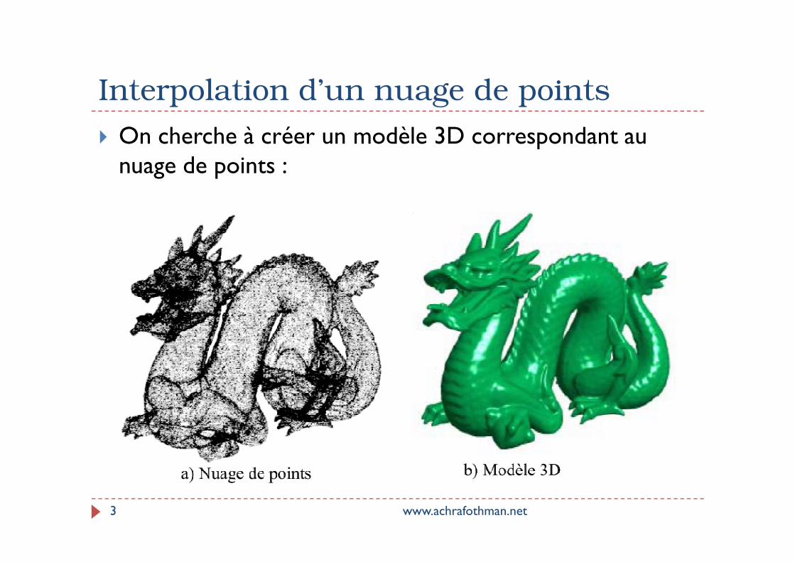
Interpolation d’un nuage de points
� On cherche à créer un modèle 3D correspondant au nuage de points :
www.achrafothman.net3

Interpolation d’un nuage de points
� Les différentes étapes du processus :
www.achrafothman.net4

Interpolation d’un nuage de points
� Les différentes étapes du processus :
www.achrafothman.net5

TriangulationDifférents types
� Approche naïve :
www.achrafothman.net6
� Approche par triangulation: deux approches d’interpolation de la hauteur

TriangulationDéfinition
� La triangulation permet de connaitre pour chaque point, ses coordonnées X,Y et Z. Suivant son utilisation elle peut donner différents résultats :
www.achrafothman.net7

TriangulationExemples
www.achrafothman.net8

TriangulationEntrée > Sortie
www.achrafothman.net9
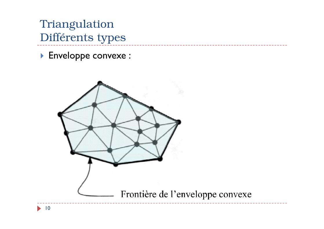
� Enveloppe convexe :
TriangulationDifférents types
10
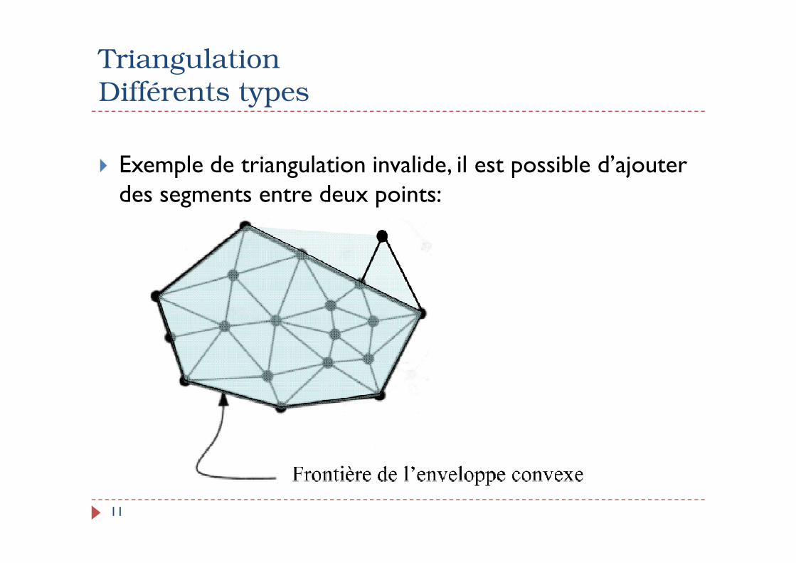
� Exemple de triangulation invalide, il est possible d’ajouter des segments entre deux points:
TriangulationDifférents types
11

� Ajout de segments pour rendre la triangulation valide:
TriangulationDifférents types
12

� Convexité des quadrilatères:
TriangulationDifférents types
13

� Pour 4 points, deux types de triangulations possibles:
TriangulationDifférents types
14
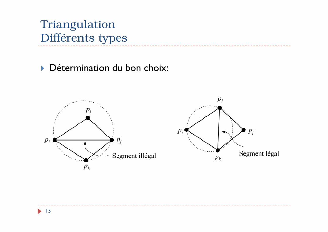
� Détermination du bon choix:
TriangulationDifférents types
15
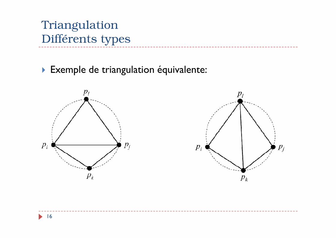
� Exemple de triangulation équivalente:
TriangulationDifférents types
16

Triangulation de Delaunay
� Algorithmes de construction d'une triangulation de Delaunay
� Deux approches
� 1- Construction d'une triangulation pour un ensemble de points donnés
www.achrafothman.net17
1- Construction d'une triangulation pour un ensemble de points donnés
� Construction du diagramme de Voronoï puis « dualisation »
� Algorithme ad-hoc incrémentaux ou non
� 2- Les points sont calculés au fur et à mesure de la construction de la triangulation
� Génération de maillage / adaptation de maillage
� Algorithme nécessairement incrémentaux

Triangulation de Delaunay
� Principe des algorithmes incrémentaux de construction d'une triangulation de Delaunay
� Insertion d'un point Pn dans une triangulation à n–1points
� Trouver l'entité contenant le nouveau point
� Insérer le point
� Modifier la triangulation pour garder le caractère « de Delaunay » de
www.achrafothman.net18
� Modifier la triangulation pour garder le caractère « de Delaunay » de celle ci
� Il existe deux algorithmes voisins (équivalents puisque la triangulation de Delaunay est unique)
� Lawson – edge swapping : Garantit une triangulation valide à toute étape de l'algorithme.
� Bowyer-Watson – trouver tous les triangles dont le centre circonscrit contient le nouveau point, détruire ces triangles et reconstruire la cavité. Inconvénient : possible de construire des cavités non étoilées (voire non connexes) si les calculs sont faits en précision finie

Triangulation de Delaunay
� Recherche de l'entité contenant le point.
� Insertion du point dans la triangulation
� Cas 1 : le point Pn est situé dans un triangle Ti
www.achrafothman.net19

Delaunay
Cercle circonscrit
Propriété du Cercle vide(Sphere) : Aucun sommet à l’intérieur du cercle ciconscrit.
En géométrie, un cercle circonscrit à un polygone est un cercle passant par tous les sommets du polygone. Le polygone est alors dit inscrit dans le cercle : on parle de polygone inscriptible. Les sommets sont alors cocycliques, situés sur un même cercle. Ce cercle est unique et son centre est le point d'intersection des médiatrices des côtés.

Delaunay Triangulation: Obeys empty-circle (sphere) property
Delaunay

X
Given a Delaunay Triangulation of n nodes, How do I insert node n+1 ?
Delaunay
Lawson Algorithm•Locate triangle containing X•Subdivide triangle•Recursively check adjoining triangles to ensure empty-circle property. Flip diagonal if needed•(Lawson,77)

X
Delaunay
Lawson Algorithm•Locate triangle containing X•Subdivide triangle•Recursively check adjoining triangles to ensure empty-circle property. Swap diagonal if needed•(Lawson,77)
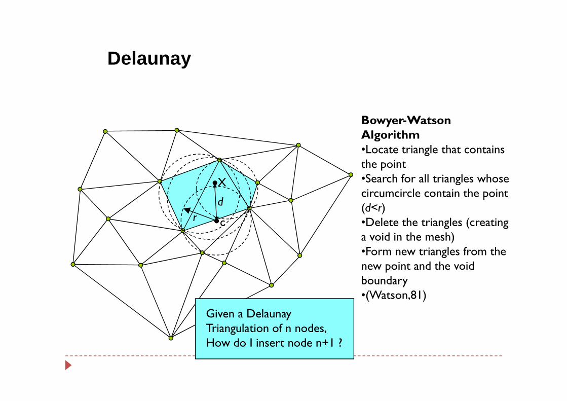
Bowyer-Watson Algorithm•Locate triangle that contains the point•Search for all triangles whose circumcircle contain the point (d<r)
X
d
Delaunay
circumcircle contain the point (d<r)•Delete the triangles (creating a void in the mesh)•Form new triangles from the new point and the void boundary•(Watson,81)
r c
d
Given a Delaunay Triangulation of n nodes, How do I insert node n+1 ?

X
Bowyer-Watson Algorithm•Locate triangle that contains the point•Search for all triangles whose circumcircle contain the point (d<r)
Delaunay
circumcircle contain the point (d<r)•Delete the triangles (creating a void in the mesh)•Form new triangles from the new point and the void boundary•(Watson,81)
Given a Delaunay Triangulation of n nodes, How do I insert node n+1 ?

Watson’s algorithm (1981)
� Given a set V of points, calculate a Delaunay triangulation with vertices at points of V
� Watson’s algorithm is one of the so-called on-line methods: based on the modification of an existing Delaunay triangulation when a new point is inserted
� In on-line methods, the first step consists of building a Delaunay triangulation of the domain (containing all data points)
� Then all points of V are added incrementally

Watson : initialisation
� In Watson’s algorithm, the initial triangulation of the domain is built by considering a fictitious triangle containing all points of V in its interior
Dataset VDataset V

Watson : procédure et algorithme
� After building the initial triangle, all points of V are added one at a time
� Finally the initial triangle and all edges incident at its vertices are deleted
� The main step in this algorithm is the insertion of a new point in the current Delaunay triangulation

Watson : insertion d’un nouveau point
� We call the influence polygon RP of a point P in a triagulation T the union of all triangles of T whose circumscribing circle contain P
� After inserting P in T, we update T by deleting all edges internal to RP and by joining P with all the vertices of RP
P
RP
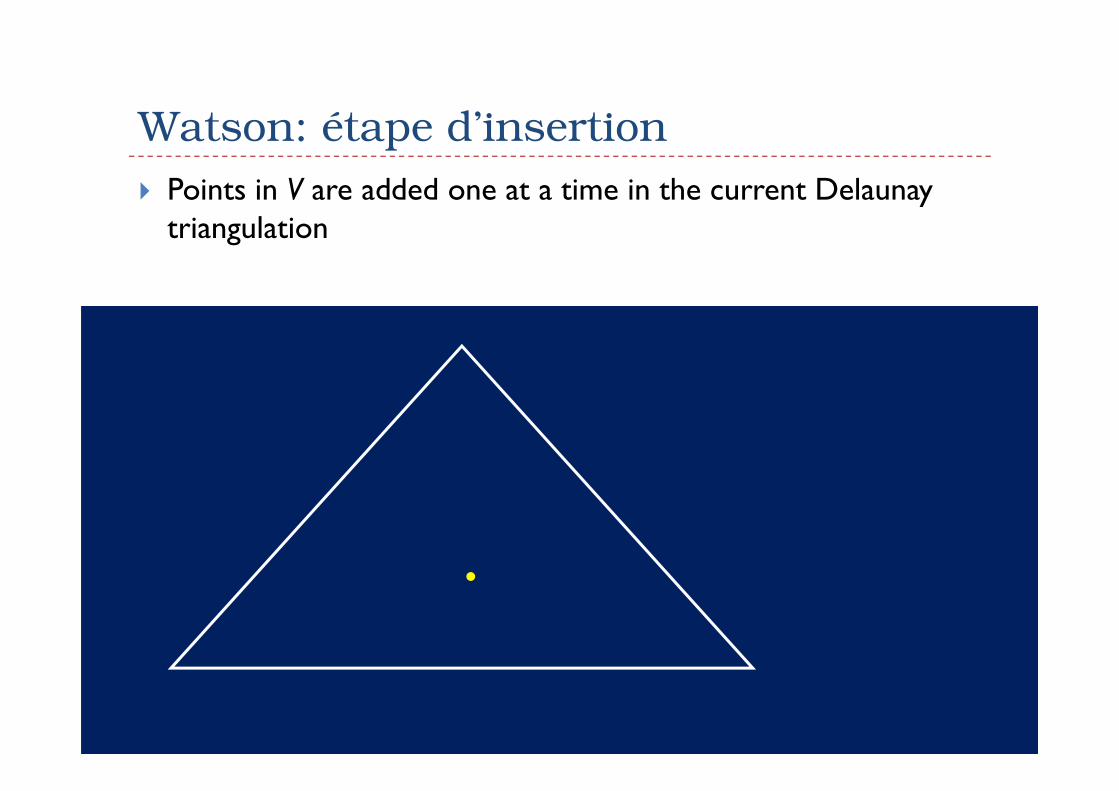
Watson: étape d’insertion
� Points in V are added one at a time in the current Delaunay triangulation

Watson : étape d’insertion (cont.d)
� First vertex P1: the fictitious triangle is its influence polygon RP1; join P1 with its three vertices

Watson : étape d’insertion (cont.d)
� Inserting the second vertex P2: calculation of RP1
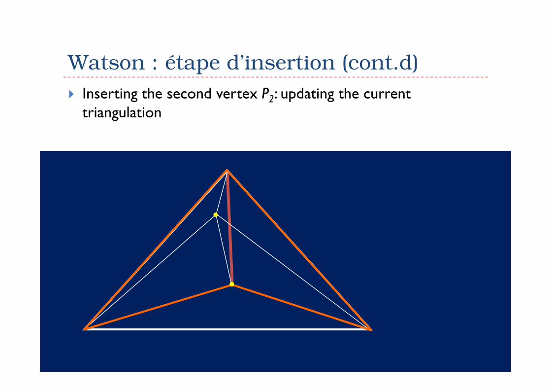
Watson : étape d’insertion (cont.d)
� Inserting the second vertex P2: updating the current triangulation

Watson : étape d’insertion (cont.d)
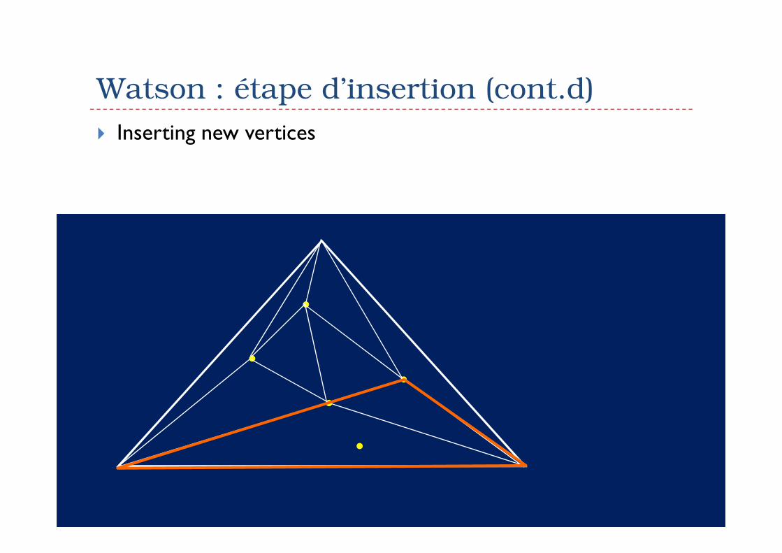
� Inserting new vertices

Watson : étape d’insertion (cont.d)
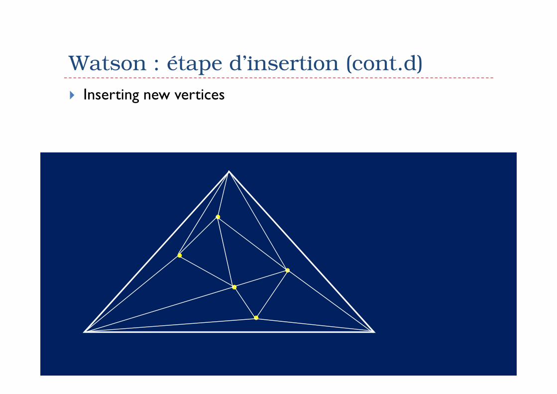
� Inserting new vertices

Watson : étape d’insertion (cont.d)
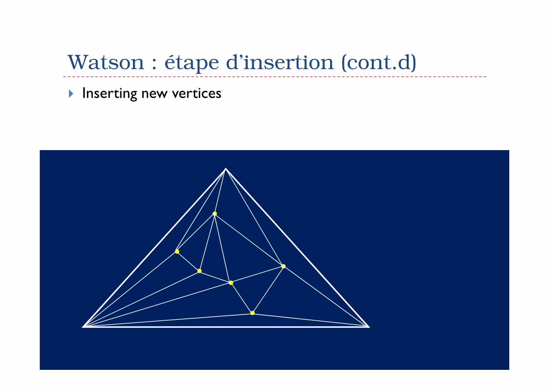
� Inserting new vertices
Watson : étape d’insertion (cont.d)
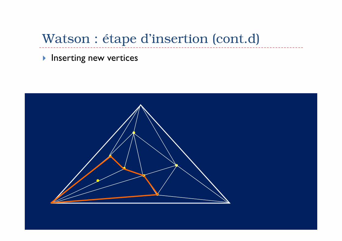
� Inserting new vertices
Watson : étape d’insertion (cont.d)
� Inserting new vertices

Watson : étape d’insertion (cont.d)
� Inserting new vertices
Watson : étape d’insertion (cont.d)
� Inserting new vertices
Watson : étape d’insertion (cont.d)
� Inserting new vertices

Watson : étape d’insertion (cont.d)
� Inserting new vertices
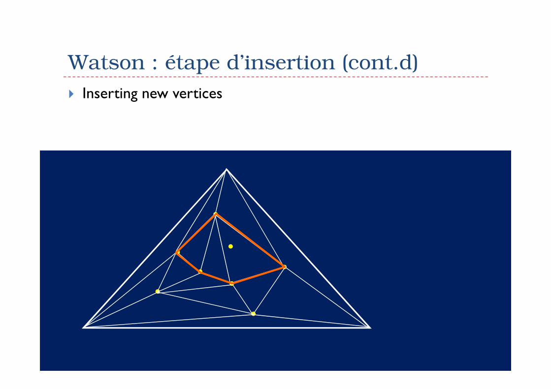
Watson : étape d’insertion (cont.d)
� Inserting new vertices

Watson : étape d’insertion (cont.d)
� Inserting new vertices
Watson : étape d’insertion (cont.d)
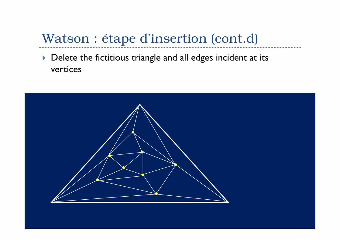
� Delete the fictitious triangle and all edges incident at its vertices

Watson : dernière étape
� Delete the fictitious triangle and all edges incident at its vertices

Watson : dernière étape
� Given V, Watson’s algorithm calculates the Delaunay triangulation with vertices at points of of V

Watson : Complexité
� The time complexity of Watson’s algorithm is O(n2) where n is the number of input points (worst case)
� This depends on the fact that the insertion of a new point requires changing all triangles of the influence polygon. In the worst case, the influence polygon includes all triangles of the worst case, the influence polygon includes all triangles of the current triangulation
� NOTE: remember that the number of triangles in a triangulation is O(v), with v the number of vertices in the triangulation
Watson : Complexité (cont.d)
� Although the worst case time complexity for Watson’s algorithm is O(n2), it has been shown that in the average case the number of triangles in the influence polygon is equal to 6 (Sibson, 1978)
� Therefore, the average case time complexity is linear in the � Therefore, the average case time complexity is linear in the number of input points


![Les Pavages du plan avec des polygones convexes ......III] Pavages par des polygones non réguliers A) Les triangles Tout triangle pave le plan. Ceci est évident car tout d’abord,](https://img.pdfslide.fr/doc/110x75/5f0828447e708231d4209f73/les-pavages-du-plan-avec-des-polygones-convexes-iii-pavages-par-des-polygones.jpg)