DOCUMENT

DE TRAVAIL

N° 408

DIRECTION GÉNÉRALE DES ÉTUDES ET DES RELATIONS INTERNATIONALES

EXPORT DYNAMICS AND SALES AT HOME

Nicolas Berman, Antoine Berthou and Jérôme Héricourt

November 2012

DIRECTION GÉNÉRALE DES ÉTUDES ET DES RELATIONS INTERNATIONALES

EXPORT DYNAMICS AND SALES AT HOME

Nicolas Berman, Antoine Berthou and Jérôme Héricourt

November 2012

Les Documents de travail reflètent les idées personnelles de leurs auteurs et n'expriment pas

nécessairement la position de la Banque de France. Ce document est disponible sur le site internet de la

Banque de France « www.banque-france.fr ».

Working Papers reflect the opinions of the authors and do not necessarily express the views of the Banque

de France. This document is available on the Banque de France Website “www.banque-france.fr”.

Export dynamics and sales at home ∗

Nicolas Berman† Antoine Berthou‡ Jerome Hericourt §

November 9, 2012

∗We are especially grateful to Richard Baldwin, Juan Carluccio, Nicolas Coeurdacier, Matthieu Crozet, Anne-Celia Disdier, Peter Egger, Lionel Fontagne, Jean Imbs, Beata Javorcik, Pamina Koenig, Miren Lafourcade,Florian Mayneris, Lise Patureau, Frederic Robert-Nicoud, Linda Tesar, Vincent Vicard, and participants atseveral seminars and conferences for very useful comments and discussions. Part of this research was funded bythe French Agence Nationale de la Recherche (ANR), under grant ANR-11-JSH1 002 01. This research doesnot reflect the views of the Banque de France. Finally, any remaining errors are ours.†Graduate Institute of International and Development Studies (IHEID) and CEPR. Address: Case Postale

136, CH - 1211, Geneva 21 - Switzerland. Tel: (0041) 22 908 5935. E-mail: nicolas.berman@graduateinstitute.ch.‡Banque de France. Address: 39 rue Croix des Petits Champs 75001 Paris - France. Tel: (0033) 01 42 92 28

76. E-mail: antoine.berthou@banque-france.fr§EQUIPPE-University of Lille. Universite de Lille 1, Faculte des Sciences Economiques et Sociales, USTL

- Cite Scientifique - Bat SH2, 59655 Villeneuve d’Ascq Cedex - France. Tel/Fax: (33) 1 44 07 82 78, Email:jerome.hericourt@univ-lille1.fr

1

Abstract: How do firms’ sales interact across markets? Are foreign and domestic sales com-

plements or substitutes? Using a large French firm-level database that combines balance-sheet

and product-destination-specific export information over the period 1995-2001, we study the

interconnections between exports and domestic sales. We identify exogenous shocks that af-

fect the firms’ demand on foreign markets to instrument yearly variations in exports. We use

alternatively as instruments product-destination specific imports or tariffs changes, and large

foreign shocks such as financial crises or civil wars. Our results show that exogenous variations

in foreign sales are positively associated with domestic sales, even after controlling for changes

in domestic demand. A 10% exogenous increase in exports generates a 1.5 to 3% increase in

domestic sales in the short-term. This result is robust to various estimation techniques, instru-

ments, controls, and sub-samples. It is also supported by the natural experiment of the Asian

crisis in the late 1990’s. We discuss various channels that may explain this complementarity.

Keywords: Export dynamics, domestic sales, markets, liquidity

JEL classification: F10, F44, L20

Resume: Les ventes des entreprises sur differents marches sont-elles liees entre elles ? Comment

les ventes sur le territoire national reagissent-elles aux variations de ventes sur leurs marches

d’exportation ? Pour repondre a ces questions relatives a l’interconnexion des marches d’une

firme, cette etude fait appel a une base de donnees d’entreprises combinant des informations

sur le chiffre d’affaire a l’export, et sur le chiffre d’affaire realise en France, par des entreprises

implantees sur le territoire national pour la periode 1995-2001. La methodologie utilisee conduit

a “instrumenter” les ventes sur les marches d’exportation d’une firme par des chocs qui lui

sont exogenes. Ces instruments incluent la demande d’importations sur chaque destination et

produit, les droits de douanes imposes par produit sur chaque destination, les crises financieres

intervenues sur les marches de la firme ou encore les guerres civiles. Les resultats des estimations

indiquent que les variations exogenes des ventes a l’exportation d’une firme conduisent a une

variation de ses ventes domestiques dans la meme direction. Ce resultat reste valide lorsque

l’estimation controle pour la possible correlation des chocs de demande entre la France et les

marches d’exportation de la firme. Une hausse exogene de 10% des ventes a l’exportation tend

a accroıtre les ventes domestiques de la firme de l’ordre de 1,5% a 3% la meme annee. Ce

resultat est robuste a un grand nombre de tests alternatifs detailles dans l’article. La derniere

partie de l’article discute des mecanismes qui pourraient engendrer cette complementarite entre

ventes domestiques et ventes a l’exportation des firmes.

Mots cle : dynamique d’exportation des firmes, ventes domestiques, liquidite

Classification JEL : F10, F44, L20

2

1 Introduction

The sales of a firm are distributed across several markets, each of these markets being identified

by a specific location and a particular product. Empirical evidence shows that large, productive

firms explore more markets and have larger average sales. How sales between these different

markets interplay, beyond the simple correlation of market-specific shocks, remains however

unclear, though it may be an important determinant of firm-level dynamics and have important

implications for the transmission of foreign shocks to the domestic economy.

This paper provides an empirical investigation of this question through the lens of the

relationship between French firms’ exports and domestic sales. As sales decisions across markets

are likely to be simultaneously determined, we develop a strategy that identifies variations

in the foreign demand addressed to the firms to predict exogenous changes in exports, and

their effect on the firms’ domestic sales. The different dimensions of our data allows us to

build instruments that capture the demand specifically addressed to a given firm in the foreign

markets (destinations and products) it serves, while controlling for the conditions it faces in

the domestic market.

Our empirical analysis relies on a large firm-level dataset containing both firm-level trade

data from the French Customs and balance-sheet information over the period 1995-2001, at a

yearly frequency. In particular, the balance-sheet data contains domestic and foreign sales, our

main variables of interest. The customs data contains firm-level exports and imports by product

and destination. This information is used to identify variations in the demand addressed to firms

in both foreign and domestic markets. We build several instruments. In our baseline estimates,

we use the sum of imports in the products-destinations served by the firms, weighted by the

share of each product-destination in the firm’s total exports.1 Importantly, we also consider a

number of alternative instruments, including firm-specific tariff changes and exposure to large

foreign shocks, such as financial crises or civil wars.

We find that a 10% exogenous increase in exports generates a 1.5 to 3% increase in domestic

sales in the short-run, depending on the specification. This complementarity is robust to various

estimation techniques, combinations of instruments, sub-samples, and inclusions of additional

controls. These variations in domestic sales are related to both factor accumulation and changes

in total factor productivity. Our results are valid in cases where the foreign demand for firms’

1A product is defined at the HS6 level.

3

products is either increasing or decreasing, the effect being slightly larger in the latter case.

Why are firms’ domestic sales positively related to exogenous changes in exports? In most

international trade models (e.g. Melitz, 2003), domestic and foreign sales are only related

through idiosyncratic firm productivity shocks. Exogenous shocks affecting a given location

have no effect on sales in other markets. While the main purpose of is paper is mainly to

provide a robust characterization of an empirical stylized fact, several theoretical mechanisms

can be used to rationalize the existence of a relation between exports and domestic sales, mainly

through cost linkages. Increasing export sales may come at the expense of domestic sales in

the short run in the presence of capacity constraints, i.e. if the marginal cost is increasing with

quantities. On the other hand, changes in exports driven by external demand shocks could

also reduce marginal cost, for instance in cases where production exhibits increasing returns to

scale, or if changes in export sales provide firms with cheap liquidity that can be used to finance

domestic operation in the short-run, i.e. to pay suppliers, hire workers or make investments.

Our results do not preclude the possibility of capacity constraints in the short-run, but sim-

ply suggest that they do not dominate when changes in exports are driven by external demand

shocks in the firms’ markets, which are orthogonal to firms’ characteristics. While the main

objective of this paper is not to provide a definitive answer to the mechanism underlying our

findings, we provide a number of results supporting the liquidity channel. First, we show that

the positive effect of exogenous changes in exports on domestic sales is stronger for firms selling

a larger part of their total sales internationally, and for small firms. Second, this complementar-

ity is higher in sectors in which firms rely more on the use of short-run liquidity - due to higher

working capital requirements -, and in sectors in which firms are less profitable and therefore

financially more vulnerable.

Our results have direct consequences for the effect of international trade on the synchronization

of international business cycles. Common wisdom generally attributes the strong correlation be-

tween openness and the synchronization of business cycles to a simple mechanism: as economies

become more open, exports and imports represent a larger share of firms’ total sales or input

purchases.2 This makes firms more sensitive to variations in foreign demand, which tends

2Theoretically, the fact that international trade causes tighter business cycle synchronization is ambiguous.If trade openness leads to greater specialization, and cycles are predominantly sector-specific, trade opennessmay actually decrease business cycle correlation. However, empirical works have found strong evidence thattrade openness amplifies international business cycles correlation. See, among many others, Frankel and Rose(1998) or Baxter and Kouparitsas (2005).

4

to propagate shocks. Our results imply that foreign business cycles may be transmitted to

domestic markets through the complementarity between firms’ domestic and foreign sales.

Our results have implications regarding the transmission of foreign trade policy, exchange

rate shocks or financial crises to the domestic economy. In the case of the 1997-98 Asian crisis,

we indeed show that firms that were more exposed to the destinations that experienced the crisis

suffered a larger drop in domestic sales during the event. More generally, our results support

the idea that changes in exports in one market, due to changes in market-specific demand

conditions, tend to affect sales in other markets in the same direction. This transmission of

firm performance across markets is not explained by business cycles’ synchronization.

A very recent, yet flourishing, body of literature has emphasized the role of cost linkages in

explaining how exports affect the volatility of firms’ sales (Vannoorenberghe, 2012, Soderbery,

2012, Nguyen and Schaur, 2011, Blum et al., 2011, Ahn and McQuoid, 2012).3 The general

idea of these papers is that firms may substitute sales away from a given market when growth

opportunities appear in other markets, if their production function exhibits convex marginal

costs. The fact that firms’ exports (or export status) are negatively correlated with their

domestic sales is consistent with this mechanism. Our results show that when changes in

exports are driven by external demand shocks, which are exogenous to firms idiosyncratic

shocks, domestic sales do vary in the same direction.

Finally, a number of recent empirical papers have tested the influence of foreign macroe-

conomic shocks on firms’ activities through factor utilization and productivity. Of particular

interest are the papers by Ekholm et al. (2012) and Hummels et al. (2010). Ekholm et al.

(2012) showed that for Norway, firms that were more exposed to the appreciation of the Krona

in the early 2000’s (through higher competitive pressure at home or reduced competitiveness on

foreign markets) restructured more. Hummels et al. (2010) showed that for Denmark, positive

export shocks lead to an expansion of firms’ employment and wages paid to all types of workers.

Our results suggest that these gains are not only directly related to foreign shocks, but may

also be the indirect consequence of the complementarity between export and domestic sales.4

3This recent literature follows a more ancient research documenting the relationship between exports anddomestic production at the country level (Ball et al., 1966, Dunlevy, 1980; Haynes and Stone, 1983; Zilberfarb,1980). Most of these papers tested the “capacity pressure” hypothesis, using aggregate data, and producedmixed results.

4To a lesser extent, our paper also contributes to the vast literature interested in the effect of internationaltrade on firm performance, which has been a major area of research since the late 1990’s. Most papers focusedon the link between exporting and productivity at the firm level, showing that the most productive firms self-

5

The next section presents the data and some descriptive statistics. Section 3 presents our

empirical methodology. Section 4 reports our baseline results, a number of robustness checks,

and an test of our results using the 1997-98 Asian crisis as a natural experiment. We discuss

various potential channels of transmission in section 5. The last section concludes.

2 Data and stylized facts

2.1 Database

Our empirical analysis relies on two main datasets that report information at the firm level.

The first source is the balance sheet dataset BRN (Benefice Reels Normaux), which relies on

fiscal declarations by domestic French firms. The BRN database is constructed from mandatory

reports of French firms to the tax administration, which are in turn transmitted to INSEE (the

French Statistical Institute). This dataset reports information including firms’ total sales and

export sales, employment, capital stock, value added, the industry, year, and balance-sheet

variables. The data covers the period 1995-2001, for which we have information on both the

total sales and export sales. This combined information is used to compute domestic sales. The

BRN contains between 650,000 and 750,000 firms per year over the period, which is around

60% of the total number of French firms.5 Importantly, this dataset is composed of both small

and large firms, since no threshold applies on the number of employees. Eaton et al. (2004)

and Eaton et al. (2011) provide a more detailed description of the database. Because we are

interested in the relationship between export flows and domestic sales, we only keep firms that

export at least once over the period 1995-2001. We also restrict our analysis to firms whose

primary activity is manufacturing. This excludes in particular wholesalers. Finally, we clean

the data by dropping the firms that have a share of exports over total sales above 90%6, and

the top and bottom percentile in terms of total average sales growth.

select on export markets. They provide only mixed evidence on the productivity gains generated by entryinto foreign markets, however (early works include Bernard and Jensen, 1999 or Bernard and Wagner, 1998;for recent contributions see De Loecker, 2007, Van Biesebroeck, 2005, Park et al., 2009). These results haveled many authors to argue that trade liberalization may affect economic growth mainly through the processof resource reallocation across firms within sector, with little contribution of productivity gains within firms.Our results suggest that export performance may affect domestic performance in the short-term, either throughfactor accumulation or TFP gains.

5The BRN files contain all firm which sales at least 763 K euros (230 K euros for services).6This drops firms located in France whose main activity is to sell goods abroad. Less than 1.8% of the

observations are dropped. Note that our results are robust to the use of the full sample.

6

The second source of data used in this paper corresponds to the French customs data,

which reports exports flows with firm, destination and product dimensions. Both the quantity

(in tons) and value of each flow are reported. The product classification system is the European

Union Combined Nomenclature at 8 digits (CN8). The customs database is quasi-exhaustive.7

After merging the two sources, we are left with about 95% of French exports contained in the

customs data each year.

Our strategy relies on the estimation of the effect of export sales on domestic sales. We use

the firm-specific structure of exports (by destination and by product) to compute measures of

the foreign demand addressed to each firm. We use either all products exported by the firms,

or their main product. These variables are used as instruments for export sales in our empirical

analysis. Their construction is further detailed in the next section. We also build alternative

instruments using the Asian crisis as a foreign demand shock, tariffs, or civil wars.

2.2 Descriptive statistics

This section provides some descriptive statistics about the characteristics of the firms contained

in our sample. Our final sample is an unbalanced panel containing 29,542 firms exporting at

least once over the period 1995-2001. On average, around 21,000 firms report exports each

year. Table 1 reports information for these firms regarding their number of employees, their

domestic sales (in thousands of euros), their export sales (in thousands of euros), export share,

which is measured as the ratio of export sales over total sales, and the log change of exports

and domestic sales. The size of the firms contained in the data is very heterogeneous: it starts

with a single employee for the smallest firm, whereas the largest has almost 82,000 employees.

The distribution of export share confirms that most of firms’ sales correspond to business

operations on the domestic market: half of firms in the sample export 13% or less of their total

sales; 75% of firms export at most a third of their total sales. Hence, this empirical pattern

confirms that firms’ sales are mostly concentrated on the domestic market, whereas exports

are concentrated on a small number of firms that have a large degree of internationalization.

Finally, both export and domestic sales exhibit, on average, a positive growth (3% and 4%

respectively), with foreign sales being significantly more volatile than domestic sales.

7Only some small shipments are excluded from this data collection. Inside the European Union (EU), firmsare required to report their shipments by product and destination country only if their annual trade valueexceeds the threshold of 150,000 euros. For exports outside the EU all flows are recorded, unless their value issmaller than 1000 euros or one ton. Those thresholds only eliminate a very small proportion of total exports.

7

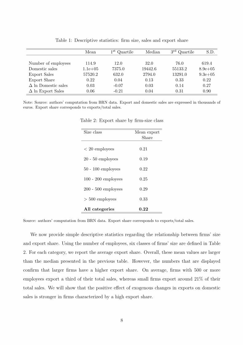
Table 1: Descriptive statistics: firm size, sales and export share

Mean 1st Quartile Median 3rd Quartile S.D.

Number of employees 114.9 12.0 32.0 76.0 619.4Domestic sales 1.1e+05 7375.0 19442.6 55133.2 8.9e+05Export Sales 57520.2 632.0 2794.0 13291.0 9.3e+05Export Share 0.22 0.04 0.13 0.33 0.22∆ ln Domestic sales 0.03 -0.07 0.03 0.14 0.27∆ ln Export Sales 0.06 -0.21 0.04 0.31 0.90

Note: Source: authors’ computation from BRN data. Export and domestic sales are expressed in thousands ofeuros. Export share corresponds to exports/total sales.

Table 2: Export share by firm-size class

Size class Mean exportShare

< 20 employees 0.21

20 - 50 employees 0.19

50 - 100 employees 0.22

100 - 200 employees 0.25

200 - 500 employees 0.29

> 500 employees 0.33

All categories 0.22

Source: authors’ computation from BRN data. Export share corresponds to exports/total sales.

We now provide simple descriptive statistics regarding the relationship between firms’ size

and export share. Using the number of employees, six classes of firms’ size are defined in Table

2. For each category, we report the average export share. Overall, these mean values are larger

than the median presented in the previous table. However, the numbers that are displayed

confirm that larger firms have a higher export share. On average, firms with 500 or more

employees export a third of their total sales, whereas small firms export around 21% of their

total sales. We will show that the positive effect of exogenous changes in exports on domestic

sales is stronger in firms characterized by a high export share.

8

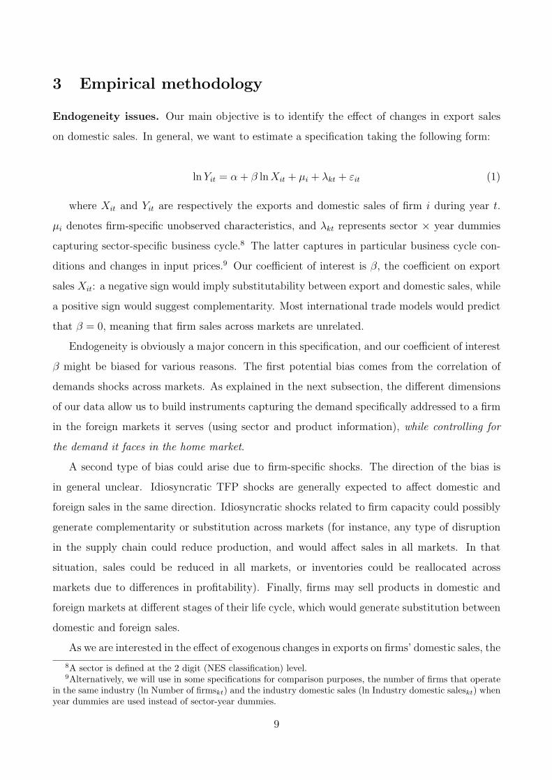
3 Empirical methodology

Endogeneity issues. Our main objective is to identify the effect of changes in export sales

on domestic sales. In general, we want to estimate a specification taking the following form:

lnYit = α + β lnXit + µi + λkt + εit (1)

where Xit and Yit are respectively the exports and domestic sales of firm i during year t.

µi denotes firm-specific unobserved characteristics, and λkt represents sector × year dummies

capturing sector-specific business cycle.8 The latter captures in particular business cycle con-

ditions and changes in input prices.9 Our coefficient of interest is β, the coefficient on export

sales Xit: a negative sign would imply substitutability between export and domestic sales, while

a positive sign would suggest complementarity. Most international trade models would predict

that β = 0, meaning that firm sales across markets are unrelated.

Endogeneity is obviously a major concern in this specification, and our coefficient of interest

β might be biased for various reasons. The first potential bias comes from the correlation of

demands shocks across markets. As explained in the next subsection, the different dimensions

of our data allow us to build instruments capturing the demand specifically addressed to a firm

in the foreign markets it serves (using sector and product information), while controlling for

the demand it faces in the home market.

A second type of bias could arise due to firm-specific shocks. The direction of the bias is

in general unclear. Idiosyncratic TFP shocks are generally expected to affect domestic and

foreign sales in the same direction. Idiosyncratic shocks related to firm capacity could possibly

generate complementarity or substitution across markets (for instance, any type of disruption

in the supply chain could reduce production, and would affect sales in all markets. In that

situation, sales could be reduced in all markets, or inventories could be reallocated across

markets due to differences in profitability). Finally, firms may sell products in domestic and

foreign markets at different stages of their life cycle, which would generate substitution between

domestic and foreign sales.

As we are interested in the effect of exogenous changes in exports on firms’ domestic sales, the

8A sector is defined at the 2 digit (NES classification) level.9Alternatively, we will use in some specifications for comparison purposes, the number of firms that operate

in the same industry (ln Number of firmskt) and the industry domestic sales (ln Industry domestic saleskt) whenyear dummies are used instead of sector-year dummies.

9

identification of this link requires instruments that are independent from firm-specific shocks,

controlling for business cycle correlation across markets. Our strategy uses demand shocks

addressed to each firm (using destination and product specialization), which are unaffected by

firm characteristics. In the robustness analysis, we check that our results are not affected by

the self-selection of firms in international markets.

Main Instruments. Our main instrument is constructed using information about the foreign

demand addressed to the firm using product and destination information. Specifically, we

compute the sum of foreign imports in the products-destinations served by the firm in year t

(using country-level imports by product from the BACI data), weighted by the average share of

each product-destination in the firm’s total exports over the period (using the firm-level exports

data). Weights are computed using the average share of the product-destination in the firm’s

total exports over the 1995-2001 period.10 A product is defined at the 6-digit (HS6) level. More

precisely, we define:

FDit =∑j,p

ωijpMj,p,t (2)

where ωijp is the average share of each product p and destination j in firm i’s exports over the

period, and is time-invariant. Mj,p,t is the total value of imports for product p and destination j

in year t. All of the time-variation of the FDit variable therefore comes from the country-level

imports by product, not from the firm-level weights. This variable is expected to impact the

firm’s exports, but not domestic sales, unless foreign demand for the firm’s products is correlated

with the domestic demand of these products. To ensure that our results are not driven by this

international business cycle correlation, we explicitly control in our baseline specification for the

domestic equivalent of our instrument. It is defined as the domestic demand addressed to the

firm (DDit). This mirror variable is the sum of the world imports from France for all products

exported by firm i (from the BACI data), weighted by the share of each product in the firm’s

exports (using the firm-level exports data that reflect product-specialization of firms):

DDit =∑

p

ωipMFR,p,t (3)

10As mentioned below, we have checked the robustness of our results with weights computed at the beginningof the period. See subsection “Alternative Instruments”.

10

Therefore, this variable provides a firm-specific measure of domestic demand addressed to

the firm. Alternatively, we compute the foreign demand and domestic demand variables using

sales for the “core” product of the firm on each destination: FDcoreit and DDcore

it , respectively.

The core product of the firm is defined at the HS4-digit level as the product with the highest

value of export over the entire period. The detailed computation of these variables is provided

in the data appendix.

Alternative instruments. Testing for overidentifying restrictions requires at least two in-

struments, as we have one endogenous regressor. To assess the exogeneity of our baseline

instruments, and to show that our results are unchanged when using other measures of for-

eign demand, we construct a number of alternative instruments. First, we build a measure of

firm-specific tariffs faced by French exporters, which depend on the destinations they serve and

products they export. It is constructed essentially in the same way as FDit above, but using

tariffs instead of imports. Tariffs are arguably more exogenous because they are less correlated

with domestic conditions. However, this instrument is weaker as tariff variations are limited

over the period. Second, we make use of the occurrence of large (negative) shocks, such as civil

wars or the 1997-98 Asian crisis, to show that our results hold whatever the source of variations

in foreign demand. More details about the computations of these variables are provided later

in the paper, as well as in the data appendix.

Are these various instruments accounting for the two endogeneity biases mentioned above?

One issue might be that our baseline instrument (FDit) is correlated with domestic demand

conditions, and that we do not control appropriately for these through the inclusion of DDit.

We will show that this is unlikely to be the case. First, because the estimates of the coefficient

on DDit are systematically positive and significant as expected, and that the omission of this

term tends to bias upward the β coefficient when using FDit as instrument, which was also

expected. Second, because using our alternative instruments such as tariffs, civil wars or the

Asian crisis, which are clearly (especially the last two ones) unlikely to be correlated with

domestic business cycles, leads to very similar results. Third, because our results hold equally

for countries in which business cycles are correlated with the French ones, and for the others.11

A second issue might be that our instruments reflect firm characteristics which might jointly

11Including or not the domestic sales variable DDit does not affect the coefficients on the export sales variablewhen the latter is instrumented by tariffs or civil wars; this clearly suggests that these variables are uncorrelatedwith domestic business cycle.

11

determine sales across different markets (in the same direction or not). Our baseline instruments

contain two parts: (i) a foreign shock (imports, tariffs, civil wars, financial crises) which is

unlikely to be correlated with firm-specific characteristics; (ii) weights which are potentially

correlated with firm-specific characteristics. Here endogeneity concerns might remain, for the

following reason. Eaton, Kortum and Kramarz (2011), among others, have shown that firms

with higher productivity self-select into the most difficult markets. If these are markets which

on average grow faster, then our baseline instrument might be correlated with firm productivity.

Our estimations include firm-fixed effects which account for the average growth in the foreign

markets served by the firm. What remains is the issue of the weights: the weights in our baseline

specification are averages over the period. This might be problematic if, say, because of good

productivity shocks a given year, the firm decides to export more to the faster-growing markets:

this would mean that our instrument is positively correlated with productivity. But this can

be remedied by constructing the weights at the beginning of the period: we will show that the

results are actually very similar in this case, and the only reason we choose the average weight is

to improve the strength of the instruments and therefore the efficiency of the estimation. Note

also that in unreported regressions we got rid of the weights by only summing imports of the

destinations-products served by the firm during the first year it exported. The results were very

similar. We have also dropped the destination-specific dimension from the weights altogether

(therefore computed initial weights by product) and again, the results were qualitatively similar.

Baseline specification. We include DDit explicitly in equation (1). The following equa-

tion assesses the effect of exogenous changes in exports (through variations in the instruments

presented above in a first stage) on domestic sales, controlling for domestic demand:

lnYit = α + β ln Xit + γDDit + µi + λkt + εit (4)

Where ln Xit is the predicted value of log exports, coming from the first stage. We expect

γ to be positive. We estimate specification (4) by two-stage-least-squares (2SLS). Note that

our results are unchanged when the two-way relationship between export and domestic sales is

jointly estimated using 3SLS, allowing for residual correlation across equations.12 Finally, in

all estimations, standard errors are robust to heteroscedasticity and clustered at the sectoral

12Results are available upon request. In general, we do not estimate jointly the two-way relationship betweenforeign and domestic sales as we do not have - apart from DDit - enough instruments for domestic sales to beable to study comprehensively the effect of domestic sales on exports.

12

(2-digit) level using Froot (1989) correction.

Using alternative instruments allows us to perform Hansen’s J-test of overidentifying restric-

tions. Insignificant test statistics indicate that the orthogonality of the instruments and the

error term cannot be rejected; thus, our choice of instruments is appropriate on that ground.

As shown later, the overidentifying restrictions cannot be rejected. Finally, we performed the

Durbin-Wu-Hausman test for exogeneity of regressors. Unsurprisingly, the null hypothesis of

exogeneity is rejected in most cases.13 This clearly shows that we need to use IV methodologies

to identify exogenous variations of exports. In all estimations, we report the F-stat form of

the Kleibergen-Paap statistic, the heteroskedastic and clustering robust version of the Cragg-

Donald statistic suggested by Stock and Yogo (2005) as a test for weak instruments. Most

statistics are comfortably above the critical values, confirming that our instruments are strong

predictors of export sales.

4 Main Results

4.1 Baseline regressions

Export-Domestic sales correlation. We start with a simple estimation of Equation (4) by

OLS where the firms’ domestic sales are explained by export sales and a set of controls for the

domestic market conditions, firm fixed-effects and year dummies (alternatively with sector ×

year dummies). This specification offers a benchmark estimation of the relationship between

domestic and foreign sales, which can be compared to our preferred estimations (presented in

the following tables) where export sales are instrumented by foreign market demand.

Table 3 presents the results of the estimation in levels (column 1 and 2) and in first differences

(columns 3 to 6). Domestic market conditions are controlled for by using a measure of the

domestic demand addressed to the firm (ln Domestic demandit as defined by (3)), and, when

the sector × year dummies are not included, the number of firms that operate in the same

industry (ln Number of firmskt) and the industry domestic sales (ln Industry domestic saleskt).

The results show that the correlation between domestic and foreign sales is slightly positive or

negative depending on whether we use a fixed effects or a first differences estimator.14 Moreover,

13Detailed results of these tests available upon request.14The results of columns (3) to (6) are consistent with Vannoorenberghe (2012) and Ahn and McQuoid (2012)

who also finds that domestic sales growth is negatively correlated with export sales growth.

13

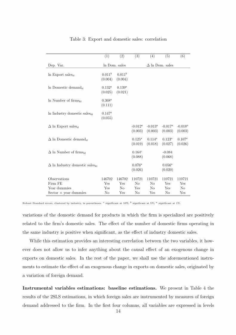
Table 3: Export and domestic sales: correlation

(1) (2) (3) (4) (5) (6)

Dep. Var. ln Dom. sales ∆ ln Dom. sales

ln Export salesit 0.011b 0.011b

(0.004) (0.004)

ln Domestic demandit 0.132a 0.139a

(0.025) (0.021)

ln Number of firmskt 0.368a

(0.111)

ln Industry domestic saleskt 0.147a

(0.055)

∆ ln Export salesit -0.012a -0.013a -0.017a -0.018a

(0.003) (0.003) (0.003) (0.003)

∆ ln Domestic demandit 0.125a 0.114a 0.123a 0.107a

(0.019) (0.018) (0.027) (0.026)

∆ ln Number of firmskt 0.164c -0.084(0.088) (0.068)

∆ ln Industry domestic saleskt 0.076a 0.056a

(0.026) (0.020)

Observations 146702 146702 110721 110721 110721 110721Firm FE Yes Yes No No Yes YesYear dummies Yes No Yes No Yes NoSector × year dummies No Yes No Yes No Yes

Robust Standard errors, clustered by industry, in parentheses. c significant at 10%; b significant at 5%; a significant at 1%.

variations of the domestic demand for products in which the firm is specialized are positively

related to the firm’s domestic sales. The effect of the number of domestic firms operating in

the same industry is positive when significant, as the effect of industry domestic sales.

While this estimation provides an interesting correlation between the two variables, it how-

ever does not allow us to infer anything about the causal effect of an exogenous change in

exports on domestic sales. In the rest of the paper, we shall use the aforementioned instru-

ments to estimate the effect of an exogenous change in exports on domestic sales, originated by

a variation of foreign demand.

Instrumental variables estimations: baseline estimations. We present in Table 4 the

results of the 2SLS estimations, in which foreign sales are instrumented by measures of foreign

demand addressed to the firm. In the first four columns, all variables are expressed in levels14

and export sales are instrumented using foreign demand in firms’ markets (FDit, as defined

in equation (2)). Column (1) includes year dummies and controls for additional variables that

identify sector-specific domestic business cycle: the industry domestic sales and the number of

domestic firms operating in the same industry. In columns (2) to (4), sector×year dummies

are included instead. Estimation (3) which controls for the domestic demand addressed to the

firm due to product-specialization is our preferred specification. Column (4) uses the foreign

demand for the core (HS4) product exported by the firm (FDcoreit as defined above) as the

instrument for exports.

The estimation results contrast with those presented in Table 3. Changes in firm exports,

as predicted by external changes in foreign demand, are positively related with the variations of

the domestic sales by the firm. This result is stable when we introduce industry×year dummies

to better control for sector-specific shocks that may affect firm-level sales simultaneously in

the domestic and export markets (column (2) to (6)). Controlling for the domestic demand

addressed to products exported by firms tends to reduce the estimated β coefficient as expected,

but it remains positive and very significant. Similarly, using as an alternative instrument the

foreign demand addressed to the core product of the firm, while still controlling for the domestic

demand addressed to the core product, leaves our estimate of the β coefficient unchanged

(column (4)). In all cases, the strength of our instruments is confirmed by the Kleibergen-Paap

statistics.

Columns (5) and (6) in Table 4 report the estimation results of the relationship between do-

mestic and foreign sales, when all variables are expressed in first differences. Both estimations

include sector×year dummies, and estimation (6) also contains firm fixed effects. These alter-

native specifications confirm that an increase in export sales, consecutive to an improvement

in foreign demand conditions, raises domestic sales. 15 Overall, results from columns (1) to (6)

suggest that a 10% exogenous increase in exports generates between 1.5 and 3.5% increase in

domestic sales.

As shown in Table 11 in the appendix, these results are robust to the use of alternative

weights in the computation of the instruments. In Table 11, columns (1) to (3), we use weights

computed the first year the firm exports. In columns (4) to (6), we use the first two years. In

all cases, the instruments are somewhat weaker than in our baseline estimates, which leads to

15These results also demonstrate that our estimates are not influenced by non-stationarity in the data thatwe use. In particular, estimates in first-difference with firm fixed effects in column (6) corrects implicitly forpotential firm-specific trend.

15

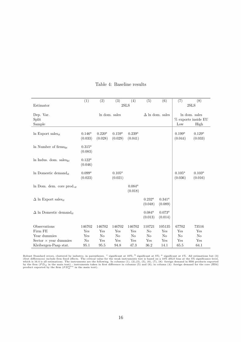
Table 4: Baseline results

(1) (2) (3) (4) (5) (6) (7) (8)Estimator 2SLS 2SLS

Dep. Var. ln dom. sales ∆ ln dom. sales ln dom. salesSplit % exports inside EUSample Low High

ln Export salesit 0.146a 0.220a 0.159a 0.239a 0.199a 0.129a

(0.033) (0.028) (0.029) (0.041) (0.044) (0.033)

ln Number of firmskt 0.315a

(0.083)

ln Indus. dom. saleskt 0.122a

(0.046)

ln Domestic demandit 0.099a 0.105a 0.105a 0.103a

(0.023) (0.021) (0.036) (0.016)

ln Dom. dem. core prod.it 0.084a

(0.018)

∆ ln Export salesit 0.232a 0.341a

(0.048) (0.089)

∆ ln Domestic demandit 0.084a 0.073a

(0.013) (0.014)

Observations 146702 146702 146702 146702 110721 105135 67702 73516Firm FE Yes Yes Yes Yes No Yes Yes YesYear dummies Yes No No No No No No NoSector × year dummies No Yes Yes Yes Yes Yes Yes YesKleibergen-Paap stat. 95.1 95.5 94.8 47.3 36.2 14.1 65.5 64.1

Robust Standard errors, clustered by industry, in parentheses. c significant at 10%; b significant at 5%; a significant at 1%. All estimations but (3)(first differences) include firm fixed effects. The critical value for the weak instruments test is based on a 10% 2SLS bias at the 5% significance level,which is 16.4 is all estimations. The instruments are the following. In columns (1), (2),(3), (5), (6), (7), (8): foreign demand in HS6 products exportedby the firm (FDit in the main text) - instruments taken in first difference in columns (5) and (6); in column (4): foreign demand for the core (HS4)product exported by the firm (FDcore

it in the main text).

16

more noisy estimates, but in all columns the effect of exogenous changes in export sales remains

positive and significant.16 Note that this is also the case when dropping from the estimations

the years used for the computation of the weights (columns (2) and (5)). Our results though

remain unaffected by the use of the initial weights in the construction of the instruments. This

clearly suggest that we are not capturing changes in firm characteristics, but rather exogenous

changes in foreign demand condition.17

Overall, these results obtained when we instrument for firm-level exports suggest that the

OLS estimates of the β coefficient (in Table 3) are biased downward. In all specifications where

firm-level exports are explained by variations of the foreign demand (Table 4), and therefore not

affected by firm-level idiosyncratic shocks, we find that the β coefficient is positive: exogenous

changes in firm-level exports are positively related to variations of firms domestic sales.

Business cycle correlation. Despite the fact that we explicitly control for firm-specific

domestic demand in all specifications, one could still argue that the positive β coefficient that

we estimate is explained by international business cycles synchronization that our controls fail

to capture entirely. If this is the case, we would expect the complementarity between exports

and domestic sales to be higher for firms exporting to countries in which business cycles are

more synchronized with the French one. This would be the case, for instance, for French firms

mainly exporting to EU destinations or more generally, to countries exhibiting a high business

cycle correlation with France.

Columns (7) and (8) of Table 4 present estimates which control explicitly for these phenom-

ena. We estimate the specification of column (3) on two different sub-samples, which include

the firms exporting more or less inside the EU (i.e. firms for which the share of exports inside

EU-15 is above or below the median of the sample), respectively: if the correlation between

foreign and domestic business cycles was driving our results, the coefficient on exports should

be higher for firms more exposed to the EU market, as business cycles are expected to be more

synchronized. Our results are robust, whatever the sample considered. The positive effect of

exports on domestic sales is found to be significantly higher for firms exporting more outside

16The Kleibergen-Paap statistic is reduced in estimations using weights in the beginning of the period for theconstruction of instruments, compared to estimation results reported in Table 4. This is all the more the casewhen we use our alternative instruments (e.g. tariffs) or when we test the channels of transmission.

17As mentioned earlier, in unreported regressions we got rid of the weights by only summing trade on thedestinations served by the firm during the first year it exported. The results were very similar. We have alsodropped the destination-specific dimension from the weights altogether (therefore computed initial weights byproduct) and again, the results were qualitatively similar. All these robustness checks are available upon request.

17

EU-15. This clearly suggests that business cycle correlation is unlikely to bias our results.

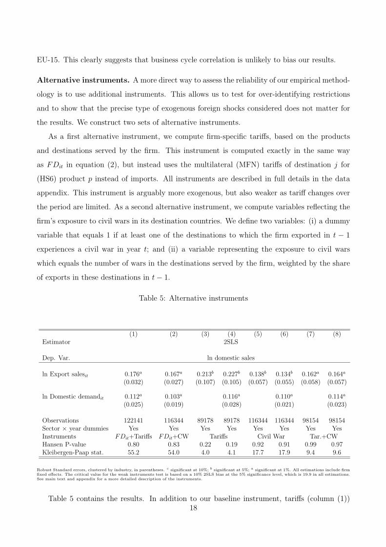
Alternative instruments. A more direct way to assess the reliability of our empirical method-

ology is to use additional instruments. This allows us to test for over-identifying restrictions

and to show that the precise type of exogenous foreign shocks considered does not matter for

the results. We construct two sets of alternative instruments.

As a first alternative instrument, we compute firm-specific tariffs, based on the products

and destinations served by the firm. This instrument is computed exactly in the same way

as FDit in equation (2), but instead uses the multilateral (MFN) tariffs of destination j for

(HS6) product p instead of imports. All instruments are described in full details in the data

appendix. This instrument is arguably more exogenous, but also weaker as tariff changes over

the period are limited. As a second alternative instrument, we compute variables reflecting the

firm’s exposure to civil wars in its destination countries. We define two variables: (i) a dummy

variable that equals 1 if at least one of the destinations to which the firm exported in t − 1

experiences a civil war in year t; and (ii) a variable representing the exposure to civil wars

which equals the number of wars in the destinations served by the firm, weighted by the share

of exports in these destinations in t− 1.

Table 5: Alternative instruments

(1) (2) (3) (4) (5) (6) (7) (8)Estimator 2SLS

Dep. Var. ln domestic sales

ln Export salesit 0.176a 0.167a 0.213b 0.227b 0.138b 0.134b 0.162a 0.164a

(0.032) (0.027) (0.107) (0.105) (0.057) (0.055) (0.058) (0.057)

ln Domestic demandit 0.112a 0.103a 0.116a 0.110a 0.114a

(0.025) (0.019) (0.028) (0.021) (0.023)

Observations 122141 116344 89178 89178 116344 116344 98154 98154Sector × year dummies Yes Yes Yes Yes Yes Yes Yes YesInstruments FDit+Tariffs FDit+CW Tariffs Civil War Tar.+CWHansen P-value 0.80 0.83 0.22 0.19 0.92 0.91 0.99 0.97Kleibergen-Paap stat. 55.2 54.0 4.0 4.1 17.7 17.9 9.4 9.6

Robust Standard errors, clustered by industry, in parentheses. c significant at 10%; b significant at 5%; a significant at 1%. All estimations include firmfixed effects. The critical value for the weak instruments test is based on a 10% 2SLS bias at the 5% significance level, which is 19.9 in all estimations.See main text and appendix for a more detailed description of the instruments.

Table 5 contains the results. In addition to our baseline instrument, tariffs (column (1))18

and exposure to civil war (column (2)) are used as additional instruments for exports. The

Hansen tests of overidentifying restrictions cannot reject the exogeneity of our instruments in

both cases, and the coefficients on exports sales are largely unaffected. Note that the number

of observations is lower because we removed from the sample the firms that export only to

countries in which there is no tariff variation over the period (this includes in particular EU

countries) or for which information on the occurrence of civil wars is missing.

Estimations in columns (3) to (8) use our alternative instruments alone. We include both

firm-specific tariff and its lag in columns (3) and (4) to test for overidentifying restrictions.

Columns (5) and (6) contain the results using both the binary and the continuous proxies for

firm-specific exposure to civil wars as instruments. Column (7) and (8) use both contempora-

neous tariffs and exposure to civil wars as instruments. In all estimations, the Hansen test does

not reject the orthogonality of our instruments, and the coefficient on export sales is always

positive and significant at least at the 5% level. The coefficients are found to be quantitatively

larger than before in columns (3) and (4), but our estimates are also less accurate. These re-

sults suggest that, whatever the (exogenous) shock affecting the firms’ foreign sales, exogenous

variations of exports are positively related to the variation of domestic sales. Interestingly,

the results obtained using civil wars in columns (5) to (8) are very similar to our benchmark

results from Table 4: a 10% decrease in exports generates an additional 1.3% to 1.6% decrease

in domestic sales.

Note that all our instruments have the expected effect on exports, as shown in the Table 10

in the appendix, which reports the first stage coefficients. Finally, our results are unchanged

when we restrict our sample to the firms that are present during the entire period (Table 12 in

the appendix): the coefficient on export sales becomes statistically insignificant only when we

use tariffs alone as an instrument, which is explained by the weakness of the instrument in this

case. Therefore, firms close to bankruptcy, which could decrease simultaneously both exports

and domestic sales, do not drive our results.

4.2 More robustness

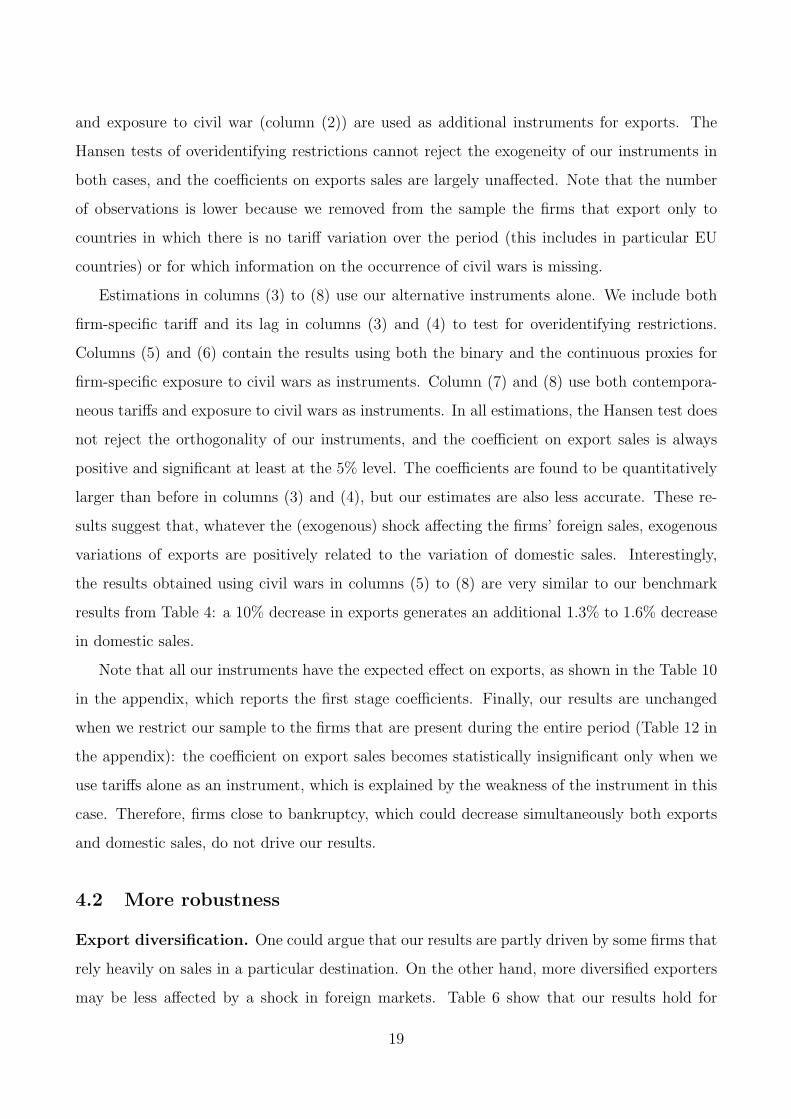
Export diversification. One could argue that our results are partly driven by some firms that

rely heavily on sales in a particular destination. On the other hand, more diversified exporters

may be less affected by a shock in foreign markets. Table 6 show that our results hold for

19

all categories of exporters, even the most diversified ones. As shown in columns (1) and (2),

the difference in the response of single versus multiple-destination exporters is not huge. In

columns (3) and (4) our sample is split according to the average number of destinations reached

by the firm over the period. The coefficient on export sales is significant at the 1% level in all

specifications. Our results are therefore not driven by firms whose exports are concentrated in

a single or few foreign markets.18

Table 6: Export and domestic sales: Export diversification

(1) (2) (3) (4)Estimator 2SLSSplit # destinationsSample Multiple Single Low High

Dep. Var. ln domestic sales

ln Export salesit 0.153a 0.187a 0.152a 0.178a

(0.030) (0.072) (0.041) (0.033)

ln Domestic demandit 0.116a 0.067b 0.087a 0.118a

(0.023) (0.029) (0.020) (0.029)

Observations 115956 30746 73348 73354Sector × year dummies Yes Yes Yes YesKleibergen-Paap stat. 93.5 21.7 42.4 118.1

Robust Standard errors, clustered by industry, in parentheses. c significant at 10%; b significant at 5%; a significant at 1%. All estimations include firmfixed effects. The critical value for the weak instruments test is based on a 10% 2SLS bias at the 5% significance level, which is 16.4 is all estimations.The instrument in all specifications is foreign demand in HS6 products exported by the firm (FDit in the main text). High / low: higher / lower thansample median.

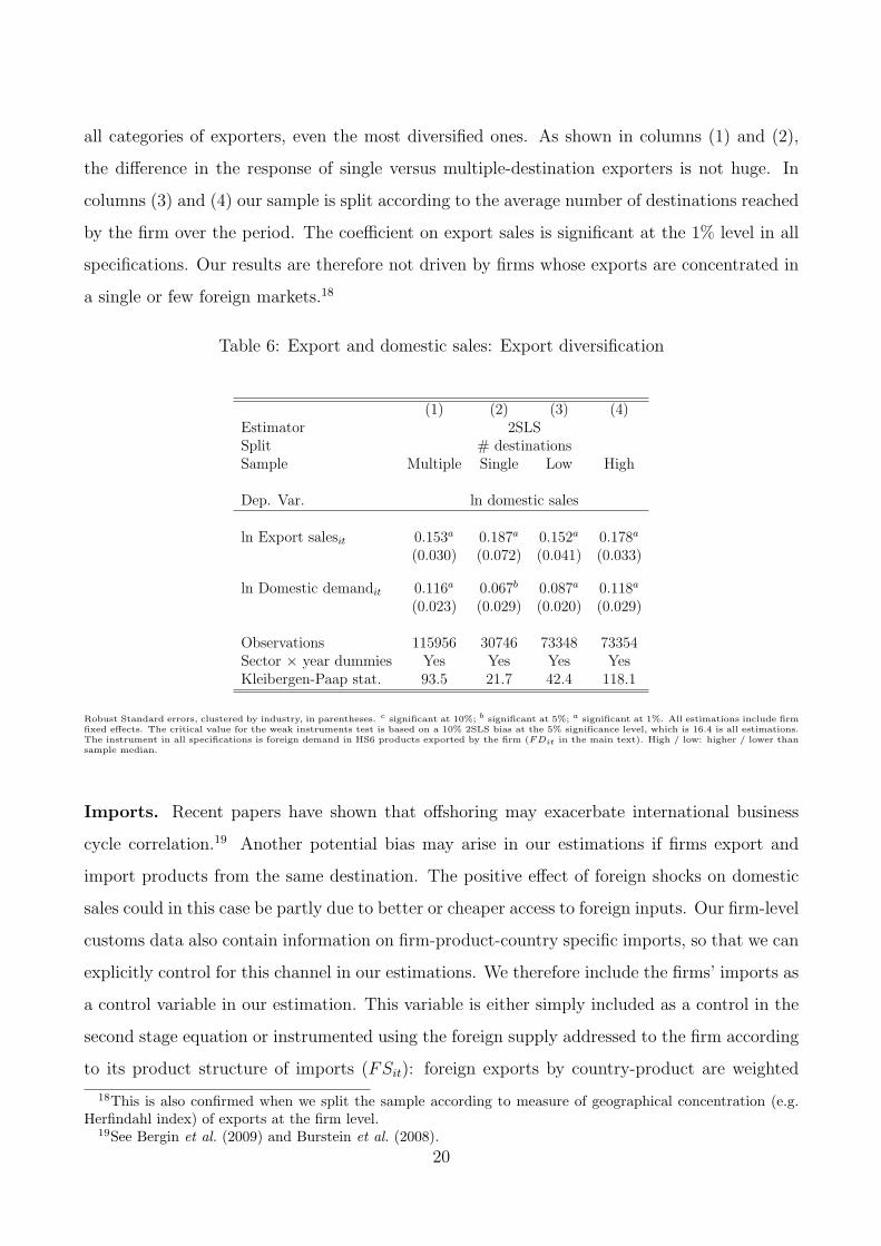
Imports. Recent papers have shown that offshoring may exacerbate international business

cycle correlation.19 Another potential bias may arise in our estimations if firms export and

import products from the same destination. The positive effect of foreign shocks on domestic

sales could in this case be partly due to better or cheaper access to foreign inputs. Our firm-level

customs data also contain information on firm-product-country specific imports, so that we can

explicitly control for this channel in our estimations. We therefore include the firms’ imports as

a control variable in our estimation. This variable is either simply included as a control in the

second stage equation or instrumented using the foreign supply addressed to the firm according

to its product structure of imports (FSit): foreign exports by country-product are weighted

18This is also confirmed when we split the sample according to measure of geographical concentration (e.g.Herfindahl index) of exports at the firm level.

19See Bergin et al. (2009) and Burstein et al. (2008).20

by the share of each country-product pair in each firm’s imports (see data appendix for more

details).

Table 7: Robustness: imports

(1) (2) (3) (4) (5)Dep. Var. ln domestic sales

ln Export salesit 0.159a 0.102a 0.217a 0.210a 0.210a

(0.029) (0.031) (0.042) (0.044) (0.052)

ln Domestic demandit 0.105a 0.087a

(0.021) (0.021)

ln Importsit 0.077a 0.059a 0.054b 0.063a

(0.017) (0.017) (0.024) (0.025)

ln Dom. demand main prod.it 0.066a 0.076a 0.087a

(0.019) (0.018) (0.021)

Observations 146702 146702 146702 116344 94573Sector × year dummies Yes Yes Yes Yes YesInstruments FDit FDit FDcore

it FDcoreit + Tar. FDcore

it + CWHansen p-value - - - 0.19 0.56Kleibergen-Paap stat. / S-Y Crit. val. (10%) 94.9/16.4 15.4/7.0 15.6/7.0 5.5/7.6 10.6/7.6

Robust Standard errors, clustered by industry, in parentheses. c significant at 10%; b significant at 5%; a significant at 1%. 2SLS estimations. Thecritical values for the weak instruments test are based on a 10% 2SLS bias at the 5% significance level. The instruments are the following: in columns

(2) to (5), foreign supply in HS6 products imported by the firm (BCMit in the main data appendix); in columns (1) and (2) foreign demand in HS6

products exported by the firm (FDit in the main text); in column (3) to (5) foreign demand for the core (HS4) product exported by the firm (FDcoreit

in the main text); in column (4), firm-specific tariff; in column (5), exposure to civil wars. See appendix for more details.

Table 7 reports the estimation results that control specifically for firms’ predicted imports.

Columns (1) to (5) differ in terms of the instruments used for export sales: foreign demand in

the HS6 product exported by the firm (columns 1 and 2), foreign demand for the core (HS4)

product exported by the firm (column 3), firm-specific tariffs (column 4) or exposure to civil war

(column 5). Imports are instrumented in all estimations but column (1). In these augmented

specifications, the effect of export decreases slightly in column (2), but remains positive and

significant at the 1% level in all specifications. The coefficient estimate of exports varies between

0.1 and 0.2, quantitatively close to our baseline results.

4.3 A quasi-natural experiment: the 1997-1998 Asian crisis

A direct implication of our results is that negative external demand shocks, such as those

implied by financial crises, are transmitted to domestic sales through trade. The time period21

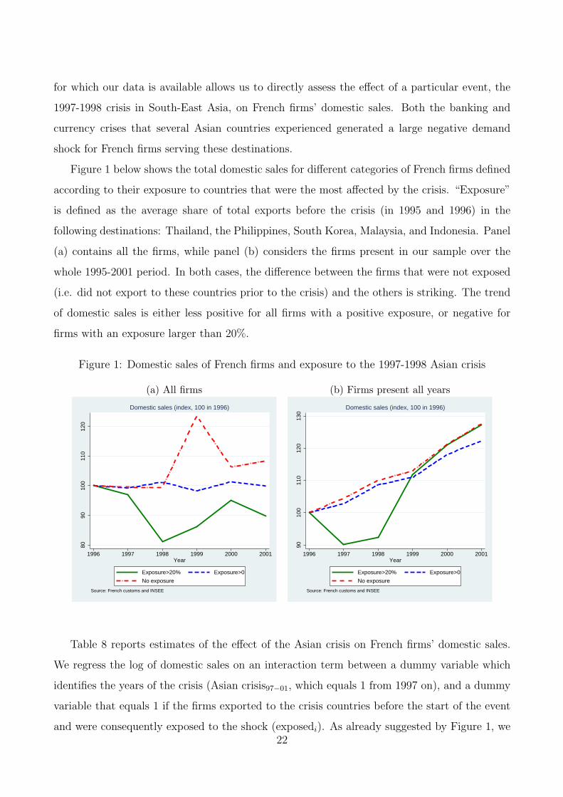
for which our data is available allows us to directly assess the effect of a particular event, the

1997-1998 crisis in South-East Asia, on French firms’ domestic sales. Both the banking and

currency crises that several Asian countries experienced generated a large negative demand

shock for French firms serving these destinations.

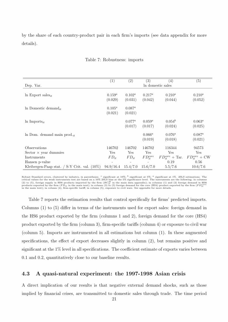
Figure 1 below shows the total domestic sales for different categories of French firms defined

according to their exposure to countries that were the most affected by the crisis. “Exposure”

is defined as the average share of total exports before the crisis (in 1995 and 1996) in the

following destinations: Thailand, the Philippines, South Korea, Malaysia, and Indonesia. Panel

(a) contains all the firms, while panel (b) considers the firms present in our sample over the

whole 1995-2001 period. In both cases, the difference between the firms that were not exposed

(i.e. did not export to these countries prior to the crisis) and the others is striking. The trend

of domestic sales is either less positive for all firms with a positive exposure, or negative for

firms with an exposure larger than 20%.

Figure 1: Domestic sales of French firms and exposure to the 1997-1998 Asian crisis

(a) All firms (b) Firms present all years

8090

100

110

120

1996 1997 1998 1999 2000 2001Year

Exposure>20% Exposure>0

No exposure

Source: French customs and INSEE

Domestic sales (index, 100 in 1996)

9010

011

012

013

0

1996 1997 1998 1999 2000 2001Year

Exposure>20% Exposure>0

No exposure

Source: French customs and INSEE

Domestic sales (index, 100 in 1996)

Table 8 reports estimates of the effect of the Asian crisis on French firms’ domestic sales.

We regress the log of domestic sales on an interaction term between a dummy variable which

identifies the years of the crisis (Asian crisis97−01, which equals 1 from 1997 on), and a dummy

variable that equals 1 if the firms exported to the crisis countries before the start of the event

and were consequently exposed to the shock (exposedi). As already suggested by Figure 1, we22

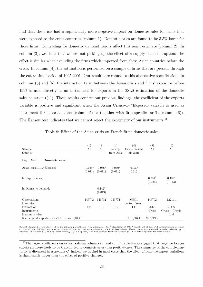
find that the crisis had a significantly more negative impact on domestic sales for firms that

were exposed to the crisis countries (column 1). Domestic sales are found to be 3.5% lower for

those firms. Controlling for domestic demand hardly affect this point estimate (column 2). In

column (3), we show that we are not picking up the effect of a supply chain disruption: the

effect is similar when excluding the firms which imported from these Asian countries before the

crisis. In column (4), the estimation is performed on a sample of firms that are present through

the entire time period of 1995-2001. Our results are robust to this alternative specification. In

columns (5) and (6), the interaction term between the Asian crisis and firms’ exposure before

1997 is used directly as an instrument for exports in the 2SLS estimation of the domestic

sales equation ((1)). These results confirm our previous findings: the coefficient of the exports

variable is positive and significant when the Asian Crisis97−01*Exposedi variable is used as

instrument for exports, alone (column 5) or together with firm-specific tariffs (column (6)).

The Hansen test indicates that we cannot reject the exogeneity of our instruments.20

Table 8: Effect of the Asian crisis on French firms domestic sales

(1) (2) (3) (4) (5) (6)Sample All All No imp. Firms present All AllSample from Asia all years

Dep. Var.: ln Domestic sales

Asian crisis97−01*Exposedi -0.035a -0.036a -0.040a -0.039a

(0.011) (0.011) (0.011) (0.013)

ln Export salesit 0.731b 0.435a

(0.335) (0.143)

ln Domestic demandit 0.142a

(0.019)

Observations 146702 146702 133774 66591 146702 122141Dummies Sector×YearEstimation FE FE FE FE 2SLS 2SLSInstruments Crisis Crisis + TariffsHansen p-value 0.46Kleibergen-Paap stat. / S-Y Crit. val. (10%) 11.9/16.4 20.5/19.9

Robust Standard errors, clustered by industry, in parentheses. c significant at 10%; b significant at 5%; a significant at 1%. OLS estimations in columns(1) and (2) and 2SLS estimations in columns (3) and (4). All estimations include firm fixed effects. Export sales instrumented by Asian crisis97−01 ×Exposedi in column (3), and by Asian crisis97−01 × Exposedi and firm-specific tariffs in column (4). See data appendix for more details.

20The larger coefficients on export sales in columns (5) and (6) of Table 8 may suggest that negative foreignshocks are more likely to be transmitted to domestic sales than positive ones. The symmetry of the complemen-tarity is discussed in Appendix C. Indeed, we do find in most cases that the effect of negative export variationsis significantly larger than the effect of positive changes.

23

5 Channels of transmission

How can we explain the export-domestic sales complementarity in the short run? As mentioned

earlier, in most international trade models, aggregate or idiosyncratic productivity shocks,

together with local demand conditions, determines simultaneously the level of sales in each

market. Exogenous changes in demand conditions in a given market have no effect on the level

of sales in other markets: the β coefficient that we estimate should not be significantly different

from zero. Our estimates of β are however systematically positive and significant, suggesting a

complementarity between exports and domestic sales when the variation of exports in a given

year is driven by changes in foreign demand conditions.

Several factors may explain why we observe a positive impact of exports on domestic sales.

Before turning to these, first note that we are looking at contemporaneous effects. In the

medium- to long-term, a rise in exports may increase the scale of domestic production through

efficiency gains - the so-called learning-by-exporting hypothesis.21 However, in the short-run,

this is unlikely to explain our findings.

While economic theory does not point to a unique mechanism that would explain the com-

plementarity we find in the data, domestic sales and exports may be connected through the

existence of cost or capacity linkages. In general, a unique production process involves labor,

equipments, and inputs for the production of a single good that will be sold in different markets.

An exogenous increase in exports might enhance domestic sales if it improves firm capacity or

its productive efficiency.22

Liquidity constraints. In the short-term, firms need liquidity to fulfill working capital re-

quirements. That is, any firm needs liquidity to purchase capital, buy intermediates, or hire

additional workers so as to increase their sales in a market. In the presence of financial con-

straints, this requires using internal liquidity rather than external borrowing.23 Exogenous

changes in export sales are directly related to the profitability of the firm, its short-run liquid-

ity, and therefore its capacity to hire additional workers, invest in new equipments, or purchase

21See Wagner (2007) for a survey, and the studies by Bernard and Jensen (1999), De Loecker (2007) and Parket al. (2010).

22The results displayed in Table 14 in the appendix indeed show that both TFP and factor accumulationseems to be affected by foreign shocks through exports.

23Hubbard (1998) shows that firms’ investments are closely linked to their financial health, which they interpretas the presence of credit constraints that lead firms to self-finance an important share of their investments. ForFrance, Berthou and Hugot (2011) use a survey of French firms in 2008 and show that among exporters, 52%of the productive investment is self-financed.

24

inputs.

Note that this channel does not exclude the presence of capacity constraints in the short run.

For a given level of aggregate domestic and foreign demand addressed to the firm, increasing

domestic sales might come at the expense of sales in other markets if the marginal cost is

increasing. This may be the case if firms structurally face financial or capacity constraints

(Ahn and McQuoid, 2012). In the case of an external shock, however, an exogenous increase of

exports may actually reduce the marginal cost, for example by providing cheap money to the

firm that reduces the cost of financing and helps to relax the liquidity constraint.

We explore this transmission channel in more details in Table 9. First, we expect the export-

domestic sales complementarity to be magnified for firms exporting a larger part of their total

sales, as in this case the liquidity shock is larger. Similarly, as the dependence on short-term

liquidity may be especially important for small firms, we should expect the effect to decrease

with firm size. In column (1), we interact the export sales variable with the initial export

to total sales ratio of the firm. This allows us to determine how the export-domestic sales

relation is affected by firm exposure to foreign demand shocks. The interaction variable is itself

instrumented by the interaction between our baseline instrument and the initial export to total

sales ratio of the firm. We indeed find that exposure to foreign shocks tends to magnify the

positive exports-domestic sales relationship, which confirms our baseline result. In column 2,

the export sales variable is interacted with the initial size of the firm.24 The coefficient of the

interaction variable is negative and significant, i.e. smaller firms tend to benefit more from

an exogenous increase in their exports than larger firms. The domestic sales of small firms

are therefore more sensitive to variations in exports revenues, which may possibly come from

tighter short-term liquidity needs.

A more direct way to assess the relevance of the liquidity mechanism is to use sectoral

heterogeneity in terms of dependence upon short-run liquidity. More precisely, we follow a

methodology akin to Rajan and Zingales (1998) and construct sector-specific indicators of

profitability and of dependence upon short-term liquidity. A low level of profitability within a

sector implies a weak capacity of firms to self-finance their investments at a low cost. In other

sectors, firms might have higher working capital requirements. In each case, we expect that

firms operating in less profitable sectors, or those operating in sectors with a higher need for

24Note that we demeaned the size variable in this column so that the coefficient on the non interacted exportsales variable represents the effect for the firm with the average size in our sample.

25

short-term capital, are more sensitive to exogenous variations of the cash flow or exports.

As Rajan and Zingales (1998), our identification strategy is based on sectoral heterogeneity,

which is not affected by individual firm characteristics. The first indicator we use is a sector-

specific measure of working capital requirement (WCRk), defined as the average working capital

requirement over cash flow. This indicator represents the need of the sector in terms of short-

run liquidity; a high value of WCR implies that firms in the considered sector have a higher

need for short-term liquidity. Heterogeneity across sectors in terms of WCR can be explained

by differences in the production or distribution processes, which can affect the frequency of

earnings and payments. The second indicator is the sector-specific price-cost margin (PCMk)

that is, sales net of expenditures on labor and materials (gross operating profit) over value

added. It can be interpreted as a sectoral indicator of profitability: firms belonging to sectors

with a high value of PCM are therefore expected to have lower needs of short-term liquidity.25

In column (3) of Table 9, we interact the export sales variable with a dummy which equals

1 if the firm belongs to a sector which is above the sample median for WCRk. The difference

across sectors is striking: a 10% exogenous increase in foreign sales generates around 2.1%

increase in sales at home for firms belonging to sectors with high working capital requirements,

but only 0.9% for the others. The difference is significant at the 5% level. Figure 2.a shows the

size of the effect for four groups of firms defined according to the quartiles of WCR ratio. 10%

confidence intervals are depicted in grey around the estimated effect. The pattern is clear: the

higher the need for short-run liquidity, the higher the effect of exogenous changes in exports

on domestic sales. We repeat these exercises with the PCM indicator in column (4) of Table 9

and in Figure 2.b. Again, for firms belonging to the sectors with the lowest price-cost margins,

and that are arguably more sensitive to changes in their cash flow, a given exogenous change

in exports implies a larger response of domestic sales. This result is confirmed by the Panel

(b) of Figure 2, which displays once again the effect for four groups of firms defined according

to the quartile of PCM ratio. The pattern shown with the quartile decomposition in 2.b is

symmetric to the one shown in 2.a: the higher the profitability of the sector, the smaller the

effect of exogenous changes in exports on domestic sales.

25A sector is defined at the 3-digit (NES 114) level, although our results are qualitatively unchanged whenusing a broader (2-digit) classification. The working capital requirement ratio (WCRk) is computed as theaverage working capital requirement divided by the average cash flow of the sector. The sector-level price-costmargin (PCMk) is constructed by taking the average gross operating profit over value added by sector. Allvariables are from the BRN database.

26

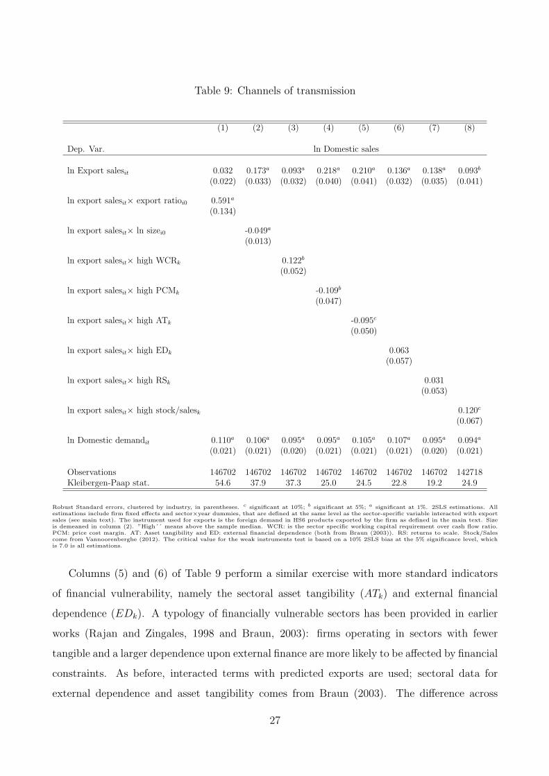
Table 9: Channels of transmission

(1) (2) (3) (4) (5) (6) (7) (8)

Dep. Var. ln Domestic sales

ln Export salesit 0.032 0.173a 0.093a 0.218a 0.210a 0.136a 0.138a 0.093b

(0.022) (0.033) (0.032) (0.040) (0.041) (0.032) (0.035) (0.041)

ln export salesit× export ratioi0 0.591a

(0.134)

ln export salesit× ln sizei0 -0.049a

(0.013)

ln export salesit× high WCRk 0.122b

(0.052)

ln export salesit× high PCMk -0.109b

(0.047)

ln export salesit× high ATk -0.095c

(0.050)

ln export salesit× high EDk 0.063(0.057)

ln export salesit× high RSk 0.031(0.053)

ln export salesit× high stock/salesk 0.120c

(0.067)

ln Domestic demandit 0.110a 0.106a 0.095a 0.095a 0.105a 0.107a 0.095a 0.094a

(0.021) (0.021) (0.020) (0.021) (0.021) (0.021) (0.020) (0.021)

Observations 146702 146702 146702 146702 146702 146702 146702 142718Kleibergen-Paap stat. 54.6 37.9 37.3 25.0 24.5 22.8 19.2 24.9

Robust Standard errors, clustered by industry, in parentheses. c significant at 10%; b significant at 5%; a significant at 1%. 2SLS estimations. Allestimations include firm fixed effects and sector×year dummies, that are defined at the same level as the sector-specific variable interacted with exportsales (see main text). The instrument used for exports is the foreign demand in HS6 products exported by the firm as defined in the main text. Sizeis demeaned in column (2). ”High´´ means above the sample median. WCR: is the sector specific working capital requirement over cash flow ratio.PCM: price cost margin. AT: Asset tangibility and ED: external financial dependence (both from Braun (2003)). RS: returns to scale. Stock/Salescome from Vannoorenberghe (2012). The critical value for the weak instruments test is based on a 10% 2SLS bias at the 5% significance level, whichis 7.0 is all estimations.

Columns (5) and (6) of Table 9 perform a similar exercise with more standard indicators

of financial vulnerability, namely the sectoral asset tangibility (ATk) and external financial

dependence (EDk). A typology of financially vulnerable sectors has been provided in earlier

works (Rajan and Zingales, 1998 and Braun, 2003): firms operating in sectors with fewer

tangible and a larger dependence upon external finance are more likely to be affected by financial

constraints. As before, interacted terms with predicted exports are used; sectoral data for

external dependence and asset tangibility comes from Braun (2003). The difference across

27

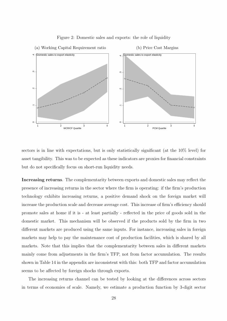
Figure 2: Domestic sales and exports: the role of liquidity

(a) Working Capital Requirement ratio (b) Price Cost Margins

0.1

.2.3

.4

1 2 3 4WCR/CF Quartile

Domestic sales to export elasticity

0.1

.2.3

.4

1 2 3 4PCM Quartile

Domestic sales to export elasticity

sectors is in line with expectations, but is only statistically significant (at the 10% level) for

asset tangibility. This was to be expected as these indicators are proxies for financial constraints

but do not specifically focus on short-run liquidity needs.

Increasing returns. The complementarity between exports and domestic sales may reflect the

presence of increasing returns in the sector where the firm is operating: if the firm’s production

technology exhibits increasing returns, a positive demand shock on the foreign market will

increase the production scale and decrease average cost. This increase of firm’s efficiency should

promote sales at home if it is - at least partially - reflected in the price of goods sold in the

domestic market. This mechanism will be observed if the products sold by the firm in two

different markets are produced using the same inputs. For instance, increasing sales in foreign

markets may help to pay the maintenance cost of production facilities, which is shared by all

markets. Note that this implies that the complementarity between sales in different markets

mainly come from adjustments in the firm’s TFP, not from factor accumulation. The results

shown in Table 14 in the appendix are inconsistent with this: both TFP and factor accumulation

seems to be affected by foreign shocks through exports.

The increasing returns channel can be tested by looking at the differences across sectors

in terms of economies of scale. Namely, we estimate a production function by 3-digit sector

28

(NES 114). Whenever the sum of the labor and capital coefficients is larger than 1, we classify

the sector as an increasing returns sector (decreasing returns otherwise). The result, shown in

column (7) of Table 9, does not validate the increasing returns channel: the coefficient has the

positive expected sign (exports have a more positive impact on domestic sales in the sectors

that exhibit increasing returns), but is small and statistically insignificant. This channel is

therefore unlikely to explain our results.

Capacity constraints. While our estimations point to a positive relationship between exoge-

nous variations of exports and changes in domestic sales, this linkage may still be affected by

the existence of capacity constraints. For instance, increased export revenues may help firms

to buy additional inputs and pay suppliers, but total sales will increase significantly only if the

firm is able to adjust its labor and total production, or use stored production. As mentioned

in introduction, a number of recent papers (Vannoorenberghe, 2012, Nguyen and Schaur, 2011,

Soderbery, 2012, Blum et al., 2011, Ahn and McQuoid, 2012) emphasize the fact that the pres-

ence of capacity constraints or convex costs may generate substitutability between sales across

destinations.

In general, we should expect the complementarity between sales across markets to be

stronger in firms facing low capacity constraints. We test this prediction using sector-specific

data on average stock over sales ratio from Vannoorenberghe (2012).26 Column (8) includes

an interaction term between export sales and a dummy which equals 1 for firms belonging to

sectors in which inventories are high (above the sample median). The results are consistent

with Vannoorenberghe (2012): in sectors where inventories are large, i.e., where firms are less

likely to face capacity constraints, the complementarity is stronger (although this difference is

significant only at the 10% level). However, the coefficient on export sales remains positive and

significant in both types of sectors.

6 Conclusions

Using a large firm-level database on French firms combining balance-sheet and destination-

specific export information over the period 1995-2001, this paper shows that firms’ domestic

26Our dataset does not contain information on capacity utilization. We are very grateful to Gonzague Van-noorenberghe who accepted to share this data. The index is computed from Amadeus data on French firms overthe period 1998-2007. For more information please refer to Vannoorenberghe (2012).

29

and export sales are complementary when exports are predicted by exogenous changes in foreign

demand. A change in foreign demand conditions, which is associated with an increase in the

foreign demand of the products sold abroad by the exporter, raises domestic sales. This implies

that shocks on foreign markets can be channeled into the domestic business cycle through the

complementarity between firms’ domestic and foreign sales.

These results are confirmed by a number of robustness checks, in which we assess the validity

of the empirical analysis through different specifications. We use alternatively as instruments

for export sales the the foreign imports for the product range exported by the firm, or for its

core product, tariff changes, or large foreign shocks such as civil wars. We take into account

the possibility that domestic and foreign macroeconomic conditions may be correlated. We also

control for the possibility that the result might be driven by the correlation between exports and

imports for each firm. Our results are valid in cases where the foreign demand for firms’ products

is increasing or decreasing. Finally, our analysis is supported by the natural experiment of the

Asian crisis in the late 1990’s. Estimation results show that firms that were more exposed to

this crisis through their exports suffered a decrease of their domestic sales as compared to firms

of the control group.

Overall, this relation between domestic and foreign sales is at odds with theoretical models

in international trade where domestic and foreign sales are only connected through exogenous

productivity, as in Melitz (2003). Our results rather suggest that exogenous shocks on the

foreign business cycle will reflect in the domestic business cycle through the relationship between

domestic and foreign sales. This result has many implications, for instance, in terms of the

exchange rate policy or trade policy transmission to the domestic economy.

The precise channel of transmission, however, remains an avenue for future research. We

provide evidence in the last section that dependence on short-run liquidity, through working

capital requirement, may be a relevant explanation. This channel is also consistent with the

fact that our result is found to be stronger for small firms than for large ones. However,

other channels may be relevant, including demand side mechanisms. Future research should

probably attempt to determine the channel of transmission that is prevalent in explaining this

export-domestic sales complementarity.

30

References

Ahn, J. and McQuoid, A. (2012), “ Capacity Constrained Exporters: Micro Evidence and

Macro Implications ”, Mimeo, International Monetary Fund.

Ball, R. J., Eaton, J. R. and Steuer, M. D. (1966), “ The Relationship Between United

Kingdom Export Performance in Manufactures and the Internal Pressure of Demand ”, The

Economic Journal, vol. 76 no 303.

Baxter, M. and Kouparitsas, M. A. (2005), “ Determinants of business cycle comovement:

a robust analysis ”, Journal of Monetary Economics, vol. 52 no 1: pp. 113–157.

Bergin, P., Feenstra, R. and Hanson, G. (2009), “ Volatility due to Outsourcing: Theory

and Evidence ”, Mimeo.

Bernard, A. and Jensen, B. (1999), “ Exceptional exporter performance: cause, effect, or

both? ”, Journal of International Economics, vol. 47 no 1: pp. 1–25.

Bernard, A. and Wagner, J. (1998), “ Export Entry and Exit by German Firms ”, NBER

Working Paper W6538.

Berthou, A. and Hugot, J. (2011), “ How does innovation affects the internationalization

patterns of firms? ”, .

Blum, B. S., Claro, S. and Horstmann, I. J. (2011), “ Occasional vs Perennial Exporters:

The Impact of Capacity on Export Mode ”, .

Braun, M. (2003), “ Financial Contractibility and Asset Hardness ”, Harvard University, De-

partment of Economics Working Paper.

Burstein, A., Kurz, C. and Tesar, L. (2008), “ Trade, production sharing, and the inter-

national transmission of business cycles ”, Journal of Monetary Economics, vol. 55 no 4: pp.

775–795.

De Loecker, J. (2007), “ Do exports generate higher productivity? Evidence from Slovenia ”,

Journal of International Economics, vol. 73 no 1: pp. 69–98.

31

Dunlevy, J. A. (1980), “ A Test of the Capacity Pressure Hypothesis within a Simultaneous

Equations Model of Export Performance ”, The Review of Economics and Statistics, vol. 62

no 1: pp. 131–35.

Eaton, J., Kortum, S. and Kramarz, F. (2004), “ Dissecting Trade: Firms, Industries, and

Export Destinations ”, American Economic Review Papers and Proceedings, vol. 94 no 2: pp.

150–154.

Eaton, J., Kortum, S. and Kramarz, F. (2011), “ An Anatomy of International Trade:

Evidence from French Firms ”, Econometrica, vol. 79 no 5: pp. 1453–1498.

Ekholm, K., Moxnes, A. and Ulltveit-Moe, K.-H. (2012), “ Manufacturing restructuring

and the role of Real exchange rate shocks: A firm level analysis ”, Journal of International

Economics, vol. 86 no 1: pp. 101–117.

Frankel, J. A. and Rose, A. K. (1998), “ The Endogeneity of the Optimum Currency Area

Criteria ”, Economic Journal, vol. 108 no 449: pp. 1009–25.

Froot, K. A. (1989), “ Consistent covariance matrix estimation with cross-sectional depen-

dence and heteroskedasticity in financial data ”, Journal of Financial and Quantitative Anal-

ysis, vol. 24: pp. 333–335.

Haynes, S. E. and Stone, J. A. (1983), “ Secular and Cyclical Responses of U.S. Trade to

Income: An Evaluation of Traditional Models ”, The Review of Economics and Statistics,

vol. 65 no 1: pp. 87–95.

Hubbard, G. (1998), “ Capital Market Imperfections and Investment ”, Journal of Economic

Literature, vol. 36 no 3: pp. 193–225.

Hummels, D., Jorgensen, R., Munch, J. and Xiang, C. (2010), “ The Wage and Employ-

ment Effects of Outsourcing: Evidence from Danish Matched Worker-Firm Data ”, Mimeo.

Melitz, M. (2003), “ The Impact of Trade on Intra-Industry Reallocations and Aggregate

Industry Productivity ”, Econometrica, vol. 71 no 6: pp. 1695–1725.

Nguyen, D. and Schaur, G. (2011), “ Cost linkages transmit volatility across markets ”,

Mimeo.

32

Park, A., Yang, D., Shi, X. and Jiang, Y. (2009), “ Exporting and Firm Performance:

Chinese Exporters and the Asian Financial Crisis ”, Nber working papers, National Bureau

of Economic Research, Inc.

Park, A., Yang, D., Shi, X. and Jiang, Y. (2010), “ Exporting and Firm Performance:

Chinese Exporters and the Asian Financial Crisis ”, The Review of Economics and Statistics,

vol. 92 no 4: pp. 822–842.

Rajan, R. G. and Zingales, L. (1998), “ Financial Dependence and Growth ”, American

Economic Review, vol. 88 no 3: pp. 559–86.

Soderbery, A. (2012), “ Market Size, Structure, and Access: Trade with Capacity Con-

straints ”, Mimeo, Purdue University.

Stock, J. H. and Yogo, M. (2005), “ Testing for Weak Instruments in Linear IV Regression ”,

in Andrews, D. W. and Stock, J. H. (editors), Identification and Inference for Econo-

metric Models: Essays in Honor of Thomas Rothenberg, Cambridge: Cambridge University

Press.

Van Biesebroeck, J. (2005), “ Exporting raises productivity in sub-Saharan African manu-

facturing firms ”, Journal of International Economics, vol. 67 no 2: pp. 373–391.

Vannoorenberghe, G. (2012), “ Firm volatility and exports ”, Journal of International Eco-

nomics, vol. 86 no 1: pp. 57–67.

Wagner, J. (2007), “ Exports and Productivity: A Survey of the Evidence from Firm-level

Data ”, The World Economy, vol. 30 no 1: pp. 60–82.

Zilberfarb, B.-Z. (1980), “ Domestic Demand Pressure, Relative Prices and the Exports

Supply Equation-More Empirical Evidence ”, Economica, vol. 47 no 188: pp. 443–50.

33

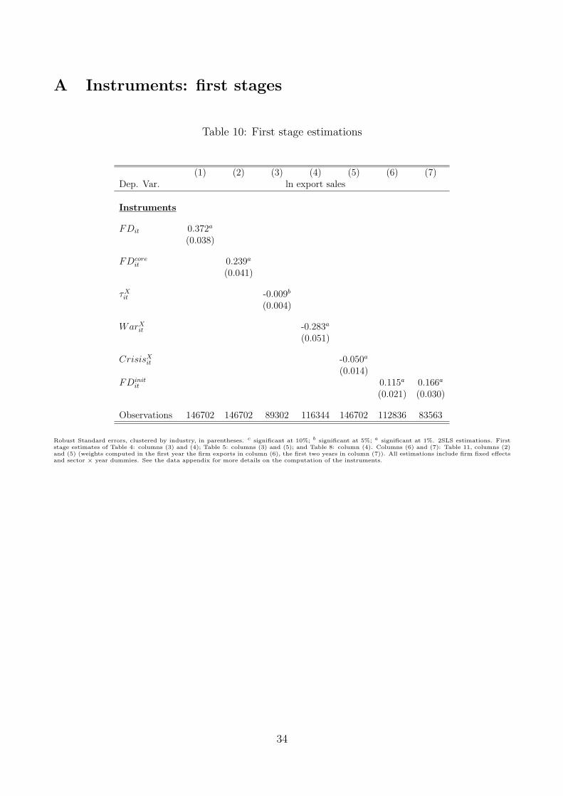
A Instruments: first stages

Table 10: First stage estimations

(1) (2) (3) (4) (5) (6) (7)Dep. Var. ln export sales

Instruments

FDit 0.372a

(0.038)

FDcoreit 0.239a

(0.041)

τXit -0.009b

(0.004)

WarXit -0.283a

(0.051)

CrisisXit -0.050a

(0.014)FDinit

it 0.115a 0.166a

(0.021) (0.030)

Observations 146702 146702 89302 116344 146702 112836 83563

Robust Standard errors, clustered by industry, in parentheses. c significant at 10%; b significant at 5%; a significant at 1%. 2SLS estimations. Firststage estimates of Table 4: columns (3) and (4); Table 5: columns (3) and (5); and Table 8: column (4). Columns (6) and (7): Table 11, columns (2)and (5) (weights computed in the first year the firm exports in column (6), the first two years in column (7)). All estimations include firm fixed effectsand sector × year dummies. See the data appendix for more details on the computation of the instruments.

34

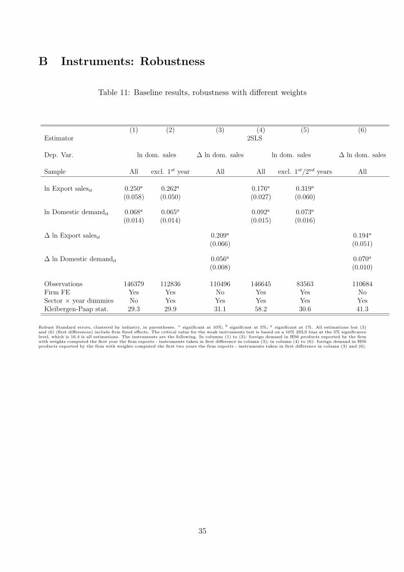
B Instruments: Robustness

Table 11: Baseline results, robustness with different weights

(1) (2) (3) (4) (5) (6)Estimator 2SLS

Dep. Var. ln dom. sales ∆ ln dom. sales ln dom. sales ∆ ln dom. sales

Sample All excl. 1st year All All excl. 1st/2nd years All

ln Export salesit 0.250a 0.262a 0.176a 0.319a

(0.058) (0.050) (0.027) (0.060)

ln Domestic demandit 0.068a 0.065a 0.092a 0.073a

(0.014) (0.014) (0.015) (0.016)

∆ ln Export salesit 0.209a 0.194a

(0.066) (0.051)

∆ ln Domestic demandit 0.056a 0.070a

(0.008) (0.010)

Observations 146379 112836 110496 146645 83563 110684Firm FE Yes Yes No Yes Yes NoSector × year dummies No Yes Yes Yes Yes YesKleibergen-Paap stat. 29.3 29.9 31.1 58.2 30.6 41.3

Robust Standard errors, clustered by industry, in parentheses. c significant at 10%; b significant at 5%; a significant at 1%. All estimations but (3)and (6) (first differences) include firm fixed effects. The critical value for the weak instruments test is based on a 10% 2SLS bias at the 5% significancelevel, which is 16.4 is all estimations. The instruments are the following. In columns (1) to (3): foreign demand in HS6 products exported by the firmwith weights computed the first year the firm exports - instruments taken in first difference in column (3); in column (4) to (6): foreign demand in HS6products exported by the firm with weights computed the first two years the firm exports - instruments taken in first difference in column (3) and (6).

35

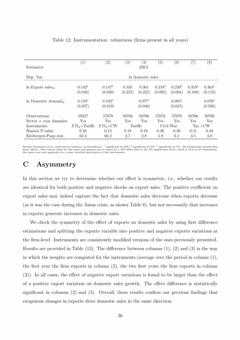
Table 12: Instrumentation: robustness (firms present in all years)

(1) (2) (3) (4) (5) (6) (7) (8)Estimator 2SLS

Dep. Var. ln domestic sales

ln Export salesit 0.142a 0.147a 0.335 0.361 0.234b 0.230b 0.359a 0.364a

(0.038) (0.030) (0.225) (0.225) (0.095) (0.094) (0.108) (0.110)

ln Domestic demandit 0.134a 0.102a 0.077c 0.085a 0.076a

(0.027) (0.019) (0.046) (0.025) (0.026)

Observations 59227 57078 50766 50766 57078 57078 50766 50766Sector × year dummies Yes Yes Yes Yes Yes Yes Yes YesInstruments FDit+Tariffs FDit+CW Tariffs Civil War Tar.+CWHansen P-value 0.28 0.15 0.18 0.18 0.30 0.30 0.51 0.48Kleibergen-Paap stat. 62.4 60.2 2.7 2.8 5.9 6.1 3.5 3.8

Robust Standard errors, clustered by industry, in parentheses. c significant at 10%; b significant at 5%; a significant at 1%. All estimations include firmfixed effects. The critical value for the weak instruments test is based on a 10% 2SLS bias at the 5% significance level, which is 19.9 in all estimations.See main text and appendix for a more detailed description of the instruments.

C Asymmetry

In this section we try to determine whether our effect is symmetric, i.e., whether our results

are identical for both positive and negative shocks on export sales. The positive coefficient on

export sales may indeed capture the fact that domestic sales decrease when exports decrease

(as it was the case during the Asian crisis, as shown Table 8), but not necessarily that increases

in exports generate increases in domestic sales.

We check the symmetry of the effect of exports on domestic sales by using first difference

estimations and splitting the exports variable into positive and negative exports variations at

the firm-level. Instruments are consistently modified versions of the ones previously presented.

Results are provided in Table (13). The difference between columns (1), (2) and (3) is the way

in which the weights are computed for the instruments (average over the period in column (1),

the first year the firm exports in column (2), the two first years the firm exports in column

(3)). In all cases, the effect of negative export variations is found to be larger than the effect

of a positive export variation on domestic sales growth. The effect difference is statistically

significant in columns (2) and (3). Overall, these results confirm our previous findings that

exogenous changes in exports drive domestic sales in the same direction.

36

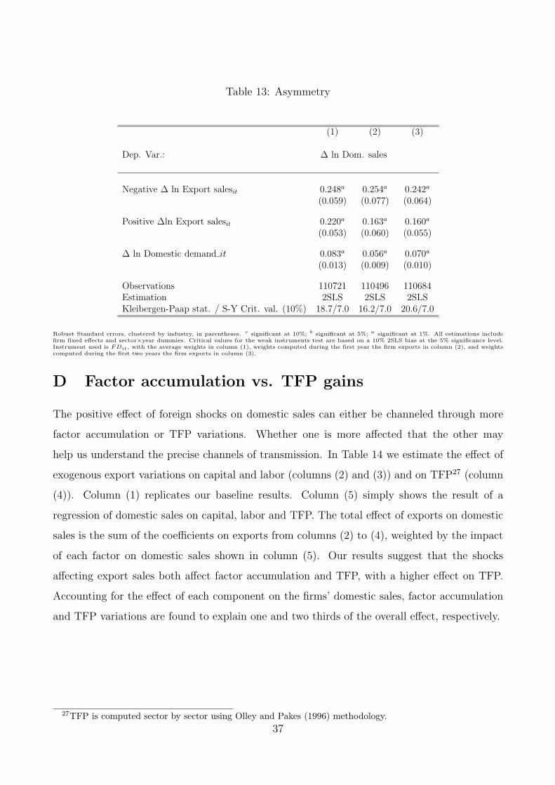
Table 13: Asymmetry

(1) (2) (3)

Dep. Var.: ∆ ln Dom. sales

Negative ∆ ln Export salesit 0.248a 0.254a 0.242a

(0.059) (0.077) (0.064)

Positive ∆ln Export salesit 0.220a 0.163a 0.160a

(0.053) (0.060) (0.055)

∆ ln Domestic demand it 0.083a 0.056a 0.070a

(0.013) (0.009) (0.010)

Observations 110721 110496 110684Estimation 2SLS 2SLS 2SLSKleibergen-Paap stat. / S-Y Crit. val. (10%) 18.7/7.0 16.2/7.0 20.6/7.0

Robust Standard errors, clustered by industry, in parentheses. c significant at 10%; b significant at 5%; a significant at 1%. All estimations includefirm fixed effects and sector×year dummies. Critical values for the weak instruments test are based on a 10% 2SLS bias at the 5% significance level.Instrument used is FDit, with the average weights in column (1), weights computed during the first year the firm exports in column (2), and weightscomputed during the first two years the firm exports in column (3).

D Factor accumulation vs. TFP gains

The positive effect of foreign shocks on domestic sales can either be channeled through more

factor accumulation or TFP variations. Whether one is more affected that the other may

help us understand the precise channels of transmission. In Table 14 we estimate the effect of

exogenous export variations on capital and labor (columns (2) and (3)) and on TFP27 (column

(4)). Column (1) replicates our baseline results. Column (5) simply shows the result of a

regression of domestic sales on capital, labor and TFP. The total effect of exports on domestic

sales is the sum of the coefficients on exports from columns (2) to (4), weighted by the impact

of each factor on domestic sales shown in column (5). Our results suggest that the shocks

affecting export sales both affect factor accumulation and TFP, with a higher effect on TFP.

Accounting for the effect of each component on the firms’ domestic sales, factor accumulation

and TFP variations are found to explain one and two thirds of the overall effect, respectively.

27TFP is computed sector by sector using Olley and Pakes (1996) methodology.37

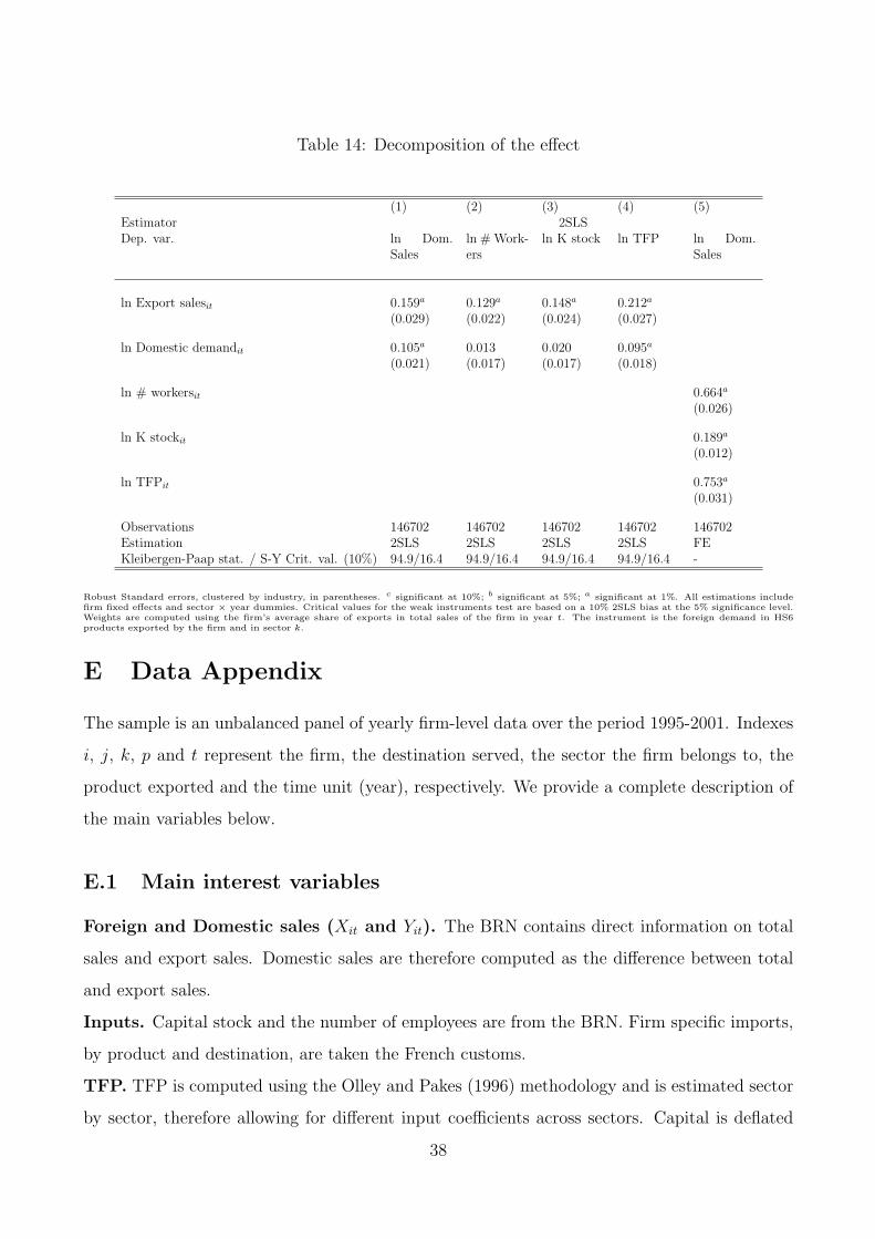
Table 14: Decomposition of the effect

(1) (2) (3) (4) (5)Estimator 2SLSDep. var. ln Dom.

Salesln # Work-ers

ln K stock ln TFP ln Dom.Sales

ln Export salesit 0.159a 0.129a 0.148a 0.212a

(0.029) (0.022) (0.024) (0.027)

ln Domestic demandit 0.105a 0.013 0.020 0.095a

(0.021) (0.017) (0.017) (0.018)

ln # workersit 0.664a

(0.026)

ln K stockit 0.189a

(0.012)

ln TFPit 0.753a

(0.031)

Observations 146702 146702 146702 146702 146702Estimation 2SLS 2SLS 2SLS 2SLS FEKleibergen-Paap stat. / S-Y Crit. val. (10%) 94.9/16.4 94.9/16.4 94.9/16.4 94.9/16.4 -

Robust Standard errors, clustered by industry, in parentheses. c significant at 10%; b significant at 5%; a significant at 1%. All estimations includefirm fixed effects and sector × year dummies. Critical values for the weak instruments test are based on a 10% 2SLS bias at the 5% significance level.Weights are computed using the firm’s average share of exports in total sales of the firm in year t. The instrument is the foreign demand in HS6products exported by the firm and in sector k.

E Data Appendix

The sample is an unbalanced panel of yearly firm-level data over the period 1995-2001. Indexes

i, j, k, p and t represent the firm, the destination served, the sector the firm belongs to, the

product exported and the time unit (year), respectively. We provide a complete description of

the main variables below.

E.1 Main interest variables

Foreign and Domestic sales (Xit and Yit). The BRN contains direct information on total

sales and export sales. Domestic sales are therefore computed as the difference between total

and export sales.

Inputs. Capital stock and the number of employees are from the BRN. Firm specific imports,

by product and destination, are taken the French customs.

TFP. TFP is computed using the Olley and Pakes (1996) methodology and is estimated sector

by sector, therefore allowing for different input coefficients across sectors. Capital is deflated

38

using a gross fixed asset deflator from the OECD economic outlook database and value added

using a sectoral deflator from the EU-Klems data.

E.2 Instruments and controls for domestic demand

Foreign and domestic demands addressed to the firms. Our preferred instrument is the

sum of foreign imports in the product-destination served by the firm in year t, weighted by

the share of each product-destination in the firm’s total export over the period. A product is

defined at the 6-digit (HS6) level. Import data comes from BACI (CEPII). Denoting ωijp the

average share of each product p and destination j in firm i’s exports over the period, and Mjp,t

the imports of destination j of product p during year t, this variable is computed as:

FDit =∑j,p

ωijpMjp,t (5)

The mirror of this variable for domestic demand is:

DDit =∑

p

ωipMFR,p,t (6)

where MFR,p,t denotes the French imports of product p during year t. Alternatively, we

use similar instruments and controls focusing on the firm’s core product, defined as the HS-

4 product with the highest average value of exports over the period. ωcoreij is the weight of

destination j in firm’s i core product exports. We compute:

FDcoreit =

∑j

ωcoreij M core

j,t (7)

And the mirror of this variable is DDcoreit , ie the French imports for each firm i core product

in t.

Firm-specific tariffs. We use information on tariff to construct alternative instruments for

export sales. Firm-specific tariffs are computed as:

τXit =

∑j,p

ωijptjp,t (8)

where tjp,t represents the MFN tariff of destination j in product p. The data comes from

39

the ITC. Similar results are obtained with bound tariffs.

Exposure to civil wars. We construct two variables reflecting the exposure of a given firm

i to a civil war in country j. The first is a dummy variable that equals 1 if at least one the

destinations to which the firm exported in t − 1 experiences a civil war in year t. The second

equals the sum of the number of civil wars the destination served by the firm, weighted by the

share of exports in these destinations in t− 1:

WarXit =

∑j

Xij,t−1

Xi,t−1

CWj,t (9)

where CWj,t is a dummy that equals 1 if the destination j experienced a civil war in t. The

data on civil wars comes from the Correlates of War (CoW).

Instruments for imports. We create instruments for firm-level imports using a similar

variable as for exports. Firms’ imports are instrumented using the foreign supplied addressed

to the firm, FSit. More precisely, we compute the sum of the foreign exports in the product-

destination from which the firm imports goods during year t, Xjpt, weighted by the share of

each product-destination in the firm’s total imports over the period ηijp. A product is defined at

the 6-digit (HS6) level, ηijp. Export data comes from BACI (CEPII). This variable is computed

as:

FSit =∑j,p

ηijpXjp,t (10)

Exposure to the 1997-1998 Asian crisis. We construct a variable similar to the one

proposed for civil wars:

CrisisXit =

∑j∗

expitCrisisj,t (11)

where Crisisj,t is a dummy variable that equals 1 after 1997 for the five Asian countries

that were hit the most by the Asian crisis (Thailand, Korea, Philippines, Indonesia, Malaysia)

and expit is a dummy variable that equals 1 if the firm exported to one of these countries in

1995 or 1996.

40

Documents de Travail

396. M. Bussiere and A. Ristiniemi, “Credit Ratings and Debt Crises,” September 2012

397. A. Monfort and F. Pegoraro, “Asset Pricing with Second-Order Esscher Transforms,” September 2012

398. S. Gabrieli, “Too-connected versus too-big-to-fail: banks’ network centrality and overnight interest rate,”

September 2012

399. Y. Kalantzis, R. Kambayashi and S. Lechevalier, “Wage and Productivity differentials in Japan. The Role of

Labor Market Mechanisms,” September 2012

400. F. Bec and M. Bessec, “Inventory Investment Dynamics and Recoveries: A Comparison of Manufacturing and

Retail Trade Sectors,” October 2012

401. P. Antipa, K. Barhoumi, V. Brunhes-Lesage and O. Darné, “Nowcasting German GDP: A comparison of bridge

and factor models,” October 2012

402. G. Gaballo, “Good Luck or Good Policy? An Expectational Theory of Macro-Volatility Switches,”

October 2012

403. J. Barthélemy and M. Marx, “Generalizing the Taylor Principle: New Comment,” October 2012

404. H. Fraisse and P. Frouté, “Households Debt Restructuring: Evidence from the French Experience,” October

2012

405. E. Kremp and P. Sevestre, “Did the crisis induce credit rationing for French SMEs?,” November 2012

406. P. Bacchetta, K. Benhima and Y. Kalantzis, “Capital Controls with International Reserve Accumulation: Can

this Be Optimal?,” November 2012

407. P. Andrade, E. Ghysels and J. Idier, “Tails of Inflation Forecasts and Tales of Monetary Policy,” November

2012

408. N. Berman, A. Berthou and J. Héricourt, “Export dynamics and sales at home,” November 2012

Pour accéder à la liste complète des Documents de Travail publiés par la Banque de France veuillez consulter le site :

www.banque-france.fr

For a complete list of Working Papers published by the Banque de France, please visit the website:

www.banque-france.fr

Pour tous commentaires ou demandes sur les Documents de Travail, contacter la bibliothèque de la Direction Générale

des Études et des Relations Internationales à l'adresse suivante :

For any comment or enquiries on the Working Papers, contact the library of the Directorate General Economics and

International Relations at the following address :

BANQUE DE FRANCE

49- 1404 Labolog

75049 Paris Cedex 01

tél : 0033 (0)1 42 97 77 24 ou 01 42 92 63 40 ou 48 90 ou 69 81

email : HU1404-ut@banque-france.fr