Embed Size (px)
Citation preview
Université du Québec INRS Eau, Terre et Environnement
GÉOCHIMIE DU MOLYBDÈNE, DU RHÉNIUM ET DE L’URANIUM DANS LES SÉDIMENTS DE LACS DU BOUCLIER CANADIEN
ET DES APPALACHES
par Anthony Chappaz
Thèse présentée pour l’obtention du grade de Philosophiae Doctor (Ph.D.)
en sciences de l’eau
Jury d’évaluation Examinateur externe Prof. Timothy Lyons University of California at Riverside Examinateur externe Prof. Yves Gélinas Université Concordia à Montréal Examinateur interne Prof. Claude Fortin INRS-ETE Directeur de recherche Prof. Charles Gobeil INRS-ETE Co-directeur de recherche Prof. André Tessier INRS-ETE
Août 2008 Droits réservés d’Anthony Chappaz, 2008

iii
À mes parents …

v
Être efficace ne signifie pas avancer toujours plus loin. Cela signifie être attentif et vigilant au moindre détour du sentier, être disponible aux appels de la vie qu’on appelle opportunités, ou occasions, ou hasard, ou encore chance. Et donc, être efficace, c’est aussi savoir rebrousser chemin, changer de route, prendre s’il le faut des chemins de traverse. Le succès n’est pas affaire de distance ou de proximité, mais de cheminement. Cité par François Garagnon

vii
REMERCIEMENTS
Mes premiers remerciements vont à M. Charles Gobeil, mon directeur de recherche, pour
m’avoir accepté comme étudiant au doctorat. Grâce à nos échanges permanents, il a su me
transmettre toutes les aptitudes indispensables pour être un scientifique accompli, notamment
l’importance de l’écriture et de la concision des idées. La qualité exceptionnelle de son
encadrement m’a permis de passer au travers de ce doctorat, je le remercie chaleureusement pour
cela. Charles demeurera toujours pour moi mon professeur.
Je doute un jour de ne plus être redevable envers M. André Tessier, mon co-directeur de
recherche. Je suis extrêmement heureux d’avoir pu au cours de mon doctorat bénéficier de ses
conseils, de son expérience et de son sens de la critique. Je le remercie également pour toutes ses
explications, ô combien bienvenues, et qui en font à mes yeux un pédagogue extraordinaire.
Mes deux superviseurs, de part leur disponibilité et leur gentillesse, tiendront toujours une
place à part. Merci pour tout.
Je remercie M. Timothy Lyons, examinateur externe, pour l’accueil chaleureux qu’il a
manifesté pour mes travaux et surtout d’avoir accepté de faire partie de mon jury. Je tiens
également à remercier M. Yves Gélinas, examinateur externe, et M. Claude Fortin, examinateur
interne, pour leur participation à mon jury.
M. Landis Hare, professeur à l’INRS-ETE, a été un support actif tout au long de mon
doctorat. Je le remercie pour la relecture de mes articles et surtout pour tous les moments
partagés.
Mon projet de doctorat a nécessité de nombreuses analyses au laboratoire. Or un
laboratoire n’est rien sans le dynamisme et la compétence de ses personnels, techniciens et agents
de recherche. Je remercie Mme Michelle Bordeleau et M. Sébastien Duval pour les analyses
qu’ils ont effectuées pour moi. Mme Pauline Fournier a toujours su m’apporter l’aide et la gaieté
dont j’avais besoin avec l’ICP-MS, qu’elle en soit remerciée. L’assistance fournie par Mme Lise
Rancourt, tant au niveau du terrain, du laboratoire et de la modélisation a été un prodigieux atout,
viii
merci Lise-san. Enfin, nos échantillonnages n’auraient jamais pu avoir lieu sans l’expertise de
M. René Rodrigue, notre plongeur de combat, et son dévouement extraordinaire pour aller
recueillir des dialyseurs, même sous la neige, je lui exprime toute ma gratitude.
Je salue mes collègues et amis de travail que j’ai pu croiser au cours de ces années
d’études. Plus spécialement, M. Raoul-Marie Couture, qui est devenu au fil de ces années un ami
avec qui j’ai partagé des moments inoubliables en Gaspésie et ailleurs… Peut-être dans les
prochaines années deviendra-t-il un proche collaborateur, je l’espère.
Ma conjointe, Mlle Aurélie Dhenain, a toujours été à mes côtés dans tous les moments
joyeux et difficiles qui jalonnent le déroulement d’un doctorat. Je la remercie énormément pour
ce cadeau inestimable.
Il ne faut pas oublier d’où l’on vient et donc je remercie du fond du cœur mes parents,
Michelle et Christian, pour tous les sacrifices qu’ils ont consentis pour que je puisse mener à bien
mes études. Je leur dédie cette thèse.
Enfin, je remercie les organismes subventionnaires qui ont rendu possible cette
recherche : le Conseil de recherche en cciences naturelles et en génie du Canada et le Fonds
québécois de la recherche sur la nature et les technologies.
ix
AVANT-PROPOS
Cette thèse présente des résultats originaux de recherche sur la géochimie du molybdène,
du rhénium et de l’uranium dans des sédiments lacustres. Elle est composée de quatre parties. La
première est une synthèse qui, en plus de situer le contexte des recherches et de préciser les
objectifs, dévoile les contrastes et similitudes entre les trois éléments. La deuxième répertorie les
trois articles qui forment le cœur de la thèse, lesquels sont cités ci-dessous. La troisième regroupe
les références bibliographiques. Enfin, une annexe où tous les résultats analytiques sont colligés
apparaît dans les dernières pages. La contribution des auteurs à chacun des articles s’établit
comme suit :
Anthony Chappaz a conçu le projet avec la collaboration de ses directeurs, réalisé les
principales analyses en laboratoire, interprété les résultats et rédigé les articles;
Charles Gobeil, directeur de thèse, a contribué à la conception du projet et à la rédaction des
articles;
André Tessier, co-directeur de thèse, a contribué à la conception du projet et à la rédaction des
articles.
Articles de la thèse
Chappaz A, Gobeil C. et Tessier A. (2008) Geochemical and anthropogenic enrichments of Mo in
sediments from perennially oxic and seasonally anoxic lakes in Eastern Canada. Geochim.
Cosmochim. Acta, 72. 170-184.
Chappaz A, Gobeil C. et Tessier A. (2008) Sequestration mechanisms and anthropogenic inputs
of rhenium in sediments from Eastern Canada lakes. Geochim. Cosmochim. Acta (soumis).
Chappaz A, Gobeil C. et Tessier A. (2008) Controls on uranium distribution in lake sediments
(en préparation).

xi
RÉSUMÉ
Cette recherche avait pour but de contribuer à mieux connaître la géochimie du
molybdène (Mo), du rhénium (Re) et de l’uranium (U) en milieu lacustre. Les enregistrements
sédimentaires de ces éléments sont utilisés par d’autres auteurs pour reconstituer les conditions
environnementales aquatiques antérieures. Pour atteindre notre objectif, trois lacs acides du
Bouclier canadien et un lac alcalin des Appalaches furent étudiés. Pour chacun de ces lacs, nous
avons déterminé les distributions verticales du pH et des concentrations en Mo, Re, U, Fe, Mn,
ΣS(-II), cations majeurs (Ca, K, Mg, Na), anions majeurs (Cl, SO4) et C organique et inorganique
dissous dans les eaux interstitielles des sédiments. Les activités en 210Pb et 137Cs et les teneurs en
Mo, Re, U, Fe, Mn, Al, S réduit volatilisé par acidification et en Corg ont aussi été mesurées dans
des carottes de sédiment prélevées aux mêmes sites. Des échantillons de matériel diagénétique
prélevés avec des plaques de Teflon insérées dans les sédiments d’un des lacs ont aussi été
analysés pour plusieurs des éléments déjà mentionnés.
La modélisation des profils de Mo, de Re et d’U dans les eaux interstitielles avec une
équation de transport-réaction a permis de dévoiler les taux des réactions dans lesquelles sont
impliqués les éléments et à identifier objectivement les couches sédimentaires dans lesquelles se
produisent les réactions. La connaissance des taux de production et de consommation des
éléments dans les eaux interstitielles a ensuite servi à estimer les teneurs des éléments ajoutés ou
soustraits à la phase solide lors de la diagenèse précoce et, subséquemment, à reconstituer les
teneurs des éléments dans les particules au moment de leur dépôt, de même que les variations
chronologiques du flux de dépôt des éléments d’origine atmosphérique à l’interface eau-
sédiment. La richesse de notre jeu de données géochimiques nous a enfin permis de vérifier ce
que prédit la thermodynamique vis-à-vis de la précipitation dans les sédiments anoxiques de
plusieurs phases minérales distinctes suggérées dans la littérature. Préalablement à ces différents
traitements de données, la spéciation des éléments dans les eaux interstitielles avait été calculée à
l’aide de modèles thermodynamiques et la datation des sédiments déterminée par les modèles
géochronologiques courants.
Nous montrons que, par rapport à la croûte terrestre, les sédiments des quatre lacs étudiés
sont enrichis en Mo et Re mais ne le sont pas ou très peu en U. Par modélisation diagénétique,
xii
nous avons conclu que la plus grande proportion des enrichissements en Mo ne s’explique pas par
la formation de Mo authigène mais par des apports anthropiques, lesquels proviennent
essentiellement de l’atmosphère. Par contre, une proportion importante du Re s’accumule dans
les sédiments suite à la fixation du Re dissous de la colonne d’eau qui diffuse à travers l’interface
eau-sédiment. À 10 cm de profondeur dans les sédiments de certains lacs, le Re authigène peut
représenter jusqu’à 50% et plus du Re total mesuré. Cependant, l’abondance du Re authigène
dans les sédiments est insuffisante pour expliquer les enrichissements décelés, ce qui suggère que
les sédiments sont aussi contaminés par des apports atmosphériques de Re. Nous démontrons que
la combustion du charbon et les émissions dans l’atmosphère des fonderies furent les sources de
contamination les plus probables en Mo et en Re dans les lacs étudiés.
La mise en évidence que les oxyhydroxydes de Fe sont des substrats importants sur
lesquels le Mo et, dans une moindre mesure, l’U s’adsorbent lorsque ces composés sont présents
dans les sédiments de surface compte aussi parmi les résultats novateurs de cette recherche. Des
calculs thermodynamiques de spéciation et d’état de saturation et la confrontation des prédictions
découlant de ces calculs avec les profils du sulfure dissous suggèrent que le Re est consommé
dans les eaux interstitielles suite à sa précipitation sous la forme ReS2(S). La formation de ce
solide dans les sédiments requiert la réduction du ReVIIO4- en ReIV(OH)4 et la présence de
concentrations micro-molaires en sulfure dissous. Par ailleurs, la comparaison des rapports
molaires U:Corg et U:Fe mesurés dans le matériel diagénétique à ceux mesurés dans les sédiments
d’un de nos lacs, celui dont l’hypolimnion est oxygéné en permanence, et une corrélation
significative entre l’U et le Corg en phase solide dans le lac des Appalaches indiquent que l’U non
détritique dans les sédiments lacustres est principalement lié à la matière organique issue du
bassin versant. Contrairement aux prédictions de différents auteurs, nous en sommes aussi venus
à la conclusion que la précipitation dans les sédiments de solides tels que UO2(S), U3O7(S) and
U3O8(S) est improbable.
xiii
TABLE DES MATIÈRES
Remerciements ......................................................................................................................vii
Avant-propos..........................................................................................................................ix
Résumé ...................................................................................................................................xi
Table des matières............................................................................................................... xiii
Liste des figures ....................................................................................................................xv
PARTIE 1 SYNTHÈSE ..............................................................................................................1
1. INTRODUCTION............................................................................................................3
2. MATÉRIELS ET MÉTHODES.......................................................................................7
2.1 Sites d’étude .............................................................................................................7
2.2 Prélèvements ............................................................................................................8
2.3 Analyses .................................................................................................................10
2.4 Modélisation des profils de Mo, de Re et d’U dans les eaux interstitielles ...........11
2.5 Prédiction thermodynamique de la spéciation .......................................................13
2.6 Quantification des fractions authigènes des éléments............................................13
2.7 Robustesse des prédictions de la modélisation diagénétique .................................14
2.8 Calculs d’indices de saturation...............................................................................15
2.9 Datation des sédiments...........................................................................................15
3. RÉSULTATS .................................................................................................................17
3.1 Molybdène..............................................................................................................17
3.2 Rhénium .................................................................................................................18
3.3 Uranium..................................................................................................................20
4. DISCUSSION ................................................................................................................25
4.1 Taux nets des réactions ( MenetR )................................................................................25
4.2 Empreinte de la diagenèse sur les enregistrements sédimentaires .........................30
4.3 Empreinte de l’activité humaine sur les enregistrements sédimentaires................33
4.3.1 Molybdène......................................................................................................33
4.3.2 Rhénium .........................................................................................................36
4.3.3 Uranium..........................................................................................................36
4.4 Complexation de surface........................................................................................36
xiv
4.5 Séquestration du Mo, du Re et de l’U en milieu anoxique ....................................41
4.5.1 Molybdène......................................................................................................41
4.5.2 Rhénium .........................................................................................................42
4.5.3 Uranium..........................................................................................................44
5. CONCLUSION ..............................................................................................................49
PARTIE 2 ARTICLES..............................................................................................................51
Article 1.................................................................................................................................53
Article 2.................................................................................................................................87
Article 3...............................................................................................................................109
PARTIE 3 RÉFÉRENCES BIBLIOGRAPHIQUES ..............................................................135
PARTIE 4 ANNEXES ............................................................................................................153
xv
LISTE DES FIGURES
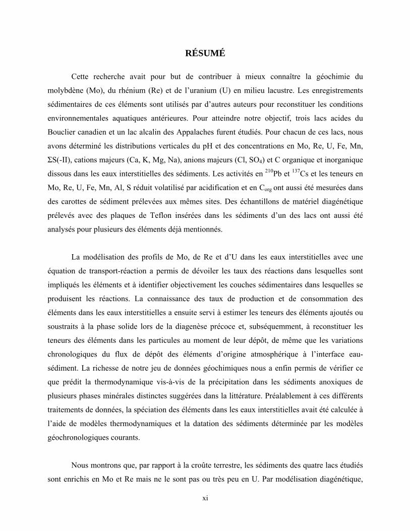
Figure 1 : Profils du Mo dans les eaux porales (trois profils pour une même date
d’échantillonnage) et dans les sédiments des lacs Tantaré, Vose, Despériers et Holland. La
ligne pointillée horizontale représente l’interface eau-sédiment. La carte montre la
localisation des lacs....................................................................................................................... 19
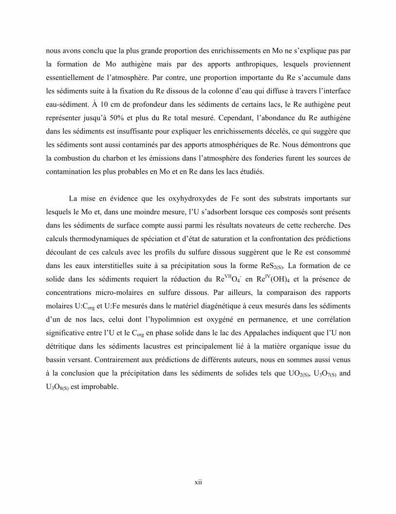
Figure 2 : Profils du Re dans les eaux porales (trois profils pour une même date
d’échantillonnage) et dans les sédiments des lacs Tantaré, Vose, Despériers et Holland. La
ligne pointillée horizontale représente l’interface eau-sédiment. La carte montre la
localisation des lacs....................................................................................................................... 21
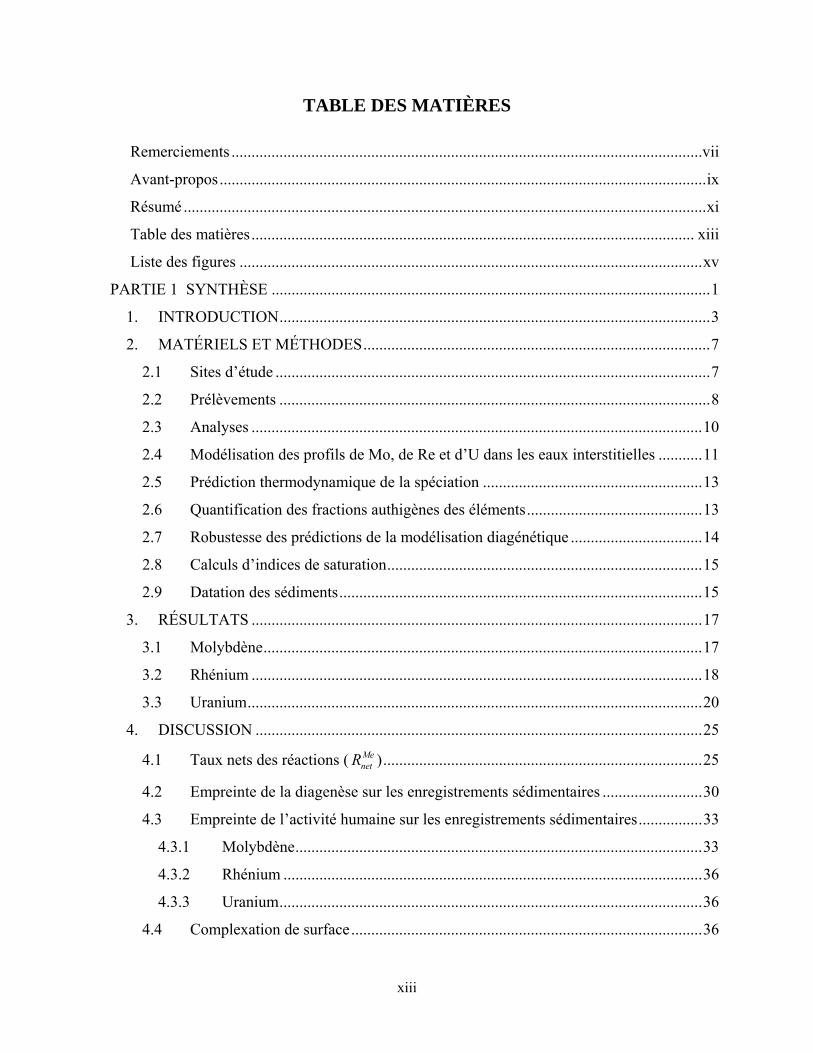
Figure 3 : Profils de l’U dans les eaux porales (trois profils pour une même date
d’échantillonnage) et dans les sédiments des lacs Tantaré, Vose, Despériers et Holland. La
ligne pointillée horizontale représente l’interface eau-sédiment. La carte montre la
localisation des lacs....................................................................................................................... 23
Figure 4 : Profil mesuré moyen (n=3) du Mo dans les eaux interstitielles des sédiments du
lac Tantaré en septembre 2003 et du lac Holland en août 2005. Sont aussi donnés pour le
lac Tantaré le profil modélisé (ligne mince), le coefficient de détermination r2 entre le profil
mesuré et le profil modélisé et le taux de production ou de consommation du Mo dans les
eaux interstitielles (ligne foncée). Par ailleurs, la ligne pointillée horizontale représente
l’interface eau-sédiment. ............................................................................................................... 27
Figure 5 : Profil mesuré moyen (n=3) du Re dans les eaux interstitielles des sédiments du
lac Tantaré en juillet 2003 et du lac Despériers en juin 2001. Sont aussi donnés pour les
deux lacs le profil modélisé (ligne mince), le coefficient de détermination r2 entre le profil
mesuré et le profil modélisé et le taux de production ou de consommation du Re dans les
eaux interstitielles (ligne foncée). Par ailleurs, la ligne pointillée horizontale représente
l’interface eau-sédiment. ............................................................................................................... 28
xvi
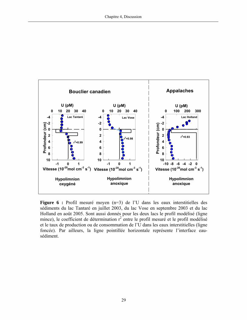
Figure 6 : Profil mesuré moyen (n=3) de l’U dans les eaux interstitielles des sédiments du
lac Tantaré en juillet 2003, du lac Vose en septembre 2003 et du lac Holland en août 2005.
Sont aussi donnés pour les deux lacs le profil modélisé (ligne mince), le coefficient de
détermination r2 entre le profil mesuré et le profil modélisé et le taux de production ou de
consommation de l’U dans les eaux interstitielles (ligne foncée). Par ailleurs, la ligne
pointillée horizontale représente l’interface eau-sédiment............................................................ 29
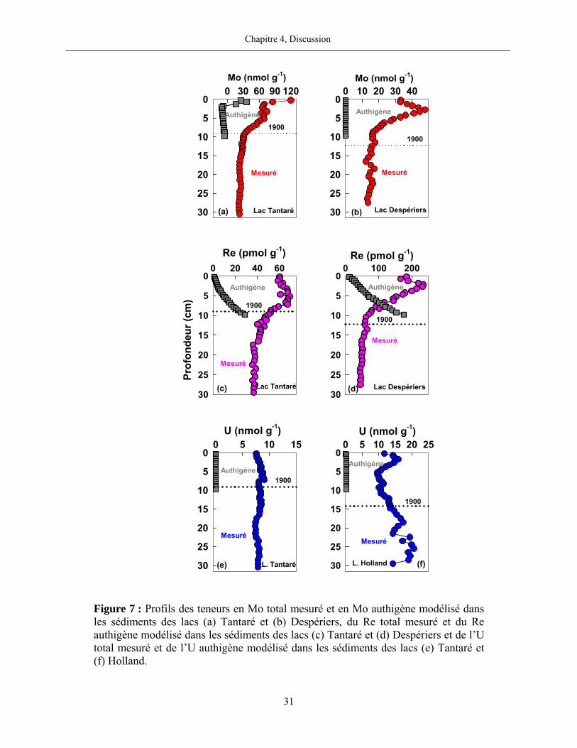
Figure 7 : Profils des teneurs en Mo total mesuré et en Mo authigène modélisé dans les
sédiments des lacs (a) Tantaré et (b) Despériers, du Re total mesuré et du Re authigène
modélisé dans les sédiments des lacs (c) Tantaré et (d) Despériers et de l’U total mesuré et
de l’U authigène modélisé dans les sédiments des lacs (e) Tantaré et (f) Holland. ...................... 31
Figure 8 : Variations chronologiques du dépôt de Mo atmosphérique d’origine anthropique
dans les lacs Tantaré, Despériers et Holland................................................................................. 35
Figure 9 : Profil en fonction de la profondeur des concentrations en Fe dans la phase solide
et dans les eaux interstitielles des sédiments du lac Tantaré en septembre 2003.......................... 38
Figure 10 : Produit d’activité ionique (PAI) et constante de solubilité (KS; ligne pointillée
verticale) pour MoS2(S) aux lacs Tantaré (a) et Holland (b) et ReS2(S) aux lacs Tantaré (c) et
Despériers (d). La ligne pointillée horizontale représente l’interface eau-sédiment..................... 43
Figure 11 : Rapport produit d’activité ionique/constante de solubilité pour UO2(S) et
U3O7(S) aux lacs Tantaré, Vose et Holland. La ligne pointillée verticale indique la saturation
(rapport = 0). La ligne pointillée horizontale représente l’interface eau-sédiment. ...................... 47
PARTIE 1
SYNTHÈSE

1. INTRODUCTION
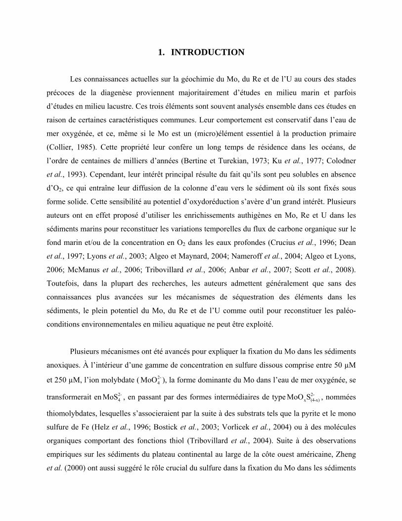
Les connaissances actuelles sur la géochimie du Mo, du Re et de l’U au cours des stades
précoces de la diagenèse proviennent majoritairement d’études en milieu marin et parfois
d’études en milieu lacustre. Ces trois éléments sont souvent analysés ensemble dans ces études en
raison de certaines caractéristiques communes. Leur comportement est conservatif dans l’eau de
mer oxygénée, et ce, même si le Mo est un (micro)élément essentiel à la production primaire
(Collier, 1985). Cette propriété leur confère un long temps de résidence dans les océans, de
l’ordre de centaines de milliers d’années (Bertine et Turekian, 1973; Ku et al., 1977; Colodner
et al., 1993). Cependant, leur intérêt principal résulte du fait qu’ils sont peu solubles en absence
d’O2, ce qui entraîne leur diffusion de la colonne d’eau vers le sédiment où ils sont fixés sous
forme solide. Cette sensibilité au potentiel d’oxydoréduction s’avère d’un grand intérêt. Plusieurs
auteurs ont en effet proposé d’utiliser les enrichissements authigènes en Mo, Re et U dans les
sédiments marins pour reconstituer les variations temporelles du flux de carbone organique sur le
fond marin et/ou de la concentration en O2 dans les eaux profondes (Crucius et al., 1996; Dean
et al., 1997; Lyons et al., 2003; Algeo et Maynard, 2004; Nameroff et al., 2004; Algeo et Lyons,
2006; McManus et al., 2006; Tribovillard et al., 2006; Anbar et al., 2007; Scott et al., 2008).
Toutefois, dans la plupart des recherches, les auteurs admettent généralement que sans des
connaissances plus avancées sur les mécanismes de séquestration des éléments dans les
sédiments, le plein potentiel du Mo, du Re et de l’U comme outil pour reconstituer les paléo-
conditions environnementales en milieu aquatique ne peut être exploité.
Plusieurs mécanismes ont été avancés pour expliquer la fixation du Mo dans les sédiments
anoxiques. À l’intérieur d’une gamme de concentration en sulfure dissous comprise entre 50 µM
et 250 µM, l’ion molybdate ( 2-4MoO ), la forme dominante du Mo dans l’eau de mer oxygénée, se
transformerait en 2-4MoS , en passant par des formes intermédiaires de type 2-
x (4-x)MoO S , nommées
thiomolybdates, lesquelles s’associeraient par la suite à des substrats tels que la pyrite et le mono
sulfure de Fe (Helz et al., 1996; Bostick et al., 2003; Vorlicek et al., 2004) ou à des molécules
organiques comportant des fonctions thiol (Tribovillard et al., 2004). Suite à des observations
empiriques sur les sédiments du plateau continental au large de la côte ouest américaine, Zheng
et al. (2000) ont aussi suggéré le rôle crucial du sulfure dans la fixation du Mo dans les sédiments
Chapitre 1, Introduction
4
anoxiques. Sans le démontrer précisément, ces auteurs évoquent la formation possible d’un
composé de type Fe–S–Mo à partir d’une concentration en sulfure dans les eaux interstitielles des
sédiments de 0,1 µM et la précipitation d’une phase solide pure de Mo et de S à une
concentration en sulfure dissous supérieure à 100 µM. L’hypothèse d’une précipitation de solides
tels que MoS2(S), consécutive à une réduction du Mo(VI) en Mo(IV), et de MoS3(S) a aussi été
suggérée par François (1988), Emerson et Huested (1991) et Nameroff et al. (2002). Enfin, suite
à la mise en évidence de corrélations significatives entre le Mo et le carbone organique dans les
sédiments, plusieurs auteurs ont suggéré que l’association du Mo avec la matière organique
constitue une voie importante d’immobilisation du Mo dans les sédiments anoxiques (Malcolm,
1985; Brumsack et Gieskes, 1983; Meyers et al., 2005; Algeo et Lyons, 2006).
Le Re est l’élément pour lequel les enrichissements authigènes les plus importants sont
observés dans les sédiments marins. Ceci s’explique notamment par le fait que, de tous les
éléments, le Re est celui dont le rapport de sa concentration dans l’eau de mer à sa teneur dans la
croûte terrestre est le plus élevé (Calvert et Pedersen, 1993). Comme pour le Mo, nous ne
connaissons pas bien les réactions qui contribuent à l’immobilisation du Re dans les sédiments.
La réduction du Re(VII) en Re(IV) dans les eaux interstitielles et sa précipitation subséquente
sous la forme de solides tels que ReO2(S), ReS2(S) et Re2S7(S) ont été proposées (Crusius et al.,
1996; Colodner et al., 1993; Nameroff et al., 2002; Morford et al., 2007). Selon Crusius et al.
(1996), le Re est réduit sous des conditions sub-oxiques, c’est-à-dire à la fois en absence
d’oxygène et de sulfure dissous. Cette hypothèse découle de la comparaison des profils verticaux
du Re dans différents sédiments à ceux d’autres éléments sensibles à l’oxydoréduction, en
particulier le Mo, mais n’a pas été formellement démontrée.
Les enrichissements authigènes en U ont par ailleurs été expliqués jusqu’à ce jour par la
réduction de l’U(VI) en U(IV)), lequel formerait des solides tels que UO2(S), U3O7(S) et U3O8(S)
(Anderson et al., 1989; McManus et al., 2005; Morford et al., 2005, 2007). La réaction de
réduction de l’U(VI) en U(IV) se déroulerait vraisemblablement dans des conditions rédox
proches de celles de la réduction du Fe(III) en Fe(II) (Klinkhammer et Palmer, 1991; Zheng
et al., 2002a; Morford et al., 2001; McManus et al., 2005) et serait catalysée par l’activité
bactérienne (Lovely et al., 1991; Fredrickson et al., 2000; Sani et al., 2004). Selon différents
Chapitre 1, Introduction
5
auteurs, l’accumulation relativement plus importante d’U authigène observée dans des sédiments
enrichis en matière organique appuie, sans toutefois le démontrer, cette idée d’un contrôle
microbien de la cinétique de réduction de l’U dans les sédiments (Zheng et al., 2002a; Sundby
et al., 2004; McManus et al., 2005).
Un débat subsiste donc toujours concernant les mécanismes d’immobilisation du Mo, du
Re et de l’U dans les sédiments. Des hypothèses ont été avancées mais elles requièrent d’être
validées. Les seules mesures de teneur en phase solide ne permettent pas d’atteindre une
compréhension complète des réactions en cause. Or, à quelques exceptions près, la grande
majorité des recherches déjà citées ne portent que sur les sédiments et n’ont pas considéré les
eaux interstitielles. Par ailleurs, les quelques études livrant des données sur le Mo, le Re et l’U
dans les eaux interstitielles des sédiments n’accompagnent généralement ces données que d’un
nombre limité, voire insuffisant, d’autres variables géochimiques importantes. Cette lacune réduit
par conséquent la capacité à interpréter la diagenèse. Par exemple, le choix des coefficients pour
le calcul des flux diffusifs des éléments, de même que le calcul des indices de saturation vis-à-vis
de phases minérales distinctes, nécessitent une connaissance de la spéciation des éléments qui ne
peut être estimée qu’avec un ensemble élaboré de données géochimiques. Enfin, nous pouvons
aussi souligner que les hypothèses émises concernant l’association du Mo avec les sulfures de Fe
dans les sédiments sont essentiellement fondées sur des expériences en laboratoire réalisées dans
des conditions qui, forcément, ne reflètent pas parfaitement le milieu naturel.
Par ailleurs, la mauvaise connaissance générale de l’impact de l’activité humaine sur les
enregistrements sédimentaires constitue un facteur supplémentaire qui empêche d’exploiter
pleinement le Mo, le Re et l’U comme traceurs de paléo-conditions environnementales. Des
sources anthropiques de ces éléments ont pourtant été identifiées. Par exemple, les fonderies de
métaux et la combustion du charbon sont des sources reconnues d’émissions dans l’atmosphère
de Mo et d’U (Nriagu and Pacyna, 1988; Pacyna et Pacyna, 2001; Telmer et al., 2004). Dans une
étude sur les sédiments d’une tourbière ombrotrophique du centre de l’Europe (Suisse), Krachler
et Shotyk (2004) concluaient notamment que le taux de dépôt du Mo atmosphérique a augmenté
de 0,2 à 10 µg m−2 a−1 au cours du dernier siècle en raison de l’industrialisation. La combustion
du charbon a aussi été suggérée comme une cause probable de contamination en Re de
Chapitre 1, Introduction
6
l’atmosphère (Colodner et al., 1995). Les principales activités responsables de la contamination
environnementale en U sont l’exploitation minière, l’épandage des engrais, l’utilisation d’armes,
la production d’énergie par les centrales nucléaires et son utilisation à des fins scientifiques
(http://www.irsn.org). Dans l’est de l’Amérique du Nord, où l’industrie minière et métallurgique
est très présente et où la consommation du charbon pour la production d’électricité est importante
depuis de nombreuses années, nous ne pouvons pas exclure que ces activités contaminent
l’atmosphère en Mo, Re et U et, suite à leur dépôt, l’eau et les sédiments du milieu aquatique.
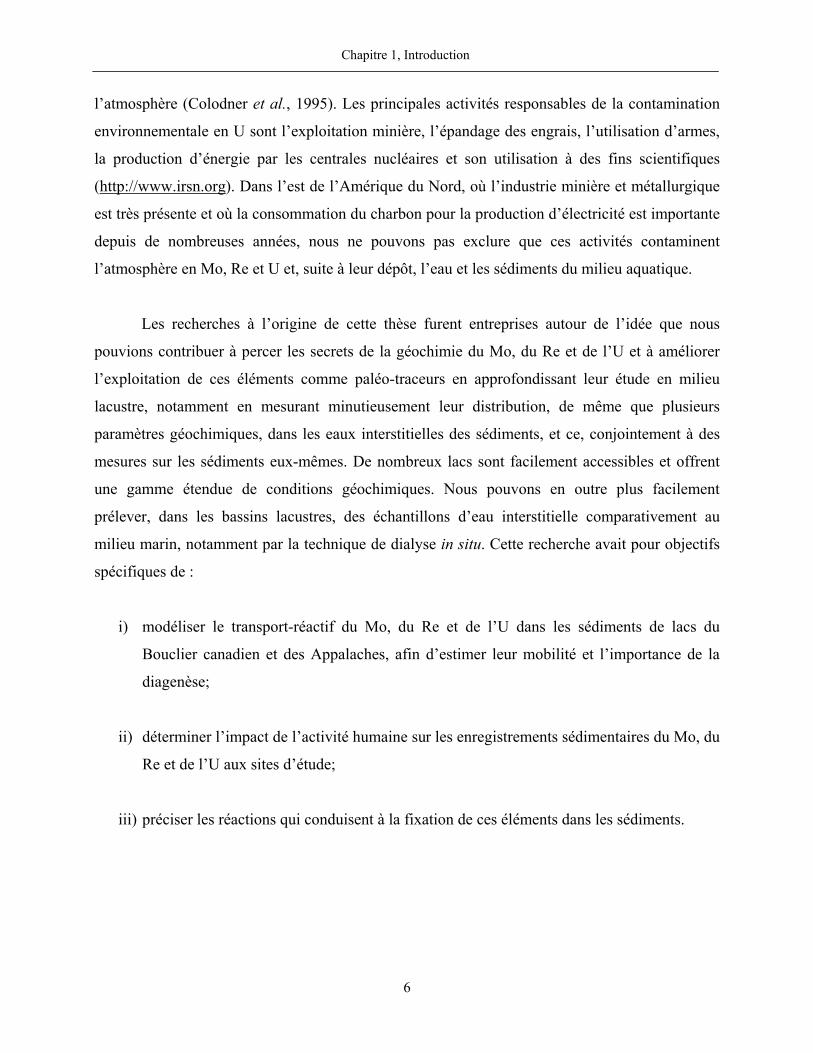
Les recherches à l’origine de cette thèse furent entreprises autour de l’idée que nous
pouvions contribuer à percer les secrets de la géochimie du Mo, du Re et de l’U et à améliorer
l’exploitation de ces éléments comme paléo-traceurs en approfondissant leur étude en milieu
lacustre, notamment en mesurant minutieusement leur distribution, de même que plusieurs
paramètres géochimiques, dans les eaux interstitielles des sédiments, et ce, conjointement à des
mesures sur les sédiments eux-mêmes. De nombreux lacs sont facilement accessibles et offrent
une gamme étendue de conditions géochimiques. Nous pouvons en outre plus facilement
prélever, dans les bassins lacustres, des échantillons d’eau interstitielle comparativement au
milieu marin, notamment par la technique de dialyse in situ. Cette recherche avait pour objectifs
spécifiques de :
i) modéliser le transport-réactif du Mo, du Re et de l’U dans les sédiments de lacs du
Bouclier canadien et des Appalaches, afin d’estimer leur mobilité et l’importance de la
diagenèse;
ii) déterminer l’impact de l’activité humaine sur les enregistrements sédimentaires du Mo, du
Re et de l’U aux sites d’étude;
iii) préciser les réactions qui conduisent à la fixation de ces éléments dans les sédiments.
2. MATÉRIELS ET MÉTHODES
Les détails de toutes les méthodes utilisées dans cette recherche sont donnés dans les
articles colligés à la partie 2. Dans les paragraphes qui suivent, je résume sommairement les
critères retenus pour la sélection des sites d’étude, les protocoles opératoires et les différentes
approches adoptées pour la modélisation géochimique.
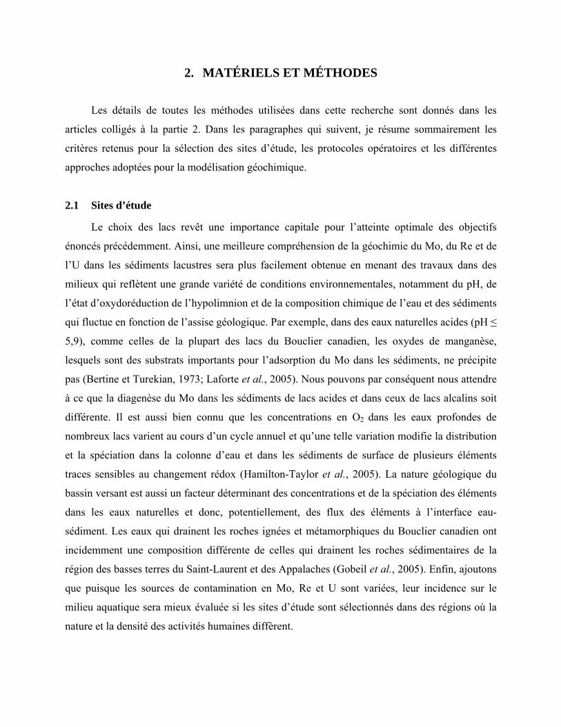
2.1 Sites d’étude
Le choix des lacs revêt une importance capitale pour l’atteinte optimale des objectifs
énoncés précédemment. Ainsi, une meilleure compréhension de la géochimie du Mo, du Re et de
l’U dans les sédiments lacustres sera plus facilement obtenue en menant des travaux dans des
milieux qui reflètent une grande variété de conditions environnementales, notamment du pH, de
l’état d’oxydoréduction de l’hypolimnion et de la composition chimique de l’eau et des sédiments
qui fluctue en fonction de l’assise géologique. Par exemple, dans des eaux naturelles acides (pH ≤
5,9), comme celles de la plupart des lacs du Bouclier canadien, les oxydes de manganèse,
lesquels sont des substrats importants pour l’adsorption du Mo dans les sédiments, ne précipite
pas (Bertine et Turekian, 1973; Laforte et al., 2005). Nous pouvons par conséquent nous attendre
à ce que la diagenèse du Mo dans les sédiments de lacs acides et dans ceux de lacs alcalins soit
différente. Il est aussi bien connu que les concentrations en O2 dans les eaux profondes de
nombreux lacs varient au cours d’un cycle annuel et qu’une telle variation modifie la distribution
et la spéciation dans la colonne d’eau et dans les sédiments de surface de plusieurs éléments
traces sensibles au changement rédox (Hamilton-Taylor et al., 2005). La nature géologique du
bassin versant est aussi un facteur déterminant des concentrations et de la spéciation des éléments
dans les eaux naturelles et donc, potentiellement, des flux des éléments à l’interface eau-
sédiment. Les eaux qui drainent les roches ignées et métamorphiques du Bouclier canadien ont
incidemment une composition différente de celles qui drainent les roches sédimentaires de la
région des basses terres du Saint-Laurent et des Appalaches (Gobeil et al., 2005). Enfin, ajoutons
que puisque les sources de contamination en Mo, Re et U sont variées, leur incidence sur le
milieu aquatique sera mieux évaluée si les sites d’étude sont sélectionnés dans des régions où la
nature et la densité des activités humaines diffèrent.
Chapitre 2, Matériels et méthodes
8
Quatre lacs situés dans la province de Québec ont été retenus pour cette étude (figure 1,
page 80). Trois d’entre eux, les lacs Tantaré, Vose et Despériers, reposent sur le Bouclier
canadien, l’autre, le lac Holland, celui qualifié de « petit lac Holland », est situé dans la région
des Appalaches. Les eaux des lacs du Bouclier canadien sont acides, celles du lac appalachien
légèrement basiques. L’altitude de tous les lacs varie entre 350 et 650 m et leur profondeur
maximale entre 10 et 17 m. Les bassins versants de chacun des lacs n’ont jamais été habités par
l’homme et n’ont jamais subi de coupe de bois ou d’incendie de forêt, sauf peut-être celui du lac
Holland. Les seuls apports anthropiques de métaux dans ces lacs proviennent donc de
l’atmosphère. Le lac Tantaré se trouve à moins de 40 km de la ville de Québec qui compte une
population de près d’un demi-million d’habitants. Les lacs Vose et Despériers se trouvent dans un
rayon de 25 km de Rouyn-Noranda, plus petite ville dont la population n’est que d’environ 30
000 habitants mais où une fonderie de minerais non-ferreux est en exploitation depuis 1925.
Enfin, proche d’une route secondaire, le lac Holland se trouve à 8 km de la petite localité de
Murdochville; une fonderie de minerais non-ferreux y fut aussi en opération de 1951 à 2002. Le
lac Tantaré fut échantillonné dans son bassin le plus à l’ouest dont l’hypolimnion demeure
oxygéné en permanence. Par contre, l’hypolimnion des autres lacs devient périodiquement
anoxique; nos prélèvements dans ces lacs furent effectués lorsque les eaux profondes étaient
anoxiques.
2.2 Prélèvements
L’étude de la diagenèse précoce des sédiments nécessite, en plus de l’analyse de la phase
solide, celle de l’eau contenue dans les interstices des particules de sédiments (Shaw et al., 1990).
Les profils des éléments dans les eaux interstitielles (ou eaux porales) permettent en effet de
mieux apprécier la réactivité des éléments dans les sédiments car de petites variations de leurs
teneurs dans la phase solide peuvent se traduire par des gradients importants de concentrations
dans les eaux porales. Dans cette thèse, j’ai donc accordé autant d’importance au prélèvement et à
l’analyse des eaux interstitielles qu’à ceux de la phase solide des sédiments.
Des échantillons d’eau interstitielle des sédiments furent obtenus par dialyse in situ à une
résolution spatiale d’échantillonnage de 0,5 ou 1 cm selon la profondeur; les volumes des loges
des dialyseurs étaient respectivement de 4-5 mL et de 8-9 mL. La décontamination préalable des
Chapitre 2, Matériels et méthodes
9
appareils à dialyse fut effectuée tel que décrite par Carignan et al. (1985) et Alfaro-De la Torre et
Tessier (2002). Ils furent d’abord immergés dans des solutions acides pendant 7 jours, rincés
abondamment et maintenus sous une atmosphère d’azote renouvelée quotidiennement pendant
deux semaines. Les loges des appareils à dialyse furent ensuite remplies d’eau ultrapure,
recouvertes d’une membrane Gelman HT-200 (0,2 µm de porosité) et maintenues de nouveau
pendant une semaine sous une atmosphère d’azote renouvelée quotidiennement, ce qui est
suffisant pour éliminer à toute fin pratique la présence d’O2 (Carignan et al., 1994). Ils furent
insérés dans les sédiments par des plongeurs, de manière à échantillonner la zone entre 2,5 ou 5
cm au-dessus de l’interface eau-sédiment et 10 cm en dessous de cette interface. Ils furent
déployés dans chaque cas pour des périodes de 3 semaines; les volumes totaux d’échantillons
obtenus, soit 12 mL, étaient suffisants pour effectuer trois mesures indépendantes, une par
appareil à dialyse, du pH et des concentrations en Mo, Re, U, Fe, Mn, Ca, K, Mg, Na, ΣS(-II), Cl,
4SO , carbone organique dissous et carbone inorganique dissous.
Deux carottes de sédiments furent également prélevées en plongée à chacun des sites
d’étude à l’aide de tubes en Plexiglas ayant un diamètre interne de 9,5 cm. Dans les deux heures
suivant les prélèvements, les carottes furent extrudées et sectionnées à intervalle de 0,5 cm entre
la surface du sédiment et 15 cm de profondeur, puis, à intervalle de 1 cm jusqu’à 30 cm. Les
échantillons d’une des carottes de chaque site furent placés dans des contenants en plastique et
conservés à 4°C pendant leur transport au laboratoire où ils furent ensuite congelés. Prévus pour
la mesure des AVS (acid volatile sulfide), les échantillons de l’autre carotte furent préservés dans
de petits sacs en plastique fermés hermétiquement et soigneusement enfouis dans un plus grand
sac rempli de boue anoxique jusqu’à ce qu’ils soient analysés au laboratoire.
Des plaques de Teflon (~110 cm2) qui avaient été insérées en octobre 1993 par le
professeur Tessier dans les sédiments du lac Tantaré, à proximité de notre site d’étude dans ce
lac, ont été retirées en août 2006. Ces plaques de Teflon permettent de prélever des
oxyhydroxydes de Fe diagénétiques, lesquels précipitent au voisinage de l’interface eau-sédiment
suite à l’oxydation du Fe(II) qui migre vers cette interface à partir des sédiments plus profonds
(Belzile et al., 1989). Les oxydes de Fe qui se fixent sur les plaques de Teflon ont été identifiés
comme étant principalement composés de ferrihydrite et de lépidocrocite faiblement cristalline
Chapitre 2, Matériels et méthodes
10
(Fortin et al., 1993). Après leur récupération, les plaques de Teflon et leur substrat ont été rincés
avec l’eau du lac et transportés dans des contenants en polyéthylène.
2.3 Analyses
Les concentrations en Mo, Re et U dans les eaux interstitielles furent déterminées à l’aide
d’un spectromètre de masse de type quadrupole couplé à un plasma induit par haute fréquence
(ICP-MS) en utilisant le Rh comme standard interne. Les concentrations des éléments Fe, Mn,
Ca, K, Mg et Na furent mesurées à l’aide d’un spectromètre d’émissions atomiques couplé à un
plasma induit à haute fréquence (ICP-AES) en utilisant le Y comme standard interne. Les
concentrations en sulfure (ΣS(-II)) furent déterminées par colorimétrie (Cline, 1969), celles en
carbone inorganique dissous par chromatographie en phase gazeuse (Carignan, 1984), celles en
carbone organique dissous à l’aide d’un analyseur de carbone et celles des anions par
chromatographie ionique (Subosa et al., 1989).
Les sédiments furent lyophilisés, homogénéisés par broyage, et complètement minéralisés
avec un mélange d’acides concentrés ultra purs (HF, HNO3 et HClO4). Les acides furent ensuite
évaporés et les résidus repris dans une solution d’acide nitrique 0,2 N (McLaren et al., 1995). Les
teneurs en Mo, Re et U dans les sédiments ont été mesurées par ICP-MS et celles en Fe, Mn, et
Al par ICP-AES. Les concentrations en AVS furent déterminées selon la méthode décrite par
Allen et al., (1993). Selon cette méthode, le sulfure qui se dégage du sédiment suite à son
acidification (HCl) est piégé dans une solution de NaOH, puis, il est mesuré par colorimétrie
(Cline, 1969). Le matériel diagénétique fixé aux plaques de Teflon fut minéralisé avec HCl et les
solutions résultantes filtrées sur des membranes de Teflon (0,4 µm).
Des aliquotes de sédiment lyophilisé ont été placées dans des contenants scellés durant au
moins un mois pour que l’équilibre séculaire entre le 222Rn et le 214Pb avec le 226Ra soit atteint.
Les activités du 137Cs, 210Pb et 214Pb ont ensuite été mesurées par spectrométrie gamma (Appleby
et al., 1986; Schelske et al., 1994). Les résultats obtenus furent corrigés pour les effets de la
géométrie des échantillons et pour le biais dû à l’auto-absorption des émissions (Appleby et al.,
1992; Appleby and Piliposian, 2004). L’activité du 210Pb non supportée (210Pbun), c'est-à-dire le
Chapitre 2, Matériels et méthodes
11
210Pb issu du dépôt atmosphérique et non de la désintégration du 226Ra dans les sédiments, a été
calculée en soustrayant l’activité mesurée du 214Pb à celle du 210Pb.
2.4 Modélisation des profils de Mo, de Re et d’U dans les eaux interstitielles
La modélisation des profils des éléments traces dans les eaux interstitielles sert à dévoiler
les taux des réactions dans lesquelles sont impliqués les éléments et à identifier objectivement les
couches sédimentaires dans lesquelles se produisent les réactions. En comparant les profils
modélisés à ceux de paramètres clés de la diagenèse précoce, notamment du sulfure, du Fe et du
Mn, nous pouvons en outre proposer la nature des réactions auxquelles les éléments traces
participent.
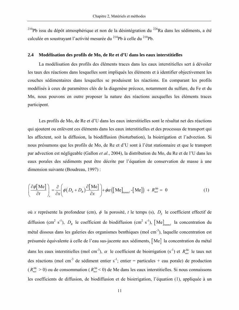
Les profils de Mo, de Re et d’U dans les eaux interstitielles sont le résultat net des réactions
qui ajoutent ou enlèvent ces éléments dans les eaux interstitielles et des processus de transport qui
les affectent, soit la diffusion, la biodiffusion (bioturbation), la bioirrigation et l’advection. Si
nous présumons que les profils de Mo, de Re et d’U sont à l’état stationnaire et que le transport
par advection est négligeable (Gallon et al., 2004), la distribution du Mo, du Re et de l’U dans les
eaux porales des sédiments peut être décrite par l’équation de conservation de masse à une
dimension suivante (Boudreau, 1997) :
[ ] ( ) [ ] [ ] [ ]( )Me MeMe - Me 0Me
S B nettunnelx
D D Rt x x
φφ φα
⎛ ⎞ ⎛ ⎞∂ ∂∂= + + + =⎜ ⎟ ⎜ ⎟∂ ∂ ∂⎝ ⎠ ⎝ ⎠
(1)
où x représente la profondeur (cm), φ la porosité, t le temps (s), SD le coefficient effectif de
diffusion (cm2 s-1), BD le coefficient de biodiffusion (cm2 s-1), [ ]Metunnel
la concentration du
métal dissous dans les galeries des organismes benthiques (mol cm-3), laquelle concentration est
présumée équivalente à celle de l’eau sus-jacente aux sédiments, [ ]Me la concentration du métal
dans les eaux interstitielles (mol cm-3), α le coefficient de bioirrigation (s-1) et MenetR le taux net
des réactions (mol cm-3 de sédiment entier s-1; entier = particules + eau porale) de production
( MenetR > 0) ou de consommation ( Me
netR < 0) de Me dans les eaux interstitielles. Si nous connaissons
les coefficients de diffusion, de biodiffusion et de bioirrigation, l’équation (1), appliquée à un
Chapitre 2, Matériels et méthodes
12
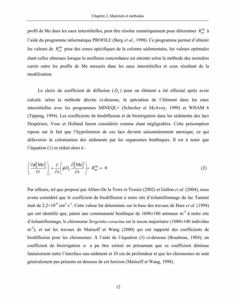
profil de Me dans les eaux interstitielles, peut être résolue numériquement pour déterminer MenetR à
l’aide du programme informatique PROFILE (Berg et al., 1998). Ce programme permet d’obtenir
les valeurs de MenetR pour des zones spécifiques de la colonne sédimentaire, les valeurs optimales
étant celles obtenues lorsque la meilleure concordance est atteinte selon la méthode des moindres
carrés entre les profils de Me mesurés dans les eaux interstitielles et ceux résultant de la
modélisation.
Le choix du coefficient de diffusion ( SD ) pour un élément a été effectué après avoir
calculé, selon la méthode décrite ci-dessous, la spéciation de l’élément dans les eaux
interstitielles avec les programmes MINEQL+ (Schecher et McAvoy, 1998) et WHAM 6
(Tipping, 1994). Les coefficients de biodiffusion et de bioirrigation dans les sédiments des lacs
Despériers, Vose et Holland furent considérés comme étant négligeables. Cette présomption
repose sur le fait que l’hypolimnion de ces lacs devient saisonnièrement anoxique, ce qui
défavorise la colonisation des sédiments par les organismes benthiques. Il est à noter que
l’équation (1) se réduit alors à :
[ ] [ ]Me Me 0Me
S netx
D Rt x x
φφ
⎛ ⎞ ⎛ ⎞∂ ∂∂= + =⎜ ⎟ ⎜ ⎟∂ ∂ ∂⎝ ⎠ ⎝ ⎠
(2)
Par ailleurs, tel que proposé par Alfaro-De la Torre et Tessier (2002) et Gallon et al. (2004), nous
avons considéré que le coefficient de biodiffusion à notre site d’échantillonnage du lac Tantaré
était de 2,2×10⁻⁹ cm2 s-1. Cette valeur fut déterminée sur la base des travaux de Hare et al. (1994)
qui ont identifié que, parmi une communauté benthique de 1690±180 animaux m-2 à notre site
d’échantillonnage, le chironome Sergentia coracina est le taxon majoritaire (1080±140 individus
m-2), et sur les travaux de Matisoff et Wang (2000) qui ont rapporté des coefficients de
biodiffusion pour les chironomes. À l’aide de l’équation (3) ci-dessous (Boudreau, 1984), un
coefficient de bioirrigation α a pu être estimé en présumant que ce coefficient diminue
linéairement entre l’interface eau-sédiment et 10 cm de profondeur et que les chironomes ne sont
généralement pas présents en dessous de cet horizon (Matisoff et Wang, 1998).
Chapitre 2, Matériels et méthodes
13
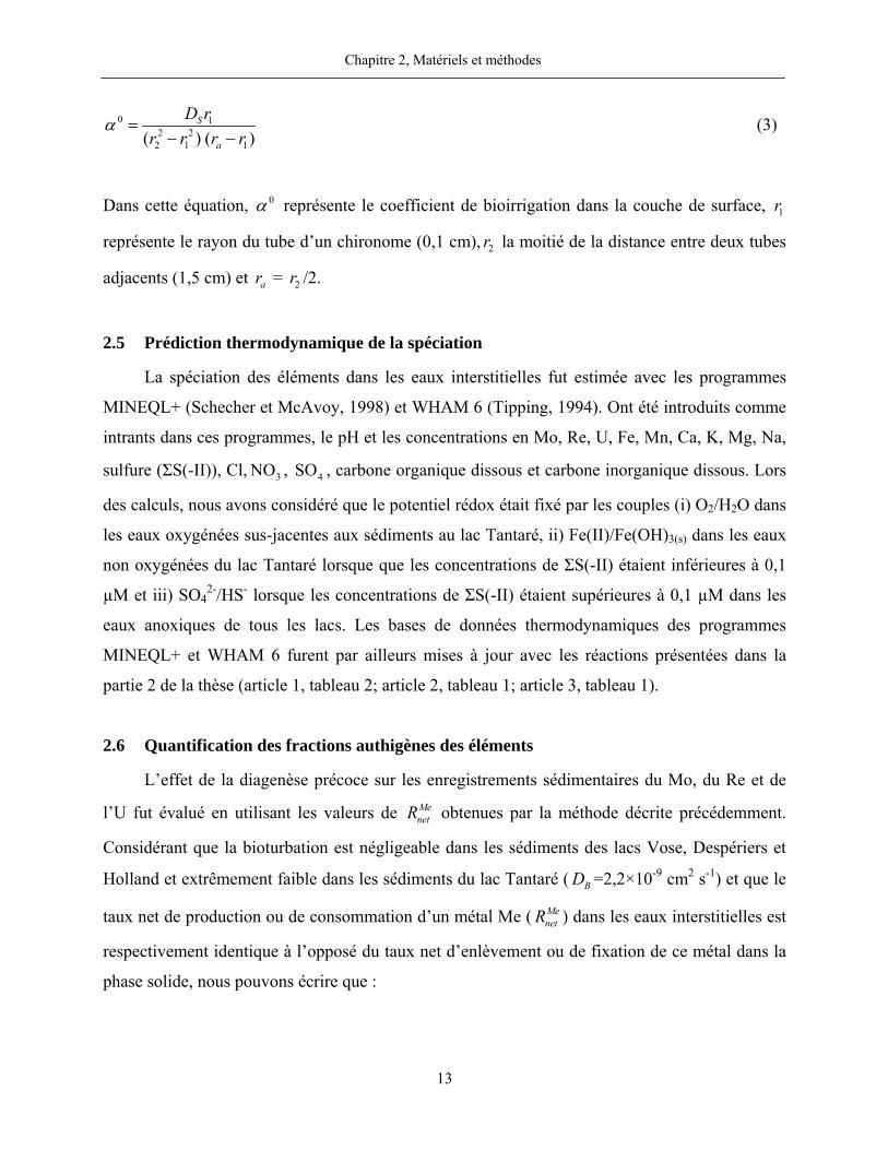
0 12 2
2 1 1( ) ( )S
a
D rr r r r
α =− −
(3)
Dans cette équation, 0α représente le coefficient de bioirrigation dans la couche de surface, 1r
représente le rayon du tube d’un chironome (0,1 cm), 2r la moitié de la distance entre deux tubes
adjacents (1,5 cm) et ar = 2r /2.
2.5 Prédiction thermodynamique de la spéciation
La spéciation des éléments dans les eaux interstitielles fut estimée avec les programmes
MINEQL+ (Schecher et McAvoy, 1998) et WHAM 6 (Tipping, 1994). Ont été introduits comme
intrants dans ces programmes, le pH et les concentrations en Mo, Re, U, Fe, Mn, Ca, K, Mg, Na,
sulfure (ΣS(-II)), Cl, 3NO , 4SO , carbone organique dissous et carbone inorganique dissous. Lors
des calculs, nous avons considéré que le potentiel rédox était fixé par les couples (i) O2/H2O dans
les eaux oxygénées sus-jacentes aux sédiments au lac Tantaré, ii) Fe(II)/Fe(OH)3(s) dans les eaux
non oxygénées du lac Tantaré lorsque que les concentrations de ΣS(-II) étaient inférieures à 0,1
µM et iii) SO42-/HS- lorsque les concentrations de ΣS(-II) étaient supérieures à 0,1 µM dans les
eaux anoxiques de tous les lacs. Les bases de données thermodynamiques des programmes
MINEQL+ et WHAM 6 furent par ailleurs mises à jour avec les réactions présentées dans la
partie 2 de la thèse (article 1, tableau 2; article 2, tableau 1; article 3, tableau 1).
2.6 Quantification des fractions authigènes des éléments
L’effet de la diagenèse précoce sur les enregistrements sédimentaires du Mo, du Re et de
l’U fut évalué en utilisant les valeurs de MenetR obtenues par la méthode décrite précédemment.
Considérant que la bioturbation est négligeable dans les sédiments des lacs Vose, Despériers et
Holland et extrêmement faible dans les sédiments du lac Tantaré ( BD =2,2×10⁻⁹ cm2 s-1) et que le
taux net de production ou de consommation d’un métal Me ( MenetR ) dans les eaux interstitielles est
respectivement identique à l’opposé du taux net d’enlèvement ou de fixation de ce métal dans la
phase solide, nous pouvons écrire que :
Chapitre 2, Matériels et méthodes
14
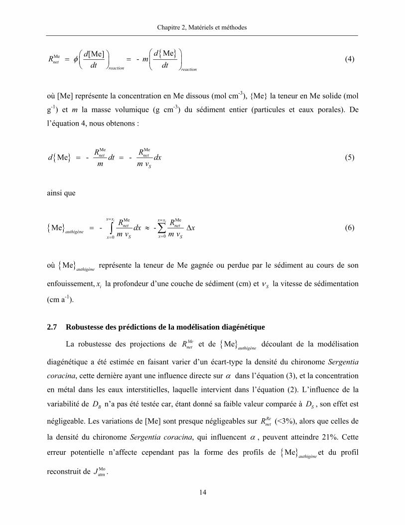
Me Me[Me] - netreaction reaction
ddR mdt dt
φ⎛ ⎞⎛ ⎞= = ⎜ ⎟⎜ ⎟
⎝ ⎠ ⎝ ⎠ (4)
où [Me] représente la concentration en Me dissous (mol cm-3), Me la teneur en Me solide (mol
g-1) et m la masse volumique (g cm-3) du sédiment entier (particules et eaux porales). De
l’équation 4, nous obtenons :
Me Me
Me - -
net net
S
R Rd dt dxm m v
= = (5)
ainsi que
Me Me
00
Me - -
i ix x x x
net netauthigène
xS Sx
R Rdx xm v m v
= =
==
= ≈ Δ∑∫ (6)
où Meauthigène
représente la teneur de Me gagnée ou perdue par le sédiment au cours de son
enfouissement, ix la profondeur d’une couche de sédiment (cm) et Sν la vitesse de sédimentation
(cm a-1).
2.7 Robustesse des prédictions de la modélisation diagénétique
La robustesse des projections de MenetR et de Me
authigène découlant de la modélisation
diagénétique a été estimée en faisant varier d’un écart-type la densité du chironome Sergentia
coracina, cette dernière ayant une influence directe sur α dans l’équation (3), et la concentration
en métal dans les eaux interstitielles, laquelle intervient dans l’équation (2). L’influence de la
variabilité de BD n’a pas été testée car, étant donné sa faible valeur comparée à SD , son effet est
négligeable. Les variations de [Me] sont presque négligeables sur RenetR (<3%), alors que celles de
la densité du chironome Sergentia coracina, qui influencent α , peuvent atteindre 21%. Cette
erreur potentielle n’affecte cependant pas la forme des profils de Meauthigène
et du profil
reconstruit de MoatmJ .
Chapitre 2, Matériels et méthodes
15
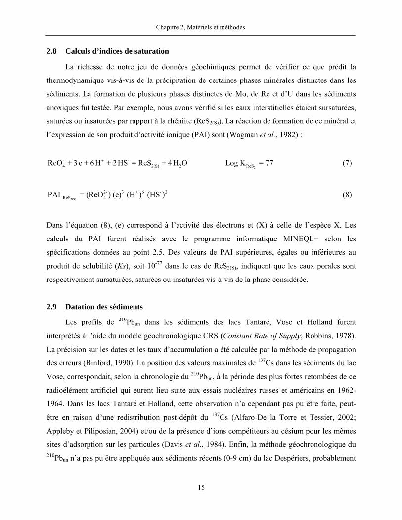
2.8 Calculs d’indices de saturation
La richesse de notre jeu de données géochimiques permet de vérifier ce que prédit la
thermodynamique vis-à-vis de la précipitation de certaines phases minérales distinctes dans les
sédiments. La formation de plusieurs phases distinctes de Mo, de Re et d’U dans les sédiments
anoxiques fut testée. Par exemple, nous avons vérifié si les eaux interstitielles étaient sursaturées,
saturées ou insaturées par rapport à la rhéniite (ReS2(S)). La réaction de formation de ce minéral et
l’expression de son produit d’activité ionique (PAI) sont (Wagman et al., 1982) :
- + -4 2(S) 2ReO + 3 e + 6 H + 2 HS = ReS + 4 H O
2ReSLog K = 77 (7)
2(S)
2- 3 + 6 - 2ReS 4PAI = (ReO ) (e) (H ) (HS ) (8)
Dans l’équation (8), (e) correspond à l’activité des électrons et (X) à celle de l’espèce X. Les
calculs du PAI furent réalisés avec le programme informatique MINEQL+ selon les
spécifications données au point 2.5. Des valeurs de PAI supérieures, égales ou inférieures au
produit de solubilité (Ks), soit 10-77 dans le cas de ReS2(S), indiquent que les eaux porales sont
respectivement sursaturées, saturées ou insaturées vis-à-vis de la phase considérée.
2.9 Datation des sédiments
Les profils de 210Pbun dans les sédiments des lacs Tantaré, Vose et Holland furent
interprétés à l’aide du modèle géochronologique CRS (Constant Rate of Supply; Robbins, 1978).
La précision sur les dates et les taux d’accumulation a été calculée par la méthode de propagation
des erreurs (Binford, 1990). La position des valeurs maximales de 137Cs dans les sédiments du lac
Vose, correspondait, selon la chronologie du 210Pbun, à la période des plus fortes retombées de ce
radioélément artificiel qui eurent lieu suite aux essais nucléaires russes et américains en 1962-
1964. Dans les lacs Tantaré et Holland, cette observation n’a cependant pas pu être faite, peut-
être en raison d’une redistribution post-dépôt du 137Cs (Alfaro-De la Torre et Tessier, 2002;
Appleby et Piliposian, 2004) et/ou de la présence d’ions compétiteurs au césium pour les mêmes
sites d’adsorption sur les particules (Davis et al., 1984). Enfin, la méthode géochronologique du 210Pbun n’a pas pu être appliquée aux sédiments récents (0-9 cm) du lac Despériers, probablement
Chapitre 2, Matériels et méthodes
16
en raison de variations temporelles de la sédimentation du 210Pb causées par l’acidification
anthropique de la colonne d’eau (Gallon et al., 2006). Nous avons présumé que le taux
d’accumulation est constant dans ce lac et estimé sa valeur à partir de la position du pic de 137Cs.
3. RÉSULTATS
Les résultats acquis dans le cadre de cette thèse révèlent des tendances claires et cohérentes
entre les lacs et entre les différentes variables géochimiques mesurées dans un même lac. Dans
les paragraphes ci-dessous, je récapitule les principales tendances observées pour le Mo, le Re et
l’U. La description complète de tous les autres résultats apparaît dans les articles de la partie 2 de
la thèse.
3.1 Molybdène
Les concentrations en Mo dissous (0,1-3,4 nM) dans les eaux sus-jacentes aux sédiments et
dans les eaux porales sont significativement inférieures aux concentrations mesurées dans l’eau
de mer mais s’apparentent à celles trouvées en eau douce (Morford et Emerson, 1999). La forme
prépondérante prédite par la thermodynamique (voir section 2.5) est l’ion molybdate ( 2-4MoO ),
sauf dans les eaux sus-jacentes aux sédiments du lac Vose où 24-MoO Sx x
− serait majoritaire. Nous
pouvons cependant noter que même si le 2-4MoO est l’espèce la plus importante (~40%) au lac
Holland, dont les eaux sont riches en calcium et magnésium comparativement aux eaux des lacs
du Bouclier canadien, les formes CaMoO40 et MgMoO4
0 représentent ensemble jusqu’à 60% du
Mo total dissous.
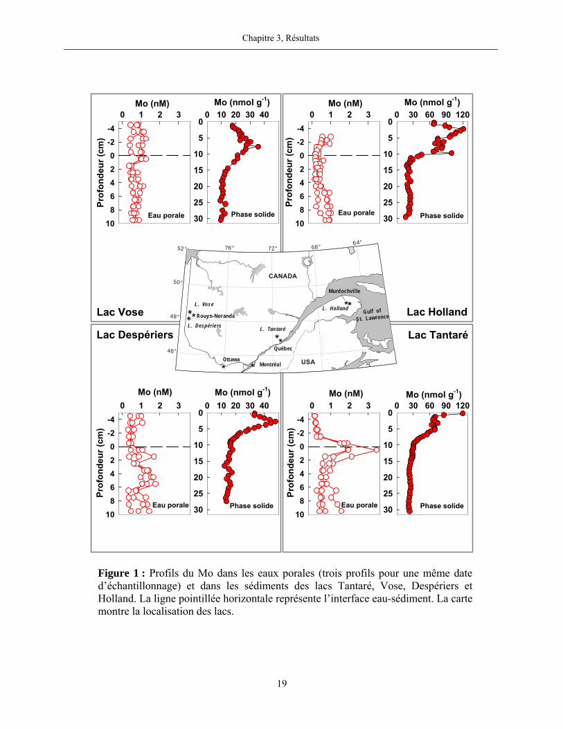
Les profils du Mo dans les eaux porales du bassin oxygéné en permanence du lac Tantaré
sont différents de ceux trouvés dans les lacs périodiquement anoxiques (figure 1). Au lac Tantaré,
les profils affichent des concentrations beaucoup plus élevées entre 1 et 2 cm de profondeur sous
l’interface eau-sédiment que dans les eaux sus-jacentes aux sédiments et que dans les couches de
sédiments plus profondes. Dans les autres lacs, les profils du Mo dissous montrent cependant très
peu de variation en fonction de la profondeur, entre autres, les concentrations dans les eaux
porales et dans les eaux sus-jacentes aux sédiments sont très similaires.
Un contraste frappant est également observé entre le profil du Mo en phase solide au lac
Tantaré et ceux déterminés dans les autres lacs. Au lac Tantaré, les teneurs diminuent
abruptement juste sous l’interface eau-sédiment, comme c’est aussi le cas pour le Fe (voir
Chapitre 3, Résultats
18
figure 4, page 83), puis, restent constantes avec la profondeur jusqu’à 5,75 cm et diminuent par la
suite. En profondeur dans la carotte du lac Tantaré, la teneur en Mo dans la phase solide est de
24±1 nmol g-1 et le rapport molaire Mo:Al (9×10⁻⁶) est typique de celui de la croûte terrestre
(6-19×10-6; Turekian et Wedepohl, 1961). Dans les autres lacs, par contre, aucune diminution
prononcée de teneur n’est observée dans les 2-3 premiers cm sous l’interface eau-sédiment. Les
teneurs en Mo dans les sédiments augmentent sous l’interface eau-sédiment, atteignent un
maximum entre 2 et 7 cm, puis, diminuent et se stabilisent vers 10-15 cm.
3.2 Rhénium
Dans tous les lacs, les concentrations les plus élevées en Re dissous (6-38 pM) furent
mesurées dans les eaux sus-jacentes aux sédiments (figure 2). Aux lacs Tantaré et Holland, ces
concentrations s’approchent de celles rapportées dans la littérature pour les eaux douces (~2,3
pM; Colodner, 1991). Aux lacs Despériers et Vose, les concentrations maximales en Re dissous
sont cependant plus élevées et, tel que discuté plus loin dans cette thèse, sont probablement dues
à des apports atmosphériques de Re d’origine anthropique. Selon la thermodynamique, deux
espèces dominent la spéciation du Re dans tous les lacs, soit -4ReO (≥ 99%) dans les eaux sus-
jacentes aux sédiments au lac Tantaré et 04Re(OH) (≥ 99%) dans les eaux sus-jacentes aux
sédiments de tous les lacs saisonnièrement anoxiques et dans les eaux porales de tous les lacs.
Contrairement à ce que nous avons observé pour le Mo, l’allure des profils du Re dans les
eaux interstitielles du bassin oxygéné en permanence du lac Tantaré est semblable à celle que
nous trouvons dans les lacs saisonnièrement anoxiques (figure 2). Dans tous les cas, les profils
montrent que le Re dissous diffuse à travers l’interface eau-sédiment à partir de la colonne d’eau
et migre en profondeur dans les sédiments tout en étant progressivement soustrait de l’eau
interstitielle. Il est à noter que cette distribution est tout à fait typique de celui observé dans les
eaux interstitielles de sédiments marins (Colodner et al., 1993; Morford et al., 2005; Morford
et al., 2007).
Chapitre 3, Résultats
19
USA
76° 72°64°
52°
50°
46°
48°
68°
Murdochville
Rouyn-Noranda
L. VoseL. Holland
L. TantaréL. Despériers
Québec
MontréalOttawa
CANADA
Gulf ofSt. Lawrence
0 1 2 3-4-202468
10
Prof
onde
ur (c
m)
Lac Vose
0 1 2 3-4-202468
10
0 1 2 3-4-202468
10
0 1 2 3-4-202468
10
0 30 60 90 1200
5
10
15
20
25
30
0 10 20 30 400
5
10
15
20
25
30
0 10 20 30 400
5
10
15
20
25
30
0 30 60 90 1200
5
10
15
20
25
30
Lac Holland
Prof
onde
ur (c
m)
Prof
onde
ur (c
m)
Prof
onde
ur (c
m)
Lac Despériers Lac Tantaré
Eau porale Phase solide
Mo (nM)
Mo (nM)
Mo (nM)
Mo (nM)
Mo (nmol g-1) Mo (nmol g-1)
Mo (nmol g-1)Mo (nmol g-1)
Eau porale Eau porale
Eau porale Phase solide
Phase solidePhase solide
Figure 1 : Profils du Mo dans les eaux porales (trois profils pour une même date d’échantillonnage) et dans les sédiments des lacs Tantaré, Vose, Despériers et Holland. La ligne pointillée horizontale représente l’interface eau-sédiment. La carte montre la localisation des lacs.
Chapitre 3, Résultats
20
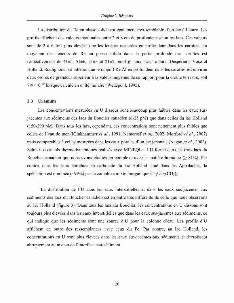
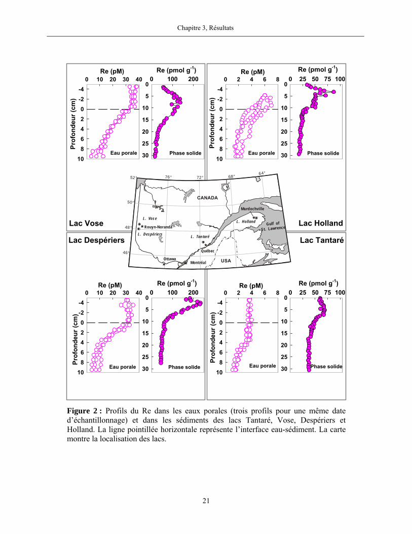
La distribution du Re en phase solide est également très semblable d’un lac à l’autre. Les
profils affichent des valeurs maximales entre 2 et 8 cm de profondeur selon les lacs. Ces valeurs
sont de 2 à 6 fois plus élevées que les teneurs mesurées en profondeur dans les carottes. La
moyenne des teneurs de Re en phase solide dans la partie profonde des carottes est
respectivement de 41±5, 51±6, 21±3 et 21±2 pmol g-1 aux lacs Tantaré, Despériers, Vose et
Holland. Soulignons par ailleurs que le rapport Re:Al en profondeur dans les carottes est environ
deux ordres de grandeur supérieur à la valeur moyenne de ce rapport pour la croûte terrestre, soit
7-9×10⁻¹⁰ lorsque calculé en unité molaire (Wedepohl, 1995).
3.3 Uranium
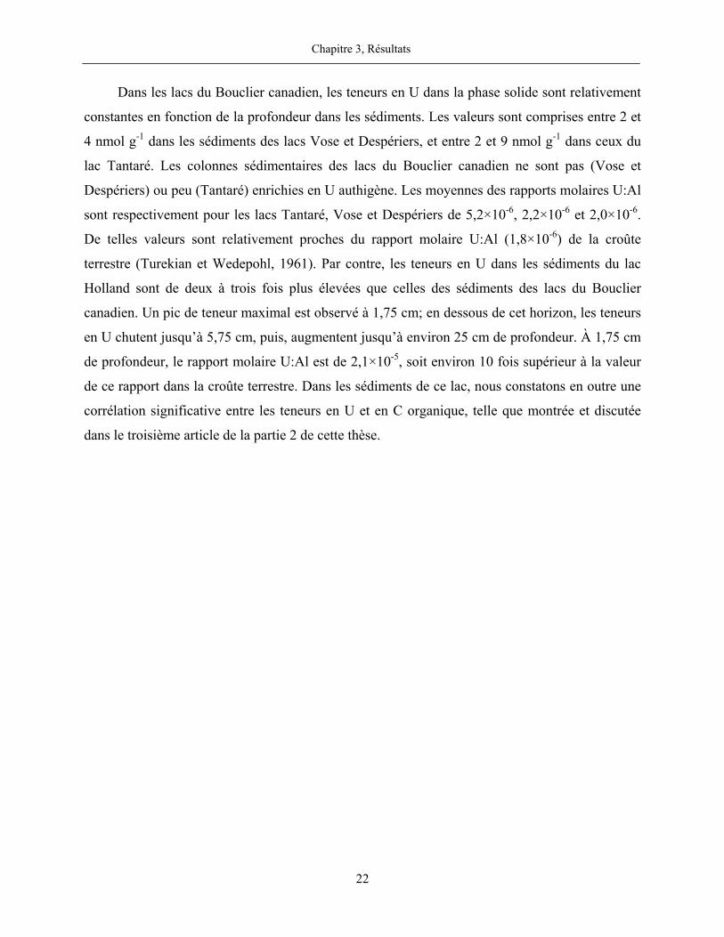
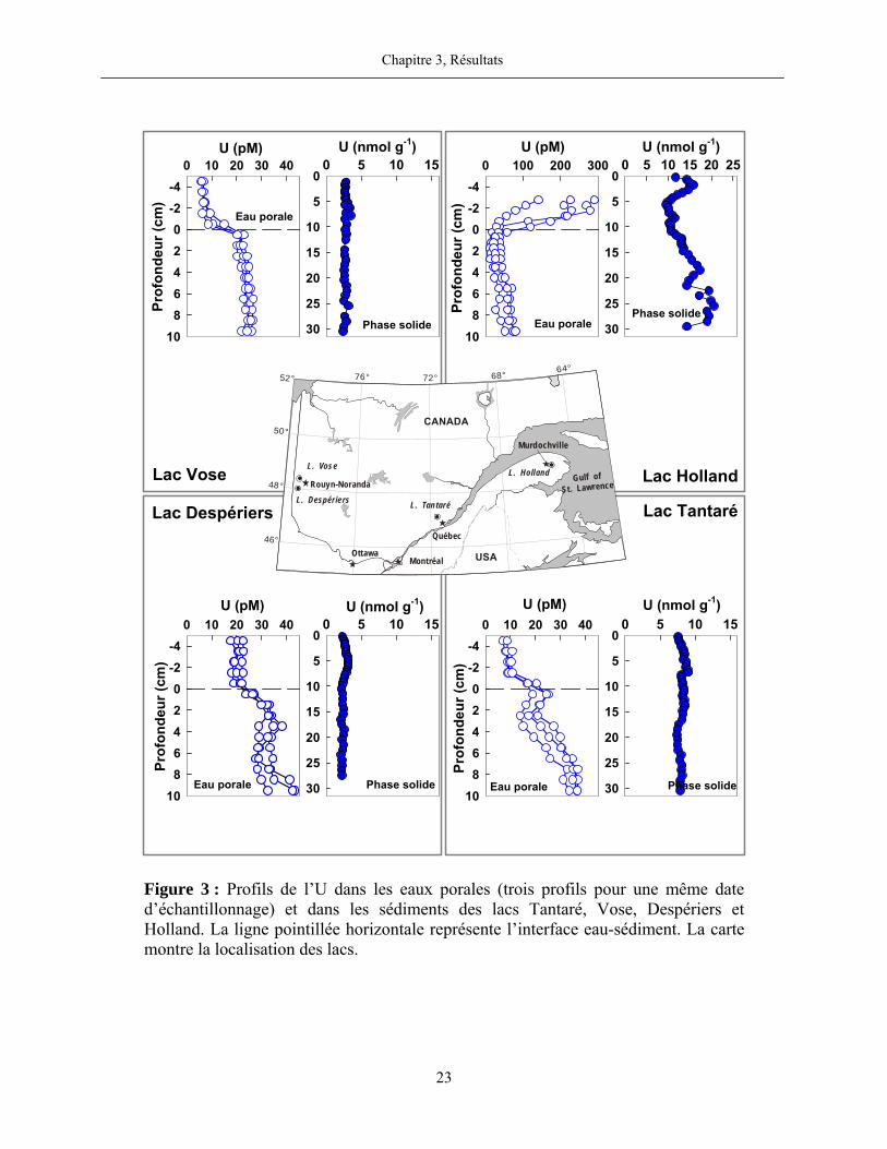
Les concentrations mesurées en U dissous sont beaucoup plus faibles dans les eaux sus-
jacentes aux sédiments des lacs du Bouclier canadien (6-25 pM) que dans celles du lac Holland
(150-290 pM). Dans tous les lacs, cependant, ces concentrations sont nettement plus faibles que
celles de l’eau de mer (Klinkhammer et al., 1991; Nameroff et al., 2002; Morford et al., 2007)
mais comparables à celles mesurées dans les eaux porales d’un lac japonais (Nagao et al., 2002).
Selon nos calculs thermodynamiques réalisés avec MINEQL+, l’U forme dans les trois lacs du
Bouclier canadien que nous avons étudiés un complexe avec la matière humique (≥ 81%). Par
contre, dans les eaux enrichies en carbonate du lac Holland situé dans les Appalaches, la
spéciation est dominée (~99%) par le complexe mixte inorganique Ca2UO2(CO3)30.
La distribution de l’U dans les eaux interstitielles et dans les eaux sus-jacentes aux
sédiments des lacs du Bouclier canadien est en outre très différente de celle que nous observons
au lac Holland (figure 3). Dans tous les lacs du Bouclier, les concentrations en U dissous sont
toujours plus élevées dans les eaux interstitielles que dans les eaux sus-jacentes aux sédiments, ce
qui indique que les sédiments sont une source d’U pour la colonne d’eau. Les profils d’U
affichent en outre des ressemblances avec ceux du Fe. Par contre, au lac Holland, les
concentrations en U sont plus élevées dans les eaux sus-jacentes aux sédiments et décroissent
abruptement au niveau de l’interface eau-sédiment.
Chapitre 3, Résultats
21
Prof
onde
ur (c
m)
0 2 4 6 8-4-202468
10
Lac Vose
0 10 20 30 40-4-202468
10
0 10 20 30 40-4-202468
10
0 2 4 6 8-4-202468
10
Lac Tantaré
0 25 50 75 1000
5
10
15
20
25
30
0 100 2000
5
10
15
20
25
30
0 100 2000
5
10
15
20
25
30
0 25 50 75 1000
5
10
15
20
25
30
Lac HollandPr
ofon
deur
(cm
)Pr
ofon
deur
(cm
)
Prof
onde
ur (c
m)
Lac Despériers
Eau porale Phase solide
Re (pM)
Re (pM)
Re (pM)
Re (pM)
Re (pmol g-1) Re (pmol g-1)
Re (pmol g-1) Re (pmol g-1)
Eau porale Phase solide
Eau porale Phase solide Eau porale Phase solide
USA
76° 72°64°
52°
50°
46°
48°
68°
Murdochville
Rouyn-Noranda
L. VoseL. Holland
L. TantaréL. Despériers
Québec
MontréalOttawa
CANADA
Gulf ofSt. Lawrence
Figure 2 : Profils du Re dans les eaux porales (trois profils pour une même date d’échantillonnage) et dans les sédiments des lacs Tantaré, Vose, Despériers et Holland. La ligne pointillée horizontale représente l’interface eau-sédiment. La carte montre la localisation des lacs.
Chapitre 3, Résultats
22
Dans les lacs du Bouclier canadien, les teneurs en U dans la phase solide sont relativement
constantes en fonction de la profondeur dans les sédiments. Les valeurs sont comprises entre 2 et
4 nmol g-1 dans les sédiments des lacs Vose et Despériers, et entre 2 et 9 nmol g-1 dans ceux du
lac Tantaré. Les colonnes sédimentaires des lacs du Bouclier canadien ne sont pas (Vose et
Despériers) ou peu (Tantaré) enrichies en U authigène. Les moyennes des rapports molaires U:Al
sont respectivement pour les lacs Tantaré, Vose et Despériers de 5,2×10⁻⁶, 2,2×10⁻⁶ et 2,0×10⁻⁶.
De telles valeurs sont relativement proches du rapport molaire U:Al (1,8×10⁻⁶) de la croûte
terrestre (Turekian et Wedepohl, 1961). Par contre, les teneurs en U dans les sédiments du lac
Holland sont de deux à trois fois plus élevées que celles des sédiments des lacs du Bouclier
canadien. Un pic de teneur maximal est observé à 1,75 cm; en dessous de cet horizon, les teneurs
en U chutent jusqu’à 5,75 cm, puis, augmentent jusqu’à environ 25 cm de profondeur. À 1,75 cm
de profondeur, le rapport molaire U:Al est de 2,1×10⁻⁵, soit environ 10 fois supérieur à la valeur
de ce rapport dans la croûte terrestre. Dans les sédiments de ce lac, nous constatons en outre une
corrélation significative entre les teneurs en U et en C organique, telle que montrée et discutée
dans le troisième article de la partie 2 de cette thèse.
Chapitre 3, Résultats
23
0 5 10 150
5
10
15
20
25
30
0 10 20 30 40-4-202468
10
Prof
onde
ur (c
m)
0 10 20 30 40-4-202468
10
0 10 20 30 40-4-202468
10
0 100 200 300-4-202468
10
Lac Vose
0 5 10 150
5
10
15
20
25
30
0 5 10 150
5
10
15
20
25
30
0 5 10 15 20 250
5
10
15
20
25
30
Lac HollandPr
ofon
deur
(cm
)Pr
ofon
deur
(cm
)
Lac Despériers
Prof
onde
ur (c
m)
Eau porale
Phase solide
U (pM) U (pM)
U (pM) U (pM) U (nmol g-1)U (nmol g-1)
U (nmol g-1) U (nmol g-1)
Eau porale Eau porale
Eau porale
Phase solide Phase solide
Phase solide
Lac Tantaré
USA
76° 72°64°
52°
50°
46°
48°
68°
Murdochville
Rouyn-Noranda
L. VoseL. Holland
L. TantaréL. Despériers
Québec
MontréalOttawa
CANADA
Gulf ofSt. Lawrence
Figure 3 : Profils de l’U dans les eaux porales (trois profils pour une même date d’échantillonnage) et dans les sédiments des lacs Tantaré, Vose, Despériers et Holland. La ligne pointillée horizontale représente l’interface eau-sédiment. La carte montre la localisation des lacs.

4. DISCUSSION
Le plan de cette discussion s’établit comme suit. J’estime d’abord les taux nets des
réactions de production et de consommation des éléments dans les eaux interstitielles et délimite
les couches de sédiments dans lesquelles ces réactions se produisent. Je quantifie ensuite les
fractions authigènes de Mo, de Re et d’U en fonction de la profondeur dans les sédiments, ce qui
m’amène à discuter l’influence de l’activité humaine sur les enregistrements sédimentaires.
J’enchaîne par une analyse du rôle des oxyhydroxydes de Fe et de la matière organique dans le
cycle diagenétique des éléments et discute les prédictions thermodynamiques vis-à-vis de la
précipitation de plusieurs phases minérales pures de Mo, de Re et d’U.
4.1 Taux nets des réactions ( MenetR )
Les profils, selon la profondeur, de Mo, de Re et d’U dans les eaux interstitielles dévoilent
dans plusieurs cas des variations de concentrations importantes. Ces variations témoignent de
l’existence de réactions qui ajoutent ces éléments aux eaux interstitielles ou qui les en soustraient.
Il est à noter que plusieurs réactions peuvent se produire simultanément, d’où l’expression "taux
net" des réactions ( MenetR ). Pour déterminer les taux nets des réactions d’un élément en fonction de
la profondeur dans les sédiments, les profils de cet élément dans les eaux interstitielles ont été
modélisés selon la méthode décrite précédemment (section 2.4) après avoir choisi un coefficient
de diffusion approprié en tenant compte de la spéciation de l’élément. Des exemples des résultats
de cet exercice de modélisation sont illustrés aux figures 4, 5 et 6. Dans tous les cas, les profils
modélisés pour le Mo, le Re et l’U sont bien corrélés avec les profils moyens mesurés pour une
même date d’échantillonnage (r2=0,81-0,99) et permettent de définir les zones de production et
de consommation des éléments en solution.
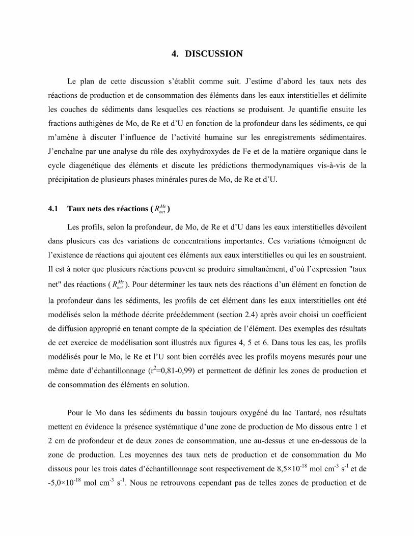
Pour le Mo dans les sédiments du bassin toujours oxygéné du lac Tantaré, nos résultats
mettent en évidence la présence systématique d’une zone de production de Mo dissous entre 1 et
2 cm de profondeur et de deux zones de consommation, une au-dessus et une en-dessous de la
zone de production. Les moyennes des taux nets de production et de consommation du Mo
dissous pour les trois dates d’échantillonnage sont respectivement de 8,5×10⁻¹⁸ mol cm-3 s-1 et de
-5,0×10⁻¹⁸ mol cm-3 s-1. Nous ne retrouvons cependant pas de telles zones de production et de
Chapitre 4, Discussion
26
consommation dans les sédiments des autres lacs, lesquels furent tous échantillonnés lorsque
l’hypolimnion était anoxique. Comme c’est le cas au lac Holland (figure 4), les profils du Mo
dans les eaux interstitielles des sédiments des lacs avec un hypolimnion anoxique montrent peu
de variations verticales importantes et n’ont, par conséquent, pas été modélisés. Nous
considérons donc que le Mo n’est pas ou peu impliqué dans des réactions au cours des stades
précoces de la diagenèse des sédiments lorsque l’hypolimnion des lacs est anoxique.
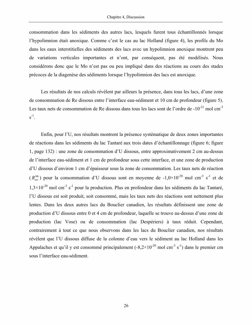
Les résultats de nos calculs révèlent par ailleurs la présence, dans tous les lacs, d’une zone
de consommation de Re dissous entre l’interface eau-sédiment et 10 cm de profondeur (figure 5).
Les taux nets de consommation de Re dissous dans tous les lacs sont de l’ordre de -10-21 mol cm-3
s-1.
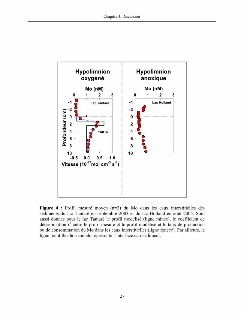
Enfin, pour l’U, nos résultats montrent la présence systématique de deux zones importantes
de réactions dans les sédiments du lac Tantaré aux trois dates d’échantillonnage (figure 6; figure
1, page 132) : une zone de consommation d’U dissous, entre approximativement 2 cm au-dessus
de l’interface eau-sédiment et 1 cm de profondeur sous cette interface, et une zone de production
d’U dissous d’environ 1 cm d’épaisseur sous la zone de consommation. Les taux nets de réaction
( MenetR ) pour la consommation d’U dissous sont en moyenne de -1,0×10⁻²⁰ mol cm-3 s-1 et de
1,3×10⁻²⁰ mol cm-3 s-1 pour la production. Plus en profondeur dans les sédiments du lac Tantaré,
l’U dissous est soit produit, soit consommé, mais les taux nets des réactions sont nettement plus
lentes. Dans les deux autres lacs du Bouclier canadien, les résultats définissent une zone de
production d’U dissous entre 0 et 4 cm de profondeur, laquelle se trouve au-dessus d’une zone de
production (lac Vose) ou de consommation (lac Despériers) à taux réduit. Cependant,
contrairement à tout ce que nous observons dans les lacs du Bouclier canadien, nos résultats
révèlent que l’U dissous diffuse de la colonne d’eau vers le sédiment au lac Holland dans les
Appalaches et qu’il y est consommé principalement (-8,2×10⁻²⁰ mol cm-3 s-1) dans le premier cm
sous l’interface eau-sédiment.
Chapitre 4, Discussion
27
Mo (nM)0 1 2 3
-4-202468
10
Vitesse (10-17mol cm-3 s-1)-0.5 0.0 0.5 1.0
Lac Tantaré
r2=0.97
0 1 2 3-4-202468
10
Lac Holland
Mo (nM)
Prof
onde
ur (c
m)
Hypolimnionoxygéné
Hypolimnionanoxique
Figure 4 : Profil mesuré moyen (n=3) du Mo dans les eaux interstitielles des sédiments du lac Tantaré en septembre 2003 et du lac Holland en août 2005. Sont aussi donnés pour le lac Tantaré le profil modélisé (ligne mince), le coefficient de détermination r2 entre le profil mesuré et le profil modélisé et le taux de production ou de consommation du Mo dans les eaux interstitielles (ligne foncée). Par ailleurs, la ligne pointillée horizontale représente l’interface eau-sédiment.
Chapitre 4, Discussion
28
Prof
onde
ur (c
m)
0 2 4 6-4-202468
10-3 -2 -1 0
r2=0.95
Re (pM)
Vitesse (10-21mol cm-3 s-1)
0 20 40-4-202468
10-3 -2 -1 0
r2=0.97
Lac Tantaré Lac Despériers
Re (pM)
Vitesse (10-21mol cm-3 s-1)
Hypolimnionoxygéné
Hypolimnionanoxique
Figure 5 : Profil mesuré moyen (n=3) du Re dans les eaux interstitielles des sédiments du lac Tantaré en juillet 2003 et du lac Despériers en juin 2001. Sont aussi donnés pour les deux lacs le profil modélisé (ligne mince), le coefficient de détermination r2 entre le profil mesuré et le profil modélisé et le taux de production ou de consommation du Re dans les eaux interstitielles (ligne foncée). Par ailleurs, la ligne pointillée horizontale représente l’interface eau-sédiment.
Chapitre 4, Discussion
29
0 10 20 30 40-4-202468
10-1 0 1
Lac Tantaré
r2=0.99
Vitesse (10-20mol cm-3 s-1)
0 10 20 30 40-4-202468
10-1 0 1
Lac Vose
r2=0.98
0 100 200 300-4-202468
10-10 -8 -6 -4 -2 0
Lac Holland
r2=0.93
Prof
onde
ur (c
m)
U (pM) U (pM) U (pM)
Vitesse (10-20mol cm-3 s-1) Vitesse (10-20mol cm-3 s-1)
Bouclier canadien Appalaches
Prof
onde
ur (c
m)
Hypolimnionoxygéné
Hypolimnionanoxique
Hypolimnionanoxique
Figure 6 : Profil mesuré moyen (n=3) de l’U dans les eaux interstitielles des sédiments du lac Tantaré en juillet 2003, du lac Vose en septembre 2003 et du lac Holland en août 2005. Sont aussi donnés pour les deux lacs le profil modélisé (ligne mince), le coefficient de détermination r2 entre le profil mesuré et le profil modélisé et le taux de production ou de consommation de l’U dans les eaux interstitielles (ligne foncée). Par ailleurs, la ligne pointillée horizontale représente l’interface eau-sédiment.
Chapitre 4, Discussion
30
L’exercice de modélisation auquel nous nous sommes livré démontre donc des différences
importantes entre le comportement du Mo, du Re et de l’U au cours de la diagenèse précoce et,
dans certains cas, entre le comportement d’un même élément selon les caractéristiques des lacs.
Les taux des réactions dans lesquelles le Mo est impliqué sont beaucoup plus rapides que celles
des réactions auxquelles participent le Re et l’U. Par ailleurs, le Mo a un comportement différent
selon que l’hypolimnion est oxygéné ou anoxique, ce qui n’est pas le cas pour le Re qui a un
comportement identique dans tous les lacs. Cet élément diffuse toujours de la colonne d’eau vers
les sédiments où il est fixé dans les 10 premiers cm sous l’interface eau-sédiment, et ce, quelque
soit l’état d’oxygénation de l’hypolimnion et même si nos calculs de spéciation suggèrent une
différence marquée au niveau de la spéciation du Re selon que l’hypolimnion est oxygéné ou
anoxique. Enfin, l’U est consommé dans les sédiments de surface du lac Tantaré, où
l’hypolimnion est oxygéné en permanence, et produit dans les sédiments de surface des autres
lacs du Bouclier, dont l’hypolimnion est saisonnièrement anoxique. Par contre, dans les eaux
alcalines enrichies en Ca, Mg et carbonate du lac Holland, où la spéciation est différente de celle
des eaux des lacs du Bouclier selon la thermodynamique, une zone de fixation d’U a clairement
pu être mise en évidence dans ce lac juste (0-1 cm) sous l’interface eau-sédiment.
4.2 Empreinte de la diagenèse sur les enregistrements sédimentaires
La connaissance des taux de production et de consommation des éléments dans les eaux
interstitielles permet de calculer pour chaque couche de sédiments, tel que décrit à la section 2.6,
les teneurs de l’élément ajouté à la phase solide ou soustrait de cette dernière, ce que nous
symbolisons par Meauthigène.
Chapitre 4, Discussion
31
0 10 20 30 400
5
10
15
20
25
30
Mo (nmol g-1)0 30 60 90 120
0
5
10
15
20
25
30 Lac Tantaré Lac Despériers
Prof
onde
ur (c
m)
1900Authigène
Mesuré
Mo (nmol g-1)
1900
Authigène
Mesuré
0 100 2000
5
10
15
20
25
30
0 20 40 600
5
10
15
20
25
30Lac Tantaré Lac Despériers
Re (pmol g-1) Re (pmol g-1)
1900
1900
Mesuré
Mesuré
Authigène Authigène
U (nmol g-1)0 5 10 15
0
5
10
15
20
25
30 L. Tantaré
Authigène
0 5 10 15 20 250
5
10
15
20
25
30 L. Holland
U (nmol g-1)
Authigène
1900
1900
(a) (b)
(c) (d)
(e) (f)
MesuréMesuré
Figure 7 : Profils des teneurs en Mo total mesuré et en Mo authigène modélisé dans les sédiments des lacs (a) Tantaré et (b) Despériers, du Re total mesuré et du Re authigène modélisé dans les sédiments des lacs (c) Tantaré et (d) Despériers et de l’U total mesuré et de l’U authigène modélisé dans les sédiments des lacs (e) Tantaré et (f) Holland.
Chapitre 4, Discussion
32
Les résultats démontrent que le Moauthigène représente entre 22 et 43% du Mo mesuré
Momesuré dans les sédiments de surface du Lac Tantaré (0 – 1,5 cm) mais moins de 14% en
dessous de cette couche de surface (figure 7a). Par contre, tel que discuté précédemment, nous
présumons que Moauthigène est négligeable dans les lacs saisonnièrement anoxiques. Cette
hypothèse est supportée par l’absence de gradient de concentration en Mo dans les eaux porales
lorsque l’hypolimnion est anoxique et par les résultats du lac Tantaré qui suggèrent que l’effet de
la diagenèse est faible sous 1,5 cm de profondeur, ce qui devrait aussi être le cas durant la période
intermittente entre deux évènements anoxiques.
Par ailleurs, les valeurs de Reauthigène représentent moins de 10% de celles de Remesuré
dans les deux premiers centimètres en dessous de l’interface eau-sédiment des lac Tantaré et
Holland (figure 7c). Plus en profondeur, cette proportion augmente progressivement pour
atteindre à 9,75 cm de profondeur 57% et 23% respectivement aux lacs Tantaré et Holland. Dans
les sédiments des lacs Despériers et Vose, le Reauthigène est inférieur à 15% des teneurs en
Remesuré à 2,25 cm, mais cette proportion augmente considérablement avec la profondeur,
excédant même les teneurs en Remesuré sous 7 cm de profondeur dans les sédiments du lac
Despériers (figure 7d). Tel que discuté ci-après, nous proposons que ce dépassement s’explique
par une augmentation progressive au cours du dernier siècle des concentrations en Re dissous
dans la colonne d’eau en raison de l’activité humaine.
Enfin, nos résultats montrent que l’Uauthigène représente moins de 3% de l’Umesuré dans
tous les lacs (figure 7).
Ainsi, nous pouvons conclure que l’importance de la fraction authigène est très variable
selon les éléments. Pour le Mo, elle est substantielle dans les sédiments de surface du bassin
toujours oxygéné du lac Tantaré mais vraisemblablement négligeable dans les autres lacs. Pour le
Re, elle est toujours importante et augmente progressivement entre l’interface eau-sédiment et 10
cm de profondeur. Pour l’U, par contre, nos résultats indiquent que cette fraction est pour ainsi
dire négligeable dans les sédiments de tous les lacs.
Chapitre 4, Discussion
33
4.3 Empreinte de l’activité humaine sur les enregistrements sédimentaires
4.3.1 Molybdène
Ayant quantifié les teneurs en Mo authigène dans les sédiments du lac Tantaré et démontré
que ces teneurs sont négligeables dans ceux des autres lacs, il est désormais possible, puisque les
taux d’accumulation et l’âge des sédiments sont connus, de déterminer les variations historiques
du taux de dépôt du Mo particulaire à l’interface eau-sédiment. Tel qu’expliqué ci-dessous, nous
pouvons en outre distinguer la fraction de ce flux attribuable à la déposition atmosphérique de
celle due à l’érosion du bassin versant.
Le flux de dépôt du Mo atmosphérique ( MoatmJ ) dans une couche de sédiment peut être
déterminé à l’aide de l’équation 9 si nous présumons que le comportement du Mo dans les
sédiments et après sa déposition à la surface terrestre est similaire à celui du 210Pb non supporté :
( )
210PbMo atmatm 210Pbmesuré authigène mesuré
sedcroûte
Mo= Mo - Mo - Al ω
AlIJI
⎡ ⎤⎛ ⎞×⎢ ⎥⎜ ⎟⎜ ⎟⎢ ⎥⎝ ⎠⎣ ⎦
(9)
Dans cette équation mesuréAl représente la teneur mesurée d’Al dans les sédiments,
(Mo/Al)croûte le rapport molaire de la teneur moyenne en Mo et en Al dans la croûte terrestre
(9×10⁻⁶; Turekian et Wedepohl, 1961), ω le taux d’accumulation des sédiments, 210PbIatm
l’inventaire théorique de 210Pb non supporté ( 210unPb ) dans les sédiments au site d’étude, lequel
est supposé identique à celui mesuré dans les sols du Bouclier canadien dans l’est de l’Ontario
(0,44 Bq cm-2; Cornett et al., 1984) et 210PbIsed l’inventaire de 210unPb mesuré dans les sédiments
au site d’étude. Le dernier terme de l’équation, soit 210PbIatm / 210PbIsed, permet de corriger pour les
biais dus aux mouvements latéraux des sédiments dans les lacs (focusing), aux apports associés à
l’érosion du bassin versant et aux pertes par les exutoires, et ainsi permettre une meilleure
comparaison entre les lacs.
Chapitre 4, Discussion
34
Les variations chronologiques de MoatmJ au lac Tantaré indiquent que le dépôt atmosphérique
de Mo a augmenté progressivement entre le début du 20ième siècle et les années 1970, puis, a
diminué pendant les deux décennies suivantes. Une seule valeur à la surface des sédiments du lac
Tantaré suggère que MoatmJ a recommencé à augmenter après 1995 (figure 8; figure 5, page 84). La
combustion du charbon étant une source connue d’émission de Mo dans l’atmosphère (Straughan
et al., 1978; Nriagu et Pacyna, 1998; Pacyna et Pacyna, 2001), nous attribuons l’augmentation de MoatmJ depuis le début du 20ième siècle jusque dans les années 1970 à cette source de contamination.
Le charbon était intensément utilisé au Québec pour le chauffage domestique et diverses activités
industrielles jusque dans les années 1950. Par ailleurs, la région du lac Tantaré est aussi affectée
par les retombées d’émissions dans l’atmosphère qui eurent lieu ailleurs, notamment dans les
régions industrialisées du sud de l’Ontario et du nord-ouest des États-Unis. Des mesures des
rapports des isotopes stables du Pb dans les sédiments du lac Tantaré ont révélé à cet effet
qu’environ la moitié du Pb d’origine anthropique accumulé dans les sédiments du lac entre 1965
et 1975 provenait des États-Unis (Gallon et al., 2005). La mise en place de mesures de réduction
des émissions et l’amélioration des technologies industrielles expliqueraient la diminution de MoatmJ entre les années 1970 et 1995. La hausse du flux de Mo déposé à la surface du sédiment
après 1995 pourrait de nouveau être due à la combustion du charbon pour la demande accrue
d’électricité en Ontario et aux États-Unis aux cours des dernières années (Freme, 2005; Energy
Statistics Handbooks, 2006).
Dans le lac de la région de Rouyn-Noranda (lac Despériers), MoatmJ a augmenté
continuellement depuis environ 1920, atteint un maximum au début des années 1980, puis, a
diminué d’environ 70%. Ces variations temporelles sont cohérentes avec l’histoire de la fonderie
Horne de Rouyn-Noranda mise en service en 1927. La productivité de cette fonderie a
continuellement augmenté au cours du 20ième siècle mais ses émissions polluantes ont commencé
à diminuer après le début des années 1980 en raison des efforts consentis par cette fonderie pour
se moderniser et réduire ses rejets de métaux dans l’atmosphère.
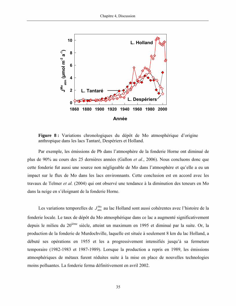
Chapitre 4, Discussion
35
1860 1880 1900 1920 1940 1960 1980 2000
JMo at
m (µ
mol
m-2
a-1
)
0
2
4
6
8
10
Année
L. Tantaré
L. Despériers
L. Holland
Figure 8 : Variations chronologiques du dépôt de Mo atmosphérique d’origine anthropique dans les lacs Tantaré, Despériers et Holland.
Par exemple, les émissions de Pb dans l’atmosphère de la fonderie Horne ont diminué de
plus de 90% au cours des 25 dernières années (Gallon et al., 2006). Nous concluons donc que
cette fonderie fut aussi une source non négligeable de Mo dans l’atmosphère et qu’elle a eu un
impact sur le flux de Mo dans les lacs environnants. Cette conclusion est en accord avec les
travaux de Telmer et al. (2004) qui ont observé une tendance à la diminution des teneurs en Mo
dans la neige en s’éloignant de la fonderie Horne.
Les variations temporelles de MoatmJ au lac Holland sont aussi cohérentes avec l’histoire de la
fonderie locale. Le taux de dépôt du Mo atmosphérique dans ce lac a augmenté significativement
depuis le milieu du 20ième siècle, atteint un maximum en 1995 et diminué par la suite. Or, la
production de la fonderie de Murdochville, laquelle est située à seulement 8 km du lac Holland, a
débuté ses opérations en 1955 et les a progressivement intensifiés jusqu’à sa fermeture
temporaire (1982-1983 et 1987-1989). Lorsque la production a repris en 1989, les émissions
atmosphériques de métaux furent réduites suite à la mise en place de nouvelles technologies
moins polluantes. La fonderie ferma définitivement en avril 2002.
Chapitre 4, Discussion
36
4.3.2 Rhénium
Les rapports molaires Re:Al dans les sédiments de tous les lacs sont, comme pour le Mo,
nettement supérieurs à la valeur de ce rapport molaire dans la croûte terrestre (7-9×10⁻¹⁰;
Wedepohl, 1995). Dans les couches profondes des carottes, lesquelles datent de l’ère pré-
industrielle, ce rapport est jusqu'à deux ordres de grandeur plus élevé que le rapport moyen de la
croûte terrestre (figure 2, page 107). Cette observation démontre que, comme observé dans
plusieurs sédiments marins, une très large proportion du Re dans les sédiments est authigène,
vraisemblablement à cause du transport du Re de la colonne d’eau vers le sédiment et à son
enlèvement subséquent des eaux interstitielles. Cependant, le fait que le rapport Re:Al soit de 2 à
7 fois plus élevé entre 2 et 8 cm de profondeur que dans les sédiments de l’époque pré-
industrielle, et ce dans tous les lacs, suggère fortement que l’activité humaine est aussi à l’origine
de contamination en Re dans les sédiments des lacs. Il est probable que le lac Tantaré fut
contaminé par des sources d’émissions non ponctuelles de Re dans l’atmosphère. Une de ces
sources pourraient être, comme pour le Mo la combustion du charbon (Colodner et al., 1995).
Quant à la contamination en Re des autres lacs, elles seraient dues aux émissions des fonderies
situées à proximité.
4.3.3 Uranium
Les rapports molaires U:Al dans les sédiments de tous les lacs du Bouclier canadien sont
peu variables et très similaires au rapport moyen molaire de cet élément dans la lithosphère
(2×10⁻⁶; McManus et al., 2005). Cette observation suggère une absence de contamination par l’U
dans ces lacs. Nous croyons que les valeurs plus élevées de ce rapport dans les sédiments du lac
Holland ne doivent pas non plus être interprétées comme un signal de contamination puisque les
teneurs en U dans les sédiments sont significativement corrélées à celles du C organique qui
varient de manière erratique en fonction de la profondeur. Cette observation suggère qu’une
fraction importante de l’U qui arrive dans ce lac est associé à la matière organique du bassin
versant et que les apports de cette matière n’ont pas été constants dans le temps.
4.4 Complexation de surface
Dans cette section, je discute des interactions possibles du Mo, du Re et de l’U avec les
oxyhydroxydes de Fe (et la matière organique associée à ces oxydes) dans les sédiments de
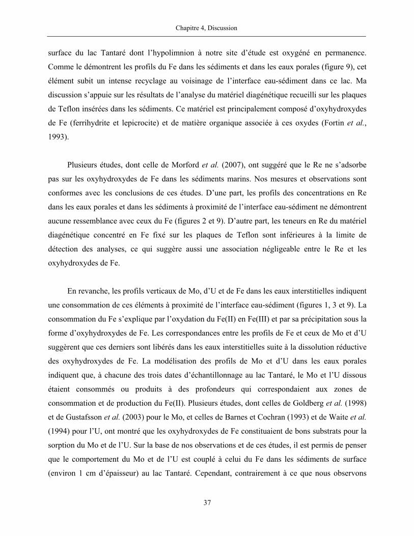
Chapitre 4, Discussion
37
surface du lac Tantaré dont l’hypolimnion à notre site d’étude est oxygéné en permanence.
Comme le démontrent les profils du Fe dans les sédiments et dans les eaux porales (figure 9), cet
élément subit un intense recyclage au voisinage de l’interface eau-sédiment dans ce lac. Ma
discussion s’appuie sur les résultats de l’analyse du matériel diagénétique recueilli sur les plaques
de Teflon insérées dans les sédiments. Ce matériel est principalement composé d’oxyhydroxydes
de Fe (ferrihydrite et lepicrocite) et de matière organique associée à ces oxydes (Fortin et al.,
1993).
Plusieurs études, dont celle de Morford et al. (2007), ont suggéré que le Re ne s’adsorbe
pas sur les oxyhydroxydes de Fe dans les sédiments marins. Nos mesures et observations sont
conformes avec les conclusions de ces études. D’une part, les profils des concentrations en Re
dans les eaux porales et dans les sédiments à proximité de l’interface eau-sédiment ne démontrent
aucune ressemblance avec ceux du Fe (figures 2 et 9). D’autre part, les teneurs en Re du matériel
diagénétique concentré en Fe fixé sur les plaques de Teflon sont inférieures à la limite de
détection des analyses, ce qui suggère aussi une association négligeable entre le Re et les
oxyhydroxydes de Fe.
En revanche, les profils verticaux de Mo, d’U et de Fe dans les eaux interstitielles indiquent
une consommation de ces éléments à proximité de l’interface eau-sédiment (figures 1, 3 et 9). La
consommation du Fe s’explique par l’oxydation du Fe(II) en Fe(III) et par sa précipitation sous la
forme d’oxyhydroxydes de Fe. Les correspondances entre les profils de Fe et ceux de Mo et d’U
suggèrent que ces derniers sont libérés dans les eaux interstitielles suite à la dissolution réductive
des oxyhydroxydes de Fe. La modélisation des profils de Mo et d’U dans les eaux porales
indiquent que, à chacune des trois dates d’échantillonnage au lac Tantaré, le Mo et l’U dissous
étaient consommés ou produits à des profondeurs qui correspondaient aux zones de
consommation et de production du Fe(II). Plusieurs études, dont celles de Goldberg et al. (1998)
et de Gustafsson et al. (2003) pour le Mo, et celles de Barnes et Cochran (1993) et de Waite et al.
(1994) pour l’U, ont montré que les oxyhydroxydes de Fe constituaient de bons substrats pour la
sorption du Mo et de l’U. Sur la base de nos observations et de ces études, il est permis de penser
que le comportement du Mo et de l’U est couplé à celui du Fe dans les sédiments de surface
(environ 1 cm d’épaisseur) au lac Tantaré. Cependant, contrairement à ce que nous observons
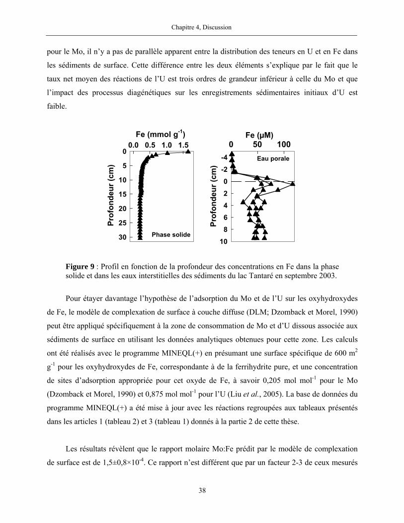
Chapitre 4, Discussion
38
pour le Mo, il n’y a pas de parallèle apparent entre la distribution des teneurs en U et en Fe dans
les sédiments de surface. Cette différence entre les deux éléments s’explique par le fait que le
taux net moyen des réactions de l’U est trois ordres de grandeur inférieur à celle du Mo et que
l’impact des processus diagénétiques sur les enregistrements sédimentaires initiaux d’U est
faible.
Pr
ofon
deur
(cm
)
Fe (mmol g-1)0.0 0.5 1.0 1.5
0
5
10
15
20
25
30
0 50 100-4-202468
10
Fe (µM)
Prof
onde
ur (c
m)
Phase solide
Eau porale
Figure 9 : Profil en fonction de la profondeur des concentrations en Fe dans la phase solide et dans les eaux interstitielles des sédiments du lac Tantaré en septembre 2003.
Pour étayer davantage l’hypothèse de l’adsorption du Mo et de l’U sur les oxyhydroxydes
de Fe, le modèle de complexation de surface à couche diffuse (DLM; Dzomback et Morel, 1990)
peut être appliqué spécifiquement à la zone de consommation de Mo et d’U dissous associée aux
sédiments de surface en utilisant les données analytiques obtenues pour cette zone. Les calculs
ont été réalisés avec le programme MINEQL(+) en présumant une surface spécifique de 600 m2
g-1 pour les oxyhydroxydes de Fe, correspondante à de la ferrihydrite pure, et une concentration
de sites d’adsorption appropriée pour cet oxyde de Fe, à savoir 0,205 mol mol-1 pour le Mo
(Dzomback et Morel, 1990) et 0,875 mol mol-1 pour l’U (Liu et al., 2005). La base de données du
programme MINEQL(+) a été mise à jour avec les réactions regroupées aux tableaux présentés
dans les articles 1 (tableau 2) et 3 (tableau 1) donnés à la partie 2 de cette thèse.
Les résultats révèlent que le rapport molaire Mo:Fe prédit par le modèle de complexation
de surface est de 1,5±0,8×10⁻⁴. Ce rapport n’est différent que par un facteur 2-3 de ceux mesurés
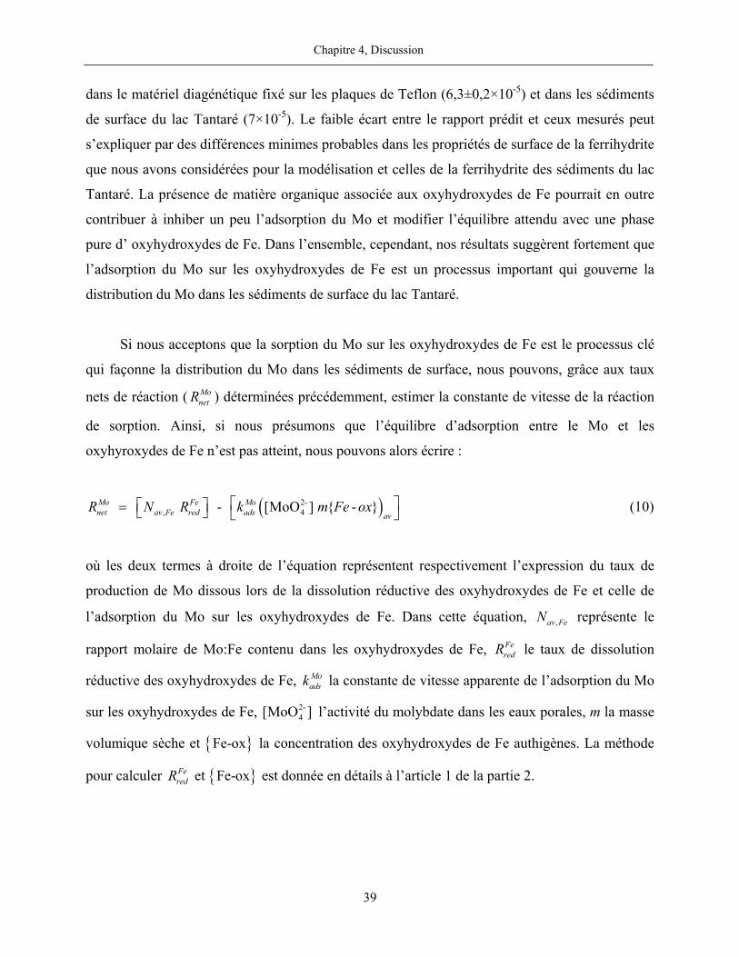
Chapitre 4, Discussion
39
dans le matériel diagénétique fixé sur les plaques de Teflon (6,3±0,2×10⁻⁵) et dans les sédiments
de surface du lac Tantaré (7×10⁻⁵). Le faible écart entre le rapport prédit et ceux mesurés peut
s’expliquer par des différences minimes probables dans les propriétés de surface de la ferrihydrite
que nous avons considérées pour la modélisation et celles de la ferrihydrite des sédiments du lac
Tantaré. La présence de matière organique associée aux oxyhydroxydes de Fe pourrait en outre
contribuer à inhiber un peu l’adsorption du Mo et modifier l’équilibre attendu avec une phase
pure d’ oxyhydroxydes de Fe. Dans l’ensemble, cependant, nos résultats suggèrent fortement que
l’adsorption du Mo sur les oxyhydroxydes de Fe est un processus important qui gouverne la
distribution du Mo dans les sédiments de surface du lac Tantaré.
Si nous acceptons que la sorption du Mo sur les oxyhydroxydes de Fe est le processus clé
qui façonne la distribution du Mo dans les sédiments de surface, nous pouvons, grâce aux taux
nets de réaction ( MonetR ) déterminées précédemment, estimer la constante de vitesse de la réaction
de sorption. Ainsi, si nous présumons que l’équilibre d’adsorption entre le Mo et les
oxyhyroxydes de Fe n’est pas atteint, nous pouvons alors écrire :
( )2-, 4 - [MoO ] - Mo Fe Mo
net av Fe red ads avR N R k m Fe ox⎡ ⎤⎡ ⎤= ⎣ ⎦ ⎣ ⎦ (10)
où les deux termes à droite de l’équation représentent respectivement l’expression du taux de
production de Mo dissous lors de la dissolution réductive des oxyhydroxydes de Fe et celle de
l’adsorption du Mo sur les oxyhydroxydes de Fe. Dans cette équation, ,av FeN représente le
rapport molaire de Mo:Fe contenu dans les oxyhydroxydes de Fe, FeredR le taux de dissolution
réductive des oxyhydroxydes de Fe, Moadsk la constante de vitesse apparente de l’adsorption du Mo
sur les oxyhydroxydes de Fe, 2-4[MoO ] l’activité du molybdate dans les eaux porales, m la masse
volumique sèche et Fe-ox la concentration des oxyhydroxydes de Fe authigènes. La méthode
pour calculer FeredR et Fe-ox est donnée en détails à l’article 1 de la partie 2.
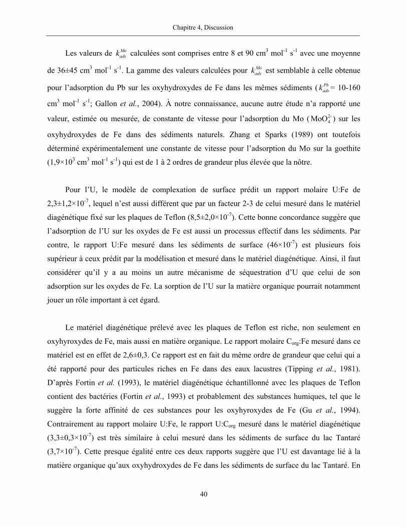
Chapitre 4, Discussion
40
Les valeurs de Moadsk calculées sont comprises entre 8 et 90 cm3 mol-1 s-1 avec une moyenne
de 36±45 cm3 mol-1 s-1. La gamme des valeurs calculées pour Moadsk est semblable à celle obtenue
pour l’adsorption du Pb sur les oxyhydroxydes de Fe dans les mêmes sédiments ( Pbadsk = 10-160
cm3 mol-1 s-1; Gallon et al., 2004). À notre connaissance, aucune autre étude n’a rapporté une
valeur, estimée ou mesurée, de constante de vitesse pour l’adsorption du Mo ( 2-4MoO ) sur les
oxyhydroxydes de Fe dans des sédiments naturels. Zhang et Sparks (1989) ont toutefois
déterminé expérimentalement une constante de vitesse pour l’adsorption du Mo sur la goethite
(1,9×103 cm3 mol-1 s-1) qui est de 1 à 2 ordres de grandeur plus élevée que la nôtre.
Pour l’U, le modèle de complexation de surface prédit un rapport molaire U:Fe de
2,3±1,2×10⁻⁷, lequel n’est aussi différent que par un facteur 2-3 de celui mesuré dans le matériel
diagénétique fixé sur les plaques de Teflon (8,5±2,0×10⁻⁷). Cette bonne concordance suggère que
l’adsorption de l’U sur les oxydes de Fe est aussi un processus effectif dans les sédiments. Par
contre, le rapport U:Fe mesuré dans les sédiments de surface (46×10-7) est plusieurs fois
supérieur à ceux prédit par la modélisation et mesuré dans le matériel diagénétique. Ainsi, il faut
considérer qu’il y a au moins un autre mécanisme de séquestration d’U que celui de son
adsorption sur les oxydes de Fe. La sorption de l’U sur la matière organique pourrait notamment
jouer un rôle important à cet égard.
Le matériel diagénétique prélevé avec les plaques de Teflon est riche, non seulement en
oxyhyroxydes de Fe, mais aussi en matière organique. Le rapport molaire Corg:Fe mesuré dans ce
matériel est en effet de 2,6±0,3. Ce rapport est en fait du même ordre de grandeur que celui qui a
été rapporté pour des particules riches en Fe dans des eaux lacustres (Tipping et al., 1981).
D’après Fortin et al. (1993), le matériel diagénétique échantillonné avec les plaques de Teflon
contient des bactéries (Fortin et al., 1993) et probablement des substances humiques, tel que le
suggère la forte affinité de ces substances pour les oxyhyroxydes de Fe (Gu et al., 1994).
Contrairement au rapport molaire U:Fe, le rapport U:Corg mesuré dans le matériel diagénétique
(3,3±0,3×10⁻⁷) est très similaire à celui mesuré dans les sédiments de surface du lac Tantaré
(3,7×10⁻⁷). Cette presque égalité entre ces deux rapports suggère que l’U est davantage lié à la
matière organique qu’aux oxyhydroxydes de Fe dans les sédiments de surface du lac Tantaré. En
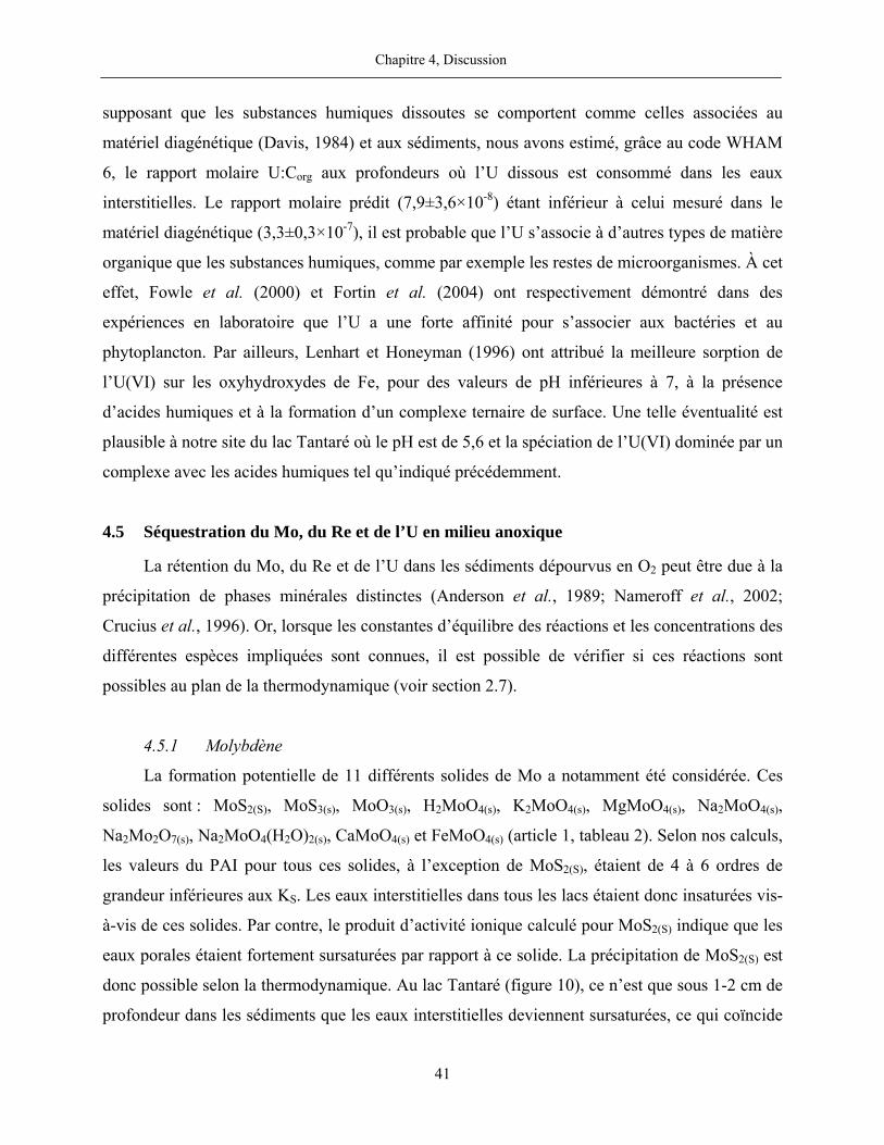
Chapitre 4, Discussion
41
supposant que les substances humiques dissoutes se comportent comme celles associées au
matériel diagénétique (Davis, 1984) et aux sédiments, nous avons estimé, grâce au code WHAM
6, le rapport molaire U:Corg aux profondeurs où l’U dissous est consommé dans les eaux
interstitielles. Le rapport molaire prédit (7,9±3,6×10⁻⁸) étant inférieur à celui mesuré dans le
matériel diagénétique (3,3±0,3×10⁻⁷), il est probable que l’U s’associe à d’autres types de matière
organique que les substances humiques, comme par exemple les restes de microorganismes. À cet
effet, Fowle et al. (2000) et Fortin et al. (2004) ont respectivement démontré dans des
expériences en laboratoire que l’U a une forte affinité pour s’associer aux bactéries et au
phytoplancton. Par ailleurs, Lenhart et Honeyman (1996) ont attribué la meilleure sorption de
l’U(VI) sur les oxyhydroxydes de Fe, pour des valeurs de pH inférieures à 7, à la présence
d’acides humiques et à la formation d’un complexe ternaire de surface. Une telle éventualité est
plausible à notre site du lac Tantaré où le pH est de 5,6 et la spéciation de l’U(VI) dominée par un
complexe avec les acides humiques tel qu’indiqué précédemment.
4.5 Séquestration du Mo, du Re et de l’U en milieu anoxique
La rétention du Mo, du Re et de l’U dans les sédiments dépourvus en O2 peut être due à la
précipitation de phases minérales distinctes (Anderson et al., 1989; Nameroff et al., 2002;
Crucius et al., 1996). Or, lorsque les constantes d’équilibre des réactions et les concentrations des
différentes espèces impliquées sont connues, il est possible de vérifier si ces réactions sont
possibles au plan de la thermodynamique (voir section 2.7).
4.5.1 Molybdène
La formation potentielle de 11 différents solides de Mo a notamment été considérée. Ces
solides sont : MoS2(S), MoS3(s), MoO3(s), H2MoO4(s), K2MoO4(s), MgMoO4(s), Na2MoO4(s),
Na2Mo2O7(s), Na2MoO4(H2O)2(s), CaMoO4(s) et FeMoO4(s) (article 1, tableau 2). Selon nos calculs,
les valeurs du PAI pour tous ces solides, à l’exception de MoS2(S), étaient de 4 à 6 ordres de
grandeur inférieures aux KS. Les eaux interstitielles dans tous les lacs étaient donc insaturées vis-
à-vis de ces solides. Par contre, le produit d’activité ionique calculé pour MoS2(S) indique que les
eaux porales étaient fortement sursaturées par rapport à ce solide. La précipitation de MoS2(S) est
donc possible selon la thermodynamique. Au lac Tantaré (figure 10), ce n’est que sous 1-2 cm de
profondeur dans les sédiments que les eaux interstitielles deviennent sursaturées, ce qui coïncide
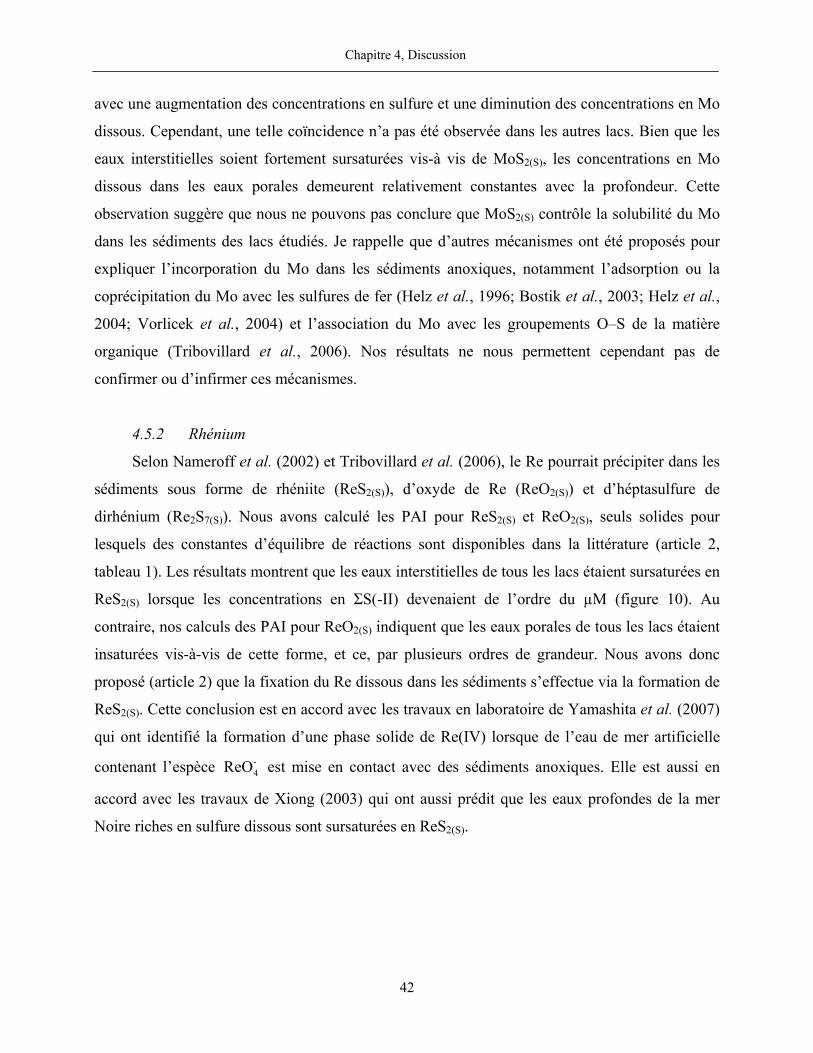
Chapitre 4, Discussion
42
avec une augmentation des concentrations en sulfure et une diminution des concentrations en Mo
dissous. Cependant, une telle coïncidence n’a pas été observée dans les autres lacs. Bien que les
eaux interstitielles soient fortement sursaturées vis-à vis de MoS2(S), les concentrations en Mo
dissous dans les eaux porales demeurent relativement constantes avec la profondeur. Cette
observation suggère que nous ne pouvons pas conclure que MoS2(S) contrôle la solubilité du Mo
dans les sédiments des lacs étudiés. Je rappelle que d’autres mécanismes ont été proposés pour
expliquer l’incorporation du Mo dans les sédiments anoxiques, notamment l’adsorption ou la
coprécipitation du Mo avec les sulfures de fer (Helz et al., 1996; Bostik et al., 2003; Helz et al.,
2004; Vorlicek et al., 2004) et l’association du Mo avec les groupements O–S de la matière
organique (Tribovillard et al., 2006). Nos résultats ne nous permettent cependant pas de
confirmer ou d’infirmer ces mécanismes.
4.5.2 Rhénium
Selon Nameroff et al. (2002) et Tribovillard et al. (2006), le Re pourrait précipiter dans les
sédiments sous forme de rhéniite (ReS2(S)), d’oxyde de Re (ReO2(S)) et d’héptasulfure de
dirhénium (Re2S7(S)). Nous avons calculé les PAI pour ReS2(S) et ReO2(S), seuls solides pour
lesquels des constantes d’équilibre de réactions sont disponibles dans la littérature (article 2,
tableau 1). Les résultats montrent que les eaux interstitielles de tous les lacs étaient sursaturées en
ReS2(S) lorsque les concentrations en ΣS(-II) devenaient de l’ordre du µM (figure 10). Au
contraire, nos calculs des PAI pour ReO2(S) indiquent que les eaux porales de tous les lacs étaient
insaturées vis-à-vis de cette forme, et ce, par plusieurs ordres de grandeur. Nous avons donc
proposé (article 2) que la fixation du Re dissous dans les sédiments s’effectue via la formation de
ReS2(S). Cette conclusion est en accord avec les travaux en laboratoire de Yamashita et al. (2007)
qui ont identifié la formation d’une phase solide de Re(IV) lorsque de l’eau de mer artificielle
contenant l’espèce -4ReO est mise en contact avec des sédiments anoxiques. Elle est aussi en
accord avec les travaux de Xiong (2003) qui ont aussi prédit que les eaux profondes de la mer
Noire riches en sulfure dissous sont sursaturées en ReS2(S).
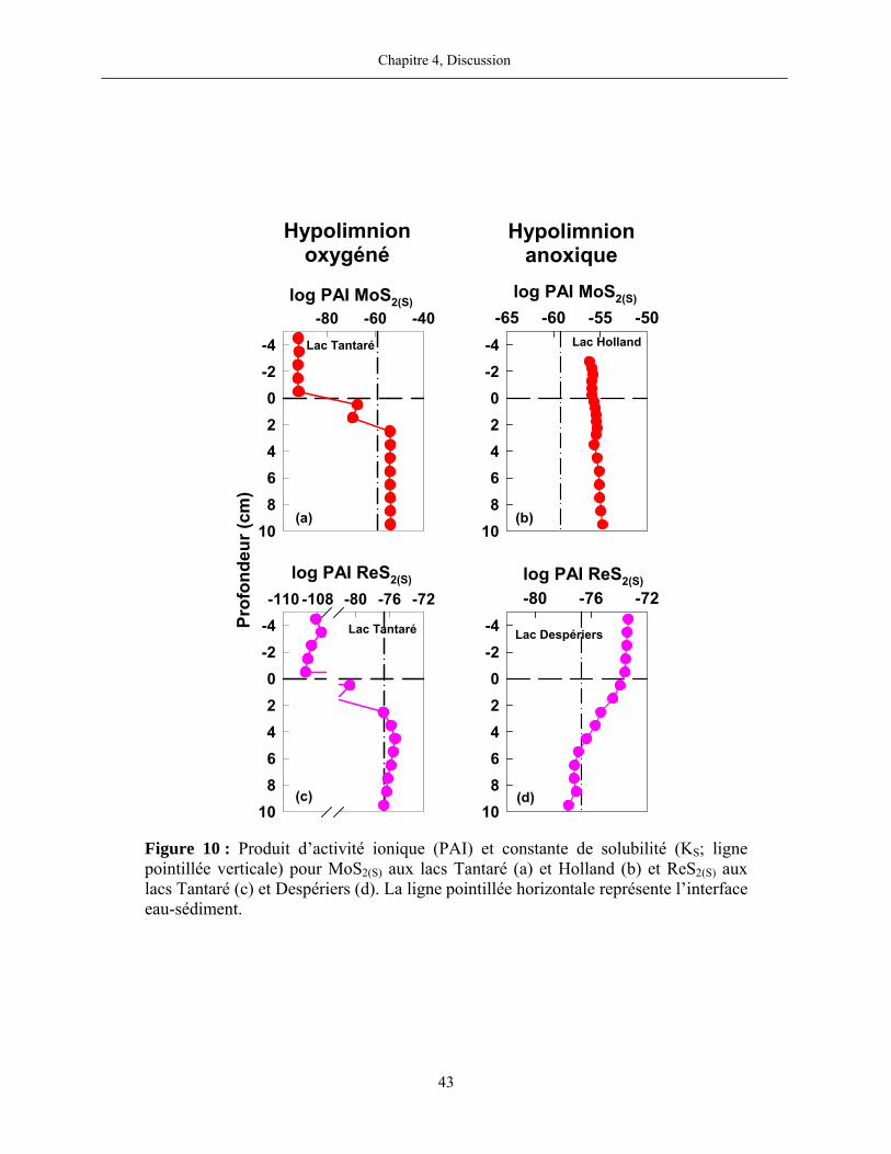
Chapitre 4, Discussion
43
-65 -60 -55 -50-4-202468
10
-80 -60 -40-4-202468
10
Lac Tantaré
Prof
onde
ur (c
m)
Hypolimnionoxygéné
Hypolimnionanoxique
log PAI MoS2(S)log PAI MoS2(S)
Lac Holland
-80 -76 -72-4-202468
10
-110 -108 -80 -76 -72-4-202468
10
Lac Tantaré
log PAI ReS2(S) log PAI ReS2(S)
Lac Despériers
(c) (d)
(a) (b)
Figure 10 : Produit d’activité ionique (PAI) et constante de solubilité (KS; ligne pointillée verticale) pour MoS2(S) aux lacs Tantaré (a) et Holland (b) et ReS2(S) aux lacs Tantaré (c) et Despériers (d). La ligne pointillée horizontale représente l’interface eau-sédiment.
Chapitre 4, Discussion
44
Si nous acceptons que la précipitation de ReS2(S) est le principal mécanisme de fixation
effectif du Re authigène dans les sédiments anoxiques, la constante de vitesse apparente de la
réaction de formation, soit Repptk , peut être estimée à partir des valeurs de Re
netR . Dans les zones ou
le Re dissous est consommé dans les eaux interstitielles et où ces dernières sont saturées en
ReS2(S), nous pouvons écrire (Meysman et al., 2003) :
- -1 Re Re Reavppt ppt net
PAIR k RKs
φ ⎛ ⎞= =⎜ ⎟⎝ ⎠
(11)
où RepptR représente le taux d’enlèvement par précipitation du Re dans l’eau interstitielle. Les
valeurs de RenetR , de PAI et de KS étant connues, Re
pptk peut alors être déterminé. Nos résultats
montrent que Re pptk varie de 0,03×10⁻²¹ à 1,3×10⁻²¹ mol cm-3 s-1. Plusieurs facteurs peuvent
expliquer cette grande variabilité. Le terme Repptk englobe des caractéristiques propres à chaque
surface réactive. Par exemple, les réactions de catalyse à la surface des solides et l’inhibition de
ces réactions par divers composés dissous peuvent modifier Repptk (Van Cappellen et al., 1993;
Meysman et al., 2003). De plus, la réduction de -4ReO en 0
4Re(OH) , laquelle doit être préalable à
la précipitation de ReS2(S), pourrait être l’étape qui limite ultimement la réaction.
4.5.3 Uranium
La réduction et la précipitation de trois phases distinctes d’U, soit UO2(S), U3O7(S) et U3O8(S)
ont été proposées pour expliquer la fixation de l’U dans les sédiments dépourvus en O2
(Klinkhammer et Palmer 1991; Morford et al., 2001; McManus et al., 2005). Nous avons donc
vérifié l’état de saturation des eaux porales vis-à-vis de ces trois phases et aussi vis-à-vis de
US(S), US2(S) et US3(S). Je souligne que les PAI ont été déterminés après l’estimation, avec le
programme WHAM 6, des constantes conditionnelles relatives à la complexation de l’U(VI) avec
les acides humiques ( condU AHK − ) et fulviques ( cond
U AFK − ) suivant les conditions prévalentes à chaque
profondeur, et a posteriori incorporées dans MINEQL+ à force ionique réelle. Les expressions
des constantes conditionnelles sont les suivantes :
Chapitre 4, Discussion
45
22+2
[UO -AH]K[UO ][AH]
condU AH
F− = (12)
et
22+2
[UO -AF]K[UO ][AF]
condU AF
F− = (13)
où [UO2-AH] et [UO2-AF] représentent respectivement les concentrations des complexes 2+2UO -
acides humiques ou 2+2UO -acides fulviques (mol L-1), [ 2+
2UO ] l’activité de l’ion libre 2+2UO (mol
L-1) et [AH]F et [AF]F les concentrations libres en acides humiques ou fulviques (g L-1). Si nous
présumons que les acides humiques et fulviques qui sont complexés avec 2+2UO représentent une
fraction négligeable des concentrations totales de ces substances, nous pouvons alors supposer
que [AH]F et [AF]F sont respectivement égales à [AH] et [AF].
Nos calculs de PAI révèlent que les eaux interstitielles sont largement insaturées (4 – 58
ordres de grandeur) vis-à-vis des solides U3O8(S), US(S), US2(S) et US3(S). Par contre, elles sont
sursaturées dans tous les lacs vis-à-vis de UO2(S) et de U3O7(S) (figure 11). Cependant, bien que
thermodynamiquement possible, l’ensemble de nos résultats ne nous permet pas de conclure que
la précipitation de ces solides est effective. D’une part, en dépit d’une consommation évidente
d’U dissous au voisinage de l’interface eau-sédiment au lac Holland, nous ne constatons pas une
diminution marquée de la sursaturation de UO2(S), de quatre ordres de grandeur supérieur, à la
même profondeur. D’autre part, bien qu’une diminution assez prononcée de la sursaturation vis-
à-vis de U3O7(S) soit observée simultanément à la consommation en U dissous au niveau de
l’interface eau-sédiment du lac Holland, il n’y a pas de consommation importante d’U dissous
dans les sédiments des autres lacs malgré une sursaturation encore plus importante vis-à-vis de
U3O7(S). Les autres mécanismes pouvant expliquer la forte consommation en U dissous au lac
Holland sont (i) l’association de l’U avec la matière organique, que nous avons proposée pour les
sédiments sub-oxiques et supportée par la corrélation observée entre les teneurs en U et en Corg
dans les sédiments (figure 3, page 134) et (ii) l’adsorption de l’U(VI) sur des minerais sulfurés
(Wersin et al., 1994; Moyes et al., 2000; Scott et al., 2007).
Chapitre 4, Discussion
46
Le calcul des indices de saturation des eaux interstitielles vis-à-vis de phases solides
spécifiques nous a donc permis de proposer la réaction impliquée dans l’incorporation du Re
authigène dans les sédiments, à savoir la réduction de Re(VII) en Re(IV) suivie de sa
précipitation sous la forme de ReS2(S). Nous avons en outre pu estimer la constante de vitesse
apparente de cette réaction ( Re pptk = 0,03×10⁻²¹ – 1,3×10⁻²¹ mol cm-3 s-1). Enfin, nous avons pu
conclure à l’infaisabilité dans les conditions de nos lacs de plusieurs réactions de précipitation de
solides purs de Mo, de Re et d’U qui avaient été évoquées dans la littérature (Anderson et al.,
1989; McManus et al., 2005; Morford et al., 2005, 2007).
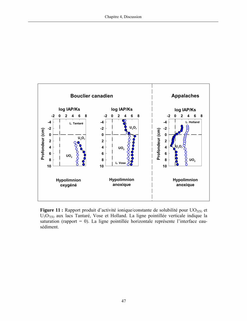
Chapitre 4, Discussion
47
-2 0 2 4 6 8-4-202468
10
-2 0 2 4 6 8-4-202468
10
-2 0 2 4 6 8-4-202468
10
Prof
onde
ur (c
m)
Bouclier canadien Appalaches
Prof
onde
ur (c
m)
L. Tantaré
L. Vose
L. Holland
Hypolimnionoxygéné
Hypolimnionanoxique
Hypolimnionanoxique
UO2
U3O7
log IAP/Ks log IAP/Ks
UO2
U3O7
log IAP/Ks
UO2
U3O7
Figure 11 : Rapport produit d’activité ionique/constante de solubilité pour UO2(S) et U3O7(S) aux lacs Tantaré, Vose et Holland. La ligne pointillée verticale indique la saturation (rapport = 0). La ligne pointillée horizontale représente l’interface eau-sédiment.

5. CONCLUSION
Nous avons démontré que les teneurs en Mo et Re dans les sédiments de tous les lacs sont
élevées comparativement aux teneurs moyennes de ces éléments dans la lithosphère. Les rapports
Mo:Al et Re:Al dans les sédiments sont respectivement jusqu’à 16 et 285 fois supérieures aux
valeurs de ces rapports dans la croûte terrestre. Pour l’U, un tel enrichissement dans les sédiments
par rapport à la composition moyenne de la lithosphère n’a pas été constaté dans les lacs du
Bouclier canadien. Il n’apparaît que dans les sédiments du lac Holland.
La modélisation du transport-réactif du Mo dans les eaux porales nous a conduit à la
conclusion que le Mo authigène représente environ un tiers du Mo total mesuré dans les
sédiments de surface du lac Tantaré mais est toujours beaucoup moins important, voire
négligeable, dans ceux des autres lacs. Par contre, en raison de la fixation dans les sédiments du
Re dissous qui diffuse à travers l’interface eau-sédiment, les teneurs en Re authigène dans les
sédiments sont considérables à tous les sites d’études, représentant dans certains cas jusqu’à 50%
et plus du Re total des sédiments. Cette observation suggère qu’en milieu lacustre, comme en
milieu marin, le Re pourrait constituer un bon traceur des variations au cours du temps de l’état
d’oxydoréduction et, indirectement, des facteurs qui déterminent cet état. Par contre, les teneurs
en U authigène déterminées par modélisation diagénétique représentent toujours moins de 3% de
l’U total mesuré dans les sédiments.
Les enrichissements en Mo et Re ne peuvent s’expliquer entièrement par la formation de
phases authigènes dans lesquelles ces éléments sont concentrés. Nous avons démontré qu’ils
doivent être attribués dans une large mesure à une augmentation, liée à l’activité humaine, des
retombées atmosphériques de ces éléments au cours du 20ième siècle. Les sources de
contamination les plus plausibles apparaissent être la combustion du charbon et les émissions
dans l’atmosphère de fonderies situées à l’intérieur des frontières du Québec. Une part de la
contamination pourrait aussi être issue de sources éloignées, comme par exemple les centrales de
production d’électricité fonctionnant au charbon en Ontario et dans le nord des États-Unis. Nous
ne croyons pas cependant que l’activité anthropique explique l’enrichissement en U dans les
sédiments du lac Holland. La corrélation significative entre l’U et le Corg en phase solide dans les
Chapitre 5, Conclusion
50
sédiments de ce lac des Appalaches suggère plutôt qu’une grande proportion de l’U contenu dans
les sédiments est déposée avec la matière organique issue du bassin versant. Cette association de
l’U avec la matière organique est aussi appuyée par la similitude des rapports molaires U:Corg
dans le matériel diagénétique prélevé avec les plaques de Teflon et dans les sédiments de surface
du lac Tantaré.
Les résultats de cette recherche font aussi ressortir que l’adsorption du Mo sur les
oxyhydroxydes de Fe est un processus qui peut influencer fortement la distribution du Mo dans
les sédiments où ces oxydes sont présents. Nous avons estimé que la constante de vitesse
apparente de l’adsorption du Mo sur les oxyhydroxydes de Fe est de 36±45 cm3 mol-1 s-1. Bien
que les réactions diagénétiques impliquant l’U soient quantitativement peu importantes, des
similitudes évidentes entre les profils d’U et de Fe dans les eaux interstitielles suggèrent que l’U
est aussi impliqué dans le cycle des oxyhydroxydes de Fe.
Enfin, nous avons démontré que les eaux interstitielles des sédiments de tous les lacs que
nous avons étudiés étaient sursaturées en ReS2(S) lorsque les concentrations en ΣS(-II)
surpassaient le niveau micro-molaire. Nous avons en outre proposé que la fixation du Re
authigène dans les sédiments s’effectue via la précipitation de cette forme minérale spécifique.
Une constante de vitesse de formation de l’ordre de 0,5±0,6×10⁻²¹ mol cm-3 s-1 a même pu être
estimée. Nos résultats nous ont finalement permis de conclure que, contrairement à ce qui est
suggéré dans la littérature, la précipitation dans les sédiments de solides tels que MoS2(S), ReO2(S),
UO2(S), U3O7(S) et U3O8(S) est improbable.
PARTIE 2
ARTICLES

ARTICLE 1
Geochemical and anthropogenic enrichments of Mo in sediments from
perennially oxic and seasonally anoxic lakes in Eastern Canada
Publié en 2008 dans Geochimica et Cosmochimica Acta 72 :170-174.
Anthony Chappaz, Charles Gobeil et André Tessier
Institut national de la recherche scientifique, Centre eau, terre et environnement, Université du
Québec, 490 de la Couronne, Québec (QC), G1K 9A9, Canada
Article 1, Géochimie et enrichissements anthropiques de Mo…
54
RÉSUMÉ
Les distributions verticales de Mo, de Fe, de Mn, de sulfure, de sulfate, de carbone
organique, des ions majeurs et du pH dans l’eau interstitielle, ainsi que celles de Mo, de S réduit
volatilisé par acidification, de Fe, de Mn, d’Al, de carbone organique, de 210Pb et de 137 Cs dans
des carottes de sédiment prélevées aux mêmes sites, ont été mesurées dans des bassins lacustres
situés dans l’est du Canada, un dont l’hypolimnion est continuellement oxygéné et trois dont les
hypolimnions sont saisonnièrement anoxiques. Le seul apport de Mo anthropique dans ces lacs
provient de la déposition atmosphérique.
Le Mo n’est pas redistribué dans les sédiments des trois bassins saisonnièrement anoxiques
comme suggéré par la distribution monotone du Mo dans les eaux porales. Au contraire, les
profils du Mo dans l’eau interstitielle des sédiments du bassin oxygéné montrent des pics
prononcés de Mo sous l’interface eau-sédiment, ce qui indique une redistribution du Mo suite à
sa déposition. La modélisation des profils du Mo dans l’eau porale avec une équation de
conservation de masse à une dimension révèle que le Mo est libéré entre 1 et 2 cm
conséquemment à la dissolution réductive des oxyhydroxydes de Fe. Par contre, il est fixé à
proximité de l’interface eau-sédiment, par adsorption sur les oxyhydroxydes de Fe authigènes, et
plus en profondeur lorsque les concentrations de sulfure sont plus élevées. Le taux net de réaction
estimé pour l’adsorption du Mo sur oxyhydroxydes de Fe est 36±45 cm3 mol-1 s-1.
Nos calculs indiquent que le Mo authigène dans les sédiments du bassin oxygéné représente
approximativement un tiers du Mo total de la phase solide dans le premier cm sous l’interface
eau-sédiment et seulement un dixième du Mo total en dessous de cet horizon. En présumant que
le Mo authigène n’est pas accumulé dans les sédiments des lacs saisonnièrement anoxiques, nous
concluons que les teneurs de Mo, qui sont de 3 à 16 fois plus élevées que l’abondance du Mo
dans la crôute terrestre, sont principalement dues à la déposition atmosphérique de Mo, et non à
la formation de Mo authigène. La reconstruction historique de la déposition atmosphérique de
Mo indique des valeurs maximales dans les années 1970 et 1980. Les émissions dans
l’atmosphère associées aux rejets des fonderies de minerais non-ferreux et de la combustion de
charbon apparaissent être des sources importantes de Mo.
Article 1, Géochimie et enrichissements anthropiques de Mo…
55
ABSTRACT
We measured the vertical distributions of Mo, Fe, Mn, sulfide, sulfate, organic carbon,
major ions, and pH in sediment porewater from one perennially oxic and three seasonally anoxic
lacustrine basins in Eastern Canada, as well as those of Mo, acid volatile sulfide, Fe, Mn, Al,
organic C, 210Pb and 137Cs in sediment cores from the same sites. The only input of anthropogenic
Mo to these lakes comes from atmospheric deposition.
The relatively monotonous distribution of Mo in the porewater of three seasonally anoxic
basins suggests that Mo is not redistributed in the sedimentary column during periods of anoxia.
In contrast, porewater Mo profiles obtained at three sampling dates in a perennially oxic basin
display sharp Mo peaks below the sediment water interface, indicating redistribution subsequent
to deposition. Modeling of these latter porewater Mo profiles with a diagenetic reaction-transport
equation coupled to comparisons among the various porewater and solid phase profiles reveal
that Mo is released at 1-2 cm depth as a consequence of the reductive dissolution of Fe
oxyhydroxides and scavenged both at the vicinity of the sediment-water interface, by re-
adsorption onto authigenic Fe oxyhydroxides, and deeper in the sediments where dissolved
sulfide concentrations are higher. The estimated rate constant for the adsorption of Mo onto Fe
oxyhydroxides is 36±45 cm3 mol-1 s-1.
Diagenetic modeling indicates that authigenic Mo in sediments of the perennially oxic
basin represents about one-third of the total solid phase Mo in the first cm below the sediment-
water interface and only one tenth below this horizon. If we assume that no authigenic Mo is
accumulated in the seasonally anoxic lake sediments we conclude that the sediment Mo
concentrations, which are up to 3-16 times higher than the average lithogenic composition,
depending on the lake, are mainly due to atmospheric deposition of anthropogenic Mo and not to
the formation of authigenic Mo phases. Reconstructed historical records of the atmospheric Mo
deposition indicate maximum values in the 1970s and 1980s and significant decreases since then.
Emissions to the atmosphere associated with the smelting of non-ferrous ores and coal
combustion appear to be the most important sources of anthropogenic Mo.
Article 1, Géochimie et enrichissements anthropiques de Mo…
56
1. INTRODUCTION
Sediments from marine and lacustrine environments are typically enriched in Mo
compared to the average crustal rock (e.g. Crusius et al., 1996; Schaller et al., 1997; Lyons et al.,
2003; McManus et al., 2006). These enrichments have generally been attributed to Mo adsorption
on manganese oxyhydroxides under oxic conditions and to Mo scavenging by sulfide minerals or
sulfidized organic matter under sub-oxic and anoxic conditions (e.g. Bertine, 1972; Zheng et al.,
2000; Tribovillard et al., 2004; Vorlicek et al., 2004). The low solubility of Mo in sulfide-
containing natural waters should allow reconstruction, from the vertical profiles of sedimentary
Mo, of the history of sulfide production and, indirectly, of the rate of organic matter
mineralization by sulfate in the aquatic environment (e.g. Schaller et al., 1997; Zheng et al.,
2000; Adelson et al., 2001; Meyers et al., 2005; Algeo et al., 2006; Tribovillard et al., 2006).
The potential of Mo as a paleoredox tracer cannot, however, be fully exploited,
particularly in coastal areas, due to our limited knowledge of the impact of human activities on
the sedimentary record of Mo. Recent study of a core from an ombrotrophic peat bog located in
the Jura Mountains, Switzerland, demonstrated that a 50-fold increase in the atmospheric
deposition of Mo occurred over the last century due to human activities (Krachler and Shotyk,
2004). To the best of our knowledge, the contribution of atmospheric deposition to the
accumulation of Mo in aquatic sediments has yet to be documented. In addition, fixation
mechanisms of Mo under various redox conditions are not well understood.
We carried out detailed analyses of sediment cores and sediment porewater from four
lakes characterized by different geochemical conditions. Our objectives were to quantify
anthropogenic contributions to sedimentary Mo enrichment at the study sites and to clarify
reactions involving Mo during the early stages of sediment diagenesis.
2. METHODS
2.1. Sampling
Four lakes located in the Province of Québec, Eastern Canada, were sampled between
June 2001 and August 2005 (Fig. 1). Lakes Tantaré, Vose and Despériers, hereafter referred to as
Lakes 1 to 3, respectively, lie on the Canadian Shield and have acidic waters, whereas Lake
Article 1, Géochimie et enrichissements anthropiques de Mo…
57
Holland, hereafter identified as Lake 4, is part of the Appalachian Region and is slightly alkaline
(Table 1). Lake 1 is 40 km from Québec City (~520,000 inhabitants), Lakes 2 and 3 are within
25 km from Rouyn-Noranda (~40,000 inhabitants), where a large copper smelter has operated
since 1927, and Lake 4 is 8 km from Murdochville (~3,000 inhabitants), where another non-
ferrous metal smelter was in operation from 1951 to 2002. The uninhabited watersheds of all
lakes have been affected by neither lumbering nor wildfires, with the possible exception of that of
Lake 4. Oxygen concentrations in the perennially oxic hypolimnion of the study basin in Lake 1
were higher than 120 µM on the sampling dates (July and September 2003 and August 2004).
The hypolimnia of the seasonally anoxic basins of Lakes 2, 3 and 4 were anoxic at the time of
sampling.
Porewater was collected by in situ dialysis using acrylic peepers deployed by divers at the
deepest site of each basin. The peepers were designed to collect samples at 1-cm intervals from
5 cm above the sediment-water interface to 10 cm below, or at 0.5-cm intervals from 2.5 cm
above the sediment-water interface to 2.5 cm below, and then at 1-cm intervals down to 10 cm
depth. Preparation of peepers is described in detail in Carignan et al. (1985) and Alfaro-De la
Torre and Tessier (2002). Briefly, peepers were immersed in an acidic solution for ≥7 d, rinsed
thoroughly with ultrapure water (>18 MΩ cm) and stored for 14 d under a nitrogen atmosphere
that was renewed daily. Peeper cells were then filled with ultrapure water and tightly covered
with a Gelman HT-200 polysulfone membrane (0.2 µm nominal pore size). The assembled
peepers were stored again for 7 d under a nitrogen atmosphere (renewed daily) to ensure
complete removal of oxygen (Carignan et al., 1994). Six peepers were deployed for 21 d at each
site and for each sampling period in order to obtain three independent profiles of pH as well as
the concentrations of Mo, Fe, Mn, Ca, K, Mg, Na, sulfide (ΣS(-II)), SO42-, dissolved organic
carbon and dissolved inorganic carbon. The methods used to withdraw water from peeper cells
and to preserve it prior to analysis are given in Alfaro-De la Torre and Tessier (2002).
Sediment cores were collected by divers at the porewater sampling site in each lake using
9.5 cm internal diameter butyrate tubes; cores were extruded within 2 h and sectioned at 0.5-cm
intervals to 10 or 15 cm depth and then at 1-cm intervals to the bottom of the cores. These
sediment samples were stored in polyethylene containers and kept at 4°C until they were returned
Article 1, Géochimie et enrichissements anthropiques de Mo…
58
to the laboratory, where they were freeze-dried. An additional core was collected in Lakes 1 and
4 to measure acid volatile sulfides (AVS). These cores were extruded and sectioned as above, but
the samples were sealed individually in plastic bags that were immediately placed in a larger
plastic bag filled with anoxic mud to prevent oxidation of the sediment samples.
Teflon sheets (7.5 cm x 15 cm) that had been inserted vertically in the sediments of Lake
1 (sheets penetrating 10 cm below the sediment-water interface and extending about 5 cm above)
in October 1993 and left in place for 12 years were retrieved in August 2006 by divers. During
this time period, the Teflon sheets collected Fe oxyhydroxides that were precipitating at depths
close to the sediment-water interface following upward migration of Fe(II) and its oxidation
(Belzile et al., 1989). Iron oxyhydroxide particles collected previously in this lake using the same
approach were identified as poorly crystallized ferrihydrite and lepidocrocite (Fortin et al., 1993).
Following their retrieval, the Teflon sheets and their diagenetic Fe oxyhydroxide deposits were
rinsed with lake water and transported in polyethylene containers.
2.2. Analyses
Porewater Mo concentrations were measured using an inductively coupled plasma
quadrupole mass spectrometer (ICP-MS; Thermo Instrument X7) using external calibration.
Analytical precision and accuracy, determined from replicate analyses (n = 9) of the certified
solution TM-DWS from Environment Canada (National Laboratory for Environmental Testing),
were 1.7% and 3.0%, respectively. Porewater Fe, Mn, Ca, K, Mg and Na concentrations were
obtained with an inductively coupled plasma optical emission spectrometer (ICP-OES; VISTA
AX CCD) using external calibration. Analytical precision and accuracy for these measurements
ranged from 2 to 10%. Sulfide concentrations were measured by colorimetry (Cline, 1969) within
48 h of sample collection, dissolved inorganic carbon by gas chromatography (Carignan, 1984),
dissolved organic carbon with a Shimadzu carbon analyzer, and sulfate by ion chromatography
(Subosa et al., 1989); precision and accuracy ranged from 0.3% to 4%.
Areas of the Teflon sheets comprising diagenetic Fe oxyhydroxide deposits were cut and
extracted with 5 mL of 50% HCl for 48 h at room temperature. The extracts were diluted to
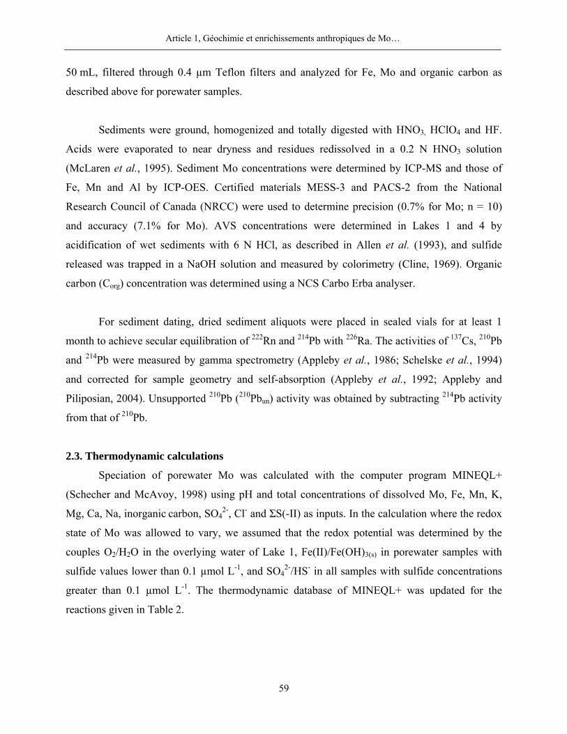
Article 1, Géochimie et enrichissements anthropiques de Mo…
59
50 mL, filtered through 0.4 µm Teflon filters and analyzed for Fe, Mo and organic carbon as
described above for porewater samples.
Sediments were ground, homogenized and totally digested with HNO3, HClO4 and HF.
Acids were evaporated to near dryness and residues redissolved in a 0.2 N HNO3 solution
(McLaren et al., 1995). Sediment Mo concentrations were determined by ICP-MS and those of
Fe, Mn and Al by ICP-OES. Certified materials MESS-3 and PACS-2 from the National
Research Council of Canada (NRCC) were used to determine precision (0.7% for Mo; n = 10)
and accuracy (7.1% for Mo). AVS concentrations were determined in Lakes 1 and 4 by
acidification of wet sediments with 6 N HCl, as described in Allen et al. (1993), and sulfide
released was trapped in a NaOH solution and measured by colorimetry (Cline, 1969). Organic
carbon (Corg) concentration was determined using a NCS Carbo Erba analyser.
For sediment dating, dried sediment aliquots were placed in sealed vials for at least 1
month to achieve secular equilibration of 222Rn and 214Pb with 226Ra. The activities of 137Cs, 210Pb
and 214Pb were measured by gamma spectrometry (Appleby et al., 1986; Schelske et al., 1994)
and corrected for sample geometry and self-absorption (Appleby et al., 1992; Appleby and
Piliposian, 2004). Unsupported 210Pb (210Pbun) activity was obtained by subtracting 214Pb activity
from that of 210Pb.
2.3. Thermodynamic calculations
Speciation of porewater Mo was calculated with the computer program MINEQL+
(Schecher and McAvoy, 1998) using pH and total concentrations of dissolved Mo, Fe, Mn, K,
Mg, Ca, Na, inorganic carbon, SO42-, Cl- and ΣS(-II) as inputs. In the calculation where the redox
state of Mo was allowed to vary, we assumed that the redox potential was determined by the
couples O2/H2O in the overlying water of Lake 1, Fe(II)/Fe(OH)3(s) in porewater samples with
sulfide values lower than 0.1 µmol L-1, and SO42-/HS- in all samples with sulfide concentrations
greater than 0.1 µmol L-1. The thermodynamic database of MINEQL+ was updated for the
reactions given in Table 2.
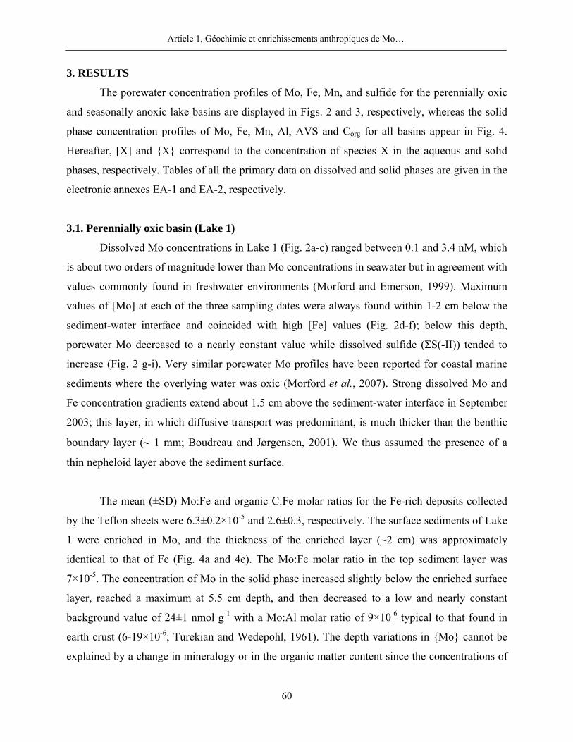
Article 1, Géochimie et enrichissements anthropiques de Mo…
60
3. RESULTS
The porewater concentration profiles of Mo, Fe, Mn, and sulfide for the perennially oxic
and seasonally anoxic lake basins are displayed in Figs. 2 and 3, respectively, whereas the solid
phase concentration profiles of Mo, Fe, Mn, Al, AVS and Corg for all basins appear in Fig. 4.
Hereafter, [X] and X correspond to the concentration of species X in the aqueous and solid
phases, respectively. Tables of all the primary data on dissolved and solid phases are given in the
electronic annexes EA-1 and EA-2, respectively.
3.1. Perennially oxic basin (Lake 1)
Dissolved Mo concentrations in Lake 1 (Fig. 2a-c) ranged between 0.1 and 3.4 nM, which
is about two orders of magnitude lower than Mo concentrations in seawater but in agreement with
values commonly found in freshwater environments (Morford and Emerson, 1999). Maximum
values of [Mo] at each of the three sampling dates were always found within 1-2 cm below the
sediment-water interface and coincided with high [Fe] values (Fig. 2d-f); below this depth,
porewater Mo decreased to a nearly constant value while dissolved sulfide (ΣS(-II)) tended to
increase (Fig. 2 g-i). Very similar porewater Mo profiles have been reported for coastal marine
sediments where the overlying water was oxic (Morford et al., 2007). Strong dissolved Mo and
Fe concentration gradients extend about 1.5 cm above the sediment-water interface in September
2003; this layer, in which diffusive transport was predominant, is much thicker than the benthic
boundary layer (∼ 1 mm; Boudreau and Jørgensen, 2001). We thus assumed the presence of a
thin nepheloid layer above the sediment surface.
The mean (±SD) Mo:Fe and organic C:Fe molar ratios for the Fe-rich deposits collected
by the Teflon sheets were 6.3±0.2×10⁻⁵ and 2.6±0.3, respectively. The surface sediments of Lake
1 were enriched in Mo, and the thickness of the enriched layer (~2 cm) was approximately
identical to that of Fe (Fig. 4a and 4e). The Mo:Fe molar ratio in the top sediment layer was
7×10⁻⁵. The concentration of Mo in the solid phase increased slightly below the enriched surface
layer, reached a maximum at 5.5 cm depth, and then decreased to a low and nearly constant
background value of 24±1 nmol g-1 with a Mo:Al molar ratio of 9×10⁻⁶ typical to that found in
earth crust (6-19×10-6; Turekian and Wedepohl, 1961). The depth variations in Mo cannot be
explained by a change in mineralogy or in the organic matter content since the concentrations of
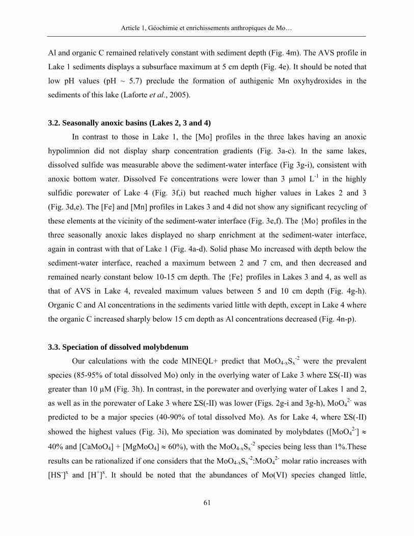
Article 1, Géochimie et enrichissements anthropiques de Mo…
61
Al and organic C remained relatively constant with sediment depth (Fig. 4m). The AVS profile in
Lake 1 sediments displays a subsurface maximum at 5 cm depth (Fig. 4e). It should be noted that
low pH values (pH ~ 5.7) preclude the formation of authigenic Mn oxyhydroxides in the
sediments of this lake (Laforte et al., 2005).
3.2. Seasonally anoxic basins (Lakes 2, 3 and 4)
In contrast to those in Lake 1, the [Mo] profiles in the three lakes having an anoxic
hypolimnion did not display sharp concentration gradients (Fig. 3a-c). In the same lakes,
dissolved sulfide was measurable above the sediment-water interface (Fig 3g-i), consistent with
anoxic bottom water. Dissolved Fe concentrations were lower than 3 µmol L-1 in the highly
sulfidic porewater of Lake 4 (Fig. 3f,i) but reached much higher values in Lakes 2 and 3
(Fig. 3d,e). The [Fe] and [Mn] profiles in Lakes 3 and 4 did not show any significant recycling of
these elements at the vicinity of the sediment-water interface (Fig. 3e,f). The Mo profiles in the
three seasonally anoxic lakes displayed no sharp enrichment at the sediment-water interface,
again in contrast with that of Lake 1 (Fig. 4a-d). Solid phase Mo increased with depth below the
sediment-water interface, reached a maximum between 2 and 7 cm, and then decreased and
remained nearly constant below 10-15 cm depth. The Fe profiles in Lakes 3 and 4, as well as
that of AVS in Lake 4, revealed maximum values between 5 and 10 cm depth (Fig. 4g-h).
Organic C and Al concentrations in the sediments varied little with depth, except in Lake 4 where
the organic C increased sharply below 15 cm depth as Al concentrations decreased (Fig. 4n-p).
3.3. Speciation of dissolved molybdenum
Our calculations with the code MINEQL+ predict that MoO4-xSx-2 were the prevalent
species (85-95% of total dissolved Mo) only in the overlying water of Lake 3 where ΣS(-II) was
greater than 10 µM (Fig. 3h). In contrast, in the porewater and overlying water of Lakes 1 and 2,
as well as in the porewater of Lake 3 where ΣS(-II) was lower (Figs. 2g-i and 3g-h), MoO42- was
predicted to be a major species (40-90% of total dissolved Mo). As for Lake 4, where ΣS(-II)
showed the highest values (Fig. 3i), Mo speciation was dominated by molybdates ([MoO42-] ≈
40% and [CaMoO4] + [MgMoO4] ≈ 60%), with the MoO4-xSx-2 species being less than 1%.These
results can be rationalized if one considers that the MoO4-xSx-2:MoO4
2- molar ratio increases with
[HS-]x and [H+]x. It should be noted that the abundances of Mo(VI) species changed little,
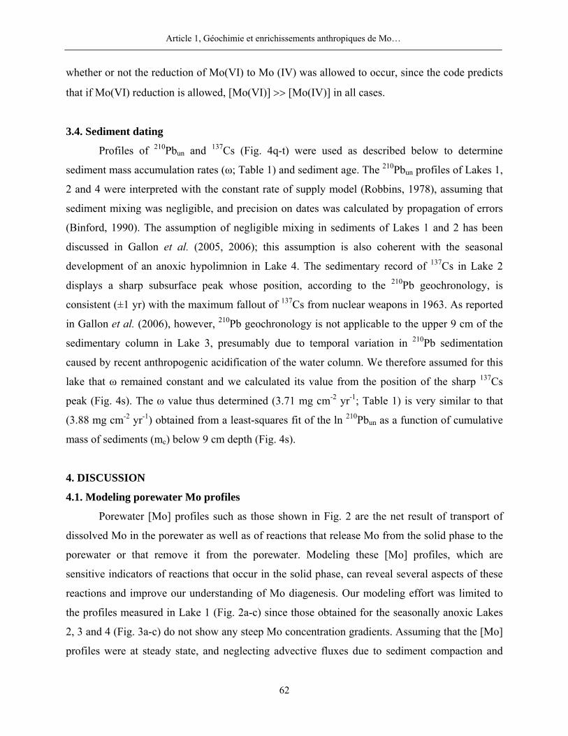
Article 1, Géochimie et enrichissements anthropiques de Mo…
62
whether or not the reduction of Mo(VI) to Mo (IV) was allowed to occur, since the code predicts
that if Mo(VI) reduction is allowed, [Mo(VI)] >> [Mo(IV)] in all cases.
3.4. Sediment dating
Profiles of 210Pbun and 137Cs (Fig. 4q-t) were used as described below to determine
sediment mass accumulation rates (ω; Table 1) and sediment age. The 210Pbun profiles of Lakes 1,
2 and 4 were interpreted with the constant rate of supply model (Robbins, 1978), assuming that
sediment mixing was negligible, and precision on dates was calculated by propagation of errors
(Binford, 1990). The assumption of negligible mixing in sediments of Lakes 1 and 2 has been
discussed in Gallon et al. (2005, 2006); this assumption is also coherent with the seasonal
development of an anoxic hypolimnion in Lake 4. The sedimentary record of 137Cs in Lake 2
displays a sharp subsurface peak whose position, according to the 210Pb geochronology, is
consistent (±1 yr) with the maximum fallout of 137Cs from nuclear weapons in 1963. As reported
in Gallon et al. (2006), however, 210Pb geochronology is not applicable to the upper 9 cm of the
sedimentary column in Lake 3, presumably due to temporal variation in 210Pb sedimentation
caused by recent anthropogenic acidification of the water column. We therefore assumed for this
lake that ω remained constant and we calculated its value from the position of the sharp 137Cs
peak (Fig. 4s). The ω value thus determined (3.71 mg cm-2 yr-1; Table 1) is very similar to that
(3.88 mg cm-2 yr-1) obtained from a least-squares fit of the ln 210Pbun as a function of cumulative
mass of sediments (mc) below 9 cm depth (Fig. 4s).
4. DISCUSSION
4.1. Modeling porewater Mo profiles
Porewater [Mo] profiles such as those shown in Fig. 2 are the net result of transport of
dissolved Mo in the porewater as well as of reactions that release Mo from the solid phase to the
porewater or that remove it from the porewater. Modeling these [Mo] profiles, which are
sensitive indicators of reactions that occur in the solid phase, can reveal several aspects of these
reactions and improve our understanding of Mo diagenesis. Our modeling effort was limited to
the profiles measured in Lake 1 (Fig. 2a-c) since those obtained for the seasonally anoxic Lakes
2, 3 and 4 (Fig. 3a-c) do not show any steep Mo concentration gradients. Assuming that the [Mo]
profiles were at steady state, and neglecting advective fluxes due to sediment compaction and
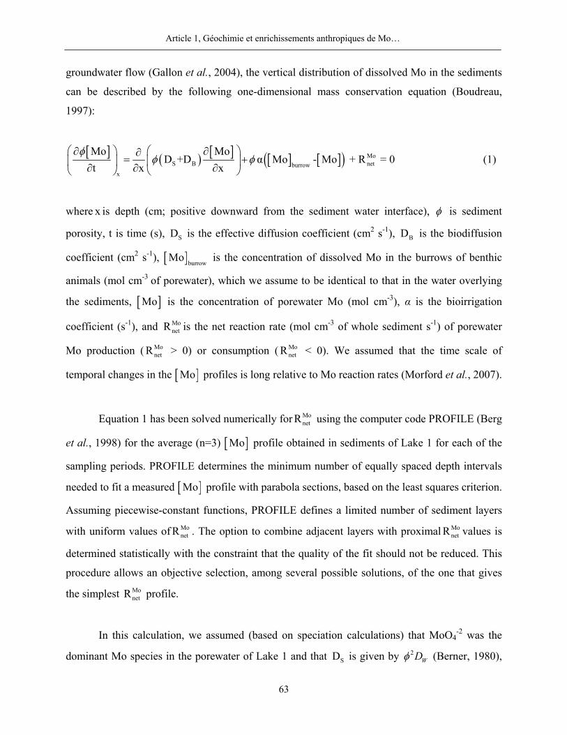
Article 1, Géochimie et enrichissements anthropiques de Mo…
63
groundwater flow (Gallon et al., 2004), the vertical distribution of dissolved Mo in the sediments
can be described by the following one-dimensional mass conservation equation (Boudreau,
1997):
[ ] ( ) [ ] [ ] [ ]( ) MoS B netburrow
x
Mo MoD +D α Mo - Mo + R = 0
t x xφ
φ φ⎛ ⎞ ⎛ ⎞∂ ∂∂
= +⎜ ⎟ ⎜ ⎟∂ ∂ ∂⎝ ⎠ ⎝ ⎠ (1)
where x is depth (cm; positive downward from the sediment water interface), φ is sediment
porosity, t is time (s), SD is the effective diffusion coefficient (cm2 s-1), BD is the biodiffusion
coefficient (cm2 s-1), [ ]burrowMo is the concentration of dissolved Mo in the burrows of benthic
animals (mol cm-3 of porewater), which we assume to be identical to that in the water overlying
the sediments, [ ]Mo is the concentration of porewater Mo (mol cm-3), α is the bioirrigation
coefficient (s-1), and MonetR is the net reaction rate (mol cm-3 of whole sediment s-1) of porewater
Mo production ( MonetR > 0) or consumption ( Mo
netR < 0). We assumed that the time scale of
temporal changes in the [ ]Mo profiles is long relative to Mo reaction rates (Morford et al., 2007).
Equation 1 has been solved numerically for MonetR using the computer code PROFILE (Berg
et al., 1998) for the average (n=3) [ ]Mo profile obtained in sediments of Lake 1 for each of the
sampling periods. PROFILE determines the minimum number of equally spaced depth intervals
needed to fit a measured [ ]Mo profile with parabola sections, based on the least squares criterion.
Assuming piecewise-constant functions, PROFILE defines a limited number of sediment layers
with uniform values of MonetR . The option to combine adjacent layers with proximal Mo
netR values is
determined statistically with the constraint that the quality of the fit should not be reduced. This
procedure allows an objective selection, among several possible solutions, of the one that gives
the simplest MonetR profile.
In this calculation, we assumed (based on speciation calculations) that MoO4-2 was the
dominant Mo species in the porewater of Lake 1 and that SD is given by 2WDφ (Berner, 1980),
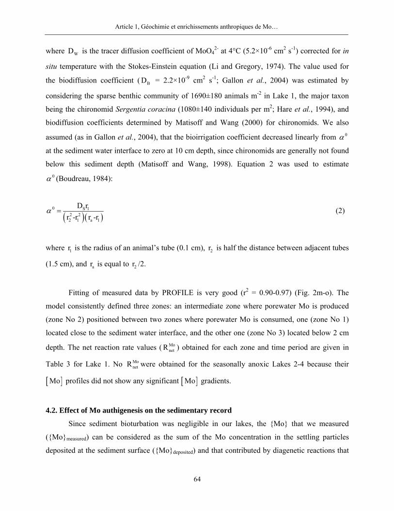
Article 1, Géochimie et enrichissements anthropiques de Mo…
64
where WD is the tracer diffusion coefficient of MoO42- at 4°C (5.2×10⁻⁶ cm2 s-1) corrected for in
situ temperature with the Stokes-Einstein equation (Li and Gregory, 1974). The value used for
the biodiffusion coefficient ( BD = 2.2×10⁻⁹ cm2 s-1; Gallon et al., 2004) was estimated by
considering the sparse benthic community of 1690±180 animals m-2 in Lake 1, the major taxon
being the chironomid Sergentia coracina (1080±140 individuals per m2; Hare et al., 1994), and
biodiffusion coefficients determined by Matisoff and Wang (2000) for chironomids. We also
assumed (as in Gallon et al., 2004), that the bioirrigation coefficient decreased linearly from 0α
at the sediment water interface to zero at 10 cm depth, since chironomids are generally not found
below this sediment depth (Matisoff and Wang, 1998). Equation 2 was used to estimate 0α (Boudreau, 1984):
( )( )0 S 1
2 22 1 a 1
D rr -r r -r
α = (2)
where 1r is the radius of an animal’s tube (0.1 cm), 2r is half the distance between adjacent tubes
(1.5 cm), and ar is equal to 2r /2.
Fitting of measured data by PROFILE is very good (r2 = 0.90-0.97) (Fig. 2m-o). The
model consistently defined three zones: an intermediate zone where porewater Mo is produced
(zone No 2) positioned between two zones where porewater Mo is consumed, one (zone No 1)
located close to the sediment water interface, and the other one (zone No 3) located below 2 cm
depth. The net reaction rate values ( MonetR ) obtained for each zone and time period are given in
Table 3 for Lake 1. No MonetR were obtained for the seasonally anoxic Lakes 2-4 because their
[ ]Mo profiles did not show any significant [ ]Mo gradients.
4.2. Effect of Mo authigenesis on the sedimentary record
Since sediment bioturbation was negligible in our lakes, the Mo that we measured
(Momeasured) can be considered as the sum of the Mo concentration in the settling particles
deposited at the sediment surface (Modeposited) and that contributed by diagenetic reactions that
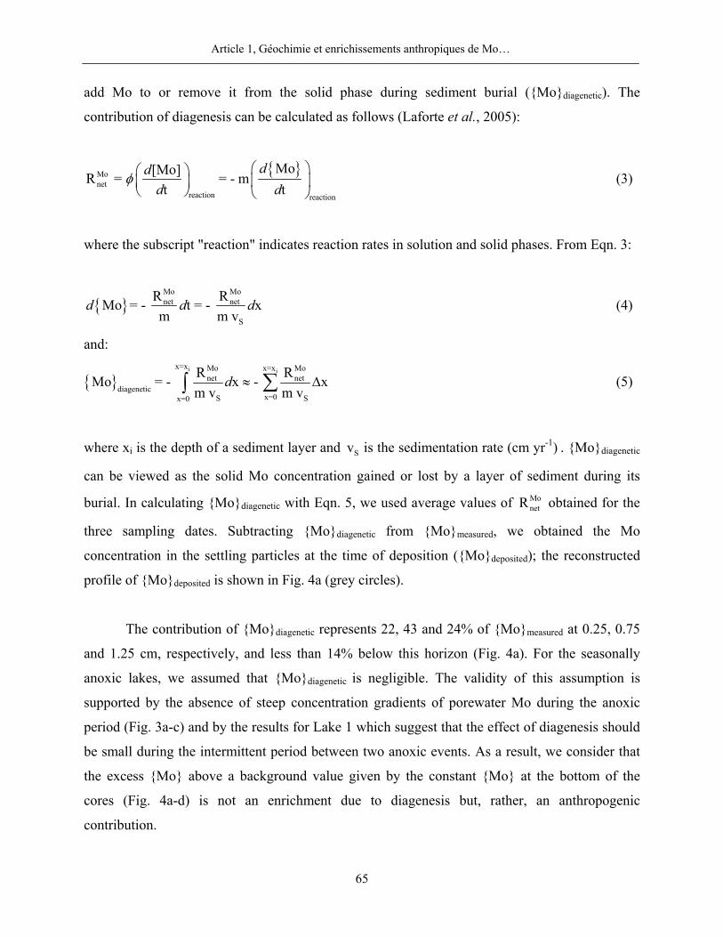
Article 1, Géochimie et enrichissements anthropiques de Mo…
65
add Mo to or remove it from the solid phase during sediment burial (Modiagenetic). The
contribution of diagenesis can be calculated as follows (Laforte et al., 2005):
Monet
reaction reaction
Mo[Mo]R = = - mt t
ddd d
φ⎛ ⎞⎛ ⎞⎜ ⎟⎜ ⎟
⎝ ⎠ ⎝ ⎠ (3)
where the subscript "reaction" indicates reaction rates in solution and solid phases. From Eqn. 3:
Mo Monet net
S
R RMo = - t = - xm m v
d d d (4)
and:
i i
x=x Mo Mox=xnet net
diageneticx=0S Sx=0
R RMo = - x - xm v m v
d ≈ Δ∑∫ (5)
where xi is the depth of a sediment layer and Sv is the sedimentation rate (cm yr-1) . Modiagenetic
can be viewed as the solid Mo concentration gained or lost by a layer of sediment during its
burial. In calculating Modiagenetic with Eqn. 5, we used average values of MonetR obtained for the
three sampling dates. Subtracting Modiagenetic from Momeasured, we obtained the Mo
concentration in the settling particles at the time of deposition (Modeposited); the reconstructed
profile of Modeposited is shown in Fig. 4a (grey circles).
The contribution of Modiagenetic represents 22, 43 and 24% of Momeasured at 0.25, 0.75
and 1.25 cm, respectively, and less than 14% below this horizon (Fig. 4a). For the seasonally
anoxic lakes, we assumed that Modiagenetic is negligible. The validity of this assumption is
supported by the absence of steep concentration gradients of porewater Mo during the anoxic
period (Fig. 3a-c) and by the results for Lake 1 which suggest that the effect of diagenesis should
be small during the intermittent period between two anoxic events. As a result, we consider that
the excess Mo above a background value given by the constant Mo at the bottom of the
cores (Fig. 4a-d) is not an enrichment due to diagenesis but, rather, an anthropogenic
contribution.
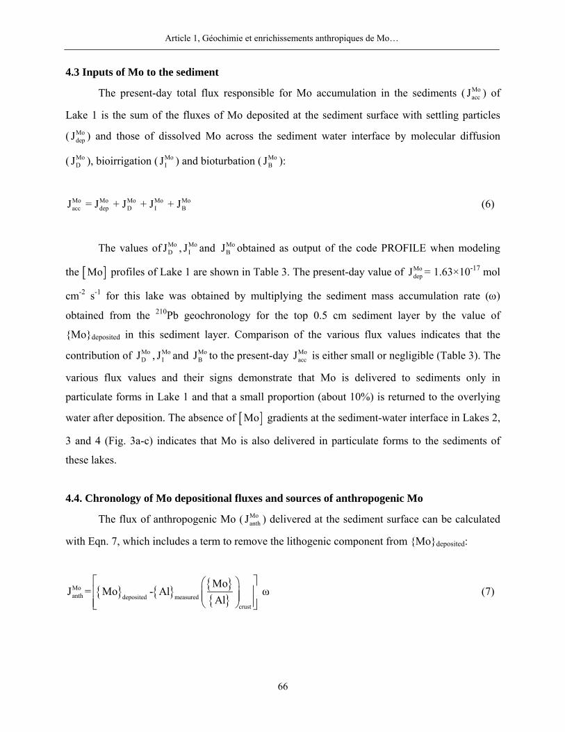
Article 1, Géochimie et enrichissements anthropiques de Mo…
66
4.3 Inputs of Mo to the sediment
The present-day total flux responsible for Mo accumulation in the sediments ( MoaccJ ) of
Lake 1 is the sum of the fluxes of Mo deposited at the sediment surface with settling particles
( ModepJ ) and those of dissolved Mo across the sediment water interface by molecular diffusion
( MoDJ ), bioirrigation ( Mo
IJ ) and bioturbation ( MoBJ ):
Mo Mo Mo Mo Moacc dep D I BJ = J + J + J + J (6)
The values of MoDJ , Mo
IJ and MoBJ obtained as output of the code PROFILE when modeling
the [ ]Mo profiles of Lake 1 are shown in Table 3. The present-day value of ModepJ = 1.63×10⁻¹⁷ mol
cm-2 s-1 for this lake was obtained by multiplying the sediment mass accumulation rate (ω)
obtained from the 210Pb geochronology for the top 0.5 cm sediment layer by the value of
Modeposited in this sediment layer. Comparison of the various flux values indicates that the
contribution of MoDJ , Mo
IJ and MoBJ to the present-day Mo
accJ is either small or negligible (Table 3). The
various flux values and their signs demonstrate that Mo is delivered to sediments only in
particulate forms in Lake 1 and that a small proportion (about 10%) is returned to the overlying
water after deposition. The absence of [ ]Mo gradients at the sediment-water interface in Lakes 2,
3 and 4 (Fig. 3a-c) indicates that Mo is also delivered in particulate forms to the sediments of
these lakes.
4.4. Chronology of Mo depositional fluxes and sources of anthropogenic Mo
The flux of anthropogenic Mo ( MoanthJ ) delivered at the sediment surface can be calculated
with Eqn. 7, which includes a term to remove the lithogenic component from Modeposited:
Moanth deposited measured
crust
MoJ = Mo - Al ω
Al
⎡ ⎤⎛ ⎞⎢ ⎥⎜ ⎟⎜ ⎟⎢ ⎥⎝ ⎠⎣ ⎦
(7)
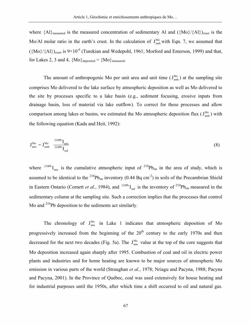
Article 1, Géochimie et enrichissements anthropiques de Mo…
67
where Almeasured is the measured concentration of sedimentary Al and (Mo/Al)crust is the
Mo/Al molar ratio in the earth’s crust. In the calculation of MoanthJ with Eqn. 7, we assumed that
(Mo/Al)crust is 9×10⁻⁶ (Turekian and Wedepohl, 1961; Morford and Emerson, 1999) and that,
for Lakes 2, 3 and 4, Modeposited = Momeasured.
The amount of anthropogenic Mo per unit area and unit time ( MoanthJ ) at the sampling site
comprises Mo delivered to the lake surface by atmospheric deposition as well as Mo delivered to
the site by processes specific to a lake basin (e.g., sediment focusing, erosive inputs from
drainage basin, loss of material via lake outflow). To correct for these processes and allow
comparison among lakes or basins, we estimated the Mo atmospheric deposition flux ( MoanthJ ) with
the following equation (Kada and Heit, 1992):
210Pb
Mo Mo atmatm anth 210Pb
sed
IJ = J I
(8)
where 210PbatmI is the cumulative atmospheric input of 210Pbun in the area of study, which is
assumed to be identical to the 210Pbun inventory (0.44 Bq cm-2) in soils of the Precambrian Shield
in Eastern Ontario (Cornett et al., 1984), and 210PbsedI is the inventory of 210Pbun measured in the
sedimentary column at the sampling site. Such a correction implies that the processes that control
Mo and 210Pb deposition to the sediments act similarly.
The chronology of MoatmJ in Lake 1 indicates that atmospheric deposition of Mo
progressively increased from the beginning of the 20th century to the early 1970s and then
decreased for the next two decades (Fig. 5a). The MoatmJ value at the top of the core suggests that
Mo deposition increased again sharply after 1995. Combustion of coal and oil in electric power
plants and industries and for home heating are known to be major sources of atmospheric Mo
emission in various parts of the world (Straughan et al., 1978; Nriagu and Pacyna, 1988; Pacyna
and Pacyna, 2001). In the Province of Québec, coal was used extensively for house heating and
for industrial purposes until the 1950s, after which time a shift occurred to oil and natural gas.
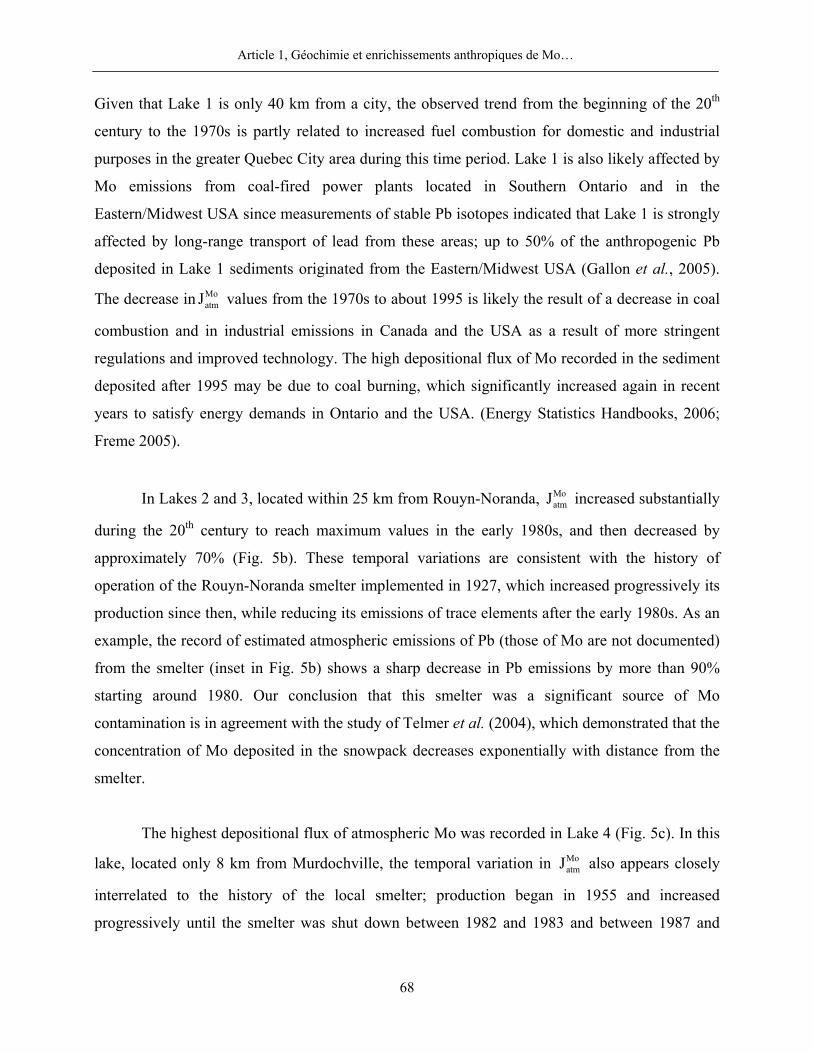
Article 1, Géochimie et enrichissements anthropiques de Mo…
68
Given that Lake 1 is only 40 km from a city, the observed trend from the beginning of the 20th
century to the 1970s is partly related to increased fuel combustion for domestic and industrial
purposes in the greater Quebec City area during this time period. Lake 1 is also likely affected by
Mo emissions from coal-fired power plants located in Southern Ontario and in the
Eastern/Midwest USA since measurements of stable Pb isotopes indicated that Lake 1 is strongly
affected by long-range transport of lead from these areas; up to 50% of the anthropogenic Pb
deposited in Lake 1 sediments originated from the Eastern/Midwest USA (Gallon et al., 2005).
The decrease in MoatmJ values from the 1970s to about 1995 is likely the result of a decrease in coal
combustion and in industrial emissions in Canada and the USA as a result of more stringent
regulations and improved technology. The high depositional flux of Mo recorded in the sediment
deposited after 1995 may be due to coal burning, which significantly increased again in recent
years to satisfy energy demands in Ontario and the USA. (Energy Statistics Handbooks, 2006;
Freme 2005).
In Lakes 2 and 3, located within 25 km from Rouyn-Noranda, MoatmJ increased substantially
during the 20th century to reach maximum values in the early 1980s, and then decreased by
approximately 70% (Fig. 5b). These temporal variations are consistent with the history of
operation of the Rouyn-Noranda smelter implemented in 1927, which increased progressively its
production since then, while reducing its emissions of trace elements after the early 1980s. As an
example, the record of estimated atmospheric emissions of Pb (those of Mo are not documented)
from the smelter (inset in Fig. 5b) shows a sharp decrease in Pb emissions by more than 90%
starting around 1980. Our conclusion that this smelter was a significant source of Mo
contamination is in agreement with the study of Telmer et al. (2004), which demonstrated that the
concentration of Mo deposited in the snowpack decreases exponentially with distance from the
smelter.
The highest depositional flux of atmospheric Mo was recorded in Lake 4 (Fig. 5c). In this
lake, located only 8 km from Murdochville, the temporal variation in MoatmJ also appears closely
interrelated to the history of the local smelter; production began in 1955 and increased
progressively until the smelter was shut down between 1982 and 1983 and between 1987 and
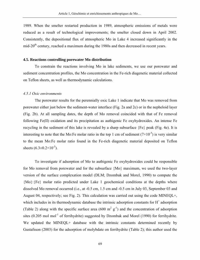
Article 1, Géochimie et enrichissements anthropiques de Mo…
69
1989. When the smelter restarted production in 1989, atmospheric emissions of metals were
reduced as a result of technological improvements; the smelter closed down in April 2002.
Consistently, the depositional flux of atmospheric Mo in Lake 4 increased significantly in the
mid-20th century, reached a maximum during the 1980s and then decreased in recent years.
4.5. Reactions controlling porewater Mo distribution
To constrain the reactions involving Mo in lake sediments, we use our porewater and
sediment concentration profiles, the Mo concentration in the Fe-rich diagenetic material collected
on Teflon sheets, as well as thermodynamic calculations.
4.5.1 Oxic environments
The porewater results for the perennially oxic Lake 1 indicate that Mo was removed from
porewater either just below the sediment-water interface (Fig. 2a and 2c) or in the nepheloid layer
(Fig. 2b). At all sampling dates, the depth of Mo removal coincided with that of Fe removal
following Fe(II) oxidation and its precipitation as authigenic Fe oxyhydroxides. An intense Fe
recycling in the sediment of this lake is revealed by a sharp subsurface Fe peak (Fig. 4e). It is
interesting to note that the Mo:Fe molar ratio in the top 1 cm of sediment (7×10⁻⁵) is very similar
to the mean Mo:Fe molar ratio found in the Fe-rich diagenetic material deposited on Teflon
sheets (6.3±0.2×10⁻⁵).
To investigate if adsorption of Mo to authigenic Fe oxyhydroxides could be responsible
for Mo removal from porewater and for the subsurface Mo maximum, we used the two-layer
version of the surface complexation model (DLM; Dzombak and Morel, 1990) to compute the
Mo:Fe molar ratio predicted under Lake 1 geochemical conditions at the depths where
dissolved Mo removal occurred (i.e., at -0.5 cm, 1.5 cm and -0.5 cm in July 03, September 03 and
August 04, respectively; see Fig. 2). This calculation was carried out using the code MINEQL+,
which includes in its thermodynamic database the intrinsic adsorption constants for H+ adsorption
(Table 2) along with the specific surface area (600 m2 g-1) and the concentration of adsorption
sites (0.205 mol mol-1 of ferrihydrite) suggested by Dzombak and Morel (1990) for ferrihydrite.
We updated the MINEQL+ database with the intrinsic constants determined recently by
Gustafsson (2003) for the adsorption of molybdate on ferrihydrite (Table 2); this author used the
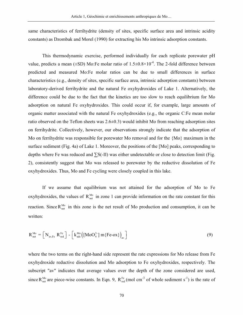
Article 1, Géochimie et enrichissements anthropiques de Mo…
70
same characteristics of ferrihydrite (density of sites, specific surface area and intrinsic acidity
constants) as Dzombak and Morel (1990) for extracting his Mo intrinsic adsorption constants.
This thermodynamic exercise, performed individually for each replicate porewater pH
value, predicts a mean (±SD) Mo:Fe molar ratio of 1.5±0.8×10⁻⁴. The 2-fold difference between
predicted and measured Mo:Fe molar ratios can be due to small differences in surface
characteristics (e.g., density of sites, specific surface area, intrinsic adsorption constants) between
laboratory-derived ferrihydrite and the natural Fe oxyhydroxides of Lake 1. Alternatively, the
difference could be due to the fact that the kinetics are too slow to reach equilibrium for Mo
adsorption on natural Fe oxyhydroxides. This could occur if, for example, large amounts of
organic matter associated with the natural Fe oxyhydroxides (e.g., the organic C:Fe mean molar
ratio observed on the Teflon sheets was 2.6±0.3) would inhibit Mo from reaching adsorption sites
on ferrihydrite. Collectively, however, our observations strongly indicate that the adsorption of
Mo on ferrihydrite was responsible for porewater Mo removal and for the Mo maximum in the
surface sediment (Fig. 4a) of Lake 1. Moreover, the positions of the [Mo] peaks, corresponding to
depths where Fe was reduced and ∑S(-II) was either undetectable or close to detection limit (Fig.
2), consistently suggest that Mo was released to porewater by the reductive dissolution of Fe
oxyhydroxides. Thus, Mo and Fe cycling were closely coupled in this lake.
If we assume that equilibrium was not attained for the adsorption of Mo to Fe
oxyhydroxides, the values of MonetR in zone 1 can provide information on the rate constant for this
reaction. Since MonetR in this zone is the net result of Mo production and consumption, it can be
written:
( )Mo Fe Mo 2-net av,Fe red ads 4 av
R = N R - k [MoO ] mFe-ox⎡ ⎤⎡ ⎤⎣ ⎦ ⎣ ⎦ (9)
where the two terms on the right-hand side represent the rate expressions for Mo release from Fe
oxyhydroxide reductive dissolution and Mo adsorption to Fe oxyhydroxides, respectively. The
subscript "av" indicates that average values over the depth of the zone considered are used,
since MonetR are piece-wise constants. In Eqn. 9, Fe
redR (mol cm-3 of whole sediment s-1) is the rate of
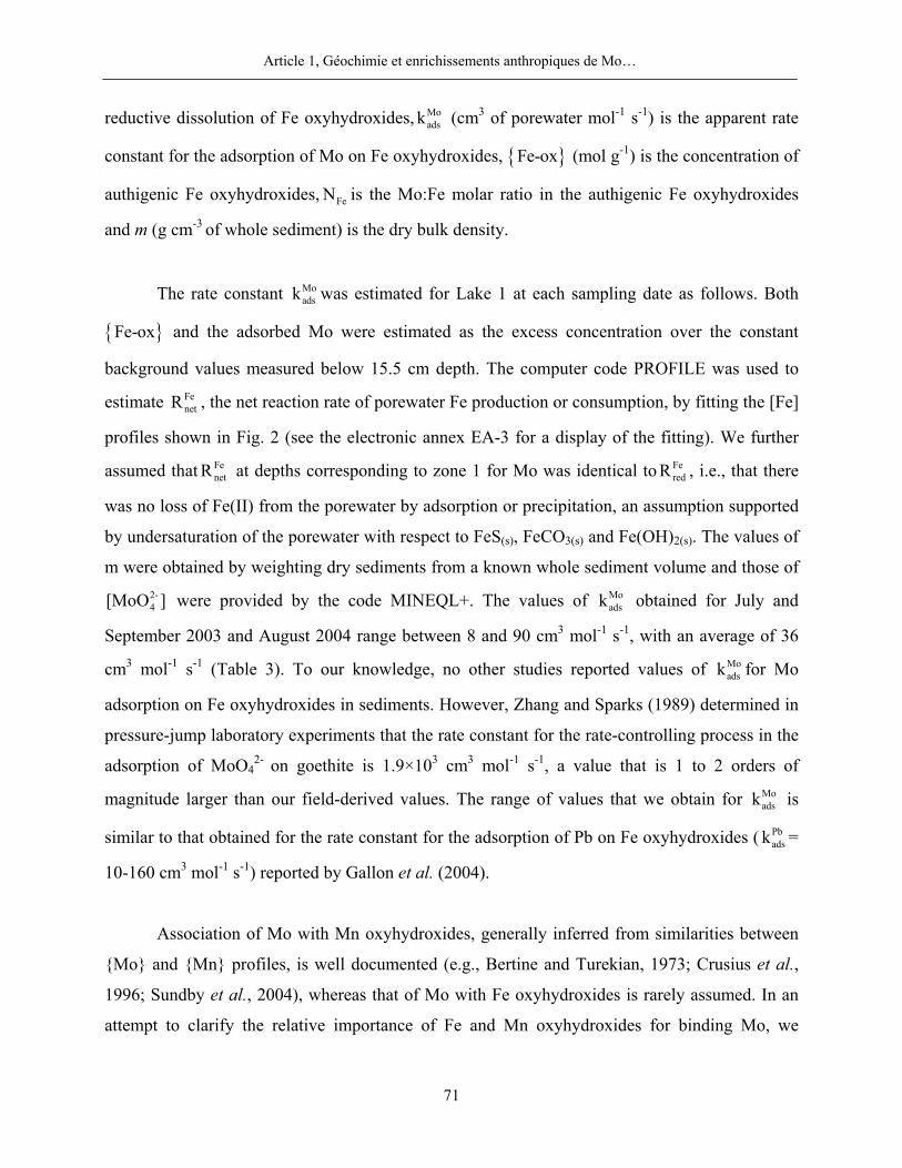
Article 1, Géochimie et enrichissements anthropiques de Mo…
71
reductive dissolution of Fe oxyhydroxides, Moadsk (cm3 of porewater mol-1 s-1) is the apparent rate
constant for the adsorption of Mo on Fe oxyhydroxides, Fe-ox (mol g-1) is the concentration of
authigenic Fe oxyhydroxides, FeN is the Mo:Fe molar ratio in the authigenic Fe oxyhydroxides
and m (g cm-3 of whole sediment) is the dry bulk density.
The rate constant Moadsk was estimated for Lake 1 at each sampling date as follows. Both
Fe-ox and the adsorbed Mo were estimated as the excess concentration over the constant
background values measured below 15.5 cm depth. The computer code PROFILE was used to
estimate FenetR , the net reaction rate of porewater Fe production or consumption, by fitting the [Fe]
profiles shown in Fig. 2 (see the electronic annex EA-3 for a display of the fitting). We further
assumed that FenetR at depths corresponding to zone 1 for Mo was identical to Fe
redR , i.e., that there
was no loss of Fe(II) from the porewater by adsorption or precipitation, an assumption supported
by undersaturation of the porewater with respect to FeS(s), FeCO3(s) and Fe(OH)2(s). The values of
m were obtained by weighting dry sediments from a known whole sediment volume and those of 2-4[MoO ] were provided by the code MINEQL+. The values of Mo
adsk obtained for July and
September 2003 and August 2004 range between 8 and 90 cm3 mol-1 s-1, with an average of 36
cm3 mol-1 s-1 (Table 3). To our knowledge, no other studies reported values of Moadsk for Mo
adsorption on Fe oxyhydroxides in sediments. However, Zhang and Sparks (1989) determined in
pressure-jump laboratory experiments that the rate constant for the rate-controlling process in the
adsorption of MoO42- on goethite is 1.9×103 cm3 mol-1 s-1, a value that is 1 to 2 orders of
magnitude larger than our field-derived values. The range of values that we obtain for Moadsk is
similar to that obtained for the rate constant for the adsorption of Pb on Fe oxyhydroxides ( Pbadsk =
10-160 cm3 mol-1 s-1) reported by Gallon et al. (2004).
Association of Mo with Mn oxyhydroxides, generally inferred from similarities between
Mo and Mn profiles, is well documented (e.g., Bertine and Turekian, 1973; Crusius et al.,
1996; Sundby et al., 2004), whereas that of Mo with Fe oxyhydroxides is rarely assumed. In an
attempt to clarify the relative importance of Fe and Mn oxyhydroxides for binding Mo, we
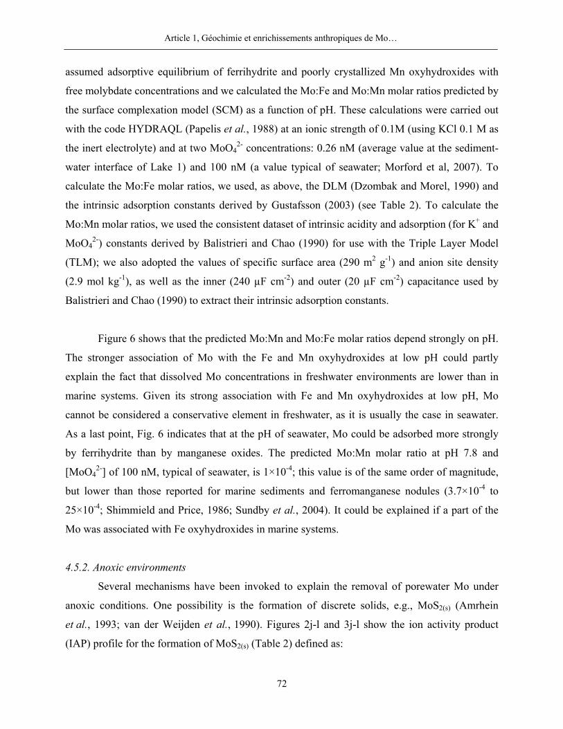
Article 1, Géochimie et enrichissements anthropiques de Mo…
72
assumed adsorptive equilibrium of ferrihydrite and poorly crystallized Mn oxyhydroxides with
free molybdate concentrations and we calculated the Mo:Fe and Mo:Mn molar ratios predicted by
the surface complexation model (SCM) as a function of pH. These calculations were carried out
with the code HYDRAQL (Papelis et al., 1988) at an ionic strength of 0.1M (using KCl 0.1 M as
the inert electrolyte) and at two MoO42- concentrations: 0.26 nM (average value at the sediment-
water interface of Lake 1) and 100 nM (a value typical of seawater; Morford et al, 2007). To
calculate the Mo:Fe molar ratios, we used, as above, the DLM (Dzombak and Morel, 1990) and
the intrinsic adsorption constants derived by Gustafsson (2003) (see Table 2). To calculate the
Mo:Mn molar ratios, we used the consistent dataset of intrinsic acidity and adsorption (for K+ and
MoO42-) constants derived by Balistrieri and Chao (1990) for use with the Triple Layer Model
(TLM); we also adopted the values of specific surface area (290 m2 g-1) and anion site density
(2.9 mol kg-1), as well as the inner (240 µF cm-2) and outer (20 µF cm-2) capacitance used by
Balistrieri and Chao (1990) to extract their intrinsic adsorption constants.
Figure 6 shows that the predicted Mo:Mn and Mo:Fe molar ratios depend strongly on pH.
The stronger association of Mo with the Fe and Mn oxyhydroxides at low pH could partly
explain the fact that dissolved Mo concentrations in freshwater environments are lower than in
marine systems. Given its strong association with Fe and Mn oxyhydroxides at low pH, Mo
cannot be considered a conservative element in freshwater, as it is usually the case in seawater.
As a last point, Fig. 6 indicates that at the pH of seawater, Mo could be adsorbed more strongly
by ferrihydrite than by manganese oxides. The predicted Mo:Mn molar ratio at pH 7.8 and
[MoO42-] of 100 nM, typical of seawater, is 1×10⁻⁴; this value is of the same order of magnitude,
but lower than those reported for marine sediments and ferromanganese nodules (3.7×10⁻⁴ to
25×10-4; Shimmield and Price, 1986; Sundby et al., 2004). It could be explained if a part of the
Mo was associated with Fe oxyhydroxides in marine systems.
4.5.2. Anoxic environments
Several mechanisms have been invoked to explain the removal of porewater Mo under
anoxic conditions. One possibility is the formation of discrete solids, e.g., MoS2(s) (Amrhein
et al., 1993; van der Weijden et al., 1990). Figures 2j-l and 3j-l show the ion activity product
(IAP) profile for the formation of MoS2(s) (Table 2) defined as:
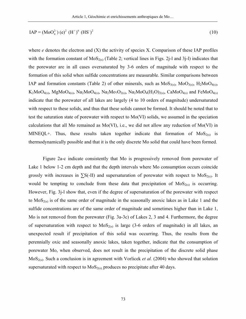
Article 1, Géochimie et enrichissements anthropiques de Mo…
73
2- 2 + 6 - 24IAP = (MoO ) (e) (H ) (HS ) (10)
where e denotes the electron and (X) the activity of species X. Comparison of these IAP profiles
with the formation constant of MoS2(s) (Table 2; vertical lines in Figs. 2j-l and 3j-l) indicates that
the porewater are in all cases oversaturated by 3-6 orders of magnitude with respect to the
formation of this solid when sulfide concentrations are measurable. Similar comparisons between
IAP and formation constants (Table 2) of other minerals, such as MoS3(s), MoO3(s), H2MoO4(s),
K2MoO4(s), MgMoO4(s), Na2MoO4(s), Na2Mo7O2(s), Na2MoO4(H2O)2(s), CaMoO4(s) and FeMoO4(s)
indicate that the porewater of all lakes are largely (4 to 10 orders of magnitude) undersaturated
with respect to these solids, and thus that these solids cannot be formed. It should be noted that to
test the saturation state of porewater with respect to Mo(VI) solids, we assumed in the speciation
calculations that all Mo remained as Mo(VI), i.e., we did not allow any reduction of Mo(VI) in
MINEQL+. Thus, these results taken together indicate that formation of MoS2(s) is
thermodynamically possible and that it is the only discrete Mo solid that could have been formed.
Figure 2a-c indicate consistently that Mo is progressively removed from porewater of
Lake 1 below 1-2 cm depth and that the depth intervals where Mo consumption occurs coincide
grossly with increases in ∑S(-II) and supersaturation of porewater with respect to MoS2(s). It
would be tempting to conclude from these data that precipitation of MoS2(s) is occurring.
However, Fig. 3j-l show that, even if the degree of supersaturation of the porewater with respect
to MoS2(s) is of the same order of magnitude in the seasonally anoxic lakes as in Lake 1 and the
sulfide concentrations are of the same order of magnitude and sometimes higher than in Lake 1,
Mo is not removed from the porewater (Fig. 3a-3c) of Lakes 2, 3 and 4. Furthermore, the degree
of supersaturation with respect to MoS2(s) is large (3-6 orders of magnitude) in all lakes, an
unexpected result if precipitation of this solid was occurring. Thus, the results from the
perennially oxic and seasonally anoxic lakes, taken together, indicate that the consumption of
porewater Mo, when observed, does not result in the precipitation of the discrete solid phase
MoS2(s). Such a conclusion is in agreement with Vorlicek et al. (2004) who showed that solution
supersaturated with respect to MoS2(s), produces no precipitate after 40 days.
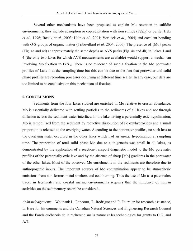
Article 1, Géochimie et enrichissements anthropiques de Mo…
74
Several other mechanisms have been proposed to explain Mo retention in sulfidic
environments; they include adsorption or coprecipitation with iron sulfide (FeS(s)) or pyrite (Helz
et al., 1996; Bostik et al., 2003; Helz et al., 2004; Vorlicek et al., 2004) and covalent bonding
with O-S groups of organic matter (Tribovillard et al. 2004; 2006). The presence of Mo peaks
(Fig. 4a and 4d) at approximately the same depths as AVS peaks (Fig. 4e and 4h) in Lakes 1 and
4 (the only two lakes for which AVS measurements are available) would support a mechanism
involving Mo fixation to FeS(s). There is no evidence of such a fixation in the Mo porewater
profiles of Lake 4 at the sampling time but this can be due to the fact that porewater and solid
phase profiles are recording processes occurring at different time scales. In any case, our data are
too limited to be conclusive on this mechanism of fixation.
5. CONCLUSIONS
Sediments from the four lakes studied are enriched in Mo relative to crustal abundance.
Mo is essentially delivered with settling particles to the sediments of all lakes and not through
diffusion across the sediment-water interface. In the lake having a perennially oxic hypolimnion,
Mo is remobilized from the sediment by reductive dissolution of Fe oxyhydroxides and a small
proportion is released to the overlying water. According to the porewater profiles, no such loss to
the overlying water occurred in the other lakes which had an anoxic hypolimnion at sampling
time. The proportion of total solid phase Mo due to authigenesis was small in all lakes, as
demonstrated by the application of a reaction-transport diagenetic model to the Mo porewater
profiles of the perennially oxic lake and by the absence of sharp [Mo] gradients in the porewater
of the other lakes. Most of the observed Mo enrichments in the sediments are therefore due to
anthropogenic inputs. The important sources of Mo contamination appear to be atmospheric
emissions from non-ferrous metal smelters and coal burning. Thus the use of Mo as a paleoredox
tracer in freshwater and coastal marine environments requires that the influence of human
activities on the sedimentary record be considered.
Acknowledgements―We thank L. Rancourt, R. Rodrigue and P. Fournier for research assistance,
L. Hare for his comments and the Canadian Natural Sciences and Engineering Research Council
and the Fonds québecois de la recherche sur la nature et les technologies for grants to C.G. and
A.T.
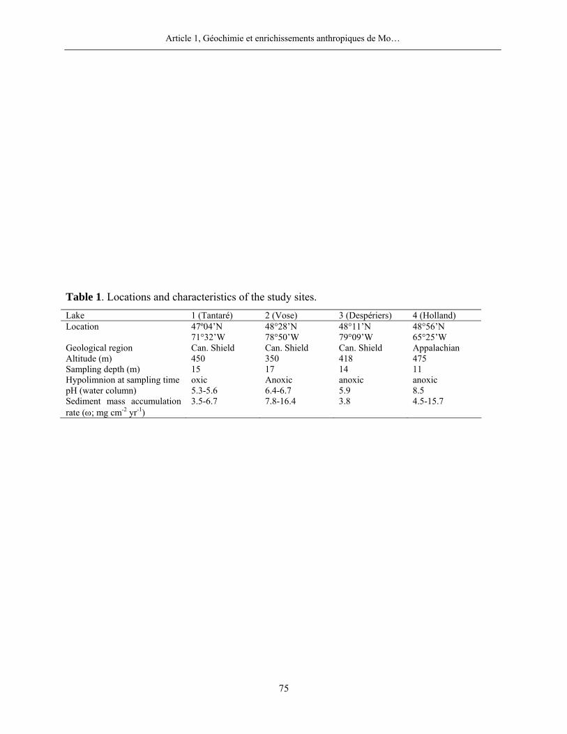
Article 1, Géochimie et enrichissements anthropiques de Mo…
75
Table 1. Locations and characteristics of the study sites. Lake 1 (Tantaré) 2 (Vose) 3 (Despériers) 4 (Holland) Location 47º04’N
71°32’W 48°28’N 78°50’W
48°11’N 79°09’W
48°56’N 65°25’W
Geological region Can. Shield Can. Shield Can. Shield Appalachian Altitude (m) 450 350 418 475 Sampling depth (m) 15 17 14 11 Hypolimnion at sampling time oxic Anoxic anoxic anoxic pH (water column) 5.3-5.6 6.4-6.7 5.9 8.5 Sediment mass accumulation rate (ω; mg cm-2 yr-1)
3.5-6.7 7.8-16.4 3.8 4.5-15.7
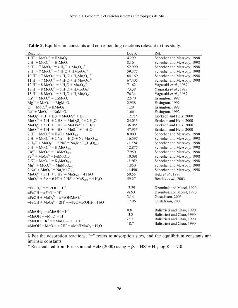
Article 1, Géochimie et enrichissements anthropiques de Mo…
76
Table 2. Equilibrium constants and corresponding reactions relevant to this study. Reaction Log K Ref. 1 H+ + MoO4
2- = HMoO4- 4.299 Schecher and McAvoy, 1998
2 H+ + MoO42- = H2MoO4 8.164 Schecher and McAvoy, 1998
8 H+ + 7 MoO42- = 4 H2O + Mo7O24
6- 52.990 Schecher and McAvoy, 1998 9 H+ + 7 MoO4
2- = 4 H2O + HMo7O245- 59.377 Schecher and McAvoy, 1998
10 H+ + 7 MoO42- = 4 H2O + H2Mo7O24
4- 64.169 Schecher and McAvoy, 1998 11 H+ + 7 MoO4
2- = 4 H2O + H3Mo7O243- 67.405 Schecher and McAvoy, 1998
12 H+ + 8 MoO42- = 6 H2O + Mo8O26
4- 71.62 Yagasaki et al., 1987 13 H+ + 8 MoO4
2- = 6 H2O + HMo8O263- 73.38 Yagasaki et al., 1987
15 H+ + 8 MoO42- = 6 H2O + H3Mo8O26
- 76.34 Yagasaki et al., 1987 Ca2+ + MoO4
2- = CaMoO4 2.570 Essington. 1992 Mg2+ + MoO4
2- = MgMoO4 2.958 Essington. 1992 K+ + MoO4
2- = KMoO4- 1.29 Essington. 1992
Na+ + MoO42- = NaMoO4
- 1.66 Essington. 1992 MoO4
2- + H+ + HS- = MoO3S2- + H2O 12.21* Erickson and Helz. 2000 MoO4
2- + 2 H+ + 2 HS- = MoO2S22- + 2 H2O 24.03* Erickson and Helz. 2000
MoO42- + 3 H+ + 3 HS- = MoOS3
2- + 3 H2O 36.05* Erickson and Helz. 2000 MoO4
2- + 4 H+ + 4 HS- = MoS42- + 4 H2O 47.95* Erickson and Helz. 2000
2 H+ + MoO42- = H2O + MoO3(s) 8.000 Schecher and McAvoy, 1998
2 H+ + MoO42- + 2 Na+ = H2O + Na2Mo7O2(s) 16.597 Schecher and McAvoy, 1998
2 H2O + MoO42- + 2 Na+ = Na2MoO4(H2O)2(s) -1.224 Schecher and McAvoy, 1998
2 H+ + MoO42- = H2MoO4(s) 12.877 Schecher and McAvoy, 1998
Ca2+ + MoO42- = CaMoO4(s) 7.950 Schecher and McAvoy, 1998
Fe2+ + MoO42- = FeMoO4(s) 10.091 Schecher and McAvoy, 1998
2 K+ + MoO42- = K2MoO4(s) -3.262 Schecher and McAvoy, 1998
Mg2+ + MoO42- = MgMoO4(s) 1.850 Schecher and McAvoy, 1998
2 Na+ + MoO42- = Na2MoO4(s) -1.490 Schecher and McAvoy, 1998
MoO42- + 5 H+ + 3 HS- = MoS3(s) + 4 H2O 50.55 Helz et al., 1996
MoO42- + 2 e + 6 H+ + 2 HS- = MoS2(s) + 4 H2O
≡FeOH2
+ = ≡FeOH + H+
≡FeOH = ≡FeO- + H+
≡FeOH + MoO42- = ≡FeOHMoO4
2-
≡FeOH + MoO42- + 2H+ = ≡FeOMo(OH)5 + H2O
≡MnOH2
+ = ≡MnOH + H+
≡MnOH = ≡MnO- + H+
≡MnOH + K+ = ≡MnO- — K+ + H+
≡MnOH + MoO42- + 2H+ = ≡MnHMoO4 + H2O
59.27 -7.29 -8.93 3.14 17.96 0.8 -3.8 -2.7 18.7
Bostick et al., 2003 Dzombak and Morel, 1990 Dzombak and Morel, 1990 Gustafsson, 2003 Gustafsson, 2003 Balistrieri and Chao, 1990 Balistrieri and Chao, 1990 Balistrieri and Chao, 1990 Balistrieri and Chao, 1990
§ For the adsorption reactions, "≡" refers to adsorption sites, and the equilibrium constants are intrinsic constants. * Recalculated from Erickson and Helz (2000) using H2S = HS- + H+; log K = -7.0.
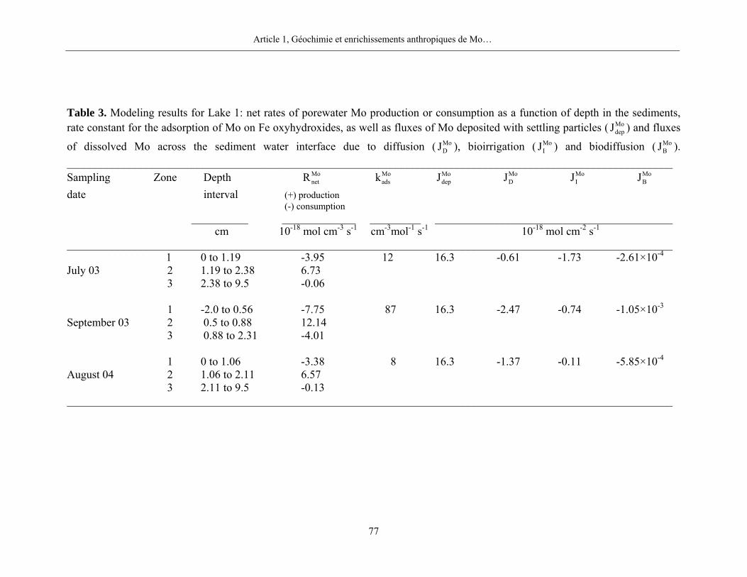
Article 1, Géochimie et enrichissements anthropiques de Mo…
77
Table 3. Modeling results for Lake 1: net rates of porewater Mo production or consumption as a function of depth in the sediments, rate constant for the adsorption of Mo on Fe oxyhydroxides, as well as fluxes of Mo deposited with settling particles ( Mo
depJ ) and fluxes
of dissolved Mo across the sediment water interface due to diffusion ( MoDJ ), bioirrigation ( Mo
IJ ) and biodiffusion ( MoBJ ).
___________________________________________________________________________________________________________ Sampling Zone Depth Mo
netR Moadsk Mo
depJ MoDJ Mo
IJ MoBJ
date interval (+) production (-) consumption __________ _____________ _________ __________________________________________ cm 10-18 mol cm-3 s-1 cm-3mol-1 s-1 10-18 mol cm-2 s-1 ___________________________________________________________________________________________________________ 1 0 to 1.19 -3.95 12 16.3 -0.61 -1.73 -2.61×10⁻⁴ July 03 2 1.19 to 2.38 6.73 3 2.38 to 9.5 -0.06 1 -2.0 to 0.56 -7.75 87 16.3 -2.47 -0.74 -1.05×10⁻³ September 03 2 0.5 to 0.88 12.14 3 0.88 to 2.31 -4.01 1 0 to 1.06 -3.38 8 16.3 -1.37 -0.11 -5.85×10⁻⁴ August 04 2 1.06 to 2.11 6.57 3 2.11 to 9.5 -0.13 ___________________________________________________________________________________________________________
Article 1, Géochimie et enrichissements anthropiques de Mo…
78
Figure captions
Figure 1. Map showing the location of Lakes Tantaré, Vose, Despériers and Holland
(numbered 1 to 4, respectively).
Figure 2. Triplicate porewater profiles of Mo (a-c), Fe and Mn (d-f), ∑S(-II) and pH
(g-i), as well as ion activity products (IAP) for MoS2(s) (j-l) and comparison of modeled
and measured average (n = 3) porewater Mo concentrations (m-o) for Lake 1 in July and
September 2003 and August 2004. The horizontal broken line indicates the sediment-
water interface. In panels j-l, the vertical dashed line indicates the solubility product of
MoS2(s) (see Table 2). In panels m-o, the thin solid line following the experimental points
(open circles) is PROFILE model fitting (r2 values indicated) and the thick solid line is
the net Mo consumption/production rate. Empty squares in panel (g) represent
concentrations below detection limit.
Figure 3. Triplicate porewater profiles of Mo (a-c), Fe and Mn (d-f), ∑S(-II) and pH
(g-i), as well as ion activity products (IAP) for MoS2(s) (j-l) for Lake 2 in September
2003, Lake 3 in June 2001 and Lake 4 in August 2005. The horizontal broken line
indicates the sediment-water interface. In panels j-l, the vertical dashed line indicates the
solubility product of MoS2(s) (see Table 2).
Figure 4. Depth concentration profiles of Mo (a-d), Fe and AVS (e-h), Mn (i-l), and Al
and Corg (m-p) as well as unsupported 210Pb and 137Cs activities as a function of
cumulative mass (q-t) in sediment cores (q-t) for all lakes. Panel (a) shows the measured
Mo concentrations (open circle) and reconstructed Mo concentrations at the time of
deposition (filled circle) in the sediments of Lake 1.
Figure 5. Historical records of atmospheric Mo fluxes in all lakes (a-c). The inset in
panel (b) represents Pb emissions from the Rouyn-Noranda smelter since 1965.
Article 1, Géochimie et enrichissements anthropiques de Mo…
79
Figure 6. Mo:Fe (grey lines) and Mo:Mn (dark lines) molar ratios as a function of pH
predicted by the surface complexation model for the adsorption of molybdate on
ferrihydrite and on poorly crystallized Mn oxyhydroxide. Solid and dashed lines are for
MoO42- equilibrium concentrations of 0.26 nM and 100 nM, respectively.
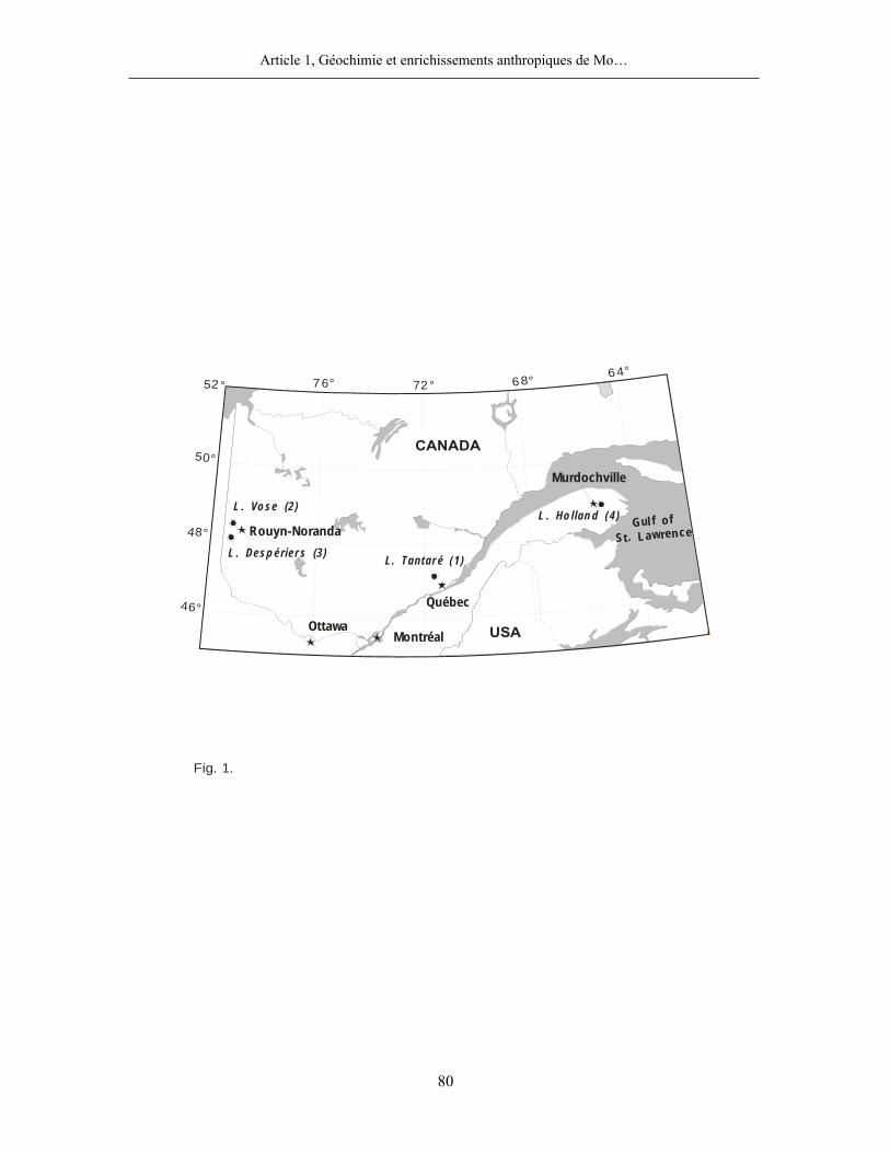
Article 1, Géochimie et enrichissements anthropiques de Mo…
80
USA
76° 72°64°
52°
50°
46°
48°
68°
Murdochville
Rouyn-Noranda
L . Vo se (2)L . Ho llan d (4)
L. Tantar é (1)L . Desp érier s (3)
Québec
MontréalOttawa
CANADA
Gul f ofSt. Lawrence
Fig. 1.
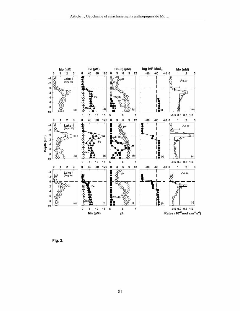
Article 1, Géochimie et enrichissements anthropiques de Mo…
81
0 1 2 3-4-202468
10
Mo (nM)0 40 80 120
Mn (µM)
0 5 10 15
0 3 6 9 12
5 6 7
Lake 1
Fe
Mn
Fe (µM) ΣS(-II) (µM)
0 1 2 3-4-202468
10
0 40 80 120
0 5 10 15
Mn
Fe
0 3 6 9 12
5 6 7
Lake 1
0 1 2 3-4-202468
10
Lake 1
0 40 80 120
0 5 10 15
Fe
Mn
0 3 6 9 12
5 6 7
Dep
th (c
m)
pH
pH
pH
pH
log IAP MoS2-80 -60 -40
Mo (nM)0 1 2 3
Rates (10-17mol cm-3 s-1)
-0.5 0.0 0.5 1.0
r2=0.97
-80 -60 -40 0 1 2 3
-0.5 0.0 0.5 1.0
r2=0.97
-80 -60 -40 0 1 2 3
-0.5 0.0 0.5 1.0
r2=0.90
(a)
(b)
(c)
(d)
(e)
(f)
(g)
(h)
(i)
(j)
(k)
(m)
(l)
(n)
(o)
ΣS(-II)
ΣS(-II)
ΣS(-II)
Fig. 2.
(July 03)
(Sept. 03)
(Aug. 04)
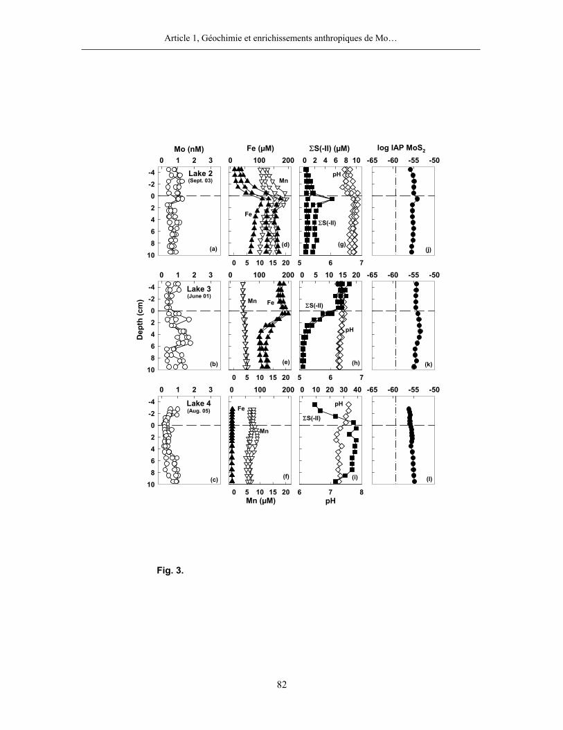
Article 1, Géochimie et enrichissements anthropiques de Mo…
82
0 10 20 30 40
6 7 8
0 100 200
0 5 10 15 20
0 100 200
0 5 10 15 20
0 2 4 6 8 10
5 6 7
Mo (nM) Fe (µM) ΣS(-II) (µM)
0 1 2 3-4-202468
10
(June 01)FeMn
0 5 10 15 20
5 6 7
0 1 2 3-4-202468
10
Lake 2Mn
Fe
0 1 2 3-4-202468
10
Lake 4
0 100 200
0 5 10 15 20
Fe
Mn
Mn (µM)
pH
pH
pH
pH
Dep
th (c
m)
log IAP MoS2
-65 -60 -55 -50
-65 -60 -55 -50
-65 -60 -55 -50
(a)
(b)
(c)
(d)
(e)
(f)
(g)
(h)
(i)
(j)
(k)
(l)
ΣS(-II)
ΣS(-II)
ΣS(-II)
(Sept. 03)
Lake 3
(Aug. 05)
Fig. 3.
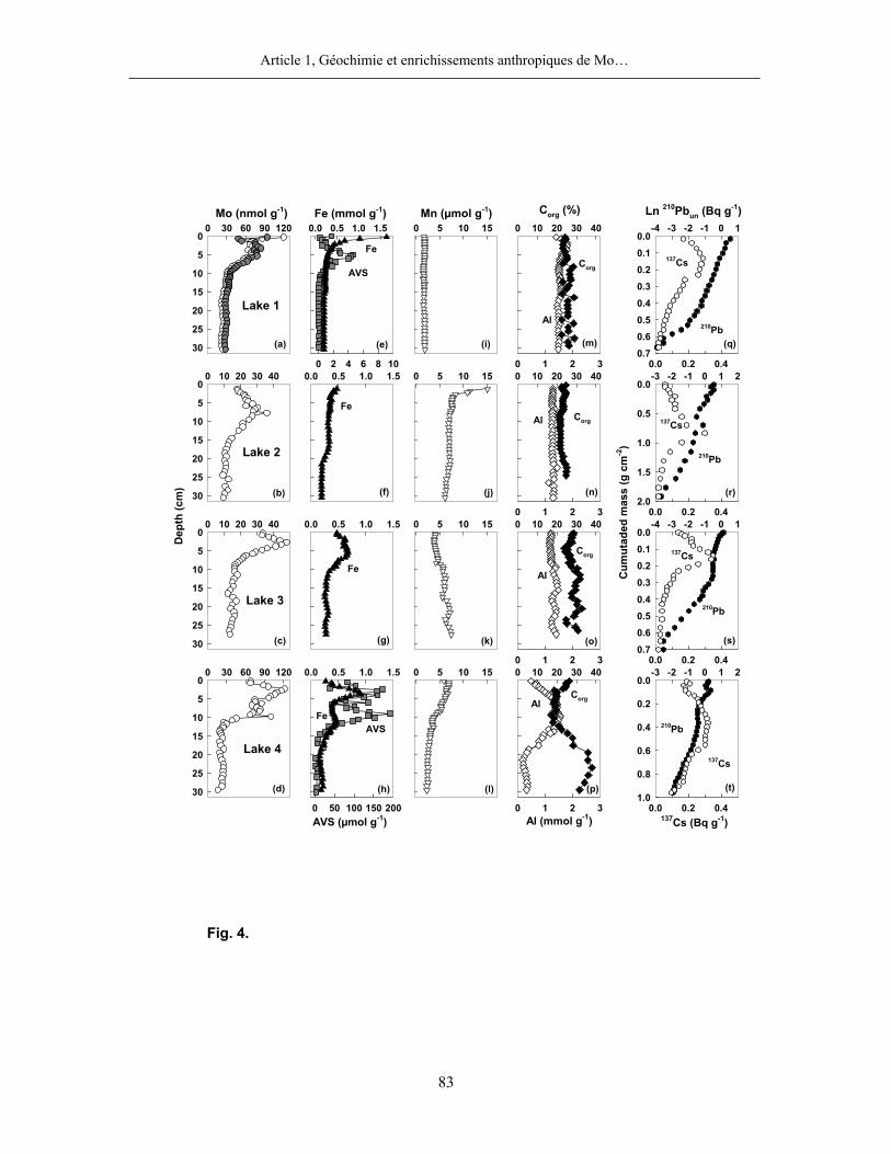
Article 1, Géochimie et enrichissements anthropiques de Mo…
83
0.0 0.5 1.0 1.5
0 50 100 150 200
-3 -2 -1 0 1 20.0
0.2
0.4
0.6
0.8
1.00.0 0.2 0.4
-4 -3 -2 -1 0 10.00.10.20.30.40.50.60.7
0.0 0.2 0.4
-3 -2 -1 0 1 20.0
0.5
1.0
1.5
2.00.0 0.2 0.4
0 10 20 30 40
0 1 2 3
0 10 20 30 40
0 1 2 3
0 10 20 30 40
0 1 2 3
0.0 0.5 1.0 1.5
Dep
th (c
m)
0 10 20 30 400
5
10
15
20
25
30
0 5 10 15
Lake 2
0 10 20 30 400
5
10
15
20
25
30
0.0 0.5 1.0 1.5 0 5 10 15
Lake 3
0 30 60 90 1200
5
10
15
20
25
30
0 5 10 15
Lake 4AVS
137Cs
137Cs
137Cs
210Pb
210Pb
Fe210Pb
CorgAl
Al
Corg
AlCorg
Cum
utad
ed m
ass
(g c
m-2
)
AVS (µmol g-1) Al (mmol g-1) 137Cs (Bq g-1)
(b)
(c)
(d)
(f)
(g)
(h)
(j)
(k)
(l)
(n)
(o)
(p)
(r)
(s)
(t)
Fe
Fe
Mo (nmol g-1)0 30 60 90 120
0
5
10
15
20
25
30
Fe (mmol g-1)0.0 0.5 1.0 1.5
0 2 4 6 8 10
Mn (µmol g-1)0 5 10 15
Lake 1
AVS
Corg (%)0 10 20 30 40
0 1 2 3
Ln 210Pbun (Bq g-1) -4 -3 -2 -1 0 1
0.00.10.20.30.40.50.60.7
0.0 0.2 0.4
137CsFe
210PbAl
Corg
(a) (e) (i) (m) (q)
Fig. 4.
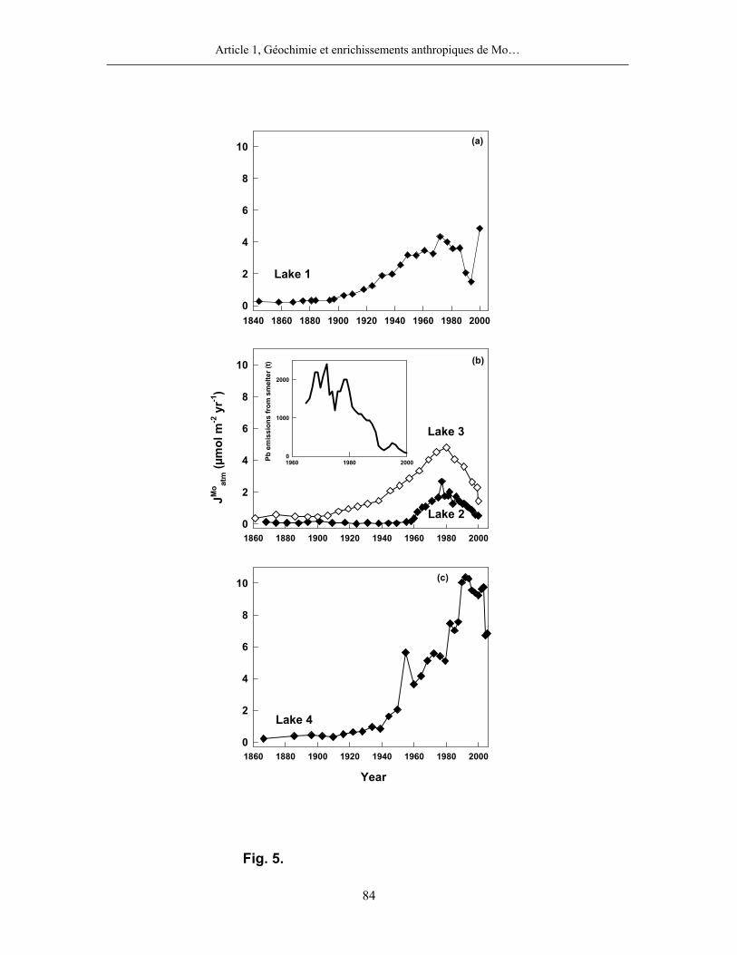
Article 1, Géochimie et enrichissements anthropiques de Mo…
84
1840 1860 1880 1900 1920 1940 1960 1980 2000
JMo at
m (µ
mol
m-2
yr-1
)
0
2
4
6
8
10
Year
1860 1880 1900 1920 1940 1960 1980 20000
2
4
6
8
10
1860 1880 1900 1920 1940 1960 1980 20000
2
4
6
8
10
1960 1980 2000Pb e
mis
sion
s fr
om s
mel
ter (
t)
0
1000
2000
Lake 1
Lake 3
Lake 2
Lake 4
(a)
(b)
(c)
Fig. 5.
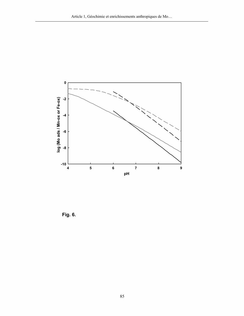
Article 1, Géochimie et enrichissements anthropiques de Mo…
85
pH4 5 6 7 8 9
log
(Mo
ads
/ Mn-
ox o
r Fe-
ox)
-10
-8
-6
-4
-2
0
Fig. 6.

ARTICLE 2
Sequestration mechanisms and anthropogenic inputs of rhenium in sediments
from Eastern Canada lakes
Soumis le 18/02/2008 dans Geochimica et Cosmochimica Acta.
Anthony Chappaz, Charles Gobeil et André Tessier
INRS-ETE, Université du Québec, 490 de la Couronne, Québec (QC), G1K 9A9, Canada
Article 2, Mécanismes de séquestration et apports anthropiques de Re…
88
RÉSUMÉ
Les concentrations de Re, ainsi que celles de plusieurs paramètres géochimiques, ont été
mesurées dans des carottes de sédiment datées et dans des échantillons d’eau interstitielle de
quatre bassins lacustres de l’est du Canada : un, oxygéné en permanence, est situé à 40 km de la
ville de Québec et trois, saisonnièrement anoxiques, sont situés dans un rayon de 25 km de
fonderies de métaux non-ferreux. Les bassins de drainage de ces lacs sont inhabités et n’ont pas
été affectés par l’activité humaine ou les feux de forêts. Tous les profils de Re dissous affichent
des concentrations de Re plus élevées dans les eaux sus-jacentes aux sédiments que dans les eaux
porales, une diminution progressive des concentrations de Re avec la profondeur et une atteinte
de valeurs minimales (~0,5 pM) entre l’interface eau-sédiment et 10 cm de profondeur. La
modélisation des profils de Re dans les eaux porales avec une équation de transport réaction
unidimensionnelle indique que le Re est retiré de l’eau interstitielle dans cet intervalle de
profondeur. Sur la base des prédictions thermodynamiques de la spéciation du Re dissous et de
l’état de saturation de phases minérales distinctes et la comparaison de ces prédictions avec les
profils de sulfure dans les eaux porales, nous proposons que le Re précipite dans les sédiments
sous forme de rheniite (ReS2(S)). La constante de vitesse, estimée par modélisation, pour la
formation de ReS2(S) dans les sédiments est de 0,51±0,64 × 10⁻²¹ mol cm-3 s-1. Comme dans les
sédiments anoxiques marins, le Re qui s’accumule comprend une forte composante authigène.
Toutefois, l’augmentation prononcée de Re, au cours du siècle dernier, dans la phase solide est
attribuée à la déposition atmosphérique de Re d’origine anthropique provenant de la combustion
du charbon et des émissions des fonderies environnantes.
Article 2, Mécanismes de séquestration et apports anthropiques de Re…
89
ABSTRACT
The concentrations of Re, as well as those of several other geochemical variables, were
measured in dated sediment cores and in porewater samples from four lacustrine basins in
Eastern Canada: one, perennially oxic, located 40 km from Québec City and three, seasonally
anoxic, located within 25 km of non-ferrous metal smelters. The drainage basins of these lakes
are uninhabited and have not been affected by human activity or wildfires. All of the depth
profiles of dissolved Re indicate: higher Re concentrations in the water overlying the sediment
than in the porewater; diffusion of Re across the sediment-water interface; a progressive decrease
in porewater Re concentrations to reach minimum values of ~0.5 pM within a 10-cm sediment
depth interval. Modeling of these Re porewater profiles with a one-dimensional transport-
reaction equation indicates that Re is removed from porewater within this depth interval. Based
on thermodynamic predictions of Re speciation and of saturation states and on comparison of
these predictions with sulfide porewater profiles, we infer that Re is removed from porewater by
precipitation of rheniite (ReS2(s)). The rate constant for the formation of ReS2(s) in sediments is
estimated from the modeling exercise to be 0.51±0.64×10⁻²¹ mol cm-3 s-1. Accumulation of
sedimentary Re shows a strong authigenic component, as in anoxic marine sediments. Sharp
increases in solid-phase Re during the last century are attributed to atmospheric deposition of
anthropogenic Re deriving from coal burning and nearby smelter emissions.
Article 2, Mécanismes de séquestration et apports anthropiques de Re…
90
1. INTRODUCTION
Studies in marine environments show a high degree of rhenium (Re) enrichment in
reducing sediments compared both to oxic sediments and to crustal abundance (Koide et al.,
1986; Ravizza et al., 1991; Crusius et al., 1996). In oxic seawater, this metal is present largely as
ReO4-, has little affinity for settling particles, remains in solution, and is considered to be a
conservative element (Anbar et al., 1992). In contrast, its solubility is low in reduced sediments.
The Re concentration gradient thus generated across the sediment-water interface drives a flux of
dissolved Re into the sediments, the importance of which should depend on the flux of organic
matter to the sediment surface and/or the bottom water oxygen content (Colodner et al., 1993;
Morford et al., 2007). Thus Re accumulation in anoxic marine sediments proceeds essentially via
the transport of dissolved Re across the sediment-water interface. Given these particularities, it
has been proposed that authigenic Re has the potential to be a tracer of paleoredox conditions
existing in the sediment and in the water column when sediments were deposited and/or to infer
past variations in organic carbon flux at the seafloor (Calvert and Pedersen, 1993; Russell and
Morford, 2001; Nameroff et al., 2002, 2004).
Adequate knowledge of Re geochemistry is a requirement for correctly reconstructing,
from sedimentary records, the past conditions prevailing when sediments were deposited.
However, because many uncertainties about the nature and kinetics of the reactions responsible
for Re removal from porewater remain, the use of Re as a paleoredox tracer is not fully reliable
(e.g. Morford and Emerson, 1999; Crusius and Thomson, 2000, 2003; Morford et al., 2001;
Sundby et al., 2004; McKay et al., 2007). Clarification of Re geochemistry is also of interest for
using Re-Os as a geochronometer for dating ancient sediments (Ravizza and Turekian, 1989;
Kendall et al., 2004) as well as to obtain a better understanding, by analogy, of the geochemistry
of 99Tc, a soluble by product of 235U fission (Kim and Boulègue, 2003). Furthermore, information
on the importance of anthropogenic inputs to sedimentary Re enrichment is very limited
(Colodner et al., 1995).
Our study focuses on porewater and sediment geochemistry of Re in four lakes exhibiting
different geochemical conditions. We determined concentration profiles of porewater and solid
phase Re as well as those of complementary variables in these lakes. Our extensive dataset is
Article 2, Mécanismes de séquestration et apports anthropiques de Re…
91
used to clarify reactions involving Re during the early stages of sediment diagenesis and to obtain
information on atmospheric sources of Re to the lakes. These results should be useful to those
working in marine geochemistry and paleoceanography.
2. METHODS
2.1. Study sites and sampling
This study took place in Lakes Tantaré, Despériers, Vose and Holland (Fig. 1). Lake
Tantaré is located in an ecological reserve, 40 km northwest of Québec City, a medium-sized city
having a population of approximately half a million. Lakes Despériers and Vose are located
within 25 km of Rouyn-Noranda, where an important copper smelter (current production of
180,000 tons yr-1 of anode copper and 600,000 tons yr-1 of sulphuric acid; www.noranda.com) has
operated since 1927, whereas Lake Holland is situated 8 km southeast of Murdochville, where a
smaller non-ferrous metal smelter (production of 102,700 tons yr-1 of anode copper and 164,600
tons yr-1 of sulphuric acid in 1995; www.ec.gc/toxics/docs/sor/bms/FR/app614.cfm) was in
operation from 1955 to 2002. The drainage basins of these four Eastern Canada oligotrophic
lakes are uninhabited and have not been affected by lumbering or wildfires for at least 100 yr,
and thus their only anthropogenic inputs are via the atmosphere. The hypolimnion of the studied
basin in Lake Tantaré, whose maximum depth is 15 m, remains oxygenated throughout the year.
The hypolimnia of Lakes Despériers, Vose and Holland, whose maximum depths are 14, 17 and
11 m, respectively, become seasonally anoxic in summer and were anoxic at the sampling time.
Sediment cores and porewater samples were collected by divers between June 2001 and August
2005 at the deepest site in each lake. Furthermore, Teflon sheets that had been inserted vertically
and left in Lake Tantaré sediments for 12 yr were retrieved along with the Fe-rich diagenetic
material that they accumulated. Details on sampling procedures are given in Chappaz et al.
(2008).
2.2. Analyses
Our measurements of Re concentrations described below were carried out on the cores,
Fe-rich diagenetic material and porewater samples collected by Chappaz et al. (2008). The
methods used for the other measurements carried out on the solid phase (Al, Fe, Mn, total N, total
C, 137Cs, 210Pb, 214Pb), on the diagenetic material collected on Teflon sheets (Fe, Mo, organic C)
Article 2, Mécanismes de séquestration et apports anthropiques de Re…
92
and on the porewater samples (pH, Mo, Fe, Mn, Ca, K, Mg, Na, sulfide (ΣS(-II)), SO42-, and
organic and inorganic carbon) are reported in Chappaz et al. (2008). Porewater Re concentrations
were determined using an inductively coupled plasma quadrupole mass spectrometer (ICP-MS;
Thermo Instrument X7) using an external calibration. Analytical precision, as determined from
replicate analysis (n=11) of a natural freshwater sample was 5%. Detection limit, defined as 3
standard deviations of replicate measurements of a blank solution, was 0.15 pM. Fe-rich
authigenic deposits were completely dissolved in 50% HCl for 48 h at room temperature, filtered
(0.4 µm Teflon filters) and the resulting solutions were analysed by ICP-MS. Freeze-dried
sediment samples were homogenized by grinding and totally digested with a mixture of HNO3,
HClO4 and HF. Acids were evaporated to near dryness and residues redissolved in a 0.2 N HNO3
solution (McLaren et al., 1995). Rhenium concentrations in these solutions were measured by
ICP-MS. The detection limit, defined as 3 standard deviations of replicate measurements of blank
solutions, was 0.1 pmol g-1. Analytical precision, determined from replicate analyses (n=9) of the
same sediment sample was 8%.
2.3. Chemical speciation and sediment dating
Speciation of porewater Re was calculated with the computer software MINEQL+
(Schecher and McAvoy, 1998), using our measured values of pH and total concentrations of
dissolved Re, Fe, Mn, K, Mg, Ca, Na, inorganic carbon, SO42-, Cl- and ΣS(-II) as inputs. We
assumed that the redox potential was fixed by the couples: O2/H2O in the overlying water of Lake
Tantaré, Fe(II)/Fe(OH)3(s) in porewater samples with sulfide values < 0.1 μM and SO42-/HS- in
samples with sulfide concentrations > 0.1 μM. For these calculations, the thermodynamic
database of MINEQL+ was updated for the reactions given in Table 1.
Methods for the determination of sediment age and accumulation rate (ω) are described in
Chappaz et al. (2008). Ranges found for ω were 3.5 - 6.7 mg cm-2 yr-1, 4.5 - 15.7 mg cm-2 yr-1,
3.8 mg cm-2 yr-1 and 7.8 - 16.4 mg cm-2 yr-1 for Lakes Tantaré, Holland, Despériers and Vose,
respectively.
Article 2, Mécanismes de séquestration et apports anthropiques de Re…
93
3. RESULTS AND DISCUSSION
3.1. Porewater Re profiles
The triplicate porewater Re profiles obtained for a given lake and sampling date were
similar (Fig. 2a-f), indicating that they were not artefacts associated with our sampling and
handling procedures. The highest dissolved Re concentrations were found in water overlying the
sediment, where they reached 6, 35, 38 and 7 pM in Lakes Tantaré, Despériers, Vose and
Holland, respectively. While the highest values measured in Lakes Tantaré and Holland were
typical of those reported for freshwater environments (~ 2.3 pM; Colodner, 1991), maximum
values in Lakes Despériers and Vose were much higher. These high dissolved Re concentrations
found in the bottom waters of Lakes Despériers and Vose can be attributed to atmospheric
deposition from the nearby smelter at Rouyn-Noranda. The dissolved Re concentration profiles
consistently showed that Re diffused across the sediment-water interface and that, as it migrated
downward, it was progressively removed from the porewater to reach minimum concentrations.
Such a trend is commonly found for dissolved Re in marine porewater (Colodner et al., 1993;
Morford et al., 2005; Morford et al., 2007). Our Re profiles did not show any evidence of Re
release to the porewater upon reductive remobilisation of Fe (Fig 2m-q) or Mn (Fig. 2q-r), which
suggests that Re was not adsorbed to Fe or Mn oxyhydroxides. Consistently, Re concentrations in
the diagenetic material collected on Teflon sheets were below the detection limit. These
observations are consistent with previous field (Anbar et al., 1992; Colodner et al., 1993;
Morford et al., 2007) and laboratory (Yamashita et al., 2007) studies which reported that ReO4-,
the predominant Re species in oxic waters, does not sorb onto particles.
Speciation calculations with MINEQL+ predict that ReO4- was the dominant species (≥
99%) in the overlying waters of Lake Tantaré whereas the neutral 04Re(OH) species became the
dominant species (≥ 99%) in the overlying water of the three anoxic lakes as well as in the
porewater of all lakes (Fig. 2ε-φ). The two dissolved Re species are interrelated by the following
equation (Xiong, 2003; Table 1):
- + 04 4ReO + 3e + 4H = Re(OH) (1)
Article 2, Mécanismes de séquestration et apports anthropiques de Re…
94
Diagenetic modeling of the porewater Re profiles can provide information on the cycling
of Re and on the reactions involved. We modeled our porewater Re profiles with the following
one-dimensional mass conservation equation, assuming steady-state and neglecting advective
fluxes due to sediment compaction and groundwater flow (Boudreau, 1997):
[ ] ( ) [ ] [ ] [ ]( ) ReRe ReRe - Re 0S B netburrow
x
D D Rt x x
φφ φα
⎛ ⎞ ⎛ ⎞∂ ∂∂= + + + =⎜ ⎟ ⎜ ⎟∂ ∂ ∂⎝ ⎠ ⎝ ⎠
(2)
In Eq. (2), x is depth (cm; positive downward from the sediment-water interface), φ is sediment
porosity, t is time (s), DS is the effective diffusion coefficient (cm2 s-1), BD is the biodiffusion
coefficient (cm2 s-1), [ ]Reburrow is the concentration of dissolved Re in the burrows of benthic
animals (mol cm-3 of porewater), which we assume to be identical to that in the water overlying
the sediments, [ ]Re is the porewater Re concentration (mol cm-3),α is the bioirrigation
coefficient (s-1), and RenetR is the net reaction rate (mol cm-3 of whole sediment s-1) of porewater Re
production (if RenetR > 0) or consumption (if Re
netR < 0).
Equation 2 was solved numerically for RenetR using the code PROFILE (Berg et al., 1998)
for the average dissolved Re profile obtained for each lake and date, using our measured values
of φ and the following values of DS, DB and α. We assumed that DS = φ2 Dw (Berner, 1980) where
Dw is the tracer diffusion coefficient of the Re species present in porewater, i.e., 04Re(OH)
according to the speciation calculation. Since the Dw value of 04Re(OH) has never been measured,
we used an estimate of 1.1×10⁻⁵ cm2 s-1 at 25 oC, on the basis that this species behaves similarly
to other uncharged species (Boudreau, 1997). This Dw value was corrected for in situ temperature
with the Stokes-Einstein equation (Boudreau, 1997). For Lake Tantaré, whose sediment-water
interface remains perennially oxic, we used in Eq. (2) the biodiffusion coefficient (2.2×10⁻⁹ cm2
s-1) provided by Gallon et al. (2004) for these sediments. This coefficient was determined on the
basis of an extensive inventory of the benthic fauna, mostly chironomids, at the sampling site
(Hare et al., 1994) and of biodiffusion coefficients measured by Matisoff and Wang (2000) for
chironomids. The bioirrigation coefficient (α ) for this lake was assumed to decrease linearly
Article 2, Mécanismes de séquestration et apports anthropiques de Re…
95
from α0 at the sediment surface to zero at 10 cm depth, because chironomids are generally not
found below this sediment depth (Matisoff and Wang, 1998), and α0 was derived from the
following relationship provided by Boudreau (1984):
( )( )0 1
2 22 1 1- -
S
a
D rr r r r
α = (3)
where 1r is the radius of a chironomid’s tube (assumed to be 0.1 cm), 2r is half the distance
between adjacent tubes (1.5 cm), and ar is equal to 2r /2. Given the seasonal development of
anoxic events in Lakes Despériers, Vose and Holland, we assumed that the biodiffusion ( BD ) and
bioirrigation (α ) coefficients were negligible for these lakes.
Fitting of the experimental data by PROFILE is excellent (r2 = 0.95-0.99; Fig. 2s-x); it
consistently shows that dissolved Re was removed from porewater over the whole depth (10 cm)
of sediment sampled, with the exception of Lake Tantaré in September 2003, for which
porewater Re consumption occured between 3 and 10 cm. Net Re removal rate ( RenetR ) ranged
between -0.3×10⁻²¹ mol cm-3 s-1 and -2.8×10⁻²¹ mol cm-3 s-1 (Table 2). The RenetR values are 4-8
times higher (-1.6×10⁻²¹ mol cm-3 s-1 to -2.8×10⁻²¹ mol cm-3 s-1) in Lakes Despériers and Vose,
which are contaminated by the Rouyn-Noranda smelter, than in the other two lakes.
3.2. Immobilization mechanism
The mechanism responsible for Re removal in marine porewater has not been clarified,
although precipitation of an unidentified authigenic Re phase has often been suggested (Ravizza
et al., 1991; Colodner et al., 1993; Crusius et al., 1996; Morford et al., 2007). According to
Nameroff et al. (2002) and Tribovillard et al. (2006), the most likely precipitates to form in
anoxic porewater are rheniite (ReS2(s)), rhenium oxide (ReO2(s)) and dirhenium heptasulfide
(Re2S7(s)). The extensive database gathered in our study allows us to verify the saturation state of
porewater samples with respect to ReS2(s) and ReO2(s), for which thermodynamic data can be
found in the literature. To this end, we used the 0fΔG data provided by Brookins (1986) and
Wagman et al. (1982) to calculate the solubility products (Ks) for the following reactions,
Article 2, Mécanismes de séquestration et apports anthropiques de Re…
96
- + -2(S) 2 4ReS + 4H O = ReO + 3e + 6H + 2HS (4)
- +2(S) 2 4ReO + 2H O = ReO + 3e + 4H (5)
which are 10-77 and 10-26, respectively, at 25 oC (Table 1). The ion activity products (IAP)
corresponding to reactions (4) and (5) are defined as:
2- 3 + 6 - 24IAP = (ReO ) (e) (H ) (HS ) (6)
2- 3 + 44IAP = (ReO ) (e) (H ) (7)
respectively, where e denotes the electron and ( ) is the activity of a given species.
Comparison of Fig. 2g-l with Fig. 2y-δ reveals that porewater was close to saturation or
slightly oversaturated with respect to ReS2(S) when ΣS(-II) was at µM levels. In contrast,
comparison of IAP with the Ks of ReO2(S) indicates that the porewater of all lakes was largely
undersaturated (IAP ≤ 10-253Ks) with respect to this solid (data not shown). These saturation state
calculations indicate that only the precipitation of ReS2(S) is thermodynamically possible. The
formation of this Re-bearing solid phase is consistent with the laboratory finding that Re was
present as Re(IV) in reducing sediments after its removal from ReO4--containing artificial
seawater (Yamashita et al. 2007). It also agrees with predictions for dissolved Re concentrations
in the water column of the Black Sea at depths where ΣS(-II) is < 30 µM (if 04Re(OH) was
assumed to be in equilibrium with ReS2(S)) (Xiong, 2003). At greater depths, where ΣS(-II)
reached higher values, Xiong (2003) predicted that Black Sea water should be oversaturated with
respect to ReS2(S), presumably due to the presence of unknown reduced Re species that were not
taken into account in his calculation. Thus, collectively, our results and the calculations of Xiong
(2003) point to the formation of ReS2(S) as the likely mechanism for the removal of dissolved Re
in sulfidic (pore)water. Note that this observation does not contradict the purported idea that
authigenic Re accumulation occurs in suboxic environments (e.g. Crusius et al., 1996; Morford
et al., 2005). Indeed, suboxic environments are loosely defined, and may contain trace amounts
of sulfide that could be sufficient to precipitate ReS2(S).
Article 2, Mécanismes de séquestration et apports anthropiques de Re…
97
If we assume that removal of Re from porewater results from the precipitation of ReS2(s),
the values of RenetR (Table 2) can be used to estimate the rate constant for this reaction. The
removal rate can be expressed as (Meysman et al., 2003):
Re Re 1avnet ppt
s
IAPR kK
φ⎛ ⎞
= − −⎜ ⎟⎝ ⎠
(8)
where Repptk (mol cm-3 s-1) is an apparent rate constant and the subscript "av" indicates average
values over the depths where Re is removed from porewater since RenetR values are piece-wise
constants. The values of Repptk , calculated with Eq. (8), are given in Table 2, with the exception of
those for Lake Tantaré in August 2004 when the porewater showed undersaturation with respect
to ReS2(s) (Fig. 2α). These values of Repptk vary between 0.03×10⁻²¹ mol cm-3 s-1 and 1.3×10⁻²¹ mol
cm-3 s-1, indicating that the actual expression for Re removal rate from porewater is more
complex than that shown in Eq. 8. Several factors could explain the high variability
in Repptk observed among lakes. The rate constant Re
pptk incorporates the effects of reactive surface
area as well as catalysis and inhibition by dissolved constituents, which can all vary among lakes
(Van Cappellen et al., 1993; Meysman et al., 2003). Furthermore, the fact that PROFILE yields
constant values of RenetR over relatively large sediment depth intervals and that the Ks value for
ReS2(s) is uncertain likely explain in part this variability. Lastly, it is possible that the reduction of
ReO4- to 0
4Re(OH) , rather than the precipitation of ReS2(s) is the limiting step in the removal of
Re from porewater. Field and laboratory measurements suggest that reduction of ReO4- is a slow
process (Crusius and Thompson, 2000; Sundby et al., 2004; Yamashita et al., 2007).
No other values of Repptk have been determined for sediments. However, Gallon et al.
(2004) reported that the rate constant for the precipitation of PbS(s) ( Pbpptk ) varied from 3×10-22 mol
cm-3 s-1 to 8×10-20 mol cm-3 s-1, depending largely on the value chosen for the Ks of PbS(s). Our
values of Repptk fall within the range of those estimated for Pb
pptk , but are 3-5 orders of magnitude
lower than the value of the rate constant currently assumed in diagenetic models for the

Article 2, Mécanismes de séquestration et apports anthropiques de Re…
98
precipitation of FeS(S), i.e. 3×10-17 mol cm-3 s-1 (Van Cappellen and Wang, 1995; Meysman et al.,
2003).
3.3. Diagenetic imprint on the sedimentary record
In all of our lakes, the concentration of measured sedimentary Re increases upwards from
a relatively constant value below the depths corresponding to the beginning of the industrial era
(∼1900), reaches a maximum between 2 and 8 cm, and then decreases toward the sediment
surface (Fig. 3). The average (±SD) pre-1900 background concentrations are 41±5, 51±6, 21±3
and 21±2 pmol g-1 in Lakes Tantaré, Despériers, Vose and Holland, respectively. These values
are in the lower range of those measured in marine sediments, i.e. 5-268 pmol g-1 (Ravizza et al.,
1991; Crusius et al., 1996; Gobeil et al., 2001; Sundby et al., 2004). Normalisation to Al is often
used to estimate the detrital contribution of an element. In our lake sediments, Al concentrations
(data not shown) varied little with depth, except in Lake Holland where they decreased sharply
above 5 cm and below 15 cm as the organic C content increased (Chappaz et al.; 2008). The
average (±SD) molar Re:Al ratios at depths below sediment from the industrial era are
2.7±0.3×10⁻⁸, 3.7±0.3×10⁻⁸, 1.6±0.2×10⁻⁸ and 2.8±0.2×10⁻⁸ in Lakes Tantaré, Despériers, Vose
and Holland, respectively (Fig. 3); the average value for Lake Holland was obtained from the
Re:Al values between 14.5 cm and 17.5 cm only. The subsurface maximum Re concentrations
are 1.9, 4.9, 6.6 and 4.2 times higher than the background Re values in Lakes Tantaré,
Despériers, Vose and Holland, respectively; the Re:Al molar ratios corresponding to these
subsurface maxima are 4.0×10⁻⁸, 19×10-8, 11×10-8, and 9.0×10⁻⁸ (Fig. 3).
The pre-1900 molar Re:Al ratios measured in the four lakes are approximately two orders
of magnitude larger than those reported for the earth’s crust (7.3×10⁻¹⁰; Wedepohl, 1995) and for
shales (8.7×10⁻¹⁰; Borchers et al., 2005). These large molar Re:Al ratios in lake sediments
indicate that the measured pre-1900 Re concentrations comprise substantial authigenic
contributions, presumably from Re transport across the sediment-water interface and its removal
from porewater. Indeed, the total flux responsible for Re accumulation in the sediments ( ReaccJ )
can be considered to be the sum of the fluxes of Re deposited at the sediment surface with
Article 2, Mécanismes de séquestration et apports anthropiques de Re…
99
settling particles ( RedepJ ) and those of dissolved Re across the sediment water interface by
molecular diffusion ( ReDJ ), bioirrigation ( Re
IJ ) and bioturbation ( ReBJ ):
Re Re Re Re Re acc dep D I BJ J J J J= + + + (9)
The present-day values of these various fluxes (Table 2) were obtained as follows. The RedepJ values for all lakes were obtained by multiplying the sediment mass accumulation rate (ω)
obtained from the 210Pb geochronology for the top 0.5-cm sediment layer by the value of the Re
concentrations measured in the sediments of this layer; we thus assumed that the diagenetic
contributions to the measured Re concentrations in this sediment layer were negligible. The
values of ReDJ , Re
IJ and ReBJ were provided as output from PROFILE; those of Re
IJ and ReBJ were
assumed to be zero for the lakes with anoxic hypolimnia. As shown in Table 2, the transport of
dissolved Re across the sediment-water interface is responsible for 20-35%, 53%, 47% and 19%
of the present-day total accumulation of Re in the sediments of Lakes Tantaré, Despériers, Vose
and Holland, respectively. Authigenic contributions of similar magnitude before the industrial era
would at least partially explain the high Re:Al molar ratios observed for background sediment
samples compared to those of earth’s crust.
We attempted to estimate the contribution of early diagenesis to the sedimentary record of
Re by using the RenetR provided by the code PROFILE, as suggested in other studies (Gallon et al.,
2004; Laforte et al., 2005; Chappaz et al., 2008). Considering that the net consumption rate of Re
( RenetR ) in porewater is identical to the negative net rate of Re fixation to the solid phase, we can
write that (Chappaz et al., 2008):
Re Re[Re] - netreaction reaction
ddR mdt dt
φ⎛ ⎞⎛ ⎞= = ⎜ ⎟⎜ ⎟
⎝ ⎠ ⎝ ⎠ (10)
Article 2, Mécanismes de séquestration et apports anthropiques de Re…
100
where [ ]Re represents the dissolved Re concentration (mol cm-3), Re is the solid phase Re
concentration (mol g-1), and m is the dry bulk density (g cm-3of whole sediment). The subscript
"reaction" indicates reaction rates in solution and in the solid phase. From Eq. 10 it follows that:
Re Re
Re - -
net net
S
R Rd dt dxm m v
= = (11)
and
Re Re
00
Re - -
i ix x x x
net netauthigenic
xS Sx
R Rdx xm v m v
= =
==
= ≈ Δ∑∫ (12)
where xi is the depth of a sediment layer and Sv is the sedimentation rate (cm yr-1). The term
Reauthigenic
can be viewed as the solid Re concentration gained by a layer of sediment during its
burial to depth xi. Calculations of authigenicRe were done using average values for Re
netR obtained
for all of the sampling dates in Lake Tantaré and the single values determined for Lakes
Despériers, Vose and Holland (Table 2). Figure 3 shows that predicted Reauthigenic
values
represent less than 10% of the measured Re concentration in the first 2 cm below the sediment-
water interface in Lakes Tantaré and Holland, with this proportion increasing progressively to
reach 57% and 23%, respectively, at 9.75 cm depth. In sediments from Lakes Despériers and
Vose, Reauthigenic
is ≤ 15% of the measured Re concentration at 2.25 cm depth, but this
proportion increases sharply with depth, even exceeding the measured Re concentrations below 7
cm depth in Lake Despériers sediments.
These results clearly indicate that Re added to the sediments through diffusion across the
sediment-water interface and subsequent immobilisation is important. However, our calculations
likely overestimate Reauthigenic
, especially in Lake Despériers sediments. This can be explained if
dissolved Re concentrations in the water column of the lakes has progressively increased over the
last century due to human activity (Re is highly soluble in oxic waters). This contention is
supported by the higher Re concentrations presently measured in the overlying waters of Lakes
Vose and Despériers (more heavily contaminated by Re) than in those of Lakes Tantaré and
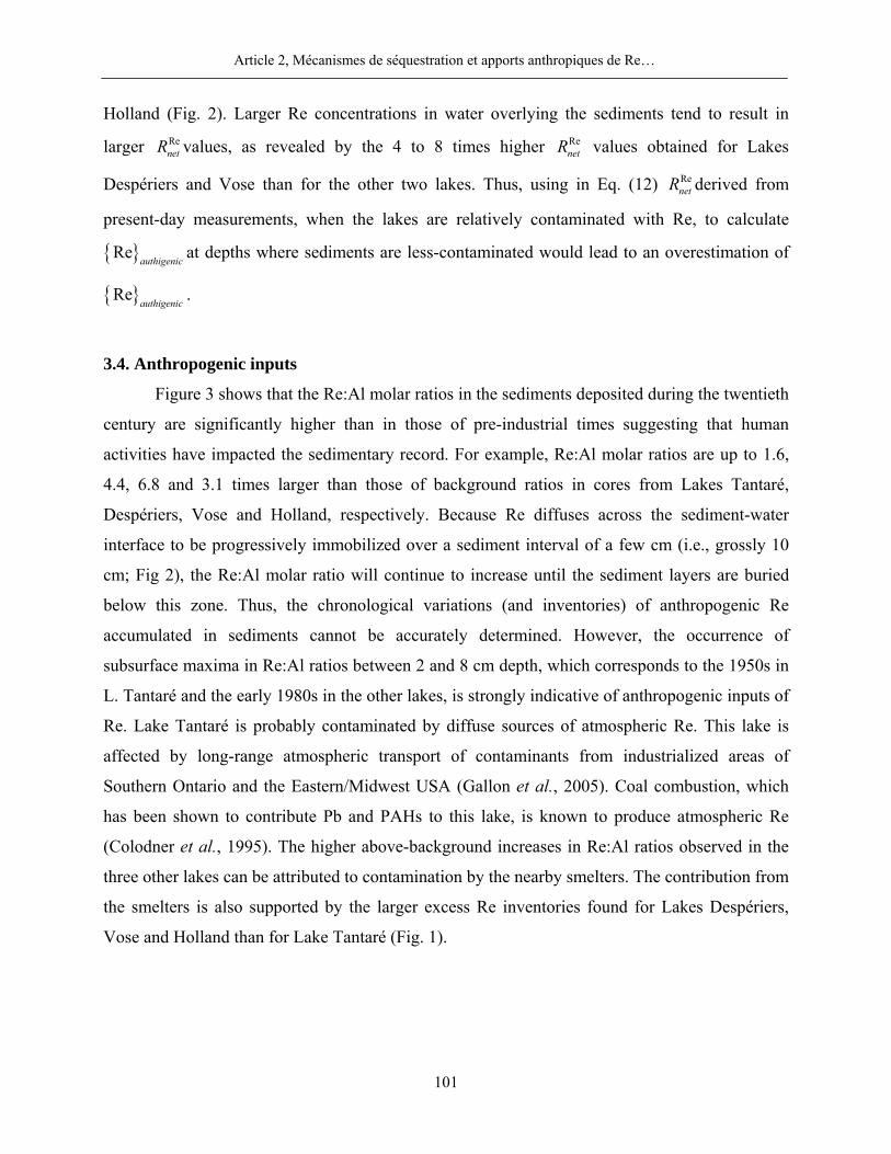
Article 2, Mécanismes de séquestration et apports anthropiques de Re…
101
Holland (Fig. 2). Larger Re concentrations in water overlying the sediments tend to result in
larger RenetR values, as revealed by the 4 to 8 times higher Re
netR values obtained for Lakes
Despériers and Vose than for the other two lakes. Thus, using in Eq. (12) RenetR derived from
present-day measurements, when the lakes are relatively contaminated with Re, to calculate
Reauthigenic
at depths where sediments are less-contaminated would lead to an overestimation of
Reauthigenic
.
3.4. Anthropogenic inputs
Figure 3 shows that the Re:Al molar ratios in the sediments deposited during the twentieth
century are significantly higher than in those of pre-industrial times suggesting that human
activities have impacted the sedimentary record. For example, Re:Al molar ratios are up to 1.6,
4.4, 6.8 and 3.1 times larger than those of background ratios in cores from Lakes Tantaré,
Despériers, Vose and Holland, respectively. Because Re diffuses across the sediment-water
interface to be progressively immobilized over a sediment interval of a few cm (i.e., grossly 10
cm; Fig 2), the Re:Al molar ratio will continue to increase until the sediment layers are buried
below this zone. Thus, the chronological variations (and inventories) of anthropogenic Re
accumulated in sediments cannot be accurately determined. However, the occurrence of
subsurface maxima in Re:Al ratios between 2 and 8 cm depth, which corresponds to the 1950s in
L. Tantaré and the early 1980s in the other lakes, is strongly indicative of anthropogenic inputs of
Re. Lake Tantaré is probably contaminated by diffuse sources of atmospheric Re. This lake is
affected by long-range atmospheric transport of contaminants from industrialized areas of
Southern Ontario and the Eastern/Midwest USA (Gallon et al., 2005). Coal combustion, which
has been shown to contribute Pb and PAHs to this lake, is known to produce atmospheric Re
(Colodner et al., 1995). The higher above-background increases in Re:Al ratios observed in the
three other lakes can be attributed to contamination by the nearby smelters. The contribution from
the smelters is also supported by the larger excess Re inventories found for Lakes Despériers,
Vose and Holland than for Lake Tantaré (Fig. 1).
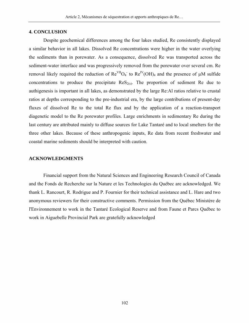
Article 2, Mécanismes de séquestration et apports anthropiques de Re…
102
4. CONCLUSION
Despite geochemical differences among the four lakes studied, Re consistently displayed
a similar behavior in all lakes. Dissolved Re concentrations were higher in the water overlying
the sediments than in porewater. As a consequence, dissolved Re was transported across the
sediment-water interface and was progressively removed from the porewater over several cm. Re
removal likely required the reduction of ReVIIO4- to ReIV(OH)4 and the presence of µM sulfide
concentrations to produce the precipitate ReS2(s). The proportion of sediment Re due to
authigenesis is important in all lakes, as demonstrated by the large Re:Al ratios relative to crustal
ratios at depths corresponding to the pre-industrial era, by the large contributions of present-day
fluxes of dissolved Re to the total Re flux and by the application of a reaction-transport
diagenetic model to the Re porewater profiles. Large enrichments in sedimentary Re during the
last century are attributed mainly to diffuse sources for Lake Tantaré and to local smelters for the
three other lakes. Because of these anthropogenic inputs, Re data from recent freshwater and
coastal marine sediments should be interpreted with caution.
ACKNOWLEDGMENTS
Financial support from the Natural Sciences and Engineering Research Council of Canada
and the Fonds de Recherche sur la Nature et les Technologies du Québec are acknowledged. We
thank L. Rancourt, R. Rodrigue and P. Fournier for their technical assistance and L. Hare and two
anonymous reviewers for their constructive comments. Permission from the Québec Ministère de
l'Environnement to work in the Tantaré Ecological Reserve and from Faune et Parcs Québec to
work in Aiguebelle Provincial Park are gratefully acknowledged
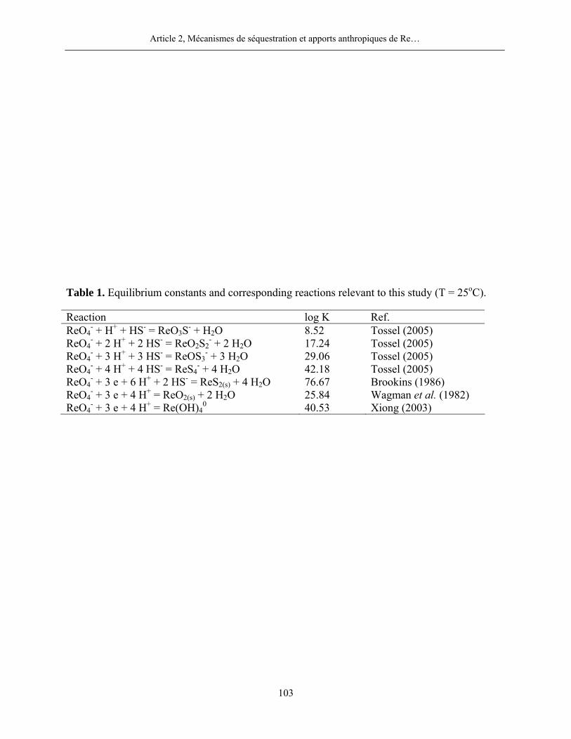
Article 2, Mécanismes de séquestration et apports anthropiques de Re…
103
Table 1. Equilibrium constants and corresponding reactions relevant to this study (T = 25oC).
Reaction log K Ref. ReO4
- + H+ + HS- = ReO3S- + H2O 8.52 Tossel (2005) ReO4
- + 2 H+ + 2 HS- = ReO2S2- + 2 H2O 17.24 Tossel (2005)
ReO4- + 3 H+ + 3 HS- = ReOS3
- + 3 H2O 29.06 Tossel (2005) ReO4
- + 4 H+ + 4 HS- = ReS4- + 4 H2O 42.18 Tossel (2005)
ReO4- + 3 e + 6 H+ + 2 HS- = ReS2(s) + 4 H2O 76.67 Brookins (1986)
ReO4- + 3 e + 4 H+ = ReO2(s) + 2 H2O 25.84 Wagman et al. (1982)
ReO4- + 3 e + 4 H+ = Re(OH)4
0 40.53 Xiong (2003)
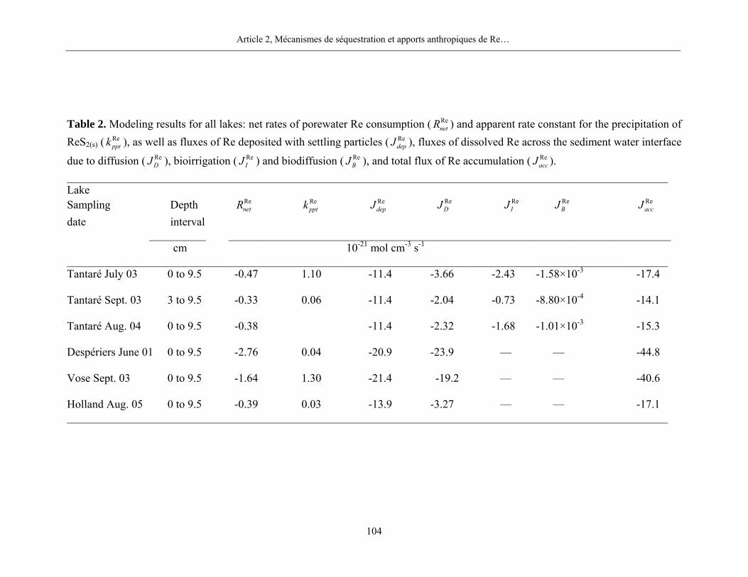
Article 2, Mécanismes de séquestration et apports anthropiques de Re…
104
Table 2. Modeling results for all lakes: net rates of porewater Re consumption ( RenetR ) and apparent rate constant for the precipitation of
ReS2(s) ( Repptk ), as well as fluxes of Re deposited with settling particles ( Re
depJ ), fluxes of dissolved Re across the sediment water interface
due to diffusion ( ReDJ ), bioirrigation ( Re
IJ ) and biodiffusion ( ReBJ ), and total flux of Re accumulation ( Re
accJ ). __________________________________________________________________________________________________________ Lake Sampling Depth Re
netR Repptk Re
depJ ReDJ Re
IJ ReBJ Re
accJ date interval __________ ______________________________________________________________________________ cm 10-21 mol cm-3 s-1 __________________________________________________________________________________________________________ Tantaré July 03 0 to 9.5 -0.47 1.10 -11.4 -3.66 -2.43 -1.58×10⁻³ -17.4 Tantaré Sept. 03 3 to 9.5 -0.33 0.06 -11.4 -2.04 -0.73 -8.80×10⁻⁴ -14.1 Tantaré Aug. 04 0 to 9.5 -0.38 -11.4 -2.32 -1.68 -1.01×10⁻³ -15.3 Despériers June 01 0 to 9.5 -2.76 0.04 -20.9 -23.9 — — -44.8 Vose Sept. 03 0 to 9.5 -1.64 1.30 -21.4 -19.2 — — -40.6 Holland Aug. 05 0 to 9.5 -0.39 0.03 -13.9 -3.27 — — -17.1 __________________________________________________________________________________________________________
Article 2, Mécanismes de séquestration et apports anthropiques de Re…
105
Figure captions
Figure 1. Map showing the location of Lakes Tantaré, Despériers, Vose and Holland and their
inventories of Re in excess of background concentrations in sediments deposited after 1900
(filled bars; pmol cm-2).
Figure 2. Triplicate porewater profiles of Re (a-f), ∑S(-II) and pH (g-l), Fe and Mn (m-r) for
Lakes Tantaré (July 2003, September 2003 and August 2004), Despériers (June 2001), Vose
(September 2003) and Holland (August 2005) and Re speciation predicted by MINEQL+ (ε-φ).
Also, comparisons of modeled (using PROFILE; thin solid line following the experimental
points; r2 values indicated) and measured average (n = 3; open circles) porewater Re
concentrations (s-x), and of ion activity products (IAP) and solubility products (KS; vertical
dashed line) for ReS2(s) (y-δ). In (s-x), the thick solid line is the net Re consumption rate. The
horizontal broken lines indicate the sediment-water interface. Empty squares in (g) indicate
concentrations below detection limit.
Figure 3. Depth profiles of measured Re concentrations (open circle), authigenic Re
concentrations (open squares) and Re:Al molar ratios (open triangles).
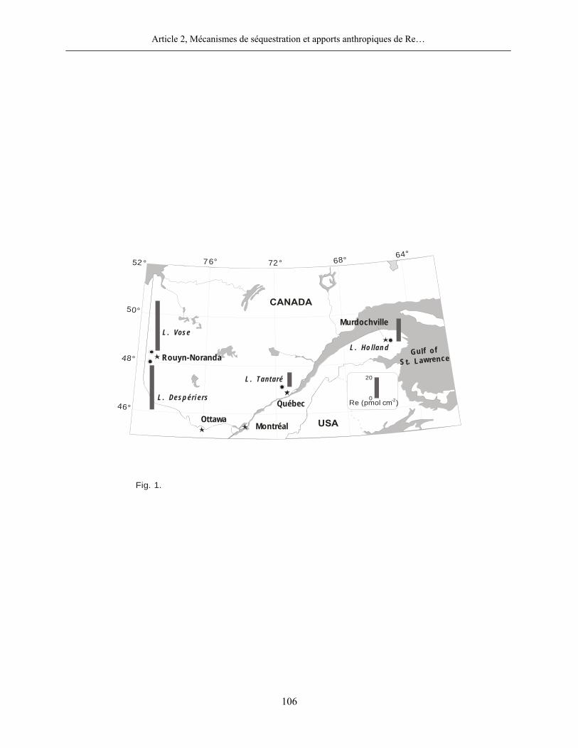
Article 2, Mécanismes de séquestration et apports anthropiques de Re…
106
USA
76° 72°64°
52°
50°
46°
48°
68°
Murdochville
Rouyn-NorandaL . Ho llan d
L . Tantaré
L . Desp éri ersQuébec
MontréalOttawa
CANADA
Gulf o fS t. Lawrence
Fig. 1.
L . Vose
20
0Re (pmol cm )-2
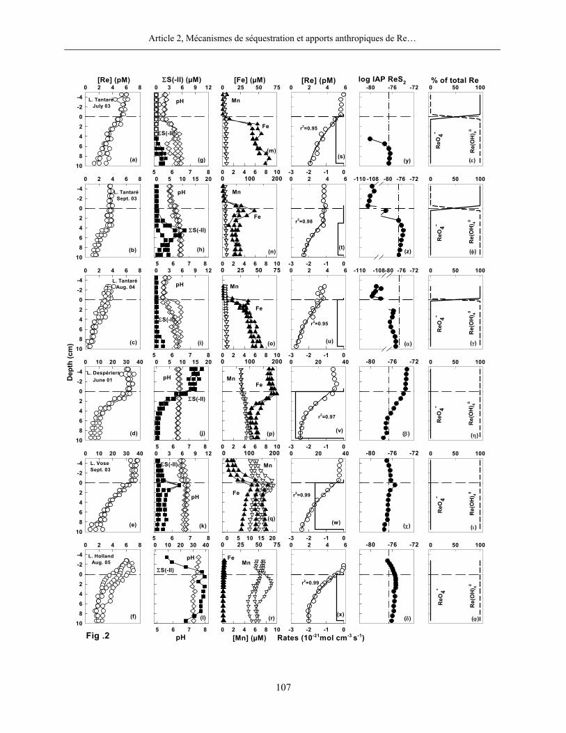
Article 2, Mécanismes de séquestration et apports anthropiques de Re…
107
0 10 20 30 40-4-202468
10
0 3 6 9 12
5 6 7 8
0 3 6 9 12
5 6 7 80 100 200
0 2 4 6 8 10
0 25 50 75
0 2 4 6 8 10
0 2 4 6 8-4-202468
10
0 10 20 30 40-4-202468
10
0 25 50 75
0 2 4 6 8 10
0 100 200
0 2 4 6 8 10
[Fe] (µM)ΣS(-II) (µM)
0 2 4 6 8-4-202468
10
0 5 10 15 20
5 6 7 8
L. Tantaré pH
(b) (n)(h)
[Re] (pM)
pH
ΣS(-II)
Sept. 03
Dep
th (c
m)
L. Despériers
0 5 10 15 20
5 6 7 8
pH
(d) (p)(j)
June 01
ΣS(-II)
0 10 20 30 40
5 6 7 8
0 2 4 6 8-4-202468
10
L. Holland pH
(e)
(r)(l)
Aug. 05ΣS(-II)
Fig .2
Fe
Mn
MnFe
FeMn
[Mn] (µM)
0 2 4 6 8-4-202468
10
0 25 50 75
0 2 4 6 8 10
L. Tantaré pH
(c) (o)(i)
ΣS(-II)
Aug. 04
Fe
Mn
L. Tantaré pH
(a)(m)
(g)
ΣS(-II)
July 03
Fe
Mn
(f)
L. VoseSept. 03
0 2 4 6
-3 -2 -1 0
r2=0.95
[Re] (pM)-80 -76 -72
log IAP ReS2
0 100 200
0 5 10 15 20
0 3 6 9 12
5 6 7 8
ΣS(-II)
pH
(k)
Mn
Fe
(q)
0 2 4 6
-3 -2 -1 0
r2=0.98
0 2 4 6
-3 -2 -1 0
r2=0.95
0 20 40
-3 -2 -1 0
r2=0.97
0 2 4 6
-3 -2 -1 0
r2=0.99
Rates (10-21mol cm-3 s-1)
0 20 40
-3 -2 -1 0
r2=0.99
-110 -108 -80 -76 -72
-110 -108-80 -76 -72
-80 -76 -72
-80 -76 -72
-80 -76 -72
(s)
(t)
(u)
(v)
(w)
(x)
(y)
(z)
(α)
(β)
(χ)
(δ)
0 50 100% of total Re
ReO
4-
Re(
OH
) 40
0 50 100
ReO
4-
Re(
OH
) 40
0 50 100
ReO
4-
Re(
OH
) 40
0 50 100
ReO
4-
Re(
OH
) 40
0 50 100
ReO
4-
Re(
OH
) 40
0 50 100
ReO
4-
Re(
OH
) 40
(ε)
(φ)
(γ)
(η)
(ι)
(ϕ)
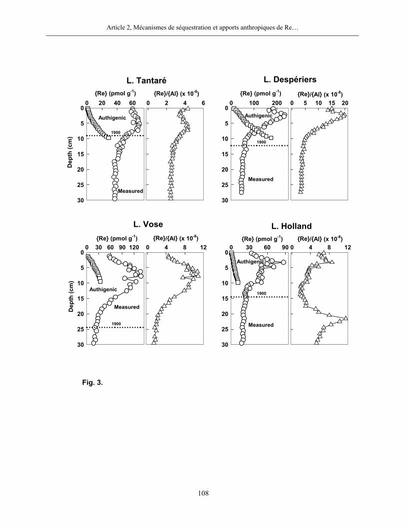
Article 2, Mécanismes de séquestration et apports anthropiques de Re…
108
0 20 40 600
5
10
15
20
25
30
Dep
th (c
m)
Fig. 3.
0 100 2000
5
10
15
20
25
30
L. Tantaré L. Despériers
0 30 60 900
5
10
15
20
25
30
L. Holland
Authigenic Authigenic
Authigenic
0 30 60 90 1200
5
10
15
20
25
30
L. Vose
Authigenic
0 2 4 6
Measured
Re/Al (x 10-8)Re (pmol g-1)
Measured
Re (pmol g-1)0 5 10 15 20
Re/Al (x 10-8)
Measured
0 4 8 12Re (pmol g-1) Re/Al (x 10-8) Re (pmol g-1)
0 4 8 12Re/Al (x 10-8)
Dep
th (c
m)
1900
1900
1900 Measured
1900
ARTICLE 3
Controls on uranium distribution in lake sediments
En préparation
Anthony Chappaz, Charles Gobeil et André Tessier
INRS-ETE, Université du Québec, 490 de la Couronne (QC), G1K 9A9, Canada
Article 3, Contrôles de la distribution de l’U…
110
RÉSUMÉ
La géochimie de l’uranium a été étudiée dans trois lacs acides situés sur le Bouclier
canadien et un lac légèrement basique de la région des Appalaches. Dans tous les lacs du
Bouclier canadien, les concentrations d’U dissous sont plus élevées dans l’eau interstitielle que
dans l’eau sus-jacente aux sédiments. Dans l’un d’eux, dontl’hypolimnion est oxygéné en
permanence, l’U était libéré dans l’eau porale à des profondeurs où le Fe était précipité en
oxyhydroxydes de Fe. Ces similitudes entre les profils d’U et de Fe indiquent qu’une partie de
l’U est associé avec les oxyhydroxydes de Fe. Les profils d’U et de Fe dissous dans les deux
autres lacs du Bouclier, dont les hypolimnions étaient anoxiques lors de l’échantillonnage,
n’affichaient pas une telle remobilisation de ces deux éléments à proximité de l’interface eau-
sédiment mais montraient plutôt une diffusion de l’U de l’eau sus-jacente vers le sédiment. Au
contraire, dans le lac appalachien, les concentrations d’U dissous étaient plus élevées dans l’eau
sus-jacente aux sédiments que dans l’eau porale, diminuaient fortement à proximité de l’interface
eau-sédiment, puis, demeuraient relativement constantes en fonction de la profondeur. La
modélisation diagénétique des profils d’U dans l’eau interstitielle, en présumant l’état
stationnaire, révèle que l’U authigène représentait toujours ≤ 3% de la teneur d’U total dans les
sédiments de tous les lacs. Cette observation montre que les réactions diagénétiques impliquant
l’U ne sont pas quantitativement importantes et que la majeure partie de l’U s’accumule dans les
sédiments sous forme particulaire et non pas par diffusion à travers l’interface eau-sédiment et
précipitation subséquente comme dans les sédiments de la marge continentale. La comparaison
entre les rapports molaires U:Corg et U:Fe, dans le matériel diagénétique prélevé avec des plaques
de Teflon insérées dans les sédiments et dans les sédiments de surface (0-0,5 cm) du lac ayant un
hypolimnion oxygéné en permanence, suggère que l’U dans la phase solide était principalement
lié à la matière organique issue du bassin versant; une corrélation significative entre l’U et le
carbone organique dans le sédiment du lac appalachien supporte également cette hypothèse. La
comparaison des profils d’U dissous à ceux de l’état de saturation de phases minérales distinctes
indique que l’U dissous n’était pas retiré de l’eau porale suite à la précipitation de UO2(S), de
U3O7(S) et de U3O8(S) comme suggéré précédemment dans la littérature.
Article 3, Contrôles de la distribution de l’U…
111
ABSTRACT
Uranium geochemistry has been investigated in three acid lakes located in the Canadian
Shield and one circumneutral in the Appalachian Region. In all Shield lakes, dissolved U
concentrations were higher in the porewater than in the overlying water. In one of them, whose
hypolimnion is perennially oxic, U was released to porewater at depths where Fe was mobilized
from the sediment and was removed from the porewater at depths where Fe was precipitated as
Fe oxyhydroxides; these similarities in the U and Fe profiles indicate that part of U becomes
associated to Fe oxyhydroxides. The dissolved U and Fe profiles in the other two Shield lakes,
whose hypolimnions were anoxic when sampled, did not show any significant recycling of these
elements at the vicinity of the sediment-water interface and both elements diffused to the
overlying water. In contrast, in the Appalachian lake, dissolved U concentrations were higher in
the overlying water than in porewater, strongly decreased at the vicinity of the sediment-water
interface and then remained relatively constant with sediment depth. Diagenetic modeling of the
porewater U profiles, assuming steady state, reveals that authigenic U always represented ≤3% of
the total U concentration in the sediments of all lakes. This observation indicates that diagenetic
reactions involving U are not quantitatively important and that most of the U was delivered to the
sediments at our study sites as particulate U and not through diffusion across the sediment-water
interface as in continental margin sediments. Comparison between the U:Corg and U:Fe molar
ratios in diagenetic material collected with Teflon sheets inserted into the sediments and those in
the top 0.5 cm layer of the sediments of the lake having a perennially oxic hypolimnion suggests
that solid phase U was mainly bound to organic matter originating from the watershed; a strong
statistical correlation between sediment U and organic carbon in the Appalachian lake supports
this contention. Comparison of dissolved U and saturation state profiles indicates that dissolved
U was not removed from porewater through precipitation of UO2(S), U3O7(S) and U3O8(S) as
previously suggested in the literature.
Article 3, Contrôles de la distribution de l’U…
112
1. INTRODUCTION
The behaviour of U during the early stages of organic matter oxidation has been examined
more often in marine than in lacustrine sediments (e.g. Klinkhammer and Palmer, 1991; Lovely
et al., 1991; Nameroff et al., 2002; Zheng et al., 2002a,b; McManus et al., 2005; Morford et al.,
2007). Considerable interest has been given to this redox-sensitive element in marine sediments
due to its potential to constrain past environmental changes of the ocean (e.g. François et al.,
1993; Mangini et al., 2001; Tribovillard et al., 2006; Arnaboldi and Meyers, 2007). Several
studies have hypothesized that uranium, which exists as a U(VI) carbonate complex in
oxygenated seawater, is reduced under sub-oxic conditions to insoluble U(IV) forms through a
microbially mediated reaction (e.g. Lovely et al., 1991, Frederickson et al., 2000; Sani et al.,
2004). This reaction would occur at a redox potential that is close to that at which Fe(III) is
reduced to Fe(II), which is often encountered close to the sediment-water interface in continental
margin sediments. This hypothesis would explain why dissolved U from oxic seawater diffuses
across the sediment-water interface and a large fraction of U is present in marine sediment as
authigenic U. The level of U enrichment is thought to be closely related to the flux organic C the
seafloor and to O2 bottom water concentration (e.g. François et al., 1997; McManus et al., 2005).
But it is recognized that the exact mechanism of U fixation to sediments is poorly known, which
limits the use of this proxy to record paleoceanographic conditions. Furthermore, information on
remobilization of uranium after its primary accumulation is limited.
This study has been initiated with the general objective to examine closely the
geochemistry of U in freshwater environments. Our specific goals were to quantify authigenic U
in sediments from perennially oxic and seasonally anoxic lacustrine basins having various water
compositions and to document the diagenetic processes that control the reactive transport of this
element at the vicinity of the sediment-water interface. Our conclusions are based on an extensive
chemical data set on both sediment and sediments porewater.
2. METHODS
2.1. Study areas and sampling
Four lakes located in Eastern Canada were sampled between July 2003 and August 2005.
Three of the lakes, namely Lakes Tantaré, Vose and Despériers, lie on the Canadian Shield and
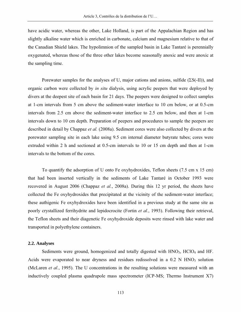
Article 3, Contrôles de la distribution de l’U…
113
have acidic water, whereas the other, Lake Holland, is part of the Appalachian Region and has
slightly alkaline water which is enriched in carbonate, calcium and magnesium relative to that of
the Canadian Shield lakes. The hypolimnion of the sampled basin in Lake Tantaré is perennially
oxygenated, whereas those of the three other lakes become seasonally anoxic and were anoxic at
the sampling time.
Porewater samples for the analyses of U, major cations and anions, sulfide (ΣS(-II)), and
organic carbon were collected by in situ dialysis, using acrylic peepers that were deployed by
divers at the deepest site of each basin for 21 days. The peepers were designed to collect samples
at 1-cm intervals from 5 cm above the sediment-water interface to 10 cm below, or at 0.5-cm
intervals from 2.5 cm above the sediment-water interface to 2.5 cm below, and then at 1-cm
intervals down to 10 cm depth. Preparation of peepers and procedures to sample the peepers are
described in detail by Chappaz et al. (2008a). Sediment cores were also collected by divers at the
porewater sampling site in each lake using 9.5 cm internal diameter butyrate tubes; cores were
extruded within 2 h and sectioned at 0.5-cm intervals to 10 or 15 cm depth and then at 1-cm
intervals to the bottom of the cores.
To quantify the adsorption of U onto Fe oxyhydroxides, Teflon sheets (7.5 cm x 15 cm)
that had been inserted vertically in the sediments of Lake Tantaré in October 1993 were
recovered in August 2006 (Chappaz et al., 2008a). During this 12 yr period, the sheets have
collected the Fe oxyhydroxides that precipitated at the vicinity of the sediment-water interface;
these authigenic Fe oxyhydroxides have been identified in a previous study at the same site as
poorly crystallized ferrihydrite and lepidocrocite (Fortin et al., 1993). Following their retrieval,
the Teflon sheets and their diagenetic Fe oxyhydroxide deposits were rinsed with lake water and
transported in polyethylene containers.
2.2. Analyses
Sediments were ground, homogenized and totally digested with HNO3, HClO4 and HF.
Acids were evaporated to near dryness and residues redissolved in a 0.2 N HNO3 solution
(McLaren et al., 1995). The U concentrations in the resulting solutions were measured with an
inductively coupled plasma quadrupole mass spectrometer (ICP-MS; Thermo Instrument X7)
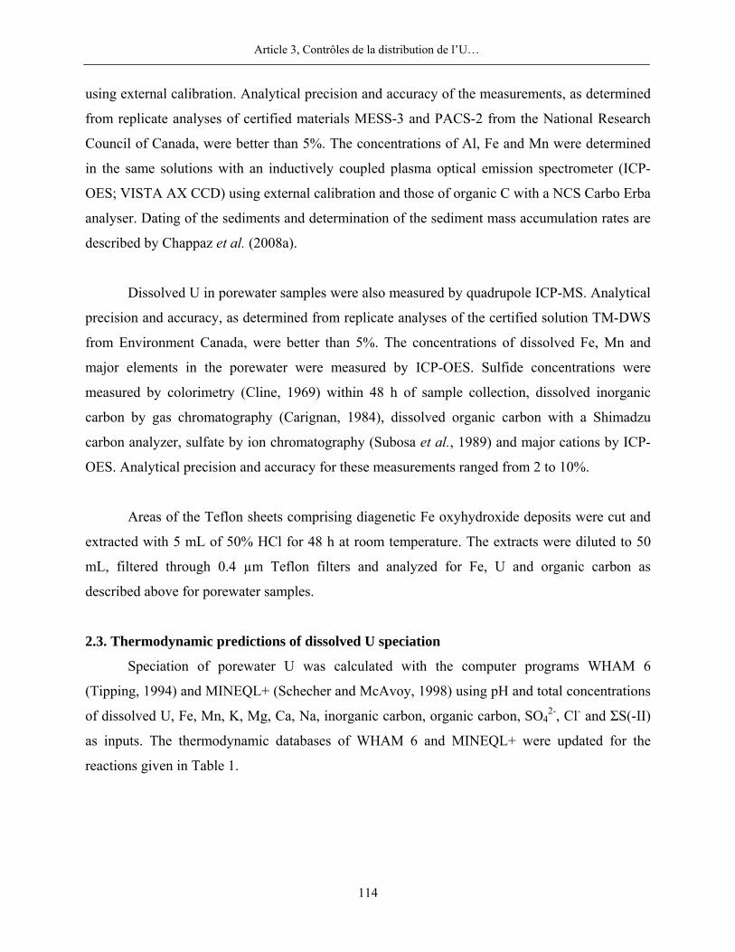
Article 3, Contrôles de la distribution de l’U…
114
using external calibration. Analytical precision and accuracy of the measurements, as determined
from replicate analyses of certified materials MESS-3 and PACS-2 from the National Research
Council of Canada, were better than 5%. The concentrations of Al, Fe and Mn were determined
in the same solutions with an inductively coupled plasma optical emission spectrometer (ICP-
OES; VISTA AX CCD) using external calibration and those of organic C with a NCS Carbo Erba
analyser. Dating of the sediments and determination of the sediment mass accumulation rates are
described by Chappaz et al. (2008a).
Dissolved U in porewater samples were also measured by quadrupole ICP-MS. Analytical
precision and accuracy, as determined from replicate analyses of the certified solution TM-DWS
from Environment Canada, were better than 5%. The concentrations of dissolved Fe, Mn and
major elements in the porewater were measured by ICP-OES. Sulfide concentrations were
measured by colorimetry (Cline, 1969) within 48 h of sample collection, dissolved inorganic
carbon by gas chromatography (Carignan, 1984), dissolved organic carbon with a Shimadzu
carbon analyzer, sulfate by ion chromatography (Subosa et al., 1989) and major cations by ICP-
OES. Analytical precision and accuracy for these measurements ranged from 2 to 10%.
Areas of the Teflon sheets comprising diagenetic Fe oxyhydroxide deposits were cut and
extracted with 5 mL of 50% HCl for 48 h at room temperature. The extracts were diluted to 50
mL, filtered through 0.4 µm Teflon filters and analyzed for Fe, U and organic carbon as
described above for porewater samples.
2.3. Thermodynamic predictions of dissolved U speciation
Speciation of porewater U was calculated with the computer programs WHAM 6
(Tipping, 1994) and MINEQL+ (Schecher and McAvoy, 1998) using pH and total concentrations
of dissolved U, Fe, Mn, K, Mg, Ca, Na, inorganic carbon, organic carbon, SO42-, Cl- and ΣS(-II)
as inputs. The thermodynamic databases of WHAM 6 and MINEQL+ were updated for the
reactions given in Table 1.
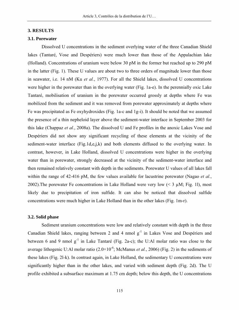
Article 3, Contrôles de la distribution de l’U…
115
3. RESULTS
3.1. Porewater
Dissolved U concentrations in the sediment overlying water of the three Canadian Shield
lakes (Tantaré, Vose and Despériers) were much lower than those of the Appalachian lake
(Holland). Concentrations of uranium were below 30 pM in the former but reached up to 290 pM
in the latter (Fig. 1). These U values are about two to three orders of magnitude lower than those
in seawater, i.e. 14 nM (Ku et al., 1977). For all the Shield lakes, dissolved U concentrations
were higher in the porewater than in the overlying water (Fig. 1a-e). In the perennially oxic Lake
Tantaré, mobilisation of uranium in the porewater occurred grossly at depths where Fe was
mobilized from the sediment and it was removed from porewater approximately at depths where
Fe was precipitated as Fe oxyhydroxides (Fig. 1a-c and 1g-i). It should be noted that we assumed
the presence of a thin nepheloid layer above the sediment-water interface in September 2003 for
this lake (Chappaz et al., 2008a). The dissolved U and Fe profiles in the anoxic Lakes Vose and
Despériers did not show any significant recycling of these elements at the vicinity of the
sediment-water interface (Fig.1d,e,j,k) and both elements diffused to the overlying water. In
contrast, however, in Lake Holland, dissolved U concentrations were higher in the overlying
water than in porewater, strongly decreased at the vicinity of the sediment-water interface and
then remained relatively constant with depth in the sediments. Porewater U values of all lakes fall
within the range of 42-416 pM, the few values available for lacustrine porewater (Nagao et al.,
2002).The porewater Fe concentrations in Lake Holland were very low (< 3 µM; Fig. 1l), most
likely due to precipitation of iron sulfide. It can also be noticed that dissolved sulfide
concentrations were much higher in Lake Holland than in the other lakes (Fig. 1m-r).
3.2. Solid phase
Sediment uranium concentrations were low and relatively constant with depth in the three
Canadian Shield lakes, ranging between 2 and 4 nmol g-1 in Lakes Vose and Despériers and
between 6 and 9 nmol g-1 in Lake Tantaré (Fig. 2a-c); the U:Al molar ratio was close to the
average lithogenic U:Al molar ratio (2.0×10⁻⁶; McManus et al., 2006) (Fig. 2) in the sediments of
these lakes (Fig. 2l-k). In contrast again, in Lake Holland, the sedimentary U concentrations were
significantly higher than in the other lakes, and varied with sediment depth (Fig. 2d). The U
profile exhibited a subsurface maximum at 1.75 cm depth; below this depth, the U concentrations
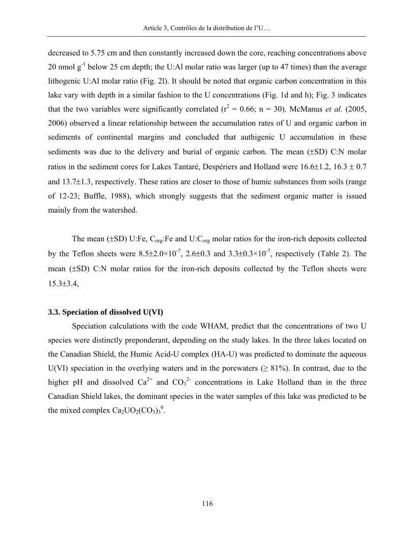
Article 3, Contrôles de la distribution de l’U…
116
decreased to 5.75 cm and then constantly increased down the core, reaching concentrations above
20 nmol g-1 below 25 cm depth; the U:Al molar ratio was larger (up to 47 times) than the average
lithogenic U:Al molar ratio (Fig. 2l). It should be noted that organic carbon concentration in this
lake vary with depth in a similar fashion to the U concentrations (Fig. 1d and h); Fig. 3 indicates
that the two variables were significantly correlated (r2 = 0.66; n = 30). McManus et al. (2005,
2006) observed a linear relationship between the accumulation rates of U and organic carbon in
sediments of continental margins and concluded that authigenic U accumulation in these
sediments was due to the delivery and burial of organic carbon. The mean (±SD) C:N molar
ratios in the sediment cores for Lakes Tantaré, Despériers and Holland were 16.6±1.2, 16.3 ± 0.7
and 13.7±1.3, respectively. These ratios are closer to those of humic substances from soils (range
of 12-23; Buffle, 1988), which strongly suggests that the sediment organic matter is issued
mainly from the watershed.
The mean (±SD) U:Fe, Corg:Fe and U:Corg molar ratios for the iron-rich deposits collected
by the Teflon sheets were 8.5±2.0×10⁻⁷, 2.6±0.3 and 3.3±0.3×10⁻⁷, respectively (Table 2). The
mean (±SD) C:N molar ratios for the iron-rich deposits collected by the Teflon sheets were
15.3±3.4,
3.3. Speciation of dissolved U(VI)
Speciation calculations with the code WHAM, predict that the concentrations of two U
species were distinctly preponderant, depending on the study lakes. In the three lakes located on
the Canadian Shield, the Humic Acid-U complex (HA-U) was predicted to dominate the aqueous
U(VI) speciation in the overlying waters and in the porewaters (≥ 81%). In contrast, due to the
higher pH and dissolved Ca2+ and CO32- concentrations in Lake Holland than in the three
Canadian Shield lakes, the dominant species in the water samples of this lake was predicted to be
the mixed complex Ca2UO2(CO3)30.
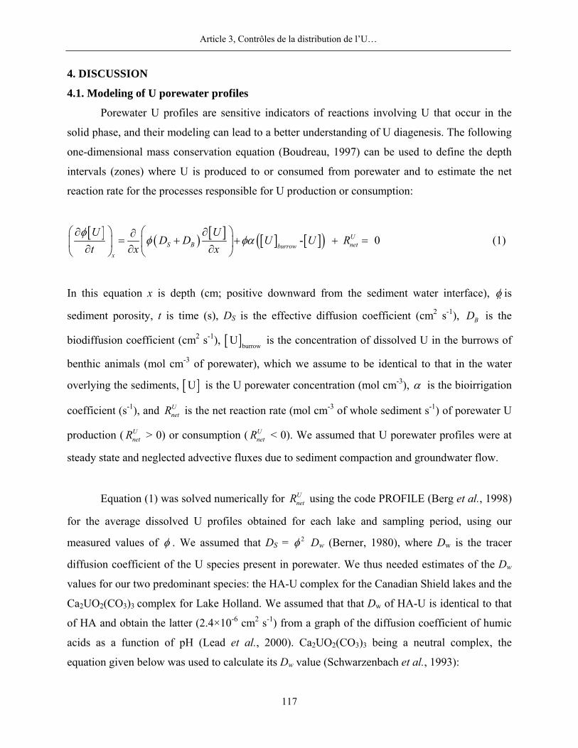
Article 3, Contrôles de la distribution de l’U…
117
4. DISCUSSION
4.1. Modeling of U porewater profiles
Porewater U profiles are sensitive indicators of reactions involving U that occur in the
solid phase, and their modeling can lead to a better understanding of U diagenesis. The following
one-dimensional mass conservation equation (Boudreau, 1997) can be used to define the depth
intervals (zones) where U is produced to or consumed from porewater and to estimate the net
reaction rate for the processes responsible for U production or consumption:
[ ] ( ) [ ] [ ] [ ]( )- 0US B netburrow
x
U UD D U U R
t x xφ
φ φα⎛ ⎞ ⎛ ⎞∂ ∂∂
= + + + =⎜ ⎟ ⎜ ⎟∂ ∂ ∂⎝ ⎠ ⎝ ⎠ (1)
In this equation x is depth (cm; positive downward from the sediment water interface), φ is
sediment porosity, t is time (s), DS is the effective diffusion coefficient (cm2 s-1), BD is the
biodiffusion coefficient (cm2 s-1), [ ]burrowU is the concentration of dissolved U in the burrows of
benthic animals (mol cm-3 of porewater), which we assume to be identical to that in the water
overlying the sediments, [ ]U is the U porewater concentration (mol cm-3), α is the bioirrigation
coefficient (s-1), and UnetR is the net reaction rate (mol cm-3 of whole sediment s-1) of porewater U
production ( UnetR > 0) or consumption ( U
netR < 0). We assumed that U porewater profiles were at
steady state and neglected advective fluxes due to sediment compaction and groundwater flow.
Equation (1) was solved numerically for UnetR using the code PROFILE (Berg et al., 1998)
for the average dissolved U profiles obtained for each lake and sampling period, using our
measured values of φ . We assumed that DS = 2φ Dw (Berner, 1980), where Dw is the tracer
diffusion coefficient of the U species present in porewater. We thus needed estimates of the Dw
values for our two predominant species: the HA-U complex for the Canadian Shield lakes and the
Ca2UO2(CO3)3 complex for Lake Holland. We assumed that that Dw of HA-U is identical to that
of HA and obtain the latter (2.4×10⁻⁶ cm2 s-1) from a graph of the diffusion coefficient of humic
acids as a function of pH (Lead et al., 2000). Ca2UO2(CO3)3 being a neutral complex, the
equation given below was used to calculate its Dw value (Schwarzenbach et al., 1993):
Article 3, Contrôles de la distribution de l’U…
118
-4
0.71
2.7 10WD
M×
= (2)
where M represents the molecular mass. We calculated a Dw value of 3.14×10⁻⁶ cm2 s-1 for
Ca2UO2(CO3)3. Those two values of Dw were corrected for a temperature of 4°C with the Stokes-
Einstein equation (Li and Gregory, 1974).
The value used for the biodiffusion coefficient BD , in Lake Tantaré, was 2.2×10⁻⁹ cm2 s-1
(Gallon et al., 2004). This estimation is based on the work of Hare et al. (1994) who determined
that the most abundant benthic animal at this site is the chironomid Sergentia coracina
(1080±140 individuals m-2), and the laboratory experiment of Matisoff and Wang (2000) who
established biodiffusion coefficients per individual for chironomids. The bioirrigation coefficient
α was assumed to vary linearly from 0α at the sediment water interface to zero at 10 cm depth
(Gallon et al., 2004), since chironomids are generally not found below this sediment depth
(Matisoff and Wang, 1998). Equation 3 was used to estimate 0α (Boudreau, 1984):
( )( )0 1
2 22 1 1- -
S
a
D rr r r r
α = (3)
where 1r is the radius of an animal’s tube (0.1 cm), 2r is half the distance between adjacent tubes
(1.5 cm), and ar is equal to 2r /2.
Seasonal anoxia events in the bottom waters of Lakes Vose, Despériers and Holland,
prevent the development of benthic communities. We assumed that the influence of bioturbation
and bioirrigation were negligible in these lakes and thus we equaled BD and α to zero.
In all lakes, the best solutions provided by PROFILE are in very good agreement with the
measurements (r2 = 0.88-0.99; Fig. 1y-δ). In Lake Tantaré, PROFILE consistently defined two
zones (sediment intervals) where reaction rates are relatively fast: a first zone just below the
sediment-water interface (July 03 and August 04) or in the nepheloid layer (September 2003),
Article 3, Contrôles de la distribution de l’U…
119
where dissolved U was consumed, and a second zone just below, where dissolved U was
produced. At greater depths, U was either slowly produced (July 03) or consumed (August 2004);
in September 03, U was consumed between 0.5 and 1.8 cm depth and slowly produced below
(Fig. 1). In the two other Canadian Shield lakes (anoxic hypolimnion), the model determined a
zone of U production between 0 and 4 cm followed by a zone of either slow U production (Lake
Vose) or of U consumption (Lake Despériers) (Fig. 1). In contrast, PROFILE defined an intense
consumption zone of dissolved U between 0 and 1cm depth in Lake Holland sediments. The net
reaction rate UnetR obtained for each zone are given in Tables 3 and 4 for each lake and time
period.
4.2. Influence of diagenesis on sedimentary records and fluxes of U
Using the UnetR provided by the code PROFILE, we can estimate the influence of
diagenetic processes on the sedimentary record of U (Chappaz et al., 2008a,b). Considering that
the net removal rate of U ( UnetR ) from the porewater is identical to the negative of the net rate of U
fixation to the solid phase, the following equations results:
[ ] - Unet
reaction reaction
d Ud UR mdt dt
φ⎛ ⎞⎛ ⎞= = ⎜ ⎟⎜ ⎟
⎝ ⎠ ⎝ ⎠ (4)
where [ ]U represents the dissolved U concentration (mol cm-3), m is the dry bulk density (g cm-3
of whole sediment), and U is the solid phase U concentration (mol g-1). The subscript
"reaction" indicates reaction rates in solution and solid phases. From equation (4):
- -
U Unet net
S
R Rd U dt dxm m v
= = (5)
It follows that:
Article 3, Contrôles de la distribution de l’U…
120
00
- -
i ix x x xU U
net netauthigenic
xS Sx
R RU dx xm v m v
= =
==
= ≈ Δ∑∫ (6)
where xi is the depth of a sediment layer and Sv is the sedimentation rate (cm yr-1). Uauthigenic
can
be viewed as the solid U concentration gained or lost by a layer of sediment during its burial.
Uauthigenic
values are subtracted from those of measured U ( Umeasured
) to obtain the U
concentration at time of sediment deposition ( Udeposited
). Our calculations show that the values
of Uauthigenic
correspond to a maximum of 3.3% of Umeasured
for all lakes. This simple exercise
indicates that the influence of the diagenetic processes on the sedimentary records of U in all
lakes is small, and that the Umeasured
profiles reflect closely the chronology of U deposition in
all lakes.
The present-day total flux responsible for U accumulation in the sediments ( UaccJ ) of Lake
Tantaré is the sum of the fluxes of U deposited at the sediment surface with settling particles
( UdepJ ) and those of dissolved U transported across the sediment water interface by molecular
diffusion ( UDJ ), bioirrigation ( U
IJ ) and bioturbation ( UBJ ):
U U U U Uacc dep D I BJ J J J J= + + + (7)
Due to the seasonal anoxia in Lakes Vose, Despériers and Holland, equation (7) can be reduced
for these lakes to:
U U Uacc dep DJ J J= + (8)
The present-day values of UdepJ for all lakes were obtained by multiplying the sediment
mass accumulation rate (ω; mg cm-2 yr-1) obtained from the 210Pb geochronology for the top 0.5
cm sediment layer by the value of depositedU in this sediment layer. The values of U
DJ , UIJ and
Article 3, Contrôles de la distribution de l’U…
121
UBJ were calculated with the code PROFILE (Tables 2 and 3). In all lakes, the contribution of
UdepJ represents more than 95% of U
accJ , indicating that U in our lacustrine sediments is essentially
from deposition of particulate U.
4.3. Uranium distribution among specific solid phases
In this section, we use thermodynamic calculations, in combination with our results
obtained from porewater, sediments and the Fe-rich authigenic material collected on Teflon
sheets to constrain the reactions involving U and its association with specific solid phases.
4.3.1 Sub-oxic sediments
Modeling of Lake Tantaré porewater U profiles with the code PROFILE consistently
shows that U was released, at all sampling dates, to porewater a few cm below the sediment-
water interface and that it was removed from porewater just above this production zone (Fig. 1y-
α). The depths of U production to and removal from porewater coincided with those reported for
Mo at the same sampling dates in this lake (Chappaz et al., 2008a); these U production and
consumption zones also coincided grossly with the depths of Fe(II) production to the porewater
and its removal as authigenic Fe oxyhydroxides following Fe(II) oxidation. Chappaz et al.
(2008a) clearly demonstrated that Mo was closely coupled to Fe, being released to porewater as a
consequence of the reductive dissolution of Fe oxyhydroxides and removed from porewater by
adsorption to diagenetic Fe oxyhydroxides. Based on the above observations, we thus conclude
that porewater U, like Mo, is closely associated to Fe redox recycling in Lake Tantaré.
Laboratory experiments have shown that U(VI) forms strong surface complexes with the
hydroxyl groups of Fe oxyhydroxides (Waite et al., 1994) and that addition of commercial humic
acid (e.g., Suwannee River HA or Aldrich HA) to the experiments at levels similar to those
present in aquatic environments enhances U(VI) adsorption to the Fe oxyhydroxydes at pH
values below about 7 compared to the HA-free system (Payne et al., 1996; Lenhart and
Honeyman, 1999; Murphy et al., 1999). The increased U(VI) adsorption has been attributed to
the formation of ternary surface complexes (Lenhart and Honeyman, 1999). Given that Lake
Tantaré has a low pH and that U(VI) speciation in its porewater is dominated by complexes with
humic acid, we hypothesize that ternary surface complexes are formed with the authigenic Fe
oxyhydroxide in this lake. It should be noted that the sediment U profile in Lake Tantaré (Fig. 2a)
Article 3, Contrôles de la distribution de l’U…
122
does not display a sharp subsurface maximum as sediment Mo and Fe profiles do (Chappaz et al.,
2008a); this peculiarity of U is to be attributed to the low contribution of diagenesis to the
measured sediment U profile (see section 4.2).
Moreover, the porewater U profiles of the three anoxic lakes are consistent with our
interpretation of a close relation between porewater U and Fe in Lake Tantaré. Indeed, in Lakes
Despériers and Vose, the depths at which U was released to porewater corresponded grossly to
the depths at which Fe was also released. No removal of U above the U production zones was
observed in these lakes simply because there was no production of authigenic Fe oxyhydroxides
at the time of our porewater sampling (Fig. 1j, k and Fig. 2b, c). As for Lake Holland, the low
and depth unvariable dissolved Fe concentrations (Fig. 1l) indicate that redox recycling of Fe in
the sediments of this lake is unimportant.
Iron-rich material previously collected on Teflon sheets in the sediments of Lake Tantaré
has been shown to contain poorly crystallized ferrihydrite and lepidocrocite (Fortin et al. (1993).
The mean (±SD) U:Fe molar ratio measured in the Fe-rich diagenetic material (8.5±2.0×10⁻⁷;
Table 2) that we collected on Teflon sheets in Lake Tantaré was smaller than that measured in the
top 0.5 cm layer of the sediments (46×10-7; Table 2). Adsorption of U(VI) on ferrihydrite has
been well studied and it has been interpreted in term of the surface complexation model (e.g.,
Waite et al., 1994). To compute the U:Fe molar ratio predicted for U(VI) adsorption on
authigenic Fe oxyhydroxides under Lake Tantaré geochemical conditions, we have used the two-
layer version of the surface complexation model (DLM) developed by Dzombak and Morel
(1990) which is incorporated into the computer code MINEQL+ (Schecher and McAvoy, 1998).
For this calculation, we updated the MINEQL+ database with the intrinsic constants for the
adsorption of U on ferrihydrite reported recently by Davis (2001; Table 1) and we adopted the
intrinsic adsorption constants for H+ adsorption, as well as the specific surface area (600 m2 g-1)
and the concentration of strong (1.8×10⁻³ mol/mol of ferrihydrite) and weak (0.8732 mol/mol of
ferrihydrite) adsorption sites suggested by Liu et al. (2005) for ferrihydrite. This calculation,
performed individually for each replicate porewater data sets at depths where removal of
dissolved U occurred (i.e., at 0.5 cm, -1.5 cm and 0.5 cm in July 03, September 03 and August
04, respectively), yielded a mean (±SD) U:Fe predicted molar ratio of 2.3±1.2×10⁻⁷; the predicted
Article 3, Contrôles de la distribution de l’U…
123
U:Fe molar ratio is lower than that measured in the Fe-rich diagenetic material and much lower
than that measured in the 0-0.5 cm layer of the sediments (Table 2). All these observations
confirm that the association of U with Fe oxyhydroxides in sediments of Lake Tantaré is small.
The Fe-rich diagenetic material also contained large amounts of organic C; the mean
(±SD) Corg:Fe molar ratio being 2.6±0.3; Corg:Fe molar ratios of similar magnitude have been
reported for Fe-rich particles in lake water (Tipping et al., 1981). The organic matter associated
with the Fe-rich material collected on Teflon sheets has been shown to contain bacterial remains
(Fortin et al., 1993); it also probably contains humic substances, given the strong affinity of these
substances for adsorption to Fe oxyhydroxides (Tipping, 1981; Gu et al., 1994). The U:Corg molar
ratio measured in the diagenetic material (3.3±0.3×10⁻⁷) collected on Teflon sheets is very similar
to that measured in the top 0.5 cm layer of the sediments (3.7×10⁻⁷; Table 2). This similarity of
the two U:Corg ratios suggests that U is associated mainly to organic matter in the sediments of
Lake Tantaré. The strong correlation observed in Lake Holland between U and Corg (Fig. 3) also
suggests the importance of organic matter for binding U in the sediments of this lake. An
estimation of the U:Corg molar ratios due to the reaction of U(VI) with humic substances was
obtained from the output of the code WHAM 6 as applied to each replicate porewater data sets at
depths where removal of dissolved U occurred (i.e., at 0.5 cm, -1.5 cm and 0.5 cm in July 03,
September 03 and August 04, respectively); we assumed those dissolved humic substances
behaved similarly to that associated to the Fe-rich diagenetic material (Davis, 1984) and to that
present in sediments. The predicted values of the U:Corg molar ratio (7.9±3.6×10⁻⁸) is lower than
that measured in the diagenetic material (3.3±0.3×10⁻⁷) collected on Teflon sheets. It suggests
that organic matter other than humic substances (e.g., microorganism remains) in the authigenic
material and in sediments contains U. Several studies have shown that U(VI) can be
bioaccumulated by bacteria (e.g., Fowle et al., 2000) and phytoplankton (e.g., Fortin et al., 2004).
4.3.2. Anoxic sediments
Fitting of the porewater U profiles predicts a zone of relatively fast removal of uranium
from the porewater located just below the sediment-water interface in Lake Holland (Fig. 1ϕ) and
a zone of slower U removal located at 4 - 9.5 cm in Lake Despériers (Fig. 1χ). For the other three
lakes, no removal of porewater U under anoxic conditions was predicted. Several mechanisms of
Article 3, Contrôles de la distribution de l’U…
124
U fixation to sediments under anoxic conditions have been proposed; among them, was the
reduction of U(VI) to U(IV) followed by the precipitation of solids such as UO2(s), U3O7(s) and
U3O8(s) (Klinkhammer and Palmer, 1991; Morford et al., 2001, McManus et al., 2005). Other
U(IV) and U(VI) solids are also possible. The reactions and formation constants, calculated from
the 0fGΔ values provided by Guillaumont et al. (2003) and Wagman et al. (1982), are listed in
Table 1. To calculate the ion activity product (IAP) and thus test the saturation state of porewater
with respect to these solids, we had to take into account both reduction of U(VI) to U(IV) and
complexation of U(VI) by humic substances. To achieve this task, we used successively the
codes WHAM 6 and MINEQL+ in the following manner. Conditional equilibrium constants for
U(VI) complexation by humic ( condHAUK − ) and fulvic ( cond
FAUK − ) acids were first estimated with the
code WHAM 6 under conditions prevailing at each depth of a porewater profile:
22+2
[UO -HA]K[UO ][HA]
condU HA
F− = (9)
and
22+2
[UO -FA]K[UO ][FA]
condU FA
F− = (10)
where [UO2-HA] and [UO2-FA] are the concentrations (mol L-1) of the humic or fulvic acid
complexes with 2+2UO and [HA]F and [FA]F are the concentrations (g L-1) of free (uncomplexed
with 2+2UO ) humic and fulvic acids. For estimating ( Kcond
U HA− ) and ( KcondU FA− ), we assumed that a
negligible fraction of HA and FA were complexed with 2+2UO , i.e., that [HA]F and [FA]F where
identical to [HA] and [FA]; [ 2+2UO ], [UO2-HA] and [UO2-HA] were provided by the output of
WHAM 6. The range of ( KcondU HA− ) and ( Kcond
U FA− ) values thus calculated are given in Table 1. The
conditional constants KcondU HA− and Kcond
U FA− were then incorporated into the code MINEQL+ and U
speciation was calculated again, allowing the redox state of U to vary; in this latter calculation,
Article 3, Contrôles de la distribution de l’U…
125
we assumed that the redox potential was determined by the couple SO42-/HS- in porewater
samples with sulfide values greater than 0.1 µM.
Comparison of the IAPs with the solubility products (Ks) for the various solids indicates
that porewater were undersaturated (log IAP/Ks < 0) by 4 - 58 orders of magnitude with respect
to U3O8(s), US(s), US2(s) and US3(s) and thus that these solids could not be formed; porewater was,
however, supersaturated (log IAP/Ks > 0) or close to saturation with respect to UO2(s) and U3O7(s)
(Fig. 1ε-ϕ) indicating that the formation of these solids was thermodynamically possible.
Precipitation of the two solids is unlikely since the saturation state of porewater does not vary in a
consistent manner. For example, porewater remained supersaturated by nearly 4 orders of
magnitude with respect to UO2(s) in all lakes, including Lake Holland at the depth where U was
consumed, an unexpected result if precipitation of this solid was occurring. Similarly, it is
difficult to explain why U3O7(s) would precipitate in Lake Holland (log IAP/Ks ≈ 0 just below the
sediment water interface) and not in the other lakes (e.g., log IAP/Ks much larger than 0 in Lakes
Despériers and Vose). Two other mechanisms have been proposed: sequestration by organic
matter or adsorption of U(VI) at the surface of sulfide minerals (Wersin et al., 1994; Moyes et al.,
2000; Scott et al., 2007), but our data are too limited to be conclusive on these mechanisms of U
removal.
5. CONCLUSION
Modeling the porewater U profiles with a reaction-transport diagenetic equation indicates
that authigenic U formation was negligible in the four studied lakes. In agreement with this
contention, present-day fluxes of dissolved U by diffusion, bioturbation and bioirrigation are
negligible compared to the flux of U delivered with settling particles. Comparison of the U and
Fe porewater profiles indicates that U is bound to Fe oxyhydroxides, probably as ternary
complexes with natural organic matter. However, the proportion of total sediment U associated
with Fe oxyhydroxides is small, and U is mostly associated with organic matter, as demonstrated
by the strong correlation between U and Corg in the Appalachian Lake sediments and by the
similarity of the U:Corg ratio in the diagenetic material and in the surface sediments of the
Canadian Shield lake whose hypolimnion is perennially oxygenated. Lastly, we infer that the
Article 3, Contrôles de la distribution de l’U…
126
previously suggested precipitation of UO2(S), U3O7(S), U3O8(S) in marine sediments is improbable
in the four studied lacustrine basins.
ACKNOWLEDGEMENTS
Financial support from the Natural Sciences and Engineering Research Council of Canada
and the Fonds de Recherche sur la Nature et les Technologies du Québec are acknowledged. We
thank L. Rancourt, R. Rodrigue and P. Fournier for their technical assistance. Permissions from
the Québec Ministère de l'Environnement to work in the Tantaré Ecological Reserve and from
Faune et Parcs Québec to work in the Aiguebelle Provincial Park are gratefully acknowledged.
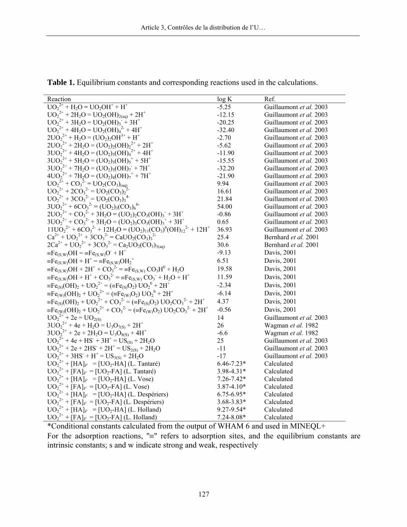
Article 3, Contrôles de la distribution de l’U…
127
Table 1. Equilibrium constants and corresponding reactions used in the calculations.
Reaction log K Ref. UO2
2+ + H2O = UO2OH+ + H+ -5.25 Guillaumont et al. 2003 UO2
2+ + 2H2O = UO2(OH)2(aq) + 2H+ -12.15 Guillaumont et al. 2003 UO2
2+ + 3H2O = UO2(OH)3- + 3H+ -20.25 Guillaumont et al. 2003
UO22+ + 4H2O = UO2(OH)4
2- + 4H+ -32.40 Guillaumont et al. 2003 2UO2
2+ + H2O = (UO2)2OH3+ + H+ -2.70 Guillaumont et al. 2003 2UO2
2+ + 2H2O = (UO2)2(OH)22+ + 2H+ -5.62 Guillaumont et al. 2003
3UO22+ + 4H2O = (UO2)3(OH)4
2+ + 4H+ -11.90 Guillaumont et al. 2003 3UO2
2+ + 5H2O = (UO2)3(OH)5+ + 5H+ -15.55 Guillaumont et al. 2003
3UO22+ + 7H2O = (UO2)3(OH)7
- + 7H+ -32.20 Guillaumont et al. 2003 4UO2
2+ + 7H2O = (UO2)4(OH)7+ + 7H+ -21.90 Guillaumont et al. 2003
UO22+ + CO3
2- = UO2(CO3)(aq) 9.94 Guillaumont et al. 2003 UO2
2+ + 2CO32- = UO2(CO3)2
2- 16.61 Guillaumont et al. 2003 UO2
2+ + 3CO32- = UO2(CO3)3
4- 21.84 Guillaumont et al. 2003 3UO2
2+ + 6CO32- = (UO2)3(CO3)6
6- 54.00 Guillaumont et al. 2003 2UO2
2+ + CO32- + 3H2O = (UO2)2CO3(OH)3
- + 3H+ -0.86 Guillaumont et al. 2003 3UO2
2+ + CO32- + 3H2O = (UO2)3CO3(OH)3
+ + 3H+ 0.65 Guillaumont et al. 2003 11UO2
2+ + 6CO32- + 12H2O = (UO2)11(CO3)6(OH)12
2- + 12H+ 36.93 Guillaumont et al. 2003 Ca2+ + UO2
2+ + 3CO32- = CaUO2(CO3)3
2- 25.4 Bernhard et al. 2001 2Ca2+ + UO2
2+ + 3CO32- = Ca2UO2(CO3)3(aq) 30.6 Bernhard et al. 2001
≡Fe(S,W)OH = ≡Fe(S,W)O- + H+ -9.13 Davis, 2001 ≡Fe(S,W)OH + H+ = ≡Fe(S,W)OH2
+ 6.51 Davis, 2001 ≡Fe(S,W)OH + 2H+ + CO3
2- = ≡Fe(S,W) CO3H0 + H2O 19.58 Davis, 2001 ≡Fe(S,W)OH + H+ + CO3
2- = ≡Fe(S,W) CO3- + H2O + H+ 11.59 Davis, 2001
≡Fe(S)(OH)2 + UO22+ = (≡Fe(S)O2) UO2
0 + 2H+ -2.34 Davis, 2001 ≡Fe(W)(OH)2 + UO2
2+ = (≡Fe(W)O2) UO20 + 2H+ -6.14 Davis, 2001
≡Fe(S)(OH)2 + UO22+ + CO3
2- = (≡Fe(S)O2) UO2CO32- + 2H+ 4.37 Davis, 2001
≡Fe(W)(OH)2 + UO22+ + CO3
2- = (≡Fe(W)O2) UO2CO32- + 2H+ -0.56 Davis, 2001
UO22+ + 2e = UO2(S) 14 Guillaumont et al. 2003
3UO22+ + 4e + H2O = U3O7(S) + 2H+ 26 Wagman et al. 1982
3UO22+ + 2e + 2H2O = U3O8(S) + 4H+ -6.6 Wagman et al. 1982
UO22+ + 4e + HS- + 3H+ = US(S) + 2H2O 25 Guillaumont et al. 2003
UO22+ + 2e + 2HS- + 2H+ = US2(S) + 2H2O -11 Guillaumont et al. 2003
UO22+ + 3HS- + H+ = US3(S) + 2H2O -17 Guillaumont et al. 2003
UO22+ + [HA]F = [UO2-HA] (L. Tantaré) 6.46-7.23* Calculated
UO22+ + [FA]F = [UO2-FA] (L. Tantaré) 3.98-4.31* Calculated
UO22+ + [HA]F = [UO2-HA] (L. Vose) 7.26-7.42* Calculated
UO22+ + [FA]F = [UO2-FA] (L. Vose) 3.87-4.10* Calculated
UO22+ + [HA]F = [UO2-HA] (L. Despériers) 6.75-6.95* Calculated
UO22+ + [FA]F = [UO2-FA] (L. Despériers) 3.68-3.83* Calculated
UO22+ + [HA]F = [UO2-HA] (L. Holland) 9.27-9.54* Calculated
UO22+ + [FA]F = [UO2-FA] (L. Holland) 7.24-8.08* Calculated
*Conditional constants calculated from the output of WHAM 6 and used in MINEQL+ For the adsorption reactions, "≡" refers to adsorption sites, and the equilibrium constants are intrinsic constants; s and w indicate strong and weak, respectively
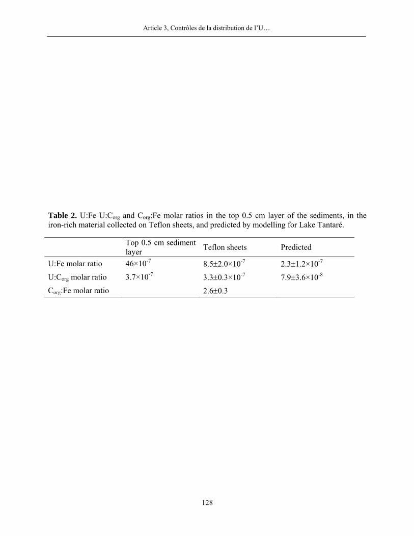
Article 3, Contrôles de la distribution de l’U…
128
Table 2. U:Fe U:Corg and Corg:Fe molar ratios in the top 0.5 cm layer of the sediments, in the iron-rich material collected on Teflon sheets, and predicted by modelling for Lake Tantaré.
Top 0.5 cm sediment layer Teflon sheets Predicted
U:Fe molar ratio 46×10-7 8.5±2.0×10⁻⁷ 2.3±1.2×10⁻⁷ U:Corg molar ratio 3.7×10⁻⁷ 3.3±0.3×10⁻⁷ 7.9±3.6×10⁻⁸ Corg:Fe molar ratio 2.6±0.3
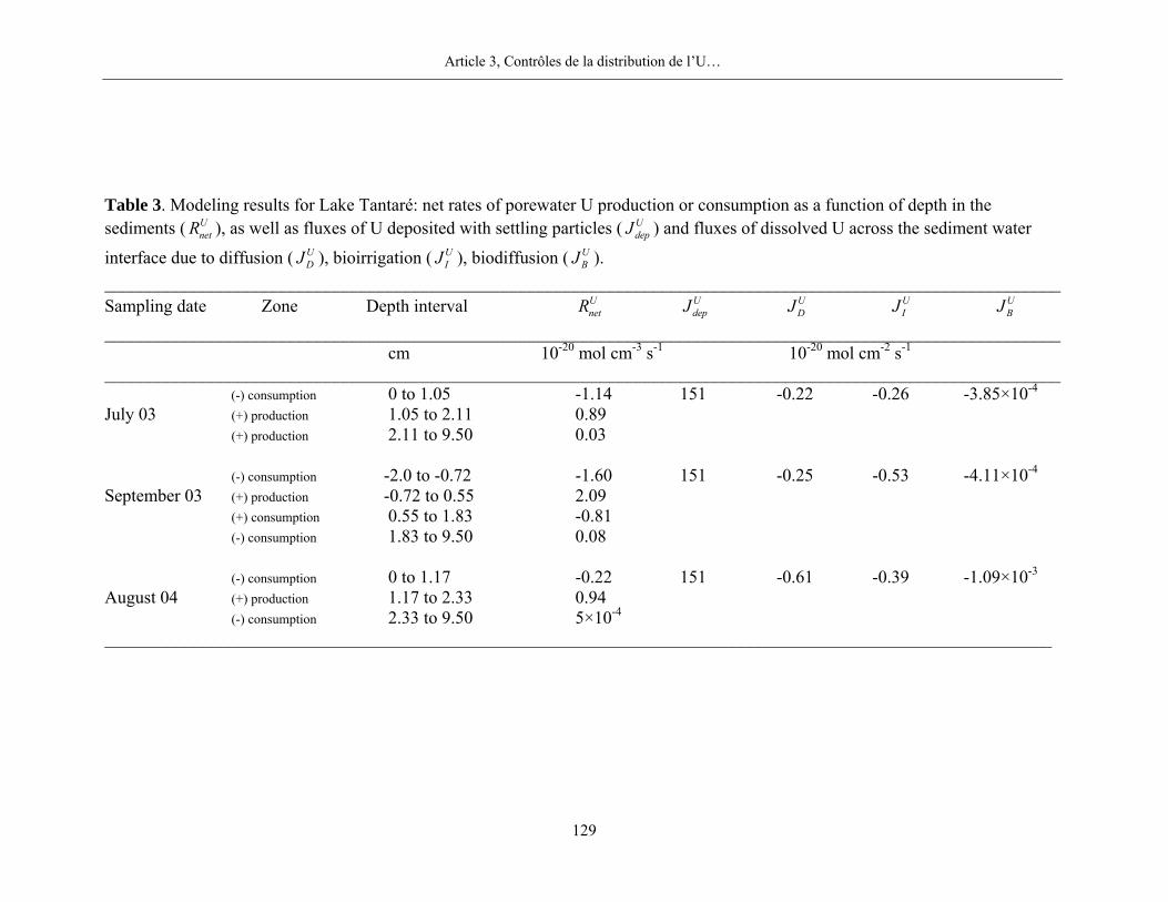
Article 3, Contrôles de la distribution de l’U…
129
Table 3. Modeling results for Lake Tantaré: net rates of porewater U production or consumption as a function of depth in the sediments ( U
netR ), as well as fluxes of U deposited with settling particles ( UdepJ ) and fluxes of dissolved U across the sediment water
interface due to diffusion ( UDJ ), bioirrigation ( U
IJ ), biodiffusion ( UBJ ).
____________________________________________________________________________________________________________ Sampling date Zone Depth interval U
netR UdepJ U
DJ UIJ U
BJ ____________________________________________________________________________________________________________ cm 10-20 mol cm-3 s-1 10-20 mol cm-2 s-1 ____________________________________________________________________________________________________________
(-) consumption 0 to 1.05 -1.14 151 -0.22 -0.26 -3.85×10⁻⁴ July 03 (+) production 1.05 to 2.11 0.89 (+) production 2.11 to 9.50 0.03 (-) consumption -2.0 to -0.72 -1.60 151 -0.25 -0.53 -4.11×10⁻⁴ September 03 (+) production -0.72 to 0.55 2.09 (+) consumption 0.55 to 1.83 -0.81 (-) consumption 1.83 to 9.50 0.08 (-) consumption 0 to 1.17 -0.22 151 -0.61 -0.39 -1.09×10⁻³ August 04 (+) production 1.17 to 2.33 0.94 (-) consumption 2.33 to 9.50 5×10⁻⁴ ___________________________________________________________________________________________________________
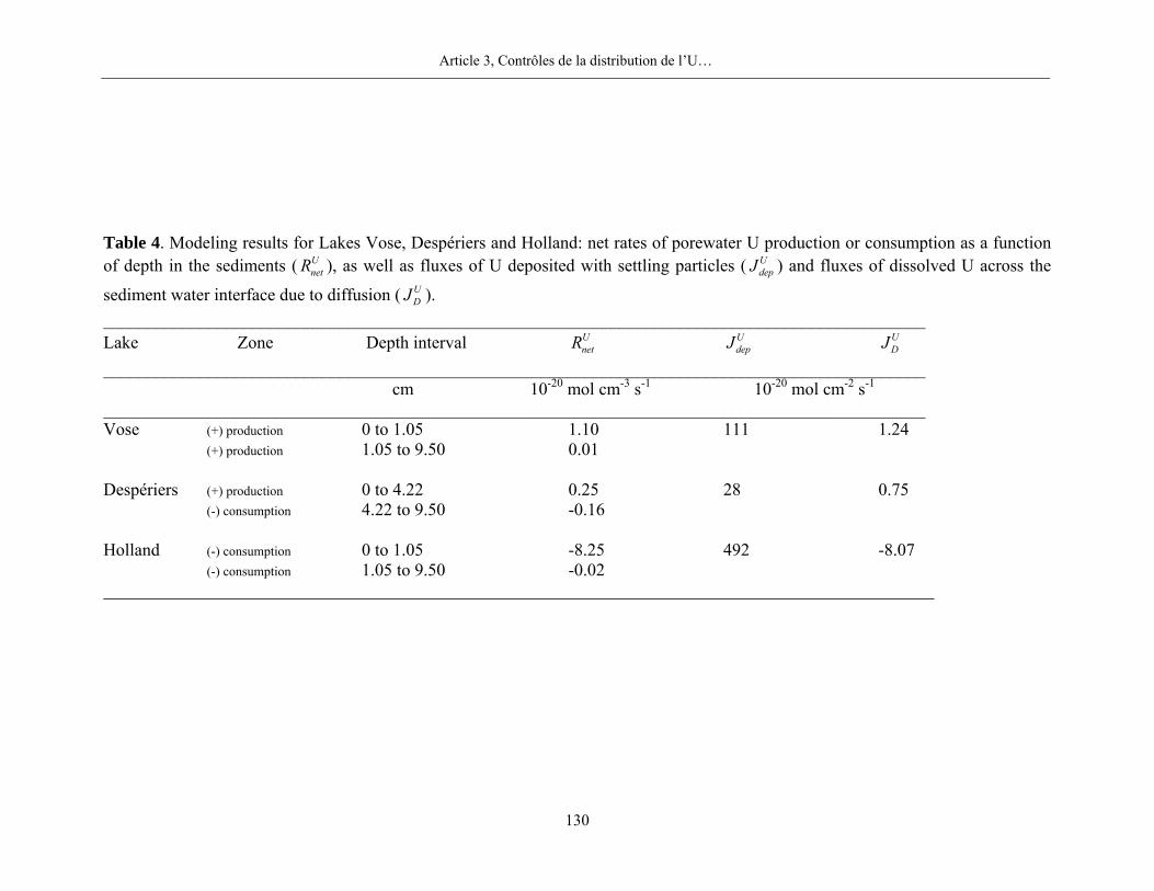
Article 3, Contrôles de la distribution de l’U…
130
Table 4. Modeling results for Lakes Vose, Despériers and Holland: net rates of porewater U production or consumption as a function of depth in the sediments ( U
netR ), as well as fluxes of U deposited with settling particles ( UdepJ ) and fluxes of dissolved U across the
sediment water interface due to diffusion ( UDJ ).
______________________________________________________________________________________________ Lake Zone Depth interval U
netR UdepJ U
DJ ______________________________________________________________________________________________ cm 10-20 mol cm-3 s-1 10-20 mol cm-2 s-1 ______________________________________________________________________________________________ Vose (+) production 0 to 1.05 1.10 111 1.24 (+) production 1.05 to 9.50 0.01 Despériers (+) production 0 to 4.22 0.25 28 0.75 (-) consumption 4.22 to 9.50 -0.16 Holland (-) consumption 0 to 1.05 -8.25 492 -8.07 (-) consumption 1.05 to 9.50 -0.02 _______________________________________________________________________________________________
Article 3, Contrôles de la distribution de l’U…
131
Figure captions
Figure 1. Triplicate porewater profiles of U (a-f), Fe (g-l), ΣS(-II) and pH (m-r), Corg (s-x) for all
lakes and sampling dates; comparisons of modeled with PROFILE (thin solid line following the
experimental points; r2 value indicated) and measured average (n = 3; open circles) porewater U
concentrations (y-ε; the thick solid line is the net Re consumption rate); comparison of measured
log IAP/Ks values with that at equilibrium (ε-ϕ). The horizontal broken line indicates the
sediment-water interface.
Figure 2. Depth profiles of measured sediment U concentrations (a-d), measured Corg and Al
concentrations (e-h) and U:Al molar ratios (i-l) in all lakes.
Figure 3. Percent of Corg versus measured sediment U concentrations in lake Holland. The thick
solid line represents the linear regression (U = 0.36×%Corg + 4.48) and r2 is the determination
coefficient.
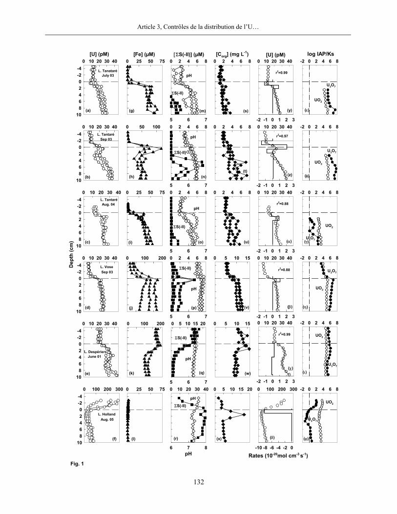
Article 3, Contrôles de la distribution de l’U…
132
0 10 20 30 40
-2 -1 0 1 2 3
0 10 20 30 40
-2 -1 0 1 2 3
0 10 20 30 40
-2 -1 0 1 2 3
0 10 20 30 40
-2 -1 0 1 2 3
0 25 50 75
0 10 20 30 40-4-202468
10
0 2 4 6 8
0 2 4 6 8
0 2 4 6 80 2 4 6 8
5 6 70 2 4 6 8
5 6 70 25 50 750 10 20 30 40
-4-202468
10
L. Tantaré
(c)
Aug. 04
Dep
th (c
m)
0 10 20 30 40-4-202468
10
L. TanataréJuly 03
(a)
(i)
(d)
0 2 4 6 8
5 6 7
(o)
(m)
pH
ΣS(-II)
ΣS(-II)
pH
(u)
(s)
(α)
(y)
Fig. 1
0 10 20 30 40-4-202468
10
L. TantaréSep 03
(b)
0 50 100
(h) (n)
pH
ΣS(-II)
(t)(z)
pH
[U] (pM) [Fe] (µM) [ΣS(-II)] (µM) [Corg] (mg L-1)
L. VoseSep 03
0 100 200 0 2 4 6 8
5 6 7
(p)
pH
ΣS(-II)
0 5 10 15
(v)(j)
(g)
0 10 20 30 40-4-202468
10
0 100 200 0 5 10 15 20
5 6 7
0 5 10 15
(e)
L. DespériersJune 01
(k)
ΣS(-II)
pH
(q) (w)
[U] (pM)
r2=0.99
Rates (10-20mol cm-3 s-1)
r2=0.97
r2=0.88
r2=0.88
(β)
0 10 20 30 40
-2 -1 0 1 2 3
r2=0.99
(χ)
0 10 20 30 40
6 7 8
0 100 200 300-4-202468
10
L. HollandAug. 05
0 25 50 75
pH
ΣS(-II)
0 5 10 15 20 0 100 200 300
-10 -8 -6 -4 -2 0
(f) (l) (r) (x) (δ)
-2 0 2 4 6 8
-2 0 2 4 6 8
-2 0 2 4 6 8
-2 0 2 4 6 8
-2 0 2 4 6 8
-2 0 2 4 6 8
UO2
U3O7
UO2
U3O7
U3O7
UO2
UO2
log IAP/Ks
(φ)
(ε)
(γ)
(η)
(ι)
(ϕ)
UO2
U3O7
UO2
U3O7
U3O7
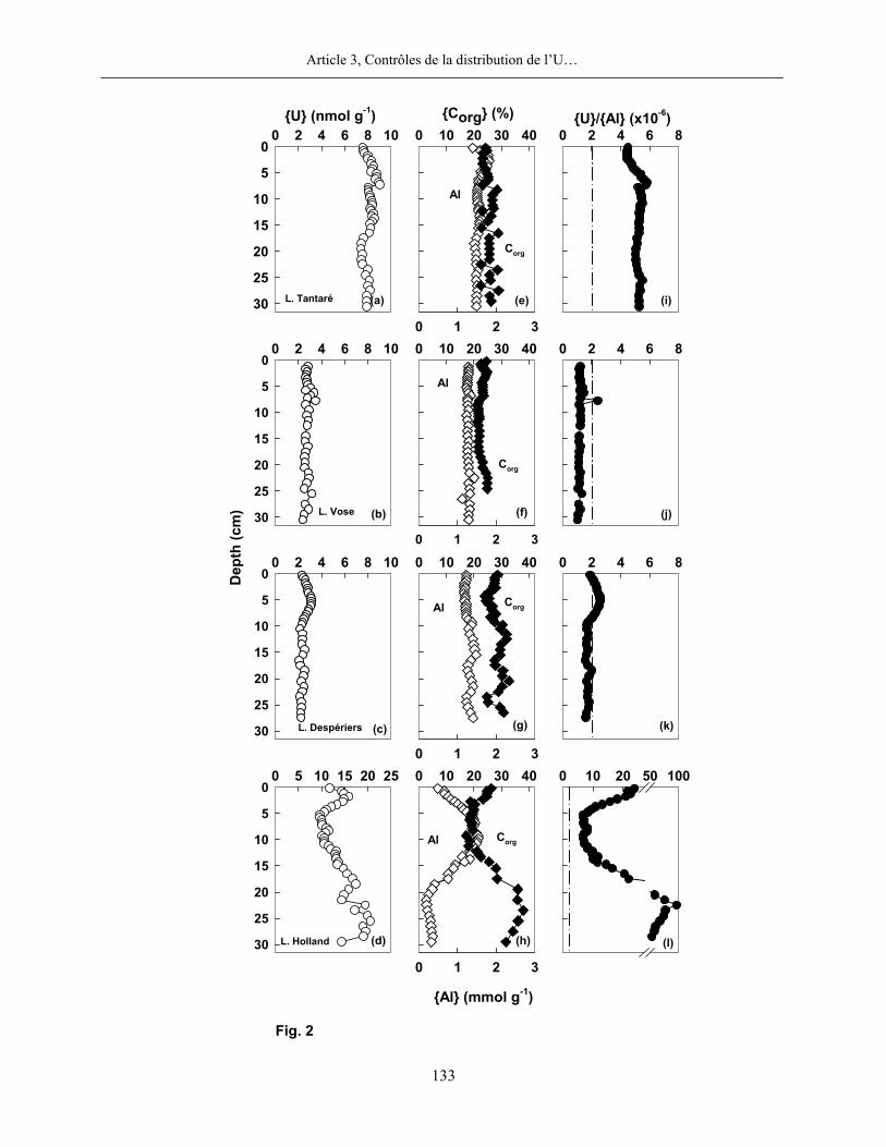
Article 3, Contrôles de la distribution de l’U…
133
0 2 4 6 80 10 20 30 40
0 1 2 3
0 2 4 6 8 100
5
10
15
20
25
30
0 2 4 6 80 10 20 30 40
0 1 2 3
0 2 4 6 8 100
5
10
15
20
25
30
U (nmol g-1)0 2 4 6 8 10
0
5
10
15
20
25
30 L. Tantaré
Fig. 2
L. Vose
Al (mmol g-1)
Corg (%)
Al
Corg
0 10 20 30 40
0 1 2 3
Al
Corg
(a)
U/Al (x10-6)0 2 4 6 8
(b)
(e)
(f)
(i)
(j)
Dep
th (c
m)
L. Despériers (c) (k)
Al Corg
(g)
0 10 20 30 40
0 1 2 3
0 5 10 15 20 250
5
10
15
20
25
30 L. Holland
Al Corg
0 10 20 50 100
(d) (h) (l)
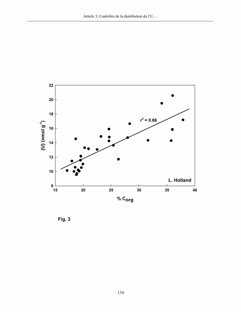
Article 3, Contrôles de la distribution de l’U…
134
% Corg
15 20 25 30 35 40
U (
nmol
g-1
)
8
10
12
14
16
18
20
22
r2 = 0.66
Fig. 3
L. Holland
PARTIE 3
RÉFÉRENCES BIBLIOGRAPHIQUES

RÉFÉRENCES BIBLIOGRAPHIQUES
Adelson J. M., Helz G. R. et Miller C. V. (2001) Reconstructing the rise of recent coastal anoxia;
molybdenum in Chesapeake Bay sediments. Geochim. Cosmochim. Acta 65, 237-252.
Alfaro-De la Torre M. C. et Tessier A. (2002) Cadmium deposition and mobility in the sediments
of an acidic oligotrophic lake. Geochim. Cosmochim. Acta 66, 3549-3562.
Algeo T. J. et Maynard J. B. (2004) Trace-element behavior and redox facies in core shales of
Upper Pennsylvanian Kansas-type cyclothems. Chem. Geol. 206, 289-318.
Algeo T. J. et Lyons T. W. (2006) Mo–total organic carbon covariation in modern anoxic marine
environments: Implications for analysis of paleoredox and paleohydrographic conditions.
Paleoceanogr. 21, PA1016. doi:10.1029/2004PA001112, 2006.
Allen H. E., Fu G. et Deng B. (1993) Analysis of Acid-Volatile Sulfide (AVS) and
Simultaneously Extracted Metals (SEM) for the estimation of potential toxicity in aquatic
sediments. Environ. Toxicol. Chem. 12, 1441-1453.
Amrhein C., Mosher P. A. et Brown A. D. (1993) The effects of redox on Mo, U, B, V, and As
solubility in evaporation pond soils. Soil Sci. 155, 249-255.
Anbar A. D., Creaser R. A., Papanastassiou D. A. et Wasserburg G. J. (1992) Rhenium in
seawater: Confirmation of generally conservative behaviour. Geochim. Cosmochim. Acta 56,
4099-4103.
Anbar A. D., Duan Y., Lyons T. W., Arnold G. L., Kendall B., Creaser R. A., Kaufman A. J.,
Gordon G. W., Scott C., Garvin J. et Buick R. (2007) A whiff of oxygen before the Great
Oxidation Event? Science. 317, 1903-1906.
Anderson R. F., Fleischer M. Q. et Lehuray A. P. (1989) Concentration, oxidation state, and
particulate flux of uranium in the Black Sea. Geochim. Cosmochim. Acta 53, 2215-2224.
Appleby P. G. et Piliposian G. T. (2004) Efficiency corrections for variable sample height in
well-type germanium gamma detectors. Nucl. Inst. Methods B. 225, 423-433.
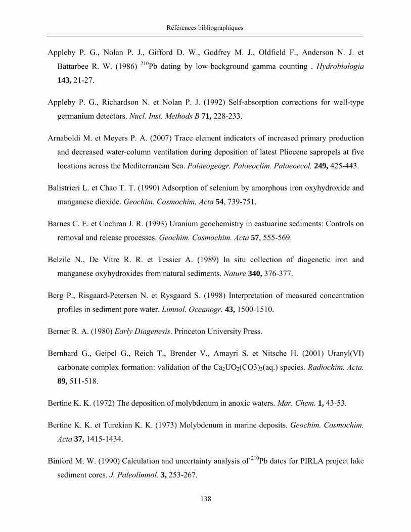
Références bibliographiques
138
Appleby P. G., Nolan P. J., Gifford D. W., Godfrey M. J., Oldfield F., Anderson N. J. et
Battarbee R. W. (1986) 210Pb dating by low-background gamma counting . Hydrobiologia
143, 21-27.
Appleby P. G., Richardson N. et Nolan P. J. (1992) Self-absorption corrections for well-type
germanium detectors. Nucl. Inst. Methods B 71, 228-233.
Arnaboldi M. et Meyers P. A. (2007) Trace element indicators of increased primary production
and decreased water-column ventilation during deposition of latest Pliocene sapropels at five
locations across the Mediterranean Sea. Palaeogeogr. Palaeoclim. Palaeoecol. 249, 425-443.
Balistrieri L. et Chao T. T. (1990) Adsorption of selenium by amorphous iron oxyhydroxide and
manganese dioxide. Geochim. Cosmochim. Acta 54, 739-751.
Barnes C. E. et Cochran J. R. (1993) Uranium geochemistry in eastuarine sediments: Controls on
removal and release processes. Geochim. Cosmochim. Acta 57, 555-569.
Belzile N., De Vitre R. R. et Tessier A. (1989) In situ collection of diagenetic iron and
manganese oxyhydroxides from natural sediments. Nature 340, 376-377.
Berg P., Risgaard-Petersen N. et Rysgaard S. (1998) Interpretation of measured concentration
profiles in sediment pore water. Limnol. Oceanogr. 43, 1500-1510.
Berner R. A. (1980) Early Diagenesis. Princeton University Press.
Bernhard G., Geipel G., Reich T., Brender V., Amayri S. et Nitsche H. (2001) Uranyl(VI)
carbonate complex formation: validation of the Ca2UO2(CO3)3(aq.) species. Radiochim. Acta.
89, 511-518.
Bertine K. K. (1972) The deposition of molybdenum in anoxic waters. Mar. Chem. 1, 43-53.
Bertine K. K. et Turekian K. K. (1973) Molybdenum in marine deposits. Geochim. Cosmochim.
Acta 37, 1415-1434.
Binford M. W. (1990) Calculation and uncertainty analysis of 210Pb dates for PIRLA project lake
sediment cores. J. Paleolimnol. 3, 253-267.
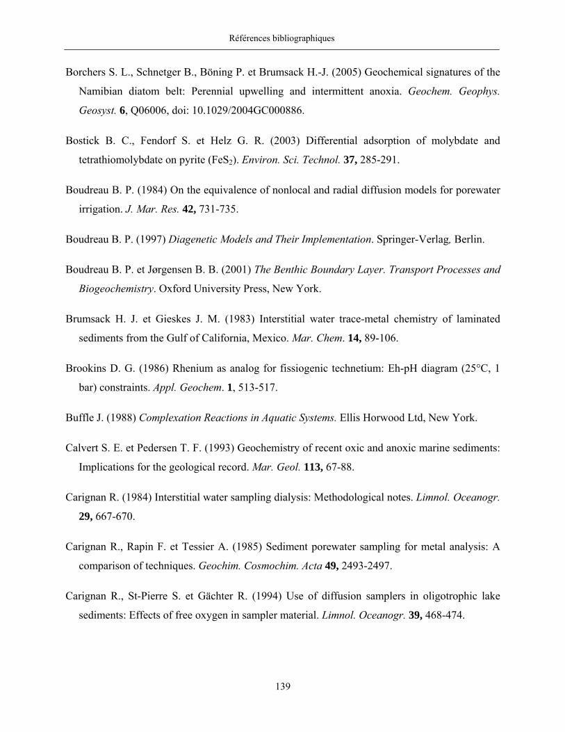
Références bibliographiques
139
Borchers S. L., Schnetger B., Böning P. et Brumsack H.-J. (2005) Geochemical signatures of the
Namibian diatom belt: Perennial upwelling and intermittent anoxia. Geochem. Geophys.
Geosyst. 6, Q06006, doi: 10.1029/2004GC000886.
Bostick B. C., Fendorf S. et Helz G. R. (2003) Differential adsorption of molybdate and
tetrathiomolybdate on pyrite (FeS2). Environ. Sci. Technol. 37, 285-291.
Boudreau B. P. (1984) On the equivalence of nonlocal and radial diffusion models for porewater
irrigation. J. Mar. Res. 42, 731-735.
Boudreau B. P. (1997) Diagenetic Models and Their Implementation. Springer-Verlag, Berlin.
Boudreau B. P. et Jørgensen B. B. (2001) The Benthic Boundary Layer. Transport Processes and
Biogeochemistry. Oxford University Press, New York.
Brumsack H. J. et Gieskes J. M. (1983) Interstitial water trace-metal chemistry of laminated
sediments from the Gulf of California, Mexico. Mar. Chem. 14, 89-106.
Brookins D. G. (1986) Rhenium as analog for fissiogenic technetium: Eh-pH diagram (25°C, 1
bar) constraints. Appl. Geochem. 1, 513-517.
Buffle J. (1988) Complexation Reactions in Aquatic Systems. Ellis Horwood Ltd, New York.
Calvert S. E. et Pedersen T. F. (1993) Geochemistry of recent oxic and anoxic marine sediments:
Implications for the geological record. Mar. Geol. 113, 67-88.
Carignan R. (1984) Interstitial water sampling dialysis: Methodological notes. Limnol. Oceanogr.
29, 667-670.
Carignan R., Rapin F. et Tessier A. (1985) Sediment porewater sampling for metal analysis: A
comparison of techniques. Geochim. Cosmochim. Acta 49, 2493-2497.
Carignan R., St-Pierre S. et Gächter R. (1994) Use of diffusion samplers in oligotrophic lake
sediments: Effects of free oxygen in sampler material. Limnol. Oceanogr. 39, 468-474.
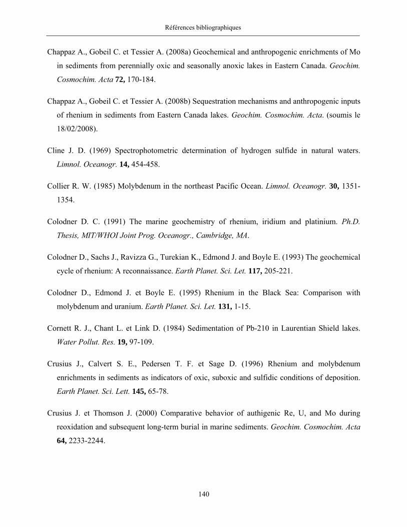
Références bibliographiques
140
Chappaz A., Gobeil C. et Tessier A. (2008a) Geochemical and anthropogenic enrichments of Mo
in sediments from perennially oxic and seasonally anoxic lakes in Eastern Canada. Geochim.
Cosmochim. Acta 72, 170-184.
Chappaz A., Gobeil C. et Tessier A. (2008b) Sequestration mechanisms and anthropogenic inputs
of rhenium in sediments from Eastern Canada lakes. Geochim. Cosmochim. Acta. (soumis le
18/02/2008).
Cline J. D. (1969) Spectrophotometric determination of hydrogen sulfide in natural waters.
Limnol. Oceanogr. 14, 454-458.
Collier R. W. (1985) Molybdenum in the northeast Pacific Ocean. Limnol. Oceanogr. 30, 1351-
1354.
Colodner D. C. (1991) The marine geochemistry of rhenium, iridium and platinium. Ph.D.
Thesis, MIT/WHOI Joint Prog. Oceanogr., Cambridge, MA.
Colodner D., Sachs J., Ravizza G., Turekian K., Edmond J. and Boyle E. (1993) The geochemical
cycle of rhenium: A reconnaissance. Earth Planet. Sci. Let. 117, 205-221.
Colodner D., Edmond J. et Boyle E. (1995) Rhenium in the Black Sea: Comparison with
molybdenum and uranium. Earth Planet. Sci. Let. 131, 1-15.
Cornett R. J., Chant L. et Link D. (1984) Sedimentation of Pb-210 in Laurentian Shield lakes.
Water Pollut. Res. 19, 97-109.
Crusius J., Calvert S. E., Pedersen T. F. et Sage D. (1996) Rhenium and molybdenum
enrichments in sediments as indicators of oxic, suboxic and sulfidic conditions of deposition.
Earth Planet. Sci. Lett. 145, 65-78.
Crusius J. et Thomson J. (2000) Comparative behavior of authigenic Re, U, and Mo during
reoxidation and subsequent long-term burial in marine sediments. Geochim. Cosmochim. Acta
64, 2233-2244.
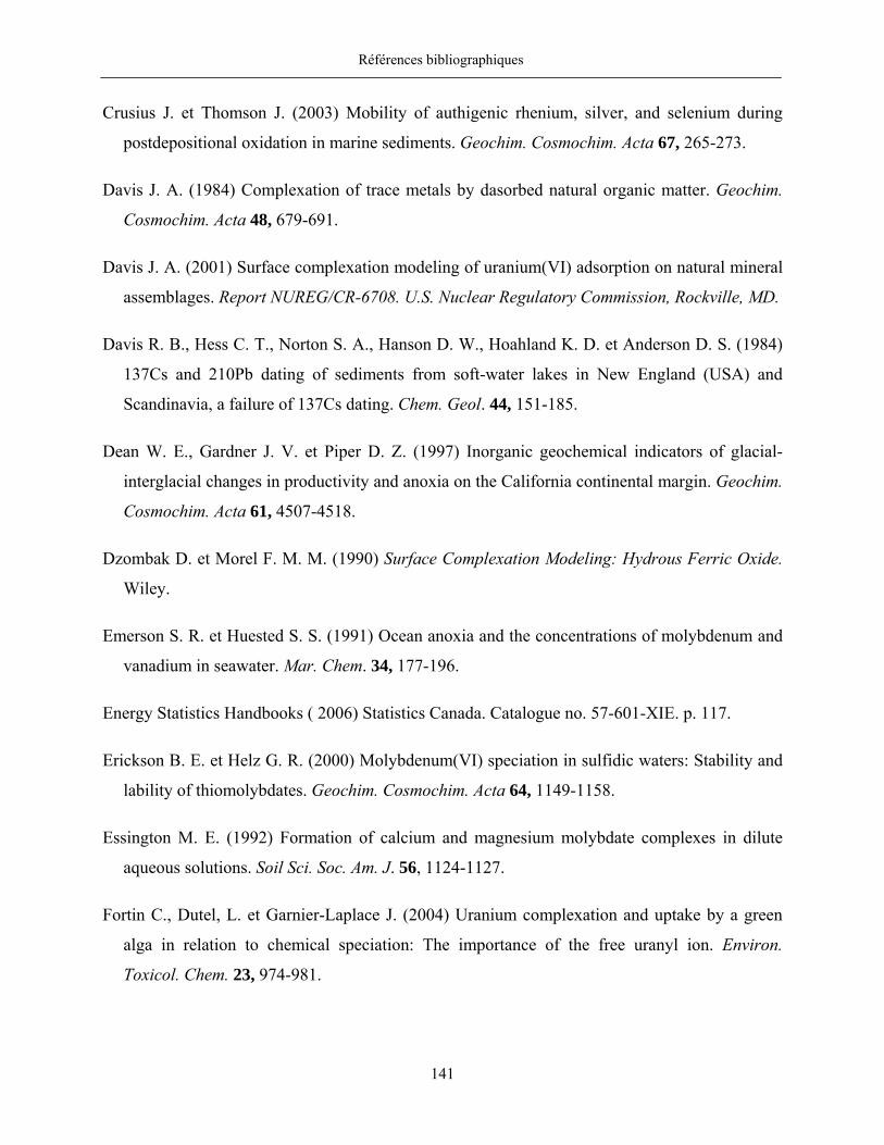
Références bibliographiques
141
Crusius J. et Thomson J. (2003) Mobility of authigenic rhenium, silver, and selenium during
postdepositional oxidation in marine sediments. Geochim. Cosmochim. Acta 67, 265-273.
Davis J. A. (1984) Complexation of trace metals by dasorbed natural organic matter. Geochim.
Cosmochim. Acta 48, 679-691.
Davis J. A. (2001) Surface complexation modeling of uranium(VI) adsorption on natural mineral
assemblages. Report NUREG/CR-6708. U.S. Nuclear Regulatory Commission, Rockville, MD.
Davis R. B., Hess C. T., Norton S. A., Hanson D. W., Hoahland K. D. et Anderson D. S. (1984)
137Cs and 210Pb dating of sediments from soft-water lakes in New England (USA) and
Scandinavia, a failure of 137Cs dating. Chem. Geol. 44, 151-185.
Dean W. E., Gardner J. V. et Piper D. Z. (1997) Inorganic geochemical indicators of glacial-
interglacial changes in productivity and anoxia on the California continental margin. Geochim.
Cosmochim. Acta 61, 4507-4518.
Dzombak D. et Morel F. M. M. (1990) Surface Complexation Modeling: Hydrous Ferric Oxide.
Wiley.
Emerson S. R. et Huested S. S. (1991) Ocean anoxia and the concentrations of molybdenum and
vanadium in seawater. Mar. Chem. 34, 177-196.
Energy Statistics Handbooks ( 2006) Statistics Canada. Catalogue no. 57-601-XIE. p. 117.
Erickson B. E. et Helz G. R. (2000) Molybdenum(VI) speciation in sulfidic waters: Stability and
lability of thiomolybdates. Geochim. Cosmochim. Acta 64, 1149-1158.
Essington M. E. (1992) Formation of calcium and magnesium molybdate complexes in dilute
aqueous solutions. Soil Sci. Soc. Am. J. 56, 1124-1127.
Fortin C., Dutel, L. et Garnier-Laplace J. (2004) Uranium complexation and uptake by a green
alga in relation to chemical speciation: The importance of the free uranyl ion. Environ.
Toxicol. Chem. 23, 974-981.
Références bibliographiques
142
Fortin D., Leppard G. G. et Tessier A. (1993) Characteristics of lacustrine diagenetic iron
oxyhydroxides. Geochim. Cosmochim. Acta 57, 4391-4404.
Fowle D. A., Fein J. B. et Martin A. M. (2000) Experimental study of uranyl adsorption onto
bacillus subtilis. Environ. Sci. Technol. 34, 3737-3741.
François R. (1988) A study on the regulation of the concentrations of some trace metals (Rb, Sr,
Zn, Pb, Cu, V, Cr, Ni, Mn and Mo) in Saanich Inlet sediments, British Colombia, Canada.
Mar. Geol. 83, 285-308.
François R., Bacon M. P., Altabet M. A. et Labeyrie L. D. (1993) Glacial interglacial changes in
sediment rain rate in the SW Indian sector of sub-antarctic waters as recorded by Th-230, Pa-
231, U, and δ-N-15. Paleoceanogr. 8, 611-629.
François R., Altabet M. A., Sigman D. M., Bacon M. P., Frank M., Bohrman G., Bareille G. et
Labeyrie L. D. (1997) Contribution of Southern Ocean surface-water stratification to low
atmospheric CO2 concentrations during the last glacial period. Nature. 389, 929-935.
Fredrickson J. K., Zachara J. M., Kennedy D. W., Duff M. C., Gorby Y. A., Li S. W. et Krupka
K. M. (2000) Reduction of U(VI) in goethite (α-FeOOH) suspensions by a dissimilatory metal-
reducing bacterium. Geochim. Cosmochim. Acta 64, 3085-3098.
Freme F. (2005) U.S. Coal Supply and Demand: 2005 Review. Energy Information
Administration.
Gallon C., Tessier A., Gobeil C. et Alfaro-De La Torre M. C. (2004) Modeling diagenesis of lead
in sediments of a Canadian Shield lake. Geochim. Cosmochim. Acta 68, 3531-3545.
Gallon C., Tessier A., Gobeil C et Beaudin L. (2005) Sources and chronology of atmospheric
lead deposition to a Canadian Shield lake: Inferences from Pb isotopes and PAH profiles.
Geochim. Cosmochim. Acta 69, 3199-3210.
Gallon C., Tessier A. et Gobeil C. (2006) Historical perspective of industrial lead emissions to
the atmosphere from a Canadian smelter. Environ. Sci. Technol. 40, 741-747.
Références bibliographiques
143
Gobeil C., Sundby B., Macdonald R. W. et Smith J. N. (2001) Recent change in organic carbon
flux to Arctic Ocean deep basins: Evidence from acid volatile sulfide, manganese and rhenium
discord in basin sediments. Geophys. Res. Let. 28, 1747-1750.
Gobeil C., Rondeau B. et Beaudin L. (2005) Contribution of municipal effluents to metal fluxes
in the St. Lawrence river. Environ. Sci. Technol. 39, 456-464.
Goldberg, S. Su, C. et Forster, H. S. (1998) Sorption of molybdenum on oxides, clay minerals,
and soils: Mechanisms and models. E.A. Jenne (ed.) Adsorption of metals by geomedia:
Variables, mechanisms, and model applications. Proc. Am. Chem. Soc. Symp. Academic
Press, San Diego. 401-426.
Gu B., Schmitt J., Chen Z., Liang L. et McCarthy J. F. (1994) Adsorption and desorption of
natural organic matter on iron oxide: Mechanisms and models. Environ. Sci. Technol. 28, 38-
46.
Guillaumont R., Fanghanel T., Neck V., Fuger J., Palmer D. A., Grenthe I. et Rand M. H. (2003)
Update on the Chemical Thermodynamic of Uranium, Neptunium, Plutonium, Americium, and
Technecium. Elsevier, Amsterdam.
Gustafsson J. P. (2003) Modelling molybdate and tungstate adsorption to ferrihydrite. Chem.
Geol. 200, 105-115.
Hamilton-Taylor J., Smith E. J., Davison W. et Sugiyama M. (2005) Resolving and modeling the
effects of Fe and Mn redox cycling on trace metal behavior in a seasonally anoxic lake.
Geochim. Cosmochim. Acta 69, 1947-1960.
Hare L., Carignan R. et Huerta-Diaz M. A. (1994) A field study of metal toxicity and
accumulation by benthic invertebrates; implications for the acid-volatile sulfide (AVS) model.
Limnol. Oceanogr. 39, 1653-1668.
Helz G. R., Miller C. V., Charnock J. M., Mosselmans J. F. W., Pattrick R. A. D., Garner C. D. et
Vaughan D. J. (1996) Mechanism of molybdenum removal from the sea and its concentration
in black shales: EXAFS evidence. Geochim. Cosmochim. Acta 60, 3631-3642.
Références bibliographiques
144
Helz G. R., Vorlicek T. P. et Kahn M. D. (2004) Molybdenum scavenging by iron monosulfide.
Environ. Sci. Technol. 38, 4263-4268.
Kada J. et Heit M. (1992) The inventories of anthropogenic Pb, Zn, As, Cd and the radionuclides
Cs-137 and excess Pb-210 in lake sediments of the Adirondack region. Hydrobiologia 246,
231-241.
Kendall B. S., Creaser R. A., Ross G. M. et Selby D. (2004) Constraints on the timing of
Marinoan “Snowball Earth” glaciation by 187Re-188Os dating of a Neoproterozoic, post-glacial
black shale in Western Canada. Earth Planet. Sci. Let. 222, 729-740.
Kim E. et Boulègue J. (2003) Chemistry of rhenium as an analogue of technetium: Experimental
studies of the dissolution of rhenium oxides in aqueous solutions. Radiochim. Acta 91, 211-
216.
Klinkhammer G. P. et Palmer M. R. (1991) Uranium in the oceans: Where it goes and why.
Geochim. Cosmochim. Acta 55, 1799-1806.
Koide M., Hodge V. F., Yang J. S., Stallard M. et Goldberg E. G. (1986) Some comparative
marine chemistries of rhenium, gold, silver and molybdenum. Appl. Geochem. 1, 705-714.
Krachler M. et Shotyk W. (2004) Natural and anthropogenic enrichments of molybdenum,
thorium, and uranium in a complete peat bog profile, Jura Mountains, Switzerland. J. Environ.
Monitor. 6, 418-426.
Ku T. L., Knauss K. G. et Mathieu G. (1977) Uranium in the open ocean: Concentration and
isotopic composition. Deep-Sea Res. 24, 1005-1017.
Laforte L., Tessier A., Gobeil C. et Carignan R. (2005) Thallium diagenesis in lacustrine
sediments. Geochim. Cosmochim. Acta 69, 5295-5306.
Lead J. R., Wilkinson K. J., Starchev K., Canonica S. et Buffle J. (2000) Determination of
diffusion coefficients of humic substances by fluorescence correlation spectroscopy: Role of
solution conditions. Environ. Sci. Technol. 34, 1365-1369.
Références bibliographiques
145
Lenhart J. J. et Honeyman B. D. (1999) Uranium(VI) sorption to hematite in the presence of
humic acid. Geochim. Cosmochim. Acta 63, 2891-2901.
Li Y.-H. et Gregory S. (1974) Diffusion of ions in sea water and in deep-sea sediments. Geochim.
Cosmochim. Acta 38, 703-714.
Liu C., Zachara J. M., Zhong L., Kukkadupa R., Szecsody J. E. et Kennedy D.W. (2005)
Influence of sediment bioreduction and reoxidation on uranium sorption. Environ. Sci.
Technol. 39, 4125-4133.
Lovely D. R., Phillips E. J. P. et Woodward J. C. (1991) Microbial reduction of uranium. Nature.
350, 413-416.
Lyons T. W., Werne J. P., Hollander D. J. et Murray R. W. (2003) Contrasting sulfur
geochemistry and Fe/Al and Mo/Al ratios across the last oxic-to-anoxic transition in the
Cariaco Basin, Venezuela. Chem. Geol. 195, 131-157.
Malcolm S. J. (1985) Early diagenesis of molybdenum in estuarine sediments. Mar. Chem. 16,
213-225.
Mangini A., Jung M. et Laukenmann S. (2001) What do we learn from peaks of uranium and of
manganese in deep sea sediments? Mar. Geol. 177, 63-78.
Matisoff G. et Wang X. (1998) Solute transport in sediments by freshwater infaunal bioirrigators.
Limnol. Oceanogr. 43, 1487-1499.
Matisoff G. et Wang X. (2000) Particle mixing by freshwater infaunal bioirrigators: Midges
(Chironomidae: Diptera) and mayflies (Ephemeridae: Ephemeroptera). J. Great Lakes Res. 26,
174-182.
Références bibliographiques
146
McKay J. L., Pedersen T. F. et Mucci A. (2007) Sedimentary redox conditions in continental
margin sediments (N.E. Pacific) — Influence on the accumulation of redox-sensitive trace
metals. Chem. Geol. 238, 180-196.
McLaren J. W., Methven B. A. J., Lam J. W. H. et Berman S. S. (1995) The use of inductively
coupled plasma mass spectrometry in the production of environmental certified materials.
Mikrochim. Acta 119, 287-295.
McManus, J., Berelson, W. M., Klinkhammer, G. P., Hammond, D. E. et Holm, C. (2005)
Authigenic uranium: relationship to oxygen penetration depth and organic carbon rain.
Geochim. Cosmochim. Acta 69, 95-108.
McManus J., Berelson W. M., Severmann S., Poulson R. L., Hammond D. E., Klinkhammer G.
P. et Holm C. (2006) Molybdenum and uranium geochemistry in continental margin
sediments: Paleoproxy potential. Geochim. Cosmochim. Acta 70, 4643-4662.
Meyers S. R., Sageman B. B. et Lyons T. W. (2005) Organic carbon burial rate and the
molybdenum proxy: Theoretical framework and application to Cenomanian-Turonian oceanic
anoxic event 2. Paleoceanogr. 20, A2002. doi:10.1029/2004PA001068, 2005.
Meysman F. J. R., Middelburg J. J., Herman P. M. J. et Heip C. H. R. (2003) Reactive transport
in surface sediments. II. Media: An object-oriented problem-solving environment for early
diagenesis. Comput. Geosci. 29, 301-318.
Morford J .L. et Emerson S. (1999) The geochemistry of redox sensitive trace metals in
sediments. Geochim. Cosmochim. Acta 63, 1735-1750.
Morford J. L., Russell A. D. et Emerson S. R. (2001) Trace metal evidence for changes in the
redox environment associated with the transition from terrigenous clay to diatomaceous
sediment, Saanich Inlet, BC. Mar. Geol. 174, 355-369.
Morford J. L., Emerson S. R., Breckel E. J. et Kim S. H. (2005) Diagenesis of oxyanions (V, U,
Re, and Mo) in pore waters and sediments from a continental margin. Geochim. Cosmochim.
Acta 69, 5021-5032.
Références bibliographiques
147
Morford J. L., Martin W. R., Kalnejais L. H., François R., Bothner M. et Karle I.-M. (2007)
Insight on geochemical cycling of U, Re and Mo from seasonal sampling in Boston Harbor,
Massachusetts, USA. Geochim. Cosmochim. Acta 71, 895-917.
Moyes L. N., Parkman R. H., Charnock J. M., Vaughan D. J., Livens F. R., Hughes C. R. et
Braithwaite A. (2000) Uranium uptake from aqueous solution by interaction with goethite,
lepidocrocite, muscovite and mackinawite: An X-ray absorption spectroscopy study. Environ.
Sci. Technol. 34, 1062-1068.
Murphy R. J., Lenhart J. J. et Honeyman B. D. (1999) The sorption of thorium(IV) and
uranium(VI) to hematite in the presence of natural organic matter. Colloids Surf. A:
Physicochem. Engineer. Aspects 157, 47-62.
Nagao S., Yanase N., Yamamoto M., Kofuji H., Sohrin Y. et Amono H. (2002) The geochemistry
of uranium in pore waters from lake sediments. J. Radioanal. Nucl. Chem. 252, 225-232.
Nameroff T. J., Balistrieri L. S. et Murray J. W. (2002) Suboxic trace metal geochemistry in the
Eastern Tropical North Pacific. Geochim. Cosmochim. Acta 66, 1139-1158.
Nameroff T. J., Calvert S. E. et Murray J. W. (2004) Glacial-interglacial variability in the eastern
tropical North Pacific oxygen minimum zone recorded by redox-sensitive trace metals.
Paleoceanogr. 19, PA1010.
Nriagu J. O. et Pacyna J. M. (1988) Quantitative assessment of worldwide contamination of air,
water and soils by trace metals. Nature 333, 134-139.
Pacyna J. M. et Pacyna E. G. (2001) An assessment of global and regional emissions of trace
metals to the atmosphere from anthropogenic sources worldwide. Environ. Rev. 9, 269-298.
Papelis C., Hayes K. F. et Leckie J. O. (1988) HYDRAQL: A Program for the Computation of
Chemical Equilibrium Composition of Aqueous Batch Systems Including Surface
Complexation Modeling of Ion Adsorption at the Oxide/Solution Interface. Stanford Univ.
Dept. Civ. Eng. Tech. Rep. 306.
Références bibliographiques
148
Payne T. E., Davis J. A. et Waite T. D. (1996) Uranium adsorption on ferrihydrite - Effects of
phosphate and humic acid. Radiochim. Acta 74, 239-243.
Ravizza G. et Turekian K. K. (1989) Application of the 187Re/188Os system to black shale
geochronometry. Geochim. Cosmochim. Acta 53, 3257-3262.
Ravizza G., Turekian K. K. et Hay B. J. (1991) The geochemistry of rhenium and osmium in
recent sediments from the Black Sea. Geochim. Cosmochim. Acta 55, 3741-3752.
Robbins J. A. (1978) Geochemical and geophysical applications of radioactive lead. In The
Biogeochemistry of Lead in the Environment (ed. J. O. Nriagu) Elsevier. pp. 285-393.
Russell A. D. et Morford J. L. (2001) The behavior of redox-sensitive metals across a laminated–
massive–laminated transition in Saanich Inlet, British Columbia. Mar. Geol. 174, 341-354.
Sani R. K., Peyton B. M., Amonette J. E. et Geesey G. G. (2004) Reduction of uranium (VI)
under sulfate-reducing conditions in the presence of Fe(III)-(hydr)oxides. Geochim.
Cosmochim. Acta 68, 2639-2648.
Schaller T., Moor H. C. et Wehrli B. (1997) Sedimentary profiles of Fe, Mn, V, As and Mo as
indicators of benthic redox conditions in Baldeggersee. Aquat. Sci. 59, 345-361.
Schecher M. E. et McAvoy D. (1998) MINEQL+. Environmental Research Software.
Schelske C. L., Peplow A., Brenner M. et Spencer C. N. (1994) Low-background gamma
counting: Applications for 210Pb dating of sediments. J. Paleolimnol. 10, 115-128.
Schwarzenbach R. P., Gschwend P. M. et Imboden, D. M. (1993) Environmental Organic
Chemistry. Wiley-Interscience, New York.
Scott C., Lyons T. W., Bekker A., Shen Y., Poulton S. W., Chu X. et Anbar A. D. (2008) Tracing
the stepwise oxygenation of the Proterozoic ocean. Nature. 452, 456-459.
Scott T. B., Riba Tort O. et Allen G. C. (2007) Aqueous uptake of uranium onto pyrite surfaces;
reactivity of fresh versus weathered material. Geochim. Cosmochim. Acta. 71, 5044-5053.
Références bibliographiques
149
Shaw T. J., Gieskes J. M. et Jahnke R. A. (1990) Early diagenesis in differing depositional-
environments – the response of transition-metals in pore water. Geochim. Cosmochim. Acta.
54, 1233-1246.
Shimmield G. B. et Price N. B. (1986) The behaviour of molybdenum and manganese during
early diagenesis - offshore Baja California, Mexico. Mar. Chem. 19, 261-280.
Straughan I., Etseewi A. A. et Page A .L. (1978) Mobilization of selected trace elements in
residues from coal combustion with special reference to fly ash. Trace Subst. Environ.
Microbiol. 45, 743-747.
Stumm W. et Morgan J. J. (1996) Aquatic Chemistry. 3rd ed. Wiley.
Subosa P. F., Kihara K., Rokushika S., Hatano H., Kubota T. et Hanaoka Y. (1989) Ion
chromatography of inorganic anions in brine samples. J. Chromatogr. Sci. 27, 680-684.
Sundby B., Martinez P. et Gobeil C. (2004) Comparative geochemistry of cadmium, rhenium,
uranium, and molybdenum in continental margin sediments. Geochim. Cosmochim. Acta. 68,
2485-2493.
Telmer K., Bonham-Carter G. F., Kliza D. A. et Hall G. E. M. (2004) The atmospheric transport
and deposition of smelter emissions: Evidence from the multi-element geochemistry of snow,
Quebec, Canada. Geochim. Cosmochim. Acta. 68, 2961-2980.
Tipping E. (1981) The adsorption of aquatic humic substances by iron oxides. Geochim.
Cosmochim. Acta 45, 191-199.
Tipping E., Woof C. et Cooke D. (1981) Iron oxide from a seasonally anoxic lake. Geochim.
Cosmochim. Acta 45, 1411-1419.
Tipping E. (1994) WHAM-A chemical equilibrium model and computer code for waters,
sediments, and soils incorporating a discrete site/electrostatic model of ion-binding by humic
substances. Comput. Geosci. 20, 973-1023.
Références bibliographiques
150
Tossel J. A. (2005) Calculation of the UV-visible spectra and the stability of Mo and Re
oxysulfides in aqueous solution. Geochim. Cosmochim. Acta 69, 2497-2503.
Tribovillard N., Riboulleau A., Lyons T. et Baudin F. O. (2004) Enhanced trapping of
molybdenum by sulfurized marine organic matter of marine origin in Mesozoic limestones and
shales. Chem. Geol. 213, 385-401.
Tribovillard N., Algeo T. J., Lyons T. et Riboulleau A. (2006) Trace metals as paleoredox and
paleoproductivity proxies: An update. Chem. Geol. 232, 12-32.
Turekian K. K. et Wedepohl K. H. (1961) Distribution of the elements in some major units of the
earth's crust. Geol. Soc. Amer. Bull. 72, 175-191.
Van Cappellen P., Gaillard J.-F. et Rabouille C. (1993) Biogeochemical transformations in
sediments: Kinetic models of early diagenesis. In Interactions of C, N, P and S
Biogeochemical Cycles and Global Change (ed. R. Wollast et al.), pp. 401-445. Springer-
Verlag.
Van Cappellen P. et Wang Y. (1995) Metal cycling in surface sediments: Modeling the interplay
of transport and reaction. In Metal Contaminated Sediments (ed. H. E. Allen), pp. 21-64. Ann
Arbor Press.
van der Weijden C. H., Middelburg J. J., De Lange G. J., van der Sloot H. A., Hoede D. et
Woittiez J. R. W. (1990) Profiles of the redox-sensitive trace elements As, Sb, V, Mo and U in
the Tyro and Bannock Basins (eastern Mediterranean). Mar. Chem. 31, 171-186.
Vorlicek T. P., Kahn M. D., Kasuya Y. et Helz G. R. (2004) Capture of molybdenum in pyrite-
forming sediments: Role of ligand-induced reduction by polysulfides. Geochim. Cosmochim.
Acta 68, 547-556.
Wagman D. D., Evans W. H., Parker V. B., Schumm R. H., Halow I., Bailey S. M., Churney K.
L. et Nuttall R. L. (1982) The NBS tables of thermochemical properties. J. Physic. Chem. Ref.
Data 11, (Suppl. 2. Am. Inst. of Physics, Melville, NY).
Références bibliographiques
151
Waite T. D., Davis J. A., Payne T. E., Waychunas G. A. et Xu N. (1994) Uranium(VI) adsorption
to ferrihydrite: Application of a surface complexation model. Geochim. Cosmochim. Acta 58,
5465-5478.
Wedepohl K. H. (1995) The composition of the continental crust. Geochim. Cosmochim. Acta 59,
1217-1232.
Wersin P., Hochella M. F., Persson P., Redden G., Leckie J. O. et Harris D. W. (1994) Interaction
between aqueous uranium (VI) and sulfide minerals: Spectroscopic evidence for sorption and
reduction. Geochim. Cosmochim. Acta 58, 2829-2843.
Xiong Y. (2003) Solubility and speciation of rhenium in anoxic environments at ambient
temperature and applications to the Black Sea. Deep-Sea Res. Part I. 50, 681-690.
Yagasaki A., Andersson I. et Pettersson L. (1987) Multicomponent polyanions. 41.
Potentiometric and 31P NMR study of equilibria in the molybdophenylphophonate system in
0.6 M Na(Cl) medium. Inorg. Chem. 26, 3926-3933.
Yamashita Y., Takahashi Y., Haba H., Enomoto S. et Shimizu H. (2007) Comparison of
reductive accumulation of Re and Os in seawater-sediment systems. Geochim. Cosmochim.
Acta 71, 3458-3475
Zhang P. C. et Sparks D. L. (1989) Kinetics and mechanisms of molybdate adsorption/desorption
at the goethite/water interface using pressure-jump relaxation. Soil. Sci. Soc. Am. J. 53, 1028-
1034.
Zheng Y., Anderson R. F., van Geen A. et Kuwabara J. (2000) Authigenic molybdenum
formation in marine sediments: A link to pore water sulfide in the Santa Barbara Basin.
Geochim. Cosmochim. Acta 64, 4165-4178.
Zheng Y., Anderson R. F., van Geen A. et Fleisher M. Q. (2002a) Preservation of particulate
non-lithogenic uranium in marine sediments. Geochim. Cosmochim. Acta 66, 3085-3092.
Zheng Y., Anderson R. F., van Geen A. et Fleisher M. Q. (2002b) Remobilization of authigenic
uranium in marine sediments by bioturbation. Geochim. Cosmochim. Acta 66, 1759-1772.

PARTIE 4
ANNEXES


Annexes
155
Lac Tantaré, bassin 4 Juillet 2003 Localisation 47º04’N 71°32’O Concentrations dans les eaux interstitielles Dialyseur #1 Profondeur
(cm) Mo 1 (nM)
Re 1 (pM)
U 1 (pM)
Fe 1 (µM)
Mn 1 (µM)
ΣS(-II) 1 (µM) pH 1 Ca 1
(µM) K 1 (µM)
Mg 1 (µM)
Na 1 (µM)
Cl- 1 (µM)
NO3- 1 (µM)
SO42- 1 (µM)
DIC 1 (mM)
DOC 1 (mg/L)
-4.5 0.23 5.96 14.23 5.73 0.54 ND 5.63 29.20 9.10 14.30 23.22 8.83 10.30 33.56 0.18 1.52 -3.5 0.10 4.38 9.99 ND ND ND 5.67 ND ND ND ND 6.74 7.17 33.92 0.16 1.39 -2.5 0.13 5.63 13.07 0.45 0.42 ND 5.58 21.81 6.24 10.20 21.60 6.67 7.91 33.44 0.06 1.22 -1.5 0.11 5.81 12.07 0.42 0.43 ND 5.61 23.16 6.26 10.07 21.20 7.44 8.12 33.82 0.18 1.52 -0.5 0.11 5.41 9.39 0.51 0.56 ND 5.54 19.13 6.54 10.59 21.66 7.11 7.40 33.69 0.17 2.06 0.5 0.33 5.10 8.51 9.55 0.60 ND 5.45 31.21 6.59 10.18 21.68 7.83 6.22 36.97 0.31 1.23 1.5 0.98 4.30 13.85 37.46 0.59 ND 5.84 35.13 6.70 10.59 21.85 7.96 1.83 27.35 0.42 2.52 2.5 1.31 3.74 20.12 41.19 0.58 ND 6.11 41.25 6.80 10.71 22.34 9.24 2.44 17.99 0.45 2.11 3.5 1.48 3.50 20.11 40.99 0.58 ND 6.39 51.70 6.94 10.93 22.89 7.43 0.42 7.56 0.43 1.82 4.5 1.65 3.56 21.05 41.62 0.57 ND 6.32 51.10 6.84 10.80 22.58 7.34 2.01 3.64 0.43 1.72 5.5 1.66 2.71 20.74 45.18 0.60 ND 6.42 55.34 6.97 11.24 22.94 6.78 0.48 4.10 0.48 2.68 6.5 1.44 2.56 21.63 48.17 0.62 0.03 6.44 71.50 7.29 11.48 23.57 7.55 2.08 7.55 0.49 3.14 7.5 1.34 3.16 21.64 50.41 0.61 0.09 6.45 66.58 7.02 11.31 22.86 7.43 2.38 9.69 0.45 2.52 8.5 1.17 1.78 23.12 ND ND 1.17 6.48 ND ND ND ND 8.36 5.18 11.77 0.52 2.46 9.5 1.08 2.02 24.30 ND ND 1.12 6.35 ND ND ND ND 6.94 1.56 14.44 0.59 3.54
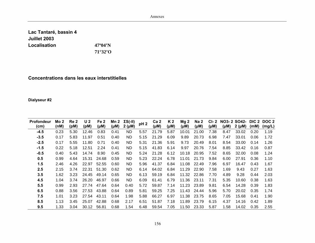
Annexes
156
Lac Tantaré, bassin 4
Juillet 2003
Localisation 47º04’N
71°32’O
Concentrations dans les eaux interstitielles
Dialyseur #2
Profondeur
(cm) Mo 2 (nM)
Re 2 (pM)
U 2 (pM)
Fe 2 (µM)
Mn 2 (µM)
ΣS(-II) 2 (µM) pH 2 Ca 2
(µM) K 2 (µM)
Mg 2 (µM)
Na 2 (µM)
Cl- 2 (µM)
NO3- 2 (µM)
SO42- 2 (µM)
DIC 2 (mM)
DOC 2 (mg/L)
-4.5 0.23 5.30 12.46 0.83 0.41 ND 5.57 21.79 5.87 10.01 21.00 7.38 8.47 33.02 0.20 1.19 -3.5 0.17 5.83 11.97 0.51 0.40 ND 5.15 21.29 6.09 9.89 20.73 6.98 7.47 33.01 0.06 1.72 -2.5 0.17 5.55 11.80 0.71 0.40 ND 5.31 21.36 5.91 9.73 20.49 8.01 8.54 33.00 0.14 1.26 -1.5 0.22 5.18 12.51 2.24 0.41 ND 5.15 41.83 6.14 9.97 20.76 7.54 8.85 33.42 0.16 0.87 -0.5 0.40 5.43 14.74 8.90 0.45 ND 5.24 21.28 6.12 10.18 20.95 7.52 8.65 32.00 0.08 1.24 0.5 0.99 4.64 15.31 24.68 0.59 ND 5.23 22.24 6.78 11.01 21.73 9.84 6.00 27.91 0.36 1.10 1.5 2.46 4.26 22.97 52.55 0.60 ND 5.96 41.37 6.84 11.08 22.49 7.96 6.97 16.47 0.43 1.67 2.5 2.15 3.74 22.31 51.30 0.62 ND 6.14 64.02 6.84 11.29 22.90 7.58 1.69 9.43 0.27 1.63 3.5 1.62 3.23 24.45 49.14 0.65 ND 6.13 59.19 6.84 11.32 22.86 7.70 4.89 9.28 0.44 2.03 4.5 1.04 3.74 26.20 46.97 0.66 ND 6.09 61.41 6.79 11.36 23.11 7.31 5.35 10.60 0.38 1.63 5.5 0.99 2.93 27.74 47.64 0.64 0.40 5.72 59.87 7.14 11.23 23.89 9.81 6.54 14.28 0.39 1.83 6.5 0.88 3.56 27.53 43.88 0.64 0.89 5.81 59.25 7.25 11.43 24.44 5.96 5.70 20.02 0.35 1.74 7.5 1.01 3.23 27.54 43.11 0.64 1.98 5.88 66.27 6.97 11.38 23.75 8.65 7.05 15.68 0.41 1.90 8.5 1.13 3.45 25.07 42.88 0.68 2.17 6.51 51.87 7.18 11.89 23.79 6.15 4.37 14.16 0.42 1.89 9.5 1.33 3.04 30.12 56.81 0.68 1.54 6.48 59.54 7.05 11.50 23.33 5.87 1.58 14.02 0.35 2.55
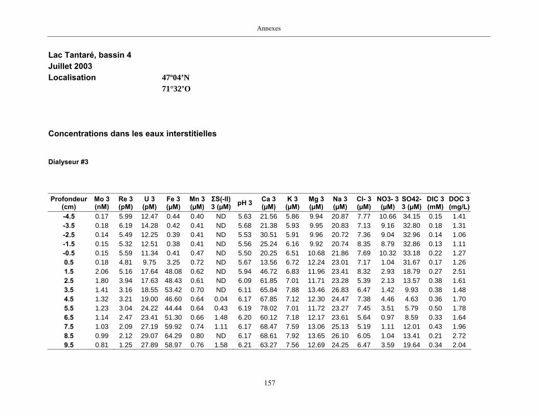
Annexes
157
Lac Tantaré, bassin 4
Juillet 2003
Localisation 47º04’N
71°32’O
Concentrations dans les eaux interstitielles
Dialyseur #3
Profondeur
(cm) Mo 3 (nM)
Re 3 (pM)
U 3 (pM)
Fe 3 (µM)
Mn 3 (µM)
ΣS(-II) 3 (µM) pH 3 Ca 3
(µM) K 3 (µM)
Mg 3 (µM)
Na 3 (µM)
Cl- 3 (µM)
NO3- 3 (µM)
SO42- 3 (µM)
DIC 3 (mM)
DOC 3 (mg/L)
-4.5 0.17 5.99 12.47 0.44 0.40 ND 5.63 21.56 5.86 9.94 20.87 7.77 10.66 34.15 0.15 1.41 -3.5 0.18 6.19 14.28 0.42 0.41 ND 5.68 21.38 5.93 9.95 20.83 7.13 9.16 32.80 0.18 1.31 -2.5 0.14 5.49 12.25 0.39 0.41 ND 5.53 30.51 5.91 9.96 20.72 7.36 9.04 32.96 0.14 1.06 -1.5 0.15 5.32 12.51 0.38 0.41 ND 5.56 25.24 6.16 9.92 20.74 8.35 8.79 32.86 0.13 1.11 -0.5 0.15 5.59 11.34 0.41 0.47 ND 5.50 20.25 6.51 10.68 21.86 7.69 10.32 33.18 0.22 1.27 0.5 0.18 4.81 9.75 3.25 0.72 ND 5.67 13.56 6.72 12.24 23.01 7.17 1.04 31.67 0.17 1.26 1.5 2.06 5.16 17.64 48.08 0.62 ND 5.94 46.72 6.83 11.96 23.41 8.32 2.93 18.79 0.27 2.51 2.5 1.80 3.94 17.63 48.43 0.61 ND 6.09 61.85 7.01 11.71 23.28 5.39 2.13 13.57 0.38 1.61 3.5 1.41 3.16 18.55 53.42 0.70 ND 6.11 65.84 7.88 13.46 26.83 6.47 1.42 9.93 0.38 1.48 4.5 1.32 3.21 19.00 46.60 0.64 0.04 6.17 67.85 7.12 12.30 24.47 7.38 4.46 4.63 0.36 1.70 5.5 1.23 3.04 24.22 44.44 0.64 0.43 6.19 78.02 7.01 11.72 23.27 7.45 3.51 5.79 0.50 1.78 6.5 1.14 2.47 23.41 51.30 0.66 1.48 6.20 60.12 7.18 12.17 23.61 5.64 0.97 8.59 0.33 1.64 7.5 1.03 2.09 27.19 59.92 0.74 1.11 6.17 68.47 7.59 13.06 25.13 5.19 1.11 12.01 0.43 1.96 8.5 0.99 2.12 29.07 64.29 0.80 ND 6.17 68.61 7.92 13.65 26.10 6.05 1.04 13.41 0.21 2.72 9.5 0.81 1.25 27.89 58.97 0.76 1.58 6.21 63.27 7.56 12.69 24.25 6.47 3.59 19.64 0.34 2.04

Annexes
158
Lac Tantaré, bassin 4 Septembre 2003 Localisation 47º04’N 71°32’O Concentrations dans les eaux interstitielles Dialyseur #1 Profondeur
(cm) Mo 1 (nM)
Re 1 (pM)
U 1 (pM)
Fe 1 (µM)
Mn 1 (µM)
ΣS(-II) 1 (µM) pH 1 Ca 1
(µM) K 1 (µM)
Mg 1 (µM)
Na 1 (µM)
Cl- 1 (µM)
NO3- 1 (µM)
SO42- 1 (µM)
DIC 1 (mM)
DOC 1 (mg/L)
-4.5 0.15 3.57 6.91 1.42 0.50 0.02 5.79 21.50 6.12 9.46 19.13 5.71 5.48 33.05 0.47 1.86 -3.5 0.20 3.59 8.14 1.58 0.41 0.02 5.73 17.64 5.25 7.67 15.63 6.09 4.59 32.92 0.48 1.80 -2.5 0.29 3.65 8.91 3.45 0.52 0.02 5.89 39.83 6.35 9.66 19.58 5.73 3.08 32.08 0.52 2.23 -1.5 0.43 3.69 8.94 6.30 0.54 0.02 5.94 24.80 6.08 9.11 18.41 6.21 3.29 32.52 0.45 2.80 -0.5 1.50 3.83 16.54 50.89 0.58 0.02 6.18 38.74 6.76 10.37 21.18 5.82 10.18 30.86 0.46 3.69 0.5 1.90 3.88 18.78 75.54 0.55 0.01 6.09 38.49 6.78 10.40 26.60 5.85 2.84 32.29 0.56 3.48 1.5 0.71 3.72 16.22 42.23 0.54 0.01 6.18 39.44 6.71 10.27 21.61 5.49 1.69 28.39 0.59 3.45 2.5 0.56 3.82 13.93 ND ND 0.40 6.35 ND ND ND ND 7.37 1.85 29.85 0.64 3.50 3.5 0.54 3.82 15.08 22.89 0.53 3.36 6.38 35.41 6.30 9.62 19.70 5.43 2.18 28.60 0.65 3.61 4.5 0.50 3.28 19.23 35.25 0.56 7.07 6.41 47.55 6.70 10.13 21.20 5.98 2.38 22.61 0.68 4.67 5.5 0.69 2.87 24.27 34.66 0.56 7.22 6.50 48.56 6.48 9.89 20.00 5.21 0.97 9.73 0.73 5.99 6.5 0.26 1.78 25.76 36.52 0.60 5.61 6.46 79.91 7.26 11.02 25.00 5.56 0.97 6.56 0.77 4.33 7.5 0.52 1.98 32.64 52.84 0.73 3.86 6.50 73.21 7.72 12.65 24.14 5.00 0.97 9.03 0.88 5.57 8.5 0.41 1.50 31.10 45.94 0.69 3.21 6.45 76.71 7.34 11.92 22.66 5.07 0.97 8.43 0.92 5.12 9.5 0.40 1.61 33.58 43.20 0.72 1.65 6.48 67.34 6.92 11.01 20.34 5.11 0.97 7.69 0.92 4.94

Annexes
159
Lac Tantaré, bassin 4
Septembre 2003
Localisation 47º04’N
71°32’O
Concentrations dans les eaux interstitielles
Dialyseur #2 Profondeur
(cm) Mo 2 (nM)
Re 2 (pM)
U 2 (pM)
Fe 2 (µM)
Mn 2 (µM)
ΣS(-II) 2 (µM) pH 2 Ca 2
(µM) K 2 (µM)
Mg 2 (µM)
Na 2 (µM)
Cl- 2 (µM)
NO3- 2 (µM)
SO42- 2 (µM)
DIC 2 (mM)
DOC 2 (mg/L)
-4.5 0.15 3.68 8.74 1.67 0.46 0.02 5.82 31.78 5.78 8.62 17.56 9.12 5.28 31.66 0.56 1.90 -3.5 0.16 3.88 8.38 2.07 0.44 0.02 5.80 20.16 5.54 8.32 16.89 5.56 4.65 31.40 0.55 2.15 -2.5 0.22 3.49 9.49 3.79 0.52 0.02 5.79 21.86 6.20 9.67 19.36 9.46 5.56 31.88 0.56 1.78 -1.5 0.26 3.64 9.34 4.57 0.54 0.02 5.78 23.49 6.31 9.85 19.88 7.07 5.43 31.10 0.58 2.85 -0.5 1.89 3.44 16.94 68.29 0.59 0.01 6.07 48.44 6.96 10.52 22.03 8.31 20.49 37.06 0.64 3.11 0.5 3.44 3.45 25.30 116.75 0.62 0.14 6.14 57.77 7.08 11.07 23.77 5.41 0.97 32.17 0.66 3.12 1.5 2.11 3.16 21.63 88.76 0.57 ND 5.95 45.67 7.04 10.18 20.83 5.67 2.42 32.51 0.61 3.01 2.5 1.10 3.72 17.26 48.94 0.55 2.30 6.21 48.90 6.47 10.23 20.17 5.36 0.97 30.77 0.60 1.95 3.5 0.95 3.20 22.06 63.21 0.65 4.97 6.27 55.11 7.04 11.41 22.74 4.93 0.97 26.33 0.66 3.29 4.5 0.74 2.44 25.45 56.34 0.68 10.79 6.36 74.31 7.44 11.71 23.50 4.99 0.97 20.69 0.82 3.24 5.5 0.78 1.78 30.34 48.83 0.65 8.84 6.35 55.86 6.85 11.28 21.07 5.06 0.97 10.01 0.84 3.25 6.5 1.29 1.66 34.80 52.60 0.66 5.47 6.42 58.31 6.85 11.29 28.44 5.03 0.97 4.73 0.82 3.08 7.5 1.02 1.37 35.21 59.87 0.73 4.32 6.45 61.26 7.37 12.40 22.64 5.11 0.97 4.63 0.89 3.41 8.5 1.35 1.22 37.10 64.87 0.78 4.28 6.43 66.30 7.61 12.93 23.26 5.11 0.97 4.89 0.89 4.64 9.5 1.55 1.07 36.55 63.39 0.78 4.53 6.39 80.56 7.56 12.78 22.96 5.72 0.97 4.08 0.93 3.54

Annexes
160
Lac Tantaré, bassin 4
Septembre 2003
Localisation 47º04’N
71°32’O
Concentrations dans les eaux interstitielles
Dialyseur #3 Profondeur
(cm) Mo 3 (nM)
Re 3 (pM)
U 3 (pM)
Fe 3 (µM)
Mn 3 (µM)
ΣS(-II) 3 (µM) pH 3 Ca 3
(µM) K 3 (µM)
Mg 3 (µM)
Na 3 (µM)
Cl- 3 (µM)
NO3- 3 (µM)
SO42- 3 (µM)
DIC 3 (mM)
DOC 3 (mg/L)
-4.5 ND ND ND 1.85 0.52 0.04 5.75 22.26 6.24 9.73 19.90 5.44 5.23 32.32 0.57 2.13 -3.5 0.20 3.50 10.68 2.11 0.52 0.06 5.85 47.56 7.03 9.80 22.40 5.16 5.01 32.13 0.43 2.11 -2.5 0.27 3.85 10.19 3.56 0.56 0.02 5.77 27.70 6.63 10.31 21.09 5.13 4.34 31.79 0.44 2.10 -1.5 0.45 3.44 10.73 8.51 0.56 0.01 5.81 63.61 6.77 10.57 21.53 5.34 4.13 31.32 0.45 1.95 -0.5 1.71 3.99 20.47 48.12 0.50 0.02 5.83 29.13 6.03 9.14 18.60 5.34 0.97 32.76 0.50 2.07 0.5 1.94 3.63 24.37 57.59 0.40 0.02 6.22 26.89 5.30 7.44 15.26 5.27 0.97 33.64 0.57 3.49 1.5 1.14 3.25 21.92 61.01 0.57 0.01 6.29 48.88 6.79 10.51 23.26 5.15 0.97 30.56 0.55 3.94 2.5 0.91 3.17 20.91 49.49 0.57 0.01 6.41 42.69 6.64 10.37 21.28 5.39 0.97 24.95 0.62 4.23 3.5 0.60 3.55 27.24 42.12 0.54 0.04 6.42 44.51 6.33 9.69 19.61 5.08 0.97 18.44 0.69 4.08 4.5 0.48 3.00 29.91 47.67 0.62 0.53 6.47 84.02 8.26 11.34 26.24 5.64 1.85 14.30 0.67 7.16 5.5 0.51 2.29 30.22 46.12 0.61 2.17 6.53 71.41 8.73 11.32 27.31 5.75 2.24 9.94 0.72 4.56 6.5 0.51 2.25 32.39 52.10 0.70 3.46 6.52 65.78 7.45 12.39 23.42 5.29 1.78 10.59 0.73 5.20 7.5 0.45 1.90 36.95 49.16 0.71 2.29 6.47 69.95 7.44 12.29 23.19 6.55 2.31 9.11 0.75 5.18 8.5 0.56 1.77 34.91 47.80 0.73 1.14 6.47 65.80 7.56 12.45 23.49 4.96 0.97 9.57 0.78 7.34 9.5 0.71 1.53 36.71 48.65 0.74 0.36 6.47 67.60 7.50 12.33 23.08 5.25 0.97 12.44 0.78 6.15
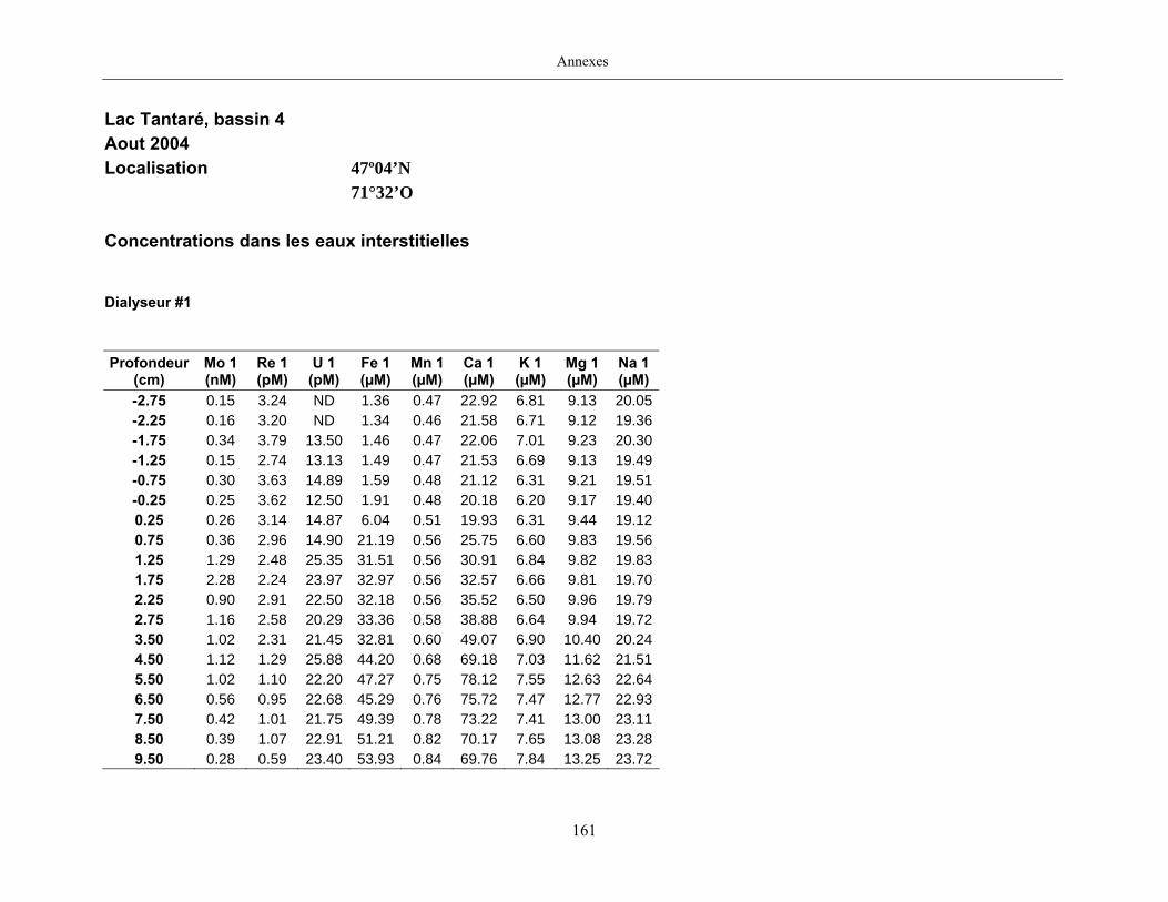
Annexes
161
Lac Tantaré, bassin 4 Aout 2004 Localisation 47º04’N 71°32’O Concentrations dans les eaux interstitielles Dialyseur #1 Profondeur
(cm) Mo 1 (nM)
Re 1 (pM)
U 1 (pM)
Fe 1 (µM)
Mn 1 (µM)
Ca 1 (µM)
K 1 (µM)
Mg 1 (µM)
Na 1 (µM)
-2.75 0.15 3.24 ND 1.36 0.47 22.92 6.81 9.13 20.05-2.25 0.16 3.20 ND 1.34 0.46 21.58 6.71 9.12 19.36-1.75 0.34 3.79 13.50 1.46 0.47 22.06 7.01 9.23 20.30-1.25 0.15 2.74 13.13 1.49 0.47 21.53 6.69 9.13 19.49-0.75 0.30 3.63 14.89 1.59 0.48 21.12 6.31 9.21 19.51-0.25 0.25 3.62 12.50 1.91 0.48 20.18 6.20 9.17 19.400.25 0.26 3.14 14.87 6.04 0.51 19.93 6.31 9.44 19.120.75 0.36 2.96 14.90 21.19 0.56 25.75 6.60 9.83 19.561.25 1.29 2.48 25.35 31.51 0.56 30.91 6.84 9.82 19.831.75 2.28 2.24 23.97 32.97 0.56 32.57 6.66 9.81 19.702.25 0.90 2.91 22.50 32.18 0.56 35.52 6.50 9.96 19.792.75 1.16 2.58 20.29 33.36 0.58 38.88 6.64 9.94 19.723.50 1.02 2.31 21.45 32.81 0.60 49.07 6.90 10.40 20.244.50 1.12 1.29 25.88 44.20 0.68 69.18 7.03 11.62 21.515.50 1.02 1.10 22.20 47.27 0.75 78.12 7.55 12.63 22.646.50 0.56 0.95 22.68 45.29 0.76 75.72 7.47 12.77 22.937.50 0.42 1.01 21.75 49.39 0.78 73.22 7.41 13.00 23.118.50 0.39 1.07 22.91 51.21 0.82 70.17 7.65 13.08 23.289.50 0.28 0.59 23.40 53.93 0.84 69.76 7.84 13.25 23.72
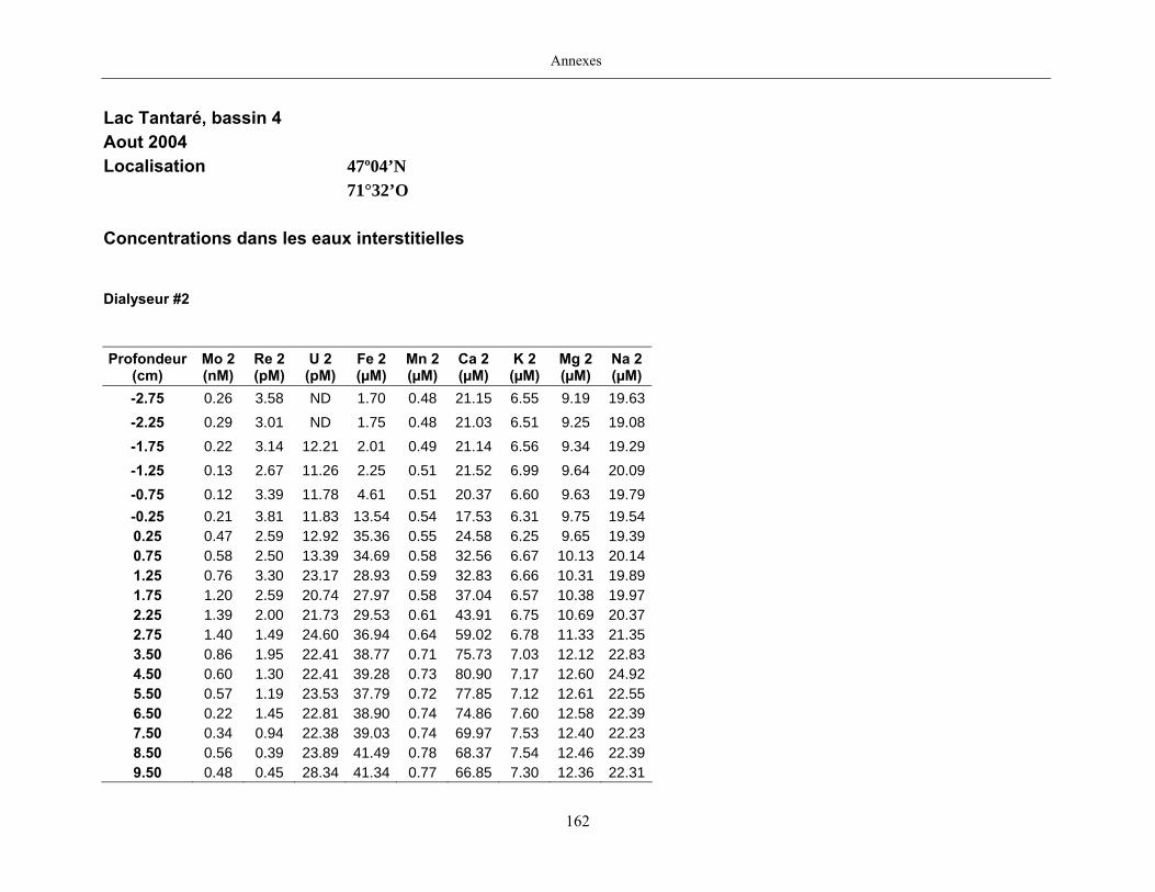
Annexes
162
Lac Tantaré, bassin 4
Aout 2004
Localisation 47º04’N
71°32’O
Concentrations dans les eaux interstitielles
Dialyseur #2 Profondeur
(cm) Mo 2 (nM)
Re 2 (pM)
U 2 (pM)
Fe 2 (µM)
Mn 2 (µM)
Ca 2 (µM)
K 2 (µM)
Mg 2 (µM)
Na 2 (µM)
-2.75 0.26 3.58 ND 1.70 0.48 21.15 6.55 9.19 19.63-2.25 0.29 3.01 ND 1.75 0.48 21.03 6.51 9.25 19.08-1.75 0.22 3.14 12.21 2.01 0.49 21.14 6.56 9.34 19.29-1.25 0.13 2.67 11.26 2.25 0.51 21.52 6.99 9.64 20.09-0.75 0.12 3.39 11.78 4.61 0.51 20.37 6.60 9.63 19.79-0.25 0.21 3.81 11.83 13.54 0.54 17.53 6.31 9.75 19.540.25 0.47 2.59 12.92 35.36 0.55 24.58 6.25 9.65 19.390.75 0.58 2.50 13.39 34.69 0.58 32.56 6.67 10.13 20.141.25 0.76 3.30 23.17 28.93 0.59 32.83 6.66 10.31 19.891.75 1.20 2.59 20.74 27.97 0.58 37.04 6.57 10.38 19.972.25 1.39 2.00 21.73 29.53 0.61 43.91 6.75 10.69 20.372.75 1.40 1.49 24.60 36.94 0.64 59.02 6.78 11.33 21.353.50 0.86 1.95 22.41 38.77 0.71 75.73 7.03 12.12 22.834.50 0.60 1.30 22.41 39.28 0.73 80.90 7.17 12.60 24.925.50 0.57 1.19 23.53 37.79 0.72 77.85 7.12 12.61 22.556.50 0.22 1.45 22.81 38.90 0.74 74.86 7.60 12.58 22.397.50 0.34 0.94 22.38 39.03 0.74 69.97 7.53 12.40 22.238.50 0.56 0.39 23.89 41.49 0.78 68.37 7.54 12.46 22.399.50 0.48 0.45 28.34 41.34 0.77 66.85 7.30 12.36 22.31
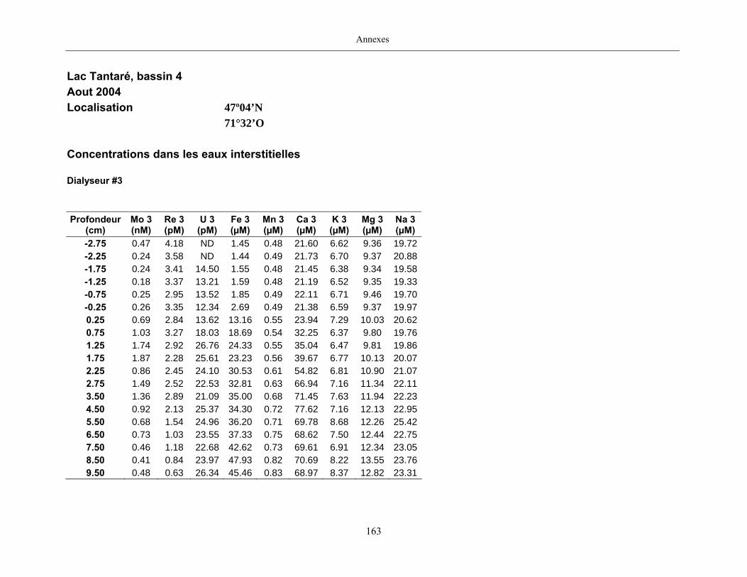
Annexes
163
Lac Tantaré, bassin 4
Aout 2004
Localisation 47º04’N
71°32’O
Concentrations dans les eaux interstitielles
Dialyseur #3 Profondeur
(cm) Mo 3 (nM)
Re 3 (pM)
U 3 (pM)
Fe 3 (µM)
Mn 3 (µM)
Ca 3 (µM)
K 3 (µM)
Mg 3 (µM)
Na 3 (µM)
-2.75 0.47 4.18 ND 1.45 0.48 21.60 6.62 9.36 19.72-2.25 0.24 3.58 ND 1.44 0.49 21.73 6.70 9.37 20.88-1.75 0.24 3.41 14.50 1.55 0.48 21.45 6.38 9.34 19.58-1.25 0.18 3.37 13.21 1.59 0.48 21.19 6.52 9.35 19.33-0.75 0.25 2.95 13.52 1.85 0.49 22.11 6.71 9.46 19.70-0.25 0.26 3.35 12.34 2.69 0.49 21.38 6.59 9.37 19.970.25 0.69 2.84 13.62 13.16 0.55 23.94 7.29 10.03 20.620.75 1.03 3.27 18.03 18.69 0.54 32.25 6.37 9.80 19.761.25 1.74 2.92 26.76 24.33 0.55 35.04 6.47 9.81 19.861.75 1.87 2.28 25.61 23.23 0.56 39.67 6.77 10.13 20.072.25 0.86 2.45 24.10 30.53 0.61 54.82 6.81 10.90 21.072.75 1.49 2.52 22.53 32.81 0.63 66.94 7.16 11.34 22.113.50 1.36 2.89 21.09 35.00 0.68 71.45 7.63 11.94 22.234.50 0.92 2.13 25.37 34.30 0.72 77.62 7.16 12.13 22.955.50 0.68 1.54 24.96 36.20 0.71 69.78 8.68 12.26 25.426.50 0.73 1.03 23.55 37.33 0.75 68.62 7.50 12.44 22.757.50 0.46 1.18 22.68 42.62 0.73 69.61 6.91 12.34 23.058.50 0.41 0.84 23.97 47.93 0.82 70.69 8.22 13.55 23.769.50 0.48 0.63 26.34 45.46 0.83 68.97 8.37 12.82 23.31

Annexes
164
Lac Tantaré, bassin 4
Aout 2004
Localisation 47º04’N
71°32’O
Concentrations dans les eaux interstitielles
Dialyseur #4 Profondeur
(cm) ΣS(-II) 4 (µM) pH 4 Cl- 4
(µM) NO3- 4
(µM) SO42- 4 (µM)
DIC 4 (mM)
DOC 4 (mg/L)
-4.5 0.01 5.82 5.89 5.80 32.08 0.36 2.89 -3.5 0.01 5.66 7.42 12.16 33.00 0.35 2.64 -2.5 0.01 5.55 5.87 4.17 32.50 0.32 2.68 -1.5 0.01 5.60 6.76 7.20 32.40 0.36 2.54 -0.5 0.01 5.46 6.59 6.68 31.53 0.45 2.22 0.5 0.02 6.30 5.79 2.08 26.46 0.67 3.77 1.5 0.06 6.46 5.79 1.99 24.36 0.66 4.25 2.5 0.08 6.49 7.07 1.22 15.48 0.67 5.31 3.5 0.07 6.47 5.41 0.38 7.12 0.64 4.84 4.5 0.03 6.39 5.61 0.95 6.09 0.67 4.88 5.5 0.03 6.26 5.27 1.44 7.93 0.93 5.62 6.5 0.29 6.44 5.66 0.76 9.80 0.73 5.23 7.5 0.23 6.51 6.72 1.07 10.14 0.78 4.90 8.5 0.04 6.40 5.60 0.62 11.27 0.74 4.56 9.5 0.02 6.33 5.34 0.48 11.99 0.76 4.44

Annexes
165
Lac Tantaré, bassin 4
Aout 2004
Localisation 47º04’N
71°32’O
Concentrations dans les eaux interstitielles
Dialyseur #5 Profondeur
(cm) ΣS(-II) 5 (µM) pH 5 Cl- 5
(µM) NO3- 5
(µM) SO42- 5 (µM)
DIC 5 (mM)
DOC 5 (mg/L)
-4.5 0.01 5.62 5.67 3.50 32.72 0.39 2.53 -3.5 0.01 5.54 5.44 4.08 32.26 0.39 2.49 -2.5 0.01 5.51 5.73 5.57 32.51 0.38 2.43 -1.5 0.01 5.53 5.41 3.44 32.82 0.37 2.42 -0.5 0.01 5.51 7.09 7.62 33.17 0.37 2.42 0.5 0.01 5.49 5.94 4.75 33.55 0.42 2.53 1.5 0.01 5.74 5.94 1.16 30.18 0.55 3.96 2.5 0.03 5.86 5.93 0.44 31.06 0.57 3.48 3.5 0.03 6.12 5.66 0.73 30.61 0.60 3.49 4.5 0.03 6.19 5.89 1.24 27.86 0.60 3.39 5.5 0.06 5.95 5.66 0.83 7.71 0.60 3.85 6.5 0.07 6.07 5.33 0.49 2.03 0.69 4.10 7.5 0.75 6.27 5.30 1.05 2.61 0.77 4.62 8.5 1.61 6.30 5.39 1.29 2.50 0.79 4.36 9.5 1.61 6.35 5.22 1.10 2.70 0.92 5.62
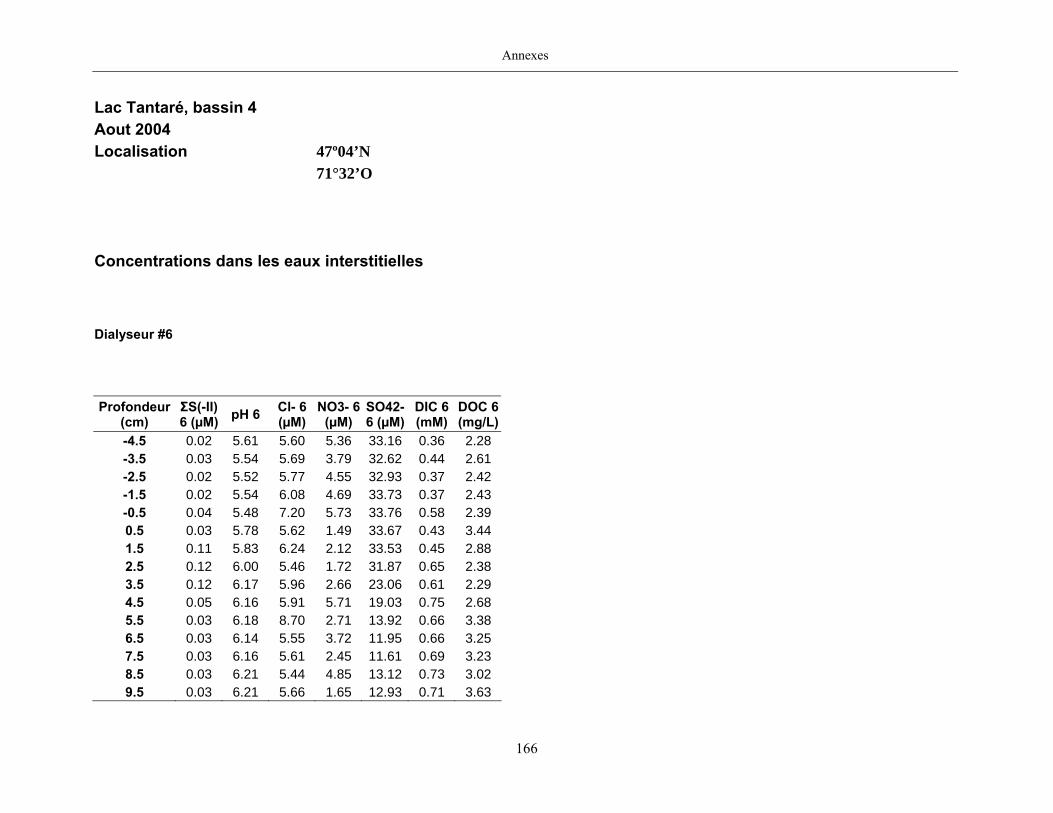
Annexes
166
Lac Tantaré, bassin 4
Aout 2004
Localisation 47º04’N
71°32’O
Concentrations dans les eaux interstitielles
Dialyseur #6 Profondeur
(cm) ΣS(-II) 6 (µM) pH 6 Cl- 6
(µM) NO3- 6
(µM) SO42- 6 (µM)
DIC 6 (mM)
DOC 6 (mg/L)
-4.5 0.02 5.61 5.60 5.36 33.16 0.36 2.28 -3.5 0.03 5.54 5.69 3.79 32.62 0.44 2.61 -2.5 0.02 5.52 5.77 4.55 32.93 0.37 2.42 -1.5 0.02 5.54 6.08 4.69 33.73 0.37 2.43 -0.5 0.04 5.48 7.20 5.73 33.76 0.58 2.39 0.5 0.03 5.78 5.62 1.49 33.67 0.43 3.44 1.5 0.11 5.83 6.24 2.12 33.53 0.45 2.88 2.5 0.12 6.00 5.46 1.72 31.87 0.65 2.38 3.5 0.12 6.17 5.96 2.66 23.06 0.61 2.29 4.5 0.05 6.16 5.91 5.71 19.03 0.75 2.68 5.5 0.03 6.18 8.70 2.71 13.92 0.66 3.38 6.5 0.03 6.14 5.55 3.72 11.95 0.66 3.25 7.5 0.03 6.16 5.61 2.45 11.61 0.69 3.23 8.5 0.03 6.21 5.44 4.85 13.12 0.73 3.02 9.5 0.03 6.21 5.66 1.65 12.93 0.71 3.63
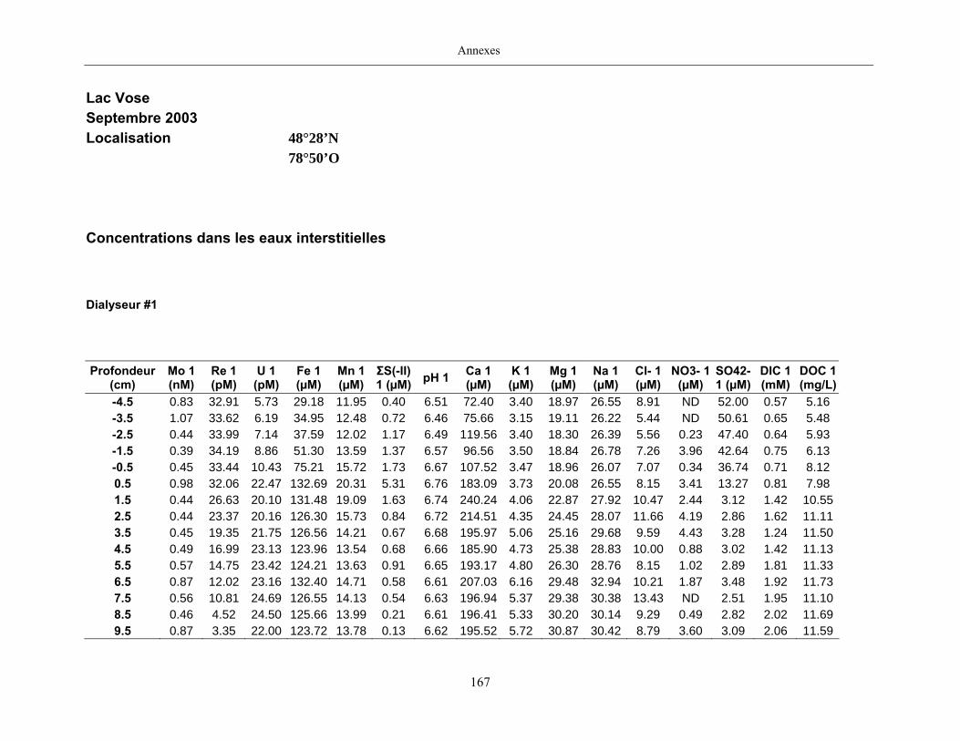
Annexes
167
Lac Vose Septembre 2003 Localisation 48°28’N 78°50’O Concentrations dans les eaux interstitielles Dialyseur #1 Profondeur
(cm) Mo 1 (nM)
Re 1 (pM)
U 1 (pM)
Fe 1 (µM)
Mn 1 (µM)
ΣS(-II) 1 (µM) pH 1 Ca 1
(µM) K 1 (µM)
Mg 1 (µM)
Na 1 (µM)
Cl- 1 (µM)
NO3- 1 (µM)
SO42- 1 (µM)
DIC 1 (mM)
DOC 1 (mg/L)
-4.5 0.83 32.91 5.73 29.18 11.95 0.40 6.51 72.40 3.40 18.97 26.55 8.91 ND 52.00 0.57 5.16 -3.5 1.07 33.62 6.19 34.95 12.48 0.72 6.46 75.66 3.15 19.11 26.22 5.44 ND 50.61 0.65 5.48 -2.5 0.44 33.99 7.14 37.59 12.02 1.17 6.49 119.56 3.40 18.30 26.39 5.56 0.23 47.40 0.64 5.93 -1.5 0.39 34.19 8.86 51.30 13.59 1.37 6.57 96.56 3.50 18.84 26.78 7.26 3.96 42.64 0.75 6.13 -0.5 0.45 33.44 10.43 75.21 15.72 1.73 6.67 107.52 3.47 18.96 26.07 7.07 0.34 36.74 0.71 8.12 0.5 0.98 32.06 22.47 132.69 20.31 5.31 6.76 183.09 3.73 20.08 26.55 8.15 3.41 13.27 0.81 7.98 1.5 0.44 26.63 20.10 131.48 19.09 1.63 6.74 240.24 4.06 22.87 27.92 10.47 2.44 3.12 1.42 10.552.5 0.44 23.37 20.16 126.30 15.73 0.84 6.72 214.51 4.35 24.45 28.07 11.66 4.19 2.86 1.62 11.113.5 0.45 19.35 21.75 126.56 14.21 0.67 6.68 195.97 5.06 25.16 29.68 9.59 4.43 3.28 1.24 11.504.5 0.49 16.99 23.13 123.96 13.54 0.68 6.66 185.90 4.73 25.38 28.83 10.00 0.88 3.02 1.42 11.135.5 0.57 14.75 23.42 124.21 13.63 0.91 6.65 193.17 4.80 26.30 28.76 8.15 1.02 2.89 1.81 11.336.5 0.87 12.02 23.16 132.40 14.71 0.58 6.61 207.03 6.16 29.48 32.94 10.21 1.87 3.48 1.92 11.737.5 0.56 10.81 24.69 126.55 14.13 0.54 6.63 196.94 5.37 29.38 30.38 13.43 ND 2.51 1.95 11.108.5 0.46 4.52 24.50 125.66 13.99 0.21 6.61 196.41 5.33 30.20 30.14 9.29 0.49 2.82 2.02 11.699.5 0.87 3.35 22.00 123.72 13.78 0.13 6.62 195.52 5.72 30.87 30.42 8.79 3.60 3.09 2.06 11.59
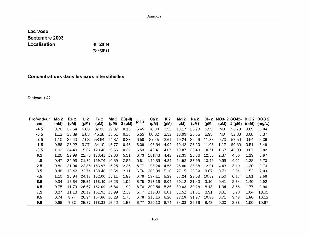
Annexes
168
Lac Vose
Septembre 2003
Localisation 48°28’N
78°50’O
Concentrations dans les eaux interstitielles Dialyseur #2 Profondeur
(cm) Mo 2 (nM)
Re 2 (pM)
U 2 (pM)
Fe 2 (µM)
Mn 2 (µM)
ΣS(-II) 2 (µM) pH 2 Ca 2
(µM) K 2 (µM)
Mg 2 (µM)
Na 2 (µM)
Cl- 2 (µM)
NO3- 2 (µM)
SO42- 2 (µM)
DIC 2 (mM)
DOC 2 (mg/L)
-4.5 0.76 37.64 6.83 37.83 12.97 0.16 6.45 78.00 3.52 19.17 26.73 5.55 ND 53.79 0.69 6.04 -3.5 1.13 35.89 6.83 45.38 13.61 0.36 6.55 80.02 3.52 18.99 25.55 5.95 ND 52.80 0.68 5.37 -2.5 1.10 35.40 7.08 58.64 14.87 0.37 6.50 87.45 3.61 19.24 26.26 11.38 0.70 52.50 0.64 5.36 -1.5 0.86 35.22 9.27 84.10 16.77 0.46 6.39 105.84 4.02 19.42 26.30 11.05 1.17 50.80 0.51 5.49 -0.5 1.03 34.40 15.07 123.46 19.65 0.37 6.53 140.41 4.07 19.87 26.40 10.71 1.67 46.08 0.67 6.82 0.5 1.26 29.99 22.76 173.41 19.36 5.31 6.73 181.48 4.42 22.35 26.86 12.55 2.87 4.06 1.19 8.97 1.5 0.47 24.93 21.22 159.76 16.89 2.89 6.81 194.35 4.84 24.92 27.99 13.49 0.65 4.01 1.28 9.73 2.5 0.80 21.94 22.85 153.97 15.25 2.25 6.77 198.24 4.53 25.80 28.38 12.91 4.43 3.10 1.20 9.73 3.5 0.48 18.42 23.74 158.48 15.54 2.11 6.76 203.34 5.10 27.15 28.89 8.67 0.70 3.04 1.53 9.93 4.5 1.10 15.94 24.17 152.00 15.11 1.89 6.78 197.11 5.23 27.24 29.03 10.53 3.50 6.17 1.51 9.58 5.5 0.94 13.64 25.51 165.49 16.28 1.99 6.75 215.16 6.04 30.12 31.40 9.10 0.41 3.64 1.40 9.92 6.5 0.75 11.79 26.67 162.09 15.84 1.99 6.78 209.54 5.86 30.03 30.26 8.13 1.04 3.56 1.77 9.98 7.5 0.87 11.18 26.19 161.92 15.99 2.32 6.77 212.00 6.01 31.52 31.31 8.91 0.01 3.70 1.64 10.058.5 0.74 8.74 26.34 164.60 16.28 1.75 6.78 216.16 6.20 33.19 31.97 10.80 0.71 3.48 1.90 10.129.5 0.66 7.33 25.87 168.38 16.42 1.58 6.77 220.10 6.74 34.38 32.66 8.43 0.00 3.88 1.90 10.67

Annexes
169
Lac Vose
Septembre 2003
Localisation 48°28’N
78°50’O
Concentrations dans les eaux interstitielles
Dialyseur #3 Profondeur
(cm) Mo 3 (nM)
Re 3 (pM)
U 3 (pM)
Fe 3 (µM)
Mn 3 (µM)
ΣS(-II) 3 (µM) pH 3 Ca 3
(µM) K 3 (µM)
Mg 3 (µM)
Na 3 (µM)
Cl- 3 (µM)
NO3- 3 (µM)
SO42- 3 (µM)
DIC 3 (mM)
DOC 3 (mg/L)
-4.5 0.44 38.36 5.94 14.76 10.11 0.41 6.62 72.04 3.23 18.66 26.46 ND ND 52.11 0.72 5.47 -3.5 0.59 37.21 6.07 16.01 10.56 0.54 6.64 71.57 3.13 18.73 25.95 6.65 0.79 49.32 0.72 5.63 -2.5 1.25 36.93 6.70 19.22 10.69 0.69 6.71 77.22 2.94 19.00 26.06 5.75 ND 46.51 0.74 6.03 -1.5 1.08 37.07 6.30 26.13 11.15 0.60 6.72 78.22 3.36 19.08 26.79 5.23 ND 40.80 0.76 6.10 -0.5 0.97 36.72 8.54 54.36 12.58 1.49 6.87 93.06 3.27 19.02 26.30 6.39 ND 12.02 1.43 8.75 0.5 1.01 27.28 20.25 110.55 15.77 0.58 6.88 159.96 3.63 19.63 26.06 7.60 ND 4.98 1.44 10.891.5 0.35 28.31 22.63 105.30 14.63 0.35 6.88 203.97 3.76 22.59 26.67 9.08 ND 5.50 1.72 11.172.5 0.55 24.91 24.21 93.21 12.47 0.38 6.84 191.19 4.05 23.93 27.09 9.63 ND 5.18 1.88 11.333.5 0.84 19.91 24.89 87.23 11.38 0.45 6.82 174.21 3.92 24.00 27.53 9.43 ND 5.03 1.77 11.324.5 0.93 18.44 24.82 83.94 10.94 0.47 6.81 159.94 3.89 23.91 27.91 9.80 ND 5.19 2.11 11.525.5 0.56 16.39 24.72 82.39 10.87 0.40 6.71 158.03 4.15 24.68 28.34 21.63 ND 4.75 2.11 11.456.5 0.66 14.19 22.68 80.29 10.99 0.31 6.77 158.71 4.41 25.89 29.93 10.16 ND 4.86 2.21 12.197.5 0.59 14.24 23.50 74.06 10.21 0.46 6.78 145.04 4.30 24.67 27.73 17.44 ND 5.21 2.26 12.318.5 0.62 10.89 25.59 72.61 10.12 0.34 6.77 146.67 4.53 25.66 28.93 24.53 ND 5.12 2.18 12.619.5 0.55 12.55 24.23 69.19 9.93 0.27 6.74 143.82 4.64 26.18 28.21 21.48 ND 5.15 2.42 12.68
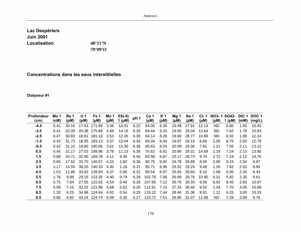
Annexes
170
Lac Despériers Juin 2001 Localisation 48°11’N 79°09’O Concentrations dans les eaux interstitielles Dialyseur #1 Profondeur
(cm) Mo 1 (nM)
Re 1 (pM)
U 1 (pM)
Fe 1 (µM)
Mn 1 (µM)
ΣS(-II) 1 (µM) pH 1 Ca 1
(µM) K 1 (µM)
Mg 1 (µM)
Na 1 (µM)
Cl- 1 (µM)
NO3- 1 (µM)
SO42- 1 (µM)
DIC 1 (mM)
DOC 1 (mg/L)
-4.5 0.41 30.16 17.63 171.89 3.46 14.91 6.22 64.05 6.35 19.48 27.91 12.13 ND 6.80 1.93 10.43-3.5 0.41 32.09 20.38 175.89 3.48 14.16 6.33 64.44 6.33 19.56 28.04 12.64 ND 7.62 1.78 10.83-2.5 0.47 30.83 18.91 181.16 3.53 12.26 6.30 64.14 6.28 19.68 28.77 10.86 ND 8.32 1.99 12.24-1.5 0.43 31.73 18.05 183.13 3.57 13.04 6.34 65.04 6.44 19.97 29.15 6.66 2.05 8.75 2.00 12.79-0.5 0.42 31.22 18.80 190.66 3.61 13.30 6.36 65.63 6.53 20.08 29.36 7.82 1.21 7.55 2.11 13.120.5 0.45 31.17 27.02 199.96 3.79 11.13 6.36 70.62 6.81 20.86 29.31 14.69 1.14 7.24 2.13 13.901.5 0.88 24.71 32.90 169.78 4.11 4.35 6.40 83.58 6.87 23.17 28.73 9.70 2.72 7.24 2.12 10.762.5 0.65 17.52 33.70 146.57 4.22 1.82 6.36 90.75 6.92 24.78 28.89 8.56 2.90 9.15 2.54 9.97 3.5 1.17 14.55 38.20 140.33 4.30 1.16 6.31 95.71 6.96 25.52 29.29 9.48 1.26 7.82 2.52 8.95 4.5 1.53 11.86 33.92 129.93 4.37 0.90 6.32 99.54 6.97 25.93 29.60 8.10 1.08 6.05 2.34 9.43 5.5 1.76 9.99 29.15 123.35 4.40 0.74 6.28 102.78 7.06 26.09 29.76 10.80 0.31 5.92 2.35 9.61 6.5 0.75 7.64 27.55 122.62 4.54 0.46 6.26 107.95 7.12 26.76 30.33 9.56 6.92 8.45 2.93 10.677.5 0.59 7.15 33.32 121.96 4.68 0.52 6.26 112.61 7.15 27.33 30.40 9.52 1.34 7.70 3.06 10.088.5 1.33 6.25 34.98 124.64 4.92 0.54 6.25 119.22 7.44 28.46 31.36 8.81 1.12 6.25 3.00 10.339.5 0.85 6.92 43.24 124.74 5.08 0.30 6.27 123.72 7.51 28.95 31.07 11.98 ND 7.29 2.99 9.76
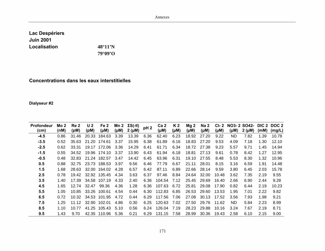
Annexes
171
Lac Despériers
Juin 2001
Localisation 48°11’N
79°09’O
Concentrations dans les eaux interstitielles
Dialyseur #2 Profondeur
(cm) Mo 2 (nM)
Re 2 (pM)
U 2 (pM)
Fe 2 (µM)
Mn 2 (µM)
ΣS(-II) 2 (µM) pH 2 Ca 2
(µM) K 2 (µM)
Mg 2 (µM)
Na 2 (µM)
Cl- 2 (µM)
NO3- 2 (µM)
SO42- 2 (µM)
DIC 2 (mM)
DOC 2 (mg/L)
-4.5 0.86 31.46 20.33 184.63 3.39 13.39 6.36 62.40 6.23 18.92 27.20 9.22 ND 7.82 1.39 10.78-3.5 0.52 35.63 21.20 174.61 3.37 15.95 6.38 61.89 6.16 18.83 27.20 9.53 4.09 7.18 1.30 12.10-2.5 0.62 33.31 19.17 172.06 3.36 14.29 6.41 61.71 6.34 18.72 27.38 9.23 5.57 9.71 1.45 14.94-1.5 0.55 34.52 19.96 174.10 3.37 13.90 6.43 61.94 6.18 18.81 27.13 9.61 0.78 8.42 1.27 12.95-0.5 0.48 32.83 21.24 182.57 3.47 14.42 6.45 63.96 6.31 19.10 27.55 8.48 5.53 8.30 1.32 10.960.5 0.88 32.75 23.73 188.53 3.97 9.56 6.46 77.79 6.67 21.11 28.01 8.15 3.16 6.59 1.91 14.481.5 1.68 28.63 32.00 164.02 4.28 6.57 6.42 87.11 6.89 22.66 28.14 9.59 3.80 6.45 2.03 15.782.5 0.78 19.42 32.92 135.45 4.34 3.63 6.37 97.46 8.84 24.64 32.00 10.48 3.62 7.35 2.19 9.55 3.5 1.40 17.39 34.58 107.19 4.33 2.40 6.36 104.54 7.12 25.45 29.69 16.40 2.66 6.90 2.44 9.28 4.5 1.65 12.74 32.47 99.36 4.36 1.28 6.36 107.63 6.72 25.81 29.08 17.90 0.82 6.44 2.19 10.235.5 1.05 10.85 33.26 100.61 4.54 0.44 6.30 112.83 6.85 26.53 29.60 13.53 1.95 7.01 2.22 9.82 6.5 0.72 10.32 34.53 101.95 4.72 0.44 6.29 117.56 7.06 27.08 30.13 17.52 3.56 7.93 1.98 9.21 7.5 1.25 11.12 32.90 102.01 4.86 0.30 6.25 120.63 7.02 27.50 29.76 11.62 ND 5.84 2.23 8.99 8.5 1.10 10.77 41.25 105.43 5.10 0.56 6.24 126.04 7.19 28.23 29.88 10.16 3.24 7.67 2.19 8.71 9.5 1.43 9.70 42.35 110.96 5.36 0.21 6.29 131.15 7.58 28.99 30.36 19.43 2.58 6.10 2.15 9.00
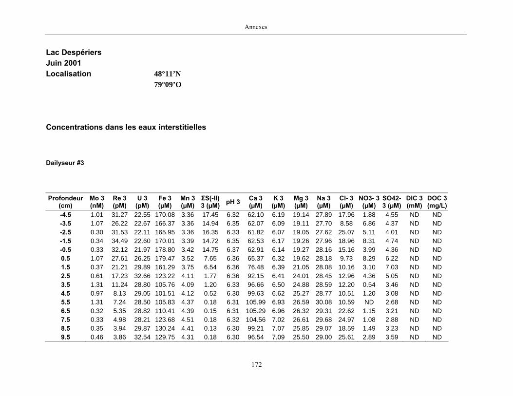
Annexes
172
Lac Despériers
Juin 2001
Localisation 48°11’N
79°09’O
Concentrations dans les eaux interstitielles
Dailyseur #3 Profondeur
(cm) Mo 3 (nM)
Re 3 (pM)
U 3 (pM)
Fe 3 (µM)
Mn 3 (µM)
ΣS(-II) 3 (µM) pH 3 Ca 3
(µM) K 3 (µM)
Mg 3 (µM)
Na 3 (µM)
Cl- 3 (µM)
NO3- 3 (µM)
SO42- 3 (µM)
DIC 3 (mM)
DOC 3 (mg/L)
-4.5 1.01 31.27 22.55 170.08 3.36 17.45 6.32 62.10 6.19 19.14 27.89 17.96 1.88 4.55 ND ND -3.5 1.07 26.22 22.67 166.37 3.36 14.94 6.35 62.07 6.09 19.11 27.70 8.58 6.86 4.37 ND ND -2.5 0.30 31.53 22.11 165.95 3.36 16.35 6.33 61.82 6.07 19.05 27.62 25.07 5.11 4.01 ND ND -1.5 0.34 34.49 22.60 170.01 3.39 14.72 6.35 62.53 6.17 19.26 27.96 18.96 8.31 4.74 ND ND -0.5 0.33 32.12 21.97 178.80 3.42 14.75 6.37 62.91 6.14 19.27 28.16 15.16 3.99 4.36 ND ND 0.5 1.07 27.61 26.25 179.47 3.52 7.65 6.36 65.37 6.32 19.62 28.18 9.73 8.29 6.22 ND ND 1.5 0.37 21.21 29.89 161.29 3.75 6.54 6.36 76.48 6.39 21.05 28.08 10.16 3.10 7.03 ND ND 2.5 0.61 17.23 32.66 123.22 4.11 1.77 6.36 92.15 6.41 24.01 28.45 12.96 4.36 5.05 ND ND 3.5 1.31 11.24 28.80 105.76 4.09 1.20 6.33 96.66 6.50 24.88 28.59 12.20 0.54 3.46 ND ND 4.5 0.97 8.13 29.05 101.51 4.12 0.52 6.30 99.63 6.62 25.27 28.77 10.51 1.20 3.08 ND ND 5.5 1.31 7.24 28.50 105.83 4.37 0.18 6.31 105.99 6.93 26.59 30.08 10.59 ND 2.68 ND ND 6.5 0.32 5.35 28.82 110.41 4.39 0.15 6.31 105.29 6.96 26.32 29.31 22.62 1.15 3.21 ND ND 7.5 0.33 4.98 28.21 123.68 4.51 0.18 6.32 104.56 7.02 26.61 29.68 24.97 1.08 2.88 ND ND 8.5 0.35 3.94 29.87 130.24 4.41 0.13 6.30 99.21 7.07 25.85 29.07 18.59 1.49 3.23 ND ND 9.5 0.46 3.86 32.54 129.75 4.31 0.18 6.30 96.54 7.09 25.50 29.00 25.61 2.89 3.59 ND ND

Annexes
173
Lac Holland Aout 2005 Localisation 48°56’N 65°25’O Concentrations dans les eaux interstitielles Dialyseur #1 Profondeur
(cm) Mo 1 (nM)
Re 1 (pM)
U 1 (pM)
Fe 1 (µM)
Mn 1 (µM)
Ca 1 (µM)
K 1 (µM)
Mg 1 (µM)
Na 1 (µM)
-2.75 0.99 6.08 290.17 3.11 6.27 1862 17.71 321.00 1791 -2.25 0.79 6.86 269.03 2.14 6.15 1861 17.52 320.94 1783 -1.75 0.51 6.39 278.99 2.03 6.21 1866 17.59 318.86 1779 -1.25 0.26 6.93 213.11 1.71 6.06 1818 17.48 304.71 1693 -0.75 0.23 7.03 114.37 1.97 6.59 2014 20.97 330.62 1817 -0.25 0.16 6.23 36.76 2.65 6.75 2136 23.42 338.89 1828 0.25 0.35 6.05 19.08 3.01 6.89 2207 25.62 349.06 1846 0.75 0.62 5.20 23.87 2.31 6.82 2196 27.76 353.29 1857 1.25 0.28 5.44 15.91 0.91 6.61 2146 27.13 349.41 1848 1.75 0.21 4.73 11.49 0.45 6.37 2113 27.35 349.56 1863 2.25 0.26 4.40 13.52 0.27 5.69 1968 23.87 324.55 1742 2.75 0.18 4.04 12.87 0.19 5.85 2096 25.65 350.77 1892 3.50 0.15 3.82 21.22 0.45 5.46 2085 24.64 349.35 1911 4.50 0.20 3.72 23.61 0.28 4.95 2028 22.23 337.82 1886 5.50 0.28 3.68 34.95 0.55 4.65 1981 21.53 328.20 1860 6.50 0.32 2.51 37.39 0.52 4.74 2027 20.83 336.16 1918 7.50 0.21 2.65 26.29 0.64 4.77 2018 19.72 333.11 1920 8.50 0.44 2.53 41.83 1.04 4.98 2025 19.43 331.84 1925 9.50 0.71 2.42 51.60 2.05 5.33 2050 19.72 335.25 1947
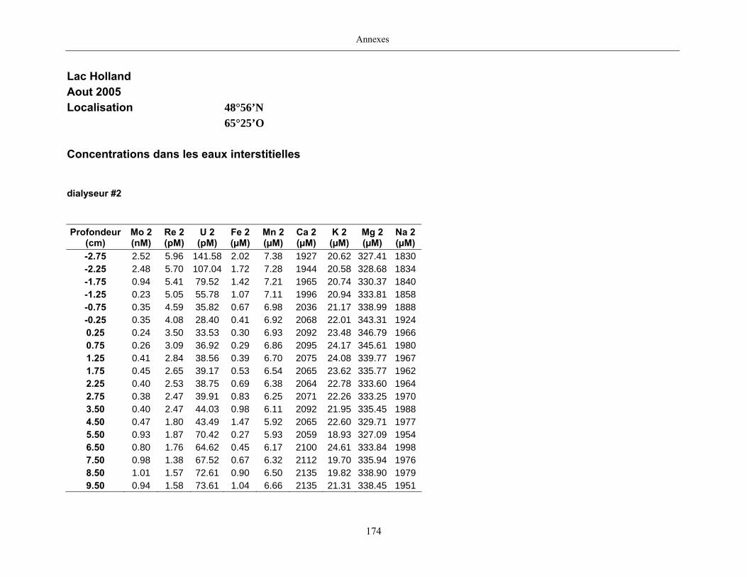
Annexes
174
Lac Holland
Aout 2005
Localisation 48°56’N
65°25’O
Concentrations dans les eaux interstitielles
dialyseur #2 Profondeur
(cm) Mo 2 (nM)
Re 2 (pM)
U 2 (pM)
Fe 2 (µM)
Mn 2 (µM)
Ca 2 (µM)
K 2 (µM)
Mg 2 (µM)
Na 2 (µM)
-2.75 2.52 5.96 141.58 2.02 7.38 1927 20.62 327.41 1830 -2.25 2.48 5.70 107.04 1.72 7.28 1944 20.58 328.68 1834 -1.75 0.94 5.41 79.52 1.42 7.21 1965 20.74 330.37 1840 -1.25 0.23 5.05 55.78 1.07 7.11 1996 20.94 333.81 1858 -0.75 0.35 4.59 35.82 0.67 6.98 2036 21.17 338.99 1888 -0.25 0.35 4.08 28.40 0.41 6.92 2068 22.01 343.31 1924 0.25 0.24 3.50 33.53 0.30 6.93 2092 23.48 346.79 1966 0.75 0.26 3.09 36.92 0.29 6.86 2095 24.17 345.61 1980 1.25 0.41 2.84 38.56 0.39 6.70 2075 24.08 339.77 1967 1.75 0.45 2.65 39.17 0.53 6.54 2065 23.62 335.77 1962 2.25 0.40 2.53 38.75 0.69 6.38 2064 22.78 333.60 1964 2.75 0.38 2.47 39.91 0.83 6.25 2071 22.26 333.25 1970 3.50 0.40 2.47 44.03 0.98 6.11 2092 21.95 335.45 1988 4.50 0.47 1.80 43.49 1.47 5.92 2065 22.60 329.71 1977 5.50 0.93 1.87 70.42 0.27 5.93 2059 18.93 327.09 1954 6.50 0.80 1.76 64.62 0.45 6.17 2100 24.61 333.84 1998 7.50 0.98 1.38 67.52 0.67 6.32 2112 19.70 335.94 1976 8.50 1.01 1.57 72.61 0.90 6.50 2135 19.82 338.90 1979 9.50 0.94 1.58 73.61 1.04 6.66 2135 21.31 338.45 1951
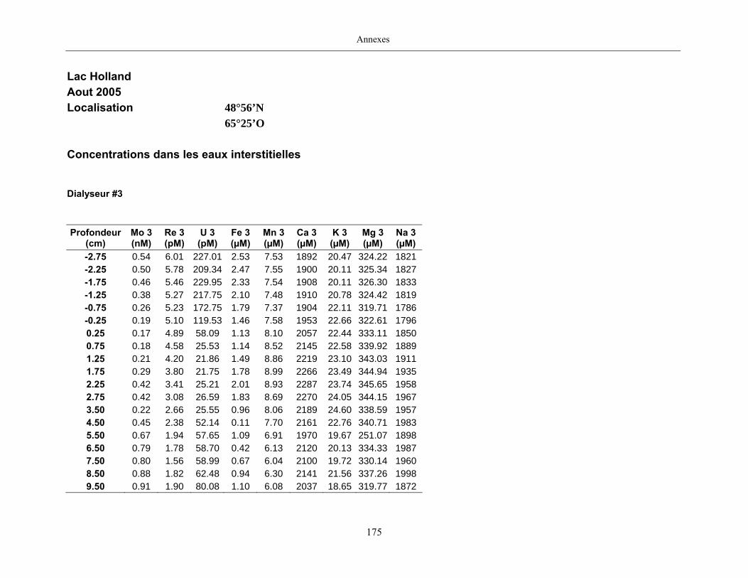
Annexes
175
Lac Holland
Aout 2005
Localisation 48°56’N
65°25’O
Concentrations dans les eaux interstitielles
Dialyseur #3 Profondeur
(cm) Mo 3 (nM)
Re 3 (pM)
U 3 (pM)
Fe 3 (µM)
Mn 3 (µM)
Ca 3 (µM)
K 3 (µM)
Mg 3 (µM)
Na 3 (µM)
-2.75 0.54 6.01 227.01 2.53 7.53 1892 20.47 324.22 1821 -2.25 0.50 5.78 209.34 2.47 7.55 1900 20.11 325.34 1827 -1.75 0.46 5.46 229.95 2.33 7.54 1908 20.11 326.30 1833 -1.25 0.38 5.27 217.75 2.10 7.48 1910 20.78 324.42 1819 -0.75 0.26 5.23 172.75 1.79 7.37 1904 22.11 319.71 1786 -0.25 0.19 5.10 119.53 1.46 7.58 1953 22.66 322.61 1796 0.25 0.17 4.89 58.09 1.13 8.10 2057 22.44 333.11 1850 0.75 0.18 4.58 25.53 1.14 8.52 2145 22.58 339.92 1889 1.25 0.21 4.20 21.86 1.49 8.86 2219 23.10 343.03 1911 1.75 0.29 3.80 21.75 1.78 8.99 2266 23.49 344.94 1935 2.25 0.42 3.41 25.21 2.01 8.93 2287 23.74 345.65 1958 2.75 0.42 3.08 26.59 1.83 8.69 2270 24.05 344.15 1967 3.50 0.22 2.66 25.55 0.96 8.06 2189 24.60 338.59 1957 4.50 0.45 2.38 52.14 0.11 7.70 2161 22.76 340.71 1983 5.50 0.67 1.94 57.65 1.09 6.91 1970 19.67 251.07 1898 6.50 0.79 1.78 58.70 0.42 6.13 2120 20.13 334.33 1987 7.50 0.80 1.56 58.99 0.67 6.04 2100 19.72 330.14 1960 8.50 0.88 1.82 62.48 0.94 6.30 2141 21.56 337.26 1998 9.50 0.91 1.90 80.08 1.10 6.08 2037 18.65 319.77 1872
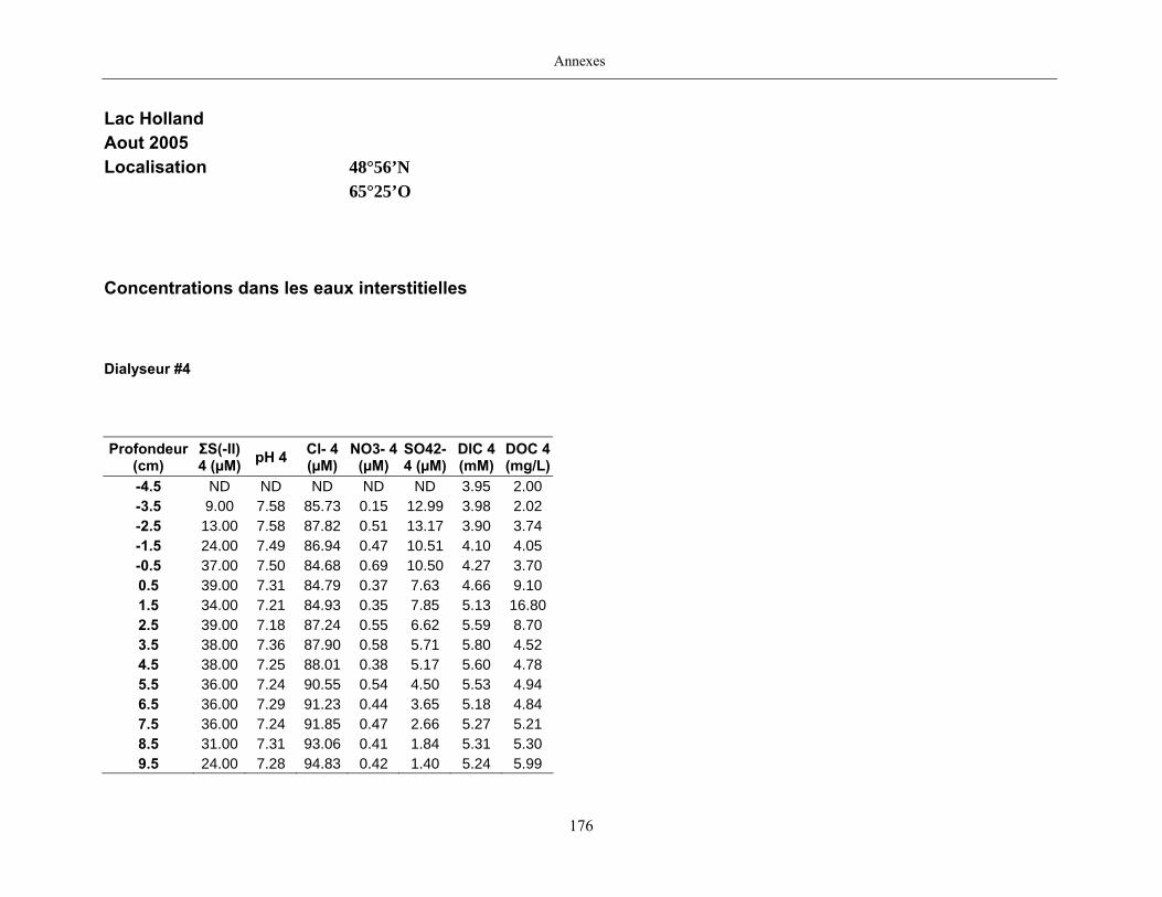
Annexes
176
Lac Holland
Aout 2005
Localisation 48°56’N
65°25’O
Concentrations dans les eaux interstitielles
Dialyseur #4 Profondeur
(cm) ΣS(-II) 4 (µM) pH 4 Cl- 4
(µM) NO3- 4
(µM) SO42- 4 (µM)
DIC 4 (mM)
DOC 4 (mg/L)
-4.5 ND ND ND ND ND 3.95 2.00 -3.5 9.00 7.58 85.73 0.15 12.99 3.98 2.02 -2.5 13.00 7.58 87.82 0.51 13.17 3.90 3.74 -1.5 24.00 7.49 86.94 0.47 10.51 4.10 4.05 -0.5 37.00 7.50 84.68 0.69 10.50 4.27 3.70 0.5 39.00 7.31 84.79 0.37 7.63 4.66 9.10 1.5 34.00 7.21 84.93 0.35 7.85 5.13 16.802.5 39.00 7.18 87.24 0.55 6.62 5.59 8.70 3.5 38.00 7.36 87.90 0.58 5.71 5.80 4.52 4.5 38.00 7.25 88.01 0.38 5.17 5.60 4.78 5.5 36.00 7.24 90.55 0.54 4.50 5.53 4.94 6.5 36.00 7.29 91.23 0.44 3.65 5.18 4.84 7.5 36.00 7.24 91.85 0.47 2.66 5.27 5.21 8.5 31.00 7.31 93.06 0.41 1.84 5.31 5.30 9.5 24.00 7.28 94.83 0.42 1.40 5.24 5.99
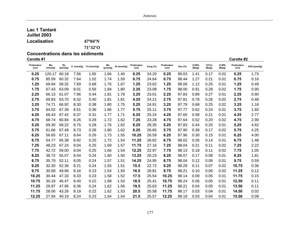
Annexes
177
Lac 1 Tantaré Juillet 2003 Localisation 47º04’N 71°32’O Concentrations dans les sédiments Carotte #1 Carotte #2
Profondeur (cm)
Mo (nmol/g)
Re (pmol/g) U (nmol/g) Fe (mmol/g) Mn
(µmol/g) Al (mmol/g) Profondeur (cm) Corg (%) Profondeur
(cm) Eau (%) 210Pb (Bq/g)
137Cs (Bq/g)
214Pb (Bq/g)
Profondeur (cm) AVS (µmol/g)
0.25 120.17 60.18 7.56 1.65 1.66 1.40 0.25 24.20 0.25 99.03 1.41 0.17 0.02 0.25 1.73 0.75 85.59 60.32 7.64 1.02 1.74 1.59 0.75 24.64 0.75 98.44 1.27 0.21 0.01 0.75 0.16 1.25 69.94 58.32 7.69 0.68 1.76 1.67 1.25 23.62 1.25 98.06 1.12 0.25 0.01 1.25 0.49 1.75 67.43 63.09 8.01 0.56 1.84 1.80 2.25 23.08 1.75 98.00 0.91 0.28 0.02 1.75 0.90 2.25 66.13 61.07 7.96 0.44 1.81 1.79 3.25 23.01 2.25 97.83 0.89 0.27 0.01 2.25 0.90 2.75 69.83 63.70 8.32 0.40 1.81 1.81 4.25 24.21 2.75 97.81 0.78 0.26 0.02 2.75 0.48 3.25 74.71 66.92 8.30 0.38 1.80 1.75 5.25 24.91 3.25 97.79 0.68 0.25 0.02 3.25 1.16 3.75 64.02 67.39 8.51 0.36 1.86 1.77 5.75 25.11 3.75 97.77 0.62 0.24 0.01 3.75 1.60 4.25 68.43 67.42 8.37 0.31 1.77 1.71 6.25 25.24 4.25 97.60 0.58 0.21 0.01 4.25 2.77 4.75 68.74 60.84 8.26 0.29 1.72 1.62 7.25 23.28 4.75 97.64 0.52 0.20 0.02 4.75 2.90 5.25 69.30 69.22 8.75 0.28 1.76 1.62 8.25 28.35 5.25 97.83 0.44 0.20 0.01 5.25 4.62 5.75 61.66 67.49 8.73 0.28 1.80 1.62 9.25 26.66 5.75 97.90 0.39 0.17 0.02 5.75 4.25 6.25 56.65 67.11 8.64 0.26 1.73 1.55 10.25 26.59 6.25 97.96 0.30 0.15 0.01 6.25 4.00 6.75 54.77 65.38 8.92 0.25 1.72 1.54 11.25 26.82 6.75 98.02 0.26 0.14 0.01 6.75 1.48 7.25 48.23 67.24 9.04 0.25 1.69 1.57 11.75 27.16 7.25 98.04 0.21 0.11 0.02 7.25 2.22 7.75 42.72 59.00 8.04 0.25 1.66 1.54 12.25 22.97 7.75 98.13 0.18 0.11 0.02 7.75 1.05 8.25 38.72 55.07 8.04 0.24 1.60 1.50 13.25 26.23 8.25 98.07 0.17 0.08 0.01 8.25 1.81 8.75 35.79 52.11 8.05 0.24 1.57 1.51 14.25 24.95 8.75 98.04 0.12 0.08 0.01 9.75 0.59 9.25 32.30 52.36 8.21 0.24 1.55 1.51 15.5 22.72 9.25 98.29 0.11 0.07 0.02 10.75 0.36 9.75 30.58 49.96 8.16 0.23 1.54 1.50 16.5 28.81 9.75 98.21 0.10 0.06 0.02 11.25 0.12 10.25 30.44 47.33 8.33 0.23 1.58 1.52 17.5 25.54 10.25 98.14 0.09 0.05 0.01 11.75 0.15 10.75 30.18 46.47 8.40 0.22 1.68 1.53 18.5 25.41 10.75 98.24 0.06 0.05 0.01 12.50 0.11 11.25 29.97 47.95 8.36 0.24 1.62 1.56 19.5 25.63 11.25 98.21 0.04 0.05 0.01 13.50 0.11 11.75 28.06 43.26 8.19 0.22 1.62 1.53 20.5 25.58 11.75 98.17 0.03 0.04 0.01 14.50 0.02 12.25 27.94 40.19 8.24 0.23 1.64 1.54 21.5 25.57 12.25 98.19 0.03 0.04 0.01 15.50 0.09
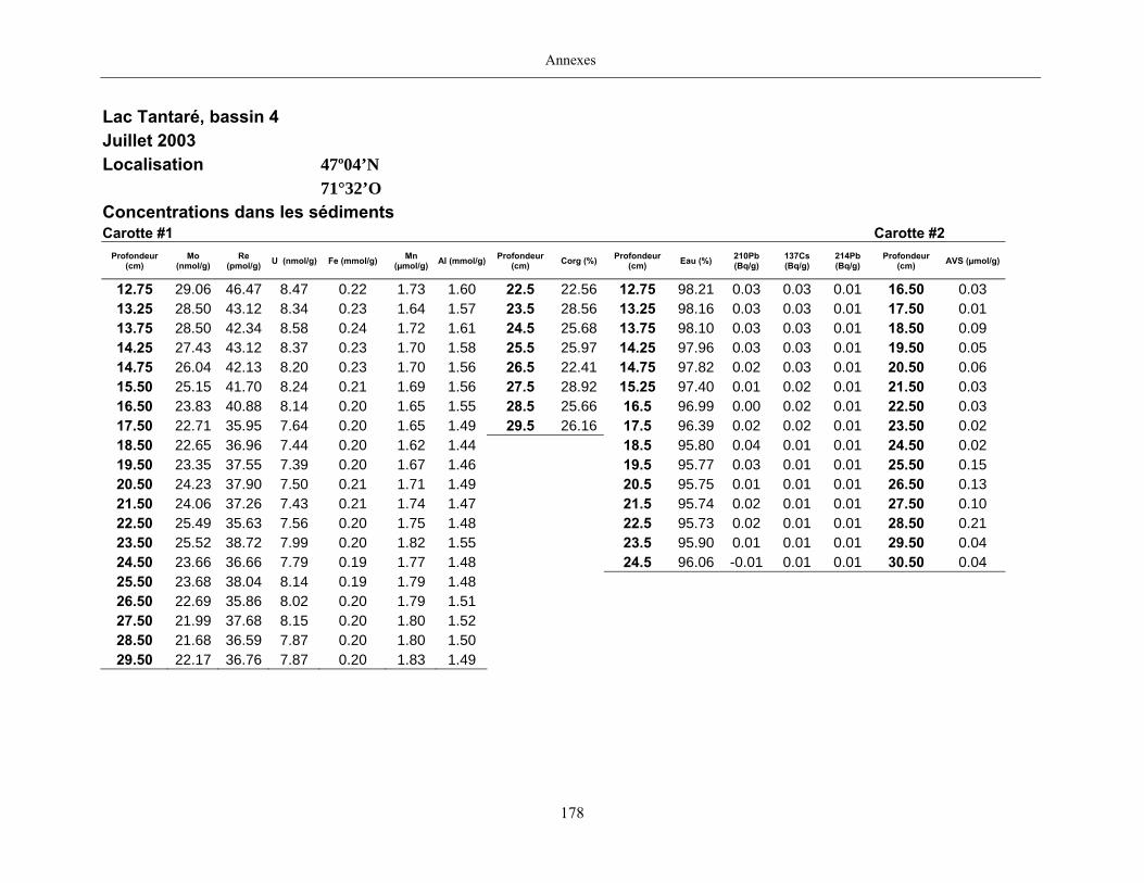
Annexes
178
Lac Tantaré, bassin 4
Juillet 2003
Localisation 47º04’N
71°32’O
Concentrations dans les sédiments Carotte #1 Carotte #2
Profondeur (cm)
Mo (nmol/g)
Re (pmol/g) U (nmol/g) Fe (mmol/g) Mn
(µmol/g) Al (mmol/g) Profondeur (cm) Corg (%) Profondeur
(cm) Eau (%) 210Pb (Bq/g)
137Cs (Bq/g)
214Pb (Bq/g)
Profondeur (cm) AVS (µmol/g)
12.75 29.06 46.47 8.47 0.22 1.73 1.60 22.5 22.56 12.75 98.21 0.03 0.03 0.01 16.50 0.03 13.25 28.50 43.12 8.34 0.23 1.64 1.57 23.5 28.56 13.25 98.16 0.03 0.03 0.01 17.50 0.01 13.75 28.50 42.34 8.58 0.24 1.72 1.61 24.5 25.68 13.75 98.10 0.03 0.03 0.01 18.50 0.09 14.25 27.43 43.12 8.37 0.23 1.70 1.58 25.5 25.97 14.25 97.96 0.03 0.03 0.01 19.50 0.05 14.75 26.04 42.13 8.20 0.23 1.70 1.56 26.5 22.41 14.75 97.82 0.02 0.03 0.01 20.50 0.06 15.50 25.15 41.70 8.24 0.21 1.69 1.56 27.5 28.92 15.25 97.40 0.01 0.02 0.01 21.50 0.03 16.50 23.83 40.88 8.14 0.20 1.65 1.55 28.5 25.66 16.5 96.99 0.00 0.02 0.01 22.50 0.03 17.50 22.71 35.95 7.64 0.20 1.65 1.49 29.5 26.16 17.5 96.39 0.02 0.02 0.01 23.50 0.02 18.50 22.65 36.96 7.44 0.20 1.62 1.44 18.5 95.80 0.04 0.01 0.01 24.50 0.02 19.50 23.35 37.55 7.39 0.20 1.67 1.46 19.5 95.77 0.03 0.01 0.01 25.50 0.15 20.50 24.23 37.90 7.50 0.21 1.71 1.49 20.5 95.75 0.01 0.01 0.01 26.50 0.13 21.50 24.06 37.26 7.43 0.21 1.74 1.47 21.5 95.74 0.02 0.01 0.01 27.50 0.10 22.50 25.49 35.63 7.56 0.20 1.75 1.48 22.5 95.73 0.02 0.01 0.01 28.50 0.21 23.50 25.52 38.72 7.99 0.20 1.82 1.55 23.5 95.90 0.01 0.01 0.01 29.50 0.04 24.50 23.66 36.66 7.79 0.19 1.77 1.48 24.5 96.06 -0.01 0.01 0.01 30.50 0.04 25.50 23.68 38.04 8.14 0.19 1.79 1.48 26.50 22.69 35.86 8.02 0.20 1.79 1.51 27.50 21.99 37.68 8.15 0.20 1.80 1.52 28.50 21.68 36.59 7.87 0.20 1.80 1.50 29.50 22.17 36.76 7.87 0.20 1.83 1.49
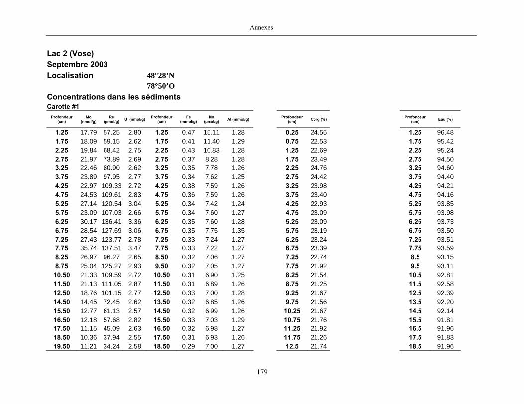
Annexes
179
Lac 2 (Vose) Septembre 2003 Localisation 48°28’N 78°50’O Concentrations dans les sédiments Carotte #1
Profondeur (cm)
Mo (nmol/g)
Re (pmol/g) U (nmol/g) Profondeur
(cm) Fe
(mmol/g) Mn
(µmol/g) Al (mmol/g)
Profondeur (cm) Corg (%)
Profondeur
(cm) Eau (%)
1.25 17.79 57.25 2.80 1.25 0.47 15.11 1.28 0.25 24.55 1.25 96.48 1.75 18.09 59.15 2.62 1.75 0.41 11.40 1.29 0.75 22.53 1.75 95.42 2.25 19.84 68.42 2.75 2.25 0.43 10.83 1.28 1.25 22.69 2.25 95.24 2.75 21.97 73.89 2.69 2.75 0.37 8.28 1.28 1.75 23.49 2.75 94.50 3.25 22.46 80.90 2.62 3.25 0.35 7.78 1.26 2.25 24.76 3.25 94.60 3.75 23.89 97.95 2.77 3.75 0.34 7.62 1.25 2.75 24.42 3.75 94.40 4.25 22.97 109.33 2.72 4.25 0.38 7.59 1.26 3.25 23.98 4.25 94.21 4.75 24.53 109.61 2.83 4.75 0.36 7.59 1.26 3.75 23.40 4.75 94.16 5.25 27.14 120.54 3.04 5.25 0.34 7.42 1.24 4.25 22.93 5.25 93.85 5.75 23.09 107.03 2.66 5.75 0.34 7.60 1.27 4.75 23.09 5.75 93.98 6.25 30.17 136.41 3.36 6.25 0.35 7.60 1.28 5.25 23.09 6.25 93.73 6.75 28.54 127.69 3.06 6.75 0.35 7.75 1.35 5.75 23.19 6.75 93.50 7.25 27.43 123.77 2.78 7.25 0.33 7.24 1.27 6.25 23.24 7.25 93.51 7.75 35.74 137.51 3.47 7.75 0.33 7.22 1.27 6.75 23.39 7.75 93.59 8.25 26.97 96.27 2.65 8.50 0.32 7.06 1.27 7.25 22.74 8.5 93.15 8.75 25.04 125.27 2.93 9.50 0.32 7.05 1.27 7.75 21.92 9.5 93.11 10.50 21.33 109.59 2.72 10.50 0.31 6.90 1.25 8.25 21.54 10.5 92.81 11.50 21.13 111.05 2.87 11.50 0.31 6.89 1.26 8.75 21.25 11.5 92.58 12.50 18.76 101.15 2.77 12.50 0.33 7.00 1.28 9.25 21.67 12.5 92.39 14.50 14.45 72.45 2.62 13.50 0.32 6.85 1.26 9.75 21.56 13.5 92.20 15.50 12.77 61.13 2.57 14.50 0.32 6.99 1.26 10.25 21.67 14.5 92.14 16.50 12.18 57.68 2.82 15.50 0.33 7.03 1.29 10.75 21.76 15.5 91.81 17.50 11.15 45.09 2.63 16.50 0.32 6.98 1.27 11.25 21.92 16.5 91.96 18.50 10.36 37.94 2.55 17.50 0.31 6.93 1.26 11.75 21.26 17.5 91.83 19.50 11.21 34.24 2.58 18.50 0.29 7.00 1.27 12.5 21.74 18.5 91.96
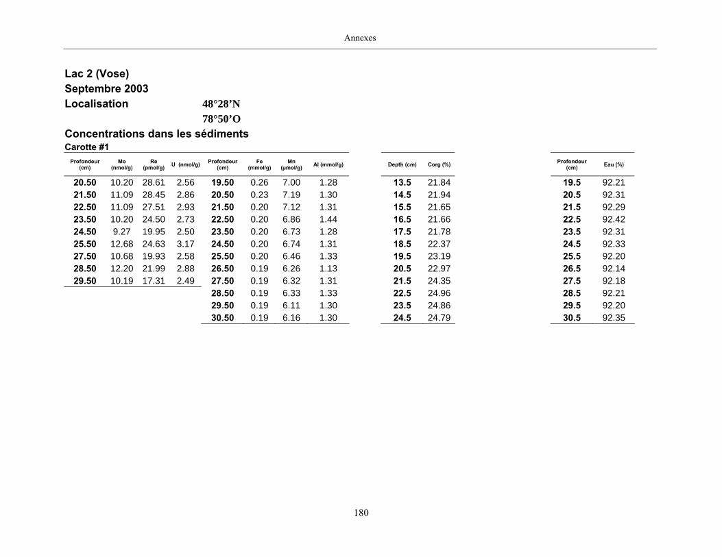
Annexes
180
Lac 2 (Vose)
Septembre 2003
Localisation 48°28’N
78°50’O
Concentrations dans les sédiments Carotte #1
Profondeur (cm)
Mo (nmol/g)
Re (pmol/g) U (nmol/g) Profondeur
(cm) Fe
(mmol/g) Mn
(µmol/g) Al (mmol/g)
Depth (cm) Corg (%) Profondeur
(cm) Eau (%)
20.50 10.20 28.61 2.56 19.50 0.26 7.00 1.28 13.5 21.84 19.5 92.21 21.50 11.09 28.45 2.86 20.50 0.23 7.19 1.30 14.5 21.94 20.5 92.31 22.50 11.09 27.51 2.93 21.50 0.20 7.12 1.31 15.5 21.65 21.5 92.29 23.50 10.20 24.50 2.73 22.50 0.20 6.86 1.44 16.5 21.66 22.5 92.42 24.50 9.27 19.95 2.50 23.50 0.20 6.73 1.28 17.5 21.78 23.5 92.31 25.50 12.68 24.63 3.17 24.50 0.20 6.74 1.31 18.5 22.37 24.5 92.33 27.50 10.68 19.93 2.58 25.50 0.20 6.46 1.33 19.5 23.19 25.5 92.20 28.50 12.20 21.99 2.88 26.50 0.19 6.26 1.13 20.5 22.97 26.5 92.14 29.50 10.19 17.31 2.49 27.50 0.19 6.32 1.31 21.5 24.35 27.5 92.18
28.50 0.19 6.33 1.33 22.5 24.96 28.5 92.21 29.50 0.19 6.11 1.30 23.5 24.86 29.5 92.20 30.50 0.19 6.16 1.30 24.5 24.79 30.5 92.35
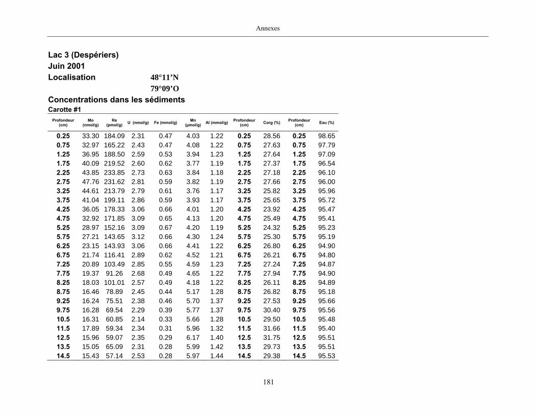
Annexes
181
Lac 3 (Despériers)
Juin 2001
Localisation 48°11’N
79°09’O
Concentrations dans les sédiments Carotte #1
Profondeur (cm)
Mo (nmol/g)
Re (pmol/g) U (nmol/g) Fe (mmol/g) Mn
(µmol/g) Al (mmol/g) Profondeur (cm) Corg (%) Profondeur
(cm) Eau (%)
0.25 33.30 184.09 2.31 0.47 4.03 1.22 0.25 28.56 0.25 98.650.75 32.97 165.22 2.43 0.47 4.08 1.22 0.75 27.63 0.75 97.791.25 36.95 188.50 2.59 0.53 3.94 1.23 1.25 27.64 1.25 97.091.75 40.09 219.52 2.60 0.62 3.77 1.19 1.75 27.37 1.75 96.542.25 43.85 233.85 2.73 0.63 3.84 1.18 2.25 27.18 2.25 96.102.75 47.76 231.62 2.81 0.59 3.82 1.19 2.75 27.66 2.75 96.003.25 44.61 213.79 2.79 0.61 3.76 1.17 3.25 25.82 3.25 95.963.75 41.04 199.11 2.86 0.59 3.93 1.17 3.75 25.65 3.75 95.724.25 36.05 178.33 3.06 0.66 4.01 1.20 4.25 23.92 4.25 95.474.75 32.92 171.85 3.09 0.65 4.13 1.20 4.75 25.49 4.75 95.415.25 28.97 152.16 3.09 0.67 4.20 1.19 5.25 24.32 5.25 95.235.75 27.21 143.65 3.12 0.66 4.30 1.24 5.75 25.30 5.75 95.196.25 23.15 143.93 3.06 0.66 4.41 1.22 6.25 26.80 6.25 94.906.75 21.74 116.41 2.89 0.62 4.52 1.21 6.75 26.21 6.75 94.807.25 20.89 103.49 2.85 0.55 4.59 1.23 7.25 27.24 7.25 94.877.75 19.37 91.26 2.68 0.49 4.65 1.22 7.75 27.94 7.75 94.908.25 18.03 101.01 2.57 0.49 4.18 1.22 8.25 26.11 8.25 94.898.75 16.46 78.89 2.45 0.44 5.17 1.28 8.75 26.82 8.75 95.189.25 16.24 75.51 2.38 0.46 5.70 1.37 9.25 27.53 9.25 95.669.75 16.28 69.54 2.29 0.39 5.77 1.37 9.75 30.40 9.75 95.5610.5 16.31 60.85 2.14 0.33 5.66 1.28 10.5 29.50 10.5 95.4811.5 17.89 59.34 2.34 0.31 5.96 1.32 11.5 31.66 11.5 95.4012.5 15.96 59.07 2.35 0.29 6.17 1.40 12.5 31.75 12.5 95.5113.5 15.05 65.09 2.31 0.28 5.99 1.42 13.5 29.73 13.5 95.5114.5 15.43 57.14 2.53 0.28 5.97 1.44 14.5 29.38 14.5 95.53
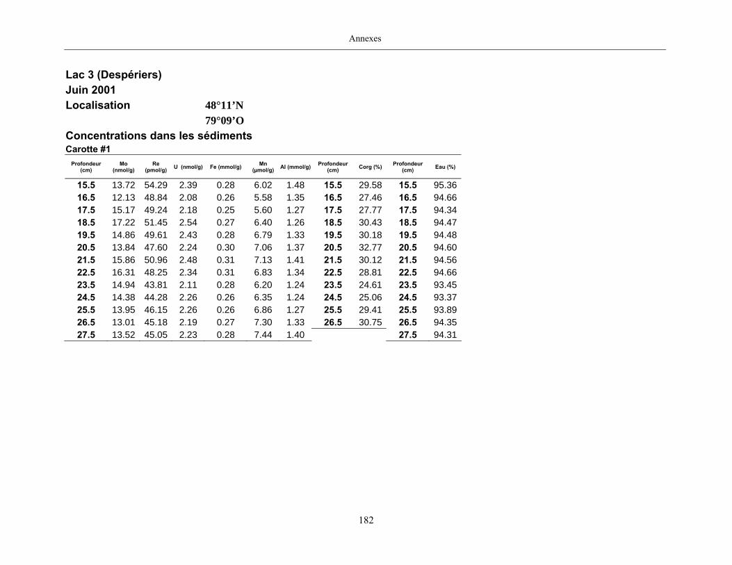
Annexes
182
Lac 3 (Despériers)
Juin 2001
Localisation 48°11’N
79°09’O
Concentrations dans les sédiments Carotte #1
Profondeur (cm)
Mo (nmol/g)
Re (pmol/g) U (nmol/g) Fe (mmol/g) Mn
(µmol/g) Al (mmol/g) Profondeur (cm) Corg (%) Profondeur
(cm) Eau (%)
15.5 13.72 54.29 2.39 0.28 6.02 1.48 15.5 29.58 15.5 95.3616.5 12.13 48.84 2.08 0.26 5.58 1.35 16.5 27.46 16.5 94.6617.5 15.17 49.24 2.18 0.25 5.60 1.27 17.5 27.77 17.5 94.3418.5 17.22 51.45 2.54 0.27 6.40 1.26 18.5 30.43 18.5 94.4719.5 14.86 49.61 2.43 0.28 6.79 1.33 19.5 30.18 19.5 94.4820.5 13.84 47.60 2.24 0.30 7.06 1.37 20.5 32.77 20.5 94.6021.5 15.86 50.96 2.48 0.31 7.13 1.41 21.5 30.12 21.5 94.5622.5 16.31 48.25 2.34 0.31 6.83 1.34 22.5 28.81 22.5 94.6623.5 14.94 43.81 2.11 0.28 6.20 1.24 23.5 24.61 23.5 93.4524.5 14.38 44.28 2.26 0.26 6.35 1.24 24.5 25.06 24.5 93.3725.5 13.95 46.15 2.26 0.26 6.86 1.27 25.5 29.41 25.5 93.8926.5 13.01 45.18 2.19 0.27 7.30 1.33 26.5 30.75 26.5 94.3527.5 13.52 45.05 2.23 0.28 7.44 1.40 27.5 94.31
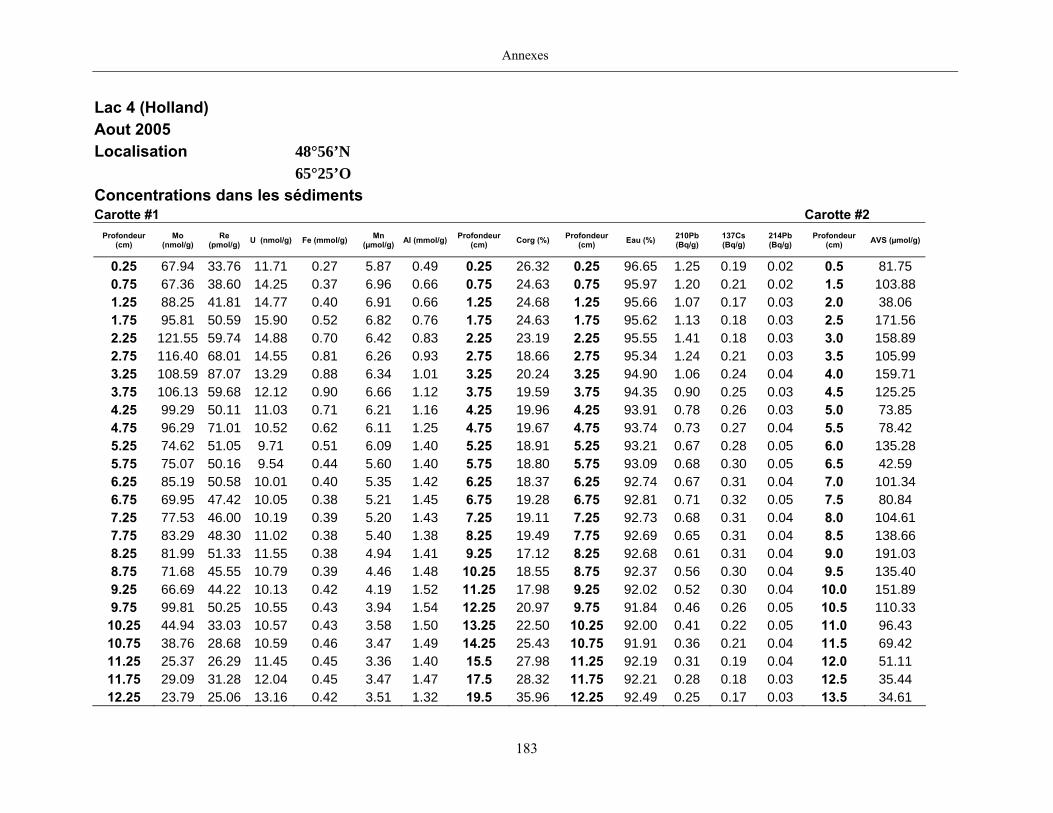
Annexes
183
Lac 4 (Holland) Aout 2005 Localisation 48°56’N 65°25’O Concentrations dans les sédiments Carotte #1 Carotte #2
Profondeur (cm)
Mo (nmol/g)
Re (pmol/g) U (nmol/g) Fe (mmol/g) Mn
(µmol/g) Al (mmol/g) Profondeur (cm) Corg (%) Profondeur
(cm) Eau (%) 210Pb (Bq/g)
137Cs (Bq/g)
214Pb (Bq/g)
Profondeur (cm) AVS (µmol/g)
0.25 67.94 33.76 11.71 0.27 5.87 0.49 0.25 26.32 0.25 96.65 1.25 0.19 0.02 0.5 81.75 0.75 67.36 38.60 14.25 0.37 6.96 0.66 0.75 24.63 0.75 95.97 1.20 0.21 0.02 1.5 103.88 1.25 88.25 41.81 14.77 0.40 6.91 0.66 1.25 24.68 1.25 95.66 1.07 0.17 0.03 2.0 38.06 1.75 95.81 50.59 15.90 0.52 6.82 0.76 1.75 24.63 1.75 95.62 1.13 0.18 0.03 2.5 171.56 2.25 121.55 59.74 14.88 0.70 6.42 0.83 2.25 23.19 2.25 95.55 1.41 0.18 0.03 3.0 158.89 2.75 116.40 68.01 14.55 0.81 6.26 0.93 2.75 18.66 2.75 95.34 1.24 0.21 0.03 3.5 105.99 3.25 108.59 87.07 13.29 0.88 6.34 1.01 3.25 20.24 3.25 94.90 1.06 0.24 0.04 4.0 159.71 3.75 106.13 59.68 12.12 0.90 6.66 1.12 3.75 19.59 3.75 94.35 0.90 0.25 0.03 4.5 125.25 4.25 99.29 50.11 11.03 0.71 6.21 1.16 4.25 19.96 4.25 93.91 0.78 0.26 0.03 5.0 73.85 4.75 96.29 71.01 10.52 0.62 6.11 1.25 4.75 19.67 4.75 93.74 0.73 0.27 0.04 5.5 78.42 5.25 74.62 51.05 9.71 0.51 6.09 1.40 5.25 18.91 5.25 93.21 0.67 0.28 0.05 6.0 135.28 5.75 75.07 50.16 9.54 0.44 5.60 1.40 5.75 18.80 5.75 93.09 0.68 0.30 0.05 6.5 42.59 6.25 85.19 50.58 10.01 0.40 5.35 1.42 6.25 18.37 6.25 92.74 0.67 0.31 0.04 7.0 101.34 6.75 69.95 47.42 10.05 0.38 5.21 1.45 6.75 19.28 6.75 92.81 0.71 0.32 0.05 7.5 80.84 7.25 77.53 46.00 10.19 0.39 5.20 1.43 7.25 19.11 7.25 92.73 0.68 0.31 0.04 8.0 104.61 7.75 83.29 48.30 11.02 0.38 5.40 1.38 8.25 19.49 7.75 92.69 0.65 0.31 0.04 8.5 138.66 8.25 81.99 51.33 11.55 0.38 4.94 1.41 9.25 17.12 8.25 92.68 0.61 0.31 0.04 9.0 191.03 8.75 71.68 45.55 10.79 0.39 4.46 1.48 10.25 18.55 8.75 92.37 0.56 0.30 0.04 9.5 135.40 9.25 66.69 44.22 10.13 0.42 4.19 1.52 11.25 17.98 9.25 92.02 0.52 0.30 0.04 10.0 151.89 9.75 99.81 50.25 10.55 0.43 3.94 1.54 12.25 20.97 9.75 91.84 0.46 0.26 0.05 10.5 110.33 10.25 44.94 33.03 10.57 0.43 3.58 1.50 13.25 22.50 10.25 92.00 0.41 0.22 0.05 11.0 96.43 10.75 38.76 28.68 10.59 0.46 3.47 1.49 14.25 25.43 10.75 91.91 0.36 0.21 0.04 11.5 69.42 11.25 25.37 26.29 11.45 0.45 3.36 1.40 15.5 27.98 11.25 92.19 0.31 0.19 0.04 12.0 51.11 11.75 29.09 31.28 12.04 0.45 3.47 1.47 17.5 28.32 11.75 92.21 0.28 0.18 0.03 12.5 35.44 12.25 23.79 25.06 13.16 0.42 3.51 1.32 19.5 35.96 12.25 92.49 0.25 0.17 0.03 13.5 34.61
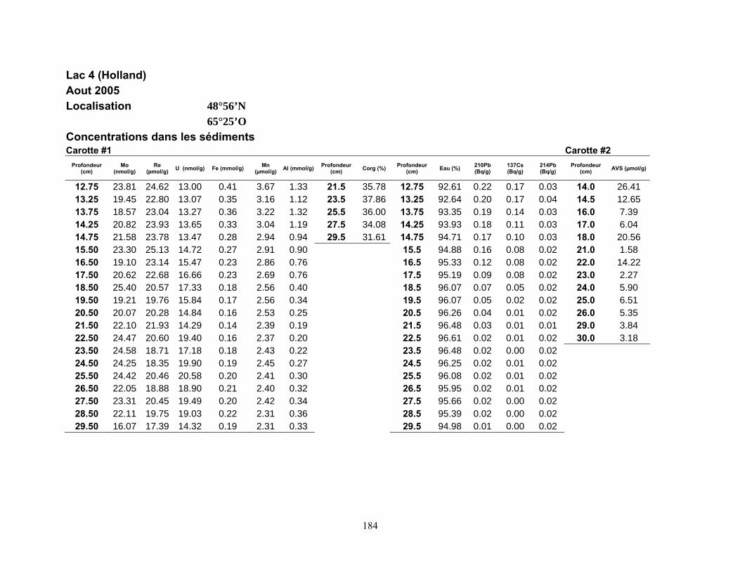
184
Lac 4 (Holland)
Aout 2005
Localisation 48°56’N
65°25’O
Concentrations dans les sédiments Carotte #1 Carotte #2
Profondeur (cm)
Mo (nmol/g)
Re (pmol/g) U (nmol/g) Fe (mmol/g) Mn
(µmol/g) Al (mmol/g) Profondeur (cm) Corg (%) Profondeur
(cm) Eau (%) 210Pb (Bq/g)
137Cs (Bq/g)
214Pb (Bq/g)
Profondeur (cm) AVS (µmol/g)
12.75 23.81 24.62 13.00 0.41 3.67 1.33 21.5 35.78 12.75 92.61 0.22 0.17 0.03 14.0 26.41 13.25 19.45 22.80 13.07 0.35 3.16 1.12 23.5 37.86 13.25 92.64 0.20 0.17 0.04 14.5 12.65 13.75 18.57 23.04 13.27 0.36 3.22 1.32 25.5 36.00 13.75 93.35 0.19 0.14 0.03 16.0 7.39 14.25 20.82 23.93 13.65 0.33 3.04 1.19 27.5 34.08 14.25 93.93 0.18 0.11 0.03 17.0 6.04 14.75 21.58 23.78 13.47 0.28 2.94 0.94 29.5 31.61 14.75 94.71 0.17 0.10 0.03 18.0 20.56 15.50 23.30 25.13 14.72 0.27 2.91 0.90 15.5 94.88 0.16 0.08 0.02 21.0 1.58 16.50 19.10 23.14 15.47 0.23 2.86 0.76 16.5 95.33 0.12 0.08 0.02 22.0 14.22 17.50 20.62 22.68 16.66 0.23 2.69 0.76 17.5 95.19 0.09 0.08 0.02 23.0 2.27 18.50 25.40 20.57 17.33 0.18 2.56 0.40 18.5 96.07 0.07 0.05 0.02 24.0 5.90 19.50 19.21 19.76 15.84 0.17 2.56 0.34 19.5 96.07 0.05 0.02 0.02 25.0 6.51 20.50 20.07 20.28 14.84 0.16 2.53 0.25 20.5 96.26 0.04 0.01 0.02 26.0 5.35 21.50 22.10 21.93 14.29 0.14 2.39 0.19 21.5 96.48 0.03 0.01 0.01 29.0 3.84 22.50 24.47 20.60 19.40 0.16 2.37 0.20 22.5 96.61 0.02 0.01 0.02 30.0 3.18 23.50 24.58 18.71 17.18 0.18 2.43 0.22 23.5 96.48 0.02 0.00 0.02 24.50 24.25 18.35 19.90 0.19 2.45 0.27 24.5 96.25 0.02 0.01 0.02 25.50 24.42 20.46 20.58 0.20 2.41 0.30 25.5 96.08 0.02 0.01 0.02 26.50 22.05 18.88 18.90 0.21 2.40 0.32 26.5 95.95 0.02 0.01 0.02 27.50 23.31 20.45 19.49 0.20 2.42 0.34 27.5 95.66 0.02 0.00 0.02 28.50 22.11 19.75 19.03 0.22 2.31 0.36 28.5 95.39 0.02 0.00 0.02 29.50 16.07 17.39 14.32 0.19 2.31 0.33 29.5 94.98 0.01 0.00 0.02