Embed Size (px)
Citation preview
JEAN-FRANCOIS PLANTE
A PROPOS D’UNE MESURE DE CORRELATION DES
RANGS DE BLEST
Memoire
presente
a la Faculte des etudes superieures
pour l’obtention
du grade de maıtre es sciences (M. Sc.)
Departement de mathematiques et de statistique
FACULTE DES SCIENCES ET DE GENIE
UNIVERSITE LAVAL
JUILLET 2002
c© Jean-Francois Plante, 2002
RESUME
La copule sous-jacente a un couple de variables aleatoires continues permet
de decrire completement le lien de dependance qui les unit. Pour resumer
sur une echelle numerique l’intensite de la dependance representee par une
copule, on emploie en general des coefficients de correlation tels que ceux de
Pearson, Spearman et Kendall. En 2000, une nouvelle mesure de correlation
basee sur les rangs a ete proposee par David C. Blest. Ce memoire presente
les proprietes du coefficient de Blest et en propose quelques variantes. Des
simulations permettent de comparer la valeur du coefficient de Blest et de ses
versions symetriques et duales en tant que statistiques de tests permettant
d’eprouver l’hypothese d’independance.
———————————————– ———————————————–
Jean-Francois Plante, etudiant Christian Genest, directeur

AVANT-PROPOS
Je voudrais d’abord exprimer ma gratitude envers mes parents, freres et sœurs
pour m’avoir permis de grandir dans un climat familial sain et dynamique.
C’est grace a eux que j’ai appris a partager et a perseverer. J’ai ete chanceux
de pouvoir profiter tous les soirs d’une atmosphere paisible et reposante a la
maison, apres une dure journee a l’ecole.
Plus particulierement, je desire remercier mon pere de m’avoir appris l’honne-
tete et l’integrite. La confiance dont il a fait preuve a mon egard des ma tendre
enfance m’a permis de m’epanouir. A ma mere, je veux dire merci pour son
devouement, son amour et son attention qui m’ont soutenu constamment.
Je voudrais aussi dire merci a tous les amis qui m’ont accompagne au cours
de mes etudes. Grace a eux, j’ai eu enormement de plaisir a evoluer dans un
milieu scolaire dynamique et enrichissant.
Au plan scientifique, j’ai eu beaucoup de plaisir a travailler avec Christian
Genest. Son habilete a comprendre les fondements des problemes et a les
transmettre est fascinante. Son enseignement et ses conseils m’ont certaine-
ment aide a apprendre comment comprendre !
Je suis egalement reconnaissant envers M. Kilani Ghoudi de m’avoir donne
acces a certains de ses programmes informatiques et d’avoir bien voulu etre
membre du jury avec M. Louis-Paul Rivest.

iv
Une partie de ce travail a ete financee par des octrois individuels et collectifs
accordes a M. Christian Genest et a l’equipe du Fond quebecois de recherche
sur la nature et les technologies qu’il coordonne. Que lui et ses collegues en
soient remercies, ainsi que le Conseil de recherches en sciences naturelles et
en genie du Canada, qui m’a accorde une bourse d’etude de deuxieme cycle.
TABLE DES MATIERES
RESUME ii
AVANT-PROPOS iii
INTRODUCTION 1
CHAPITRE I. ON BLEST’S MEASURE OF RANK CORRE-
LATION 3
1.1 Introduction . . . . . . . . . . . . . . . . . . . . . . . . . . . . 3
1.2 Limiting Distribution of Blest’s Coefficients . . . . . . . . . . 7
1.3 Properties of Blest’s Index . . . . . . . . . . . . . . . . . . . . 10
1.4 A Symmetrized Version of Blest’s Measure of Association . . . 13
1.5 Performance as a Test of Independence . . . . . . . . . . . . . 19
1.5.1 Pitman Efficiency . . . . . . . . . . . . . . . . . . . . . 19
1.5.2 Power Comparisons in Finite Samples . . . . . . . . . . 25
1.6 Conclusion . . . . . . . . . . . . . . . . . . . . . . . . . . . . . 29
1.7 Appendix . . . . . . . . . . . . . . . . . . . . . . . . . . . . . 30
CHAPITRE II. MESURES DE CORRELATION BASEES SUR
LES RANGS 33
2.1 Terminologie . . . . . . . . . . . . . . . . . . . . . . . . . . . . 33
2.2 Formes des coefficients . . . . . . . . . . . . . . . . . . . . . . 33
2.2.1 Elimination des marges . . . . . . . . . . . . . . . . . . 34
2.2.2 Parametre estime et loi asymptotique . . . . . . . . . . 34
v
vi
2.2.3 Degre des polynomes consideres . . . . . . . . . . . . . 35
2.2.4 Role des constantes . . . . . . . . . . . . . . . . . . . . 35
2.3 Mesures considerees . . . . . . . . . . . . . . . . . . . . . . . . 36
2.4 Resume des proprietes . . . . . . . . . . . . . . . . . . . . . . 38
2.4.1 Dualite et symetrie radiale . . . . . . . . . . . . . . . . 38
2.4.2 Dualite et test d’independance . . . . . . . . . . . . . . 39
2.4.3 Liens lineaires . . . . . . . . . . . . . . . . . . . . . . . 39
2.4.4 Proprietes individuelles . . . . . . . . . . . . . . . . . . 40
CHAPITRE III. CALCULS EXPLICITES 43
3.1 Variance des coefficients sous l’hypothese d’independance . . . 43
3.1.1 Rho de Spearman . . . . . . . . . . . . . . . . . . . . . 43
3.1.2 Coefficient de Blest . . . . . . . . . . . . . . . . . . . . 45
3.1.3 Coefficient de Plantagenet . . . . . . . . . . . . . . . . 47
3.2 Correlation entre les coefficients sous l’hypothese d’independance 50
3.2.1 Blest vs Spearman . . . . . . . . . . . . . . . . . . . . 50
3.2.2 Plantagenet vs Spearman . . . . . . . . . . . . . . . . 52
3.2.3 Blest vs Plantagenet . . . . . . . . . . . . . . . . . . . 53
3.3 Valeur theorique de certains parametres . . . . . . . . . . . . . 54
3.3.1 Copule de Farlie–Gumbel–Morgenstern generalisee . . . 55
3.3.2 Copule de Cuadras–Auge . . . . . . . . . . . . . . . . . 58
3.4 Variance asymptotique . . . . . . . . . . . . . . . . . . . . . . 59
3.5 Efficacite relative asymptotique . . . . . . . . . . . . . . . . . 63
3.5.1 Illustration de la premiere methode : copule de Cuadras–
Auge . . . . . . . . . . . . . . . . . . . . . . . . . . . . 65
3.5.2 Illustration de la deuxieme methode : copule de Clayton 66
vii
CHAPITRE IV. SIMULATIONS 69
4.1 Loi normale bivariee . . . . . . . . . . . . . . . . . . . . . . . 70
4.2 Copule de Frank . . . . . . . . . . . . . . . . . . . . . . . . . 73
4.3 Copule de Clayton . . . . . . . . . . . . . . . . . . . . . . . . 75
4.4 Copule de valeurs extremes de Gumbel . . . . . . . . . . . . . 78
4.5 Copule de valeurs extremes de Galambos . . . . . . . . . . . . 80
4.6 Transposition du minimum . . . . . . . . . . . . . . . . . . . . 83
4.6.1 Copule (6) . . . . . . . . . . . . . . . . . . . . . . . . . 83
4.6.2 Copule (7) . . . . . . . . . . . . . . . . . . . . . . . . . 86
CONCLUSION 89
BIBLIOGRAPHIE 90
INTRODUCTION
Pour quantifier la dependance entre deux variables, la mesure la plus clas-
sique est sans doute le coefficient de correlation de Pearson. Malheureuse-
ment, cette statistique depend des lois marginales des observations, ce qui en
limite souvent les valeurs possibles et en complique l’interpretation.
Une facon efficace de contourner ce probleme consiste a utiliser des coef-
ficients bases sur les rangs tels que le ρ de Spearman et le τ de Kendall. Les
coefficients bases sur les rangs presentent l’avantage de ne pas etre influences
par les lois marginales des observations.
En 2000, David C. Blest a propose un coefficient de correlation base sur
les rangs qui ressemble au ρ de Spearman, mais qui a la particularite de
ponderer differemment les ecarts observes entre les classements induits par
les deux variables, selon qu’ils se produisent dans les premiers ou les derniers
rangs.
Ce memoire complete le travail de Blest en precisant la loi asymptotique
de son coefficient et en en proposant des versions symetriques et duales.
Le chapitre I presente l’ensemble des resultats obtenus. Il s’agit d’un ar-
ticle ecrit en anglais qui est actuellement en cours d’evaluation.
INTRODUCTION 2
Le chapitre II apporte quelques explications supplementaires qui viennent
completer le contenu de l’article. On y presente un point de vue plus intuitif
des resultats obtenus et on y retrouve un resume des proprietes de chaque
coefficient.
Des exemples de calculs explicites, omis dans l’article, sont donnes au cha-
pitre III. La plupart d’entre eux ont ete realises a l’aide du logiciel de calcul
symbolique Maple. Dans chaque cas, le code utilise est presente.
Pour evaluer la performance du coefficient de Blest et de ses variantes a
titre de statistiques permettant de tester l’hypothese d’independance, des
simulations ont ete effectuees. Les resultats de cette etude de Monte–Carlo
sont consignes au chapitre IV.
Enfin, la conclusion du memoire souleve plusieurs questions sur les differentes
mesures de correlation qu’il est possible de construire a partir de polynomes
et sur l’avantage des unes par rapport aux autres.
CHAPITRE I
ON BLEST’S MEASURE OF RANK
CORRELATION
Christian GENEST and Jean-Francois PLANTE
Blest (2000, Austral. and New Zealand J. Statist.) a propose une mesure
non parametrique de correlation entre des aleas X et Y . Son coefficient,
asymetrique dans ses arguments, pondere differemment les ecarts observes
dans les classements induits par ces variables selon qu’ils se produisent dans
les premiers ou les derniers rangs. Les auteurs determinent la loi limite de
l’indice de Blest et en suggerent des variantes symetriques dont ils explorent
les merites au moyen de calculs d’efficacite relative asymptotique et d’une
etude de Monte–Carlo.
1.1 Introduction
Although Pearson’s correlation coefficient is one of the most ubiquitous con-
cepts in the scientific literature, it is now widely recognized, at least among
statisticians, that the degree of stochastic dependence between random va-
riables X and Y with joint cumulative distribution function H and marginals
F and G is much more appropriately characterized and measured in terms
I. ON BLEST’S MEASURE OF RANK CORRELATION 4
of the joint distribution C of the pair (F (X), G(Y )), viz.
C(u, v) = P{F (X) ≤ u, G(Y ) ≤ v}, 0 ≤ u, v ≤ 1
whose marginals are uniform on the interval (0, 1). Indeed, most modern
concepts and measures of dependence, not to mention stochastic orderings
(see for example Joe 1997, Nelsen 1999 or Drouet–Mari & Kotz 2001), are
functions of the so-called “copula” C, which is uniquely determined on Ran-
ge(F )×Range(G) and hence everywhere in the special case where F and G
are continuous, as will be assumed henceforth.
In particular, classical nonparametric measures of dependence such as Spear-
man’s rho
ρ(X, Y ) = 12
∫IR2
F (x)G(y) dH(x, y)− 3
= 12
∫[0,1]2
uv dC(u, v) − 3 = 12
∫ 1
0
∫ 1
0
C(u, v) dv du − 3 (1)
and Kendall’s tau
τ(X, Y ) = 4
∫IR2
H(x, y) dH(x, y)− 1 = 4
∫[0,1]2
C(u, v) dC(u, v)− 1
are superior to Pearson’s coefficient in that while they vanish when the va-
riables are independent, they always exist and take their extreme values ±1
when X and Y are in perfect (positive or negative) functional dependence,
i.e., when either Y = G−1{F (X)} or Y = G−1{1 − F (X)} with probability
one. Except in very special circumstances, these cases of complete depen-
dence are not instances of linear dependence. Thus when considering random
data (X1, Y1), . . . , (Xn, Yn) from an unknown distribution H whose support
I. ON BLEST’S MEASURE OF RANK CORRELATION 5
is all of [0,∞)2, for instance, the values of ρ and τ are unconstrained, whe-
reas Pearson’s correlation can only span an interval [r, 1] whose lower bound
r > −1 depends on the choice of marginals F and G. When the latter are
unknown, it is thus difficult to know what to make of an observed Pearson
correlation of −0.2, say.
Because copulas are margin-free and ranks are maximally invariant statis-
tics of the observations under monotone transformations of the marginal
distributions, ρ, τ and indeed all other copula-based measures of dependence
(e.g., the index of Schweizer & Wolf 1981) should be estimated by functions
of the ranks Ri and Sj of the Xi’s and Yj’s. Letting Fn and Gn stand for
the empirical distribution functions of X and Y respectively, the classical
estimate for ρ is
ρn = corr{Fn(X), Gn(Y )} =12
n3 − n
n∑i=1
RiSi − 3n + 1
n − 1
since Fn(Xi) = Ri/n and Gn(Yj) = Sj/n for all 1 ≤ i, j ≤ n. Likewise, τ is
traditionally estimated by the scaled difference in the numbers of concordant
and discordant pairs, or equivalently by
τn =2
n2 − n
∑1≤i<j≤n
sign(Ri − Rj) sign(Si − Sj).
In comparing ρn and τn in terms of their implicit weighing of differences
Ri−Si, Blest (2000) was led to propose an alternative measure of rank corre-
lation that “... attaches more significance to the early ranking of an initially
given order.” Assume, for example, that Xi and Yi represent the running
times of sprinter i = 1, . . . , n in two successive track-and-field meetings. The
I. ON BLEST’S MEASURE OF RANK CORRELATION 6
correlation in the pairs (Ri, Si) then gives an idea of the consistency bet-
ween the two rankings. However, differences in the top ranks would seem to
be more critical, in that they matter in awarding medals. As a result, Blest
suggests that these discrepancies should be emphasized, whereas all rank re-
versals are given the same weight in Spearman’s or Kendall’s coefficient.
To be specific, Blest’s index is defined by
νn =2n + 1
n − 1− 12
n2 − n
n∑i=1
(1 − Ri
n + 1
)2
Si.
The constants are rigged so that the coefficient varies between 1 and −1
and is most extreme when the rankings coincide (Si = Ri) or are antithe-
tic (Si = n + 1 − Ri). Numerical results and calculations reported by Blest
(2000) also indicate that his measure can discriminate more easily between
individual permutations than either ρn or τn while being highly correlated
with both of them. Furthermore, partial evidence is provided which indicates
that the large-sample distribution of νn is normal.
The first objective of this paper is to show that νn is an asymptotically
unbiased estimator of the population parameter
ν(X, Y ) = 2 − 12
∫IR2
{1 − F (x)}2G(y) dH(x, y) (2)
= 2 − 12
∫[0,1]2
(1 − u)2v dC(u, v)
and that√
n(νn − ν) converges in distribution to a centered normal random
variable whose variance is specified in Section 1.2. While νn may be appro-
priate as an index of discrepancy between two rankings, it is pointed out
I. ON BLEST’S MEASURE OF RANK CORRELATION 7
in Section 1.3 that since in general ν(X, Y ) 6= ν(Y, X), the parameter (2)
estimated by νn is not a measure of concordance, in the sense of Scarsini
(1984). The properties of a symmetrized version of νn are thus considered in
Section 1.4, and the relative merits of this new statistic (and a natural com-
plement thereof) for testing independence are then examined in Section 1.5
through asymptotic relative efficiency calculations and a small Monte Carlo
simulation study. Brief concluding comments are given in Section 1.6 and the
Appendix (Section 1.7) contains some technical details.
1.2 Limiting Distribution of Blest’s Coeffi-
cients
Define J(t) = (1−t)2 and K(t) = t for all 0 ≤ t ≤ 1, and for arbitrary integers
n and i ∈ {1, . . . , n}, let Jn(t) = J{i/(n + 1)} and Kn(t) = K{i/(n + 1)} if
(i − 1)/n < t ≤ i/n. The large-sample behaviour of Blest’s sample measure
of association is clearly the same as that of
2 − 12
n
n∑i=1
(1 − Ri
n + 1
)2Si
n + 1,
which may be written as
2 − 12
∫Jn(Fn)Kn(Gn)dHn
in terms of the empirical cumulative distribution function Hn of H and its
marginals Fn and Gn. Since the functions J and K and their derivatives are
bounded on [0, 1], and in view of Remark 2.1 of Ruymgaart, Shorack & van
Zwet (1972), a direct application of Theorem 2.1 of these authors implies that
I. ON BLEST’S MEASURE OF RANK CORRELATION 8
√n(νn − ν) is asymptotically normally distributed with mean and variance
as specified below.
Proposition 1. Under the assumption of random sampling from a conti-
nuous bivariate distribution H with underlying copula C,√
n(νn−ν) conver-
ges weakly to a normal random variable with zero mean and the same variance
as
12
[(1 − U)2V − 2
∫ 1
U
(1 − u)E(V |U = u) du
+
∫ 1
V
E{(1 − U)2|V = v} dv
], (3)
where the pair (U, V ) is distributed as C. In particular, the variance of the
latter expression equals 16/15 when U and V are independent.
As is the case for Spearman’s rho, compact algebraic formulas for ν can be
found for relatively few models. Examples 1 and 2 illustrate, in two special
cases of interest, the explicit calculations that can sometimes be made using
a symbolic calculator such as Maple ; see Chapter III for details. Example 3,
which concerns the pervasive normal model, is somewhat more subtle.
Example 1. Suppose that (X, Y ) follows a Farlie–Gumbel–Morgenstern dis-
tribution with marginals F and G, viz.
Hθ(x, y) = F (x)G(y) + θF (x)G(y){1 − F (x)}{1 − G(y)}, x, y ∈ IR
with parameter θ ∈ [−1, 1]. Then
νθ(X, Y ) = ρθ(X, Y ) =3
2τθ(X, Y ) =
θ
3
I. ON BLEST’S MEASURE OF RANK CORRELATION 9
and the variance of (3) equals
16
15− 16
63θ2.
Example 2. For arbitrary a, b ∈ [0, 1] and θ ∈ [−1, 1], let
Hθ,a,b(x, y) = F (x)G(y)[1 + θ {1 − F (x)a}{1 − G(y)b
}]= Π
{F (x)1−a, G(y)1−b
}Cθ
{F (x)a, G(y)b
}, x, y ∈ IR
where Cθ(u, v) = Hθ {F−1(u), G−1(v)} is the Farlie–Gumbel–Morgenstern
copula and Π(u, v) = uv denotes the independence copula. By Khoudraji’s
device (see Genest, Ghoudi & Rivest 1998), Hθ,a,b is an asymmetric exten-
sion of the Farlie–Gumbel–Morgenstern distribution, recently considered in
a somewhat more general form by Bairamov, Kotz & Bekci (2000). For any
pair (X, Y ) distributed as Hθ,a,b, one finds
νθ,a,b(X, Y ) =2ab(a + 5)θ
(a + 2)(a + 3)(b + 2),
while
ρθ,a,b(X, Y ) =3abθ
(a + 2)(b + 2)=
3
2τθ,a,b(X, Y ).
Note that
νθ,a,b(X, Y ) 6= νθ,a,b(Y, X) = νθ,b,a(X, Y ),
unless of course a = b, in which case the copula is symmetric in its arguments.
An explicit but long formula (not shown here) for the asymptotic variance
of√
n(νn − ν) is also available in this case.
Example 3. Suppose that (X, Y ) has a bivariate normal distribution and
that corr(X, Y ) = r ∈ [−1, 1]. Then
νr(X, Y ) = ρr(X, Y ) =6
πarcsin
(r
2
)
I. ON BLEST’S MEASURE OF RANK CORRELATION 10
while
τr(X, Y ) =2
πarcsin(r).
The fact that ν(X, Y ) = ρ(X, Y ) arises whenever a copula C is radially
symmetric, i.e., when its associated survival function C(u, v) = 1 − u − v +
C(u, v) satisfies the condition
C(u, v) = C(1 − u, 1 − v), 0 ≤ u, v ≤ 1. (4)
Indeed, since the measure C is then invariant by the change of variable
(x, y) = (1 − u, 1 − v), one must have∫[0,1]2
(1 − u)2v dC =
∫[0,1]2
u2(1 − v) dC.
Expanding both sides and using the fact that C has uniform marginals on
[0, 1] yields ∫[0,1]2
u2v dC =
∫[0,1]2
uv dC − 1
12,
from which it follows at once that ν(X, Y ) = ρ(X, Y ) (and hence equals
ν(Y, X) as well). The formulas for ρr(X, Y ) and τr(X, Y ) are standard nor-
mal theory ; see for example Exercise 2.14, p. 54 of Joe (1997).
Unfortunately, the variance of (3) can only be computed numerically in
Example 3. Additional properties of ν(X, Y ) are described next.
1.3 Properties of Blest’s Index
According to Scarsini (1984), the following are fundamental properties that
any measure κ of concordance should satisfy :
I. ON BLEST’S MEASURE OF RANK CORRELATION 11
a) κ is defined for every pair (X, Y ) of continuous random variables.
b) −1 ≤ κ(X, Y ) ≤ 1, κ(X, X) = 1, and κ(X,−X) = −1.
c) κ(X, Y ) = κ(Y, X).
d) If X and Y are independent, then κ(X, Y ) = 0.
e) κ(−X, Y ) = κ(X,−Y ) = −κ(X, Y ).
f) If (X, Y ) ≺ (X∗, Y ∗) in the positive quadrant dependence ordering,
then κ(X, Y ) ≤ κ(X∗, Y ∗).
g) If (X1, Y1), (X2, Y2), . . . is a sequence of continuous random vectors
that converges weakly to a pair (X, Y ), then κ(Xn, Yn) → κ(X, Y ) as
n → ∞.
It is well known that both ρ and τ meet all these conditions, and it is easy
to check that the index ν defined in (2) has properties a), b), d), f), and g).
To show the latter two, it is actually more convenient to use the alternative
representation
ν(X, Y ) = −2 + 24
∫[0,1]2
(1 − u)C(u, v) du dv,
which follows immediately from an extension of Hoeffding’s identity (1) due
to Quesada–Molina (1992).
As was already pointed out in Example 2, however, Blest’s measure does
not satisfy condition c). Furthermore, property e) is not verified either. For,
if (X, Y ) has copula C, then C∗(u, v) = v−C(1−u, v) is the copula associated
with the pair (−X, Y ), and hence
ν(−X, Y ) = ν(X, Y ) − 2ρ(X, Y ), (5)
I. ON BLEST’S MEASURE OF RANK CORRELATION 12
so that ν(−X, Y ) 6= −ν(X, Y ) except in the special case where ν(X, Y ) =
ρ(X, Y ). Note, however, that ν(X,−Y ) = −ν(X, Y ) by a similar argument
involving the copula C∗∗(u, v) = u − C(u, 1 − v) of the pair (X,−Y ).
The following simple example provides a concrete illustration of the failure
of condition e) for Blest’s index.
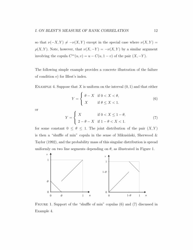
Example 4. Suppose that X is uniform on the interval (0, 1) and that either
Y =
θ − X if 0 < X < θ,
X if θ ≤ X < 1.(6)
or
Y =
X if 0 < X ≤ 1 − θ,
2 − θ − X if 1 − θ < X < 1.(7)
for some constant 0 ≤ θ ≤ 1. The joint distribution of the pair (X, Y )
is then a “shuffle of min” copula in the sense of Mikusinski, Sherwood &
Taylor (1992), and the probability mass of this singular distribution is spread
uniformly on two line segments depending on θ, as illustrated in Figure 1.
Figure 1. Support of the “shuffle of min” copulas (6) and (7) discussed in
Example 4.
I. ON BLEST’S MEASURE OF RANK CORRELATION 13
When (X, Y ) is distributed as (6), one finds
νθ(X, Y ) = 1 − 4θ3 + 2θ4,
while if (X, Y ) is distributed as (7), one gets
νθ(X, Y ) = 1 − 2θ4.
Had Blest’s coefficient met condition e) above, the two expressions would
have been equal, since the two supports displayed in Figure 1 are equivalent
up to a rotation of 180 degrees about the point (1/2, 1/2), i.e., a reflection
through the line u = 1/2 followed by another reflection through the line
v = 1/2.
1.4 A Symmetrized Version of Blest’s Mea-
sure of Association
While the coefficient νn and its population equivalent ν(X, Y ) may be ap-
propriate as an index of discrepancy between a fixed order, say given by the
Xi’s, and an alternate order given by the other variable, the above discussion
makes it clear that neither can be used to measure concordance.
There may be interest, however, in symmetrized versions of Blest’s proposal,
viz.
ξn = −4n + 5
n − 1+
6
n3 − n
n∑i=1
RiSi
(4 − Ri + Si
n + 1
)(8)
I. ON BLEST’S MEASURE OF RANK CORRELATION 14
and its theoretical counterpart
ξ(X, Y ) =ν(X, Y ) + ν(Y, X)
2= −4 + 6
∫[0,1]2
uv(4 − u − v) dC(u, v)
= −2 + 12
∫[0,1]2
(2 − u − v)C(u, v) du dv.
Because of an obvious connection between English history and the concate-
nation of their names, the authors jokingly refer to these quantities as the
(empirical and theoretical) “Plantagenet” coefficients. Nevertheless, they be-
lieve that Blest should be credited for ξn and ξ.
As explained in Section 4 of Blest (2000), E(νn) = 0 under the null hy-
pothesis of independence, and hence E(ξn) = 0 as well. Under H0, it is also
a simple matter to prove (see Appendix for details) that
var(ξn) =31n2 + 60n + 26
30(n + 1)2(n − 1)
and that cov(ρn, ξn) = var(ρn) = 1/(n − 1), so that
corr(ρn, ξn) =
√30(n + 1)2
31n2 + 60n + 26→√
30
31≈ 0.9837,
while corr(ρn, νn) →√15/16 ≈ 0.9682.
Although it is not generally true that ξn is an unbiased estimator of ξ un-
der other distributional hypotheses between X and Y , it is asymptotically
unbiased, as implied by the following result.
Proposition 2. Under the assumption of random sampling from a conti-
nuous bivariate distribution H with underlying copula C,√
n(ξn−ξ) converges
I. ON BLEST’S MEASURE OF RANK CORRELATION 15
weakly to a normal random variable with zero mean and the same variance as
6
[UV (4 − U − V ) +
∫ 1
U
{2(2 − u)E(V |U = u) − E
(V 2|U = u
)}du
+
∫ 1
V
{2(2 − v)E(U |V = v) − E
(U2|V = v
)}dv
],
where the pair (U, V ) is distributed as C. In particular, the variance of the
latter expression equals 31/30 when U and V are independent.
Proof. The asymptotic behaviour of ξn is obviously the same as that of
−4 +6
n
n∑i=1
Ri
n + 1
Si
n + 1
(4 − Ri
n + 1− Si
n + 1
),
which may be written alternatively as
−4 + 6
∫[0,1]2
uv(4 − u − v) dCn(u, v)
in terms of the rescaled empirical copula function, as defined by Genest,
Ghoudi & Rivest (1995). The conclusion is then an immediate consequence
of their Proposition A·1, upon choosing J(u, v) = uv(4−u− v), δ = 1/4 and
M = p = q = 2, say, to satisfy conditions (i) and (ii) of their result. �
Proceeding as above but with J(u, v) = auv + buv(4− u− v) with arbitrary
reals a and b actually shows that any linear combination of√
n(ρn − ρ) and√
n(ξn − ξ) is normally distributed with zero mean and the same variance as
I. ON BLEST’S MEASURE OF RANK CORRELATION 16
6
[UV {2a + b(4 − U − V )}
+
∫ 1
U
[2{a + b(2 − u)}E(V |U = u) − bE
(V 2|U = u
)]du
+
∫ 1
V
[2{a + b(2 − v)}E(U |V = v) − bE
(U2|V = v
)]dv
]. (9)
Consequently, the joint distribution of√
n(ρn − ρ) and√
n(ξn − ξ) must
be asymptotically normal with zero mean and a covariance matrix whose
diagonal entries correspond to the choices (a, b) = (1, 0) and (0, 1). The
limiting covariance between these two quantities can also be derived from
these large-sample variances and that of the linear combination corresponding
to a = 2 and b = −1, for instance. These observations are formally gathered
below.
Proposition 3. Under the assumption of random sampling from a conti-
nuous bivariate distribution H with underlying copula C,√
n(ξn − ξ, ρn − ρ)′
converges weakly to a normal random vector with zero mean and covariance
matrix σ2
ξ κ
κ σ2ρ
with κ =
4σ2ρ + σ2
ξ − σ22ρ−ξ
4,
where σ2ξ , σ2
ρ and σ22ρ−ξ are the variances of (9) corresponding to the choices
(a, b) = (1, 0), (0, 1), and (2,−1), and where the pair (U, V ) is distributed as
C. In particular, σ2ξ = 31/30 and σ2
ρ = κ = 1 under independence.
Remark 1. When condition (4) holds, making the change of variables (x, y) =
(1−u, 1− v) in Equation (9) shows that one must then have σ2ξ = σ2
2ρ−ξ and
I. ON BLEST’S MEASURE OF RANK CORRELATION 17
hence κ = σ2ρ in Proposition 3. Models for which C = C include the Farlie–
Gumbel–Morgenstern, the Gaussian, the Plackett (1965), and Frank’s copula
(Nelsen 1986 ; Genest 1987) ; note that the latter is the only Archimedean
copula that is radially symmetric (see for example Nelsen 1999, p. 97).
Remark 2. Since the joint distribution of√
n(ρn − ρ) and√
n(τn − τ) is
also known to be normal with limiting correlation equal to 1, Proposition 3
implies that
limn→∞
corr(ξn, τn) = limn→∞
corr(ξn, ρn) =
√30
31
under the null hypothesis of independence.
The following examples provide numerical illustrations of these various facts.
Example 1 (continued). If (X, Y ) follows a Farlie–Gumbel–Morgenstern
distribution with marginals F and G and parameter θ ∈ [−1, 1], then
ξθ(X, Y ) = ρθ(X, Y ) =3
2τθ(X, Y ) =
θ
3
and√
n(ξn − ξθ) −→ N
(0,
1
450θ3 − 157
630θ2 +
2
225θ +
31
30
).
Furthermore, cov(√
nξn,√
nρn) → 1 − 11 θ2/45 and
corr(ξn, ρn) −→√
3150 − 770 θ2
3255 + 28 θ − 785 θ2 + 7 θ3
as n → ∞. The latter is a decreasing function of θ taking values in the
interval [0.9747, 0.9887].
Example 2 (continued). For any pair (X, Y ) distributed as Hθ,a,b, one
finds
ξθ,a,b(X, Y ) =2ab(ab + 4a + 4b + 15)θ
(a + 2)(a + 3)(b + 2)(b + 3),
I. ON BLEST’S MEASURE OF RANK CORRELATION 18
which is (happily !) symmetric in a and b. An algebraic expression for the
asymptotic variance of√
n(ξn − ξ) exists but is rather unwieldy.
Example 3 (continued). When the population is bivariate normal with
(Pearson) correlation r, it was seen earlier that νr(X, Y ) = ρr(X, Y ), and
hence ξr(X, Y ) = ρr(X, Y ). Note, however, that ξn is not necessarily equal to
ρn. In this case, numerical integration must be used to compute the asymp-
totic variance of√
n(ξn − ξ) or the correlation between that statistic and
ρn.
Example 4 (continued). Whether the pair (X, Y ) is distributed as shuffle
of min (6) or (7), one has ξθ(X, Y ) = νθ(X, Y ), since both of these copulas
are symmetric in their arguments. Accordingly, the symmetrized version ξ
of Blest’s index satisfies all the conditions listed by Scarsini (1984), except e).
If (X, Y ) is distributed as (6),
√n(ξn − ξθ) → N
[0, 16 θ5(1 − θ)(3 − 2θ)2
]while if (X, Y ) is distributed as (7), then
√n(ξn − ξθ) → N
[0, 64 θ7(1 − θ)
].
In both cases, ρθ(X, Y ) = 1−2θ3 (because Spearman’s rho satisfies condition
e) and corr(ξn, ρn) → 1 as n → ∞, for all values of 0 ≤ θ ≤ 1.
Remark 3. Should a nonparametric measure of dependence κ attach more
significance to early ranks, as suggested by Blest (2000), it is clear from
Example 4 that such a construct could not possibly satisfy condition e).
I. ON BLEST’S MEASURE OF RANK CORRELATION 19
Indeed, if (U, V ) and (U∗, V ∗) followed distributions (6) and (7) with the
same parameter, say θ < 1/2, Blest’s concept would imply that κ(U, V ) <
κ(U∗, V ∗), since it is plain from Figure 1 that reversals occur in small ranks
under (6) while they occur in large ranks under (7). In view of property e),
it would thus follow that
κ(U, V ) < κ(U∗, V ∗) = κ(−U∗,−V ∗),
but this is impossible since κ(−U∗,−V ∗) = κ(1 − U∗, 1 − V ∗) = κ(U, V )
because these three pairs of variables have the same underlying copula.
1.5 Performance as a Test of Independence
In order to assess the potential of the symmetrized version of Blest’s coef-
ficient for testing against independence in bivariate models, it may be of
interest to compare its performance with that of Spearman’s rho and Ken-
dall’s tau, which are the two most common rank statistics used to this end.
Asymptotic and finite-sample comparisons are presented in turn.
1.5.1 Pitman Efficiency
Using Proposition 3, it is a simple matter to compute Pitman’s asymptotic
relative efficiency (ARE) of tests Tξ and Tρ based on ξn and ρn, respectively.
Given a family (Cθ) of copulas with θ = θ0 corresponding to independence,
standard theory (see for example Lehmann 1998, p. 371 ff.) implies that
ARE (Tξ, Tρ) =30
31
(ξ′0ρ′
0
)2
,
I. ON BLEST’S MEASURE OF RANK CORRELATION 20
where ξ′0 ≡ dξθ/dθ evaluated at θ = θ0 and ρ′0 is defined mutatis mutandis.
The factor 30/31 comes about because as pointed out in Proposition 3, the
asymptotic variances of√
nξn and√
nρn are 31/30 and 1, respectively.
As is obvious from Remark 1,
ARE (Tξ, Tρ) =30
31≈ 96.77%
when the copula model under which Pitman’s efficiency is computed is ra-
dially symmetric. There is thus no reason to base a test of independence on
ξn (whose variance is larger than that of ρn) if the alternative satisfies condi-
tion (4), as is the case for the normal distribution and the Farlie–Gumbel–
Morgenstern, Plackett and Frank copulas, for instance. Additional examples
of explicit calculations are given below.
Example 5. Suppose that the copula of a pair (X, Y ) is of the form
Cθ(u, v) =(u−θ + v−θ − 1
)−1/θ, θ > 0
with C0(u, v) = limθ→0 Cθ(u, v) = uv for all 0 ≤ u, v ≤ 1. This Archimedean
copula model, generally attributed to Clayton (1978), is quite popular in
survival analysis, where it provides a natural bivariate extension of Cox’s
proportional hazards model ; see for example Oakes (2001, §7.3). One can
check easily that
C0(u, v) ≡ limθ→0
∂Cθ(u, v)
∂θ= uv log(u) log(v),
so that
ρ′0 = 12
∫ 1
0
∫ 1
0
C0(u, v) du dv =3
4,
I. ON BLEST’S MEASURE OF RANK CORRELATION 21
while
ξ′0 = 12
∫ 1
0
∫ 1
0
(2 − u − v)C0(u, v) du dv =5
6,
yielding ARE(Tξ, Tρ) = 1000/837 ≈ 119.47%. Consequently, an improvement
of some 20% can be achieved by using ξn instead of ρn for testing against
independence. The same would be true of τn, since ARE(Tτ , Tρ) = 1 in this
case (and all subsequent ones considered here).
Example 6. Suppose that the pair (X, Y ) is distributed as Gumbel’s biva-
riate exponential distribution (Gumbel 1960a), whose copula (Nelsen 1999,
p. 94) is
Cθ(u, v) = uv exp{−θ log(u) log(v)}, 0 < θ < 1
with C0(u, v) = limθ→0 Cθ(u, v) = uv. In this case, C0(u, v) = −uv log(u)
log(v), so that ρ′0 = −3/4 and ξ′0 = −5/6, and ARE(Tξ, Tρ) = 1000/837, as
above.
Example 7. Suppose that the pair (X, Y ) follows a bivariate logistic distri-
bution as defined by Ali, Mikhail & Haq (1978). The corresponding copula
is then (Nelsen 1999, p. 25)
Cθ(u, v) =uv
1 + θ(1 − u)(1 − v), −1 < θ < 1.
In this case, ρ′0 = ξ′0 = 1/3, whence ARE(Tξ, Tρ) = 30/31, as is the case for
radially symmetric copulas (which this one isn’t).
Example 8. Suppose that the distribution of (X, Y ) is a member of the
bivariate exponential family of Marshall & Olkin (1967), considered as a
prime example of “common shock” model in reliability theory. Its associated
I. ON BLEST’S MEASURE OF RANK CORRELATION 22
copula, known as the generalized Cuadras–Auge copula (Nelsen 1999, §3.1.1),
is
Ca,b(u, v) = min(u1−av, uv1−b
)with 0 ≤ a, b ≤ 1. For this family, independence occurs whenever min(a, b) =
0 and
ρa,b =3ab
2a + 2b − ab
with the convention that ρa,b = 0 when a = b = 0, so that
∂ρ′a,b
∂b
∣∣∣∣b=0
=∂ρ′
a,b
∂a
∣∣∣∣a=0
=3
2
when the other parameter is fixed. A closed-form expression (not reproduced
here) is also available for ξa,b, and symbolic calculation yields
∂ξ′a,b
∂b
∣∣∣∣b=0
=∂ξ′a,b
∂a
∣∣∣∣a=0
=4
3,
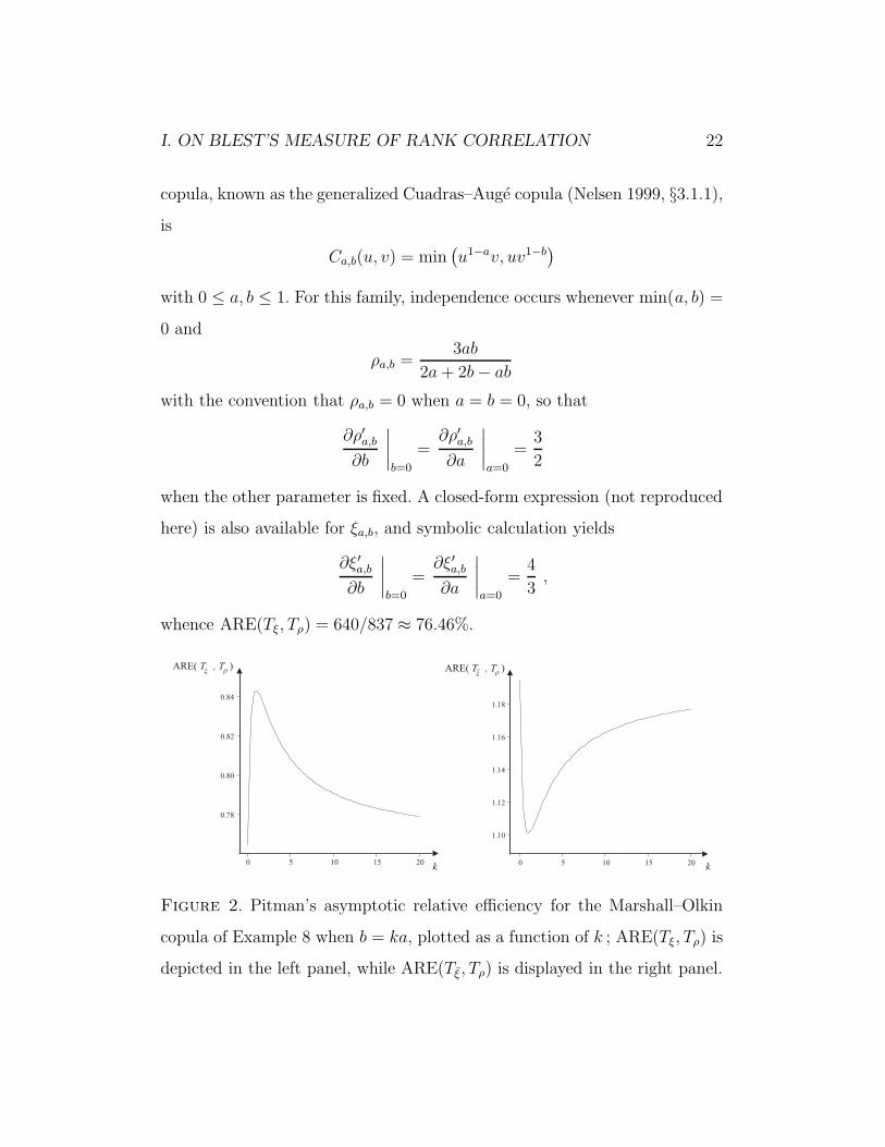
whence ARE(Tξ, Tρ) = 640/837 ≈ 76.46%.
Figure 2. Pitman’s asymptotic relative efficiency for the Marshall–Olkin
copula of Example 8 when b = ka, plotted as a function of k ; ARE(Tξ, Tρ) is
depicted in the left panel, while ARE(Tξ, Tρ) is displayed in the right panel.
I. ON BLEST’S MEASURE OF RANK CORRELATION 23
As an additional example, consider the one-parameter family obtained by
setting b = ka for some fixed 0 < k < 1/a. Then ρ′0 = 3k/(2k + 2) and
ξ′0 =k(8 + 19k + 8k2)
(2 + 3k)(3 + 2k)(1 + k),
so that Pitman’s ARE is a function of the constant k that is plotted in the
left panel of Figure 2. The ARE is seen to reach its minimum value of 640/837
when k → 0 or ∞. Its maximum, viz., 392/465 ≈ 84.30%, occurs when k = 1,
which corresponds to the standard copula of Cuadras & Auge (1981).
Examples 5 to 8 show that a test of independence based on the symme-
trized version of Blest’s coefficient is sometimes preferable, but not always,
to Spearman’s test. Interestingly, however, it is generally possible to outper-
form the test based on ρn (or τn, since the latter two are usually equivalent
asymptotically) by using either the test involving ξn or a similar procedure
founded on the complementary statistic
ξn = −4n + 5
n − 1+
6
n3 − n
n∑i=1
RiSi
(4 − Ri + Si
n + 1
)
= −2n + 1
n − 1+
6
n3 − n
n∑i=1
RiSi
(Ri + Si
n + 1
)
defined as in (8), but with Ri = (n + 1) − Ri and Si = (n + 1) − Si instead
of Ri and Si, respectively.
Since using the reverse ranks amounts to working with the transformed data
(−X1,−Y1), . . ., (−Xn,−Yn), and in view of the discussion surrounding equa-
I. ON BLEST’S MEASURE OF RANK CORRELATION 24
tion (5), it is plain that ξn is an asymptotically unbiased estimator of
ξ(X, Y ) = ξ(−X,−Y ) = 2ρ(X, Y ) − ξ(X, Y ). (10)
Calling on Proposition 2, one can also check readily that the limiting distri-
bution of ξn is actually the same as that which ξn would have if the underlying
dependence function were what Nelsen (1999, p. 28) calls the survival copula,
i.e., C(u, v) = u + v− 1+C(1−u, 1− v). Furthermore, var(ξn) = var(ξn) for
any sample size n ≥ 1 under the null hypothesis of independence.
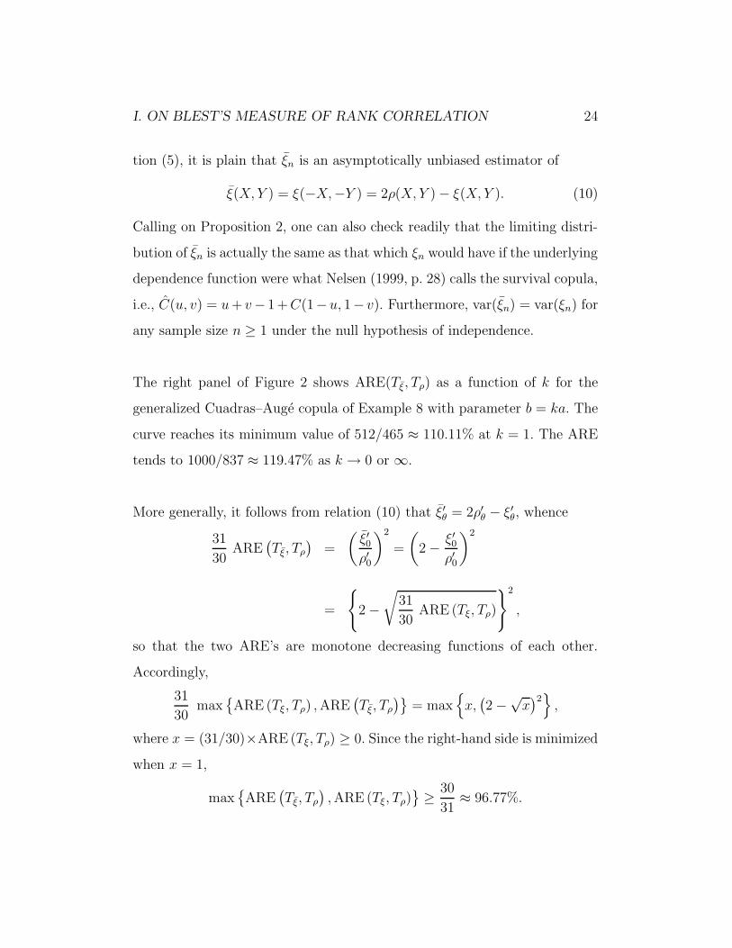
The right panel of Figure 2 shows ARE(Tξ, Tρ) as a function of k for the
generalized Cuadras–Auge copula of Example 8 with parameter b = ka. The
curve reaches its minimum value of 512/465 ≈ 110.11% at k = 1. The ARE
tends to 1000/837 ≈ 119.47% as k → 0 or ∞.
More generally, it follows from relation (10) that ξ′θ = 2ρ′θ − ξ′θ, whence
31
30ARE
(Tξ, Tρ
)=
(ξ′0ρ′
0
)2
=
(2 − ξ′0
ρ′0
)2
=
{2 −
√31
30ARE (Tξ, Tρ)
}2
,
so that the two ARE’s are monotone decreasing functions of each other.
Accordingly,
31
30max
{ARE (Tξ, Tρ) , ARE
(Tξ, Tρ
)}= max
{x,(2 −√
x)2}
,
where x = (31/30)×ARE(Tξ, Tρ) ≥ 0. Since the right-hand side is minimized
when x = 1,
max{ARE
(Tξ, Tρ
), ARE (Tξ, Tρ)
} ≥ 30
31≈ 96.77%.
I. ON BLEST’S MEASURE OF RANK CORRELATION 25
Moreover, at least one of Tξ or Tξ provides an improvement over Spearman’s
test unless
√x =
ξ′0ρ′
0
∈(
2 −√
31
30,
√31
30
)≈ (0.9834, 1.0165).
From the above examples and the authors’ experience with other copula
models, it would appear that for “smooth” families of distributions, the lar-
gest possible asymptotic relative efficiency attainable with either Tξ or Tξ is
1000/837, i.e., when√
x = 9/10 or 10/9, as in Examples 5, 6 and 8. The
exact conditions under which this occurs remain to be determined, however.
1.5.2 Power Comparisons in Finite Samples
To examine the performance of tests of independence based on ξn and ξn,
Monte Carlo simulations were carried out for various sample sizes and fami-
lies of copulas spanning all possible degrees of association between stochastic
independence (ρ = 0) and complete positive dependence (ρ = 1), whose un-
derlying copula is the Frechet upper bound M(u, v) = min(u, v).
Results reported herein are for pseudo-random samples of size n = 25 and
100 for the normal (which is archetypical of radially symmetric copulas),
the Clayton (Example 5), and the bivariate extreme value distributions of
Gumbel (1960b) and Galambos (1975). The latter two have copulas of the
form
Cθ(u, v) = exp
[log(uv)A
{log(u)
log(uv)
}]with
A(t) ={tθ + (1 − t)θ
}1/θ, θ ≥ 1
I. ON BLEST’S MEASURE OF RANK CORRELATION 26
for Gumbel’s model and
A(t) = 1 − {t−θ + (1 − t)−θ}−1/θ
, θ ≥ 0
for Galambos’ model ; see for example Ghoudi, Khoudraji & Rivest (1998).
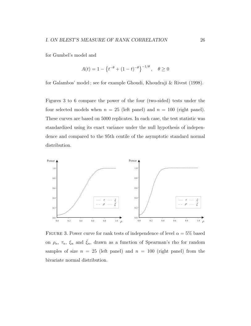
Figures 3 to 6 compare the power of the four (two-sided) tests under the
four selected models when n = 25 (left panel) and n = 100 (right panel).
These curves are based on 5000 replicates. In each case, the test statistic was
standardized using its exact variance under the null hypothesis of indepen-
dence and compared to the 95th centile of the asymptotic standard normal
distribution.
Figure 3. Power curve for rank tests of independence of level α = 5% based
on ρn, τn, ξn and ξn, drawn as a function of Spearman’s rho for random
samples of size n = 25 (left panel) and n = 100 (right panel) from the
bivariate normal distribution.
I. ON BLEST’S MEASURE OF RANK CORRELATION 27
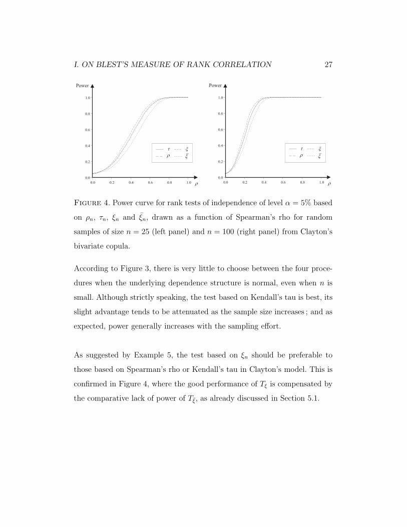
Figure 4. Power curve for rank tests of independence of level α = 5% based
on ρn, τn, ξn and ξn, drawn as a function of Spearman’s rho for random
samples of size n = 25 (left panel) and n = 100 (right panel) from Clayton’s
bivariate copula.
According to Figure 3, there is very little to choose between the four proce-
dures when the underlying dependence structure is normal, even when n is
small. Although strictly speaking, the test based on Kendall’s tau is best, its
slight advantage tends to be attenuated as the sample size increases ; and as
expected, power generally increases with the sampling effort.
As suggested by Example 5, the test based on ξn should be preferable to
those based on Spearman’s rho or Kendall’s tau in Clayton’s model. This is
confirmed in Figure 4, where the good performance of Tξ is compensated by
the comparative lack of power of Tξ, as already discussed in Section 5.1.
I. ON BLEST’S MEASURE OF RANK CORRELATION 28
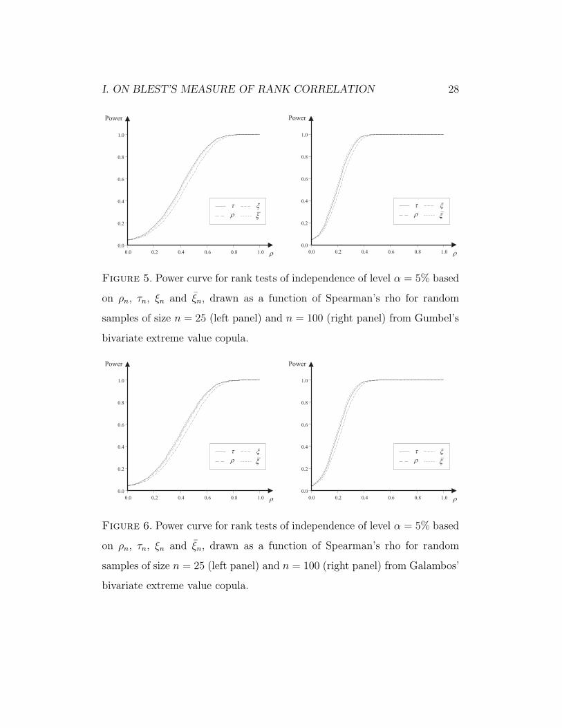
Figure 5. Power curve for rank tests of independence of level α = 5% based
on ρn, τn, ξn and ξn, drawn as a function of Spearman’s rho for random
samples of size n = 25 (left panel) and n = 100 (right panel) from Gumbel’s
bivariate extreme value copula.
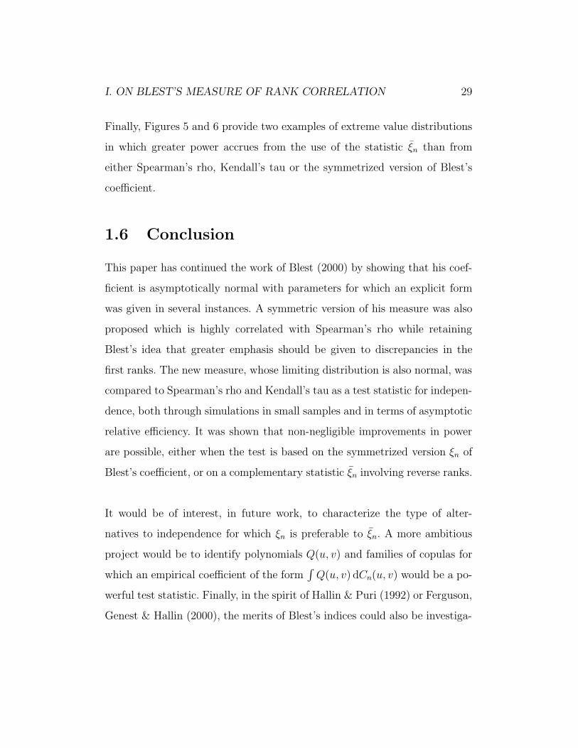
Figure 6. Power curve for rank tests of independence of level α = 5% based
on ρn, τn, ξn and ξn, drawn as a function of Spearman’s rho for random
samples of size n = 25 (left panel) and n = 100 (right panel) from Galambos’
bivariate extreme value copula.
I. ON BLEST’S MEASURE OF RANK CORRELATION 29
Finally, Figures 5 and 6 provide two examples of extreme value distributions
in which greater power accrues from the use of the statistic ξn than from
either Spearman’s rho, Kendall’s tau or the symmetrized version of Blest’s
coefficient.
1.6 Conclusion
This paper has continued the work of Blest (2000) by showing that his coef-
ficient is asymptotically normal with parameters for which an explicit form
was given in several instances. A symmetric version of his measure was also
proposed which is highly correlated with Spearman’s rho while retaining
Blest’s idea that greater emphasis should be given to discrepancies in the
first ranks. The new measure, whose limiting distribution is also normal, was
compared to Spearman’s rho and Kendall’s tau as a test statistic for indepen-
dence, both through simulations in small samples and in terms of asymptotic
relative efficiency. It was shown that non-negligible improvements in power
are possible, either when the test is based on the symmetrized version ξn of
Blest’s coefficient, or on a complementary statistic ξn involving reverse ranks.
It would be of interest, in future work, to characterize the type of alter-
natives to independence for which ξn is preferable to ξn. A more ambitious
project would be to identify polynomials Q(u, v) and families of copulas for
which an empirical coefficient of the form∫
Q(u, v) dCn(u, v) would be a po-
werful test statistic. Finally, in the spirit of Hallin & Puri (1992) or Ferguson,
Genest & Hallin (2000), the merits of Blest’s indices could also be investiga-
I. ON BLEST’S MEASURE OF RANK CORRELATION 30
ted as a measure of serial dependence or as a test of randomness in a time
series context.
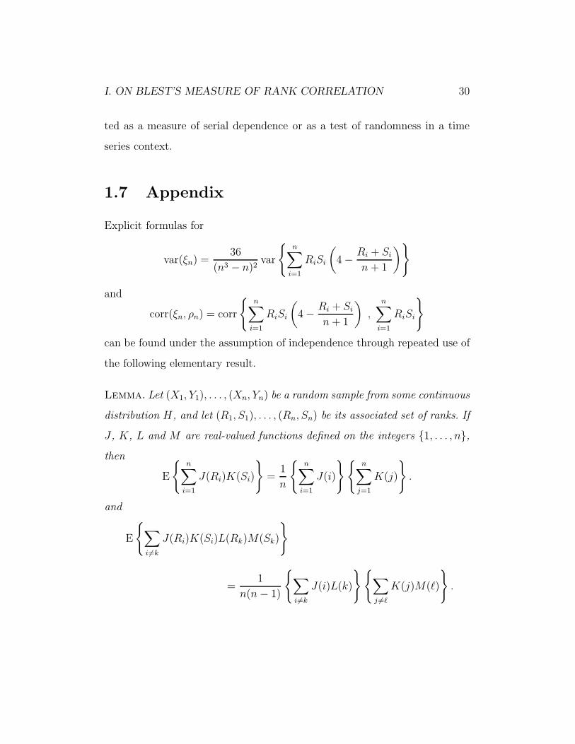
1.7 Appendix
Explicit formulas for
var(ξn) =36
(n3 − n)2var
{n∑
i=1
RiSi
(4 − Ri + Si
n + 1
)}
and
corr(ξn, ρn) = corr
{n∑
i=1
RiSi
(4 − Ri + Si
n + 1
),
n∑i=1
RiSi
}
can be found under the assumption of independence through repeated use of
the following elementary result.
Lemma. Let (X1, Y1), . . . , (Xn, Yn) be a random sample from some continuous
distribution H, and let (R1, S1), . . . , (Rn, Sn) be its associated set of ranks. If
J , K, L and M are real-valued functions defined on the integers {1, . . . , n},then
E
{n∑
i=1
J(Ri)K(Si)
}=
1
n
{n∑
i=1
J(i)
}{n∑
j=1
K(j)
}.
and
E
{∑i6=k
J(Ri)K(Si)L(Rk)M(Sk)
}
=1
n(n − 1)
{∑i6=k
J(i)L(k)
}{∑j 6=`
K(j)M(`)
}.
I. ON BLEST’S MEASURE OF RANK CORRELATION 31
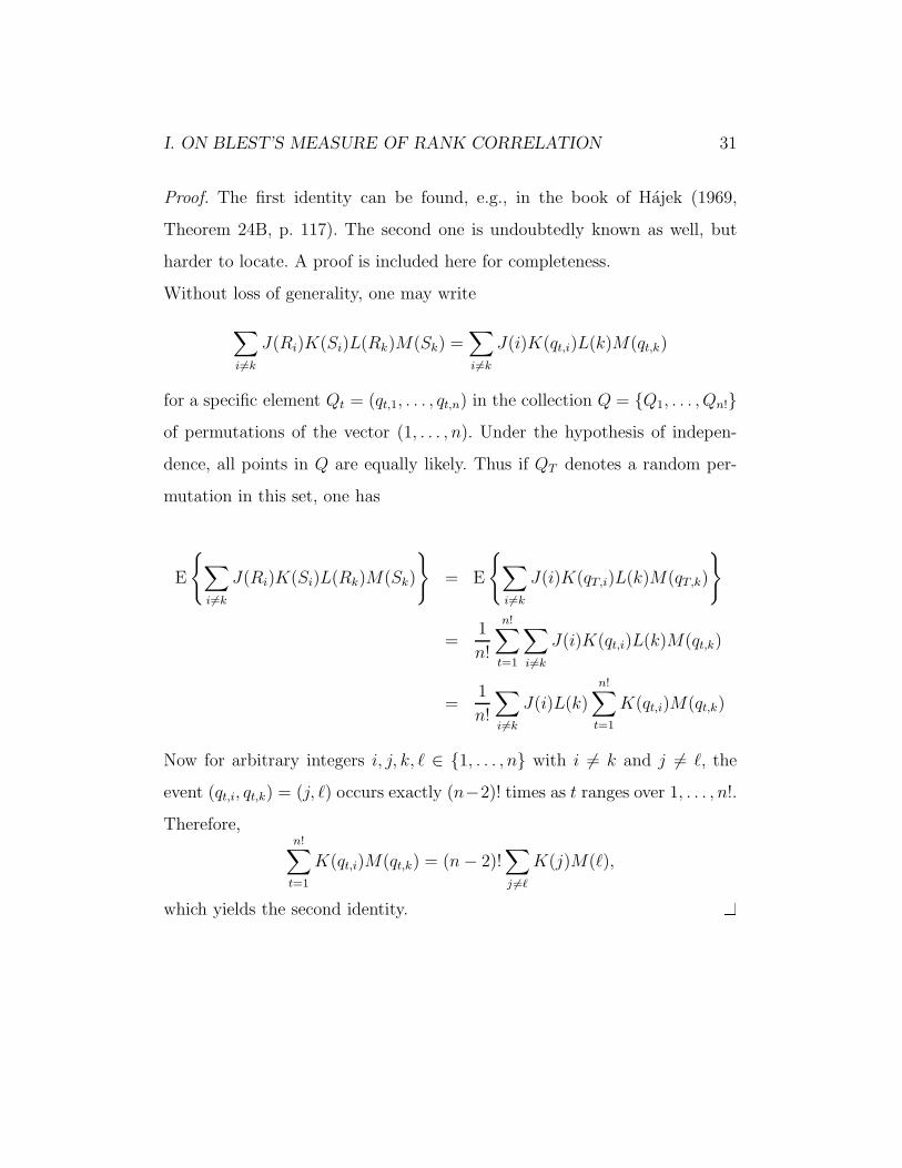
Proof. The first identity can be found, e.g., in the book of Hajek (1969,
Theorem 24B, p. 117). The second one is undoubtedly known as well, but
harder to locate. A proof is included here for completeness.
Without loss of generality, one may write
∑i6=k
J(Ri)K(Si)L(Rk)M(Sk) =∑i6=k
J(i)K(qt,i)L(k)M(qt,k)
for a specific element Qt = (qt,1, . . . , qt,n) in the collection Q = {Q1, . . . , Qn!}of permutations of the vector (1, . . . , n). Under the hypothesis of indepen-
dence, all points in Q are equally likely. Thus if QT denotes a random per-
mutation in this set, one has
E
{∑i6=k
J(Ri)K(Si)L(Rk)M(Sk)
}= E
{∑i6=k
J(i)K(qT,i)L(k)M(qT,k)
}
=1
n!
n!∑t=1
∑i6=k
J(i)K(qt,i)L(k)M(qt,k)
=1
n!
∑i6=k
J(i)L(k)
n!∑t=1
K(qt,i)M(qt,k)
Now for arbitrary integers i, j, k, ` ∈ {1, . . . , n} with i 6= k and j 6= `, the
event (qt,i, qt,k) = (j, `) occurs exactly (n−2)! times as t ranges over 1, . . . , n!.
Therefore,n!∑
t=1
K(qt,i)M(qt,k) = (n − 2)!∑j 6=`
K(j)M(`),
which yields the second identity. �
I. ON BLEST’S MEASURE OF RANK CORRELATION 32
As an example of application,
E
{n∑
i=1
RiSi
(4 − Ri + Si
n + 1
)}= 4 E
(n∑
i=1
RiSi
)− 2
n + 1E
(n∑
i=1
R2i Si
)
=4
n
(n∑
i=1
i
)2
− 2
n3 − n
(n∑
i=1
i
)(n∑
i=1
i2
)
=n(n + 1)(4n + 5)
6,
from which it follows that E(ξn) = 0 under the assumption of independence.
All other computations are similar and are easily performed with a symbolic
calculator such as Maple.
CHAPITRE II
MESURES DE CORRELATION BASEES
SUR LES RANGS
L’objectif ambitieux de ce chapitre consiste a partager avec le lecteur l’in-
tuition et les raisonnements qui sous-tendent les resultats presentes au cha-
pitre I.
2.1 Terminologie
Au chapitre I, les axiomes de Scarsini offrent une liste de proprietes que de-
vrait idealement posseder toute mesure de concordance. Il est clair qu’une
statistique ne repondant pas au moins aux axiomes a, b et d de Scarsini ne
saurait etre consideree comme “mesure de correlation.” Les seules mesures
considerees dans la suite sont celles basees sur les rangs.
2.2 Formes des coefficients
Dans le chapitre precedent, les mesures de correlation utilisees (a l’exception
de τ) sont toutes de la forme
κn = an
n∑i=1
p
(Ri
n + 1,
Si
n + 1
)+ bn,
II. MESURES DE CORRELATION BASEES SUR LES RANGS 34
ou p(u, v) est un polynome et an, bn sont des constantes choisies de telle
sorte que κn ∈ [−1, 1]. Dans tous les cas, les valeurs ±1 ne sont prises
que si les rangs Ri et Si sont les memes ou sont antithetiques (c’est-a-dire
Si = n + 1 − Ri, pour 1 ≤ i ≤ n).
Les quatre remarques suivantes presentent des simplifications qui permettent
de se concentrer sur ce qui constitue vraiment un coefficient de correlation
des rangs.
2.2.1 Elimination des marges
Comme les rangs sont invariants sous toute transformation monotone crois-
sante des marges, ils ne dependent pas des lois marginales des observations.
Ainsi, sans perte de generalite, on peut se limiter a considerer des lois dont
les marges sont uniformes, a savoir des copules !
2.2.2 Parametre estime et loi asymptotique
David C. Blest a defini un coefficient de correlation echantillonnal sans tou-
tefois preciser sa valeur dans la population. En general, il est possible de
determiner quel parametre estime un coefficient κn base sur les rangs grace a
une generalisation d’un resultat de Ruymgaart, Shorack & van Zwet (1972)
proposee par Genest, Ghoudi & Rivest (1995). On obtient en boni la loi
asymptotique de κn.
Puisque le polynome p(u, v) est une fonction continue definie sur le com-
pact [0, 1]2, les conditions de regularite de leur proposition A·1 sont toujours
II. MESURES DE CORRELATION BASEES SUR LES RANGS 35
respectees. Ainsi,√
n(κn − κ)loi→ N(0, σ2)
avec
κ = a E{p(U, V )} + b = a
∫p(u, v) dC(u, v) + b
et
σ2 = a2 var
[p(U, V ) +
∫11(U ≤ u)
∂
∂up(u, v) du
+
∫11(V ≤ v)
∂
∂vp(u, v) dv
],
ou a = limn→∞ nan et b = limn→∞ bn. Bref, peu importe le polynome p(u, v)
utilise, κn estime κ = a E{p(U, V )} + b sans biais.
2.2.3 Degre des polynomes consideres
Tous les termes ne contenant pas d’interaction (c’est-a-dire les monomes uk et
vk pour k = 0, 1, . . .) constituent en fait des constantes pouvant etre incluses
dans bn lorsque sommes ou integres. Par exemple, p(u, v) = (1 − u)2v et
p(u, v) = u2v − 2uv conduisent tous deux a la mesure de Blest.
2.2.4 Role des constantes
Comme les constantes an et bn sont choisies pour que κn ∈ [−1, 1], les mul-
tiples d’un polynome menent au meme coefficient de correlation. Par exemple,
p(u, v) = uv − u2v/2 conduit aussi a la mesure de Blest.
II. MESURES DE CORRELATION BASEES SUR LES RANGS 36
En laissant de cote les constantes et les symboles de sommation, on ecrit
dans la suite
κn ∼ p(U, V ) ou κ ∼ p(U, V )
pour signifier que κ est la mesure de correlation basee sur p(u, v), c’est-a-dire
que
κn = an
n∑i=1
p
(Ri
n + 1,
Si
n + 1
)+ bn
et
κ = a
∫p(u, v) dC + b .
Cette notation plus sobre permet de mieux comprendre la nature des coeffi-
cients envisages.
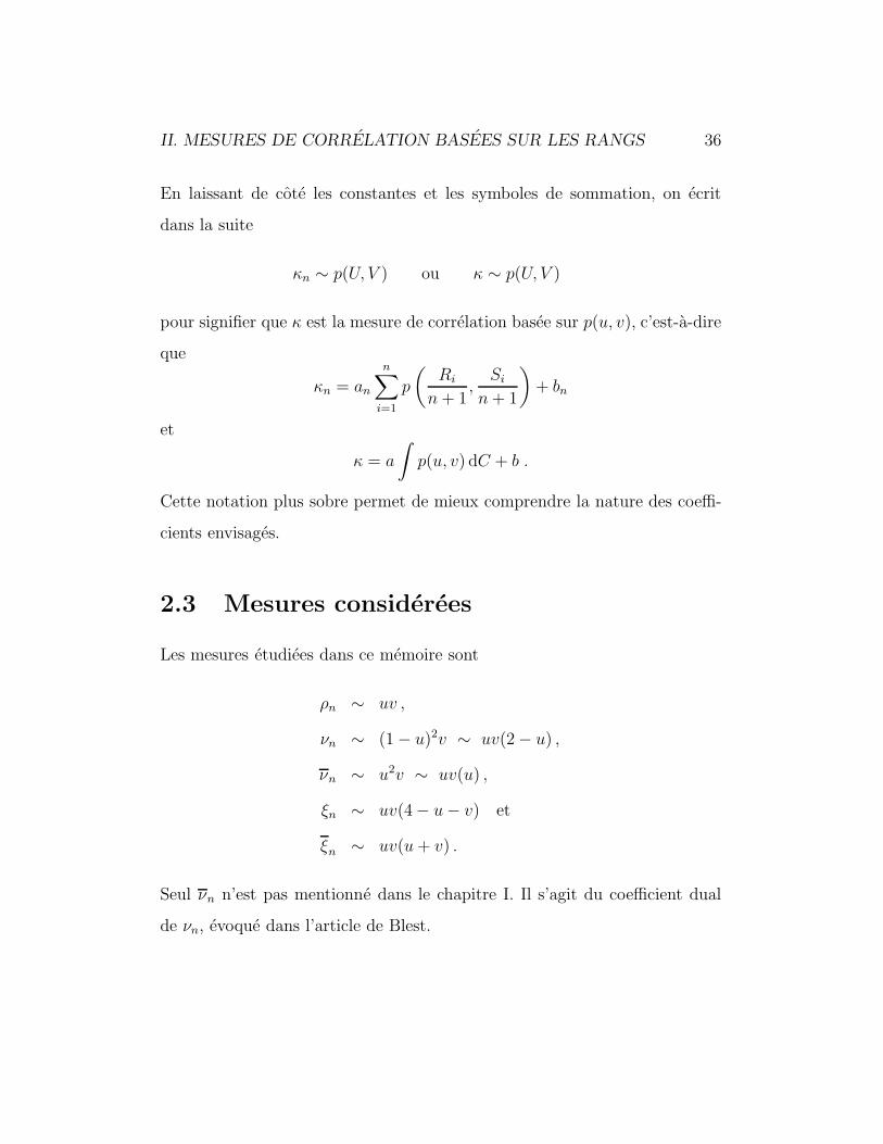
2.3 Mesures considerees
Les mesures etudiees dans ce memoire sont
ρn ∼ uv ,
νn ∼ (1 − u)2v ∼ uv(2 − u) ,
νn ∼ u2v ∼ uv(u) ,
ξn ∼ uv(4 − u − v) et
ξn ∼ uv(u + v) .
Seul νn n’est pas mentionne dans le chapitre I. Il s’agit du coefficient dual
de νn, evoque dans l’article de Blest.
II. MESURES DE CORRELATION BASEES SUR LES RANGS 37
L’ecriture depouillee des sommes et des constantes donne une meilleure vision
de la nature des coefficients. Ainsi, ρn peut etre interprete comme une simple
mesure d’interaction, alors que νn, νn, ξn et ξn sont des versions ponderees de
cette meme interaction. Il est a noter que contrairement a νn et ξn, νn et ξn
accordent plus d’importance aux ecarts observes dans les derniers rangs que
dans les premiers. De telles mesures pourraient s’averer utiles pour comparer
deux jeux de donnees dans lesquels des inversions constatees dans les grandes
valeurs importent beaucoup ; pensons par exemple aux notes accordees par
deux juges lors d’une epreuve de patinage artistique.
Tel que mentionne precedemment, les termes n’impliquant qu’une seule va-
riable peuvent etre relegues aux constantes. Ainsi, il est toujours possible de
mettre uv en evidence et d’ecrire
κn ∼ uv q(u, v)
pour un certain polynome q(u, v) qui pondere l’interaction. Malheureuse-
ment, tous les polynomes q(u, v) ne conduisent pas a des mesures de correla-
tion acceptables. Une interpretation geometrique du comportement des coef-
ficients liee a la forme de q(u, v) permettrait d’appuyer l’intuition et aiderait
sans doute a cerner les polynomes acceptables, mais aucun progres significatif
n’a ete realise en ce sens dans le cadre de ce memoire.
II. MESURES DE CORRELATION BASEES SUR LES RANGS 38
2.4 Resume des proprietes
2.4.1 Dualite et symetrie radiale
Si une copule est radialement symetrique, les couples (U, V ) et (1 − U, 1 −V ) sont de meme loi. Cette propriete se traduit par le fait que (Ri, Si) et
(Ri, Si) = (n + 1 − Ri, n + 1 − Si) ont la meme distribution.
Soit κn une mesure de correlation basee sur les rangs et κn le meme coef-
ficient calcule au moyen des rangs inverses (Ri, Si). On appelle κn le dual de
κn. Les deux indices ont la meme loi (puisqu’il s’agit de la meme fonction
calculee sur des variables aleatoires de meme loi). Ainsi, on aura toujours
var(κn) = var(κn)
et
κ = E(κn) = E(κn) = κ .
Comme les coefficients νn et ξn sont les duaux de νn et ξn, les proprietes ci-
haut continuent de valoir. En particulier, comme la copule d’independance
est radialement symetrique, on a
var(νn) = var(νn) , var(ξn) = var(ξn)
et
ν = ν = ξ = ξ
sous l’hypothese d’independance.
II. MESURES DE CORRELATION BASEES SUR LES RANGS 39
2.4.2 Dualite et test d’independance
Soit
γn =κn + κn
2.
Sous l’hypothese d’independance, γ = κ = κ. Par le meme argument que
celui utilise au chapitre I, on a alors :
max {ARE(Tκ, Tγ), ARE(Tκ, Tγ)} ≥ var(γn)
var(κn)
avec egalite si la copule est radialement symetrique car alors, κ′0 = γ′
0.
Dans le cas de νn et de ξn, (νn + νn) /2 =(ξn + ξn
)/2 = ρn. Par consequent,
la borne obtenue compare les coefficients au ρ de Spearman, ce qui la rend
beaucoup plus interessante.
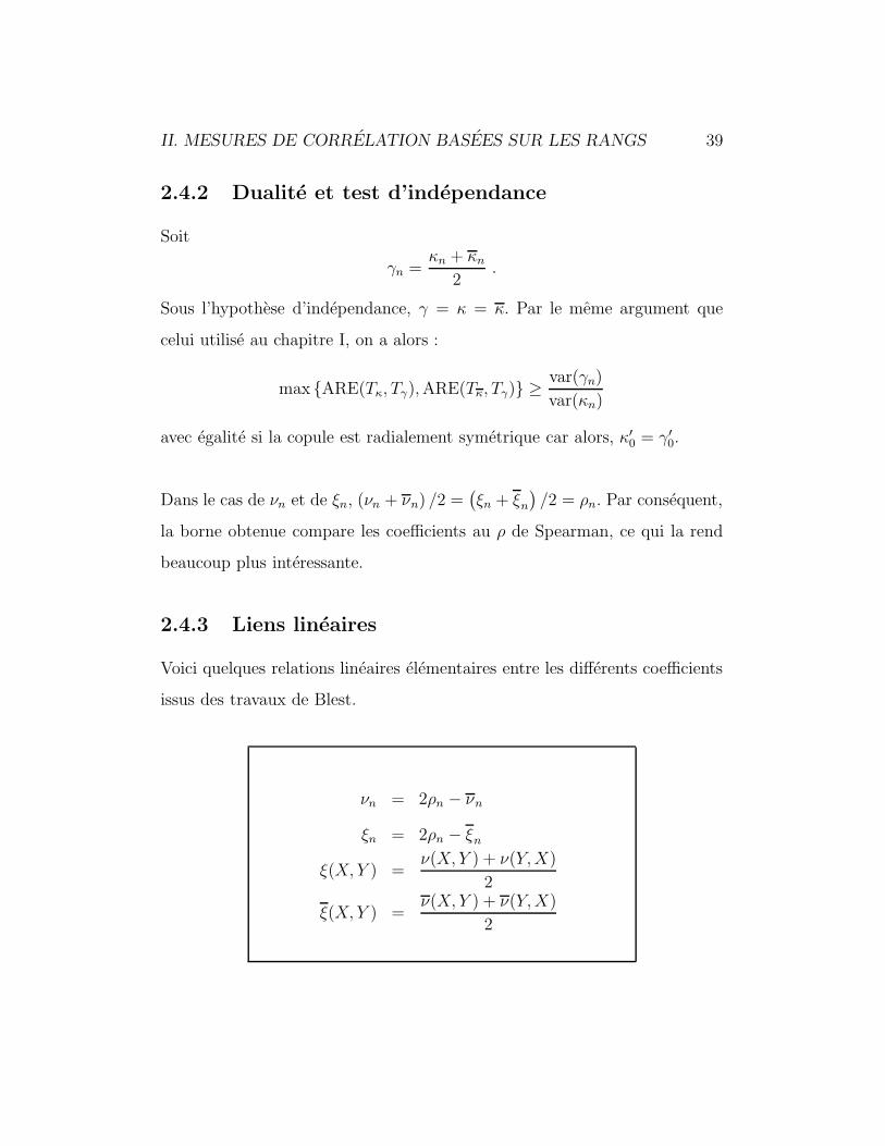
2.4.3 Liens lineaires
Voici quelques relations lineaires elementaires entre les differents coefficients
issus des travaux de Blest.
νn = 2ρn − νn
ξn = 2ρn − ξn
ξ(X, Y ) =ν(X, Y ) + ν(Y, X)
2
ξ(X, Y ) =ν(X, Y ) + ν(Y, X)
2
II. MESURES DE CORRELATION BASEES SUR LES RANGS 40
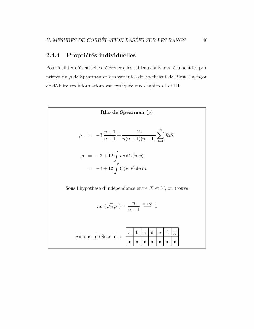
2.4.4 Proprietes individuelles
Pour faciliter d’eventuelles references, les tableaux suivants resument les pro-
prietes du ρ de Spearman et des variantes du coefficient de Blest. La facon
de deduire ces informations est expliquee aux chapitres I et III.
Rho de Spearman (ρ)
ρn = −3n + 1
n − 1+
12
n(n + 1)(n − 1)
n∑i=1
RiSi
ρ = −3 + 12
∫uv dC(u, v)
= −3 + 12
∫C(u, v) du dv
Sous l’hypothese d’independance entre X et Y , on trouve
var(√
n ρn
)=
n
n − 1
n→∞−→ 1
Axiomes de Scarsini :a b c d e f g
• • • • • • •
II. MESURES DE CORRELATION BASEES SUR LES RANGS 41
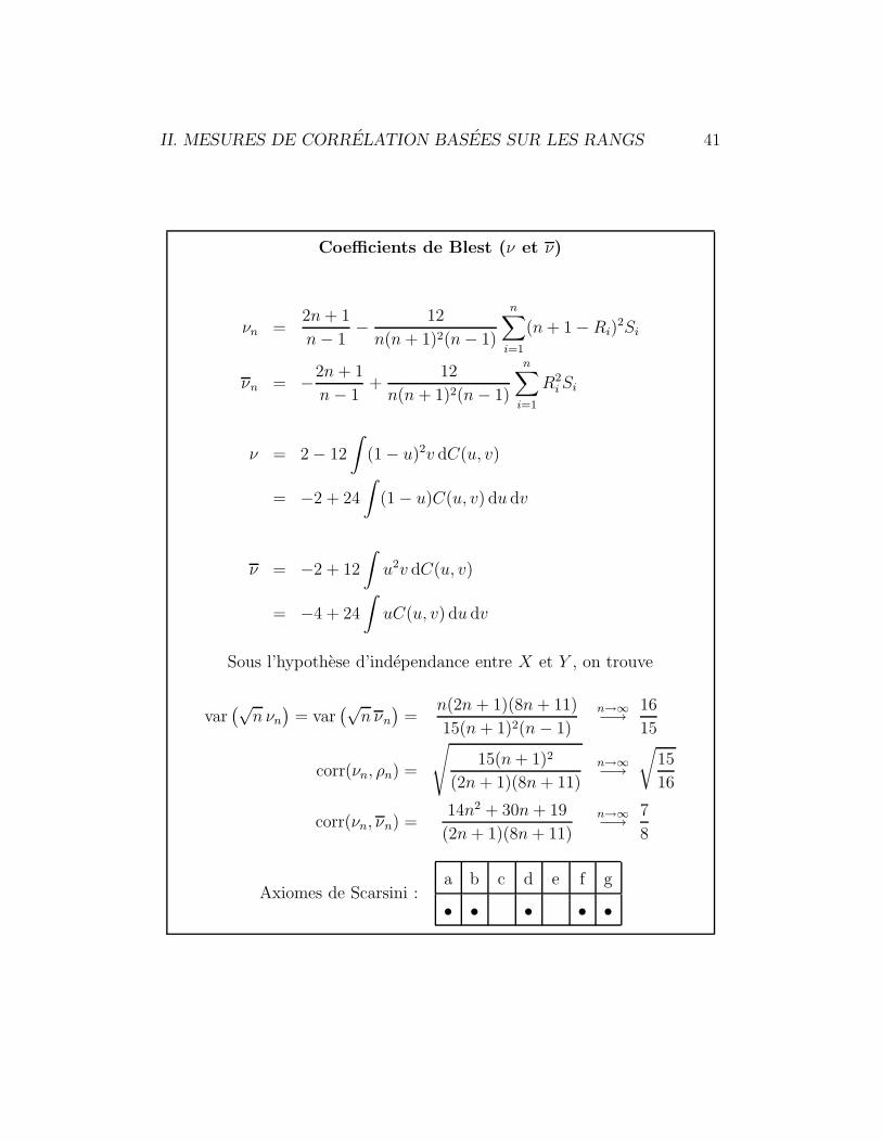
Coefficients de Blest (ν et ν)
νn =2n + 1
n − 1− 12
n(n + 1)2(n − 1)
n∑i=1
(n + 1 − Ri)2Si
νn = −2n + 1
n − 1+
12
n(n + 1)2(n − 1)
n∑i=1
R2i Si
ν = 2 − 12
∫(1 − u)2v dC(u, v)
= −2 + 24
∫(1 − u)C(u, v) du dv
ν = −2 + 12
∫u2v dC(u, v)
= −4 + 24
∫uC(u, v) du dv
Sous l’hypothese d’independance entre X et Y , on trouve
var(√
n νn
)= var
(√n νn
)=
n(2n + 1)(8n + 11)
15(n + 1)2(n − 1)
n→∞−→ 16
15
corr(νn, ρn) =
√15(n + 1)2
(2n + 1)(8n + 11)
n→∞−→√
15
16
corr(νn, νn) =14n2 + 30n + 19
(2n + 1)(8n + 11)
n→∞−→ 7
8
Axiomes de Scarsini :a b c d e f g
• • • • •
II. MESURES DE CORRELATION BASEES SUR LES RANGS 42
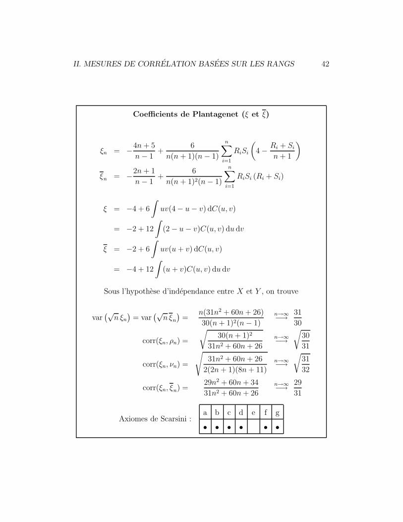
Coefficients de Plantagenet (ξ et ξ)
ξn = −4n + 5
n − 1+
6
n(n + 1)(n − 1)
n∑i=1
RiSi
(4 − Ri + Si
n + 1
)
ξn = −2n + 1
n − 1+
6
n(n + 1)2(n − 1)
n∑i=1
RiSi (Ri + Si)
ξ = −4 + 6
∫uv(4 − u − v) dC(u, v)
= −2 + 12
∫(2 − u − v)C(u, v) du dv
ξ = −2 + 6
∫uv(u + v) dC(u, v)
= −4 + 12
∫(u + v)C(u, v) du dv
Sous l’hypothese d’independance entre X et Y , on trouve
var(√
n ξn
)= var
(√n ξn
)=
n(31n2 + 60n + 26)
30(n + 1)2(n − 1)
n→∞−→ 31
30
corr(ξn, ρn) =
√30(n + 1)2
31n2 + 60n + 26
n→∞−→√
30
31
corr(ξn, νn) =
√31n2 + 60n + 26
2(2n + 1)(8n + 11)
n→∞−→√
31
32
corr(ξn, ξn) =29n2 + 60n + 34
31n2 + 60n + 26n→∞−→ 29
31
Axiomes de Scarsini :a b c d e f g
• • • • • •
CHAPITRE III
CALCULS EXPLICITES
Ce chapitre explicite quelques-uns des calculs qui ont conduit aux resultats
des chapitres precedents.
3.1 Variance des coefficients sous l’hypothese
d’independance
Les calculs de cette section exploitent essentiellement le resultat de la sec-
tion 1.7.
3.1.1 Rho de Spearman
Rappelons que
ρn = −3n + 1
n − 1+
12
n(n + 1)(n − 1)
n∑i=1
RiSi
et que
var(ρn) =144
n2(n + 1)2(n − 1)2var
(n∑
i=1
RiSi
).
On doit donc calculer, a l’aide du resultat de la section 1.7 :
E
(n∑
i=1
RiSi
)=
1
n
(n∑
i=1
i
)2
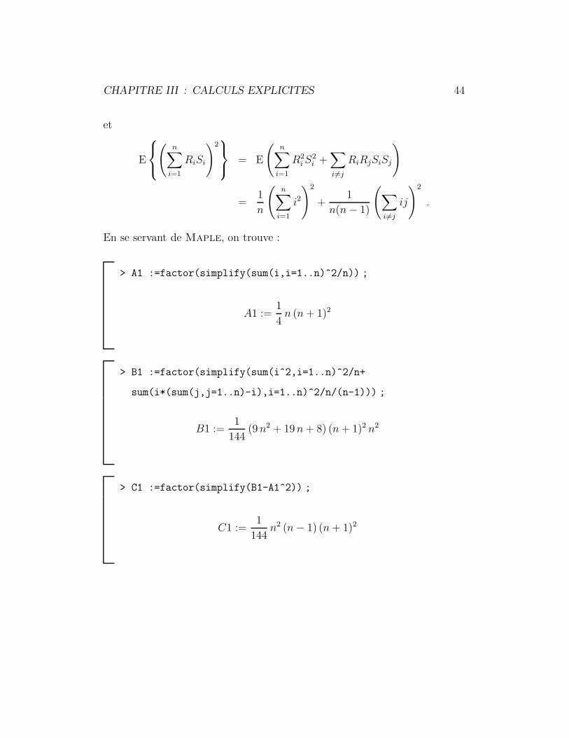
CHAPITRE III : CALCULS EXPLICITES 44
et
E
(
n∑i=1
RiSi
)2 = E
(n∑
i=1
R2i S
2i +
∑i6=j
RiRjSiSj
)
=1
n
(n∑
i=1
i2
)2
+1
n(n − 1)
(∑i6=j
ij
)2
.
En se servant de Maple, on trouve :
> A1 :=factor(simplify(sum(i,i=1..n)^2/n)) ;
A1 :=1
4n (n + 1)2
> B1 :=factor(simplify(sum(i^2,i=1..n)^2/n+
sum(i*(sum(j,j=1..n)-i),i=1..n)^2/n/(n-1))) ;
B1 :=1
144(9 n2 + 19 n + 8) (n + 1)2 n2
> C1 :=factor(simplify(B1-A1^2)) ;
C1 :=1
144n2 (n − 1) (n + 1)2
CHAPITRE III : CALCULS EXPLICITES 45
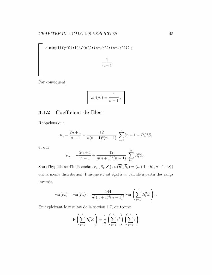
> simplify(C1*144/(n^2*(n-1)^2*(n+1)^2)) ;
1
n − 1
Par consequent,
var(ρn) =1
n − 1.
3.1.2 Coefficient de Blest
Rappelons que
νn =2n + 1
n − 1− 12
n(n + 1)2(n − 1)
n∑i=1
(n + 1 − Ri)2Si
et que
νn = −2n + 1
n − 1+
12
n(n + 1)2(n − 1)
n∑i=1
R2i Si .
Sous l’hypothese d’independance, (Ri, Si) et (Ri, Si) = (n+1−Ri, n+1−Si)
ont la meme distribution. Puisque νn est egal a νn calcule a partir des rangs
inverses,
var(νn) = var(νn) =144
n2(n + 1)4(n − 1)2var
(n∑
i=1
R2i Si
).
En exploitant le resultat de la section 1.7, on trouve
E
(n∑
i=1
R2i Si
)=
1
n
(n∑
i=1
i2
)(n∑
i=1
i
)
CHAPITRE III : CALCULS EXPLICITES 46
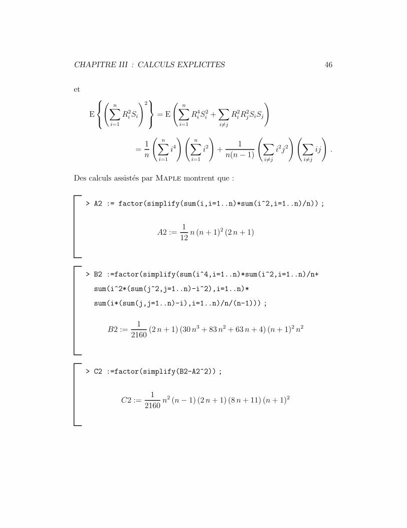
et
E
(
n∑i=1
R2i Si
)2 = E
(n∑
i=1
R4i S
2i +
∑i6=j
R2i R
2jSiSj
)
=1
n
(n∑
i=1
i4
)(n∑
i=1
i2
)+
1
n(n − 1)
(∑i6=j
i2j2
)(∑i6=j
ij
).
Des calculs assistes par Maple montrent que :
> A2 := factor(simplify(sum(i,i=1..n)*sum(i^2,i=1..n)/n)) ;
A2 :=1
12n (n + 1)2 (2 n + 1)
> B2 :=factor(simplify(sum(i^4,i=1..n)*sum(i^2,i=1..n)/n+
sum(i^2*(sum(j^2,j=1..n)-i^2),i=1..n)*
sum(i*(sum(j,j=1..n)-i),i=1..n)/n/(n-1))) ;
B2 :=1
2160(2 n + 1) (30 n3 + 83 n2 + 63 n + 4) (n + 1)2 n2
> C2 :=factor(simplify(B2-A2^2)) ;
C2 :=1
2160n2 (n − 1) (2 n + 1) (8 n + 11) (n + 1)2
CHAPITRE III : CALCULS EXPLICITES 47
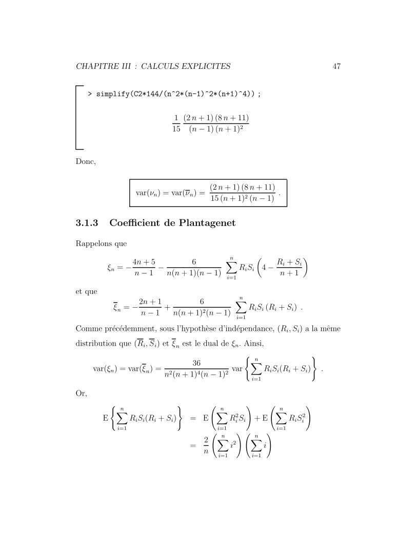
> simplify(C2*144/(n^2*(n-1)^2*(n+1)^4)) ;
1
15
(2 n + 1) (8 n + 11)
(n − 1) (n + 1)2
Donc,
var(νn) = var(νn) =(2 n + 1) (8 n + 11)
15 (n + 1)2 (n − 1).
3.1.3 Coefficient de Plantagenet
Rappelons que
ξn = −4n + 5
n − 1− 6
n(n + 1)(n − 1)
n∑i=1
RiSi
(4 − Ri + Si
n + 1
)
et que
ξn = −2n + 1
n − 1+
6
n(n + 1)2(n − 1)
n∑i=1
RiSi (Ri + Si) .
Comme precedemment, sous l’hypothese d’independance, (Ri, Si) a la meme
distribution que (Ri, Si) et ξn est le dual de ξn. Ainsi,
var(ξn) = var(ξn) =36
n2(n + 1)4(n − 1)2var
{n∑
i=1
RiSi(Ri + Si)
}.
Or,
E
{n∑
i=1
RiSi(Ri + Si)
}= E
(n∑
i=1
R2i Si
)+ E
(n∑
i=1
RiS2i
)
=2
n
(n∑
i=1
i2
)(n∑
i=1
i
)
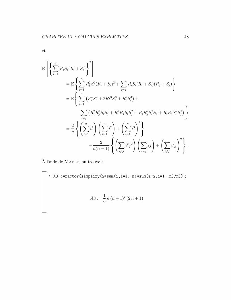
CHAPITRE III : CALCULS EXPLICITES 48
et
E
{ n∑
i=1
RiSi(Ri + Si)
}2
= E
{n∑
i=1
R2i S
2i (Ri + Si)
2 +∑i6=j
RiSi(Ri + Si)(Rj + Sj)
}
= E
{n∑
i=1
(R4
i S2i + 2Ri3S3
i + R2i S
4i
)+
∑i6=j
(R2
i R2jSiSj + R2
i RjSiS2j + RiR
2jS
2i Sj + RiRjS
2i S
2j
)}
=2
n
(
n∑i=1
i4
)(n∑
i=1
i2
)+
(n∑
i=1
i3
)2
+2
n(n − 1)
(∑
i6=j
i2j2
)(∑i6=j
ij
)+
(∑i6=j
i2j
)2 .
A l’aide de Maple, on trouve :
> A3 :=factor(simplify(2*sum(i,i=1..n)*sum(i^2,i=1..n)/n)) ;
A3 :=1
6n (n + 1)2 (2 n + 1)
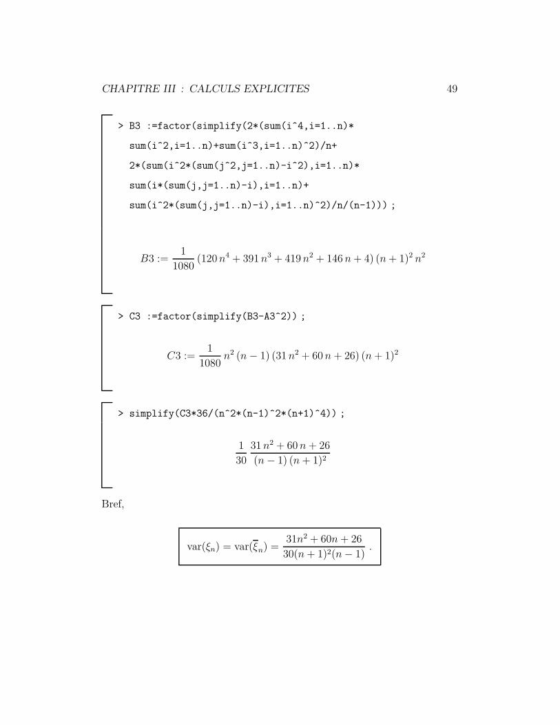
CHAPITRE III : CALCULS EXPLICITES 49
> B3 :=factor(simplify(2*(sum(i^4,i=1..n)*
sum(i^2,i=1..n)+sum(i^3,i=1..n)^2)/n+
2*(sum(i^2*(sum(j^2,j=1..n)-i^2),i=1..n)*
sum(i*(sum(j,j=1..n)-i),i=1..n)+
sum(i^2*(sum(j,j=1..n)-i),i=1..n)^2)/n/(n-1))) ;
B3 :=1
1080(120 n4 + 391 n3 + 419 n2 + 146 n + 4) (n + 1)2 n2
> C3 :=factor(simplify(B3-A3^2)) ;
C3 :=1
1080n2 (n − 1) (31 n2 + 60 n + 26) (n + 1)2
> simplify(C3*36/(n^2*(n-1)^2*(n+1)^4)) ;
1
30
31 n2 + 60 n + 26
(n − 1) (n + 1)2
Bref,
var(ξn) = var(ξn) =31n2 + 60n + 26
30(n + 1)2(n − 1).
CHAPITRE III : CALCULS EXPLICITES 50
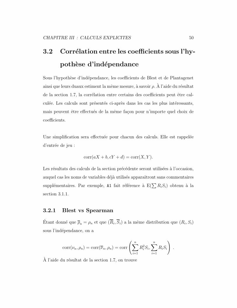
3.2 Correlation entre les coefficients sous l’hy-
pothese d’independance
Sous l’hypothese d’independance, les coefficients de Blest et de Plantagenet
ainsi que leurs duaux estiment la meme mesure, a savoir ρ. A l’aide du resultat
de la section 1.7, la correlation entre certains des coefficients peut etre cal-
culee. Les calculs sont presentes ci-apres dans les cas les plus interessants,
mais peuvent etre effectues de la meme facon pour n’importe quel choix de
coefficients.
Une simplification sera effectuee pour chacun des calculs. Elle est rappelee
d’entree de jeu :
corr(aX + b, cY + d) = corr(X, Y ).
Les resultats des calculs de la section precedente seront utilisees a l’occasion,
auquel cas les noms de variables deja utilises apparaıtront sans commentaires
supplementaires. Par exemple, A1 fait reference a E(∑
RiSi) obtenu a la
section 3.1.1.
3.2.1 Blest vs Spearman
Etant donne que ρn = ρn et que (Ri, Si) a la meme distribution que (Ri, Si)
sous l’independance, on a
corr(νn, ρn) = corr(νn, ρn) = corr
(n∑
i=1
R2i Si,
n∑i=1
RiSi
).
A l’aide du resultat de la section 1.7, on trouve
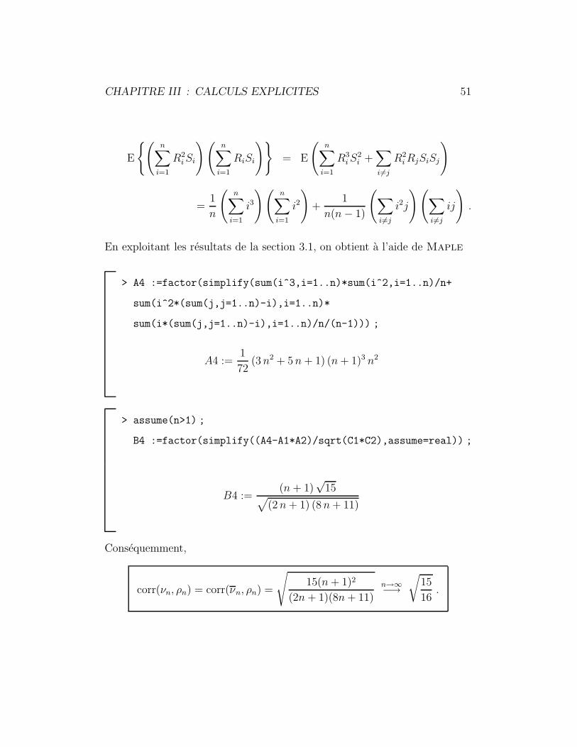
CHAPITRE III : CALCULS EXPLICITES 51
E
{(n∑
i=1
R2i Si
)(n∑
i=1
RiSi
)}= E
(n∑
i=1
R3i S
2i +
∑i6=j
R2i RjSiSj
)
=1
n
(n∑
i=1
i3
)(n∑
i=1
i2
)+
1
n(n − 1)
(∑i6=j
i2j
)(∑i6=j
ij
).
En exploitant les resultats de la section 3.1, on obtient a l’aide de Maple
> A4 :=factor(simplify(sum(i^3,i=1..n)*sum(i^2,i=1..n)/n+
sum(i^2*(sum(j,j=1..n)-i),i=1..n)*
sum(i*(sum(j,j=1..n)-i),i=1..n)/n/(n-1))) ;
A4 :=1
72(3 n2 + 5 n + 1) (n + 1)3 n2
> assume(n>1) ;
B4 :=factor(simplify((A4-A1*A2)/sqrt(C1*C2),assume=real)) ;
B4 :=(n + 1)
√15√
(2 n + 1) (8 n + 11)
Consequemment,
corr(νn, ρn) = corr(νn, ρn) =
√15(n + 1)2
(2n + 1)(8n + 11)
n→∞−→√
15
16.
CHAPITRE III : CALCULS EXPLICITES 52
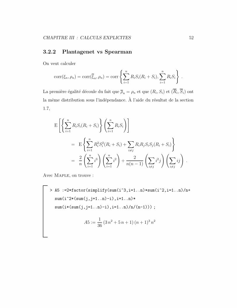
3.2.2 Plantagenet vs Spearman
On veut calculer
corr(ξn, ρn) = corr(ξn, ρn) = corr
{n∑
i=1
RiSi(Ri + Si),n∑
i=1
RiSi
}.
La premiere egalite decoule du fait que ρn = ρn et que (Ri, Si) et (Ri, Si) ont
la meme distribution sous l’independance. A l’aide du resultat de la section
1.7,
E
[{n∑
i=1
RiSi(Ri + Si)
}(n∑
i=1
RiSi
)]
= E
{n∑
i=1
R2i S
2i (Ri + Si) +
∑i6=j
RiRjSiSj(Ri + Si)
}
=2
n
(n∑
i=1
i3
)(n∑
i=1
i2
)+
2
n(n − 1)
(∑i6=j
i2j
)(∑i6=j
ij
).
Avec Maple, on trouve :
> A5 :=2*factor(simplify(sum(i^3,i=1..n)*sum(i^2,i=1..n)/n+
sum(i^2*(sum(j,j=1..n)-i),i=1..n)*
sum(i*(sum(j,j=1..n)-i),i=1..n)/n/(n-1))) ;
A5 :=1
36(3 n2 + 5 n + 1) (n + 1)3 n2
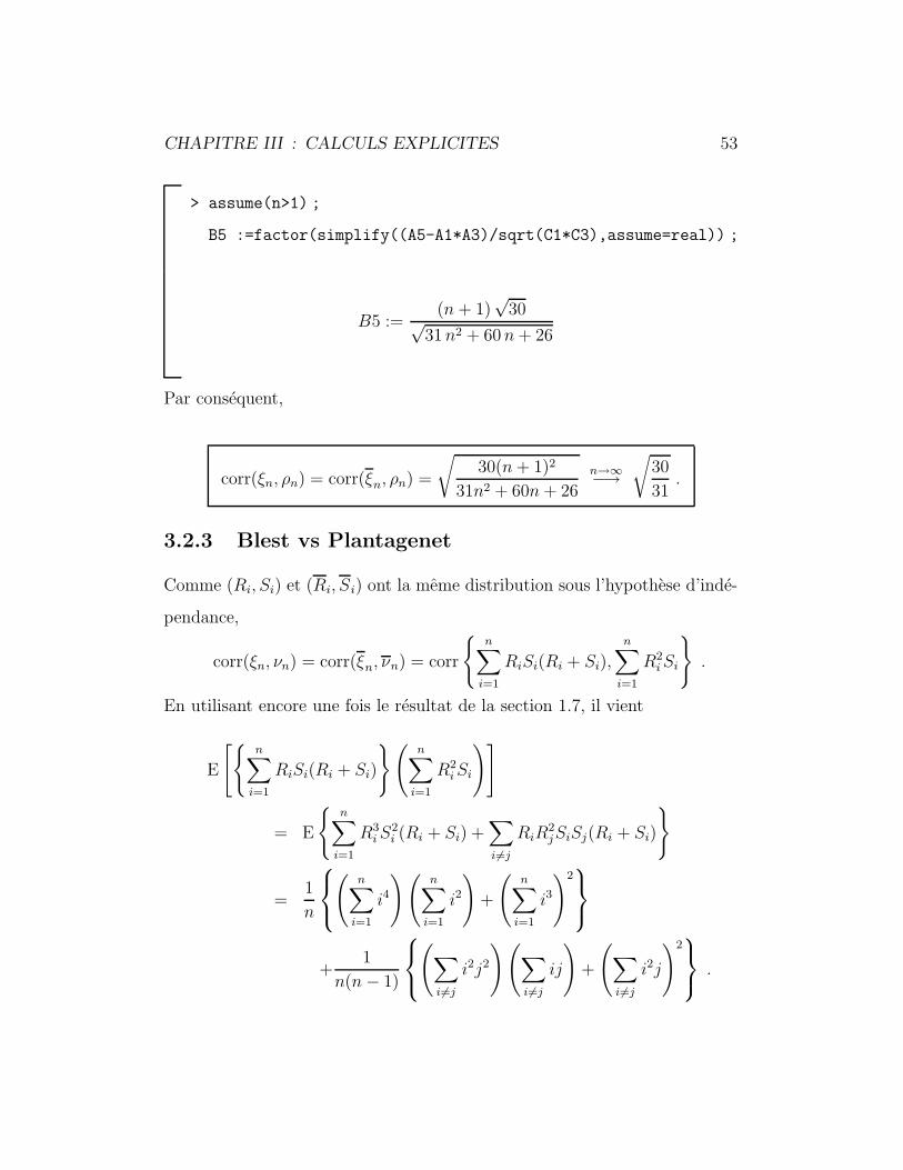
CHAPITRE III : CALCULS EXPLICITES 53
> assume(n>1) ;
B5 :=factor(simplify((A5-A1*A3)/sqrt(C1*C3),assume=real)) ;
B5 :=(n + 1)
√30√
31 n2 + 60 n + 26
Par consequent,
corr(ξn, ρn) = corr(ξn, ρn) =
√30(n + 1)2
31n2 + 60n + 26
n→∞−→√
30
31.
3.2.3 Blest vs Plantagenet
Comme (Ri, Si) et (Ri, Si) ont la meme distribution sous l’hypothese d’inde-
pendance,
corr(ξn, νn) = corr(ξn, νn) = corr
{n∑
i=1
RiSi(Ri + Si),
n∑i=1
R2i Si
}.
En utilisant encore une fois le resultat de la section 1.7, il vient
E
[{n∑
i=1
RiSi(Ri + Si)
}(n∑
i=1
R2i Si
)]
= E
{n∑
i=1
R3i S
2i (Ri + Si) +
∑i6=j
RiR2jSiSj(Ri + Si)
}
=1
n
(
n∑i=1
i4
)(n∑
i=1
i2
)+
(n∑
i=1
i3
)2
+1
n(n − 1)
(∑
i6=j
i2j2
)(∑i6=j
ij
)+
(∑i6=j
i2j
)2 .
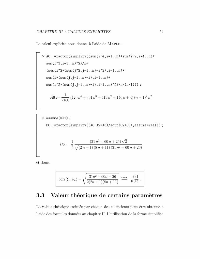
CHAPITRE III : CALCULS EXPLICITES 54
Le calcul explicite nous donne, a l’aide de Maple :
> A6 :=factor(simplify((sum(i^4,i=1..n)*sum(i^2,i=1..n)+
sum(i^3,i=1..n)^2)/n+
(sum(i^2*(sum(j^2,j=1..n)-i^2),i=1..n)*
sum(i*(sum(j,j=1..n)-i),i=1..n)+
sum(i^2*(sum(j,j=1..n)-i),i=1..n)^2)/n/(n-1))) ;
A6 :=1
2160(120 n4 + 391 n3 + 419 n2 + 146 n + 4) (n + 1)2 n2
> assume(n>1) ;
B6 :=factor(simplify((A6-A2*A3)/sqrt(C2*C3),assume=real)) ;
B6 :=1
2
(31 n2 + 60 n + 26)√
2√(2 n + 1) (8 n + 11) (31 n2 + 60 n + 26)
et donc,
corr(ξn, νn) =
√31n2 + 60n + 26
2(2n + 1)(8n + 11)
n→∞−→√
31
32.
3.3 Valeur theorique de certains parametres
La valeur theorique estimee par chacun des coefficients peut etre obtenue a
l’aide des formules donnees au chapitre II. L’utilisation de la forme simplifiee
CHAPITRE III : CALCULS EXPLICITES 55
a l’aide du resultat de Quesada–Molina (1992) evite de deriver la copule, ce
qui simplifie les calculs et permet de traiter sans tracas les copules possedant
une composante singuliere. En fait, il suffit de calculer trois integrales pour
deduire tous les coefficients consideres, a savoir :∫ ∫C(u, v) du dv ,
∫ ∫uC(u, v) du dv et
∫ ∫vC(u, v) du dv .
En effet,
ρ = −3 + 12
∫ ∫C(u, v) du dv ,
ν = −2 + 24
∫ ∫(1 − u)C(u, v) du dv ,
ν = −4 + 24
∫ ∫uC(u, v) du dv ,
ξ = −2 + 12
∫ ∫(2 − u − v)C(u, v) du dv ,
ξ = −4 + 12
∫ ∫(u + v)C(u, v) du dv .
L’utilisation de Maple permet d’eviter de faire manuellement des calculs
simples, mais parfois fastidieux. Etant donne que les commandes sont sem-
blables d’un cas a l’autre, seuls deux exemples sont donnes ici en details.
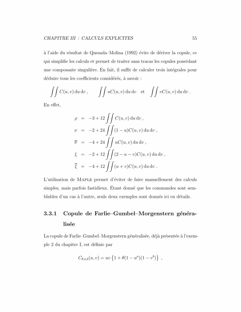
3.3.1 Copule de Farlie–Gumbel–Morgenstern genera-
lisee
La copule de Farlie–Gumbel–Morgenstern generalisee, deja presentee a l’exem-
ple 2 du chapitre I, est definie par
Cθ,a,b(u, v) = uv{1 + θ(1 − ua)(1 − vb)
},
CHAPITRE III : CALCULS EXPLICITES 56
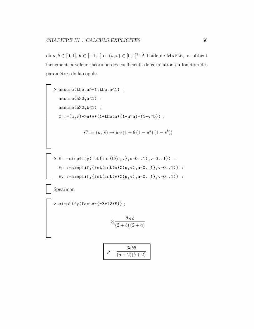
ou a, b ∈ [0, 1], θ ∈ [−1, 1] et (u, v) ∈ [0, 1]2. A l’aide de Maple, on obtient
facilement la valeur theorique des coefficients de correlation en fonction des
parametres de la copule.
> assume(theta>-1,theta<1) :
assume(a>0,a<1) :
assume(b>0,b<1) :
C :=(u,v)->u*v*(1+theta*(1-u^a)*(1-v^b)) ;
C := (u, v) → u v (1 + θ (1 − ua) (1 − vb))
> E :=simplify(int(int(C(u,v),u=0..1),v=0..1)) :
Eu :=simplify(int(int(u*C(u,v),u=0..1),v=0..1)) :
Ev :=simplify(int(int(v*C(u,v),u=0..1),v=0..1)) :
Spearman
> simplify(factor(-3+12*E)) ;
3θ a b
(2 + b) (2 + a)
ρ =3abθ
(a + 2)(b + 2)
CHAPITRE III : CALCULS EXPLICITES 57
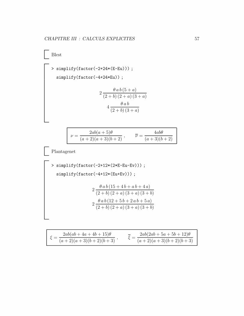
Blest
> simplify(factor(-2+24*(E-Eu))) ;
simplify(factor(-4+24*Eu)) ;
2θ a b (5 + a)
(2 + b) (2 + a) (3 + a)
4θ a b
(2 + b) (3 + a)
ν =2ab(a + 5)θ
(a + 2)(a + 3)(b + 2), ν =
4abθ
(a + 3)(b + 2)
Plantagenet
> simplify(factor(-2+12*(2*E-Eu-Ev))) ;
simplify(factor(-4+12*(Eu+Ev))) ;
2θ a b (15 + 4 b + a b + 4 a)
(2 + b) (2 + a) (3 + a) (3 + b)
2θ a b (12 + 5 b + 2 a b + 5 a)
(2 + b) (2 + a) (3 + a) (3 + b)
ξ =2ab(ab + 4a + 4b + 15)θ
(a + 2)(a + 3)(b + 2)(b + 3), ξ =
2ab(2ab + 5a + 5b + 12)θ
(a + 2)(a + 3)(b + 2)(b + 3)
CHAPITRE III : CALCULS EXPLICITES 58
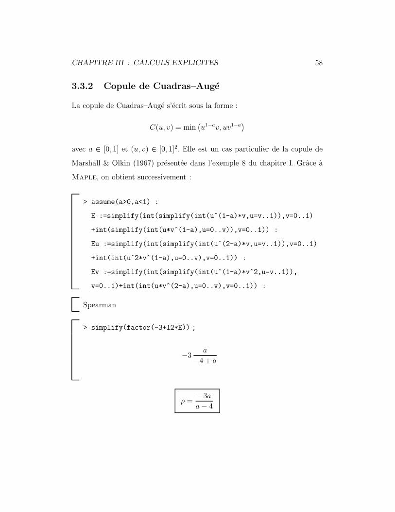
3.3.2 Copule de Cuadras–Auge
La copule de Cuadras–Auge s’ecrit sous la forme :
C(u, v) = min(u1−av, uv1−a
)avec a ∈ [0, 1] et (u, v) ∈ [0, 1]2. Elle est un cas particulier de la copule de
Marshall & Olkin (1967) presentee dans l’exemple 8 du chapitre I. Grace a
Maple, on obtient successivement :
> assume(a>0,a<1) :
E :=simplify(int(simplify(int(u^(1-a)*v,u=v..1)),v=0..1)
+int(simplify(int(u*v^(1-a),u=0..v)),v=0..1)) :
Eu :=simplify(int(simplify(int(u^(2-a)*v,u=v..1)),v=0..1)
+int(int(u^2*v^(1-a),u=0..v),v=0..1)) :
Ev :=simplify(int(simplify(int(u^(1-a)*v^2,u=v..1)),
v=0..1)+int(int(u*v^(2-a),u=0..v),v=0..1)) :
Spearman
> simplify(factor(-3+12*E)) ;
−3a
−4 + a
ρ =−3a
a − 4
CHAPITRE III : CALCULS EXPLICITES 59
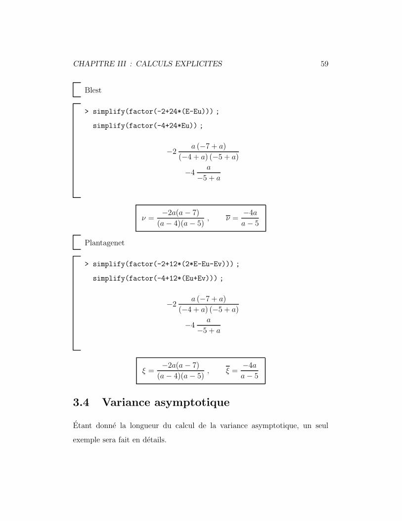
Blest
> simplify(factor(-2+24*(E-Eu))) ;
simplify(factor(-4+24*Eu)) ;
−2a (−7 + a)
(−4 + a) (−5 + a)
−4a
−5 + a
ν =−2a(a − 7)
(a − 4)(a − 5), ν =
−4a
a − 5
Plantagenet
> simplify(factor(-2+12*(2*E-Eu-Ev))) ;
simplify(factor(-4+12*(Eu+Ev))) ;
−2a (−7 + a)
(−4 + a) (−5 + a)
−4a
−5 + a
ξ =−2a(a − 7)
(a − 4)(a − 5), ξ =
−4a
a − 5
3.4 Variance asymptotique
Etant donne la longueur du calcul de la variance asymptotique, un seul
exemple sera fait en details.
CHAPITRE III : CALCULS EXPLICITES 60
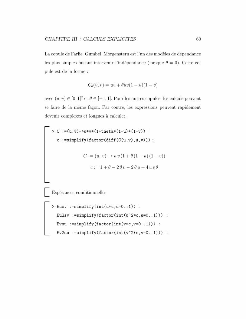
La copule de Farlie–Gumbel–Morgenstern est l’un des modeles de dependance
les plus simples faisant intervenir l’independance (lorsque θ = 0). Cette co-
pule est de la forme :
Cθ(u, v) = uv + θuv(1 − u)(1 − v)
avec (u, v) ∈ [0, 1]2 et θ ∈ [−1, 1]. Pour les autres copules, les calculs peuvent
se faire de la meme facon. Par contre, les expressions peuvent rapidement
devenir complexes et longues a calculer.
> C :=(u,v)->u*v*(1+theta*(1-u)*(1-v)) ;
c :=simplify(factor(diff(C(u,v),u,v))) ;
C := (u, v) → u v (1 + θ (1 − u) (1 − v))
c := 1 + θ − 2 θ v − 2 θ u + 4 u v θ
Esperances conditionnelles
> Eusv :=simplify(int(u*c,u=0..1)) :
Eu2sv :=simplify(factor(int(u^2*c,u=0..1))) :
Evsu :=simplify(factor(int(v*c,v=0..1))) :
Ev2su :=simplify(factor(int(v^2*c,v=0..1))) :
CHAPITRE III : CALCULS EXPLICITES 61
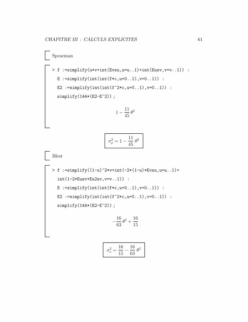
Spearman
> f :=simplify(u*v+int(Evsu,u=u..1)+int(Eusv,v=v..1)) :
E :=simplify(int(int(f*c,u=0..1),v=0..1)) :
E2 :=simplify(int(int(f^2*c,u=0..1),v=0..1)) :
simplify(144*(E2-E^2)) ;
1 − 11
45θ2
σ2ρ = 1 − 11
45θ2
Blest
> f :=simplify((1-u)^2*v+int(-2*(1-u)*Evsu,u=u..1)+
int(1-2*Eusv+Eu2sv,v=v..1)) :
E :=simplify(int(int(f*c,u=0..1),v=0..1)) :
E2 :=simplify(int(int(f^2*c,u=0..1),v=0..1)) :
simplify(144*(E2-E^2)) ;
−16
63θ2 +
16
15
σ2ν =
16
15− 16
63θ2
CHAPITRE III : CALCULS EXPLICITES 62
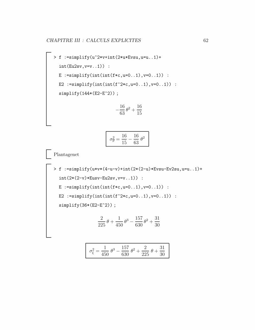
> f :=simplify(u^2*v+int(2*u*Evsu,u=u..1)+
int(Eu2sv,v=v..1)) :
E :=simplify(int(int(f*c,u=0..1),v=0..1)) :
E2 :=simplify(int(int(f^2*c,u=0..1),v=0..1)) :
simplify(144*(E2-E^2)) ;
−16
63θ2 +
16
15
σ2ν =
16
15− 16
63θ2
Plantagenet
> f :=simplify(u*v*(4-u-v)+int(2*(2-u)*Evsu-Ev2su,u=u..1)+
int(2*(2-v)*Eusv-Eu2sv,v=v..1)) :
E :=simplify(int(int(f*c,u=0..1),v=0..1)) :
E2 :=simplify(int(int(f^2*c,u=0..1),v=0..1)) :
simplify(36*(E2-E^2)) ;
2
225θ +
1
450θ3 − 157
630θ2 +
31
30
σ2ξ =
1
450θ3 − 157
630θ2 +
2
225θ +
31
30
CHAPITRE III : CALCULS EXPLICITES 63
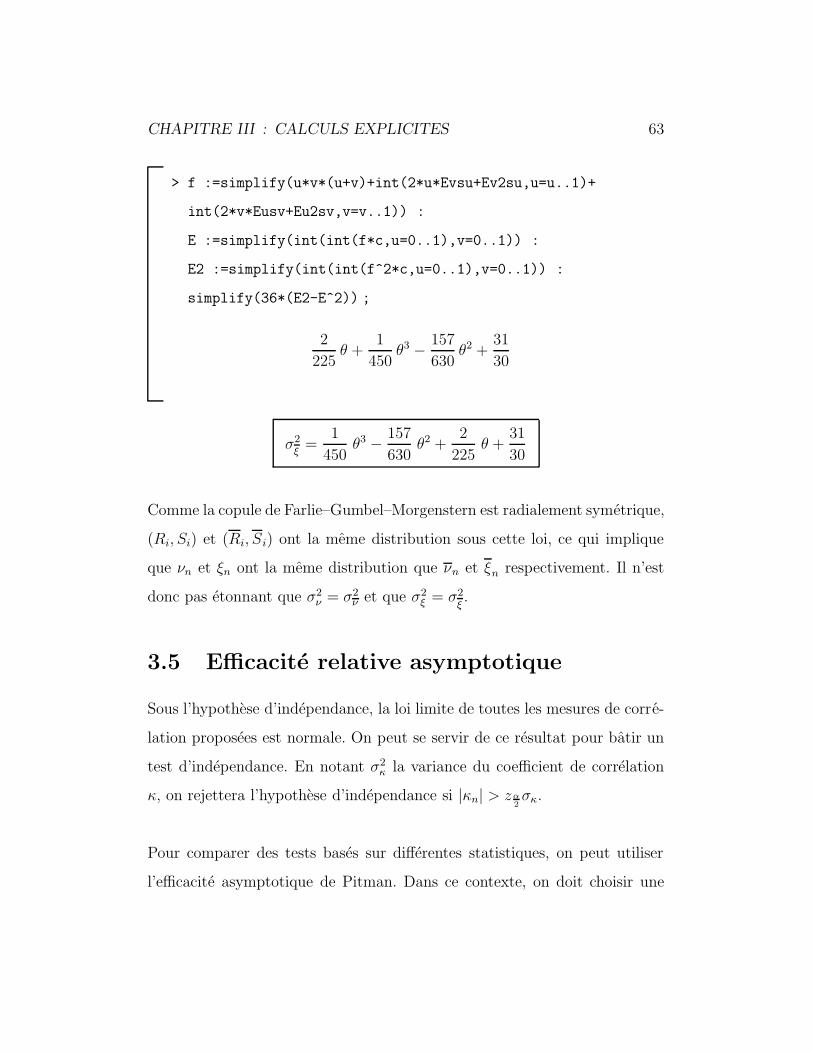
> f :=simplify(u*v*(u+v)+int(2*u*Evsu+Ev2su,u=u..1)+
int(2*v*Eusv+Eu2sv,v=v..1)) :
E :=simplify(int(int(f*c,u=0..1),v=0..1)) :
E2 :=simplify(int(int(f^2*c,u=0..1),v=0..1)) :
simplify(36*(E2-E^2)) ;
2
225θ +
1
450θ3 − 157
630θ2 +
31
30
σ2ξ
=1
450θ3 − 157
630θ2 +
2
225θ +
31
30
Comme la copule de Farlie–Gumbel–Morgenstern est radialement symetrique,
(Ri, Si) et (Ri, Si) ont la meme distribution sous cette loi, ce qui implique
que νn et ξn ont la meme distribution que νn et ξn respectivement. Il n’est
donc pas etonnant que σ2ν = σ2
ν et que σ2ξ = σ2
ξ.
3.5 Efficacite relative asymptotique
Sous l’hypothese d’independance, la loi limite de toutes les mesures de corre-
lation proposees est normale. On peut se servir de ce resultat pour batir un
test d’independance. En notant σ2κ la variance du coefficient de correlation
κ, on rejettera l’hypothese d’independance si |κn| > zα2σκ.
Pour comparer des tests bases sur differentes statistiques, on peut utiliser
l’efficacite asymptotique de Pitman. Dans ce contexte, on doit choisir une
CHAPITRE III : CALCULS EXPLICITES 64
contre-hypothese qui ne depend que d’un parametre continu (disons θ) in-
cluant l’independance comme cas particulier. En notant Tρ et Tκ les tests
bases sur ρ et κ,
ARE(Tκ, Tρ) =nρ
nκ,
la proportion des tailles d’echantillons necessaires pour obtenir la meme puis-
sance avec les deux tests lorsque la contre-hypothese tend vers l’independance.
Si l’independance est atteinte pour θ = 0, on trouve dans Lehmann (1998,
p. 375) que
ARE(Tκ, Tρ) =σ2
ρ
σ2κ
(κ′
0
ρ′0
)2
,
ou ρ′0 = ∂
∂θρθ
∣∣θ=0
et κ′0 = ∂
∂θκθ
∣∣θ=0
.
Pour les calculs explicites, la partie cruciale consiste a evaluer κ′0 et ρ′
0. Deux
approches sont possibles ; elles sont toutes les deux illustrees ci-apres a l’aide
de Maple.
1. Utiliser les formes explicites du parametre estime (tel que calcule a la
section 3.3) et calculer directement les derivees.
2. Faire passer la derivee sous l’integrale dans les formules de la section
3.4 pour obtenir, par exemple
ρ′0 = 12
1∫0
1∫0
∂
∂θCθ(u, v)
∣∣∣∣θ=0
du dv .
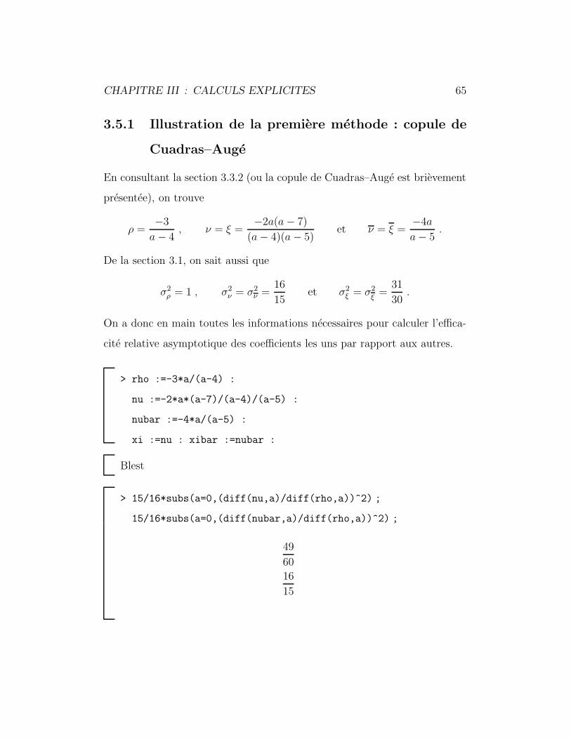
CHAPITRE III : CALCULS EXPLICITES 65
3.5.1 Illustration de la premiere methode : copule de
Cuadras–Auge
En consultant la section 3.3.2 (ou la copule de Cuadras–Auge est brievement
presentee), on trouve
ρ =−3
a − 4, ν = ξ =
−2a(a − 7)
(a − 4)(a − 5)et ν = ξ =
−4a
a − 5.
De la section 3.1, on sait aussi que
σ2ρ = 1 , σ2
ν = σ2ν =
16
15et σ2
ξ = σ2ξ
=31
30.
On a donc en main toutes les informations necessaires pour calculer l’effica-
cite relative asymptotique des coefficients les uns par rapport aux autres.
> rho :=-3*a/(a-4) :
nu :=-2*a*(a-7)/(a-4)/(a-5) :
nubar :=-4*a/(a-5) :
xi :=nu : xibar :=nubar :
Blest
> 15/16*subs(a=0,(diff(nu,a)/diff(rho,a))^2) ;
15/16*subs(a=0,(diff(nubar,a)/diff(rho,a))^2) ;
49
60
16
15
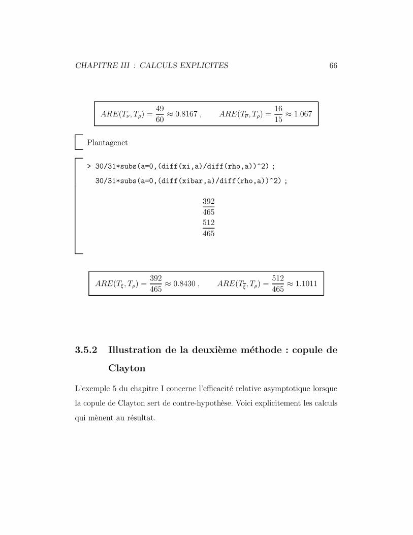
CHAPITRE III : CALCULS EXPLICITES 66
ARE(Tν , Tρ) =49
60≈ 0.8167 , ARE(Tν , Tρ) =
16
15≈ 1.067
Plantagenet
> 30/31*subs(a=0,(diff(xi,a)/diff(rho,a))^2) ;
30/31*subs(a=0,(diff(xibar,a)/diff(rho,a))^2) ;
392
465
512
465
ARE(Tξ, Tρ) =392
465≈ 0.8430 , ARE(Tξ, Tρ) =
512
465≈ 1.1011
3.5.2 Illustration de la deuxieme methode : copule de
Clayton
L’exemple 5 du chapitre I concerne l’efficacite relative asymptotique lorsque
la copule de Clayton sert de contre-hypothese. Voici explicitement les calculs
qui menent au resultat.
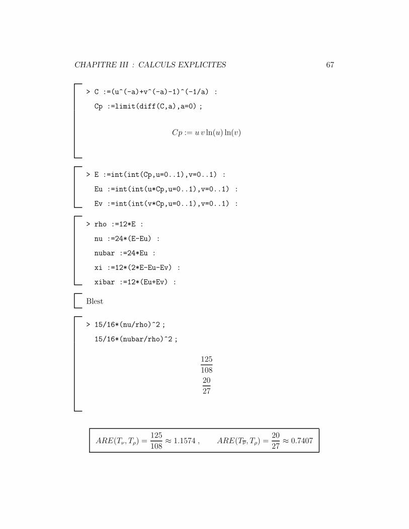
CHAPITRE III : CALCULS EXPLICITES 67
> C :=(u^(-a)+v^(-a)-1)^(-1/a) :
Cp :=limit(diff(C,a),a=0) ;
Cp := u v ln(u) ln(v)
> E :=int(int(Cp,u=0..1),v=0..1) :
Eu :=int(int(u*Cp,u=0..1),v=0..1) :
Ev :=int(int(v*Cp,u=0..1),v=0..1) :
> rho :=12*E :
nu :=24*(E-Eu) :
nubar :=24*Eu :
xi :=12*(2*E-Eu-Ev) :
xibar :=12*(Eu+Ev) :
Blest
> 15/16*(nu/rho)^2 ;
15/16*(nubar/rho)^2 ;
125
108
20
27
ARE(Tν , Tρ) =125
108≈ 1.1574 , ARE(Tν , Tρ) =
20
27≈ 0.7407
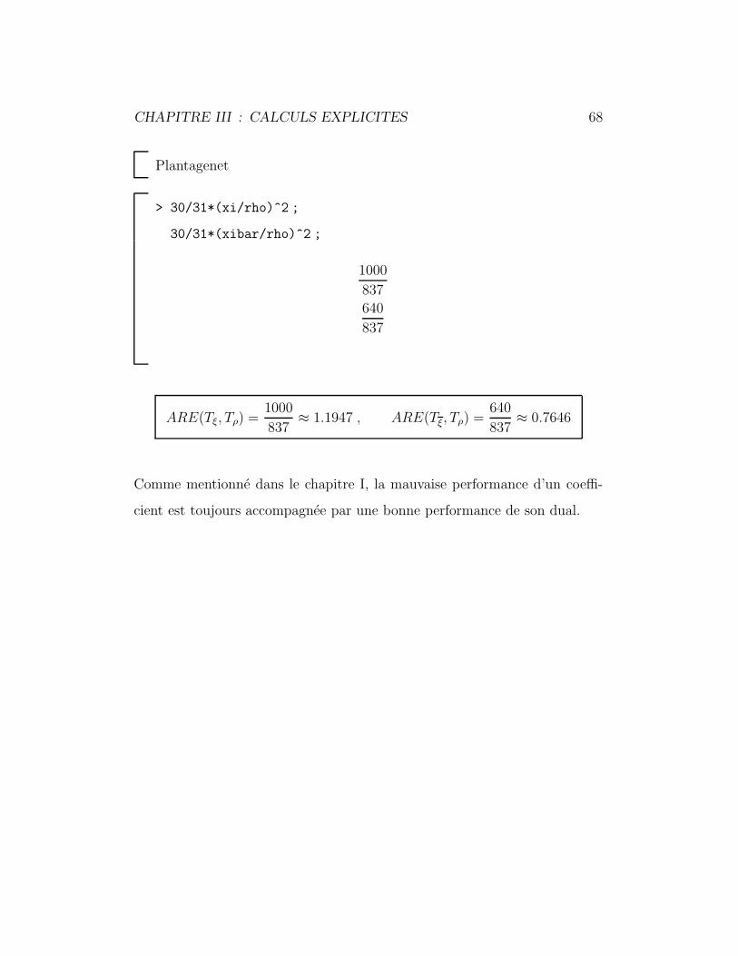
CHAPITRE III : CALCULS EXPLICITES 68
Plantagenet
> 30/31*(xi/rho)^2 ;
30/31*(xibar/rho)^2 ;
1000
837
640
837
ARE(Tξ, Tρ) =1000
837≈ 1.1947 , ARE(Tξ, Tρ) =
640
837≈ 0.7646
Comme mentionne dans le chapitre I, la mauvaise performance d’un coeffi-
cient est toujours accompagnee par une bonne performance de son dual.
CHAPITRE IV
SIMULATIONS
Des simulations ont ete realisees afin de determiner le seuil et la puissance des
differents tests d’independance a taille finie. Ces resultats visent a completer
les comparaisons effectuees au moyen de l’efficacite relative asymptotique de
Pitman.
Pour chaque loi consideree, 4 tailles d’echantillon ont ete utilisees (n = 25, 50,
100 et 250). Les contre-hypotheses sont exprimees en terme du coefficient de
correlation de Pearson afin de rendre les graphiques comparables d’une loi a
l’autre. Pour la construction des graphiques de puissance, les valeurs de r ont
ete discretisees avec un pas de 0.01. Pour chacune de ces valeurs, 5000 tests
bilateraux de seuil 5 % ont ete effectues a partir des versions experimentales
des six mesures de correlation suivantes : ρ, τ , ν, ν, ξ et ξ. Chaque statistique
de test a ete standardisee a l’aide de sa variance exacte sous l’independance
et le seuil observe a ete calcule au moyen de la loi asymptotique.
Lorsque les courbes de puissance sont rapprochees ou se superposent, il de-
vient tres difficile de determiner a quels coefficients elles correspondent. Sou-
vent, les courbes associees a νn et ξn sont pratiquement confondues ; il en
va de meme pour celles de νn et ξn. De fait, elles ne sont distinguables que
CHAPITRE IV : SIMULATIONS 70
si n = 25, auquel cas νn et νn sont legerement plus puissants que ξn et ξn.
Ainsi, seuls ρn, τn, ξn et ξn ont ete retenus pour les graphiques.
La bibliotheque publique Ranlib a servi a generer les nombres pseudo-
aleatoires univaries. En ce qui concerne les algorithmes specifiques aux lois
bivariees, ils sont precises dans leurs sections respectives.
4.1 Loi normale bivariee
La loi normale bivariee comporte cinq parametres, a savoir les moyennes et les
variances des deux variables, ainsi que le coefficient r caracterisant le degre
de correlation qu’il y a entre elles (r = 0 correspondant a l’independance).
Puisque la copule sous-jacente ne depend que de r, on a genere des observa-
tions Xi
Yi
iid∼ N2
0
0
,
1 r
r 1
de densite
f(x, y) =1
2π√
1 − r2exp
(x2 + y2 − 2rxy
),
ou r ∈ [−1, 1] et (x, y) ∈ IR2. Une fonction de Ranlib a ete utilisee pour
generer ces observations.
Tel que mentionne au chapitre I, ρn, ξn et ξn estiment tous la meme valeur
lorsque la loi est radialement symetrique. Le comportement tres semblable de
tous les coefficients observe dans ce cas n’est donc pas etonnant. La variance
plus elevee des coefficients de Plantagenet explique qu’ils soient legerement
moins puissants (on voit apparaıtre les pointilles sous le trait plein).
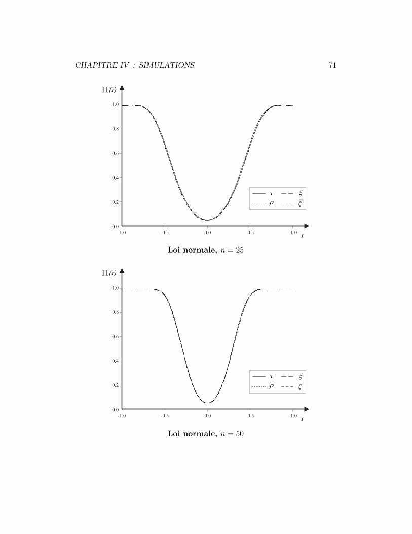
CHAPITRE IV : SIMULATIONS 71
Loi normale, n = 25
Loi normale, n = 50
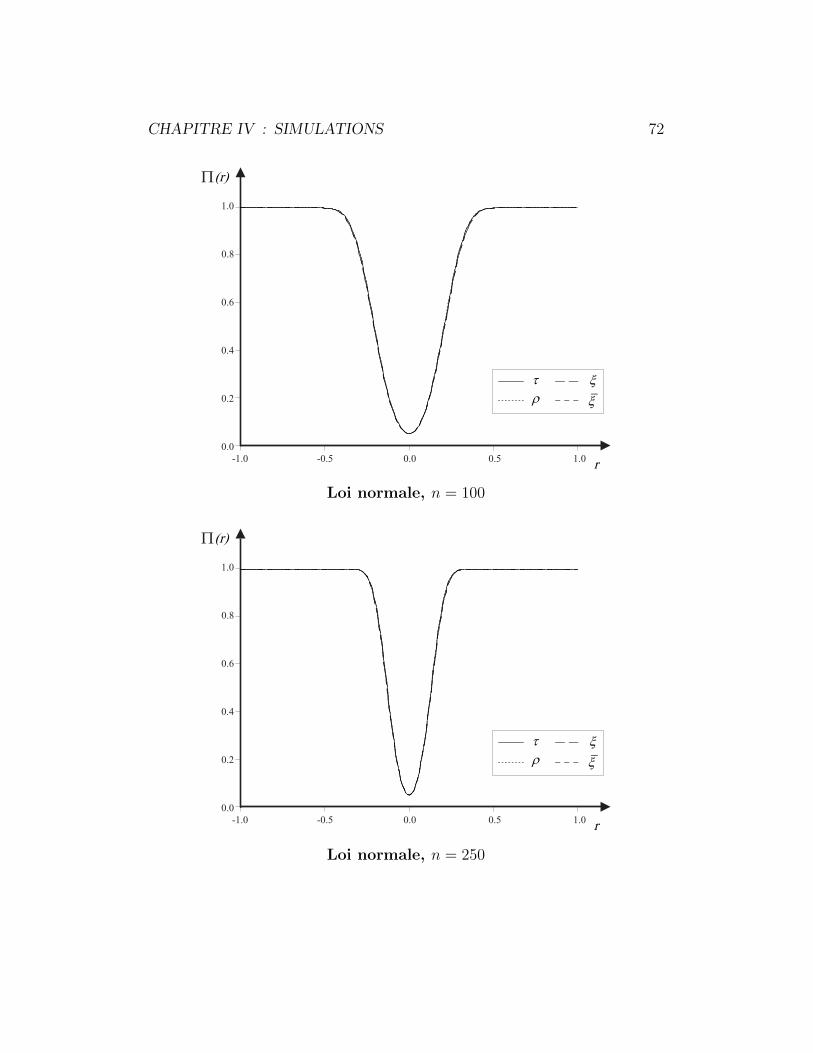
CHAPITRE IV : SIMULATIONS 72
Loi normale, n = 100
Loi normale, n = 250
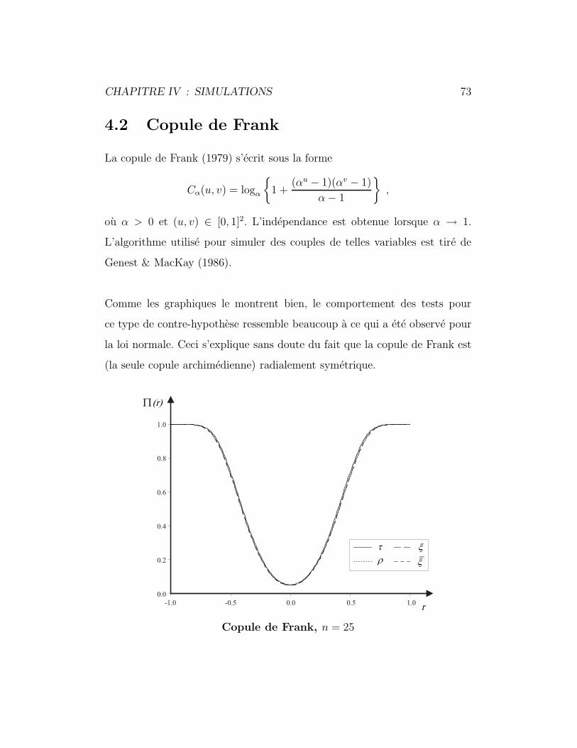
CHAPITRE IV : SIMULATIONS 73
4.2 Copule de Frank
La copule de Frank (1979) s’ecrit sous la forme
Cα(u, v) = logα
{1 +
(αu − 1)(αv − 1)
α − 1
},
ou α > 0 et (u, v) ∈ [0, 1]2. L’independance est obtenue lorsque α → 1.
L’algorithme utilise pour simuler des couples de telles variables est tire de
Genest & MacKay (1986).
Comme les graphiques le montrent bien, le comportement des tests pour
ce type de contre-hypothese ressemble beaucoup a ce qui a ete observe pour
la loi normale. Ceci s’explique sans doute du fait que la copule de Frank est
(la seule copule archimedienne) radialement symetrique.
Copule de Frank, n = 25
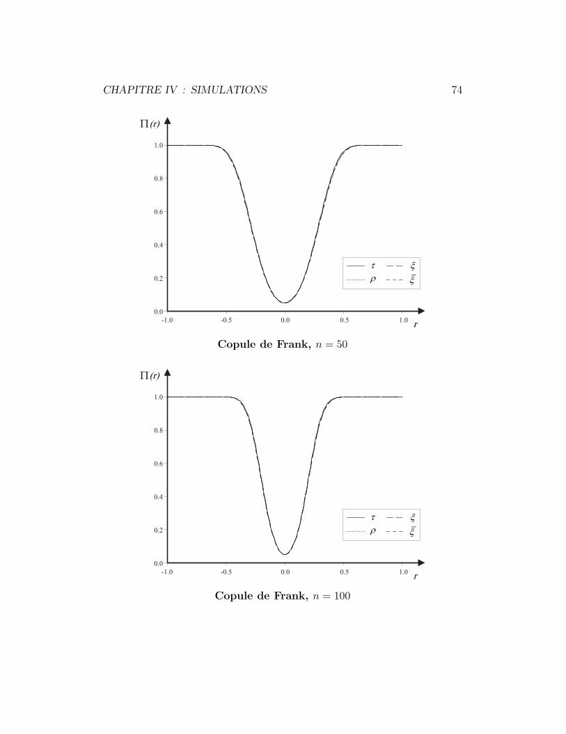
CHAPITRE IV : SIMULATIONS 74
Copule de Frank, n = 50
Copule de Frank, n = 100
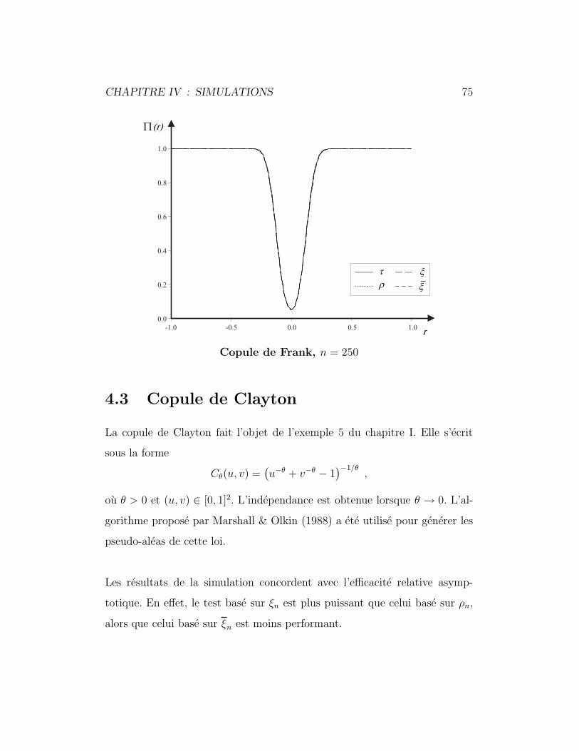
CHAPITRE IV : SIMULATIONS 75
Copule de Frank, n = 250
4.3 Copule de Clayton
La copule de Clayton fait l’objet de l’exemple 5 du chapitre I. Elle s’ecrit
sous la forme
Cθ(u, v) =(u−θ + v−θ − 1
)−1/θ,
ou θ > 0 et (u, v) ∈ [0, 1]2. L’independance est obtenue lorsque θ → 0. L’al-
gorithme propose par Marshall & Olkin (1988) a ete utilise pour generer les
pseudo-aleas de cette loi.
Les resultats de la simulation concordent avec l’efficacite relative asymp-
totique. En effet, le test base sur ξn est plus puissant que celui base sur ρn,
alors que celui base sur ξn est moins performant.
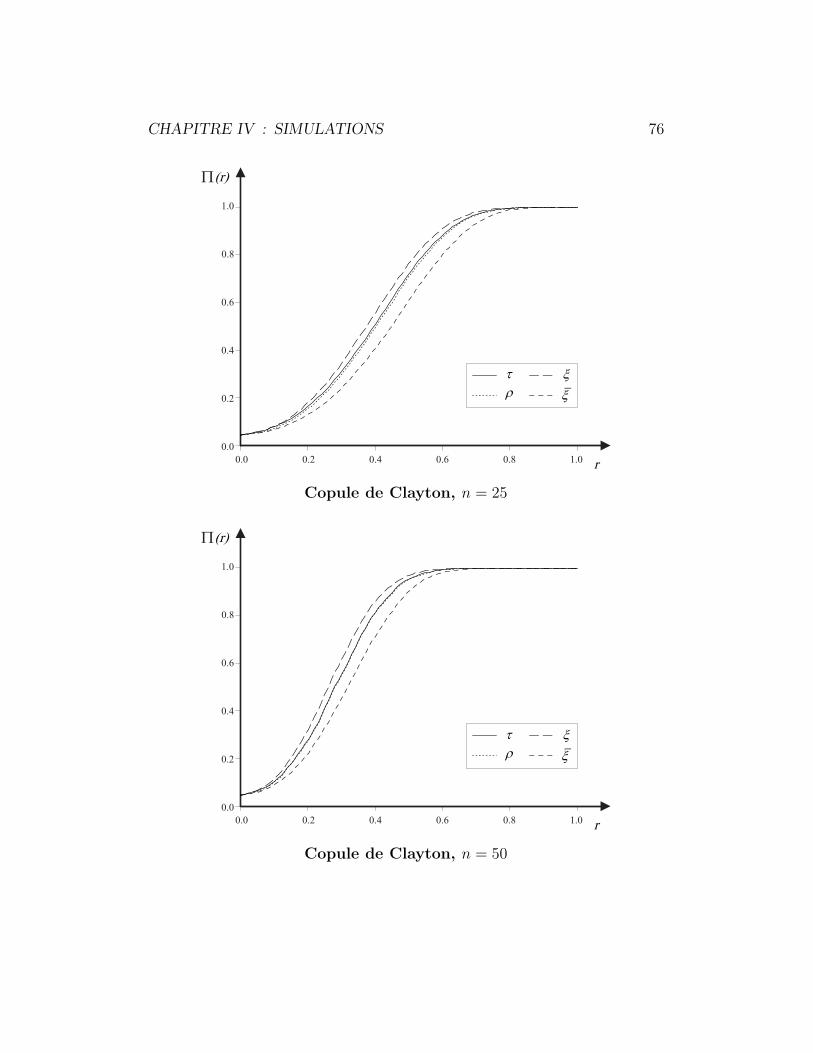
CHAPITRE IV : SIMULATIONS 76
Copule de Clayton, n = 25
Copule de Clayton, n = 50
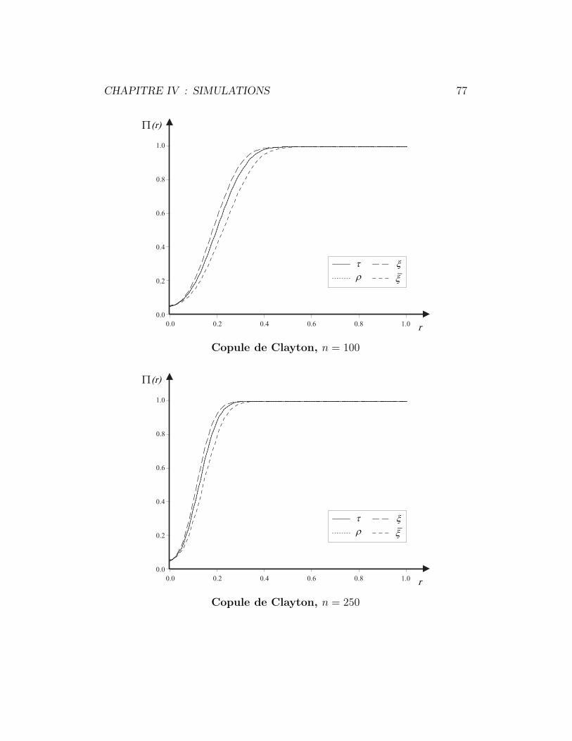
CHAPITRE IV : SIMULATIONS 77
Copule de Clayton, n = 100
Copule de Clayton, n = 250
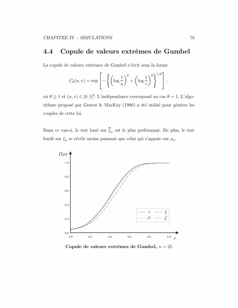
CHAPITRE IV : SIMULATIONS 78
4.4 Copule de valeurs extremes de Gumbel
La copule de valeurs extremes de Gumbel s’ecrit sous la forme
Cθ(u, v) = exp
−
{(log
1
u
)θ
+
(log
1
v
)θ}1/θ
,
ou θ ≥ 1 et (u, v) ∈ [0, 1]2. L’independance correspond au cas θ = 1. L’algo-
rithme propose par Genest & MacKay (1986) a ete utilise pour generer les
couples de cette loi.
Dans ce cas-ci, le test base sur ξn est le plus performant. De plus, le test
fonde sur ξn se revele moins puissant que celui qui s’appuie sur ρn.
Copule de valeurs extremes de Gumbel, n = 25
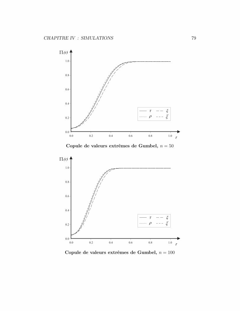
CHAPITRE IV : SIMULATIONS 79
Copule de valeurs extremes de Gumbel, n = 50
Copule de valeurs extremes de Gumbel, n = 100
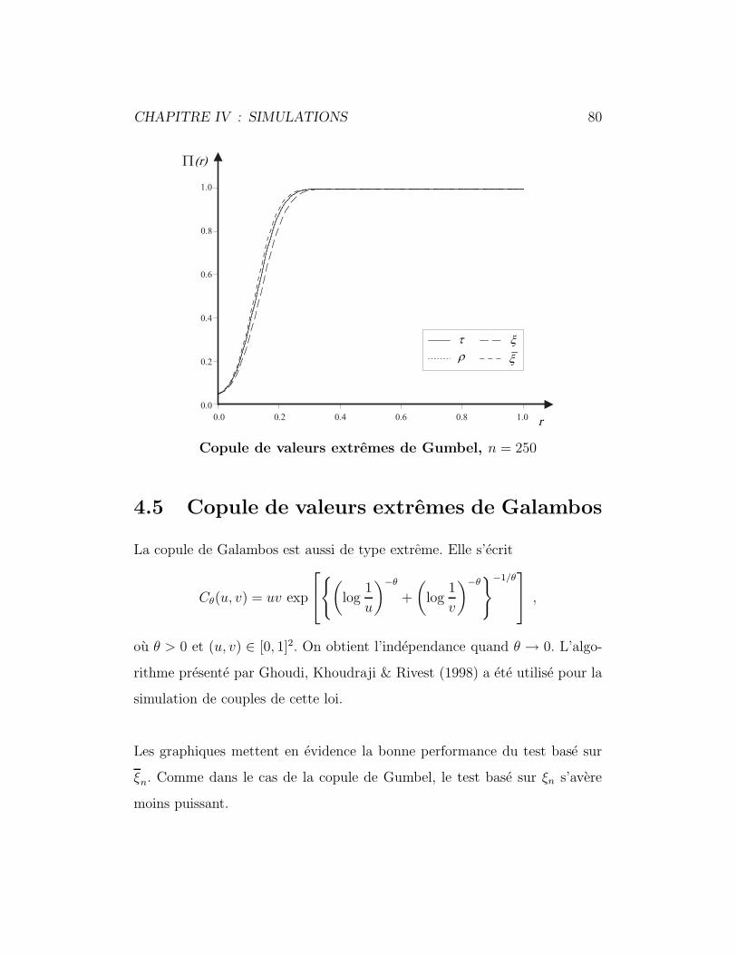
CHAPITRE IV : SIMULATIONS 80
Copule de valeurs extremes de Gumbel, n = 250
4.5 Copule de valeurs extremes de Galambos
La copule de Galambos est aussi de type extreme. Elle s’ecrit
Cθ(u, v) = uv exp
{(log
1
u
)−θ
+
(log
1
v
)−θ}−1/θ
,
ou θ > 0 et (u, v) ∈ [0, 1]2. On obtient l’independance quand θ → 0. L’algo-
rithme presente par Ghoudi, Khoudraji & Rivest (1998) a ete utilise pour la
simulation de couples de cette loi.
Les graphiques mettent en evidence la bonne performance du test base sur
ξn. Comme dans le cas de la copule de Gumbel, le test base sur ξn s’avere
moins puissant.
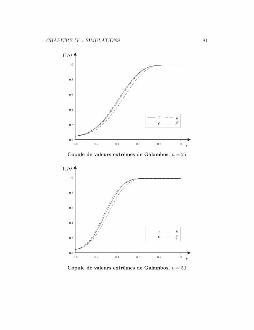
CHAPITRE IV : SIMULATIONS 81
Copule de valeurs extremes de Galambos, n = 25
Copule de valeurs extremes de Galambos, n = 50
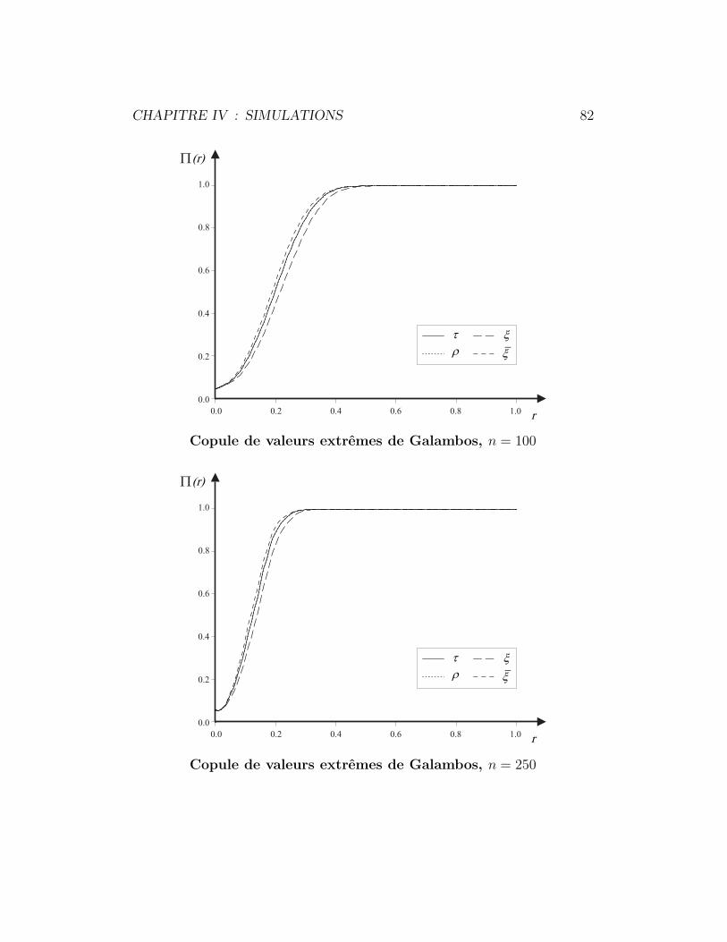
CHAPITRE IV : SIMULATIONS 82
Copule de valeurs extremes de Galambos, n = 100
Copule de valeurs extremes de Galambos, n = 250
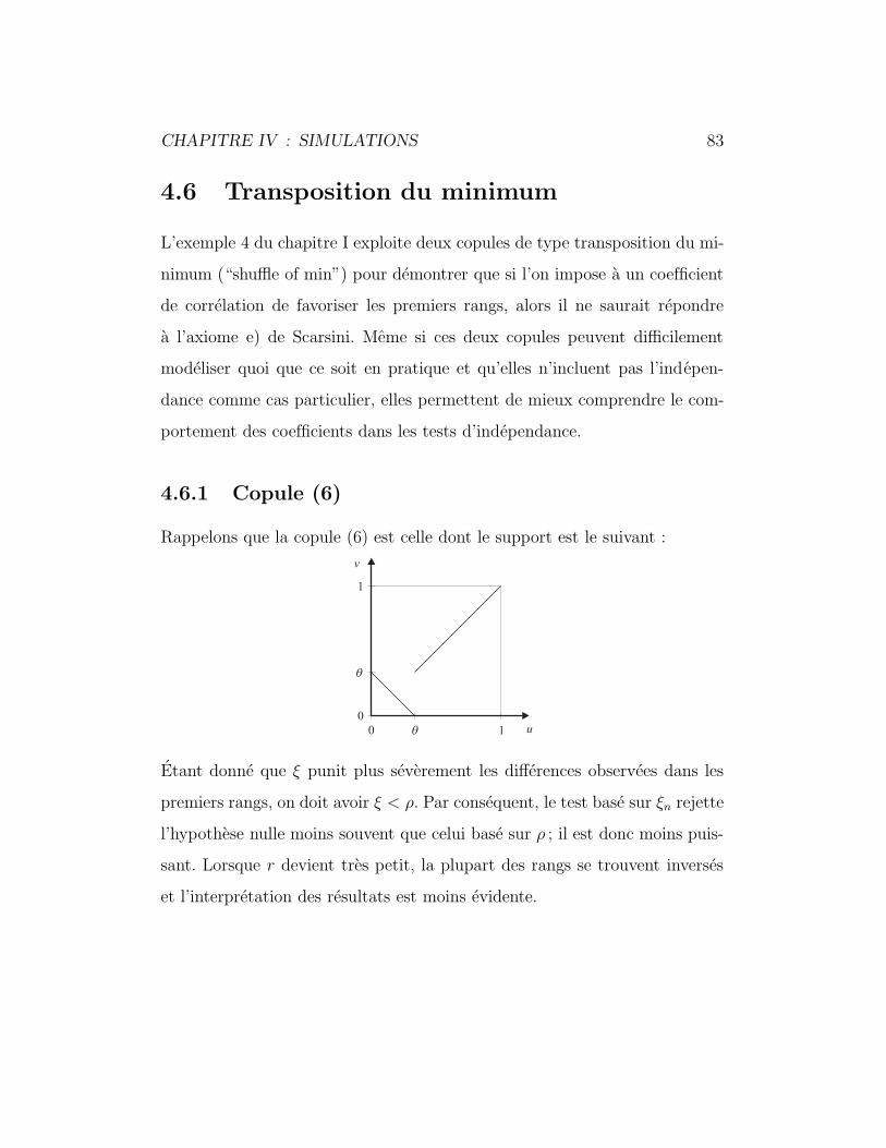
CHAPITRE IV : SIMULATIONS 83
4.6 Transposition du minimum
L’exemple 4 du chapitre I exploite deux copules de type transposition du mi-
nimum (“shuffle of min”) pour demontrer que si l’on impose a un coefficient
de correlation de favoriser les premiers rangs, alors il ne saurait repondre
a l’axiome e) de Scarsini. Meme si ces deux copules peuvent difficilement
modeliser quoi que ce soit en pratique et qu’elles n’incluent pas l’indepen-
dance comme cas particulier, elles permettent de mieux comprendre le com-
portement des coefficients dans les tests d’independance.
4.6.1 Copule (6)
Rappelons que la copule (6) est celle dont le support est le suivant :
Etant donne que ξ punit plus severement les differences observees dans les
premiers rangs, on doit avoir ξ < ρ. Par consequent, le test base sur ξn rejette
l’hypothese nulle moins souvent que celui base sur ρ ; il est donc moins puis-
sant. Lorsque r devient tres petit, la plupart des rangs se trouvent inverses
et l’interpretation des resultats est moins evidente.

CHAPITRE IV : SIMULATIONS 84
Copule (6), n = 25
Copule (6), n = 50
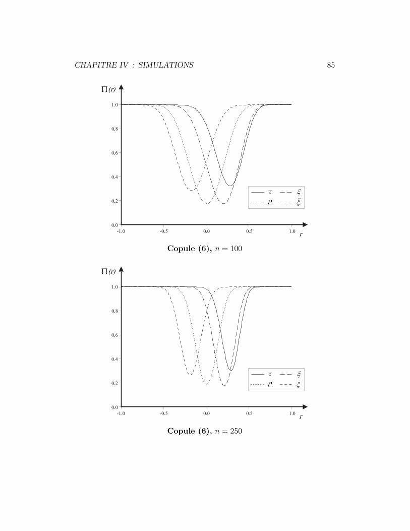
CHAPITRE IV : SIMULATIONS 85
Copule (6), n = 100
Copule (6), n = 250
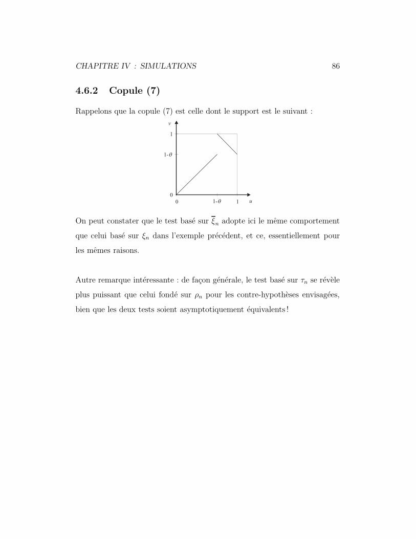
CHAPITRE IV : SIMULATIONS 86
4.6.2 Copule (7)
Rappelons que la copule (7) est celle dont le support est le suivant :
On peut constater que le test base sur ξn adopte ici le meme comportement
que celui base sur ξn dans l’exemple precedent, et ce, essentiellement pour
les memes raisons.
Autre remarque interessante : de facon generale, le test base sur τn se revele
plus puissant que celui fonde sur ρn pour les contre-hypotheses envisagees,
bien que les deux tests soient asymptotiquement equivalents !
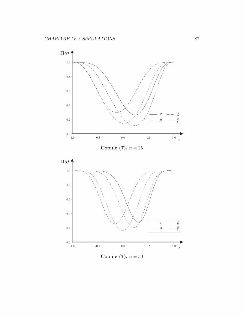
CHAPITRE IV : SIMULATIONS 87
Copule (7), n = 25
Copule (7), n = 50

CHAPITRE IV : SIMULATIONS 88
Copule (7), n = 100
Copule (7), n = 250
CONCLUSION
David C. Blest a propose un coefficient de correlation des rangs qui visait
a affiner le ρ de Spearman. Ce memoire complete son travail en precisant
la loi asymptotique du coefficient de Blest et en en proposant des versions
symetriques et duales.
Si la copule qui caracterise la dependance d’un couple de variables aleatoires
est radialement symetrique, le coefficient de Blest et ses variantes sont la plu-
part du temps des estimateurs (legerement) inefficaces du ρ de Spearman. De
facon plus generale, le lien entre ces coefficients duaux conduit a une borne
minimale pour l’efficacite relative asymptotique de la meilleure variante du
coefficient de Blest par rapport a ρ. Des simulations ont d’ailleurs permis
de verifier que les nouveaux coefficients pouvaient surpasser τ et ρ comme
statistiques d’un test d’independance.
En formulant sa proposition, Blest a ouvert la porte a tout un ensemble
de nouvelles mesures de correlation basees sur des fonctions polynomiales
des rangs. Une piste interessante a explorer serait de verifier quels poly-
nomes debouchent sur des coefficients de correlation acceptables et quels
sont, geometriquement parlant, les avantages des uns par rapport aux autres.
Une autre question en suspens est de savoir s’il existe des polynomes autres
que uv qui permettent de construire un coefficient de correlation respectant
tous les axiomes de Scarsini. Il y a fort a parier que non !
BIBLIOGRAPHIE
M. M. Ali, N. N. Mikhail & M. S. Haq (1978). A class of bivariate distribu-
tions including the bivariate logistic. Journal of Multivariate Analysis,
8, 405–412.
I. G. Bairamov, S. Kotz & M. Bekci (2000). New Generalized Farlie–Gumbel–
Morgenstern Distributions and Concomitants of Order Statistics. Tech-
nical Report, George Washington University, Washington, DC.
D. C. Blest (2000). Rank correlation — An alternative measure. Australian
and New Zealand Journal of Statistics, 42, 101—111.
D. G. Clayton (1978). A model for association in bivariate life tables and
its application in epidemiological studies of familial tendency in chronic
disease incidence. Biometrika, 65, 141–151.
C. M. Cuadras & J. Auge (1981). A continuous general multivariate dis-
tribution and its properties. Communications in Statistics, Theory and
Methods, 10, 339–353.
D. Drouet–Mari & S. Kotz (2001). Correlation and Dependence. Imperial
College Press, London.
T. S. Ferguson, C. Genest & M. Hallin (2000). Kendall’s tau for serial de-
pendence. La revue canadienne de statistique, 28, 587–604.
M. J. Frank (1979). On the simultaneous associativity of F (x, y) and x +
y − F (x, y). Aequationes Mathematicae, 19, 194–226.
BIBLIOGRAPHIE 91
J. Galambos (1975). Order statistics of samples from multivariate distribu-
tions. Journal of the American Statistical Association, 70, 674–680.
C. Genest (1987). Frank’s family of bivariate distributions. Biometrika, 74,
549–555.
C. Genest, K. Ghoudi & L.-P. Rivest (1995). A semiparametric estimation
procedure of dependence parameters in multivariate families of distri-
butions. Biometrika, 82, 543–552.
C. Genest, K. Ghoudi & L.-P. Rivest (1998). Commentaire sur un article de
E. W. Frees et de E. A. Valdez intitule “Understanding relationships
using copulas.” North American Actuarial Journal, 2, 143–149.
C. Genest & R. J. MacKay (1986). Copules archimediennes et familles de lois
bidimensionnelles dont les marges sont donnees. La revue canadienne
de statistique, 14, 145–159.
K. Ghoudi, A. Khoudraji & L.-P. Rivest (1998). Proprietes statistiques des
copules de valeurs extremes bidimensionnelles. La revue canadienne de
statistique, 26, 187–197.
E. J. Gumbel (1960a). Bivariate exponential distributions. Journal of the
American Statistical Association, 55, 698–707.
E. J. Gumbel (1960b). Distributions des valeurs extremes en plusieurs di-
mensions. Bulletin de l’Institut de statistique de l’Universite de Paris,
9, 171–173.
J. Hajek (1969). A Course in Nonparametric Statistics. Holden-Day, San
Francisco, CA.
BIBLIOGRAPHIE 92
M. Hallin & M. L. Puri (1992). Rank test for time series analysis : A survey.
Dans New Directions in Time Series Analysis, publie sous la direction
de D. R. Brillinger, E. Parzen et M. Rosenblatt, pp. 112–153. Springer,
New York.
H. Joe (1997). Multivariate Models and Dependence Concepts. Chapman
and Hall, London.
E. L. Lehmann (1998). Nonparametrics : Statistical Methods Based on Ranks,
Premiere edition revisee. Upper Prentice Hall, Saddle River, NJ.
A. W. Marshall & I. Olkin (1967). A generalized bivariate exponential dis-
tribution. Journal of Applied Probability, 4, 291–302.
A. W. Marshall & I. Olkin (1988). Families of multivariate distributions.
Journal of the American Statistical Society, 83, 834–841.
P. Mikusinski, H. Sherwood & M. D. Taylor (1992). Shuffles of min. Sto-
chastica, 13, 61–74.
R. B. Nelsen (1986). Properties of a one-parameter family of bivariate distri-
butions with specified marginals. Communications in Statistics, Theory
and Methods, 15, 3277–3285.
R. B. Nelsen (1999). An Introduction to Copulas. Lecture Notes in Statistics
No 139. Springer, Berlin.
D. Oakes (2001). Biometrika centenary : Survival analysis. Biometrika, 88,
99–142.
R. L. Plackett (1965). A class of bivariate distributions. Journal of the
American Statistical Association, 60, 516–522.
BIBLIOGRAPHIE 93
J. J. Quesada–Molina (1992). A generalization of an identity of Hoeffding
and some applications. Journal of the Italian Statistical Society, 1, 405–
411.
F. H. Ruymgaart, G. R. Shorack & W. R. van Zwet (1972). Asymptotic
normality of nonparametric tests for independence. The Annals of Ma-
thematical Statistics, 43, 1122–1135.
M. Scarsini (1984). On measures on concordance. Stochastica, 8, 201–208.
B. Schweizer & E. F. Wolff (1981). On nonparametric measures of depen-
dence for random variables. The Annals of Statistics, 9, 879–885.