Embed Size (px)
Citation preview
THESE de DOCTORAT
de l’UNIVERSITE PARIS 7 - DENIS DIDEROT
Ecole Doctorale: Constituants Elementaires, Systemes Complexes
Specialite: Champs, Particules, Matiere
et
de l’UNIVERSITA DEGLI STUDI DI MILANO
Dottorato di Ricerca in Fisica, Astrofisica e Fisica Applicata
presentee par
Maria Elena MONZANI
CHARACTERIZATION AND CALIBRATION
OF THE BOREXINO DETECTOR
FOR SOLAR AND SUPERNOVA NEUTRINOS
Soutenue le 21 Janvier 2005 devant le jury compose par:
Gianpaolo BELLINI Directeur de TheseHerve DE KERRET Directeur de These
Giulio MANUZIO ExaminateurMarco PALLAVICINI Rapporteur
Charling TAO RapporteurFrancois VANNUCCI President du jury


To Mgr. Luigi Giussani,in the 50th anniversary of
Communion and Liberation

A la memoire de la petite Teresa
Et j’ai voulu de nouveau me serrer contre le tombeau vide, mettre ma main dans letrou de la croix, comme cet apotre dans celui des mains et des pieds et du coeur.
Mais ma petite fille Violaine a ete plus sage!Est-ce que le but de la vie est vivre? est-ce que les pieds des enfants de Dieu sont
attaches a cette terre miserable?Il n’est pas de vivre, mais de mourir! et non point de charpentier la croix, mais
d’y monter et de donner ce que nous avons en riant!De quel prix est le monde aupres de la vie? et de quel prix la vie, sinon pour
s’en servir et pour la donner?Et pourquoi se tourmenter quand il est si simple d’obeir et que l’ordre est la?C’est ainsi que Violaine toute prompte suit la main qui prend la sienne.
(Paul Claudel, L’annonce fait a Marie, Ed. Gallimard, Paris, 1940)


Acknowledgements
At the end of this work, is a great pleasure for me to acknowledge all the peoplethat made possible the achievement of my thesis.
Fist of all, I thank my thesis advisors, Gianpaolo and Herve, for their help andencouragement; my co-advisor, Marco, for his interest in my work and for his talk atthe ISAPP School in 2004; my “unofficial” advisor, Emanuela, for the innumerableforms of help and kindness she provided me.
I thank all the Borexino members which helped me under various respects; fistof all the “on-line” people, for the wonderful experience of these three years ofwork: Alessandro, Andrew, Daniela, Davide D., Kevin, Marco, Olivier and Tristan;the CTF-analysis group, for the interesting discussions: Aldo, Andrea P., Barbara,Davide F., Gioacchino, Laura C., Sandra and Silvia; the PMT group, for theirhelp during the Air-Runs: Augusto B., George, Massimo and Paolo L.; all theother members of the Borexino group in Milano (Marco G. and Sergio), Gran Sasso(Andrea I., Augusto G., Christian L., Laszlo, Ludwig, Stefano G.) and Paris (Alain,Didier, Michel and Serge); finally I thank prof. Vignaud and all the staff of the PPCLaboratory at College de France for their hospitality.
I thank all my friends at Gran Sasso Lab for their affection during the last fiveyears: Alba, Carlo, Cristina, Federica, Maria, Paolo and Stefano.
I thank my parents, for their help and support: since their first visit to Gran SassoLab, they wondered how was it possible that their little girl liked to work in sucha “peculiar” place; but nevertheless, they always provided my with comprehensionand encouragement: I would not have made it, without them!
I thank Fr. Giussani, for that day of fifty years ago, when he decided to abandonteaching in the seminary of Venegono and throw himself into the fray (becomingan High School teacher): this was the first day of an adventure which reached memany years later and upset my life. I due to Fr. Giussani most of what I am now;and especially I due to him the discovery that “the unknown generates fear, themystery generates amazement”: without this experience, the scientific work wouldnot have been possible for me. Along with him, I thank my friend Giorgio, forsharing with me the amazing experience of his life during the last three years andfor accompanying me in many difficult steps.
I thank my friends Caterina, Chapeau, Fanta and Ninja, for their firm and faith-ful friendship: thanks to them, I experienced that whatever happens in my life is forme (and not against me). I thank all the other friends of the physics community, for
7
8 Acknowledgements
several reasons that I do not list here: Benny, Cate & Marco, Marisa, Melissa, Nicola,Silvia P., Cawlo, Giovanni & Simona, Rossella, Silvia I., Caggio, Cella, Francy B.,Mario, Matteo D.A., Noda, Redde, Angelo, Bolzi, Cecilia, Francy G., Samu, SimoP., Ben, Diego, Emilio, Giuliano, Paolo M., Rover, Tommy C., Tommy M., Tossico,Ciccio, Decio, Fefe, Krissy, Manu, Paola F., Ale, Ave (AZUICT), Chicco, Jack,Maria, Delo, Ire, Ivan, Jo, Moro, µ, Vale P., 2, Astea, Cheba, Jackie, Marmo, Cuc-ciolo, Francesca and Maddalena. I also thank my “mathematician” friend Giacomo,for his affection to me (and for his frankness).
I thank all the girls I lived with during these three years: Daniela G., Elena,Laura, Marta, Valeria F. (Minu, I’m coming to see you!), Paola, Sara, Caterina, Va-leria R., Viviana, Lucia, Chiara & Chiara (“appa” Grossich); Letizia, Maria Chiara,Daniela, Sara, Maria (“appa” Saldini); Daniela and Silvia (“appa” Jenner); Luciana(“appa” Scarlatti). I am grateful to all of them, for their infinite patience with me,and for taking care of all I could need (food, sleep, holidays, encouragement...). Ialso thank the “appa” Lombardia boys, for hosting me during the long weekendsand nights when I was writing my thesis.
I thank all my friends in L’Aquila (and surroundings): Alessia & Gabbriele,Angelo (I’m waiting for you in Milano!), Antonella, Ercole, Federica & Fabbio,Giorgio, Graziella & Matteo (and Giovanni), Marco, Marta & Paolo, Mimmo, Mirko,Peppe, Stefano (good luck for your new life in Trento!), Valentina and Vincenzo.
I thank all my friends in Paris (“et environs”): Ana G., Anna C., Cecile, Claudia& Jeff (and my little sister, Laetitia), Daniel, Isabelle, Marco F., Meriem, Paulo;Agnese, Ambrogio, Delphine D., Eric W., Francois B., Katja, Ilaria P., Ilaria R.,Lele, Luca S., Marta, Mauro B., Mauro Z., Mimmo, Pasha, Violaine; Alessandra& Silvio (and my favorite nightmare, Matteo), Chiara B., Chiara N., Corentin,Delphine J., Dino, Elena M., Elo & Mirco, Ezio & Rosella, Genevieve & Paul (andMadeleine), Giovanni D., Irene M., Ivanah, Jerome, Julie C., Julie F., Laura &Paolo, Laurence, Luca, Ludovic, Pauline S., Peter, Tina & Lionel. I thank themall, because they succeeded in making me to feel at home: and what in principlecould be a bad luck, become a wonderful adventure. I also thank all the peoplewho went and see us: Davide, Widmer, Desa, Francesco, Maria, Michael, Pippo (I’llnever forget your songs during that lunch at the Latin Quartier!), Benny, Francy,Giovanni, Ilaria and Martina.
Finally, I want to remember two people, who left me very early and that I miss somuch. The first one was my first master, Roberto: even if he never understood whya “resonable” person like me could abandon my piano studies to enter the physicsfaculty, he was always very proud of me: I hope he is still very proud of me now!The second one was a little baby, Teresa: she left me well before I had time to loveher; but nevertheless she took the time to teach me that the accomplishment of mylife does not rely on what I can realize, but on what I belong to. Along with Teresa,I thank her mother, Marta, and all of them who were with me since the beginningof the whole story: Giovanni, Francesca, Matteo, Paolo, Simona and Valentina.
Resume
Depuis la premiere detection des neutrinos solaires en 1967, la physique de ces par-ticules a constitue l’un des domaines les plus passionnants de toute la physique.Bien qu’au cours des six dernieres annees notre connaissance des proprietes du neu-trino se soit considerablement amelioree grace aux resultats des experiences Super-Kamiokande et SNO [49, 2], 99% du spectre du neutrino solaire se situe dans uneregion encore presque inconnue, parce qu’aucune mesure sur les neutrinos solairesn’a jamais ete effectuee par un detecteur en temps reel avec une sensibilite sub-MeV .
L’experience Borexino (actuellement dans sa phase finale d’installation aux labo-ratoires de Gran Sasso, en Italie) a ete concue afin d’explorer la region sub-MeV duspectre du neutrino solaire, notamment la raie monochromatique du 8Be a 860 keV(9% du flux solaire). Cette mesure represente un vrai defi experimental, parce qu’elleexige des niveaux de radioactivite extremement bas pour tous les composants dudetecteur, avec des valeurs de contamination jamais atteintes auparavant.
Le detecteur Borexino se compose de 300 t de scintillateur liquide, observes parune rangee de 2212 photomultiplicateurs. La detection des neutrinos solaires de 7Beest le but principal de Borexino, mais le detecteur peut etre employe pour etudierles neutrinos (ou les anti-neutrinos) d’autres sources, notamment les anti-neutrinosde l’interieur de la Terre et de reacteurs nucleaires, ainsi que les neutrinos et lesanti-neutrinos d’explosion de Supernova.
Dans cette these, la caracterisation et la calibration du detecteur Borexino ontete realisees a la fois pour la detection des neutrinos solaires et pour la detection desneutrinos d’autres sources; une attention particuliere a ete consacree aux neutrinosd’energie elevee emis pendant les evenements de supernova, parce que la reconstruc-tion de leur spectre d’energie et de leur temps d’arrivee peut exiger l’utilisationd’outils specifiques.
Les tres bas niveaux de radioactivite exiges par Borexino ont ete atteints pourla premiere fois en 1995, quand un prototype du detecteur (Counting Test Facility)a ete realise pour detecter des niveaux de contamination de l’ordre de 10−16 g/g,pour les isotopes radioactifs de l’U et du Th dans le scintillateur.
La prise de donnees de CTF est recommencee en 2000 (apres une revision dudetecteur), pour la qualification finale des composants de Borexino. Une campagnede mesure concernant la qualite du scintillateur a ete executee: pendant cette cam-
9
10 Resume
pagne, plusieurs methodes de purification du scintillateur ont ete testees, avec desresultats encourageants. Dans cette these, je presente une analyse detaillee desdonnees acquises pendant les differents tests de purification, en ce qui concernel’efficacite des methodes de purification pour eliminer les contaminants issus deschaınes radioactives de l’U et du Th.
Le but principal de cette these a consiste a etudier les prestations du detecteurBorexino, en atteignant les performances exigees par la physique. L’identificationdu signal de neutrino dans un grand domaine energetique exige une reconstructionprecise de l’energie et de la position des evenements. Pendant les trois dernieresannees, le systeme d’acquisition de Borexino a ete installe et entierement teste: moneffort personnel a concerne plusieurs aspects de ce travail d’achevement.
Tout d’abord, j’ai concu et realise une base de donnees pour l’experience, con-tenant toutes les informations du detecteur, de la disposition des PMT aux pro-prietes du scintillateur; les informations stockees seront essentielles pour reconstruireet interpreter toutes les donnees de Borexino.
Apres l’installation des phototubes et de l’electronique, le systeme complet a eteteste en operation, executant de vraies runs, avec le detecteur vide (ce qu’on appelleles “Air-Runs”). Pendant ces tests, plusieurs modalites de run ont ete appliquees,afin d’examiner differents sous-ensembles du systeme: cela a permis une etude glob-ale des performances de l’electronique, et une mise au point des canaux simples,ainsi que des photomultiplicateurs.
Un systeme de calibration a ete concu pour le controle de stabilite des PMT deBorexino: un test complet de ce systeme a ete realise. Les evenements synchronesfournis par le systeme de calibration ont permis aussi l’evaluation de la precisionde mesure du temps de la chaıne d’acquisition. En outre, les conditions d’eclairagedes PMT etant reglables, les evenements du laser ont permis une evaluation de lagamme dynamique de l’electronique.
Plusieurs tests ont ete egalement realises par l’insertion de plusieurs sourcesradioactives dans la sphere de Borexino. Ces sources etaient composees des petitsechantillons de scintillateur charges en 222Rn: ces mesures ont donc represente untest realiste du systeme d’acquisition. Le comportement de la chaıne de lecture aete analyse et a donne d’excellentes performances: les capacites du detecteur dereconstruire l’energie et la position des evenements ont ete evaluees et ont prouveque le systeme est pret et operationnel pour la prise de donnees.
Une chaıne electronique supplementaire a ete installee, avec l’objectif d’explorerle domaine de haute energie, jusqu’a la region des 10 MeV et au-dela (notammentpour la detection des neutrinos de Supernova). Ce deuxieme systeme de lecture aete egalement examine pendant les “Air-Runs” de Borexino, a l’aide des donneeslaser et des sources radioactives. Les resultats de ces tests ont demontre le tres boncomportement du systeme, qui est actuellement en voie d’achevement, notammenten ce qui concerne l’ajustement de la dynamique des cartes.
Contents
Introduction 15
1 Solar Neutrino Physics in 2004 191.1 The Standard Solar Model (SSM) . . . . . . . . . . . . . . . . . . . . 20
1.1.1 Solar neutrino fluxes . . . . . . . . . . . . . . . . . . . . . . . 221.2 The solar neutrino problem before 2001 . . . . . . . . . . . . . . . . . 24
1.2.1 Radiochemical and water Cerenkov experiments . . . . . . . . 241.2.2 Data analysis: three neutrino problems . . . . . . . . . . . . . 281.2.3 Astrophysical solutions . . . . . . . . . . . . . . . . . . . . . . 31
1.3 Neutrino oscillations . . . . . . . . . . . . . . . . . . . . . . . . . . . 321.3.1 Neutrino masses . . . . . . . . . . . . . . . . . . . . . . . . . . 331.3.2 Experimental limits to neutrino masses . . . . . . . . . . . . . 341.3.3 Mixing of the mass eigenstates and vacuum oscillations . . . . 371.3.4 Matter enhanced neutrino oscillations . . . . . . . . . . . . . . 39
1.4 Neutrino oscillation experiments . . . . . . . . . . . . . . . . . . . . . 401.4.1 Solar neutrino experiments as oscillation experiments . . . . . 411.4.2 Atmospheric neutrinos and the Super-Kamiokande evidence . 421.4.3 The SNO experiment: direct test of solar neutrino oscillations 451.4.4 Reactor neutrino experiments before 2002 . . . . . . . . . . . 501.4.5 The KamLAND result: solar neutrino oscillation parameters . 521.4.6 Accelerator neutrino experiments . . . . . . . . . . . . . . . . 54
2 Borexino: physics goals and detector design 592.1 Physics goals . . . . . . . . . . . . . . . . . . . . . . . . . . . . . . . 59
2.1.1 Neutrino signal in the SSM case . . . . . . . . . . . . . . . . . 612.1.2 Neutrino signal in oscillation scenario . . . . . . . . . . . . . . 622.1.3 Internal background . . . . . . . . . . . . . . . . . . . . . . . 622.1.4 Surface background . . . . . . . . . . . . . . . . . . . . . . . . 662.1.5 External background . . . . . . . . . . . . . . . . . . . . . . . 662.1.6 Muon induced background . . . . . . . . . . . . . . . . . . . . 67
2.2 Borexino detector . . . . . . . . . . . . . . . . . . . . . . . . . . . . . 672.2.1 Detector structure . . . . . . . . . . . . . . . . . . . . . . . . 682.2.2 Auxiliary systems . . . . . . . . . . . . . . . . . . . . . . . . . 73
11

12 CONTENTS
3 Non-solar neutrino physics with the Borexino detector 753.1 Anti-neutrino detection in Borexino . . . . . . . . . . . . . . . . . . . 75
3.1.1 Anti-neutrinos from the Earth’s interior . . . . . . . . . . . . 753.1.2 Long-baseline νe from European reactors . . . . . . . . . . . . 773.1.3 Anti-neutrinos from the Sun . . . . . . . . . . . . . . . . . . . 77
3.2 Supernova neutrino detection in Borexino . . . . . . . . . . . . . . . . 783.2.1 Supernova explosions . . . . . . . . . . . . . . . . . . . . . . . 783.2.2 The role of neutrinos in the Supernova explosion . . . . . . . . 803.2.3 Supernova neutrino signatures in Borexino . . . . . . . . . . . 823.2.4 Neutral current detection capabilities . . . . . . . . . . . . . . 843.2.5 Neutrino mass limits from time of flight . . . . . . . . . . . . 863.2.6 Neutrino oscillations from reactions on 12C . . . . . . . . . . . 903.2.7 Detection of supernova neutrinos by ν − p elastic scattering . 91
4 The Counting Test Facility (CTF) of Borexino 954.1 Feasibility of Borexino: CTF-1 . . . . . . . . . . . . . . . . . . . . . . 95
4.1.1 Structure of the detector . . . . . . . . . . . . . . . . . . . . . 954.1.2 Main results of the test . . . . . . . . . . . . . . . . . . . . . . 97
4.2 Quality control for Borexino: CTF-2 . . . . . . . . . . . . . . . . . . 1004.2.1 Detector upgrade . . . . . . . . . . . . . . . . . . . . . . . . . 1004.2.2 Sequence of measurements . . . . . . . . . . . . . . . . . . . . 1014.2.3 Detector performances . . . . . . . . . . . . . . . . . . . . . . 1024.2.4 α/β discrimination . . . . . . . . . . . . . . . . . . . . . . . . 1024.2.5 PXE test results . . . . . . . . . . . . . . . . . . . . . . . . . 104
4.3 Test of the purification systems: CTF-3 . . . . . . . . . . . . . . . . . 1074.3.1 A starting point for scintillator quality . . . . . . . . . . . . . 1094.3.2 Results of the 14C tests on the four PC batches . . . . . . . . 1164.3.3 The Si-Gel column purification system . . . . . . . . . . . . . 1174.3.4 Test of the water extraction procedure . . . . . . . . . . . . . 1184.3.5 A proposal for the future measurements sequence . . . . . . . 120
5 An overview of the Borexino read-out system 1255.1 Borexino Photomultipliers . . . . . . . . . . . . . . . . . . . . . . . . 125
5.1.1 PMT encapsulation and mounting structure . . . . . . . . . . 1275.1.2 Light concentrators and µ−metal . . . . . . . . . . . . . . . . 1285.1.3 Cables and connectors . . . . . . . . . . . . . . . . . . . . . . 1295.1.4 Test of the PMTs and sealing design . . . . . . . . . . . . . . 1315.1.5 The HV power supply . . . . . . . . . . . . . . . . . . . . . . 132
5.2 The “solar neutrino” electronics and trigger system . . . . . . . . . . 1345.2.1 The analog front-end stage . . . . . . . . . . . . . . . . . . . . 1355.2.2 The digital read out stage . . . . . . . . . . . . . . . . . . . . 1375.2.3 Layout of the trigger system . . . . . . . . . . . . . . . . . . . 1425.2.4 The Borexino Trigger Board . . . . . . . . . . . . . . . . . . . 144
CONTENTS 13
5.3 The Data Acquisition software . . . . . . . . . . . . . . . . . . . . . . 1475.3.1 Computing architecture . . . . . . . . . . . . . . . . . . . . . 1475.3.2 DAQ software architecture . . . . . . . . . . . . . . . . . . . . 1485.3.3 Power PC software . . . . . . . . . . . . . . . . . . . . . . . . 1495.3.4 Main DAQ software . . . . . . . . . . . . . . . . . . . . . . . . 1525.3.5 The WEB interface . . . . . . . . . . . . . . . . . . . . . . . . 1535.3.6 The event monitor . . . . . . . . . . . . . . . . . . . . . . . . 1555.3.7 The Data Base collection . . . . . . . . . . . . . . . . . . . . . 1565.3.8 The slow control . . . . . . . . . . . . . . . . . . . . . . . . . 158
6 Tests of the Borexino read-out system 1616.1 General status of detector: from the first PMT test to the detector
completion . . . . . . . . . . . . . . . . . . . . . . . . . . . . . . . . . 1626.1.1 The “flashing” phototubes . . . . . . . . . . . . . . . . . . . . 1646.1.2 PMTs and electronics debugging . . . . . . . . . . . . . . . . 166
6.2 A time measurement problem . . . . . . . . . . . . . . . . . . . . . . 1676.2.1 The single hit time reconstruction . . . . . . . . . . . . . . . . 1686.2.2 The “pre-calibration” events . . . . . . . . . . . . . . . . . . . 170
6.3 A charge measurement problem . . . . . . . . . . . . . . . . . . . . . 1716.4 The radioactive source tests . . . . . . . . . . . . . . . . . . . . . . . 173
6.4.1 Delayed coincidence analysis . . . . . . . . . . . . . . . . . . . 1756.4.2 Analysis of the energy spectra . . . . . . . . . . . . . . . . . . 1776.4.3 The position reconstruction code . . . . . . . . . . . . . . . . 179
7 The PMT calibration system 1817.1 System design . . . . . . . . . . . . . . . . . . . . . . . . . . . . . . . 181
7.1.1 Light source . . . . . . . . . . . . . . . . . . . . . . . . . . . . 1837.1.2 External fibers . . . . . . . . . . . . . . . . . . . . . . . . . . 1847.1.3 Light-transmitting feed-through . . . . . . . . . . . . . . . . . 1857.1.4 Internal fibers . . . . . . . . . . . . . . . . . . . . . . . . . . . 185
7.2 System feasibility tests . . . . . . . . . . . . . . . . . . . . . . . . . . 1857.2.1 Radioactivity and chemical measurements . . . . . . . . . . . 1867.2.2 Light transmission test: the two-liquid test tank . . . . . . . . 1877.2.3 TLTT results: time/charge calibration and uniformity . . . . . 1877.2.4 Assembled system results . . . . . . . . . . . . . . . . . . . . . 188
7.3 Test of the Borexino PMT calibration system . . . . . . . . . . . . . 1897.3.1 Description of the calibration data . . . . . . . . . . . . . . . 1897.3.2 The time calibration algorithm . . . . . . . . . . . . . . . . . 1917.3.3 Status of the detector . . . . . . . . . . . . . . . . . . . . . . . 1937.3.4 Rough estimation of the SSS reflectivity . . . . . . . . . . . . 194
7.4 Calibration test of the complete detector (AirRun9) . . . . . . . . . . 1967.4.1 Time calibration results . . . . . . . . . . . . . . . . . . . . . 1987.4.2 Charge calibration routine . . . . . . . . . . . . . . . . . . . . 199
14 CONTENTS
7.4.3 Status of the detector . . . . . . . . . . . . . . . . . . . . . . . 2017.4.4 Charge saturation study . . . . . . . . . . . . . . . . . . . . . 203
8 The high energy read-out system 2058.1 Set-up of the sums acquisition in Borexino . . . . . . . . . . . . . . . 206
8.1.1 Summing devices . . . . . . . . . . . . . . . . . . . . . . . . . 2068.1.2 The Fast Waveform Digitizers . . . . . . . . . . . . . . . . . . 2088.1.3 Read-out system layout . . . . . . . . . . . . . . . . . . . . . 2088.1.4 Online data processing . . . . . . . . . . . . . . . . . . . . . . 210
8.2 Test of the sums system in Borexino Air-Runs . . . . . . . . . . . . . 2138.2.1 Laser data . . . . . . . . . . . . . . . . . . . . . . . . . . . . . 2138.2.2 Dynamics study . . . . . . . . . . . . . . . . . . . . . . . . . . 2148.2.3 Radioactive source data . . . . . . . . . . . . . . . . . . . . . 216
8.3 Simulation of the sums system . . . . . . . . . . . . . . . . . . . . . . 218
Conclusions 221
Appendix 223The 238U radioactive chain . . . . . . . . . . . . . . . . . . . . . . . . . . . 223The 232Th radioactive chain . . . . . . . . . . . . . . . . . . . . . . . . . . 224
Bibliograpy 225
Introduction
Since the detection of the first neutrinos from the sun in 1967, the physics of solarneutrinos has been one of the most exciting fields of the entire scientific domain.During the last 40 years, thousands of physicists, chemists, astronomers and en-gineers have produced an amazing community effort to improve nuclear physics,astrophysics and detectors, so that the subject could become a precision test ofstellar evolution and of the weak interaction theory. Although in the last six yearsour understanding of the neutrino properties has been greatly improved thanks tothe results of the Super-Kamiokande and SNO experiments [49, 2], 99% of the solarneutrino spectrum lies in a mostly unexplored region, because no measurement onsolar neutrinos has ever been performed by a real time detector with the sub-MeVsensitivity.
The Borexino experiment (presently in its final installation phase at the GranSasso Laboratories, Italy) has been designed and built in order to explore the sub-MeV region of the solar neutrino spectrum, namely the monochromatic 8Be lineat 860keV (9% of the total solar flux). This measurement represents a real ex-perimental challenge, because it requires extremely low radioactivity levels for allthe detector components, with contamination values which have never been reachedbefore.
The Borexino detector is composed of 300 t of liquid scintillator, observed byan array of 2212 photomultipliers. The complete detector is designed in order toreduce γ-ray background in the core via a graded shielding, made of different layersof increasingly radio-pure materials.
7Be solar neutrino detection is the main goal of Borexino, but the detector canbe used to study neutrinos (or anti-neutrinos) from other sources, namely anti-neutrinos from the Earth interior (or from nuclear power reactor), and neutrinosand anti-neutrinos from Supernova explosions.
In this thesis, the characterization and calibration of the Borexino detector hasbeen performed, both for sub-MeV solar neutrino detection, and for detection ofneutrinos from other sources; a particular attention has been devoted to the highenergy neutrinos emitted during Supernova events, because the reconstruction oftheir energy spectrum and arrival time requires the use of special tools.
15
16 Introduction
The extremely low radioactivity levels required for Borexino have been reachedfor the first time in 1995, when a prototype of the detector (Counting Test Facility)was built to detect contamination levels as low as 10−16 g/g, for U an Th radioactiveisotopes in the scintillator.
The CTF data taking has been resumed in 2000 (after a detector upgrade), forthe final qualification of the Borexino components. In particular, a measurementcampaign concerning the scintillator quality has been performed: during this cam-paign, several purification methods have been tested on the scintillator and showedencouraging results. In this thesis, a detailed data analysis of the different purifi-cation tests is presented, concerning the effectiveness of the methods in removingfrom the scintillator the most dangerous contaminants for Borexino. Besides that,some supplementary results on scintillator characterization are described: namely,the study of the pulse shape discrimination capabilities of a large scintillation de-tector such as the CTF.
The aim of this thesis has been to study the whole detector capabilities, andto operate it at the performance level demanded by physics. The neutrino signalidentification in a wide energy range and the 7Be neutrino flux measurement, re-quire a precise energy and position reconstruction and an accurate detector stabilitymonitor.
During the last three years, the Borexino read-out system has been installed,completed and fully tested: my personal work concerned many aspects of this final-ization procedure, as listed below.
First of all, a complete Data Base of the experiment has been designed andimplemented, containing all the relevant informations of the detector, from the PMTlayout and electronics configuration to the fluid handling parameters and scintillatorproperties; the stored informations will be essential to reconstruct and interpret allthe Borexino data.
After the installation of phototubes and electronics, the full system has beentested in realistic operation conditions, performing real runs, with the detectorempty (the so-called “Air-Runs”). During these tests, several run conditions wereapplied, in order to test different sub-sets of the system.
First of all, the generation of pure electronics events (produced by pulsing directlythe channels) allowed a global study of the electronics performances, as well as anaccurate debugging on a single channel basis. With these events, it was possibleto find out and solve both a problem on the digital boards (concerning the timemeasurement of the single hit) and a problem on the analog boards (concerning thecharge measurement). Several pure dark noise runs were also acquired, allowing anaccurate test of the photomultipliers.
For stability monitor purpose, a calibration system was designed for the BorexinoPMTs, allowing to keep under control the working conditions of the phototubes andof the electronics chain: an extensive test of this system was performed as well. The
17
synchronous pulses delivered by the calibration system allowed an accurate test ofthe time measurement precision of our read-out system, along with an estimation ofthe final time resolution of the detector. Furthermore, the illumination conditions ofthe PMTs being adjustable, the laser events allowed an estimation of the dynamicalrange of our electronics.
Several tests have been also performed through the insertion of some radioactivesources in the Borexino sphere. These sources were made up of some small samplesof 222Rn loaded scintillator, therefore these measurements represented a realistic testof our read-out system, in operating conditions. The behavior of our entire read-out chain was analyzed, showing very good global performances. In particular, theenergy and position reconstruction capabilities of the detector have been evaluated,demonstrating that the system is ready and operational for Borexino data taking.
Besides the standard “solar neutrino” read-out system, a second electronics chainhas been designed and installed in Borexino, with the specific aim to provide furtherinformations on the high energy range up to the 10 MeV region and beyond. Thetarget of this high energy electronics is the detection of: the anti-neutrinos from theEarth interior and from the nuclear reactors, the 8B solar neutrino spectrum, theneutrino and anti-neutrino reactions from a Supernova event.
This further read-out system has also been tested during the Borexino “Air-Runs”, both with laser and radioactive source data. The results of these testsshowed the very good general behavior of the system, and its finalization is under-way, especially concerning the adjustment of the dynamical range of the boards.
In the first chapter of this thesis, the solar neutrino physics is introduced; inchapter 2, are described the physics goals and the detector design of the Borexinoexperiment, while the detection possibilities concerning non-solar neutrino physicsare explained in chapter 3. In chapter 4, the Counting Test Facility is described,with particular emphasis on scintillator characterization.
The Borexino read-out system is delineated in chapter 5, while the main testsresults of the read-out chain are reported in chapter 6. In chapter 7, are sketchedthe features of the PMT laser calibration system, along with the calibration systemtest results. Finally, in chapter 8 is described the high energy electronics, with therespective test results.

Chapter 1
Solar Neutrino Physics in 2004
The physics framework of the Borexino experiment is the experimental research onsolar neutrinos. Many experiments have been realized in that field during the last40 years; some of these experiments are now mentioned among the milestones of theelementary particle physics and have opened a “New Window on the Universe”, asdocumented in the Press Release of the 2002 Nobel Prize in Physics (awarded toRaymond Davis Jr and Masatoshi Koshiba “for pioneering contributions to astro-physics, in particular for the detection of cosmic neutrinos” [79]).
These “historical” experiments (before 1999) have provided several measure-ments of the flux of neutrinos coming from the sun; their common result is a deficitin neutrino fluxes, if compared to the predictions of the Standard Solar Model: thisfact is known as solar neutrino problem. This problem has been for more then 30years one of the major concerns of the physicists, both in theoretical and in experi-mental field; the final solution of such a puzzle has recently been proved to rely onthe propagation mechanism of neutrinos, especially inside the matter [49, 2, 3, 40](the so-called oscillation mechanism will be described in section 1.3).
The study of a so long-standing problem has induced a deep investigation of thereliability of solar and particle physics models (especially, the Solar Standard Modeland the Standard Model of Electro-Weak Interaction have been carefully reviewed),since the solution of the solar neutrino problem could in principle rely both on theneutrino production mechanism (solar astrophysics) or on the neutrino propagationproperties (particle physics). On the other hand, both fields took great advantagesfrom the studies on solar neutrinos: in astrophysics, neutrino experiments allowed adirect verification of the theories on the stellar evolution and on the nuclear originof the stellar energy (it is useful to remind that neutrinos are the only probe whichallow the direct observation of the sun core); in particle physics, solar neutrinoexperiments can be used (and have effectively been used, like in [2, 3]) to determinenon-standard properties of neutrinos themselves, like the non-conservation of theleptonic number and the introduction of a non-zero mass term.
In this chapter, we will first illustrate the Standard Solar Model, and its predic-tions on solar neutrino fluxes; then we will describe the results of the first experi-
19
20 Solar Neutrino Physics in 2004
ments on solar neutrinos, explaining the details of the solar neutrino problem; we willexplore the possible solutions to the problem, both in the astrophysics and particlephysics fields; finally we will describe the experiments which helped in finding outthe present solution (including experiments on atmospheric and reactor neutrinos):this last section will allow us to outline the experimental framework of Borexino.
1.1 The Standard Solar Model (SSM)
The interpretation of solar neutrino experiments relies on a theoretical model of theSun which predicts the neutrino fluxes, along with their spectral composition (sincethe energy of emitted neutrinos depends on the particular reaction that producesthem, the spectral distribution is a crucial point of solar models).
The most commonly accepted solar model (SSM) [82] is built up according tothe following assumptions:
• Hydrostatic Equilibrium: the gravity force inside the star is supposed tobe balanced by the outward pressure of the particle gas; such an assumptionis mandatory in the model, because any deviation from the hydrostatic equi-librium condition would rapidly lead to the collapse or to the explosion of thestar;
• Thermal Equilibrium: the net energy flux through each layer in the stellarcore is balanced by the energy production due to the nuclear reactions; onthe contrary of the thermal equilibrium, the hydrostatic one can be violatedfor long periods during the life of the star: during these phases, energeticequilibrium is granted by the gravitational energy, through contractions andexpansions of the star;
• Radiative Equilibrium: the total luminosity of the star does not depend onthe particular mechanism of energy production, but only on the temperaturegradient between the layers of the star; the outward energy flux is mainly dueto radiative transport, that is to photons diffusion: for this reason, the opacityof stellar medium is one of the critical parameters of computations;
• Convective Equilibrium: whenever the radiative equilibrium is not stable,convective motions are generated inside the star, which allow the reductionof temperature gradients inside the single layers; these convective motionsprovide, on the other hand, an effective mixing of the material inside eachconvective zone: this mechanism produces then a chemical homogeneity on amacroscopic scale;
• Only nuclear reactions can provide a modification in isotopic abun-dances: the Sun is supposed to be chemically homogeneous at its formationtime; this means that inside the zones not affected by convective mixing, localchanges in abundances can be produced only by nuclear reactions.
1.1 The Standard Solar Model (SSM) 21
The SSM is the iterative resolution of a set of state equations (namely the equa-tions describing the above mentioned equilibrium conditions), with well definedboundary conditions, such as the present mass, total luminosity, radius and ageof the Sun:
- Mass: M¯ = 1.99 · 1033 g
- Luminosity: L¯ = 3.844 · 1033 erg/sec
- Radius: R¯ = 6.96 · 1010 cm
- Age: t¯ = 4.57 · 109 y
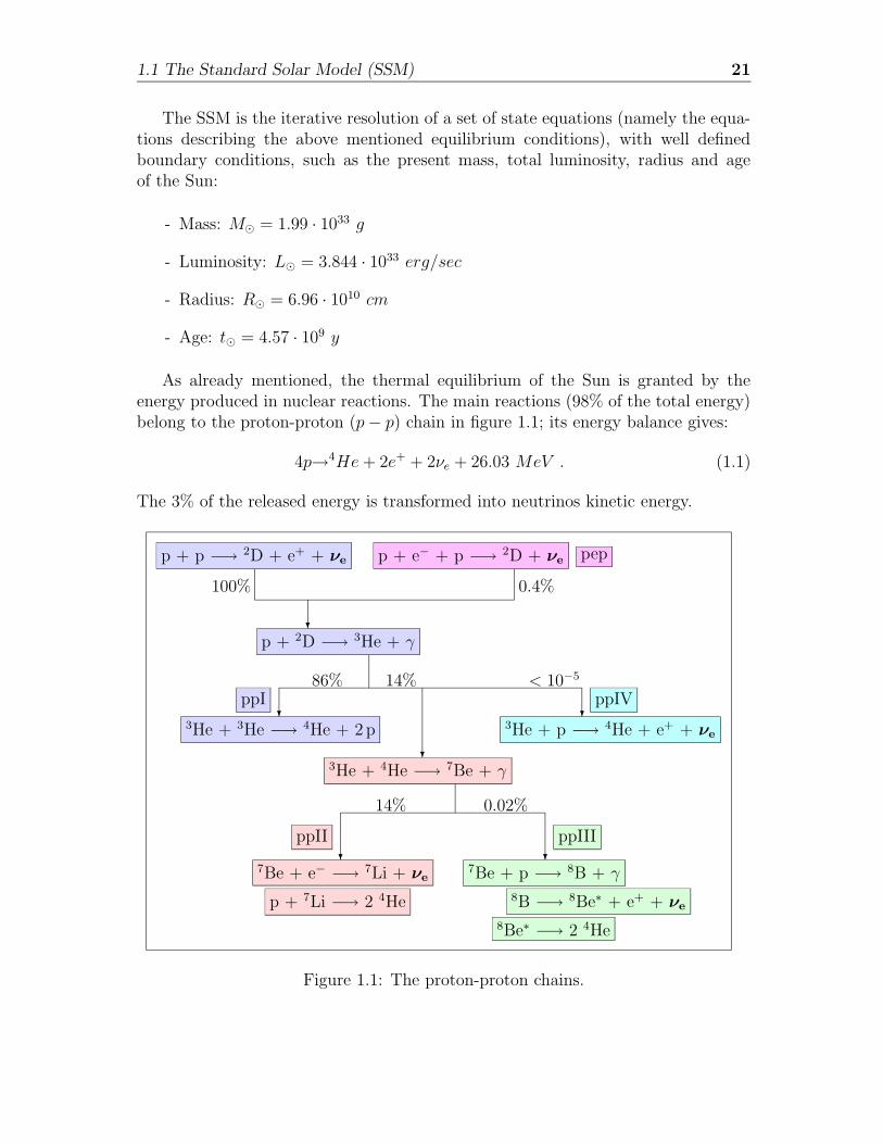
As already mentioned, the thermal equilibrium of the Sun is granted by theenergy produced in nuclear reactions. The main reactions (98% of the total energy)belong to the proton-proton (p− p) chain in figure 1.1; its energy balance gives:
4p→4He+ 2e+ + 2νe + 26.03 MeV . (1.1)
The 3% of the released energy is transformed into neutrinos kinetic energy.
p + p −→ 2D + e+ + νe p + e− + p −→ 2D + νe pep
100% 0.4%
?p + 2D −→ 3He + γ
86% 14% < 10−5
?
?
?ppI ppIV
3He + 3He −→ 4He + 2p 3He + p −→ 4He + e+ + νe
3He + 4He −→ 7Be + γ
14% 0.02%
? ?ppII ppIII
7Be + e− −→ 7Li + νe
p + 7Li −→ 2 4He
7Be + p −→ 8B + γ
8B −→ 8Be∗ + e+ + νe
8Be∗ −→ 2 4He
Figure 1.1: The proton-proton chains.
22 Solar Neutrino Physics in 2004
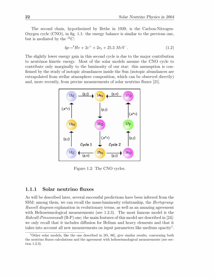
The second chain, hypothesized by Bethe in 1939, is the Carbon-Nitrogen-Oxygen cycle (CNO), in fig. 1.1: the energy balance is similar to the previous one,but is mediated by the 12C:
4p→4He+ 2e+ + 2νe + 25.3 MeV . (1.2)
The slightly lower energy gain in this second cycle is due to the major contributionto neutrinos kinetic energy. Most of the solar models assume the CNO cycle tocontribute only marginally to the luminosity of our star: this assumption is con-firmed by the study of isotopic abundances inside the Sun (isotopic abundances areextrapolated from stellar atmosphere composition, which can be observed directly)and, more recently, from precise measurements of solar neutrino fluxes [21].
Figure 1.2: The CNO cycles.
1.1.1 Solar neutrino fluxes
As will be described later, several successful predictions have been inferred from theSSM: among them, we can recall the mass-luminosity relationship, the Hertsprung-Russell diagram explanation in evolutionary terms, as well as an amazing agreementwith Helioseismological measurements (see 1.2.3). The most famous model is theBahcall-Pinsonneault (B-P) one; the main features of this model are described in [24]:we only recall that it includes diffusion for Helium and heavy elements and that ittakes into account all new measurements on input parameters like medium opacity1.
1Other solar models, like the one described in [85, 86], give similar results, concerning boththe neutrino fluxes calculations and the agreement with helioseismological measurements (see sec-tion 1.2.3).

1.1.1 Solar neutrino fluxes 23
Figure 1.3: A cross section of the sun, where core and convective zone are shown.
The Bahcall-Pinsonneault model is commonly used for solar neutrino fluxes com-putations; a rough estimate of such a flux can be obtained as follows:
- the Sun is supposed to be in an equilibrium state: the produced thermal energyis then equal to the energy irradiated from the surface;
- the solar energy flux reaching our planet is:
S = 8.5×10¹¹ MeV cm−2s−1;
- each 13 MeV of produced thermal energy, a neutrino is emitted2;
- therefore, the approximate neutrino flux is:
Φν = S/13 = 6×10¹⁰ νe cm−2s−1. (1.3)
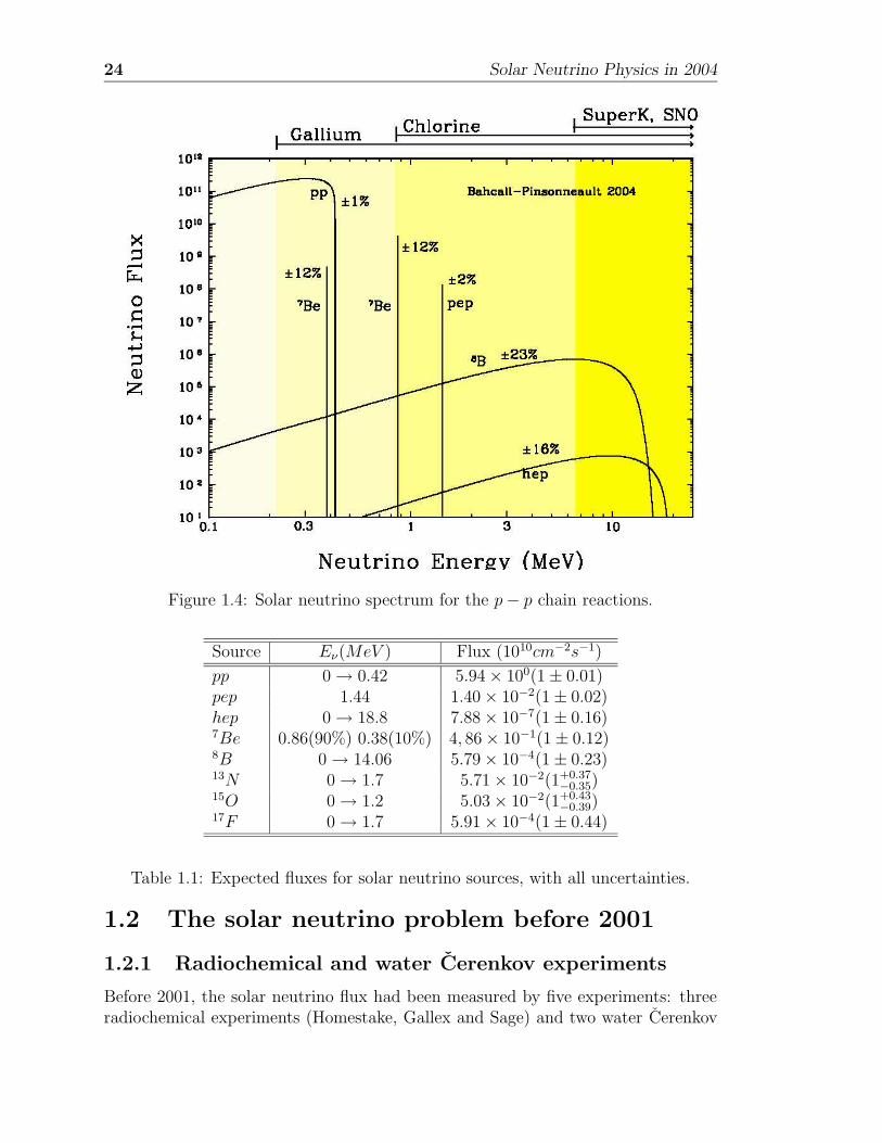
The Bahcall-Pinsonneault model allows the calculation of spectral shape of thesolar neutrino flux [23], as shown in fig. 1.4; in table 1.1 neutrino fluxes are listedwith their errors (due to all uncertainties on input parameters) [23].
2This assumption explains why the Sun luminosity constraint infers the total neutrino flux andnot the p− p one [19].
24 Solar Neutrino Physics in 2004
Figure 1.4: Solar neutrino spectrum for the p− p chain reactions.
Source Eν(MeV ) Flux (1010cm−2s−1)
pp 0→ 0.42 5.94× 100(1± 0.01)pep 1.44 1.40× 10⁻²(1± 0.02)hep 0→ 18.8 7.88× 10⁻⁷(1± 0.16)7Be 0.86(90%) 0.38(10%) 4, 86× 10−1(1± 0.12)8B 0→ 14.06 5.79× 10⁻⁴(1± 0.23)13N 0→ 1.7 5.71× 10⁻²(1+0.37
−0.35)15O 0→ 1.2 5.03× 10⁻²(1+0.43
−0.39)17F 0→ 1.7 5.91× 10⁻⁴(1± 0.44)
Table 1.1: Expected fluxes for solar neutrino sources, with all uncertainties.
1.2 The solar neutrino problem before 2001
1.2.1 Radiochemical and water Cerenkov experiments
Before 2001, the solar neutrino flux had been measured by five experiments: threeradiochemical experiments (Homestake, Gallex and Sage) and two water Cerenkov
1.2.1 Radiochemical and water Cerenkov experiments 25
experiments (Kamiokande and Super-Kamiokande). Before describing the details ofeach experiment, it is useful to remark that the realization of each of them constitutesa big technological challenge: since solar neutrinos have a very small interaction crosssection (' 10−44 ÷ 10−43 cm2), a huge target volume (> 100 t) has to be built ineach detector, in order to get a reasonable signal/background ratio; furthermore,all the background has to be dramatically reduced, concerning natural radioactivityof employed materials and cosmic rays induced background (for this reason, solarneutrino experiments are located underground, inside tunnels or mines, under thickrock layers).
• Homestake: the first solar neutrino experiment was installed in the late 60’sin the Homestake gold mine (South Dakota), at a depth of 4200 meters of waterequivalent (mwe) [39, 38]; the original concept of the Homestake detector wasdesigned by Ray Davis, acknowledged for this work with the 2002 Nobel Prizein Physics [79]. Detector target is made of 2.2×1030 37Cl atoms, in the formof 615 t of tetrachloroethylene (C2Cl4); neutrino detection interaction is:
νe +37 Cl→e− +37 Ar. (1.4)
This reaction has an energy threshold of 0.814 MeV , therefore it is sensitiveto 8B and 7Be neutrinos, but not to the p − p ones; moreover, this reactionis a charged current mediated interaction, then is only sensitive to electronneutrinos.
The experiment is radiochemistry based: 37Ar atoms are periodically extracted(37Ar decays back into 37Cl, with the emission of Auger electrons; mean lifeof 37Ar is 35 days); then they are inserted in low background proportionalcounters and observed during 250 to 400 days (7 to 11 mean lives).
The result for solar neutrino flux (after 25 years of runs) is [24]:
(2.56± 0.23) SNU 3
to be compared with the SSM prediction [23]:
(8.5± 1.8) SNU
(the 77% and 14% of this flux are due to the 8B and 7Be neutrinos respectively,while the contribution of pep and CNO neutrinos is lower then 1 SNU).
• GALLEX and SAGE: both experiments are based on the reaction
νe +71 Ga→ e− +71 Ge∗
31 SNU = 10−36 interactions per target atom per second;
26 Solar Neutrino Physics in 2004
featuring a very low energy threshold (0.2332 MeV ); this threshold allows todetect neutrinos produced in the first reaction of the solar chain, the p − pfusion (accounting for 91% of the total solar neutrino flux).
The GALLEX experiment was located underground at Gran Sasso NationalLaboratories (LNGS, Italy), at 1400m rock depth (3800mwe); detector targetis composed of 30.3 t of dissolved Gallium, in the form of 60 m3 of GaCl3.Germanium atoms produced in the reaction are chemically extracted every∼ 30 days (τGe = 16.4 d); their activity is then measured with the samemethod as the Homestake experiment.
The final measured flux (after 6 years of GALLEX, 1991-1997) is [58]:
(77.5± 6.2(stat) +4.5−4.3(syst)) SNU.
The B-P model foresees the following neutrino rate, for a Ga experiment [23]:
(131 +12−10) SNU,
with a partial contribution of 60% from the p − p reaction, and of 29% from7Be.
The GALLEX collaboration, in order to demonstrate the reliability and theprecision of their results, performed a set of calibration runs using two verystrong (and calibrated) neutrino sources (> 60 PBq of 51Cr); the combinedresult for 1994 and 1996 runs can be expressed in terms of the ratio between theneutrino source strength (derived from the measured rate of 71Ge production,divided by the directly determined source strength; this combined ratio (forthe two source experiments) is [59]:
0.93± 0.08,
which shows that the> 40% deficit of solar neutrino flux observed by GALLEXcannot be attributed to experimental artifacts.
GALLEX was concluded in 1997; after a complete reconstruction of propor-tional counters and related electronics, the experiment was restarted in 1998with the name of GNO (GNO was definitively closed in 2003). The combinedneutrino flux measured in GALLEX/GNO, for the period from 1991 to 2003,is [36]:
(69.3± 4.1(stat)± 3.6(syst)) SNU.
The SAGE experiment is located in Baksan underground Laboratory (4700mwe)in the Northern Caucasus Mountains; the target volume are 50 t of Galliumin metallic state [1]. The average measured flux (during the period from 1990to 2003) is [36]:
(66.9 +3.9−3.8(stat)
+3.6−3.2(syst)) SNU.
1.2.1 Radiochemical and water Cerenkov experiments 27
The ratios between measured and expected fluxes in Ga experiments are then:
GALLEX/GNO (52.9± 6.4)%
SAGE (51.1± 6.2)%
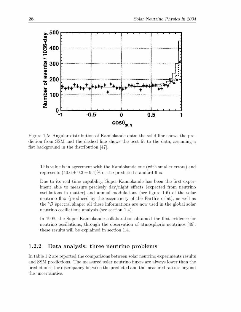
• Kamiokande: it was located in the Kamioka mine (Japan), at 2700 mwedepth; neutrinos are detected through the Cerenkov light produced in thescattering reaction (νx + e−→νx + e−) on the electrons of the 680 t of ultra-pure water which compose the fiducial volume; light is detected by means of948 photomultipliers (with a 20 inch photocathode). The energy threshold ofthis experiment is 7.5 MeV : this threshold is not due to the physics of thescattering process, but to the necessity to remove background events producedby natural radioactivity of materials (mainly water). Because of this threshold,only 8B neutrinos can be detected. Thanks to the scattering process, alsonon-electronics neutrinos can be detected (with a cross section of ∼ 1/6 of theelectron one).
Kamiokande has been the first experiment in real time, namely capable toidentify and reconstruct single events; for this reason, the detector was ableto measure not only the total neutrino flux, but also the direction and energyof neutrinos4. In this way, the solar origin of neutrinos was demonstrated forthe first time, since electrons are mainly scattered along the Sun-Earth vector(see figure 1.5).
Published results [47] report a measured 8B neutrino flux of:
(2.80± 0.19(stat)± 0.33(syst))×106cm−2s−1,
which is (48± 12± 13)% of the standard solar models.
The Kamiokande detector was also the first one capable to detect supernovaneutrinos in 1987 (see chapter 2); for this reason (as well as for solar neutrinoobservation), Kamiokande spokesperson Masatoshi Koshiba was awarded ofthe Nobel Prize in Physics in 2002 [79].
• Super-Kamiokande: this experiment is an enlargement of the Kamiokandeconcept, with bigger dimensions (50000 t of water, 22500 t of which are fiducialvolume, observed by 11146 20 inch PMTs) and a lower threshold (5 MeV ).
Super-Kamiokande phase I started in May 1996 and finished in July 20015; 8Bsolar neutrino flux observed during 1496 days of live time is [64]:
(2.35± 0.02(stat)± 0.08(syst))×106 cm−2s−1.
4Cerenkov detector measure the energy of each scattered electron, reconstructing then energyand direction of the incoming neutrinos.
5In July 2001, during some routine maintenance jobs, detector underwent a big accident: ap-proximately 50% of PMTs imploded during a water filling of the detector; after a re-positioning ofthe 5182 survived PMTs, the experiment was restarted in December 2002 with the so-called phaseII (data taking will continue until autumn 2005; the upgrade of the detector to the original PMTcoverage is foreseen in 2006).
28 Solar Neutrino Physics in 2004
Figure 1.5: Angular distribution of Kamiokande data; the solid line shows the pre-diction from SSM and the dashed line shows the best fit to the data, assuming aflat background in the distribution [47].
This value is in agreement with the Kamiokande one (with smaller errors) andrepresents (40.6± 9.3± 9.4)% of the predicted standard flux.
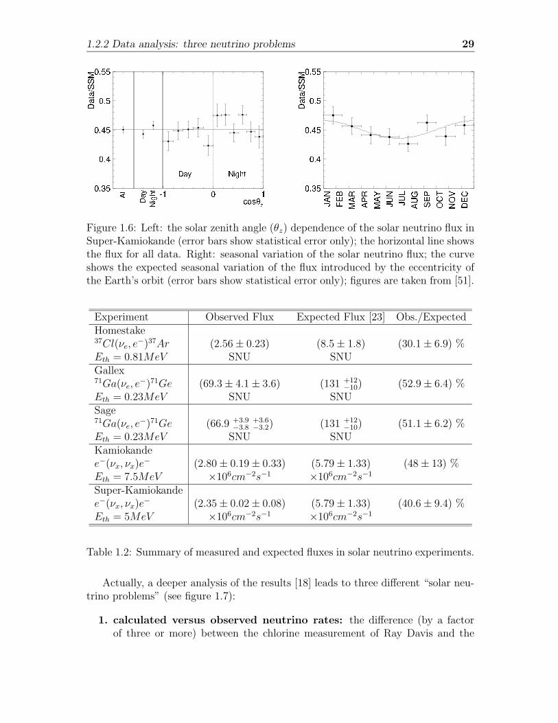
Due to its real time capability, Super-Kamiokande has been the first exper-iment able to measure precisely day/night effects (expected from neutrinooscillations in matter) and annual modulations (see figure 1.6) of the solarneutrino flux (produced by the eccentricity of the Earth’s orbit), as well asthe 8B spectral shape: all these informations are now used in the global solarneutrino oscillations analysis (see section 1.4).
In 1998, the Super-Kamiokande collaboration obtained the first evidence forneutrino oscillations, through the observation of atmospheric neutrinos [49];these results will be explained in section 1.4.
1.2.2 Data analysis: three neutrino problems
In table 1.2 are reported the comparisons between solar neutrino experiments resultsand SSM predictions. The measured solar neutrino fluxes are always lower than thepredictions: the discrepancy between the predicted and the measured rates is beyondthe uncertainties.
1.2.2 Data analysis: three neutrino problems 29
Figure 1.6: Left: the solar zenith angle (θz) dependence of the solar neutrino flux inSuper-Kamiokande (error bars show statistical error only); the horizontal line showsthe flux for all data. Right: seasonal variation of the solar neutrino flux; the curveshows the expected seasonal variation of the flux introduced by the eccentricity ofthe Earth’s orbit (error bars show statistical error only); figures are taken from [51].
Experiment Observed Flux Expected Flux [23] Obs./ExpectedHomestake37Cl(νe, e
−)37Ar (2.56± 0.23) (8.5± 1.8) (30.1± 6.9) %Eth = 0.81MeV SNU SNUGallex71Ga(νe, e
−)71Ge (69.3± 4.1± 3.6) (131 +12−10) (52.9± 6.4) %
Eth = 0.23MeV SNU SNUSage71Ga(νe, e
−)71Ge (66.9 +3.9−3.8
+3.6−3.2) (131 +12
−10) (51.1± 6.2) %Eth = 0.23MeV SNU SNUKamiokandee−(νx, νx)e
− (2.80± 0.19± 0.33) (5.79± 1.33) (48± 13) %Eth = 7.5MeV ×106cm−2s−1 ×106cm−2s−1
Super-Kamiokandee−(νx, νx)e
− (2.35± 0.02± 0.08) (5.79± 1.33) (40.6± 9.4) %Eth = 5MeV ×106cm−2s−1 ×106cm−2s−1
Table 1.2: Summary of measured and expected fluxes in solar neutrino experiments.
Actually, a deeper analysis of the results [18] leads to three different “solar neu-trino problems” (see figure 1.7):
1. calculated versus observed neutrino rates: the difference (by a factorof three or more) between the chlorine measurement of Ray Davis and the
30 Solar Neutrino Physics in 2004
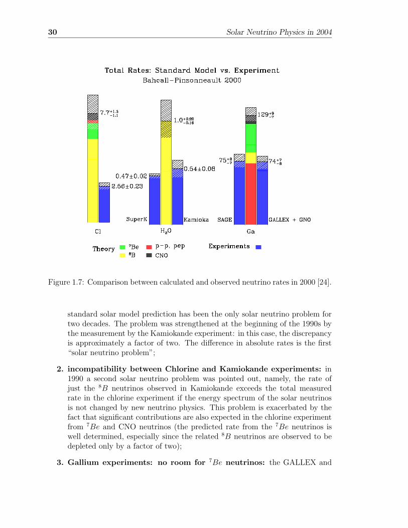
Figure 1.7: Comparison between calculated and observed neutrino rates in 2000 [24].
standard solar model prediction has been the only solar neutrino problem fortwo decades. The problem was strengthened at the beginning of the 1990s bythe measurement by the Kamiokande experiment: in this case, the discrepancyis approximately a factor of two. The difference in absolute rates is the first“solar neutrino problem”;
2. incompatibility between Chlorine and Kamiokande experiments: in1990 a second solar neutrino problem was pointed out, namely, the rate ofjust the 8B neutrinos observed in Kamiokande exceeds the total measuredrate in the chlorine experiment if the energy spectrum of the solar neutrinosis not changed by new neutrino physics. This problem is exacerbated by thefact that significant contributions are also expected in the chlorine experimentfrom 7Be and CNO neutrinos (the predicted rate from the 7Be neutrinos iswell determined, especially since the related 8B neutrinos are observed to bedepleted only by a factor of two);
3. Gallium experiments: no room for 7Be neutrinos: the GALLEX and
1.2.3 Astrophysical solutions 31
SAGE experiments present the third, essentially independent solar neutrinoproblem. The total observed rate is accounted for by the pp neutrinos, whoseflux can be calculated to an accuracy of 1%; therefore, the gallium experimentsdo not leave any room for the reliably calculated 7Be neutrinos (this is thereason why the third solar neutrino problem is sometimes referred to as “theproblem of the missing 7Be neutrinos”). Moreover, both the GALLEX andSAGE experiments have been directly calibrated with a radioactive source(51Cr) that emits neutrinos with similar energies to the 7Be neutrinos.
The “problem of the missing 7Be neutrinos” was the first hint that the solutionof the puzzle should have a physical (not astrophysical) nature; actually, the 7Beneutrinos suppression cannot be explained by modification of solar models, since the8B neutrinos detected in Kamiokande are produced in a competitive reaction withthe missing 7Be neutrinos, but solar model explanations that reduce the predicted7Be flux reduce much more the predictions for the observed 8B flux. For this reason,an independent measurement of the 7Be neutrino flux appeared strategic since 1990,in order to demonstrate the physical origin of the solar neutrino problems: the mainpurpose of the Borexino experiment is indeed a measurement of 7Be neutrinos.
1.2.3 Astrophysical solutions
Since the publication of the first Homestake results, a big improvement of the solarmodels took place in order to calculate more accurately solar neutrino fluxes: in thisway, a deep understanding of solar fluxes was obtained; the theoretical models havegradually been refined as improved input data, more accurate physics descriptionand more precise numerical techniques have been employed. In the meanwhile,there have been many studies of “non-standard” solar models that were designedto “solve” the solar neutrino problem: some of these models adopt different inputparameters (such as the metallicity of the sun or the radius of the convective zone),some other use different values for nuclear cross sections (for example, cross sectionof the process 3He +4 He →7 Be + γ is set to zero in one of these models), somehypothesize an artificially mixed sun core or suppress diffusion for helium and heavyelements [24].
None of these models succeeded in solving the puzzle; moreover, they show abig disagreement with helioseismological measurements. Helioseismology studiesoscillatory phenomena that occur inside the sun (and that can be observed on itssurface), in order to make accurate determinations of quantities such as: the interiorsound speeds, the density profile, the interior rotational speed, the depth of theconvective zone, the helium abundance and the heavy-element to hydrogen ratioin the convective zone, and even the radius of the sun. Opacity calculations andequation of state calculations can be therefore tested and improved by comparingtheory with observation of solar eigenfrequencies.
In figure 1.8, is shown the excellent agreement between the measured soundspeeds and the SSM computed ones, in the range from 0.05 R¯ to 0.95 R¯ (the
32 Solar Neutrino Physics in 2004
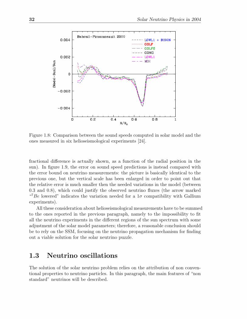
Figure 1.8: Comparison between the sound speeds computed in solar model and theones measured in six helioseismological experiments [24].
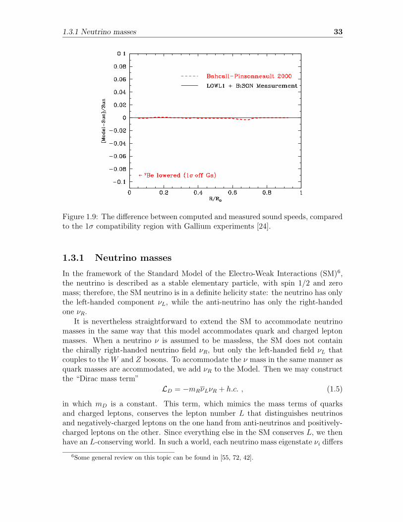
fractional difference is actually shown, as a function of the radial position in thesun). In figure 1.9, the error on sound speed predictions is instead compared withthe error bound on neutrino measurements: the picture is basically identical to theprevious one, but the vertical scale has been enlarged in order to point out thatthe relative error is much smaller then the needed variations in the model (between0.3 and 0.8), which could justify the observed neutrino fluxes (the arrow marked“7Be lowered” indicates the variation needed for a 1σ compatibility with Galliumexperiments).
All these consideration about helioseismological measurements have to be summedto the ones reported in the previous paragraph, namely to the impossibility to fitall the neutrino experiments in the different regions of the sun spectrum with someadjustment of the solar model parameters; therefore, a reasonable conclusion shouldbe to rely on the SSM, focusing on the neutrino propagation mechanism for findingout a viable solution for the solar neutrino puzzle.
1.3 Neutrino oscillations
The solution of the solar neutrino problem relies on the attribution of non conven-tional properties to neutrino particles. In this paragraph, the main features of “nonstandard” neutrinos will be described.
1.3.1 Neutrino masses 33
Figure 1.9: The difference between computed and measured sound speeds, comparedto the 1σ compatibility region with Gallium experiments [24].
1.3.1 Neutrino masses
In the framework of the Standard Model of the Electro-Weak Interactions (SM)6,the neutrino is described as a stable elementary particle, with spin 1/2 and zeromass; therefore, the SM neutrino is in a definite helicity state: the neutrino has onlythe left-handed component νL, while the anti-neutrino has only the right-handedone νR.
It is nevertheless straightforward to extend the SM to accommodate neutrinomasses in the same way that this model accommodates quark and charged leptonmasses. When a neutrino ν is assumed to be massless, the SM does not containthe chirally right-handed neutrino field νR, but only the left-handed field νL thatcouples to theW and Z bosons. To accommodate the ν mass in the same manner asquark masses are accommodated, we add νR to the Model. Then we may constructthe “Dirac mass term”
LD = −mRνLνR + h.c. , (1.5)
in which mD is a constant. This term, which mimics the mass terms of quarksand charged leptons, conserves the lepton number L that distinguishes neutrinosand negatively-charged leptons on the one hand from anti-neutrinos and positively-charged leptons on the other. Since everything else in the SM conserves L, we thenhave an L-conserving world. In such a world, each neutrino mass eigenstate νi differs
6Some general review on this topic can be found in [55, 72, 42].
34 Solar Neutrino Physics in 2004
from its antiparticle ν i, the difference being that L(ν i) = −L(νi). When νi 6= νi, werefer to the νi − νi complex as a “Dirac neutrino”.
Once νR has been added to our description of neutrinos, a “Majorana massterm”,
LM = −mRνcRνR + h.c. , (1.6)
can be constructed out of νR and its charge conjugate, νcR. In this term, mR is
another constant. Since both νR and νcR absorb ν and create ν, LM mixes ν and
ν. Thus, a Majorana mass term does not conserve L. There is then no conservedlepton number to distinguish a neutrino mass eigenstate νi from its antiparticle.Hence, when Majorana mass terms are present, ν i = νi. That is, for a given helicityh, νi(h) = νi(h). We then refer to νi as a “Majorana neutrino”.
Suppose the right-handed neutrinos required by Dirac mass terms have beenadded to the SM. If we insist that this extended SM conserve L, then, of course,Majorana mass terms are forbidden. However, if we do not impose L conservation,but require only the general principles of gauge invariance and renormalizability,then Majorana mass terms like that of equation (1.6) are expected to be present.As a result, L is violated, and neutrinos are Majorana particles.
If neutrino are massive particles, typically both mass terms (Dirac and Majorana)are possible. In this case, for a single neutrino generation, the Dirac-Majorana massterm is described by the lagrangian:
Lmass = −1
2
(
νL, νcR
)
(
mML mD
mD mMR
)(
νcL
νR
)
+ h.c. , (1.7)
where mD is the usual Dirac mass term, while mML and mM
R are the two Majoranamass terms; if CP is conserved for leptons, the mass matrix is real and the masseigenstates are Majorana neutrinos.
The experiments produce upper limits to neutrino masses and show how lightthe neutrino should be with respect to the charged leptons of the same generations.Many theoretical procedures can be invoked, in order to produce very small neutrinomasses: amongst them, the most natural one is the “see-saw” mechanism, in whichboth Dirac and Majorana mass terms are present [55]. If in (1.7) we set mM
L = 0(that is to say we introduce only the Majorana term constructed out of νR and itscharge conjugate) and M ≡ mM
R À mD (that is to say we introduce a very largemass term), the mixing matrix can be diagonalized with two eigenstates, m1 ' Mand m2 ' (mD)2/M . In this case, M can be an arbitrary large mass; a naturalchoice for this mass scale is suggested by the renormalizability constraint to be aslarge as the GUT scale (∼ 1015 GeV ). Since mD is the typical electro-weak scale(∼ 100 GeV ), m2 can be reduced down to 10−3 eV .
1.3.2 Experimental limits to neutrino masses
Until now, no attempt for the direct determination of neutrino masses has beensuccessful; nevertheless, upper bounds on neutrino masses have been set, according
1.3.2 Experimental limits to neutrino masses 35
to various methods:
• Kinematic limits to neutrino masses: the most common technique for theνe mass determination relies on tritium β decay (3H −→3 He+ e− + νe); mν
is computed from the β spectrum, close to the end-point. The lowest limits toνe mass have been set by two similar experiments (Moscow and Mainz), usingan electrostatic spectrometer with magnetic collimation; Moscow experimentuses a gaseous tritium source, while Mainz experiment uses a molecular tritiumfilm condensed on an aluminium layer. The best upper limits are:
mνe ≤ 2.5 eV (95%C.L.) (Moscow [67]),
mνe ≤ 2.2 eV (95%C.L.) (Mainz [32]).
Concerning νµ mass determination, the most efficient process is pion decay(π+ −→ µ+ + νµ). Present limits are referred to an experiment held at thePaul Scherrer Institut (Switzerland); the experiment implies a proton beamcolliding on a graphite target to produce π+; π+ decay in µ+ + νµ is analyzedby means of a muon spectrometer and of a micro-strip detector. The upperlimit quoted for this experiment is [14]:
mνµ ≤ 170KeV (90%C.L.).
The present upper limit to ντ mass has been set studying τ decay in pionsand a ντ ; this decay has been analyzed by the ALEPH experiment, during theLEP runs from 1991 to 1995; combining 3 and 5 pions decays, the followinglimit for mντ has been established [25]:
mντ ≤ 18.2MeV (95%C.L.).
• Double beta decay experiments: the 0νββ-decay ((A,Z)→ (A,Z + 2) +2e−) is the most promising process to investigate the Majorana nature of neu-trinos: this decay, if observed, would signal violation of the total lepton numberconservation. The process can be mediated by an exchange of a light Majo-rana neutrino, or by an exchange of other particles: however, the existenceof 0νββ-decay requires Majorana neutrino mass, no matter what the actualmechanism is. As long as only a limit on the lifetime is available, limits onthe effective Majorana neutrino mass < mββ > can be obtained7.
Present limits on half-life measurements of 0νββ-decay are in the range 1021÷1025 yr (depending on nuclear isotope and experimental technique) [42], while
7< mββ >=∑n
i=1 U21jmνj
, where n is the number of neutrino generations and νj is a Majorananeutrino.
36 Solar Neutrino Physics in 2004
the best available limits on< mββ > have been obtained with enriched 76Ge de-tectors and are in the range [42]8: < mββ > < (0.33÷1.35) eV (at 90% C.L.)9.Very interesting results, in the eV range, have been obtained also with otherisotopes, like 130Te, 116Cd, 136Xe, 100Mo and 128Te.
• Cosmological and astrophysical limits to neutrino masses: some fun-damental properties of neutrinos can be deduced by astrophysics and cosmol-ogy measurements. Copious numbers of neutrinos were produced in the earlyuniverse: if these neutrinos have non-negligible mass, they can make a non-trivial contribution to the total energy density of the universe during bothmatter and radiation domination10. The contribution of neutrinos to the en-ergy density of the universe depends upon the sum of the mass of the lightneutrino species:
Ωνh2 =
∑
imi
94.0 eV
(note that the sum only includes neutrino species light enough to decouplewhile still relativistic).
Combining data from Cosmic Microwave Background and from measurementsof large scale structures, the following limit on energy density in neutrinos canbe set [83]:
Ωνh2 < 0.0076 (95%C.L.).
This implies that∑
i
mi < 0.76 eV (95%C.L.).
Finally, upper limits on neutrino masses can be inferred from the observa-tion of neutrino bursts from supernova explosions. During the explosion of1987A supernova, about 4 ·1015ν/m2 neutrinos reached the earth during a fewseconds. The Kamiokande detector was capable to observe these supernovaneutrinos [79]; from the time distribution of the burst data, some upper limitscould be calculated on electron neutrino mass [61], ranging from a few eV to24 eV (depending on different models and calculations).
8Presently, the only claim for positive observation of 0νββ-decay comes from [65]: this result isstill unconfirmed.
9The extrapolation from half-life to effective Majorana mass is complicated by big uncertaintieson nuclear matrix elements: this explains the wide range in effective mass limits.
10Furthermore, neutrinos can influence smaller scale fluctuations during matter domination,changing the shape of CMB angular power spectrum and suppressing the amplitude of fluctuations;they also can leave an observable imprint on the galaxy large scale structure power spectrum [83].
1.3.3 Mixing of the mass eigenstates and vacuum oscillations 37
1.3.3 Mixing of the mass eigenstates and vacuum oscilla-tions
If neutrinos are massive, there is a spectrum of three or more neutrino mass eigen-states νi (i = 1, 2, 3, ...), that are the analogues of the charged-lepton mass eigen-states e,µ and τ . If lepton mix, neutrino flavor eigenstates νl (l = e, µ, τ), are notsupposed to be coincident with mass eigenstates, but to be a superposition of themass eigenstates. In this case, such a superposition can be represented through amixing matrix [72]:
νl =3∑
i=1
Uliνi , (1.8)
where U is an unitary matrix (U †U = I). In this representation, neutrino masslimits quoted in 1.3.2 have to be referred to the dominant state for each generation(for example, the limit on νe mass applies to the ν1 state).
A mixing scenario for neutrinos was first proposed in 1967 by B. Pontecorvo [74]:at that time, only one generation of neutrinos was known. Pontecorvo assumed anonzero neutrino mass and supposed that the neutrino observed in interactions withelementary particles was a superposition of two Majorana neutrinos with differentmasses. In this case, an oscillatory phenomenon νL ↔ νL would have been possiblein a neutrino beam. Later on, after the discovery of a second neutrino generation,oscillations νeL ↔ νµL between different flavors were considered.
Therefore, the mixing hypothesis allows the possibility of neutrino oscillations,namely the possibility that an electron neutrino (for example) could be detected asa muon neutrino at some distance from its emitting source. In case of two neutrinogenerations11, the equation (1.8) can be parameterized with a mixing angle θ [72]:
(
νeνµ
)
=
(
cos θ sin θ− sin θ cos θ
)(
ν1ν2
)
. (1.9)
We are interested in computing the probability for a neutrino with a well-definedstarting flavor να, created at a time t = 0 in x = 0 by a weak process, to interactas another flavor neutrino νβ, in a detector at a distance x = L from its productionsite.
The time evolution of mass eigenstates νi (i = 1, 2) follows Schrodinger equation:
νi(t) = e−iEitνi(0), where Ei =√
p2 +mi2 . (1.10)
Since m1 6= m2, the flavor eigenstates νe, produced at t = 0, evolve in time into a
11Even if the two neutrino generations case is not realistic, its study is useful, since typicallythe three generations problem can be reduced to a pair of simpler two generations problems; adescription of the complete 3 ν formalism can be found in [45].
38 Solar Neutrino Physics in 2004
superposition of νe and νµ states. If we set νi ≡ νi(0),
νe(t) = cos θe−iE1tν1 + sin θe−iE2tν2
=[
cos2 θe−iE1t + sin2 θe−iE2t]
νe +[
cos θ sin θ(
e−iE2t − e−iE1t)]
νµ
= Aee(t)νe + Aeµ(t)νµ . (1.11)
Using equation (1.11), the probability for the state νe(t) to be in a flavor eigenstateνe or νµ at a time t can be computed:
P (νe → νe; t) = |Aee(t)|2 = 1− 1
2sin2 2θ [1− cos(E2 − E1)t] (1.12)
P (νe → νµ; t) = |Aeµ(t)|2 =1
2sin2 2θ [1− cos(E2 − E1)t] . (1.13)
When neutrino masses are small compared to their momentum, we can write:
Ei =√
p2 +mi2 ' |p|+ m2
i
2|p| , where t ' L , (1.14)
and L is the distance covered by neutrinos in the time t (we recall that c ≡ 1 in ourequations). The equation (1.13) can therefore be rewritten as:
P (νe → νµ; t) =1
2sin2 2θ
[
1− cosδm2
2|p|L]
= sin2 2θ sin2πL
λ0, (1.15)
where δm2 = |m22 −m2
1| and λ0 = 4πE/δm2 is the oscillation length in vacuum (werecall that |p| ' E). Substituting the numerical values, we obtain:
λ0 =4πEν
δm2' 2.47 ·
(
Eν
1MeV
)
·(
1eV 2
δm2
)
m . (1.16)
Maximum oscillation amplitude is present if θ = π/4 (this case is called maximalmixing).
The first consequence of the oscillation mechanism is the non-conservation ofleptonic number l for each family: in case of neutrino oscillation (να ↔ νβ), leptonflavor is not conserved and δl = ±1: in the Dirac neutrino case, the global conservedsymmetry is the total leptonic number (le + lµ + lτ ), while in the Majorana case thetotal leptonic number is not conserved.
The second consequence is the possibility to study the order of magnitude ofneutrino masses difference, also in the regions well below 1 eV . Looking at equa-tions (1.15) and (1.16), it is easy to conclude that the δm2 sensitivity for an exper-iment depends on the E/L ratio, since δm2[eV 2] ≈ E[MeV ]/L[m]. Depending onthe experiment type, this ratio can be in the range between 102 and 10−11 eV 2.
1.3.4 Matter enhanced neutrino oscillations 39
1.3.4 Matter enhanced neutrino oscillations
The previously discussed oscillation mechanism is based on the vacuum propagationof ultra-relativistic neutrinos:
νi(t) = νiei(px−Eit)' νie−it
mi2
2p (1.17)
When propagation takes place in matter, the phase factor ipx becomes ipnx, wheren is the refraction index. The possibility for a neutrino to change its lepton flavor istherefore modified [87] and oscillations can be enhanced in special conditions [70]:the model describing such a phenomena is known as MSW, from the initials of thephysicists who first discussed it.
The refraction index in matter is different from 1 due to the weak interactionsof neutrinos:
nl = 1 +2πN
p2fl(0) , (1.18)
where N is the density of diffusion centers and fl(0) is the forward scattering prob-ability amplitude for l-flavored neutrinos (neutrino absorption can be neglected andonly the real component of fl(0) is considered).
The origin of the MSW effect is connected to the fact that electron neutrinos caninteract in matter also through charged current interactions with electrons. Whileall neutrino species have the same interactions in matter due to the neutral currents,the νe weak interaction eigenstates (because of their charged current interactions),as they propagate in matter, experience a slightly different index of refraction thanthe νµ and ντ weak interaction eigenstates: this different index of refraction for νealters the time evolution of the system from what happens in vacuum.
The computation of the Feynman diagrams for charged and neutral current in-teractions holds (for energies much lower than the W boson mass):
∆f(0) = fe(0)− fα(0) = −√2GFp
2π, (1.19)
where α is a non-electronic neutrino flavor and GF is the usual Fermi constant. Wethen obtain a contribution to the time evolution of the neutrino beam:
νe(x) = νe(0)eipnx = νe(0)e
−√2GFNex . (1.20)
Therefore, an oscillation length in matter λ0m can be defined:
λ0m =2π√
2GFNe
' 1.7×10⁷ρ[g cm−3]Z
A
m , (1.21)
where Ne is the electron density in matter. Let’s point out that, on the contraryto λ0, λ0m is independent from neutrino energy. Including the forward scattering inmatter, we obtain the time evolution equation for mass eigenstates ν1 and ν2:
id
dt
(
ν1ν2
)
=
(
m12
2p+√2GFNe cos
2 θ +√2GFNe sin θ cos θ
+√2GFNe sin θ cos θ
m22
2p+√2GFNe sin
2 θ
)
(
ν1ν2
)
(1.22)
40 Solar Neutrino Physics in 2004
This matrix can be diagonalized, and the mixing angle in matter is:
tan 2θm = tan 2θ
(
1 +λ0λ0m
sec 2θ
)−1
. (1.23)
The difference between the matrix eigenvalues gives the effective oscillation lengthin matter:
λm = λ0sin 2θmsin 2θ
= λ0
[
1 +
(
λ0λ0m
)2
+2λ0λ0m
cos 2θ
]−1/2
, (1.24)
while the νe survival probability at a distance L from the production site is:
P (Eν , L, θ, δm2) = 1− sin2 θm sin2
πL
λm
, (1.25)
where θm e λm depend on the vacuum oscillation parameters θ and λ0.Three different possibilities arise for λ0 and λ0m:
• |λ0| ¿ λ0m: matter has no substantial effects on oscillations;
• |λ0| À λ0m: the oscillation amplitude is suppressed by the factor λ0m/|λ0|,and the effective oscillation length λm ' λ0m does not depend on vacuumoscillation parameters;
• |λ0|'λ0m: in this case the oscillation effect is enhanced (resonant); in theparticular case λ0/λ0m = − cos 2θ, we obtain sin2 2θm = 1 (that is to sayθm = π/4) and the effective oscillation length is: λm = λ0/ sin
2 2θ. For amaterial where Z/A ' 1/2, the resonance condition can be written as:
Enu[MeV ]
δm2[eV 2]' 0.65× 10⁻⁷ cos 2θ
ρ[g cm−3].
1.4 Neutrino oscillation experiments
On the experimental side, oscillation phenomena can be studied by means of a knownneutrino source να and observing either the appearance of a second neutrino flavorνβ at a given distance (appearance experiments), or measuring a possible reductionof the initial flux (disappearance experiments).
Equations in (1.15) and (1.16) can be merged into:
P (νe → νµ; t) = sin2 2θ sin2δm2L
4Eν
' sin2 2θ sin2(
1.27L[m]
Eν [MeV ]δm2[eV 2]
)
,
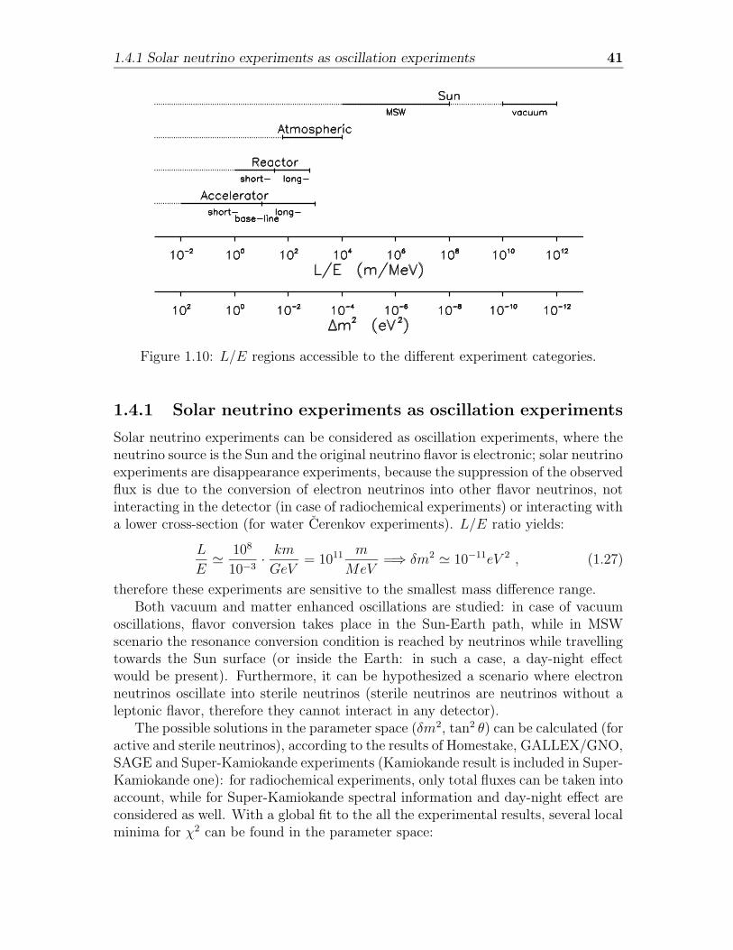
(1.26)from which we can understand that the sensitivity of a given oscillation experimentdepend on its L/E ratio, which determines the detectable values of δm2 and sin2 2θ.In figure 1.10 the experimental sensitivity is shown for each experiment type.
In the following, a somewhat historical account of the determination of the νoscillation parameters is adopted.
1.4.1 Solar neutrino experiments as oscillation experiments 41
Figure 1.10: L/E regions accessible to the different experiment categories.
1.4.1 Solar neutrino experiments as oscillation experiments
Solar neutrino experiments can be considered as oscillation experiments, where theneutrino source is the Sun and the original neutrino flavor is electronic; solar neutrinoexperiments are disappearance experiments, because the suppression of the observedflux is due to the conversion of electron neutrinos into other flavor neutrinos, notinteracting in the detector (in case of radiochemical experiments) or interacting witha lower cross-section (for water Cerenkov experiments). L/E ratio yields:
L
E' 108
10−3· kmGeV
= 1011m
MeV=⇒ δm2 ' 10−11eV 2 , (1.27)
therefore these experiments are sensitive to the smallest mass difference range.Both vacuum and matter enhanced oscillations are studied: in case of vacuum
oscillations, flavor conversion takes place in the Sun-Earth path, while in MSWscenario the resonance conversion condition is reached by neutrinos while travellingtowards the Sun surface (or inside the Earth: in such a case, a day-night effectwould be present). Furthermore, it can be hypothesized a scenario where electronneutrinos oscillate into sterile neutrinos (sterile neutrinos are neutrinos without aleptonic flavor, therefore they cannot interact in any detector).
The possible solutions in the parameter space (δm2, tan2 θ) can be calculated (foractive and sterile neutrinos), according to the results of Homestake, GALLEX/GNO,SAGE and Super-Kamiokande experiments (Kamiokande result is included in Super-Kamiokande one): for radiochemical experiments, only total fluxes can be taken intoaccount, while for Super-Kamiokande spectral information and day-night effect areconsidered as well. With a global fit to the all the experimental results, several localminima for χ2 can be found in the parameter space:
42 Solar Neutrino Physics in 2004
• MSW solutions: three solutions are present for matter enhanced oscillations:LMA (Large Mixing Angle), SMA (Small Mixing Angle) and LOW (Low prob-ability, Low mass);
• vacuum oscillations: two different vacuum oscillation solutions are present,called VAC an JustSo2;
• sterile neutrino oscillations: in this scenario, only one SMA and two vac-uum solutions are possible.
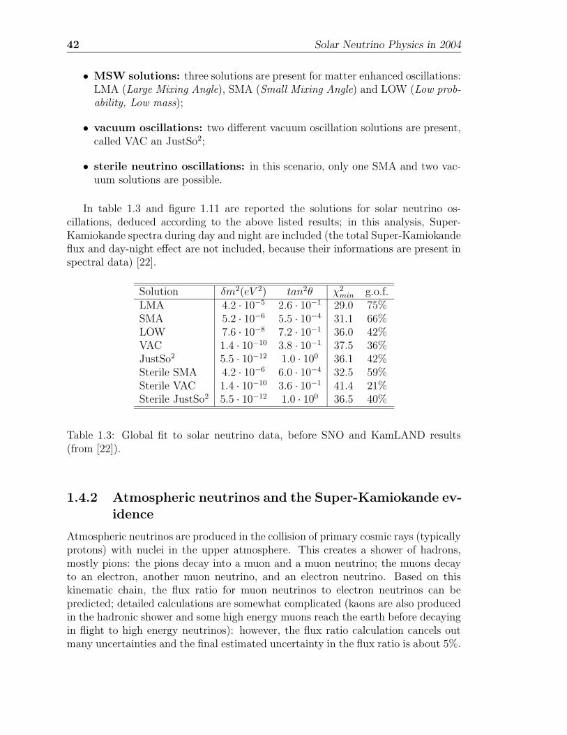
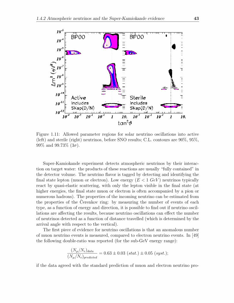
In table 1.3 and figure 1.11 are reported the solutions for solar neutrino os-cillations, deduced according to the above listed results; in this analysis, Super-Kamiokande spectra during day and night are included (the total Super-Kamiokandeflux and day-night effect are not included, because their informations are present inspectral data) [22].
Solution δm2(eV 2) tan2θ χ2min g.o.f.
LMA 4.2 · 10−5 2.6 · 10−1 29.0 75%SMA 5.2 · 10−6 5.5 · 10−4 31.1 66%LOW 7.6 · 10−8 7.2 · 10−1 36.0 42%VAC 1.4 · 10−10 3.8 · 10−1 37.5 36%JustSo2 5.5 · 10−12 1.0 · 100 36.1 42%Sterile SMA 4.2 · 10−6 6.0 · 10−4 32.5 59%Sterile VAC 1.4 · 10−10 3.6 · 10−1 41.4 21%Sterile JustSo2 5.5 · 10−12 1.0 · 100 36.5 40%
Table 1.3: Global fit to solar neutrino data, before SNO and KamLAND results(from [22]).
1.4.2 Atmospheric neutrinos and the Super-Kamiokande ev-idence
Atmospheric neutrinos are produced in the collision of primary cosmic rays (typicallyprotons) with nuclei in the upper atmosphere. This creates a shower of hadrons,mostly pions: the pions decay into a muon and a muon neutrino; the muons decayto an electron, another muon neutrino, and an electron neutrino. Based on thiskinematic chain, the flux ratio for muon neutrinos to electron neutrinos can bepredicted; detailed calculations are somewhat complicated (kaons are also producedin the hadronic shower and some high energy muons reach the earth before decayingin flight to high energy neutrinos): however, the flux ratio calculation cancels outmany uncertainties and the final estimated uncertainty in the flux ratio is about 5%.
1.4.2 Atmospheric neutrinos and the Super-Kamiokande evidence 43
Figure 1.11: Allowed parameter regions for solar neutrino oscillations into active(left) and sterile (right) neutrinos, before SNO results; C.L. contours are 90%, 95%,99% and 99.73% (3σ).
Super-Kamiokande experiment detects atmospheric neutrinos by their interac-tion on target water: the products of these reactions are usually “fully contained” inthe detector volume. The neutrino flavor is tagged by detecting and identifying thefinal state lepton (muon or electron). Low energy (E < 1 GeV ) neutrinos typicallyreact by quasi-elastic scattering, with only the lepton visible in the final state (athigher energies, the final state muon or electron is often accompanied by a pion ornumerous hadrons). The properties of the incoming neutrino can be estimated fromthe properties of the Cerenkov ring: by measuring the number of events of eachtype, as a function of energy and direction, it is possible to find out if neutrino oscil-lations are affecting the results, because neutrino oscillations can effect the numberof neutrinos detected as a function of distance travelled (which is determined by thearrival angle with respect to the vertical).
The first piece of evidence for neutrino oscillations is that an anomalous numberof muon neutrino events is measured, compared to electron neutrino events. In [49]the following double-ratio was reported (for the sub-GeV energy range):
(Nµ/Ne)data(Nµ/Ne)predicted
= 0.63± 0.03 (stat.)± 0.05 (syst.);
if the data agreed with the standard prediction of muon and electron neutrino pro-
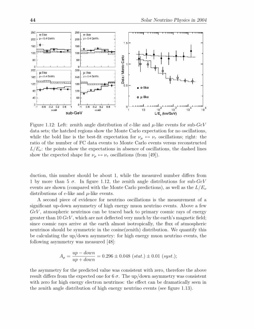
44 Solar Neutrino Physics in 2004
Figure 1.12: Left: zenith angle distribution of e-like and µ-like events for sub-GeVdata sets; the hatched regions show the Monte Carlo expectation for no oscillations,while the bold line is the best-fit expectation for νµ ↔ ντ oscillations; right: theratio of the number of FC data events to Monte Carlo events versus reconstructedL/Eν : the points show the expectations in absence of oscillations, the dashed linesshow the expected shape for νµ ↔ ντ oscillations (from [49]).
duction, this number should be about 1, while the measured number differs from1 by more than 5 σ. In figure 1.12, the zenith angle distributions for sub-GeVevents are shown (compared with the Monte Carlo predictions), as well as the L/Eν
distributions of e-like and µ-like events.
A second piece of evidence for neutrino oscillations is the measurement of asignificant up-down asymmetry of high energy muon neutrino events. Above a fewGeV , atmospheric neutrinos can be traced back to primary cosmic rays of energygreater than 10GeV , which are not deflected very much by the earth’s magnetic field;since cosmic rays arrive at the earth almost isotropically, the flux of atmosphericneutrinos should be symmetric in the cosine(zenith) distribution. We quantify thisbe calculating the up/down asymmetry: for high energy muon neutrino events, thefollowing asymmetry was measured [48]:
Aµ =up− downup+ down
= 0.296± 0.048 (stat.)± 0.01 (syst.);
the asymmetry for the predicted value was consistent with zero, therefore the aboveresult differs from the expected one for 6 σ. The up/down asymmetry was consistentwith zero for high energy electron neutrinos: the effect can be dramatically seen inthe zenith angle distribution of high energy neutrino events (see figure 1.13).
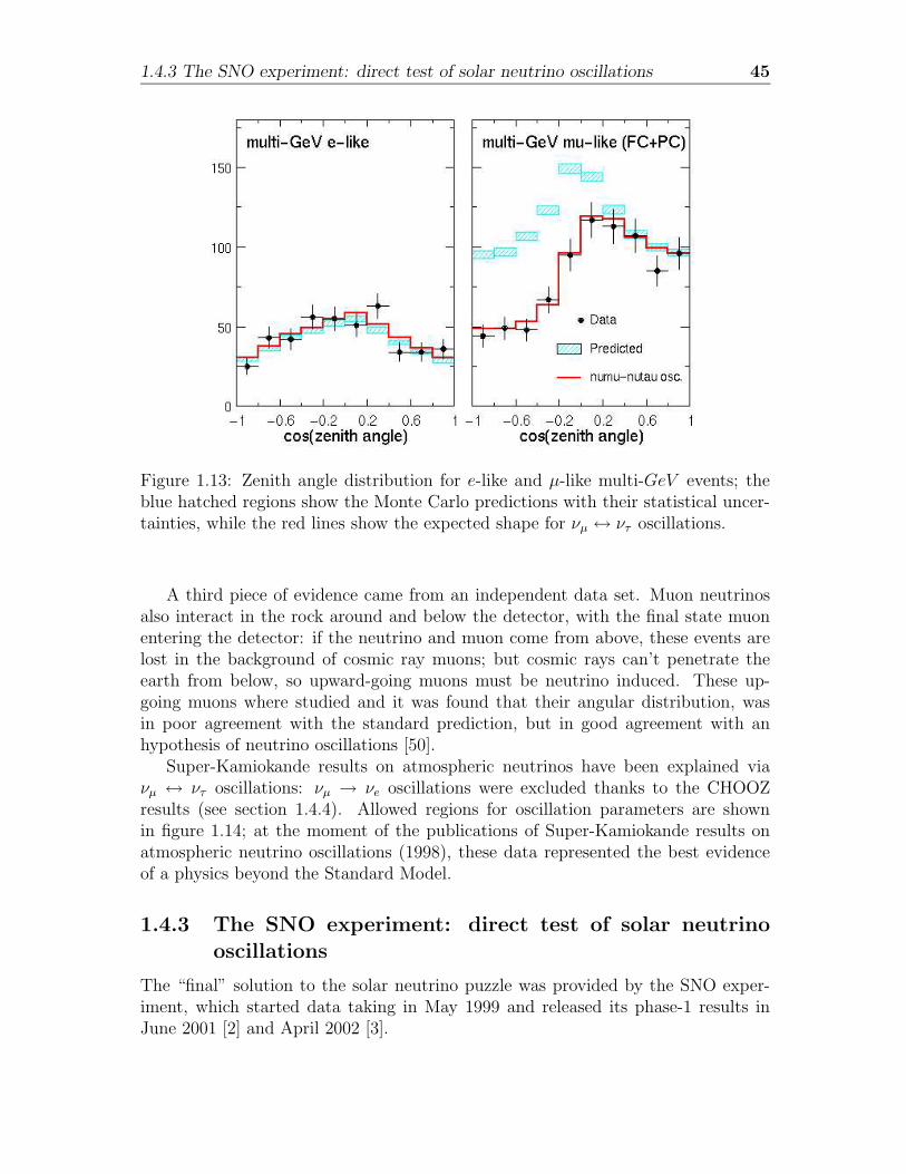
1.4.3 The SNO experiment: direct test of solar neutrino oscillations 45
Figure 1.13: Zenith angle distribution for e-like and µ-like multi-GeV events; theblue hatched regions show the Monte Carlo predictions with their statistical uncer-tainties, while the red lines show the expected shape for νµ ↔ ντ oscillations.
A third piece of evidence came from an independent data set. Muon neutrinosalso interact in the rock around and below the detector, with the final state muonentering the detector: if the neutrino and muon come from above, these events arelost in the background of cosmic ray muons; but cosmic rays can’t penetrate theearth from below, so upward-going muons must be neutrino induced. These up-going muons where studied and it was found that their angular distribution, wasin poor agreement with the standard prediction, but in good agreement with anhypothesis of neutrino oscillations [50].
Super-Kamiokande results on atmospheric neutrinos have been explained viaνµ ↔ ντ oscillations: νµ → νe oscillations were excluded thanks to the CHOOZresults (see section 1.4.4). Allowed regions for oscillation parameters are shownin figure 1.14; at the moment of the publications of Super-Kamiokande results onatmospheric neutrino oscillations (1998), these data represented the best evidenceof a physics beyond the Standard Model.
1.4.3 The SNO experiment: direct test of solar neutrinooscillations
The “final” solution to the solar neutrino puzzle was provided by the SNO exper-iment, which started data taking in May 1999 and released its phase-1 results inJune 2001 [2] and April 2002 [3].
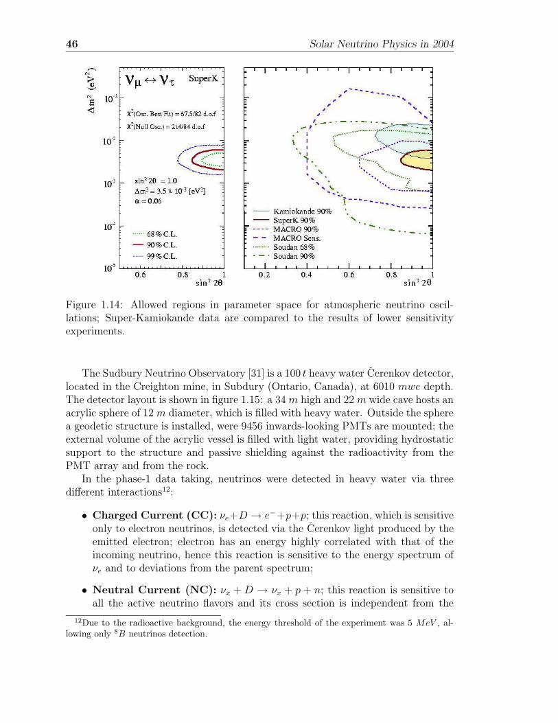
46 Solar Neutrino Physics in 2004
Figure 1.14: Allowed regions in parameter space for atmospheric neutrino oscil-lations; Super-Kamiokande data are compared to the results of lower sensitivityexperiments.
The Sudbury Neutrino Observatory [31] is a 100 t heavy water Cerenkov detector,located in the Creighton mine, in Subdury (Ontario, Canada), at 6010 mwe depth.The detector layout is shown in figure 1.15: a 34m high and 22m wide cave hosts anacrylic sphere of 12 m diameter, which is filled with heavy water. Outside the spherea geodetic structure is installed, were 9456 inwards-looking PMTs are mounted; theexternal volume of the acrylic vessel is filled with light water, providing hydrostaticsupport to the structure and passive shielding against the radioactivity from thePMT array and from the rock.
In the phase-1 data taking, neutrinos were detected in heavy water via threedifferent interactions12:
• Charged Current (CC): νe+D → e−+p+p; this reaction, which is sensitiveonly to electron neutrinos, is detected via the Cerenkov light produced by theemitted electron; electron has an energy highly correlated with that of theincoming neutrino, hence this reaction is sensitive to the energy spectrum ofνe and to deviations from the parent spectrum;
• Neutral Current (NC): νx +D → νx + p + n; this reaction is sensitive toall the active neutrino flavors and its cross section is independent from the
12Due to the radioactive background, the energy threshold of the experiment was 5 MeV , al-lowing only 8B neutrinos detection.
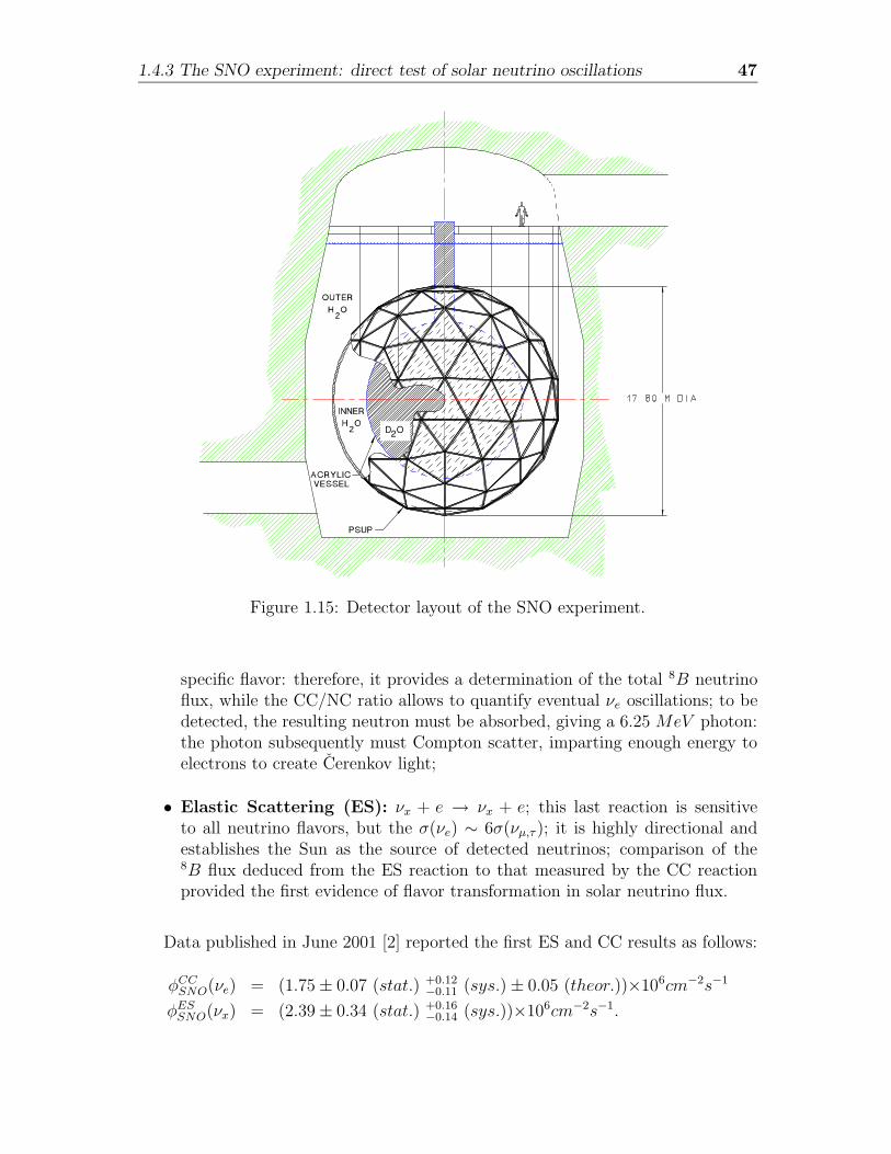
1.4.3 The SNO experiment: direct test of solar neutrino oscillations 47
D O2
Figure 1.15: Detector layout of the SNO experiment.
specific flavor: therefore, it provides a determination of the total 8B neutrinoflux, while the CC/NC ratio allows to quantify eventual νe oscillations; to bedetected, the resulting neutron must be absorbed, giving a 6.25 MeV photon:the photon subsequently must Compton scatter, imparting enough energy toelectrons to create Cerenkov light;
• Elastic Scattering (ES): νx + e → νx + e; this last reaction is sensitiveto all neutrino flavors, but the σ(νe) ∼ 6σ(νµ,τ ); it is highly directional andestablishes the Sun as the source of detected neutrinos; comparison of the8B flux deduced from the ES reaction to that measured by the CC reactionprovided the first evidence of flavor transformation in solar neutrino flux.
Data published in June 2001 [2] reported the first ES and CC results as follows:
φCCSNO(νe) = (1.75± 0.07 (stat.) +0.12
−0.11 (sys.)± 0.05 (theor.))×106cm−2s−1
φESSNO(νx) = (2.39± 0.34 (stat.) +0.16
−0.14 (sys.))×106cm−2s−1.
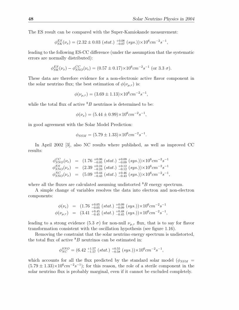
48 Solar Neutrino Physics in 2004
The ES result can be compared with the Super-Kamiokande measurement:
φESSK(νx) = (2.32± 0.03 (stat.) +0.08
−0.07 (sys.))×106cm−2s−1,
leading to the following ES-CC difference (under the assumption that the systematicerrors are normally distributed):
φESSK(νx)− φCC
SNO(νe) = (0.57± 0.17)×106cm−2s−1 (or 3.3 σ).
These data are therefore evidence for a non-electronic active flavor component inthe solar neutrino flux; the best estimation of φ(νµ,τ ) is:
φ(νµ,τ ) = (3.69± 1.13)×106cm−2s−1,
while the total flux of active 8B neutrinos is determined to be:
φ(νx) = (5.44± 0.99)×106cm−2s−1,
in good agreement with the Solar Model Prediction:
φSSM = (5.79± 1.33)×106cm−2s−1.
In April 2002 [3], also NC results where published, as well as improved CCresults:
φCCSNO(νe) = (1.76 +0.06
−0.05 (stat.) +0.09−0.09 (sys.))×106cm−2s−1
φESSNO(νx) = (2.39 +0.24
−0.23 (stat.) +0.12−0.12 (sys.))×106cm−2s−1
φNCSNO(νx) = (5.09 +0.44
−0.43 (stat.) +0.46−0.43 (sys.))×106cm−2s−1,
where all the fluxes are calculated assuming undistorted 8B energy spectrum.A simple change of variables resolves the data into electron and non-electron
components:
φ(νe) = (1.76 +0.05−0.05 (stat.) +0.09
−0.09 (sys.))×106cm−2s−1
φ(νµ,τ ) = (3.41 +0.45−0.45 (stat.) +0.48
−0.45 (sys.))×106cm−2s−1,
leading to a strong evidence (5.3 σ) for non-null νµ,τ flux, that is to say for flavortransformation consistent with the oscillation hypothesis (see figure 1.16).
Removing the constraint that the solar neutrino energy spectrum is undistorted,the total flux of active 8B neutrinos can be estimated in:
φSNONC = (6.42 +1.57
−1.57 (stat.) +0.55−0.58 (sys.))×106cm−2s−1,
which accounts for all the flux predicted by the standard solar model (φSSM =(5.79 ± 1.33)×106cm−2s−1); for this reason, the role of a sterile component in thesolar neutrino flux is probably marginal, even if it cannot be excluded completely.
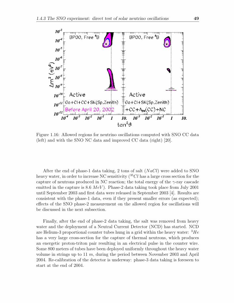
1.4.3 The SNO experiment: direct test of solar neutrino oscillations 49
JHEP07(2002)054
Figure 1.16: Allowed regions for neutrino oscillations computed with SNO CC data(left) and with the SNO NC data and improved CC data (right) [20].
After the end of phase-1 data taking, 2 tons of salt (NaCl) were added to SNOheavy water, in order to increase NC sensitivity (35Cl has a large cross section for thecapture of neutrons produced in NC reaction; the total energy of the γ-ray cascadeemitted in the capture is 8.6 MeV ). Phase-2 data taking took place from July 2001until September 2003 and first data were released in September 2003 [4]. Results areconsistent with the phase-1 data, even if they present smaller errors (as expected);effects of the SNO phase-2 measurement on the allowed region for oscillations willbe discussed in the next subsection.
Finally, after the end of phase-2 data taking, the salt was removed from heavywater and the deployment of a Neutral Current Detector (NCD) has started. NCDare Helium-3 proportional counter tubes hung in a grid within the heavy water: 3Hehas a very large cross-section for the capture of thermal neutrons, which producesan energetic proton-triton pair resulting in an electrical pulse in the counter wire.Some 800 meters of tubes have been deployed uniformly throughout the heavy watervolume in strings up to 11 m, during the period between November 2003 and April2004. Re-calibration of the detector is underway: phase-3 data taking is foreseen tostart at the end of 2004.
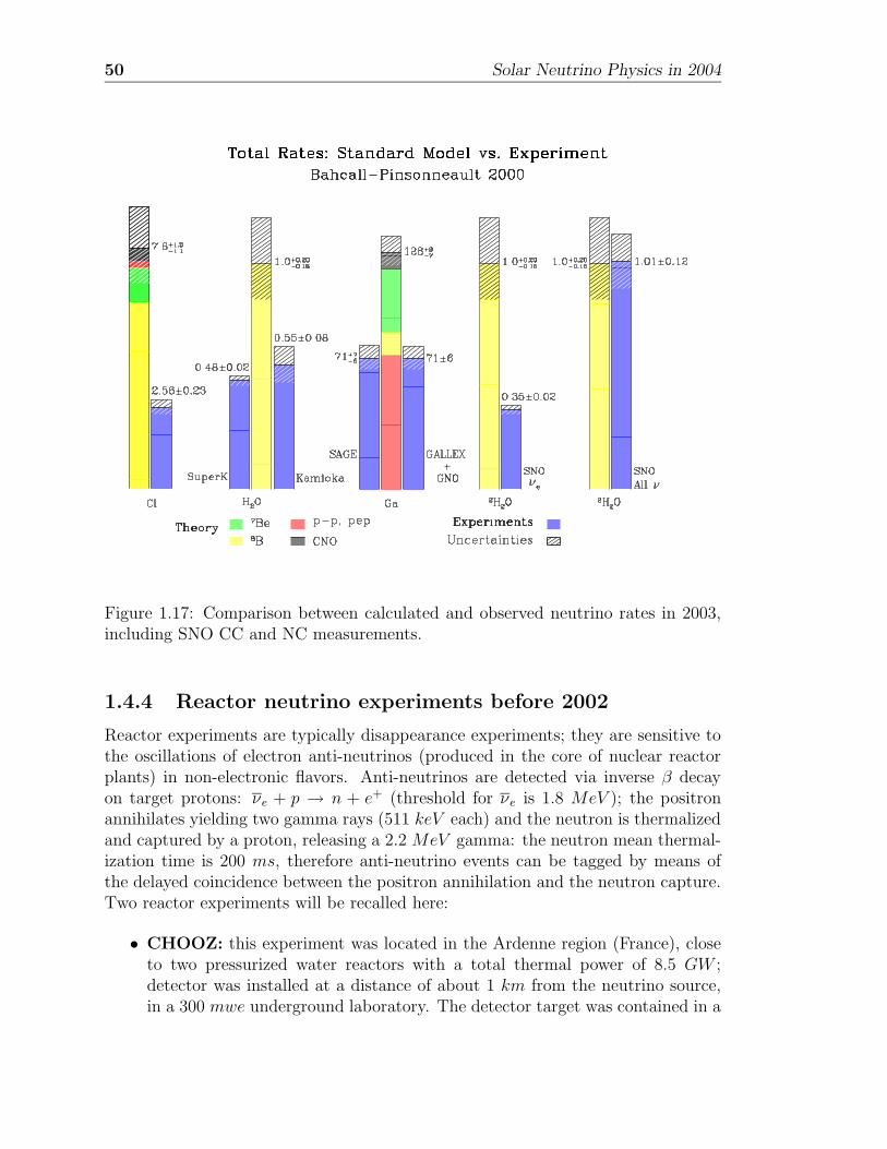
50 Solar Neutrino Physics in 2004
Figure 1.17: Comparison between calculated and observed neutrino rates in 2003,including SNO CC and NC measurements.
1.4.4 Reactor neutrino experiments before 2002
Reactor experiments are typically disappearance experiments; they are sensitive tothe oscillations of electron anti-neutrinos (produced in the core of nuclear reactorplants) in non-electronic flavors. Anti-neutrinos are detected via inverse β decayon target protons: νe + p → n + e+ (threshold for νe is 1.8 MeV ); the positronannihilates yielding two gamma rays (511 keV each) and the neutron is thermalizedand captured by a proton, releasing a 2.2 MeV gamma: the neutron mean thermal-ization time is 200 ms, therefore anti-neutrino events can be tagged by means ofthe delayed coincidence between the positron annihilation and the neutron capture.Two reactor experiments will be recalled here:
• CHOOZ: this experiment was located in the Ardenne region (France), closeto two pressurized water reactors with a total thermal power of 8.5 GW ;detector was installed at a distance of about 1 km from the neutrino source,in a 300 mwe underground laboratory. The detector target was contained in a
1.4.4 Reactor neutrino experiments before 2002 51
welded cylindrical steel vessel, filled with a paraffinic liquid scintillator loadedwith 0.09% gadolinium (which has a large neutron capture cross section) [11]:real target had a 5 tmass; a 17 t active buffer and a 91 t passive buffer were alsopresent. After the April 1997 - July 1998 data taking, the total anti-neutrinorate and energy spectrum data were published [12], showing no deviations fromthe non-oscillation hypothesis; the measured versus expected ratio, averagedover the energy spectrum is: R = 1.01± 2.8%(stat.)± 2.7%(sys.).
Considering these results, the excluded parameters region for νe ↔ νx os-cillations is: δm2 > 7 × 10⁻⁴ eV 2 for maximal mixing and sin2 2θ > 0.10for large δm2 (as shown in figure 1.18). These constraints have three mainconsequences:
- provide an upper bound on δm2 for solar neutrino oscillations: δm212 <
7× 10⁻⁴ eV 2;
- provide an upper limit on θ13 mixing parameter: sin2 2θ13 < 0.1013;
- exclude the Super-Kamiokande region for atmospheric neutrino oscilla-tions: electron neutrinos are not involved in atmospheric oscillations andthe Super-Kamiokande result has to be explained via νµ ↔ ντ oscillations.
• Palo Verde: this experiment was performed at the Palo Verde Nuclear Gen-erating Station in Arizona (USA); the plant consists of three identical pres-surized water reactors with a total thermal power of 11.63 GW . The detectorwas located in a shallow underground site (32 mwe), 890 m from two of thereactors and 750 m from the third. The segmented detector consisted of 66acrylic cells, filled with 11.34 t of Gd-loaded liquid scintillator; a mineral oilbuffer and a water (105 t) buffer were present. The obtained observed ver-sus expected ratio was [30]: Robs/Rcalc = 1.01 ± 0.024 (stat.) ± 0.053 (syst.),consistent with the non-oscillation hypothesis.
Two different analysis of Palo Verde data have been performed: the standard“reactor power” analysis and the “swap” analysis (based on a swapped set ofcuts for coincidence events); the second method allows to reduce systematicsvia a direct background subtraction: therefore it enhances the experimentsensitivity. Nevertheless, the Palo Verde final sensitivity never reached theCHOOZ sensitivity (Palo Verde and CHOOZ excluded regions are shown infigure 1.18).
13A recent paper on the global neutrino oscillation analysis performed in a 3 ν formalism, canbe found in reference [45].
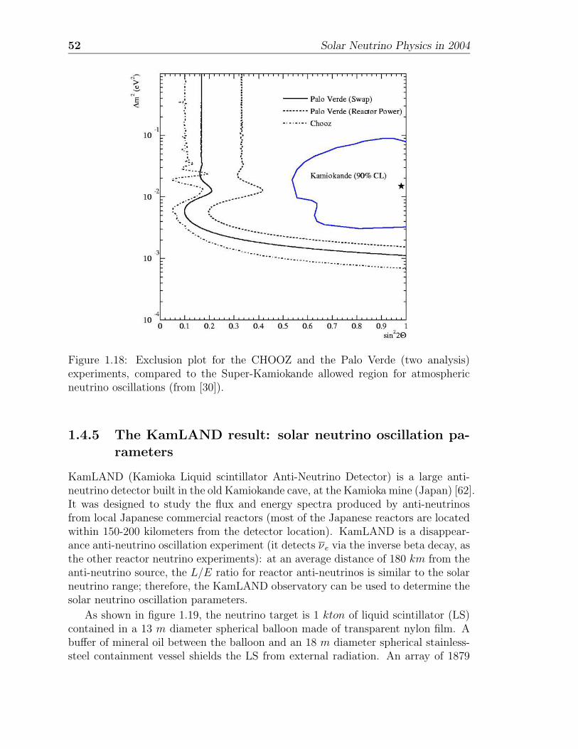
52 Solar Neutrino Physics in 2004
Figure 1.18: Exclusion plot for the CHOOZ and the Palo Verde (two analysis)experiments, compared to the Super-Kamiokande allowed region for atmosphericneutrino oscillations (from [30]).
1.4.5 The KamLAND result: solar neutrino oscillation pa-rameters
KamLAND (Kamioka Liquid scintillator Anti-Neutrino Detector) is a large anti-neutrino detector built in the old Kamiokande cave, at the Kamioka mine (Japan) [62].It was designed to study the flux and energy spectra produced by anti-neutrinosfrom local Japanese commercial reactors (most of the Japanese reactors are locatedwithin 150-200 kilometers from the detector location). KamLAND is a disappear-ance anti-neutrino oscillation experiment (it detects νe via the inverse beta decay, asthe other reactor neutrino experiments): at an average distance of 180 km from theanti-neutrino source, the L/E ratio for reactor anti-neutrinos is similar to the solarneutrino range; therefore, the KamLAND observatory can be used to determine thesolar neutrino oscillation parameters.
As shown in figure 1.19, the neutrino target is 1 kton of liquid scintillator (LS)contained in a 13 m diameter spherical balloon made of transparent nylon film. Abuffer of mineral oil between the balloon and an 18 m diameter spherical stainless-steel containment vessel shields the LS from external radiation. An array of 1879
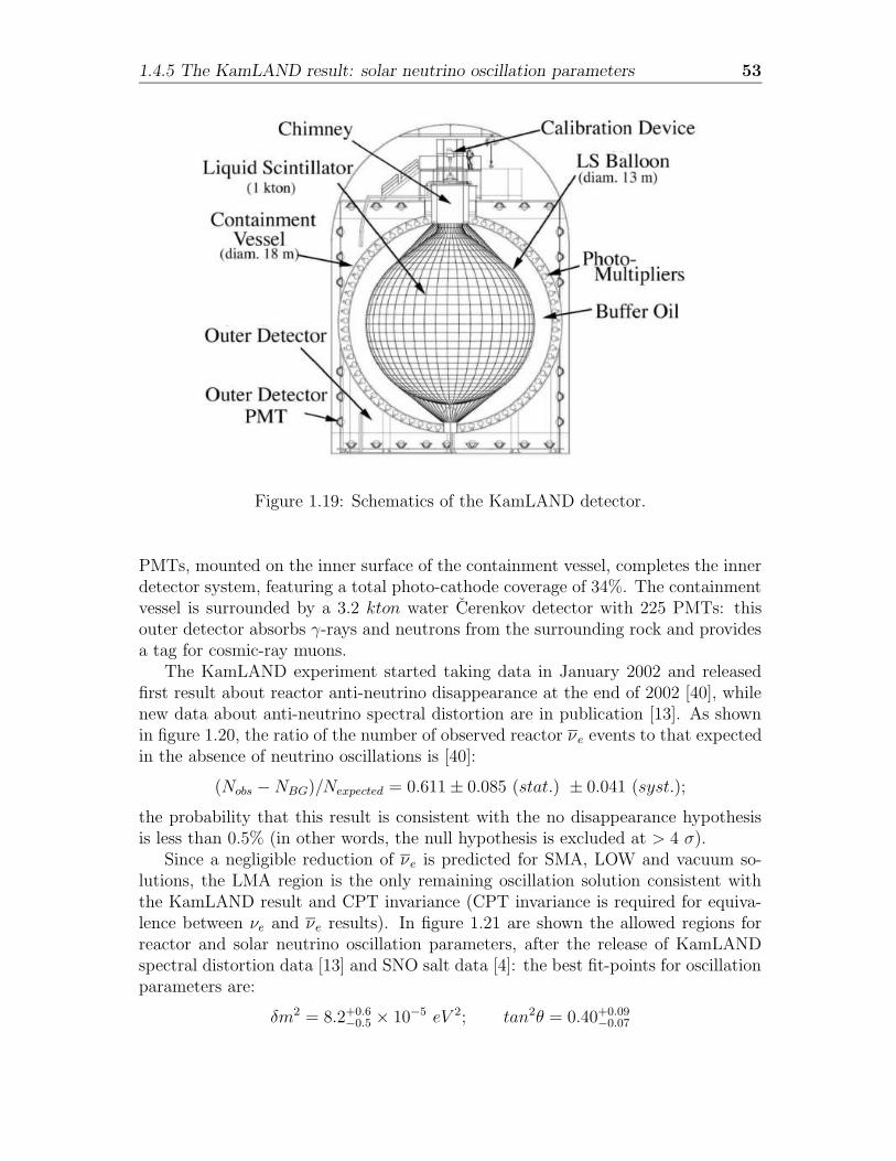
1.4.5 The KamLAND result: solar neutrino oscillation parameters 53
Figure 1.19: Schematics of the KamLAND detector.
PMTs, mounted on the inner surface of the containment vessel, completes the innerdetector system, featuring a total photo-cathode coverage of 34%. The containmentvessel is surrounded by a 3.2 kton water Cerenkov detector with 225 PMTs: thisouter detector absorbs γ-rays and neutrons from the surrounding rock and providesa tag for cosmic-ray muons.
The KamLAND experiment started taking data in January 2002 and releasedfirst result about reactor anti-neutrino disappearance at the end of 2002 [40], whilenew data about anti-neutrino spectral distortion are in publication [13]. As shownin figure 1.20, the ratio of the number of observed reactor νe events to that expectedin the absence of neutrino oscillations is [40]:
(Nobs −NBG)/Nexpected = 0.611± 0.085 (stat.) ± 0.041 (syst.);
the probability that this result is consistent with the no disappearance hypothesisis less than 0.5% (in other words, the null hypothesis is excluded at > 4 σ).
Since a negligible reduction of νe is predicted for SMA, LOW and vacuum so-lutions, the LMA region is the only remaining oscillation solution consistent withthe KamLAND result and CPT invariance (CPT invariance is required for equiva-lence between νe and νe results). In figure 1.21 are shown the allowed regions forreactor and solar neutrino oscillation parameters, after the release of KamLANDspectral distortion data [13] and SNO salt data [4]: the best fit-points for oscillationparameters are:
δm2 = 8.2+0.6−0.5 × 10⁻⁵ eV 2; tan2θ = 0.40+0.09
−0.07
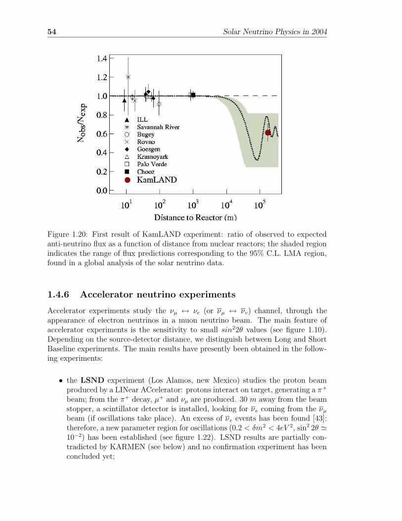
54 Solar Neutrino Physics in 2004
Figure 1.20: First result of KamLAND experiment: ratio of observed to expectedanti-neutrino flux as a function of distance from nuclear reactors; the shaded regionindicates the range of flux predictions corresponding to the 95% C.L. LMA region,found in a global analysis of the solar neutrino data.
1.4.6 Accelerator neutrino experiments
Accelerator experiments study the νµ ↔ νe (or νµ ↔ νe) channel, through theappearance of electron neutrinos in a muon neutrino beam. The main feature ofaccelerator experiments is the sensitivity to small sin22θ values (see figure 1.10).Depending on the source-detector distance, we distinguish between Long and ShortBaseline experiments. The main results have presently been obtained in the follow-ing experiments:
• the LSND experiment (Los Alamos, new Mexico) studies the proton beamproduced by a LINear ACcelerator: protons interact on target, generating a π+
beam; from the π+ decay, µ+ and νµ are produced. 30 m away from the beamstopper, a scintillator detector is installed, looking for νe coming from the νµ
beam (if oscillations take place). An excess of νe events has been found [43]:therefore, a new parameter region for oscillations (0.2 < δm2 < 4eV 2, sin2 2θ '10−2) has been established (see figure 1.22). LSND results are partially con-tradicted by KARMEN (see below) and no confirmation experiment has beenconcluded yet;
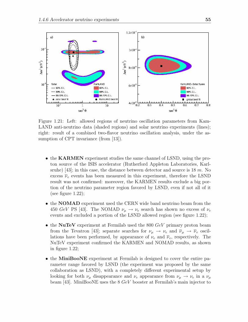
1.4.6 Accelerator neutrino experiments 55
Figure 1.21: Left: allowed regions of neutrino oscillation parameters from Kam-LAND anti-neutrino data (shaded regions) and solar neutrino experiments (lines);right: result of a combined two-flavor neutrino oscillation analysis, under the as-sumption of CPT invariance (from [13]).
• the KARMEN experiment studies the same channel of LSND, using the pro-ton source of the ISIS accelerator (Rutherford Appleton Laboratories, Karl-sruhe) [43]; in this case, the distance between detector and source is 18 m. Noexcess νe events has been measured in this experiment, therefore the LSNDresult was not confirmed: moreover, the KARMEN results exclude a big por-tion of the neutrino parameter region favored by LSND, even if not all of it(see figure 1.22);
• the NOMAD experiment used the CERN wide band neutrino beam from the450 GeV PS [43]. The NOMAD νµ → νe search has shown no excess of νeevents and excluded a portion of the LSND allowed region (see figure 1.22);
• the NuTeV experiment at Fermilab used the 800 GeV primary proton beamfrom the Tevatron [43]; separate searches for νµ → νe and νµ → νe oscil-lations have been performed, by appearance of νe and νe, respectively. TheNuTeV experiment confirmed the KARMEN and NOMAD results, as shownin figure 1.22;
• the MiniBooNE experiment at Fermilab is designed to cover the entire pa-rameter range favored by LSND (the experiment was proposed by the samecollaboration as LSND), with a completely different experimental setup bylooking for both νµ disappearance and νe appearance from νµ → νe in a νµbeam [43]. MiniBooNE uses the 8 GeV booster at Fermilab’s main injector to
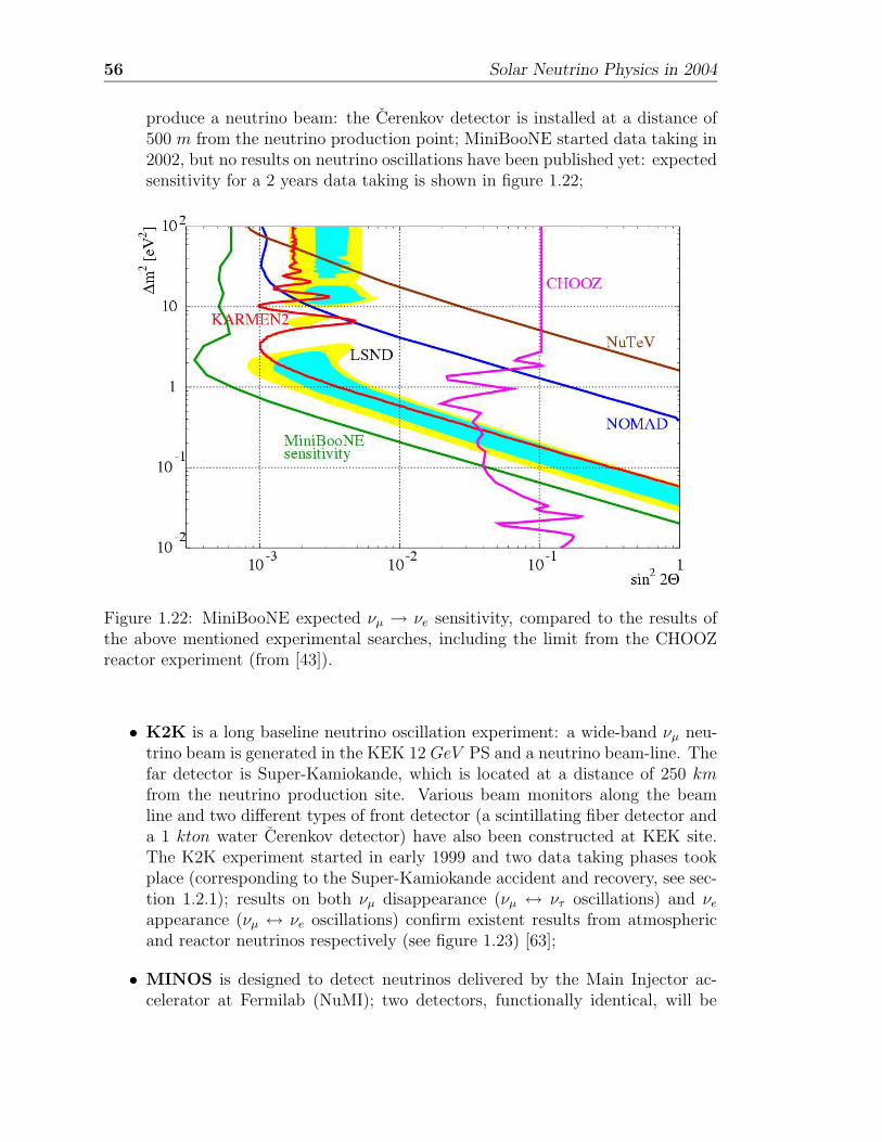
56 Solar Neutrino Physics in 2004
produce a neutrino beam: the Cerenkov detector is installed at a distance of500 m from the neutrino production point; MiniBooNE started data taking in2002, but no results on neutrino oscillations have been published yet: expectedsensitivity for a 2 years data taking is shown in figure 1.22;
Figure 1.22: MiniBooNE expected νµ → νe sensitivity, compared to the results ofthe above mentioned experimental searches, including the limit from the CHOOZreactor experiment (from [43]).
• K2K is a long baseline neutrino oscillation experiment: a wide-band νµ neu-trino beam is generated in the KEK 12 GeV PS and a neutrino beam-line. Thefar detector is Super-Kamiokande, which is located at a distance of 250 kmfrom the neutrino production site. Various beam monitors along the beamline and two different types of front detector (a scintillating fiber detector anda 1 kton water Cerenkov detector) have also been constructed at KEK site.The K2K experiment started in early 1999 and two data taking phases tookplace (corresponding to the Super-Kamiokande accident and recovery, see sec-tion 1.2.1); results on both νµ disappearance (νµ ↔ ντ oscillations) and νeappearance (νµ ↔ νe oscillations) confirm existent results from atmosphericand reactor neutrinos respectively (see figure 1.23) [63];
• MINOS is designed to detect neutrinos delivered by the Main Injector ac-celerator at Fermilab (NuMI); two detectors, functionally identical, will be
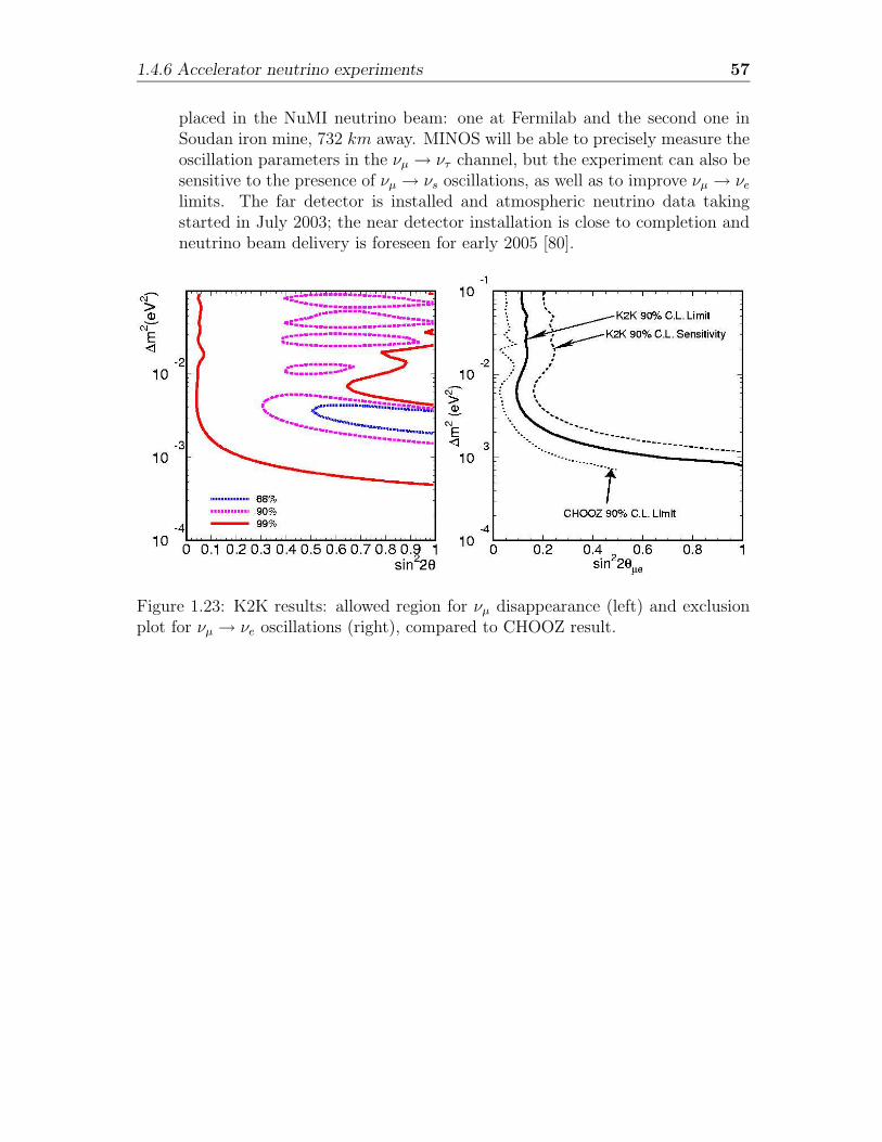
1.4.6 Accelerator neutrino experiments 57
placed in the NuMI neutrino beam: one at Fermilab and the second one inSoudan iron mine, 732 km away. MINOS will be able to precisely measure theoscillation parameters in the νµ → ντ channel, but the experiment can also besensitive to the presence of νµ → νs oscillations, as well as to improve νµ → νelimits. The far detector is installed and atmospheric neutrino data takingstarted in July 2003; the near detector installation is close to completion andneutrino beam delivery is foreseen for early 2005 [80].
Figure 1.23: K2K results: allowed region for νµ disappearance (left) and exclusionplot for νµ → νe oscillations (right), compared to CHOOZ result.

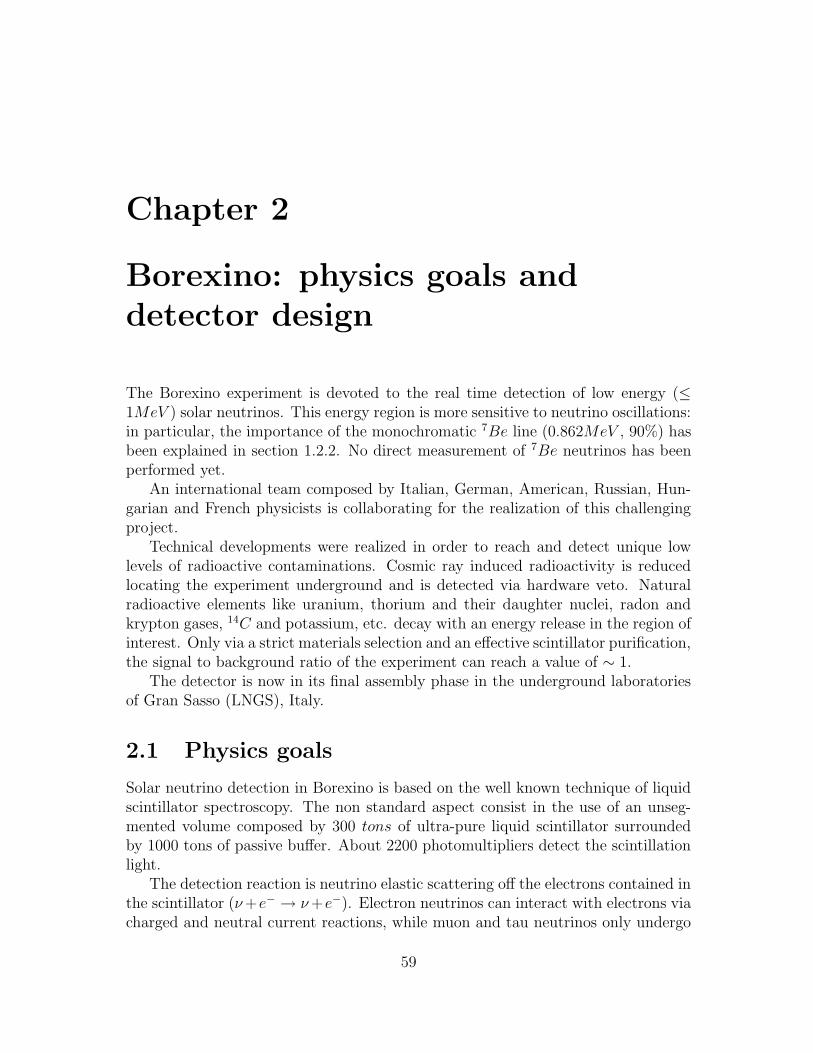
Chapter 2
Borexino: physics goals anddetector design
The Borexino experiment is devoted to the real time detection of low energy (≤1MeV ) solar neutrinos. This energy region is more sensitive to neutrino oscillations:in particular, the importance of the monochromatic 7Be line (0.862MeV , 90%) hasbeen explained in section 1.2.2. No direct measurement of 7Be neutrinos has beenperformed yet.
An international team composed by Italian, German, American, Russian, Hun-garian and French physicists is collaborating for the realization of this challengingproject.
Technical developments were realized in order to reach and detect unique lowlevels of radioactive contaminations. Cosmic ray induced radioactivity is reducedlocating the experiment underground and is detected via hardware veto. Naturalradioactive elements like uranium, thorium and their daughter nuclei, radon andkrypton gases, 14C and potassium, etc. decay with an energy release in the region ofinterest. Only via a strict materials selection and an effective scintillator purification,the signal to background ratio of the experiment can reach a value of ∼ 1.
The detector is now in its final assembly phase in the underground laboratoriesof Gran Sasso (LNGS), Italy.
2.1 Physics goals
Solar neutrino detection in Borexino is based on the well known technique of liquidscintillator spectroscopy. The non standard aspect consist in the use of an unseg-mented volume composed by 300 tons of ultra-pure liquid scintillator surroundedby 1000 tons of passive buffer. About 2200 photomultipliers detect the scintillationlight.
The detection reaction is neutrino elastic scattering off the electrons contained inthe scintillator (ν+e− → ν+e−). Electron neutrinos can interact with electrons viacharged and neutral current reactions, while muon and tau neutrinos only undergo
59
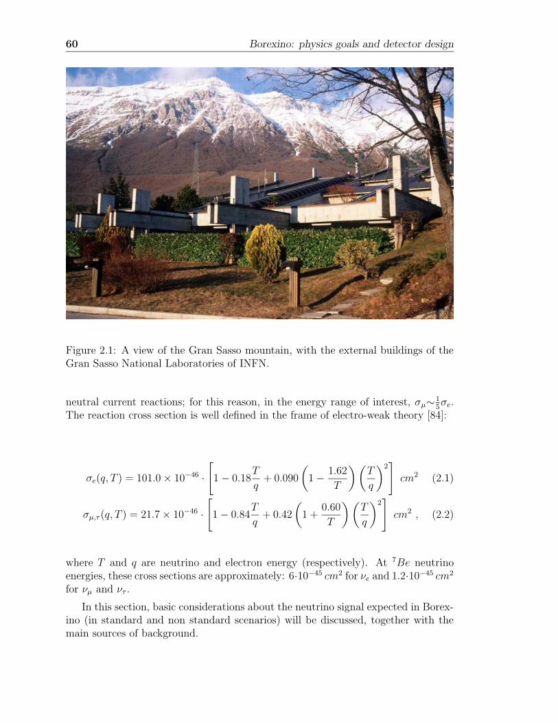
60 Borexino: physics goals and detector design
Figure 2.1: A view of the Gran Sasso mountain, with the external buildings of theGran Sasso National Laboratories of INFN.
neutral current reactions; for this reason, in the energy range of interest, σµ∼15σe.
The reaction cross section is well defined in the frame of electro-weak theory [84]:
σe(q, T ) = 101.0× 10−46 ·[
1− 0.18T
q+ 0.090
(
1− 1.62
T
)(
T
q
)2]
cm2 (2.1)
σµ,τ (q, T ) = 21.7× 10−46 ·[
1− 0.84T
q+ 0.42
(
1 +0.60
T
)(
T
q
)2]
cm2 , (2.2)
where T and q are neutrino and electron energy (respectively). At 7Be neutrinoenergies, these cross sections are approximately: 6·10−45 cm2 for νe and 1.2·10−45 cm2
for νµ and ντ .
In this section, basic considerations about the neutrino signal expected in Borex-ino (in standard and non standard scenarios) will be discussed, together with themain sources of background.
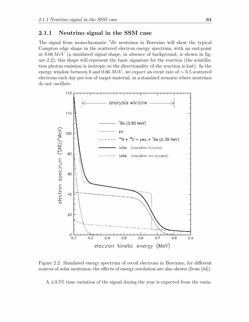
2.1.1 Neutrino signal in the SSM case 61
2.1.1 Neutrino signal in the SSM case
The signal from monochromatic 7Be neutrinos in Borexino will show the typicalCompton edge shape in the scattered electron energy spectrum, with an end-pointat 0.66MeV (a simulated signal shape, in absence of background, is shown in fig-ure 2.2); this shape will represent the basic signature for the reaction (the scintilla-tion photon emission is isotropic so the directionality of the reaction is lost). In theenergy window between 0 and 0.66 MeV , we expect an event rate of ∼ 0.5 scatteredelectrons each day per ton of target material, in a standard scenario where neutrinosdo not oscillate.
Figure 2.2: Simulated energy spectrum of recoil electrons in Borexino, for differentsources of solar neutrinos; the effects of energy resolution are also shown (from [44]).
A ±3.5% time variation of the signal during the year is expected from the varia-
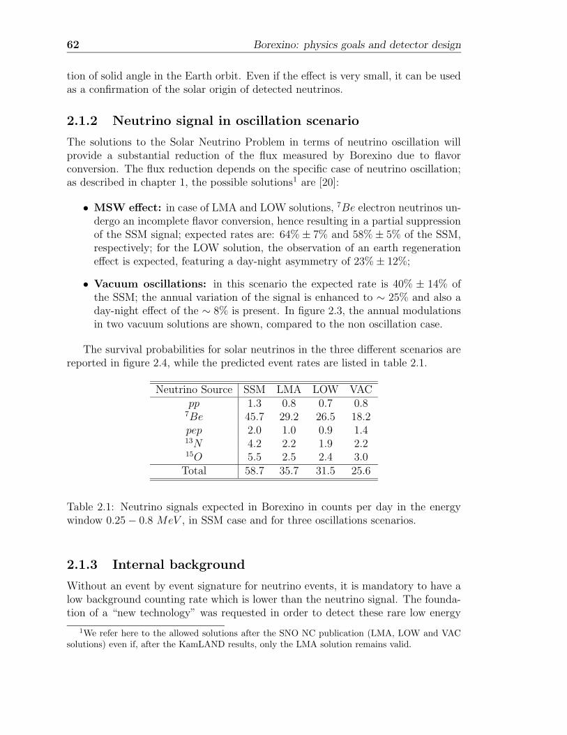
62 Borexino: physics goals and detector design
tion of solid angle in the Earth orbit. Even if the effect is very small, it can be usedas a confirmation of the solar origin of detected neutrinos.
2.1.2 Neutrino signal in oscillation scenario
The solutions to the Solar Neutrino Problem in terms of neutrino oscillation willprovide a substantial reduction of the flux measured by Borexino due to flavorconversion. The flux reduction depends on the specific case of neutrino oscillation;as described in chapter 1, the possible solutions1 are [20]:
• MSW effect: in case of LMA and LOW solutions, 7Be electron neutrinos un-dergo an incomplete flavor conversion, hence resulting in a partial suppressionof the SSM signal; expected rates are: 64%± 7% and 58%± 5% of the SSM,respectively; for the LOW solution, the observation of an earth regenerationeffect is expected, featuring a day-night asymmetry of 23%± 12%;
• Vacuum oscillations: in this scenario the expected rate is 40% ± 14% ofthe SSM; the annual variation of the signal is enhanced to ∼ 25% and also aday-night effect of the ∼ 8% is present. In figure 2.3, the annual modulationsin two vacuum solutions are shown, compared to the non oscillation case.
The survival probabilities for solar neutrinos in the three different scenarios arereported in figure 2.4, while the predicted event rates are listed in table 2.1.
Neutrino Source SSM LMA LOW VACpp 1.3 0.8 0.7 0.87Be 45.7 29.2 26.5 18.2pep 2.0 1.0 0.9 1.413N 4.2 2.2 1.9 2.215O 5.5 2.5 2.4 3.0Total 58.7 35.7 31.5 25.6
Table 2.1: Neutrino signals expected in Borexino in counts per day in the energywindow 0.25− 0.8 MeV , in SSM case and for three oscillations scenarios.
2.1.3 Internal background
Without an event by event signature for neutrino events, it is mandatory to have alow background counting rate which is lower than the neutrino signal. The founda-tion of a “new technology” was requested in order to detect these rare low energy
1We refer here to the allowed solutions after the SNO NC publication (LMA, LOW and VACsolutions) even if, after the KamLAND results, only the LMA solution remains valid.
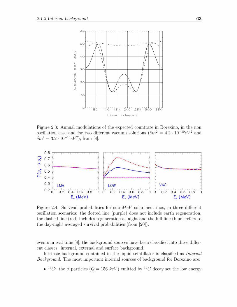
2.1.3 Internal background 63
Figure 2.3: Annual modulations of the expected countrate in Borexino, in the nonoscillation case and for two different vacuum solutions (δm2 = 4.2 · 10−10eV 2 andδm2 = 3.2 · 10−10eV 2); from [8].
Figure 2.4: Survival probabilities for sub-MeV solar neutrinos, in three differentoscillation scenarios: the dotted line (purple) does not include earth regeneration,the dashed line (red) includes regeneration at night and the full line (blue) refers tothe day-night averaged survival probabilities (from [20]).
events in real time [8]; the background sources have been classified into three differ-ent classes: internal, external and surface background.
Intrinsic background contained in the liquid scintillator is classified as InternalBackground. The most important internal sources of background for Borexino are:
• 14C: the β particles (Q = 156 keV ) emitted by 14C decay set the low energy
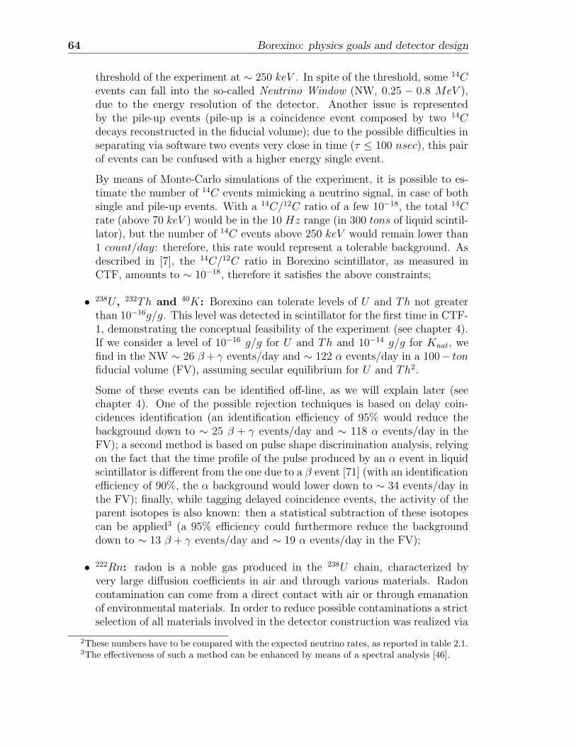
64 Borexino: physics goals and detector design
threshold of the experiment at ∼ 250 keV . In spite of the threshold, some 14Cevents can fall into the so-called Neutrino Window (NW, 0.25 − 0.8 MeV ),due to the energy resolution of the detector. Another issue is representedby the pile-up events (pile-up is a coincidence event composed by two 14Cdecays reconstructed in the fiducial volume); due to the possible difficulties inseparating via software two events very close in time (τ ≤ 100 nsec), this pairof events can be confused with a higher energy single event.
By means of Monte-Carlo simulations of the experiment, it is possible to es-timate the number of 14C events mimicking a neutrino signal, in case of bothsingle and pile-up events. With a 14C/12C ratio of a few 10−18, the total 14Crate (above 70 keV ) would be in the 10 Hz range (in 300 tons of liquid scintil-lator), but the number of 14C events above 250 keV would remain lower than1 count/day: therefore, this rate would represent a tolerable background. Asdescribed in [7], the 14C/12C ratio in Borexino scintillator, as measured inCTF, amounts to ∼ 10−18, therefore it satisfies the above constraints;
• 238U , 232Th and 40K: Borexino can tolerate levels of U and Th not greaterthan 10−16g/g. This level was detected in scintillator for the first time in CTF-1, demonstrating the conceptual feasibility of the experiment (see chapter 4).If we consider a level of 10−16 g/g for U and Th and 10−14 g/g for Knat, wefind in the NW ∼ 26 β+ γ events/day and ∼ 122 α events/day in a 100− tonfiducial volume (FV), assuming secular equilibrium for U and Th2.
Some of these events can be identified off-line, as we will explain later (seechapter 4). One of the possible rejection techniques is based on delay coin-cidences identification (an identification efficiency of 95% would reduce thebackground down to ∼ 25 β + γ events/day and ∼ 118 α events/day in theFV); a second method is based on pulse shape discrimination analysis, relyingon the fact that the time profile of the pulse produced by an α event in liquidscintillator is different from the one due to a β event [71] (with an identificationefficiency of 90%, the α background would lower down to ∼ 34 events/day inthe FV); finally, while tagging delayed coincidence events, the activity of theparent isotopes is also known: then a statistical subtraction of these isotopescan be applied3 (a 95% efficiency could furthermore reduce the backgrounddown to ∼ 13 β + γ events/day and ∼ 19 α events/day in the FV);
• 222Rn: radon is a noble gas produced in the 238U chain, characterized byvery large diffusion coefficients in air and through various materials. Radoncontamination can come from a direct contact with air or through emanationof environmental materials. In order to reduce possible contaminations a strictselection of all materials involved in the detector construction was realized via
2These numbers have to be compared with the expected neutrino rates, as reported in table 2.1.3The effectiveness of such a method can be enhanced by means of a spectral analysis [46].
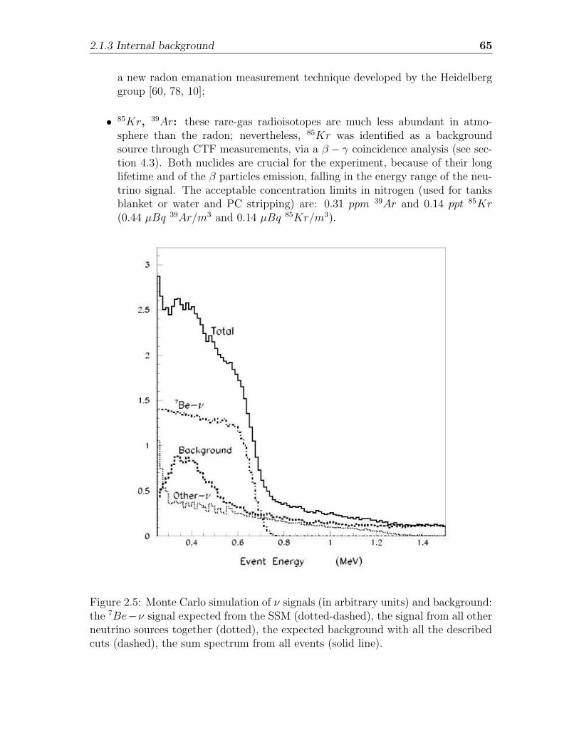
2.1.3 Internal background 65
a new radon emanation measurement technique developed by the Heidelberggroup [60, 78, 10];
• 85Kr, 39Ar: these rare-gas radioisotopes are much less abundant in atmo-sphere than the radon; nevertheless, 85Kr was identified as a backgroundsource through CTF measurements, via a β − γ coincidence analysis (see sec-tion 4.3). Both nuclides are crucial for the experiment, because of their longlifetime and of the β particles emission, falling in the energy range of the neu-trino signal. The acceptable concentration limits in nitrogen (used for tanksblanket or water and PC stripping) are: 0.31 ppm 39Ar and 0.14 ppt 85Kr(0.44 µBq 39Ar/m3 and 0.14 µBq 85Kr/m3).
Figure 2.5: Monte Carlo simulation of ν signals (in arbitrary units) and background:the 7Be−ν signal expected from the SSM (dotted-dashed), the signal from all otherneutrino sources together (dotted), the expected background with all the describedcuts (dashed), the sum spectrum from all events (solid line).
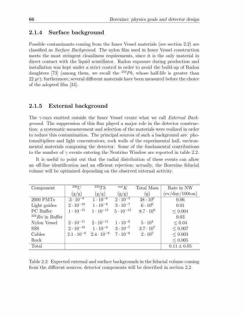
66 Borexino: physics goals and detector design
2.1.4 Surface background
Possible contaminants coming from the Inner Vessel materials (see section 2.2) areclassified as Surface Background. The nylon film used in Inner Vessel constructionmeets the most stringent cleanliness requirements, since it is the only material indirect contact with the liquid scintillator. Radon exposure during production andinstallation was kept under a strict control in order to avoid the build-up of Radondaughters [73] (among them, we recall the 210Pb, whose half-life is greater than22 yr); furthermore, several different materials have been measured before the choiceof the adopted film [34].
2.1.5 External background
The γ-rays emitted outside the Inner Vessel create what we call External Back-ground. The suppression of this flux played a major role in the detector construc-tion: a systematic measurement and selection of the materials were realized in orderto reduce this contamination. The principal sources of such a background are: pho-tomultipliers and light concentrators, rock walls of the experimental hall, environ-mental materials composing the detector. Some of the fundamental contributionsto the number of γ events entering the Neutrino Window are reported in table 2.2.
It is useful to point out that the radial distribution of these events can allowan off-line identification and an efficient rejection; actually, the Borexino fiducialvolume will be optimized depending on the observed external activity.
Component 238U 232Th natK Total Mass Rate in NW(g/g) (g/g) (g/g) (g) (ev/day/100ton)
2000 PMTs 3 · 10−8 1 · 10−8 2 · 10−5 38 · 106 0.06Light guides 2 · 10−10 1 · 10−9 3 · 10−7 6 · 106 0.01PC Buffer 1 · 10−15 1 · 10−15 5 · 10−12 8.7 · 108 ≤ 0.004222Rn in Buffer 0.03Nylon Vessel 2 · 10−11 2 · 10−11 1 · 10−8 5 · 104 ≤ 0.04SSS 2 · 10−10 1 · 10−9 3 · 10−7 3.7 · 107 ≤ 0.007Cables 2.1 · 10−8 2.4 · 10−8 7 · 10−6 2 · 105 ≤ 0.003Rock ≤ 0.005Total 0.11± 0.05
Table 2.2: Expected external and surface backgrounds in the fiducial volume comingfrom the different sources; detector components will be described in section 2.2
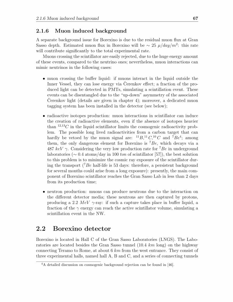
2.1.6 Muon induced background 67
2.1.6 Muon induced background
A separate background issue for Borexino is due to the residual muon flux at GranSasso depth. Estimated muon flux in Borexino will be ∼ 25 µ/day/m2: this ratewill contribute significantly to the total experimental rate.
Muons crossing the scintillator are easily rejected, due to the huge energy amountof these events, compared to the neutrino ones; nevertheless, muon interactions canmimic neutrinos in the following cases:
• muon crossing the buffer liquid: if muons interact in the liquid outside theInner Vessel, they can lose energy via Cerenkov effect; a fraction of the pro-duced light can be detected in PMTs, simulating a scintillation event. Theseevents can be disentangled due to the “up-down” asymmetry of the associatedCerenkov light (details are given in chapter 4); moreover, a dedicated muontagging system has been installed in the detector (see below);
• radioactive isotopes production: muon interactions in scintillator can inducethe creation of radioactive elements, even if the absence of isotopes heavierthan 12,13C in the liquid scintillator limits the cosmogenic radioactivity prob-lem. The possible long lived radioactivities from a carbon target that canhardly be vetoed by the muon signal are: 11B,11 C,10C and 7Be4; amongthem, the only dangerous element for Borexino is 7Be, which decays via a487 keV γ. Considering the very low production rate for 7Be in undergroundlaboratories (∼ 0.4 atoms/day in 100 ton of scintillator [57]), the best solutionto this problem is to minimize the cosmic ray exposure of the scintillator dur-ing the transport (7Be half-life is 53 days: therefore, a persistent backgroundfor several months could arise from a long exposure): presently, the main com-ponent of Borexino scintillator reaches the Gran Sasso Lab in less than 2 daysfrom its production time;
• neutron production: muons can produce neutrons due to the interaction onthe different detector media; these neutrons are then captured by protons,producing a 2.2 MeV γ-ray: if such a capture takes place in buffer liquid, afraction of the γ energy can reach the active scintillator volume, simulating ascintillation event in the NW.
2.2 Borexino detector
Borexino is located in Hall C of the Gran Sasso Laboratories (LNGS). The Labo-ratories are located besides the Gran Sasso tunnel (10.4 km long) on the highwayconnecting Teramo to Rome, at about 6 km from the west entrance. They consist ofthree experimental halls, named hall A, B and C, and a series of connecting tunnels
4A detailed discussion on cosmogenic background rejection can be found in [46].
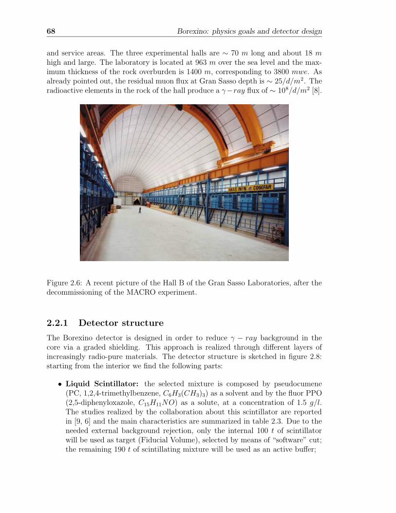
68 Borexino: physics goals and detector design
and service areas. The three experimental halls are ∼ 70 m long and about 18 mhigh and large. The laboratory is located at 963 m over the sea level and the max-imum thickness of the rock overburden is 1400 m, corresponding to 3800 mwe. Asalready pointed out, the residual muon flux at Gran Sasso depth is ∼ 25/d/m2. Theradioactive elements in the rock of the hall produce a γ−ray flux of ∼ 108/d/m2 [8].
Figure 2.6: A recent picture of the Hall B of the Gran Sasso Laboratories, after thedecommissioning of the MACRO experiment.
2.2.1 Detector structure
The Borexino detector is designed in order to reduce γ − ray background in thecore via a graded shielding. This approach is realized through different layers ofincreasingly radio-pure materials. The detector structure is sketched in figure 2.8:starting from the interior we find the following parts:
• Liquid Scintillator: the selected mixture is composed by pseudocumene(PC, 1,2,4-trimethylbenzene, C6H3(CH3)3) as a solvent and by the fluor PPO(2,5-diphenyloxazole, C15H11NO) as a solute, at a concentration of 1.5 g/l.The studies realized by the collaboration about this scintillator are reportedin [9, 6] and the main characteristics are summarized in table 2.3. Due to theneeded external background rejection, only the internal 100 t of scintillatorwill be used as target (Fiducial Volume), selected by means of “software” cut;the remaining 190 t of scintillating mixture will be used as an active buffer;
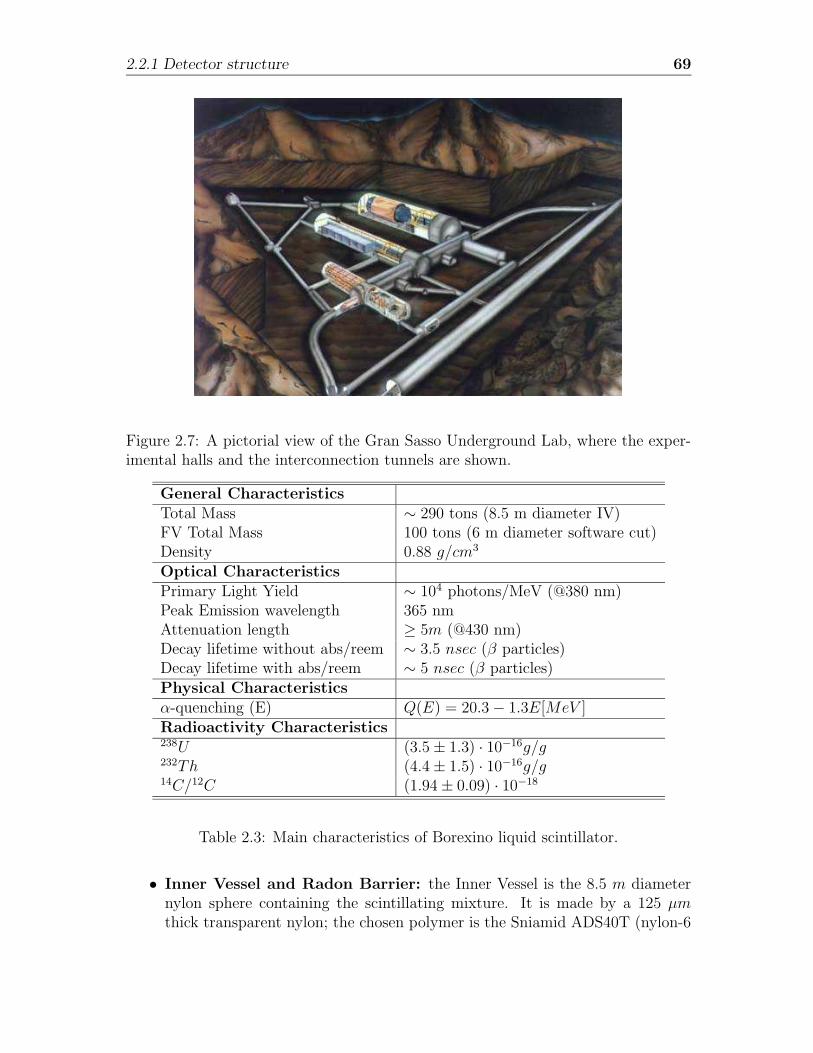
2.2.1 Detector structure 69
Figure 2.7: A pictorial view of the Gran Sasso Underground Lab, where the exper-imental halls and the interconnection tunnels are shown.
General CharacteristicsTotal Mass ∼ 290 tons (8.5 m diameter IV)FV Total Mass 100 tons (6 m diameter software cut)Density 0.88 g/cm3
Optical CharacteristicsPrimary Light Yield ∼ 104 photons/MeV (@380 nm)Peak Emission wavelength 365 nmAttenuation length ≥ 5m (@430 nm)Decay lifetime without abs/reem ∼ 3.5 nsec (β particles)Decay lifetime with abs/reem ∼ 5 nsec (β particles)Physical Characteristicsα-quenching (E) Q(E) = 20.3− 1.3E[MeV ]Radioactivity Characteristics238U (3.5± 1.3) · 10−16g/g232Th (4.4± 1.5) · 10−16g/g14C/12C (1.94± 0.09) · 10−18
Table 2.3: Main characteristics of Borexino liquid scintillator.
• Inner Vessel and Radon Barrier: the Inner Vessel is the 8.5 m diameternylon sphere containing the scintillating mixture. It is made by a 125 µmthick transparent nylon; the chosen polymer is the Sniamid ADS40T (nylon-6
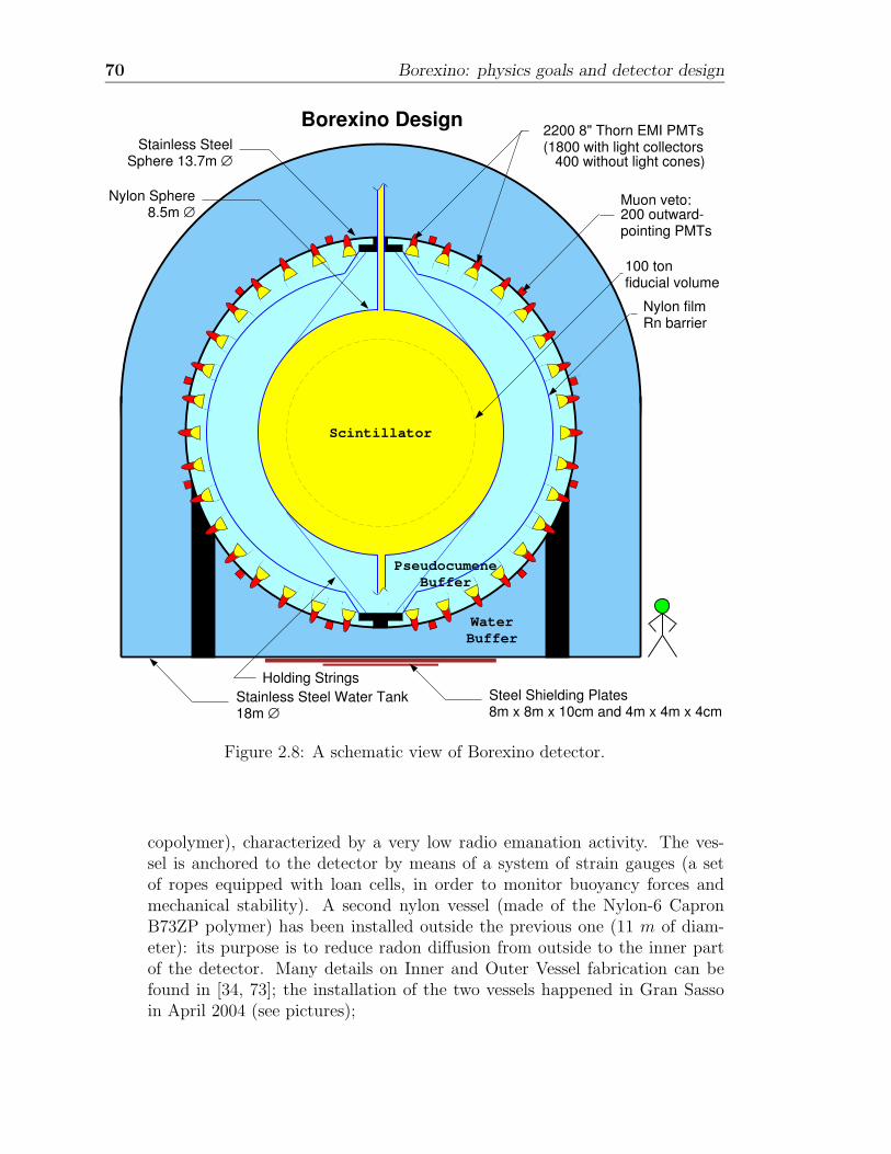
70 Borexino: physics goals and detector design
Stainless Steel Water Tank18m ∅
Stainless SteelSphere 13.7m ∅
2200 8" Thorn EMI PMTs(1800 with light collectors
WaterBuffer
100 ton fiducial volume
Borexino Design
PseudocumeneBuffer
Steel Shielding Plates8m x 8m x 10cm and 4m x 4m x 4cm
Scintillator
Nylon Sphere8.5m ∅
Holding Strings
200 outward-pointing PMTs
Muon veto:
Nylon filmRn barrier
400 without light cones)
Figure 2.8: A schematic view of Borexino detector.
copolymer), characterized by a very low radio emanation activity. The ves-sel is anchored to the detector by means of a system of strain gauges (a setof ropes equipped with loan cells, in order to monitor buoyancy forces andmechanical stability). A second nylon vessel (made of the Nylon-6 CapronB73ZP polymer) has been installed outside the previous one (11 m of diam-eter): its purpose is to reduce radon diffusion from outside to the inner partof the detector. Many details on Inner and Outer Vessel fabrication can befound in [34, 73]; the installation of the two vessels happened in Gran Sassoin April 2004 (see pictures);
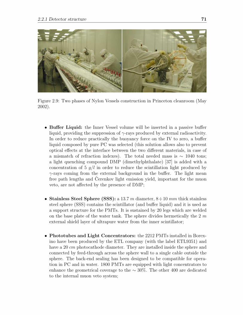
2.2.1 Detector structure 71
Figure 2.9: Two phases of Nylon Vessels construction in Princeton cleanroom (May2002).
• Buffer Liquid: the Inner Vessel volume will be inserted in a passive bufferliquid, providing the suppression of γ-rays produced by external radioactivity.In order to reduce practically the buoyancy force on the IV to zero, a bufferliquid composed by pure PC was selected (this solution allows also to preventoptical effects at the interface between the two different materials, in case ofa mismatch of refraction indexes). The total needed mass is ∼ 1040 tons;a light quenching compound DMP (dimethylphthalate) [37] is added with aconcentration of 5 g/l in order to reduce the scintillation light produced byγ-rays coming from the external background in the buffer. The light meanfree path lengths and Cerenkov light emission yield, important for the muonveto, are not affected by the presence of DMP;
• Stainless Steel Sphere (SSS): a 13.7 m diameter, 8÷10 mm thick stainlesssteel sphere (SSS) contains the scintillator (and buffer liquid) and it is used asa support structure for the PMTs. It is sustained by 20 legs which are weldedon the base plate of the water tank. The sphere divides hermetically the 2 mexternal shield layer of ultrapure water from the inner scintillator;
• Phototubes and Light Concentrators: the 2212 PMTs installed in Borex-ino have been produced by the ETL company (with the label ETL9351) andhave a 20 cm photocathode diameter. They are installed inside the sphere andconnected by feed-through across the sphere wall to a single cable outside thesphere. The back-end sealing has been designed to be compatible for opera-tion in PC and in water. 1800 PMTs are equipped with light concentrators toenhance the geometrical coverage to the ∼ 30%. The other 400 are dedicatedto the internal muon veto system;
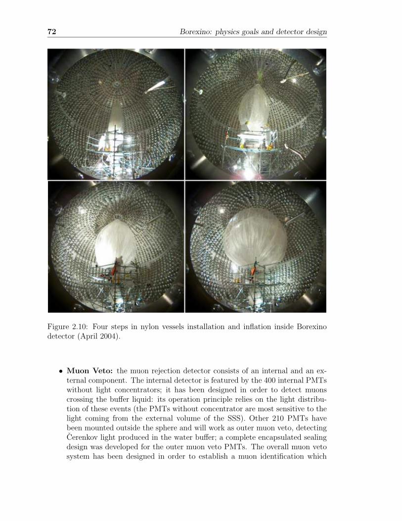
72 Borexino: physics goals and detector design
Figure 2.10: Four steps in nylon vessels installation and inflation inside Borexinodetector (April 2004).
• Muon Veto: the muon rejection detector consists of an internal and an ex-ternal component. The internal detector is featured by the 400 internal PMTswithout light concentrators; it has been designed in order to detect muonscrossing the buffer liquid: its operation principle relies on the light distribu-tion of these events (the PMTs without concentrator are most sensitive to thelight coming from the external volume of the SSS). Other 210 PMTs havebeen mounted outside the sphere and will work as outer muon veto, detectingCerenkov light produced in the water buffer; a complete encapsulated sealingdesign was developed for the outer muon veto PMTs. The overall muon vetosystem has been designed in order to establish a muon identification which
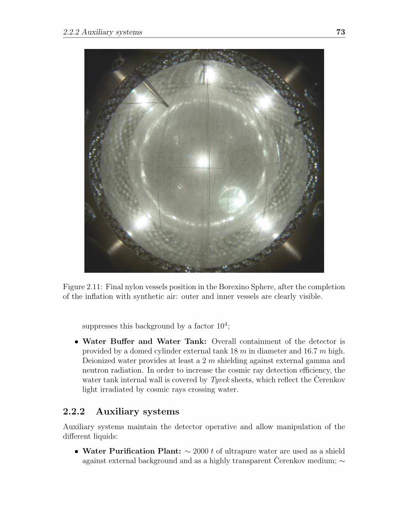
2.2.2 Auxiliary systems 73
Figure 2.11: Final nylon vessels position in the Borexino Sphere, after the completionof the inflation with synthetic air: outer and inner vessels are clearly visible.
suppresses this background by a factor 104;
• Water Buffer and Water Tank: Overall containment of the detector isprovided by a domed cylinder external tank 18m in diameter and 16.7m high.Deionized water provides at least a 2 m shielding against external gamma andneutron radiation. In order to increase the cosmic ray detection efficiency, thewater tank internal wall is covered by Tyvek sheets, which reflect the Cerenkovlight irradiated by cosmic rays crossing water.
2.2.2 Auxiliary systems
Auxiliary systems maintain the detector operative and allow manipulation of thedifferent liquids:
• Water Purification Plant: ∼ 2000 t of ultrapure water are used as a shieldagainst external background and as a highly transparent Cerenkov medium; ∼
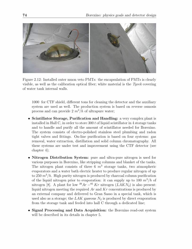
74 Borexino: physics goals and detector design
Figure 2.12: Installed outer muon veto PMTs: the encapsulation of PMTs is clearlyvisible, as well as the calibration optical fiber; white material is the Tyvek coveringof water tank internal walls.
1000 for CTF shield, different tons for cleaning the detector and the auxiliarysystem are used as well. The production system is based on reverse osmosisprocess and can provide 2 m3/h of ultrapure water;
• Scintillator Storage, Purification and Handling: a very complex plant isinstalled in Hall C, in order to store 300 t of liquid scintillator in 4 storage tanksand to handle and purify all the amount of scintillator needed for Borexino.The system consists of electro-polished stainless steel plumbing and radontight valves and fittings. On-line purification is based on four systems: gasremoval, water extraction, distillation and solid column chromatography. Allthese systems are under test and improvement using the CTF detector (seechapter 4);
• Nitrogen Distribution System: pure and ultra-pure nitrogen is used forvarious purposes in Borexino, like stripping columns and blanket of the tanks.The nitrogen plant consists of three 6 m3 storage tanks, two atmosphericevaporators and a water bath electric heater to produce regular nitrogen of upto 250m3/h. High purity nitrogen is produced by charcoal column purificationof the liquid nitrogen prior to evaporation: it can supply up to 100 m3/h ofnitrogen [8]. A plant for low 39Ar −85 Kr nitrogen (LAKN2) is also present:liquid nitrogen meeting the required Ar and Kr concentrations is produced byan external company and delivered to Gran Sasso in a special tank, which isused also as a storage; the LAK gaseous N2 is produced by direct evaporationfrom the storage tank and feeded into hall C through a dedicated line;
• Signal Processing and Data Acquisition: the Borexino read-out systemwill be described in its details in chapter 5.
Chapter 3
Non-solar neutrino physics withthe Borexino detector
While the basic objective of Borexino is the direct observation and measurementof the solar 7Be − ν flux, the facility can be applied to a broad range of frontierquestions in particle physics, astrophysics and geophysics. The unique low energysensitivity and ultra-low background in Borexino bring new capabilities to attackproblems in these fields. Much of this research can be undertaken simultaneouslywith solar ν observations; in particular, antineutrino (νe) spectroscopy can be per-formed simultaneously with a distinct tag independent of solar−ν spectroscopy.
3.1 Anti-neutrino detection in Borexino
The best method to detect (νe) is the classic Reines reaction of capture by protonsin the scintillator liquid: νe + p → n + e+. The positron visible energy (kineticenergy +1.02 MeV annihilation energy) yields E = E(νe)−Q, where the thresholdenergy is Q = 1.8 MeV . The νe tag is made possible by the delayed coincidencebetween the positron signal and the 2.2 MeV γ−ray emitted by neutron captureon proton, after a 200 µs delay; the tag suppresses background by a factor ∼ 100,therefore the presence of an active buffer is not crucial: in favorable circumstances,the entire scintillator mass (300 t) may be utilized. Overall, a signal rate of a fewνe event per year in 300 t appears measurable. The most interesting νe sourcesare supernovae, the Sun itself, the Earth and nuclear power reactors, which canbe distinguished from each other mainly by the characteristically different energyspectra of the signals.
3.1.1 Anti-neutrinos from the Earth’s interior
The Earth emits a very small heat flux, with an average energy value of φH =80 mW/m2; integrating over the whole Earth surface, we obtain nevertheless animportant heat flux of ΦH = 40 TW . The source of this energy is not understood
75
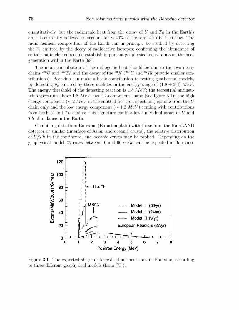
76 Non-solar neutrino physics with the Borexino detector
quantitatively, but the radiogenic heat from the decay of U and Th in the Earth’scrust is currently believed to account for ∼ 40% of the total 40 TW heat flow. Theradiochemical composition of the Earth can in principle be studied by detectingthe νe emitted by the decay of radioactive isotopes; confirming the abundance ofcertain radio-elements could establish important geophysical constraints on the heatgeneration within the Earth [68].
The main contribution of the radiogenic heat should be due to the two decaychains 238U and 232Th and the decay of the 40K (235U and 87Rb provide smaller con-tributions). Borexino can make a basic contribution to testing geothermal models,by detecting νe emitted by these nuclides in the energy range of (1.8 ÷ 3.3) MeV .The energy threshold of the detecting reaction is 1.8 MeV ; the terrestrial antineu-trino spectrum above 1.8 MeV has a 2-component shape (see figure 3.1): the highenergy component (∼ 2 MeV in the emitted positron spectrum) coming from the Uchain only and the low energy component (∼ 1.2 MeV ) coming with contributionsfrom both U and Th chains: this signature could allow individual assay of U andTh abundance in the Earth.
Combining data from Borexino (Eurasian plate) with those from the KamLANDdetector or similar (interface of Asian and oceanic crusts), the relative distributionof U/Th in the continental and oceanic crusts may be probed. Depending on thegeophysical model, νe rates between 10 and 60 ev/yr can be expected in Borexino.
Figure 3.1: The expected shape of terrestrial antineutrinos in Borexino, accordingto three different geophysical models (from [75]).
3.1.2 Long-baseline νe from European reactors 77
3.1.2 Long-baseline νe from European reactors
The νe fluxes from astrophysical sources (including the Earth) are essentially model-dependent; on the contrary, nuclear power reactors emit νe with a known flux andspectral shape, with energies up to ∼ 8 MeV . Borexino is sensitive to this fluxfrom power reactors situated all over Europe (European reactors produce about500 GWof thermal power) at an average baseline distance of ∼ 800 km (Italy hasno nuclear power reactors): reactor anti-neutrino flux will account for ∼ 30 ev/yr inBorexino. Since the distances to the reactors are known, and the fuel compositionand operating cycle of the reactors can also be known very well, the multi-reactorνe event rate and the positron spectrum in Borexino can be calculated with an errorlower than 3%.
The well defined set-up offered by this combination makes an ideal terrestriallong-baseline experiment for a model-independent search for ν oscillations. Evi-dence for neutrino oscillations would come from the disappearance of these neutrinosand from distortions in their spectral shape. As usual, the characteristic oscillationlength varies inversely with energy (1.26): therefore, reactor neutrinos, with ener-gies up to 8 MeV , allow very small mass differences to be probed. In Borexino, thesensitivity for vacuum ν oscillations is in the range δm2 ' (10−3÷ 10−5) eV 2, fillingthe gap between the results of the CHOOZ experiment and solar neutrinos. The Eu-ropean reactor-Borexino combination is also suitable to probe neutrino oscillationsin the LMA-MSW area, as is done in the KamLAND experiment.
3.1.3 Anti-neutrinos from the Sun
The SSM predicts no νe emission from the Sun. However, non-standard physics cancreate νe by some conversion mechanisms. For instance, a non-vanishing neutrinomagnetic moment at the level of 10−12÷10−11 µB could lead to the presence of anti-neutrinos in the solar neutrino spectrum. This scenario could play a subdominantrole in the physics of solar neutrinos, the MSW-LMA being the dominant one. Themechanism of neutrino-antineutrino conversion due to spin-flavor precession (SFP)induced by neutrino transition magnetic moment was discussed for the first timeas a possible solution to the Solar neutrino deficit problem: the interaction of theneutrino magnetic moment with solar magnetic fields could produce the requiredspin-flavor precession, with a flavor conversion into µ or τ antineutrinos. Because ofthe maximal mixing inherent in the model, the resulting µ/τ anti-neutrinos wouldin turn oscillate into νe thanks to the vacuum oscillation mechanism; they wouldthen be detected as νe when reaching the Earth.
Recently, the interest in a large neutrino magnetic moment was revised, due tothe new experimental data available from KamLAND detector [41]. In the energyrange 8.3 < Eνe < 14.8 MeV , no candidate anti-neutrino events were observed inKamLAND, during a 185.5 live days measurement period; considering the expectedbackground, the computed limit on solar νe flux in the above energy range is: φνe <
78 Non-solar neutrino physics with the Borexino detector
3.7×102 cm−2 s−1 at the 90% C.L., corresponding to an upper limit on the neutrinoconversion probability of 2.8× 10⁻⁴ at the 90% C.L. (normalizing to the solar 8B νeflux). Expected Borexino sensitivity to solar anti-neutrinos can be estimated bythe CTF performances (see chapter 4); it will be comparable to the KamLANDsensitivity (even if with a much smaller target mass), but will be in a wider energyrange due to its distant location from nuclear reactors.
3.2 Supernova neutrino detection in Borexino
A typical Type II supernova explosion at a distance of 10 kpc would produce inBorexino a burst of around 110 neutrino events, reaching the detector within a timeinterval of about 10 s [35]. Most of these events would come from the reaction chan-nel νe + p→ e+ + n, while about 30 events would be induced by the interaction ofthe supernova neutrinos on 12C in the liquid scintillator: the detection of the neu-trino interactions with 12C atoms, is an unique feature of Borexino and KamLANDdetectors. Borexino can clearly distinguish between the neutral-current excitations12C(ν, ν ′)12C∗ and the charged-current reactions 12C(νe, e
−)12N and 12C(νe, e+)12B,
via their distinctive event signatures. The ratio of the charged-current to neutral-current neutrino event rates and their time profiles, with respect to each other, canprovide a handle on supernova and non-standard neutrino physics (neutrino massand flavor oscillation).
3.2.1 Supernova explosions
As explained in section 1.1, at any time during its life a star is in hydrostaticequilibrium: the nuclear energy counter-balances the gravitational energy. Everytime the fuel reservoir is exhausted and the resistance to gravitational pressuredrops, the star starts collapsing: the temperature of the core increases and newfusion reactions (higher Z) are triggered. By the end of their lives, stars as massivered giants (Mass > 8M¯) present an “onion” structure, with a very dense corecomposed of heavy elements, such as Ni and Si, and a gaseous external Hydrogenenvelope: for a 18M¯ star at the end of its life, the Silicon core is 108 times moredense than the Hydrogen layer.
When 57Fe is produced at the core, by Silicon burning, the star enters the finalstage of its life. Energy keeps flowing out, fuel is exhausted, the core pressure dropsand the core loses its support. As a consequence, the star implodes under its ownweight. To have an idea of the dimensions involved, the diameter of the core dropsfrom 8000 to 20 km and the density increases 7 orders of magnitude in less than asecond [81].
The temperature rises to 5×10⁹ K (0.5MeV/particle) and the density of the core(> 1010 g/cm3) makes it a degenerate Fermi gas. The contraction becomes a free-fall and stops only when the core density reaches the nuclear density (1014 g/cm3).
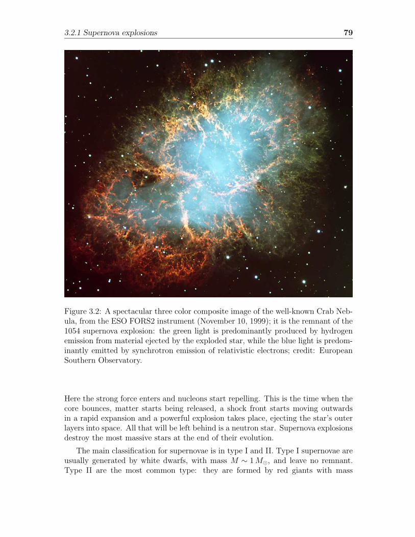
3.2.1 Supernova explosions 79
Figure 3.2: A spectacular three color composite image of the well-known Crab Neb-ula, from the ESO FORS2 instrument (November 10, 1999); it is the remnant of the1054 supernova explosion: the green light is predominantly produced by hydrogenemission from material ejected by the exploded star, while the blue light is predom-inantly emitted by synchrotron emission of relativistic electrons; credit: EuropeanSouthern Observatory.
Here the strong force enters and nucleons start repelling. This is the time when thecore bounces, matter starts being released, a shock front starts moving outwardsin a rapid expansion and a powerful explosion takes place, ejecting the star’s outerlayers into space. All that will be left behind is a neutron star. Supernova explosionsdestroy the most massive stars at the end of their evolution.
The main classification for supernovae is in type I and II. Type I supernovae areusually generated by white dwarfs, with mass M ∼ 1M¯, and leave no remnant.Type II are the most common type: they are formed by red giants with mass
80 Non-solar neutrino physics with the Borexino detector
M > 8M¯ and they leave a neutron star behind.The frequency of supernova explosions in our Galaxy has been calculated in
several independent ways. An analysis based on theories of the stellar evolution, theluminosity function of nearby stars and a model of stellar population yields a rateof (2.6 ± 1.3)/century. A comparison with the occurrence of supernovae in othergalaxies gives a consistent result: (3± 1)(H0/75)
2/century.During the last 2000 years, though, only four supernovae from core collapse
(both type I and II) have been identified in our Galaxy, within 4 kpc from the Sun,in the years 185, 1054, 1181, 1670. This gives a rate of (0.2 ± 0.1)/century. Itis a real puzzle that no more near supernovae have been observed in the last fourcenturies: a simple Poisson statistics calculation shows that the probability of nothaving any supernova in the last 100 years is only 8.2%, assuming a mean galacticrate of 2.5/century. Thousands supernovae are being observed in distant galaxies,but to date the most interesting to us is SN1987A [81] in the nearby LMC, whoseneutrinos have been detected by the Kamiokande [61] and IMB detector [29].
3.2.2 The role of neutrinos in the Supernova explosion
The gravitational collapse events associated with type II supernovae and neutronstar formation are copious producers of neutrinos. As stated in [81], regardless ofthe detail of the collapse, core bounce and explosion processes, in order to form aremnant neutron star there must be an energy release equal to the binding energyεB ' 3×1053 ergs. The total light emitted in the supernova outburst is about 1% ofthis energy; the remainder of the binding energy comes off in the form of neutrinos.
Neutrinos are produced at different stages of the supernova event, through dif-ferent processes, but most of the binding energy of the star is carried away by theνν pairs produced during the thermal cooling phase of the hot remnant core. Theseneutrinos, created in pair-production processes such as: e+ + e− → νi + νi, are themost efficient energy carriers and constitute the main neutrino signal we can receive,on Earth, from the supernova event [81].
The νi−νi pairs produced during the cooling phase do not immediately escape thecore. The reason is the weak interaction: at densities > 1011 g/cm3 the scattering ofneutrinos off nuclei happens so often that the neutrinos get trapped. Despite this, theneutrino mean free path remains large, so that they are still efficient energy carriersand they can escape as soon as they pass the neutrino-sphere, defined as the surfacewithin which neutrinos are trapped. This occurs at a density ∼ 5× 10¹⁰ g/cm3.
The temperature of the neutrino-sphere characterizes the energy distributionspectrum of the neutrinos. νµ and ντ and their antiparticles present lower opacitiesthan νe and νe, since they interact only via neutral current weak interaction (νeand νe also do charged current). This means their neutrino-sphere is deeper insidethe core and their spectrum is hotter than the one of νe and νe. Moreover, theneutrino decoupling takes place in a neutron rich matter, less transparent to νe thanνe. The temperature hierarchy is, then: Tνe < Tνe < Tνx (νx refers to νµ, ντ and
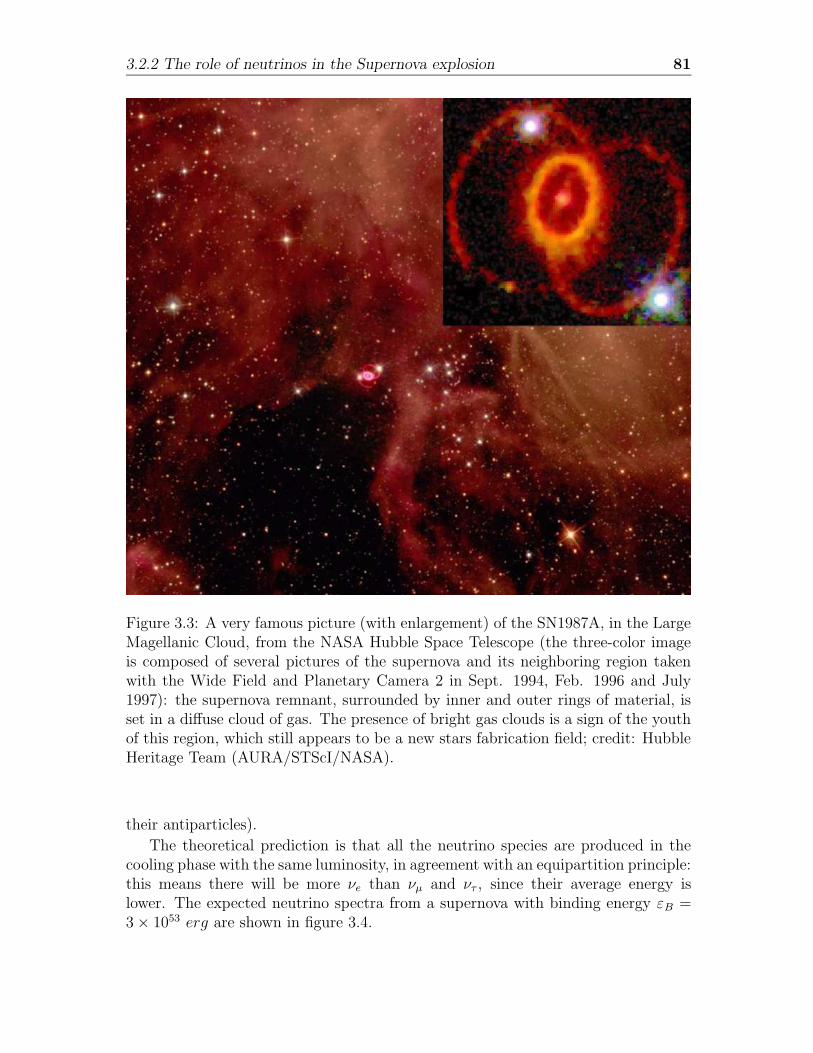
3.2.2 The role of neutrinos in the Supernova explosion 81
Figure 3.3: A very famous picture (with enlargement) of the SN1987A, in the LargeMagellanic Cloud, from the NASA Hubble Space Telescope (the three-color imageis composed of several pictures of the supernova and its neighboring region takenwith the Wide Field and Planetary Camera 2 in Sept. 1994, Feb. 1996 and July1997): the supernova remnant, surrounded by inner and outer rings of material, isset in a diffuse cloud of gas. The presence of bright gas clouds is a sign of the youthof this region, which still appears to be a new stars fabrication field; credit: HubbleHeritage Team (AURA/STScI/NASA).
their antiparticles).
The theoretical prediction is that all the neutrino species are produced in thecooling phase with the same luminosity, in agreement with an equipartition principle:this means there will be more νe than νµ and ντ , since their average energy islower. The expected neutrino spectra from a supernova with binding energy εB =3× 1053 erg are shown in figure 3.4.
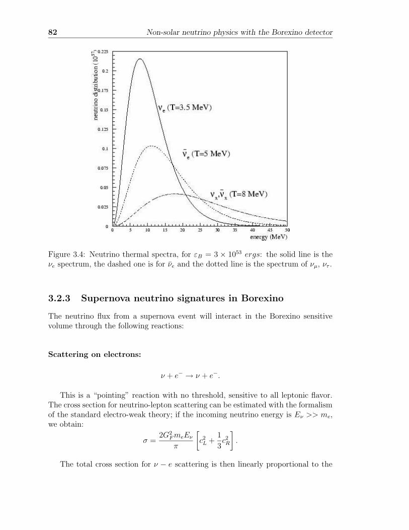
82 Non-solar neutrino physics with the Borexino detector
Figure 3.4: Neutrino thermal spectra, for εB = 3 × 1053 ergs: the solid line is theνe spectrum, the dashed one is for νe and the dotted line is the spectrum of νµ, ντ .
3.2.3 Supernova neutrino signatures in Borexino
The neutrino flux from a supernova event will interact in the Borexino sensitivevolume through the following reactions:
Scattering on electrons:
ν + e− → ν + e−.
This is a “pointing” reaction with no threshold, sensitive to all leptonic flavor.The cross section for neutrino-lepton scattering can be estimated with the formalismof the standard electro-weak theory; if the incoming neutrino energy is Eν >> me,we obtain:
σ =2G2
FmeEν
π
[
c2L +1
3c2R
]
.
The total cross section for ν − e scattering is then linearly proportional to the
3.2.3 Supernova neutrino signatures in Borexino 83
neutrino energy: σ(Eν) = σ · Eν , with σ ' constant. The numerical values are:
σ(νe) = 9.20× 10−45 Eν [MeV ] cm2
σ(νe) = 3.83× 10−45 Eν [MeV ] cm2
σ(νµ,τ ) = 1.57× 10−45 Eν [MeV ] cm2
σ(νµ,τ ) = 1.29× 10−45 Eν [MeV ] cm2.
These cross sections can be averaged over the proper thermal neutrino spectrum,with Ethr = 0; it is then straightforward to calculate the expected number of eventsof this type in Borexino, as a consequence of a supernova collapse: in 300 t of liquidscintillator there would be ∼ 5 scattering events due to a type II supernova withbinding energy εB = 3× 1053 erg at 10 kpc distance.
Inverse β decay of the proton:
νe + p→ e+ + n.
This reaction, with an energy threshold of 1.80 MeV , is the favorite channel forthe detection of supernova neutrinos.
The total cross section for this reaction, for sufficiently low energy, is given by:
σ =G2
FE2ν
π| cos2 θc|2
[
1 + 3
(
gAgV
)2]
.
This approximation is valid for neutrino energies up to about 50 MeV ; in ourcase, the average νe energy is 〈Eνe〉 = 16 MeV and only 0.3% of the νe spectrumis above 50 MeV . It is safe, then, to assume the cross section for this reactiondepends on the neutrino energy as σ(Eν) = σ(Eν − 1.3)2, with σ = constant =9.5× 10−44 cm2/MeV 2.
The expected event number in Borexino (300 t sensitive volume) results to be∼ 79 counts, for the “usual” 10 kpc type II supernova.
Reactions on 12C:
Although the main supernova signal comes from the ν capture, the reactions ofneutrino capture on 12C are particularly interesting in detectors based on organicscintillator, such as Borexino. Three different reactions are possible:
- charged current capture of νe:
νe +12 C → 12B + e+ Q = 13.37 MeV
12B →12 C + e− + νe τ1/2 = 20.20 ms
84 Non-solar neutrino physics with the Borexino detector
- charged current capture of νe:
νe +12 C → 12N + e− Q = 17.34 MeV
12N →12 C + e+ + νe τ1/2 = 11.00 ms
- inelastic scattering of νx:
νx +12 C → 12C∗ + ν ′x Ethr = 15.11 MeV
12C∗ →12 C + γ Eγ = 15.11 MeV
All these three reactions on 12C can be tagged in Borexino: both 12C(νe, e−)12N
and 12C(νe, e+)12B present a delayed coincidence of an electron and a positron, with
a few milliseconds delay; while the inelastic scattering 12C(ν, ν ′)12C∗ is followed bya mono-energetic γ ray at 15.11 MeV .
The cross sections for the neutrino-carbon reactions are complicated by the pres-ence of nuclear matrix elements: for this reason, they have been investigated the-oretically and experimentally over the past 20 years and are now well established.The agreement between the theoretical predictions to the measured data is goodand a combined theoretical and experimental average value for the 12C(νe, e
−)12Nreaction, can be set as 〈σ〉exp = 9.2×10−42cm2 [35]. The cross section measurementswere averaged over the neutrino energies relevant to the experiments, namely neutri-nos from muon decay at rest: it is straightforward to scale these measured values togive averaged cross sections for supernova neutrinos. Since 12N and 12B are “mirrornuclei”, the matrix elements and energy-independent terms in the cross section areessentially identical (only the Coulomb correction differs when calculating the νerates).
The neutral-current cross section can also be extracted from the experimental12C(ν, ν ′)12C∗ cross section data. Using an averaged value 〈σ〉exp = 10 × 10−42cm2
and assuming the contribution of νe and νµ to the nuclear inelastic scattering tobe the same, we scaled this data for supernova neutrino fluxes and energies. Thesecalculations allow to estimate the following event numbers in Borexino (300 t): 23neutral-current events, 4 events due to νe capture on 12C and less than one eventdue to νe capture, from a typical Galactic supernova at 10 kpc.
The contributions of the different neutrino flavors to the neutral current reaction12C(ν, ν ′)12C∗(15.11 MeV ) are shown in figure 3.5, where incoming neutrino energyspectra are compared with their convolution with the cross section: the summedcontribution of νµ, ντ (and their antiparticles) gives the only significant fraction ofevents above threshold; the summary of expectations on supernova neutrino eventsfrom the various contributions is listed in table 3.1.
3.2.4 Neutral current detection capabilities
The neutrino burst from a supernova rises steeply and decays exponentially in time:the neutrino luminosity, decays exponentially in time as Lν ∼ et/τν , with τν ∼ 3
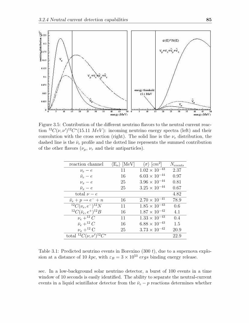
3.2.4 Neutral current detection capabilities 85
Figure 3.5: Contribution of the different neutrino flavors to the neutral current reac-tion 12C(ν, ν ′)12C∗(15.11 MeV ): incoming neutrino energy spectra (left) and theirconvolution with the cross section (right). The solid line is the νe distribution, thedashed line is the νe profile and the dotted line represents the summed contributionof the other flavors (νµ, ντ and their antiparticles).
reaction channel 〈Eν〉 [MeV] 〈σ〉 [cm2] Nevents
νe − e 11 1.02× 10−43 2.37νe − e 16 6.03× 10−44 0.97νx − e 25 3.96× 10−44 0.81νx − e 25 3.25× 10−44 0.67
total ν − e 4.82νe + p→ e− + n 16 2.70× 10−41 78.912C(νe, e
−)12N 11 1.85× 10−43 0.612C(νe, e
+)12B 16 1.87× 10−42 4.1νe +
12 C 11 1.33× 10−43 0.4νe +
12 C 16 6.88× 10−43 1.5νx +
12 C 25 3.73× 10−42 20.9total 12C(ν, ν ′)12C∗ 22.9
Table 3.1: Predicted neutrino events in Borexino (300 t), due to a supernova explo-sion at a distance of 10 kpc, with εB = 3× 1053 ergs binding energy release.
sec. In a low-background solar neutrino detector, a burst of 100 events in a timewindow of 10 seconds is easily identified. The ability to separate the neutral-currentevents in a liquid scintillator detector from the νe − p reactions determines whether
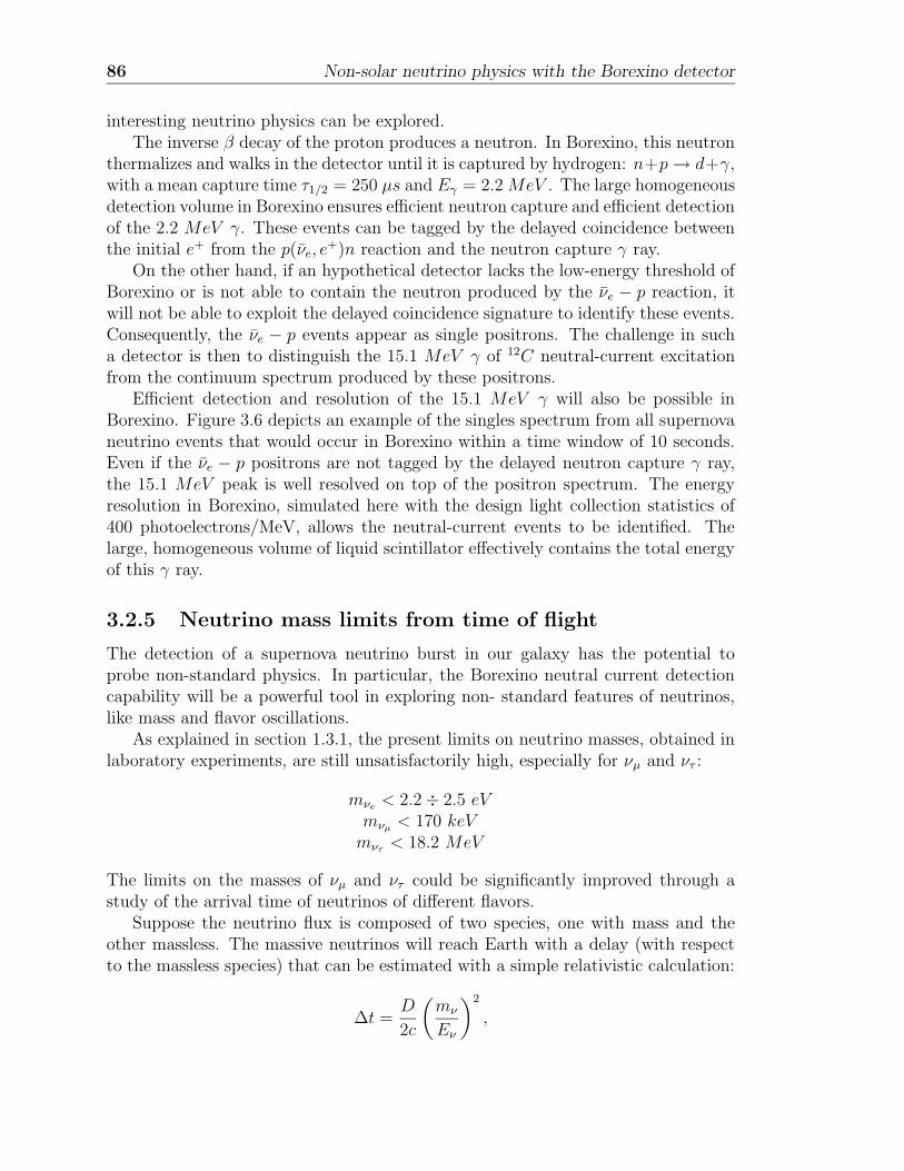
86 Non-solar neutrino physics with the Borexino detector
interesting neutrino physics can be explored.The inverse β decay of the proton produces a neutron. In Borexino, this neutron
thermalizes and walks in the detector until it is captured by hydrogen: n+p→ d+γ,with a mean capture time τ1/2 = 250 µs and Eγ = 2.2MeV . The large homogeneousdetection volume in Borexino ensures efficient neutron capture and efficient detectionof the 2.2 MeV γ. These events can be tagged by the delayed coincidence betweenthe initial e+ from the p(νe, e
+)n reaction and the neutron capture γ ray.On the other hand, if an hypothetical detector lacks the low-energy threshold of
Borexino or is not able to contain the neutron produced by the νe − p reaction, itwill not be able to exploit the delayed coincidence signature to identify these events.Consequently, the νe − p events appear as single positrons. The challenge in sucha detector is then to distinguish the 15.1 MeV γ of 12C neutral-current excitationfrom the continuum spectrum produced by these positrons.
Efficient detection and resolution of the 15.1 MeV γ will also be possible inBorexino. Figure 3.6 depicts an example of the singles spectrum from all supernovaneutrino events that would occur in Borexino within a time window of 10 seconds.Even if the νe − p positrons are not tagged by the delayed neutron capture γ ray,the 15.1 MeV peak is well resolved on top of the positron spectrum. The energyresolution in Borexino, simulated here with the design light collection statistics of400 photoelectrons/MeV, allows the neutral-current events to be identified. Thelarge, homogeneous volume of liquid scintillator effectively contains the total energyof this γ ray.
3.2.5 Neutrino mass limits from time of flight
The detection of a supernova neutrino burst in our galaxy has the potential toprobe non-standard physics. In particular, the Borexino neutral current detectioncapability will be a powerful tool in exploring non- standard features of neutrinos,like mass and flavor oscillations.
As explained in section 1.3.1, the present limits on neutrino masses, obtained inlaboratory experiments, are still unsatisfactorily high, especially for νµ and ντ :
mνe < 2.2÷ 2.5 eVmνµ < 170 keVmντ < 18.2 MeV
The limits on the masses of νµ and ντ could be significantly improved through astudy of the arrival time of neutrinos of different flavors.
Suppose the neutrino flux is composed of two species, one with mass and theother massless. The massive neutrinos will reach Earth with a delay (with respectto the massless species) that can be estimated with a simple relativistic calculation:
∆t =D
2c
(
mν
Eν
)2
,
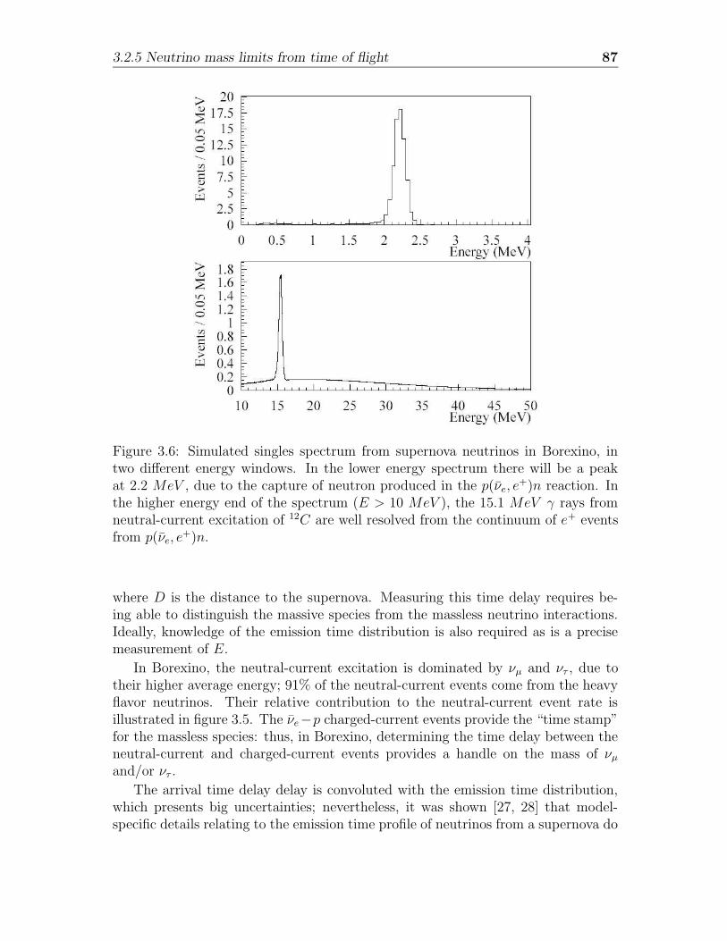
3.2.5 Neutrino mass limits from time of flight 87
Figure 3.6: Simulated singles spectrum from supernova neutrinos in Borexino, intwo different energy windows. In the lower energy spectrum there will be a peakat 2.2 MeV , due to the capture of neutron produced in the p(νe, e
+)n reaction. Inthe higher energy end of the spectrum (E > 10 MeV ), the 15.1 MeV γ rays fromneutral-current excitation of 12C are well resolved from the continuum of e+ eventsfrom p(νe, e
+)n.
where D is the distance to the supernova. Measuring this time delay requires be-ing able to distinguish the massive species from the massless neutrino interactions.Ideally, knowledge of the emission time distribution is also required as is a precisemeasurement of E.
In Borexino, the neutral-current excitation is dominated by νµ and ντ , due totheir higher average energy; 91% of the neutral-current events come from the heavyflavor neutrinos. Their relative contribution to the neutral-current event rate isillustrated in figure 3.5. The νe−p charged-current events provide the “time stamp”for the massless species: thus, in Borexino, determining the time delay between theneutral-current and charged-current events provides a handle on the mass of νµand/or ντ .
The arrival time delay delay is convoluted with the emission time distribution,which presents big uncertainties; nevertheless, it was shown [27, 28] that model-specific details relating to the emission time profile of neutrinos from a supernova do
88 Non-solar neutrino physics with the Borexino detector
not have a pronounced effect on the arrival time distribution, since the overwhelmingconsideration in analyzing the time delay for massive neutrinos is the time constantof the exponential decay of the neutrino luminosity; the averaged quantities such as:
∆t =< t >NC − < t >CC
can then be used as sensitive probes for extraction of the neutrino mass from super-nova neutrino data.
We considered a model for a supernova neutrino burst that rises linearly, reachingmaximum in the first ∼ 20 ms after the core bounce; the sharp increase is thenfollowed by an exponential decay, with lifetime τ ∼ 3s. Figure 3.7 shows the expectedtime distribution of the 12C(ν, ν ′)12C∗ events in Borexino, for two scenarios. In bothcases, νe is assumed massless and: (a) νµ is massless and ντ is massive ⇒ 46% ofthe 12C(ν, ν ′)12C∗ events are delayed; (b) νµ and ντ are both massive ⇒ 91% of the12C(ν, ν ′)12C∗ events are delayed.
Figure 3.7: Time distribution for the 12C(ν, ν ′)12C∗ events, for two cases: (a) 46%of the events are from massive neutrinos (ντ ); (b) 91% of the events are massive (νµand ντ ).
Figure 3.8 shows the distribution of average time of arrival of the 12C(ν, ν ′)12C∗
events, for different values of the heavy neutrino mass. It is based on the results of aMonte Carlo simulation of 105 supernovae (distance 10 kpc) producing 12C neutral-current events in Borexino [35]. The arrival times for the, on average, 23 eventswere drawn from the distributions shown in figure 3.7. Time zero is the theoreticalinstant of the earliest possible arrival (possibly determined by the earliest detectionof νe). To obtain ∆t, we subtract the average arrival time of the light neutrinos,that is 〈t〉CC = 3 s.
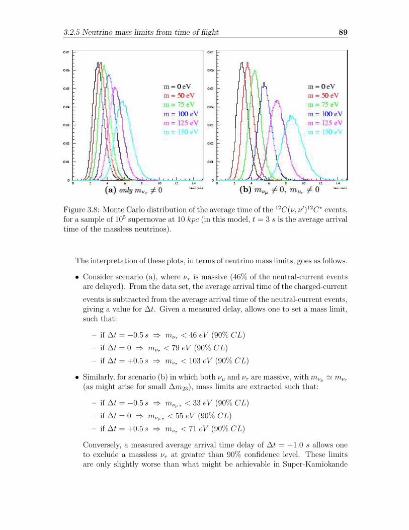
3.2.5 Neutrino mass limits from time of flight 89
Figure 3.8: Monte Carlo distribution of the average time of the 12C(ν, ν ′)12C∗ events,for a sample of 105 supernovae at 10 kpc (in this model, t = 3 s is the average arrivaltime of the massless neutrinos).
The interpretation of these plots, in terms of neutrino mass limits, goes as follows.
• Consider scenario (a), where ντ is massive (46% of the neutral-current eventsare delayed). From the data set, the average arrival time of the charged-current
events is subtracted from the average arrival time of the neutral-current events,giving a value for ∆t. Given a measured delay, allows one to set a mass limit,such that:
– if ∆t = −0.5 s ⇒ mντ < 46 eV (90% CL)
– if ∆t = 0 ⇒ mντ < 79 eV (90% CL)
– if ∆t = +0.5 s ⇒ mντ < 103 eV (90% CL)
• Similarly, for scenario (b) in which both νµ and ντ are massive, withmνµ ' mντ
(as might arise for small ∆m23), mass limits are extracted such that:
– if ∆t = −0.5 s ⇒ mνµ τ< 33 eV (90% CL)
– if ∆t = 0 ⇒ mνµ τ< 55 eV (90% CL)
– if ∆t = +0.5 s ⇒ mντ < 71 eV (90% CL)
Conversely, a measured average arrival time delay of ∆t = +1.0 s allows oneto exclude a massless ντ at greater than 90% confidence level. These limitsare only slightly worse than what might be achievable in Super-Kamiokande
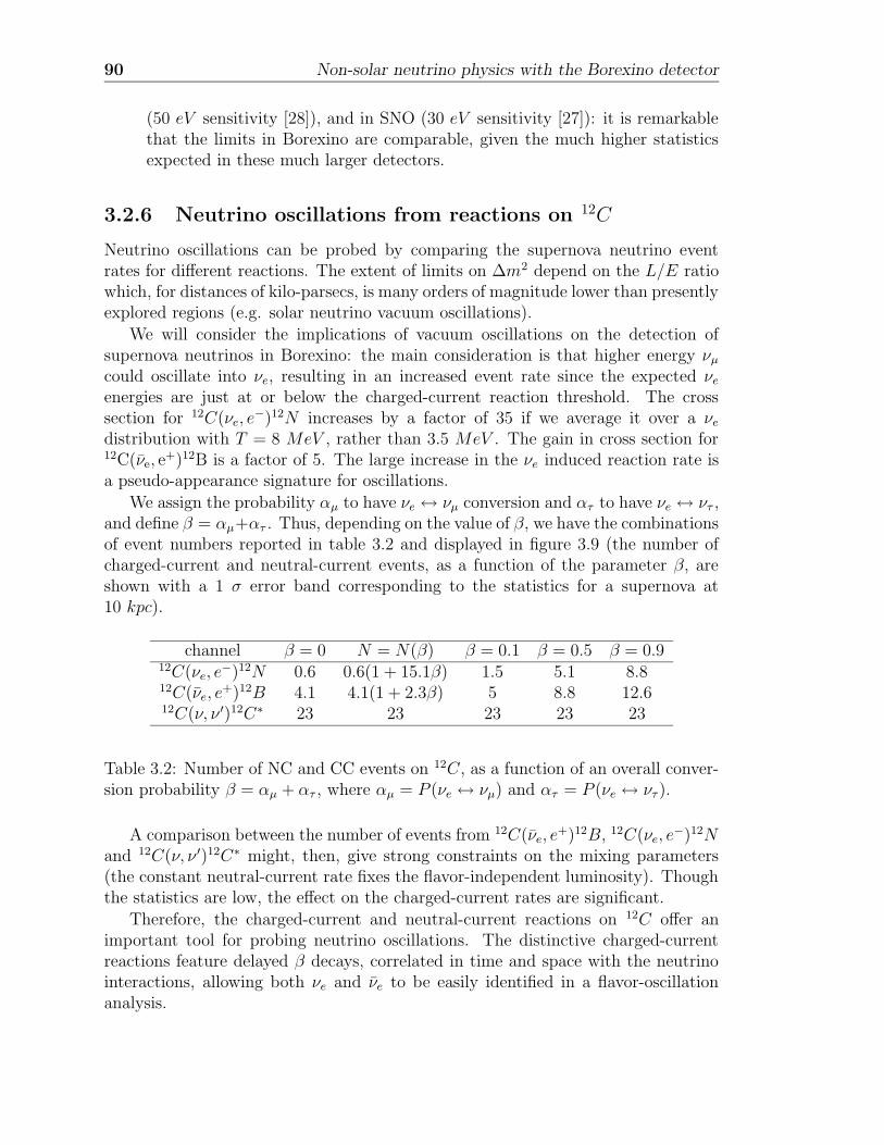
90 Non-solar neutrino physics with the Borexino detector
(50 eV sensitivity [28]), and in SNO (30 eV sensitivity [27]): it is remarkablethat the limits in Borexino are comparable, given the much higher statisticsexpected in these much larger detectors.
3.2.6 Neutrino oscillations from reactions on 12C
Neutrino oscillations can be probed by comparing the supernova neutrino eventrates for different reactions. The extent of limits on ∆m2 depend on the L/E ratiowhich, for distances of kilo-parsecs, is many orders of magnitude lower than presentlyexplored regions (e.g. solar neutrino vacuum oscillations).
We will consider the implications of vacuum oscillations on the detection ofsupernova neutrinos in Borexino: the main consideration is that higher energy νµcould oscillate into νe, resulting in an increased event rate since the expected νeenergies are just at or below the charged-current reaction threshold. The crosssection for 12C(νe, e
−)12N increases by a factor of 35 if we average it over a νedistribution with T = 8 MeV , rather than 3.5 MeV . The gain in cross section for12C(νe, e
+)12B is a factor of 5. The large increase in the νe induced reaction rate isa pseudo-appearance signature for oscillations.
We assign the probability αµ to have νe ↔ νµ conversion and ατ to have νe ↔ ντ ,and define β = αµ+ατ . Thus, depending on the value of β, we have the combinationsof event numbers reported in table 3.2 and displayed in figure 3.9 (the number ofcharged-current and neutral-current events, as a function of the parameter β, areshown with a 1 σ error band corresponding to the statistics for a supernova at10 kpc).
channel β = 0 N = N(β) β = 0.1 β = 0.5 β = 0.912C(νe, e
−)12N 0.6 0.6(1 + 15.1β) 1.5 5.1 8.812C(νe, e
+)12B 4.1 4.1(1 + 2.3β) 5 8.8 12.612C(ν, ν ′)12C∗ 23 23 23 23 23
Table 3.2: Number of NC and CC events on 12C, as a function of an overall conver-sion probability β = αµ + ατ , where αµ = P (νe ↔ νµ) and ατ = P (νe ↔ ντ ).
A comparison between the number of events from 12C(νe, e+)12B, 12C(νe, e
−)12Nand 12C(ν, ν ′)12C∗ might, then, give strong constraints on the mixing parameters(the constant neutral-current rate fixes the flavor-independent luminosity). Thoughthe statistics are low, the effect on the charged-current rates are significant.
Therefore, the charged-current and neutral-current reactions on 12C offer animportant tool for probing neutrino oscillations. The distinctive charged-currentreactions feature delayed β decays, correlated in time and space with the neutrinointeractions, allowing both νe and νe to be easily identified in a flavor-oscillationanalysis.
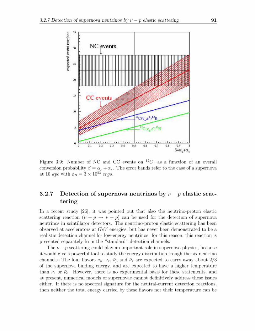
3.2.7 Detection of supernova neutrinos by ν − p elastic scattering 91
Figure 3.9: Number of NC and CC events on 12C, as a function of an overallconversion probability β = αµ+ατ . The error bands refer to the case of a supernovaat 10 kpc with εB = 3× 1053 ergs.
3.2.7 Detection of supernova neutrinos by ν−p elastic scat-tering
In a recent study [26], it was pointed out that also the neutrino-proton elasticscattering reaction (ν + p → ν + p) can be used for the detection of supernovaneutrinos in scintillator detectors. The neutrino-proton elastic scattering has beenobserved at accelerators at GeV energies, but has never been demonstrated to be arealistic detection channel for low-energy neutrinos: for this reason, this reaction ispresented separately from the “standard” detection channels.
The ν − p scattering could play an important role in supernova physics, becauseit would give a powerful tool to study the energy distribution trough the six neutrinochannels. The four flavors νµ, ντ , νµ and ντ are expected to carry away about 2/3of the supernova binding energy, and are expected to have a higher temperaturethan νe or νe. However, there is no experimental basis for these statements, andat present, numerical models of supernovae cannot definitively address these issueseither. If there is no spectral signature for the neutral-current detection reactions,then neither the total energy carried by these flavors nor their temperature can be
92 Non-solar neutrino physics with the Borexino detector
separately determined from the detected number of events: the ν − p representsan exception to this statement, since the measured proton spectrum is related tothe incident neutrino spectrum, which helps in reconstructing the total energy andtemperature of νµ, ντ , νµ and ντ .
The theoretical cross section for neutrino-proton elastic scattering has been con-firmed by extensive measurements at GeV energies. At the energies considered here,the total cross section yields [26]:
σ =G2
FE2ν
π(c2V + 3c2A).
This cross section is of the same form as the total cross section for the charged-current reaction νe + p → e+ + n, but is approximately 4 times smaller. However,this is compensated in the yield by the contributions of all six flavors, as well as thehigher temperature assumed for νµ and ντ (T = 8 MeV instead of 5 MeV ): thus,the total yield from ν + p → ν + p is larger than from νe + p → e+ + n, when thedetector threshold is neglected.
The elastically-scattered protons will have kinetic energies of a few MeV . Obvi-ously, these very non-relativistic protons will be completely invisible in any Cerenkovdetector like Super-Kamiokande. However, such small energy depositions can bereadily detected in scintillator detectors such as KamLAND and Borexino. Theproton recoil spectrum for KamLAND detector is shown in figure 3.10 (left): inBorexino, the spectrum will have the same shape, but the total numbers will bereduced by a factor 4.7 (taking into account the reduced number of target protons).
For highly ionizing particles like low-energy protons, the quenching effect inscintillator has to be considered; the observable light output Eequiv is given by Birk’sLaw:
dEequiv
dx=
dE/dx
1 +KB(dE/dx)
where kB is a constant of the scintillation material, assumed to be kB ' 0.015 forKamLAND and kB ' 0.010 ÷ 0.015 for Borexino1. Visible proton spectrum forKamLAND is shown in figure 3.10: the effect of the quenching is a significant shiftof the spectrum towards lower energy values.
In absence of threshold, ∼ 133 scattered protons would be detected in Borexino;but the real number of νe + p → e+ + n events will be determined by the naturalradioactivity of the scintillator (namely by the 14C countrate): since the supernovaevent rate will be of the order of 10 Hz, an acceptable threshold could be slightlylower than in the solar neutrino case (∼ 200 keV ), where the 14C rate will be of theHz order. In these conditions, ∼ 45 ÷ 55% of the ν − p signal would be conserved(depending on the real quenching factor that will be measured in the scintillator),giving a total countrate comparable with the νe + p→ e+ + n one.
1The value kB = 0.015 has been measured in laboratory measurement but never published;some recent studies on CTF-III data (see chapter 4) suggest a value closer to 0.010.
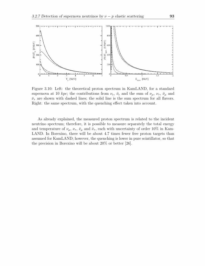
3.2.7 Detection of supernova neutrinos by ν − p elastic scattering 93
Figure 3.10: Left: the theoretical proton spectrum in KamLAND, for a standardsupernova at 10 kpc; the contributions from νe, νe and the sum of νµ, ντ , νµ andντ are shown with dashed lines; the solid line is the sum spectrum for all flavors.Right: the same spectrum, with the quenching effect taken into account.
As already explained, the measured proton spectrum is related to the incidentneutrino spectrum; therefore, it is possible to measure separately the total energyand temperature of νµ, ντ , νµ and ντ , each with uncertainty of order 10% in Kam-LAND. In Borexino, there will be about 4.7 times fewer free proton targets thanassumed for KamLAND; however, the quenching is lower in pure scintillator, so thatthe precision in Borexino will be about 20% or better [26].

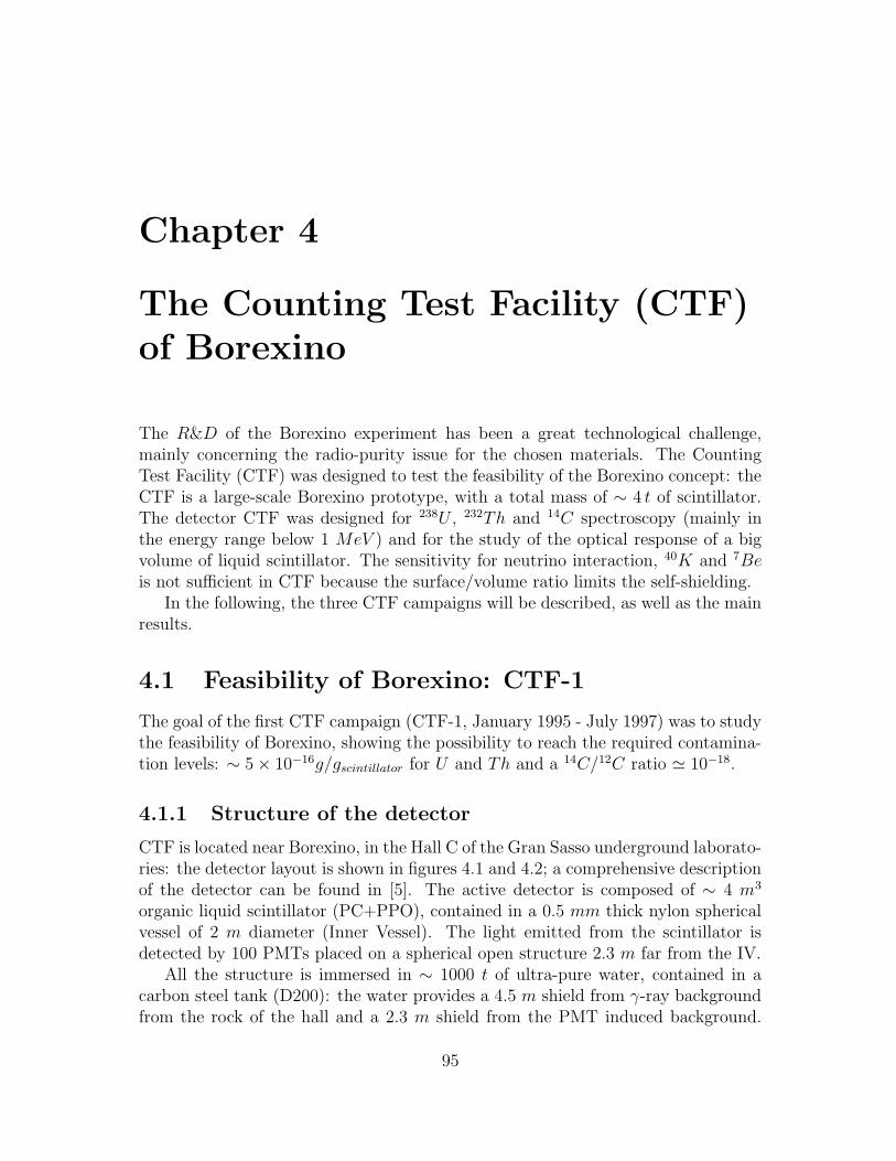
Chapter 4
The Counting Test Facility (CTF)of Borexino
The R&D of the Borexino experiment has been a great technological challenge,mainly concerning the radio-purity issue for the chosen materials. The CountingTest Facility (CTF) was designed to test the feasibility of the Borexino concept: theCTF is a large-scale Borexino prototype, with a total mass of ∼ 4 t of scintillator.The detector CTF was designed for 238U , 232Th and 14C spectroscopy (mainly inthe energy range below 1 MeV ) and for the study of the optical response of a bigvolume of liquid scintillator. The sensitivity for neutrino interaction, 40K and 7Beis not sufficient in CTF because the surface/volume ratio limits the self-shielding.
In the following, the three CTF campaigns will be described, as well as the mainresults.
4.1 Feasibility of Borexino: CTF-1
The goal of the first CTF campaign (CTF-1, January 1995 - July 1997) was to studythe feasibility of Borexino, showing the possibility to reach the required contamina-tion levels: ∼ 5× 10⁻¹⁶g/gscintillator for U and Th and a 14C/12C ratio ' 10−18.
4.1.1 Structure of the detector
CTF is located near Borexino, in the Hall C of the Gran Sasso underground laborato-ries: the detector layout is shown in figures 4.1 and 4.2; a comprehensive descriptionof the detector can be found in [5]. The active detector is composed of ∼ 4 m3
organic liquid scintillator (PC+PPO), contained in a 0.5 mm thick nylon sphericalvessel of 2 m diameter (Inner Vessel). The light emitted from the scintillator isdetected by 100 PMTs placed on a spherical open structure 2.3 m far from the IV.
All the structure is immersed in ∼ 1000 t of ultra-pure water, contained in acarbon steel tank (D200): the water provides a 4.5 m shield from γ-ray backgroundfrom the rock of the hall and a 2.3 m shield from the PMT induced background.
95
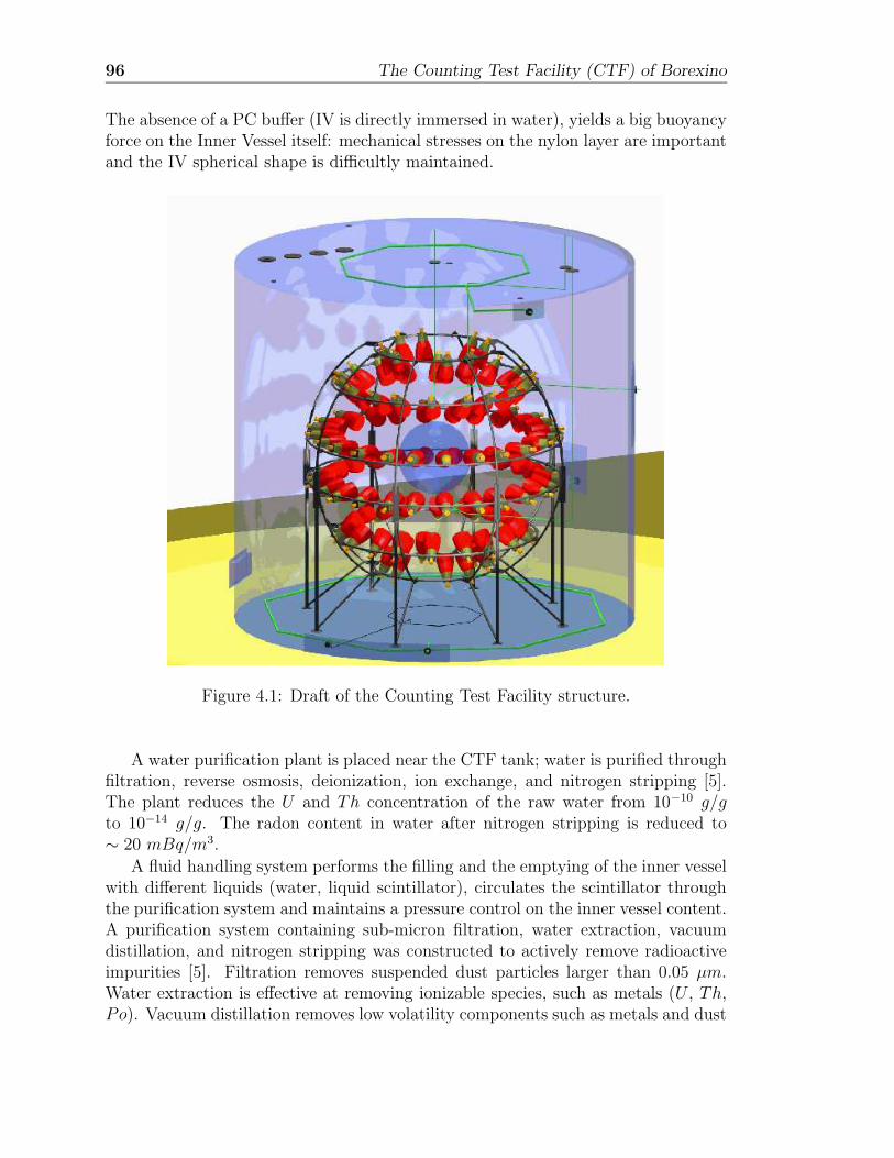
96 The Counting Test Facility (CTF) of Borexino
The absence of a PC buffer (IV is directly immersed in water), yields a big buoyancyforce on the Inner Vessel itself: mechanical stresses on the nylon layer are importantand the IV spherical shape is difficultly maintained.
Figure 4.1: Draft of the Counting Test Facility structure.
A water purification plant is placed near the CTF tank; water is purified throughfiltration, reverse osmosis, deionization, ion exchange, and nitrogen stripping [5].The plant reduces the U and Th concentration of the raw water from 10−10 g/gto 10−14 g/g. The radon content in water after nitrogen stripping is reduced to∼ 20 mBq/m3.
A fluid handling system performs the filling and the emptying of the inner vesselwith different liquids (water, liquid scintillator), circulates the scintillator throughthe purification system and maintains a pressure control on the inner vessel content.A purification system containing sub-micron filtration, water extraction, vacuumdistillation, and nitrogen stripping was constructed to actively remove radioactiveimpurities [5]. Filtration removes suspended dust particles larger than 0.05 µm.Water extraction is effective at removing ionizable species, such as metals (U , Th,Po). Vacuum distillation removes low volatility components such as metals and dust
4.1.2 Main results of the test 97
Figure 4.2: A picture taken inside the D200 tank, during the CTF-1 data taking.
particles. Nitrogen stripping removes dissolved gas impurities, such as 85Kr, as wellas water and oxygen dissolved in the scintillator.
The scintillation light is detected by 100 20 cm diameter photomultiplier tubes(Thorn EMI 9351). The tubes have a cathode efficiency of ∼ 25% (at 380 nm),transit time spread of 1 ns, dark noise of ∼ 500 Hz, low afterpulse (∼ 2.5%)and amplification of 107; the dynodes of the PMT are shielded against magneticfields with mu-metal collar. The PMTs are coupled to “truncated string cone” lightconcentrators, which collect the light from the scintillator containment vessel: thegeometrical coverage of the scintillator region is 21%. The PMTs and their assemblycomponents were selected to minimize the radioactivity; the final γ-ray activity ofeach tube assembly is ∼ 3.8 Bq.
4.1.2 Main results of the test
The CTF installation was completed in early 1995. The detector was filled withwater in January 1995 and the scintillator filling happened in February-April 1995.The data taking went on continuously since it was filled with water (in January1995), until July 1997. The main results of CTF-1 are described in [5, 9, 7, 6] andcan be summarized as follows:
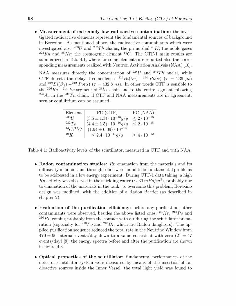
98 The Counting Test Facility (CTF) of Borexino
• Measurement of extremely low radioactive contamination: the inves-tigated radioactive elements represent the fundamental sources of backgroundin Borexino. As mentioned above, the radioactive contaminants which wereinvestigated are: 238U and 232Th chains, the primordial 40K; the noble gases222Rn and 85Kr; the cosmogenic element 14C. The CTF-1 main results aresummarized in Tab. 4.1, where for some elements are reported also the corre-sponding measurements realized with Neutron Activation Analysis (NAA) [10].
NAA measures directly the concentration of 238U and 232Th nuclei, whileCTF detects the delayed coincidences 214Bi(βγ) −214 Po(α) (τ = 236 µs)and 212Bi(βγ) −212 Po(α) (τ = 432.8 ns). In other words CTF is sensible tothe 226Ra −214 Po segment of 238U chain and to the entire segment following226Ac in the 232Th chain: if CTF and NAA measurements are in agreement,secular equilibrium can be assumed.
Element PC (CTF) PC (NAA)238U (3.5± 1.3) · 10−16g/g ≤ 2 · 10−16
232Th (4.4± 1.5) · 10−16g/g ≤ 2 · 10−15
14C/12C (1.94± 0.09) · 10−18 -40K ≤ 2.4 · 10−11g/g ≤ 4 · 10−12
Table 4.1: Radioactivity levels of the scintillator, measured in CTF and with NAA.
• Radon contamination studies: Rn emanation from the materials and itsdiffusivity in liquids and through solids were found to be fundamental problemsto be addressed in a low energy experiment. During CTF-1 data taking, a highRn activity was observed in the shielding water (∼ 30mBq/m3), probably dueto emanation of the materials in the tank: to overcome this problem, Borexinodesign was modified, with the addition of a Radon Barrier (as described inchapter 2).
• Evaluation of the purification efficiency: before any purification, othercontaminants were observed, besides the above listed ones: 85Kr, 210Po and210Bi, coming probably from the contact with air during the scintillator prepa-ration (especially for 210Po and 210Bi, which are Radon daughters). The ap-plied purification sequence reduced the total rate in the Neutrino Window from470 ± 90 internal events/day down to a value consistent with zero (21 ± 47events/day) [9]; the energy spectra before and after the purification are shownin figure 4.3.
• Optical properties of the scintillator: fundamental performances of thedetector-scintillator system were measured by means of the insertion of ra-dioactive sources inside the Inner Vessel; the total light yield was found to
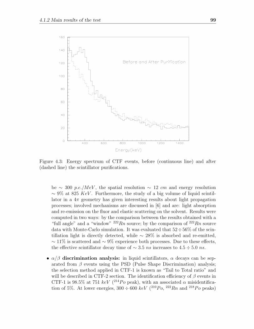
4.1.2 Main results of the test 99
Figure 4.3: Energy spectrum of CTF events, before (continuous line) and after(dashed line) the scintillator purifications.
be ∼ 300 p.e./MeV , the spatial resolution ∼ 12 cm and energy resolution∼ 9% at 825 KeV . Furthermore, the study of a big volume of liquid scintil-lator in a 4π geometry has given interesting results about light propagationprocesses; involved mechanisms are discussed in [6] and are: light absorptionand re-emission on the fluor and elastic scattering on the solvent. Results werecomputed in two ways: by the comparison between the results obtained with a“full angle” and a “window” 222Rn source; by the comparison of 222Rn sourcedata with Monte-Carlo simulation. It was evaluated that 52÷56% of the scin-tillation light is directly detected, while ∼ 28% is absorbed and re-emitted,∼ 11% is scattered and ∼ 9% experience both processes. Due to these effects,the effective scintillator decay time of ∼ 3.5 ns increases to 4.5÷ 5.0 ns.
• α/β discrimination analysis: in liquid scintillators, α decays can be sep-arated from β events using the PSD (Pulse Shape Discrimination) analysis;the selection method applied in CTF-1 is known as “Tail to Total ratio” andwill be described in CTF-2 section. The identification efficiency of β events inCTF-1 is 98.5% at 751 keV (214Po peak), with an associated α misidentifica-tion of 5%. At lower energies, 300÷ 600 keV (210Po, 222Rn and 218Po peaks)
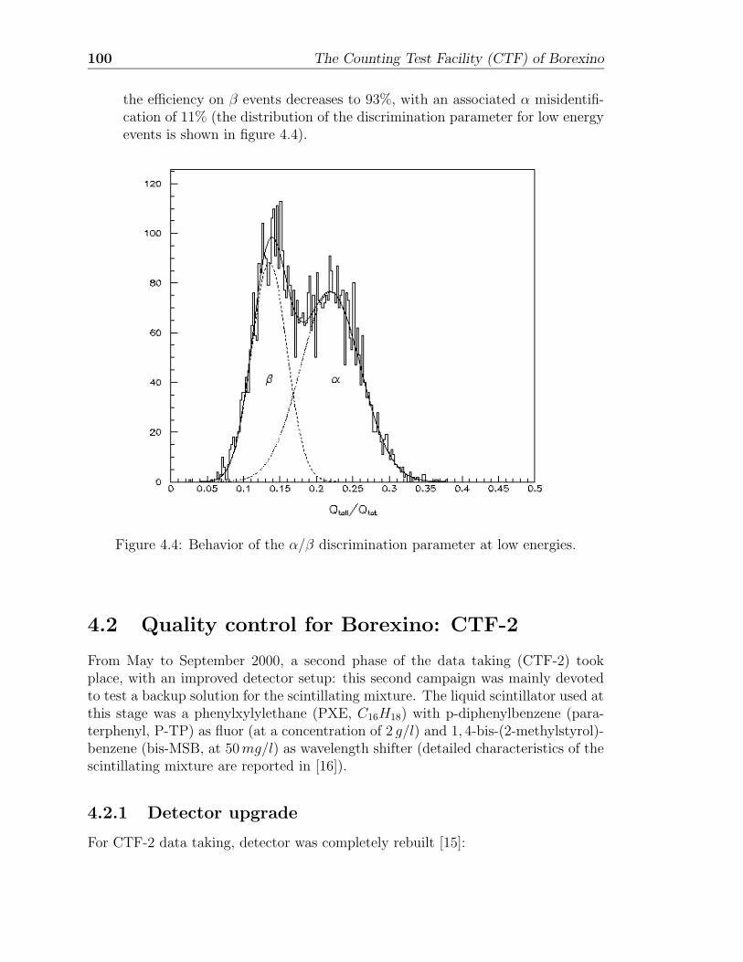
100 The Counting Test Facility (CTF) of Borexino
the efficiency on β events decreases to 93%, with an associated α misidentifi-cation of 11% (the distribution of the discrimination parameter for low energyevents is shown in figure 4.4).
Figure 4.4: Behavior of the α/β discrimination parameter at low energies.
4.2 Quality control for Borexino: CTF-2
From May to September 2000, a second phase of the data taking (CTF-2) tookplace, with an improved detector setup: this second campaign was mainly devotedto test a backup solution for the scintillating mixture. The liquid scintillator used atthis stage was a phenylxylylethane (PXE, C16H18) with p-diphenylbenzene (para-terphenyl, P-TP) as fluor (at a concentration of 2 g/l) and 1, 4-bis-(2-methylstyrol)-benzene (bis-MSB, at 50mg/l) as wavelength shifter (detailed characteristics of thescintillating mixture are reported in [16]).
4.2.1 Detector upgrade
For CTF-2 data taking, detector was completely rebuilt [15]:
4.2.2 Sequence of measurements 101
• 100 new phototubes were installed, of Borexino type (Thorn EMI 9351 of 20 cmdiameter); a completely new sealing design was developed for these PMTs;
• electronics was redesigned, in order to meet data taking requirements; a newboard (Digital Pulse Shape Analyzer) was installed, in order to improve α/βdiscrimination capabilities: details about the board are reported in [76], whileits implementation in CTF is described in [71]; the main results are describedin section 4.2.4;
• an additional nylon screen between the scintillator vessel and PMTs (againstradon penetration) was installed, as it will be done in Borexino as well (Radonbarrier);
• the detector was equipped with a carefully designed muon veto system, con-sisting of 2 rings of 8 PMTs each, installed at the bottom of the tank; muonveto PMTs are looking upward and have no light concentrators. The muonveto system was optimized in order to have a negligible probability of regis-tering the scintillation events in the Neutrino Window; its performances werecalculated by a Monte-Carlo method accounting for specific features of thelight propagation in the CTF and checked by means of a radioactive source,which allowed to tune-up Monte-Carlo parameters [15].
4.2.2 Sequence of measurements
The CTF-2 campaign can be divided into four distinct phases:
1. Water run: first data were taken during May 2000 with both the inner vesseland the external tank filled with water. These data were used to test and tunethe electronics and to determine criteria to identify muon events.
2. Scintillator filling: loading of the scintillator into the Inner Vessel was donein four batches of 1 ton each separated by short periods of data taking. Fillingoperations lasted from June 3 until July 15, 2000.
3. Data taking: data were taken from July 16 until September 5, 2000, corre-sponding to 52 days with 4.2 t of PXE. The Inner Vessel was valved off andno operations were performed during this period.
4. Calibration: after completion of the data taking period, a series of calibrationmeasurements with a 222Rn point-like source were carried out. The sourcewas moved inside the inner vessel to map the detector response and tune theposition reconstruction software1.
1Some details about the Borexino and CTF position reconstruction algorithm are given insection 7.4.
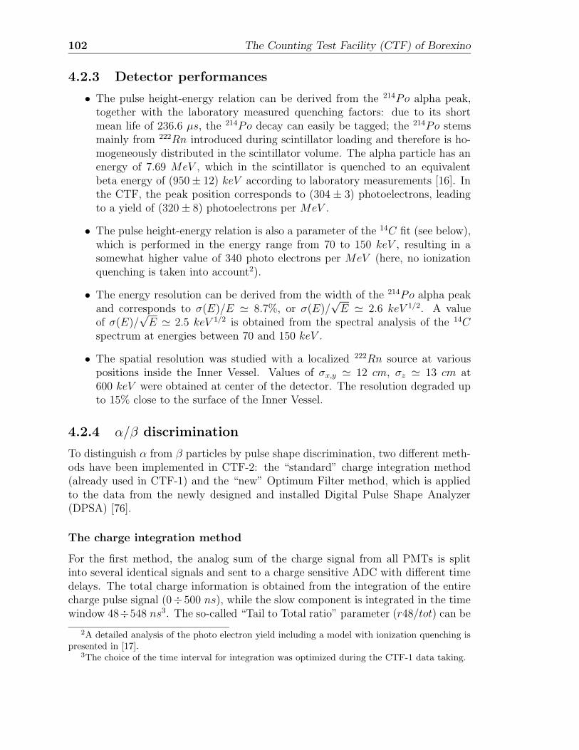
102 The Counting Test Facility (CTF) of Borexino
4.2.3 Detector performances
• The pulse height-energy relation can be derived from the 214Po alpha peak,together with the laboratory measured quenching factors: due to its shortmean life of 236.6 µs, the 214Po decay can easily be tagged; the 214Po stemsmainly from 222Rn introduced during scintillator loading and therefore is ho-mogeneously distributed in the scintillator volume. The alpha particle has anenergy of 7.69 MeV , which in the scintillator is quenched to an equivalentbeta energy of (950± 12) keV according to laboratory measurements [16]. Inthe CTF, the peak position corresponds to (304 ± 3) photoelectrons, leadingto a yield of (320± 8) photoelectrons per MeV .
• The pulse height-energy relation is also a parameter of the 14C fit (see below),which is performed in the energy range from 70 to 150 keV , resulting in asomewhat higher value of 340 photo electrons per MeV (here, no ionizationquenching is taken into account2).
• The energy resolution can be derived from the width of the 214Po alpha peakand corresponds to σ(E)/E ' 8.7%, or σ(E)/
√E ' 2.6 keV 1/2. A value
of σ(E)/√E ' 2.5 keV 1/2 is obtained from the spectral analysis of the 14C
spectrum at energies between 70 and 150 keV .
• The spatial resolution was studied with a localized 222Rn source at variouspositions inside the Inner Vessel. Values of σx,y ' 12 cm, σz ' 13 cm at600 keV were obtained at center of the detector. The resolution degraded upto 15% close to the surface of the Inner Vessel.
4.2.4 α/β discrimination
To distinguish α from β particles by pulse shape discrimination, two different meth-ods have been implemented in CTF-2: the “standard” charge integration method(already used in CTF-1) and the “new” Optimum Filter method, which is appliedto the data from the newly designed and installed Digital Pulse Shape Analyzer(DPSA) [76].
The charge integration method
For the first method, the analog sum of the charge signal from all PMTs is splitinto several identical signals and sent to a charge sensitive ADC with different timedelays. The total charge information is obtained from the integration of the entirecharge pulse signal (0÷ 500 ns), while the slow component is integrated in the timewindow 48÷548 ns3. The so-called “Tail to Total ratio” parameter (r48/tot) can be
2A detailed analysis of the photo electron yield including a model with ionization quenching ispresented in [17].
3The choice of the time interval for integration was optimized during the CTF-1 data taking.
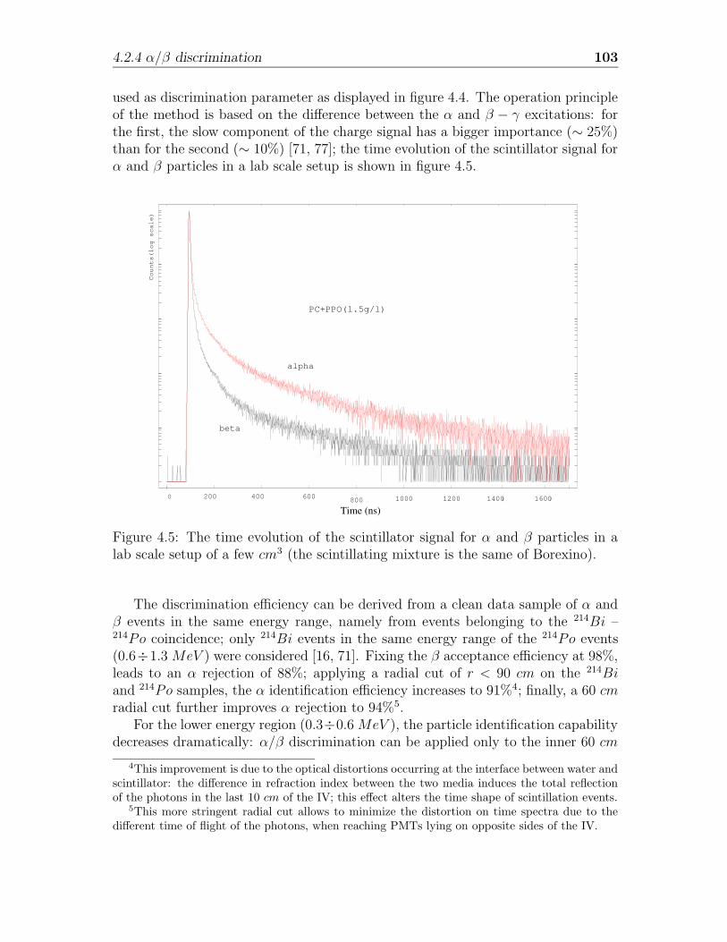
4.2.4 α/β discrimination 103
used as discrimination parameter as displayed in figure 4.4. The operation principleof the method is based on the difference between the α and β − γ excitations: forthe first, the slow component of the charge signal has a bigger importance (∼ 25%)than for the second (∼ 10%) [71, 77]; the time evolution of the scintillator signal forα and β particles in a lab scale setup is shown in figure 4.5.
800 1000 1200 1400 1600
Time (ns)0 200 400 600 800 1000 1200 1400 1600
alpha
beta
PC+PPO(1.5g/l)
Counts(log scale)
Figure 4.5: The time evolution of the scintillator signal for α and β particles in alab scale setup of a few cm3 (the scintillating mixture is the same of Borexino).
The discrimination efficiency can be derived from a clean data sample of α andβ events in the same energy range, namely from events belonging to the 214Bi –214Po coincidence; only 214Bi events in the same energy range of the 214Po events(0.6÷1.3MeV ) were considered [16, 71]. Fixing the β acceptance efficiency at 98%,leads to an α rejection of 88%; applying a radial cut of r < 90 cm on the 214Biand 214Po samples, the α identification efficiency increases to 91%4; finally, a 60 cmradial cut further improves α rejection to 94%5.
For the lower energy region (0.3÷0.6MeV ), the particle identification capabilitydecreases dramatically: α/β discrimination can be applied only to the inner 60 cm
4This improvement is due to the optical distortions occurring at the interface between water andscintillator: the difference in refraction index between the two media induces the total reflectionof the photons in the last 10 cm of the IV; this effect alters the time shape of scintillation events.
5This more stringent radial cut allows to minimize the distortion on time spectra due to thedifferent time of flight of the photons, when reaching PMTs lying on opposite sides of the IV.
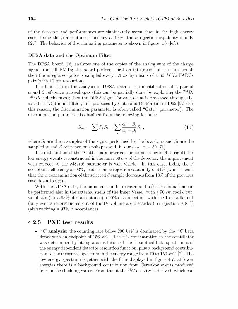
104 The Counting Test Facility (CTF) of Borexino
of the detector and performances are significantly worst than in the high energycase: fixing the β acceptance efficiency at 93%, the α rejection capability is only82%. The behavior of discriminating parameter is shown in figure 4.6 (left).
DPSA data and the Optimum Filter
The DPSA board [76] analyzes one of the copies of the analog sum of the chargesignal from all PMTs; the board performs first an integration of the sum signal;then the integrated pulse is sampled every 8.3 ns by means of a 60 MHz FADCspair (with 10 bit resolution).
The first step in the analysis of DPSA data is the identification of a pair ofα and β reference pulse-shapes (this can be partially done by exploiting the 214Bi–214Po coincidences); then the DPSA signal for each event is processed through theso-called “Optimum filter”, first proposed by Gatti and De Martini in 1962 [52] (forthis reason, the discrimination parameter is often called “Gatti” parameter). Thediscrimination parameter is obtained from the following formula:
Gαβ =∑
i
Pi Si =∑
i
αi − βi
αi + βi
Si , (4.1)
where Si are the n samples of the signal performed by the board, αi and βi are thesampled α and β reference pulse-shapes and, in our case, n = 50 [71].
The distribution of the “Gatti” parameter can be found in figure 4.6 (right), forlow energy events reconstructed in the inner 60 cm of the detector: the improvementwith respect to the r48/tot parameter is well visible. In this case, fixing the βacceptance efficiency at 93%, leads to an α rejection capability of 94% (which meansthat the α contamination of the selected β sample decreases from 18% of the previouscase down to 6%).
With the DPSA data, the radial cut can be released and α/β discrimination canbe performed also in the external shells of the Inner Vessel; with a 90 cm radial cut,we obtain (for a 93% of β acceptance) a 90% of α rejection; with the 1 m radial cut(only events reconstructed out of the IV volume are discarded), α rejection is 88%(always fixing a 93% β acceptance).
4.2.5 PXE test results
• 14C analysis: the counting rate below 200 keV is dominated by the 14C betadecay with an endpoint of 156 keV . The 14C concentration in the scintillatorwas determined by fitting a convolution of the theoretical beta spectrum andthe energy dependent detector resolution function, plus a background contribu-tion to the measured spectrum in the energy range from 70 to 150 keV [7]. Thelow energy spectrum together with the fit is displayed in figure 4.7: at lowerenergies there is a background contribution from Cerenkov events producedby γ in the shielding water. From the fit the 14C activity is derived, which can
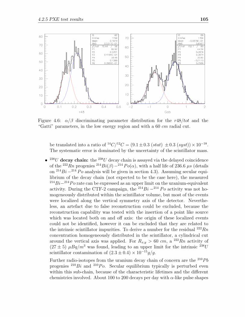
4.2.5 PXE test results 105
Figure 4.6: α/β discriminating parameter distribution for the r48/tot and the“Gatti” parameters, in the low energy region and with a 60 cm radial cut.
be translated into a ratio of 14C/12C = (9.1± 0.3 (stat) ± 0.3 (syst))× 10−18.The systematic error is dominated by the uncertainty of the scintillator mass.
• 238U decay chain: the 238U decay chain is assayed via the delayed coincidenceof the 222Rn progenies 214Bi(β)−214Po(α), with a half life of 236.6 µs (detailson 214Bi−214 Po analysis will be given in section 4.3). Assuming secular equi-librium of the decay chain (not expected to be the case here), the measured214Bi−214Po rate can be expressed as an upper limit on the uranium-equivalentactivity. During the CTF-2 campaign, the 214Bi−214 Po activity was not ho-mogeneously distributed within the scintillator volume, but most of the eventswere localized along the vertical symmetry axis of the detector. Neverthe-less, an artefact due to false reconstruction could be excluded, because thereconstruction capability was tested with the insertion of a point like sourcewhich was located both on and off axis: the origin of these localized eventscould not be identified, however it can be excluded that they are related tothe intrinsic scintillator impurities. To derive a number for the residual 222Rnconcentration homogeneously distributed in the scintillator, a cylindrical cutaround the vertical axis was applied. For Rx,y > 60 cm, a 222Rn activity of(27 ± 5) µBq/m3 was found, leading to an upper limit for the intrinsic 238Uscintillator contamination of (2.3± 0.4)× 10−15g/g.
Further radio-isotopes from the uranium decay chain of concern are the 210Pbprogenies 210Bi and 210Po. Secular equilibrium typically is perturbed evenwithin this sub-chain, because of the characteristic lifetimes and the differentchemistries involved. About 100 to 200 decays per day with α-like pulse shapes
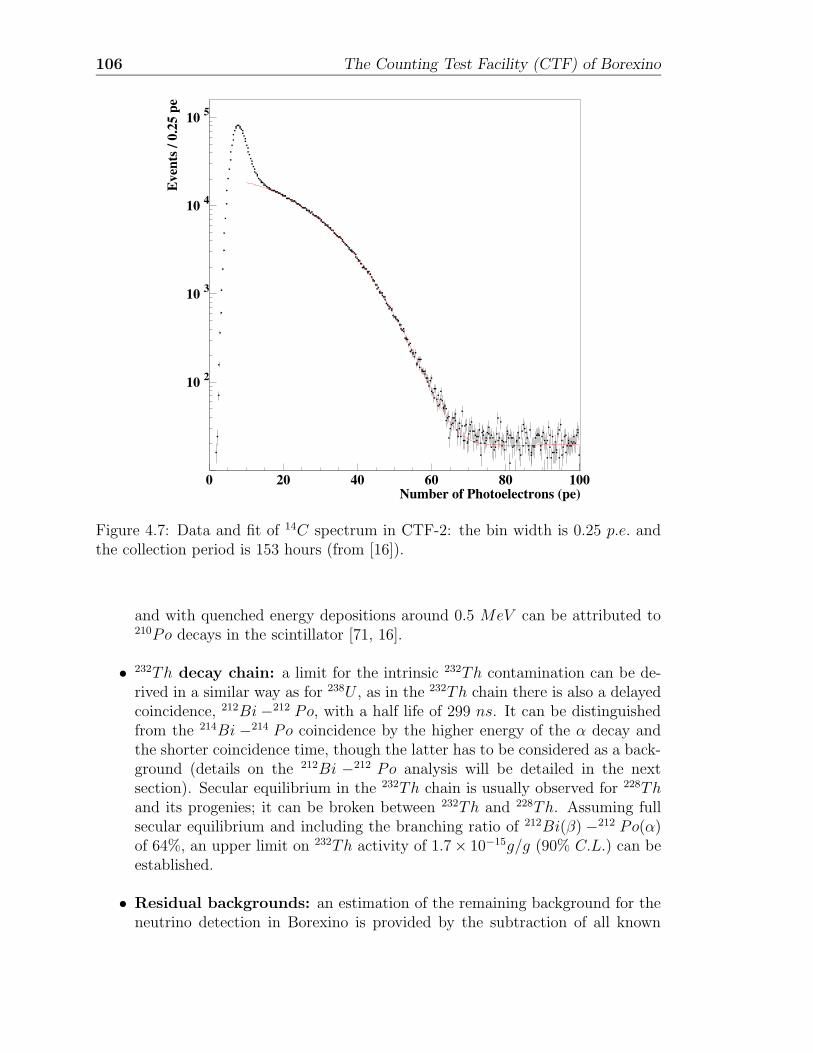
106 The Counting Test Facility (CTF) of Borexino
10 2
10 3
10 4
10 5
0 20 40 60 80 100Number of Photoelectrons (pe)
Eve
nts /
0.2
5 pe
Figure 4.7: Data and fit of 14C spectrum in CTF-2: the bin width is 0.25 p.e. andthe collection period is 153 hours (from [16]).
and with quenched energy depositions around 0.5 MeV can be attributed to210Po decays in the scintillator [71, 16].
• 232Th decay chain: a limit for the intrinsic 232Th contamination can be de-rived in a similar way as for 238U , as in the 232Th chain there is also a delayedcoincidence, 212Bi−212 Po, with a half life of 299 ns. It can be distinguishedfrom the 214Bi −214 Po coincidence by the higher energy of the α decay andthe shorter coincidence time, though the latter has to be considered as a back-ground (details on the 212Bi −212 Po analysis will be detailed in the nextsection). Secular equilibrium in the 232Th chain is usually observed for 228Thand its progenies; it can be broken between 232Th and 228Th. Assuming fullsecular equilibrium and including the branching ratio of 212Bi(β) −212 Po(α)of 64%, an upper limit on 232Th activity of 1.7× 10⁻¹⁵g/g (90% C.L.) can beestablished.
• Residual backgrounds: an estimation of the remaining background for theneutrino detection in Borexino is provided by the subtraction of all known
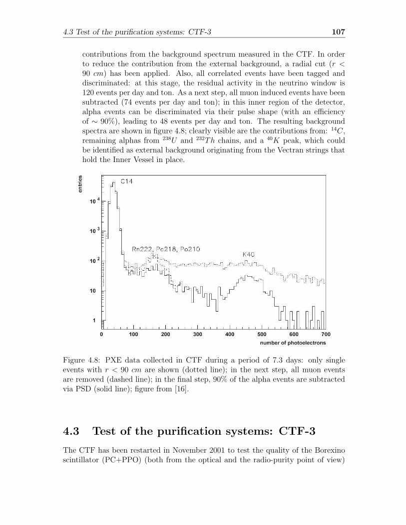
4.3 Test of the purification systems: CTF-3 107
contributions from the background spectrum measured in the CTF. In orderto reduce the contribution from the external background, a radial cut (r <90 cm) has been applied. Also, all correlated events have been tagged anddiscriminated: at this stage, the residual activity in the neutrino window is120 events per day and ton. As a next step, all muon induced events have beensubtracted (74 events per day and ton); in this inner region of the detector,alpha events can be discriminated via their pulse shape (with an efficiencyof ∼ 90%), leading to 48 events per day and ton. The resulting backgroundspectra are shown in figure 4.8; clearly visible are the contributions from: 14C,remaining alphas from 238U and 232Th chains, and a 40K peak, which couldbe identified as external background originating from the Vectran strings thathold the Inner Vessel in place.
Figure 4.8: PXE data collected in CTF during a period of 7.3 days: only singleevents with r < 90 cm are shown (dotted line); in the next step, all muon eventsare removed (dashed line); in the final step, 90% of the alpha events are subtractedvia PSD (solid line); figure from [16].
4.3 Test of the purification systems: CTF-3
The CTF has been restarted in November 2001 to test the quality of the Borexinoscintillator (PC+PPO) (both from the optical and the radio-purity point of view)
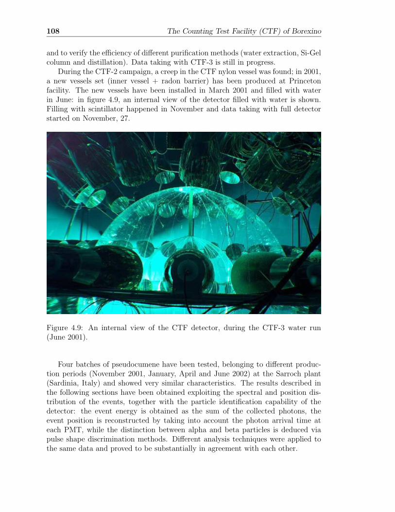
108 The Counting Test Facility (CTF) of Borexino
and to verify the efficiency of different purification methods (water extraction, Si-Gelcolumn and distillation). Data taking with CTF-3 is still in progress.
During the CTF-2 campaign, a creep in the CTF nylon vessel was found; in 2001,a new vessels set (inner vessel + radon barrier) has been produced at Princetonfacility. The new vessels have been installed in March 2001 and filled with waterin June: in figure 4.9, an internal view of the detector filled with water is shown.Filling with scintillator happened in November and data taking with full detectorstarted on November, 27.
Figure 4.9: An internal view of the CTF detector, during the CTF-3 water run(June 2001).
Four batches of pseudocumene have been tested, belonging to different produc-tion periods (November 2001, January, April and June 2002) at the Sarroch plant(Sardinia, Italy) and showed very similar characteristics. The results described inthe following sections have been obtained exploiting the spectral and position dis-tribution of the events, together with the particle identification capability of thedetector: the event energy is obtained as the sum of the collected photons, theevent position is reconstructed by taking into account the photon arrival time ateach PMT, while the distinction between alpha and beta particles is deduced viapulse shape discrimination methods. Different analysis techniques were applied tothe same data and proved to be substantially in agreement with each other.
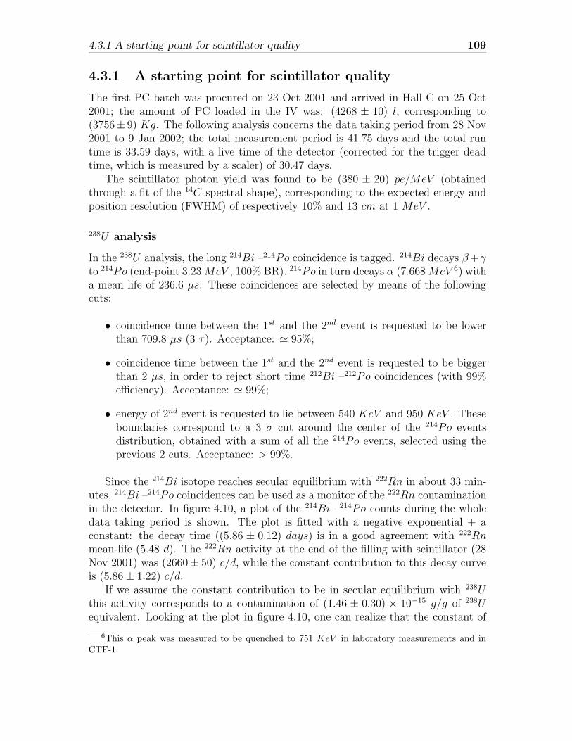
4.3.1 A starting point for scintillator quality 109
4.3.1 A starting point for scintillator quality
The first PC batch was procured on 23 Oct 2001 and arrived in Hall C on 25 Oct2001; the amount of PC loaded in the IV was: (4268 ± 10) l, corresponding to(3756± 9) Kg. The following analysis concerns the data taking period from 28 Nov2001 to 9 Jan 2002; the total measurement period is 41.75 days and the total runtime is 33.59 days, with a live time of the detector (corrected for the trigger deadtime, which is measured by a scaler) of 30.47 days.
The scintillator photon yield was found to be (380 ± 20) pe/MeV (obtainedthrough a fit of the 14C spectral shape), corresponding to the expected energy andposition resolution (FWHM) of respectively 10% and 13 cm at 1 MeV .
238U analysis
In the 238U analysis, the long 214Bi –214Po coincidence is tagged. 214Bi decays β+γto 214Po (end-point 3.23MeV , 100% BR). 214Po in turn decays α (7.668MeV 6) witha mean life of 236.6 µs. These coincidences are selected by means of the followingcuts:
• coincidence time between the 1st and the 2nd event is requested to be lowerthan 709.8 µs (3 τ). Acceptance: ' 95%;
• coincidence time between the 1st and the 2nd event is requested to be biggerthan 2 µs, in order to reject short time 212Bi –212Po coincidences (with 99%efficiency). Acceptance: ' 99%;
• energy of 2nd event is requested to lie between 540 KeV and 950 KeV . Theseboundaries correspond to a 3 σ cut around the center of the 214Po eventsdistribution, obtained with a sum of all the 214Po events, selected using theprevious 2 cuts. Acceptance: > 99%.
Since the 214Bi isotope reaches secular equilibrium with 222Rn in about 33 min-utes, 214Bi –214Po coincidences can be used as a monitor of the 222Rn contaminationin the detector. In figure 4.10, a plot of the 214Bi –214Po counts during the wholedata taking period is shown. The plot is fitted with a negative exponential + aconstant: the decay time ((5.86 ± 0.12) days) is in a good agreement with 222Rnmean-life (5.48 d). The 222Rn activity at the end of the filling with scintillator (28Nov 2001) was (2660± 50) c/d, while the constant contribution to this decay curveis (5.86± 1.22) c/d.
If we assume the constant contribution to be in secular equilibrium with 238Uthis activity corresponds to a contamination of (1.46 ± 0.30) × 10−15 g/g of 238Uequivalent. Looking at the plot in figure 4.10, one can realize that the constant of
6This α peak was measured to be quenched to 751 KeV in laboratory measurements and inCTF-1.
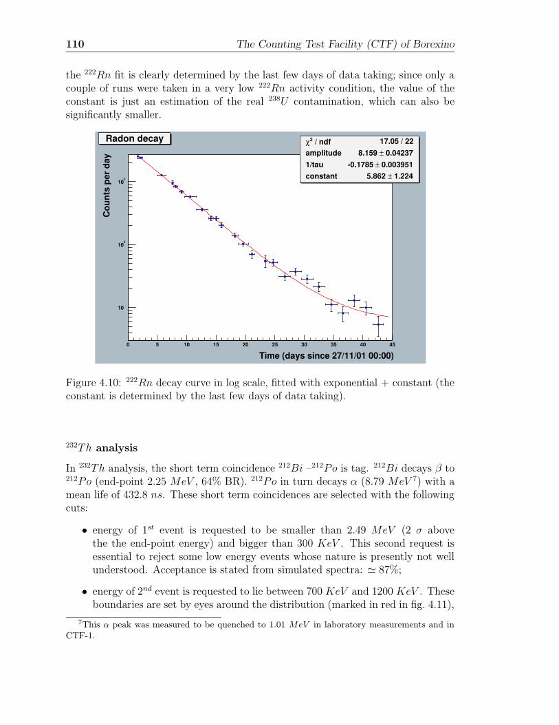
110 The Counting Test Facility (CTF) of Borexino
the 222Rn fit is clearly determined by the last few days of data taking; since only acouple of runs were taken in a very low 222Rn activity condition, the value of theconstant is just an estimation of the real 238U contamination, which can also besignificantly smaller.
Time (days since 27/11/01 00:00)0 5 10 15 20 25 30 35 40 45
Cou
nts
per
day
10
102
103
/ ndf 2χ 17.05 / 22amplitude 0.04237± 8.159 1/tau 0.003951± -0.1785 constant 1.224± 5.862
/ ndf 2χ 17.05 / 22amplitude 0.04237± 8.159 1/tau 0.003951± -0.1785 constant 1.224± 5.862
Radon decay
Figure 4.10: 222Rn decay curve in log scale, fitted with exponential + constant (theconstant is determined by the last few days of data taking).
232Th analysis
In 232Th analysis, the short term coincidence 212Bi –212Po is tag. 212Bi decays β to212Po (end-point 2.25 MeV , 64% BR). 212Po in turn decays α (8.79 MeV 7) with amean life of 432.8 ns. These short term coincidences are selected with the followingcuts:
• energy of 1st event is requested to be smaller than 2.49 MeV (2 σ abovethe the end-point energy) and bigger than 300 KeV . This second request isessential to reject some low energy events whose nature is presently not wellunderstood. Acceptance is stated from simulated spectra: ' 87%;
• energy of 2nd event is requested to lie between 700 KeV and 1200 KeV . Theseboundaries are set by eyes around the distribution (marked in red in fig. 4.11),
7This α peak was measured to be quenched to 1.01 MeV in laboratory measurements and inCTF-1.
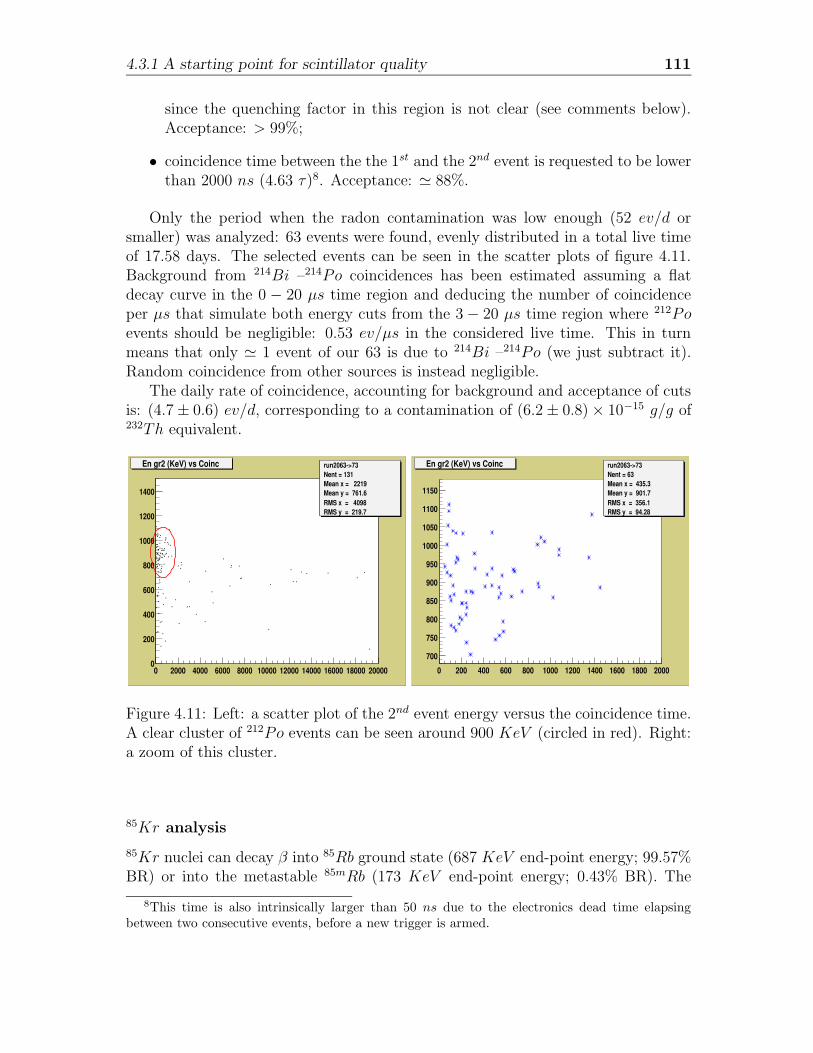
4.3.1 A starting point for scintillator quality 111
since the quenching factor in this region is not clear (see comments below).Acceptance: > 99%;
• coincidence time between the the 1st and the 2nd event is requested to be lowerthan 2000 ns (4.63 τ)8. Acceptance: ' 88%.
Only the period when the radon contamination was low enough (52 ev/d orsmaller) was analyzed: 63 events were found, evenly distributed in a total live timeof 17.58 days. The selected events can be seen in the scatter plots of figure 4.11.Background from 214Bi –214Po coincidences has been estimated assuming a flatdecay curve in the 0 − 20 µs time region and deducing the number of coincidenceper µs that simulate both energy cuts from the 3− 20 µs time region where 212Poevents should be negligible: 0.53 ev/µs in the considered live time. This in turnmeans that only ' 1 event of our 63 is due to 214Bi –214Po (we just subtract it).Random coincidence from other sources is instead negligible.
The daily rate of coincidence, accounting for background and acceptance of cutsis: (4.7± 0.6) ev/d, corresponding to a contamination of (6.2± 0.8)× 10−15 g/g of232Th equivalent.
0 2000 4000 6000 8000 10000 12000 14000 16000 18000 200000
200
400
600
800
1000
1200
1400
run2063->73Nent = 131 Mean x = 2219Mean y = 761.6RMS x = 4098RMS y = 219.7
En gr2 (KeV) vs Coinc run2063->73Nent = 131 Mean x = 2219Mean y = 761.6RMS x = 4098RMS y = 219.7
0 200 400 600 800 1000 1200 1400 1600 1800 2000
700
750
800
850
900
950
1000
1050
1100
1150
run2063->73Nent = 63 Mean x = 435.3Mean y = 901.7RMS x = 356.1RMS y = 94.28
En gr2 (KeV) vs Coinc run2063->73Nent = 63 Mean x = 435.3Mean y = 901.7RMS x = 356.1RMS y = 94.28
Figure 4.11: Left: a scatter plot of the 2nd event energy versus the coincidence time.A clear cluster of 212Po events can be seen around 900 KeV (circled in red). Right:a zoom of this cluster.
85Kr analysis
85Kr nuclei can decay β into 85Rb ground state (687 KeV end-point energy; 99.57%BR) or into the metastable 85mRb (173 KeV end-point energy; 0.43% BR). The
8This time is also intrinsically larger than 50 ns due to the electronics dead time elapsingbetween two consecutive events, before a new trigger is armed.
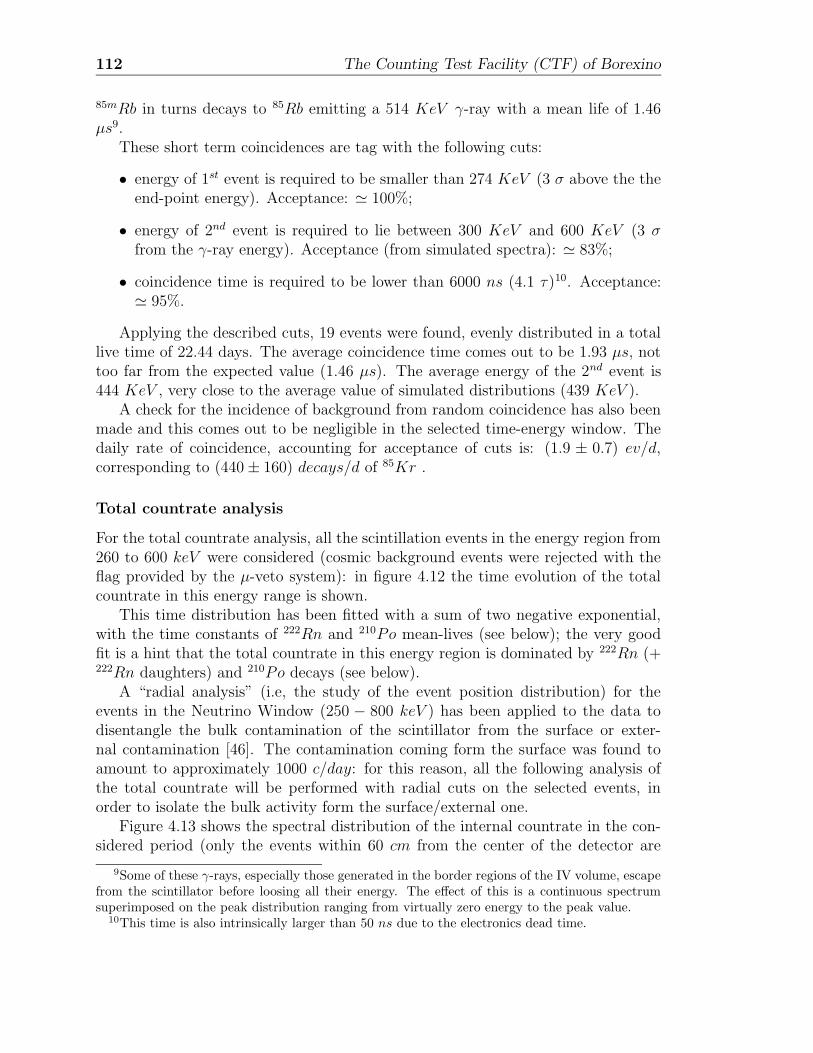
112 The Counting Test Facility (CTF) of Borexino
85mRb in turns decays to 85Rb emitting a 514 KeV γ-ray with a mean life of 1.46µs9.
These short term coincidences are tag with the following cuts:
• energy of 1st event is required to be smaller than 274 KeV (3 σ above the theend-point energy). Acceptance: ' 100%;
• energy of 2nd event is required to lie between 300 KeV and 600 KeV (3 σfrom the γ-ray energy). Acceptance (from simulated spectra): ' 83%;
• coincidence time is required to be lower than 6000 ns (4.1 τ)10. Acceptance:' 95%.
Applying the described cuts, 19 events were found, evenly distributed in a totallive time of 22.44 days. The average coincidence time comes out to be 1.93 µs, nottoo far from the expected value (1.46 µs). The average energy of the 2nd event is444 KeV , very close to the average value of simulated distributions (439 KeV ).
A check for the incidence of background from random coincidence has also beenmade and this comes out to be negligible in the selected time-energy window. Thedaily rate of coincidence, accounting for acceptance of cuts is: (1.9 ± 0.7) ev/d,corresponding to (440± 160) decays/d of 85Kr .
Total countrate analysis
For the total countrate analysis, all the scintillation events in the energy region from260 to 600 keV were considered (cosmic background events were rejected with theflag provided by the µ-veto system): in figure 4.12 the time evolution of the totalcountrate in this energy range is shown.
This time distribution has been fitted with a sum of two negative exponential,with the time constants of 222Rn and 210Po mean-lives (see below); the very goodfit is a hint that the total countrate in this energy region is dominated by 222Rn (+222Rn daughters) and 210Po decays (see below).
A “radial analysis” (i.e, the study of the event position distribution) for theevents in the Neutrino Window (250 − 800 keV ) has been applied to the data todisentangle the bulk contamination of the scintillator from the surface or exter-nal contamination [46]. The contamination coming form the surface was found toamount to approximately 1000 c/day: for this reason, all the following analysis ofthe total countrate will be performed with radial cuts on the selected events, inorder to isolate the bulk activity form the surface/external one.
Figure 4.13 shows the spectral distribution of the internal countrate in the con-sidered period (only the events within 60 cm from the center of the detector are
9Some of these γ-rays, especially those generated in the border regions of the IV volume, escapefrom the scintillator before loosing all their energy. The effect of this is a continuous spectrumsuperimposed on the peak distribution ranging from virtually zero energy to the peak value.
10This time is also intrinsically larger than 50 ns due to the electronics dead time.
4.3.1 A starting point for scintillator quality 113
Time (days since 27/11/01 00:00)0 5 10 15 20 25 30 35 40 45
Cou
nts
per
day
2000
3000
4000
5000
6000
7000
8000
9000
10000
11000
12000
/ ndf 2χ 19.7 / 23Rn ampl 0.03167± 9.26 1/tau 0± -0.182 Po ampl 0.006579± 8.044 1/tau 0± -0.005
/ ndf 2χ 19.7 / 23Rn ampl 0.03167± 9.26 1/tau 0± -0.182 Po ampl 0.006579± 8.044 1/tau 0± -0.005
total events
Figure 4.12: Total countrate in the energy range 260 − 600 keV , as a function ofthe date of the run (errors are statistical only).
selected): the peak at about 0.40 ÷ 0.50 MeV is the sum of the activity from the210Po, the 222Rn and the 218Po, while the higher energy peak (∼ 0.75 MeV ) is dueto the 214Po decay; underlying there is the β + γ activity from the 222Rn chain andfrom the 40K and 85Kr; a shape analysis of this energy spectrum [46] indicates asignificant contribution from 210Po, as suggested by the time decay fit of the totalactivity.
α/β discrimination
In the above considered energy region, a continuous β + γ spectrum is present:for this reason, the number of events in the α peak have to be computed usingPulse-Shape discrimination techniques.
α/β discrimination is performed in CTF using different techniques. The mosteffective one was found to be the so-called “Optimum filter” (or “Gatti method”)applied to the pulses produced by the DPSA board [76], which was described in theprevious section.
An optimization procedure of the DPSA data processing was performed at thebeginning of the analysis procedure: the most important achievement was the opti-mization of the total integration time, which was found to be about 370 ns (DPSAdata were therefore processed over a 367 ns interval).
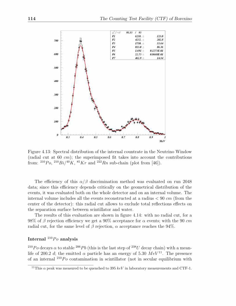
114 The Counting Test Facility (CTF) of Borexino
Figure 4.13: Spectral distribution of the internal countrate in the Neutrino Window(radial cut at 60 cm); the superimposed fit takes into account the contributionsfrom: 210Po, 210Bi/40K, 85Kr and 222Rn sub-chain (plot from [46]).
The efficiency of this α/β discrimination method was evaluated on run 2048data; since this efficiency depends critically on the geometrical distribution of theevents, it was evaluated both on the whole detector and on an internal volume. Theinternal volume includes all the events reconstructed at a radius < 90 cm (from thecenter of the detector): this radial cut allows to exclude total reflections effects onthe separation surface between scintillator and water.
The results of this evaluation are shown in figure 4.14: with no radial cut, for a98% of β rejection efficiency we get a 90% acceptance for α events; with the 90 cmradial cut, for the same level of β rejection, α acceptance reaches the 94%.
Internal 210Po analysis
210Po decays α to stable 206Pb (this is the last step of 238U decay chain) with a mean-life of 200.2 d; the emitted α particle has an energy of 5.30 MeV 11. The presenceof an internal 210Po contamination in scintillator (not in secular equilibrium with
11This α peak was measured to be quenched to 395 keV in laboratory measurements and CTF-1.
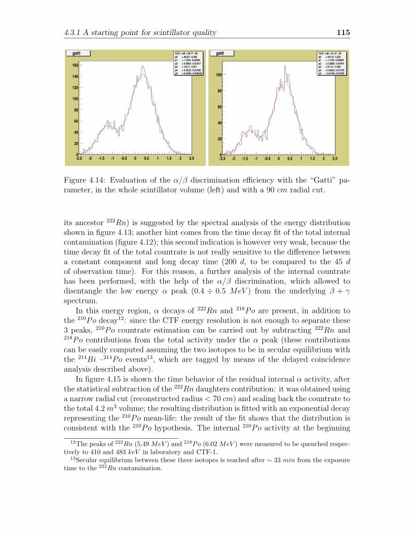
4.3.1 A starting point for scintillator quality 115
-2.5 -2 -1.5 -1 -0.5 0 0.5 1 1.5 2 2.50
20
40
60
80
100
120
140
160
Chi2 / ndf = 66.71 / 86 2.046 ±p0 = 48.67 0.02604 ±p1 = -1.264 0.01817 ±p2 = 0.4364
2.971 ±p3 = 142.7 0.01298 ±p4 = 0.3232 0.009526 ±p5 = 0.5439
gatti Chi2 / ndf = 66.71 / 86 2.046 ±p0 = 48.67 0.02604 ±p1 = -1.264 0.01817 ±p2 = 0.4364
2.971 ±p3 = 142.7 0.01298 ±p4 = 0.3232 0.009526 ±p5 = 0.5439
-2.5 -2 -1.5 -1 -0.5 0 0.5 1 1.5 2 2.50
20
40
60
80
100
Chi2 / ndf = 81.31 / 83 1.623 ±p0 = 29.13 0.02683 ±p1 = -1.319 0.01941 ±p2 = 0.3885
2.402 ±p3 = 91.41 0.01376 ±p4 = 0.2633 0.01053 ±p5 = 0.5149
gatti Chi2 / ndf = 81.31 / 83 1.623 ±p0 = 29.13 0.02683 ±p1 = -1.319 0.01941 ±p2 = 0.3885
2.402 ±p3 = 91.41 0.01376 ±p4 = 0.2633 0.01053 ±p5 = 0.5149
Figure 4.14: Evaluation of the α/β discrimination efficiency with the “Gatti” pa-rameter, in the whole scintillator volume (left) and with a 90 cm radial cut.
its ancestor 222Rn) is suggested by the spectral analysis of the energy distributionshown in figure 4.13; another hint comes from the time decay fit of the total internalcontamination (figure 4.12); this second indication is however very weak, because thetime decay fit of the total countrate is not really sensitive to the difference betweena constant component and long decay time (200 d, to be compared to the 45 dof observation time). For this reason, a further analysis of the internal countratehas been performed, with the help of the α/β discrimination, which allowed todisentangle the low energy α peak (0.4 ÷ 0.5 MeV ) from the underlying β + γspectrum.
In this energy region, α decays of 222Rn and 218Po are present, in addition tothe 210Po decay12: since the CTF energy resolution is not enough to separate these3 peaks, 210Po countrate estimation can be carried out by subtracting 222Rn and218Po contributions from the total activity under the α peak (these contributionscan be easily computed assuming the two isotopes to be in secular equilibrium withthe 214Bi –214Po events13, which are tagged by means of the delayed coincidenceanalysis described above).
In figure 4.15 is shown the time behavior of the residual internal α activity, afterthe statistical subtraction of the 222Rn daughters contribution: it was obtained usinga narrow radial cut (reconstructed radius < 70 cm) and scaling back the countrate tothe total 4.2m3 volume; the resulting distribution is fitted with an exponential decayrepresenting the 210Po mean-life: the result of the fit shows that the distribution isconsistent with the 210Po hypothesis. The internal 210Po activity at the beginning
12The peaks of 222Rn (5.49 MeV ) and 218Po (6.02 MeV ) were measured to be quenched respec-tively to 410 and 483 keV in laboratory and CTF-1.
13Secular equilibrium between these three isotopes is reached after ∼ 33 min from the exposuretime to the 222Rn contamination.
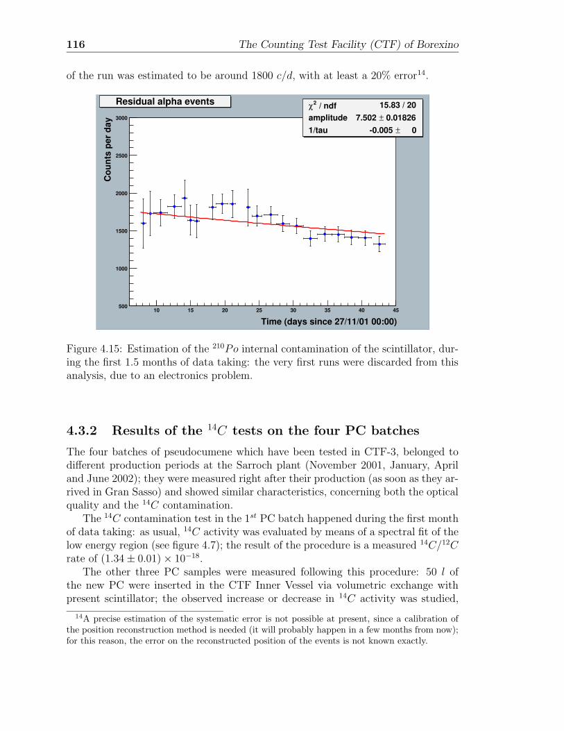
116 The Counting Test Facility (CTF) of Borexino
of the run was estimated to be around 1800 c/d, with at least a 20% error14.
Time (days since 27/11/01 00:00)10 15 20 25 30 35 40 45
Cou
nts
per
day
500
1000
1500
2000
2500
3000
/ ndf 2χ 15.83 / 20amplitude 0.01826± 7.502 1/tau 0± -0.005
/ ndf 2χ 15.83 / 20amplitude 0.01826± 7.502 1/tau 0± -0.005
Residual alpha events
Figure 4.15: Estimation of the 210Po internal contamination of the scintillator, dur-ing the first 1.5 months of data taking: the very first runs were discarded from thisanalysis, due to an electronics problem.
4.3.2 Results of the 14C tests on the four PC batches
The four batches of pseudocumene which have been tested in CTF-3, belonged todifferent production periods at the Sarroch plant (November 2001, January, Apriland June 2002); they were measured right after their production (as soon as they ar-rived in Gran Sasso) and showed similar characteristics, concerning both the opticalquality and the 14C contamination.
The 14C contamination test in the 1st PC batch happened during the first monthof data taking: as usual, 14C activity was evaluated by means of a spectral fit of thelow energy region (see figure 4.7); the result of the procedure is a measured 14C/12Crate of (1.34± 0.01)× 10−18.
The other three PC samples were measured following this procedure: 50 l ofthe new PC were inserted in the CTF Inner Vessel via volumetric exchange withpresent scintillator; the observed increase or decrease in 14C activity was studied,
14A precise estimation of the systematic error is not possible at present, since a calibration ofthe position reconstruction method is needed (it will probably happen in a few months from now);for this reason, the error on the reconstructed position of the events is not known exactly.
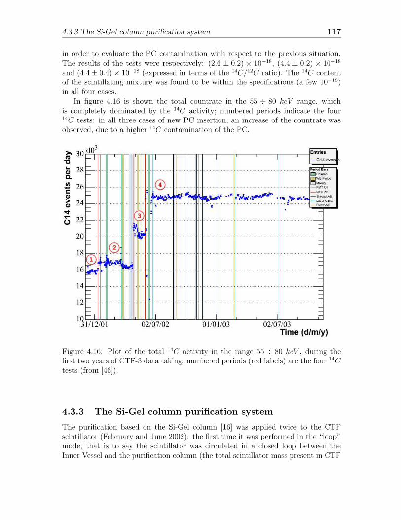
4.3.3 The Si-Gel column purification system 117
in order to evaluate the PC contamination with respect to the previous situation.The results of the tests were respectively: (2.6 ± 0.2) × 10−18, (4.4 ± 0.2) × 10−18
and (4.4± 0.4)× 10−18 (expressed in terms of the 14C/12C ratio). The 14C contentof the scintillating mixture was found to be within the specifications (a few 10−18)in all four cases.
In figure 4.16 is shown the total countrate in the 55 ÷ 80 keV range, whichis completely dominated by the 14C activity; numbered periods indicate the four14C tests: in all three cases of new PC insertion, an increase of the countrate wasobserved, due to a higher 14C contamination of the PC.
Figure 4.16: Plot of the total 14C activity in the range 55 ÷ 80 keV , during thefirst two years of CTF-3 data taking; numbered periods (red labels) are the four 14Ctests (from [46]).
4.3.3 The Si-Gel column purification system
The purification based on the Si-Gel column [16] was applied twice to the CTFscintillator (February and June 2002): the first time it was performed in the “loop”mode, that is to say the scintillator was circulated in a closed loop between theInner Vessel and the purification column (the total scintillator mass present in CTF
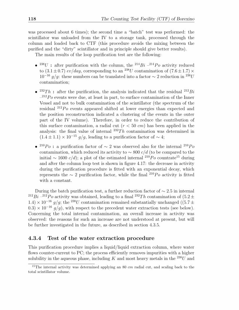
118 The Counting Test Facility (CTF) of Borexino
was processed about 6 times); the second time a “batch” test was performed: thescintillator was unloaded from the IV to a storage tank, processed through thecolumn and loaded back to CTF (this procedure avoids the mixing between thepurified and the “dirty” scintillator and in principle should give better results).
The main results of the loop purification test are the following:
• 238U : after purification with the column, the 214Bi –214Po activity reducedto (3.1± 0.7) ev/day, corresponding to an 238U contamination of (7.6± 1.7)×10−16 g/g: these numbers can be translated into a factor ∼ 2 reduction in 238Ucontamination;
• 232Th : after the purification, the analysis indicated that the residual 212Bi–212Po events were due, at least in part, to surface contamination of the InnerVessel and not to bulk contamination of the scintillator (the spectrum of theresidual 212Po events appeared shifted at lower energies than expected andthe position reconstruction indicated a clustering of the events in the outerpart of the IV volume). Therefore, in order to reduce the contribution ofthis surface contamination, a radial cut (r < 50 cm) has been applied in theanalysis: the final value of internal 232Th contamination was determined in(1.4± 1.1)× 10−15 g/g, leading to a purification factor of ∼ 4;
• 210Po : a purification factor of ∼ 2 was observed also for the internal 210Pocontamination, which reduced its activity to ∼ 800 c/d (to be compared to theinitial ∼ 1600 c/d); a plot of the estimated internal 210Po countrate15 duringand after the column loop test is shown in figure 4.17: the decrease in activityduring the purification procedure is fitted with an exponential decay, whichrepresents the ∼ 2 purification factor, while the final 210Po activity is fittedwith a constant.
During the batch purification test, a further reduction factor of ∼ 2.5 in internal212Bi –212Po activity was obtained, leading to a final 232Th contamination of (5.2±1.4)× 10−16 g/g; the 238U contamination remained substantially unchanged ((5.7±0.3)× 10−16 g/g), with respect to the precedent water extraction tests (see below).Concerning the total internal contamination, an overall increase in activity wasobserved: the reasons for such an increase are not understood at present, but willbe further investigated in the future, as described in section 4.3.5.
4.3.4 Test of the water extraction procedure
This purification procedure implies a liquid/liquid extraction column, where waterflows counter-current to PC; the process efficiently removes impurities with a highersolubility in the aqueous phase, including K and most heavy metals in the 238U and
15The internal activity was determined applying an 80 cm radial cut, and scaling back to thetotal scintillator volume.
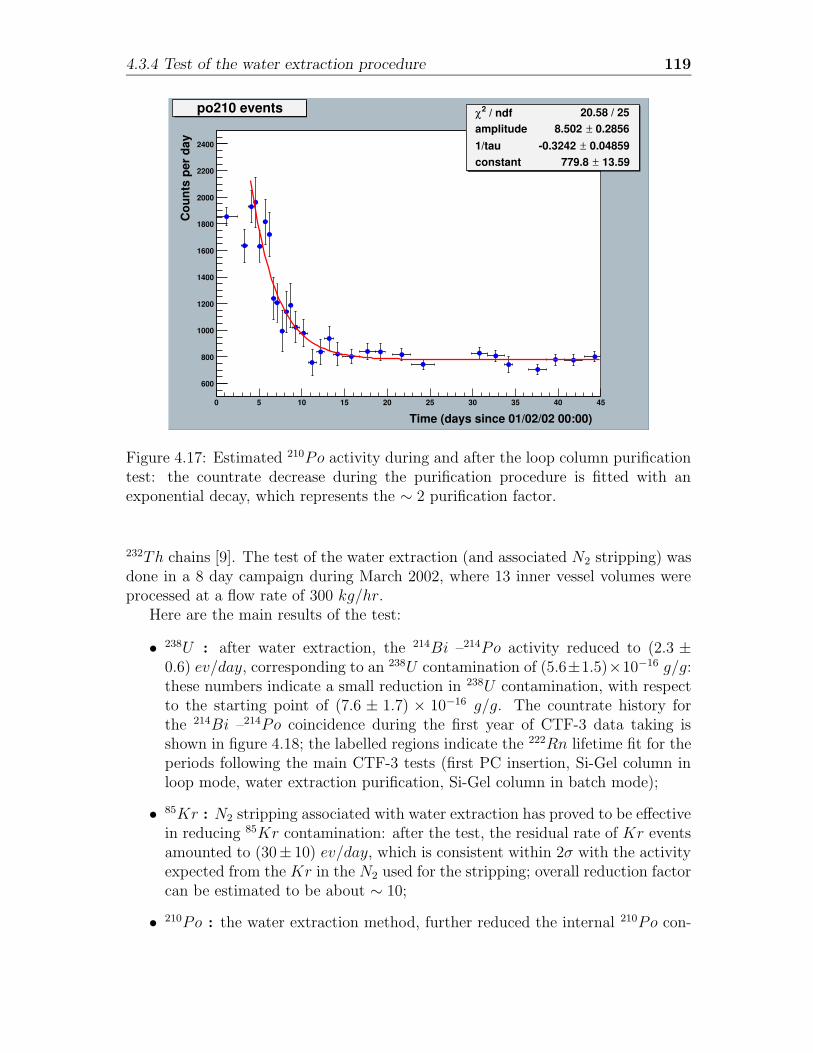
4.3.4 Test of the water extraction procedure 119
Time (days since 01/02/02 00:00)0 5 10 15 20 25 30 35 40 45
Cou
nts
per
day
600
800
1000
1200
1400
1600
1800
2000
2200
2400
/ ndf 2χ 20.58 / 25amplitude 0.2856± 8.502 1/tau 0.04859± -0.3242 constant 13.59± 779.8
/ ndf 2χ 20.58 / 25amplitude 0.2856± 8.502 1/tau 0.04859± -0.3242 constant 13.59± 779.8
po210 events
Figure 4.17: Estimated 210Po activity during and after the loop column purificationtest: the countrate decrease during the purification procedure is fitted with anexponential decay, which represents the ∼ 2 purification factor.
232Th chains [9]. The test of the water extraction (and associated N2 stripping) wasdone in a 8 day campaign during March 2002, where 13 inner vessel volumes wereprocessed at a flow rate of 300 kg/hr.
Here are the main results of the test:
• 238U : after water extraction, the 214Bi –214Po activity reduced to (2.3 ±0.6) ev/day, corresponding to an 238U contamination of (5.6±1.5)×10−16 g/g:these numbers indicate a small reduction in 238U contamination, with respectto the starting point of (7.6 ± 1.7) × 10−16 g/g. The countrate history forthe 214Bi –214Po coincidence during the first year of CTF-3 data taking isshown in figure 4.18; the labelled regions indicate the 222Rn lifetime fit for theperiods following the main CTF-3 tests (first PC insertion, Si-Gel column inloop mode, water extraction purification, Si-Gel column in batch mode);
• 85Kr : N2 stripping associated with water extraction has proved to be effectivein reducing 85Kr contamination: after the test, the residual rate of Kr eventsamounted to (30± 10) ev/day, which is consistent within 2σ with the activityexpected from the Kr in the N2 used for the stripping; overall reduction factorcan be estimated to be about ∼ 10;
• 210Po : the water extraction method, further reduced the internal 210Po con-
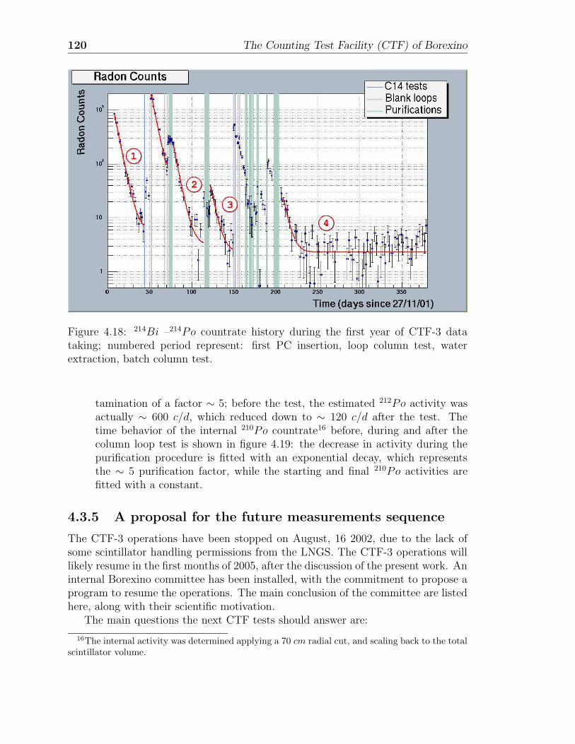
120 The Counting Test Facility (CTF) of Borexino
Figure 4.18: 214Bi –214Po countrate history during the first year of CTF-3 datataking; numbered period represent: first PC insertion, loop column test, waterextraction, batch column test.
tamination of a factor ∼ 5; before the test, the estimated 212Po activity wasactually ∼ 600 c/d, which reduced down to ∼ 120 c/d after the test. Thetime behavior of the internal 210Po countrate16 before, during and after thecolumn loop test is shown in figure 4.19: the decrease in activity during thepurification procedure is fitted with an exponential decay, which representsthe ∼ 5 purification factor, while the starting and final 210Po activities arefitted with a constant.
4.3.5 A proposal for the future measurements sequence
The CTF-3 operations have been stopped on August, 16 2002, due to the lack ofsome scintillator handling permissions from the LNGS. The CTF-3 operations willlikely resume in the first months of 2005, after the discussion of the present work. Aninternal Borexino committee has been installed, with the commitment to propose aprogram to resume the operations. The main conclusion of the committee are listedhere, along with their scientific motivation.
The main questions the next CTF tests should answer are:
16The internal activity was determined applying a 70 cm radial cut, and scaling back to the totalscintillator volume.
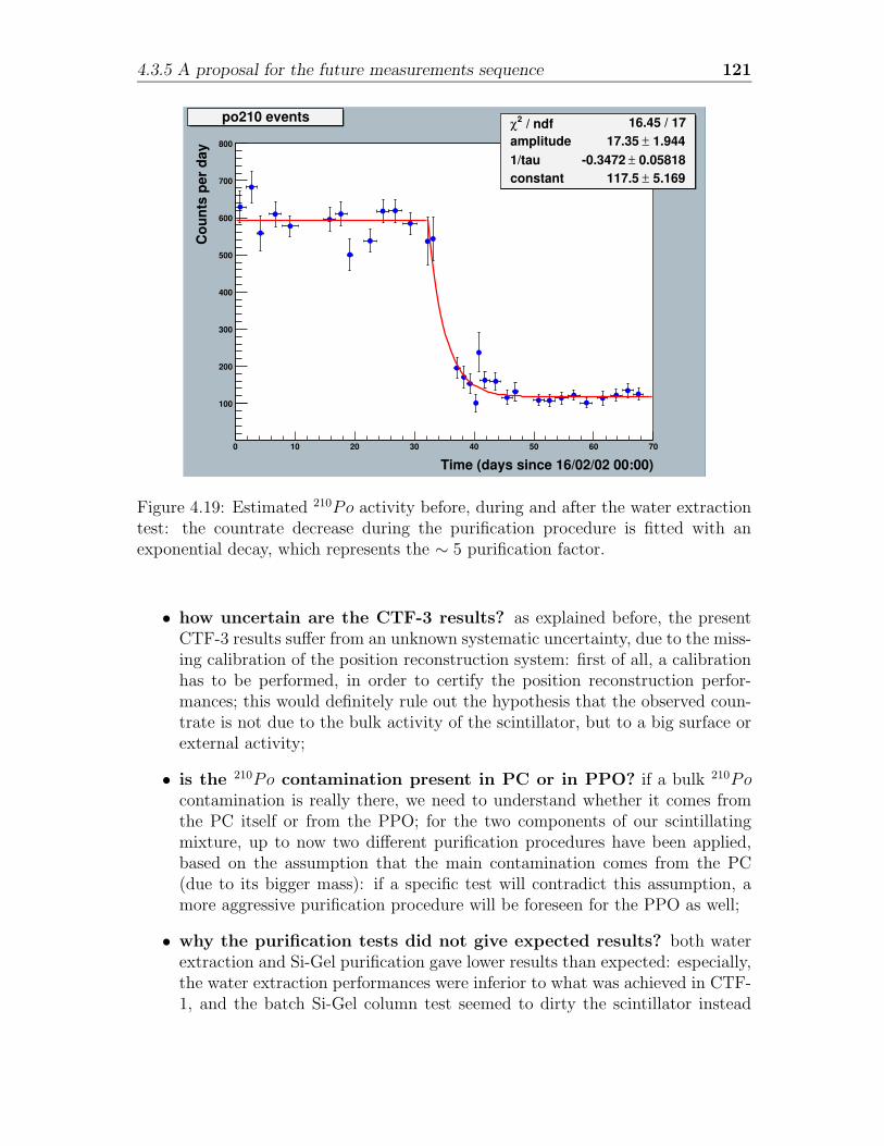
4.3.5 A proposal for the future measurements sequence 121
Time (days since 16/02/02 00:00)0 10 20 30 40 50 60 70
Cou
nts
per
day
100
200
300
400
500
600
700
800
/ ndf 2χ 16.45 / 17amplitude 1.944± 17.35 1/tau 0.05818± -0.3472 constant 5.169± 117.5
/ ndf 2χ 16.45 / 17amplitude 1.944± 17.35 1/tau 0.05818± -0.3472 constant 5.169± 117.5
po210 events
Figure 4.19: Estimated 210Po activity before, during and after the water extractiontest: the countrate decrease during the purification procedure is fitted with anexponential decay, which represents the ∼ 5 purification factor.
• how uncertain are the CTF-3 results? as explained before, the presentCTF-3 results suffer from an unknown systematic uncertainty, due to the miss-ing calibration of the position reconstruction system: first of all, a calibrationhas to be performed, in order to certify the position reconstruction perfor-mances; this would definitely rule out the hypothesis that the observed coun-trate is not due to the bulk activity of the scintillator, but to a big surface orexternal activity;
• is the 210Po contamination present in PC or in PPO? if a bulk 210Pocontamination is really there, we need to understand whether it comes fromthe PC itself or from the PPO; for the two components of our scintillatingmixture, up to now two different purification procedures have been applied,based on the assumption that the main contamination comes from the PC(due to its bigger mass): if a specific test will contradict this assumption, amore aggressive purification procedure will be foreseen for the PPO as well;
• why the purification tests did not give expected results? both waterextraction and Si-Gel purification gave lower results than expected: especially,the water extraction performances were inferior to what was achieved in CTF-1, and the batch Si-Gel column test seemed to dirty the scintillator instead
122 The Counting Test Facility (CTF) of Borexino
of cleaning it (while the loop test showed a reduction in contaminations, evenif lower than expected); at present, the most reasonable hypothesis is thatthe scintillator flows into some lines which are not really clean (in spite ofthe careful cleaning work done before the use of the line) and it undergoesa recontamination effect from the lines itself, before coming back to CTF: acheck of the lines cleanliness is then desirable;
• what is the present status of the PC in Storage Area? ∼ 300 t ofpseudocumene are sealed in SA tanks since 2.5 years: before its use (and itspurification), the PC has to be carefully checked (both on optical and radioac-tivity point of view), in order to study the possible contamination effects dueto long stop in the SA tanks (contact with the Stainless Steel, possible 222Rnemanation or leak, etc.);
• what else can we do, for PC purification? Among the three purificationmethods implemented in Borexino, the distillation has not been tested yet: thistest is quite crucial, because the CTF-1 results indicate a big purification factoras a combined result of both water extraction and distillation (the separateeffects of the two methods were not established with sufficient accuracy). Afterthe distillation test, also water extraction and Si-Gel column will likely berepeated: but it is very important that this second round of purification teststakes place after the re-cleaning of the lines and the PPO tests, otherwise thepossible inefficiencies of the method will be confused with other effects.
The proposed CTF tests sequence follows from the previous considerations andis composed of ten steps:
1. position reconstruction calibration: it will be made by means of a movableradon loaded source (like the one used in CTF-2) and an optical fiber. Theradon source will help in reducing the uncertainties concerning radial analysis(and, if the quality of the source is very high, it will provide a cross-check ofthe α/β discrimination methods). Fiber optics will allow to study the validityof the Borexino concept for position calibrations;
2. lines cleaning: some lines in the purification skids have never been cleaned;before continuing the tests, these two groups of lines need a precision cleaning;
3. blank test of the lines, done by circulating the scintillator that is now inCTF through the purification skids and the Module 0 (the module containingthe Si-Gel plant and some buffer tanks). The test should involve alreadycleaned lines; it will be done in two steps: the first time without going throughthe skids; the second time going through the skids. The test should be longenough to test also radon leaks in the lines;

4.3.5 A proposal for the future measurements sequence 123
4. check the optical quality of the PC in the Storage Area: if the opticalquality is too bad, a supplementary purification program need to be estab-lished;
5. a blank test of the PPO system: all the lines involved in PPO plant willundergo a blank test, similar to the one done in the main lines; this test willallow the disentangle the possible contamination coming from the PPO itselffrom the effect of the lines;
6. precision cleaning of remaining lines: filling stations and other lines (notinvolved in previous tests) will be cleaned, before their use during Borexinofilling (lines not involved in CTF tests will be cleaned later than others);
7. PPO test: it consists of an insertion in CTF of a few liters of “master solu-tion” (a concentrated solution of PPO in PC). In principle, this test requiresdistillation plant to be operational, in order to check in the same time the pro-cedure for Borexino; alternatively, a lab-scale procedure can be applied just tocheck PPO purity, and the full test will be performed later;
8. test in CTF of the PC in the Storage Area: of course, this test will bedone only if the optical quality is not too bad; otherwise, either an attempt toimprove the optical quality of the PC will be performed (for example by meansof an intensive nitrogen stripping) or some new PC arrival (for the buffer liquidof Borexino) will be waited for;
9. distillation test with Borexino skids: for this test, the PC in the SAwill be used (a sample of this PC will have been tested just before, so that a“pre-distillation” measurement of the same PC batch is not strictly needed).This is the most important test of all, but it cannot happen before the others:all the possible contamination sources (lines, PPO, etc.) have to be identified(or discarded) before doing it;
10. possible further tests of Si-Gel column purification and water ex-traction: this second round of tests will be decided upon the outcome ofprevious tests and will hopefully allow to define the final procedure for scin-tillator purification in Borexino.

Chapter 5
An overview of the Borexinoread-out system
The design and the implementation of the Borexino read-out system is optimizedfor the measurement of the 7Be solar neutrino flux. For each scintillation event, theenergy and position informations have to be reconstructed: energy is needed for thespectral analysis of the neutrino signal, while position allows the determination ofthe Fiducial Volume (see chapter 2).
The scintillation light produced in events has then to be detected with highprecision:
• the emitted photons have to be efficiently collected and their number accu-rately measured, because it determines the total energy of the event;
• the arrival time of each photon must be determined at the ns level, for precisereconstruction of the event position and for the exploitation of Pulse ShapeDiscrimination techniques (section 4.2.4).
In addition, the time difference between consecutive events has to be knownprecisely, to allow Delayed Coincidence analysis (a technique for identification ofradioactive background). A determination of the absolute (astronomical) time of theevent would provide this information, and would be useful for the field of SupernovaNeutrinos (section 3.2).
The read-out system is based on the well-known technique of the Photomultipliertubes; this chapter describes the main features of the Borexino PMTs, as well asthe specific implementation of the electronics and data acquisition.
5.1 Borexino Photomultipliers
Borexino detector will use a large number of photomultipliers. At the first stage ofthe experiment a long test activity was carried out on several large photocathode
125
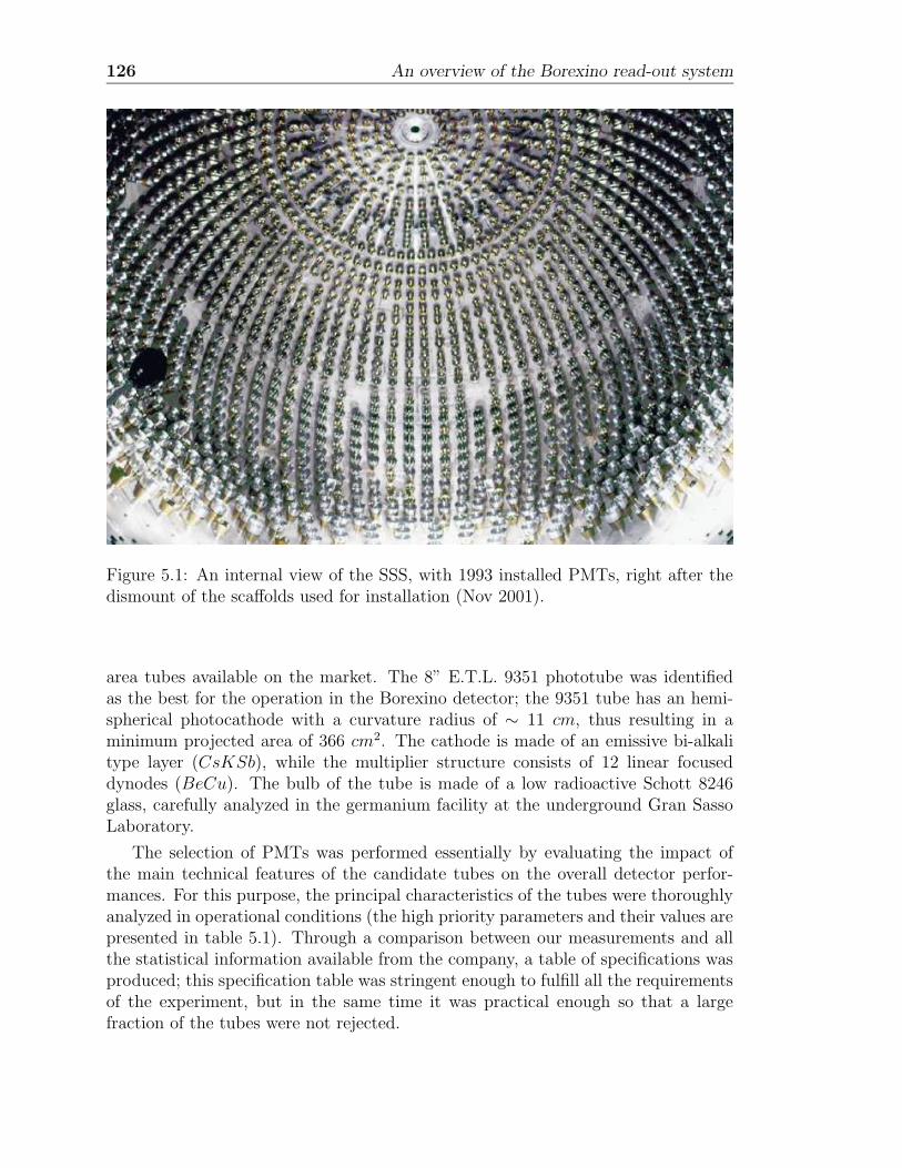
126 An overview of the Borexino read-out system
Figure 5.1: An internal view of the SSS, with 1993 installed PMTs, right after thedismount of the scaffolds used for installation (Nov 2001).
area tubes available on the market. The 8” E.T.L. 9351 phototube was identifiedas the best for the operation in the Borexino detector; the 9351 tube has an hemi-spherical photocathode with a curvature radius of ∼ 11 cm, thus resulting in aminimum projected area of 366 cm2. The cathode is made of an emissive bi-alkalitype layer (CsKSb), while the multiplier structure consists of 12 linear focuseddynodes (BeCu). The bulb of the tube is made of a low radioactive Schott 8246glass, carefully analyzed in the germanium facility at the underground Gran SassoLaboratory.
The selection of PMTs was performed essentially by evaluating the impact ofthe main technical features of the candidate tubes on the overall detector perfor-mances. For this purpose, the principal characteristics of the tubes were thoroughlyanalyzed in operational conditions (the high priority parameters and their values arepresented in table 5.1). Through a comparison between our measurements and allthe statistical information available from the company, a table of specifications wasproduced; this specification table was stringent enough to fulfill all the requirementsof the experiment, but in the same time it was practical enough so that a largefraction of the tubes were not rejected.
5.1.1 PMT encapsulation and mounting structure 127
High Priority ParametersPhotocathode quantum efficiency > 21%
After-pulses < 5%Single p.e. transit time spread < 1.3 ns
Dark count rate < 20 kHzLate pulses < 4%
Single p.e. peak to valley ratio > 1.5
Table 5.1: High priority parameters for the choice of Borexino PMTs.
The adopted voltage divider scheme is suited for the twofold purpose of mini-mizing the simple photoelectron transit time spread and properly shaping the out-put analog signal for the subsequent front-end processing (signal and HV are cou-pled/decoupled at the input of the front-end electronics). The dividers are suppliedwith positive high voltage in the range of 1100 ÷ 2000 V . The voltage across thecathode and the first dynode is fixed (by means of two Zener diodes) to the value(600 V ) suggested by the manufacturer for the optimum PMT performance.
5.1.1 PMT encapsulation and mounting structure
The 2200 Borexino PMT’s are mounted on the internal surface of the SSS. Thesphere will be filled with PC, while the tank will be filled with water (see chapter 2).In this way, the front part of the PMT will be immersed in PC and the rear part inwater. To ensure a reliable operation of the devices in such a complex environment,it was necessary to develop an encapsulation of the neck of the bulb and the dividerin order to fulfill all the mechanical and environmental constraints. The design hasbeen based upon the broad experience gained in the research and development ofthe Counting Test Facility (see chapter 4).
The base and the neck of the tube is enclosed in a cylindrical stainless steelhousing whose external diameter is equal to 90 mm, as shown in figure 5.3. Thehousing is fixed to the glass of the neck of the tube through a PC proof epoxyresin, which acts as a structural adhesive as well as a protection barrier againstthe PC permeation. The end-cap of the cylindrical housing, welded to it and leaktested, carries the feed-through intended to ensure the mounting of the devices tothe sphere.
The PMT installation is realized inserting the feed-through into a SSS hole andthen securing it through a rear nut. An important role in this mounting is playedby an isolating material (phenolic resin) that electrically decouples the device toavoid ground loops and also act as the groove for the Viton o-ring used to assurethe tightness between the tank and the sphere. All the 2200 feeds-through havebeen tested by means of a custom made mass spectrometer, using argon as a tracegas to evaluate the leak rate. The feed-through is also designed to accommodate
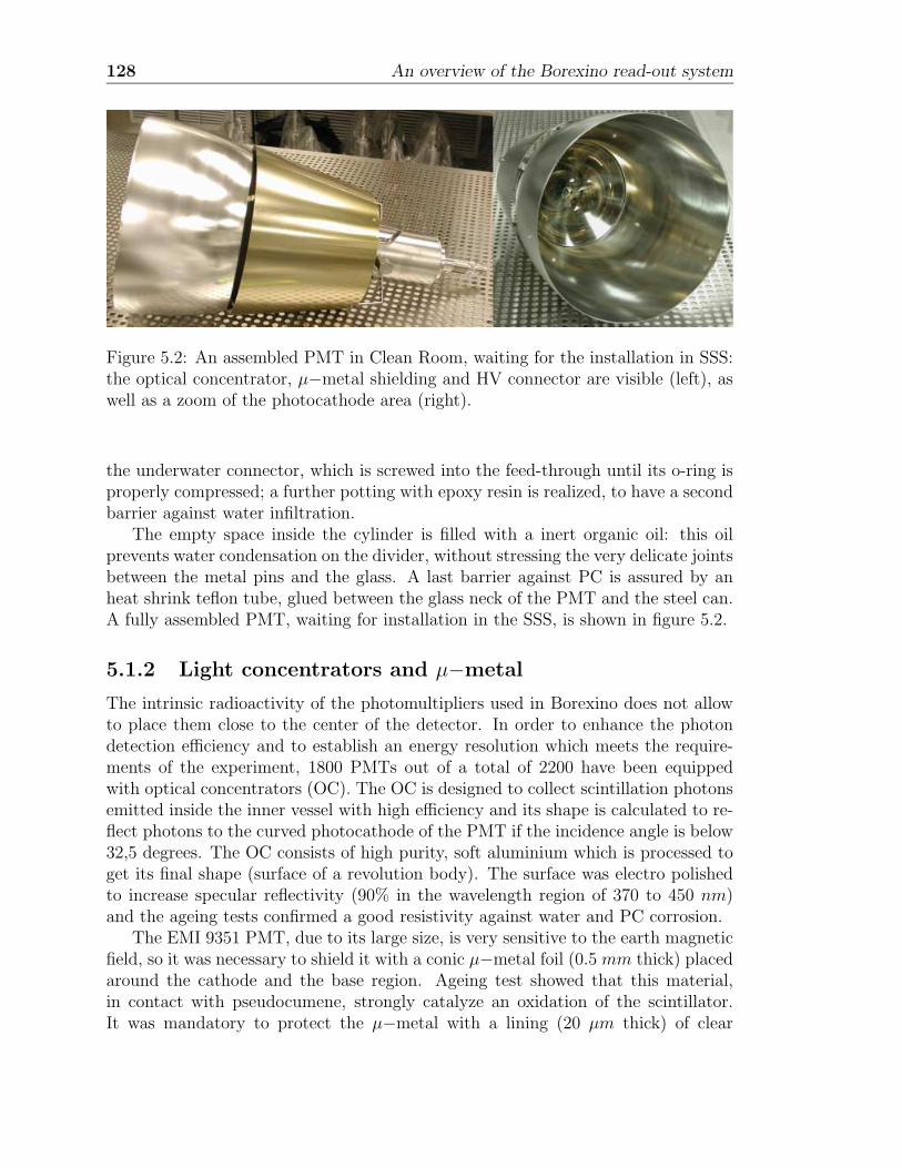
128 An overview of the Borexino read-out system
Figure 5.2: An assembled PMT in Clean Room, waiting for the installation in SSS:the optical concentrator, µ−metal shielding and HV connector are visible (left), aswell as a zoom of the photocathode area (right).
the underwater connector, which is screwed into the feed-through until its o-ring isproperly compressed; a further potting with epoxy resin is realized, to have a secondbarrier against water infiltration.
The empty space inside the cylinder is filled with a inert organic oil: this oilprevents water condensation on the divider, without stressing the very delicate jointsbetween the metal pins and the glass. A last barrier against PC is assured by anheat shrink teflon tube, glued between the glass neck of the PMT and the steel can.A fully assembled PMT, waiting for installation in the SSS, is shown in figure 5.2.
5.1.2 Light concentrators and µ−metal
The intrinsic radioactivity of the photomultipliers used in Borexino does not allowto place them close to the center of the detector. In order to enhance the photondetection efficiency and to establish an energy resolution which meets the require-ments of the experiment, 1800 PMTs out of a total of 2200 have been equippedwith optical concentrators (OC). The OC is designed to collect scintillation photonsemitted inside the inner vessel with high efficiency and its shape is calculated to re-flect photons to the curved photocathode of the PMT if the incidence angle is below32,5 degrees. The OC consists of high purity, soft aluminium which is processed toget its final shape (surface of a revolution body). The surface was electro polishedto increase specular reflectivity (90% in the wavelength region of 370 to 450 nm)and the ageing tests confirmed a good resistivity against water and PC corrosion.
The EMI 9351 PMT, due to its large size, is very sensitive to the earth magneticfield, so it was necessary to shield it with a conic µ−metal foil (0.5 mm thick) placedaround the cathode and the base region. Ageing test showed that this material,in contact with pseudocumene, strongly catalyze an oxidation of the scintillator.It was mandatory to protect the µ−metal with a lining (20 µm thick) of clear
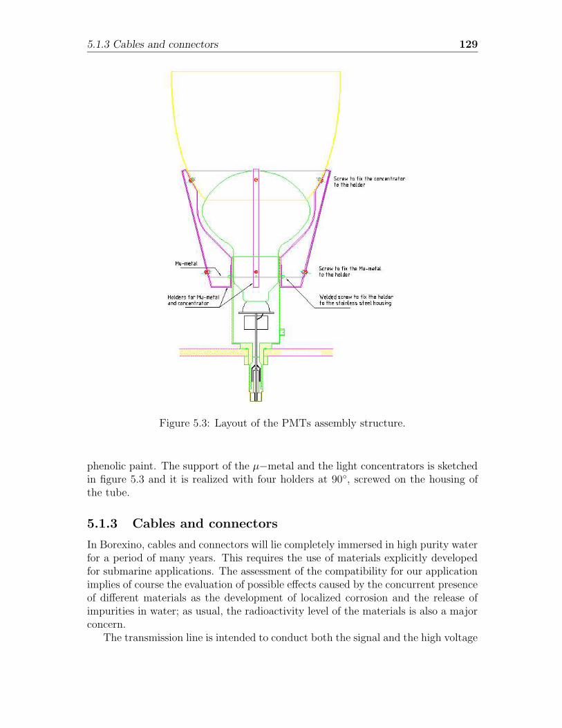
5.1.3 Cables and connectors 129
Figure 5.3: Layout of the PMTs assembly structure.
phenolic paint. The support of the µ−metal and the light concentrators is sketchedin figure 5.3 and it is realized with four holders at 90, screwed on the housing ofthe tube.
5.1.3 Cables and connectors
In Borexino, cables and connectors will lie completely immersed in high purity waterfor a period of many years. This requires the use of materials explicitly developedfor submarine applications. The assessment of the compatibility for our applicationimplies of course the evaluation of possible effects caused by the concurrent presenceof different materials as the development of localized corrosion and the release ofimpurities in water; as usual, the radioactivity level of the materials is also a majorconcern.
The transmission line is intended to conduct both the signal and the high voltage
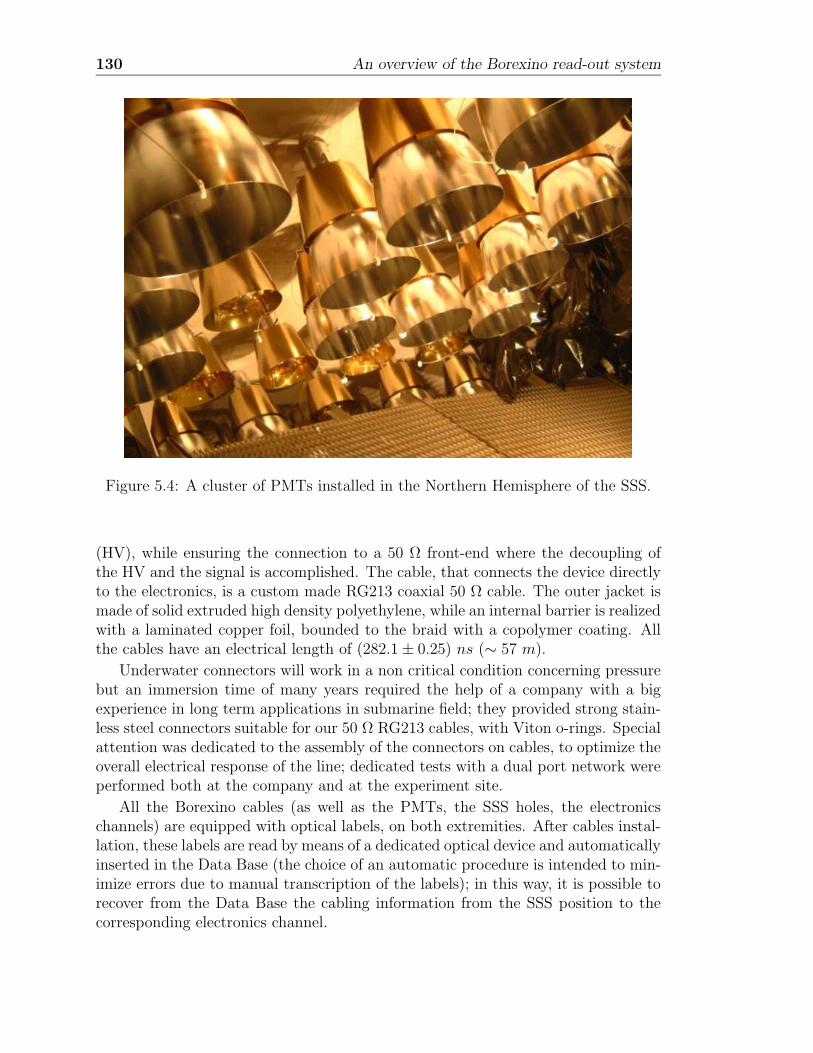
130 An overview of the Borexino read-out system
Figure 5.4: A cluster of PMTs installed in the Northern Hemisphere of the SSS.
(HV), while ensuring the connection to a 50 Ω front-end where the decoupling ofthe HV and the signal is accomplished. The cable, that connects the device directlyto the electronics, is a custom made RG213 coaxial 50 Ω cable. The outer jacket ismade of solid extruded high density polyethylene, while an internal barrier is realizedwith a laminated copper foil, bounded to the braid with a copolymer coating. Allthe cables have an electrical length of (282.1± 0.25) ns (∼ 57 m).
Underwater connectors will work in a non critical condition concerning pressurebut an immersion time of many years required the help of a company with a bigexperience in long term applications in submarine field; they provided strong stain-less steel connectors suitable for our 50 Ω RG213 cables, with Viton o-rings. Specialattention was dedicated to the assembly of the connectors on cables, to optimize theoverall electrical response of the line; dedicated tests with a dual port network wereperformed both at the company and at the experiment site.
All the Borexino cables (as well as the PMTs, the SSS holes, the electronicschannels) are equipped with optical labels, on both extremities. After cables instal-lation, these labels are read by means of a dedicated optical device and automaticallyinserted in the Data Base (the choice of an automatic procedure is intended to min-imize errors due to manual transcription of the labels); in this way, it is possible torecover from the Data Base the cabling information from the SSS position to thecorresponding electronics channel.
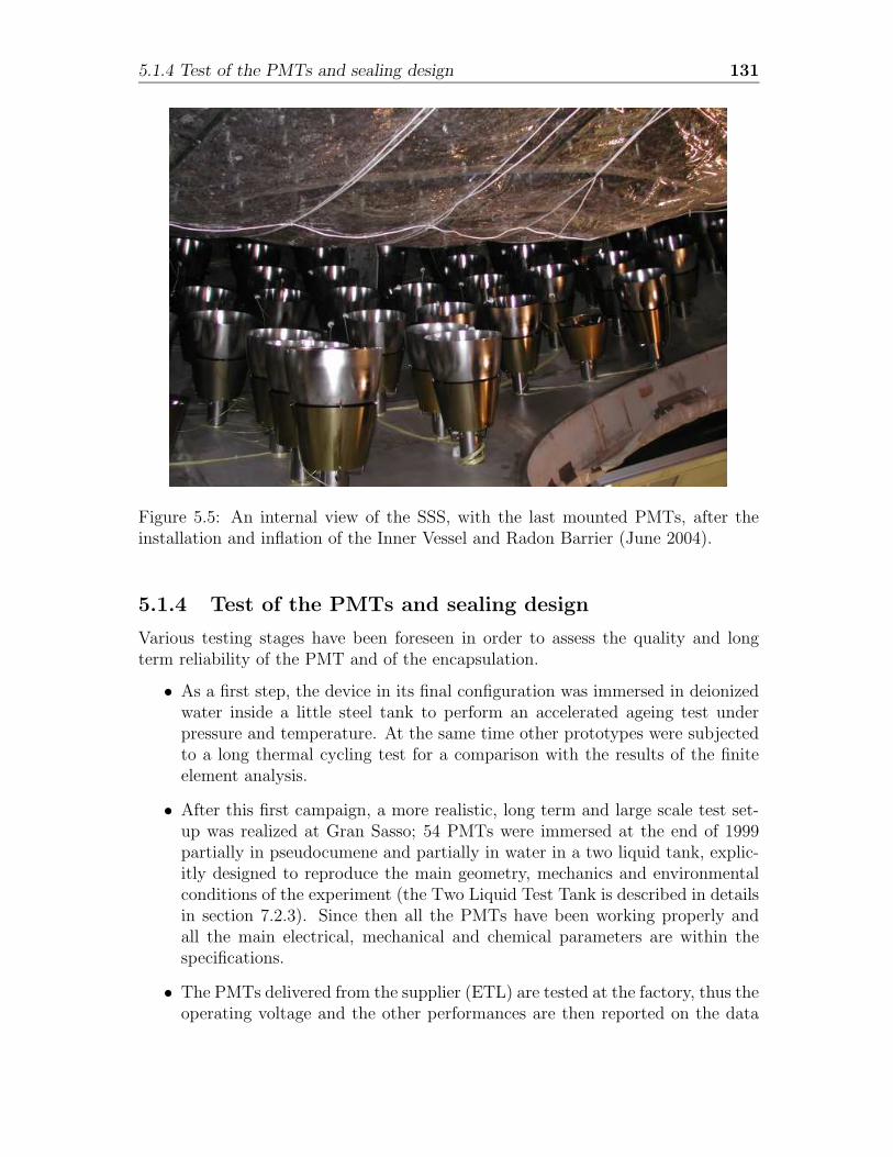
5.1.4 Test of the PMTs and sealing design 131
Figure 5.5: An internal view of the SSS, with the last mounted PMTs, after theinstallation and inflation of the Inner Vessel and Radon Barrier (June 2004).
5.1.4 Test of the PMTs and sealing design
Various testing stages have been foreseen in order to assess the quality and longterm reliability of the PMT and of the encapsulation.
• As a first step, the device in its final configuration was immersed in deionizedwater inside a little steel tank to perform an accelerated ageing test underpressure and temperature. At the same time other prototypes were subjectedto a long thermal cycling test for a comparison with the results of the finiteelement analysis.
• After this first campaign, a more realistic, long term and large scale test set-up was realized at Gran Sasso; 54 PMTs were immersed at the end of 1999partially in pseudocumene and partially in water in a two liquid tank, explic-itly designed to reproduce the main geometry, mechanics and environmentalconditions of the experiment (the Two Liquid Test Tank is described in detailsin section 7.2.3). Since then all the PMTs have been working properly andall the main electrical, mechanical and chemical parameters are within thespecifications.
• The PMTs delivered from the supplier (ETL) are tested at the factory, thus theoperating voltage and the other performances are then reported on the data
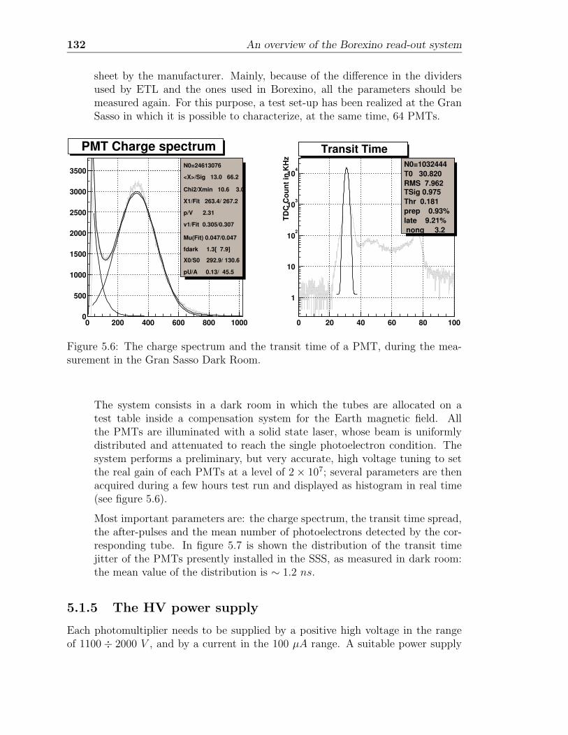
132 An overview of the Borexino read-out system
sheet by the manufacturer. Mainly, because of the difference in the dividersused by ETL and the ones used in Borexino, all the parameters should bemeasured again. For this purpose, a test set-up has been realized at the GranSasso in which it is possible to characterize, at the same time, 64 PMTs.
02 b1_01_02 ETL2088 2001-18-01
0 200 400 600 800 10000
500
1000
1500
2000
2500
3000
3500
PMT Charge spectrumN0=24613076
<X>/Sig 13.0 66.2
Chi2/Xmin 10.6 3.0
X1/Fit 263.4/ 267.2
p/V 2.31
v1/Fit 0.305/0.307
Mu(Fit) 0.047/0.047
fdark 1.3[ 7.9]
X0/S0 292.9/ 130.6
pU/A 0.13/ 45.5
PMT Charge spectrum
0 20 40 60 80 100
TDC
Cou
nt in
KH
z
1
10
102
103
104
Transit TimeN0=1032444T0 30.820RMS 7.962TSig 0.975Thr 0.181prep 0.93%late 9.21% nong 3.2
Transit Time
0 5 10 15 20 25 30
Aft
erpu
lses
Cou
nt in
KH
z
0
2
4
6
8
10
12
Afterpulses[ 0.42- 0.99] 0.3%[ 0.99- 3.60] 1.3%[ 3.60-12.39] 3.3%[ 0.42-12.39] 4.8%Fdark= 1.5 ( 1.5) kHzMu=0.044
Afterpulses
Figure 5.6: The charge spectrum and the transit time of a PMT, during the mea-surement in the Gran Sasso Dark Room.
The system consists in a dark room in which the tubes are allocated on atest table inside a compensation system for the Earth magnetic field. Allthe PMTs are illuminated with a solid state laser, whose beam is uniformlydistributed and attenuated to reach the single photoelectron condition. Thesystem performs a preliminary, but very accurate, high voltage tuning to setthe real gain of each PMTs at a level of 2 × 10⁷; several parameters are thenacquired during a few hours test run and displayed as histogram in real time(see figure 5.6).
Most important parameters are: the charge spectrum, the transit time spread,the after-pulses and the mean number of photoelectrons detected by the cor-responding tube. In figure 5.7 is shown the distribution of the transit timejitter of the PMTs presently installed in the SSS, as measured in dark room:the mean value of the distribution is ∼ 1.2 ns.
5.1.5 The HV power supply
Each photomultiplier needs to be supplied by a positive high voltage in the rangeof 1100 ÷ 2000 V , and by a current in the 100 µA range. A suitable power supply
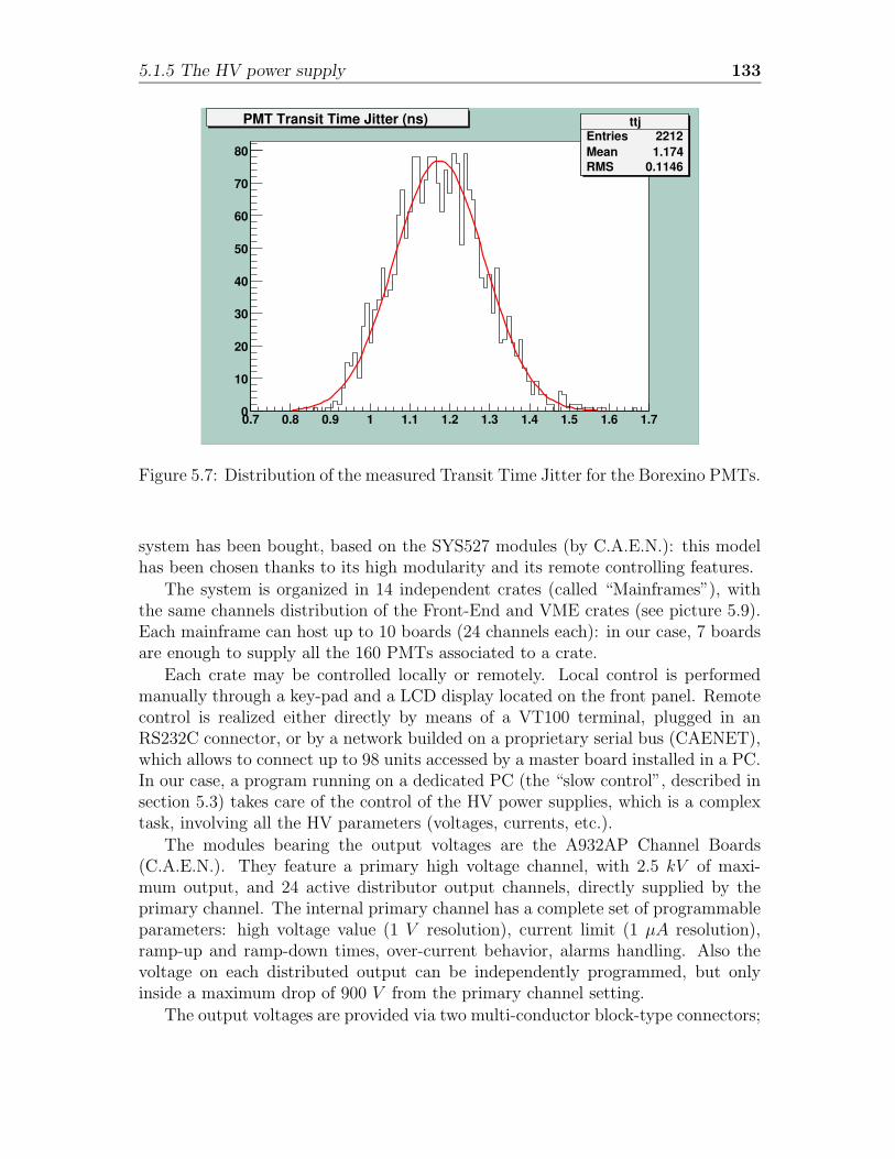
5.1.5 The HV power supply 133
ttjEntries 2212Mean 1.174RMS 0.1146
0.7 0.8 0.9 1 1.1 1.2 1.3 1.4 1.5 1.6 1.70
10
20
30
40
50
60
70
80
ttjEntries 2212Mean 1.174RMS 0.1146
PMT Transit Time Jitter (ns)
Figure 5.7: Distribution of the measured Transit Time Jitter for the Borexino PMTs.
system has been bought, based on the SYS527 modules (by C.A.E.N.): this modelhas been chosen thanks to its high modularity and its remote controlling features.
The system is organized in 14 independent crates (called “Mainframes”), withthe same channels distribution of the Front-End and VME crates (see picture 5.9).Each mainframe can host up to 10 boards (24 channels each): in our case, 7 boardsare enough to supply all the 160 PMTs associated to a crate.
Each crate may be controlled locally or remotely. Local control is performedmanually through a key-pad and a LCD display located on the front panel. Remotecontrol is realized either directly by means of a VT100 terminal, plugged in anRS232C connector, or by a network builded on a proprietary serial bus (CAENET),which allows to connect up to 98 units accessed by a master board installed in a PC.In our case, a program running on a dedicated PC (the “slow control”, described insection 5.3) takes care of the control of the HV power supplies, which is a complextask, involving all the HV parameters (voltages, currents, etc.).
The modules bearing the output voltages are the A932AP Channel Boards(C.A.E.N.). They feature a primary high voltage channel, with 2.5 kV of maxi-mum output, and 24 active distributor output channels, directly supplied by theprimary channel. The internal primary channel has a complete set of programmableparameters: high voltage value (1 V resolution), current limit (1 µA resolution),ramp-up and ramp-down times, over-current behavior, alarms handling. Also thevoltage on each distributed output can be independently programmed, but onlyinside a maximum drop of 900 V from the primary channel setting.
The output voltages are provided via two multi-conductor block-type connectors;
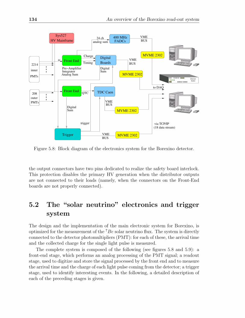
134 An overview of the Borexino read-out system
MVME 2302
Ethernet Switch
acTiming
Charge
PMTs
2214VMEBUS
inner
208
PMTsouter
Pre−AmplifierIntegratorAnalog Sum
VMEBUS
DigitalSum
analog sum24 ch VME
BUS
MVME 2302
MVME 2302
Front End Boards Digital
TDC Caen
400 MHzFADCs
Trigger
Sys527HV Mainframe
trigger
VMEBUS
QTC
SumDigital
Front End
MVME 2302
to DAQ
via TCP/IP(18 data stream)
Figure 5.8: Block diagram of the electronics system for the Borexino detector.
the output connectors have two pins dedicated to realize the safety board interlock.This protection disables the primary HV generation when the distributor outputsare not connected to their loads (namely, when the connectors on the Front-Endboards are not properly connected).
5.2 The “solar neutrino” electronics and trigger
system
The design and the implementation of the main electronic system for Borexino, isoptimized for the measurement of the 7Be solar neutrino flux. The system is directlyconnected to the detector photomultipliers (PMT): for each of these, the arrival timeand the collected charge for the single light pulse is measured.
The complete system is composed of the following (see figures 5.8 and 5.9): afront-end stage, which performs an analog processing of the PMT signal; a readoutstage, used to digitize and store the signal processed by the front end and to measurethe arrival time and the charge of each light pulse coming from the detector; a triggerstage, used to identify interesting events. In the following, a detailed description ofeach of the preceding stages is given.
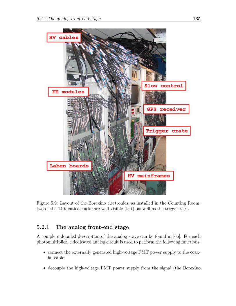
5.2.1 The analog front-end stage 135
Figure 5.9: Layout of the Borexino electronics, as installed in the Counting Room:two of the 14 identical racks are well visible (left), as well as the trigger rack.
5.2.1 The analog front-end stage
A complete detailed description of the analog stage can be found in [66]. For eachphotomultiplier, a dedicated analog circuit is used to perform the following functions:
• connect the externally generated high-voltage PMT power supply to the coax-ial cable;
• decouple the high-voltage PMT power supply from the signal (the Borexino
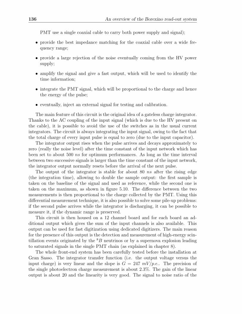
136 An overview of the Borexino read-out system
PMT use a single coaxial cable to carry both power supply and signal);
• provide the best impedance matching for the coaxial cable over a wide fre-quency range;
• provide a large rejection of the noise eventually coming from the HV powersupply;
• amplify the signal and give a fast output, which will be used to identify thetime information;
• integrate the PMT signal, which will be proportional to the charge and hencethe energy of the pulse;
• eventually, inject an external signal for testing and calibration.
The main feature of this circuit is the original idea of a gateless charge integrator.Thanks to the AC coupling of the input signal (which is due to the HV present onthe cable), it is possible to avoid the use of the switches as in the usual currentintegrators. The circuit is always integrating the input signal, owing to the fact thatthe total charge of every input pulse is equal to zero (due to the input capacitor).
The integrator output rises when the pulse arrives and decays approximately tozero (really the noise level) after the time constant of the input network which hasbeen set to about 500 ns for optimum performances. As long as the time intervalbetween two successive signals is larger than the time constant of the input network,the integrator output normally resets before the arrival of the next pulse.
The output of the integrator is stable for about 80 ns after the rising edge(the integration time), allowing to double the sample output: the first sample istaken on the baseline of the signal and used as reference, while the second one istaken on the maximum, as shown in figure 5.10. The difference between the twomeasurements is then proportional to the charge collected by the PMT. Using thisdifferential measurement technique, it is also possible to solve some pile-up problems:if the second pulse arrives while the integrator is discharging, it can be possible tomeasure it, if the dynamic range is preserved.
This circuit is then housed on a 12 channel board and for each board an ad-ditional output which gives the sum of the input channels is also available. Thisoutput can be used for fast digitization using dedicated digitizers. The main reasonfor the presence of this output is the detection and measurement of high-energy scin-tillation events originated by the 8B neutrinos or by a supernova explosion leadingto saturated signals in the single PMT chain (as explained in chapter 8).
The whole front-end system has been carefully tested before the installation atGran Sasso. The integrator transfer function (i.e. the output voltage versus theinput charge) is very linear and the slope is G = 247 mV/p.e.. The precision ofthe single photoelectron charge measurement is about 2.3%. The gain of the linearoutput is about 20 and the linearity is very good. The signal to noise ratio of the
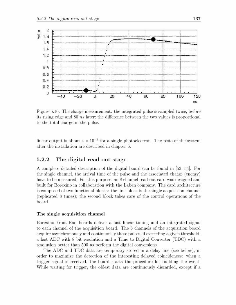
5.2.2 The digital read out stage 137
Figure 5.10: The charge measurement: the integrated pulse is sampled twice, beforeits rising edge and 80 ns later; the difference between the two values is proportionalto the total charge in the pulse.
linear output is about 4 × 10⁻³ for a single photoelectron. The tests of the systemafter the installation are described in chapter 6.
5.2.2 The digital read out stage
A complete detailed description of the digital board can be found in [53, 54]. Forthe single channel, the arrival time of the pulse and the associated charge (energy)have to be measured. For this purpose, an 8 channel read-out card was designed andbuilt for Borexino in collaboration with the Laben company. The card architectureis composed of two functional blocks: the first block is the single acquisition channel(replicated 8 times); the second block takes care of the control operations of theboard.
The single acquisition channel
Borexino Front-End boards deliver a fast linear timing and an integrated signalto each channel of the acquisition board. The 8 channels of the acquisition boardacquire asynchronously and continuously these pulses, if exceeding a given threshold;a fast ADC with 8 bit resolution and a Time to Digital Converter (TDC) with aresolution better than 500 ps perform the digital conversions.
The ADC and TDC data are temporary stored in a delay line (see below), inorder to maximize the detection of the interesting delayed coincidences: when atrigger signal is received, the board starts the procedure for building the event.While waiting for trigger, the oldest data are continuously discarded, except if a
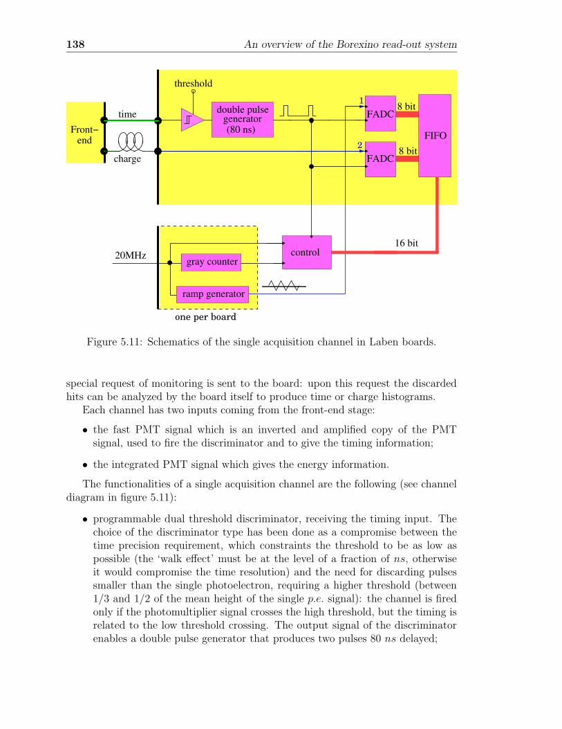
138 An overview of the Borexino read-out system
one per board
2
1
threshold
control
FADC
FADC
gray counter
ramp generator
endFront−
time
charge
(80 ns)
double pulse generator
20MHz
FIFO
16 bit
8 bit
8 bit
Figure 5.11: Schematics of the single acquisition channel in Laben boards.
special request of monitoring is sent to the board: upon this request the discardedhits can be analyzed by the board itself to produce time or charge histograms.
Each channel has two inputs coming from the front-end stage:
• the fast PMT signal which is an inverted and amplified copy of the PMTsignal, used to fire the discriminator and to give the timing information;
• the integrated PMT signal which gives the energy information.
The functionalities of a single acquisition channel are the following (see channeldiagram in figure 5.11):
• programmable dual threshold discriminator, receiving the timing input. Thechoice of the discriminator type has been done as a compromise between thetime precision requirement, which constraints the threshold to be as low aspossible (the ‘walk effect’ must be at the level of a fraction of ns, otherwiseit would compromise the time resolution) and the need for discarding pulsessmaller than the single photoelectron, requiring a higher threshold (between1/3 and 1/2 of the mean height of the single p.e. signal): the channel is firedonly if the photomultiplier signal crosses the high threshold, but the timing isrelated to the low threshold crossing. The output signal of the discriminatorenables a double pulse generator that produces two pulses 80 ns delayed;
5.2.2 The digital read out stage 139
0 [ns]
1 2 3 4 5 6 70
∆t
100 150 200 250 300 [ns] [ns] [ns] [ns] [ns]
50 ns
8
80 ns
3.27675 [ms]
50 [ns]
20MHzgray counter
sampling:
10MHztriangular wave
sampling:
t0 t1 t2
Figure 5.12: Timing informations provided for each event by the single acquisitionchannel: a sample of the 16 bit gray counter (50 ns resolution) and two samples ofthe 10 MHz triangular wave synchronous with the clock.
• the discrimination pulses are sent, as a trigger signal, to a dual input 8-bitFADC. The input of the first FADC is the integrated signal of the hit: acalibrated delay line between the front-end charge output and the Laben boardinput is intended to have the double sampling in coincidence, respectively, withthe baseline and the peak value of the signal (see figure 5.10);
• Time to Digital Converter (TDC) with resolution better than 500 ps (seebelow);
• local FIFO buffer, 24 bit wide, 1024 word deep, used to temporarily store thedata while the system is waiting for a possible trigger. The maximum triggerlatency possible is 6.4 µs.
The TDC is composed of two sections:
1. the coarse timing is given by a 16 bit Gray coded counter driven by the 20MHzgeneral clock, which gives a resolution of 50 ns;
2. the fine timing is given by sampling twice with a 10 MHz triangular signal,generated on the board from the 20 MHz base clock. The operation is per-formed by the second 8-bit FADC, triggered by the dual pulse signal comingfrom the discriminator.
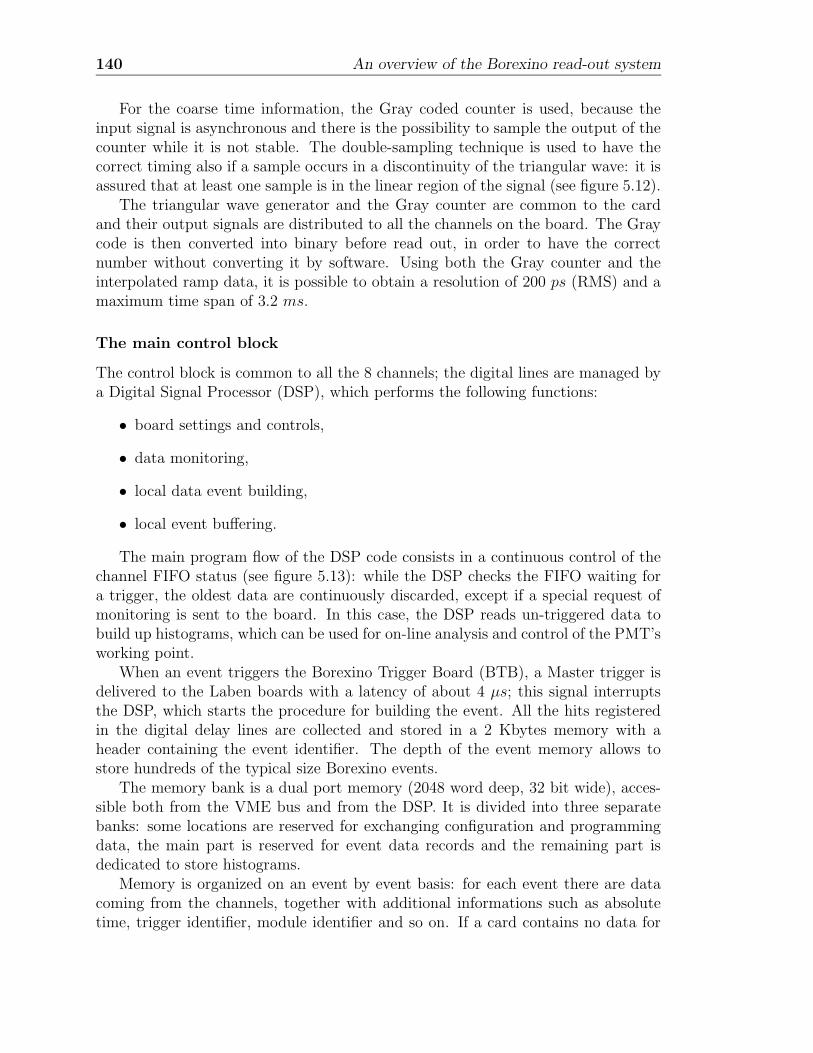
140 An overview of the Borexino read-out system
For the coarse time information, the Gray coded counter is used, because theinput signal is asynchronous and there is the possibility to sample the output of thecounter while it is not stable. The double-sampling technique is used to have thecorrect timing also if a sample occurs in a discontinuity of the triangular wave: it isassured that at least one sample is in the linear region of the signal (see figure 5.12).
The triangular wave generator and the Gray counter are common to the cardand their output signals are distributed to all the channels on the board. The Graycode is then converted into binary before read out, in order to have the correctnumber without converting it by software. Using both the Gray counter and theinterpolated ramp data, it is possible to obtain a resolution of 200 ps (RMS) and amaximum time span of 3.2 ms.
The main control block
The control block is common to all the 8 channels; the digital lines are managed bya Digital Signal Processor (DSP), which performs the following functions:
• board settings and controls,
• data monitoring,
• local data event building,
• local event buffering.
The main program flow of the DSP code consists in a continuous control of thechannel FIFO status (see figure 5.13): while the DSP checks the FIFO waiting fora trigger, the oldest data are continuously discarded, except if a special request ofmonitoring is sent to the board. In this case, the DSP reads un-triggered data tobuild up histograms, which can be used for on-line analysis and control of the PMT’sworking point.
When an event triggers the Borexino Trigger Board (BTB), a Master trigger isdelivered to the Laben boards with a latency of about 4 µs; this signal interruptsthe DSP, which starts the procedure for building the event. All the hits registeredin the digital delay lines are collected and stored in a 2 Kbytes memory with aheader containing the event identifier. The depth of the event memory allows tostore hundreds of the typical size Borexino events.
The memory bank is a dual port memory (2048 word deep, 32 bit wide), acces-sible both from the VME bus and from the DSP. It is divided into three separatebanks: some locations are reserved for exchanging configuration and programmingdata, the main part is reserved for event data records and the remaining part isdedicated to store histograms.
Memory is organized on an event by event basis: for each event there are datacoming from the channels, together with additional informations such as absolutetime, trigger identifier, module identifier and so on. If a card contains no data for
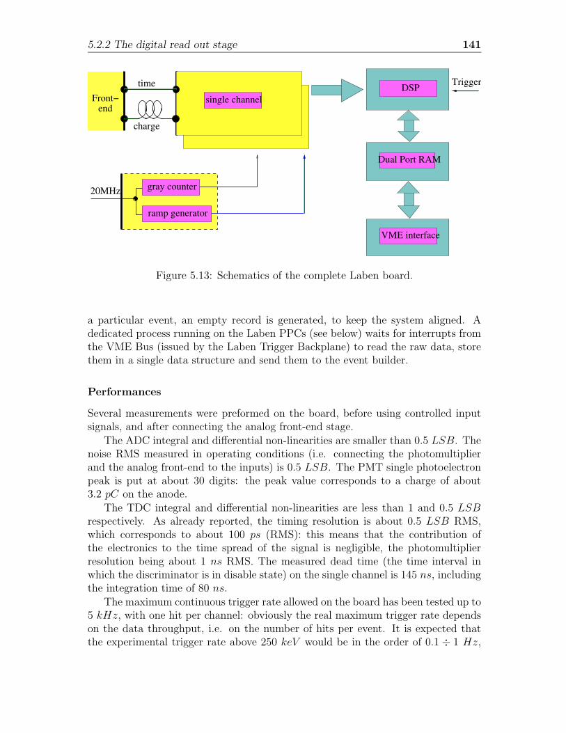
5.2.2 The digital read out stage 141
single channel
ramp generator
gray counter
DSP
Dual Port RAM
VME interface
endFront−
time
charge
20MHz
Trigger
Figure 5.13: Schematics of the complete Laben board.
a particular event, an empty record is generated, to keep the system aligned. Adedicated process running on the Laben PPCs (see below) waits for interrupts fromthe VME Bus (issued by the Laben Trigger Backplane) to read the raw data, storethem in a single data structure and send them to the event builder.
Performances
Several measurements were preformed on the board, before using controlled inputsignals, and after connecting the analog front-end stage.
The ADC integral and differential non-linearities are smaller than 0.5 LSB. Thenoise RMS measured in operating conditions (i.e. connecting the photomultiplierand the analog front-end to the inputs) is 0.5 LSB. The PMT single photoelectronpeak is put at about 30 digits: the peak value corresponds to a charge of about3.2 pC on the anode.
The TDC integral and differential non-linearities are less than 1 and 0.5 LSBrespectively. As already reported, the timing resolution is about 0.5 LSB RMS,which corresponds to about 100 ps (RMS): this means that the contribution ofthe electronics to the time spread of the signal is negligible, the photomultiplierresolution being about 1 ns RMS. The measured dead time (the time interval inwhich the discriminator is in disable state) on the single channel is 145 ns, includingthe integration time of 80 ns.
The maximum continuous trigger rate allowed on the board has been tested up to5 kHz, with one hit per channel: obviously the real maximum trigger rate dependson the data throughput, i.e. on the number of hits per event. It is expected thatthe experimental trigger rate above 250 keV would be in the order of 0.1 ÷ 1 Hz,
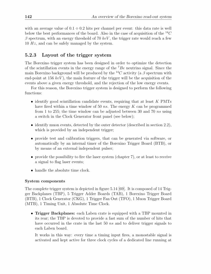
142 An overview of the Borexino read-out system
with an average value of 0.1÷ 0.2 hits per channel per event: this data rate is wellbelow the best performances of the board. Also in the case of acquisition of the 14Cβ spectrum, with an energy threshold of 70 keV , the trigger rate would reach a few10 Hz, and can be safely managed by the system.
5.2.3 Layout of the trigger system
The Borexino trigger system has been designed in order to optimize the detectionof the scintillation events in the energy range of the 7Be neutrino signal. Since themain Borexino background will be produced by the 14C activity (a β spectrum withend-point at 156 keV ), the main feature of the trigger will be the acquisition of theevents above a given energy threshold, and the rejection of the low energy events.
For this reason, the Borexino trigger system is designed to perform the followingfunctions:
• identify good scintillation candidate events, requiring that at least K PMTshave fired within a time window of 50 ns. The energy K can be programmedfrom 1 to 255; the time window can be adjusted between 30 and 70 ns usinga switch in the Clock Generator front panel (see below);
• identify muon events, detected by the outer detector (described in section 2.2),which is provided by an independent trigger;
• provide test and calibration triggers, that can be generated via software, orautomatically by an internal timer of the Borexino Trigger Board (BTB), orby means of an external independent pulser;
• provide the possibility to fire the laser system (chapter 7), or at least to receivea signal to flag laser events;
• handle the absolute time clock.
System components
The complete trigger system is depicted in figure 5.14 [69]. It is composed of 14 Trig-ger Backplanes (TBP), 5 Trigger Adder Boards (TAB), 1 Borexino Trigger Board(BTB), 1 Clock Generator (CKG), 1 Trigger Fan Out (TFO), 1 Muon Trigger Board(MTB), 1 Timing Unit, 1 Absolute Time Clock.
• Trigger Backplanes: each Laben crate is equipped with a TBP mounted inits rear; the TBP is devoted to provide a fast sum of the number of hits thathave occurred in the crate in the last 50 ns and to deliver trigger signals toeach Laben board.
It works in this way: every time a timing input fires, a monostable signal isactivated and kept active for three clock cycles of a dedicated line running at
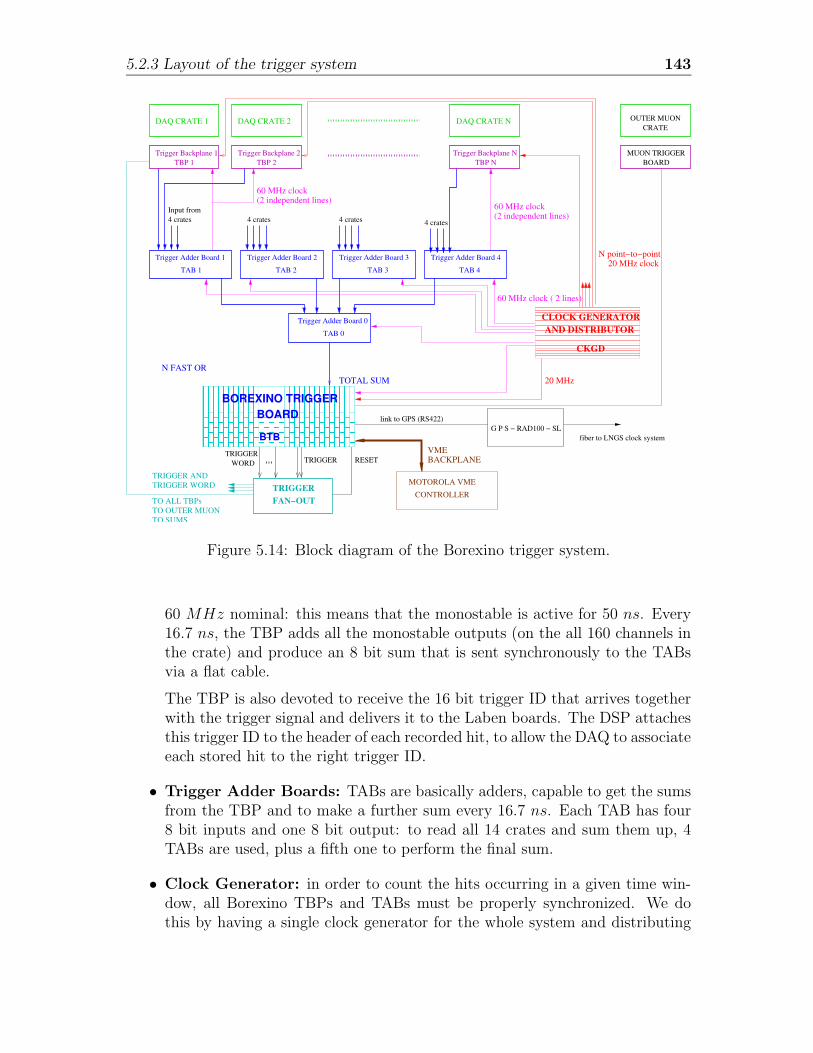
5.2.3 Layout of the trigger system 143
20 MHz
RESET
FAN−OUT
(2 independent lines)
(2 independent lines)
MUON TRIGGERBOARD
CRATEOUTER MUON
fiber to LNGS clock system
Trigger Backplane 1 Trigger Backplane 2TBP 1
TAB 1
Trigger Adder Board 2 Trigger Adder Board 3
TAB 2 TAB 3 TAB 4
Trigger Adder Board 4
TAB 0
Trigger Adder Board 0
Input from 4 crates 4 crates 4 crates 4 crates
TRIGGERTRIGGER
WORD
VMEBACKPLANE
link to GPS (RS422)
DAQ CRATE 1 DAQ CRATE 2 DAQ CRATE N
Trigger Backplane NTBP NTBP 2
TRIGGERTRIGGER ANDTRIGGER WORD
Trigger Adder Board 1
60 MHz clock
N FAST ORTOTAL SUM
60 MHz clock ( 2 lines)
60 MHz clock
MOTOROLA VME
CONTROLLER
N point−to−point20 MHz clock
BOREXINO TRIGGERBOARD
BTB
CLOCK GENERATOR
CKGD
AND DISTRIBUTOR
TO ALL TBPsTO OUTER MUONTO SUMS
G P S − RAD100 − SL
Figure 5.14: Block diagram of the Borexino trigger system.
60 MHz nominal: this means that the monostable is active for 50 ns. Every16.7 ns, the TBP adds all the monostable outputs (on the all 160 channels inthe crate) and produce an 8 bit sum that is sent synchronously to the TABsvia a flat cable.
The TBP is also devoted to receive the 16 bit trigger ID that arrives togetherwith the trigger signal and delivers it to the Laben boards. The DSP attachesthis trigger ID to the header of each recorded hit, to allow the DAQ to associateeach stored hit to the right trigger ID.
• Trigger Adder Boards: TABs are basically adders, capable to get the sumsfrom the TBP and to make a further sum every 16.7 ns. Each TAB has four8 bit inputs and one 8 bit output: to read all 14 crates and sum them up, 4TABs are used, plus a fifth one to perform the final sum.
• Clock Generator: in order to count the hits occurring in a given time win-dow, all Borexino TBPs and TABs must be properly synchronized. We dothis by having a single clock generator for the whole system and distributing
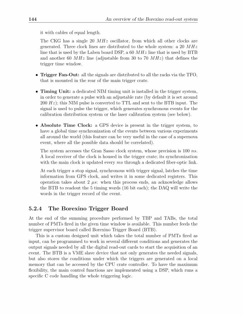
144 An overview of the Borexino read-out system
it with cables of equal length.
The CKG has a single 20 MHz oscillator, from which all other clocks aregenerated. Three clock lines are distributed to the whole system: a 20 MHzline that is used by the Laben board DSP, a 60MHz line that is used by BTBand another 60 MHz line (adjustable from 30 to 70 MHz) that defines thetrigger time window.
• Trigger Fan-Out: all the signals are distributed to all the racks via the TFO,that is mounted in the rear of the main trigger crate.
• Timing Unit: a dedicated NIM timing unit is installed in the trigger system,in order to generate a pulse with an adjustable rate (by default it is set around200 Hz); this NIM pulse is converted to TTL and sent to the BTB input. Thesignal is used to pulse the trigger, which generates synchronous events for thecalibration distribution system or the laser calibration system (see below).
• Absolute Time Clock: a GPS device is present in the trigger system, tohave a global time synchronization of the events between various experimentsall around the world (this feature can be very useful in the case of a supernovaevent, where all the possible data should be correlated).
The system accesses the Gran Sasso clock system, whose precision is 100 ns.A local receiver of the clock is housed in the trigger crate; its synchronizationwith the main clock is updated every ms through a dedicated fiber-optic link.
At each trigger a stop signal, synchronous with trigger signal, latches the timeinformation from GPS clock, and writes it in some dedicated registers. Thisoperation takes about 2 µs: when this process ends, an acknowledge allowsthe BTB to readout the 5 timing words (16 bit each); the DAQ will write thewords in the trigger record of the event.
5.2.4 The Borexino Trigger Board
At the end of the summing procedure performed by TBP and TABs, the totalnumber of PMTs fired in the given time window is available. This number feeds thetrigger supervisor board called Borexino Trigger Board (BTB).
This is a custom designed unit which takes the total number of PMTs fired asinput, can be programmed to work in several different conditions and generates theoutput signals needed by all the digital read-out cards to start the acquisition of anevent. The BTB is a VME slave device that not only generates the needed signals,but also stores the conditions under which the triggers are generated on a localmemory that can be accessed by the CPU crate controller. To have the maximumflexibility, the main control functions are implemented using a DSP, which runs aspecific C code handling the whole triggering logic.
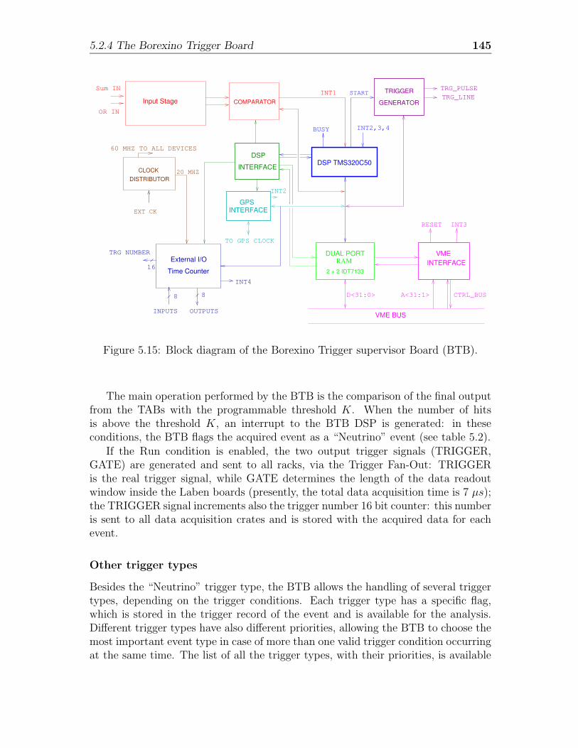
5.2.4 The Borexino Trigger Board 145
RAM
Input Stage COMPARATOR
INT3RESET
8 8
16
OR IN
Sum IN
OUTPUTSINPUTS
TRG_PULSETRG_LINE
INTERFACEDUAL PORT
VME BUS
GPSINTERFACE
DISTRIBUTORCLOCK
External I/O
Time Counter
DSPDSP TMS320C50
INTERFACE
VME
2 + 2 IDT7133
TRG NUMBER
TRIGGER
GENERATOR
STARTINT1
TO GPS CLOCK
INT4
INT2
EXT CK
60 MHZ TO ALL DEVICES
INT2,3,4BUSY
20 MHZ
D<31:0> A<31:1> CTRL_BUS
Figure 5.15: Block diagram of the Borexino Trigger supervisor Board (BTB).
The main operation performed by the BTB is the comparison of the final outputfrom the TABs with the programmable threshold K. When the number of hitsis above the threshold K, an interrupt to the BTB DSP is generated: in theseconditions, the BTB flags the acquired event as a “Neutrino” event (see table 5.2).
If the Run condition is enabled, the two output trigger signals (TRIGGER,GATE) are generated and sent to all racks, via the Trigger Fan-Out: TRIGGERis the real trigger signal, while GATE determines the length of the data readoutwindow inside the Laben boards (presently, the total data acquisition time is 7 µs);the TRIGGER signal increments also the trigger number 16 bit counter: this numberis sent to all data acquisition crates and is stored with the acquired data for eachevent.
Other trigger types
Besides the “Neutrino” trigger type, the BTB allows the handling of several triggertypes, depending on the trigger conditions. Each trigger type has a specific flag,which is stored in the trigger record of the event and is available for the analysis.Different trigger types have also different priorities, allowing the BTB to choose themost important event type in case of more than one valid trigger condition occurringat the same time. The list of all the trigger types, with their priorities, is available
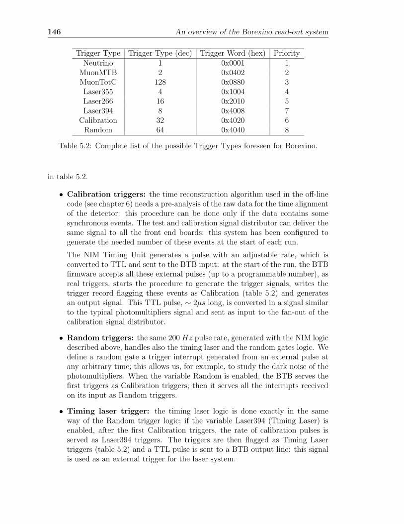
146 An overview of the Borexino read-out system
Trigger Type Trigger Type (dec) Trigger Word (hex) PriorityNeutrino 1 0x0001 1
MuonMTB 2 0x0402 2MuonTotC 128 0x0880 3Laser355 4 0x1004 4Laser266 16 0x2010 5Laser394 8 0x4008 7
Calibration 32 0x4020 6Random 64 0x4040 8
Table 5.2: Complete list of the possible Trigger Types foreseen for Borexino.
in table 5.2.
• Calibration triggers: the time reconstruction algorithm used in the off-linecode (see chapter 6) needs a pre-analysis of the raw data for the time alignmentof the detector: this procedure can be done only if the data contains somesynchronous events. The test and calibration signal distributor can deliver thesame signal to all the front end boards: this system has been configured togenerate the needed number of these events at the start of each run.
The NIM Timing Unit generates a pulse with an adjustable rate, which isconverted to TTL and sent to the BTB input: at the start of the run, the BTBfirmware accepts all these external pulses (up to a programmable number), asreal triggers, starts the procedure to generate the trigger signals, writes thetrigger record flagging these events as Calibration (table 5.2) and generatesan output signal. This TTL pulse, ∼ 2µs long, is converted in a signal similarto the typical photomultipliers signal and sent as input to the fan-out of thecalibration signal distributor.
• Random triggers: the same 200Hz pulse rate, generated with the NIM logicdescribed above, handles also the timing laser and the random gates logic. Wedefine a random gate a trigger interrupt generated from an external pulse atany arbitrary time; this allows us, for example, to study the dark noise of thephotomultipliers. When the variable Random is enabled, the BTB serves thefirst triggers as Calibration triggers; then it serves all the interrupts receivedon its input as Random triggers.
• Timing laser trigger: the timing laser logic is done exactly in the sameway of the Random trigger logic; if the variable Laser394 (Timing Laser) isenabled, after the first Calibration triggers, the rate of calibration pulses isserved as Laser394 triggers. The triggers are then flagged as Timing Lasertriggers (table 5.2) and a TTL pulse is sent to a BTB output line: this signalis used as an external trigger for the laser system.
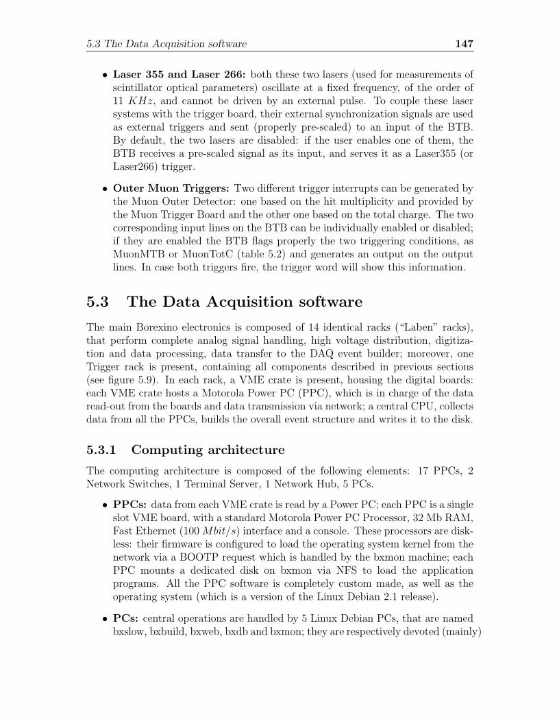
5.3 The Data Acquisition software 147
• Laser 355 and Laser 266: both these two lasers (used for measurements ofscintillator optical parameters) oscillate at a fixed frequency, of the order of11 KHz, and cannot be driven by an external pulse. To couple these lasersystems with the trigger board, their external synchronization signals are usedas external triggers and sent (properly pre-scaled) to an input of the BTB.By default, the two lasers are disabled: if the user enables one of them, theBTB receives a pre-scaled signal as its input, and serves it as a Laser355 (orLaser266) trigger.
• Outer Muon Triggers: Two different trigger interrupts can be generated bythe Muon Outer Detector: one based on the hit multiplicity and provided bythe Muon Trigger Board and the other one based on the total charge. The twocorresponding input lines on the BTB can be individually enabled or disabled;if they are enabled the BTB flags properly the two triggering conditions, asMuonMTB or MuonTotC (table 5.2) and generates an output on the outputlines. In case both triggers fire, the trigger word will show this information.
5.3 The Data Acquisition software
The main Borexino electronics is composed of 14 identical racks (“Laben” racks),that perform complete analog signal handling, high voltage distribution, digitiza-tion and data processing, data transfer to the DAQ event builder; moreover, oneTrigger rack is present, containing all components described in previous sections(see figure 5.9). In each rack, a VME crate is present, housing the digital boards:each VME crate hosts a Motorola Power PC (PPC), which is in charge of the dataread-out from the boards and data transmission via network; a central CPU, collectsdata from all the PPCs, builds the overall event structure and writes it to the disk.
5.3.1 Computing architecture
The computing architecture is composed of the following elements: 17 PPCs, 2Network Switches, 1 Terminal Server, 1 Network Hub, 5 PCs.
• PPCs: data from each VME crate is read by a Power PC; each PPC is a singleslot VME board, with a standard Motorola Power PC Processor, 32 Mb RAM,Fast Ethernet (100Mbit/s) interface and a console. These processors are disk-less: their firmware is configured to load the operating system kernel from thenetwork via a BOOTP request which is handled by the bxmon machine; eachPPC mounts a dedicated disk on bxmon via NFS to load the applicationprograms. All the PPC software is completely custom made, as well as theoperating system (which is a version of the Linux Debian 2.1 release).
• PCs: central operations are handled by 5 Linux Debian PCs, that are namedbxslow, bxbuild, bxweb, bxdb and bxmon; they are respectively devoted (mainly)
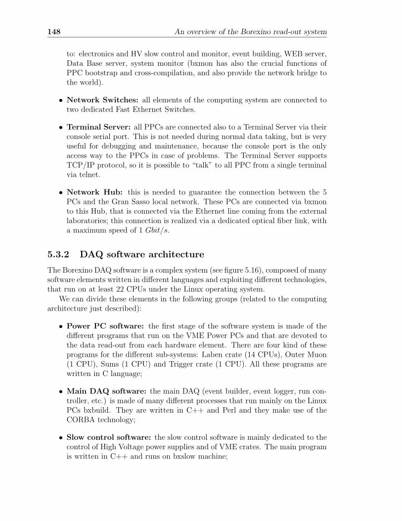
148 An overview of the Borexino read-out system
to: electronics and HV slow control and monitor, event building, WEB server,Data Base server, system monitor (bxmon has also the crucial functions ofPPC bootstrap and cross-compilation, and also provide the network bridge tothe world).
• Network Switches: all elements of the computing system are connected totwo dedicated Fast Ethernet Switches.
• Terminal Server: all PPCs are connected also to a Terminal Server via theirconsole serial port. This is not needed during normal data taking, but is veryuseful for debugging and maintenance, because the console port is the onlyaccess way to the PPCs in case of problems. The Terminal Server supportsTCP/IP protocol, so it is possible to “talk” to all PPC from a single terminalvia telnet.
• Network Hub: this is needed to guarantee the connection between the 5PCs and the Gran Sasso local network. These PCs are connected via bxmonto this Hub, that is connected via the Ethernet line coming from the externallaboratories; this connection is realized via a dedicated optical fiber link, witha maximum speed of 1 Gbit/s.
5.3.2 DAQ software architecture
The Borexino DAQ software is a complex system (see figure 5.16), composed of manysoftware elements written in different languages and exploiting different technologies,that run on at least 22 CPUs under the Linux operating system.
We can divide these elements in the following groups (related to the computingarchitecture just described):
• Power PC software: the first stage of the software system is made of thedifferent programs that run on the VME Power PCs and that are devoted tothe data read-out from each hardware element. There are four kind of theseprograms for the different sub-systems: Laben crate (14 CPUs), Outer Muon(1 CPU), Sums (1 CPU) and Trigger crate (1 CPU). All these programs arewritten in C language;
• Main DAQ software: the main DAQ (event builder, event logger, run con-troller, etc.) is made of many different processes that run mainly on the LinuxPCs bxbuild. They are written in C++ and Perl and they make use of theCORBA technology;
• Slow control software: the slow control software is mainly dedicated to thecontrol of High Voltage power supplies and of VME crates. The main programis written in C++ and runs on bxslow machine;
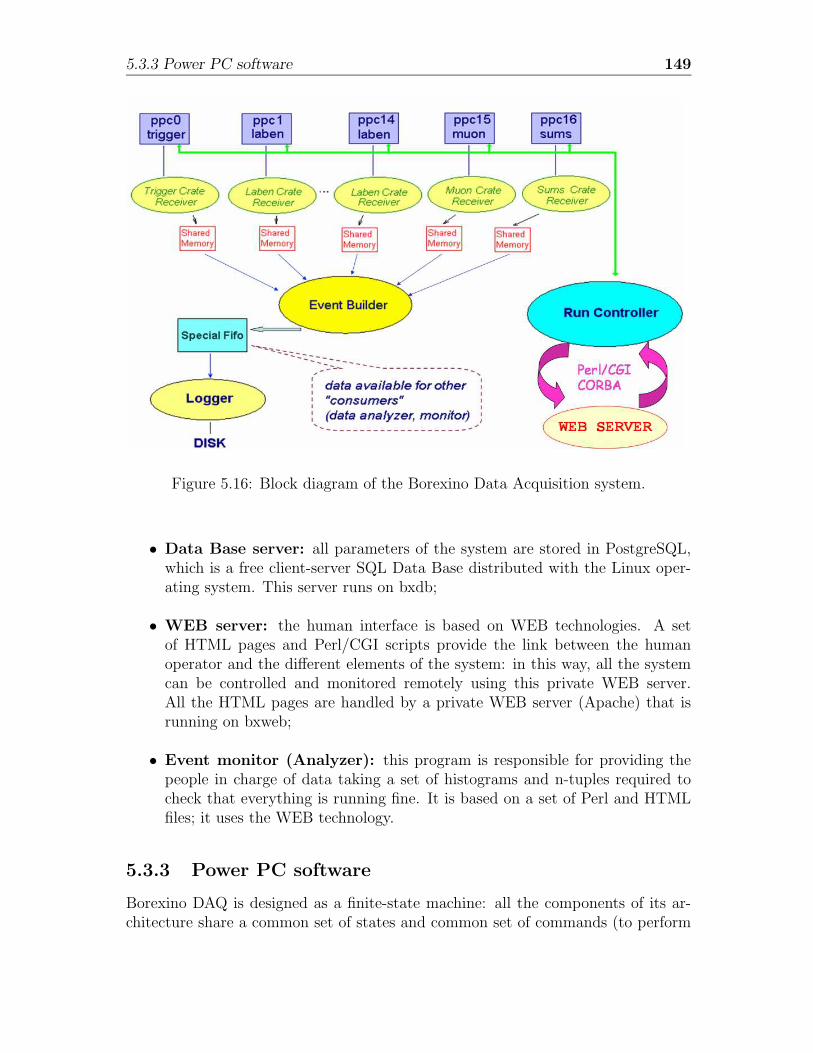
5.3.3 Power PC software 149
Figure 5.16: Block diagram of the Borexino Data Acquisition system.
• Data Base server: all parameters of the system are stored in PostgreSQL,which is a free client-server SQL Data Base distributed with the Linux oper-ating system. This server runs on bxdb;
• WEB server: the human interface is based on WEB technologies. A setof HTML pages and Perl/CGI scripts provide the link between the humanoperator and the different elements of the system: in this way, all the systemcan be controlled and monitored remotely using this private WEB server.All the HTML pages are handled by a private WEB server (Apache) that isrunning on bxweb;
• Event monitor (Analyzer): this program is responsible for providing thepeople in charge of data taking a set of histograms and n-tuples required tocheck that everything is running fine. It is based on a set of Perl and HTMLfiles; it uses the WEB technology.
5.3.3 Power PC software
Borexino DAQ is designed as a finite-state machine: all the components of its ar-chitecture share a common set of states and common set of commands (to perform
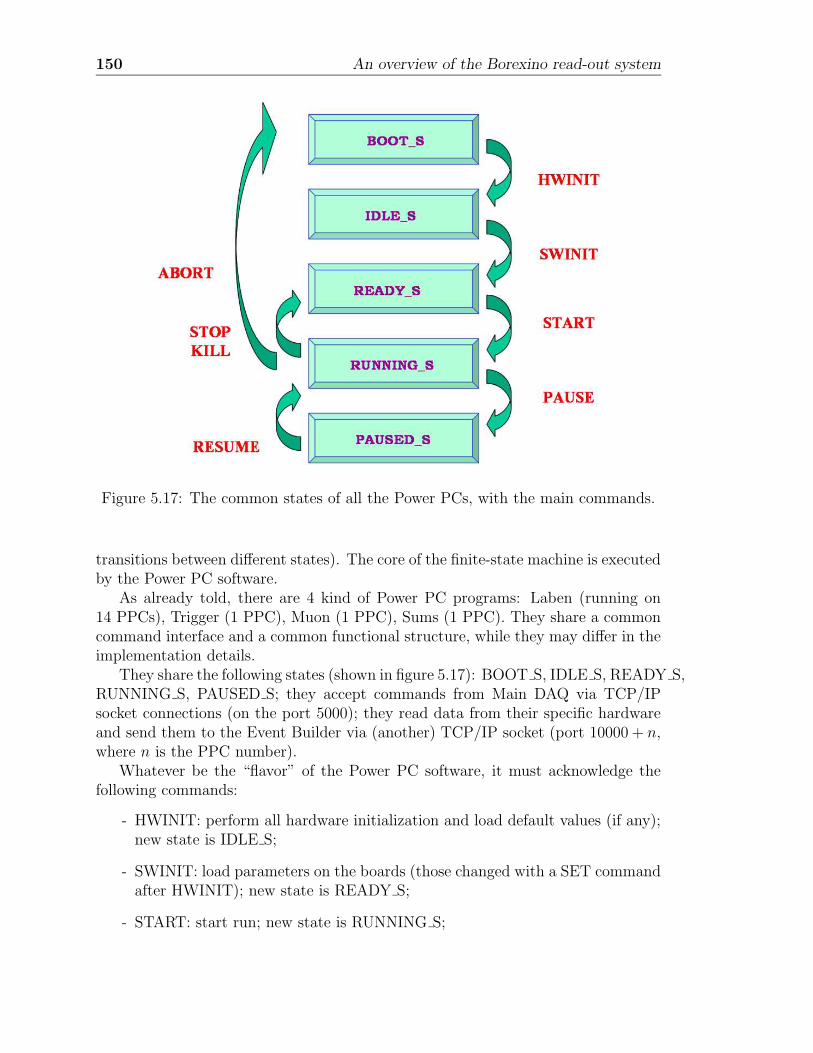
150 An overview of the Borexino read-out system
Figure 5.17: The common states of all the Power PCs, with the main commands.
transitions between different states). The core of the finite-state machine is executedby the Power PC software.
As already told, there are 4 kind of Power PC programs: Laben (running on14 PPCs), Trigger (1 PPC), Muon (1 PPC), Sums (1 PPC). They share a commoncommand interface and a common functional structure, while they may differ in theimplementation details.
They share the following states (shown in figure 5.17): BOOT S, IDLE S, READY S,RUNNING S, PAUSED S; they accept commands from Main DAQ via TCP/IPsocket connections (on the port 5000); they read data from their specific hardwareand send them to the Event Builder via (another) TCP/IP socket (port 10000 + n,where n is the PPC number).
Whatever be the “flavor” of the Power PC software, it must acknowledge thefollowing commands:
- HWINIT: perform all hardware initialization and load default values (if any);new state is IDLE S;
- SWINIT: load parameters on the boards (those changed with a SET commandafter HWINIT); new state is READY S;
- START: start run; new state is RUNNING S;

5.3.3 Power PC software 151
- STOP: stop current run; flush the data in memory before stopping; new stateis READY S;
- PAUSE: pause the current run; new state is PAUSED S;
- RESUME: resume the paused run; new state is RUNNING S;
- ABORT: abort the run with no data flushing; new state is BOOT S;
- KILL: abort the run with no data flushing; new state is READY S;
- GET HWID: returns hardware ID (Ethernet) of the Power PC;
- GET STATUS, MACHINE STATUS: return the program status, expressed asstring (BOOT S, etc.), or the system status, expressed as a number (1,2,4,8,16);
- (GET) SET TADD, TPORT, CID, TSEND: (get) set respectively: the TCP/IPaddress where DATA must be sent to (usually bxbuild); the TCP/IP portwhere DATA must be sent to (default is 10000 + n); the logical crate ID; theevent block size (data are sent to the network in blocks of TSEND events);
- REBOOT, TEST: reboot the Power PC; test the hardware.
Laben Power PC software
The Laben Software has a multi-process structure, featuring four logical functionsidentified (for historical reasons) with the names M1, M2, M3 and M4 (see figure5.18). M1 reads data and sends them to the builder; M2 reads histograms andsends them to the histogram receiver; M3 and M4 handle commands and send errormessages. M1 is in turn composed by three main processes: “main t” receivescommands issued by the M4 area; “cpu” continuously reads data from the VMEbackplane and store them in an internal Shared Memory; “sped” reads the SharedMemory and sends the data to the network.
The Laben power PCs keep 4 different Network connections during normal datataking, for handling commands, data, histograms and errors (see figure 5.18): S1 isused for commands and links each PPC to the Run Controller; S2 and S4 are usedto send data respectively to the Event Builder and to the Histogram Server; S3 isused for error messages that are gathered by the standard UNIX Syslogd processrunning on bxmon.
Besides the common set of commands of all the PPCs, the Laben software fea-tures specific commands allowing to perform actions on the Laben Board set-upparameters: for example, it is possible to set (get) the threshold for each channel,to enable/disable specific channels (boards) from the DAQ or from the trigger, toset or check internal parameters.
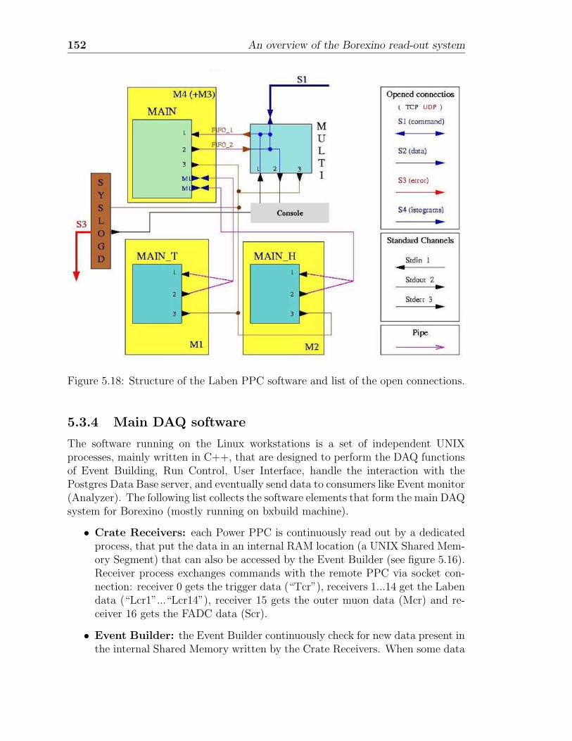
152 An overview of the Borexino read-out system
Figure 5.18: Structure of the Laben PPC software and list of the open connections.
5.3.4 Main DAQ software
The software running on the Linux workstations is a set of independent UNIXprocesses, mainly written in C++, that are designed to perform the DAQ functionsof Event Building, Run Control, User Interface, handle the interaction with thePostgres Data Base server, and eventually send data to consumers like Event monitor(Analyzer). The following list collects the software elements that form the main DAQsystem for Borexino (mostly running on bxbuild machine).
• Crate Receivers: each Power PPC is continuously read out by a dedicatedprocess, that put the data in an internal RAM location (a UNIX Shared Mem-ory Segment) that can also be accessed by the Event Builder (see figure 5.16).Receiver process exchanges commands with the remote PPC via socket con-nection: receiver 0 gets the trigger data (“Tcr”), receivers 1...14 get the Labendata (“Lcr1”...“Lcr14”), receiver 15 gets the outer muon data (Mcr) and re-ceiver 16 gets the FADC data (Scr).
• Event Builder: the Event Builder continuously check for new data present inthe internal Shared Memory written by the Crate Receivers. When some data
5.3.5 The WEB interface 153
are present in all the segments, the EB proceeds to identify the correspondingevent blocks (using the 16 bit Trigger ID that each Power PC writes in thedata), converts the hardware encoding of the channels in the logical map thatis defined in the Data Base and writers each built event in a special FIFO,where data are available for the Logger process and other consumers like theEvent Monitor.
• Logger: this is a very simple program that reads data from the special FIFOfilled by the Event Builder and writes them in the final raw data file (presently,data can only be written on disk). To handle the FIFO, a special piece ofLinux kernel code has been written, in order to allow the possibility thatmany different consumers can get the data during normal data taking withoutaffecting the data flow.
• Run Controller: this is the core of the system. It is a program capable toget the commands from the WEB User Interface (see above) and to dispatchthem to the different processes and/or to the Power PCs. It is also responsibleto start the other processes of the system; finally, it receives exceptions fromother streams and takes proper actions when these exceptions occur. TheRun Controller communicates with the Event Builder (and other processes)via socket connections; the synchronization between the different streams isguaranteed by the use of standard UNIX semaphores.
5.3.5 The WEB interface
The human interface to DAQ software is based on WEB technologies. A set ofHTML pages (dynamically generated via Perl/CGI scripts) provide the link betweenthe human operator and the different elements of the system: in this way, all thesystem can be controlled and monitored remotely using this private WEB server.
The WEB interface handles all the DAQ operations: Borexino shifters can followa sequence of allowed operations, for all needed procedures of data taking. For thisreason, the interface has been designed to be reliable, easy to use, intuitive, andtolerant to operator errors (this last item is realized thanks to the weak interactionto the controlled finite-state machine: it can even be started and stopped with noinfluence on data taking).
It provides five main functions (see figure 5.19):
• run controller: it handles the controller of the finite-state machine, allowingto configure the system, the trigger setup, to perform the main data takingactions, etc.; a screenshot of the main run controller page is in figure 5.20: DAQis in PAUSED S state and the allowed operations are RESUME or ABORT(see also figure 5.17);
• profile manager: it allows the management of the Borexino Data Base col-lection (see below);
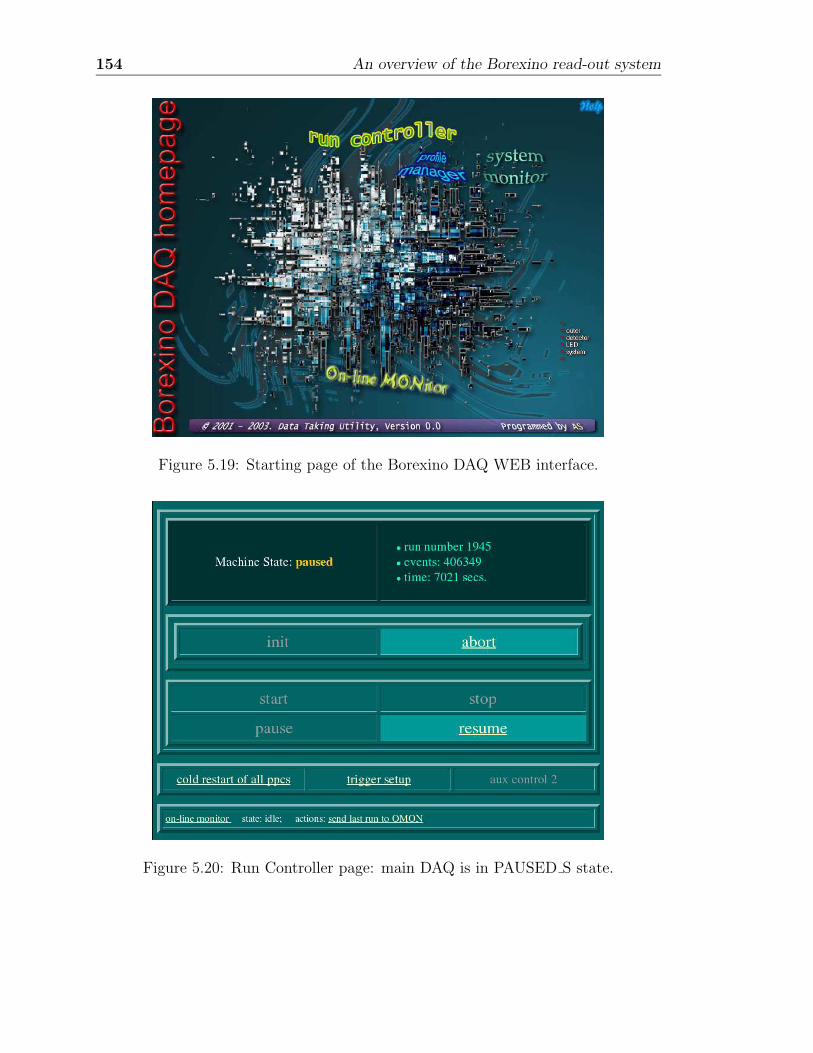
154 An overview of the Borexino read-out system
Figure 5.19: Starting page of the Borexino DAQ WEB interface.
Figure 5.20: Run Controller page: main DAQ is in PAUSED S state.
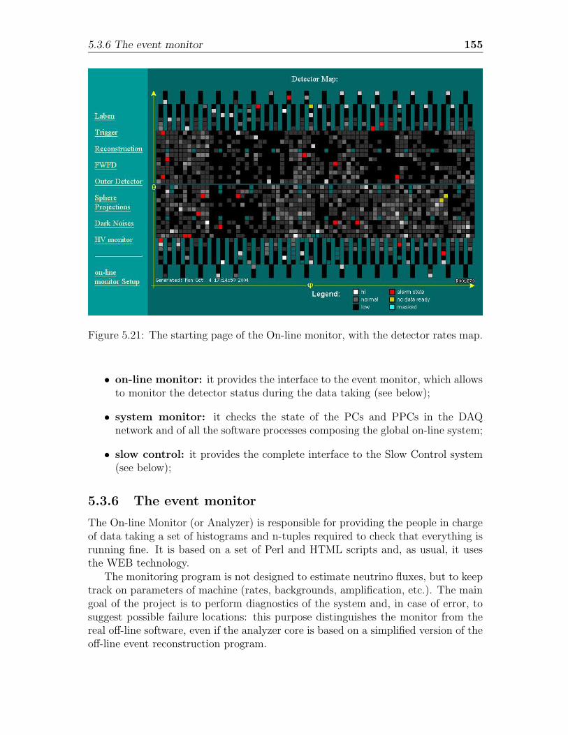
5.3.6 The event monitor 155
Figure 5.21: The starting page of the On-line monitor, with the detector rates map.
• on-line monitor: it provides the interface to the event monitor, which allowsto monitor the detector status during the data taking (see below);
• system monitor: it checks the state of the PCs and PPCs in the DAQnetwork and of all the software processes composing the global on-line system;
• slow control: it provides the complete interface to the Slow Control system(see below);
5.3.6 The event monitor
The On-line Monitor (or Analyzer) is responsible for providing the people in chargeof data taking a set of histograms and n-tuples required to check that everything isrunning fine. It is based on a set of Perl and HTML scripts and, as usual, it usesthe WEB technology.
The monitoring program is not designed to estimate neutrino fluxes, but to keeptrack on parameters of machine (rates, backgrounds, amplification, etc.). The maingoal of the project is to perform diagnostics of the system and, in case of error, tosuggest possible failure locations: this purpose distinguishes the monitor from thereal off-line software, even if the analyzer core is based on a simplified version of theoff-line event reconstruction program.
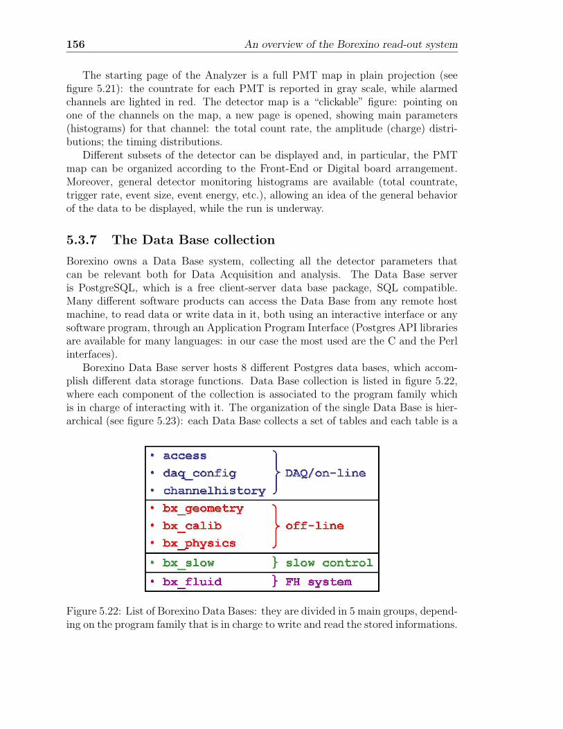
156 An overview of the Borexino read-out system
The starting page of the Analyzer is a full PMT map in plain projection (seefigure 5.21): the countrate for each PMT is reported in gray scale, while alarmedchannels are lighted in red. The detector map is a “clickable” figure: pointing onone of the channels on the map, a new page is opened, showing main parameters(histograms) for that channel: the total count rate, the amplitude (charge) distri-butions; the timing distributions.
Different subsets of the detector can be displayed and, in particular, the PMTmap can be organized according to the Front-End or Digital board arrangement.Moreover, general detector monitoring histograms are available (total countrate,trigger rate, event size, event energy, etc.), allowing an idea of the general behaviorof the data to be displayed, while the run is underway.
5.3.7 The Data Base collection
Borexino owns a Data Base system, collecting all the detector parameters thatcan be relevant both for Data Acquisition and analysis. The Data Base serveris PostgreSQL, which is a free client-server data base package, SQL compatible.Many different software products can access the Data Base from any remote hostmachine, to read data or write data in it, both using an interactive interface or anysoftware program, through an Application Program Interface (Postgres API librariesare available for many languages: in our case the most used are the C and the Perlinterfaces).
Borexino Data Base server hosts 8 different Postgres data bases, which accom-plish different data storage functions. Data Base collection is listed in figure 5.22,where each component of the collection is associated to the program family whichis in charge of interacting with it. The organization of the single Data Base is hier-archical (see figure 5.23): each Data Base collects a set of tables and each table is a
Figure 5.22: List of Borexino Data Bases: they are divided in 5 main groups, depend-ing on the program family that is in charge to write and read the stored informations.
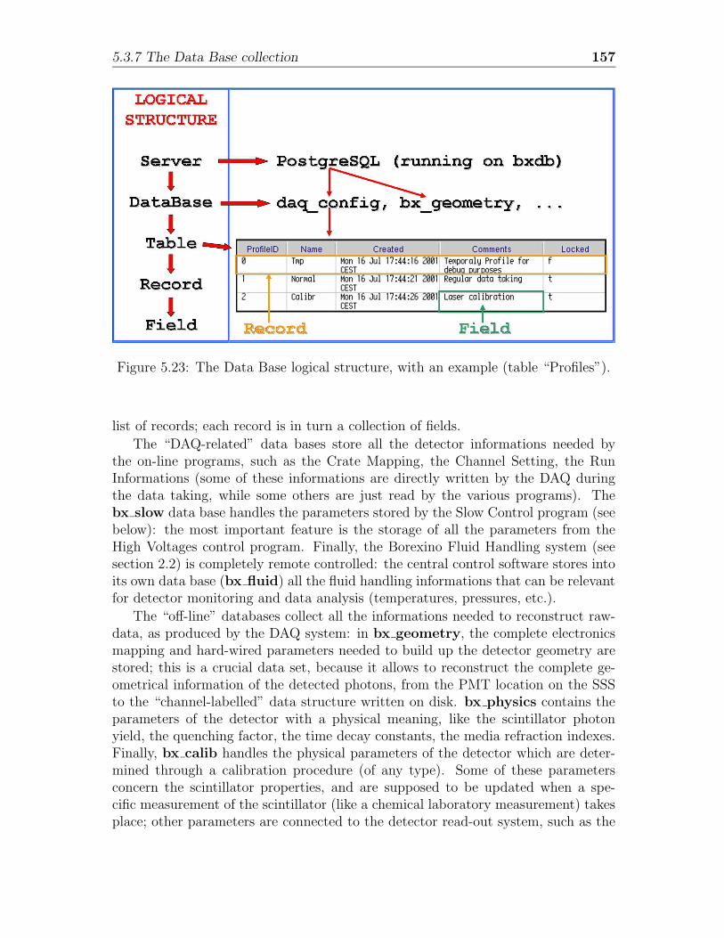
5.3.7 The Data Base collection 157
Figure 5.23: The Data Base logical structure, with an example (table “Profiles”).
list of records; each record is in turn a collection of fields.
The “DAQ-related” data bases store all the detector informations needed bythe on-line programs, such as the Crate Mapping, the Channel Setting, the RunInformations (some of these informations are directly written by the DAQ duringthe data taking, while some others are just read by the various programs). Thebx slow data base handles the parameters stored by the Slow Control program (seebelow): the most important feature is the storage of all the parameters from theHigh Voltages control program. Finally, the Borexino Fluid Handling system (seesection 2.2) is completely remote controlled: the central control software stores intoits own data base (bx fluid) all the fluid handling informations that can be relevantfor detector monitoring and data analysis (temperatures, pressures, etc.).
The “off-line” databases collect all the informations needed to reconstruct raw-data, as produced by the DAQ system: in bx geometry, the complete electronicsmapping and hard-wired parameters needed to build up the detector geometry arestored; this is a crucial data set, because it allows to reconstruct the complete ge-ometrical information of the detected photons, from the PMT location on the SSSto the “channel-labelled” data structure written on disk. bx physics contains theparameters of the detector with a physical meaning, like the scintillator photonyield, the quenching factor, the time decay constants, the media refraction indexes.Finally, bx calib handles the physical parameters of the detector which are deter-mined through a calibration procedure (of any type). Some of these parametersconcern the scintillator properties, and are supposed to be updated when a spe-cific measurement of the scintillator (like a chemical laboratory measurement) takesplace; other parameters are connected to the detector read-out system, such as the
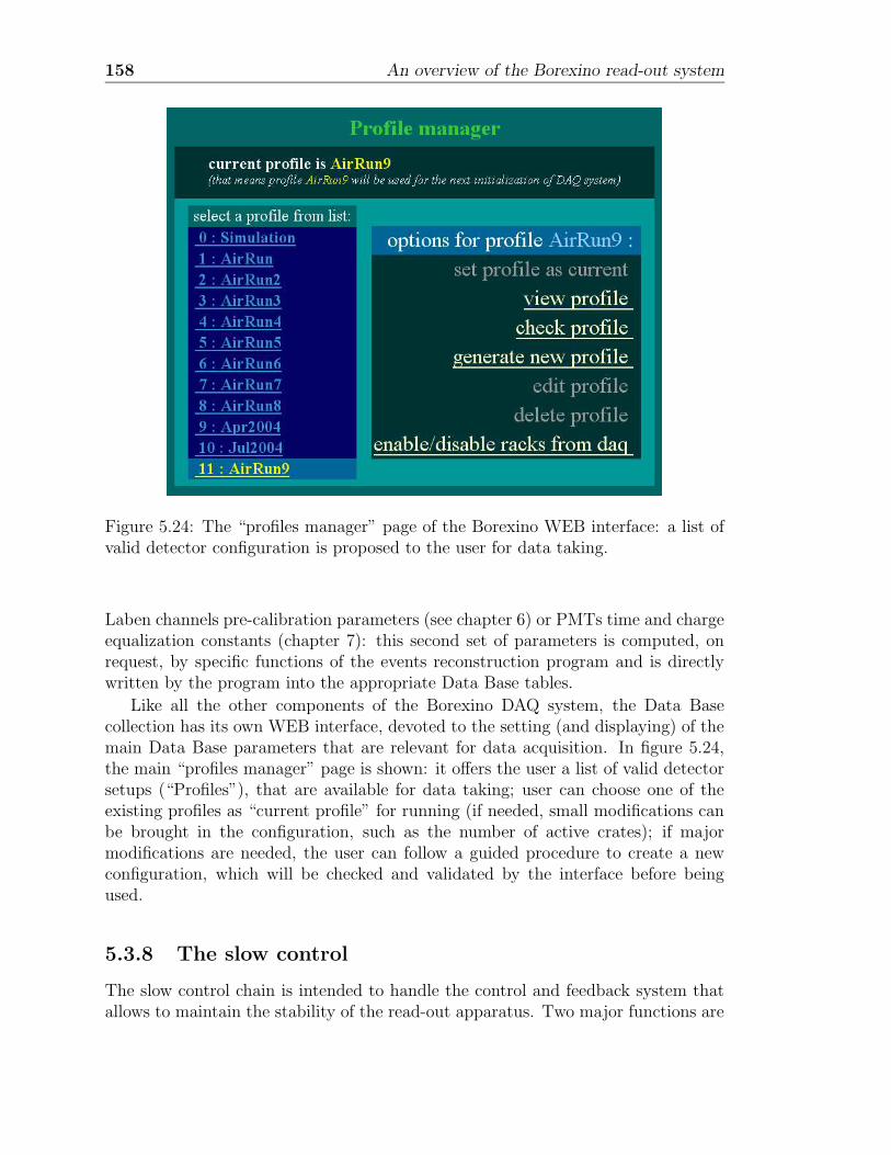
158 An overview of the Borexino read-out system
Figure 5.24: The “profiles manager” page of the Borexino WEB interface: a list ofvalid detector configuration is proposed to the user for data taking.
Laben channels pre-calibration parameters (see chapter 6) or PMTs time and chargeequalization constants (chapter 7): this second set of parameters is computed, onrequest, by specific functions of the events reconstruction program and is directlywritten by the program into the appropriate Data Base tables.
Like all the other components of the Borexino DAQ system, the Data Basecollection has its own WEB interface, devoted to the setting (and displaying) of themain Data Base parameters that are relevant for data acquisition. In figure 5.24,the main “profiles manager” page is shown: it offers the user a list of valid detectorsetups (“Profiles”), that are available for data taking; user can choose one of theexisting profiles as “current profile” for running (if needed, small modifications canbe brought in the configuration, such as the number of active crates); if majormodifications are needed, the user can follow a guided procedure to create a newconfiguration, which will be checked and validated by the interface before beingused.
5.3.8 The slow control
The slow control chain is intended to handle the control and feedback system thatallows to maintain the stability of the read-out apparatus. Two major functions are
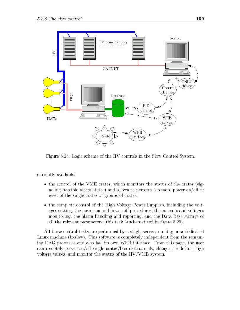
5.3.8 The slow control 159
Figure 5.25: Logic scheme of the HV controls in the Slow Control System.
currently available:
• the control of the VME crates, which monitors the status of the crates (sig-naling possible alarm states) and allows to perform a remote power-on/off orreset of the single crates or groups of crates;
• the complete control of the High Voltage Power Supplies, including the volt-ages setting, the power-on and power-off procedures, the currents and voltagesmonitoring, the alarm handling and reporting, and the Data Base storage ofall the relevant parameters (this task is schematized in figure 5.25).
All these control tasks are performed by a single server, running on a dedicatedLinux machine (bxslow). This software is completely independent from the remain-ing DAQ processes and also has its own WEB interface. From this page, the usercan remotely power on/off single crates/boards/channels, change the default highvoltage values, and monitor the status of the HV/VME system.

Chapter 6
Tests of the Borexino read-outsystem
In the period from February 2002 to August 2004, the Borexino detector underwentmany global tests of its read-out system. These tests are operated in the form of“Air-Runs”; an Air-Run consists in a real run of the detector, with all PMTs onand the electronics and DAQ chain enabled. They are called Air-Runs because theBorexino detector is not yet filled with water or scintillator. The complete list ofBorexino Air-Runs is reported in table 6.1.
The main purposes of these tests are:
• check of the general status of the photomultipliers and of the HV power sup-plies; if needed, fine tuning of the working conditions of the single PMT;
• test of the electronics status, with the complete event read-out chain: Front-End and digital modules are tested, but also sums system (see chapter 8); thiswill result in a general improvement of the electronics performances, as wellas in the fine debugging of single boards or channels;
• set-up and finalization of the trigger system, allowing the possibility of differenttrigger configurations (dark noise runs, laser runs, etc.; details are given insection 5.2.4);
• complete test of the on-line software, including the main DAQ system, theOn-line Monitor, the Slow Control, the Data Base collection, etc. (the systemis described in section 5.3);
• finalization and test of the PMT laser calibration apparatus (see chapter 7);
• check and improvement of many components of the events reconstruction pro-gram (splitting algorithm, position reconstruction software, etc.).
Four types of measurement have been performed:
161
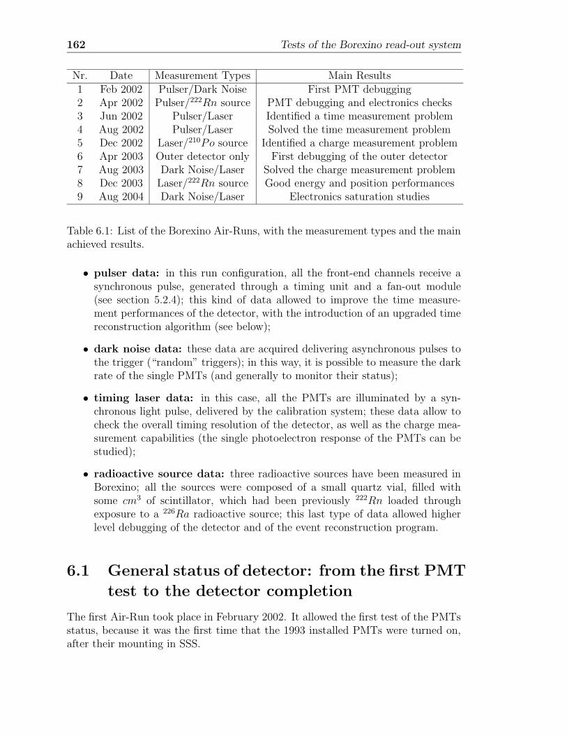
162 Tests of the Borexino read-out system
Nr. Date Measurement Types Main Results1 Feb 2002 Pulser/Dark Noise First PMT debugging2 Apr 2002 Pulser/222Rn source PMT debugging and electronics checks3 Jun 2002 Pulser/Laser Identified a time measurement problem4 Aug 2002 Pulser/Laser Solved the time measurement problem5 Dec 2002 Laser/210Po source Identified a charge measurement problem6 Apr 2003 Outer detector only First debugging of the outer detector7 Aug 2003 Dark Noise/Laser Solved the charge measurement problem8 Dec 2003 Laser/222Rn source Good energy and position performances9 Aug 2004 Dark Noise/Laser Electronics saturation studies
Table 6.1: List of the Borexino Air-Runs, with the measurement types and the mainachieved results.
• pulser data: in this run configuration, all the front-end channels receive asynchronous pulse, generated through a timing unit and a fan-out module(see section 5.2.4); this kind of data allowed to improve the time measure-ment performances of the detector, with the introduction of an upgraded timereconstruction algorithm (see below);
• dark noise data: these data are acquired delivering asynchronous pulses tothe trigger (“random” triggers); in this way, it is possible to measure the darkrate of the single PMTs (and generally to monitor their status);
• timing laser data: in this case, all the PMTs are illuminated by a syn-chronous light pulse, delivered by the calibration system; these data allow tocheck the overall timing resolution of the detector, as well as the charge mea-surement capabilities (the single photoelectron response of the PMTs can bestudied);
• radioactive source data: three radioactive sources have been measured inBorexino; all the sources were composed of a small quartz vial, filled withsome cm3 of scintillator, which had been previously 222Rn loaded throughexposure to a 226Ra radioactive source; this last type of data allowed higherlevel debugging of the detector and of the event reconstruction program.
6.1 General status of detector: from the first PMT
test to the detector completion
The first Air-Run took place in February 2002. It allowed the first test of the PMTsstatus, because it was the first time that the 1993 installed PMTs were turned on,after their mounting in SSS.
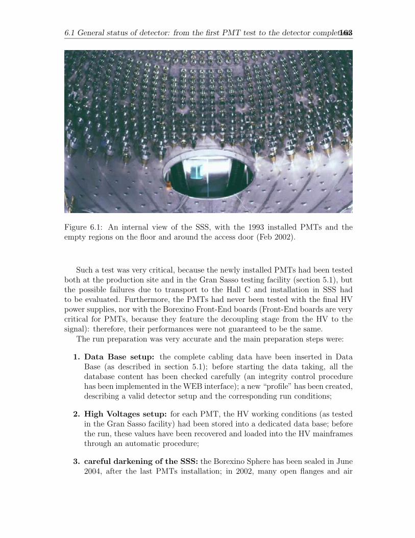
6.1 General status of detector: from the first PMT test to the detector completion163
Figure 6.1: An internal view of the SSS, with the 1993 installed PMTs and theempty regions on the floor and around the access door (Feb 2002).
Such a test was very critical, because the newly installed PMTs had been testedboth at the production site and in the Gran Sasso testing facility (section 5.1), butthe possible failures due to transport to the Hall C and installation in SSS hadto be evaluated. Furthermore, the PMTs had never been tested with the final HVpower supplies, nor with the Borexino Front-End boards (Front-End boards are verycritical for PMTs, because they feature the decoupling stage from the HV to thesignal): therefore, their performances were not guaranteed to be the same.
The run preparation was very accurate and the main preparation steps were:
1. Data Base setup: the complete cabling data have been inserted in DataBase (as described in section 5.1); before starting the data taking, all thedatabase content has been checked carefully (an integrity control procedurehas been implemented in the WEB interface); a new “profile” has been created,describing a valid detector setup and the corresponding run conditions;
2. High Voltages setup: for each PMT, the HV working conditions (as testedin the Gran Sasso facility) had been stored into a dedicated data base; beforethe run, these values have been recovered and loaded into the HV mainframesthrough an automatic procedure;
3. careful darkening of the SSS: the Borexino Sphere has been sealed in June2004, after the last PMTs installation; in 2002, many open flanges and air
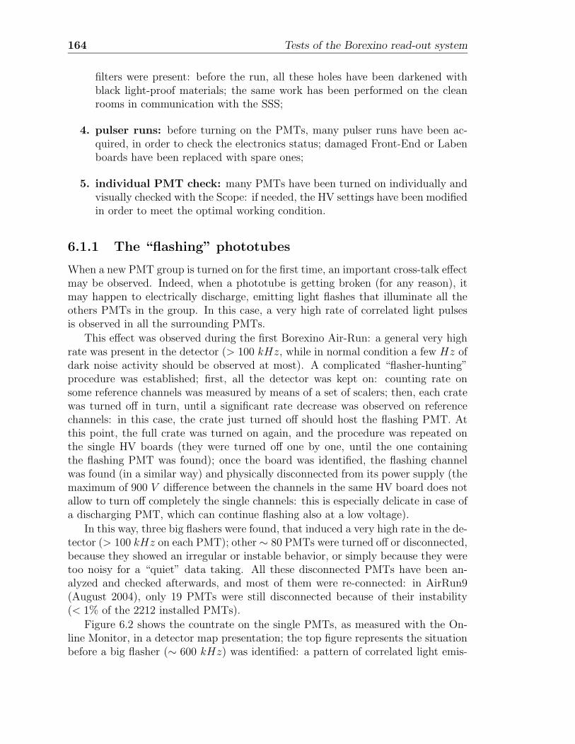
164 Tests of the Borexino read-out system
filters were present: before the run, all these holes have been darkened withblack light-proof materials; the same work has been performed on the cleanrooms in communication with the SSS;
4. pulser runs: before turning on the PMTs, many pulser runs have been ac-quired, in order to check the electronics status; damaged Front-End or Labenboards have been replaced with spare ones;
5. individual PMT check: many PMTs have been turned on individually andvisually checked with the Scope: if needed, the HV settings have been modifiedin order to meet the optimal working condition.
6.1.1 The “flashing” phototubes
When a new PMT group is turned on for the first time, an important cross-talk effectmay be observed. Indeed, when a phototube is getting broken (for any reason), itmay happen to electrically discharge, emitting light flashes that illuminate all theothers PMTs in the group. In this case, a very high rate of correlated light pulsesis observed in all the surrounding PMTs.
This effect was observed during the first Borexino Air-Run: a general very highrate was present in the detector (> 100 kHz, while in normal condition a few Hz ofdark noise activity should be observed at most). A complicated “flasher-hunting”procedure was established; first, all the detector was kept on: counting rate onsome reference channels was measured by means of a set of scalers; then, each cratewas turned off in turn, until a significant rate decrease was observed on referencechannels: in this case, the crate just turned off should host the flashing PMT. Atthis point, the full crate was turned on again, and the procedure was repeated onthe single HV boards (they were turned off one by one, until the one containingthe flashing PMT was found); once the board was identified, the flashing channelwas found (in a similar way) and physically disconnected from its power supply (themaximum of 900 V difference between the channels in the same HV board does notallow to turn off completely the single channels: this is especially delicate in case ofa discharging PMT, which can continue flashing also at a low voltage).
In this way, three big flashers were found, that induced a very high rate in the de-tector (> 100 kHz on each PMT); other ∼ 80 PMTs were turned off or disconnected,because they showed an irregular or instable behavior, or simply because they weretoo noisy for a “quiet” data taking. All these disconnected PMTs have been an-alyzed and checked afterwards, and most of them were re-connected: in AirRun9(August 2004), only 19 PMTs were still disconnected because of their instability(< 1% of the 2212 installed PMTs).
Figure 6.2 shows the countrate on the single PMTs, as measured with the On-line Monitor, in a detector map presentation; the top figure represents the situationbefore a big flasher (∼ 600 kHz) was identified: a pattern of correlated light emis-
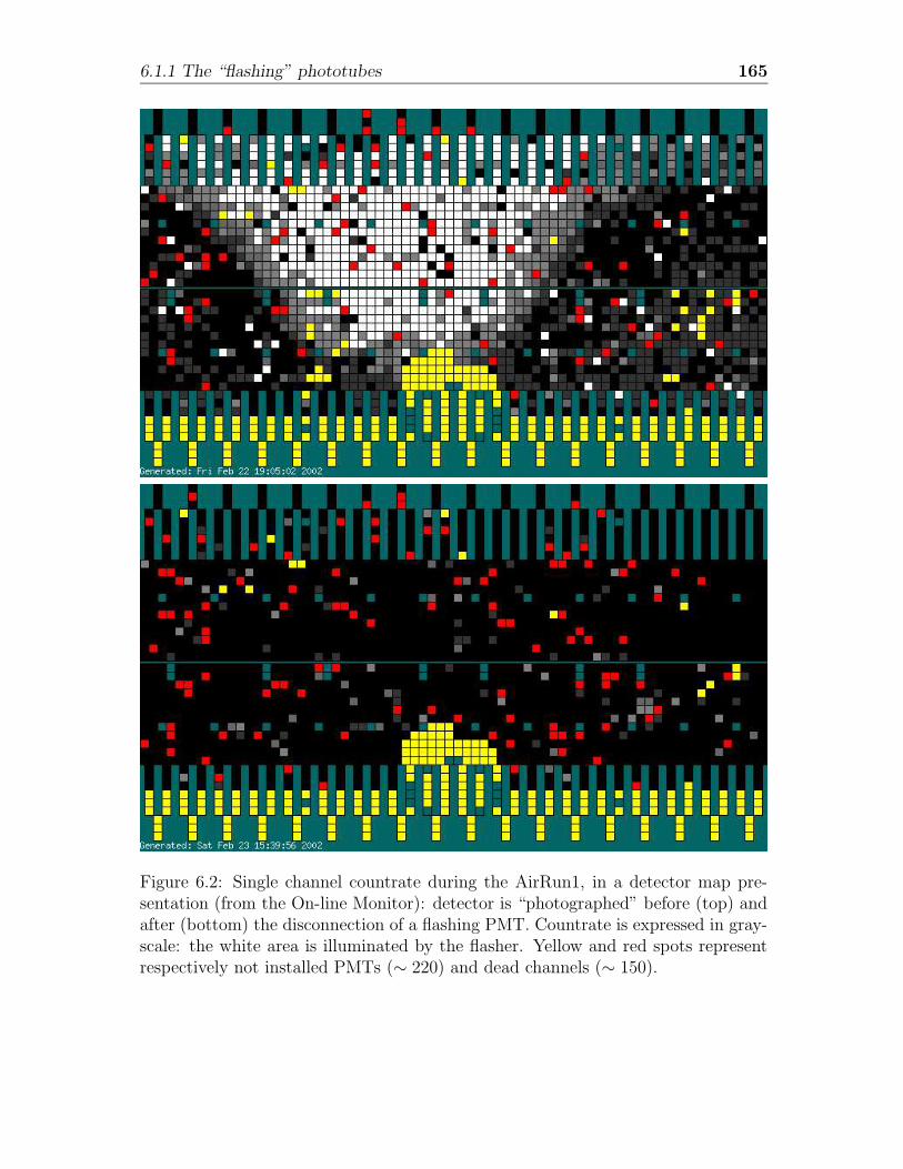
6.1.1 The “flashing” phototubes 165
Figure 6.2: Single channel countrate during the AirRun1, in a detector map pre-sentation (from the On-line Monitor): detector is “photographed” before (top) andafter (bottom) the disconnection of a flashing PMT. Countrate is expressed in gray-scale: the white area is illuminated by the flasher. Yellow and red spots representrespectively not installed PMTs (∼ 220) and dead channels (∼ 150).
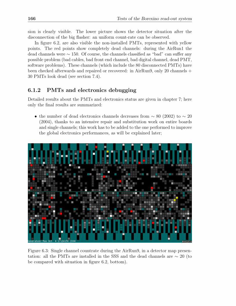
166 Tests of the Borexino read-out system
sion is clearly visible. The lower picture shows the detector situation after thedisconnection of the big flasher: an uniform count-rate can be observed.
In figure 6.2, are also visible the non-installed PMTs, represented with yellowpoints. The red points show completely dead channels: during the AirRun1 thedead channels were ∼ 150. Of course, the channels classified as “bad” can suffer anypossible problem (bad cables, bad front end channel, bad digital channel, dead PMT,software problems). These channels (which include the 80 disconnected PMTs) havebeen checked afterwards and repaired or recovered: in AirRun9, only 20 channels +30 PMTs look dead (see section 7.4).
6.1.2 PMTs and electronics debugging
Detailed results about the PMTs and electronics status are given in chapter 7; hereonly the final results are summarized:
• the number of dead electronics channels decreases from ∼ 80 (2002) to ∼ 20(2004), thanks to an intensive repair and substitution work on entire boardsand single channels; this work has to be added to the one performed to improvethe global electronics performances, as will be explained later;
Figure 6.3: Single channel countrate during the AirRun9, in a detector map presen-tation: all the PMTs are installed in the SSS and the dead channels are ∼ 20 (tobe compared with situation in figure 6.2, bottom).
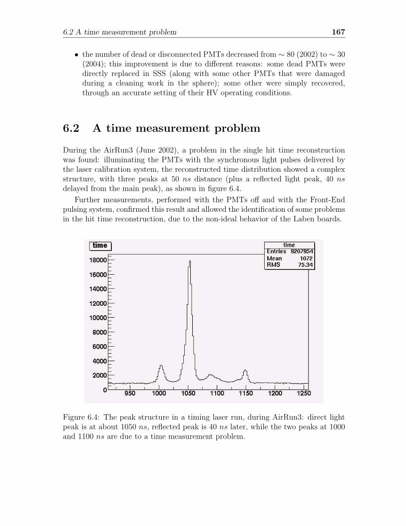
6.2 A time measurement problem 167
• the number of dead or disconnected PMTs decreased from ∼ 80 (2002) to ∼ 30(2004); this improvement is due to different reasons: some dead PMTs weredirectly replaced in SSS (along with some other PMTs that were damagedduring a cleaning work in the sphere); some other were simply recovered,through an accurate setting of their HV operating conditions.
6.2 A time measurement problem
During the AirRun3 (June 2002), a problem in the single hit time reconstructionwas found: illuminating the PMTs with the synchronous light pulses delivered bythe laser calibration system, the reconstructed time distribution showed a complexstructure, with three peaks at 50 ns distance (plus a reflected light peak, 40 nsdelayed from the main peak), as shown in figure 6.4.
Further measurements, performed with the PMTs off and with the Front-Endpulsing system, confirmed this result and allowed the identification of some problemsin the hit time reconstruction, due to the non-ideal behavior of the Laben boards.
Figure 6.4: The peak structure in a timing laser run, during AirRun3: direct lightpeak is at about 1050 ns, reflected peak is 40 ns later, while the two peaks at 1000and 1100 ns are due to a time measurement problem.
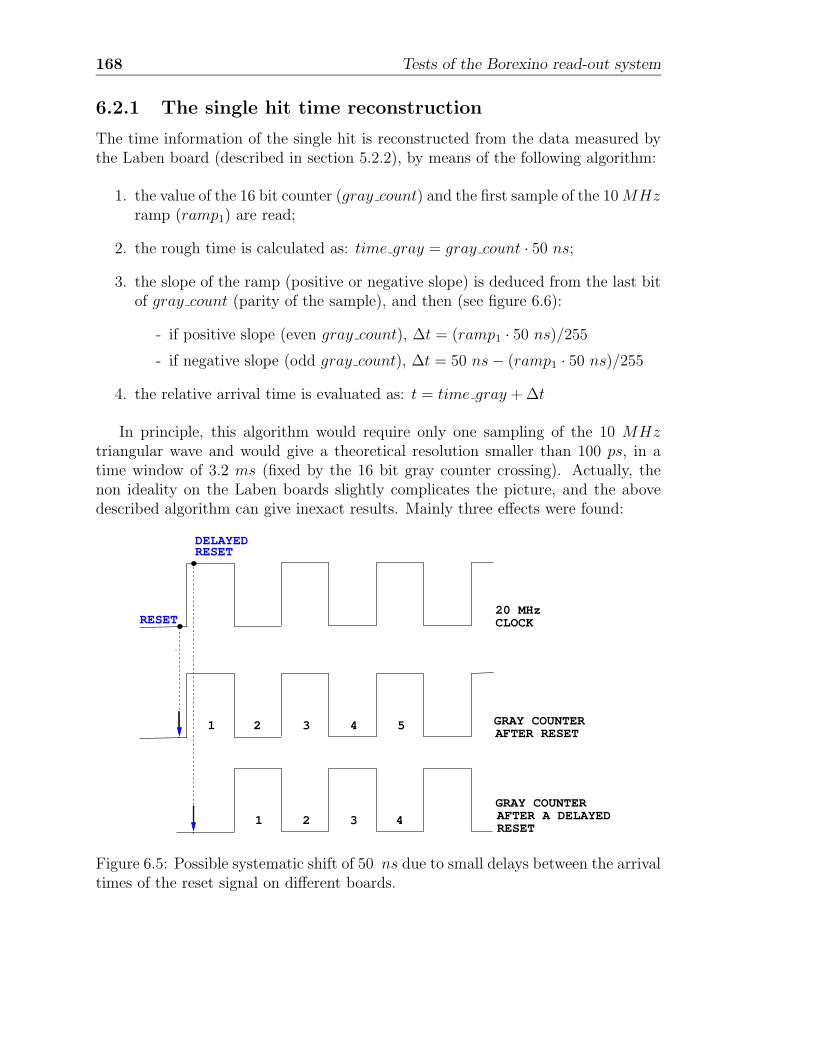
168 Tests of the Borexino read-out system
6.2.1 The single hit time reconstruction
The time information of the single hit is reconstructed from the data measured bythe Laben board (described in section 5.2.2), by means of the following algorithm:
1. the value of the 16 bit counter (gray count) and the first sample of the 10MHzramp (ramp1) are read;
2. the rough time is calculated as: time gray = gray count · 50 ns;
3. the slope of the ramp (positive or negative slope) is deduced from the last bitof gray count (parity of the sample), and then (see figure 6.6):
- if positive slope (even gray count), ∆t = (ramp1 · 50 ns)/255- if negative slope (odd gray count), ∆t = 50 ns− (ramp1 · 50 ns)/255
4. the relative arrival time is evaluated as: t = time gray +∆t
In principle, this algorithm would require only one sampling of the 10 MHztriangular wave and would give a theoretical resolution smaller than 100 ps, in atime window of 3.2 ms (fixed by the 16 bit gray counter crossing). Actually, thenon ideality on the Laben boards slightly complicates the picture, and the abovedescribed algorithm can give inexact results. Mainly three effects were found:
CLOCK20 MHz
AFTER RESETGRAY COUNTER1 2 3 54
1 2 3 4RESETAFTER A DELAYEDGRAY COUNTER
RESET
RESETDELAYED
Figure 6.5: Possible systematic shift of 50 ns due to small delays between the arrivaltimes of the reset signal on different boards.
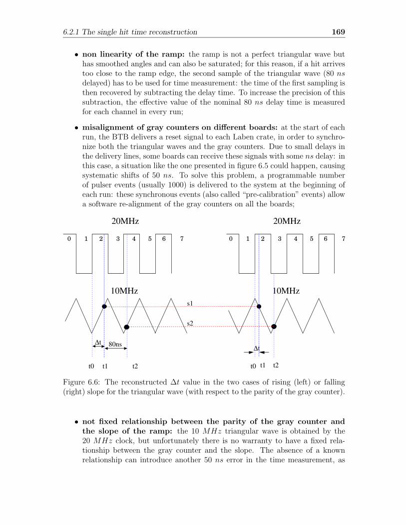
6.2.1 The single hit time reconstruction 169
• non linearity of the ramp: the ramp is not a perfect triangular wave buthas smoothed angles and can also be saturated; for this reason, if a hit arrivestoo close to the ramp edge, the second sample of the triangular wave (80 nsdelayed) has to be used for time measurement: the time of the first sampling isthen recovered by subtracting the delay time. To increase the precision of thissubtraction, the effective value of the nominal 80 ns delay time is measuredfor each channel in every run;
• misalignment of gray counters on different boards: at the start of eachrun, the BTB delivers a reset signal to each Laben crate, in order to synchro-nize both the triangular waves and the gray counters. Due to small delays inthe delivery lines, some boards can receive these signals with some ns delay: inthis case, a situation like the one presented in figure 6.5 could happen, causingsystematic shifts of 50 ns. To solve this problem, a programmable numberof pulser events (usually 1000) is delivered to the system at the beginning ofeach run: these synchronous events (also called “pre-calibration” events) allowa software re-alignment of the gray counters on all the boards;
0 1 2 3 4 5 6 7 0 1 2 3 4 5 6 7
∆t∆t80ns
t2t1t0
10MHz
20MHz
t0
20MHz
10MHz
t1 t2
s2
s1
Figure 6.6: The reconstructed ∆t value in the two cases of rising (left) or falling(right) slope for the triangular wave (with respect to the parity of the gray counter).
• not fixed relationship between the parity of the gray counter andthe slope of the ramp: the 10 MHz triangular wave is obtained by the20 MHz clock, but unfortunately there is no warranty to have a fixed rela-tionship between the gray counter and the slope. The absence of a knownrelationship can introduce another 50 ns error in the time measurement, as
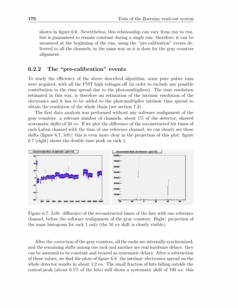
170 Tests of the Borexino read-out system
shown in figure 6.6. Nevertheless, this relationship can vary from run to run,but is guaranteed to remain constant during a single run: therefore, it can bemeasured at the beginning of the run, using the “pre-calibration” events de-livered to all the channels, in the same way as it is done for the gray countersalignment.
6.2.2 The “pre-calibration” events
To study the efficiency of the above described algorithm, some pure pulser runswere acquired, with all the PMT high voltages off (in order to exclude any possiblecontribution to the time spread due to the photomultipliers). The time resolutionestimated in this way, is therefore an estimation of the intrinsic resolution of theelectronics and it has to be added to the photomultiplier intrinsic time spread toobtain the resolution of the whole chain (see section 7.3).
The first data analysis was performed without any software realignment of thegray counters: a relevant number of channels, about 1% of the detector, showedsystematic shifts of 50 ns. If we plot the difference of the reconstructed hit times ofeach Laben channel with the time of one reference channel, we can clearly see theseshifts (figure 6.7, left); this is even more clear in the projection of this plot: figure6.7 (right) shows the double time peak on rack 1.
Figure 6.7: Left: difference of the reconstructed times of the hits with one referencechannel, before the software realignment of the gray counters. Right: projection ofthe same histogram for rack 1 only (the 50 ns shift is clearly visible).
After the correction of the gray counters, all the racks are internally synchronized,and the remaining shifts among one rack and another are real hardware delays: theycan be assumed to be constant and treated as systematic delays. After a subtractionof these values, we find the plots of figure 6.8: the intrinsic electronics spread on thewhole detector results in about 1.2 ns. The small fraction of hits falling outside thecentral peak (about 0.1% of the hits) still shows a systematic shift of 100 ns: this
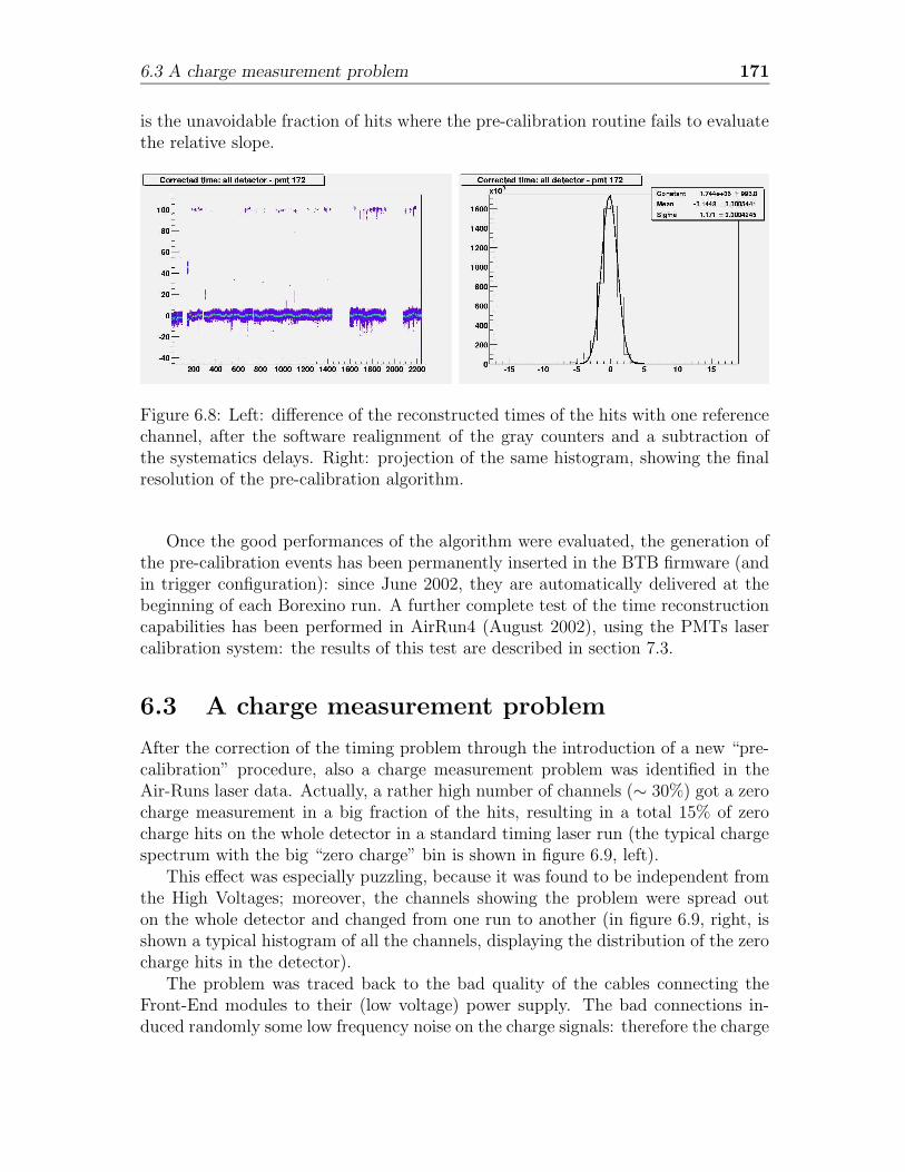
6.3 A charge measurement problem 171
is the unavoidable fraction of hits where the pre-calibration routine fails to evaluatethe relative slope.
Figure 6.8: Left: difference of the reconstructed times of the hits with one referencechannel, after the software realignment of the gray counters and a subtraction ofthe systematics delays. Right: projection of the same histogram, showing the finalresolution of the pre-calibration algorithm.
Once the good performances of the algorithm were evaluated, the generation ofthe pre-calibration events has been permanently inserted in the BTB firmware (andin trigger configuration): since June 2002, they are automatically delivered at thebeginning of each Borexino run. A further complete test of the time reconstructioncapabilities has been performed in AirRun4 (August 2002), using the PMTs lasercalibration system: the results of this test are described in section 7.3.
6.3 A charge measurement problem
After the correction of the timing problem through the introduction of a new “pre-calibration” procedure, also a charge measurement problem was identified in theAir-Runs laser data. Actually, a rather high number of channels (∼ 30%) got a zerocharge measurement in a big fraction of the hits, resulting in a total 15% of zerocharge hits on the whole detector in a standard timing laser run (the typical chargespectrum with the big “zero charge” bin is shown in figure 6.9, left).
This effect was especially puzzling, because it was found to be independent fromthe High Voltages; moreover, the channels showing the problem were spread outon the whole detector and changed from one run to another (in figure 6.9, right, isshown a typical histogram of all the channels, displaying the distribution of the zerocharge hits in the detector).
The problem was traced back to the bad quality of the cables connecting theFront-End modules to their (low voltage) power supply. The bad connections in-duced randomly some low frequency noise on the charge signals: therefore the charge
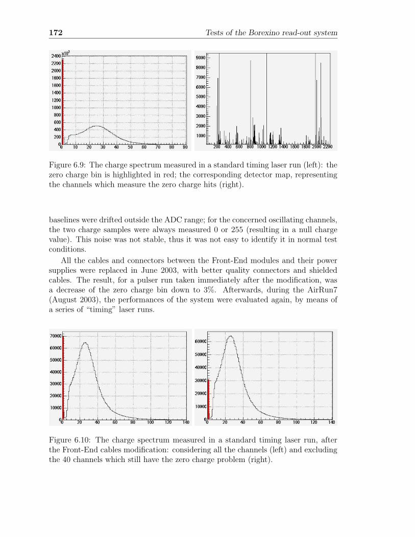
172 Tests of the Borexino read-out system
Figure 6.9: The charge spectrum measured in a standard timing laser run (left): thezero charge bin is highlighted in red; the corresponding detector map, representingthe channels which measure the zero charge hits (right).
baselines were drifted outside the ADC range; for the concerned oscillating channels,the two charge samples were always measured 0 or 255 (resulting in a null chargevalue). This noise was not stable, thus it was not easy to identify it in normal testconditions.
All the cables and connectors between the Front-End modules and their powersupplies were replaced in June 2003, with better quality connectors and shieldedcables. The result, for a pulser run taken immediately after the modification, wasa decrease of the zero charge bin down to 3%. Afterwards, during the AirRun7(August 2003), the performances of the system were evaluated again, by means ofa series of “timing” laser runs.
Figure 6.10: The charge spectrum measured in a standard timing laser run, afterthe Front-End cables modification: considering all the channels (left) and excludingthe 40 channels which still have the zero charge problem (right).
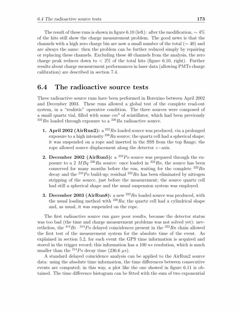
6.4 The radioactive source tests 173
The result of these runs is shown in figure 6.10 (left): after the modification, ∼ 4%of the hits still show the charge measurement problem. The good news is that thechannels with a high zero charge bin are now a small number of the total (∼ 40) andare always the same: then the problem can be further reduced simply by repairingor replacing these channels. Excluding these 40 channels from the analysis, the zerocharge peak reduces down to < 2% of the total hits (figure 6.10, right). Furtherresults about charge measurement performances in laser data (allowing PMTs chargecalibration) are described in section 7.4.
6.4 The radioactive source tests
Three radioactive source runs have been performed in Borexino between April 2002and December 2003. These runs allowed a global test of the complete read-outsystem, in a “realistic” operative condition. The three sources were composed ofa small quartz vial, filled with some cm3 of scintillator, which had been previously222Rn loaded through exposure to a 226Ra radioactive source.
1. April 2002 (AirRun2): a 222Rn loaded source was produced, via a prolongedexposure to a high intensity 226Ra source; the quartz cell had a spherical shape;it was suspended on a rope and inserted in the SSS from the top flange; therope allowed source displacement along the detector z−axis.
2. December 2002 (AirRun5): a 210Po source was prepared through the ex-posure to a 2 MBq 226Ra source: once loaded in 222Rn, the source has beenconserved for many months before the run, waiting for the complete 222Rndecay and the 210Po build-up; residual 222Rn has been eliminated by nitrogenstripping of the source, just before the measurement; the source quartz cellhad still a spherical shape and the usual suspension system was employed.
3. December 2003 (AirRun8): a new 222Rn loaded source was produced, withthe usual loading method with 226Ra; the quartz cell had a cylindrical shapeand, as usual, it was suspended on the rope.
The first radioactive source run gave poor results, because the detector statuswas too bad (the time and charge measurement problems was not solved yet): nev-ertheless, the 214Bi –214Po delayed coincidences present in the 222Rn chain allowedthe first test of the measurement system for the absolute time of the event. Asexplained in section 5.2, for each event the GPS time information is acquired andstored in the trigger record; this information has a 100 ns resolution, which is muchsmaller than the 214Po decay time (236.6 µs).
A standard delayed coincidence analysis can be applied to the AirRun2 sourcedata: using the absolute time information, the time differences between consecutiveevents are computed; in this way, a plot like the one showed in figure 6.11 is ob-tained. The time difference histogram can be fitted with the sum of two exponential
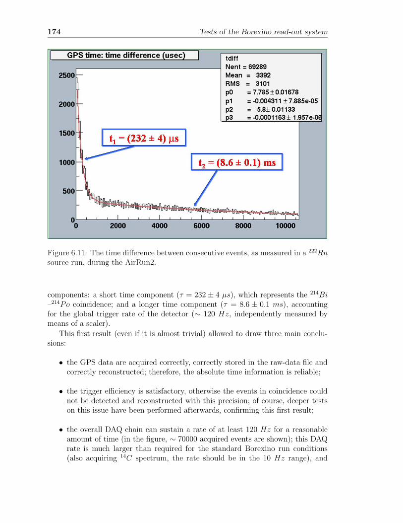
174 Tests of the Borexino read-out system
Figure 6.11: The time difference between consecutive events, as measured in a 222Rnsource run, during the AirRun2.
components: a short time component (τ = 232± 4 µs), which represents the 214Bi–214Po coincidence; and a longer time component (τ = 8.6 ± 0.1 ms), accountingfor the global trigger rate of the detector (∼ 120 Hz, independently measured bymeans of a scaler).
This first result (even if it is almost trivial) allowed to draw three main conclu-sions:
• the GPS data are acquired correctly, correctly stored in the raw-data file andcorrectly reconstructed; therefore, the absolute time information is reliable;
• the trigger efficiency is satisfactory, otherwise the events in coincidence couldnot be detected and reconstructed with this precision; of course, deeper testson this issue have been performed afterwards, confirming this first result;
• the overall DAQ chain can sustain a rate of at least 120 Hz for a reasonableamount of time (in the figure, ∼ 70000 acquired events are shown); this DAQrate is much larger than required for the standard Borexino run conditions(also acquiring 14C spectrum, the rate should be in the 10 Hz range), and
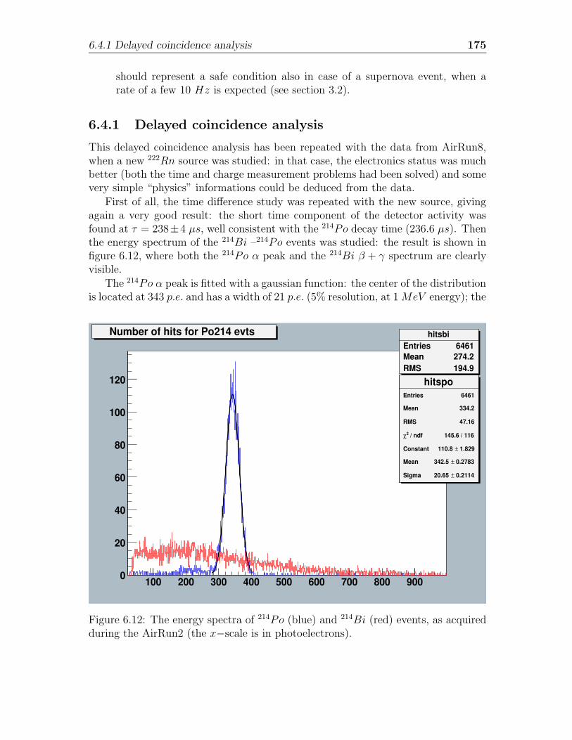
6.4.1 Delayed coincidence analysis 175
should represent a safe condition also in case of a supernova event, when arate of a few 10 Hz is expected (see section 3.2).
6.4.1 Delayed coincidence analysis
This delayed coincidence analysis has been repeated with the data from AirRun8,when a new 222Rn source was studied: in that case, the electronics status was muchbetter (both the time and charge measurement problems had been solved) and somevery simple “physics” informations could be deduced from the data.
First of all, the time difference study was repeated with the new source, givingagain a very good result: the short time component of the detector activity wasfound at τ = 238±4 µs, well consistent with the 214Po decay time (236.6 µs). Thenthe energy spectrum of the 214Bi –214Po events was studied: the result is shown infigure 6.12, where both the 214Po α peak and the 214Bi β + γ spectrum are clearlyvisible.
The 214Po α peak is fitted with a gaussian function: the center of the distributionis located at 343 p.e. and has a width of 21 p.e. (5% resolution, at 1MeV energy); the
hitspoEntries 6461
Mean 334.2
RMS 47.16
/ ndf 2χ 145.6 / 116
Constant 1.829± 110.8
Mean 0.2783± 342.5
Sigma 0.2114± 20.65
100 200 300 400 500 600 700 800 9000
20
40
60
80
100
120 hitspoEntries 6461
Mean 334.2
RMS 47.16
/ ndf 2χ 145.6 / 116
Constant 1.829± 110.8
Mean 0.2783± 342.5
Sigma 0.2114± 20.65
Number of hits for Po214 evts hitsbiEntries 6461Mean 274.2RMS 194.9
Figure 6.12: The energy spectra of 214Po (blue) and 214Bi (red) events, as acquiredduring the AirRun2 (the x−scale is in photoelectrons).
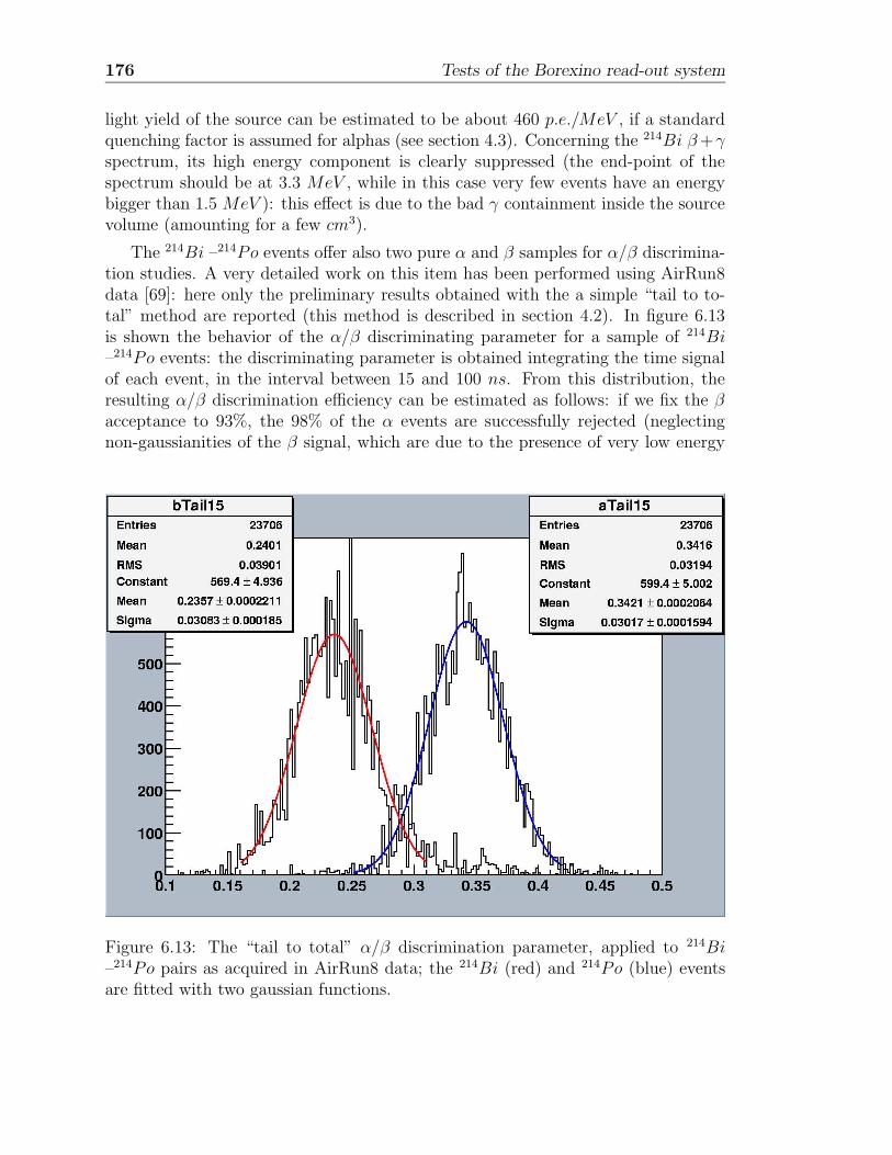
176 Tests of the Borexino read-out system
light yield of the source can be estimated to be about 460 p.e./MeV , if a standardquenching factor is assumed for alphas (see section 4.3). Concerning the 214Bi β+γspectrum, its high energy component is clearly suppressed (the end-point of thespectrum should be at 3.3 MeV , while in this case very few events have an energybigger than 1.5 MeV ): this effect is due to the bad γ containment inside the sourcevolume (amounting for a few cm3).
The 214Bi –214Po events offer also two pure α and β samples for α/β discrimina-tion studies. A very detailed work on this item has been performed using AirRun8data [69]: here only the preliminary results obtained with the a simple “tail to to-tal” method are reported (this method is described in section 4.2). In figure 6.13is shown the behavior of the α/β discriminating parameter for a sample of 214Bi–214Po events: the discriminating parameter is obtained integrating the time signalof each event, in the interval between 15 and 100 ns. From this distribution, theresulting α/β discrimination efficiency can be estimated as follows: if we fix the βacceptance to 93%, the 98% of the α events are successfully rejected (neglectingnon-gaussianities of the β signal, which are due to the presence of very low energy
Figure 6.13: The “tail to total” α/β discrimination parameter, applied to 214Bi–214Po pairs as acquired in AirRun8 data; the 214Bi (red) and 214Po (blue) eventsare fitted with two gaussian functions.
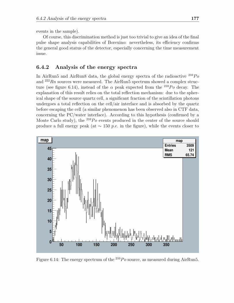
6.4.2 Analysis of the energy spectra 177
events in the sample).Of course, this discrimination method is just too trivial to give an idea of the final
pulse shape analysis capabilities of Borexino: nevertheless, its efficiency confirmsthe general good status of the detector, especially concerning the time measurementissue.
6.4.2 Analysis of the energy spectra
In AirRun5 and AirRun8 data, the global energy spectra of the radioactive 210Poand 222Rn sources were measured. The AirRun5 spectrum showed a complex struc-ture (see figure 6.14), instead of the α peak expected from the 210Po decay. Theexplanation of this result relies on the total reflection mechanism: due to the spher-ical shape of the source quartz cell, a significant fraction of the scintillation photonsundergoes a total reflection on the cell/air interface and is absorbed by the quartzbefore escaping the cell (a similar phenomenon has been observed also in CTF data,concerning the PC/water interface). According to this hypothesis (confirmed by aMonte Carlo study), the 210Po events produced in the center of the source shouldproduce a full energy peak (at ∼ 150 p.e. in the figure), while the events closer to
mapEntries 3509Mean 121RMS 65.74
50 100 150 200 250 300 3500
5
10
15
20
25
30
35
40
45
mapEntries 3509Mean 121RMS 65.74
map
Figure 6.14: The energy spectrum of the 210Po source, as measured during AirRun5.
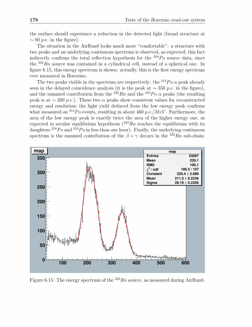
178 Tests of the Borexino read-out system
the surface should experience a reduction in the detected light (broad structure at∼ 80 p.e. in the figure).
The situation in the AirRun8 looks much more “comfortable”: a structure withtwo peaks and an underlying continuous spectrum is observed, as expected; this factindirectly confirms the total reflection hypothesis for the 210Po source data, sincethe 222Rn source was contained in a cylindrical cell, instead of a spherical one. Infigure 6.15, this energy spectrum is shown: actually, this is the first energy spectrumever measured in Borexino.
The two peaks visible in the spectrum are respectively: the 214Po α peak alreadyseen in the delayed coincidence analysis (it is the peak at ∼ 350 p.e. in the figure),and the summed contribution from the 222Rn and the 218Po α peaks (the resultingpeak is at ∼ 200 p.e.). These two α peaks show consistent values for reconstructedenergy and resolution; the light yield deduced from the low energy peak confirmswhat measured on 214Po events, resulting in about 460 p.e./MeV . Furthermore, thearea of the low energy peak is exactly twice the area of the higher energy one, asexpected in secular equilibrium hypothesis (222Rn reaches the equilibrium with itsdaughters 218Po and 214Po in less than one hour). Finally, the underlying continuousspectrum is the summed contribution of the β + γ decays in the 222Rn sub-chain:
mapEntries 43097Mean 229.1RMS 100.1
/ ndf 2χ 186.5 / 107Constant 2.886± 320.4 Mean 0.2236± 211.5 Sigma 0.2208± 28.19
100 200 300 400 500 6000
50
100
150
200
250
300
350map
Entries 43097Mean 229.1RMS 100.1
/ ndf 2χ 186.5 / 107Constant 2.886± 320.4 Mean 0.2236± 211.5 Sigma 0.2208± 28.19
map
Figure 6.15: The energy spectrum of the 222Rn source, as measured during AirRun8.
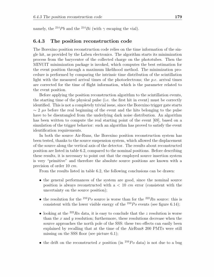
6.4.3 The position reconstruction code 179
namely, the 214Pb and the 214Bi (with γ escaping the vial).
6.4.3 The position reconstruction code
The Borexino position reconstruction code relies on the time information of the sin-gle hit, as provided by the Laben electronics. The algorithm starts its minimizationprocess from the barycenter of the collected charge on the phototubes. Then theMINUIT minimization package is invoked, which computes the best estimation forthe event position through a maximum likelihood method. The minimization pro-cedure is performed by comparing the intrinsic time distribution of the scintillationlight with the measured arrival times of the photoelectrons; the p.e. arrival timesare corrected for the time of flight information, which is the parameter related tothe event position.
Before applying the position reconstruction algorithm to the scintillation events,the starting time of the physical pulse (i.e. the first hit in event) must be correctlyidentified. This is not a completely trivial issue, since the Borexino trigger gate starts∼ 2 µs before the real beginning of the event and the hits belonging to the pulsehave to be disentangled from the underlying dark noise distribution. An algorithmhas been written to compute the real starting point of the event [69], based on asimulation of the trigger behavior: such an algorithm has proved to satisfy the eventidentification requirements.
In both the source Air-Runs, the Borexino position reconstruction system hasbeen tested, thanks to the source suspension system, which allowed the displacementof the source along the vertical axis of the detector. The results about reconstructedposition are listed in table 6.2, compared to the nominal positions. Before describingthese results, it is necessary to point out that the employed source insertion systemis very “primitive” and therefore the absolute source positions are known with aprecision of order 10 cm.
From the results listed in table 6.2, the following conclusions can be drawn:
• the general performances of the system are good, since the nominal sourceposition is always reconstructed with a < 10 cm error (consistent with theuncertainty on the source position);
• the resolution for the 210Po source is worse than for the 222Rn source: this isconsistent with the lower visible energy of the 210Po events (see figure 6.14);
• looking at the 222Rn data, it is easy to conclude that the z resolution is worsethan the x and y resolution; furthermore, these resolutions decrease when thesource approaches the north pole of the SSS: these two effects can easily beenexplained by recalling that at the time of the AirRun8 200 PMTs were stillmissing on the SSS floor (see picture 6.1);
• the drift on the reconstructed x position (in 210Po data) is not due to a bug
180 Tests of the Borexino read-out system
210Po source position x σx y σy z σz
x = 0; y = 0; z = 0 -1.7 25 2.6 16 8.4 25x = 0; y = 0; z = 100 4.6 20 5.0 13 93 29x = 0; y = 0; z = 200 -0.4 22 5.0 18 192 25222Rn source position x σx y σy z σz
x = 10; y = 0; z = 60 12 13 0.7 12 71 18x = 10; y = 0; z = z1 10 13 1.3 12 -21 15
x = 10; y = 0; z = z1 + 53 11 13 -1.6 12 24 16x = 10; y = 0; z = z1 + 153 12 13 2.3 13 112 20x = 10; y = 0; z = z1 + 253 13 14 1.0 14 219 22x = 10; y = 0; z = z1 + 403 14 16 -0.8 16 373 28
Table 6.2: Nominal and reconstructed positions, for the 210Po and 222Rn sources, asmeasured respectively in AirRun5 and in AirRun8. All numbers are quoted in cm.
in the program (or to a misalignment of the SSS axis), but to a real sourcedisplacement due to the rope movement;
• the x and y position resolutions, for events close to the SSS center, are in therange 12 ÷ 13 cm (without any cut on the energy of the events); with thecompleted detector, the z resolution should be of the same order.
Chapter 7
The PMT calibration system
A multiplexed system of optical fibers has been designed for the photomultipliercalibration of the Borexino detector. Both time and energy calibration are of capitalimportance in Borexino for the measurement of the solar 7Be neutrino flux.
Accuracy in the time measurement of the single hit infers the accuracy on po-sition reconstruction, which is required to define the Borexino Fiducial Volume;position resolution is limited by the scintillator fluorescence decay time of 3.5 ns(effectively increased to 5.5 ns after light propagation effects [6]), by the PMTtransit-time jitter of ∼ 1 ns and by the inter-PMT time equalization, which shouldbe maintained at sub-nanosecond level and regularly checked. The accuracy of thetime measurement is also crucial for α/β discrimination, based on the different flu-orescence time profiles for α and β scintillation events (see chapter 4). An accurateenergy determination and resolution are crucial for the spectral shape recognitionof the neutrino signal: the energy resolution of the detector depends on good PMTcharge calibration, the energy being determined, through a proportionality relation,from the number of detected photons.
The size of the detector, its tightness and radioactivity constraints require specialcare in the material selection and mechanical handling of the system. The solutionof multiplexed fiber chains has been realized for the first time in a large undergrounddetector.
7.1 System design
In the design of the calibration system for the time and charge response of theBorexino PMTs, the following requirements have been taken into account:
1. accuracy in time equalization: inter-PMT equalization inaccuracy should becontained within the PMT time jitter, which is ∼ 1 ns;
2. accuracy in charge calibration: the system must illuminate all 2212 PMTs atthe single photoelectron level in order to measure the Single Electron Response
181
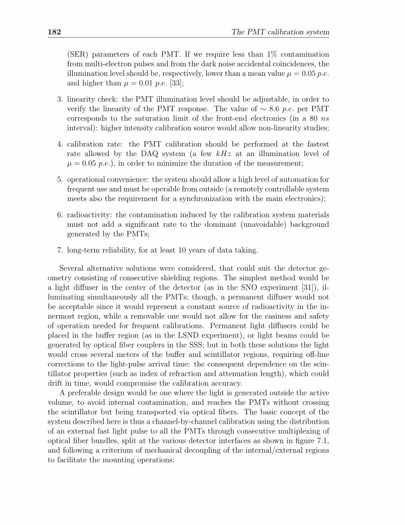
182 The PMT calibration system
(SER) parameters of each PMT. If we require less than 1% contaminationfrom multi-electron pulses and from the dark noise accidental coincidences, theillumination level should be, respectively, lower than a mean value µ = 0.05 p.e.and higher than µ = 0.01 p.e. [33];
3. linearity check: the PMT illumination level should be adjustable, in order toverify the linearity of the PMT response. The value of ∼ 8.6 p.e. per PMTcorresponds to the saturation limit of the front-end electronics (in a 80 nsinterval): higher intensity calibration source would allow non-linearity studies;
4. calibration rate: the PMT calibration should be performed at the fastestrate allowed by the DAQ system (a few kHz at an illumination level ofµ = 0.05 p.e.), in order to minimize the duration of the measurement;
5. operational convenience: the system should allow a high level of automation forfrequent use and must be operable from outside (a remotely controllable systemmeets also the requirement for a synchronization with the main electronics);
6. radioactivity: the contamination induced by the calibration system materialsmust not add a significant rate to the dominant (unavoidable) backgroundgenerated by the PMTs;
7. long-term reliability, for at least 10 years of data taking.
Several alternative solutions were considered, that could suit the detector ge-ometry consisting of consecutive shielding regions. The simplest method would bea light diffuser in the center of the detector (as in the SNO experiment [31]), il-luminating simultaneously all the PMTs; though, a permanent diffuser would notbe acceptable since it would represent a constant source of radioactivity in the in-nermost region, while a removable one would not allow for the easiness and safetyof operation needed for frequent calibrations. Permanent light diffusers could beplaced in the buffer region (as in the LSND experiment), or light beams could begenerated by optical fiber couplers in the SSS; but in both these solutions the lightwould cross several meters of the buffer and scintillator regions, requiring off-linecorrections to the light-pulse arrival time: the consequent dependence on the scin-tillator properties (such as index of refraction and attenuation length), which coulddrift in time, would compromise the calibration accuracy.
A preferable design would be one where the light is generated outside the activevolume, to avoid internal contamination, and reaches the PMTs without crossingthe scintillator but being transported via optical fibers. The basic concept of thesystem described here is thus a channel-by-channel calibration using the distributionof an external fast light pulse to all the PMTs through consecutive multiplexing ofoptical fiber bundles, split at the various detector interfaces as shown in figure 7.1,and following a criterium of mechanical decoupling of the internal/external regionsto facilitate the mounting operations:
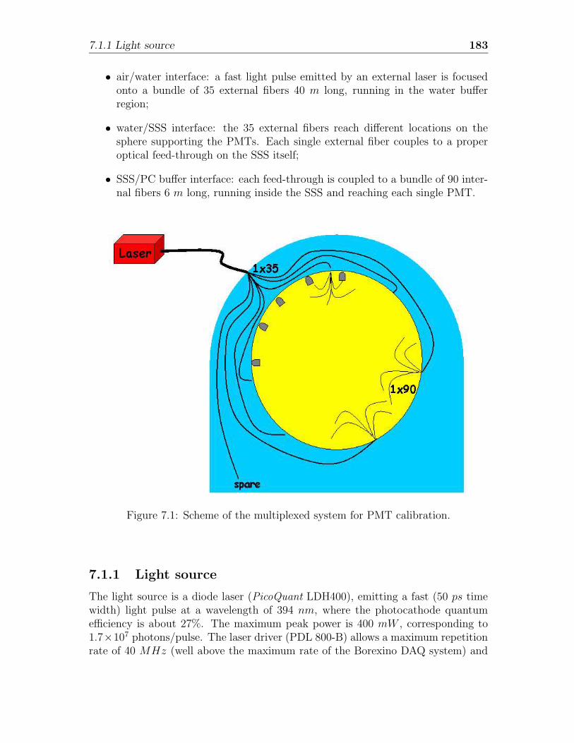
7.1.1 Light source 183
• air/water interface: a fast light pulse emitted by an external laser is focusedonto a bundle of 35 external fibers 40 m long, running in the water bufferregion;
• water/SSS interface: the 35 external fibers reach different locations on thesphere supporting the PMTs. Each single external fiber couples to a properoptical feed-through on the SSS itself;
• SSS/PC buffer interface: each feed-through is coupled to a bundle of 90 inter-nal fibers 6 m long, running inside the SSS and reaching each single PMT.
Figure 7.1: Scheme of the multiplexed system for PMT calibration.
7.1.1 Light source
The light source is a diode laser (PicoQuant LDH400), emitting a fast (50 ps timewidth) light pulse at a wavelength of 394 nm, where the photocathode quantumefficiency is about 27%. The maximum peak power is 400 mW , corresponding to1.7×107 photons/pulse. The laser driver (PDL 800-B) allows a maximum repetitionrate of 40 MHz (well above the maximum rate of the Borexino DAQ system) and
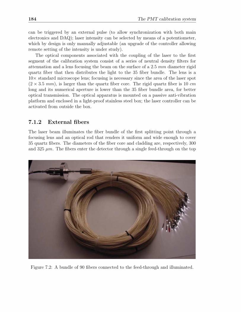
184 The PMT calibration system
can be triggered by an external pulse (to allow synchronization with both mainelectronics and DAQ); laser intensity can be selected by means of a potentiometer,which by design is only manually adjustable (an upgrade of the controller allowingremote setting of the intensity is under study).
The optical components associated with the coupling of the laser to the firstsegment of the calibration system consist of a series of neutral density filters forattenuation and a lens focusing the beam on the surface of a 2.5 mm diameter rigidquartz fiber that then distributes the light to the 35 fiber bundle. The lens is a10× standard microscope lens; focusing is necessary since the area of the laser spot(2 × 3.5 mm), is larger than the quartz fiber core. The rigid quartz fiber is 10 cmlong and its numerical aperture is lower than the 35 fiber bundle area, for betteroptical transmission. The optical apparatus is mounted on a passive anti-vibrationplatform and enclosed in a light-proof stainless steel box; the laser controller can beactivated from outside the box.
7.1.2 External fibers
The laser beam illuminates the fiber bundle of the first splitting point through afocusing lens and an optical rod that renders it uniform and wide enough to cover35 quartz fibers. The diameters of the fiber core and cladding are, respectively, 300and 325 µm. The fibers enter the detector through a single feed-through on the top
Figure 7.2: A bundle of 90 fibers connected to the feed-through and illuminated.
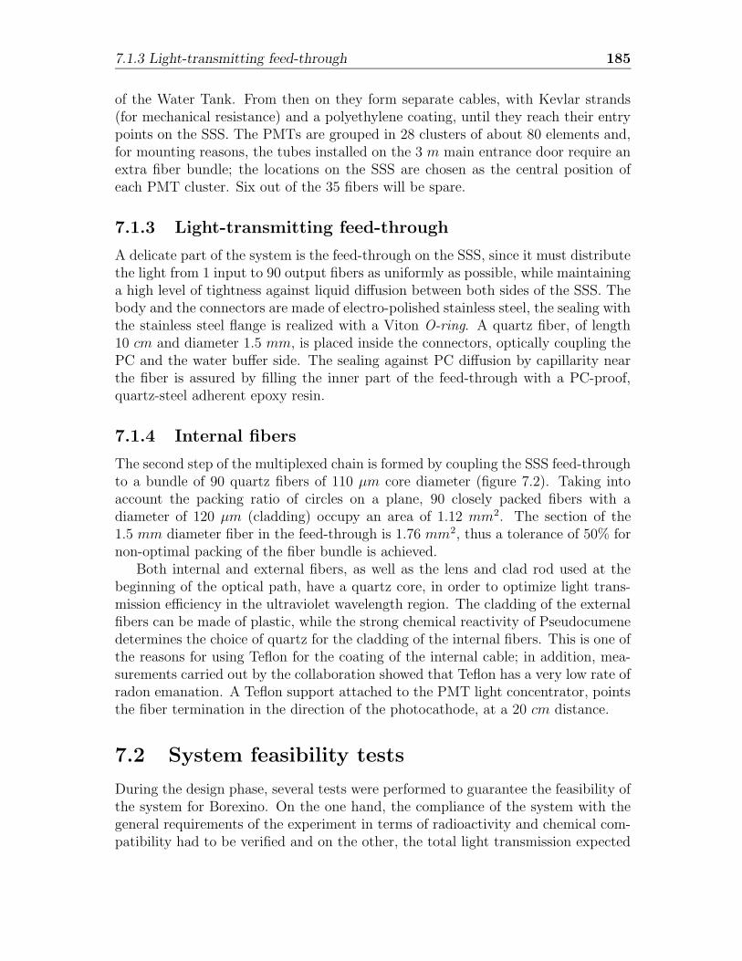
7.1.3 Light-transmitting feed-through 185
of the Water Tank. From then on they form separate cables, with Kevlar strands(for mechanical resistance) and a polyethylene coating, until they reach their entrypoints on the SSS. The PMTs are grouped in 28 clusters of about 80 elements and,for mounting reasons, the tubes installed on the 3 m main entrance door require anextra fiber bundle; the locations on the SSS are chosen as the central position ofeach PMT cluster. Six out of the 35 fibers will be spare.
7.1.3 Light-transmitting feed-through
A delicate part of the system is the feed-through on the SSS, since it must distributethe light from 1 input to 90 output fibers as uniformly as possible, while maintaininga high level of tightness against liquid diffusion between both sides of the SSS. Thebody and the connectors are made of electro-polished stainless steel, the sealing withthe stainless steel flange is realized with a Viton O-ring. A quartz fiber, of length10 cm and diameter 1.5 mm, is placed inside the connectors, optically coupling thePC and the water buffer side. The sealing against PC diffusion by capillarity nearthe fiber is assured by filling the inner part of the feed-through with a PC-proof,quartz-steel adherent epoxy resin.
7.1.4 Internal fibers
The second step of the multiplexed chain is formed by coupling the SSS feed-throughto a bundle of 90 quartz fibers of 110 µm core diameter (figure 7.2). Taking intoaccount the packing ratio of circles on a plane, 90 closely packed fibers with adiameter of 120 µm (cladding) occupy an area of 1.12 mm2. The section of the1.5 mm diameter fiber in the feed-through is 1.76 mm2, thus a tolerance of 50% fornon-optimal packing of the fiber bundle is achieved.
Both internal and external fibers, as well as the lens and clad rod used at thebeginning of the optical path, have a quartz core, in order to optimize light trans-mission efficiency in the ultraviolet wavelength region. The cladding of the externalfibers can be made of plastic, while the strong chemical reactivity of Pseudocumenedetermines the choice of quartz for the cladding of the internal fibers. This is one ofthe reasons for using Teflon for the coating of the internal cable; in addition, mea-surements carried out by the collaboration showed that Teflon has a very low rate ofradon emanation. A Teflon support attached to the PMT light concentrator, pointsthe fiber termination in the direction of the photocathode, at a 20 cm distance.
7.2 System feasibility tests
During the design phase, several tests were performed to guarantee the feasibility ofthe system for Borexino. On the one hand, the compliance of the system with thegeneral requirements of the experiment in terms of radioactivity and chemical com-patibility had to be verified and on the other, the total light transmission expected
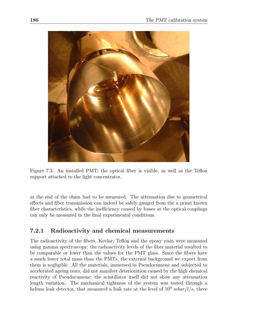
186 The PMT calibration system
Figure 7.3: An installed PMT: the optical fiber is visible, as well as the Teflonsupport attached to the light concentrator.
at the end of the chain had to be measured. The attenuation due to geometricaleffects and fiber transmission can indeed be safely gauged from the a priori knownfiber characteristics, while the inefficiency caused by losses at the optical couplingscan only be measured in the final experimental conditions.
7.2.1 Radioactivity and chemical measurements
The radioactivity of the fibers, Kevlar, Teflon and the epoxy resin were measuredusing gamma spectroscopy; the radioactivity levels of the fiber material resulted tobe comparable or lower than the values for the PMT glass. Since the fibers havea much lower total mass than the PMTs, the external background we expect fromthem is negligible. All the materials, immersed in Pseudocumene and subjected toaccelerated ageing tests, did not manifest deterioration caused by the high chemicalreactivity of Pseudocumene; the scintillator itself did not show any attenuationlength variation. The mechanical tightness of the system was tested through ahelium leak detector, that measured a leak rate at the level of 109 mbar/l/s, three
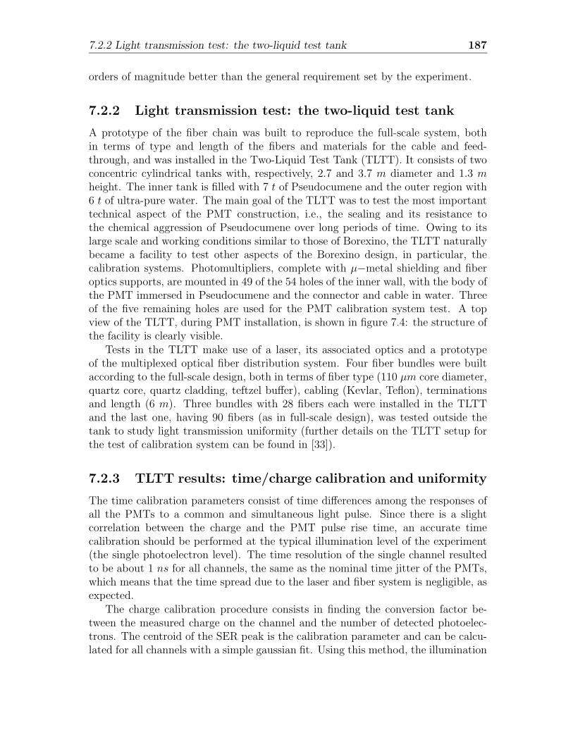
7.2.2 Light transmission test: the two-liquid test tank 187
orders of magnitude better than the general requirement set by the experiment.
7.2.2 Light transmission test: the two-liquid test tank
A prototype of the fiber chain was built to reproduce the full-scale system, bothin terms of type and length of the fibers and materials for the cable and feed-through, and was installed in the Two-Liquid Test Tank (TLTT). It consists of twoconcentric cylindrical tanks with, respectively, 2.7 and 3.7 m diameter and 1.3 mheight. The inner tank is filled with 7 t of Pseudocumene and the outer region with6 t of ultra-pure water. The main goal of the TLTT was to test the most importanttechnical aspect of the PMT construction, i.e., the sealing and its resistance tothe chemical aggression of Pseudocumene over long periods of time. Owing to itslarge scale and working conditions similar to those of Borexino, the TLTT naturallybecame a facility to test other aspects of the Borexino design, in particular, thecalibration systems. Photomultipliers, complete with µ−metal shielding and fiberoptics supports, are mounted in 49 of the 54 holes of the inner wall, with the body ofthe PMT immersed in Pseudocumene and the connector and cable in water. Threeof the five remaining holes are used for the PMT calibration system test. A topview of the TLTT, during PMT installation, is shown in figure 7.4: the structure ofthe facility is clearly visible.
Tests in the TLTT make use of a laser, its associated optics and a prototypeof the multiplexed optical fiber distribution system. Four fiber bundles were builtaccording to the full-scale design, both in terms of fiber type (110 µm core diameter,quartz core, quartz cladding, teftzel buffer), cabling (Kevlar, Teflon), terminationsand length (6 m). Three bundles with 28 fibers each were installed in the TLTTand the last one, having 90 fibers (as in full-scale design), was tested outside thetank to study light transmission uniformity (further details on the TLTT setup forthe test of calibration system can be found in [33]).
7.2.3 TLTT results: time/charge calibration and uniformity
The time calibration parameters consist of time differences among the responses ofall the PMTs to a common and simultaneous light pulse. Since there is a slightcorrelation between the charge and the PMT pulse rise time, an accurate timecalibration should be performed at the typical illumination level of the experiment(the single photoelectron level). The time resolution of the single channel resultedto be about 1 ns for all channels, the same as the nominal time jitter of the PMTs,which means that the time spread due to the laser and fiber system is negligible, asexpected.
The charge calibration procedure consists in finding the conversion factor be-tween the measured charge on the channel and the number of detected photoelec-trons. The centroid of the SER peak is the calibration parameter and can be calcu-lated for all channels with a simple gaussian fit. Using this method, the illumination
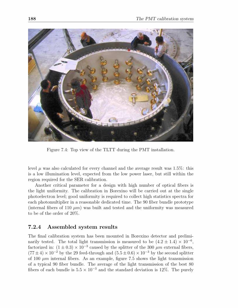
188 The PMT calibration system
Figure 7.4: Top view of the TLTT during the PMT installation.
level µ was also calculated for every channel and the average result was 1.5%: thisis a low illumination level, expected from the low power laser, but still within theregion required for the SER calibration.
Another critical parameter for a design with high number of optical fibers isthe light uniformity. The calibration in Borexino will be carried out at the singlephotoelectron level; good uniformity is required to collect high statistics spectra foreach photomultiplier in a reasonable dedicated time. The 90 fiber bundle prototype(internal fibers of 110 µm) was built and tested and the uniformity was measuredto be of the order of 20%.
7.2.4 Assembled system results
The final calibration system has been mounted in Borexino detector and prelimi-narily tested. The total light transmission is measured to be (4.2 ± 1.4) × 10−6,factorized in: (1± 0.3)× 10−3 caused by the splitter of the 300 µm external fibers,(77± 4)× 10−2 by the 29 feed-through and (5.5± 0.6)× 10−3 by the second splitterof 100 µm internal fibers. As an example, figure 7.5 shows the light transmissionof a typical 90 fiber bundle. The average of the light transmission of the best 80fibers of each bundle is 5.5 × 10⁻³ and the standard deviation is 12%. The purely
7.3 Test of the Borexino PMT calibration system 189
geometrical efficiency for the light transmission is 5.9× 10⁻³, so the fiber couplingspresent very few losses. The measured ratio between the transmission of the worstand best channels is about 0.5, which guarantees a good operation condition.
Figure 7.5: Fraction of transmitted light for each fiber in a 90 fibers bundle [33].
7.3 Test of the Borexino PMT calibration system
In August 2002, several data were taken with the 1993 PMTs installed in Borexinosphere, with high voltages on, by means of the PMT laser calibration system. Thisperiod of data taking has been a good test for the trigger and for the electronicsystems and allowed an accurate debugging of the time reconstruction algorithmdescribed in section 6.2, since the synchronous events provided by the laser timingsystem are a natural test of its efficiency. A PMT timing calibration test wasperformed and the applied time equalization algorithm was found to reduce the timespread of the whole detector to its theoretical value. Finally, the laser data couldbe used for a very preliminary estimation of the Stainless Steel Sphere reflectivity.
7.3.1 Description of the calibration data
As already mentioned in section 5.2.4, during normal data taking the laser systemwill be run with an external trigger. A NIM timing unit, placed in the triggerrack, automatically delivers a programmable rate of pulses to the Borexino TriggerBoard; if the laser condition is disabled the BTB simply ignores these externalinputs. Otherwise, not only the trigger signals, but also the driving signal thatenables the laser light pulse, are generated. To allow a precise measurement of the
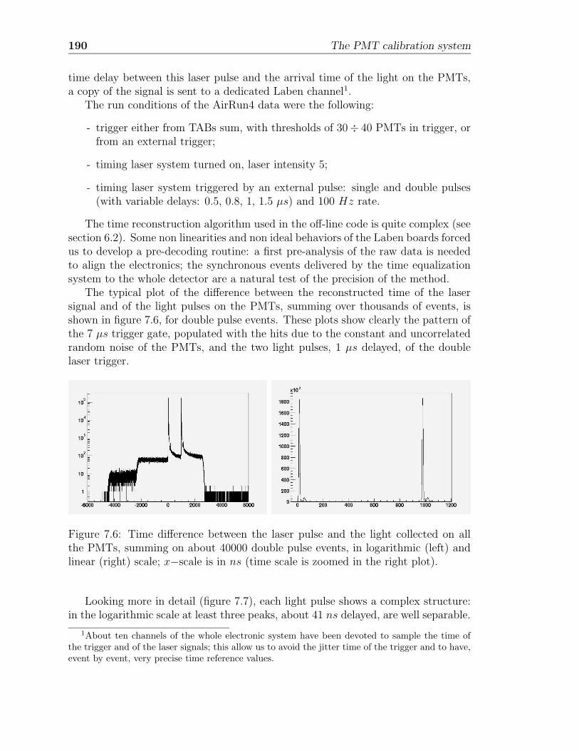
190 The PMT calibration system
time delay between this laser pulse and the arrival time of the light on the PMTs,a copy of the signal is sent to a dedicated Laben channel1.
The run conditions of the AirRun4 data were the following:
- trigger either from TABs sum, with thresholds of 30÷ 40 PMTs in trigger, orfrom an external trigger;
- timing laser system turned on, laser intensity 5;
- timing laser system triggered by an external pulse: single and double pulses(with variable delays: 0.5, 0.8, 1, 1.5 µs) and 100 Hz rate.
The time reconstruction algorithm used in the off-line code is quite complex (seesection 6.2). Some non linearities and non ideal behaviors of the Laben boards forcedus to develop a pre-decoding routine: a first pre-analysis of the raw data is neededto align the electronics; the synchronous events delivered by the time equalizationsystem to the whole detector are a natural test of the precision of the method.
The typical plot of the difference between the reconstructed time of the lasersignal and of the light pulses on the PMTs, summing over thousands of events, isshown in figure 7.6, for double pulse events. These plots show clearly the pattern ofthe 7 µs trigger gate, populated with the hits due to the constant and uncorrelatedrandom noise of the PMTs, and the two light pulses, 1 µs delayed, of the doublelaser trigger.
Figure 7.6: Time difference between the laser pulse and the light collected on allthe PMTs, summing on about 40000 double pulse events, in logarithmic (left) andlinear (right) scale; x−scale is in ns (time scale is zoomed in the right plot).
Looking more in detail (figure 7.7), each light pulse shows a complex structure:in the logarithmic scale at least three peaks, about 41 ns delayed, are well separable.
1About ten channels of the whole electronic system have been devoted to sample the time ofthe trigger and of the laser signals; this allow us to avoid the jitter time of the trigger and to have,event by event, very precise time reference values.
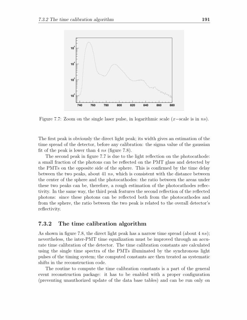
7.3.2 The time calibration algorithm 191
740 760 780 800 820 840 860 880
102
103
104
105
Figure 7.7: Zoom on the single laser pulse, in logarithmic scale (x−scale is in ns).
The first peak is obviously the direct light peak; its width gives an estimation of thetime spread of the detector, before any calibration: the sigma value of the gaussianfit of the peak is lower than 4 ns (figure 7.8).
The second peak in figure 7.7 is due to the light reflection on the photocathode:a small fraction of the photons can be reflected on the PMT glass and detected bythe PMTs on the opposite side of the sphere. This is confirmed by the time delaybetween the two peaks, about 41 ns, which is consistent with the distance betweenthe center of the sphere and the photocathodes: the ratio between the areas underthese two peaks can be, therefore, a rough estimation of the photocathodes reflec-tivity. In the same way, the third peak features the second reflection of the reflectedphotons: since these photons can be reflected both from the photocathodes andfrom the sphere, the ratio between the two peak is related to the overall detector’sreflectivity.
7.3.2 The time calibration algorithm
As shown in figure 7.8, the direct light peak has a narrow time spread (about 4 ns);nevertheless, the inter-PMT time equalization must be improved through an accu-rate time calibration of the detector. The time calibration constants are calculatedusing the single time spectra of the PMTs illuminated by the synchronous lightpulses of the timing system; the computed constants are then treated as systematicshifts in the reconstruction code.
The routine to compute the time calibration constants is a part of the generalevent reconstruction package: it has to be enabled with a proper configuration(preventing unauthorized update of the data base tables) and can be run only on
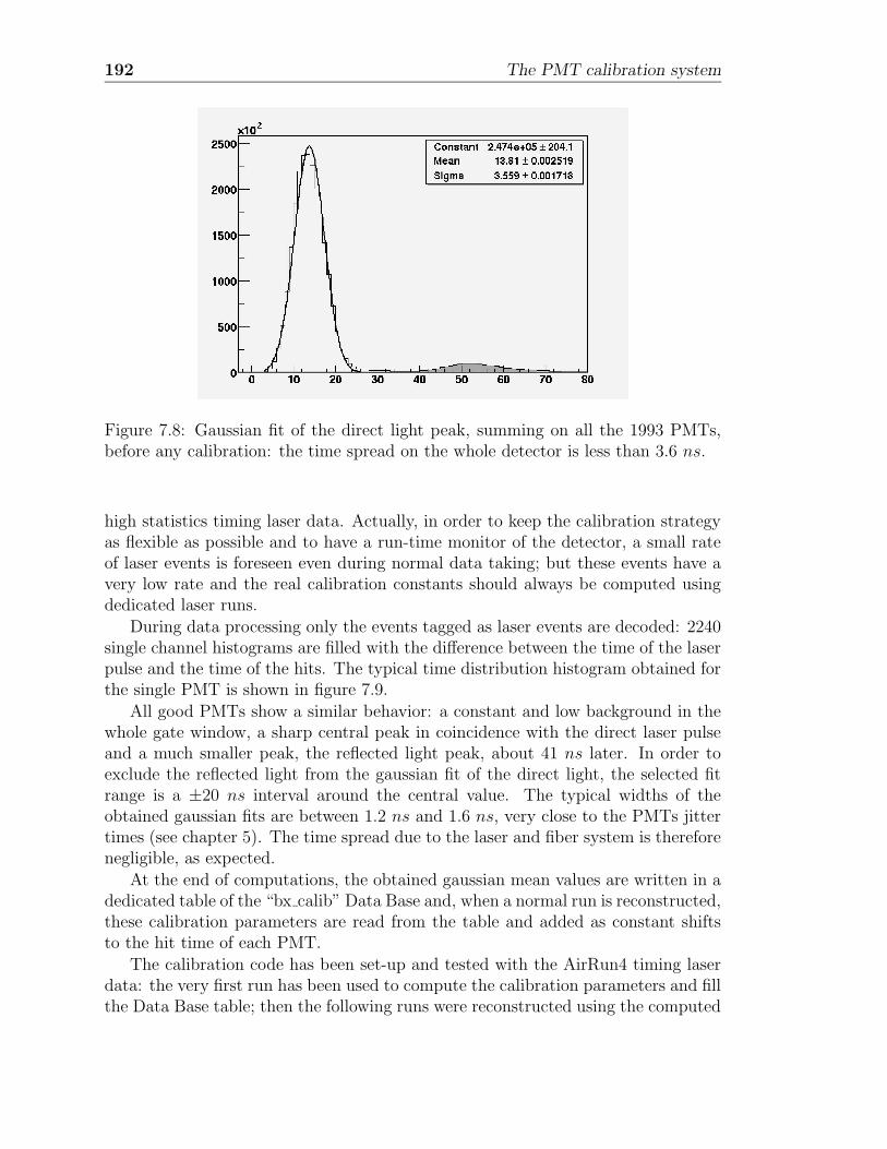
192 The PMT calibration system
Figure 7.8: Gaussian fit of the direct light peak, summing on all the 1993 PMTs,before any calibration: the time spread on the whole detector is less than 3.6 ns.
high statistics timing laser data. Actually, in order to keep the calibration strategyas flexible as possible and to have a run-time monitor of the detector, a small rateof laser events is foreseen even during normal data taking; but these events have avery low rate and the real calibration constants should always be computed usingdedicated laser runs.
During data processing only the events tagged as laser events are decoded: 2240single channel histograms are filled with the difference between the time of the laserpulse and the time of the hits. The typical time distribution histogram obtained forthe single PMT is shown in figure 7.9.
All good PMTs show a similar behavior: a constant and low background in thewhole gate window, a sharp central peak in coincidence with the direct laser pulseand a much smaller peak, the reflected light peak, about 41 ns later. In order toexclude the reflected light from the gaussian fit of the direct light, the selected fitrange is a ±20 ns interval around the central value. The typical widths of theobtained gaussian fits are between 1.2 ns and 1.6 ns, very close to the PMTs jittertimes (see chapter 5). The time spread due to the laser and fiber system is thereforenegligible, as expected.
At the end of computations, the obtained gaussian mean values are written in adedicated table of the “bx calib” Data Base and, when a normal run is reconstructed,these calibration parameters are read from the table and added as constant shiftsto the hit time of each PMT.
The calibration code has been set-up and tested with the AirRun4 timing laserdata: the very first run has been used to compute the calibration parameters and fillthe Data Base table; then the following runs were reconstructed using the computed
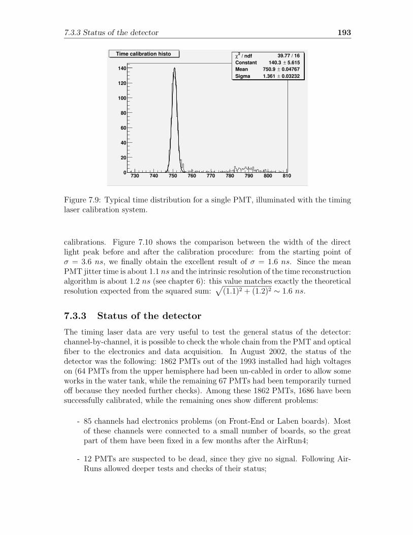
7.3.3 Status of the detector 193
730 740 750 760 770 780 790 800 8100
20
40
60
80
100
120
140
/ ndf 2χ 39.77 / 16Constant 5.615± 140.3 Mean 0.04767± 750.9 Sigma 0.03232± 1.361
Time calibration histo / ndf 2χ 39.77 / 16Constant 5.615± 140.3 Mean 0.04767± 750.9 Sigma 0.03232± 1.361
Figure 7.9: Typical time distribution for a single PMT, illuminated with the timinglaser calibration system.
calibrations. Figure 7.10 shows the comparison between the width of the directlight peak before and after the calibration procedure: from the starting point ofσ = 3.6 ns, we finally obtain the excellent result of σ = 1.6 ns. Since the meanPMT jitter time is about 1.1 ns and the intrinsic resolution of the time reconstructionalgorithm is about 1.2 ns (see chapter 6): this value matches exactly the theoreticalresolution expected from the squared sum:
√
(1.1)2 + (1.2)2 ∼ 1.6 ns.
7.3.3 Status of the detector
The timing laser data are very useful to test the general status of the detector:channel-by-channel, it is possible to check the whole chain from the PMT and opticalfiber to the electronics and data acquisition. In August 2002, the status of thedetector was the following: 1862 PMTs out of the 1993 installed had high voltageson (64 PMTs from the upper hemisphere had been un-cabled in order to allow someworks in the water tank, while the remaining 67 PMTs had been temporarily turnedoff because they needed further checks). Among these 1862 PMTs, 1686 have beensuccessfully calibrated, while the remaining ones show different problems:
- 85 channels had electronics problems (on Front-End or Laben boards). Mostof these channels were connected to a small number of boards, so the greatpart of them have been fixed in a few months after the AirRun4;
- 12 PMTs are suspected to be dead, since they give no signal. Following Air-Runs allowed deeper tests and checks of their status;
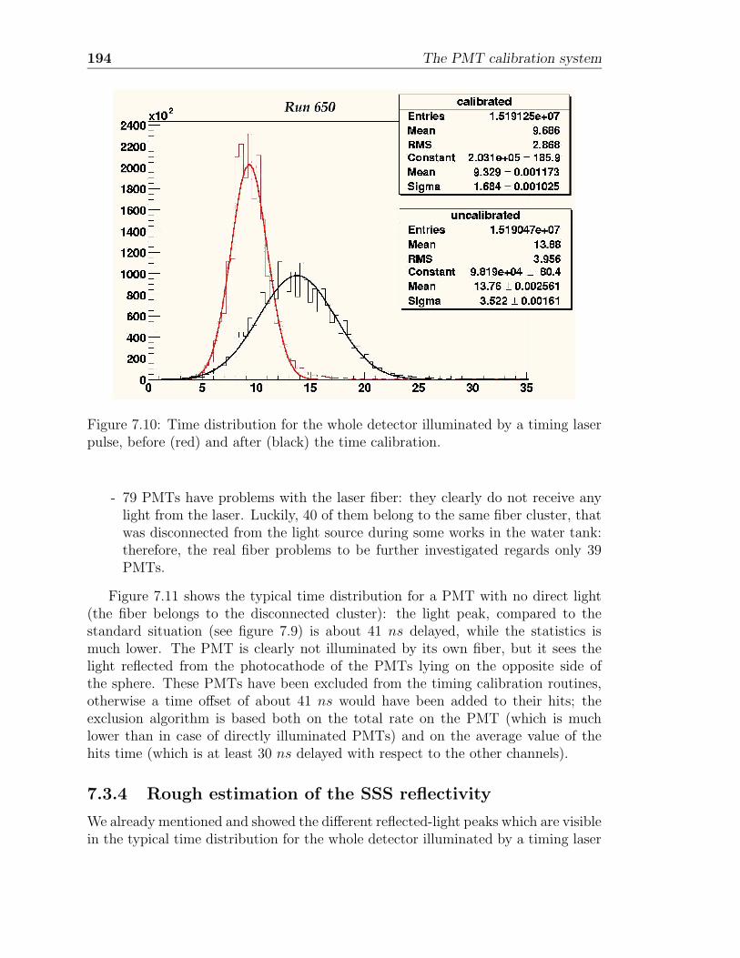
194 The PMT calibration system
Figure 7.10: Time distribution for the whole detector illuminated by a timing laserpulse, before (red) and after (black) the time calibration.
- 79 PMTs have problems with the laser fiber: they clearly do not receive anylight from the laser. Luckily, 40 of them belong to the same fiber cluster, thatwas disconnected from the light source during some works in the water tank:therefore, the real fiber problems to be further investigated regards only 39PMTs.
Figure 7.11 shows the typical time distribution for a PMT with no direct light(the fiber belongs to the disconnected cluster): the light peak, compared to thestandard situation (see figure 7.9) is about 41 ns delayed, while the statistics ismuch lower. The PMT is clearly not illuminated by its own fiber, but it sees thelight reflected from the photocathode of the PMTs lying on the opposite side ofthe sphere. These PMTs have been excluded from the timing calibration routines,otherwise a time offset of about 41 ns would have been added to their hits; theexclusion algorithm is based both on the total rate on the PMT (which is muchlower than in case of directly illuminated PMTs) and on the average value of thehits time (which is at least 30 ns delayed with respect to the other channels).
7.3.4 Rough estimation of the SSS reflectivity
We already mentioned and showed the different reflected-light peaks which are visiblein the typical time distribution for the whole detector illuminated by a timing laser
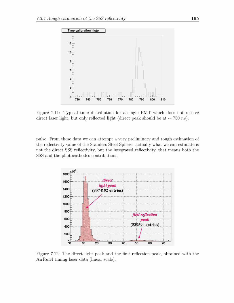
7.3.4 Rough estimation of the SSS reflectivity 195
730 740 750 760 770 780 790 800 8100
2
4
6
8
10
12
Time calibration histo
Figure 7.11: Typical time distribution for a single PMT which does not receivedirect laser light, but only reflected light (direct peak should be at ∼ 750 ns).
pulse. From these data we can attempt a very preliminary and rough estimation ofthe reflectivity value of the Stainless Steel Sphere: actually what we can estimate isnot the direct SSS reflectivity, but the integrated reflectivity, that means both theSSS and the photocathodes contributions.
Figure 7.12: The direct light peak and the first reflection peak, obtained with theAirRun4 timing laser data (linear scale).
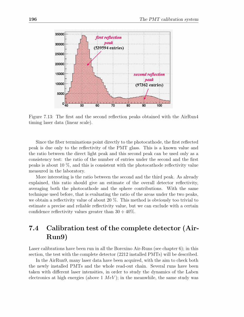
196 The PMT calibration system
Figure 7.13: The first and the second reflection peaks obtained with the AirRun4timing laser data (linear scale).
Since the fiber terminations point directly to the photocathode, the first reflectedpeak is due only to the reflectivity of the PMT glass. This is a known value andthe ratio between the direct light peak and this second peak can be used only as aconsistency test: the ratio of the number of entries under the second and the firstpeaks is about 10 %, and this is consistent with the photocathode reflectivity valuemeasured in the laboratory.
More interesting is the ratio between the second and the third peak. As alreadyexplained, this ratio should give an estimate of the overall detector reflectivity,averaging both the photocathode and the sphere contributions. With the sametechnique used before, that is evaluating the ratio of the areas under the two peaks,we obtain a reflectivity value of about 20 %. This method is obviously too trivial toestimate a precise and reliable reflectivity value, but we can exclude with a certainconfidence reflectivity values greater than 30÷ 40%.
7.4 Calibration test of the complete detector (Air-
Run9)
Laser calibrations have been run in all the Borexino Air-Runs (see chapter 6); in thissection, the test with the complete detector (2212 installed PMTs) will be described.
In the AirRun9, many laser data have been acquired, with the aim to check boththe newly installed PMTs and the whole read-out chain. Several runs have beentaken with different laser intensities, in order to study the dynamics of the Labenelectronics at high energies (above 1 MeV ); in the meanwhile, the same study was
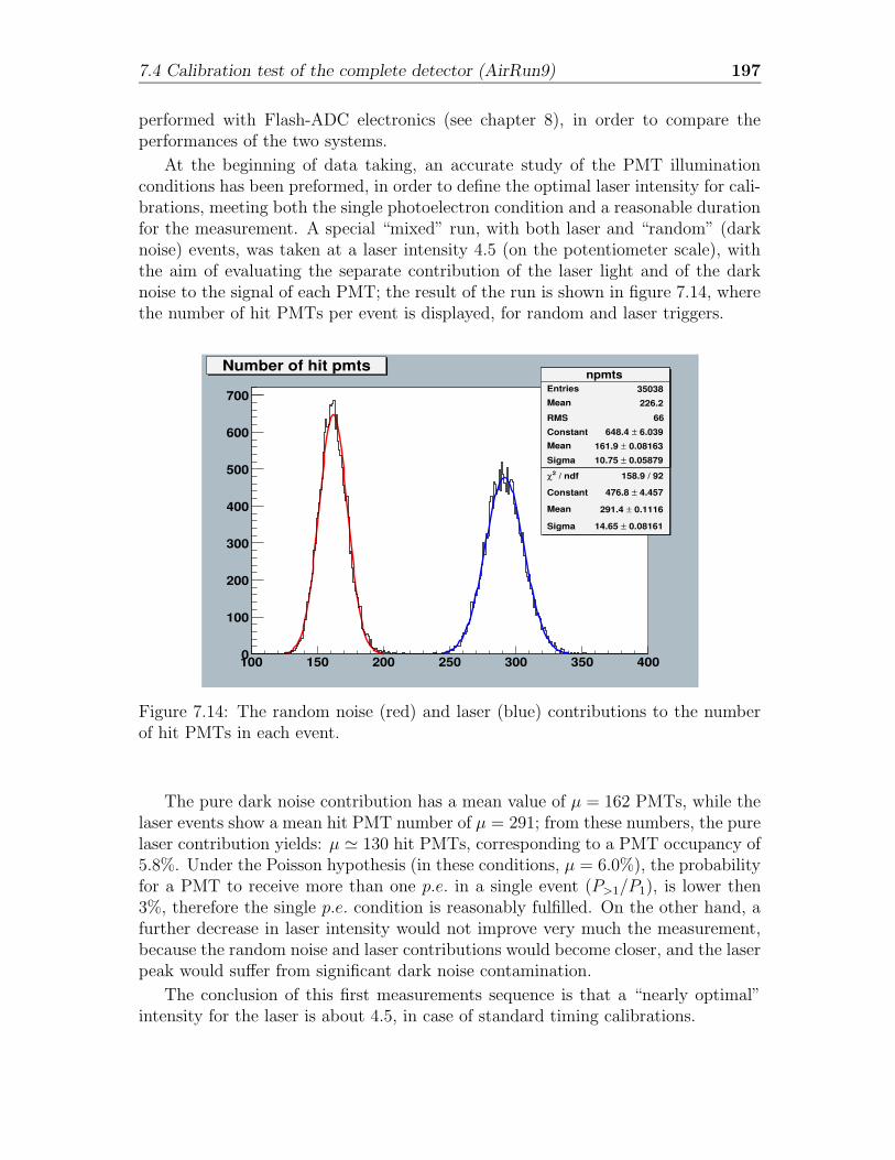
7.4 Calibration test of the complete detector (AirRun9) 197
performed with Flash-ADC electronics (see chapter 8), in order to compare theperformances of the two systems.
At the beginning of data taking, an accurate study of the PMT illuminationconditions has been preformed, in order to define the optimal laser intensity for cali-brations, meeting both the single photoelectron condition and a reasonable durationfor the measurement. A special “mixed” run, with both laser and “random” (darknoise) events, was taken at a laser intensity 4.5 (on the potentiometer scale), withthe aim of evaluating the separate contribution of the laser light and of the darknoise to the signal of each PMT; the result of the run is shown in figure 7.14, wherethe number of hit PMTs per event is displayed, for random and laser triggers.
npmtsEntries 35038
Mean 226.2
RMS 66
Constant 6.039± 648.4
Mean 0.08163± 161.9
Sigma 0.05879± 10.75
100 150 200 250 300 350 4000
100
200
300
400
500
600
700
npmtsEntries 35038
Mean 226.2
RMS 66
Constant 6.039± 648.4
Mean 0.08163± 161.9
Sigma 0.05879± 10.75
Number of hit pmts
/ ndf 2χ 158.9 / 92
Constant 4.457± 476.8
Mean 0.1116± 291.4
Sigma 0.08161± 14.65
Figure 7.14: The random noise (red) and laser (blue) contributions to the numberof hit PMTs in each event.
The pure dark noise contribution has a mean value of µ = 162 PMTs, while thelaser events show a mean hit PMT number of µ = 291; from these numbers, the purelaser contribution yields: µ ' 130 hit PMTs, corresponding to a PMT occupancy of5.8%. Under the Poisson hypothesis (in these conditions, µ = 6.0%), the probabilityfor a PMT to receive more than one p.e. in a single event (P>1/P1), is lower then3%, therefore the single p.e. condition is reasonably fulfilled. On the other hand, afurther decrease in laser intensity would not improve very much the measurement,because the random noise and laser contributions would become closer, and the laserpeak would suffer from significant dark noise contamination.
The conclusion of this first measurements sequence is that a “nearly optimal”intensity for the laser is about 4.5, in case of standard timing calibrations.
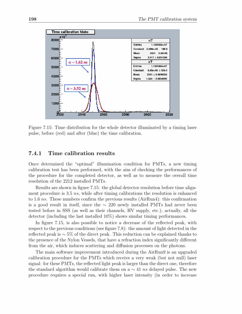
198 The PMT calibration system
Figure 7.15: Time distribution for the whole detector illuminated by a timing laserpulse, before (red) and after (blue) the time calibration.
7.4.1 Time calibration results
Once determined the “optimal” illumination condition for PMTs, a new timingcalibration test has been performed, with the aim of checking the performances ofthe procedure for the completed detector, as well as to measure the overall timeresolution of the 2212 installed PMTs.
Results are shown in figure 7.15: the global detector resolution before time align-ment procedure is 3.5 ns, while after timing calibrations the resolution is enhancedto 1.6 ns. These numbers confirm the previous results (AirRun4): this confirmationis a good result in itself, since the ∼ 220 newly installed PMTs had never beentested before in SSS (as well as their channels, HV supply, etc.); actually, all thedetector (including the last installed 10%) shows similar timing performances.
In figure 7.15, is also possible to notice a decrease of the reflected peak, withrespect to the previous conditions (see figure 7.8): the amount of light detected in thereflected peak is ∼ 5% of the direct peak. This reduction can be explained thanks tothe presence of the Nylon Vessels, that have a refraction index significantly differentfrom the air, which induces scattering and diffusion processes on the photons.
The main software improvement introduced during the AirRun9 is an upgradedcalibration procedure for the PMTs which receive a very weak (but not null) lasersignal: for these PMTs, the reflected light peak is larger than the direct one, thereforethe standard algorithm would calibrate them on a ∼ 41 ns delayed pulse. The newprocedure requires a special run, with higher laser intensity (in order to increase
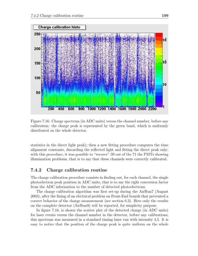
7.4.2 Charge calibration routine 199
Figure 7.16: Charge spectrum (in ADC units) versus the channel number, before anycalibration: the charge peak is represented by the green band, which is uniformlydistributed on the whole detector.
statistics in the direct light peak); then a new fitting procedure computes the timealignment constants, discarding the reflected light and fitting the direct peak only:with this procedure, it was possible to “recover” 39 out of the 71 the PMTs showingillumination problems, that is to say that these channels were correctly calibrated.
7.4.2 Charge calibration routine
The charge calibration procedure consists in finding out, for each channel, the singlephotoelectron peak position in ADC units, that is to say the right conversion factorfrom the ADC information to the number of detected photoelectrons.
The charge calibration algorithm was first set-up during the AirRun7 (August2003), after the fixing of an electrical problem on Front-End boards that prevented acorrect behavior of the charge measurement (see section 6.3). Here only the resultson the complete detector (AirRun9) will be reported, for simplicity purpose.
In figure 7.16, is shown the scatter plot of the detected charge (in ADC units)for laser events versus the channel number in the detector, before any calibrations;this spectrum was measured in a standard timing laser run with intensity 4.5. It iseasy to notice that the position of the charge peak is quite uniform on the whole
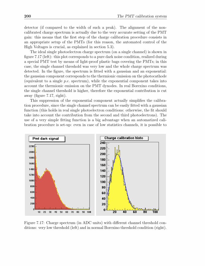
200 The PMT calibration system
detector (if compared to the width of such a peak). The alignment of the non-calibrated charge spectrum is actually due to the very accurate setting of the PMTgain: this means that the first step of the charge calibration procedure consists inan appropriate setup of the PMTs (for this reason, the automated control of theHigh Voltages is crucial, as explained in section 5.3).
The ideal single photoelectron charge spectrum (on a single channel) is shown infigure 7.17 (left): this plot corresponds to a pure dark noise condition, realized duringa special PMT test by means of light-proof plastic bags covering the PMTs; in thiscase, the single channel threshold was very low and the whole charge spectrum wasdetected. In the figure, the spectrum is fitted with a gaussian and an exponential:the gaussian component corresponds to the thermionic emission on the photocathode(equivalent to a single p.e. spectrum), while the exponential component takes intoaccount the thermionic emission on the PMT dynodes. In real Borexino conditions,the single channel threshold is higher, therefore the exponential contribution is cutaway (figure 7.17, right).
This suppression of the exponential component actually simplifies the calibra-tion procedure, since the single channel spectrum can be easily fitted with a gaussianfunction (this holds in real single photoelectron conditions: otherwise, the fit shouldtake into account the contribution from the second and third photoelectrons). Theuse of a very simple fitting function is a big advantage when an automatized cali-bration procedure is set-up: even in case of low statistics channels, it is possible to
Figure 7.17: Charge spectrum (in ADC units) with different channel threshold con-ditions: very low threshold (left) and in normal Borexino threshold condition (right).
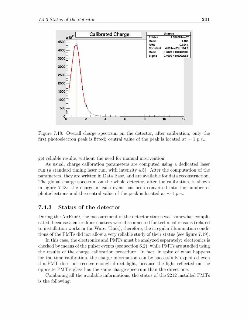
7.4.3 Status of the detector 201
Figure 7.18: Overall charge spectrum on the detector, after calibration; only thefirst photoelectron peak is fitted: central value of the peak is located at ∼ 1 p.e..
get reliable results, without the need for manual intervention.As usual, charge calibration parameters are computed using a dedicated laser
run (a standard timing laser run, with intensity 4.5). After the computation of theparameters, they are written in Data Base, and are available for data reconstruction.The global charge spectrum on the whole detector, after the calibration, is shownin figure 7.18: the charge in each event has been converted into the number ofphotoelectrons and the central value of the peak is located at ∼ 1 p.e..
7.4.3 Status of the detector
During the AirRun9, the measurement of the detector status was somewhat compli-cated, because 5 entire fiber clusters were disconnected for technical reasons (relatedto installation works in the Water Tank); therefore, the irregular illumination condi-tions of the PMTs did not allow a very reliable study of their status (see figure 7.19).
In this case, the electronics and PMTs must be analyzed separately: electronics ischecked by means of the pulser events (see section 6.2), while PMTs are studied usingthe results of the charge calibration procedure. In fact, in spite of what happensfor the time calibration, the charge information can be successfully exploited evenif a PMT does not receive enough direct light, because the light reflected on theopposite PMT’s glass has the same charge spectrum than the direct one.
Combining all the available informations, the status of the 2212 installed PMTsis the following:
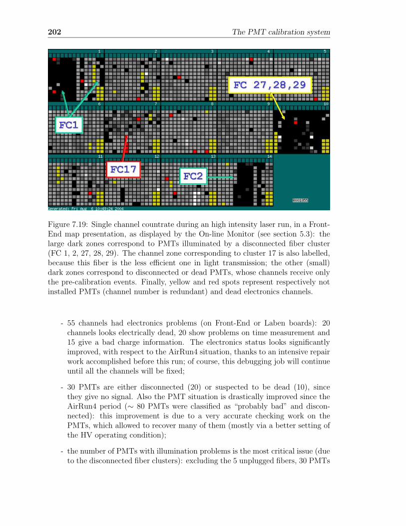
202 The PMT calibration system
Figure 7.19: Single channel countrate during an high intensity laser run, in a Front-End map presentation, as displayed by the On-line Monitor (see section 5.3): thelarge dark zones correspond to PMTs illuminated by a disconnected fiber cluster(FC 1, 2, 27, 28, 29). The channel zone corresponding to cluster 17 is also labelled,because this fiber is the less efficient one in light transmission; the other (small)dark zones correspond to disconnected or dead PMTs, whose channels receive onlythe pre-calibration events. Finally, yellow and red spots represent respectively notinstalled PMTs (channel number is redundant) and dead electronics channels.
- 55 channels had electronics problems (on Front-End or Laben boards): 20channels looks electrically dead, 20 show problems on time measurement and15 give a bad charge information. The electronics status looks significantlyimproved, with respect to the AirRun4 situation, thanks to an intensive repairwork accomplished before this run; of course, this debugging job will continueuntil all the channels will be fixed;
- 30 PMTs are either disconnected (20) or suspected to be dead (10), sincethey give no signal. Also the PMT situation is drastically improved since theAirRun4 period (∼ 80 PMTs were classified as “probably bad” and discon-nected): this improvement is due to a very accurate checking work on thePMTs, which allowed to recover many of them (mostly via a better setting ofthe HV operating condition);
- the number of PMTs with illumination problems is the most critical issue (dueto the disconnected fiber clusters): excluding the 5 unplugged fibers, 30 PMTs
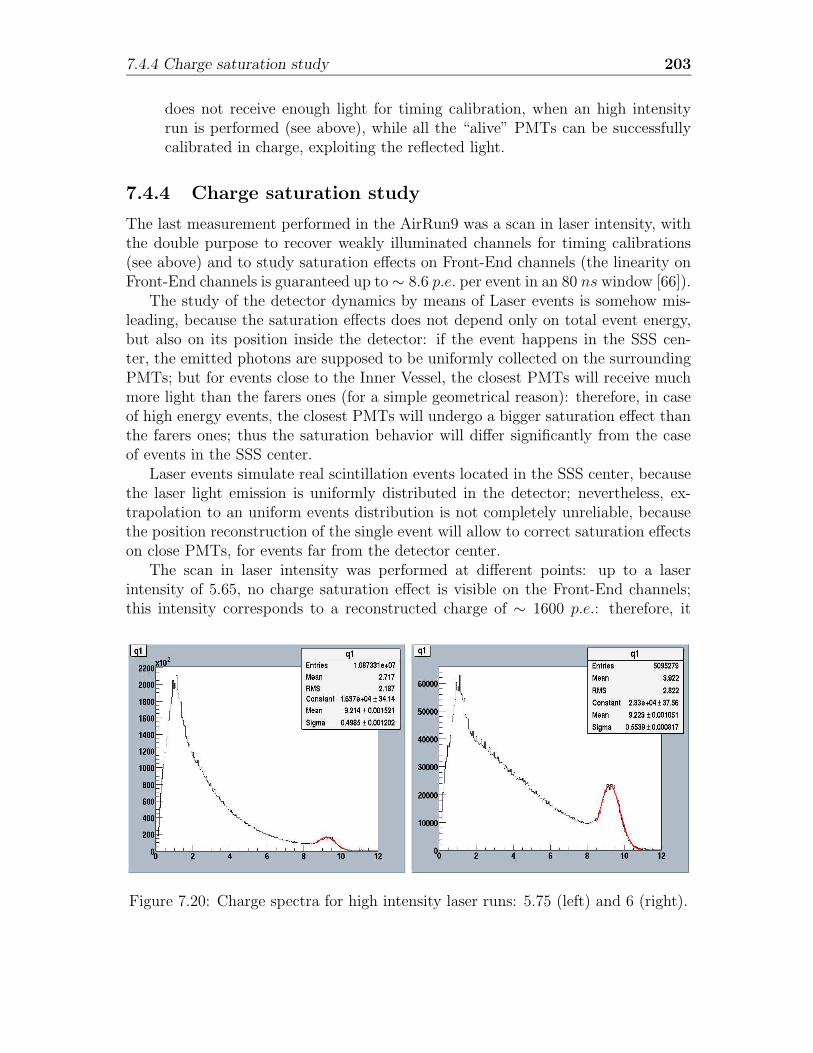
7.4.4 Charge saturation study 203
does not receive enough light for timing calibration, when an high intensityrun is performed (see above), while all the “alive” PMTs can be successfullycalibrated in charge, exploiting the reflected light.
7.4.4 Charge saturation study
The last measurement performed in the AirRun9 was a scan in laser intensity, withthe double purpose to recover weakly illuminated channels for timing calibrations(see above) and to study saturation effects on Front-End channels (the linearity onFront-End channels is guaranteed up to∼ 8.6 p.e. per event in an 80 ns window [66]).
The study of the detector dynamics by means of Laser events is somehow mis-leading, because the saturation effects does not depend only on total event energy,but also on its position inside the detector: if the event happens in the SSS cen-ter, the emitted photons are supposed to be uniformly collected on the surroundingPMTs; but for events close to the Inner Vessel, the closest PMTs will receive muchmore light than the farers ones (for a simple geometrical reason): therefore, in caseof high energy events, the closest PMTs will undergo a bigger saturation effect thanthe farers ones; thus the saturation behavior will differ significantly from the caseof events in the SSS center.
Laser events simulate real scintillation events located in the SSS center, becausethe laser light emission is uniformly distributed in the detector; nevertheless, ex-trapolation to an uniform events distribution is not completely unreliable, becausethe position reconstruction of the single event will allow to correct saturation effectson close PMTs, for events far from the detector center.
The scan in laser intensity was performed at different points: up to a laserintensity of 5.65, no charge saturation effect is visible on the Front-End channels;this intensity corresponds to a reconstructed charge of ∼ 1600 p.e.: therefore, it
Figure 7.20: Charge spectra for high intensity laser runs: 5.75 (left) and 6 (right).
204 The PMT calibration system
would be the saturation condition of an event at the SSS center, with an energy of4 MeV (assuming a total light yield of 400 p.e./MeV ). At the following intensitystep (5.75) a small saturated peak appears (see figure 7.20, left), accounting for 3.6%of the hits; in this case, the reconstructed charge (without saturation correction) is∼ 3900 p.e., corresponding to a 9.7 MeV event at the SSS center. Finally, thelaser intensity 6.0 was tried: in this case, 11% of the hits show a saturated charge(figure 7.20, right); the total reconstructed charge is ∼ 6650 p.e. (without saturationcorrection), corresponding to a 16.8 MeV event in the detector center.
The energies of coincidence events in the NC and CC reactions on 12C in scin-tillator from Supernova Neutrinos (section 3.2) are respectively 15.11 MeV (NC)and 13.37 MeV (CC, from νe) or 17.34 MeV (CC, from νe); these very preliminarysaturation results allow to conclude that a reconstruction of event energy is possiblefor events up to 18 ÷ 20 MeV (applying saturation corrections and reconstructedposition extrapolations): therefore, in case of an high intensity supernova event, itwill probably possible to distinguish the NC from the CC events.
Chapter 8
The high energy read-out system
The main acquisition system of Borexino has been designed and optimized for thedetection of low energy neutrinos in the sub-MeV range, which are the main scopeof the experiment.
As described in chapter 3, some interesting physics lies above this range, fromthe few MeV region (anti-neutrinos from reactors and from the earth’s interior), upto the ∼ 15÷ 20 MeV range (end point of the solar 8B neutrino spectrum, CC andNC reactions on 12C from supernova neutrinos).
Concerning the energy measurement in the 15 MeV range, some preliminarytests of the “solar neutrino” read-out system showed very encouraging results, asdescribed in section 7.4: the limited amount of saturated channels in each eventshould guarantee the possibility to reconstruct the event energy in all the interestinginterval.
Nevertheless, the energy measurement in the low energy spectrum is redundant,because in the single photoelectron regime (almost always valid in the sub-MeVregion) the charge information can be integrated by a simple hit counting, allowinga cross check of the measurement. A similar redundancy would be desirable also inthe higher energy range, where the hit counting information is no more reliable. Inprinciple, a redundant read-out system in which no saturation correction has to beapplied to events up to 20 MeV , would fit all the possible requirements.
A system based on phototubes clustering and waveform recording has been im-plemented, with the aim to cover at least the 1 ÷ 10 MeV range. The phototubesare summed by groups of 24, and each of these 98 sums is recorded by a 400 MHzwaveform digitizer.
The main physical interest in registering the full waveform of each event relies onthe possibility to exploit the time shape information of the event for a pulse shapediscrimination analysis (some application of the PSD techniques for α/β discrimi-nation in CTF are described in section 4.2). In the single photoelectron regime, thepulse shape of each event can be reconstructed in the Laben system using the arrivaltime information for the single hit. In the high energy range, this information is notmore available in the Laben electronics, since only the first hit in each channel will
205
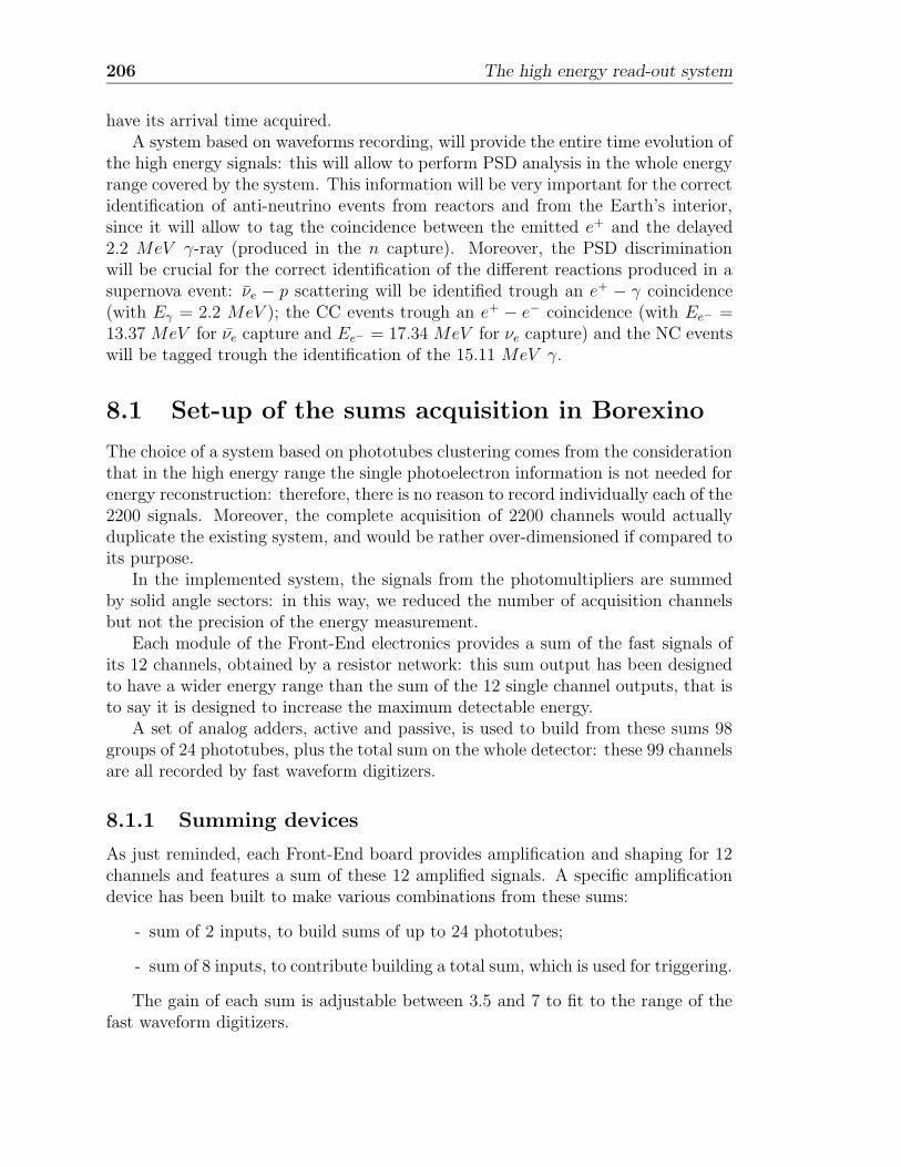
206 The high energy read-out system
have its arrival time acquired.A system based on waveforms recording, will provide the entire time evolution of
the high energy signals: this will allow to perform PSD analysis in the whole energyrange covered by the system. This information will be very important for the correctidentification of anti-neutrino events from reactors and from the Earth’s interior,since it will allow to tag the coincidence between the emitted e+ and the delayed2.2 MeV γ-ray (produced in the n capture). Moreover, the PSD discriminationwill be crucial for the correct identification of the different reactions produced in asupernova event: νe − p scattering will be identified trough an e+ − γ coincidence(with Eγ = 2.2 MeV ); the CC events trough an e+ − e− coincidence (with Ee− =13.37 MeV for νe capture and Ee− = 17.34 MeV for νe capture) and the NC eventswill be tagged trough the identification of the 15.11 MeV γ.
8.1 Set-up of the sums acquisition in Borexino
The choice of a system based on phototubes clustering comes from the considerationthat in the high energy range the single photoelectron information is not needed forenergy reconstruction: therefore, there is no reason to record individually each of the2200 signals. Moreover, the complete acquisition of 2200 channels would actuallyduplicate the existing system, and would be rather over-dimensioned if compared toits purpose.
In the implemented system, the signals from the photomultipliers are summedby solid angle sectors: in this way, we reduced the number of acquisition channelsbut not the precision of the energy measurement.
Each module of the Front-End electronics provides a sum of the fast signals ofits 12 channels, obtained by a resistor network: this sum output has been designedto have a wider energy range than the sum of the 12 single channel outputs, that isto say it is designed to increase the maximum detectable energy.
A set of analog adders, active and passive, is used to build from these sums 98groups of 24 phototubes, plus the total sum on the whole detector: these 99 channelsare all recorded by fast waveform digitizers.
8.1.1 Summing devices
As just reminded, each Front-End board provides amplification and shaping for 12channels and features a sum of these 12 amplified signals. A specific amplificationdevice has been built to make various combinations from these sums:
- sum of 2 inputs, to build sums of up to 24 phototubes;
- sum of 8 inputs, to contribute building a total sum, which is used for triggering.
The gain of each sum is adjustable between 3.5 and 7 to fit to the range of thefast waveform digitizers.
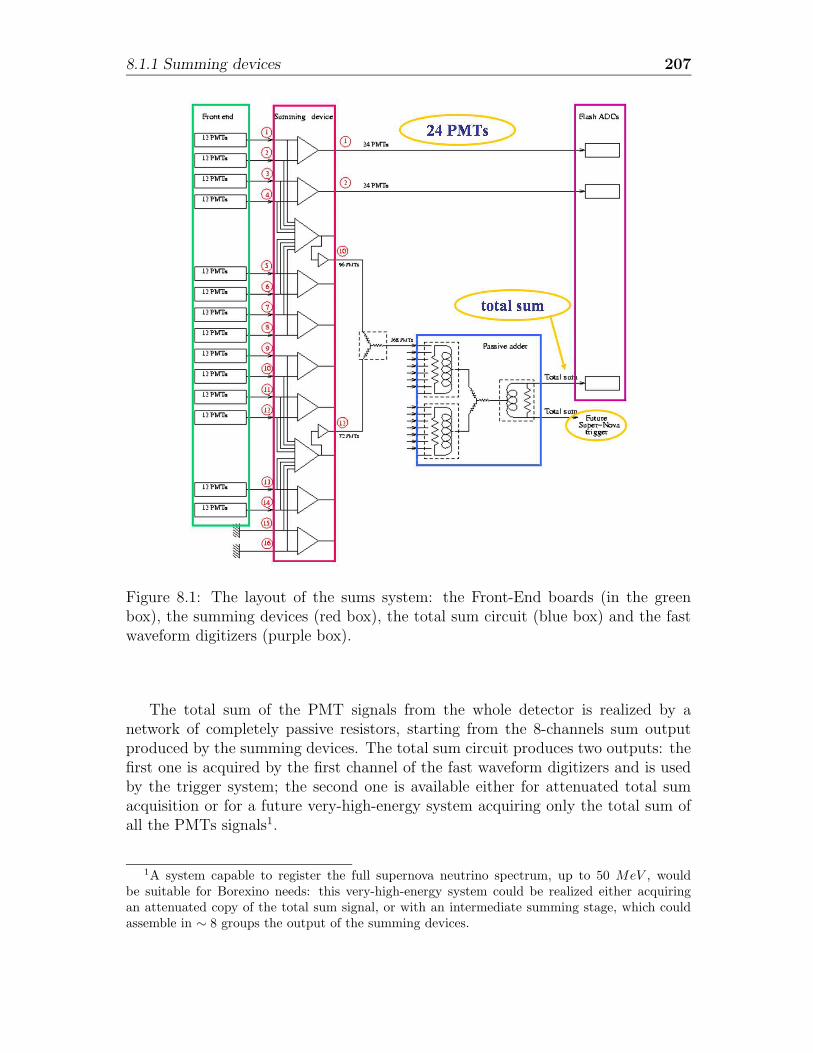
8.1.1 Summing devices 207
Figure 8.1: The layout of the sums system: the Front-End boards (in the greenbox), the summing devices (red box), the total sum circuit (blue box) and the fastwaveform digitizers (purple box).
The total sum of the PMT signals from the whole detector is realized by anetwork of completely passive resistors, starting from the 8-channels sum outputproduced by the summing devices. The total sum circuit produces two outputs: thefirst one is acquired by the first channel of the fast waveform digitizers and is usedby the trigger system; the second one is available either for attenuated total sumacquisition or for a future very-high-energy system acquiring only the total sum ofall the PMTs signals1.
1A system capable to register the full supernova neutrino spectrum, up to 50 MeV , wouldbe suitable for Borexino needs: this very-high-energy system could be realized either acquiringan attenuated copy of the total sum signal, or with an intermediate summing stage, which couldassemble in ∼ 8 groups the output of the summing devices.
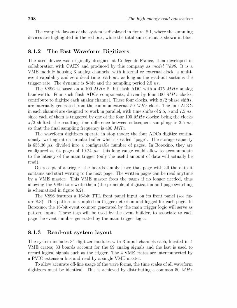
208 The high energy read-out system
The complete layout of the system is displayed in figure 8.1, where the summingdevices are highlighted in the red box, while the total sum circuit is shown in blue.
8.1.2 The Fast Waveform Digitizers
The used device was originally designed at College-de-France, then developed incollaboration with CAEN and produced by this company as model V896. It is aVME module housing 3 analog channels, with internal or external clock, a multi-event capability and zero dead time read-out, as long as the read-out sustains thetrigger rate. The dynamic is 8-bit and the sampling period 2.5 ns.
The V896 is based on a 100 MHz 8−bit flash ADC with a 475 MHz analogbandwidth. Four such flash ADCs components, driven by four 100 MHz clocks,contribute to digitize each analog channel. These four clocks, with π/2 phase shifts,are internally generated from the common external 50 MHz clock. The four ADCsin each channel are designed to work in parallel, with time shifts of 2.5, 5 and 7.5 ns,since each of them is triggered by one of the four 100 MHz clocks: being the clocksπ/2 shifted, the resulting time difference between subsequent samplings is 2.5 ns,so that the final sampling frequency is 400 MHz.
The waveform digitizers operate in stop mode; the four ADCs digitize contin-uously, writing into a circular buffer which is called “page”. The storage capacityis 655.36 µs, divided into a configurable number of pages. In Borexino, they areconfigured as 64 pages of 10.24 µs: this long range could allow to accommodateto the latency of the main trigger (only the useful amount of data will actually beread).
On receipt of a trigger, the boards simply leave that page with all the data itcontains and start writing to the next page. The written pages can be read anytimeby a VME master. This VME master frees the pages if no longer needed, thusallowing the V896 to rewrite them (the principle of digitization and page switchingis schematized in figure 8.2).
The V896 features a 16-bit TTL front panel input on its front panel (see fig-ure 8.3). This pattern is sampled on trigger detection and logged for each page. InBorexino, the 16-bit event counter generated by the main trigger logic will serve aspattern input. These tags will be used by the event builder, to associate to eachpage the event number generated by the main trigger logic.
8.1.3 Read-out system layout
The system includes 34 digitizer modules with 3 input channels each, located in 4VME crates; 33 boards account for the 99 analog signals and the last is used torecord logical signals such as the trigger. The 4 VME crates are interconnected bya PVIC extension bus and read by a single VME master.
To allow accurate off-line usage of the wave forms, the time scales of all waveformdigitizers must be identical. This is achieved by distributing a common 50 MHz
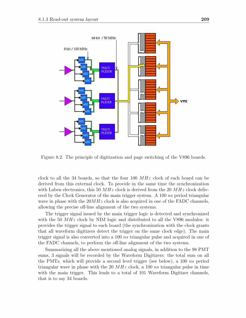
8.1.3 Read-out system layout 209
Figure 8.2: The principle of digitization and page switching of the V896 boards.
clock to all the 34 boards, so that the four 100 MHz clock of each board can bederived from this external clock. To provide in the same time the synchronizationwith Laben electronics, this 50 MHz clock is derived from the 20 MHz clock deliv-ered by the Clock Generator of the main trigger system. A 100 ns period triangularwave in phase with the 20MHz clock is also acquired in one of the FADC channels,allowing the precise off-line alignment of the two systems.
The trigger signal issued by the main trigger logic is detected and synchronizedwith the 50 MHz clock by NIM logic and distributed to all the V896 modules: itprovides the trigger signal to each board (the synchronization with the clock grantsthat all waveform digitizers detect the trigger on the same clock edge). The maintrigger signal is also converted into a 100 ns triangular pulse and acquired in one ofthe FADC channels, to perform the off-line alignment of the two systems.
Summarizing all the above mentioned analog signals, in addition to the 98 PMTsums, 3 signals will be recorded by the Waveform Digitizers: the total sum on allthe PMTs, which will provide a second level trigger (see below), a 100 ns periodtriangular wave in phase with the 20 MHz clock, a 100 ns triangular pulse in timewith the main trigger. This leads to a total of 101 Waveform Digitizer channels,that is to say 34 boards.
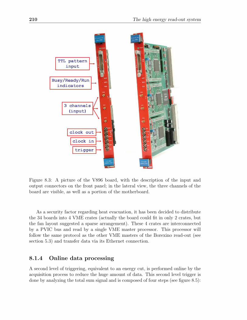
210 The high energy read-out system
Figure 8.3: A picture of the V896 board, with the description of the input andoutput connectors on the front panel; in the lateral view, the three channels of theboard are visible, as well as a portion of the motherboard.
As a security factor regarding heat evacuation, it has been decided to distributethe 34 boards into 4 VME crates (actually the board could fit in only 2 crates, butthe fan layout suggested a sparse arrangement). These 4 crates are interconnectedby a PVIC bus and read by a single VME master processor. This processor willfollow the same protocol as the other VME masters of the Borexino read-out (seesection 5.3) and transfer data via its Ethernet connection.
8.1.4 Online data processing
A second level of triggering, equivalent to an energy cut, is performed online by theacquisition process to reduce the huge amount of data. This second level trigger isdone by analyzing the total sum signal and is composed of four steps (see figure 8.5):
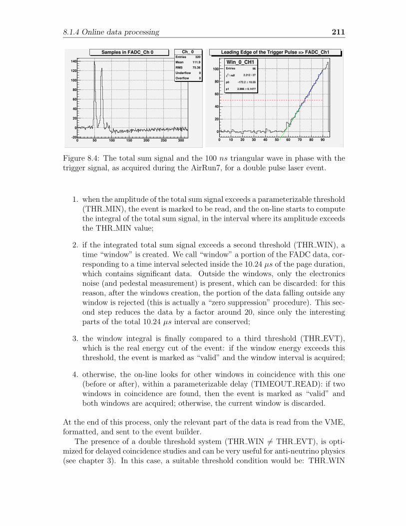
8.1.4 Online data processing 211
Ch_ 0Entries 320
Mean 111.9
RMS 75.36
Underflow 0
Overflow 0
0 50 100 150 200 250 300-20
0
20
40
60
80
100
120
140
Ch_ 0Entries 320
Mean 111.9
RMS 75.36
Underflow 0
Overflow 0
Samples in FADC_Ch 0
WindowsEntries 24960
Mean 144.8
RMS 90.58
Underflow 0
Overflow 0
0 50 100 150 200 250 300
0
200
400
600
800
WindowsEntries 24960
Mean 144.8
RMS 90.58
Underflow 0
Overflow 0
All Channels Samples
Win_0_CH2Entries 96Mean 48.7RMS 15.09
Underflow 0Overflow 0
0 10 20 30 40 50 60 70 80 90
0
20
40
60
80
Win_0_CH2Entries 96Mean 48.7RMS 15.09
Underflow 0Overflow 0
Samples in Window_0 CH2Laben Trigger Pulse Shape => FADC_Ch2
Win_0_CH1Entries 96
/ ndf 2χ 2.212 / 27
p0 10.55± -172.2
p1 0.1477± 2.998
0 10 20 30 40 50 60 70 80 90
0
20
40
60
80
100
Win_0_CH1Entries 96
/ ndf 2χ 2.212 / 27
p0 10.55± -172.2
p1 0.1477± 2.998
Samples in Window_0 CH1Leading Edge of the Trigger Pulse => FADC_Ch1
Run_1429 Event=1000 Laser -> 5.3
Ch_ 0Entries 320
Mean 111.9
RMS 75.36
Underflow 0
Overflow 0
0 50 100 150 200 250 300-20
0
20
40
60
80
100
120
140
Ch_ 0Entries 320
Mean 111.9
RMS 75.36
Underflow 0
Overflow 0
Samples in FADC_Ch 0
WindowsEntries 24960
Mean 144.8
RMS 90.58
Underflow 0
Overflow 0
0 50 100 150 200 250 300
0
200
400
600
800
WindowsEntries 24960
Mean 144.8
RMS 90.58
Underflow 0
Overflow 0
All Channels Samples
Win_0_CH2Entries 96Mean 48.7RMS 15.09
Underflow 0Overflow 0
0 10 20 30 40 50 60 70 80 90
0
20
40
60
80
Win_0_CH2Entries 96Mean 48.7RMS 15.09
Underflow 0Overflow 0
Samples in Window_0 CH2Laben Trigger Pulse Shape => FADC_Ch2
Win_0_CH1Entries 96
/ ndf 2χ 2.212 / 27
p0 10.55± -172.2
p1 0.1477± 2.998
0 10 20 30 40 50 60 70 80 90
0
20
40
60
80
100
Win_0_CH1Entries 96
/ ndf 2χ 2.212 / 27
p0 10.55± -172.2
p1 0.1477± 2.998
Samples in Window_0 CH1Leading Edge of the Trigger Pulse => FADC_Ch1
Run_1429 Event=1000 Laser -> 5.3
Figure 8.4: The total sum signal and the 100 ns triangular wave in phase with thetrigger signal, as acquired during the AirRun7, for a double pulse laser event.
1. when the amplitude of the total sum signal exceeds a parameterizable threshold(THR MIN), the event is marked to be read, and the on-line starts to computethe integral of the total sum signal, in the interval where its amplitude exceedsthe THR MIN value;
2. if the integrated total sum signal exceeds a second threshold (THR WIN), atime “window” is created. We call “window” a portion of the FADC data, cor-responding to a time interval selected inside the 10.24 µs of the page duration,which contains significant data. Outside the windows, only the electronicsnoise (and pedestal measurement) is present, which can be discarded: for thisreason, after the windows creation, the portion of the data falling outside anywindow is rejected (this is actually a “zero suppression” procedure). This sec-ond step reduces the data by a factor around 20, since only the interestingparts of the total 10.24 µs interval are conserved;
3. the window integral is finally compared to a third threshold (THR EVT),which is the real energy cut of the event: if the window energy exceeds thisthreshold, the event is marked as “valid” and the window interval is acquired;
4. otherwise, the on-line looks for other windows in coincidence with this one(before or after), within a parameterizable delay (TIMEOUT READ): if twowindows in coincidence are found, then the event is marked as “valid” andboth windows are acquired; otherwise, the current window is discarded.
At the end of this process, only the relevant part of the data is read from the VME,formatted, and sent to the event builder.
The presence of a double threshold system (THR WIN 6= THR EVT), is opti-mized for delayed coincidence studies and can be very useful for anti-neutrino physics(see chapter 3). In this case, a suitable threshold condition would be: THR WIN
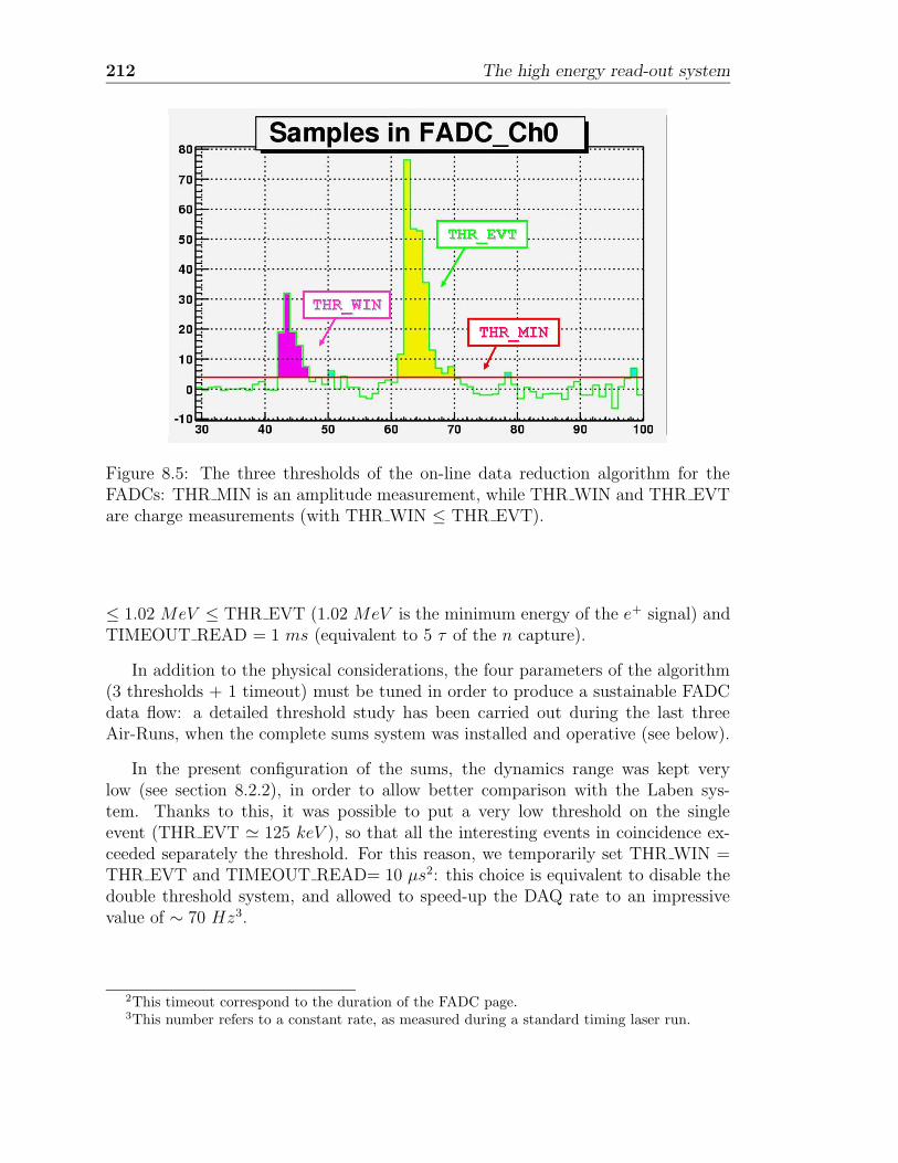
212 The high energy read-out system
Figure 8.5: The three thresholds of the on-line data reduction algorithm for theFADCs: THR MIN is an amplitude measurement, while THR WIN and THR EVTare charge measurements (with THR WIN ≤ THR EVT).
≤ 1.02 MeV ≤ THR EVT (1.02 MeV is the minimum energy of the e+ signal) andTIMEOUT READ = 1 ms (equivalent to 5 τ of the n capture).
In addition to the physical considerations, the four parameters of the algorithm(3 thresholds + 1 timeout) must be tuned in order to produce a sustainable FADCdata flow: a detailed threshold study has been carried out during the last threeAir-Runs, when the complete sums system was installed and operative (see below).
In the present configuration of the sums, the dynamics range was kept verylow (see section 8.2.2), in order to allow better comparison with the Laben sys-tem. Thanks to this, it was possible to put a very low threshold on the singleevent (THR EVT ' 125 keV ), so that all the interesting events in coincidence ex-ceeded separately the threshold. For this reason, we temporarily set THR WIN =THR EVT and TIMEOUT READ= 10 µs2: this choice is equivalent to disable thedouble threshold system, and allowed to speed-up the DAQ rate to an impressivevalue of ∼ 70 Hz3.
2This timeout correspond to the duration of the FADC page.3This number refers to a constant rate, as measured during a standard timing laser run.
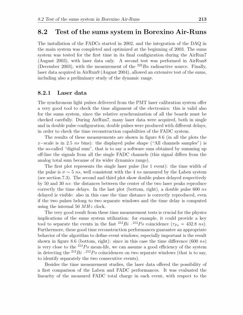
8.2 Test of the sums system in Borexino Air-Runs 213
8.2 Test of the sums system in Borexino Air-Runs
The installation of the FADCs started in 2002, and the integration of the DAQ inthe main system was completed and optimized at the beginning of 2003. The sumssystem was tested for the first time in its final configuration during the AirRun7(August 2003), with laser data only. A second test was performed in AirRun8(December 2003), with the measurement of the 222Rn radioactive source. Finally,laser data acquired in AirRun9 (August 2004), allowed an extensive test of the sums,including also a preliminary study of the dynamic range.
8.2.1 Laser data
The synchronous light pulses delivered from the PMT laser calibration system offera very good tool to check the time alignment of the electronics: this is valid alsofor the sums system, since the relative synchronization of all the boards must bechecked carefully. During AirRun7, many laser data were acquired, both in singleand in double pulse configuration; double pulses were produced with different delays,in order to check the time reconstruction capabilities of the FADC system.
The results of these measurements are shown in figure 8.6 (in all the plots thex−scale is in 2.5 ns bins): the displayed pulse shape (“All channels samples”) isthe so-called “digital sum”, that is to say a software sum obtained by summing upoff-line the signals from all the single FADC channels (this signal differs from theanalog total sum because of its wider dynamics range).
The first plot represents the single laser pulse (for 1 event): the time width ofthe pulse is σ ∼ 5 ns, well consistent with the 4 ns measured by the Laben system(see section 7.3). The second and third plot show double pulses delayed respectivelyby 50 and 30 ns: the distances between the center of the two laser peaks reproducecorrectly the time delays. In the last plot (bottom, right), a double pulse 600 nsdelayed is visible: also in this case the time distance is correctly reproduced, evenif the two pulses belong to two separate windows and the time delay is computedusing the internal 50 MHz clock.
The very good result from these time measurement tests is crucial for the physicsimplications of the sums system utilization: for example, it could provide a keytool to separate the events in the fast 212Bi –212Po coincidence (τPo = 432.8 ns).Furthermore, these good time reconstruction performances guarantee an appropriatebehavior of the algorithm to define event windows; especially important is the resultshown in figure 8.6 (bottom, right): since in this case the time difference (600 ns)is very close to the 212Po mean-life, we can assume a good efficiency of the systemin detecting the 212Bi –212Po coincidences on two separate windows (that is to say,to identify separately the two consecutive events).
Besides the time measurement studies, the laser data offered the possibility ofa first comparison of the Laben and FADC performances. It was evaluated thelinearity of the measured FADC total charge in each event, with respect to the
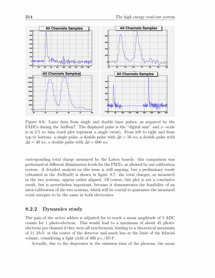
214 The high energy read-out system
WindowsEntries 14976Mean 92.5
RMS 51.93
Underflow 0
Overflow 0
0 20 40 60 80 100 120 140 160 180-100
0
100
200
300
400
500
600
700
WindowsEntries 14976Mean 92.5
RMS 51.93
Underflow 0
Overflow 0
All Channels SamplesCh_65
Entries 192Mean 75.17
RMS 46.79
Underflow 0
Overflow 0
0 20 40 60 80 100 120 140 160 180
-10
0
10
20
30
40
50
60
70
80
Ch_65Entries 192Mean 75.17
RMS 46.79
Underflow 0
Overflow 0
Samples in FADC_Ch65
Ch_76Entries 192Mean 94.22
RMS 54.07
Underflow 0
Overflow 0
0 20 40 60 80 100 120 140 160 180
-5
0
5
10
15
Ch_76Entries 192Mean 94.22
RMS 54.07
Underflow 0
Overflow 0
Samples in FADC_Ch76Ch_17
Entries 192
Mean 100.1
RMS 53.89
Underflow 0Overflow 0
0 20 40 60 80 100 120 140 160 180
-6
-4
-2
0
2
4
6
Ch_17Entries 192
Mean 100.1
RMS 53.89
Underflow 0Overflow 0
Samples in FADC_Ch17
LASER -> 5.0 Single PulseRun_1420 Event=11000
Ch_14Entries 320
Mean 62.12
RMS 15.77
Underflow 0Overflow 0
30 40 50 60 70 80 90 100-5
0
5
10
15
Ch_14Entries 320
Mean 62.12
RMS 15.77
Underflow 0Overflow 0
Samples in FADC_Ch14
Ch_65Entries 320Mean 62.26
RMS 13.74
Underflow 0
Overflow 0
30 40 50 60 70 80 90 100-10
0
10
20
30
40
50
60
70
80
Ch_65Entries 320Mean 62.26
RMS 13.74
Underflow 0
Overflow 0
Samples in FADC_Ch65
Ch_ 4Entries 320Mean 64.49
RMS 13.84
Underflow 0
Overflow 0
30 40 50 60 70 80 90 100-5
0
5
10
15
20
25
30
Ch_ 4Entries 320Mean 64.49
RMS 13.84
Underflow 0
Overflow 0
Samples in FADC_Ch 4
WindowsEntries 24960
Mean 58.6
RMS 13.86
Underflow 0Overflow 0
30 40 50 60 70 80 90 100
0
200
400
600
800
WindowsEntries 24960
Mean 58.6
RMS 13.86
Underflow 0Overflow 0
All Channels Samples
LASER -> 5.3 Double Pulse 50 ns. Run_1429 Event=1000
Ch_63Entries 1632
Mean 52.2
RMS 7.626
Underflow 0Overflow 0
30 40 50 60 70 80
0
50
100
150
200
Ch_63Entries 1632
Mean 52.2
RMS 7.626
Underflow 0Overflow 0
Samples in FADC_Ch63
Ch_10Entries 1632Mean 51.68
RMS 7.985
Underflow 0
Overflow 0
30 40 50 60 70 80
0
20
40
60
80
100
120
140
160
180
Ch_10Entries 1632Mean 51.68
RMS 7.985
Underflow 0
Overflow 0
Samples in FADC_Ch10
Ch_ 5Entries 1632Mean 51.48
RMS 9.021
Underflow 0
Overflow 0
30 40 50 60 70 80-10
0
10
20
30
40
50
60
70
80
Ch_ 5Entries 1632Mean 51.48
RMS 9.021
Underflow 0
Overflow 0
Samples in FADC_Ch 5
WindowsEntries 127296
Mean 52.3
RMS 7.663
Underflow 0Overflow 0
30 40 50 60 70 80
0
2000
4000
6000
8000
10000
12000
14000
WindowsEntries 127296
Mean 52.3
RMS 7.663
Underflow 0Overflow 0
All Channels Samples
LASER -> 5.7 Double Pulse 30 ns. Run_1429 Event=30970
Ch_10Entries 264
Mean 241.8
RMS 125.6
Underflow 0Overflow 0
0 50 100 150 200 250 300 350 400-5
0
5
10
15
20
25
Ch_10Entries 264
Mean 241.8
RMS 125.6
Underflow 0Overflow 0
Samples in FADC_Ch10
Ch_52Entries 264
Mean 189.2
RMS 142.6
Underflow 0Overflow 0
0 50 100 150 200 250 300 350 400-5
0
5
10
15
Ch_52Entries 264
Mean 189.2
RMS 142.6
Underflow 0Overflow 0
Samples in FADC_Ch52
Ch_30Entries 264Mean 204
RMS 139
Underflow 0
Overflow 0
0 50 100 150 200 250 300 350 400-4
-2
0
2
4
6
8
10
12
14
16
18
Ch_30Entries 264Mean 204
RMS 139
Underflow 0
Overflow 0
Samples in FADC_Ch30
WindowsEntries 20592
Mean 222.1
RMS 137
Underflow 0Overflow 0
0 50 100 150 200 250 300 350 400-100
0
100
200
300
400
WindowsEntries 20592
Mean 222.1
RMS 137
Underflow 0Overflow 0
All Channels Samples
LASER -> 4.5 Double Pulse 600 ns. Run_1418 Event=1234
Figure 8.6: Laser data from single and double laser pulses, as acquired by theFADCs during the AirRun7. The displayed pulse is the “digital sum” and x−scaleis in 2.5 ns bins (each plot represent a single event). From left to right and fromtop to bottom: a single pulse, a double pulse with ∆t = 50 ns, a double pulse with∆t = 30 ns, a double pulse with ∆t = 600 ns.
corresponding total charge measured by the Laben boards: this comparison wasperformed at different illumination levels for the PMTs, as allowed by our calibrationsystem. A detailed analysis on this issue is still ongoing, but a preliminary result(obtained in the AirRun9) is shown in figure 8.7: the total charges, as measuredin the two systems, appear rather aligned. Of course, this plot is not a conclusiveresult, but is nevertheless important, because it demonstrates the feasibility of aninter-calibration of the two systems, which will be crucial to guarantee the measuredevent energies to be the same in both electronics.
8.2.2 Dynamics study
The gain of the active adders is adjusted for to reach a mean amplitude of 5 ADCcounts for 1 photo-electron. This would lead to a maximum of about 45 photo-electrons per channel if they were all synchronous, leading to a theoretical maximumof 11 MeV at the center of the detector and much less at the limit of the fiducialvolume, considering a light yield of 400 p.e./MeV .
Actually, due to the dispersion in the emission time of the photons, the mean
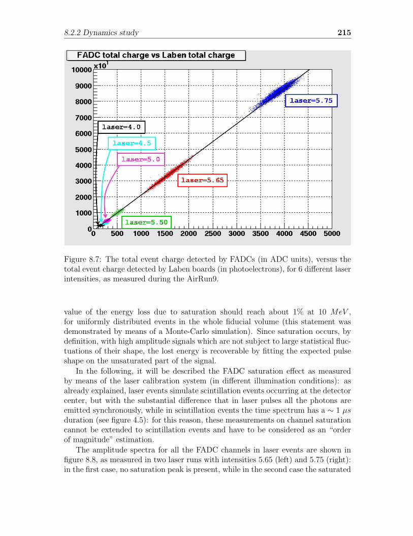
8.2.2 Dynamics study 215
Figure 8.7: The total event charge detected by FADCs (in ADC units), versus thetotal event charge detected by Laben boards (in photoelectrons), for 6 different laserintensities, as measured during the AirRun9.
value of the energy loss due to saturation should reach about 1% at 10 MeV ,for uniformly distributed events in the whole fiducial volume (this statement wasdemonstrated by means of a Monte-Carlo simulation). Since saturation occurs, bydefinition, with high amplitude signals which are not subject to large statistical fluc-tuations of their shape, the lost energy is recoverable by fitting the expected pulseshape on the unsaturated part of the signal.
In the following, it will be described the FADC saturation effect as measuredby means of the laser calibration system (in different illumination conditions): asalready explained, laser events simulate scintillation events occurring at the detectorcenter, but with the substantial difference that in laser pulses all the photons areemitted synchronously, while in scintillation events the time spectrum has a ∼ 1 µsduration (see figure 4.5): for this reason, these measurements on channel saturationcannot be extended to scintillation events and have to be considered as an “orderof magnitude” estimation.
The amplitude spectra for all the FADC channels in laser events are shown infigure 8.8, as measured in two laser runs with intensities 5.65 (left) and 5.75 (right):in the first case, no saturation peak is present, while in the second case the saturated
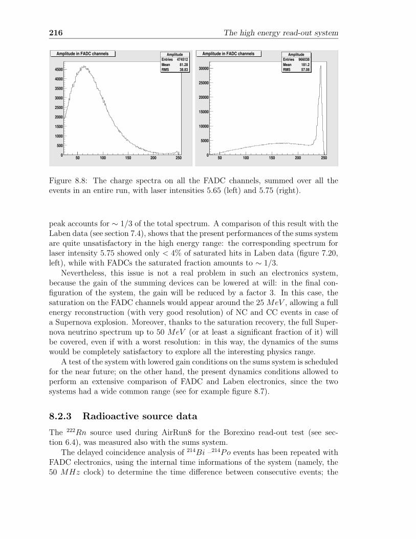
216 The high energy read-out system
AmplitudeEntries 474512Mean 81.28RMS 38.83
50 100 150 200 2500
500
1000
1500
2000
2500
3000
3500
4000
4500
AmplitudeEntries 474512Mean 81.28RMS 38.83
Amplitude in FADC channels AmplitudeEntries 966038Mean 181.2RMS 57.08
50 100 150 200 2500
5000
10000
15000
20000
25000
30000
AmplitudeEntries 966038Mean 181.2RMS 57.08
Amplitude in FADC channels
Figure 8.8: The charge spectra on all the FADC channels, summed over all theevents in an entire run, with laser intensities 5.65 (left) and 5.75 (right).
peak accounts for ∼ 1/3 of the total spectrum. A comparison of this result with theLaben data (see section 7.4), shows that the present performances of the sums systemare quite unsatisfactory in the high energy range: the corresponding spectrum forlaser intensity 5.75 showed only < 4% of saturated hits in Laben data (figure 7.20,left), while with FADCs the saturated fraction amounts to ∼ 1/3.
Nevertheless, this issue is not a real problem in such an electronics system,because the gain of the summing devices can be lowered at will: in the final con-figuration of the system, the gain will be reduced by a factor 3. In this case, thesaturation on the FADC channels would appear around the 25 MeV , allowing a fullenergy reconstruction (with very good resolution) of NC and CC events in case ofa Supernova explosion. Moreover, thanks to the saturation recovery, the full Super-nova neutrino spectrum up to 50 MeV (or at least a significant fraction of it) willbe covered, even if with a worst resolution: in this way, the dynamics of the sumswould be completely satisfactory to explore all the interesting physics range.
A test of the system with lowered gain conditions on the sums system is scheduledfor the near future; on the other hand, the present dynamics conditions allowed toperform an extensive comparison of FADC and Laben electronics, since the twosystems had a wide common range (see for example figure 8.7).
8.2.3 Radioactive source data
The 222Rn source used during AirRun8 for the Borexino read-out test (see sec-tion 6.4), was measured also with the sums system.
The delayed coincidence analysis of 214Bi –214Po events has been repeated withFADC electronics, using the internal time informations of the system (namely, the50 MHz clock) to determine the time difference between consecutive events; the
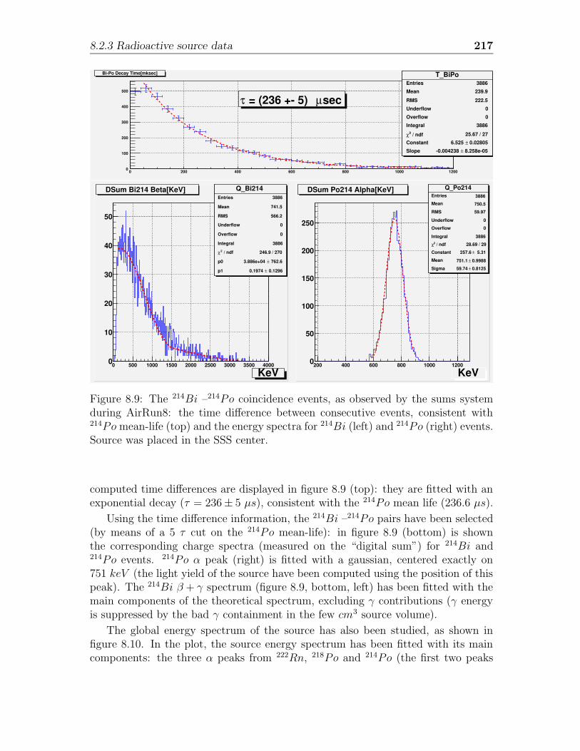
8.2.3 Radioactive source data 217
Q_Bi214Entries 3886
Mean 741.5
RMS 566.2
Underflow 0
Overflow 0
Integral 3886
/ ndf 2χ 246.9 / 270
p0 762.6± 3.886e+04
p1 0.1296± 0.1974
0 500 1000 1500 2000 2500 3000 3500 40000
10
20
30
40
50
Q_Bi214Entries 3886
Mean 741.5
RMS 566.2
Underflow 0
Overflow 0
Integral 3886
/ ndf 2χ 246.9 / 270
p0 762.6± 3.886e+04
p1 0.1296± 0.1974
DSum Bi214 Beta[KeV]
KeV
Q_Po214Entries 3886
Mean 750.5
RMS 59.97
Underflow 0
Overflow 0
Integral 3886
/ ndf 2χ 28.69 / 29
Constant 5.31± 257.6
Mean 0.9988± 751.1
Sigma 0.8125± 59.74
200 400 600 800 1000 12000
50
100
150
200
250
Q_Po214Entries 3886
Mean 750.5
RMS 59.97
Underflow 0
Overflow 0
Integral 3886
/ ndf 2χ 28.69 / 29
Constant 5.31± 257.6
Mean 0.9988± 751.1
Sigma 0.8125± 59.74
DSum Po214 Alpha[KeV]
KeVT_BiPo
Entries 3886
Mean 239.9
RMS 222.5
Underflow 0
Overflow 0
Integral 3886
/ ndf 2χ 25.67 / 27
Constant 0.02805± 6.525
Slope 8.258e-05± -0.004238
0 200 400 600 800 1000 12000
100
200
300
400
500
T_BiPoEntries 3886
Mean 239.9
RMS 222.5
Underflow 0
Overflow 0
Integral 3886
/ ndf 2χ 25.67 / 27
Constant 0.02805± 6.525
Slope 8.258e-05± -0.004238
Bi-Po Decay Time[mksec]
secµ = (236 +- 5) τ
Q_Bi214Entries 3886
Mean 741.5
RMS 566.2
Underflow 0
Overflow 0
Integral 3886
/ ndf 2χ 246.9 / 270
p0 762.6± 3.886e+04
p1 0.1296± 0.1974
0 500 1000 1500 2000 2500 3000 3500 40000
10
20
30
40
50
Q_Bi214Entries 3886
Mean 741.5
RMS 566.2
Underflow 0
Overflow 0
Integral 3886
/ ndf 2χ 246.9 / 270
p0 762.6± 3.886e+04
p1 0.1296± 0.1974
DSum Bi214 Beta[KeV]
KeV
Q_Po214Entries 3886
Mean 750.5
RMS 59.97
Underflow 0
Overflow 0
Integral 3886
/ ndf 2χ 28.69 / 29
Constant 5.31± 257.6
Mean 0.9988± 751.1
Sigma 0.8125± 59.74
200 400 600 800 1000 12000
50
100
150
200
250
Q_Po214Entries 3886
Mean 750.5
RMS 59.97
Underflow 0
Overflow 0
Integral 3886
/ ndf 2χ 28.69 / 29
Constant 5.31± 257.6
Mean 0.9988± 751.1
Sigma 0.8125± 59.74
DSum Po214 Alpha[KeV]
KeVT_BiPo
Entries 3886
Mean 239.9
RMS 222.5
Underflow 0
Overflow 0
Integral 3886
/ ndf 2χ 25.67 / 27
Constant 0.02805± 6.525
Slope 8.258e-05± -0.004238
0 200 400 600 800 1000 12000
100
200
300
400
500
T_BiPoEntries 3886
Mean 239.9
RMS 222.5
Underflow 0
Overflow 0
Integral 3886
/ ndf 2χ 25.67 / 27
Constant 0.02805± 6.525
Slope 8.258e-05± -0.004238
Bi-Po Decay Time[mksec]
secµ = (236 +- 5) τFigure 8.9: The 214Bi –214Po coincidence events, as observed by the sums systemduring AirRun8: the time difference between consecutive events, consistent with214Pomean-life (top) and the energy spectra for 214Bi (left) and 214Po (right) events.Source was placed in the SSS center.
computed time differences are displayed in figure 8.9 (top): they are fitted with anexponential decay (τ = 236± 5 µs), consistent with the 214Po mean life (236.6 µs).
Using the time difference information, the 214Bi –214Po pairs have been selected(by means of a 5 τ cut on the 214Po mean-life): in figure 8.9 (bottom) is shownthe corresponding charge spectra (measured on the “digital sum”) for 214Bi and214Po events. 214Po α peak (right) is fitted with a gaussian, centered exactly on751 keV (the light yield of the source have been computed using the position of thispeak). The 214Bi β + γ spectrum (figure 8.9, bottom, left) has been fitted with themain components of the theoretical spectrum, excluding γ contributions (γ energyis suppressed by the bad γ containment in the few cm3 source volume).
The global energy spectrum of the source has also been studied, as shown infigure 8.10. In the plot, the source energy spectrum has been fitted with its maincomponents: the three α peaks from 222Rn, 218Po and 214Po (the first two peaks
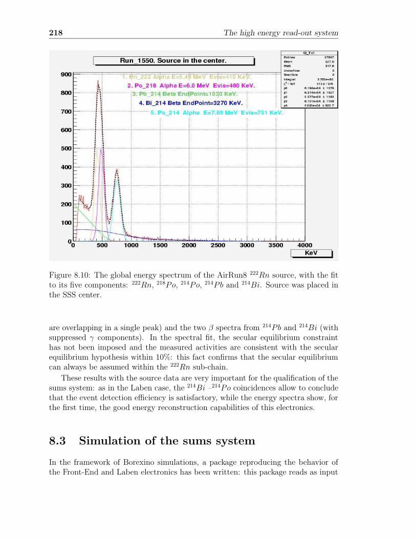
218 The high energy read-out system
Figure 8.10: The global energy spectrum of the AirRun8 222Rn source, with the fitto its five components: 222Rn, 218Po, 214Po, 214Pb and 214Bi. Source was placed inthe SSS center.
are overlapping in a single peak) and the two β spectra from 214Pb and 214Bi (withsuppressed γ components). In the spectral fit, the secular equilibrium constrainthas not been imposed and the measured activities are consistent with the secularequilibrium hypothesis within 10%: this fact confirms that the secular equilibriumcan always be assumed within the 222Rn sub-chain.
These results with the source data are very important for the qualification of thesums system: as in the Laben case, the 214Bi –214Po coincidences allow to concludethat the event detection efficiency is satisfactory, while the energy spectra show, forthe first time, the good energy reconstruction capabilities of this electronics.
8.3 Simulation of the sums system
In the framework of Borexino simulations, a package reproducing the behavior ofthe Front-End and Laben electronics has been written: this package reads as input

8.3 Simulation of the sums system 219
the data produced by the general Borexino simulation codes4 and transforms theminto a real data structure, identical to the one produced by the DAQ system. Notonly the basic performances of the electronics are reproduced by the simulation, butalso all its known “non ideal” behaviors.
In order to compare correctly the results from FADC and Laben electronics, isvery important to have a common simulation of the two electronics. The additionof the sums system to the general Borexino electronics simulation, is in principle asimple operation, because the package is based in an Object Oriented design andis written in C++: by definition, this technology guarantees a simple and safeintegration of new functionalities in the code.
The main components of the sums electronics which need to be simulated are:
1. the summed signals, in groups of 16 or 24 PMTs (depending on the mapping),and also the total sum on 2212 PMTs;
2. the digitization procedure (i.e. the output of the FADC channels, includingthe noise on channel and the pedestal generation);
3. the behavior of the zero suppression algorithm;
4. other signals present in the system, such as the attenuated sum and the triggerramp.
In the Borexino electronics simulation, a “channel” is an object (in the C++sense) performing 3 main operations: it can receive a photoelectron; it triggers(when detector is triggered); it writes event on the file. The same implementationhas been chosen for the “fadc channel” object: each of the simulated FADC channelsowns a list of the frontend hits produced in the associated PMTs (16,24,2214); thislist represents the interface of the channel to the main detector object.
In the code logic, the operations requested to the FADC channels are performedin the following way:
1. receiving a photoelectron means that a new frontend hit is added to the internallist of frontend hits (of course, only photoelectrons produced in the associatedPMTs can be received by a FADC channel);
2. when the channel is triggered, the frontend hit list is transformed into a dig-itized signal; this operation consists of five steps: hits are ordered in time; asimple shape is simulated for each hit; the shape of the single hit is dividedinto the 2.5 ns bins; hits are summed, to obtain total signal; for each bin, thetotal signal is converted into an integer number (from 1 to 255).
4Two simulation programs have been written for Borexino: a fast one, FORTRAN based, anda more complex one, based on the GEANT4 package from CERN.
220 The high energy read-out system
3. the procedure for writing events to file reproduces the behavior of the zerosuppression algorithm (for this reason, the total sum is processed first); toguarantee the most realistic result, this step is performed by a code identicalto the one running in the FADC on-line program (it has just been “re-coded”in C++). The noise and pedestal informations are generated (for each of thefour ADCs in the channel) only inside the windows (it would have been uselessto generate noise in the preceding step in order to rejected it now5).
This simulation code has been written and is in its test phase: in particular, theparameters of the code, such as the gains, pedestals and noise are undergoing a fineregulation based on real data. When the project will be finished, it will providea powerful tool for understanding the FADC data and for comparison with Labenresults.
5A similar strategy has been chosen for the Laben section: the dark noise hits on each PMTare generated only inside the trigger gate.
Conclusions
In this thesis, the characterization and calibration of the Borexino detector havebeen performed, both for sub-MeV solar neutrino detection, and for detection ofthe high energy neutrinos emitted during Supernova events.
The CTF-3 measurement campaign (focussed on the assessment of the scintillatorproperties) is described: during this campaign, several purification methods havebeen tested on the scintillator and showed encouraging results. A detailed dataanalysis of the different purification tests is presented in this work, concerning theeffectiveness of the methods in removing from the scintillator the most dangerouscontaminants for Borexino.
The Borexino detector has been operated at the performance level demandedby physics and its overall capabilities have been carefully studied. The read-outsystem of the experiment has been completed, finalized and fully tested in realisticoperation conditions; these tests happened during the 9 “Air-Runs”: several runconfigurations were applied, allowing a global study of the system performances, aswell as an accurate debugging on a single channel basis (both on the electronics andon the photomultipliers).
The PMT calibration system has been thoroughly tested, providing the assess-ment of the time measurement precision of the complete read-out system, along withan estimation of the final time resolution of the detector. Several runs have also beenperformed through the insertion of some radioactive sources in the Borexino sphere:these measurements represented a realistic test of our read-out system in operatingconditions. In this way, the behavior of the complete chain was analyzed, showingvery good global performances.
In particular, the energy and position reconstruction capabilities of the detectorhave been evaluated, demonstrating that the system is ready and operational forBorexino data taking: the good performances of the read-out chain will allow theneutrino signal identification in a wide energy range and the measurement of the7Be neutrino flux.
221

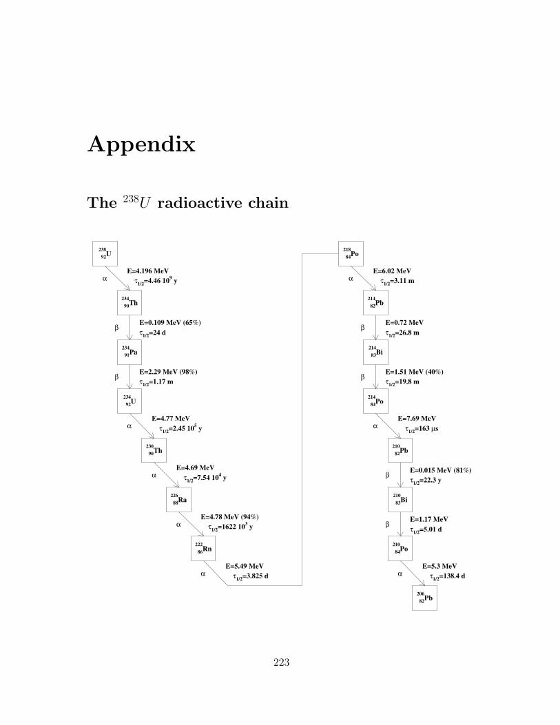
Appendix
The 238U radioactive chain
23892U
23490Th
23491Pa
23492U
23090Th
22688Ra
22286Rn
21884Po
21482Pb
21483Bi
21484Po
21082Pb
21083Bi
21084Po
20682Pb
α
β
β
α
α
α
α
α
β
β
α
β
β
α
E=4.196 MeVτ1/2=4.46 109 y
E=0.109 MeV (65%)τ1/2=24 d
E=2.29 MeV (98%)τ1/2=1.17 m
E=4.77 MeVτ1/2=2.45 105 y
E=4.69 MeVτ1/2=7.54 104 y
E=4.78 MeV (94%)τ1/2=1622 103 y
E=5.49 MeVτ1/2=3.825 d
E=6.02 MeVτ1/2=3.11 m
E=0.72 MeVτ1/2=26.8 m
E=1.51 MeV (40%)τ1/2=19.8 m
E=7.69 MeVτ1/2=163 µs
E=0.015 MeV (81%)τ1/2=22.3 y
E=1.17 MeVτ1/2=5.01 d
E=5.3 MeVτ1/2=138.4 d
223
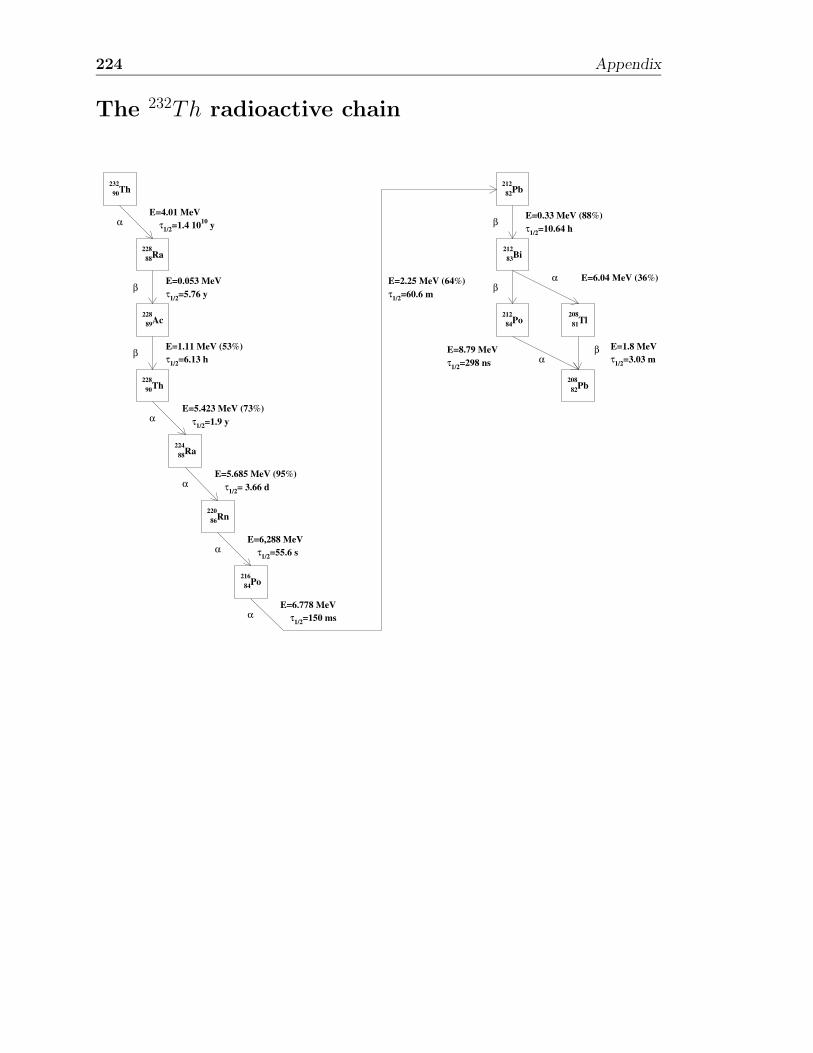
224 Appendix
The 232Th radioactive chain
23290Th
22888Ra
22889Ac
22890Th
22488Ra
22086Rn
21684Po
21282Pb
21283Bi
21284Po
20881Tl
20882Pb
αE=4.01 MeV
τ1/2=1.4 1010 y
βE=0.053 MeVτ1/2=5.76 y
βE=1.11 MeV (53%)τ1/2=6.13 h
αE=5.423 MeV (73%)
τ1/2=1.9 y
αE=5.685 MeV (95%)
τ1/2= 3.66 d
αE=6,288 MeV
τ1/2=55.6 s
αE=6.778 MeV
τ1/2=150 ms
βE=0.33 MeV (88%)τ1/2=10.64 h
βE=2.25 MeV (64%)τ1/2=60.6 m
αE=8.79 MeVτ1/2=298 ns
α E=6.04 MeV (36%)
β E=1.8 MeVτ1/2=3.03 m

Bibliography
[1] J.N. Abdurashitov et al. [SAGE Collaboration], J. Exp. Theor. Phys. 95, 181(2002).
[2] Q.R. Ahmad et al. [SNO Collaboration], Phys. Rev. Lett. 87, 071301 (2001).
[3] Q.R. Ahmad et al. [SNO Collaboration], Phys. Rev. Lett. 89, 011301 (2002).
[4] S.N. Ahmed et al. [SNO Collaboration], Phys. Rev. Lett. 92, 181301 (2004).
[5] G. Alimonti et al. [Borexino Collaboration], A large-scale low background liquidscintillator detector: the counting test facility at Gran Sasso, Nucl. Instrum.Meth. A 406, 411 (1998).
[6] G. Alimonti et al. [Borexino Collaboration], Light propagation in a large volumeliquid scintillator, Nucl. Instrum. Meth. A 440, 360 (2000).
[7] G. Alimonti et al. [Borexino Collaboration], Measurement of the C-14 abun-dance in a low-background liquid scintillator, Phys. Lett. B 422, 349 (1998).
[8] G. Alimonti et al. [Borexino Collaboration], Science and technology of Borexino:A real time detector for low energy solar neutrinos, Astropart. Phys. 16, 205(2002).
[9] G. Alimonti et al. [Borexino Collaboration], Ultra-low background measurementsin a large volume underground detector, Astropart. Phys. 8, 141 (1998).
[10] C. Arpesella et al. [BOREXINO Collaboration], Measurements of extremely lowradioactivity levels in BOREXINO, Astropart. Phys. 18, 1 (2002).
[11] M. Apollonio et al. [CHOOZ Collaboration], Phys. Lett. B 420, 397 (1998).
[12] M. Apollonio et al. [CHOOZ Collaboration], Phys. Lett. B 466, 415 (1999).
[13] T. Araki et al. [KamLAND Collaboration], arXiv:hep-ex/0406035 (2004).
[14] K. Assamagan et al., Phys. Rev. D 53, 6065 (1996).
225

226 BIBLIOGRAPHY
[15] H.O. Back et al. [Borexino Collaboration], New limits on nucleon decays intoinvisible channels with the BOREXINO Counting Test Facility Phys. Lett. B563, 23 (2003).
[16] H.O. Back et al. [Borexino Collaboration], Phenylxylylethane (PXE): A high-density, high-flashpoint organic liquid scintillator for applications in low-energyparticle and astrophysics experiments, arXiv:physics/0408032.
[17] H.O. Back et al. [Borexino Collaboration], Study of the neutrino electromagneticproperties with prototype of Borexino detector, Phys. Lett. B 563, 35 (2003).
[18] J.N. Bahcall, Astrophys. J. 467 475 (1996).
[19] J.N. Bahcall, Nucl. Phys. B (Proc. Suppl.) 118, 77 (2003).
[20] J.N. Bahcall, M.C. Gonzalez-Garcia, C. Pena-Garay, JHEP 0207, 054 (2002).
[21] J.N. Bahcall, M.C. Gonzalez-Garcia, C. Pena-Garay, Phys. Rev. Lett. 90,131301 (2003).
[22] J.N. Bahcall, P.I. Krastev, A.Y. Smirnov, JHEP 0105, 015 (2001).
[23] J.N. Bahcall, M.H. Pinsonneault, Phys. Rew. Lett. 92, 121301 (2004).
[24] J.N. Bahcall, M.H. Pinsonneault, S.Basu, Astrophys. J. 555, 990 (2001).
[25] R. Barate et al. [ALEPH Collaboration], Eur. Phys. J. C 2, 395 (1998).
[26] J.F. Beacom, W.M. Farr, P. Vogel, Phys. Rev. D 66, 033001 (2002).
[27] J.F. Beacom, P. Vogel, Phys. Rev. D 58, 093012 (1998).
[28] J.F. Beacom, P. Vogel, Phys. Rev. D 58, 053010 (1998).
[29] R.M. Bionta et al., Phys. Rev. Lett. 58, 1494 (1987).
[30] F. Boehm et al., Phys. Rev. D 64, 112001 (2001).
[31] J. Boger et al. [SNO Collaboration], Nucl. Instrum. Meth. A 449, 172 (2000).
[32] J. Bonn et al., Nucl. Phys. Proc. Suppl. 91, 273 (2001).
[33] B. Caccianiga et al., A multiplexed optical-fiber system for the PMT calibrationof the Borexino experiment, Nucl. Instrum. Meth. A 496, 353 (2003).
[34] L. Cadonati, The Borexino Solar Neutrino Experiment and its Scintillator Con-tainment Vessel, Ph. D. Thesis, Princeton University (2001), UMI-99-93687.
[35] L. Cadonati, F.P. Calaprice, M.C. Chen, Supernova neutrino detection inBorexino, Astropart. Phys. 16, 361 (2002).

BIBLIOGRAPHY 227
[36] C. Cattadori, talk given at Neutrino 2004 conference, 14-19 June 2004, Paris.
[37] M. Chen et al., Nucl. Instrum. Meth. A 420, 189 (1999).
[38] B.T. Cleveland et al., Astrophys. J. 496, 505 (1998).
[39] R.J. Davis, D.S. Harmer, K.C. Hoffman, Phys. Rev. Lett. 20, 1205 (1968).
[40] K. Eguchi et al. [KamLAND Collaboration], Phys. Rev. Lett. 90, 021802 (2003).
[41] K. Eguchi et al. [KamLAND Collaboration], Phys. Rev. Lett. 92, 071301 (2004).
[42] S. Eidelman et al. [Particle Data Group Collaboration], Phys. Lett. B 592, 1(2004).
[43] K. Eitel, eConf C020620 SAAT03, arXiv:hep-ex/0209019 (2002).
[44] B. Faid et al., Astropart. Phys. 10, 93 (1999).
[45] G.L. Fogli et al., Phys. Rev. D 66, 093008 (2002).
[46] D. Franco, The Borexino Experiment: Test of the Purification Systems by theCounting Test Facility, Ph. D. Thesis, Universita degli Studi di Milano (2005).
[47] Y. Fukuda et al. [Kamiokande Collaboration], Phys. Rev. Lett. 77, 1683 (1996).
[48] Y. Fukuda et al. [Super-Kamiokande Collaboration], Phys. Lett. B 436, 33(1998).
[49] Y. Fukuda et al. [Super-Kamiokande Collaboration], Phys. Rev. Lett. 81, 1562(1998).
[50] Y. Fukuda et al. [Super-Kamiokande Collaboration], Phys. Rev. Lett. 82, 2644(1999).
[51] S. Fukuda et al. [Super-Kamiokande Collaboration], Phys. Rev. Lett. 86, 5651(2001).
[52] E. Gatti and F. De Martini, A new linear method of discrimination betweenelementary particles in scintillation counters, IAEA Wien, pp.265-276 (1962).
[53] F. Gatti et al., Nucl. Instrum. Meth. A 461, 474 (2001).
[54] F. Gatti et al. [BOREXINO Collaboration], Nucl. Phys. Proc. Suppl. 78, 111(1999).
[55] G. Gelmini, E. Roulet, Rept. Prog. Phys, 58 1207 (1995).
[56] A. Goretti, P. Lombardi and G. Ranucci, Pulse Shape Discrimination of liquidscintillators, Nucl. Instr. Meth. A, 412, 374 (1998).

228 BIBLIOGRAPHY
[57] T. Hagner et al., Astropart. Phys. 14, 33 (2000).
[58] W. Hampel et al. [GALLEX Collaboration], Phys. Lett. B 447, 127 (1999).
[59] W. Hampel et al. [GALLEX Collaboration], Phys. Lett. B 420, 114 (1998).
[60] G. Heusser et al., Appl. Rad. Isot. 52, 691 (2000).
[61] K. Hirata et al. [KAMIOKANDE-II Collaboration], Phys. Rev. Lett. 58, 1490(1987).
[62] K. Ishihara, Nucl. Instrum. Meth. A 503, 144 (2003).
[63] T. Ishii [K2K Collaboration], arXiv:hep-ex/0406055.
[64] M. Ishitsuka et al. [Super-Kamiokande Collaboration], hep-ex/0406076 (2004).
[65] H.V. Klapdor-Kleingrothaus et al., Mod. Phys. Lett. A 16, 2409 (2001).
[66] V. Lagomarsino and G. Testera, Nucl. Instrum. Meth. A 430, 435 (1999).
[67] V.M. Lobashev et al., Nucl. Phys. Proc. Suppl. 91, 280 (2001).
[68] F. Mantovani et al., Phys. Rev. D 69, 013001 (2004).
[69] D. Manuzio, Towards the detection of subMeV solar neutrinos in Borexino:data reconstruction and analysys tools, Ph. D. Thesis, Universita degli Studi diGenova (2004).
[70] S.P. Mikheev, A.Y. Smirnov, Sov. J. Nucl. Phys. 42, 913 (1985).
[71] M.E. Monzani, Metodi di identificazione delle particelle α/β in grandi volumidi scintillatore liquido, per la reiezione del fondo radioattivo nell’esperimentoBorexino, Tesi di Laurea, Universita degli Studi di Milano (2001).
[72] R. D. Peccei, AIP Conf. Proc. 490, 80 (1999).
[73] A.P. Pocar, Low background techniques and experimental challenges for Borex-ino and its nylon vessels, Ph. D. Thesis, Princeton University (2003), UMI-31-03047.
[74] B. Pontecorvo, Sov. Phys. JETP 26, 984 (1968).
[75] R.S. Raghavan et al., Phys. Rev. Lett. 80, 635 (1998).
[76] G. Ranucci et al., A sampling board optimized for pulse shape discriminationin liquid scintillator applications, Ieee Trans. Nucl. Sci. 51, 1784 (2004).

BIBLIOGRAPHY 229
[77] G. Ranucci et al, Scintillation decay time and pulse shape discrimination ofbinary organic liquid scintillators for the Borexino detector, Nucl. Instr. Meth.A, 350, 338 (1994).
[78] W. Rau, G. Heusser, Appl. Rad. Isot. 53, 371 (2000).
[79] The Royal Swedish Academy of Sciences, Press Release: The 2002 Nobel Prizein Physics (2002).
[80] R. Saakian [MINOS Collaboration], Phys. Atom. Nucl. 67, 1084 (2004).
[81] D.N. Schramm, Comments Nucl. Part. Phys. 17, 239 (1987).
[82] M. Schwarzschild, Structure and Evolution of the Stars, Princeton UniversityPress, 1958.
[83] D.N. Spergel et al. [WMAP Collaboration], Astrophys. J. Suppl. 148, 175(2003).
[84] G. ‘t Hooft, Phys. Lett. B 37, 195 (1971).
[85] S. Turck-Chieze and I. Lopes, Astrophys. J. 408, 347 (1993).
[86] S. Turck-Chieze et al., Phys. Rev. Lett. 93, 211102 (2004).
[87] L. Wolfenstein, Phys. Rev. D 17, 2369 (1978).