RAPPORT DE RECHERCHE :

Séquestration des gaz à effet de serre,

compétitivité relative des énergies primaires et diversité de leurs usages

Présenté par

L’INSTITUT D’ECONOMIE INDUSTRIELLE (IDEI)

Université de Toulouse 1 Capitole Manufacture des Tabacs – Bât F

Aile Jean-Jacques Laffont 21 allée de Brienne

31000 Toulouse

au

CONSEIL FRANÇAIS DE L’ENERGIE (CFE)

12 rue de Saint-Quentin 75010 Paris

Avril 2012

Contrat CFE - 70

Avant-propos Ce document est le rapport de recherche présenté par l’IDEI conformément aux dispositions du contrat CFE – 70 : « Séquestration des gaz à effet de serre, compétitivité relative des énergies primaires et diversité de leurs usages ».

1

Séquestration des gaz à effet de serre, compétitivité relative des énergies

primaires et diversité de leurs usages

Rapport de recherche

Michel Moreaux, Toulouse School of Economics (LERNA, IDEI)

Jean-Pierre Amigues, Toulouse School of Economics (LERNA, INRA)

Gilles Lafforgue, Toulouse School of Economics (LERNA, INRA)

Avril 2012

2

SOMMAIRE

SYNTHESE DE LA RECHERCHE .................................................................................................... 3

1 INTRODUCTION ............................................................................................................................... 6

2 STRUCTURE COMMUNE AUX DIFFERENTS MODELES DEVELOPPES ........................... 8

3 RESULTATS DE LA RECHERCHE ............................................................................................. 11

3.1 Rappel des résultats du modèle initial .................................................................................. 11

3.2 Hétérogénéité des usagers .................................................................................................... 12

3.3 Structures alternatives des fonctions de coût de CSC ....................................................... 15

3.4 Progrès technique drastique, apprentissage et R&D ......................................................... 18

4 CONCLUSION ................................................................................................................................. 20

REFERENCES .................................................................................................................................... 22

ANNEXES ............................................................................................................................................ 24

3

SYNTHESE DE LA RECHERCHE

Parmi les nombreux facteurs qui déterminent la compétitivité des énergies carbonées fossiles par rapport à d’autres sources d’énergie, en particulier l’énergie nucléaire et les énergies renouvelables réputées propres, un facteur clé est la possibilité de maîtriser à coûts raisonnables les rejets de gaz à effet de serre qu’implique leur utilisation massive.

Les deux premières études annexées au présent rapport supposent donnée cette possibilité et caractérisent les sentiers d’exploitation optimale de ce type de ressource et les politiques de capture et de séquestration qui en résultent. La troisième étude est un essai de définition des politiques qu’il conviendrait de promouvoir pour obtenir les coûts raisonnables supposés déjà acquis dans les deux premiers essais.

Le plus simple pour aller à l’essentiel est de retenir comme modèle des dommages induits par la concentration atmosphérique de gaz à effet de serre le modèle dit « modèle à plafond » dans lequel les dommages en question sont « minimes » tant qu’un seuil critique de concentration n’a pas été dépassé mais sont incommensurablement élevés dès que ce seuil est franchi. Dans ce type de modèle, puisque les ressources carbonées fossiles sont abondantes et d’un coût de mobilisation relativement modeste, la contrainte de non-franchissement est nécessairement active. Dès lors la date à partir de laquelle la contrainte en question restreint la consommation d’énergie fossile et oblige peut-être à recourir aux moyens de capture et de séquestration apparaît comme une date phare. Le problème est alors de savoir s’il faut mobiliser ces moyens avant la date phare en question ou attendre d’être contraint. Une interprétation large du principe de précaution suggèrerait qu’il ne faudrait pas trop attendre, c’est-à-dire qu’il ne faudrait pas attendre d’être contraint.

Les deux premiers essais démontrent qu’une politique active de séquestration ne doit être mise en œuvre avant d’avoir atteint le seuil critique de concentration que dans deux cas :

- lorsque les possibilités de capture, et donc leurs coûts moyens, sont différents selon l’usage des ressources ;

- lorsque ces possibilités de capture sont les mêmes quels qu’en soient les usages, le coût moyen de capture dépendant alors du flux de rejets à traiter.

Un résultat fort de notre recherche est de montrer que dans ce dernier cas, même lorsque le coût moyen de capture décroît avec l’expérience accumulée dans cette activité et donc qu’on pourrait être tenté de croire qu’il faille démarrer assez tôt

4

la politique de séquestration, il faut toujours attendre d’être au plafond pour commencer à capturer.

La diversité des structures des sentiers optimaux de substitution entre énergies carbonées fossiles et énergies renouvelables propres selon que la ressource fossile est plus ou moins abondante et que l’effet d’apprentissage, bien que dominant, est plus ou moins prégnant est un second résultat de la recherche qui mérite d’être d’autant plus souligné qu’il n’était pas attendu. Lorsque les effets d’apprentissage sont si faibles que, le stock des rejets capturés et séquestrés augmentant, le coût moyen de capture et de séquestration lui-même augmente, nous montrons qu’il n’y a plus alors qu’un seul type de sentier optimal, à quelques variations mineures près.

Pouvoir disposer de techniques de capture et de séquestration à des coûts raisonnables n’est pas un don du Ciel, mais le fruit soit de l’expérience, soit d’efforts de recherche conséquents, soit d’une conjugaison des deux.

La recherche présente deux avantages par rapport à l’apprentissage. Elle évite de mettre en œuvre trop tôt une technologie de coût initial par hypothèse excessivement élevé tant que l’on n’a pas suffisamment appris. Elle permet aussi l’exploration d’un éventail beaucoup plus large d’options techniques. Le troisième essai s’attache à préciser d’abord les politiques optimales permettant une percée technologique, une réduction drastique des coûts d’abattement, qui ne reposeraient que sur l’un ou l’autre des leviers permettant de la déclencher en supposant que chacun de ces leviers puisse être assez puissant pour provoquer un tel bouleversement des coûts.

Une pure politique de recherche devrait faire en sorte que la percée technologique a lieu lorsque la contrainte de plafond commence à restreindre la consommation d’énergie polluante et pas avant. Il ne sert à rien de disposer dès aujourd’hui d’une technologie que l’on n’aura à mettre en œuvre que demain. Mais il faut noter que la date à laquelle les effets de cette contrainte doivent être pris en compte est elle-même endogène.

Une mobilisation optimale des possibilités d’apprentissage suppose de combiner un prix des rejets dans l’atmosphère à une subvention en faveur de l’utilisation de technologies de dépollution. Tel n’est pas le cas lorsque la percée est obtenue par la R&D seule. La taxation des émissions est alors suffisante pour induire des efforts optimaux de recherche.

La possibilité de combiner apprentissage à partir des technologies initialement existantes et efforts de recherche conduit à élargir considérablement la perspective. L’accumulation du carbone dans l’atmosphère et le développement de technologies d’atténuation des émissions apparaissent alors comme deux processus dynamiques en interaction avec leurs propres logiques et contraintes. On montre ainsi qu’il est possible qu’il faille introduire l’abattement avant d’atteindre le plafond. On montre

5

aussi que les politiques optimales de mobilisation combinée peuvent initialement s’appuyer uniquement sur de l’apprentissage ou uniquement sur des efforts de recherche. Dans des scénarios où il convient de recourir simultanément à la recherche et à l’apprentissage pour provoquer une percée technologique, on montre enfin que l’effort d’apprentissage doit croître à un rythme plus soutenu que celui des efforts de recherche. Ces derniers en effet ne produisent de résultats qu’au moment de la percée, ce qui n’est pas le cas des efforts d’apprentissage, l’abattement de la pollution qu’ils permettent contribuant à réduire le poids de la contrainte climatique.

6

1 INTRODUCTION

Les ressources carbonées fossiles sont des énergies primaires abondantes dont la mobilisation permet à la plupart d’entre elles de satisfaire les besoins en services énergétiques des usagers à des coûts relativement modestes. Leur compétitivité par rapport à d’autres ressources primaires, en particulier l’énergie nucléaire et ses différentes filières et les énergies renouvelables qui exploitent à court terme l’énergie solaire incidente, énergies réputées propres, semblerait donc assurée1. Cette perspective de développement risque cependant d’être compromise par les rejets conséquents de gaz à effet de serre (GES) qu’implique leur utilisation massive, gaz dont l’accumulation dans l’atmosphère, dès lors qu’elle est trop forte, peut déclencher des dommages difficilement supportables. Par difficilement supportable, il faut comprendre que les coûts qu’induit cette concentration sont sans commune mesure avec les bénéfices tirés de la consommation d’énergie fossile dont elle est issue.

Pour contourner un handicap qui serait susceptible de s’avérer à terme dirimant, un facteur clé est la possibilité de maîtriser à coûts raisonnables les rejets de GES qu’implique l’exploitation soutenue de ces ressources fossiles. Le GES d’origine anthropique le plus important est le CO2 puisqu’il représente à lui seul entre 72 et 76% des émissions totales. L’un des moyens envisagés pour réduire ces rejets de CO2 dans l’atmosphère est le captage et la séquestration géologique du carbone (CSC), solution préconisée par le GIEC (Groupe d’Experts Intergouvernemental sur l’Evolution du Climat) dans un rapport dédié à cette technologie (IPCC, 2005). Sans entrer dans les détails techniques, qui font par ailleurs l’objet d’une abondante littérature spécialisée, ce procédé d’abattement consiste à capter à la source les émissions de composés carbonées avant rejet dans l’atmosphère et à les injecter ensuite dans des réservoirs naturels, des aquifères salins par exemple, ou dans d’anciens sites miniers ou encore dans des gisements d’hydrocarbures soit actifs, soit éteints2.

Les études empiriques visant à évaluer le potentiel de cette technologie sont relativement nombreuses et sont, le plus souvent, réalisées au moyen de modèles complexes d’évaluation intégrée (Edmonds et al., 2004, Hamilton et al., 2009, Kurosawa, 2004, Gerlagh and van der Zwaan, 2006, Grimaud et al., 2011). Cette complexité apparaît comme le prix à payer pour pouvoir disposer de modèles opérationnels et suffisamment précis pour pouvoir définir des politiques énergétiques 1 Près de 85% de l’énergie commerciale provient aujourd’hui des trois principales sources d’énergie fossile carbonée : charbon, pétrole et gaz naturel (IPCC, 2007). 2 Cependant, comme le fait remarquer Herzog (2011), les préoccupations à propos du changement climatique ne sont pas à l’origine de cette idée de séparer et de capturer le CO2 des rejets provenant des centrales thermiques. Les premières unités de CSC construites aux Etats-Unis dans les années 70 avaient pour but d’améliorer le rendement de l’extraction des puits en cours d’exploitation, puits dont la pression peut être augmentée grâce à l’injection des émissions de CO2 ainsi captées.

7

et d’abattement. Mais la multitude des rétroactions à l’œuvre dans de tels modèles tend le plus souvent à brouiller les lignes de force le long desquelles ces politiques devraient se déployer. De plus, du fait de cette complexité, ces modèles sont réduits à prendre comme données nombre de paramètres, pour certains essentiels dans l’explication de ces politiques. Pour marquer ces lignes de force et pour endogénéiser autant que faire se peut ces paramètres, un modèle théorique plus épuré se révèle plus approprié. Le développement d’un tel modèle constitue l’objet de la recherche présentée dans ce rapport.

Le modèle sur lequel notre recherche est fondée est issu des travaux de Lafforgue, Magné et Moreaux (2008-a et 2008-b), qui constituent eux-mêmes une extension du modèle séminal de Chakravorty, Magné et Moreaux (2006), et tiennent compte du fait que les capacités de stockage des rejets capturés ne sont pas illimitées. Les objectifs de ces travaux sont premièrement de déterminer quand et à quelle échelle la CSC doit être utilisée et, deuxièmement, de déterminer comment le recours à ce mode d’abattement du flux d’émission modifie le sentier optimal de consommation des ressources carbonées fossiles, et ce, lorsque la concentration atmosphérique en carbone ne doit pas dépasser un certain seuil jugé critique, ce qui est l’objectif déclaré de l’accord de Kyoto.

Les trois extensions que nous proposons ont pour objet d’identifier les facteurs économiques qui déterminent les coûts d’utilisation de la CSC, et qui régissent de ce fait la compétitivité relative des énergies non-renouvelables carbonées par rapport aux énergies renouvelables non émettrices de CO2.

Les deux premières études supposent ce coût donné et caractérisent les sentiers d’exploitation optimale des deux types d’énergie ainsi que les politiques de séquestration qui en résultent. La première étude considère un coût moyen de séquestration constant, mais prend en compte le fait que les capacités de déploiement de la CSC dépendent des secteurs d’usages dans lesquels elles sont mises en œuvre. Il semble en effet évident que capter les rejets d’une centrale thermique au gaz sera moins coûteux que capter les rejets d’un parc de véhicules fonctionnant grâce à cette même source d’énergie.

Dans la deuxième étude, nous envisageons différentes configurations de structure du coût moyen de séquestration. Ce coût moyen peut dépendre soit du flux de rejets à traiter, soit du cumul de ces rejets, soit enfin des deux. Le coût moyen de capture peut être soit une fonction croissante du cumul des rejets séquestrés afin de rendre compte de la rareté des sites d’enfouissement les plus accessibles, et donc les moins coûteux, soit une fonction décroissante de ce même cumul grâce aux effets d’apprentissage dont bénéficie le secteur au fur et à mesure qu’il déploie la technologie de capture en question.

Enfin, la troisième étude est un essai de définition des politiques qu’il conviendrait de promouvoir pour obtenir les coûts raisonnables supposés déjà acquis dans les deux premiers essais. En effet, pouvoir disposer d’un dispositif de CSC à

8

des coûts non prohibitifs n’est pas un don du Ciel, mais le fruit soit de l’expérience, soit d’efforts de recherche conséquents, soit d’une conjugaison des deux. Cet essai s’attache d’abord à préciser les politiques optimales permettant une percée technologique dans le secteur de la CSC, i.e. une réduction drastique du coût d’abattement, qui ne reposeraient que sur l’un ou l’autre des leviers permettant de la déclencher. Elle envisage ensuite la possibilité de combiner apprentissage à partir des technologies initialement existantes et effort de recherche pour réaliser la dite percée.

Le rapport est organisé comme suit. Les hypothèses communes aux différents modèles développés ainsi que les grandes lignes de leurs principes de fonctionnement sont exposés dans la section 2. Les résultats du modèle initial et ceux des trois extensions que nous proposons font l’objet de la section 3. En particulier on compare les différents scénarios de mise en place des politiques d’exploitation des différents types d’énergie et d’abattement obtenues dans les trois cas. Enfin dans la dernière section nous présentons la façon dont nous comptons valoriser les fruits de cette recherche.

2 STRUCTURE COMMUNE AUX DIFFERENTS MODELES DEVELOPPES

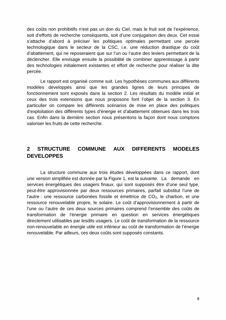
La structure commune aux trois études développées dans ce rapport, dont une version simplifiée est donnée par la Figure 1, est la suivante. La demande en services énergétiques des usagers finaux, qui sont supposés être d’une seul type, peut-être approvisionnée par deux ressources primaires, parfait substitut l’une de l’autre : une ressource carbonées fossile et émettrice de CO2, le charbon, et une ressource renouvelable propre, le solaire. Le coût d’approvisionnement à partir de l’une ou l’autre de ces deux sources primaires comprend l’ensemble des coûts de transformation de l’énergie primaire en question en services énergétiques directement utilisables par lesdits usagers. Le coût de transformation de la ressource non-renouvelable en énergie utile est inférieur au coût de transformation de l’énergie renouvelable. Par ailleurs, ces deux coûts sont supposés constants.

9

Usagers

Stocks de ressources

fossiles

Flux de ressources

renouvelables

Stocks de polluant capturé

et séquestré

Stock de polluant atmosphérique

Stocks naturels de polluant (océans, etc.)

Surplus net des usagers

autorégénération

flux de

polluant

production de services énergétiques

Figure 1 : La structure commune des modèles

L’exploitation de la ressource fossile carbonée génère des flux de rejets de CO2 qui s’accumulent dans l’atmosphère. Une partie de ces gaz accumulés est progressivement éliminée par régénération naturelle3, la partie restante est source de dommages pour les usagers. Cependant, possibilité est donnée à ces usagers de réduire leur empreinte carbone en capturant et en séquestrant tout ou partie de leurs émissions grâce à un dispositif de CSC. Partant de ce postulat, nous considérons alors deux types d’énergies fossiles aptes à approvisionner la demande finale en services énergétiques selon que leurs rejets polluants soient séquestrés ou non. Nous convenons d’appeler « charbon propre » la partie de la production de charbon dont les émissions sont capturées et « charbon sale », la partie dont les émissions sont directement relâchées dans l’atmosphère. La production de charbon propre implique donc, par rapport à la production de charbon sale, un surcoût correspondant au coût de capture et de séquestration.

Pour aller à l’essentiel, nous retenons comme modèle des dommages le modèle dit « à plafond », introduit par Chakravorty et al. (2006), qui consiste à poser que les dommages sont négligeables tant qu’un seuil critique de concentration atmosphérique n’est pas dépassé mais sont incommensurablement élevés dès que ce seuil est franchi4. Dans ce type de modèle, puisque les ressources carbonées fossiles sont disponibles en grande quantité et d’un coût de mobilisation relativement

3 Il s’agit en réalité d’un processus de séquestration naturelle, donc gratuit, dans des puits de très grande capacité, essentiellement les océans (voir IPCC, 2007, pour plus de détails). 4 La prise en compte de dommages commensurables pour des niveaux de concentration en-deçà du seuil en question ne modifie pas sensiblement les conclusions de l’analyse pour autant qu’on ne s’intéresse qu’aux propriétés qualitatives des sentiers optimaux, comme l’ont montré Amigues, Moreaux et Schubert (2011).

10

modeste, si le seuil de déclenchement d’évènements catastrophiques n’est pas excessivement élevé, la contrainte de non-franchissement du dit seuil sera nécessairement active le long du sentier optimal d’exploitation des ressources polluantes5.

Deux points méritent alors d’être soulignés. Le premier est le fait que, le long d’un sentier optimal, la date à partir de laquelle la contrainte de plafond restreint la consommation de charbon sale est une date phare. Etant fonction du sentier de consommation de ce type de charbon suivi depuis l’instant initial, elle est de ce fait endogène. La contrainte de plafond doit donc faire sentir ses effets sur la totalité du sentier d’exploitation du charbon sale, mais aussi sur celui du charbon propre et celui de la ressource renouvelable puisque ces trois sources d’énergie sont de parfaits substituts les unes des autres. Le second point à souligner est que la société dispose de deux options pour relâcher cette contrainte de plafond, ces deux options pouvant être combinées. L’une consiste à recourir aux moyens de capture et de séquestration, et donc à substituer du charbon propre au charbon sale, l’autre à substituer la ressource renouvelable au charbon sale. De ce fait, le problème est double :

- Pour déverrouiller la contrainte, à supposer qu’il faille la déverrouiller, faut-il privilégier la capture et la séquestration des rejets émis par les ressources polluantes et retarder l’exploitation des ressources naturellement propres ? Ou faut-il au contraire privilégier d’abord l’exploitation des ressources naturelles dites propres ?

- Quelle que soit la réponse à la question précédente, faut-il attendre d’être contraint pour mobiliser l’une ou l’autre de ces deux sortes de ressources, naturellement propre ou rendue propre après traitement approprié, ou faut-il au contraire s’efforcer de les mettre en œuvre avant d’avoir à subir directement les effets de la contrainte comme le suggèrerait une acceptation large du principe de précaution ?

Clairement, les réponses à ces deux questions sont liées. L’argumentation est fondée sur la confrontation des coûts moyens totaux de chacune des trois options énergétiques : charbon propre, charbon sale et énergie renouvelable. La détermination du coût moyen de cette dernière option, à la fois non-polluante et abondante, est immédiate puisque ce coût ne comprend que le coût monétaire de transformation, supposé constant. En revanche, le coût des deux premières options implique trois composantes. Produire du charbon présente d’abord un coût de

5 Si le seuil était suffisamment élevé et les stocks disponibles en ressource fossile suffisamment petits, la contrainte pourrait être négligée. Il faudrait alors mettre l’accent sur les dommages commensurables et mesurer au trébuchet ces dommages et les bienfaits des services procurés par la consommation d’énergie. Les seuils généralement admis sont compris entre 450 et 650 ppm (parties par million par volume). Le spectre peut sembler extrêmement large. Mais, compte tenu des stocks exploitables de ressources carbonées fossiles, tous les travaux de simulation montrent que la contrainte la moins prégnante, lorsque le plafond est fixé à 650 ppm, est active le long du sentier optimal (cf. par exemple Chakravorty, Magné et Moreaux, 2012).

11

transformation, également constant et supposé inférieur à celui de l’énergie renouvelable. Ensuite, à la consommation de charbon, qu’il soit propre ou sale, doit être associé un coût d’opportunité – une rente minière – comme pour toute ressource non-renouvelable disponible en quantité limitée. Ces deux premières composantes sont communes aux deux types de charbon exploité. Dans le cas de la production de charbon sale, il faut ajouter à ce coût commun un second coût d’opportunité correspondant au stock de carbone présent dans l’atmosphère. Ce coût marginal social de la pollution est équivalent au niveau de taxe, mesuré en termes de surplus marginal des utilisateurs, qu’il faudrait appliquer sur les flux d’émissions dans une économie décentralisée afin d’implémenter l’optimum de premier rang. Enfin, la production de charbon propre présente un coût additionnel direct correspondant à la séquestration des rejets ainsi qu’un coût d’opportunité spécifique correspondant au stock de carbone déjà séquestré. Les propriétés de ces coûts additionnels étant propres à chacune des trois études développées, elles seront explicitées plus loin.

3 RESULTATS DE LA RECHERCHE

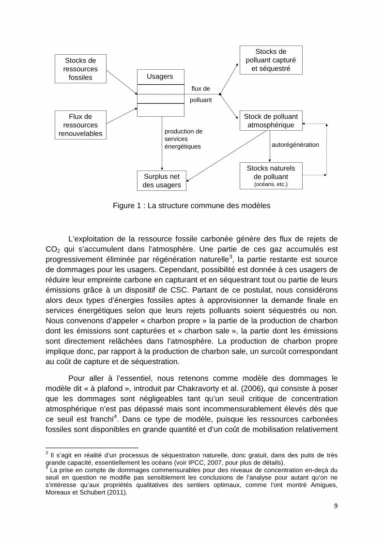
3.1 Rappel des résultats du modèle initial

Les premières études théoriques (Chakravorty et al., 2006, Lafforgue et al., 2008-a et 2008-b) sur lesquelles s’appuient notre recherche considéraient un seul type d’utilisateur de services énergétiques pour lequel le coût moyen de capture et de séquestration est constant. Elles ont mis en évidence l’importance des capacités de stockage du carbone à différents coûts et des potentialités d’exploitation de leurs substituts renouvelables, plus ou moins abondants. La conclusion principale de ces études est que le recours à la CSC permet de prolonger un usage soutenu de la ressource fossile compatible avec le respect de la contrainte de plafond. Par ailleurs, il n’est pas optimal d’avoir recours à la CSC avant d’avoir atteint le dit plafond ni, lorsque cette option est exercée, de séquestrer la totalité des émissions polluantes. L’enchaînement type des différentes phases de consommation d’énergie et d’abattement est illustré à la Figure 2.

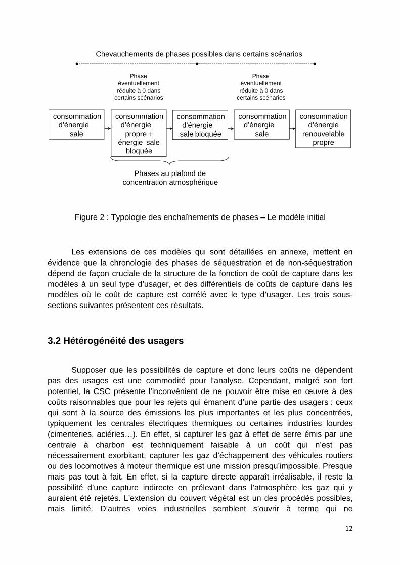
12

Figure 2 : Typologie des enchaînements de phases – Le modèle initial

Les extensions de ces modèles qui sont détaillées en annexe, mettent en évidence que la chronologie des phases de séquestration et de non-séquestration dépend de façon cruciale de la structure de la fonction de coût de capture dans les modèles à un seul type d’usager, et des différentiels de coûts de capture dans les modèles où le coût de capture est corrélé avec le type d’usager. Les trois sous-sections suivantes présentent ces résultats.

3.2 Hétérogénéité des usagers

Supposer que les possibilités de capture et donc leurs coûts ne dépendent pas des usages est une commodité pour l’analyse. Cependant, malgré son fort potentiel, la CSC présente l’inconvénient de ne pouvoir être mise en œuvre à des coûts raisonnables que pour les rejets qui émanent d’une partie des usagers : ceux qui sont à la source des émissions les plus importantes et les plus concentrées, typiquement les centrales électriques thermiques ou certaines industries lourdes (cimenteries, aciéries…). En effet, si capturer les gaz à effet de serre émis par une centrale à charbon est techniquement faisable à un coût qui n’est pas nécessairement exorbitant, capturer les gaz d’échappement des véhicules routiers ou des locomotives à moteur thermique est une mission presqu’impossible. Presque mais pas tout à fait. En effet, si la capture directe apparaît irréalisable, il reste la possibilité d’une capture indirecte en prélevant dans l’atmosphère les gaz qui y auraient été rejetés. L’extension du couvert végétal est un des procédés possibles, mais limité. D’autres voies industrielles semblent s’ouvrir à terme qui ne

consommation d’énergie

sale

consommation d’énergie

propre + énergie sale

bloquée

consommation d’énergie

sale bloquée

consommation d’énergie

sale

consommation d’énergie

renouvelable propre

Phases au plafond de concentration atmosphérique

Phase éventuellement réduite à 0 dans

certains scénarios

Phase éventuellement réduite à 0 dans

certains scénarios

Chevauchements de phases possibles dans certains scénarios

13

rencontreraient pas ces limites bien que probablement très coûteuses6. L’autre possibilité est d’imposer une norme de rejet sur les véhicules. Le différentiel de coût de production entre des véhicules qui satisfont la norme et ceux qui ne la satisfont pas peut être vu comme un coût d’abattement.

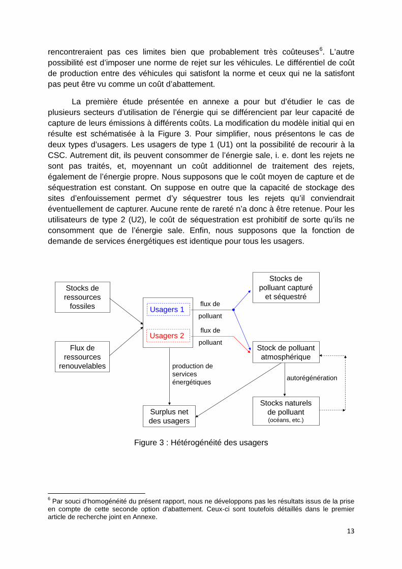
La première étude présentée en annexe a pour but d’étudier le cas de plusieurs secteurs d’utilisation de l’énergie qui se différencient par leur capacité de capture de leurs émissions à différents coûts. La modification du modèle initial qui en résulte est schématisée à la Figure 3. Pour simplifier, nous présentons le cas de deux types d’usagers. Les usagers de type 1 (U1) ont la possibilité de recourir à la CSC. Autrement dit, ils peuvent consommer de l’énergie sale, i. e. dont les rejets ne sont pas traités, et, moyennant un coût additionnel de traitement des rejets, également de l’énergie propre. Nous supposons que le coût moyen de capture et de séquestration est constant. On suppose en outre que la capacité de stockage des sites d’enfouissement permet d’y séquestrer tous les rejets qu’il conviendrait éventuellement de capturer. Aucune rente de rareté n’a donc à être retenue. Pour les utilisateurs de type 2 (U2), le coût de séquestration est prohibitif de sorte qu’ils ne consomment que de l’énergie sale. Enfin, nous supposons que la fonction de demande de services énergétiques est identique pour tous les usagers.

Usagers 1

Stocks de ressources

fossiles

Flux de ressources

renouvelables

Stocks de polluant capturé

et séquestré

Stock de polluant atmosphérique

Stocks naturels de polluant (océans, etc.)

Surplus net des usagers

autorégénération

flux de

polluant

Usagers 2

production de services énergétiques

flux de

polluant

Figure 3 : Hétérogénéité des usagers

6 Par souci d’homogénéité du présent rapport, nous ne développons pas les résultats issus de la prise en compte de cette seconde option d’abattement. Ceux-ci sont toutefois détaillés dans le premier article de recherche joint en Annexe.

14

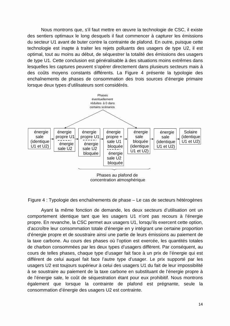
Nous montrons que, s’il faut mettre en œuvre la technologie de CSC, il existe des sentiers optimaux le long desquels il faut commencer à capturer les émissions du secteur U1 avant de buter contre la contrainte de plafond. En outre, puisque cette technologie est inapte à traiter les rejets polluants des usagers de type U2, il est optimal, tout au moins au début, de séquestrer la totalité des émissions des usagers de type U1. Cette conclusion est généralisable à des situations moins extrêmes dans lesquelles les captures peuvent s’opérer directement dans plusieurs secteurs mais à des coûts moyens constants différents. La Figure 4 présente la typologie des enchaînements de phases de consommation des trois sources d’énergie primaire lorsque deux types d’utilisateurs sont considérés.

Figure 4 : Typologie des enchaînements de phase – Le cas de secteurs hétérogènes

Ayant la même fonction de demande, les deux secteurs d’utilisation ont un comportement identique tant que les usagers U1 n’ont pas recours à l’énergie propre. En revanche, la CSC permet aux usagers U1, lorsqu’ils exercent cette option, d’accroître leur consommation totale d’énergie en y intégrant une certaine proportion d’énergie propre et de soustraire ainsi une partie de leurs émissions au paiement de la taxe carbone. Au cours des phases où l’option est exercée, les quantités totales de charbon consommées par les deux types d’usagers diffèrent. Par conséquent, au cours de telles phases, chaque type d’usager fait face à un prix de l’énergie qui est différent de celui auquel fait face l’autre type d’usager. Le prix supporté par les usagers U2 est toujours supérieur à celui des usagers U1 du fait de leur impossibilité à se soustraire au paiement de la taxe carbone en substituant de l’énergie propre à de l’énergie sale, le coût de séquestration étant pour eux prohibitif. Nous montrons également que lorsque la contrainte de plafond est prégnante, seule la consommation d’énergie des usagers U2 est contrainte.

énergie sale

(identique U1 et U2)

énergie propre U1

énergie sale U2

Solaire (identique U1 et U2)

Phases au plafond de concentration atmosphérique

Phases éventuellement

réduites à 0 dans certains scénarios

énergie propre U1

énergie sale U2 bloquée

énergie propre + sale U1 bloquée

énergie sale U2 bloquée

énergie sale

bloquée (identique U1 et U2)

énergie sale

(identique U1 et U2)

15

3.3 Structures alternatives des fonctions de coût de CSC

Dans ce deuxième essai, nous considérons un seul type d’usager final, mais supposons que les coûts spécifiques de séquestration ne sont pas constants. La structure générale du modèle reste la même que celle illustrée à la Figure 1. Deux types extrêmes de fonctions de coûts sont a priori envisageables. A chaque instant le coût moyen de capture peut être soit dépendant des quantités de rejets polluants à séquestrer, soit dépendant du cumul des émissions. Dans ce dernier cas, deux possibilités sont à considérer :

- Les sites de séquestration sont plus ou moins faciles d’accès et/ou requièrent des aménagements plus ou moins coûteux. L’actualisation commande de les mobiliser par ordre croissant de leur coût, les moins coûteux devant être mobilisés en priorité. Il en résulte qu’à chaque date, le coût moyen de capture et de séquestration est une fonction croissante du cumul des séquestrations effectuées jusqu’à cette date.

- Il est bien connu que toute activité est d’autant mieux organisée que l’expérience accumulée est grande. Si cet effet d’apprentissage devait être suffisamment puissant alors, à chaque instant, le coût moyen de capture et de séquestration devrait au contraire apparaître comme une fonction décroissante du cumul des séquestrations effectuées jusqu’à l’instant en question.

Ce que montre notre recherche c’est que, quel que soit celui des premiers effets qui est dominant, une politique active de capture et de séquestration ne doit jamais débuter avant que soit atteint le plafond de concentration en carbone lorsque les coûts moyens instantanés de capture sont indépendants des quantités à capturer au même instant.

Ce résultat était plus ou moins attendu lorsque le premier effet est dominant, effet qu’on appellera « effet de rareté » (sous-entendu des sites de séquestration facilement aménageables). En effet, le coût additionnel moyen induit par l’exploitation de l’énergie propre comprend à présent un coût monétaire direct de séquestration qui augmente à mesure que la capacité disponible d’enfouissement diminue, accru d’un coût d’opportunité associé à la limitation de cette capacité. La dominance de l’effet rareté pénalise donc la compétitivité de l’énergie propre par rapport à une situation où son coût additionnel serait constant. Il n’y a donc aucune raison de démarrer son exploitation avant d’être contraint par le plafond de concentration atmosphérique des gaz à effet de serre.

En outre, nous montrons que ce résultat ne dépend pas du coût du substitut renouvelable non carboné. Lorsque ce coût est élevé, l’enchaînement type des différentes phases est le même que celui de la Figure 2. Lorsque le coût de l’énergie solaire est faible, cet enchaînement est celui qui est illustré à la Figure 5.

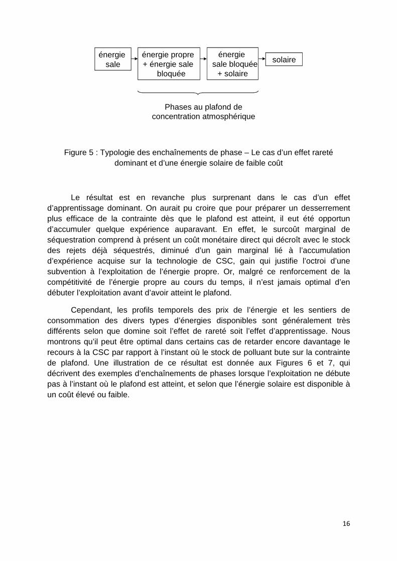
16

Figure 5 : Typologie des enchaînements de phase – Le cas d’un effet rareté dominant et d’une énergie solaire de faible coût

Le résultat est en revanche plus surprenant dans le cas d’un effet d’apprentissage dominant. On aurait pu croire que pour préparer un desserrement plus efficace de la contrainte dès que le plafond est atteint, il eut été opportun d’accumuler quelque expérience auparavant. En effet, le surcoût marginal de séquestration comprend à présent un coût monétaire direct qui décroît avec le stock des rejets déjà séquestrés, diminué d’un gain marginal lié à l’accumulation d’expérience acquise sur la technologie de CSC, gain qui justifie l’octroi d’une subvention à l’exploitation de l’énergie propre. Or, malgré ce renforcement de la compétitivité de l’énergie propre au cours du temps, il n’est jamais optimal d’en débuter l’exploitation avant d’avoir atteint le plafond.

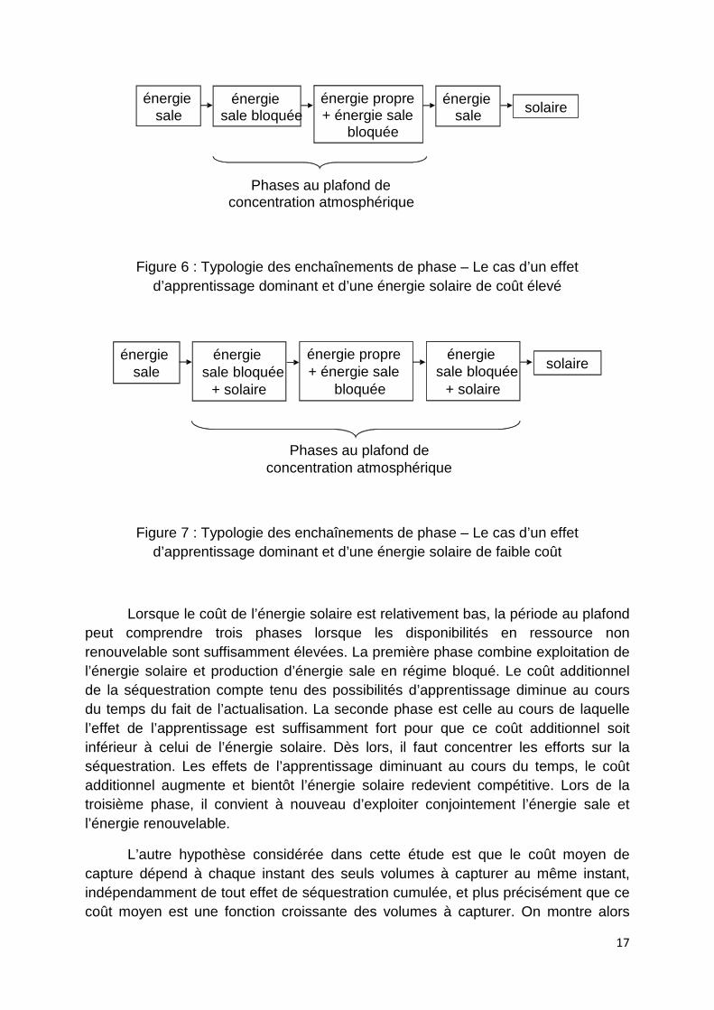
Cependant, les profils temporels des prix de l’énergie et les sentiers de consommation des divers types d’énergies disponibles sont généralement très différents selon que domine soit l’effet de rareté soit l’effet d’apprentissage. Nous montrons qu’il peut être optimal dans certains cas de retarder encore davantage le recours à la CSC par rapport à l’instant où le stock de polluant bute sur la contrainte de plafond. Une illustration de ce résultat est donnée aux Figures 6 et 7, qui décrivent des exemples d’enchaînements de phases lorsque l’exploitation ne débute pas à l’instant où le plafond est atteint, et selon que l’énergie solaire est disponible à un coût élevé ou faible.

énergie sale

énergie propre + énergie sale

bloquée

solaire

Phases au plafond de concentration atmosphérique

énergie sale bloquée

+ solaire

17

Figure 6 : Typologie des enchaînements de phase – Le cas d’un effet d’apprentissage dominant et d’une énergie solaire de coût élevé

Figure 7 : Typologie des enchaînements de phase – Le cas d’un effet d’apprentissage dominant et d’une énergie solaire de faible coût

Lorsque le coût de l’énergie solaire est relativement bas, la période au plafond peut comprendre trois phases lorsque les disponibilités en ressource non renouvelable sont suffisamment élevées. La première phase combine exploitation de l’énergie solaire et production d’énergie sale en régime bloqué. Le coût additionnel de la séquestration compte tenu des possibilités d’apprentissage diminue au cours du temps du fait de l’actualisation. La seconde phase est celle au cours de laquelle l’effet de l’apprentissage est suffisamment fort pour que ce coût additionnel soit inférieur à celui de l’énergie solaire. Dès lors, il faut concentrer les efforts sur la séquestration. Les effets de l’apprentissage diminuant au cours du temps, le coût additionnel augmente et bientôt l’énergie solaire redevient compétitive. Lors de la troisième phase, il convient à nouveau d’exploiter conjointement l’énergie sale et l’énergie renouvelable.

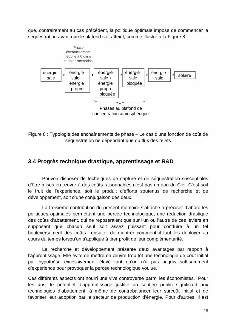
L’autre hypothèse considérée dans cette étude est que le coût moyen de capture dépend à chaque instant des seuls volumes à capturer au même instant, indépendamment de tout effet de séquestration cumulée, et plus précisément que ce coût moyen est une fonction croissante des volumes à capturer. On montre alors

énergie sale

énergie propre + énergie sale

bloquée

solaire

Phases au plafond de concentration atmosphérique

énergie sale bloquée

+ solaire

énergie sale bloquée

+ solaire

énergie sale

énergie propre + énergie sale

bloquée

solaire

Phases au plafond de concentration atmosphérique

énergie sale bloquée

énergie sale

18

que, contrairement au cas précédent, la politique optimale impose de commencer la séquestration avant que le plafond soit atteint, comme illustré à la Figure 8.

Figure 8 : Typologie des enchaînements de phase – Le cas d’une fonction de coût de séquestration ne dépendant que du flux des rejets

3.4 Progrès technique drastique, apprentissage et R&D

Pouvoir disposer de techniques de capture et de séquestration susceptibles d’être mises en œuvre à des coûts raisonnables n’est pas un don du Ciel. C’est soit le fruit de l’expérience, soit le produit d’efforts soutenus de recherche et de développement, soit d’une conjugaison des deux.

La troisième contribution du présent mémoire s’attache à préciser d’abord les politiques optimales permettant une percée technologique, une réduction drastique des coûts d’abattement, qui ne reposeraient que sur l’un ou l’autre de ces leviers en supposant que chacun seul soit assez puissant pour conduire à un tel bouleversement des coûts ; ensuite, de montrer comment il faut les déployer au cours du temps lorsqu’on s’applique à tirer profit de leur complémentarité.

La recherche et développement présente deux avantages par rapport à l’apprentissage. Elle évite de mettre en œuvre trop tôt une technologie de coût initial par hypothèse excessivement élevé tant qu’on n’a pas acquis suffisamment d’expérience pour provoquer la percée technologique voulue.

Ces différents aspects ont nourri une vive controverse parmi les économistes. Pour les uns, le potentiel d’apprentissage justifie un soutien public significatif aux technologies d’abattement, à même de contrebalancer leur surcoût initial et de favoriser leur adoption par le secteur de production d’énergie. Pour d’autres, il est

énergie sale

énergie sale +

énergie propre

énergie sale

bloquée

énergie sale solaire

Phases au plafond de concentration atmosphérique

Phase éventuellement réduite à 0 dans

certains scénarios

énergie sale +

énergie propre bloquée

19

préférable de laisser le temps à la recherche d’identifier les options les plus prometteuses techniquement et économiquement et d’en assurer le développement. Un soutien trop précoce à des technologies immatures peut s’avérer contre-productif et devrait donc être évité.

Les premières réflexions sur cette question ont confirmé ce diagnostic : la prise en compte des possibilités d’apprentissage induit une action optimale plus précoce tandis que la prise en compte des potentialités de la recherche conduit à retarder l’action. La faiblesse de ces analyses vient de ce qu’elles ne considèrent que des cas extrêmes où l’avancement technologique ne résulterait soit que de l’apprentissage, soit que de la recherche. Mais une politique de soutien public à l’abattement va conduire les entreprises du secteur énergétique vers des stratégies de réponse variées, combinant dans des proportions diverses des efforts de déploiement précoce de la séquestration pour bénéficier d’effets d’apprentissage avec des efforts d’innovation vers des options techniques nouvelles et potentiellement moins coûteuses à mettre en œuvre. L’objet de la troisième étude présentée en annexe est de construire une analyse endogène du choix entre apprentissage et recherche dans un modèle où les deux effets se combinent pour provoquer une percée technologique dans le secteur de l’abattement.

Dans un premier temps, on explore les cas extrêmes où le progrès technique ne résulterait que de l’apprentissage ou bien de la seule recherche. Les trajectoires technologiques combinant recherche et apprentissage sont étudiées dans un second temps.

Une politique fondée sur la seule recherche-développement ne devrait déboucher sur une révolution des coûts qu’à la date à partir de laquelle la contrainte de plafond commence à restreindre directement la consommation d’énergie polluante et pas avant, dans la mesure où les sommes à engager sont d’autant plus élevées qu’il faut réussir la percée plus tôt. Il ne sert à rien de disposer dès aujourd’hui d’une technologie que l’on aura à mettre en œuvre que demain7. Mais il faut noter que la date à laquelle les effets directs de cette contrainte doivent être pris en compte est elle-même endogène.

Une mobilisation des possibilités d’apprentissage nécessite la combinaison de deux moyens de pilotage, une taxe sur les dégagements de gaz dans l’atmosphère et une subvention pour utilisation des technologies de dépollution. Tel n’est pas le cas lorsque la percée est obtenue par la recherche-développement seule. La taxation des émissions suffit alors pour inciter à produire les efforts de recherche optimaux.

La possibilité de combiner apprentissage à partir de technologies initialement existantes et parfois balbutiantes, et efforts de recherche, permet d’élargir 7 L’argument est similaire à celui mis en avant par Henriet (2012) qui étudie les politiques de recherche optimales visant à mettre au point des techniques d’exploitation à coûts modérés des ressources renouvelables propres.

20

considérablement la perspective. L’accumulation de carbone dans l’atmosphère et son élimination progressive, et le développement de technologies d’atténuation des émissions apparaissent alors comme deux processus dynamiques en interaction mais avec leurs propres logiques et leurs propres contraintes. On montre ainsi qu’il est possible qu’il faille introduire la capture et la séquestration avant d’atteindre le plafond. On montre aussi que les politiques optimales de recours aux deux types de moyens peuvent s’appuyer initialement soit uniquement sur de l’apprentissage, soit uniquement sur des efforts de recherche.

Dans des scénarios où il convient de recourir simultanément à la recherche et à l’apprentissage pour provoquer une rupture technologique, on montre enfin que l’effort d’apprentissage doit croître à un rythme plus soutenu que celui des efforts de recherche. Ces derniers en effet ne produisent de résultats qu’au moment de la percée. Les efforts conjugués de l’apprentissage ne produisent eux aussi de résultats qu’au même moment pour autant qu’on ne considère que la seule percée. Mais avant que cette percée ait lieu, ils réduisent les rejets dans l’atmosphère et contribuent à réduire le poids de la contrainte.

4 CONCLUSION

Les recherches sur l’économie de l’abattement des émissions de gaz à effet de serre sont actuellement en plein essor. La stratégie de valorisation des résultats de nos travaux que nous comptons mettre en œuvre est la suivante.

La première étude, mise en forme comme article de recherche, est actuellement en révision pour la revue Environmental and Resources Economics, revue phare en Europe dans le domaine de l’économie de l’environnement. Les deux études suivantes sont beaucoup plus récentes et pas encore soumises à des revues internationales. Un travail de réécriture préalable est nécessaire pour les réduire au format usuel des supports de publication en économie. Ce travail accompli, nous comptons soumettre ces recherches à l’automne à des revues cibles. La seconde étude pourrait être soumise au Journal of Environmental Economics and Management ou à Resource and Energy Economics. Ces deux revues sont les supports majeurs de publication internationale en économie des ressources naturelles et de l’environnement. L’intérêt suscité aujourd’hui par le sujet laisse espérer des chances raisonnables de succès dans l’un ou l’autre support. La troisième étude soulève des questions d’ordre plus général, portées à l’attention des économistes par Scott Barrett dans l’Américan Economic Review en 2006. Nous prévoyons de toucher un lectorat plus large pour cette contribution en visant une revue de théorie économique générale.

21

Cet effort principal de valorisation sera complété par d’autres initiatives. Nous sommes sollicités pour une participation à un numéro spécial d’Economie et Prévision sur le thème de l’économie des ressources naturelles. Une synthèse destinée à un lectorat francophone plus large pourrait être réalisée pour la Revue Française de l’Energie. Enfin différentes opportunités de présentation de nos travaux dans des colloques ou séminaires internationaux nous sont offertes. Citons les prochaines journées du CREE (Canadian Resource and Environmental Economics Study Group Annual Conference 2012, University of British Columbia, Vancouver, 28-30 septembre, 2012) et la vingtième édition de la conférence annuelle de l’Association Européenne des économistes de l’environnement à Toulouse en juin 2013.

22

REFERENCES

Amigues J-P., Moreaux M., Schubert K. (2011). Optimal use of a polluting non renewable resource generating both manageable and catastrophic damages. Annals of Economics and Statistics, 103/104, 107-141.

Chakravorty U., Magné B., Moreaux M. (2006). A Hotelling model with a ceiling on the stock of pollution. Journal of Economic Dynamics and Control, 30, 2875-2904.

Chakravorty U., Magné B., Moreaux M. (2012). Can nuclear power provide clean energy ? Journal of Public Economic Theory, 14(2), 349-389.

Chakravorty U., Leach A., Moreaux M., (2012). Cycles in nonrenewable resource prices with pollution and learning-by-doing, Journal of Economic Dynamics & Control, http://dx.doi.org/10.1016/j.jedc.2012.04.005

Edmonds J., Clarke J., Dooley J., KIM S.H., Smith S.J. (2004). Stabilization of CO2 in a B2 world: Insights on the roles of carbon capture and disposal, hydrogen and transportation technologies. Energy Economics, 26, 517-537.

Gerlagh R., van der Zwaan B. (2006). Options and instruments for a deep cut in CO2 emissions: Carbon capture or renewable, taxes or subsidies? Energy Journal, 27, 25-48.

Grimaud A., Lafforgue G., Magné B. (2011). Climate change mitigation options and directed technical change : A decentralized equilibrium analysis. Resource and Energy Economics, 33(4), 938-962.

Hamilton M., Herzog H.M, Parsons J. (2009). Cost and U.S. public policy for new coal power plants with carbon capture and sequestration. Energy Procedia, GHGT9 Procedia, 1, 2511-2518.

Henriet F. (2012). Optimal extraction of a polluting non-renewable resource with R&D toward a clean backstop technology. Journal of Public Economic Theory 14(2), 311-347.

Herzog H.J. (2011). Scaling up carbon dioxide capture and storage : From megatons to gigatons. Energy Economics, 33, 597-604.

Intergovernmental Panel on Climate Change (2005). Special Report on Carbon Dioxide Capture and Storage, Working Group III.

Intergovernmental Panel on Climate Change (2007). Climate Change 2007, Synthesis Assessment Report, Working Group III.

23

Kurosawa A. (2004). Carbon concentration target and technical choice. Energy Economics, 26, 675-684.

Lafforgue G., Magne B., Moreaux M. (2008-a). Energy substitutions, climate change and carbon sinks. Ecological Economics, 67, 589-597.

Lafforgue G., Magne B., Moreaux M. (2008-b). The optimal sequestration policy with a ceiling on the stock of carbon in the atmosphere. In: Guesnerie, R., Tulkens, H. (Eds), The Design of Climate Policy. The MIT Press, Boston, pp. 273-304.

24

ANNEXES

Article 1: Optimal carbon capture and sequestration from heterogeneous consuming sectors.

Article 2: Optimal timing of carbon capture policies under alternative CCS cost function.

Article 3: Triggering the technological revolution in carbon capture and sequestration costs.

Optimal Carbon Capture and Sequestration

From Heterogeneous Energy Consuming Sectors

Jean-Pierre Amigues∗, Gilles La�orgue†

and

Michel Moreaux‡

April 2012

∗Toulouse School of Economics (INRA and LERNA). E-mail address: amigues@toulouse.inra.fr.†Corresponding author. Toulouse School of Economics (INRA and LERNA), 21 allée de Bri-

enne, 31000 Toulouse, France. E-mail address: gla�org@toulouse.inra.fr. The authors acknowledge�nancial support from the French Energy Council.‡Toulouse School of Economics (IDEI and LERNA). E-mail address: mmichel@cict.fr

Optimal Carbon Capture and Sequestration

From Heterogeneous Energy Consuming Sectors

Abstract

We characterize the optimal exploitation paths of two primary energy resources, anon-renewable polluting resource and a carbon-free renewable one. Both resources cansupply the energy needs of two sectors. Sector 1 is able to reduce its carbon footprintat a reasonable cost owing to a CCS device. Sector 2 has only access to the air capturetechnology, but at a signi�cantly higher cost. We assume that the atmospheric carbonstock cannot exceed some given ceiling. We show that there may exist paths along whichit is optimal to begin by fully capturing the sector 1's emissions before the ceiling has beenreached. Also there may exist optimal paths along which both capture devices have to beactivated, in which case the sector 1's emissions are �rst fully abated and next sector 2partially abates.

Keywords: Air capture; Carbon stabilization cap; CCS; Fossil resource; Heterogene-ity.

JEL classi�cations: Q32, Q42, Q54, Q58.

1

Contents

1 Introduction 3

2 Model and notations 6

3 Social planner problem and optimality conditions 9

4 Optimal policy without atmospheric carbon capture device 12

4.1 Restricted social planner problem . . . . . . . . . . . . . . . . . . . . . . . . 13

4.2 Optimal paths along which it is optimal to capture and sequester before

being at the ceiling . . . . . . . . . . . . . . . . . . . . . . . . . . . . . . . . 13

4.3 Paths along which the oil price is the same for the two sectors . . . . . . . . 19

4.3.1 Paths along which it is optimal to abate sector 1's emissions . . . . . 19

4.3.2 Paths along which it is never optimal to capture sector 1's emissions 20

5 Optimal policies requiring to activate both capture devices 21

5.1 Checking whether the atmospheric carbon capture device must be used along

the optimal path . . . . . . . . . . . . . . . . . . . . . . . . . . . . . . . . . 21

5.2 Optimal paths . . . . . . . . . . . . . . . . . . . . . . . . . . . . . . . . . . . 21

5.3 Time pro�le of the optimal carbon tax . . . . . . . . . . . . . . . . . . . . . 24

5.4 Time pro�le of the tax burdens and the sequestration costs . . . . . . . . . 25

6 Conclusion 27

References 31

1 Introduction

Among all the alternative abatement technologies aiming at reducing the anthropogenic

carbon dioxide emissions, a particular interest should be given to the carbon capture and

sequestration (CCS) according to the IPCC (2005, 2007). Even if the e�ciency of this tech-

nology is still under assessment1, current engineering estimates suggest that CCS could be

a credible cost-e�ective approach for eliminating most of the emissions from coal and nat-

ural gas power plants (MIT, 2007). Along this line of arguments, Islegen and Reichelstein

(2009) point out that CCS has considerable potential to reduce CO2 emissions at a "reason-

able" social cost, given the social costs of carbon emissions predicted for a business-as-usual

scenario. CCS is also intended to have a major role in limiting the e�ective carbon tax,

or the market price for CO2 emission permits under a cap-and-trade system. The crucial

point is then to estimate how far would the CO2 price have to rise before the operator of

power plants would �nd it advantageous to install CCS technology rather then buy emission

permits or pay the carbon tax. The International Energy Agency (2006) estimates such

a break-even price in the range of $30-90/tCO2 (depending on technology) but, assuming

reasonable technology advances, projected CCS cost by 2030 is around $25/tCO2.

However, geologic CCS presents the disadvantage to apply to the sole large point sources

of pollution such as power plants or huge manufacturings. This technology is prohibitively

costly to �lter for instance the CO2 emissions from transportation as far as the energy

input is gasoline or kerosene, small residence heating or scattered agricultural activities.

Hence, the ultimate device to abate carbon dioxide �uxes from any concentrated as well

as di�use sources would consist in capturing them directly from the atmosphere.

According to Keith et al. (2006), atmospheric carbon capture � or air capture � di�ers

from conventional mitigation in three key aspects. First, it removes emissions from any

part of the economy with equal ease of di�culty, so its cost provides an absolute cap on

the mitigation cost. Second, it permits reduction in concentrations faster than the natural

carbon cycle. Third, because it is weakly coupled with existing energy infrastructure, air

capture may o�er stronger economies of scale and smaller adjustment costs than the more

1CCS technology consists in �ltering CO2 �uxes at the source of emission, that is, in fossil energy-fueled power plants, by use of scrubbers installed near the top of chimney stacks. The carbon would besequestered in reservoirs, such as depleted oil and gas �elds or deep saline aquifers.

3

conventional mitigation technologies. As underlined by Keith (2009), though this abate-

ment technology costs more than CCS, it allows one to treat small and mobile emission

sources, advantage that may compensate for the intrinsic di�culty of capturing carbon

from the air. Finally, deliberately expressing a double meaning, McKay (2009) claims

about this alternative that "capturing carbon dioxide from thin air is the last thing we

should talk about" (p.240). On the one hand, the energy requirements for atmospheric

carbon capture are so enormous that, according to McKay, it seems actually almost ab-

surd to talk about it. But on the other hand, "we should talk about it because capturing

carbon from thin air may turn out to be our last line of defense if humanity fails to take

the cheaper and more sensible options that may still be available today" (p.240).

Technically speaking, sucking carbon from thin air can be achieved in di�erent ways.2

The probably most credible one is to use a chemical process. This involves a technology

that brings air into contact with a chemical "sorbent" (an alkaline liquid). The sorbent

absorbs CO2 in the air, and the chemical process then separates out the CO2 and recycles

the sorbent. The captured CO2 is stored in geologic deposits, just like the CCS from power

plant. However, chemical air capture is expensive. Estimates of marginal cost range from

$100-200/tCO2, which is larger than the cost of alternatives for reducing emissions such

as CCS. They are also larger than current estimates of the social cost of carbon, which

range from about $7-85/tCO2. But, as concluded by Barrett (2009), bearing the cost of

chemical air capture can become pro�table in the future under constraining cap-and-trade

scenarios. Furthermore, we may hope that the cost will decrease, thanks to R&D and

learning by doing.

In the present study, we address the question of the heterogeneity of energy users

regarding the way their carbon footprint can be reduced. We then consider two abatement

technologies and two sectors. The �rst technology is a conventional emission abatement

device (CCS) which is available at a marginal cost assumed to be socially acceptable.

2The most obvious approach consists in exploiting the process of photosynthesis by increasing theforestlands or changing the agricultural processes, but this is not the type of device we consider in thepresent paper. A close idea can be transposed to the oceans. To make them able to capture carbon fasterthen normal, phytoplankton blooms can be stimulated by fertilizing some oceanic iron-limited regions.A third way is to enhance weathering of rocks, that is to pulverize rocks that are capable of absorbingCO2, and leave them in the open air. This idea can be pitched as the acceleration of a natural process.Unfortunately, as claimed by Barrett (2009), the e�ects of all these devices are di�cult to verify, theirpotential is limited in any event, and there are concerns about some unknown ecological consequences.

4

However, this abatement technology cannot apply to carbon emissions from any type of

activity, but only from large point sources of emissions. The second technology directly

captures carbon in the atmosphere. Its marginal cost is much higher than the emission

capture technology, but it allows to reduce carbon from any sources since the capture

process and the generation of emissions are now disconnected. The �rst sector, in which

pollution sources are spatially concentrated, can abate its carbon emissions, but not the

second one since energy users are too small and too scattered. The ultimate way for abating

pollution is to directly capture carbon in the atmosphere. But since the atmosphere is a

public good, this kind of pollution reduction will also bene�t to sector 1. Whatever the

capture process, we assume that carbon is stockpiled into reservoirs whose size is very

large. Then, as in Chakravorty et al. (2006), this suggests a generic abatement scheme of

unlimited capacity. Finally, energy in each sector can be supplied either by a carbon-based

fossil fuel, contributing to climate change (oil, coal, gas), or by a carbon-free renewable

and non biological resource such, as solar energy.

Using a standard Hotelling model for the non-renewable resource and assuming that

the atmospheric carbon stock should not exceed some critical threshold � as in Chakravorty

et al. (2006) � we characterize the optimal time path of sectoral energy prices, sectoral

energy consumptions, emission and atmospheric abatements. The key results of the paper

are: i) Irrespective of the availability of the air capture technology, it may happen that it

is optimal for the �rst sector to abate its carbon emissions before the atmospheric carbon

concentration cap is attained.3 ii) Since this type of carbon capture is unable to �lter the

emissions from the second sector, it is also optimal for the �rst sector to abate the totality

of its own emissions, at least at the beginning. These two �rst results are at variance

with Chakravorty et al. (2006), La�orgue et al. (2008-a) and (2008-b) who consider a

single sector using energy and a single abatement technology. iii) The atmospheric carbon

capture is only used when the atmospheric carbon stock reaches the ceiling, maintaining

the stock at its critical level. Hence the �ow of carbon captured in the atmosphere is lower

than the emission �ow of the second sector and the whole carbon emissions coming from

3This result is in accordance with Coulomb and Henriet (2010) who show that, in a model with a singleabatement technology, when technical constraints make it impossible to capture emissions from all energyconsumers, CCS should be used before the ceiling is reached if non capturable emissions are large enough.

5

the two sectors are only partially abated.

The paper is organized as follows. Section 2 presents the model. In section 3, we lay

down the social planner program and we derive the optimality conditions. In section 4,

we examine the restricted problem in which only the emission carbon capture device is

available. In section 5, we examine how the model reacts when the atmospheric carbon

capture technology is introduced. We also investigate the time pro�le of the optimal carbon

tax as well as, for each sector, the total burden induced by the mitigation of their emissions.

Finally, we brie�y conclude in section 6.

2 Model and notations

Let us consider a stationary economy with two sectors, indexed by i = 1, 2, in which

the instantaneous gross surplus derived from energy consumption are the same.4 For an

identical energy consumption in the two sectors, q1 = q2 = q, the sectoral gross surplus

u1(q) and u2(q) are such that: u1(q) = u2(q) = u(q). We assume that this common function

u satis�es the following standard assumptions. u : R+ → R+ is a function of class C2,

strictly increasing, strictly concave and verifying the Inada conditions: limq↓0 u′(q) = +∞

and limq↑+∞ u′(q) = 0. We denote by p(q) the sectoral marginal gross surplus function

and by qd(p) = p−1(q), the sectoral direct demand function.

In each sector, energy can be supplied by two primary natural resources: a dirty non-

renewable resource (let say oil for instance) and a carbon-free renewable resource (let say

solar energy). Let us denote by X0 the initial oil endowment of the economy, by X(t) the

remaining part of this initial endowment at time t, and by xi(t), i = 1, 2, the instantaneous

consumption �ow of oil in sector i at time t, so that:

X(t) = −[x1(t) + x2(t)], with X(0) ≡ X0 and X(t) ≥ 0 (2.1)

xi(t) ≥ 0, i = 1, 2. (2.2)

The delivery cost of oil is the same for both sectors. We denote by cx the corresponding

4Since the focus of the paper is on the e�ect of the heterogeneity of the energy consumers regardingthe type of abatement technologies they can use, we consider the simple case of two sectors with the samegross surplus function and the same cost structure, excepted the abatement cost. Introducing di�erentdemand functions and/or di�erent delivery costs for these sectors would imply a more complex analysiswithout altering the key message of the paper.

6

average cost, assumed to be constant and hence equal to the marginal cost. The delivery

cost includes the extraction cost of the resource, the cost of industrial processing (re�ning

of the crude oil) and the transportation cost, so that the resource is ready for use by the

consumer in the concerned sector. To keep matter as simple as possible, we assume that no

oil is lost during the delivery process. Equivalently, the oil stock X(t) may be understood

as measured in ready for use units.

Let Z(t) be the stock of carbon within the atmosphere at time t, and Z0 be the initial

stock, Z0 ≡ Z(0). We assume that a carbon cap policy is prescribed to prevent catastrophic

damages which would be in�nitely costly. This policy consists in forcing the atmospheric

stock to stay under some critical level Z, with Z > Z0.

The atmospheric carbon stock is fed by carbon emission �ows resulting from the use

of oil. Let ζ be the quantity of carbon which would be potentially released per unit of oil

consumption whatever the sector in which the oil is used. Thus, the gross pollutant �ow

amounts to ζ[x1(t) + x2(t)]. However, this gross emission �ow can be abated before being

released into the atmosphere. We assume that emissions from sector 1 can be abated, but

not emissions from sector 2 (or at a prohibitive cost). Emission abatement by carbon cap-

ture and sequestration (CCS) can be achieved when burning oil is spatially concentrated,

as it is the case for instance in the electricity or cement industries, which are good examples

of sector 1's activities. At the other extreme of the spectrum, i.e. in sector 2, there exists

some activities with prohibitively costing emission captures since users are too small or

too scattered. Transportation by cars, trucks and diesel train are good examples of sector

2's industry.5

Let se(t) be this part of carbon emissions from sector 1 which is captured and se-

questered at some average cost ce, assumed to be constant. Then the net pollution �ow

issued from sector 1 amounts to:

ζx1(t)− se(t) ≥ 0, se(t) ≥ 0. (2.3)

In sector 2, the net pollution �ow amounts to ζx2(t).

5Note that electric traction trains could be good examples of sector 1 users, as well as electric cars (cf.Chakravorty et al., 2010).

7

Carbon emission capture is not the unique way to reduce the atmospheric carbon con-

centration. The other process consists in capturing the carbon present in the atmosphere

itself. We denote by sa(t) the instantaneous carbon �ow which is abated owing to this

second device, and by ca the corresponding average cost, also assumed to be constant.

Although atmospheric carbon capture seems technically feasible, it is proved to be more

costly than emission capture: ca > ce. The only constraint on this capture �ow is:

sa(t) ≥ 0. (2.4)

Whatever the capture process, from emissions or from the atmosphere, we assume that

carbon is stockpiled into reservoirs whose capacities are unlimited.6

Last, there is also some natural self regeneration e�ect of the atmospheric carbon stock.

We assume that the natural proportional rate of decay, denoted by α > 0, is constant.

Taking into account all the components of the dynamics of Z(t) results into:

Z(t) = ζ[x1(t) + x2(t)]− [sa(t) + se(t)]− αZ(t), Z(0) ≡ Z0 < Z (2.5)

Z − Z(t) ≥ 0. (2.6)

When the atmospheric carbon stock reaches its critical level, i.e. when Z(t) = Z, and

absent any active capture policy, i.e. sa(t) = se(t) = 0, then the total oil consumption

x(t) ≡ x1(t)+x2(t) is constrained to be at most equal to x, where x is solution of ζx−αZ =

0, that is x = αZ/ζ. Then, since the two sectors have the same weight, each one consumes

the quantity x/2 of oil at the ceiling when neither CCS nor air capture are activated.

We assume that it may be optimal to abate the pollution for delaying the date of arrival

at the critical threshold and for relaxing the constraint on the oil consumption �ow, that

is: cx + ce < cx + ca < u′(x).

The alternative energy source is supplied by the carbon-free renewable resource, the

solar energy. We denote by yi(t) the solar energy consumption in sector i, i = 1, 2, and by

cy the average delivery cost of this alternative energy. Because cx and cy both include all

6In order to focus on the abatement options for each sector and their respective costs, we dispense fromconsidering reservoirs of limited capacity. The question of the size of carbon sinks and of the time pro�leof their �lling up is addressed by La�orgue et al. (2008-a) and (2008-b).

8

the costs necessary to deliver a ready for use energy unit to the potential users, then both

resources may be seen as perfect substitutes for the consumers, so that we may de�ne the

aggregate energy consumption of sector i as qi = xi + yi, i = 1, 2, as far as the costs cx

and cy are incurred.

The average cost cy is assumed to be constant, the same for both sectors, and higher

than u′(x/2). This last condition implies that the optimal energy consumption paths can

be split into two periods: a �rst one during which only oil is consumed and a second

one during which only solar energy is used.7 We also have to assume that the natural

�ow of available solar energy, denoted by yn, is large enough to supply the energy needs

in both sectors during the second period described above.8 Let y be the sectoral energy

consumption that it would be optimal to consume at the marginal cost cy, that is y = qd(cy)

for which u′(y) = cy. Then we assume that yn > 2y. Under this assumption, no rent has

ever to be imputed for using the solar energy. Thus the only constraint on yi(t) having to

be taken into account along any optimal path is a non-negativity constraint:

yi(t) ≥ 0, i = 1, 2. (2.7)

Finally, the instantaneous social rate of discount, denoted by ρ, ρ > 0, is assumed to

be constant over time.

3 Social planner problem and optimality conditions

The problem of the social planner consists in maximizing the sum of the discounted net

current surplus. Let (P ) be this program:

(P ) maxsa,se,xi,yi,i=1,2

∫ ∞0{u [x1(t) + y1(t)] + u [x2(t) + y2(t)]− cx [x1(t) + x2(t)]

−cy [y1(t) + y2(t)]− casa(t)− cese(t)} e−ρtdt

subject to (2.1)-(2.7).

7Since both cx and cy are set constant, oil and solar cannot be used simultaneously. Using a stock-dependent marginal extraction cost, but a constant marginal cost of the backstop, together with a damagefunction increasing with the atmospheric carbon stock, Hoel and Kverndokk (1996) and Tahvonen (1997)have shown that there may be a period of simultaneous use of the nonrenewable and the renewable resource.Furthermore, as underlined by Tahvonen (1997), the conjunction of these assumptions gives rise to amultiplicity of possible scenarios.

8The case of a rare renewable substitute is analyzed in La�orgue et al. (2008-b).

9

Let us denote by λX the costate variable of the state variable X, by λZ minus the

costate variable of the state variable Z, by γ's the Lagrange multipliers associated with

the non-negativity constraints on the command variables, and by ν the Lagrange multiplier

associated with the ceiling constraint on Z. As usually done in this kind of problem, we

do not take explicitly into account the non-negativity constraint on X. Thus, droping out

the time index for notational convenience, we may write the current value Lagrangian L

of problem (P ) as follows:

L = u(x1 + y1) + u(x2 + y2)− cx(x1 + x2)− cy(y1 + y2)− casa − cese

−λX(x1 + x2)− λZ [ζ(x1 + x2)− (sa + se)− αZ] + ν(Z − Z)

+∑i

γxixi +∑i

γyiyi + γsasa + γsese + γse(ζx1 − se)

The static and dynamic �rst-order conditions are:

u′[x1(t) + y1(t)] = cx + λX(t) + ζ[λZ(t)− γse(t)]− γx1(t) (3.8)

u′[x2(t) + y2(t)] = cx + λX(t) + ζλZ(t)− γx2(t) (3.9)

u′[xi(t) + yi(t)] = cy − γyi(t), i = 1, 2 (3.10)

ca = λZ(t) + γsa(t) (3.11)

ce = λZ(t)− γse(t) + γse(t) (3.12)

λX(t) = ρλX(t) (3.13)

λZ(t) = (ρ+ α)λZ(t)− ν(t) (3.14)

together with the associated complementary slackness conditions. Last, the transversality

conditions take the following forms:

limt↑∞

e−ρtλX(t)X(t) = 0 (3.15)

limt↑∞

e−ρtλZ(t)Z(t) = 0 (3.16)

Remarks:

1. As expected with a constant marginal delivery cost, the shadow marginal value of the

stock of oil, or mining rent, λX(t), must grow at the social rate of discount ρ. From

(3.13), we get: λX(t) = λX0eρt, with λX0 ≡ λX(0). Thus the transversality condition

10

(3.15) reduces to λX0 limt↑∞X(t) = 0. If oil is to have some value, λX0 > 0, then it

must be exhausted along the optimal path.

2. Concerning the shadow marginal cost of the atmospheric carbon stock, λZ(t), note

that before the date tZ at which the ceiling constraint is beginning to be active, we

must have ν(t) = 0 since Z − Z(t) > 0. Then (3.14) reduces to λZ = (ρ + α)λZ so

that: t < tZ ⇒ λZ(t) = λZ0e(ρ+α)t, with λZ0 ≡ λZ(0). Once the ceiling constraint

is no more active and forever, λZ(t) = 0. Thus, denoting by tZ the latest date at

which Z(t) = Z, we get: t > tZ ⇒ λZ(t) = 0.9

3. In order to simplify the notations in the next sections, it is useful to de�ne the

following prices or full marginal costs and the corresponding sectoral consumption

levels for which the F.O.C's (3.8) and (3.9) relative to x1(t) and to x2(t), respectively,

are satis�ed:10

- Price or full marginal cost of oil and sectoral oil consumption before the ceiling and

absent any abatement, whatever the sector under consideration: p1(t, λX0 , λZ0) ≡

cx + λX0eρt + ζλZ0e

(ρ+α)t and q1(t, λX0 , λZ0) ≡ qd(p1(t, λX0 , λZ0)

).

- Price or full marginal cost of oil for consumption in sector 1 given that emissions

from this sector are fully or partially abated, i.e. se(t) > 0, and corresponding oil con-

sumption of sector 1: p2e(t, λX0) ≡ cx +λX0e

ρt + ζce and q2e(t, λX0) ≡ qd

(p2e(t, λX0)

).

- Price or full marginal cost of oil for consumption in sector 2 given that some part of

the atmospheric carbon stock is captured, sa(t) > 0, and corresponding consumption

in this sector: p2a(t, λX0) ≡ cx + λX0e

ρt + ζca and q2a(t, λX0) ≡ qd

(p2a(t, λX0)

).

- Price or full marginal cost of oil once the ceiling constraint Z−Z(t) ≥ 0 is no more

active and forever, and corresponding sectoral consumptions, whatever the sector:

p3(t, λX0) ≡ cx + λX0eρt and q3(t, λX0) ≡ qd

(p3(t, λX0)

). This last case corresponds

to a pure Hotelling regime.

9This characteristics is standard under the assumption of a linear natural regeneration function of theatmospheric carbon stock. For non linear decay functions, see Toman and Withagen (2000) for instance.

10The upper indexes n = 1, 2, 3 correspond to the order in which the price pn and the quantity qn areappearing along the optimal path. If both pn(t, ...) and pn+m(t′, ...) are appearing along the same path,then it implies that t < t′.

11

Solving strategy of the social planner:

In order to solve her problem (P ), the social planner can proceed as follows. First, she

checks whether the most costly device to capture the carbon has ever to be used. The test

consists in solving her problem assuming that the atmospheric carbon capture device is

not available. This is inducing some path of atmospheric carbon shadow cost λZ(t). Next,

according to the outcome of the �rst step:

- either this shadow cost is permanently lower than the marginal cost of atmospheric

carbon capture, that is λZ(t) < ca for any t ≥ 0, and then the atmospheric carbon capture

device has never to be used because too costly;

- or there exists some time interval during which λZ(t) is higher than ca so that, in

this case, the atmospheric carbon capture device must be activated since the loss in the

marginal net surplus induced by not using it is higher than its marginal cost of use.

This test is performed in Section 4. Section 5 deals with the case in which it is optimal

to activate the air capture device.

4 Optimal policy without atmospheric carbon capture device

This kind of policies have been investigated and characterized in Chakravorty et al. (2006),

and in La�orgue et al. (2008-a) and (2008-b), but for economies in which any potential

emissions can be captured and sequestered irrespective of the oil consumption sector. Thus,

in their models, there is a single consumption sector, similar to the sector 1 of the present

model. Two important conclusions of these studies are that: i) it is never optimal to abate

the potential �ow of emissions before attaining the critical level Z of atmospheric carbon

concentration; ii) along the phase at the ceiling during which it is optimal to abate, only

some part of the potential emission �ow must be abated. Because abating is never optimal

excepted during this phase, then it is never optimal to fully abate the potential �ow of

emissions along the optimal path.

As we shall show, it may happen in the present context that: i) abating the potential

emissions of the sector 1 has to begin before the ceiling level Z is attained; ii) when it is

optimal to begin to capture the sector 1 potential emissions, before the ceiling is attained,

then it is optimal to capture its whole potential emission �ow.

12

4.1 Restricted social planner problem

Assuming that the atmospheric carbon capture technology is not available, the social

planner problem reduces to the following restricted problem (R.P ):

(R.P ) maxse,xi,yi,i=1,2

∫ ∞0{u [x1(t) + y1(t)] + u [x2(t) + y2(t)]− cx [x1(t) + x2(t)]

−cy [y1(t) + y2(t)]− cese(t)} e−ρtdt

subject to (2.1), (2.2), (2.3), (2.6), (2.7) and:

Z(t) = ζ[x1(t) + x2(t)]− se(t)− αZ(t), Z(0) = Z0 < Z (4.17)

The new F.O.C's relative to the command variables, except sa, and to the state variables

are the same then the ones of the unrestricted problem (P ), namely (3.8)-(3.14). Also the

associated complementary slackness condition and the transversality conditions (3.15) and

(3.16) must hold. We can conclude that remarks 1 and 2 of the previous section 3 also

hold in the present restricted context.

The opportunity for sector 1 to fully or partially abate its emissions strongly depends

upon the level of ce. Hence, we have to distinguish the cases of a full abatement phase

or a partial abatement phase, before or after being at the ceiling. The next subsections

describe these di�erent possibilities.

4.2 Optimal paths along which it is optimal to capture and sequester

before being at the ceiling

Let us assume that the initial oil endowment is large enough to justify some period at

the ceiling during which Z(t) = Z, and that there exists some period during which the

emissions of sector 1 are abated, se(t) > 0. Figure 1 below illustrates the optimal price

path which is obtained in this case.

The optimal price path is a seven phases path. Denoting by pi(t), for i = 1, 2, the price

� or full marginal cost � of oil for sector i, these phases are the following:

- Phase 1, before the ceiling and without abatement: [0, te)

During this phase, the oil price is the same for each sector and it is given by p1(t) = p2(t) =

p1(t, λX0 , λZ0). The existence of such a phase requires that λZ0 < ce, so p1(t, λX0 , λZ0) <

13

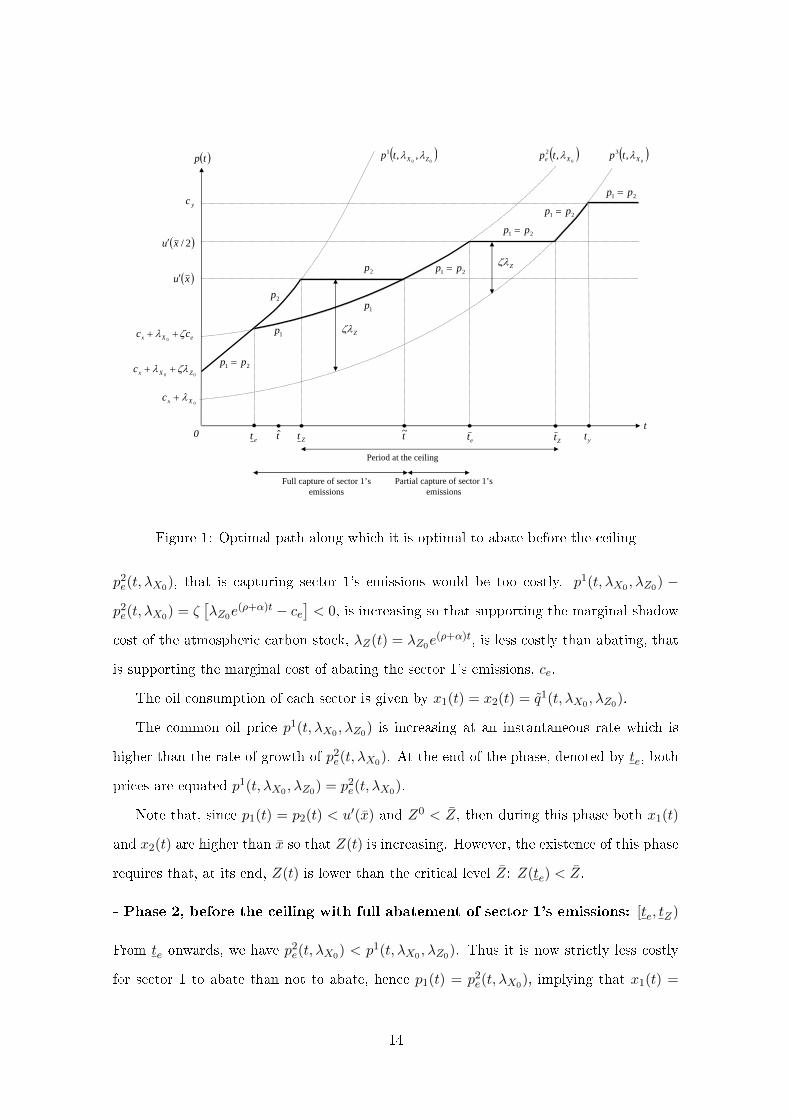
0t

yc

( )tp

0Xxc λ+

00 ZXxc ζλλ ++

eXx cc ζλ ++0

( )2/xu′

( )xu′

( )0

,3Xtp λ

et t etZt t~ Zt yt

( )0

,2Xe tp λ( )

00,,1

ZXtp λλ

21 pp =

21 pp =

21 pp =

21 pp =

21 pp =

1p

1p2p

2p

Zζλ

Zζλ

Period at the ceiling

Full capture of sector 1’s emissions

Partial capture of sector 1’s emissions

Figure 1: Optimal path along which it is optimal to abate before the ceiling

p2e(t, λX0), that is capturing sector 1's emissions would be too costly. p1(t, λX0 , λZ0) −

p2e(t, λX0) = ζ

[λZ0e

(ρ+α)t − ce]< 0, is increasing so that supporting the marginal shadow

cost of the atmospheric carbon stock, λZ(t) = λZ0e(ρ+α)t, is less costly than abating, that

is supporting the marginal cost of abating the sector 1's emissions, ce.

The oil consumption of each sector is given by x1(t) = x2(t) = q1(t, λX0 , λZ0).

The common oil price p1(t, λX0 , λZ0) is increasing at an instantaneous rate which is

higher than the rate of growth of p2e(t, λX0). At the end of the phase, denoted by te, both

prices are equated p1(t, λX0 , λZ0) = p2e(t, λX0).

Note that, since p1(t) = p2(t) < u′(x) and Z0 < Z, then during this phase both x1(t)

and x2(t) are higher than x so that Z(t) is increasing. However, the existence of this phase

requires that, at its end, Z(t) is lower than the critical level Z: Z(te) < Z.

- Phase 2, before the ceiling with full abatement of sector 1's emissions: [te, tZ)

From te onwards, we have p2e(t, λX0) < p1(t, λX0 , λZ0). Thus it is now strictly less costly

for sector 1 to abate than not to abate, hence p1(t) = p2e(t, λX0), implying that x1(t) =

14

q2e(t, λX0).11 Moreover, since the inequality is strict then the potential sector 1's emissions

are fully abated: se(t) = ζx1(t).

Sector 2 is not able to abate its emissions and it must support the carbon shadow

cost ζλZ0e(ρ+α)t per unit of burned oil, so that p2(t) = p1(t, λX0 , λZ0) and x2(t) =

q1(t, λX0 , λZ0).

Note that, during this phase, since Z(te) < Z and p2(t) < u′(x), then x2(t) > x and

the atmospheric carbon stock increases. Finally, since p2(t) > p1(t), the �rst of these two

prices reaching u′(x) is p2(t). However, in order that sector 2's consumption begins to be

blockaded at t = tZ , we must have simultaneously p2(t) = u′(x) and Z(t) = Z at the end

of the phase.

- Phase 3, at the ceiling with sector 2's oil consumption blockaded and sector

1's emissions fully abated: [tZ , t)

During this phase, the oil price in sector 2 is given by p2(t) = u′(x) and the oil consumption

of this sector is set to the maximum consumption level allowed by the ceiling constraint,

i.e. x2(t) = x. Note that this implies that λZ(t) = [u′(x)− p3(t, λX0)]/ζ is decreasing over

time during the phase.12

Since p2e(tZ , λX0) < u′(x), then ce < λZ(t) at the beginning of the phase. Then,

once again, abating emissions is proved to be less costly for sector 1 than supporting the

shadow cost of the atmospheric carbon stock. Consequently, the sector 1's emissions are

fully captured: se(t) = ζx1(t). Since p1(t) = p2e(tZ , λX0), we still have x1(t) = q2

e(t, λX0).

Given that sector 2's emissions are ζx2(t) = ζx, full abatement in sector 1 implies that,

during this phase at the ceiling, the atmospheric carbon stock stays at its critical level:

Z(t) = 0 and Z(t) = Z. Finally, p1(t) = p2e(t, λX0) is increasing during the phase. At the

end of the phase, p2e(t, λX0) = u′(x) or, equivalently, λZ(t) = ce.

11Note that during such a phase, because se(t) > 0 then γse(t) = 0, so that from (3.12) we obtain:λZ(t) = ce+γse(t). Substituting for λZ(t) in (3.8) and taking into account that x1(t) > 0, hence γx1(t) = 0,and y1(t) = 0, we get: u′ (x1(t)) = cx + λX0e

ρt + ζce, from which we conclude that p1(t) = p2e(t, λX0) andx1(t) = q2e(t, λX0).

12Since the ceiling constraint is active, then ν(t) is strictly positive and su�ciently high so that λZ(t) =(ρ+ α)λZ(t) − ν(t) < 0.

15

- Phase 4, at the ceiling with partial abatement of sector 1's emissions: [t, te)

From time t onwards, p2e(t, λX0) becomes higher than u′(x). Thus, the only way to satisfy

simultaneously the F.O.C's (3.8) and (3.9) on the xi's is to set p1(t) = p2(t) = p2e(t, λX0),

which implies x1(t) = x2(t) = q2e(t, λX0) together with a partial abatement of sector 1's

emissions. As far as p2e(t, λX0) is staying under u′(x/2), then the potential emissions

amount to 2ζq2e(t, λX0) > ζx = αZ. As far as p2

e(t, λX0) is now higher than u′(x), then the

potential emissions 2ζq2e(t, λX0) stays at a lower level than 2ζx, so that:

x < 2q2e(t, λX0) < 2x. (4.18)

In order to satisfy the atmospheric carbon constraint Z(t) = Z, it is su�cient to abate

this part se(t) of the sector 1's emissions for which Z(t) = 0. Thus we may have:

2ζq2e(t, λX0)− se(t) = ζx. (4.19)

Conditions (4.18) and (4.19) imply that:

se(t) = ζ[2q2e(t, λX0)− x

]< ζq2

e(t, λX0) = ζx1(t). (4.20)

Hence, during this phase, emissions from sector 1 are only partially abated and, since

q2e(t, λX0) is decreasing through time then the instantaneous rate of capture se(t) is also

decreasing. This solution may be optimal if and only if abating and supporting the shadow

marginal cost of the atmospheric carbon stock are resulting into the same full marginal

cost, that is if and only if λZ(t) is constant and equal to ce. Since sector 2 cannot abate

its emissions, it is supporting the marginal shadow cost of atmospheric carbon and the

condition p1(t) = p2(t) = p2e(t, λX0) = cx + λX0e

ρt + ζλZ(t) guarantees that λZ(t) = ce is

satis�ed.13

Since p2e(t, λX0) is increasing over time, there exists some date te at which p

2e(t, λX0) =

u′(x/2). At this date, x1(t) = x2(t) = x/2 and sector 1 ceases to capture its emissions,

se(t) = 0. From te onwards, we have p2e(t, λX0) > u′(x/2) so that the cost of capture of

sector 1's emissions becomes prohibitive.

13Again, because the ceiling constraint is e�ective then ν(t) > 0 and, in order that λZ(t) = 0, we have:ν(t) = (ρ+ α)λZ(t) = (ρ+ α)ce.

16

- Phase 5, at the ceiling and without abatement of sector 1's emissions: [te, tZ)

Since abating the sector 1's emissions is now too costly, there is no more abatement and, in

order to not overshoot the critical atmospheric carbon level, we must have p1(t) = p2(t) =

u′(x/2) and x1(t) = x2(t) = x/2, so that Z(t) = 0.

During such a phase, λZ(t) = [u′(x)− p3(t, λX0)]/ζ is decreasing. The phase is ending

at time t = tZ when λZ(t) = 0, which implies that p3(t, λX0) > u′(x/2) for t > tZ .

- Phase 6, pure Hotelling phase: [tZ , ty)

This phase is the last one during which energy needs are supplied by oil. This is a pure

Hotelling phase. The energy price is the same for the two sectors: p1(t) = p2(t) =

p3(t, λX0) > u′(x/2), also generating an identical oil consumption in the two sectors:

x1(t) = x2(t) < x/2⇒ x(t) < x.

Since x(t) < x and Z(t) = Z at the beginning of the phase, then Z(t) < Z for t > tZ

justifying the fact that now λZ(t) = 0 from tZ onwards.14 Then λZ(t)Z(t) = 0 and the

transversality condition (3.16) is satis�ed.

During the phase, the price is ever increasing and there must exist some time t = ty

at which p3(t, λX0) = cy. At this time, this level of oil price makes the renewable resource

competitive. To be optimal, the switch from the pure Hotelling regime to a pure renewable

regime requires that, at time t = ty, X(t) = 0 so that from ty onwards λX(t)X(t) = 0

warranting that the transversality condition (3.15) relative to X is satis�ed.

- Phase 7, carbon-free renewable energy permanent regime: [ty,+∞)

From ty onwards, the economy follows a pure renewable energy regime which is free of

carbon emissions: p1(t) = p2(t) = cy, x1(t) = x2(t) = 0 and y1(t) = y2(t) = y. Since

xi(t) = 0, i = 1, 2, then Z(t) = −αZ(t) so that Z(t) is permanently decreasing down to 0

at in�nity: Z(t) = Z(ty)e−α(t−ty).

14However, note that Z(t) is not necessarily monotonically decreasing during this phase. What is sureis that there exists some critical time interval (tZ , tZ + ε), with ε positive and small enough, during whichZ(t) < 0. For t > tZ +ε, it may happen that Z(t) > 0. But, because x(t) < x, even if Z(t) were temporallyincreasing, it would not be able to go back to Z.

17

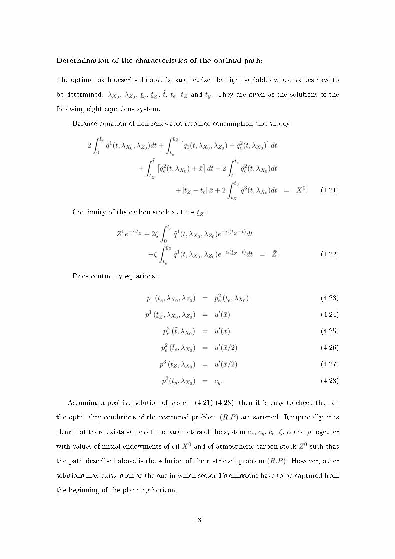
Determination of the characteristics of the optimal path:

The optimal path described above is parametrized by eight variables whose values have to

be determined: λX0 , λZ0 , te, tZ , t, te, tZ and ty. They are given as the solutions of the

following eight equations system.

- Balance equation of non-renewable resource consumption and supply:

2

∫ te

0q1(t, λX0 , λZ0)dt+

∫ tZ

te

[q1(t, λX0 , λZ0) + q2

e(t, λX0)]dt

+

∫ t

tZ

[q2e(t, λX0) + x

]dt+ 2

∫ te

tq2e(t, λX0)dt

+ [tZ − te] x+ 2

∫ ty

tZ

q3(t, λX0)dt = X0. (4.21)

- Continuity of the carbon stock at time tZ :

Z0e−αtZ + 2ζ

∫ te

0q1(t, λX0 , λZ0)e−α(tZ−t)dt

+ζ

∫ tZ

te

q1(t, λX0 , λZ0)e−α(tZ−t)dt = Z. (4.22)

- Price continuity equations:

p1 (te, λX0 , λZ0) = p2e (te, λX0) (4.23)

p1 (tZ , λX0 , λZ0) = u′(x) (4.24)

p2e

(t, λX0

)= u′(x) (4.25)

p2e (te, λX0) = u′(x/2) (4.26)

p3 (tZ , λX0) = u′(x/2) (4.27)

p3(ty, λX0) = cy. (4.28)

Assuming a positive solution of system (4.21)-(4.28), then it is easy to check that all

the optimality conditions of the restricted problem (R.P ) are satis�ed. Reciprocally, it is

clear that there exists values of the parameters of the system cx, cy, ce, ζ, α and ρ together

with values of initial endowments of oil X0 and of atmospheric carbon stock Z0 such that

the path described above is the solution of the restricted problem (R.P ). However, other

solutions may exist, such as the one in which sector 1's emissions have to be captured from

the beginning of the planning horizon.

18

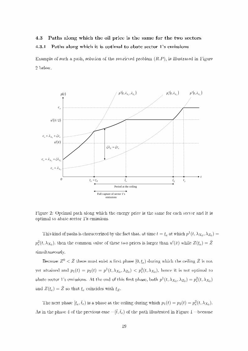
4.3 Paths along which the oil price is the same for the two sectors

4.3.1 Paths along which it is optimal to abate sector 1's emissions

Example of such a path, solution of the restricted problem (R.P ), is illustrated in Figure

2 below.

0t

yc

( )tp

0Xxc λ+

00 ZXxc ζλλ ++

eXx cc ζλ ++0

( )2/xu′

( )xu′

( )0

,3Xtp λ

etZe tt = Zt yt

( )0

,2Xe tp λ( )

00,,1

ZXtp λλ

Period at the ceiling

Full capture of sector 1’s emissions

eZ cζζλ =

Figure 2: Optimal path along which the energy price is the same for each sector and it isoptimal to abate sector 1's emissions

This kind of paths is characterized by the fact that, at time t = te at which p1(t, λX0 , λZ0) =

p2e(t, λX0), then the common value of these two prices is larger than u′(x) while Z(te) = Z

simultaneously.

Because Z0 < Z there must exist a �rst phase [0, te) during which the ceiling Z is not

yet attained and p1(t) = p2(t) = p1(t, λX0 , λZ0) < p2e(t, λX0), hence it is not optimal to

abate sector 1's emissions. At the end of this �rst phase, both p1(t, λX0 , λZ0) = p2e(t, λX0)

and Z(te) = Z so that te coincides with tZ .

The next phase [te, te) is a phase at the ceiling during which p1(t) = p2(t) = p2e(t, λX0).

As in the phase 4 of the previous case � [t, te) of the path illustrated in Figure 1 � because

19

sector 2 cannot abate its emissions, we must have λZ(t) = ce during the second phase

of the present path. Also because u′(x) < p2e(t, λX0) < u′(x/2), then only some part

of the sector 1's emissions have to be captured (cf. the above equation (4.20)), se(t) <

ζq2e(t, λX0) = ζx1(t), and the capture intensity se(t) diminishes. At the end of this phase,

p2e(t, λX0) = u′(x/2), x1(t) = x2(t) = x/2 and se(t) = 0.

The third phase [te, tZ) is still a phase at the ceiling but without capture of sector 1's

emissions: p1(t) = p2(t) = u′(x/2) and x1(t) = x2(t) = x/2. The phase is ending when

p3(t, λX0) = u′(x/2), that is when λZ(t) = 0. The fourth and �fth phases are respectively

the standard pure Hotelling phase [tZ , ty) and the pure renewable energy phase [ty,∞).

4.3.2 Paths along which it is never optimal to capture sector 1's emissions

When the abatement cost ce is very high, capturing is proved to never be an optimal

strategy. In this case, we get a four phases optimal price path as illustrated in Figure 3.

0t

yc

( )tp

0Xxc λ+

00 ZXxc ζλλ ++

eXx cc ζλ ++0

( )2/xu′

( )0

,3Xtp λ

Zt Zt yt

( )0

,2Xe tp λ( )

00,,1

ZXtp λλ

Period at the ceiling

Figure 3: Optimal path along which the energy price is the same for each sector and it isnot optimal to abate sector 1's emissions

In Figure 3, p2e(t, λX0) is higher than p1(t, λX0 , λZ0) along the whole time interval [0, tZ)

20

before the ceiling. Hence, it is never optimal to capture sector 1's emissions. Such optimal

paths have been characterized in Chakravorty et al. (2006).

5 Optimal policies requiring to activate both capture devices

In this section, we �rst determine the conditions under which it is optimal to activate the

atmospheric carbon capture device. Next we characterize the optimal paths along which

both carbon capture technologies must be used. Last, we discuss about the time pro�le of

the optimal carbon marginal shadow cost, that is the optimal unitary carbon tax, as well

as the total burden induced by climate change mitigation policies in each sector, including

the tax burden and the abatement cost.

5.1 Checking whether the atmospheric carbon capture device must be

used along the optimal path

Let us consider the three kinds of optimal price paths which may solve the planner restricted

problem (R.P ) and which have been discussed in the previous section. Clearly, since

p2a(t, λX0) > p2

e(t, λX0), then for the two last kinds of optimal paths illustrated in Figures

2 and 3 in subsection 4.3, the price trajectory p2a(t, λX0) (not depicted in these �gures)

is always located above the optimal price path. Hence, it is never optimal to use the

atmospheric carbon capture device.

For the optimal path illustrated in Figure 1 in subsection 4.2, it may happen that

using the atmospheric carbon capture technology reveals optimal. To check whether this

technology is optimal or not, the test runs as follows. Consider the price path p2a(t, λX0)

(not depicted in Figure 1). Then at time t = tZ , either p2a(t, λX0) < u′(x) or p2

a(t, λX0) ≥

u′(x). In the �rst case, there must exist a time interval around t = tZ such that p2(t) >

p2a(t, λX0) and it would be less costly for sector 2 to bear the cost of the atmospheric

capture ca than the burden of the shadow cost of the atmospheric carbon stock λZ(t).

In the second case, using the atmospheric carbon capture technology could not allow to

improve the welfare.

5.2 Optimal paths

Let us assume now that the atmospheric carbon capture technology has to be used. Then

we may obtain two kinds of optimal paths depending on whether the least costly emission

21

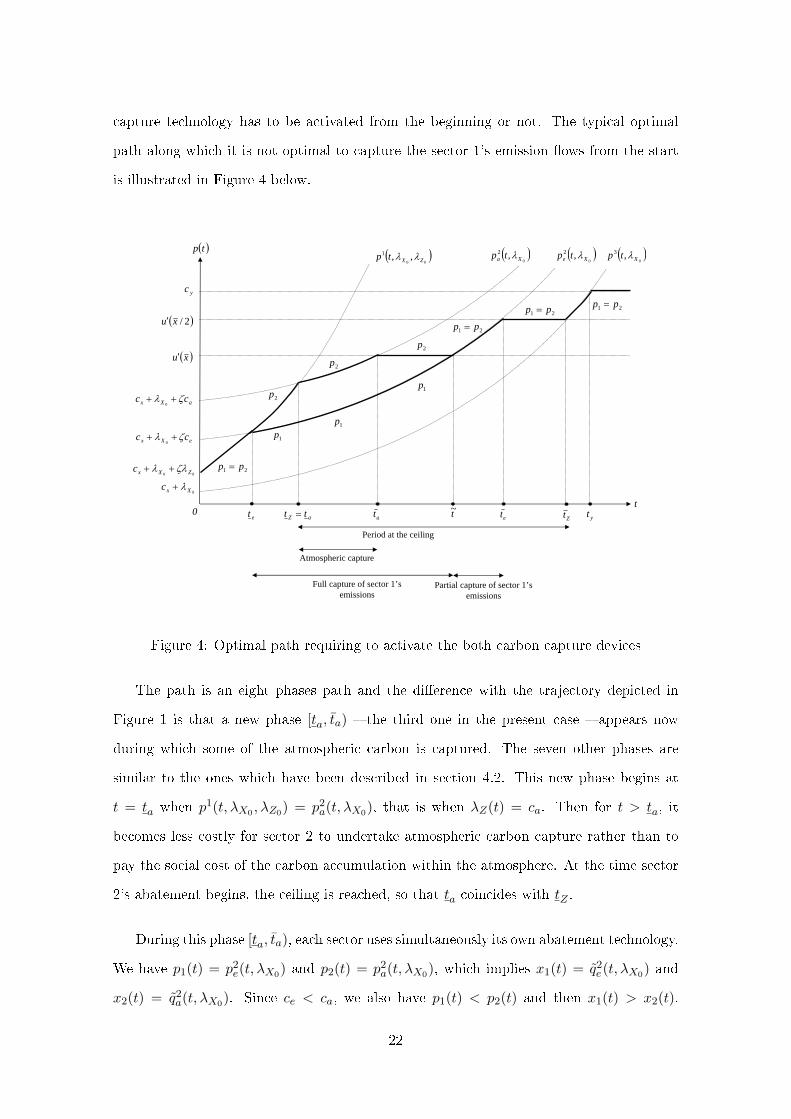
capture technology has to be activated from the beginning or not. The typical optimal

path along which it is not optimal to capture the sector 1's emission �ows from the start

is illustrated in Figure 4 below.

0t

yc

( )tp

0Xxc λ+00 ZXxc ζλλ ++

eXx cc ζλ ++0

( )2/xu′

( )xu′

( )0

,3Xtp λ

et etaZ tt = t~ Zt yt

( )0

,2Xe tp λ( )

00,,1

ZXtp λλ

21 pp =

21 pp =21 pp = 21 pp =

1p1p

2p

2p

Period at the ceiling

Full capture of sector 1’s emissions

Partial capture of sector 1’s emissions

( )0

,2Xa tp λ

aXx cc ζλ ++0

at

2p

1p

Atmospheric capture

Figure 4: Optimal path requiring to activate the both carbon capture devices

The path is an eight phases path and the di�erence with the trajectory depicted in

Figure 1 is that a new phase [ta, ta) � the third one in the present case � appears now

during which some of the atmospheric carbon is captured. The seven other phases are

similar to the ones which have been described in section 4.2. This new phase begins at

t = ta when p1(t, λX0 , λZ0) = p2a(t, λX0), that is when λZ(t) = ca. Then for t > ta, it

becomes less costly for sector 2 to undertake atmospheric carbon capture rather than to

pay the social cost of the carbon accumulation within the atmosphere. At the time sector

2's abatement begins, the ceiling is reached, so that ta coincides with tZ .

During this phase [ta, ta), each sector uses simultaneously its own abatement technology.

We have p1(t) = p2e(t, λX0) and p2(t) = p2

a(t, λX0), which implies x1(t) = q2e(t, λX0) and

x2(t) = q2a(t, λX0). Since ce < ca, we also have p1(t) < p2(t) and then x1(t) > x2(t).

22

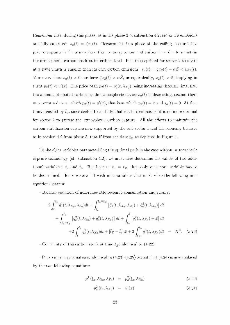
Remember that, during this phase, as in the phase 3 of subsection 4.2, sector 1's emissions

are fully captured: se(t) = ζx1(t). Because this is a phase at the ceiling, sector 2 has

just to capture in the atmosphere the necessary amount of carbon in order to maintain

the atmospheric carbon stock at its critical level. It is thus optimal for sector 2 to abate

at a level which is smaller than its own carbon emissions: sa(t) = ζx2(t) − αZ < ζx2(t).

Moreover, since sa(t) > 0, we have ζx2(t) > αZ, or equivalently, x2(t) > x, implying in

turns p2(t) < u′(x). The price path p2(t) = p2a(t, λX0) being increasing through time, �rst

the amount of abated carbon by the atmospheric device sa(t) is decreasing, second there

must exist a date at which p2(t) = u′(x), that is at which x2(t) = x and sa(t) = 0. At that

time, denoted by ta, since sector 1 still fully abates all its emissions, it is no more optimal

for sector 2 to pursue the atmospheric carbon capture. All the e�orts to maintain the

carbon stabilization cap are now supported by the sole sector 1 and the economy behaves

as in section 4.2 from phase 3, that if from the date tZ as depicted in Figure 1.

To the eight variables parameterizing the optimal path in the case without atmospheric

capture technology (cf. subsection 4.2), we must here determine the values of two addi-

tional variables: ta and ta. But because ta = tZ , then only one more variable has to

be determined. Hence we are left with nine variables that must solve the following nine

equations system:

- Balance equation of non-renewable resource consumption and supply:

2

∫ te

0q1(t, λX0 , λZ0)dt+

∫ ta=tZ

te

[q1(t, λX0 , λZ0) + q2

e(t, λX0)]dt

+

∫ ta

ta=tZ

[q2e(t, λX0) + q2

a(t, λX0)]dt+

∫ t

ta

[q2e(t, λX0) + x

]dt

+2

∫ te

tq2e(t, λX0)dt+ [tZ − te] x+ 2

∫ ty

tZ

q3(t, λX0)dt = X0. (5.29)

- Continuity of the carbon stock at time tZ : identical to (4.22).

- Price continuity equations: identical to (4.23)-(4.28) except that (4.24) is now replaced

by the two following equations:

p1 (ta, λX0 , λZ0) = p2a(ta, λX0) (5.30)

p2a (ta, λX0) = u′(x) (5.31)

23

5.3 Time pro�le of the optimal carbon tax

The trajectory of the carbon marginal shadow cost corresponding to the optimal path

illustrated in Figure 4 is characterized by:

λZ(t) =

λZ0e(ρ+α)t , t ∈ [0, tZ)

ca , t ∈ [tZ , ta)[u′(x)− p3(t, λX0)

]/ζ , t ∈ [ta, t)

ce , t ∈ [t, te)[u′(x/2)− p3(t, λX0)

]/ζ , t ∈ [te, tZ)

0 , t ∈ [tZ ,∞)

(5.32)

This shadow cost can be interpreted as the optimal unitary tax to be levied on the net

carbon emissions. Its time pro�le is illustrated in Figure 5 below.

0t

( )tZλ

ec

et etaZ tt = t~ Ztat

tZ e )(

0

αρλ +

ac

0Zλ

Figure 5: Time pro�le of the optimal unitary carbon tax

The unitary tax rate is �rst increasing but is bounded from above by the highest

marginal abatement cost ca which is attained when it becomes optimal to use this abate-

ment device and, simultaneously, when the atmospheric carbon stock constraint begins to

24

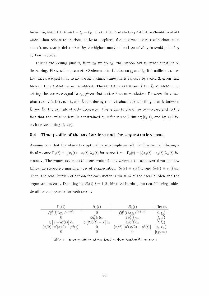
be active, that is at time t = ta = tZ . Given that it is always possible to choose to abate

rather than release the carbon in the atmosphere, the maximal tax rate of carbon emis-

sions is necessarily determined by the highest marginal cost permitting to avoid polluting

carbon releases.

During the ceiling phases, from tZ up to tZ , the carbon tax is either constant or

decreasing. First, as long as sector 2 abates, that is between ta and ta, it is su�cient to set

the tax rate equal to ca to induce an optimal atmospheric capture by sector 2, given that

sector 1 fully abates its own emissions. The same applies between t and te for sector 1 by

setting the tax rate equal to ce, given that sector 2 no more abates. Between these two

phases, that is between ta and t, and during the last phase at the ceiling, that is between

te and tZ , the tax rate strictly decreases. This is due to the oil price increase and to the

fact that the emission level is constrained by x for sector 2 during [ta, t), and by x/2 for

each sector during [te, tZ).

5.4 Time pro�le of the tax burdens and the sequestration costs

Assume now that the above tax optimal rate is implemented. Such a tax is inducing a

�scal income Γ1(t) ≡ [ζx1(t)− se(t)]λZ(t) for sector 1 and Γ2(t) ≡ [ζx2(t)− sa(t)]λZ(t) for

sector 2. The sequestration cost in each sector simply writes as the sequestered carbon �ow

times the respective marginal cost of sequestration: S1(t) ≡ se(t)ce and S2(t) ≡ sa(t)ca.

Then, the total burden of carbon for each sector is the sum of the �scal burden and the

sequestration cost. Denoting by Bi(t) i = 1, 2 this total burden, the two following tables

detail its components for each sector.

Γ1(t) S1(t) B1(t) Phases

ζq1(t)λZ0e(ρ+α)t 0 ζq1(t)λZ0e

(ρ+α)t [0, te)0 ζq2

e(t)ce ζq2e(t)ce [te, t)

ζ[x− q2

e(t)]ce ζ

[2q2e(t)− x

]ce ζq2

e(t)ce [t, te)(x/2)

[u′(x/2)− p3(t)

]0 (x/2)

[u′(x/2)− p3(t)

][te, tZ)

0 0 0 [tZ ,∞)

Table 1. Decomposition of the total carbon burden for sector 1

25

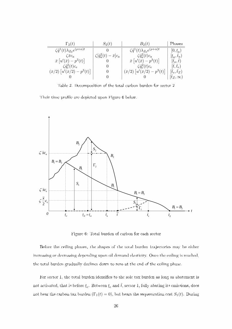
Γ2(t) S2(t) B2(t) Phases

ζq1(t)λZ0e(ρ+α)t 0 ζq1(t)λZ0e

(ρ+α)t [0, ta)ζxca ζ[q2

a(t)− x]ca ζq2a(t)ca [ta, ta)

x[u′(x)− p3(t)

]0 x

[u′(x)− p3(t)

][ta, t)

ζq2e(t)ce 0 ζq2

e(t)ce [t, te)(x/2)

[u′(x/2)− p3(t)

]0 (x/2)

[u′(x/2)− p3(t)

][te, tZ)

0 0 0 [tZ ,∞)

Table 2. Decomposition of the total carbon burden for sector 2

Their time pro�le are depicted upon Figure 6 below.

0t

et etaZ tt = t~ Ztat

acxζ

21 BB =

1B

2B

2Γ

2S

2B

21 BB =

21 BB =

1B

1S

1Γ

1S

ecxζ

ecx2

ζ

Figure 6: Total burden of carbon for each sector

Before the ceiling phases, the shapes of the total burden trajectories may be either

increasing or decreasing depending upon oil demand elasticity. Once the ceiling is reached,

the total burden gradually declines down to zero at the end of the ceiling phase.

For sector 1, the total burden identi�es to the sole tax burden as long as abatement is

not activated, that is before te. Between te and t, sector 1, fully abating its emissions, does

not bear the carbon tax burden (Γ1(t) = 0), but bears the sequestration cost S1(t). During

26

this phase, since sector 1's emissions decrease, so does its sequestration cost and then its

total burden. During the next phase, between t and te, it is no more optimal for sector 1

to fully abate its emissions and then, this sector bears a mix of tax burden and abatement

cost. Its gross carbon emissions decrease, but its sequestration �ow decreases at an even

higher rate resulting in an increase in the net emission �ow. The cost of sequestration thus

decreases. Since the tax rate is constant and equal to the sequestration marginal cost ce,

the �scal burden rises. The combined e�ect of these two evolutions results in a declining

total carbon burden for sector 1. Over the last ceiling phase, between te and tZ , sector 1

no more abates and bears only the �scal burden. Then its total burden is declining down

to zero when the ceiling constraint becomes no more active, that is at time tZ .

During the atmospheric capture phase, that is between ta and ta, sector 2 is indi�erent

between paying the tax and abating from the atmosphere. Since it does not fully abate,

it bears both the tax on this part of its emissions which are not captured, and the seques-

tration cost burden. During this phase, its carbon burden is constant because i) the tax

rate is constant and equal to ca and ii) sector 1 fully abates its emissions and sector 2's

net emissions are constrained by x. Its sequestration e�ort decreases since gross emissions

decline. After ta and during all next phases at the ceiling, the total burden of sector 2

reduces to the sole �scal burden and it is thus decreasing over time as discussed above.

We conclude by two remarks. First, the total �scal income, that is Γ1(t) + Γ2(t),

jumps down twice at each time when either sector 1 or sector 2 begins to abate. Hence,

any environmental policy should take into account the ability of polluters to undertake

abatement activities and thus to escape from the tax. Second, since sector 2 is constrained

by the higher cost of its abatement technology, its �scal contribution as well as its total

burden are larger or equal than the total burden of sector 1 when pollutive potential

intensities and demand functions are the same for both sectors.

6 Conclusion

In a Hotelling model, we have determined the optimal CCS and air capture policies for an

economy composed of two kinds of energy users di�ering by the degree of concentration of

their carbon emissions. The concentrated emissions sector has access to geological carbon

27

capture in addition to air capture while the di�use emissions sector can only abate its

emissions through air capture. Both sectors face a global maximal atmospheric carbon

concentration constraint.

In this framework, we have shown that carbon sequestration by the �rst sector must

begin strictly before the atmospheric carbon stock reaches its critical threshold and that

sector 1's emissions have to be fully abated during a �rst time phase with constant marginal

costs of abatement and a stationary demand schedule. This result stands in contrast with

the �ndings of Chakravorty et al. (2006) that abatement should begin only whence the

atmospheric ceiling has been attained in a model with one energy using sector and a single

abatement technology.

This di�erence appears as a consequence of the emission concentration heterogeneity of

energy users, CCS being only available for concentrated emissions sectors like thermic elec-

tricity plants, steel mills or cement factories and not for the di�use emissions by transport

of house heating. This heterogeneity constrains the potential of CCS to be at most equal

to the sole emissions of sector 1 and thus to be always smaller than the total carbon emis-

sions of fossil energy consumers. In a constant CCS cost setting there is no limitation over

the amount of abated emissions below the gross emission level and in a case where di�use

emissions alone would drive atmospheric concentration up to its maximum threshold, full

abatement by sector 1 of its emissions appears as the only optimal choice for the economy.

Furthermore, with or without air capture possibilities, delaying CCS after the atmospheric

carbon stock reaches is maximum level is dominated by an earlier development of CCS by

sector 1 because of the inability of sector 2 to use carbon sequestration. However, even with

air capture availability, the total carbon emission �ow from the two sectors remains only

partially abated resulting in a time phase during which the atmospheric carbon constraint

binds over the fossil fuel consumption possibilities of the two sectors.

Note also that atmospheric capture is undertaken only after the beginning of the at-

mospheric carbon ceiling phase and that sector 2's abatement e�ort is always smaller than

its gross contribution to carbon emissions, a result which stands now in accordance with

Chakravorty et al. (2006). It is interesting to observe that the economy may experience a

rather complex dynamic pattern of energy price while being constrained by the atmospheric

carbon ceiling. With constant abatement unit costs, the energy price at the consumer stage

28

is composed of a sequence of constant price phases separated by increasing price phases.

This complex shape translates to the time pro�le of the carbon tax implemented to meet

the atmospheric concentration objective.

The carbon tax must increase over time before the ceiling but note that sector 1 escapes

the tax when fully abating its emissions and bears a comparatively lower sequestration cost,

the �scal burden being transferred over sector 2. Such a discrepancy between sectors is

justi�ed by the fact that sector 2 bene�ts from the carbon sequestration e�orts of sector

1, a sort of positive "external" e�ect of sector 1 upon sector 2. Of course this is not a true

external e�ect since it comes through the carbon price. But this opens interesting policy

questions regarding the use of carbon regulation to develop non polluting transportation

devices, like the electric car, electricity being provided by plants making use of CCS tech-

nologies. During the ceiling phase, the carbon tax has an overall decreasing shape down

to zero at the end of the phase. But this general shape is actually composed of a complex

sequence of decreasing rates phases separated by constant rates phases, these last phases

corresponding respectively to the air capture phase and to the partial carbon sequestra-

tion phase by sector 1 which should follow the full carbon abatement phase by this sector.

Thus inducing through the carbon tax the optimal sequence of abatement e�orts by the

two sectors appears as a rather complicated exercise in �scal policy, the policy maker hav-

ing to adjust over time the carbon tax rate according to the optimal sequence of abatement

phases.

A second source of heterogeneity between sectors comes from the di�ering availability

of the two carbon abatement technologies. As stated before, CCS is only available for

sector 1 while air capture may apply to emissions coming from any source. Alternatively

we could have assumed that sector 2 abates its emissions at a unit cost ca through some

dedicated technology while sector 1 abates through CCS at a unit cost ce, ce < ca, without

altering the results of our analysis. To reinforce the heterogeneity argument, it can be

shown (Amigues et al., 2011) that, when energy users have a access to a single carbon

abatement technology, then even learning or R&D over this technology do not justify to

abate before being at the atmospheric ceiling. However, because the time at which the

ceiling is attained is endogenous, learning by doing will a�ect the time pro�le of the ceiling

phase. An interesting extension of the work would be to analyze the e�ects of learning by

29

doing or dedicated R&D over CCS and air capture in an heterogeneous use framework.

30

References

Amigues J.P, La�orgue G, Moreaux M (2011). Optimal abatement policies of potential

carbon emissions with learning by doing in abatement. Work in progress.

Barrett S (2009). Climate treaties with a backstop technology. Working Paper, Columbia

University.

Chakravorty U, Magné B, Moreaux M (2006). A Hotelling model with a ceiling on the

stock of pollution. Journal of Economic Dynamics and Control 30:2875-2904.

Chakravorty U, Leach A, Moreaux M (2010). Would Hotelling Kill the Electric Car?

Journal of Environmental Economics and Management, 61, 281-296..

Coulomb R, Henriet F (2010). Carbon price and optimal extraction of a polluting fossil

fuel with restricted carbon capture. Working paper n°2010-11, Paris School of Economics.

Edmonds J, Clarke J, Dooley J, Kim S.H, Smith S.J (2004). Stabilization of CO2 in a B2

world: insights on the roles of carbon capture and disposal, hydrogen, and transportation

technologies. Energy Economics 26:517-537.

Gerlagh R, van der Zwaan B.C (2006). Options and instruments for a deep Cut in CO2

emissions: carbon capture or renewable, taxes or subsidies? Energy Journal 27:25-48.

Hoel M, Kverndokk S (1996). Depletion of fossil fuels and the impacts of global warming.

Resource and Energy Economics 18:115-136.

IEA (2006). IEA Energy Technology Essentials: CO2 Capture and Storage. Available at:

www.iea.org/Textbase/techno/essentials.htm.

IPCC (2005). Special Report on Carbon Dioxide Capture and Storage, Working Group

III.

IPCC (2007). Climate Change 2007, Synthesis Assessment Report, Working Group III.

Islegen O, Reichelstein S (2009). The economics of carbon capture. The Economist's Voice,

December: The Berkeley Electronic Press.

31

Keith D, Ha-Duong M, Stolaro� J (2006). Climate strategy with CO2 capture from the

air. Climatic Change 74(1-3):17-45.

Keith D (2009). Why capturing CO2 from the atmosphere? Science 325:1654-1655.

La�orgue G, Magne B, Moreaux M (2008-a). Energy substitutions, climate change and

carbon sinks. Ecological Economics 67:589-597.

La�orgue G, Magne B, Moreaux M (2008-b). The optimal sequestration policy with a

ceiling on the stock of carbon in the atmosphere. In: Guesnerie, R., Tulkens, H. (Eds),

The Design of Climate Policy. The MIT Press, Boston, pp. 273-304.

McFarland J.R, Herzog H.J, Reilly J.M (2003). Economic modeling of the global adoption

of carbon capture and sequestration technologies. In: Gale, J., Kaya, Y. (Eds.), Proceed-

ings of the Sixth International Conference on Greenhouse Gas Control Technologies, Vol.2.

Elsevier Science, Oxford, pp.1083-1089.

McKay D (2009). Sustainable energy - Without the hot air. UIT Cambridge Ltd., Cam-

bridge.

MIT (2007). The future of coal. Available at: http://web.mit.edu/coal.

Tahvonen O (1997). Fossil fuels, stock externalities and backstop technology. Canadian

Journal of Economics 22:367-384.

Toman M.A, Withagen C (2000). Accumulative pollution, clean technology and policy

design. Resource and Energy Economics 22:367-384.

32

Optimal Timing of Carbon Capture Policies

Under Alternative CCS Cost Functions

Jean-Pierre Amigues∗, Gilles La�orgue†

and

Michel Moreaux‡

April 2012

∗Toulouse School of Economics (INRA and LERNA). E-mail address: amigues@toulouse.inra.fr.†Corresponding author. Toulouse School of Economics (INRA and LERNA), 21 all�e de Bri-

enne, 31000 Toulouse, France. E-mail address: gla�org@toulouse.inra.fr. The authors acknowledge�nancial support from the French Energy Council.‡Toulouse School of Economics (IDEI and LERNA). E-mail address: mmichel@cict.fr

Optimal Timing of Carbon Capture Policies

Under Alternative CCS Cost Functions

Abstract

We determine the optimal exploitation time-paths of three types of perfect substituteenergy resources: The �rst one is depletable and carbon-emitting (dirty coal), the secondone is also depletable but carbon-free thanks to a carbon capture and storage (CCS)process (clean coal) and the last one is renewable and clean (solar energy). We assumethat the atmospheric carbon stock cannot exceed some given ceiling. These optimal pathsare considered along with alternative structures of the CCS cost function depending onwhether the marginal sequestration cost depends on the �ow of clean coal consumptionor on its cumulated stock. In the later case, the marginal cost function can be eitherincreasing in the stock thus revealing a scarcity e�ect on the storage capacity of carbonemissions, or decreasing in order to take into account some learning process. We showamong others the following results: Under a stock-dependent CCS cost function, the cleancoal exploitation must begin at the earliest when the carbon cap is reached while it mustbegin before under a �ow-dependent cost function. Under stock-dependent cost functionwith a dominant learning e�ect, the energy price path can evolve non-monotonically overtime. When the solar cost is low enough, this last case can give rise to an unusual sequenceof energy consumption along which the solar energy consumption is interrupted for sometime and replaced by the clean coal exploitation. Last, the scarcity e�ect implies a carbontax trajectory which is also unusual in this kind of ceiling models, its increasing part beenextended for some time during the period at the ceiling.

Keywords: Carbon capture and storage; Energy substitution; Learning e�ect; Scarcitye�ect; Carbon stabilization cap.

JEL classi�cations: Q32, Q42, Q54, Q55, Q58.

1

Contents

1 Introduction 3

2 The model 5

2.1 The polluting non-renewable primary resource . . . . . . . . . . . . . . . . . 5

2.2 Atmospheric pollution stock . . . . . . . . . . . . . . . . . . . . . . . . . . . 6

2.3 Clean versus dirty energy services . . . . . . . . . . . . . . . . . . . . . . . . 6

2.4 Sequestration costs . . . . . . . . . . . . . . . . . . . . . . . . . . . . . . . . 7

2.5 The clean renewable primary resource . . . . . . . . . . . . . . . . . . . . . 9

2.6 Gross surplus generated by energy service consumption . . . . . . . . . . . . 9

2.7 Pollution damages . . . . . . . . . . . . . . . . . . . . . . . . . . . . . . . . 10

2.8 The social rate of discount and the social planner program . . . . . . . . . . 10

3 Flow-dependent CCS cost functions 10

3.1 Problem formulation and preliminary remarks . . . . . . . . . . . . . . . . . 10

3.2 The optimal paths . . . . . . . . . . . . . . . . . . . . . . . . . . . . . . . . 12

3.2.1 The high solar cost case: cy > u′(xd) . . . . . . . . . . . . . . . . . . 13

3.2.2 The low solar cost case: cy < u′(xd) . . . . . . . . . . . . . . . . . . 19

4 Stock-dependent CCS cost functions 22

4.1 Problem formulation and preliminary remarks . . . . . . . . . . . . . . . . . 22

4.2 The case of a dominant scarcity e�ect . . . . . . . . . . . . . . . . . . . . . 23

4.2.1 The high solar cost case: cy > u′(xd) . . . . . . . . . . . . . . . . . . 27

4.2.2 The low solar cost case: cy < u′(xd) . . . . . . . . . . . . . . . . . . 31

4.3 The case of a dominant learning e�ect . . . . . . . . . . . . . . . . . . . . . 34

4.3.1 The high solar cost case: cy > u′(xd) . . . . . . . . . . . . . . . . . . 39

4.3.2 The low solar cost case: cy < u′(xd) . . . . . . . . . . . . . . . . . . 44

5 Optimal time pro�le of the carbon tax 46

6 Conclusion 48

References 50

Appendix 52

1 Introduction

Carbon dioxide capture and storage (CCS) is a process consisting of the separation of CO2

from the emissions stream from fossil fuel combustion, transporting it to storage location,

and storing it in a manner that ensures its long-run isolation from the atmosphere (IPCC,

2005). Currently, the major CCS e�ort focus on the removal of CO2 directly from industrial

or utility plants and storing it in secure geological reservoirs. Given that fossil fuels supply

over 85% of all primary energy demands, CCS appears as the only technology that can

substantially reduce CO2 emissions while allowing fossil fuels to meet the world's pressing

needs (Herzog, 2011). Moreover, CCS technology may have considerable potential to reduce

CO2 at a "reasonable" social cost, given the social costs of carbon emissions predicted for

a business-as-usual scenario (Islegen and Reichelstein, 2009). According to Hamilton et al.

(2009), the mitigation cost for capture and compression of the emissions from power plants

running with gas is about $52 per metric ton CO2. Adding the transport and storage

costs1 in a range of $5-15 per metric ton CO2, a carbon price of about $60-65 per metric

ton CO2 is needed to make these plants competitive.

The CCS technology has motivated a large number of empirical studies, mainly through

complex integrated assessment models (see for instance McFarland et al. (2003), Kurosawa,

2004, Edenhofer et al., Gerlagh, 2006, Gerlagh and van der Zwaan, 2006, Grimaud et al.,

2011). In these models, the only reason to use CCS technologies is to reduce CO2 emissions2

and then, climate policies are essential to create a signi�cant market for these technologies.

These empirical models generally conclude that an early introduction of sequestration can

lead to a substantial decrease in the social cost of climate change. However a high level

of complexity for such models, aimed at de�ning some speci�c climate policies and energy

scenarios, may be required so as to take into account the various interactions at the hand.

The theoretical economic literature on CCS is more succinct. Grimaud and Rouge

(2009) study the implications of the CCS technology availability on the optimal use of pol-

luting exhaustible resources and on optimal climate policies within an endogenous growth

model. Ayong Le kama et al. (2010) develop a growth model aiming at exhibiting the main

driving forces that should determine the optimal CCS policy when the command variable

1As explained in Hamilton et al. (2009), the transport and storage costs are very site speci�c.2As mentioned by Herzog (2009), the idea of separating and capturing CO2 from the �ue gas of power

plants did not originate out of concern about climate change. The �rst commercial CCS plants thathave been built in the late 1970s in the United States aimed at achieving enhanced oil recovery (EOR)operations, where CO2 is injected into oil reservoirs to increase the pressure and thus the output of thereservoir.

3

of such a policy is the sequestration rate instead of the sequestration �ow. La�orgue et al.

(2008-a) characterize the optimal timing of the CCS policy in a model of energy substitu-

tion when carbon emissions can be stockpiled into several reservoirs of �nite size. However,

the outcomes of these models cannot be easily compared since they strongly vary according

to a crucial feature: the structure of the CCS cost function.

In the present study, we address the question of the qualitative impacts of such cost

function properties on the optimal use of carbon capture and storage. Using a standard

Hotelling model for the fossil resource and assuming, as in Chakravorty et al. (2006), that

the atmospheric carbon stock should not exceed some critical threshold, we characterize the

optimal time paths of energy price, energy consumption, carbon emissions and atmospheric

abatement for various types of CCS cost functions. In that sense, we generalize the model of

La�orgue et al. (2008) in which the marginal sequestration cost is assumed to be constant.

The sketch of the model is the following. The energy needs can be supplied by three

types of energy resources that are perfect substitutes: The �rst one is depletable and

carbon-emitting (dirty coal), the second one is also depletable but carbon-free thanks to

a CCS device (clean coal) and the last one is renewable and clean (solar energy). Hence,

we consider two alternative mitigation options allowing to relax the carbon cap constraint:

the exploitation of the solar energy and of the clean coal. The design of the optimal energy

consumption path thus results from the comparison of the respective marginal costs of these

three energy sources. Both the marginal extraction cost of coal and the marginal production

cost of the solar energy are assumed to be constant, the former been lower than the later.

However, producing clean coal requires an additional CCS cost whose characteristics can

vary. We consider alternative structures of the CCS cost function depending on whether

the marginal sequestration cost depends on the �ow of clean coal consumption or on its

cumulated stock. In the later case, the marginal cost function can �rst be increasing in the

stock thus revealing a scarcity e�ect on the storage capacity of carbon emissions3. Second,

since as pointed out by Gerlagh (2006) or by Mannea and Richelsb (2004), the cumulated

experience in carbon capture generates in most cases some bene�cial learning tending to

reduce the involved costs, the average cost function can be decreasing in the cumulated

clean coal consumption.

We show among others the following results: Under a stock-dependent CCS cost func-

3This e�ect is taken into account in La�orgue et al. (2008) through the de�nition of a physical limitof sequestration. In the present study, such a limit in capacity is also tackled in an economical way byassuming that the marginal sequestration cost increases as the carbon reservoir is �lled up.

4

tion, the clean coal exploitation must begin at the earliest when the carbon cap is reached

while it must begin before under a �ow-dependent cost function. Under stock-dependent

cost function with a dominant learning e�ect, the energy price path can evolve non-

monotonically over time. When the solar cost is low enough, this last case can give rise to

an unusual sequence of energy consumption along which the solar energy consumption is

interrupted for some time and replaced by the clean coal exploitation. Last, the scarcity

e�ect implies a carbon tax trajectory which is unusual in this kind of ceiling models, its

increasing part been extended for some time during the period at the ceiling.

The paper is organized as follows. Section 2 presents the model and characterizes the

various structures of CCS cost function that are under study. Section 3 describes the

optimal path in the case of �ow-dependent CCS cost functions by distinguishing di�erent

possibilities for the solar energy to be more or less expensive as compared with the clean

coal exploitation. Section 4 studies the optimal paths under cost-dependent CCS cost

functions according to whether the scarcity e�ect or the learning e�ect dominates and

according to whether the solar energy cost is high or low. Section 5 investigates the main

qualitative dynamical properties of the carbon tax required to enforce the carbon cap

constraint that are obtained in the various cases described above, and it compares them.

Last Section 6 brie�y concludes.

2 The model

Let us consider an economy in which the energy services can be produced from two primary

resources, a polluting non-renewable one, say coal, and a clean renewable one, say solar.

2.1 The polluting non-renewable primary resource

Let X(t) be the available stock of coal at time t, X0 be its initial endowment, X(0) =

X0 > 0, and x(t) its instantaneous extraction rate so that:

X(t) = −x(t), X(t) ≥ 0, t ≥ 0 and X(0) = X0 > 0 (2.1)

x(t) ≥ 0, t ≥ 0 (2.2)

The average cost of coal exploitation, denoted by cx, is assumed to be constant, hence

equal to its marginal cost. This cost includes all the di�erent costs having to be borne

5

to produce ready-for-use energy services to the �nal users, that is the extraction cost, the

processing cost and the transportation and distribution costs.

Let ζ be the unitary pollutant content of coal so that, absent any abatement policy,

the pollution �ow which would be released into the atmosphere would amount to ζx(t).

2.2 Atmospheric pollution stock

Denote by Z(t) the current level of the atmospheric carbon concentration at time t and

by Z0 the initial concentration inherited from the past: Z(0) = Z0 ≥ 0. This atmospheric

pollution stock is assumed to be self-regenerating at some constant proportional rate α,

α > 0.

To get the dynamics of Z(t), we must take into account that its supplying �ow can

be lower than the potential pollution �ow ζx(t) generated by coal burning thanks to some

carbon capture and sequestration option. Let s(t) be this share of the potential emission

�ow which is captured and sequestered:

s(t) ≥ 0 and ζx(t)− s(t) ≥ 0 (2.3)

The dynamics of the atmospheric pollution stock is driven by both the coal consumption

policy and the capture and sequestration policy, that is:

Z = ζx(t)− s(t)− αZ(t), Z(0) = Z0 ≥ 0 (2.4)

Having adopted this formalization, the next step consists in introducing the CCS av-

erage cost as some function of either the current emission captured �ow s(t), or of the

cumulated captures S(t), S(t) = S0 +∫ t

0 s(τ)dτ , where S0 ≡ S(0), in order to take into

account the scarcity of accessible sequestering sites and/or the learning e�ects resulting

from the experience in the capture and sequestration activity.

2.3 Clean versus dirty energy services

Instead of expressing the CCS cost as some function of the sequestration �ow s(t) and/or of

the cumulated sequestration S(t), we proceed formally otherwise by considering two types

of fossil energies allowing to produce �nal energy services together with the clean renewable

substitute. We de�ne the clean coal as this part of coal consumption whose emissions are

captured and the dirty coal as this part whose emissions are directly released into the

atmosphere. Let us denote respectively by xc(t) and xd(t) the instantaneous consumption

6

rates of clean and dirty coals. Since xc(t) + xd(t) = x(t), then (2.1) and (2.2) have to be

rewritten as:

X(t) = −[xc(t) + xd(t)], X(t) ≥ 0 t ≥ 0 and X(0) = X0 > 0 (2.5)

xc(t) ≥ 0 and xd(t) ≥ 0 (2.6)

We denote by Sc(t) be the cumulated clean coal consumption from time 0 up to time t.

For the sake of simplicity, we assume that Sc(0) = 0, so that:

Sc(t) =

∫ t

0xc(τ)dτ ⇒ Sc(t) = xc(t) (2.7)

equivalently:

Sc(t) =1

ζS(t) (2.8)

Since only the dirty coal is supplying the atmospheric carbon stock, its dynamics (2.4)

may be simply rewritten as:

Z(t) = ζxd(t)− αZ(t), t ≥ 0 and Z(0) = Z0 ≥ 0 (2.9)

2.4 Sequestration costs

Producing energy services from clean coal is more costly than from dirty coal since some

additional capture and sequestration costs must be incurred. Let cs be the additional

cost per unit of clean coal. Clearly, the implications of such a way to relax the pollution

constraint should depend upon the characteristics of this additional cost.

The CCS average cost cs may �rst depend upon the current quantity of clean coal

which is consumed, and only upon this �ow.

• CCS.1 Flow-dependent capture cost function:

cs : R+ → R∗+ is a C2 function, strictly increasing and strictly convex, c′s(xc) > 0 and

c′′s(xc) > 0 for any xc > 0, with limxc↓0 cs(xc) = cs > 0.

Under CCS.1, the total additional cost required for consuming clean coal rather than

dirty coal thus amounts to cs(xc)xc. The associated marginal cost of clean coal, denoted

by cms(xc), amounts to: cms(xc) = cs(xc) + c′s(xc)xc > 0, and is increasing: c′ms(xc) =

2c′s(xc) + c′′s(xc)xc > 0.

Second, the CCS cost function may depend upon the cumulated clean coal consumption,

which may give rise to two di�erent e�ects working in quite opposite directions. On the

7

one hand, due to the scarcity of the most accessible sites into which the carbon can be

sequestered4, the average CCS cost may increase with Sc up to some upper bound Sc

corresponding to the global capacity of such reservoir sites, hence the following constraint:

Sc − Sc(t) ≥ 0 (2.10)

Although not su�cient, a necessary condition for such a condition to be e�ective is that

Sc be lower than the maximal cumulated emissions of coal, that is: Sc < X0.

On the other hand, the higher Sc, the larger the cumulated experience in carbon capture

generating in most cases some bene�cial learning tending to reduce the involved costs, in

which case the CCS cost function decreases with Sc.

We de�ne stock-dependent capture costs as average capture cost functions depending

upon the cumulated clean coal consumption Sc and only the cumulated clean coal con-

sumption, so that at any time t the total additional cost having to be incurred for using the

friendly environmental coal instead of the carbon emitting one, amounts to cs(Sc(t))xc(t).

A stock-dependent capture cost with a dominant e�ect is a cost function for which the

marginal balance sheet between the scarcity and the learning e�ects does not depend upon

the cumulated clean coal consumption. In brief, it is the polar case in which the sign of

the derivative of cs(Sc) does not depend upon Sc and thus, cannot alternate.

In the case of a dominant scarcity e�ect, cs must be de�ned in the range [0, Sc].

• CCS.2 Stock-dependent capture cost with dominant scarcity e�ect:

cs :[0, Sc

]→ R∗+ is a C2 function, strictly increasing and strictly convex, c′s(Sc) > 0

and c′′s(Sc) > 0 for any Sc ∈(0, Sc

), with limSc↓0 cs(Sc) = cs > 0.

In the case of a pure dominant learning e�ect, no restriction has to be put on the global

capacity of the reservoirs. Such a constraint would introduce in some sense a scarcity e�ect

blurring the learning e�ect. The objective of the paper being to isolate the pure learning

e�ect, we neglect an eventual locking of this process that would be involved by a constrained

capacity of the reservoirs, even if such a constraint is empirically relevant.

• CCS.3 Stock-dependent capture cost with dominant learning e�ect:

cs :[0, X0

]→ R∗+ is a C2 function, strictly decreasing and strictly convex, c′s(Sc) < 0

4La�orgue et al. (2008-a) show that the di�erent reservoirs should be completely �lled by increasingorder of their respective sequestration costs. The present setting assumes that there is no correlationbetween the extraction and consumption costs and the sequestration costs.

8

and c′′s(Sc) > 0 for any Sc ∈(0, X0

), with limSc↓0 cs(Sc) = cs < ∞ and cs(X

0) =

cs > 0.

2.5 The clean renewable primary resource

The other primary resource can be processed at some constant average cost cy. As for the

non-renewable resource this cost includes all the costs having to be supported to supply

ready-for-use energy services to the �nal users. Thus once cx, possibly cs, and cy are

supported, the both types of the main primary energy resources are perfect substitutes as

far as consuming energy services generates some surplus. Denoting by y(t) the renewable

energy consumption, we may de�ne the aggregate energy consumption q(t) as q(t) =

x(t) + y(t) = xc(t) + xd(t) + y(t), with the usual non-negativity constraint:

y(t) ≥ 0 (2.11)

The natural �ow of solar energy yn is assumed to be su�ciently large to provide all the

energy needs of the society at the marginal cost cy so that no rent has ever to be charged

for an e�cient exploitation of the resource. Last, we assume that cy is larger than cx to

justify the use of coal during some time period. Since relaxing the ceiling constraint can

be achieved by using either clean coal or solar energy, the relative competitiveness of these

two options may depend upon their respective costs. That is why we will distinguish the

cases of a "high" or a "low" solar energy costs in the following analysis. What we mean

by "high" or "low" will be made more precise in the next sections.

2.6 Gross surplus generated by energy service consumption

The energy service consumption q(t) is generating an instantaneous gross surplus u(q(t)).

Function u(.) is assumed to satisfy the following standard assumptions: u : R+ → R

is a C2 function, strictly increasing and strictly concave verifying the Inada condition:

limq↓0 u′(q) = +∞.

We denote by p(q) the marginal gross surplus function u′(q), and by q(p) its inverse,

i.e. the energy demand function. When the solar energy is the unique energy source, then

its optimal consumption would amount to y solution of u′(q) = cy, provided that yn is not

smaller than y, what we mean by assuming that yn is su�ciently large.

9

2.7 Pollution damages

Turning now to the main focus of the paper, we assume that, as far as the atmospheric

pollution stock does not overshoot some critical level Z, the damages due to the atmo-

spheric carbon accumulation are negligible5. However, for pollution stocks that are larger

than Z, the damages would be immeasurably larger than the sum of the discounted gross

surplus generated along any path triggering this overshoot. By doing that, we assume a

lexicographic structure of the preferences over the set of the time paths of energy con-

sumption and pollution stock. Technically, this lexicographic structure translates into two

constraints, the �rst one on the state variable Z and the second one on the control variable

xd.

Since the overshoot of this critical cap would destroy all that could be gained otherwise,

then we must impose:

Z − Z(t) ≥ 0 t ≥ 0 (2.12)

The other constraint states that, when the ceiling is reached, the maximum quantity of

dirty coal which can be consumed is this quantity whose emissions are balanced by the

natural regeneration of the atmosphere. Denoting by xd this maximum consumption rate

of dirty coal, (2.9) implies that xd = αZ/ζ.

2.8 The social rate of discount and the social planner program

We denote by ρ the instantaneous rate of discount, which is assumed to be constant over

time and strictly positive. The social planner program thus consists in determining the

paths of xc, xd and y that maximize the sum of the discounted net surplus.

3 Flow-dependent CCS cost functions

3.1 Problem formulation and preliminary remarks

Under CCS.1, the social planner program takes the following form:

(P ) maxxc,xd,y

∫ ∞0{u(xc(t) + xd(t) + y(t))− cx[xc(t) + xd(t)]− cs(xc(t))xc(t)− cyy(t)} e−ρtdt

subject to constraints (2.5), (2.9) and to the inequality constraints (2.6), (2.11) and (2.12).

5See Amigues, Moreaux and Schubert (2011) for a model in which the both types of e�ects are explicitlytaken into account.

10

Let H be the Hamiltonian in current value of problem (P ) (we drop the time argument

for notational convenience):

H = u(xc + xd + y)− cx[xc + xd]− cs(xc)xc − cyy − λX [xc + xd]− λZ [ζxd − αZ]

where λX and −λZ are the costate variables of X and Z respectively6. Denoting by ν's the

Lagrange multipliers associated with the inequality constraints on the state variables and

by γ's the multipliers corresponding to the inequality constraints on the control variables,

the Lagrangian in current value writes:

L = H+ νXX + νZ [Z − Z] + γxcxc + γxdxd + γyy

The �rst order optimality conditions are:

∂L∂xc

= 0 ⇒ u′(xc + xd + y) = cx + λX + cms(xc)− γxc (3.13)

∂L∂xd

= 0 ⇒ u′(xc + xd + y) = cx + λX + ζλZ − γxd (3.14)

∂L∂y

= 0 ⇒ u′(xc + xd + y) = cy − γy (3.15)

λX = ρλX −∂L∂X

⇒ λX = ρλX − νX (3.16)

λZ = ρλZ +∂L∂Z

⇒ λZ = (ρ+ α)λZ − νZ (3.17)

together with the usual complementary slackness conditions.

The transversality conditions are:

limt↑∞

e−ρtλX(t)X(t) = 0 (3.18)

limt↑∞

e−ρtλZ(t)Z(t) = 0 (3.19)

As it is well known, with a constant marginal extraction cost cx, the mining rent λX

must grow at the social rate of discount as long as the stock of coal is not exhausted. From

(3.16), we have:

X(t) > 0⇒ λX(t) = λX0eρt, λX0 = λX(0) (3.20)

so that e−ρtλX(t)X(t) = λX0X(t). Hence from the transversality condition (3.18), if coal

have some positive initial value, i.e. if λX0 > 0, then its stock must be exhausted in the

long run along the optimal path.

6Using −λZ as the costate variable of Z makes it possible to directly interpret λZ ≥ 0 as the unitarytax having to be charged for the pollution emissions generated by dirty coal consumption.

11

Initially, we have νZ = 0 as long as the ceiling constraint is not binding. Denoting by

tZ the time at which the atmospheric carbon cap Z is reached, (3.17) implies:

t ≤ tZ ⇒ λZ(t) = λZ0e(ρ+α)t, where λZ0 = λZ(0) (3.21)

Once the ceiling constraint is no more active and forever, λZ must be nil. Denoting by tZ

the last time at which the constraint is active, it comes7:

t ≥ tZ ⇒ λZ(t) = 0 (3.22)

3.2 The optimal paths

The dynamics of consumption of the two types of coal is driven by the dynamics of their

respective full marginal costs. A common component of these costs is the processing cost

cx augmented by the mining rent λX(t). We denote by pF (t) (F for free of tax and free of

cleaning cost) this common component:

pF (t) = cx + λX0eρt ⇒ pF (t) = ρλX0e

ρt > 0 (3.23)

In addition to this common component, the full marginal cost of the dirty coal, which is

denoted by cdm(xd), must also include the imputed marginal cost of the carbon emissions

generated by its consumption:

cdm(xd(t)) = pF (t) + ζλZ(t) (3.24)

The full marginal cost of the clean coal must include the marginal cleaning cost. Thus

denoting by ccm(xc) this full marginal cost, we get:

ccm(xc(t)) = pF (t) + cms(xc(t)) (3.25)

where cms(xc(t)) = cs(xc) + c′s(xc)xc > 0.

The day-to-day dynamics of exploitation of the two types of coal and solar energy are

driven by the dynamics of their instantaneous full marginal costs. Given that we assume a

constant marginal cost of the solar energy, free of pollution tax since clean, we may organize

the discussion depending on whether this marginal cost of the clean renewable substitute

7Solving the ordinary di�erential equations (2.9) and (3.17) respectively results in Z(t) =[Z0 +

∫ t0ζxd(τ)e

ατdτ]e−αt and λZ(t) =

[λZ0 −

∫ t0νZ(τ)e

−(ρ+α)τdτ]e(ρ+α)t. The transversality con-

dition (3.19) can thus be written as: limt→∞

[λZ0 −

∫ t0νZ(τ)e

−(ρ+α)τdτ] [Z0 +

∫ t0ζxd(τ)e

ατdτ]

= 0,

which implies λZ0 =∫∞0νZ(τ)e

−(ρ+α)τdτ . Then, λZ(t) =∫∞tνZ(τ)e

−(ρ+α)(τ−t)dτ and, as a consequence,λZ(t) = 0 for any t ≥ tZ .

12

is "high" or "low", meaning that either cy > u′(xd) or cy < u′(xd) and assuming that the

initial coal endowment X0 is large enough for having the ceiling constraint Z − Z(t) ≥ 0

binding along the optimal path.

3.2.1 The high solar cost case: cy > u′(xd)

Let us assume that solar cost is high. In this case, we show that the optimal path is a �ve

or six phases path when the ceiling constraint is active.

Types of phases

For su�ciently low λZ(t), that is for ζλZ(t) < cs, dirty coal is more competitive than dirty

coal and than solar energy, and it thus must be the only source of supplied energy.

Consider now a phase of simultaneous exploitation of the both types of coal and the

composition of the resulting energy supply. Denote by tc the time at which clean coal

begins to be exploited. If a simultaneous use of both types of coal is possible before the

ceiling is attained, tc < tZ , then the full marginal costs of the both types of coal must

be equal, that is ζλZ0e(ρ+α)t = cms(xc(t)). Di�erentiating this expression with respect to

time and solving for xc, we get:

xc(t) =ζ(ρ+ α)λZ0e

(ρ+α)t

c′ms(xc(t))> 0 (3.26)

where c′ms(xc(t)) = 2c′s(xc(t)) + c′′s(xc(t))xc(t) > 0. The consumption of clean coal must

increase over time during such a phase. Since the energy price pF (t) + ζλZ0e(ρ+α)t is

increasing, then the consumption of energy services decreases hence the consumption of

the dirty coal must simultaneously decrease.

During a phase along which the ceiling constraint is binding and both types of coal

are used, assuming again that it is possible, minimizing the energy production cost implies

that the dirty coal must be used as far as possible: xd(t) = xd. The clean coal consumption

is thus determined by the condition (3.13): u′(xc(t)+ xd) = cx+λX0eρt+cms(xc(t)). Time

di�erentiating this expression and solving for xc, we obtain:

xc(t) =ρλX0e

ρt

u′′(xc(t) + xd)− c′ms(xc(t))< 0 (3.27)

Since the energy consumption q(t) = xc(t)+xd decreases during such a phase at the ceiling,

the energy price must increase.

13

A crucial problem for characterizing the optimal path is to identify the timing of the

di�erent types of phases and their sequencing. The following Proposition 1 states that if

the clean coal has to be ever exploited because the ceiling constraint is e�ective during some

phase of the optimal path, then its exploitation must begin before the ceiling constraint

is attained. Thus the clean coal use must be seen as some costly device allowing to delay

the time at which the ceiling constraint will become e�ective. Another possibility would

be to use the solar energy, but it is assumed to be too costly here, too costly meaning that

cy > u′(xd).

Proposition 1 Under �ow-dependent CCS cost functions CCS.1, assuming that the solar

energy cost is high, that clean coal is exploited and that the ceiling constraint is e�ective

along the optimal path, then the clean coal exploitation must begin before the ceiling con-

straint is active: tc < tZ .

Proof: We �rst show that ζλZ(t) is always decreasing for t ∈ [tZ , tZ). During this

interval of time, either xc(t) = 0 so that ζλZ(t) = u′(xd)−pF (t) and ζλZ(t) = −pF (t) < 0,

or xc(t) > 0 so that ζλZ(t) = cms(xc(t)) and ζλZ(t) = c′ms(xc(t))xc(t), which is also

negative from (3.27). Hence, since we know that λZ(t) = λZ0e(ρ+α)t for t ∈ [0, tZ), the

maximal value of ζλZ(t) is attained at time tZ : tZ = argmax {λZ(t)}.

At this point of time, assume that sequestration has not begun yet: tc > tZ so that

xc(tZ) = 0. It means that ζλZ(tZ) < cs and then, since ζλZ(t) is decreasing for t ≥ tZ ,

we must have xc(t) = 0 for any t ≥ tZ . If sequestration has not begun yet at time tZ , it

will never be used thereafter. In order to have any interest, the problem must be such that

ζλZ(tZ) = cms(xc(tZ)) > cs. Consequently, any clean coal consumption phase must begin

at some date tc < tZ . �

Proposition 2 below characterizes the behavior the economy during any phase at the

ceiling.

Proposition 2 Under a �ow-dependent cleaning cost function, assuming that the cost of

solar energy is high, if clean coal has to be used, then there must exist two phases at the

ceiling, the �rst one during which the both types of coal are exploited and the next one

during which only dirty coal must be exploited.

Proof: According to Proposition 1 and (3.26), the clean coal production is strictly

positive when the ceiling is attained. This is possible if and only if ζλZ(tZ) > cs. Since

14

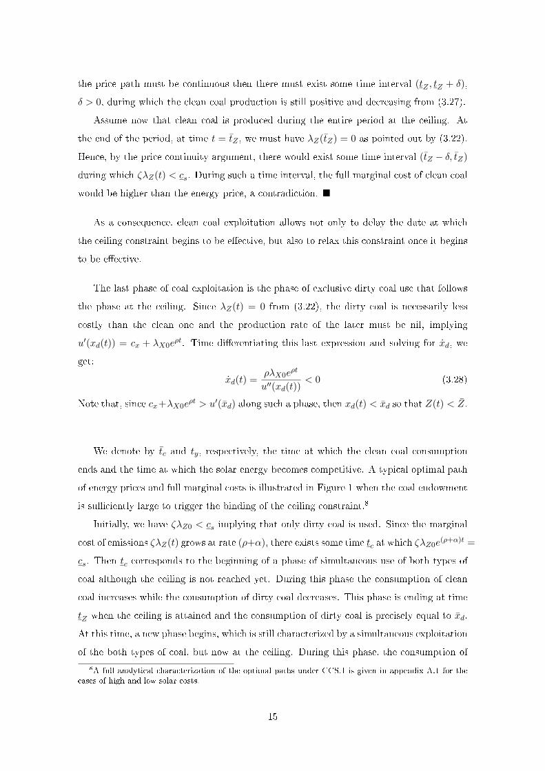
the price path must be continuous then there must exist some time interval (tZ , tZ + δ),

δ > 0, during which the clean coal production is still positive and decreasing from (3.27).

Assume now that clean coal is produced during the entire period at the ceiling. At

the end of the period, at time t = tZ , we must have λZ(tZ) = 0 as pointed out by (3.22).

Hence, by the price continuity argument, there would exist some time interval (tZ − δ, tZ)

during which ζλZ(t) < cs. During such a time interval, the full marginal cost of clean coal

would be higher than the energy price, a contradiction. �

As a consequence, clean coal exploitation allows not only to delay the date at which

the ceiling constraint begins to be e�ective, but also to relax this constraint once it begins

to be e�ective.

The last phase of coal exploitation is the phase of exclusive dirty coal use that follows

the phase at the ceiling. Since λZ(t) = 0 from (3.22), the dirty coal is necessarily less

costly than the clean one and the production rate of the later must be nil, implying

u′(xd(t)) = cx + λX0eρt. Time di�erentiating this last expression and solving for xd, we

get:

xd(t) =ρλX0e

ρt

u′′(xd(t))< 0 (3.28)

Note that, since cx+λX0eρt > u′(xd) along such a phase, then xd(t) < xd so that Z(t) < Z.

We denote by tc and ty, respectively, the time at which the clean coal consumption

ends and the time at which the solar energy becomes competitive. A typical optimal path

of energy prices and full marginal costs is illustrated in Figure 1 when the coal endowment

is su�ciently large to trigger the binding of the ceiling constraint.8

Initially, we have ζλZ0 < cs implying that only dirty coal is used. Since the marginal

cost of emissions ζλZ(t) grows at rate (ρ+α), there exists some time tc at which ζλZ0e(ρ+α)t =

cs. Then tc corresponds to the beginning of a phase of simultaneous use of both types of

coal although the ceiling is not reached yet. During this phase the consumption of clean

coal increases while the consumption of dirty coal decreases. This phase is ending at time

tZ when the ceiling is attained and the consumption of dirty coal is precisely equal to xd.

At this time, a new phase begins, which is still characterized by a simultaneous exploitation

of the both types of coal, but now at the ceiling. During this phase, the consumption of

8A full analytical characterization of the optimal paths under CCS.1 is given in appendix A.1 for thecases of high and low solar costs.

15

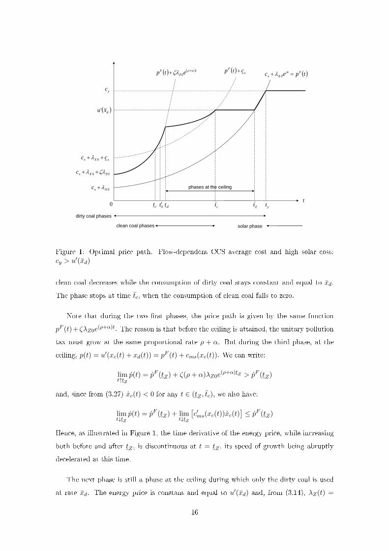
t0

tpec FtXx 0

yc

Zt Zt

00 ZXxc

0Xxc

sXx cc 0

dxu'

sF ctp t

ZF etp 0

ctct yt

phases at the ceiling

clean coal phases

dirty coal phases

solar phase

0t

Figure 1: Optimal price path. Flow-dependent CCS average cost and high solar cost:cy > u′(xd)

clean coal decreases while the consumption of dirty coal stays constant and equal to xd.

The phase stops at time tc, when the consumption of clean coal falls to zero.

Note that during the two �rst phases, the price path is given by the same function

pF (t)+ ζλZ0e(ρ+α)t. The reason is that before the ceiling is attained, the unitary pollution

tax must grow at the same proportional rate ρ + α. But during the third phase, at the

ceiling, p(t) = u′(xc(t) + xd(t)) = pF (t) + cms(xc(t)). We can write:

limt↑tZ

p(t) = pF (tZ) + ζ(ρ+ α)λZ0e(ρ+α)tZ > pF (tZ)

and, since from (3.27) xc(t) < 0 for any t ∈ (tZ , tc), we also have:

limt↓tZ

p(t) = pF (tZ) + limt↓tZ

[c′ms(xc(t))xc(t)

]≤ pF (tZ)

Hence, as illustrated in Figure 1, the time derivative of the energy price, while increasing

both before and after tZ , is discontinuous at t = tZ , its speed of growth being abruptly

decelerated at this time.

The next phase is still a phase at the ceiling during which only the dirty coal is used

at rate xd. The energy price is constant and equal to u′(xd) and, from (3.14), λZ(t) =

16

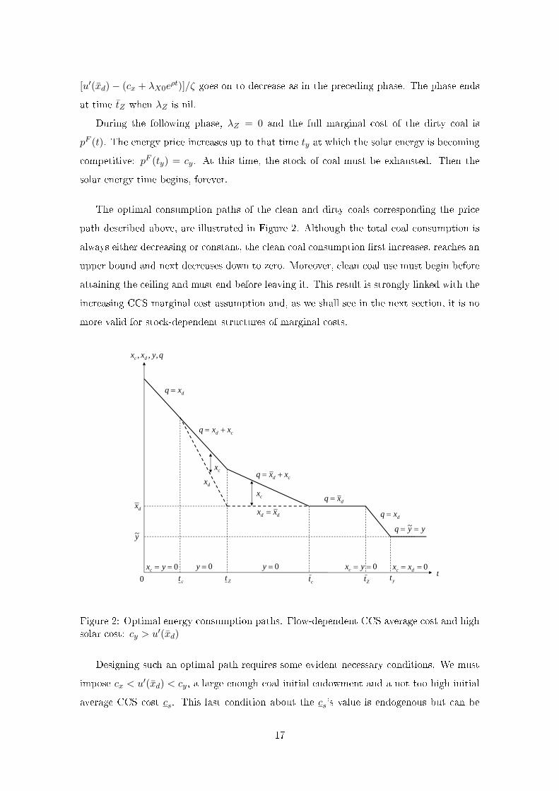
[u′(xd)− (cx + λX0eρt)]/ζ goes on to decrease as in the preceding phase. The phase ends

at time tZ when λZ is nil.

During the following phase, λZ = 0 and the full marginal cost of the dirty coal is

pF (t). The energy price increases up to that time ty at which the solar energy is becoming

competitive: pF (ty) = cy. At this time, the stock of coal must be exhausted. Then the

solar energy time begins, forever.

The optimal consumption paths of the clean and dirty coals corresponding the price

path described above, are illustrated in Figure 2. Although the total coal consumption is

always either decreasing or constant, the clean coal consumption �rst increases, reaches an

upper bound and next decreases down to zero. Moreover, clean coal use must begin before

attaining the ceiling and must end before leaving it. This result is strongly linked with the

increasing CCS marginal cost assumption and, as we shall see in the next section, it is no

more valid for stock-dependent structures of marginal costs.

t0 Zt Ztctct yt

qyxx dc ,,,

y~

dx

dxq

cd xxq

cd xxq

dxq

dxq

yyq ~

dx

dd xx

0y 0y 0 yxc 0 dc xx0 yxc

cx

cx

Figure 2: Optimal energy consumption paths. Flow-dependent CCS average cost and highsolar cost: cy > u′(xd)

Designing such an optimal path requires some evident necessary conditions. We must

impose cx < u′(xd) < cy, a large enough coal initial endowment and a not too high initial

average CCS cost cs. This last condition about the cs's value is endogenous but can be

17

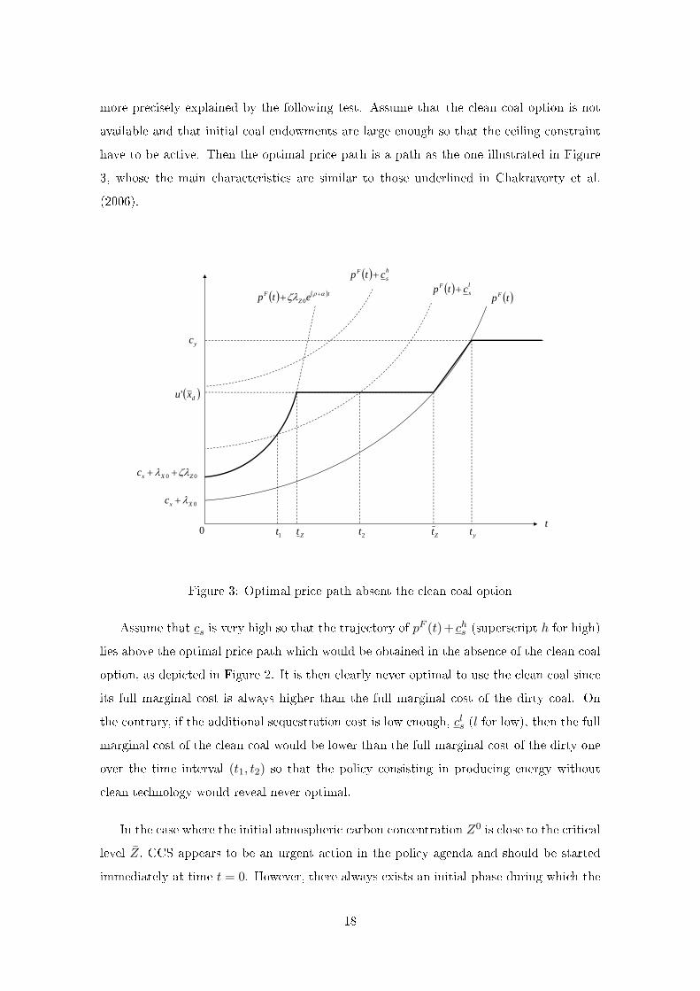
more precisely explained by the following test. Assume that the clean coal option is not

available and that initial coal endowments are large enough so that the ceiling constraint

have to be active. Then the optimal price path is a path as the one illustrated in Figure

3, whose the main characteristics are similar to those underlined in Chakravorty et al.

(2006).

t0

tpF

yc

Zt Zt

00 ZXxc

0Xxc

dxu'

ls

F ctp tZ

F etp 0

2t1t yt

hs

F ctp

Figure 3: Optimal price path absent the clean coal option

Assume that cs is very high so that the trajectory of pF (t)+ chs (superscript h for high)

lies above the optimal price path which would be obtained in the absence of the clean coal

option, as depicted in Figure 2. It is then clearly never optimal to use the clean coal since

its full marginal cost is always higher than the full marginal cost of the dirty coal. On

the contrary, if the additional sequestration cost is low enough, cls (l for low), then the full

marginal cost of the clean coal would be lower than the full marginal cost of the dirty one

over the time interval (t1, t2) so that the policy consisting in producing energy without

clean technology would reveal never optimal.

In the case where the initial atmospheric carbon concentration Z0 is close to the critical

level Z, CCS appears to be an urgent action in the policy agenda and should be started

immediately at time t = 0. However, there always exists an initial phase during which the

18

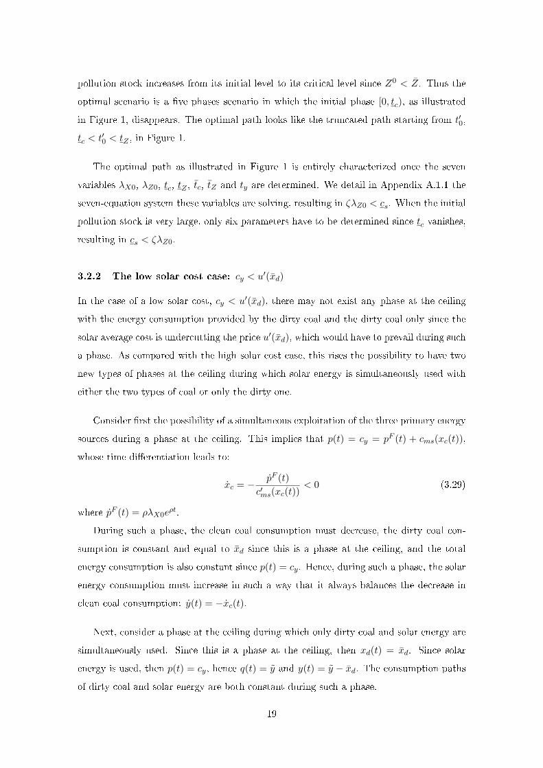
pollution stock increases from its initial level to its critical level since Z0 < Z. Thus the

optimal scenario is a �ve phases scenario in which the initial phase [0, tc), as illustrated

in Figure 1, disappears. The optimal path looks like the truncated path starting from t′0,

tc < t′0 < tZ , in Figure 1.

The optimal path as illustrated in Figure 1 is entirely characterized once the seven

variables λX0, λZ0, tc, tZ , tc, tZ and ty are determined. We detail in Appendix A.1.1 the

seven-equation system these variables are solving, resulting in ζλZ0 < cs. When the initial

pollution stock is very large, only six parameters have to be determined since tc vanishes,

resulting in cs < ζλZ0.

3.2.2 The low solar cost case: cy < u′(xd)

In the case of a low solar cost, cy < u′(xd), there may not exist any phase at the ceiling

with the energy consumption provided by the dirty coal and the dirty coal only since the

solar average cost is undercutting the price u′(xd), which would have to prevail during such

a phase. As compared with the high solar cost case, this rises the possibility to have two

new types of phases at the ceiling during which solar energy is simultaneously used with

either the two types of coal or only the dirty one.

Consider �rst the possibility of a simultaneous exploitation of the three primary energy

sources during a phase at the ceiling. This implies that p(t) = cy = pF (t) + cms(xc(t)),

whose time di�erentiation leads to:

xc = − pF (t)

c′ms(xc(t))< 0 (3.29)

where pF (t) = ρλX0eρt.

During such a phase, the clean coal consumption must decrease, the dirty coal con-

sumption is constant and equal to xd since this is a phase at the ceiling, and the total

energy consumption is also constant since p(t) = cy. Hence, during such a phase, the solar

energy consumption must increase in such a way that it always balances the decrease in

clean coal consumption: y(t) = −xc(t).

Next, consider a phase at the ceiling during which only dirty coal and solar energy are

simultaneously used. Since this is a phase at the ceiling, then xd(t) = xd. Since solar

energy is used, then p(t) = cy, hence q(t) = y and y(t) = y − xd. The consumption paths

of dirty coal and solar energy are both constant during such a phase.

19

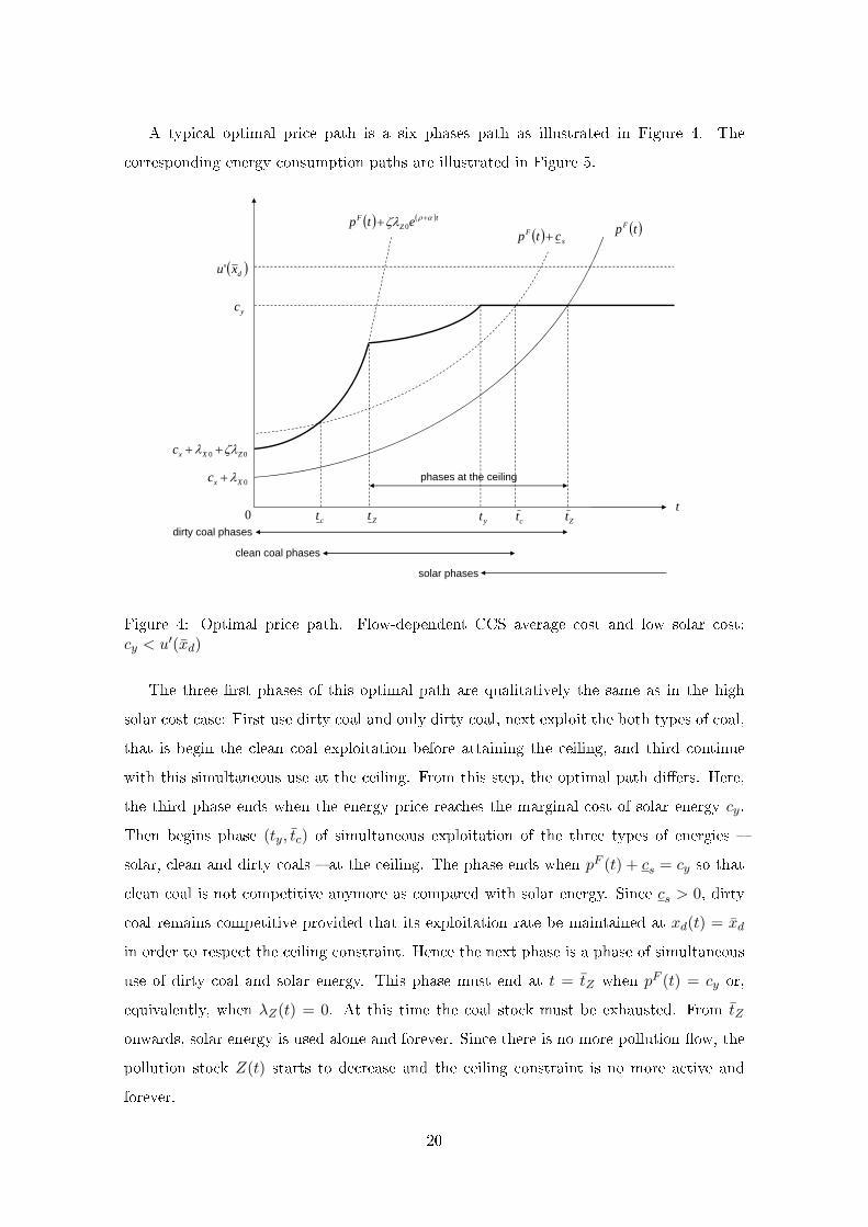
A typical optimal price path is a six phases path as illustrated in Figure 4. The

corresponding energy consumption paths are illustrated in Figure 5.

t0

tpF

yc

Zt Zt

00 ZXxc

0Xxc

dxu'

sF ctp

tZ

F etp 0

ctct yt

phases at the ceiling

dirty coal phases

clean coal phases

solar phases

Figure 4: Optimal price path. Flow-dependent CCS average cost and low solar cost:cy < u′(xd)

The three �rst phases of this optimal path are qualitatively the same as in the high

solar cost case: First use dirty coal and only dirty coal, next exploit the both types of coal,

that is begin the clean coal exploitation before attaining the ceiling, and third continue

with this simultaneous use at the ceiling. From this step, the optimal path di�ers. Here,

the third phase ends when the energy price reaches the marginal cost of solar energy cy.

Then begins phase (ty, tc) of simultaneous exploitation of the three types of energies �

solar, clean and dirty coals � at the ceiling. The phase ends when pF (t) + cs = cy so that

clean coal is not competitive anymore as compared with solar energy. Since cs > 0, dirty

coal remains competitive provided that its exploitation rate be maintained at xd(t) = xd

in order to respect the ceiling constraint. Hence the next phase is a phase of simultaneous

use of dirty coal and solar energy. This phase must end at t = tZ when pF (t) = cy or,

equivalently, when λZ(t) = 0. At this time the coal stock must be exhausted. From tZ

onwards, solar energy is used alone and forever. Since there is no more pollution �ow, the

pollution stock Z(t) starts to decrease and the ceiling constraint is no more active and

forever.

20

t0 Zt Ztctct yt

qyxx dc ,,,

y~

dx

dxq

cd xxq

cd xxq

yxxyq cd ~

yyq ~dx

dd xx dd xx

0y 0y 0y 0cx 0 dc xx

yxyq d ~

yycx

cx

cx

Figure 5: Optimal energy consumption paths. Flow-dependent CCS average cost and lowsolar cost: cy < u′(xd)

The system of equations allowing to determine the endogenous variables λX0, λZ0, tc,

tZ , ty and tZ in the case of a low solar cost is detailed in Appendix A.1.2.

The main conclusion of this section is that, whatever the marginal cost of the solar

clean substitute, either high or low provided that it is constant, assuming that the average

abatement cost of the potential pollution �ow is an increasing and convex function of the

�ow of abatement implies that abatement must be activated before the pollution stock

constraint begins to bind. Moreover, in the case of low solar costs, the three types of

resources � clean coal, dirty coal and solar energy � are simultaneously exploited during

the second and the third phases of the period at the ceiling (the third and fourth phases

of the scenarios).

As we shall see in the next section, such characteristics of the optimal paths can never

be obtained with stock-dependent CCS average cost functions.

21

4 Stock-dependent CCS cost functions

Although giving rise to contrasted optimal paths according to whether the scarcity e�ect

or the learning one dominates, the optimal paths generated by CCS stock-dependent cost

functions have some strongly similar formal features. We �rst point out these similarities

before focusing on the speci�cities induced by the dominance of each e�ect.

4.1 Problem formulation and preliminary remarks

Whatever the e�ect of clean coal cumulative production which is dominant, either the

scarcity e�ect or the learning e�ect, the social planner problem has the same following

general structure:

maxxc,xd,y

∫ ∞0{u(xc(t) + xd(t) + y(t))− cx[xc(t) + xd(t)]− cs(Sc(t))xc(t)− cyy(t)} e−ρtdt

subject to constraints (2.5), (2.7), (2.9), to the inequality constraints (2.6), (2.11) and

(2.12), all common to the both cases, and to the constraint (2.10) for the case of a dominant

scarcity e�ect. This last condition is the only one which is di�erentiating the two dominant

e�ect sub-cases.

Let us denote by λS the costate variable of Sc and keep the notations of the previous

section for the other costate variables, that is λX for X and −λZ for Z. Then the current

valued Hamiltonian of the program reads:

H = u(xc + xd + y)− cx(xc + xd)− cs(Sc)xc − cyy − λX [xc + xd]− λZ [ζxd − αZ] + λSxc

Also adopting the same notations for the Lagrange multipliers and denoting by νS the

multiplier associated with constraint (2.10), the current valued Lagrangian is:

L = H+ νXX + νZ [Z − Z] + νS [Sc − Sc] + γxcxc + γxdxd + γyy

with νS = 0 for all Sc ∈ [0, X0] in the dominant learning e�ect case, a formal device to

include the both CCS.2 and CCS.3 cases in a generic expression of the Lagrangian.

Among the �rst-order conditions (3.13)-(3.17) of the �ow-dependent case, the condition

(3.13) relative to the optimal use of xc must be replaced by:

u′(xc + xd + y) = cx + λX + cs(Sc)− λS − γxc (4.30)

22

A new condition relative to the dynamics of λS must be introduced:

λS = ρλS + c′s(Sc)xc + νS (4.31)

together with the usual complementary slackness condition on νS . The associated transver-

sality condition is:

limt↑∞

e−ρtλS(t)Sc(t) = 0 (4.32)

The other �rst-order conditions (3.14)-(3.17) relative to the use of the other primary en-

ergies, xd and y, and to the dynamics of λX and λZ remain unchanged, as well as the

transversality conditions (3.18) and (3.19) relative to the long run values of X and Z.

Finally, note that from (4.31), as long as the clean coal has not yet been exploited, that

is during an hypothetic initial phase of exclusive dirty coal consumption, we must have

λS = ρλS , hence:

t ≤ tc ⇒ λS(t) = λS0eρt, where λS0 ≡ λS(0) (4.33)

4.2 The case of a dominant scarcity e�ect

In the case of a dominant scarcity e�ect, the more the clean coal has been used in the past,

the higher its present and future exploitation costs assuming that such exploitation is still

possible, that is Sc(t) < Sc. This suggests that λS should be negative.

Proposition 3 Under a stock-dependent cost function CCS.2 with a dominant scarcity

e�ect, assuming that the clean coal has to be exploited along the optimal path, the costate

variable associated with the clean coal cumulated production is negative as long as its ex-

ploitation is not yet de�nitively closed:

∀t ≥ 0 :

∫ ∞t

xc(τ)dτ > 0 ⇒ λS(t) < 0 (4.34)

Proof: Solving the non-homogenous di�erential equation (4.31) results in:

λS(t) =

{λS0 +

∫ t

0[c′s(Sc(τ))xc(τ) + νS(τ)]e−ρτdτ

}eρt (4.35)

where νS(t) ≥ 0. Next, using the transversality condition (4.32) and the condition

limt↑∞ Sc(t) ≤ Sc bounding Sc(t) from above, we obtain the value of λS0:

λS0 = −∫ ∞

0[c′s(Sc(t))xc(t) + νS(t)]e−ρtdt

23

Substituting this value for λS0 in the above expression (4.35) of λS(t), we �nally get:

λS(t) = −∫ ∞t

[c′s(Sc(τ))xc(τ) + νS(τ)]e−ρ(τ−t)dτ (4.36)

which is negative under the qualifying assumption∫∞t xc(τ)dτ > 0 since c′s(Sc) > 0 under

CCS.2. �

From (4.36), it should be clear that λS(t) includes two components. Increasing at time

t the cumulated clean coal consumption by xc(t) units has two e�ects on the sum of the

optimal future discounted9 net surplus:

- �rst through the increase in the future sequestration costs by c′s(Sc(τ))xc(τ), τ > t;

- second through the tightening of the available capacity constraint restricting the size

of the stock of carbon which could be stockpiled in the future, this second e�ect being

captured by νS(τ), τ > t.

It remains to determine the behavior of λS(t) once the qualifying condition (4.34) does

not hold anymore, that is once the sequestration option is de�nitively closed, from time

t = tc onwards.

Proposition 4 Under a stock-dependent cleaning cost function with a dominant scarcity

e�ect, once the sequestration is de�nitively closed:

- either the carbon reservoir capacity constraint is not binding at the closing time and

then λS(t) = 0, more precisely:

Sc(tc) < Sc ⇒ λS(t) = 0, t ≥ tc (4.37)

- or the carbon stockpiling constraint is e�ective at the closing time and then:

Sc(tc) = Sc ⇒ λS(t) = −∫ ∞t

νS(τ)e−ρ(τ−t)dτ, t ≥ tc (4.38)

Proof: This result is an immediate implication of (4.36) which holds at any time. For

all t ≥ tc, xc = 0. If �rst Sc(tc) < Sc, then for all t ≥ tc, Sc(t) < Sc hence νS(t) = 0 and

thus, from (4.36), λS(t) = 0. Second if Sc(tc) = Sc then Sc(t) = Sc for all t ≥ tc and, from

(4.36) again, we get (4.38). �

The important point is that even if sequestration is de�nitively closed , λS(t) may be

still strictly negative at least for some time. We shall come back soon on the meaning of

9Discounted in value at time t.

24

the analytical expression of λS when the reservoir capacity constraint is tight at the closing

date of the clean coal exploitation.

Since λS(t) < 0, at least as long as the sequestration is not de�nitively closed, then the

full marginal cost of the clean coal amounts now to:

ccm(xc(t)) = pF (t) + cs(Sc(t))− λS(t) > pF (t) + cs(Sc(t)) (4.39)

This suggests �rst that, along the optimal path, the clean coal exploitation cannot begin

before having attained the pollution cap Z (Proposition 5) and, second, that if the clean

coal has ever to be used, then its exploitation must be closed before the end of the period

at the ceiling (Proposition 6).

Proposition 5 Under a stock-dependent CCS cost function with a dominant scarcity ef-

fect, if clean coal has ever to be used along the optimal path and provided that the ceiling

constraint is binding along the path, then its exploitation cannot begin before the ceiling

constraint is binding, in brief: tc ≥ tZ .

Proof: Assume that the clean coal is exploited while the ceiling is not attained yet:

tc < tZ . Then, either only the clean coal is used during the time interval [tc, tZ ], or there

exists a subinterval [t′c, t′Z ], tc ≤ t′c < t′Z ≤ tZ , during which the both types of coal are

exploited, or, last, there exists a subinterval [t′′c , t′′Z ], tc ≤ t′′c < t′′Z ≤ tZ , during which the

clean coal and the solar energy are simultaneously exploited.

First, if only the clean coal is used during [tc, tZ ], then from Z(tc) < Z and Z(t) =

−αZ(t) < 0 for t ∈ [tc, tZ ], we conclude that Z(tZ) < Z, a contradiction.

Second, assume that the both types of coal are simultaneously exploited during [t′c, t′Z ].

Then their full marginal costs must be equal. Since the ceiling is not attained yet, the dirty

coal full marginal cost amounts to pF (t) + ζλZ0e(ρ+α)t while the clean coal full marginal

cost amounts to pF (t) + cs(Sc(t))− λS(t), λS(t) < 0. Hence:

λS(t) = cs(S(t))− ζλZ0e(ρ+α)t, t ∈ [t′c, t

′Z ] (4.40)

Time di�erentiating the above equality leads to:

λS(t) = c′S(S(t))xc(t)− ζ(ρ+ α)λZ0e(ρ+α)t

Substituting the left-hand-side of (4.31) with νS = 0 for λS(t), and simplifying, we obtain:

ρλS(t) = −ζ(ρ+ α)λZ0e(ρ+α)t

25

Last, substitute the right-hand-side of (4.40) for λS(t) in the above equality and simplify

to get:

0 < ρcs(Sc(t)) = −αζλZ0e(ρ+α)t < 0, t ∈ [t′c, t

′Z ]

again a contradiction.

Last, we prove in Proposition 8 that clean coal and solar energy may never be simul-

taneously exploited during any time interval along the optimal path. �

At this stage, we know that the clean coal exploitation cannot begin before the ceiling is

reached. Proposition 6 below shows that it cannot either be introduced after the beginning

of the ceiling period.

Proposition 6 Under a stock-dependent CCS cost function with a dominant scarcity ef-

fect, if clean coal has ever to be used along the optimal path, then its exploitation may not

start after the beginning of the period at the ceiling: tc ≤ tZ .

Proof: Assume that tZ ≤ tc, then during the time interval [tZ , tc], either y(t) = 0

so that xd(t) = xd, or y(t) > 0 and y(t) + xd(t) = y(t) + xd = y, depending on wether

cy ≥ u′(xd) or cy < u′(xd), hence p(t) = min {u′(xd), cy} ≡ p, t ∈ [tZ , tc].

Since the clean coal is not competitive at tZ , its full marginal cost may not be lower

than p at this time: pF (t)(tZ) + cs − λS0eρtZ > p. Moreover, since pF (t) is increasing and

λS0 is negative, we have: pF (t)(t) + cs − λS0eρt > p, ∀t ∈ [tZ , tc], so that the clean coal

consumption cannot become competitive at tc, hence a contradiction. �

Thus from Propositions 5 and 6 we conclude that the exploitation of the clean coal

must begin when the ceiling is attained: tc = tZ . The following Proposition 7 shows that

its exploitation must be closed before the end of the ceiling period.

Proposition 7 Under a stock-dependent CCS cost function with a dominant scarcity ef-

fect, if clean coal has ever to be used along the optimal path and provided that the ceiling

constraint be binding along the path, then its exploitation must be closed before the end of

the period at the ceiling.

Proof: Assume that at the end of the period at the ceiling, the both types of coal

are simultaneously used, that is xc(tZ) > 0 and xd(tZ) > 0. At this date, we know from

(3.22) that the shadow marginal cost of the pollution stock must be nil: λZ(tZ) = 0. Then

the dirty coal full marginal cost amounts to pF (tZ) while the clean coal full marginal cost

26

amounts to pF (tZ) + cs(S(tZ)) − λS(tZ) > pF (tZ). Since the marginal cost of the clean

coal is larger than the cost of the dirty one, only the dirty one has to be used, hence a

contradiction. �

Last, Proposition 8 will permit, together with the above propositions, to fully charac-

terize the optimal path provided that the ceiling constraint has to be e�ective. It shows

that the clean coal and the solar energy may never be simultaneously exploited.

Proposition 8 Under a stock-dependent CCS.2 cost function with a dominant scarcity

e�ect, the clean coal and the solar energy may never be exploited simultaneously along the

optimal path.

Proof: Let us assume that clean coal and solar energy are simultaneously used over

some time interval. Their full marginal costs must be equal, that is: cy = cx + λX0eρt +

cs(S(t)) − λS(t). Time di�erentiating, substituting the RHS of (4.31) (with νS = 0 since

Sc(t) < Sc) and simplifying, we get:

0 < λX0eρt = λS(t) < 0

the RHS of this inequality directly coming from Proposition 3, hence a contradiction. �

The Propositions 5, 6, 7 and 8 have di�erent implications depending upon wether the

cost of the solar energy is high or low.

4.2.1 The high solar cost case: cy > u′(xd)

In this case, we may conclude from the above Propositions 5-8 that, if the ceiling constraint

has to be e�ective and if the clean coal has to be exploited, then the period at the ceiling

contains two phases, the �rst one being a phase during which the both types of coal are

used and the second one a phase during which only the dirty coal is exploited. This is due

to the fact that, at a price cy even if only the dirty coal were exploited then xd would be

smaller than xd hence the ceiling constraint could not be active.

A typical optimal path is a �ve-phases path as illustrated in Figure 6 for the energy

price and in Figure 7 for the energy consumptions.10

10A full analytical characterization of the optimal path under CCS.2 is given in Appendix A.2 for theboth cases of high and low solar costs.

27

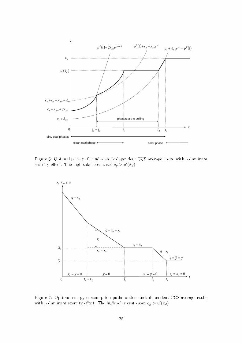
t0

tpec FtXx 0

yc

Zt

00 ZXxc

0Xxc

00 SXsx cc

dxu'

tSs

F ectp 0 tZ

F etp 0

ctZc tt yt

phases at the ceiling

clean coal phase

dirty coal phases

solar phase

Figure 6: Optimal price path under stock-dependent CCS average costs, with a dominantscarcity e�ect. The high solar cost case: cy > u′(xd)

t0 ZtctZc tt yt

qyxx dc ,,,

y~

dx

dxq

cd xxq

dxq

dxq

yyq ~dd xx

0y 0 dc xx0 yxc

cx

0 yxc

Figure 7: Optimal energy consumption paths under stock-dependent CCS average costs,with a dominant scarcity e�ect. The high solar cost case: cy > u′(xd)

28

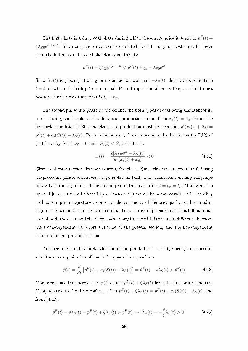
The �rst phase is a dirty coal phase during which the energy price is equal to pF (t) +

ζλZ0e(ρ+α)t. Since only the dirty coal is exploited, its full marginal cost must be lower

than the full marginal cost of the clean one, that is:

pF (t) + ζλZ0e(ρ+α)t < pF (t) + cs − λS0e

ρt

Since λZ(t) is growing at a higher proportional rate than −λS(t), there exists some time

t = tc at which the both prices are equal. From Proposition 5, the ceiling constraint must

begin to bind at this time, that is tc = tZ .

The second phase is a phase at the ceiling, the both types of coal being simultaneously

used. During such a phase, the dirty coal production amounts to xd(t) = xd. From the

�rst-order-condition (4.30), the clean coal production must be such that u′(xc(t) + xd) =

pF (t) + cs(S(t))− λS(t). Time di�erentiating this expression and substituting the RHS of

(4.31) for λS (with νS = 0 since Sc(t) < Sc), results in:

xc(t) =ρ[λX0e

ρt − λS(t)]

u′′(xc(t) + xd)< 0 (4.41)

Clean coal consumption decreases during the phase. Since this consumption is nil during

the preceding phase, such a result is possible if and only if the clean coal consumption jumps

upwards at the beginning of the second phase, that is at time t = tZ = tc. Moreover, this

upward jump must be balanced by a downward jump of the same magnitude in the dirty

coal consumption trajectory to preserve the continuity of the price path, as illustrated in

Figure 6. Such discontinuities can arise thanks to the assumptions of constant full marginal

cost of both the clean and the dirty coals at any time, which is the main di�erence between

the stock-dependent CCS cost structure of the present section, and the �ow-dependent

structure of the previous section.

Another important remark which must be pointed out is that, during this phase of

simultaneous exploitation of the both types of coal, we have:

p(t) =d

dt

[pF (t) + cs(S(t))− λS(t)

]= pF (t)− ρλS(t) > pF (t) (4.42)

Moreover, since the energy price p(t) equals pF (t) + ζλZ(t) from the �rst-order condition

(3.14) relative to the dirty coal use, then pF (t) + ζλZ(t) = pF (t) + cs(S(t)) − λS(t), and

from (4.42):

pF (t)− ρλS(t) = pF (t) + ζλZ(t) > pF (t) ⇒ λZ(t) = −ρζλS(t) > 0 (4.43)

29

However the instantaneous proportional growth rate of λZ is now lower than ρ+α because

the ceiling constraint is tight, hence νZ(t) > 0 (see (3.17)). Thus during this phase at the

ceiling, the marginal social cost of the atmospheric carbon stock is growing as illustrated

in Figure 6. However, the proportional growth rate of λZ is lower at the beginning of this

phase than at the end of the preceding one, so that limt↑tZ p(t) > limt↓tZ p(t), as in the

case of �ow-dependent cost function when the ceiling is reached.

This second phase ends at time t = tc when the energy price attains the level u′(xd)

and, simultaneously, the consumption of clean coal falls down to zero since xd(tc) = xd.

The third phase is a phase at the ceiling during which only the dirty coal is used: xd(t) =

xd, xc(t) = 0. During this phase, λZ(t) = u′(xd) − pF (t) hence λZ(t) = −ρλX0eρt < 0.

The marginal social cost of the pollution stock is now decreasing. The phase ends at the

time t = tZ when λZ is nil.

From tZ onwards, λZ is always nil and the next phase is the standard Hotelling phase

of exclusive exploitation of the dirty coal up to that time t = ty at which the increasing

energy price attains the level cy allowing the solar energy to be a competitive substitute

of the dirty coal and, simultaneously, the stock of coal is exhausted.

Note that, in this case, tc = tZ . Let us denote by t this common date: t ≡ tZ = tc.

Thus we have again seven endogenous variables to determine, as in the �ow-dependent

CCS cost case, but with one date missing and one more initial costate variable: λX0, λZ0,

λS0, t, tc, tZ and ty. The seven equations system they are solving is detailed in Appendix

A.2.1.

The value of λS after the end of the sequestration phase:

As pointed out in Proposition 4, when the stockpiling constraint is e�ective at the end

of the sequestration phase, λS(t) may then be still strictly negative for some time after

the closing time of the clean coal exploitation. But how much time? It is clear that any

additional stockpiling capacity which would be available only after tZ would be worthless

since the pollution ceiling constraint is not binding anymore from tZ onwards. Let us show

that the time period during which an additional stockpiling capacity would be exploited if

it was available is shorter than tZ − tc.

Since we assume that the average CCS cost function is increasing in Sc, the reservoir

capacity impacts the optimal scenarios by stopping the availability of stockpiling capacities

30

at an average cost which is at least equal to cs(Sc). The logic of the model would be to

assume that any additional capacity ∆Sc could be exploited at an average CCS cost cs(Sc)

which is increasing over the interval (Sc, Sc + ∆Sc). Over [0, Sc + ∆Sc], cs(Sc) should have

the same general properties than over [0, Sc]. However, in order to show that the time

interval during which such an additional capacity has some value is shorter than tZ − tc,

it is su�cient to show that this is the case even if the average CCS cost is the lowest one,

that is equal to cs(Sc).

From (3.14) and (4.30), the time t at which the full marginal costs of the both types

of coal would be equal while λS(t) = 0, is given as the solution of:

cs(Sc) = ζλZ(t)

From (3.14), since u′(q(t)) = u′(xd) over the time interval [tc, tZ ], we have:

ζλZ(t) = u′(xd)− (cx + λX0eρt), t ∈ [tc, tZ ]

together with ζλZ(tc) = cs(Sc) − λS(tc) > cs(Sc) and ζλZ(tZ) = 0. Thus there exists

a unique time t: tc < t < tZ , at which ζλZ(t) = cs(Sc) and from which any additional

reservoir capacity is worthless.

4.2.2 The low solar cost case: cy < u′(xd)

As in the case of �ow-dependent costs, and for the same reasons, there may not exist

a phase at the ceiling during which the dirty coal and only the dirty coal is exploited.

Assuming that such a phase could exist, the energy price would have to be equal to u′(xd),

a price higher than the solar energy average cost cy meaning that this alternative energy

primary source should have to be exploited, thus a contradiction.

We know from Proposition 5 that if clean coal has to be used, it may not be before

the pollution cap Z is reached and, from Proposition 7, that clean coal and solar energy

may never be exploited simultaneously. Furthermore from Proposition 6, the clean coal

exploitation must be closed before the end of the period at the ceiling. Thus if clean coal

has to be used and the ceiling constraint has to be active along the optimal path, then the

only possible period at the ceiling is a two-phases period. During the �rst one, the both

clean and dirty coals are simultaneously exploited and during the second period, both the

dirty coal and the solar energy. Typical paths � four-phases paths in the current case �

of energy price and the associated energy consumptions are illustrated in Figures 8 and 9

respectively.

31

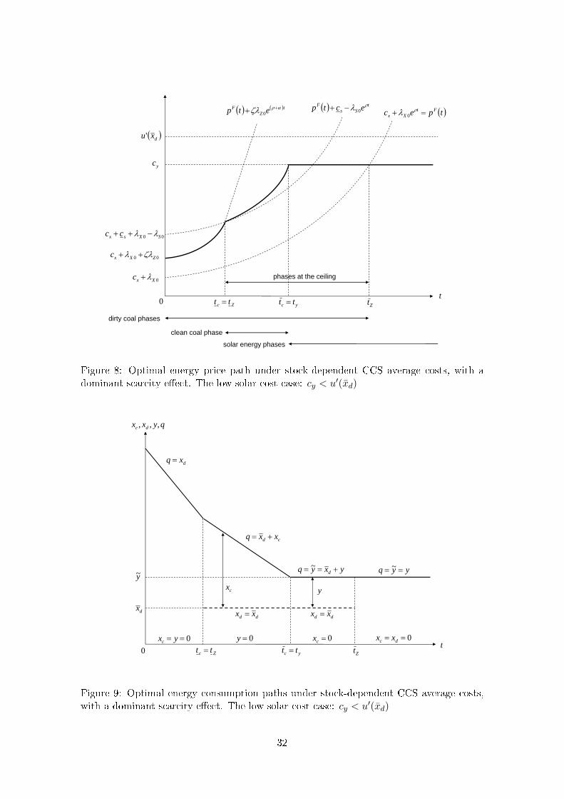
t0

tpec FtXx 0

yc

Zt

00 ZXxc

0Xxc

00 SXsx cc

dxu'

tSs

F ectp 0 tZ

F etp 0

yc tt Zc tt

phases at the ceiling

clean coal phase

dirty coal phases

solar energy phases

Figure 8: Optimal energy price path under stock-dependent CCS average costs, with adominant scarcity e�ect. The low solar cost case: cy < u′(xd)

t0 Ztyc tt Zc tt

qyxx dc ,,,

y~

dx

dxq

cd xxq

yxyq d ~ yyq ~

dd xx

0y 0 dc xx0 yxc

cx

0cx

dd xx

y

Figure 9: Optimal energy consumption paths under stock-dependent CCS average costs,with a dominant scarcity e�ect. The low solar cost case: cy < u′(xd)

32

The two �rst phases are similar to the two �rst phases of the high solar cost case. The

�rst phase is the usual phase of exclusive use of the dirty coal during which the atmospheric

carbon stock grows up to the time tZ at which the carbon cap is attained.

At time tZ , the clean coal becomes competitive, tZ = tc, and the resulting second phase

is a phase of joint exploitation of the two types of coal while at the ceiling: xd(t) = xd and

xc(t) is decreasing according to (4.41). Thus at time t = tZ , the dirty coal consumption is

instantaneously reduced and this downward jump must be balanced by an upward jump of

the same magnitude in the clean coal consumption. As in the high solar cost case during

this phase:

d

dt=[pF (t) + cs(S(t))− λS(t)

]> pF (t) and λZ(t) = −ρ

ζλS(t) > 0

The argument is the same as the argument leading to expressions (4.42) and (4.43). The

main di�erence with the high solar cost case is that now, the phase ends when the energy

price is equal to cy. At this point, the phases of competitiveness of the solar energy begin.

Just before this time ty, since cy < u′(xd) and xd(ty) = xd, then xc(t) = y − xd > 0.

However, since the solar energy is competitive just after ty and, from Proposition 7, both

clean coal and solar energy may not be simultaneously used, hence the exploitation of the

clean coal must be closed so that ty = tc. Thus the clean coal consumption falls from

y − xd down to 0 and the production of the solar energy jumps from 0 up to y − xd to

keep the continuity of the energy services consumption path. During this third phase, the

production of dirty coal and solar energy are both constant, xd(t) = xd and y(t) = y− xd,

while the pollution stock remains at the ceiling level Z(t) = Z. The associated shadow

cost declines: λZ(t) = (cy − cx − λX0eρt)/ζ. The phase ends at time t = tZ when λZ has

been reduced to 0, that is when pF (t) = cy. The exploitation of the dirty coal must be

closed and simultaneously, the stock of coal must be exhausted.

The last phase from tZ onwards is a phase of exclusive solar energy consumption,

q(t) = y(t) = y. Then the pollution stock is gradually eliminated by natural absorption,

Z(t) = Z(tZ)e−α(t−tZ) = Ze−α(t−tZ) < Z, t ≥ tZ .

Note that in this low solar cost case, we have not only tc = tZ(≡ t), but also tc = ty.

Let us denote by t this other common date. Hence, only six variables have to be determined

now: λX0, λZ0, λS0, t, t and tZ . The system of six equations that they solve is exposed in

Appendix A.2.2.

33

The value of λS after the end of the clean coal exploitation phase:

Here again, λS may be strictly negative over some time interval (tc, t), tc = tZ < t < tZ ,

occurring at the end of the clean coal exploitation phase when the carbon capture policy

is restricted by the reservoir capacity. The argument runs along the same lines than the

argument developed in the high solar cost case, but during the phase [tc, tZ ], the λZ-path

is now established from cy instead of u′(xd) since the energy price path is determined by

cy during this time interval. More precisely, we have:

ζλZ(t) = cy − (cx + λX0eρt), t ∈ [tc, tZ ]

together with ζλZ(tc) = cs(Sc) − λS(tc) > cs(Sc) and ζλZ(tZ) = 0. Hence there exists

a unique time t = t solving ζλZ(t) = cs(Sc) and de�ning the date from which λS is nil

forever.

4.3 The case of a dominant learning e�ect

Now, the more the clean coal has been used in the past, the lower its marginal additional

cost as compared with the dirty coal. This suggests that λS should be positive up to the

time at which its exploitation is de�nitively closed.

Proposition 9 Under a stock-dependent CCS cost function with a dominant learning ef-

fect, assuming that the clean coal has to be exploited along the optimal path, the costate

variable associated with the clean coal cumulated production is positive as long as its ex-

ploitation is not de�nitively closed:

∀t ≥ 0 :

∫ ∞t

xc(τ)dτ > 0⇒ λS(t) > 0 (4.44)

Proof: This is a direct implication of (4.36) with νS = 0 and c′s < 0:

λS(t) = −∫ ∞t

c′s(Sc(τ))xc(τ)e−ρ(τ−t)dτ > 0 � (4.45)

Integrating by parts (4.45) we get the following alternative expression of λS(t) which

will turn out to be useful in the proof of Propositions 10, 11 and 12:

λS(t) = cs(Sc(t))− ρ∫ ∞t

cs(Sc(τ))e−ρ(τ−t)dτ (4.46)

Note that in the present case, once the exploitation of the clean coal is de�nitively closed,

then λS is nil:

∀t ≥ tc : λS(t) = 0 (4.47)

34

The following Propositions 10 and 11 show that, as in the case of a dominant scarcity

e�ect, the exploitation of the clean coal cannot begin before the ceiling constraint is binding

and must be closed before the end of the ceiling period in the case of a learning e�ect.

However, as we shall see, it may happen that the optimal clean coal exploitation has to

begin after the time at which the ceiling is attained. Under a dominant learning e�ect,

the equivalent of Proposition 7 obtained under a dominant scarcity e�ect does not hold

anymore.

Proposition 10 Under a stock-dependent CCS cost function with a dominant learning

e�ect, if clean coal has ever to be used along the optimal path and provided that the ceiling

constraint be active along the path, then its exploitation may not begin before the ceiling

constraint is binding: tc ≥ tZ .

Proof: The proof runs along the lines of the proof of Proposition 5, but some details

of the arguments must be adapted. Assume that tc < tZ . First, if during the time interval

[tc, tZ ] only the clean coal is used, then the argument is the same.

Second, assume that both the dirty and clean coals are exploited during some interval

[t′c, t′Z ]. Equating their respective full marginal costs results in:

ζλZ0e(ρ+α)t = cs(Sc(t))− λS(t), t ∈ (t′c, t

′Z)

Substituting the R.H.S. of (4.46) for λS(t), we get:

ζλZ0e(ρ+α)t = ρ

∫ ∞t

cs(Sc(τ))e−ρ(τ−t)dτ (4.48)

Time di�erentiate to obtain:

ζ(ρ+ α)λZ0e(ρ+α)t = −ρcs(Sc(t)) + ρ2

∫ ∞t

cs(Sc(τ))e−ρ(τ−t)dτ

that is, taking (4.48) into account:

0 < ζαλZ0e(ρ+α)t = −ρcs(Sc(t)) < 0, t ∈ [t′c, t

′Z ]

hence a contradiction.

Last we show in Proposition 12 that clean coal and solar energy may never be exploited

simultaneously. �

Proposition 11 Under a stock-dependent CCS cost function with a dominant learning

e�ect, if clean coal has ever to be used along the optimal path and provided that the ceiling

constraint be active along the path, then its exploitation must be closed before the end of

the ceiling period.

35

Proof: Assume that at tZ , the ending time of the ceiling period, the both types of coal

are still used, that is xc(tZ) > 0 and xd(tZ) = xd. Equating their full marginal costs and

taking into account that λZ(tZ) = 0 from (3.22), we get:

pF (tZ) = pF (tZ) + cs(Sc(tZ))− λS(tZ)

Substituting the R.H.S. of (4.46) for λS(tZ) results in:

pF (tZ) = pF (tZ) + ρ

∫ ∞tZ

cs(Sc(τ))e−ρ(τ−t)dτ > pF (tZ)

a contradiction. �

The last common feature of the optimal paths for the both cases of scarcity and learning

dominant e�ects stands in the impossibility of using simultaneously the clean coal and the

solar energy. Here again, the proof has to be adapted from Proposition 8.

Proposition 12 Under a stock-dependent CCS cost function with a dominant learning

e�ect, the clean coal and the solar energy may never be exploited simultaneously along the

optimal path.

Proof: Assume that the clean coal and the solar energy are simultaneously used during

some interval [t1, t2]. Equating their full marginal costs results in:

cy = cx + λX0eρt + cs(Sc(t))− λS(t), t ∈ [t1, t2]

Substituting the R.H.S. of (4.46) for λS(t), we get:

cy − cx = λX0eρt + ρ

∫ ∞t

cs(Sc(τ))e−ρ(τ−t)dτ (4.49)

Time di�erentiating, we obtain:

0 = ρ[λX0eρt − cs(Sc(t))] + ρ2

∫ ∞t

cs(Sc(τ))e−ρ(τ−t)dτ

and taking (4.49) into account:

0 = ρ[cy − cx]− ρcs(Sc(t))

Time di�erentiating again, we �nally get:

0 = −ρc′s(Sc(t))xc(t) > 0, t ∈ [t1, t2]

a contradiction �

36

Having reviewed the common features of the optimal paths in the cases of scarcity and

learning dominant e�ects, let us turn now to their di�erences.

From Propositions 10, 11 and 12, the only kind of phases during which the clean coal

is used is a phase of joint exploitation of the both types of coal while at the ceiling. Thus

if the scarcity and learning dominant e�ects have di�erent implications, and they should

have at least in some cases, this may be because:

- either what happens during this kind of phase is di�erent in the two cases,

- or the position of this phase within the optimal sequence of phases is di�erent in the

two cases,

- or the both.

Let us examine �rst the reasons for which what happens within this kind of phase could

be di�erent. During such a phase, q(t) = xc(t) + xd, t ∈ [tc, tc], and the time derivative of

xc is given formally by (see (4.41)):

xc(t) =ρ[λX0e

ρt − λS(t)]

u′′(xc(t) + xd)(4.50)

the di�erence with (4.41) being that we cannot conclude here about the sign of xc(t)

since λS(t) > 0. However, we can show that xc(t), hence p(t), may follow two types of

trajectories and only two during the phase.

First remark that, from (4.47), λS(t) is tending to 0 at the end of the phase. Thus, since

λS(t) is necessarily continuous in such a model, there must exist some terminal interval

[tc−∆, tc], 0 < ∆ ≤ tc−tc, during which xc(t) is negative and the energy price is increasing.

We have now to determine what could happen at the beginning of the phase when this

terminal interval is strictly shorter than the entire phase, that is when ∆ < tc − tc.

The following Proposition 13 states that the sign of xc(t) may change at most only

once within the phase.

Proposition 13 Under a stock-dependent CCS cost function with a dominant learning

e�ect, assuming that there exists a phase during which the both types of coal are exploited

while at the ceiling, then during such a phase:

- either the price of the energy services is monotonically increasing,

- or the price of the energy services is �rst decreasing and next increasing.

37

Proof: Assume that limt↓tc xc(t) > 0. De�ne t0 as the �rst date at which xc(t)

alternates in sign, since in this case the sign is changing at least once:

t0 = inf {t : xc(t) ≤ 0, t ∈ [tc, tc)} ⇒ xc(t0) = 0

From (4.30) and (4.31) respectively, we get:

u′(xc(t) + xd) = cx + λX0eρt + cs(Sc(t))− λS(t)

λS(t) = ρλS(t) + c′s(Sc(t))xc(t) = ρλS(t) + cs(Sc(t))

with cs(Sc(t)) < 0. Time di�erentiating the �rst expression and using the second one, we

get:

u′′(xc(t) + xd)xc(t) = ρ[λX0eρt − λS(t)]

De�ne φ(t) = λX0eρt − λS(t). Then u′′ < 0 implies that:

xc(t) > / = / < 0⇔ φ(t) < / = / > 0

Time di�erentiating φ(t) and using (4.31), we get:

φ(t) = ρλX0eρt − ρλS(t)− cs(Sc(t)) = ρφ(t)− cs(Sc(t))

Integrating over [t0, t], t0 < t ≤ tc, and taking into account that φ(t0) = 0, we obtain:

φ(t) = −eρt∫ t

t0

cs(Sc(τ))e−ρτdτ > 0, t ∈ (t0, tc]

We conclude that, if the sign of φ(t), hence the sign of xc(t) and p(t), is changing over

[tc, tc), it is only once. �

The last common characteristics shared by all the paths is about their behavior during

the pre-ceiling phase, hence also before the beginning of the clean coal exploitation ac-

cording to Proposition 10, that is over the time interval [0, tZ ] ⊆ [0, tc]. During this initial

phase, from (4.35), the shadow full marginal cost of the clean coal amounts to:

ccm = cx + cs + (λX0 − λS0)eρt

which may be either increasing or decreasing depending on whether the shadow marginal

cost of coal λX0 is larger or smaller than the shadow marginal value of the cumulated

experience in cleaning some part of its available stock, λS0. Such a formulation could

prove to be paradoxical since no experience has been yet accumulated. But this is the

marginal value of a zero-experience and this marginal value may be very high.

38

The sign of λX0 − λS0, which is endogenous, determines the position of the phase of

simultaneous exploitation of the both types of coal in the optimal sequence of phases.

However, as in the case of a dominant scarcity e�ect, the types of optimal sequences are

depending upon whether the solar energy cost is high or low.

4.3.1 The high solar cost case: cy > u′(xd)

We examine the di�erent possible types of paths according to the sign of λX0 − λS0.

- Case where λX0 > λS0

In this case, the shadow marginal value of the experience is relatively low as compared

with the coal scarcity rent and the structure of the optimal path is strongly determined by

the dominance of this scarcity e�ect.

Since λX0 > λS0 and provided that there exists a phase of joint use of the both types

of coal while at the ceiling, the clean coal exploitation must precisely begin at the time

at which the pollution cap Z is reached. The argument is given by Figure 10. At the

crossing point of the trajectories pF (t) + cs− λS0eρt and pF (t) + ζλZ0e

(ρ+α)t (remind that

pF (t) = cx+λX0eρt), either the common full marginal cost is lower than u′(xd) as illustrated

in Figure 10, or it is higher (not depicted) so that the clean coal is never competitive. Thus

the unique possible optimal sequence of phases is: i) only dirty coal up to the time at which

the ceiling is attained and, simultaneously, the clean coal becomes competitive, ii) both

the dirty and clean coals while at the ceiling, iii) only dirty coal while at the ceiling, iv)

again dirty coal only during a post-ceiling phase, and v) the in�nite phase of solar energy

use.

The other implication of λX0 > λS0 is that at time t+c , at the beginning of the phase

of joint exploitation of the both types of coal, due to the continuity of λS(t) in the present

case, then:

λX0eρt+c − λS(t+c ) ' (λX0 − λS0)eρt

+c > 0 (4.51)

From (4.50) we conclude that xc(t+c ) < 0, hence from Proposition 13, that xc(t) < 0 for all

t during the phase and the energy price is increasing.

Although the optimal price path depicted by Figure 10 could look quite similar to the

optimal price path determined in the case of a dominant scarcity e�ect with high solar

cost as illustrated in Figure 6, these two cases notably di�er during the phase of a joint

39

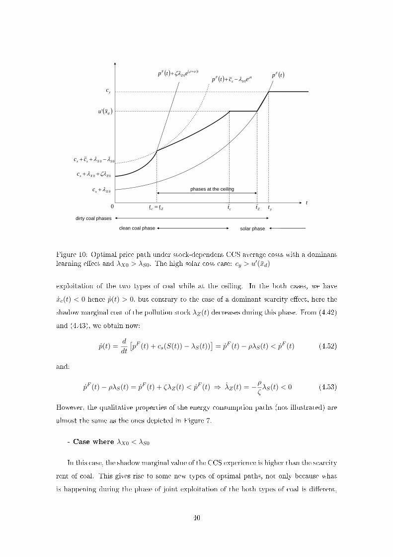
t0

tpF

yc

Zt

00 ZXxc

0Xxc

00 SXsx cc

dxu'

tSs

F ectp 0 t

ZF etp 0

ctZc tt yt

phases at the ceiling

clean coal phase

dirty coal phases

solar phase

Figure 10: Optimal price path under stock-dependent CCS average costs with a dominantlearning e�ect and λX0 > λS0. The high solar cost case: cy > u′(xd)

exploitation of the two types of coal while at the ceiling. In the both cases, we have

xc(t) < 0 hence p(t) > 0, but contrary to the case of a dominant scarcity e�ect, here the

shadow marginal cost of the pollution stock λZ(t) decreases during this phase. From (4.42)

and (4.43), we obtain now:

p(t) =d

dt

[pF (t) + cs(S(t))− λS(t))

]= pF (t)− ρλS(t) < pF (t) (4.52)

and:

pF (t)− ρλS(t) = pF (t) + ζλZ(t) < pF (t) ⇒ λZ(t) = −ρζλS(t) < 0 (4.53)

However, the qualitative properties of the energy consumption paths (not illustrated) are

almost the same as the ones depicted in Figure 7.

- Case where λX0 < λS0

In this case, the shadow marginal value of the CCS experience is higher than the scarcity

rent of coal. This gives rise to some new types of optimal paths, not only because what

is happening during the phase of joint exploitation of the both types of coal is di�erent,

40

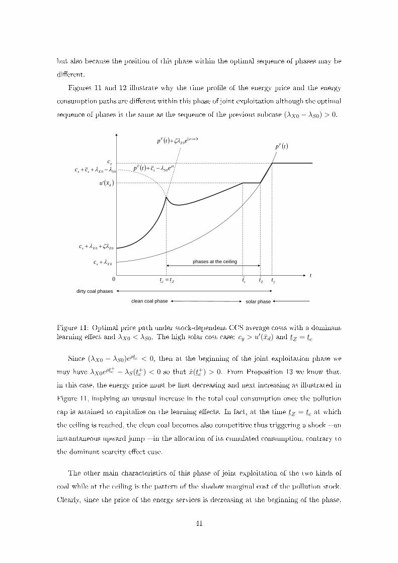
but also because the position of this phase within the optimal sequence of phases may be

di�erent.

Figures 11 and 12 illustrate why the time pro�le of the energy price and the energy

consumption paths are di�erent within this phase of joint exploitation although the optimal

sequence of phases is the same as the sequence of the previous subcase (λX0 − λS0) > 0.

t0

tpF

yc

Zt

00 ZXxc

0Xxc

00 SXsx cc

dxu'

tSs

F ectp 0

tZ

F etp 0

ctZc tt yt

phases at the ceiling

clean coal phase

dirty coal phases

solar phase

Figure 11: Optimal price path under stock-dependent CCS average costs with a dominantlearning e�ect and λX0 < λS0. The high solar cost case: cy > u′(xd) and tZ = tc

Since (λX0 − λS0)eρtc < 0, then at the beginning of the joint exploitation phase we

may have λX0eρt+c − λS(t+c ) < 0 so that x(t+c ) > 0. From Proposition 13 we know that,

in this case, the energy price must be �rst decreasing and next increasing as illustrated in

Figure 11, implying an unusual increase in the total coal consumption once the pollution

cap is attained to capitalize on the learning e�ects. In fact, at the time tZ = tc at which

the ceiling is reached, the clean coal becomes also competitive thus triggering a shock � an

instantaneous upward jump � in the allocation of its cumulated consumption, contrary to

the dominant scarcity e�ect case.

The other main characteristics of this phase of joint exploitation of the two kinds of

coal while at the ceiling is the pattern of the shadow marginal cost of the pollution stock.

Clearly, since the price of the energy services is decreasing at the beginning of the phase,

41

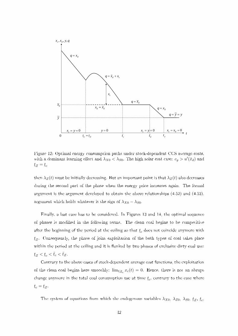
t0 ZtctZc tt yt

qyxx dc ,,,

y~

dx

dxq

cd xxq

dxq

dxq

yyq ~dd xx

0y 0 dc xx0 yxc

cx

0 yxc

Figure 12: Optimal energy consumption paths under stock-dependent CCS average costs,with a dominant learning e�ect and λX0 < λS0. The high solar cost case: cy > u′(xd) andtZ = tc

then λZ(t) must be initially decreasing. But an important point is that λZ(t) also decreases

during the second part of the phase when the energy price increases again. The formal

argument is the argument developed to obtain the above relationships (4.52) and (4.53),

argument which holds whatever is the sign of λX0 − λS0.

Finally, a last case has to be considered. In Figures 13 and 14, the optimal sequence

of phases is modi�ed in the following terms. The clean coal begins to be competitive

after the beginning of the period at the ceiling so that tc does not coincide anymore with

tZ . Consequently, the phase of joint exploitation of the both types of coal takes place

within the period at the ceiling and it is �anked by two phases of exclusive dirty coal use:

tZ < tc < tc < tZ .

Contrary to the above cases of stock-dependent average cost functions, the exploitation

of the clean coal begins here smoothly: limt↓tc xc(t) = 0. Hence, there is not an abrupt

change anymore in the total coal consumption use at time tc, contrary to the case where

tc = tZ .

The system of equations from which the endogenous variables λX0, λZ0, λS0, tZ , tc,

42

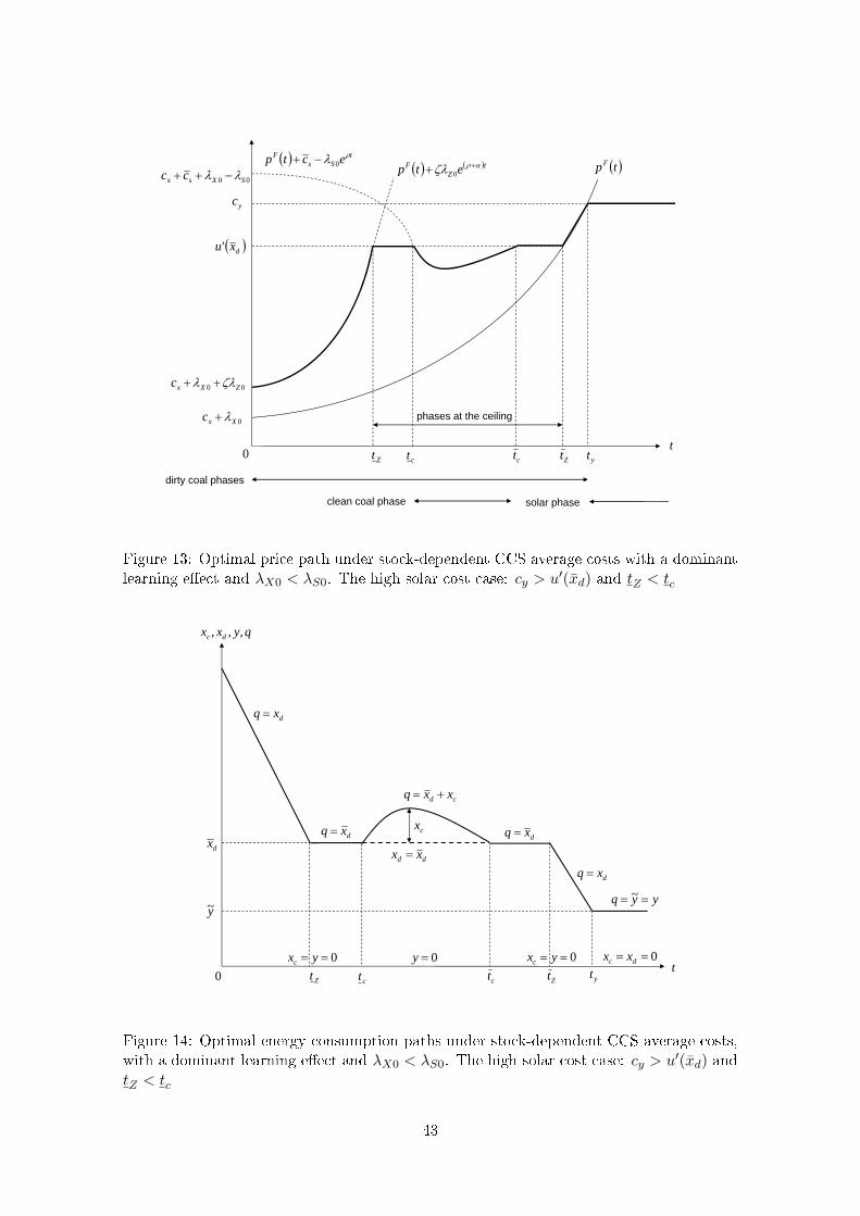
t0

tpF

yc

Zt

00 ZXxc

0Xxc

00 SXsx cc

dxu'

tSs

F ectp 0 tZ

F etp 0

ctZt yt

phases at the ceiling

clean coal phase

dirty coal phases

solar phase

ct

Figure 13: Optimal price path under stock-dependent CCS average costs with a dominantlearning e�ect and λX0 < λS0. The high solar cost case: cy > u′(xd) and tZ < tc

t0 ZtctZt yt

qyxx dc ,,,

y~

dx

dxq

cd xxq

dxq

dxq

yyq ~

dd xx

0y 0 dc xx0 yxc

cx

0 yxc

ct

dxq

Figure 14: Optimal energy consumption paths under stock-dependent CCS average costs,with a dominant learning e�ect and λX0 < λS0. The high solar cost case: cy > u′(xd) andtZ < tc

43

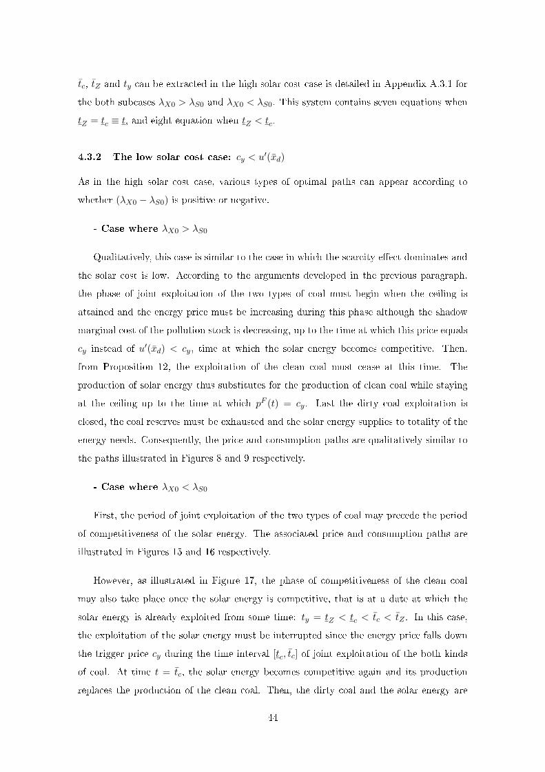
tc, tZ and ty can be extracted in the high solar cost case is detailed in Appendix A.3.1 for

the both subcases λX0 > λS0 and λX0 < λS0. This system contains seven equations when

tZ = tc ≡ t, and eight equation when tZ < tc.

4.3.2 The low solar cost case: cy < u′(xd)

As in the high solar cost case, various types of optimal paths can appear according to

whether (λX0 − λS0) is positive or negative.

- Case where λX0 > λS0

Qualitatively, this case is similar to the case in which the scarcity e�ect dominates and

the solar cost is low. According to the arguments developed in the previous paragraph,

the phase of joint exploitation of the two types of coal must begin when the ceiling is

attained and the energy price must be increasing during this phase although the shadow

marginal cost of the pollution stock is decreasing, up to the time at which this price equals

cy instead of u′(xd) < cy, time at which the solar energy becomes competitive. Then,

from Proposition 12, the exploitation of the clean coal must cease at this time. The

production of solar energy thus substitutes for the production of clean coal while staying

at the ceiling up to the time at which pF (t) = cy. Last the dirty coal exploitation is

closed, the coal reserves must be exhausted and the solar energy supplies to totality of the

energy needs. Consequently, the price and consumption paths are qualitatively similar to

the paths illustrated in Figures 8 and 9 respectively.

- Case where λX0 < λS0

First, the period of joint exploitation of the two types of coal may precede the period

of competitiveness of the solar energy. The associated price and consumption paths are

illustrated in Figures 15 and 16 respectively.

However, as illustrated in Figure 17, the phase of competitiveness of the clean coal

may also take place once the solar energy is competitive, that is at a date at which the

solar energy is already exploited from some time: ty = tZ < tc < tc < tZ . In this case,

the exploitation of the solar energy must be interrupted since the energy price falls down

the trigger price cy during the time interval [tc, tc] of joint exploitation of the both kinds

of coal. At time t = tc, the solar energy becomes competitive again and its production

replaces the production of the clean coal. Then, the dirty coal and the solar energy are

44

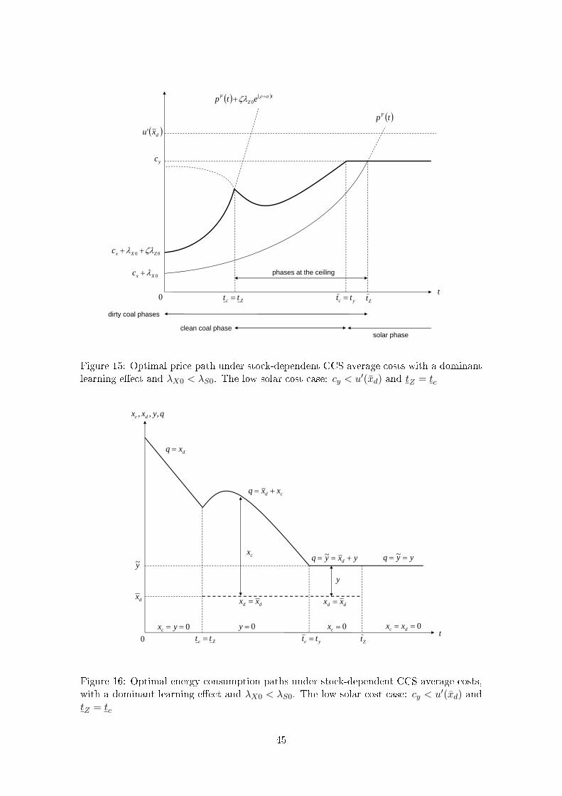
t0

tpF

yc

Zt

00 ZXxc

0Xxc

dxu'

tZ

F etp 0

yc tt Zc tt

phases at the ceiling

clean coal phase

dirty coal phases

solar phase

Figure 15: Optimal price path under stock-dependent CCS average costs with a dominantlearning e�ect and λX0 < λS0. The low solar cost case: cy < u′(xd) and tZ = tc

t0 Ztyc tt Zc tt

qyxx dc ,,,

y~

dx

dxq

cd xxq

yxyq d ~

y

dd xx

0y 0 dc xx0 yxc

cx

0cx

yyq ~

dd xx

Figure 16: Optimal energy consumption paths under stock-dependent CCS average costs,with a dominant learning e�ect and λX0 < λS0. The low solar cost case: cy < u′(xd) andtZ = tc

45

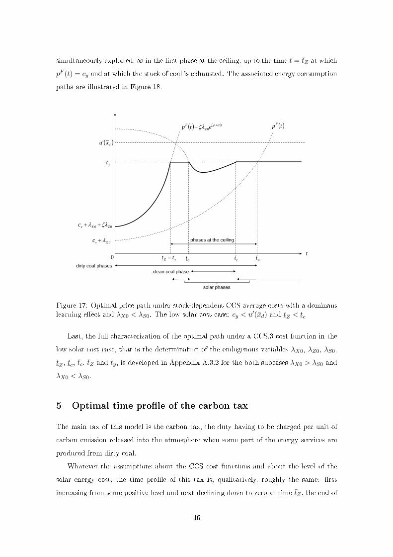
simultaneously exploited, as in the �rst phase at the ceiling, up to the time t = tZ at which

pF (t) = cy and at which the stock of coal is exhausted. The associated energy consumption

paths are illustrated in Figure 18.

t0

tpF

yc

Zt

00 ZXxc

0Xxc

dxu'

tZ

F etp 0

ctyZ tt

phases at the ceiling

clean coal phasedirty coal phases

solar phases

ct

Figure 17: Optimal price path under stock-dependent CCS average costs with a dominantlearning e�ect and λX0 < λS0. The low solar cost case: cy < u′(xd) and tZ < tc

Last, the full characterization of the optimal path under a CCS.3 cost function in the

low solar cost case, that is the determination of the endogenous variables λX0, λZ0, λS0,

tZ , tc, tc, tZ and ty, is developed in Appendix A.3.2 for the both subcases λX0 > λS0 and

λX0 < λS0.

5 Optimal time pro�le of the carbon tax

The main tax of this model is the carbon tax, the duty having to be charged per unit of

carbon emission released into the atmosphere when some part of the energy services are

produced from dirty coal.

Whatever the assumptions about the CCS cost functions and about the level of the

solar energy cost, the time pro�le of this tax is, qualitatively, roughly the same: �rst

increasing from some positive level and next declining down to zero at time tZ , the end of

46

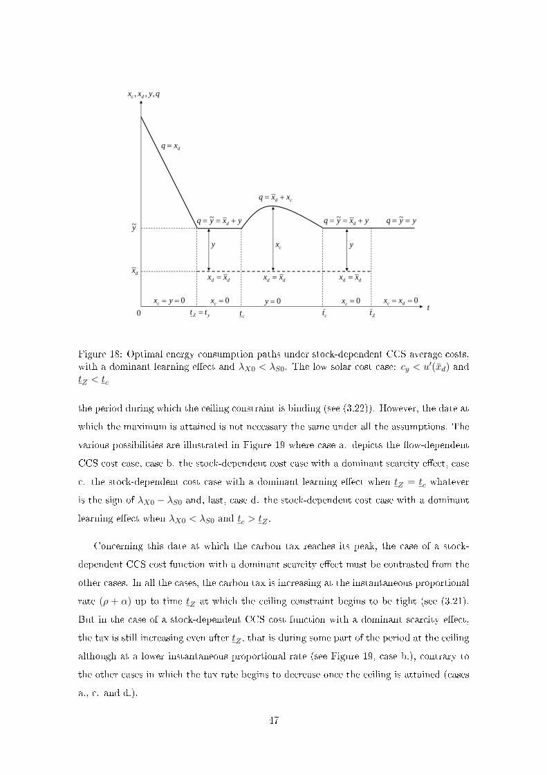
t0 ZtctyZ tt

qyxx dc ,,,

y~

dx

dxq

cd xxq

dd xx

0y 0 dc xx0 yxc

cx

0cx

ct

yxyq d ~

0cx

yxyq d ~ yyq ~

dd xx dd xx

y y

Figure 18: Optimal energy consumption paths under stock-dependent CCS average costs,with a dominant learning e�ect and λX0 < λS0. The low solar cost case: cy < u′(xd) andtZ < tc

the period during which the ceiling constraint is binding (see (3.22)). However, the date at

which the maximum is attained is not necessary the same under all the assumptions. The

various possibilities are illustrated in Figure 19 where case a. depicts the �ow-dependent

CCS cost case, case b. the stock-dependent cost case with a dominant scarcity e�ect, case

c. the stock-dependent cost case with a dominant learning e�ect when tZ = tc whatever

is the sign of λX0 − λS0 and, last, case d. the stock-dependent cost case with a dominant

learning e�ect when λX0 < λS0 and tc > tZ .

Concerning this date at which the carbon tax reaches its peak, the case of a stock-

dependent CCS cost function with a dominant scarcity e�ect must be contrasted from the

other cases. In all the cases, the carbon tax is increasing at the instantaneous proportional

rate (ρ + α) up to time tZ at which the ceiling constraint begins to be tight (see (3.21).

But in the case of a stock-dependent CCS cost function with a dominant scarcity e�ect,

the tax is still increasing even after tZ , that is during some part of the period at the ceiling

although at a lower instantaneous proportional rate (see Figure 19, case b.), contrary to

the other cases in which the tax rate begins to decrease once the ceiling is attained (cases

a., c. and d.).

47

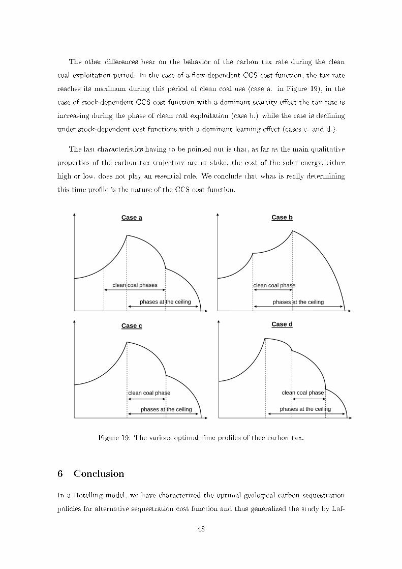
The other di�erences bear on the behavior of the carbon tax rate during the clean

coal exploitation period. In the case of a �ow-dependent CCS cost function, the tax rate

reaches its maximum during this period of clean coal use (case a. in Figure 19), in the

case of stock-dependent CCS cost function with a dominant scarcity e�ect the tax rate is

increasing during the phase of clean coal exploitation (case b.) while the rate is declining

under stock-dependent cost functions with a dominant learning e�ect (cases c. and d.).

The last characteristics having to be pointed out is that, as far as the main qualitative

properties of the carbon tax trajectory are at stake, the cost of the solar energy, either

high or low, does not play an essential role. We conclude that what is really determining

this time pro�le is the nature of the CCS cost function.

phases at the ceiling

clean coal phases

Case a Case b

Case c Case d

clean coal phase

phases at the ceiling

phases at the ceiling

clean coal phase

phases at the ceiling

clean coal phase

Figure 19: The various optimal time pro�les of thee carbon tax.

6 Conclusion

In a Hotelling model, we have characterized the optimal geological carbon sequestration

policies for alternative sequestration cost function and thus generalized the study by Laf-

48

forgue et al. (2008). The key features of the model were the following. i) The energy needs

can be supplied by three types of energy resources that are perfectly substitutable: dirty

coal (depletable and carbon-emitting), clean coal (also depletable but carbon-free thanks

to a CCS device) and solar energy (renewable and carbon-free). ii) The atmospheric carbon

stock cannot exceed some given institutional threshold as in Chakravorty et al. (2006).

iii) The CCS cost function depends either on the �ow of clean coal consumption or on its

cumulated stock. In the later case, the marginal cost function can be either increasing in

the stock (dominant scarcity e�ect) or decreasing (dominant learning e�ect).

Within this framework, we have shown that, under a stock-dependent CCS cost func-

tion, the clean coal exploitation must begin at the earliest when the carbon cap is reached

while it must begin before under a �ow-dependent cost function. Under stock-dependent

cost function with a dominant learning e�ect, the energy price path can evolve non-

monotonically over time. When the solar cost is low enough, this last case can give rise to

an unusual sequence of energy consumption along which the solar energy consumption is

interrupted for some time and replaced by the clean coal exploitation. Last under stock-

dependent cost function, even if the qualitative properties of the price path can be roughly

similar in some cases whatever be the dominant e�ect � scarcity or learning � they can

imply some contrasting repercussions on the social marginal cost of the pollution stock.

In particular, the scarcity e�ect can lead to a carbon tax trajectory which is still increas-

ing even after the ceiling has been reached while, in this kind of ceiling models, the tax

generally begins to decrease precisely at this date.

49

References

Amigues J-P., La�orgue G., Moreaux M. (2011). Optimal CCS and air capture from

heterogeneous energy consuming sectors. LERNA working paper n�11.16.350, Toulouse

School of Economics.

Amigues J-P., Moreaux M., Schubert K. (2011). Optimal use of a polluting non renewable

resource generating both manageable and catastrophic damages. Annals of Economics and

Statistics, 103, 107-141.

Ayong le Kama A., La�orgue G., Fodha M. (2009). Optimal carbon capture and storage

policies. LERNA working paper n�09.24.300, Toulouse School of Economics.

Chakravorty U., Leach A., Moreaux M. (2011). Would Hotelling Kill the Electric Car?

Journal of Environmental Economics and Management, 61, 281-296.

Chakravorty U., Magn� B., Moreaux M. (2006). A Hotelling model with a ceiling on

the stock of pollution. Journal of Economic Dynamics and Control, 30, 2875-2904.

Coulomb R., Henriet F. (2010). Carbon price and optimal extraction of a polluting fossil

fuel with restricted carbon capture. Working paper n�2010-11, Paris School of Eco-

nomics.

Edenhofer O., Bauer N., Kriegler E. (2005). The impact of technological change on climate

protection and welfare: Insights from the model MIND. Ecological Economics, 54, 277-

292.

Gerlagh R. (2006). ITC in a global growth-climate model with CCS. The value of nduced

technical change for climate stabilization. Energy Journal, Special Issue, 55-72.

Gerlagh R., van der Zwaan B.C. (2006). Options and instruments for a deep Cut in CO2

emissions: carbon capture or renewable, taxes or subsidies? Energy Journal, 27, 25-48.

Grimaud A., Roug� L. (2009). S�questration du carbone et politique climatique opti-

male. Economie et Pr�vision, 190-191, 53-69.

Grimaud A., La�orgue G., Magn� B. (2011). Climate change mitigation options and

directed technical change: A decentralized equilibrium analysis. Resource and Energy

Economics, 33, 938-962.

50

Hamilton M., Herzog H., Parsons J. (2009). Cost and U.S. public policy for new coal

power plants with carbon capture and sequestration. Energy Procedia, GHGT9 Procedia,

1, 2511-2518.

Herzog H.J. (2011). Scaling up carbon dioxide capture and storage: From megatons to

gigatons. Energy Economics, 33, 597-604.

Hoel M., Kverndokk S. (1996). Depletion of fossil fuels and the impacts of global warming.

Resource and Energy Economics, 18, 115-136.

IPCC (2005). Special report on carbon dioxide capture and storage, Working Group III.

Islegen O., Reichelstein S. (2009). The economics of carbon capture. The Economist's

Voice, December: The Berkeley Electronic Press.

Kurosawa A. (2004). Carbon concentration target and technological choice. Energy Eco-

nomics, 26, 675-684.

La�orgue G., Magne B., Moreaux M. (2008-a). Energy substitutions, climate change and

carbon sinks. Ecological Economics, 67, 589-597.

La�orgue G., Magne B., Moreaux M. (2008-b). The optimal sequestration policy with a

ceiling on the stock of carbon in the atmosphere. In: Guesnerie, R., Tulkens, H. (Eds),

The Design of Climate Policy. The MIT Press, Boston, pp. 273-304.

Mannea A., Richelsb R. (2004). The impact of learning-by-doing on the timing and costs

of CO2 abatement. Energy Economics, 26, 603-619.

McFarland J.R., Herzog H.J., Reilly J.M. (2003). Economic modeling of the global adop-

tion of carbon capture and sequestration technologies. In: Gale, J., Kaya, Y. (Eds.),

Proceedings of the Sixth International Conference on Greenhouse Gas Control Technolo-

gies, Vol.2. Elsevier Science, Oxford, pp.1083-1089.

Tahvonen O. (1997). Fossil fuels, stock externalities and backstop technology. Canadian

Journal of Economics, 22, 367-384.

Toman M.A., Withagen C. (2000). Accumulative pollution, clean technology and policy

design. Resource and Energy Economics, 22, 367-384.

51

Appendix

A.1 Full characterization of the optimal price path under CCS.1

A.1.1 The high solar cost case: u′(xd) < cy

Let us denote by x1c(t, λZ0) and x2

c(t, λX0) the clean coal consumption during the phases

[tc, tZ) and [tZ , tc), respectively. During the phase [tc, tZ), x1c(t, λZ0) reads as the solution

of:

ζλZ0e(ρ+α)t = cs(xc) + c′s(xc)xc

and during the phase [tZ , tc), x2c(t, λX0) solves:

u′(xc + xd) = cx + λX0eρt + cs(xc) + c′s(xc)xc

When the atmospheric carbon cap Z is su�ciently high and the initial pollution stock

Z0 is su�ciently low so that there exists an initial phase of dirty coal consumption without

CCS, then the optimal path is the six-phase path as illustrated in Figure 1. To fully

characterize this optimal path, the seven variables λX0, λZ0, tc, tZ , tc, tZ and ty have to

be determined. They solve the following system of seven equations:

- The cumulated coal consumption/coal endowment balance equation:∫ tZ

0q(cx + λX0e

ρt + ζλZ0e(ρ+α)t)dt+

∫ tc

tZ

x2c(t, λX0)dt

+xd[tZ − tZ ] +

∫ ty

tZ

q(cx + λX0eρt)dt = X0 (6.54)

- The atmospheric carbon stock continuity equation at tZ :

Z0 + ζ

∫ tc

0q(cx + λX0e

ρt + ζλZ0e(ρ+α)t)eαtdt

+ζ

∫ tZ

tc

[q(cx + λX0e

ρt + ζλZ0e(ρ+α)t)− x1

c(t, λZ0)]eαtdt = ZeαtZ (6.55)

- The full marginal costs equality equation at the beginning time tc of clean coal ex-

ploitation:

ζλZ0e(ρ+α)tc = cs(0) (6.56)

- The continuity equation of the energy price path at the date tZ at which the ceiling

constraint is binding:

cx + λX0eρtZ + ζλZ0e

(ρ+α)tZ = u′(x2c(tZ , λX0), xd

)⇔ x1

c(tZ , λZ0) = x2c(tZ , λX0) (6.57)

52

- The continuity equation of the energy price path at the closing time tc of clean coal

exploitation:

cx + λX0eρtc + cs(0) = u′(xd) ⇔ x2

c(tc, λX0) = 0 (6.58)

- The continuity equation of the energy price path at the date tZ at which the ceiling

constraint ends to be active:

cx + λX0eρtZ = u′(xd) (6.59)

- The continuity equation of the energy price path at the time ty at which solar energy

becomes competitive:

cx + λX0eρty = cy (6.60)

For any set {λX0, λZ0, tc, tZ , tc, tZ , ty} satisfying the above system of seven equations

and such that ζλZ0 < cs(0), then the necessary conditions (3.13)-(3.17) are satis�ed. Since

the problem is strictly convex, these conditions are also su�cient.

When the initial pollution stock Z0 is su�ciently close to Z so that the clean coal

exploitation must be started immediately, i.e. tc = 0, only six variables have to be deter-

mined. The equation (6.55) must be modi�ed as follows:

Z0 + ζ

∫ tZ

0

[q(cx + λX0e

ρt + ζλZ0e(ρ+α)t)− x1

c(t, λZ0)]eαtdt = ZeαtZ (6.61)

and the equation (6.56) must be suppressed.

A.1.2 The low solar cost case u′(xd) > cy

Now x2c(t, λX0) as de�ned in the previous paragraph is the clean coal consumption during

the phase [tZ , ty), and we de�ne x3c(t, λX0), the clean coal consumption during the phase

[ty, tc), as the solution of the following equation:

cy = cx + λX0eρt + cs(xc) + c′s(xc)xc

First, when Z0 is large enough and/or cy is large enough so that the optimal price path

is the six-phase path illustrated in Figure 3, the same seven variables λX0, λZ0, tc, tZ , ty,

tc and tZ have to be determined. The system of seven equations they solve now becomes:

- The cumulated coal consumption/coal endowment balance equation:∫ tZ

0q(cx + λX0e

ρt + ζλZ0e(ρ+α)t)dt+

∫ ty

tZ

x2c(t, λX0)dt

+

∫ tc

ty

x3c(t, λX0)dt+ xd[tZ − tZ ] = X0 (6.62)

53

- The equation (6.55) for the continuity of the atmospheric pollution stock at tZ .

- The equations (6.56) and (6.57) for the price path continuity at tc and tZ , respectively.

- The continuity equation of the energy price path at ty:

u′(x2c(ty, λX0), xd) = cy ⇔ x2

c(ty, λX0) = x3c(ty, λX0) (6.63)

- The continuity equation of the energy price path at tc:

cx + λX0eρtc + cs(0) = cy ⇔ x3

c(tc, λX0) = 0 (6.64)

- The continuity equation of the energy price path at tZ :

cx + λX0eρtZ = cy (6.65)

Again, when Z0 is su�ciently close to cy, it is necessary to immediately begin the

CCS activity at t = 0, in which case equation (6.62) has to be substituted for (6.55) and

equation (6.56) has to be deleted.

A.2 Full characterization of the optimal price path under CCS.2

When the scarcity e�ect is purely dominant, and whatever the level of the average solar

cost cy as compared with u′(xd), two cases have to be considered depending on whether

the reservoir capacity constraint is binding or not at the closing time of the clean coal

exploitation (see Proposition 4). This implies that four cases have to be investigated.

A.2.1 The high solar cost case u′(xd) < cy

a. Case where Sc(tc) < Sc

In this case, the capacity constraint on the cumulated clean coal exploitation is never

binding, thus implying that νS(t) = 0 for any t ≥ 0 and that λS(t) = 0 for t ≥ tc. The

expression (4.36) of the costate variable of the cumulated clean coal production can be

simpli�ed into:

λS(t) = −eρt∫ tc

tc′s(Sc(τ))xc(τ)e−ρτdτ

Integrating by parts the above expression results in:

λS(t) = cs(Sc(t))− eρt[cs(Sc(tc))e

−ρtc + ρ

∫ tc

tcs(Sc(τ))e−ρτdτ

](6.66)

54

The seven endogenous variables λX0, λZ0, λS0, t (with t = tZ = tc), tc, tZ and ty solve

the following system of seven equations:

- The initial condition on the costate variable λS(t) which, from (6.66), results in:

λS0 = λS(0) = cse−ρt − cs(Sc(tc))e−ρtc − ρ

∫ tc

tcs(Sc(t))e

−ρtdt (6.67)

- The cumulated coal consumption/coal endowment balance equation:∫ t

0q(cx + λX0e

ρt + ζλZ0e(ρ+α)t)dt+

∫ tc

tq(ccm(xc(t)))dt

+xd[tZ − tc] +

∫ ty

tZ

q(cx + λX0eρt)dt = X0 (6.68)

where, from (6.66), the full marginal cost ccm(xc(t)) of the clean coal amounts to:

ccm(xc(t)) = cx + λX0eρt + eρt

[cs(Sc(tc))e

−ρtc + ρ

∫ tc

tcs(Sc(τ))e−ρτdτ

], t ∈ [t, tc)

- The atmospheric carbon stock continuity equation at time t:

Z0 + ζ

∫ t

0q(cx + λX0e

ρt + ζλZ0e(ρ+α)t)eαtdt = Zeαt (6.69)

- The continuity equation of the energy price path at the date t at which the ceiling

constraint is binding and, simultaneously, the clean coal exploitation begins:

ζλZ0e(ρ+α)t = cs − λS0e

ρt (6.70)

- The continuity equation of the energy price path at the closing time tc of the clean

coal exploitation:

cx + λX0eρtc + cs(Sc(tc)) = u′(xd) (6.71)

- The equations (6.59) and (6.60) for the continuity of the energy price path at times

tZ and ty, respectively.

b. Case where Sc(tc) = Sc

In this case, the reservoir is ful�lled at time tc implying λS(tc) < 0. Here we cannot

deduce λS0 from the general expression of λS(t) as in the previous case. This missing

information must be replaced by an additional terminal condition on the cumulated clean

coal production: Sc(tc) = Sc.

55

Integrating by parts (4.36), we have now:

λS(t) = cs(Sc(t))− eρt[cs(Sc)e

−ρtc + ρ

∫ tc

tcs(Sc(τ))e−ρτdτ +

∫ ∞t

νS(τ)e−ρτdτ

](6.72)

thus implying:

λS0 = cse−ρt − cs(Sc)e−ρtc − ρ

∫ tc

tcs(Sc(t))e

−ρtdt−∫ ∞tc

νS(t)e−ρtdt (6.73)

Replacing into (6.72) the term∫∞t νS(t)e−ρtdt by its expression coming from (6.73), with

νS(t) = 0 for t ∈ [0, tc), we obtain after simpli�cations:

∀t ∈ [t, tc) : λS(t) = cs(Sc(t))− eρt[cse−ρt − ρ

∫ t

tcs(Sc(τ))e−ρτdτ − λS0

](6.74)

at time tc : λS(tc) = cs(Sc)− eρtc[cse−ρt − ρ

∫ tc

tcs(Sc(t))e

−ρtdt− λS0

](6.75)

The seven endogenous variables λX0, λZ0, λS0, t (with t = tZ = tc), tc, tZ and ty are

determined as the solution of the following seven-equations system:

- The continuity equation of the cumulated clean coal production at tc:∫ tc

txc(t)dt =

∫ tc

tq(ccm(xc(t)))dt− xd[tc − t] = Sc (6.76)

where, from (6.74), the full marginal cost ccm(xc(t)) of the clean coal is now equal to:

ccm(xc(t)) = cx + λX0eρt + eρt

[cse−ρt − ρ

∫ t

tcs(Sc(τ))e−ρτdτ − λS0

], t ∈ [t, tc)

- The cumulated coal consumption/coal endowment balance equation:∫ t

0q(cx + λX0e

ρt + ζλZ0e(ρ+α)t)dt+ xd[tZ − t] + Sc +

∫ ty

tZ

q(cx + λX0eρt)dt = X0 (6.77)

- The equation (6.69) for the continuity of the atmospheric carbon stock at t.

- The continuity equation of the energy price path at t:

ζλZ0e(ρ+α)t = cs − λS0e

ρt (6.78)

- The continuity equation of the energy price path at tc which, using (6.75), implies:

cx + λX0eρtc + cs(Sc)− λS(tc) = u′(xd)

⇒ cx + λX0eρtc + eρtc

[cse−ρt − ρ

∫ tc

tcs(Sc(t))e

−ρtdt− λS0

]= u′(xd) (6.79)

- The equations (6.59) and (6.60) for the continuity of the energy price path at times

tZ and ty, respectively.

56

A.2.2 The low solar cost case u′(xd) > cy

a. Case where Sc(tc) < Sc

As explained in Section 4.2.2, only the six endogenous variables λX0, λZ0, λS0, t (with

t = tZ = tc), t (with t = tc = ty) and tZ have now to be determined. They solve the

following system of six equations:

- The equation (6.67) for the initial condition on λS(t), with tc = t.

- The cumulated coal consumption/coal endowment balance equation:∫ t

0q(cx + λX0e

ρt + ζλZ0e(ρ+α)t)dt+

∫ t

tq(ccm(xc(t)))dt+ xd[tZ − t] = X0 (6.80)

where, the full marginal cost ccm(xc(t)) has the same expression as in the corresponding

high solar cost case for t ∈ [t, t).

- The equation (6.69) for the continuity of the atmospheric carbon stock at t.

- The equation (6.70) for the continuity of the energy price path at time t.

- The continuity equation of the energy price path at time t:

cx + λX0eρt + cs(Sc(t)) = cy (6.81)

- The equation (6.65) for the continuity of the energy price path at time tZ .

b. Case where Sc(tc) = Sc

The six endogenous variables λX0, λZ0, λS0, t, t and tZ are determined as the solution

of the following six-equations system:

- The equation (6.76) for the continuity of the cumulated clean coal production at t,

with t = tc.

- The cumulated coal consumption/coal endowment balance equation:∫ t

0q(cx + λX0e

ρt + ζλZ0e(ρ+α)t)dt+ xd[tZ − t] + Sc = X0 (6.82)

- The equation (6.69) for the continuity of the atmospheric carbon stock at t.

- The equation (6.78) for the continuity of the energy price path at t.

- The equation (6.79) for the continuity of the energy price path at t, with t = tc.

- The equation (6.65) for the continuity of the energy price path at time tZ .

57

A.3 Full characterization of the optimal price path under CCS.3

Under a stock-dependent CCS cost function with a dominant learning e�ect, the expression

of the costate variable of the cumulated clean coal production is given by (4.46). Expanding

the integral term and simplifying, it comes:

λS(t) = cs(Sc(t))− eρt[cs(Sc(tc))e

−ρtc + ρ

∫ tc

tcs(Sc(τ))e−ρτdτ

](6.83)

which the same expression as (6.66) obtained in the dominant scarcity e�ect case. However,

the initial value of λS slightly di�ers since the CCS cost function is now decreasing in S:

λS0 = cse−ρtc − cs(Sc(tc))e−ρtc − ρ

∫ tc

tc

cs(Sc(t))e−ρtdt (6.84)

Finally, since in this case the reservoir that hosts the sequestered carbon emissions is not

constrained by any limit in capacity, the associated costate variable must be nil at the

closing time of the clean coal exploitation, as speci�ed by (4.47): λS(t) = 0 ∀t ≥ tc.

A.3.1 The high solar cost case u′(xd) < cy

a. Case where λX0 > λS0

As mentioned in Section 4.3.1, the energy price and consumption paths are qualitatively

very similar to the ones obtained in the dominant scarcity e�ect case with high solar cost

when the capacity constraint on the cumulated clean coal production is never binding.

Hence, the seven endogenous variables λX0, λZ0, λS0, t (with t = tZ = tc), tc, tZ and ty

solve almost the same seven-equations system as in Appendix A.2.1.a:

- The equation (6.84) for the initial condition on λS(t).

- The equation (6.68) for the cumulated coal consumption/coal endowment balance.

- The equation (6.69) for the continuity of the atmospheric carbon stock at time t.

- The continuity equation of the energy price path at time t:

ζλZ0e(ρ+α)t = cs − λS0e

ρt (6.85)

- The equation (6.71) for the continuity of the energy price path at time tc.

- The equations (6.59) and (6.60) for the continuity of the energy price path at times

tZ and ty, respectively.

58

b. Case where λX0 < λS0

As seen in Section 4.3, when λX0 − λS0 < 0 two subcases have to be considered

according to whether the dates at which the carbon cap is reached and at which the clean

coal exploitation begins coincide are not.

First, if tZ = tc ≡ t, then the seven variables λX0, λZ0, λS0, t, tc, tZ and ty exactly

solve the same system of equations than the previous one (see Appendix A.3.1 case a.).

Second, if tZ < tc ≡ t, then we have now to determine eight endogenous variables:

λX0, λZ0, λS0, tZ , tc, tc, tZ and ty. They solve the following system of seven equations:

- The equation (6.84) for the initial condition on λS(t).

- The cumulated coal consumption/coal endowment balance equation:∫ tZ

0q(cx + λX0e

ρt + ζλZ0e(ρ+α)t)dt+

∫ tc

tc

q(ccm(xc(t)))dt

+xd[(tZ − tZ)− (tc − tc)] +

∫ ty

tZ

q(cx + λX0eρt)dt = X0 (6.86)

where, ccm(xc(t)) = cx + λX0eρt + cs(Sc(t))− λS(t), with λS(t) given by (6.83).

- The atmospheric carbon stock continuity equation at time tZ :

Z0 + ζ

∫ tZ

0q(cx + λX0e

ρt + ζλZ0e(ρ+α)t)eαtdt = ZeαtZ (6.87)

- The continuity equation of the energy price path at time tZ :

cx + λX0eρtZ + ζλZ0e

(ρ+α)tZ = u′(xd) (6.88)

- The continuity equation of the energy price path at time tc:

cx + cs + (λX0 − λS0)eρtc = u′(xd) (6.89)

- The equation (6.71) for the continuity of the energy price path at time tc.

- The equations (6.59) and (6.60) for the continuity of the energy price path at times

tZ and ty, respectively.

59

A.3.2 The low solar cost case u′(xd) > cy

a. Cases where λX0 > λS0 or where λX0 < λS0 and tZ = tc

The six endogenous variables λX0, λZ0, λS0, t, t and tZ are determined as the solution

of the following six-equations system:

- The equation (6.84) for the initial condition on λS(t).

- The equation (6.80) for the cumulated coal consumption/coal endowment balance.

- The equation (6.69) for the continuity of the atmospheric carbon stock at time t =

tZ = tc.

- The equation (6.85) for the continuity of the energy price path at time t.

- The equation (6.81) for the continuity of the price path at time t = tc = ty.

- The equation (6.65) for the continuity of the price path at time tZ .

b. Case where λX0 < λS0 and tZ < tc

In this last case, the seven endogenous variables λX0, λZ0, λS0, tZ = ty, tc, tc and tZ

solve the following system:

- The equation (6.84) for the initial condition on λS(t).

- The cumulated coal consumption/coal endowment balance equation:∫ tZ

0q(cx + λX0e

ρt + ζλZ0e(ρ+α)t)dt+

∫ tc

tc

q(ccm(xc(t)))dt

+xd[(tZ − tZ)− (tc − tc)] = X0 (6.90)

where, ccm(xc(t)) = cx + λX0eρt + cs(Sc(t))− λS(t), with λS(t) given by (6.83).

- The equation (6.69) for the continuity of the atmospheric carbon stock at time tZ .

- The continuity equation of the energy price path at time tZ = ty:

cx + λX0eρtZ + ζλZ0e

(ρ+α)tZ = cy (6.91)

60

- The continuity equation of the energy price path at time tc:

cx + cs + (λX0 − λS0)eρtc = cy (6.92)

- The continuity equation of the energy price path at time tc:

cx + λX0eρtc + cs(Sc(tc)) = cy (6.93)

- The equation (6.65) for the continuity of the price path at time tZ .

61

Triggering the Technological Revolution in Carbon Capture

and Sequestration Costs

I/ The Polluting Resource is Abundant ∗

Jean-Pierre Amigues†

Gilles La�orgue‡

and

Michel Moreaux§

∗We thank the Conseil Français de l'Energie for �nancial support.†Toulouse School of Economics(INRA, IDEI and LERNA), 21 allée de Brienne, 31000 Toulouse, France.‡Toulouse School of Economics(INRA, IDEI and LERNA), 21 allée de Brienne, 31000 Toulouse, France.§Toulouse School of Economics (IDEI, LERNA), 21 allée de Brienne, 31000 Toulouse, France.

1

Triggering the Technological Revolution in Carbon Capture

and Sequestration Costs

I: The Polluting Resource is Abundant

Abstract

The nature of optimal environmental policies able to induce su�cient technical

progress in pollution abatement technologies has raised a vivid debate between eco-

nomics over the last decade. Some emphasize the importance of learning-by-doing on

these technologies, an argument in favor of early action. Other insisted upon the time

needed for R&D to identify the best abatement options, an incentive to delay action

in the future. Either triggering technical progress from learning e�ects of research,

all analysis conclude to ambiguous e�ects of environmental policies on the speed of

technical change. One strong limitation of previous approaches is that they do not

endogenize the best ways to improve the e�ciency of abatement technologies, either

through learning on existing techniques or through research to discover new ones. We

consider an economy that can trigger some cost breakdown in CCS costs thanks to

both learning and R&D. We �rst reconsider the results of the literature about the ex-

treme cases of a pure learning induced technical revolution and a pure R&D induced

cost breakdown in the context of an atmospheric carbon ceiling framework. We show

how this setting helps to clarify the existing results from the literature and remove

some of their ambiguities. In particular we perform a sensitivity analysis of the op-

timal policies with respect to relevant parameters, providing strong intuitions about

the various e�ects a�ecting their dynamics. We next examine the case of a combined

learning and R&D policy. We show that the economy may initially perform only re-

search e�orts or rely only upon learning to trigger the cost breakdown. A combined

policy may only follow pure R&D or learning policies. Combining learning and R&D

requires to increase both research e�orts and the use of the abatement technology,

but the growth rate of pollution abatement must be higher than the growth rate of

the research e�orts. Contrarily to what is commonly observed in models with con-

stant average and marginal costs of abatement, the use of cleaning technologies may

begin before the atmospheric constraint begins to bind. In such situation, the time

constraints upon technological development outweighs the environmental constraints

and result in early introduction of abatement technologies. But the contrary may also

be optimal and we provide a complete discussion of the relevance of these various

scenarios.

Keywords: Carbon capture and storage; Energy substitution; Learning-by-doing;

Research and development; Carbon stabilization cap.

JEL classi�cations: Q32, Q42, Q54, Q55, Q58.

2

Contents

1 Introduction 4

2 The model 8

3 Technological revolution induced by learning 11

4 The R&D induced technical revolution in abatement 24

5 Combining learning and R&D to trigger the technological revolution 32

5.1 Know-how accumulation scenarios . . . . . . . . . . . . . . . . . . . . . . . 34

5.2 Terminal condition at the revolution time tA . . . . . . . . . . . . . . . . . . 45

5.3 Optimal policies triggering the revolution during the ceiling phase . . . . . . 47

5.4 Optimal policies triggering the revolution when the ceiling is attained . . . . 52

6 Conclusion 53

References 57

Appendix 58

A.1Appendix 1: Proof that pure dirty and combined dirty and clean energy

scenarios may be welfare equivalent 58

A.2Appendix 2: Comparative dynamics in the pure learning case 59

A.3Appendix 3: Comparative dynamics in the pure R&D model 65

A.4Appendix 4. Proof that σ < 0 66

A.5Appendix 5. 67

3

1 Introduction

Technology plays a prominent role in all re�ections about �nding ways out of the global

warming problem. This issue has been forcefully raised by Scott Barret in several occa-

sions (Barret, 2006). For him, instead of seeking for an almost impossible international

agreement on carbon emissions mitigation, governments should better cooperate over a

common target of triggering a technological revolution in clean energy generation. The

help of technical progress is particularly expected in three domains: the enhancement of

the productive e�ciency of fossil fuels, the development of non carbon based energy pro-

duction techniques and the improvement of the e�ciency of carbon pollution abatement

technologies, the future of carbon capture and storage (CCS) technologies appearing as

an important issue in this respect. If the economic literature fully agrees to this general

statement, it largely diverges in assessing both the policy implications of technical progress

opportunities in carbon emissions mitigation and the e�ects of environmental policies upon

technical change in the energy production and consumption sectors. These issues have pro-

voked a vivid debate among economist during the last decade.

Two main reasons may explain this di�culty to reach an agreement about the nature of

the relationships between environmental policy and technological development. First, the

topic of technical change, or more precisely of endogenous technical change, has emerged

only recently in the economic literature. A lot remains to be done on this issue, espe-

cially to build a consistent view of the various advances coming both from the microeco-

nomic approaches developed in industrial organization economics and the macroeconomic

approaches of the endogenous growth literature. Second, global warming and technical

progress are two dynamical processes with their own drivers and constraints, and reaching

a reasonable understanding of the time links between these two processes is a modeling

challenge, both on the theoretical and on the empirical side.

A �rst motive of dissent relies in the desirable speed of action to introduce pollution

abatement technologies. One main set of arguments in favor of delaying abatement roots

in discounting arguments, the abatement options being today typically costly and thus be

favorably delayed in the future (Wigley et al., 1996). A second set of arguments advances

that in their present sate, existing abatement technologies are too costly, and time should

4

be given to research to develop new and more a�ordable technical options.

This line of thought has been heavily criticized by Van der Zwaan et al., (2002), and

Kverndokk and Rosendhal (2007), among others, because it does not take into account the

potential of experience and learning-by-doing in pollution abatement technologies. Taking

bene�t of such learning opportunities rather requires early action than delay. The argument

is reinforced by a capital accumulation motive, the replacement of old and costly vintages

by new and cheaper one is a costly process requiring a signi�cant time. This time to

build issue appears to be particularly relevant for CCS technologies, their development

being submitted to costly capacity expansion constraints. The early action these is also

endorsed by industrial organization views. By announcing su�ciently early a credible

path of action, in terms of an announced increasing time schedule of a carbon tax for

example, the industry will react to this incentive scheme by investing today in abatement

technologies, the uncertainty about what the regulator plans to do in the future being

removed.

However, learning-by-doing is not the only way to induce technical advances. Another

main option is R&D. R&D has two main advantages with respect to learning. First, it does

not require to actually use the technology. With su�cient time and e�ort, it is possible

to achieve in the lab potential cost cuts without bearing the high initial cost of using non

mature technologies. Second, R&D can span much more potential technical options than

actual use, which requires speci�c technical choices before beginning the exploitation of a

given technique, the risk being to be trapped into inferior options or inappropriate initial

choices.

It appears immediately that in an R&D induced technical change world, early devel-

opment of infant abatement technologies may be counterproductive. In policy terms, this

means that subsidizing non mature abatement technologies in the hope that learning can

reduce their costs in the future may be suboptimal. It would be better to give more time to

research to assert the economic potential of di�erent technological options. This issue has

been examined carefully by Goulder and Matthai (2000). Comparing a learning induced

technical change model with a R&D induced technical change model, they conclude that

in a R&D world, delaying actual abatement is optimal while the interest to advance or

delay a policy action promoting pollution abatement is usually ambiguous in a learning

5

world.

Induced technical change in carbon emission mitigation technologies is only one aspect

of a more general problem involving also alternative clean energy production, like solar

energy. These alternative energy sources may also bene�t from both learning and R&D

cost cutting progress. Such technical advances possibilities should modify the timing of

optimal transitions between energy sources, as shown by Chakravorty et al. in a recent

paper (Chakravorty, 2012) in the case of learning-by-doing. The same type of conclusions

emerges from the study of Henriet (2012) for a R&D induced technical breakthrough in a

clean energy source production cost (Henriet, 2012).

As remarked by Gerlagh et al.(2009), the Goulder-Matthai analysis does not exhaust

the concern expressed by Ja�e, Newell and Stavins (2001) concerning the need of a better

understanding of the impact of environmental policies upon the nature of induced techno-

logical change and the feedback e�ect of technical change upon the environment itself and

thus upon environmental policies.

Contributing to this understanding is the main objective of the present work. Many

confusions arise in the previous literature because of the usual incremental way of modeling

technical progress. This is especially true when comparing learning-by-doing and research

induced technical change. In an incremental model, technical change is a sequence of small

improvements progressively reducing the cost of the abatement technology. But incremen-

tal actual cost cuts achieved through learning and potential cost cuts achieved by research

activity are not really comparable. This is one of the main reason for the ambiguous e�ects

of an environmental policy in a learning-by-doing model shown by Goulder and Matthai.

To escape this di�culty, we adopt a drastic view of technical change, more in line of the

Barret initial proposal. Thanks to a combination of R&D activity and learning-by-doing,

it is possible to increase over time some know-how index. Once the index has reached a

given target, it induces an abrupt revolution in abatement technologies, taking the form

of a cost drop from a high level to a low level. To simplify, we assume only one revolution

of this kind, meaning that future learning or research activity will become worthless after

the revolution.

We make a parallel simpli�cation concerning the dynamics of the environment. Most

papers model the environmental dynamics as a progressive accumulation of carbon into the

6

atmosphere, the size of the carbon stock generating welfare damages at each point of time.

These damages are increasing with the size of the pollution stock. We depart from this

approach by using an alternative route pioneered by Chakravorty et al. (2006, 2008) . We

assume that the atmospheric carbon stock does not harm directly welfare, but be crossed

over some critical threshold level in carbon concentration, earth climate conditions would

become catastrophic. This echoes the current policy proposals of targeting a temperature

rise of no more than 20 C, that is actually trying to stabilize the carbon concentration to

a constant level by the end of the century. Hence the environmental policy takes the form

of a given mandate over the maximum level of the atmospheric carbon stock.

To simplify farther, we assume in the present paper that fossil fuels are not exhaustible.

Introducing depletion constraints over fossil fuels will result in complex Hotelling e�ects

a�ecting both the timing of carbon accumulation and the timing of technological devel-

opment. We deserve the study of these issues to a companion paper (Amigues et al.,

2012).

One drawback of the Goulder-Matthai analysis is that they focus on the polar cases of

learning and R&D induced technical change, but these polar cases are extreme situations

where the economy would be constrained to use only one device to trigger technological

advances. We encompass this limitation by examining a model where both activities con-

tribute to technical progress. This will allow a much better understanding of the delay

problem raised in the earlier literature. In particular we show how can be endogenously de-

termined time periods during which the economy should perform only R&D to enhance the

technical e�ciency of pollution abatement and time periods during which a combination

of learning processes and research activity is optimal.

The model is laid down in section 2. In order to drive interesting comparisons with

previous results of the literature, we study in section 3 the case of a pure learning-by-

doing induced technological revolution and in section 4 the case of a pure R&D induced

technological break. We improve on earlier studies by performing rather systematically a

sensitivity analysis of the main variables. Usually, one �nds such sensitivity analysis in

simulation models, but their results are typically hard, if not impossible, to interpret. Our

simple setting allows us to derive sensitivity results in the analytical domain, providing

strong intuitions on our �ndings. In particular, we shall exhibit the similarities and the

7

di�erences between the cases of a learning induced or a R&D induced technical change.

In section 5, we examine the general case of a combined learning and R&D process. We

derive the implications of such a process for an optimal environmental policy. We also

describe the optimal technological development policy which may be of a combined type,

a pure learning or a pure R&D type depending upon the model fundamentals. The last

section 6 concludes.

2 The model

The economy has access to two primary energy sources. The �rst one is a polluting resource

(let say coal). We assume an in�nite supply of this resource, meaning that it will never be

exhausted, that is we treat coal as a kind of a renewable polluting resource, or equivalently

assume that coal is abundant. Let x(t) be the rate of coal extraction. The second energy

source is a clean renewable resource (let say solar) and we denote by y(t) the used �ow of

solar energy.

Assuming for the sake of simplicity a one to one transformation process of primary

energy sources units into energy services units, the production of solar energy services bears

a cost cyy(t). The processing of coal into the generation of energy services may take two

forms. Coal may be processed without consideration for the environmental consequences

of burning this fossil fuel to produce energy. We call dirty coal processing this energy

generation process and xd(t) denotes the corresponding coal energy services generation rate.

The cost of dirty coal processing is cxxd(t). It results into a pollution �ow ζxd(t) assumed

proportional to the dirty coal energy generation. Under our one to one transformation

process assumption, xd is also that fraction of coal extraction involved into dirty processing

and ζ is the polluting content of coal.

The pollution �ow accumulates into the environment and Z(t) is the pollution stock

size at time t. There exists a self-cleaning capacity of the environment, assumed to simplify

proportional to the pollution stock size, so that the motion of Z(t) over time is given by:

Z(t) = ζxd(t)− αZ(t) .

The initial pollution stock is Z(0) = Z0.

Coal may be also processed through a clean energy generation process, thanks for

8

example to CCS e�ort, resulting in no carbon emissions into the atmosphere. xc(t) is

the rate of clean coal services generation and (cx + cs(t))xc is the cost of clean coal energy

services. Under our transformation assumption, xc(t) is also that fraction of coal extraction

involved in clean coal energy production, so that: x(t) = xd(t) + xc(t).

Energy services di�er by their primary sources (coal or solar) and by their type of coal

processing (either dirty or clean coal energy generation) but they are perfect substitutes

for the �nal users. Let q(t) ≡ xd(t) + xc(t) + y(t) be the instantaneous consumption rate

of energy services. This consumption generates a gross surplus, u(q), assumed increasing

and concave and satisfying the �rst Inada condition: limq↓0 u′(q) = +∞.

As in Chakravorty et al. (2006), we assume that pollution does not harm directly

welfare but be crossed over some critical threshold Z, earth climate conditions would

become catastrophic. Thus the society decides to maintain the carbon concentration below

this critical level. To give content to the problem we have to assume that Z0 ≤ Z.

Operating clean coal energy production equipments bene�ts both from learning-by-

doing and dedicated research e�orts. The cost reduction that may be achieved through

these two processes may be de�ned in di�erent ways. Here we adopt a drastic view of

technical progress. The combination of the accumulation of experience with R&D e�orts

results into a technological revolution in the clean coal energy generation process. To

describe this combined process, we adopt the simplest formulation able to retain the main

aspects of the problem. Both learning-by-doing and R&D contribute to the accumulation

over time of some stock of know-how. Let A(t) be the level of this stock at time t. A(t)

grows over time at a rate depending upon the production scale of clean coal energy, xc(t),

and upon the R&D e�ort rate, r(t), through the following relation:

A(t) = a(xc(t), r(t)) .

a(xc, r) is twice continuously di�erentiable and both ac ≡ ∂a/∂xc > 0, ar ≡ ∂a/∂r > 0.

Know-how may be increased through only learning or R&D, that is: a(0, r) > 0 if r > 0

together with a(xc, 0) > 0 if xc > 0, while a(0, 0) = 0. Assume that A(0) = 0, that is

normalize to zero the initial know-how index. Once some su�cient level of know-how, A,

has been attained, the technological revolution occurs, resulting into a sudden drop down

of the cost of clean coal energy generation, from a high level cs, to a low level cs. Thus the

9

additional clean coal energy cost is a function of A(t), cs(A(t)), such that:

cs(A(t)) =

cs if A(t) < A

cs if A(t) ≥ A.

We assume to simplify only one technological revolution of this kind, meaning that future

learning will be worthless after the revolution and that further R&D e�orts will not allow

for future cost breaks.

R&D activity has a cost Cr(r), a cost function we assume twice continuously di�er-

entiable over r ∈ (0,∞), increasing and convex in r while Cr(0) = 0. So the marginal

cost function cr(r) ≡ dCr(r)/dr de�ned over (0,∞) veri�es: cr(r) ≥ 0, c′r(r) > 0 and in

addition limr↓0 cr(r) = c0r ≥ 0, the right end limit of the marginal R&D cost at zero is not

necessarily zero.

The society has to determine a primary resources policy use, a split between dirty and

clean coal energy generation, together with a R&D policy maximizing a discounted sum

of instantaneous net surpluses, ρ > 0 being the constant level of the social discount rate,

while taking into account the atmospheric carbon concentration constraint, Z ≤ Z.

This problem may be given di�erent formulations depending upon the model funda-

mentals. If the cost of the clean solar energy is lower than the cost of dirty coal generation,

then coal is never used and the pollution problem disappears. So we assume that cx < cy.

It may be the case that clean coal energy generation is so costly even after the revolution

that the society will prefer to produce only dirty coal energy services. In such a case, there

will be no learning about the clean coal technology and R&D e�orts will be worthless and

thus no cost breakthrough can occur. This scenario where x(t) = xd(t) has been already

studied by Chakravorty et al.(2006). It may also be the case that the pollution ceiling is

never attained, a scenario where the more costly clean coal option would never be engaged.

In order to drive an interesting discussion, we assume �rst that the ceiling constraint

binds eventually along the optimal path and, second, that the clean cost option is not

too costly to be used at least over some time interval, maybe only after the technological

revolution. We shall be more precise about the relevant assumptions for that to be the case

in the sequel. If clean coal energy generation is pro�table it will be used permanently after

its introduction inside the energy mix. Either as a pure consequence of learning-by-doing,

in case of no R&D e�orts, or as a result of the combination of learning and R&D, the

10

level of know-how will permanently rise, triggering the revolution at some time, tA. Then

the optimal program may be designed as a sequential optimal control problem composed

of two phases: a �rst phase [0, tA) before the break and a second phase [tA,∞) after the

break.

An optimal policy is hence a solution of the following program OP :

maxxc,xd,y,r,tA

∫ tA

0[u(q(t))− cxx(t)− csxc(t)− cyy(t)− Cr(r(t))] e−ρtdt+ e−ρtA V

s.t. Z(t) = ζxd(t)− αZ(t) Z(0) = Z0 given

A(t) = a(xc(t), r(t)) A(0) = 0

xc(t) ≥ 0 , xd(t) ≥ 0 , y(t) ≥ 0 , r(t) ≥ 0

xc(t) + xd(t) ≤ x(t)

Z(t) ≤ Z

A(tA) ≥ A .

V is the continuation value obtained by solving the following continuation problem after

the technological revolution:

maxxc,xd,y

∫ ∞tA

[u(q(t))− cxx(t)− csxc(t)− cyy(t)] e−ρ(t−tA)dt

s.t. Z(t) = ζxd(t)− αZ(t) Z(tA) = ZA given

xc(t) ≥ 0 , xd(t) ≥ 0 , y(t) ≥ 0

xc(t) + xd(t) ≤ x(t)

Z(t) ≤ Z .

Before examining the policies solving the program OP , it is useful to consider as bench-

marks two polar cases, the case of a pure learning-by doing know-how generation and the

case of a pure R&D generation of know-how. We devote the next two sections to these

polar cases before turning to the general case.

3 Technological revolution induced by learning

Assume no R&D opportunities. The economy has to rely only upon learning-by-doing, that

is on experience accumulation, to trigger the technological revolution. The simplest way to

de�ne experience, and thus here the know-how index, is to identify it with the cumulated

11

number of clean coal energy services units generated since the beginning of clean coal

energy production. Let tc be the beginning time of clean coal energy production, then:

A(t) ≡∫ t

tc

xc(τ)dτ .

Denote by λA(t) and λZ(t) respectively the costate variables associated to the state vari-

ables A(t) and Z(t). Denote also by νxc, νxd, νy, the Lagrange multipliers associated to

the positivity constraints over xc, xd, y, respectively, and by νZ , the Lagrange multiplier

associated to the constraint Z(t) ≤ Z; The optimality conditions over the time interval

[0, tA) are:

u′(q) = cx + cs − λA − νxc (3.1)

u′(q) = cx + ζλZ − νxd (3.2)

u′(q) = cy − νy (3.3)

λZ = (ρ+ α)λZ − νZ (3.4)

λA = ρλA . (3.5)

Let us �rst sketch as a benchmark the optimal policy absent any learning abilities, the

extra cost of producing clean coal energy with respect to dirty coal energy being cs . A

relevant scenario involves hitting the ceiling at some �nite time tZ . We have to consider

two possibilities. Either cy > cx + cs, the high solar cost case, either cy < cx + cs, the low

solar cost case.

In the high solar cost case, solar energy is never introduced inside the energy mix.

When at the ceiling, dirty coal energy generation is constrained by the natural regeneration

capacity, so that the production of dirty coal energy is given by xd ≡ αZ/ζ. Let p ≡ u′(xd).

If p < cx+cs < cy, then the economy prefers to rely only upon dirty coal energy generation

and never uses either clean coal energy generation or solar energy generation. The optimal

path is a two phases path. During the �rst phase [0, tZ), the economy produces only dirty

coal energy, pollution accumulates and xd(t) is the solution of u′(x) = cx + ζλZ0e(ρ+α)t,

where λZ0 = λZ(0). This phase ends when the pollution stock reaches the ceiling Z. Then

begins a phase of in�nite duration, [tZ ,∞) of dirty coal generation at the level xd.

If cx + cs < p, clean coal energy is never introduced before the beginning of the ceiling

phase. Identifying (3.2) and (3.1), we get during any time interval below the ceiling where

12

dirty and clean coal generation would be simultaneously operated: ζλZ(t) = cs, which is

incompatible with λZ(t) growing at the rate ρ + α. But since solar energy is even more

costly than clean coal energy, solar energy is also never used before the ceiling. Thus,

the economy produces only dirty energy until the ceiling constraint begins to be binding.

During this �rst phase [0, tZ), the implicit energy price p(t) ≡ u′(q(t) is de�ned through

(3.2) and (3.4) by: p(t) = cx + λZ0e(ρ+α)t. Thus, the implicit energy price increases over

time while dirty coal energy generation is progressively reduced. When at the ceiling, the

economy starts to produce clean coal energy. The energy implicit price p(t) is now constant

and equal to the marginal cost of clean coal energy production cx + cs. Since solar energy

is more expensive than clean coal energy, it is also never used during this time phase. The

optimal policy when at the ceiling combines the production of dirty coal energy at the

constant rate xd with the production of clean coal energy at the constant rate xc, solution

of u′(xd+xc) = cx+ cs. Note that the energy price continuity at tZ requires that the dirty

coal energy production path jumps down at tZ from the level xd + xc to the level xd while

the clean coal energy production rate jumps up from 0 to xc.

Last, in the low solar cost case, we have to distinguish the possibilities cy < p and

p < cy. If cy < p, solar energy is introduced when the ceiling constraint becomes to be

binding and clean coal energy generation is never put in operation. Thus after tZ , energy

production combines dirty coal energy generation at the rate xd and solar energy generation

at the rate y, solution of u′(xd + y) = cy. If p < cy, the economy prefers to rely only upon

dirty coal energy generation and never uses clean energy in any form: clean coal energy or

solar energy.

We turn now to a sensitivity analysis of the optimal policy with respect to some relevant

parameters. Consider the optimal scenario in the high solar cost case with cx + cs < p.

To completely characterize the optimal policy, one has to identify two variables, λZ0, the

initial level of the pollution opportunity cost, and tZ , the time at which the ceiling is

attained. Let xd(t, λZ0) be implicitly de�ned as the solution of u′(x) = cx + ζλZ0e(ρ+α)t.

(λZ0, tZ) are solutions of the following system of conditions:

ζλZ0e(ρ+α)t = cs

ZeαtZ = Z0 + ζ

∫ tZ

0xd(t, λZ0)eαtdt .

13

We concentrate upon the parameters cs, Z0 and Z.

Let IZZ ≡ −∫ tZ

0 (1/u′′(q(t))e(ρ+2α)tdt and ∆0 ≡ ζ[ζ(ρ+ α)λZ0I

ZZ + xc(tZ)eαtZ

]. Then

it is easily veri�ed that:

dλZ0

dcs=xc(tZ)e−ρtZ

∆0> 0 ;

dtZdcs

=ζIZZ e

−(ρ+α)tZ

∆0> 0

dλZ0

dZ0=

(ρ+ α)λZ0

∆0> 0 ;

dtZdZ0

= − 1

∆0< 0

dλZ0

dZ= −(ρ+ α)λZ0e

αtZ

∆0< 0 ;

dtZdZ

=eαtZ

∆0> 0 .

As expected, a higher clean coal energy cost translates into a larger opportunity cost of

pollution. This is an immediate consequence of the fact that a higher clean coal cost means

a lower clean coal energy production and thus a lower energy consumption rate when at the

ceiling. Since the energy price level at the ceiling (equal to the clean coal marginal cost)

is increased while the rise of the opportunity cost of pollution makes increase the energy

price also before the ceiling, the overall e�ect over the time length before the ceiling could

be ambiguous. However, the analysis shows that it must increase, the direct e�ect over

the energy price at the ceiling being larger than the indirect e�ect over the energy price

before the ceiling. The e�ects of either a larger initial pollution stock or a stricter ceiling

constraint are straightforward. Both result in an increased opportunity cost of pollution

and a faster attainment of the ceiling.

Next, we examine the changes introduced by learning abilities to this benchmark sce-

nario. Learning abilities do not modify our original result that clean coal energy is never

introduced before the ceiling phase. They do not change either our conclusion that solar

energy is never introduced inside the energy mix if cx + cs < cy and eliminates the clean

coal energy option in the reverse case. Let us thus assume that solar energy is more costly

than clean coal energy and that cx + cs < p.

The optimal path is composed of three phases. During a �rst phase [0, tZ), the economy

produces only dirty coal energy at a declining rate, the energy price growing at the rate

(ρ + α). The pollution threshold Z is attained at tZ , the end of this phase. Then begins

a second phase [tZ , tA) during which the environmental constraint binds, the economy

combines dirty coal energy generation constrained by the constant rate xd = αZ/ζ and

clean coal energy generation. (3.5) de�nes λA(t) = λA0eρt, λA0 = λA(0), t ≤ tA. Then,

u′(xd+xc(t)) = cx+cs−λA0eρt de�nes implicitly xc(t, λA0) during the time interval [tZ , tA)

14

and xc(t) = −ρλA0eρt/u′′(xd + xc) > 0. Clean coal energy generation increases before the

cost break while the implicit energy price decreases. The use of the pollution abatement

technology results in experience accumulation up to the level A, attained at time tA, at

which the technological revolution occurs and the pollution abatement cost falls from the

level cs down to cs. Last, the economy enters an in�nite duration phase [tA,∞) combining

dirty and clean coal energy generation, the energy price being constant and equal to the

post-revolution clean coal energy marginal cost cx + cs.

After the cost breakdown, the economy produces clean coal energy at the constant rate

xc solution of: u′(xd + xc) = cs. Thus, V the continuation value after the cost break in

current terms at tA is given by:

V =1

ρ[u(xd + xc)− cx(xd + xc)− csxc] .

tA must verify the following transversality condition:

H(tA) = − ∂

∂tAV e−ρtA .

Since the economy is blockaded at the ceiling during the �rst phase of clean coal energy

generation [tZ , tA), Z(tA) = 0. Denote by limt↑tA xc(t) = x−c , the above condition is

equivalent to:

u(xd + x−c )− cx(xd + x−c )− csx−c + λA(tA)x−c = u(xd + xc)− cx(xd + xc)

−csxc .

Simplifying the cxxd term on both sides and taking into account (3.1): u′(xd + x−c ) =

cx + cs − λA(tA) while u′(xd + xc) = cx + cs, we get:

u(xd + x−c )− u′(xd + x−c )x−c = u(xd + xc)− u′(xd + xc)xc .

Let Γ(x) ≡ u(xd + x) − u′(xd + x)x. Then dΓ(x)/dx = −u′′(xd + x)x > 0 shows that

Γ(x) is a monotonously increasing function of x, hence is bijective, showing that x−c = xc.

The clean coal energy generation rate is a continuous time function at tA. The Figure 1

illustrates the dynamics of the corresponding energy price path.

During the �rst phase [0, tZ) before the ceiling constraint begins to be binding, only

dirty coal energy is produced and the energy price rises at the rate ρ + α, just as in the

15

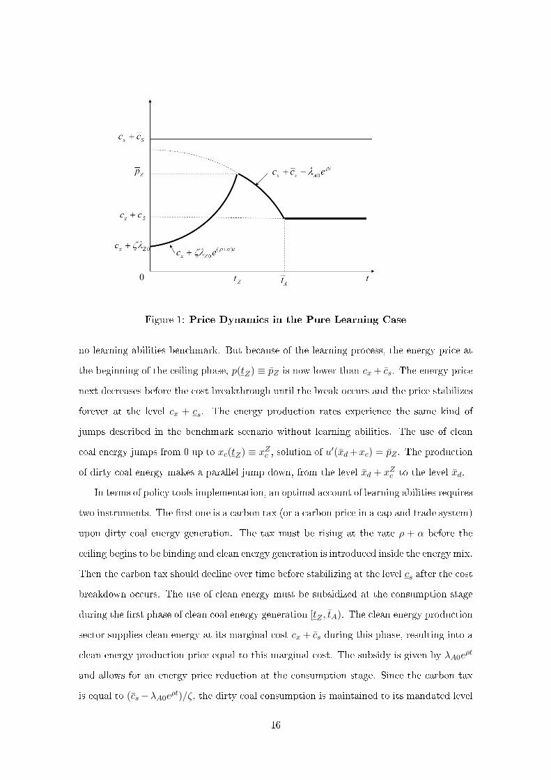
Figure 1: Price Dynamics in the Pure Learning Case

no learning abilities benchmark. But because of the learning process, the energy price at

the beginning of the ceiling phase, p(tZ) ≡ pZ is now lower than cx + cs. The energy price

next decreases before the cost breakthrough until the break occurs and the price stabilizes

forever at the level cx + cs. The energy production rates experience the same kind of

jumps described in the benchmark scenario without learning abilities. The use of clean

coal energy jumps from 0 up to xc(tZ) ≡ xZc , solution of u′(xd +xc) = pZ . The production

of dirty coal energy makes a parallel jump down, from the level xd + xZc to the level xd.

In terms of policy tools implementation, an optimal account of learning abilities requires

two instruments. The �rst one is a carbon tax (or a carbon price in a cap and trade system)

upon dirty coal energy generation. The tax must be rising at the rate ρ + α before the

ceiling begins to be binding and clean energy generation is introduced inside the energy mix.

Then the carbon tax should decline over time before stabilizing at the level cs after the cost

breakdown occurs. The use of clean energy must be subsidized at the consumption stage

during the �rst phase of clean coal energy generation [tZ , tA). The clean energy production

sector supplies clean energy at its marginal cost cx + cs during this phase, resulting into a

clean energy production price equal to this marginal cost. The subsidy is given by λA0eρt

and allows for an energy price reduction at the consumption stage. Since the carbon tax

is equal to (cs−λA0eρt)/ζ, the dirty coal consumption is maintained to its mandated level

16

xd. The subsidy increases over time, allowing for a permanent increase of clean coal energy

consumption until the cost breakdown occurs. After tA, the subsidy is removed and the

production and consumption prices of clean energy are identical and equal to cx + cs. The

maximum level of the subsidy, attained at time tA is the cost gap cs − cs. The current

value level of the subsidy is thus (cs − cs)e−ρ(tA−t) at time t, tZ ≤ t ≤ tA.

We have shown previously that without learning abilities, the economy prefers to rely

only upon dirty coal generation if p < cx + cs. The same happens with learning abilities

if p < cx + cs. In this situation, the technological breakthrough is unable to induce a

su�ciently low level of the pollution abatement marginal cost to justify beginning clean

coal energy generation. In the intermediate case: cx + cs < p < cx + cs, a new possible

scenario emerges. In this scenario, clean coal energy use is delayed after the attainment of

the ceiling until some time tc. Then clean coal energy generation expands until the cost

breakdown occurs. Remark that there should be no quantity discontinuity in this scenario.

The use of dirty coal energy is maintained to the level xd while the use of clean coal energy

is initially nill at tc. However, Appendix A.1 shows that the economy cannot improve over

a policy based upon the sole use of dirty coal energy by adopting such a combined policy.

Let us retain the case cx + cs < p. To characterize the optimal policy with learning

abilities, we have to identify four variables, the initial values of λZ and λA together with

the optimal time to attain the ceiling tZ and the optimal time to trigger the technological

revolution, tA. Let xd(t, λZ0) be implicitly de�ned by u′(x) = cx + ζλZ0e(ρ+α)t over the

time interval [0, tZ) and xc(t, λA0) be implicitly de�ned by u′(xd + xc) = cx + cs − λA0eρt

over the time interval [tZ , tA). (λZ0, λA0, tZ , tA) are solutions of the following system of

four conditions:

• The ceiling attainment condition, Z(tZ) = Z:

ZeαtZ = Z0 + ζ

∫ tZ

0xd(t, λZ0)eαtdt

• The critical experience level attainment condition at the revolution time, A(tA) = A:

A =

∫ tA

tZ

xc(t, λA0)dt

• The price continuity requirement at tZ :

ζλZ0e(ρ+α)tZ = cs − λA0e

ρtZ

17

• The price continuity requirement at the cost break time:

λA0eρtA = cs − cs

Denote by:

IZZ ≡ −∫ tZ

0

e(ρ+2α)t

u′′(q(t))dt > 0 ; IA ≡ −

∫ tA

tZ

eρt

u′′(q(t))dt > 0

JcA ≡ −∫ tA

tZ

dt

u′′(q(t))> 0 ; xZc ≡ xc(tZ) ; xAc ≡ xc(tA)

TA ≡ tA − tZ ; πZ ≡ ζ(ρ+ α)λZ0eαtZ + ρλA0

∆0 ≡ ζ[ζ(ρ+ α)λZ0I

ZZ + xZc e

αtZ].

We refer to Appendix A.2 for calculation details. We show the following e�ects of a

higher initial pollution stock over the optimal path features:

dλZ0

dZ0=

(ρ+ α)λZ0

∆0> 0 ;

dtZdZ0

=dtAdZ0

= − 1

∆0< 0

dλA0

dZ0=ρλA0

∆0> 0

The impact of a higher Z0 is qualitatively the same as in the case without learning abilities:

the pollution opportunity cost is higher and the attainment of the ceiling is accelerated.

We remark that even if the levels of the variables are of course di�erent, the qualitative

expressions of the partial derivatives are the same with and without learning abilities. This

is a consequence of the fact that a higher initial pollution stock mainly a�ects the optimal

path before the ceiling phase. Computing the e�ect of a higher Z0 over the price level at

the beginning of the ceiling phase, pZ , con�rms this result:

dpZdZ0

=

[dλZ0

dZ0+ (ρ+ α)λZ0

dtZdZ0

]e(ρ+α)tZ

= [(ρ+ α)λZ0 − (ρ+ α)λZ0]e(ρ+α)tZ

∆0= 0

A higher initial pollution stock has no e�ect over the energy price at the beginning of

the ceiling phase, and thus no e�ect over the production rate of clean coal energy at tZ .

Furthermore, dtZ/dZ0 = dtA/dZ

0 < 0 shows that the �rst phase at the ceiling keeps the

same length, thus the production plan of clean coal energy is just translated sooner in

time by a higher initial pollution level. This property induces an upper shift of the initial

18

level of the learning rent λA completely neutral in terms of current value subsidy levels

throughout the phase [tZ , tA).

One could be tempted to think that a stricter ceiling constraint would have the same

qualitative e�ects than a higher initial pollution stock. But the induced change over dirty

coal energy production modi�es the comparative advantage of dirty coal versus clean coal

energy generation and thus the value of experience acquisition. More precisely:

dλZ0

dZ= −(ρ+ α)λZ0e

αtZ

∆0+αρλA0TAζ∆0

?

dtZdZ

=eαtZ

∆0+αρλA0TAI

ZZ

xZc ∆0eαtZ> 0

dλA0

dZ= −ρλA0e

αtZ

∆0−αρλA0TA(πZI

ZZ + xZc e

2αtZ )

xZc ∆0eαtZ< 0

dtAdZ

=eαtZ

∆0+αTA(πZI

ZZ + xZc e

2αtZ )

xZc ∆0eαtZ> 0

A stricter ceiling constraint (dZ < 0) has an ambiguous e�ect over the initial pollution

opportunity cost. This translates into an ambiguous consequence over the energy implicit

price path before the beginning of the ceiling phase. However the analysis shows a faster

attainment of the ceiling, a higher learning rent together with a sooner technological rev-

olution time. The e�ect of a stricter environmental standard combines two components

shown in the above expressions. The �rst component is the e�ect of a change of Z for

a given clean energy production path. As expected, this component works in the same

direction as the e�ect of higher initial Z0. It increases the pollution opportunity cost,

fastens the ceiling attainment, increases the value of learning and fastens the revolution.

The second component expresses the induced e�ect of a stricter ceiling upon xc(t), the

clean coal energy production rate, during the pre-revolution phase at the ceiling, [tZ , tA).

This e�ect is depending upon TA, the length of this time phase. This e�ect has a nega-

tive impact over the pollution opportunity cost, it reduces tZ , makes increase the value of

learning and fastens the revolution. Thus these two e�ects work in the same direction for

tZ , λA0 and tA but in an opposite direction for λZ0.

This does not mean that the e�ect of a ceiling modi�cation over the energy price at

the beginning of the ceiling phase, pZ , and upon TA, the time length of the �rst phase of

19

clean coal production, is indeterminate. More precisely:

dpZdZ

=αρλA0TAζxZc

eρtZ > 0

dTAdZ

=αTAζxZc

> 0 .

Thus a stricter ceiling constraint results into a lower energy price at the beginning of the

ceiling phase together with a shorter time period before the revolution once clean coal

production begins. This implies that the production of clean coal energy is increased by a

stricter ceiling constraint and hence that the energy implicit price is lower during the time

phase [tZ , tA). To this lower price level correspond both a higher subsidy level to clean coal

energy and a lower carbon price. Note that a lower pZ and a lower tZ are compatible with

either a higher or a lower level of ζλZ0, the initial level of the carbon price. Note also that

learning abilities reverses the usual result that a stricter environmental constraint should

translate into a higher optimal carbon tax. The analysis shows to the contrary that, in

between the beginning of the ceiling period and the technological revolution, the carbon

tax level is lowered by a stricter ceiling constraint.

We have shown also that a stricter ceiling means an increased use of clean coal en-

ergy and thus a faster technological revolution. This is reminiscent of the Porter, Van

der Linde hypothesis (1995). Following Michael Porter, imposing 'tight' environmental

regulation (that is 'more' than Pigouvian) should spur more R&D e�orts from the energy

industry. In the present context, improving the e�ciency of pollution abatement requires

an increased use of the clean coal energy generation technology. A stricter environmental

standard, though perfectly 'Pigouvian', achieves this outcome quite naturally, by reducing

the comparative advantage of dirty energy with respect to clean energy. However, this

does not mean that before the beginning of clean coal energy use, a stricter environmental

standard should translate into a higher carbon tax.

Turn to the consequences of a higher experience threshold triggering the technological

revolution in clean coal energy generation. After computations, we get:

dλZ0

dA=ρλA0

∆0> 0 ;

dλA0

dA= −ρλA0

xZc

[1 +

ζρλA0IZZ

xZc ∆0eαtZ

]< 0

dtZdA

=ζρλA0I

ZZ

xZc ∆0eαtZ> 0 ;

dtAdA

=1

xZc

[1 +

ζρλA0IZZ

∆0eαtZ

]> 0

dpZdA

=ρλA0e

ρtZ

xZc> 0 ;

dTAdA

=1

xZc> 0 .

20

As expected, a higher experience requirement to trigger the cost break results into a lower

level of the learning rent and a longer time before the cost break. The opportunity cost of

pollution is increased together with the energy price at the beginning of the ceiling phase

but because the learning rent is decreased in a higher proportion than λZ is increased, the

attainment of the ceiling is delayed.

The sensitivity analysis of a small increase of the clean energy cost before the break

is more intricate since it a�ects simultaneously the price convergence condition towards

the ceiling, the relative pro�tability of clean coal energy before the break and the value of

learning in getting an increased cost cut. Denote by:

Ic ≡∫ tA

tZ

xc(t)e−ρtdt > 0 .

Then we get �rst:

dλZ0

dcs=

ρIc∆0

> 0 ;

dtZdcs

=ζρIZZ Ic

xZc ∆0eαtZ> 0 ;

dpZdcs

= ζe(ρ+α)tZ

[dλZ0

dcs+ (ρ+ α)λZ0

dtZdcs

]> 0 .

Hence a higher clean energy cost induces a higher pollution opportunity cost together with

a delayed attainment of the ceiling. The energy price at the beginning of the ceiling is

also increased. These results are expected, note that the direct e�ect of the cost increase

dominates the indirect e�ect over the energy price before the ceiling phase, resulting into

a slower move towards the ceiling.

The e�ect of a higher initial clean coal energy cost over the learning rent is indetermi-

nate but it is possible to show that:

dtAdcs

=ζ

xZc ∆0eαtZ

[(πZI

ZZ + xZc e

2αtZ )(JcA − IAe−ρtA) + xZc IZZ (e−ρtZ − e−ρtA)

]> 0

dTAdcs

=JcA − IAe−ρtA

xZc> 0

Hence a higher initial clean coal energy cost means a longer period before the cost break-

down. Since the energy price is shifted upward at the beginning of the ceiling phase, the

exploitation of clean coal energy is reduced, implying a slower learning process and thus a

delayed, although more signi�cant, cost cut.

21

Last, considering the consequences of a lower clean energy cost after the break, we �nd

that:

dλZ0

dcs> 0 ;

dλA0

dcs< 0

dtZdcs

> 0 ;dtAdcs

> 0

dpZdcs

> 0 ;dTAdcs

> 0

These e�ects �t the intuition. A higher clean energy cost level after the break, that is a

lower cost cut thanks to learning, results into a higher pollution opportunity cost together

with a delayed attainment of the ceiling. On the other hand, the learning rent is reduced

and the time length before the cost break to occur is enlarged.

The following propositions summarize our �ndings:

Proposition 1 (i) With only learning abilities, clean coal energy generation is never

introduced before the atmospheric ceiling constraint begins to be binding. If solar

energy production is cheaper than clean coal energy, it eliminates this option and

is itself eliminated in the reverse case. The optimal energy policy is a three phases

path composed of a �rst phase of only dirty energy generation at a declining rate

until the carbon ceiling level is attained. Then clean coal energy generation begins at

an increasing rate while the production of dirty energy is constrained by the ceiling.

This second phase ends at the technological revolution time. After the revolution, the

economy stays permanently at the ceiling and produces a constant rate of clean coal

energy at the post-revolution low marginal cost.

(ii) The possibility of a learning induced technological revolution in CCS lowers the carbon

opportunity cost before the attainment of the ceiling, this cost being rising exponen-

tially at the rate (ρ + α). During the pre-revolution phase at the ceiling, the energy

implicit price decreases over time. There is no price cut at the technological break-

through. After the break, the energy price remains constant and equal to the clean

coal energy marginal production cost.

(iii) The implementation of the optimal policy requires to combine a carbon tax (or a

carbon price in a cap and trade system) and a subsidy at the consumption stage to

22

clean energy use. The carbon tax increases before the atmospheric ceiling constraint

begins to be binding , decreases during the second phase and stays constant after the

cost revolution. The subsidy is introduced whence the ceiling is attained, it increases

exponentially at the rate ρ before the revolution and is suppressed after the cost break-

through. Its current value level at time t is given by (cs − cs)e−ρ(tA−t), the cost gap

in present value from t.

Concerning the sensitivity analysis with respect to some relevant parameters, we show

that:

Proposition 2 (i) The pollution opportunity cost, or the optimal carbon tax, is in-

creased by a higher initial pollution stock, a higher know-how requirement to trigger

the technological revolution or a higher CCS cost before the revolution. A stricter

environment standard, that is a lower Z, has an ambiguous e�ect over the carbon

price before the ceiling constraint begins to be binding and lowers this price whence

the ceiling is binding.

(ii) The learning rent, or equivalently the subsidy needed to induce the optimal level of

clean coal energy generation, is reduced by a higher initial pollution stock or a higher

required know-how level to trigger the technological revolution. It is increased by a

stricter environmental standard while a higher pre-revolution CCS cost has ambiguous

e�ects over the learning rent.

(iii) The ceiling constraint binds earlier if the initial pollution stock is higher, the ceiling

constraint more stringent, the know-how requirement to trigger the cost cut in CCS

operation less stringent or the abatement cost before the revolution less expensive.

(iv) The length of the learning phase between the beginning of the ceiling phase and the

revolution time is independent from the initial pollution stock. It decreases with a

stricter ceiling constraint, a less stringent know-how target and a lower pre-revolution

CCS abatement cost.

23

4 The R&D induced technical revolution in abatement

Consider the reverse case of no learning abilities. The technical revolution only results from

su�cient e�orts in R&D. Take the simplest form for the consequences of such e�orts over

the accumulation of know-how, that is assume that A = r. Then the optimality conditions

before the revolution become:

u′(q) = cx + cs − νxc (4.1)

u′(q) = cx + ζλZ − νxd (4.2)

u′(q) = cy − νy (4.3)

λA = cr(r)− νr (4.4)

λZ = (ρ+ α)λZ − νZ (4.5)

λA = ρλA . (4.6)

Assume that cy > p > cx + cs, hence solar energy never enters the energy mix. As

in the preceding case, clean coal energy generation should not be introduced before the

beginning of the ceiling phase. Since R&D only a�ects the time of the revolution, whatever

be the cost level, the pre-revolution high cost level or the post-revolution low cost level,

the constancy of unit costs is incompatible with the rise of the pollution opportunity cost

before the ceiling.

This in turn implies that the revolution should not occur strictly before the beginning of

the ceiling phase. Assume to the contrary that tA < tZ . Then clean coal energy production

begins at tZ with the best technology of cost cs. Since there are no learning abilities, we

are in the benchmark case exposed at the beginning of section 3. After reaching the ceiling,

the energy price is constant and given by cx + cs. Before tZ , the energy price is given by:

p(t) = cx+ζλZ0e(ρ+α)t until pZ = cx+cs is attained at time tZ . Consider a small decrease

of the research e�ort dr < 0 at each time during the time interval [0, tA). The revolution

time tA would be slightly delayed but for a su�ciently low dr, the revolution occurs before

tZ . Thus nothing would be changed to the resource use policy before and after tZ , the

only consequence being a reduction in the R&D cost. Thus such a reduction would be

bene�cial, resulting in an optimal time of the revolution happening at least whence the

ceiling has been attained, that is tZ ≤ tA in any optimal scenario.

24

Next let us assume that the know-how requirement is su�ciently stringent to have

tZ < tA. We shall be more precise later over the conditions for the revolution to occur only

strictly after the beginning of the ceiling phase. After the revolution, the economy remains

blockaded at the ceiling, the energy price is given by cx + cs, the production of dirty coal

energy by xd and the production of clean coal energy by xc, thus, V , the continuation

value after the revolution is the same as before and given by:

V =1

ρ[u(xd + xc)− cx(xd + xc)− csxc] .

Denote h− ≡ limt↑tA h(t) for any time function h(t). The transversality condition at tA is

now expressed as:

u(xd + x−c )− cx(xd + x−c )− csx−c − Cr(r−) + λ−Ar− = u(xd + xc)− cx(xd + xc)− csxc .

Taking (4.1) and (4.4) into account, this is equivalent to:

u(q−)− u′(q−)x−c − Cr(r−) + cr(r−)r− = u(xd + xc)− u′(xd + xc)xc

Denote by: Γr(r) ≡ cr(r)r − Cr(r). Since Cr(0) = 0, Γr(0) = 0 and Γ′r = c′r(r)r > 0

under our cost convexity assumption. Thus Γr(r) > 0 if r > 0. Denote by Γ(xc) ≡

u(xd + xc) − u′(xd + xc)xc, an increasing function of xc, as shown before. Then the

transversality condition is equivalent to:

Γ(xc)− Γ(x−c ) = Γr(r−) > 0

At the revolution time, tA, the energy price jumps down from the level cx + cs to the level

cx+cs. This corresponds to an upward jump of clean coal energy generation from the level

x−c , solution of u′(xd+xc) = cx+cs, up to the level xc, itself solution of: u

′(xd+xc) = cx+cs.

The transversality condition shows that to this quantity jump corresponds a unique level

of r−, the research e�ort just before the revolution. Since λ−A(tA) = cr(r−), the terminal

level of the R&D knowledge rent is thus also determined. Let λA be this level, then:

λA0eρtA = λA, taking (4.6) into account.

This shows a �rst di�erence between the R&D strategy to trigger the technological

revolution and the learning strategy. Inducing the right level of experience acquisition,

and thus the right level of clean coal energy production, required a speci�c subsidy in the

25

preceding case. Such a subsidy device is no more needed to induce the optimal level of R&D

investments, the carbon tax being a su�cient tool to implement the optimal scenario. The

optimal time pro�le of the subsidy also resulted into a continuous energy price trajectory

despite the cost revolution. This is no more the case under a R&D induced technological

revolution and one obtains the usual conclusion that energy services are permanently priced

at their marginal cost, the cost break resulting into a price breakdown at the revolution

time.

A second di�erence appears in the computation of the R&D rent. While the learning

rent simply identi�ed with the cost gap in the preceding section, the R&D rent at the

revolution time is de�ned through the transversality condition by a complex relation de-

pending upon not only the shape of the R&D cost function but also upon the energy gross

surplus function.

Third, the relative independency between the dynamics of energy use and the dynamics

of know-how induced by the R&D policy widens the space of possible energy scenarios.

Assume that the solar energy cost, cy, is such that: cs < cy < cs. In the learning induced

revolution framework, solar energy would eliminate the use of clean coal energy and thus the

possibility of a revolution. In the R&D induced revolution framework, the corresponding

optimal scenario is the following. During a �rst phase [0, tZ), the economy only relies upon

the use of dirty coal energy until the ceiling is attained. Then solar energy is introduced in

combination with dirty coal energy generation up to a level y solution of: u′(xd + y) = cy.

Thus, before the technological revolution, that is during the time interval [tZ , tA), the

economy is constrained by the ceiling but never produces clean coal energy, this one being

more costly than solar energy. After the revolution, solar energy is eliminated from the

energy mix and the economy combines the production of dirty energy at the rate xd and

of clean coal energy at the rate xc. Thus the energy transition scenario is composed of a

�rst phase using only coal, a second phase using both coal and solar energy and a third

phase using only coal but with a positive amount of clean coal energy.

Next, let us turn to the description of the optimal R&D policy. If cr(0) = c0r > 0, R&D

investment may be delayed. Taking (4.4) into account, λA(t) ≥ c0r appears as a necessary

condition for strictly positive R&D e�orts, r(t) > 0. Since λA0 = λA(0) is determined

by the whole model structure, this may or not be the case at time t = 0. If λA0 > c0r ,

26

R&D e�ort is set immediately at a positive level. Since c′r(r) > 0, the optimal R&D

e�ort is implicitly de�ned by λA(t) = cr(r(t)) as an increasing function of λA and thus

an increasing function of time since λA(t) is growing exponentially. Let r(t) = rA(λA(t))

be that function. Then r(t) grows permanently over time. If λA0 < c0r , R&D investments

are delayed until tA solution of λA(t) = c0r . At tA, R&D activity shows a smooth start

from a zero level and then increases permanently over time as in the preceding case. One

may observe that this feature goes in the opposite direction of many endogenous growth

models where R&D e�orts should be set initially at a high level and then be decreased.

This is because these models usually assume the existence of increasing returns to scale in

the knowledge generation process, returns to scale resulting from an inheritance e�ect of

previously accumulated knowledge. Such e�ects are absent in the present model and we

obtain the usual conclusion that because of discounting, R&D costs should be delayed in

time. The result is an increasing R&D e�ort path, maybe from a zero initial level after

some time period without research activity.

Let us �rst consider the optimal scenario in a situation where λA0 > c0r . If c0

r = 0,

this is the only optimal solution. It is identi�ed by computing the vector of variables

(λZ0, λA0, tZ , tA), a vector solution of the following set of conditions:

• The ceiling attainment condition, Z(tZ) = Z:

ZeαtZ = Z0 + ζ

∫ tZ

0xd(t)e

αtdt .

• The know-how requirement condition, A(tA) = A:

A =

∫ tA

0rA(λA0e

ρt)dt .

• The price continuity requirement at tZ :

ζλZ0e(ρ+α)tZ = cs

• The R&D rent condition at tA:

Γ(xc)− Γ(x−c ) = Γr(rA(λA0eρtA)) .

It is worth contrasting the pure learning and pure R&D induced technological break-

through models through a parallel comparative dynamics exercise to the one performed in

27

Section 3. The computations details are presented in Appendix A.3. The main conclusions

are the following.

Denote as before ∆0 = ζ[ζ(ρ+ α)λZ0 + xZc e

αtZ]and by: r = limt↑tA r(t) and r0 ≡

r(0).

The e�ects of a larger initial pollution stock Z0 or a stricter ceiling constraint are the

following:

dλZ0

dZ0= −dλZ0

dZe−αtZ =

(ρ+ α)λZ0

∆0> 0 ;

dtZdZ0

= −dtZdZ

e−αtZ = − 1

∆0

dλA0

dZ0=dtAdZ0

= 0

dλA0

dZ= − rρλA0

r − r0

dtAdZ

= −α(cs − cs)e−ρtAζr0

< 0

The decoupling of the know-how dynamics from the economic arbitrages driving the energy

policy removes the indeterminacy problem identi�ed in the learning model. It appears

clearly that a larger initial pollution stock or a stricter ceiling constraint have the same

qualitative e�ects over the energy implicit price trajectory. Both make rise the pollution

opportunity cost, and thus the energy price before the ceiling, and fasten the attainment

of the ceiling.

The di�erences between a stricter ceiling an a higher initial pollution stock appear

when considering the R&D optimal policy. There is no e�ect of the initial pollution stock

over the R&D policy. Since the economy is permanently constrained by the ceiling after

tZ , a stricter ceiling results into a higher R&D e�ort and thus in earlier technological

revolution. We observed a similar accelerating e�ect in the learning model. Imposing a

stricter environmental standard makes rise the R&D e�ort to trigger the cost revolution.

The consequences of a higher know-how requirement, A, to trigger the technical revo-

lution o�er another illustration of the relative independency between the R&D policy and

the energy policy. After computations, we get:

dλZ0

dA=dtZdA

= 0

dλA0

dA= −ρλA0

dtAdA

= −ρλA0

r0< 0

A higher knowledge target induces a slow down of the research e�orts and thus a delayed

technical revolution. A larger know-how requirement has no e�ect over the energy con-

28

sumption policy, the ceiling being attained at the same time and the pollution opportunity

cost being una�ected by a higher A.

The independency feature disappears when considering the additional cost of clean

coal energy production before the revolution, since this cost both a�ects the convergence

condition of the energy price towards its ceiling level and the size of the cost breakdown.

The calculus shows that:

dλZ0

dcs=xzc∆0

e−ρtZ > 0 ;dtZdcs

=ζIZZ∆0

e−(ρ+α)tZ > 0

dλA0

dcs=x−cr0e−ρtA > 0 ;

dtAdcs

= −x−c (r − r0)

r0rρλA0e−ρtA < 0

As in the pure learning model, a higher initial clean coal energy cost means a higher

pollution opportunity cost together with a delayed arrival at the ceiling. As before, the

direct e�ect over the energy price after tZ resulting from a higher cs dominates the indirect

e�ect over the energy price of a higher pollution opportunity cost resulting in a longer time

before the beginning of the ceiling phase. Contrarily to the learning model where the time

length between the beginning of the learning process and the revolution time was enlarged

by a higher cs, R&D is accelerated by the perspective of a larger cost breakthrough and

the revolution comes earlier.

Since the clean coal cost level a�ects only the post-revolution phase, one should expect

that a higher cs has no e�ect upon the energy use before the revolution. Furthermore,

the perspective of a smaller cost breakthrough should discourage research and delay the

revolution time. The calculus con�rms these straightforward intuitions.

Up to now we considered only scenarios where λA0 > c0r , but we need to make precise

the domain of validity of such policies. Let us consider an R&D policy starting at time 0

from r(0) = 0, that is λA0 = c0r . Then the cost breakthrough occurs at a time TA solution

of:

A =

∫ T

0rA(c0

reρt)dt

TA is the maximum time delay to get the breakthrough since the economy starts from the

lowest possible level of research e�orts. Let (λ0Z0, t

0Z) be de�ned as the solutions of:

ZeαtZ = Z0 + ζ

∫ tZ

0xd(t)e

αtdt

ζλZ0e(ρ+α)tZ = cs .

29

(λ0Z0, t

0Z) are the optimal initial levels of the pollution opportunity cost and time delay

before the ceiling in a situation where the cost breakthrough would occur just when the

ceiling constraint begins to be binding. If t0Z > TA, the active R&D phase has to be

delayed until tA = t0Z − TA as noticed before. In this scenario, clean energy production is

introduced at t0Z with the best technology, the cost breakthrough occurring at t0Z .

In the contrary case, triggering the technological revolution when attaining the ceiling

requires to set λA0 above c0r and thus r(0) > 0. To t0Z corresponds a unique value of λA0,

we denote by λ0A0 solution of:

A =

∫ t0Z

0rA(λA0e

ρt)dt .

Let λ0A ≡ λ0

A0eρt0Z .

We have to consider the transversality condition while taking explicitly into account

the constraint: tZ ≤ tA, which requires to modify this condition as such. Denote by µZ ,

the Lagrange multiplier associated to the constraint tZ ≤ tA. Then optimality requires

that:

H(tA) + µZ = − ∂

∂tAV e−ρtA

with µZ ≥ 0 and µZ(tA − tZ) = 0. This is equivalent to:

Γ ≡ Γ(xc)− Γ(x−c ) = Γr(r−) + µZ ≥ Γr(r

−)

Note that Γ is given by the cost parameters and the energy demand shape, and is indepen-

dent from either the R&D policy or the ceiling attainment condition. Let r be the solution

of Γ = Γr(r) and λA = cr(r) ≡ λA(Γ). Then, Γr(r) being an increasing function of r, r is

an increasing function of Γ and hence λA(Γ) is an increasing function of Γ. This implies

that if λA(Γ) < λ0A, the constraint tZ ≤ tA does not bind, while it is binding in the reverse

case.

Consider the case of a binding constraint, that is λA(Γ) ≥ λ0A. Let r0(t) ≡ rA(λ0

A0eρt),

the optimal R&D policy may be of two types. If t0Z < Ta, it is de�ned by r0(t) over the

time interval [0, t0Z). The research e�ort is initially strictly positive (r0(0) > 0) and the

cost break occurs at t0Z . If t0Z > Ta, then the active research phase is delayed until some

time tA = t0Z − TA.

30

Turn now to the case of a non binding constraint: λA(Γ) < λ0A. Then λA(Γ) < λ0

A is

equivalent to r(tA) < r(t0Z), implying that tA > t0Z to satisfy the knowledge accumulation

constraint. Hence, λA0 < λ0A0. The economy follows a less active R&D policy. To lower

levels of Γ correspond lower levels of λA(Γ) and thus lower paths of R&D e�orts. If Γ is

such that λA(Γ) < c0r , R&D e�orts become unpro�table and there is no cost breakthrough.

We conclude that the optimal policy is one of the four possible types described in the

following Proposition:

Proposition 3 1. If λA(Γ) < c0r, there is no R&D activity and trivially the cost break

never occurs, the society prefers to use clean coal energy when at the ceiling at the

high cost level.

2. If c0r < λA(Γ) < λ0

A, the active R&D policy starts immediately at time 0. R&D e�orts

increase over time and the cost breakthrough occurs strictly after the beginning of the

ceiling phase, resulting in a time phase [tZ , tA) where the economy uses the clean coal

energy technology at its highest cost cs.

3. If λ0A < λA and t0Z < TA, then the economy starts to perform R&D e�orts right

from t = 0, the optimal R&D e�ort is given by r0(t) resulting in a cost breakthrough

occurring just at the time t0Z when the ceiling constraint begins to bind.

4. If λ0A < λA and t0Z > TA, then the active R&D phase is delayed until some time tA

such that tA = t0Z − TA, also triggering the technological revolution just at the arrival

at the ceiling.

Concerning the sensitivity of the optimal path to some relevant parameters in the case

c0r < λA(Γ) < λ0

A, we have shown that:

Proposition 4 (i) The pollution opportunity cost before the ceiling constraint begins to

bind, or equivalently the optimal carbon tax, is increased by a larger initial pollu-

tion stock, a stricter ceiling constraint or a higher CCS cost before the technological

revolution. It is una�ected by the know-how target to trigger the revolution.

(ii) The ceiling constraint binds earlier with a higher initial pollution stock, a stricter

ceiling constraint, a higher CCS cost before the revolution and is una�ected by the

revolution know-how target.

31

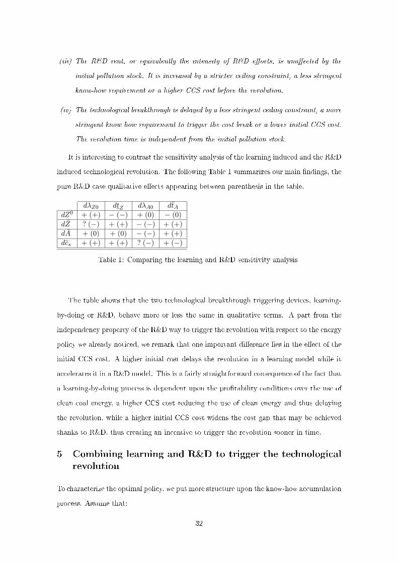
(iii) The R&D rent, or equivalently the intensity of R&D e�orts, is una�ected by the

initial pollution stock. It is increased by a stricter ceiling constraint, a less stringent

know-how requirement or a higher CCS cost before the revolution.

(iv) The technological breakthrough is delayed by a less stringent ceiling constraint, a more

stringent know-how requirement to trigger the cost break or a lower initial CCS cost.

The revolution time is independent from the initial pollution stock.

It is interesting to contrast the sensitivity analysis of the learning induced and the R&D

induced technological revolution. The following Table 1 summarizes our main �ndings, the

pure R&D case qualitative e�ects appearing between parenthesis in the table.

dλZ0 dtZ dλA0 dtAdZ0 + (+) − (−) + (0) − (0)

dZ ? (−) + (+) − (−) + (+)

dA + (0) + (0) − (−) + (+)

dcs + (+) + (+) ? (−) + (−)

Table 1: Comparing the learning and R&D sensitivity analysis

The table shows that the two technological breakthrough triggering devices, learning-

by-doing or R&D, behave more or less the same in qualitative terms. A part from the

independency property of the R&D way to trigger the revolution with respect to the energy

policy we already noticed, we remark that one important di�erence lies in the e�ect of the

initial CCS cost. A higher initial cost delays the revolution in a learning model while it

accelerates it in a R&D model. This is a fairly straightforward consequence of the fact that

a learning-by-doing process is dependent upon the pro�tability conditions over the use of

clean coal energy, a higher CCS cost reducing the use of clean energy and thus delaying

the revolution, while a higher initial CCS cost widens the cost gap that may be achieved

thanks to R&D, thus creating an incentive to trigger the revolution sooner in time.

5 Combining learning and R&D to trigger the technological

revolution

To characterize the optimal policy, we put more structure upon the know-how accumulation

process. Assume that:

32

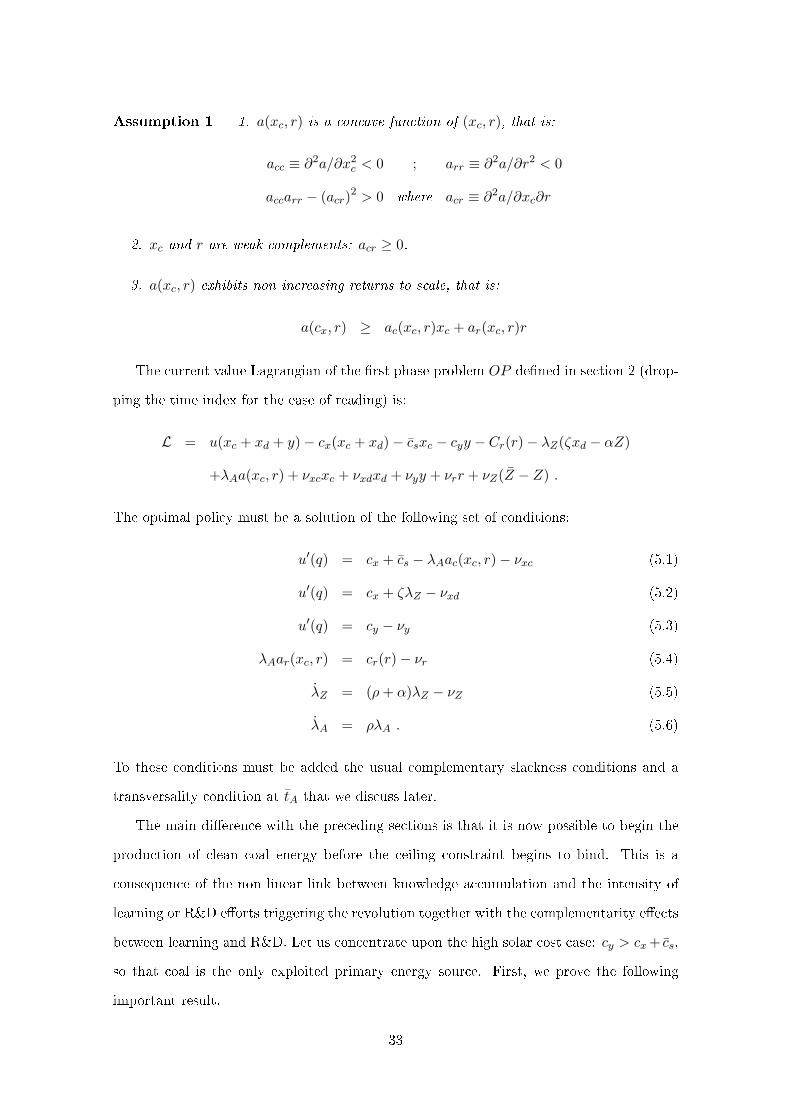
Assumption 1 1. a(xc, r) is a concave function of (xc, r), that is:

acc ≡ ∂2a/∂x2c < 0 ; arr ≡ ∂2a/∂r2 < 0

accarr − (acr)2 > 0 where acr ≡ ∂2a/∂xc∂r

2. xc and r are weak complements: acr ≥ 0.

3. a(xc, r) exhibits non increasing returns to scale, that is:

a(cx, r) ≥ ac(xc, r)xc + ar(xc, r)r

The current value Lagrangian of the �rst phase problem OP de�ned in section 2 (drop-

ping the time index for the ease of reading) is:

L = u(xc + xd + y)− cx(xc + xd)− csxc − cyy − Cr(r)− λZ(ζxd − αZ)

+λAa(xc, r) + νxcxc + νxdxd + νyy + νrr + νZ(Z − Z) .

The optimal policy must be a solution of the following set of conditions:

u′(q) = cx + cs − λAac(xc, r)− νxc (5.1)

u′(q) = cx + ζλZ − νxd (5.2)

u′(q) = cy − νy (5.3)

λAar(xc, r) = cr(r)− νr (5.4)

λZ = (ρ+ α)λZ − νZ (5.5)

λA = ρλA . (5.6)

To these conditions must be added the usual complementary slackness conditions and a

transversality condition at tA that we discuss later.

The main di�erence with the preceding sections is that it is now possible to begin the

production of clean coal energy before the ceiling constraint begins to bind. This is a

consequence of the non linear link between knowledge accumulation and the intensity of

learning or R&D e�orts triggering the revolution together with the complementarity e�ects

between learning and R&D. Let us concentrate upon the high solar cost case: cy > cx+ cs,

so that coal is the only exploited primary energy source. First, we prove the following

important result.

33

Proposition 5 Along an optimal energy and know-how accumulation policy, the cost break-

through happens either strictly after the ceiling has been attained or either at the time when

the ceiling begins to bind, that is tZ ≤ tA in all optimal scenarios.

Proof: Assume to the contrary that tA < tZ . Over a time interval [t0, tA) we may

be in three possible situations: either the cost break is triggered only by research, either

it is triggered only through learning, or either it is triggered by a combination of research

and learning. In the �rst case, slowing down slightly the research e�ort is bene�cial, as

noticed in section 3. In the second and third cases, λA will be zero after the cost break

and since the production of clean coal energy is positive in these two cases, ζλZ = cs is

incompatible with λZ growing exponentially during the time interval [tA, tZ). Hence clean

coal exploitation should be interrupted after the cost break, meaning that delaying the

revolution by reducing the use of clean coal energy before the revolution is bene�cial.

5.1 Know-how accumulation scenarios

An optimal policy of knowledge accumulation is a sequence of time phases composed of

the three following types of transitory tails:

(i) A Combined tail during which both research and learning are used to accumulate

know-how. Let T C be such a time phase, then xc(t) > 0 and r(t) > 0, t ∈ T C .

(ii) A Pure R&D tail during which there is no exploitation of clean coal energy and

the economy performs only research activity. Let T R be such a time phase, then

xc(t) = 0 and r(t) > 0, t ∈ T R.

(iii) A Pure learning tail during which there is no research activity and know-how ac-

cumulates only because of learning. Let T L be such a time phase, xc(t) > 0 and

r(t) = 0, t ∈ T R.

Such transitory phases can happen indi�erently before or during the ceiling phase. The

main complexity now is that there is no more a simple link between the energy production

path, and thus the timing of the pre-ceiling and ceiling phases, and the structure of the

combined learning and R&D know-how accumulation path.

We thus have to describe the main features of the possible transitory tails in the two

cases of a pre-ceiling phase and a ceiling phase.

34

Combined tails

Assume �rst that T C ⊂ [0, tZ). During this time phase, (xc(t), xd(t), r(t)) are de-

�ned as functions of (λZ(t), λA(t)) by (5.1), (5.2) and (5.4) with νxd = νxc = νr =

0. Let xc(λZ , λA), xd(λZ , λA), r(λZ , λA) be the corresponding implicit functions. Let

δ ≡ accarr − (acr)2. δ > 0 through the concavity assumption over a(xc, r) and let

∆1 ≡ −u′′(q(t))λA(t) [λA(t)δ − accc′r] > 0. Di�erentiating the relevant optimality con-

ditions and dropping the arguments of the functions for the ease of reading gets:

∂xd∂λZ

= − ζ

∆1

[u′′(λAarr − c′r) + λ2

Aδ − λAaccc′r]< 0 ; (5.7)

∂xd∂λA

= − u′′

∆1

[ac(λAarr − c′r)− λAaracr

]< 0 ; (5.8)

∂xc∂λZ

=ζu′′

∆1

(λAarr − c′r

)> 0 ; (5.9)

∂xc∂λA

= − ∂xd∂λA

> 0 ; (5.10)

∂r

∂λZ= −ζu

′′

∆1λAacr > 0 ; (5.11)

∂r

∂λA= −u

′′λA∆1

[acacr − aracc] > 0 . (5.12)

Since λZ(t) = λZ0e(ρ+α)t and λA(t) = λA0e

ρt during the time phase [0, tZ), we conclude

that both λZ(t) and λA(t) are time increasing and thus:

dxddt

< 0 ;dxcdt

> 0 ;dr

dt> 0 .

Before the ceiling phase, the use of dirty coal energy should decline while the use of clean

coal energy should expand, together with an ever increasing level of R&D e�orts. Note

however that λZ being increasing, q(t) has to decrease. The increased use of clean energy

does not compensate for the declining rate of use of dirty energy, the aggregate use of

energy being strictly decreasing with time before the ceiling is attained.

Next, assume that T C ⊂ [tZ , tA). Now xd(t) = xd and (xc(t), r(t)) are implicitly

de�ned by (5.1) and (5.4) as functions of λA only. Let xc(λA), r(λA) be these functions.

Denote:

∆2 ≡ u′′(q)(λAarr − c′r)− λAaccc′r + λ2Aδ > 0 .

35

Di�erentiating (5.1) and (5.4), we get:

dxc(λ)

dλA=

1

∆2

[λAacrar − ac(λAarr − c′r)

]> 0 ; (5.13)

dr(λA)

dλA=

1

∆2

[λAacacr − (u′′(q) + λAacc)ar

]> 0 . (5.14)

This shows that xc(λA) and r(λA) are increasing functions of λA, and thus of time, also

during the ceiling phase. This implies in turn that a(λA) ≡ a(xc(λA), r(λA)) is also an

increasing function of λA. Since λA increases over time, a(λA) increases over time, the

accumulation of know-how through the combined e�ect of learning and R&D accelerates

over time. Last, we conclude that xc(t) being increasing through time, the energy implicit

price should permanently decrease during such a T C time phase.

Let us denote by σ ≡ ac/ar the marginal rate of substitution (MRS) between learning

and R&D. We are going to show that during a combined tail, σ is declining over time.

Consider �rst the case T C ⊂ [0, tZ). The MRS is de�ned implicitly as a function of

(λZ , λA) during Tc. Let σ(λZ , λA) be this implicit function:

σ(λZ , λA) =ac(xc(λZ , λA), r(λZ , λA))

ar(xc(λZ , λA), r(λZ , λA)).

Making use of (5.9)-(5.12), we get the following expressions of the partial derivatives of

the function σ(λZ , λA) with respect to (λZ , λA):

∂σ(λZ , λA)

∂λZ=

ζu′′

ar∆1

[λAδ + c′r(σarc − acc)

]< 0 (5.15)

∂σ(λZ , λA)

∂λA=

σc′ru′′

∆1[σarc − acc] < 0 . (5.16)

Hence we conclude from λZ(t) > 0 and λA(t) > 0, t ∈ [0, tZ), that:

σ(t) =∂σ

∂λZλZ(t) +

∂σ

∂λAλA(t) < 0 .

In the case T C ⊂ [tZ , tA), Appendix A.4 shows that σ < 0. This property of combined

tails does not translate to the other types of phases, a point we check below. The dynamics

of σ(t) has important implications over the dynamics of xc(t) and r(t) during a combined

phase.

Proposition 6 During any time phase accumulating know-how through both learning and

R&D, either before the ceiling phase or either during the ceiling phase, the learning e�ort

increases at a higher rate than the R&D e�ort.

36

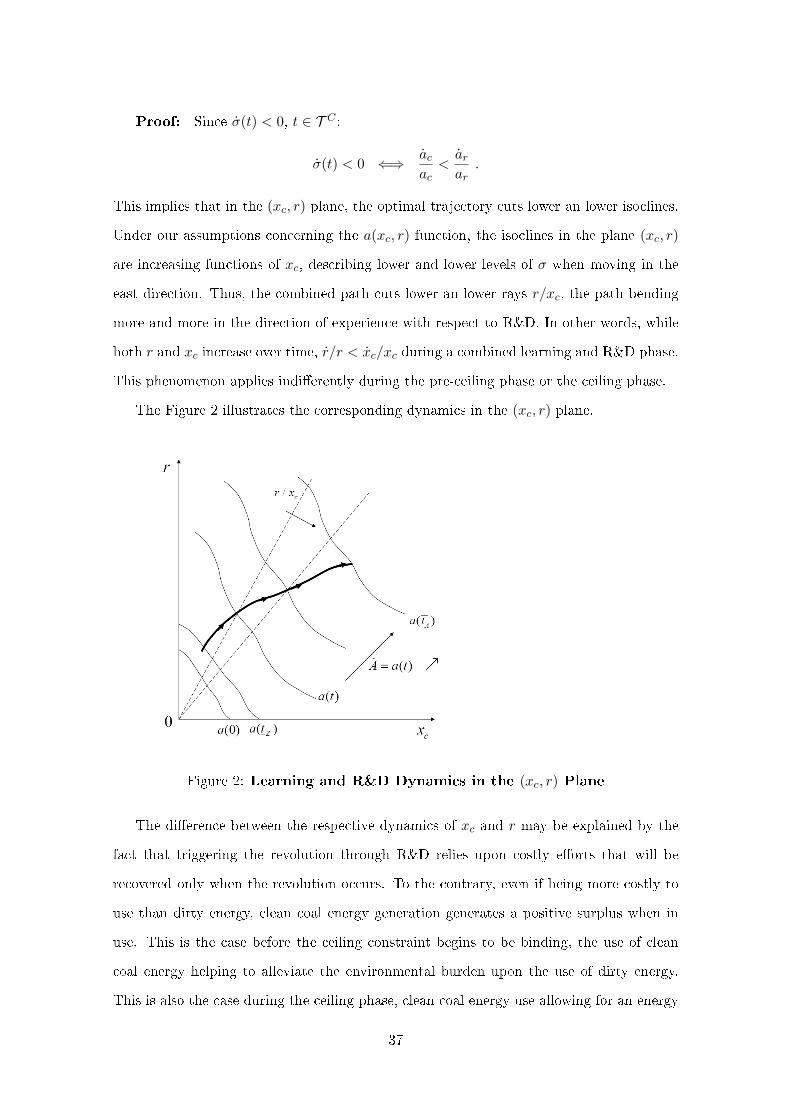
Proof: Since σ(t) < 0, t ∈ T C :

σ(t) < 0 ⇐⇒ acac<arar

.

This implies that in the (xc, r) plane, the optimal trajectory cuts lower an lower isoclines.

Under our assumptions concerning the a(xc, r) function, the isoclines in the plane (xc, r)

are increasing functions of xc, describing lower and lower levels of σ when moving in the

east direction. Thus, the combined path cuts lower an lower rays r/xc, the path bending

more and more in the direction of experience with respect to R&D. In other words, while

both r and xc increase over time, r/r < xc/xc during a combined learning and R&D phase.

This phenomenon applies indi�erently during the pre-ceiling phase or the ceiling phase.

The Figure 2 illustrates the corresponding dynamics in the (xc, r) plane.

Figure 2: Learning and R&D Dynamics in the (xc, r) Plane

The di�erence between the respective dynamics of xc and r may be explained by the

fact that triggering the revolution through R&D relies upon costly e�orts that will be

recovered only when the revolution occurs. To the contrary, even if being more costly to

use than dirty energy, clean coal energy generation generates a positive surplus when in

use. This is the case before the ceiling constraint begins to be binding, the use of clean

coal energy helping to alleviate the environmental burden upon the use of dirty energy.

This is also the case during the ceiling phase, clean coal energy use allowing for an energy

37

consumption increase above the constrained level xd. The consequence is that the economy

should rely more and more over time upon learning with respect to research activity to

trigger the technological revolution. The interesting aspect of this result is its degree

of generality. It does not involve any kind of speci�c experience capital in learning or

particular assumptions upon the relative productiveness of learning and R&D in boosting

the acquisition of know-how.

Pure R&D tails

Let us now consider a time phase T R involving only R&D activity without clean energy

production and hence no learning on the CCS technology. Then (5.4) de�nes r(t) as an

implicit function of λA and:

dr(λA)

dλA=

arc′r − λAarr

> 0 .

λA(t) being increasing over time, r(t) grows also over time. Since acr > 0, this implies that

ac(0, r) = acrr > 0 and hence that λAac(0, r) is an increasing function of time. Assume

�rst that T R ⊂ [0, tZ). Then over the time interval T R:

νxc(t) = cs − [λA(t)ac(0, r(t)) + ζλZ(t)] .

It appears that νxc(t) is a strictly decreasing time function during a time interval T R.

This implies that a corner path where xc = 0 and r > 0 cannot follow an interior path

where both xc > 0 and r > 0. Furthermore we remark that r(t) being increasing over

time, ac(0, r) increases over time, since acr > 0, while ar(0, r) decreases over time, since

arr < 0. Hence σ = ac/ar increases over time during the time interval T R. Last, note that

the border condition:

ζλZ = cs − λAac(0, r(λA))

de�nes an implicit relation between λZ and λA such that:

dλAdλZ

∣∣∣∣xc=0

= − ζ(c′r − λAarr)aracrλA + ac(c′r − λAarr)

< 0 .

Assume now that Tr ⊂ [tZ , tA). Since xc = 0, u′(xd) = p then νxc = cs−λA(t)ac(0, r(λA))−

p, also a decreasing time function. Note that, as in the case Tr ⊂ [0, tZ), σ(t) increases

over time. The border condition is now:

p = cs − λAac(0, r(λA)) .

38

This condition de�nes a unique level of λA, we denote by λRA. λA(t) > λRA is incompatible

with a policy performing only research activity without clean coal energy production.

Pure learning tails

Next, consider the case of a time phase T L. Note that this requires c0r > 0. Assume

�rst that T L ⊂ [0, tZ). Then (5.1), (5.2) de�ne implicitly xc and xd as functions of

(λZ , λA). Let xc(λZ , λA) and xd(λZ , λA) be the corresponding implicit functions. Denote

by ∆3 ≡ λAu′′(q)acc(xc, 0) > 0. Then it is easily checked that:

∂xc∂λZ

= −ζu′′(q)

∆3> 0 ;

∂xc∂λA

= −acu′′(q)

∆x> 0 ;

∂xd∂λZ

=ζ(u′′(q) + λAacc)

∆3< 0 ;

∂xd∂λA

=u′′(q)ac

∆x< 0 .

Since λZ(t) and λA(t) are increasing time functions before tZ , this shows that xd(t) declines

over time while xc(t) increases over time. Hence ac(xc, 0) decreases over time, since acc < 0

and ar(xc, 0) increases over time, since acr > 0. We conclude that σ(t) = ac(t)/ar(t)

decreases during a T L type time interval. Furthermore νr(t) is given by:

νr(t) = c0r − λA(t)ar(xc(λZ(t), λA(t)), 0) .

ar(xc, 0) being increasing over time, νr(t) decreases, implying that a time phase where

xc > 0 and r = 0 cannot follow a time phase where both xc > 0 and r > 0. Next consider

the border condition:

λAar(xc(λZ , λA), 0) = c0r .

This condition de�nes an implicit relationship between λZ and λA such that:

dλAdλZ

∣∣∣∣r=0

= − ζarcacarc − aracc

< 0 .

Next, assume that T L ⊂ [tZ , tA). Then xd = xd and (5.1) de�nes an implicit function

xc(λA) such that:

dxcdλA

= − acu′′ + λAacc

> 0 .

We thus conclude that λA being an increasing time function, xc(t) should also grow over

time. Hence λA(t)ar(xc(λA(t)), 0) increases over time, implying that νr(t) should decrease

39

over time. Once again, we have veri�ed that a time phase during which xc(t) > 0 and

r(t) = 0 cannot follow a time phase where both xc > 0 and r > 0. The border condition:

λAar(xc(λA), 0) = c0r ,

now de�nes a unique value of λA we denote by λLA. If λA > λLA a pure learning policy is

no more optimal.

Taking stock, we can now describe the optimal know-how acquisition policies. Denote

by PR (Pure R&D) a time phase of the T R type, where the know-how index increases

thanks to only research e�orts, by PL (Pure Learning) a time phase of the T L type and by

C (Combined) a time phase combining the use of research e�orts and the clean coal energy

technology. We have shown that xc, xd and r are de�ned as continuous functions of either

both λZ and λA during the pre-ceiling phase, and that xc and r are de�ned as continuous

functions of λA during the ceiling phase if tZ < tA. Since λZ(t) and λA(t) are continuous

time functions over the time interval [0, tA), that is to the exception of the revolution time

tA, we conclude that xc, xd and r must be continuous time functions. This implies in turn

that νxc and νr are also continuous time functions. A transition from a PR phase to a

LR phase requires an upward jump down of νxc from zero to some strictly positive level

since νxc will have to decrease strictly during the LR phase. This cannot be optimal. The

same argument applies to a transition from a LR phase to a PR phase, such a transition

requiring an upward jump of νr at the transition time. It applies also to transitions from

a C phase to either a PR phase or a LR phase, the �rst transition requiring an upward

jump of νr and the second one an upward jump of νxc. Hence we conclude that a PR

phase or a PL phase can only precede a combined C phase. Of course, it remains possible

that the optimal path begins with an inactive phase, during which the economy makes no

e�orts at all to trigger the technological revolution.

Let us �rst consider the case tZ < tA, that is the revolution occurs only strictly after

the beginning of the ceiling phase. Then the optimal know-how active acquisition policy

is one of the following scenarios:

(i) A PR phase followed until tA, the revolution time;

(ii) A PL phase followed until tA;

40

(iii) A PR phase followed by a C phase until tA;

(iv) A PL phase followed by a C phase until tA;

(v) A C phase followed until tA.

The relevance of the preceding scenarios depends upon the models fundamentals, in

particular the knowledge generation function. Let us brie�y sketch the main features of

these di�erent scenarios.

Scenario 1 : Pure R&D policies

In this scenario, the research e�orts are constantly increasing until the cost break-

through. The energy implicit price is given by cx + ζλZ0e(ρ+α)t before tZ , growing expo-

nentially while the use of dirty energy declines. Then the price stabilizes at p until the cost

break occurs and clean energy is introduced inside the energy mix in combination with

dirty energy.

Scenario 2 : Pure learning policies

Such a scenario requires a su�ciently high level of c0r > 0 to prevent R&D to be

pro�table. The use of clean energy starts at time 0 and increases permanently until the

technological revolution occurs. Before the ceiling phase, the aggregate energy production

declines, the expansion in the use of clean energy does not compensate for the sharper

decline of the use of dirty energy. After tZ , the continuous expansion of the use of clean

energy makes decrease the energy price until the revolution occurs and the price stabilizes

at the level cx + cs.

Scenario 3 : Pure research then combined policies

These policies may be of two kinds, depending upon the ceiling beginning to bind

during the pure R&D phase or during the combined phase. In the �rst case, the energy

price increases up to p, a level attained at the beginning of the ceiling phase. Then begins

a �rst phase at the ceiling [tZ , tr) during which only dirty coal energy is exploited. At tr,

the economy begins to produce clean coal energy and the energy price decreases until tA,

when the cost break occurs and the energy price stabilizes forever at the level cx + cs. The

research e�orts increase over time until the technological revolution time. Thus the MRS

between learning intensity and research �rst increases until tr before decreasing during the

time phase [tr, tA).

41

In the second case, the clean coal energy option is introduced before the ceiling con-

straint begins to be binding, thus during a time phase where the energy price grows at the

rate (ρ+ α). During a �rst phase [0, tr), only dirty energy is produced at a declining rate

and the economy performs increasing R&D e�orts. At tr, clean coal energy is introduced

from a null level. Then clean coal energy production expands while the use of dirty energy

decreases, the aggregate trend being a decreasing energy use until the ceiling is attained.

During this second time phase [tr, tZ), the research e�ort continues to increase while the

MRS between learning and R&D decreases, implying a higher rate of growth of clean coal

production than the research e�orts growth rate. Then begins a �rst phase at the ceil-

ing [tZ , tA) until the cost revolution. Know-how accumulation accelerates also during this

phase, learning expansion remaining higher than research e�orts increases.

Scenario 4 : Pure learning then combined policies

As in the preceding scenario, the ceiling constraint may bind before or after the be-

ginning of the combined phase of knowledge accumulation. In the �rst case, the learning

process relies on a continuous expansion of the use of clean coal energy until tZ . The

energy price increases exponentially during the time phase [0, tZ), implying a declining

energy consumption, the use of dirty energy being decreasing at a higher rate than the

growth rate of use of clean energy. The MRS between learning and R&D declines during

this time interval. Then begins a second phase [tZ , tc), during which the economy does not

perform R&D e�orts, clean coal energy use continues to increase, the use of dirty energy is

constrained at the level xd and the energy price decreases. After this phase, the economy

enter a combined regime of know-how accumulation based upon the use of clean coal energy

and research activities. Such a scenario supposes that cr(0) = c0r be strictly positive and

su�ciently high to prevent research activities before the ceiling has been attained. During

the combined phase [tc, tA) the energy price continues to decrease, the know-how accumu-

lation accelerates, the MRS between learning and R&D decreases, the rate of growth of xc

being larger than the rate of growth of r(t). At the end of this phase, the cost revolution

occurs and the energy use stabilizes to its optimal post-revolution level.

In the second case, the optimal path is composed of a �rst phase below the ceiling [0, tc)

without research activity but with a combined use of clean energy at an increasing rate

and dirty energy at a declining rate. The aggregate energy use decreases while the energy

42

price increases. Then begins a second phase below the ceiling [tc, tZ) where the economy

accumulates know-how both from learning and R&D activity. The energy price continues

to increase and the MRS between learning and R&D being decreasing, r(t) increases at

a lower rate than xc(t). This phase is followed by a phase at the ceiling until the cost

breakdown occurs, [tZ , tA). The energy price now decreases during this phase, clean coal

energy use and R&D activity continue to grow until tA and the MRS being also decreasing,

clean coal use grows at a higher rate than the research e�ort level.

Scenario 5 : Combined Policies

In this scenario, the economy accumulates know-how by using clean coal energy and an

active R&D policy right from the beginning of time. During a �rst phase [0, tZ), the energy

price increases, the energy supply decreases but the use of dirty energy declines while the

use of clean energy increases, together with the intensity of R&D e�orts. Then the ceiling

is reached and the economy enters a second phase of combined learning and R&D know-

how accumulation, [tZ , tA) until the technological revolution occurs. The energy price now

decreases. Clean coal energy use continues to grow together with intensity of research

activity. The MRS between learning and R&D being decreasing, the growth rate of xc(t)

is higher than the growth rate of r(t).

Figure 3 illustrates the shape of the energy price path if tZ < tA for all scenarios

expected a pure R&D policy followed until the cost break. In this last case, the energy

price grows up to p, attained at tZ . Then it stays constant at this level until the cost break

occurs. At tA, the energy price jumps down from the level p to the level cx + cs, last it

stays permanently at this level, clean coal energy generation beginning after tA. The proof

that the energy price should jump down at tA is presented in the next subsection.

Figure 3 shows that the energy implicit price path combines in a straightforward way

the features of the energy use dynamics exposed in the preceding sections. Before the

ceiling constraint begins to bind, the energy price rises exponentially at the rate (ρ + α),

and thus the aggregate supply of energy decreases. This means that even if clean coal

energy is used during the pre-ceiling phase, its expansion over time does not compensate

for the reduction of the use of dirty coal energy. During the �rst phase at the ceiling

preceding the revolution, the use of dirty energy is constrained at the constant level xd

while the use of clean coal energy continues to expand. The result is a decreasing energy

43

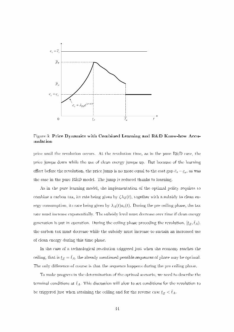
Figure 3: Price Dynamics with Combined Learning and R&D Know-how Accu-

mulation

price until the revolution occurs. At the revolution time, as in the pure R&D case, the

price jumps down while the use of clean energy jumps up. But because of the learning

e�ect before the revolution, the price jump is no more equal to the cost gap cs− cs, as was

the case in the pure R&D model. The jump is reduced thanks to learning.

As in the pure learning model, the implementation of the optimal policy requires to

combine a carbon tax, its rate being given by ζλZ(t), together with a subsidy to clean en-

ergy consumption, its rate being given by λA(t)ac(t). During the pre-ceiling phase, the tax

rate must increase exponentially. The subsidy level must decrease over time if clean energy

generation is put in operation. During the ceiling phase preceding the revolution, [tZ , tA),

the carbon tax must decrease while the subsidy must increase to sustain an increased use

of clean energy during this time phase.

In the case of a technological revolution triggered just when the economy reaches the

ceiling, that is tZ = tA, the already mentioned possible sequences of phase may be optimal.

The only di�erence of course is that the sequence happens during the pre-ceiling phase.

To make progress in the determination of the optimal scenario, we need to describe the

terminal conditions at tA. This discussion will alow to set conditions for the revolution to

be triggered just when attaining the ceiling and for the reverse case tZ < tA.

44

5.2 Terminal condition at the revolution time tA

Thanks to Proposition 5, we know that two cases have to be considered, the case of

a revolution happening during a ceiling phase, tZ = tA, and the case of a revolution

happening just at the time at which the ceiling is attained, tZ = tA.

Let us compute the transversality condition at tA, the revolution time. The con-

tinuation value after the break, V , keeps the same expression as before, being indepen-

dent from the device triggering the breakthrough. Denote by h− ≡ limt↑tA h(t) and by

h+ ≡ limt↓tA h(t) for any time function h(t). Denote also by µZ the multiplier associated

to the constraint tA ≥ tZ . Then the condition reads:

u(q−)− cxq− − csx−c − Cr(r−) + λ−Aa(x−c , r−) + µZ = u(q+)− cxq+ − csx+

c .

Simplifying on both sides the cxxd term while taking into account (5.1) and u′(q+) = cx+cs,

we obtain:

Γ(x−c )− Cr(r−) + λ−Aa(x−c , r−)− λ−Aac(x

−c , r

−)x−c + µZ = Γ(x+c ) .

Since x+c is independent from the devices used to trigger the revolution, the r.h.s is in-

dependent from what happens before tA. Denote it by Γ ≡ Γ(x+c ). Then adding and

subtracting cr(r−)r−, remembering the expression of Γr and taking (5.4) into account:

Γ− Γ(x−c )− µZ = cr(r−)r− − Cr(r−)

+λA[a(x−c , r

−)− ac(x−c , r−)x−c]− cr(r−)r−

= Γr(r−) + λ−A

[a(x−c , r

−)− ac(x−c , r−)x−c − ar(x−c , r−)r−].

Assume tZ < tA, then µZ = 0. The r.h.s. is positive under our assumptions, showing

that x+c > x−c and thus that the energy price should jump down at the revolution time.

Figure 3 illustrates this feature of the energy price path. Furthermore, the transversality

condition when tZ < tA appears as an equation linking together (x−c , r−, λ−A) of the form:

Φ(x−c , r−, λ−A) ≡ u(xd + x−c )− cx(xd + x−c )− cxx−c − Cr(r−) + λ−Aa(x−c , r

−)

= ρV .

Di�erentiating we obtain:

dΦ =[u′(q−)− cx − cs − λAac

]dxc + [λAar − cr] dr − dλ−Aa(x−c , r

−) .

45

Taking (5.1) and (5.4) into account, dΦ = dλ−Aa(x−c , r−) > 0 if x−c > 0 and r− > 0. The

same applies if either x−c > 0, r− = 0 or either x−c = 0, r− > 0. Hence Φ = ρV de�nes a

unique value of λA at tA, a value we denote by λA. Furthermore, since dΦ/dλA > 0, λA

is an increasing function of V , the continuation value. Let λA(V ) be the corresponding

implicit function.

Next, consider the case tZ = tA. As noticed before, the technological revolution may

be triggered through any of the possible sequence of phases already described. It results

that the revolution may occur from �ve possible paths before tZ . To these �ve possible

paths correspond �ve possible terminal levels of λA, a vector (λRA, λLA, λ

CA, λ

RCA , λLCA ). The

conditions allowing to determine this vector are presented in Appendix A.5.

Under the constraint tZ = tA, only one of these scenarios is an optimum. To identify

the optimal path, remark that the Hamilton-Bellman-Jacobi equation de�nes the value

function from time 0 as W = ρH∗(0), where H∗(0) is the optimized hamiltonian function

at time 0. Di�erentiating and remembering that ∂H∗/∂xd = ∂H∗/∂xc = ∂H∗/∂r = 0 we

obtain:

dW

ρ= −dλZ0Z(0) + dλA0A(0) .

This shows that the value function is a decreasing function of λZ and an increasing function

of λA. Since λZ(t) and λA(t) are de�ned as exponentially increasing time functions at

two di�erent rates (ρ + α) and ρ, the {λZ(t), λA(t) trajectories never cross themselves

during a pre-ceiling phase. From the fact that λZ(tZ) = (cs − cx)/ζ in all scenarios, we

conclude that the optimal scenario is the scenario giving the higher value of λA at tZ . Let

λA ≡ max((λRA, λLA, λ

CA, λ

RCA , λLCA ).

Since λA(V ) is an increasing function of V , it appears that the constraint tZ ≤ tA does

not bind if λA ≤ λA while it is binding in the reverse case λA < λA.

We are now in position of examining the relevance of the previously sketched scenarios.

We proceed by considering the dual space (λZ0, λA0). In the next section we describe the

optimal policy in the case λA < λA, that is we consider the optimal scenario in a situation

where tZ < tA, the technological revolution occurs only after the beginning of the ceiling

phase. Then we study the case of a technological revolution occurring just when the ceiling

is attained.

46

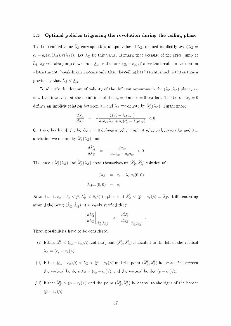
5.3 Optimal policies triggering the revolution during the ceiling phase

To the terminal value λA corresponds a unique value of λZ , de�ned implicitly by: ζλZ =

cs − ac(xc(λA), r(λA)). Let λZ be this value. Remark that because of the price jump at

tA, λZ will also jump down from λZ to the level (cs− cx)/ζ after the break. In a situation

where the cost breakthrough occurs only after the ceiling has been attained, we have shown

previously that λA < λA.

To identify the domain of validity of the di�erent scenarios in the (λZ , λA) plane, we

now take into account the de�nitions of the xc = 0 and r = 0 borders. The border xc = 0

de�nes an implicit relation between λZ and λA we denote by λxA(λZ). Furthermore:

dλxAdλZ

= − ζ(c′r − λAarr)aracrλA + ac(c′r − λAarr)

< 0

On the other hand, the border r = 0 de�nes another implicit relation between λZ and λA,

a relation we denote by λrA(λZ) and:

dλrAdλZ

= − ζacraracc − acacr

< 0

The curves λxA(λZ) and λrA(λZ) cross themselves at (λ0Z , λ

0A) solution of:

ζλZ = cs − λAac(0, 0)

λAar(0, 0) = c0r

Note that is cx + cs < p, λ0Z < cs/ζ implies that λ0

Z < (p − cx)/ζ ≡ λZ . Di�erentiating

around the point (λ0Z , λ

0A), it is easily veri�ed that:∣∣∣∣∣dλxAdλZ

∣∣∣∣∣(λ0Z ,λ

0A)

>

∣∣∣∣∣dλrAdλZ

∣∣∣∣∣(λ0Z ,λ

0A)

.

Three possibilities have to be considered:

(i) Either λ0Z < (cs − cx)/ζ and the point (λ0

Z , λ0A) is located to the left of the vertical

λZ = (cs − cx)/ζ.

(ii) Either (cs − cx)/ζ < λZ < (p − cx)/ζ and the point (λ0Z , λ

0A) is located in between

the vertical borders λZ = (cs − cx)/ζ and the vertical border (p− cx)/ζ.

(iii) Either λ0Z > (p − cx)/ζ and the point (λ0

Z , λ0A) is located to the right of the border

(p− cx)/ζ.

47

Note that the implicit energy price is at most equal to p in any optimal scenario. This

means that λZ(t) < (p − cx)/ζ ≡ λZ . The vertical λZ = λZ de�nes the upper border of

possible value of λZ in all optimal scenario. The Figure 4 illustrates the three possible

cases.

Figure 4: Activity Constraints in the (λZ , λA) Plane

Optimal combined policies

Let us �rst consider the combined policies. The condition xd = xd(λZ , λA) de�nes an

implicit relation between λZ and λA we denote by λcA(λZ). Taking (5.7), (5.8) into account,

it is immediately veri�ed that: dλcA(λZ)/dλZ < 0. In the case tZ < tA, λZ ∈ [λZ , λZ ]

de�nes the relevant domain of possible values of λZ . On one hand, λcA(λZ) = λA in a

combined scenario and on the other hand we denote by λcA ≡ λcA(λZ).

To a combined policy corresponds a {λZ(t), λA(t)} trajectory initiating below the curve

λcA(λZ) at some point (λZ0, λA0). Before tZ , the trajectory is de�ned by (λZ0e(ρ+α)t,

λA0eρt). hence {λZ(t), λA(t)} moves in the north east direction in the dual plane. At

tZ , the trajectory hits the border λcA(λZ). Then it follows this curve until tA is reached,

that is at the point λZ(tA) = λZ , λA(tA) = λA. The following Figure 5 illustrates this

construction.

The combined scenario is optimal from any point (λZ0, λA0) located above the border

max(λxA(λZ), λrA(λZ)), that is the region where both xc > 0 and r > 0.

48

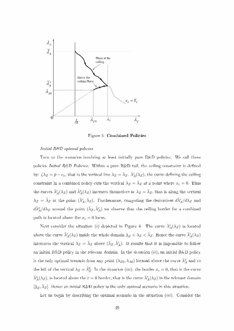
Figure 5: Combined Policies

Initial R&D optimal policies

Turn to the scenarios involving at least initially pure R&D policies. We call these

policies Initial R&D Policies. Within a pure R&D tail, the ceiling constraint is de�ned

by: ζλZ = p− cx, that is the vertical line λZ = λZ . λcA(λZ), the curve de�ning the ceiling

constraint in a combined policy cuts the vertical λZ = λZ at a point where xc = 0. Thus

the curves λcA(λZ) and λxA(λZ) intersect themselves at λZ = λZ , that is along the vertical

λZ = λZ at the point (λcA, λZ). Furthermore, computing the derivatives dλcA/dλZ and

dλxA/dλZ around the point (λZ , λcA) we observe that the ceiling border for a combined

path is located above the xc = 0 locus.

Next consider the situation (i) depicted in Figure 4. The curve λrA(λZ) is located

above the curve λcA(λZ) inside the whole domain λZ < λZ < λZ . Hence the curve λrA(λZ)

intersects the vertical λZ = λZ above (λZ , λcA). It results that it is impossible to follow

an initial R&D policy in the relevant domain. In the situation (ii), an initial R&D policy

is the only optimal scenario from any point (λZ0, λA0) located above the curve λxA and to

the left of the vertical λZ = λ0Z . In the situation (iii), the border xc = 0, that is the curve

λxA(λZ), is located above the r = 0 border, that is the curve λrA(λZ) in the relevant domain

[λZ , λZ ]. Hence an initial R&D policy is the only optimal scenario in this situation.

Let us begin by describing the optimal scenario in the situation (iii). Consider the

49

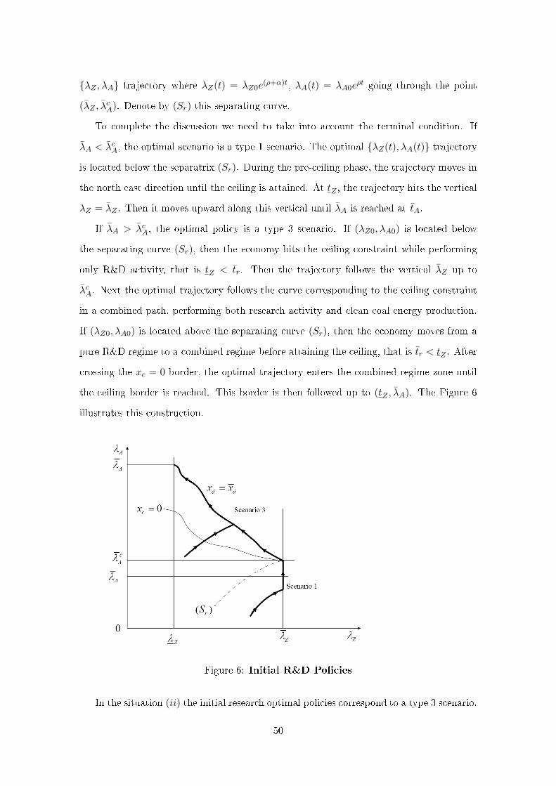
{λZ , λA} trajectory where λZ(t) = λZ0e(ρ+α)t, λA(t) = λA0e

ρt going through the point

(λZ , λcA). Denote by (Sr) this separating curve.

To complete the discussion we need to take into account the terminal condition. If

λA < λcA, the optimal scenario is a type 1 scenario. The optimal {λZ(t), λA(t)} trajectory

is located below the separatrix (Sr). During the pre-ceiling phase, the trajectory moves in

the north east direction until the ceiling is attained. At tZ , the trajectory hits the vertical

λZ = λZ . Then it moves upward along this vertical until λA is reached at tA.

If λA > λcA, the optimal policy is a type 3 scenario. If (λZ0, λA0) is located below

the separating curve (Sr), then the economy hits the ceiling constraint while performing

only R&D activity, that is tZ < tr. Then the trajectory follows the vertical λZ up to

λcA. Next the optimal trajectory follows the curve corresponding to the ceiling constraint

in a combined path, performing both research activity and clean coal energy production.

If (λZ0, λA0) is located above the separating curve (Sr), then the economy moves from a

pure R&D regime to a combined regime before attaining the ceiling, that is tr < tZ . After

crossing the xc = 0 border, the optimal trajectory enters the combined regime zone until

the ceiling border is reached. This border is then followed up to (tZ , λA). The Figure 6

illustrates this construction.

Figure 6: Initial R&D Policies

In the situation (ii) the initial research optimal policies correspond to a type 3 scenario.

50

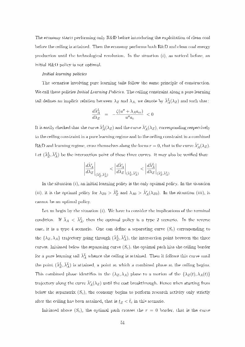
The economy starts performing only R&D before introducing the exploitation of clean coal

before the ceiling is attained. Then the economy performs both R&D and clean coal energy

production until the technological revolution. In the situation (i), as noticed before, an

initial R&D policy is not optimal.

Initial learning policies

The scenarios involving pure learning tails follow the same principle of construction.

We call these policies Initial Learning Policies. The ceiling constraint along a pure learning

tail de�nes an implicit relation between λZ and λA, we denote by λLA(λZ) and such that:

dλLAdλZ

= −ζ(u′′ + λAacc)

u′′ac< 0

It is easily checked that the curve λLA(λZ) and the curve λcA(λZ), corresponding respectively

to the ceiling constraint in a pure learning regime and to the ceiling constraint in a combined

R&D and learning regime, cross themselves along the locus r = 0, that is the curve λrA(λZ).

Let (λLZ , λLA) be the intersection point of these three curves. It may also be veri�ed that:∣∣∣∣∣dλrAdλZ

∣∣∣∣∣(λLZ ,λ

LA)

<

∣∣∣∣dλcAdλZ

∣∣∣∣(λLZ ,λ

LA)

<

∣∣∣∣dλLAdλZ

∣∣∣∣(λLZ ,λ

LA)

In the situation (i), an initial learning policy is the only optimal policy. In the situation

(ii), it is the optimal policy for λZ0 > λ0Z and λA0 > λrA(λZ0). In the situation (iii), it

cannot be an optimal policy.

Let us begin by the situation (i). We have to consider the implications of the terminal

condition. If λA < λLA, then the optimal policy is a type 2 scenario. In the reverse

case, it is a type 4 scenario. One can de�ne a separating curve (Sc) corresponding to

the {λZ , λA} trajectory going through (λLZ , λLA), the intersection point between the three

curves. Initiated below the separating curve (Sc), the optimal path hits the ceiling border

for a pure learning tail λLA whence the ceiling is attained. Then it follows this curve until

the point (λLZ , λLA) is attained, a point at which a combined phase at the ceiling begins.

This combined phase identi�es in the (λZ , λA) plane to a motion of the {λZ(t), λA(t)}

trajectory along the curve λcA(λZ) until the cost breakthrough. Hence when starting from

below the separatrix (Sc), the economy begins to perform research activity only strictly

after the ceiling has been attained, that is tZ < tc in this scenario.

Initiated above (Sc), the optimal path crosses the r = 0 border, that is the curve

51

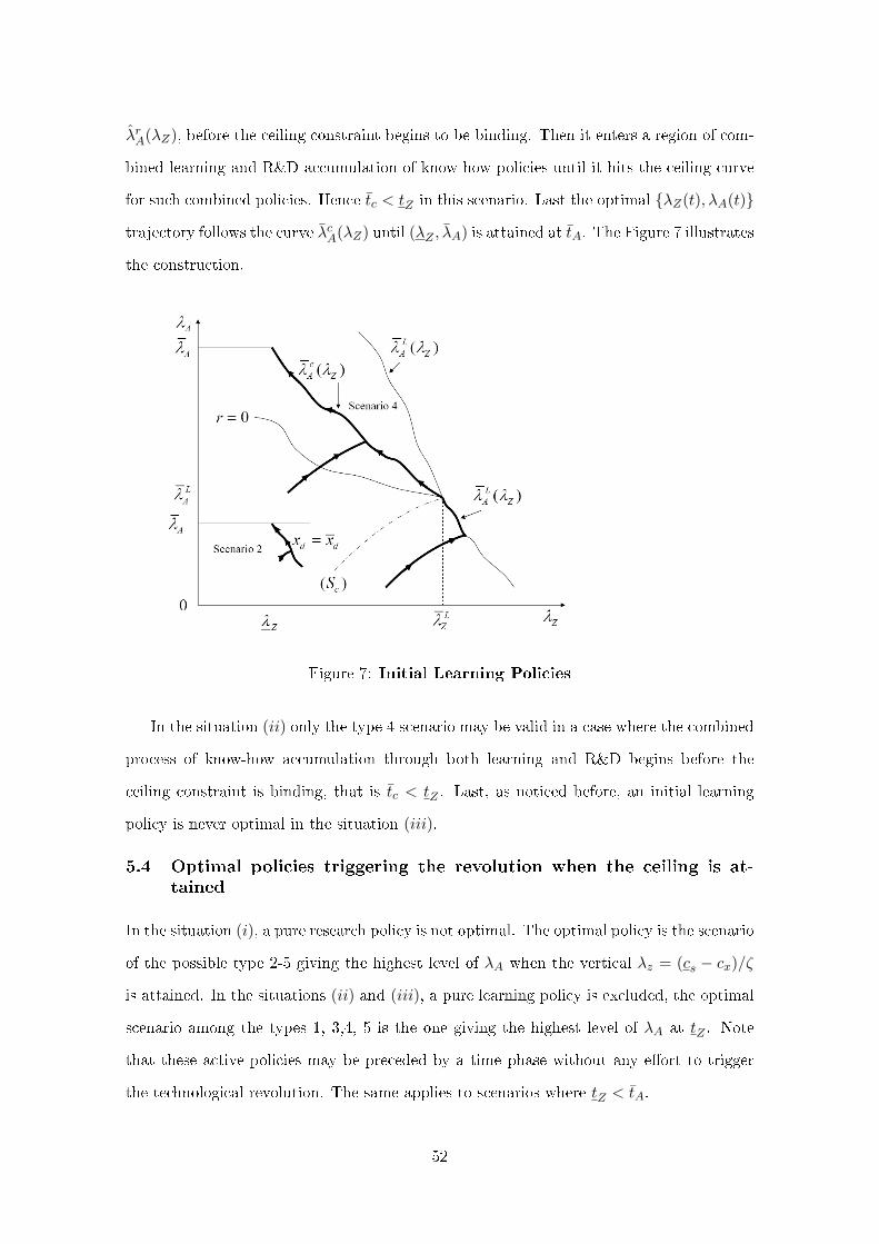
λrA(λZ), before the ceiling constraint begins to be binding. Then it enters a region of com-

bined learning and R&D accumulation of know-how policies until it hits the ceiling curve

for such combined policies. Hence tc < tZ in this scenario. Last the optimal {λZ(t), λA(t)}

trajectory follows the curve λcA(λZ) until (λZ , λA) is attained at tA. The Figure 7 illustrates

the construction.

Figure 7: Initial Learning Policies

In the situation (ii) only the type 4 scenario may be valid in a case where the combined

process of know-how accumulation through both learning and R&D begins before the

ceiling constraint is binding, that is tc < tZ . Last, as noticed before, an initial learning

policy is never optimal in the situation (iii).

5.4 Optimal policies triggering the revolution when the ceiling is at-

tained

In the situation (i), a pure research policy is not optimal. The optimal policy is the scenario

of the possible type 2-5 giving the highest level of λA when the vertical λz = (cs − cx)/ζ

is attained. In the situations (ii) and (iii), a pure learning policy is excluded, the optimal

scenario among the types 1, 3,4, 5 is the one giving the highest level of λA at tZ . Note

that these active policies may be preceded by a time phase without any e�ort to trigger

the technological revolution. The same applies to scenarios where tZ < tA.

52

6 Conclusion

Since Goulder, Matthai (2000), it is frequently advanced in the economic literature that

carbon pricing policies should not be too stringent in order for R&D to have su�cient

time to select and develop better abatement technological options. The present analysis

invites to reconsider seriously such statements. Instead of an incremental process of tech-

nical improvement, we have modeled technical change as a drastic process able to trigger

a technological revolution in the form of an abrupt cost break in pollution abatement,

provided that a su�ciently high level of know-how has been previously accumulated. This

framework allows for a much clearer view of the e�ects of an environmental policy upon

the trend of e�orts to trigger a technological improvement in abatement technologies. The

Goulder-Matthai analysis proceeded by contrasting situations where technical progress re-

sulted from learning-by-doing in pollution abatement techniques from situations where

technical advances could be obtained only through dedicated R&D e�orts. We have �rst

followed this approach by studying the polar cases of a pure learning induced technological

revolution and a pure R&D induced breakthrough.

When the revolution is triggered by learning-by-doing, the optimal policy implemen-

tation requires to combine a price upon carbon emissions and a subsidy to clean energy

generation. This subsidy must grow over time during the learning period preceding the

technological revolution, inducing a permanent rise of the use of clean energy. The optimal

carbon tax should increase before the beginning of the learning process and decrease after-

wards. We show also that a stricter environmental standard, here modeled in terms of a

critical atmospheric carbon concentration not to be crossed over, has the e�ect of increas-

ing the use of abatement technologies before the technical breakthrough, resulting in an

earlier revolution. However, this does not mean that the optimal carbon tax corresponding

to a stricter atmospheric concentration mandate needs to be increased. A stricter mandate

has an ambiguous e�ect over the carbon tax level before the beginning of the clean energy

generation phase and reduces this level during the learning phase.

In a R&D induced technological revolution framework, the optimal policy implemen-

tation no more requires speci�c subsidies, an optimal carbon price being a su�cient tool

to induce the optimal level of R&D e�orts. Under the reasonable assumption of increasing

53

and convex costs of research, discounting favors delaying the R&D e�orts, resulting in an

increasing time pattern for such e�orts until the technological breakthrough occurs. In all

cases, it is not optimal to trigger the revolution strictly before the atmospheric concentra-

tion constraint begins to be binding. The optimal carbon tax should rise until the carbon

concentration ceiling has been attained and then should be maintained at a constant level

before jumping down at the technological revolution time. As for the learning induced

technical revolution, a stricter environmental standard spurs more R&D e�orts from the

carbon abatement industry and reduces the time delay before the cost breakthrough. This

is reminiscent of the Porter hypothesis.

However the initial cost level of the abatement technology has ambiguous e�ects upon

the intensity of R&D e�orts. This was not the case in the learning induced technical

break. A higher initial pollution abatement cost reduces the use of clean energy before the

revolution, slowing down the learning process and delaying the breakthrough. In a R&D

induced technical break context, a higher initial pollution abatement cost widens the cost

gap that can be achieved thanks to R&D, an incentive to increase R&D e�orts. On the

other hand, it also increases the cost of using clean energy before the break, an incentive

to reduce the research e�orts, in order to diminish the total costs of the energy policy.

A main drawback of the Goulder-Matthai analysis is that the pure R&D and the

pure learning-by-doing technical change models are not really comparable. These extreme

cases describe situations where the economy is constrained to rely upon only one of these

devices to achieve a technological improvement of the pollution abatement technologies. A

correct account of the e�ects of an environmental policy upon induced technical progress in

abatement technologies requires a framework where both R&D and learning can contribute

to technology advances. We thus turn to the study of such a combined process. We

show that the R&D e�orts should permanently increase before the technical revolution.

This is a straightforward consequence of discounting and our increasing marginal cost of

research assumption. The use of clean energy should also increase over time, meaning an

accelerating learning process.

Even under the assumption of constant average and marginal costs of producing clean

energy, it may now be the case that clean coal production starts before the atmospheric

carbon concentration constraint begins to bind. But this has no qualitative consequences

54

over the optimal time pro�le of the carbon price. The carbon price must increase before the

atmospheric ceiling constraint is attained and decrease afterwards until the technological

revolution occurs. As in the pure learning case, the carbon price tool has to be completed

by a subsidy to the consumption of clean energy. The subsidy level rises all along the

pre-revolution phase of clean energy production.

Concerning the priority that may be given to research with respect to learning in

generating technical advances, we show that the growth rate of use of clean energy should

be higher than the growth rate of research e�orts. In a drastic technical progress framework,

research activity bears only costs before the revolution, the prize in terms of cost cut being

ripped only at the end of the research process. This is not the case for learning, since the use

of the abatement technology, even at the high pre-revolution cost level, allows to generate

some positive surplus. The consequence is that the economy gives more an more weight to

learning with respect to R&D in achieving the technological breakthrough, independently

of the respective marginal contributions of learning and research to the accumulation of

know-how.

Technical progress paths combining research and learning are not the only optimal ones.

We show also that an optimal policy may involve an initial period of only R&D activity

before launching the use of the pollution abatement technology or an initial period based

only upon learning, research being too costly to be justi�ed until the time before the

revolution be su�ciently short.

This work may be extended in several directions. The �rst one is to take explicitly

into account the scarcity of fossil fuels. We assume an in�nite supply of such resources, an

assumption frequently made in the relevant literature. However fuel scarcity should result

in Hotelling e�ects, a�ecting both the timing of the environmental policy and the timing of

the technological investment policy before the breakthrough. The drastic technical progress

framework is useful to obtain clear cut results concerning the relationships between an en-

vironmental policy and a technical development policy. It appears interesting to compare

its conclusions with the results derived from incremental technical progress models. This

should allow to shed some light on the various puzzles which have been identi�ed in this

literature. We focus primarily upon technical progress in pollution abatement technolo-

gies, but the analysis could be extended to technological competition between abatement

55

techniques and clean energy generation process, like solar energy production for example.

56

References

Amigues J. P. La�orgue G. and M. Moreaux, (2012), Triggering the technological revolution

in carbon capture and sequestration costs. II/ The polluting resource is scarce, work in

progress.

Barret S., (2006), Climate Treaties and "Breakthrough" Technologies, The American

Economic Review, Vol. 96, No. 2 (May, 2006), pp. 22-25

Chakravorty, U, Magne, B. and M. Moreaux, (2006) A Hotelling model with a ceiling on

the stock of pollution, Journal of Economic Dynamics and Control, Vol 30(12), 2875-2904.

Chakravorty U, Moreaux M. and M. Tidball, (2008), Ordering the extraction of pol-

luting nonrenewable resources, American Economic Review, Vol 98(3), 1128-1144.

Chakravorty U, Leach A. and M. Moreaux,(2012), Cycles in nonrenewable resource

prices with pollution and learning-by-doing, Journal of Economic Dynamics & Control,

http://dx.doi.org/10.1016/j.jedc.2012.04.005

Ja�e, A., Newell R. G. and R. N. Stavins, (2001), Technological change and the envi-

ronment, RFF Disc Paper 00-47REV, Resources for the Future, Washington D. C.

Gerlargh R., Kverndokk S. and K. E. Rosendhal, (2009), Optimal timing of climate

change policy: interaction between carbon tax and innovation externalities, Environmental

and Resources Economics, 43, 369-390.

Goulder L.H., K. Mathai (2000), "Optimal CO2 Abatement in the Presence of Induced

Technical Change", Journal of Environmental Economics and Management 39, p. 1-38.

Henriet F., (2012), Optimal extraction of a polluting non renewable resource with R&D

toward a clean backstop technology, Journal of Public Economic Theory, 14 (2), 311-347.

Kverndokk S. and K. E. Rosendhal, (2007), Climate policies and learning by doing:

impacts and timing of technological subsidies, Resources and Energy Economics, 29, 58-

82.

Wigley T.M.L., Richels R., Edmonds J.A. (1996), "Economic and environmental choices

in the stabilization of atmospheric CO2 concentrations". Nature, 18, January.

Zwaan B.C.C. van der, R. Gerlagh, G. Klaassen and L. Schrattenholzer (2002), En-

dogenous technological change in climate change modeling, Energy Economics, 24, p. 1-19.

57

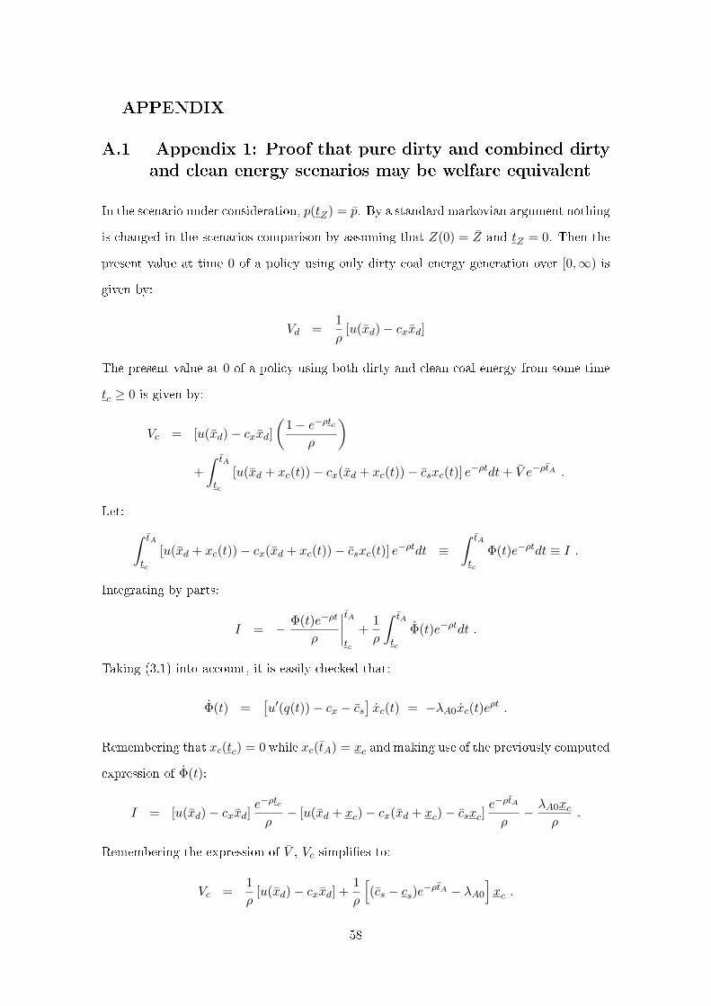
APPENDIX

A.1 Appendix 1: Proof that pure dirty and combined dirty

and clean energy scenarios may be welfare equivalent

In the scenario under consideration, p(tZ) = p. By a standard markovian argument nothing

is changed in the scenarios comparison by assuming that Z(0) = Z and tZ = 0. Then the

present value at time 0 of a policy using only dirty coal energy generation over [0,∞) is

given by:

Vd =1

ρ[u(xd)− cxxd]

The present value at 0 of a policy using both dirty and clean coal energy from some time

tc ≥ 0 is given by:

Vc = [u(xd)− cxxd](

1− e−ρtcρ

)+

∫ tA

tc

[u(xd + xc(t))− cx(xd + xc(t))− csxc(t)] e−ρtdt+ V e−ρtA .

Let: ∫ tA

tc

[u(xd + xc(t))− cx(xd + xc(t))− csxc(t)] e−ρtdt ≡∫ tA

tc

Φ(t)e−ρtdt ≡ I .

Integrating by parts:

I = − Φ(t)e−ρt

ρ

∣∣∣∣tAtc

+1

ρ

∫ tA

tc

Φ(t)e−ρtdt .

Taking (3.1) into account, it is easily checked that:

Φ(t) =[u′(q(t))− cx − cs

]xc(t) = −λA0xc(t)e

ρt .

Remembering that xc(tc) = 0 while xc(tA) = xc and making use of the previously computed

expression of Φ(t):

I = [u(xd)− cxxd]e−ρtc

ρ− [u(xd + xc)− cx(xd + xc)− csxc]

e−ρtA

ρ− λA0xc

ρ.

Remembering the expression of V , Vc simpli�es to:

Vc =1

ρ[u(xd)− cxxd] +

1

ρ

[(cs − cs)e−ρtA − λA0

]xc .

58

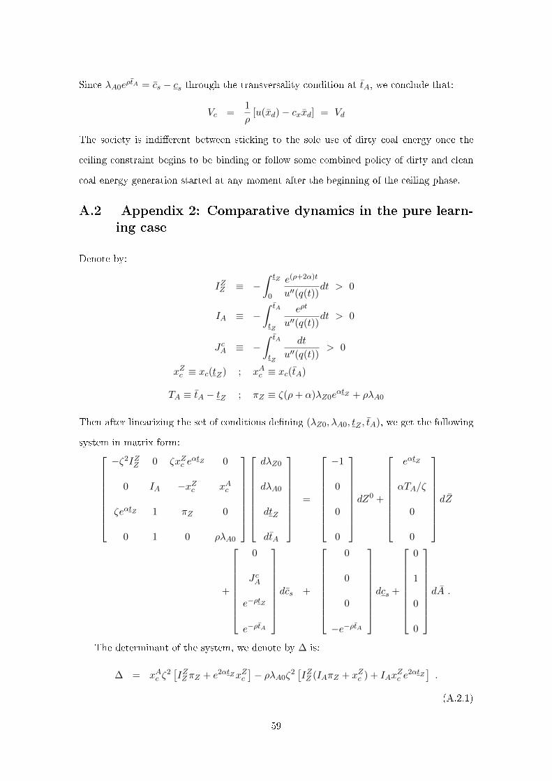
Since λA0eρtA = cs − cs through the transversality condition at tA, we conclude that:

Vc =1

ρ[u(xd)− cxxd] = Vd

The society is indi�erent between sticking to the sole use of dirty coal energy once the

ceiling constraint begins to be binding or follow some combined policy of dirty and clean

coal energy generation started at any moment after the beginning of the ceiling phase.

A.2 Appendix 2: Comparative dynamics in the pure learn-

ing case

Denote by:

IZZ ≡ −∫ tZ

0

e(ρ+2α)t

u′′(q(t))dt > 0

IA ≡ −∫ tA

tZ

eρt

u′′(q(t))dt > 0

JcA ≡ −∫ tA

tZ

dt

u′′(q(t))> 0

xZc ≡ xc(tZ) ; xAc ≡ xc(tA)

TA ≡ tA − tZ ; πZ ≡ ζ(ρ+ α)λZ0eαtZ + ρλA0

Then after linearizing the set of conditions de�ning (λZ0, λA0, tZ , tA), we get the following

system in matrix form:

−ζ2IZZ 0 ζxZc eαtZ 0

0 IA −xZc xAc

ζeαtZ 1 πZ 0

0 1 0 ρλA0

dλZ0

dλA0

dtZ

dtA

=

−1

0

0

0

dZ0 +

eαtZ

αTA/ζ

0

0

dZ

+

0

JcA

e−ρtZ

e−ρtA

dcs +

0

0

0

−e−ρtA

dcs +

0

1

0

0

dA .

The determinant of the system, we denote by ∆ is:

∆ = xAc ζ2[IZZ πZ + e2αtZxZc

]− ρλA0ζ

2[IZZ (IAπZ + xZc ) + IAx

Zc e

2αtZ].

(A.2.1)

59

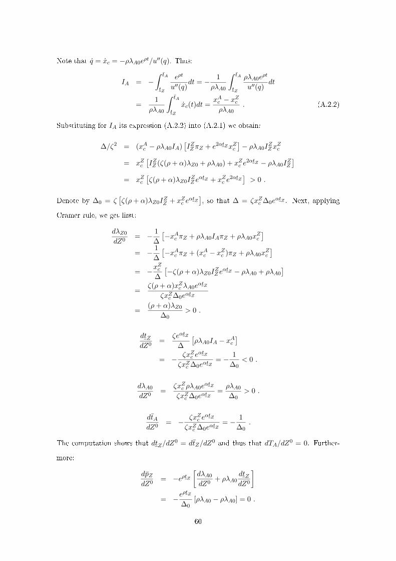
Note that q = xc = −ρλA0eρt/u′′(q). Thus:

IA = −∫ tA

tZ

eρt

u′′(q)dt = − 1

ρλA0

∫ tA

tZ

ρλA0eρt

u′′(q)dt

=1

ρλA0

∫ tA

tZ

xc(t)dt =xAc − xZcρλA0

. (A.2.2)

Substituting for IA its expression (A.2.2) into (A.2.1) we obtain:

∆/ζ2 = (xAc − ρλA0IA)[IZZ πZ + e2αtZxZc

]− ρλA0I

ZZ x

Zc

= xZc[IZZ (ζ(ρ+ α)λZ0 + ρλA0) + xZc e

2αtZ − ρλA0IZZ

]= xZc

[ζ(ρ+ α)λZ0I

ZZ e

αtZ + xZc e2αtZ

]> 0 .

Denote by ∆0 = ζ[ζ(ρ+ α)λZ0I

ZZ + xZc e

αtZ], so that ∆ = ζxZc ∆0e

αtZ . Next, applying

Cramer rule, we get �rst:

dλZ0

dZ0= − 1

∆

[−xAc πZ + ρλA0IAπZ + ρλA0x

Zc

]= − 1

∆

[−xAc πZ + (xAc − xZc )πZ + ρλA0x

Zc

]= −x

Zc

∆

[−ζ(ρ+ α)λZ0I

ZZ e

αtZ − ρλA0 + ρλA0

]=

ζ(ρ+ α)xZc λA0eαtZ

ζxZc ∆0eαtZ

=(ρ+ α)λZ0

∆0> 0 .

dtZdZ0

=ζeαtZ

∆

[ρλA0IA − xAc

]= − ζxZc e

αtZ

ζxZc ∆0eαtZ= − 1

∆0< 0 .

dλA0

dZ0=

ζxZc ρλA0eαtZ

ζxZc ∆0eαtZ=ρλA0

∆0> 0 .

dtAdZ0

= − ζxZc eαtZ

ζxZc ∆0eαtZ= − 1

∆0.

The computation shows that dtZ/dZ0 = dtZ/dZ

0 and thus that dTA/dZ0 = 0. Further-

more:

dpZdZ0

= −eρtZ[dλA0

dZ0+ ρλA0

dtZdZ0

]= −e

ρtZ

∆0[ρλA0 − ρλA0] = 0 .

60

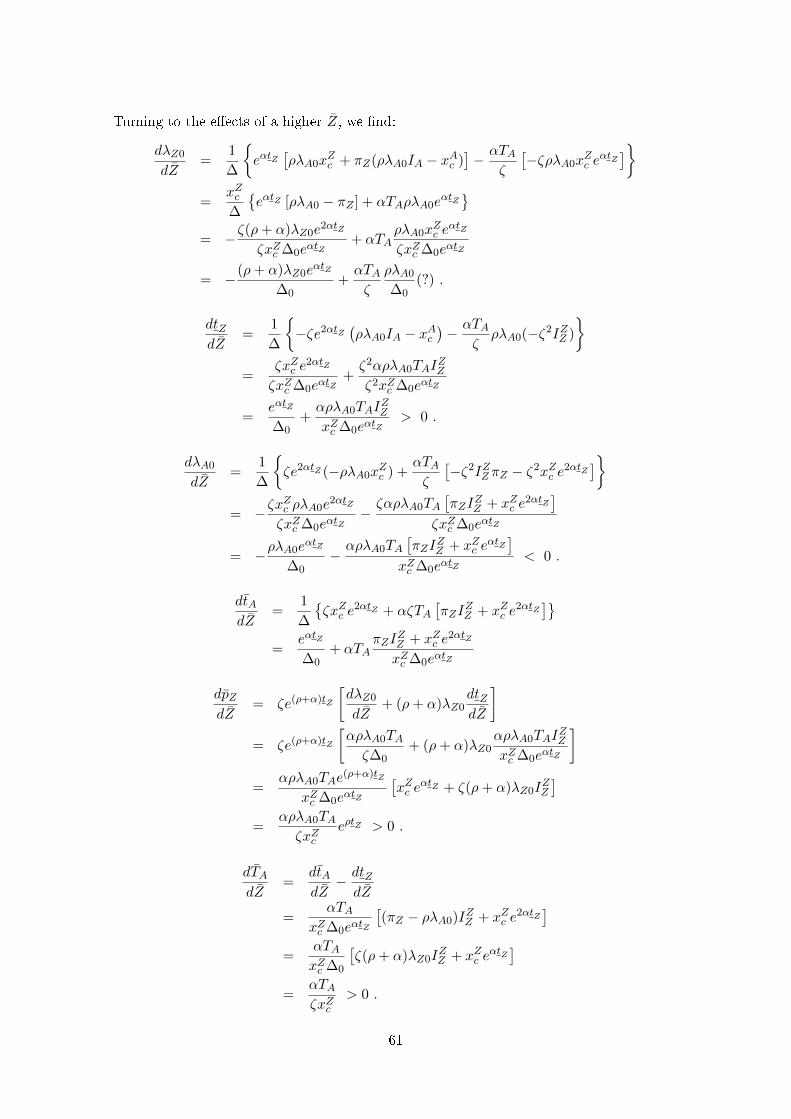
Turning to the e�ects of a higher Z, we �nd:

dλZ0

dZ=

1

∆

{eαtZ

[ρλA0x

Zc + πZ(ρλA0IA − xAc )

]− αTA

ζ

[−ζρλA0x

Zc e

αtZ]}

=xZc∆

{eαtZ [ρλA0 − πZ ] + αTAρλA0e

αtZ}

= −ζ(ρ+ α)λZ0e2αtZ

ζxZc ∆0eαtZ+ αTA

ρλA0xZc e

αtZ

ζxZc ∆0eαtZ

= −(ρ+ α)λZ0eαtZ

∆0+αTAζ

ρλA0

∆0(?) .

dtZdZ

=1

∆

{−ζe2αtZ

(ρλA0IA − xAc

)− αTA

ζρλA0(−ζ2IZZ )

}=

ζxZc e2αtZ

ζxZc ∆0eαtZ+ζ2αρλA0TAI

ZZ

ζ2xZc ∆0eαtZ

=eαtZ

∆0+αρλA0TAI

ZZ

xZc ∆0eαtZ> 0 .

dλA0

dZ=

1

∆

{ζe2αtZ (−ρλA0x

Zc ) +

αTAζ

[−ζ2IZZ πZ − ζ2xZc e

2αtZ]}

= −ζxZc ρλA0e

2αtZ

ζxZc ∆0eαtZ−ζαρλA0TA

[πZI

ZZ + xZc e

2αtZ]

ζxZc ∆0eαtZ

= −ρλA0eαtZ

∆0−αρλA0TA

[πZI

ZZ + xZc e

αtZ]

xZc ∆0eαtZ< 0 .

dtAdZ

=1

∆

{ζxZc e

2αtZ + αζTA[πZI

ZZ + xZc e

2αtZ]}

=eαtZ

∆0+ αTA

πZIZZ + xZc e

2αtZ

xZc ∆0eαtZ

dpZdZ

= ζe(ρ+α)tZ

[dλZ0

dZ+ (ρ+ α)λZ0

dtZdZ

]= ζe(ρ+α)tZ

[αρλA0TAζ∆0

+ (ρ+ α)λZ0αρλA0TAI

ZZ

xZc ∆0eαtZ

]=

αρλA0TAe(ρ+α)tZ

xZc ∆0eαtZ

[xZc e

αtZ + ζ(ρ+ α)λZ0IZZ

]=

αρλA0TAζxZc

eρtZ > 0 .

dTAdZ

=dtAdZ− dtZdZ

=αTA

xZc ∆0eαtZ

[(πZ − ρλA0)IZZ + xZc e

2αtZ]

=αTAxZc ∆0

[ζ(ρ+ α)λZ0I

ZZ + xZc e

αtZ]

=αTAζxZc

> 0 .

61

Next turning to the e�ects of a higher initial clean coal energy cost, we obtain:

dλZ0

dcs=

ζxZc eαtZ

∆

[xAc (e−ρtZ − e−ρtA) + ρλA0(JcA − IAe−ρtZ )

]=

1

∆0

[(xAc − ρλA0IA)e−ρtZ − xAc e−ρtA + ρλA0J

cA

]=

1

∆0

[xZc e

−ρtZ − xAc e−ρtA + ρλA0JcA

](A.2.3)

This expression is of indeterminate sign. However taking into account the expression of

xc:

ρλA0JcA = −

∫ tA

tZ

ρλA0eρt

u′′(q(t))e−ρtdt =

∫ tA

tZ

xc(t)e−ρtdt

Integrating by parts:

ρλA0JcA = xc(t)e

−ρt∣∣tAtZ

+ ρ

∫ tA

tZ

xc(t)e−ρtdt

= xAc e−ρtA − xZc e−ρtZ + ρ

∫ tA

tZ

xc(t)e−ρtdt . (A.2.4)

Inserting the expression (A.2.4) of ρλA0JcA into (A.2.3), we obtain:

dλZ0

dcs=

ρ

∆0

∫ tA

tZ

xc(t)e−ρtdt ≡ ρIc

∆0> 0

The e�ect of a higher cs over λA0 is indeterminate. Next turning upon the impact over tZ

and tA, we obtain:

dtZdcs

= −ζ2IZZ

∆

{xAc (e−ρtA − e−ρtZ ) + ρλA0(IAe

−ρtZ − JcA)}

= −ζ2IZZ

∆

{xAc e

−ρtA + (ρλA0IA − xAc )e−ρtZ − ρλA0JcA

}= −

ζ2IZZ∆

{xAc e

−ρtA − xZc e−ρtZ −[xAc e

−ρtA − xZc e−ρtZ + ρIc

]}=

ζ2ρIZZ Ic∆

> 0

Then:

dtAdcs

=1

∆

{−ζ2IZZ

[xZc (e−ρtA − e−ρtZ ) + πZ(IAe

−ρtA − JcA)]

−ζ2xZc e2αtZ

[IAe−ρtA − JcA

]}=

1

∆

{−ζ2IZZ x

Zc (e−ρtA − e−ρtZ )− (IAe

−ρtA − JcA)ζ2[πZI

ZZ + xZc e

2αtZ]}

=ζ2

∆

{IZZ x

Zc (e−ρtZ − e−ρtA) + (JcA − IAe−ρtA)

[πZI

ZZ + xZc e

2αtZ]}

.

62

Since:

JcA − IAe−ρtA = −∫ tA

tZ

1

u′′(q(t))

[1− e−ρ(tA−t)

]dt > 0 ,

while tZ < tA implies that e−ρtZ − e−ρtA > 0, we conclude that dtA/dcs > 0.

This gives the following e�ects over pZ and TA:

dpZdcs

= ζe(ρ+α)tZ

[ρIc∆0

+ (ρ+ α)λZ0ρζ2IcI

ZZ

∆

]=

ζ2ρIce(ρ+α)tZ

∆

[xZc e

αtZ + ζ(ρ+ α)λZ0IZZ

]=

ζρIce(ρ+α)tZ∆0

ζxZc ∆0eαtZ

=ρIcxZc

eρtZ > 0 .

dTAdcs

=ζ2

∆

{IZZ x

Zc (e−ρtZ − e−ρtA) + (JcA − e−ρtAIA)(πZI

ZZ + xZc e

2αtZ )− ρIcIZZ}.

Since ρIc = ρλA0JAc − xAc e−ρtA + xZc e

−ρtZ , the expression into brackets is equivalent to:

{} = IZZ

[xZc (e−ρtZ − e−ρtA) + πZ(JcA − e−ρtAIA)− ρλA0J

cA + xAc e

−ρtA − xZc e−ρtZ]

+xZc (JcA − IAe−ρtA)e2αtZ

= IZZ

[(xAc − xZc )e−ρtA + JcA(πZ − ρλA0)− πZIAe−ρtA

]+ xZc (JcA − IAe−ρtA)

= IZZ

[(xAc − xZc )e−ρtA + ζ(ρ+ α)λZ0e

αtZ (JcA − IAe−ρtA)− ρλA0IAe−ρtA

]+ xZc (JcA − IAe−ρtA) .

Since ρλA0IA = xAc − xZc , we obtain after simpli�cation:

dTAdcs

=ζ2eαtZ

δ

[ζ(ρ+ α)λZ0I

ZZ + xZc e

αtZ]

(JcA − IAe−ρtA)

=ζeαtZ∆0(JcA − IAe−ρtA)

ζxZc ∆0eαtZ

=JcA − IAe−ρtAIA

xZc> 0 .

The e�ects of a higher cs are the following.

dλZ0

dcs=

ζxZc eαtZxAc e

−ρtA

ζxZc ∆0eαtZ=xAc∆0

e−ρtA > 0 .

dλA0

dcs= −

ζ(πZIZZ + xZc e

2αtZ )xAc e−ρtA

xZc ∆0eαtZ< 0 .

63

dtZdcs

=ζ2IZZ x

Ac e−ρtA

∆=

ζxAc IZZ

xZc ∆0eαtZe−ρtA > 0 .

dtAdcs

=ζ2e−ρtA

∆

[IA(πZI

ZZ + xZc e

2αtZ ) + IZZ xZc

]> 0 .

dpZdcs

= ζe(ρ+α)tZ

[dλZ0

dcs+ (ρ+ α)λZ0

dtZdcs

]> 0 .

dTAdcs

=ζ2e−ρtA

δ

[IA(πZI

ZZ + xZc e

2αtZ ) + IZZ xZc − xAc IZZ

]=

ζ2e−ρtA

δ

[IZZ (πZIA + xZc − xAc ) + xZc IAe

2αtZ]

=ζ2e−ρtA

δ

[IZZ (ζ(ρ+ α)λZ0IAe

αtZ + ρλA0IA + xZc − xAc ) + xZc IAe2αtZ

]=

ζ2IAe−ρtAeαtZ

δ

[ζ(ρ+ α)λZ0I

ZZ + xZc e

αtZ]

=ζIAe

αtZe−ρtA∆0

xZc ∆0eαtZ=IAxZc

e−ρtA > 0 .

Last, the e�ects of a higher know-how target A are:

dλZ0

dA=

ζxZc eαtZ

∆ρλA0 =

ρλA0

∆0> 0 .

dλA0

dA= −ζρλA0

∆

[πZI

ZZ + xZc e

2cαtZ]< 0 .

dtZdA

=ζ2ρλA0I

ZZ

∆> 0 .

dtAdA

=ζ2

∆

[πZI

ZZ + xZc e

2αtZ]> 0 .

dpZdA

= ζe(ρ+α)tZ

[dλZ0

dA+ (ρ+ α)λZ0

dtZdA

]=

ζρλA0e(ρ+α)tZ

∆0

[1 +

ζ(ρ+ α)λZ0IZZ

xZc eαtZ

]=

ζρλA0e(ρ+α)tZ

xZc ∆0eαtZ∆0

=ρλA0

xZceρtZ > 0 .

dTAdbarA

=ζ2

∆

[IZZ (πZ − ρλA0) + xZc e

2αtZ]

=ζ2

∆

[ζ(ρ+ α)λZ0I

ZZ e

αtZ + xZc e2cαtZ

]=

ζδ0eαtZ

ζxZc ∆0eαtZ=

1

xZc> 0 .

64

A.3 Appendix 3: Comparative dynamics in the pure R&D

model

The relative independency of the R&D policy with respect to the energy policy results

in a pair of two dimensional linearized systems, the �rst one describing the e�ects over

(λZ0, tZ) while the second one describes the e�ects over (λA0, tA). Denote by:

IZZ ≡∫ tZ

0

e(ρ+2α)t

u′′(q(t))dt > 0 ; IA ≡

∫ tA

0

eρt

c′r(r(t))dt > 0

r = r(tA) ; r(0) = r0

Then the systems are expressed as: −ζ2IZZ ζxZc eαtZ

1 (ρ+ α)λZ0

dλZ0

dtZ

=

−1

0

dZ0 +

−eαtZ0

dZ +

0

e−(ρ+α)tZ/ζ

dcs IA r

1 ρλA0

dλA0

dtA

=

1

0

dA+

0

−α(cs−cs)ζr e−ρtA

dZ+

0

x−cr e−ρtA

dcs − 0

xcr e−ρtA

dcsThe determinant of the �rst system is −ζ(ζ(ρ+α)λZ0I

ZZ +xZc e

αtZ ) ≡ −∆0 < 0. Applying

Cramer rule, we obtain:

dλZ0

dZ0=

(ρ+ α)λZ0

∆0;dλZ0

dZ=

(ρ+ α)λZ0eαtZ

∆0;dλZ0

dcs=xZc e

−ρtZ

∆0

dtZdZ0

= − 1

∆0;dtZdZ

= −eαtZ

∆0;dtZdcs

=ζIZZ e

−(ρ+α)tZ

∆0

By construction: dλZ0/dA = dtZ/dA = 0 and dλZ0/dcs = dtZ/dcs = 0. The features of

the energy policy before the cost breakthrough do not depend of the know-how requirement

to trigger the break or of the clean energy additional cost after the break.

Next turn to the second system. The determinant of this system is: ρλA0IA− r. Since

r(t) = ρλA0eρt/c′r(r), we obtain:

ρλA0IA = ρλA0

∫ tA

0

eρt

c′r(r(t))dt =

∫ tA

0r(t)dt = r − r0

Hence: ρλA0IA − r = −r0 < 0. Remember that the strict negativity of the determinant

is a consequence of the assumption λ!A0 > cr(0), which implies that r0 > 0. Applying

65

Cramer rule, we then get:

dλA0

dA= −ρλA0

r0;dλA0

dZ= −α(cs − cs)e−ρtA

ζr0

dλA0

dcs=x−c e

−ρtA

r0;dλA0

dcs= −xce

−ρtA

r0

dtAdA

=1

r0;dtAdZ

=α(cs − cs)IAe−ρtA

ζr0r

dtAdcs

= −x−c IAe

−ρtA

r0r;dtAdcs

=xcIAe

−ρtA

r0r

A.4 Appendix 4. Proof that σ < 0

We get from (5.4): λA = cr/ar. Denote σ = ac/ar, then (5.1) becomes: u′(q) = cx+cs−σcr

during the time interval [tZ , tA). Time di�erentiating, we obtain:

σcr = −[σc′rr + u′′(q)xc

]Taking (5.13) and (5.14) into account, this is equivalent to:

σcr = − λA∆1

{u′′[λA(acrar − acarr) + acc

′r

]+σc′r

[λA(acrac − aracc)− u′′ar

]}= − λA

∆1

{λA[u′′(acrar − acarr) + σc′r(acrac − aracc)

]+u′′acc

′r − u′′

acararc′r

}= −

ρλ2Aar

∆1

[u′′(acr − σarr) + σc′r(acrσ − acc)

]Let: P (σ) ≡ c′racrσ2 − σ(u′′arr + c′racc) + u′′acr, then:

σ = −ρλ2

Aar∆1cr

P (σ)

c′racr > 0 and u′′acr < 0 imply that P (σ) has two real roots of opposite signs. Denote by

σ the positive root. Then:

σ T 0 ⇐⇒ P (σ) S 0 ⇐⇒ σ S σ

We conclude that during the time interval [tZ , tA), σ(t) must be a monotonous time

function, either constantly increasing or either constantly decreasing. Then denoting by

66

pZ = u′(q(tZ)) and by pA = u′(q−(tA)), σZ ≡ σ(tZ) and σA ≡ σ−(tA) may be expressed

as:

σZ =pZ − cx − cscr(r(tZ))

and σA =pA − cx − cscr(r−(tA))

And pA < pZ together with r(tZ) < r−(tA), that is cr(r(tZ)) < cr(r−(tA)) imply that

σA < σZ . We thus conclude that σ(t) having to be monotonous, σ(t) is a decreasing time

function over the interval [tZ , tA).

A.5 Appendix 5.

Pure research paths

Let tR be the date of both the arrival at the ceiling and the revolution: tZ = tA = tR

in a scenario where the revolution is triggered only through R&D e�orts. Assume that

initially r(0) > 0. Then (λZ0, λA0, tR) are solution of the following system of conditions:

ZeαtR

= Z0 +

∫ tR

0xd(λZ0e

(ρ+α)t)eαtdt

A =

∫ tR

0a(0, r(λA0e

ρt))dt

cs = cx + ζλZ0e(ρ+α)tR

Let λRA ≡ λA0eρtR .

Pure learning phases

Let tL be the common date of arrival at the ceiling and the revolution when the

policy scenario involves only learning-by-doing. Assume that initially xc(0) > 0, then

(λZ0, λA0, tL) are solution of:

ZeαtL

= Z0 +

∫ tL

0xd(λZ0e

(ρ+α)t, λA0eρt)eαtdt

A =

∫ tL

0a(xc(λZ0e

(ρ+α)t, λA0eρt), 0)dt

cs = cx + ζλZ0e(ρ+α)tL

Let λLA ≡ λA0eρtL .

Combined phases

Let tC be given by tC = tZ = tA in a scenario involving both learning and R&D to

trigger the technological breakthrough. In a case where initially xc(0) > 0 and r(0) > 0,

67

(λZ0, λA0, tC are solution of:

ZeαtC

= Z0 +

∫ tC

0xd(λZ0e

(ρ+α)t, λA0eρt)eαtdt

A =

∫ tC

0a(xc(λZ0e

(ρ+α)t, λA0eρt), r(λZ0e

(ρ+α)t, λA0eρt))dt

cs = cx + ζλZ0e(ρ+α)tC

Let λCA ≡ λA0eρtC .

Pure R&D then combined phases

Let tRC = tZ = tA in a two phases scenario during which the economy performs only

research during a time interval [0, tr) and next both clean coal production and research

during a time phase [tr, tRC). Assume that initially r(0) > 0, then (λZ0, λA0, tr, t

RC) are

de�ned by the following set of conditions:

ZeαtLC

= Z0 +

∫ tr

0xd(λZ0e

(ρ+α)tdt+

∫ tRC

tr

xd(λZ0e(ρ+α)t, λA0e

ρt)eαtdt

A =

∫ tr

0a(0, r(λA0e

ρt)dt+

∫ tC

tr

a(xc(λZ0e(ρ+α)t, λA0e

ρt), r(λZ0e(ρ+α)t, λA0e

ρt))dt

cs = λA0ac(0, r(λA0eρtt)eρtr + ζλZ0e

(ρ+α)tr

cs = cx + ζλZ0e(ρ+α)tC

Let λRCA ≡ λA0eρtRC

.

Pure learning then combined phases

Let tLC = tZ = tA in a two phases scenario where the economy increases the know-how

level only through learning during a �rst time phase [0, tl) and then through a combination

of learning and R&D during the phase [tl, tLC). Assume that initially xc(0) = 0, then

(λZ0, λA0, tl, tLC) are solutions of the following system of conditions:

ZeαtLC

= Z0 +

∫ tl

0xd(λZ0e

(ρ+α)t, λA0eρt))dt+

∫ tLC

tl

xd(λZ0e(ρ+α)t, λA0e

ρt)eαtdt

A =

∫ tl

0a(xc(λZ0e

(ρ+α)t, λA0eρt, 0)dt+

∫ tLC

tl

a(xc(λZ0e(ρ+α)t, λA0e

ρt), r(λZ0e(ρ+α)t, λA0e

ρt))dt

cs = λA0ac(xc(λZ0e(ρ+α)tl , λA0e

ρtl), 0)eρtl + ζλZ0e(ρ+α)tl

cs = cx + ζλZ0e(ρ+α)tC

Let λLCA ≡ λA0eρtLC

.

68