ANNALI DI GEOFISICA, Vol. 40, No 5, pp. 1311-1328, October 1997

Seismic pulse propagation with constant Q

and stable probability distributions

Francesco MAINARDI (1) and Massimo TOMIROTTI (2)

(1) Dipartimento di Fisica, Universita di BolognaVia Irnerio 46, I-40126 Bologna, Italy

e-mail: mainardi@bo.infn.it(2) Dipartimento di Ingegneria Idraulica, Ambientale e del Rilevamento

Politecnico di Milano, Piazza Leonardo da Vinci 32, I-20133 Milano, Italye-mail: tom@idra5.iar.polimi.it

This note is dedicated to Professor Michele Caputo in occasion of his 70-thbirthday. Throughout his intensive and outstanding career Professor Caputohas recognized the importance of the quality factor Q and fractional calculus inseismology, providing interesting contributions on these topics.

Abstract

The one-dimensional propagation of seismic waves with constant Q is shown tobe governed by an evolution equation of fractional order in time, which interpo-lates the heat equation and the wave equation. The fundamental solutions forthe Cauchy and Signalling problems are expressed in terms of entire functions(of Wright type) in the similarity variable and their behaviours turn out to beintermediate between those for the limiting cases of a perfectly viscous fluid anda perfectly elastic solid. In view of the small dissipation exhibited by the seis-mic pulses, the nearly elastic limit is considered. Furthermore, the fundamentalsolutions for the Cauchy and Signalling problems are shown to be related tostable probability distributions with index of stability determined by the orderof the fractional time derivative in the evolution equation.

Key words: Earth anelasticity - quality factor - wave propagation - fractionalderivatives - stable probability distributions

1 Introduction

In seismology the problem of wave attenuation due to anelasticity of the Earthis described by the so-called quality factor Q , or, better, by its inverse Q−1

(internal friction or loss tangent), which is related to the dissipation of theelastic energy during the wave propagation. Because of its great relevance indetermining the composition and the mechanical properties of the Earth, theproblem has been considered from different points of view by many researchers.Without pretending to be exhaustive, we quote (in alphabetic order of the firstauthor) some original contributions and reviews among those which have at-tracted our attention, e.g. Aki and Richards (1980), Ben-Menhahem and Singh(1981), Caputo (1966, 1967, 1969, 1976, 1979, 1981, 1985, 1996a) Caputo andMainardi (1971), Carcione et al. (1988), Chin (1980), Futterman (1962), Gor-don and Nelson (1966), Jackson and Anderson (1970), Kanamori and Anderson(1977), Kang and McMechan (1993) Kjartansson (1979), Knopoff (1964), Kornigand Muller (1989), Mitchell (1995), Murphy (1982), O’Connel and Budiansky(1978), Ranalli (1987), Sabadini et al. (1985, 1987), Savage and O’Neill (1975),Spencer (1981), Strick (1967, 1970, 1982, 1984), Strick and Mainardi (1982),Yuen et al. (1986).

It is known that seismic pulse propagation mostly occurs with a quality factorQ constant over a wide range of frequencies. As pointed out by Caputo andMainardi (1971) and Caputo (1976), this factor turns out to be independentof frequency only in special linear viscoelastic media for which the stress isproportional to a fractional derivative of the strain, of order ν less than one.Since these media exhibit a creep compliance depending on time by a power-lawwith exponent ν, we refer to them as power-law solids, according to the notationby Kolsky (1956) and Pipkin (1972-1986).

For the sake of convenience, the generalized operators of integration anddifferentiation of arbitrary order are recalled in the Appendix in the frameworkof the so-called Riemann-Liouville Fractional Calculus. In this paper we adoptthe Caputo definition for the fractional derivative of order α > 0 of a causalfunction f(t) (i.e. vanishing for t < 0),

dα

dtαf(t) :=

f (m)(t) if α = m ∈ IN ,1

Γ(m− α)

∫ t

0

f (m)(τ)(t− τ)α+1−m

dτ if m− 1 < α < m ,(1.1)

where f (m)(t) denotes the derivative of integer order m and Γ is the Gammafunction.

In Section 2 we derive the general evolution equation governing the propaga-tion of uniaxial stress waves, in the framework of the dynamical theory of linearviscoelasticity. For a power-law solid the evolution equation is shown to be offractional order in time, which is intermediate between the heat equation andthe wave equation. In fact, denoting the space and time variables by x and tand the response field variable by w(x, t), the evolution equation will be shownto be

∂2βw

∂t2β= D

∂2w

∂x2, 2β = 2− ν . (1.2)

2

The order of the time derivative has been denoted by 2β for reasons that willappear later. Since 0 < ν ≤ 1 , we get 1/2 ≤ β < 1 .

In Section 3 we review the analysis of the fractional evolution equation (1.2)in the general case 0 < β < 1 , essentially based on our works, Mainardi (1994,1995, 1996a, 1996b). We first analyse the two basic boundary-value problems,referred to as the Cauchy problem and the Signalling problem, by the techniqueof the Laplace transform and we derive the transformed expressions of the re-spective fundamental solutions (the Green functions). Then, we carry out theinversion of the relevant Laplace transforms and we outline a reciprocity relationbetween the Green functions in the space-time domain. In view of this relationthe Green functions can be expressed in terms of two interrelated auxiliary func-tions in the similarity variable r = |x|/(

√Dtβ) . These auxiliary functions can be

analytically continued in the whole complex plane as entire functions of Wrighttype.

In Section 4 we show the evolution of the fundamental solutions for 1/2 ≤β < 1, that can be relevant in seismology to simulate the propagation of seismicpulses. Accounting for the low dissipation occurring in the Earth, the nearlyelastic limit must be considered; in this case the pulse response becomes anarrow, sharply peaked function and the arguments by Pipkin (1972-1986) andKreis and Pipkin (1986) must be adopted in order to obtain an evaluation ofthe solutions, which is suitable from numerical point of view.

Finally, in Section 5, following Kreis and Pipkin (1986), we point out theinteresting connection between the fundamental solution for the Signalling prob-lem and the density of a certain (unilateral) stable probability distribution. Wenote that this connection generalizes the one known for the standard heat equa-tion for which the fundamental solution for the Signalling problem is related tothe density of the stable Levy distribution. Since the above property is expectedto provide a further insight into our evolution equation of fractional order, theseismic pulse propagation with constant Q assumes an additional interest froma mathematical-physical point of view.

2 Linear Viscoelastic Waves and the FractionalDiffusion-Wave Equation

According to the elementary one-dimensional theory of linear viscoelasticity, themedium is assumed to be homogeneous (of density ρ), semi-infinite or infinite inextent (0 ≤ x < +∞ or −∞ < x < +∞) and undisturbed for t < 0 . The basicequations are known to be, see e.g. Hunter (1960), Caputo & Mainardi (1971),Pipkin (1972-1986), Christensen (1972-1982), Chin (1980), Graffi (1982),

σx(x, t) = ρ utt(x, t) , (2.1)

ε(x, t) = ux(x, t) , (2.2)

ε(x, t) = [J0 + J(t)∗ ]σ(x, t) . (2.3)

Here the suffices x and t denote partial derivation with respect to space andtime respectively, the dot ordinary time-derivation, and the star integral time-convolution from 0+ to t. The following notations have been used: σ for the

3

stress, ε for the strain, J(t) for the creep compliance (the strain response to a unitstep input of stress); the constant J0 := J(0+) ≥ 0 denotes the instantaneous(or glass) compliance.

The evolution equation for the response variable w(x, t) (chosen among thefield variables: the displacement u, the stress σ, the strain ε or the particlevelocity v = ut) can be derived through the application of the Laplace transformto the basic equations. We use the following notation for the Laplace transformof a function f(t) , locally summable for t ≥ 0 ,

L {f(t)} :=∫ ∞

0

e−st f(t) dt = f(s) , s ∈ C ,

and we adopt the sign ÷ to denote a Laplace transform pair, i.e. f(t)÷ f(s) .We first obtain in the transform domain, the second order differential equa-

tion [d2

dx2− µ2(s)

]w(x, s) = 0 , (2.4)

in which

µ(s) := s[ρ sJ(s)

]1/2

(2.5)

is real and positive for s real and positive. As a matter of fact, µ(s) turns outto be an analytic function of s over the entire s-plane cut along the negativereal axis; the cut can be limited or unlimited in accordance with the particularviscoelastic model assumed.

Wave like or diffusion like character of the evolution equation can be drawnfrom (2.5) by taking into account the asymptotic representation of the creepcompliance for short times,

J(t) = J0 +O(tν) , as t→ 0+ , (2.6)

with J0 ≥ 0 , and 0 < ν ≤ 1 . If J0 > 0 then

lims→∞

µ(s)s

=√ρJ0 :=

1c, (2.7)

we have a wave like behaviour with c as the wave-front velocity; otherwise(J0 = 0) we have a diffusion like behaviour. In the case J0 > 0 the wave likeevolution equation for w(x, t) can be derived by inverting (2.4-5), using (2.6-7)and introducing the non dimensional rate of creep

ψ(t) :=1J0

dJ(t)dt

≥ 0 , t > 0 . (2.8)

We get

µ2(s) := s2[ρ sJ(s)] =(sc

)2

[1 + ψ(s)] , (2.9)

so that the evolution equation turns out to be

{1 + ψ(t) ∗ } ∂2w

∂t2= c2

∂2w

∂x2. (2.10)

4

This is a generalization of D’Alembert wave equation in that it is an integro-differential equation where the convolution integral can be interpreted as a per-turbation term. This case has been investigated by Buchen and Mainardi (1975)and by Mainardi and Turchetti (1975), who have provided wave-front expansionsfor the solutions.

In the case J0 = 0 we can re-write (2.6) as

J(t) =1ρD

tν

Γ(ν + 1)+ o (tν) , as t→ 0+ , (2.11)

where, for the sake of convenience, we have introduced the positive constantD (whose dimensions are L2 T ν−2) and the Gamma function Γ(ν + 1) . Thenwe can introduce the non-dimensional function φ(t) whose Laplace transform issuch that

µ2(s) := s2 [ρ sJ(s)] =s2−ν

D[1 + φ(s)] . (2.12)

Using (2.12), the Laplace inversion of (2.4-5) yields

{1 + φ(t) ∗ } ∂2βw

∂t2β= D

∂2w

∂x2, (2.13)

where 2β = 2 − ν so 1/2 ≤ β < 1 . Here the time-derivative turns out to bejust the fractional derivative of order 2β (in Caputo’s sense), according to theRiemann-Liouville theory of Fractional Calculus recalled in the Appendix.

When the creep compliance satisfies the simple power-law

J(t) =1ρD

tν

Γ(ν + 1), t > 0 , (2.14)

we obtain φ(t) ≡ 0 , and the evolution equation (2.13) simply reduces to (1.2).As pointed out by Caputo and Mainardi (1971), the creep law (2.14) is providedby viscoelastic models whose stress-strain relation (2.3) can be simply expressedby a fractional derivative of order ν . In the present notation this stress-strainrelation reads

σ = ρDdν

dtνε , 0 < ν ≤ 1 . (2.15)

For ν = 1 the Newton law for a viscous fluid is recovered from (2.15) where Dnow represents the kinematic viscosity; in this case, since β = 1/2 in (1.2), theclassical diffusion equation (or heat equation) holds for w(x, t) . When 0 < ν < 1the evolution equation (1.2) turns out to be intermediate between the heatequation and the wave equation. In general we refer to (1.2) as the fractionaldiffusion-wave equation, and its solutions can be interpreted as fractional diffu-sive waves, see Mainardi (1995).

We point out that the viscoelastic models based on (2.14) or (2.15) with0 < ν < 1 and henceforth governed by an evolution equation of fractional orderin time, see (1.2) with 1/2 < β < 1 , are of great interest in material sciencesand seismology. In fact, as shown by Caputo and Mainardi (1971), these modelsexhibit an internal friction independent on frequency according to the law

Q−1 = tan(ν π

2

)⇐⇒ ν =

2π

arctan(Q−1

). (2.16)

5

The independence of the Q from the frequency is in fact experimentally verifiedin pulse propagation phenomena for many materials including those of seismo-logical interest. From (2.16) we note that the Q is also independent on thematerial constants ρ and D which, however, play a role in the phenomenon ofwave dispersion.

The limiting cases of absence of energy dissipation (the elastic energy is fullystored) and of absence of energy storage (the elastic energy is fully dissipated)are recovered from (2.16) for ν = 0 (perfectly elastic solid) and ν = 1 (perfectlyviscous fluid), respectively.

To obtain values of seismological interest for the dissipation (Q ≈ 1000) weneed to choose the parameter ν sufficiently close to zero, which corresponds to anearly elastic material; from (2.16) we obtain the approximate relations betweenν and Q , namely

ν ≈(

2πQ

)≈ 0.64Q−1 ⇐⇒ Q−1 ≈ π

2ν ≈ 1.57 ν . (2.17)

As a matter of fact the evolution equation (1.2) turns out to be a linearVolterra integro-differential equation of convolution type with a weakly singularkernel of Abel type. Equations of this kind have been treated, both with andwithout reference to the fractional calculus, by a number of authors includingCaputo (1969, 1976, 1996b), Meshkov and Rossikhin (1970), Pipkin (1972-1986),Buchen and Mainardi (1975), Kreis and Pipkin (1986), Nigmatullin (1986),Schneider and Wyss (1989), Giona and Roman (1992), Metzler et al. (1994)and Mainardi (1994, 1995, 1996a, 1996b). For recent reviews on related topicswe refer to Rossikhin and Shitikova (1997) and Mainardi (1997).

3 The Reciprocity Relation and the AuxiliaryFunctions

The two basic problems for our fractional wave equation (1.2) concern, for t ≥ 0,the infinite interval −∞ < x < +∞ and the semi-infinite interval x ≥ 0 ,respectively; the former is an initial - value problem, referred to as the Cauchyproblem, the latter is an initial boundary - value problem, referred to as theSignalling problem.

Extending the classical analysis to our fractional equation (1.2), and denot-ing by g(x) and h(t) two given, sufficiently well-behaving functions, the basicproblems are thus formulated as following,a) Cauchy problem,

w(x, 0+) = g(x) , −∞ < x < +∞ ; w(∓∞, t) = 0 , t > 0 ; (3.1a)

b) Signalling problem,

w(x, 0+) = 0 , x > 0 ; w(0+, t) = h(t) , w(+∞, t) = 0 , t > 0 . (3.1b)

6

If 1/2 < β < 1 , we must add in (3.1a) and (3.1b) the initial values of the firsttime derivative of the field variable, wt(x, 0+) , since in this case (1.2) contains atime derivative of the second order. To ensure the continuous dependence of oursolution with respect to the parameter β also in the transition from β = (1/2)−

to β = (1/2)+ , we agree to assume wt(x, 0+) = 0 .In view of our analysis we find it convenient from now on to add the para-

meter β to the independent space-time variables x , t in the solutions, writingw = w(x, t;β) .

For the Cauchy and Signalling problems we introduce the so-called Greenfunctions Gc(x, t;β) and Gs(x, t;β), which represent the respective fundamentalsolutions, obtained when g(x) = δ(x) and h(t) = δ(t) . As a consequence, thesolutions of the two basic problems are obtained by a space or time convolutionaccording to

w(x, t;β) =∫ +∞

−∞Gc(x− ξ, t;β) g(ξ) dξ , (3.2a)

w(x, t;β) =∫ t+

0−Gs(x, t− τ ;β)h(τ) dτ . (3.2b)

It should be noted that in (3.2a) Gc(x, t;β) = Gc(|x|, t;β) since the Green func-tion of the Cauchy problem turns out to be an even function of x. According toa usual convention, in (3.2b) the limits of integration are extended to take intoaccount for the possibility of impulse functions centred at the extremes.

For the standard diffusion equation (β = 1/2) it is well known that

Gc(x, t; 1/2) := Gdc (x, t) =

12√πD

t−1/2 e−x2/(4D t) , (3.3a)

Gs(x, t; 1/2) := Gds (x, t) =

x

2√πD

t−3/2 e−x2/(4D t) . (3.3b)

In the limiting case β = 1 we recover the standard wave equation, for which,putting c =

√D ,

Gc(x, t; 1) := Gwc (x, t) =

12

[δ(x− ct) + δ(x+ ct)] , (3.4a)

Gs(x, t; 1) := Gws (x, t) = δ(t− x/c) . (3.4b)

In the general case 0 < β < 1 the two Green functions will be determined byusing the technique of the Laplace transform. This technique allows us to obtainthe transformed functions Gc(x, s;β), Gs(x, s;β), by solving ordinary differentialequations of the 2-nd order in x and then, by inversion, Gc(x, t;β) and Gs(x, t;β).

For the Cauchy problem (3.1a) the application of the Laplace transformto (1.2) with w(x, t) = Gc(x, t;β) leads to the non homogeneous differentialequation satisfied by the image of the Green function, Gc(x, s;β) ,

Dd2Gc

dx2− s2β Gc = − δ(x) s2β−1 , −∞ < x < +∞ . (3.5)

7

Because of the singular term δ(x) we have to consider the above equation sepa-rately in the two intervals x < 0 and x > 0, imposing the boundary conditions atx = ∓∞ , Gc(∓∞, t;β) = 0 , and the necessary matching conditions at x = 0±.We obtain

Gc(x, s;β) =1

2√Ds1−β

e−(|x|/√D)sβ

, −∞ < x < +∞ . (3.6)

For the Signalling problem (3.1b) the application of the Laplace transformto (1.2) with w(x, t) = Gs(x, t;β) leads to the homogeneous differential equation

Dd2Gs

dx2− s2β Gs = 0 , x ≥ 0 . (3.7)

Imposing the boundary conditions at x = 0 , Gs(0+, t;β) = h(t) = δ(t) , and atx = +∞ , Gs(+∞, t;β) = 0 , we obtain

Gs(x, s;β) = e−(x/√D)sβ

, x ≥ 0 . (3.8)

From (3.6) and (3.8) we recognize for the original Green functions the followingreciprocity relation

2β xGc(x, t;β) = tGs(x, t;β) , x > 0 , t > 0 . (3.9)

This relation can be easily verified in the case of standard diffusion (β = 1/2),where the explicit expressions (3.4) of the Green functions leads to the identity

xGdc (x, t) = tGd

s (x, t) =1

2√π

x√D t

e−x2/(4D t) = F d(r) =

r

2Md(r) , (3.10)

where r = x/(√D t1/2) > 0 is the well-known similarity variable and

Md(r) =1√π

e−r2/4 . (3.11)

We refer to F d(r) and Md(r) as to the auxiliary functions for the diffusionequation because each of them provides the fundamental solution through (3.10).We note that Md(r) satisfies the normalization condition

∫∞0Md(r) dr = 1.

Applying in the reciprocity relation (3.9) the complex inversion formula forthe transformed Green functions (3.6) and (3.8), and changing the integrationvariable in σ = s t , we obtain

2β xGc(x, t;β) = tGs(x, t;β) = F (r;β) = βrM(r;β) . (3.12)

wherer = x/(

√D tβ) > 0 (3.13)

is the similarity variable and

F (r;β) :=1

2πi

∫Br

eσ − rσβdσ , M(r;β) :=

12πi

∫Br

eσ − rσβ dσ

σ1−β(3.14)

are the auxiliary functions. In (3.14) Br denotes the Bromwich path and r > 0 ,0 < β < 1 .

8

The above definitions of F (r;β) andM(r;β) by the Bromwich representationcan be analytically continued from r > 0 to any z ∈ C, by deforming theBromwich path Br into the Hankel path Ha , a contour that begins at σ =−∞− ia (a > 0), encircles the branch cut that lies along the negative real axis,and ends up at σ = −∞+ ib (b > 0).

The integral and series representations of F (z;β) and M(z;β), valid on allof C , with 0 < β < 1 turn out to be

F (z;β) =1

2πi

∫Ha

eσ − zσβdσ

=∞∑

n=1

(−z)n

n! Γ(−βn)

= − 1π

∞∑n=1

(−z)n

n!Γ(βn+ 1) sin(πβn)

(3.15)

M(z;β) =1

2πi

∫Ha

eσ − zσβ dσ

σ1−β

=∞∑

n=0

(−z)n

n! Γ[−βn+ (1− β)]

=1π

∞∑n=1

(−z)n−1

(n− 1)!Γ(βn) sin(πβn)

(3.16)

In the theory of special functions, see Erdelyi (1955), we find an entirefunction, referred to as the Wright function, which reads (in our notation)

Wλ,µ(z) :=1

2πi

∫Ha

eσ + zσ−λ dσ

σµ:=

∞∑n=0

zn

n! Γ(λn+ µ), z ∈ C , (3.17)

where λ > −1 and µ > 0 . From a comparison among (3.15-16) and (3.17)we recognize that the auxiliary functions are related to the Wright functionaccording to

F (z;β) = W−β,0(−z) = β zM(z;β) , M(z;β) = W−β,1−β(−z) . (3.18)

Although convergent in all of C, the series representations in (3.15-16) canbe used to provide a numerical evaluation of our auxiliary functions only forrelatively small values of r , so that asymptotic evaluations as r → +∞ arerequired. Choosing as a variable r/β rather than r , the computation by thesaddle-point method for the M function is easier and yields, see Mainardi andTomirotti (1995),

M(r/β;β) ∼ r(β − 1/2)/(1− β)√2π (1− β)

exp[−1− β

βr1/(1− β)

], r → +∞ . (3.19)

We note that the saddle-point method for β = 1/2 provides the exact result(3.11), i.e.M(r; 1/2) = Md(r) = exp(−r2/4)/

√π , but breaks down for β → 1−.

The case β = 1 , for which (1.2) reduces to the standard wave equation, is ofcourse a singular limit also for the series representation since M(r; 1) = δ(r−1).

9

The exponential decay for r → +∞ ensures that all the moments of M(r;β)in IR+ are finite; in particular, see Mainardi (1997), we obtain∫ +∞

0

r nM(r;β) dr =Γ(n+ 1)Γ(βn+ 1)

, n = 0 , 1 , 2 . . . (3.20)

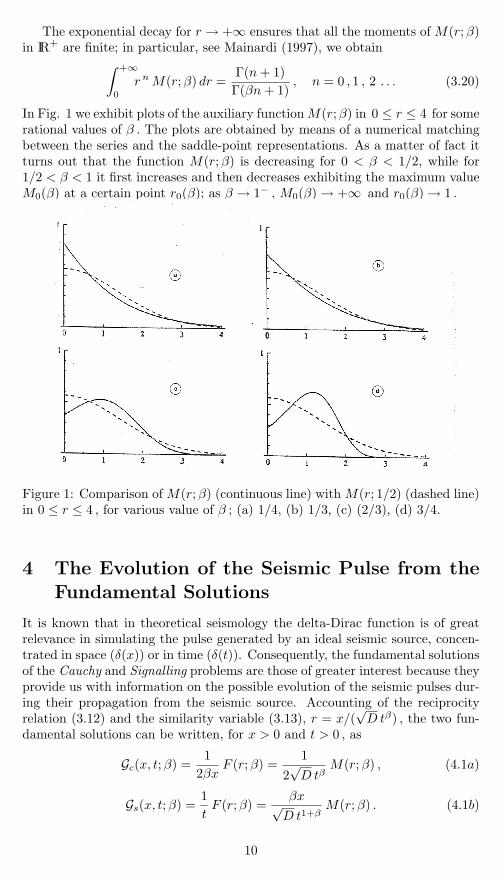
In Fig. 1 we exhibit plots of the auxiliary functionM(r;β) in 0 ≤ r ≤ 4 for somerational values of β . The plots are obtained by means of a numerical matchingbetween the series and the saddle-point representations. As a matter of fact itturns out that the function M(r;β) is decreasing for 0 < β < 1/2, while for1/2 < β < 1 it first increases and then decreases exhibiting the maximum valueM0(β) at a certain point r0(β); as β → 1− , M0(β) → +∞ and r0(β) → 1 .

Figure 1: Comparison of M(r;β) (continuous line) with M(r; 1/2) (dashed line)in 0 ≤ r ≤ 4 , for various value of β ; (a) 1/4, (b) 1/3, (c) (2/3), (d) 3/4.

4 The Evolution of the Seismic Pulse from theFundamental Solutions

It is known that in theoretical seismology the delta-Dirac function is of greatrelevance in simulating the pulse generated by an ideal seismic source, concen-trated in space (δ(x)) or in time (δ(t)). Consequently, the fundamental solutionsof the Cauchy and Signalling problems are those of greater interest because theyprovide us with information on the possible evolution of the seismic pulses dur-ing their propagation from the seismic source. Accounting of the reciprocityrelation (3.12) and the similarity variable (3.13), r = x/(

√D tβ) , the two fun-

damental solutions can be written, for x > 0 and t > 0 , as

Gc(x, t;β) =1

2βxF (r;β) =

12√D tβ

M(r;β) , (4.1a)

Gs(x, t;β) =1tF (r;β) =

βx√D t1+β

M(r;β) . (4.1b)

10

The above equations mean that for the fundamental solution of the Cauchy[Signalling] problem the time [spatial] shape is the same at each position [in-stant], the only changes being due to space [time] - dependent changes of widthand amplitude. The maximum amplitude in time [space] varies precisely as 1/x[1/t]. The two fundamental solutions exhibit scaling properties that make easiertheir plots versus distance (at fixed instant) and versus time (at fixed position).In fact, using the well-known scaling properties of the Laplace transform in (3.6)and (3.8), we easily prove, for any p , q > 0 , that

Gc(px, qt;β) =1qβGc(px/qβ , t;β) , (4.2a)

Gs(px, qt;β) =1qGs(px/qβ , t;β) , (4.2b)

and, consequently, in plotting we can choose suitable values for the fixed vari-able.

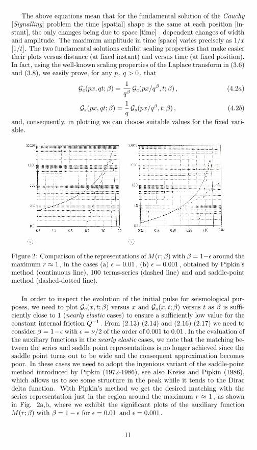
Figure 2: Comparison of the representations ofM(r;β) with β = 1−ε around themaximum r ≈ 1 , in the cases (a) ε = 0.01 , (b) ε = 0.001 , obtained by Pipkin’smethod (continuous line), 100 terms-series (dashed line) and and saddle-pointmethod (dashed-dotted line).

In order to inspect the evolution of the initial pulse for seismological pur-poses, we need to plot Gc(x, t;β) versus x and Gs(x, t;β) versus t as β is suffi-ciently close to 1 (nearly elastic cases) to ensure a sufficiently low value for theconstant internal friction Q−1 . From (2.13)-(2.14) and (2.16)-(2.17) we need toconsider β = 1−ε with ε = ν/2 of the order of 0.001 to 0.01 . In the evaluation ofthe auxiliary functions in the nearly elastic cases, we note that the matching be-tween the series and saddle point representations is no longer achieved since thesaddle point turns out to be wide and the consequent approximation becomespoor. In these cases we need to adopt the ingenious variant of the saddle-pointmethod introduced by Pipkin (1972-1986), see also Kreiss and Pipkin (1986),which allows us to see some structure in the peak while it tends to the Diracdelta function. With Pipkin’s method we get the desired matching with theseries representation just in the region around the maximum r ≈ 1 , as shownin Fig. 2a,b, where we exhibit the significant plots of the auxiliary functionM(r;β) with β = 1− ε for ε = 0.01 and ε = 0.001 .

11

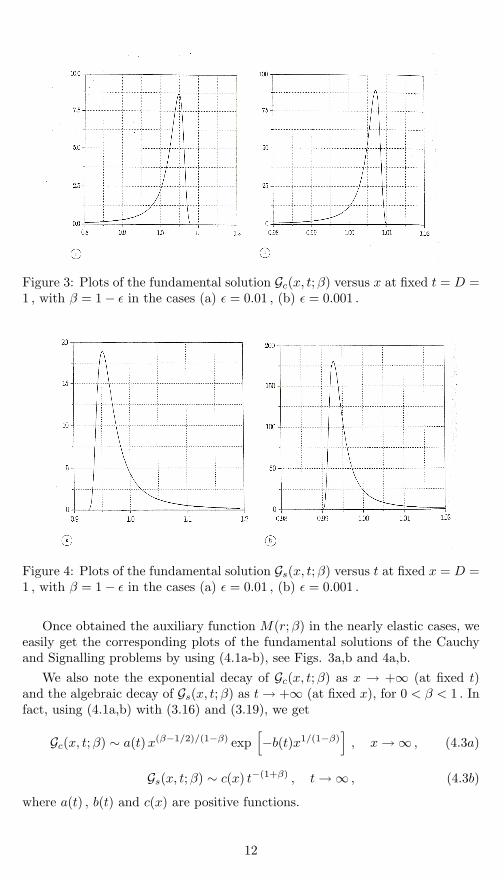
Figure 3: Plots of the fundamental solution Gc(x, t;β) versus x at fixed t = D =1 , with β = 1− ε in the cases (a) ε = 0.01 , (b) ε = 0.001 .

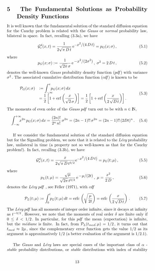
Figure 4: Plots of the fundamental solution Gs(x, t;β) versus t at fixed x = D =1 , with β = 1− ε in the cases (a) ε = 0.01 , (b) ε = 0.001 .

Once obtained the auxiliary function M(r;β) in the nearly elastic cases, weeasily get the corresponding plots of the fundamental solutions of the Cauchyand Signalling problems by using (4.1a-b), see Figs. 3a,b and 4a,b.

We also note the exponential decay of Gc(x, t;β) as x → +∞ (at fixed t)and the algebraic decay of Gs(x, t;β) as t→ +∞ (at fixed x), for 0 < β < 1 . Infact, using (4.1a,b) with (3.16) and (3.19), we get

Gc(x, t;β) ∼ a(t)x(β−1/2)/(1−β) exp[−b(t)x1/(1−β)

], x→∞ , (4.3a)

Gs(x, t;β) ∼ c(x) t−(1+β) , t→∞ , (4.3b)

where a(t) , b(t) and c(x) are positive functions.

12

5 The Fundamental Solutions as ProbabilityDensity Functions

It is well known that the fundamental solution of the standard diffusion equationfor the Cauchy problem is related with the Gauss or normal probability law,bilateral in space. In fact, recalling (3.3a), we have

Gdc (x, t) =

12√πD t

e−x2/(4D t) = pG(x;σ) , (5.1)

wherepG(x;σ) :=

1√2π σ

e−x2/(2σ2) , σ2 = 2D t , (5.2)

denotes the well-known Gauss probability density function (pdf) with varianceσ2 . The associated cumulative distribution function (cdf) is known to be

PG(x;σ) :=∫ x

−∞pG(x;σ) dx

=12

[1 + erf

(x√2σ

)]=

12

[1 + erf

(x

2√D t

)].

(5.3)

The moments of even order of the Gauss pdf turn out to be with n ∈ IN,∫ +∞

−∞x2n pG(x;σ) dx =

(2n)!2n n!

σ2n = (2n− 1)!!σ2n = (2n− 1)!! (2Dt)n . (5.4)

If we consider the fundamental solution of the standard diffusion equationbut for the Signalling problem, we note that it is related to the Levy probabilitylaw, unilateral in time (a property not so well-known as that for the Cauchyproblem!). In fact, recalling (3.3b), we have

Gds (x, t) =

x

2√πD t3/2

e−x2/(4D t) = pL(t;µ) , (5.5)

where

pL(t;µ) =√µ

√2π t3/2

e−µ/(2t) , µ =x2

2D, (5.6)

denotes the Levy pdf , see Feller (1971), with cdf

PL(t;µ) :=∫ t

0

pL(t;µ) dt = erfc(√

µ

2t

)= erfc

(x

2√D t

). (5.7)

The Levy pdf has all moments of integer order infinite, since it decays at infinityas t−3/2 . However, we note that the moments of real order δ are finite only if0 ≤ δ < 1/2 . In particular, for this pdf the mean (expectation) is infinite,but the mediane is finite. In fact, from PL(tmed;µ) = 1/2 , it turns out thattmed ≈ 2µ , since the complementary error function gets the value 1/2 as itsargument is approximatively 1/2 (a better evaluation of the argument is 1/2.1).

The Gauss and Levy laws are special cases of the important class of α -stable probability distributions, or stable distributions with index of stability

13

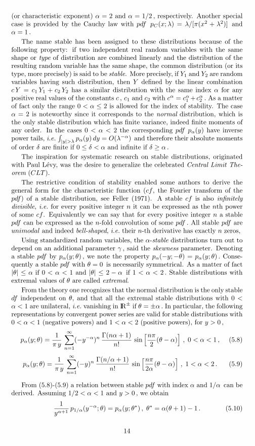
(or characteristic exponent) α = 2 and α = 1/2 , respectively. Another specialcase is provided by the Cauchy law with pdf pC(x;λ) = λ/[π(x2 + λ2)] andα = 1 .

The name stable has been assigned to these distributions because of thefollowing property: if two independent real random variables with the sameshape or type of distribution are combined linearly and the distribution of theresulting random variable has the same shape, the common distribution (or itstype, more precisely) is said to be stable. More precisely, if Y1 and Y2 are randomvariables having such distribution, then Y defined by the linear combinationc Y = c1 Y1 + c2 Y2 has a similar distribution with the same index α for anypositive real values of the constants c , c1 and c2 with cα = cα1 +cα2 . As a matterof fact only the range 0 < α ≤ 2 is allowed for the index of stability. The caseα = 2 is noteworthy since it corresponds to the normal distribution, which isthe only stable distribution which has finite variance, indeed finite moments ofany order. In the cases 0 < α < 2 the corresponding pdf pα(y) have inversepower tails, i.e.

∫|y|>λ

pα(y) dy = O(λ−α) and therefore their absolute momentsof order δ are finite if 0 ≤ δ < α and infinite if δ ≥ α .

The inspiration for systematic research on stable distributions, originatedwith Paul Levy, was the desire to generalize the celebrated Central Limit The-orem (CLT ).

The restrictive condition of stability enabled some authors to derive thegeneral form for the characteristic function (cf , the Fourier transform of thepdf) of a stable distribution, see Feller (1971). A stable cf is also infinitelydivisible, i.e. for every positive integer n it can be expressed as the nth powerof some cf . Equivalently we can say that for every positive integer n a stablepdf can be expressed as the n-fold convolution of some pdf . All stable pdf areunimodal and indeed bell-shaped, i.e. their n-th derivative has exactly n zeros,

Using standardized random variables, the α-stable distributions turn out todepend on an additional parameter γ , said the skewness parameter. Denotinga stable pdf by pα(y; θ) , we note the property pα(−y;−θ) = pα(y; θ) . Conse-quently a stable pdf with θ = 0 is necessarily symmetrical. As a matter of fact|θ| ≤ α if 0 < α < 1 and |θ| ≤ 2 − α if 1 < α < 2 . Stable distributions withextremal values of θ are called extremal.

From the theory one recognizes that the normal distribution is the only stabledf independent on θ, and that all the extremal stable distributions with 0 <α < 1 are unilateral, i.e. vanishing in IR± if θ = ±α . In particular, the followingrepresentations by convergent power series are valid for stable distributions with0 < α < 1 (negative powers) and 1 < α < 2 (positive powers), for y > 0 ,

pα(y; θ) =1π y

∞∑n=1

(−y−α)n Γ(nα+ 1)n!

sin[nπ

2(θ − α)

], 0 < α < 1 , (5.8)

pα(y; θ) =1π y

∞∑n=1

(−y)n Γ(n/α+ 1)n!

sin[nπ2α

(θ − α)], 1 < α < 2 . (5.9)

From (5.8)-(5.9) a relation between stable pdf with index α and 1/α can bederived. Assuming 1/2 < α < 1 and y > 0 , we obtain

1yα+1

p1/α(y−α; θ) = pα(y; θ∗) , θ∗ = α(θ + 1)− 1 . (5.10)

14

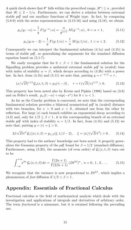
A quick check shows that θ∗ falls within the prescribed range, |θ∗| ≤ α , providedthat |θ| ≤ 2 − 1/α . Furthermore, we can derive a relation between extremalstable pdf and our auxiliary functions of Wright type. In fact, by comparing(5.8-9) with the series representations in (3.15-16) and using (3.18), we obtain

pα(y;−α) =1yF (y−α;α) =

α

yα+1M(y−α;α) , 0 < α < 1 , (5.11)

pα(y;α− 2) =1yF (y; 1/α) =

1αM(y; 1/α) , 1 < α < 2 . (5.12)

Consequently we can interpret the fundamental solutions (4.1a) and (4.1b) interms of stable pdf , so generalizing the arguments for the standard diffusionequation based on (5.1-7).

We easily recognize that for 0 < β < 1 the fundamental solution for theSignalling problem provides a unilateral extremal stable pdf in (scaled) timewith index of stability α = β , which decays according to (4.3b) with a powerlaw. In fact, from (4.1b) and (5.11) we note that, putting y = r−1/β = τ ,

(x/√D)1/β Gs(x, t;β) = pβ(τ ;−β) , τ = t (

√D/x)1/β > 0 . (5.13)

This property has been noted also by Kreiss and Pipkin (1986) based on (3.8)and on Feller’s result, pα(t;−α)÷ exp(−sα) for 0 < α < 1 .

As far as the Cauchy problem is concerned, we note that the correspondingfundamental solution provides a bilateral symmetrical pdf in (scaled) distancewith two branches, for x > 0 and x < 0 , obtained one from the other byreflection. For large |x| each branch exhibits an exponential decay according to(4.3) and, only for 1/2 ≤ β < 1 , it is the corresponding branch of an extremalstable pdf with index of stability α = 1/β . In fact, from (4.1b) and (5.12) wenote that, putting y = |r| = ξ > 0 ,

2β√D tβ Gc(|x|, t;β) = p1/β(ξ, 1/β − 2) , ξ = |x|/(

√D tβ) > 0 . (5.14)

This property had to the authors’ knowledge not been noted: it properly gener-alizes the Gaussian property of the pdf found for β = 1/2 (standard diffusion).Furthermore, using (3.20), the moments (of even order) of Gc(x, t;β) turn outto be∫ +∞

−∞x2n Gc(x, t;β) dx =

Γ(2n+ 1)Γ(2βn+ 1)

(Dt2β)n , n = 0 , 1 , 2 , . . . (5.15)

We recognize that the variance is now proportional to Dt2β , which implies aphenomenon of fast diffusion if 1/2 < β < 1 .

Appendix: Essentials of Fractional Calculus

Fractional calculus is the field of mathematical analysis which deals with theinvestigation and applications of integrals and derivatives of arbitrary order.The term fractional is a misnomer, but it is retained following the prevailinguse.

15

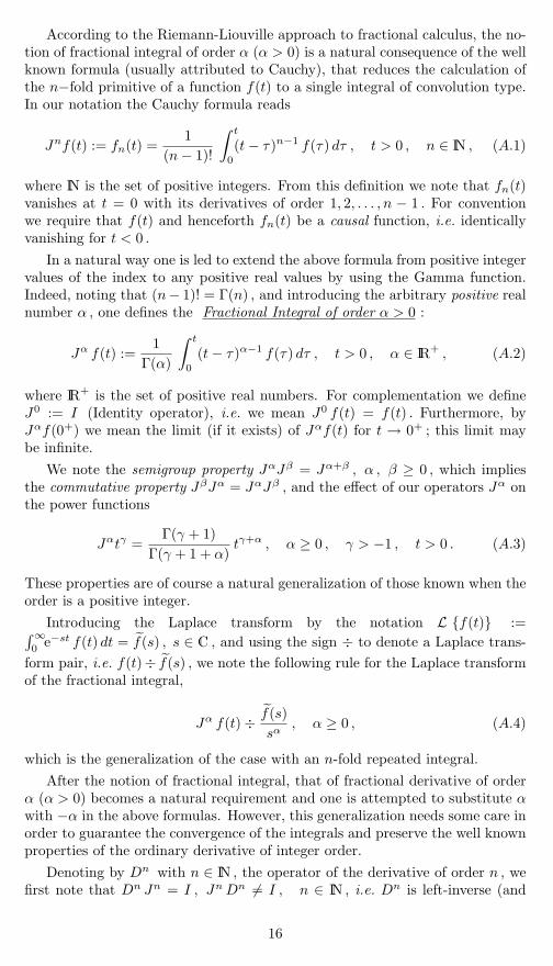
According to the Riemann-Liouville approach to fractional calculus, the no-tion of fractional integral of order α (α > 0) is a natural consequence of the wellknown formula (usually attributed to Cauchy), that reduces the calculation ofthe n−fold primitive of a function f(t) to a single integral of convolution type.In our notation the Cauchy formula reads

Jnf(t) := fn(t) =1

(n− 1)!

∫ t

0

(t− τ)n−1 f(τ) dτ , t > 0 , n ∈ IN , (A.1)

where IN is the set of positive integers. From this definition we note that fn(t)vanishes at t = 0 with its derivatives of order 1, 2, . . . , n − 1 . For conventionwe require that f(t) and henceforth fn(t) be a causal function, i.e. identicallyvanishing for t < 0 .

In a natural way one is led to extend the above formula from positive integervalues of the index to any positive real values by using the Gamma function.Indeed, noting that (n− 1)! = Γ(n) , and introducing the arbitrary positive realnumber α , one defines the Fractional Integral of order α > 0 :

Jα f(t) :=1

Γ(α)

∫ t

0

(t− τ)α−1 f(τ) dτ , t > 0 , α ∈ IR+ , (A.2)

where IR+ is the set of positive real numbers. For complementation we defineJ0 := I (Identity operator), i.e. we mean J0 f(t) = f(t) . Furthermore, byJαf(0+) we mean the limit (if it exists) of Jαf(t) for t → 0+ ; this limit maybe infinite.

We note the semigroup property JαJβ = Jα+β , α , β ≥ 0 , which impliesthe commutative property JβJα = JαJβ , and the effect of our operators Jα onthe power functions

Jαtγ =Γ(γ + 1)

Γ(γ + 1 + α)tγ+α , α ≥ 0 , γ > −1 , t > 0 . (A.3)

These properties are of course a natural generalization of those known when theorder is a positive integer.

Introducing the Laplace transform by the notation L {f(t)} :=∫∞0

e−st f(t) dt = f(s) , s ∈ C , and using the sign ÷ to denote a Laplace trans-form pair, i.e. f(t)÷ f(s) , we note the following rule for the Laplace transformof the fractional integral,

Jα f(t)÷ f(s)sα

, α ≥ 0 , (A.4)

which is the generalization of the case with an n-fold repeated integral.After the notion of fractional integral, that of fractional derivative of order

α (α > 0) becomes a natural requirement and one is attempted to substitute αwith −α in the above formulas. However, this generalization needs some care inorder to guarantee the convergence of the integrals and preserve the well knownproperties of the ordinary derivative of integer order.

Denoting by Dn with n ∈ IN , the operator of the derivative of order n , wefirst note that Dn Jn = I , JnDn 6= I , n ∈ IN , i.e. Dn is left-inverse (and

16

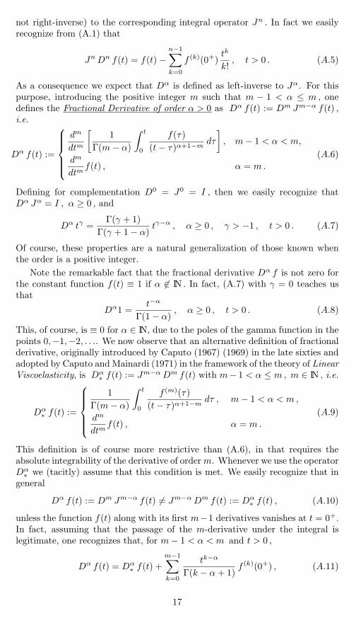
not right-inverse) to the corresponding integral operator Jn . In fact we easilyrecognize from (A.1) that

JnDn f(t) = f(t)−n−1∑k=0

f (k)(0+)tk

k!, t > 0 . (A.5)

As a consequence we expect that Dα is defined as left-inverse to Jα. For thispurpose, introducing the positive integer m such that m − 1 < α ≤ m, onedefines the Fractional Derivative of order α > 0 as Dα f(t) := Dm Jm−α f(t) ,i.e.

Dα f(t) :=

dm

dtm

[1

Γ(m− α)

∫ t

0

f(τ)(t− τ)α+1−m

dτ

], m− 1 < α < m,

dm

dtmf(t) , α = m.

(A.6)

Defining for complementation D0 = J0 = I , then we easily recognize thatDα Jα = I , α ≥ 0 , and

Dα tγ =Γ(γ + 1)

Γ(γ + 1− α)tγ−α , α ≥ 0 , γ > −1 , t > 0 . (A.7)

Of course, these properties are a natural generalization of those known whenthe order is a positive integer.

Note the remarkable fact that the fractional derivative Dα f is not zero forthe constant function f(t) ≡ 1 if α 6∈ IN . In fact, (A.7) with γ = 0 teaches usthat

Dα1 =t−α

Γ(1− α), α ≥ 0 , t > 0 . (A.8)

This, of course, is ≡ 0 for α ∈ IN, due to the poles of the gamma function in thepoints 0,−1,−2, . . .. We now observe that an alternative definition of fractionalderivative, originally introduced by Caputo (1967) (1969) in the late sixties andadopted by Caputo and Mainardi (1971) in the framework of the theory of LinearViscoelasticity, is Dα

∗ f(t) := Jm−αDm f(t) with m− 1 < α ≤ m, m ∈ IN , i.e.

Dα∗ f(t) :=

1

Γ(m− α)

∫ t

0

f (m)(τ)(t− τ)α+1−m

dτ , m− 1 < α < m ,

dm

dtmf(t) , α = m.

(A.9)

This definition is of course more restrictive than (A.6), in that requires theabsolute integrability of the derivative of orderm. Whenever we use the operatorDα∗ we (tacitly) assume that this condition is met. We easily recognize that in

general

Dα f(t) := Dm Jm−α f(t) 6= Jm−αDm f(t) := Dα∗ f(t) , (A.10)

unless the function f(t) along with its first m−1 derivatives vanishes at t = 0+.In fact, assuming that the passage of the m-derivative under the integral islegitimate, one recognizes that, for m− 1 < α < m and t > 0 ,

Dα f(t) = Dα∗ f(t) +

m−1∑k=0

tk−α

Γ(k − α+ 1)f (k)(0+) , (A.11)

17

and therefore, recalling the fractional derivative of the power functions (A.7),

Dα

(f(t)−

m−1∑k=0

tk

k!f (k)(0+)

)= Dα

∗ f(t) . (A.12)

The alternative definition (A.9) for the fractional derivative thus incorporatesthe initial values of the function and of its integer derivatives of lower order. Thesubtraction of the Taylor polynomial of degree m−1 at t = 0+ from f(t) meansa sort of regularization of the fractional derivative. In particular, according tothis definition, the relevant property for which the fractional derivative of aconstant is still zero can be easily recognized, i.e.

Dα∗ 1 ≡ 0 , α > 0 . (A.13)

We now explore the most relevant differences between the two fractionalderivatives (A.6) and (A.9). We agree to denote (A.9) as the Caputo frac-tional derivative to distinguish it from the standard Riemann-Liouville frac-tional derivative (A.6). We observe, again by looking at (A.7), that Dαtα−1 ≡0 , α > 0 , t > 0 . From above we thus recognize the following statements aboutfunctions which for t > 0 admit the same fractional derivative of order α , withm− 1 < α ≤ m, m ∈ IN ,

Dα f(t) = Dα g(t) ⇐⇒ f(t) = g(t) +m∑

j=1

cj tα−j , (A.14)

Dα∗ f(t) = Dα

∗ g(t) ⇐⇒ f(t) = g(t) +m∑

j=1

cj tm−j . (A.15)

In these formulas the coefficients cj are arbitrary constants.For the two definitions we also note a difference with respect to the formal

limit as α→ (m− 1)+. From (A.6) and (A.9) we obtain respectively,

α→ (m− 1)+ =⇒ Dα f(t) → Dm J f(t) = Dm−1 f(t) ; (A.16)

α→ (m− 1)+ =⇒ Dα∗ f(t) → J Dm f(t) = Dm−1 f(t)− f (m−1)(0+) . (A.17)

We now consider the Laplace transform of the two fractional derivatives.For the standard fractional derivative Dα the Laplace transform, assumed toexist, requires the knowledge of the (bounded) initial values of the fractionalintegral Jm−α and of its integer derivatives of order k = 1, 2, . . . ,m − 1 . Thecorresponding rule reads, in our notation,

Dα f(t)÷ sα f(s)−m−1∑k=0

Dk J (m−α) f(0+) sm−1−k , m− 1 < α ≤ m. (A.18)

The Caputo fractional derivative appears more suitable to be treated bythe Laplace transform technique in that it requires the knowledge of the

18

(bounded) initial values of the function and of its integer derivatives of orderk = 1, 2, . . . ,m − 1 , in analogy with the case when α = m. In fact, by using(A.4) and noting that

JαDα∗ f(t) = Jα Jm−αDm f(t) = JmDm f(t) = f(t)−

m−1∑k=0

f (k)(0+)tk

k!. (A.19)

we easily prove the following rule for the Laplace transform,

Dα∗ f(t)÷ sα f(s)−

m−1∑k=0

f (k)(0+) sα−1−k , m− 1 < α ≤ m. (A.20)

Indeed, the result (A.20), first stated by Caputo (1969) by using the Fubini-Tonelli theorem, appears as the most ”natural” generalization of the corre-sponding result well known for α = m.

This appendix is based on the review by Gorenflo and Mainardi (1997). Formore details on the classical treatment of fractional calculus the reader is referredto Erdelyi (1954), Oldham and Spanier (1974), Samko et al. (1987-1993) andMiller and Ross (1993). Gorenflo and Mainardi have pointed out the major util-ity of the Caputo fractional derivative in the treatment of differential equationsof fractional order for physical applications. In fact, in physical problems, theinitial conditions are usually expressed in terms of a given number of boundedvalues assumed by the field variable and its derivatives of integer order, nomatter if the governing evolution equation may be a generic integro-differentialequation and therefore, in particular, a fractional differential equation.

References

– Aki, K. and P.G. Richards (1980): Quantitative Seismology (Freeman, SanFrancisco), Vol. 1, Ch. 5, pp. 167-185.

– Ben-Menahem, A., and S.J. Singh (1981): Seismic Waves and Sources(Springer-Verlag, New York), Ch. 10, pp. 840-944.

– Buchen, P.W. and F. Mainardi (1975): Asymptotic expansions for transientviscoelastic waves, J. Mec. 14, 597-608.

– Caputo, M. (1966) : Linear models of dissipation whose Q is almost frequencyindependent, Annali di Geofisica, 19, 383-393.

– Caputo, M. (1967) : Linear models of dissipation whose Q is almost frequencyindependent, Part II., Geophys. J. R. Astr. Soc., 13, 529-539.

– Caputo, M. (1969): Elasticita e Dissipazione (Zanichelli Bologna). [in Italian]

– Caputo, M. and F. Mainardi (1971): Linear models of dissipation in anelasticsolids, Riv. Nuovo Cimento (Ser II) 1, 161-198.

– Caputo, M. (1976): Vibrations of an infinite plate with a frequency indepen-dent Q , J. Acoust. Soc. Am., 60, 634-639.

19

– Caputo, M. (1979): A model for the fatigue in elastic materials with frequencyindependent Q , J. Acoust. Soc. Am., 66, 176-179.

– Caputo, M. (1981): Elastic radiation from a source in a medium with analmost frequency independent Q , J. Phys. Earth, 29, 487-497.

– Caputo, M. (1985) : Generalized rheology and geophysical consequences,Tectonophysics, 116, 163-172.

– Caputo, M. (1996)a: Modern rheology and electric induction: multivaluedindex of refraction, splitting of eigenvalues and fatigues, Annali di Geofisica,39, 941-966.

– Caputo, M. (1996)b: The Green function of the diffusion in porous mediawith memory, Rend. Fis. Acc. Lincei (Ser. 9), 7, 243-250.

– Carcione, J.M., Kosloff, D. and R. Kosloff (1988): Wave propagation in alinear viscoelastic medium, Geophys. J., 95, 597-611.

– Chin, R.C.Y. (1980): Wave propagation in viscoelastic media, in Physics ofthe Earth’s Interior, edited by A. Dziewonski and E. Boschi (North-Holland,Amsterdam), pp. 213-246. [E. Fermi Int. School, Course 78]

– Christensen, R.M. (1982): Theory of Viscoelasticity (Academic Press, NewYork). [1-st ed. (1972)]

– Erdelyi, A. Editor (1954): Tables of Integral Transforms, Bateman Project(McGraw-Hill, New York), Vol. 2, Ch. 13, pp. 181-212.

– Erdelyi, A. Editor (1955): Higher Transcendental Functions, Bateman Project(McGraw-Hill, New York), Vol. 3, Ch. 18, pp. 206-227.

– Feller, W. (1971), An Introduction to Probability Theory and its Applications,(Wiley, New York), Vol. II, Ch. 6: pp. 169-176, Ch. 13: pp. 448-454. [1-st ed.(1966)]

– Futterman, W.I. (1962): Dispersive Body Waves, J. Geophys. Res., 67,5279-5291.

– Gel’fand, I.M. and G.E. Shilov (1964): Generalized Functions, (AcademicPress, New York), Vol. I.

– Giona, M. and H.E. Roman (1992): Fractional diffusion equation for transportphenomena in random media, Physica A, 185, 82-97.

– Gordon, R.B. and C.W. Nelson (1966): Anelastic properties of the Earth,Rev. Geophys., 4, 457-474 (1966).

– Gorenflo, R. and F. Mainardi (1997): Fractional calculus: integral and dif-ferential equations of fractional order, in Fractals and Fractional Calculus inContinuum Mechanics, edited by A. Carpinteri and F. Mainardi (Springer Ver-lag, Wien), 223-276.

– Graffi, D. (1982): Mathematical models and waves in linear viscoelasticity,in Wave Propagation in Viscoelastic Media, edited by F. Mainardi (Pitman,London), pp. 1-27. [Res. Notes in Maths, Vol. 52]

20

– Hunter, S.C. (1960): Viscoelastic Waves, in Progress in Solid Mechanics,edited by I. Sneddon and R. Hill (North-Holland, Amsterdam), Vol 1, pp. 3-60.

– Jackson, D.D. and D.L. Anderson (1970): Physical mechanisms for seismicwave attenuation, Rev. Geophys., 2, 625-660 (1964).

– Kanamori, H. and D.L. Anderson (1977): Importance of physical dispersion insurface wave and free oscillation problems, Rev. Geophys., 15, 105-112 (1977).

– Kang, I.B. and G.A. McMechan (1993): Effects of viscoelasticity on wavepropagation in fault zones, near-surfaces sediments and inclusions, Bull. Seism.Soc. Am., 83, 890-906.

– Kjartansson, E. (1979): Constant-Q wave propagation and attenuation, J.Geophys. Res., 94, 4737-4748.

– Knopoff, L. (1964): Q , Rev. Geophys., 2, 625-660.

– Kolsky, H. (1956): The propagation of stress pulses in viscoelastic solids,Phil. Mag. (Ser 8), 2, 693-710.

– Kornig, M. and G. Muller (1989): Rheological models and interpretation ofpostglacial uplift, Geophys. J. Int., 98, 243-253.

– Kreis, A. and A.C. Pipkin (1986): Viscoelastic pulse propagation and stableprobability distributions, Quart. Appl. Math., 44, 353-360.

– Mainardi, F. and G. Turchetti (1975): Wave front expansion for transientviscoelastic waves, Mech. Res. Comm. 2, 107-112.

– Mainardi, F. (1994): On the initial value problem for the fractional diffusion-wave equation, in Waves and Stability in Continuous Media edited by S. Rioneroand T. Ruggeri, (World Scientific, Singapore), pp. 246-251.

– Mainardi, F. (1995): Fractional diffusive waves in viscoelastic solids in IUTAMSymposium - Nonlinear Waves in Solids, edited by J. L. Wegner and F. R.Norwood (ASME/AMR, Fairfield NJ), pp. 93-97. [Abstract in Appl. Mech.Rev., 46 (1993), 549]

– Mainardi, F. and M. Tomirotti (1995): On a special function arising in thetime fractional diffusion-wave equation, in Transform Methods and Special Func-tions, Sofia 1994, edited by P. Rusev, I. Dimovski and V. Kiryakova, (ScienceCulture Technology, Singapore), pp. 171-183.

– Mainardi, F. (1996)a: Fractional relaxation-oscillation and fractionaldiffusion-wave phenomena, Chaos, Solitons & Fractals, 7, 1461-1477.

– Mainardi, F. (1996)b: The fundamental solutions for the fractional diffusion-wave equation, Applied Mathematics Letters, 9, No 6, 23-28.

– Mainardi, F. (1997): Fractional calculus; some basic problems in continuumand statistical mechanics, in Fractals and Fractional Calculus in ContinuumMechanics, edited by. A. Carpinteri and F. Mainardi (Springer-Verlag, Wien),291-348.

21

– Meshkov, S.I. and Yu. A. Rossikhin (1970): Sound wave propagation in aviscoelastic medium whose hereditary properties are determined by weakly sin-gular kernels, in Waves in Inelastic Media, edited by Yu. N. Rabotnov (Kish-niev), pp. 162-172. [in Russian]

– Metzler, R., Glockle, W.G. and T.F. Nonnenmacher (1994): Fractional modelequation for anomalous diffusion, Physica A, 211, 13-24.

– Miller, K.S. and B. Ross (1993): An Introduction to the Fractional Calculusand Fractional Differential Equations (Wiley, New York).

– Mitchell, B.J. (1995): Anelastic structure and evolution of the continentalcrust and upper mantle from seismic surface wave attenuation, Rev. Geophys.,33, 441-462 (1995).

– Murphy, W.F. (1982): Effect of partial water saturation on attenuation insandstones, J. Acoust. Soc. Am., 71, 1458-1468.

– Nigmatullin, R.R. (1986): The realization of the generalized transfer equationin a medium with fractal geometry, Phys. Stat. Sol. B, 133, 425-430. [Englishtransl. from Russian]

– O’Connell, R.J. and B. Budiansky (1978): Measures of dissipation in visco-elastic media, Geophys. Res. Lett., 5, 5-8.

– Oldham, K.B. and J. Spanier (1974): The Fractional Calculus (AcademicPress, New York).

– Pipkin, A.C. (1986): Lectures on Viscoelastic Theory (Springer-Verlag, NewYork), Ch. 4, pp. 56-76. [1-st ed, 1972]

– Ranalli, G. (1987): Rheology of the Earth (Allen & Unwin, London).

– Rossikhin, Yu. A. and M.V. Shitikova (1997): Application of fractionalcalculus to dynamic problems of linear and nonlinear hereditary mechanics ofsolids, Appl. Mech. Rev, 50, 15-67.

– Sabadini, R., Yuen, D.A. and P. Gasperini (1985): The effects of transientrheology on the interpretation of lower mantle viscosity, Geophys. Res. Lett.,12, 361-364.

– Sabadini, R., Smith, B.K. and D.A. Yuen (1987): Consequences of experi-mental transient rheology, Geophys. Res. Lett., 14, 816-819.

– Samko S.G., Kilbas, A.A. and O.I. Marichev (1993): Fractional Integralsand Derivatives, Theory and Applications, (Gordon and Breach, Amsterdam).[Engl. Transl. from Russian, Integrals and Derivatives of Fractional Order andSome of Their Applications, Nauka i Tekhnika, Minsk (1987)]

– Savage, J.C. and M.E. O’Neill (1975): The relation between the Lomnitz andthe Futterman theories of internal friction, J. Geophys. Res., 80, 249-251.

– Schneider, W.R. and W. Wyss (1989): Fractional diffusion and wave equa-tions, J. Math. Phys., 30, 134-144.

– Spencer , J. W. (1981): Stress relaxation at low frequencies in fluid saturatedrocks; attenuation and modulus dispersion, J. Geophys. Res., 86, 1803-1812.

22

– Strick, E. (1967): The determination of Q , dynamic viscosity and creepcurves from wave propagation measurements, Geophys. J. R. Astr. Soc., 13,197-218.

– Strick, E. (1970): A predicted pedestal effect for pulse propagation inconstant-Q solids, Geophysics, 35, 387-403.

– Strick, E. (1982): Application of linear viscoelasticity to seismic wave prop-agation, in Wave Propagation in Viscoelastic Media, edited by F. Mainardi(Pitman, London), pp. 169-193. [Res. Notes in Maths, Vol. 52]

– Strick, E. and F. Mainardi (1982): On a general class of constant Q solids,Geophys. J. R. Astr. Soc., 69, 415-429.

– Strick, E. (1984): Implication of Jeffreys-Lomnitz transient creep, J. Geophys.Res., 89, 437-451.

– Yuen, D.A., Sabadini, R., Gasperini, P. and E. Boschi (1986): On transientrheology and glacial isostasy, J. Geophys. Res., 91, 11420-11438.

23