Embed Size (px)
Citation preview

ED n°431 : ICMS
T H E S E
pour obtenir le grade de
DOCTEUR DE L’ECOLE NATIONALE SUPERIEURE DES MINES DE PARIS
Spécialité “Mathématiques et Automatique”
présentée et soutenue publiquement par Erwan SALAÜN
le 13 janvier 2009
ALGORITHMES DE FILTRAGE ET SYSTEMES AVIONIQUES POUR VEHICULES AERIENS AUTONOMES
Directeur de thèse : Philippe MARTIN
Jury
M. Tarek HAMEL Président M. Eric FERON Rapporteur
M. Robert MAHONY Rapporteur Mme Cécile DURIEU Examinateur M. Pascal MORIN Examinateur M. Philippe MARTIN Examinateur


Erwan SALAÜN
FILTERING ALGORITHMS AND
AVIONICS SYSTEMS FOR
UNMANNED AERIAL VEHICLES
Erwan SALAÜN
Mines ParisTech, Centre Automatique et Systèmes, 60, Bd. Saint-Michel, 75272 ParisCedex 06, France.
E-mail : [email protected]
Key words and phrases. Unmanned aerial vehicles, low-cost embedded avionicssystems, data fusion, navigation solutions, attitude and heading reference system, nonlin-ear observers, invariance, symmetry, extended Kalman lter, quadrotor, rotor drag.
Mots clés. Véhicules aériens autonomes, systèmes avioniques embarqués bas-coûts,fusion de données, solutions de navigation, système de référence d'attitude et de cap, ob-servateurs non-linéaires, invariance, symétrie, ltre de Kalman étendu, quadrotor, traînéede rotor.
July 8, 2010
FILTERING ALGORITHMS AND AVIONICS
SYSTEMS FOR UNMANNED AERIAL VEHICLES
Erwan SALAÜN
iv
Résumé (Algorithmes de ltrage et systèmes avioniques pour véhicules aériensautonomes)L'essor récent des mini-véhicules aériens autonomes (ou mini-drones) est intrasèquement
lié au développement des diérentes composantes des systèmes avioniques embarqués(capteurs, calculateurs et liaison de données), à la fois au niveau de leur coût, de leurpoids, de leurs dimensions et de leurs performances. Ces engins volants doivent en eetrépondre à un cahier des charges spécique très exigeant: être capable d'accomplir desmissions de surveillance ou de poursuite de manière autonome, tout en étant léger (<2kg),de petite envergure (<1m) et assez bon marché. L'avionique embarquée, dite bas-coûts, doit elle-même satisfaire ces contraintes: elle ne peut contenir que des systèmesaux performances médiocres (e.g. mesures des capteurs fortement biaisées ou bruitées,calculateur peu puissant), qui doivent alors être compensés par des algorithmes de fusionde données et de contrôle intelligement pensés et implémentés.Le travail présenté dans ce mémoire concerne le développement théorique et la valida-
tion expérimentale d'algorithmes de fusion de données originaux pour mini-drones, dé-passant les limitations des estimateurs communément utilisés. En eet, les observateursusuels (e.g. le Filtre de Kalman Etendu ou les ltres particulaires) possèdent plusieursinconvénients: leur convergence, même au premier ordre, est dicile à prouver, leur com-portement local est souvent mal appréhendé et leur réglage est délicat (de nombreuxcoecients sont à régler). Ils sont de plus gourmand en calculs (nombreuses opérationsmatricielles), ce qui les empêchent d'être implémentés sur des calculateurs bon marché etdonc peu puissants. Ce mémoire présente des solutions alternatives à ces ltres, remédiantaux défauts précédents et pouvant être implémentés aisément et ecacement dans uneavionique bas-coûts.Nous proposons tout d'abord des observateurs invariants génériques, préservant les
symétries naturelles du système physique. Ces observateurs fusionnent les mesures decapteurs bon marché usuels (tels qu'inertiels, magnétomètres, GPS ou baromètre) and'estimer avec précision l'état de l'appareil (angles d'attitude et de cap, vitesse et posi-tion). Ils possèdent un large domaine de convergence; ils sont également faciles à régleret très économiques en temps de calcul. Ils ne supposent pas de modèle connu de l'engin(hormis les lois cinématiques habituelles) et peuvent donc être adaptés à toute plateformemobile.Puis nous développons des observateurs spéciques, adaptés au type de véhicule aérien
considéré, en l'occurence un mini-quadrotor. Nous décrivons tout d'abord son modèlephysique, tenant compte explicitement de la traînée de rotor. Ce modèle nous permetalors de contruire des observateurs estimant la vitesse du quadrotor à partir de mesuresuniquement inertielles, menant à un contrôle en vitesse de l'appareil. Cette approche estvalidée par des vols stabilisés autonomes.Enn, nous présentons en détails l'intégration du système avionique bas-coûts utilisé,
composé de capteurs bruts et d'un microcontrôleur sur lequel sont implémentés lesobservateurs précédents. Nous validons ces algorithmes en comparant leurs estimationsavec ceux fournit par un produit commercial coûteux, mettant ainsi en évidence leurexcellent rapport qualité/prix.
REMERCIEMENTS
Je remercie Tarek Hamel, président du jury, Eric Feron et Robert Mahony, rapporteurs,Cécile Durieu et Pascal Morin, examinateurs de ma thèse.Je tiens également à remercier toute l'équipe du centre, en particulier Nicolas Petit et
Pierre Rouchon, pour leurs conseils et l'intérêt qu'ils ont porté à mon travail.J'ai une grande pensée pour mes compagnons de route qui m'ont aidé par bien des
manières: Laure et Jonathan pour s'être brûlés avec moi au fer à souder; Caroline etChristophe pour avoir partagé ma passion de l'ATmega128; Pierre-Jean et Johann pourm'avoir aidé à construire notre quadricoptère; Silvère pour m'avoir initié au monde del'invariance.Merci à mes proches, en particulier à Marine, qui ont su m'épauler pendant toutes ces
années et me faire vivre tant de bons moments qui m'ont permis de me ressourcer.Je souhaite enn remercier Philippe Martin qui a été beaucoup plus qu'un simple
directeur de thèse. Merci d'avoir toujours été à mes côtés: de la gestion des interruptionsdu microcontrôleur au lemme de Barbalat, en passant par le choix et l'achat de connecteursen tous genres. Je vais regretter nos (longues) pauses cafés, les nitions d'articles à 4h dumatin et les vols du quadri dans le jardin des Mines.

CONTENTS
1. Problem position . . . . . . . . . . . . . . . . . . . . . . . . . . . . . . . . . . . . . . . . . . . . . . . . . . . . . . . . . . . . 3
1.1. Roles of the embedded avionics system . . . . . . . . . . . . . . . . . . . . . . . . . . . . . . . . . . . . 3
1.2. Challenges of the ltering algorithms . . . . . . . . . . . . . . . . . . . . . . . . . . . . . . . . . . . . . . 4
1.3. Sensors and commercial navigation systems . . . . . . . . . . . . . . . . . . . . . . . . . . . . . . . . 6
1.4. Symmetry-preserving observers theory . . . . . . . . . . . . . . . . . . . . . . . . . . . . . . . . . . . . . . 11
1.5. Thesis outline . . . . . . . . . . . . . . . . . . . . . . . . . . . . . . . . . . . . . . . . . . . . . . . . . . . . . . . . . . . . . . 14
2. Models for navigation systems . . . . . . . . . . . . . . . . . . . . . . . . . . . . . . . . . . . . . . . . . . . . 17
2.1. Round Earth model and true inertial navigation . . . . . . . . . . . . . . . . . . . . . . . . . . 17
2.2. Flat Earth model . . . . . . . . . . . . . . . . . . . . . . . . . . . . . . . . . . . . . . . . . . . . . . . . . . . . . . . . . . 26
2.3. Model for AHRS . . . . . . . . . . . . . . . . . . . . . . . . . . . . . . . . . . . . . . . . . . . . . . . . . . . . . . . . . . 30
2.4. Model for aided AHRS . . . . . . . . . . . . . . . . . . . . . . . . . . . . . . . . . . . . . . . . . . . . . . . . . . . . 33
2.5. Invariance properties of the at Earth model . . . . . . . . . . . . . . . . . . . . . . . . . . . . . . 35
2.6. Quaternions . . . . . . . . . . . . . . . . . . . . . . . . . . . . . . . . . . . . . . . . . . . . . . . . . . . . . . . . . . . . . . . . 38
3. Symmetry-preserving observers for Attitude and Heading Reference
Systems . . . . . . . . . . . . . . . . . . . . . . . . . . . . . . . . . . . . . . . . . . . . . . . . . . . . . . . . . . . . . . . . . . . . . . 41
3.1. Nonlinear observer . . . . . . . . . . . . . . . . . . . . . . . . . . . . . . . . . . . . . . . . . . . . . . . . . . . . . . . . 41
3.2. Design of the observer gain matrices . . . . . . . . . . . . . . . . . . . . . . . . . . . . . . . . . . . . . . . . 48
3.3. Eects of disturbances . . . . . . . . . . . . . . . . . . . . . . . . . . . . . . . . . . . . . . . . . . . . . . . . . . . . . . 53
3.4. Experimental validation . . . . . . . . . . . . . . . . . . . . . . . . . . . . . . . . . . . . . . . . . . . . . . . . . . . . 54
4. Symmetry-preserving observers for aided Attitude and Heading Reference
Systems . . . . . . . . . . . . . . . . . . . . . . . . . . . . . . . . . . . . . . . . . . . . . . . . . . . . . . . . . . . . . . . . . . . . . . 59
4.1. Earth-velocity-aided AHRS . . . . . . . . . . . . . . . . . . . . . . . . . . . . . . . . . . . . . . . . . . . . . . . . 59
2 CONTENTS
4.2. Earth-velocity-and-position-aided AHRS . . . . . . . . . . . . . . . . . . . . . . . . . . . . . . . . . . . . 73
4.3. General invariant observer for aided AHRS . . . . . . . . . . . . . . . . . . . . . . . . . . . . . . . . 93
5. Invariant Kalman Filter . . . . . . . . . . . . . . . . . . . . . . . . . . . . . . . . . . . . . . . . . . . . . . . . . . . . 107
5.1. Introduction . . . . . . . . . . . . . . . . . . . . . . . . . . . . . . . . . . . . . . . . . . . . . . . . . . . . . . . . . . . . . . . . 107
5.2. System with symmetries and Gaussian noises . . . . . . . . . . . . . . . . . . . . . . . . . . . . . . 109
5.3. Invariant Extended Kalman Filter . . . . . . . . . . . . . . . . . . . . . . . . . . . . . . . . . . . . . . . . . . 109
5.4. Considered system . . . . . . . . . . . . . . . . . . . . . . . . . . . . . . . . . . . . . . . . . . . . . . . . . . . . . . . . . . 112
5.5. Multiplicative Extended Kalman Filter . . . . . . . . . . . . . . . . . . . . . . . . . . . . . . . . . . . . 113
5.6. Left Invariant Extended Kalman Filter . . . . . . . . . . . . . . . . . . . . . . . . . . . . . . . . . . . . 115
5.7. Right Invariant Extended Kalman Filter . . . . . . . . . . . . . . . . . . . . . . . . . . . . . . . . . . . . 118
5.8. Numerical results . . . . . . . . . . . . . . . . . . . . . . . . . . . . . . . . . . . . . . . . . . . . . . . . . . . . . . . . . . 121
6. Specic observer for mini quadrotor . . . . . . . . . . . . . . . . . . . . . . . . . . . . . . . . . . . . . . 125
6.1. Introduction . . . . . . . . . . . . . . . . . . . . . . . . . . . . . . . . . . . . . . . . . . . . . . . . . . . . . . . . . . . . . . . . 125
6.2. Revisited quadrotor model . . . . . . . . . . . . . . . . . . . . . . . . . . . . . . . . . . . . . . . . . . . . . . . . . . 128
6.3. Experimental validation . . . . . . . . . . . . . . . . . . . . . . . . . . . . . . . . . . . . . . . . . . . . . . . . . . . . 136
6.4. Implications on control schemes . . . . . . . . . . . . . . . . . . . . . . . . . . . . . . . . . . . . . . . . . . . . 140
7. Real-time implementation and low-cost embedded prototype system . . 147
7.1. Real-time implementation on a cheap microcontroller . . . . . . . . . . . . . . . . . . . . . . 147
7.2. Low-cost embedded avionics system . . . . . . . . . . . . . . . . . . . . . . . . . . . . . . . . . . . . . . . . 151
Bibliography . . . . . . . . . . . . . . . . . . . . . . . . . . . . . . . . . . . . . . . . . . . . . . . . . . . . . . . . . . . . . . . . . . . . 161
CHAPTER 1
PROBLEM POSITION
Dans ce chapitre introductif nous présentons la problématique des algorithmes de l-
trage pour mini-drones, mettant en perspective certains travaux menés dans ce domaine,
ainsi que les diérents types de capteurs et systèmes de navigation commerciaux util-
isés. Nous faisons également un rappel de la théorie des observateurs invariants, élément
essentiel à la construction des estimateurs génériques développés par la suite.
1.1. Roles of the embedded avionics system
The mini-Unmanned Aerial Vehicles (or mini-UAVs) have been subject to an exponen-
tial growth for the past 15 years, created to satisfy rst military and then civilian needs.
There is a wide variety of mini-UAV shapes and congurations, but they all share several
common characteristics:
they are small (<1m), light (<2kg) and low-cost
they can be autonomous and accomplish many tasks (hovering, following waypoints,...)
by themselves
they can be remotely controlled by a non-specialist pilot giving high-level orders (e.g.
go forward, go left, take o)
they should be able to y in many dierent environments: indoor/outdoor, in pres-
ence of wind, obstacles,...
In order to meet these very demanding requirements, an embedded avionics system is
used: it is composed of a computational board that is interfaced with the sensors, the
actuators, and the communication devices. This system must accomplish two main tasks:
4 CHAPTER 1. PROBLEM POSITION
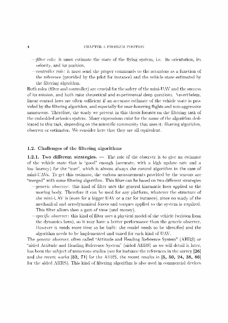
lter role: it must estimate the state of the ying system, i.e. its orientation, its
velocity, and its position,
controller role: it must send the proper commands to the actuators as a function of
the reference (provided by the pilot for instance) and the vehicle state estimated by
the ltering algorithm.
Both roles (lter and controller) are crucial for the safety of the mini-UAV and the success
of its mission, and both raise theoretical and experimental deep questions. Nevertheless,
linear control laws are often sucient if an accurate estimate of the vehicle state is pro-
vided by the ltering algorithm, and especially for near-hovering ights and non-aggressive
maneuvers. Therefore, the study we present in this thesis focuses on the ltering task of
the embedded avionics system. Many expressions exist for the name of the algorithm ded-
icated to this task, depending on the scientic community that uses it: ltering algorithm,
observer or estimator. We consider here that they are all equivalent.
1.2. Challenges of the ltering algorithms
1.2.1. Two dierent strategies. The role of the observer is to give an estimate
of the vehicle state that is good enough (accurate, with a high update rate and a
low latency) for the user, which is almost always the control algorithm in the case of
mini-UAVs. To get this estimate, the various measurements provided by the sensors are
merged" with some ltering algorithm. This lter can be based on two dierent strategies
generic observer : this kind of lter uses the general kinematic laws applied to the
moving body. Therefore it can be used for any platform, whatever the structure of
the mini-UAV is (even for a bigger UAV or a car for instance), since no study of the
mechanical and aerodynamical forces and torques applied to the system is required.
This lter allows then a gain of time (and money).
specic observer : this kind of lter uses a physical model of the vehicle (written from
the dynamics laws), so it may have a better performance than the generic observer.
However it needs more time to be built: the model needs to be identied and the
algorithm needs to be implemented and tuned for each kind of UAV.
The generic observer, often called Attitude and Heading Reference System (AHRS) or
aided Attitude and Heading Reference System (aided AHRS) as we will detail it later,
has been the subject of numerous studies (see for instance the references in the survey [26]
and the recent works [52, 71] for the AHRS, the recent results in [5, 50, 24, 38, 86]
for the aided AHRS). This kind of ltering algorithm is also used in commercial devices
1.2. CHALLENGES OF THE FILTERING ALGORITHMS 5
that can be mounted on any UAV (i.e. the MIDG II from Microbotics, the MTi from
Xsens, the 3DM-GX1 from Microstrain or the GuideStar from Athena). On the contrary,
few works developed specic observers since much more eort in the system modeling is
required (see for instance [87, 88]).
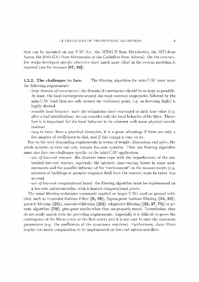
1.2.2. The challenges to face. The ltering algorithm for mini-UAV must meet
the following requirements
large domain of convergence: the domain of convergence should be as large as possible.
At least, the local convergence around the most common trajectories followed by the
mini-UAV (and then not only around the stationary point, e.g. an hovering ight) is
highly desired
sensible local behavior : once the estimations have converged to their true value (e.g.
after a bad initialization), we can consider only the local behavior of the lter. There-
fore it is important for the local behavior to be coherent with some physical consid-
erations
easy to tune: from a practical viewpoint, it is a great advantage if there are only a
few number of coecients to dial, and if this tuning is easy to do.
Due to the very demanding requirements in terms of weight, dimensions and price, the
whole avionics system can only contain low-cost systems. Then the ltering algorithm
must also face two challenges specic to the mini-UAV application:
use of low-cost sensors : the observer must cope with the imperfections of the em-
bedded low-cost sensors, especially the intrinsic time-varying biases in some mea-
surements and the possible inuence of the environment on the measurements (e.g.
presence of buildings or parasite magnetic eld from the motors) must be taken into
account
use of low-cost computational board : the ltering algorithm must be implemented on
a low-cost microcontroller, with a limited computational power.
The usual ltering techniques commonly applied on larger UAVs (and on ground vehi-
cles), such as Extended Kalman Filter ([8, 29]), Sigma-point Kalman ltering ([24, 82]),
particle ltering ([21]), unscented ltering ([25]), adaptative ltering ([22, 37, 75]) or ge-
netic algorithm ([70]), give great results when they are properly tuned. Nevertheless, they
do not really match with the preceding requirements. Especially it is dicult to prove the
convergence of the lters (even at the rst order) and it is not easy to tune the numerous
parameters (e.g. the coecients of the covariance matrices). Furthermore, these lters
require too much computation to be implemented on low-cost microcontrollers.
6 CHAPTER 1. PROBLEM POSITION
In order to bypass these limitations, many nonlinear ltering algorithms have been
developed, for AHRS (see [35, 52, 55, 67, 81, 26, 53, 54, 73]) as well as for aided
AHRS (see [84, 86, 3, 85]). Another approach has been recently proposed, introducing
nonlinear lters preserving by construction the natural symmetries of the considered sys-
tem. Therefore they are often called invariant or symmetry-preserving observers. A
theoretical investigation of such lters is presented in [11, 12, 13, 46, 47, 48], including
the denition of invariance properties and a systematic method to construct the invariant
lters. A brief recall of the main results is given in section 1.4. The majority of the
observers we develop in this thesis is based on this approach.
1.3. Sensors and commercial navigation systems
The ltering algorithms we present in this thesis handle with measurements from the
most usual low-cost sensors embedded on a mini-UAV. We present here their character-
istics (price (in e), weight (in g), dimensions (in mm), update rate (in Hz)), as well as
an inertial class inertial measurement unit (IMU) Sigma 30 from Sagem and the two
commercial devices used to validate the estimations given by our algorithms (the MIDG II
from Microbotics and the 3DM-GX1 from Microstrain). For clarity, we divide the sensors
into two groups: the sensors that give measurements in the Body-xed frame and those
that give measurements in the Earth-xed frame.
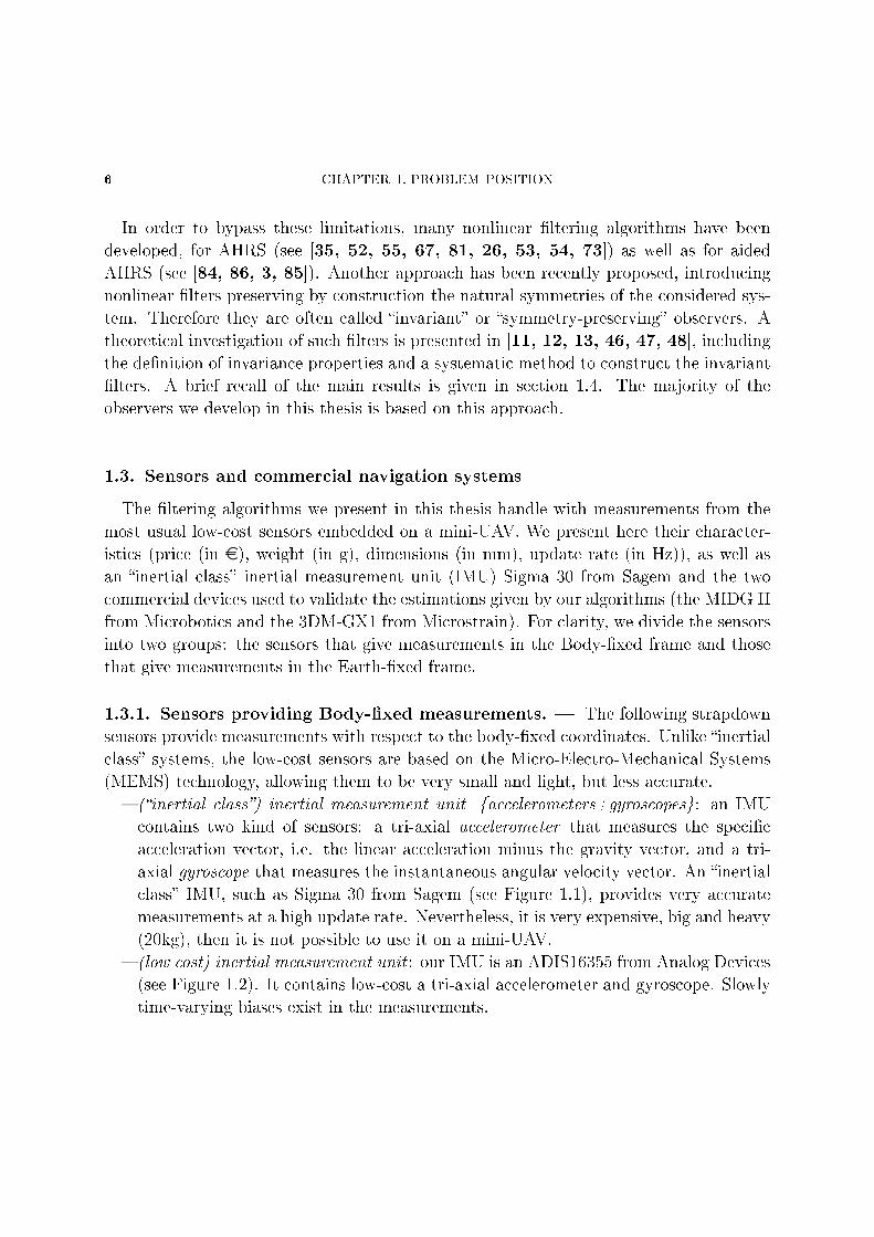
1.3.1. Sensors providing Body-xed measurements. The following strapdown
sensors provide measurements with respect to the body-xed coordinates. Unlike inertial
class systems, the low-cost sensors are based on the Micro-Electro-Mechanical Systems
(MEMS) technology, allowing them to be very small and light, but less accurate.
(inertial class) inertial measurement unit=accelerometers+gyroscopes: an IMU
contains two kind of sensors: a tri-axial accelerometer that measures the specic
acceleration vector, i.e. the linear acceleration minus the gravity vector, and a tri-
axial gyroscope that measures the instantaneous angular velocity vector. An inertial
class IMU, such as Sigma 30 from Sagem (see Figure 1.1), provides very accurate
measurements at a high update rate. Nevertheless, it is very expensive, big and heavy
(20kg), then it is not possible to use it on a mini-UAV.
(low cost) inertial measurement unit : our IMU is an ADIS16355 from Analog Devices
(see Figure 1.2). It contains low-cost a tri-axial accelerometer and gyroscope. Slowly
time-varying biases exist in the measurements.

1.3. SENSORS AND COMMERCIAL NAVIGATION SYSTEMS 7
Figure 1.1. Inertial class IMU Sigma 30
Cost Weight Size Update rate
300 25 23,32,23 100
Figure 1.2. Inertial measurement unit ADIS16355
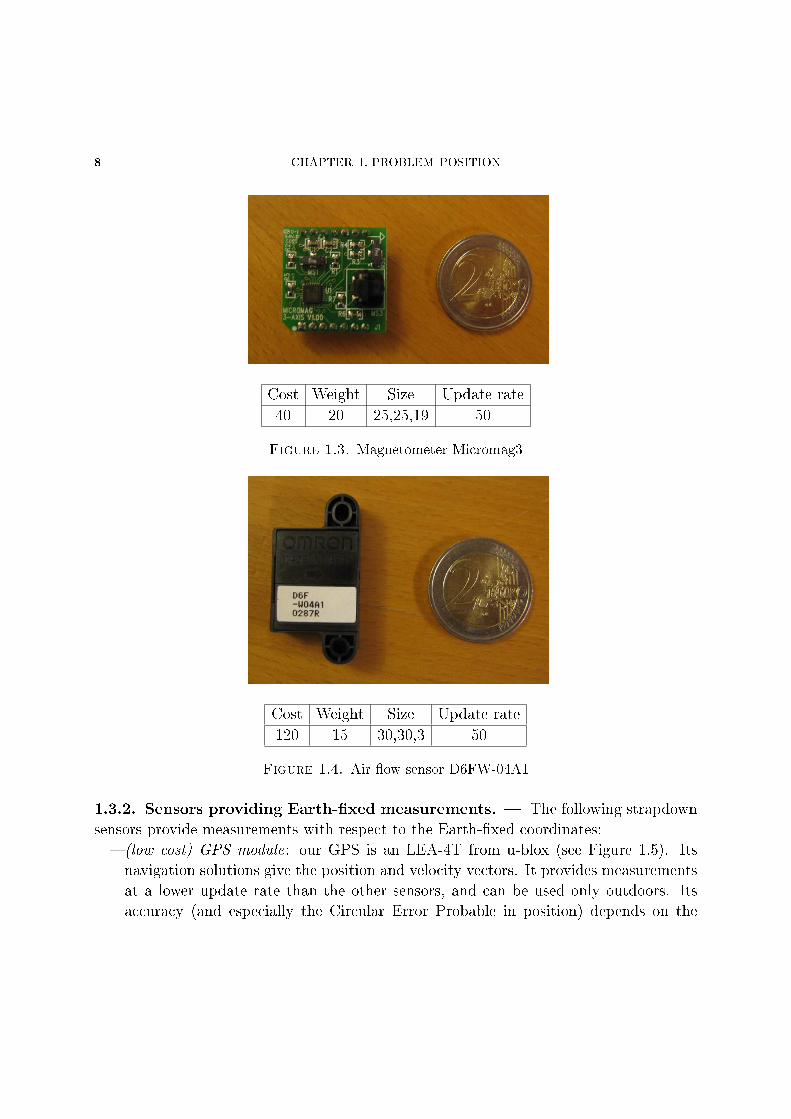
(low cost) magnetometers : our tri-axial magnetometer is a Micromag3 from PNI (see
Figure 1.3). It measures the magnetic eld, which then may be subject to magnetic
disturbances (in urban areas for instance).
(low cost) air velocity sensor : we use the D6FW-04A1 from Omron that measures
the air ow (see Figure 1.4).
8 CHAPTER 1. PROBLEM POSITION
Cost Weight Size Update rate
40 20 25,25,19 50
Figure 1.3. Magnetometer Micromag3
Cost Weight Size Update rate
120 15 30,30,3 50
Figure 1.4. Air ow sensor D6FW-04A1
1.3.2. Sensors providing Earth-xed measurements. The following strapdown
sensors provide measurements with respect to the Earth-xed coordinates:
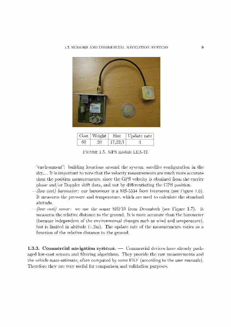
(low cost) GPS module: our GPS is an LEA-4T from u-blox (see Figure 1.5). Its
navigation solutions give the position and velocity vectors. It provides measurements
at a lower update rate than the other sensors, and can be used only outdoors. Its
accuracy (and especially the Circular Error Probable in position) depends on the
1.3. SENSORS AND COMMERCIAL NAVIGATION SYSTEMS 9
Cost Weight Size Update rate
60 20 17,22,3 4
Figure 1.5. GPS module LEA-4T
environment: building locations around the system, satellite conguration in the
sky,... It is important to note that the velocity measurements are much more accurate
than the position measurements, since the GPS velocity is obtained from the carrier
phase and/or Doppler shift data, and not by dierentiating the GPS position.
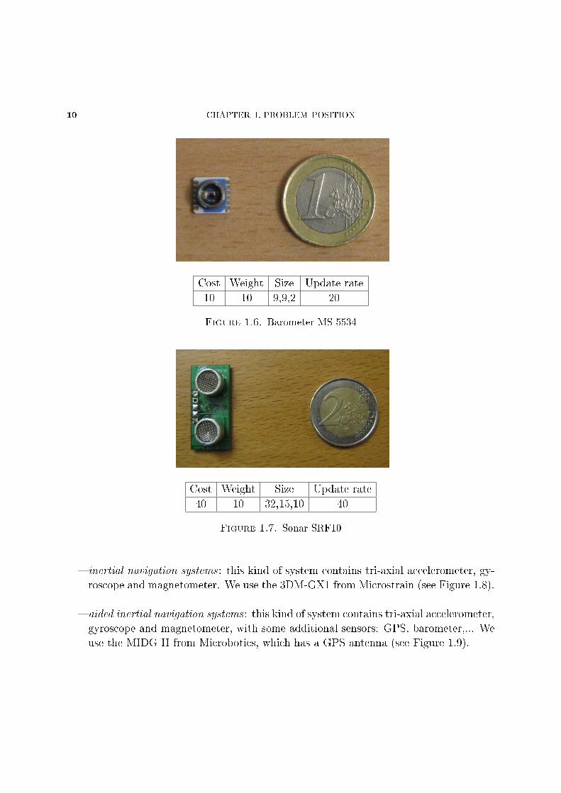
(low cost) barometer : our barometer is a MS-5534 from Intersema (see Figure 1.6).
It measures the pressure and temperature, which are used to calculate the standard
altitude.
(low cost) sonar : we use the sonar SRF10 from Devantech (see Figure 1.7). It
measures the relative distance to the ground. It is more accurate than the barometer
(because independent of the environmental changes such as wind and temperature),
but is limited in altitude (<2m). The update rate of the measurements varies as a
function of the relative distance to the ground.
1.3.3. Commercial navigation systems. Commercial devices have already pack-
aged low-cost sensors and ltering algorithms. They provide the raw measurements and
the vehicle state estimate, often computed by some EKF (according to the user manuals).
Therefore they are very useful for comparison and validation purposes.
10 CHAPTER 1. PROBLEM POSITION
Cost Weight Size Update rate
10 10 9,9,2 20
Figure 1.6. Barometer MS-5534
Cost Weight Size Update rate
40 10 32,15,10 40
Figure 1.7. Sonar SRF10
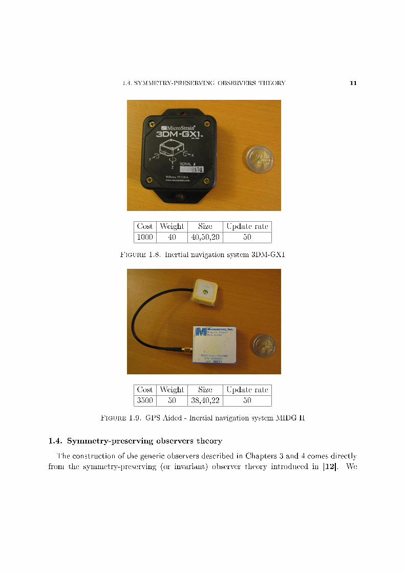
inertial navigation systems : this kind of system contains tri-axial accelerometer, gy-
roscope and magnetometer. We use the 3DM-GX1 from Microstrain (see Figure 1.8).
aided inertial navigation systems : this kind of system contains tri-axial accelerometer,
gyroscope and magnetometer, with some additional sensors: GPS, barometer,... We
use the MIDG II from Microbotics, which has a GPS antenna (see Figure 1.9).
1.4. SYMMETRY-PRESERVING OBSERVERS THEORY 11
Cost Weight Size Update rate
1000 40 40,50,20 50
Figure 1.8. Inertial navigation system 3DM-GX1
Cost Weight Size Update rate
3500 50 38,40,22 50
Figure 1.9. GPS Aided - Inertial navigation system MIDG II
1.4. Symmetry-preserving observers theory
The construction of the generic observers described in Chapters 3 and 4 comes directly
from the symmetry-preserving (or invariant) observer theory introduced in [12]. We
12 CHAPTER 1. PROBLEM POSITION
briey recall here the main ideas and denitions of this previous work, completed with an
additional result (for further details, see [12]).
1.4.1. Invariant systems and equivariant outputs.
Denition. Let G be a Lie Group with identity e and Σ an open set (or more generally
a manifold). An action of a transformation group (φg)g∈G on Σ is a smooth map
(g, ξ) ∈ G× Σ 7→ φg(ξ) ∈ Σ
such that:
φe(ξ) = ξ for all ξ
φg2 φg1(ξ) = φg2g1(ξ) for all g1, g2, ξ.
By construction φg is a dieomorphism on Σ for all g. The transformation group is
local if φg(ξ) is dened only for g in a neighborhood of e. In this case the transformation
law φg2 φg1(ξ) = φg2g1(ξ) is dened only when it makes sense. We consider only local
transformation groups. For all g thus means for all g around e, and for all ξ means
for all ξ in some neighborhood.
Consider now the smooth output system
x = f(x, u)(1)
y = h(x, u)(2)
where x belongs to an open subset X ⊂ Rn, u to an open subset U ⊂ Rm and y to an
open subset Y ⊂ Rp, p ≤ n.
We assume the signals u(t), y(t) to be known (y is measured, and u is measured or
known as a control input).
Consider also the local group of transformations on X × U dened by (X,U) =(ϕg(x), ψg(u)
), where ϕg and ψg are local dieomorphisms.
Denition. The system x = f(x, u) is G-invariant if
f(ϕg(x), ψg(u)
)= Dϕg(x) · f(x, u) for all g, x, u.
With (X,U) =(ϕg(x), ψg(u)
), the property also reads X = f(X,U), i.e., the system is
left unchanged by the transformation.
Denition. The output y = h(x, u) is G-equivariant if there exists a transformation
group (ρg)g∈G on Y such that h(ϕg(x), ψg(u)
)= ρg
(h(x, u)
)for all g, x, u.
With (X,U) =(ϕg(x), ψg(u)
)and Y = %g(y), the denition reads Y = h(X,U).
1.4. SYMMETRY-PRESERVING OBSERVERS THEORY 13
1.4.2. Invariant preobservers.
Denition (Preobserver). The system ˙x = F (x, u, y) is a preobserver of the sys-
tem (1)-(2) if F(x, u, h(x)
)= f(x, u) for all x, u.
An observer is then a preobserver such that x(t)→ x(t) (possibly only locally).
Denition. The preobserver ˙x = F (x, u, y) is G-invariant if
F(ϕg(x), ψg(u), ρg(y)
)= Dϕg(x) · F (x, u, y) for all g, x, u, y.
The property also reads˙X = F (X, U, Y ), i.e., the system is left unchanged by the
transformation.
The key idea to build an invariant preobserver is to use an invariant output error.
Denition. The smooth map (x, u, y) 7→ E(x, u, y) ∈ Y is an invariant output error
if
the map y 7→ E(x, u, y) is invertible for all x, u
E(x, u, h(x, u)
)= 0 for all x, u
E(ϕg(x), ψg(u), ρg(y)
)= E(x, u, y) for all x, u, y
The rst and second properties mean E is an output error", i.e. it is zero if and
only if h(x, u) = y; the third property, which also reads E(X, U, Y ) = E(x, u, y), denes
invariance.
Similarly, the key idea to study the convergence of an invariant preobserver is to use
an invariant state error.
Denition. The smooth map (x, x) 7→ η(x, x) ∈ X is an invariant state error if
it is a dieomorphism on X × X η(x, x) = 0 for all x
η(ϕg(x), ϕg(x)
)= η(x, x) for all x, x.
We now state the two main results based on the Cartan moving frame method in
the special case where g 7→ ϕg(x) is a free and transitive action, see [12] for the general
case. The moving frame x 7→ γ(x) is obtained by solving for g the so-called normalization
equation ϕg(x) = c for some arbitrary constant c; in other words ϕγ(x)(x) = c. The func-
tion ψg may also be used in the normalization equation(ϕg(x), ψg(u)
)= c, as illustrated
in section 4.3.
14 CHAPTER 1. PROBLEM POSITION
Theorem. The general form of any invariant preobserver is
F (x, u, y) = f(x, u) +n∑i=1
(Li(E, I) · E
)wi(x),
where:
wi,i = 1, . . . , n, is the invariant vector eld dened by
wi(x) =[Dϕγ(x)(x)
]−1 · ∂∂xi
,
with ∂∂xi
the ith canonical vector eld on X , E is the invariant error dened by
E(x, u, y) = ργ(x)
(h(x, u)
)− ργ(x)(y),
I is the (complete) invariant dened by
I(x, u) = ψγ(x)(u),
Li, i = 1, . . . , n, is a 1 × p matrix with entries possibly depending on E and I, and
can be freely chosen.
Theorem. The error system reads η = Υ(η, I) for some smooth function Υ, where η
is the invariant state error dened by
η(x, x) = ϕγ(x)(x)− ϕγ(x)(x).
This result greatly simplies the convergence analysis of the preobserver, since the error
equation is autonomous but for the free known invariant I. Indeed for a general nonlinear
(not invariant) observer the error equation depends on the trajectory t 7→(x(t), u(t)) of
the system, hence is in fact of dimension 2n+m, whereas the dimension of the invariant
state error equation is only 2n + m − dim(G). To simplify, we will use from now on the
term observer instead of preobserver.
1.5. Thesis outline
The thesis contains three main parts:
in Chapters 3, 4 and 5, we propose symmetry-preserving generic nonlinear observers
for a moving body, and validate them through experimental comparisons with a
commercial device. In Chapter 2, we present an discuss the moving body models
that we considered to build these observers.
1.5. THESIS OUTLINE 15
in Chapter 6, we construct specic observers for a mini-quadrotor based on the rotor
drag, and validate them through ight tests
in Chapter 7, we present the real-time implementation of the preceding observers on
a home-built low-cost embedded prototype system.
In Chapter 2, we rst introduce dierent models used in the navigation systems and
highlight the dierences between true inertial navigation based on the Schuler eect
thanks to very accurate inertial sensors, and the low-cost navigation systems based on
a at Earth assumption. These low-cost navigation systems are called Attitude and
Heading Reference Systems (AHRS) when they use only inertial sensors (often completed
by magnetometers), and they are called aided Attitude and Heading Reference Systems
(aided AHRS) when they have additional velocity and/or position sensors. Then we
construct invariant (or symmetry-preserving) nonlinear observers for AHRS in Chapter 3
(see [60, 62]), and for aided AHRS in Chapter 4 (see [61, 64, 63]): by preserving
the geometrical properties of the system, they bypass the limitations of the usual ltering
methods. Especially we study their nice rst-order behavior (even in presence of magnetic
disturbances), their large convergence domain and their easy tuning. We validate these
lters by comparing their estimations with those provided by commercial devices. We also
present the Invariant Extended Kalman Filter in Chapter 5 (see [14]), which combines
the EKF approach and the advantages of the invariant observers. Especially we extend
the Multiplicative Extended Kalman Filter (MEKF), commonly used in avionics systems.
In Chapter 6, we rst give the physical model of the mini-quadrotor: in this model,
we consider especially the rotor drag that comes in addition to the usual thrust and drag
torques (see [59]). Then we construct a specic observer based on this model, which
estimates the velocity of the quadrotor with only inertial sensors measurements. This
allows to control the quadrotor velocity thanks to a linear control laws and to achieve
a hovering ight with only inertial sensors. We validate this model trough experimental
ights, giving by the way new perspectives in the mini-quadrotor modeling and control.
Moreover, it gives a new interpretation of the usual approach followed by the previous
researches in this area, which assume a small linear acceleration to estimate the attitude
angles thanks to the accelerometer. measurementsor which use commercial AHRS.
In Chapter 7, we rst implement the generic observers of Chapters 3 and 4 on a cheap
8-bit microcontroller, highlighting their computational eciency compared to the usual
ltering algorithms. Then we detail the hardware and software architecture of the embed-
ded avionics system we developed, which contains low-cost sensors and microcontroller
and can be easily mounted on any kind of mini-UAV. We validate the preceding lters on

16 CHAPTER 1. PROBLEM POSITION
this prototype system by comparing the estimations given by our generic observers with
those provided by commercial devices (see [66, 65, 61]).
CHAPTER 2
MODELS FOR NAVIGATION SYSTEMS
Dans ce chapitre, nous présentons les diérents modèles génériques, principalement
fonctions du type et de la nature des capteurs embarqués, utilisés habituellement dans
les systèmes de navigation. Dans la section 2.1, nous rappelons l'eet Schuler, basé sur
un modèle de terre ronde, et dont on peut bénécier lorsque l'on a accès à des capteurs
inertiels haut de gamme. Seuls des capteurs bas-coûts sont utilisés sur un mini-drone,
nous ne pouvons donc pas bénecier de l'eet Schuler, et le modèle de terre plate décrit
dans la section 2.2 est amplement susant. Nous présentons alors les modèles utilisés par
la suite pour construire les ltres des Attitude and Heading Reference Systems (section
2.4) et des aided Attitude and Heading Reference Systems (section 2.4). Les propriétés
d'invariance des diérents modèles sont présentées dans la section 2.5.
2.1. Round Earth model and true inertial navigation
2.1.1. Earth and moving rigid body models. The true inertial navigation
is mainly based on measurements provided by two strap-down high-precision sensors:
a tri-axial accelerometer that measures the specic acceleration vector, i.e. the linear
18 CHAPTER 2. MODELS FOR NAVIGATION SYSTEMS
acceleration minus the gravity vector, and a tri-axial gyroscope that measures the angular
velocity vector. These measurements are given in the body-xed frame and are very
accurate (small and very time-stable biases, small noise). An accurate model of the Earth
is used in the observer algorithm: it is considered as a rotating ellipsoid with a gravity
vector depending on the altitude. To illustrate the benets of this kind of system, and
especially the Schuler eect, we consider for simplicity a 3-dimensional non-rotating
round Earth (radius R): indeed the main conclusions depend only on the roundness of
the Earth and its gravity vector varying with the altitude. A more detailed study of the
Schuler eect can be found in [28, 23, 31, 6, 76, 30, 19].
We dene the three following frames:
the body-xed frame: Rb = (−→ib ,−→jb ,−→kb )
the local North-East-Down frame: Rl = (−→il ,−→jl ,−→kl )
the Earth-xed frame: Re = (−→ie ,−→je ,−→ke)
For a 3×1 vector−→P we dene
−→P |i as the projection of
−→P on the frame Ri and the matrix
Mi/j as the rotation matrix from the frame Rj to the frame Ri, where i, j ∈ b, l, e. Forinstance
−→P |b = Mb/l
−→P |l. We dene also the instantaneous angular velocity vector
−→Ω i/j
of the frame Ri with respect to the frame Rj. For more details in the denition of the
dierent frames we use, see [28, 23, 79, 69].
The motion equations of a moving rigid body are
−→V = −→g +−→a(3)
−→X =
−→V(4)
where:
−→V is the velocity vector of the center of mass with respect to the Earth-xed frame
−→g is the gravitational acceleration vector
−→a is the specic acceleration vector
−→X is the position vector of the center of mass
2.1. ROUND EARTH MODEL AND TRUE INERTIAL NAVIGATION 19
We dene the following projected vectors
V =−→V |l = (VN , VE, VD)
v =−→V |b
Xe =−→X |e = (x0, y0, z0) with the altitude h dened by R + h =
√x2
0 + y20 + z2
0
A = −→g |l = (0, 0, g(h))
a = −→a |bωb/l =
−−→Ωb/l|b
ωb/e =−−→Ωb/e|b
Ωl/e =−−→Ωl/e|l = (
VER + h
,−VNR + h
,−VER + h
tanλ) where λ is the latitude.
To be coherent with the North-East-Down frame we dene z = −h. For a vector
P = (P1, P2, P3) we dene P× the skew-symmetric matrix
P× =
0 −P3 P2
P3 0 −P1
−P2 P1 0
.
Let (φ, θ, ψ) the usual Euler angles (roll, pitch, yaw). Then the rotation matrix Mb/l
writes (cθ = cos θ and sθ = sin θ)
Mb/l =
cθcψ cθsψ −sθsφsθcψ − cφsψ sφsθsψ + cφcψ sφcθ
cφsθcψ + sφsψ cφsθsψ − sφcψ cφcθ
.
The projected motion equations write
Mb/l = Mb/lω×b/l = Mb/l(ω
×b/e −Mb/lΩ
×l/e)(5)
V = −Ωl/e × V + A+Ml/ba(6)
z = VD.(7)
We suppose that the gravity varies with altitude according to the inverse square law:
g(z) =g0
(1− zR
)2.
We use 2 kinds of sensors: a tri-axial gyroscope measures ωm (= ωb/e if perfect) and
a tri-axial accelerometer measures am (= a if perfect). Even if very accurate sensors are
20 CHAPTER 2. MODELS FOR NAVIGATION SYSTEMS
used in true inertial navigation, some imperfections still remain in their measurements,
and especially biases. With such high-precision sensors, their biases are small and very
stable in time. Then we consider that the gyroscope measures ωm = ωb/e + ωb and the
accelerometer measures am = a+ ab, where ωb and ab are constant biases.
Considering these imperfections in the measurements, the system (5)(7) becomes
Mb/l = Mb/l((ωm − ωb)× −Mb/lΩ×l/e)(8)
V = −Ωl/e × V + A+Ml/b(am − ab)(9)
z = VD(10)
ωb = 0(11)
ab = 0.(12)
2.1.2. Can we estimate the state? To estimate the state of the moving rigid body,
we must construct an observer based on Equations (8)(12). The correction terms of
the estimator depend on the estimations and the measurements that are considered as
outputs of the system.
The 6 measurements provided by the inertial sensors are the inputs of the system (8)
(12). So this system has no output, and then it is not observable. The only way to
estimate the state is writing an observer as just a copy of the nonlinear system (8)
(12). Since the observer has no correction terms, we need to gure out the behavior of
the estimated state in the presence of errors: does the system diverge or not? It is an
analysis of its detectability. We rst study the system linearized around the equilibrium
point(Mb/l, V , z, λ, ωb, ab)
δMb/l = δMb/l((ωm − ωb)× −Mb/lΩl/e×
) +Mb/l((δωm − δωb)× −Mb/lδΩ×l/e − δMb/lΩl/e
×)
δV = −Ωl/e × δV − δΩl/e × V + A+Ml/b(δam − δab) + δMl/b(am − ab)δz = δVD
δωb = 0
δab = 0.
For simplicity, we consider the nominal equilibrium point
(Mb/l, V , z, λ, ωb, ab) = (I3, 0, z, λ, ωm, am + A).
The linearized system splits into three decoupled subsystems and one cascaded subsystem:
2.1. ROUND EARTH MODEL AND TRUE INERTIAL NAVIGATION 21
the lateral subsystem
δφ = − δVER− z
− δωb1 + δωm1
δVE = g(z)δφ− δab2 + δam2
δωb1 = 0
δab2 = 0
the longitudinal subsystem
δθ =δVNR− z
− δωb2 + δωm2
δVN = −g(z)δθ − δab1 + δam1
δωb2 = 0
δab1 = 0
the vertical subsystem
δVD =2g(z)
R− zδz − δab3 + δam3
δz = δVD
δab3 = 0
the heading subsystem (cascaded with the lateral subsystem)
δψ =tanλ
R− zδVE − δωb3 + δωm3
δωb3 = 0.
We construct the corresponding linearized observer:
the lateral subsystem
δ˙φ = − δVE
R− z− δωb1 + δωm1
δ˙VE = g(z)δφ− δab2 + δam2
δ ˙ωb1 = 0
δ ˙ab2 = 0
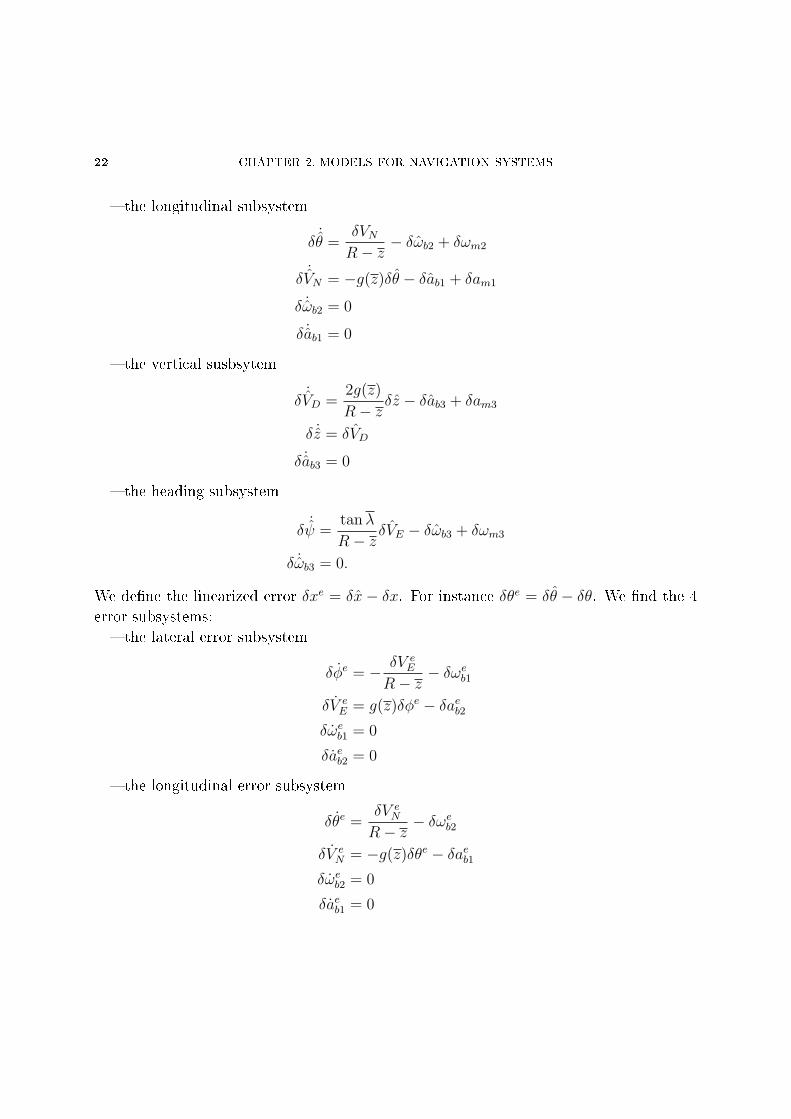
22 CHAPTER 2. MODELS FOR NAVIGATION SYSTEMS
the longitudinal subsystem
δ˙θ =
δVNR− z
− δωb2 + δωm2
δ˙VN = −g(z)δθ − δab1 + δam1
δ ˙ωb2 = 0
δ ˙ab1 = 0
the vertical susbsytem
δ˙VD =
2g(z)
R− zδz − δab3 + δam3
δ ˙z = δVD
δ ˙ab3 = 0
the heading subsystem
δ˙ψ =
tanλ
R− zδVE − δωb3 + δωm3
δ ˙ωb3 = 0.
We dene the linearized error δxe = δx− δx. For instance δθe = δθ − δθ. We nd the 4
error subsystems:
the lateral error subsystem
δφe = − δV eE
R− z− δωeb1
δV eE = g(z)δφe − δaeb2
δωeb1 = 0
δaeb2 = 0
the longitudinal error subsystem
δθe =δV e
N
R− z− δωeb2
δV eN = −g(z)δθe − δaeb1
δωeb2 = 0
δaeb1 = 0
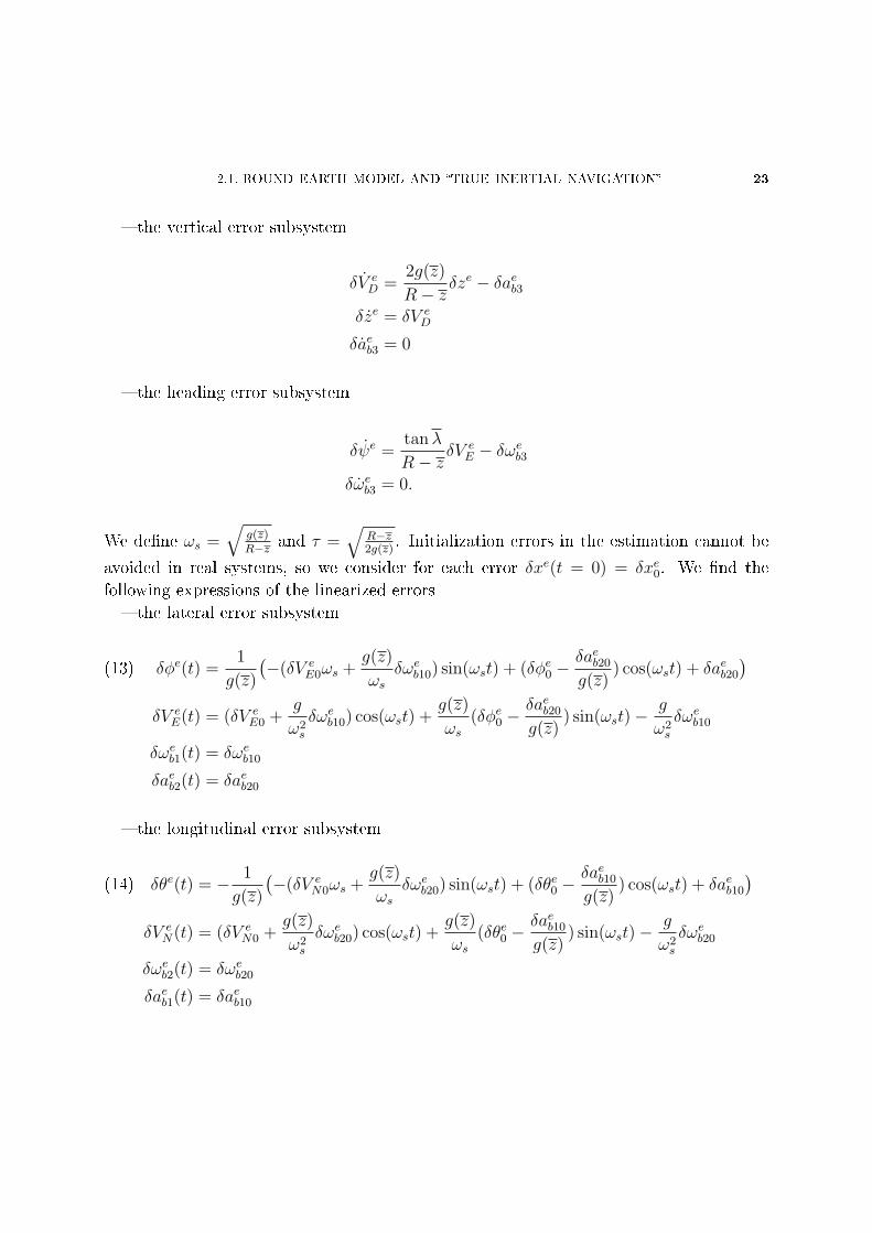
2.1. ROUND EARTH MODEL AND TRUE INERTIAL NAVIGATION 23
the vertical error subsystem
δV eD =
2g(z)
R− zδze − δaeb3
δze = δV eD
δaeb3 = 0
the heading error subsystem
δψe =tanλ
R− zδV e
E − δωeb3δωeb3 = 0.
We dene ωs =√
g(z)R−z and τ =
√R−z2g(z)
. Initialization errors in the estimation cannot be
avoided in real systems, so we consider for each error δxe(t = 0) = δxe0. We nd the
following expressions of the linearized errors
the lateral error subsystem
δφe(t) =1
g(z)
(−(δV e
E0ωs +g(z)
ωsδωeb10) sin(ωst) + (δφe0 −
δaeb20
g(z)) cos(ωst) + δaeb20
)(13)
δV eE(t) = (δV e
E0 +g
ω2s
δωeb10) cos(ωst) +g(z)
ωs(δφe0 −
δaeb20
g(z)) sin(ωst)−
g
ω2s
δωeb10
δωeb1(t) = δωeb10
δaeb2(t) = δaeb20
the longitudinal error subsystem
δθe(t) = − 1
g(z)
(−(δV e
N0ωs +g(z)
ωsδωeb20) sin(ωst) + (δθe0 −
δaeb10
g(z)) cos(ωst) + δaeb10
)(14)
δV eN(t) = (δV e
N0 +g(z)
ω2s
δωeb20) cos(ωst) +g(z)
ωs(δθe0 −
δaeb10
g(z)) sin(ωst)−
g
ω2s
δωeb20
δωeb2(t) = δωeb20
δaeb1(t) = δaeb10
24 CHAPTER 2. MODELS FOR NAVIGATION SYSTEMS
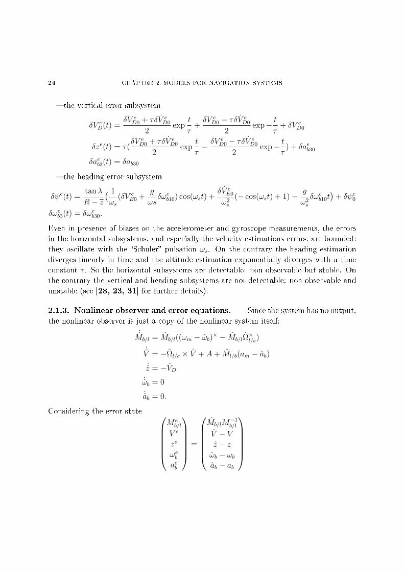
the vertical error subsystem
δV eD(t) =
δV eD0 + τδV e
D0
2exp
t
τ+δV e
D0 − τδV eD0
2exp− t
τ+ δV e
D0
δze(t) = τ(δV e
D0 + τδV eD0
2exp
t
τ− δV e
D0 − τδV eD0
2exp− t
τ) + δaeb30
δaeb3(t) = δab30
the heading error subsystem
δψe(t) =tanλ
R− z( 1
ωs(δV e
E0 +g
ωsδωeb10) cos(ωst) +
δV eE0
ω2s
(− cos(ωst) + 1)− g
ω2s
δωeb10t)
+ δψe0
δωeb3(t) = δωeb30.
Even in presence of biases on the accelerometer and gyroscope measurements, the errors
in the horizontal subsystems, and especially the velocity estimations errors, are bounded:
they oscillate with the Schuler pulsation ωs. On the contrary the heading estimation
diverges linearly in time and the altitude estimation exponentially diverges with a time
constant τ . So the horizontal subsystems are detectable: non observable but stable. On
the contrary the vertical and heading subsystems are not detectable: non observable and
unstable (see [28, 23, 31] for further details).
2.1.3. Nonlinear observer and error equations. Since the system has no output,
the nonlinear observer is just a copy of the nonlinear system itself:
˙Mb/l = Mb/l((ωm − ωb)× − Mb/lΩ
×l/e)
˙V = −Ωl/e × V + A+ Ml/b(am − ab)˙z = −VD
˙ωb = 0
˙ab = 0.
Considering the error state M e
b/l
V e
ze
ωebaeb
=
Mb/lM
−1b/l
V − Vz − zωb − ωbab − ab
2.1. ROUND EARTH MODEL AND TRUE INERTIAL NAVIGATION 25
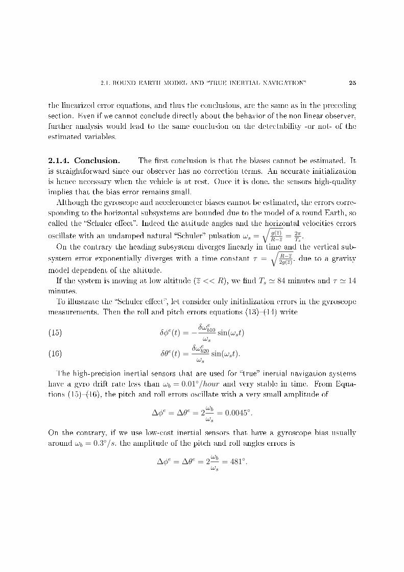
the linearized error equations, and thus the conclusions, are the same as in the preceding
section. Even if we cannot conclude directly about the behavior of the non linear observer,
further analysis would lead to the same conclusion on the detectability -or not- of the
estimated variables.
2.1.4. Conclusion. The rst conclusion is that the biases cannot be estimated. It
is straightforward since our observer has no correction terms. An accurate initialization
is hence necessary when the vehicle is at rest. Once it is done, the sensors high-quality
implies that the bias error remains small.
Although the gyroscope and accelerometer biases cannot be estimated, the errors corre-
sponding to the horizontal subsystems are bounded due to the model of a round Earth, so
called the Schuler eect. Indeed the attitude angles and the horizontal velocities errors
oscillate with an undamped natural Schuler pulsation ωs =√
g(z)R−z = 2π
Ts.
On the contrary the heading subsystem diverges linearly in time and the vertical sub-
system error exponentially diverges with a time constant τ =√
R−z2g(z)
, due to a gravity
model dependent of the altitude.
If the system is moving at low altitude (z << R), we nd Ts ' 84 minutes and τ ' 14
minutes.
To illustrate the Schuler eect, let consider only initialization errors in the gyroscope
measurements. Then the roll and pitch errors equations (13)(14) write
δφe(t) = −δωeb10
ωssin(ωst)(15)
δθe(t) =δωeb20
ωssin(ωst).(16)
The high-precision inertial sensors that are used for true inertial navigation systems
have a gyro drift rate less than ωb = 0.01/hour and very stable in time. From Equa-
tions (15)(16), the pitch and roll errors oscillate with a very small amplitude of
∆φe = ∆θe = 2ωbωs
= 0.0045.
On the contrary, if we use low-cost inertial sensors that have a gyroscope bias usually
around ωb = 0.3/s, the amplitude of the pitch and roll angles errors is
∆φe = ∆θe = 2ωbωs
= 481.
26 CHAPTER 2. MODELS FOR NAVIGATION SYSTEMS
So we denitely cannot use the Schuler eect with low-cost inertial sensors: the amplitude
of the oscillations of the estimations becomes too important too quickly. Then we need
correction terms in our observer, and thus additional measurements or assumptions.
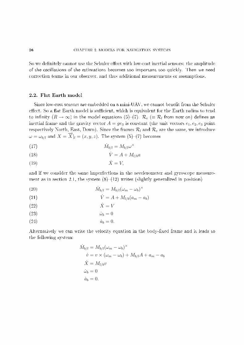
2.2. Flat Earth model
Since low-cost sensors are embedded on a mini-UAV, we cannot benet from the Schuler
eect. So a at Earth model is sucient, which is equivalent for the Earth radius to tend
to innity (R → ∞) in the model equations (5)(7). Re (≡ Rl from now on) denes an
inertial frame and the gravity vector A = ge3 is constant (the unit vectors e1, e2, e3 point
respectively North, East, Down). Since the frames Rl and Re are the same, we introduce
ω = ωb/l and X =−→X |l = (x, y, z). The system (5)(7) becomes
Mb/l = Mb/lω×(17)
V = A+Ml/ba(18)
X = V,(19)
and if we consider the same imperfections in the accelerometer and gyroscope measure-
ment as in section 2.1, the system (8)(12) writes (slightly generalized in position)
Mb/l = Mb/l(ωm − ωb)×(20)
V = A+Ml/b(am − ab)(21)
X = V(22)
ωb = 0(23)
ab = 0.(24)
Alternatively we can write the velocity equation in the body-xed frame and it leads to
the following system:
Mb/l = Mb/l(ωm − ωb)×
v = v × (ωm − ωb) +Mb/lA+ am − abX = Ml/bv
ωb = 0
ab = 0.
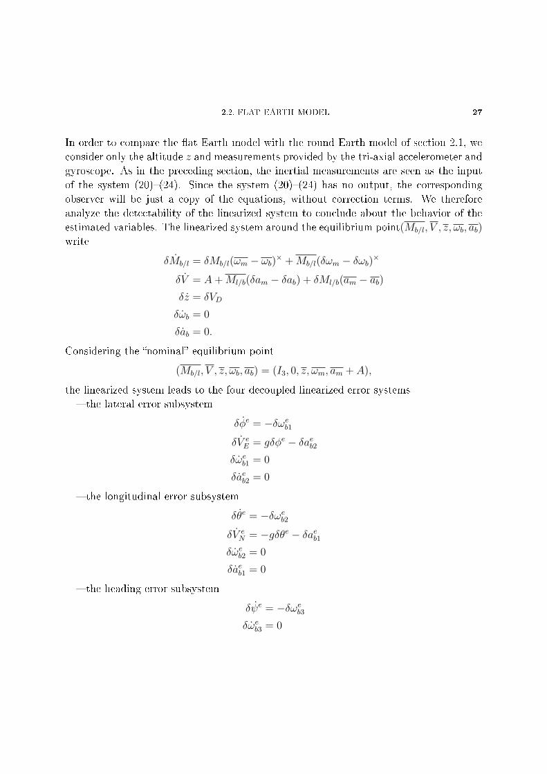
2.2. FLAT EARTH MODEL 27
In order to compare the at Earth model with the round Earth model of section 2.1, we
consider only the altitude z and measurements provided by the tri-axial accelerometer and
gyroscope. As in the preceding section, the inertial measurements are seen as the input
of the system (20)(24). Since the system (20)(24) has no output, the corresponding
observer will be just a copy of the equations, without correction terms. We therefore
analyze the detectability of the linearized system to conclude about the behavior of the
estimated variables. The linearized system around the equilibrium point(Mb/l, V , z, ωb, ab)
write
δMb/l = δMb/l(ωm − ωb)× +Mb/l(δωm − δωb)×
δV = A+Ml/b(δam − δab) + δMl/b(am − ab)δz = δVD
δωb = 0
δab = 0.
Considering the nominal equilibrium point
(Mb/l, V , z, ωb, ab) = (I3, 0, z, ωm, am + A),
the linearized system leads to the four decoupled linearized error systems
the lateral error subsystem
δφe = −δωeb1δV e
E = gδφe − δaeb2δωeb1 = 0
δaeb2 = 0
the longitudinal error subsystem
δθe = −δωeb2δV e
N = −gδθe − δaeb1δωeb2 = 0
δaeb1 = 0
the heading error subsystem
δψe = −δωeb3δωeb3 = 0
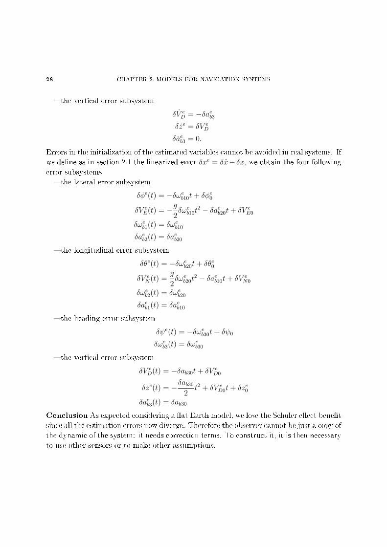
28 CHAPTER 2. MODELS FOR NAVIGATION SYSTEMS
the vertical error subsystem
δV eD = −δaeb3
δze = δV eD
δaeb3 = 0.
Errors in the initialization of the estimated variables cannot be avoided in real systems. If
we dene as in section 2.1 the linearized error δxe = δx− δx, we obtain the four following
error subsystems
the lateral error subsystem
δφe(t) = −δωeb10t+ δφe0
δV eE(t) = −g
2δωeb10t
2 − δaeb20t+ δV eE0
δωeb1(t) = δωeb10
δaeb2(t) = δaeb20
the longitudinal error subsystem
δθe(t) = −δωeb20t+ δθe0
δV eN(t) =
g
2δωeb20t
2 − δaeb10t+ δV eN0
δωeb2(t) = δωeb20
δaeb1(t) = δaeb10
the heading error subsystem
δψe(t) = −δωeb30t+ δψ0
δωeb3(t) = δωeb30
the vertical error subsystem
δV eD(t) = −δab30t+ δV e
D0
δze(t) = −δab30
2t2 + δV e
D0t+ δze0
δaeb3(t) = δab30
Conclusion As expected considering a at Earth model, we lose the Schuler eect benet
since all the estimation errors now diverge. Therefore the observer cannot be just a copy of
the dynamic of the system: it needs correction terms. To construct it, it is then necessary
to use other sensors or to make other assumptions.
2.2. FLAT EARTH MODEL 29
If we do not have measurements from other sensors (giving information of the velocity
or position of the vehicle, for instance), the additional assumption we make is that the
linear acceleration is small, i.e. V = 0. Then we can construct an observer that estimates
the attitude angles despite sensors biases. To also estimate the yaw angle, a tri-axial
magnetometer is usually used as well, leading to an Attitude and Heading Reference
System (AHRS).
On the contrary, if we have additional measurements (velocity, position, altitude), the
aided Attitude and Heading Reference Systems (aided AHRS) can estimate the whole
sate without making the preceding assumption.
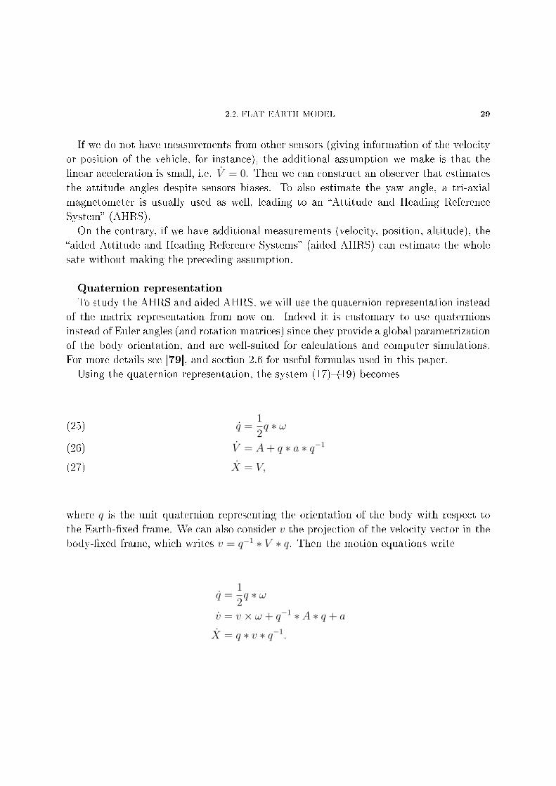
Quaternion representation
To study the AHRS and aided AHRS, we will use the quaternion representation instead
of the matrix representation from now on. Indeed it is customary to use quaternions
instead of Euler angles (and rotation matrices) since they provide a global parametrization
of the body orientation, and are well-suited for calculations and computer simulations.
For more details see [79], and section 2.6 for useful formulas used in this paper.
Using the quaternion representation, the system (17)(19) becomes
q =1
2q ∗ ω(25)
V = A+ q ∗ a ∗ q−1(26)
X = V,(27)
where q is the unit quaternion representing the orientation of the body with respect to
the Earth-xed frame. We can also consider v the projection of the velocity vector in the
body-xed frame, which writes v = q−1 ∗ V ∗ q. Then the motion equations write
q =1
2q ∗ ω
v = v × ω + q−1 ∗ A ∗ q + a
X = q ∗ v ∗ q−1.
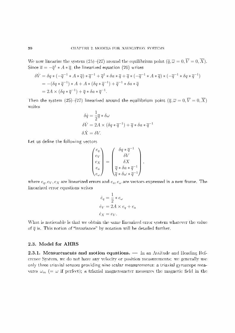
30 CHAPTER 2. MODELS FOR NAVIGATION SYSTEMS
We now linearize the system (25)(27) around the equilibrium point (q, ω = 0, V = 0, X).
Since a = −q1 ∗ A ∗ q, the linearized equation (26) writes
δV = δq ∗ (−q−1 ∗ A ∗ q) ∗ q−1 + q1 ∗ δa ∗ q + q ∗ (−q−1 ∗ A ∗ q) ∗ (−q−1 ∗ δq ∗ q−1)
= −(δq ∗ q−1) ∗ A+ A ∗ (δq ∗ q−1) + q−1 ∗ δa ∗ q= 2A× (δq ∗ q−1) + q ∗ δa ∗ q−1.
Then the system (25)(27) linearized around the equilibrium point (q, ω = 0, V = 0, X)
writes
δq =1
2q ∗ δω
δV = 2A× (δq ∗ q−1) + q ∗ δa ∗ q−1
δX = δV.
Let us dene the following vectorseqeVeXeaeω
=
δq ∗ q−1
δV
δX
q ∗ δa ∗ q−1
q ∗ δω ∗ q−1
,
where eq, eV , eX are linearized errors and ea, eω are vectors expressed in a new frame. The
linearized error equations writes
eq =1
2∗ eω
eV = 2A× eq + ea
eX = eV .
What is noticeable is that we obtain the same linearized error system whatever the value
of q is. This notion of invariance by rotation will be detailed further.
2.3. Model for AHRS
2.3.1. Measurements and motion equations. In an Attitude and Heading Ref-
erence System, we do not have any velocity or position measurements: we generally use
only three triaxial sensors providing nine scalar measurements: a triaxial gyroscope mea-
sures ωm (= ω if perfect); a triaxial magnetometer measures the magnetic eld in the
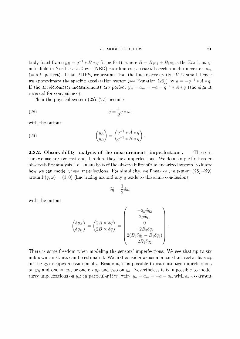
2.3. MODEL FOR AHRS 31
body-xed frame yB = q−1 ∗B ∗ q (if perfect), where B = B1e1 +B3e3 is the Earth mag-
netic eld in North-East-Down (NED) coordinates ; a triaxial accelerometer measures am(= a if perfect). In an AHRS, we assume that the linear acceleration V is small, hence
we approximate the specic acceleration vector (see Equation (26)) by a = −q−1 ∗ A ∗ q.If the accelerometer measurements are perfect yA = am = −a = q−1 ∗ A ∗ q (the sign is
reversed for convenience).
Then the physical system (25)(27) becomes
(28) q =1
2q ∗ ω,
with the output (yAyB
)=
(q−1 ∗ A ∗ qq−1 ∗B ∗ q
).(29)
2.3.2. Observability analysis of the measurements imperfections. The sen-
sors we use are low-cost and therefore they have imperfections. We do a simple rst-order
observability analysis, i.e. an analysis of the observability of the linearized system, to know
how we can model these imperfections. For simplicity, we linearize the system (28)(29)
around (q, ω) = (1, 0) (linearizing around any q leads to the same conclusion):
δq =1
2δω,
with the output
(δyAδyB
)=
(2A× δq2B × δq
)=
−2gδq2
2gδq1
0
−2B3δq2
2(B3δq1 −B1δq3)
2B1δq2
.
There is some freedom when modeling the sensors' imperfections. We see that up to six
unknown constants can be estimated. We rst consider as usual a constant vector bias ωbon the gyroscopes measurements. Beside it, it is possible to estimate two imperfections
on yB and one on ya, or one on yB and two on ya. Nevertheless it is impossible to model
three imperfections on ya: in particular if we write ya = am = −a− ab, with ab a constant
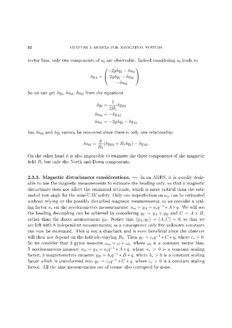
32 CHAPTER 2. MODELS FOR NAVIGATION SYSTEMS
vector bias, only two components of ab are observable. Indeed considering ab leads to
δyA =
−2gδq2 − δab12gδq1 − δab2−δab3
.
So we can get δq2, δab3, δab1 from the equations
δq2 =1
2B1
δyB3
δab3 = −δyA3
δab1 = −2gδq2 − δyA1
but δab2 and δq3 cannot be recovered since there is only one relationship:
δab2 =g
B3
(δyB2 +B1δq3)− δyA2.
On the other hand it is also impossible to estimate the three components of the magnetic
eld B, but only the North and Down components.
2.3.3. Magnetic disturbances considerations. In an AHRS, it is usually desir-
able to use the magnetic measurements to estimate the heading only, so that a magnetic
disturbance does not aect the estimated attitude, which is more critical than the esti-
mated yaw angle for the mini-UAV safety. Only one imperfection on am can be estimated
without relying on the possibly disturbed magnetic measurements, so we consider a scal-
ing factor as on the accelerometers measurements: am = yA = asq−1 ∗ A ∗ q. We will see
the heading decoupling can be achieved by considering yC = yA × yB and C = A × B,rather than the direct measurement yB. Notice that 〈yA, yC〉 = 〈A,C〉 = 0, so that we
are left with 8 independent measurements; as a consequence only ve unknown constants
can now be estimated. This is not a drawback and is even benecial since the observer
will then not depend on the latitude-varying B3. Then yC = csq−1 ∗ C ∗ q, where cs > 0.
So we consider that 3 gyros measure ωm = ω + ωb, where ωb is a constant vector bias;
3 accelerometers measure am = yA = asq−1 ∗ A ∗ q, where as > 0 is a constant scaling
factor; 3 magnetometers measure yB = bsq−1 ∗ B ∗ q, where bs > 0 is a constant scaling
factor which is transformed into yC = csq−1 ∗ C ∗ q, where cs > 0 is a constant scaling
factor. All the nine measurements are of course also corrupted by noise.
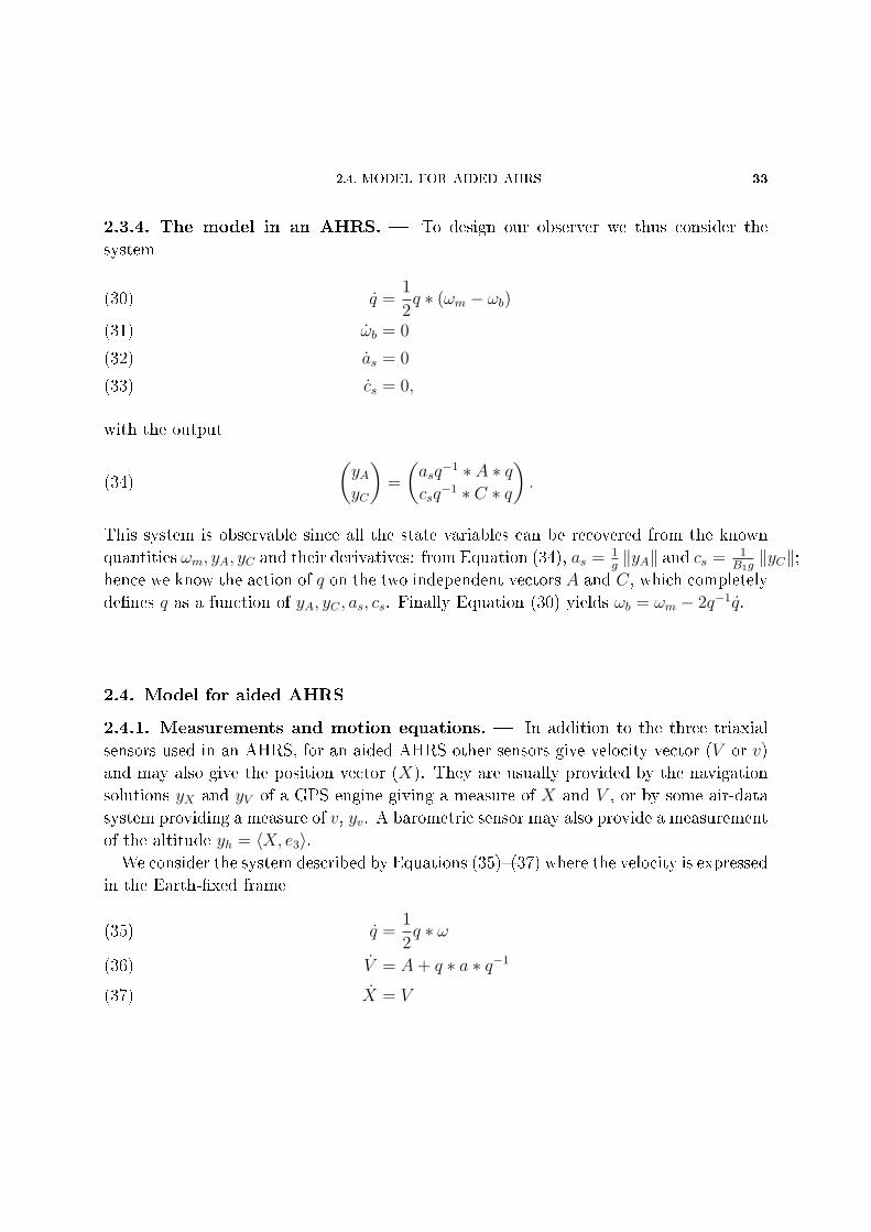
2.4. MODEL FOR AIDED AHRS 33
2.3.4. The model in an AHRS. To design our observer we thus consider the
system
q =1
2q ∗ (ωm − ωb)(30)
ωb = 0(31)
as = 0(32)
cs = 0,(33)
with the output
(34)
(yAyC
)=
(asq−1 ∗ A ∗ q
csq−1 ∗ C ∗ q
).
This system is observable since all the state variables can be recovered from the known
quantities ωm, yA, yC and their derivatives: from Equation (34), as = 1g‖yA‖ and cs = 1
B1g‖yC‖;
hence we know the action of q on the two independent vectors A and C, which completely
denes q as a function of yA, yC , as, cs. Finally Equation (30) yields ωb = ωm − 2q−1q.
2.4. Model for aided AHRS
2.4.1. Measurements and motion equations. In addition to the three triaxial
sensors used in an AHRS, for an aided AHRS other sensors give velocity vector (V or v)
and may also give the position vector (X). They are usually provided by the navigation
solutions yX and yV of a GPS engine giving a measure of X and V , or by some air-data
system providing a measure of v, yv. A barometric sensor may also provide a measurement
of the altitude yh = 〈X, e3〉.We consider the system described by Equations (35)(37) where the velocity is expressed
in the Earth-xed frame
q =1
2q ∗ ω(35)
V = A+ q ∗ a ∗ q−1(36)
X = V(37)
34 CHAPTER 2. MODELS FOR NAVIGATION SYSTEMS
or the system described by Equations (38)(40) where the velocity is expressed in the
body-xed frame
q =1
2q ∗ ω(38)
v = v × ω + q−1 ∗ A ∗ q + a(39)
X = q ∗ v ∗ q−1,(40)
the input is the inertial sensors' measurement (a and ω) and the output
yVyvyXyhyB
=
V
v
X
〈X, e3〉q−1 ∗B ∗ q
.(41)
We have some freedom to express the velocity in the Earth-xed frame of body-xed
frame, since yV = V = q−1 ∗ v ∗ q and yv = v = q−1 ∗ V ∗ q.
2.4.2. Imperfections of the measurements. As in section 2.3, a simple rst-order
observability analysis reveals that up to thirteen unknown constants can be estimated.
There are many ways to model the eight additional imperfections on the measurements.
We choose to use only ve extra constants to model imperfections: we consider here
3 biases on the gyroscope, one scaling factor on the accelerometer and one bias on the
altitude measurement, in order to ensure that the estimated velocity equals the measured
velocity (see 4.1.5.2) during level ight. The barometric sensor thus provides a measure
of the altitude yh = 〈X, e3〉−hb, where hb is a constant scalar bias. All these measurements
are of course also corrupted by noise.
2.5. INVARIANCE PROPERTIES OF THE FLAT EARTH MODEL 35
2.4.3. The considered system. To design our observers, we therefore consider the
system
q =1
2q ∗ (ωm − ωb)(42)
V = A+1
asq ∗ am ∗ q−1(43)
X = V(44)
ωb = 0(45)
as = 0(46)
hb = 0(47)
where ωm and am are seen as known inputs, together with the measured outputyVyvyXyhyB
=
V
v
X
〈X, e3〉 − hbq−1 ∗B ∗ q
.(48)
This system is observable provided B × (q ∗ am ∗ q−1) 6= 0 since all the state variables
can be recovered from the known quantities ωm, am, yV , yX , yh, yB and their derivatives.
Indeed from Equation (43), as = ‖am‖‖yV −A‖
and am
‖am‖ = q−1 ∗ yV −A‖yV −A‖
∗ q. We thus know the
action of q on the two known vectors B and yV −A, which are independent by the above
assumption; this completely denes q as a function of yB, yB, am. Finally ωb = ωm−2q−1q
is determined from Equation (42) and hb = 〈yX , e3〉 − yh from Equation (48).
2.5. Invariance properties of the at Earth model
The generic observers we construct in this thesis are based on the invariance prop-
erties of the considered system. So we are looking for frame changes that leave the
system (35)(41) unchanged. For simplicity, we consider here only ideal measurements:
the imperfections of the sensors will be taken into account in the next chapters. Several
transformations will be considered:
a right rotation: dened by the unit quaternion q0 and the relationship q → q ∗ q0
a left rotation: dened by the unit quaternion p0 and the relationship q → p0 ∗ q
36 CHAPTER 2. MODELS FOR NAVIGATION SYSTEMS
a translation in the body-xed frame: dened by the 3 × 1 vector v0 and the rela-
tionship v → v + v0
a translation in the Earth-xed frame: dened by the 3 × 1 vector V0 and the rela-
tionship V → V + V0
We do not rst consider the position variable X, since some additional diculties appear
as we will see later. So we consider the systems
(49)q =
1
2q ∗ ω
V = A+ q ∗ a ∗ q−1and
q =1
2q ∗ ω
v = v × ω + q−1 ∗ A ∗ q + a.
A global transformation of the variables (q, V ) and (q, v) is a combination of the four
preceding transformations. We dene the group composition law ? by(p0
V0
)?
(p1
V1
)=
(p0 ∗ p1
V0 + p0 ∗ V1 ∗ p−10
).
A global coordinate change of (q, V ) is the transformation group action dened by
ϕ(p0,q0,V0,v0)(q, V ) =
(q
V
)=
(p0
V0
)?
(q
V
)?
(q0
v0
)=
(p0 ∗ q ∗ q0
V0 + p0 ∗ (V + q ∗ v0 ∗ q−1)p−10
)where p0, q0 are unit quaternions and V0, v0 are vectors in R3. This transformation group
consists of the mix of left and right multiplication by ?, i.e. the mix of rotations and
translations in the Earth-xed and the body-xed frames. The associated group law isp0
q0
V0
v0
p1
q1
V1
v1
=
p0 ∗ p1
q0 ∗ q1
V0 + p0 ∗ V1 ∗ p−10
v1 + q1 ∗ v0 ∗ q−11
.
It is indeed a transformation group since
ϕ(p1,q1,V1,v1) ϕ(p0,q0,V0,v0)
(q
V
)= ϕ(p1,q1,V1,v1)(p0,q0,V0,v0)
(q
V
).
In the considered system (49), other vectors must be taken into account in addition to
(q, V ) in order to have a transformation group action on the complete set of variables.
2.5. INVARIANCE PROPERTIES OF THE FLAT EARTH MODEL 37
Indeed, the vectors (ω, a,A) must be changed into
ω = q0 ∗ ω ∗ q−10
a = q−10 ∗ (a+ ω × v0) ∗ q0
A = p0 ∗ A ∗ p−10
if we want the system (49) to be invariant by a transformation group action. Therefore,
a global coordinate change of (q, ω, V, a, A) is the transformation group action dened by
ϕ(p0,q0,V0,v0)(q, ω, V, a, A) =
q
ω
V
a
A
=
p0 ∗ q ∗ q0
V0 + p0 ∗ (V + q ∗ v0 ∗ q−1) ∗ p−10
q−10 ∗ ω ∗ q0
q−10 ∗ (a+ ω × v0) ∗ q0
p0 ∗ A ∗ p−10
.
The system (49) is invariant by this transformation group since
˙q =˙︷ ︸︸ ︷
p0 ∗ q ∗ q0 = p0 ∗ q ∗ q0 =1
2(p0 ∗ q ∗ q0) ∗ (q−1
0 ∗ ω ∗ q0) =1
2q ∗ ω
˙V =˙︷ ︸︸ ︷
V0 + p0 ∗ (V + q ∗ v0 ∗ q−1) ∗ p−10
= p0 ∗ V ∗ p−10 + p0 ∗ q ∗ v0 ∗ q−1 ∗ p−1
0 − p0 ∗ q ∗ v0 ∗ q−1 ∗ q ∗ q−1 ∗ p−10
= p0 ∗ A ∗ p−10 + p0 ∗ q ∗ a ∗ q−1 ∗ p−1
0 + p0 ∗ q ∗ (ω × v0) ∗ q−1 ∗ p−10
= p0 ∗ A ∗ p−10 + p0 ∗ q ∗ q0 ∗ (q−1
0 ∗ (a+ ω × v0) ∗ q0) ∗ (p0 ∗ q ∗ q0)−1
= A+ q ∗ a ∗ q−1.
When we consider imperfections on the measurements, the global transformation group
needs to be completed. The choice of the values of the parameters (p0, q0, V0, v0) depends
on the considered output (since the output must also be left unchanged by the transforma-
tion group) and on the position X considered or not in the equations (it is impossible then
to consider a translation in the body-xed frame in the transformation group: v0 would
be automatically set to 0). Therefore the value of some parameters will be automatically
dened in order to preserve invariance properties:
in Section 3 (inertial and magnetic measurements): p0 = V0 = v0 = 0 and any q0
in Section 4.1 (inertial, magnetic and Earth-xed velocity measurements): p0 = v0 = 0
and any q0, V0
in Section 4.2 (inertial, magnetic, Earth-xed velocity and position measurements):
v0 = V0 = 0 and any p0, q0
38 CHAPTER 2. MODELS FOR NAVIGATION SYSTEMS
in Section 4.3 (inertial, magnetic, Earth-xed and body-xed velocity measurements):
v0 = V0 = 0 and any p0, q0.
2.6. Quaternions
Thanks to their four coordinates, quaternions provide a global parametrization of the
orientation of a rigid body (whereas a parametrization with three Euler angles necessarily
has singularities). Indeed, to any quaternion q with unit norm is associated a rotation
matrix Rq ∈ SO(3) by
q−1 ∗ ~p ∗ q = Rq · ~p for all ~p ∈ R3.
A quaternion p can be thought of as a scalar p0 ∈ R together with a vector ~p ∈ R3,
p =
(p0
~p
).
The (non commutative) quaternion product ∗ then reads
p ∗ q ,
(p0q0 − ~p · ~q
p0~q + q0~p+ ~p× ~q
).
The unit element is e ,
(1~0
), and (p ∗ q)−1 = q−1 ∗ p−1.
Any scalar p0 ∈ R can be seen as the quaternion
(p0
~0
), and any vector ~p ∈ R3 can
be seen as the quaternion
(0
~p
). We systematically use these identications in the thesis,
which greatly simplify the notations.
We have the useful formulas
p× q , ~p× ~q =1
2(p ∗ q − q ∗ p)
(~p · ~q)~r = −1
2(p ∗ q + q ∗ p) ∗ r.
If q depends on time, then q−1 = −q−1 ∗ q ∗ q−1.
Finally, consider the dierential equation q = q ∗ u+ v ∗ q where u, v are vectors ∈ R3.
Let qT be dened by
(q0
−~q
). Then q ∗ qT = ‖q‖2. Therefore,
˙︷ ︸︸ ︷q ∗ qT = q ∗ (u+ uT ) ∗ qT + ‖q‖2 (v + vT ) = 0

2.6. QUATERNIONS 39
since u, v are vectors. Hence the norm of q is constant.

CHAPTER 3
SYMMETRY-PRESERVING OBSERVERS FOR
ATTITUDE AND HEADING REFERENCE
SYSTEMS
Dans ce chapitre nous nous intéressons aux observateurs pour les Attitude and Heading
Reference Systems, dans lesquels seuls des capteurs bas-coûts inertiels et magnétiques
sont utilisés. Le ltre présenté est un observateur nonlinéaire invariant, qui préserve
certaines symétries naturelles et propriétés physiques du système considéré. Le choix
des termes de correction permet d'assurer un large domaine de convergence, ainsi qu'un
découplage intéressant d'estimations des angles d'attitude et de lacet. Ce dernier sera
alors le seul vraiment aecté par une perturbation magnétique tandis que les estimations
d'angles d'attitude, plus importantes pour le contrôle d'un mini-drone, restent très bonnes.
Il est également facile à régler grâce à un nombre réduit de paramètres à choisir.
3.1. Nonlinear observer
3.1.1. Model of the rigid body. Attitude and Heading References Systems rely
on low-cost inertial and magnetic sensors. Therefore we consider the system (30)(34)
42 CHAPTER 3. SYMMETRY-PRESERVING OBSERVERS FOR AHRS
described in section 2.3 and repeated here for convenience:
q =1
2q ∗ (ωm − ωb)(50)
ωb = 0(51)
as = 0(52)
cs = 0(53)
with the output
(54)
(yAyC
)=
(asq−1 ∗ A ∗ q
csq−1 ∗ C ∗ q
).
3.1.2. Invariance of the system equations. We presented in section 2.5 a global
transformation group on the variables (q, ω, V, a, A) depending on the parameters p0, q0,
v0, V0. We adapt this transformation to our system (with no velocity) and therefore we
consider only the quaternion transformation. We also extend this transformation to the
new state variables. All the measurements are expressed in the body-xed frame. From a
physical and engineering viewpoint, a sensible observer using these measurements should
not be aected by the actual choice of body-xed coordinates, i.e. by a constant rotation in
the body-xed frame. Similarly, a translation of the gyro bias by a vector that is constant
in the body-xed frame and a scaling of the output should not aect the observer. We
therefore consider the transformation group generated by constant rotations, translations
in the body-xed frame and scaling (i.e. dened by constant parameters)
ϕ(q0,ω0,a0,c0)
q
ωbascs
=
q ∗ q0
q−10 ∗ ωb ∗ q0 + ω0
a0asc0cs
ψ(q0,ω0,a0,c0)(ωm) = q−1
0 ∗ ωm ∗ q0 + ω0
ρ(q0,ω0,a0,c0)
(yAyC
)=
(a0q−10 ∗ yA ∗ q0
c0q−10 ∗ yC ∗ q0
),
3.1. NONLINEAR OBSERVER 43
where q0 is a unit quaternion, ω0 a vector in R3 and a0, c0 > 0. It is indeed a transformation
group since
ϕ(q1,ω1,a1,c1) ϕ(q0,ω0,a0,c0)
q
ωbascs
= ϕ(q1,ω1,a1,c1)(q0,ω0,a0,c0)
q
ωbascs
ψ(q1,ω1,a1,c1) ψ(q0,ω0,a0,c0)(ωm) = ψ(q1,ω1,a1,c1)(q0,ω0,a0,c0)(ωm)
ρ(q1,ω1,a1,c1) ρ(q0,ω0,a0,c0)
(yAyC
)= ρ(q1,ω1,a1,c1)(q0,ω0,a0,c0)
(yAyC
),
where the group composition law is dened byq1
ω1
a1
c1
q0
ω0
a0
c0
=
q0 ∗ q1
q−11 ∗ ω0 ∗ q1 + ω1
a1a0
c1c0
.
The system (50)-(53) is of course invariant by the transformation group since
˙︷ ︸︸ ︷q ∗ q0 = q ∗ q0 =
1
2(q ∗ q0) ∗
((q−1
0 ∗ ωm ∗ q0 + ω0)− (q−10 ∗ ωb ∗ q0 + ω0)
)˙︷ ︸︸ ︷
q−10 ∗ ωb ∗ q0 + ω0 = q−1
0 ∗ ωb ∗ q0 = 0
˙︷︸︸︷a0as = a0as = 0
˙︷︸︸︷c0cs = c0cs = 0,
whereas the output (54) is equivariant since((a0as)(q ∗ q0)−1 ∗ A ∗ (q ∗ q0)
(c0cs)(q ∗ q0)−1 ∗ C ∗ (q ∗ q0)
)= ρ(q0,ω0,a0,c0)
(asq−1 ∗ A ∗ q
csq−1 ∗ C ∗ q
).
3.1.3. Construction of the general invariant observer. We solve the normal-
ization equations for (q0, ω0, a0, c0)
q ∗ q0 = 1
q−10 ∗ ωb ∗ q0 + ω0 = 0
a0as = 1
c0cs = 1
44 CHAPTER 3. SYMMETRY-PRESERVING OBSERVERS FOR AHRS
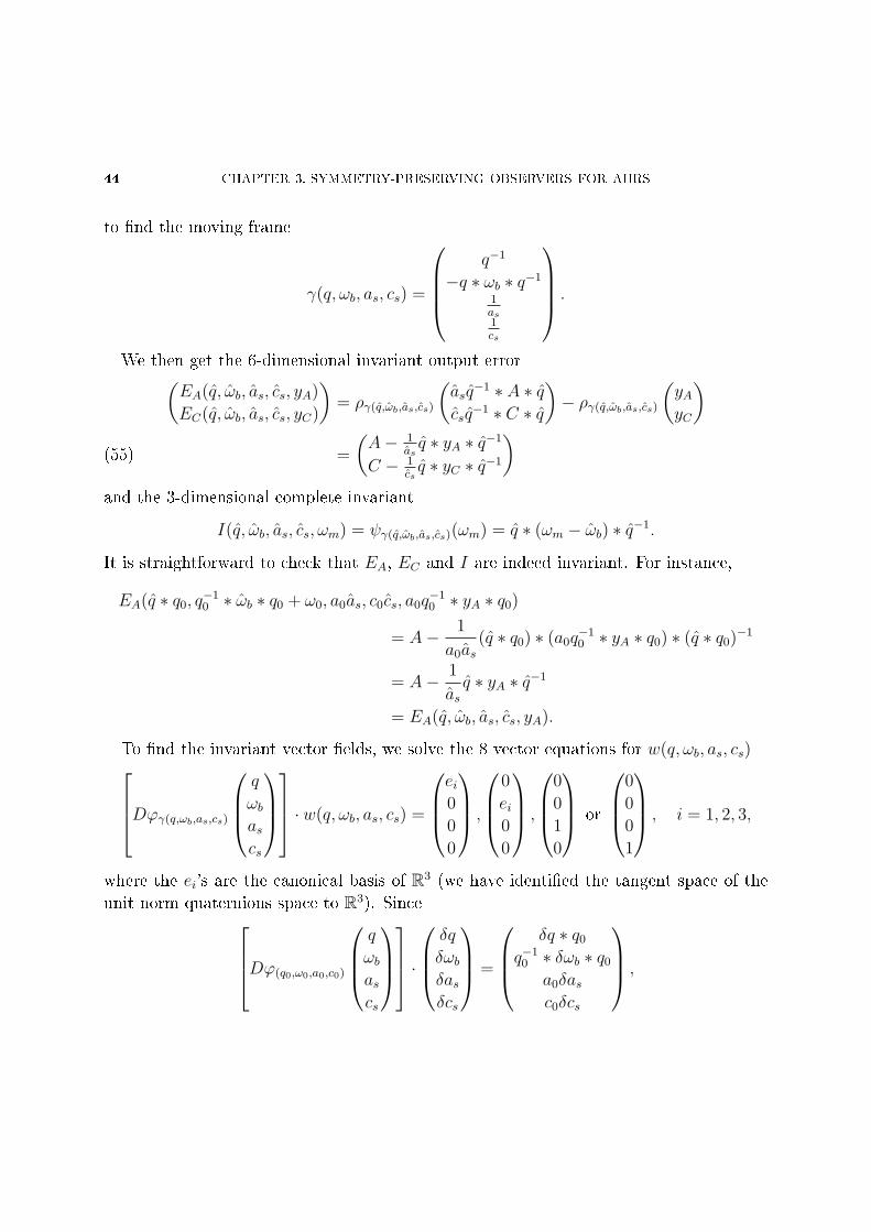
to nd the moving frame
γ(q, ωb, as, cs) =
q−1
−q ∗ ωb ∗ q−1
1as1cs
.
We then get the 6-dimensional invariant output error(EA(q, ωb, as, cs, yA)
EC(q, ωb, as, cs, yC)
)= ργ(q,ωb,as,cs)
(asq−1 ∗ A ∗ q
csq−1 ∗ C ∗ q
)− ργ(q,ωb,as,cs)
(yAyC
)=
(A− 1
asq ∗ yA ∗ q−1
C − 1csq ∗ yC ∗ q−1
)(55)
and the 3-dimensional complete invariant
I(q, ωb, as, cs, ωm) = ψγ(q,ωb,as,cs)(ωm) = q ∗ (ωm − ωb) ∗ q−1.
It is straightforward to check that EA, EC and I are indeed invariant. For instance,
EA(q ∗ q0, q−10 ∗ ωb ∗ q0 + ω0, a0as, c0cs, a0q
−10 ∗ yA ∗ q0)
= A− 1
a0as(q ∗ q0) ∗ (a0q
−10 ∗ yA ∗ q0) ∗ (q ∗ q0)−1
= A− 1
asq ∗ yA ∗ q−1
= EA(q, ωb, as, cs, yA).
To nd the invariant vector elds, we solve the 8 vector equations for w(q, ωb, as, cs)Dϕγ(q,ωb,as,cs)
q
ωbascs
· w(q, ωb, as, cs) =
ei0
0
0
,
0
ei0
0
,
0
0
1
0
or
0
0
0
1
, i = 1, 2, 3,
where the ei's are the canonical basis of R3 (we have identied the tangent space of the
unit norm quaternions space to R3). SinceDϕ(q0,ω0,a0,c0)
q
ωbascs
·δq
δωbδasδcs
=
δq ∗ q0
q−10 ∗ δωb ∗ q0
a0δasc0δcs
,
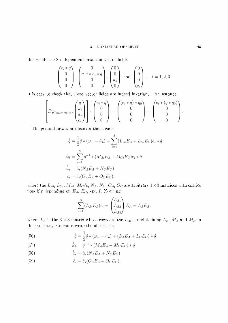
3.1. NONLINEAR OBSERVER 45
this yields the 8 independent invariant vector eldsei ∗ q
0
0
0
,
0
q−1 ∗ ei ∗ q0
0
,
0
0
as0
and
0
0
0
cs
, i = 1, 2, 3.
It is easy to check that these vector elds are indeed invariant. For instance,Dϕ(q0,ω0,a0,c0)
q
ωbascs
·ei ∗ q
0
0
0
=
(ei ∗ q) ∗ q0
0
0
0
=
ei ∗ (q ∗ q0)
0
0
0
.
The general invariant observer then reads
˙q =1
2q ∗ (ωm − ωb) +
3∑i=1
(LAiEA + LCiEC)ei ∗ q
˙ωb =3∑i=1
q−1 ∗ (MAiEA +MCiEC)ei ∗ q
˙as = as(NAEA +NCEC)
˙cs = cs(OAEA +OCEC),
where the LAi, LCi,MAi,MCi's, NA, NC , OA, OC are arbitrary 1×3 matrices with entries
possibly depending on EA, EC , and I. Noticing
3∑i=1
(LAiEA)ei =
LA1
LA2
LA3
EA = LAEA,
where LA is the 3× 3 matrix whose rows are the LAi's, and dening LB, MA and MB in
the same way, we can rewrite the observer as
˙q =1
2q ∗ (ωm − ωb) + (LAEA + LCEC) ∗ q(56)
˙ωb = q−1 ∗ (MAEA +MCEC) ∗ q(57)
˙as = as(NAEA +NCEC)(58)
˙cs = cs(OAEA +OCEC).(59)
46 CHAPTER 3. SYMMETRY-PRESERVING OBSERVERS FOR AHRS
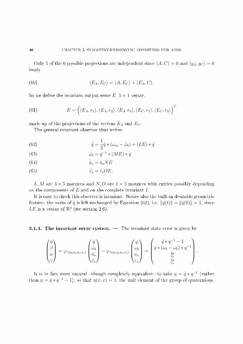
Only 5 of the 6 possible projections are independent since 〈A,C〉 = 0 and 〈yA, yC〉 = 0
imply
(60) 〈EA, EC〉 = 〈A,EC〉+ 〈EA, C〉.
So we dene the invariant output error E, 5× 1 vector,
(61) E =(〈EA, e1〉, 〈EA, e2〉, 〈EA, e3〉, 〈EC , e1〉, 〈EC , e2〉
)Tmade up of the projections of the vectors EA and EC .
The general invariant observer thus writes
˙q =1
2q ∗ (ωm − ωb) + (LE) ∗ q(62)
˙ωb = q−1 ∗ (ME) ∗ q(63)
˙as = asNE(64)
˙cs = csOE.(65)
L,M are 3× 5 matrices and N,O are 1 × 5 matrices with entries possibly depending
on the components of E and on the complete invariant I.
It is easy to check this observer is invariant. Notice also the built-in desirable geometric
feature: the norm of q is left unchanged by Equation (62), i.e. ‖q(t)‖ = ‖q(0)‖ = 1, since
LE is a vector of R3 (see section 2.6).
3.1.4. The invariant error system. The invariant state error is given by
η
β
α
γ
= ϕγ(q,ωb,as,cs)
q
ωbascs
− ϕγ(q,ωb,as,cs)
q
ωbascs
=
q ∗ q−1 − 1
q ∗ (ωb − ωb) ∗ q−1
as
ascscs
.
It is in fact more natural though completely equivalent to take η = q ∗ q−1 (rather
than η = q ∗ q−1 − 1), so that η(x, x) = 1, the unit element of the group of quaternions.
3.1. NONLINEAR OBSERVER 47
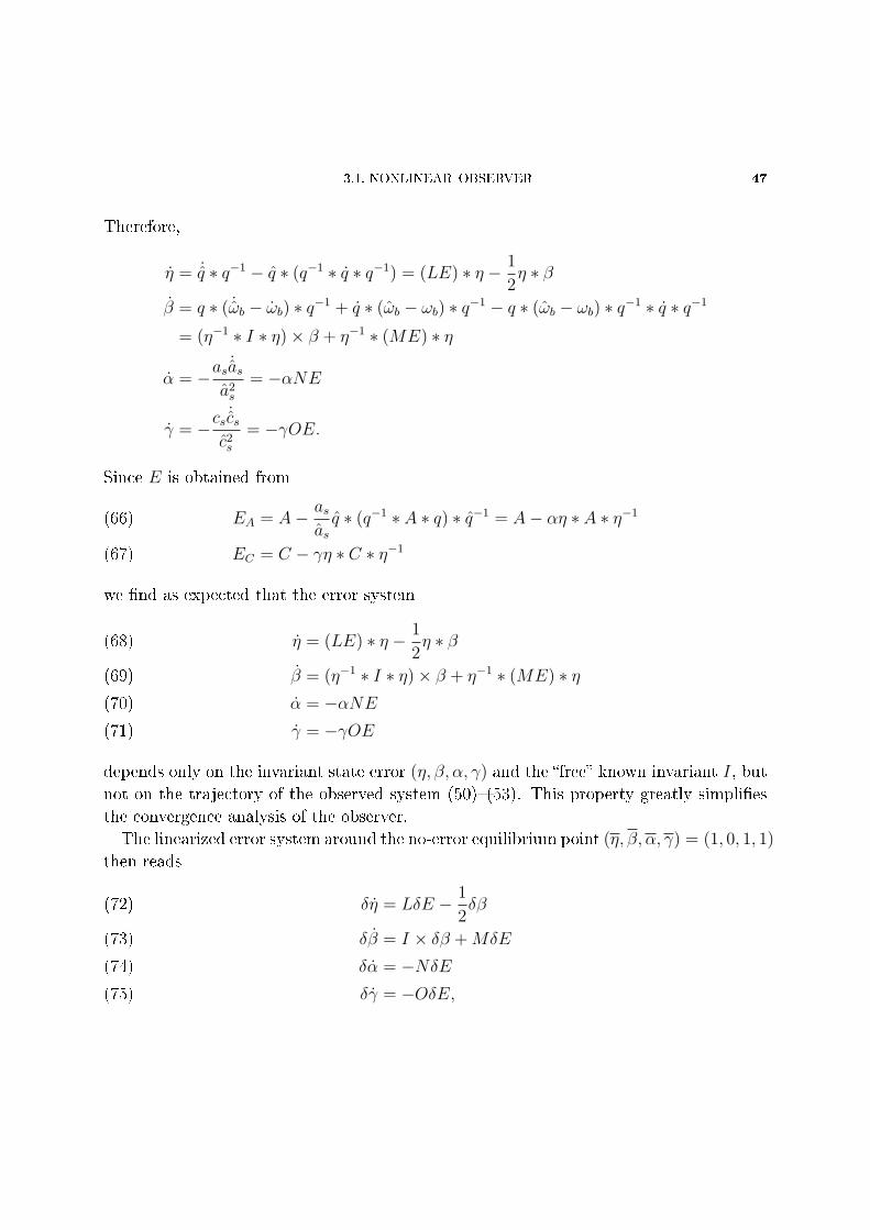
Therefore,
η = ˙q ∗ q−1 − q ∗ (q−1 ∗ q ∗ q−1) = (LE) ∗ η − 1
2η ∗ β
β = q ∗ ( ˙ωb − ωb) ∗ q−1 + q ∗ (ωb − ωb) ∗ q−1 − q ∗ (ωb − ωb) ∗ q−1 ∗ q ∗ q−1
= (η−1 ∗ I ∗ η)× β + η−1 ∗ (ME) ∗ η
α = −as˙asa2s
= −αNE
γ = −cs˙csc2s
= −γOE.
Since E is obtained from
EA = A− asasq ∗ (q−1 ∗ A ∗ q) ∗ q−1 = A− αη ∗ A ∗ η−1(66)
EC = C − γη ∗ C ∗ η−1(67)
we nd as expected that the error system
η = (LE) ∗ η − 1
2η ∗ β(68)
β = (η−1 ∗ I ∗ η)× β + η−1 ∗ (ME) ∗ η(69)
α = −αNE(70)
γ = −γOE(71)
depends only on the invariant state error (η, β, α, γ) and the free known invariant I, but
not on the trajectory of the observed system (50)(53). This property greatly simplies
the convergence analysis of the observer.
The linearized error system around the no-error equilibrium point (η, β, α, γ) = (1, 0, 1, 1)
then reads
δη = LδE − 1
2δβ(72)
δβ = I × δβ +MδE(73)
δα = −NδE(74)
δγ = −OδE,(75)
48 CHAPTER 3. SYMMETRY-PRESERVING OBSERVERS FOR AHRS
where δE is the 5× 1 vector(〈δEA, e1〉, 〈δEA, e2〉, 〈δEA, e3〉, 〈δEC , e1〉, 〈δEC , e2〉
)T= g(−2δη2, 2δη1,−δα, 2B1δη3,−B1δγ
)Tmade up from the projections of the vectors
δEA = A ∗ δη − δη ∗ A− δαA = 2A× δη − δαAδEC = 2C × δη − δγC.
3.2. Design of the observer gain matrices
Up to now, we have only investigated the structure of the observer. We now must choose
the gain matrices L,M,N,O to meet the following requirements:
the error must converge to zero, at least locally
the local error behavior should be easily tunable, if possible with a clear physical
interpretation
the magnetic measurements should not aect the attitude estimate, but only the
heading
the behavior of the lter under acceleration and/or magnetic disturbances should be
sensible and understandable.
3.2.1. Local design. It turns out that the previous requirements can easily be met
locally around every trajectory by taking
L =1
2g
0 −l1 0 0 0
l2 0 0 0 0
0 0 0 − 1B1l3 0
M =1
2g
0 m1 0 0 0
−m2 0 0 0 0
0 0 0 1B1m3 0
(76)
N =1
g
(0 0 −n 0 0
)O =
1
B1g
(0 0 0 0 −o
)(77)
for any constant l1, l2, l3,m1,m2,m3, n, o > 0. This will follow from the very simple form
of the linearized error system (72)(75). We insist that it is not usually obvious to come
up with a similar convergence result for an EKF.
3.2. DESIGN OF THE OBSERVER GAIN MATRICES 49
Indeed, Equations (72)(75) now read
δη = Dlδη −1
2δβ(78)
δβ = Dmδη + I × δβ(79)
δα = −nδα(80)
δγ = −oδγ(81)
where
Dl =
−l1 0 0
0 −l2 0
0 0 −l3
and Dm =
m1 0 0
0 m2 0
0 0 m3
.
When I = 0 (i.e. the system is at rest) the system completely decouples into:
the longitudinal subsystem(δη1
δβ1
)=
(−l1 −1
2
m1 0
)(δη1
δβ1
) the lateral subsystem (
δη2
δβ2
)=
(−l2 −1
2
m2 0
)(δη2
δβ2
) the heading subsystem (
δη3
δβ3
)=
(−l3 −1
2
m3 0
)(δη3
δβ3
) the scaling subsystem
δα = −nδαδγ = −oδγ.
When I 6= 0 the longitudinal, lateral and heading subsystems are slightly coupled by the
biases errors δβ.
We now prove the local asymptotically convergence around every trajectory of the ob-
server (62)(65) with the preceding choice of correction terms, i.e. (δη, δβ, δα, δγ)→ (0, 0, 0, 0),
whatever (l1, l2, l3,m1,m2,m3, n, o) > 0.
50 CHAPTER 3. SYMMETRY-PRESERVING OBSERVERS FOR AHRS
Theorem 1. Consider the physical system (50)(53) with the measurements (54).
Consider the nonlinear invariant observer dened by
˙q =1
2q ∗ (ωm − ωb) + (LE) ∗ q
˙ωb = q−1 ∗ (ME) ∗ q˙as = asNE
˙cs = csOE
with the expression of the output errors given by Equations (55) and (61), and the gain
matrices given by Equations (76)(77), and assume ω(t) = ωm(t)− ωb is bounded, whichis physically sensible. Then for any value (l1, l2, l3,m1,m2,m3, n, o) > 0, the solution
(q(t), ωb(t), as(t), cs(t)) locally asymptotically converges to (q(t), ωb, as, cs) around every
trajectory.
Proof 1. Proving the asymptotic local convergence of the observer around every trajec-
tory means proving (δη, δβ, δα, δγ)→ (0, 0, 0, 0) whatever (l1, l2, l3,m1,m2,m3, n, o) > 0,
i.e. the convergence of the preceding longitudinal, lateral, heading, and scaling subsystems.
The scaling subsystem obviously converges. For the other variables we consider the
candidate Lyapunov function
V =l12δη2
1 +l22δη2
2 +l32δη2
3 +1
4‖δβ‖2.
Dierentiating V and using 〈δβ, I × δβ〉 = 0, we get
V =− (l1m1δη21 + l2m2δη
22 + l3m3δη
23) ≤ 0.
Since V is bounded from below, this implies that V (δη(t), δβ(t)) converges when t → ∞.
Since
limt→∞
∫ t
0
V (δη(τ), δβ(τ))dτ = limt→∞
V (δη(t), δβ(t))− V (δη(0), δβ(0)),
we conclude limt→∞∫ t
0V (δη(τ), δβ(τ))dτ exists and is nite. On the other hand, V ≤ 0
also implies
0 ≤ V (δη(t), δβ(t)) ≤ V (δη(0), δβ(0)).
Therefore δη(t) and δβ(t) are bounded. Equation (78) implies that δη(t) is bounded too,
and nally that V is bounded. Hence V is uniformly continuous and by Barbalat's lemma
V → 0 ⇒ δη → 0.
3.2. DESIGN OF THE OBSERVER GAIN MATRICES 51
Integrating Equation (78), we get∫ t
0
δη(τ)dτ = δη(t)− δη(0) =
∫ t
0
(Dlδη(τ)− 1
2δβ(τ))dτ .
Since δη(t)→ 0, it follows
limt→∞
∫ t
0
(Dlδη(τ)− 1
2δβ(τ))dτ = −δη(0).
We assumed ω is bounded, so I is bounded too. Since δη(t) and δβ(t) are bounded,
Dlδη(t)− 12δβ(t) is bounded too. Hence Dlδη(t)− 1
2δβ(t) is uniformly continuous. Ap-
plying Barbalat's lemma once again yields
limt→∞
(Dlδη(t)− 1
2δβ(t)) = 0.
Since δη → 0, we conclude δβ → 0, which ends the proof.
3.2.2. Global design. The tuning in the previous section ensures local convergence
around every trajectory of the system, which is already a very strong property. It is
possible to further improve the convergence domain by modifying the correction terms at
higher-order. Consider the new vector yD := yC × yA = q−1 ∗D ∗ q, where D := C×A =
g2B1e1, and the associated invariant error
ED := D − 1
ascsq ∗ yD ∗ q−1.
Of course ED carries no new information since by construction D − ED = (C − EC) ×(A− EA). But it is a convenient means to express the observer matrices; a related trick
is used in [67]. Dene now L,M,N,O by
LE :=lag2A× EA +
lc(B1g)2
C × EC +ld
(B1g2)2D × ED
ME := −σLE
NE :=n
la + ld
(la〈EA, EA − A〉
g2+ld〈ED, ED −D〉
(B1g2)2
)OE :=
o
lc + ld
(lc〈EC , EC − C〉
(B1g)2+ld〈ED, ED −D〉
(B1g2)2
)with la, lc, ld, σ, n, o > 0. LE is the same as in Section 3.2.1 up to rst order with
(l1, l2, l3) = 2(la+ lc, la+ ld, lc+ ld); so isME with (m1,m2,m3) = 2σ(la+ lc, la+ ld, lc+ ld).
52 CHAPTER 3. SYMMETRY-PRESERVING OBSERVERS FOR AHRS
the rst order expansion of the new tuning thus gives a special case of (78)-(79). As
for (80)-(81), they become coupled since
NδE = −ng
(0 0 1 0 ld
(la+ld)B1
)δE
OδE = −og
(0 0 ld
(lc+ld)B10 1
B1
)δE.
This choice of matrices provides a Lyapunov function that guarantees a large domain
of convergence, while essentially preserving the nice local behavior of the error dynamics,
as described in the previous section. Indeed, time dierentiating the function
W := ‖β‖2 +σlag2‖EA‖2 +
σlc(B1g)2
‖EC‖2 +σld
(B1g2)2‖ED‖2
and using EA = (A−EA)NE+ (A−EA)× (2LE−β) and similar expressions for EC , EDyields
W = −2(LE)2 − 2la + ldn
(NE)2 − 2lc + ldo
(OE)2 ≤ 0.
Therefore W is a Lyapunov function which globally decreases for all la, lc, ld, σ, n, o > 0.
Though it ensures a large domain of convergence, it is not clear it is enough for global
convergence; see [52] for a convergence result in a simpler case (only gyro biases).
Notice the Lyapunov function V used in Section 3.2.1 can be seen as a low-order
approximation of W since
ma
g2‖δEA‖2 +
mc
(B1g)2‖δEC‖2 +
md
(B1g2)2‖δED‖2 + ‖δβ‖2
= V +maδα2 +mcδγ
2 +md(δα + δγ)2.
The tuning proposed in Section 3.2.1 is very simple and ensures the observer converges
locally around every trajectory. This is already a very strong property, but there is no
guarantee regarding a larger convergence domain. The tuning proposed in this section is
computationally slightly more complicated. It also ensures a nice local behavior, though
with less freedom: since there are now only 4 parameters (instead of 6) for (78)-(79), the
longitudinal, lateral and heading subsystems may have dierent settling times but must
have the same damping; the scaling subsystem (80)-(81) is now coupled but still has 2
tuning parameters. The guaranteed domain of convergence is much larger. Also notice
the observer structure is exible enough to accommodate yet other tunings.
3.3. EFFECTS OF DISTURBANCES 53
3.3. Eects of disturbances
Two main disturbances may aect the model. When V 6= 0, the accelerometers measure
in fact asq−1 ∗ A∗ ∗ q where A∗ = −V +A. Magnetic disturbances will also change B into
some B∗. For simplicity we consider that A∗, B∗ are constant. The measured outputs
now become (yA∗
yC∗
)=
(asq−1 ∗ A∗ ∗ q
csq−1 ∗ C∗ ∗ q
).
The error system is unchanged but E is now the 5× 1 vector
E =(〈EA, e1〉, 〈EA, e2〉, 〈EA, e3〉, 〈EC , e1〉, 〈EC , e2〉
)Tmade up of the projections of the vectors
EA = A− 1
asq ∗ yA∗ ∗ q−1 and EC = C − 1
csq ∗ yC∗ ∗ q−1.
Let us dene the points (η, β, α, γ) as follows
β = 0
η ∗ A∗ ∗ η−1 = (0 0 ‖A∗‖)η ∗ C∗ ∗ η−1 = (0 ‖C∗‖ 0)
α =‖A∗‖‖A‖
and γ =‖C∗‖‖C‖
Doing the frame rotation dened by η we can dene the new variables
η = η ∗ η−1 β = η ∗ β ∗ η−1
α = αα γ = γγ.
The error system with these new variables writes
˙η = −1
2η ∗ β + (LE) ∗ η
˙β = (η−1 ∗ I ∗ η)× β + η−1 ∗ (ME) ∗ η˙α = −αNE˙γ = −γOE
where the new output error E is made up of the projections of the vectors
EA = A− αη ∗ A ∗ η−1 and EC = C − αη ∗ C ∗ η−1.
54 CHAPTER 3. SYMMETRY-PRESERVING OBSERVERS FOR AHRS
So (η, β, α, γ) satisfy the same error system as (η, β, α, γ). In the new frame (A∗, C∗) play
the same role as (A,C). All the properties of the observer are therefore preserved in the
new frame.
An important case is when only the magnetic eld is perturbed, where we consider
A and C∗ = (C∗1 C∗2 0) (instead of C = (0 gB1 0)). Writing the new equilibrium point
(η, β, α, γ) of the error system explicitly it can be seen that
φ = θ = 0 and ψ = arctanC∗1C∗2
β = α = 0 and γ =‖C∗‖‖C‖
,
where (φ, θ, ψ) are the Euler angles corresponding to η. In particular only the yaw angle
ψ and γ are aected by the magnetic disturbance.
3.4. Experimental validation
We now compare the behavior of our observer with the commercial Microbotics MIDG II
system used in Vertical Gyro mode. The following results have been obtained with the
observer
˙q =1
2q ∗ (ωm − ωb) + (LE) ∗ q + k(1− ‖q‖2)q(82)
˙ωb = q−1 ∗ (ME) ∗ q(83)
˙as = asNE(84)
˙cs = csOE,(85)
and the choice of matrices dened by the parameters below. Compared to the observer
(62)(65), the added term k(1− ‖q‖2)q is a well-known numerical trick to keep ‖q‖ = 1.
Notice this term is also invariant.
We feed the observer with the raw measurements from the MIDG II gyroscopes, ac-
celerometers and magnetic sensors. The observer is implemented in Matlab Simulink and
its values are compared to the MIDG II results (computed according to the user manual
by some Kalman lter). In order to have similar behaviors between MIDG II lter and
3.4. EXPERIMENTAL VALIDATION 55
the invariant observer, we have chosen
la = 6e− 2 lc = 1e− 1 ld = 6e− 2
ma = 3.2e− 3 mc = 5.3e− 3 md = 3.2e− 3
n = 0.25 o = 0.5.
3.4.1. Comparison with a commercial device (Figure 3.1). We rst want to
illustrate the dierent invariant observer properties mentioned in Section 3.2. Therefore
we performed a long-lasting experiment, which can be divided into 3 parts:
for t < 240s the system is left at rest until the biases reach constant values. Fig-
ure 3.1(a) highlights the importance of the correction term in the angle estimation:
without correction the estimated roll angle diverges with a slope of −0.18/s (bot-
tom plot), which is indeed the nal value of the estimated bias (middle plot) (Fig-
ures 3.1(a) and 3.1(b)).
for 240s < t < 293s we move the system in all directions. The observer and the
MDG II give very similar results (Figure 3.1(c)).
at t = 385s the system is motionless and a magnet is put close to the sensors for 10s.
As expected only the estimated yaw angle is aected by the magnetic disturbance
(Figure 3.1(d)); the MIDG II exhibits a similar behavior.
3.4.2. Inuence of the observer correction terms (Figure 3.2). We have cho-
sen the correction terms so that the magnetic measurements correct essentially the yaw
angle and its corresponding bias, whereas the accelerometers measurements act on the
other variables. We highlight this property on the following experiment (Figure 3.2).
Once the biases have reached constant values, the system is left at rest during 35 minutes:
for t < 600s the results are very similar for the observer and the MIDG II.
at t = 600s the magnetic correction terms" are switched o, i.e. the gains lc,ld,mc,md
and o are set to 0. The yaw angle estimated by the observer diverges because the cor-
responding bias is not perfectly estimated. Indeed, these variables are not observable
without the magnetic measurements. The other variables are not aected.
at t = 1300s the accelerometers correction terms" are also switched o, i.e. la,ma
and n are set to 0. All the estimated angles now diverge.
3.4.3. Acceleration disturbance: V 6= 0 (Figure 3.3). The hypothesis V = 0
may be wrong. In this case the observer does not converge to the true values anymore.
Indeed we illustrate this point on Figure 3.3 by comparing the roll angle estimated by
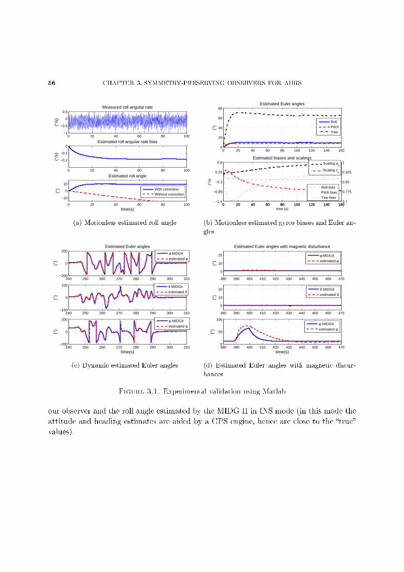
56 CHAPTER 3. SYMMETRY-PRESERVING OBSERVERS FOR AHRS
0 20 40 60 80 100−1
−0.5
0
0.5Measured roll angular rate
(°/s
)
0 20 40 60 80 100
−0.2
−0.1
0Estimated roll angular rate bias
(°/s
)
0 20 40 60 80 100
−10
0
10
Estimated roll angle
time(s)
(°)
With correctionWithout correction
(a) Motionless estimated roll angle
0 20 40 60 80 100 120 140 1600
20
40
60
80Estimated Euler angles
(°)
RollPitchYaw
0 20 40 60 80 100 120 140 160−1.4
−0.85
−0.3
0.25
0.8
time (s)(°
/s)
Estimated biases and scalings
0 20 40 60 80 100 120 140 1600.7
0.775
0.85
0.925
1
Roll biasPitch biasYaw bias
Scaling as
Scaling cs
(b) Motionless estimated gyros biases and Euler an-
gles
240 250 260 270 280 290 300 310−200
0
200Estimated Euler angles
(°)
φ MIDGII
estimated φ
240 250 260 270 280 290 300 310−100
0
100
(°)
θ MIDGII
estimated θ
240 250 260 270 280 290 300 310−200
0
200
time(s)
(°)
ψ MIDGII
estimated ψ
(c) Dynamic estimated Euler angles
380 390 400 410 420 430 440 450 460 470
0
10
20
Estimated Euler angles with magnetic disturbance
(°)
380 390 400 410 420 430 440 450 460 470
0
10
20
(°)
380 390 400 410 420 430 440 450 460 4700
50
100
time(s)
(°)
φ MIDGII
estimated φ
θ MIDGII
estimated θ
ψ MIDGII
estimated ψ
(d) Estimated Euler angles with magnetic distur-
bances
Figure 3.1. Experimental validation using Matlab
our observer and the roll angle estimated by the MIDG II in INS mode (in this mode the
attitude and heading estimates are aided by a GPS engine, hence are close to the true
values).
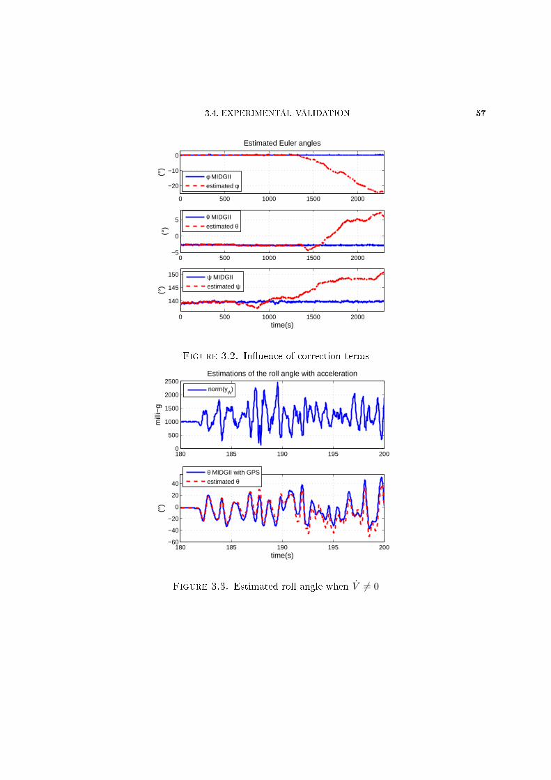
3.4. EXPERIMENTAL VALIDATION 57
0 500 1000 1500 2000
−20
−10
0
Estimated Euler angles
(°)
φ MIDGII
estimated φ
0 500 1000 1500 2000−5
0
5
(°)
θ MIDGII
estimated θ
0 500 1000 1500 2000
140
145
150
time(s)
(°)
ψ MIDGII
estimated ψ
Figure 3.2. Inuence of correction terms
180 185 190 195 2000
500
1000
1500
2000
2500Estimations of the roll angle with acceleration
mill
i−g
180 185 190 195 200−60
−40
−20
0
20
40
(°)
time(s)
norm(yA)
θ MIDGII with GPS
estimated θ
Figure 3.3. Estimated roll angle when V 6= 0

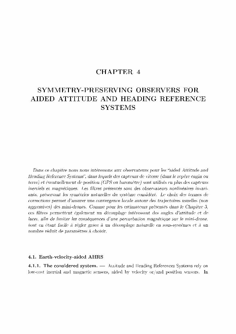
CHAPTER 4
SYMMETRY-PRESERVING OBSERVERS FOR
AIDED ATTITUDE AND HEADING REFERENCE
SYSTEMS
Dans ce chapitre nous nous intéressons aux observateurs pour les aided Attitude and
Heading Reference Systems, dans lequels des capteurs de vitesse (dans le repère engin ou
terre) et éventuellement de position (GPS ou baromètre) sont utilisés en plus des capteurs
inertiels et magnétiques. Les ltres présentés sont des observateurs nonlinéaires invari-
ants, préservant les symétries naturelles du système considéré. Le choix des termes de
corrections permet d'assurer une convergence locale autour des trajectoires usuelles (non
aggressives) des mini-drones. Comme pour les estimateurs présentés dans le Chapitre 3,
ces ltres permettent également un découplage intéressant des angles d'attitude et de
lacet, an de limiter les conséquences d'une perturbation magnétique sur le mini-drone,
tout en étant facile à régler grâce à un découplage naturelle en sous-systèmes et à un
nombre réduit de paramètres à choisir.
4.1. Earth-velocity-aided AHRS
4.1.1. The considered system. Attitude and Heading References Systems rely on
low-cost inertial and magnetic sensors, aided by velocity or/and position sensors. In
60 CHAPTER 4. SYMMETRY-PRESERVING OBSERVERS FOR AIDED AHRS
this section, we consider only velocity measurements in Earth-xed coordinates (e.g.
from a GPS engine) coming in addition to the accelerometers, gyroscopes and magne-
tometers measurements. Therefore we consider the following system, coming from Equa-
tions (42),(43),(45),(46) described in Section 2.4
q =1
2q ∗ (ωm − ωb)(86)
V = A+1
asq ∗ am ∗ q−1(87)
ωb = 0(88)
as = 0,(89)
where ωm and am are seen as known inputs, together with the output(yVyB
)=
(V
q−1 ∗B ∗ q
).(90)
4.1.2. Invariance of the system equations. The physical system is obviously un-
aected by a constant velocity translation in the Earth-xed frame and a constant rotation
of the body-xed frame. It is natural to expect a similar behavior from an observer. We
therefore consider the following transformation group generated by rotations, translations
and scaling
ϕ(q0,V0,ω0,a0)
q
V
ωbas
=
q ∗ q0
V + V0
q−10 ∗ ωb ∗ q0 + ω0
asa0
ψ(q0,V0,ω0,a0)
(ωmam
)=
(q−1
0 ∗ ωm ∗ q0 + ω0
a0q−10 ∗ am ∗ q0
)ρ(q0,V0,ω0,a0)
(yVyB
)=
(yV + V0
q−10 ∗ yB ∗ q0
).
There are 3 + 2 ∗ 3 + 1 = 10 parameters: the unit quaternion q0, the R3-vectors V0, ω0 and
the positive scalar a0. The group composition law is given byq1
V1
ω1
a1
q0
V0
ω0
a0
=
q0 ∗ q1
V0 + V1
q−11 ∗ ω0 ∗ q1 + ω1
a0a1
.
4.1. EARTH-VELOCITY-AIDED AHRS 61
The system (86)(89) is of course invariant by the transformation group since
˙︷ ︸︸ ︷q ∗ q0 = q ∗ q0 =
1
2(q ∗ q0) ∗
((q−1
0 ∗ ωm ∗ q0 + ω0)− (q−10 ∗ ωb ∗ q0 + ω0)
)˙︷ ︸︸ ︷
V + V0 = V = A+1
asa0
(q ∗ q0) ∗ (asq−10 ∗ am ∗ q0) ∗ (q ∗ q0)−1
˙︷ ︸︸ ︷q−1
0 ∗ ωb ∗ q0 + ω0 = q−10 ∗ ωb ∗ q0 = 0
˙︷︸︸︷asa0 = asa0 = 0,
whereas the output (90) is equivariant since(V + V0
(q ∗ q0)−1 ∗B ∗ (q ∗ q0)
)= ρ(q0,V0,ω0,a0)
(V
q−1 ∗B ∗ q
).
4.1.3. Construction of the general invariant observer. We solve for (q0, V0, ω0, a0)
the normalization equations
q ∗ q0 = 1
V + V0 = 0and
q−10 ∗ ωb ∗ q0 + ω0 = 0
asa0 = 1
to nd the moving frame
γ(q, V, ωb, as) =
q−1
−V−q ∗ ωb ∗ q−1
1/as
.
We then get the 6-dimensional invariant error(EVEB
)= ργ(q,V ,ωb,as)
(yVyB
)− ργ(q,V ,ωb,as)
(yVyB
)=
(yV − yV
B − q ∗ q−1 ∗B ∗ q ∗ q−1
)=
(yV − yV
B − q ∗ yB ∗ q−1
)(91)
and the 6-dimensional complete invariant(IωIa
)= ψγ(q,V ,ωb,as)
(ωmam
)=
(q ∗ (ωm − ωb) ∗ q−1
1asq ∗ am ∗ q−1
).
Notice that Iω,Ia,EV and EB are functions of the estimates and the measurements. Hence
they are known quantities which can be used in the construction of the observer. It is
62 CHAPTER 4. SYMMETRY-PRESERVING OBSERVERS FOR AIDED AHRS
straightforward to check they are indeed invariant. For instance,
EB(q ∗ q0, V + V0, q−10 ∗ ωb ∗ q0 + ω0, asa0, q
−10 ∗ yB ∗ q0)
= B − (q ∗ q0) ∗ (q−10 ∗ yB ∗ q0) ∗ (q ∗ q0)−1
= B − q ∗ yB ∗ q−1
= EB(q, V , ωb, as, yB).
To nd invariant vector elds, we solve for w(q, V, ωb, as) the 10 vector equationsDϕγ(q,V,ωb,as)
q
V
ωbas
· w(q, V, ωb, as) =
ei0
0
0
,
0
ei0
0
,
0
0
ei0
,
0
0
0
e10
, i = 1, 2, 3,
where the ei's are the canonical basis of R3 (we have identied the tangent space of the
unit norm quaternions space to R3). SinceDϕ(q0,V0,ω0,a0)
q
V
ωbas
·δq
δV
δωbδas
=
δq ∗ q0
δV
q−10 ∗ δωb ∗ q0
a0δas
,
this yields the 10 independent invariant vector eldsei ∗ q
0
0
0
,
0
ei0
0
,
0
0
q−1 ∗ ei ∗ q0
,
0
0
0
ase10
, i = 1, 2, 3.
These vector elds are invariant. Indeed for instance,Dϕ(q0,V0,ω0,a0)
q
V
ωbas
·ei ∗ q
0
0
0
=
(ei ∗ q) ∗ q0
0
0
0
=
ei ∗ (q ∗ q0)
0
0
0
.
4.1. EARTH-VELOCITY-AIDED AHRS 63
The general invariant observer then reads
˙q =1
2q ∗ (ωm − ωb) +
3∑i=1
(LV iEV + LBiEB)ei ∗ q
˙V = A+
1
asq ∗ am ∗ q−1 +
3∑i=1
(MV iEV + LBiEB)ei
˙ωb =3∑i=1
q−1 ∗ (NV iEV +NBiEB)ei ∗ q
˙as = as(OVEV +OBEB),
where the LV i, LBi,MV i,MBi, NV i, NBi, OV , OB are arbitrary 1×3 matrices with entries
possibly depending on EV , EB, Iω and Ia. Noticing
3∑i=1
(LV iEV )ei =
LV 1
LV 2
LV 3
EV = LVEV ,
where LV is the 3 × 3 matrix whose rows are the LV i's, and dening LB, MV , MB, NV
and NB in the same way, we can rewrite the observer as
˙q =1
2q ∗ (ωm − ωb) + (LVEV + LBEB) ∗ q(92)
˙V =
1
asq ∗ am ∗ q−1 + A+ (MVEV +MBEB)(93)
˙ωb = q−1 ∗ (NVEV +NBEB) ∗ q(94)
˙as = as(OVEV +OBEB).(95)
As a by-product of its geometric structure, the observer automatically has a desirable
feature: the norm of q is left unchanged by Equations (92), since LVEV + LBEB is a
vector in R3 (see section 2.6).
4.1.4. The invariant error system. The invariant state error is given byη
ν
β
α
= ϕγ(q,V,ωb,as)
q
V
ωbas
− ϕγ(q,V,ωb,as)
q
V
ωbas
=
q ∗ q−1 − 1
V − Vq ∗ (ωb − ωb) ∗ q−1
as
as− 1
.
64 CHAPTER 4. SYMMETRY-PRESERVING OBSERVERS FOR AIDED AHRS
As in section 3.1, we consider η = q ∗q−1 (rather than η = q ∗q−1−1), so that η(x, x) = 1,
the unit element of the group of quaternions. In the same way, we take α = as
asto keep α
in R+. Hence,
η = ˙q ∗ q−1 + q ∗ (−q−1 ∗ q ∗ q−1) = −1
2η ∗ β + (LAEA + LCEC) ∗ η
ν =˙V − V = Ia − αη−1 ∗ Ia ∗ η + (MVEV +MBEB)
β = q ∗ (ωb − ωb) ∗ q−1 − q ∗ (ωb − ωb) ∗ q−1 ∗ q ∗ q−1 + q ∗ ( ˙ωb − ωb) ∗ q−1
= (η−1 ∗ Iω ∗ η)× β + η−1 ∗ (NVEV +NBEB) ∗ η
α =˙asas
= α(OVEV +OBEB).
Since we can write
EV = ν and EB = B − η ∗B ∗ η−1,
we nd that the error system
η = −1
2η ∗ β + (LAEA + LCEC) ∗ η(96)
ν = Ia − αη−1 ∗ Ia ∗ η + (MVEV +MBEB)(97)
β = (η−1 ∗ Iω ∗ η)× β + η−1 ∗ (NVEV +NBEB) ∗ η(98)
α = α(OVEV +OBEB)(99)
depends only on the invariant state error (η, ν, β, α) and the free known invariants Iωand Ia, but not on the trajectory of the observed system (86)(89).
The linearized error system around (η, ν, β, α) = (1, 0, 0, 1), i.e. the estimated state
equals the actual state, is given by
δη = −1
2δβ + (LV δEV + LBδEB)
δν = −2Ia × δη − δαIa + (MV δEV +MBδEB)
δβ = Iω × δβ + (NV δEV +NBδEB)
δα = (OV δEV +OBδEB),
4.1. EARTH-VELOCITY-AIDED AHRS 65
where
δEV = δν
δEB = −δη ∗B ∗ η−1 − η ∗B ∗ (−η−1 ∗ δη ∗ η−1)
= 2(η ∗B ∗ η−1)× (δη ∗ η−1) = 2B × δη.
4.1.5. Design of the observer gain matrices.
4.1.5.1. Choice of the gain matrices. The linearized error system without correction
terms turns out to be decoupled into 4 independent subsystems when Ia is constant and
Iω = 0 (in particular when the aircraft is in level ight). To make sure tuning remains
simple, the gain matrices should respect this decoupling. On the other hand, the Earth
magnetic eld is quite perturbed in urban areas, which are usual areas of operation for
a small UAV. We do not want these magnetic disturbances which unavoidably corrupt
the heading estimate to aect the attitude and velocity estimates too much. The idea
is thus to rely on the magnetic measurement yB as little as possible. Therefore we choose
LVEV = −lV Ia × EV LBEB = lB〈B × EB, Ia〉Ia(100)
MVEV = −mVEV MBEB = 0(101)
NVEV = nV Ia × EV NBEB = −nB〈B × EB, Ia〉Ia(102)
OVEV = oV 〈Ia, EV 〉 OBEB = 0(103)
with (lV , lB,mV , nV , nB, oV ) > 0.
4.1.5.2. Equilibrium points of the observer equations. When the observer has con-
verged, the last two equations of the observer write
NVEV +NBEB = 0 and OVEV = 0.
With the choice of gain matrices above it leads to
Ia × EV = 0 and 〈Ia, EV 〉 = 0.
So even if the model is wrong, for example if the Earth magnetic eld is perturbed,
the observer equations ensure V = V once it has converged. This important property
is satised because we considered the scaling on the accelerometers measurements as in
addition to the usual gyroscopes biases ωb. A similar conclusion is not possible with the
Euler angles even if we consider additional biases: EB = 0 does not ensure that the yaw
angle, for example, is correctly estimated.
66 CHAPTER 4. SYMMETRY-PRESERVING OBSERVERS FOR AIDED AHRS
4.1.5.3. First-order approximation and coordinate change. Considering the gain matri-
ces described above, the linearized error equations around the equilibrium point (1, 0, 0, 1)
write
δη = −1
2δβ − lV Ia × δEV + lB〈B × δEB, Ia〉Ia
δν = −2Ia × δη − δαIa −mV δEV
δβ = Iω × δβ + nV Ia × δEV − nB〈B × δEB, Ia〉Iaδα = oV 〈Ia, δEV 〉
with δEV = δν and δEB = 2B × δη.We change the coordinate so that the estimated specic acceleration vector Ia is vertical.
Let η0 be this frame rotation dened by
η−10 ∗ Ia ∗ η0 = −kA, where k > 0(104)
η−10 ∗B ∗ η0 = B with B = (B1 0 B3).(105)
It follows
η = η−10 ∗ η ∗ η0 ν = η−1
0 ∗ ν ∗ η0
β = η−10 ∗ β ∗ η0.
The error system then becomes
δ ˙η = 2δη × (η−10 ∗ η0)− 1
2δβ + klVA× δEV + k2lB〈B × δEB, A〉A
δ ˙ν = 2δν × (η−10 ∗ η0) + 2kA× δη + kδαA−mV δEV
δ ˙β = 2δβ × (η−10 ∗ η0) + Iω × δβ − knVA× δEV − k2nB〈B × δEB, A〉A
δα = −oV k〈A, δEV 〉
with δEV = δν and δEB = 2B × δη.We suppose now that the system is moving along a smooth trajectory, i.e the magni-
tudes of η0, Ia, and Iω are negligible. All the terms of the form ·×(η−10 ∗ η0) then disappear
and k is now constant. The error system splits into three decoupled subsystems and one
cascaded subsystem:
4.1. EARTH-VELOCITY-AIDED AHRS 67
the longitudinal subsystemδ ˙η2
δ ˙ν1
δ ˙β2
=
0 klV g −12
−2kg −mV 0
0 −knV g 0
δη2
δν1
δβ2
the lateral subsystemδ ˙η1
δ ˙ν2
δ ˙β1
=
0 −klV g −12
2kg −mV 0
0 knV g 0
δη1
δν2
δβ1
the vertical subsystem (
δ ˙ν3
δα
)=
(−mV kg
−kgoV 0
)(δν3
δα
) the heading subsystem(
δ ˙η3
δ ˙β3
)=
(−2k2g2lBB
21 −1
2
2k2g2nBB21 0
)(δη3
δβ3
)+
(2k2g2lBB3B1
−2k2g2nBB3B1
)δη1.
Thanks to this decoupled structure, the convergence of each subsystem, and then the
local convergence of the invariant observer, is straightforward, and leads to Theorem 2.
Theorem 2. Consider the physical system (86)(89) with the measurements (90).
Consider the nonlinear invariant observer dened by
˙q =1
2q ∗ (ωm − ωb) + (LVEV + LBEB) ∗ q
˙V =
1
asq ∗ am ∗ q−1 + A+ (MVEV )
˙ωb = q−1 ∗ (NVEV +NBEB) ∗ q˙as = as(OVEV ),
with the expression of the output errors given by Equation (91) and the gain matrices given
by Equations (100)(103). Then for any value (lV , lB,mV , nV , nB, oV ) > 0, the solution
(q(t), V (t), ωb(t), as(t)) locally asymptotically converges to (q(t), V (t), ωb, as) around every
smooth trajectory, i.e when η0, Ia, and Iω can be neglected (rst order terms).
We insist that it is not usually obvious to come up with a similar convergence result for
an EKF. The gains lV , lB,mV , nV , nB, oV are also easy to tune, since the behaviors of each
68 CHAPTER 4. SYMMETRY-PRESERVING OBSERVERS FOR AIDED AHRS
subsystem are independent. Moreover the lateral, longitudinal and vertical subsystems
do not depend on the magnetic measurements, so they are not aected if the magnetic
eld is perturbed.
4.1.5.4. Inuence of magnetic disturbances on static behavior. We now investigate
how the equilibrium point (1, 0, 0, 1) is modied when the magnetic eld is (statically)
perturbed. We show that only the yaw angle ψ is aected while all the other variables,
in particular the attitude angles φ, θ, remain unchanged. Here the Euler angles φ, θ, ψ
correspond to the error quaternion η in the new frame described by Equations (104)-(105).
The equilibrium points (η, ν, ω, α) are dened by
(lV kA× ν + lB〈B × EB, kA〉kA) ∗ η − 1
2η ∗ β = 0
−kA+ αη−1 ∗ kA ∗ η −mV ν = 0
η−1 ∗ (−nV kA× ν − nB〈B × EB, kA〉kA) ∗ η + (η
−1 ∗ Iω ∗ η)× β = 0
oV 〈kA, ν〉α = 0.
We ensure β = 0 by choosing LVEV + LBEB colinear to NVEV +NBEB, that isnV
lV= nB
lB, σ. This implies ν = 0, αη ∗ A ∗ η−1 − A = 0 and 〈B × EB, kA〉 = 0.
Finally (η, ν, β, α) = (η, 0, 0, 1); moreover φ = θ = 0 and ψ is determined by 〈B × EB, kA〉 = 0,
where the Euler angles φ, θ, ψ correspond to the error quaternion η.
4.1.6. Simulation results. We rst use simulations to illustrate the behavior of the
invariant observer
˙q =1
2q ∗ (ωm − ωb) + (LVEV + LBEB) ∗ q + λ(1− ‖q‖2)q
˙V =
1
asq ∗ am ∗ q−1 + A+ (MVEV +MBEB)
˙ωb = q−1 ∗ (NVEV +NBEB) ∗ q˙as = as(OVEV +OBEB)
with the choice of gain matrices described in 4.1.5.1.
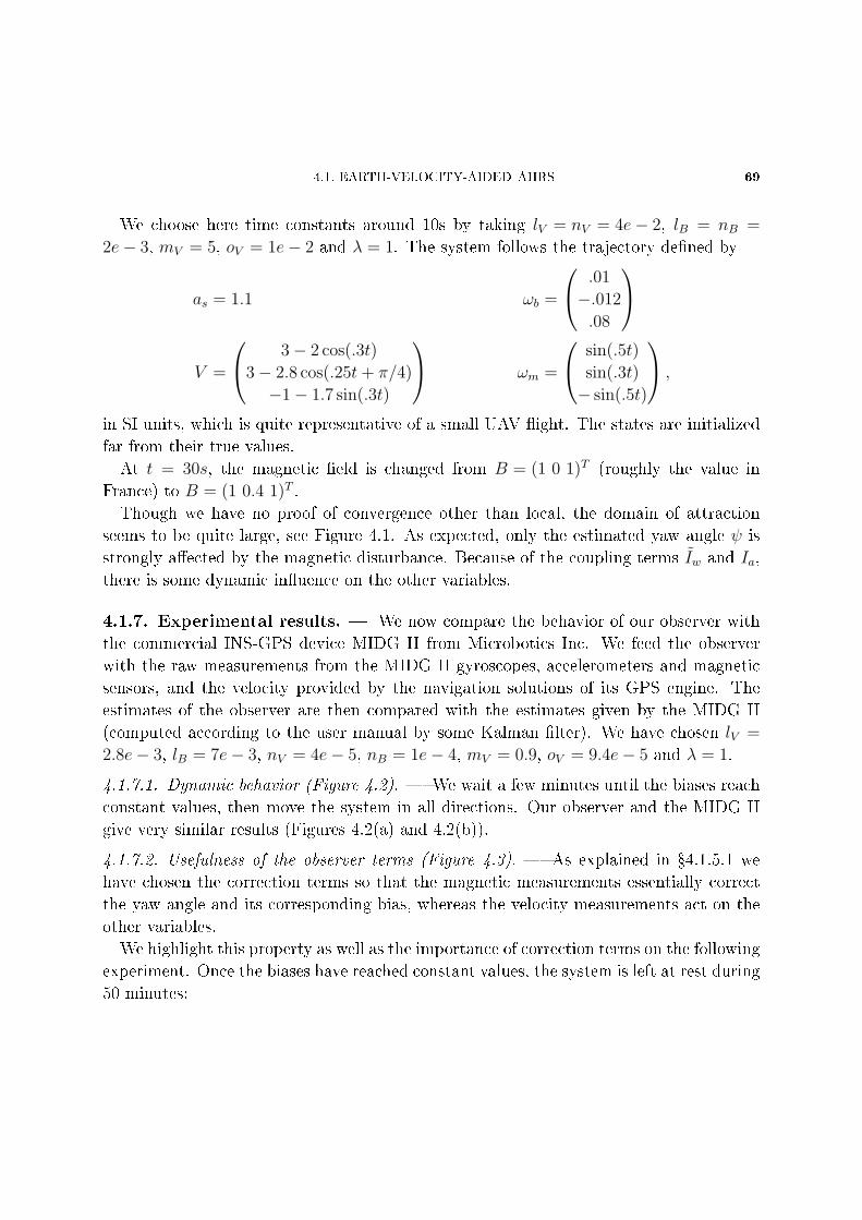
4.1. EARTH-VELOCITY-AIDED AHRS 69
We choose here time constants around 10s by taking lV = nV = 4e− 2, lB = nB =
2e− 3, mV = 5, oV = 1e− 2 and λ = 1. The system follows the trajectory dened by
as = 1.1 ωb =
.01
−.012
.08
V =
3− 2 cos(.3t)
3− 2.8 cos(.25t+ π/4)
−1− 1.7 sin(.3t)
ωm =
sin(.5t)
sin(.3t)
− sin(.5t)
,
in SI units, which is quite representative of a small UAV ight. The states are initialized
far from their true values.
At t = 30s, the magnetic eld is changed from B = (1 0 1)T (roughly the value in
France) to B = (1 0.4 1)T .
Though we have no proof of convergence other than local, the domain of attraction
seems to be quite large, see Figure 4.1. As expected, only the estimated yaw angle ψ is
strongly aected by the magnetic disturbance. Because of the coupling terms Iw and Ia,
there is some dynamic inuence on the other variables.
4.1.7. Experimental results. We now compare the behavior of our observer with
the commercial INS-GPS device MIDG II from Microbotics Inc. We feed the observer
with the raw measurements from the MIDG II gyroscopes, accelerometers and magnetic
sensors, and the velocity provided by the navigation solutions of its GPS engine. The
estimates of the observer are then compared with the estimates given by the MIDG II
(computed according to the user manual by some Kalman lter). We have chosen lV =
2.8e− 3, lB = 7e− 3, nV = 4e− 5, nB = 1e− 4, mV = 0.9, oV = 9.4e− 5 and λ = 1.
4.1.7.1. Dynamic behavior (Figure 4.2). We wait a few minutes until the biases reach
constant values, then move the system in all directions. Our observer and the MIDG II
give very similar results (Figures 4.2(a) and 4.2(b)).
4.1.7.2. Usefulness of the observer terms (Figure 4.3). As explained in 4.1.5.1 we
have chosen the correction terms so that the magnetic measurements essentially correct
the yaw angle and its corresponding bias, whereas the velocity measurements act on the
other variables.
We highlight this property as well as the importance of correction terms on the following
experiment. Once the biases have reached constant values, the system is left at rest during
50 minutes:
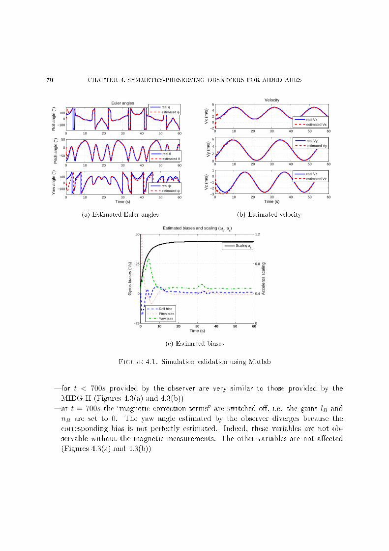
70 CHAPTER 4. SYMMETRY-PRESERVING OBSERVERS FOR AIDED AHRS
0 10 20 30 40 50 60
−100
0
100
Euler angles
Rol
l ang
le (
°)
real φestimated φ
0 10 20 30 40 50 60
−50
0
50
Pitc
h an
gle
(°)
real θestimated θ
0 10 20 30 40 50 60
−100
0
100
Time (s)
Yaw
ang
le (
°)
real ψestimated ψ
(a) Estimated Euler angles
0 10 20 30 40 50 60−2
0
2
4
6Velocity
Vx
(m/s
)
real Vxestimated Vx
0 10 20 30 40 50 600
2
4
6
Vy
(m/s
)
real Vyestimated Vy
0 10 20 30 40 50 60−3
−2
−1
0
1
Time (s)V
z (m
/s)
real Vzestimated Vz
(b) Estimated velocity
0 10 20 30 40 50 60−25
0
25
50
Time (s)
Gyr
os b
iase
s (°
/s)
Estimated biases and scaling (ωb, a
s)
0 10 20 30 40 50 600
0.4
0.8
1.2
Acc
eler
os s
calin
g
Roll biasPitch biasYaw bias
Scaling as
(c) Estimated biases
Figure 4.1. Simulation validation using Matlab
for t < 700s provided by the observer are very similar to those provided by the
MIDG II (Figures 4.3(a) and 4.3(b))
at t = 700s the magnetic correction terms are switched o, i.e. the gains lB and
nB are set to 0. The yaw angle estimated by the observer diverges because the
corresponding bias is not perfectly estimated. Indeed, these variables are not ob-
servable without the magnetic measurements. The other variables are not aected
(Figures 4.3(a) and 4.3(b))
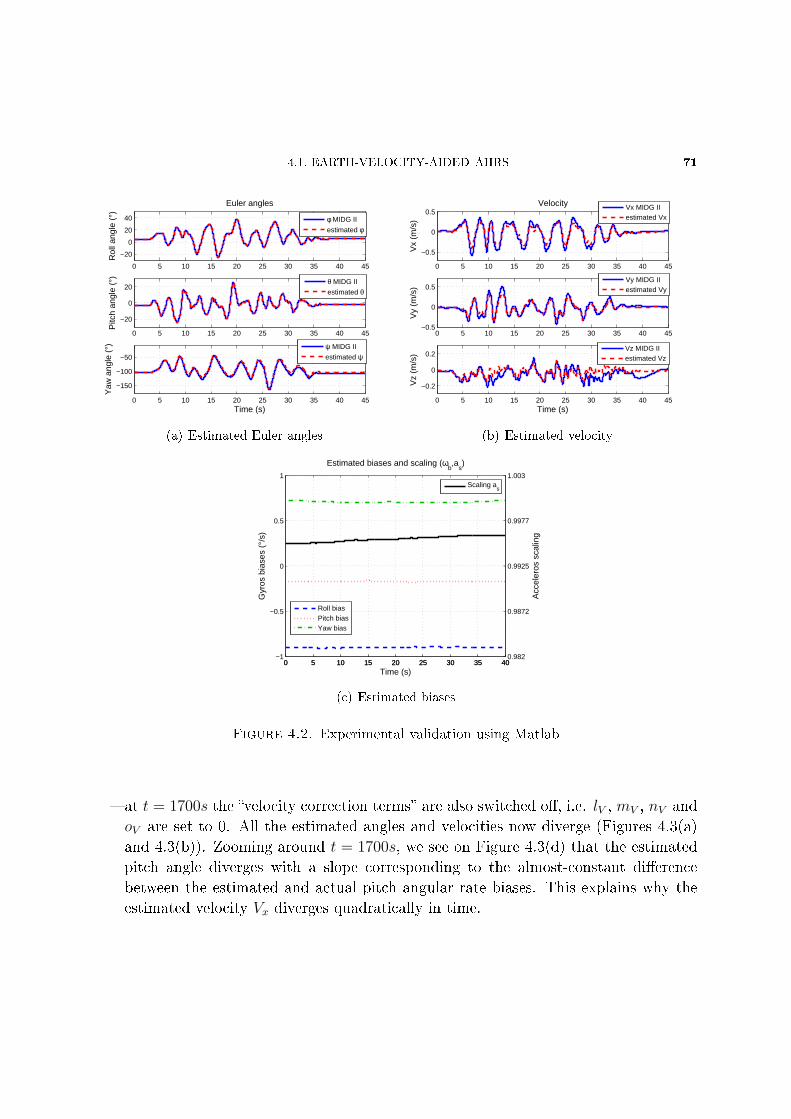
4.1. EARTH-VELOCITY-AIDED AHRS 71
0 5 10 15 20 25 30 35 40 45
−20
0
20
40
Euler angles
Rol
l ang
le (
°)
0 5 10 15 20 25 30 35 40 45
−20
0
20
Pitc
h an
gle
(°)
0 5 10 15 20 25 30 35 40 45
−150
−100
−50
Time (s)
Yaw
ang
le (
°)
φ MIDG II
estimated φ
θ MIDG II
estimated θ
ψ MIDG II
estimated ψ
(a) Estimated Euler angles
0 5 10 15 20 25 30 35 40 45
−0.5
0
0.5Velocity
Vx
(m/s
)
0 5 10 15 20 25 30 35 40 45−0.5
0
0.5
Vy
(m/s
)
0 5 10 15 20 25 30 35 40 45
−0.2
0
0.2
Time (s)V
z (m
/s)
Vx MIDG IIestimated Vx
Vy MIDG IIestimated Vy
Vz MIDG IIestimated Vz
(b) Estimated velocity
0 5 10 15 20 25 30 35 40−1
−0.5
0
0.5
1
Time (s)
Gyr
os b
iase
s (°
/s)
Estimated biases and scaling (ωb,a
s)
0 5 10 15 20 25 30 35 400.982
0.9872
0.9925
0.9977
1.003
Acc
eler
os s
calin
g
Roll biasPitch biasYaw bias
Scaling as
(c) Estimated biases
Figure 4.2. Experimental validation using Matlab
at t = 1700s the velocity correction terms are also switched o, i.e. lV , mV , nV and
oV are set to 0. All the estimated angles and velocities now diverge (Figures 4.3(a)
and 4.3(b)). Zooming around t = 1700s, we see on Figure 4.3(d) that the estimated
pitch angle diverges with a slope corresponding to the almost-constant dierence
between the estimated and actual pitch angular rate biases. This explains why the
estimated velocity Vx diverges quadratically in time.
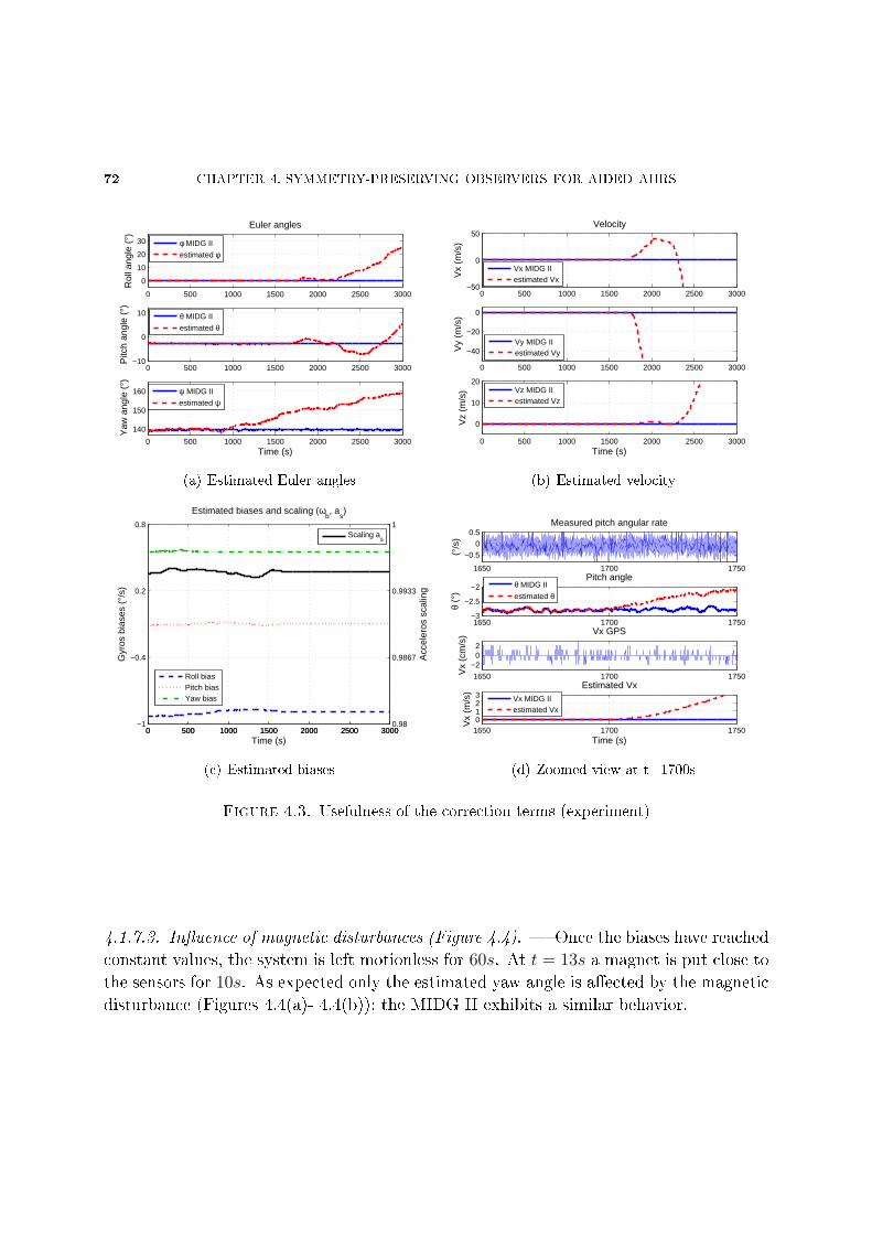
72 CHAPTER 4. SYMMETRY-PRESERVING OBSERVERS FOR AIDED AHRS
0 500 1000 1500 2000 2500 3000
0
10
20
30
Euler angles
Rol
l ang
le (
°)
0 500 1000 1500 2000 2500 3000−10
0
10
Pitc
h an
gle
(°)
0 500 1000 1500 2000 2500 3000
140
150
160
Time (s)
Yaw
ang
le (
°)
φ MIDG II
estimated φ
θ MIDG II
estimated θ
ψ MIDG II
estimated ψ
(a) Estimated Euler angles
0 500 1000 1500 2000 2500 3000−50
0
50Velocity
Vx
(m/s
)
0 500 1000 1500 2000 2500 3000
−40
−20
0
Vy
(m/s
)
0 500 1000 1500 2000 2500 3000
0
10
20
Time (s)V
z (m
/s)
Vx MIDG IIestimated Vx
Vy MIDG IIestimated Vy
Vz MIDG IIestimated Vz
(b) Estimated velocity
0 500 1000 1500 2000 2500 3000−1
−0.4
0.2
0.8
Time (s)
Gyr
os b
iase
s (°
/s)
Estimated biases and scaling (ωb, a
s)
0 500 1000 1500 2000 2500 30000.98
0.9867
0.9933
1
Acc
eler
os s
calin
g
Roll biasPitch biasYaw bias
Scaling as
(c) Estimated biases
1650 1700 1750
−0.50
0.5Measured pitch angular rate
(°/s
)
1650 1700 1750−3
−2.5
−2
θ (°
)
Pitch angle
1650 1700 1750
−202
Vx GPS
Vx
(cm
/s)
1650 1700 17500123
Time (s)
Vx
(m/s
)
Estimated Vx
θ MIDG II
estimated θ
Vx MIDG IIestimated Vx
(d) Zoomed view at t=1700s
Figure 4.3. Usefulness of the correction terms (experiment)
4.1.7.3. Inuence of magnetic disturbances (Figure 4.4). Once the biases have reached
constant values, the system is left motionless for 60s. At t = 13s a magnet is put close to
the sensors for 10s. As expected only the estimated yaw angle is aected by the magnetic
disturbance (Figures 4.4(a)- 4.4(b)); the MIDG II exhibits a similar behavior.
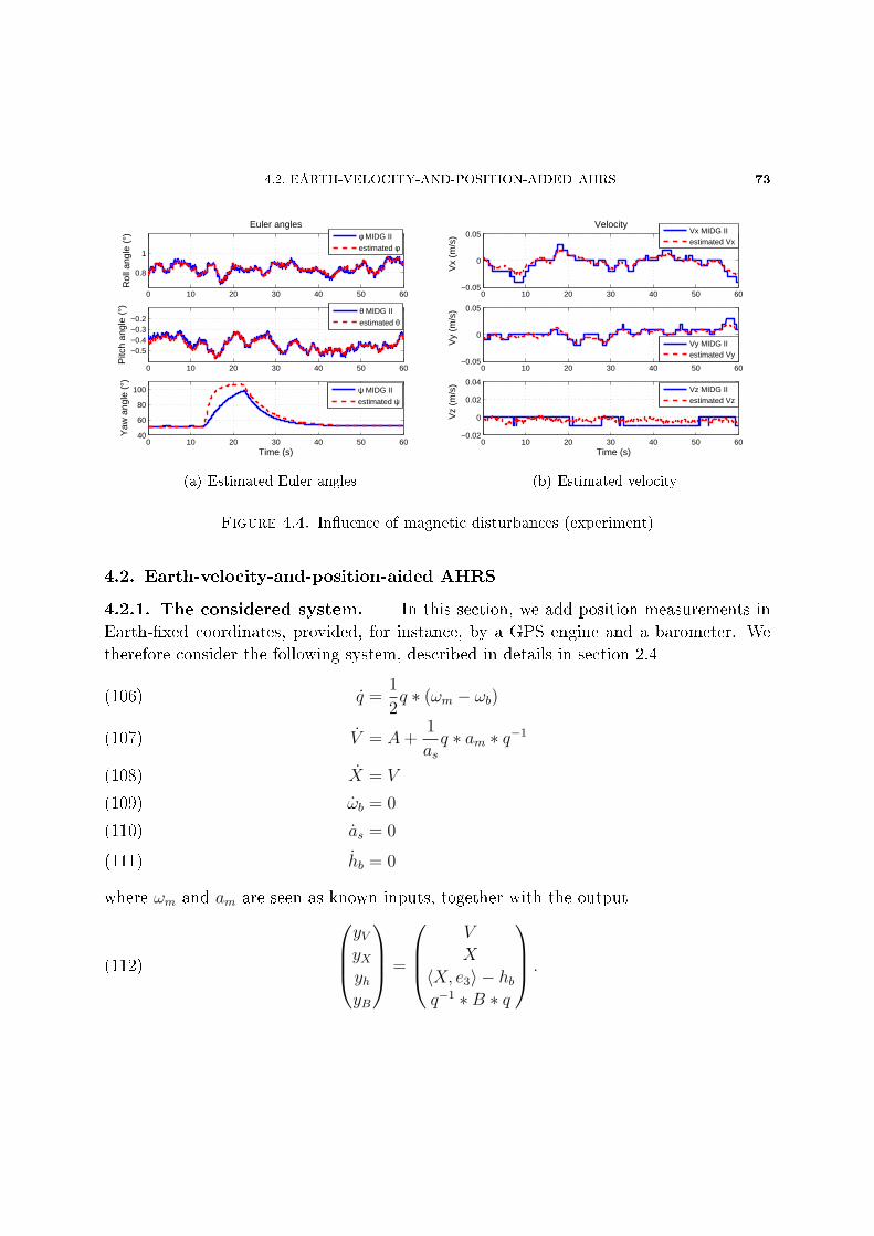
4.2. EARTH-VELOCITY-AND-POSITION-AIDED AHRS 73
0 10 20 30 40 50 60
0.8
1
Euler angles
Rol
l ang
le (
°)
0 10 20 30 40 50 60
−0.5−0.4−0.3−0.2
Pitc
h an
gle
(°)
0 10 20 30 40 50 6040
60
80
100
Time (s)
Yaw
ang
le (
°)
φ MIDG II
estimated φ
θ MIDG II
estimated θ
ψ MIDG II
estimated ψ
(a) Estimated Euler angles
0 10 20 30 40 50 60−0.05
0
0.05Velocity
Vx
(m/s
)
0 10 20 30 40 50 60−0.05
0
0.05
Vy
(m/s
)
0 10 20 30 40 50 60−0.02
0
0.02
0.04
Time (s)V
z (m
/s)
Vx MIDG IIestimated Vx
Vy MIDG IIestimated Vy
Vz MIDG IIestimated Vz
(b) Estimated velocity
Figure 4.4. Inuence of magnetic disturbances (experiment)
4.2. Earth-velocity-and-position-aided AHRS
4.2.1. The considered system. In this section, we add position measurements in
Earth-xed coordinates, provided, for instance, by a GPS engine and a barometer. We
therefore consider the following system, described in details in section 2.4
q =1
2q ∗ (ωm − ωb)(106)
V = A+1
asq ∗ am ∗ q−1(107)
X = V(108)
ωb = 0(109)
as = 0(110)
hb = 0(111)
where ωm and am are seen as known inputs, together with the outputyVyXyhyB
=
V
X
〈X, e3〉 − hbq−1 ∗B ∗ q
.(112)
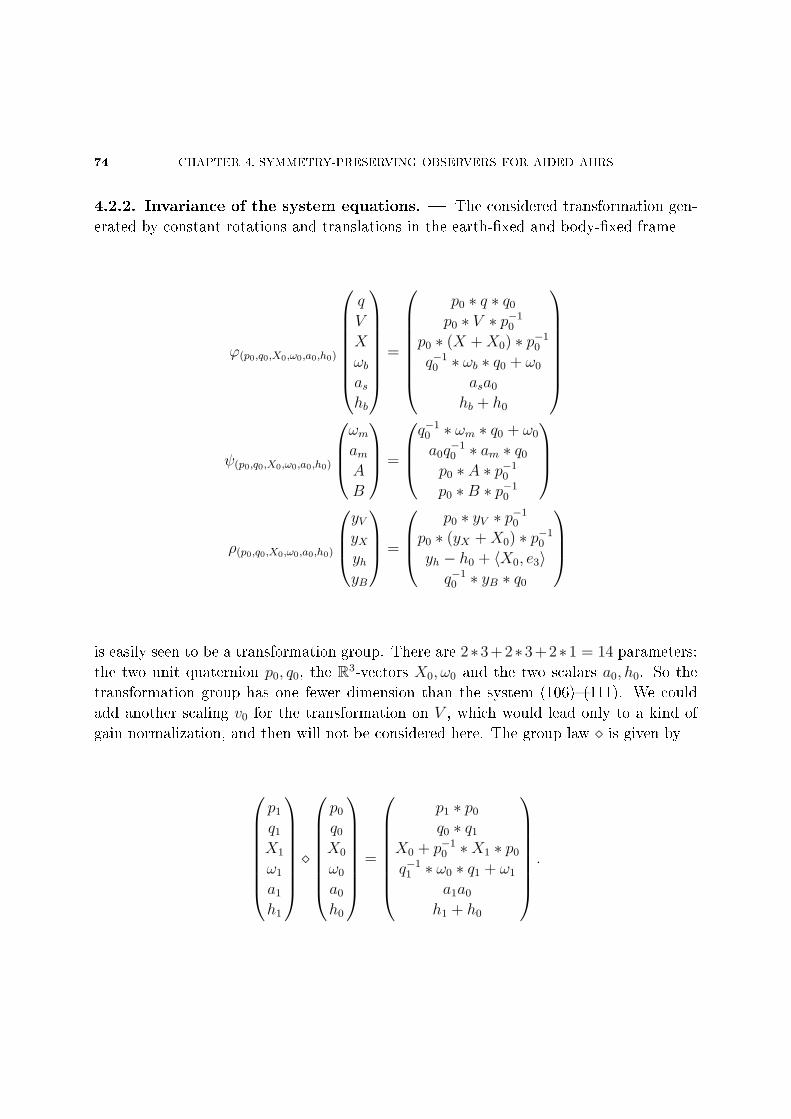
74 CHAPTER 4. SYMMETRY-PRESERVING OBSERVERS FOR AIDED AHRS
4.2.2. Invariance of the system equations. The considered transformation gen-
erated by constant rotations and translations in the earth-xed and body-xed frame
ϕ(p0,q0,X0,ω0,a0,h0)
q
V
X
ωbashb
=
p0 ∗ q ∗ q0
p0 ∗ V ∗ p−10
p0 ∗ (X +X0) ∗ p−10
q−10 ∗ ωb ∗ q0 + ω0
asa0
hb + h0
ψ(p0,q0,X0,ω0,a0,h0)
ωmamA
B
=
q−1
0 ∗ ωm ∗ q0 + ω0
a0q−10 ∗ am ∗ q0
p0 ∗ A ∗ p−10
p0 ∗B ∗ p−10
ρ(p0,q0,X0,ω0,a0,h0)
yVyXyhyB
=
p0 ∗ yV ∗ p−1
0
p0 ∗ (yX +X0) ∗ p−10
yh − h0 + 〈X0, e3〉q−1
0 ∗ yB ∗ q0
is easily seen to be a transformation group. There are 2∗3+2∗3+2∗1 = 14 parameters:
the two unit quaternion p0, q0, the R3-vectors X0, ω0 and the two scalars a0, h0. So the
transformation group has one fewer dimension than the system (106)(111). We could
add another scaling v0 for the transformation on V , which would lead only to a kind of
gain normalization, and then will not be considered here. The group law is given by
p1
q1
X1
ω1
a1
h1
p0
q0
X0
ω0
a0
h0
=
p1 ∗ p0
q0 ∗ q1
X0 + p−10 ∗X1 ∗ p0
q−11 ∗ ω0 ∗ q1 + ω1
a1a0
h1 + h0
.
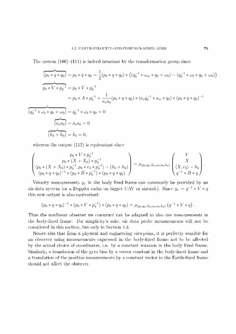
4.2. EARTH-VELOCITY-AND-POSITION-AIDED AHRS 75
The system (106)(111) is indeed invariant by the transformation group since
˙︷ ︸︸ ︷(p0 ∗ q ∗ q0) = p0 ∗ q ∗ q0 =
1
2(p0 ∗ q ∗ q0) ∗
((q−1
0 ∗ ωm ∗ q0 + ω0)− (q−10 ∗ ωb ∗ q0 + ω0)
)˙︷ ︸︸ ︷
p0 ∗ V ∗ p−10 = p0 ∗ V ∗ p−1
0
= p0 ∗ A ∗ p−10 +
1
asa0
(p0 ∗ q ∗ q0) ∗ (asq−10 ∗ am ∗ q0) ∗ (p0 ∗ q ∗ q0)−1
˙︷ ︸︸ ︷(q−1
0 ∗ ωb ∗ q0 + ω0) = q−10 ∗ ωb ∗ q0 = 0
˙︷ ︸︸ ︷(asa0) = asa0 = 0
˙︷ ︸︸ ︷(hb + h0) = hb = 0,
whereas the output (112) is equivariant sincep0 ∗ V ∗ p−1
0
p0 ∗ (X +X0) ∗ p−10
〈p0 ∗ (X +X0) ∗ p−10 , p0 ∗ e3 ∗ p−1
0 〉 − (hb + h0)
(p0 ∗ q ∗ q0)−1 ∗ (p0 ∗B ∗ p−10 ) ∗ (p0 ∗ q ∗ q0)
= ρ(p0,q0,X0,ω0,a0,h0)
V
X
〈X, e3〉 − hbq−1 ∗B ∗ q
.
Velocity measurements yv in the body-xed frame can commonly be provided by an
air-data system (or a Doppler radar on bigger UAV or aircraft). Since yv = q−1 ∗ V ∗ qthis new output is also equivariant:
(p0 ∗ q ∗ q0)−1 ∗ (p0 ∗ V ∗ p−10 ) ∗ (p0 ∗ q ∗ q0) = ρ(p0,q0,X0,ω0,a0,h0)
(q−1 ∗ V ∗ q
).
Thus the nonlinear observer we construct can be adapted to also use measurements in
the body-xed frame. For simplicity's sake, air data probe measurements will not be
considered in this section, but only in Section 4.3.
Notice also that from a physical and engineering viewpoint, it is perfectly sensible for
an observer using measurements expressed in the body-xed frame not to be aected
by the actual choice of coordinates, i.e. by a constant rotation in the body-xed frame.
Similarly, a translation of the gyro bias by a vector constant in the body-xed frame and
a translation of the position measurements by a constant vector in the Earth-xed frame
should not aect the observer.
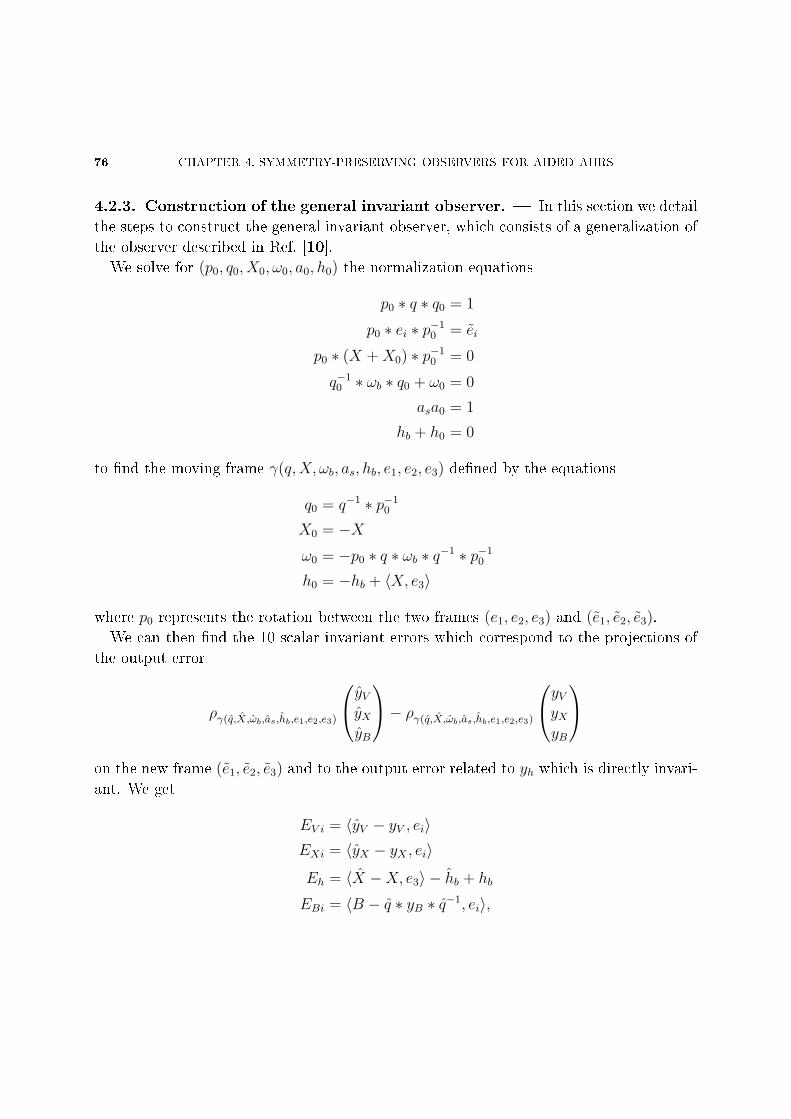
76 CHAPTER 4. SYMMETRY-PRESERVING OBSERVERS FOR AIDED AHRS
4.2.3. Construction of the general invariant observer. In this section we detail
the steps to construct the general invariant observer, which consists of a generalization of
the observer described in Ref. [10].
We solve for (p0, q0, X0, ω0, a0, h0) the normalization equations
p0 ∗ q ∗ q0 = 1
p0 ∗ ei ∗ p−10 = ei
p0 ∗ (X +X0) ∗ p−10 = 0
q−10 ∗ ωb ∗ q0 + ω0 = 0
asa0 = 1
hb + h0 = 0
to nd the moving frame γ(q,X, ωb, as, hb, e1, e2, e3) dened by the equations
q0 = q−1 ∗ p−10
X0 = −Xω0 = −p0 ∗ q ∗ ωb ∗ q−1 ∗ p−1
0
h0 = −hb + 〈X, e3〉
where p0 represents the rotation between the two frames (e1, e2, e3) and (e1, e2, e3).
We can then nd the 10 scalar invariant errors which correspond to the projections of
the output error
ργ(q,X,ωb,as,hb,e1,e2,e3)
yVyXyB
− ργ(q,X,ωb,as,hb,e1,e2,e3)
yVyXyB
on the new frame (e1, e2, e3) and to the output error related to yh which is directly invari-
ant. We get
EV i = 〈yV − yV , ei〉EXi = 〈yX − yX , ei〉
Eh = 〈X −X, e3〉 − hb + hb
EBi = 〈B − q ∗ yB ∗ q−1, ei〉,
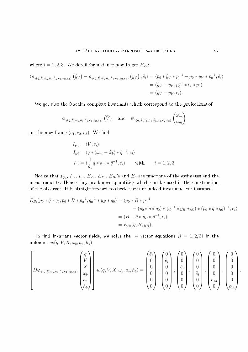
4.2. EARTH-VELOCITY-AND-POSITION-AIDED AHRS 77
where i = 1, 2, 3. We detail for instance how to get EV i:
〈ργ(q,X,ωb,as,hb,e1,e2,e3)
(yV)− ργ(q,X,ωb,as,hb,e1,e2,e3)
(yV), ei〉 = 〈p0 ∗ yV ∗ p−1
0 − p0 ∗ yV ∗ p−10 , ei〉
= 〈yV − yV , p−10 ∗ ei ∗ p0〉
= 〈yV − yV , ei〉.
We get also the 9 scalar complete invariants which correspond to the projections of
φγ(q,X,ωb,as,hb,e1,e2,e3)
(V)
and ψγ(q,X,ωb,as,hb,e1,e2,e3)
(ωmam
)on the new frame (e1, e2, e3). We nd
IV i = 〈V , ei〉Iωi = 〈q ∗ (ωm − ωb) ∗ q−1, ei〉
Iai = 〈 1
asq ∗ am ∗ q−1, ei〉 with i = 1, 2, 3.
Notice that IV i, Iωi, Iai, EV i, EXi, EBi's and Eh are functions of the estimates and the
measurements. Hence they are known quantities which can be used in the construction
of the observer. It is straightforward to check they are indeed invariant. For instance,
EBi(p0 ∗ q ∗ q0, p0 ∗B ∗ p−10 , q−1
0 ∗ yB ∗ q0) = 〈p0 ∗B ∗ p−10
− (p0 ∗ q ∗ q0) ∗ (q−10 ∗ yB ∗ q0) ∗ (p0 ∗ q ∗ q0)−1, ei〉
= 〈B − q ∗ yB ∗ q−1, ei〉= EBi(q, B, yB).
To nd invariant vector elds, we solve the 14 vector equations (i = 1, 2, 3) in the
unknown w(q, V,X, ωb, as, hb)Dϕγ(q,X,ωb,as,hb,e1,e2,e3)
q
V
X
ωbashb
·w(q, V,X, ωb, as, hb) =
ei0
0
0
0
0
,
0
ei0
0
0
0
,
0
0
ei0
0
0
,
0
0
0
ei0
0
,
0
0
0
0
e13
0
,
0
0
0
0
0
e14
.
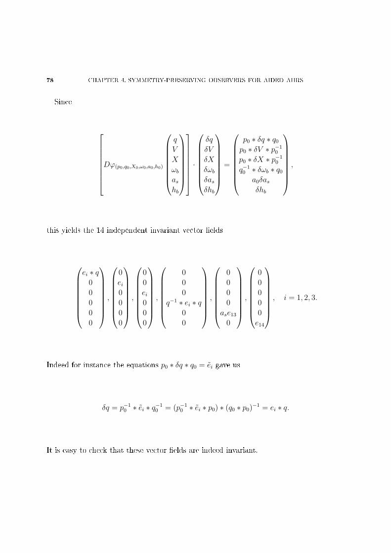
78 CHAPTER 4. SYMMETRY-PRESERVING OBSERVERS FOR AIDED AHRS
Since
Dϕ(p0,q0,X0,ω0,a0,h0)
q
V
X
ωbashb
·
δq
δV
δX
δωbδasδhb
=
p0 ∗ δq ∗ q0
p0 ∗ δV ∗ p−10
p0 ∗ δX ∗ p−10
q−10 ∗ δωb ∗ q0
a0δasδhb
,
this yields the 14 independent invariant vector elds
ei ∗ q0
0
0
0
0
,
0
ei0
0
0
0
,
0
0
ei0
0
0
,
0
0
0
q−1 ∗ ei ∗ q0
0
,
0
0
0
0
ase13
0
,
0
0
0
0
0
e14
, i = 1, 2, 3.
Indeed for instance the equations p0 ∗ δq ∗ q0 = ei gave us
δq = p−10 ∗ ei ∗ q−1
0 = (p−10 ∗ ei ∗ p0) ∗ (q0 ∗ p0)−1 = ei ∗ q.
It is easy to check that these vector elds are indeed invariant.
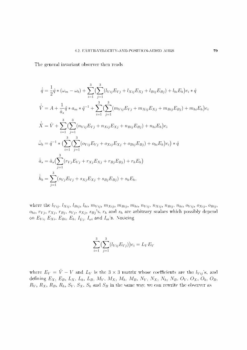
4.2. EARTH-VELOCITY-AND-POSITION-AIDED AHRS 79
The general invariant observer then reads
˙q =1
2q ∗ (ωm − ωb) +
3∑i=1
( 3∑j=1
(lV ijEV j + lXijEXj + lBijEBj) + lhiEh)ei ∗ q
˙V = A+
1
asq ∗ am ∗ q−1 +
3∑i=1
( 3∑j=1
(mV ijEV j +mXijEXj +mBijEBj) +mhiEh)ei
˙X = V +
3∑i=1
( 3∑j=1
(nV ijEV j + nXijEXj + nBijEBj) + nhiEh)ei
˙ωb = q−1 ∗( 3∑i=1
( 3∑j=1
(oV ijEV j + oXijEXj + oBijEBj) + ohiEh)ei)∗ q
˙as = as( 3∑j=1
(rV jEV j + rXjEXj + rBjEBj) + rhEh)
˙hb =
3∑j=1
(sV jEV j + sXjEXj + sBjEBj) + shEh,
where the lV ij, lXij, lBij, lhi, mV ij, mXij, mBij, mhi, nV ij, nXij, nBij, nhi, oV ij, oXij, oBij,
ohi, rV j, rXj, rBj, sV j, sXj, sBj's, rh and sh are arbitrary scalars which possibly depend
on EV i, EXi, EBi, Eh, IV i, Iωi and Iai's. Noticing
3∑i=1
( 3∑j=1
(lV ijEV j))ei = LVEV
where EV = V − V and LV is the 3 × 3 matrix whose coecients are the lV ij's, and
dening EX , EB, LX , Lh, LB, MV , MX , Mh, MB, NV , NX , Nh, NB, OV , OX , Oh, OB,
RV , RX , RB, Rh, SV , SX , Sh and SB in the same way, we can rewrite the observer as
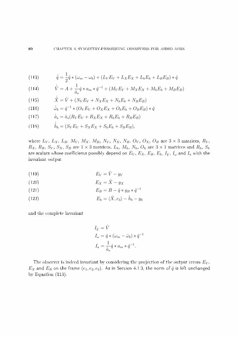
80 CHAPTER 4. SYMMETRY-PRESERVING OBSERVERS FOR AIDED AHRS
˙q =1
2q ∗ (ωm − ωb) + (LVEV + LXEX + LhEh + LBEB) ∗ q(113)
˙V = A+
1
asq ∗ am ∗ q−1 + (MVEV +MXEX +MhEh +MBEB)(114)
˙X = V + (NVEV +NXEX +NhEh +NBEB)(115)
˙ωb = q−1 ∗ (OVEV +OXEX +OhEh +OBEB) ∗ q(116)
˙as = as(RVEV +RXEX +RhEh +RBEB)(117)
˙hb = (SVEV + SXEX + ShEh + SBEB),(118)
where LV , LX , LB, MV , MX , MB, NV , NX , NB, OV , OX , OB are 3 × 3 matrices, RV ,
RX , RB, SV , SX , SB are 1 × 3 matrices, Lh, Mh, Nh, Oh are 3 × 1 matrices and Rh, Share scalars whose coecients possibly depend on EV , EX , EB, Eh, IV , Iω and Ia with the
invariant output
EV = V − yV(119)
EX = X − yX(120)
EB = B − q ∗ yB ∗ q−1(121)
Eh = 〈X, e3〉 − hb − yh(122)
and the complete invariant
IV = V
Iω = q ∗ (ωm − ωb) ∗ q−1
Ia =1
asq ∗ am ∗ q−1.
The observer is indeed invariant by considering the projection of the output errors EV ,
EX and EB on the frame (e1, e2, e3). As in Section 4.1.3, the norm of q is left unchanged
by Equation (113).
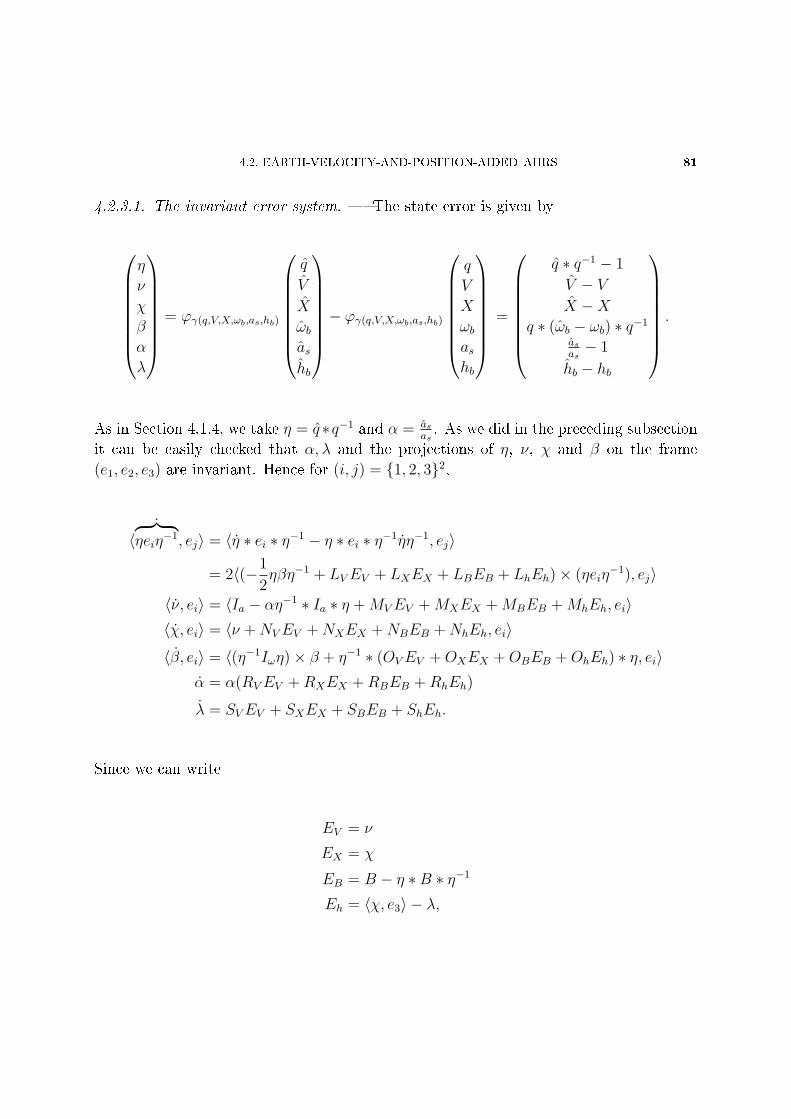
4.2. EARTH-VELOCITY-AND-POSITION-AIDED AHRS 81
4.2.3.1. The invariant error system. The state error is given by
η
ν
χ
β
α
λ
= ϕγ(q,V,X,ωb,as,hb)
q
V
X
ωbashb
− ϕγ(q,V,X,ωb,as,hb)
q
V
X
ωbashb
=
q ∗ q−1 − 1
V − VX −X
q ∗ (ωb − ωb) ∗ q−1
as
as− 1
hb − hb
.
As in Section 4.1.4, we take η = q ∗q−1 and α = as
as. As we did in the preceding subsection
it can be easily checked that α, λ and the projections of η, ν, χ and β on the frame
(e1, e2, e3) are invariant. Hence for (i, j) = 1, 2, 32,
〈˙︷ ︸︸ ︷
ηeiη−1, ej〉 = 〈η ∗ ei ∗ η−1 − η ∗ ei ∗ η−1ηη−1, ej〉
= 2〈(−1
2ηβη−1 + LVEV + LXEX + LBEB + LhEh)× (ηeiη
−1), ej〉
〈ν, ei〉 = 〈Ia − αη−1 ∗ Ia ∗ η +MVEV +MXEX +MBEB +MhEh, ei〉〈χ, ei〉 = 〈ν +NVEV +NXEX +NBEB +NhEh, ei〉
〈β, ei〉 = 〈(η−1Iωη)× β + η−1 ∗ (OVEV +OXEX +OBEB +OhEh) ∗ η, ei〉α = α(RVEV +RXEX +RBEB +RhEh)
λ = SVEV + SXEX + SBEB + ShEh.
Since we can write
EV = ν
EX = χ
EB = B − η ∗B ∗ η−1
Eh = 〈χ, e3〉 − λ,
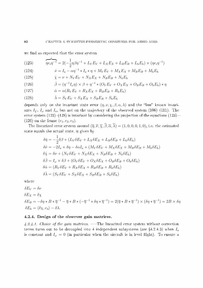
82 CHAPTER 4. SYMMETRY-PRESERVING OBSERVERS FOR AIDED AHRS
we nd as expected that the error system
˙︷ ︸︸ ︷ηeiη
−1 = 2(−1
2ηβη−1 + LVEV + LXEX + LBEB + LhEh)× (ηeiη
−1)(123)
ν = Ia − αη−1 ∗ Ia ∗ η +MVEV +MXEX +MBEB +MhEh(124)
χ = ν +NVEV +NXEX +NBEB +NhEh(125)
β = (η−1Iωη)× β + η−1 ∗ (OVEV +OXEX +OBEB +OhEh) ∗ η(126)
α = α(RVEV +RXEX +RBEB +RhEh)(127)
λ = SVEV + SXEX + SBEB + ShEh(128)
depends only on the invariant state error (η, ν, χ, β, α, λ) and the free known invari-
ants IV , Iω and Ia, but not on the trajectory of the observed system (106)(111). The
error system (123)(128) is invariant by considering the projection of the equations (123)
(126) on the frame (e1, e2, e3).
The linearized error system around (η, ν, χ, β, α, λ) = (1, 0, 0, 0, 1, 0), i.e. the estimated
state equals the actual state, is given by
δη = −1
2δβ + (LV δEV + LXδEX + LBδEB + LhδEh)
δν = −2Ia × δη − δαIa + (MV δEV +MXδEX +MBδEB +MhδEh)
δχ = δν + (NV δEV +NXδEX +NBδEB +NhδEh)
δβ = Iω × δβ + (OV δEV +OXδEX +OBδEB +OhδEh)
δα = (RV δEV +RXδEX +RBδEB +RhδEh)
δλ = (SV δEV + SXδEX + SBδEB + ShδEh)
where
δEV = δν
δEX = δχ
δEB = −δη ∗B ∗ η−1 − η ∗B ∗ (−η−1 ∗ δη ∗ η−1) = 2(η ∗B ∗ η−1)× (δη ∗ η−1) = 2B × δηδEh = 〈δχ, e3〉 − δλ.
4.2.4. Design of the observer gain matrices.
4.2.4.1. Choice of the gain matrices. The linearized error system without correction
terms turns out to be decoupled into 4 independent subsystems (see 4.2.4.3) when Iais constant and Iω = 0 (in particular when the aircraft is in level ight). To ensure a
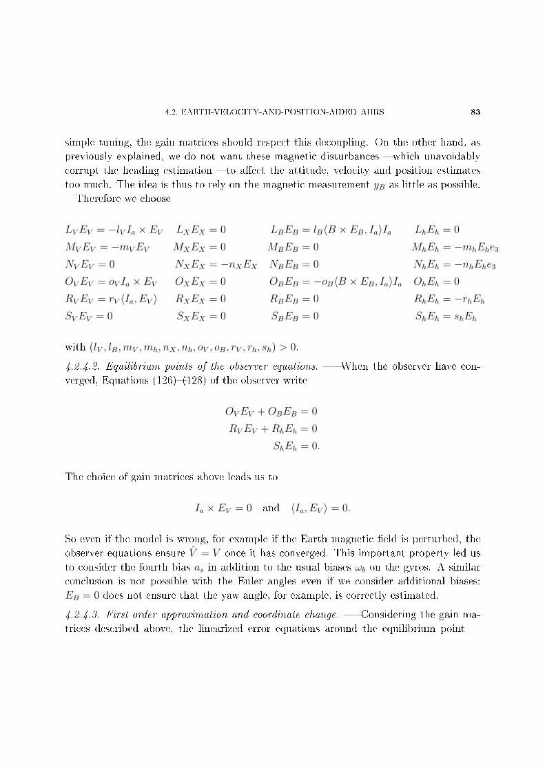
4.2. EARTH-VELOCITY-AND-POSITION-AIDED AHRS 83
simple tuning, the gain matrices should respect this decoupling. On the other hand, as
previously explained, we do not want these magnetic disturbances which unavoidably
corrupt the heading estimation to aect the attitude, velocity and position estimates
too much. The idea is thus to rely on the magnetic measurement yB as little as possible.
Therefore we choose
LVEV = −lV Ia × EV LXEX = 0 LBEB = lB〈B × EB, Ia〉Ia LhEh = 0
MVEV = −mVEV MXEX = 0 MBEB = 0 MhEh = −mhEhe3
NVEV = 0 NXEX = −nXEX NBEB = 0 NhEh = −nhEhe3
OVEV = oV Ia × EV OXEX = 0 OBEB = −oB〈B × EB, Ia〉Ia OhEh = 0
RVEV = rV 〈Ia, EV 〉 RXEX = 0 RBEB = 0 RhEh = −rhEhSVEV = 0 SXEX = 0 SBEB = 0 ShEh = shEh
with (lV , lB,mV ,mh, nX , nh, oV , oB, rV , rh, sh) > 0.
4.2.4.2. Equilibrium points of the observer equations. When the observer have con-
verged, Equations (126)(128) of the observer write
OVEV +OBEB = 0
RVEV +RhEh = 0
ShEh = 0.
The choice of gain matrices above leads us to
Ia × EV = 0 and 〈Ia, EV 〉 = 0.
So even if the model is wrong, for example if the Earth magnetic eld is perturbed, the
observer equations ensure V = V once it has converged. This important property led us
to consider the fourth bias as in addition to the usual biases ωb on the gyros. A similar
conclusion is not possible with the Euler angles even if we consider additional biases:
EB = 0 does not ensure that the yaw angle, for example, is correctly estimated.
4.2.4.3. First-order approximation and coordinate change. Considering the gain ma-
trices described above, the linearized error equations around the equilibrium point
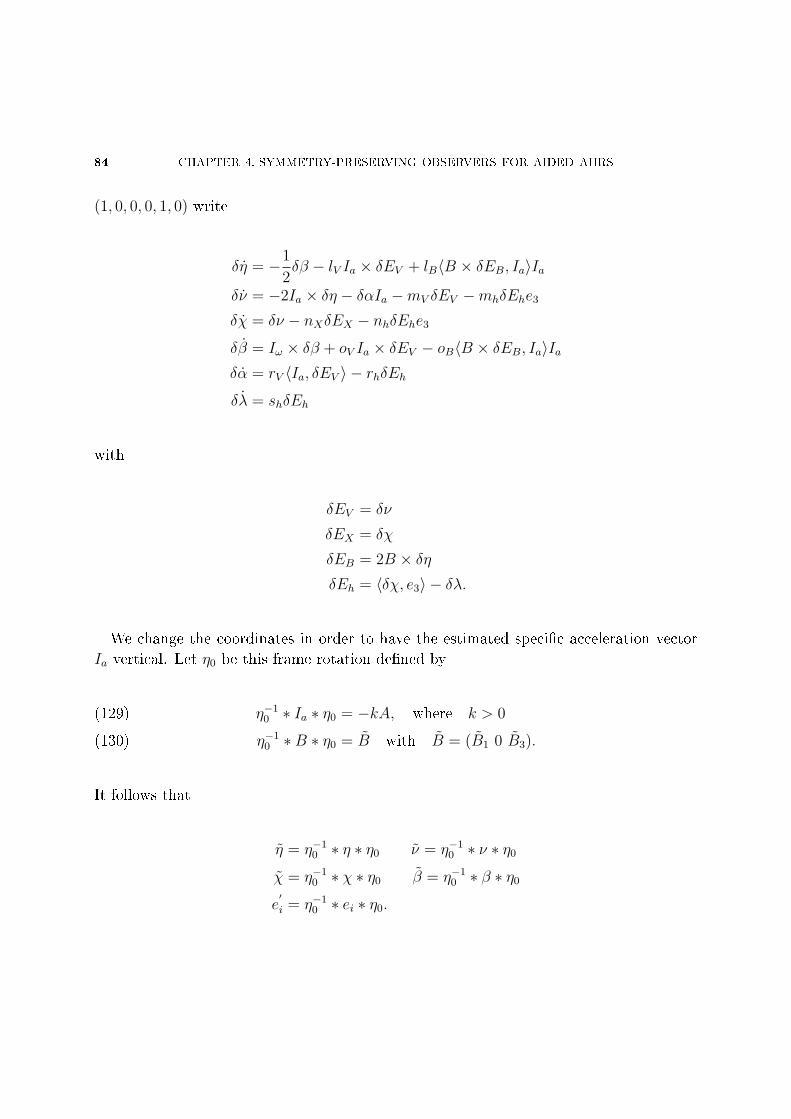
84 CHAPTER 4. SYMMETRY-PRESERVING OBSERVERS FOR AIDED AHRS
(1, 0, 0, 0, 1, 0) write
δη = −1
2δβ − lV Ia × δEV + lB〈B × δEB, Ia〉Ia
δν = −2Ia × δη − δαIa −mV δEV −mhδEhe3
δχ = δν − nXδEX − nhδEhe3
δβ = Iω × δβ + oV Ia × δEV − oB〈B × δEB, Ia〉Iaδα = rV 〈Ia, δEV 〉 − rhδEhδλ = shδEh
with
δEV = δν
δEX = δχ
δEB = 2B × δηδEh = 〈δχ, e3〉 − δλ.
We change the coordinates in order to have the estimated specic acceleration vector
Ia vertical. Let η0 be this frame rotation dened by
η−10 ∗ Ia ∗ η0 = −kA, where k > 0(129)
η−10 ∗B ∗ η0 = B with B = (B1 0 B3).(130)
It follows that
η = η−10 ∗ η ∗ η0 ν = η−1
0 ∗ ν ∗ η0
χ = η−10 ∗ χ ∗ η0 β = η−1
0 ∗ β ∗ η0
e′
i = η−10 ∗ ei ∗ η0.
4.2. EARTH-VELOCITY-AND-POSITION-AIDED AHRS 85
The error system then becomes
δ ˙η = 2δη × (η−10 ∗ η0)− 1
2δβ + klVA× δEV + k2lB〈B × δEB, A〉A
δ ˙ν = 2δν × (η−10 ∗ η0) + 2kA× δη + kδαA−mV δEV −mhδEhe
′
3
δ ˙χ = 2δχ× (η−10 ∗ η0) + δν − nXδEX − nhδEhe
′
3
δ ˙β = 2δβ × (η−10 ∗ η0) + Iω × δω − koVA× δEV − k2oB〈B × δEB, A〉A
δα = −rV k〈A, δEV 〉 − rhδEhδλ = shδEh
with
δEV = δν
δEX = δχ
δEB = 2B × δη
δEh = 〈δχ, e′3〉 − δλ.
We suppose now that the system is moving along a smooth trajectory, i.e η0, Ia and
Iω are negligible (rst order terms). All the terms of the form ·× (η−10 ∗ η0) then disappear
and k is now constant. The error system splits into three decoupled subsystems and one
cascaded subsystem:
the longitudinal subsystemsδ ˙η2
δ ˙ν1
δ ˙β2
=
0 klV g −12
−2kg −mV 0
0 −koV g 0
δη2
δν1
δβ2
δχ1 = δν1 − nXδχ1
the lateral subsystemsδ ˙η1
δ ˙ν2
δ ˙β1
=
0 −klV g −12
2kg −mV 0
0 koV g 0
δη1
δν2
δβ1
δχ2 = δν2 − nXδχ2
86 CHAPTER 4. SYMMETRY-PRESERVING OBSERVERS FOR AIDED AHRS
the vertical subsystemδ ˙ν3
δα
δ ˙χ3
δλ
=
−mV kg −mh mh
−kgrV 0 −rh rh1 0 −(nX + nh) nh0 0 sh −sh
δν3
δα
δχ3
δλ
the heading subsystem
(δ ˙η3
δ ˙β3
)=
(−2k2g2lBB
21 −1
2
2k2g2oBB21 0
)(δη3
δβ3
)+
(2k2g2lBB3B1
−2k2g2oBB3B1
)δη1.
Thanks to this decoupled structure, the convergence of each subsystem, and then the
local convergence of the invariant observer, is straightforward, and leads to Theorem 3.
Theorem 3. Consider the physical system (106)(111) with the measurements (112).
Consider the nonlinear invariant observer dened by
˙q =1
2q ∗ (ωm − ωb) + (LVEV + LBEB) ∗ q
˙V = A+
1
asq ∗ am ∗ q−1 + (MVEV +MhEh)
˙X = V + (NXEX +NhEh)
˙ωb = q−1 ∗ (OVEV +OBEB) ∗ q˙as = as(RVEV +RhEh)
˙hb = (ShEh),
with the expression of the output errors given by Equations (119)(122) and the gain
matrices given in Section 4.2.4.1. Then for any value
(lV , lB,mV ,mh, nX , nh, oV , oB, rV , rh, sh) > 0, the solution (q(t), V (t), X(t), ωb(t), as(t), hb(t))
locally asymptotically converges to (q(t), V (t), X(t), ωb, as, hb) around every smooth tra-
jectory, i.e when η0, Ia, and Iω are rst order terms.
We insist that it is not usually obvious to come up with a similar convergence result
for an EKF. The gains lV , lB,mV ,mh, nX , nh, oV , oB, rV , rh, sh are also easy to tune, since
the behaviors of each subsystem are independent. Moreover, the lateral, longitudinal and
vertical subsystems do not depend on the magnetic measurements, so will not be aected
if the magnetic eld is perturbed.
4.2. EARTH-VELOCITY-AND-POSITION-AIDED AHRS 87
4.2.4.4. Inuence of magnetic disturbances on static behavior. We now investigate
how the equilibrium point (1, 0, 0, 0, 1, 0) is modied when the magnetic eld is (statically)
perturbed. We show that only the yaw angle ψ is aected while all the other variables,
in particular the attitude angles φ, θ, remain unchanged. Here the Euler angles φ, θ, ψ
correspond to the error quaternion η in the new frame described by Equations (129)-(130).
The equilibrium points (η, ν, χ, ω, α, λ) are dened by
(lV kA× ν + lB〈B × EB, kA〉kA) ∗ η − 1
2η ∗ ω = 0
−kA+ αη−1 ∗ kA ∗ η −mV ν −mh(〈χ, e
′
3〉 − λ)e′
3 = 0
ν − nX χ− nh(〈χ, e′
3〉 − λ)e′
3 = 0
η−1 ∗ (−oV kA× ν − oB〈B × EB, kA〉kA) ∗ η + (η
−1 ∗ Iω ∗ η)× ω = 0
rV 〈kA, ν〉α− rh(〈χ, e′
3〉 − λ) = 0
sh(〈χ, e′
3〉 − λ) = 0.
We ensure ω = 0 by choosing LVEV + LBEB colinear with OVEV +OBEB, that isoV
lV= oB
lB, σ. This implies ν = 0, αη ∗A ∗ η−1−A = 0, 〈B× EB, kA〉 = 0, 〈χ, e′3〉−λ = 0
and χ = 0.
Finally, the new equilibrium points is (η, ν, χ, ω, α, λ) = (η, 0, 0, 0, 1, 0); moreover φ =
θ = 0 and ψ is determined by 〈B×EB, kA〉 = 0, where the Euler angles φ, θ, ψ correspond
to the error quaternion η.
4.2.5. Simulation results. We rst illustrate on simulation the behavior of the
invariant observer
˙q =1
2q ∗ (ωm − ωb) + (LVEV + LXEX + LhEh + LBEB) ∗ q + ε(1− ‖q‖2)q(131)
˙V = A+
1
asq ∗ am ∗ q−1 + (MVEV +MXEX +MhEh +MBEB)(132)
˙X = V + (NVEV +NXEX +NhEh +NBEB)(133)
˙ωb = q−1 ∗ (OVEV +OXEX +OhEh +OBEB) ∗ q(134)
˙as = as(RVEV +RXEX +RhEh +RBEB)(135)
˙hb = (SVEV + SXEX + ShEh + SBEB).(136)
with the choice of gain matrices described in 4.2.4.1.
88 CHAPTER 4. SYMMETRY-PRESERVING OBSERVERS FOR AIDED AHRS
We choose here time constants around 10s by taking lV = oV = 4e− 2, lB = oB = 1e− 3,
mV = 5, mh = 0.2, rV = 1e− 2, rh = 8e− 4, nX = 0.8, nh = 0.9, sh = 0.4 and ε = 1. The
system follows the trajectory dened by
as = 1.1 and hb = 1 ωb =
0.01
−0.012
0.08
V =
3− 4 cos(0.23t)
3− 5.6 cos(0.25t+ π/4)
−1− 3.4 sin(.02t)
ωm =
sin(0.5t+ π/5)
sin(0.3t+ π/4)
− sin(0.2t+ π/3)
,
in SI units, which is quite representative of a small UAV ight. The states are initialized
far from their true values. At t = 35s, the magnetic eld is changed from B = (1 0 1)T
to B = (0.7 0.7 0.8)T .
Though we have no proof of convergence but local, the domain of attraction seems to
be large enough, see Figure 4.5. As expected, only the estimated yaw angle ψ is strongly
aected by the magnetic disturbance. Because of the coupling terms Iωm and Ia, there is
some dynamic inuence on the other variables.
4.2.6. Experimental results. We now compare the behavior of our observer with
the commercial INS-GPS device MIDG II from Microbotics Inc. For each experiment
we rst save the raw measurements from the MIDG II gyroscopes, accelerometers and
magnetic sensors (at a 50Hz refresh rate), the position and velocity provided by the
navigation solutions of its GPS engine (at a 5 Hz refresh rate) and the raw measure-
ments from a barometer module Intersema MS5534B (at a 12.5 Hz refresh rate). A
microcontroller on a development kit communicates with these devices and sends the
measurements to a computer via the serial port (see Figure 4.6). On Matlab Simulink
we feed the observer with these data oine and then compare the estimations of the
observer to the estimations given by the MIDG II. In order to have similar behaviors
and considering the units of the raw measurements provided by the MIDG II, we have
chosen lV = 2.8e− 5,lB = 1.4e− 6, mV = 9e− 3, mh = 5e− 4, nX = 1e− 3, nh = 5e− 2,
oV = 4e− 7, oB = 2e− 8, rV = 9.4e− 11, rh = 1e− 9, sh = 5e− 3 and ε = 1.
4.2.6.1. Dynamic behavior (Figure 4.7). We wait a few minutes until the biases reach
constant values, then move the system in all directions. The observer and the MIDG II
give very similar results (Figures 4.7(a)4.7(d)). On Figure 4.7(d) it is in fact hb + 148m
which is represented to plot as and hb on the same axis. We can also notice on Figure 4.7(b)
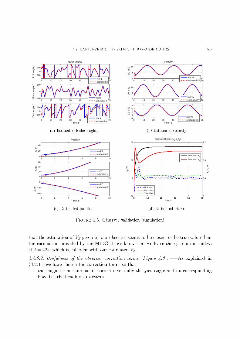
4.2. EARTH-VELOCITY-AND-POSITION-AIDED AHRS 89
0 10 20 30 40 50 60 70
−100
0
100
Euler angles
Rol
l ang
le, °
0 10 20 30 40 50 60 70−100
0
100
Pitc
h an
gle,
°
0 10 20 30 40 50 60 70
−100
0
100
Time, s
Yaw
ang
le, °
real φestimated φ
real θestimated θ
real ψestimated ψ
(a) Estimated Euler angles
0 10 20 30 40 50 60 700
5
10
Velocity
Vx,
m/s
0 10 20 30 40 50 60 700
5
10
Vy,
m/s
0 10 20 30 40 50 60 70−8
−6
−4
−2
0
Time, s
Vz,
m/s
real Vxestimated Vx
real Vyestimated Vy
real Vzestimated Vz
(b) Estimated velocity
0 2 4 6 8 100
20
40
Position
X, m
0 2 4 6 8 100
20
40
60
Y, m
0 2 4 6 8 10
−40
−20
0
Time, s
Z, m
real Xestimated X
real Yestimated Y
real Zestimated Z
(c) Estimated position
0 14 28 42 56 70−30
0
30
60
Time, s
ωb, °
/s
Estimated biases (ωb,a
s,h
b)
0 14 28 42 56 700
0.4
0.8
1.2
a s, hb, m
Roll biasPitch biasYaw bias
Estimated as
Estimated hb
(d) Estimated biases
Figure 4.5. Observer validation (simulation)
that the estimation of VZ given by our observer seems to be closer to the true value than
the estimation provided by the MIDG II: we know that we leave the system motionless
at t = 42s, which is coherent with our estimated VZ .
4.2.6.2. Usefulness of the observer correction terms (Figure 4.8). As explained in
4.2.4.1 we have chosen the correction terms so that:
the magnetic measurements correct essentially the yaw angle and its corresponding
bias, i.e. the heading subsystem
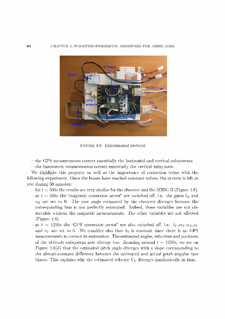
90 CHAPTER 4. SYMMETRY-PRESERVING OBSERVERS FOR AIDED AHRS
Figure 4.6. Experimental protocol
the GPS measurements correct essentially the horizontal and vertical subsystems
the barometric measurements correct essentially the vertical subsystem.
We highlight this property as well as the importance of correction terms with the
following experiment. Once the biases have reached constant values, the system is left at
rest during 50 minutes:
for t < 500s the results are very similar for the observer and the MIDG II (Figure 4.8).
at t = 500s the magnetic correction terms are switched o, i.e. the gains lB and
oB are set to 0. The yaw angle estimated by the observer diverges because the
corresponding bias is not perfectly estimated. Indeed, these variables are not ob-
servable without the magnetic measurements. The other variables are not aected
(Figure 4.8).
at t = 1250s the GPS correction terms are also switched o, i.e. lV ,mV ,nX ,oVand rV are set to 0. We consider also that hb is constant since there is no GPS
measurements to correct its estimation. The estimated angles, velocities and positions
of the attitude subsystem now diverge too. Zooming around t = 1250s, we see on
Figure 4.8(d) that the estimated pitch angle diverges with a slope corresponding to
the almost-constant dierence between the estimated and actual pitch angular rate
biases. This explains why the estimated velocity VX diverges quadratically in time.
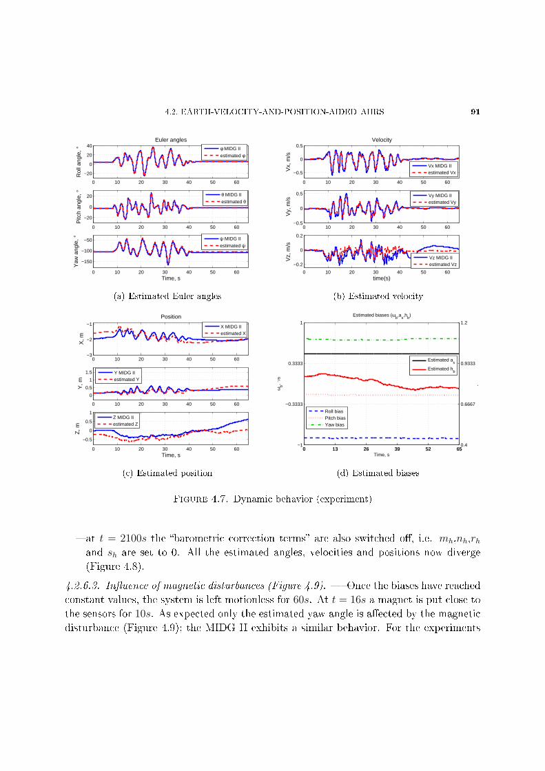
4.2. EARTH-VELOCITY-AND-POSITION-AIDED AHRS 91
0 10 20 30 40 50 60
−20
0
20
40Euler angles
Rol
l ang
le, °
0 10 20 30 40 50 60
−20
0
20
Pitc
h an
gle,
°
0 10 20 30 40 50 60
−150
−100
−50
Time, s
Yaw
ang
le, °
φ MIDG II
estimated φ
θ MIDG II
estimated θ
ψ MIDG II
estimated ψ
(a) Estimated Euler angles
0 10 20 30 40 50 60
−0.5
0
0.5Velocity
Vx,
m/s
0 10 20 30 40 50 60−0.5
0
0.5
Vy,
m/s
0 10 20 30 40 50 60
−0.2
0
0.2
time(s)
Vz,
m/s
Vx MIDG IIestimated Vx
Vy MIDG IIestimated Vy
Vz MIDG IIestimated Vz
(b) Estimated velocity
0 10 20 30 40 50 60−3
−2
−1
Position
X, m
0 10 20 30 40 50 60
0
0.5
1
1.5
Y, m
0 10 20 30 40 50 60
−0.5
0
0.5
1
Time, s
Z, m
X MIDG IIestimated X
Y MIDG IIestimated Y
Z MIDG IIestimated Z
(c) Estimated position
0 13 26 39 52 65−1
−0.3333
0.3333
1
Time, s
ωb, °
/s
Estimated biases (ωb,a
s,h
b)
0 13 26 39 52 650.4
0.6667
0.9333
1.2
a, h
, m
Roll biasPitch biasYaw bias
Estimated as
Estimated hb
(d) Estimated biases
Figure 4.7. Dynamic behavior (experiment)
at t = 2100s the barometric correction terms are also switched o, i.e. mh,nh,rhand sh are set to 0. All the estimated angles, velocities and positions now diverge
(Figure 4.8).
4.2.6.3. Inuence of magnetic disturbances (Figure 4.9). Once the biases have reached
constant values, the system is left motionless for 60s. At t = 16s a magnet is put close to
the sensors for 10s. As expected only the estimated yaw angle is aected by the magnetic
disturbance (Figure 4.9); the MIDG II exhibits a similar behavior. For the experiments
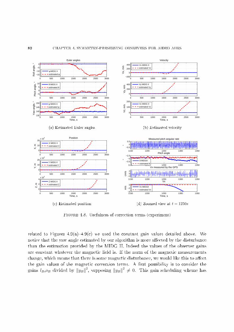
92 CHAPTER 4. SYMMETRY-PRESERVING OBSERVERS FOR AIDED AHRS
0 500 1000 1500 2000 2500 3000
−15
−10
−5
0
Euler angles
Rol
l ang
le, °
0 500 1000 1500 2000 2500 3000
−5
0
5
10
Pitc
h an
gle,
°
0 500 1000 1500 2000 2500 3000135
140
145
150
Time, s
Yaw
ang
le, °
φ MIDG II
estimated φ
θ MIDG II
estimated θ
ψ MIDG II
estimated ψ
(a) Estimated Euler angles
0 500 1000 1500 2000 2500 3000−200
0
200
400
Velocity
Vx,
m/s
0 500 1000 1500 2000 2500 3000
0
200
400
Vy,
m/s
0 500 1000 1500 2000 2500 3000
0
100
200
Time, s
Vz,
m/s
Vx MIDG IIestimated Vx
Vy MIDG IIestimated Vy
Vz MIDG IIestimated Vz
(b) Estimated velocity
0 500 1000 1500 2000 2500 3000
0
10
20x 10
4 Position
X, m
0 500 1000 1500 2000 2500 3000
0
10
20x 10
4
Y, m
0 500 1000 1500 2000 2500 3000
0
2
4x 10
4
Time, s
Z, m
X MIDG IIestimated X
Y MIDG IIestimated Y
Z MIDG IIestimated Z
(c) Estimated position
1150 1200 1250 1300 1350
−0.50
0.5Measured pitch angular rate
°
1150 1200 1250 1300 1350
−3.5−3
−2.5Pitch angle
°
1150 1200 1250 1300 1350
−202
Vx measured by the GPS
cm/s
1150 1200 1250 1300 1350−4
−2
0
Vx
Time, s
m/s
θ MIDGII
estimated θ
Vx MIDGIIestimated Vx
(d) Zoomed view at t = 1250s
Figure 4.8. Usefulness of correction terms (experiment)
related to Figures 4.9(a)4.9(c) we used the constant gain values detailed above. We
notice that the yaw angle estimated by our algorithm is more aected by the disturbance
than the estimation provided by the MIDG II. Indeed the values of the observer gains
are constant whatever the magnetic eld is. If the norm of the magnetic measurements
change, which means that there is some magnetic disturbance, we would like this to aect
the gain values of the magnetic correction terms. A rst possibility is to consider the
gains lB,oB divided by ‖yB‖2, supposing ‖yB‖2 6= 0. This gain scheduling scheme has
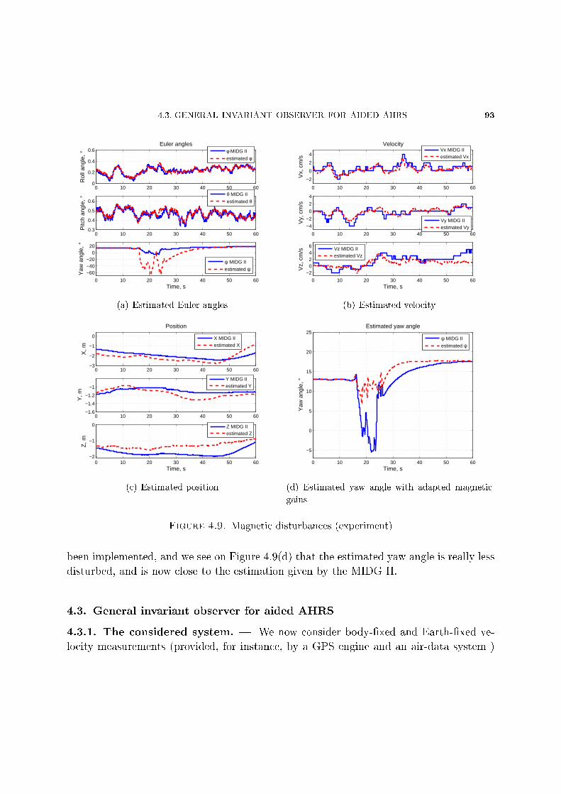
4.3. GENERAL INVARIANT OBSERVER FOR AIDED AHRS 93
0 10 20 30 40 50 600
0.2
0.4
0.6Euler angles
Rol
l ang
le, °
0 10 20 30 40 50 600.3
0.4
0.5
0.6
Pitc
h an
gle,
°
0 10 20 30 40 50 60
−60−40−20
020
Time, s
Yaw
ang
le, °
φ MIDG II
estimated φ
θ MIDG II
estimated θ
ψ MIDG II
estimated ψ
(a) Estimated Euler angles
0 10 20 30 40 50 60
−2
0
2
4
Velocity
Vx,
cm
/s
0 10 20 30 40 50 60
−4
−2
0
2
4
Vy,
cm
/s
0 10 20 30 40 50 60
−20246
Time, s
Vz,
cm
/s
Vx MIDG IIestimated Vx
Vy MIDG IIestimated Vy
Vz MIDG IIestimated Vz
(b) Estimated velocity
0 10 20 30 40 50 60−3
−2
−1
0
Position
X, m
0 10 20 30 40 50 60−1.6
−1.4
−1.2
−1
Y, m
0 10 20 30 40 50 60−2
−1
0
Time, s
Z, m
X MIDG IIestimated X
Y MIDG IIestimated Y
Z MIDG IIestimated Z
(c) Estimated position
0 10 20 30 40 50 60
−5
0
5
10
15
20
25Estimated yaw angle
Time, s
Yaw
ang
le, °
ψ MIDG II
estimated ψ
(d) Estimated yaw angle with adapted magnetic
gains
Figure 4.9. Magnetic disturbances (experiment)
been implemented, and we see on Figure 4.9(d) that the estimated yaw angle is really less
disturbed, and is now close to the estimation given by the MIDG II.
4.3. General invariant observer for aided AHRS
4.3.1. The considered system. We now consider body-xed and Earth-xed ve-
locity measurements (provided, for instance, by a GPS engine and an air-data system )
94 CHAPTER 4. SYMMETRY-PRESERVING OBSERVERS FOR AIDED AHRS
and altitude measurement (provided, for instance, by a barometric module). We therefore
consider the following system, described in details in section 2.4
q =1
2q ∗ (ωm − ωb)(137)
v = v × (ωm − ωb) + q−1 ∗ A ∗ q + a(138)
h = 〈q ∗ v ∗ q−1, e3〉(139)
ωb = 0(140)
where ωm and a are seen as known inputs, together with the output
yvyVyByh
=
v
q ∗ v ∗ q−1
q−1 ∗B ∗ qh
.(141)
4.3.1.1. Invariance of the system equations. We consider the following transformation
group generated by constant rotations and translation in the body-xed and Earth-xed
frames
ϕ(p0,q0,h0,ω0)
q
v
h
ωb
=
p0 ∗ q ∗ q0
q−10 ∗ v ∗ q0
h+ h0
q−10 ∗ ωb ∗ q0 + ω0
=
q
v
h
ωb
ψ(p0,q0,h0,ω0)
ωma
A
B
=
q−1
0 ∗ ωm ∗ q0 + ω0
q−10 ∗ a ∗ q0
p0 ∗ A ∗ p−10
p0 ∗B ∗ p−10
=
ωma
A
B
ρ(p0,q0,h0,ω0)
yvyVyByh
=
q−1
0 ∗ yv ∗ q0
p0 ∗ yV ∗ p−10
q−10 ∗ yB ∗ q0
yh + h0
=
yvyVyByh
.
4.3. GENERAL INVARIANT OBSERVER FOR AIDED AHRS 95
There are 3 + 3 + 1 + 3 = 10 parameters: the two unit quaternions p0 and q0, the scalar
h0 and the R3-vector ω0. The group law is given byp1
q1
h1
ω1
p0
q0
h0
ω0
=
p1 ∗ p0
q0 ∗ q1
h1 + h0
q−11 ∗ ω0 ∗ q1 + ω1
.
The system (137)(140) is of course invariant by the transformation group since
˙q = p0 ∗ q ∗ q0 = p0 ∗ (1
2q ∗ ω) ∗ q0 =
1
2(p0 ∗ q ∗ q0) ∗ (q−1
0 ∗ ω ∗ q0) =1
2q ∗ ω
˙v = q−10 ∗ v ∗ q0
= (q−10 ∗ v ∗ q0)× (q−1
0 ∗ ω ∗ q0) + q−10 ∗ a ∗ q0 + (p0 ∗ q ∗ q0)−1 ∗ (p0 ∗ A ∗ p−1
0 ) ∗ (p0 ∗ q ∗ q0)
= v × ω + q−1 ∗ A ∗ q + a
˙h = h = 〈q ∗ v ∗ q−1, e3〉 = 〈q ∗ v ∗ q−1, e3〉˙ωb = q−1
0 ∗ ωb ∗ q0 = 0,
whereas the output (141) is equivariant since
v
q ∗ v ∗ q−1
q−1 ∗ B ∗ qh
= ρ(p0,q0,h0,ω0)
v
q ∗ v ∗ q−1
q−1 ∗B ∗ qh
.
4.3.2. Construction of the general invariant observer. We solve for (p0, q0, h0, ω0)
the normalization equations
p0 ∗ q ∗ q0 = 1
p0 ∗ ei ∗ p−10 = ei with i = 1, 2, 3(142)
h+ h0 = 0
q−10 ∗ ωb ∗ q0 + ω0 = 0
96 CHAPTER 4. SYMMETRY-PRESERVING OBSERVERS FOR AIDED AHRS
where (e1, e2, e3) denes a new orthonormal frame. The moving frame γ(q, h, ωb, e1, e2, e3)
is then dened by
q0 = q−1 ∗ p−10
h0 = −hω0 = −p0 ∗ q ∗ ωb ∗ q−1 ∗ p−1
0
where p0 represents the rotation between the two frames (e1, e2, e3) and (e1, e2, e3). We
generalize the construction in [12] since we normalize not only with respect to ϕ but also
with respect to ψ.
We can then nd the 10 scalar invariant errors which correspond to the projections of
the output error
ργ(q,h,ωb,e1,e2,e3)
yvyVyB
− ργ(q,h,ωb,e1,e2,e3)
yvyVyB
on the new frame (e1, e2, e3) and to the output error for yh which is invariant. We get
Evi = 〈q ∗ (yv − yv) ∗ q−1, ei〉EV i = 〈yV − yV , ei〉EBi = 〈B − q ∗ yB ∗ q−1, ei〉
Eh = h− h,
where i = 1, 2, 3. We detail how to get Evi:
〈ργ(q,h,ωb,e1,e2,e3)
(yv)− ργ(q,h,ωb,e1,e2,e3)
(yv), ei〉
= 〈p0 ∗ q ∗ yv ∗ q−1 ∗ p−10 − p0 ∗ q ∗ yv ∗ q−1 ∗ p−1
0 , ei〉= 〈q ∗ yv ∗ q−1 − q ∗ yv ∗ q−1, p−1
0 ∗ ei ∗ p0〉= 〈q ∗ (yv − yv) ∗ q−1, ei〉.
We get also the 9 scalar complete invariants which correspond to the projections of
φγ(q,v,ωb,e1,e2,e3)
(v)
and ψγ(q,v,ωb,e1,e2,e3)
(ωma
)
4.3. GENERAL INVARIANT OBSERVER FOR AIDED AHRS 97
on the new frame (e1, e2, e3). We nd
Ivi = 〈q ∗ v ∗ q−1, ei〉Iωi = 〈q ∗ (ωm − ωb) ∗ q−1, ei〉Iai = 〈q ∗ a ∗ q−1, ei〉 where i = 1, 2, 3.
Notice that Ivi, Iωi, Iai, Evi, EV i, EBi's and Eh are functions of the estimates and the
measurements. Hence they are known quantities which can be used in the construction
of the observer. It is straightforward to check they are indeed invariant. For instance,
〈q ∗ v ∗ q−1, ei〉 = 〈p0 ∗ q ∗ v ∗ q−1 ∗ p−10 , p0 ∗ ei ∗ p−1
0 〉= 〈(p0 ∗ q ∗ q0) ∗ (q−1
0 ∗ v ∗ q0) ∗ (p0 ∗ q ∗ q0)−1, ei〉.
To nd invariant vector elds, we solve for w(q, v, h, ωb) the 10 vector equationsDϕγ(q,v,ωb,e1,e2,e3)
q
v
h
ωb
· w(q, v, h, ωb) =
ei0
0
0
,
0
ei0
0
,
0
0
e7
0
,
0
0
0
ei
i = 1, 2, 3.
Since Dϕ(p0,q0,h0,ω0)
q
v
h
ωb
·δq
δv
δh
δωb
=
p0 ∗ δq ∗ q0
q−10 ∗ δv ∗ q0
δh
q−10 ∗ δωb ∗ q0
,
this yields the 10 independent invariant vector elds (i = 1, 2, 3)ei ∗ q
0
0
0
,
0
q−1 ∗ ei ∗ q0
0
,
0
0
e7
0
,
0
0
0
q−1 ∗ ei ∗ q
.
Indeed for instance the equations p0 ∗ δq ∗ q0 = ei gave us
δq = p−10 ∗ ei ∗ q−1
0 = (p−10 ∗ ei ∗ p0) ∗ (q0 ∗ p0)−1 = ei ∗ q.
98 CHAPTER 4. SYMMETRY-PRESERVING OBSERVERS FOR AIDED AHRS
It is easy to check that these vector elds are invariant. The general invariant observer
then reads
˙q =1
2q ∗ (ωm − ωb) +
3∑i=1
( 3∑j=1
(lvijEvj + lV ijEV j + lBijEBj) + lhiEh)ei ∗ q
˙v = v × (ωm − ωb) + q−1 ∗ A ∗ q + a
+ q−1 ∗( 3∑i=1
( 3∑j=1
(mvijEvj +mV ijEV j +mBijEBj) +mhiEh)ei)∗ q
˙h = 〈q ∗ v ∗ q−1, e3〉+
3∑j=1
(nvjEvj + nV jEV j + nBjEBj) + nhEh
˙ωb = q−1 ∗( 3∑i=1
( 3∑j=1
(ovijEvj + oV ijEV j + oBijEBj) + ohiEh)ei)∗ q,
where the lvij, lV ij, lBij, lhi, mvij, mV ij, mBij, mhi, nvj, nV j, nBj, ovij, oV ij, oBij, ohi's and
nh are arbitrary scalars which possibly depend on Evi, EV i, EBi, Eh, Ivi, Iωi and Iai's.
Noticing3∑i=1
( 3∑j=1
(lvijEvj))ei = LvEv
where Ev = q ∗ (v − v) ∗ q−1 and Lv is the 3 × 3 matrix whose coecients are the lvij's,
and dening EV , EB, LV , LB, Lh, Mv, MV , MB, Mh, Nv, NV , NB, Nh, Ov, OV , OB and
Oh in the same way, the correction terms can be rewritten with the matrices E,L,M,N
and O such as E = (Ev EV EB Eh)T and
LvEv + LVEV + LBEB + LhEh = LE,
and the same notation for M,N and O.
Then we can rewrite the observer as
˙q =1
2q ∗ (ωm − ωb) + (LE) ∗ q(143)
˙v = v × (ωm − ωb) + q−1 ∗ A ∗ q + a+ q−1 ∗ (ME) ∗ q(144)
˙h = 〈q ∗ v ∗ q−1, e3〉+ (NE)(145)
˙ωb = q−1 ∗ (OE) ∗ q.(146)
4.3. GENERAL INVARIANT OBSERVER FOR AIDED AHRS 99
The observer is indeed invariant by considering the projection of the output errors Ev,
EV and EB on the frame (e1, e2, e3). As in section 4.1.3, the norm of q is left unchanged
by Equation (143).
4.3.3. The invariant error system. The state error is given by
η
ν
λ
β
= ϕγ(q,v,ωb,e1,e2,e3)
q
v
h
ωb
− ϕγ(q,v,ωb,e1,e2,e3)
q
v
h
ωb
=
q ∗ q−1 − 1
q ∗ (v − v) ∗ q−1
h− hq ∗ (ωb − ωb) ∗ q−1
.
As in Section 4.1.3, we take η = q ∗ q−1. As we did above, it can be easily checked that
λ and the projections of η, ν and β on the frame (e1, e2, e3) are invariant. Hence for
(i, j) = 1, 2, 3,
˙︷ ︸︸ ︷〈η ∗ ei ∗ η−1, ej〉 = 〈η ∗ ei ∗ η−1 − η ∗ ei ∗ η−1 ∗ η ∗ η−1, ej〉
= 2〈(−1
2η ∗ β ∗ η−1)× (η ∗ ei ∗ η−1), ej〉+ 2〈(LE)× (η ∗ ei ∗ η−1), ej〉
〈ν, ei〉 = 〈(η−1 ∗ Iv ∗ η)× β + η−1 ∗ A ∗ η − A, ei〉+ 〈η−1 ∗ (ME) ∗ η, ei〉
λ =˙h− h = 〈Iv − η−1 ∗ Iv ∗ η − η−1 ∗ ν ∗ η, e3〉+ (NE)
〈β, ei〉 = 〈(η−1 ∗ Iω ∗ η)× β + η−1 ∗ (OE) ∗ η, ei〉.
Since we can write
Ev = η ∗ ν ∗ η−1 EV = Iv − η−1 ∗ Iv ∗ η + ν
EB = B − η ∗B ∗ η−1 Eh = λ,
100 CHAPTER 4. SYMMETRY-PRESERVING OBSERVERS FOR AIDED AHRS
we nd as expected that the error system
˙︷ ︸︸ ︷η ∗ ei ∗ η−1 = 2(−1
2η ∗ β ∗ η−1)× (η ∗ ei ∗ η−1) + 2(LE)× (η ∗ ei ∗ η−1)(147)
ν = (η−1 ∗ Iv ∗ η)× β + η−1 ∗ A ∗ η − A+ η−1 ∗ (ME) ∗ η(148)
λ = 〈Iv − η−1 ∗ Iv ∗ η − η−1 ∗ ν ∗ η, e3〉+ (NE)(149)
β = (η−1 ∗ Iω ∗ η)× β + η−1 ∗ (OE) ∗ η(150)
depends only on the invariant state error (η, ν, λ, β) and the free known invariants Iv and
Iω, but not on the trajectory of the observed system (137)(140). The error system (147)
(150) is invariant by considering the projection of the equations (147),(148) and (150) on
the frame (e1, e2, e3).
The linearized error system around (η, ν, λ, β) = (1, 0, 0, 0), i.e. the estimated state
equals the actual state, is given by
δη = −1
2δβ + (LδE)(151)
δν = Iv × δβ + 2A× δη + (MδE)(152)
δλ = 〈−Iv × δη − δν, e3〉+ (NδE)(153)
δβ = Iω × β + (OδE),(154)
where
δEv = δν δEV = δν − 2Iv × δνδEB = 2B × δη δEh = δλ.
We notice that the normalization equation (142) led us to consider the velocity error ν
in the Earth-xed frame. Instead, choosing q−10 ∗ ei ∗ q0 = ei would lead us to a velocity
error ν = v− v in the body-xed frame which seems more natural" since Equation (138)
is written in body-xed coordinates. But in this case, the output error δEB would be-
come δEB = 2(q−1 ∗B ∗ q)× δν; so the error system, and its convergence behavior, would
depend on the trajectory q(t).
4.3.4. Design of the observer gain matrices. Up to now, we have only inves-
tigated the structure of the observer. We now must choose the gain matrices Lv, LV ,
LB, Lh, Mv, MV , MB, Mh, Nv, NV , NB, Nh, Ov, OV , OB, Oh to meet the following
requirements locally around any trajectory :
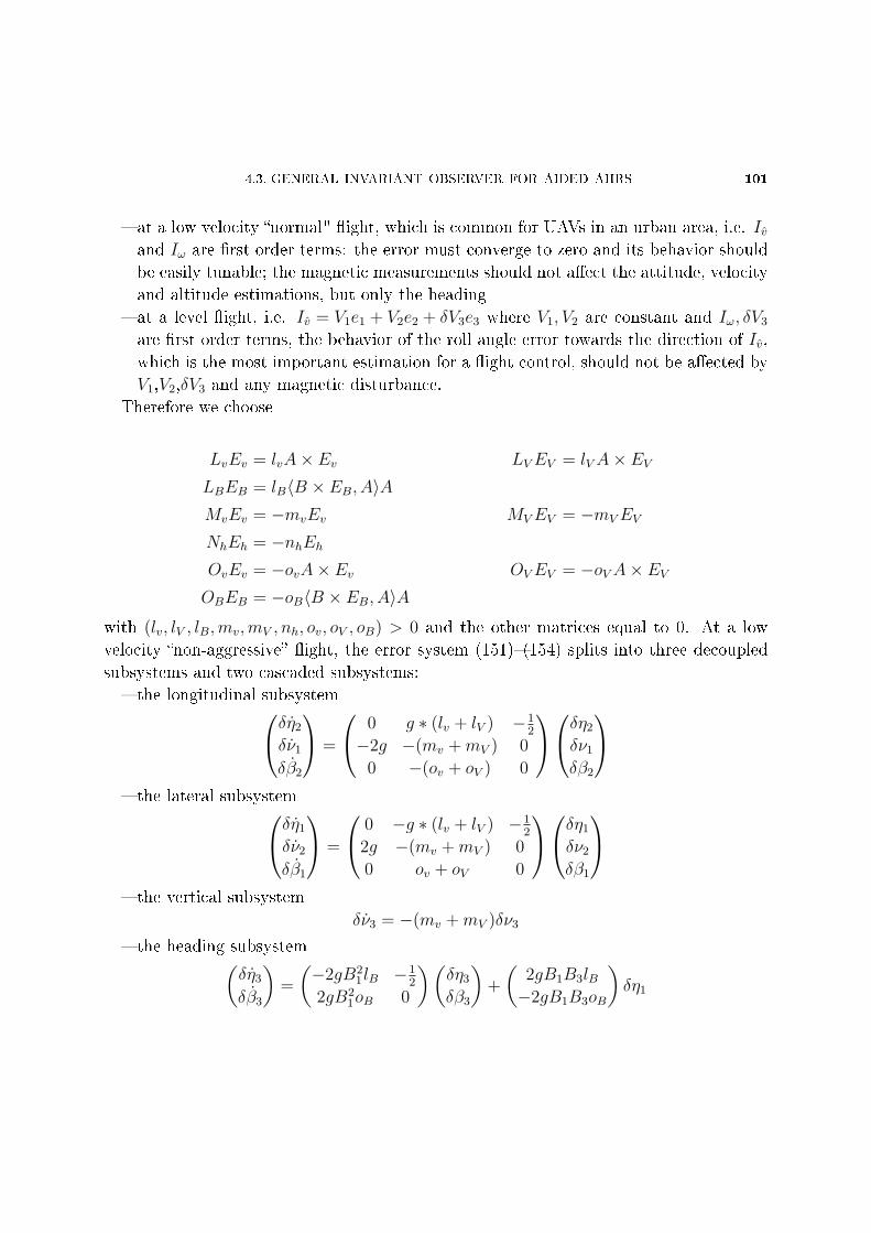
4.3. GENERAL INVARIANT OBSERVER FOR AIDED AHRS 101
at a low velocity normal" ight, which is common for UAVs in an urban area, i.e. Ivand Iω are rst order terms: the error must converge to zero and its behavior should
be easily tunable; the magnetic measurements should not aect the attitude, velocity
and altitude estimations, but only the heading
at a level ight, i.e. Iv = V1e1 + V2e2 + δV3e3 where V1, V2 are constant and Iω, δV3
are rst order terms, the behavior of the roll angle error towards the direction of Iv,
which is the most important estimation for a ight control, should not be aected by
V1,V2,δV3 and any magnetic disturbance.
Therefore we choose
LvEv = lvA× Ev LVEV = lVA× EVLBEB = lB〈B × EB, A〉AMvEv = −mvEv MVEV = −mVEV
NhEh = −nhEhOvEv = −ovA× Ev OVEV = −oVA× EVOBEB = −oB〈B × EB, A〉A
with (lv, lV , lB,mv,mV , nh, ov, oV , oB) > 0 and the other matrices equal to 0. At a low
velocity non-aggressive ight, the error system (151)(154) splits into three decoupled
subsystems and two cascaded subsystems:
the longitudinal subsystemδη2
δν1
δβ2
=
0 g ∗ (lv + lV ) −12
−2g −(mv +mV ) 0
0 −(ov + oV ) 0
δη2
δν1
δβ2
the lateral subsystemδη1
δν2
δβ1
=
0 −g ∗ (lv + lV ) −12
2g −(mv +mV ) 0
0 ov + oV 0
δη1
δν2
δβ1
the vertical subsystem
δν3 = −(mv +mV )δν3
the heading subsystem(δη3
δβ3
)=
(−2gB2
1 lB −12
2gB21oB 0
)(δη3
δβ3
)+
(2gB1B3lB−2gB1B3oB
)δη1
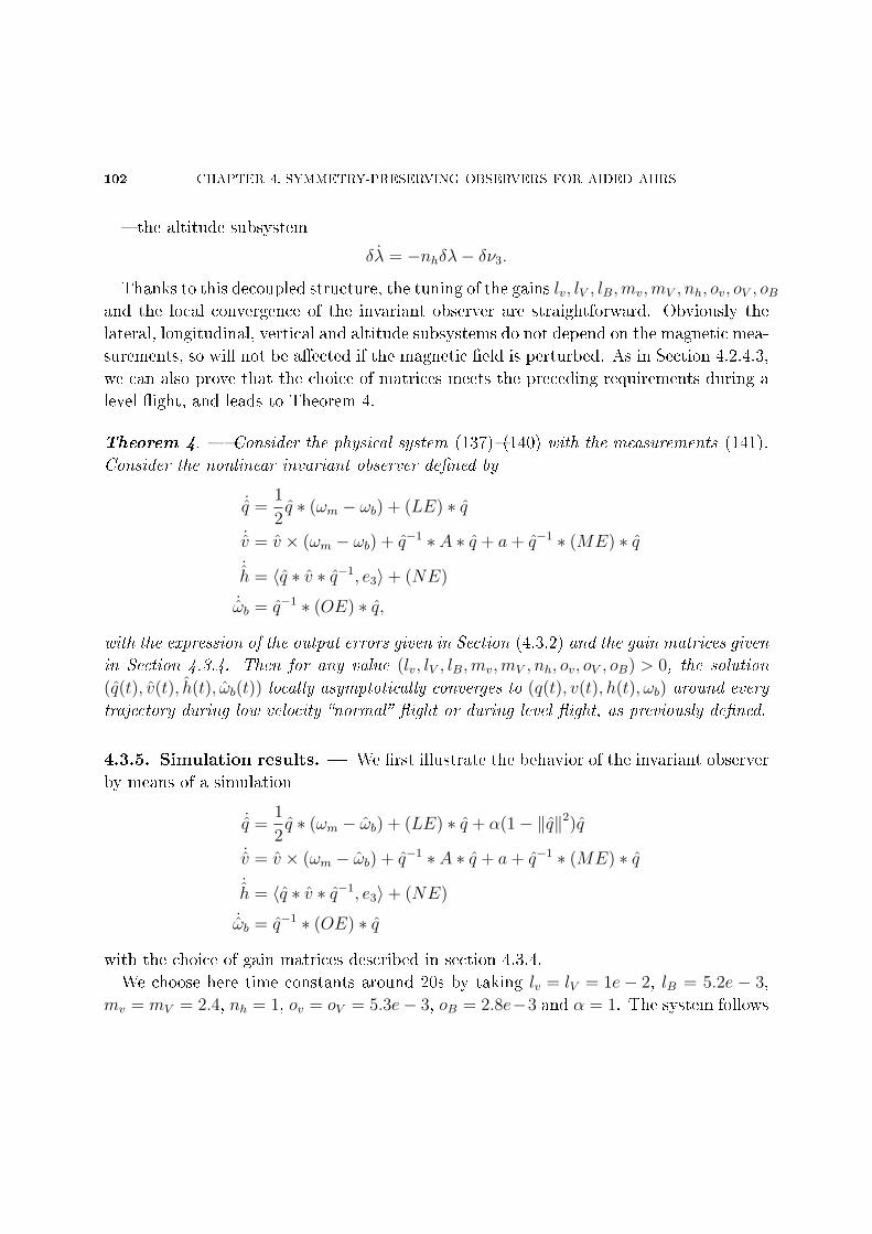
102 CHAPTER 4. SYMMETRY-PRESERVING OBSERVERS FOR AIDED AHRS
the altitude subsystem
δλ = −nhδλ− δν3.
Thanks to this decoupled structure, the tuning of the gains lv, lV , lB,mv,mV , nh, ov, oV , oBand the local convergence of the invariant observer are straightforward. Obviously the
lateral, longitudinal, vertical and altitude subsystems do not depend on the magnetic mea-
surements, so will not be aected if the magnetic eld is perturbed. As in Section 4.2.4.3,
we can also prove that the choice of matrices meets the preceding requirements during a
level ight, and leads to Theorem 4.
Theorem 4. Consider the physical system (137)(140) with the measurements (141).
Consider the nonlinear invariant observer dened by
˙q =1
2q ∗ (ωm − ωb) + (LE) ∗ q
˙v = v × (ωm − ωb) + q−1 ∗ A ∗ q + a+ q−1 ∗ (ME) ∗ q˙h = 〈q ∗ v ∗ q−1, e3〉+ (NE)
˙ωb = q−1 ∗ (OE) ∗ q,
with the expression of the output errors given in Section (4.3.2) and the gain matrices given
in Section 4.3.4. Then for any value (lv, lV , lB,mv,mV , nh, ov, oV , oB) > 0, the solution
(q(t), v(t), h(t), ωb(t)) locally asymptotically converges to (q(t), v(t), h(t), ωb) around every
trajectory during low velocity normal ight or during level ight, as previously dened.
4.3.5. Simulation results. We rst illustrate the behavior of the invariant observer
by means of a simulation
˙q =1
2q ∗ (ωm − ωb) + (LE) ∗ q + α(1− ‖q‖2)q
˙v = v × (ωm − ωb) + q−1 ∗ A ∗ q + a+ q−1 ∗ (ME) ∗ q˙h = 〈q ∗ v ∗ q−1, e3〉+ (NE)
˙ωb = q−1 ∗ (OE) ∗ q
with the choice of gain matrices described in section 4.3.4.
We choose here time constants around 20s by taking lv = lV = 1e− 2, lB = 5.2e − 3,
mv = mV = 2.4, nh = 1, ov = oV = 5.3e− 3, oB = 2.8e−3 and α = 1. The system follows
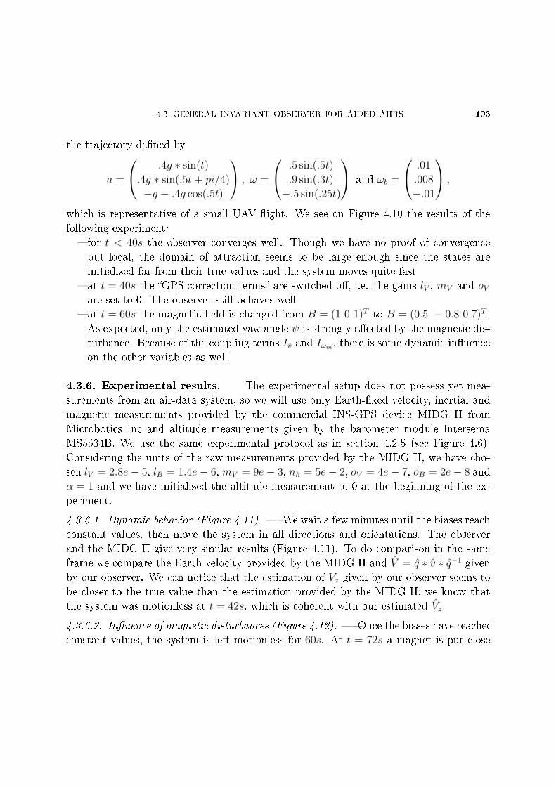
4.3. GENERAL INVARIANT OBSERVER FOR AIDED AHRS 103
the trajectory dened by
a =
.4g ∗ sin(t)
.4g ∗ sin(.5t+ pi/4)
−g − .4g cos(.5t)
, ω =
.5 sin(.5t)
.9 sin(.3t)
−.5 sin(.25t)
and ωb =
.01
.008
−.01
,
which is representative of a small UAV ight. We see on Figure 4.10 the results of the
following experiment:
for t < 40s the observer converges well. Though we have no proof of convergence
but local, the domain of attraction seems to be large enough since the states are
initialized far from their true values and the system moves quite fast
at t = 40s the GPS correction terms are switched o, i.e. the gains lV , mV and oVare set to 0. The observer still behaves well
at t = 60s the magnetic eld is changed from B = (1 0 1)T to B = (0.5 − 0.8 0.7)T .
As expected, only the estimated yaw angle ψ is strongly aected by the magnetic dis-
turbance. Because of the coupling terms Iv and Iωm , there is some dynamic inuence
on the other variables as well.
4.3.6. Experimental results. The experimental setup does not possess yet mea-
surements from an air-data system, so we will use only Earth-xed velocity, inertial and
magnetic measurements provided by the commercial INS-GPS device MIDG II from
Microbotics Inc and altitude measurements given by the barometer module Intersema
MS5534B. We use the same experimental protocol as in section 4.2.5 (see Figure 4.6).
Considering the units of the raw measurements provided by the MIDG II, we have cho-
sen lV = 2.8e− 5, lB = 1.4e− 6, mV = 9e− 3, nh = 5e− 2, oV = 4e− 7, oB = 2e− 8 and
α = 1 and we have initialized the altitude measurement to 0 at the beginning of the ex-
periment.
4.3.6.1. Dynamic behavior (Figure 4.11). We wait a few minutes until the biases reach
constant values, then move the system in all directions and orientations. The observer
and the MIDG II give very similar results (Figure 4.11). To do comparison in the same
frame we compare the Earth velocity provided by the MIDG II and V = q ∗ v ∗ q−1 given
by our observer. We can notice that the estimation of Vz given by our observer seems to
be closer to the true value than the estimation provided by the MIDG II: we know that
the system was motionless at t = 42s, which is coherent with our estimated Vz.
4.3.6.2. Inuence of magnetic disturbances (Figure 4.12). Once the biases have reached
constant values, the system is left motionless for 60s. At t = 72s a magnet is put close
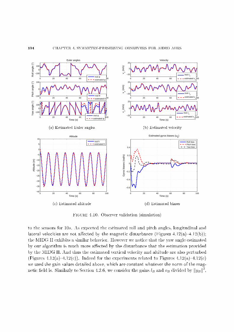
104 CHAPTER 4. SYMMETRY-PRESERVING OBSERVERS FOR AIDED AHRS
0 20 40 60 80 100
−100
0
100
Euler angles
Rol
l ang
le (
°)
0 20 40 60 80 100−100
0
100
Pitc
h an
gle
(°)
0 20 40 60 80 100
−100
0
100
Time (s)
Yaw
ang
le (
°)
real φestimated φ
real θestimated θ
real ψestimated ψ
(a) Estimated Euler angles
0 20 40 60 80 100
−20
0
20Velocity
v x (m
/s)
0 20 40 60 80 100
−20
0
20
v y (m
/s)
0 20 40 60 80 100−20
0
20
Time (s)v z (
m/s
)
real vx
estimated vx
real vy
estimated vy
real vz
estimated vz
(b) Estimated velocity
0 20 40 60 80 100−40
−35
−30
−25
−20
−15
−10
−5
0
5
10Altitude
Time (s)
Alti
tude
(m
)
real hestimated h
(c) Estimated altitude
0 20 40 60 80 100
−0.6
−0.4
−0.2
0
0.2
0.4
Estimated gyros biases (ωb)
Time (s)
Gyr
os b
iase
s (r
ad/s
)
Roll biasPitch biasYaw bias
(d) Estimated biases
Figure 4.10. Observer validation (simulation)
to the sensors for 10s. As expected the estimated roll and pitch angles, longitudinal and
lateral velocities are not aected by the magnetic disturbance (Figures 4.12(a)4.12(b));
the MIDG II exhibits a similar behavior. However we notice that the yaw angle estimated
by our algorithm is much more aected by the disturbance that the estimation provided
by the MIDG II. And thus the estimated vertical velocity and altitude are also perturbed
(Figures 4.12(a)4.12(c)). Indeed for the experiments related to Figures 4.12(a)4.12(c)
we used the gain values detailed above, which are constant whatever the norm of the mag-
netic eld is. Similarly to Section 4.2.6, we consider the gains lB and oB divided by ‖yB‖2,
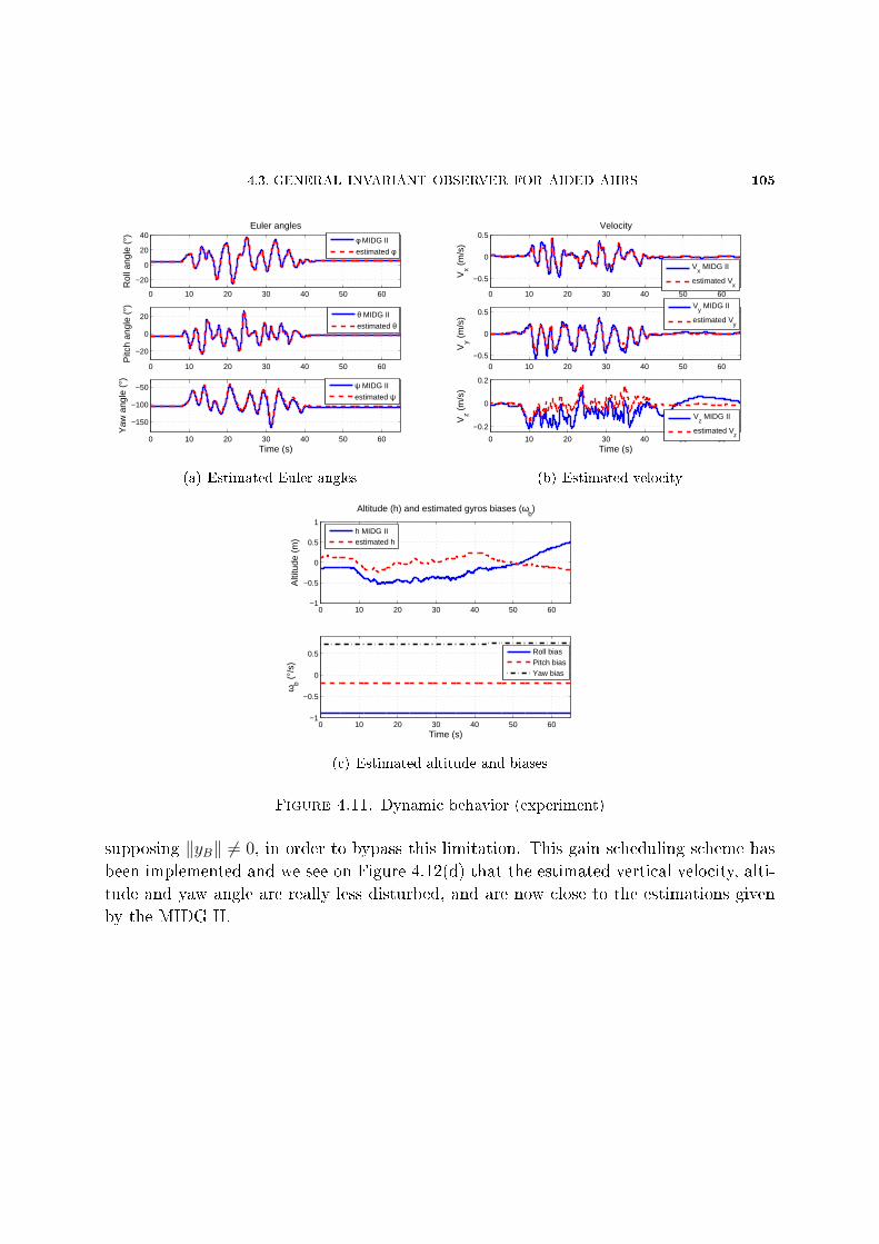
4.3. GENERAL INVARIANT OBSERVER FOR AIDED AHRS 105
0 10 20 30 40 50 60
−20
0
20
40Euler angles
Rol
l ang
le (
°)
0 10 20 30 40 50 60
−20
0
20
Pitc
h an
gle
(°)
0 10 20 30 40 50 60
−150
−100
−50
Time (s)
Yaw
ang
le (
°)
φ MIDG II
estimated φ
θ MIDG II
estimated θ
ψ MIDG II
estimated ψ
(a) Estimated Euler angles
0 10 20 30 40 50 60
−0.5
0
0.5Velocity
Vx (
m/s
)
0 10 20 30 40 50 60−0.5
0
0.5
Vy (
m/s
)
0 10 20 30 40 50 60
−0.2
0
0.2
Time (s)V
z (m
/s)
Vx MIDG II
estimated Vx
Vy MIDG II
estimated Vy
Vz MIDG II
estimated Vz
(b) Estimated velocity
0 10 20 30 40 50 60−1
−0.5
0
0.5
1
Altitude (h) and estimated gyros biases (ωb)
Alti
tude
(m
)
0 10 20 30 40 50 60−1
−0.5
0
0.5
ωb (
°/s)
Time (s)
h MIDG IIestimated h
Roll biasPitch biasYaw bias
(c) Estimated altitude and biases
Figure 4.11. Dynamic behavior (experiment)
supposing ‖yB‖ 6= 0, in order to bypass this limitation. This gain scheduling scheme has
been implemented and we see on Figure 4.12(d) that the estimated vertical velocity, alti-
tude and yaw angle are really less disturbed, and are now close to the estimations given
by the MIDG II.
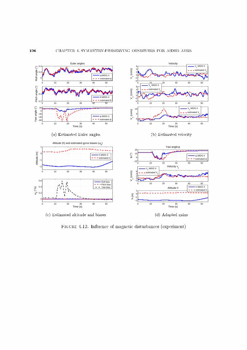
106 CHAPTER 4. SYMMETRY-PRESERVING OBSERVERS FOR AIDED AHRS
0 10 20 30 40 50
0
0.2
0.4Euler angles
Rol
l ang
le (
°)
0 10 20 30 40 500.2
0.4
Pitc
h an
gle
(°)
0 10 20 30 40 50
−60−40−20
020
Time (s)
Yaw
ang
le (
°)
φ MIDG II
estimated φ
θ MIDG II
estimated θ
ψ MIDG II
estimated ψ
(a) Estimated Euler angles
0 10 20 30 40 50−4−2
0246
Velocity
Vx (
cm/s
)
0 10 20 30 40 50−4−2
0246
Vy (
cm/s
)
0 10 20 30 40 50
0
5
10
Time (s)
Vz (
cm/s
)
Vx MIDG II
estimated Vx
Vy MIDG II
estimated Vy
Vz MIDG II
estimated Vz
(b) Estimated velocity
0 10 20 30 40 50
−2
−1
0
1
Altitude (h) and estimated gyros biases (ωb)
Alti
tude
(m
)
0 10 20 30 40 50
0
0.2
0.4
0.6
ωb (
°/s)
Time (s)
h MIDG IIestimated h
Roll biasPitch biasYaw bias
(c) Estimated altitude and biases
0 10 20 30 40 50−10
0
10
20Yaw angle ψ
ψ (
°)
0 10 20 30 40 50−2
0246
Velocity vz
Vz (
cm/s
)
0 10 20 30 40 50
−2
−1
0
1Altitude h
Time (s)
h (m
)
ψ MIDG II
estimated ψ
Vz MIDG II
estimated Vz
h MIDG IIestimated h
(d) Adapted gains
Figure 4.12. Inuence of magnetic disturbances (experiment)
CHAPTER 5
INVARIANT KALMAN FILTER
Dans ce chapitre nous proposons une nouvelle version du ltre de Kalman étendu,
l'Invariant Extended Kalman Filter, qui tient compte des symétries naturelles du système
dans la construction de ses termes de correction. Les matrices de gains et de covariance de
ce ltre convergent vers des constantes pour un large éventail de trajectoires, permettant
alors d'espérer une meilleure estimation de l'état qu'en utilisant un ltre de Kalman
étendu. Nous illustrons l'intérêt de ce ltre en l'appliquant à un aided Attitude and
Heading Reference System.
5.1. Introduction
In the EKF, the system is seen as a stochastic dierential equation,
x = f(x, u) +Mw(155)
y = h(x, u) +Nv,(156)
where x, u, y belong to an open subset of Rn × Rm × Rp; w, v are independent white
gaussian noises of size n and p with unit power spectral density, and M,N are square
108 CHAPTER 5. INVARIANT KALMAN FILTER
matrices. The input u and output y are known signals, and the state x must be estimated.
An estimation x(t) of x(t) is then computed by the EKF
˙x = f(x, u) +K(y − h(x, u)
)P = AP + PAT +MMT − PCT (NNT )−1CP,
with K = PCT (NNT )−1, A = ∂1f(x, u) and C = ∂1h(x, u) (∂i means the partial deriva-
tive with respect to the ith argument). The rationale is to compute the gain K as in a
linear Kalman lter since the estimation error ∆x = x − x satises the linear equation
∆x = (A − KC)∆x up to rst-order terms. Of course the convergence of the EKF is
not guaranteed in general as in the linear case, see e.g. [78] for some (local) convergence
results.
Another drawback of this linear approach is that it does not respect the geometry of
the problem when (part of) the state space is a manifold. This situation frequently arises
e.g. in the context of aerospace engineering, where the attitude of an aircraft is usually
represented by a unit quaternion rather than Euler angles; ad hoc modications of the
EKF are then used, in particular the so-called Multiplicative EKF (MEKF) introduced
in [77, 49, 58].
We propose a modication of the EKF for nonlinear systems that possess symmetries.
Instead of using a linear correction term based on a linear output error, the proposed lter
uses a geometrically adapted correction term based on an invariant output error; in the
same way the gain matrix is not updated from of a linear state error, but from an invariant
state error. For that to make sense from a stochastic point of view, we assume the driving
and observation noise enter the system in an invariant way. As for the generic observers
we developed in the preceding chapters, this Invariant EKF (IEKF) builds on the ideas
developed in [12, 13, 9], see also [56, 46, 52] for related approaches. More generally it
adds to the several attempts to introduce geometry in the problem of nonlinear ltering,
see e.g. [18, 57, 45].
The main benet of the IEKF is that the matrices A and C are constant on a much
larger set of trajectories (so-called permanent trajectories [13]) than equilibrium points
as is the case for the EKF. Near such trajectories, we are back to the true, i.e. linear,
Kalman lter where convergence is guaranteed. Informally, this means the IEKF should
in general converge at least around any slowly-varying permanent trajectory, rather than
just around any slowly-varying equilibrium point for the EKF.
We then apply the IEKF to the practically relevant problem of estimating the velocity
and attitude of a moving rigid body, e.g. an aircraft, from velocity, inertial and magnetic
5.3. INVARIANT EXTENDED KALMAN FILTER 109
measurements. We design two dierent versions (Left and Right IEKF), which can be
seen as extensions of the MEKF. Finally we present experimental and simulation results.
5.2. System with symmetries and Gaussian noises
Consider the system
x = f(x, u) +M(x)w(157)
y = h(x, u) +N(x)v(158)
where x ∈ X an n-dimensional manifold, u ∈ U = Rm, y ∈ Y = Rp, and w, v are
independent white gaussian noises.
The denitions recalled in Chapter 1.4 can be easily adapted to the system (157)
(158) by assuming the noise is turned o. Then, with the notations given in Section 1.4,
the system (157)-(158) with noise turned o is left-invariant with equivariant output if
for all g ∈ G it is unaected by the transformation that changes (u, x, y) into (U,X, Y ):ddtX(t) = f(X,U), Y = h(X,U). We also want the driving noise w and observation noise v
to preserve invariance and extend the denitions of recalled in Chapter 1.4.
Denition. Consider the change of variables X = ϕg(x), U = ψg(u) and Y =
ρg(y).The system with noise (157)-(158) is invariant with equivariant output and in-
variant noises if for all g, x, u,
f(ϕg(x), ψg(u)
)+M
(ϕg(x)
)w = Dϕg(x) ·
(f(x, u) +M(x)w
)h(ϕg(x), ψg(u)
)+N
(ϕg(x)
)v = ρg
(h(x, u) +N(x)v
),
i.e. if the system (157)-(158) is unaected by the considered transformation
X = f(X,U) +M(X)w
Y = h(X,U) +N(X)v.
Moreover, we assume ρg is linear for all g (which is the case in many examples), so that
ρg(y1 + y2) = ρg(y1) + ρg(y2) for all g, y1, y2.
5.3. Invariant Extended Kalman Filter
For simplicity we restrict to the case where the dimension of the group is r = n, and
the action is free and eective, so that X can be identied with G (up to a discrete
group action). Then G = X by left translation Lg(x) = gx, i.e. ϕg(x) = Lg(x) = gx.
110 CHAPTER 5. INVARIANT KALMAN FILTER
An invariant driving noise then reads DLx M(e)w, and an invariant output noise reads
Dρx N(e)v. since DLgM(x) = M(Lg(x))
5.3.1. A symmetry-preserving observer. As recalled in Chapter 1.4, a symmetry-
preserving observer reads (see [12] for details)
˙x = f(x, u) +DLxK(ρx−1(y)− ρx−1(h(x, u))
),
where K is a gain which only depends on the invariant I(x, u) = ψx−1(u).
5.3.1.1. Error equation. Instead of the usual state error ∆x = x − x, we use the
invariant error η = x−1x. We then have
η = DLηf(e, ψη−1(I))−DRη(f(e, I) +M(e)w)
+DLηK[h(η−1, ψη−1(I))− h(e, ψη−1(I)) +N(η−1)v]
where Rη denotes the right multiplication by η. A remarkable feature is this equation
only depends on the trajectory via the invariant term I.
This leads to dene a new class of trajectories, so-called permanent trajectories. They
are characterized by the fact that I(x, u) is constant over these trajectories. Thus, for
a class of trajectories which can be large, the nonlinear error equation above becomes
completely autonomous, which reminds the linear stationary case.
5.3.1.2. Linearized error equation. For a small error, i.e. η close to e, the rst order
approximation of the error equation reads
(159)ξ = [ξ, f(e, ψx−1(u))]− ∂f
∂u(e, ψx−1(u))
∂ψ
∂g(e, ψx−1(u))ξ −M(e)w − r(ξ)M(e)w
−K∂h
∂x(e, ψx−1(u))ξ + l(ξ)KN(e)v +K
(N(e)v − d(ξ)N(e)v
),
where [ , ] is the Lie bracket of the Lie algebra of G,l, r and d are the derivative at e of
DL, DR and Dρ: l(ξ) = ddsDLexp(sξ), r(ξ) = d
dsDRexp(sξ) and d(ξ) = d
dsDρexp(sξ), see [13]
for details.
5.3.2. Equations of the Invariant Extended Kalman Filter. The Invariant
EKF then reads
˙x = f(x, u) +DLxK(ρx−1(y)− ρx−1(h(x, u))
)K = PCT (NNT )−1
P = AP + PAT +MMT − PCT (NNT )−1CP
5.3. INVARIANT EXTENDED KALMAN FILTER 111
where
A(I) : ξ 7→ [ξ, f(e, I)]− ∂f
∂u(e, I)
∂ψ
∂g(e, I)ξ
C = Dh(e, I), M = M(e), N = N(e).
It relies on the same ideas as the usual EKF, but instead of using a linear correction term
based on a linear output error, it uses a geometrically adapted correction term based on
an invariant output error; in the same way the gain matrix is not updated from of a linear
state error, but from an invariant state error.
There is nevertheless a slight problem with the linearized invariant error equation (159),
because of the quadratic terms of the type r(ξ)M(e)w which do not appear in the usual
linearized equation of the EKF
d
dtξ = (A−KC)ξ −Mw +KNv.(160)
Instead, here the linearized error equation is rather a multiplicative inhomogeneous equa-
tion of the formd
dtξ = A0(t)ξ + αW1(t) + αW2(t)ξ(161)
rather than of the formd
dtζ = A0(t)ζ + αW1(t).(162)
W1 and W2 are time-varying matrices, with entries being linear scalar functions of the
white mutually independent noises w and v (thus 〈W1〉 = 〈W2〉 = 0), and α is a parameter
measuring the magnitude of the noises. Linear multiplicative stochastic equations are
standard in physics and chemistry, but unlike the linear inhomogeneous equations of the
form (162) (as the Langevin equation) it can only be solved in special cases. Nevertheless,
a rather general approach is based on approximations, since the true solution is written
in the form of a series expansion in powers of α [83].
We are going to prove that the average and covariance matrix of the solution of (161) are
solutions to order α2 of the non-stochastic dierential equations veried by the average
and the covariance of the solution of Equation (162). Then: if the observer made for
Equation (160) is robust, the expectation of ξ (verifying Equation (159)) will also tend
to 0 when t→∞; and the covariance matrix of the solution of Equation (160) will be an
approximation of the covariance of the solution of the true linearized equation (159). This
argument is standard in mathematical physics, since multiplicative noise generally yields
a shift of order α2. For instance, the criterion for energy of the damped random frequency
112 CHAPTER 5. INVARIANT KALMAN FILTER
oscillator with frequency ω20(1 + αw(t)) to tend to zero is that the damping coecient,
instead of being only strictly positive, is bounded from below by a linear function of α2
(see [83]).
According to [83] (p403, rigourously proved a few pages later) we see we have for the
solution of Equation (161)
d
dt〈ξ(t)〉 = [A0(t) + α 〈W2(t)〉+ α2
⟨W2(t)2
⟩] 〈ξ(t)〉+ α2〈W1(t)W2(t)〉+O(α3)
and thus, as 〈W2(t)〉 = 0, the mean values 〈ξ〉 and 〈ζ〉 obey to the same equation up
to terms of order α2. Still using [83] p404 we also see that the covariances obey the
same dierential equations up to terms of order α2, once again because the α 〈W2〉 termvanishes.
5.4. Considered system
We now apply the IEKF to the aided AHRS problem, with velocity, inertial and mag-
netic measurements from low-cost sensors. We therefore consider the system presented
in 4.1, i.e.
q =1
2q ∗ (ωm − ωb)(163)
V = A+1
asq ∗ am ∗ q−1(164)
ωb = 0(165)
as = 0,(166)
where ωm and am are seen as known inputs, together with the output(yVyB
)=
(V
q−1 ∗B ∗ q
).(167)
It is reasonable to assume each scalar sensor is corrupted by an additive gaussian white
noise with identical variance for each of the three scalar sensors constituting a triaxial
sensor, and all the noises are mutually independent (this is technologically motivated for
the accelerometers, gyroscopes and magnetic sensors, though much more questionable for
the GPS engine). Hence we can see each triaxial sensor as corrupted by a coordinate-free
vector noise whose coordinates are gaussian in the body frame as well as the Earth frame
(or any other smooth time-varying frame). Indeed, the mean and the auto-correlation time
of such a noise is not aected by a (smoothly) time-varying rotation.
5.5. MULTIPLICATIVE EXTENDED KALMAN FILTER 113
5.5. Multiplicative Extended Kalman Filter
We begin with the design of a Multiplicative EKF (MEKF) in the spirit of [77, 49, 58]
(see also [41, 8]), in order to compare the structure and the properties of an IEKF with
the well-known MEKF. The idea is to respect the geometry of the quaternion space,
by using for the quaternion estimation a multiplicative correction term q ∗ KqE which
preserves the unit norm, and by computing the error equation with the error q−1 ∗ q (orequivalently q−1 ∗ q = (q−1 ∗ q)−1). Notice the standard linear correction term does not
preserve the norm, hence some projection would be needed, whereas the standard linear
error q − q does not really make sense for quaternions.
We assume the noise enters the system as
q =1
2q ∗ (ωm − ωb) + q ∗Mqwq(168)
V = A+1
asq ∗ am ∗ q−1 + q ∗MVwV ∗ q−1(169)
ωb = Mωwω(170)
as = Mawa,(171)
and the output as (yVyB
)=
(V +NV vV
q−1 ∗B ∗ q +NBvB
),(172)
withMq,MV ,Mω, NV , NB diagonal matrices. The driving and observation noises are thus
consistent with a scalar additive noise on each individual sensor. The term q ∗ Mqwqpreserves the norm of the quaternion.
The MEKF then takes the form
˙q =1
2q ∗ (ωm − ωb) + q ∗KqE(173)
˙V = A+
1
asq ∗ am ∗ q−1 +KVE(174)
˙ωb = KωE(175)
˙as = KaE.(176)
where the output error is given by
E =
(yV − yVyB − yB
)=
(V − V −NV vV
q−1 ∗B ∗ q − yB −NBvB
).
114 CHAPTER 5. INVARIANT KALMAN FILTER
We consider the state error µ = q−1 ∗ q, ν = V − V , β = ωb − ωb and α = as − as. Atedious but simple computation yields the error system
µ = −1
2β ∗ µ+ µ× Jω −Mqwq ∗ µ+ µ ∗KqE
ν = Ia −1
as − αqµ ∗ am ∗ µ−1 ∗ q−1 − µ ∗ q ∗MVwV ∗ q−1 ∗ µ−1 +KVE
β = KωE −Mωwω
α = αKaE − αMawa,
where the output error is rewritten as
E =
(ν −NV vV
JB − µ−1 ∗ JB ∗ µ−NBvB
),
and Jω = ωm − ωb, Ia = 1asq ∗ am ∗ q−1 and JB = q−1 ∗B ∗ q.
We next linearize this error system around (µ, ν, β, α) = (1, 0, 0, 0), drop all the quadratic
terms in noise and innitesimal state error according to the approximation in section 5.3.2,
and eventually ndδµ
δν
δβ
δα
= (A−KC)
δµ
δν
δβ
δα
−MwqwVwωwa
+KN
(vVvB
),
which has the desired form of Equation (160) with
A =
−Jω× 033 −1
2I3 031
2Ja×R(q) 033 Jω× −Ja033 033 033 031
031 031 031 031
C =
(033 I3 033 031
−2JB× 033 033 031
)
M = Diag(Mq, R(q)MV ,Mω,Ma) N = Diag(NV , NB)
K = −(Kq, KV , Kω, Ka)T .
We have used the matrices I× and R(q) dened by I×u = I × u and R(q)u = q ∗ u ∗ q−1
for all for u ∈ R3.
Features of the MEKF
Sound geometric structure for the quaternion estimation equation: by construction
Equation (178) preserves the unit norm of the estimated quaternion.
5.6. LEFT INVARIANT EXTENDED KALMAN FILTER 115
Possible convergence issues of the error equation (and then of the lter) in many
situations: indeed, the matrices A and C used for computing the gain matrix K are
constant only in level ight, i.e. Iω ' 0 and Ia ' −A, because of the trajectory-
dependent terms R(q) in A.
5.6. Left Invariant Extended Kalman Filter
We now design a rst Invariant Extended Kalman Filter, which can be seen as a gen-
eralization and an improvement of the MEKF. It is a direct application of the method
presented in section 5.3. It is termed Left IEKF (LIEKF) because in the transformation
group dened below the quaternion q is multiplied on the left by a constant quaternion p0.
5.6.1. Problem setting in terms of transformation groups. We notice the state
space is a group for the law given byp0
V0
ω0
a0
q
V
ωbas
=
p0 ∗ q
p0 ∗ (V + V0) ∗ p−10
ωb + ω0
asa0
,
and hence acts on itself (the physical meaning is clear: rotation and translation in Earth
axes, translation in body axes, and scaling). It also yields the transformation groups
ψ(p0,V0,ω0,a0)
ωmamA
B
=
ωm + ω0
a0amp0 ∗ A ∗ p−1
0
p0 ∗B ∗ p−10
ρ(p0,V0,ω0,a0)
(yVyB
)=
(p0 ∗ (yV + V0) ∗ p−1
0
yB
).
The system (163)(166) is clearly invariant, for instance
˙︷ ︸︸ ︷p0 ∗ q = p0 ∗ q =
1
2(p0 ∗ q) ∗
((ωm + ω0)− (ωb + ω0)
),
whereas the output (167) is equivariant since(p0 ∗ (V + V0) ∗ p−1
0
(p0 ∗ q)−1 ∗ (p0 ∗B ∗ p−10 ) ∗ (p0 ∗ q)
)ρ(q0,V0,ω0,a0)
(V
q−1 ∗B ∗ q
).
116 CHAPTER 5. INVARIANT KALMAN FILTER
The complete set of invariants is given by ψx−1(u), with x−1 = (q−1,−V ,−ωb, 1as
), hence
reads JωJaJAJB
=
ωm − ωb
1asam
q−1 ∗ A ∗ qq−1 ∗B ∗ q
.
Moreover the driving noise as dened in Equations (168)(171) for the MEKF is also
invariant. We nally dene an invariant observation noise by(yVyB
)=
(V + q ∗NV vV ∗ q−1
q−1 ∗B ∗ q +NBvB
).(177)
Notice the noise on yV is dierent from the noise in Equation (172), which is not invariant:
it is additive in body axes rather than in Earth axes, see section 5.4 for a tentative physical
justication.
5.6.2. Left IEKF equations. We directly follow section 5.3 to derive the structure
of the LIEKF and the linearized error equation (160) used to compute the gains. The
LIEKF takes the form
˙q =1
2q ∗ (ωm − ωb) + q ∗ (KqE)(178)
˙V = A+
1
asq ∗ am ∗ q−1 + q ∗ (KVE) ∗ q−1(179)
˙ωb = KωE(180)
˙as = asKaE,(181)
where the invariant output error is given by
E = ρx−1
(yVyB
)− ρx−1
(yVyB
)=
(q−1 ∗ (V − yV ) ∗ qq−1 ∗B ∗ q − yB
).
Notice Equation (178) and Equation (180) are the same as Equation (173) and Equa-
tion (175) in the MEKF, while Equation (179) and Equation (181) are dierent from
Equation (174) and Equation (176).
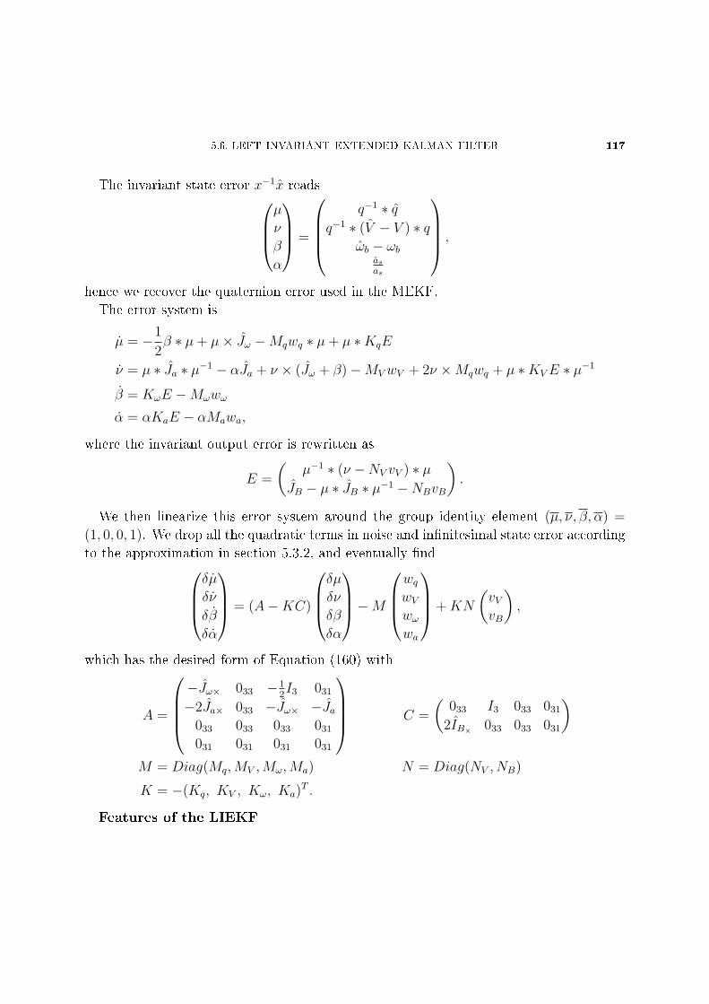
5.6. LEFT INVARIANT EXTENDED KALMAN FILTER 117
The invariant state error x−1x readsµ
ν
β
α
=
q−1 ∗ q
q−1 ∗ (V − V ) ∗ qωb − ωb
as
as
,
hence we recover the quaternion error used in the MEKF.
The error system is
µ = −1
2β ∗ µ+ µ× Jω −Mqwq ∗ µ+ µ ∗KqE
ν = µ ∗ Ja ∗ µ−1 − αJa + ν × (Jω + β)−MVwV + 2ν ×Mqwq + µ ∗KVE ∗ µ−1
β = KωE −Mωwω
α = αKaE − αMawa,
where the invariant output error is rewritten as
E =
(µ−1 ∗ (ν −NV vV ) ∗ µ
JB − µ ∗ JB ∗ µ−1 −NBvB
).
We then linearize this error system around the group identity element (µ, ν, β, α) =
(1, 0, 0, 1). We drop all the quadratic terms in noise and innitesimal state error according
to the approximation in section 5.3.2, and eventually ndδµ
δν
δβ
δα
= (A−KC)
δµ
δν
δβ
δα
−MwqwVwωwa
+KN
(vVvB
),
which has the desired form of Equation (160) with
A =
−Jω× 033 −1
2I3 031
−2Ja× 033 −Jω× −Ja033 033 033 031
031 031 031 031
C =
(033 I3 033 031
2IB× 033 033 031
)
M = Diag(Mq,MV ,Mω,Ma) N = Diag(NV , NB)
K = −(Kq, KV , Kω, Ka)T .
Features of the LIEKF
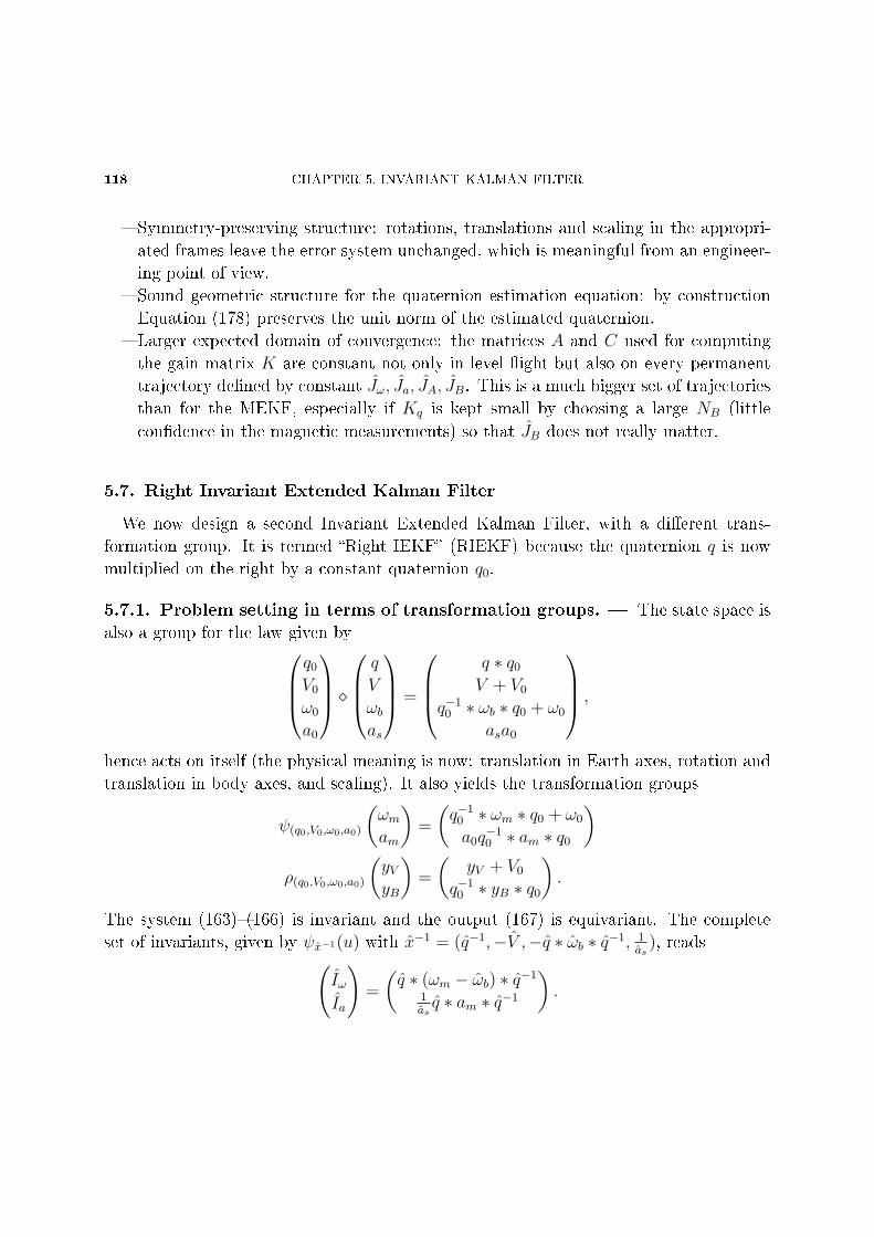
118 CHAPTER 5. INVARIANT KALMAN FILTER
Symmetry-preserving structure: rotations, translations and scaling in the appropri-
ated frames leave the error system unchanged, which is meaningful from an engineer-
ing point of view.
Sound geometric structure for the quaternion estimation equation: by construction
Equation (178) preserves the unit norm of the estimated quaternion.
Larger expected domain of convergence: the matrices A and C used for computing
the gain matrix K are constant not only in level ight but also on every permanent
trajectory dened by constant Jω, Ja, JA, JB. This is a much bigger set of trajectories
than for the MEKF, especially if Kq is kept small by choosing a large NB (little
condence in the magnetic measurements) so that JB does not really matter.
5.7. Right Invariant Extended Kalman Filter
We now design a second Invariant Extended Kalman Filter, with a dierent trans-
formation group. It is termed Right IEKF (RIEKF) because the quaternion q is now
multiplied on the right by a constant quaternion q0.
5.7.1. Problem setting in terms of transformation groups. The state space is
also a group for the law given byq0
V0
ω0
a0
q
V
ωbas
=
q ∗ q0
V + V0
q−10 ∗ ωb ∗ q0 + ω0
asa0
,
hence acts on itself (the physical meaning is now: translation in Earth axes, rotation and
translation in body axes, and scaling). It also yields the transformation groups
ψ(q0,V0,ω0,a0)
(ωmam
)=
(q−1
0 ∗ ωm ∗ q0 + ω0
a0q−10 ∗ am ∗ q0
)ρ(q0,V0,ω0,a0)
(yVyB
)=
(yV + V0
q−10 ∗ yB ∗ q0
).
The system (163)(166) is invariant and the output (167) is equivariant. The complete
set of invariants, given by ψx−1(u) with x−1 = (q−1,−V ,−q ∗ ωb ∗ q−1, 1as
), reads(IωIa
)=
(q ∗ (ωm − ωb) ∗ q−1
1asq ∗ am ∗ q−1
).
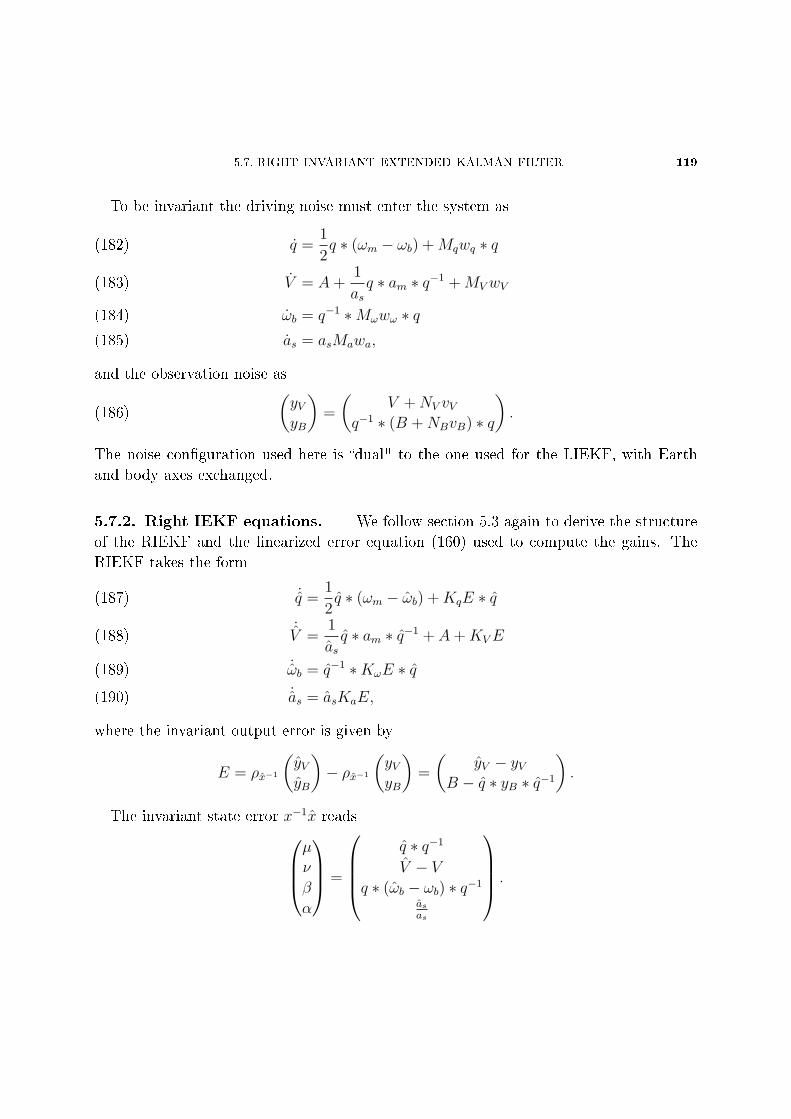
5.7. RIGHT INVARIANT EXTENDED KALMAN FILTER 119
To be invariant the driving noise must enter the system as
q =1
2q ∗ (ωm − ωb) +Mqwq ∗ q(182)
V = A+1
asq ∗ am ∗ q−1 +MVwV(183)
ωb = q−1 ∗Mωwω ∗ q(184)
as = asMawa,(185)
and the observation noise as(yVyB
)=
(V +NV vV
q−1 ∗ (B +NBvB) ∗ q
).(186)
The noise conguration used here is dual" to the one used for the LIEKF, with Earth
and body axes exchanged.
5.7.2. Right IEKF equations. We follow section 5.3 again to derive the structure
of the RIEKF and the linearized error equation (160) used to compute the gains. The
RIEKF takes the form
˙q =1
2q ∗ (ωm − ωb) +KqE ∗ q(187)
˙V =
1
asq ∗ am ∗ q−1 + A+KVE(188)
˙ωb = q−1 ∗KωE ∗ q(189)
˙as = asKaE,(190)
where the invariant output error is given by
E = ρx−1
(yVyB
)− ρx−1
(yVyB
)=
(yV − yV
B − q ∗ yB ∗ q−1
).
The invariant state error x−1x readsµ
ν
β
α
=
q ∗ q−1
V − Vq ∗ (ωb − ωb) ∗ q−1
as
as
.
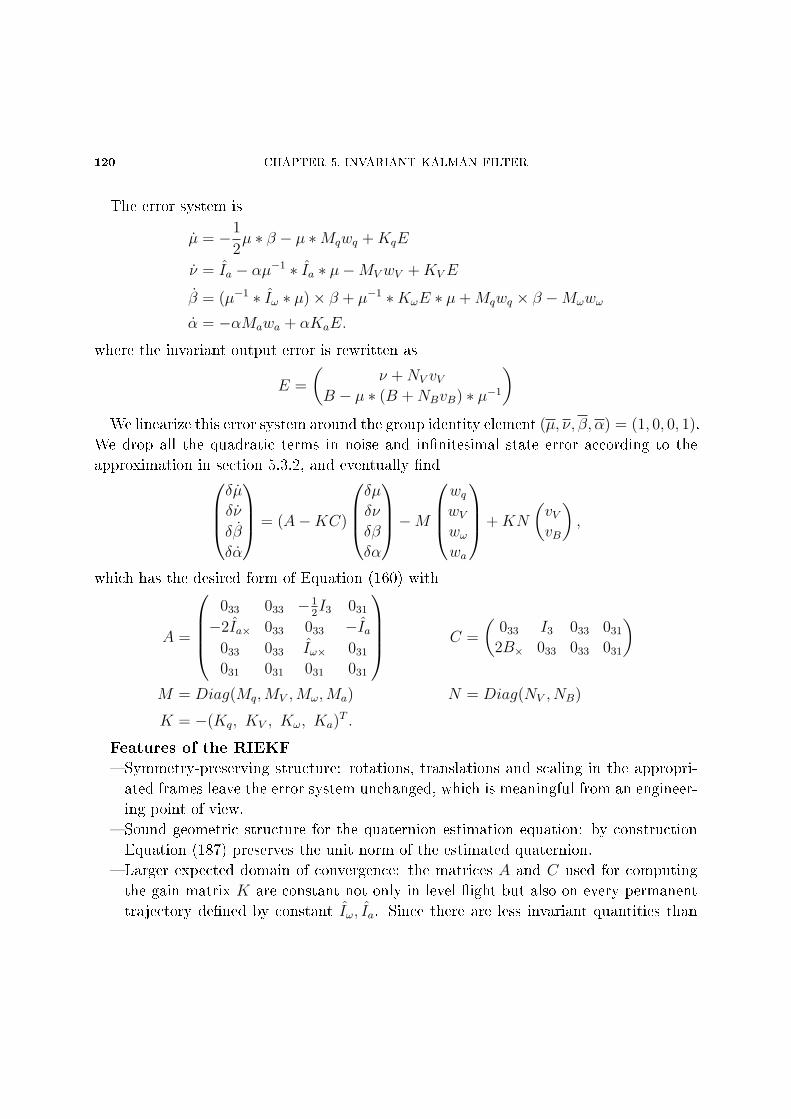
120 CHAPTER 5. INVARIANT KALMAN FILTER
The error system is
µ = −1
2µ ∗ β − µ ∗Mqwq +KqE
ν = Ia − αµ−1 ∗ Ia ∗ µ−MVwV +KVE
β = (µ−1 ∗ Iω ∗ µ)× β + µ−1 ∗KωE ∗ µ+Mqwq × β −Mωwω
α = −αMawa + αKaE.
where the invariant output error is rewritten as
E =
(ν +NV vV
B − µ ∗ (B +NBvB) ∗ µ−1
)We linearize this error system around the group identity element (µ, ν, β, α) = (1, 0, 0, 1).
We drop all the quadratic terms in noise and innitesimal state error according to the
approximation in section 5.3.2, and eventually ndδµ
δν
δβ
δα
= (A−KC)
δµ
δν
δβ
δα
−MwqwVwωwa
+KN
(vVvB
),
which has the desired form of Equation (160) with
A =
033 033 −1
2I3 031
−2Ia× 033 033 −Ia033 033 Iω× 031
031 031 031 031
C =
(033 I3 033 031
2B× 033 033 031
)
M = Diag(Mq,MV ,Mω,Ma) N = Diag(NV , NB)
K = −(Kq, KV , Kω, Ka)T .
Features of the RIEKF
Symmetry-preserving structure: rotations, translations and scaling in the appropri-
ated frames leave the error system unchanged, which is meaningful from an engineer-
ing point of view.
Sound geometric structure for the quaternion estimation equation: by construction
Equation (187) preserves the unit norm of the estimated quaternion.
Larger expected domain of convergence: the matrices A and C used for computing
the gain matrix K are constant not only in level ight but also on every permanent
trajectory dened by constant Iω, Ia. Since there are less invariant quantities than
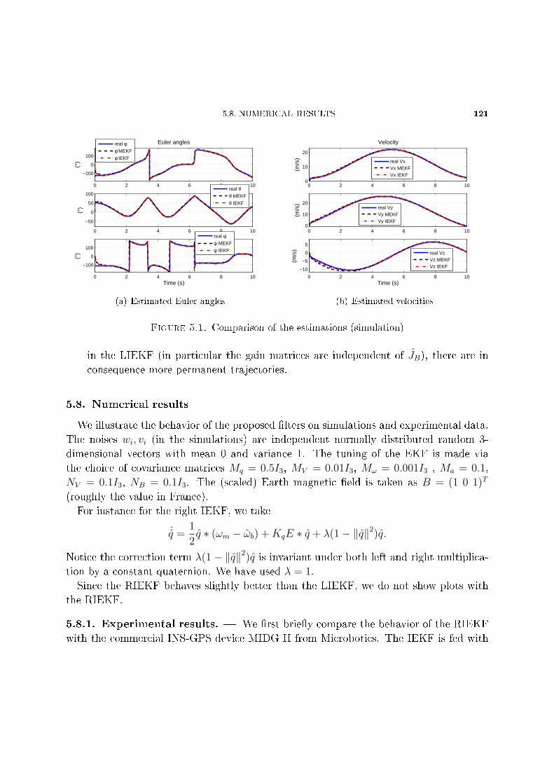
5.8. NUMERICAL RESULTS 121
0 2 4 6 8 10
−100
0
100
Euler angles
(°)
0 2 4 6 8 10
−50
0
50
100
(°)
0 2 4 6 8 10
−100
0
100
Time (s)
(°)
real φφ MEKF
φ IEKF
real θθ MEKF
θ IEKF
real ψψ MEKF
ψ IEKF
(a) Estimated Euler angles
0 2 4 6 8 100
10
20
Velocity
(m/s
)
0 2 4 6 8 100
10
20
(m/s
)
0 2 4 6 8 10
−10
−5
0
5
Time (s)
(m/s
)
real VxVx MEKFVx IEKF
real VyVy MEKFVy IEKF
real VzVz MEKFVz IEKF
(b) Estimated velocities
Figure 5.1. Comparison of the estimations (simulation)
in the LIEKF (in particular the gain matrices are independent of JB), there are in
consequence more permanent trajectories.
5.8. Numerical results
We illustrate the behavior of the proposed lters on simulations and experimental data.
The noises wi, vi (in the simulations) are independent normally distributed random 3-
dimensional vectors with mean 0 and variance 1. The tuning of the EKF is made via
the choice of covariance matrices Mq = 0.5I3, MV = 0.01I3, Mω = 0.001I3 , Ma = 0.1,
NV = 0.1I3, NB = 0.1I3. The (scaled) Earth magnetic eld is taken as B = (1 0 1)T
(roughly the value in France).
For instance for the right IEKF, we take
˙q =1
2q ∗ (ωm − ωb) +KqE ∗ q + λ(1− ‖q‖2)q.
Notice the correction term λ(1− ‖q‖2)q is invariant under both left and right multiplica-
tion by a constant quaternion. We have used λ = 1.
Since the RIEKF behaves slightly better than the LIEKF, we do not show plots with
the RIEKF.
5.8.1. Experimental results. We rst briey compare the behavior of the RIEKF
with the commercial INS-GPS device MIDG II from Microbotics. The IEKF is fed with
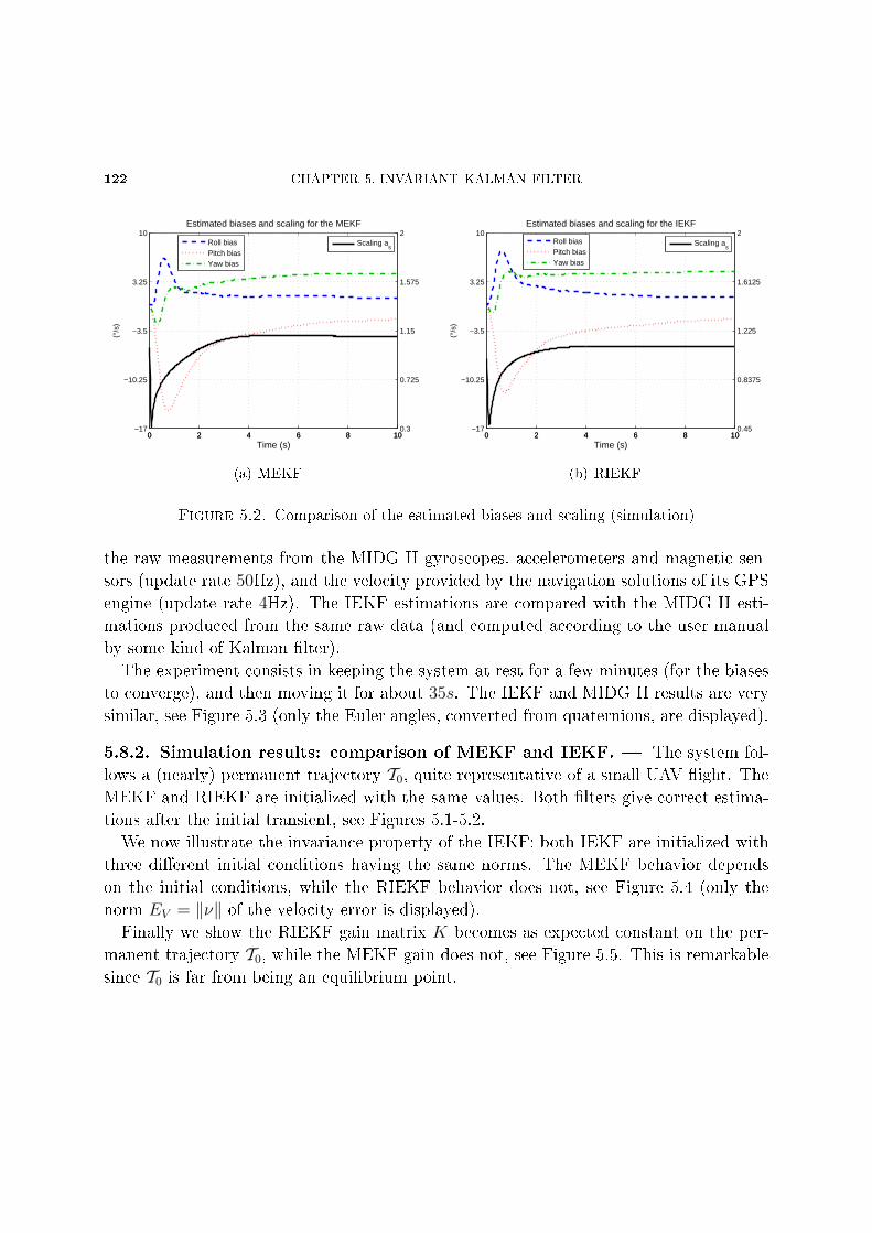
122 CHAPTER 5. INVARIANT KALMAN FILTER
0 2 4 6 8 10−17
−10.25
−3.5
3.25
10
Time (s)
(°/s
)
Estimated biases and scaling for the MEKF
0 2 4 6 8 100.3
0.725
1.15
1.575
2
Roll biasPitch biasYaw bias
Scaling as
(a) MEKF
0 2 4 6 8 10−17
−10.25
−3.5
3.25
10
Time (s)(°
/s)
Estimated biases and scaling for the IEKF
0 2 4 6 8 100.45
0.8375
1.225
1.6125
2
Roll biasPitch biasYaw bias
Scaling as
(b) RIEKF
Figure 5.2. Comparison of the estimated biases and scaling (simulation)
the raw measurements from the MIDG II gyroscopes, accelerometers and magnetic sen-
sors (update rate 50Hz), and the velocity provided by the navigation solutions of its GPS
engine (update rate 4Hz). The IEKF estimations are compared with the MIDG II esti-
mations produced from the same raw data (and computed according to the user manual
by some kind of Kalman lter).
The experiment consists in keeping the system at rest for a few minutes (for the biases
to converge), and then moving it for about 35s. The IEKF and MIDG II results are very
similar, see Figure 5.3 (only the Euler angles, converted from quaternions, are displayed).
5.8.2. Simulation results: comparison of MEKF and IEKF. The system fol-
lows a (nearly) permanent trajectory T0, quite representative of a small UAV ight. The
MEKF and RIEKF are initialized with the same values. Both lters give correct estima-
tions after the initial transient, see Figures 5.1-5.2.
We now illustrate the invariance property of the IEKF: both IEKF are initialized with
three dierent initial conditions having the same norms. The MEKF behavior depends
on the initial conditions, while the RIEKF behavior does not, see Figure 5.4 (only the
norm EV = ‖ν‖ of the velocity error is displayed).
Finally we show the RIEKF gain matrix K becomes as expected constant on the per-
manent trajectory T0, while the MEKF gain does not, see Figure 5.5. This is remarkable
since T0 is far from being an equilibrium point.
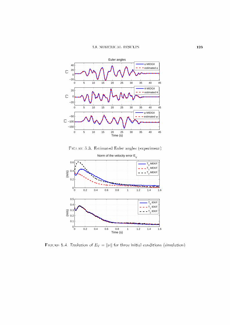
5.8. NUMERICAL RESULTS 123
0 5 10 15 20 25 30 35 40 45−20
0
20
40
Euler angles
(°)
0 5 10 15 20 25 30 35 40 45
−20
0
20
(°)
0 5 10 15 20 25 30 35 40 45
−150
−100
−50
Time (s)
(°)
φ MIDGII
estimated φ
θ MIDGII
estimated θ
ψ MIDGII
estimated ψ
Figure 5.3. Estimated Euler angles (experiment)
0 0.2 0.4 0.6 0.8 1 1.2 1.4 1.60
0.2
0.4
0.6
Norm of the velocity error EV
(m/s
)
0 0.2 0.4 0.6 0.8 1 1.2 1.4 1.60
0.1
0.2
0.3
0.4
0.5
Time (s)
(m/s
)
T0 MEKF
T1 MEKF
T2 MEKF
T0 IEKF
T1 IEKF
T2 IEKF
Figure 5.4. Evolution of EV = ‖ν‖ for three initial conditions (simulation)
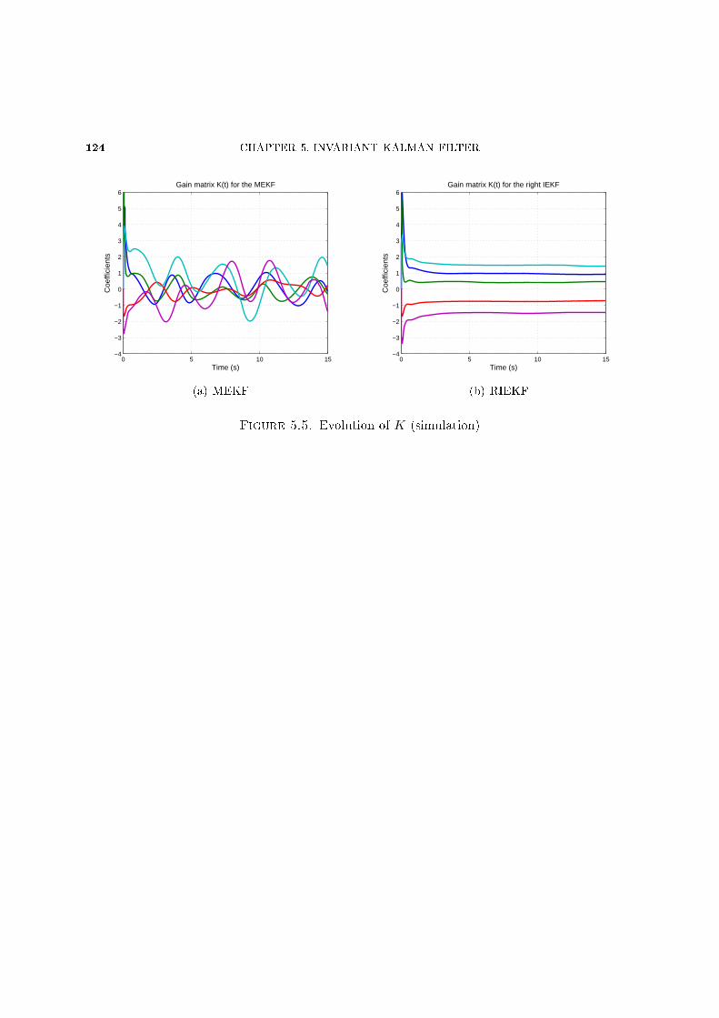
124 CHAPTER 5. INVARIANT KALMAN FILTER
0 5 10 15−4
−3
−2
−1
0
1
2
3
4
5
6Gain matrix K(t) for the MEKF
Coe
ffici
ents
Time (s)
(a) MEKF
0 5 10 15−4
−3
−2
−1
0
1
2
3
4
5
6Gain matrix K(t) for the right IEKF
Coe
ffici
ents
Time (s)
(b) RIEKF
Figure 5.5. Evolution of K (simulation)
CHAPTER 6
SPECIFIC OBSERVER FOR MINI QUADROTOR
Nous nous interessons dans ce chapitre aux mini-drones de type quadrirotors. Nous en
proposons un nouveau modèle prenant en compte des forces aérodynamiques jamais ex-
ploitées dans les travaux réalisés jusqu'à présent sur ce type de drone. Cette force permet
d'estimer la vitesse à travers les mesures fournies par les accéléromètres. Nous constru-
isons alors un observateur spécique basé sur ce modèle, qui nous permets de contrôler
le quadrotor en vitesse avec uniquement des capteurs inertiels. De plus, cette approche
nous permets de voir d'un oeil neuf les algorithmes de ltrages et de contrôles habituelle-
ment utilisés sur les quadrotors (contrôle de l'assiette et estimation des angles d'attitude
selon l'hypothèse d'une faible accélération linéaire), justiant les résultats expérimentaux
obtenus.
6.1. Introduction
Quadrotor control has been an active area of investigation for several years. On the
one hand the quadrotor has several qualities, among them its very simple mechanical
design, and qualies as a viable concept of mini Unmanned Aerial Vehicle (UAV) for
real-life missions; on the other hand it is perceived in the control community as a very
126 CHAPTER 6. SPECIFIC OBSERVER FOR MINI QUADROTOR
rich case study in theoretical and applied control. The rst control objective is to ensure
a stable ight at moderate velocities and in particular in hovering; this fundamental
building block is then used to develop higher-level tasks (e.g. autonomous ight including
waypoint following, obstacle avoidance, automatic take o and landing, etc.).
Putting aside purely control-theoretic works focused on the detailed analysis of control
laws without real-world sensors in mind, as well as experiments designed to work only in
the laboratory with an o-board measuring device (e.g. [20] use an electromagnetic motion
tracking system, with very short range), real quadrotor designs all rely at the heart on
strapdown MEMS inertial sensors (gyroscopes and accelerometers). Such sensors are also
used in preliminary experiments where the quadrotor is tethered to a test rig and free
only to rotate [15, 80, 72]. These inertial sensors may be used alone (as far as horizontal
stabilization is concerned) [34], or supplemented by other sensors which provide usually
some position-related information. Representative designs are: 3 ultrasonic rangers [43];
a (simple) GPS module when outdoors and 4 infrared rangers when indoors [74]; a carrier
phase dierential GPS [40, 89, 39]; a vision system [16, 33, 36, 68]; a laser scanner [2, 1].
Since these extra sensors have inherent drawbacks (low bandwidth, possible temporary
unavailability, etc.), inertial sensors remain essential for basic stabilization.
Nearly all the above-mentioned works rely on essentially the same physical model: only
aerodynamic forces and moments proportional to the square of the propellers angular
velocities are explicitly taken into account. Other aerodynamics eects are omitted and
considered as unmodeled disturbances to be rejected by the control law. The alleged rea-
son is that these eects are proportional to the square of the quadrotor linear velocity [7],
hence very small near hovering. Few authors explicitly consider other aerodynamic eects:
[72] consider aerodynamic stability derivatives, but draw no clear-cut conclusion about
their importance; [27, 51] consider without physical motivations aerodynamic eects lin-
ear w.r.t. the quadrotor linear and angular velocities, but propose negligible numerical
values; [40] judge them negligible at low velocities, and focus on nonlinear aspects at
moderate velocities; [17] physically motivates the presence of eects nearly linear w.r.t
the quadrotor linear and angular velocities, but provide no experimental data and are
concerned only with the open-loop system.
As for accelerometers, they are usually considered as giving approximately the compo-
nents of gravity in body axes, under the assumption that the quadrotor linear acceleration
is small (as explained in Section 2.3. Accordingly, the pitch and roll angles are estimated
from gyroscope and accelerometer measurements thanks to some sensor fusion algorithm:
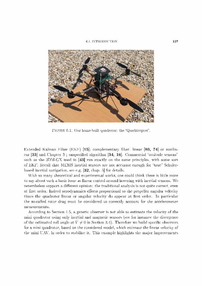
6.1. INTRODUCTION 127
Figure 6.1. Our home-built quadrotor: the Quadricopter.
Extended Kalman Filter (EKF) [15]; complementary lter, linear [80, 74] or nonlin-
ear [33] and Chapter 3 ; unspecied algorithm [34, 16]. Commercial attitude sensors
such as the 3DM-GX used in [43] run exactly on the same principles, with some sort
of EKF. Recall that MEMS inertial sensors are not accurate enough for true Schuler-
based inertial navigation, see e.g. [32, chap. 5] for details.
With so many theoretical and experimental works, one could think there is little more
to say about such a basic issue as linear control around hovering with inertial sensors. We
nevertheless support a dierent opinion: the traditional analysis is not quite correct, even
at rst order. Indeed aerodynamics eects proportional to the propeller angular velocity
times the quadrotor linear or angular velocity do appear at rst order. In particular
the so-called rotor drag must be considered to correctly account for the accelerometer
measurements.
According to Section 1.5, a generic observer is not able to estimate the velocity of the
mini quadrotor using only inertial and magnetic sensors (see for instance the divergence
of the estimated roll angle at V 6= 0 in Section 3.4). Therefore we build specic observers
for a mini quadrotor, based on the considered model, which estimate the linear velocity of
the mini UAV, in order to stabilize it. This example highlights the major improvements
128 CHAPTER 6. SPECIFIC OBSERVER FOR MINI QUADROTOR
allowable by specic observers, which take into account the physical model of the vehicle
(written from the dynamics laws).
6.2. Revisited quadrotor model
6.2.1. Model of a single propeller near hovering. We rst consider a single
propeller rotating with angular velocity εiωi around its axis ~kb; ωi is positive, with εi = 1
(resp. −1) for counterclockwise (resp. clockwise) rotation. The geometric center Ai of the
propeller moves with a given velocity ~VAiwhile the rotor plane (by denition perpendicular
to ~kb) undergoes angular velocity ~Ω; the total angular velocity of the propeller is thus~Ω + εiωi~kb. Following e.g. [42], the aerodynamic eorts on the propeller resolve into the
force ~Fi and moment ~Mi at Ai,
~Fi = −aω2i~kb − ωi
(λ1~V ⊥Ai− λ2
~Ω× ~kb)
+ εiωi
(λ3~VAi× ~kb − λ4
~Ω⊥)
(191)
~Mi = −bεiω2i~kb − ωi
(µ1~V ⊥Ai
+ µ2~Ω× ~kb
)− εiωi
(µ3~VAi× ~kb + µ4
~Ω⊥),(192)
where a, b, the λi's and µi's are positive constants; the projection of a vector ~u on the
rotor plane is
~u⊥ := ~kb ×(~u× ~kb
)= ~u−
(~u · ~kb
)~kb.
The above relations rely on classical blade element theory, with two extra simplica-
tions, and (approximately) apply to any propeller, rigid or not:
higher-order terms in linear and angular velocities have been neglected. This is valid
near hovering, i.e. for small ~VAiand ~Ω. Here ~VAi
small means small with respect to
the propeller tip speed (about 40m/s in our case), so that 5m/s can be considered
small
linear and angular accelerations have been neglected. Their contribution is small
since the mass of the propeller is in our case very small with respect to the total mass
of the quadrotor.
The velocities in the previous equations are of course velocities with respect to the air
stream, not with respect to the ground. They coincide when there is no wind, which we
assume in the sequel.
The term ωiλ1~V ⊥Ai
in (191) is often called H-force or rotor drag in the helicopter lit-
erature. Also notice the simplied expressions (191)-(192), though directly based on
textbook aerodynamics, do not seem to appear in the literature under this compact form
very handy for control purposes.
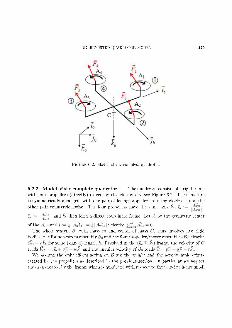
6.2. REVISITED QUADROTOR MODEL 129
Figure 6.2. Sketch of the complete quadrotor.
6.2.2. Model of the complete quadrotor. The quadrotor consists of a rigid frame
with four propellers (directly) driven by electric motors, see Figure 6.2. The structure
is symmetrically arranged, with one pair of facing propellers rotating clockwise and the
other pair counterclockwise. The four propellers have the same axis ~kb; ~ıb :=~A3A1
‖ ~A3A1‖ ,
~b :=~A4A2
‖ ~A4A2‖ and ~kb then form a direct coordinate frame. Let A be the geometric center
of the Ai's and l := 12
~‖A3A1‖ = 12
~‖A2A4‖; clearly,∑4
i=1~AAi = 0.
The whole system B, with mass m and center of mass C, thus involves ve rigid
bodies: the frame/stators assembly B0 and the four propeller/motor assemblies Bi; clearly,~CA = h~kb for some (signed) length h. Resolved in the (~ıb, ~b, ~kb) frame, the velocity of C
reads ~VC = u~ıb + v~b + w~kb and the angular velocity of B0 reads ~Ω = p~ıb + q~b + r~kb.
We assume the only eorts acting on B are the weight and the aerodynamic eorts
created by the propellers as described in the previous section. In particular we neglect
the drag created by the frame, which is quadratic with respect to the velocity, hence small
130 CHAPTER 6. SPECIFIC OBSERVER FOR MINI QUADROTOR
at low velocities. Newton's laws for the whole system then read
m~VC = m~g +4∑i=1
~Fi(193)
~σBC =4∑i=1
~CAi × ~Fi + ~Mi,(194)
where ~σBC =∫B~CM × ~CMdµ(M) is the kinetic momentum of B.
In hovering ~VC and ~Ω, hence ~VAiare zero; from (191)(194), see also (196)-(197), this
implies a(ω21 + ω2
2 + ω23 + ω2
4) = g and ω21 − ω2
2 + ω23 − ω2
4 = ω21 − ω2
3 = ω22 − ω2
4 = 0, hence
ωi = ω :=√
mg4a.
For each Bi, we can also write
~σBiAi· ~kb = ~Mi · ~kb + εiΓi,(195)
where ~σBiAi
=∫Bi
~AiM× ~AiMdµ(M) is the kinetic momentum of Bi, and Γi is the (positive)
torque created by the motor. For simplicity we have considered Ai as the center of mass
of Bi (in fact the two points are slightly apart). We also consider the Γi's as the control
inputs (it is nevertheless easy to include the behavior of the electric motors both for
modeling and control).
We now evaluate the right-hand sides of (193)-(194)-(195). Since
~VAi= ~VC + ~CA+ ~AAi = ~VC + h~Ω× ~kb + ~Ω× ~AAi,
we nd
λ1~V ⊥Ai− λ2
~Ω× ~kb = λ1
(~V ⊥C +
(h~Ω× ~kb
)⊥+(~Ω× ~AAi
)⊥)− λ2~Ω× ~kb
= λ1~V ⊥C − λ′2~Ω× ~kb − rλ1
~AAi × ~kb
λ3~VAi× ~kb − λ4
~Ω⊥ = λ3
(~VC + h~Ω× ~kb + ~Ω× ~AAi
)× ~kb − λ4
~Ω⊥
= λ3~VC × ~kb + λ′4
~Ω⊥ + rλ3~AAi.
6.2. REVISITED QUADROTOR MODEL 131
We have used the fact that ~AAi is colinear to either ~ıb or ~b, and set λ′2 =: λ2 − hλ1 and
λ′4 := λ4 + hλ3. Therefore,
4∑i=1
~Fi = −a
(4∑i=1
ω2i
)~kb −
(4∑i=1
ωi
)(λ1~V ⊥C − λ′2~Ω× ~kb
)+
(4∑i=1
εiωi
)(λ3~VC × ~kb − λ′4~Ω⊥
)+ rλ1
(4∑i=1
ωi ~AAi
)× ~kb + rλ3
(4∑i=1
εiωi ~AAi
).
Notice the last two lines contain only second order terms: indeed, ~Ω, ~VC ,∑4
i=1εiωi,∑4i=1ωi
~AAi and∑4
i=1εiωi~AAi all vanish in hovering. Neglecting these terms, we have
4∑i=1
~Fi ≈ −a
(4∑i=1
ω2i
)~kb −
(4∑i=1
ωi
)(λ1~V ⊥C − λ′2~Ω× ~kb
).
Likewise,
4∑i=1
~CA× ~Fi + ~AAi × ~Fi + ~Mi ≈ −a
(4∑i=1
ω2i~AAi
)× ~kb − b
(4∑i=1
εiω2i
)~kb
− rλ1l2
(4∑i=1
ωi
)~kb −
(4∑i=1
ωi
)(µ′1~VC × ~kb + µ′′2
~Ω⊥),
where µ′1 := µ1 − hλ1, µ′2 := µ2 − hµ1 and µ′′2 := µ′2 − hλ2.
A further simplication, valid for a rather rigid propeller, is to consider that λ′2 is zero.
Indeed h is by design small, and for a rather rigid propeller so is λ2. This yields
4∑i=1
~Fi ≈ −a
(4∑i=1
ω2i
)~kb − λ1
(4∑i=1
ωi
)~V ⊥C .
132 CHAPTER 6. SPECIFIC OBSERVER FOR MINI QUADROTOR
Gathering the previous computations, (193)-(194)-(195) now read
m~VC = m~g − a(ω2
1 + ω22 + ω2
3 + ω24
)~kb − λ1(ω1 + ω2 + ω3 + ω4)~V ⊥C(196)
~σBC = −b(ω2
1 − ω22 + ω2
3 − ω24
)~kb + al(ω2
1 − ω23)~b − al(ω2
2 − ω24)~ıb
− (ω1 + ω2 + ω3 + ω4)(µ′1~VC × ~kb + µ′′2~Ω
⊥)
− rλ1l2(ω1 + ω2 + ω3 + ω4)~kb(197)
~σBiAi· ~kb = εi(Γi − bω2
i ).(198)
We then evaluate the left-hand sides of (193)-(194)-(195). The approach is fairly stan-
dard.
~σBC =
∫B
~CM × ~CMdµ(M)
=
∫B0
~CM × ~CMdµ(M) +4∑i=1
∫Bi
~CM ×(~CAi + ~AiM
)dµ(M)
=
∫B0
~CM ×(~Ω× ~CM
)dµ(M) +
4∑i=1
∫Bi
~CM ×(~Ω× ~CAi +
(~Ω + εiωi~kb
)× ~AiM
)dµ(M)
=
∫B
~CM ×(~Ω× ~CM
)dµ(M) +
4∑i=1
∫Bi
~AiM ×(εiωi~kb × ~AiM
)dµ(M)
= IBC · ~Ω +4∑i=1
εiωi
(IBiAi· ~kb)
= Ip~ıb + Iq~b +
(Jr + Jr
4∑i=1
εiωi
)~kb,
where I, J, Jr are strictly positive constants. In the last equation we replaced in the com-
putation of the inertia tensors IB, IBiAi
the actual propellers by disks with the same masses
and radii, and took advantage of the various symmetries; this averaging approximation
is justied by the fact that the propeller angles vary much faster than all the other kine-
matic variables (besides this approximation is already heavily used in the blade element
theory used to derive (191)-(192)).
6.2. REVISITED QUADROTOR MODEL 133
Using the same approximation,
~σBiAi
=
∫Bi
~AiM × ~AiMdµ(M)
=
∫Bi
~AiM ×((~Ω + εiωi~kb
)× ~AiM
)dµ(M)
= IBiAi·(~Ω + εiωi~kb
)= Irp~ıb + Irq~b + Jr(r + εiωi)~kb,
where Ir is a strictly positive constant.
Eventually, ~VC ·~ıb~VC · ~b~VC · ~kb
=
u+ qw − rvv + ru− pww + pv − qu
(199)
~σBC ·~ıb~σBC · ~b~σBC · ~kb
=
Ip+ (J − I)qr + Jrq∑4
i=1εiωiIq − (J − I)pr − Jrp
∑4i=1εiωi
Jr + Jr∑4
i=1εiωi
(200)
~σBiAi· ~kb = Jr(r + εiωi), i = 1, 2, 3, 4.(201)
To describe the orientation of the quadrotor we use the classical φ, θ, ψ Euler angles
(quaternions could of course be used). The direction cosine matrix Rφ,θ,ψ to go from Earth
coordinates to aircraft coordinates is then CθCψ CθSψ −SθSφSθCψ − CφSψ SφSθSψ + CφCψ SφCθ
CφSθCψ + SφSψ CφSθSψ − SφSψ CφCθ
,
so that
~g = g(−~ıb sin θ + ~b sinφ cos θ + ~kb cosφ cos θ).(202)
Finally the angles and angular velocities are linked by
φ = p+ tan θ(q sinφ+ r cosφ)(203)
θ = q cosφ− r sinφ(204)
ψ =q sinφ+ r cosφ
cos θ.(205)
The thirteen equations (196)(205) form the complete quadrotor model.
134 CHAPTER 6. SPECIFIC OBSERVER FOR MINI QUADROTOR
6.2.3. Model of the inertial sensors. The quadrotor is equipped with strapdown
triaxial gyroscope and accelerometer. Without restriction, we assume the sensing axes
coincide with ~ıb, ~b, ~kb. The gyroscope measures the angular velocity ~Ω, projected on its
sensing axes, i.e. (gx, gy, gz) := (p, q, r); the accelerometer measures the specic acceler-
ation ~a := ~VP − ~g of the point P where it is located, projected on its sensing axe; see
e.g. Chapter 2 and [32, chap. 4] for details on inertial sensors. Hence by (193) if the
accelerometer is located at the center of mass C, which is the case for most quadrotors,
it measures ~a = ~VC − ~g = 1m
∑4i=1
~Fi; by (196) the accelerometer thus measures
ax := ~a ·~ıb ≈ −λ1
m(ω1 + ω2 + ω3 + ω4)u(206)
ay := ~a · ~b ≈ −λ1
m(ω1 + ω2 + ω3 + ω4)v(207)
az := ~a · ~kb ≈ − a
m
(ω2
1 + ω22 + ω2
3 + ω24
).(208)
6.2.4. Linearized model. To highlight the salient features of the revisited model (196)
(205), it is enough to consider its rst-order approximation. Suitably putting together
variables, this linearized model splits into four independent subsystems:
longitudinal subsystem
mu ≈ −mgθ − 4λ1ωu
θ ≈ q
Iq ≈ 4µ′1ωu− 4µ′′2ωq + 2alω(ω1 − ω3)
Jr(ω1 − ω3) ≈ Γ1 − Γ3 − 2bω(ω1 − ω3),
with measurements ax ≈ −4λ1ωmu and gy = q
lateral subsystem
mv ≈ mgφ− 4λ1ωv
φ ≈ p
Ip ≈ −4µ′1ωv − 4µ′′2ωp+ 2alω(ω4 − ω2)
Jr(ω4 − ω2) ≈ Γ4 − Γ2 − 2bω(ω4 − ω2),
with measurements ay ≈ −4λ1ωmv and gx = p
6.2. REVISITED QUADROTOR MODEL 135
vertical subsystem
mw ≈ −2aω
((4∑i=1
ωi
)− 4ω)
)
Jr
(4∑i=1
ωi
)≈
(4∑i=1
Γi
)− 2bω
(4∑i=1
ωi
),
with measurement az ≈ −g − 2aωm
(∑4i=1ωi
) heading subsystem
ψ ≈ r
(J − 4Jr)r ≈ −
(4∑i=1
εiΓi
)− 4wλ1l
2r(4∑i=1
εiωi
)≈ J
Jr(J − 4Jr)
(4∑i=1
εiΓi
)− 2bω
Jr
(4∑i=1
εiωi
)+
16λ1ωl2
J − 4Jrr,
with measurement gz = r.
In the sequel we concentrate on the longitudinal system, where accelerometer feed-
back is of paramount importance (the lateral subsystem is the same up to sign-reversing
coordinate changes). Setting
(f1, f2, f3, f4, f5) :=(4λ1ω
m,4µ′1ω
I,4µ′′2ω
I,2alω
I,2bω
Jr
)and ωq := ω1 − ω3, Γq := Γ1−Γ3
Jr, it reads
u = −f1u− gθ(209)
θ = q(210)
q = f2u− f3q + f4ωq(211)
ωq = Γq − f5ωq,(212)
with measurements ax = −f1u and gy = q.
6.2.5. Departure from literature. Most authors consider a propeller model with
only the ~kb terms in (191)-(192), i.e. with all λi's and µi's equal to zero. They thus end
136 CHAPTER 6. SPECIFIC OBSERVER FOR MINI QUADROTOR
up with the quadrotor model
m~VC = m~g − a(ω2
1 + ω22 + ω2
3 + ω24
)~kb(213)
~σC = −b(ω2
1 − ω22 + ω2
3 − ω24
)~kb + al(ω2
1 − ω23)~b − al(ω2
2 − ω24)~ıb.(214)
Now a big problem should arise with such a model: indeed ~a = ~VC − ~g is now colinear
with ~kb, hence ax = ay = 0, which is certainly not true! Without clearly acknowledging
this paradox, the approximation ~a ≈ −~g is used instead, i.e.
(215) (ax, ay, az) ≈ (g sin θ,−g sinφ cos θ,−g cosφ cos θ).
The alleged motivation is that ~VC is small near hovering. This is indeed true if the aircraft
were stabilized by some extraneous means, but a very questionable assumption to use in
a closed-loop perspective. Nevertheless, successful ights with controllers relying on this
approximation have been reported. We suggest in section 6.4.3 an explanation reconciling
all those facts in the light of the revisited quadrotor model.
The longitudinal subsystem traditionally considered is then
u = −gθ(216)
θ = q(217)
q = f4ωq(218)
ωq = Γq − f5ωq,(219)
with measurements ax = gθ and gy = q, to be compared with (209)(212) with measure-
ments ax = −f1u and gy = q.
6.3. Experimental validation
6.3.1. Experimental setup. To validate our modeling assumptions, we recorded
ight data with our home-built Quadricopter, see Figure 6.1. Due to limitations of our
experimental setup, we could collect data to validate only the force model (209), but
not the moment model (211); this is nevertheless the most important part of the model
since it accounts for the accelerometer measurements. The quadrotor was tted with a
MIDG II with its GPS engine and a radio data link towards the ground station. The
raw measurements are merged on the onboard computer to provide estimates of the
orientation and of the velocity vector in Earth axes. The MIDG II is an independent
device with no knowledge of the specic system it is tted on; it heavily relies on the GPS
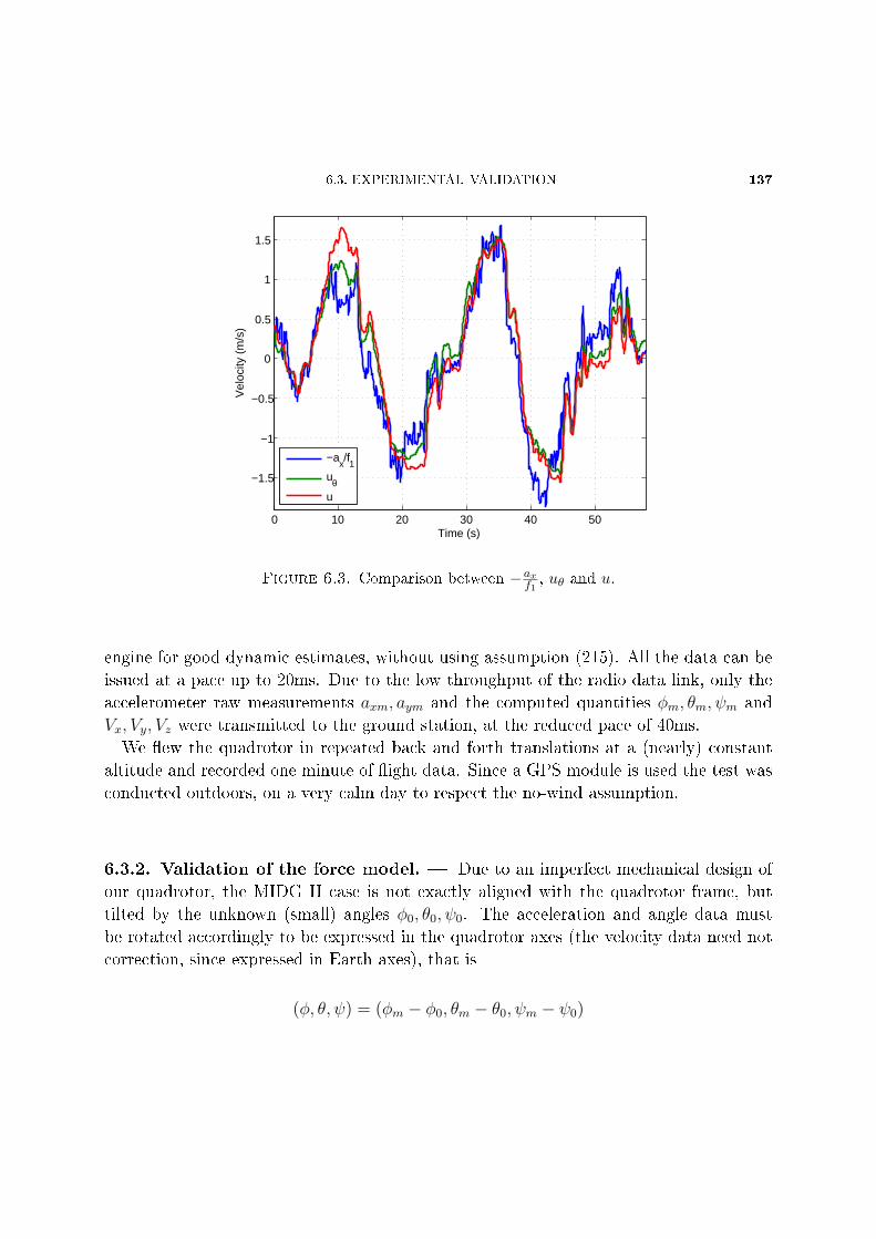
6.3. EXPERIMENTAL VALIDATION 137
0 10 20 30 40 50
−1.5
−1
−0.5
0
0.5
1
1.5
Time (s)
Vel
ocity
(m
/s)
−ax/f
1
uθu
Figure 6.3. Comparison between −axf1, uθ and u.
engine for good dynamic estimates, without using assumption (215). All the data can be
issued at a pace up to 20ms. Due to the low throughput of the radio data link, only the
accelerometer raw measurements axm, aym and the computed quantities φm, θm, ψm and
Vx, Vy, Vz were transmitted to the ground station, at the reduced pace of 40ms.
We ew the quadrotor in repeated back and forth translations at a (nearly) constant
altitude and recorded one minute of ight data. Since a GPS module is used the test was
conducted outdoors, on a very calm day to respect the no-wind assumption.
6.3.2. Validation of the force model. Due to an imperfect mechanical design of
our quadrotor, the MIDG II case is not exactly aligned with the quadrotor frame, but
tilted by the unknown (small) angles φ0, θ0, ψ0. The acceleration and angle data must
be rotated accordingly to be expressed in the quadrotor axes (the velocity data need not
correction, since expressed in Earth axes), that is
(φ, θ, ψ) = (φm − φ0, θm − θ0, ψm − ψ0)
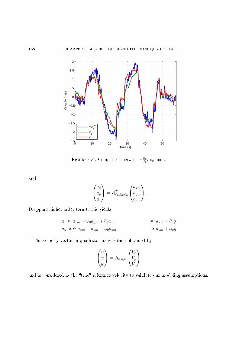
138 CHAPTER 6. SPECIFIC OBSERVER FOR MINI QUADROTOR
0 10 20 30 40 50−2.5
−2
−1.5
−1
−0.5
0
0.5
1
1.5
2
Time (s)
Vel
ocity
(m
/s)
−ay/f
1
vφv
Figure 6.4. Comparison between −ay
f1, vφ and v.
and axayaz
= RTφ0,θ0,ψ0
axmaymazm
.
Dropping higher-order terms, this yields
ax ≈ axm − ψ0aym + θ0azm ≈ axm − θ0g
ay ≈ ψ0axm + aym − φ0azm ≈ aym + φ0g.
The velocity vector in quadrotor axes is then obtained byuvw
= Rφ,θ,ψ
VxVyVz
,
and is considered as the true reference velocity to validate our modeling assumptions.
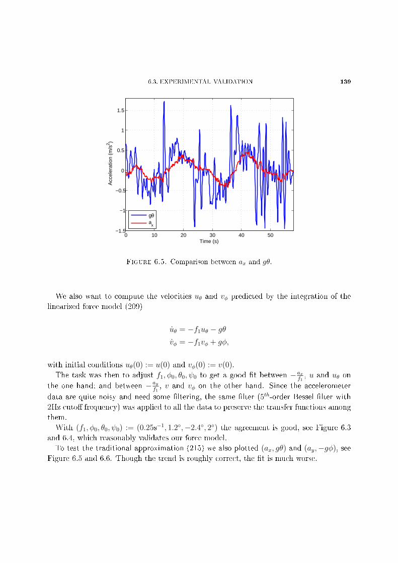
6.3. EXPERIMENTAL VALIDATION 139
0 10 20 30 40 50−1.5
−1
−0.5
0
0.5
1
1.5
Time (s)
Acc
eler
atio
n (m
/s2 )
gθa
x
Figure 6.5. Comparison between ax and gθ.
We also want to compute the velocities uθ and vφ predicted by the integration of the
linearized force model (209)
uθ = −f1uθ − gθvφ = −f1vφ + gφ,
with initial conditions uθ(0) := u(0) and vφ(0) := v(0).
The task was then to adjust f1, φ0, θ0, ψ0 to get a good t between −ax
f1, u and uθ on
the one hand; and between −ay
f1, v and vφ on the other hand. Since the accelerometer
data are quite noisy and need some ltering, the same lter (5th-order Bessel lter with
2Hz cuto frequency) was applied to all the data to preserve the transfer functions among
them.
With (f1, φ0, θ0, ψ0) := (0.25s−1, 1.2,−2.4, 2) the agreement is good, see Figure 6.3
and 6.4, which reasonably validates our force model.
To test the traditional approximation (215) we also plotted (ax, gθ) and (ay,−gφ), see
Figure 6.5 and 6.6. Though the trend is roughly correct, the t is much worse.
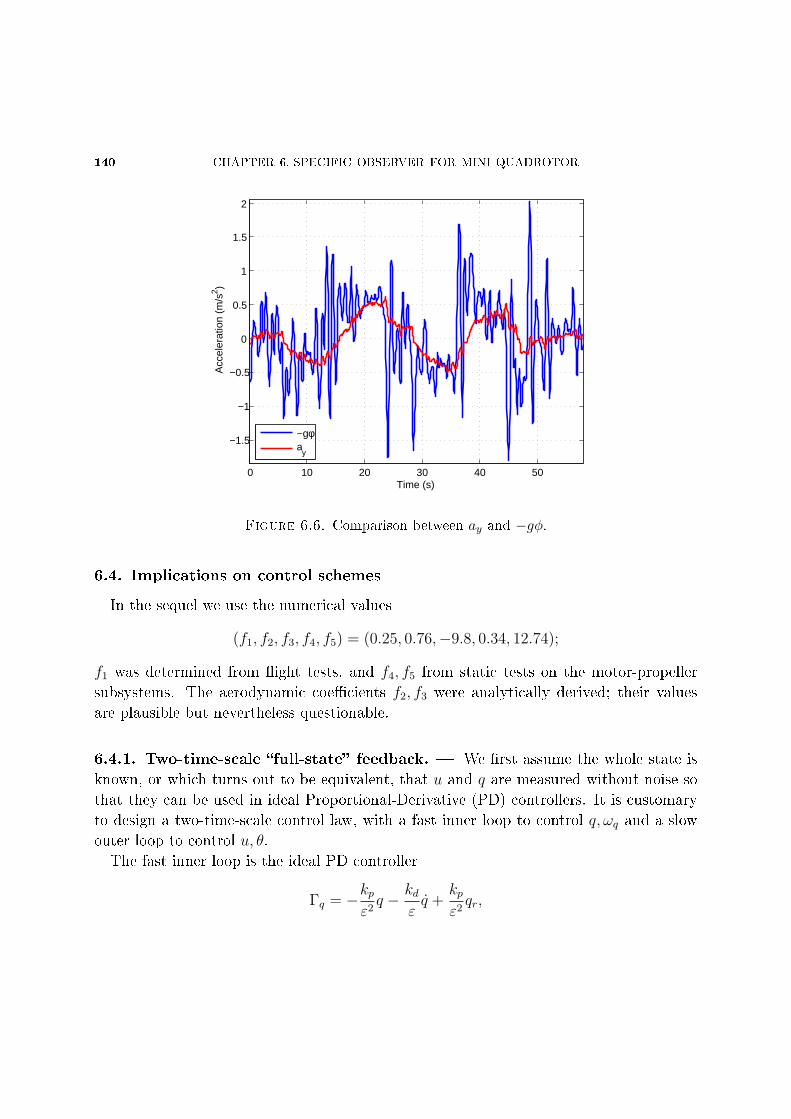
140 CHAPTER 6. SPECIFIC OBSERVER FOR MINI QUADROTOR
0 10 20 30 40 50
−1.5
−1
−0.5
0
0.5
1
1.5
2
Time (s)
Acc
eler
atio
n (m
/s2 )
−gφa
y
Figure 6.6. Comparison between ay and −gφ.
6.4. Implications on control schemes
In the sequel we use the numerical values
(f1, f2, f3, f4, f5) = (0.25, 0.76,−9.8, 0.34, 12.74);
f1 was determined from ight tests, and f4, f5 from static tests on the motor-propeller
subsystems. The aerodynamic coecients f2, f3 were analytically derived; their values
are plausible but nevertheless questionable.
6.4.1. Two-time-scale full-state feedback. We rst assume the whole state is
known, or which turns out to be equivalent, that u and q are measured without noise so
that they can be used in ideal Proportional-Derivative (PD) controllers. It is customary
to design a two-time-scale control law, with a fast inner loop to control q, ωq and a slow
outer loop to control u, θ.
The fast inner loop is the ideal PD controller
Γq = −kpε2q − kd
εq +
kpε2qr,
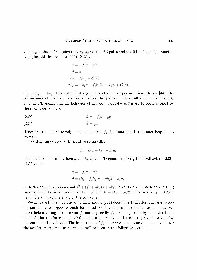
6.4. IMPLICATIONS ON CONTROL SCHEMES 141
where qr is the desired pitch rate; kp, kd are the PD gains and ε > 0 is a small parameter.
Applying this feedback to (209)-(212) yields
u = −f1u− gθ
θ = q
εq = f4ωq +O(ε)
ε ˙ωq = −kpq − f4kdωq + kpqr +O(ε),
where ωq := εωq. From standard arguments of singular perturbations theory [44], the
convergence of the fast variables is up to order ε ruled by the well-known coecient f4
and the PD gains; and the behavior of the slow variables u, θ is up to order ε ruled by
the slow approximation
u = −f1u− gθ(220)
θ = qr.(221)
Hence the role of the aerodynamic coecients f2, f3 is marginal is the inner loop is fast
enough.
The slow outer loop is the ideal PD controller
qr = k1u+ k2u− k1ur,
where ur is the desired velocity, and k1, k2 the PD gains. Applying this feedback to (220)-
(221) yields
u = −f1u− gθ
θ = (k1 − f1k2)u− gk2θ − k1ur,
with characteristic polynomial s2 + (f1 + gk2)s + gk1. A reasonable closed-loop settling
time is about 1s, which requires gk1 = 62 and f1 + gk2 = 6√
2. This means f1 = 0.25 is
negligible w.r.t to the eect of the controller.
We thus see that the revisited moment model (211) does not rely matter if the gyroscope
measurements are good enough for a fast loop, which is usually the case in practice;
nevertheless taking into account f2 and especially f3 may help to design a better inner
loop. As for the force model (209), it does not really matter either, provided a velocity
measurement is available. The importance of f1 is nevertheless paramount to account for
the accelerometer measurements, as will be seen in the following sections.
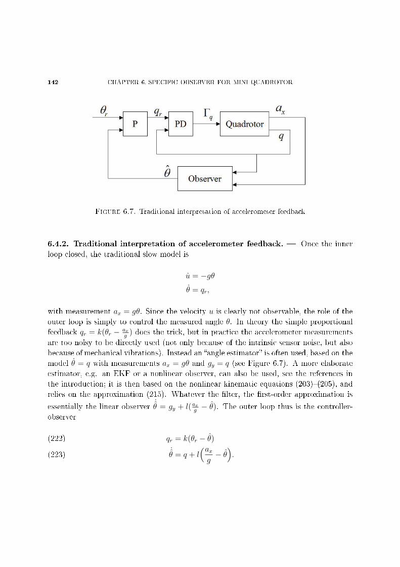
142 CHAPTER 6. SPECIFIC OBSERVER FOR MINI QUADROTOR
Figure 6.7. Traditional interpretation of accelerometer feedback
6.4.2. Traditional interpretation of accelerometer feedback. Once the inner
loop closed, the traditional slow model is
u = −gθ
θ = qr,
with measurement ax = gθ. Since the velocity u is clearly not observable, the role of the
outer loop is simply to control the measured angle θ. In theory the simple proportional
feedback qr = k(θr − ax
g) does the trick, but in practice the accelerometer measurements
are too noisy to be directly used (not only because of the intrinsic sensor noise, but also
because of mechanical vibrations). Instead an angle estimator is often used, based on the
model θ = q with measurements ax = gθ and gy = q (see Figure 6.7). A more elaborate
estimator, e.g. an EKF or a nonlinear observer, can also be used, see the references in
the introduction; it is then based on the nonlinear kinematic equations (203)(205), and
relies on the approximation (215). Whatever the lter, the rst-order approximation is
essentially the linear observer˙θ = gy + l(ax
g− θ). The outer loop thus is the controller-
observer
qr = k(θr − θ)(222)
˙θ = q + l
(axg− θ).(223)
6.4. IMPLICATIONS ON CONTROL SCHEMES 143
Applied to the traditional model and dening the observation error eθ := θ − θ, it yieldsthe closed-loop system
u = −gθ
θ = k(θr − θ − eθ)eθ = −leθ.
For θr constant, the last two equations have the unique steady state (θ, eθ) = (θr, 0). The
characteristic polynomial is
∆0 := (s+ k)(s+ l),
and the closed-loop transfer functions are
θ =k
s+ kθr(224)
u =−gk
s(s+ k)θr.(225)
Provided k, l > 0 we have as desired (θ, eθ)→ (θr, 0), while u grows linearly unbounded.
A good tuning of (222)-(223) requires for robustness that the controller and observer act
in distinct time scales (Loop Transfer Recovery), i.e. k l or l k. We consider in the
sequel a slow observer, which is representative of commercial angle sensors such as the
3DM-GX, and a fast controller; for a settling time of about 1s, we choose e.g. k := 10.3
and l := 112.
We tested this control scheme experimentally, with a rather satisfying result: the angle θ
reaches the desired θr, though the dynamics is somewhat more sluggish than expected.
The traditional analysis could thus be considered as reasonably justied. Nevertheless it
does not account for the following experimental observations already visible to the naked
eye:
when pushed away from hovering, the quadrotor returns to hovering (of course at a
dierent position)
when ying at a constant velocity u, the angle θ is not zero but approximately
proportional to u
in response to a constant θr, u does not grow unbounded but reaches a value approx-
imately proportional to θr.
Though these experimental facts are well-known to people in the eld, they do not seem
to be reported in the literature. The discrepancy is usually attributed to the neglected
second-order aerodynamical drag and the inevitably unperfect experimental conditions.
144 CHAPTER 6. SPECIFIC OBSERVER FOR MINI QUADROTOR
Another more subtle discrepancy is that the observer gain l must be smaller than predicted
by the theory to avoid a badly damped transient (e.g. l = 1/3 does not work well in
practice).
As will be seen in the following section, these experimental facts can be explained by
the revisited model.
6.4.3. Revisited interpretation of accelerometer feedback. We now apply the
controller-observer (222)-(223) to the revisited longitudinal model. The closed-loop sys-
tem is now
u = −f1u− gθ
θ = k(θr − θ − eθ)
eθ = −l(f1
gu+ θ + eθ
),
with eθ := θ − θ. For θr constant, the only steady state is (u, θ, eθ) = (− gf1θr, θr, 0); the
characteristic polynomial is
∆ = s3 + (k + l + f1)s2 + f1(k + l)s+ f1kl.
If k l, ∆ ' (s + k)(s2 + f1s + f1l), so that the closed-loop system is stable as soon
as k, l > 0. Hence θ → θr as desired, and eθ → 0 as expected from the observer; u
now tends to the nite value − gf1θr, which is more consistent with experimental tests. If
moreover l f1,
∆ ≈ (s+ f1)(s+ k)(s+ l) = (s+ f1)∆0.
As a consequence, the closed-loop transfer functions are
θ =k(s+ f1)(s+ l)
∆θr ≈ k
s+ kθr
u =−gk(s+ l)
∆θr ≈ −gk
(s+ f1)(s+ k)θr,
to be compared with (224)-(225): the angle dynamics is nearly the same as the one given
by the traditional interpretation, while the velocity dynamics is dominated by the rotor
drag time constant 1f1. Dening the reference velocity ur := − g
f1θr, we see the traditional
control scheme, designed as an angle controller, is in fact a velocity controller!
The behavior experienced in practice is qualitatively and quantitatively well predicted
by the revisited model, see Figure 6.8 (traditional design) the time response to a −1.5
step in θr (i.e. a 1m/s step in ur).
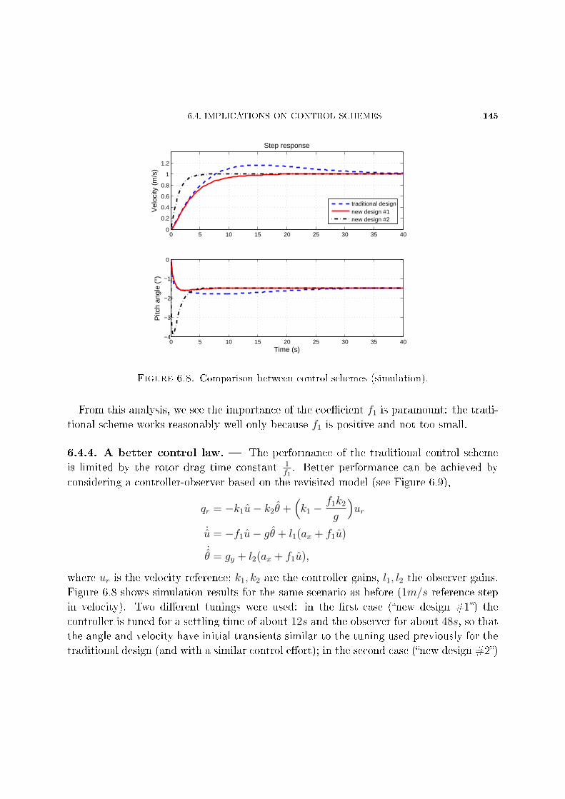
6.4. IMPLICATIONS ON CONTROL SCHEMES 145
0 5 10 15 20 25 30 35 400
0.2
0.4
0.6
0.8
1
1.2
Step responseV
eloc
ity (
m/s
)
0 5 10 15 20 25 30 35 40−4
−3
−2
−1
0
Time (s)
Pitc
h an
gle
(°)
traditional designnew design #1new design #2
Figure 6.8. Comparison between control schemes (simulation).
From this analysis, we see the importance of the coecient f1 is paramount: the tradi-
tional scheme works reasonably well only because f1 is positive and not too small.
6.4.4. A better control law. The performance of the traditional control scheme
is limited by the rotor drag time constant 1f1. Better performance can be achieved by
considering a controller-observer based on the revisited model (see Figure 6.9),
qr = −k1u− k2θ +(k1 −
f1k2
g
)ur
˙u = −f1u− gθ + l1(ax + f1u)
˙θ = gy + l2(ax + f1u),
where ur is the velocity reference; k1, k2 are the controller gains, l1, l2 the observer gains.
Figure 6.8 shows simulation results for the same scenario as before (1m/s reference step
in velocity). Two dierent tunings were used: in the rst case (new design #1) the
controller is tuned for a settling time of about 12s and the observer for about 48s, so that
the angle and velocity have initial transients similar to the tuning used previously for the
traditional design (and with a similar control eort); in the second case (new design #2)
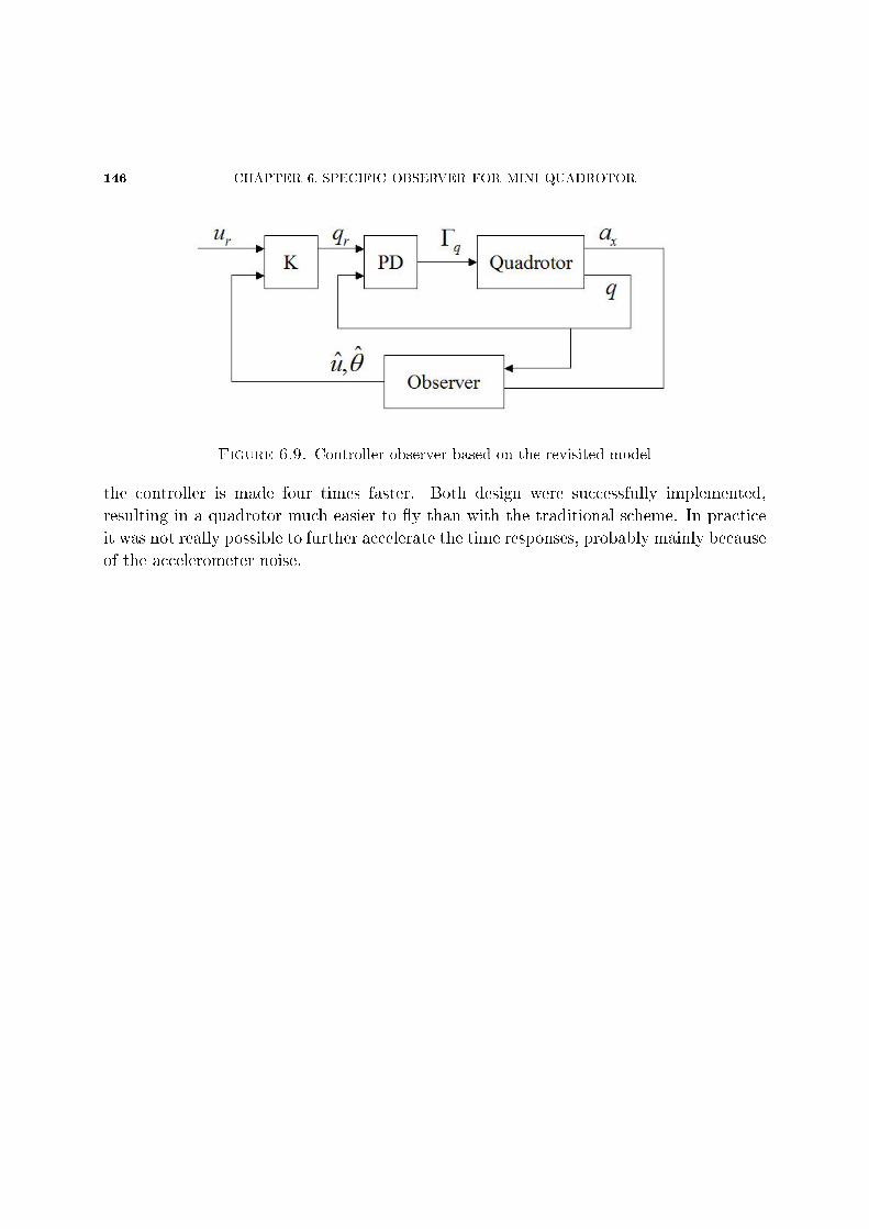
146 CHAPTER 6. SPECIFIC OBSERVER FOR MINI QUADROTOR
Figure 6.9. Controller-observer based on the revisited model
the controller is made four times faster. Both design were successfully implemented,
resulting in a quadrotor much easier to y than with the traditional scheme. In practice
it was not really possible to further accelerate the time responses, probably mainly because
of the accelerometer noise.
CHAPTER 7
REAL-TIME IMPLEMENTATION AND LOW-COST
EMBEDDED PROTOTYPE SYSTEM
Dans ce chapitre nous validons l'implémentation des observateurs génériques invariants
pour les (aided) Attitude and Heading Reference Systems en temps-réel sur un micro-
contrôleur bon marché, à savoir un ATmega128 de chez Atmel. Nous mettons ainsi en év-
idence une autre propriété très interessante de ces estimateurs par rapport aux techniques
de ltrage habituelles: ils sont très économiques en temps de calcul, et donc tout-à-fait
adaptés à la problématique des mini-drones. Dans ce chapitre, nous présentons et vali-
dons également notre propre système avionique bas-coûts, composé de capteurs bruts et
du microcontrôleur sur lequel sont implantés les observateurs invariants. Nous donnons
l'architecture du code permettant l'interface avec les diérents capteurs, l'estimation des
variables et l'envoi des estimées via un port série.
7.1. Real-time implementation on a cheap microcontroller
7.1.1. Real-time implementation of invariant observers for AHRS. In Chap-
ter 3 we developed an invariant nonlinear observer for AHRS. We validated it by using
measurements from a commercial navigation system (MIDG II from Microstrain in Verti-
cal Gyro mode) and by implementing the estimator algorithm (see Equations (82)(85))
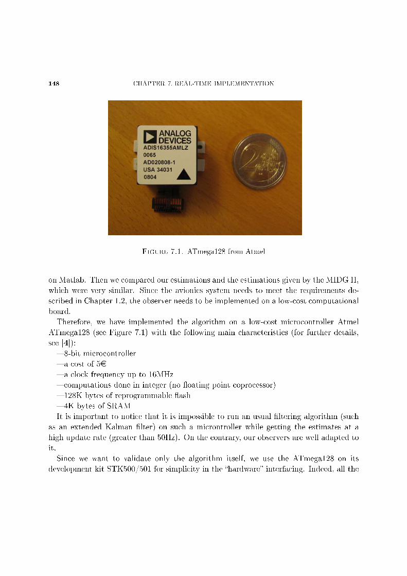
148 CHAPTER 7. REAL-TIME IMPLEMENTATION
Figure 7.1. ATmega128 from Atmel
on Matlab. Then we compared our estimations and the estimations given by the MIDG II,
which were very similar. Since the avionics system needs to meet the requirements de-
scribed in Chapter 1.2, the observer needs to be implemented on a low-cost computational
board.
Therefore, we have implemented the algorithm on a low-cost microcontroller Atmel
ATmega128 (see Figure 7.1) with the following main characteristics (for further details,
see [4]):
8-bit microcontroller
a cost of 5e a clock frequency up to 16MHz
computations done in integer (no oating point coprocessor)
128K bytes of reprogrammable ash
4K bytes of SRAM
It is important to notice that it is impossible to run an usual ltering algorithm (such
as an extended Kalman lter) on such a microntroller while getting the estimates at a
high update rate (greater than 50Hz). On the contrary, our observers are well adapted to
it.
Since we want to validate only the algorithm itself, we use the ATmega128 on its
development kit STK500/501 for simplicity in the hardware interfacing. Indeed, all the

7.1. REAL-TIME IMPLEMENTATION ON A CHEAP MICROCONTROLLER 149
Figure 7.2. Experimental protocol
pins are easily accessible and a TTL/RS232 converter (i.e. microcontroller/PC serial port)
is built-in. The computations of Equations (82)(85) are done in C with the standard
oating point emulation. We have used a simple Euler explicit approximation for the
integration scheme.
The experimental protocol was the following:
1. move the sensors in all directions and save on a computer the MIDG II raw mea-
surements and estimations at 50Hz.
2. use of xPCTarget to feed the ATmega with these data at 50Hz via a serial port and
send to a computer at 50Hz the estimated variables given by the microcontroller.
3. save these estimates.
4. compare oine the estimations given by the microcontroller and those given by the
observer written in the Matlab embedded function.
This protocol can be illustrated by the gure 7.2, where the computer with xPCTarget
has been replaced by the MIDG II. We use xPCTarget instead of feeding directly the
microcontroller with the MIDG II raw data because it allows us to run dierent algorithms
on the microcontroller with the same set of data (e.g. in order to do some corrections in
the C code).
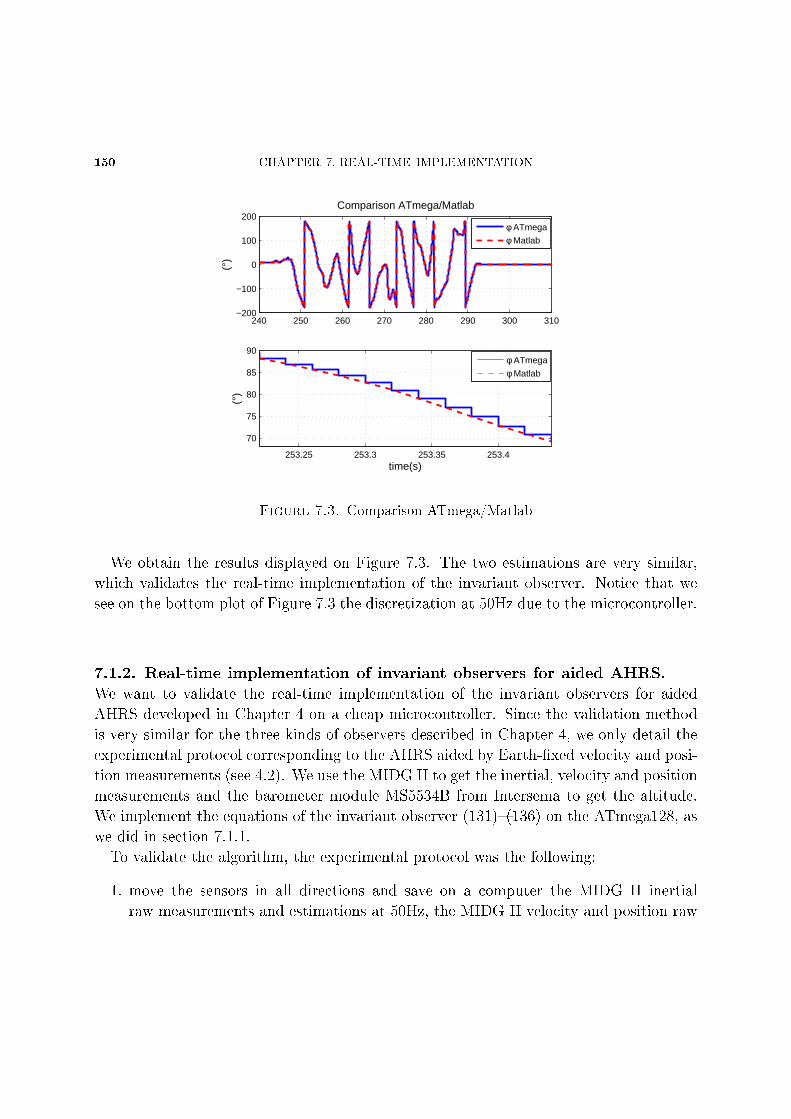
150 CHAPTER 7. REAL-TIME IMPLEMENTATION
240 250 260 270 280 290 300 310−200
−100
0
100
200Comparison ATmega/Matlab
(°)
253.25 253.3 253.35 253.4
70
75
80
85
90
(°)
time(s)
φ ATmega
φ Matlab
φ ATmega
φ Matlab
Figure 7.3. Comparison ATmega/Matlab
We obtain the results displayed on Figure 7.3. The two estimations are very similar,
which validates the real-time implementation of the invariant observer. Notice that we
see on the bottom plot of Figure 7.3 the discretization at 50Hz due to the microcontroller.
7.1.2. Real-time implementation of invariant observers for aided AHRS.
We want to validate the real-time implementation of the invariant observers for aided
AHRS developed in Chapter 4 on a cheap microcontroller. Since the validation method
is very similar for the three kinds of observers described in Chapter 4, we only detail the
experimental protocol corresponding to the AHRS aided by Earth-xed velocity and posi-
tion measurements (see 4.2). We use the MIDG II to get the inertial, velocity and position
measurements and the barometer module MS5534B from Intersema to get the altitude.
We implement the equations of the invariant observer (131)(136) on the ATmega128, as
we did in section 7.1.1.
To validate the algorithm, the experimental protocol was the following:
1. move the sensors in all directions and save on a computer the MIDG II inertial
raw measurements and estimations at 50Hz, the MIDG II velocity and position raw
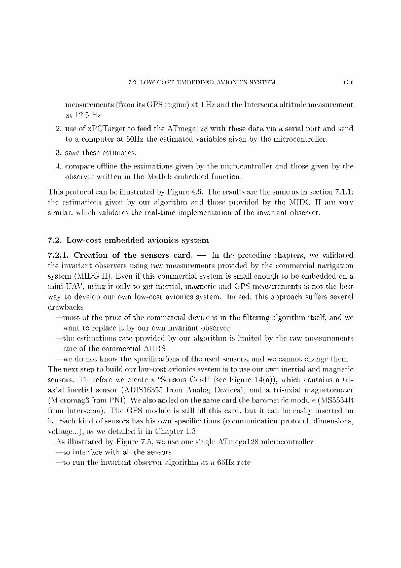
7.2. LOW-COST EMBEDDED AVIONICS SYSTEM 151
measurements (from its GPS engine) at 4 Hz and the Intersema altitude measurement
at 12.5 Hz
2. use of xPCTarget to feed the ATmega128 with these data via a serial port and send
to a computer at 50Hz the estimated variables given by the microcontroller.
3. save these estimates.
4. compare oine the estimations given by the microcontroller and those given by the
observer written in the Matlab embedded function.
This protocol can be illustrated by Figure 4.6. The results are the same as in section 7.1.1:
the estimations given by our algorithm and those provided by the MIDG II are very
similar, which validates the real-time implementation of the invariant observer.
7.2. Low-cost embedded avionics system
7.2.1. Creation of the sensors card. In the preceding chapters, we validated
the invariant observers using raw measurements provided by the commercial navigation
system (MIDG II). Even if this commercial system is small enough to be embedded on a
mini-UAV, using it only to get inertial, magnetic and GPS measurements is not the best
way to develop our own low-cost avionics system. Indeed, this approach suers several
drawbacks
most of the price of the commercial device is in the ltering algorithm itself, and we
want to replace it by our own invariant observer
the estimations rate provided by our algorithm is limited by the raw measurements
rate of the commercial AHRS
we do not know the specications of the used sensors, and we cannot change them
The next step to build our low-cost avionics system is to use our own inertial and magnetic
sensors. Therefore we create a Sensors Card (see Figure 14(a)), which contains a tri-
axial inertial sensor (ADIS16355 from Analog Devices), and a tri-axial magnetometer
(Micromag3 from PNI). We also added on the same card the barometric module (MS5534B
from Intersema). The GPS module is still o this card, but it can be easily inserted on
it. Each kind of sensors has his own specications (communication protocol, dimensions,
voltage...), as we detailed it in Chapter 1.3.
As illustrated by Figure 7.5, we use one single ATmega128 microcontroller
to interface with all the sensors
to run the invariant observer algorithm at a 65Hz rate
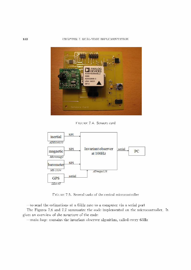
152 CHAPTER 7. REAL-TIME IMPLEMENTATION
Figure 7.4. Sensors card
Figure 7.5. Several tasks of the central microcontroller
to send the estimations at a 65Hz rate to a computer via a serial port
The Figures 7.6 and 7.7 summarize the code implemented on the microcontroller. It
gives an overview of the structure of the code:
main loop: contains the invariant observer algorithm, called every 65Hz
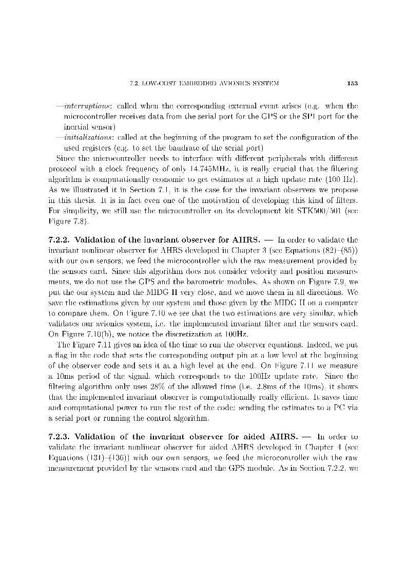
7.2. LOW-COST EMBEDDED AVIONICS SYSTEM 153
interruptions : called when the corresponding external event arises (e.g. when the
microcontroller receives data from the serial port for the GPS or the SPI port for the
inertial sensor)
initializations : called at the beginning of the program to set the conguration of the
used registers (e.g. to set the baudrate of the serial port)
Since the microcontroller needs to interface with dierent peripherals with dierent
protocol with a clock frequency of only 14.745MHz, it is really crucial that the ltering
algorithm is computationally economic to get estimates at a high update rate (100 Hz).
As we illustrated it in Section 7.1, it is the case for the invariant observers we propose
in this thesis. It is in fact even one of the motivation of developing this kind of lters.
For simplicity, we still use the microcontroller on its development kit STK500/501 (see
Figure 7.8).
7.2.2. Validation of the invariant observer for AHRS. In order to validate the
invariant nonlinear observer for AHRS developed in Chapter 3 (see Equations (82)(85))
with our own sensors, we feed the microcontroller with the raw measurement provided by
the sensors card. Since this algorithm does not consider velocity and position measure-
ments, we do not use the GPS and the barometric modules. As shown on Figure 7.9, we
put the our system and the MIDG II very close, and we move them in all directions. We
save the estimations given by our system and those given by the MIDG II on a computer
to compare them. On Figure 7.10 we see that the two estimations are very similar, which
validates our avionics system, i.e. the implemented invariant lter and the sensors card.
On Figure 7.10(b), we notice the discretization at 100Hz.
The Figure 7.11 gives an idea of the time to run the observer equations. Indeed, we put
a ag in the code that sets the corresponding output pin at a low level at the beginning
of the observer code and sets it at a high level at the end. On Figure 7.11 we measure
a 10ms period of the signal, which corresponds to the 100Hz update rate. Since the
ltering algorithm only uses 28% of the allowed time (i.e. 2.8ms of the 10ms), it shows
that the implemented invariant observer is computationally really ecient. It saves time
and computational power to run the rest of the code: sending the estimates to a PC via
a serial port or running the control algorithm.
7.2.3. Validation of the invariant observer for aided AHRS. In order to
validate the invariant nonlinear observer for aided AHRS developed in Chapter 4 (see
Equations (131)(136)) with our own sensors, we feed the microcontroller with the raw
measurement provided by the sensors card and the GPS module. As in Section 7.2.2, we
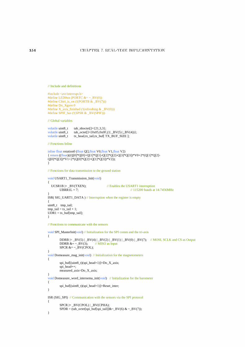
154 CHAPTER 7. REAL-TIME IMPLEMENTATION
// Include and definitions #include <avr/interrupt.h> #define LED0on (PORTC &= ~_BV(0)) #define CStri_is_on (!(PORTB & _BV(7))) #define Do_Xgyro 0 #define X_axis_finished (!(refreshing & _BV(0))) #define SPIF_bas (!(SPSR & _BV(SPIF))) // Global variables volatile uint8_t tab_nboctet[]=21,3,3; volatile uint8_t tab_octet[]=0x05,0x0F,(1| _BV(5) |_BV(4)); volatile uint8_t tx_head,tx_tail,tx_buf[ TX_BUF_SIZE ]; // Fonctions Inline inline float rotation0 (float Q[],float V0,float V1,float V2) return ((float)((Q[0]*Q[0]+Q[1]*Q[1]-Q[2]*Q[2]-Q[3]*Q[3])*V0+2*(Q[1]*Q[2]-Q[0]*Q[3])*V1+2*(Q[0]*Q[2]+Q[1]*Q[3])*V2)); // Fonctions for data transmission to the ground station void USART1_Transmission_Init(void) UCSR1B |= _BV(TXEN); // Enables the USART1 interruption UBRR1L = 7; // 115200 bauds at 14.7456MHz ISR( SIG_UART1_DATA ) // Interruption when the register is empty uint8_t tmp_tail; tmp_tail = tx_tail + 1; UDR1 = tx_buf[tmp_tail]; // Fonctions to communicate with the sensors void SPI_MasterInit(void) // Initialization for the SPI comm and the tri-axis DDRB |= _BV(5) | _BV(4) | _BV(2) | _BV(1) | _BV(0) | _BV(7); // MOSI, SCLK and CS as Output DDRB &= ~_BV(3); // MISO as Input SPCR &= ~_BV(CPOL); void Domeasure_mag_init(void) // Initialization for the magnetometers spi_buf[(uint8_t)(spi_head+1)]=Do_X_axis; spi_head++; measured_axis=Do_X_axis; void Domeasure_word_intersema_init(void) // Initialization for the barometer spi_buf[(uint8_t)(spi_head+1)]=Reset_inter; ISR (SIG_SPI) // Communication with the sensors via the SPI protocol SPCR |= _BV(CPOL) | _BV(CPHA); SPDR = (tab_octet[spi_buf[spi_tail]]&~_BV(6) & ~_BV(7));
Figure 7.6. Architecture of the implemented code (page 1)
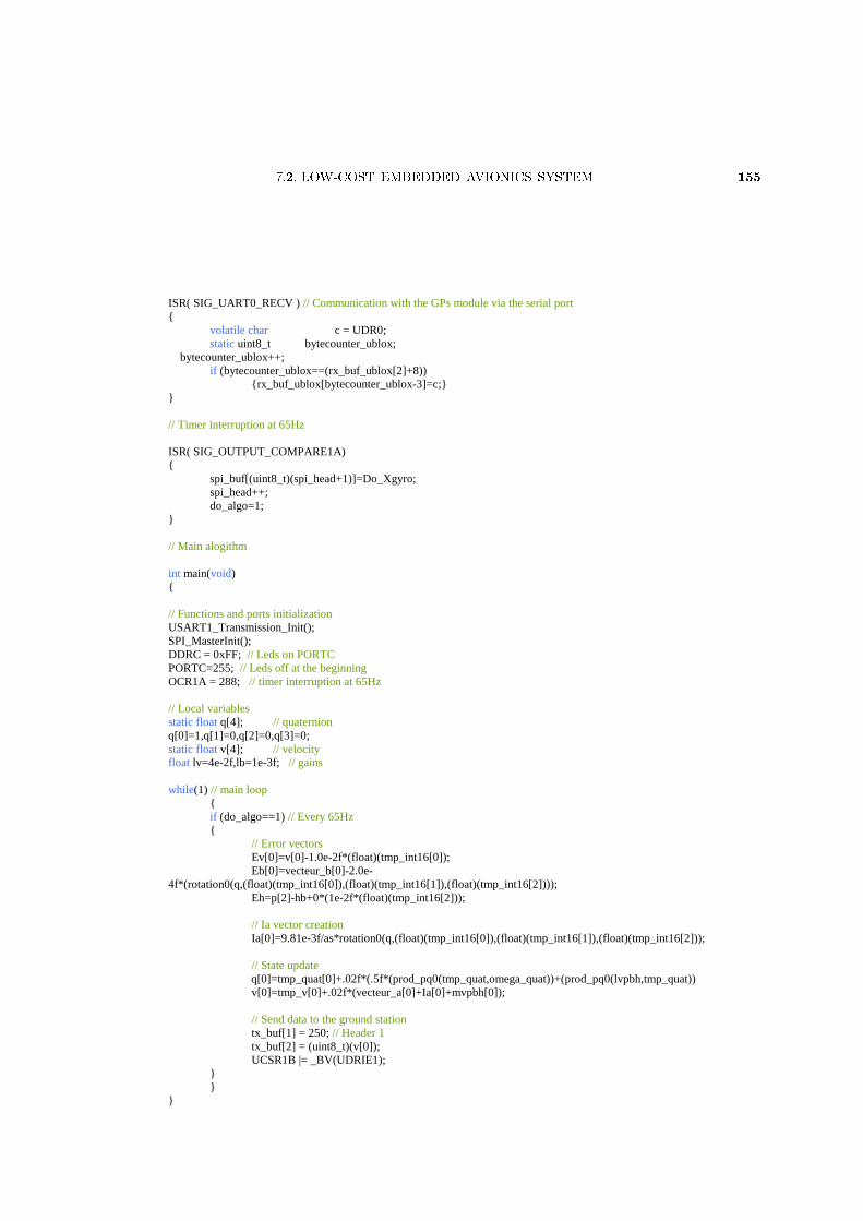
7.2. LOW-COST EMBEDDED AVIONICS SYSTEM 155
ISR( SIG_UART0_RECV ) // Communication with the GPs module via the serial port volatile char c = UDR0; static uint8_t bytecounter_ublox; bytecounter_ublox++; if (bytecounter_ublox==(rx_buf_ublox[2]+8)) rx_buf_ublox[bytecounter_ublox-3]=c; // Timer interruption at 65Hz ISR( SIG_OUTPUT_COMPARE1A) spi_buf[(uint8_t)(spi_head+1)]=Do_Xgyro; spi_head++; do_algo=1; // Main alogithm int main(void) // Functions and ports initialization USART1_Transmission_Init(); SPI_MasterInit(); DDRC = 0xFF; // Leds on PORTC PORTC=255; // Leds off at the beginning OCR1A = 288; // timer interruption at 65Hz // Local variables static float q[4]; // quaternion q[0]=1,q[1]=0,q[2]=0,q[3]=0; static float v[4]; // velocity float lv=4e-2f,lb=1e-3f; // gains while(1) // main loop if (do_algo==1) // Every 65Hz // Error vectors Ev[0]=v[0]-1.0e-2f*(float)(tmp_int16[0]); Eb[0]=vecteur_b[0]-2.0e-4f*(rotation0(q,(float)(tmp_int16[0]),(float)(tmp_int16[1]),(float)(tmp_int16[2]))); Eh=p[2]-hb+0*(1e-2f*(float)(tmp_int16[2])); // Ia vector creation Ia[0]=9.81e-3f/as*rotation0(q,(float)(tmp_int16[0]),(float)(tmp_int16[1]),(float)(tmp_int16[2])); // State update
q[0]=tmp_quat[0]+.02f*(.5f*(prod_pq0(tmp_quat,omega_quat))+(prod_pq0(lvpbh,tmp_quat)) v[0]=tmp_v[0]+.02f*(vecteur_a[0]+Ia[0]+mvpbh[0]); // Send data to the ground station tx_buf[1] = 250; // Header 1 tx_buf[2] = (uint8_t)(v[0]); UCSR1B |= _BV(UDRIE1);
Figure 7.7. Architecture of the implemented code (page 2)
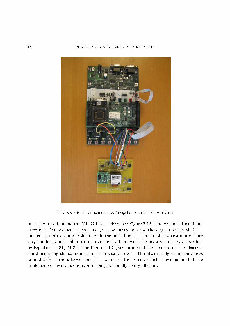
156 CHAPTER 7. REAL-TIME IMPLEMENTATION
Figure 7.8. Interfacing the ATmega128 with the sensors card
put the our system and the MIDG II very close (see Figure 7.12), and we move them in all
directions. We save the estimations given by our system and those given by the MIDG II
on a computer to compare them. As in the preceding experiment, the two estimations are
very similar, which validates our avionics systems with the invariant observer desribed
by Equations (131)(136). The Figure 7.13 gives an idea of the time to run the observer
equations using the same method as in section 7.2.2. The ltering algorithm only uses
around 53% of the allowed time (i.e. 5.3ms of the 10ms), which shows again that the
implemented invariant observer is computationally really ecient.
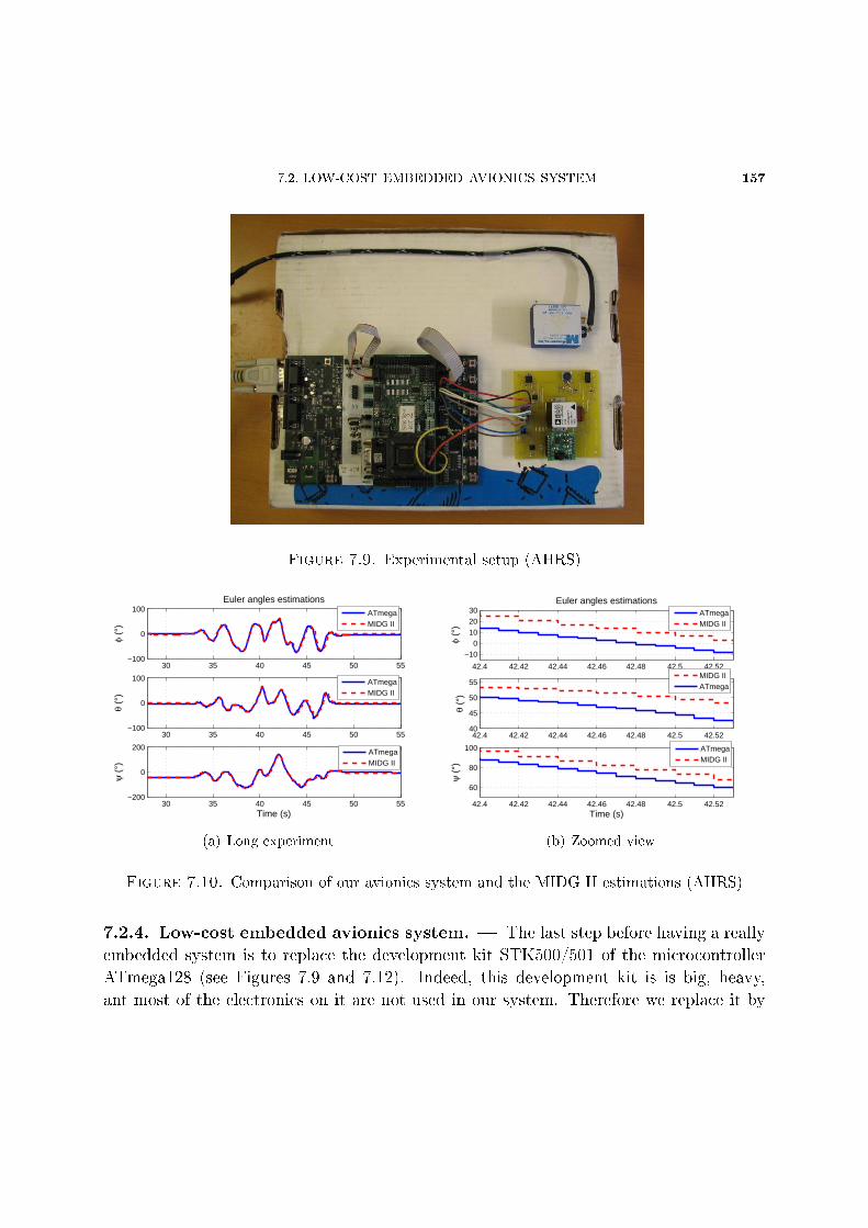
7.2. LOW-COST EMBEDDED AVIONICS SYSTEM 157
Figure 7.9. Experimental setup (AHRS)
30 35 40 45 50 55−100
0
100Euler angles estimations
φ (°
)
ATmegaMIDG II
30 35 40 45 50 55−100
0
100
θ (°
)
ATmegaMIDG II
30 35 40 45 50 55−200
0
200
Time (s)
ψ (
°)
ATmegaMIDG II
(a) Long experiment
42.4 42.42 42.44 42.46 42.48 42.5 42.52
−100
102030
Euler angles estimations
φ (°
)
ATmegaMIDG II
42.4 42.42 42.44 42.46 42.48 42.5 42.5240
45
50
55
θ (°
)
MIDG IIATmega
42.4 42.42 42.44 42.46 42.48 42.5 42.52
60
80
100
Time (s)
ψ (
°)
ATmegaMIDG II
(b) Zoomed view
Figure 7.10. Comparison of our avionics system and the MIDG II estimations (AHRS)
7.2.4. Low-cost embedded avionics system. The last step before having a really
embedded system is to replace the development kit STK500/501 of the microcontroller
ATmega128 (see Figures 7.9 and 7.12). Indeed, this development kit is is big, heavy,
ant most of the electronics on it are not used in our system. Therefore we replace it by
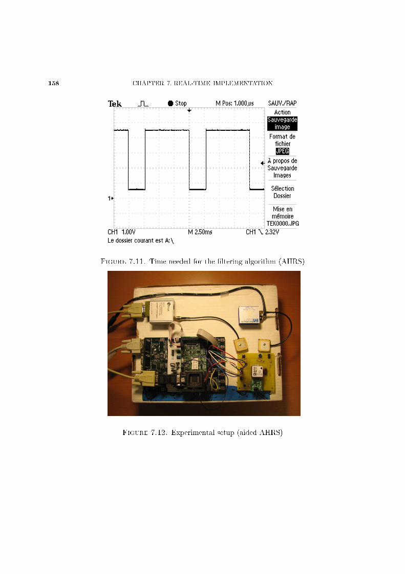
158 CHAPTER 7. REAL-TIME IMPLEMENTATION
Figure 7.11. Time needed for the ltering algorithm (AHRS)
Figure 7.12. Experimental setup (aided AHRS)
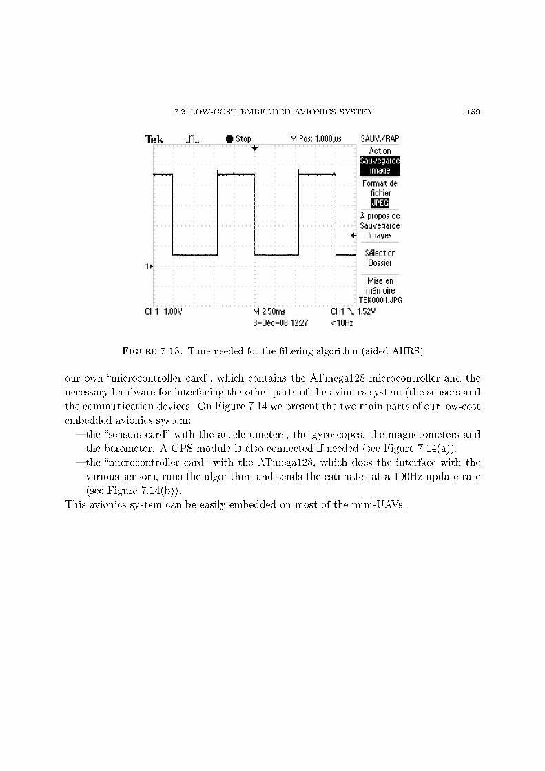
7.2. LOW-COST EMBEDDED AVIONICS SYSTEM 159
Figure 7.13. Time needed for the ltering algorithm (aided AHRS)
our own microcontroller card, which contains the ATmega128 microcontroller and the
necessary hardware for interfacing the other parts of the avionics system (the sensors and
the communication devices. On Figure 7.14 we present the two main parts of our low-cost
embedded avionics system:
the sensors card with the accelerometers, the gyroscopes, the magnetometers and
the barometer. A GPS module is also connected if needed (see Figure 7.14(a)).
the microcontroller card with the ATmega128, which does the interface with the
various sensors, runs the algorithm, and sends the estimates at a 100Hz update rate
(see Figure 7.14(b)).
This avionics system can be easily embedded on most of the mini-UAVs.
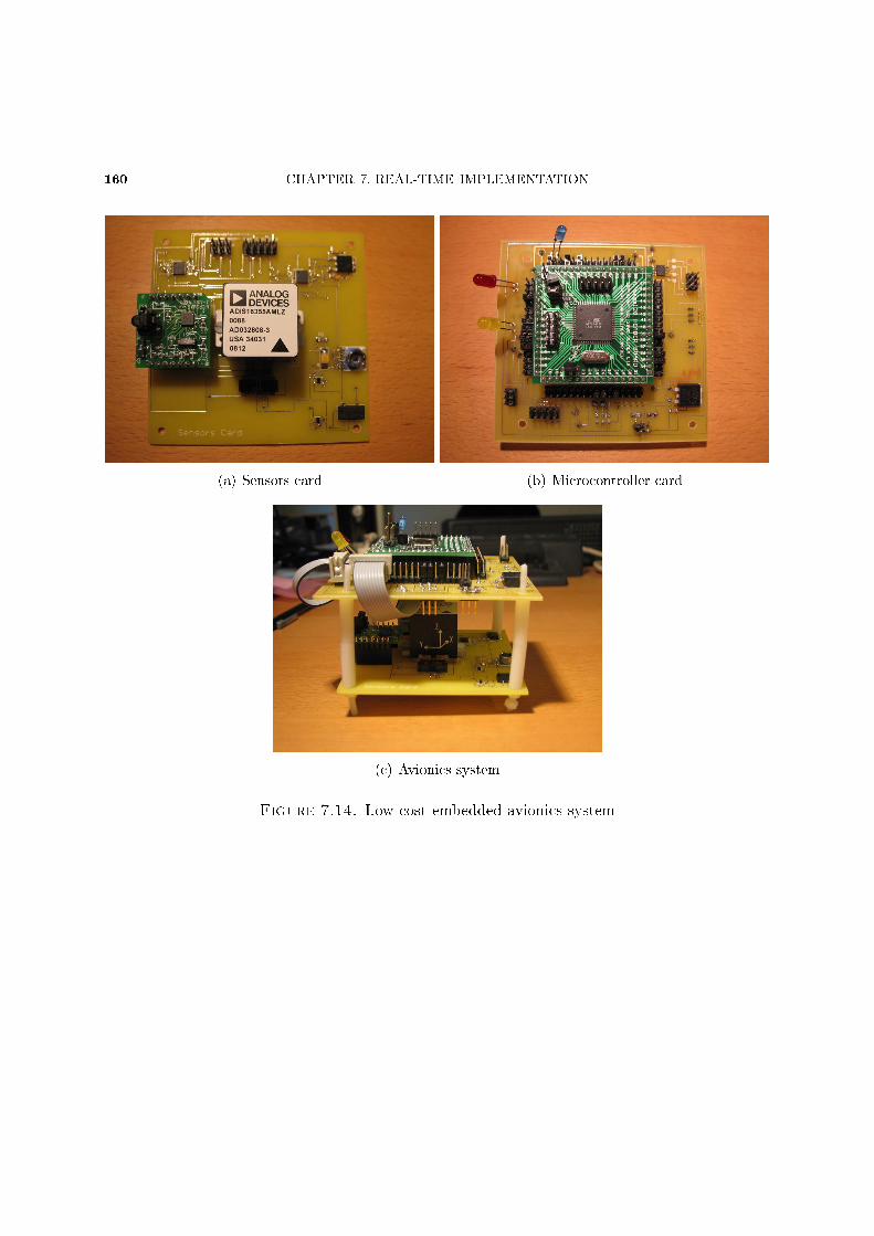
160 CHAPTER 7. REAL-TIME IMPLEMENTATION
(a) Sensors card (b) Microcontroller card
(c) Avionics system
Figure 7.14. Low-cost embedded avionics system
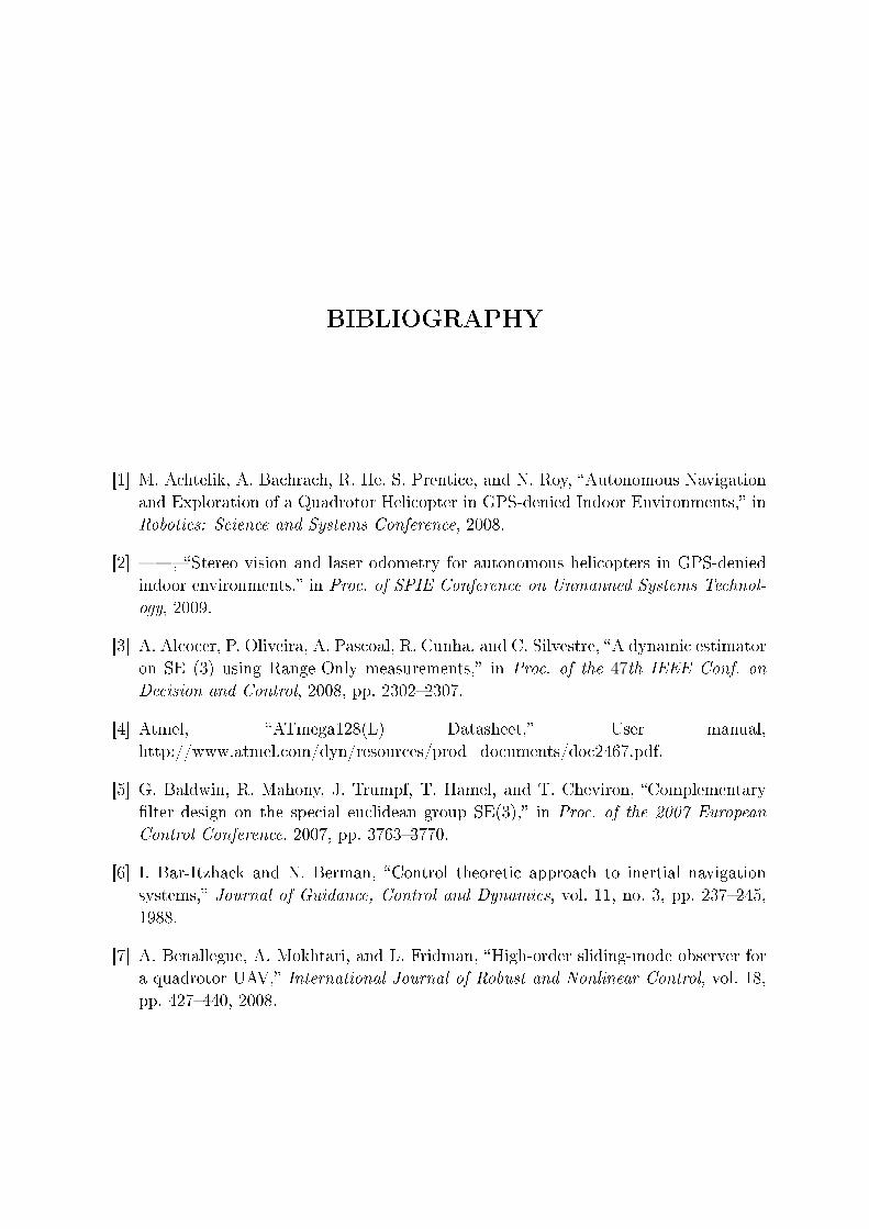
BIBLIOGRAPHY
[1] M. Achtelik, A. Bachrach, R. He, S. Prentice, and N. Roy, Autonomous Navigation
and Exploration of a Quadrotor Helicopter in GPS-denied Indoor Environments, in
Robotics: Science and Systems Conference, 2008.
[2] , Stereo vision and laser odometry for autonomous helicopters in GPS-denied
indoor environments, in Proc. of SPIE Conference on Unmanned Systems Technol-
ogy, 2009.
[3] A. Alcocer, P. Oliveira, A. Pascoal, R. Cunha, and C. Silvestre, A dynamic estimator
on SE (3) using Range-Only measurements, in Proc. of the 47th IEEE Conf. on
Decision and Control, 2008, pp. 23022307.
[4] Atmel, ATmega128(L) Datasheet, User manual,
http://www.atmel.com/dyn/resources/prod_documents/doc2467.pdf.
[5] G. Baldwin, R. Mahony, J. Trumpf, T. Hamel, and T. Cheviron, Complementary
lter design on the special euclidean group SE(3), in Proc. of the 2007 European
Control Conference, 2007, pp. 37633770.
[6] I. Bar-Itzhack and N. Berman, Control theoretic approach to inertial navigation
systems, Journal of Guidance, Control and Dynamics, vol. 11, no. 3, pp. 237245,
1988.
[7] A. Benallegue, A. Mokhtari, and L. Fridman, High-order sliding-mode observer for
a quadrotor UAV, International Journal of Robust and Nonlinear Control, vol. 18,
pp. 427440, 2008.
162 BIBLIOGRAPHY
[8] J. Bijker and W. Steyn, Kalman lter congurations for a low-cost loosely integrated
inertial navigation system on an airship, Control Engineering Practice, vol. 16,
no. 12, pp. 15091518, 2008.
[9] S. Bonnabel, Left-invariant extended Kalman lter and attitude estimation, 2007,
pp. 10271032.
[10] S. Bonnabel, P. Martin, and P. Rouchon, A non-linear symmetry-preserving ob-
server for velocity-aided inertial navigation, in Proc. of the 2006 American Control
Conference, 2006, pp. 29102914.
[11] , Non-linear observer on Lie group for left-invariant dynamics with right-left
equivariant output, in Proc. of the 17th IFAC World Congress, 2008, pp. 85948598.
[12] , Symmetry-preserving observers, IEEE Trans. Automat. Control, vol. 53,
no. 11, pp. 25142526, 2008.
[13] , Non-linear symmetry-preserving observers on Lie groups, IEEE
Trans. Automat. Control, To appear in 2009, preliminary version
http://arxiv.org/abs/0707.2286.
[14] S. Bonnabel, P. Martin, and E. Salaün, Invariant Extended Kalman Filter: theory
and application to a velocity-aided attitude estimation problem, in Proc. of the 48th
IEEE Conf. on Decision and Control, 2009, pp. 12971304.
[15] S. Bouabdallah, A. Noth, and R. Siegwart, Pid vs lq control techniques applied to an
indoor micro quadrotor, in Proc. of the 2004 IEEE/RSJ International Conference
on Intelligent Robots and Systems, vol. 3, 2004, pp. 24512456.
[16] S. Bouabdallah and R. Siegwart, Full control of a quadrotor, in Proc. of the 2007
IEEE/RSJ International Conference on Intelligent Robots and Systems, 2007, pp.
153158.
[17] P.-J. Bristeau, P. Martin, E. Salaün, and N. Petit, The role of propeller aerodynamics
in the model of a quadrotor UAV, in Proc. of the 2009 European Control Conference,
2009, pp. 683688.
[18] R. Brockett, Remarks on nite dimensional nonlinear estimation, Astersique, vol.
75-76, pp. 4755, 1980.
BIBLIOGRAPHY 163
[19] J. Carpenter and I. Bar-Itzhack, On the commonality between Schuler-period in
terrestrial INS and LEO satellites, in Proc. of the 2004 AIAA/AAS Astrodynamics
Specialist Conference and Exhibit, 2004, pp. 48504858.
[20] P. Castillo, A. Dzul, and R. Lozano, Real-time stabilization and tracking of a four-
rotor mini rotorcraft, IEEE Trans. Control Systems Technology, vol. 12, no. 4, pp.
510516, 2004.
[21] Y. Cheng and J. Crassidis, Particle ltering for sequential spacecraft attitude esti-
mation, in Proc. of the 2004 AIAA Guidance, Navigation, and Control Conference,
2004, pp. 53375354.
[22] D. Choukroun, Adaptative optimal-REQUEST algorithm for attitude determina-
tion, in Proc. of the 2007 AIAA Guidance, Navigation, and Control Conference,
2007, pp. 68136837.
[23] R. Collinson, Introduction to avionics systems, 2nd ed. Kluwer Academic Publishers,
2003.
[24] J. Crassidis, Sigma-point Kalman ltering for integrated GPS and inertial naviga-
tion, IEEE Trans. on Aerospace and Electronic Systems, vol. 42, no. 2, pp. 750756,
2006.
[25] J. Crassidis and F. Markley, Unscented ltering for spacecraft attitude estimation,
Journal of Guidance, Control and Dynamics, vol. 26, no. 4, pp. 536542, 2003.
[26] J. Crassidis, F. Markley, and Y. Cheng, Survey of nonlinear attitude estimation
methods, Journal of Guidance, Control and Dynamics, vol. 30, no. 1, pp. 1228,
2007.
[27] L. Derafa, T. Madani, and A. Benallegue, Dynamic modelling and experirnental
identication of four rotors helicopter pararmeters, in Proc. of the 2006 IEEE In-
ternational Conference on Industrial Technology, 2006, pp. 18341839.
[28] J. Farrell and M. Barth, The global positioning system and inertial navigation.
McGraw-Hill, 1998.
164 BIBLIOGRAPHY
[29] F. Faruqi and K. Turner, Extended Kalman lter synthesis for integrated global
positioning/inertial navigation systems, Applied Mathematics and Computation, vol.
115, no. 2-3, pp. 213227, 2000.
[30] D. Gleason and A. Hanscom, Critical role of gravity compensation in a stand-alone
precision INS, in Proc. of the 2003 DARPA Precision Inertial Navigation Systems
Meeting, 2003.
[31] M. Grewal, L. Weill, and A. Andrews, Global positioning systems, inertial navigation,
and integration. Wiley, 2001.
[32] P. D. Groves, Principles of GNSS, inertial, and multisensor integrated navigation
systems. Artech House, 2008.
[33] N. Guenard, T. Hamel, and R. Mahony, A practical visual servo control for an
unmanned aerial vehicle, IEEE Trans. on Robotics, vol. 24, no. 2, pp. 331340,
2008.
[34] N. Guenard, T. Hamel, and V. Moreau, Dynamic modeling and intuitive control
strategy for an "X4-yer", in Proc. of the 2005 International Conference on Control
and Automation, 2005, pp. 141146.
[35] T. Hamel and R. Mahony, Attitude estimation on SO(3) based on direct inertial
measurements, in Proc. of the 2006 IEEE International Conference on Robotics and
Automation, 2006, pp. 21702175.
[36] B. Herisse, F. Russotto, T. Hamel, and R. Mahony, Hovering ight and vertical
landing control of a VTOL Unmanned Aerial Vehicle using Optical Flow, in Proc.
of the 2008 IEEE/RSJ International Conference on Intelligent Robots and Systems,
2008, pp. 801806.
[37] C. Hide, T. Moore, and M. Smith, Adaptive Kalman ltering for low-cost INS/GPS,
The Journal of Navigation, vol. 56, no. 01, pp. 143152, 2003.
[38] , Adaptive Kalman ltering algorithms for integrating GPS and low cost INS,
in Proc. of the Position Location and Navigation Symposium, 2004, pp. 227233.
BIBLIOGRAPHY 165
[39] G. Homann, D. Rajnarayan, S. Waslander, D. Dostal, J. Jang, and C. Tomlin,
The stanford testbed of autonomous rotorcraft for multi agent control (starmac),
in Proc. of the 2004 Digital Avionics Systems Conference, vol. 2, 2004.
[40] G. Homann, H. Huang, S. Waslander, and C. Tomlin, Quadrotor helicopter ight
dynamics and control: Theory and experiment, in Proc. of the 2007 AIAA Guidance,
Navigation, and Control Conference, 2007, pp. 64616480.
[41] Y. Huang, F. Chang, and L. Wang, The attitude determination algorithm using
integrated GPS/INS data, in Proc. of the 16th IFAC World Congress, 2005.
[42] W. Johnson, Helicopter Theory. Princeton University Press, 1980.
[43] F. Kendoul, D. Lara, I. Fantoni-Coichot, and R. Lozano, Real-time nonlinear embed-
ded control for an autonomous quadrotor helicopter, Journal of Guidance, Control
and Dynamics, vol. 30, no. 4, pp. 10491061, 2007.
[44] P. Kokotovic, H. K. Khalil, and J. O'Reilly, Singular Perturbation Methods in Control:
Analysis and Design. SIAM, 1999.
[45] A. Krener, Algebraic and Geometric Methods in Nonlinear Control Theory. D. Reidel
Publishing Company, 1986, ch. The intrinsic geometry of dynamic observations, pp.
7787.
[46] C. Lageman, R. Mahony, and J. Trumpf, State observers for invariant dynamics on
a Lie group, in Proc. of the International Conference on the Mathematical Theory
of Networks and Systems, 2008.
[47] C. Lageman, J. Trumpf, and R. Mahony, Gradient-like observers for invariant dy-
namics on a Lie group, IEEE Trans. Automat. Control, 2008.
[48] , Observer design for invariant systems with homogeneous observations, Arxiv
preprint arXiv:0810.0748, 2008.
[49] E. Leerts, F. Markley, and M. Shuster, Kalman ltering for spacecraft attitude,
Journal of Guidance, Control and Dynamics, vol. 5, no. 5, pp. 417429, 1982.
166 BIBLIOGRAPHY
[50] Y. Li, J. Wang, C. Rizos, P. Mumford, and W. Ding, Low-cost tightly coupled
GPS/INS integration based on a nonlinear Kalman ltering design, in Proc. of ION
National Technical Meeting, 2006, pp. 1826.
[51] T. Madani and A. Benallegue, Backstepping control with exact 2-sliding mode es-
timation for a quadrotor unmanned aerial vehicle, in Proc. of the 2007 IEEE/RSJ
International Conference on Intelligent Robots and Systems, 2007, pp. 141146.
[52] R. Mahony, T. Hamel, and J.-M. Pmlin, Nonlinear complementary lters on the
special orthogonal group, IEEE Trans. Automat. Control, vol. 53, no. 5, pp. 1203
1218, 2008.
[53] R. Mahony, T. Hamel, and J. Pimlin, Complementary lter design on the special
orthogonal group SO (3), in Proc. of the 2005 European Control Conference, 2005,
pp. 14771484.
[54] D. Maithripala, J. Berg, and W. Dayawansa, An intrinsic observer for a class of
simple mechanical systems on a lie group, in Proc. of the 2004 American Control
Conference, vol. 2, 2004, pp. 15461551.
[55] , Almost-global tracking of simple mechanical systems on a general class of lie
groups, IEEE Trans. Automat. Control, vol. 51, no. 1, pp. 216225, 2006.
[56] D. Maithripala, W. Dayawansa, and J. Berg, Intrinsec observer-based stabilization
for simple mechanical systems on Lie groups, SIAM J. Control and Optim., vol. 44,
pp. 16911711, 2005.
[57] S. Marcus, Algebric and geometric methods in nonlinear ltering, SIAM J. Control
Optimization, vol. 22, pp. 817844, 1984.
[58] F. Markley, Attitude error representations for kalman ltering, Journal of Guid-
ance, Control and Dynamics, vol. 26, no. 2, pp. 311317, 2003.
[59] P. Martin and E. Salaün, The True Role of Accelerometer Feedback in Quadro-
tor Control, in Proc. of the 2009 IEEE International Conference on Robotics and
Automation, pp. 16231629.
BIBLIOGRAPHY 167
[60] , Invariant observers for attitude and heading estimation from low-cost inertial
and magnetic sensors, in Proc. of the 46th IEEE Conf. on Decision and Control,
2007, pp. 10391045.
[61] , Design and implementation of a low-cost aided attitude and heading reference
system, in Proc. of the 2008 AIAA Guidance, Navigation, and Control Conference,
2008, pp. 71697187.
[62] , Design and implementation of a low-cost attitude and heading nonlinear es-
timator, in Proc. of the 5th International Conference on Informatics in Control,
Automation and Robotics, 2008, pp. 5361.
[63] , A general symmetry-preserving observer for aided attitude heading reference
systems, in Proc. of the 47th IEEE Conf. on Decision and Control, 2008, pp. 2294
2301.
[64] , An invariant observer for Earth-velocity-aided attitude heading reference sys-
tems, in Proc. of the 17th IFAC World Congress, 2008, pp. 98579864.
[65] , An embedded attitude and heading reference system based on a nonlinear
lter, Lecture Notes in Electrical Engineering, vol. 37, pp. 267281, 2009.
[66] , Design and implementation of a low-cost observer-based attitude and heading
reference system, Control Engineering Practice, vol. 18, no. 7, pp. 712722, 2010.
[67] N. Metni, J.-M. Pmlin, T. Hamel, and P. Souères, Attitude and gyro bias estimation
for a VTOL UAV, Control Engineering Practice, vol. 14, no. 12, pp. 15111520, 2006.
[68] A. Ne, D. Lee, V. Chitrakaran, D. Dawson, and T. Burg, Velocity control for a
quad-rotor uav y-by-camera interface, in Proc. of the IEEE SoutheastCon, 2007,
pp. 273278.
[69] R. Nelson, Flight stability and automatic control. McGraw-Hill College, 1989.
[70] Y. Oshman and A. Carmi, Attitude estimation from vector observations using
genetic-algorithm-embedded quaternion particle lter, Journal of Guidance Control
and Dynamics, vol. 29, no. 4, pp. 879891, 2006.
168 BIBLIOGRAPHY
[71] P. Pounds, T. Hamel, and R. Mahony, Attitude control of rigid body dynamics from
biased imu measurements, in Proc. of the 46th IEEE Conf. on Decision and Control,
2007, pp. 46204625.
[72] P. Pounds, R. Mahony, and P. Corke, Modelling and control of a quad-rotor robot,
in Proc. of the 2006 Australasian Conference on Robotics and Automation, 2006.
[73] H. Rehbinder and B. Ghosh, Pose estimation using line-based dynamic vision and
inertial sensors, IEEE Trans. Automat. Control, vol. 48, no. 2, pp. 186199, 2003.
[74] S. Salazar-Cruz, J. Escareño, D. Lara, and R. Lozano, Embedded control system for
a four-rotor UAV, International Journal of Adaptive Control and Signal Processing,
vol. 21, no. 2-3, pp. 189204, 2007.
[75] J. Sasiadek, Q. Wang, and M. Zeremba, Fuzzy adaptive Kalman ltering for
INS/GPS data fusion, in Proc. of the 2000 IEEE International Symposium on In-
telligent Control, 2000, pp. 181186.
[76] Y. Shin, J. Park, and C. Kim, Fast calibration technique for a gimballed inertial nav-
igation system, in Proc. of the 23rd International Congress of Aeronautical Sciences,
2002, pp. 742.1742.7.
[77] M. Shuster and S. Oh, Three-axis attitude determination from vector observations,
Journal of Guidance, Control and Dynamics, vol. 4, no. 1, pp. 7077, 1981.
[78] Y. Song and J. Grizzle, The extended Kalman lter as a local asymptotic observer,
Estimation and Control, vol. 5, pp. 5978, 1995.
[79] B. Stevens and F. Lewis, Aircraft control and simulation, 2nd ed. Wiley, 2003.
[80] A. Tayebi and S. McGilvray, Attitude stabilization of a vtol quadrotor aircraft,
IEEE Trans. Control Systems Technology, vol. 14, no. 3, pp. 562571, 2006.
[81] A. Tayebi, S. McGilvray, A. Roberts, and M. Moallem, Attitude estimation and
stabilization of a rigid body using low-cost sensors, in Proc. of the 46th IEEE Conf.
on Decision and Control, 2007, pp. 64246429.
BIBLIOGRAPHY 169
[82] R. van der Merwe, E. Wan, and S. Julier, Sigma-point Kalman lters for nonlinear
estimation and sensor-fusion: Applications to integrated navigation, in Proceedings
of the AIAA Guidance, Navigation & Control Conference, 2004, pp. 51205150.
[83] N. Van Kampen, Stochastic process in physics and chemistry. Elsevier, North Hol-
land Personal Library, 1992.
[84] J. Vasconcelos, R. Cunha, C. Silvestre, and P. Oliveira, Landmark based nonlinear
observer for rigid body attitude and position estimation, in Proc. of the 46th IEEE
Conf. on Decision and Control, 2007, pp. 10331038.
[85] J. Vasconcelos, P. Oliveira, and C. Silvestre, Inertial navigation system aided by
GPS and selective frequency contents of vector measurements, in Proc. of the 2005
AIAA Guidance, Navigation, and Control Conference, 2005, pp. 60576072.
[86] J. Vasconcelos, C. Silvestre, and P. Oliveira, A Nonlinear GPS/IMU Based Observer
for Rigid Body Attitude and Position Estimation, in Proc. of the 47th IEEE Conf.
on Decision and Control, 2008, pp. 12551260.
[87] D. Vissière, P.-J. Bristeau, A. Martin, and N. Petit, Experimental autonomous ight
of a small-scaled helicopter using accurate dynamics model and low-cost sensors, in
Proc. of the 17th IFAC World Congress, pp. 14 64314 650.
[88] D. Vissière and N. Petit, An embedded system for small-scaled autonomous vehi-
cles, in Proc. of the 5th International Conference on Informatics in Control, Au-
tomation and Robotics, 2008.
[89] S. Waslander, G. Homann, J. Jang, and C. Tomlin, Multi-agent quadrotor testbed
control design: Integral sliding mode vs. reinforcement learning, in Proc. of the
IEEE/RSJ International Conference on Intelligent Robotics and Systems, 2005, pp.
468473.