Embed Size (px)
Citation preview
ED n°431 : ICMS
N° attribué par la bibliothèque |__|__|__|__|__|__|__|__|__|__|
T H E S E
pour obtenir le grade de Docteur de l’Ecole des Mines de Paris
Spécialité “Mathématiques et Automatique”
présentée et soutenue publiquement par David VISSIERE
le 24 juin 2008
SOLUTION DE GUIDAGE NAVIGATION PILOTAGE POUR VEHICULES AUTONOMES HETEROGENES EN VUE D’UNE
MISSION COLLABORATIVE
Directeur de thèse : Nicolas PETIT
Jury
M. Bernard BROGLIATO Président M. Bernard METTLER Rapporteur M. Tarek HAMEL Rapporteur M. Gaël DESILLES Examinateur M. Patrick FABIANI Examinateur M. Nicolas PETIT Examinateur

David VISSIERE
GUIDANCE, NAVIGATION,AND CONTROL SOLUTIONSFOR UNMANNEDHETEROGENEOUSVEHICLES IN ACOLLABORATIVE MISSION
David VISSIEREÉcole Nationale Supérieure des Mines de Paris, Centre Automatique etSystèmes, 60, Bd. Saint-Michel, 75272 Paris Cedex 06, France.E-mail : [email protected]
Key words and phrases. — Unmanned, autonomous vehicles, naviga-tion, guidance, control, UAV, UGV, pedestrian, Kalman filter, extendedKalman filter, data fusion, observer, parameter estimation, path plan-ning, trajectory generation.
Mots clés. — Autonomie, véhicule autonome, navigation, guidage, pi-lotage,contrôle, véhicule aérien autonome, véhicule terrestre autonome,soldat, fantassin, filtre de Kalman, filtre de Kalman étendu, fusion dedonnées, observateur, estimation de paramètres, planification de trajec-toire, génération de trajectoire.
July 30, 2008
GUIDANCE, NAVIGATION, ANDCONTROL SOLUTIONS FOR
UNMANNED HETEROGENEOUSVEHICLES IN A COLLABORATIVE
MISSION
David VISSIERE
iv
Résumé (Solution de guidage navigation pilotage pour véhiculesautonomes hétérogènes en vue d’une mission collaborative)
L’application classique des techniques d’estimation et de contrôle, ba–sées sur des capteurs de haute performance, à des systèmes utilisant descapteurs de performances médiocres mais adaptés aux besoins nouveauxdes troupes légères et à leurs contraintes est un enjeu pour l’avenir. Letravail présenté dans ce mémoire concerne le développement et l’applica–tion expérimentale de solutions de guidage-navigation-pilotage à de telssystèmes.
Nous étudions d’abord le cas d’un robot terrestre sur lequel nousapportons une preuve de convergence pour une technique d’évitementd’obstacle décentralisée. Nous implémentons expérimentalement avecsuccès un algorithme de planification de trajectoire hors ligne dont nousutilisons les résultats en temps réel pour réaliser, via un estimateur nonlinéaire, un bouclage par retour dynamique.
Dans un deuxième temps, nous mettons en évidence l’aspect critiquelié au système informatique embarqué temps-réel nécessaire pour pou-voir envisager un vol autonome sur une plate-forme aérienne instable dutype hélicoptère. Nous décrivons le système que nous avons développéet l’électronique embarquée utilisée. Ce système permet d’obtenir, avecune fiabilité et une fréquence suffisante, l’ensemble des informations descapteurs et sert à calculer des lois de commande.
Le développement d’un modèle rigoureux pour notre hélicoptère échelleréduite s’est fait en 3 étapes successives, nous nous sommes dabord baséssur les études proposés dans la littérature pour élaborer un premier mod-èle dynamique d’hélicoptère modèle réduit, puis,dans un deuxième temps,nous avons construit un estimateur d’état incluant ce modèle dynamiquede l’engin, recalé par les capteurs. Les résultats de filtrage obtenus ontpermis dans un troisième temps d’améliorer le modèle par des phases suc-cessives d’identification et de réglages. L’implémentation en temps-réelde l’estimateur sur le calculateur embarqué a été réalisée ensuite ainsique la stabilisation.
Les erreurs d’estimation du cap lors de l’utilisation des différentesplate-formes (terrestre comme aérienne) nous ont guidé vers une util-isation nouvelle du champ magnétique ou plutôt de ses perturbations.Par une technique que nous exposons nous montrons comment utiliserles perturbations du champ magnétique pour améliorer considérablementl’estimation de position d’une centrale bas-coût au point qu’elle devientun instrument de localisation.
CONTENTS
Introduction . . . . . . . . . . . . . . . . . . . . . . . . . . . . . . . . . . . . . . . . . . . . . . . . . . . . 5
Contexte, historique . . . . . . . . . . . . . . . . . . . . . . . . . . . . . . . . . . . . . . . . . . 7
Présentation du rapport . . . . . . . . . . . . . . . . . . . . . . . . . . . . . . . . . . . . . . 11Introduction . . . . . . . . . . . . . . . . . . . . . . . . . . . . . . . . . . . . . . . . . . . . . . . . . . 11Travail sur les véhicules terrestres . . . . . . . . . . . . . . . . . . . . . . . . . . . . . . 12Travail sur les hélicoptères . . . . . . . . . . . . . . . . . . . . . . . . . . . . . . . . . . . . 14Travail sur le podomètre du fantassin . . . . . . . . . . . . . . . . . . . . . . . . . . 15Conclusion et perspectives . . . . . . . . . . . . . . . . . . . . . . . . . . . . . . . . . . . . . . 15
Part I. Control of unmanned ground vehicles . . . . . . . . . . . . 17
1. Issues in unmanned mobile systems . . . . . . . . . . . . . . . . . . . . . . 191.1. Non-holonomic systems and underactuated systems . . . . . . . . 191.2. Trajectory tracking and path tracking . . . . . . . . . . . . . . . . . . . . . . 201.3. Some known issues . . . . . . . . . . . . . . . . . . . . . . . . . . . . . . . . . . . . . . . . 211.4. Dynamic inversion . . . . . . . . . . . . . . . . . . . . . . . . . . . . . . . . . . . . . . . . 221.5. Multivehicle cooperative control . . . . . . . . . . . . . . . . . . . . . . . . . . . . 23
2. Guidance, navigation, control, and obstacle avoidance fora UGV . . . . . . . . . . . . . . . . . . . . . . . . . . . . . . . . . . . . . . . . . . . . . . . . . . . . . . 252.1. Introduction . . . . . . . . . . . . . . . . . . . . . . . . . . . . . . . . . . . . . . . . . . . . . . 262.2. Experimental testbed . . . . . . . . . . . . . . . . . . . . . . . . . . . . . . . . . . . . . . 272.3. Vehicle dynamic model . . . . . . . . . . . . . . . . . . . . . . . . . . . . . . . . . . . . 28
2 CONTENTS
2.4. Decentralized obstacle avoidance algorithm . . . . . . . . . . . . . . . . 282.5. Trajectory generation . . . . . . . . . . . . . . . . . . . . . . . . . . . . . . . . . . . . . . 382.6. Dynamic feedback control law and indoor results . . . . . . . . . . 412.7. Trajectory and state reconstruction, outdoor results . . . . . . . . 422.8. Future directions . . . . . . . . . . . . . . . . . . . . . . . . . . . . . . . . . . . . . . . . . . 44
Part II. Navigation and control solutions for an experimentalVTOL UAV . . . . . . . . . . . . . . . . . . . . . . . . . . . . . . . . . . . . . . . . . . . . . . . . . . 47
3. An embedded real-time navigation system . . . . . . . . . . . . . . 493.1. Introduction . . . . . . . . . . . . . . . . . . . . . . . . . . . . . . . . . . . . . . . . . . . . . . 493.2. Requirements . . . . . . . . . . . . . . . . . . . . . . . . . . . . . . . . . . . . . . . . . . . . . . 513.3. Sensors performances and protocols . . . . . . . . . . . . . . . . . . . . . . . . 533.4. MPC555 micro-controller : sensors and actuators interface . . 553.5. Embedded PC : computation board . . . . . . . . . . . . . . . . . . . . . . . . 563.6. Successive iterations and issues raised . . . . . . . . . . . . . . . . . . . . . . 58
4. Autonomous flight of a small-scale helicopter using a model-based observer . . . . . . . . . . . . . . . . . . . . . . . . . . . . . . . . . . . . . . . . . . . . . . 634.1. Introduction . . . . . . . . . . . . . . . . . . . . . . . . . . . . . . . . . . . . . . . . . . . . . . 644.2. Experimental small-scale helicopter . . . . . . . . . . . . . . . . . . . . . . . . 664.3. Experimental setup, vibrations and electrical issues . . . . . . . . 704.4. Small-scale helicopter: rigid-body model . . . . . . . . . . . . . . . . . . 754.5. Small-scale helicopter: rotor dynamics . . . . . . . . . . . . . . . . . . . . 794.6. Small-scale helicopter: tail rotor . . . . . . . . . . . . . . . . . . . . . . . . . . 874.7. Modeling improvements, Filter design . . . . . . . . . . . . . . . . . . . . . . 884.8. Experimental estimation results . . . . . . . . . . . . . . . . . . . . . . . . . . . . 984.9. Stabilization in hovering mode . . . . . . . . . . . . . . . . . . . . . . . . . . . . 1044.10. Future directions . . . . . . . . . . . . . . . . . . . . . . . . . . . . . . . . . . . . . . . . 106
Part III. Positioning techniques using magnetic field disturbances. . . . . . . . . . . . . . . . . . . . . . . . . . . . . . . . . . . . . . . . . . . . . . . . . . . . . . . . . . . . . . . . . . 113
5. Taking advantage of magnetic-field disturbances in navigation. . . . . . . . . . . . . . . . . . . . . . . . . . . . . . . . . . . . . . . . . . . . . . . . . . . . . . . . . . . . . . . . 115
5.1. Introduction . . . . . . . . . . . . . . . . . . . . . . . . . . . . . . . . . . . . . . . . . . . . . . 1165.2. Problem statement . . . . . . . . . . . . . . . . . . . . . . . . . . . . . . . . . . . . . . . . 120
CONTENTS 3
5.3. Using magnetic field gradients increase observability . . . . . . . . 1235.4. A possible filter design . . . . . . . . . . . . . . . . . . . . . . . . . . . . . . . . . . . . 1255.5. Gain in observability . . . . . . . . . . . . . . . . . . . . . . . . . . . . . . . . . . . . . . 130
6. Direct measurement of magnetic-field gradients for navigation. . . . . . . . . . . . . . . . . . . . . . . . . . . . . . . . . . . . . . . . . . . . . . . . . . . . . . . . . . . . . . . . 137
6.1. Introduction . . . . . . . . . . . . . . . . . . . . . . . . . . . . . . . . . . . . . . . . . . . . . . 1376.2. Measuring magnetic fields gradients to derive velocity . . . . . . 1386.3. Gain of observability . . . . . . . . . . . . . . . . . . . . . . . . . . . . . . . . . . . . . . 1406.4. Filter design and experimental results . . . . . . . . . . . . . . . . . . . . . . 1486.5. Future directions . . . . . . . . . . . . . . . . . . . . . . . . . . . . . . . . . . . . . . . . . . 150
Bibliography . . . . . . . . . . . . . . . . . . . . . . . . . . . . . . . . . . . . . . . . . . . . . . . . . . . . 155


INTRODUCTION

CONTEXTE, HISTORIQUE
Quand j’ai commencé ce travail en Août 2004, les activités liées auxdrones connaissaient leur plein envol aux Etats Unis et commençaient àintéresser fortement les européens.La Délégation Générale pour l’Armement (DGA) par l’intermédiaire deplusieurs plans d’étude amont (PEA) a souhaité développer son exper-tise sur les systèmes de navigation embarquables sur des engins de petitetaille.L’utilisation de capteurs de performance médiocre, légers et peu coûteuxcorrespond à un besoin nouveau des forces à destination des troupeslégères. Il est très vite apparu que les techniques traditionnelles decontrôle-commande, basées sur des capteurs de haute performance, util-isant des algorithmes complexes mais éprouvés ne permettraient pas derépondre aux besoins pour des engins légers, sensibles aux perturbations,disposant d’une charge utile réduite.Dès 2004 les résultats du premier challenge mini drones du concours DGAONERA ont montré les difficultés liées aux systèmes échelle réduite.On a pensé à tort qu’il serait plus facile de donner de l’autonomie à desengins de taille réduite.Pour le Laboratoire de Recherches Balistiques et Aérodynamiques (LRBA),centre de la défense expert en systèmes de navigation, la compréhensiondes difficultés liées à ces systèmes est devenu un enjeu d’avenir.De 2004 à 2007 j’ai eu l’occasion de travailler sur la problématique dessystèmes de navigation bas-coût dans le cadre d’une collaboration entrele LRBA et l’ENSMP, et de faire ainsi un thèse sur cette problématique
8 CONTEXTE, HISTORIQUE
nouvelle.Le plan de mon exposé suivra l’évolution de nos travaux de 2004 à 2007.Je dis nous car j’ai eu la chance d’être entouré d’une équipe compétente,tant au niveau du LRBA où m’ont rejoint Johann Forgeard technicien Pi-lote, Alain Pierre Martin ingénieur expert en navigation, Pierre Financeouvrier spécialisé et où j’ai encadré de nombreux stagiaires sur ce projet(Eric Dorveaux, Nicolas Douziech, Alain Vissière, Sebastien , EmmanuelChaplais, Quentin Desile, Pierre-Jean Bristeau) que du coté de l’Ecoledes Mines avec un environnement particulièrement simulant sur le planscientifique avec Philippe Martin et son doctorant Erwann Salaun, quicontinuent à travailler sur les drones, Jonathan Chauvin, Laure Sinègre,Silvere Bonnabel avec qui j’ai partagé les tables du labo, Pierre Rouchonqui m’a permis de découvrir l’Automatique à l’Ecole Polytechnique il y a8 ans, et enfin Nicolas Petit qui m’a encadré, supporté et soutenu depuismon stage de fin d’étude sous sa tutelle en 2002 à la raffinerie de Feyzin(Total).Au delà du cadre de travail exceptionnel, c’est un environnement parti-culièrement motivant et agréable qui m’a été offert.
Mon premier support de travail a été le robot mobile Pioneer. Ilm’a permis d’appliquer un certain nombre de méthodes liées à la boucleguidage-navigation-pilotage, mais surtout de mesurer l’étendue des diffi-cultés liées à la mise en place expérimentale d’un développement réaliséen simulation et la pertinence de l’experience. Il aura fallu en pointillépresque 2 ans pour avoir un modèle réaliste du Pioneer, trouver et prou-ver une méthode d’évitement d’obstacle décentralisée efficace, réaliser unfiltre non linéaire d’estimation de trajectoire satisfaisant, un bouclage parretour dynamique et mettre en place une méthode efficace de planificationde trajectoire. Implémenter l’ensemble sur la plateforme expérimentalea représenté une lourde tâche. La plupart des résultats ont été publiésdans l’article [83].
Les difficultés liées au reverse engineering sur le Pioneer équipé d’origined’un système informatique embarqué avec un OS Linux, l’expérience duCAS acquise sur le concours DGA où il obtient les 1ère et 4ième places,
CONTEXTE, HISTORIQUE 9
la criticité enfin des flots de données dans le cadre d’une plateformeaérienne m’ont conduit à développer mon propre système informatiquetemps-réel embarqué pour les applications liées aux véhicules autonomes.Avec Johann Forgeard deux ans ont été nécessaires pour mettre au pointles 3 versions successives de la carte électronique embarquée, du logicieltemps-réel d’acquisition des données sur micro contrôleur et de la carte decalcul. L’ensemble fonctionnant en temps-réel avec moins de 1 trames deperdue pour 1000 envoyées et jamais plus de deux d’affilée. Ces travauxont fait l’objet de la publication [90].
En parallèle du travail mené sur le système informatique embarquétemps-réel nous avons travaillé avec Alain Pierre Martin sur la mise aupoint d’un observateur type EKF pour estimer l’état de l’hélicoptère ainsique sur le développement d’un modèle précis d’hélicoptère échelle réduite,pour la commande, mais aussi et surtout pour améliorer l’estimationd’état. Un premier essai en extérieur a été fait en avril 2006, les résul-tats de l’estimateur étaient alors insuffisants. Avec Pierre-Jean Bristeauqui pour son travail durant son stage a obtenu le grand prix d’optionde l’École Polytechnique, nous avons mis au point un modèle plus précispour l’hélicoptère utilisé et développé le filtre final aujourd’hui embar-qué. Ce travail a fait l’objet de la publication [82]. Ce projet m’aurademandé 2 ans de travail et des compétences portant sur plusieurs disci-plines difficiles à mettre en oeuvre.
Au printemps 2006, une visite lors du salon Eurosatory au stand deVectronix m’a fait prendre conscience de l’absence de solution de posi-tionnement en intérieur pour les applications militaires. Durant l’été puisl’automne, nous avons travaillé avec Alain Pierre Martin au développe-ment d’une nouvelle solution, en reproduisant d’abord celle de Vectronix.L’utilisation des magnétomètres et les difficultés que nous avions ren-contrées avec l’hélicoptère (notamment pour l’estimation du cap), mon-traient l’existence de perturbations importantes du champ magnétiqueen particulier en intérieur. Nous avons alors eu l’idée d’utiliser le champmagnétique, ou plutôt ses gradients, qui sous l’hypothèse d’un champstationnaire relient le champ magnétique à la vitesse du corps.

10 CONTEXTE, HISTORIQUE
Cette découverte a fait l’objet d’un dépôt de brevet de notre part [86] etles résultats et méthodes employées ont été publiés dans [84]et [85].
Il semble aujourd’hui que si les difficultés liées aux systèmes de naviga-tion bas-coût peuvent être surmontées par une étude technique rigoureuseet des algorithmes de guidage navigation pilotage performants, les défail-lances liées aux capteurs notamment le GPS sont critiques, en particulierpour les engins à voilures tournantes. La recherche de solutions au prob-lème d’estimation en prenant en compte les faiblesses capteurs est un axede travail important, les résultats sont capitaux pour l’entrée de systèmesde navigation bas-coût en opération dans les forces.
PRÉSENTATION DU RAPPORT
Introduction
Dans ce document, nous allons mettre en perspective le travail effectuépendant les trois dernières années (2004-2007) en collaboration entre lespersonnels du LRBA et ceux de l’Ecole des Mines de Paris. Nous avonscherché à développer des techniques rendant autonomes des véhiculesayant un intérêt pour les applications militaires. Les spécificités desapplications envisagées sont les suivantes: environnement extérieur ouintérieur souvent incertain, besoin de véhicules de types divers, fréquenteindisponibilité des signaux GPS.
Il est apparu rapidement qu’un important travail de validation expéri-mentale serait nécessaire pour nous permettre de proposer des solutionsréalistes. A cette fin nous avons décidé de considérer trois types de loco-motion: véhicule à roues, véhicule aérien à voilure tournante, piéton.
Nous avons développé une technologie commune de système embarquédont les performances sont compatibles avec les trois cas envisagés. Cestravaux ont fait l’objet de la publication [90]. Puis, nous avons étudiéchacun des systèmes de locomotion en en soulignant les difficultés et enproposant des méthodes adaptées.
Dans un premier temps, nous avons établi les spécifications des logicielsembarqués à bord des véhicules et le type d’information qui devraient êtrecommuniquées à un utilisateur distant opérant depuis une station sol.
Ensuite nous avons défini différents scénarios d’utilisations opération–nelles. Au cours de cette étude, nous avons réalisé qu’il était crucial
12 PRÉSENTATION DU RAPPORT
de mettre au point une méthode d’autonomie permettant de prendre encompte des contraintes d’évitement entre les différents engins à utiliser.Cette méthode doit aussi être adaptée à la physique de chacun des por-teurs et, dans le but d’être performante, tirer parti des spécificités deleurs dynamiques.
Nous avons proposé la méthode de contrôle suivante : ramener chaquesystème à un simple point matériel grâce à un régulateur de bas niveausophistiqué et adapté aux équations différentielles régissant son mouve-ment. Dans chaque cas, un modèle de connaissance a été considéré.
Une fois les systèmes considérés ramenés à des points matériels, on peutles intégrer dans tout type de scénarios. En particulier, dans un cadrecollaboratif type ordonnancement, un véhicule est donc simplement unpoint matériel avec des limitations (contraintes) d’encombrement et dedéplacement à vitesse et accélération limitée. Pour être pertinente dansles scénarios que nous avons définis, la méthode de contrôle doit êtreversatile, c’est à dire capable de prendre en compte des changementsdans le scénario tel qu’un obstacle non connu à l’avance.
Travail sur les véhicules terrestres
Les véhicules Pioneer sur lesquels nous avons travaillé sont ceux duLaboratoire de Recherche en Balistique et Aérodynamique. Dans un pre-mier temps, nous avons identifié un modèle dynamique de ces véhiculesprenant la forme d’un système “uni-cycle”. Ce système est “plat” [29, 30].Ainsi, par bouclage dynamique, c’est à dire par changement de variablesprécédé d’une extension des équations dynamiques par des intégrateurspurs, le véhicule se ramène à la dynamique de ses sorties plates (ici soncentre de gravité). La dynamique équivalente est du quatrième ordre.D’un point de vue applicatif, il est important de prendre en compte lapuissance limitée des moteurs mettant en mouvement les quatre rouesindépendantes. En nous inspirant de [21, 59, 74, 20, 22], nous avonsdéveloppé une technique de planification de trajectoire sous contraintes,tirant pleinement partie de la platitude du système. Les contraintes sontles limitations des moteurs, auxquelles on a ajouté les obstacles connusà l’avance. Les problèmes d’optimisation sous contraintes correspondant
TRAVAIL SUR LES VÉHICULES TERRESTRES 13
aux différents scénarios d’utilisation sont détaillés dans le Chapitre 2.Lorsque l’environnement est incertain, et qu’en particulier des obstaclesimprévus sont détectés au cours de la mission, il est nécessaire de prendredes actions correctives immédiates. Pour cela nous avons mis au pointune méthode reposant sur les “forces gyroscopiques” [17], garantissantl’évitement d’obstacles, sous des conditions analytiques que nous avonsétablies.
Au cours de ces travaux, nous avons pu identifier que les technologiesde localisation étaient le principal frein à l’expérimentation pratique.Il est en effet indispensable de disposer d’estimations fiables des com-posantes de l’état du système que l’on souhaite contrôler. Cette logiquevaut pour toute méthode de contrôle, y-compris celle que nous avonsproposée. Nous avons donc équipé les véhicules Pioneer d’un système delocalisation GPS et rajouté des capteurs odométriques dont nous avonshybridé les signaux pour obtenir une estimation fiable de la localisationdes véhicules. Il s’est révélé difficile, mais faisable, de modifier le systèmelogiciel embarqué fourni avec les véhicules afin d’y intégrer les algorithmesde fusion de données. En outre, la puissance de calcul disponible étaitassez faible, ce qui nous a demandé de réaliser certains autres algorithmeshors-ligne sur des machines distantes. Une autre limitation du systèmeembarqué que nous voulons mentionner est la variabilité de la cadenced’exécution des mesures et des commandes. Elle est la source de cer-taines dégradations de performances qui ne sont pas critiques dans le casdu véhicule Pioneer. Dans l’avenir, nous préfèrerons à ce système fournipar le constructeur, notre système embarqué présenté au Chapitre 3.
En conclusion, nous avons pu, comme le montrent les résultats deplanification et d’asservissement des trajectoires, mettre en œuvre avecsuccès notre technique. Cette méthode est performante et pertinenteen raison de son faible coût en terme de moyens de calculs et par laqualité des asservissements obtenus. En dépit des limites du systèmetemps-réel fourni avec le véhicule, les résultats ont été concluants, ce quimontre la robustesse de cette approche. Ces travaux ont fait l’objet dela publication [83].
D’un point de vue méthodologique, nous pensons que les limites dusystème temps-réel ne se sont pas montré critique dans le cas des véhicules
14 PRÉSENTATION DU RAPPORT
terrestres car ceux-ci sont assez lents et ne sont pas instables par nature.Dans le cas des véhicules aériens qui suit, la situation est très différente.
Travail sur les hélicoptères
Les véhicules aériens à voilure tournante que nous avons considérés sontdes hélicoptères Vario Benzin Acrobatic dont le rotor principal mesure1.8 m. Nous avons acheté, équipé, et instrumentés les hélicoptères VarioBenzin Acrobatic sur lesquels nous avons travaillé. Nous avons égalementconçu et réalisé l’ensemble du système électronique embarqué ainsi que lesystème temps-réel pour les raisons évoquées précédemment. Ce système,inspiré du système des robots terrestres Pioneer, utilise une architectureouverte Linux.
Tout comme les véhicules terrestres, l’hélicoptère est un système dy-namique qui se ramène, une fois stabilisé par bouclage, à un point matérielpour l’étude des algorithmes permettant un haut niveau d’autonomie.Néanmoins, il possède des différences bien marquées : il est rapide etprésente un comportement instable en boucle ouverte. C’est d’ailleurspour cette raison que nous l’avons choisi : il est capable de manœuvresagressives.
On pourra, dans un futur proche, appliquer à l’hélicoptère les mêmestechniques de planification de trajectoire (par exemple en spécifiant despoints de passage en tant qu’ordres de haut niveau) et aussi en les inté-grant dans des scénarios d’ordonnancement.
En revanche, pour réaliser expérimentalement la stabilisation, qui estéquivalente à la transformation en un point matériel, les difficultés sontnombreuses. Une fois de plus, la localisation est un problème central. Iln’existe pas (dans la gamme des prix inférieurs à 20000 euros) de capteurpermettant de mesurer avec précision l’attitude de l’hélicoptère. Or, ilest important, si on veut pouvoir utiliser de manière généralisée de telsvecteurs aériens en tant que drones, de limiter les coûts de construction.Cela implique de rester dans la gamme “low-cost” (bas coût). En complé-ment des capteurs, il est naturel d’utiliser une technique d’hybridation dedonnées. Les performances requises en termes d’estimation de donnéessont assez importantes. Ceci est dû au caractère agressif de la dynamique
CONCLUSION ET PERSPECTIVES 15
de l’hélicoptère. En particulier, il est important de respecter les cadencesde mesures, de calcul et de commande : le système temps-réel doit êtreprécis et non pas fluctuant. En outre, il est utile, pour obtenir une pré-cision suffisante d’estimation, de considérer un modèle assez complet del’hélicoptère, prenant en compte des effets aérodynamiques entres autres.Ce travail est détaillé au Chapitre 4. Il a abouti avec succès à un volstationnaire autonome. Ils ont fait l’objet de la publication [82].
Travail sur le podomètre du fantassin
Les travaux que nous avons menés sur le déplacement des piétons àl’intérieur de bâtiments ont porté sur le développement d’une méthodenouvelle de positionnement par fusion de données magnétométriques etinertielles sans avoir recours au GPS. C’est un problème important pourles troupes d’assaut ainsi que dans de nombreuses applications civiles,comme le secours à des personnes dans des bâtiments où la visibilité esttrès réduite (comme lors d’incendies avec fumée épaisse notamment). Latechnologie GPS est inutilisable dans de telles situations et nous avonscherché à développer une méthode permettant de s’en affranchir. Cestravaux, qui ont fait l’objet d’un dépôt de brevet [86] suivi de publica-tions [85, 84] sont également à l’origine d’un travail de recherche dansle pôle de compétitivité SYSTEM@TIC (projet LOCINDOOR).
Conclusion et perspectives
Nous pensons avoir mis en évidence une méthode générale de contrôle,utilisable dans le cadre du contrôle collaboratif d’engins hétérogènes telsque des véhicules terrestres et des engins aériens à voilure tournante.Grâce à des régulations de bas niveau, les deux types de véhicules con-sidérés sont chacun équivalent à un point matériel et un ensemble decontraintes.
Nous avons réalisé cette transformation sur deux engins expérimentauxet il nous a fallu en construire complètement un (l’hélicoptère).
Il est crucial d’utiliser un système temps-réel dont on maîtrise l’archi–tecture logicielle, pour pouvoir lui adjoindre des sous systèmes physiques
16 PRÉSENTATION DU RAPPORT
ou logiciels, tout en garantissant ses performances. Néanmoins aujourd’–hui, nous pensons que le véritable goulot d’étranglement aux futurs pro-grès dans le domaine des drones et véhicules terrestres autonomes sont lescapteurs et que la technologie limitant les applications est l’hybridationen vue de la localisation (au sens des systèmes dynamiques, c’est à direla connaissance de tous les états). Dans cet esprit, nous avons travaillé àd’autres techniques, telles que la localisation magnétométrique [85], [84].Je vais continuer à travailler, en partenariat avec le Centre Automatiqueet Systèmes sur le thème de l’autonomie des engins terrestres et aériensen inscrivant le travail qui va suivre dans la continuité du travail qui aété réalisé en collaboration entre le LRBA et l’Ecole des Mines de Paris.
Organisation du manuscrit. — Le manuscrit est organisé en trois par-ties. La première partie est consacrée aux véhicules terrestres. Onprésente le contexte dans lequel on souhaite les utiliser et certaines dif-ficultés répertoriées dans la littérature qui nous ont parues essentiellesau Chapitre 1. On présente les méthodes de contrôle que nous avonsutilisées ou développées pour l’optimisation, le suivi de trajectoires etl’évitement d’obstacles au Chapitre 2.
La seconde partie est consacrée aux véhicules aériens. En tout premierlieu, au Chapitre 3, nous présentons le système embarqué temps-réel àdeux processeurs que nous avons conçu et mis à bord de notre hélicoptère.Au Chapitre 4, nous donnons tous les détails du modèle de la dynamiquedu vol que nous avons utilisé dans la fusion de données multi-capteursimplémentée à bord de l’hélicoptère. Nous détaillons aussi les techniquesde contrôle utilisées pour le vol stationnaire. Il s’agit ici de compenserla faible précision de mesure des capteurs bas-coûts par un modèle deconnaissance de l’engin à contrôler.
La troisième partie est consacrée au système de positionnement parusage de capteurs magnétométriques distribués. Nous expliquons lesprincipes de cette méthode innovante au Chapitre 5 et détaillons la miseen oeuvre expérimentale au Chapitre 6.
PART I
CONTROL OF UNMANNEDGROUND VEHICLES

CHAPTER 1
ISSUES IN UNMANNED MOBILESYSTEMS
Ce chapitre présente certains travaux menés dans le domaine du con-trôle des véhicules autonomes que nous avons considérés (Pioneers ethélicoptères). Cette introduction vise à mettre en lumière les problèmesliés aux systèmes non holonomes, à l’asservissement de trajectoires et dechemins.
1.1. Non-holonomic systems and underactuated systems
The Pioneer vehicles under consideration in the first part of this thesisbelong to a class of non-holonomic systems in which a large number ofmobile robots can be found (e.g. [47, 48, 79]). This class of systemscontains unicycle-type systems. Essentially, all these systems are con-trollable, in the sense that it is possible to steer them from one pointin their state space to another. However, this controllability does not
20 CHAPTER 1. COORDINATION AND COLLABORATION
hold to first order: it cannot be established from their approximate lin-earized models. Indeed, linear approximations do not allow (transverse)motions at the sides of the vehicle. These vehicles are not small-timecontrollable, because some maneuvers require displacements that are notasymptotically small for the same reason.
Stabilization of these systems can be difficult because of the Brockettobstruction, which states that the origin of the state space is not asymp-totically stabilizable by continuous feedback. See [63, 61, 64, 65] formore details.
All of the experiments and studies described in this part of the thesisused Pioneer vehicles. These are in fact unicycle systems. Interestingly,numerous other vehicles (e.g. carangiform systems [81, 62]) could havebeen considered because they belong to the same class of systems.
Examples of underactuated systems can be encountered for variousactuation structures. A prime example is the helicopter, which we studyin the second part of this thesis.
1.2. Trajectory tracking and path tracking
To complete a mission (in particular, one of military interest), a ba-sic control requirement is that the vehicle under consideration follows acertain path on the ground. If the timing along the path is important,then the problem is a trajectory-tracking problem. If not, it is only apath-tracking problem.
There exists a vast literature on both subjects. In numerous cases, itis assumed that the whole state vector of the system can be measured.Unfortunately, the robustness analysis problem has very few known so-lutions. In particular, the following issues are very rarely treated: modeluncertainty, neglected dynamics (of the actuators), and ground-slippingeffects. It seems important in this context to perform some representativeexperiments in order to validate any proposed control laws.
For trajectory tracking, two cases are usually treated separately: steadystates and (non-stationary) trajectories. In the latter case, it proves verychallenging to prove controllability along any trajectory. In the dual
1.3. SOME KNOWN ISSUES 21
problem of observability along a trajectory, the observability of the time-varying linear model obtained from a first-order approximation of the dy-namics along a given trajectory can usually be studied by approximatelyevaluating the observability Gramian or, at least, estimates can be ob-tained for this Gramian. Under relaxed persistency conditions (see [72]),which are often difficult to guarantee in practice, it can be shown thatthis Gramian has full rank, which, in turn, proves observability (and,correspondingly, controllability). It may be necessary to generate largeamounts of rotation of the vehicle to obtain this condition of sufficientcontrollability. See [44, 5, 4] for more details.
1.3. Some known issues
There is general consensus today on a list of several key issues in thepractical control of non-holonomic or underactuated systems:
– a lack of robustness with respect to model uncertainties;– frequent unnecessary maneuvers derived from approximate linear
models;– the relatively poor quality of the state information that can be ob-
tained from specific sensors.
Indeed, we soon experienced these issues with our Pioneer vehicles andhad to develop solutions for them. We now briefly sketch these solutions.
– We quickly realized that the slipping laws for the Pioneer vehiclesdepended greatly on the ground under consideration. We performedsome indoor and outdoor identification experiments to evaluate howmuch authority for feedback control actuation would be necessary.
– To avoid the artifacts stemming from linearized models mentionedabove, we decided to treat directly the nonlinearity of the unicyclemodel through its flatness property.
– To compensate for the relatively poor quality of the on-board sen-sors, we installed some extra sensors (including a GPS receiver) andused a data fusion algorithm. The resulting information was ulti-mately used in the dynamic linearizing feedback derived from thenonlinear model.
22 CHAPTER 1. COORDINATION AND COLLABORATION
Despite the encouraging results we obtained, there were also someweaknesses in our system. In particular, we did not use any vision sys-tem, which would certainly have helped in determining position informa-tion. A vision system would certainly be very effective for simultaneouslocalization and mapping (SLAM) or tracking a given target as is shownin [31, 80, 38, 37, 49].
1.4. Dynamic inversion
The feed-forward terms in the control laws are of paramount impor-tance for the systems under consideration here. These terms can becomputed by inverting the model of the dynamics. For fully actuatedsystems, inverting the differential dynamics is straightforward. Indeed,given a set of histories of the configuration variables, the correspondinggeneralized forces (inputs) can be directly computed by use of the Euler–Lagrange equations. For underactuated and non-holonomic systems, thisis a much more complex problem. The zero dynamics plays a key role.Given some desired histories for the outputs of the system, what can besaid about the other states? A good example is provided by the PVTOL(Planar Vertical Take Off and Landing) system [53]. In its simplestform, it has three configuration variables (six states) and only two con-trols. A natural solution might seem to be to focus on positions only, byneglecting the rotational dynamics. Unfortunately, these dynamics areunstable, which compromises the proposed control strategy. A differentapproach must be considered.
Nevertheless, instability of the zero dynamics is not the most frequentcase. Very often, it is possible to neglect it to simplify the control prob-lem. By inverting the rest of the dynamics (the fully actuated part), ap-proximate open-loop control histories can easily be determined. A closed-loop stabilizing control remains to be designed. For minimum-phase sys-tems, a high-gain controller is a possible choice. For non-minimum-phasesystems, an LQR controller can be used. See [7, 6] for more details.
More generally, we propose the following methodology. For a givensystem, we look for linearizing outputs (in the sense of [30, 40]) or,at least, maximum-relative-degree outputs. In this way, we reduce the
1.5. MULTIVEHICLE COOPERATIVE CONTROL 23
dimension of the zero dynamics as much as possible. This is the approachthat we use for trajectory generation. It permits us to substantiallyreduce the dimensionality of the numerical schemes that may be usedto solve trajectory optimization problems [74, 22]. This approach wasused to determine open-loop time-optimal trajectories for the Pioneervehicles. It could be extended to the helicopters studied in the secondpart of this thesis.
1.5. Multivehicle cooperative control
It is helpful, from a military viewpoint, to use several vehicles simul-taneously to achieve a mission objective. Lately, cooperative control hasbeen extensively studied by the control community. Typical two-vehiclescenarios are presented in [12, 13, 11, 46, 75].
For example, two marine vehicles may be used to obtain a map ofthe ocean floor. The reason for this cooperation is that marine datatransmission can only be performed at a very low bandwidth. Whilethe first vehicle moves under the sea to obtain mapping information,the second remains at the sea surface level. The relatively close rangebetween the two vehicles allows efficient data transmission. In turn,the surface-level vehicle can send data by wireless transmission using anefficient aerial technology (i.e. with a high bandwidth).
The key problem in this scenario is that the two vehicles must remainclose enough together to avoid becoming separated. It seems quite evi-dent that a leader–follower strategy must be considered here. This is alsothe case in the “carrier supply” problem. In this scenario, a carrier shipis supplied by a smaller ship. The smaller ship tracks the larger one.
The respective roles of the numerous vehicles that might be underconsideration in a cooperative mission might be less simple to determinethan in the introductory problems discussed above. Let us consider thefollowing scenario. A platoon of vehicles is asked to occupy an areaclose to the entrance to a bridge. The platoon is composed of a “leader”,who constantly keeps an eye on the entry to the bridge and can ask forfirepower (bombing) in the zone if necessary to prevent an overwhelmingnumber of enemy units from crossing the bridge; a “gunner”, who has

24 CHAPTER 1. COORDINATION AND COLLABORATION
to remain in front of the entrance to the bridge to shoot any enemyforces who might try to cross the bridge; and a “supplier”, who goes backand forth between an ammunition storage facility and the gunner. Thegunner must not move too much; he must remain in a position suitablefor shooting. The leader can move to remain hidden in a safe position. Attimes, he must get close to the gunner to give him shooting orders andinformation about incoming enemy forces. Finally, the supplier mustmove frequently. In particular, he must always be able to reach thegunner. Once more, the mission defines the respective roles of the platoonmembers and who tracks whom.(1) In this context, all of the tools wehave developed are necessary: trajectory generation, obstacle avoidance,and tracking. These are presented in the next chapter.
(1)More details of scenarios of military interest can be found in [87, 88, 89].
CHAPTER 2
GUIDANCE, NAVIGATION, CONTROL,AND OBSTACLE AVOIDANCE FOR A
UGV
Dans ce chapitre nous détaillons les méthodes développées et implé-mentées expérimentalement sur un robot mobile dont le modèle est celuid’un unicycle. En utilisant une technique d’inversion dynamique (plat-itude ici), on calcule une trajectoire optimale en boucle ouverte dont lesuivi est assuré au moyen d’un retour d’état dynamique. En présenced’obstacles imprévus le contrôle découle de l’utilisation de forces gy-roscopiques. Des résultats expérimentaux sont présentés ainsi qu’unepreuve théorique d’évitement d’obstacle.
In this chapter, we report results of investigations conducted on amobile robot. The vehicles under consideration were in fact similar tounicycles. We investigated a flatness-based approach (combining open-loop optimization and closed-loop tracking) and gyroscopic-force controllaws. Experimental results are presented. A theoretical proof of obstacleavoidance for a gyroscopic scheme is also presented.
26 CHAPTER 2. UGV
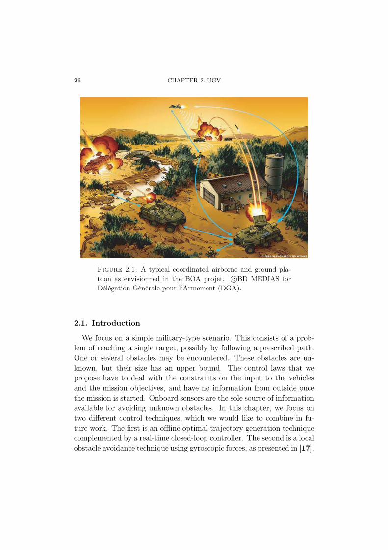
Figure 2.1. A typical coordinated airborne and ground pla-toon as envisionned in the BOA projet. c©BD MEDIAS forDélégation Générale pour l’Armement (DGA).
2.1. Introduction
We focus on a simple military-type scenario. This consists of a prob-lem of reaching a single target, possibly by following a prescribed path.One or several obstacles may be encountered. These obstacles are un-known, but their size has an upper bound. The control laws that wepropose have to deal with the constraints on the input to the vehiclesand the mission objectives, and have no information from outside oncethe mission is started. Onboard sensors are the sole source of informationavailable for avoiding unknown obstacles. In this chapter, we focus ontwo different control techniques, which we would like to combine in fu-ture work. The first is an offline optimal trajectory generation techniquecomplemented by a real-time closed-loop controller. The second is a localobstacle avoidance technique using gyroscopic forces, as presented in [17].
2.2. EXPERIMENTAL TESTBED 27
Combining the two approaches could be done in the following way. Be-fore an obstacle is encountered, the vehicles should track in a closed-loopmanner (using onboard sensors) the optimal trajectory computed duringthe mission preparation phase. When an obstacle is detected, the controlshould switch to the obstacle avoidance phase, where the vehicle slowsdown and passes by the obstacle. Once a point on the initial trajectoryis approximately reached again, the controller should switch back to thefirst control phase. Certainly, designing appropriate switching strategieswill not be an easy task and will require further investigation.
The chapter is organized as follows. In Section 2.1, we briefly describethe envisioned scenario. Section 2.2 presents the vehicle under consid-eration (a Pioneer IV from MobileRobotsTM) and the onboard systems(including the CPU and sensors). The dynamics of the vehicle, givenin Section 2.3, is the same as that of the unicycle. In Section 2.4, weconsider gyroscopic-force controllers. We give details of experimental re-sults obtained using second-order schemes (from the literature [17]). Aknown problem is the possibility of zero-velocity collisions (pointed outat early on in [17]). For that reason, we propose a first-order controllerand actually prove a new result concerning convergence under assump-tions on the size of the obstacle. This constructive proof could serve as aguideline for tuning. A generalization to second order systems could beconsidered by a dynamic extension. In Section 2.5, we use the flatnessproperty of this controller to parameterize and optimize its trajectories.Constrained minimum-time problems are considered. Then, as presentedin Section 2.6, we use dynamic linearizing feedback for tracking pur-poses. Experimental results are presented. The presented methodologywas also tested outdoors; Section 2.7 describes the observer implementedon board, and experimental results are detailed.
2.2. Experimental testbed
Our experimental testbed includes three MobileRobotsTM Pioneer IV-AT vehicles similar to the one depicted in Figure 2.2. These vehicleshave 4 electrically powered independent wheels and are capable of run-ning outdoor. The onboard system consists of a Pentium III 800 MHz
28 CHAPTER 2. UGV
based PC104 system running under Linux, 16 sonars (8 forward and 8rear) located on the sides of the main frame (above the wheels), a one-axis gyroscope, and a wireless network adapter. It is possible to derivepositioning information from odometers. Each vehicle is equipped within-wheels 100 tick encoders with inertial correction to compensate forskid steering. By default, the vehicle does not possess any GPS. Wedecided to install a uBloxTM TIM-LR with added antenna. As will bedetailed next, we designed our own filter for GPS/odometer/gyroscopehybridation.
2.3. Vehicle dynamic model
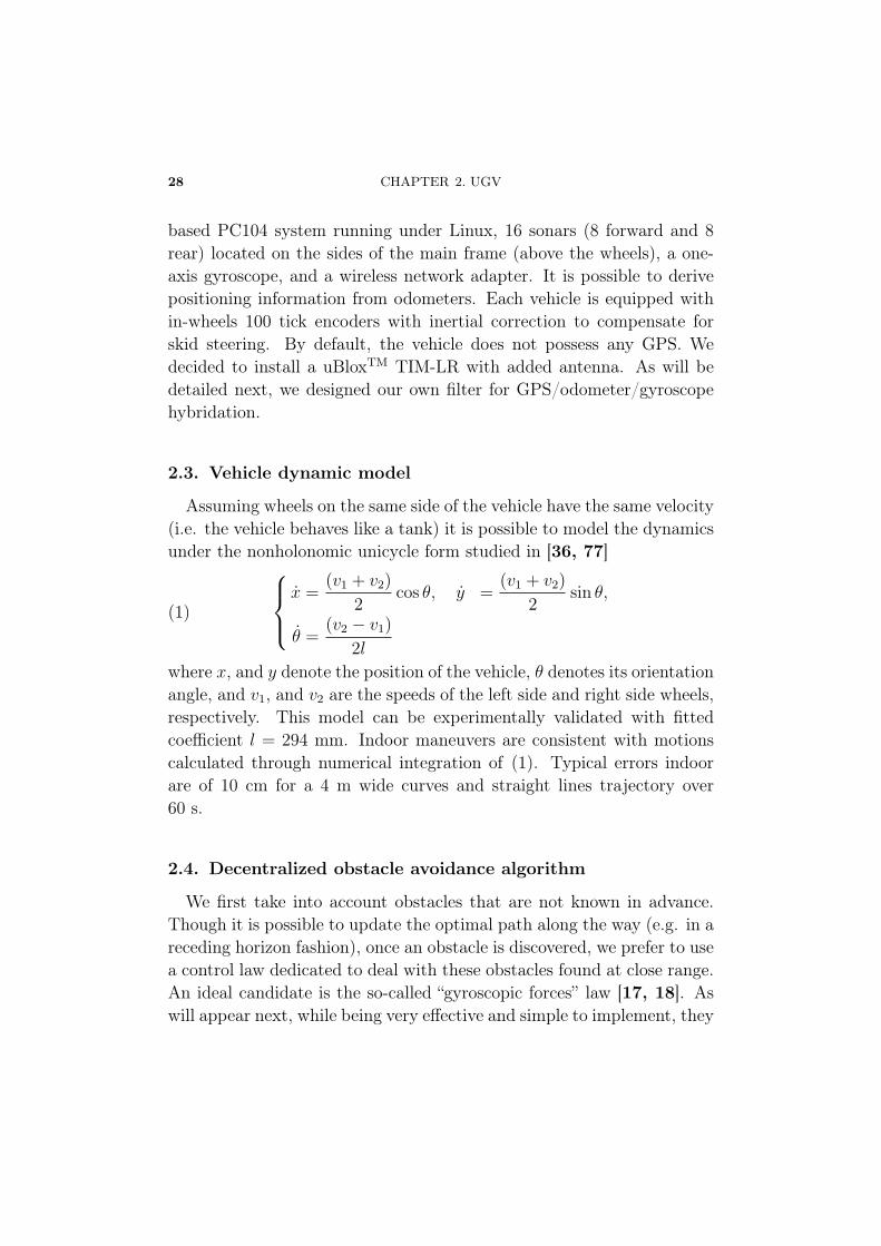
Assuming wheels on the same side of the vehicle have the same velocity(i.e. the vehicle behaves like a tank) it is possible to model the dynamicsunder the nonholonomic unicycle form studied in [36, 77]
(1)
⎧⎪⎨⎪⎩x =
(v1 + v2)
2cos θ, y =
(v1 + v2)
2sin θ,
θ =(v2 − v1)
2l
where x, and y denote the position of the vehicle, θ denotes its orientationangle, and v1, and v2 are the speeds of the left side and right side wheels,respectively. This model can be experimentally validated with fittedcoefficient l = 294 mm. Indoor maneuvers are consistent with motionscalculated through numerical integration of (1). Typical errors indoorare of 10 cm for a 4 m wide curves and straight lines trajectory over60 s.
2.4. Decentralized obstacle avoidance algorithm
We first take into account obstacles that are not known in advance.Though it is possible to update the optimal path along the way (e.g. in areceding horizon fashion), once an obstacle is discovered, we prefer to usea control law dedicated to deal with these obstacles found at close range.An ideal candidate is the so-called “gyroscopic forces” law [17, 18]. Aswill appear next, while being very effective and simple to implement, they
2.4. DECENTRALIZED OBSTACLE AVOIDANCE ALGORITHM 29
Sonar
Sonar
Independent wheels
Wifi antenna
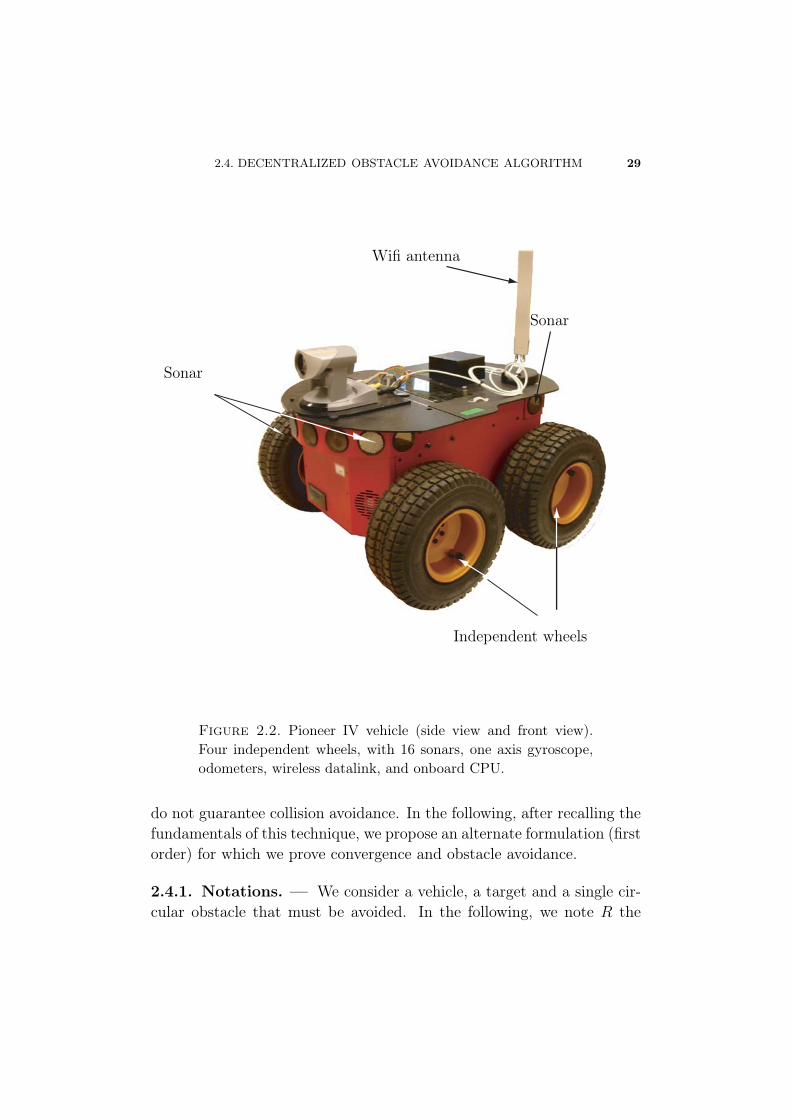
Figure 2.2. Pioneer IV vehicle (side view and front view).Four independent wheels, with 16 sonars, one axis gyroscope,odometers, wireless datalink, and onboard CPU.
do not guarantee collision avoidance. In the following, after recalling thefundamentals of this technique, we propose an alternate formulation (firstorder) for which we prove convergence and obstacle avoidance.
2.4.1. Notations. — We consider a vehicle, a target and a single cir-cular obstacle that must be avoided. In the following, we note R the
30 CHAPTER 2. UGV
obstacle radius, r the detection radius, A the center of the obstacle, Bthe most distant point from the origin in the disc C(A, r), q = (x, y)T
the position of the center of gravity of the vehicle, qT the target point.Further, dq denotes the vector difference between q and its orthogonalprojection onto the obstacle.
dq � (A− q)‖A− q‖ −R
‖A− q‖ ∈ R2
ε is a scalar valued function defined by
q �→ ε(q) =
⎧⎪⎪⎪⎪⎨⎪⎪⎪⎪⎩− sign det(qT − q, dq)
if ‖dq‖ ≤ (r −R)
and |arg(q − qT )| ≤ arcsin(R/OA)
0 otherwise
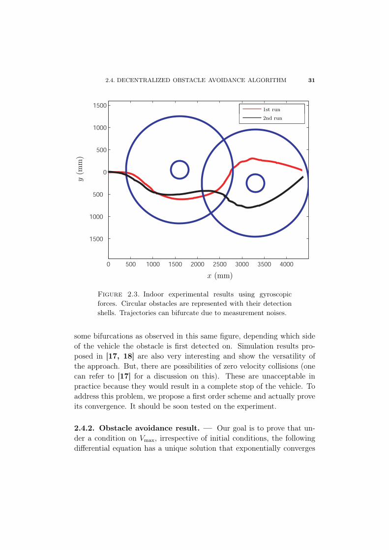
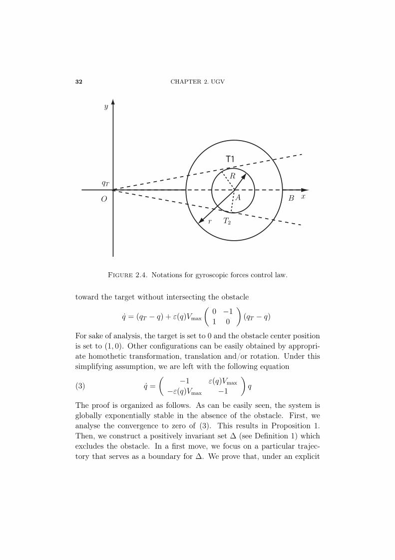
We use Vmax a (positive) avoidance constant. Two geometric points playa particular role in the convergence analysis. These are noted T1, andT2 (see Figure 2.4). They are located at the intersections of the circleC(A,R) and the two tangent lines originating in 0. Finally, we noteH = (OA) ∩ C(A,R).
2.4.1.1. Proposed gyroscopic scheme. — The second order scheme usu-ally reported in the literature is given in (2) (where ∧ stands for thelogical AND)
q =
(−2 −w(q, q)
w(q, q) −2
)q − (q − qT )
with w given in (2).
w(q, q) =
⎧⎪⎪⎪⎪⎪⎨⎪⎪⎪⎪⎪⎩
πVmax
d(q)if {d(q) ≤ r} ∧ {d(q).q > 0} ∧ {det(d(q), q) ≥ 0}
− πVmax
d(q)if {d(q) ≤ r} ∧ {d(q).q > 0} ∧ {det(d(q), q) < 0}
0 otherwise
(2)
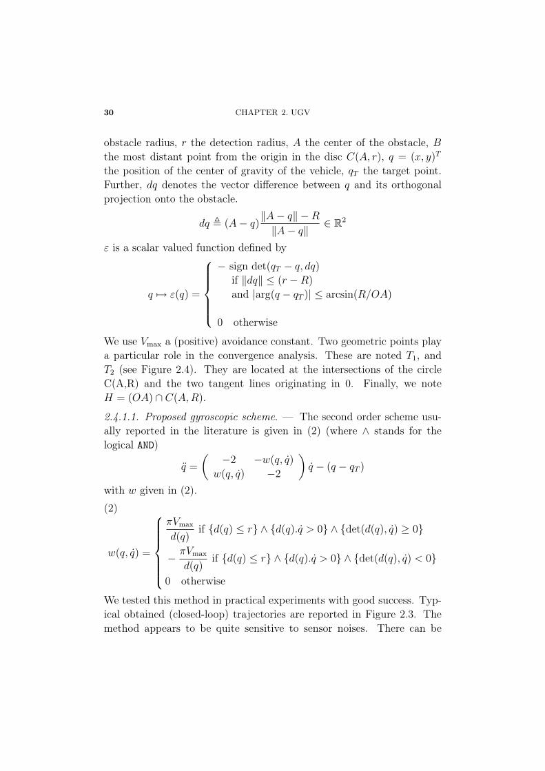
We tested this method in practical experiments with good success. Typ-ical obtained (closed-loop) trajectories are reported in Figure 2.3. Themethod appears to be quite sensitive to sensor noises. There can be
2.4. DECENTRALIZED OBSTACLE AVOIDANCE ALGORITHM 31
0 500 1000 1500 2000 2500 3000 3500 4000
1500
1000
500
0
500
1000
15001st run
2nd run
x (mm)
y(m
m)
Figure 2.3. Indoor experimental results using gyroscopicforces. Circular obstacles are represented with their detectionshells. Trajectories can bifurcate due to measurement noises.
some bifurcations as observed in this same figure, depending which sideof the vehicle the obstacle is first detected on. Simulation results pro-posed in [17, 18] are also very interesting and show the versatility ofthe approach. But, there are possibilities of zero velocity collisions (onecan refer to [17] for a discussion on this). These are unacceptable inpractice because they would result in a complete stop of the vehicle. Toaddress this problem, we propose a first order scheme and actually proveits convergence. It should be soon tested on the experiment.
2.4.2. Obstacle avoidance result. — Our goal is to prove that un-der a condition on Vmax, irrespective of initial conditions, the followingdifferential equation has a unique solution that exponentially converges
32 CHAPTER 2. UGV
T1
qT
T2
A B
R
r
x
y
O
Figure 2.4. Notations for gyroscopic forces control law.
toward the target without intersecting the obstacle
q = (qT − q) + ε(q)Vmax
(0 −1
1 0
)(qT − q)
For sake of analysis, the target is set to 0 and the obstacle center positionis set to (1, 0). Other configurations can be easily obtained by appropri-ate homothetic transformation, translation and/or rotation. Under thissimplifying assumption, we are left with the following equation
q =
(−1 ε(q)Vmax
−ε(q)Vmax −1
)q(3)
The proof is organized as follows. As can be easily seen, the system isglobally exponentially stable in the absence of the obstacle. First, weanalyse the convergence to zero of (3). This results in Proposition 1.Then, we construct a positively invariant set Δ (see Definition 1) whichexcludes the obstacle. In a first move, we focus on a particular trajec-tory that serves as a boundary for Δ. We prove that, under an explicit
2.4. DECENTRALIZED OBSTACLE AVOIDANCE ALGORITHM 33
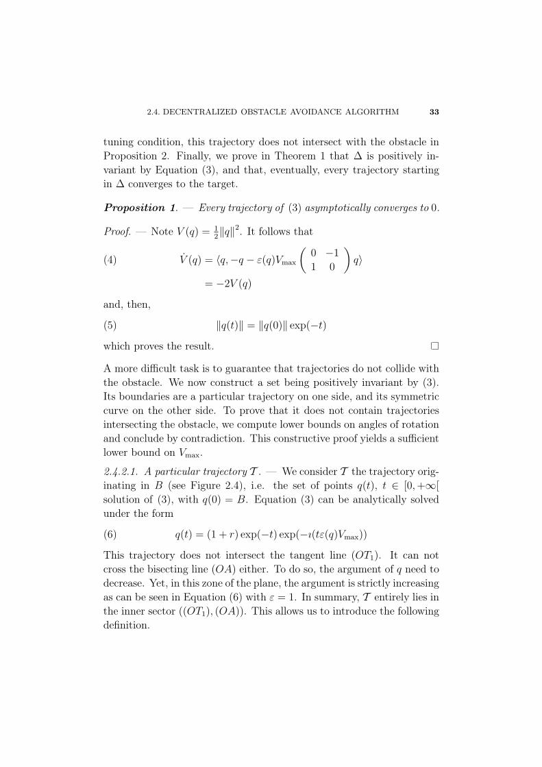
tuning condition, this trajectory does not intersect with the obstacle inProposition 2. Finally, we prove in Theorem 1 that Δ is positively in-variant by Equation (3), and that, eventually, every trajectory startingin Δ converges to the target.
Proposition 1. — Every trajectory of (3) asymptotically converges to 0.
Proof. — Note V (q) = 12‖q‖2. It follows that
V (q) = 〈q,−q − ε(q)Vmax
(0 −1
1 0
)q〉(4)
= −2V (q)
and, then,
‖q(t)‖ = ‖q(0)‖ exp(−t)(5)
which proves the result.
A more difficult task is to guarantee that trajectories do not collide withthe obstacle. We now construct a set being positively invariant by (3).Its boundaries are a particular trajectory on one side, and its symmetriccurve on the other side. To prove that it does not contain trajectoriesintersecting the obstacle, we compute lower bounds on angles of rotationand conclude by contradiction. This constructive proof yields a sufficientlower bound on Vmax.
2.4.2.1. A particular trajectory T . — We consider T the trajectory orig-inating in B (see Figure 2.4), i.e. the set of points q(t), t ∈ [0,+∞[
solution of (3), with q(0) = B. Equation (3) can be analytically solvedunder the form
q(t) = (1 + r) exp(−t) exp(−ı(tε(q)Vmax))(6)
This trajectory does not intersect the tangent line (OT1). It can notcross the bisecting line (OA) either. To do so, the argument of q need todecrease. Yet, in this zone of the plane, the argument is strictly increasingas can be seen in Equation (6) with ε = 1. In summary, T entirely lies inthe inner sector ((OT1), (OA)). This allows us to introduce the followingdefinition.
34 CHAPTER 2. UGV
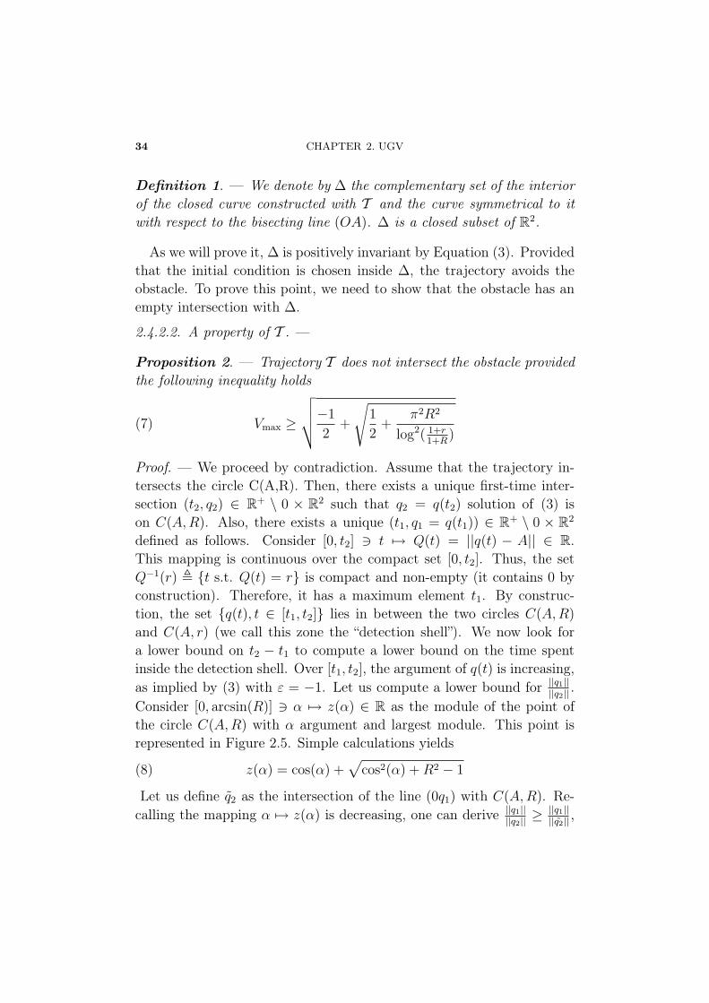
Definition 1. — We denote by Δ the complementary set of the interiorof the closed curve constructed with T and the curve symmetrical to itwith respect to the bisecting line (OA). Δ is a closed subset of R
2.
As we will prove it, Δ is positively invariant by Equation (3). Providedthat the initial condition is chosen inside Δ, the trajectory avoids theobstacle. To prove this point, we need to show that the obstacle has anempty intersection with Δ.
2.4.2.2. A property of T . —
Proposition 2. — Trajectory T does not intersect the obstacle providedthe following inequality holds
Vmax ≥
√√√√−1
2+
√1
2+
π2R2
log2( 1+r1+R
)(7)
Proof. — We proceed by contradiction. Assume that the trajectory in-tersects the circle C(A,R). Then, there exists a unique first-time inter-section (t2, q2) ∈ R
+ \ 0 × R2 such that q2 = q(t2) solution of (3) is
on C(A,R). Also, there exists a unique (t1, q1 = q(t1)) ∈ R+ \ 0 × R
2
defined as follows. Consider [0, t2] � t �→ Q(t) = ||q(t) − A|| ∈ R.This mapping is continuous over the compact set [0, t2]. Thus, the setQ−1(r) � {t s.t. Q(t) = r} is compact and non-empty (it contains 0 byconstruction). Therefore, it has a maximum element t1. By construc-tion, the set {q(t), t ∈ [t1, t2]} lies in between the two circles C(A,R)
and C(A, r) (we call this zone the “detection shell”). We now look fora lower bound on t2 − t1 to compute a lower bound on the time spentinside the detection shell. Over [t1, t2], the argument of q(t) is increasing,as implied by (3) with ε = −1. Let us compute a lower bound for ||q1||
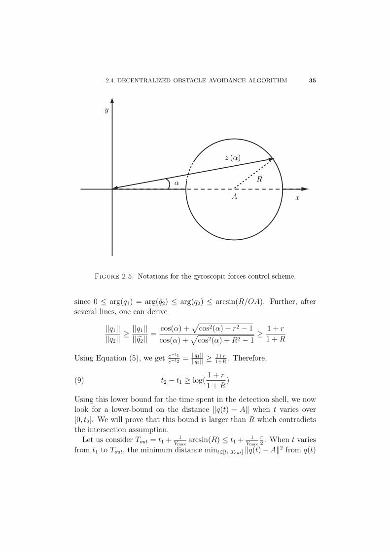
||q2|| .Consider [0, arcsin(R)] � α �→ z(α) ∈ R as the module of the point ofthe circle C(A,R) with α argument and largest module. This point isrepresented in Figure 2.5. Simple calculations yields
z(α) = cos(α) +√
cos2(α) +R2 − 1(8)
Let us define q2 as the intersection of the line (0q1) with C(A,R). Re-calling the mapping α �→ z(α) is decreasing, one can derive ||q1||
||q2|| ≥||q1||||q2|| ,
2.4. DECENTRALIZED OBSTACLE AVOIDANCE ALGORITHM 35
α
z (α)
A
R
x
y
Figure 2.5. Notations for the gyroscopic forces control scheme.
since 0 ≤ arg(q1) = arg(q2) ≤ arg(q2) ≤ arcsin(R/OA). Further, afterseveral lines, one can derive
||q1||||q2||
≥ ||q1||||q2||
=cos(α) +
√cos2(α) + r2 − 1
cos(α) +√
cos2(α) +R2 − 1≥ 1 + r
1 +R
Using Equation (5), we get e−t1
e−t2= ||q1||
||q2|| ≥1+r1+R
. Therefore,
t2 − t1 ≥ log(1 + r
1 +R)(9)
Using this lower bound for the time spent in the detection shell, we nowlook for a lower-bound on the distance ‖q(t) − A‖ when t varies over[0, t2]. We will prove that this bound is larger than R which contradictsthe intersection assumption.
Let us consider Tout = t1 + 1Vmax
arcsin(R) ≤ t1 + 1Vmax
π2. When t varies
from t1 to Tout, the minimum distance mint∈[t1,Tout] ‖q(t)−A‖2 from q(t)
36 CHAPTER 2. UGV
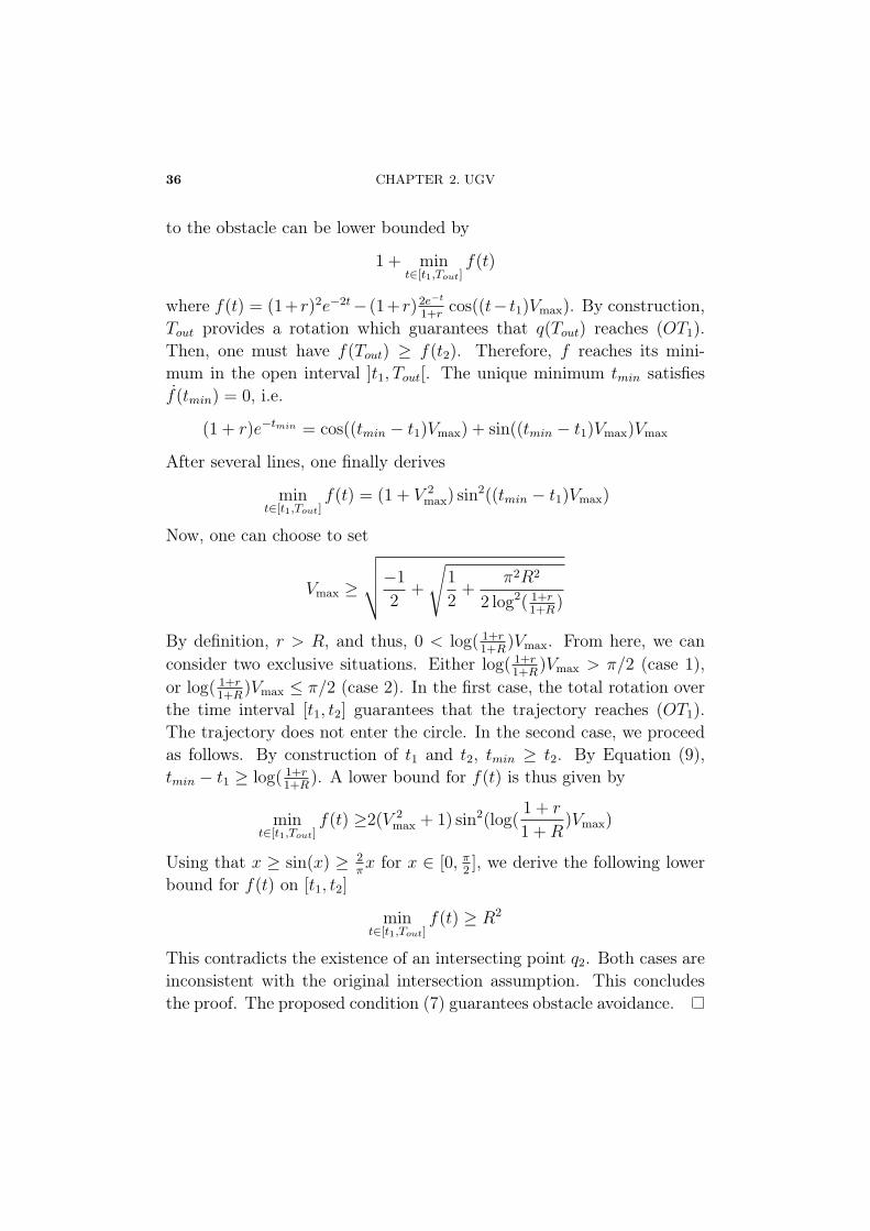
to the obstacle can be lower bounded by
1 + mint∈[t1,Tout]
f(t)
where f(t) = (1+r)2e−2t− (1+r)2e−t
1+rcos((t− t1)Vmax). By construction,
Tout provides a rotation which guarantees that q(Tout) reaches (OT1).Then, one must have f(Tout) ≥ f(t2). Therefore, f reaches its mini-mum in the open interval ]t1, Tout[. The unique minimum tmin satisfiesf(tmin) = 0, i.e.
(1 + r)e−tmin = cos((tmin − t1)Vmax) + sin((tmin − t1)Vmax)Vmax
After several lines, one finally derives
mint∈[t1,Tout]
f(t) = (1 + V 2max) sin2((tmin − t1)Vmax)
Now, one can choose to set
Vmax ≥
√√√√−1
2+
√1
2+
π2R2
2 log2( 1+r1+R
)
By definition, r > R, and thus, 0 < log( 1+r1+R
)Vmax. From here, we canconsider two exclusive situations. Either log( 1+r
1+R)Vmax > π/2 (case 1),
or log( 1+r1+R
)Vmax ≤ π/2 (case 2). In the first case, the total rotation overthe time interval [t1, t2] guarantees that the trajectory reaches (OT1).The trajectory does not enter the circle. In the second case, we proceedas follows. By construction of t1 and t2, tmin ≥ t2. By Equation (9),tmin − t1 ≥ log( 1+r
1+R). A lower bound for f(t) is thus given by
mint∈[t1,Tout]
f(t) ≥2(V 2max + 1) sin2(log(
1 + r
1 +R)Vmax)
Using that x ≥ sin(x) ≥ 2πx for x ∈ [0, π
2], we derive the following lower
bound for f(t) on [t1, t2]
mint∈[t1,Tout]
f(t) ≥ R2
This contradicts the existence of an intersecting point q2. Both cases areinconsistent with the original intersection assumption. This concludesthe proof. The proposed condition (7) guarantees obstacle avoidance.
2.4. DECENTRALIZED OBSTACLE AVOIDANCE ALGORITHM 37
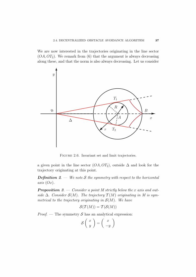
We are now interested in the trajectories originating in the line sector(OA,OT2). We remark from (6) that the argument is always decreasingalong these, and that the norm is also always decreasing. Let us consider
qt
A
B
r
R
T1
T2
Δx
y
Figure 2.6. Invariant set and limit trajectories.
a given point in the line sector (OA,OT2), outside Δ and look for thetrajectory originating at this point.
Definition 2. — We note S the symmetry with respect to the horizontalaxis (Ox).
Proposition 3. — Consider a point M strictly below the x axis and out-side Δ. Consider S(M). The trajectory T (M) originating in M is sym-metrical to the trajectory originating in S(M). We have
S(T (M)) = T (S(M))
Proof. — The symmetry S has an analytical expression:
S(x
y
)=
(x
−y
)
38 CHAPTER 2. UGV
The differential Equation (3) shows a difference in ε when one crosses thex axis. For all t ≥ 0, we note Tt(M) the point of the trajectory initiatedin M after time t. For all t ≥ 0, we have
S(Tt(S(M)))
=S(∫ t
0
(−1 εM(t)Vmax
−εM(t)Vmax −1
)(xM−yM
))=Tt(M)
Let us now consider a trajectory starting from a point below the x axis.Using the result above and (2), we can deduce that the trajectory doesnot intersect the boundary of Δ. The obstacle is thus avoided.
Theorem 1. — Consider Equation (3). Provided that Vmax satisfies (7),and that the initial condition is chosen inside Δ, the trajectory avoids theobstacle and exponentially reaches the target 0.
Remark 1. — The 3-D case is covered by this obstacle avoidance method.In the 2-D plane defined by the target point on the 3-D trajectory andthe velocity at the first time the vehicle detects an obstacle, the obstacleavoidance problem has as solution the one presented above.
2.5. Trajectory generation
2.5.1. Open-loop design. — The two inputs system is flat [30], i.e.its trajectories can be summarized by those of two flat outputs x and y.
(10)
⎧⎪⎨⎪⎩x =
(v1 + v2)
2cos θ, y =
(v1 + v2)
2sin θ,
θ =(v2 − v1)
2l
Considering x and y, one can recover the other variables, i.e. the re-maining state θ and the two controls, from x, y and their derivatives.
2.5. TRAJECTORY GENERATION 39
Explicitly,
θ = arctan(y
x)(11)
v1 =√x2 + y2 − l
yx− yx√x2 + y2
(12)
v2 =√x2 + y2 + l
yx− yx√x2 + y2
(13)
Thanks to this property, constrained trajectory optimization can be per-formed using the approach proposed in [73, 59, 68]. The flat outputshistories are then parameterized using B-splines functions, and, in con-sidered cost functionals and constraints variables, are substituted withtheir expressions (11), (12), and (13). Here, we consider two differentconstrained minimum time problems.
2.5.1.1. Optimal trajectory along a prescribed path. — The first problemwe consider corresponds to the case of a well described path (e.g. a road)the vehicle has to follow as fast as possible, under its dynamic constraints.Given a path s ∈ [0, 1] �→ (xref(s), yref(s)) ∈ R
2, it is desired to determineT and [0, T ] � t �→ σ(t) ∈ [0, 1] solution of the following optimal controlproblem
minσ,T
T
subject to the following constraints (where ε is a strictly positive con-stant) ⎧⎪⎪⎪⎪⎨⎪⎪⎪⎪⎩
T > 0, σ ∈ C2[0, T ], σ(0) = 0, σ(T ) = 1,
∀t ∈ [0, T ], σ(t) > 0,
|vi(t)| ≤ vmax i ∈ {1, 2},|vi(t)| ≤ Amax i ∈ {1, 2}
(14)
The last inequality can be omitted because (v1, v2) does not need to bedifferentiable (it is convenient to include this last constraint to obtainsmooth control histories). If obstacles locations are known, they can beincluded as state constraints.
2.5.1.2. Free trajectory planning. — In a second setup, we optimize overthe possible trajectories originating in a given point A, reaching a desired
40 CHAPTER 2. UGV
target point B, and avoiding known obstacles. It is desired to find thesolution of the following optimal control problem
minx,y,T
T
subject to the constraints (where ε is a strictly positive constant)⎧⎪⎪⎪⎪⎪⎪⎪⎪⎪⎪⎨⎪⎪⎪⎪⎪⎪⎪⎪⎪⎪⎩
T > 0, (x, y) ∈(C2[0, T ]
)2,
(x(0), y(0))T = A, (x(T ), y(T ))T = B,
∀t ∈ [0, T ], (x(σ(t)), y(σ(t))) /∈ obstacles,|vi(t)| ≤ vmax i ∈ {1, 2},|vi(t)| ≤ Amax i ∈ {1, 2},x2 + y2 ≥ ε
The last constraint is added to avoid the singularity of our dynamicfeedback controller around zero velocity.
2.5.1.3. Numerical treatment. — Those two problems can be rewrittenusing only the parameter T and the flat outputs x and y or σ (in thefirst problem) by substituting v1 and v2 in the constraints by their ex-pressions in terms of first and second derivatives of the flat outputs (12)and (13). In the case of constraints given by (14), v1 and v2 are computedthrough the time derivatives of t �→ xref (σ(t)) and t �→ yref (σ(t)). Then,the variables are represented by basis functions (typically B-splines). Theinduced nonlinear program (NLP) can be solved using standard packages(e.g. NPSOL or SNOPT). Compared to a standard collocation approach,in which every state and control variables is represented by distinct basisfunctions, the proposed substitution technique yields a reduction in thenumber of variables. This positively impacts the computational burdenof solving a NLP (as noted in [60, 10]). Typically, using B-Splines andthe Matlab Optimization toolbox, either problem can be solved with areasonable accuracy in less than 5 sec on a 1 GHz PC (this time increasesfor complex trajectories where the number of B-splines coefficients canget large). Interestingly, this remark stresses the possibility of real-timetrajectory updates as proposed in [68] (for receding horizon control tech-niques or on-demand mission reconfiguration). Finally, once the optimal
2.6. DYNAMIC FEEDBACK CONTROL LAW AND INDOOR RESULTS 41
transient time T and flat outputs histories (x, y) are found, the open-loopcontrol values are recovered from (12) and (13).
2.6. Dynamic feedback control law and indoor results
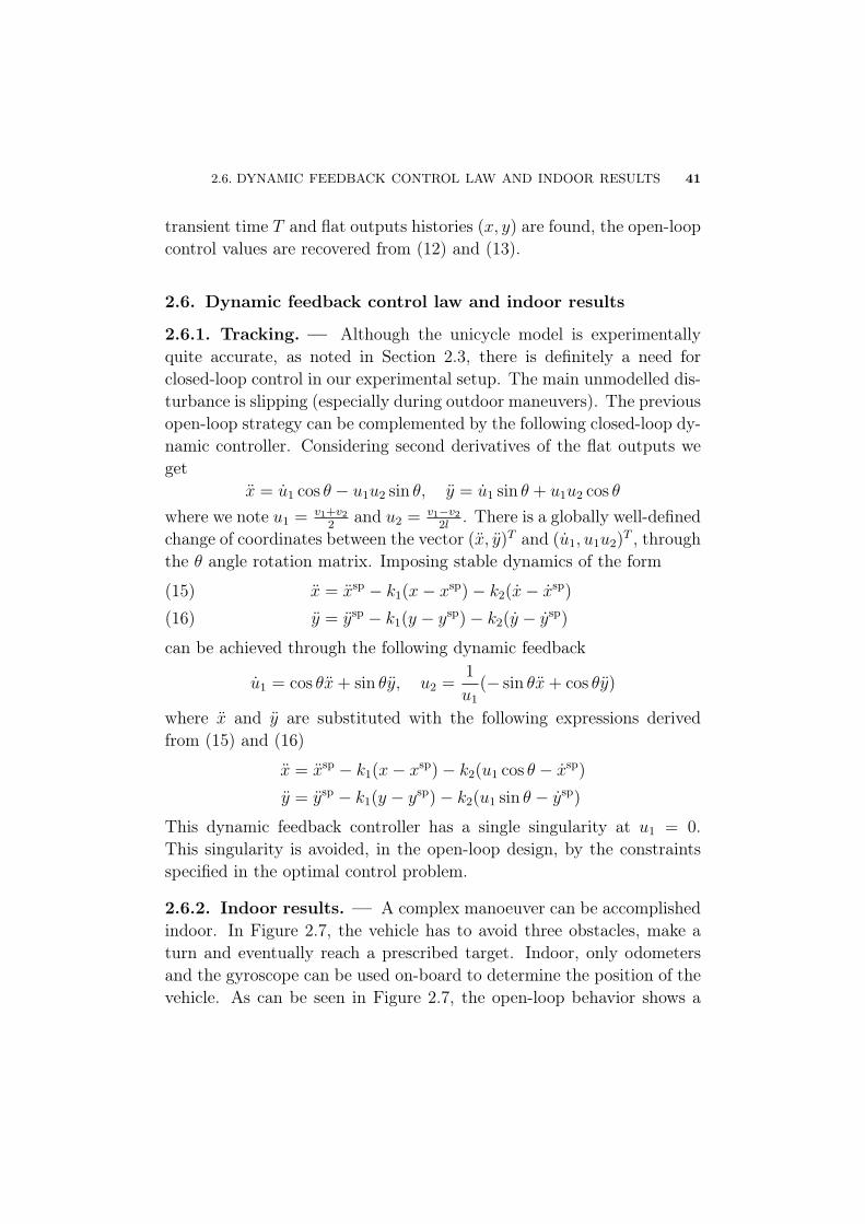
2.6.1. Tracking. — Although the unicycle model is experimentallyquite accurate, as noted in Section 2.3, there is definitely a need forclosed-loop control in our experimental setup. The main unmodelled dis-turbance is slipping (especially during outdoor maneuvers). The previousopen-loop strategy can be complemented by the following closed-loop dy-namic controller. Considering second derivatives of the flat outputs weget
x = u1 cos θ − u1u2 sin θ, y = u1 sin θ + u1u2 cos θ
where we note u1 = v1+v22
and u2 = v1−v22l
. There is a globally well-definedchange of coordinates between the vector (x, y)T and (u1, u1u2)
T , throughthe θ angle rotation matrix. Imposing stable dynamics of the form
x = xsp − k1(x− xsp) − k2(x− xsp)(15)y = ysp − k1(y − ysp) − k2(y − ysp)(16)
can be achieved through the following dynamic feedback
u1 = cos θx+ sin θy, u2 =1
u1
(− sin θx+ cos θy)
where x and y are substituted with the following expressions derivedfrom (15) and (16)
x = xsp − k1(x− xsp) − k2(u1 cos θ − xsp)
y = ysp − k1(y − ysp) − k2(u1 sin θ − ysp)
This dynamic feedback controller has a single singularity at u1 = 0.This singularity is avoided, in the open-loop design, by the constraintsspecified in the optimal control problem.
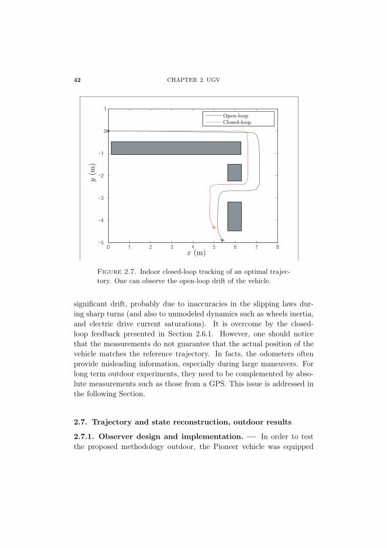
2.6.2. Indoor results. — A complex manoeuver can be accomplishedindoor. In Figure 2.7, the vehicle has to avoid three obstacles, make aturn and eventually reach a prescribed target. Indoor, only odometersand the gyroscope can be used on-board to determine the position of thevehicle. As can be seen in Figure 2.7, the open-loop behavior shows a
42 CHAPTER 2. UGV
0 1 2 3 4 5 6 7 85
4
3
2
1
0
1
-
-
-
-
-
x (m)
y(m
)
Open-loopClosed-loop
Figure 2.7. Indoor closed-loop tracking of an optimal trajec-tory. One can observe the open-loop drift of the vehicle.
significant drift, probably due to inaccuracies in the slipping laws dur-ing sharp turns (and also to unmodeled dynamics such as wheels inertia,and electric drive current saturations). It is overcome by the closed-loop feedback presented in Section 2.6.1. However, one should noticethat the measurements do not guarantee that the actual position of thevehicle matches the reference trajectory. In facts, the odometers oftenprovide misleading information, especially during large maneuvers. Forlong term outdoor experiments, they need to be complemented by abso-lute measurements such as those from a GPS. This issue is addressed inthe following Section.
2.7. Trajectory and state reconstruction, outdoor results
2.7.1. Observer design and implementation. — In order to testthe proposed methodology outdoor, the Pioneer vehicle was equipped
2.7. TRAJECTORY AND STATE RECONSTRUCTION, OUTDOOR RESULTS 43
Map
Vehicle
Waypoints selection
Remote PC
Minimum timeTrajectory generation
Wifi
GPS Odometers
HybridPosition
Gyroscope
Controller Electric drives
(xsp, ysp)
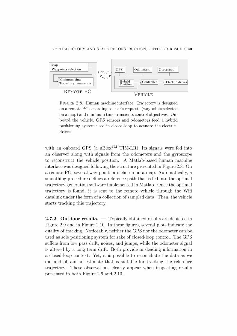
Figure 2.8. Human machine interface. Trajectory is designedon a remote PC according to user’s requests (waypoints selectedon a map) and minimum time transients control objectives. On-board the vehicle, GPS sensors and odometers feed a hybridpositioning system used in closed-loop to actuate the electricdrives.
with an onboard GPS (a uBloxTM TIM-LR). Its signals were fed intoan observer along with signals from the odometers and the gyroscopeto reconstruct the vehicle position. A Matlab-based human machineinterface was designed following the structure presented in Figure 2.8. Ona remote PC, several way-points are chosen on a map. Automatically, asmoothing procedure defines a reference path that is fed into the optimaltrajectory generation software implemented in Matlab. Once the optimaltrajectory is found, it is sent to the remote vehicle through the Wifidatalink under the form of a collection of sampled data. Then, the vehiclestarts tracking this trajectory.
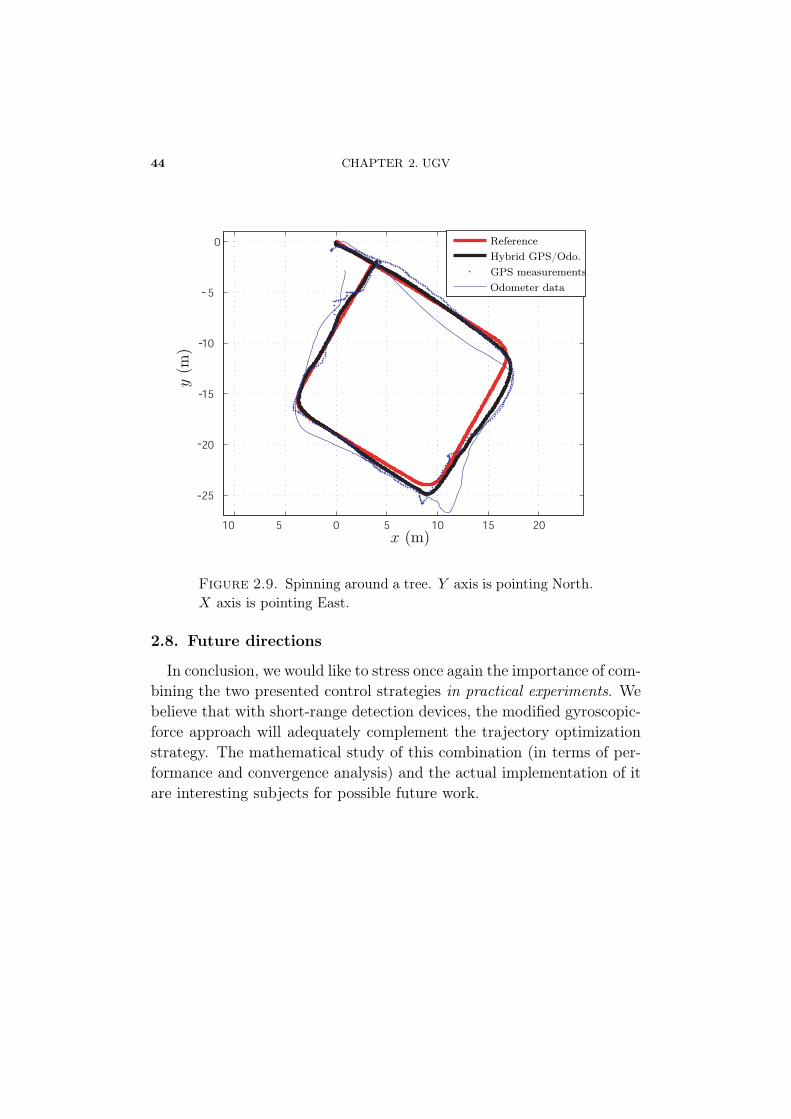
2.7.2. Outdoor results. — Typically obtained results are depicted inFigure 2.9 and in Figure 2.10. In these figures, several plots indicate thequality of tracking. Noticeably, neither the GPS nor the odometer can beused as sole positioning system for sake of closed-loop control. The GPSsuffers from low pass drift, noises, and jumps, while the odometer signalis altered by a long term drift. Both provide misleading information ina closed-loop context. Yet, it is possible to reconciliate the data as wedid and obtain an estimate that is suitable for tracking the referencetrajectory. These observations clearly appear when inspecting resultspresented in both Figure 2.9 and 2.10.
44 CHAPTER 2. UGV
10 5 0 5 10 15 20
25
20
15
10
5
0
-
-
-
-
-
x (m)
y(m
)
ReferenceHybrid GPS/Odo.GPS measurementsOdometer data
Figure 2.9. Spinning around a tree. Y axis is pointing North.X axis is pointing East.
2.8. Future directions
In conclusion, we would like to stress once again the importance of com-bining the two presented control strategies in practical experiments. Webelieve that with short-range detection devices, the modified gyroscopic-force approach will adequately complement the trajectory optimizationstrategy. The mathematical study of this combination (in terms of per-formance and convergence analysis) and the actual implementation of itare interesting subjects for possible future work.
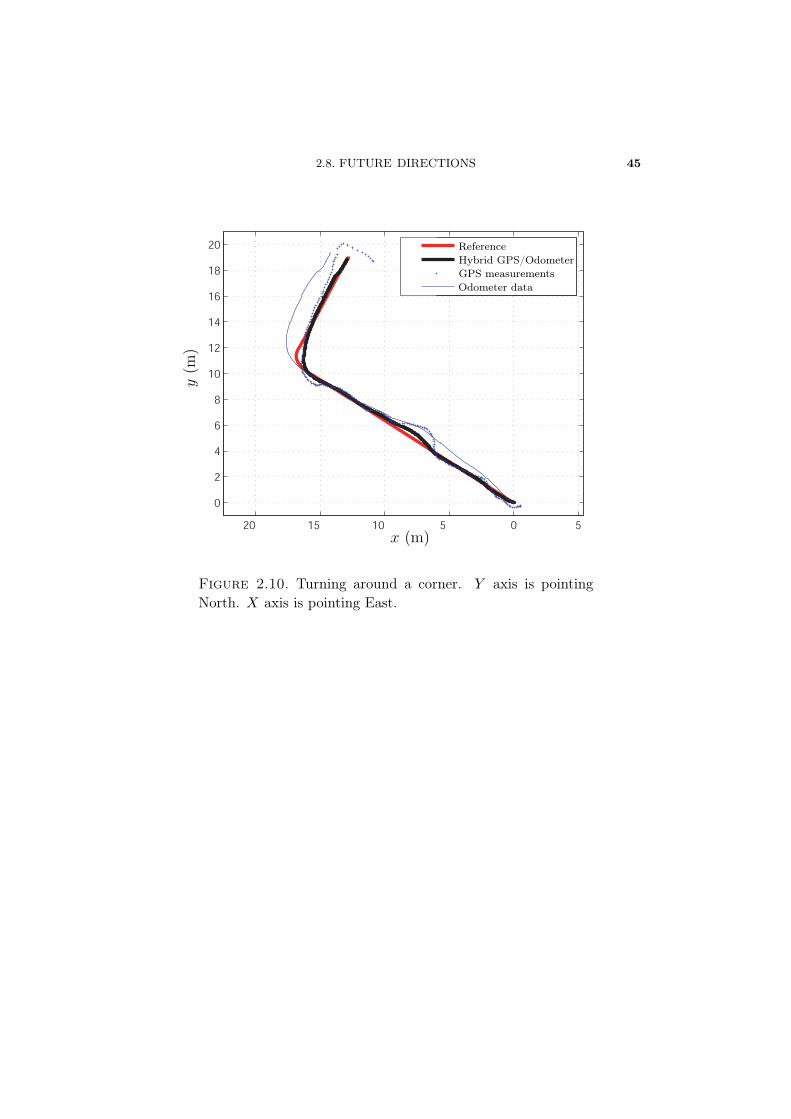
2.8. FUTURE DIRECTIONS 45
20 15 10 5 0 5
0
2
4
6
8
10
12
14
16
18
20
x (m)
y(m
)
ReferenceHybrid GPS/OdometerGPS measurementsOdometer data
Figure 2.10. Turning around a corner. Y axis is pointingNorth. X axis is pointing East.

PART II
NAVIGATION ANDCONTROL SOLUTIONS FORAN EXPERIMENTAL VTOL
UAV

CHAPTER 3
AN EMBEDDED REAL-TIMENAVIGATION SYSTEM
Dans ce chapitre, nous détaillons l’architecture du système embarquétemps-réel que nous avons conçu et mis au point pour assurer la naviga-tion et le pilotage embarqué d’engins autonomes, en particulier des héli-coptères comme celui traité au chapitre suivant. Les performances de cesystème et sa modularité sont des points essentiels en vue de l’applicationexpérimentale sur l’hélicoptère sujet du Chapitre 4.
3.1. Introduction
In this chapter, we present a versatile, real-time embedded system,which can easily be used as a real-time guidance and navigation systemon various platforms. As will be apparent in Chapter 5, our work inthe field of unmanned air vehicles (UAVs) has focused on small-scale(typically less than 2 m wide) vertical take-off and landing (VTOL) aerialvehicles (as described in [16]).
Compared with fixed-wing aircraft and with ground vehicles with tank-like dynamics (as described in [66] and in Chapter 2), these aerial vehiclesrepresent more challenging applications in terms of navigation and guid-ance. The main reason for this is that these vehicles cannot easily gointo any safe mode, unlike ground vehicles, which are, in comparison,
50 CHAPTER 3. NAVIGATION SYSTEM
slower and simpler. While it has been proven that, with lowered per-formance expectations, it is possible to stabilize a fixed-wing UAV bydirectly closing the loop with signals from well-chosen sensors (e.g., theauthors of [50] proposed a solution to the problem of automatically con-trolling a fixed-wing UAV using only a single-antenna GPS receiver), it isconsidered by the vast majority of the UAV community that navigationsystems require data fusion [23]. In fact, each sensor technology has itsown flaws (among which are drift, noise, and possibly low resolution or alow update frequency). However, increases in accuracy by large factorscan be gained by reconciling the data from various sensor technologies.
Example of onboard data fusion applications are ubiquitous amongautonomous-vehicle-control experiments. Reconciling GPS and inertial-measurement-unit (IMU) measurements provides a classic case study.In [91], results of data fusion from a BeeLine GPS receiver from NovatelTM
and a miniaturized IMU were presented. In [25], the development of high-speed data fusion systems in response to the DARPA Grand Challengewas described. In that publication, several technological breakthroughsachieved using a high-end, powerful computer architecture are presented.The software components communicate in a machine-independent fash-ion through a module management system.
Our experiments could not use such a high-end setup, because thetypical payload of our aerial vehicle did not exceed 5 kg. Much smaller,lower-weight systems can be considered, though. In [43], an embeddedsystem was proposed which did not incorporate any powerful calculationboard. Instead, a simple Rabbit Semiconductor RCM-3400TM microcon-troller was used to perform complementary-filtering data fusion usinglimited computational power. In the same spirit, in [42], a low-cost testbed for UAVs was presented. It has been reported that the main ad-vantage of designing such an autopilot from scratch is that, in contrastto commercially available products [24, 58], such a system provides fullaccess to the internal control structures. We totally agree with this pointof view.
In this chapter, we present a solution that lies midway between thetwo categories mentioned above. Our system uses two processors. Oneprocessor is used to gather data from the sensors and to control the
3.2. REQUIREMENTS 51
actuators, and the other processor is used to perform the data fusioncalculations (and possibly the control algorithms). The advantages ofthis structure are as follows: (i) task scheduling is easily programmed,because only one of the two processors is in charge of handling the numer-ous devices and the I/O; (ii) the computations are performed as one singlethread on a dedicated board (of PC type); (iii) depending on the com-putational requirements, the computation board can be easily upgradedwithout requiring any software changes or raising any concern about taskscheduling; and (iv) finally, the overall system is quite low-cost, since itrelies on off-the-shelf components and can be easily maintained.
The chapter is organized as follows. In Section 3.2, we present thearchitecture of our system. The sensor protocols and the main specifica-tions are briefly described in Section 3.3. We detail our computationalhardware and our acquisition boards and comment on the choices madehere in Sections 3.4 and 3.5. In Section 3.6, we present the specifica-tions of successive versions of our embedded system. Numerous detailsof implementation are provided throughout the chapter.
3.2. Requirements
Our primary goal was to develop an embedded system to test al-gorithms of various complexity on-board various small-scale platforms.Early in the design process, one first constraint which appeared to uswas the payload limitations of the considered flying machines. This leadus to focus on designing a low-weight embedded system.
A second issue that was also raised early in the design stage was thatthe real-time requirements of a control system for such small UAVs arevery strong. This is mostly due to the short time horizons instabilities.Yet, in the context of embedded systems, real-time scheduling of a num-ber of sensing and computation tasks is known to be a difficult problem.More precisely, as exposed in [14], the problem of determining the fea-sibility of a periodic sequence of prioritized tasks is often (NP)-hard.Sufficient, but not necessary tests are pessimistic. Popular strategiessuch as the Rate-Monotonic policy (see again [14]), which consists ofputting the highest priority on the shortest task can be proven to be
52 CHAPTER 3. NAVIGATION SYSTEM
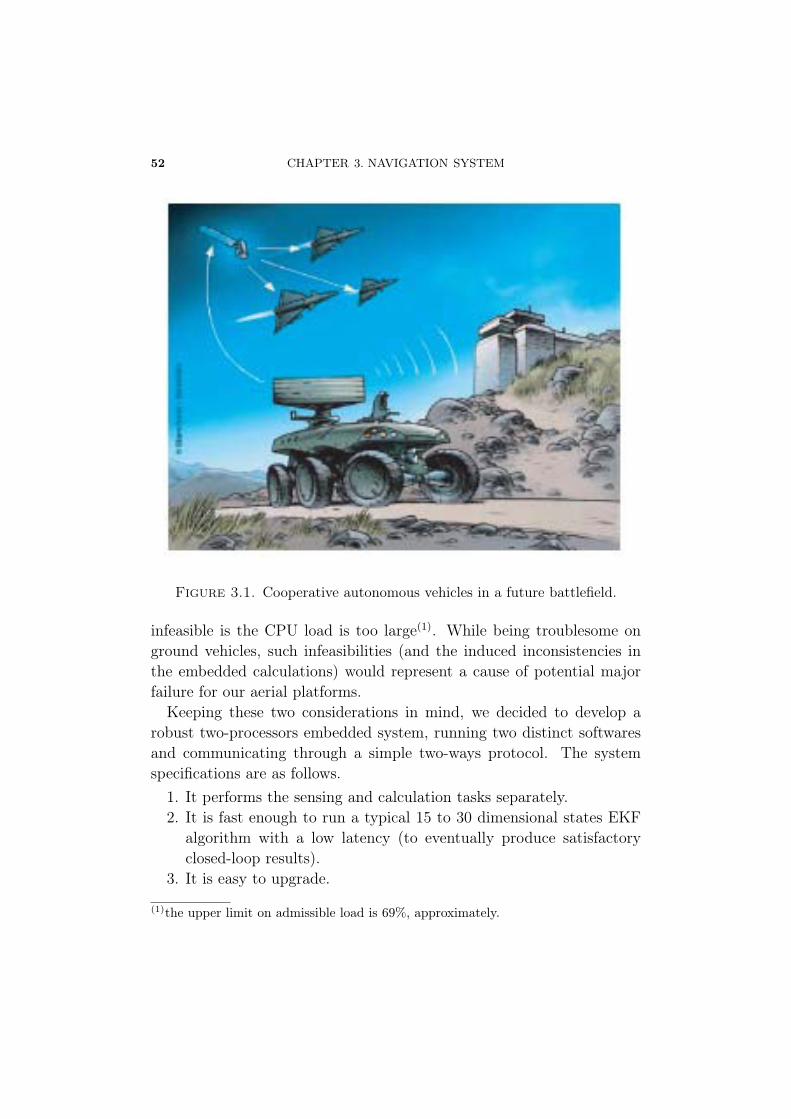
Figure 3.1. Cooperative autonomous vehicles in a future battlefield.
infeasible is the CPU load is too large(1). While being troublesome onground vehicles, such infeasibilities (and the induced inconsistencies inthe embedded calculations) would represent a cause of potential majorfailure for our aerial platforms.
Keeping these two considerations in mind, we decided to develop arobust two-processors embedded system, running two distinct softwaresand communicating through a simple two-ways protocol. The systemspecifications are as follows.
1. It performs the sensing and calculation tasks separately.2. It is fast enough to run a typical 15 to 30 dimensional states EKF
algorithm with a low latency (to eventually produce satisfactoryclosed-loop results).
3. It is easy to upgrade.
(1)the upper limit on admissible load is 69%, approximately.
3.3. SENSORS PERFORMANCES AND PROTOCOLS 53
4. It is versatile enough to handle various type of sensors and commu-nication protocols.
As exposed in Figure 3.2 and Figure 3.3, this (modular) embeddedsystem is composed of a micro-controller, which is in charge of gatheringinformation from all the sensors, and a calculation board. These twoelements are connected by a serial interface. The micro-controller alsohas a downlink to a ground station. We now present the details of thehardware components of our system.
3.3. Sensors performances and protocols
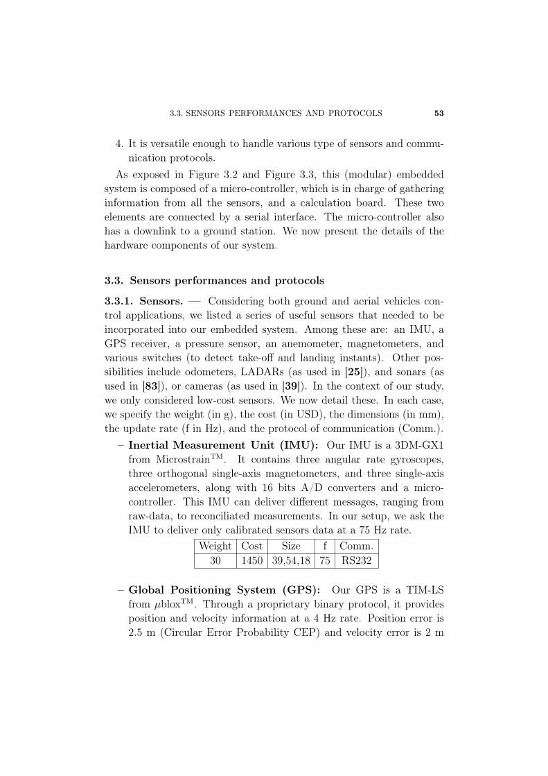
3.3.1. Sensors. — Considering both ground and aerial vehicles con-trol applications, we listed a series of useful sensors that needed to beincorporated into our embedded system. Among these are: an IMU, aGPS receiver, a pressure sensor, an anemometer, magnetometers, andvarious switches (to detect take-off and landing instants). Other pos-sibilities include odometers, LADARs (as used in [25]), and sonars (asused in [83]), or cameras (as used in [39]). In the context of our study,we only considered low-cost sensors. We now detail these. In each case,we specify the weight (in g), the cost (in USD), the dimensions (in mm),the update rate (f in Hz), and the protocol of communication (Comm.).
– Inertial Measurement Unit (IMU): Our IMU is a 3DM-GX1from MicrostrainTM. It contains three angular rate gyroscopes,three orthogonal single-axis magnetometers, and three single-axisaccelerometers, along with 16 bits A/D converters and a micro-controller. This IMU can deliver different messages, ranging fromraw-data, to reconciliated measurements. In our setup, we ask theIMU to deliver only calibrated sensors data at a 75 Hz rate.
Weight Cost Size f Comm.30 1450 39,54,18 75 RS232
– Global Positioning System (GPS): Our GPS is a TIM-LSfrom μbloxTM. Through a proprietary binary protocol, it providesposition and velocity information at a 4 Hz rate. Position error is2.5 m (Circular Error Probability CEP) and velocity error is 2 m
54 CHAPTER 3. NAVIGATION SYSTEM
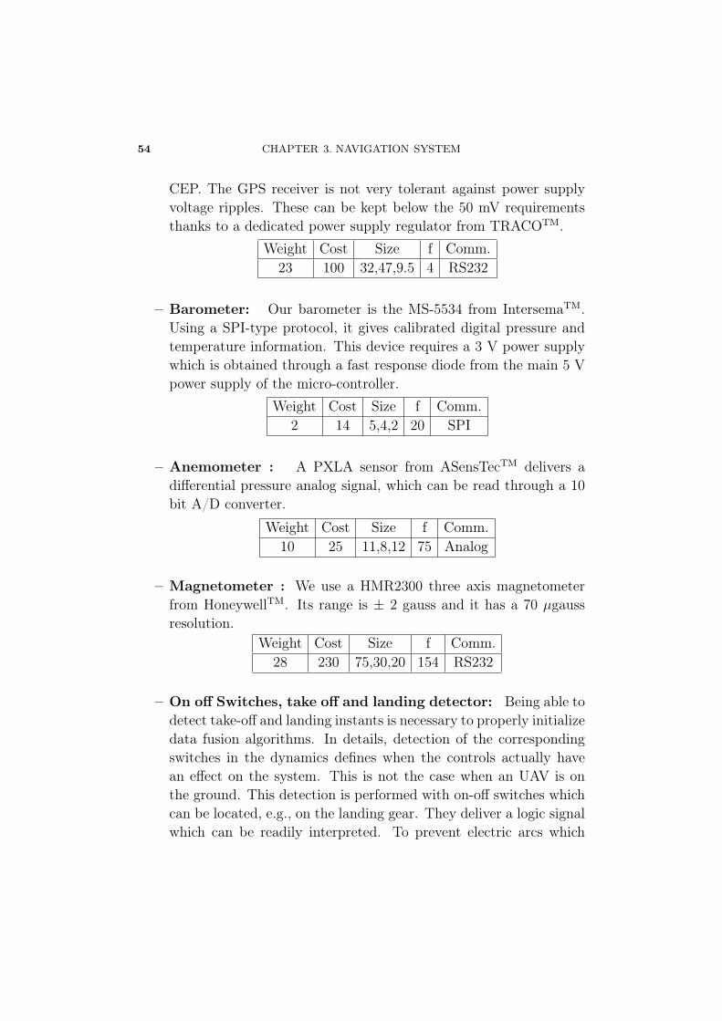
CEP. The GPS receiver is not very tolerant against power supplyvoltage ripples. These can be kept below the 50 mV requirementsthanks to a dedicated power supply regulator from TRACOTM.
Weight Cost Size f Comm.23 100 32,47,9.5 4 RS232
– Barometer: Our barometer is the MS-5534 from IntersemaTM.Using a SPI-type protocol, it gives calibrated digital pressure andtemperature information. This device requires a 3 V power supplywhich is obtained through a fast response diode from the main 5 Vpower supply of the micro-controller.
Weight Cost Size f Comm.2 14 5,4,2 20 SPI
– Anemometer : A PXLA sensor from ASensTecTM delivers adifferential pressure analog signal, which can be read through a 10bit A/D converter.
Weight Cost Size f Comm.10 25 11,8,12 75 Analog
– Magnetometer : We use a HMR2300 three axis magnetometerfrom HoneywellTM. Its range is ± 2 gauss and it has a 70 μgaussresolution.
Weight Cost Size f Comm.28 230 75,30,20 154 RS232
– On off Switches, take off and landing detector: Being able todetect take-off and landing instants is necessary to properly initializedata fusion algorithms. In details, detection of the correspondingswitches in the dynamics defines when the controls actually havean effect on the system. This is not the case when an UAV is onthe ground. This detection is performed with on-off switches whichcan be located, e.g., on the landing gear. They deliver a logic signalwhich can be readily interpreted. To prevent electric arcs which
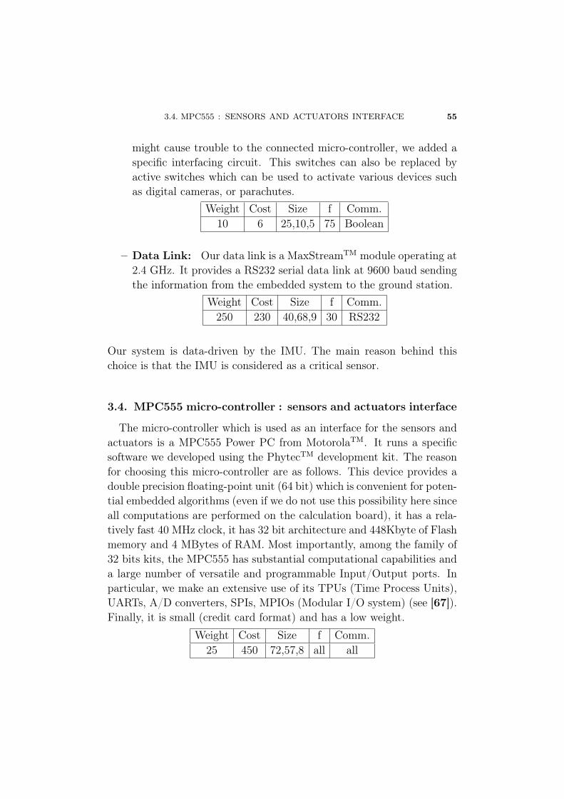
3.4. MPC555 : SENSORS AND ACTUATORS INTERFACE 55
might cause trouble to the connected micro-controller, we added aspecific interfacing circuit. This switches can also be replaced byactive switches which can be used to activate various devices suchas digital cameras, or parachutes.
Weight Cost Size f Comm.10 6 25,10,5 75 Boolean
– Data Link: Our data link is a MaxStreamTM module operating at2.4 GHz. It provides a RS232 serial data link at 9600 baud sendingthe information from the embedded system to the ground station.
Weight Cost Size f Comm.250 230 40,68,9 30 RS232
Our system is data-driven by the IMU. The main reason behind thischoice is that the IMU is considered as a critical sensor.
3.4. MPC555 micro-controller : sensors and actuators interface
The micro-controller which is used as an interface for the sensors andactuators is a MPC555 Power PC from MotorolaTM. It runs a specificsoftware we developed using the PhytecTM development kit. The reasonfor choosing this micro-controller are as follows. This device provides adouble precision floating-point unit (64 bit) which is convenient for poten-tial embedded algorithms (even if we do not use this possibility here sinceall computations are performed on the calculation board), it has a rela-tively fast 40 MHz clock, it has 32 bit architecture and 448Kbyte of Flashmemory and 4 MBytes of RAM. Most importantly, among the family of32 bits kits, the MPC555 has substantial computational capabilities anda large number of versatile and programmable Input/Output ports. Inparticular, we make an extensive use of its TPUs (Time Process Units),UARTs, A/D converters, SPIs, MPIOs (Modular I/O system) (see [67]).Finally, it is small (credit card format) and has a low weight.
Weight Cost Size f Comm.25 450 72,57,8 all all
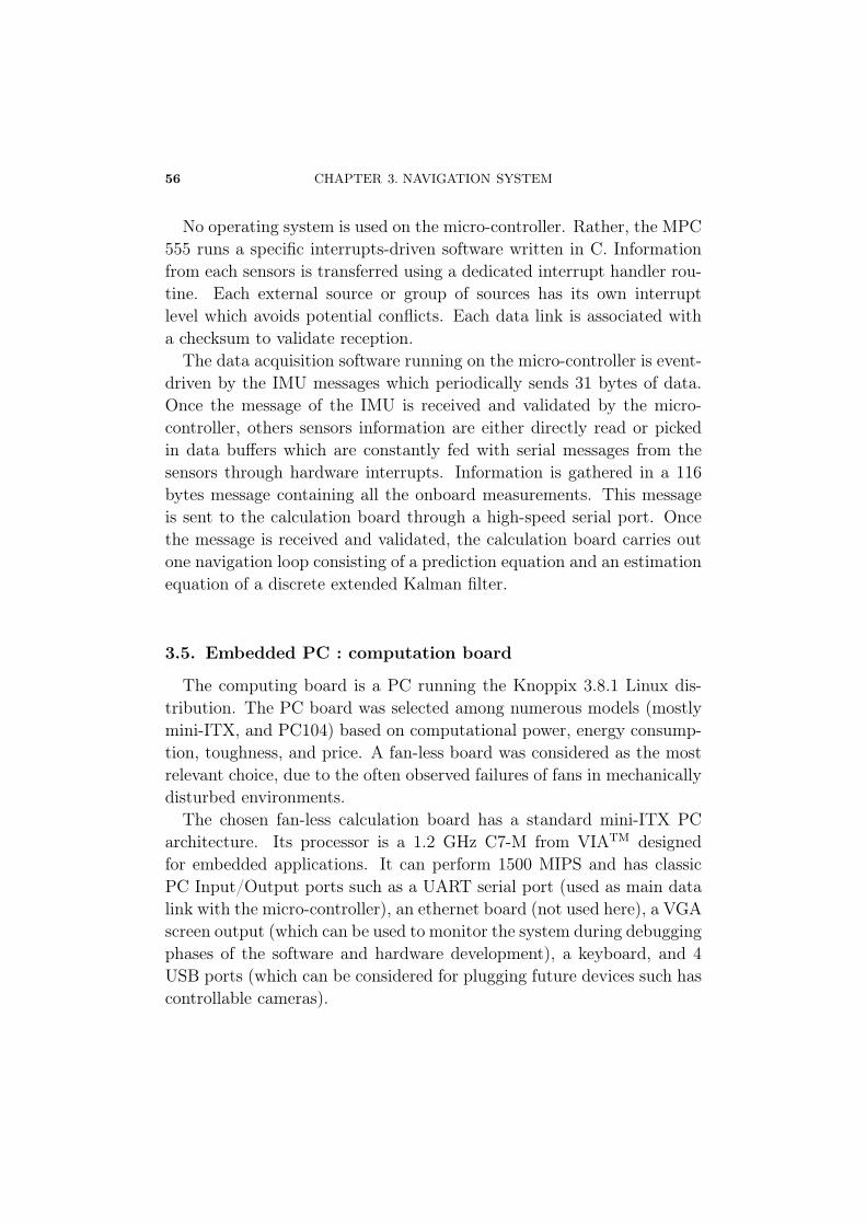
56 CHAPTER 3. NAVIGATION SYSTEM
No operating system is used on the micro-controller. Rather, the MPC555 runs a specific interrupts-driven software written in C. Informationfrom each sensors is transferred using a dedicated interrupt handler rou-tine. Each external source or group of sources has its own interruptlevel which avoids potential conflicts. Each data link is associated witha checksum to validate reception.
The data acquisition software running on the micro-controller is event-driven by the IMU messages which periodically sends 31 bytes of data.Once the message of the IMU is received and validated by the micro-controller, others sensors information are either directly read or pickedin data buffers which are constantly fed with serial messages from thesensors through hardware interrupts. Information is gathered in a 116bytes message containing all the onboard measurements. This messageis sent to the calculation board through a high-speed serial port. Oncethe message is received and validated, the calculation board carries outone navigation loop consisting of a prediction equation and an estimationequation of a discrete extended Kalman filter.
3.5. Embedded PC : computation board
The computing board is a PC running the Knoppix 3.8.1 Linux dis-tribution. The PC board was selected among numerous models (mostlymini-ITX, and PC104) based on computational power, energy consump-tion, toughness, and price. A fan-less board was considered as the mostrelevant choice, due to the often observed failures of fans in mechanicallydisturbed environments.
The chosen fan-less calculation board has a standard mini-ITX PCarchitecture. Its processor is a 1.2 GHz C7-M from VIATM designedfor embedded applications. It can perform 1500 MIPS and has classicPC Input/Output ports such as a UART serial port (used as main datalink with the micro-controller), an ethernet board (not used here), a VGAscreen output (which can be used to monitor the system during debuggingphases of the software and hardware development), a keyboard, and 4USB ports (which can be considered for plugging future devices such hascontrollable cameras).
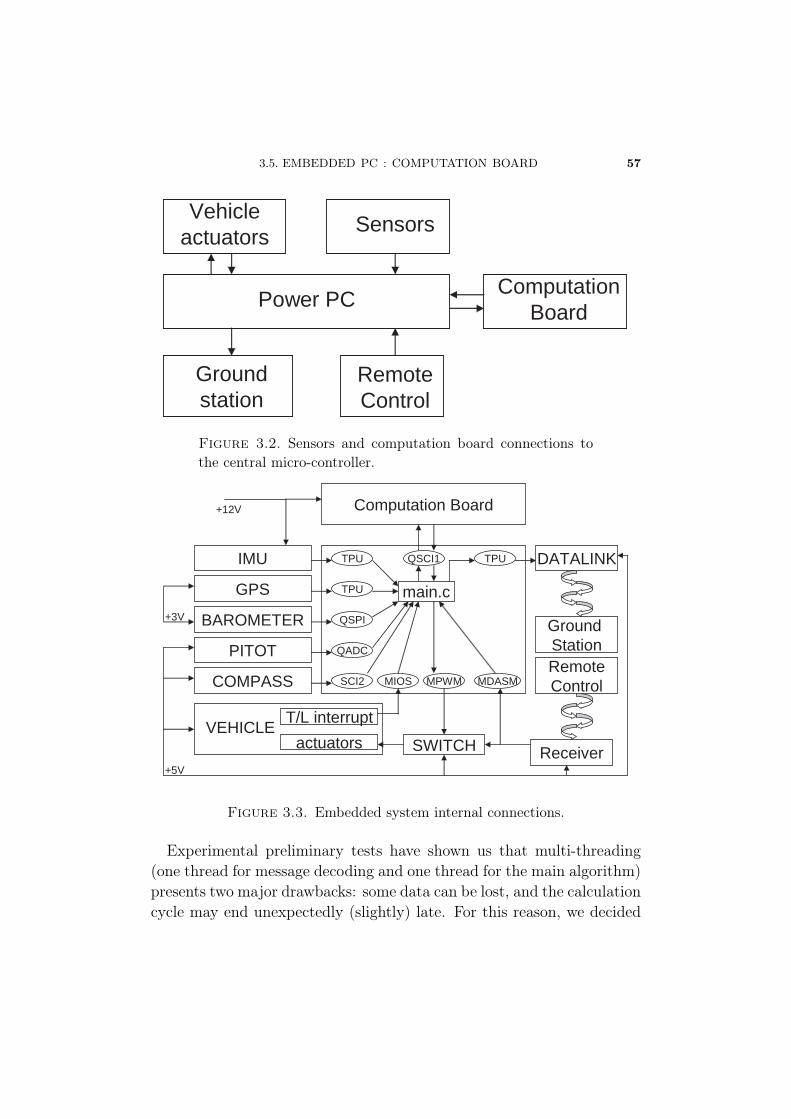
3.5. EMBEDDED PC : COMPUTATION BOARD 57
Sensors
Groundstation
RemoteControl
Power PC
Vehicleactuators
Computation Board
Figure 3.2. Sensors and computation board connections tothe central micro-controller.
TPU
TPU
SCI2 MPWM
QSPI
IMU
QADC
GPS
BAROMETER
PITOT
COMPASS
GroundStation
DATALINK
RemoteControl
ReceiverSWITCHactuators
MDASM
QSCI1
Computation Board
TPU
T/L interrupt
MIOS
VEHICLE
+3V
+5V
+12V
main.c
Figure 3.3. Embedded system internal connections.
Experimental preliminary tests have shown us that multi-threading(one thread for message decoding and one thread for the main algorithm)presents two major drawbacks: some data can be lost, and the calculationcycle may end unexpectedly (slightly) late. For this reason, we decided
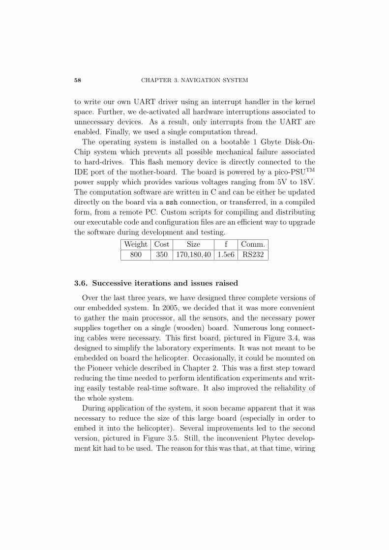
58 CHAPTER 3. NAVIGATION SYSTEM
to write our own UART driver using an interrupt handler in the kernelspace. Further, we de-activated all hardware interruptions associated tounnecessary devices. As a result, only interrupts from the UART areenabled. Finally, we used a single computation thread.
The operating system is installed on a bootable 1 Gbyte Disk-On-Chip system which prevents all possible mechanical failure associatedto hard-drives. This flash memory device is directly connected to theIDE port of the mother-board. The board is powered by a pico-PSUTM
power supply which provides various voltages ranging from 5V to 18V.The computation software are written in C and can be either be updateddirectly on the board via a ssh connection, or transferred, in a compiledform, from a remote PC. Custom scripts for compiling and distributingour executable code and configuration files are an efficient way to upgradethe software during development and testing.
Weight Cost Size f Comm.800 350 170,180,40 1.5e6 RS232
3.6. Successive iterations and issues raised
Over the last three years, we have designed three complete versions ofour embedded system. In 2005, we decided that it was more convenientto gather the main processor, all the sensors, and the necessary powersupplies together on a single (wooden) board. Numerous long connect-ing cables were necessary. This first board, pictured in Figure 3.4, wasdesigned to simplify the laboratory experiments. It was not meant to beembedded on board the helicopter. Occasionally, it could be mounted onthe Pioneer vehicle described in Chapter 2. This was a first step towardreducing the time needed to perform identification experiments and writ-ing easily testable real-time software. It also improved the reliability ofthe whole system.
During application of the system, it soon became apparent that it wasnecessary to reduce the size of this large board (especially in order toembed it into the helicopter). Several improvements led to the secondversion, pictured in Figure 3.5. Still, the inconvenient Phytec develop-ment kit had to be used. The reason for this was that, at that time, wiring
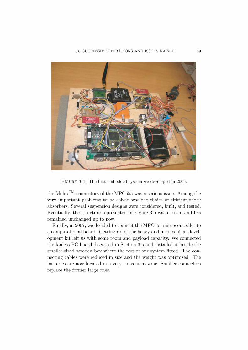
3.6. SUCCESSIVE ITERATIONS AND ISSUES RAISED 59
Figure 3.4. The first embedded system we developed in 2005.
the MolexTM connectors of the MPC555 was a serious issue. Among thevery important problems to be solved was the choice of efficient shockabsorbers. Several suspension designs were considered, built, and tested.Eventually, the structure represented in Figure 3.5 was chosen, and hasremained unchanged up to now.
Finally, in 2007, we decided to connect the MPC555 microcontroller toa computational board. Getting rid of the heavy and inconvenient devel-opment kit left us with some room and payload capacity. We connectedthe fanless PC board discussed in Section 3.5 and installed it beside thesmaller-sized wooden box where the rest of our system fitted. The con-necting cables were reduced in size and the weight was optimized. Thebatteries are now located in a very convenient zone. Smaller connectorsreplace the former large ones.
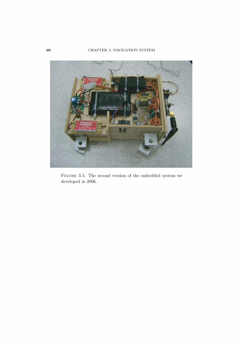
60 CHAPTER 3. NAVIGATION SYSTEM
Figure 3.5. The second version of the embedded system wedeveloped in 2006.
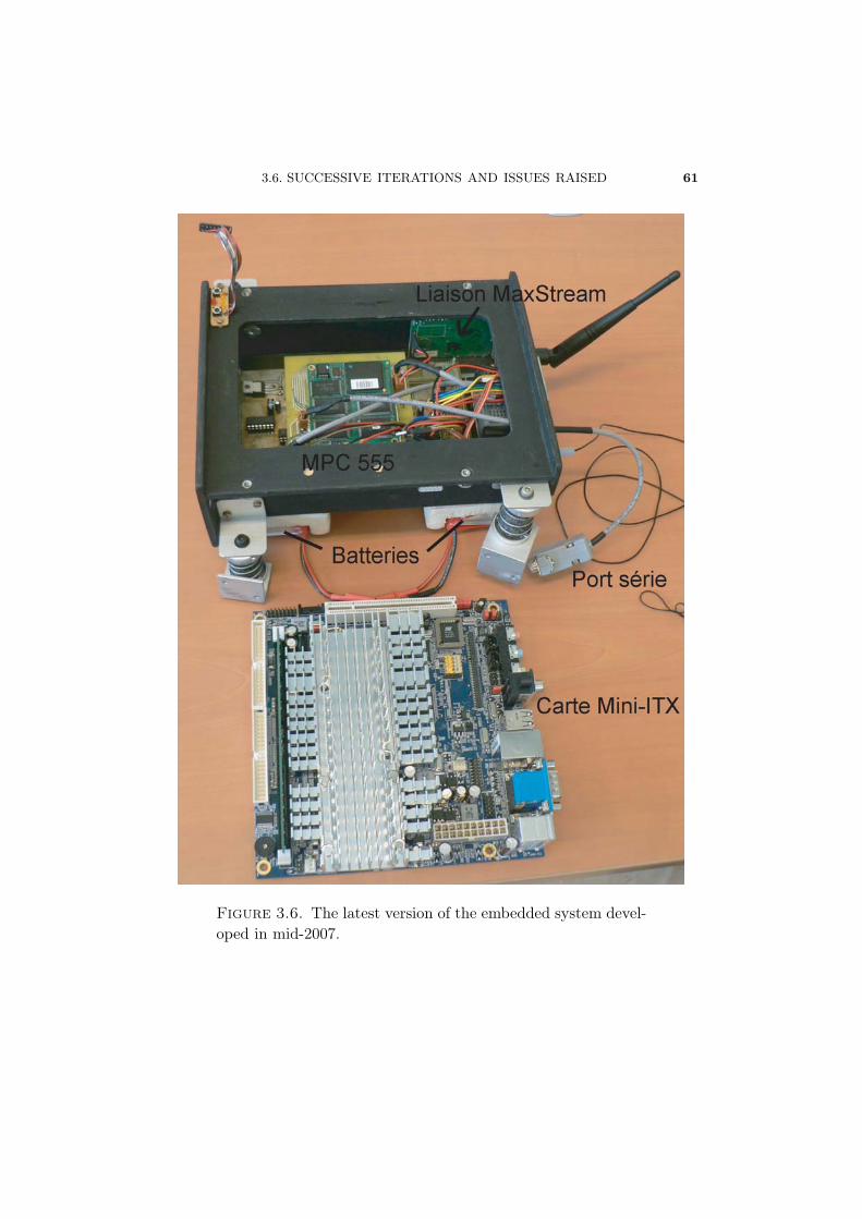
3.6. SUCCESSIVE ITERATIONS AND ISSUES RAISED 61
Figure 3.6. The latest version of the embedded system devel-oped in mid-2007.

CHAPTER 4
AUTONOMOUS FLIGHT OF ASMALL-SCALE HELICOPTER USING A
MODEL-BASED OBSERVER
Dans ce chapitre, nous détaillons notre travail de conception d’undrone à voilure tournante sur base d’hélicoptère de modélisme. Il s’agitd’un engin de 1.8 m de rotor que nous avons équipé d’un système denavigation du type exposé au Chapitre 3. Pour compenser les défauts descapteurs de ce système bas-coût (moins de 3000 dollars de capteurs et decalculateurs), nous utilisons un modèle de connaissance de la dynamiquedu vol d’un tel hélicoptère.
In this chapter, we address the problem of the guidance and control ofa small-scale helicopter (Benzin Acrobatic from VarioTM, with a 1.8 mdiameter rotor) equipped with the low-cost embedded system presentedin Chapter 3. This system used various sensors, namely an IMU, a GPSreceiver, and a barometer, which represented a total cost of USD 3000(including one PC board and one microcontroller). In contrast to otherexperiments reported in the literature, we did not rely on accurate IMUor GPS systems, the costs of which alone would be very much above the
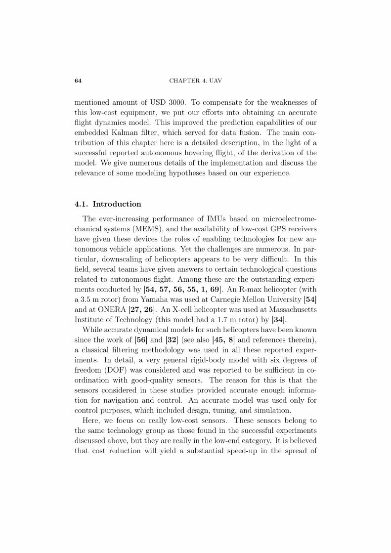
64 CHAPTER 4. UAV
mentioned amount of USD 3000. To compensate for the weaknesses ofthis low-cost equipment, we put our efforts into obtaining an accurateflight dynamics model. This improved the prediction capabilities of ourembedded Kalman filter, which served for data fusion. The main con-tribution of this chapter here is a detailed description, in the light of asuccessful reported autonomous hovering flight, of the derivation of themodel. We give numerous details of the implementation and discuss therelevance of some modeling hypotheses based on our experience.
4.1. Introduction
The ever-increasing performance of IMUs based on microelectrome-chanical systems (MEMS), and the availability of low-cost GPS receivershave given these devices the roles of enabling technologies for new au-tonomous vehicle applications. Yet the challenges are numerous. In par-ticular, downscaling of helicopters appears to be very difficult. In thisfield, several teams have given answers to certain technological questionsrelated to autonomous flight. Among these are the outstanding experi-ments conducted by [54, 57, 56, 55, 1, 69]. An R-max helicopter (witha 3.5 m rotor) from Yamaha was used at Carnegie Mellon University [54]and at ONERA [27, 26]. An X-cell helicopter was used at MassachusettsInstitute of Technology (this model had a 1.7 m rotor) by [34].
While accurate dynamical models for such helicopters have been knownsince the work of [56] and [32] (see also [45, 8] and references therein),a classical filtering methodology was used in all these reported exper-iments. In detail, a very general rigid-body model with six degrees offreedom (DOF) was considered and was reported to be sufficient in co-ordination with good-quality sensors. The reason for this is that thesensors considered in these studies provided accurate enough informa-tion for navigation and control. An accurate model was used only forcontrol purposes, which included design, tuning, and simulation.
Here, we focus on really low-cost sensors. These sensors belong tothe same technology group as those found in the successful experimentsdiscussed above, but they are really in the low-end category. It is believedthat cost reduction will yield a substantial speed-up in the spread of
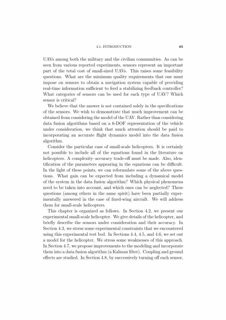
4.1. INTRODUCTION 65
UAVs among both the military and the civilian communities. As can beseen from various reported experiments, sensors represent an importantpart of the total cost of small-sized UAVs. This raises some feasibilityquestions. What are the minimum quality requirements that one mustimpose on sensors to obtain a navigation system capable of providingreal-time information sufficient to feed a stabilizing feedback controller?What categories of sensors can be used for each type of UAV? Whichsensor is critical?
We believe that the answer is not contained solely in the specificationsof the sensors. We wish to demonstrate that much improvement can beobtained from considering the model of the UAV. Rather than consideringdata fusion algorithms based on a 6-DOF representation of the vehicleunder consideration, we think that much attention should be paid toincorporating an accurate flight dynamics model into the data fusionalgorithm.
Consider the particular case of small-scale helicopters. It is certainlynot possible to include all of the equations found in the literature onhelicopters. A complexity–accuracy trade-off must be made. Also, iden-tification of the parameters appearing in the equations can be difficult.In the light of these points, we can reformulate some of the above ques-tions. What gain can be expected from including a dynamical modelof the system in the data fusion algorithm? Which physical phenomenaneed to be taken into account, and which ones can be neglected? Thesequestions (among others in the same spirit) have been partially exper-imentally answered in the case of fixed-wing aircraft. We will addressthem for small-scale helicopters.
This chapter is organized as follows. In Section 4.2, we present ourexperimental small-scale helicopter. We give details of the helicopter, andbriefly describe the sensors under consideration and their accuracy. InSection 4.3, we stress some experimental constraints that we encounteredusing this experimental test bed. In Sections 4.4, 4.5, and 4.6, we set outa model for the helicopter. We stress some weaknesses of this approach.In Section 4.7, we propose improvements to the modeling and incorporatethem into a data fusion algorithm (a Kalman filter). Coupling and groundeffects are studied. In Section 4.8, by successively turning off each sensor,
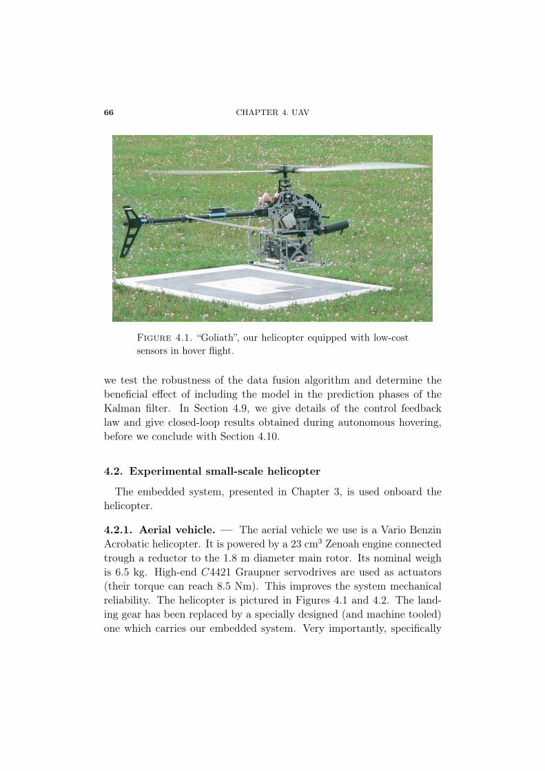
66 CHAPTER 4. UAV
Figure 4.1. “Goliath”, our helicopter equipped with low-costsensors in hover flight.
we test the robustness of the data fusion algorithm and determine thebeneficial effect of including the model in the prediction phases of theKalman filter. In Section 4.9, we give details of the control feedbacklaw and give closed-loop results obtained during autonomous hovering,before we conclude with Section 4.10.
4.2. Experimental small-scale helicopter
The embedded system, presented in Chapter 3, is used onboard thehelicopter.
4.2.1. Aerial vehicle. — The aerial vehicle we use is a Vario BenzinAcrobatic helicopter. It is powered by a 23 cm3 Zenoah engine connectedtrough a reductor to the 1.8 m diameter main rotor. Its nominal weighis 6.5 kg. High-end C4421 Graupner servodrives are used as actuators(their torque can reach 8.5 Nm). This improves the system mechanicalreliability. The helicopter is pictured in Figures 4.1 and 4.2. The land-ing gear has been replaced by a specially designed (and machine tooled)one which carries our embedded system. Very importantly, specifically
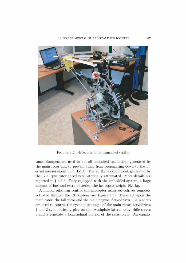
4.2. EXPERIMENTAL SMALL-SCALE HELICOPTER 67
Figure 4.2. Helicopter in its unmanned version
tuned dampers are used to cut-off undesired oscillations generated bythe main rotor and to prevent them from propagating down to the in-ertial measurement unit (IMU). The 25 Hz resonant peak generated bythe 1700 rpm rotor speed is substantially attenuated. More details arereported in § 4.3.3. Fully equipped with the embedded system, a largeamount of fuel and extra batteries, the helicopter weight 10.1 kg.
A human pilot can control the helicopter using servodrives remotelyactuated through the RC system (see Figure 4.3). These act upon themain rotor, the tail rotor and the main engine. Servodrives 1, 2, 3 and 5are used to control the cyclic pitch angle of the main rotor: servodrives1 and 2 symmetrically play on the swashplate lateral axis, while servos3 and 5 generate a longitudinal motion of the swashplate. An equally
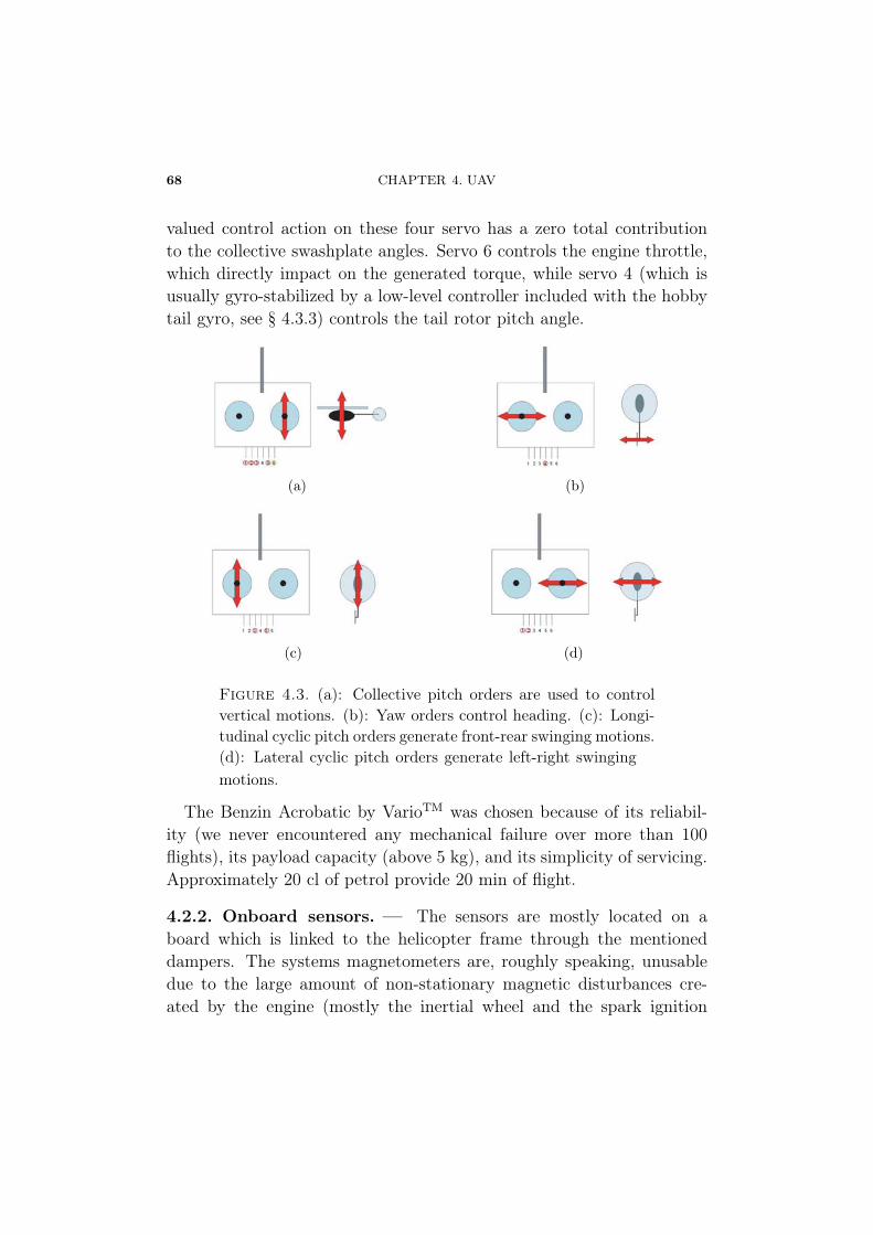
68 CHAPTER 4. UAV
valued control action on these four servo has a zero total contributionto the collective swashplate angles. Servo 6 controls the engine throttle,which directly impact on the generated torque, while servo 4 (which isusually gyro-stabilized by a low-level controller included with the hobbytail gyro, see § 4.3.3) controls the tail rotor pitch angle.
(a) (b)
(c) (d)
Figure 4.3. (a): Collective pitch orders are used to controlvertical motions. (b): Yaw orders control heading. (c): Longi-tudinal cyclic pitch orders generate front-rear swinging motions.(d): Lateral cyclic pitch orders generate left-right swingingmotions.
The Benzin Acrobatic by VarioTM was chosen because of its reliabil-ity (we never encountered any mechanical failure over more than 100flights), its payload capacity (above 5 kg), and its simplicity of servicing.Approximately 20 cl of petrol provide 20 min of flight.
4.2.2. Onboard sensors. — The sensors are mostly located on aboard which is linked to the helicopter frame through the mentioneddampers. The systems magnetometers are, roughly speaking, unusabledue to the large amount of non-stationary magnetic disturbances cre-ated by the engine (mostly the inertial wheel and the spark ignition
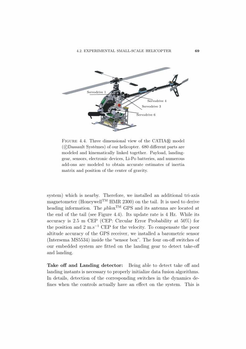
4.2. EXPERIMENTAL SMALL-SCALE HELICOPTER 69
Servodrive 1
Servodrive 3
Servodrive 4
Servodrive 6
Figure 4.4. Three dimensional view of the CATIA� model( c©Dassault Systèmes) of our helicopter. 680 different parts aremodeled and kinematically linked together. Payload, landing-gear, sensors, electronic devices, Li-Po batteries, and numerousadd-ons are modeled to obtain accurate estimates of inertiamatrix and position of the center of gravity.
system) which is nearby. Therefore, we installed an additional tri-axismagnetometer (HoneywellTM HMR 2300) on the tail. It is used to deriveheading information. The μbloxTM GPS and its antenna are located atthe end of the tail (see Figure 4.4). Its update rate is 4 Hz. While itsaccuracy is 2.5 m CEP (CEP: Circular Error Probability at 50%) forthe position and 2 m.s−1 CEP for the velocity. To compensate the pooraltitude accuracy of the GPS receiver, we installed a barometric sensor(Intersema MS5534) inside the “sensor box”. The four on-off switches ofour embedded system are fitted on the landing gear to detect take-offand landing.
Take off and Landing detector: Being able to detect take off andlanding instants is necessary to properly initialize data fusion algorithms.In details, detection of the corresponding switches in the dynamics de-fines when the controls actually have an effect on the system. This is
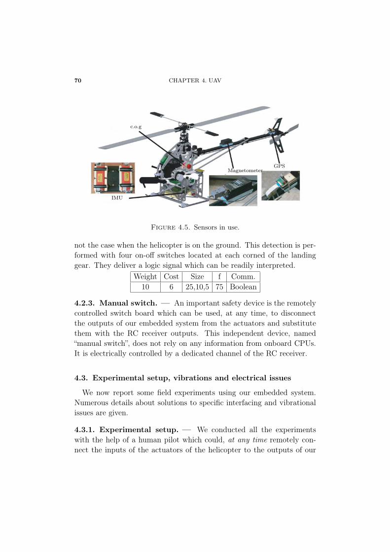
70 CHAPTER 4. UAV
MagnetometerGPS
IMU
c.o.g
Figure 4.5. Sensors in use.
not the case when the helicopter is on the ground. This detection is per-formed with four on-off switches located at each corned of the landinggear. They deliver a logic signal which can be readily interpreted.
Weight Cost Size f Comm.10 6 25,10,5 75 Boolean
4.2.3. Manual switch. — An important safety device is the remotelycontrolled switch board which can be used, at any time, to disconnectthe outputs of our embedded system from the actuators and substitutethem with the RC receiver outputs. This independent device, named“manual switch”, does not rely on any information from onboard CPUs.It is electrically controlled by a dedicated channel of the RC receiver.
4.3. Experimental setup, vibrations and electrical issues
We now report some field experiments using our embedded system.Numerous details about solutions to specific interfacing and vibrationalissues are given.
4.3.1. Experimental setup. — We conducted all the experimentswith the help of a human pilot which could, at any time remotely con-nect the inputs of the actuators of the helicopter to the outputs of our
4.3. EXPERIMENTAL SETUP, VIBRATIONS AND ELECTRICAL ISSUES 71
embedded system or directly to the outputs of the radio receiver (andthus take direct control of the helicopter) through the manual switchboard (see§ 4.2.3).
During all flights, the pilot could see images from an on-board cameraand read measurements from the embedded system received through thedown datalink. A convenient dual-screen Head-Up display system on theground station was designed for that purpose (see Figure 4.6).
4.3.2. Interfacing and vibrational issues. — Wiring the embeddedsystem to the existing helicopter circuitry was achieved using some spe-cific additional boards and connectors. To measure the pilot’s commandsin real-time, we used a 6 channels voltage follower circuit. NumerousLEDs were added to check the status of our system.
As already discussed, a central problem observed on-board helicoptersis the 25 Hz vibrations induced by the main rotor blades. These vi-brations generate a large amount of noise on the inertial sensors. Inpractice, these noises totally overwhelm the useful signals. Fortunately,it is possible to solve this issue by using well-chosen vibration dampers.On our helicopter, we decided that the micro-controller and the sensorswould all be located on a board which would be physically connected tothe frame of the helicopter through four spring-damper systems (see Fig-ure 4.7). Experiments conducted on a vibrating table have shown thatit was advantageous to keep the embedded system as compact and asrigid as possible. The total weight of the subsystem is about 600 g. Wedecided to attach some of the batteries to it to bring the weight close to1.8 kg. This enabled us to use off-the-shelf dampers yielding appropriatecut-off frequencies. MV801-5CC dampers from PaulstraTM were chosenfor their ability to work with low masses vibrating at low frequencies.With these, we obtained a satisfactory vibration damping, with a cut-offfrequency around 9 Hz. This is represented in Figure 4.8. Further, res-onant frequencies due to the engine frequency (around 160 Hz), the tailrotor frequency (around 115 Hz), and the tail boom were removed usinga digital notch filter. The presented solution attenuates high frequencyvibration inputs down to negligible levels.
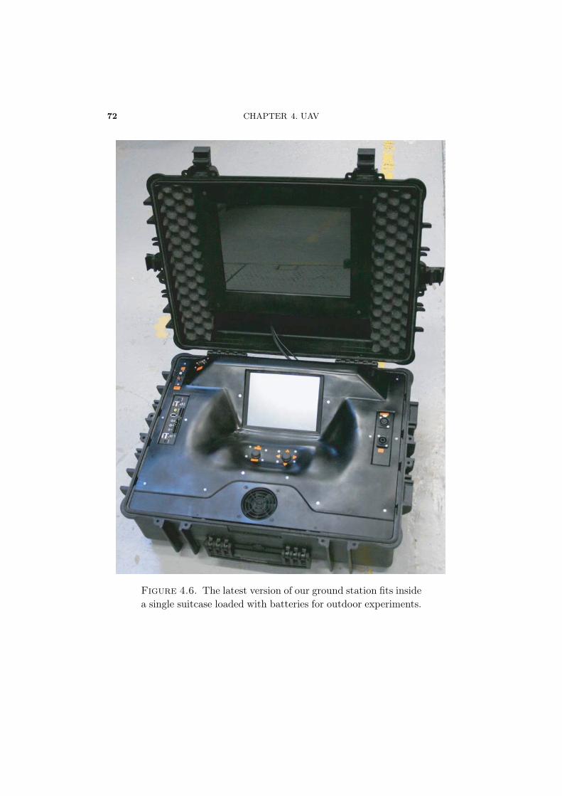
72 CHAPTER 4. UAV
Figure 4.6. The latest version of our ground station fits insidea single suitcase loaded with batteries for outdoor experiments.
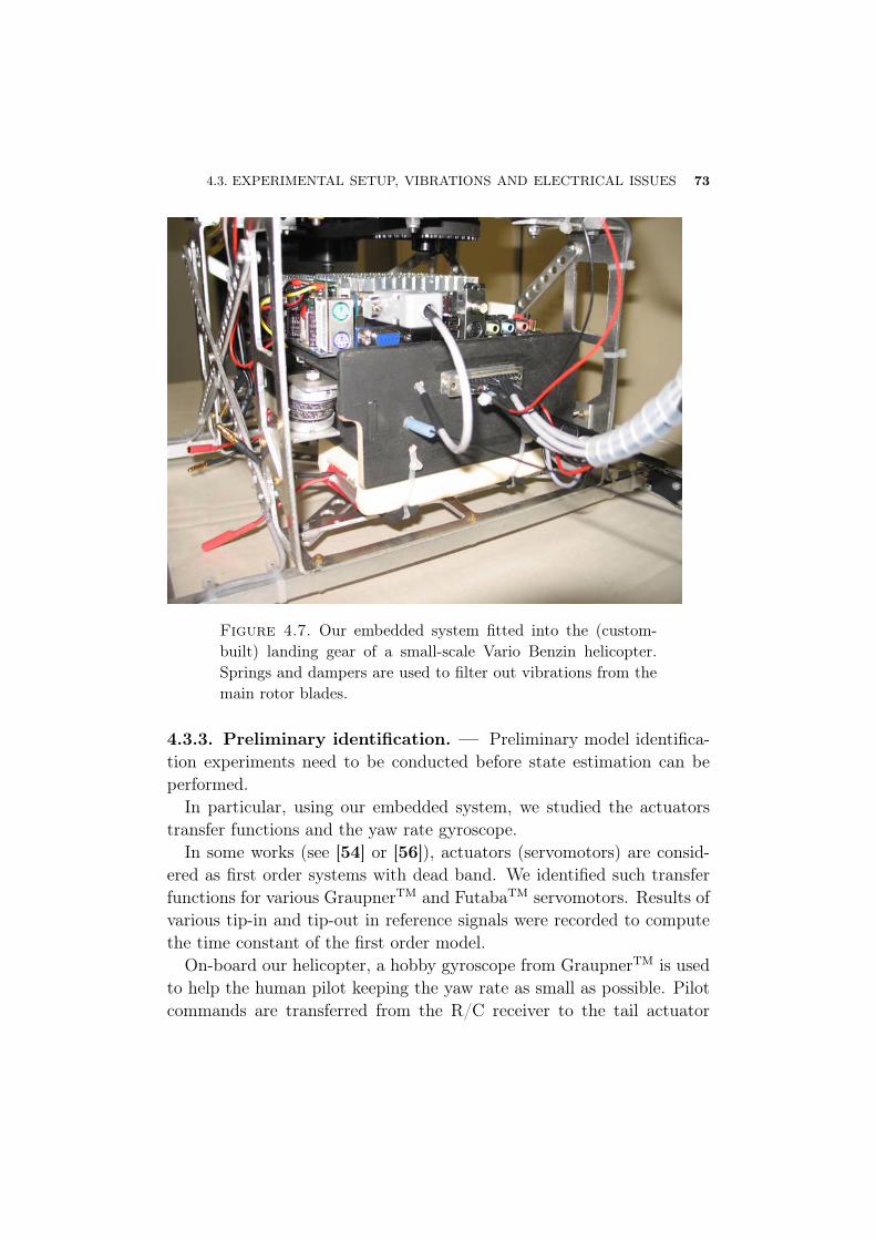
4.3. EXPERIMENTAL SETUP, VIBRATIONS AND ELECTRICAL ISSUES 73
Figure 4.7. Our embedded system fitted into the (custom-built) landing gear of a small-scale Vario Benzin helicopter.Springs and dampers are used to filter out vibrations from themain rotor blades.
4.3.3. Preliminary identification. — Preliminary model identifica-tion experiments need to be conducted before state estimation can beperformed.
In particular, using our embedded system, we studied the actuatorstransfer functions and the yaw rate gyroscope.
In some works (see [54] or [56]), actuators (servomotors) are consid-ered as first order systems with dead band. We identified such transferfunctions for various GraupnerTM and FutabaTM servomotors. Results ofvarious tip-in and tip-out in reference signals were recorded to computethe time constant of the first order model.
On-board our helicopter, a hobby gyroscope from GraupnerTM is usedto help the human pilot keeping the yaw rate as small as possible. Pilotcommands are transferred from the R/C receiver to the tail actuator
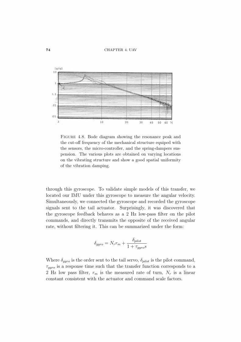
74 CHAPTER 4. UAV
Figure 4.8. Bode diagram showing the resonance peak andthe cut-off frequency of the mechanical structure equiped withthe sensors, the micro-controller, and the spring-dampers sus-pension. The various plots are obtained on varying locationson the vibrating structure and show a good spatial uniformityof the vibration damping.
through this gyroscope. To validate simple models of this transfer, welocated our IMU under this gyroscope to measure the angular velocity.Simultaneously, we connected the gyroscope and recorded the gyroscopesignals sent to the tail actuator. Surprisingly, it was discovered thatthe gyroscope feedback behaves as a 2 Hz low-pass filter on the pilotcommands, and directly transmits the opposite of the received angularrate, without filtering it. This can be summarized under the form:
δgyro = Nrrm +δpilot
1 + τgyros
Where δgyro is the order sent to the tail servo, δpilot is the pilot command,τgyro is a response time such that the transfer function corresponds to a2 Hz low pass filter, rm is the measured rate of turn, Nr is a linearconstant consistent with the actuator and command scale factors.
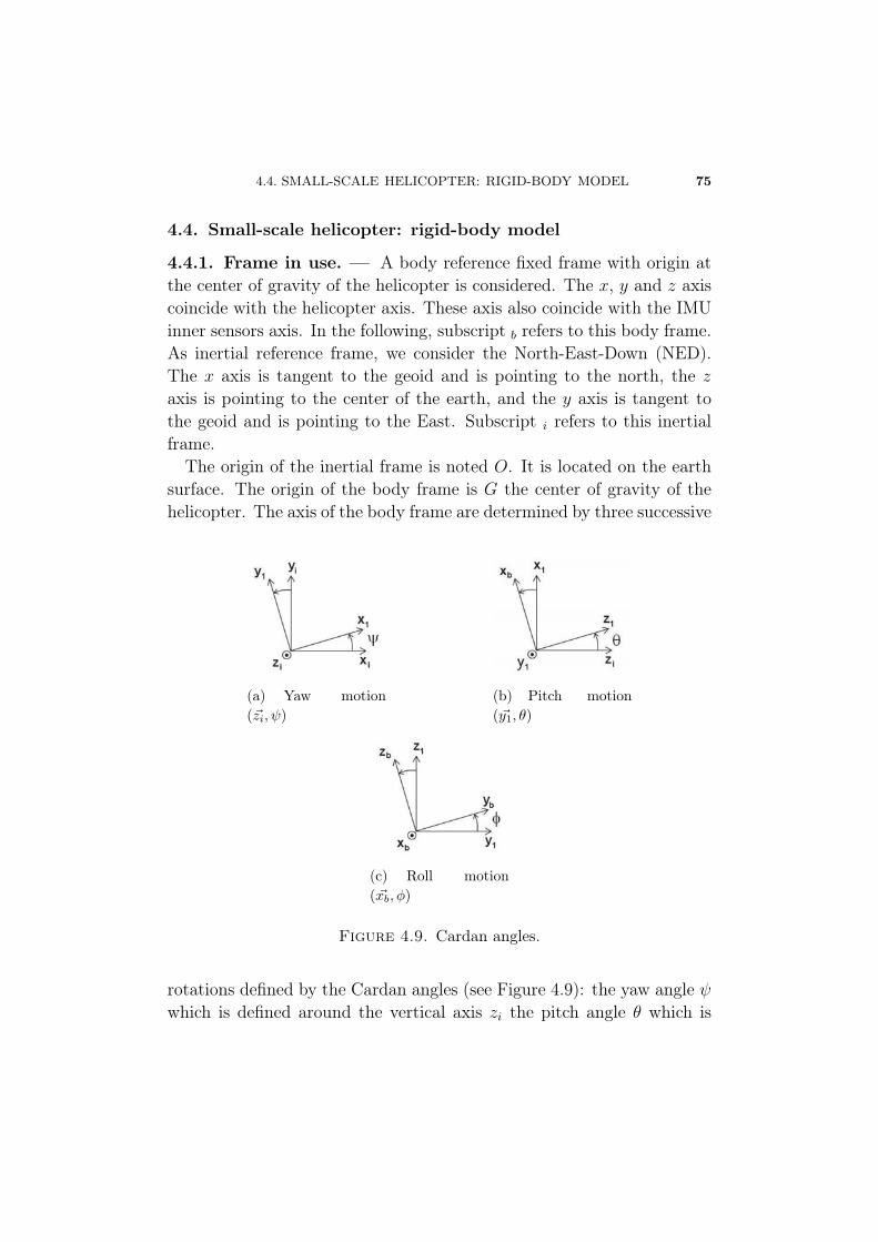
4.4. SMALL-SCALE HELICOPTER: RIGID-BODY MODEL 75
4.4. Small-scale helicopter: rigid-body model
4.4.1. Frame in use. — A body reference fixed frame with origin atthe center of gravity of the helicopter is considered. The x, y and z axiscoincide with the helicopter axis. These axis also coincide with the IMUinner sensors axis. In the following, subscript b refers to this body frame.As inertial reference frame, we consider the North-East-Down (NED).The x axis is tangent to the geoid and is pointing to the north, the zaxis is pointing to the center of the earth, and the y axis is tangent tothe geoid and is pointing to the East. Subscript i refers to this inertialframe.
The origin of the inertial frame is noted O. It is located on the earthsurface. The origin of the body frame is G the center of gravity of thehelicopter. The axis of the body frame are determined by three successive
(a) Yaw motion(�zi, ψ)
(b) Pitch motion(�y1, θ)
(c) Roll motion( �xb, φ)
Figure 4.9. Cardan angles.
rotations defined by the Cardan angles (see Figure 4.9): the yaw angle ψwhich is defined around the vertical axis zi the pitch angle θ which is
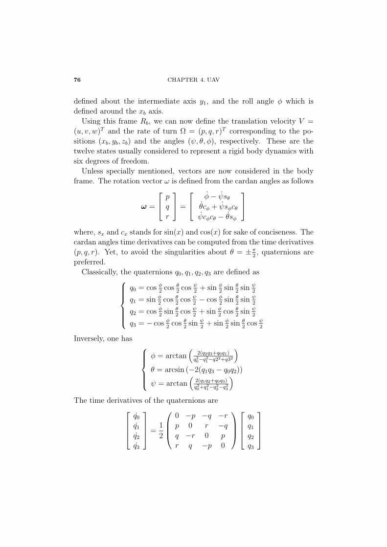
76 CHAPTER 4. UAV
defined about the intermediate axis y1, and the roll angle φ which isdefined around the xb axis.
Using this frame Rb, we can now define the translation velocity V =
(u, v, w)T and the rate of turn Ω = (p, q, r)T corresponding to the po-sitions (xb, yb, zb) and the angles (ψ, θ, φ), respectively. These are thetwelve states usually considered to represent a rigid body dynamics withsix degrees of freedom.
Unless specially mentioned, vectors are now considered in the bodyframe. The rotation vector ω is defined from the cardan angles as follows
ω =
⎡⎣ p
q
r
⎤⎦ =
⎡⎣ φ− ψsθθcφ + ψsφcθψcφcθ − θsφ
⎤⎦where, sx and cx stands for sin(x) and cos(x) for sake of conciseness. Thecardan angles time derivatives can be computed from the time derivatives(p, q, r). Yet, to avoid the singularities about θ = ±π
2, quaternions are
preferred.Classically, the quaternions q0, q1, q2, q3 are defined as⎧⎪⎪⎪⎪⎨⎪⎪⎪⎪⎩
q0 = cos φ2
cos θ2cos ψ
2+ sin φ
2sin θ
2sin ψ
2
q1 = sin φ2
cos θ2cos ψ
2− cos φ
2sin θ
2sin ψ
2
q2 = cos φ2
sin θ2cos ψ
2+ sin φ
2cos θ
2sin ψ
2
q3 = − cos φ2
cos θ2sin ψ
2+ sin φ
2sin θ
2cos ψ
2
Inversely, one has ⎧⎪⎪⎪⎨⎪⎪⎪⎩φ = arctan
(2(q2q3+q0q1)
q20−q21−q22+q32
)θ = arcsin (−2(q1q3 − q0q2))
ψ = arctan(
2(q1q2+q0q3)
q20+q21−q22−q23
)The time derivatives of the quaternions are⎡⎢⎢⎣
q0q1q2q3
⎤⎥⎥⎦ =1
2
⎛⎜⎜⎝0 −p −q −rp 0 r −qq −r 0 p
r q −p 0
⎞⎟⎟⎠⎡⎢⎢⎣q0q1q2q3
⎤⎥⎥⎦
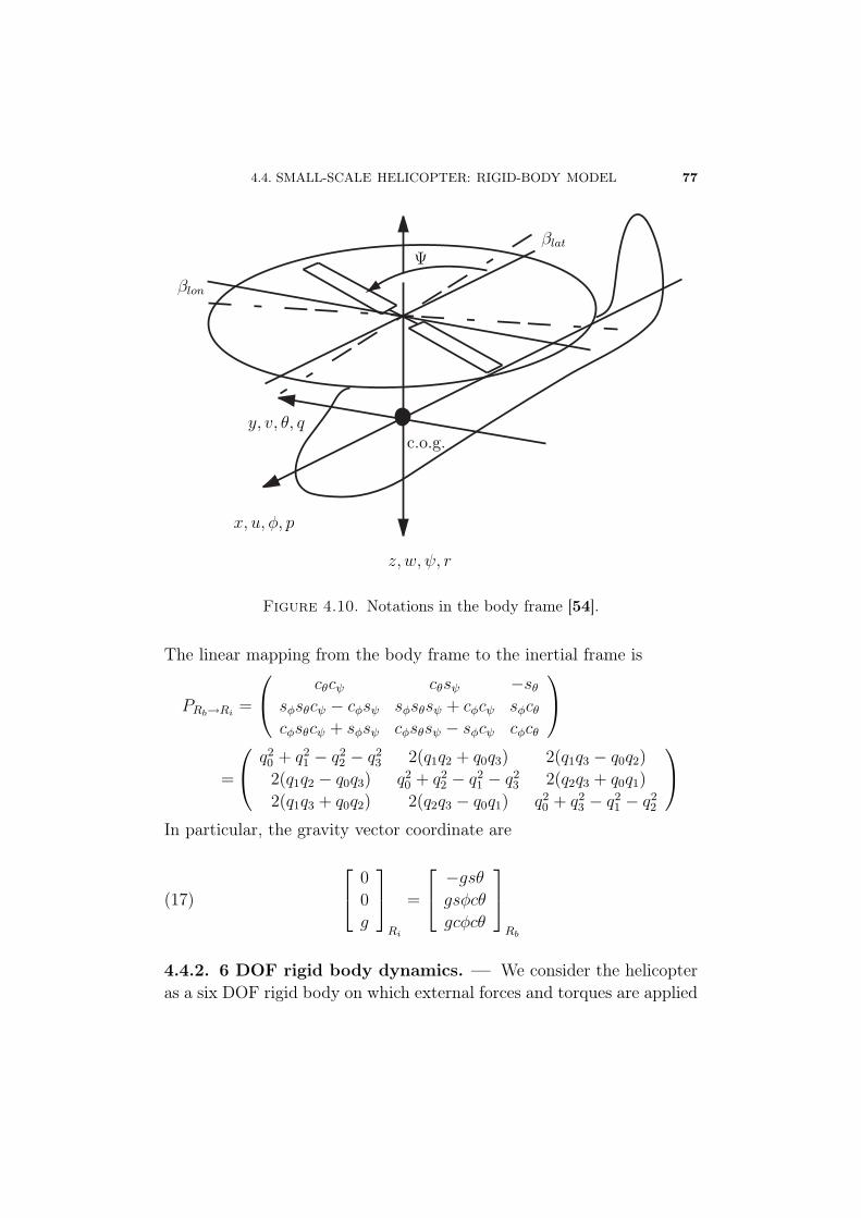
4.4. SMALL-SCALE HELICOPTER: RIGID-BODY MODEL 77
βlon
y, v, θ, q
x, u, φ, p
z, w, ψ, r
Ψβlat
c.o.g.
Figure 4.10. Notations in the body frame [54].
The linear mapping from the body frame to the inertial frame is
PRb→Ri=
⎛⎝ cθcψ cθsψ −sθsφsθcψ − cφsψ sφsθsψ + cφcψ sφcθcφsθcψ + sφsψ cφsθsψ − sφcψ cφcθ
⎞⎠=
⎛⎝ q20 + q2
1 − q22 − q2
3 2(q1q2 + q0q3) 2(q1q3 − q0q2)
2(q1q2 − q0q3) q20 + q2
2 − q21 − q2
3 2(q2q3 + q0q1)
2(q1q3 + q0q2) 2(q2q3 − q0q1) q20 + q2
3 − q21 − q2
2
⎞⎠In particular, the gravity vector coordinate are
⎡⎣ 0
0
g
⎤⎦Ri
=
⎡⎣ −gsθgsφcθ
gcφcθ
⎤⎦Rb
(17)
4.4.2. 6 DOF rigid body dynamics. — We consider the helicopteras a six DOF rigid body on which external forces and torques are applied
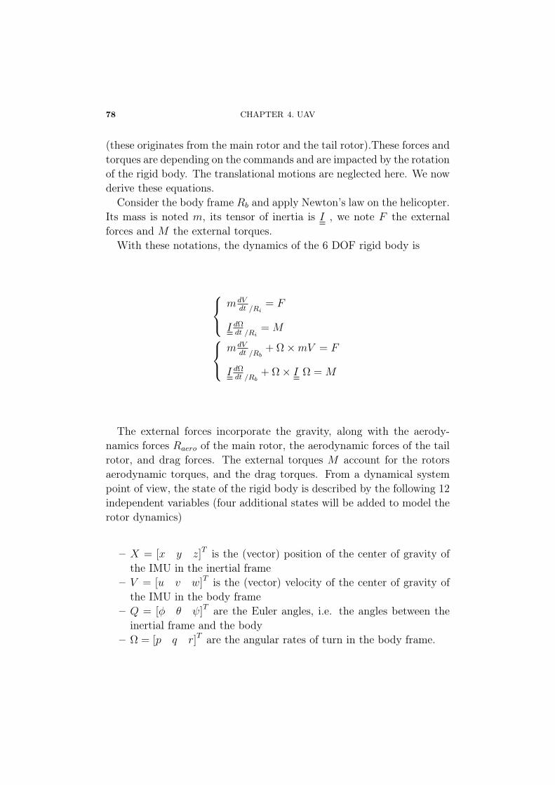
78 CHAPTER 4. UAV
(these originates from the main rotor and the tail rotor).These forces andtorques are depending on the commands and are impacted by the rotationof the rigid body. The translational motions are neglected here. We nowderive these equations.
Consider the body frame Rb and apply Newton’s law on the helicopter.Its mass is noted m, its tensor of inertia is I , we note F the externalforces and M the external torques.
With these notations, the dynamics of the 6 DOF rigid body is
⎧⎨⎩ mdVdt /Ri
= F
I dΩdt /Ri
= M⎧⎨⎩ mdVdt /Rb
+ Ω ×mV = F
I dΩdt /Rb
+ Ω × I Ω = M
The external forces incorporate the gravity, along with the aerody-namics forces Raero of the main rotor, the aerodynamic forces of the tailrotor, and drag forces. The external torques M account for the rotorsaerodynamic torques, and the drag torques. From a dynamical systempoint of view, the state of the rigid body is described by the following 12independent variables (four additional states will be added to model therotor dynamics)
– X = [x y z]T is the (vector) position of the center of gravity ofthe IMU in the inertial frame
– V = [u v w]T is the (vector) velocity of the center of gravity ofthe IMU in the body frame
– Q = [φ θ ψ]T are the Euler angles, i.e. the angles between theinertial frame and the body
– Ω = [p q r]T are the angular rates of turn in the body frame.
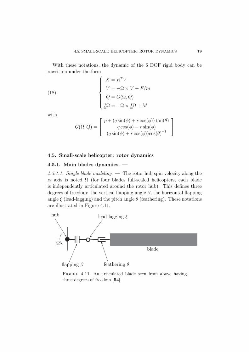
4.5. SMALL-SCALE HELICOPTER: ROTOR DYNAMICS 79
With these notations, the dynamic of the 6 DOF rigid body can berewritten under the form
(18)
⎧⎪⎪⎪⎪⎪⎨⎪⎪⎪⎪⎪⎩
X = RTV
V = −Ω × V + F/m
Q = G(Ω, Q)
IΩ = −Ω × IΩ +M
with
G(Ω, Q) =
⎡⎣ p+ (q sin(φ) + r cos(φ)) tan(θ)
q cos(φ) − r sin(φ)
(q sin(φ) + r cos(φ))cos(θ)−1
⎤⎦
4.5. Small-scale helicopter: rotor dynamics
4.5.1. Main blades dynamics. —
4.5.1.1. Single blade modeling. — The rotor hub spin velocity along thezb axis is noted Ω (for four blades full-scaled helicopters, each bladeis independently articulated around the rotor hub). This defines threedegrees of freedom: the vertical flapping angle β, the horizontal flappingangle ξ (lead-lagging) and the pitch angle θ (feathering). These notationsare illustrated in Figure 4.11.
hub
Ω
lead-lagging ξ
blade
feathering θflapping β
Figure 4.11. An articulated blade seen from above havingthree degrees of freedom [54].
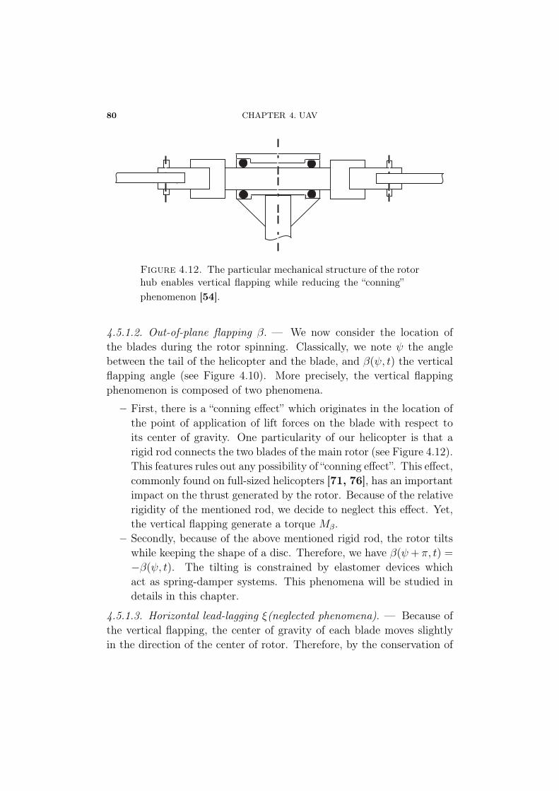
80 CHAPTER 4. UAV
Figure 4.12. The particular mechanical structure of the rotorhub enables vertical flapping while reducing the “conning”phenomenon [54].
4.5.1.2. Out-of-plane flapping β. — We now consider the location ofthe blades during the rotor spinning. Classically, we note ψ the anglebetween the tail of the helicopter and the blade, and β(ψ, t) the verticalflapping angle (see Figure 4.10). More precisely, the vertical flappingphenomenon is composed of two phenomena.
– First, there is a “conning effect” which originates in the location ofthe point of application of lift forces on the blade with respect toits center of gravity. One particularity of our helicopter is that arigid rod connects the two blades of the main rotor (see Figure 4.12).This features rules out any possibility of “conning effect”. This effect,commonly found on full-sized helicopters [71, 76], has an importantimpact on the thrust generated by the rotor. Because of the relativerigidity of the mentioned rod, we decide to neglect this effect. Yet,the vertical flapping generate a torque Mβ.
– Secondly, because of the above mentioned rigid rod, the rotor tiltswhile keeping the shape of a disc. Therefore, we have β(ψ+ π, t) =
−β(ψ, t). The tilting is constrained by elastomer devices whichact as spring-damper systems. This phenomena will be studied indetails in this chapter.
4.5.1.3. Horizontal lead-lagging ξ(neglected phenomena). — Because ofthe vertical flapping, the center of gravity of each blade moves slightlyin the direction of the center of rotor. Therefore, by the conservation of
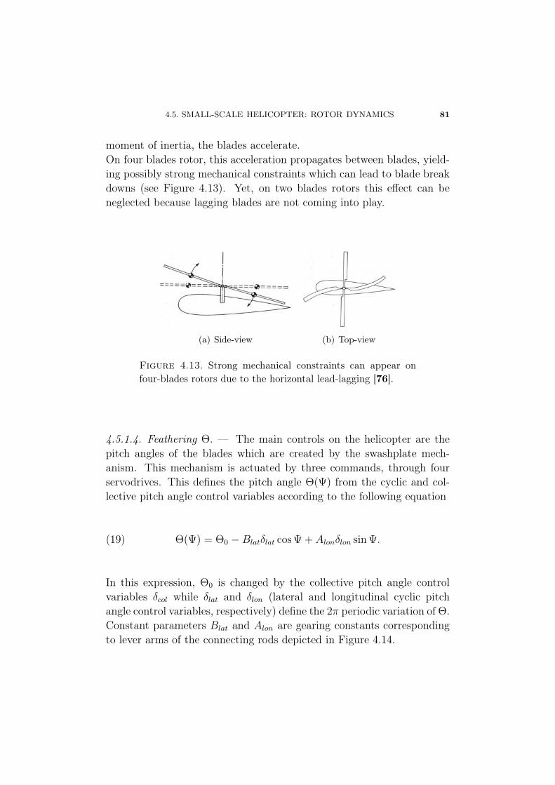
4.5. SMALL-SCALE HELICOPTER: ROTOR DYNAMICS 81
moment of inertia, the blades accelerate.On four blades rotor, this acceleration propagates between blades, yield-ing possibly strong mechanical constraints which can lead to blade breakdowns (see Figure 4.13). Yet, on two blades rotors this effect can beneglected because lagging blades are not coming into play.
(a) Side-view (b) Top-view
Figure 4.13. Strong mechanical constraints can appear onfour-blades rotors due to the horizontal lead-lagging [76].
4.5.1.4. Feathering Θ. — The main controls on the helicopter are thepitch angles of the blades which are created by the swashplate mech-anism. This mechanism is actuated by three commands, through fourservodrives. This defines the pitch angle Θ(Ψ) from the cyclic and col-lective pitch angle control variables according to the following equation
(19) Θ(Ψ) = Θ0 −Blatδlat cos Ψ + Alonδlon sin Ψ.
In this expression, Θ0 is changed by the collective pitch angle controlvariables δcol while δlat and δlon (lateral and longitudinal cyclic pitchangle control variables, respectively) define the 2π periodic variation of Θ.Constant parameters Blat and Alon are gearing constants correspondingto lever arms of the connecting rods depicted in Figure 4.14.
82 CHAPTER 4. UAV
4.5.1.5. Differential equation for the vertical flapping β. — The localrelative wind speed is used to define the dynamics of β(20)
β + Ω2β − 2Ω(p cos Ψ − q sin Ψ) − (q cos Ψ + p sin Ψ)
=1
8γΩ2
(−Blatδlat cos Ψ + Alonδlon sin Ψ +
1
Ω(q cos Ψ + p sin Ψ)
)...− 1
8γΩ2(
β
Ω) − kβ
Iββ
By expressing β over R×R as a 2π periodic function of ψ, it becomespossible to expand it as a Fourier series. In facts, it is verified that thefirst harmonic term dominates the higher orders. Therefore, we look foran approximate solution of Equation (20) in the form
(21) β(Ψ, t) ≈ −a(t) cos Ψ − b(t) sin Ψ.
As will appear later, the variables a(t) and b(t) are in facts angles ofthe vector aerodynamic forces Raero. Assuming Equation (21), we easilycompute β and β as
β = −(a+ Ωb) cos Ψ − (b− Ωa) sin Ψ(22)
β = −(a+ 2Ωb− Ω2a) cos Ψ − (b− 2Ωa− Ω2b) sin Ψ(23)
By matching the terms of Fourier expansion in Equations (20,21,22,23),we obtain the following second order differential equation for a and b
(24)
[a
b
]+MA
[a
b
]+MR
[a
b
]= MF
MA = Ω
[γ8
2
−2 γ8
], MR = Ω2
[kβ
IβΩ2γ8
−γ8
kβ
IβΩ2
]
MF = Ω2
[γ8
0
0 −γ8
] [BlatδlatAlonδlon
]+ Ω
[−2 −γ
8
−γ8
2
] [p
q
]+
[0 −1
−1 0
] [p
q
]The matrix MA is a “damping matrix”, MR is referred to as “stiffnessmatrix” while MF is the “forcing matrix”.To simplify Equations (24) further, the following assumptions are made.Assumptions:
4.5. SMALL-SCALE HELICOPTER: ROTOR DYNAMICS 83
– angular accelerations are much smaller than the angular rates mul-tiplied by the rotation speed.
– the term γ16
is “much smaller” than 1. This last assumption is con-sidered because γ = 4.
With these simplifying assumptions, Equation (24) becomes, after a sin-gular perturbation analysis,⎧⎨⎩
16γΩ
(a− γ
16b)
+ a = − 16γΩ
(q − γ
16p)
+ 8γΩ2
kβ
Iβb+ Alonδlon
16γΩ
(b+ γ
16a)
+ b = − 16γΩ
(p+ γ
16q)− 8
γΩ2
kβ
Iβa+Blatδlat
Noting τf = 16γΩ
≈ 40 ms, we finally obtain
(25)
{τf a+ a = −τfq + 8
γΩ2
kβ
Iβb+ Alonδlon
τf b+ b = −τfp− 8γΩ2
kβ
Iβa+Blatδlat
where γ is the Lock number, kβ is the flapping hinge restraint springconstant, Iβ is the blade moment of inertia about the flapping hinge andτf > 0. Alon is the longitudinal stick to cyclic pitch gearings, Blat is thelateral stick to cyclic pitch gearings for the main bar.
These two first order differential equations define, through Equation (21),the effects of the two control δlon et δlat on the motion of the helicopterand on the vertical flapping.
4.5.2. Bell-bar dynamics. —
4.5.2.1. Vertical flapping. — The Bell-bar is a relatively small bar, or-thogonal to the true blades, which bears two winglets and two punctualmasses. It has a rotation degree of freedom. Therefore, its vertical flap-ping is not subject to any mechanical torque, and is independent of themain rotor vertical flapping. The winglet’s profile is chosen such thatthey generate negligible lift and drag forces compared to the main rotor.Yet these generated forces, which are opposed to the centrifugal effect,determine the Bell rotor equilibrium which is parameterized by β. Noting
(26){c(t) = −β(Ψ = 0, t)
d(t) = −β(Ψ = π2, t)
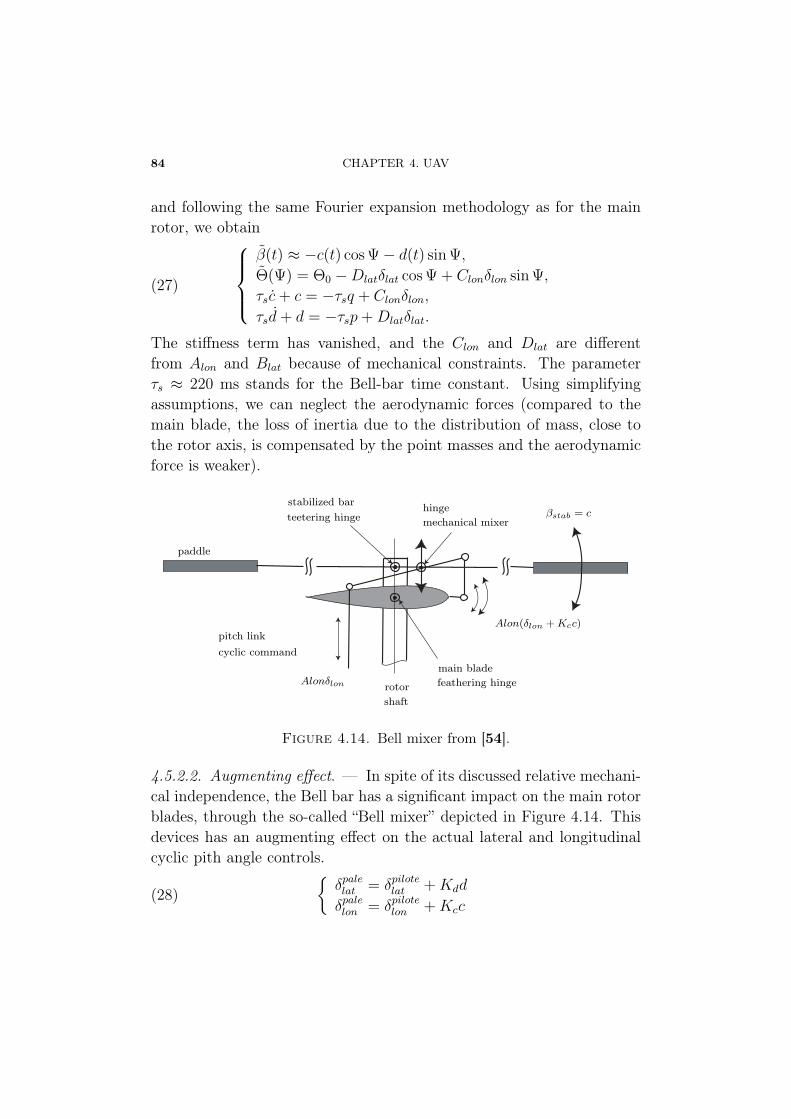
84 CHAPTER 4. UAV
and following the same Fourier expansion methodology as for the mainrotor, we obtain
(27)
⎧⎪⎪⎨⎪⎪⎩β(t) ≈ −c(t) cos Ψ − d(t) sin Ψ,
Θ(Ψ) = Θ0 −Dlatδlat cos Ψ + Clonδlon sin Ψ,
τsc+ c = −τsq + Clonδlon,
τsd+ d = −τsp+Dlatδlat.
The stiffness term has vanished, and the Clon and Dlat are differentfrom Alon and Blat because of mechanical constraints. The parameterτs ≈ 220 ms stands for the Bell-bar time constant. Using simplifyingassumptions, we can neglect the aerodynamic forces (compared to themain blade, the loss of inertia due to the distribution of mass, close tothe rotor axis, is compensated by the point masses and the aerodynamicforce is weaker).
paddle
pitch linkcyclic command
Alonδlon rotorshaft
main bladefeathering hinge
Alon(δlon +Kcc)
βstab = chingemechanical mixer
stabilized barteetering hinge
Figure 4.14. Bell mixer from [54].
4.5.2.2. Augmenting effect. — In spite of its discussed relative mechani-cal independence, the Bell bar has a significant impact on the main rotorblades, through the so-called “Bell mixer” depicted in Figure 4.14. Thisdevices has an augmenting effect on the actual lateral and longitudinalcyclic pith angle controls.
(28){δpalelat = δpilotelat +Kdd
δpalelon = δpilotelon +Kcc

4.5. SMALL-SCALE HELICOPTER: ROTOR DYNAMICS 85
4.5.2.3. Stabilizing effect. — The term “stabilizing effect” can be mis-leading for anyone with a background in control and dynamical systems.In facts, the Bell bar does not stabilize the helicopter, but slows downthe rotor dynamics by increasing its response time.
The punctual masses can be used to tune this “stabilizing effect”. With-out the Bell bar, the main rotor response time would be close to 40 ms,and will be conflicting with the capabilities of a human pilot (1).
4.5.2.4. Aerodynamic forces. — The following two vectors are containedin the plane of the main rotor.
(29){
xr = − cos a xb + sin a zb
yr = cos b yb + sin b zb
Under simplifying assumptions, the drag generated by the blades is hor-izontal. Therefore, when the rotor is tilted, the drags of the Bell bar andof the main rotor do not cancel out. There exists a resulting drag forcein the (xb,yb) plane and a counter-rotative torque.
This drag force must be added to the drag of the helicopter body,while the additional counter-rotative torque can be compensated by anoffset in the main engine produced power, to keep the rotation speed Ω
constant.
Remark 2. — We do not try to compute the norm of the thrust gen-erated by the rotor. Its value can be obtained experimentally, using itsproportionality to the collective pitch angle δcol.
4.5.3. Summary. —
4.5.3.1. Model for the Bell-bar. — The two additional states, c and d,corresponding to the Bell-bar blades satisfy a set of two uncoupled lin-ear first order dynamics driven by inputs corresponding to the controlvariables acting upon the rotor head
(30)
{τsc+ c = −τsq + Clonδlon
τsd+ d = −τsp+Dlatδlat
(1)in acrobatic helicopter contests, lightened Bell bars can be observed.
86 CHAPTER 4. UAV
where Clon is the longitudinal stick to cyclic pitch gearings, Dlat is thelateral stick to cyclic pitch gearings for the Bell-bar and τs > 0. TheBell-bar has an effect on the main blades dynamics due to so-called “Bellmixer” mechanism. One can consider that the actual inputs in Equa-tion (25) are “augmented” following Equation (28).
4.5.3.2. Model for the main blades. — The two state variables a and b
correspond to a first harmonic expansion of the periodic motion of theblades. These two states satisfy coupled, linear, first order dynamicsdriven by inputs corresponding to the control variables acting upon therotor head, see Equation (31). Accordingly, the vertical flapping dynam-ics is modified as
(31)
{τf a+ a = −τfq + 8
γΩ2
kβ
Iβb+ Alon(δlon +Kcc)
τf b+ b = −τfp− 8γΩ2
kβ
Iβa+Blat(δlat +Kdd)
4.5.3.3. Resulting forces and torques on the rigid body. — The aerody-namics states a, b, c, d presented above can be used to define the orien-tation of the rotor thrust Raero and the torque Maero acting upon therigid body of the helicopter. Mβ represents the torque corresponding tothe spring effect of the rotor hub. Around steady state, these are
(32)
Raero = T
⎡⎣ −ab
−1
⎤⎦Maero = hT
⎡⎣ b
a
0
⎤⎦Mβ = kβ
⎡⎣ b
a
0
⎤⎦where T is the norm of the thrust generated by the main rotor, andh is the distance between the center of application of the thrust andthe center of gravity of the helicopter. Around hovering, T ≈ mg. Aswill be discussed later on, the thrust is depending on δcol (and on z).
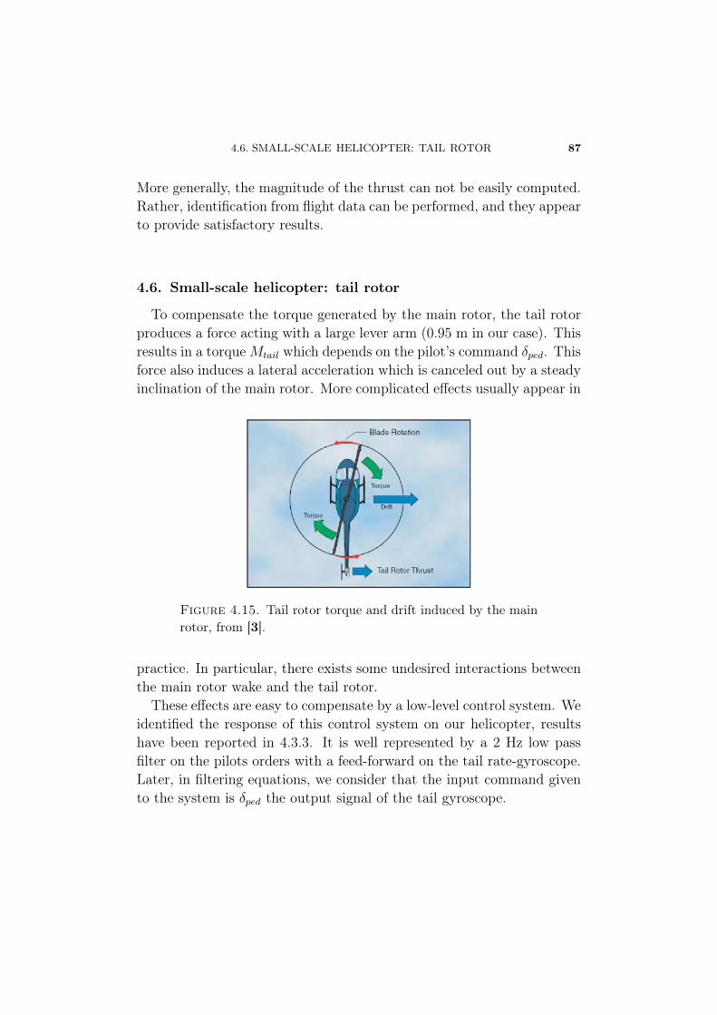
4.6. SMALL-SCALE HELICOPTER: TAIL ROTOR 87
More generally, the magnitude of the thrust can not be easily computed.Rather, identification from flight data can be performed, and they appearto provide satisfactory results.
4.6. Small-scale helicopter: tail rotor
To compensate the torque generated by the main rotor, the tail rotorproduces a force acting with a large lever arm (0.95 m in our case). Thisresults in a torque Mtail which depends on the pilot’s command δped. Thisforce also induces a lateral acceleration which is canceled out by a steadyinclination of the main rotor. More complicated effects usually appear in
Figure 4.15. Tail rotor torque and drift induced by the mainrotor, from [3].
practice. In particular, there exists some undesired interactions betweenthe main rotor wake and the tail rotor.
These effects are easy to compensate by a low-level control system. Weidentified the response of this control system on our helicopter, resultshave been reported in 4.3.3. It is well represented by a 2 Hz low passfilter on the pilots orders with a feed-forward on the tail rate-gyroscope.Later, in filtering equations, we consider that the input command givento the system is δped the output signal of the tail gyroscope.
88 CHAPTER 4. UAV
4.6.1. Weaknesses of the model. — Before we proceed further andincorporate equations (18)-(25)-(30)-(28)-(32) into a data fusion algo-rithm, it is important that we comment on some of their apparent weak-nesses.
4.6.1.1. Neglected phenomena. — The model (18)-(25)-(30)-(28)-(32) pre-sented above where the forces and torques are Raero added to the gravityforces and the tail rotor thrust and Maero + Mβ + Mtail, respectively,is sufficient for state feedback control purposes. This point was raisedby [54], with extensive supportive experimental results. Yet, when thequestion is to estimate the attitude and position of the helicopter, it canbe useful to account for further details. Among these are ground effet,actuators-induced lags and response time, and aerodynamics effect of theair flow from the main rotor passing by the body of the helicopter (rotor-induced body drag). These points will be developed in Section 4.7.2.
4.6.1.2. Parameter identification. — Another point worth mentioningis that several key parameters must be available to obtain accurate esti-mates from the model (18)-(25)-(30)-(28)-(32). In particular, the inertiamatrix I, and expression of the magnitude of the thrust T as a functionof δcol (see Equation (32)) and the tail rotor torque Mtail as a functionof δped, response times of both the main rotor and the Bell-bar (τf andτs in Equation (25) and (30)), as well as kβ, Iβ, γ, Alon, Blat, Clon, Dlat
and the position of the center of gravity are needed. In Section 4.7.2, weexplain how to identify these parameters.
4.7. Modeling improvements, Filter design
4.7.1. Filter design and implementation. — For state estimation,we use an Extended Kalman Filter which serves as a data fusion algo-rithm. The state of our filter has a total dimension of 23 in its currentversion. In details, we use 13 states to represent the 12 (independent)configuration states of our 6 DOF helicopter (quaternions are used toavoid well know singularities at θ = π
2), we use 4 states to model the
rotor dynamic (as discussed in Section 4.6), we use 6 states to modeladditional external (unknown) torques and forces. Theses forces and
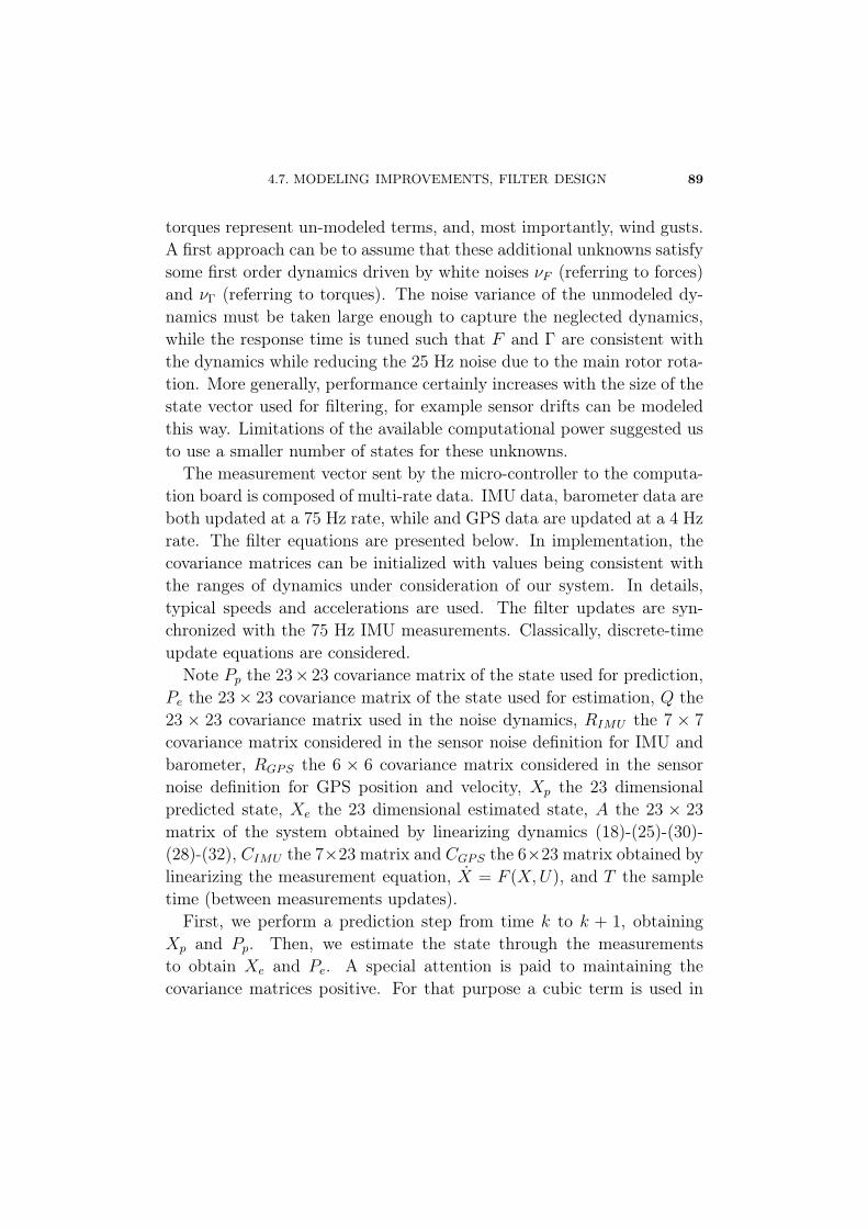
4.7. MODELING IMPROVEMENTS, FILTER DESIGN 89
torques represent un-modeled terms, and, most importantly, wind gusts.A first approach can be to assume that these additional unknowns satisfysome first order dynamics driven by white noises νF (referring to forces)and νΓ (referring to torques). The noise variance of the unmodeled dy-namics must be taken large enough to capture the neglected dynamics,while the response time is tuned such that F and Γ are consistent withthe dynamics while reducing the 25 Hz noise due to the main rotor rota-tion. More generally, performance certainly increases with the size of thestate vector used for filtering, for example sensor drifts can be modeledthis way. Limitations of the available computational power suggested usto use a smaller number of states for these unknowns.
The measurement vector sent by the micro-controller to the computa-tion board is composed of multi-rate data. IMU data, barometer data areboth updated at a 75 Hz rate, while and GPS data are updated at a 4 Hzrate. The filter equations are presented below. In implementation, thecovariance matrices can be initialized with values being consistent withthe ranges of dynamics under consideration of our system. In details,typical speeds and accelerations are used. The filter updates are syn-chronized with the 75 Hz IMU measurements. Classically, discrete-timeupdate equations are considered.
Note Pp the 23× 23 covariance matrix of the state used for prediction,Pe the 23 × 23 covariance matrix of the state used for estimation, Q the23 × 23 covariance matrix used in the noise dynamics, RIMU the 7 × 7
covariance matrix considered in the sensor noise definition for IMU andbarometer, RGPS the 6 × 6 covariance matrix considered in the sensornoise definition for GPS position and velocity, Xp the 23 dimensionalpredicted state, Xe the 23 dimensional estimated state, A the 23 × 23
matrix of the system obtained by linearizing dynamics (18)-(25)-(30)-(28)-(32), CIMU the 7×23 matrix and CGPS the 6×23 matrix obtained bylinearizing the measurement equation, X = F (X,U), and T the sampletime (between measurements updates).
First, we perform a prediction step from time k to k + 1, obtainingXp and Pp. Then, we estimate the state through the measurementsto obtain Xe and Pe. A special attention is paid to maintaining thecovariance matrices positive. For that purpose a cubic term is used in
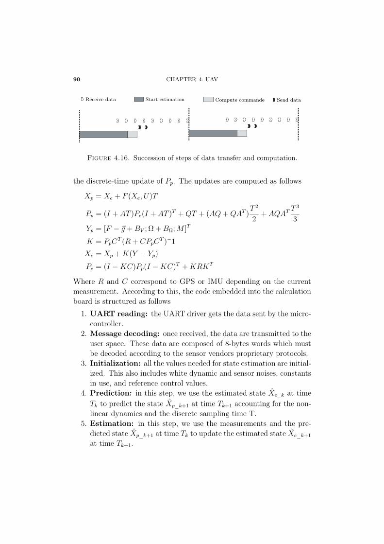
90 CHAPTER 4. UAV
Receive data Start estimation Compute commande Send data
Figure 4.16. Succession of steps of data transfer and computation.
the discrete-time update of Pp. The updates are computed as follows
Xp = Xe + F (Xe, U)T
Pp = (I + AT )Pe(I + AT )T +QT + (AQ+QAT )T 2
2+ AQAT
T 3
3Yp = [F − �g +BV ; Ω +BΩ;M ]T
K = PpCT (R + CPpC
T )−1
Xe = Xp +K(Y − Yp)
Pe = (I −KC)Pp(I −KC)T +KRKT
Where R and C correspond to GPS or IMU depending on the currentmeasurement. According to this, the code embedded into the calculationboard is structured as follows
1. UART reading: the UART driver gets the data sent by the micro-controller.
2. Message decoding: once received, the data are transmitted to theuser space. These data are composed of 8-bytes words which mustbe decoded according to the sensor vendors proprietary protocols.
3. Initialization: all the values needed for state estimation are initial-ized. This also includes white dynamic and sensor noises, constantsin use, and reference control values.
4. Prediction: in this step, we use the estimated state Xe_k at timeTk to predict the state Xp_k+1 at time Tk+1 accounting for the non-linear dynamics and the discrete sampling time T.
5. Estimation: in this step, we use the measurements and the pre-dicted state Xp_k+1 at time Tk to update the estimated state Xe_k+1
at time Tk+1.
4.7. MODELING IMPROVEMENTS, FILTER DESIGN 91
6. Control: new values of the control are computed with, e.g., a statefeedback on the estimated state.
7. Sending orders: the UART driver is used (in interrupt mode) totransmit control values back to the micro-controller. In turn, themicro-controllers acts upon the servos.
These tasks are scheduled according to the chart given in Figure 4.16.The main loop detailed above is executed at a 75 Hz rate (approx. every13.33 ms). Among the numerous tasks, the filter calculations take ap-proximatively 6 ms, while receiving the data takes about 10 ms (mostlywaiting time), and computing and sending back the control values takes1 ms. An interrupt driven approach much be used to run all these taskwithin the allowed 13.33 ms.
4.7.2. Details of the prediction step. — In this subsection, we wishto expose the numerous details and phenomena we take into account inthe model. In particular, we detail the identification of physical parame-ters, the effect of the collective pitch and the induced speed, the groundeffect, the effect of the tail rotor pitch control, and the effect of the lon-gitudinal and lateral cyclic pitch angles.
4.7.2.1. Identification of the inertia matrix and the center of gravity. —As mentioned in Section 4.6.1.2, we desire, for sake of state estimationaccuracy, to have good estimates of the inertia matrix and the positionof the center of gravity of our helicopter. For that purpose, we used theCAD CATIA� software ( c©Dassault Systèmes). Taking into accounttheir various geometries and densities, 688 different parts were modeledand kinematically linked together, see Figure 4.4. In particular, thebasic structure, the engine, the blades, the payload, the landing-gear,the GPS, the power supplies, the Li-Po batteries, and numerous add-ons(such as flat cables or reservoir) were modeled. The obtained informationis directly used to compute lever-arms of forces and to correct the IMUand GPS information. It should be noted that, while originally locatedunder the rotor axis, the center of gravity is now 1.9 cm behind it.
4.7.2.2. Effect of collective pitch angle in vertical climb. — The verticalmotion of the helicopter is directly impacted by the value of Θ0 whichstands for the collective pitch angle. For small inflow angles, we can
92 CHAPTER 4. UAV
model the magnitude of the generated thrust as a linear function of themean value of the angle of attack. Linearization around hovering equi-librium values yields
T = −mg − Zcol(δcol − Cols)(33)
where Zcol can be experimentally obtained as the ratio between the verti-cal acceleration and the control values δcol, Cols is the mean value of thecontrol generated by the pilot for a stationary hovering flight outside theground effect. It can be noticed that ZcolCols is greater than the gravitydue to the compensation of Coli which represents the reduction of pitchangle due to the rotor induced velocity. In practice, the control δcol isdirectly measured by the micro-controller which captures the signal sentto the servos (the fit quality of the proposed affine law can be checked inFigure 4.18).
4.7.2.3. Ground effect. — Experimentally, substantial errors of the pre-ceding model (33) are observed when the helicopter flies at low altitude.This phenomenon is a ground effect for which we propose to introducecorrective terms in (33). Generally, a helicopter flying close to the groundrequires less power than when it is flying far from it. Numerous mod-els have been proposed in the literature for this phenomenon seen onvarious aircrafts. For helicopters, [78] has proposed a ground effect the-ory appearing when the altitude is less than the main blade length. Inthis approach, an additional thrust inversely proportional to the distanceto the ground is considered. Separately, [51] proposes another point ofview, and model the induced speed as being inversely proportional to thesquare of the distance between the rotor hub and the ground, when thealtitude is less than one length of blade. Here, we simply use an expo-nentially decaying model which fits the experimental results well. Thismodel is
T = −mg − Zcol
(δcol − Cols + ColGE exp
(z
ZGE
))(34)
where Cols equals the value of the control signal sent to maintain astationary flight when the ground effect is negligible. Parameters ColGEand ZGE are positive. Their values were experimentally obtained duringsome long time hovering flights at various altitude. In Figure 4.17, we
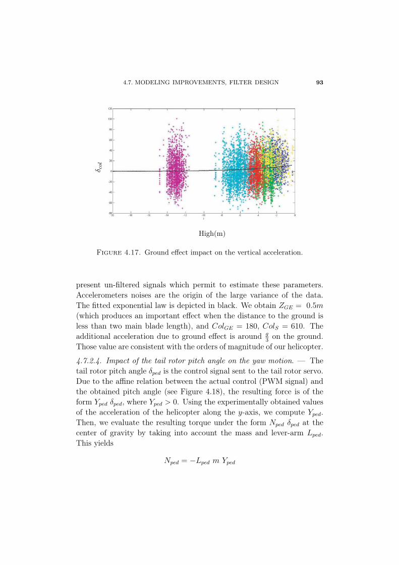
4.7. MODELING IMPROVEMENTS, FILTER DESIGN 93
High(m)
δ col
Figure 4.17. Ground effect impact on the vertical acceleration.
present un-filtered signals which permit to estimate these parameters.Accelerometers noises are the origin of the large variance of the data.The fitted exponential law is depicted in black. We obtain ZGE = 0.5m
(which produces an important effect when the distance to the ground isless than two main blade length), and ColGE = 180, ColS = 610. Theadditional acceleration due to ground effect is around g
3on the ground.
Those value are consistent with the orders of magnitude of our helicopter.
4.7.2.4. Impact of the tail rotor pitch angle on the yaw motion. — Thetail rotor pitch angle δped is the control signal sent to the tail rotor servo.Due to the affine relation between the actual control (PWM signal) andthe obtained pitch angle (see Figure 4.18), the resulting force is of theform Yped δped, where Yped > 0. Using the experimentally obtained valuesof the acceleration of the helicopter along the y-axis, we compute Yped.Then, we evaluate the resulting torque under the form Nped δped at thecenter of gravity by taking into account the mass and lever-arm Lped.This yields
Nped = −Lped m Yped
94 CHAPTER 4. UAV
In the absence of yaw variation, δped is such that the torque due to thetail rotor thrust and the torque generated by the main rotor cancel eachother. The mean value for δped during a stationary flight, noted δpeds,provides us with an estimate for the aerodynamic moment. The influenceof the tail rotor on the helicopter dynamics is as follows. It generates ay-axis force Ftail and impacts on the rotational dynamics along the r-axisby a torque Mtail = Npedδped. In details, one obtains{
Ftail = Yped δpedIZZ r = Nped(δped − δpeds)
where IZZ is the third diagonal term of the inertia matrix I. Model-ing improvements could include the impact of a variation of collectivepitch angle δcol onto the aerodynamic moment (when δcol increases, theaerodynamic moment on main blade also increases, which explains whythe engine throttle control is statically coupled to δcol in order to keepa constant angular velocity for the rotor hub). This would imply thatδpeds is in fact a function of δcol. Theoretically, this coupling could beidentified on-line but it appears to be very difficult to estimate due tothe high noise/signal ratio of the yaw gyroscope of our IMU. Therefore,we neglect this phenomenon.
4.7.2.5. Effects of the the longitudinal and lateral cyclic pitch angle ontothe horizontal motion of the helicopter. —
Flapping dynamic. — According to Equations (25) and (30), the dy-namics of the rotor hub are as follows
(35)
⎧⎪⎨⎪⎩Θ(Ψ) = Θ0 −Blat(δlat +Kdd) cos Ψ
+ Alon(δlon +Kcc) sin Ψ
Θ(Ψ) = Θ0 −Dlatδlat cos Ψ + Clonδlon sin Ψ
where Θ(Ψ) (resp Θ(Ψ)) is the blade pitch angle for the main bar (respfor the Bell-bar) which depends on Ψ the blade azimuth angle. Its formalharmonic decomposition, through the c and d variable in particular, canbe used in identification experiments to derive Kc, Kd, Alon, Blat, Clon,and Dlat. In Equation (35) collective pitch angle θ0 depends on δcol.Interestingly, these experiments can be carried out under rest conditions,and need not in-flight data (swashplate is a "kinematic" device).

4.7. MODELING IMPROVEMENTS, FILTER DESIGN 95
(a)
(b)(c)
(d)
Figure 4.18. Affine relation between (a) δlon and Θ, (b) δlonand Θ,(c) δcol and Θ0, (d) δped and pitch angle for tail rotor.
The static gains Alon, Blat, Clon and Dlat play a role in the main rotorand the Bell-bar. The control variables δlon and δlat are such that theirzero values correspond to a null pitch angle of the blade (without takinginto account collective angle of attack). The static gain Clon (resp Dlat)is the gain between cyclic controls and the pitch angle of Bell-bar. Itis directly measured by aligning the Bell-bar with the lateral axis (resplongitudinal axis), see Figure 4.18(a). Similarly, Alon (resp. Blat) wasexperimentally obtained while keeping the Bell-bar horizontal, see Fig-ure 4.18.
The amplifying effect of the Bell-bar on control variables is character-ized by the two gains AC = AlonKc and BD = BlatKd. Those two gainswere measured as the ratio between the angle of attack of the Bell-barand the main bar, for various values of c and d see Figure 4.18. The rotorhub spring constant kβ was obtained by attaching masses on main bladeand measuring the return torque as a function of flapping of the mainbar see Figure 4.19). The gain AB = 8
γΩ2
kβ
Iβmay be computed vias the
value of Iβ (obtained from CATIA c©Dassault Systèmes)
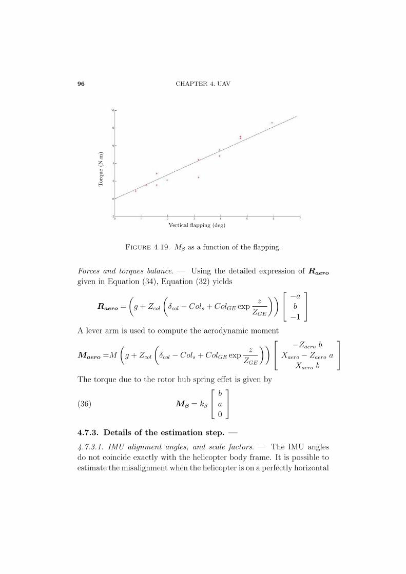
96 CHAPTER 4. UAV
Tor
que
(N.m
)
Vertical flapping (deg)
Figure 4.19. Mβ as a function of the flapping.
Forces and torques balance. — Using the detailed expression of Raero
given in Equation (34), Equation (32) yields
Raero =
(g + Zcol
(δcol − Cols + ColGE exp
z
ZGE
))⎡⎣ −ab
−1
⎤⎦A lever arm is used to compute the aerodynamic moment
Maero =M
(g + Zcol
(δcol − Cols + ColGE exp
z
ZGE
))⎡⎣ −Zaero bXaero − Zaero a
Xaero b
⎤⎦The torque due to the rotor hub spring effet is given by
(36) Mβ = kβ
⎡⎣ b
a
0
⎤⎦4.7.3. Details of the estimation step. —
4.7.3.1. IMU alignment angles, and scale factors. — The IMU anglesdo not coincide exactly with the helicopter body frame. It is possible toestimate the misalignment when the helicopter is on a perfectly horizontal
4.7. MODELING IMPROVEMENTS, FILTER DESIGN 97
ground. In this setup, the gravity vector −g is clearly visible on theaccelerometers. Then, Equation (17) yields estimates for the roll andpitch angles. ⎡⎣ Γx
ΓyΓz
⎤⎦ =
⎡⎣ g sin θm−g sinφm cos θm−g cosφm cos θm
⎤⎦Accuracy can be gained by accounting for the accelerometers scale factorswhich can be estimated from the absolute value of the gravity g.
These obtained factors are used at a low-level in the measurementsoftware to derive accurate acceleration and rate of turn information.
4.7.3.2. Sensor lever arms. — As already discussed in 4.7.3.1, the sen-sors are not located at the center of gravity of the helicopter. Therefore,great care must be taken when interpreting their measurements.
In particular, the sensed accelerations are different from those of thecenter of gravity. Consider [ximuyimuzimu]
T the position of the center ofthe IMU and note XIMU , ZIMU the two distances between the IMUcenter and the center of gravity of the helicopter. We have⎡⎣ x
y
z
⎤⎦Ri
=
⎡⎣ ximuyimuzimu
⎤⎦Ri
−
⎡⎣ XIMU
0
ZIMU
⎤⎦Rb
UG/Ri= U imu/Ri
− Ω ×
⎡⎣ XIMU
0
ZIMU
⎤⎦Rb
= U imu/Ri−
⎡⎣ ZIMUq
XIMUr − ZIMUp
−XIMUq
⎤⎦Rb
ΓG/Ri= Γimu/Ri
−
⎡⎣ ZIMUq
XIMUr − ZIMUp
−XIMUq
⎤⎦Rb
− Ω ×
⎡⎣ ZIMUq
XIMUr − ZIMUp
−XIMUq
⎤⎦Rb
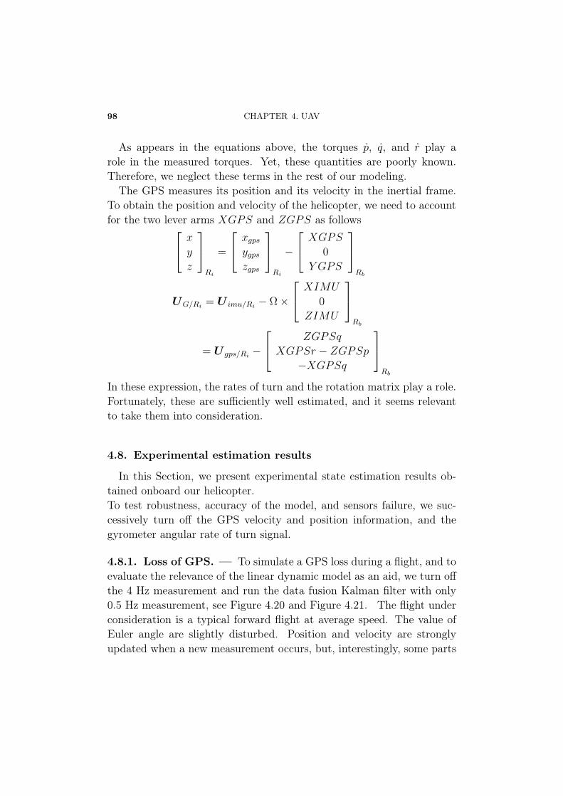
98 CHAPTER 4. UAV
As appears in the equations above, the torques p, q, and r play arole in the measured torques. Yet, these quantities are poorly known.Therefore, we neglect these terms in the rest of our modeling.
The GPS measures its position and its velocity in the inertial frame.To obtain the position and velocity of the helicopter, we need to accountfor the two lever arms XGPS and ZGPS as follows⎡⎣ x
y
z
⎤⎦Ri
=
⎡⎣ xgpsygpszgps
⎤⎦Ri
−
⎡⎣ XGPS
0
Y GPS
⎤⎦Rb
UG/Ri= U imu/Ri
− Ω ×
⎡⎣ XIMU
0
ZIMU
⎤⎦Rb
= U gps/Ri−
⎡⎣ ZGPSq
XGPSr − ZGPSp
−XGPSq
⎤⎦Rb
In these expression, the rates of turn and the rotation matrix play a role.Fortunately, these are sufficiently well estimated, and it seems relevantto take them into consideration.
4.8. Experimental estimation results
In this Section, we present experimental state estimation results ob-tained onboard our helicopter.To test robustness, accuracy of the model, and sensors failure, we suc-cessively turn off the GPS velocity and position information, and thegyrometer angular rate of turn signal.
4.8.1. Loss of GPS. — To simulate a GPS loss during a flight, and toevaluate the relevance of the linear dynamic model as an aid, we turn offthe 4 Hz measurement and run the data fusion Kalman filter with only0.5 Hz measurement, see Figure 4.20 and Figure 4.21. The flight underconsideration is a typical forward flight at average speed. The value ofEuler angle are slightly disturbed. Position and velocity are stronglyupdated when a new measurement occurs, but, interestingly, some parts
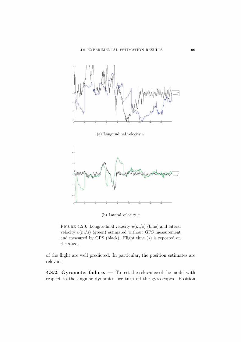
4.8. EXPERIMENTAL ESTIMATION RESULTS 99
(a) Longitudinal velocity u
(b) Lateral velocity v
Figure 4.20. Longitudinal velocity u(m/s) (blue) and lateralvelocity v(m/s) (green) estimated without GPS measurementand measured by GPS (black). Flight time (s) is reported onthe x-axis.
of the flight are well predicted. In particular, the position estimates arerelevant.
4.8.2. Gyrometer failure. — To test the relevance of the model withrespect to the angular dynamics, we turn off the gyroscopes. Position
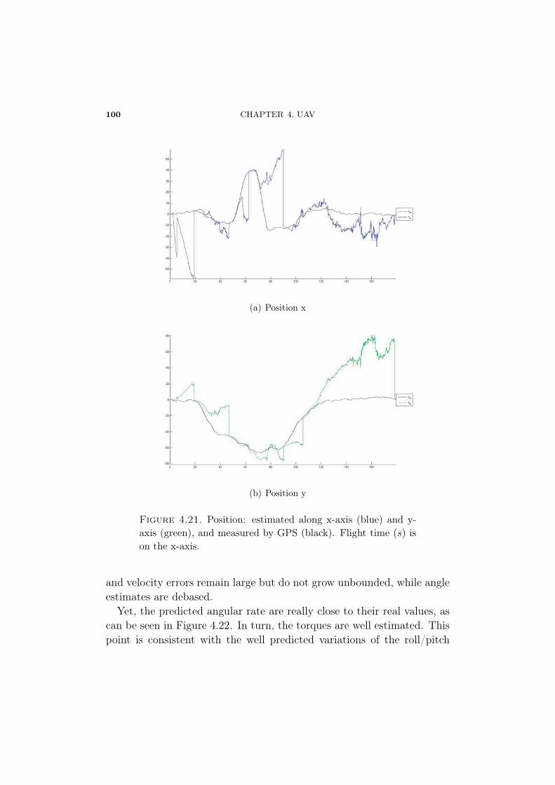
100 CHAPTER 4. UAV
(a) Position x
(b) Position y
Figure 4.21. Position: estimated along x-axis (blue) and y-axis (green), and measured by GPS (black). Flight time (s) ison the x-axis.
and velocity errors remain large but do not grow unbounded, while angleestimates are debased.
Yet, the predicted angular rate are really close to their real values, ascan be seen in Figure 4.22. In turn, the torques are well estimated. Thispoint is consistent with the well predicted variations of the roll/pitch
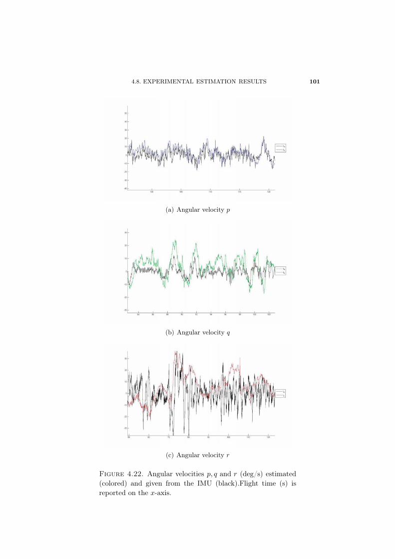
4.8. EXPERIMENTAL ESTIMATION RESULTS 101
(a) Angular velocity p
(b) Angular velocity q
(c) Angular velocity r
Figure 4.22. Angular velocities p, q and r (deg/s) estimated(colored) and given from the IMU (black).Flight time (s) isreported on the x-axis.

102 CHAPTER 4. UAV
(a) Angle φ
(b) Angle θ
(c) Angle ψ
Figure 4.23. Angle φ, θ and ψ (deg): estimated (colored) andgiven by the IMU filter (black).Flight time (s) is reported onthe x-axis.
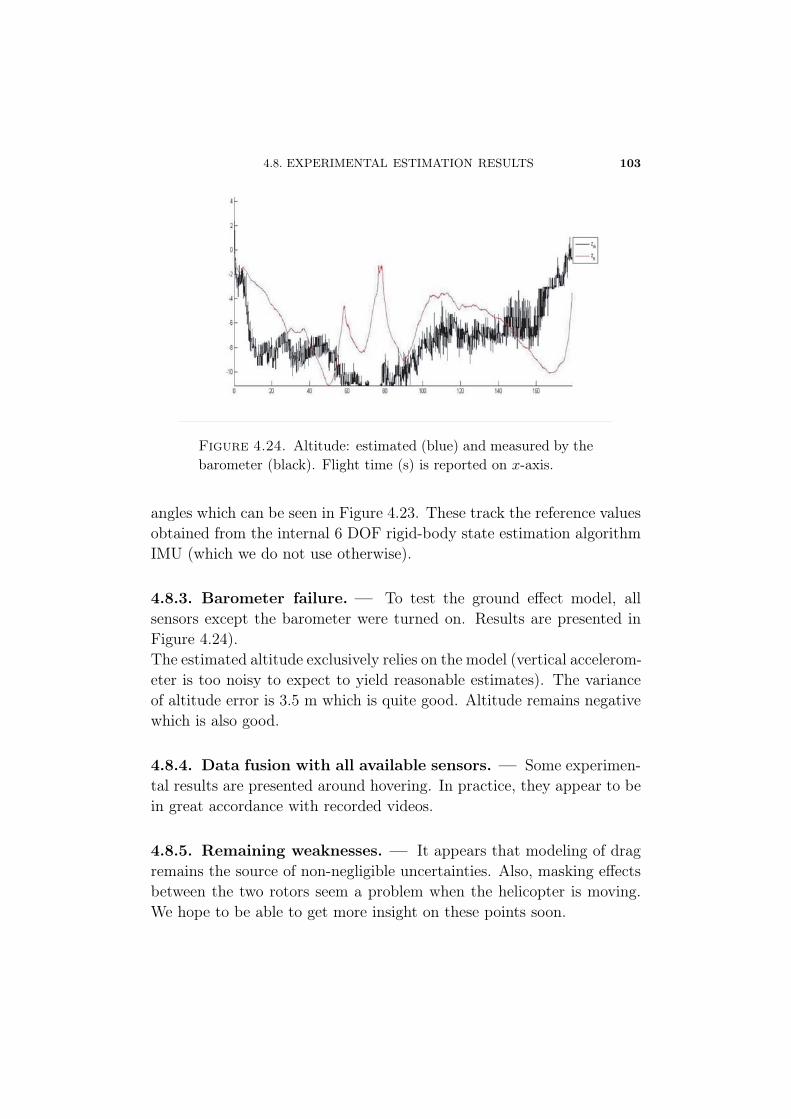
4.8. EXPERIMENTAL ESTIMATION RESULTS 103
Figure 4.24. Altitude: estimated (blue) and measured by thebarometer (black). Flight time (s) is reported on x-axis.
angles which can be seen in Figure 4.23. These track the reference valuesobtained from the internal 6 DOF rigid-body state estimation algorithmIMU (which we do not use otherwise).
4.8.3. Barometer failure. — To test the ground effect model, allsensors except the barometer were turned on. Results are presented inFigure 4.24).The estimated altitude exclusively relies on the model (vertical accelerom-eter is too noisy to expect to yield reasonable estimates). The varianceof altitude error is 3.5 m which is quite good. Altitude remains negativewhich is also good.
4.8.4. Data fusion with all available sensors. — Some experimen-tal results are presented around hovering. In practice, they appear to bein great accordance with recorded videos.
4.8.5. Remaining weaknesses. — It appears that modeling of dragremains the source of non-negligible uncertainties. Also, masking effectsbetween the two rotors seem a problem when the helicopter is moving.We hope to be able to get more insight on these points soon.
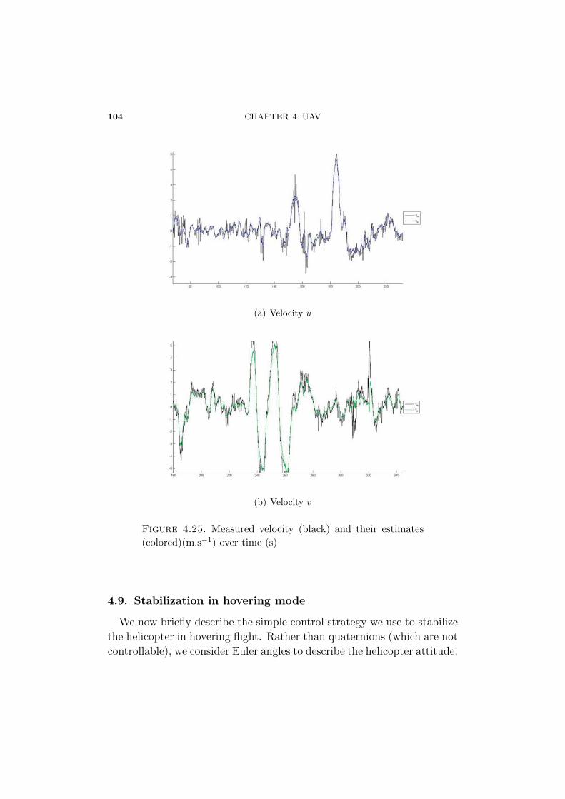
104 CHAPTER 4. UAV
(a) Velocity u
(b) Velocity v
Figure 4.25. Measured velocity (black) and their estimates(colored)(m.s−1) over time (s)
4.9. Stabilization in hovering mode
We now briefly describe the simple control strategy we use to stabilizethe helicopter in hovering flight. Rather than quaternions (which are notcontrollable), we consider Euler angles to describe the helicopter attitude.
4.9. STABILIZATION IN HOVERING MODE 105
The state variable are
[xb, yb, zb, u, v, w, φ, θ, ψ, p, q, r, a, b, c, d]T
Due to the important coupling effects of this multi-variable system, wefollow [9], and consider an LQR controller. We consider that the positionis expressed in the body frame instead of the reference frame. Implic-itly, this approach neglects changes in the initial heading angle from oneexperiment to the other. Indeed, the correction due to xb (resp yb) onlyappears in δlon (resp δlat).
Stabilizing control gains of the LQR were obtained combining a sim-ple decoupling of all axis and appropriate control variables. Weightingmatrices were obtained such that closed-loop eigenvalues were consistentwith our human pilot past experience.
The yaw controller is computed to mimic the damping of classic tailgyros controllers while preventing any overshoot during transients of theresulting second order system.
Other facts can be accounted for in the controller design, such as:slow/fast separation of open-loop eigenvalues, and the discussed cou-plings. Finally, several experiments were conducted to tune the weight-ing matrices. For collective pitch angle, tuning was chosen such that nooscillation could be observed in the controlled altitude{
δlon = −Kqq −Kθθ
q ≈ −MgZaero+kβ
IY YALONδlon − KQ
IY Yq
This yields a second order equation involving the main bar response timeτp and the inertia matrix I
1
Kθ
IY Y
Alon(kbeta −MgZaero)θ +
1
Kθ
(Kq +KQ
Alon(kβ −MgZaero))θ + θ = 0
(37)
⎧⎪⎪⎪⎨⎪⎪⎪⎩ωlon0 = 1
τf+IY Y/KQ
Kθ = ω2lon0
IY YALON(−MgZaero+kβ)
Kq = 1ALON(−MgZaero+kβ)
(2 ξ ωlon0 IY Y −KQ)
106 CHAPTER 4. UAV
Remark 3. — Due to our spring/damping system for filtering at 25 Hzwe get a resonance at 3 − 4 Hz which prevents us from using high gainon roll and pitch gyro.
Following a similar procedure for the roll axis, we get
(38)
⎧⎪⎪⎪⎪⎪⎪⎨⎪⎪⎪⎪⎪⎪⎩
δlat = −Kpp−Kφφ
ωlat0 = 1τf+IXX/KP
Kφ = ω2lat0
IXXBLAT (−MgZaero+kβ)
Kp = 1BLAT (−MgZaero+kβ)
(2 ξ ωlat0 IXX −KP )
Once this first low-level controller is designed, one can now focus onacceleration by assuming that the control acts directly on the helicopterorientation angles. This yields
δlon = −Kqq −Kθθ −Kuu−Kx(xb − xbcons)
θ ≈ −δlon −Kuu−KxxbKθ
xb ≈ −g θ −KUu
Kθ
g Kx
xb + (Ku
Kx
+KU Kθ
g Kx
) xb + xb = xbcons
the gains appearing in the previous equations, following an approachsimilar to the collective pitch control, we analyze experimental runs andstudy the pilot’s commands.
Eventually, we design a closed-loop control for the altitude and itstime derivative. Some experimental results are presented in Figure 4.29.Position estimates around hovering are reported.
4.10. Future directions
In this chapter, we have focused on incorporating important detailsabout the vehicle flight dynamics within an extended Kalman filter sys-tem. The results of estimations using an experimental small-scale heli-copter demonstrate the relevance of an approach which relies solely on
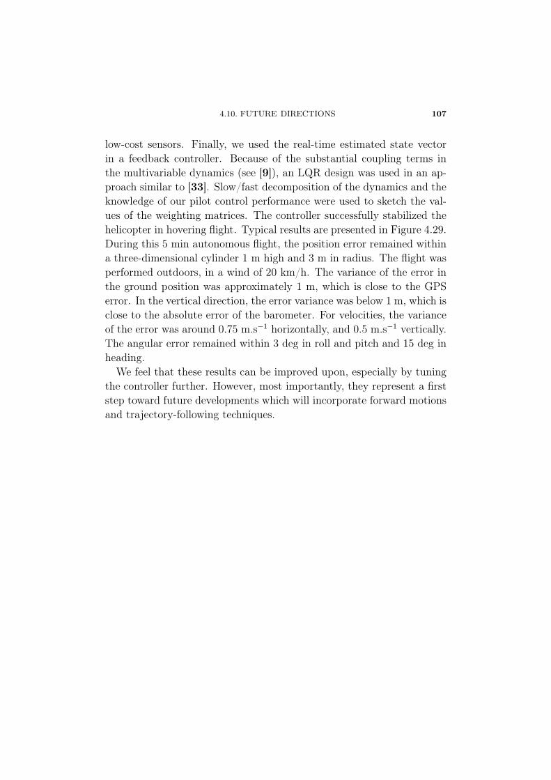
4.10. FUTURE DIRECTIONS 107
low-cost sensors. Finally, we used the real-time estimated state vectorin a feedback controller. Because of the substantial coupling terms inthe multivariable dynamics (see [9]), an LQR design was used in an ap-proach similar to [33]. Slow/fast decomposition of the dynamics and theknowledge of our pilot control performance were used to sketch the val-ues of the weighting matrices. The controller successfully stabilized thehelicopter in hovering flight. Typical results are presented in Figure 4.29.During this 5 min autonomous flight, the position error remained withina three-dimensional cylinder 1 m high and 3 m in radius. The flight wasperformed outdoors, in a wind of 20 km/h. The variance of the error inthe ground position was approximately 1 m, which is close to the GPSerror. In the vertical direction, the error variance was below 1 m, which isclose to the absolute error of the barometer. For velocities, the varianceof the error was around 0.75 m.s−1 horizontally, and 0.5 m.s−1 vertically.The angular error remained within 3 deg in roll and pitch and 15 deg inheading.
We feel that these results can be improved upon, especially by tuningthe controller further. However, most importantly, they represent a firststep toward future developments which will incorporate forward motionsand trajectory-following techniques.
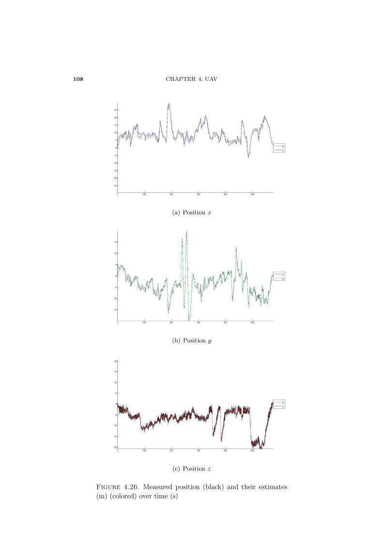
108 CHAPTER 4. UAV
(a) Position x
(b) Position y
(c) Position z
Figure 4.26. Measured position (black) and their estimates(m) (colored) over time (s)
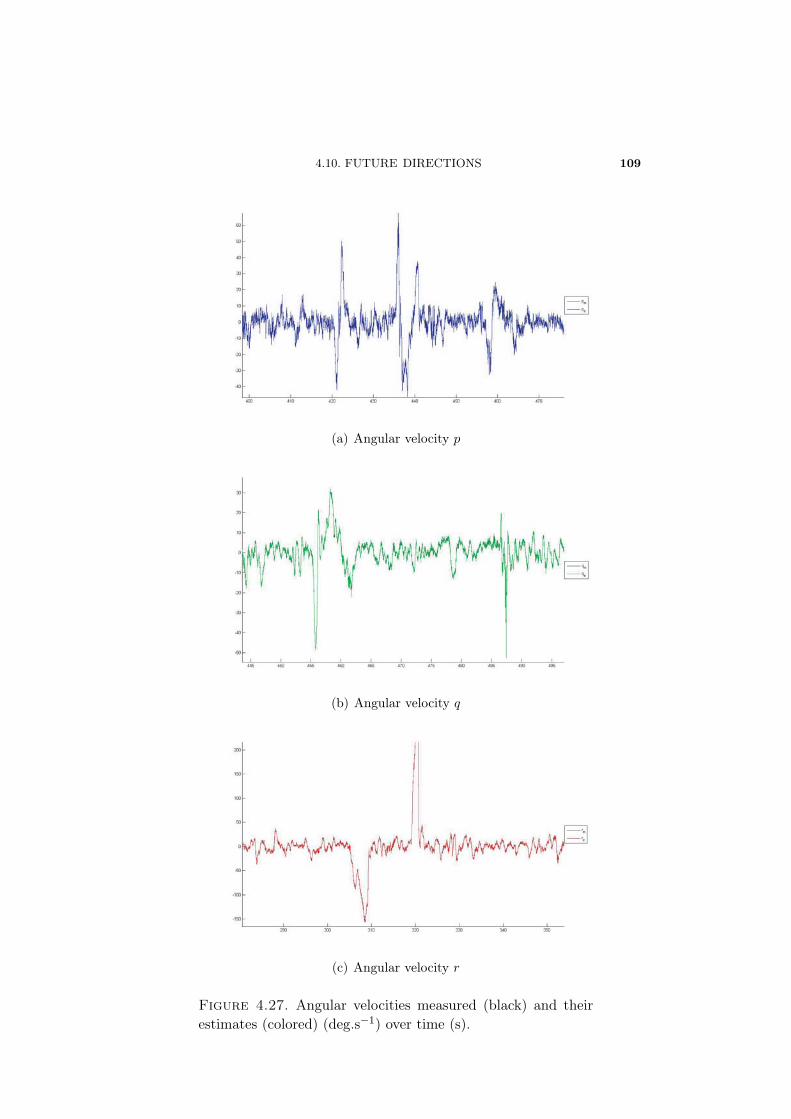
4.10. FUTURE DIRECTIONS 109
(a) Angular velocity p
(b) Angular velocity q
(c) Angular velocity r
Figure 4.27. Angular velocities measured (black) and theirestimates (colored) (deg.s−1) over time (s).
110 CHAPTER 4. UAV
(a) Angle φ
(b) Angle θ
(c) Angle ψ
Figure 4.28. Attitude angles measured (black) and their es-timates (colored) (deg), over time (s).
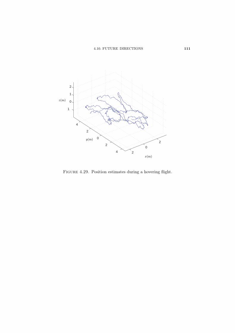
4.10. FUTURE DIRECTIONS 111
2
0
2
4
2
0
2
4
1
0
1
2
x(m)y(m)
z(m
)
x(m)
y(m)
z(m)
Figure 4.29. Position estimates during a hovering flight.

PART III
POSITIONING TECHNIQUESUSING MAGNETIC FIELD
DISTURBANCES

CHAPTER 5
TAKING ADVANTAGE OFMAGNETIC-FIELD DISTURBANCES IN
NAVIGATION
Un problème crucial pour le contrôle-commande des engins aériens outerrestres dont nous avons considéré des exemples aux Chapitres 2 et 4 estcelui de l’estimation d’état à partir des capteurs embarqués. Nous avonsmontré, pour chacun des deux exemples considérés, comment développeret mettre en œuvre des techniques d’observateurs pour le filtrage et lafusion de données multi-capteurs.
Néanmoins d’importants problèmes demeurent. En particulier, il estcommunément admis que la technologie GPS est nécessaire pour l’esti–mation des positions. L’information absolue permet un recalage, à bassefréquence, relativement aisé. Il est connu que ce signal souffre de sérieuxdéfauts: de nombreuses aberrations dues aux multi-trajets des signaux(en particulier dans les environnements urbains) peuvent apparaître subite-ment, de même que la disponibilité des différents satellites de la constel-lation peut être rapidement mise en cause du fait des obstacles. Enoutre, l’utilisation du GPS dans un contexte militaire est très probléma-tique étant donnée la facilité avec laquelle il peut être brouillé. Enfin,pour les interventions à l’intérieur de bâtiments, le GPS est totalementinutilisable (sauf, de manière très dégradée, près des fenêtres et portes).
Conscients de tous ces problèmes, nous avons cherché à développer unetechnique d’estimation de position qui n’utilise pas le GPS. A l’intérieurde bâtiments, le champ magnétique est fortement perturbé. On pourraiten conclure que les signaux magnétométriques ne sont pas exploitablesdans le cadre de la fusion de données avec des capteurs inertiels. Notreméthode vient en contradiction avec ce constat. Bien au contraire, en
116 CHAPTER 5. PEDESTRIAN
utilisant les équations de Maxwell qui structurent ces perturbations, ilest possible de déduire de précieuses informations sur le vecteur vitessedu porteur des capteurs.
We address here the problem of position estimation for a rigid bodyusing an IMU. We present a Kalman filtering technique which takes ad-vantage of the magnetic disturbances usually observed indoors. This isan important topic for military operations in urban areas, where a GPSsignal is often unavailable. This approach yields significant improve-ments in estimation accuracy. We illustrate our technique with severalexperimental results obtained with a low-cost IMU.
5.1. Introduction
As exemplified in Chapters 2 and 4, numerous military and civiliancontrol applications require high-accuracy estimations of the position,speed, and attitude of a solid body. A widely considered solution (seee.g. Chapter 3), is to use embedded IMUs. Signals from accelerometersand gyroscopes (and possibly magnetometers) can be used to derive posi-tion information through a double integration process [35, 28]. Becauseof sensor drift, this approach requires very high-precision IMUs (not be-longing to the MEMS class that we are considering) such as those found incertain full-sized aircraft, military submarines, and missiles. When cost,space, and weight constraints become stringent, other solutions need tobe used. Two prime examples are provided by the fusion of sensors inground vehicles equipped with odometers and a GPS receiver (for out-door and non-military-critical applications, as considered in Chapter 2),and computer vision using cameras for indoor robotics. It is interest-ing to get an idea of prices and the performance obtained. Typically,a ground navigator based on IMU measurements used for petroleum re-search costs more than USD 20,000, and its position estimate drifts by3 nautical miles per hour (when the navigation system is used only dur-ing maneuvers and it is manually forced to perform a zero update around
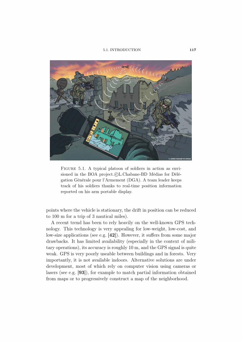
5.1. INTRODUCTION 117
Figure 5.1. A typical platoon of soldiers in action as envi-sioned in the BOA project. c©L.Chabane-BD Médias for Délé-gation Générale pour l’Armement (DGA). A team leader keepstrack of his soldiers thanks to real-time position informationreported on his arm portable display.
points where the vehicle is stationary, the drift in position can be reducedto 100 m for a trip of 3 nautical miles).
A recent trend has been to rely heavily on the well-known GPS tech-nology. This technology is very appealing for low-weight, low-cost, andlow-size applications (see e.g. [42]). However, it suffers from some majordrawbacks. It has limited availability (especially in the context of mili-tary operations), its accuracy is roughly 10 m, and the GPS signal is quiteweak. GPS is very poorly useable between buildings and in forests. Veryimportantly, it is not available indoors. Alternative solutions are underdevelopment, most of which rely on computer vision using cameras orlasers (see e.g. [93]), for example to match partial information obtainedfrom maps or to progressively construct a map of the neighborhood.
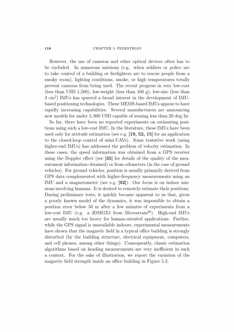
118 CHAPTER 5. PEDESTRIAN
However, the use of cameras and other optical devices often has tobe excluded. In numerous missions (e.g. when soldiers or police areto take control of a building or firefighters are to rescue people from asmoky room), lighting conditions, smoke, or high temperatures totallyprevent cameras from being used. The recent progress in very low-cost(less than USD 1,500), low-weight (less than 100 g), low-size (less than3 cm2) IMUs has spurred a broad interest in the development of IMU-based positioning technologies. These MEMS-based IMUs appear to haverapidly increasing capabilities. Several manufacturers are announcingnew models for under 5, 000 USD capable of sensing less than 20 deg/hr.
So far, there have been no reported experiments on estimating posi-tions using such a low-cost IMU. In the literature, these IMUs have beenused only for attitude estimation (see e.g. [19, 52, 15] for an applicationto the closed-loop control of mini-UAVs). Some tentative work (usinghigher-end IMUs) has addressed the problem of velocity estimation. Inthese cases, the speed information was obtained from a GPS receiverusing the Doppler effect (see [35] for details of the quality of the mea-surement information obtained) or from odometers (in the case of groundvehicles). For ground vehicles, position is usually primarily derived fromGPS data complemented with higher-frequency measurements using anIMU and a magnetometer (see e.g. [92]). Our focus is on indoor mis-sions involving humans. It is desired to remotely estimate their positions.During preliminary tests, it quickly became apparent to us that, givena poorly known model of the dynamics, it was impossible to obtain aposition error below 50 m after a few minutes of experiments from alow-cost IMU (e.g. a 3DMGX1 from Microstrain�). High-end IMUsare usually much too heavy for human-oriented applications. Further,while the GPS signal is unavailable indoors, experimental measurementshave shown that the magnetic field in a typical office building is stronglydisturbed (by the building structure, electrical equipment, computers,and cell phones, among other things). Consequently, classic estimationalgorithms based on heading measurements are very inefficient in sucha context. For the sake of illustration, we report the variation of themagnetic field strength inside an office building in Figure 5.2.
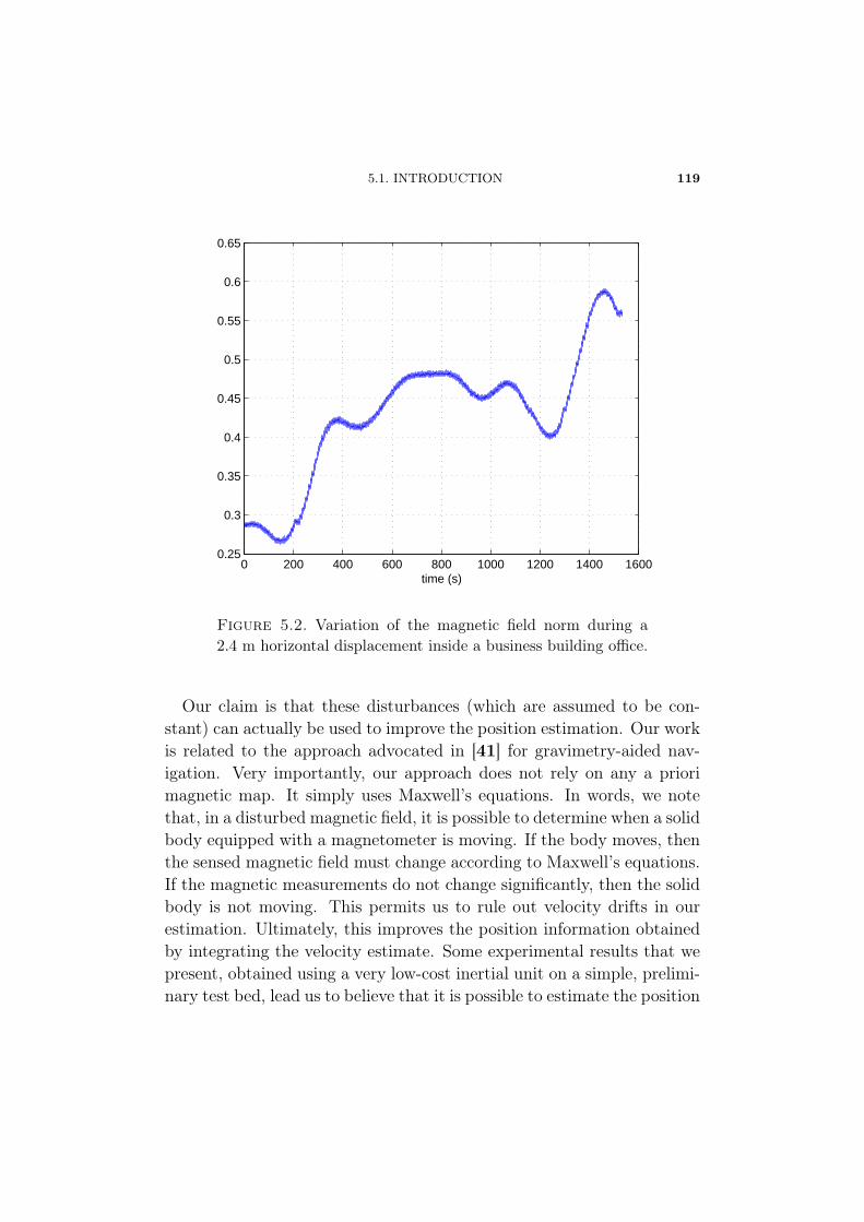
5.1. INTRODUCTION 119
0 200 400 600 800 1000 1200 1400 16000.25
0.3
0.35
0.4
0.45
0.5
0.55
0.6
0.65
time (s)
Figure 5.2. Variation of the magnetic field norm during a2.4 m horizontal displacement inside a business building office.
Our claim is that these disturbances (which are assumed to be con-stant) can actually be used to improve the position estimation. Our workis related to the approach advocated in [41] for gravimetry-aided nav-igation. Very importantly, our approach does not rely on any a priorimagnetic map. It simply uses Maxwell’s equations. In words, we notethat, in a disturbed magnetic field, it is possible to determine when a solidbody equipped with a magnetometer is moving. If the body moves, thenthe sensed magnetic field must change according to Maxwell’s equations.If the magnetic measurements do not change significantly, then the solidbody is not moving. This permits us to rule out velocity drifts in ourestimation. Ultimately, this improves the position information obtainedby integrating the velocity estimate. Some experimental results that wepresent, obtained using a very low-cost inertial unit on a simple, prelimi-nary test bed, lead us to believe that it is possible to estimate the position
120 CHAPTER 5. PEDESTRIAN
of a man carrying a low-cost IMU who is taking part in the investing of abuilding. This objective fits into the context of network-centric warfare(as defined in [70]), and was studied in the project “Bulle OpérationnelleAéroterrestre” (BOA), led by the Délégation Générale pour l’Armement(DGA) for the French Department of Defense. A typical mission in theBOA environment is depicted in Figure 5.1.
The chapter is organized as follows. In Section 5.2, we define theposition estimation problem. The notation required is presented. InSection 5.3, we describe our use of magnetic disturbances. In particular,we focus on eliminating bias in velocity estimates. In Section 5.4, wepresent some experimental results and give implementation details. InSection 5.5, we conclude, and suggest several directions for improvement.
5.2. Problem statement
We do not describe in details the dynamics sensed by the IMU. Ourprimary goal is to stress the information from the magnetic sensor thatcan be exploited. When actually implementing the estimation filter, weoften include numerous terms in the dynamics model for sake of accuracy,but very good estimates can be recovered from the basic equations wepresent here.
5.2.1. Coordinate frames, system of equations, notations. —We consider the motion of an IMU (viewed as a material point) located atthe center of gravity of a moving body we wish to estimate the position of.The system can simultaneously rotate and translate. It has six degreesof freedom. A body reference fixed frame with origin at the center ofgravity of the IMU can be considered. In that case, the x, y and z axisare the IMU axis (i.e. are consistent with the inner sensors orientations).In the following, subscript b refers to this body frame.
As inertial reference frame, we consider the NED frame: North-East-Down, the x axis is tangent to the geoid and is pointing to the north, thez axis is pointing to the center of the earth, and the y axis is tangent tothe geoid and is pointing to the East. Subscript i refers to this inertialframe.
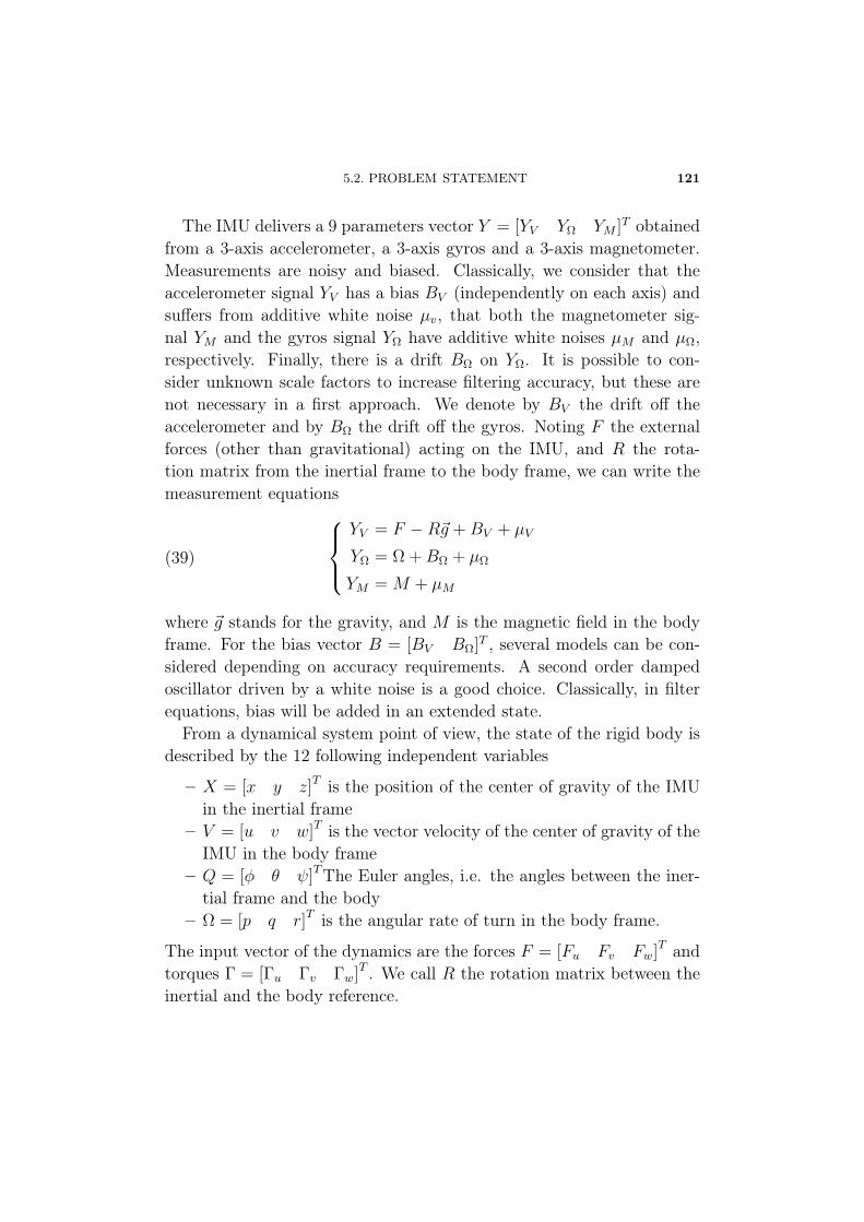
5.2. PROBLEM STATEMENT 121
The IMU delivers a 9 parameters vector Y = [YV YΩ YM ]T obtainedfrom a 3-axis accelerometer, a 3-axis gyros and a 3-axis magnetometer.Measurements are noisy and biased. Classically, we consider that theaccelerometer signal YV has a bias BV (independently on each axis) andsuffers from additive white noise μv, that both the magnetometer sig-nal YM and the gyros signal YΩ have additive white noises μM and μΩ,respectively. Finally, there is a drift BΩ on YΩ. It is possible to con-sider unknown scale factors to increase filtering accuracy, but these arenot necessary in a first approach. We denote by BV the drift off theaccelerometer and by BΩ the drift off the gyros. Noting F the externalforces (other than gravitational) acting on the IMU, and R the rota-tion matrix from the inertial frame to the body frame, we can write themeasurement equations
(39)
⎧⎪⎨⎪⎩YV = F −R�g +BV + μV
YΩ = Ω +BΩ + μΩ
YM = M + μM
where �g stands for the gravity, and M is the magnetic field in the bodyframe. For the bias vector B = [BV BΩ]T , several models can be con-sidered depending on accuracy requirements. A second order dampedoscillator driven by a white noise is a good choice. Classically, in filterequations, bias will be added in an extended state.
From a dynamical system point of view, the state of the rigid body isdescribed by the 12 following independent variables
– X = [x y z]T is the position of the center of gravity of the IMUin the inertial frame
– V = [u v w]T is the vector velocity of the center of gravity of theIMU in the body frame
– Q = [φ θ ψ]TThe Euler angles, i.e. the angles between the iner-tial frame and the body
– Ω = [p q r]T is the angular rate of turn in the body frame.
The input vector of the dynamics are the forces F = [Fu Fv Fw]T andtorques Γ = [Γu Γv Γw]T . We call R the rotation matrix between theinertial and the body reference.
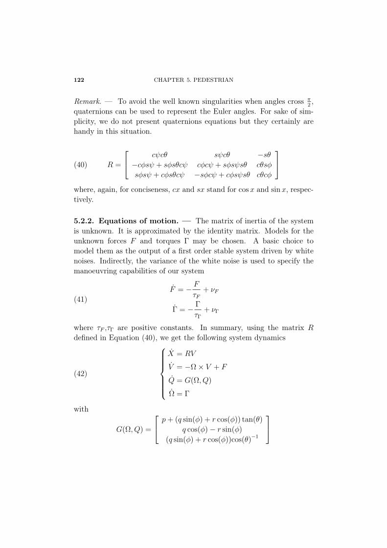
122 CHAPTER 5. PEDESTRIAN
Remark. — To avoid the well known singularities when angles cross π2,
quaternions can be used to represent the Euler angles. For sake of sim-plicity, we do not present quaternions equations but they certainly arehandy in this situation.
R =
⎡⎣ cψcθ sψcθ −sθ−cφsψ + sφsθcψ cφcψ + sφsψsθ cθsφ
sφsψ + cφsθcψ −sφcψ + cφsψsθ cθcφ
⎤⎦(40)
where, again, for conciseness, cx and sx stand for cos x and sin x, respec-tively.
5.2.2. Equations of motion. — The matrix of inertia of the systemis unknown. It is approximated by the identity matrix. Models for theunknown forces F and torques Γ may be chosen. A basic choice tomodel them as the output of a first order stable system driven by whitenoises. Indirectly, the variance of the white noise is used to specify themanoeuvring capabilities of our system
(41)F = − F
τF+ νF
Γ = − Γ
τΓ+ νΓ
where τF ,τΓ are positive constants. In summary, using the matrix R
defined in Equation (40), we get the following system dynamics
(42)
⎧⎪⎪⎪⎪⎪⎨⎪⎪⎪⎪⎪⎩
X = RV
V = −Ω × V + F
Q = G(Ω, Q)
Ω = Γ
with
G(Ω, Q) =
⎡⎣ p+ (q sin(φ) + r cos(φ)) tan(θ)
q cos(φ) − r sin(φ)
(q sin(φ) + r cos(φ))cos(θ)−1
⎤⎦
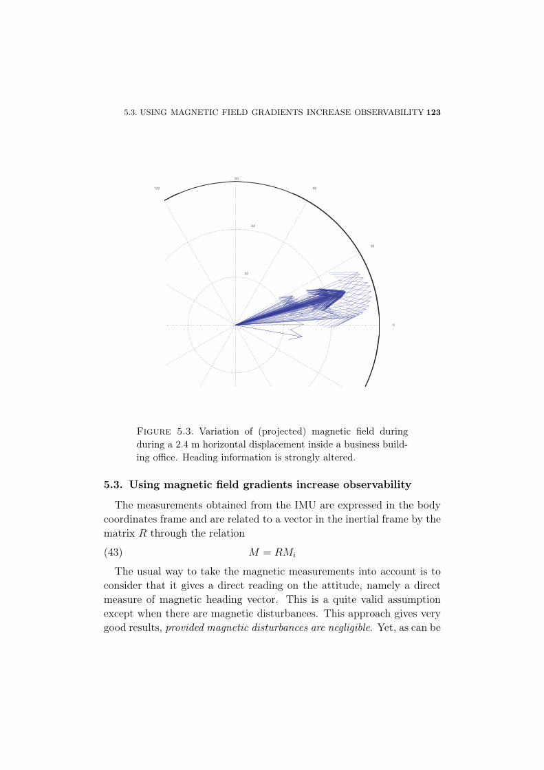
5.3. USING MAGNETIC FIELD GRADIENTS INCREASE OBSERVABILITY 123
0.2
0.4
0.9
30
60120
0
Figure 5.3. Variation of (projected) magnetic field duringduring a 2.4 m horizontal displacement inside a business build-ing office. Heading information is strongly altered.
5.3. Using magnetic field gradients increase observability
The measurements obtained from the IMU are expressed in the bodycoordinates frame and are related to a vector in the inertial frame by thematrix R through the relation
M = RMi(43)
The usual way to take the magnetic measurements into account is toconsider that it gives a direct reading on the attitude, namely a directmeasure of magnetic heading vector. This is a quite valid assumptionexcept when there are magnetic disturbances. This approach gives verygood results, provided magnetic disturbances are negligible. Yet, as can be
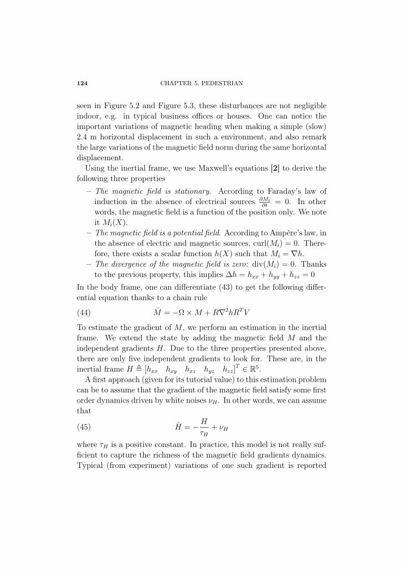
124 CHAPTER 5. PEDESTRIAN
seen in Figure 5.2 and Figure 5.3, these disturbances are not negligibleindoor, e.g. in typical business offices or houses. One can notice theimportant variations of magnetic heading when making a simple (slow)2.4 m horizontal displacement in such a environment, and also remarkthe large variations of the magnetic field norm during the same horizontaldisplacement.
Using the inertial frame, we use Maxwell’s equations [2] to derive thefollowing three properties
– The magnetic field is stationary. According to Faraday’s law ofinduction in the absence of electrical sources ∂Mi
∂t= 0. In other
words, the magnetic field is a function of the position only. We noteit Mi(X).
– The magnetic field is a potential field. According to Ampère’s law, inthe absence of electric and magnetic sources, curl(Mi) = 0. There-fore, there exists a scalar function h(X) such that Mi = ∇h.
– The divergence of the magnetic field is zero: div(Mi) = 0. Thanksto the previous property, this implies Δh = hxx + hyy + hzz = 0
In the body frame, one can differentiate (43) to get the following differ-ential equation thanks to a chain rule
M = −Ω ×M +R∇2hRTV(44)
To estimate the gradient of M , we perform an estimation in the inertialframe. We extend the state by adding the magnetic field M and theindependent gradients H. Due to the three properties presented above,there are only five independent gradients to look for. These are, in theinertial frame H � [hxx hxy hxz hyz hzz]
T ∈ R5.
A first approach (given for its tutorial value) to this estimation problemcan be to assume that the gradient of the magnetic field satisfy some firstorder dynamics driven by white noises νH . In other words, we can assumethat
H = −H
τH+ νH(45)
where τH is a positive constant. In practice, this model is not really suf-ficient to capture the richness of the magnetic field gradients dynamics.Typical (from experiment) variations of one such gradient is reported
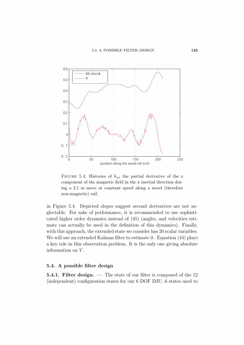
5.4. A POSSIBLE FILTER DESIGN 125
0 50 100 150 200 2500. 2
0. 1
0
0.1
0.2
0.3
0.4
0.5
0.6
position along the wood rail (cm)
Mz discretff
Figure 5.4. Histories of hzx the partial derivative of the zcomponent of the magnetic field in the x inertial direction dur-ing a 2.1 m move at constant speed along a wood (thereforenon-magnetic) rail.
in Figure 5.4. Depicted slopes suggest second derivatives are not ne-glectable. For sake of performance, it is recommended to use sophisti-cated higher order dynamics instead of (45) (angles, and velocities esti-mate can actually be used in the definition of this dynamics). Finally,with this approach, the extended state we consider has 20 scalar variables.We will use an extended Kalman filter to estimate it. Equation (44) playsa key role in this observation problem. It is the only one giving absoluteinformation on V .
5.4. A possible filter design
5.4.1. Filter design. — The state of our filter is composed of the 12(independent) configuration states for our 6 DOF IMU, 6 states used to
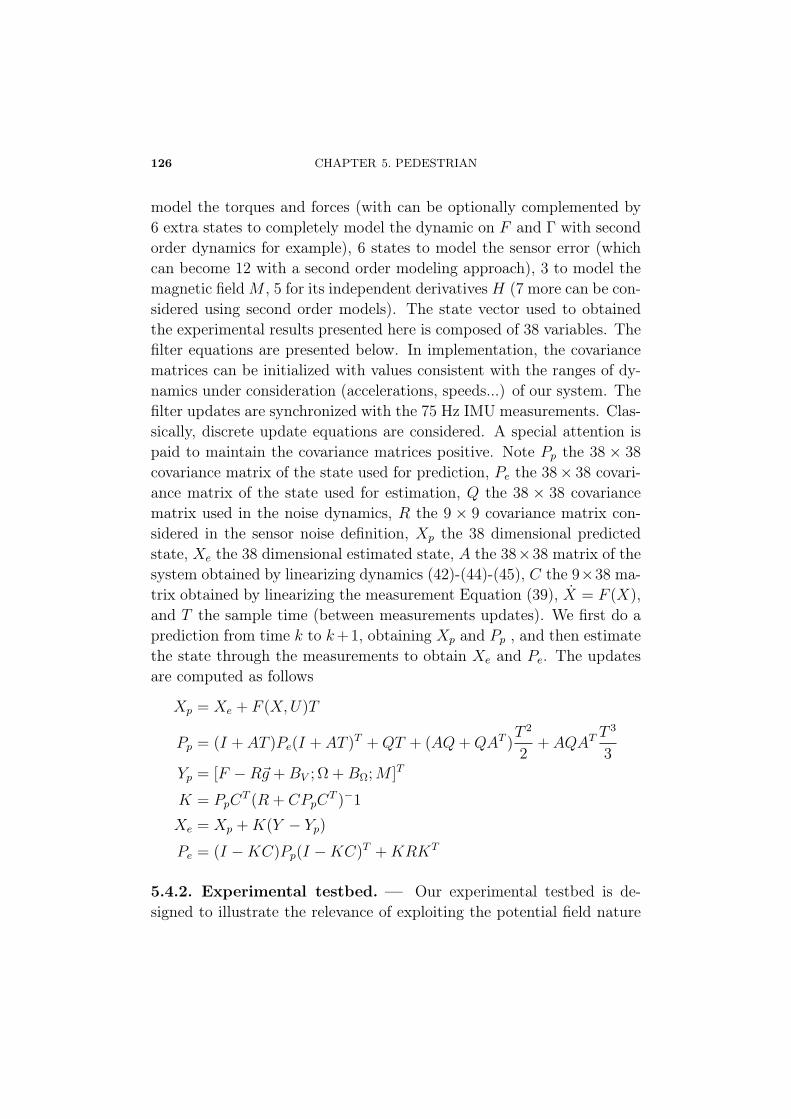
126 CHAPTER 5. PEDESTRIAN
model the torques and forces (with can be optionally complemented by6 extra states to completely model the dynamic on F and Γ with secondorder dynamics for example), 6 states to model the sensor error (whichcan become 12 with a second order modeling approach), 3 to model themagnetic field M , 5 for its independent derivatives H (7 more can be con-sidered using second order models). The state vector used to obtainedthe experimental results presented here is composed of 38 variables. Thefilter equations are presented below. In implementation, the covariancematrices can be initialized with values consistent with the ranges of dy-namics under consideration (accelerations, speeds...) of our system. Thefilter updates are synchronized with the 75 Hz IMU measurements. Clas-sically, discrete update equations are considered. A special attention ispaid to maintain the covariance matrices positive. Note Pp the 38 × 38
covariance matrix of the state used for prediction, Pe the 38× 38 covari-ance matrix of the state used for estimation, Q the 38 × 38 covariancematrix used in the noise dynamics, R the 9 × 9 covariance matrix con-sidered in the sensor noise definition, Xp the 38 dimensional predictedstate, Xe the 38 dimensional estimated state, A the 38×38 matrix of thesystem obtained by linearizing dynamics (42)-(44)-(45), C the 9×38 ma-trix obtained by linearizing the measurement Equation (39), X = F (X),and T the sample time (between measurements updates). We first do aprediction from time k to k+1, obtaining Xp and Pp , and then estimatethe state through the measurements to obtain Xe and Pe. The updatesare computed as follows
Xp = Xe + F (X,U)T
Pp = (I + AT )Pe(I + AT )T +QT + (AQ+QAT )T 2
2+ AQAT
T 3
3Yp = [F −R�g +BV ; Ω +BΩ;M ]T
K = PpCT (R + CPpC
T )−1
Xe = Xp +K(Y − Yp)
Pe = (I −KC)Pp(I −KC)T +KRKT
5.4.2. Experimental testbed. — Our experimental testbed is de-signed to illustrate the relevance of exploiting the potential field nature
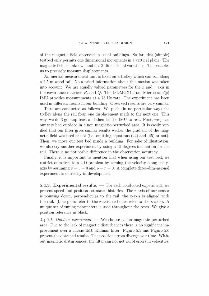
5.4. A POSSIBLE FILTER DESIGN 127
of the magnetic field observed in usual buildings. So far, this (simple)testbed only permits one dimensional movements in a vertical plane. Themagnetic field is unknown and has 3-dimensional variations. This enablesus to precisely measure displacements.
An inertial measurement unit is fixed on a trolley which can roll alonga 2.5 m wood rail. No a priori information about this motion was takeninto account. We use equally valued parameters for the x and z axis inthe covariance matrices Pe and Q. The (3DMGX1 from Microstrain�)IMU provides measurements at a 75 Hz rate. The experiment has beenused in different rooms in our building. Observed results are very similar.
Tests are conducted as follows. We push (in no particular way) thetrolley along the rail from one displacement mark to the next one. Thisway, we do 3 go-stop-back and then let the IMU to rest. First, we placeour test bed outdoor in a non magnetic-perturbed area. It is easily ver-ified that our filter gives similar results wether the gradient of the mag-netic field was used or not (i.e. omitting equations (44) and (45) or not).Then, we move our test bed inside a building. For sake of illustration,we also try another experiment by using a 15 degrees inclination for therail. There is no noticeable difference in the observation accuracy.
Finally, it is important to mention that when using our test bed, werestrict ourselves to a 2-D problem by zeroing the velocity along the y-axis by assuming y = v = 0 and p = r = 0. A complete three-dimensionalexperiment is currently in development.
5.4.3. Experimental results. — For each conducted experiment, wepresent speed and position estimates histories. The z-axis of our sensoris pointing down, perpendicular to the rail, the x-axis is aligned withthe rail. (blue plots refer to the z-axis, red ones refer to the x-axis). Aunique set of tuning parameters is used throughout the tests. We give aposition reference in black.
5.4.3.1. Outdoor experiment. — We choose a non magnetic perturbedarea. Due to the lack of magnetic disturbances there is no significant im-provement over a classic IMU Kalman filter. Figure 5.5 and Figure 5.6present the obtained results. The position errors diverge over time. With-out magnetic disturbances, the filter can not get rid of errors in velocities.
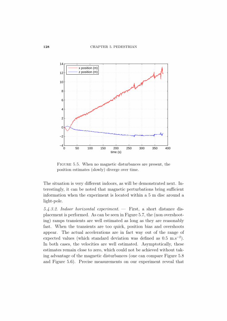
128 CHAPTER 5. PEDESTRIAN
0 50 100 150 200 250 300 350 400−4
−2
0
2
4
6
8
10
12
14
time (s)
x position (m)z position (m)
Figure 5.5. When no magnetic disturbances are present, theposition estimates (slowly) diverge over time.
The situation is very different indoors, as will be demonstrated next. In-terestingly, it can be noted that magnetic perturbations bring sufficientinformation when the experiment is located within a 5 m disc around alight-pole.
5.4.3.2. Indoor horizontal experiment. — First, a short distance dis-placement is performed. As can be seen in Figure 5.7, the (non overshoot-ing) ramps transients are well estimated as long as they are reasonablyfast. When the transients are too quick, position bias and overshootsappear. The actual accelerations are in fact way out of the range ofexpected values (which standard deviation was defined as 0.5 m.s−2).In both cases, the velocities are well estimated. Asymptotically, theseestimates remain close to zero, which could not be achieved without tak-ing advantage of the magnetic disturbances (one can compare Figure 5.8and Figure 5.6). Precise measurements on our experiment reveal that
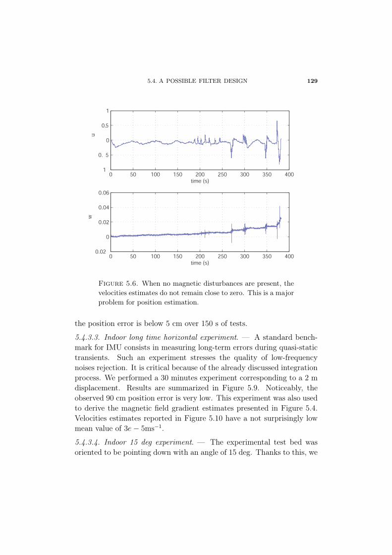
5.4. A POSSIBLE FILTER DESIGN 129
0 50 100 150 200 250 300 350 4001
0. 5
0
0.5
1
time (s)
u
0 50 100 150 200 250 300 350 4000.02
0
0.02
0.04
0.06
time (s)
w
Figure 5.6. When no magnetic disturbances are present, thevelocities estimates do not remain close to zero. This is a majorproblem for position estimation.
the position error is below 5 cm over 150 s of tests.
5.4.3.3. Indoor long time horizontal experiment. — A standard bench-mark for IMU consists in measuring long-term errors during quasi-statictransients. Such an experiment stresses the quality of low-frequencynoises rejection. It is critical because of the already discussed integrationprocess. We performed a 30 minutes experiment corresponding to a 2 mdisplacement. Results are summarized in Figure 5.9. Noticeably, theobserved 90 cm position error is very low. This experiment was also usedto derive the magnetic field gradient estimates presented in Figure 5.4.Velocities estimates reported in Figure 5.10 have a not surprisingly lowmean value of 3e− 5ms−1.
5.4.3.4. Indoor 15 deg experiment. — The experimental test bed wasoriented to be pointing down with an angle of 15 deg. Thanks to this, we
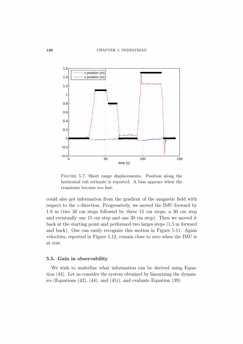
130 CHAPTER 5. PEDESTRIAN
0 50 100 150−0.4
−0.2
0
0.2
0.4
0.6
0.8
1
1.2
1.4
1.6
time (s)
x position (m)z position (m)
Figure 5.7. Short range displacements. Position along thehorizontal rail estimate is reported. A bias appears when thetransients become too fast.
could also get information from the gradient of the magnetic field withrespect to the z-direction. Progressively, we moved the IMU forward by1.8 m (two 30 cm steps followed by three 15 cm steps, a 30 cm stepand eventually one 15 cm step and one 30 cm step). Then we moved itback at the starting point and performed two larges steps (1.5 m forwardand back). One can easily recognize this motion in Figure 5.11. Againvelocities, reported in Figure 5.12, remain close to zero when the IMU isat rest.
5.5. Gain in observability
We wish to underline what information can be derived using Equa-tion (44). Let us consider the system obtained by linearizing the dynam-ics (Equations (42), (44), and (45)), and evaluate Equation (39).
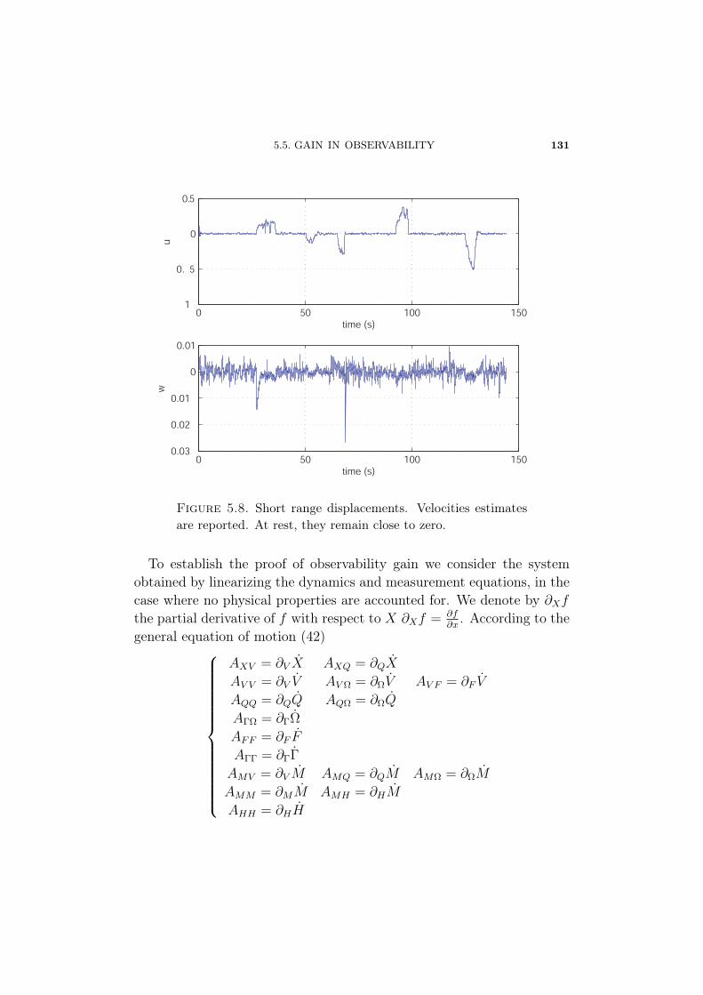
5.5. GAIN IN OBSERVABILITY 131
0 50 100 1501
0. 5
0
0.5
time (s)
u
0 50 100 1500.03
0.02
0.01
0
0.01
time (s)
w
Figure 5.8. Short range displacements. Velocities estimatesare reported. At rest, they remain close to zero.
To establish the proof of observability gain we consider the systemobtained by linearizing the dynamics and measurement equations, in thecase where no physical properties are accounted for. We denote by ∂Xfthe partial derivative of f with respect to X ∂Xf = ∂f
∂x. According to the
general equation of motion (42)⎧⎪⎪⎪⎪⎪⎪⎪⎪⎪⎪⎪⎪⎪⎨⎪⎪⎪⎪⎪⎪⎪⎪⎪⎪⎪⎪⎪⎩
AXV = ∂V X AXQ = ∂QX
AV V = ∂V V AV Ω = ∂ΩV AV F = ∂F V
AQQ = ∂QQ AQΩ = ∂ΩQ
AΓΩ = ∂ΓΩ
AFF = ∂F F
AΓΓ = ∂ΓΓ
AMV = ∂V M AMQ = ∂QM AMΩ = ∂ΩM
AMM = ∂MM AMH = ∂HM
AHH = ∂HH
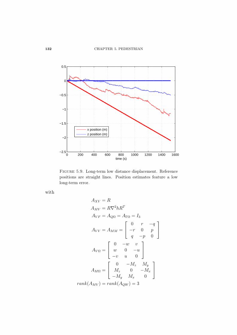
132 CHAPTER 5. PEDESTRIAN
0 200 400 600 800 1000 1200 1400 1600−2.5
−2
−1.5
−1
−0.5
0
0.5
time (s)
x position (m)z position (m)
Figure 5.9. Long-term low distance displacement. Referencepositions are straight lines. Position estimates feature a lowlong-term error.
with
AXV = R
AMV = R∇2hRT
AV F = AQΩ = AΓΩ = I3
AV V = AMM =
⎡⎣ 0 r −q−r 0 p
q −p 0
⎤⎦AV Ω =
⎡⎣ 0 −w v
w 0 −u−v u 0
⎤⎦AMΩ =
⎡⎣ 0 −Mz My
Mz 0 −Mx
−My Mx 0
⎤⎦rank(AMV ) = rank(AQW ) = 3
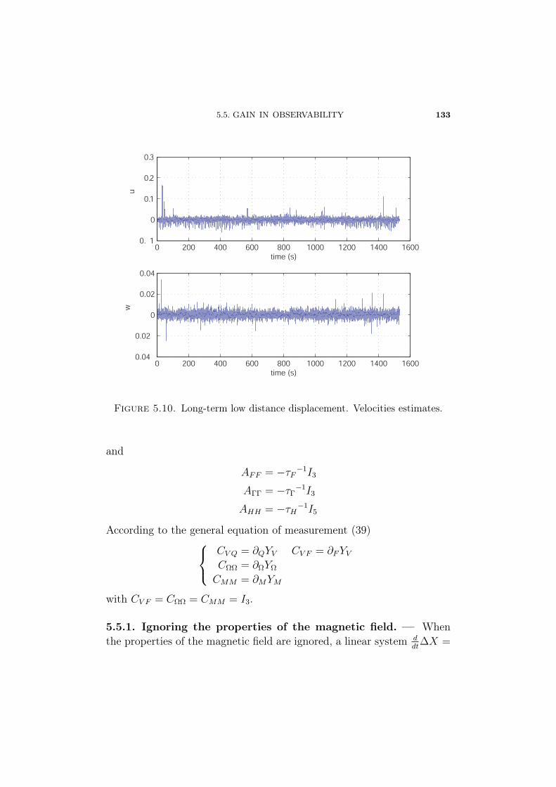
5.5. GAIN IN OBSERVABILITY 133
0 200 400 600 800 1000 1200 1400 16000. 1
0
0.1
0.2
0.3
time (s)
u
0 200 400 600 800 1000 1200 1400 16000.04
0.02
0
0.02
0.04
time (s)
w
Figure 5.10. Long-term low distance displacement. Velocities estimates.
and
AFF = −τF−1I3
AΓΓ = −τΓ−1I3
AHH = −τH−1I5
According to the general equation of measurement (39)⎧⎨⎩CV Q = ∂QYV CV F = ∂FYVCΩΩ = ∂ΩYΩ
CMM = ∂MYM
with CV F = CΩΩ = CMM = I3.
5.5.1. Ignoring the properties of the magnetic field. — Whenthe properties of the magnetic field are ignored, a linear system d
dtΔX =
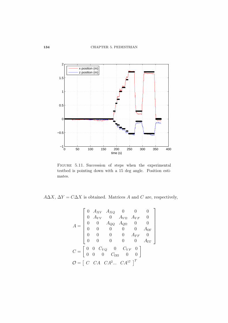
134 CHAPTER 5. PEDESTRIAN
0 50 100 150 200 250 300 350 400−1
−0.5
0
0.5
1
1.5
2
time (s)
x position (m)z position (m)
Figure 5.11. Succession of steps when the experimentaltestbed is pointing down with a 15 deg angle. Position esti-mates.
AΔX, ΔY = CΔX is obtained. Matrices A and C are, respectively,
A =
⎡⎢⎢⎢⎢⎢⎢⎢⎣
0 AXV AXQ 0 0 0
0 AV V 0 AV Ω AV F 0
0 0 AQQ AQΩ 0 0
0 0 0 0 0 AΩΓ
0 0 0 0 AFF 0
0 0 0 0 0 AΓΓ
⎤⎥⎥⎥⎥⎥⎥⎥⎦C =
[0 0 CV Q 0 CV F 0
0 0 0 CΩΩ 0 0
]O =
[C CA CA2... CA17
]T
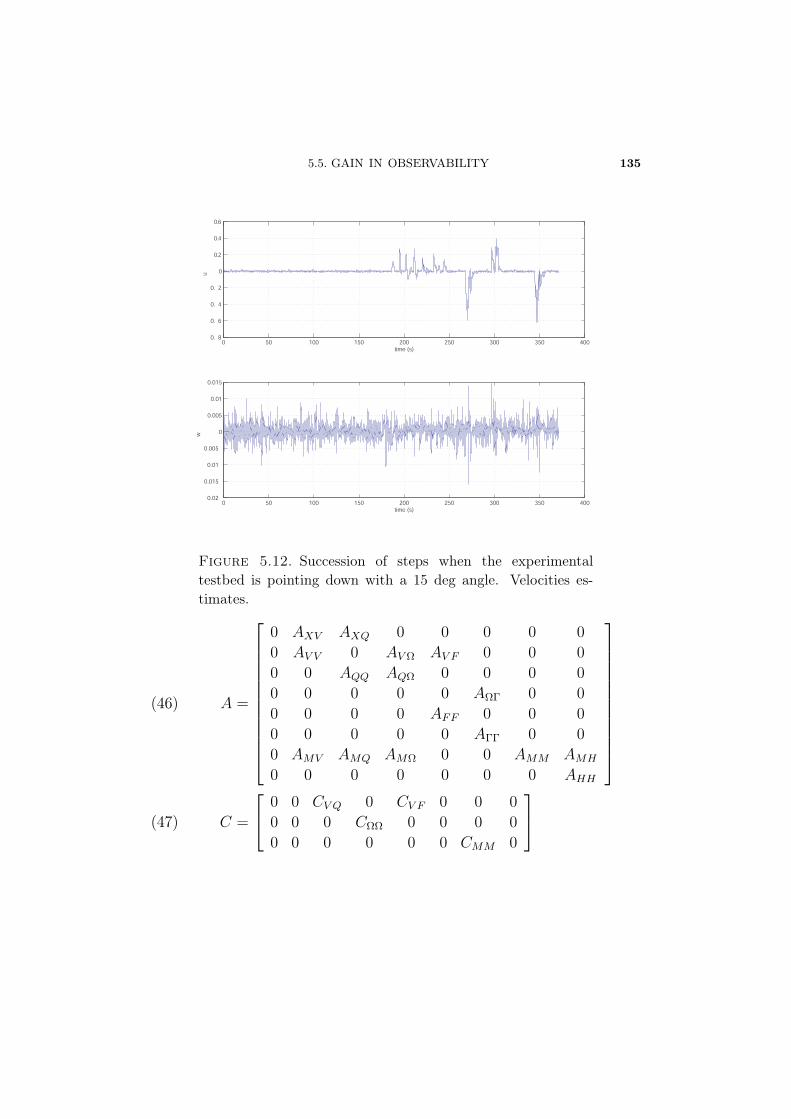
5.5. GAIN IN OBSERVABILITY 135
0 50 100 150 200 250 300 350 4000. 8
0. 6
0. 4
0. 2
0
0.2
0.4
0.6
time (s)
u
0 50 100 150 200 250 300 350 4000.02
0.015
0.01
0.005
0
0.005
0.01
0.015
time (s)
w
Figure 5.12. Succession of steps when the experimentaltestbed is pointing down with a 15 deg angle. Velocities es-timates.
A =
⎡⎢⎢⎢⎢⎢⎢⎢⎢⎢⎢⎢⎣
0 AXV AXQ 0 0 0 0 0
0 AV V 0 AV Ω AV F 0 0 0
0 0 AQQ AQΩ 0 0 0 0
0 0 0 0 0 AΩΓ 0 0
0 0 0 0 AFF 0 0 0
0 0 0 0 0 AΓΓ 0 0
0 AMV AMQ AMΩ 0 0 AMM AMH
0 0 0 0 0 0 0 AHH
⎤⎥⎥⎥⎥⎥⎥⎥⎥⎥⎥⎥⎦(46)
C =
⎡⎣ 0 0 CV Q 0 CV F 0 0 0
0 0 0 CΩΩ 0 0 0 0
0 0 0 0 0 0 CMM 0
⎤⎦(47)
136 CHAPTER 5. PEDESTRIAN
When computing the observability matrix O, one easily realizes that thefirst two columns are equal to zero. The positions and velocities are notobservable.
The rank of O is equal to rank(CV Q)+rank(CV FAFF )+rank(CΩΩ)+
rank(CΩΩAΩΓ) = 11.
5.5.2. Taking the properties of the magnetic field into account.— If we account for the discussed three properties of the magnetic field,and extend the state as previously presented, we obtain a linear systemwith A and C matrices given in equations (46) and (47). When comput-ing the observability matrix O =
[C CA CA2... CA25
]T , one caneasily realize that only the first column is equal to zero (due to the termAMV which corresponds to the partial derivative of the magnetic fieldswith respect to the velocity V ). The rank of O is equal torank(O) = rank(CMMAMV ) +max(rank(AMQ), rank(CV Q))
...+ rank(CΩΩ) + rank(CV F ) + rank(CΩΩAΩΓ) + rank(CMM)
...+ rank(AMH) = 18 +max(rank(AMQ), rank(CV Q)) ≥ 20
We believe that further investigations of the sub-blocks AMQ, and CV Qwould reveal that the rank is actually 21. The defect in observability isnow of 6 = 26 − 20 which is lower than the previously obtained value of7 = 18 − 11. It is due to the impact of the velocity onto the magneticfield, as previously stressed. Inspecting the observability matrix O, onecan also note that H can only appear in the successive derivatives ofthe measurements under the form of the matrix product AMHH. Thisvector is of dimension 3 instead of the original 5 dimensional vector H.Two unobservable modes are in fact taking their origin in this rank loss.This indirectly shows that from the original 12 configuration variables,at most 4 linear combinations are lost. Due to the role of velocitiesin the magnetic field, we believe that, this gain of observability rankprimarily focus on velocities variables. A substantially positive impacton the velocity estimation error can be observed.
CHAPTER 6
DIRECT MEASUREMENT OFMAGNETIC-FIELD GRADIENTS FOR
NAVIGATION
Dans ce chapitre, nous utilisons, comme au chapitre précédent, l’équationde Maxwell gouvernant le champ magnétique. Cette fois, on utilise unemesure directe des gradients du champs (obtenus par un dispositif spéci-fique que nous avons construit) pour obtenir des informations de vitesses.
In this chapter, we focus again on Maxwell’s equations, but this time,we propose a specific device to directly measure magnetic-field gradients.This yields direct information about the velocity.
6.1. Introduction
This chapter is organized as follows. In Section 6.2, we define the posi-tion estimation problem. In Section 6.3, we describe our use of magneticdisturbances and of sensors. In particular, we prove the observabilityof the velocity in the case considered here. In Section 6.4, we presentexperimental results, discuss implementation details, and comment oncalibration issues.
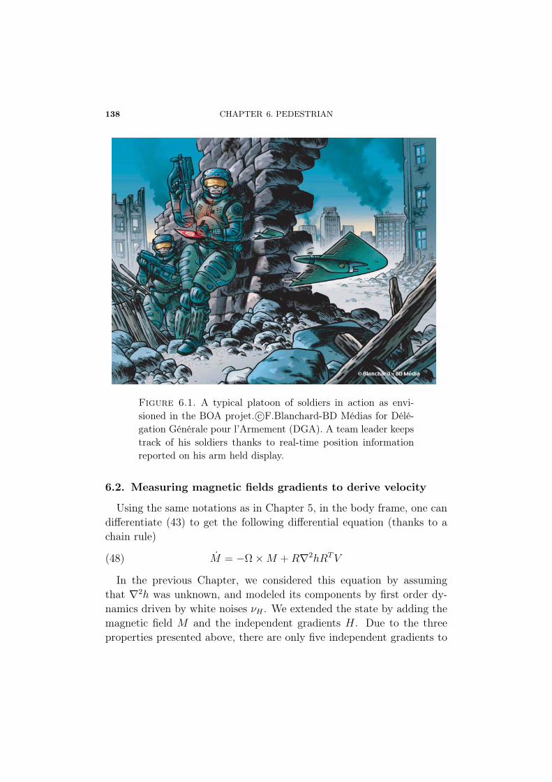
138 CHAPTER 6. PEDESTRIAN
Figure 6.1. A typical platoon of soldiers in action as envi-sioned in the BOA projet. c©F.Blanchard-BD Médias for Délé-gation Générale pour l’Armement (DGA). A team leader keepstrack of his soldiers thanks to real-time position informationreported on his arm held display.
6.2. Measuring magnetic fields gradients to derive velocity
Using the same notations as in Chapter 5, in the body frame, one candifferentiate (43) to get the following differential equation (thanks to achain rule)
M = −Ω ×M +R∇2hRTV(48)
In the previous Chapter, we considered this equation by assumingthat ∇2h was unknown, and modeled its components by first order dy-namics driven by white noises νH . We extended the state by adding themagnetic field M and the independent gradients H. Due to the threeproperties presented above, there are only five independent gradients to
6.2. MEASURING MAGNETIC FIELDS GRADIENTS TO DERIVE VELOCITY139
reconstruct. These are, in the inertial frame:
H � [hxx hxy hxz hyy hyz]T ∈ R
5
Some experiments have shown that strongly varying magnetic fieldsare difficult to estimate using this approach.
In this Chapter, we use a set of magnetometers to evaluate ∇2h. Three3-axis magnetometers are precisely mounted on a board, see Figure 6.2.The exact locations are defined by vector lever arms l1, l2, and l3 whichdefine a direct orthogonal trihedron. The sought after variables H are ob-tained from finite difference schemes. Further, we model their dynamicsby a white noise
H = νH(49)
Slopes depicted in Figure 5.3 suggest that spatial derivatives of H are notnegligible. For sake of performance, it is recommended to include somehigher order dynamics in both measurement and dynamics equations.For sake of simplicity, we do not present them here, but they can beeasily taken into account.
Under the preceding assumptions, the vector of measurement obtainedfrom the IMU, and the orthogonal trihedron of magnetometers is modeledas
(50)
⎧⎪⎪⎪⎪⎪⎪⎪⎪⎪⎨⎪⎪⎪⎪⎪⎪⎪⎪⎪⎩
YV = F −Rg +BV + μV
YΩ = Ω +BΩ + μΩ
YM0 = M + μM0
YM1 = M +R∇2hRT l1 + μM1
YM2 = M +R∇2hRT l2 + μM2
YM3 = M +R∇2hRT l3 + μM3
As will now appear, Equation (44) plays a key role in this observationproblem. It is the only one giving direct information on V .
140 CHAPTER 6. PEDESTRIAN
6.3. Gain of observability
6.3.1. Linearization. — In a general approach, let us consider thesystem obtained by linearizing the dynamics (42)-(48)-(49), and the mea-surement Equation (50). We denote by ∂Xf the partial derivative of fwith respect to X,∂Xf = ∂f
∂x.
From Equations (42)-(48)-(49), we obtain⎧⎪⎪⎪⎪⎪⎪⎪⎪⎪⎪⎪⎨⎪⎪⎪⎪⎪⎪⎪⎪⎪⎪⎪⎩
AXV = ∂V X, AXQ = ∂QX
AV V = ∂V V , AV Ω = ∂ΩV , AV F = ∂F V
AQQ = ∂QQ, AQΩ = ∂ΩQ
AFF = 0
AΓΓ = 0
AMV = ∂V M, AMQ = ∂QM, AMΩ = ∂ΩM
AMM = ∂MM, AMH = ∂HM
AHH = 0
with
AXV = RT
AMV = R∇2hRT
AV F = AQΩ = AΓΩ = I3
AV V = AMM =
⎡⎣ 0 r −q−r 0 p
q −p 0
⎤⎦AV Ω =
⎡⎣ 0 −w v
w 0 −u−v u 0
⎤⎦AMΩ =
⎡⎣ 0 −Mz My
Mz 0 −Mx
−My Mx 0
⎤⎦
AQΩ =
⎡⎢⎣ 1 sin(φ) tan(θ) cos(φ) tan(θ)
0 cos(φ) − sin(φ)
0 sin(φ)cos(θ)
cos(φ)cos(θ)
⎤⎥⎦
6.3. GAIN OF OBSERVABILITY 141
and
AQQ =
⎡⎢⎣(qcφ−rsφ)sθ
cθqsφ+rcφcθ2
0
−qsφ− rcφ 0 0qcφ−rsφ
cθ(qsφ+rcφ)cθ
tan(θ)0
⎤⎥⎦From Equation (50), we derive⎧⎪⎪⎪⎪⎪⎪⎪⎨⎪⎪⎪⎪⎪⎪⎪⎩
CV Q = ∂QYV , CV F = ∂FYVCΩΩ = ∂ΩYΩ
CM0M = ∂MYM0
CM1M = ∂MYM1 , CM1Q = ∂QYM1 , CM1H = ∂HYM1
CM2M = ∂MYM2 , CM2Q = ∂QYM2 , CM2H = ∂HYM2
CM3M = ∂MYM3 , CM3Q = ∂QYM3 , CM3H = ∂HYM3
with CV F = CΩΩ = CM0M = CM1M = CM2M = CM3M = I3.One can easily realize that the position X is not observable (it does
not appear anywhere in the right-hand side of the dynamics). We nowfocus on the reduced state [V ;Q; Ω;F ;M ;H]T .
6.3.2. Ignoring the properties of the magnetic field. — Whenthe properties of the magnetic field are ignored, a linear system Σ = AΣ,ΔY = CΣ is obtained from the preceding linearization. The state vectoris [V ;Q; Ω;F ]T ∈ R
12. Matrices A and C are, respectively,
A =
⎡⎢⎢⎣AV V 0 AV Ω AV F
0 AQQ AQΩ 0
0 0 0 0
0 0 0 0
⎤⎥⎥⎦C =
[0 CV Q 0 CV F0 0 CΩΩ 0
]O =
[C; CA; CA2; ...; CA11
]When computing the observability matrix O, one easily realizes that itsfirst column is identically equal to zero. In fact, the rank of O is
rank[O] = rank[CV QAQQ] + rank[CV F ] + rank[CΩΩ] = 8
142 CHAPTER 6. PEDESTRIAN
When ignoring the properties of the magnetic field, it appears thatV and ψ are not observable. Using only gyroscopes and accelerometers,only φ, θ, Ω, and F can be observed.
6.3.3. Accounting for the properties of the magnetic field. —In this setup, we consider the full state [V ;Q; Ω;F,M,H]T ∈ R
20. Weobtain another linear system Σ = AΣ, ΔY = CΣ with
A =
⎡⎢⎢⎢⎢⎢⎢⎢⎣
AV V 0 AV Ω AV F 0 0
0 AQQ AQΩ 0 0 0
0 0 0 0 0 0
0 0 0 0 0 0
AMV AMQ AMΩ 0 AMM AMH
0 0 0 0 0 0
⎤⎥⎥⎥⎥⎥⎥⎥⎦
C =
⎡⎢⎢⎢⎢⎢⎢⎢⎣
0 CV Q 0 CV F 0 0
0 0 CΩΩ 0 0 0
0 0 0 0 CMM 0
0 CM1Q 0 0 CMM CM1H
0 CM2Q 0 0 CMM CM2H
0 CM3Q 0 0 CMM CM3H
⎤⎥⎥⎥⎥⎥⎥⎥⎦O =
[C; CA; CA2; ...; CA19;
]The observability matrix is O. In its first column, a term appears,
namely AMV (which corresponds to the partial derivative of the magneticfields with respect to the velocity V ). In details,
rank[O] ≥rank[AMV ] + rank
[CV QAMQ
]+ rank[CΩΩ]
+ rank[AMVAV F ] + rank[CMM ] + rank
⎡⎣ CM1H
CM2H
CM3H
⎤⎦As proven later on, O is full rank (20) under the following conditions:
– |θ| < π2
– ∇2h is invertible– ∇2h is not of the diagonal form diag(a, a,−2a), a ∈ R and at least
one of the first two components of RTθ R
TφV is non zero.

6.3. GAIN OF OBSERVABILITY 143
If the last condition is not satisfied, then rank(O) = 19 and the nonobservable state is ψ. It is possible to get some physical insight intothese conditions: the first two components of RT
θ RTφV correspond (up to
a Rψ rotation) to the coordinates of the velocity vector in the inertialframe (x, y)-plane. At least, one of these has to be non zero, so that ψcan be recovered. Also, if the ∇2h is of the mentioned diagonal form,then the magnetic disturbances are insufficient to recover the headingvariable.
6.3.4. Observability. — We wish to compute the observability matrixO = [C;CA; ...;CA19] with C and A defined in Section 6.4. O is givenin the following equation. Bold elements (in brackets) play a key role inthe rank computation.
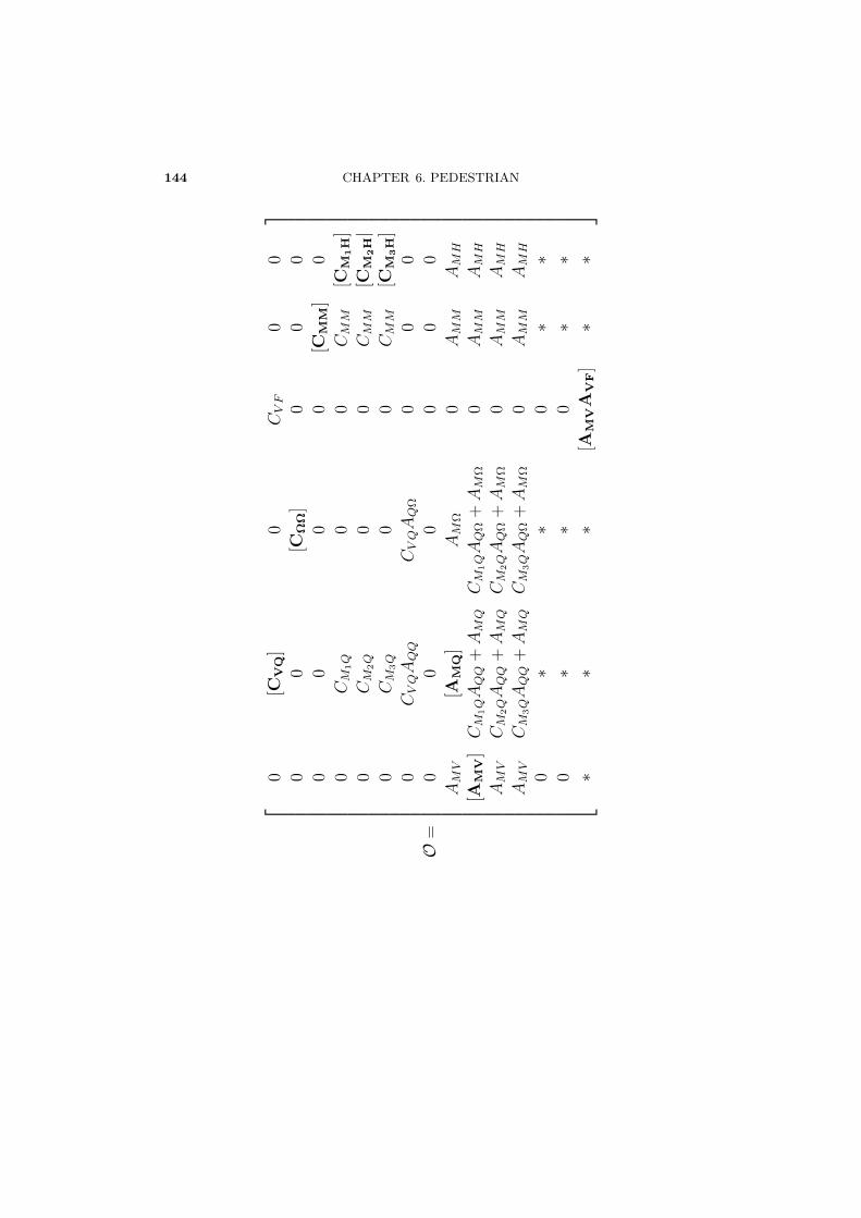
144 CHAPTER 6. PEDESTRIAN
O=
⎡ ⎢ ⎢ ⎢ ⎢ ⎢ ⎢ ⎢ ⎢ ⎢ ⎢ ⎢ ⎢ ⎢ ⎢ ⎢ ⎢ ⎢ ⎢ ⎢ ⎢ ⎢ ⎢ ⎢ ⎢ ⎢ ⎢ ⎣
0[C
VQ
]0
CVF
00
00
[CΩ
Ω]
00
0
00
00
[CM
M]
0
0CM
1Q
00
CMM
[CM
1H
]
0CM
2Q
00
CMM
[CM
2H|
0CM
3Q
00
CMM
[CM
3H
]
0CVQAQQ
CVQAQ
Ω0
00
00
00
00
AMV
[AM
Q]
AM
Ω0
AMM
AMH
[AM
V]CM
1QAQQ
+AMQ
CM
1QAQ
Ω+AM
Ω0
AMM
AMH
AMV
CM
2QAQQ
+AMQ
CM
2QAQ
Ω+AM
Ω0
AMM
AMH
AMV
CM
3QAQQ
+AMQ
CM
3QAQ
Ω+AM
Ω0
AMM
AMH
0∗
∗0
∗∗
0∗
∗0
∗∗
∗∗
∗[A
MVA
VF]
∗∗
⎤ ⎥ ⎥ ⎥ ⎥ ⎥ ⎥ ⎥ ⎥ ⎥ ⎥ ⎥ ⎥ ⎥ ⎥ ⎥ ⎥ ⎥ ⎥ ⎥ ⎥ ⎥ ⎥ ⎥ ⎥ ⎥ ⎥ ⎦
6.3. GAIN OF OBSERVABILITY 145
We have seen that
rank[O] = rank[AMV ] + rank
[CV QAMQ
]+ rank[CΩΩ]
+rank[AMVAV F ] + rank[CMM ] + rank
⎡⎣ CM1H
CM2H
CM3H
⎤⎦We now study each of these terms.
First, rank[AMV ] = 3, provided that ∇2h is invertible. Then, as is
proven in Proposition 5, rank[CV QAMQ
]= 3. Simply, rank[CΩΩ] = 3.
Provided that ∇2h is invertible, rank[AMVAV F ] = rank[AMV ] = 3. Di-
rectly, rank[CMM ] = 3. And finally, rank
⎡⎣ CM1H
CM2H
CM3H
⎤⎦ = 5, as is proven
in Proposition 4.
Proposition 4. — rank
⎡⎣ CM1H
CM2H
CM3H
⎤⎦ = 5
Proof. — Let us now consider the measurement Equation (50) for thefour magnetometers. We note the lever arm in the inertial frame for eachmagnetometer j by lji = [ljxi ljyi ljzi]
T = RT lj. Considering the jth,magnetometer we get
CMjH =∂R∇2hRT lj
∂H
= R∂
∂H
⎛⎝⎡⎣ hxx hxy hxz
hxy hyy hyz
hxz hyz −(hxx+ hyy)
⎤⎦⎡⎣ ljxiljyiljzi
⎤⎦⎞⎠= R
⎡⎣ ljxi ljyi ljzi 0 0
0 ljxi 0 ljyi ljzi−ljzi 0 ljxi −ljzi ljyi
⎤⎦
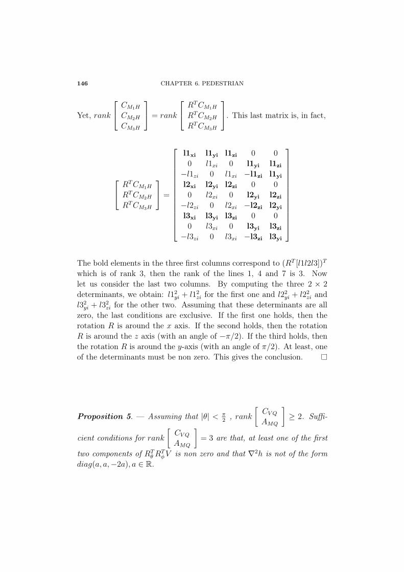
146 CHAPTER 6. PEDESTRIAN
Yet, rank
⎡⎣ CM1H
CM2H
CM3H
⎤⎦ = rank
⎡⎣ RTCM1H
RTCM2H
RTCM3H
⎤⎦. This last matrix is, in fact,
⎡⎣ RTCM1H
RTCM2H
RTCM3H
⎤⎦ =
⎡⎢⎢⎢⎢⎢⎢⎢⎢⎢⎢⎢⎢⎢⎣
l1xi l1yi l1zi 0 0
0 l1xi 0 l1yi l1zi
−l1zi 0 l1xi −l1zi l1yi
l2xi l2yi l2zi 0 0
0 l2xi 0 l2yi l2zi
−l2zi 0 l2xi −l2zi l2yi
l3xi l3yi l3zi 0 0
0 l3xi 0 l3yi l3zi
−l3zi 0 l3xi −l3zi l3yi
⎤⎥⎥⎥⎥⎥⎥⎥⎥⎥⎥⎥⎥⎥⎦
The bold elements in the three first columns correspond to (RT [l1l2l3])T
which is of rank 3, then the rank of the lines 1, 4 and 7 is 3. Nowlet us consider the last two columns. By computing the three 2 × 2
determinants, we obtain: l12yi + l12
zi for the first one and l22yi + l22
zi andl32yi + l32
zi for the other two. Assuming that these determinants are allzero, the last conditions are exclusive. If the first one holds, then therotation R is around the x axis. If the second holds, then the rotationR is around the z axis (with an angle of −π/2). If the third holds, thenthe rotation R is around the y-axis (with an angle of π/2). At least, oneof the determinants must be non zero. This gives the conclusion.
Proposition 5. — Assuming that |θ| < π2
, rank[CV QAMQ
]≥ 2. Suffi-
cient conditions for rank[CV QAMQ
]= 3 are that, at least one of the first
two components of RTθ R
TφV is non zero and that ∇2h is not of the form
diag(a, a,−2a), a ∈ R.
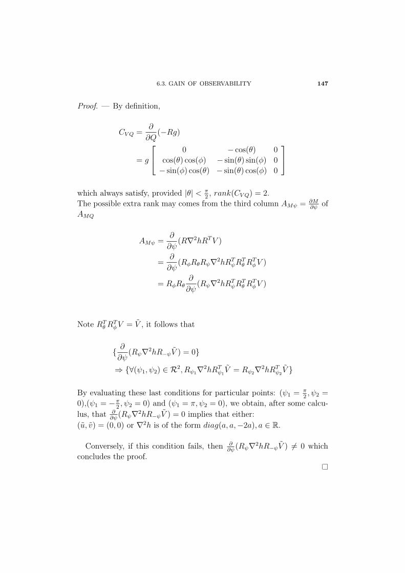
6.3. GAIN OF OBSERVABILITY 147
Proof. — By definition,
CV Q =∂
∂Q(−Rg)
= g
⎡⎣ 0 − cos(θ) 0
cos(θ) cos(φ) − sin(θ) sin(φ) 0
− sin(φ) cos(θ) − sin(θ) cos(φ) 0
⎤⎦which always satisfy, provided |θ| < π
2, rank(CV Q) = 2.
The possible extra rank may comes from the third column AMψ = ∂M∂ψ
ofAMQ
AMψ =∂
∂ψ(R∇2hRTV )
=∂
∂ψ(RφRθRψ∇2hRT
ψRTθ R
TφV )
= RφRθ∂
∂ψ(Rψ∇2hRT
ψRTθ R
TφV )
Note RTθ R
TφV = V , it follows that
{ ∂
∂ψ(Rψ∇2hR−ψV ) = 0}
⇒ {∀(ψ1, ψ2) ∈ R2, Rψ1∇2hRTψ1V = Rψ2∇2hRT
ψ2V }
By evaluating these last conditions for particular points: (ψ1 = π2, ψ2 =
0),(ψ1 = −π2, ψ2 = 0) and (ψ1 = π, ψ2 = 0), we obtain, after some calcu-
lus, that ∂∂ψ
(Rψ∇2hR−ψV ) = 0 implies that either:(u, v) = (0, 0) or ∇2h is of the form diag(a, a,−2a), a ∈ R.
Conversely, if this condition fails, then ∂∂ψ
(Rψ∇2hR−ψV ) �= 0 whichconcludes the proof.
148 CHAPTER 6. PEDESTRIAN
6.4. Filter design and experimental results
Thanks to the discussed observability property of the system (42)-(48)-(49)-(50), we implemented an extended Kalman filter (EKF) to re-construct the state [V,Q,Ω, F,M,H]T ∈ R
20, and, eventually, use it toestimate the position X ∈ R
3.
6.4.1. Filter design. — In practice, the state of our EKF is composedof 45 variables including configuration states (12 variables), magneticfield and its independent first and second derivatives (3+5+7 variables),forces and torques (3+3 variables), sensors biases (6 variables). We usedequally valued tuning parameters for the 3 axis. These are chosen to cap-ture fast dynamics (σacceleration = 8 m.s−2, σtorque = 4 rad.s−2). Classi-cally, discrete-time updates are implemented. Updates are synchronizedwith the 75 Hz measurements from the IMU.The EKF state X evolves according to the following continuous timemodel X = F (X,U) where U is the input variable.First, a prediction from time k to k+1 is performed, this gives Xp and Pp,and then the EKF estimates the state from the measurements, yieldingXe and Pe. We note T the sampling time, Q and R being the covariancesmatrix of the zero-mean dynamic and sensors white noises, respectively.
6.4.2. Experimental testing bench and calibration issues. —
6.4.2.1. Testing bench:— Our experimental testing bench is designed toillustrate the relevance of our approach in standard buildings inside whichthe magnetic field is unknown and has significant 3-dimensional varia-tions. Off the shelves IMUs are used (e.g. a 3DMGX1 from Microstrain�)
Four IMUs are fixed on a board which can simultaneously rotate andtranslate in 3D. Only one out of the four is actually used as an IMU.The remaining three are used as 3-D magnetometers. This board hasbeen used in different rooms in our building. Obtained results are verysimilar.
6.4.2.2. Calibration issues. — While the four IMU are supposed to bevery similar, experimentally, a serious practical issue is sensors calibra-tion. Even if mechanical tolerances are indeed small, we quickly realizedthat it was absolutely necessary to determine bias, misalignment angles,
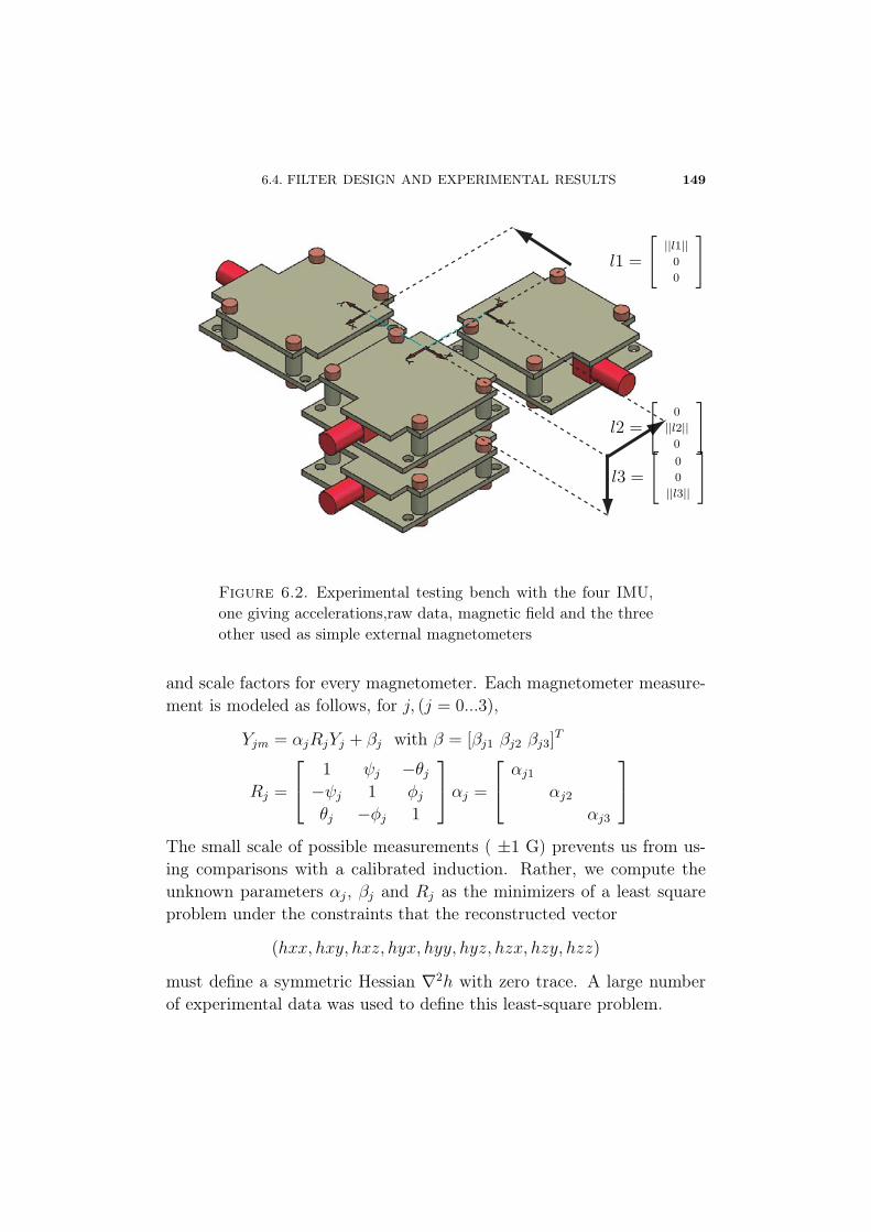
6.4. FILTER DESIGN AND EXPERIMENTAL RESULTS 149
l1 =
[||l1||
0
0
]
l2 =
[0
||l2||0
]l3 =
[0
0
||l3||
]
Figure 6.2. Experimental testing bench with the four IMU,one giving accelerations,raw data, magnetic field and the threeother used as simple external magnetometers
and scale factors for every magnetometer. Each magnetometer measure-ment is modeled as follows, for j, (j = 0...3),
Yjm = αjRjYj + βj with β = [βj1 βj2 βj3]T
Rj =
⎡⎣ 1 ψj −θj−ψj 1 φjθj −φj 1
⎤⎦αj =
⎡⎣ αj1αj2
αj3
⎤⎦The small scale of possible measurements ( ±1 G) prevents us from us-ing comparisons with a calibrated induction. Rather, we compute theunknown parameters αj, βj and Rj as the minimizers of a least squareproblem under the constraints that the reconstructed vector
(hxx, hxy, hxz, hyx, hyy, hyz, hzx, hzy, hzz)
must define a symmetric Hessian ∇2h with zero trace. A large numberof experimental data was used to define this least-square problem.
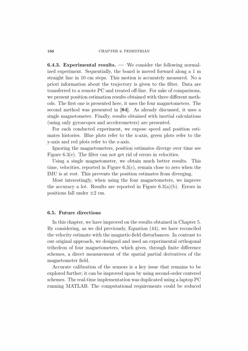
150 CHAPTER 6. PEDESTRIAN
6.4.3. Experimental results. — We consider the following normal-ized experiment. Sequentially, the board is moved forward along a 1 mstraight line in 10 cm steps. This motion is accurately measured. No apriori information about the trajectory is given to the filter. Data aretransferred to a remote PC and treated off-line. For sake of comparisons,we present position estimation results obtained with three different meth-ods. The first one is presented here, it uses the four magnetometers. Thesecond method was presented in [84]. As already discussed, it uses asingle magnetometer. Finally, results obtained with inertial calculations(using only gyroscopes and accelerometers) are presented.
For each conducted experiment, we expose speed and position esti-mates histories. Blue plots refer to the x-axis, green plots refer to they-axis and red plots refer to the z-axis.
Ignoring the magnetometers, position estimates diverge over time seeFigure 6.3(e). The filter can not get rid of errors in velocities.
Using a single magnetometer, we obtain much better results. Thistime, velocities, reported in Figure 6.3(c), remain close to zero when theIMU is at rest. This prevents the position estimates from diverging.
Most interestingly, when using the four magnetometers, we improvethe accuracy a lot. Results are reported in Figure 6.3(a)(b). Errors inpositions fall under ±2 cm.
6.5. Future directions
In this chapter, we have improved on the results obtained in Chapter 5.By considering, as we did previously, Equation (44), we have reconciledthe velocity estimate with the magnetic-field disturbances. In contrast toour original approach, we designed and used an experimental orthogonaltrihedron of four magnetometers, which gives, through finite differenceschemes, a direct measurement of the spatial partial derivatives of themagnetometer field.
Accurate calibration of the sensors is a key issue that remains to beexplored further; it can be improved upon by using second-order centeredschemes. The real-time implementation was duplicated using a laptop PCrunning MATLAB. The computational requirements could be reduced
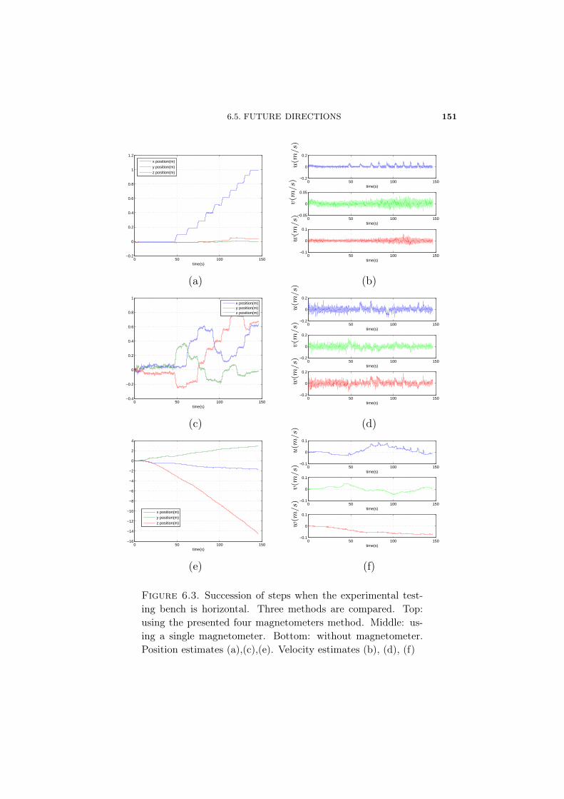
6.5. FUTURE DIRECTIONS 151
0 50 100 150−0.2
0
0.2
0.4
0.6
0.8
1
1.2
time(s)
x position(m)y position(m)z position(m)
0 50 100 150−0.2
0
0.2
time(s)
0 50 100 150−0.05
0
0.05
time(s)
0 50 100 150−0.1
0
0.1
time(s)
u(m/s)
v(m/s)
w(m/s)
(a) (b)
0 50 100 150−0.4
−0.2
0
0.2
0.4
0.6
0.8
1
time(s)
x position(m)y position(m)z position(m)
0 50 100 150−0.2
0
0.2
time(s)
0 50 100 150−0.2
0
0.2
time(s)
0 50 100 150−0.2
0
0.2
time(s)
u(m/s)
v(m/s)
w(m/s)
(c) (d)
0 50 100 150−16
−14
−12
−10
−8
−6
−4
−2
0
2
4
time(s)
x position(m)y position(m)z position(m)
0 50 100 150−0.1
0
0.1
time(s)
0 50 100 150−0.1
0
0.1
time(s)
0 50 100 150−0.1
0
0.1
time(s)
u(m/s)
v(m/s)
w(m/s)
(e) (f)
Figure 6.3. Succession of steps when the experimental test-ing bench is horizontal. Three methods are compared. Top:using the presented four magnetometers method. Middle: us-ing a single magnetometer. Bottom: without magnetometer.Position estimates (a),(c),(e). Velocity estimates (b), (d), (f)
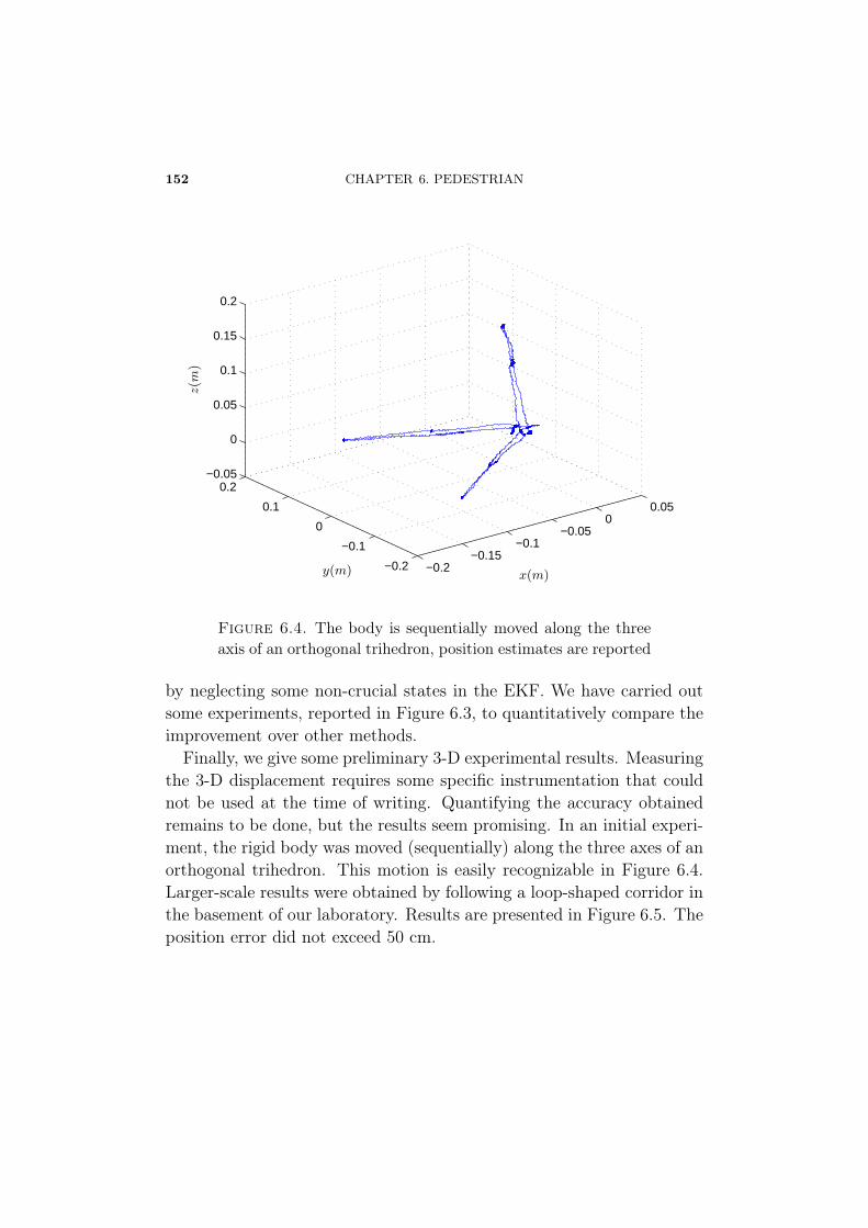
152 CHAPTER 6. PEDESTRIAN
−0.2−0.15
−0.1−0.05
00.05
−0.2
−0.1
0
0.1
0.2−0.05
0
0.05
0.1
0.15
0.2
x(m)y(m)
z(m
)
Figure 6.4. The body is sequentially moved along the threeaxis of an orthogonal trihedron, position estimates are reported
by neglecting some non-crucial states in the EKF. We have carried outsome experiments, reported in Figure 6.3, to quantitatively compare theimprovement over other methods.
Finally, we give some preliminary 3-D experimental results. Measuringthe 3-D displacement requires some specific instrumentation that couldnot be used at the time of writing. Quantifying the accuracy obtainedremains to be done, but the results seem promising. In an initial experi-ment, the rigid body was moved (sequentially) along the three axes of anorthogonal trihedron. This motion is easily recognizable in Figure 6.4.Larger-scale results were obtained by following a loop-shaped corridor inthe basement of our laboratory. Results are presented in Figure 6.5. Theposition error did not exceed 50 cm.
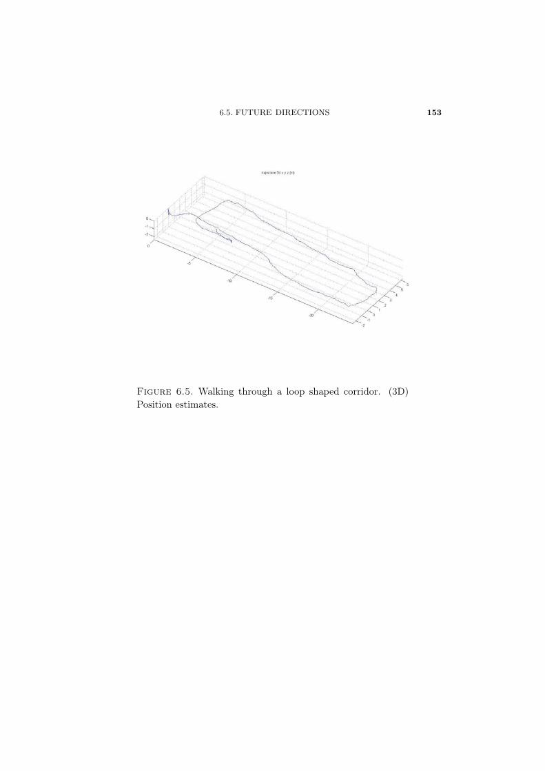
6.5. FUTURE DIRECTIONS 153
Figure 6.5. Walking through a loop shaped corridor. (3D)Position estimates.

BIBLIOGRAPHY
[1] P. Abbeel, A. Coates, M. Quigley, and A. Y. Ng. An application ofreinforcement learning to aerobatic helicopter flight. Neural Infor-mation Processing Systems (NIPS) 19, 2007.
[2] R. Abraham, J. E. Marsden, and T. Ratiu. Manifolds, Tensor Anal-ysis, and Applications. Springer, second edition, 1988.
[3] Federal Aviation Administration. Rotorcraft flying handbook. InWashington : U.S. Government Printing Office, 2000, 208 p., 2000.
[4] A. P. Aguiar, J. P. Hespanha, and P. Kokotovic. Limits of perfor-mance in reference-tracking and path-following for nonlinear sys-tems. In Proc. of the 16th IFAC World Congress, 2005.
[5] A. P. Aguiar, J. P. Hespanha, and P. Kokotovic. Path-followingfor non-minimum phase systems removes performance limitations.IEEE Transactions on Automatic Control, 50(2):234–239, 2005.
[6] S. A. Al-Hiddabi and N. H. McClamroch. Aggressive longitudinalaircraft trajectory tracking using nonlinear control. Journal of Guid-ance, Control, and Dynamics, 25(1):26–32, 2002.
[7] S. A. Al-Hiddabi and N. H. McClamroch. Tracking and maneuverregulation control for nonlinear nonminimum phase systems: Ap-plication to flight control. IEEE Transactions on Control SystemsTechnology, 10(6):780–792, 2002.
156 BIBLIOGRAPHY
[8] J. C. Avila-Vilchis, B. Brogliato, A. Dzul, and R. Lozano. Nonlinearmodelling and control of helicopters. Automatica, 39(9):1583–1596,2003.
[9] G. J. Balas. Flight control law design : An industry perspective infundamental issues in control. In Special issue of European Journalof Control, 2003.
[10] R. Bhattacharya. OPTRAGEN a Matlab toolbox for optimal trajec-tory generation. User’s manual, Aerospace Engineering Department,Texas A& M University, 2006.
[11] E. Børhaug, A. Pavlov, and K. Y. Pettersen. Cross-track formationcontrol of underactuated autonomous underwater vehicles. GroupCoordination and Cooperative Control. Springer Verlag, 2006.
[12] E. Børhaug and K. Y. Pettersen. Cross-track control for underac-tuated autonomous vehicles. In Proc. of the 44th IEEE Conf. onDecision and Control, and the European Control Conference 2005,2005.
[13] E. Børhaug and K. Y. Pettersen. Los path following for underac-tuated underwater vehicle. In 7th IFAC Conference on Manoeu-vringand Control of Marine Craft (MCMC’2006), 2006.
[14] M. Caccamo, Th. Baker, A. Burns, G. Buttazzo, and L. Sha. Real-time scheduling for embedded systems. In D. Hristu-Varsakelis andW. S. Levine, editors, Handbook of networked and embedded controlsystems. Birkhäuser, 2005.
[15] P. Castillo, A. Dzul, and R. Lozano. Real-time stabilization andtracking of a four rotor mini rotorcraft. IEEE Trans. Control Sys-tems Technology, 12(4):510–516, 2004.
[16] P. Castillo, R. Lozano, and A. E. Dzul. Modelling and control ofmini-flying machines. Advances in industrial control. Springer, 2005.
[17] D. E. Chang and J. E. Marsden. Gyroscopic forces and collisionavoidance with convex obstacles. Nonlinear Dynamics and Control,295:145–160, 2003.
BIBLIOGRAPHY 157
[18] D. E. Chang, S. Shadden, J. E. Marsden, and R. Olfati-Saber. Colli-sion avoidance for multiple agent systems. In Proc. of the 42nd IEEEConf. on Decision and Control, 2003.
[19] S. Changey, D. Beauvois, and V. Fleck. A mixed extended-unscentedfilter for attitude estimation with magnetometer sensor. In Proc. ofthe 2006 American Control Conference, 2006.
[20] F. Chaplais and N. Petit. Inversion in indirect optimal control. InProc. of the 7th European Control Conf., 2003.
[21] F. Chaplais and N. Petit. Inversion in indirect optimal control: con-strained and unconstrained cases. In Proc. of the 46th IEEE Conf.on Decision and Control, 2007.
[22] F. Chaplais and N. Petit. Inversion in indirect optimal control ofmultivariable systems. ESAIM: Control, Optimisation and Calculusof Variations, 14:294–317, 2008.
[23] J. Cheng, Y. Lu, E. R. Thomas, and J. A. Farrell. Data fusion viaKalman filter: GPS and INS. In Sam. S. Ge and F. L. Lewis, editors,Autonomous mobile robots, Control engineering series. Taylor andFrancis, 2006.
[24] Cloud Cap Technologies. http://www.cloudcaptech.com. Hood River,OR, USA, 2004.
[25] L. B. Cremean, T. B. Foote, J. H. Gillula, G. H. Hines, D. Ko-gan, K. L. Kriechbaum, J. C. Lamb, J. Leibs, L. Lindzey, C. E.Rasmussen, A. D. Stewart, J. W. Burdick, and R. M. Murray. Al-ice: An information-rich autonomous vehicle for high-speed desertnavigation. Journal of Field Robotics, (9), 2005.
[26] P. Fabiani, V. Fuertes, G. Le Besnerais, R. Mampey, A. Piquereau,and F. Teichteil-Königsbuch. ReSSAC: UAV exploring, deciding andlanding in a partially known environment. In IAV 07, 2007.
[27] P. Fabiani, V. Fuertes, G. Le Besnerais, A. Piquereau, R. Mam-pey, and F. Teichteil-Königsbuch. ReSSAC: Flying an autonomous
158 BIBLIOGRAPHY
helicopter in a non-cooperative uncertain world. In AHS SpecialistMeeting on Unmanned Rotorcraft, 2007.
[28] P. Faurre. Navigation inertielle et filtrage stochastique. Méthodesmathématiques de l’informatique. Dunod, 1971.
[29] M. Fliess, J. Lévine, P. Martin, and P. Rouchon. Flatness and de-fect of nonlinear systems: introductory theory and examples. Int. J.Control, 61(6):1327–1361, 1995.
[30] M. Fliess, J. Lévine, P. Martin, and P. Rouchon. A Lie-Bäcklundapproach to equivalence and flatness of nonlinear systems. IEEETrans. Automat. Control, 44:922–937, 1999.
[31] M. Fruchard, P. Morin, and C. Samson. A framework for the controlof nonholonomic mobile manipulators. In I. J. Robotic Res.25(8).,2006.
[32] V. Gavrilets, B. Mettler, and E. Feron. Nonlinear model for a small-size acrobatic helicopter. In AIAA Guidance, Navigation and Con-trol Conference, 2001.
[33] V. Gavrilets, B. Mettler, and E. Feron. Human-inspired controllogic for automated maneuvering of miniature helicopter. Journalof Guidance, Control, and Dynamics, 27(5):752–759, 2004.
[34] V. Gavrilets, A. Shterenberg, M. A. Dahleh, and E. Feron. Avionicssystem for a small unmanned helicopter performing agressive ma-neuvers. In 19th Digital Avionics Systems Conferences, 2000.
[35] M. S. Grewal, L. R. Weill, and A. P. Andrews. Global positioningsystems, inertial navigation, and integration. Wiley Inter-science,2001.
[36] C. Guarino Lo Bianco, A. Piazzi, and Romano M. Smooth motiongeneration for unicycle mobile robots via dynamic path inversion.IEEE Tr. on robotics, 20(5):884–892, 2004.
[37] N. Guénard, T. Hamel, and L. Eck. Control laws for the teleopera-tion of an aerial vehicle known as an X4-Flyer. In IROS, 2006.
BIBLIOGRAPHY 159
[38] N. Guénard, T. Hamel, and R. Mahony. Practical visual servo con-trol for a unmanned aerial vehicle. IEEE-Transactions on Roboticsand Automation, to appear( ): , 2008.
[39] T. Hamel and R. Mahony. Image based visual servo-control for aclass of aerial robotic systems. Automatica, 43(11):1975–1983, 2007.
[40] A. Isidori. Nonlinear Control Systems. Springer, New York, 2nd edi-tion, 1989.
[41] C. Jekeli. Precision free-inertial navigation with gravity compensa-tion by an onboard gradiometer. J. Guidance, Control and Dynam-ics, 29(3):704–713, 2006.
[42] D. Jung, E. J. Levy, D. Zhou, R. Fink, J. Moshe, A. Earl, andP. Tsiotras. Design and development of a low-cost test-bed for un-dergraduate education in UAVs. In Proc. of the 44th IEEE Conf. onDecision and Control, and the European Control Conference 2005,2005.
[43] D. Jung and P. Tsiotras. Inertial attitude and position reference sys-tem development for a small UAV. In AIAA Infotech at Aerospace,2007.
[44] I. Kaminer, O. Yakimenko, V. Dobrokhodov, M. Lizaraga, andA. Pascoal. Cooperative control of small UAVs for naval applica-tions. In Proc. of the 43rd IEEE Conf. on Decision and Control,2004.
[45] S. Kolb. Théorie des bifurcations appliquée à l’analyse de la dy-namique du vol des hélicoptères. PhD thesis, Institut National Poly-technique de Grenoble, 2007.
[46] E. Kyrkjebø and K. Y. Pettersen. Output synchronization controlof euler-lagrange systems with nonlinear damping terms. In Proc.of the 44th IEEE Conf. on Decision and Control, and the EuropeanControl Conference 2005, 2005.
160 BIBLIOGRAPHY
[47] J.-P. Laumond. Nonholonomic motion planning for mobile robots. InProc. of the ICRA 1998, IEEE International Conference on Roboticsand Automation, 1998.
[48] J.-P. Laumond, P. E. Jacobs, M. Taix, and R. M. Murray. A motionplanner for nonholonomic robots. IEEE T. Robotics and Automa-tion, 5:577–593, 1994.
[49] F. Le-Bras, T. Hamel, and R. Mahony. Nonlinear observer-basedvisual control of a VTOL UAV. In Proc. of the 9th European ControlConf., 2007.
[50] S. Lee, T. Lee, S. Park, and C. Kee. Flight test results of UAVautomatic control using a single-antenna GPS receiver. In AIAAGuidance, Navigation, and Control Conference and Exhibit, 2003.
[51] P. Lefort and J. Hamann. L’hélicoptère. Chiron, 2e edition., 1988.
[52] R. Mahony, T. Hamel, and J.-M. Pflimlin. Complementary filterdesign on the special orthogonal group SO(3). In Proc. of the 44thIEEE Conf. on Decision and Control, and the European ControlConference 2005, 2005.
[53] P. Martin, S. Devasia, and B. Paden. A different look at outputtracking: control of a VTOL aircraft. In Proc. 33nd IEEE Conf.Decision and Control, San Antonio, pages 2376–2381, Lake BuenaVista, 1994.
[54] B. Mettler. Identification Modeling and Characteristics of MiniatureRotorcraft. Boston : Kluwer Academic Publishers, 2003.
[55] B. Mettler, M. B. Tischler, and T. Kanade. Attitude control opti-mization for a small-scale unmanned helicopter. In AIAA Guidance,Navigation and Control Conference, 2000.
[56] B. Mettler, M. B. Tischler, and T. Kanade. System identificationof a model-scale helicopter. Technical Report CMU-RI-TR-00-03,Carnegie Mellon University, january 2000.
BIBLIOGRAPHY 161
[57] B. Mettler, M. B. Tischler, and T. Kanade. System identificationmodeling of a small-scale unmanned rotorcraft for flight control de-sign. Journal of the American Helicopter Society, 47:50–63, 2002.
[58] Micro Pilot. http://www.micropilot.com. Stony Mountain, Canada,2004.
[59] M. B. Milam. Real-time optimal trajectory generation for constrainedsystems. PhD thesis, California Institute of Technology, 2003.
[60] M. B. Milam, K. Mushambi, and R. M. Murray. A new computa-tional approach to real-time trajectory generation for constrainedmechanical systems. In IEEE Conference on Decision and Control,2000.
[61] K. A. Morgansen and R. W. Brockett. Nonholonomic control basedon approximate inversion. In Proc. of the 1999 American ControlConference, 1999.
[62] K. A. Morgansen, P. A. Vela, and J. W. Burdick. Trajectory stabi-lization for a planar carangiform robot fish. In Proc. of the ICRA2002, IEEE International Conference on Robotics and Automation,2002.
[63] P. Morin and C. Samson. Practical stabilization of driftless systemson lie groups: The transverse function approach. IEEE Transactionson Automatic Control, 48(9):1496–1508, 2003.
[64] P. Morin and C. Samson. Control with transverse functions and asingle generator of underactuated mechanical systems. In Proc. ofthe 45th IEEE Conf. on Decision and Control, 2006.
[65] P. Morin and C. Samson. Trajectory tracking for nonholonomic ve-hicles. Robot Motion Control: Recent Developments", K.Kozlowski.Springer, 2006.
[66] P. Morin and C. Samson. Trajectory tracking for nonholonomic ve-hicles. In K. Kozlowski, editor, Robot Motion Control: Recent De-velopments. Springer, 2006.
162 BIBLIOGRAPHY
[67] Motorola. MPC555 / MPC556 user’s manual. User’s manual, Mo-torola, 2000.
[68] R. M. Murray, J. Hauser, A. Jadbabaie, M. B. Milam, N. Pe-tit, W. B. Dunbar, and R. Franz. Online control customizationvia optimization-based control. In T. Samad and G. Balas, edi-tors, Software-Enabled Control, Information technology for dynami-cal systems, pages 149–174. Wiley-Interscience, 2003.
[69] A. Y. Ng, A. Coates, M. Diel, V. Ganapathi, J Schulte, B. Tse,E. Berger, and E. Liang. Inverted autonomous helicopter flight viareinforcement learning. In International Symposium on Experimen-tal Robotics, 2004.
[70] Department of Defense. Network centric warfare. Technical report,Report to Congress, 2001.
[71] G. D. Padfield. Helicopter Flight Dynamics. Blackwell Publishing,2007.
[72] E. Panteley, A. Loria, and A. Teel. Relaxed persistency of excitationfor uniform asymptotic stability. IEEE Trans. on Automat. Contr.,46(12):1874–1886, 2001.
[73] N. Petit, M. B. Milam, and R. M. Murray. Inversion based con-strained trajectory optimization. In 5th IFAC Symposium on Non-linear Control Systems, 2001.
[74] N. Petit, M. B. Milam, and R. M. Murray. A new computationalmethod for optimal control of a class of constrained systems gov-erned by partial differential equations. In Proc. of the 15th IFACWorld Congress, 2002.
[75] K.Y. Pettersen and E. Lefeber. Way-point tracking control of ships.In Proc. of the 40th IEEE Conf. on Decision and Control, 2001.
[76] R. W. Prouty. Helicopter Performance, Stability, and Control. Mal-abar : Krieger Publishing Company Inc., 2003.
BIBLIOGRAPHY 163
[77] R. Rao, V. Kumar, and C. Taylor. Visual servoing of a UGV from aUAV using differential flatness. In Proc. of the 2003 IEEE/RSJ Int.Conference on Intelligent Robots and Systems, 2003.
[78] K. V. Rozhdestvensky. Aerodynamics of a Lifting System in ExtremeGround Effect. 1st Edition, Springer-Verlag, 2000.
[79] A. Teel, R. M. Murray, and G. C. Walsh. Nonholonomic controlsystems: from steering to stabilization with sinuoids. InternationalJournal of Control 62, 4:849–870, 1995.
[80] D. Tsakiris, K. Kapellos, C. Samson, P. Rives, and J.-J. Orrelly.Experiments in Real-time Vision-based Point Stabilization of a Non-holonomic Mobile Manipulator. Experimental Robotics V: The FifthInternational Symposium, A. Casals et A. de Almeida. Springer-Verlag, 1998.
[81] P. A. Vela, K. A. Morgansen, and J. W. Burdick. Underwater lo-comotion from oscillatory shape deformations. In Proc. of the 41thIEEE Conf. on Decision and Control, 2002.
[82] D. Vissière, P.-J. Bristeau, A. P. Martin, and N. Petit. Experimen-tal autonomous flight of a small-scaled helicopter using accurate dy-namics model and low-cost sensors. In Proc. of the 17th IFAC WorldCongress, 2008.
[83] D. Vissière, D. E. Chang, and N. Petit. Experiments of trajectorygeneration and obstacle avoidance for a UGV. In Proc. of the 2007American Control Conference, 2007.
[84] D. Vissière, A. P. Martin, and N. Petit. Using magnetic disturbancesto improve IMU-based position estimation. In Proc. of the 9th Eu-ropean Control Conf., 2007.
[85] D. Vissière, A. P. Martin, and N. Petit. Using spatially distributedmagnetometers to increase IMU-based velocity estimation in per-turbed areas. In Proc. of the 46th IEEE Conf. on Decision andControl, 2007.
164 BIBLIOGRAPHY
[86] D. Vissière, A. P. Martin, and N. Petit. Système fournissant vitesseet position d’un corps en utilisant les variations du champ magné-tique évaluées grâce aux mesures de un ou des magnétomètres et deune ou des centrales inertielles. In Brevet nř07/02431, déposé le 3avril 2007.
[87] D. Vissière and N. Petit. Choix des missions. Technical report, Ecoledes Mines de Paris-DGA, 2005.
[88] D. Vissière and N. Petit. Scénarios opérationnels d’emploi desdrones. Technical report, Ecole des Mines de Paris-DGA, 2005.
[89] D. Vissière and N. Petit. Analyse du besoin en positionnement desdrones aériens ou terrestres. Technical report, Ecole des Mines deParis-DGA, 2006.
[90] D. Vissière and N. Petit. An embedded system for small-scaledautonomous vehicles. In Proc. of the ICINCO 2008, IEEE Inter-national Conference on Informatics in Control, Automation andRobotics, 2008.
[91] Y. Xiaokui and Y. Jianping. Study on low-cost GPS/DMU inte-grated navigation system. In AIAA/AAS Astrodynamics SpecialistConference and Exhibit, 2002.
[92] Y. Yang and J.A. Farrell. Magnetometer and differential carrierphase GPS-aided INS for advanced vehicle control. IEEE Trans.Robotics Automation, 19(2):269–282, 2003.
[93] H. Zhao and R. Shibasaki. A vehicle-borne urban 3-d acquisition sys-tem using single-row laser range scanners. IEEE Trans. on Systems,Man and Cybernetics, Part B, 33(4):658–666, 2003.