The estimation of ood quantiles in ungauged sites using ...scientiairanica.sharif.edu/article_4185_ef5663df49324ea7f3902749cd7815c6.pdfusing teaching-learning based optimization and

Scientia Iranica A (2018) 25(2), 632{645

Sharif University of TechnologyScientia Iranica

Transactions A: Civil Engineeringhttp://scientiairanica.sharif.edu

The estimation of ood quantiles in ungauged sitesusing teaching-learning based optimization andarti�cial bee colony algorithms

T. An�lan�, E. Uzlu, M. Kankal, and �O. Y�uksek

Department of Civil Engineering, Faculty of Engineering, Karadeniz Technical University, 61080 Trabzon, Turkey.

Received 29 February 2016; accepted 12 November 2016

KEYWORDSRegional oodfrequency analysis;L-moments;Teaching-learningbased optimization;Arti�cial bee colonyalgorithm;Turkey.

Abstract. In this study, a Regional Flood Frequency Analysis (RFFA) was appliedto 33 stream gauging stations in the Eastern Black Sea Basin, Turkey. Homogeneity ofthe region was determined by discordancy (Di) and heterogeneity measures (Hi) basedon L-moments. Generalized extreme-value, lognormal, Pearson type III, and generalizedlogistic distributions were �tted to the ood data of the homogeneous region. Basedon the appropriate distribution for the region, ood quantiles were estimated for returnperiods of T = 5; 10; 25; 50; 100, and 500 years. A non-linear regression model was thendeveloped to determine the relationship between ood discharges and meteorological andhydrological characteristics of the catchment. In order to compare regression analysiswith other models, Arti�cial Bee Colony algorithm (ABC) and Teaching-Learning BasedOptimization (TLBO) models were developed. The equations were obtained using theABC and TLBO algorithms to estimate ood discharges for di�erent return periods. Theanalysis showed that the TLBO and ABC results were superior to the regression analysis.Error values indicated that the TLBO method yielded better results for the estimation of ood quantiles for di�erent independent variables.© 2018 Sharif University of Technology. All rights reserved.

1. Introduction

Reliable estimation of ood discharges has great im-portance in the planning, design, and management ofhydraulic structures. Regional Flood Frequency Anal-ysis (RFFA) enables estimation of ood magnitudes indi�erent return periods at any stream location wherestream ow data are quite limited or completely absent.Thus, RFFA is frequently used to obtain design oodestimates.

*. Corresponding author. Tel.: +90 462 3772654;Fax: +90 462 3772606E-mail addresses: [email protected] (T. An�lan);[email protected] (E. Uzlu); [email protected](M. Kankal); [email protected] ( �O. Y�uksek).

doi: 10.24200/sci.2017.4185

Identi�cation of homogeneous regions, selectionof appropriate regional frequency distribution, andestimation of ood quantiles at sites of interest are thebasic concepts of RFFA. Many RFFA methods havebeen developed up to now. Some of the most commonlyadopted RFFA methods in practice include (i) therational method, (ii) index ood procedures with prob-ability weighted moments and L-moments, and (iii)regression and arti�cial intelligence based methods [1].As an example of rational method, Jiapeng et al. [2]proposed formulas that are modi�cations of the tradi-tional rational formula and able to calculate the ooddesign peak discharges. The use of the index oodprocedure started with Wallis [3], who used it in con-junction with probability weighted moments and theWakeby (WAK) distribution as a method of estimatingquantiles in the frequency distribution. Probability

T. An�lan et al./Scientia Iranica, Transactions A: Civil Engineering 25 (2018) 632{645 633

weighted moments were found to perform well forother distributions, but were hard to interpret [4].Hosking [5] found that certain linear combinations ofprobability weighted moments, which he called the\L-moments", have some theoretical advantages overconventional moments of being able to characterizewider range of distributions.

So far, a variety of L-moments based methodshave been extensively investigated in RFFA across theworld to obtain more reliable estimates. Rao et al. [6]analyzed maximum ow data from 93 sites in theWabash River, USA, using L-moments, and concludedthat Generalized-Extreme Value (GEV) distributionappeared to be more robust to the region. Parida etal. [7] performed a regional ood frequency analysis onMahi-Sabarmati basin in India using the L-momentsand index ood procedure. They modeled oods in theregion using the Lognormal (LN) distribution as theappropriate distribution. Adamowski [8] studied prob-ability density functions for oods in the Provinces ofOntario and Quebec, Canada. In Turkey, Haktanir [9],Sorman and Okur [10], Atiem and Harmancioglu [11],Saf [12], and Bayazit and Onoz [13] carried out L-moments based RFFA. In recent years, Seckin et al.(2011) showed that GEV and WAK distributions,whose parameters are computed by the L-momentsmethod, are adequate in predicting quantile estimatesin Turkey. Seckin et al. [14] then enhanced their L-moments based study with arti�cial intelligence tech-niques to predict ood peaks of various return periodsat ungauged sites in that basin in Turkey. It was con-cluded that the Multi-Layer Perceptrons (MLP) modelis observed to ensure estimates close to the L-momentsapproach. Aydogan et al. [15] applied a RFFA toCoruh Basin by L-moments method in Turkey. Theyestimated ood quantiles and compared them withthose estimated previously by an at-site frequencyanalysis (Gumbel distribution) on the basin masterplan for four large dams in the Coruh Basin. F�rat etal. [16] also calculated ood discharges for Turkey usingdistribution function parameters and observed highererror values with the increase of recurrence period.

The spatial variations in ow statistics are closelyrelated with the variations in regional physiographicaland meteorological factors. Quantile Regression (QR)models are often used to make estimates of owstatistics for ungauged sites and their relationshipsbetween catchment properties [17,18]. Ouarda etal. [19] applied the Canonical Correlation Analysis(CCA) technique to a dataset of 106 stations fromthe province of Ontario, Canada, and presented itsusefulness in RFFA. Jingyi and Hall [20] performedResiduals method, Ward's cluster method, the fuzzyc-means method, and Kohonen neural network on 86sites in the Gan River Basin and the Ming River Basinin China to identify homogeneous regions based on

site characteristics; they also examined the discordancyand homogeneity of the groups by L-moments ofthe distribution of annual oods. Reis et al. [21]introduced a Bayesian analysis of the GeneralizedLeast Squares (GLS) model, which provides measuresof the model error variance that are more accurate.Many studies with regression-based techniques [22-31]have been used to describe quantitative relationshipsbetween independent and dependent variables.

As an alternative to these methods, arti�cialintelligence methods can be applied to RFFA by com-bining several methods [32]. Dawson et al. [33] usedArti�cial Neural Networks (ANN) model for RFFA,and concluded that ANN provided more accurate ood quantile estimates than the traditional regressiontechniques. Shu and Ouarda [34] integrated CCAand ANN for ood quantile estimation at ungaugedsites in Quebec, Canada. They concluded that theproposed CCA-based ANN models presented betterperformance than the original ANN models. Shuand Ouarda [35] provided a general framework namedas Adaptive Neuro-Fuzzy Inference System (ANFIS)with combining two techniques, i.e. ANN and fuzzysystems. Their study revealed that the ANFIS modelprovided an integrated mechanism for identifying thehydrological regions and ood estimates with non-linear modeling capability. Aziz et al. [36] comparedthe performances of the ANN-based RFFA model withclassical regression techniques, and indicated that ANNpresented the best performing RFFA model. Seckinet al. [14] applied ANN models to compare themwith multiple regression ones. They found that theperformance of the ANN-MLP model is superior to theothers.

With the increase in the application of arti�cialintelligence techniques in hydrology, optimization tech-niques have also been frequently used in this area inrecent years. Chau [37] used Particle Swarm Opti-mization training algorithm (PSO) to predict waterlevels in Shing Mun River of Hong Kong with di�erentlead times based on the upstream gauging stations orstage/time history at the speci�c station. It was shownthat the PSO technique could act as an alternativetraining algorithm for ANNs. Jiong-feng and Wan-chang [38] applied Genetic Algorithm model (GA)to the daily rainfall-runo� simulations, and indicatedthat the proposed approach was feasible and of highcomputational e�ciency and could be transferred tomodel parameter calibrations for conceptual hydrolog-ical models in the similar categories. Jun et al. [39]proposed an Ant Colony Optimization-based (ACO)support vector machine algorithm SVM model (ACO-SVM) to optimize the parameters using an ACOrandom-seeking strategy. It was concluded that ACO-SVM is much more e�cient in global optimization andits forecasting accuracy is better than that of the con-

634 T. An�lan et al./Scientia Iranica, Transactions A: Civil Engineering 25 (2018) 632{645

ventional parameter-choosing method. Kisi et al. [40]investigated Arti�cial Bee Colony algorithm (ABC) formodeling discharge-suspended sediment relationshipand compared the model with neural di�erential evolu-tion, adaptive neuro-fuzzy, neural networks, and ratingcurve models. They concluded that the ANN-ABC wasable to produce better results than the other models.ANN-ABC model was used by Salimi et al. [41] topredict the average weekly discharge of Tang-e Karzinstation, Iran, through the discharge information. It wasobserved that applying ABC to ANN could improvethe estimations of the network outputs. Uzlu et al.[42] applied ABC and a recently developed advancedoptimization algorithm, Teaching-Learning Based Op-timization (TLBO), to the regression functions of thedata for the estimation of the berm parameters inunderstanding sediment movements. Although theseoptimization techniques have been applied to a widerange of hydrological and hydraulics problems, suchas rainfall runo� modeling, hydrologic forecasting, andcoastal engineering, there is not any in RFFA with theABC and TLBO. Therefore, this study will be the �rstto use the ABC and TLBO algorithms in a RFFA.

The object of the study is to compare the tradi-tional Regression Analysis (RA) with the ANN-basedalgorithms of ABC and TLBO using both physicaland meteorological characteristics of the Eastern BlackSea Basin (EBSB), Turkey. This study examinesthe applicability of the algorithms to RFFA using anextensive and elaborated data. In accordance withthis purpose, L-moments method is also used for theestimation of ood quantiles, and regression models aredeveloped for the selection of independent variables.An overview of L-moments, ABC, and TLBO methodsis presented in Section 3. Model development is alsopresented in this section. Section 4 presents the detailsof the RFFA with ABC and TLBO. In Section 5, the

results obtained by applying the proposed approachesare presented and discussed. Finally, in Section 6, theconclusions are presented.

2. The study area and data description

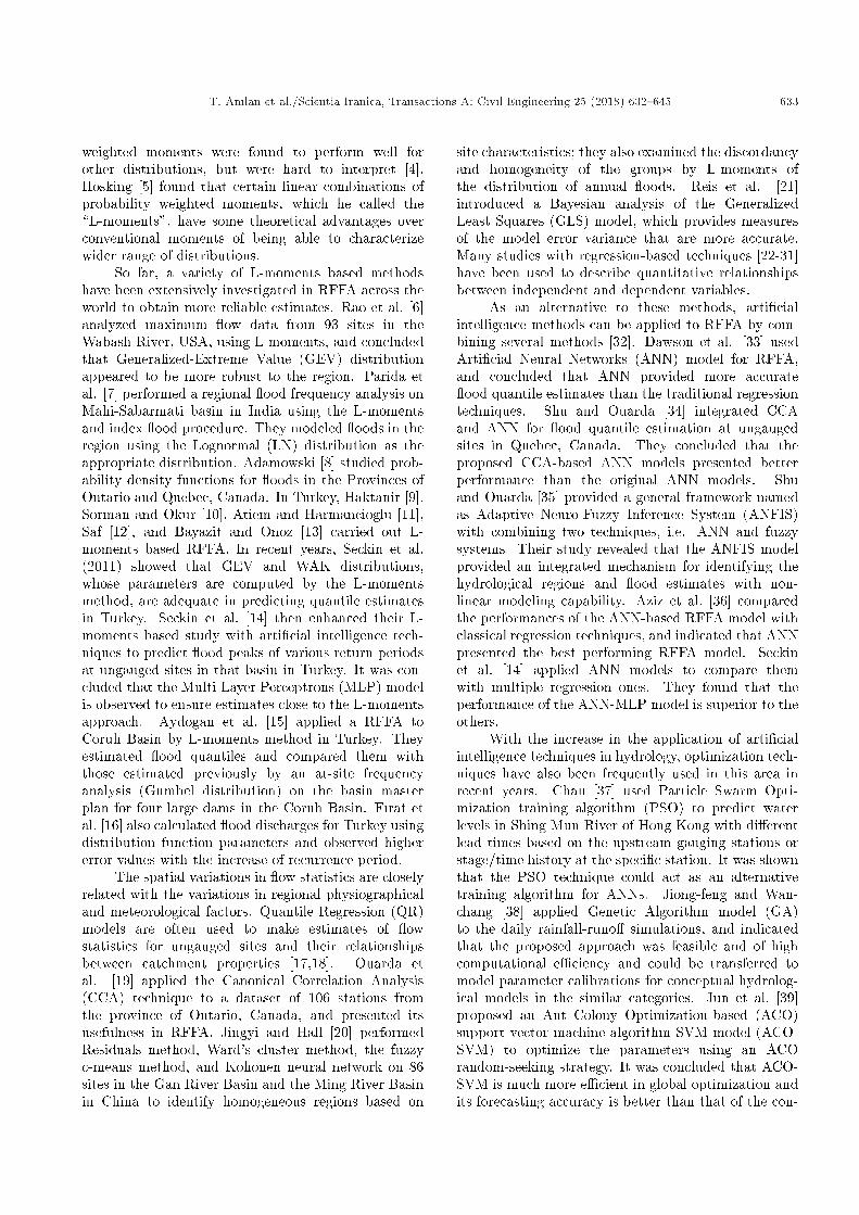
With respect to its river stream ow, Turkey is dividedinto 26 basins [43]. Among them, the Black SeaCoast receives rainfall all the year round and alsothe greatest amount of rainfall in Turkey [44]. TheEBSB is located on the northeastern coast of Turkey(Figure 1). The basin is surrounded by the EasternBlack Sea Mountains on the south and the Black Sea onthe north. It averages nearly 1,100 mm annually; this�gure can reach 2,300 mm near Rize Province. Thisregion was selected as the study area since it has a greatpotential risk against oods due to its meteorologicaland topographic characteristics. Devastating oodevents have occurred in the EBSB, especially in recentyears. In this region, nearly 50 destructive oods havetaken place between the years 1955 and 2010, causing258 deaths and nearly US $500,000,000 of damage [44].Therefore, reliable estimation of peak discharges isessential for the design of hydraulic structures and alsofor ood risk management.

Two types of data were used in this study: (i)stream ow data (the annual maximum ood data)for RFFA and estimation of ood quantiles and(ii) physiographical, meteorological, and hydrologicaldata for regression analysis techniques. The annualmaximum ood data of 33 Stream-Gauging Stations(SGS) used in the study were obtained from bothGeneral Directorate of State Hydraulic works (DSI)and General Directorate of Electrical Power Resourcesand Development Administration (EIE). The locationsof the stations used are shown in Figure 1. Thelonger the period of the record is, the more accurate

Figure 1. Location map of EBSB and studied area.


and representative statistical results will be in RFFA.Therefore, a minimum of ten years of SGSs wereselected for the quality of the estimates. Record lengthsof the selected 33 SGSs range 10-42 years (mean: 28years). Flood quantiles of these stations were estimatedfor the selected return periods T = 5; 10; 25; 50; 100,and 500 years (Q5; Q10; Q25; Q50; Q100, and Q500) by�tting the best distribution with the region.

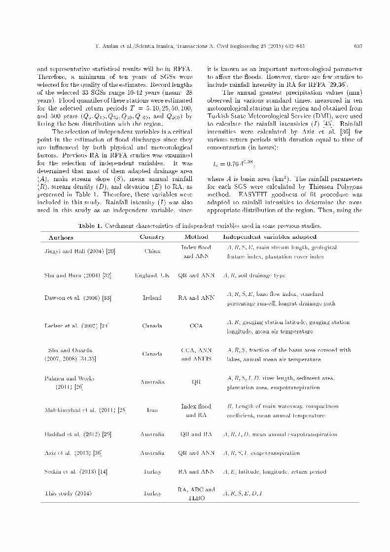
The selection of independent variables is a criticalpoint in the estimation of ood discharges since theyare in uenced by both physical and meteorologicalfactors. Previous RA in RFFA studies was examinedfor the selection of independent variables. It wasdetermined that most of them adapted drainage area(A), main stream slope (S), mean annual rainfall(R), stream density (D), and elevation (E) to RA, aspresented in Table 1. Therefore, these variables wereincluded in this study. Rainfall intensity (I) was alsoused in this study as an independent variable, since

it is known as an important meteorological parameterto a�ect the oods. However, there are few studies toinclude rainfall intensity in RA for RFFA [29,36].

The annual greatest precipitation values (mm)observed in various standard times, measured in tenmeteorological stations in the region and obtained fromTurkish State Meteorological Service (DMI), were usedto calculate the rainfall intensities (I) [45]. Rainfallintensities were calculated by Aziz et al. [36] forvarious return periods with duration equal to time ofconcentration (in hours):

tc = 0:76A0:38;

where A is basin area (km2). The rainfall parametersfor each SGS were calculated by Thiessen Polygonsmethod. EASYFIT goodness of �t procedure wasadapted to rainfall intensities to determine the mostappropriate distribution of the region. Then, using the

Table 1. Catchment characteristics of independent variables used in some previous studies.

Authors Country Method Independent variables adopted

Jingyi and Hall (2004) [20] China Index oodand ANN

A;R; S;E, main stream length, geologicalfeature index, plantation cover index

Shu and Burn (2004) [32] England, UK QR and ANN A;R, soil drainage type

Dawson et al. (2006) [33] Ireland RA and ANNA;R; S;E, base ow index, standardpercentage run-o�, longest drainage path

Leclerc et al. (2007) [24] Canada CCAA;R, gauging station latitude, gauging stationlongitude, mean air temperature

Shu and Ouarda(2007, 2008) [34,35]

Canada CCA, ANNand ANFIS

A;R; S, fraction of the basin area covered withlakes, annual mean air temperature

Palmen and Weeks(2011) [26]

Australia QRA;R; S; I;D, river length, sediment area,plantation area, evapotranspiration

Malekinezhad et al. (2011) [28] Iran Index oodand RA

R, Length of main waterway, compactnesscoe�cient, mean annual temperature

Haddad et al. (2012) [29] Australia QR and RA A;R; I;D, mean annual evapotranspiration

Aziz et al. (2013) [36] Australia QR and ANN A;R; S; I, evapotranspiration

Seckin et al. (2013) [14] Turkey RA and ANN A;E, latitude, longitude, return period

This study (2014) Turkey RA, ABC andTLBO

A;R; S;E;D; I


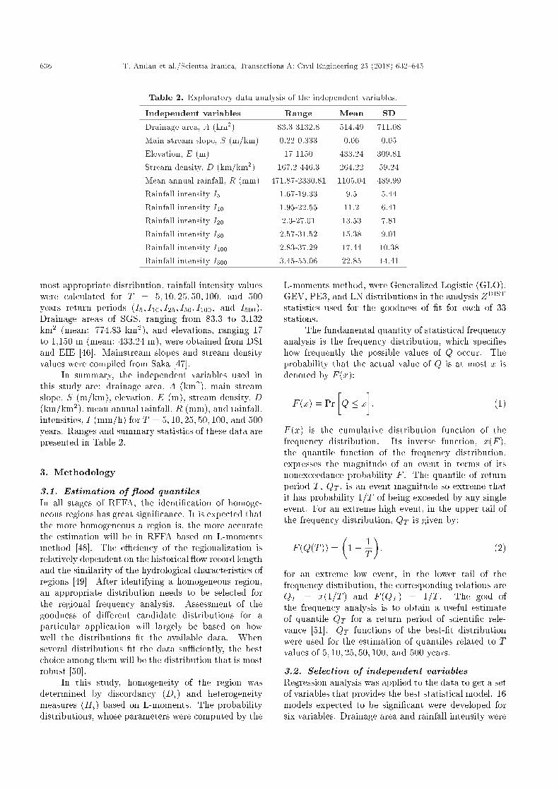
Table 2. Exploratory data analysis of the independent variables.

Independent variables Range Mean SD

Drainage area, A (km2) 83.3-3132.8 514.49 711.08Main stream slope, S (m/km) 0.22-0.333 0.06 0.05Elevation, E (m) 17-1150 433.24 309.81Stream density, D (km/km2) 167.2-446.3 264.22 59.24Mean annual rainfall, R (mm) 471.87-2330.81 1105.04 489.99Rainfall intensity I5 1.67-19.33 9.5 5.44Rainfall intensity I10 1.95-22.55 11.2 6.41Rainfall intensity I20 2.3-27.01 13.53 7.81Rainfall intensity I50 2.57-31.52 15.38 9.01Rainfall intensity I100 2.83-37.29 17.44 10.38Rainfall intensity I500 3.45-55.06 22.85 14.41

most appropriate distribution, rainfall intensity valueswere calculated for T = 5; 10; 25; 50; 100, and 500years return periods (I5; I10; I25; I50; I100, and I500).Drainage areas of SGS, ranging from 83.3 to 3,132km2 (mean: 774.83 km2), and elevations, ranging 17to 1,150 m (mean: 433.24 m), were obtained from DSIand EIE [46]. Mainstream slopes and stream densityvalues were compiled from Saka [47].

In summary, the independent variables used inthis study are: drainage area, A (km2), main streamslope, S (m/km), elevation, E (m), stream density, D(km/km2), mean annual rainfall, R (mm), and rainfall,intensities, I (mm/h) for T = 5; 10; 25; 50; 100, and 500years. Ranges and summary statistics of these data arepresented in Table 2.

3. Methodology

3.1. Estimation of ood quantilesIn all stages of RFFA, the identi�cation of homoge-neous regions has great signi�cance. It is expected thatthe more homogeneous a region is, the more accuratethe estimation will be in RFFA based on L-momentsmethod [48]. The e�ciency of the regionalization isrelatively dependent on the historical ow record lengthand the similarity of the hydrological characteristics ofregions [49]. After identifying a homogeneous region,an appropriate distribution needs to be selected forthe regional frequency analysis. Assessment of thegoodness of di�erent candidate distributions for aparticular application will largely be based on howwell the distributions �t the available data. Whenseveral distributions �t the data su�ciently, the bestchoice among them will be the distribution that is mostrobust [50].

In this study, homogeneity of the region wasdetermined by discordancy (Di) and heterogeneitymeasures (Hi) based on L-moments. The probabilitydistributions, whose parameters were computed by the

L-moments method, were Generalized Logistic (GLO),GEV, PE3, and LN distributions in the analysis ZDIST

statistics used for the goodness of �t for each of 33stations.

The fundamental quantity of statistical frequencyanalysis is the frequency distribution, which speci�eshow frequently the possible values of Q occur. Theprobability that the actual value of Q is at most x isdenoted by F (x):

F (x) = Pr�Q � x

�: (1)

F (x) is the cumulative distribution function of thefrequency distribution. Its inverse function, x(F ),the quantile function of the frequency distribution,expresses the magnitude of an event in terms of itsnonexceedance probability F . The quantile of returnperiod T , QT , is an event magnitude so extreme thatit has probability 1=T of being exceeded by any singleevent. For an extreme high event, in the upper tail ofthe frequency distribution, QT is given by:

F (Q(T )) =�

1� 1T

�; (2)

for an extreme low event, in the lower tail of thefrequency distribution, the corresponding relations areQT = x(1=T ) and F (QT ) = 1=T . The goal ofthe frequency analysis is to obtain a useful estimateof quantile QT for a return period of scienti�c rele-vance [51]. QT functions of the best-�t distributionwere used for the estimation of quantiles related to Tvalues of 5; 10; 25; 50; 100, and 500 years.

3.2. Selection of independent variablesRegression analysis was applied to the data to get a setof variables that provides the best statistical model. 16models expected to be signi�cant were developed forsix variables. Drainage area and rainfall intensity were


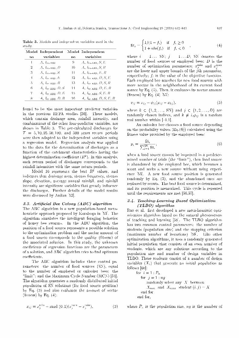
Table 3. Models and independent variables used in thestudy.

Modelno

Independentvariables

Modelno

Independentvariables

1 A, Itc-ARI 9 A, Itc-ARI; S; E2 A, Itc-ARI; D 10 A, Itc-ARI; S;R3 A, Itc-ARI; S 11 A, Itc-ARI; E;R4 A, Itc-ARI; E 12 A, Itc-ARI; D; S;E5 A, Itc-ARI; R 13 A, Itc-ARI; D; S;R6 A, Itc-ARI; D; S 14 A, Itc-ARI; D;E;R7 A, Itc-ARI; D;E 15 A, Itc-ARI; S; E;R8 A, Itc-ARI; D;R 16 A, Itc-ARI; D; S;E;R

found to be the most important predictor variablesin the previous RFFA studies [36]. These models,which contain drainage area, rainfall intensity, andcombinations of the other four-predictor variables, areshown in Table 3. The pre-calculated discharges forT = 5; 10; 25; 50; 100, and 500 years return periodswere then adapted to the independent variables usinga regression model. Regression analysis was appliedto the data for the determination of discharges as afunction of the catchment characteristics having thehighest determination coe�cient (R2). In this analysis,each return period of discharges corresponds to therainfall intensities with the same return periods.

Model 16 represents the best R2 values, andindicates that drainage area, stream frequency, streamslope, elevation, average annual rainfall, and rainfallintensity are signi�cant variables that greatly in uencethe discharges. Further details of the model resultswere discussed by Anilan [52].

3.3. Arti�cial Bee Colony (ABC) algorithmThe ABC algorithm is a new population-based meta-heuristic approach proposed by Karaboga in [53]. Thealgorithm simulates the intelligent foraging behaviorof honey bee swarms. In the ABC algorithm, theposition of a food source represents a possible solutionto the optimization problem and the nectar amount ofa food source corresponds to the quality (�tness) ofthe associated solution. In this study, the unknowncoe�cients of regression functions are the parametersof a solution, and ABC algorithm tries to �nd optimumcoe�cients.

The ABC algorithm includes three control pa-rameters: the number of food sources (SN), equalto the number of employed or onlooker bees; the\limit"; and the Maximum Cycle Number (MCN) [54].The algorithm generates a randomly distributed initialpopulation of SN solutions (for food source position)by Eq. (3) and also evaluates the amount of nectar(�tness) by Eq. (4):

xij = xminj + rand (0; 1)(xmax

j � xminj ); (3)

�ti =

(1=(1 + fi) if fi � 01 + abs(fi) if fi < 0

; (4)

where i = 1 : : : SN; j = 1 : : : D; SN denotes thenumber of food sources or employed bees; D is thenumber of optimization parameters; xmin

j and xmaxj

are the lower and upper bounds of the jth parameter,respectively; fi is the value of the objective function.Each employed bee searches for new food sources withmore nectar in the neighborhood of its current foodsource by Eq. (5). Then, it evaluates its nectar amount(�tness) by Eq. (4) [55]:

vij = xij + �ij(xij � xkj); (5)

where k 2 f1; 2; : : : ; SNg and j 2 f1; 2; : : : ; Dg arerandomly chosen indices, and k 6= i:'ij is a randomreal number within [{1,1].

An onlooker bee chooses a food source dependingon the probability values (Eq.(6)) calculated using the�tness value provided by the employed bees:

pi =�tiPSNi=1 �ti

; (6)

when a food source cannot be improved in a predeter-mined number of trials (the \limit"), then food sourceis abandoned by the employed bee, which becomes ascout and seeks a new source without using experi-ence [53]. A new food source position is generatedrandomly by Eq. (3), and the abandoned ones arereplaced by scouts. The best food source is determined,and its position is memorized. This cycle is repeateduntil the requirements are met [56,57].

3.4. Teaching-Learning Based Optimization(TLBO) algorithm

Rao et al. �rst developed a new meta-heuristic opti-mization algorithm based on the natural phenomenonof teaching and learning [58]. The TLBO algorithmhas two common control parameters: the number ofstudents (population size) and the stopping criterion(maximum number of iterations) [59]. Like otheroptimization algorithms, it uses a randomly generatedinitial population that consists of an even number ofstudents, which are any solutions according to thepopulation size and number of design variables inTLBO. These students consist of a number of designvariables (Xi) that generate an initial population asfollows [60]:

for i = 1 : Pnfor j = 1 : ng

randomly select any X betweenXmin and Xmax student (i; j) = X

end forend for,

where Pn is the population size, ng is the number of


groups if the design variables are categorized, Xminand Xmax are the minimum and maximum values,respectively, of the design variables of the regressionfunctions in this study.

In the TLBO algorithm, a new population isobtained as a result of two basic stages: the \teacherphase" or learning from the teacher, and the \learningphase," or trade of information between learners [61].In the teacher phase, the student, with minimumobjective function, f , in the entire population, is foundand mimicked as a teacher. Other students in thecurrent population are modi�ed as the neighborhoodof the teacher using the following equations:

studenti=�Xi;1Xi;2:::Xi; Dn

�i=1; 2; ::::; Pn; (7)

mean=�mean (X1) mean (X2)::::mean (XDN)

�; (8)

studentnew�t=studenti+r�(teacher�TF �mean); (9)

where DN is the number of design variables, Pn is thepopulation size, r is a random number varying in [0,1],and TF is the teaching factor (1 or 2). Xi is theunknown coe�cient of a regression function:

TF = round (1 + rand � (2� 1)): (10)

The size of r must be equal to that of thestudent for the scalar multiplication given in Eq. (7).The teaching phase is carried out with the hope ofupgrading the students' level to teachers' [60]. Inthe learning phase, modi�ed students increase theirknowledge by interacting with each other according tothe teaching-learning process [59].

At the end of the learning phase, a cycle (iter-ation) is completed for the TLBO algorithm. Thelearning and teaching phases are continued until thetermination criterion is reached [59]. Uzlu et al. [42]presented detailed information about the TLBO algo-rithm and its implementation.

4. Regional ood frequency analysis based onthe ABC and TLBO algorithms

In the prediction process, three regression functions,i.e. Linear Function (LF, Eq. (11)), Power Func-tion (PF, Eq. (12)), and Exponential Function (EF,Eq. (13)), were used to estimate the regional oodfrequency for the EBSB, Turkey. The general form ofLF, PF, and EF can be expressed as follows:

ylinear =w0 + w1x1 + w2x2 + w3x3

+ w4x4 + � � �+ wnxn; (11)

ypower = w0xw11 xw2

2 xw33 xw4

4 : : : xbnn ; (12)

yexponential =w0 + exp(w1 + w2x1 + w3x2 + w4x3

+ w5x4 + � � �+ wn+1xn); (13)

where y is the dependent variable, wis are the regres-sion coe�cients, and xis are independent variables forgeneral signi�cation. In this study, y corresponds to Q,and xis are drainage area (A), rainfall intensities (I),stream density (D), mean annual rainfall (R), mainstream slope (S), elevation (E), respectively.

Since the values of the independent variablesare in extremely di�erent ranges, optimization of thecoe�cients will become so di�cult. This is becausesome values will be too big and some too small.Therefore, each group of input and output values isnormalized into the range between [0.1, 0.9] in the ABCand TLBO models as follows:

Normalized value =�

Raw value - Min valueMax value - Min value

�� (0:9� 0:1) + 0:1: (14)

The aim of estimating regional ood frequency is to �ndthe �ttest model to the observed data. The equationsfor six parameters were evaluated using 33 experimen-tal data and the best equations with minimum SSEwere determined. In addition, performances of ABCand TLBO models were compared using Mean RelativeError (MRE), Root Mean Square Error (RMSE), andMean Absolute Error (MAE). MRE, RMSE, and MAEare calculated as follows:

MRE=1N

NXi=1

��Ln(Q)iobserved�Ln(Q)ipredicted

Ln(Q)iobserved

��100;(15)

RMSE=�

1N

NXi=1

�Ln(Q)iobserved�Ln(Q)ipredicted

��1=2

;(16)

MAE =1N

NXi=1

��Ln(Q)iobserved � Ln(Q)ipredicted

��; (17)

where N is the number of elements in the series.The parameters of the ABC algorithms were set

to the same values for all models: colony size (NP) =200, number of food sources (SN) = 100, limit = 700-800, and the maximum number of cycles was MCN =3,000. On the other hand, control parameters of TLBOwere adjusted as follows: number of maximum itera-tion (NMI)= 50,000 and size of population (SP)=50.Both TLBO and ABC parameters' ranges were setbetween [{5,5]. After setting control parameters, thirtyindependent runs were performed using TLBO and


Table 4. Control parameter settings and convergence values.

Control parameter settings

ABC parameters TLBO parametersColony size (NP) SN (NP/2) MCN Limit range NMI SP

200 100 3000 700-800 50000 50

Convergence values

Linear function Power function Exponential functionABC TLBO ABC TLBO ABC TLBO

Q5 0.1088 0.1053 0.1453 0.1285 0.1165 0.1009Q10 0.1445 0.1301 0.1835 0.1668 0.1587 0.1297Q25 0.2278 0.1807 0.2464 0.2384 0.2408 0.1839Q50 0.2546 0.2508 0.3048 0.2886 0.3004 0.2454Q100 0.3697 0.3302 0.4008 0.3703 0.3986 0.3386Q500 0.6107 0.5656 0.5678 0.5539 0.6645 0.5873

ABC algorithms for each of dimensional and non-dimensional regression equations. Table 4 providescontrol parameters and convergence values used inABC and TLBO algorithms.

5. Results and discussion

Homogeneity of the region was determined by discor-dancy measure (Di) and heterogeneity measure (Hi)tests based on L-moments. As a result of these tests,�ve of the stations which failed to pass the homogeneitycriteria were extracted from consideration. The rest of33 stations indicated that the region was homogeneous.There was no site identifying that Di value exceededthe critical value of Dcr = 3 in these 33 stations. Theregion was also considered homogeneous according toheterogeneity measure, as H1 (1.69) value took partbetween Hcr ranging 1 to 2.

GLO, LN, PE3, and GEV distributions were

�tted with the ood data of the homogeneous region.The parameters of these distributions were estimatedby L-moments approach. ZDIST statistics goodnessof �t test expressed that the data of 33 stations �twith LN distribution for the region. Seckin et al.(2011) accepted the GEV distribution for whole Turkeyaccording to the ZDIST goodness of �t test. In thisstudy, LN distribution was approved for the EBSB.The reason for the di�erence may be the fact that theyapplied the distribution to the heterogeneous region.Based on the appropriate distributions for each site, ood discharges were estimated for return periods ofT = 5; 10; 25; 50; 100, and 500 years and representedas dependent variables for the regression analysis. QTfunctions of the best-�t distribution were used for theestimation of quantiles related to T values of 5, 10, 25,50, 100, and 500 years. Summary of the L-momentsstatistics and ood quantiles is presented in Tables 5and 6.

Table 5. Summary of L-moments statistics.

Homogeneity measure

Di values of 33 stations are between 0.14-2.85< Dcr = 3 (Di criteria by Hosking 1994)

Heterogeneity measure

H1 = 1:69The region is possibly homogeneous

1 < Hi < 2(Hi criteria by Hosking 1994)H2 = �0:41H3 = �0:96

Values of ZDIST statistic of various distributions

Distributions L-kurtosis ZDIST

Absolute Z-statistics valuesu�ciently closer to zero is the 0.33

with Ln distribution(Z-statistics criteria by

Hosking 1994)

Log Normal (LN) 0.239 {0.33Gen. Extreme Value (GEV) 0.212 {1.72

Gen. logistik (GLO) 0.191 {2.78Pearson tip III (PE3) 0.156 {4.59


Table 6. Summary statistics of ood quantiles as dependent variables.Flood quantile Range Mean Standard deviationQ5 (m3/s) 24.1-449.57 126.75 89.00Q10 (m3/s) 28.59-523.98 159.05 107.69Q20 (m3/s) 34.44-613.63 206.20 133.57Q50 (m3/s) 38.92-678.53 246.54 155.36Q100 (m3/s) 43.52-741.43 291.75 180.54Q500 (m3/s) 54.8-1037.93 422.09 260.84

For developing the regional ood-prediction equa-tions, the relation of the ood quantiles of selectedintervals and basin characteristics was determined bynon-linear RA. 16 models expected to be signi�cantwere developed for six variables. LP, PF, and EF wereused in the non-linear RA. The results of di�erentcombinations showed that drainage area and rainfallintensity were the variables with the most signi�cantin uence on the performance of the model. R2 valuesappeared to signi�cantly decrease as the quantiles in-creased in all of 16 models as expected. This approachshowed that the development of non-regression modelusing di�erent independent variables leads to e�cientmodels of di�erent ood quantiles for the range of 5to 500 years. On the basis of this assumption, MRE,RMSE, and MAE values were applied to Model 16 toevaluate the performance of regression analysis. Inorder to compare them with RA, the ABC and TLBOmodels were also developed for Model 16.

Similarly, six independent variables were relatedto ood quantiles and three functions were adaptedto the model. The coe�cients obtained from theABC and TLBO are presented in Tables 7 and 8,

respectively. Results of the analysis with RA, ABC,and TLBO were compared in terms of the MRE, MAE,and RMSE, as given in Table 9. Among all of the errorvalues of di�erent return periods, the smallest one wasobtained through the exponential function for Q5 withthe TLBO model as 23.42 (MAE) as marked in bold inTable 9.

As shown in the table, the analysis showed areasonable performance, and the comparison with eachother showed that results of the TLBO and ABC weresuperior to those of RA. Furthermore, when comparedthe ABC with TLBO, TLBO model outperformed ABCmodel in terms of RMSE values for all functions,while ABC presented better results in terms of REvalues, except for exponential function. There wereno signi�cant di�erence observed between TLBO andABC in terms of MAE values for the three functions.TLBO-EF was performed as the best model with theMRE = 26.87, MAE = 23.42, and RMSE = 29.41.

When they were generally considered for eachreturn period (T = 5; 10; 25; 50; 100, and 500), MRE,RMSE, and MAE error values indicated that TLBOmethod gave better results for the estimation of ood

Table 7. Coe�cients obtained from ABC.Coe�cients

w0 w1 w2 w3 w4 w5 w6 w7

ylinear = w0 + w1x1 + w2x2 + w3x3 + w4x4 + w5x5 + w6x6

Q5 0.0013 0.9281 0.0138 {0.0728 {0.1191 0.3003 0.0728 {Q10 {0.039 0.9652 0.0536 {0.0342 {0.106 0.3987 0.0384 {Q25 0.057 1.008 {0.0413 {0.1462 {0.1854 0.4126 0.0072 {Q50 {0.0203 1.016 0.0912 0.0096 {0.1721 0.3185 0.1533 {Q100 {0.076 1.0788 0.16 0.0343 {0.1521 0.3489 0.1963 {Q500 {0.0538 0.9677 0.2788 0.0773 {0.2028 0.1145 0.381 {

ypower = w0xw11 xw2

2 xw33 xw4

4 xw55 xw6

6Q5 3.0383 1.0011 0.0077 0.0928 {0.1745 0.728 {0.033 {Q10 2.9856 1.0187 0.0359 0.0882 {0.2043 0.4263 0.2173 {Q25 3.9857 1.0245 0.1402 0.1707 {0.2576 0.2357 0.4237 {Q50 3.2846 0.989 0.105 0.1622 {0.3203 0.0508 0.5546 {Q100 2.2542 0.8708 0.0046 0.2208 {0.4241 {0.096 0.5833 {Q500 2.8765 0.7379 0.2109 0.2558 {0.3612 {0.1302 0.6105 {

yexponential = w0 + exp (w1 + w2x1 + w3x2 + w4x3 + w5x4 + w6x5 + w7x6)Q5 {0.3094 {1.0171 1.2824 0.0011 {0.0232 {0.16 0.3408 0.3076Q10 {0.5406 {0.5813 1.0105 0.0438 {0.0208 {0.0989 0.1751 0.3021Q25 {1.0501 {0.0072 0.7229 0.0751 0.0091 {0.0644 0.1124 0.2512Q50 {0.5823 {0.5284 0.9689 0.1548 0.0342 {0.1434 0.067 0.443Q100 {0.0937 {1.1584 1.3921 {0.0859 0.2376 {0.6509 0.044 0.6473Q500 {0.3793 {0.7914 1.0202 0.2534 0.1178 {0.2271 {0.0615 0.6863


Table 8. Coe�cients obtained from TLBO.

Coe�cientsw0 w1 w2 w3 w4 w5 w6 w7

ylinear = w0 + w1x1 + w2x2 + w3x3 + w4x4 + w5x5 + w6x6

Q5 0.0502 0.892 {0.0211 {0.0552 {0.1493 0.2647 0.0691 {Q10 0.0586 0.9079 {0.0199 {0.0288 {0.1701 0.2586 0.0926 {Q25 0.069 0.9299 {0.0012 0.0017 {0.2024 0.2204 0.1461 {Q50 0.0344 1.0212 0.047 {0.048 {0.2048 0.3196 0.1221 {Q100 0.0943 0.9632 0.0438 0.0493 {0.2639 0.1217 0.2669 {Q500 0.1502 0.8286 0.0993 0.0913 {0.3031 {0.0092 0.3471 {

ypower = w0xw11 xw2

2 xw33 xw4

4 xw55 xw6

6

Q5 1.977 0.8727 0.0254 0.0822 {0.2283 0.4945 0.0142 {Q10 2.1365 0.8595 0.0464 0.1032 {0.2396 0.4274 0.0825 {Q25 3.3168 0.9848 0.1099 0.1106 {0.2273 0.2911 0.3282 {Q50 2.9393 0.8793 0.1563 0.1627 {0.2873 0.169 0.3608 {Q100 2.9461 0.8518 0.1389 0.1831 {0.3157 0.0668 0.4581 {Q500 3.4762 0.7869 0.2724 0.1933 {0.279 {0.1048 0.6151 {

yexponential = w0 + exp (w1 + w2x1 + w3x2 + w4x3 + w5x4 + w6x5 + w7x6)Q5 {0.7275 {0.1863 0.7551 {0.0579 {0.0281 {0.1509 0.2435 0.0692Q10 {1.1919 0.2549 0.5428 {0.0294 {0.0086 {0.1169 0.1595 0.067Q25 {2.3066 0.8731 0.3298 {0.0047 0.0054 {0.0783 0.084 0.0571Q50 {2.6204 0.9993 0.2969 0.0048 0.0138 {0.0761 0.0527 0.0722Q100 {3.0389 1.1457 0.2683 0.0116 0.0184 {0.0762 0.0333 0.0809Q500 {1.8907 0.7184 0.3326 0.0492 0.0523 {0.142 {0.0227 0.1714

Table 9. MRE, MAE, and RMSE values.

Regression Analysis (RA)Linear function Power function Exponential function

MRE MAE RMSE MRE MAE RMSE MRE MAE RMSEQ5 25.54 24.54 30.0 30.48 29.74 38.5 33.34 26.14 31.9Q10 26.90 31.38 38.9 33.14 39.75 50.9 35.26 35.40 42.9Q25 29.64 43.08 53.6 36.31 54.94 69.5 37.90 49.82 60.6Q50 32.75 55.87 68.1 38.73 68.28 85.9 39.81 62.05 77.3Q100 36.18 70.82 87.3 41.56 83.90 105.1 42.62 77.25 98.4Q500 47.88 126.14 160.9 46.05 145.56 178.5 53.34 130.01 175.7

Arti�cial Bee Colony Algorithms (ABC)Linear function Power function Exponential function

MRE MAE RMSE MRE MAE RMSE MRE MAE RMSEQ5 23.92 24.25 30.53 23.72 26.98 35.29 27.36 24.96 31.6Q10 25.17 31.57 40.98 23.7 34 46.18 27.47 33.03 42.94Q25 24.67 46.49 60.15 27.88 47.81 62.55 30.57 48.39 61.84Q50 29.72 54.54 70.22 30.27 57.71 76.84 33.09 58.34 76.28Q100 33.77 72.2 92.34 33.61 73.07 96.14 37.99 74.02 95.88Q500 45.41 126.84 167.17 44.71 126.86 161.2 44.94 123.9 174.38

Teaching-Learning Based Optimization (TLBO)Linear function Power function Exponential function

MRE MAE RMSE MRE MAE RMSE MRE MAE RMSEQ5 25.43 24.42 30.04 26.97 26.33 33.19 26.87 23.42 29.41Q10 26.90 31.39 38.88 29.24 35.07 44.02 27.36 30.56 38.81Q25 29.64 43.08 53.58 27.96 46.29 61.53 29.54 43.59 54.04Q50 29.46 55.23 69.70 31.69 57.23 74.77 32.60 56.07 68.94Q100 36.18 70.82 87.27 34.25 70.35 92.41 35.84 71.08 88.37Q500 47.89 126.15 160.89 47.01 127.27 159.21 46.31 125.04 163.95


Table 10. Best equations for Q5; Q10; Q25; Q50; Q100; and Q500.

QT Method Func. Equation

Q5 TLBO Exp. y = �0:7275 + exp (�0:1863 + 0:7551x1 � 0:0579x2 � 0:0281x3 � 0:1509x4 + 0:2435x5

+0:0692x6)

Q10 TLBO Exp. y = �1:1919 + exp (0:2549 + 0:5428x1 � 0:0294x2 � 0:0086x3 � 0:1169x4 + 0:1595x5

+0:067x6)

Q25 TLBO Lin. y = 0:069 + 0:9299x1 � 0:0012x2 + 0:0017x3 � 0:2024x4 + 0:2204x5

+0:1461x6

Q50 TLBO Exp. y = �2:6204 + exp (0:9993 + 0:2969x1 + 0:0048x2 + 0:0138x3 � 0:0761x4 + 0:0527x5

+0:0722x6)

Q100 TLBO Pow. y = 2:9461x0:85181 x0:1389

2 x0:18313 x�0:3157

4 x0:06685 x0:4581

6

Q500 ABC Pow. y = 2:8765x10:7379x0:2109

2 x0:25583 x�0:3612

4 x�0:13025 x0:6105

6

Figure 2. The best functions in terms of comparison ofABC and TLBO for Q5.


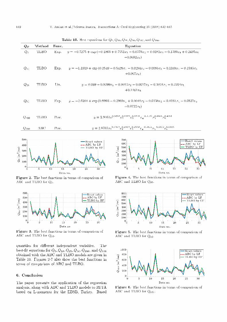
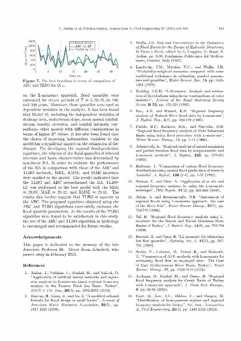
quantiles for di�erent independent variables. Thebest-�t equations for Q5; Q10; Q25; Q50; Q100, and Q500obtained with the ABC and TLBO models are given inTable 10. Figures 2-7 also show the best functions interms of comparison of ABC and TLBO.

6. Conclusion

The paper presents the application of the regressionanalysis, along with ABC and TLBO models to RFFAbased on L-moments for the EBSB, Turkey. Based






on the L-moments approach, ood quantiles wereestimated for return periods of T = 5; 10; 25; 50; 100,and 500 years. Moreover, these quantiles were used asdependent variables in the analysis. It has been foundthat Model 16, including the independent variables ofdrainage area, mainstream slope, mean annual rainfall,stream density, elevation, and rainfall intensity, out-performs other models with di�erent combinations interms of higher R2 values. It has also been found thatthe choice of inputting independent variables to themodel has a signi�cant impact on the estimation of dis-charges. For developing the regional ood-predictionequations, the relation of the ood quantiles of selectedintervals and basin characteristics was determined bynon-linear RA. In order to evaluate the performanceof the RA in comparison with those of the ABC andTLBO methods, MRE, RMSE, and MAE measureswere applied to the model. The results indicated thatthe TLBO and ABC outperformed the RA. TLBO-EF was performed as the best model with the MRE= 26.87, MAE = 23.42, and RMSE = 29.41. Theresults also further suggest that TLBO is superior tothe ABC. The proposed equations obtained using theABC and TLBO algorithms successfully estimate the ood quantile parameters. As the results of the TLBOalgorithm were found to be satisfactory in this study,the use of the ABC and TLBO algorithm in hydrologyis encouraged and recommended for future studies.

Acknowledgements

This paper is dedicated to the memory of the lateAssociate Professor Dr. Murat _Ihsan K�om�urc�u, whopassed away in February 2013.

References

1. Anilan, T., Sat�lm�s, U., Kankal, M., and Yuksek, O.\Application of arti�cial neural networks and regres-sion analysis to L-moments based regional frequencyanalysis in the Eastern Black Sea Basin, Turkey",KSCE J. Civ. Eng., 20(5), pp. 2082-2092 (2016).

2. Jiapeng, H., Liang, Z., and Yu, Z. \A modi�ed rationalformula for ood design in small basins", Journal ofAmerican Water Resources Association, 39(5), pp.1017-1025 (2003).

3. Wallis, J.R. Risk and Uncertainties in the Evaluationof Flood Events for the Design of Hydraulic Structures,In Piene e Siccit, edited by E. Guggino, G. Rossi, E.Todini, pp. 3-36. Fondazione Politecnica del Mediter-raneo, Catania, Italy (1982).

4. Landwehr, J.M., Matalas, N.C., and Wallis, J.R.\Probability-weighted moments compared with sometraditional techniques in estimating gumbel parame-ters and quantiles", Water Resour. Res., 15, pp. 1055-1064 (1979).

5. Hosking, J.R.M. \L-Moments: Analysis and estima-tion of distributions using linear combinations of orderstatistics", Journal of the Royal Statistical SocietySeries, B 52, pp. 105-124 (1990).

6. Rao, A.R. and Hamed, K.H. \Regional frequencyanalysis of Wabash River ood data by L-moments",J. Hydrol. Eng., 2(4), pp. 169-179 (1997).

7. Parida, B.P., Kachroo, R.K., and Shrestha, D.B.\Regional ood frequency analysis of Mahi-SabarmatiBasin using index ood procedure with L-moments",Water Resour. Manag., 12, pp. 1-12 (1998).

8. Adamowski, K. \Regional analysis of annual maximumand partial duration ood data by nonparametric andL-moment methods", J. Hydrol., 229, pp. 219-231(2000).

9. Haktanir, T. \Comparison of various ood frequencydistributions using annual ood peaks data of rivers inAnatolia", J. Hydrol., 136 (1-4), pp. 1-31 (1992).

10. Sorman, U. and Okur, A. \Application of at site andregional frequency analyses by using the L-momentstechnique", _IMO Digest., 11(3), pp. 665-668 (2000).

11. Atiem, A. and Harman�coglu, N.B. \Assessment ofregional oods using L-moments approach: the caseof the River Nile", Water Resour Manag., 20(5), pp.723-747 (2006).

12. Saf, B. \Regional ood frequency analysis using L-moments for the Buyuk and Kucuk Menderes RiverBasins of Turkey", J. Hydrol. Eng., 14(8), pp. 783-794(2009).

13. Bayaz�t, M. and Onoz, B. \LL-moments for estimatinglow ow quantiles", Hydrolog. Sci. J., 47(5), pp. 707-702 (2009).

14. Seckin, N., Cobaner, M., Yurtal, R., and Haktanir,T. \Comparison of ANN methods with L-moments forestimating ood ow at ungauged sites: The Caseof East Mediterranean River Basin, Turkey", WaterResour. Manag., 27, pp. 2103-2124 (2013).

15. Aydogan, D., Kankal, M., and Onsoy, H. \Regional ood frequency analysis for Coruh Basin of Turkeywith L-moments approach", J. Flood Risk Manage.,9, pp. 69-86 (2016).

16. Firat, M., Koc, A.C., Dikbas, F., and Gungor, M.\Identi�cation of homogeneous regions and regionalfrequency analysis for Turkey", Sci. Iran., TransactionA, Civil Engineering, 21(5), pp. 1492-1502 (2014).


17. Fill, H.D. and Stedinger, J.R. \Using regional regres-sion within index ood procedures and an empiricalBayesian estimator", J. Hydrol., 210, pp. 128-145,(1998).

18. Pandey, G.R. and Nguyen, V.T.V. \A comparativestudy of regression based methods in regional ood fre-quency analysis", J. Hydrol., 225, pp. 92-101 (1999).

19. Ouarda, T.B.M.J., Girard, C., Cavadias, G.S., andBobee, B. \Regional ood frequency estimation withcanonical correlation analysis", J. Hydrol., 254, pp.157-173 (2001).

20. Jingy, I.Z. and Hall, M.J. \Regional ood frequencyanalysis for the Gan-Ming River Basin in China", J.Hydrol., 296, pp. 98-117 (2004).

21. Reis, J.R., D.S., Stedinger, J.R., and Martins, E.S.\Bayesian GLS regression with application to LPE3regional skew estimation", Water Resour Res., 41,W10419 (2005). DOI: 10.1029/ 2004WR00344

22. Rahman, A. \A quantile regression technique toestimate design oods for ungauged catchments insouth-east Australia", Australian Journal of WaterResources, 9(1), pp. 81-89 (2005).

23. Gri�s, V.W. and Stedinger, J.R. \The use of GLSregression in regional hydrologic analysis", J. Hydrol.,344, pp. 82-95 (2007).

24. Leclerc, M. and Ouarda, T.B.M.J. \Non stationary re-gional frequency analysis at ungaged sites", J. Hydrol.,343, pp. 254-265 (2007).

25. Haddad, Kh., Rahman, A., Weinmann, P.E., Kucz-era, G., and Ball, J. \Stream ow data preparationfor regional ood frequency analysis: Lessons fromsoutheast Australia", Australian Journal of WaterResources, 14(1), pp. 17-32 (2010).

26. Palmen, L.B. and Weeks, W.D. \Regional ood fre-quency for Queesland using the quantile regressiontechnique", Australian Journal of Water Resources,15(1), pp. 47-56 (2011).

27. Rahman, A., Haddad, K., Zaman, M., Kuczera,G., and Weinmann, P.E. \Design ood estimationin ungauged catchments: a comparison between theprobabilistic rational method and quantile regressiontechnique for NSW", Australian Journal of WaterResources, 14(2), pp. 127-137 (2011).

28. Malekinezhad, H., Nactnebel, H.D., and Klik, A.\Comparing the index ood and multiple regressionmethods using L-moments", Phys. Chem. Earth, 36,pp. 54-60 (2011).

29. Haddad, K. and Rahman, A. \Regional ood fre-quency analysis in Eastern Australia: Bayesian GLSregression-based methods within �xed region and ROIframework-quantile regression and parameter regres-sion technique", J. Hydrol., 430-431, pp. 142-161(2012).

30. Zaman, M.A., Rahman, A., and Haddad, K. \Regional ood frequency analysis in arid regions: A case studyfor Australia", J. Hydrol., 475, pp. 74-83 (2012).

31. Rezaeianzadeh, M., Tabari, H., Yazdi, A.A., Isik, S.,and Kalin, L. \Flood ow forecasting using ANN,ANFIS and regression models", Neural Comput. Appl.,25(1), pp. 25-37 (2014).

32. Shu, C. and Burn, D.H. \Homogeneous pooling groupdelineation for ood frequency analysis using a fuzzyexpert system with genetic enhancement", J. Hydrol.,291, pp. 132-149 (2004).

33. Dawson, C.W., Abrahart, R.J., Shamseldin, A.Y., andWilby, R.L \Flood estimation at ungauged sites usingarti�cial neural networks", J. Hydrol., 319, pp. 391-409 (2006).

34. Shu, C. and Ouarda, T.B.M.J \Flood frequency anal-ysis at ungauged sites using ANN in canonical correla-tion analysis physiographic space" Water Resour Res.,43, W07438 (2007). DOI: 10.1029/2006WR005142

35. Shu, C. and Ouarda, T.B.M.J \Regional ood fre-quency analysis at ungauged sites using the adaptiveneuro-fuzzy inference system", J. Hydrol., 349, pp. 31-43 (2008).

36. Aziz, K., Rahman, A., Fang, G., and Shrestha, S.\Application of arti�cial neural networks in regional ood frequency analysis: a case study for Australia",Stoch. Env. Res. Risk A., 28(3), pp. 541-554 (2014).

37. Chau, K.W. \Particle swarm optimization trainingalgorithm for ANNs in stage prediction of Shing MunRiver", J. Hydrol., 329, pp. 363-367 (2006).

38. Jiong-feng, C., and Wan-chang, Z. \Application ofgenetic algorithm for model parameter calibration indaily rainfall-runo� simulations with the Xinanjiangmodel", Journal of China Hydrology, 26(4), pp. 32-38(2006).

39. Jun, Z., Chuntian, C., Jianjian, S., and Shiqin, Z. \Antcolony optimization-based support-vector machine formid-and-long term hydrological forecasting", Journalof Hydroelectric Engineering, 06 (2010).

40. Kisi, O., Ozkan, C., and Akay, B. \Modeling discharge-sediment relationship using neural networks with arti-�cial bee colony algorithm", J. Hydrol., 428-429, pp.94-103 (2012).

41. Salimi, S., Mahmoodi, H., and Barahman, N. \Weekly-discharge estimation for Tang-Karzin's station, usingMLP network optimized by ABC algorithm" Interna-tional Journal of Basic and Applied Science, 02(02),pp. 242-253 (2013).

42. Uzlu, E., Kankal, M., Akpinar, A., and Dede, T.\Estimates of energy consumption in Turkey usingneural networks with the teaching-learning-based opti-mization algorithm." Energy, 75, pp. 295-303 (2014).

43. Yerdelen, C. \Change point of river stream ow inTurkey." Sci. Iran., Transaction A, Civil Engineering,21(2), p. 306 (2014).

44. Yuksek, O., Kankal, M., and Ucuncu, O. \Assessmentof big oods in the Eastern Black Sea Basin of Turkey"Environmental Monit Assess, 185, pp. 797-814 (2013).


45. DMi, Analysis of Turkey's Maximum PrecipitationValues and their Return Periods, Ankara, Turkey:Turkish State Meteorological Service (2001).

46. DSi \Annual ood reports" Ankara, Turkey, GeneralDirectorate of State Hydraulic Works (1970-2005).

47. Saka, F. \Determination of synthetic ow durationcurves by using mathematical methods and a casestudy in the Eastern Black Sea" PhD Thesis, Karad-eniz Technical University, Turkey (2012).

48. Yang, T., Shao, Q., Hao, Z.C., Chen, X., Zhang, Z.,Xu, C.Y., and Sun, L. \Regional frequency analysisand spatio temporal pattern characterization of rainfallextremes in Pearl River Basin, China", J. Hydrol., 380,pp. 386-405 (2010).

49. Nyeko-Ogiramoi, P., Willems, P., Mutua, F.M., andMoges, S.A. \An elusive search for regional ood fre-quency estimates in the River Nile Basin", Hydrologyand Earth System Sciences, 16, pp. 3149-3163 (2012).

50. Hosking, J.R.M. \On the characterization of distri-butions by their L-moments", Journal of StatisticalPlanning and Inference, 136, pp. 193-198 (2004).

51. Hosking, J.R.M. L-Moments, John Wiley & Sons, Inc.(1998).

52. Anilan, T. \Application of arti�cial intelligence meth-ods to L-moments based regional frequency analysis inthe Eastern Black Sea Basin", PhD Thesis, KaradenizTechnical University, Turkey (2014).

53. Karaboga, D. \An idea based on honey bee swarmfor numerical optimization", Technical Report- TR06,Erciyes University Engineering Faculty of ComputerEngineering Department (2005).

54. Ozt�urk, H.T. and Durmus, A. \Optimum cost designof RC columns using arti�cial bee colony algorithm",Struct. Eng. Mech., 45(5), pp. 643-54 (2013).

55. Pan, Q.K., Tasgetiren, M.F., Suganthan, P.N., andChua, T.J. \A discrete arti�cial bee colony algorithmfor the lot-streaming ow shop scheduling problem",Inf. Sci., 181, pp. 2455-60 (2011).

56. Karaboga, D. and Basturk, B. \Arti�cial bee colony(ABC) optimization algorithm for solving constrainedoptimization problems", Found Fuzzy Log Soft Com-put, 4529, pp. 789-798 (2007).

57. Uzlu, E., Akp�nar, A., Ozturk, H.T., Nacar, S., andKankal, M. \Estimates of hydroelectric generation us-ing neural networks with ABC algorithm for Turkey",Energy, 69, pp. 638-647 (2014).

58. Rao, R.V., Savsani, V.J., and Vakharia, D.P.\Teaching-learning based optimization: A novel

method for constrained mechanical design optimiza-tion problems", Computer-Aided Design, 43, pp. 303-315 (2011).

59. Togan, V. \Design of planar steel frames usingteaching-learning based optimization", Eng. Struct.,34, pp. 225-32 (2012).

60. Togan, V. \Design of pin jointed structures usingteaching learning based optimization", Struct. Eng.Mech., 47, pp. 209-225 (2013).

61. Dede, T. \Optimum design of grillage structures toLRFD-AISC with teaching-learning based optimiza-tion", Structural and Multidisciplinary Optimization,48, pp. 955-964 (2013).

Biographies

Tu�g�ce An�lan is an Assistant Professor in Civil Engi-neering Department in Karadeniz Technical University,Trabzon, Turkey. Her current research focuses on oodfrequency analysis, oods and sea outfalls.

Ergun Uzlu received BS, MS, and PhD degrees inCivil Engineering from Karadeniz Technical University,Trabzon, Turkey in 2008, 2011, and 2016, respectively.He is currently a Research Assistant in KaradenizTechnical University, Trabzon, Turkey. His researchinterests include coastal engineering, energy estimatemodels, and arti�cial intelligence techniques.

Murat Kankal is an Assistant Professor in CivilEngineering Department in Karadeniz Technical Uni-versity, Trabzon, Turkey. His current research focuseson sediment transport in coastal area, regional oodfrequency analysis, hydropower, and arti�cial neuralnetworks.

�Omer Y�uksek was born in C�aykara, Trabzon, Turkeyin 1962. He graduated from Mara�s� Village PrimarySchool, from C�aykara _In�on�u Secondary School, fromTrabzon Religious Vocational High School, and fromKaradeniz Technical University (KTU) EngineeringFaculty (EF) at Civil Engineering Department (CED).He completed Post Graduate and Doctorate Educa-tions in KTU CED Hydraulic Division (HD) in 1986and 1992, respectively. He studied in KTU EF CEDHD as a Research Assistant between 1984-1993, as anAssistant Professor between 1993-1996, as an AssociateProfessor between 1996-2005, and as a Professor from2005 until now. He is the Head of Hydraulic Division.

Documents

The estimation of ood quantiles in ungauged sites using ...scientiairanica.sharif.edu/article_4185_ef5663df49324ea7f3902749cd7815c6.pdfusing teaching-learning based optimization and