The Role of Global Value Chains in Carbon Intensity

1

The Role of Global Value Chains in Carbon Intensity

Convergence: A Spatial Econometrics Approach

May 22, 2021

Kazem Biabany Khameneh

Faculty of Management and Economics, Tarbiat Modares University

Email: [email protected] Tel: +98(21)82884640

Address: Nasr, Jalal AleAhmad, Tehran, Iran

Reza Najarzadeh

Faculty of Management and Economics, Tarbiat Modares University

Email: [email protected]

Tel: +98(21)82884640 Address: Nasr, Jalal AleAhmad, Tehran, Iran

P.O. Box: 14115-111

Corresponding Author

Hassan Dargahi

Faculty of Economics and Political Sciences, Shahid Beheshti University

Email: [email protected] Tel: +98(21)29902977

Address: Evin, Tehran, Iran

P.O. Box: 193 581 3654

Lotfali Agheli

Economic Research Institute, Tarbiat Modares University

Email: [email protected]

Tel: +98(912)6186317

Address: Nasr, Jalal AleAhmad, Tehran, Iran

P.O. Box: 14115-111

2

The Role of Global Value Chains in Carbon Intensity

Convergence: A Spatial Econometrics Approach

Abstract: The expansion of trade agreements has provided a potential basis for

trade integration and economic convergence of different countries. Moreover,

developing and expanding global value chains (GVCs) have provided more

opportunities for knowledge and technology spillovers and the potential

convergence of production techniques. This can result in conceivable

environmental outcomes in developed and developing countries. This study

investigates whether GVCs can become a basis for the carbon intensity (CI)

convergence of different countries. To answer this question, data from 101

countries from 1997 to 2014 are analyzed using spatial panel data econometrics.

The results indicate a spatial correlation between GVCs trade partners in terms of

CI growth, and they confirm the GVCs-based conditional CI convergence of the

countries. Moreover, estimates indicate that expanding GVCs even stimulates

bridging the CI gap between countries, i.e., directly and indirectly through

spillover effects. According to the results, GVCs have the potential capacity to

improve the effectiveness of carbon efficiency policies. Therefore, different

dimensions of GVCs and their benefits should be taken into account when

devising environmental policies.

Keywords: global value chains, carbon intensity, conditional convergence,

spatial panel data regression, trade in value-added

3

1. Introduction

The impacts of trade on the environment and greenhouse gas emissions have been

among the controversial topics in the economic literature over the past three

decades, and it is still difficult to determine whether trade is good for the

environment or not (Frankel and Rose, 2005). Apart from how trade affects the

environment, trade agreements and integrations have raised the likelihood for the

potential convergence of environmental indicators of various countries (Apergis

and Payne, 2020; Baghdadi et al., 2013). Meanwhile, dramatic changes in trade

and globalization processes, such as the emergence of GVCs and the international

fragmentation of production, have provided more opportunities for trade

integration and further expansion of knowledge and technology flows among

countries.

This study aims to determine if GVCs can provide a basis for the CI convergence

of countries and how expanding participation in GVCs affects CI growth. The

answers to these questions can somewhat clarify how this new form of trade can

bridge the CI gap between countries, and how expanding participation in GVCs

can be a strategy to reduce environmental degradation. The answers might even

reveal that this new form of trade is not only detrimental, but also beneficial to

the environment. As acknowledged by Thomakos and Alexopoulos (2016), CI is

the strongest explanatory variable in the Environmental Performance Index1

(EPI). In other words, these two are two sides of the same coin. Therefore, CI

changes can properly measure the environmental performance of countries. If we

find out how GVCs affect the CI changes of countries, we can then appropriately

generalize it to environmental performance, benefit from GVC capacities to

formulate environmental protection policies and regulations, and reach

multilateral agreements to mitigate climate change.

1 https://epi.yale.edu/

4

The rest of this paper is organized as follows: Sections 2 and 3 review the

theoretical foundations and the research background. The methodology for the

data analysis is introduced in Section 4, and the results are presented in Section

5. Finally, Section 6 discusses the results and draws the conclusions.

2. Theoretical Foundations

There are different views on the link between trade and the environment in the

economic literature. Some refer to the positive environmental impacts of trade

through technology development and transfer and spillover effects, while others

discuss the pollution haven hypothesis (PHH) and the potential degradation of the

environment in developing countries through trade with developed countries.

However, some argue that trade is detrimental to the environment because it

scales up the economic activities that are inherently harmful to the environment

and encourages the polluting countries to engage more extensively in highly-

polluting activities (Copeland and Taylor, 2013; Weber et al., 2021). Thus, trade

is a double-edged sword that can both help protect the environment through the

development and spillover of eco-friendly technologies (Lovely and Popp, 2011;

Nemati et al., 2019) and be a ground for environmental degradation, as suggested

by the pollution haven hypothesis and the factor endowment theory (Antweiler et

al., 2001; Cherniwchan et al., 2017; Shen, 2008).

The recent increase in the number of trade agreements and the emergence of

GVCs, which account for more than half of the global trade, have fundamentally

altered the structure and organization of international trade, encouraging the

establishment of international production networks and massive developments in

bilateral trade, especially for intermediate goods. This new wave of globalization

has also redrawn the boundaries of knowledge, production structure, and

comparative advantages of different countries, while changing the relations

between developed and developing countries (Baldwin, 2017). GVCs have

5

facilitated the transfer of technical innovations, skills, and knowledge from

developed countries to developing countries (Jangam and Rath, 2020), allowing

developing countries to enter global markets and reap potential benefits without

having to develop ancillary industries and resorting to the local production of all

the required inputs (Rodrik, 2018).

Countries have already been participating in international trade (e.g., developing

countries import parts and technology to produce and supply goods to the

domestic market). However, the new form of trade has increased the countries’

use of international production networks, intensified the knowledge information

flows (Taglioni et al., 2016), and facilitated further knowledge spillovers

compared to the traditional trade methods (Piermartini and Rubínová, 2014).

Knowledge flows more easily within the supply chain because the outsourcer

transfers the necessary knowledge and technology to the input producer firm to

ensure the efficient production of inputs and compliance with its production

standards (Piermartini and Rubínová, 2014).

By reallocating scarce resources to the most profitable activities, GVCs can

increase the efficiency of an economy by improving static efficiency (i.e.,

modifying existing processes and capacities) and dynamic efficiency (i.e.,

creating new processes and capacities). As shown by Kummritz (2016), the

expansion of GVCs is expected to raise per capita income, investment,

productivity, and domestic value-added production. Participation in supply

chains and international production networks can also lead to learning-by-doing

benefits, economies of scale, and technology progress and spillovers, and even

accelerate the industrialization process and the development of the country’s

service sector (Bernhardt and Pollak, 2016; Dorrucci et al., 2019; Ignatenko et

al., 2019; Kummritz, 2016; Pigato et al., 2020; Taglioni et al., 2016). Markusen

(1984) also argues that the increasing global technical efficiency is associated

6

with the growth of multinational enterprises (a key element of GVCs) as there is

evidence of technology spillovers following their activities (Keller, 2010).

The outcomes and effects of expanding participation in GVCs are beyond

economic growth. For example, the growth of GVCs and trade in intermediate

inputs can improve South-South trade (Hanson, 2012). Moreover, expanding

GVCs can intensify the transmission of shocks, the synchronization of global

business cycles, and changes in specialization patterns, while also causing

transformations in international trade policies (Dorrucci et al., 2019; Wang et al.,

2017). However, the effects of GVCs on the environmental performance of

countries and their role in environmental phenomena have received little attention

in the relevant literature.

If GVCs facilitate the convergence of production techniques as expected (Rodrik,

2018), integration of GVCs with technological advancement and transfer will

increase the countries’ income level, thus possibly helping to converge some of

their economic indicators (Ignatenko et al., 2019). The existing evidence also

suggests that trade, trade integration, and regional cooperation help increase the

convergence of energy efficiency, energy intensity, and environmental

performance of the countries (Han et al., 2018; Qi et al., 2019; Wan et al., 2015).

Meanwhile, trade integration requires changes in the existing standards and

regulations (even environmental standards and regulations) of the countries to

reduce trade frictions and facilitate trade flows (Nicoletti et al., 2003). Holzinger

et al. (2008) also showed that increasing international links would lead to the

convergence of the involved countries’ environmental policies. The expansion of

multinational corporations also contributes to sustainable management,

knowledge transfer, and the development of low-CI production technologies

(López et al., 2019).

7

On the other hand, the new form of trade may not only help countries converge

by equalizing the prices of production factors, but also improve the environmental

performance of the countries by increasing technology spillovers and

environmentally-efficient knowledge. Along with technical progress, the

spillover, diffusion, and transfer of cleaner technologies to countries with lower

energy and environmental efficiency, especially developing countries, will

further improve environmental performance (Gerlagh and Kuik, 2014; Huang et

al., 2020; Jaffe et al., 2002; LeSage and Fischer, 2008; Wan et al., 2015). Jiang et

al. (2019) reported that countries with technologically-advantageous trading

partners emitted less carbon because they were allowed to share the produced

resources with their major trading partners. Additionally, the flow of knowledge

between firms in GVCs can accelerate advances in eco-friendly technologies. The

expansion of GVCs can also bring more affordable and less expensive

technologies for the generation and consumption of clean and more efficient

sources of energy (WDR, 2020).

Therefore, expanding GVCs can potentially provide more opportunities for the

convergence of the environmental performance of the involved countries.

Nevertheless, confirming or rejecting such hypotheses will require empirical

tests, which is the purpose of this study.

3. Research Background

To the best of our knowledge, the role of GVCs in converging the environmental

performance of countries has not yet been studied. However, some studies have

dealt with the effects of trade and foreign direct investment (FDI) on the

convergence of energy intensity and carbon emissions. For example, Wan et al.

(2015) analyzed the effects of trade spillovers on the energy efficiency

convergence of 16 EU countries using spatial panel data. Their results indicated

a correlation (spatial autocorrelation) between two trading partners in terms of

8

energy efficiency. They confirmed the existence of a convergence and found that

countries with greater reliance on trade had higher energy efficiency growth and

a higher convergence rate because trade facilitated competition and technological

influences, preventing the occurrence of the race to the bottom.

Jiang et al. (2018) studied the convergence of energy intensity in Chinese

provinces in the period from 2003 to 2015 using a spatial regression model. They

concluded that neglecting spatial spillovers would lead to the underestimation of

conditional convergence. They argued that reduced energy intensity depended on

the internal factors of each province, while it was also influenced by spatial

spillover effects of the neighbors, especially technology and knowledge

spillovers and input-output relationships. Their findings also revealed that FDI

played a major role in reducing energy intensity.

You and Lv (2018) studied the spatial effects of economic globalization on CO2

emissions in 83 countries over the period from 1985 to 2013 using a spatial panel

approach. They found a spatial correlation in the CO2 emission of countries.

Moreover, they concluded that having highly-globalized neighbors would

improve the environmental quality of a country, indicating that international

cooperation and economic integration are important for the environment.

Huang et al. (2019) conducted a study on 61 countries based on data from 1992

to 2016 using the panel smooth transition regression (PSTR) model. They report

that the globalization threshold (KOF index) affects the conditional convergence

of energy intensity in a nonlinear manner, i.e., as the globalizations crosses the

threshold, convergence speeds up. They suggest that increasing interactions

between countries through trade and political, social, and interregional

cooperation can reduce energy intensity.

Xin-gang et al. (2019) studied the role of FDI in reducing the energy efficiency

gap between different regions of China in the period from 2005 to 2014 using

9

spatial econometric models. Their results showed that there was no absolute

convergence; however, they found conditional convergence in the energy

intensity of the studied regions, which was strengthened by FDI. They also

reported the spatial spillover effects of FDI.

Huang et al. (2019) analyzed the CI convergence of Chinese provinces in the

period from 2000 to 2016 using a dynamic spatial regression approach. They

concluded that there was a CI convergence in Chinese provinces, stating that FDI,

trade openness, and spatial spillover effects could help reduce energy intensity.

Awad (2019) estimated panel cointegration regressions to determine the effects

of intercontinental trade (trade with countries outside Africa) of 46 African

countries on CO2 and PM10 emissions from 1990 to 2017. The results indicated

that intercontinental trade improved Africa’s environmental quality because

countries of this continent were able to achieve sustainable development by

overcoming challenges such as poverty and internal strife through trade

mechanisms.

Qi et al. (2019) studied the energy intensity convergence in 56 countries of the

Belt and Road Initiative (BRI) using the smooth transition regression (STR)

model with an emphasis on the role of China’s trade with these countries in

energy intensity convergence. The results indicated that trade facilitated energy

intensity convergence and the convergence rate was higher in countries with large

bilateral trade with or considerable technology imports from China. They also

provided evidence of spillover effects of technology.

Some studies have recently analyzed the effects of GVCs on the environment and

energy. For instance, Kaltenegger et al. (2017) studied the effects of GVCs on

the energy footprint in 40 countries using structural decomposition analysis. The

results showed that there was an increase of about 29% in the global energy

footprint from 1995 to 2009 mainly due to the growth of economic activities. On

10

the other hand, the reduced sectoral energy intensity was the main factor slowing

down energy consumption. Changes in GVCs were responsible for a 7.5%

increase in the global energy consumption, 5.5% of which was related to the

increased backward linkages, and 1.8% could be attributed to changes in the

regional composition of intermediate inputs. Although the global economic boom

in East Asia has increased the global energy footprint, the sectoral composition

of GVCs has negligible effects on the energy footprint.

Liu et al. (2018) studied the effects of the GVC position of 14 Chinese

manufacturing industries on their energy and environmental efficiency in the

period from 1995 to 2009. They concluded that there was a positive feedback

relationship between these industries, and the improved GVC position of the

industries caused a 35% improvement in their energy and environmental

efficiency. They suggested that the allocation of more budget to research and

development activities and the promotion of knowledge absorption capacities

were necessary to achieve a better GVC position and improve the environment.

Sun et al. (2019) analyzed the effects of the GVC position on the carbon

efficiency of 60 countries in the period from 2000 to 2011 using data envelopment

analysis (DEA) and panel remission. They concluded that the promoted GVC

position improved both energy efficiency and carbon efficiency. They also

showed that the effects of promoting the GVC position were greater on

technological industries than labor-intensive and resource-intensive industries.

Yasmeen et al. (2019) studied the effects of trade in value-added (TiVA) on air

pollutants in 39 countries in the period from 1995 to 2009. The panel regression

results indicated that there was an inverted-U relationship between TiVA and the

concentration of air pollutants, and the effects of TiVA were greater on carbon

monoxide than other pollutants. They concluded that the early stages of TiVA

11

might increase environmental pollution; however, further development of TiVA

and production methods could reduce the concentration of air pollutants.

4. Methodology

This study first analyzes whether there is a GVC-based correlation between

countries in terms of CI growth. Then, it investigates the role of expanding

participation in GVCs in the CI convergence of the countries. The possible

spillover effects of participation in GVCs are also addressed. Therefore, it is

necessary to employ appropriate statistical techniques that can both consider

spatial dimensions of the statistical data and model spillover effects. The spatial

statistics used in this study for data analysis will be discussed in the next

subsections.

4.1. Spatial Autocorrelation

Spatial autocorrelation is based on the assumption that adjacent subjects are more

similar to each other. Suppose that countries i and j have a very high volume/value

of bilateral TiVA and considerable trade relations. In other words, they are trade

neighbors. Can this neighborhood play a role in their correlation in terms of CI

growth? Measures such as Moran’s I and Geary’s C are usually used to examine

such a spatial autocorrelation. These two measures show whether there is a

correlation between the two countries in terms of CI growth concerning GVCs.

Moran’s I for a dataset is calculated using the following equation

(Gangodagamage et al., 2008; Kalkhan, 2011, chap. 3):

(1)

𝐼 =

1𝑊

∑ ∑ 𝑤𝑖𝑗(𝑧𝑖 − 𝑧̅) ⋅ (𝑧𝑗 − 𝑧̅)𝑖≠𝑗𝑖

1𝑛

∑ (𝑧𝑖 − 𝑧̅)2𝑖

.

In which, I represents Moran’s I, 𝑧𝑖 denotes CI growth, and i and j represent 1

through n (i.e., the number of sample countries). Moreover, 𝑤𝑖𝑗 is a spatial weight

12

matrix that shows how close i and j are (this was measured based on GVCs in

this study, and the definition of this matrix is presented in Section 4.3), and 𝑊 is

their sum. Similar to Pearson’s correlation coefficient, positive and negative

values of Moran’s I indicate positive and negative spatial autocorrelation,

respectively.

A difference between Geary’s C and Moran’s I is that the former measures the

interaction between i and j based on their difference, and not based on standard

deviation (Gangodagamage et al., 2008; Kalkhan, 2011, chap. 3):

(2) 𝐶 =

(𝑛 − 1)∑ ∑ 𝑤𝑖𝑗(𝑧𝑖 − 𝑧𝑗)2

𝑗𝑖

2∑ ∑ 𝑤𝑖𝑗(𝑧𝑖 − 𝑧̅)2𝑗𝑖

.

In this equation, 𝐶 represents Geary’s C, which ranges from 0 to 2. Values smaller

than 1 correspond to positive autocorrelation, while values greater than 1

correspond to negative autocorrelation. The significance of both Geary’s C and

Moran’s I can be examined by assuming the spatial randomness under the

standard normal distribution.2

4.2. Spatial Panel Data Regression

Spatial autocorrelation measures the possible correlation of CI growth between

countries i and j due to their GVC-based neighborhood. Spatial panel data

regression examines whether there is a CI growth convergence and how

expanding GVCs affects this convergence. It also identifies the potential spillover

effects of GVCs. These models are of special importance as Anselin (2003a)

argues that some phenomena, such as neighborhood effects and the race to the

bottom, are among the instances of interactions between economic agents,

2 The statistics of Moran’s I and Geary’s C are

𝐼−𝐸(𝐼)

𝑆𝑑(𝐼) and

𝐶−𝐸(𝐶)

𝑆𝑑(𝐶), respectively, in which, E () and SD denote the expectation

and standard deviation, respectively.

13

suggesting that interactive and spatial models must be used to analyze such

situations.

In general, there are three types of commonly-used spatial econometric data panel

models, i.e., the Spatial Lag Model (SLM), the Spatial Error Model (SEM), and

the Spatial Durbin Model (SDM) (LeSage and Pace, 2009). The SLM model

assumes that the observed value of the dependent variable in a section is affected

by both exogenous regressors and the spatial mean weight of the dependent

variables of its neighbors. The regression can be presented as follows:

(3)

𝑦𝑖𝑡 = 𝜌∑𝑤𝑖𝑗𝑦𝑗𝑡

𝑁

𝑗=1

+ 𝑥𝑖𝑡𝛽 + 𝜇𝑖 + 휀𝑖𝑡 .

In this equation, 𝑦 represents the dependent variable for section i at time t,

∑ 𝑤𝑖𝑗𝑦𝑗𝑡𝑁𝑗=1 denotes endogenous interactive effects of the dependent variables 𝑦𝑖𝑡

and 𝑦𝑗𝑡 in neighboring sections (N sections), and 𝜌 is the spatial autoregression

coefficient that measures the size of the simultaneous spatial correlation between

a section and its neighboring sections. Moreover, 𝑥𝑖𝑡 is the matrix of independent

explaining variables, and the 𝛽 vector represents the effects of these independent

variables (also known as the exogenous regressor), while 𝜇𝑖 shows the fixed

effects that capture the specific effects of each section. The 휀𝑖𝑡 error component

is also assumed to be i.i.d. with a zero mean and a constant variance. In addition,

𝑤𝑖𝑗 is the spatial weights matrix, which can be established based on both

economic and geographical measures (as described in Section 4.3).

SEM also takes into account the interactive effects between the error components.

This model is of greater importance when independent variables excluded from

the regression affect the interactive effects of the sections. This model can be

presented as follows:

14

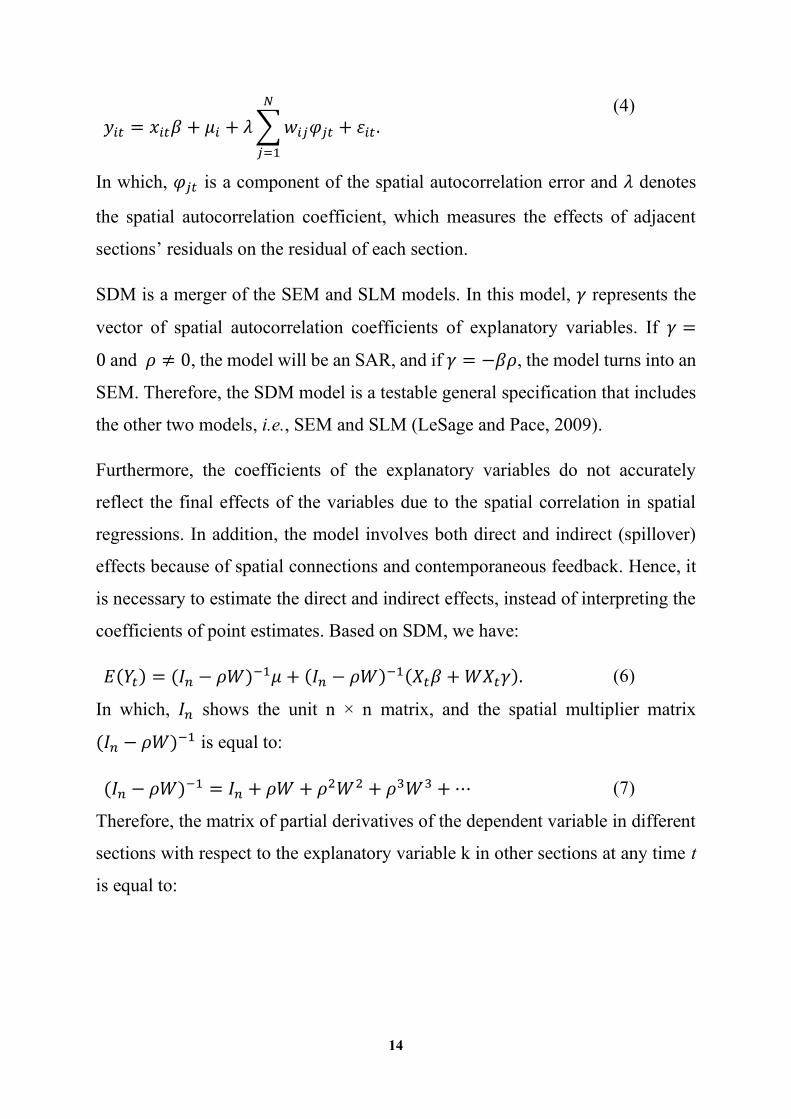
(4)

𝑦𝑖𝑡 = 𝑥𝑖𝑡𝛽 + 𝜇𝑖 + 𝜆 ∑𝑤𝑖𝑗𝜑𝑗𝑡

𝑁

𝑗=1

+ 휀𝑖𝑡 .

In which, 𝜑𝑗𝑡 is a component of the spatial autocorrelation error and 𝜆 denotes

the spatial autocorrelation coefficient, which measures the effects of adjacent

sections’ residuals on the residual of each section.

SDM is a merger of the SEM and SLM models. In this model, 𝛾 represents the

vector of spatial autocorrelation coefficients of explanatory variables. If 𝛾 =

0 and 𝜌 ≠ 0, the model will be an SAR, and if 𝛾 = −𝛽𝜌, the model turns into an

SEM. Therefore, the SDM model is a testable general specification that includes

the other two models, i.e., SEM and SLM (LeSage and Pace, 2009).

Furthermore, the coefficients of the explanatory variables do not accurately

reflect the final effects of the variables due to the spatial correlation in spatial

regressions. In addition, the model involves both direct and indirect (spillover)

effects because of spatial connections and contemporaneous feedback. Hence, it

is necessary to estimate the direct and indirect effects, instead of interpreting the

coefficients of point estimates. Based on SDM, we have:

(6) 𝐸(𝑌𝑡) = (𝐼𝑛 − 𝜌𝑊)−1𝜇 + (𝐼𝑛 − 𝜌𝑊)−1(𝑋𝑡𝛽 + 𝑊𝑋𝑡𝛾).

In which, 𝐼𝑛 shows the unit n × n matrix, and the spatial multiplier matrix

(𝐼𝑛 − 𝜌𝑊)−1 is equal to:

(7) (𝐼𝑛 − 𝜌𝑊)−1 = 𝐼𝑛 + 𝜌𝑊 + 𝜌2𝑊2 + 𝜌3𝑊3 + ⋯

Therefore, the matrix of partial derivatives of the dependent variable in different

sections with respect to the explanatory variable k in other sections at any time t

is equal to:

15

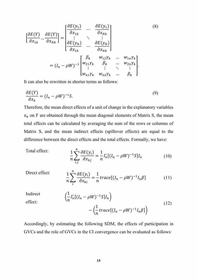
(8)

[𝜕𝐸(𝑌)

𝜕𝑥1𝑘…

𝜕𝐸(𝑌)

𝜕𝑥𝑁𝑘] =

[ 𝜕𝐸(𝑦1)

𝜕𝑥1𝑘⋯

𝜕𝐸(𝑦1)

𝜕𝑥𝑁𝑘

⋮ ⋱ ⋮𝜕𝐸(𝑦𝑁)

𝜕𝑥1𝑘⋯

𝜕𝐸(𝑦𝑁)

𝜕𝑥𝑁𝑘 ]

= (𝐼𝑛 − 𝜌𝑊)−1 [

𝛽𝑘 𝑤12𝛾𝑘 … 𝑤1𝑛𝛾𝑘

𝑤21𝛾𝑘 𝛽𝑘 … 𝑤2𝑛𝛾𝑘

⋮ ⋮ ⋱ ⋮𝑤𝑛1𝛾𝑘 𝑤𝑛2𝛾𝑘 … 𝛽𝑘

].

It can also be rewritten in shorter terms as follows:

(9) 𝜕𝐸(𝑌)

𝜕𝑥𝑘= (𝐼𝑛 − 𝜌𝑊)−1𝑆.

Therefore, the mean direct effects of a unit of change in the explanatory variables

𝑥𝑘 on 𝑌 are obtained through the mean diagonal elements of Matrix S, the mean

total effects can be calculated by averaging the sum of the rows or columns of

Matrix S, and the mean indirect effects (spillover effects) are equal to the

difference between the direct effects and the total effects. Formally, we have:

(10) 1

𝑛∑

𝜕𝐸(𝑦𝑖)

𝜕𝑥𝑘𝑗

𝑛

𝑖,𝑗

=1

𝑛𝐼𝑛′ [(𝐼𝑛 − 𝜌𝑊)−1𝑆]𝐼𝑛

Total effect:

(11) 1

𝑛∑

𝜕𝐸(𝑦𝑖)

𝜕𝑥𝑘𝑖

𝑛

𝑖

=1

𝑛𝑡𝑟𝑎𝑐𝑒[(𝐼𝑛 − 𝜌𝑊)−1𝐼𝑛𝛽]

Direct effect:

(12)

(1

𝑛𝐼𝑛′ [(𝐼𝑛 − 𝜌𝑊)−1𝑆]𝐼𝑛)

− (1

𝑛𝑡𝑟𝑎𝑐𝑒[(𝐼𝑛 − 𝜌𝑊)−1𝐼𝑛𝛽])

Indirect

effect:

Accordingly, by estimating the following SDM, the effects of participation in

GVCs and the role of GVCs in the CI convergence can be evaluated as follows:

16

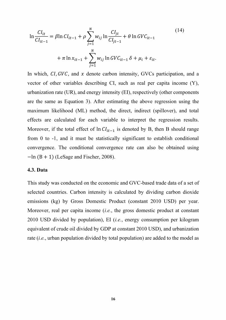
(14)

ln𝐶𝐼𝑖𝑡

𝐶𝐼𝑖𝑡−1= 𝛽ln𝐶𝐼𝑖𝑡−1 + 𝜌 ∑𝑤𝑖𝑗 ln

𝐶𝐼𝑗𝑡𝐶𝐼𝑗𝑡−1

𝑁

𝑗=1

+ 𝜃 ln𝐺𝑉𝐶𝑖𝑡−1

+ 𝜋 ln 𝑥𝑖𝑡−1 + ∑𝑤𝑖𝑗 ln 𝐺𝑉𝐶𝑖𝑡−1 𝛿

𝑁

𝑗=1

+ 𝜇𝑖 + 휀𝑖𝑡 .

In which, 𝐶𝐼, 𝐺𝑉𝐶, and 𝑥 denote carbon intensity, GVCs participation, and a

vector of other variables describing CI, such as real per capita income (Y),

urbanization rate (UR), and energy intensity (EI), respectively (other components

are the same as Equation 3). After estimating the above regression using the

maximum likelihood (ML) method, the direct, indirect (spillover), and total

effects are calculated for each variable to interpret the regression results.

Moreover, if the total effect of ln 𝐶𝐼𝑖𝑡−1 is denoted by B, then B should range

from 0 to -1, and it must be statistically significant to establish conditional

convergence. The conditional convergence rate can also be obtained using

−ln (Β + 1) (LeSage and Fischer, 2008).

4.3. Data

This study was conducted on the economic and GVC-based trade data of a set of

selected countries. Carbon intensity is calculated by dividing carbon dioxide

emissions (kg) by Gross Domestic Product (constant 2010 USD) per year.

Moreover, real per capita income (i.e., the gross domestic product at constant

2010 USD divided by population), EI (i.e., energy consumption per kilogram

equivalent of crude oil divided by GDP at constant 2010 USD), and urbanization

rate (i.e., urban population divided by total population) are added to the model as

17

regressors. The data for 101 countries3 in the period from 1997 to 2014 were

extracted from the World Bank’s WDI Database.4

Following Aslam et al. (2017), the method proposed by Koopman et al. (2014)

was employed to measure participation in GVCs. In this method, the level of

participation of country i in GVCs at time t is equal to:

(14) 𝐺𝑉𝐶𝑖𝑡 =𝐷𝑉𝑋𝑖𝑡 + 𝐹𝑉𝐴𝑖𝑡

𝐺𝑟𝑜𝑠𝑠 𝐸𝑥𝑝𝑜𝑟𝑡𝑠𝑖𝑡.

In which, FVA, DVX, and Gross Exports represent foreign value-added, indirect

domestic value-added, and the total value of a country’s exports in each period,

respectively5. This indicator measures the level of a country’s participation in

GVCs regardless of its scale of economy. The data on FVA, DVX, and Gross

Exports were extracted from the UNCTAD-EORA Database (Casella et al.,

2019)6.

According to Section 3.1, a spatial weight matrix should be developed to capture

the spatial distance between the countries (i.e., sections) in the sample. This

weight matrix, which is also called the distance matrix, can be developed either

geographically to show the geographical distance between the countries or

economically to reveal the economic distance between them (Anselin, 2003b).

Similar to studies conducted by Conley et al. (2002), Wan et al. (2015), Jiang et

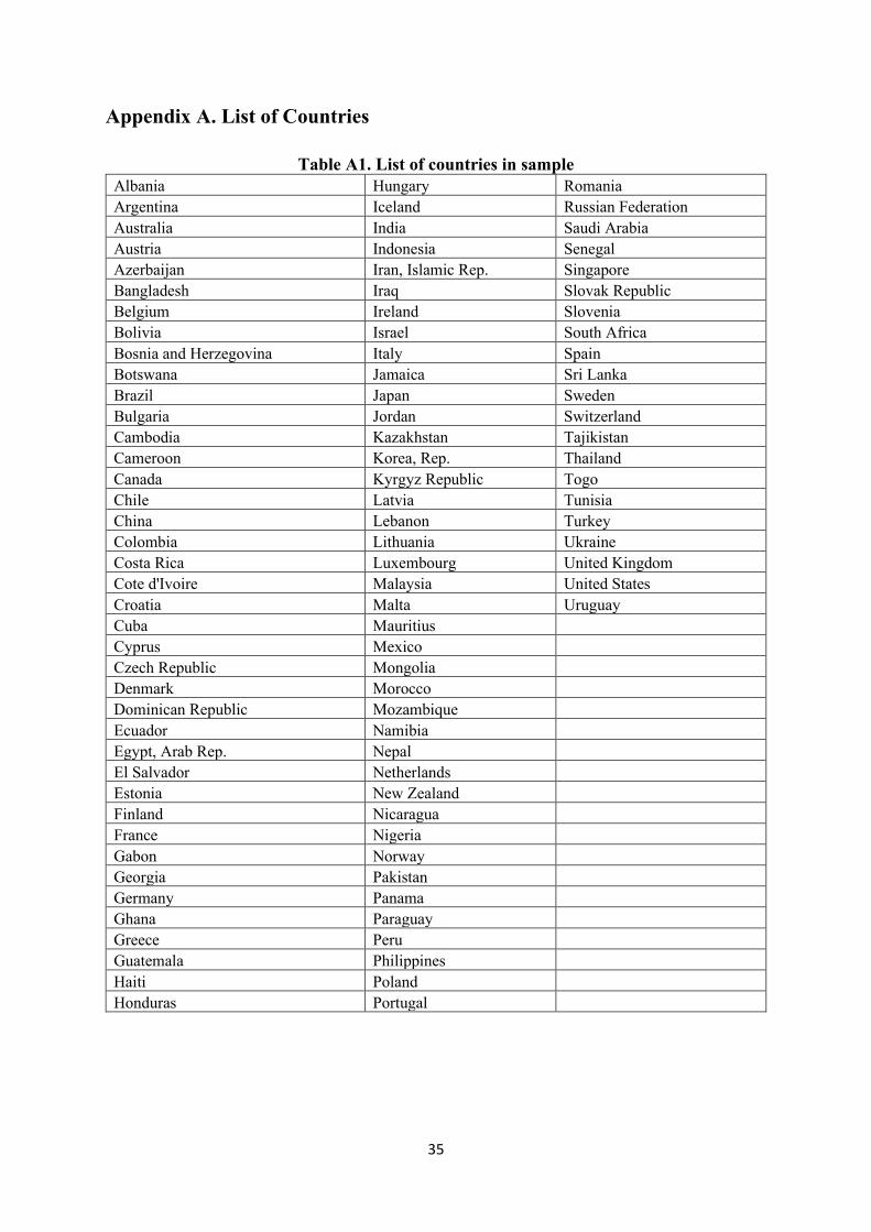
3 The countries are listed in Appendix A.

4 The main reason for choosing this number of countries and this time period was the availability of data because spatial

data panel regressions should not contain missing data. In other words, only a balanced data panel should be used that

includes the same data for all the countries in a given period.

5 Foreign value-added corresponds to the value added of inputs that were imported in order to produce intermediate or

final goods/services to be exported. Indirect domestic value-added is part of the domestic value-added exported to other

countries (exported input) that is used as input in other countries’ exports. Gross exports or total exports is the sum of GVCs-

based trade and traditional trade, which is the same as the export statistics reported by the countries’ customs.

6 Levin et al. (2002) unit root test has been performed, indicating that all variables follow an I(0) process (see

Appendix B)

18

al. (2018), and Servén and Abate (2020), the economic distance is employed in

this study to develop the spatial weight matrix. Servén and Abate (2020)

developed economic distance matrices for pairs of countries based on the size of

their bilateral trade. However, the spatial weight matrix in this study will be

constructed based on the bilateral TiVA between countries within GVCs7:

(15) 𝑤𝑖𝑗 =𝐸𝑥𝑝𝑜𝑟𝑡𝑠𝑖𝑗 + 𝐼𝑚𝑝𝑜𝑟𝑡𝑠𝑖𝑗

∑ 𝐸𝑥𝑝𝑜𝑟𝑡𝑠𝑖𝑘 + ∑ 𝐼𝑚𝑝𝑜𝑟𝑡𝑠𝑖𝑘𝐾=𝑁𝐾=1

𝐾=𝑁𝐾=1

= 𝑤𝑗𝑖 .

In which, Exports, Imports, and N denote the exports of value added from country

i to country j, the imports of value added from country j to country i, and the total

number of countries, respectively. The higher the 𝑤 value between the two

countries, the shorter the distance between them and the greater their proximity.

Since the sample consists of 101 countries, the spatial weight matrix has 101 rows

and columns, and the sum of each row is equal to 18. It should be noted that since

the spatial weight matrix is time-invariant, the weight matrix is developed based

on the sum of value-added imports and exports of countries during the period

from 1997 to 2014. The data on TiVA were extracted from the UNCTAD-EORA

Database (Casella et al., 2019), which are calculated using World Input-Output

Tables. Figure 1 shows the graph of connectivity for the countries according to

Equation 15, where the graph nodes are the countries and the edge between

countries i and j is the trade flow between them with a strength of 𝑤𝑖𝑗 = 𝑤𝑗𝑖 (the

strength of an edge is indicated by its thickness in the graph). Moreover, the size

of a node indicates the weighted degree9 of that node. In addition, countries with

a higher 𝑤𝑖𝑗 = 𝑤𝑗𝑖 are closest to each other in the graph.

7 The difference between bilateral trade and bilateral TiVA precisely lies in the concept of GVCs, i.e., bilateral trade includes

traditional trade and GVCs-based trade, whereas TiVA refers to GVCs-based trade.

8 This is called row standardization.

9 The weighted degree is a centrality measurement in graph theory, which measures the number of edges

(links) of a node, and the edges are also weighted by their strength.

19

Figure 1. The connections between countries according to the spatial

weight matrix

5. Results

First, Moran’s I and Geary’s C are estimated to analyze the GVC-based spatial

autocorrelation of the CI growth of the countries. The CI growth of each country

from 1997 to 2014 is the variable whose spatial autocorrelation is estimated, and

the weight matrix is developed according to Equation 15. The main objective of

the study is to determine whether there is a correlation in the CI growth between

the countries with bilateral TiVA. Table 1 presents the results of Moran’s I and

Geary’s C. Both coefficients revealed the GVC-based positive spatial

20

autocorrelation of CI growth as the null hypothesis indicating spatial randomness

for both tests is rejected at a confidence level of 95%.

As a result, countries with the same CI growth rate are closer to each other within

GVCs. In other words, there is a correlation between countries that have more

bilateral TiVA. In spatial econometrics, this is referred to as spatial clustering. In

this study, this space refers to GVC-based TiVA. A concept in spatial

autocorrelation is biasedness, which occurs when spatial effects are not

considered in estimating a regression.

Table 1. Spatial autocorrelation of CI growth

Moran’s I I E(I) SD(I) Z P-value

0.05 -0.01 0.02 2.71 0.00

Geary’s c C E(C) SD(C) Z P-value

0.66 1.00 0.16 -2.10 0.03

*2-tail test, null hypothesis: spatial randomization

Once the spatial autocorrelation is estimated, spatial data panel regressions are

estimated to analyze the CI growth convergence of the countries. The results of

SAR, SEM, and SDM are shown in Table 2. The results of fixed-effects (FE)

panel regression are also reported to compare their coefficients with the spatial

regressions.

Specification and model selection tests will be evaluated before interpreting the

results. Based on the Wald test results, the significance of all regressions is

confirmed. The Hausman specification test indicates that FE regression is

preferred to random effects. Moreover, the model selection tests show that SDM

is preferred to both SAR and SEM. Thus, it can be concluded that SDM is the

best regression model.

The 𝜌 coefficient indicates that there is a positive spatial autocorrelation in

regression (the λ coefficient in SEM shows the same result). Considering Moran’s

I and Geary’s C, since spatial regression involves spillover effects, the direct,

21

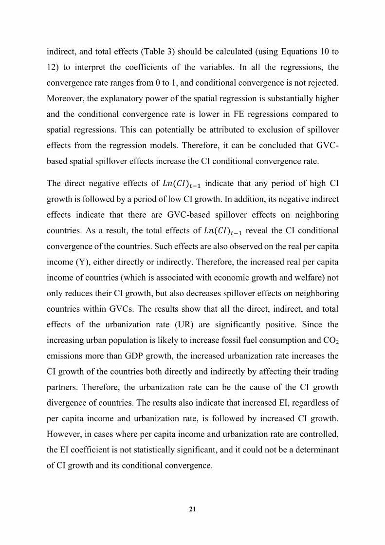
indirect, and total effects (Table 3) should be calculated (using Equations 10 to

12) to interpret the coefficients of the variables. In all the regressions, the

convergence rate ranges from 0 to 1, and conditional convergence is not rejected.

Moreover, the explanatory power of the spatial regression is substantially higher

and the conditional convergence rate is lower in FE regressions compared to

spatial regressions. This can potentially be attributed to exclusion of spillover

effects from the regression models. Therefore, it can be concluded that GVC-

based spatial spillover effects increase the CI conditional convergence rate.

The direct negative effects of 𝐿𝑛(𝐶𝐼)𝑡−1 indicate that any period of high CI

growth is followed by a period of low CI growth. In addition, its negative indirect

effects indicate that there are GVC-based spillover effects on neighboring

countries. As a result, the total effects of 𝐿𝑛(𝐶𝐼)𝑡−1 reveal the CI conditional

convergence of the countries. Such effects are also observed on the real per capita

income (Y), either directly or indirectly. Therefore, the increased real per capita

income of countries (which is associated with economic growth and welfare) not

only reduces their CI growth, but also decreases spillover effects on neighboring

countries within GVCs. The results show that all the direct, indirect, and total

effects of the urbanization rate (UR) are significantly positive. Since the

increasing urban population is likely to increase fossil fuel consumption and CO2

emissions more than GDP growth, the increased urbanization rate increases the

CI growth of the countries both directly and indirectly by affecting their trading

partners. Therefore, the urbanization rate can be the cause of the CI growth

divergence of countries. The results also indicate that increased EI, regardless of

per capita income and urbanization rate, is followed by increased CI growth.

However, in cases where per capita income and urbanization rate are controlled,

the EI coefficient is not statistically significant, and it could not be a determinant

of CI growth and its conditional convergence.

22

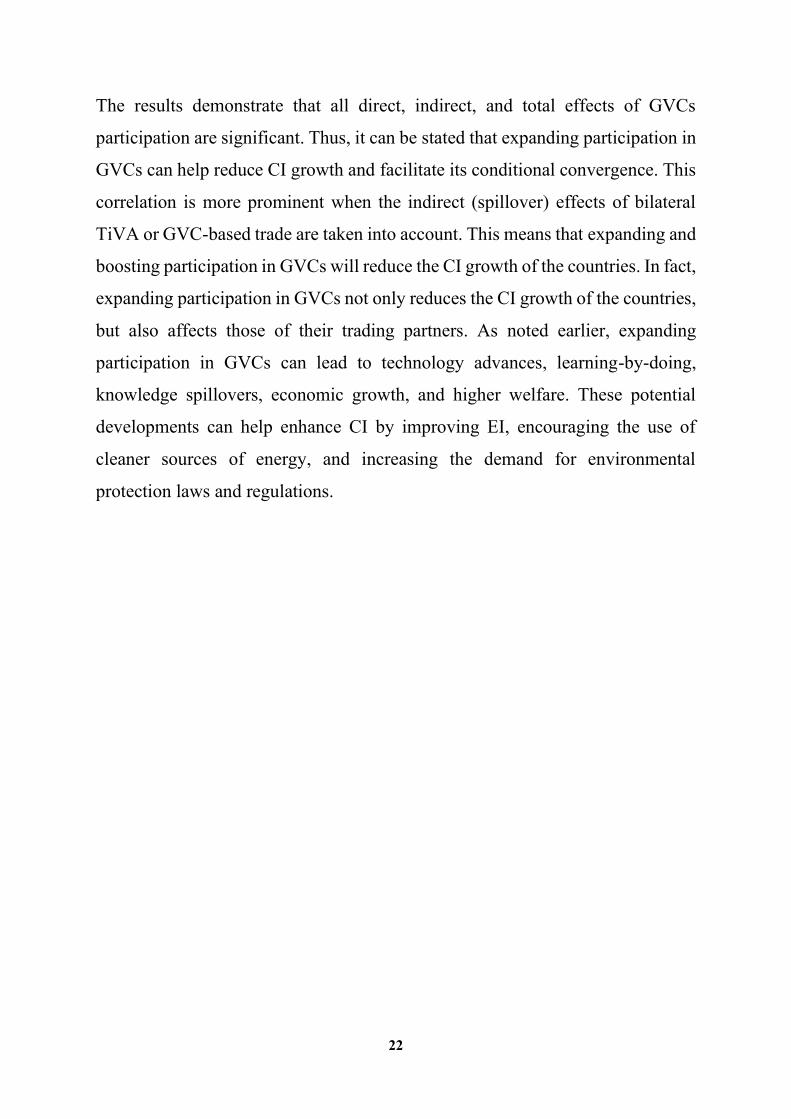
The results demonstrate that all direct, indirect, and total effects of GVCs

participation are significant. Thus, it can be stated that expanding participation in

GVCs can help reduce CI growth and facilitate its conditional convergence. This

correlation is more prominent when the indirect (spillover) effects of bilateral

TiVA or GVC-based trade are taken into account. This means that expanding and

boosting participation in GVCs will reduce the CI growth of the countries. In fact,

expanding participation in GVCs not only reduces the CI growth of the countries,

but also affects those of their trading partners. As noted earlier, expanding

participation in GVCs can lead to technology advances, learning-by-doing,

knowledge spillovers, economic growth, and higher welfare. These potential

developments can help enhance CI by improving EI, encouraging the use of

cleaner sources of energy, and increasing the demand for environmental

protection laws and regulations.

23

Table 2. Estimated spatial panel data regressions

Dependent Variable:

𝐿𝑛(𝐶𝐼𝑡/𝐶𝐼𝑡−1)

Model

1 2 3 4 5 6 7 8 9 10 11 12 13 14 15 16

Method FE SAR SEM SDM FE SAR SEM SDM FE SAR SEM SDM FE SAR SEM SDM

Independent Variable

Main

𝐿𝑛(𝐶𝐼)𝑡−1 -.20a -.20a -.22a -.21a -.20a -.20a -.23a -.22a -.17a -.17a -.23a -.21a -.21a -.22a -.25a -.23a

[.01] [.01] [.01] [.01] [.01] [.01] [.01] [.01] [.01] [.01] [.01] [.01] [.01] [.01] [.01] [.01]

𝐿𝑛(𝑌)𝑡−1 -.06a -.06a -.03b -.03b -.10a -.1a -.07a -.06a

[.01] [.01] [.01] [.01] [.01] [.02] [.01] [.02]

𝐿𝑛(𝐸𝐼)𝑡−1 .05a .05a .03 .02 -.01 -.01 -.008 -.004

[.01] [.01] [.01] [.01] [.02] [.02] [.02] [.02]

𝐿𝑛(𝑈𝑅)𝑡−1 .01 .01 .20a .15a .17a .17a .26a .23a

[.04] [.04] [.05] [.05] [.05] [.05] [.05] [.05]

𝐿𝑛(𝐺𝑉𝐶)𝑡−1 -.03c -.03c -.007 -.02 -.05a -.05a -.009 -.02 -.06a -.06a -.01 -.03c -.05b -.04b -.017 -.03c

[.02] [.01] [.01] [.01] [.01] [.01] [.02] [.02] [.02] [.01] [.02] [.01] [.02] [.01] [.02] [.01]

Spatial

𝜌 .40a .38a .40a .38a .40a .37a .40a .37a

[.07] [.07] [.07] [.07] [.07] [.07] [.07] [.07]

𝜆 .47a .51a .59a .52a

[.06] [.06] [.05] [.06]

𝑊𝐿𝑛(𝐺𝑉𝐶)𝑡−1 -.16a -.20a -.28a -.21a

[.04] [.04] [.04] [.04]

Wald test statistic 62 231 253 244 58 217 217 242 55 208 291 251 39 243 292 265

(p-value) (.00) (.00) (.00) (.00) (.00) (.00) (.00) (.00) (.00) (.00) (.00) (.00) (.00) (.00) (.00) (.00)

Pseudo R2 0.16 0.37 0.38 0.38 0.10 0.35 0.37 0.38 0.08 0.34 0.35 0.38 0.15 0.36 0.38 0.39

Model Selection

Tests

Hausman test chi2(3)

=166.1

Prob > chi2 =

0.00

chi2(3)

=158.4

Prob > chi2 =

0.00

chi2(4)

=151.5

Prob > chi2 =

0.00

chi2(4)

=176.6

Prob > chi2 =

0.00

SAR vs SDM chi2(1) = 11.8 Prob > chi2 =

0.00 chi2(1) =23.1

Prob > chi2 =

0.00 chi2(1) =38.6

Prob > chi2 =

0.00 chi2(1) =19.6

Prob > chi2 =

0.00

SEM vs SDM chi2(1) = 13.6 Prob > chi2 =

0.00 chi2(1) =27.9

Prob > chi2 =

0.00 chi2(1) =44.7

Prob > chi2 =

0.00 chi2(1) =22.8

Prob > chi2 =

0.00

*a: p-value <0.01, b: p-value <0.05, c: p-value <0.1 **Standard Errors are in the brackets.

24

Table 3. Estimated direct, indirect, and total effects of the regressors and the conditional convergence rate of CI

Dependent Variable:

𝐿𝑛(𝐶𝐼𝑡/𝐶𝐼𝑡−1)

Model

1 2 3 4 5 6 7 8 9 10 11 12 13 14 15 16

Method FE SAR SEM SDM FE SAR SEM SDM FE SAR SEM SDM FE SAR SEM SDM

Independent Variable

Direct Effect


[.01] [.01] [.01] [.01] [.01] [.01] [.01] [.01] [.01] [.01] [.01] [.01] [.01] [.01] [.01] [.01]

𝐿𝑛(𝑌)𝑡−1 -.06a -.06a -.03b -.03b -.10a -.10a -.07a -.06a

[.01] [.01] [.01] [.01] [.01] [.02] [.01] [.03]

𝐿𝑛(𝐸𝐼)𝑡−1 .05a .05a .03 .02 -.01 -.01 -.008 -.003

[.01] [.01] [.01] [.01] [.02] [.02] [.02] [.02]

𝐿𝑛(𝑈𝑅)𝑡−1 .01 .01 .20a .15a .17a .17a .26a .23a

[.04] [.04] [.05] [.05] [.05] [.05] [.05] [.05]

𝐿𝑛(𝐺𝑉𝐶)𝑡−1 -.03c -.03c -.007 -.02 -.05a -.05c -.009 -.02 -.06a -.06a -.01 -.03c -.05b -.04a -.017 -.03c

[.02] [.01] [.01] [.01] [.01] [.01] [.02] [.01] [.02] [.01] [.02] [.01] [.02] [.01] [.02] [.01]

Indirect Effect

𝐿𝑛(𝐶𝐼)𝑡−1 -.14a -.13a -.14a -.14a -.12a -.13a -.15a -.15a

[.04] [.05] [.04] [.04] [.04] [.04] [.05] [.05]

𝐿𝑛(𝑌)𝑡−1 -.04b -.02c .51a -.07b -.04a

[.01] [.012] [.06] [.02] [.01]

𝐿𝑛(𝐸𝐼)𝑡−1 .03b .01 -.007 -.002

[.01] [.01] [.01] [.01]

𝐿𝑛(𝑈𝑅)𝑡−1 .007 .09b .12b .14b

[.03] [.04] [.05] [.06]

𝐿𝑛(𝐺𝑉𝐶)𝑡−1 -.02 -.28a -.03b -.3b -.04b -.47a -.03c -.36a

[.01] [.08] [.01] [.07] [.01] [.09] [.01] [.09]

Total Effect


[.01] [.05] [.01] [.05] [.01] [.05] [.01] [.05] [.01] [.05] [.01] [.04] [.01] [.06] [.01] [.06]

𝐿𝑛(𝑌)𝑡−1 -.06a -.11a -.03b -.05b -.10a -.17a -.07a -.10a

[.01] [.03] [.01] [.02] [.01] [.04] [.01] [.03]

𝐿𝑛(𝐸𝐼)𝑡−1 .05a .08b .03 .04 -.01 -.01 -.008 -.006

[.01] [.03] [.01] [.03] [.02] [.03] [.02] [.03]

𝐿𝑛(𝑈𝑅)𝑡−1 .01 .01 .20a .25a .17a .29a .26a .37a

[.04] [.07] [.05] [.08] [.05] [.09] [.05] [.09]

𝐿𝑛(𝐺𝑉𝐶)𝑡−1 -.03c -.05c -.007 -.30a -.05a -.09a -.009 -.36a -.06a -.10a -.01 -.51a -.05b -.08c -.017 -.40a

[.02] [.03] [.01] [.08] [.01] [.03] [.02] [.07] [.02] [.03] [.02] [.09] [.02] [.03] [.02] [.09]

Convergence rate 0.22 0.43 0.24 0.43 0.22 0.43 0.26 0.44 0.18 0.43 0.26 0.41 0.23 0.46 0.28 0.49

*a: p-value <0.01, b: p-value <0.05, c: p-value <0.1 **Standard Errors are in the brackets.

25

6. Conclusion

Having transformed the structure and processes of production in most developing

and developed countries, GVCs provide a new form of trade that allows countries

to benefit from their comparative advantages in production tasks. Apart from the

economic benefits of GVC-based trade and expanding participation in GVCs,

their environmental advantages and disadvantages are also among controversial

topics in the economic literature.

This study analyzed the role of GVCs in the environmental performance of

countries and sought to determine whether GVC-based trade could facilitate the

CI convergence of the countries. The study also evaluated the effects of

participation in GVCs on the CI growth of the countries. Spatial statistics were

employed to model and analyze the data collected from 101 countries in the

period from 1997 to 2014. Moreover, the economic distance between the

countries was defined in terms of their bilateral TiVA within GVCs. The results

of statistical tests showed that there was a CI growth correlation between

countries that had more bilateral GVC-based trade. In addition, considering the

GVC-based trade between countries, the conditional convergence of countries in

terms of the CI growth was confirmed. The results also demonstrate that

expanding participation in GVCs not only helps reduce the CI growth of the

countries, but it also affects the CI growth of their trading partners (through

spillover effects). Hence, the environmental performance of a country with

GVCs-based trade partners that have better environmental performance will

relatively improve.

It can also be stated that this new form of trade provides various capacities,

especially for developing countries, to benefit from the knowledge and

technology of their trading partners for economic and environmental purposes. In

this regard, the necessity of adapting local production processes to global

26

processes within GVCs can encourage the promotion of production processes and

their adaptation to the global production structure. Additionally, the

environmental policies of countries within the context of GVC-based trade are

more likely to become more convergent. For instance, multinational enterprises

that outsource their production processes within GVCs will probably not only

transfer technology and knowledge to their partners in other countries, but also

require them to comply with certain laws and regulations, including

environmental standards. Furthermore, GVCs can serve as a potential platform

for improving the environmental performance of countries (at least reduce their

CI growth) and converging their environmental indicators.

According to the findings, the capacities of GVCs should be considered in

environmental policies and measures to combat climate change. The results

showed that expanding participation in GVCs improved the carbon efficiency of

the countries, i.e., an important and fundamental (albeit insufficient) step in

advancing environmental goals, even with the existence of carbon leakage in

trade. Moreover, increasing TiVA with countries on the path of improving carbon

efficiency can be an appropriate strategy for developing countries to enhance their

environmental performance.

This study contributes to the empirical literature on the link between trade and

the environment by analyzing the CI correlation and conditional convergence of

countries within the context of GVC-based trade. Nevertheless, more studies

must be conducted on the subject, especially on the emission of greenhouse gases

and pollutants such as SO2 to gain a better insight into the role of GVCs in the

convergence of the countries’ environmental performance. The scale,

composition, and technical effects of expanding GVCs on the environmental

performance of countries can also be an important area of research for future

studies to separately analyze different mechanisms of impacts for the GVCs on

the environment.

27

References

Anselin, L., 2003a. Spatial externalities, spatial multipliers, and spatial

econometrics. Int. Reg. Sci. Rev. 26, 153–166.

https://doi.org/10.1177/0160017602250972

Anselin, L., 2003b. Spatial Econometrics, in: A Companion to Theoretical

Econometrics. John Wiley & Sons, Ltd, pp. 310–330.

https://doi.org/https://doi.org/10.1002/9780470996249.ch15

Antweiler, W., Copeland, B.R., Taylor, M.S., 2001. Is free trade good for the

environment? Am. Econ. Rev. 91, 877–908.

https://doi.org/10.1257/aer.91.4.877

Apergis, N., Payne, J.E., 2020. NAFTA and the convergence of CO2 emissions

intensity and its determinants. Int. Econ. 161, 1–9.

https://doi.org/10.1016/j.inteco.2019.10.002

Aslam, A., Novta, N., Rodrigues-Bastos, F., 2017. Calculating Trade in Value

Added, WP/17/178, July 2017.

Awad, A., 2019. Does economic integration damage or benefit the

environment? Africa’s experience. Energy Policy 132, 991–999.

https://doi.org/10.1016/j.enpol.2019.06.072

Baghdadi, L., Martinez-Zarzoso, I., Zitouna, H., 2013. Are RTA agreements

with environmental provisions reducing emissions? J. Int. Econ. 90, 378–

390. https://doi.org/10.1016/j.jinteco.2013.04.001

Baldwin, R., 2017. The great convergence: Information technology and the New

Globalization, Ekonomicheskaya Sotsiologiya.

https://doi.org/10.17323/1726-3247-2017-5-40-51

Bernhardt, T., Pollak, R., 2016. Economic and social upgrading dynamics in

28

global manufacturing value chains: A comparative analysis. Environ. Plan.

A 48, 1220–1243. https://doi.org/10.1177/0308518X15614683

Casella, B., Bolwijn, R., Moran, D., Kanemoto, K., 2019. UNCTAD insights:

Improving the analysis of global value chains: the UNCTAD-Eora

Database. Transnatl. Corp. 26, 115–142. https://doi.org/10.18356/3aad0f6a-

en

Cherniwchan, J., Copeland, B.R., Taylor, M.S., 2017. Trade and the

environment: New methods, measurements, and results. Annu. Rev.

Econom. 9, 59–85. https://doi.org/10.1146/annurev-economics-063016-

103756

Conley, T.G., Topa, G., 2002. Socio-economic distance and spatial patterns in

unemployment. J. Appl. Econom. 17, 303–327.

Copeland, B.R., Taylor, M.S., 2013. Trade and the environment: Theory and

evidence, Trade and the Environment: Theory and Evidence.

https://doi.org/10.2307/3552527

Dorrucci, E., Gunnella, V., Al-Haschimi, A., Benkovskis, K., Chiacchio, F., de

Soyres, F., Lupidio, B. Di, Fidora, M., Franco-Bedoya, S., Frohm, E.,

Gradeva, K., López-Garcia, P., Koester, G., Nickel, C., Osbat, C., Pavlova,

E., Schmitz, M., Schroth, J., Skudelny, F., Tagliabracci, A., Vaccarino, E.,

Wörz, J., 2019. The impact of global value chains onthe euro area economy.

European Central Bank (ECB), Frankfurt a. M.

https://doi.org/10.2866/870210

Frankel, J.A., Rose, A.K., 2005. Is trade good or bad for the environment?

sorting out the causality. Rev. Econ. Stat. 87, 85–91.

https://doi.org/10.1162/0034653053327577

Gangodagamage, C., Zhou, X., Lin, H., 2008. Autocorrelation, Spatial, in:

29

Shekhar, S., Xiong, H. (Eds.), Encyclopedia of GIS. Springer US, Boston,

MA, pp. 32–37. https://doi.org/10.1007/978-0-387-35973-1_83

Gerlagh, R., Kuik, O., 2014. Spill or leak? Carbon leakage with international

technology spillovers: A CGE analysis. Energy Econ. 45, 381–388.

https://doi.org/10.1016/j.eneco.2014.07.017

Han, L., Han, B., Shi, X., Su, B., Lv, X., Lei, X., 2018. Energy efficiency

convergence across countries in the context of China’s Belt and Road

initiative. Appl. Energy 213, 112–122.

https://doi.org/10.1016/j.apenergy.2018.01.030

Hanson, G.H., 2012. The rise of middle kingdoms: Emerging economies in

global trade. J. Econ. Perspect. 26, 41–64.

https://doi.org/10.1257/jep.26.2.41

Holzinger, K., Knill, C., Sommerer, T., 2008. Environmental policy

convergence: The impact of international harmonization, transnational

communication, and regulatory competition. Int. Organ. 62, 553–587.

https://doi.org/10.1017/S002081830808020X

Huang, J., Liu, C., Chen, S., Huang, X., Hao, Y., 2019. The convergence

characteristics of China’s carbon intensity: Evidence from a dynamic spatial

panel approach. Sci. Total Environ. 668, 685–695.

https://doi.org/10.1016/j.scitotenv.2019.02.413

Huang, R., Chen, G., Lv, G., Malik, A., Shi, X., Xie, X., 2020. The effect of

technology spillover on CO2 emissions embodied in China-Australia trade.

Energy Policy 144, 111544. https://doi.org/10.1016/j.enpol.2020.111544

Huang, Z., Zhang, H., Duan, H., 2019. Nonlinear globalization threshold effect

of energy intensity convergence in Belt and Road countries. J. Clean. Prod.

237. https://doi.org/10.1016/j.jclepro.2019.117750

30

Ignatenko, A., Raei, F., Mircheva, B., 2019. Global Value Chains: What are the

Benefits and Why Do Countries Participate? IMF Working Paper European

Department Global Value Chains: What are the Benefits and Why Do

Countries Participate ? IMF Work. Pap.

Jaffe, A.B., Newell, R.G., Stavins, R.N., 2002. Environmental policy and

technological change. Environ. Resour. Econ. 22, 41–70.

Jangam, B.P., Rath, B.N., 2020. Cross-country convergence in global value

chains: Evidence from club convergence analysis. Int. Econ. 163, 134–146.

https://doi.org/10.1016/j.inteco.2020.06.002

Jiang, L., Folmer, H., Ji, M., Zhou, P., 2018. Revisiting cross-province energy

intensity convergence in China: A spatial panel analysis. Energy Policy

121, 252–263. https://doi.org/10.1016/j.enpol.2018.06.043

Jiang, M., An, H., Gao, X., Liu, S., Xi, X., 2019. Factors driving global carbon

emissions: A complex network perspective. Resour. Conserv. Recycl. 146,

431–440. https://doi.org/10.1016/j.resconrec.2019.04.012

Kalkhan, M.A., 2011. Spatial statistics: geospatial information modeling and

thematic mapping. CRC press.

Kaltenegger, O., Löschel, A., Pothen, F., 2017. The effect of globalisation on

energy footprints: Disentangling the links of global value chains. Energy

Econ. 68, 148–168. https://doi.org/10.1016/j.eneco.2018.01.008

Keller, W., 2010. International trade, foreign direct investment, and technology

spillovers, 1st ed, Handbook of the Economics of Innovation. Elsevier B.V.

https://doi.org/10.1016/S0169-7218(10)02003-4

Koopman, R., Wang, Z., Wei, S.J., 2014. Tracing value-added and double

counting in gross exports. Am. Econ. Rev. 104, 459–494.

31

https://doi.org/10.1257/aer.104.2.459

Kummritz, V., 2016. Do Global Value Chains Cause Industrial Development?,

CTEI Working Paper No 2016-01.

LeSage, J., Pace, R.K., 2009. Introduction to Spatial Econometrics. Chapman

and Hall/CRC. https://doi.org/10.1201/9781420064254

LeSage, J.P., Fischer, M.M., 2008. Spatial growth regressions: Model

specification, estimation and interpretation. Spat. Econ. Anal. 3, 275–304.

https://doi.org/10.1080/17421770802353758

Levin, A., Lin, C.F., Chu, C.S.J., 2002. Unit root tests in panel data: Asymptotic

and finite-sample properties. J. Econom. 108, 1–24.

https://doi.org/10.1016/S0304-4076(01)00098-7

Liu, H., Li, J., Long, H., Li, Z., Le, C., 2018. Promoting energy and

environmental efficiency within a positive feedback loop: Insights from

global value chain. Energy Policy 121, 175–184.


López, L.A., Cadarso, M.Á., Zafrilla, J., Arce, G., 2019. The carbon footprint of

the U.S. multinationals’ foreign affiliates. Nat. Commun. 10, 1–11.

https://doi.org/10.1038/s41467-019-09473-7

Lovely, M., Popp, D., 2011. Trade, technology, and the environment: Does

access to technology promote environmental regulation? J. Environ. Econ.

Manage. 61, 16–35. https://doi.org/10.1016/j.jeem.2010.08.003

Markusen, J.R., 1984. Multinationals, multi-plant economies, and the gains

from trade. J. Int. Econ. 16, 205–226.

Nemati, M., Hu, W., Reed, M., 2019. Are free trade agreements good for the

environment? A panel data analysis. Rev. Dev. Econ. 23, 435–453.

32

https://doi.org/10.1111/rode.12554

Nicoletti, G., Golub, S.S., Hajkova, D., Mirza, D., Yoo, K.-Y., 2003. Policies

and international integration: influences on trade and foreign direct

investment (No. 359), OECD Economics Department Working Papers.

https://doi.org/http://dx.doi.org/10.1787/062321126487

Piermartini, R., Rubínová, S., 2014. Knowledge spillovers through international

supply chains, WTO Staff Working Papers.

Pigato, M., Black, S.J., Dussaux, D., Mao, Z., McKenna, M., Rafaty, R.,

Touboul, S., 2020. Technology Transfer and Innovation for Low-Carbon

Development. Washington, DC: World Bank. https://doi.org/10.1596/978-

1-4648-1500-3

Qi, S.Z., Peng, H.R., Zhang, Y.J., 2019. Energy intensity convergence in Belt

and Road Initiative (BRI) countries: What role does China-BRI trade play?

J. Clean. Prod. 239, 118022. https://doi.org/10.1016/j.jclepro.2019.118022

Rodrik, D., 2018. New Technologies, Global Value Chains, and Developing

Economies. Oxford. United Kingdom, Cambridge, MA.

https://doi.org/10.3386/w25164

Servén, L., Abate, G.D., 2020. Adding space to the international business cycle.

J. Macroecon. 65. https://doi.org/10.1016/j.jmacro.2020.103211

Shen, J., 2008. Trade liberalization and environmental degradation in China.

Appl. Econ. 40, 997–1004. https://doi.org/10.1080/00036840600771148

Sun, C., Li, Z., Ma, T., He, R., 2019. Carbon efficiency and international

specialization position: Evidence from global value chain position index of

manufacture. Energy Policy 128, 235–242.


33

Taglioni, D., Winkler, D., Taglioni, D., Winkler, D., 2016. Making Global

Value Chains Work for Development, in: Making Global Value Chains

Work for Development. The World Bank, pp. i–xxii.

https://doi.org/10.1596/978-1-4648-0157-0_fm

Thomakos, D.D., Alexopoulos, T.A., 2016. Carbon intensity as a proxy for

environmental performance and the informational content of the EPI.

Energy Policy 94, 179–190. https://doi.org/10.1016/j.enpol.2016.03.030

Wan, J., Baylis, K., Mulder, P., 2015. Trade-facilitated technology spillovers in

energy productivity convergence processes across EU countries. Energy

Econ. 48, 253–264. https://doi.org/10.1016/j.eneco.2014.12.014

Wang, Z., Wei, S.-J., Yu, X., Zhu, K., 2017. NBER WORKING PAPER

SERIES MEASURES OF PARTICIPATION IN GLOBAL VALUE

CHAINS AND GLOBAL BUSINESS CYCLES Measures of Participation

in Global Value Chains and Global Business Cycles. NBER Work. Pap.

WDR, 2020. World Development Report 2020: Trading for Development in the

Age of Global Value Chains. Washington, DC: World Bank, Washington,

DC. https://doi.org/10.1596/978-1-4648-1457-0

Weber, S., Gerlagh, R., Mathys, N.A., Moran, D., 2021. CO2 embodied in

trade: trends and fossil fuel drivers. Environ. Sci. Pollut. Res. 1–19.

https://doi.org/10.1007/s11356-020-12178-w

Xin-gang, Z., Yuan-feng, Z., Yan-bin, L., 2019. The spillovers of foreign direct

investment and the convergence of energy intensity. J. Clean. Prod. 206,

611–621. https://doi.org/10.1016/j.jclepro.2018.09.225

Yasmeen, R., Li, Y., Hafeez, M., 2019. Tracing the trade–pollution nexus in

global value chains: evidence from air pollution indicators. Environ. Sci.

Pollut. Res. 26, 5221–5233. https://doi.org/10.1007/s11356-018-3956-0

34

You, W., Lv, Z., 2018. Spillover effects of economic globalization on CO2

emissions: A spatial panel approach. Energy Econ. 73, 248–257.

https://doi.org/10.1016/j.eneco.2018.05.016

35

Appendix A. List of Countries

Table A1. List of countries in sample

Albania Hungary Romania

Argentina Iceland Russian Federation

Australia India Saudi Arabia

Austria Indonesia Senegal

Azerbaijan Iran, Islamic Rep. Singapore

Bangladesh Iraq Slovak Republic

Belgium Ireland Slovenia

Bolivia Israel South Africa

Bosnia and Herzegovina Italy Spain

Botswana Jamaica Sri Lanka

Brazil Japan Sweden

Bulgaria Jordan Switzerland

Cambodia Kazakhstan Tajikistan

Cameroon Korea, Rep. Thailand

Canada Kyrgyz Republic Togo

Chile Latvia Tunisia

China Lebanon Turkey

Colombia Lithuania Ukraine

Costa Rica Luxembourg United Kingdom

Cote d'Ivoire Malaysia United States

Croatia Malta Uruguay

Cuba Mauritius Cyprus Mexico Czech Republic Mongolia Denmark Morocco Dominican Republic Mozambique

Ecuador Namibia Egypt, Arab Rep. Nepal El Salvador Netherlands

Estonia New Zealand

Finland Nicaragua

France Nigeria Gabon Norway Georgia Pakistan Germany Panama Ghana Paraguay Greece Peru Guatemala Philippines

Haiti Poland Honduras Portugal

36

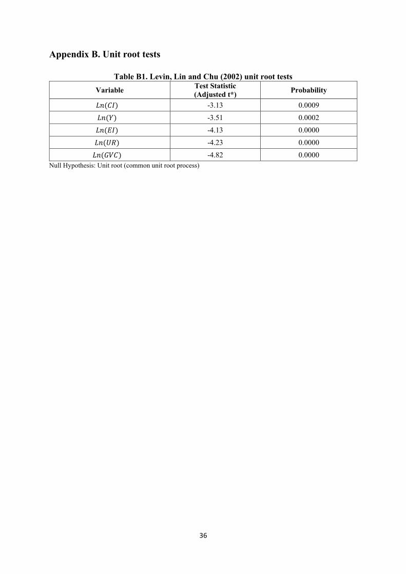
Appendix B. Unit root tests

Table B1. Levin, Lin and Chu (2002) unit root tests

Variable Test Statistic

(Adjusted t*) Probability

𝐿𝑛(𝐶𝐼) -3.13 0.0009

𝐿𝑛(𝑌) -3.51 0.0002

𝐿𝑛(𝐸𝐼) -4.13 0.0000

𝐿𝑛(𝑈𝑅) -4.23 0.0000

𝐿𝑛(𝐺𝑉𝐶) -4.82 0.0000

Null Hypothesis: Unit root (common unit root process)

Documents

The Role of Global Value Chains in Carbon Intensity