INP Grenoble – ENSIMAGÉcole Nationale Supérieure dInformatique et de Mathématiques Appliquées de

Grenoble

Rapport de projet de fin d’études

Effectué chez Sophis

Value-at-Risk for commodityportfolios

Martin Ottenwaelter

3e année – Option MIF

17 mars 2008 – 12 septembre 2008

Sophis Responsables de stage24-26 place de la Madeleine Gregory Cobena et Arnaud Seguin75008 Paris Tuteur de l’école

Ollivier Taramasco

Contents

1 Introduction: Value at Risk, a single number risk indicator 4

2 VaR definition 6

2.1 Introduction . . . . . . . . . . . . . . . . . . . . . . . . . . . . . . . . . . . 6

2.2 VaR definition . . . . . . . . . . . . . . . . . . . . . . . . . . . . . . . . . . 6

2.3 Time horizon . . . . . . . . . . . . . . . . . . . . . . . . . . . . . . . . . . . 7

2.4 Backtesting . . . . . . . . . . . . . . . . . . . . . . . . . . . . . . . . . . . . 7

2.5 Conclusion . . . . . . . . . . . . . . . . . . . . . . . . . . . . . . . . . . . . 8

3 Historical VaR 9

3.1 Introduction . . . . . . . . . . . . . . . . . . . . . . . . . . . . . . . . . . . 9

3.2 Method . . . . . . . . . . . . . . . . . . . . . . . . . . . . . . . . . . . . . . 9

3.3 Experiments . . . . . . . . . . . . . . . . . . . . . . . . . . . . . . . . . . . 9

3.4 Historical VaR in RISQUE . . . . . . . . . . . . . . . . . . . . . . . . . . . . 13

3.5 Conclusion . . . . . . . . . . . . . . . . . . . . . . . . . . . . . . . . . . . . 14

4 1st order VaR 15

4.1 Introduction . . . . . . . . . . . . . . . . . . . . . . . . . . . . . . . . . . . 15

4.2 The 1st order approximation formula . . . . . . . . . . . . . . . . . . . . 15

4.3 A simple example . . . . . . . . . . . . . . . . . . . . . . . . . . . . . . . . 16

4.4 Comparison of historical and 1st order VaR . . . . . . . . . . . . . . . . 18

4.5 RISQUE’s answer to the particularities of commodities . . . . . . . . . . 20

4.6 Variance-covariance interpolation . . . . . . . . . . . . . . . . . . . . . . 22

4.7 Experimental results . . . . . . . . . . . . . . . . . . . . . . . . . . . . . . 24

4.8 Conclusion . . . . . . . . . . . . . . . . . . . . . . . . . . . . . . . . . . . . 28

2

5 Principal Component Analysis: an attempt to understand the variance-covariance matrix 29

5.1 Introduction . . . . . . . . . . . . . . . . . . . . . . . . . . . . . . . . . . . 29

5.2 The PCA methodology . . . . . . . . . . . . . . . . . . . . . . . . . . . . . 29

5.3 Understanding the variance-covariance matrix . . . . . . . . . . . . . . 31

5.4 PCA applied to 1st order VaR . . . . . . . . . . . . . . . . . . . . . . . . . 34

5.5 Conclusion . . . . . . . . . . . . . . . . . . . . . . . . . . . . . . . . . . . . 35

6 Conclusion 36

A Mathematical formulas 37

A.1 Daily returns . . . . . . . . . . . . . . . . . . . . . . . . . . . . . . . . . . . 37

A.2 An unbiased estimate of the covariance, skewness and kurtosis . . . . 37

A.3 Delta, delta-cash . . . . . . . . . . . . . . . . . . . . . . . . . . . . . . . . . 37

B RISQUE 38

B.1 VaR computation steps . . . . . . . . . . . . . . . . . . . . . . . . . . . . . 38

C Historical VaR Server 42

3

1 Introduction: Value at Risk, a single number riskindicator

Managing market risk is now an integral part of the financial world. Today’s mostwidely used tool to measure and control market risk was introduced and popu-larised in 1994 by J.P. MORGAN’s RISKMETRICS software and is called Value-at-Risk–henceforth VaR. VaR “is an attempt to provide a single number summarising thetotal risk in a portfolio of financial assets” ([Hul06]). Its simplicity in both itsunderstanding and computation makes it such a widely used technique.

There are three methods to compute VaR:

• historical

• analytical (or paramatric)

• Monte-Carlo

SOPHIS RISQUE, the portfolio and risk management solution, already features thethree methods. But in this paper, we only focus on the historical and analyticalmethods in the particular case of commodity portfolios. We have three clear goals:(i) understand and explain the current computation methods, (ii) validate thosemethods and (iii) propose improvements; by keeping our focus on commodity por-folios that have certain particularities, the most important being that commoditiesare mostly traded with future contracts.

In the first section, we start by defining VaR and give the mathematical formulawhich is the foundation of any VaR method. Then, we present the backtestingmethod that is used in the next sections to validate the VaR models. Backtestingconsists in verifying, using past records, that the portfolio losses in worst cases iswell represented by the VaR. We also introduce another important aspect knownas the time horizon formula, giving a relationship between a 1-day and a N -dayVaR. In other words, it gives a relation between a very short-term risk and a longermedium-term risk.

In the second section, we start by defining the historical VaR method which consistsin applying changes to the portfolio based on real past events. We then validatethe method by performing a backtest on a set of sample portfolios. We also studya concrete case in which a large amount of data is artificially created for electricitycontracts using the available historical data. Then, using the same historical data,we study the time horizon formula. Our experiments show that one must be carefulwith that formula since even pure lognormal data does not fully validate it.

Historical VaR has the advantage of being very similar to real world past eventsbut requires many costly simulations. For this reason, the parametric VaR is analternative. Not only it reduces the calculation time and the number of simulations,but it proposes a model of the portfolio risk. The parametric VaR is typically a 1st or2nd order VaR, which corresponds to an analysis of the 1st or 2nd order derivatives

4

of the portfolio with respect to the various risk sources: spot values, volatilities,interest rates, credit spreads, etc.

In the third section, we start by computing the 1st order approximation VaR for-mula. After showing an example on how it is computed, both by hand and inRISQUE, we once again validate the method with a series of backtests. The methodis then compared with the historical VaR and it is concluded that the 1st orderVaR always underestimates the historical VaR, which is due to the skewed and lep-tokurtic historical portfolios distributions. We then jump into the particularitiesof commodities and propose a subtle modification to RISQUE’s variance-covariancematrix mapping method, but find that the inital method is better.

In the fourth section, we pursue the work on the variance-covariance matrix butchoose to study it from a much different angle. We apply the statistical methodknown as Principal Component Analysis in an attempt to better understand thematrix. Although the method gives good results for interest rates, we cannot clearlymake any conclusions regarding commodity portfolios with PCA.

In conclusion, we find that there is an interesting parallel between the historicalVaR which is a data-hungry method and the mapping and PCA techniques that,on the contrary, try to trim existing data in order to keep only the meaningfulcharacterics. The first method requires so much data that we must sometimes findworkarounds to generate the data, while the second is a model-based approachthat tries to extract the important variables.

5

2 VaR definition

2.1 Introduction

In this section, we will first define VaR. We will then see the so-called and frequentlyused time horizon formula that gives the expression of the N -day VaR in functionof the 1-day VaR. We will finally see backtesting, a method that tests the validityof a VaR computation. Backtesting will then be used in the following sections tovalidate both historical and analytical VaR.

2.2 VaR definition

Let V be the VaR of a porfolio, V is defined by the statement ([Hul06]):

We are α% certain that we will not loose more than V dollars in thenext N days.

V is function of two variables:

• N , the time horizon in days

• α, the confidence level

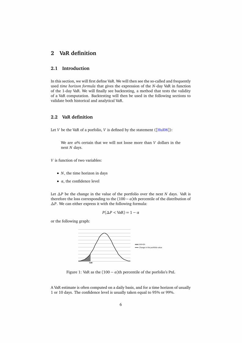
Let ∆P be the change in the value of the portfolio over the next N days. VaR istherefore the loss corresponding to the (100−α)th percentile of the distribution of∆P. We can either express it with the following formula:

P(∆P < VaR) = 1−α

or the following graph:

!"##$%&'

()*+,)-.)/(01/2.3+*.45+.)0

!"#

!"#$%&'($')"&'*+,-+.(+'/#.0&

Figure 1: VaR as the (100−α)th percentile of the porfolio’s PnL

A VaR estimate is often computed on a daily basis, and for a time horizon of usually1 or 10 days. The confidence level is usually taken equal to 95% or 99%.

6

2.3 Time horizon

When the daily changes in the value of the portfolio have identical normal distri-butions with mean zero, the relation between the 1-day VaR and the N-day VaR isexactly:

N -day VaR= 1-day VaR×p

N (1)

Experiments to test this formula are conducted in section (3.3.2).

2.4 Backtesting

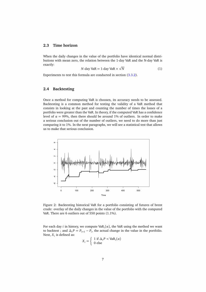
Once a method for computing VaR is choosen, its accuracy needs to be assessed.Backtesting is a common method for testing the validity of a VaR method thatconsists in looking at the past and counting the number of times the losses of aportfolio were greater than the VaR. In theory, if the computed VaR has a confidencelevel of α = 99%, then there should be around 1% of outliers. In order to makea serious conclusion out of the number of outliers, we need to do more than justcomparing it to 1%. In the next paragraphs, we will see a statistical test that allowsus to make that serious conclusion.

0 100 200 300 400 500

-6-4

-20

24

6

Time

Value ($)

Figure 2: Backtesting historical VaR for a portfolio consisting of futures of brentcrude: overlay of the daily changes in the value of the portfolio with the computedVaR. There are 6 outliers out of 550 points (1.1%).

For each day i in history, we compute VaRi(α), the VaR using the method we wantto backtest ; and ∆i P = Pi+1 − Pi , the actual change in the value in the portfolio.Next, X i is defined as:

X i =�

1 if ∆i P < VaRi(α)0 else

7

(X i)1¶i¶n is a sequence of Bernouilli trials. If they are assumed independent, therandom variable X =

∑ni=1 X i follows a Binomial distribution with parameters

(n,α). If α =∑

X i/n is an estimator of α, we can perform the statistical testH0 : α ¶ α against H1 : α > α and see when hypothesis H0 is rejected. [Gau07]provides an asymptotic approximation for the critical region of the test:

W =

x − nαp

nα(1−α)> u2a

where x =∑

x i is the number of outliers and a is the significance of the test.

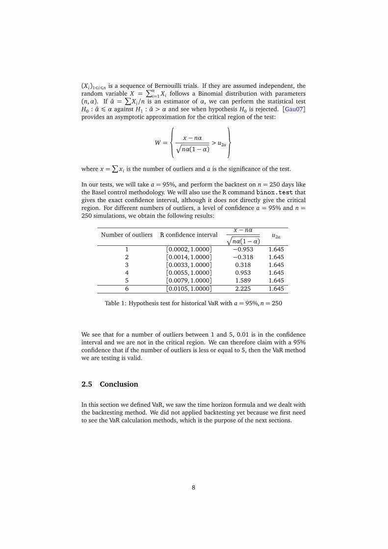
In our tests, we will take a = 95%, and perform the backtest on n = 250 days likethe Basel control methodology. We will also use the R command binom.test thatgives the exact confidence interval, although it does not directly give the criticalregion. For different numbers of outliers, a level of confidence a = 95% and n =250 simulations, we obtain the following results:

Number of outliers R confidence intervalx − nα

p

nα(1−α)u2a

1 [0.0002,1.0000] −0.953 1.6452 [0.0014, 1.0000] −0.318 1.6453 [0.0033, 1.0000] 0.318 1.6454 [0.0055, 1.0000] 0.953 1.6455 [0.0079, 1.0000] 1.589 1.6456 [0.0105,1.0000] 2.225 1.645

Table 1: Hypothesis test for historical VaR with a = 95%, n= 250

We see that for a number of outliers between 1 and 5, 0.01 is in the confidenceinterval and we are not in the critical region. We can therefore claim with a 95%confidence that if the number of outliers is less or equal to 5, then the VaR methodwe are testing is valid.

2.5 Conclusion

In this section we defined VaR, we saw the time horizon formula and we dealt withthe backtesting method. We did not applied backtesting yet because we first needto see the VaR calculation methods, which is the purpose of the next sections.

8

3 Historical VaR

3.1 Introduction

In this section we will define historical VaR and detail the computation steps. Wewill then backtest the VaR on a set of commodity porfolios and perform some ex-periments with the time horizon formula. We will finally describe how RISQUE

computes the historical VaR.

3.2 Method

Historical VaR is a method that uses past data to make the VaR computation. Al-though there are a few implicit assumptions made when doing historical VaR, theyare much less strong than the model assumptions made for parametric VaR.

Suppose that we wish to compute the 99%, 1-day VaR of a portfolio. HistoricalVaR can be computed if we have a certain amount —500 days, for example— ofhistorical data for every risk source of the portfolio. The algorithm goes as follow:

• for every day i of the historical data:

– compute the daily return (A.1) between day i and day i+1 of every risksource

– apply these returns to the current portfolio Pc to obtain a new portfoliovalue Pi

– compute ∆i P = Pi − Pc , the difference between this new value and thecurrent portfolio’s value

• estimate the 1% quantile of the ∆i Ps distribution, this is the historical VaR

Historical VaR is a method that consists in applying past shocks to today’s portfolio.The first assumption made here is that what happened in the past is what is likelyto happen tomorrow. The second assumption is that the returns are independentin time.

3.3 Experiments

In this paper, theory will need to be tested with real data. We therefore usedhistorical data of future contracts of aluminium, brent crude, copper, WTI andPowerNext ; and conducted experiments on these data sets.

9

3.3.1 Counting the outliers

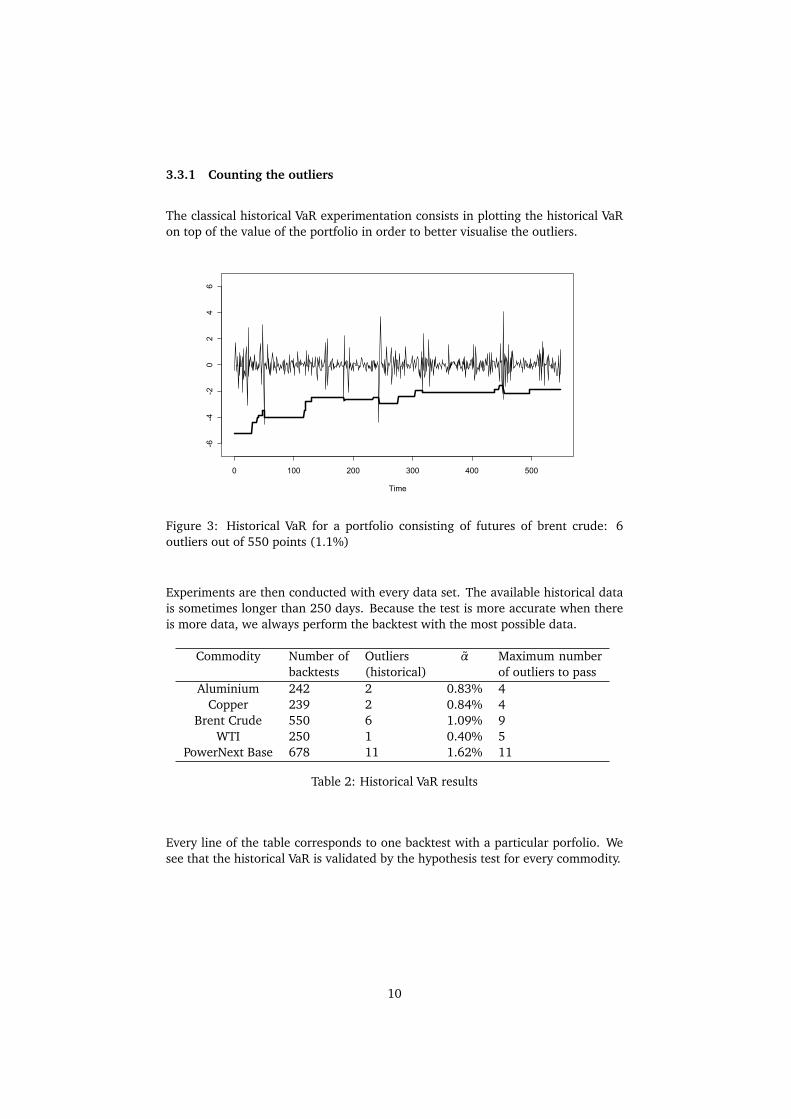
The classical historical VaR experimentation consists in plotting the historical VaRon top of the value of the portfolio in order to better visualise the outliers.

0 100 200 300 400 500

-6-4

-20

24

6

Time

Value ($)

Figure 3: Historical VaR for a portfolio consisting of futures of brent crude: 6outliers out of 550 points (1.1%)

Experiments are then conducted with every data set. The available historical datais sometimes longer than 250 days. Because the test is more accurate when thereis more data, we always perform the backtest with the most possible data.

Commodity Number ofbacktests

Outliers(historical)

α Maximum numberof outliers to pass

Aluminium 242 2 0.83% 4Copper 239 2 0.84% 4

Brent Crude 550 6 1.09% 9WTI 250 1 0.40% 5

PowerNext Base 678 11 1.62% 11

Table 2: Historical VaR results

Every line of the table corresponds to one backtest with a particular porfolio. Wesee that the historical VaR is validated by the hypothesis test for every commodity.

10

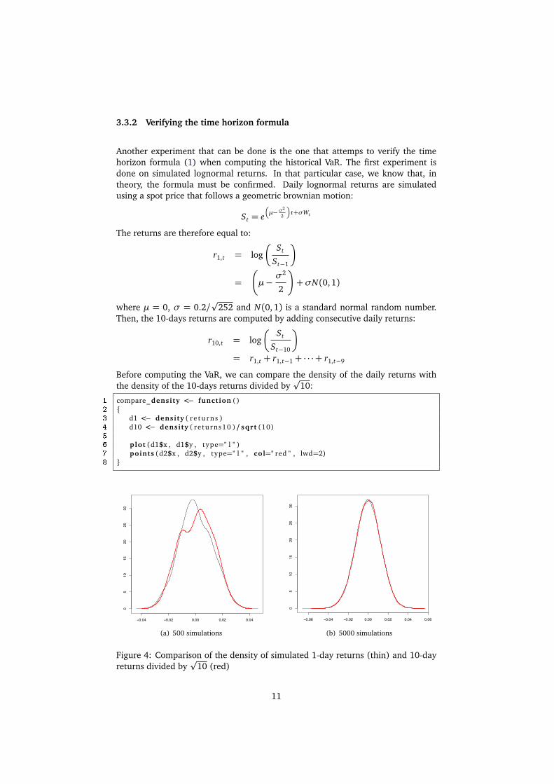
3.3.2 Verifying the time horizon formula

Another experiment that can be done is the one that attemps to verify the timehorizon formula (1) when computing the historical VaR. The first experiment isdone on simulated lognormal returns. In that particular case, we know that, intheory, the formula must be confirmed. Daily lognormal returns are simulatedusing a spot price that follows a geometric brownian motion:

St = e�

µ− σ2

2

�

t+σWt

The returns are therefore equal to:

r1,t = log�

St

St−1

�

=

�

µ−σ2

2

�

+σN(0, 1)

where µ = 0, σ = 0.2/p

252 and N(0,1) is a standard normal random number.Then, the 10-days returns are computed by adding consecutive daily returns:

r10,t = log�

St

St−10

�

= r1,t + r1,t−1 + · · ·+ r1,t−9

Before computing the VaR, we can compare the density of the daily returns withthe density of the 10-days returns divided by

p10:

1 compare_ density <− function ()2 {3 d1 <− density ( r e tu rns )4 d10 <− density ( returns10 )/ sqrt (10)5

6 plot (d1$x , d1$y , type=" l " )7 points (d2$x , d2$y , type=" l " , col=" red " , lwd=2)8 }

−0.04 −0.02 0.00 0.02 0.04

05

1015

2025

30

x1

y1

(a) 500 simulations

−0.06 −0.04 −0.02 0.00 0.02 0.04 0.06

05

1015

2025

30

x1

y1

(b) 5000 simulations

Figure 4: Comparison of the density of simulated 1-day returns (thin) and 10-dayreturns divided by

p10 (red)

11

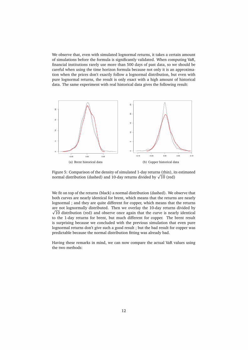
We observe that, even with simulated lognormal returns, it takes a certain amountof simulations before the formula is significantly validated. When computing VaR,financial institutions rarely use more than 500 days of past data, so we should becareful when using the time horizon formula because not only it is an approxima-tion when the prices don’t exactly follow a lognormal distribution, but even withpure lognormal returns, the result is only exact with a high amount of historicaldata. The same experiment with real historical data gives the following result:

−0.05 0.00 0.05

05

1015

20

x1

y1

(a) Brent historical data

−0.10 −0.05 0.00 0.05 0.10

05

1015

2025

x1

y1

(b) Copper historical data

Figure 5: Comparison of the density of simulated 1-day returns (thin), its estimatednormal distribution (dashed) and 10-day returns divided by

p10 (red)

We fit on top of the returns (black) a normal distribution (dashed). We observe thatboth curves are nearly identical for brent, which means that the returns are nearlylognormal ; and they are quite different for copper, which means that the returnsare not lognormally distributed. Then we overlay the 10-day returns divided byp

10 distribution (red) and observe once again that the curve is nearly identicalto the 1-day returns for brent, but much different for copper. The brent resultis surprising because we concluded with the previous simulation that even purelognormal returns don’t give such a good result ; but the bad result for copper waspredictable because the normal distribution fitting was already bad.

Having these remarks in mind, we can now compare the actual VaR values usingthe two methods:

12

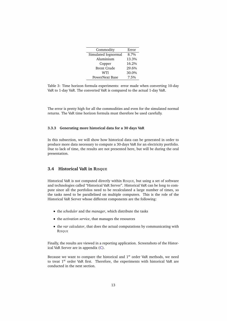
Commodity ErrorSimulated lognormal 8.7%

Aluminium 13.3%Copper 16.2%

Brent Crude 29.6%WTI 30.0%

PowerNext Base 7.5%

Table 3: Time horizon formula experiments: error made when converting 10-dayVaR to 1-day VaR. The converted VaR is compared to the actual 1-day VaR.

The error is pretty high for all the commodities and even for the simulated normalreturns. The VaR time horizon formula must therefore be used carefully.

3.3.3 Generating more historical data for a 30 days VaR

In this subsection, we will show how historical data can be generated in order toproduce more data necessary to compute a 30-days VaR for an electricity portfolio.Due to lack of time, the results are not presented here, but will be during the oralpresentation.

3.4 Historical VaR in RISQUE

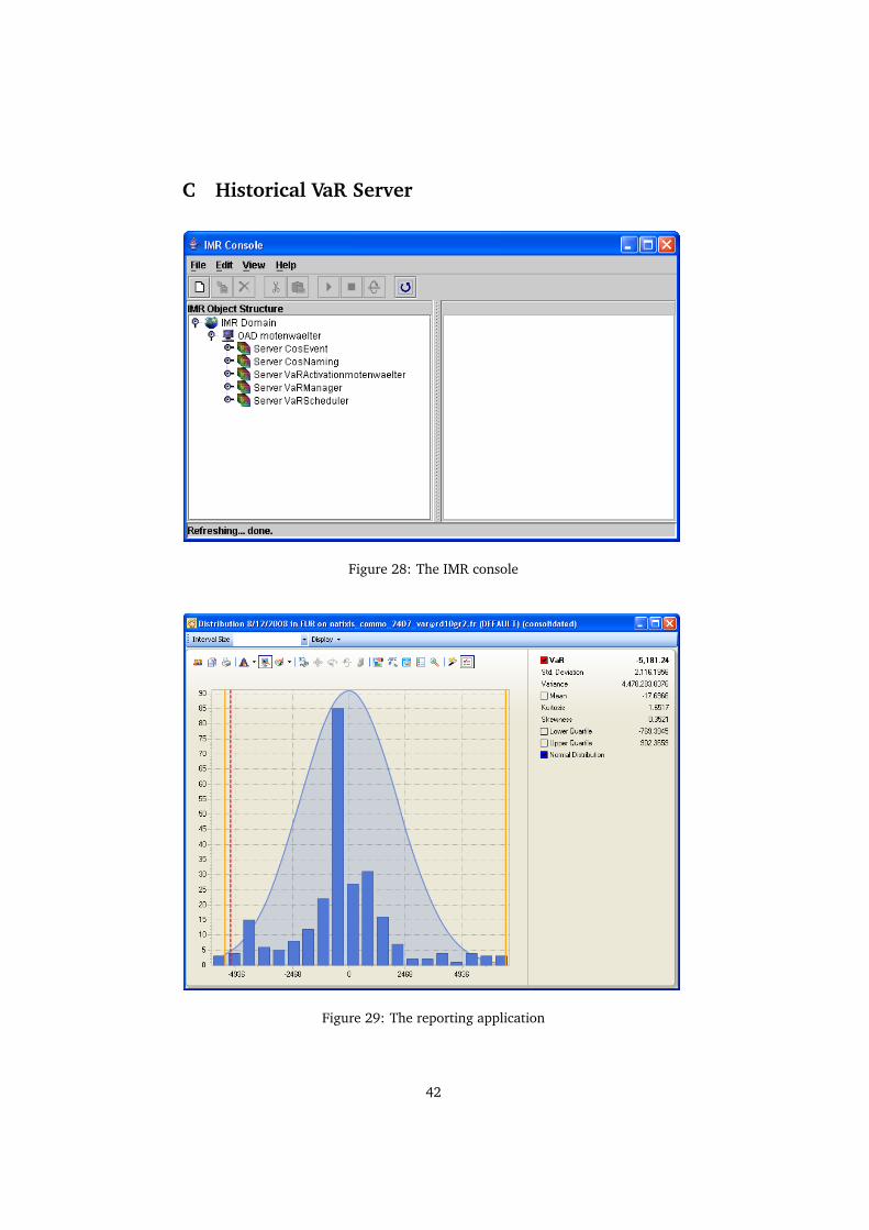
Historical VaR is not computed directly within RISQUE, but using a set of softwareand technologies called “Historical VaR Server”. Historical VaR can be long to com-pute since all the portfolios need to be recalculated a large number of times, sothe tasks need to be parallelised on multiple computers. This is the role of theHistorical VaR Server whose different components are the following:

• the scheduler and the manager, which distribute the tasks

• the activation service, that manages the resources

• the var calculator, that does the actual computations by communicating withRISQUE

Finally, the results are viewed in a reporting application. Screenshots of the Histor-ical VaR Server are in appendix (C).

Because we want to compare the historical and 1st order VaR methods, we needto treat 1st order VaR first. Therefore, the experiments with historical VaR areconducted in the next section.

13

3.5 Conclusion

In this section we defined historical VaR and detailed the computation steps. Wethen saw that the historical VaR on commodity portfolios was validated by thebacktest. Experiments with the time horizon formula showed that its accuracycan be limited: even with simulated lognormal returns, the approximation is quitesevere. We finally described how RISQUE computes the historical VaR, but left theactual computation for the next section, in which it will be compared with the 1st

order VaR.

14

4 1st order VaR

4.1 Introduction

In this section, we will see the 1st order approximation formula for analytical VaRand immediately apply it to a simple example. We will then see more complexexamples and compare the results with the historical VaR, as defined in the previoussection. Finally, we will try to enhance the mapping method used by RISQUE as ananswer to the particularities of commodity portfolios.

4.2 The 1st order approximation formula

Let P be the value of a portfolio with n risk sources which are typically spot prices,volatilities, rates or CDS spreads, for example. Let δi be the delta-cash sensitivity(A.3) of the porfolio to the ith asset (1 ¶ i ¶ n). If ri is the return (as defined inA.1) on asset i in 1 day, then the dollar change of our investment sensitive to asseti is δi ri . It follows that a linear approximation of the variation of the value of theportfolio is

∆P =n∑

i=1

δi ri (2)

Recall that the VaR for an α confidence level and a N days horizon is defined by∫ VaR

−∞δP(x)d x = 1−α

If we assume the ri follow a centered normal distrubution, then δP is normallydistributed and

VaR= σP · N −1(1−α) ·p

N/252

where

• N −1 is the inverse standard normal distribution function,

• σP =p

∆>Σ∆ is the portfolio’s volatility where Σ is the joint distributionr1, . . . , rn’s variance-covariance matrix and ∆= (δi) ∈Mn,1.

In conclusion,

VaR=p

∆>Σ∆ · N −1(1−α) ·p

N/252 (3)

Remarks:

• we did two approximations here: a first order approximation on ∆P and theassumption that the returns are normally distributed.

• formula (3) is a direct proof of the time horizon formula (1).

15

4.3 A simple example

4.3.1 Computation by hand

Consider a porfolio consisting of $10 million in shares of Apple and $7 million inshares of Microsoft, i.e. ∆= ( 10 7 )>. We suppose that the variance-covariancematrix of the pair (Apple, Microsoft) is

Σ =�

0.4 −0.2−0.2 0.1

�

The 99% 1-day VaR is therefore equal to

VaR =p

102 × 0.42 + 72 × 0.12 + 2× 10× 7× (−0.2)× 0.4× 0.1

×N −1(0.01)×p

1/365

= −$0.477381 million

In conclusion, we are 99% certain that we will not loose more than $477,381 bytomorrow.

4.3.2 Computation in RISQUE

We now want to confirm this result by making the same computation in RISQUE:

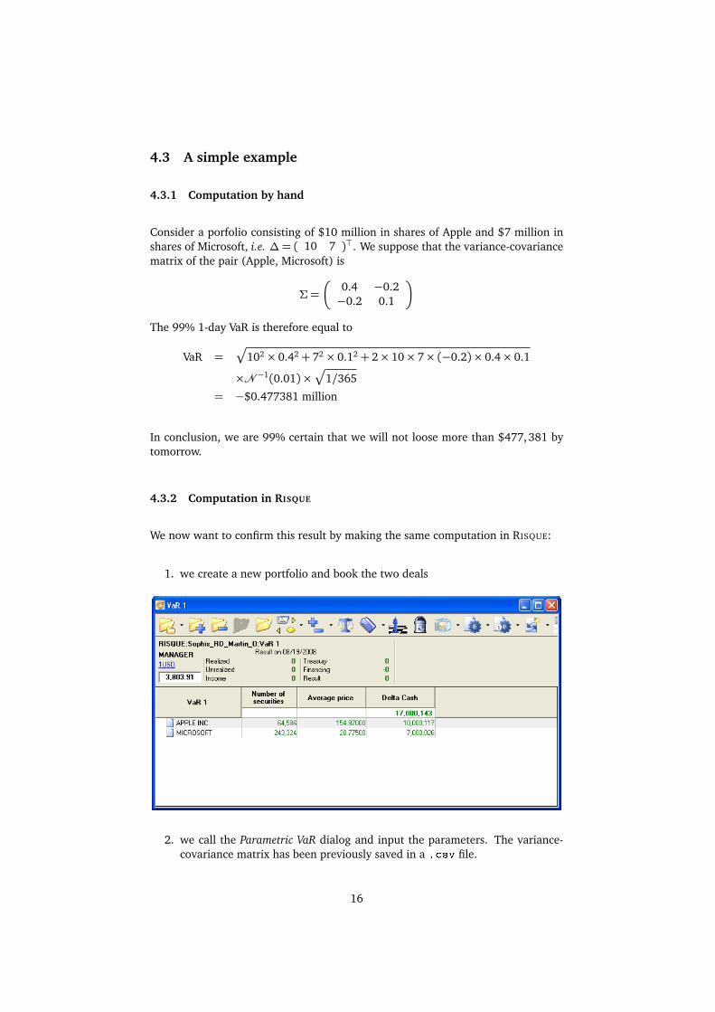
1. we create a new portfolio and book the two deals

2. we call the Parametric VaR dialog and input the parameters. The variance-covariance matrix has been previously saved in a .csv file.

16

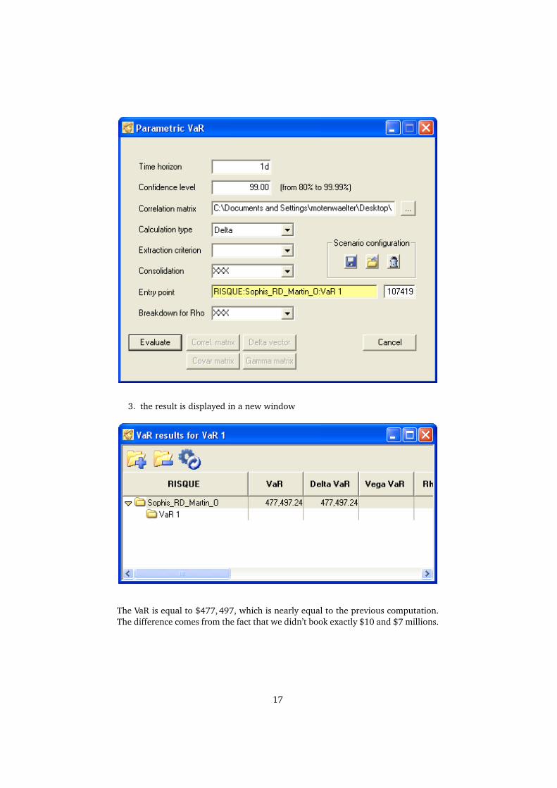
3. the result is displayed in a new window

The VaR is equal to $477,497, which is nearly equal to the previous computation.The difference comes from the fact that we didn’t book exactly $10 and $7 millions.

17

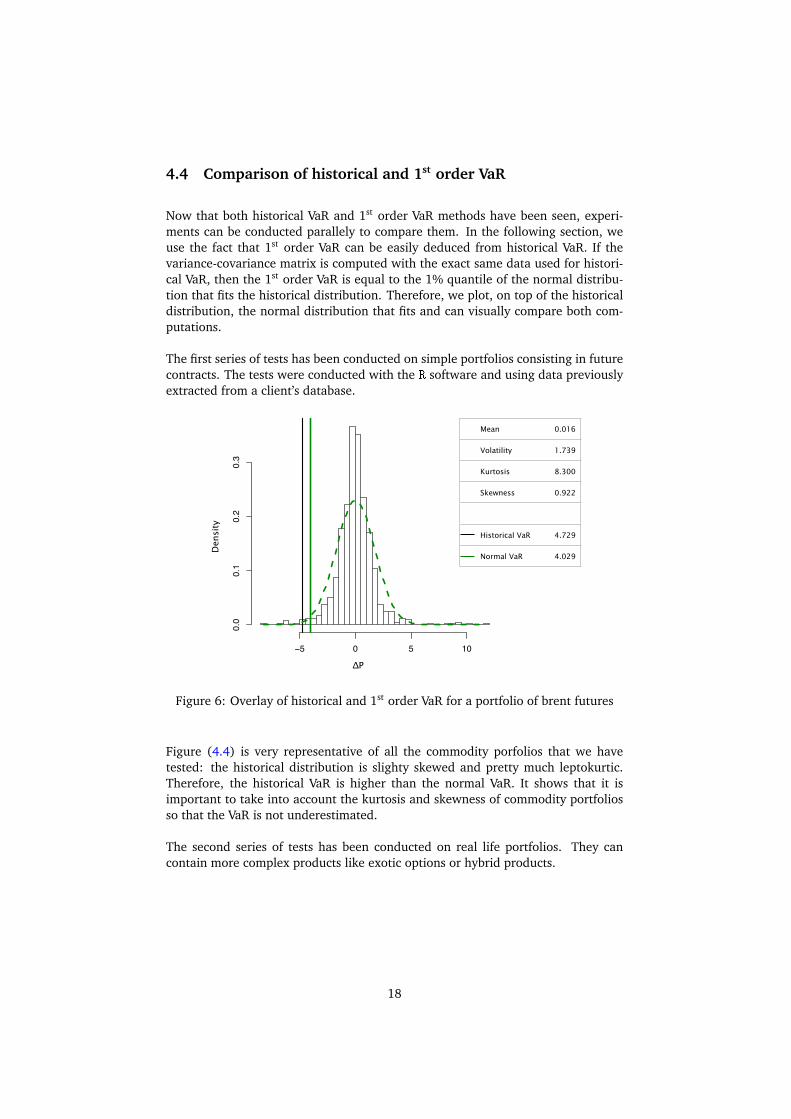
4.4 Comparison of historical and 1st order VaR

Now that both historical VaR and 1st order VaR methods have been seen, experi-ments can be conducted parallely to compare them. In the following section, weuse the fact that 1st order VaR can be easily deduced from historical VaR. If thevariance-covariance matrix is computed with the exact same data used for histori-cal VaR, then the 1st order VaR is equal to the 1% quantile of the normal distribu-tion that fits the historical distribution. Therefore, we plot, on top of the historicaldistribution, the normal distribution that fits and can visually compare both com-putations.

The first series of tests has been conducted on simple portfolios consisting in futurecontracts. The tests were conducted with the R software and using data previouslyextracted from a client’s database.

Mean 0.016

Volatility 1.739

Kurtosis 8.300

Skewness 0.922

Historical VaR 4.729

Normal VaR 4.029

!"#$%"&'"()*'&+(#,$-#.

/,.0'$+

!1 2 1 32

242

243

245

246

7'0$"#'8*&9'#0$("#),#

!P

Densit

y

Figure 6: Overlay of historical and 1st order VaR for a portfolio of brent futures

Figure (4.4) is very representative of all the commodity porfolios that we havetested: the historical distribution is slighty skewed and pretty much leptokurtic.Therefore, the historical VaR is higher than the normal VaR. It shows that it isimportant to take into account the kurtosis and skewness of commodity portfoliosso that the VaR is not underestimated.

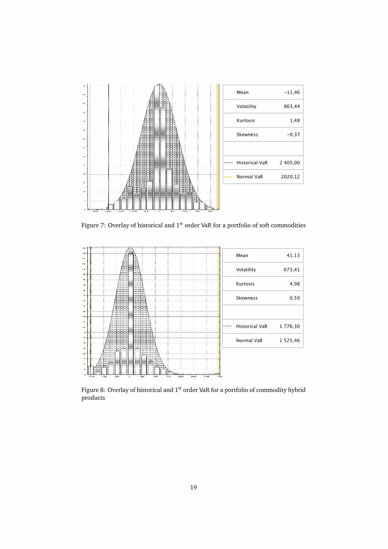
The second series of tests has been conducted on real life portfolios. They cancontain more complex products like exotic options or hybrid products.

18

Mean -11,46

Volatility 863,44

Kurtosis 1,48

Skewness -0,37

Historical VaR 2!405,00

Normal VaR 2020,12

Figure 7: Overlay of historical and 1st order VaR for a portfolio of soft commodities

Mean 41,13

Volatility 673,41

Kurtosis 4,98

Skewness 0,59

Historical VaR 1!776,30

Normal VaR 1!525,46

Figure 8: Overlay of historical and 1st order VaR for a portfolio of commodity hybridproducts

19

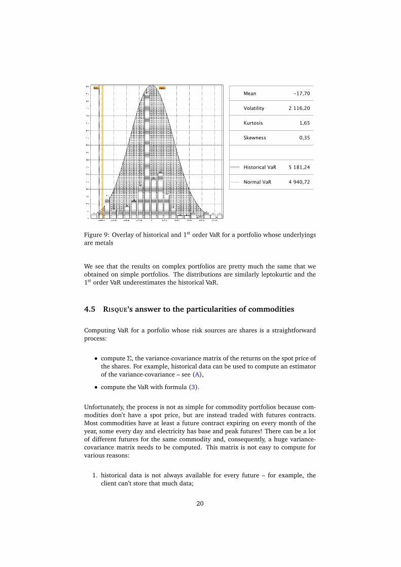
Mean -17,70

Volatility 2!116,20

Kurtosis 1,65

Skewness 0,35

Historical VaR 5!181,24

Normal VaR 4!940,72

Figure 9: Overlay of historical and 1st order VaR for a portfolio whose underlyingsare metals

We see that the results on complex portfolios are pretty much the same that weobtained on simple portfolios. The distributions are similarly leptokurtic and the1st order VaR underestimates the historical VaR.

4.5 RISQUE’s answer to the particularities of commodities

Computing VaR for a porfolio whose risk sources are shares is a straightforwardprocess:

• compute Σ, the variance-covariance matrix of the returns on the spot price ofthe shares. For example, historical data can be used to compute an estimatorof the variance-covariance – see (A),

• compute the VaR with formula (3).

Unfortunately, the process is not as simple for commodity portfolios because com-modities don’t have a spot price, but are instead traded with futures contracts.Most commodities have at least a future contract expiring on every month of theyear, some every day and electricity has base and peak futures! There can be a lotof different futures for the same commodity and, consequently, a huge variance-covariance matrix needs to be computed. This matrix is not easy to compute forvarious reasons:

1. historical data is not always available for every future – for example, theclient can’t store that much data;

20

2. some historical data is not reliable enough to compute the variance – forexample, because there are so many futures, some have a too low tradingvolume for the price to be meaningful;

3. it is better to look at the historical data of futures with the same time tomaturity rather than at the plain historical data. This is done by a techniquecalled future rolling;

4. in some cases, finding the future with the same time to maurity is not suffi-cient: the futures should also be with a similar seasonality.

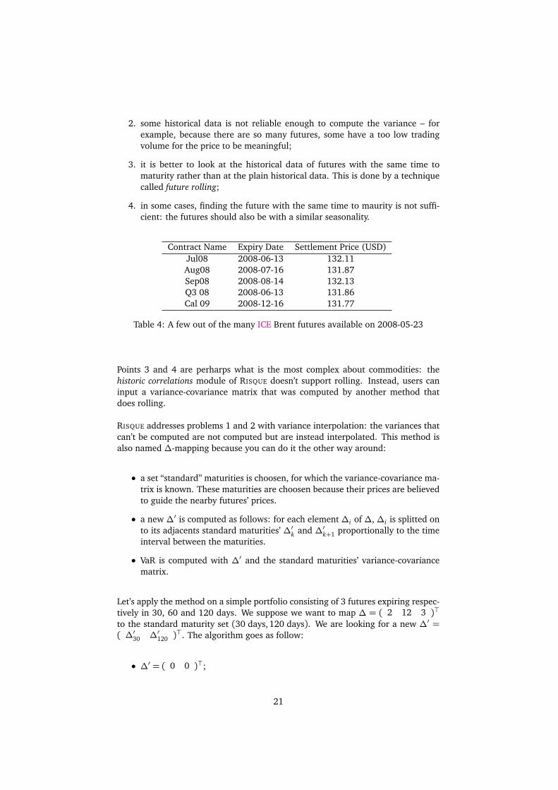
Contract Name Expiry Date Settlement Price (USD)Jul08 2008-06-13 132.11Aug08 2008-07-16 131.87Sep08 2008-08-14 132.13Q3 08 2008-06-13 131.86Cal 09 2008-12-16 131.77

Table 4: A few out of the many ICE Brent futures available on 2008-05-23

Points 3 and 4 are perharps what is the most complex about commodities: thehistoric correlations module of RISQUE doesn’t support rolling. Instead, users caninput a variance-covariance matrix that was computed by another method thatdoes rolling.

RISQUE addresses problems 1 and 2 with variance interpolation: the variances thatcan’t be computed are not computed but are instead interpolated. This method isalso named ∆-mapping because you can do it the other way around:

• a set “standard” maturities is choosen, for which the variance-covariance ma-trix is known. These maturities are choosen because their prices are believedto guide the nearby futures’ prices.

• a new ∆′ is computed as follows: for each element ∆i of ∆, ∆i is splitted onto its adjacents standard maturities’ ∆′k and ∆′k+1 proportionally to the timeinterval between the maturities.

• VaR is computed with ∆′ and the standard maturities’ variance-covariancematrix.

Let’s apply the method on a simple portfolio consisting of 3 futures expiring respec-tively in 30, 60 and 120 days. We suppose we want to map ∆ = ( 2 12 3 )>

to the standard maturity set (30 days, 120 days). We are looking for a new ∆′ =( ∆′30 ∆′120 )

>. The algorithm goes as follow:

• ∆′ = ( 0 0 )>;

21

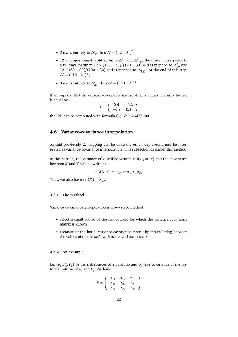
• 2 maps entirely to ∆′30 thus ∆′ = ( 2 0 )>;

• 12 is proportionnaly splitted on to ∆′30 and ∆′120. Because it corresponds toa 60 days maturity, 12× (120− 60)/(120− 30) = 8 is mapped to ∆′30 and12× (60− 30)/(120− 30) = 4 is mapped to ∆′120. At the end of this step,∆′ = ( 10 4 )>;

• 3 maps entirely to ∆′30, thus ∆′ = ( 10 7 )>.

If we suppose that the variance-covariance matrix of the standard maturity futuresis equal to:

Σ =�

0.4 −0.2−0.2 0.1

�

the VaR can be computed with formula (3), VaR=$477,000.

4.6 Variance-covariance interpolation

As said previously, ∆-mapping can be done the other way around and be inter-preted as variance-covariance interpolation. This subsection describes this method.

In this section, the variance of X will be written var(X ) = σ2x and the covariance

between X and Y will be written:

cov(X , Y ) = σx y = σxσyρx y

Thus, we also have var(X ) = σx x .

4.6.1 The method

Variance-covariance interpolation is a two steps method:

• select a small subset of the risk sources for which the variance-covariancematrix is known

• reconstruct the initial variance-covariance matrix by interpolating betweenthe values of the subset’s variance-covariance matrix

4.6.2 An example

Let (F1, F2, F3) be the risk sources of a portfolio and σi j the covariance of the his-torical returns of Fi and F j . We have

Σ =

σ11 σ12 σ13σ21 σ22 σ23σ31 σ32 σ33

22

We choose (F1, F3) as the subset, the values σ11,σ13,σ31,σ33 are known. We needto fill the gaps in Σ′ the new variance-covariance matrix:

Σ′ =

σ11 σ13

σ31 σ33

If we assume that the time between two expiry dates of two adjacents futures is 1month, bilinear interpolation gives:

Σ′ =

σ1112(σ11 +σ13) σ13

12(σ11 +σ31)

14(σ11 +σ13 +σ31 +σ33)

12(σ33 +σ33)

σ3112(σ31 +σ33) σ33

4.6.3 Interpolation coefficients

Method in RISQUE Let us formalise the previous example: the interpolation coef-ficients are computed using the expiry dates of the futures. Let Fx be the future forwhich the covariance needs to be interpolated and t x its expiry date. There are 3cases:

• if there exists Fa, Fb such as ta < t x < tb, then

σax =tb − t x

tb − taσaa +

t x − ta

tb − taσab

σbx =tb − t x

tb − taσab +

t x − ta

tb − taσbb

σx x =tb − t x

tb − taσax +

t x − ta

tb − taσbx

=�

tb − t x

tb − ta

�2

σaa + 2�

tb − t x

tb − ta

��

t x − ta

tb − ta

�

σab +�

t x − ta

tb − ta

�2

σbb

• otherwise there exists Fa such as t x < ta, then σax = σx x = σaa,

• or there exists Fb such as tb < t x , then σbx = σx x = σbb.

Giving more importance to the variances In this paragraph, we will follow[Ale01] that suggests that we should rather interpolate the variances instead ofthe covariance. We consider the case where there exists Fa, Fb such as ta < t x < tb.We are looking for a new interpolation coefficient λ such that Fx = λFa+(1−λ)Fb.In this case,

σx x = λ2σaa + (1−λ)2σbb + 2λ(1−λ)σab

23

Because we want to give importance to the variances rather than to the covariances,we suppose that the variance σx x is a linear combination of the variances σaa andσbb:

σx x =tb − t x

tb − taσaa +

t x − ta

tb − taσbb

λ is found by picking the positive solution of the quadratic equation

λ2σaa + (1−λ)2σbb + 2λ(1−λ)σab =tb − t x

tb − taσaa +

t x − ta

tb − taσbb

Once lambda is found, the previous method can be applied with the new interpo-lation coefficient.

4.7 Experimental results

4.7.1 Graphical interpretation of interpolation

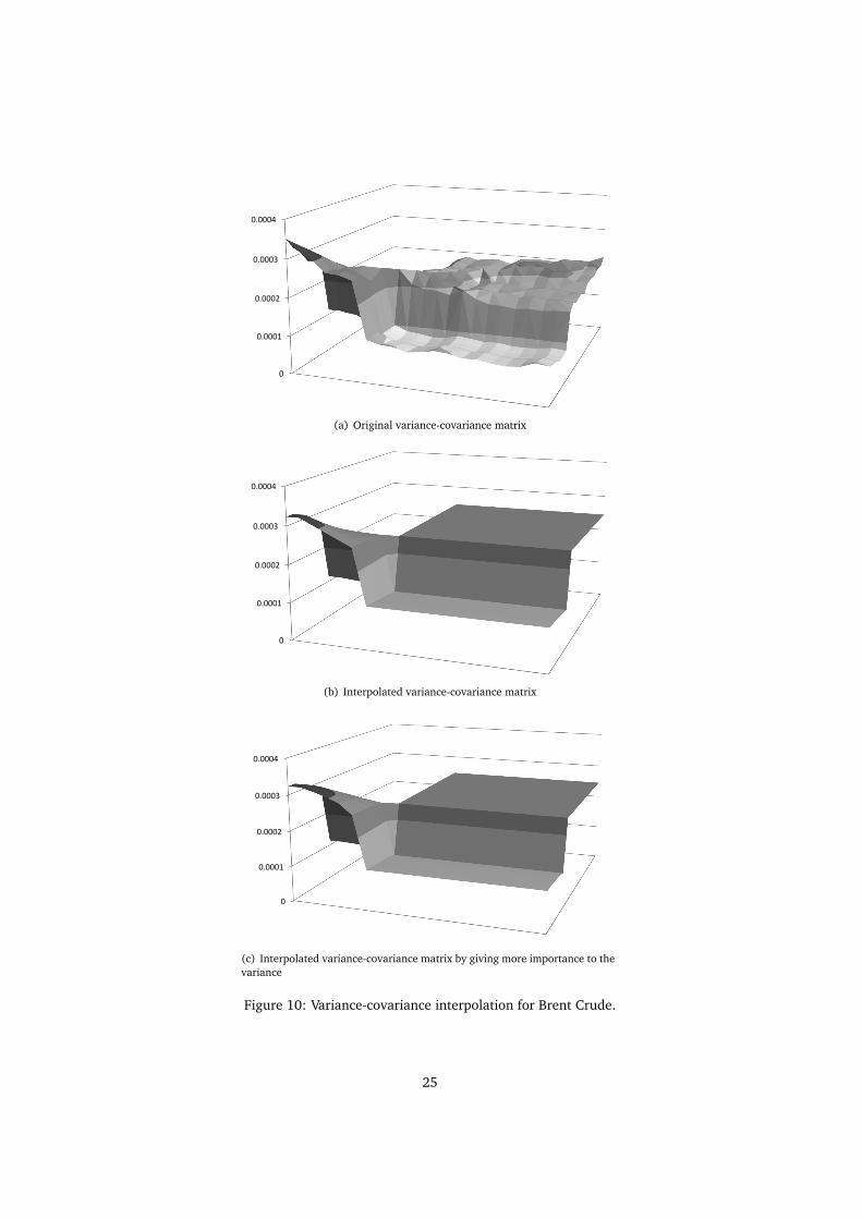
The first experiment consists in plotting in three dimensions the brent’s variance-covariance matrix and its two interpolated variants.

24

0

0.0001

0.0002

0.0003

0.0004

(a) Original variance-covariance matrix

0

0.0001

0.0002

0.0003

0.0004

(b) Interpolated variance-covariance matrix

0

0.0001

0.0002

0.0003

0.0004

(c) Interpolated variance-covariance matrix by giving more importance to thevariance

Figure 10: Variance-covariance interpolation for Brent Crude.

25

We clearly see the effect of the interpolation between the two first graphs. Thedifference between the two last graphs is more subtle, but we can still see that thedifference is on the diagonal. It is normal because the difference between the twomapping methods resides in the way the variance is interpolated.

We also see that the quality of the result depends heavily on the choice of thereference futures, the ones on which the mapping is done. This particular brentvariance-covariance matrix has such a particular shape that a poor choice in thereference futures could result in an important error. This choice is therefore left tothe user that knows which maturities are known to guide the market. For example,for aluminium, the most traded future are the 3, 15 and 27 months.

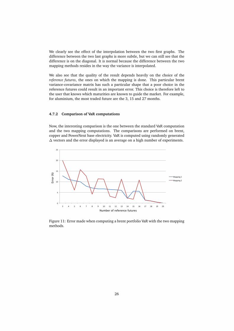
4.7.2 Comparison of VaR computations

Now, the interesting comparison is the one between the standard VaR computationand the two mapping computations. The comparisons are performed on brent,copper and PowerNext base electricity. VaR is computed using randomly generated∆ vectors and the error displayed is an average on a high number of experiments.

!"

!#!$"

!#%"

!#%$"

!#&"

!#&$"

'" (" $" )" *" +" ," %!" %%" %&" %'" %(" %$" %)" %*" %+" %," &!"

-.//012"%"

-.//012"&"

Number of reference futures

!

"#

"!

$#

$!

Err

or

(%)

#

Figure 11: Error made when computing a brent portfolio VaR with the two mappingmethods.

26

!"

!#!$"

!#!%"

!#!&"

!#!'"

!#!("

!#!)"

!#!*"

!#!+"

&" '" (" )" *" +" ," $!" $$" $%" $&" $'" $(" $)" $*" $+" $," %!" %$" %%" %&" %'" %(" %)" %*" %+" %," &!" &$" &%" &&" &'" &(" &)" &*" &+"

-.//012"$"

-.//012"%"

Number of reference futures

!

"

#

$

%Err

or

(%)

&

'

(

)

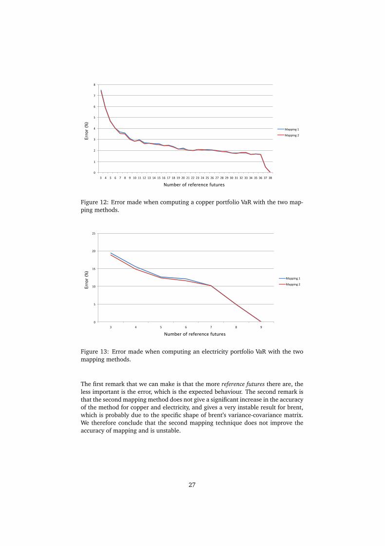
Figure 12: Error made when computing a copper portfolio VaR with the two map-ping methods.

!"

!#!$"

!#%"

!#%$"

!#&"

!#&$"

'" (" $" )" *" +" ,"

-.//012"%"

-.//012"&"

Number of reference futures

!

"#

"!

$#

$!

Err

or

(%)

#

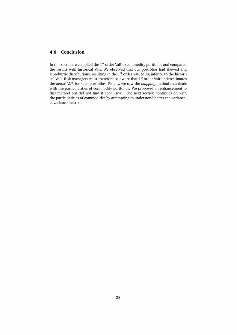
Figure 13: Error made when computing an electricity portfolio VaR with the twomapping methods.

The first remark that we can make is that the more reference futures there are, theless important is the error, which is the expected behaviour. The second remark isthat the second mapping method does not give a significant increase in the accuracyof the method for copper and electricity, and gives a very instable result for brent,which is probably due to the specific shape of brent’s variance-covariance matrix.We therefore conclude that the second mapping technique does not improve theaccuracy of mapping and is unstable.

27

4.8 Conclusion

In this section, we applied the 1st order VaR to commodity portfolios and comparedthe results with historical VaR. We observed that our portfolios had skewed andleptokurtic distributions, resulting in the 1st order VaR being inferior to the histori-cal VaR. Risk managers must therefore be aware that 1st order VaR underestimatesthe actual VaR for such portfolios. Finally, we saw the mapping method that dealswith the particularities of commodity portfolios. We proposed an enhancement tothis method but did not find it conclusive. The next section continues on withthe particularities of commodities by attempting to understand better the variance-covariance matrix.

28

5 Principal Component Analysis: an attempt to un-derstand the variance-covariance matrix

5.1 Introduction

We have seen in the previous section that the complexity of computing 1st orderVaR resides in the computation of the variance-covariance matrix. In this section,we attack the variance-covariance matrix with a different angle, in an attempt tounderstand it better. To do so, we applied a method known as Principal ComponentAnalysis (PCA).

5.2 The PCA methodology

5.2.1 Introduction

“PCA is a rotation of axes in multi-dimensional space that allows one to find linearcombinations –the principal components– of the original variables that summariseas much of the information as possible. The eigenvalue of each component is anestimate of the amount of total variance explained by that particular component.Inspecting the eigenvalues allows one to pick the minimum number of componentssummarising enough of the total variance, while inspecting the eigenvectors leadsto financial interpretations of the principal components.” ([PV02])

In the current context, the goal is similar to what we did with mapping: reducethe amount of initial data by only selecting data that has a meaning. In the caseof mapping, there was a simple and natural choice of meaningful data: the mosttraded maturities. In this case, we are looking for more complex combinations.

5.2.2 Data

Let X = (x i j) ∈ Mm,n be a matrix of data. In the case of financial data, x i j is theith historical return on the jth asset.

Before performing PCA, data must be normalised. Let X j and σ(X j) respectivelybe the empirical average and empirical volatility of the jth column. If X is thenormalised matrix, then:

x i j =x i j − X j

σ(X j)(4)

29

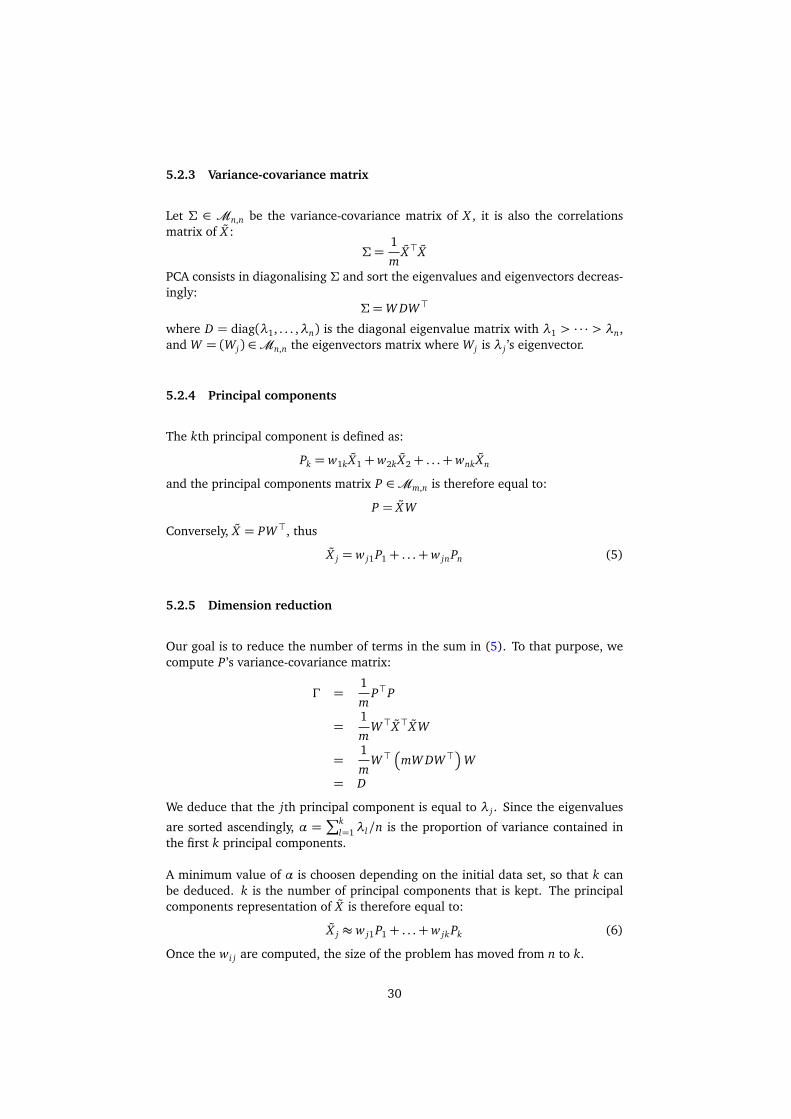
5.2.3 Variance-covariance matrix

Let Σ ∈ Mn,n be the variance-covariance matrix of X , it is also the correlationsmatrix of X :

Σ =1

mX>X

PCA consists in diagonalising Σ and sort the eigenvalues and eigenvectors decreas-ingly:

Σ =W DW>

where D = diag(λ1, . . . ,λn) is the diagonal eigenvalue matrix with λ1 > · · · > λn,and W = (Wj) ∈Mn,n the eigenvectors matrix where Wj is λ j ’s eigenvector.

5.2.4 Principal components

The kth principal component is defined as:

Pk = w1k X1 +w2k X2 + . . .+wnk Xn

and the principal components matrix P ∈Mm,n is therefore equal to:

P = XW

Conversely, X = PW>, thus

X j = w j1P1 + . . .+w jnPn (5)

5.2.5 Dimension reduction

Our goal is to reduce the number of terms in the sum in (5). To that purpose, wecompute P ’s variance-covariance matrix:

Γ =1

mP>P

=1

mW>X>XW

=1

mW>

�

mW DW>�

W

= D

We deduce that the jth principal component is equal to λ j . Since the eigenvalues

are sorted ascendingly, α =∑k

l=1λl/n is the proportion of variance contained inthe first k principal components.

A minimum value of α is choosen depending on the initial data set, so that k canbe deduced. k is the number of principal components that is kept. The principalcomponents representation of X is therefore equal to:

X j ≈ w j1P1 + . . .+w jk Pk (6)

Once the wi j are computed, the size of the problem has moved from n to k.

30

5.2.6 Recipe

PCA can be summarised with the following recipe:

• normalise the data

• diagonalise Σ, the variance-covariance matrix

• for 1 ¶ k ¶ n, plot the sum of the k first eigenvalues. Each sum is a percent-age that tells us how much the first k principal components are responsiblefor the variance of the initial data.

• plot the first few eigenvectors to study their shape

• compute Σk, an estimation of Σ using only k principal components

5.3 Understanding the variance-covariance matrix

5.3.1 Theory

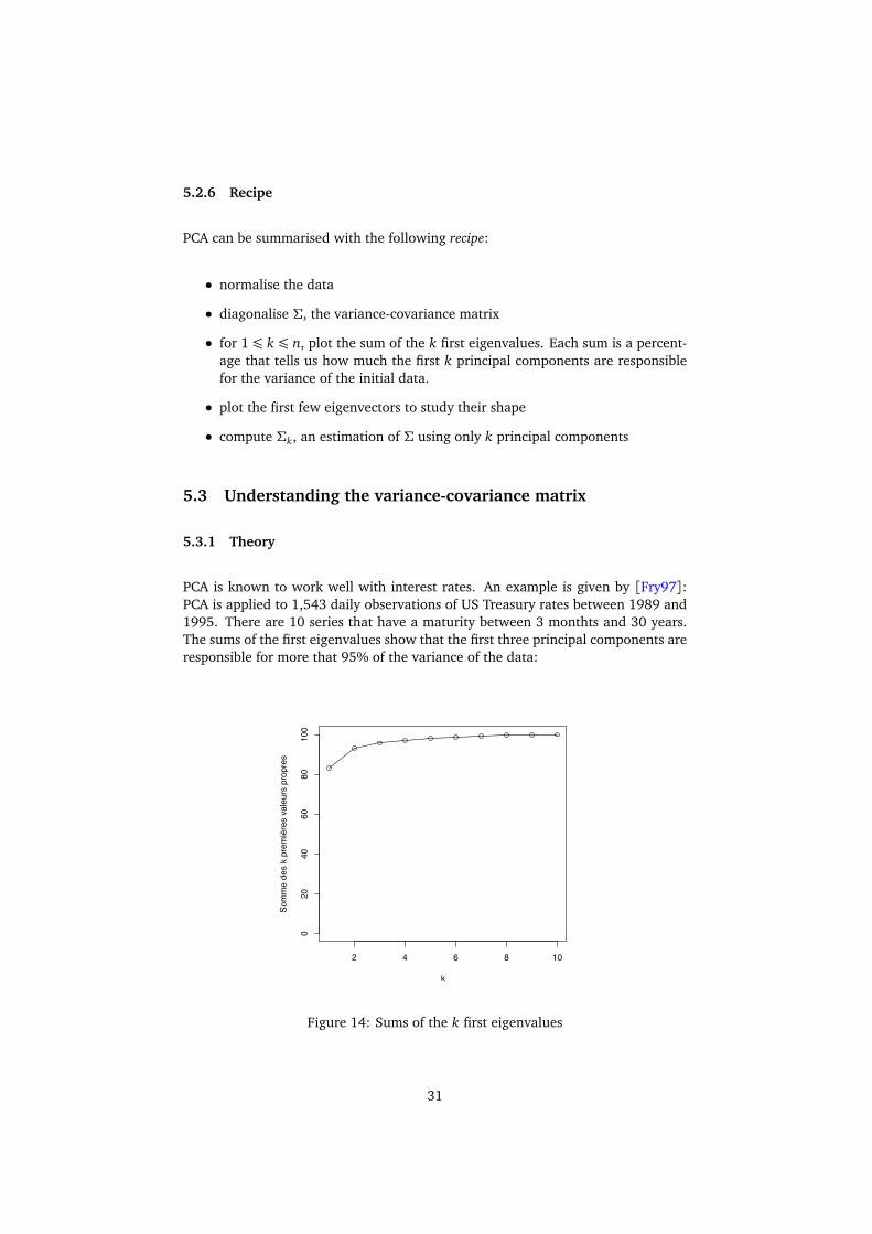
PCA is known to work well with interest rates. An example is given by [Fry97]:PCA is applied to 1,543 daily observations of US Treasury rates between 1989 and1995. There are 10 series that have a maturity between 3 monthts and 30 years.The sums of the first eigenvalues show that the first three principal components areresponsible for more that 95% of the variance of the data:

2 4 6 8 10

020

4060

8010

0

k

Som

me

des

k pr

emiè

res

vale

urs

prop

res

Figure 14: Sums of the k first eigenvalues

31

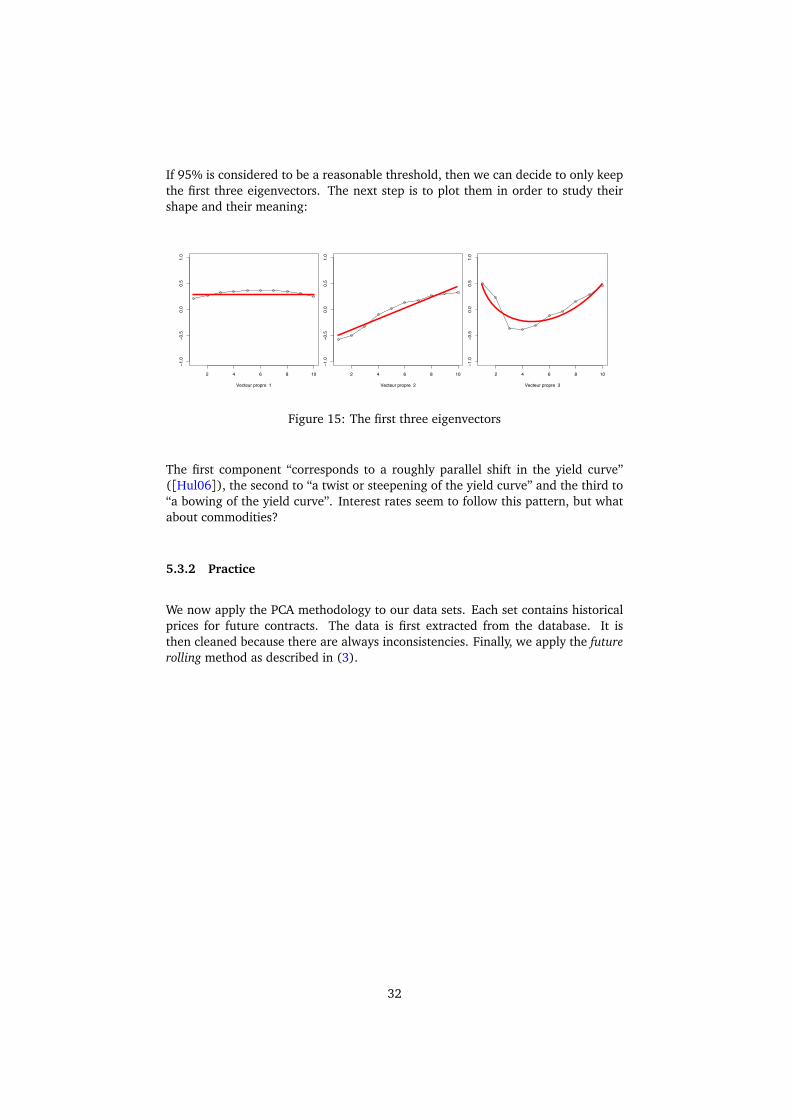
If 95% is considered to be a reasonable threshold, then we can decide to only keepthe first three eigenvectors. The next step is to plot them in order to study theirshape and their meaning:

! " # $ %&

!%'&

!&'(

&'&

&'(

%'&

)*+,*-./0.10.*//%

! " # $ %&

!%'&

!&'(

&'&

&'(

%'&

)*+,*-./0.10.*//!

! " # $ %&

!%'&

!&'(

&'&

&'(

%'&

)*+,*-./0.10.*//2

Figure 15: The first three eigenvectors

The first component “corresponds to a roughly parallel shift in the yield curve”([Hul06]), the second to “a twist or steepening of the yield curve” and the third to“a bowing of the yield curve”. Interest rates seem to follow this pattern, but whatabout commodities?

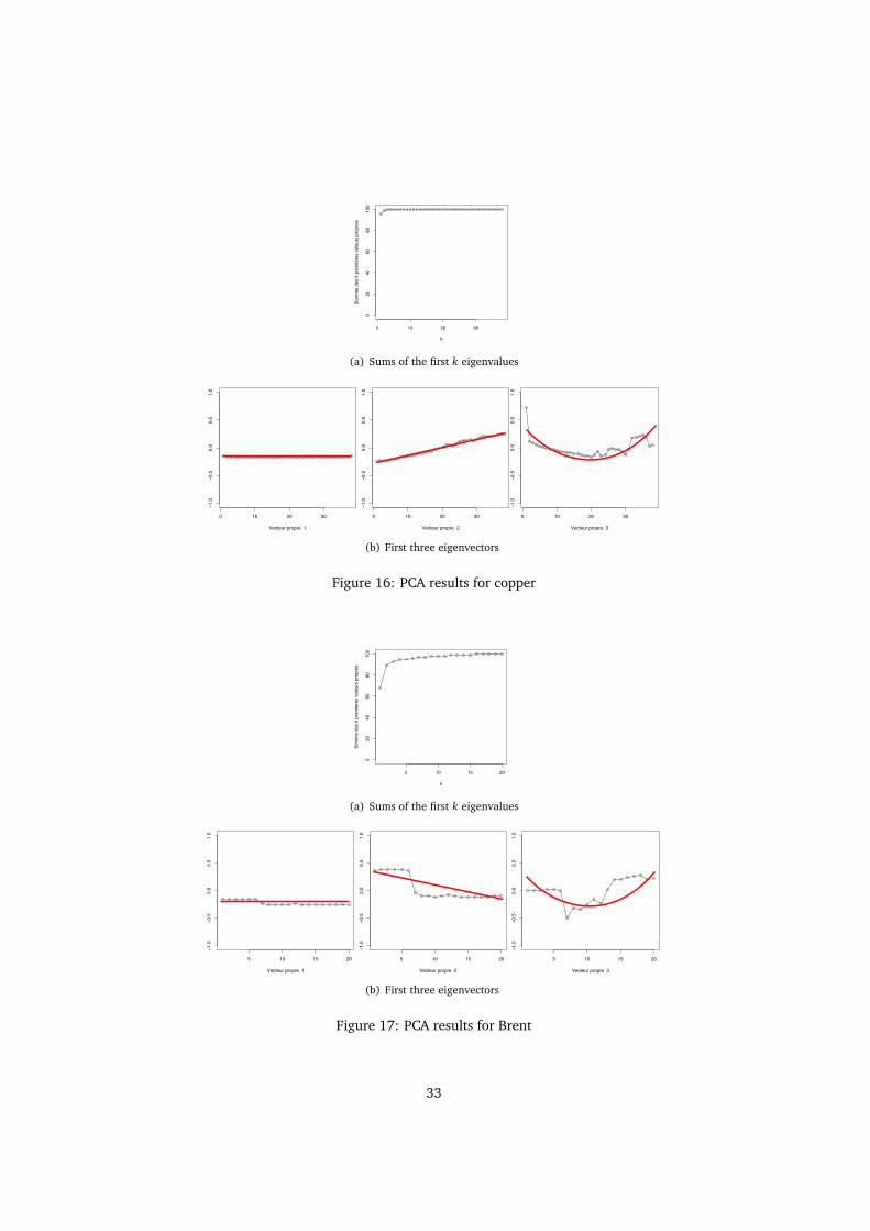
5.3.2 Practice

We now apply the PCA methodology to our data sets. Each set contains historicalprices for future contracts. The data is first extracted from the database. It isthen cleaned because there are always inconsistencies. Finally, we apply the futurerolling method as described in (3).

32

0 10 20 30

02

04

06

08

01

00

k

So

mm

e d

es k

pre

miè

res v

ale

urs

pro

pre

s

(a) Sums of the first k eigenvalues

! "! #! $!

!"%!

!!%&

!%!

!%&

"%!

'()*(+,-.,/.,(--"

0)12(3,(*+,40%.)15,/*1*6/478-69

! "! #! $!

!"%!

!!%&

!%!

!%&

"%!

'()*(+,-.,/.,(--#

0)12(3,(*+,40%.)15,/*1*6/478-69

! "! #! $!!"%!

!!%&

!%!

!%&

"%!

'()*(+,-.,/.,(--$

0)12(3,(*+,40%.)15,/*1*6/478-69

(b) First three eigenvectors

Figure 16: PCA results for copper

5 10 15 20

02

04

06

08

01

00

k

So

mm

e d

es k

pre

miè

res v

ale

urs

pro

pre

s

(a) Sums of the first k eigenvalues

! "# "! $#

!"%#

!#%!

#%#

#%!

"%#

&'()'*+,-+.-+',,"

/(01'2+')*+3/%-(04+.)0)5.367,58

! "# "! $#

!"%#

!#%!

#%#

#%!

"%#

&'()'*+,-+.-+',,$

/(01'2+')*+3/%-(04+.)0)5.367,58

! "# "! $#

!"%#

!#%!

#%#

#%!

"%#

&'()'*+,-+.-+',,/

0(12'3+')*+40%-(15+.)1)6.478,69

(b) First three eigenvectors

Figure 17: PCA results for Brent

33

2 4 6 8

02

04

06

08

01

00

k

So

mm

e d

es k

pre

miè

res v

ale

urs

pro

pre

s

(a) Sums of the first k eigenvalues

! " # $!%&'

!'&(

'&'

'&(

%&'

)*+,*-./0.10.*//2

3+45*6.*,-.73&0+48.1,4,917:;/9<

! " # $

!%&'

!'&(

'&'

'&(

%&'

)*+,*-./0.10.*//!

2+34*5.*,-.62&0+37.1,3,8169:/8;

! " # $

!%&'

!'&(

'&'

'&(

%&'

)*+,*-./0.10.*//%

2+34*5.*,-.62&0+37.1,3,8169:/8;

(b) First three eigenvectors

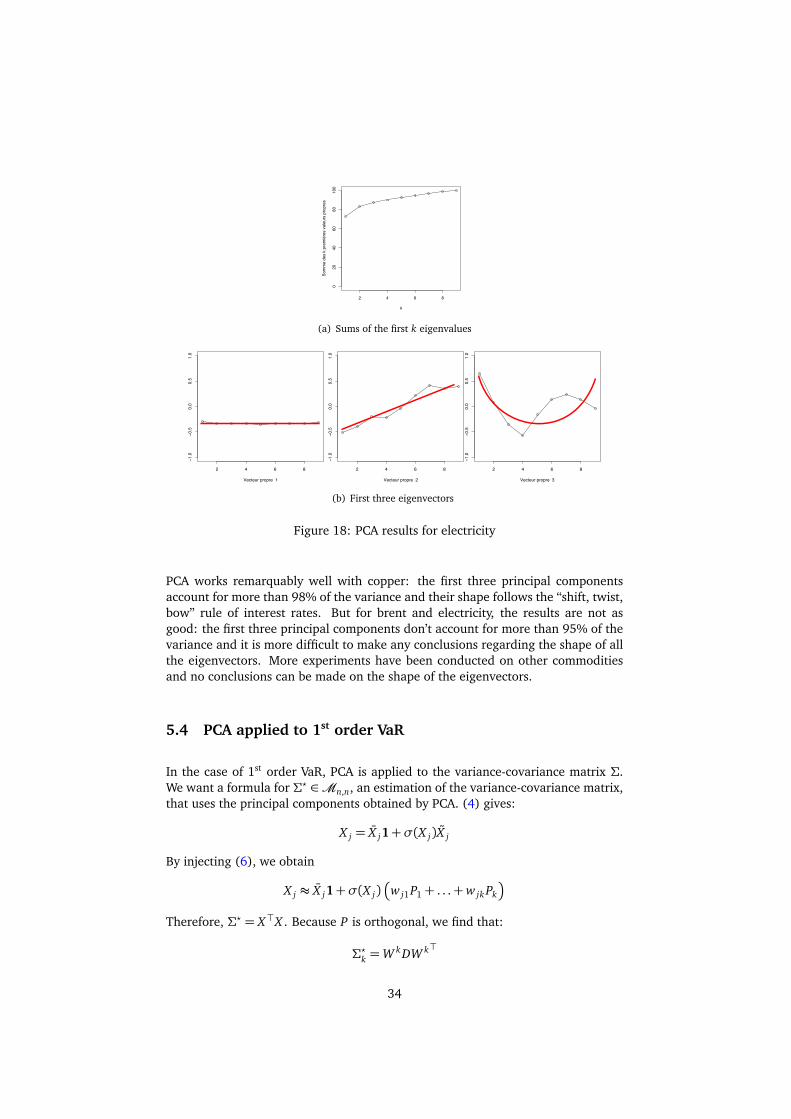
Figure 18: PCA results for electricity

PCA works remarquably well with copper: the first three principal componentsaccount for more than 98% of the variance and their shape follows the “shift, twist,bow” rule of interest rates. But for brent and electricity, the results are not asgood: the first three principal components don’t account for more than 95% of thevariance and it is more difficult to make any conclusions regarding the shape of allthe eigenvectors. More experiments have been conducted on other commoditiesand no conclusions can be made on the shape of the eigenvectors.

5.4 PCA applied to 1st order VaR

In the case of 1st order VaR, PCA is applied to the variance-covariance matrix Σ.We want a formula for Σ? ∈Mn,n, an estimation of the variance-covariance matrix,that uses the principal components obtained by PCA. (4) gives:

X j = X j1+σ(X j)X j

By injecting (6), we obtain

X j ≈ X j1+σ(X j)�

w j1P1 + . . .+w jk Pk

�

Therefore, Σ? = X>X . Because P is orthogonal, we find that:

Σ?k =W k DW k>

34

where¨

W k =�

wi jσ(X i)�

∈Mn,k

D = diag�

σ(P1), . . . ,σ(Pk)�

Recall that the formula for 1st order VaR is known (3):

VaR=p

∆>Σ∆ · N −1(1−α) ·p

N/252

An approximation of the VaR using PCA is given by:

VaRk =Æ

∆>Σ?k∆ · N−1(1−α) ·

p

N/252

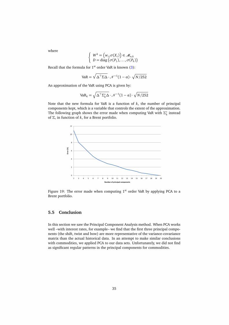
Note that the new formula for VaR is a function of k, the number of principalcomponents kept, which is a variable that controls the extent of the approximation.The following graph shows the error made when computing VaR with Σ?k insteadof Σ, in function of k, for a Brent portfolio.

0

2

4

6

8

10

12

2 3 4 5 6 7 8 9 10 11 12 13 14 15 16 17 18 19 20

Error (%)

Number of principal components

Figure 19: The error made when computing 1st order VaR by applying PCA to aBrent portfolio.

5.5 Conclusion

In this section we saw the Principal Component Analysis method. When PCA workswell –with interest rates, for example– we find that the first three principal compo-nents (the shift, twist and bow) are more representative of the variance-covariancematrix than the actual historical data. In an attempt to make similar conclusionswith commodities, we applied PCA to our data sets. Unfortunately, we did not findas significant regular patterns in the principal components for commodities.

35

6 Conclusion

In this paper, we studied Value-at-Risk for commodity portfolios. We started bydefining VaR. Then we saw the historical and 1st order methods. We concludedwith a backtest that these methods are valid. We also compared each of the meth-ods and found out that since our portfolios have skewed and leptokurtic distribu-tions, the 1st order VaR will always underestimate the historical VaR. We comparedtwo mapping techniques and concluded that RISQUE’s method is already satisfying.Finally, we studied Principal Component Analysis in an attempt to better under-stand the variance-covariance matrix. But the experiments were not as conclusivefor commodities as they are for interest rates.

36

Appendix

A Mathematical formulas

A.1 Daily returns

Let Si be the price of a financial asset at the end of day i. The ith daily return isdefined by:

ri =Si − Si−1

Si−1

In finance, log-returns are more commonly used:

ri = log�

Si

Si−1

�

A.2 An unbiased estimate of the covariance, skewness and kur-tosis

Let x = (x i)1¶i¶n and y = (yi)1¶i¶n be two series of historical data. An unbiasedestimate of the covariance is:

σx y =1

n− 1

n∑

k=1

�

xk − x��

yk − y�

The kth sample moment of x is defined by:

mk =n∑

i=1

�

x i − x�k

An unbiased estimate of the skewness of x is:

skx =n2

(n− 1)(n− 2)m3

and an unbiased estimate of the kurtosis of x is:

kux =n2

(n− 1)(n− 2)(n− 3)

�

(n+ 1)m4 − 3(n− 1)m22

�

A.3 Delta, delta-cash

Let P be a portfolio. The delta sensitivity to the ith risk source whose price is Si isdefined as:

∆i =∂ P

∂ Si

37

and the similar delta-cash sensitivity is equal to:

δi = Si∆i

B RISQUE

B.1 VaR computation steps

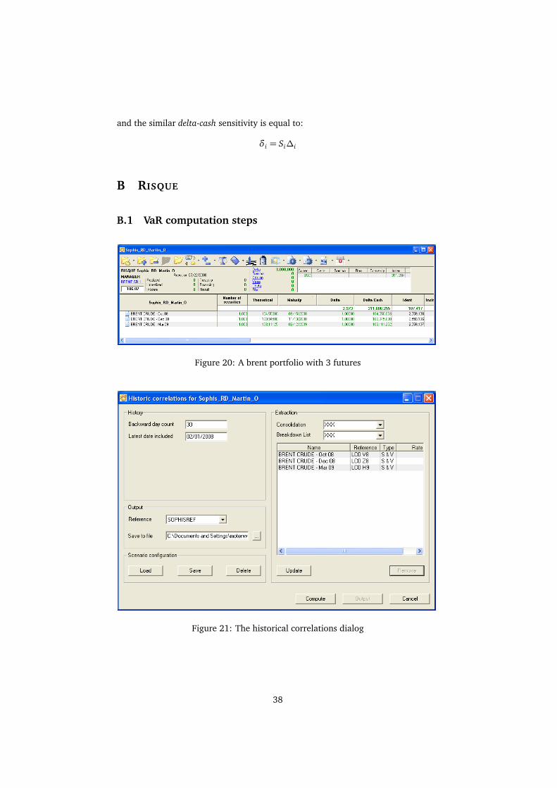
Figure 20: A brent portfolio with 3 futures

Figure 21: The historical correlations dialog

38

Figure 22: The VaR computation dialog

Figure 23: The 1st order VaR result

39

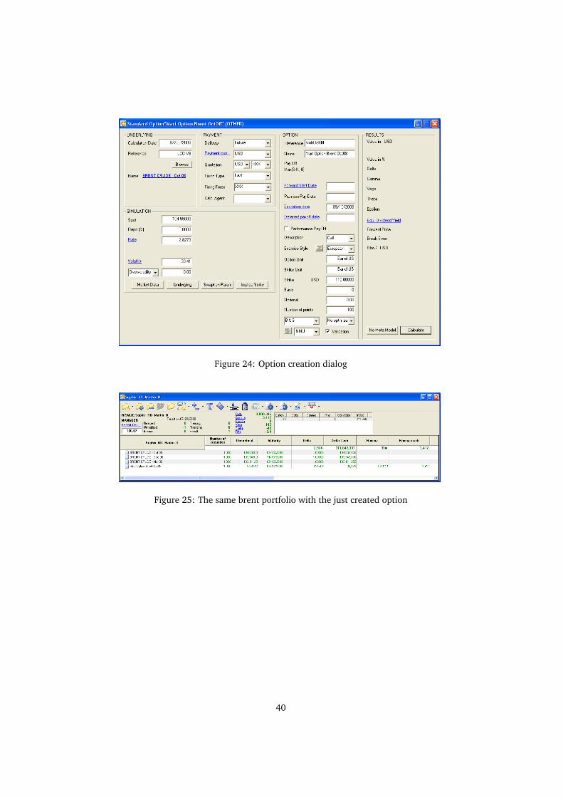
Figure 24: Option creation dialog

Figure 25: The same brent portfolio with the just created option

40

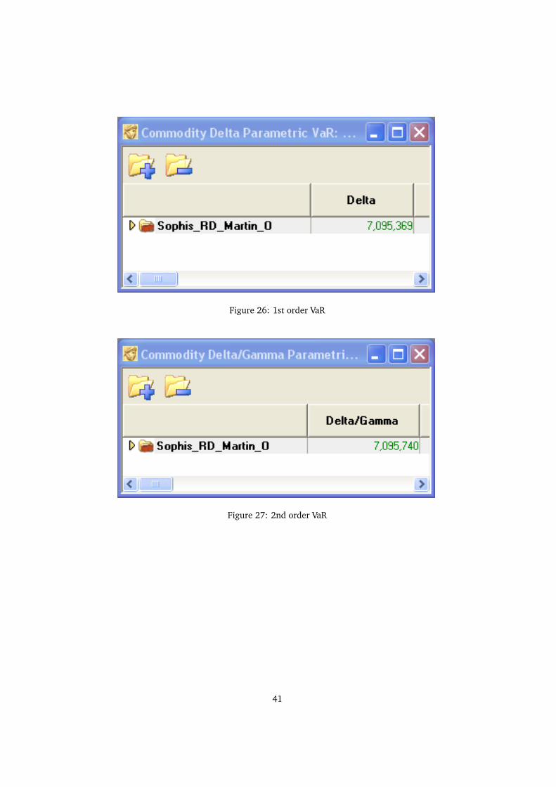
Figure 26: 1st order VaR

Figure 27: 2nd order VaR

41

C Historical VaR Server

Figure 28: The IMR console

Figure 29: The reporting application

42

References

[Ale01] Carol Alexander. Market Models: A Guide to Financial Data Analysis. Wi-ley, 2001.

[Fry97] Jon Frye. Principals of risk: Finding var through factor-based interestrate scenarios. Risk Publications, 1997.

[Gau07] Olivier Gaudoin. Principe et méthodes statistiques, 2007.

[Hul06] John C. Hull. Options, Futures and Other Derivatives. Pearson, 2006.

[PV02] Christophe Pérignon and Christophe Villa. Components proponents. Risk,2002.

43