Embed Size (px)
Citation preview
POUR L'OBTENTION DU GRADE DE DOCTEUR ÈS SCIENCES
acceptée sur proposition du jury:
Prof. J.-F. Molinari, président du juryProf. L. Vulliet, directeur de thèseProf. H. Di Benedetto, rapporteur Prof. D. Muir Wood, rapporteur
Prof. J. Zhao, rapporteur
Cyclic Properties of Sand: Dynamic Behaviour for Seismic Applications
THÈSE NO 4546 (2009)
ÉCOLE POLYTECHNIQUE FÉDÉRALE DE LAUSANNE
PRÉSENTÉE LE 11 DÉCEMBRE 2009
À LA FACULTÉ ENVIRONNEMENT NATUREL, ARCHITECTURAL ET CONSTRUIT
LABORATOIRE DE MÉCANIQUE DES SOLS
PROGRAMME DOCTORAL EN MÉCANIQUE
Suisse2009
PAR
Emilie RASCOL


à mes parents,
à mon frère

i
Résumé
La propagation des ondes sismiques dans les sols granulaires peut induire des déformations de grande
amplitude en cas de tremblements de terre de forte magnitude. Tous les mouvements sismiques ont un
contenu fréquentiel variable, des amplitudes irrégulières, et trois différentes composantes dans des
directions orthogonales. Dans ce contexte, l’objectif principal de cette recherche est de traiter des effets
non-linéaires observés dans les sols granulaires soumis à de tels chargements complexes. Les
hypothèses et les simplifications utilisées habituellement pour représenter le chargement sismique sont
évaluées en se concentrant sur deux aspects principaux: (i) la fréquence de la contrainte cyclique
appliquée à l’échantillon et (ii) la superposition de deux contraintes indépendantes. Pour cela, le
comportement non-linéaire de deux sables différents, le Sable du Leman et le Sable de Fonderie, est
exploré grâce à des tests triaxiaux cycliques et sismiques. Ces tests sont effectués en condition de
chargement unidirectionnel ou bidirectionnel, pour des déformations de moyennes et grandes
amplitudes, avec des fréquences correspondant à celles induites par les tremblements de terre.
Une presse triaxiale dynamique a été développée pour effectuer ces essais, sur des échantillons de
sable secs ou saturés non-drainés. Les contraintes latérales et axiales peuvent être appliquées
indépendamment avec de grandes amplitudes et de nombreuses formes de signaux dynamiques. Un
système innovant de capteurs sans contact a été développé pour mesurer, en continu, le rayon de
l’échantillon. Cet équipement se compose de trois capteurs lasers, installés autour de la cellule triaxiale
et qui détectent la position de la surface de l’échantillon grâce à la triangulation optique. Les données
mesurées sont traitées grâce à un système complexe de calibration, pour fournir au final l’évolution des
déformations radiales à mi-hauteur de l’échantillon. La structure qui supporte les capteurs permet leur
positionnement précis, et est équipée d'un mécanisme manuel de balayage vertical du profil de
l'échantillon.
Des premiers tests triaxiaux sont effectués avec des chargements cycliques classiques pour caractériser
le comportement des deux sables dans des conditions pseudo-dynamiques. Ces tests secs et saturés
permettent de décrire la diminution de la rigidité et le développement d’un état de rupture, qui peut se
produire par liquéfaction lorsque le sable est saturé non-drainé.
RÉSUMÉ
ii
Des tests cycliques secs et non-drainés effectués sur le Sable du Leman à différentes fréquences de 0.1
à 6.5 Hz montrent que le comportement de ce matériau granulaire dépend de la fréquence. La rigidité
du sol, qui prend des valeurs différentes selon l’état de contrainte imposé, semble influencer les effets
de la fréquence de chargement sur le comportement du sol: lorsque la rigidité est faible, la réponse de
l’échantillon est significativement amplifiée dans les basses fréquences (les amplitudes de déformation
sont plus grandes, la pression interstitielle augmente plus, etc...) par rapport aux plus hautes fréquences
testées. La forte sensibilité de ce sable aux effets de la fréquence pourrait être liée à l’angularité des
grains constituant le Sable du Leman.
D’autres tests cycliques saturés non-drainés démontrent que la superposition de deux chargements
indépendants, l’un axial et l’autre latéral (tests bidirectionnels), induisent des effets de couplage dans le
comportement non-linéaire du sol. Les effets bidirectionnels entrainent une amplification de la réponse
du sable jusqu’au développement de la liquéfaction cyclique. Le déphasage entre les contraintes axiales
et latérales est le paramètre clé influençant le couplage. De plus, des tests unidirectionnels et
bidirectionnels sont effectués pour des amplitudes irrégulières représentant un chargement sismique. Ils
montrent que les conditions bidirectionnelles irrégulières influencent légèrement la réponse non-
drainée du sable, avec des effets d’amplification très similaires aux tests cycliques bidirectionnels.
Les résultats expérimentaux cycliques sont finalement modélisés avec un modèle linéaire équivalent et
avec un modèle élastoplastique à multi-mécanismes (ECP Hujeux). Les effets non-linéaires observés en
laboratoire sont bien représentés par le modèle élastoplastique, en particulier (i) l’augmentation de
l’amplitude des déformations qui mène à la liquéfaction cyclique du sable dense, et (ii) le couplage de
la déformation avec la pression interstitielle. Le modèle linéaire équivalent donne une approximation
rudimentaire du comportement cyclique non-drainé, même pour des déformations de moyenne
amplitude, et n’est pas adapté à l’évaluation de la diminution de la rigidité observée dans nos tests
cycliques.
Pour conclure, l’évaluation du comportement des sols granulaires sous chargement sismique nécessite
de prendre en compte les aspects non-linéaires du comportement du sable, en terme de génération de
pressions interstitielles et d’amplitudes de déformation. En particulier, le contenu fréquentiel et les
chargements bidirectionnels influencent la réponse du sable pour des déformations moyennes à
grandes. Ces résultats expérimentaux pourraient être pris en compte pour améliorer l’analyse des
mouvements de terrain de forte amplitude. Ils constituent une contribution importante à la promotion de
modélisations non-linéaires plus précises des effets de site dans les sables naturels.
Mots clés: chargement bidirectionnel; fréquence; tremblement de terre; test triaxial dynamique; sable;
comportement non-linéaire; liquéfaction cyclique; modèle élastoplastique; modèle linéaire équivalent.
iii
Abstract
Seismic wave propagation in granular soils can induce large strain amplitudes in case of strong
earthquakes. Seismic motions are irregular in frequency content and in amplitude, and have three
different components in orthogonal directions. In this context, the main objective of this PhD research
deals with nonlinear effects observed in granular soils under such complex loadings. The assumptions
and simplifications usually considered for representing seismic loadings are evaluated, focusing on
two main aspects: (i) cyclic stress frequency applied to the sample (ii) superposition of two
independent stresses. For that purpose, the nonlinear behaviour of two different sands, Leman Sand
and Fonderie Sand, is explored with cyclic and seismic triaxial tests. These tests are performed with
unidirectional or bidirectional loadings, at medium to high strain amplitude, and in the earthquake
frequency range.
A dynamic triaxial press was developed to perform such tests, with dry and undrained saturated sand
samples. Axial and lateral stresses can be applied independently with large amplitudes for various
loading shapes. An innovative non-contact measurement technique was developed to continuously
monitor the sample radius; this testing equipment is based on three laser sensors, set up around the
triaxial cell, which detect the position of the sample surface thanks to optical triangulation. The
obtained data are processed through a complex calibration system to provide the radial strain evolution
at mid-height of the sample. The mounting structure supporting the sensors allows precise positioning
and is equipped for manual vertical scanning of the sample profile.
The first triaxial tests are performed with classical cyclic loadings, to characterize the behaviour of the
two sands in pseudo-dynamic conditions. These dry and undrained saturated tests allow to describe the
decrease of stiffness which leads to failure of the sand sample. Failure of undrained saturated sand
occurs by liquefaction.
Dry and undrained cyclic tests performed on Leman Sand at various frequencies from 0.1 to 6.5 Hz
show that the behaviour of this granular material is frequency-dependent at medium to large strains.
SUMMARY
iv
Sand stiffness, which depends on stress conditions, seems to influence the extent of frequency effects
on soil behaviour: for tests with lower stiffness, the soil response to low frequency is significantly
amplified (i.e. higher strain amplitude, more pore pressure increase, etc...) compared to the high
frequency range. The overall rate-sensitivity may be enhanced by the angularity of the grains.
Other cyclic undrained saturated tests on Leman Sand demonstrate that the superposition of two
different loadings, one axial and one lateral (bidirectional tests), induce coupling effects in the
nonlinear soil response. Bidirectional effects result in an amplification of the sand response until the
occurrence of cyclic liquefaction. The phase angle between axial and lateral stresses is the key
parameter influencing the coupling. Moreover, the comparison between unidirectional and bidirectional
irregular seismic loadings show that bidirectional conditions slightly influence undrained sand
response, with conditions of amplification very similar to cyclic tests.
Experimental results are finally modelled with the linear equivalent method and with a multi-
mechanism elastoplastic model (ECP Hujeux). Nonlinear effects observed in laboratory experiments,
and particularly the increase of strain amplitude leading to cyclic liquefaction of dense sand, are well
captured by the elastoplastic model. The linear equivalent method gives a very crude approximation,
even at medium strain level, and is not suitable for accurate evaluation of stiffness degradation
observed during our cyclic tests.
To conclude, assessing the behaviour of granular soils under earthquake loadings requires to take into
account the nonlinear features of sand behaviour in terms of pore pressure generation and strain
amplitude. In particular, frequency content and bidirectional loadings influence the sand response for
medium to large strains. These experimental results could be considered for improving the analysis of
strong ground motions. They constitute an important contribution for promoting more accurate
nonlinear modelling of site effects in natural sands.
Key words: bidirectional loading; frequency; earthquake; dynamic triaxial test; sand; nonlinear
behaviour; cyclic liquefaction; elastoplastic model; linear equivalent model.
v
Remerciements
Chaleureux merci tout d’abord à mon directeur de thèse, le Professeur Laurent Vulliet, pour m’avoir
guidée dans ce travail de thèse. Je salue la justesse et la pertinence de ses conseils, et je tiens à le
remercier pour la liberté qu’il m’a laissée pour mener à bien ce travail, et pour sa confiance répétée en
mon jugement.
Mes remerciements vont ensuite aux membres de mon jury de thèse, les Professeurs Zhao, Di
Benedetto et Muir Wood, pour avoir accepté de me faire l’honneur d’être les rapporteurs de ma thèse.
Merci également au Professeur Molinari d’avoir accepté de présider le jury de thèse.
Le soutien du Professeur Lyesse Laloui, directeur du Laboratoire de Mécanique des Sols, m’a permis
de réaliser mon doctorat dans d’excellentes conditions. Je tiens à le remercier pour son accueil et ses
conseils précieux.
J’ai eu la chance de rencontrer des chercheurs talentueux, qui m’ont donné conseils, commentaires
positifs et idées pour avancer: Dr. Jean-François Semblat, Prof. Arézou Modaressi, Dr. Stanislav
Lenart, Dr. Luca Lenti et certainement quelques autres. Un merci spécial à Dr. Clotaire Michel, qui a
été mon expert en sismologie.
Je remercie ensuite les personnes qui m’ont aidé à venir à bout des nombreux essais en laboratoire que
j’ai dû effectuer. Merci de tout coeur à Gilbert Gruaz, Patrick Dubey et Laurent Gastaldo pour leurs
conseils et leur disponibilité. Merci à Jean-Marc Terraz, super mécanicien, qui a donné forme à toutes
les concepts que j’ai pu imaginer. Merci aussi aux apprentis, Jérôme, Qazim et Samuel. Je remercie
également l’équipe de Temeco, qui m’a aidée à maîtriser la presse dynamique, Messieurs Conrad
Keiser et Beat Renner. Concernant les lasers, je remercie Beat Rudolf et Peter Bischoff pour l’intérêt
qu’ils ont porté à mon projet. Merci aussi à Irina Andria-Ntoanina et François Huot pour leurs conseils.
Merci à «mon stagiaire» Emad Jahangir, pour le courage dont il a fait preuve et les bons résultats
expérimentaux qu’il a obtenus avec le Sable de Fonderie.
REMERCIEMENTS
vi
Pour le support technique, je n’oublie pas les informaticiens du laboratoire, Laurent et Thierry, et merci
aussi à Nicolas et Stefano ainsi qu’à leurs apprentis. Merci aux secrétaires de choc, Karine Barone,
Antonella Simone et Rosa-Ana Menendez, ainsi qu’à Anh Le. J’en profite aussi pour reconnaître la
disponibilité de Jean-Paul Dudt et la convivialité de Gilbert Steinmann, et je n’oublie pas Messieurs
Jean-François Mathier et Vincent Labiouse.
Merci à tous les doctorants et post-docs du LMS et LMR. Certains m’ont particulièrement aidé au
niveau scientifique, en discutant ou simplement en m’écoutant quand j’en avais besoin. Je pense
particulièrement à Simon, Mathieu, et Rafal. Un grand merci à mes collègues de bureau, qui se sont
relayés pour donner une ambiance de travail toujours conviviale : Nina Mattsson, Yonggeng Ye, Marta
Rizzi, Davide Ceresetti et Yanyan Duan. Merci aux collègues et amis, qui ont tous participé à
l’ambiance chaleureuse de ces quelques trois ans et demi : Rafal Obrzud, Suzanne Fauriel, Mathieu
Nuth, Bertrand François, Simon Salager, Azad Koliji, Irene Manzella, Federica Sandrone, Hervé Péron,
Claire Silvani, Raphaël Rojas, Thibaud Meynet, Alessio Ferrari, sans oublier Andréa Battiato, Ma
Hongsu, Claire Sauthier, Jacopo Abbruzzese et Tohid Kazerani. Je pense aussi aux moitiés, tellement
importantes pour les bières à Sat’ et les barbecues : Jennifer, Anne-Christine, Jonathan, Solène, Stefano,
Ewa, Azin, Véronique, Paul, Marco. Merci aussi à mes alpinistes préférés, Valérie et Yannick. Une
mention spéciale pour John Eichenberger, qui a produit des efforts très appréciés de soutien moral
durant les derniers mois de la thèse.
Merci à mes amis de France, ceux qui sont venus jusqu’à Lausanne et aussi ceux avec qui j’ai pu passer
des week-ends et vacances françaises tellement sympathiques. Je pense particulièrement à Mohamed, à
Cécile, aux nantais et aux «filles».
Pour finir, un gros merci collectif à ma famille, qui m’a encouragé et donné la possibilité d’en arriver là.
Merci aussi pour votre compréhension, et pour le soutien que vous m’avez apporté.
Cette recherche a été financée principalement par le Fonds National Suisse de la Recherche
Scientifique, bourse n°200021-108174.
vii
Table of Contents
RÉSUMÉ i
ABSTRACT iii
REMERCIEMENTS v
LIST OF SYMBOLS xv
CHAPTER 1. INTRODUCTION 1
1.1 General framework 2
1.2 Objectives 3
1.3 Structure of the thesis 4
CHAPTER 2. DYNAMIC GRANULAR SOIL BEHAVIOUR 5
2.1 Introduction 6
2.2 The dynamic problem 62.2.1 Cyclic, dynamic and static load 62.2.2 Nature of dynamic loadings 8
2.3 Geotechnical earthquake engineering 92.3.1 Introduction to geotechnical earthquake engineering 92.3.2 Seismic hazard in Switzerland 102.3.3 Earthquake characterization 102.3.4 Seismic wave propagation 132.3.5 Site effects 15
CONTENTS
viii
2.4 Introduction to soil behaviour under cyclic loading 172.4.1 Effective stress 172.4.2 Notations of stress and strain 172.4.3 Monotonic loading in triaxial compression and triaxial extension 212.4.4 Critical state and steady state 222.4.5 Dilatancy and phase transformation in granular media 232.4.6 Qualitative soil response to cyclic loading 242.4.7 Effect of the number of cycles 262.4.8 Link between cyclic behaviour and dilatancy 262.4.9 Strain range dependency of cyclic soil behaviour 272.4.10 Volumetric cyclic threshold shear strain and stiffness degradation 282.4.11 Pore water pressure increase in undrained saturated conditions 282.4.12 Definition of failure 292.4.13 Liquefaction and cyclic softening 302.4.14 Conclusions 37
2.5 Dynamic material parameters 382.5.1 Secant shear modulus 382.5.2 Damping ratio 392.5.3 Strain dependency of dynamic parameters 442.5.4 Evaluation of the elastic shear modulus 462.5.5 Factors influencing the secant shear modulus and damping ratio 47
2.6 Constitutive modelling of granular soils for cyclic loading 502.6.1 Introduction 502.6.2 Linear elastic model 502.6.3 Linear viscoelastic model 512.6.4 Linear equivalent model 512.6.5 Elastoplastic models 532.6.6 Domain of application 57
2.7 Rate effects in granular materials 592.7.1 Phenomenons involved in time-dependent sand behaviour 592.7.2 Interpretation of rate effects 602.7.3 Influence of viscous behaviour on cyclic loading 612.7.4 Time-dependency in granular media from laboratory experiments 612.7.5 Constitutive modelling and numerical approach of rate effects in sand 652.7.6 Conclusions 66
2.8 Superposition of loadings 672.8.1 Introduction 672.8.2 Laboratory experiments 67
CONTENTS
ix
2.8.3 Multidirectional site effect analyses 692.8.4 Conclusions 70
2.9 Irregular loading of sand under seismic motion 702.9.1 Introduction 702.9.2 A few laboratory studies 702.9.3 Use of test data for design purposes 732.9.4 Summary 74
2.10Conclusions 74
CHAPTER 3. CYCLIC TRIAXIAL EXPERIMENTS 77
3.1 Dynamic measurement techniques 783.1.1 Introduction 783.1.2 Laboratory testing 783.1.3 Conclusions 85
3.2 Experimental device for cyclic triaxial loading 853.2.1 Description of the cyclic triaxial press 853.2.2 Stress and strain states of the sample 923.2.3 Laser-based measurement of radial strains 95
3.3 Validation tests 115
3.4 Experimental procedures 1163.4.1 Sand sample mounting 1163.4.2 Saturation 1193.4.3 State of the sample for cyclic shear 119
3.5 Soil characteristics 1193.5.1 Leman Sand 1193.5.2 Fonderie Sand 120
3.6 Conclusions 121
CHAPTER 4. CHARACTERIZATION OF NONLINEAR SAND BEHAVIOUR WITH MONOTONIC AND CYCLIC TRIAXIAL TESTS 123
4.1 Introduction 124
4.2 Monotonic tests on Leman Sand 1254.2.1 Presentation 1254.2.2 Description of typical test results in compression and extension 1264.2.3 Summary of observed monotonic behaviour of dense Leman Sand 1294.2.4 Phase transformation lines 129
CONTENTS
x
4.2.5 Behaviour at large strain 1314.2.6 Comments and conclusions on the monotonic results 131
4.3 Preliminary undrained cyclic triaxial tests 1324.3.1 Introduction 1324.3.2 Typical stress-controlled test results 1334.3.3 Effect of loading conditions 1364.3.4 Conclusions 139
4.4 Detailed description of cyclic undrained tests on Leman Sand for small to large strains 140
4.4.1 Introduction 1404.4.2 Example of a cyclic test with failure by cyclic liquefaction 1414.4.3 Excess pore pressure increase 1434.4.4 Comparison of criterion for failure 1434.4.5 Small strain secant shear modulus 1474.4.6 Analysis of the Gsec - g curve 1484.4.7 Evolution of the damping ratio with the number of cycles 1494.4.8 Analysis of the D - g curve 1514.4.9 Effect of the initial state 1514.4.10 Discussion 1524.4.11 Conclusions 153
4.5 Nonlinear Fonderie Sand behaviour in undrained saturated conditions 1544.5.1 Introduction 1544.5.2 Summary of monotonic behaviour 1554.5.3 Overview of cyclic test results and failure with Fonderie Sand 1554.5.4 Excess pore pressure ratio increase in cyclic tests with stress reversal 1604.5.5 Dynamic parameters 1614.5.6 Discussion 1654.5.7 Summary 165
4.6 Evaluation of the laser measurement technique with an undrained test 1664.6.1 Presentation 1664.6.2 At medium to large strain 1674.6.3 At small to medium strain 1694.6.4 Conclusions 172
4.7 Dry cyclic triaxial tests on Leman Sand 1734.7.1 Introduction 1734.7.2 Presentation of a typical dry cyclic triaxial test 1734.7.3 Effect of initial conditions on strain accommodation and failure 1774.7.4 Volumetric behaviour 179
CONTENTS
xi
4.7.5 Secant shear modulus 1814.7.6 Comparison with undrained test results 1834.7.7 Damping ratio 1834.7.8 Induced anisotropy 1844.7.9 Conclusions 185
4.8 Shear strain localization in cyclic tests at large strain amplitude 1864.8.1 Tests concerned 1864.8.2 Direct observation of shear strain localization with laser sensors 1874.8.3 Consequences on test results 1884.8.4 Conclusions 189
4.9 Summary 190
CHAPTER 5. FREQUENCY EFFECTS IN LEMAN SAND 193
5.1 Introduction 194
5.2 Monotonic undrained conditions 1945.2.1 Tests characteristics 1945.2.2 Results 1955.2.3 Discussion 1975.2.4 Conclusions 197
5.3 Preliminary cyclic tests 1985.3.1 Presentation of the tests 1985.3.2 Cyclic test results 1995.3.3 Conclusions 200
5.4 Frequency effect in undrained conditions at medium strain level 2035.4.1 Presentation 2035.4.2 Frequency effect on tests characteristics 2045.4.3 Discussion 2105.4.4 Conclusions 212
5.5 Frequency effect in cyclic dry conditions 2125.5.1 Test presentation 2125.5.2 Frequency effect on dry Leman Sand test results 2135.5.3 Discussion 2175.5.4 Conclusions 218
5.6 Discussions on rate effect in Leman sand 2195.6.1 Experimental artefacts 2195.6.2 Physical interpretation and general comments 220
5.7 Conclusions 222
CONTENTS
xii
CHAPTER 6. EFFECT OF MULTIDIRECTIONAL AND IRREGULAR STRONG LOADINGS 223
6.1 Introduction 224
6.2 Multidirectional effects on cyclic behaviour 2256.2.1 Tests characteristics and examples 2256.2.2 Introduction to test results 2306.2.3 Stress-strain relation 2306.2.4 Deviatoric strain amplitude 2306.2.5 Number of cycles to failure 2326.2.6 Effective stress paths 2336.2.7 Excess pore pressure 2346.2.8 Multidirectional effects on dynamic parameters 2366.2.9 Analyses of multidirectional effects 2396.2.10 Conclusions 242
6.3 Irregular seismic loading in multidirectional condition 2436.3.1 Description of irregular loadings with a seismic signal 2436.3.2 Description of stress paths 2476.3.3 Deviatoric strains 2486.3.4 Stress-strain relation 2516.3.5 Pore pressure increase 2516.3.6 Discussion on seismic bidirectional triaxial tests 2536.3.7 Conclusions 257
6.4 Comments on bidirectional and irregular effects 2586.4.1 Effect of complex loadings on nonlinear soil behaviour 2586.4.2 Physical interpretation 2596.4.3 Consequences for modelling and design purposes 260
6.5 Conclusions 260
CHAPTER 7. CONSTITUTIVE MODELLING OF CYCLIC SAND BEHAVIOUR 263
7.1 Introduction 264
7.2 Cyclic modelling of Leman Sand with a viscoelastic linear equivalent analysis 265
7.2.1 Introduction 2657.2.2 Description of the procedure for linear equivalent simulations 2657.2.3 Results 2687.2.4 Effect of frequency and complex loading in the linear equivalent model 271
CONTENTS
xiii
7.2.5 Discussion 2727.2.6 Summary 272
7.3 Behaviour of Leman Sand with a multi-mechanism elastoplastic constitutive law 273
7.3.1 Introduction 2737.3.2 Model calibration 2737.3.3 Results 2767.3.4 Discussion 2867.3.5 Summary 287
7.4 Comparison and evaluation of the models 288
7.5 Conclusions 290
CHAPTER 8. CONCLUSIONS AND PERSPECTIVES 291
8.1 Achievements 2928.1.1 Developments of laboratory equipment 2928.1.2 Cyclic dense sand behaviour 2938.1.3 Frequency-dependence of granular materials 2948.1.4 Effect of cyclic bidirectional conditions on undrained sand behaviour 2958.1.5 Seismic unidirectional and bidirectional loading 2968.1.6 Modelling the cyclic behaviour of dense sand 296
8.2 Outlook 297
REFERENCES 299
Appendix 1. In situ testing for the evaluation of dynamic soil behaviour 1
Appendix 2. Determination of deviatoric and confining stresses from seismic acceleration recordings 7
Appendix 3. Additional results: modelling of an undrained cyclic test with the elastoplastic model 13
Appendix 4. Test data are provided in a CD-ROM

CONTENTS
xiv

xv
List of symbols
Roman Symbols
1D, 2D, 3D multidimensional (Chapter 2).
1D unidirectional.
2D bidirectional.
a function of the Hujeux model which appears in the calculation of the degree ofplastification (Eq. 2.49).
a, a’ slope of the two bisectors which define the centre of the sample for the calculationof the radius with laser sensors (Eq. 3.7 and Eq. 3.8).
A empirical parameter for the determination of Gmax (Eq. 2.36).
acyc parameter of the Hujeux model for the cyclic part of the hardening law ofdeviatoric mechanisms.
ai model parameter for the empirical evaluation of Gmax (Eq. 4.2).
Aloop area of the stress - strain loop in the εq - q plane.
area of the stress - strain loop in the ε1 - q plane.
am parameter of the Hujeux model for the monotonic part of the hardening law ofdeviatoric mechanisms.
b parameter of the Hujeux model for the shape of the yield surface (Eq. 2.47).
b, b’ intercept point of the bisectors which define the centre of the sample for thecalculation of the radius with laser sensors (Eq. 3.7 and Eq. 3.8).
B coefficient Skempton’s B coefficient, which indicates the degree of saturation of the soilsample (B = 1 involves full saturation).
B1 in-phase bidirectional loading (straight line in the p - q plane).
B2 out-of-phase bidirectional loading (oval shape in the p - q plane).
bi model parameter for the empirical evaluation of Gmax (Eq. 4.2).
Aloop

LIST OF SYMBOLS
xvi
c volumetric hardening parameter of the Hujeux model (Eq. 2.51).
c viscous damping (section 2.6.2).
C centre of the circle defined from the three points measured by laser sensors.
cc critical damping coefficient (section 2.6.2).
ccyc volumetric hardening parameter of the Hujeux model for cyclic loading.
cm volumetric hardening parameter of the Hujeux model for monotonic loading.
CM test irregular unidirectional triaxial test with the maximum stress in compression.
cp velocity of P wave.
CPT cone penetration test.
cs velocity of S wave.
CSR cyclic stress ratio.
CSREQ maximum cyclic stress ratio in irregular loading.
CTC conventional triaxial compression.
Cw compressibility of water.
d parameter of the isotropic hardening law for the Hujeux model.
d displacements (1*3) (Chapter 2).
D damping ratio.
D rigidity tensor (6*6 for the matrix formulation of Hooke’s law).
d60 diameter of the sieve which lets pass 60% of the soil mass.
DA double amplitude.
dext external measure of the vertical displacement in the dynamic press.
DI degradation index.
dint internal measure of the vertical displacement in the dynamic press.
Dmin small strain damping ratio.
e deviatoric strain tensor (3*3 matrix) (Chapter 2).
e or e0 void ratio.
E Young’s modulus.
E* Anisotropic Young’s modulus, equal to Ev.
Eh, Ev Anisotropic Young’s moduli in the horizontal and vertical direction.
LIST OF SYMBOLS
xvii
EM test irregular unidirectional triaxial test with the maximum stress in extension.
emax, emin maximum and minimum void ratios.
ep thickness of membrane and paint layer in the laser calibration function.
Esec secant Young’s modulus.
f frequency.
F force exerted on the SDOF system in forced harmonic vibrations (section 2.6.2).
Fax axial force applied to the loading bar of the dynamic press.
Fc compacity function (Eq. 2.36 and Eq. 2.37).
fext body forces.
FFT Fast Fourier transform.
fiso isotropic yield limit of the Hujeux model.
fk yield limit of the deviatoric mechanism k of the Hujeux model.
Fk function included in the yield limit of the deviatoric mechanism k of the Hujeuxmodel (Eq. 2.47).
g gravity acceleration.
G shear modulus.
G* complex modulus.
GDS laboratory equipment company (http://www.gdsinstruments.com/).
Gmax small strain or maximum shear modulus.
Gref reference value of the shear modulus in the elastoplastic Hujeux model (definitionin Eq. 2.43).
Gsec secant shear modulus.
, secant shear modulus at the Nth cycle and 1st cycle.
I2D second unvariant of the strain tensor.
ic critical refraction angle in seismic refraction.
ID relative density.
J2D second unvariant of the stress tensor.
k stiffness (section 2.6.2).
k empirical soil parameter for the determination of Gmax (Eq. 2.36).
k Darcy permeability.
Gsec
NGsec
1

LIST OF SYMBOLS
xviii
K0 coefficient of earth at rest.
Kb bulk modulus.
KC, LC two bisectors which meet at the centre C of the sample (calculation of the radiuswith laser sensors).
Kmax small strain bulk modulus (Hujeux model).
Kref reference value of the bulk modulus in the elastoplastic Hujeux model (definitionin Eq. 2.43).
L coefficient of reduction between the maximum strain measured by laser sensorsand the average strain over the height of the sample.
LVDT Linear Variable Differential Transformer, displacement sensor.
m soil parameter of the Hujeux model for the hysteretic domain.
m mass (section 2.6.2).
Max moment applied to the loading bar of the dynamic press.
Mc slope of the steady state line in compression.
Me slope of the failure line in extension.
Minst slope of the instability line in the p’ - q plane (Chapter 2).
MPT slope of the phase transformation line in the p’ - q plane.
MPTc slope of the phase transformation line in compression.
MPTe slope of the phase transformation line in extension.
MR1 measuring range of the laser sensor in the air (normal conditions).
MR2 measuring range of the laser sensor through the cell glass window and water layer.
mref laser measurement of the three points at the surface of the reference steel cylinderfor the calibration function (1*3).
MSS slope of the stead state line in the p’ - q plane.
Mw moment magnitude of an earthquake.
n porosity.
N number of cycles.
N scale reduction number in centrifuge tests (Chapter 3).
n1, n2, n3 refractive index of air, glass and water (Chapter 3).
N1, N2, N3 coordinates of the three points at the sample surface, calculated from the lasermeasurements at any time (1*2).
NI number of SPT blowcount (Chapter 3).
LIST OF SYMBOLS
xix
Ncrit critical cycle, during which flow liquefaction occurs (Chapter 2).
ne empirical adimentional parameter for the stress-dependency of elastic moduli.
Nf number of cycles at failure for the criterion based on strain amplitude threshold.
Nfd number of cycles at failure for the criterion based on DI threshold.
Nfu number of cycles at failure for the criterion based on pore pressure threshold.
OCR overconsolidation ratio.
p and p’ mean total and effective stress in triaxial conditions, also called spherical stress.
P wave compressional wave.
preconsolidation pressure in the Hujeux model.
initial preconsolidation pressure in the Hujeux model.
PGA peak ground acceleration.
PIDR proportional, integrative, derivative and las gain in the motion regulation system ofthe dynamic press (Chapter 3).
PI plasticity index.
mean effective stress of the deviatoric mechanism k in the Hujeux model.
pref reference value of the spherical stress (1 MPa).
PT phase transformation.
PU polyurethane cylinder.
q deviatoric stress in triaxial conditions.
Q quality factor (Chapter 2).
qav mean / initial deviatoric stress.
qk deviatoric stress in the deviatoric mechanism k (Hujeux model).
r radius of the wave front (Chapter 2).
r radius of the reference steel cylinder (Chapter 3)
R radius of the soil sample, measured at all time steps by the laser sensors.
R0 initial radius of the soil sample, measured at the beginning of each loading by thelaser sensors.
R1 shape of the stress path corresponding to unidirectional loading of CTC and RTEtype.
R1, R2, R3 coordinates of the reference cylinder for laser calibration in Eq. 3.5 and Eq. 3.6.
R2 shape of the stress path corresponding to hydrostatic compression (horizontal line
pc
pc0
pk
LIST OF SYMBOLS
xx
in the p - q plane).
rd stress reduction factor to calculate seismic loadings (section 2.10).
REV representative elementary volume.
riso degree of plastification of the isotropic mechanism (Hujeux model).
radius of the elastic domain of the isotropic mechanism (Hujeux model).
rk degree of plastification of the deviatoric mechanism k (Hujeux model Eq. 2.48).
radius of the elastic domain of the deviatoric mechanism k (Hujeux model).
radius of the hysteretic domain of the deviatoric mechanism k (Hujeux model).
radius of the mobilized domain of the deviatoric mechanism k (Hujeux model).
RTE reduced triaxial extension.
S surface of the cylindrical sample.
S wave shear wave.
SASW geophysical test, spectral analysis of surface waves.
SDOF single degree of freedom.
SH wave horizontal plane component of the shear wave.
SPT standard penetration test.
SS steady state.
std standard deviation.
SV wave vertical plane component of the shear wave.
t deviatoric part of the stress tensor (Chapter 2) (3*3 matrix).
t time.
u pore water pressure.
u0 amplitude of the displacement in the forced SDOF system (section 2.6.2).
ur pore (water) pressure ratio.
ur,m Maximum pore (water) pressure ratio during one cycle.
pore pressure ratio resulting from the radial stress (defined in Eq. 6.2).
pore pressure ratio resulting from the axial stress (defined in Eq. 6.3).
displacement, velocity, acceleration (Chapter 2, Eq. 2.1 and Eq. 2.29).
V volume of the sample or domain.
riso
ela
rk
ela
rk
hys
rk
mob
ur
comp
ur
q
u u u, ,
LIST OF SYMBOLS
xxi
V1, V2 velocity of wave propagation in seismic refraction method (Fig. 3.7).
W work.
WD energy dissipated during one cycle (section 2.6.2).
WS maximum elastic stored energy (section 2.6.2).
x1, x2, x3 coordinate on the x-axis of the points N1, N2 and N3 (laser calibration).
x equivalent laser measurement in the air (real distance).
X, Y coordinates of the centre C of the sample (calculation of the radius with lasersensors).
xr laser measurement through the cell glass window and the water layer.
y1, y2, y3 coordinate on the y-axis of the points N1, N2 and N3 (laser calibration).
z depth.
Greek Symbols
α dilatancy coefficient of the Hujeux model (associated flow rule when α = 1).
α angle of diffuse reflection of the laser beam in the air (Fig. 3.21a).
α, β, γ incident and refracted angles in the air, glass and water (Fig. 3.21b).
α∗ Anisotropy coefficient.
αk function defining the degree of mobilization of the deviatoric mechanism k,depending on rk (Hujeux model).
β plastic compressibility of the soil (Hujeux model).
δ angle if internal friction (Chapter 2).
δc1 uncertainty on the scaling coefficient Γ for calibration of laser sensors.
δc2 uncertainty on the effect of the confining pressure on the calibration of lasersensors
δc3 uncertainty on the position of the reference cylinder for calibration of lasersensors.
δΔR uncertainty on the variation of the sample radius during a cyclic test.
δε3,l uncertainty on the local radial strain measured with laser sensors.
δε3,m uncertainty on the radial strain averaged over the sample.
LIST OF SYMBOLS
xxii
δi1 uncertainty on the vertical misalignment due to scanning procedure of lasersensors.
δl1 uncertainty on the thickness of the paint layer.
δl2 uncertainty due to the transmission of the laser beam through interfaces.
δR uncertainty on the sample radius measured by laser sensors.
δθ uncertainty on the angular horizontal and vertical misalignment of the position ofthe laser.
Δε, Δe general increment of the strain tensor and of the deviatoric part of the strain tensor(3*3 matrix) (Eq. 2.16).
Δε1, Δε3, Δεq, ΔεV general increment of the axial, radial, deviatoric and volumetric strain (Eq. 2.16and Eq. 2.17).
Δε1, Δε3 axial and radial strain amplitude in sinusoidal loading (simple amplitude).
Δεq deviatoric strain amplitude in sinusoidal loading (simple amplitude).
Δεv volumetric strain amplitude in sinusoidal loading (simple amplitude).
Δp’, Δq, general increment of the spherical stress, deviatoric stress and effective confiningpressure (Eq. 2.9).
Δq deviatoric stress amplitude in sinusoidal loading (simple amplitude).
Δp’ spherical stress amplitude in sinusoidal loading (simple amplitude).
ΔR variation of the sample radius during a cyclic test.
Δσ3, total and effective confining pressure amplitude in sinusoidal loading (simpleamplitude).
maximum amplitude of confining pressure during seismic loading.
general increment of the stress tensor and of the deviatoric part of the stress tensor(3*3 matrix) (Eq. 2.9).
Δτ shear stress amplitude in sinusoidal loading (simple amplitude).
Δu excess pore water pressure.
strain tensor (3*3 matrix).
ε1 axial strain.
axial strain rate for monotonic (strain-controlled) loading at constant strain rate.
ε3 radial strain.
ε3,l local radial strain calculated from the sample measure at mid-height.
ε3,m mean radial strain averaged over the total sample height.
εq deviatoric strain.
3
3
3
EQ
ij ijt,
1
LIST OF SYMBOLS
xxiii
mean deviatoric strain rate, defined Eq. 5.1.
maximum deviatoric strain rate over the cycle.
plastic component of the deviatoric strain induced by the deviatoric mechanism k.
εv volumetric strain.
volumetric plastic strain (Hujeux model).
volumetric plastic strain induced by isotropic mechanism (Hujeux model).
rate of increase of the volumetric plastic strain induced by the deviatoricmechanism k.
φ’ effective friction angle mobilized at critical state.
φPT friction angle mobilized at phase transformation.
φSS friction angle mobilized at steady state.
γ shear strain.
Γ scaling coefficient obtained from the laser calibration procedure for transformingthe measured value into the real distance.
γw volumetric weight of water.
γtv volumetric cyclic threshold shear strain.
η loss factor (Chapter 2).
κ Slope of the elastic isotropic compression line in the e - ln(p’) plane (Eq. 7.1).
λ Lamé coefficient.
λc Slope of the virgin isotropic compression line in the e - ln(p’) plane (Eq. 7.1).
λiso plastic multiplier of the isotropic mechanism (Hujeux model).
plastic multiplier of the deviatoric mechanism k (Hujeux model).
λw wave length .
μ Lamé coefficient.
ν Poisson’s ratio.
ν∗ Anisotropic Poisson’s ratio.
ρ soil density.
stress tensor (3*3 matrix).
σ’ effective stress tensor (3*3 matrix).
total and effective vertical (principal) stress in triaxial conditions.
q
q
max
q k
p
,
V
p
v iso
p
,
v k
p
,
k
p
11,
LIST OF SYMBOLS
xxiv
total and effective confining pressure (lateral principal stress in triaxialconditions).
initial effective confining pressure.
mean confining pressure (bidirectional tests).
σn normal stress.
total and effective overburden pressure.
effective vertical and horizontal stress for in situ conditions.
τ shear stress.
ω angular frequency.
ω0 natural angular frequency (section 2.6.2).
harmonic angular frequency in the forced SDOF system (section 2.6.2).
ψ dilatancy angle (Hujeux model).
Ψ specific damping capacity (Chapter 2).
ζ phase angle.
Operators
: inner product of tensor with double contraction.
d(.) incremental value.
temporal derivative of the variable x.
δij Kronecker delta type function, δij = 1 if i = j and δij = 0 otherwise.
Nota Bene: Throughout this dissertation, the sign convention is the usual convention in soil mechanics, i.e. compression is positive.
33,
3
0
t t,
V H,
xx
t
d
d

CHAPTER 1
INTRODUCTION
INTRODUCTION
2
1.1 General framework
Soil dynamics is a special branch of geotechnical engineering which has important consequences on
mitigation of seismic risks. Actually, the developments of soil dynamics over the last decades were
motivated by the occurrence of catastrophic seismic events. Ground motion itself may not be a major
threat, but it is the main triggering phenomenon of most seismic hazards, like building collapse among
the most dramatic cases. A well-known consequence of strong ground motion is liquefaction, which is
the total loss of strength of the granular medium. Another major issue is the stability of slopes and of
earth structures subjected to seismic loading.
Ground shaking results from the travelling of seismic waves through the earth’s crust and through the
upper rock and soil layers. Looking at a particular area, the intensity of surface motion highly depends
on the magnitude of the earthquake associated to the mechanical properties of the ground material.
Indeed, local amplification of the ground surface acceleration can occur as a result of disadvantageous
soil properties. This phenomenon, called site effects, should be accurately taken into account to
guarantee a safe design of foundations, structures and buildings. From that point of view, it is crucial to
be able to evaluate soil behaviour in conditions of strong and transient loading characterising ground
motions during large earthquakes.
The behaviour of granular materials subjected to dynamic loading remains not fully understood, and is
currently the subject of interesting research worldwide. Advanced laboratory testing techniques are
specifically developed to understand and characterise soil response to dynamic loading. Numerical
tools as well are adapted to this particular problem, to solve complex multi-physics equation systems.
Site effects being a significant part of the estimation of earthquake hazard, specific tools are developed
for modelling dynamic soil behaviour. Some of them are now used in engineering problems; they
should be carefully evaluated and can be improved to take into account new knowledge issued from the
research community.
The idea behind this research project is to produce high quality laboratory test results on dynamic soil
behaviour, which are directly applicable to strong earthquake motion and in particular for modelling
site effects. This means that the tests are performed in conditions close to in situ soil layers subjected to
strong seismic waves, where stress amplitudes are large and irregular, the signal is complex in terms of
frequency content, and the soil element is subjected to stress components in three orthogonal directions.
The study focuses on the dynamic behaviour of granular materials with regard to these complex
features of seismic loading. For that purpose, a special triaxial press was installed and further developed
in the Soil Mechanics Laboratory (LMS) at EPFL thanks to grants from the Swiss National Science
CHAPTER 1
3
Foundation R’Equip programme and from the EPFL.
At first sight, the context of western Europe seismicity may look inappropriate for the study of strong
ground motions. However, strong destructive earthquakes can occur in countries like Switzerland, as
demonstrated by the most famous Basel event of 1356. As a consequence, seismic risks are taken into
account, especially for the centre of the alpine region of Valais and around Basel. Indeed, seismic
hazard is non negligible in these regions, and may concern densely populated areas, were the
occurrence of an earthquake could threaten the lives and properties of tens of thousands inhabitants.
1.2 Objectives
The main objective of this PhD thesis is to assess, in the laboratory, the effect of complex loading
features of strong earthquake motions on granular soil behaviour. More precisely, the assumptions and
simplifications usually considered for seismic loading conditions are questioned, focusing on two main
aspects: (i) cyclic loading frequency (ii) superposition of loading. The parameters influencing these
complex loading features, in particular the importance of the pore fluid, are neither well known nor
understood. The impact of loading conditions on nonlinear behaviour of granular materials and on the
development of large strains within saturated and dry sand samples will be evaluated.
An intermediate issue is to characterise dynamic nonlinear sand behaviour with cyclic and seismic
triaxial tests in the earthquake frequency range, at medium to high strain amplitude. This work involves
practical developments of laboratory equipment, to provide experimental results of adequate quality.
The limits of the device will be carefully analysed, and the reliability of test results will be
demonstrated.
Finally, two very different constitutive models designed for geotechnical earthquake engineering will
be evaluated with regard to the experimental results: the linear equivalent model and the multi-
mechanisms elastoplastic model of Hujeux. The ability and limits of these numerical tools for dynamic
modelling of sand behaviour at medium to large strains will be assessed.
INTRODUCTION
4
1.3 Structure of the thesis
The content of the PhD thesis is organised in line with the objectives above-mentioned.
The context of the research is presented in Chapter 2. Geotechnical earthquake engineering issues
related to the present work are recalled. The notions necessary to understand the general nonlinear
behaviour of sand subjected to cyclic and seismic loading are then summarized. A particular attention is
paid to the review of the state of the art on dynamic material parameters, modelling of sand under cyclic
loading, rate and viscous effects, multidirectional effects and irregular loading effects.
The description of the testing methods and of the techniques developed to obtain high quality test
results is the core of Chapter 3. In particular, the dynamic triaxial press and the new laser sensors are
presented in detail and fully validated.
In Chapter 4, different tests performed under «classical» cyclic triaxial conditions are presented and
analysed. The effects of boundary conditions on cyclic sand behaviour are outlined, by means of dry or
saturated undrained tests performed under various initial stress states. The importance of soil fabric is
addressed by comparing the cyclic response of two different soils, Leman Sand and Fonderie Sand,
which have quite different grain size distribution and particle shapes. Validations of the experimental
processes are also presented in this chapter, with an evaluation of the laser sensor measurement system
for an undrained sand sample and with the analyses of shear strain localization occurring at large strain.
In Chapter 5, rate effects observed in cyclic dry and undrained saturated triaxial tests are described for
Leman Sand. Loading frequency is shown to influence the behaviour of this granular material at
medium strain amplitudes.
Chapter 6 focuses on the effects of bidirectional cyclic and seismic loading on Leman Sand behaviour
for synchronised variations of axial and radial stresses in the dynamic triaxial press. Leman Sand is
tested in undrained conditions corresponding to the development of failure by cyclic liquefaction.
In Chapter 7, the determination of material parameters of Leman Sand is presented for the two
different models, the linear equivalent model and the multi-mechanism elastoplastic Hujeux model.
Both of them can take into account cyclic loading of granular soils. Some of the triaxial test results
presented in the previous chapters are modelled with these two constitutive laws. It is thus possible to
evaluate the ability of both models to describe the cyclic behaviour of sand at medium to large strain.
Chapter 8 concludes this work and proposes perspectives for future research based on the numerical
and laboratory results.

CHAPTER 2
DYNAMIC GRANULAR SOIL
BEHAVIOUR
DYNAMIC GRANULAR SOIL BEHAVIOUR
6
2.1 IntroductionCharacterizing soil behaviour under seismic loading was one of the first issues that led part of the
geotechnical community to focus on dynamic problems. Seismic waves can induce strong motions in
the upper ground layers, even far from the epicentre. These motions may even be amplified within
particular topographical and geological conditions: this phenomenon is called site effects. A wider
range of applications for dynamic soil behaviour was then introduced: fatigue behaviour linked with
human activities as traffic, vibratory excitations from various industries, effect of underground blasting.
Measurement techniques for soil in motion were specially designed to obtain accurate dynamic soil
models and safe design rules.
In this chapter, a synthetic broad introduction to soil dynamics is presented, before the more detailed
overview of cyclic sand behaviour in laboratory tests. To be more precise, a brief clarification on the
dynamic problem in soils (section 2.2) is followed by some considerations on geotechnical earthquake
engineering (section 2.3), with a special focus on site effects which introduces the importance of
nonlinear dynamic soil behaviour. The concepts needed for describing the actual mechanical behaviour
of granular soils under cyclic loading, which are extensively used in the next chapters of the thesis, are
described in section 2.4. A detailed overview on dynamic material parameters, namely secant shear
modulus and damping ratio, follows in section 2.5. The constitutive models used in the thesis
(Chapter 7) are described in section 2.6. The three next sections present particular features of loading
characteristics: rate effects (section 2.7), the effects of multidirectional loading (section 2.8) and the
effect of irregular loading (section 2.9) on cyclic soil behaviour. These subjects are treated in Chapter 5
and Chapter 6 of the dissertation. Finally, the conclusions close this chapter (section 2.10).
2.2 The dynamic problem
2.2.1 Cyclic, dynamic and static loadStrictly speaking, the concept of dynamic loading of soil refers to the propagation of stress waves
within the continuous medium. The general dynamic equation of motion of a homogeneous solid is
(e.g. Martin 2007):
(2.1)
where fext are body forces, is the stress tensor, ρ is the density and ü the acceleration. By combining
this equation with the constitutive law, which relates the stress tensor to the strain tensor (and possibly
f uext div
CHAPTER 2
7
other field variables like strain rate), field equations can be derived. The definitions of stress and strain
tensors for triaxial conditions can be found in section 2.4. Developments of the constitutive laws for
sand loaded in cyclic conditions are described in section 2.6.
For fluids, the equation of motion has the same pattern, although very different conditions prevail (e.g.
the notion of small deformations is not valid any more), velocities are used instead of accelerations, and
the definition of the terms of this equation, in particular the stress tensor, are different for fluids and
solids. Details of the modelling of pore fluid behaviour is out of the scope of this work, and will not be
mentioned further.
Dynamic loading is opposed to static loading, which refers to slow monotonic variations of the soil
state. Referring to Eq. 2.1, one could say that the loading is static (or pseudo-static) when the inertia
term (right side of the equation) is negligible.
In laboratory experiments, the limit between static and dynamic is not a clear boundary. Instead, the
change is continuous and scattered with intermediate states, such as quasi-static and pseudo-dynamic.
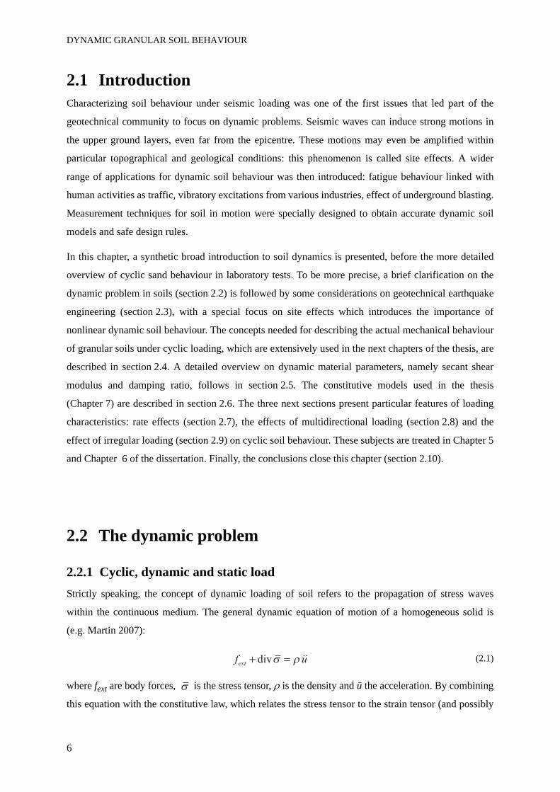
In between, periodic cyclic loadings are a particular case. Fig. 2.1 compares the different types of
loading.
The term «cyclic loading» refers to systems oscillating with constant amplitude and frequency.
According to parameters such as loading frequency or wave length, the soil volume of interest may
experience wave propagation inside its boundaries (true dynamic load), or a homogeneous stress with
an amplitude which evolves with time (pseudo-static load). However, both situations can be used for
the purpose of creating constitutive models which take into account dynamic soil behaviour. Actually,
cyclic loading is commonly classified within dynamic loading, as its purpose is intrinsically linked with
the dynamic problem.
Fig. 2.1. Loading types.
Rapid loading
Slow static loading
Cyclic loading
time
Shear
str
ess
DYNAMIC GRANULAR SOIL BEHAVIOUR
8
2.2.2 Nature of dynamic loadings
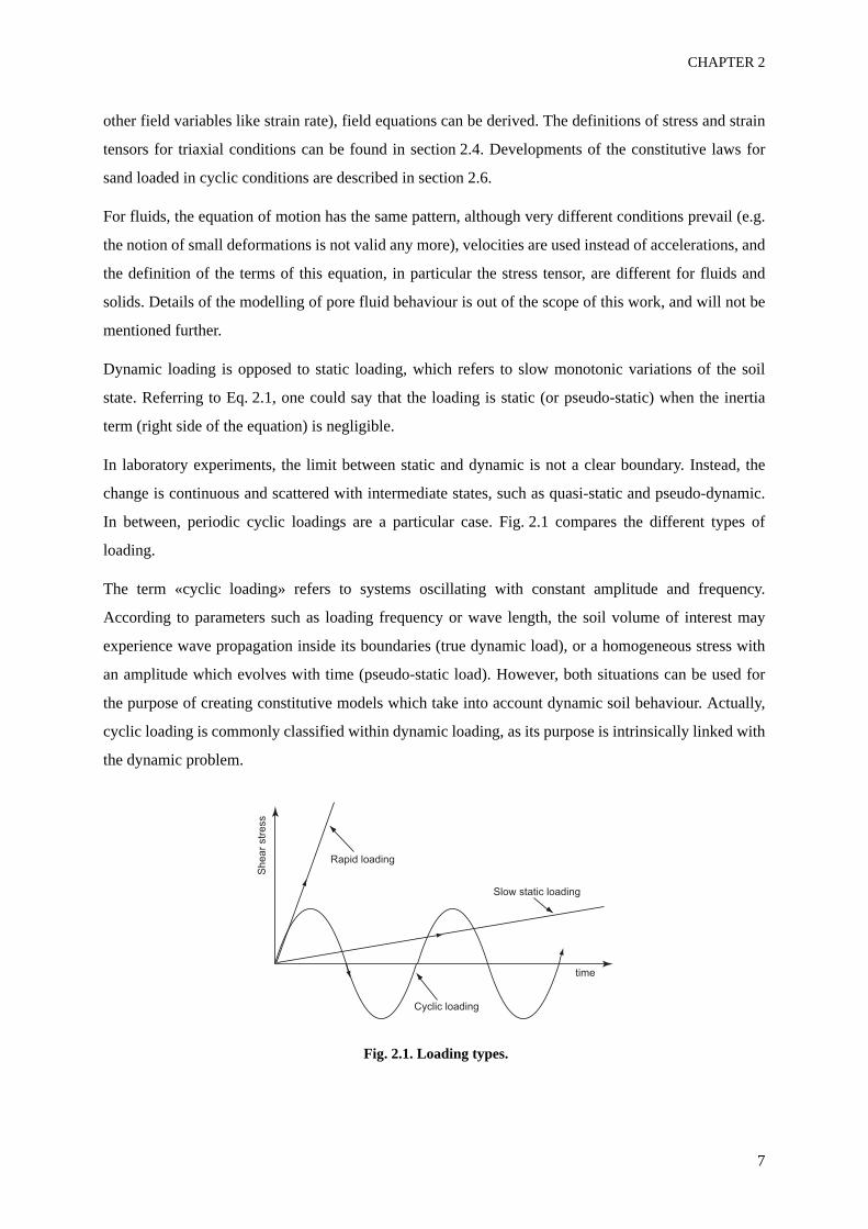
2.2.2.1 IntroductionIn the field of soil mechanics, dynamic loadings are the consequences of numerous kinds of excitations.
The various possible sources induce different oscillations of the ground. Fig. 2.2 presents a qualitative
classification of the dynamic sources. Each problem is classified by its number of cycles and by the
time of loading.
Fig. 2.2. Classification of dynamic problems (Ishihara 1996).
2.2.2.2 Seismic waves («Earthquake» in Fig. 2.2): transient loadingEarthquakes are due to plate tectonics, which is the phenomenon of interaction and motion of the parts
which constitute the earth's crust. These interactions manifest themselves both at the boundaries of the
plates and at their core. Upon motion of the different plates, large stresses accumulate in several points
near the boundaries, where they eventually induce breaking along fault lines. The energy liberated by
the sudden displacement is the origin of seismic waves, which diffuse inside the plates. In a given area,
ground motion depends on many parameters, such as the magnitude of the earthquake, the distance with
the epicentre, global and local physical characteristics of the ground.
Soil elements submitted to seismic wave propagation are considered to undergo cyclic stress conditions
(Seed 1979). Stress time series have random pattern, but there is agreement on their cyclic nature
(confirmed experimentally by our triaxial tests in Chapter 6). Seismic motion is generally characterized
by 10 to 20 loads of irregular amplitudes. The frequency content of a seismic excitation is also irregular
and varies mostly from 0.1 to 10 Hz. More details on geotechnical earthquake engineering issues are
given in section 2.3.

CHAPTER 2
9
2.2.2.3 Vibrations due to human activities («Pile driving compaction», «machine foundation» and «traffic loads» in Fig. 2.2)
They are essentially due to civil engineering (drilling, pile driving), circulation of heavy vehicles
(trucks, train) and operation of industrial mechanical devices (vibrations due to cyclic machines, shock
associated to fabrication process). These excitations are characterized by small amplitude motions with
an enormous amount of cycles. Because of that, they can induce or increase settlement of soft soil
layers.
2.2.2.4 Blasting and bombing (Fig. 2.2): shock wavesShock waves are characterized by the liberation of an enormous amount of energy (at the scale of a very
big seism) in a single loading cycle. The most powerful blasting excitation can arise because of
underground or surface tests of atomic and thermonuclear bombs.
A more civil application to blasting is linked to mining, underground work and foundation engineering,
where blasting is one of possible excavation technique. Blasting can also be purposely used to densify
loose ground previous to building construction.
A new field of activity for geotechnics is the resistance to terrorism attacks.
2.3 Geotechnical earthquake engineering
2.3.1 Introduction to geotechnical earthquake engineeringEarthquake engineering is a young discipline which deals with the effect of earthquakes on people,
structures and more generally the environment, and the means developed to reduce these effects. These
broad objectives concern geologists, seismologists, structural and geotechnical engineers, risk analysts
among the technical field, but also sociologists, insurers, economists and politicians.
The geotechnical aspect of earthquake engineering is a major component of this large battlefield,
because ground shaking amplitude, duration and frequency content are key parameters influencing the
costs of an earthquake in terms of human life and structures. The name geotechnical earthquake
engineering covers site effects and microzonation, soil-structure interaction, strong ground motion,
wave propagation, soil dynamics, slope stability, dams, embankments, earth structures and quay walls
behaviour under transient loading. Among popular research subjects, there are in situ soil
characterization, laboratory testing for soil behaviour characterization, physical models in centrifuge
DYNAMIC GRANULAR SOIL BEHAVIOUR
10
testing, and modelling of soil stratum and structures in one, two or three dimensions.
Soil dynamics is described in details in other chapters. The following part focuses on a few chosen
aspects of geotechnical earthquake engineering: the evaluation of seismic hazard and the
characterization of earthquakes, a short description of seismic wave propagation, and the application of
soil dynamics to site effects.
2.3.2 Seismic hazard in SwitzerlandSeismic hazard in a particular region is evaluated through careful analysis of both history of seismic
activity and geological evidences. Each country produces hazard maps and delimits regions according
to different degrees of seismic hazard (e.g. Demircioglu et al. 2007 for Turkey). These maps are based
on a classification according to peak ground acceleration (PGA, defined in section 2.3.3) induced by
representative seismic events of the region.
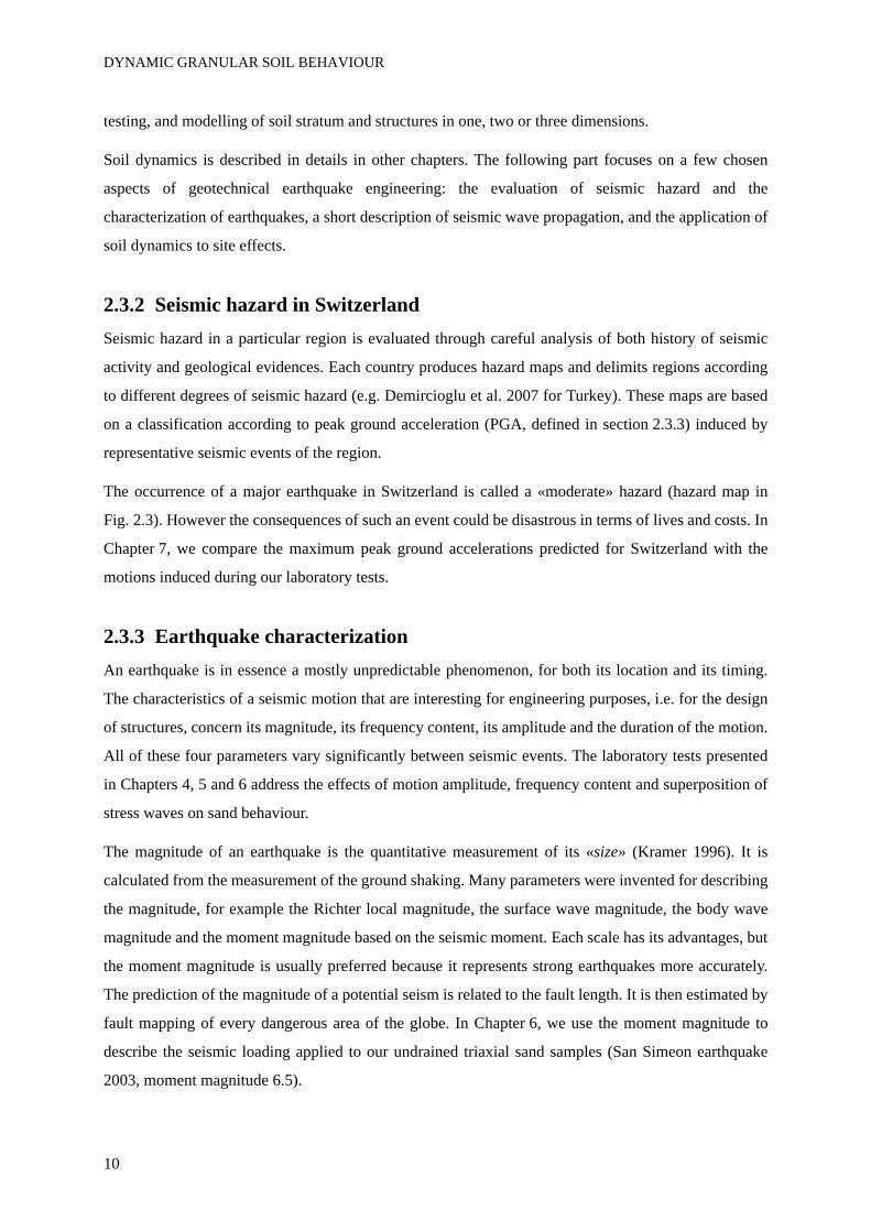
The occurrence of a major earthquake in Switzerland is called a «moderate» hazard (hazard map in
Fig. 2.3). However the consequences of such an event could be disastrous in terms of lives and costs. In
Chapter 7, we compare the maximum peak ground accelerations predicted for Switzerland with the
motions induced during our laboratory tests.
2.3.3 Earthquake characterizationAn earthquake is in essence a mostly unpredictable phenomenon, for both its location and its timing.
The characteristics of a seismic motion that are interesting for engineering purposes, i.e. for the design
of structures, concern its magnitude, its frequency content, its amplitude and the duration of the motion.
All of these four parameters vary significantly between seismic events. The laboratory tests presented
in Chapters 4, 5 and 6 address the effects of motion amplitude, frequency content and superposition of
stress waves on sand behaviour.
The magnitude of an earthquake is the quantitative measurement of its «size» (Kramer 1996). It is
calculated from the measurement of the ground shaking. Many parameters were invented for describing
the magnitude, for example the Richter local magnitude, the surface wave magnitude, the body wave
magnitude and the moment magnitude based on the seismic moment. Each scale has its advantages, but
the moment magnitude is usually preferred because it represents strong earthquakes more accurately.
The prediction of the magnitude of a potential seism is related to the fault length. It is then estimated by
fault mapping of every dangerous area of the globe. In Chapter 6, we use the moment magnitude to
describe the seismic loading applied to our undrained triaxial sand samples (San Simeon earthquake
2003, moment magnitude 6.5).
CHAPTER 2
11
Fig. 2.3. Seismic hazard in Switzerland (Giardini et al. 2004).
DYNAMIC GRANULAR SOIL BEHAVIOUR
12
Ground motions in a particular site can be recorded by various instruments, such as seismographs and
accelerographs (an acceleration time history is shown in Appendix 2). The sensor usually records three
orthogonal acceleration of the ground in translation. Laboratory tests with sinusoidal and seismic
bidirectional conditions are presented in Chapter 6; they take into account two perpendicular motions.
Acceleration time histories are too complex to be used as raw data, also ground motion parameters are
extracted from these curves. The amplitude of each component is commonly measured by the peak
ground acceleration (PGA), in the horizontal or vertical direction. The frequency content of the motion
is also important, as it greatly influences the damage to structures. The Fourier amplitude spectrum of
acceleration clearly depicts the distribution of the motion amplitude with respect to the frequency (e.g.
Appendix 2).
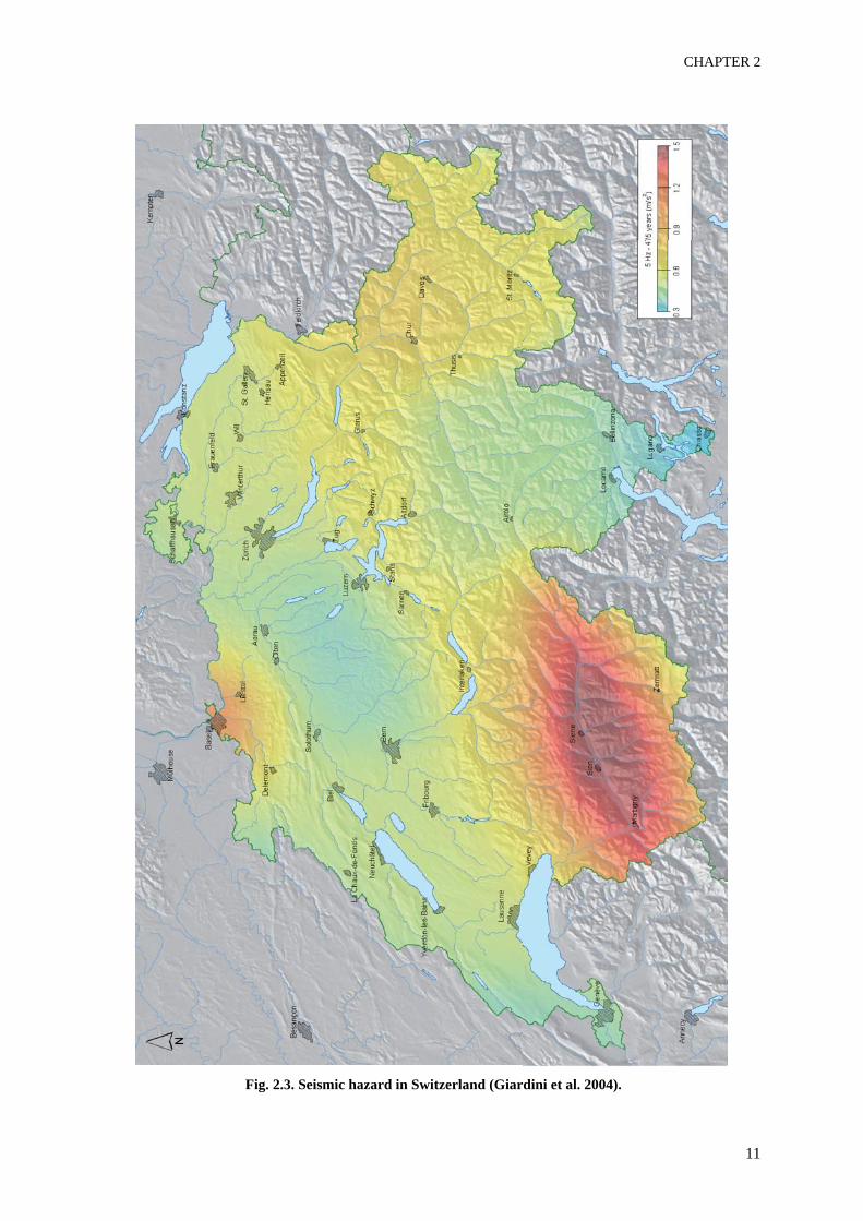
Fig. 2.4. Design response spectrum (Kalkan & Gülkan 2004).
When seismic hazard is considered for the design of a structure, the most potentially damaging
earthquake frequency content for the structure should be used for its design. This parameter is unknown
CHAPTER 2
13
a priori. That is why design response spectra (e.g. Fig. 2.4), forged with probabilistic analysis, are
provided by statutory procedures. For example, Studer et al. (2004) review design spectra used in
Switzerland and suggest a new soil classification for the response to strong motions. Fig. 2.4 shows the
influence of the type of geomaterials on the amplification of the spectral acceleration. In the same
conditions, soils involve higher accelerations than rock (cf. site effects in section 2.3.5).
2.3.4 Seismic wave propagation
2.3.4.1 Elastic volumetric wavesSeismic wave propagation inside an elastic continuum has been extensively described (e.g. Kramer
1996). Soil is assumed as a homogenous monophasic isotropic elastic medium. A more complex theory,
poroelasticity, has been developed since Biot (1956) for wave propagation inside a biphasic porous
material, where the pores are saturated with a fluid.
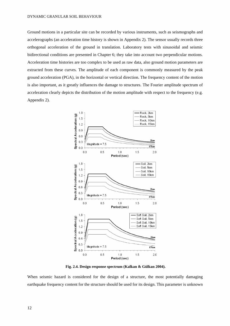
An elastic wave is a discontinuity surface separating two elastic volumes (Nowacki 1978). Ground
shaking during an earthquake is due to the upward propagation of body waves from an underlying rock
formation. Those body waves propagating inside a homogenous isotropic soil can be distinguished into
two kinds (Fig. 2.5):
• Compressional (also called longitudinal and primary) waves (P waves) alternately induce
compressional and dilational stresses in the soil body.
• Shear (or secondary or transverse) waves (S waves) induce a shearing deformation with motions
perpendicular to the propagation direction. S waves can be divided into two components: SV
(vertical plane motion) and SH (horizontal plane motion). In elastic medium, they do not induce
volumetric changes, nor can be sustained by fluids. S waves propagate slower than P waves.
Fig. 2.5. Elastic body waves: P wave and S wave.
The celerity, or propagation velocity, of body waves plays an important role in soil dynamics. The
velocity of P wave (cp) and S wave (cs) depends on elastic soil properties, i.e. any of two of the
following constants: Lamé coefficients λ and μ, Young’s modulus (E), shear modulus (G) and Poisson’s
ratio (ν):
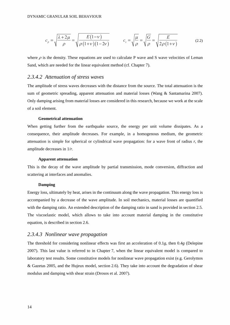
DYNAMIC GRANULAR SOIL BEHAVIOUR
14
(2.2)
where ρ is the density. These equations are used to calculate P wave and S wave velocities of Leman
Sand, which are needed for the linear equivalent method (cf. Chapter 7).
2.3.4.2 Attenuation of stress wavesThe amplitude of stress waves decreases with the distance from the source. The total attenuation is the
sum of geometric spreading, apparent attenuation and material losses (Wang & Santamarina 2007).
Only damping arising from material losses are considered in this research, because we work at the scale
of a soil element.
Geometrical attenuation
When getting further from the earthquake source, the energy per unit volume dissipates. As a
consequence, their amplitude decreases. For example, in a homogenous medium, the geometric
attenuation is simple for spherical or cylindrical wave propagation: for a wave front of radius r, the
amplitude decreases in 1/r.
Apparent attenuation
This is the decay of the wave amplitude by partial transmission, mode conversion, diffraction and
scattering at interfaces and anomalies.
Damping
Energy loss, ultimately by heat, arises in the continuum along the wave propagation. This energy loss is
accompanied by a decrease of the wave amplitude. In soil mechanics, material losses are quantified
with the damping ratio. An extended description of the damping ratio in sand is provided in section 2.5.
The viscoelastic model, which allows to take into account material damping in the constitutive
equation, is described in section 2.6.
2.3.4.3 Nonlinear wave propagationThe threshold for considering nonlinear effects was first an acceleration of 0.1g, then 0.4g (Delepine
2007). This last value is referred to in Chapter 7, when the linear equivalent model is compared to
laboratory test results. Some constitutive models for nonlinear wave propagation exist (e.g. Gerolymos
& Gazetas 2005, and the Hujeux model, section 2.6). They take into account the degradation of shear
modulus and damping with shear strain (Drosos et al. 2007).
cE
cG E
p s
2 1
1 1 2 2 1
CHAPTER 2
15
2.3.5 Site effectsSite effects are shortly described now, to evaluate the importance of soil dynamics in a geotechnical
earthquake engineering application. This problem is particularly concerned by the choice of a soil
model, which should take into account dynamic effects. The comparison, in Chapter 7, of two different
models, both suitable for seismic wave propagation simulations, could have important impact on the
evaluation of site effects.
2.3.5.1 Definition and description of site effectsThere can be great differences in the degree of damages resulting from an earthquake depending on
ground conditions. This phenomenon is called site effects. It is of major importance for the design of
buildings in seismic areas. Three main effects are considered in this perspective (Okamoto 1973) for
unidimentional amplification:
• The influence of soil type on the intensity, waveform and velocity of earthquake motion (e.g.
Fig. 2.4)
• The influence of soil characteristics (density, damping) on soil - structure interaction
• The decrease in strength of soil when subjected to earthquake loading.
In simple cases, motion amplification in a particular site is characterized by the ratio of the peak ground
acceleration (PGA) at the soil surface over the PGA at a reference rock surface. The ratio depends on
soil type, peak acceleration value and soil layer thickness. It is usually higher than one for peak
acceleration until 0.5g. However this threshold could be higher for thin layers of sandy material.
Amplification spectra only roughly takes into account site amplification phenomenon (Semblat et al.
2005).
The topography of the area is also known to play an important role in site effects. Indeed, site
amplification can be the consequence of seismic wave reflections and surface wave propagation in
geometrically complex situations, like earth dams or valleys. More precisely, in an earth structure,
seismic waves are trapped above the bedrock. These trapped waves can induce resonance of the ground
motion when the wave frequency reaches the natural frequency of the structure. For complex
topography, the amplification is thus frequency-dependent. Bard & Riepl (2000) report three physical
phenomena for explaining topography effect: (i) the sensitivity to the incidence angle of shear waves,
(ii) their multiple reflections and corresponding motion amplitude increase and (iii) interference
patterns between direct and diffracted waves.
2.3.5.2 Multidimensional amplificationAmplification analysis is very sensitive to the numerical model; there is sometimes a non negligible
DYNAMIC GRANULAR SOIL BEHAVIOUR
16
difference between unidimentional (1D) and multidimensional (2D and 3D) responses. The choice of
the type of analysis then depends on the site configuration and on the importance of the accuracy of the
investigation. Bard & Riepl (2000) computes the spectral response of simple cosine-shaped basin,
which shows that resonance frequencies are higher for multidimensional basin. Moreover, the
amplification ratio is higher for 3D computations. Delepine (2007) also models 1D, 2D and 3D
ellipsoidal basins. He concludes that 2D models gives higher amplification ratios than the
unidimentional simulation. They are even higher with 3D computation of sedimentary basin.
2.3.5.3 Estimation of site effects by microzonationIntroduction
Methods for estimating site effects can be classified in three types (Bard & Riepl 2000): experimental
methods, numerical methods and empirical methods. For microzonation purpose, experimental
methods are more widely used because their cost is lower, and they allow large scale estimations.
Numerical methods are reserved to highly hazardous areas, or for case studies of previously damaged
sites. Empirical correlations, based on surface geology and geotechnical properties, can be applied to
sites of known ground composition. Some numerical methods are briefly compared below.
Numerical modelling
The choice of the constitutive law used for characterizing site effects depends on the earthquake
intensity which can be expected in the studied area. For regions of low to medium seismic activity,
linear equivalent models are commonly used. Viscoelastic models can also be appropriate for site
effects modelling. The use of more complicated models for site effects estimation is uncommon, despite
the fact that nonlinear behaviour is critical for large motions (e.g. Iai & Tobita 2006).
For 1D amplification analysis, the linear equivalent method, performed in the frequency domain, is
widely used. Linear equivalent models can lead to an overestimation of the amplification as a result of
«spurious resonance». Its main shortcoming is that it can not represent pore water pressure increase.
But it can be more efficient, in terms of computer cost, than nonlinear analyses. For low strain level, it
is usually considered as accurate enough.
Nonlinear models for microzonation can be implemented by a direct integration in the time domain.
They are mostly based on simple models following the Masing’s rule, like the Ramberg-Osgood model
or the hyperbolic model. It is also possible to use advanced constitutive models, like in DYNAFLOW
(Popescu et al. 2006). Nonlinear models, which can also reproduce pore water pressure generation, are
particularly recommended for stronger strain levels. Their main shortcoming is the difficulty which
arises at the determination of soil parameters.
CHAPTER 2
17
Hartzell et al. (2004) compare site amplification for five soil types and increasing peak input motions
from 0.1g to 0.9g. Different models are tested, the simplest being the linear equivalent method and the
more complex being an advanced coupled model NOAHB. For very stiff soils, there is not much
difference between the models, but nonlinear effects increase in soft and medium soils, for high
deformation amplitude. The nonlinear approach is recommended in these cases.
For such inelastic soil behaviour, two site amplification characteristics should be accounted for. The
fundamental frequency of the soil deposit decreases if the seismic frequency band is lower than the
natural soil frequency. This decrease changes in turn the spectral amplification. On the other hand, the
damping ratio increases, which reduces the peak ground acceleration, especially for high frequencies.
2.3.5.4 Extension towards soil dynamics issuesThe development of nonlinear soil models based on effective stress principles is thus essential for
increasing the accuracy of site effects analyses in case of strong ground motion. The ease of calibration
of such models is a priority, and should not be an obstacle towards the use of advanced nonlinear soil
models. Chapter 7 provides examples and additional insight into this subject.
2.4 Introduction to soil behaviour under cyclic loadingAfter the description of important features of monotonic soil behaviour, a few chosen aspects of cyclic
soil behaviour are presented, thanks to the description of laboratory studies from the literature. Only the
behaviour of granular material is addressed in the thesis.
2.4.1 Effective stressThe system studied is composed of a soil matrix, made of sand grains, and a one-phase fluid, saturating
the pores. This fluid is either air or water. The stresses within the porous medium are ruled by the
concept of Terzaghi of effective stress (Terzaghi 1943). The effective stress σ’ is defined as the
difference between the total stress σ and the pore fluid pressure u.
2.4.2 Notations of stress and strainThe definitions of stress and strains rely on the assumption of small strains, which is assumed valid for
all experimental results. For limit cases, at large strain above failure, a special care is taken to monitor
localization (cf. section 4.8).
DYNAMIC GRANULAR SOIL BEHAVIOUR
18
2.4.2.1 Stress field for triaxial testThe effective stress tensor is written as follows, in the case of an axisymmetric triaxial test:
(2.3)
where σ’3 is the effective confining pressure. In the triaxial cell, the confining stress is isotropically
applied and the axial stress σ’1 can be calculated by:
(2.4)
where Fax is the force applied by the axial loading rod (Chapter 3) and S is the surface of the sample.
It is useful to introduce the classical decomposition of the stress tensor in a deviatoric (tij) and a
spherical part (p’):
(2.5)
The first invariant of the stress is p’ = 1/3 σ’kk. The deviatoric part is then:
(2.6)
The second invariant of the deviatoric part of the stress, J2D, is defined and calculated below:
(2.7)
another form of the second invariant is generally used in the case of the triaxial test:
(2.8)
also called the deviatoric stress.
It is useful, for the determination of dynamic parameters in complex loadings, to define a general
effective stress increment corresponding to a change in both the deviatoric stress (Δq) and the confining
pressure (Δσ’3). The following equation gives the effective stress increment, the deviatoric and the
1
3
3
0 0
0 0
0 0
CHAPTER 2
19
spherical increments ( ):
(2.9)
Major and minor principal stresses are either the axial stress (on the top of the cylinder), either the
lateral stress. By convention, the total stress applied onto the top cap is always called σ1, and the lateral
stress σ3. Even in case of extension, when there is rotation of principle stresses of 90°, their name is not
exchanged for the sake of clarity. Because of that, the deviatoric stress can be negative and, if so, is the
opposite of the second stress invariant.
2.4.2.2 Strain field for triaxial testThe strain tensor inside the sample is also diagonal:
(2.10)
As all the strain components are in the principal directions, they are written:
(2.11)
with di the displacement in the ith direction. The measurement of the strain component is made between
two points x1 and x2. The integration of di over the domain gives the relations:
(2.12)
In the same manner as the stress tensor, strain is separated into two parts:
(2.13)
The first invariant of εij is and the deviatoric strain tensor eij is then:
1
3
3
0 0
0 0
0 0
)
V kk 1 32
DYNAMIC GRANULAR SOIL BEHAVIOUR
20
(2.14)
The second invariant of strain, called here the deviatoric strain, can be defined in two forms:
(2.15)
The definition of deviatoric strain selected for our work is this value εq, which is more convenient than
the alternative definition taken as 2/3 (ε1 - ε3).
As for the stress increment, the general strain increment corresponding to any state change is defined
by:
(2.16)
(2.17)
The work W of any general loading path in triaxial conditions can be calculated by:
(2.18)
that can be rewritten as:
(2.19)
with p’, εv, q and εq defined in Eq. 2.5, Eq. 2.13, Eq. 2.8 and Eq. 2.15. The work can be used to
calculate the stored energy and dissipated energy in cyclic stress - strain loops (section 2.5.2).
With this precise definition of the stress and strain components, soil behaviour can be described in
monotonic and cyclic conditions.
eij1 3
3
2 0 0
0 1 0
0 0 1
I e e and ID ij ij q D2
1 3
2
2 1 3
1
2 33
1
3
3
0 0
0 0
0 03
2 0 0
0 1 0
0 0 13
1 0q V
00
0 1 0
0 0 1
W 1 1 32
W p qv q
2
3
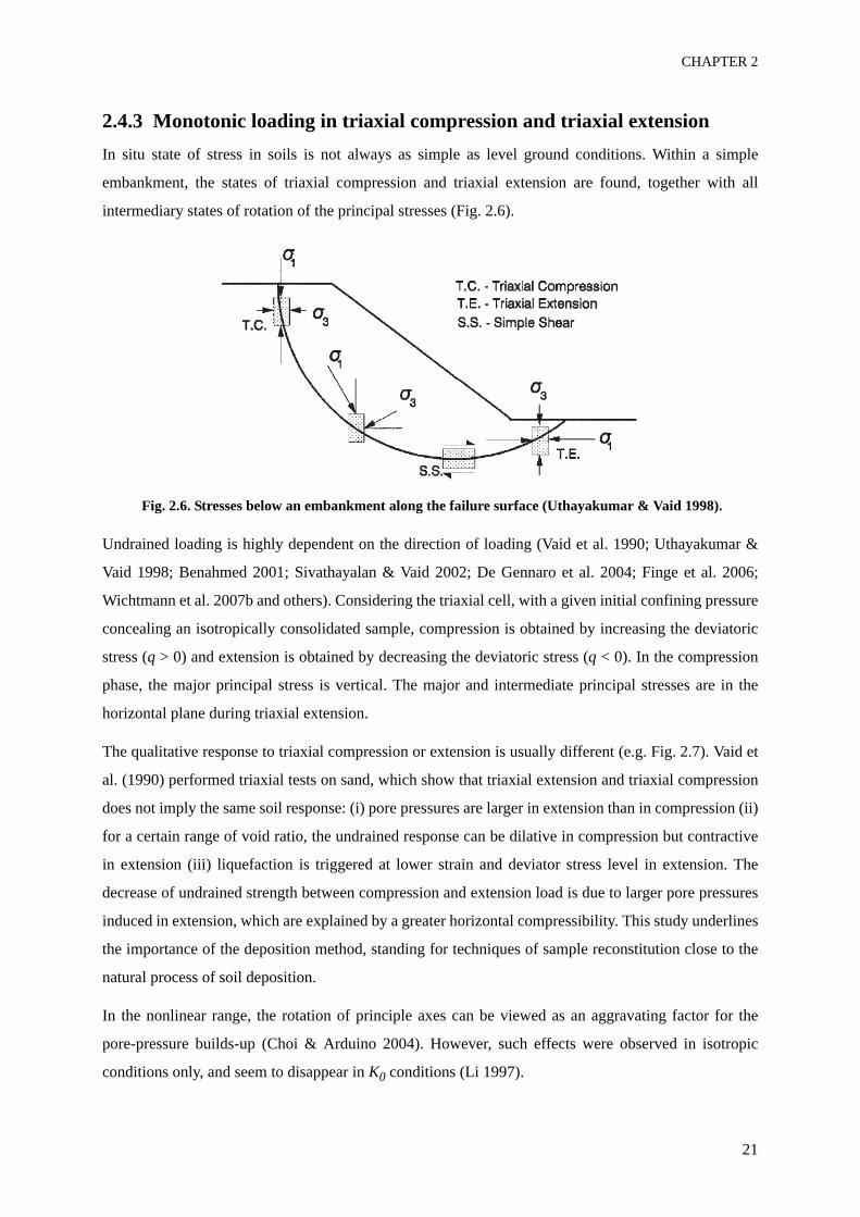
CHAPTER 2
21
2.4.3 Monotonic loading in triaxial compression and triaxial extensionIn situ state of stress in soils is not always as simple as level ground conditions. Within a simple
embankment, the states of triaxial compression and triaxial extension are found, together with all
intermediary states of rotation of the principal stresses (Fig. 2.6).
Fig. 2.6. Stresses below an embankment along the failure surface (Uthayakumar & Vaid 1998).
Undrained loading is highly dependent on the direction of loading (Vaid et al. 1990; Uthayakumar &
Vaid 1998; Benahmed 2001; Sivathayalan & Vaid 2002; De Gennaro et al. 2004; Finge et al. 2006;
Wichtmann et al. 2007b and others). Considering the triaxial cell, with a given initial confining pressure
concealing an isotropically consolidated sample, compression is obtained by increasing the deviatoric
stress (q > 0) and extension is obtained by decreasing the deviatoric stress (q < 0). In the compression
phase, the major principal stress is vertical. The major and intermediate principal stresses are in the
horizontal plane during triaxial extension.
The qualitative response to triaxial compression or extension is usually different (e.g. Fig. 2.7). Vaid et
al. (1990) performed triaxial tests on sand, which show that triaxial extension and triaxial compression
does not imply the same soil response: (i) pore pressures are larger in extension than in compression (ii)
for a certain range of void ratio, the undrained response can be dilative in compression but contractive
in extension (iii) liquefaction is triggered at lower strain and deviator stress level in extension. The
decrease of undrained strength between compression and extension load is due to larger pore pressures
induced in extension, which are explained by a greater horizontal compressibility. This study underlines
the importance of the deposition method, standing for techniques of sample reconstitution close to the
natural process of soil deposition.
In the nonlinear range, the rotation of principle axes can be viewed as an aggravating factor for the
pore-pressure builds-up (Choi & Arduino 2004). However, such effects were observed in isotropic
conditions only, and seem to disappear in K0 conditions (Li 1997).
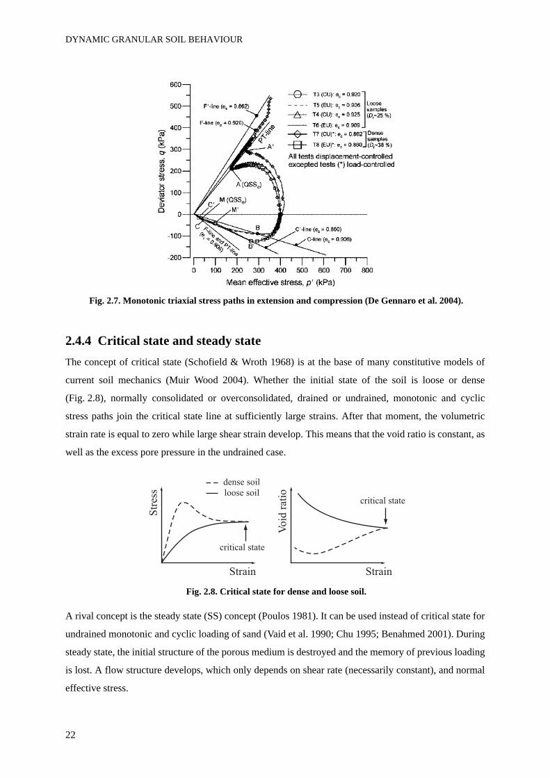
DYNAMIC GRANULAR SOIL BEHAVIOUR
22
Fig. 2.7. Monotonic triaxial stress paths in extension and compression (De Gennaro et al. 2004).
2.4.4 Critical state and steady stateThe concept of critical state (Schofield & Wroth 1968) is at the base of many constitutive models of
current soil mechanics (Muir Wood 2004). Whether the initial state of the soil is loose or dense
(Fig. 2.8), normally consolidated or overconsolidated, drained or undrained, monotonic and cyclic
stress paths join the critical state line at sufficiently large strains. After that moment, the volumetric
strain rate is equal to zero while large shear strain develop. This means that the void ratio is constant, as
well as the excess pore pressure in the undrained case.
Fig. 2.8. Critical state for dense and loose soil.
A rival concept is the steady state (SS) concept (Poulos 1981). It can be used instead of critical state for
undrained monotonic and cyclic loading of sand (Vaid et al. 1990; Chu 1995; Benahmed 2001). During
steady state, the initial structure of the porous medium is destroyed and the memory of previous loading
is lost. A flow structure develops, which only depends on shear rate (necessarily constant), and normal
effective stress.
critical state
dense soil
loose soilcritical state
Strain Strain
Str
ess
Void
rat
io
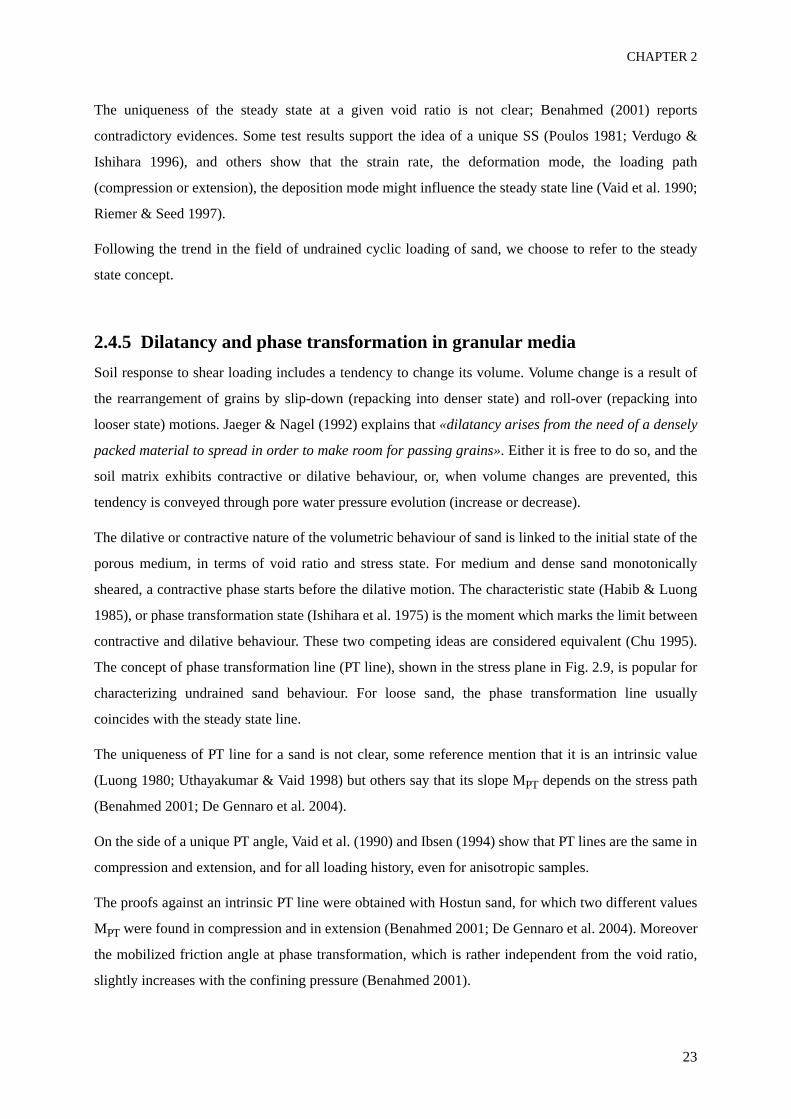
CHAPTER 2
23
The uniqueness of the steady state at a given void ratio is not clear; Benahmed (2001) reports
contradictory evidences. Some test results support the idea of a unique SS (Poulos 1981; Verdugo &
Ishihara 1996), and others show that the strain rate, the deformation mode, the loading path
(compression or extension), the deposition mode might influence the steady state line (Vaid et al. 1990;
Riemer & Seed 1997).
Following the trend in the field of undrained cyclic loading of sand, we choose to refer to the steady
state concept.
2.4.5 Dilatancy and phase transformation in granular mediaSoil response to shear loading includes a tendency to change its volume. Volume change is a result of
the rearrangement of grains by slip-down (repacking into denser state) and roll-over (repacking into
looser state) motions. Jaeger & Nagel (1992) explains that «dilatancy arises from the need of a densely
packed material to spread in order to make room for passing grains». Either it is free to do so, and the
soil matrix exhibits contractive or dilative behaviour, or, when volume changes are prevented, this
tendency is conveyed through pore water pressure evolution (increase or decrease).
The dilative or contractive nature of the volumetric behaviour of sand is linked to the initial state of the
porous medium, in terms of void ratio and stress state. For medium and dense sand monotonically
sheared, a contractive phase starts before the dilative motion. The characteristic state (Habib & Luong
1985), or phase transformation state (Ishihara et al. 1975) is the moment which marks the limit between
contractive and dilative behaviour. These two competing ideas are considered equivalent (Chu 1995).
The concept of phase transformation line (PT line), shown in the stress plane in Fig. 2.9, is popular for
characterizing undrained sand behaviour. For loose sand, the phase transformation line usually
coincides with the steady state line.
The uniqueness of PT line for a sand is not clear, some reference mention that it is an intrinsic value
(Luong 1980; Uthayakumar & Vaid 1998) but others say that its slope MPT depends on the stress path
(Benahmed 2001; De Gennaro et al. 2004).
On the side of a unique PT angle, Vaid et al. (1990) and Ibsen (1994) show that PT lines are the same in
compression and extension, and for all loading history, even for anisotropic samples.
The proofs against an intrinsic PT line were obtained with Hostun sand, for which two different values
MPT were found in compression and in extension (Benahmed 2001; De Gennaro et al. 2004). Moreover
the mobilized friction angle at phase transformation, which is rather independent from the void ratio,
slightly increases with the confining pressure (Benahmed 2001).
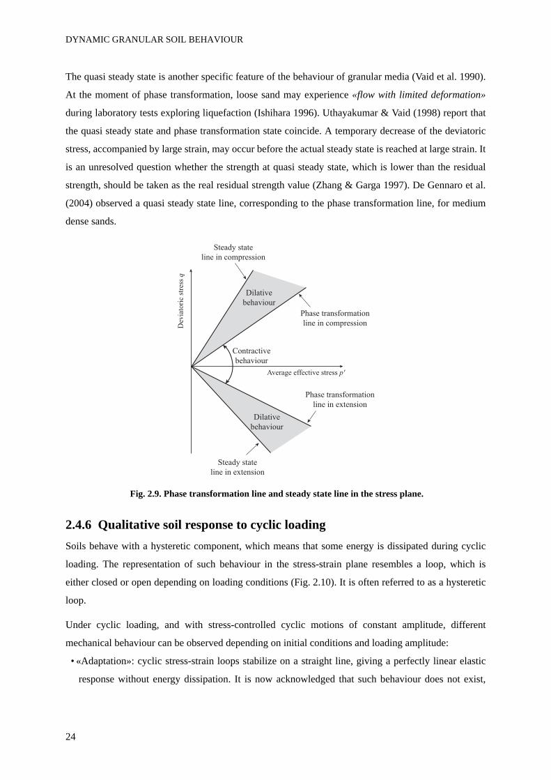
DYNAMIC GRANULAR SOIL BEHAVIOUR
24
The quasi steady state is another specific feature of the behaviour of granular media (Vaid et al. 1990).
At the moment of phase transformation, loose sand may experience «flow with limited deformation»
during laboratory tests exploring liquefaction (Ishihara 1996). Uthayakumar & Vaid (1998) report that
the quasi steady state and phase transformation state coincide. A temporary decrease of the deviatoric
stress, accompanied by large strain, may occur before the actual steady state is reached at large strain. It
is an unresolved question whether the strength at quasi steady state, which is lower than the residual
strength, should be taken as the real residual strength value (Zhang & Garga 1997). De Gennaro et al.
(2004) observed a quasi steady state line, corresponding to the phase transformation line, for medium
dense sands.
Fig. 2.9. Phase transformation line and steady state line in the stress plane.
2.4.6 Qualitative soil response to cyclic loadingSoils behave with a hysteretic component, which means that some energy is dissipated during cyclic
loading. The representation of such behaviour in the stress-strain plane resembles a loop, which is
either closed or open depending on loading conditions (Fig. 2.10). It is often referred to as a hysteretic
loop.
Under cyclic loading, and with stress-controlled cyclic motions of constant amplitude, different
mechanical behaviour can be observed depending on initial conditions and loading amplitude:
• «Adaptation»: cyclic stress-strain loops stabilize on a straight line, giving a perfectly linear elastic
response without energy dissipation. It is now acknowledged that such behaviour does not exist,
Dev
iato
ric
stre
ss q
Average effective stress p'
Phase transformation
line in compression
Steady state
line in compression
Contractive
behaviour
Dilative
behaviour
Dilative
behaviour
Phase transformation
line in extension
Steady state
line in extension
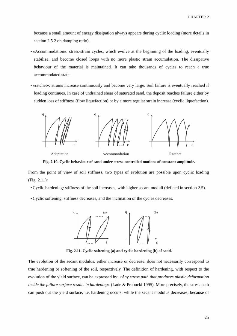
CHAPTER 2
25
because a small amount of energy dissipation always appears during cyclic loading (more details in
section 2.5.2 on damping ratio).
• «Accommodation»: stress-strain cycles, which evolve at the beginning of the loading, eventually
stabilize, and become closed loops with no more plastic strain accumulation. The dissipative
behaviour of the material is maintained. It can take thousands of cycles to reach a true
accommodated state.
• «ratchet»: strains increase continuously and become very large. Soil failure is eventually reached if
loading continues. In case of undrained shear of saturated sand, the deposit reaches failure either by
sudden loss of stiffness (flow liquefaction) or by a more regular strain increase (cyclic liquefaction).
Fig. 2.10. Cyclic behaviour of sand under stress-controlled motions of constant amplitude.
From the point of view of soil stiffness, two types of evolution are possible upon cyclic loading
(Fig. 2.11):
• Cyclic hardening: stiffness of the soil increases, with higher secant moduli (defined in section 2.5).
• Cyclic softening: stiffness decreases, and the inclination of the cycles decreases.
Fig. 2.11. Cyclic softening (a) and cyclic hardening (b) of sand.
The evolution of the secant modulus, either increase or decrease, does not necessarily correspond to
true hardening or softening of the soil, respectively. The definition of hardening, with respect to the
evolution of the yield surface, can be expressed by: «Any stress path that produces plastic deformation
inside the failure surface results in hardening» (Lade & Prabucki 1995). More precisely, the stress path
can push out the yield surface, i.e. hardening occurs, while the secant modulus decreases, because of
q
Adaptation
q
Accommodation
q
Ratchet
q q(a) (b)
DYNAMIC GRANULAR SOIL BEHAVIOUR
26
the coupling of the volumetric and deviatoric shear. Moreover, «true softening occurs past the peak
failure surface». Anyway, for the description of cyclic test results, the expressions «cyclic softening»
and «cyclic hardening» will be used as a simple way to evoke decrease and increase of soil stiffness,
respectively.
2.4.7 Effect of the number of cyclesThe accumulation of cyclic loads corresponds to a particular soil behaviour, very different from
monotonic behaviour. The effect of the number of cycles depends on the inversion of the sign of strain
or stress rate (Ishihara 1996); it is also referred to as stress/strain reversal effect. The increasing number
of cycles may induce stiffness degradation, or cyclic softening of the soil and as well as energy
dissipation, ultimately by heat. The two major consequences of the effect of the number of cycles, even
at very low frequencies, are (i) the generation of resilient deformations under stress controlled cycles,
and (ii) excess pore water pressure increase in undrained conditions (Pecker 1984; O'Reilly & Brown
1991).
When a very large amount of cycles occur, it may induce cyclic effects that can be referred to as fatigue.
For example, Wichtmann et al. (2005) studied the effect of thousands to millions of low amplitude
cycles on strain accumulation in sand. Li & Yang (1998) studied the effect of vibration loading history
on shear modulus and damping ratio of dry sand.
2.4.8 Link between cyclic behaviour and dilatancyUnder monotonic loading, medium and densely packed granular soils first contract, and then rapidly
develop dilative behaviour (e.g. Kramer 1996). For cyclic loading, medium and dense sand behaviour is
more complex. In case of undrained conditions, an increase of excess pore water pressure first occurs
(which would be contractive behaviour in drained conditions), at a rate which depends on the shear
strain amplitude (Dobry et al. 1982). In the stress plane, the increase of excess pore pressure
corresponds to a displacement of the loops towards lower effective average stress p’. At one point, the
effective stress path eventually crosses the phase transformation line and punctual decrease of the
excess pore pressure (which would be dilative behaviour in drained conditions) occur (point number 1
in Fig. 2.12). During one cycle, contractive and dilative parts alternate at each intersection with the
phase transformation line. High strain amplitudes are rapidly reached, while the rate of increase of the
pore pressure is high, leading to «ratchet» behaviour. On the contrary, if the phase transformation line is
not reached, the rate of increase of the pore pressure can decrease to zero: this is the accommodation
phenomenon.
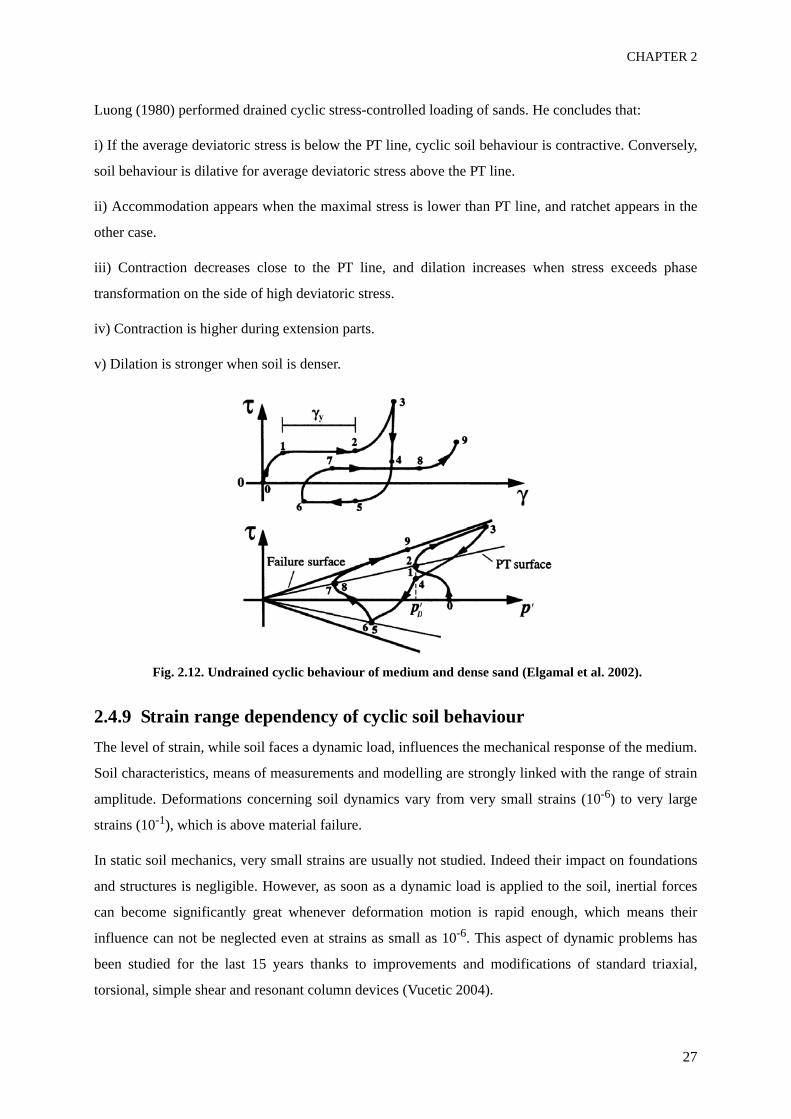
CHAPTER 2
27
Luong (1980) performed drained cyclic stress-controlled loading of sands. He concludes that:
i) If the average deviatoric stress is below the PT line, cyclic soil behaviour is contractive. Conversely,
soil behaviour is dilative for average deviatoric stress above the PT line.
ii) Accommodation appears when the maximal stress is lower than PT line, and ratchet appears in the
other case.
iii) Contraction decreases close to the PT line, and dilation increases when stress exceeds phase
transformation on the side of high deviatoric stress.
iv) Contraction is higher during extension parts.
v) Dilation is stronger when soil is denser.
Fig. 2.12. Undrained cyclic behaviour of medium and dense sand (Elgamal et al. 2002).
2.4.9 Strain range dependency of cyclic soil behaviourThe level of strain, while soil faces a dynamic load, influences the mechanical response of the medium.
Soil characteristics, means of measurements and modelling are strongly linked with the range of strain
amplitude. Deformations concerning soil dynamics vary from very small strains (10-6) to very large
strains (10-1), which is above material failure.
In static soil mechanics, very small strains are usually not studied. Indeed their impact on foundations
and structures is negligible. However, as soon as a dynamic load is applied to the soil, inertial forces
can become significantly great whenever deformation motion is rapid enough, which means their
influence can not be neglected even at strains as small as 10-6. This aspect of dynamic problems has
been studied for the last 15 years thanks to improvements and modifications of standard triaxial,
torsional, simple shear and resonant column devices (Vucetic 2004).
DYNAMIC GRANULAR SOIL BEHAVIOUR
28
While strain increases above the linear threshold (10-5 to 10-4), soil specimens tend to present nonlinear
viscoelastic behaviour with decreasing shear modulus (Ishihara 1996) and energy dissipation occurring
during cyclic loading. The number of cycles is not known to influence soil behaviour, which mostly
depends on the shear strain amplitude. This range of strain will be called small strain from now on.
At larger strains, the volumetric cyclic threshold shear strain, further detailed in section 2.4.10, is
usually exceeded. This is the medium strain range, from 10-4 to 10-2. Numerous changes progressively
appear in soil behaviour, in particular pore water pressure increase, stiffness degradation of saturated
soils and hardening of dry and unsaturated soils. Large irrecoverable plastic strains occur, they induce
cracks and differential settlement in soil. The number of cycles has an impact on soil properties and the
stress - strain relation.
Large strains, above 10-2, induce failure like slope instability or liquefaction (cf. section 2.4.13).
2.4.10 Volumetric cyclic threshold shear strain and stiffness degradationThere is a shear strain amplitude, called the volumetric cyclic threshold shear strain γtv, above which
significant permanent volume changes or permanent development of excess pore water pressure occur
in the soil (Vucetic 1994). This threshold is higher than the linear cyclic threshold of approximately 1.5
log-scale. It increases, for any soil, with (i) OCR (ii) initial average stress (iii) plasticity index (iv)
degree of saturation (v) smaller diameter of the grains. In sand, it is independent from relative density,
initial effective confining pressure and fabric. The threshold shear strain is around 10-4 for most sands
and silty sands, independently from relative densities (Dobry et al. 1982; Erten & Maher 1995). We also
evaluate this parameter for Leman Sand in Chapter 4.
For cyclic strains below the volumetric cyclic threshold shear strain, there is no permanent
microstructural change, residual excess pore water pressure does not develop in undrained conditions
and there is no permanent volume change in drained conditions. This corresponds to the stabilized
hysteretic behaviour.
Above the threshold, there is irreversible alteration of the microstructure, permanent pore water
pressure develop or permanent volume change accumulate, and the soil stiffness changes irreversibly:
cyclic softening occurs in undrained condition. «Stiffness degradation» is another expression used for
that phenomenon.
2.4.11 Pore water pressure increase in undrained saturated conditionsThe pore water pressure tends to increase during cyclic loading for strain amplitudes above γtv. Excess
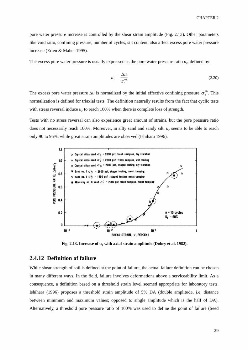
CHAPTER 2
29
pore water pressure increase is controlled by the shear strain amplitude (Fig. 2.13). Other parameters
like void ratio, confining pressure, number of cycles, silt content, also affect excess pore water pressure
increase (Erten & Maher 1995).
The excess pore water pressure is usually expressed as the pore water pressure ratio ur, defined by:
(2.20)
The excess pore water pressure Δu is normalized by the initial effective confining pressure . This
normalization is defined for triaxial tests. The definition naturally results from the fact that cyclic tests
with stress reversal induce ur to reach 100% when there is complete loss of strength.
Tests with no stress reversal can also experience great amount of strains, but the pore pressure ratio
does not necessarily reach 100%. Moreover, in silty sand and sandy silt, ur seems to be able to reach
only 90 to 95%, while great strain amplitudes are observed (Ishihara 1996).
Fig. 2.13. Increase of ur with axial strain amplitude (Dobry et al. 1982).
2.4.12 Definition of failureWhile shear strength of soil is defined at the point of failure, the actual failure definition can be chosen
in many different ways. In the field, failure involves deformations above a serviceability limit. As a
consequence, a definition based on a threshold strain level seemed appropriate for laboratory tests.
Ishihara (1996) proposes a threshold strain amplitude of 5% DA (double amplitude, i.e. distance
between minimum and maximum values; opposed to single amplitude which is the half of DA).
Alternatively, a threshold pore pressure ratio of 100% was used to define the point of failure (Seed
DYNAMIC GRANULAR SOIL BEHAVIOUR
30
1979). Due to limitations of the pore pressure ratio exposed in section 2.4.11, the failure criterion based
on a threshold strain is preferred for consistency between all kinds of soils and stress paths. A
comparison of failure criteria is developed in section 4.4.4.
2.4.13 Liquefaction and cyclic softening
2.4.13.1 IntroductionLiquefaction, which is induced by strong soil vibration, is a secondary effect of earthquakes which can
cause major damage if it happens in inhabited areas. It has long been acknowledged that all soil types
are not susceptible to liquefy. All kinds of soil submitted to strong cyclic motions can experience large
deformations, but flow behaviour characterizing liquefaction seems to happen only in granular media.
Many granular soils are prone to liquefaction, from silty sand (Erten & Maher 1995; Amini & Qi 2000;
Sitharam et al. 2004; Tsukamoto et al. 2004) to gravels (Kokusho et al. 2004; Choi & Arduino 2004).
Usually, the development of such instability happens in saturated granular soils loaded in undrained
conditions.
The initial state and the volumetric behaviour of sands greatly influences the response of a deposit to
cyclic loading. There is a progressive evolution of the cyclic soil response from very stable behaviour
of dense dilative materials to very unstable behaviour of loose contractive sands. Concepts like phase
transformation lines, flow liquefaction line, critical state line are very important characteristics for the
estimation of soil motions upon cyclic loading.
Over the years, different phenomena emerged from the initial concept of liquefaction. Flow
liquefaction, cyclic softening, cyclic liquefaction, and cyclic mobility are different ways of considering
soil failure, depending on the initial soil conditions. Robertson (1994) described the liquefaction-related
terminology.
2.4.13.2 Flow liquefactionDefinition
Flow liquefaction is a possible consequence of either static or dynamic loadings (Kramer 1996). It
typically appears in very loose soils submitted to high confining pressure which can produce high
increase of the excess pore pressure (contractive tendency in undrained conditions). These conditions
are not commonly found in situ, also flow liquefaction seldom spontaneously occurs.
Flow liquefaction is characterized by a sudden and complete loss of strength which follows a rapid
increase of the pore water pressure. The pore pressure converges towards the initial effective stress,
which is reached at a critical cycle, called Ncrit. When the effective stress is equal to zero, any
CHAPTER 2
31
additional load induces very large strains, followed by secondary effects like localization in shear
bands, slope failure, sinking of building into the soil, lurching of structures, damage of underground
structures, etc...
Flow liquefaction can appear only when the total shear stress (static and dynamic) exceeds the residual
strength. In natural environment, large static shear stress can be induced by the presence of a slope, a
retaining wall or a basement pile (Kramer 1996). If a small perturbation arises, failure can occur. On the
contrary, if the static shear stress is low, a large dynamic excitation is needed to initiate flow
liquefaction.
Flow liquefaction under cyclic conditions can be obtained in laboratory experiments by various
devices, among which the most famous ones are the triaxial test (example in Fig. 2.14), the simple
shear test and the torsion shear test (Finn et al. 1971; Nagase & Ishihara 1988; Boulanger & Seed 1995;
Endo & Komanobe 1995; Vaid & Sivathalayan 1996; Hyodo et al. 1998; Benahmed 2001; De Gennaro
et al. 2004; Kokusho et al. 2004; Toyota et al. 2004; Hyde et al. 2006; Lopez-Querol & Blazquez 2007;
Georgiannou et al. 2008; Georgiannou & Tsomokos 2008).
Conditions of occurrence of flow liquefaction
The conditions of initiation of flow liquefaction (Vaid et al. 1989) require that (i) the soil is contractive
during drained monotonic loading (ii) the maximum shear (static value + cyclic amplitude) must be
above the residual strength (i.e. the stress at steady state) (iii) the number of cycles must be large
enough, so that the stress path reaches the instability line.
The instability line, defined in the stress space, marks the boundary between stable and unstable states
during undrained shearing. It is also called flow liquefaction surface (Kramer 1996), or CSR line (Vaid
et al. 1989), in reference to the cyclic stress ratio (defined in Eq. 2.21). The locus of instability in the
p’ - q plane is a straight line which crosses the origin of the stress plane and depends on the void ratio.
Its slope Minst decreases when the void ratio increases, i.e. looser materials are more unstable. The
slope of the instability line linearly increases with the relative density (Benahmed 2001). For large
relative density, the instability line reaches the phase transformation line, excess pore pressure
decreases and flow liquefaction is prevented. For a given soil, the evaluation of the instability line is
mainly obtained by the cyclic stress approach or the cyclic strain approach. Advanced models based on
effective stress provide a more rigorous approach to liquefaction problems, although the number of soil
parameters and their complexity prevent their extensive use outside of research laboratories.
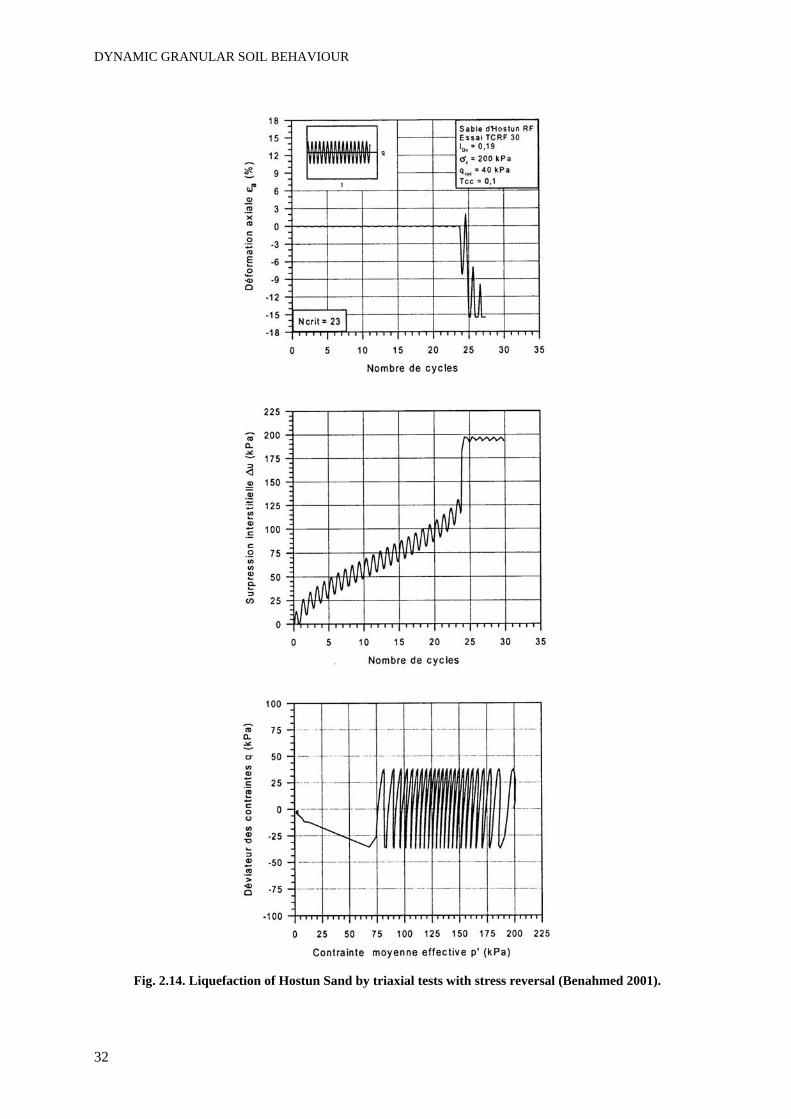
DYNAMIC GRANULAR SOIL BEHAVIOUR
32
Fig. 2.14. Liquefaction of Hostun Sand by triaxial tests with stress reversal (Benahmed 2001).
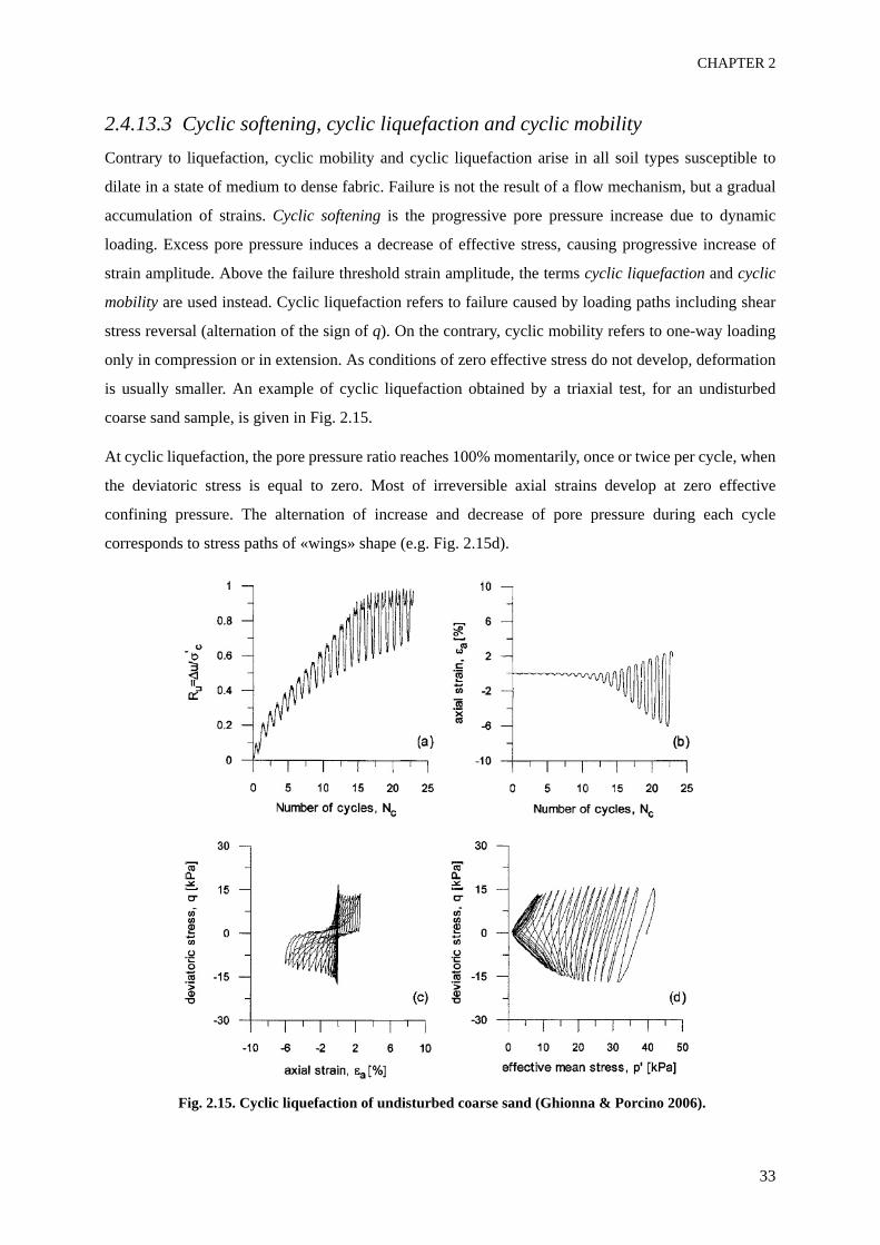
CHAPTER 2
33
2.4.13.3 Cyclic softening, cyclic liquefaction and cyclic mobilityContrary to liquefaction, cyclic mobility and cyclic liquefaction arise in all soil types susceptible to
dilate in a state of medium to dense fabric. Failure is not the result of a flow mechanism, but a gradual
accumulation of strains. Cyclic softening is the progressive pore pressure increase due to dynamic
loading. Excess pore pressure induces a decrease of effective stress, causing progressive increase of
strain amplitude. Above the failure threshold strain amplitude, the terms cyclic liquefaction and cyclic
mobility are used instead. Cyclic liquefaction refers to failure caused by loading paths including shear
stress reversal (alternation of the sign of q). On the contrary, cyclic mobility refers to one-way loading
only in compression or in extension. As conditions of zero effective stress do not develop, deformation
is usually smaller. An example of cyclic liquefaction obtained by a triaxial test, for an undisturbed
coarse sand sample, is given in Fig. 2.15.
At cyclic liquefaction, the pore pressure ratio reaches 100% momentarily, once or twice per cycle, when
the deviatoric stress is equal to zero. Most of irreversible axial strains develop at zero effective
confining pressure. The alternation of increase and decrease of pore pressure during each cycle
corresponds to stress paths of «wings» shape (e.g. Fig. 2.15d).
Fig. 2.15. Cyclic liquefaction of undisturbed coarse sand (Ghionna & Porcino 2006).

DYNAMIC GRANULAR SOIL BEHAVIOUR
34
Cyclic liquefaction has been observed in many experimental study, for silts, sands and gravels, for
reconstituted or intact samples (Luong 1980; Mohkam 1983; Ishihara & Nagase 1988; Vaid et al. 1989;
Endo & Komanobe 1995; Hyodo et al. 1998; Benahmed 2001; Choi & Arduino 2004; Toyota et al.
2004; Bray & Sancio 2006; Ghionna & Porcino 2006; Sanin & Wijewickreme 2006; Hyde et al. 2006;
Porcino et al. 2008).
2.4.13.4 The cyclic stress approachFor a given soil layer, the assessment of liquefaction susceptibility by the cyclic stress approach follows
three steps:
• Characterization of earthquake loading: an irregular earthquake motion of known moment magnitude
is turned into an equivalent cyclic loading of regular amplitudes with a certain number of cycles.
• Characterization of liquefaction resistance of soil: the cyclic stress ratio CSR at a given number of
cycles and a given void ratio is obtained by laboratory tests or correlations with in situ tests.
• Evaluation of the factor of safety, which is the ratio of the CSR required to cause liquefaction on the
CSR equivalent to earthquake-induced shear stress.
The cyclic stress ratio CSR is a simple concept widely used to evaluate the strength of soil upon cyclic
load, for both flow liquefaction and cyclic liquefaction failure type. This parameter is obtained for
stress-controlled laboratory tests. CSR is defined as the ratio of the maximum cyclic shear stress to the
initial average effective normal stress. For the triaxial test, it is calculated by:
(2.21)
For a given void ratio and a given soil, the CSR is supposedly uniquely related to the number of cycles
at failure (Finn et al. 1971), where the criterion for failure is usually based on a strain amplitude of 5%
DA. An example of CSR curves determined for silty sand is shown in (Fig. 2.16). CSR mainly depends
on relative density, also it is used as a criterion for instability upon liquefaction.
The CSR obtained by triaxial tests is multiplied by a correction factor for matching the values of CSR
in simple shear tests or in the field (Kramer 1996). The loading pattern also is important; Benahmed
(2001) showed that CSR is higher for tests without stress reversal (q > 0 only) than for tests with stress
reversal. CSR is finally very sensitive to sample preparation, prestraining, OCR and aging effects
(Dobry et al. 1982). The comparison between angular sand (Hostun sand) and round sand
(Fontainebleau sand) shows that cyclic strength is higher for angular materials (Benahmed 2001).
CSRqmax
2 3
0
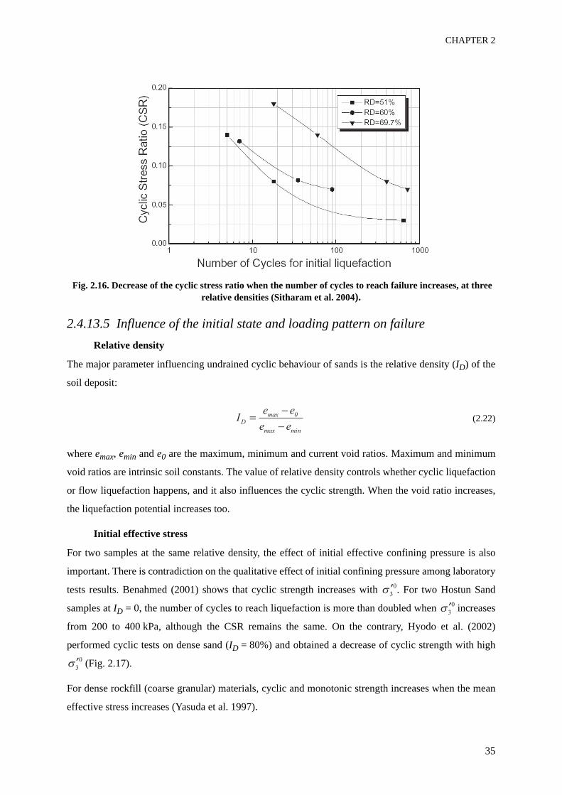
CHAPTER 2
35
Fig. 2.16. Decrease of the cyclic stress ratio when the number of cycles to reach failure increases, at three relative densities (Sitharam et al. 2004).
2.4.13.5 Influence of the initial state and loading pattern on failureRelative density
The major parameter influencing undrained cyclic behaviour of sands is the relative density (ID) of the
soil deposit:
(2.22)
where emax, emin and e0 are the maximum, minimum and current void ratios. Maximum and minimum
void ratios are intrinsic soil constants. The value of relative density controls whether cyclic liquefaction
or flow liquefaction happens, and it also influences the cyclic strength. When the void ratio increases,
the liquefaction potential increases too.
Initial effective stress
For two samples at the same relative density, the effect of initial effective confining pressure is also
important. There is contradiction on the qualitative effect of initial confining pressure among laboratory
tests results. Benahmed (2001) shows that cyclic strength increases with . For two Hostun Sand
samples at ID = 0, the number of cycles to reach liquefaction is more than doubled when increases
from 200 to 400 kPa, although the CSR remains the same. On the contrary, Hyodo et al. (2002)
performed cyclic tests on dense sand (ID = 80%) and obtained a decrease of cyclic strength with high
(Fig. 2.17).
For dense rockfill (coarse granular) materials, cyclic and monotonic strength increases when the mean
effective stress increases (Yasuda et al. 1997).
Ie e
e eD
max
max
0
min
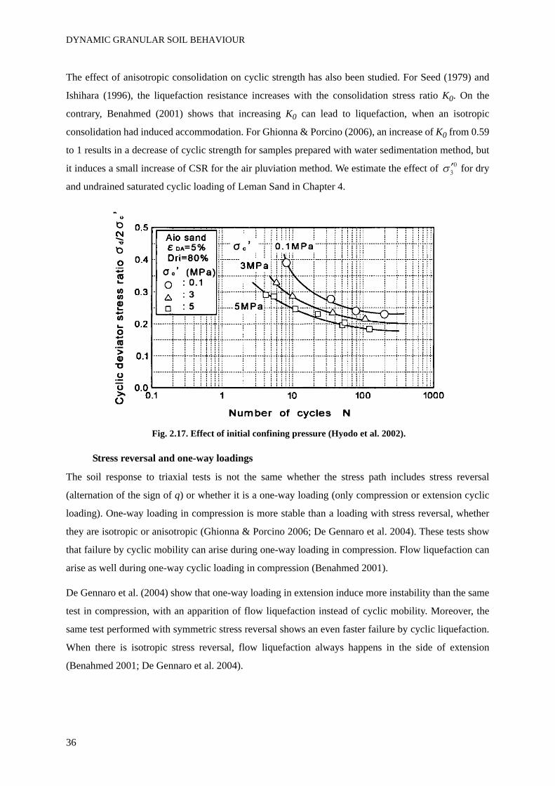
DYNAMIC GRANULAR SOIL BEHAVIOUR
36
The effect of anisotropic consolidation on cyclic strength has also been studied. For Seed (1979) and
Ishihara (1996), the liquefaction resistance increases with the consolidation stress ratio K0. On the
contrary, Benahmed (2001) shows that increasing K0 can lead to liquefaction, when an isotropic
consolidation had induced accommodation. For Ghionna & Porcino (2006), an increase of K0 from 0.59
to 1 results in a decrease of cyclic strength for samples prepared with water sedimentation method, but
it induces a small increase of CSR for the air pluviation method. We estimate the effect of for dry
and undrained saturated cyclic loading of Leman Sand in Chapter 4.
Fig. 2.17. Effect of initial confining pressure (Hyodo et al. 2002).
Stress reversal and one-way loadings
The soil response to triaxial tests is not the same whether the stress path includes stress reversal
(alternation of the sign of q) or whether it is a one-way loading (only compression or extension cyclic
loading). One-way loading in compression is more stable than a loading with stress reversal, whether
they are isotropic or anisotropic (Ghionna & Porcino 2006; De Gennaro et al. 2004). These tests show
that failure by cyclic mobility can arise during one-way loading in compression. Flow liquefaction can
arise as well during one-way cyclic loading in compression (Benahmed 2001).
De Gennaro et al. (2004) show that one-way loading in extension induce more instability than the same
test in compression, with an apparition of flow liquefaction instead of cyclic mobility. Moreover, the
same test performed with symmetric stress reversal shows an even faster failure by cyclic liquefaction.
When there is isotropic stress reversal, flow liquefaction always happens in the side of extension
(Benahmed 2001; De Gennaro et al. 2004).
CHAPTER 2
37
2.4.14 ConclusionsThe principles and phenomena necessary to understand and analyse cyclic sand behaviour are described
in this section, with an emphasis on conditions prevailing in triaxial tests. Indeed, these concepts are all
used further during the interpretation of our test results, presented in Chapters 4, 5 and 6. The key
concepts are summarized with a short mention of the context in which they are used for our triaxial
tests:
• The distinction between triaxial extension and triaxial compression is of major importance to
understand all monotonic and cyclic test results including stress reversal.
• The definition of steady state and phase transformation introduces the SS and PT lines (in the p’ - q
plane), which are obtained for the two sands tested during this project. These concepts are also used
in the elastoplastic model described in section 2.6 and implemented in Chapter 7.
• The importance of strain amplitude for identifying the soil response is mentioned several times in
this section, and is repeatedly observed in our tests. The classification of cyclic motions into small,
medium and large strain amplitude is often used further for the description of soil behaviour
(Chapters 4 to 7).
• Dilatancy phenomenon and the increase of pore pressure ratio are important to understand failure by
cyclic liquefaction, which is often mentioned in all experimental and numerical results on dense
sand.
• Stiffness degradation and failure mechanisms under cyclic loading are presented, with mentions of
triggering factors. The definition of failure, based on a threshold deviatoric strain amplitude, is
analysed in Chapter 4 for cyclic liquefaction of Leman Sand. Both stiffness degradation and failure
are analysed for many experimental conditions, and they are also important for the evaluation of the
two models presented in Chapter 7.
After this qualitative description of sand behaviour under cyclic loading, the dynamic material
parameters are introduced below to allow a quantitative estimation of the soil response.
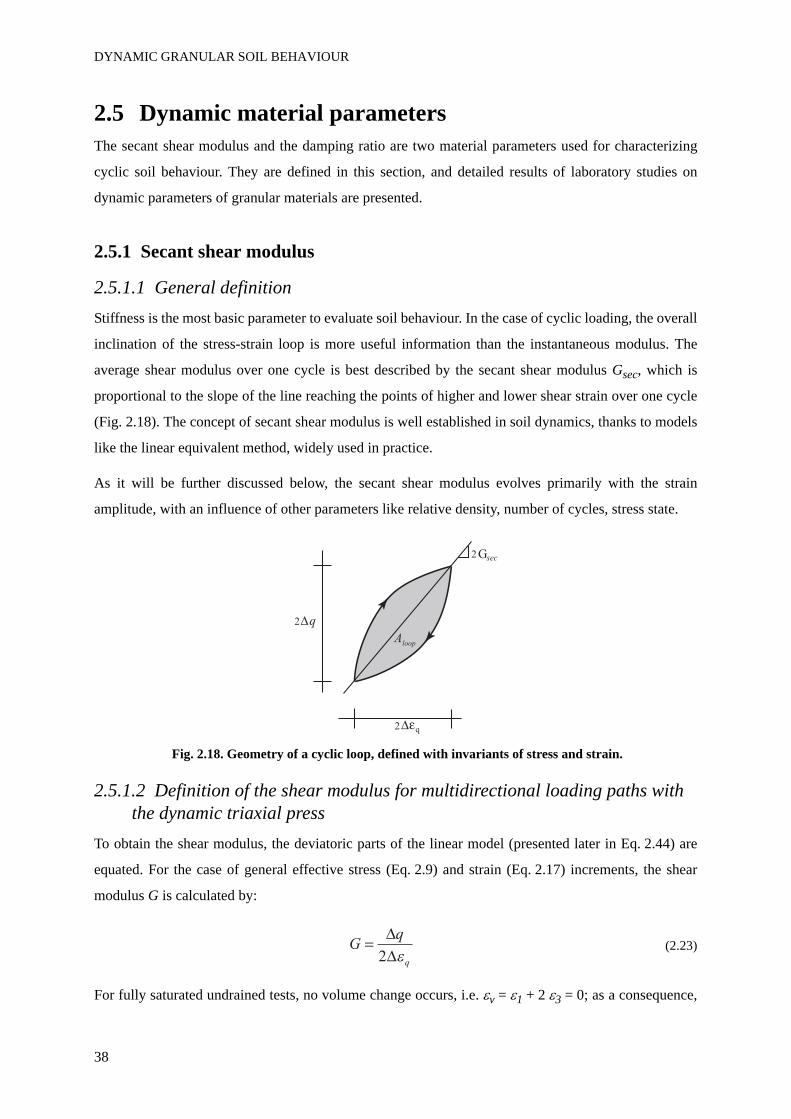
DYNAMIC GRANULAR SOIL BEHAVIOUR
38
2.5 Dynamic material parametersThe secant shear modulus and the damping ratio are two material parameters used for characterizing
cyclic soil behaviour. They are defined in this section, and detailed results of laboratory studies on
dynamic parameters of granular materials are presented.
2.5.1 Secant shear modulus
2.5.1.1 General definitionStiffness is the most basic parameter to evaluate soil behaviour. In the case of cyclic loading, the overall
inclination of the stress-strain loop is more useful information than the instantaneous modulus. The
average shear modulus over one cycle is best described by the secant shear modulus Gsec, which is
proportional to the slope of the line reaching the points of higher and lower shear strain over one cycle
(Fig. 2.18). The concept of secant shear modulus is well established in soil dynamics, thanks to models
like the linear equivalent method, widely used in practice.
As it will be further discussed below, the secant shear modulus evolves primarily with the strain
amplitude, with an influence of other parameters like relative density, number of cycles, stress state.
Fig. 2.18. Geometry of a cyclic loop, defined with invariants of stress and strain.
2.5.1.2 Definition of the shear modulus for multidirectional loading paths with the dynamic triaxial press
To obtain the shear modulus, the deviatoric parts of the linear model (presented later in Eq. 2.44) are
equated. For the case of general effective stress (Eq. 2.9) and strain (Eq. 2.17) increments, the shear
modulus G is calculated by:
(2.23)
For fully saturated undrained tests, no volume change occurs, i.e. εv = ε1 + 2 ε3 = 0; as a consequence,
CHAPTER 2
39
ε3 = -1/2 ε1 and εq = 3/2 ε1. Thus the shear modulus can be calculated by:
(2.24)
Considering a cyclic loading, the secant shear modulus Gsec is usually used (cf. below).
2.5.1.3 Other elastic parametersYoung’s modulus and Poisson’s ratio
The linear elastic equation with E and ν can be written, for the triaxial case and for an effective stress
increment (defined in Eq. 2.9), as
(2.25)
The constants E andν can be determined in this general stress increment since this reduces to two
equations with two unknowns, which are easy to solve numerically.
In the simplified case of constant confining pressure (Δσ3 = 0), E and ν are simply found by:
(2.26)
Bulk modulus
For drained tests with volume change, the bulk modulus can be calculated by identifying the spherical
parts of the linear model (Eq. 2.44), in the case of a general stress increment:
(2.27)
2.5.2 Damping ratio
2.5.2.1 IntroductionStress waves in a soil substratum induce cyclic shearing and compressional loadings with decay of the
amplitude away from the source, which is partly due to material losses (cf. section 2.3.4). The energy
transformation in the material is observed through its hysteretic behaviour. Loops of varying amplitude
and direction appear in the stress-strain plane, which is a major difference between considering cyclic
loading of soils from monotonic loadings. In the laboratory also, during harmonic or triangular loading,
stress-strain curves form series of loops. The damping ratio quantifies those material losses. More than
ij
1
3
3
0 0
0 0
0 0
1 0 0
0 0
0 0
1 2q
E
3
1 0 0
0 1 0
0 0 1E
Eq
and1 3
1
Kp
b
V
'
DYNAMIC GRANULAR SOIL BEHAVIOUR
40
just a model parameter, its physical meaning is crucial for understanding cyclic soil behaviour.
The most common way, among geotechnical engineers, to apprehend the energy loss of a soil submitted
to cyclic loading is the damping ratio (D or ξ). There are other parameters which could also be used,
and which are related in some way to the damping ratio (Kramer 1996; Wolf 1994):
• the Quality factor Q = 1/(2D) is used by seismologists
• the loss factor η = 2D is used in vibration analysis
• the specific damping capacity Ψ = 2πD
• the coefficient of friction tanδ = 2D, where δ is an angle of internal friction of the soil
In seismic analysis, the damping ratio can include both the material damping and the radiation, which is
the geometrical decrease of stress waves with the increasing distance from the source. Semblat &
Luong (1998) provide experimental evidences on the separation of the attenuation of spherical waves,
propagating in a finite medium in centrifuge tests, into a material and a geometrical attenuation. The
radiation damping is not taken into account in the following chapters.
2.5.2.2 Physical interpretation of dampingIt is commonly admitted that the hysteretic behaviour of soils is caused by energy dissipation. The
mechanisms causing material damping include friction, plastic yielding and ultimately heat generation
(Kramer 1996). The damping ratio of a soil, for a given stress-strain loop, is associated with the
dissipated energy divided by the maximum stored (i.e. elastic) energy per cycle.
Material damping is generally considered to include two types of mechanisms (Bolton & Wilson 1990;
Wang & Santamarina 2007). The first is a frequency-dependent viscous loss, caused by the pore fluid
and internal energy coupling. The second is a frequency-independent hysteretic loss due to the
displacements in the soil matrix, namely friction occurring at contact points. In essence, dry granular
material is generally assumed to be hysteretic and to absorb energy as a function of cyclic strain. Above
the linear threshold, energy dissipation of cyclically loaded dry grains is preponderantly of frictional
nature (Wang & Santamarina 2007).
For dry cohesionless soils, the deformation of the system is essentially due to rearrangement of the soil
matrix, and not to the deformation of the grains (Verruijt & Cordova 2001). The sliding or slipping of
grains involves friction at interparticle contact, which is associated with hysteretic damping ratio. It is
also important that the rearrangement of the grains occurs during both loading and unloading parts of
the cycle. The sliding can be irreversible, or reversible if the grains come back to their original place
after unloading.
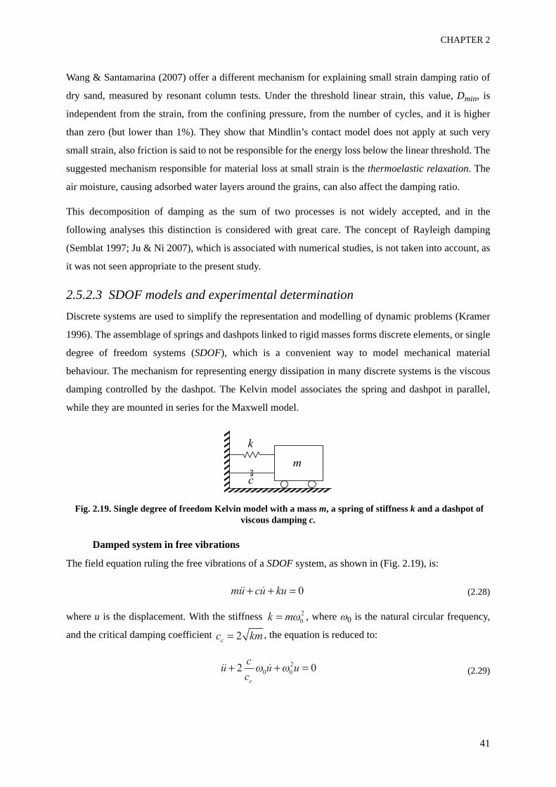
CHAPTER 2
41
Wang & Santamarina (2007) offer a different mechanism for explaining small strain damping ratio of
dry sand, measured by resonant column tests. Under the threshold linear strain, this value, Dmin, is
independent from the strain, from the confining pressure, from the number of cycles, and it is higher
than zero (but lower than 1%). They show that Mindlin’s contact model does not apply at such very
small strain, also friction is said to not be responsible for the energy loss below the linear threshold. The
suggested mechanism responsible for material loss at small strain is the thermoelastic relaxation. The
air moisture, causing adsorbed water layers around the grains, can also affect the damping ratio.
This decomposition of damping as the sum of two processes is not widely accepted, and in the
following analyses this distinction is considered with great care. The concept of Rayleigh damping
(Semblat 1997; Ju & Ni 2007), which is associated with numerical studies, is not taken into account, as
it was not seen appropriate to the present study.
2.5.2.3 SDOF models and experimental determinationDiscrete systems are used to simplify the representation and modelling of dynamic problems (Kramer
1996). The assemblage of springs and dashpots linked to rigid masses forms discrete elements, or single
degree of freedom systems (SDOF), which is a convenient way to model mechanical material
behaviour. The mechanism for representing energy dissipation in many discrete systems is the viscous
damping controlled by the dashpot. The Kelvin model associates the spring and dashpot in parallel,
while they are mounted in series for the Maxwell model.
Fig. 2.19. Single degree of freedom Kelvin model with a mass m, a spring of stiffness k and a dashpot of viscous damping c.
Damped system in free vibrations
The field equation ruling the free vibrations of a SDOF system, as shown in (Fig. 2.19), is:
(2.28)
where u is the displacement. With the stiffness , where ω0 is the natural circular frequency,
and the critical damping coefficient , the equation is reduced to:
(2.29)
m
k
c
mu cu ku 0
k m 0
2
c kmc 2
uc
cu u
c
2 00 0
2
DYNAMIC GRANULAR SOIL BEHAVIOUR
42
The damping ratio is defined as the ratio . The solution of the differential equation depends
on the damping ratio value:
• if D > 1, the system is called overdamped. It monotonically reaches an equilibrium value.
• if D = 1, there is a unique oscillation before reaching the equilibrium value. This is the critically
damped case.
• if D < 1, oscillations occur with a decreasing amplitude. This is an underdamped system. The smaller
the damping ratio, the faster oscillation amplitudes decrease.
The underdamped case is the one that concerns earthquake engineering and vibratory analysis of
structures.
The experimental evaluation of damping ratio can be performed in a free vibratory system. The
resonant column test can be used in that way: after reaching the resonant frequency, the drive system is
cut off. The decay of free vibrations is observed to determine the damping ratio (Ishihara 1996).
Damped system in forced harmonic vibrations
In such a SDOF system, the combination of the spring and the dashpot exerts a net force
on the mass. Considering a harmonic forced vibration , the
hysteresis force - displacement loops of the system are inclined ellipses, as depicted in Fig. 2.20.
The damping ratio of that system can be experimentally obtained from the force - displacement loop.
The calculation of the energy dissipated during one cycle (WD) gives:
(2.30)
Resulting in . Another parameter used for calculating the damping ratio is the
maximum elastic stored energy (WS), which is obtained at the point of maximum displacement. The
calculation of WS gives:
(2.31)
thus . The damping ratio definition for free vibrations can be expressed as .
Replacing c and k by the relations obtained above, and assuming , leads to the famous relation:
(2.32)
The damping ratio is obtained experimentally, from the geometry of stress-strain loops, thanks to this
relationship (Eq. 2.32).
D c cc
F ku t cu t( ) ( ) u t u t( ) sin( )0
W Fdu
dtdt c uD
t
t
0
0 2
0
2
W kuS1
2 0
2
D c k0 2
0
DW
W
D
S4
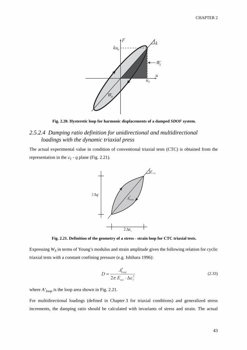
CHAPTER 2
43
Fig. 2.20. Hysteretic loop for harmonic displacements of a damped SDOF system.
2.5.2.4 Damping ratio definition for unidirectional and multidirectional loadings with the dynamic triaxial press
The actual experimental value in condition of conventional triaxial tests (CTC) is obtained from the
representation in the ε1 - q plane (Fig. 2.21).
Fig. 2.21. Definition of the geometry of a stress - strain loop for CTC triaxial tests.
Expressing WS in terms of Young’s modulus and strain amplitude gives the following relation for cyclic
triaxial tests with a constant confining pressure (e.g. Ishihara 1996):
(2.33)
where A’loop is the loop area shown in Fig. 2.21.
For multidirectional loadings (defined in Chapter 3 for triaxial conditions) and generalized stress
increments, the damping ratio should be calculated with invariants of stress and strain. The actual
k
DA
E
loop
sec 12 2
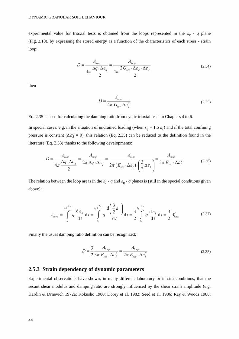
DYNAMIC GRANULAR SOIL BEHAVIOUR
44
experimental value for triaxial tests is obtained from the loops represented in the εq - q plane
(Fig. 2.18), by expressing the stored energy as a function of the characteristics of each stress - strain
loop:
(2.34)
then
(2.35)
Eq. 2.35 is used for calculating the damping ratio from cyclic triaxial tests in Chapters 4 to 6.
In special cases, e.g. in the situation of undrained loading (when εq = 1.5 ε1) and if the total confining
pressure is constant (Δσ3 = 0), this relation (Eq. 2.35) can be reduced to the definition found in the
literature (Eq. 2.33) thanks to the following developments:
(2.36)
The relation between the loop areas in the ε1 - q and εq - q planes is (still in the special conditions given
above):
(2.37)
Finally the usual damping ratio definition can be recognized:
(2.38)
2.5.3 Strain dependency of dynamic parametersExperimental observations have shown, in many different laboratory or in situ conditions, that the
secant shear modulus and damping ratio are strongly influenced by the shear strain amplitude (e.g.
Hardin & Drnevich 1972a; Kokusho 1980; Dobry et al. 1982; Seed et al. 1986; Ray & Woods 1988;
DA
q
A
Gloop
q
loop
sec q q4
24
2
2
DA
q
A
q
A
E
loop
q
loop
q
loop
sec 1 142
22
3
2
A
E
loop
sec 13 2
A qt
t qt
t qt
loop
q
t
t1
t
t
1d
dd
d
dd
d
d0
0
0
0
2 2 3
2 3
2tt
t
loopt A
0
0
2
3
2d
DA
E
A
E
loop
sec 1
loop
sec 1
3
2 3 22 2
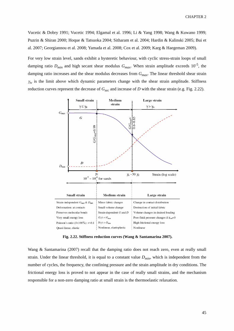
CHAPTER 2
45
Vucetic & Dobry 1991; Vucetic 1994; Elgamal et al. 1996; Li & Yang 1998; Wang & Kuwano 1999;
Puzrin & Shiran 2000; Hoque & Tatsuoka 2004; Sitharam et al. 2004; Hardin & Kalinski 2005; Bui et
al. 2007; Georgiannou et al. 2008; Yamada et al. 2008; Cox et al. 2009; Karg & Haegeman 2009).
For very low strain level, sands exhibit a hysteretic behaviour, with cyclic stress-strain loops of small
damping ratio Dmin and high secant shear modulus Gmax. When strain amplitude exceeds 10-5, the
damping ratio increases and the shear modulus decreases from Gmax. The linear threshold shear strain
γtv is the limit above which dynamic parameters change with the shear strain amplitude. Stiffness
reduction curves represent the decrease of Gsec and increase of D with the shear strain (e.g. Fig. 2.22).
Fig. 2.22. Stiffness reduction curves (Wang & Santamarina 2007).
Wang & Santamarina (2007) recall that the damping ratio does not reach zero, even at really small
strain. Under the linear threshold, it is equal to a constant value Dmin, which is independent from the
number of cycles, the frequency, the confining pressure and the strain amplitude in dry conditions. The
frictional energy loss is proved to not appear in the case of really small strains, and the mechanism
responsible for a non-zero damping ratio at small strain is the thermoelastic relaxation.
DYNAMIC GRANULAR SOIL BEHAVIOUR
46
2.5.4 Evaluation of the elastic shear modulus The elastic shear modulus, or maximum shear modulus, or initial shear modulus Gmax can be calculated
from the shear wave velocity (cs), measured by in situ geophysical tests (cf. Appendix 1):
(2.39)
Laboratory studies, like bender element tests, resonant column tests and cyclic triaxial tests at small
strain also allow to measure Gmax on reconstituted or intact samples. Huot (1999) shows that Gmax has
the same value, whether it is obtained with ultra-sonic technique (acoustic transmission) or by pseudo-
dynamic tests. There is now general agreement that soil elastic properties evaluated at very small
strains by pseudo-static tests are consistent with the ones evaluated by dynamic tests, when same
conditions prevail (Tatsuoka 2006).
If experimental or in situ data are not available, empirical equations derived from laboratory studies are
numerous. Elastic shear modulus is usually given under the form (e.g. Kokusho 1980; Ishihara 1996):
(2.40)
where A is a parameter depending on soil, Fc is the compacity function depending on void ratio e, pref is
a reference value of pressure, ne is an adimentional parameter, and the soil parameter k depends on
OCR. The linear shear modulus mainly depends on void ratio and confining pressure. The function
Fc(e) can be evaluated by (Hardin & Drnevich 1972b):
(2.41)
The ne coefficient is often defined by ne = 0.5, although it can be determined by laboratory tests,
depending of the soil type. Moreover, OCR widely influences elastic modulus value through the
plasticity index PI. The most important factors influencing Gmax and Dmin are summarized in Tab. 2.1.
G cmax s
2
G AF ep
pmax c
k
ref
ne
OCR
F ee
c
1
0 3 0 7 2. .
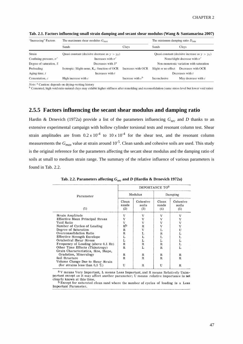
CHAPTER 2
47
Tab. 2.1. Factors influencing small strain damping and secant shear modulus (Wang & Santamarina 2007)
2.5.5 Factors influencing the secant shear modulus and damping ratioHardin & Drnevich (1972a) provide a list of the parameters influencing Gsec and D thanks to an
extensive experimental campaign with hollow cylinder torsional tests and resonant column test. Shear
strain amplitudes are from 0.2 x 10⁻⁴ to 10 x 10-4 for the shear test, and the resonant column
measurements the Gmax value at strain around 10-5. Clean sands and cohesive soils are used. This study
is the original reference for the parameters affecting the secant shear modulus and the damping ratio of
soils at small to medium strain range. The summary of the relative influence of various parameters is
found in Tab. 2.2.
Tab. 2.2. Parameters affecting Gsec and D (Hardin & Drnevich 1972a)
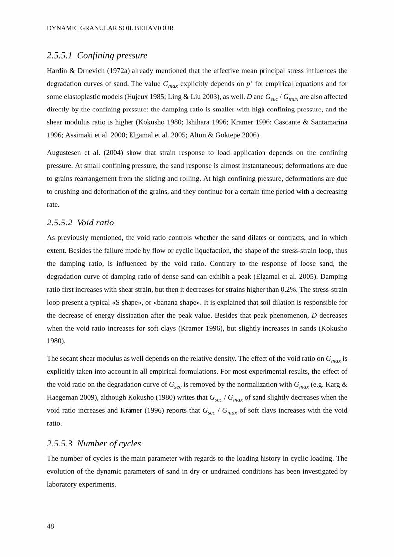
DYNAMIC GRANULAR SOIL BEHAVIOUR
48
2.5.5.1 Confining pressureHardin & Drnevich (1972a) already mentioned that the effective mean principal stress influences the
degradation curves of sand. The value Gmax explicitly depends on p’ for empirical equations and for
some elastoplastic models (Hujeux 1985; Ling & Liu 2003), as well. D and Gsec / Gmax are also affected
directly by the confining pressure: the damping ratio is smaller with high confining pressure, and the
shear modulus ratio is higher (Kokusho 1980; Ishihara 1996; Kramer 1996; Cascante & Santamarina
1996; Assimaki et al. 2000; Elgamal et al. 2005; Altun & Goktepe 2006).
Augustesen et al. (2004) show that strain response to load application depends on the confining
pressure. At small confining pressure, the sand response is almost instantaneous; deformations are due
to grains rearrangement from the sliding and rolling. At high confining pressure, deformations are due
to crushing and deformation of the grains, and they continue for a certain time period with a decreasing
rate.
2.5.5.2 Void ratioAs previously mentioned, the void ratio controls whether the sand dilates or contracts, and in which
extent. Besides the failure mode by flow or cyclic liquefaction, the shape of the stress-strain loop, thus
the damping ratio, is influenced by the void ratio. Contrary to the response of loose sand, the
degradation curve of damping ratio of dense sand can exhibit a peak (Elgamal et al. 2005). Damping
ratio first increases with shear strain, but then it decreases for strains higher than 0.2%. The stress-strain
loop present a typical «S shape», or «banana shape». It is explained that soil dilation is responsible for
the decrease of energy dissipation after the peak value. Besides that peak phenomenon, D decreases
when the void ratio increases for soft clays (Kramer 1996), but slightly increases in sands (Kokusho
1980).
The secant shear modulus as well depends on the relative density. The effect of the void ratio on Gmax is
explicitly taken into account in all empirical formulations. For most experimental results, the effect of
the void ratio on the degradation curve of Gsec is removed by the normalization with Gmax (e.g. Karg &
Haegeman 2009), although Kokusho (1980) writes that Gsec / Gmax of sand slightly decreases when the
void ratio increases and Kramer (1996) reports that Gsec / Gmax of soft clays increases with the void
ratio.
2.5.5.3 Number of cyclesThe number of cycles is the main parameter with regards to the loading history in cyclic loading. The
evolution of the dynamic parameters of sand in dry or undrained conditions has been investigated by
laboratory experiments.
CHAPTER 2
49
Undrained conditions
Kramer (1996) summarizes the effect of the number of cycles on dynamic parameters for sands, under
undrained stress-controlled conditions: (i) Gsec / Gmax decreases after N for large enough strains (above
the volumetric cyclic threshold shear strain) and (ii) the effect of N on D is not significant at moderate
strain and number of cycles.
Stiffness degradation during cyclic loading is then viewed as a consequence of the variation (increase or
decrease) of excess pore pressure, and strongly depends on the soil type. The degradation index DI is
defined, to obtain a quantitative description of the phenomenon. For the Nth cycle, it can be expressed
by:
(2.42)
where is the shear modulus determined at the Nth cycle and is the initial shear modulus
(during the first cycle).
Dry conditions
Contrary to the undrained case, the secant shear modulus of dry sand increases with the number of
cycles, i.e. stiffness increases, while the damping ratio markedly decreases (Ray & Woods 1988; Li &
Yang 1998). This observations holds only at strain amplitude above the volumetric cyclic threshold
shear strain (Li & Yang 1998).
2.5.5.4 Other effectsOther soil or test parameters influence the dynamic parameters, such as soil anisotropy (Chaudhary et
al. 2002; AnhDan et al. 2006), fine content of clayey sand (Wang & Kuwano 1999), plasticity index of
fine-grained soils (Okur & Ansal 2007), irregular loading (Ray & Woods 1988), particle shape (Bui et
al. 2007; Khan et al. 2008), degree of saturation (Wang & Santamarina 2007).
DIG
G
sec
N
sec
1
Gsec
NGsec
1
DYNAMIC GRANULAR SOIL BEHAVIOUR
50
2.6 Constitutive modelling of granular soils for cyclic loading
2.6.1 IntroductionMany constitutive models may be selected for an overview of existing tools for dynamic modelling of
soils. However, it is not the aim here to list all of them; it is intended instead to describe only those
explicitly mentioned further within the exploitation of laboratory results (see Chapter 7). In particular,
all the hysteretic models based on Masing’s rule (hyperbolic model, Ramberg-Osgood model, Iwan
model, Cundall-Pyke model, logarithmic function (Puzrin & Shiran 2000)), of intermediary complexity
between the equivalent linear model and the multi-mechanisms elastoplastic model, are not mentioned
anymore.
A concise description of four different models of increasing complexity is presented below:
• The linear model
• The linear viscoelastic model
• The linear equivalent model
• The multi-mechanisms elastoplastic model of Hujeux.
2.6.2 Linear elastic modelWhen strain is small enough (γ < 10-5), soil is assumed to behave linearly. The deformations of granular
soils are elastic and recoverable. The relationship between stress tensor and strain tensor is given by:
(2.43)
where D is the rigidity tensor, which is of the fourth order in the general case. For the linear isotropic
model, only two parameters are necessary to describe the system. The symmetry allows simplification
to the relationship:
(2.44)
where G is the shear modulus and K is the bulk modulus. Other equivalent relations are used with
different parameters: the Lamé coefficients μ and λ, the Young’s modulus E and the Poisson’s ratio ν
are also used in soil mechanics.
The main subject of interest for this simple model is the influence of initial conditions, such as void
ratio, confining pressure or overconsolidation state of the medium.
D : or Dij ijkl kl
ij ij ij ij b V ijt p G e K2
CHAPTER 2
51
However, experimental evidences tend to show that even at very small strain, energy dissipation
through damping exists as well during cyclic loading (Huot 1999; Wang & Santamarina 2007).
Damping is neglected in linear elasticity, which is a major disadvantage. A viscoelastic model can be
used instead, which uses a complex modulus with a viscosity parameter included.
2.6.3 Linear viscoelastic modelThe linear viscoelastic model is a way of introducing a damping component, which induces stress -
strain curves with hysteresis shapes. In unidimensional condition, the material is seen as a spring -
dashpot system, in which model parameters are the spring constant (G) and the dashpot constant (η).
The Kelvin-Voigt model, with spring and dashpot mounted in parallel, gives the constitutive relation
(for the 1D problem):
(2.45)
Where τ the shear stress and γ the shear strain. A complex modulus G* is defined, written as a function
of the angular frequency (ω):
(2.46)
The viscoelastic model has a simple expression in the frequency domain:
(2.47)
2.6.4 Linear equivalent modelNonlinear soil behaviour can be simply taken into account by considering the evolution of the dynamic
parameters (Gsec, D) with shear strain within a modified viscoelastic model (e.g the programme
SHAKE91 (Idriss & Sun 1992)). In the linear equivalent model, the complex modulus (G*) is also a
function of the shear strain γ, i.e. , thanks to numerical iterations. The complex modulus
(Eq. 2.46) depends on the secant shear modulus (G = Gsec) and the damping ratio (η = 2D), which are
the model parameters defined for each soil as a function of γ. Actually, the input parameter of the linear
equivalent model is not directly Gsec, but the normalized function Gsec / Gmax vs. γ.
The curves of the decrease of Gsec / Gmax and increase of D with γ are usually obtained from laboratory
tests or from the literature. For example, Fig. 2.23 and Fig. 2.24 present the evolution of both
parameters as a function of shear strain for different initial pressures. We provide such curves for
Leman Sand and Fonderie Sand in various conditions (Chapters 4 to 6).
Gt
d
d
G G i*
G*
G G* * ,
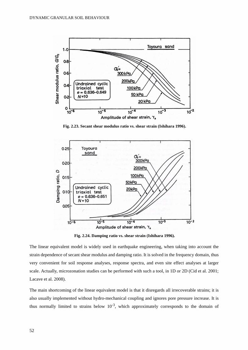
DYNAMIC GRANULAR SOIL BEHAVIOUR
52
Fig. 2.23. Secant shear modulus ratio vs. shear strain (Ishihara 1996).
Fig. 2.24. Damping ratio vs. shear strain (Ishihara 1996).
The linear equivalent model is widely used in earthquake engineering, when taking into account the
strain dependence of secant shear modulus and damping ratio. It is solved in the frequency domain, thus
very convenient for soil response analyses, response spectra, and even site effect analyses at larger
scale. Actually, microzonation studies can be performed with such a tool, in 1D or 2D (Cid et al. 2001;
Lacave et al. 2008).
The main shortcoming of the linear equivalent model is that it disregards all irrecoverable strains; it is
also usually implemented without hydro-mechanical coupling and ignores pore pressure increase. It is
thus normally limited to strains below 10-3, which approximately corresponds to the domain of
CHAPTER 2
53
stabilized hysteretic behaviour (Hujeux 1985). Another drawback is the removal of most of the high-
frequency content of the response, because of an overdamping of high frequencies (Hartzell et al.
2004). We implement the linear equivalent model in Chapter 7, and evaluate these problems with
regard to our test results.
An example of a modified equivalent linear model by Yoshida et al. (2002) shows that this model is
perfectible, and can still be promising. This new model is claimed «to be applicable at more than 1%
shear strain». Assimaki & Kausel (2002) also propose a new algorithm for the linear equivalent
method, which improves the modelling of nonlinear site amplification, compared to the initial model.
2.6.5 Elastoplastic models
2.6.5.1 IntroductionAdvanced constitutive models suitable for cyclic loading were also adapted from existing theories of
plasticity, elastoplasticity, viscoplasticity, hypoplasticity. Those complete effective stress models
describe soil behaviour on a range of stress paths. Their development is based on incremental relations
between strain and effective stress. Such models predict transient and permanent deformations within
the soil mass, and are then much more interesting than the linear equivalent model for modelling
catastrophic displacements or collapse of soil structures (e.g. Muir Wood 1998).
Among advanced elastoplastic models, the multi-surface theory (Mroz et al. 1981) can reproduce cyclic
behaviour with either two surfaces or an infinite number of nesting surfaces. An example of a multiple
surface plasticity model with the «u - p» formulation is presented by Elgamal et al. (2002) for granular
soils. Another family of models is the bounding surface theory. For example Khalili et al. (2005)
applied it to cyclic loading of sand.
The advanced model used in this thesis (Chapter 7) is based on multi-mechanisms elastoplasticity.
Hujeux (1985) describes its application to cyclic loading of sand. Laloui (1992), Mellal (1997), Lopez-
Caballero (2003), Cekerevac (2003) thoroughly developed the Hujeux model for all kinds of
environmental loading, such as thermal loading, unsaturated soil behaviour and dynamic loading from
earthquake. The thermo-hydro-mechanical coupling is included in the last advances of the model
ACMEG in various PhD thesis presented at EPFL (François 2008; Koliji 2008; Péron 2008; Nuth
2009).
2.6.5.2 Description of the Hujeux model for cyclic loadingUsing the concept of multi-mechanisms plasticity (Hujeux, 1985), the total irreversible deviatoric strain
increment is induced by coupled dissipative processes: an isotropic and three deviatoric plasticq
p
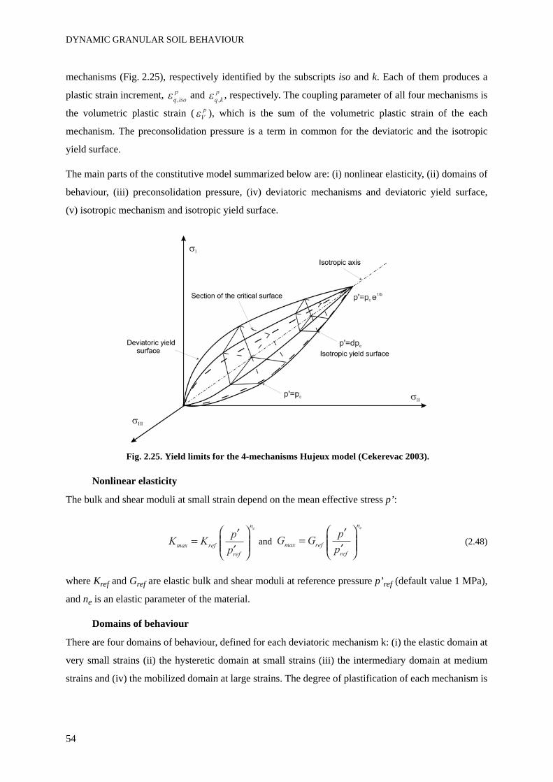
DYNAMIC GRANULAR SOIL BEHAVIOUR
54
mechanisms (Fig. 2.25), respectively identified by the subscripts iso and k. Each of them produces a
plastic strain increment, and , respectively. The coupling parameter of all four mechanisms is
the volumetric plastic strain ( ), which is the sum of the volumetric plastic strain of the each
mechanism. The preconsolidation pressure is a term in common for the deviatoric and the isotropic
yield surface.
The main parts of the constitutive model summarized below are: (i) nonlinear elasticity, (ii) domains of
behaviour, (iii) preconsolidation pressure, (iv) deviatoric mechanisms and deviatoric yield surface,
(v) isotropic mechanism and isotropic yield surface.
Fig. 2.25. Yield limits for the 4-mechanisms Hujeux model (Cekerevac 2003).
Nonlinear elasticity
The bulk and shear moduli at small strain depend on the mean effective stress p’:
and (2.48)
where Kref and Gref are elastic bulk and shear moduli at reference pressure p’ref (default value 1 MPa),
and ne is an elastic parameter of the material.
Domains of behaviour
There are four domains of behaviour, defined for each deviatoric mechanism k: (i) the elastic domain at
very small strains (ii) the hysteretic domain at small strains (iii) the intermediary domain at medium
strains and (iv) the mobilized domain at large strains. The degree of plastification of each mechanism is
q iso
p
, q k
p
,
V
p
K Kp
pmax ref
ref
ne
G Gp
pmax ref
ref
ne
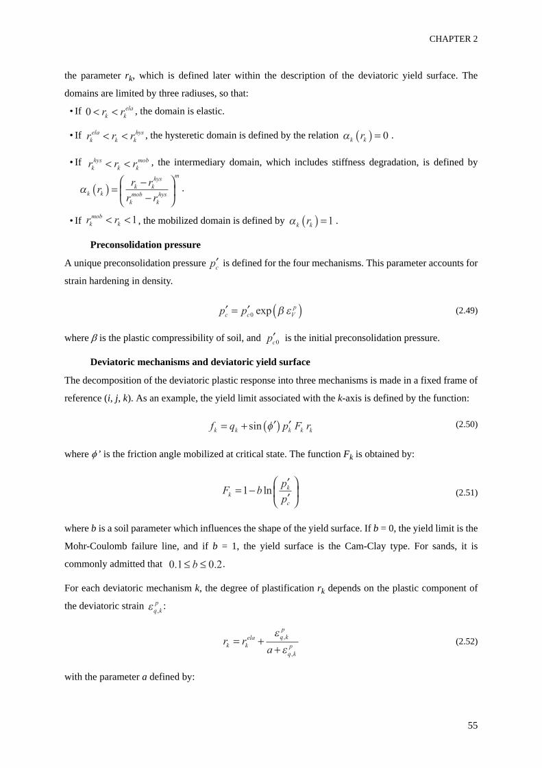
CHAPTER 2
55
the parameter rk, which is defined later within the description of the deviatoric yield surface. The
domains are limited by three radiuses, so that:
• If , the domain is elastic.
• If , the hysteretic domain is defined by the relation .
• If , the intermediary domain, which includes stiffness degradation, is defined by
.
• If , the mobilized domain is defined by .
Preconsolidation pressure
A unique preconsolidation pressure is defined for the four mechanisms. This parameter accounts for
strain hardening in density.
(2.49)
where β is the plastic compressibility of soil, and is the initial preconsolidation pressure.
Deviatoric mechanisms and deviatoric yield surface
The decomposition of the deviatoric plastic response into three mechanisms is made in a fixed frame of
reference (i, j, k). As an example, the yield limit associated with the k-axis is defined by the function:
(2.50)
where φ’ is the friction angle mobilized at critical state. The function Fk is obtained by:
(2.51)
where b is a soil parameter which influences the shape of the yield surface. If b = 0, the yield limit is the
Mohr-Coulomb failure line, and if b = 1, the yield surface is the Cam-Clay type. For sands, it is
commonly admitted that .
For each deviatoric mechanism k, the degree of plastification rk depends on the plastic component of
the deviatoric strain :
(2.52)
with the parameter a defined by:
0 r rk k
ela
r r rk
ela
k k
hys
k kr 0
r r rk
hys
k k
mob
k kk k
hys
k
mob
k
hys
m
rr r
r r
r rk
mob
k 1k kr 1
pc
p pc c V
p
0 exp
pc0
f q p F rk k k k ksin
F bp
pk
k
c
1 ln
0 1 0 2. .b
q k
p
,
r ra
k k
ela q k
p
q k
p
,
,
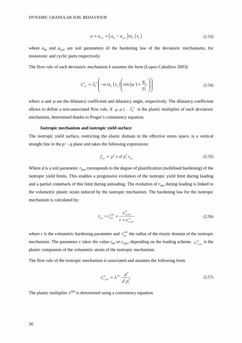
DYNAMIC GRANULAR SOIL BEHAVIOUR
56
(2.53)
where am and acyc are soil parameters of the hardening law of the deviatoric mechanisms, for
monotonic and cyclic parts respectively.
The flow rule of each deviatoric mechanism k assumes the form (Lopez-Caballero 2003):
(2.54)
where α and ψ are the dilatancy coefficient and dilatancy angle, respectively. The dilatancy coefficient
allows to define a non-associated flow rule, if . is the plastic multiplier of each deviatoric
mechanism, determined thanks to Prager’s consistency equation.
Isotropic mechanism and isotropic yield surface
The isotropic yield surface, restricting the elastic domain in the effective stress space, is a vertical
straight line in the p’ - q plane and takes the following expressions:
(2.55)
Where d is a soil parameter. riso corresponds to the degree of plastification (mobilised hardening) of the
isotropic yield limits. This enables a progressive evolution of the isotropic yield limit during loading
and a partial comeback of this limit during unloading. The evolution of riso during loading is linked to
the volumetric plastic strain induced by the isotropic mechanism. The hardening law for the isotropic
mechanism is calculated by:
(2.56)
where c is the volumetric hardening parameter and the radius of the elastic domain of the isotropic
mechanism. The parameter c takes the value cm or ccyc, depending on the loading scheme. is the
plastic component of the volumetric strain of the isotropic mechanism.
The flow rule of the isotropic mechanism is associated and assumes the following form:
(2.57)
The plastic multiplier λiso is determined using a consistency equation.
a a a a rcyc m cyc k k
v k
p
k
p
k kk
k
rq
p, sin
1 k
p
f p d p riso c iso
r rc
iso iso
ela v iso
p
v iso
p
,
,
riso
ela
v iso
p
,
v iso
p iso
c
p
d p,
CHAPTER 2
57
Summary of material parameters in the Hujeux model
Tab. 2.3 presents a summary of the 19 material parameters included in the Hujeux model for cyclic
loading, with an indication of values found in the literature (e.g. Lopez-Caballero 2003).
2.6.6 Domain of applicationAs several models can account for cyclic soil behaviour, the choice of one model to solve geotechnical
problems is linked with the particular application: although linear viscoelasticity reasonably fits very
small cyclic strains, one can use perfect plasticity to account for strong motions near failure. A few
models, including the Hujeux model, were specially adapted to take into account cyclic mobility or
liquefaction (Ishihara et al. 1975; Pastor et al. 1990; Li et al. 1999; Elgamal et al. 2002; Elgamal et al.
2003; Ling & Liu 2003; Lopez-Caballero 2003; Gerolymos & Gazetas 2005; Lopez-Querol & Blazquez
2006; Popescu et al. 2006; Jeremic et al. 2008).
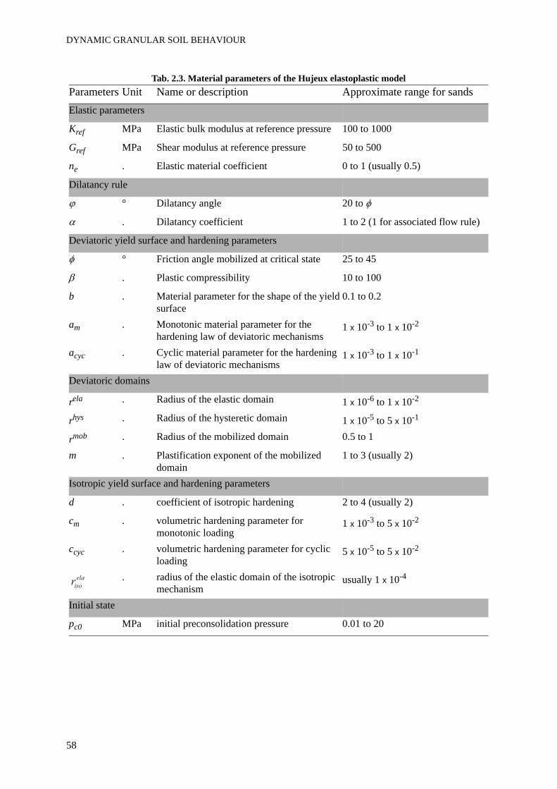
DYNAMIC GRANULAR SOIL BEHAVIOUR
58
Tab. 2.3. Material parameters of the Hujeux elastoplastic modelParameters Unit Name or description Approximate range for sandsElastic parameters
Kref MPa Elastic bulk modulus at reference pressure 100 to 1000
Gref MPa Shear modulus at reference pressure 50 to 500
ne . Elastic material coefficient 0 to 1 (usually 0.5)
Dilatancy rule
ϕ ° Dilatancy angle 20 to φ
α . Dilatancy coefficient 1 to 2 (1 for associated flow rule)
Deviatoric yield surface and hardening parameters
φ ° Friction angle mobilized at critical state 25 to 45
β . Plastic compressibility 10 to 100
b . Material parameter for the shape of the yield surface
0.1 to 0.2
am . Monotonic material parameter for the hardening law of deviatoric mechanisms
1 x 10⁻³ to 1 x 10⁻²
acyc . Cyclic material parameter for the hardening law of deviatoric mechanisms
1 x 10⁻³ to 1 x 10⁻¹
Deviatoric domains
rela . Radius of the elastic domain 1 x 10⁻⁶ to 1 x 10⁻²
rhys . Radius of the hysteretic domain 1 x 10⁻⁵ to 5 x 10⁻¹
rmob . Radius of the mobilized domain 0.5 to 1
m . Plastification exponent of the mobilized domain
1 to 3 (usually 2)
Isotropic yield surface and hardening parameters
d . coefficient of isotropic hardening 2 to 4 (usually 2)
cm . volumetric hardening parameter for monotonic loading
1 x 10⁻³ to 5 x 10⁻²
ccyc . volumetric hardening parameter for cyclic loading
5 x 10⁻⁵ to 5 x 10⁻²
. radius of the elastic domain of the isotropic mechanism
usually 1 x 10⁻⁴
Initial state
pc0 MPa initial preconsolidation pressure 0.01 to 20
riso
ela
CHAPTER 2
59
2.7 Rate effects in granular materialsDifferent aspects of rate effects in granular materials, which are further used to analyse our triaxial test
results presented in Chapter 5 of this dissertation, are studied in this section.
2.7.1 Phenomenons involved in time-dependent sand behaviourIn soils, time-dependency can be due to different mechanisms, and implies several concepts depending
on the loading characteristics. Three categories of time-dependent behaviours are reported here: viscous
effects, dynamic effects and effects of coupling with the pore fluid. This separation is quite arbitrary,
because there are some links between them. Moreover, the effect of ageing is totally disregarded here.
2.7.1.1 Viscosity in granular materialsThe pseudo-static time-dependency, named viscous effect, is related to changes within the soil skeleton,
as creep, relaxation, strain rate or frequency effect. Leroueil & Marques (1996) and Augustesen et al.
(2004) give a large overview of the viscous time-dependency. An analogy is built between liquid or gas
and soils: soils behave like extremely viscous fluids (Vulliet & Hutter 1988). This means that the
material, subjected to a shear stress, offers a resistance to flow. The more viscous the material, the
larger the resistance to flow. As they creep and relax less, i.e. they flow less, sands are considered more
viscous than clays.
2.7.1.2 Dynamic time effectLike all structures, soil mass is also prone to dynamic amplification which arises around a resonance
frequency due to inertial effects within the porous medium. The frequency of wave propagation thus
influences the response of dynamically loaded soil deposit (e.g. Iverson & LaHusen 1989; Popescu et
al. 2006).
2.7.1.3 Coupling with the pore fluidThe influence of the pore fluid on the behaviour of the porous medium is not negligible in dynamic
analysis of two-phase media. According to poroelasticity theory (Biot 1956), three kind of coupling
appear in the wave propagation equations between the soil matrix and the fluid saturating the pores:
inertial, mechanical and viscous (Gajo 1995; Gajo 1996). The viscous coupling has an effect on soil
behaviour, in particular the interpretation of dynamic tests depends on the value of the coefficient
n2 γw / k, with n the porosity and k the Darcy permeability (Gajo 1995). If there is a large amount of
high frequency content and high soil permeability, the intrinsic two-phase nature of the porous material
may exhibit clear signs of viscous coupling.
DYNAMIC GRANULAR SOIL BEHAVIOUR
60
In the pseudo-static range, the coupling between the granular matrix and the pore fluid is mainly
mechanical, as contraction and dilation of the solid matrix influence the pore fluid pressure. However,
the viscous behaviour of the two-phase medium is partly generated by the fluid flow within the pores
even in pseudo-static tests (Gallage et al. 2005).
Another important fact is that the pore pressure dissipation can take time within the soil volume. This
effect is viewed as an artefact of laboratory tests, and is not representative of true rate-dependent
material behaviour (e.g. Muir Wood 2004). The main parameter which controls that time-dependent
dissipation is the permeability coefficient. A short analysis, presented in Chapter 3, evaluates the time
delay of pore pressure dissipation in our test conditions.
2.7.2 Interpretation of rate effectsOne of the component of time effect is the loading rate (or strain rate), which represents the influence of
speed of load application (respectively strain application) on soil behaviour. For our tests (Chapter 5),
the expressions frequency effect and rate effect are equally used, as they both refer to loading rate
effect in cyclic stress-controlled conditions; the difference with strain rate effect is commented below
and in Chapter 5.
Rate effects in granular materials were observed during both monotonic (e.g. Yamamuro & Lade 1993;
Augustesen et al. 2004; AnhDan et al. 2006) or cyclic loadings (e.g. Lin et al. 1996; Hoque & Tatsuoka
2004; Sassa et al. 2005; Meng 2007; Salvati & AnhDan 2008).
The usual interpretation of the viscous rate effect is explained by Matesic & Vucetic (2003):
«If the rate of loading or straining is smaller, more time is allowed for the soil to creep and relax,
allowing the development of larger deformations at a given load increment and smaller shear stresses
at a given deformation increment. The final result is a stress-strain curve that plots lower.»
This point of view can be completed. The rate-dependency is claimed to be due to interparticle viscous
action added to flow of pore water in drained conditions (Gallage et al. 2005). The effect of particle
crushing at high pressure is also an interesting assumption proposed by Yamamuro & Lade (1993).
They state that at high strain rate, there is less time for particle crushing and rearranging, also the soil
dilative behaviour is influenced. Dynamic amplification, which arises around a resonance frequency
due to inertial effects, can also be included in rate effect phenomenons (Ghosh & Madabhushi 2003).
There is a difference between loading rate effects and strain rate effects. It is sometimes pointed up that
loading rate exists only as a consequence of the change of time length of the strain application. For
example, Sassa et al. (2005) explain that rate effects observed in torque-controlled laboratory tests are
CHAPTER 2
61
due to the evolution of the shear strain amplitude with the frequency. They also show that displacement-
controlled tests are independent from the frequency. This difference is explained by an energy-approach
analysis.
2.7.3 Influence of viscous behaviour on cyclic loadingThe viscous behaviour of granular material can influence its response to cyclic loading (Tatsuoka
2006):
«The pure effect of cyclic loading [...] can be accurately evaluated only when taking into account the
viscous effect».
Part of our cyclic tests can be viewed as a confirmation of that statement, as non negligible viscous
effects are isolated during cyclic loadings of granular materials (Chapter 5).
A discrimination between inviscid cyclic loading effects and viscous effects is proposed by Tatsuoka
(2006). A laboratory study shows that in certain conditions (e.g. small cyclic amplitude), for dry sand
under cyclic loading, the viscous property of sand is responsible for most of the residual strain while
inviscid cyclic loading effect is small. At larger strain amplitude and with a high number of cycles,
inviscid cyclic loading effect is more important. Moreover, the inviscid cyclic loading effect continues
for a longer duration than the viscous effect.
2.7.4 Time-dependency in granular media from laboratory experimentsLaboratory studies reported below mainly deal with creep, relaxation, step change of rate, monotonic or
cyclic loading of granular soils. In particular, the rate effect on strength of cohesive materials, which is
very well documented (e.g. Richardson & Whitman 1963), is not further mentioned.
2.7.4.1 Creep, relaxation and step change in strain rate and monotonic loadingAugustesen et al. (2004) summarise viscous monotonic time-dependent behaviour in sands and clays.
Strain rate effect on strength of cohesionless soil is addressed: it is mainly a temporary effect (over- and
undershooting) which appears during a step change of strain rate, but it does not affect the stress-strain
behaviour for monotonic loading with a constant strain rate. Creep and relaxation appear in sands as
well as in clays, with a smaller intensity.
Results from laboratory experiments on creep, relaxation and change of strain rate in dry sand were
obtained with various kind of tests (Tatsuoka 2006; Di Benedetto 2006; Pham Van Bang et al. 2007;
Duttine et al. 2008). It appears that sand behaviour is sensitive to a change in strain rate, rather than the
absolute value of strain rate. Saturated drained creep tests and step change of strain rate also exhibit
DYNAMIC GRANULAR SOIL BEHAVIOUR
62
viscous behaviour (Matsushita et al. 1999; Kuwano & Jardine 2002; Enomoto et al. 2006; Ibraim et al.
2009).
Gallage et al. (2005) show that liquefied sands of various fine content under low confining pressure
exhibit viscous behaviour and is sensitive to rate effect. Viscous behaviour is influenced by relative
density, effective confining pressure, OCR, fines content, previous strain history and pore fluid. There
is more creep deformation with water-saturated pores than for pores filled with air or vacuum. The
authors assume that the viscous behaviour results mainly from the vortex flow of pore fluid among sand
grains upon shear, and that grain-to-grain contact may also be responsible for additional viscosity.
The particle shape has an effect on dense dry sand creep behaviour (Enomoto et al. 2006; Tatsuoka
2006): the rounder the particle shape, the less creep appears. More generally, particle shape has a
systematic effect on the viscosity type and the relative importance between the viscous effect and the
inviscid cyclic loading effect.
Drained and undrained monotonic tests on sand is usually seen as not very sensitive to strain rate (e.g.
Matsushita et al. 1999). However, Yamamuro & Lade (1993) present monotonic loading of dense sand
under high confining pressure, for which the dilative behaviour, and thus the strength, is influenced by
the strain rate. The friction angle at the peak deviatoric stress decreases when strain rate increases. The
effect of strain rate appears to be more pronounced for undrained loading. The instability line, for the
triggering of liquefaction, remains the same at all strain rates.
Concerning dynamic flow of matter, Iverson & LaHusen (1989) explore pore pressure gradients inside
rapidly shearing granular materials. Artificial landslides are triggered, in order to measure the pore
pressure inside the moving mass at different height. The fluctuations of pore pressure, when the
shearing speed is high enough (critical speed, which is unknown, is linked with the properties of the
matrix and viscosity of the fluid), locally induce contraction and dilation of the porous medium.
Because of those local fluctuations, the effective stress is possibly significantly reduced, leading to
large deformations in the sheared area.
2.7.4.2 Frequency effect in dry cyclic conditionsSeveral experimental studies focused on frequency effects in dry sand. Bolton & Wilson (1989, 1990)
Hardin & Drnevich (1972a) and Karg & Haegeman (2009) concluded that dry sand behaviour was
frequency-independent, and of purely hysteretic nature. However many other test results tend to show
that there is an effect of the frequency on dry sand behaviour. The damping ratio at least is found
frequency-dependent in different kind of tests, for small to medium strains (Lin et al. 1996; Hoque &
Tatsuoka 2004; Zambelli et al. 2006; Khan et al. 2008). The test results are reported here with more
CHAPTER 2
63
details.
Secant shear modulus
With full cylinder torsional tests at small strains on dense dry Ottawa Sand, Lin et al. (1996) found that
the shear modulus is not very much rate sensitive, as it is constant until 50 Hz and then very slowly
decreases.
For Matesic & Vucetic (2003), the secant shear modulus of Toyoura and Nevada Sands at small to
medium strain increases with the average strain rate. The relation is approximately
linear for constant strain rate tests. However, the Gsec / Gmax curve at small to medium strain is almost
independent from the strain rate.
Zambelli et al. (2006) explore dry Toyoura Sand behaviour with a torsional shear device, at small to
high strains, and from 0.01 to 2 Hz. At small strains, the secant shear modulus increases with the
frequency while it is constant at higher strain level.
Damping ratio
With full cylinder torsional tests at small strains on dense dry Ottawa Sand, Lin et al. (1996) found that
damping ratio is very rate sensitive between 0.1 and 100 Hz, with a peak around 50 Hz and much
smaller values at frequencies around 1 Hz or 100 Hz. It can also be noticed that the peak of the damping
ratio arises before the resonance frequency, i.e. the maximum strain amplitude. A more detailed
analysis is performed for earthquake frequency range, where inertial effects are neglected. The damping
ratio vs. frequency is a linear relation. It is the sum of a hysteretic part and a rate-dependent viscous
part, which both depend on shear strain amplitude, confining pressure and relative density.
Moreover, Hoque & Tatsuoka (2004) performed small strain triaxial tests on dry Hostun Sand at
frequencies from 0.005 to 2 Hz, and also concluded on the frequency-dependence of damping. The
waveform, sinusoidal or triangular, does not influence the dynamic parameters.
For Zambelli et al. (2006) with dry Toyoura Sand, the damping ratio evolves non-linearly at small strain
and small frequency and it increases linearly at higher frequency for both small and large strain level.
Khan et al. (2008) adds that dynamic parameters of dry sand at small strains just below the volumetric
cyclic threshold shear strain are slightly frequency-dependent for frequencies of 40 Hz to 70 Hz, but it
is considered as negligible in the paper.
Accumulated strain
Salvati & AnhDan (2008) performed triaxial tests on two dense dry sands of different particle shape.
With two frequency levels 0.1 Hz and 1.5 Hz, the total accumulated strain is lower at high frequency in
certain conditions. The influence of frequency is more marked at low confining pressure, and for high
log Gsec
DYNAMIC GRANULAR SOIL BEHAVIOUR
64
ratio Δq / σ3. It is the change in strain rate which is significant, rather than the change of loading
frequency.
2.7.4.3 Frequency and strain rate effects in saturated cyclic conditionsConcerning frequency and strain rate effects, the results of several laboratory studies in drained and
undrained saturated conditions are summarized below. There are some contradictions between these
results. Those defending rate-independent behaviour of saturated sand, for pores filled with water, are
first mentioned, followed by others which describe rate-dependent behaviour of granular soils.
Some laboratory studies suggest that loading frequency has no influence on cyclic saturated drained
and undrained sand behaviour. For example, stiffness is found to be frequency-independent during
drained cyclic test at γ < 0.1% (Karg & Haegeman 2009). An undrained strain-controlled study
mentioned that frequency has no effect on pore water pressure builds up, liquefaction potential and
shear modulus (Govindaraju & Sitharam 2007).
Quasi-static and dynamic torsional tests on sand were performed by Bolton & Wilson (1990) to provide
insight into viscous damping. With oil filling the voids, this viscous part of the damping is not
negligible, while damping ratio clearly increases with the frequency. But the frequency effect on D is
found very small when pores are filled with water at frequency below 100 Hz.
On the contrary, other studies on various sands show that cyclic frequency effects occur in drained and
undrained granular materials. They are summarized below.
As for dry tests, damping ratio is shown to increase with frequency around earthquake frequency range
in undrained conditions (Govindaraju & Sitharam 2007).
Vucetic & Tabata (2003) performed laboratory tests on unremolded natural sands at different low
frequencies and small to medium strain. The frequency-dependence is evaluated through the slope of
secant shear modulus vs. shear strain rate. Rate effects are higher for clay than sand, but they are not
totally negligible in sands. In this study, rate effects tend to decrease when the strain amplitude
increases.
Sassa et al. (2005) present test results on liquefaction of saturated Osaka sand. While shear-torque-
controlled tests are frequency-dependent, shear-displacement-controlled tests are frequency-
independent (although the frequency range is lower for the latter). At the highest frequency for shear-
torque-controlled tests, energy dissipation becomes lower, as well as total strain accumulation. Excess
pore pressure generation is frequency-dependent in shear-torque-controlled tests.
Meng (2007) studied unidimensional variations of shear wave velocity (cs) and quality factor (Q) for
CHAPTER 2
65
natural soils, including a clayey sand, with a frequency range from 0.01 to 30 Hz at very small strains.
This experimental study was performed with a non-resonance method, and a model issued with the
definition of two functions cs ( f ) and Q ( f ).
2.7.4.4 Summary and conclusionsIn sand, viscous behaviour is observed during creep, relaxation and step change of strain rate. Some
experimental works exist on frequency effects, but that phenomenon is far from being understood.
Indeed, a few contradictions can be found concerning dry and saturated drained sand behaviour.
There seems to be an agreement on the fact that damping ratio increases with frequency around 0.01 to
20 Hz. Strain accumulation may decrease when frequency increases in both dry and drained conditions.
The results are more contradictory concerning the secant shear modulus: some studies defend its rate-
independency in sand, others show that it increases slightly with frequency around 0.01 to 20 Hz. The
secant Young’s modulus and the shear wave velocity may also increase with the frequency.
Most studies are based on quasi-static procedures or at very small strains and the nonlinear dynamic
effects were not really considered. It seems that there is no laboratory test available in literature that has
both frequencies up to 10 Hz and medium to large strain amplitudes (> 10-3), especially during
undrained cyclic tests.
2.7.5 Constitutive modelling and numerical approach of rate effects in sandElasto-viscoplastic, viscoelastic-viscoplastic and viscoplastic models were primarily developed for
modelling time-dependent monotonic behaviour of fine soils, but some of them are adapted to model
viscous effects in granular materials, even under cyclic strains. Boukpeti et al. (2004) propose an elasto-
viscoplastic model which takes into account undrained monotonic loading of sand with creep and large
strain rate. A cyclic viscoelastic-viscoplastic model for clay is proposed by Oka et al. (2004), and
applied to a site amplification analysis for a multi-layered soil deposit. Pham Van Bang et al. (2007)
model creep, relaxation and step change in strain rate at small to medium strain. Modelling creep and
relaxation of dry sand, with specific effects such as non-isotach or TESRA behaviour, is possible thanks
to the 3 component model (e.g. Di Benedetto & Tatsuoka 1997; Di Benedetto et al. 2002; Tatsuoka et
al. 2002; Di Benedetto 2006).
In Ghosh & Madabhushi (2003), the authors have numerically investigated the behaviour of loose silica
sand under large amplitude dynamic strains with different frequencies. The finite element software
SWANDYNE implements differential equations of the solid and fluid phases fully coupled with the
mass balance equation. The constitutive model is based on generalized plasticity, which allows here to
take into account cyclic loadings.
DYNAMIC GRANULAR SOIL BEHAVIOUR
66
The results show a significant dependency of pore water pressure to the frequency of the input motion.
A peak of the pore pressure ratio is found for 1 Hz excitation, with a greater rate of generation of the
excess pore pressure. This resonance frequency is characterized by a strong nonlinear response of the
soil deposit, with high shear strains, liquefaction and stiffness degradation. While quasi-linear
behaviour is obtained at higher and lower frequencies, with stiffer behaviour and less increase in the
pore pressure. The rate-dependency is assumed to be linked with the closeness of the input loading
frequency to the natural frequency of the soil deposit.
Other numerical studies related to seismic wave propagation raise interest about the importance of the
frequency effect in soil deposits:
• Carvajal et al. (2002) perform inverse analysis of a site near Mexico City. The analysis compares
results with frequency-dependent and frequency-independent dynamic properties. With frequency-
dependent dynamic parameters, the acceleration time history are improved compared to the
measured response of several seismic events. The displacements however are not improved.
• Meng (2007) performs a unidirectional seismic simulation using either frequency-dependent or
frequency-independent dynamic soil properties. The two conditions give different results, thus
proving the importance of taking into account rate-dependency within site amplification studies.
• Popescu (2002) performs finite element simulation of earth structures under earthquake loading. The
frequency content of the seismic motion influences the dynamic response of the structures, in terms
of pore water pressure generation, horizontal displacements and overall stability.
2.7.6 ConclusionsThere are some contradictions on the effects of frequency experimentally observed in granular
materials. They may not be very large, but time-dependent effects arise in sands. Several physical
interpretations of time-dependent behaviour of sand are available, including viscous and dynamic
effects, coupling with the pore fluid or particle breakage. The part attributed to the coupling with pore
water is not very clear, but even dry sand exhibits rate-dependent behaviour. Although experimental
results are not in total agreement with each other, dynamic parameters, and particularly the damping
ratio, seem to increase with the frequency around earthquake frequency range. There is a lack of
available test data on frequency effects in sands, in the earthquake frequency range and for medium to
large strain amplitude, especially in undrained conditions. We present such results in Chapter 5.
Moreover, time-dependent behaviour of soils has a non-negligible influence on the modelling of site
effects.
CHAPTER 2
67
2.8 Superposition of loadings
2.8.1 IntroductionFor linear elastic soil behaviour, seismic wave propagation is the sum of several kinds of wave which
are superimposed. In earth structures in particular, the amplification, reflection and refraction of the
stress waves give very different wave pattern from the simple assumption of a unidimentional vertical
propagation of a shear wave. Moreover, Ishihara (1996), while explaining the effect of stress waves on
the soil behaviour, states that the compressional stress is transmitted through water in the pores, and that
it does not affect the effective stress.
The principle of superposition does not apply in the range of nonlinear soil behaviour, i.e. for large
acceleration above 0.4g (Bernardie et al. 2006). The superposition of confining and deviatoric stresses
into a complex loading is thus another feature of loading characteristics which might influence the
response of the soil.
On the other hand, in the poroelasticity theory, the propagation of earthquake-induced elastic stress
waves in a saturated granular medium is based on two compressional waves and one rotational wave
(Biot 1956). The displacements of the fluid and the granular phases are coupled within the dynamic
equations. Disregarding the dynamic coupling effect between the water and the soil matrix might be of
great importance.
These remarks explain our interest on the effect of superposition of stress loadings on soil behaviour.
Laboratory experiments reporting the superposition of cyclic loading components and the effects on
granular soil behaviour are described below. First, the superposition of two shear loads is briefly
summarised. However, our tests concern the superposition of a confining and a shear loading, for which
very few test data are available.
Finally, we would like to emphasize the difference between multidimensional soil analyses and
multidirectional soil analyses. The multidimensional study, namely 2D or 3D effect, takes into account
the geometry of the investigated area. For example site effects in a complex valley can be investigated
with 2D or 3D models (e.g. Delepine 2007). In the multidirectional study, the loading has two or three
orthogonal loading component, which accounts for the complexity of in situ wave propagation. A
multidirectional study can be performed on a 1D soil column (e.g. Bernardie et al. 2006).
2.8.2 Laboratory experiments
2.8.2.1 Superposition of two shear stressesThe superposition of two shear stresses in orthogonal directions had been performed with bidirectional
DYNAMIC GRANULAR SOIL BEHAVIOUR
68
simple shear tests (described in Chapter 3), or torsional shear tests with an axial vertical load. A few
laboratory studies aimed at demonstrating the non negligible effect of cyclic bidirectional loading stress
paths instead of the usual assumption of a single loading (Boulanger & Seed 1995; Seed et al. 2001).
Multidirectional shaking table tests are also used since Pyke (1973).
Ishihara & Yamazaki (1980) studied saturated sand failure with a bidirectional simple shear apparatus.
The pore water pressure ratio does not reach 1 during rotational shear tests, although high strains
develop within the sample. Moreover, a release of the applied cyclic stress caused the pore pressure to
immediately reach the initial confining pressure. The authors concluded that the number of cycles to
reach failure decreases with bidirectional loading, i.e. cyclic strength decreases. The time lag and
amplitude ratio between the two perpendicular shear stresses influence the value of cyclic stress ratio at
failure.
Ishihara & Nagase (1988) performed bidirectional irregular loading tests on sand with a bidirectional
simple shear device. They applied horizontal acceleration time histories of real japanese earthquakes to
sand with a reduced time scale. It was observed that multidirectional loading effect, which slightly
decreases soil strength, is almost independent from the relative density of sand. A design curve is
produced, with one load irregularity factor and one multidirectional load factor. The multidirectional
factor ranges from 0.82 for dense sand to 0.86 for loose sand, which means that cyclic strength is
slightly reduced in bidirectional load conditions.
Kammerer et al. (2003; 2004) describe the behaviour of sand under bidirectional loading conditions,
using an advanced bidirectional simple shear apparatus (Seed et al. 2001). The results emphasize
several observations on liquefaction triggering. The bidirectional loading limits the maximum value of
the excess pore pressure ratio to a threshold value lower than the custom value of 1 obtained in the
unidirectional configuration. Though, large strains develop and the threshold value, which is for
example 0.7 for Monterey 0/30 sand (Kammerer et al. 2004), is reached faster than in unidirectional
conditions.
A different testing device is used in Aggour & Zhang (2006). The experimental study is based on a
combination of longitudinal and torsional loadings in a resonant column. It appears that the rate of
decrease of the shear modulus ratio and the rate of increase of the damping ratio is influenced by the
combination of the two loadings. A threshold strain ratio between longitudinal and torsional strains is
defined, above which the stiffness degradation of the sample has a higher rate than unidirectional
loading.
The bidirectional application of load prevents the apparition of ur = 1, and in the same time decreases
the cyclic strength (failure definition with the threshold shear strain amplitude) of saturated sand in
CHAPTER 2
69
bidirectional simple shear. In the same way, the bidirectional loading increases the rate of stiffness
degradation in the case of the superposition of a torsional and deviatoric load.
2.8.2.2 Superposition of confining and deviatoric stresses in triaxial devicesChoi & Arduino (2004) performed true triaxial testing of gravelly soils, with monotonic, cyclic and
rotational stress paths on narrow-graded Pea gravels. For several monotonic loadings in various
directions, the peak stress ratio varies depending on the stress path direction. Circular (polarized) cyclic
tests induce an increase of the pore water pressure.
Another interesting study addresses the evolution of sand behaviour with a high number of cycles in a
bidirectional triaxial device developed in Bochum (Wichtmann & Triantafyllidis 2004; Wichtmann et
al. 2005; Wichtmann et al. 2007a; Wichtmann et al. 2007b). Strain accumulation under drained cyclic
loading depends on the shape and polarization of bidirectional stress-strain loops. The volumetric and
deviatoric components of stress have a complex effect: the actual polarization and loop shape does not
directly influence strain accumulation vs. the number of cycles, but a change of the polarization
increases residual strains.
2.8.2.3 RemarksIt seems that the superposition of a cyclic confining stress to the deviatoric stress in the triaxial
apparatus was not studied in undrained situations, in the range of medium to high strains. That is why
there is no direct element of comparison with our cyclic bidirectional tests presented in Chapter 6. The
results available (Wichtmann et al. 2007a) on drained situations at smaller strains tend to show that the
shape of the input stress loop (cf. examples in Chapter 6) does not significantly influence strain
accumulation.
2.8.3 Multidirectional site effect analysesLi (1990) proposes a bounding surface hypoplasticity model which takes into account the rotation of
shear stresses and multidirectional loading. The model is used with a fully coupled dynamic
formulation to simulate a 1D column with multidirectional load (Li et al. 1998), i.e. with the
superposition of three loadings in orthogonal directions. Compared to a real seismic event, there is
reasonable agreement between the measured site effects and the simulation.
Bernardie et al. (2006) also model a 1D column with multidirectional loads, i.e. by taking into account
the three components of motion NS, EW and UP. They propagate within an elastoplastic soil model
implemented in a coupled dynamic formulation. In conclusions, the necessity to take into account the
multidirectional load is emphasized, in order to «obtain more realistic predictions».
DYNAMIC GRANULAR SOIL BEHAVIOUR
70
2.8.4 ConclusionsLaboratory studies have shown that the superposition of two shear loads on the boundary conditions
affects soil behaviour. The most frequently used device for the superposition of loadings is the
bidirectional simple shear apparatus, tested with sandy soils (Ishihara & Yamazaki 1980, Ishihara &
Nagase 1988, Boulanger & Seed 1995, Kammerer et al. 2003, Ueng et al. 2006). Some experimental
studies with a triaxial apparatus (Wichtmann et al. 2007a), a true triaxial apparatus (Choi & Arduino
2004) and a resonant column (Aggour & Zhang 2006) have also been performed. Multidirectional
effects are mainly taken into account with a correction factor included in unidirectional procedures.
While some numerical studies show that coupled soil behaviour of the pore fluid with the solid matrix
influence the response of the soil deposit in case of multidirectional load, the transient behaviour of
saturated sand under earthquake loading with a triaxial device under cyclic bidirectional loading have
no available test data. We provide such results in Chapter 6.
2.9 Irregular loading of sand under seismic motion
2.9.1 IntroductionLaboratory testing of sand under seismic motion is technologically possible thanks to automated
motion regulators and pseudo-dynamic or dynamic devices. Irregular loadings of sand were performed
in triaxial, simple shear, torsional and centrifuge tests, as described in section 2.9.2. The consequences
of observed behaviour for design procedures are briefly mentioned in section 2.9.3. These test results
are compared to our irregular bidirectional tests performed in undrained conditions (cf. Chapter 6).
2.9.2 A few laboratory studiesThe usual procedure for converting horizontal accelerations at the soil surface into stresses in the
shallow regions of soil deposits was proposed by Seed & Idriss (1971): as the soil layers move together
as a rigid body in the horizontal direction, the shear stress at a given depth is evaluated by the surface
acceleration times the soil mass above that depth (Ishihara & Yasuda 1975). The equivalence between
horizontal acceleration at a given time and the in situ stress at a certain depth z can be extrapolated, for
simple shear devices, by:
(2.58)
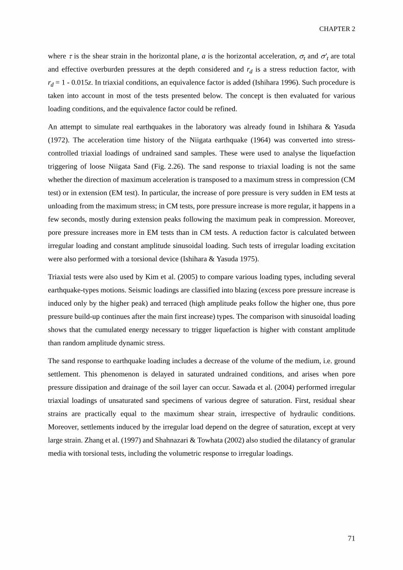
CHAPTER 2
71
where τ is the shear strain in the horizontal plane, a is the horizontal acceleration, σt and σ't are total
and effective overburden pressures at the depth considered and rd is a stress reduction factor, with
rd = 1 - 0.015z. In triaxial conditions, an equivalence factor is added (Ishihara 1996). Such procedure is
taken into account in most of the tests presented below. The concept is then evaluated for various
loading conditions, and the equivalence factor could be refined.
An attempt to simulate real earthquakes in the laboratory was already found in Ishihara & Yasuda
(1972). The acceleration time history of the Niigata earthquake (1964) was converted into stress-
controlled triaxial loadings of undrained sand samples. These were used to analyse the liquefaction
triggering of loose Niigata Sand (Fig. 2.26). The sand response to triaxial loading is not the same
whether the direction of maximum acceleration is transposed to a maximum stress in compression (CM
test) or in extension (EM test). In particular, the increase of pore pressure is very sudden in EM tests at
unloading from the maximum stress; in CM tests, pore pressure increase is more regular, it happens in a
few seconds, mostly during extension peaks following the maximum peak in compression. Moreover,
pore pressure increases more in EM tests than in CM tests. A reduction factor is calculated between
irregular loading and constant amplitude sinusoidal loading. Such tests of irregular loading excitation
were also performed with a torsional device (Ishihara & Yasuda 1975).
Triaxial tests were also used by Kim et al. (2005) to compare various loading types, including several
earthquake-types motions. Seismic loadings are classified into blazing (excess pore pressure increase is
induced only by the higher peak) and terraced (high amplitude peaks follow the higher one, thus pore
pressure build-up continues after the main first increase) types. The comparison with sinusoidal loading
shows that the cumulated energy necessary to trigger liquefaction is higher with constant amplitude
than random amplitude dynamic stress.
The sand response to earthquake loading includes a decrease of the volume of the medium, i.e. ground
settlement. This phenomenon is delayed in saturated undrained conditions, and arises when pore
pressure dissipation and drainage of the soil layer can occur. Sawada et al. (2004) performed irregular
triaxial loadings of unsaturated sand specimens of various degree of saturation. First, residual shear
strains are practically equal to the maximum shear strain, irrespective of hydraulic conditions.
Moreover, settlements induced by the irregular load depend on the degree of saturation, except at very
large strain. Zhang et al. (1997) and Shahnazari & Towhata (2002) also studied the dilatancy of granular
media with torsional tests, including the volumetric response to irregular loadings.
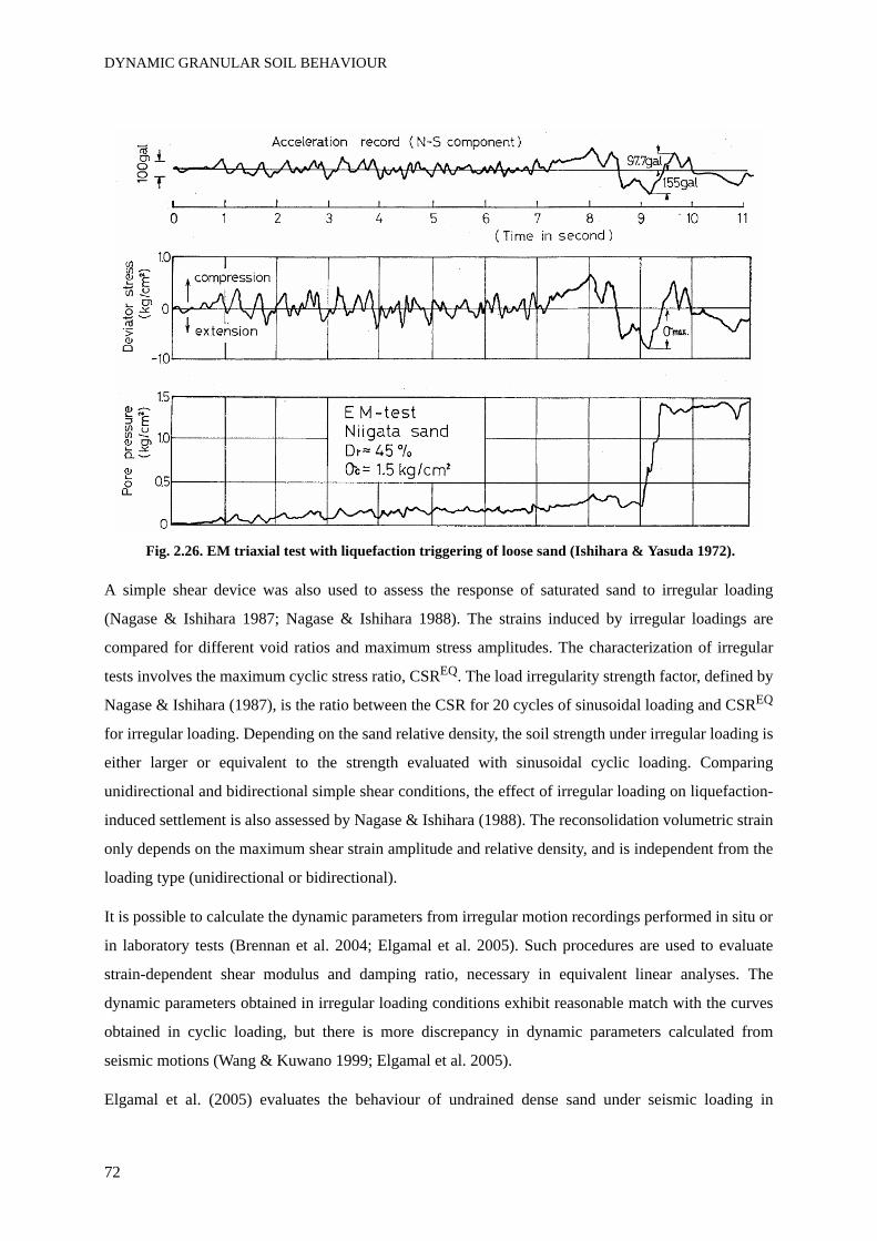
DYNAMIC GRANULAR SOIL BEHAVIOUR
72
Fig. 2.26. EM triaxial test with liquefaction triggering of loose sand (Ishihara & Yasuda 1972).
A simple shear device was also used to assess the response of saturated sand to irregular loading
(Nagase & Ishihara 1987; Nagase & Ishihara 1988). The strains induced by irregular loadings are
compared for different void ratios and maximum stress amplitudes. The characterization of irregular
tests involves the maximum cyclic stress ratio, CSREQ. The load irregularity strength factor, defined by
Nagase & Ishihara (1987), is the ratio between the CSR for 20 cycles of sinusoidal loading and CSREQ
for irregular loading. Depending on the sand relative density, the soil strength under irregular loading is
either larger or equivalent to the strength evaluated with sinusoidal cyclic loading. Comparing
unidirectional and bidirectional simple shear conditions, the effect of irregular loading on liquefaction-
induced settlement is also assessed by Nagase & Ishihara (1988). The reconsolidation volumetric strain
only depends on the maximum shear strain amplitude and relative density, and is independent from the
loading type (unidirectional or bidirectional).
It is possible to calculate the dynamic parameters from irregular motion recordings performed in situ or
in laboratory tests (Brennan et al. 2004; Elgamal et al. 2005). Such procedures are used to evaluate
strain-dependent shear modulus and damping ratio, necessary in equivalent linear analyses. The
dynamic parameters obtained in irregular loading conditions exhibit reasonable match with the curves
obtained in cyclic loading, but there is more discrepancy in dynamic parameters calculated from
seismic motions (Wang & Kuwano 1999; Elgamal et al. 2005).
Elgamal et al. (2005) evaluates the behaviour of undrained dense sand under seismic loading in
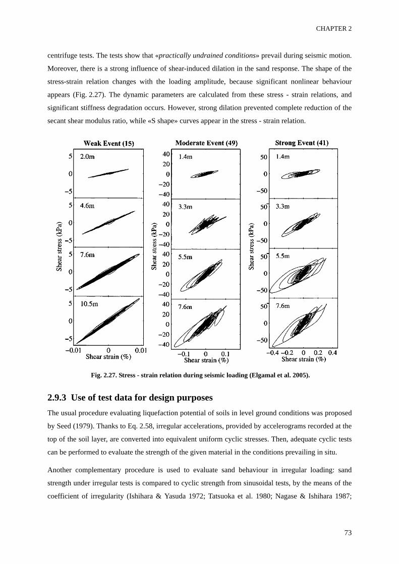
CHAPTER 2
73
centrifuge tests. The tests show that «practically undrained conditions» prevail during seismic motion.
Moreover, there is a strong influence of shear-induced dilation in the sand response. The shape of the
stress-strain relation changes with the loading amplitude, because significant nonlinear behaviour
appears (Fig. 2.27). The dynamic parameters are calculated from these stress - strain relations, and
significant stiffness degradation occurs. However, strong dilation prevented complete reduction of the
secant shear modulus ratio, while «S shape» curves appear in the stress - strain relation.
Fig. 2.27. Stress - strain relation during seismic loading (Elgamal et al. 2005).
2.9.3 Use of test data for design purposesThe usual procedure evaluating liquefaction potential of soils in level ground conditions was proposed
by Seed (1979). Thanks to Eq. 2.58, irregular accelerations, provided by accelerograms recorded at the
top of the soil layer, are converted into equivalent uniform cyclic stresses. Then, adequate cyclic tests
can be performed to evaluate the strength of the given material in the conditions prevailing in situ.
Another complementary procedure is used to evaluate sand behaviour in irregular loading: sand
strength under irregular tests is compared to cyclic strength from sinusoidal tests, by the means of the
coefficient of irregularity (Ishihara & Yasuda 1972; Tatsuoka et al. 1980; Nagase & Ishihara 1987;
DYNAMIC GRANULAR SOIL BEHAVIOUR
74
Ishihara 1996). This multiplicative factor is similar to the coefficient used for multidirectional loading,
and both are actually combined to evaluate soil strength in japanese earthquake-resistant design.
Cyclic or irregular laboratory studies are used in soil modelling which can account for irregular seismic
motions. The models have to be able to reproduce irreversible strains and excess pore pressure increase.
For example, the requirements for modelling irregular seismic loading are summarized by Ishihara et
al. (1975), and a deformation model for undrained sand results from these «postulates». Muravskii
(2001) and Osinov (2003) incorporate constitutive laws based on Masing’s rules into finite element
codes, and they provide examples of nonlinear soil behaviour under irregular loading. Comparing
laboratory tests and simulations with a Ramberg-Osgood model, Ray & Woods (1988) show that dry
sand behaviour can be well reproduced by computing irregular loadings.
2.9.4 SummaryThe effect of irregularity of loading, inherent to seismic motions, is addressed in laboratory studies on
granular materials. Their nonlinear behaviour is observed in different tests equivalent to seismic
motions. In undrained conditions especially, failure by cyclic liquefaction and flow liquefaction usually
occurs after the peak of maximum stress. Shear strains and pore pressure ratio develop as a result of
stiffness degradation which follows that peak. The equivalence between soil response to cyclic loading
(with a sinusoidal shape) and irregular stresses (derived from earthquake acceleration recordings) is
quantitatively evaluated thanks to multiplying coefficients. In particular, irregular and cyclic CSR
provide an equivalence factor for the strength. Following a very different approach, several constitutive
models suitable for cyclic liquefaction of sand are proved capable of modelling seismic motions. The
irregular tests presented here do not take into account bidirectional effects in triaxial conditions, which
are explored in Chapter 6.
2.10 ConclusionsThe cyclic behaviour of sands was described with a focus on applications to earthquake geotechnical
engineering. In particular site effects can be concerned by nonlinear soil behaviour in 1D, 2D or 3D site
amplification. The importance of an accurate effective stress modelling, which takes into account
plastic strain accumulation and pore water pressure increase, is acknowledged.
The particularities of cyclic soil behaviour were described, with many important factors: (i) importance
of the variation of excess pore pressure (increase or decrease, assimilated to contractive and dilative
CHAPTER 2
75
behaviour of the soil matrix prevented by the impossibility for volume change), (ii) effect of the number
of cycles, with the difference between dry and undrained conditions, (iii) loading in compression and
extension, and alternation of principle directions, (iv) strong strain dependency of nonlinear behaviour,
with the definition of two important threshold shear strains: the linear threshold and the volumetric
cyclic threshold, (v) pore pressure accumulation during undrained cyclic loading, (vi) failure by either
flow liquefaction or cyclic mobility and (vii) the influence of initial conditions, in particular void ratio
and isotropic or anisotropic consolidation. These subjects are addressed, particularly in Chapter 4, for
the interpretation of our cyclic triaxial test results performed on two different sands in various
conditions.
The dynamic parameters Gsec and D were defined, and their possible physical interpretation is
presented. We calculated the secant shear modulus and damping ratio in triaxial conditions with stress
and strain invariants, to use a unified definition in all loading conditions. The strain dependency,
notions of maximum secant shear modulus and factors influencing Gsec and D (in particular confining
pressure, void ratio and number of cycles) were described. These two parameters are evaluated, for
various test conditions on Leman and Fonderie Sand, in Chapters 4 to 6. They are also used in
Chapter 7 for the linear equivalent model.
A few constitutive models suitable for modelling granular soils under cyclic loading were presented in
section 2.6. The viscoelastic equivalent linear method, which is widely used with the programme
SHAKE91, takes into account soil non-linearity but does not allow strain accumulation or pore pressure
increase. On the contrary, the elastoplastic multi-mechanism Hujeux model can account for them. The
test results presented in Chapters 4 to 6 are used to evaluate and compare these two models in
Chapter 7.
Rate effect in granular materials mainly results from viscosity, dynamic effects, coupling between the
soil matrix and the pore fluid. Viscous behaviour is different in sands than in clays. In creep tests on
sand, the transient effect of the change of strain rate is more important than the strain rate level. Viscous
behaviour also influences cyclic behaviour. The loading frequency has an effect in dry and in saturated
conditions. For both cases, experimental studies prove that the damping ratio increases with the
frequency in the earthquake frequency range. In that same frequency range, the results are less clear for
the secant shear modulus, but it seems that Gsec slightly increases with the frequency. Undrained
frequency-dependence at medium strain range has not been experimentally evaluated. However,
numerical approaches of this problem show that the frequency-dependence can be important, in
particular it influences the results on site effect analysis. In Chapter 5, we provide new test results for
cyclic loading conditions which correspond to this problem; they allow to isolate rate-dependent cyclic
behaviour of granular soils.
DYNAMIC GRANULAR SOIL BEHAVIOUR
76
The impact of loading characteristics on nonlinear soil behaviour is also addressed through the
superposition of two loadings. Laboratory test results show that the superposition of two shear tests
reduce cyclic strength, though the pore pressure ratio is apparently limited to values below 1 during
bidirectional shear. The superposition of a confining and a deviatoric stress was not studied for transient
undrained loading in earthquake applications. This is the subject of Chapter 6. It is possible to apply
such boundary conditions for a fully coupled dynamic framework which uses constitutive models
designed for cyclic soil behaviour (cf. Chapter 7).
It is finally shown, under various experimental conditions, that seismic motions also induce nonlinear
behaviour and stiffness degradation of undrained saturated sand. In most laboratory tests, an effort is
made to evaluate the equivalence between irregular and cyclic motions, so that regular cyclic tests,
performed in repeatable conditions, are sufficient to evaluate sand response to seismic loading.
Complementary experimental results are described in Chapter 6, with bidirectional irregular triaxial
tests on Leman Sand.
The bibliographical study summarized above embraces all the concepts necessary to understand the
relevance of our laboratory experiments. The nonlinear behaviour of sand under cyclic loading is
strongly strain-dependent, but the influence of other characteristics of the applied load are non
negligible. We chose to focus on the frequency effect and the effect of multidirectional loadings with
the superposition of a cyclic compression with a cyclic deviatoric stress. None of these two loading
characteristics had been studied in conditions of strong earthquake loading, i.e. in undrained conditions
with medium to large strains and a frequency range between 0.1 and 10 Hz.
CHAPTER 3
CYCLIC TRIAXIAL EXPERIMENTS

CYCLIC TRIAXIAL EXPERIMENTS
78
3.1 Dynamic measurement techniques
3.1.1 IntroductionTesting methods applied to geotechnical earthquake engineering and soil dynamics had long existed,
although the addition of automation and programming to experimental devices allowed major
improvements in the last decade. Many kinds of dynamic laboratory apparatus were developed to assess
dynamic soil behaviour. They are characterized by their strain range, frequency range, allowed stress
paths and possible rotation of stress (Fig. 3.1). Then practical means which allow rapid characterization
of soil for engineering purposes are needed. In situ measurement and correlations with mechanical
characteristics of the soil layers proved to be useful (cf. Appendix 1). It is not the goal here to provide a
detailed list of all existing testing methods. The intent is rather to outline the main advances and to
situate our testing programme among other published works.
The review of laboratory equipment for dynamic soil testing can be found here, with the description of
the dynamic triaxial press used for our tests.
Fig. 3.1. Variation of soil properties and experimental methods (Ishihara 1996).
3.1.2 Laboratory testing
3.1.2.1 Idealization of real field wave propagation It is a requirement for laboratory tests to reproduce, within the soil sample, stress and strain states of
soil compatible with the field reality. Considering the stress waves in level ground conditions, the most
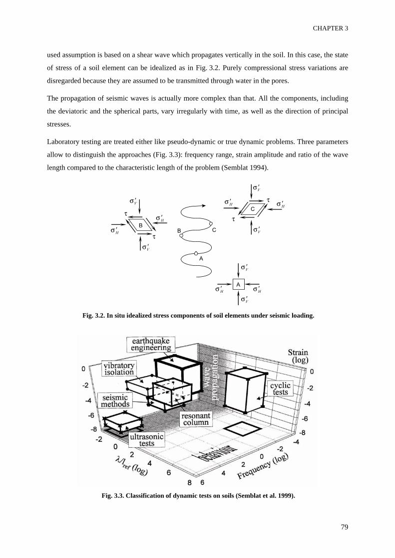
CHAPTER 3
79
used assumption is based on a shear wave which propagates vertically in the soil. In this case, the state
of stress of a soil element can be idealized as in Fig. 3.2. Purely compressional stress variations are
disregarded because they are assumed to be transmitted through water in the pores.
The propagation of seismic waves is actually more complex than that. All the components, including
the deviatoric and the spherical parts, vary irregularly with time, as well as the direction of principal
stresses.
Laboratory testing are treated either like pseudo-dynamic or true dynamic problems. Three parameters
allow to distinguish the approaches (Fig. 3.3): frequency range, strain amplitude and ratio of the wave
length compared to the characteristic length of the problem (Semblat 1994).
Fig. 3.2. In situ idealized stress components of soil elements under seismic loading.
Fig. 3.3. Classification of dynamic tests on soils (Semblat et al. 1999).
A
B C
A
B
CV
V
V
V
HH
HH
H
H V
V
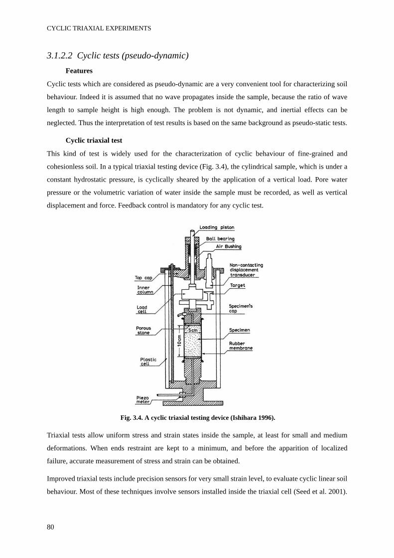
CYCLIC TRIAXIAL EXPERIMENTS
80
3.1.2.2 Cyclic tests (pseudo-dynamic)Features
Cyclic tests which are considered as pseudo-dynamic are a very convenient tool for characterizing soil
behaviour. Indeed it is assumed that no wave propagates inside the sample, because the ratio of wave
length to sample height is high enough. The problem is not dynamic, and inertial effects can be
neglected. Thus the interpretation of test results is based on the same background as pseudo-static tests.
Cyclic triaxial test
This kind of test is widely used for the characterization of cyclic behaviour of fine-grained and
cohesionless soil. In a typical triaxial testing device (Fig. 3.4), the cylindrical sample, which is under a
constant hydrostatic pressure, is cyclically sheared by the application of a vertical load. Pore water
pressure or the volumetric variation of water inside the sample must be recorded, as well as vertical
displacement and force. Feedback control is mandatory for any cyclic test.
Fig. 3.4. A cyclic triaxial testing device (Ishihara 1996).
Triaxial tests allow uniform stress and strain states inside the sample, at least for small and medium
deformations. When ends restraint are kept to a minimum, and before the apparition of localized
failure, accurate measurement of stress and strain can be obtained.
Improved triaxial tests include precision sensors for very small strain level, to evaluate cyclic linear soil
behaviour. Most of these techniques involve sensors installed inside the triaxial cell (Seed et al. 2001).
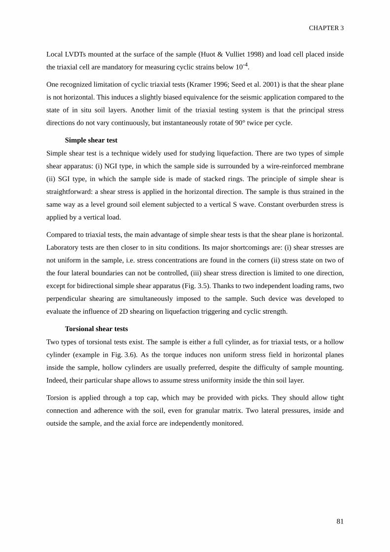
CHAPTER 3
81
Local LVDTs mounted at the surface of the sample (Huot & Vulliet 1998) and load cell placed inside
the triaxial cell are mandatory for measuring cyclic strains below 10-4.
One recognized limitation of cyclic triaxial tests (Kramer 1996; Seed et al. 2001) is that the shear plane
is not horizontal. This induces a slightly biased equivalence for the seismic application compared to the
state of in situ soil layers. Another limit of the triaxial testing system is that the principal stress
directions do not vary continuously, but instantaneously rotate of 90° twice per cycle.
Simple shear test
Simple shear test is a technique widely used for studying liquefaction. There are two types of simple
shear apparatus: (i) NGI type, in which the sample side is surrounded by a wire-reinforced membrane
(ii) SGI type, in which the sample side is made of stacked rings. The principle of simple shear is
straightforward: a shear stress is applied in the horizontal direction. The sample is thus strained in the
same way as a level ground soil element subjected to a vertical S wave. Constant overburden stress is
applied by a vertical load.
Compared to triaxial tests, the main advantage of simple shear tests is that the shear plane is horizontal.
Laboratory tests are then closer to in situ conditions. Its major shortcomings are: (i) shear stresses are
not uniform in the sample, i.e. stress concentrations are found in the corners (ii) stress state on two of
the four lateral boundaries can not be controlled, (iii) shear stress direction is limited to one direction,
except for bidirectional simple shear apparatus (Fig. 3.5). Thanks to two independent loading rams, two
perpendicular shearing are simultaneously imposed to the sample. Such device was developed to
evaluate the influence of 2D shearing on liquefaction triggering and cyclic strength.
Torsional shear tests
Two types of torsional tests exist. The sample is either a full cylinder, as for triaxial tests, or a hollow
cylinder (example in Fig. 3.6). As the torque induces non uniform stress field in horizontal planes
inside the sample, hollow cylinders are usually preferred, despite the difficulty of sample mounting.
Indeed, their particular shape allows to assume stress uniformity inside the thin soil layer.
Torsion is applied through a top cap, which may be provided with picks. They should allow tight
connection and adherence with the soil, even for granular matrix. Two lateral pressures, inside and
outside the sample, and the axial force are independently monitored.
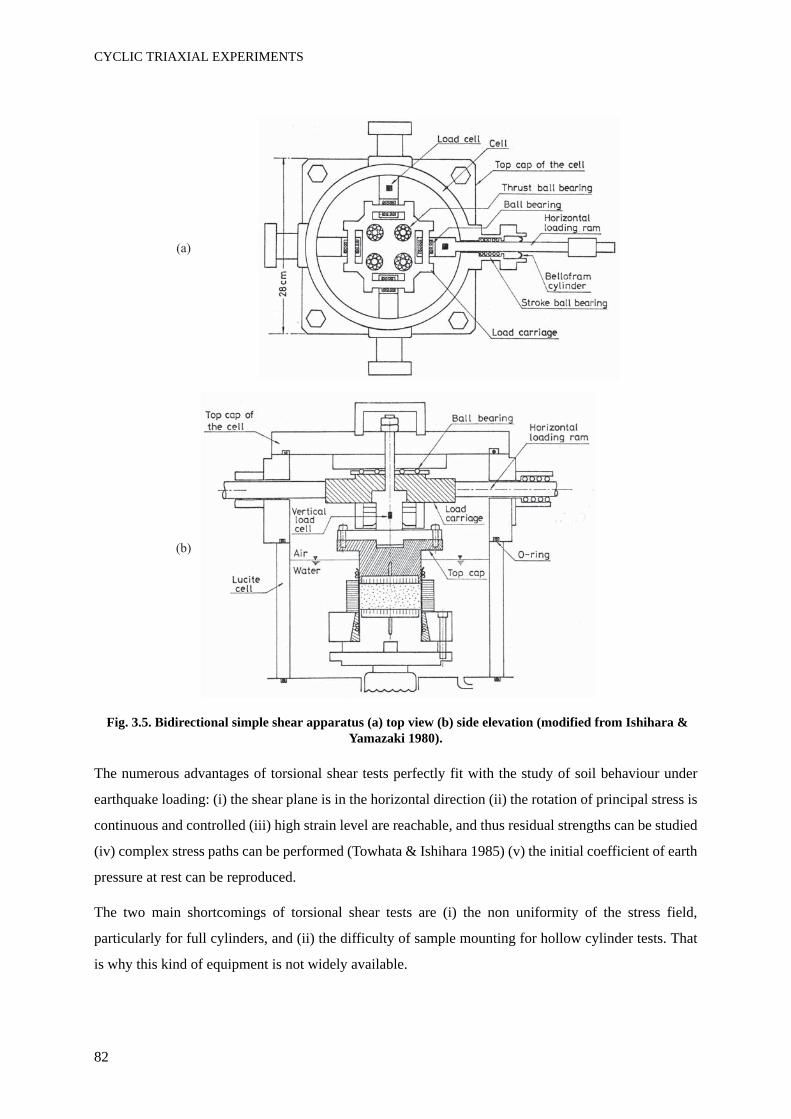
CYCLIC TRIAXIAL EXPERIMENTS
82
Fig. 3.5. Bidirectional simple shear apparatus (a) top view (b) side elevation (modified from Ishihara & Yamazaki 1980).
The numerous advantages of torsional shear tests perfectly fit with the study of soil behaviour under
earthquake loading: (i) the shear plane is in the horizontal direction (ii) the rotation of principal stress is
continuous and controlled (iii) high strain level are reachable, and thus residual strengths can be studied
(iv) complex stress paths can be performed (Towhata & Ishihara 1985) (v) the initial coefficient of earth
pressure at rest can be reproduced.
The two main shortcomings of torsional shear tests are (i) the non uniformity of the stress field,
particularly for full cylinders, and (ii) the difficulty of sample mounting for hollow cylinder tests. That
is why this kind of equipment is not widely available.
(a)
(b)
CHAPTER 3
83
Fig. 3.6. Triaxial torsional test (Kramer 1996).
3.1.2.3 Wave propagation at low strain levelResonant column test
The resonant column test allows to study true dynamic soil behaviour at small strain (Ishihara 1996;
Kramer 1996; Pecker 1984). Small strain Young’s modulus and shear modulus of the soil are calculated
at the resonance frequency of the first vibration mode. The damping ratio is obtained from the decay of
amplitudes during free vibrations, also at the resonance frequency. Full samples or hollow cylinders are
used, either in torsional or vertical loading. The torsional load, applied by coils, can be harmonic waves
or random irregular loading depending on the equipment.
Acoustic transmission
Piezoelectric elements induce P waves inside the sample, while bender elements induce S waves (Huot
1999). The measurement of the elastic wave velocity gives information on the linear behaviour of the
soil tested. It is possible to induce both compression and shearing waves in the same time (Huot 1999;
Muir Wood 2007; Sadek et al. 2007).
3.1.2.4 Very high strain rateAlternative techniques had been developed for testing very high strain rates. A single shock is applied
to the soil sample and strains are recorded through advanced measurement techniques. For example
Hopkinson bars (Semblat 1994; Semblat et al. 1999) or dropping weight systems (Abrantes &
Yamamuro 2002) were used to obtain strain rates up to 1000 s-1. Hopkinson bars are designed to load
materials at high speed and for a brief shock by the mean of cylindrical metallic bars. The shock wave
propagates through the sample, and the deformation of surrounding bars is measured so that forces and
displacements are calculated at every time step. Though this device is mostly used for metals, rocks or
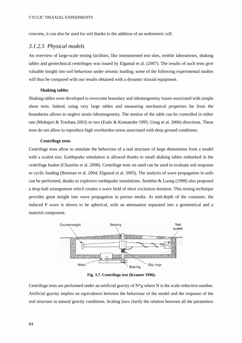
CYCLIC TRIAXIAL EXPERIMENTS
84
concrete, it can also be used for soil thanks to the addition of an oedometric cell.
3.1.2.5 Physical modelsAn overview of large-scale testing facilities, like instrumented test sites, mobile laboratories, shaking
tables and geotechnical centrifuges was issued by Elgamal et al. (2007). The results of such tests give
valuable insight into soil behaviour under seismic loading; some of the following experimental studies
will thus be compared with our results obtained with a dynamic triaxial equipment.
Shaking tables
Shaking tables were developed to overcome boundary and inhomogeneity issues associated with simple
shear tests. Indeed, using very large tables and measuring mechanical properties far from the
boundaries allows to neglect strain inhomogeneity. The motion of the table can be controlled in either
one (Mohajeri & Towhata 2003) or two (Endo & Komanobe 1995; Ueng et al. 2006) directions. These
tests do not allow to reproduce high overburden stress associated with deep ground conditions.
Centrifuge tests
Centrifuge tests allow to simulate the behaviour of a real structure of large dimensions from a model
with a scaled size. Earthquake simulation is allowed thanks to small shaking tables embarked in the
centrifuge basket (Chazelas et al. 2008). Centrifuge tests on sand can be used to evaluate soil response
to cyclic loading (Brennan et al. 2004; Elgamal et al. 2005). The analysis of wave propagation in soils
can be performed, thanks to explosive earthquake simulations. Semblat & Luong (1998) also proposed
a drop-ball arrangement which creates a wave field of short excitation duration. This testing technique
provides great insight into wave propagation in porous media. At mid-depth of the container, the
induced P wave is shown to be spherical, with an attenuation separated into a geometrical and a
material component.
Fig. 3.7. Centrifuge test (Kramer 1996).
Centrifuge tests are performed under an artificial gravity of N*g where N is the scale reduction number.
Artificial gravity implies an equivalence between the behaviour of the model and the response of the
real structure in natural gravity conditions. Scaling laws clarify the relation between all the parameters
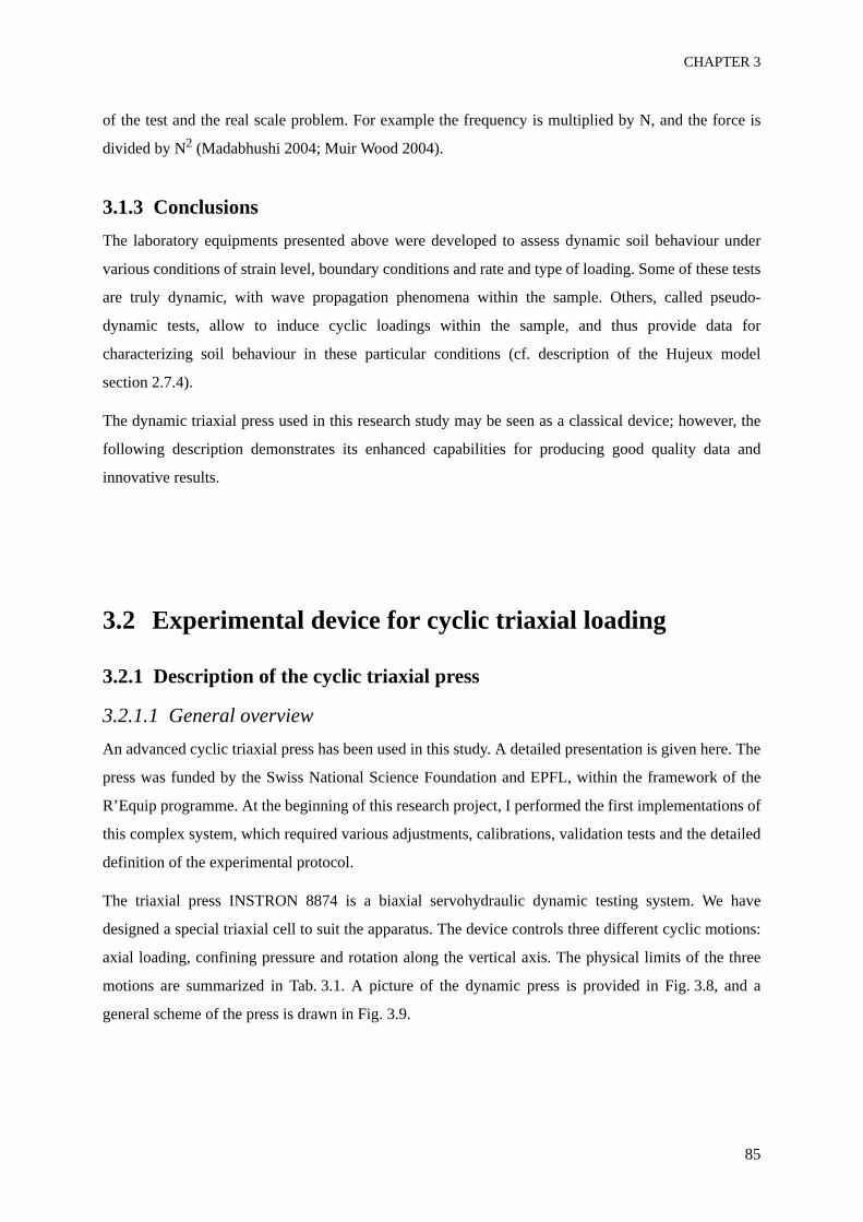
CHAPTER 3
85
of the test and the real scale problem. For example the frequency is multiplied by N, and the force is
divided by N2 (Madabhushi 2004; Muir Wood 2004).
3.1.3 ConclusionsThe laboratory equipments presented above were developed to assess dynamic soil behaviour under
various conditions of strain level, boundary conditions and rate and type of loading. Some of these tests
are truly dynamic, with wave propagation phenomena within the sample. Others, called pseudo-
dynamic tests, allow to induce cyclic loadings within the sample, and thus provide data for
characterizing soil behaviour in these particular conditions (cf. description of the Hujeux model
section 2.7.4).
The dynamic triaxial press used in this research study may be seen as a classical device; however, the
following description demonstrates its enhanced capabilities for producing good quality data and
innovative results.
3.2 Experimental device for cyclic triaxial loading
3.2.1 Description of the cyclic triaxial press
3.2.1.1 General overviewAn advanced cyclic triaxial press has been used in this study. A detailed presentation is given here. The
press was funded by the Swiss National Science Foundation and EPFL, within the framework of the
R’Equip programme. At the beginning of this research project, I performed the first implementations of
this complex system, which required various adjustments, calibrations, validation tests and the detailed
definition of the experimental protocol.
The triaxial press INSTRON 8874 is a biaxial servohydraulic dynamic testing system. We have
designed a special triaxial cell to suit the apparatus. The device controls three different cyclic motions:
axial loading, confining pressure and rotation along the vertical axis. The physical limits of the three
motions are summarized in Tab. 3.1. A picture of the dynamic press is provided in Fig. 3.8, and a
general scheme of the press is drawn in Fig. 3.9.
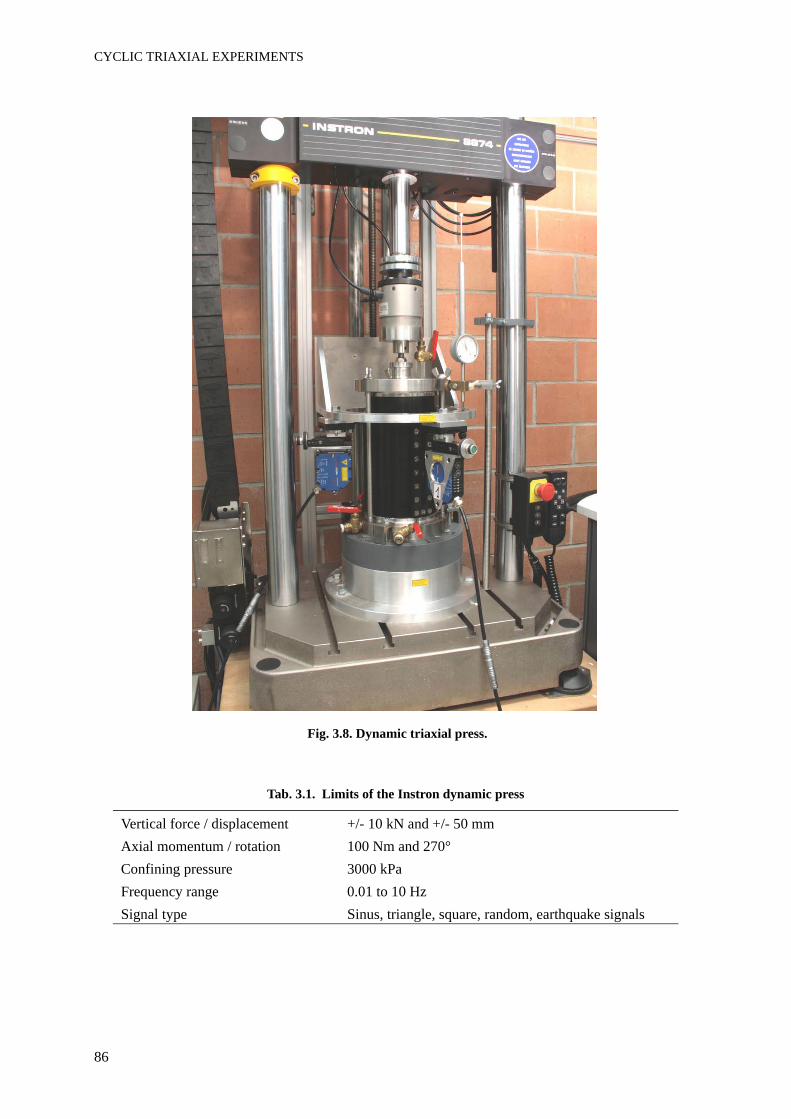
CYCLIC TRIAXIAL EXPERIMENTS
86
Fig. 3.8. Dynamic triaxial press.
Tab. 3.1. Limits of the Instron dynamic press
Vertical force / displacement +/- 10 kN and +/- 50 mmAxial momentum / rotation 100 Nm and 270°Confining pressure 3000 kPaFrequency range 0.01 to 10 HzSignal type Sinus, triangle, square, random, earthquake signals
CHAPTER 3
87
Fig. 3.9. Scheme of the dynamic press.
For the interpretation of test results, it is necessary to determine whether the press performs pseudo-
dynamic or true dynamic loadings. In usual loading configurations, the minimum wave length (λw) is
estimated by:
(3.1)
where f is the loading frequency and cs the velocity of S wave propagation. The value cs = 100 m/s is a
low approximation for typical sand.
For samples of height 160 mm, which is the customary size, the ratio of the wave length to the sample
height is around 60. This is why we consider that propagation phenomena are negligible within the
sample (Semblat 1994).
Vertical motion
IAC board
Pressuremeter
Position
sensor
I
II
Rotative
IAC board
Confining pressure
IAC board
Instron FastTrack
RS Console
Project Manager
Computer
Windows 2000
Hydraulic
pump 2
Servo valve for
confining pressure
Rotary manifold
Servo valve
for
rotation
Hydraulic
pump 1
Vertical motion
manifold
Servo valve
for vertical
motion
Confining pressure
manifold
Controller
external LVDT
3
triaxial cell
biaxial
load cell
internal LVDT
Confining pressure actuator
c
fms 100
1010w
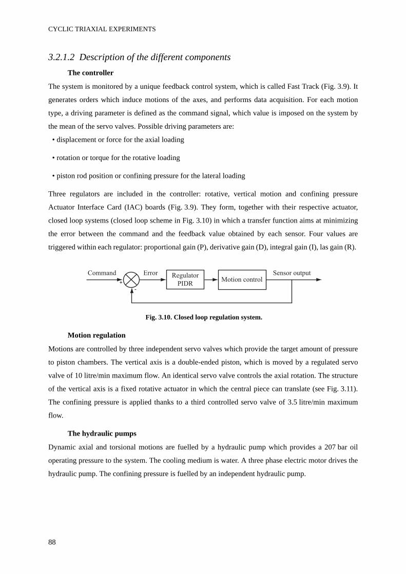
CYCLIC TRIAXIAL EXPERIMENTS
88
3.2.1.2 Description of the different componentsThe controller
The system is monitored by a unique feedback control system, which is called Fast Track (Fig. 3.9). It
generates orders which induce motions of the axes, and performs data acquisition. For each motion
type, a driving parameter is defined as the command signal, which value is imposed on the system by
the mean of the servo valves. Possible driving parameters are:
• displacement or force for the axial loading
• rotation or torque for the rotative loading
• piston rod position or confining pressure for the lateral loading
Three regulators are included in the controller: rotative, vertical motion and confining pressure
Actuator Interface Card (IAC) boards (Fig. 3.9). They form, together with their respective actuator,
closed loop systems (closed loop scheme in Fig. 3.10) in which a transfer function aims at minimizing
the error between the command and the feedback value obtained by each sensor. Four values are
triggered within each regulator: proportional gain (P), derivative gain (D), integral gain (I), las gain (R).
Fig. 3.10. Closed loop regulation system.
Motion regulation
Motions are controlled by three independent servo valves which provide the target amount of pressure
to piston chambers. The vertical axis is a double-ended piston, which is moved by a regulated servo
valve of 10 litre/min maximum flow. An identical servo valve controls the axial rotation. The structure
of the vertical axis is a fixed rotative actuator in which the central piece can translate (see Fig. 3.11).
The confining pressure is applied thanks to a third controlled servo valve of 3.5 litre/min maximum
flow.
The hydraulic pumps
Dynamic axial and torsional motions are fuelled by a hydraulic pump which provides a 207 bar oil
operating pressure to the system. The cooling medium is water. A three phase electric motor drives the
hydraulic pump. The confining pressure is fuelled by an independent hydraulic pump.
Command Error Regulator
PIDRMotion control
Sensor output
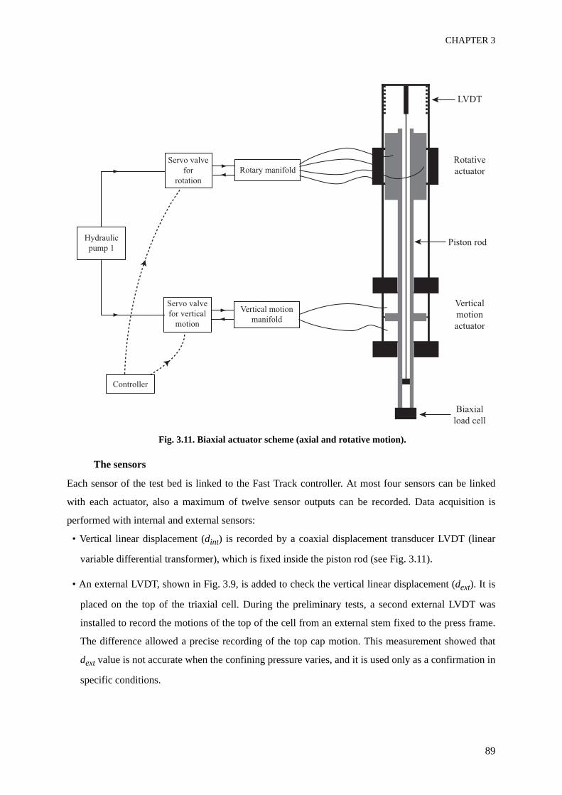
CHAPTER 3
89
Fig. 3.11. Biaxial actuator scheme (axial and rotative motion).
The sensors
Each sensor of the test bed is linked to the Fast Track controller. At most four sensors can be linked
with each actuator, also a maximum of twelve sensor outputs can be recorded. Data acquisition is
performed with internal and external sensors:
• Vertical linear displacement (dint) is recorded by a coaxial displacement transducer LVDT (linear
variable differential transformer), which is fixed inside the piston rod (see Fig. 3.11).
• An external LVDT, shown in Fig. 3.9, is added to check the vertical linear displacement (dext). It is
placed on the top of the triaxial cell. During the preliminary tests, a second external LVDT was
installed to record the motions of the top of the cell from an external stem fixed to the press frame.
The difference allowed a precise recording of the top cap motion. This measurement showed that
dext value is not accurate when the confining pressure varies, and it is used only as a confirmation in
specific conditions.
Biaxial
load cell
LVDT
Rotative
actuator
Vertical
motion
actuator
Rotary manifold
Servo valve
for
rotation
Hydraulic
pump 1
Vertical motion
manifold
Servo valve
for vertical
motion
Controller
Piston rod
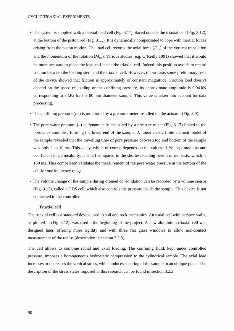
CYCLIC TRIAXIAL EXPERIMENTS
90
• The system is supplied with a biaxial load cell (Fig. 3.11) placed outside the triaxial cell (Fig. 3.12),
at the bottom of the piston rod (Fig. 3.11). It is dynamically compensated to cope with inertial forces
arising from the piston motion. The load cell records the axial force (Fax) of the vertical translation
and the momentum of the rotation (Max). Various studies (e.g. O’Reilly 1991) showed that it would
be more accurate to place the load cell inside the triaxial cell. Indeed this position avoids to record
friction between the loading stem and the triaxial cell. However, in our case, some preliminary tests
of the device showed that friction is approximately of constant magnitude. Friction load doesn’t
depend on the speed of loading or the confining pressure, its approximate amplitude is 0.04 kN
corresponding to 8 kPa for the 80 mm diameter sample. This value is taken into account for data
processing.
• The confining pressure (σ3) is monitored by a pressure meter installed on the actuator (Fig. 3.9).
• The pore water pressure (u) is dynamically measured by a pressure meter (Fig. 3.12) linked to the
porous ceramic disc forming the lower end of the sample. A linear elastic finite element model of
the sample revealed that the travelling time of pore pressure between top and bottom of the sample
was only 1 to 10 ms. This delay, which of course depends on the values of Young's modulus and
coefficient of permeability, is small compared to the shortest loading period of our tests, which is
150 ms. This comparison validates the measurement of the pore water pressure at the bottom of the
cell for our frequency range.
• The volume change of the sample during drained consolidation can be recorded by a volume sensor
(Fig. 3.12), called a GDS cell, which also controls the pressure inside the sample. This device is not
connected to the controller.
Triaxial cell
The triaxial cell is a standard device used in soil and rock mechanics. An usual cell with perspex walls,
as plotted in (Fig. 3.12), was used a the beginning of the project. A new aluminium triaxial cell was
designed later, offering more rigidity and with three flat glass windows to allow non-contact
measurement of the radius (description in section 3.2.3).
The cell allows to combine radial and axial loading. The confining fluid, kept under controlled
pressure, imposes a homogeneous hydrostatic compression to the cylindrical sample. The axial load
increases or decreases the vertical stress, which induces shearing of the sample in an oblique plane. The
description of the stress states imposed in this research can be found in section 3.2.2.
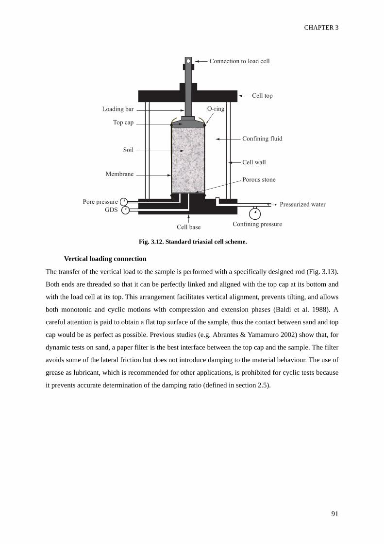
CHAPTER 3
91
Fig. 3.12. Standard triaxial cell scheme.
Vertical loading connection
The transfer of the vertical load to the sample is performed with a specifically designed rod (Fig. 3.13).
Both ends are threaded so that it can be perfectly linked and aligned with the top cap at its bottom and
with the load cell at its top. This arrangement facilitates vertical alignment, prevents tilting, and allows
both monotonic and cyclic motions with compression and extension phases (Baldi et al. 1988). A
careful attention is paid to obtain a flat top surface of the sample, thus the contact between sand and top
cap would be as perfect as possible. Previous studies (e.g. Abrantes & Yamamuro 2002) show that, for
dynamic tests on sand, a paper filter is the best interface between the top cap and the sample. The filter
avoids some of the lateral friction but does not introduce damping to the material behaviour. The use of
grease as lubricant, which is recommended for other applications, is prohibited for cyclic tests because
it prevents accurate determination of the damping ratio (defined in section 2.5).
Cell wall
O-ring
Confining fluid
Porous stone
Soil
Membrane
Pore pressure
GDS
Confining pressure
Pressurized water
Connection to load cell
Loading bar
Top cap
Cell top
Cell base
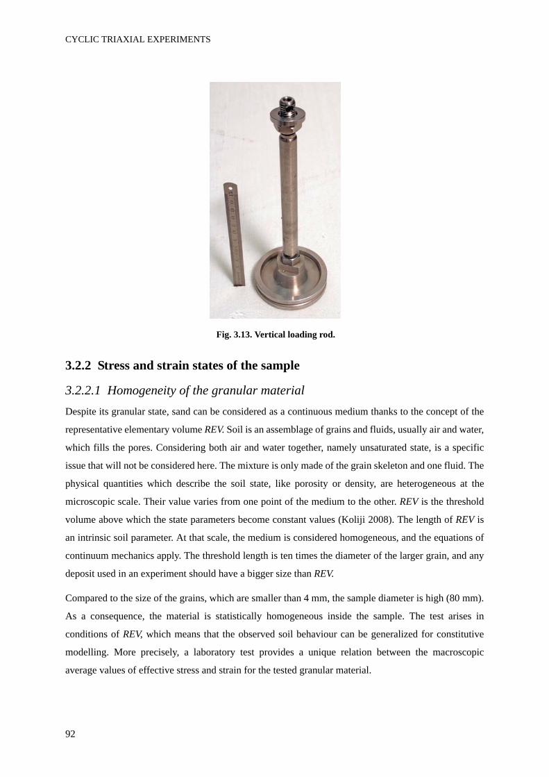
CYCLIC TRIAXIAL EXPERIMENTS
92
Fig. 3.13. Vertical loading rod.
3.2.2 Stress and strain states of the sample
3.2.2.1 Homogeneity of the granular materialDespite its granular state, sand can be considered as a continuous medium thanks to the concept of the
representative elementary volume REV. Soil is an assemblage of grains and fluids, usually air and water,
which fills the pores. Considering both air and water together, namely unsaturated state, is a specific
issue that will not be considered here. The mixture is only made of the grain skeleton and one fluid. The
physical quantities which describe the soil state, like porosity or density, are heterogeneous at the
microscopic scale. Their value varies from one point of the medium to the other. REV is the threshold
volume above which the state parameters become constant values (Koliji 2008). The length of REV is
an intrinsic soil parameter. At that scale, the medium is considered homogeneous, and the equations of
continuum mechanics apply. The threshold length is ten times the diameter of the larger grain, and any
deposit used in an experiment should have a bigger size than REV.
Compared to the size of the grains, which are smaller than 4 mm, the sample diameter is high (80 mm).
As a consequence, the material is statistically homogeneous inside the sample. The test arises in
conditions of REV, which means that the observed soil behaviour can be generalized for constitutive
modelling. More precisely, a laboratory test provides a unique relation between the macroscopic
average values of effective stress and strain for the tested granular material.
CHAPTER 3
93
3.2.2.2 Boundary conditionsIn this study, various boundary conditions are applied to the sample and different stress paths are
considered:
• monotonic loading, with a constant radial stress and an increasing axial stress (i.e. conventional
triaxial compression test, or CTC).
• unidirectional cyclic loading, with a constant radial stress and an axial stress which non-
monotonically varies with time (e.g. the sinusoidal mode).
• bidirectional loading, with both axial and radial stresses varying with time.
Further, two initial conditions of the sample will be considered: dry or fully saturated with water.
Finally, two drainage conditions will be applied: fully drained (zero relative pore-fluid pressure) or
fully undrained. Details on volume change measurement are given below.
Stress- and strain-controlled tests
Monotonic tests have a mixed uniform boundary condition, with a displacement imposed on the top of
the sample, and a pressure applied along its side.
Cyclic tests have stress-controlled uniform boundary conditions. Actually on the top of the sample, the
force only is controlled while the axial stress is calculated knowing the cross-section area. A known
pressure is applied along the side of the sample. In undrained conditions, only the total pressure can be
controlled because the effective stress depends on pore water pressure variations.
Saturated undrained conditions
For undrained conditions, water saturating the pores is blocked inside the medium, with no possibility
of flowing between the grains. Upon loading, excess pore pressure develops, either positive or negative
depending on the dilative behaviour of the granular matrix.
In most cases, monotonic and cyclic saturated tests are performed in undrained conditions. That means
that the system is closed. The total volume of the sample is constant, assuming that:
• membrane penetration is neglected
• sand grains are incompressible
• Water compressibility is neglected. The bulk modulus of water is traditionally evaluated at 2 GPa. If
one water bubble is included inside the closed volume of a triaxial sample, it decreases of a ratio of
at least 10 (Huot 1999).
Saturated samples are submitted to back pressure to avoid any presence of air bubble (details in
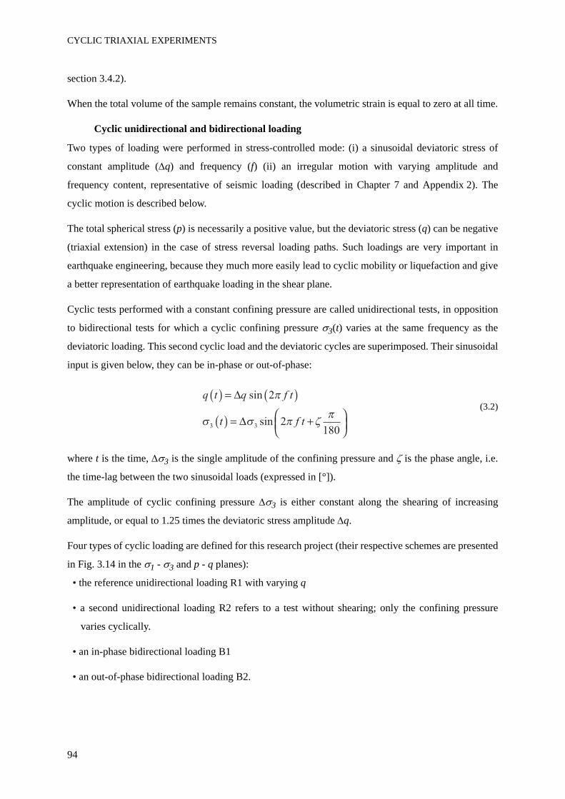
CYCLIC TRIAXIAL EXPERIMENTS
94
section 3.4.2).
When the total volume of the sample remains constant, the volumetric strain is equal to zero at all time.
Cyclic unidirectional and bidirectional loading
Two types of loading were performed in stress-controlled mode: (i) a sinusoidal deviatoric stress of
constant amplitude (Δq) and frequency (f) (ii) an irregular motion with varying amplitude and
frequency content, representative of seismic loading (described in Chapter 7 and Appendix 2). The
cyclic motion is described below.
The total spherical stress (p) is necessarily a positive value, but the deviatoric stress (q) can be negative
(triaxial extension) in the case of stress reversal loading paths. Such loadings are very important in
earthquake engineering, because they much more easily lead to cyclic mobility or liquefaction and give
a better representation of earthquake loading in the shear plane.
Cyclic tests performed with a constant confining pressure are called unidirectional tests, in opposition
to bidirectional tests for which a cyclic confining pressure σ3(t) varies at the same frequency as the
deviatoric loading. This second cyclic load and the deviatoric cycles are superimposed. Their sinusoidal
input is given below, they can be in-phase or out-of-phase:
(3.2)
where t is the time, Δσ3 is the single amplitude of the confining pressure and ζ is the phase angle, i.e.
the time-lag between the two sinusoidal loads (expressed in [°]).
The amplitude of cyclic confining pressure Δσ3 is either constant along the shearing of increasing
amplitude, or equal to 1.25 times the deviatoric stress amplitude Δq.
Four types of cyclic loading are defined for this research project (their respective schemes are presented
in Fig. 3.14 in the σ1 - σ3 and p - q planes):
• the reference unidirectional loading R1 with varying q
• a second unidirectional loading R2 refers to a test without shearing; only the confining pressure
varies cyclically.
• an in-phase bidirectional loading B1
• an out-of-phase bidirectional loading B2.
q t q f t
t f t
sin
sin
2
2180
3 3
CHAPTER 3
95
Fig. 3.14. Unidirectional and bidirectional loading paths.
3.2.3 Laser-based measurement of radial strains
3.2.3.1 PrinciplesMeasuring the evolution of the radius of a cylindrical sample and its radial strain (ε3) inside a triaxial
cell can be a complex issue. This is especially the case when conventional technique consisting of
measuring the outflow of interstitial water volume fails, as in the case of unsaturated or dry samples.
Special attention has been paid for this matter in this study.
Depending on the loading amplitude and frequency, and also on the type of soil, the requirements are
numerous for the design of a sensor used for such radial measurements: (i) it should not disturb the
sample (ii) it should be applicable to the larger possible strain and frequency range (iii) it should not be
influenced by the conditions of pressure, temperature, fluids in the cell as well as in the sample (iv) it
should fit into the allowed space (v) it should preferably measure the variations of ε3 along the height of
the sample (vi) data acquisition must be fully automatic.
Several techniques are available. Local measurement with contact includes horizontally mounted
LVDTs, local deformation collars or Hall effect transducers. They are fixed on the surface of the
membrane, forming rings, and they record the evolution of the diameter. The problem is that they are
both too heavy and too big for the case of medium to high strain measurement. Indeed their weight
might disturb the sample. In general, non-contact techniques are preferred for the measurement of
diameters of loose soils and for a wide range of strains. Possible candidates are contactless sensors or
even image processing techniques. A major difficulty arises when dynamic loading is considered,
where system response time is the key.
A contactless technique based on lasers, proposed for quasi-static conditions by Romero (1999), or
p
q
p
q
p
q
p
q
3
1
R1
R2
B1
B2
3
1
3
1
3
1
3
1
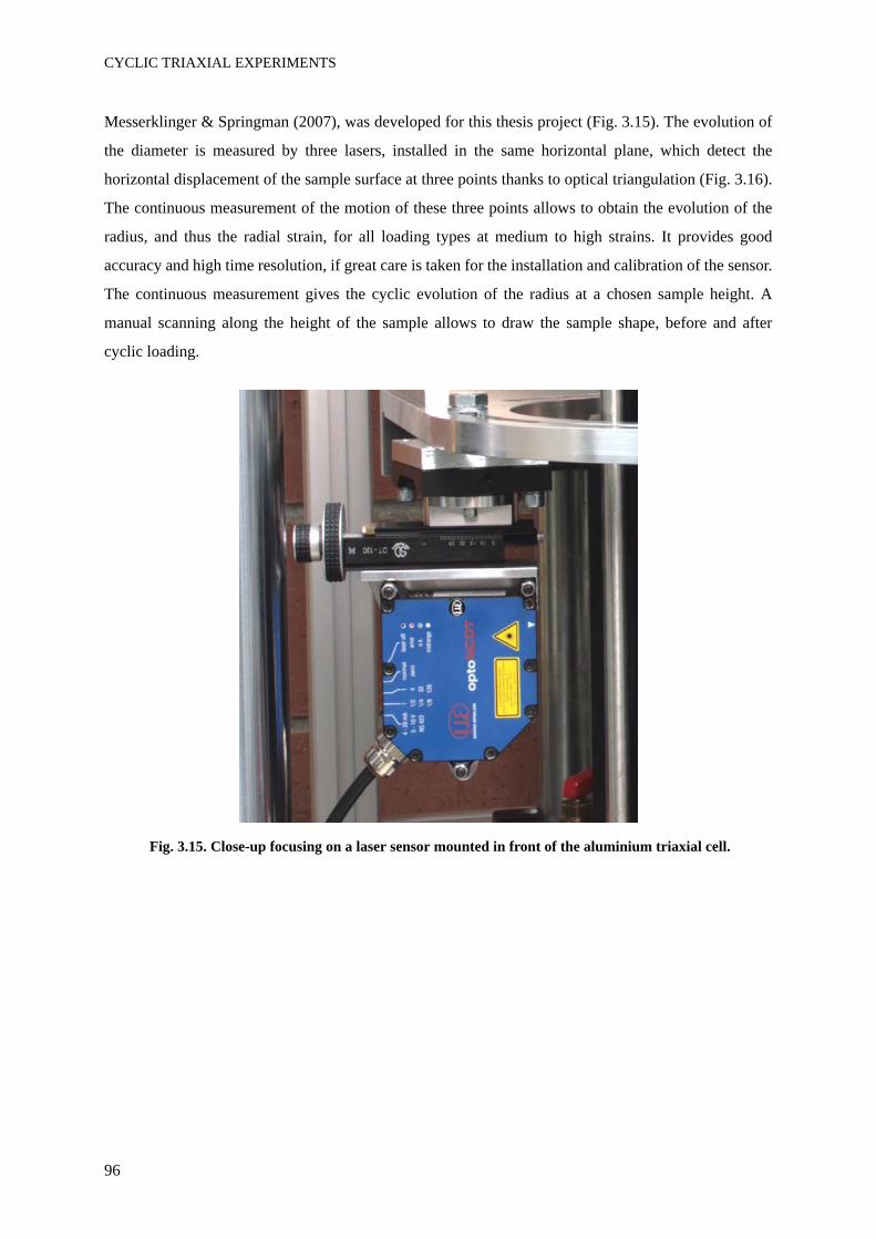
CYCLIC TRIAXIAL EXPERIMENTS
96
Messerklinger & Springman (2007), was developed for this thesis project (Fig. 3.15). The evolution of
the diameter is measured by three lasers, installed in the same horizontal plane, which detect the
horizontal displacement of the sample surface at three points thanks to optical triangulation (Fig. 3.16).
The continuous measurement of the motion of these three points allows to obtain the evolution of the
radius, and thus the radial strain, for all loading types at medium to high strains. It provides good
accuracy and high time resolution, if great care is taken for the installation and calibration of the sensor.
The continuous measurement gives the cyclic evolution of the radius at a chosen sample height. A
manual scanning along the height of the sample allows to draw the sample shape, before and after
cyclic loading.
Fig. 3.15. Close-up focusing on a laser sensor mounted in front of the aluminium triaxial cell.
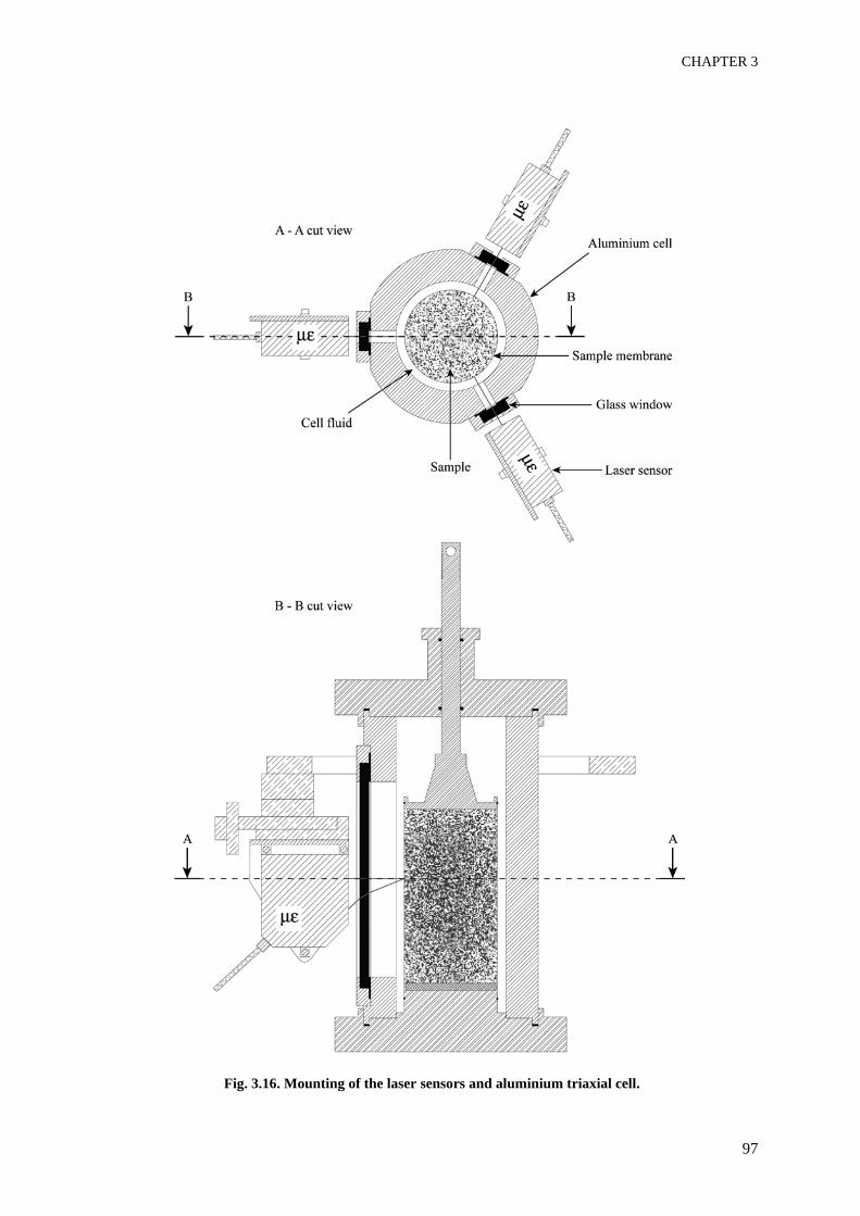
CHAPTER 3
97
Fig. 3.16. Mounting of the laser sensors and aluminium triaxial cell.
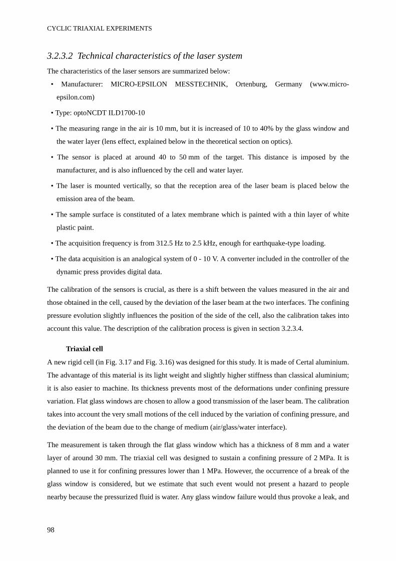
CYCLIC TRIAXIAL EXPERIMENTS
98
3.2.3.2 Technical characteristics of the laser systemThe characteristics of the laser sensors are summarized below:
• Manufacturer: MICRO-EPSILON MESSTECHNIK, Ortenburg, Germany (www.micro-
epsilon.com)
• Type: optoNCDT ILD1700-10
• The measuring range in the air is 10 mm, but it is increased of 10 to 40% by the glass window and
the water layer (lens effect, explained below in the theoretical section on optics).
• The sensor is placed at around 40 to 50 mm of the target. This distance is imposed by the
manufacturer, and is also influenced by the cell and water layer.
• The laser is mounted vertically, so that the reception area of the laser beam is placed below the
emission area of the beam.
• The sample surface is constituted of a latex membrane which is painted with a thin layer of white
plastic paint.
• The acquisition frequency is from 312.5 Hz to 2.5 kHz, enough for earthquake-type loading.
• The data acquisition is an analogical system of 0 - 10 V. A converter included in the controller of the
dynamic press provides digital data.
The calibration of the sensors is crucial, as there is a shift between the values measured in the air and
those obtained in the cell, caused by the deviation of the laser beam at the two interfaces. The confining
pressure evolution slightly influences the position of the side of the cell, also the calibration takes into
account this value. The description of the calibration process is given in section 3.2.3.4.
Triaxial cell
A new rigid cell (in Fig. 3.17 and Fig. 3.16) was designed for this study. It is made of Certal aluminium.
The advantage of this material is its light weight and slightly higher stiffness than classical aluminium;
it is also easier to machine. Its thickness prevents most of the deformations under confining pressure
variation. Flat glass windows are chosen to allow a good transmission of the laser beam. The calibration
takes into account the very small motions of the cell induced by the variation of confining pressure, and
the deviation of the beam due to the change of medium (air/glass/water interface).
The measurement is taken through the flat glass window which has a thickness of 8 mm and a water
layer of around 30 mm. The triaxial cell was designed to sustain a confining pressure of 2 MPa. It is
planned to use it for confining pressures lower than 1 MPa. However, the occurrence of a break of the
glass window is considered, but we estimate that such event would not present a hazard to people
nearby because the pressurized fluid is water. Any glass window failure would thus provoke a leak, and
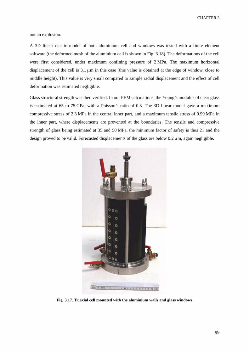
CHAPTER 3
99
not an explosion.
A 3D linear elastic model of both aluminium cell and windows was tested with a finite element
software (the deformed mesh of the aluminium cell is shown in Fig. 3.18). The deformations of the cell
were first considered, under maximum confining pressure of 2 MPa. The maximum horizontal
displacement of the cell is 3.1 μm in this case (this value is obtained at the edge of window, close to
middle height). This value is very small compared to sample radial displacement and the effect of cell
deformation was estimated negligible.
Glass structural strength was then verified. In our FEM calculations, the Young’s modulus of clear glass
is estimated at 65 to 75 GPa, with a Poisson’s ratio of 0.3. The 3D linear model gave a maximum
compressive stress of 2.3 MPa in the central inner part, and a maximum tensile stress of 0.99 MPa in
the inner part, where displacements are prevented at the boundaries. The tensile and compressive
strength of glass being estimated at 35 and 50 MPa, the minimum factor of safety is thus 21 and the
design proved to be valid. Forecasted displacements of the glass are below 0.2 μm, again negligible.
Fig. 3.17. Triaxial cell mounted with the aluminium walls and glass windows.
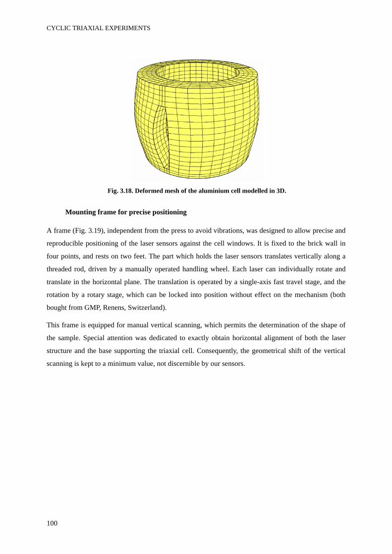
CYCLIC TRIAXIAL EXPERIMENTS
100
Fig. 3.18. Deformed mesh of the aluminium cell modelled in 3D.
Mounting frame for precise positioning
A frame (Fig. 3.19), independent from the press to avoid vibrations, was designed to allow precise and
reproducible positioning of the laser sensors against the cell windows. It is fixed to the brick wall in
four points, and rests on two feet. The part which holds the laser sensors translates vertically along a
threaded rod, driven by a manually operated handling wheel. Each laser can individually rotate and
translate in the horizontal plane. The translation is operated by a single-axis fast travel stage, and the
rotation by a rotary stage, which can be locked into position without effect on the mechanism (both
bought from GMP, Renens, Switzerland).
This frame is equipped for manual vertical scanning, which permits the determination of the shape of
the sample. Special attention was dedicated to exactly obtain horizontal alignment of both the laser
structure and the base supporting the triaxial cell. Consequently, the geometrical shift of the vertical
scanning is kept to a minimum value, not discernible by our sensors.
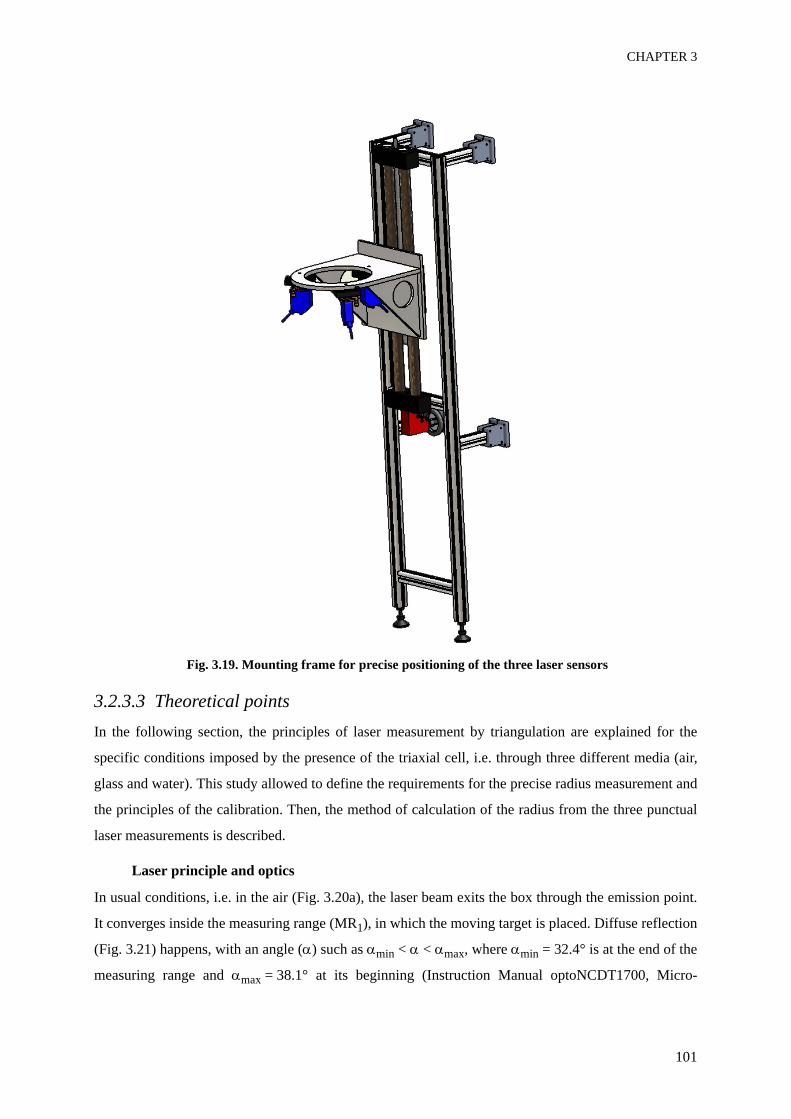
CHAPTER 3
101
Fig. 3.19. Mounting frame for precise positioning of the three laser sensors
3.2.3.3 Theoretical pointsIn the following section, the principles of laser measurement by triangulation are explained for the
specific conditions imposed by the presence of the triaxial cell, i.e. through three different media (air,
glass and water). This study allowed to define the requirements for the precise radius measurement and
the principles of the calibration. Then, the method of calculation of the radius from the three punctual
laser measurements is described.
Laser principle and optics
In usual conditions, i.e. in the air (Fig. 3.20a), the laser beam exits the box through the emission point.
It converges inside the measuring range (MR1), in which the moving target is placed. Diffuse reflection
(Fig. 3.21) happens, with an angle (α) such as αmin < α < αmax, where αmin = 32.4° is at the end of the
measuring range and αmax = 38.1° at its beginning (Instruction Manual optoNCDT1700, Micro-
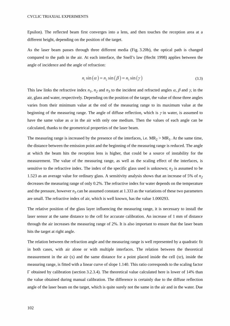
CYCLIC TRIAXIAL EXPERIMENTS
102
Epsilon). The reflected beam first converges into a lens, and then touches the reception area at a
different height, depending on the position of the target.
As the laser beam passes through three different media (Fig. 3.20b), the optical path is changed
compared to the path in the air. At each interface, the Snell’s law (Hecht 1998) applies between the
angle of incidence and the angle of refraction:
(3.3)
This law links the refractive index n1, n2 and n3 to the incident and refracted angles α, β and γ, in the
air, glass and water, respectively. Depending on the position of the target, the value of those three angles
varies from their minimum value at the end of the measuring range to its maximum value at the
beginning of the measuring range. The angle of diffuse reflection, which is γ in water, is assumed to
have the same value as α in the air with only one medium. Then the values of each angle can be
calculated, thanks to the geometrical properties of the laser beam.
The measuring range is increased by the presence of the interfaces, i.e. MR2 > MR1. At the same time,
the distance between the emission point and the beginning of the measuring range is reduced. The angle
at which the beam hits the reception lens is higher, that could be a source of instability for the
measurement. The value of the measuring range, as well as the scaling effect of the interfaces, is
sensitive to the refractive index. The index of the specific glass used is unknown; n2 is assumed to be
1.523 as an average value for ordinary glass. A sensitivity analysis shows that an increase of 5% of n2
decreases the measuring range of only 0.2%. The refractive index for water depends on the temperature
and the pressure, however n3 can be assumed constant at 1.333 as the variations of these two parameters
are small. The refractive index of air, which is well known, has the value 1.000293.
The relative position of the glass layer influencing the measuring range, it is necessary to install the
laser sensor at the same distance to the cell for accurate calibration. An increase of 1 mm of distance
through the air increases the measuring range of 2%. It is also important to ensure that the laser beam
hits the target at right angle.
The relation between the refraction angle and the measuring range is well represented by a quadratic fit
in both cases, with air alone or with multiple interfaces. The relation between the theoretical
measurement in the air (x) and the same distance for a point placed inside the cell (xr), inside the
measuring range, is fitted with a linear curve of slope 1.140. This ratio corresponds to the scaling factor
Γ obtained by calibration (section 3.2.3.4). The theoretical value calculated here is lower of 14% than
the value obtained during manual calibration. The difference is certainly due to the diffuse reflection
angle of the laser beam on the target, which is quite surely not the same in the air and in the water. Due
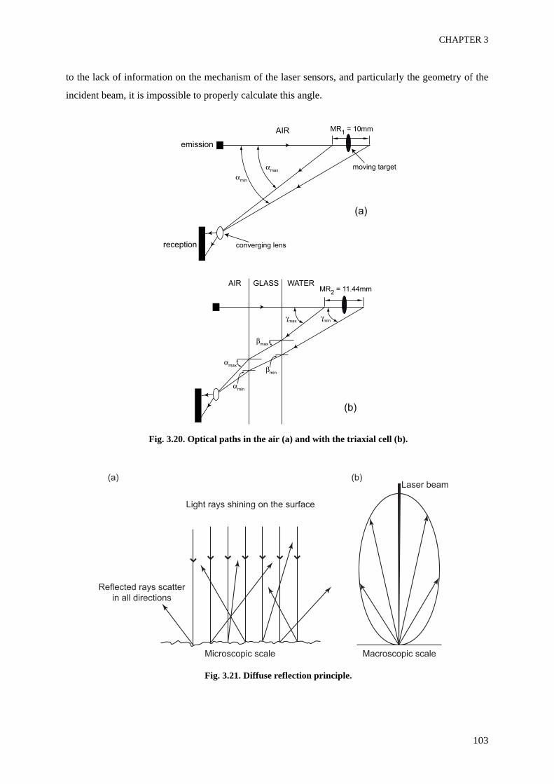
CHAPTER 3
103
to the lack of information on the mechanism of the laser sensors, and particularly the geometry of the
incident beam, it is impossible to properly calculate this angle.
Fig. 3.20. Optical paths in the air (a) and with the triaxial cell (b).
Fig. 3.21. Diffuse reflection principle.
AIR GLASS WATER
AIR MR1 = 10mm
MR2 = 11.44mm
min
max
min
max
min
max
minmax
emission
reception
(a)
(b)
moving target
converging lens
Macroscopic scale
Laser beam(a) (b)
Microscopic scale
Light rays shining on the surface
Reflected rays scatter
in all directions
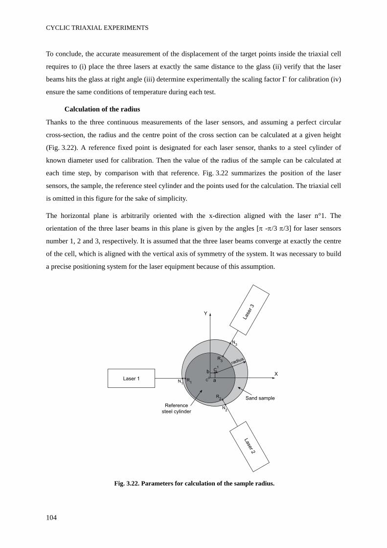
CYCLIC TRIAXIAL EXPERIMENTS
104
To conclude, the accurate measurement of the displacement of the target points inside the triaxial cell
requires to (i) place the three lasers at exactly the same distance to the glass (ii) verify that the laser
beams hits the glass at right angle (iii) determine experimentally the scaling factor Γ for calibration (iv)
ensure the same conditions of temperature during each test.
Calculation of the radius
Thanks to the three continuous measurements of the laser sensors, and assuming a perfect circular
cross-section, the radius and the centre point of the cross section can be calculated at a given height
(Fig. 3.22). A reference fixed point is designated for each laser sensor, thanks to a steel cylinder of
known diameter used for calibration. Then the value of the radius of the sample can be calculated at
each time step, by comparison with that reference. Fig. 3.22 summarizes the position of the laser
sensors, the sample, the reference steel cylinder and the points used for the calculation. The triaxial cell
is omitted in this figure for the sake of simplicity.
The horizontal plane is arbitrarily oriented with the x-direction aligned with the laser n°1. The
orientation of the three laser beams in this plane is given by the angles [π -π/3 π/3] for laser sensors
number 1, 2 and 3, respectively. It is assumed that the three laser beams converge at exactly the centre
of the cell, which is aligned with the vertical axis of symmetry of the system. It was necessary to build
a precise positioning system for the laser equipment because of this assumption.
Fig. 3.22. Parameters for calculation of the sample radius.
Reference
steel cylinder
Laser 1
Lase
r 2
Lase
r 3
R1
R2
R3
N1
N2
N3
C0
C1
Sand sample
X
Y
a
b
radius
CHAPTER 3
105
The reference cylinder being centred, the coordinates of the points R1, R2 and R3 are:
(3.4)
The radius of the reference steel cylinder is r = 39.79 mm at its middle height, including a thin
homogeneous layer of white sprayed paint. The position of the reference points is associated with the
respective measured values of the three laser sensors. Including the calibration at zero confining
pressure, those measured values are called mref ; they depend on the distance between the lasers and
cell, also they are associated with a given calibration.
The points are taken on the external surface of the sample, also the thickness of the membrane and the
paint layer are included in each initial laser measurement. The membrane thickness is directly measured
with a slide callipers before each test. The paint layer thickness was evaluated at approximately 0.2+/-
0.05 mm from several measurements taken after dismounting of the cell and sample, by carefully
peeling off the paint from the membrane. The addition of these two constant shifts is called ep.
The absolute coordinates, in the cross section plane, of the points N1, N2 and N3 situated on the inner
surface of the sample, i.e. below the membrane, can be calculated now. The values measured by the
laser sensors are n1, n2 and n3. At each time step t, the points coordinates are:
(3.5)
The centre of the circle C(t) which passes through the three points N1(t), N2(t) and N3(t) is the
intersection of the two perpendicular bisectors, KC and LC, of the lines N1N2 and N2N3, respectively
(Fig. 3.23). It is necessary to calculate the equations of the two perpendicular bisectors in order to
obtain the coordinates of C, X(t) and Y(t).
Rr
R
r
rR
r
r1 2 3
0
2
3
2
2
3
2
N tx
yR m n t ep
N tx
y
ref1
1
1
1 1
2
2
2
11
0( )
R m n t ep
N tx
y
ref2 2
3
3
3
2
1
2
3
2
( )
R m n t epref3 33
1
2
3
2
( )

CYCLIC TRIAXIAL EXPERIMENTS
106
(3.6)
Then the coordinates of their intersection are calculated by:
(3.7)
The radius is simply deduced from the distance between the centre and one of the points, for example
here with N2:
(3.8)
Fig. 3.23. Geometrical determination of the centre of the sample cross-section.
y ax b y a x bKC LC
ax x
y y
2 1
2 1
bx x y y
y y
2
2
1
2
2
2
1
2
2 12
ax x
y y
3 2
3 2
bx x y y
y y
3
2
2
2
3
2
2
2
3 22
X tb b
a a
Y t a X t b
( )
( )
radius x X y Y2
2
2
2
N1
N2
N3
C1
C0 X
Y
L
K
CHAPTER 3
107
3.2.3.4 Detailed use of the laser sensorsElectrical connection
The power supply is a DC battery. The output data is recorded through analogical connection to the
Instron data acquisition tower by a D-sub connector.
Parameters setting
The setting of the output parameters of the laser sensor is performed with the two buttons placed on the
laser box. An internal filter averages the data, so that noise can be reduced. A recursive average is
chosen. The sampling frequency can be 2.5 kHz at maximum, but decreasing that value increases the
exposure time, which helps for signals of lower power. The minimum value 312.5 Hz was finally
chosen.
Description of the precise positioning
The angular position of the three laser sensors at 120° from each other is fixed. However, each of them
can rotate around that fixed position thanks to a manual rotary stage, which allows alignment in front of
the glass window. A translation stage allows to adjust the distance from the cell, so that the measuring
range covers the expected radial displacement of the sample. Two templates of different thickness were
selected, also it is possible to chose between two reference positions. A calibration was performed for
each of them. The larger one is preferred when an increase of the diameter is expected, and the thinner
one corresponds to a decrease of the diameter in the case of triaxial extension tests.
The position of the cell is fixed thanks to a groove extruded from the upper surface of the base of the
dynamic press. The cell is placed so that the glass windows are perpendicular to the laser beam. Before
fixing the rotation of the cell by linking the vertical loading rod with the dynamic press, it is always
checked that laser beams hit their respective glass window at the middle of the aperture, in order to
avoid any misalignment with the vertical central axis. Once aligned, the position of both the triaxial cell
and the laser sensors is tightly secured. The laser beam should hit the target at right angle. A difference
of 5° induces a small error on the measured value, lower than 12 μm according to the user’s manual of
the laser sensors.
Calibration procedure
The laser sensor is first automatically calibrated thanks to the controller of the dynamic press. It
transfers the measured voltage range into a length, with a scale of 1 mm corresponding to 1 V. Then a
precise calibration is performed. The manual calibration is first done in the air, by targeting a moving
element. Possible external drifts are tested; the laser beams are not highly sensitive to light and
vibrations from the press. They are more sensitive to the target surface quality. This calibration shows
that the automated calibration is valid, with a precision higher than 99.99%.
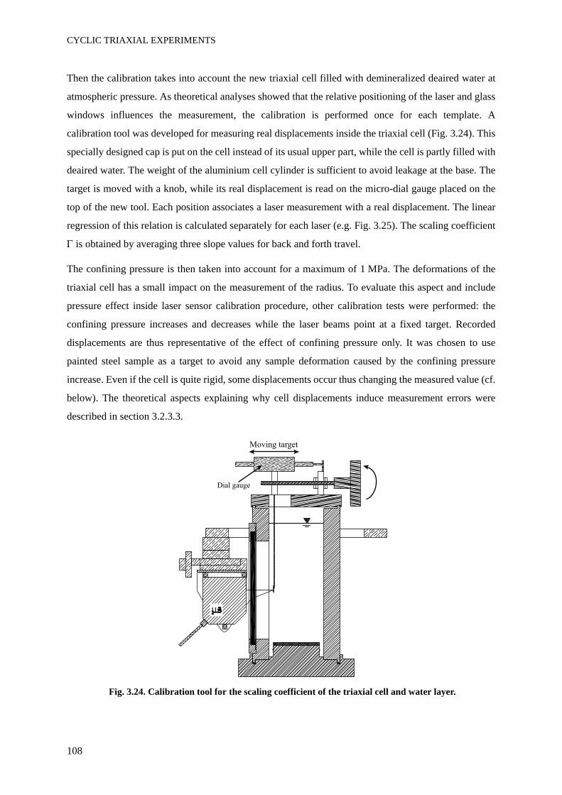
CYCLIC TRIAXIAL EXPERIMENTS
108
Then the calibration takes into account the new triaxial cell filled with demineralized deaired water at
atmospheric pressure. As theoretical analyses showed that the relative positioning of the laser and glass
windows influences the measurement, the calibration is performed once for each template. A
calibration tool was developed for measuring real displacements inside the triaxial cell (Fig. 3.24). This
specially designed cap is put on the cell instead of its usual upper part, while the cell is partly filled with
deaired water. The weight of the aluminium cell cylinder is sufficient to avoid leakage at the base. The
target is moved with a knob, while its real displacement is read on the micro-dial gauge placed on the
top of the new tool. Each position associates a laser measurement with a real displacement. The linear
regression of this relation is calculated separately for each laser (e.g. Fig. 3.25). The scaling coefficient
Γ is obtained by averaging three slope values for back and forth travel.
The confining pressure is then taken into account for a maximum of 1 MPa. The deformations of the
triaxial cell has a small impact on the measurement of the radius. To evaluate this aspect and include
pressure effect inside laser sensor calibration procedure, other calibration tests were performed: the
confining pressure increases and decreases while the laser beams point at a fixed target. Recorded
displacements are thus representative of the effect of confining pressure only. It was chosen to use
painted steel sample as a target to avoid any sample deformation caused by the confining pressure
increase. Even if the cell is quite rigid, some displacements occur thus changing the measured value (cf.
below). The theoretical aspects explaining why cell displacements induce measurement errors were
described in section 3.2.3.3.
Fig. 3.24. Calibration tool for the scaling coefficient of the triaxial cell and water layer.
Moving target
Dial gauge
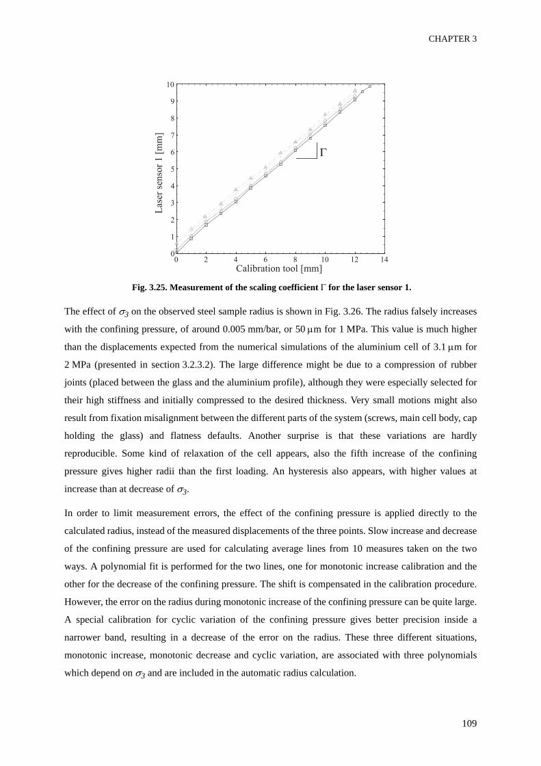
CHAPTER 3
109
Fig. 3.25. Measurement of the scaling coefficient Γ for the laser sensor 1.
The effect of σ3 on the observed steel sample radius is shown in Fig. 3.26. The radius falsely increases
with the confining pressure, of around 0.005 mm/bar, or 50 μm for 1 MPa. This value is much higher
than the displacements expected from the numerical simulations of the aluminium cell of 3.1 μm for
2 MPa (presented in section 3.2.3.2). The large difference might be due to a compression of rubber
joints (placed between the glass and the aluminium profile), although they were especially selected for
their high stiffness and initially compressed to the desired thickness. Very small motions might also
result from fixation misalignment between the different parts of the system (screws, main cell body, cap
holding the glass) and flatness defaults. Another surprise is that these variations are hardly
reproducible. Some kind of relaxation of the cell appears, also the fifth increase of the confining
pressure gives higher radii than the first loading. An hysteresis also appears, with higher values at
increase than at decrease of σ3.
In order to limit measurement errors, the effect of the confining pressure is applied directly to the
calculated radius, instead of the measured displacements of the three points. Slow increase and decrease
of the confining pressure are used for calculating average lines from 10 measures taken on the two
ways. A polynomial fit is performed for the two lines, one for monotonic increase calibration and the
other for the decrease of the confining pressure. The shift is compensated in the calibration procedure.
However, the error on the radius during monotonic increase of the confining pressure can be quite large.
A special calibration for cyclic variation of the confining pressure gives better precision inside a
narrower band, resulting in a decrease of the error on the radius. These three different situations,
monotonic increase, monotonic decrease and cyclic variation, are associated with three polynomials
which depend on σ3 and are included in the automatic radius calculation.
0 2 4 6 8 10 12 140
1
2
3
4
5
6
7
8
9
10
Las
er s
enso
r 1
[m
m]
Calibration tool [mm]
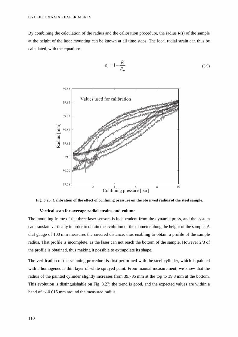
CYCLIC TRIAXIAL EXPERIMENTS
110
By combining the calculation of the radius and the calibration procedure, the radius R(t) of the sample
at the height of the laser mounting can be known at all time steps. The local radial strain can thus be
calculated, with the equation:
(3.9)
Fig. 3.26. Calibration of the effect of confining pressure on the observed radius of the steel sample.
Vertical scan for average radial strains and volume
The mounting frame of the three laser sensors is independent from the dynamic press, and the system
can translate vertically in order to obtain the evolution of the diameter along the height of the sample. A
dial gauge of 100 mm measures the covered distance, thus enabling to obtain a profile of the sample
radius. That profile is incomplete, as the laser can not reach the bottom of the sample. However 2/3 of
the profile is obtained, thus making it possible to extrapolate its shape.
The verification of the scanning procedure is first performed with the steel cylinder, which is painted
with a homogeneous thin layer of white sprayed paint. From manual measurement, we know that the
radius of the painted cylinder slightly increases from 39.785 mm at the top to 39.8 mm at the bottom.
This evolution is distinguishable on Fig. 3.27; the trend is good, and the expected values are within a
band of +/-0.015 mm around the measured radius.
3
0
1R
R
0 2 4 6 8 1039.78
39.79
39.8
39.81
39.82
39.83
39.84
39.85
Confining pressure [bar]
Rad
ius
[mm
]
Values used for calibration
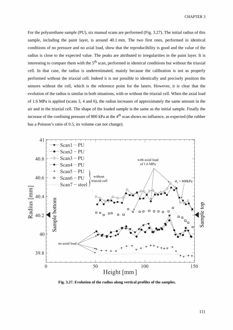
CHAPTER 3
111
For the polyurethane sample (PU), six manual scans are performed (Fig. 3.27). The initial radius of this
sample, including the paint layer, is around 40.1 mm. The two first ones, performed in identical
conditions of no pressure and no axial load, show that the reproducibility is good and the value of the
radius is close to the expected value. The peaks are attributed to irregularities in the paint layer. It is
interesting to compare them with the 5th scan, performed in identical conditions but without the triaxial
cell. In that case, the radius is underestimated, mainly because the calibration is not as properly
performed without the triaxial cell. Indeed it is not possible to identically and precisely position the
sensors without the cell, which is the reference point for the lasers. However, it is clear that the
evolution of the radius is similar in both situations, with or without the triaxial cell. When the axial load
of 1.6 MPa is applied (scans 3, 4 and 6), the radius increases of approximately the same amount in the
air and in the triaxial cell. The shape of the loaded sample is the same as the initial sample. Finally the
increase of the confining pressure of 800 kPa at the 4th scan shows no influence, as expected (the rubber
has a Poisson’s ratio of 0.5, its volume can not change).
Fig. 3.27. Evolution of the radius along vertical profiles of the samples.
0 50 100 150
39.8
40
40.2
40.4
40.6
40.8
41
Rad
ius
[mm
]
Height [mm ]
without} 3
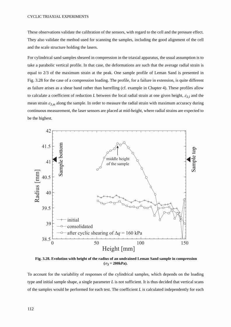
CYCLIC TRIAXIAL EXPERIMENTS
112
These observations validate the calibration of the sensors, with regard to the cell and the pressure effect.
They also validate the method used for scanning the samples, including the good alignment of the cell
and the scale structure holding the lasers.
For cylindrical sand samples sheared in compression in the triaxial apparatus, the usual assumption is to
take a parabolic vertical profile. In that case, the deformations are such that the average radial strain is
equal to 2/3 of the maximum strain at the peak. One sample profile of Leman Sand is presented in
Fig. 3.28 for the case of a compression loading. The profile, for a failure in extension, is quite different
as failure arises as a shear band rather than barrelling (cf. example in Chapter 4). These profiles allow
to calculate a coefficient of reduction L between the local radial strain at one given height, ε3,l and the
mean strain ε3,m along the sample. In order to measure the radial strain with maximum accuracy during
continuous measurement, the laser sensors are placed at mid-height, where radial strains are expected to
be the highest.
Fig. 3.28. Evolution with height of the radius of an undrained Leman Sand sample in compression (σ3 = 200kPa).
To account for the variability of responses of the cylindrical samples, which depends on the loading
type and initial sample shape, a single parameter L is not sufficient. It is thus decided that vertical scans
of the samples would be performed for each test. The coefficient L is calculated independently for each
0 50 100 15038.5
39
39.5
40
40.5
41
41.5
42
Rad
ius
[mm
]
Height [mm]
initial
consolidated
after cyclic shearing of q = 160 kPa
middle height
of the sample
Sam
ple
bott
om
Sam
ple
top
CHAPTER 3
113
sample. An initial scan allows to evaluate the initial average radius and shape, and the scan performed
after shearing gives the deformed shape. The coefficient L is calculated with the deformed shape.
To summarize, the scanning process increases the efficiency of the laser device, by taking into account
the real shape of the sample. It is clear by that method that the assumption of a parabolic profile is not
enough, especially for tests in extension.
3.2.3.5 Estimation of uncertaintiesThe uncertainties of the non-contact measurement technique with laser sensors are evaluated now. The
uncertainties linked with the physical measurements are:
• The intrinsic laser sensor measurement error is neglected, it is around 0.5 μm.
• Thickness of the paint layer (δl1 = 0.01 mm estimated from comparison of the thickness after the
test)
• Thickness of the membrane, from initial thickness, membrane compressibility and membrane
penetration. Membrane penetration is the most important of these three factors in undrained tests,
because it evolves with the effective confining pressure. In dry tests however, the effective confining
pressure remains constant and the error on the radius is thus constant during cyclic tests, after
consolidation. The uncertainty on total membrane thickness can be neglected for the calculation of
radial strain uncertainty because cyclic radial strains are not affected by the static errors on the
radius. For the sample radius uncertainty, membrane penetration is usually broadly estimated by the
half of D50 of the soil. But the paint layer clearly decreases membrane penetration also this value
does not really reflect this uncertainty. It is finally assumed that the error on membrane thickness is
negligible compared to the error on the thickness of the paint layer.
• Error at transmission of the laser beam through interfaces, from small heterogeneities of the glass
and particles within the water (δl2 = 0.005 mm, i.e. ten times the resolution of the laser used in the
air)
• Angular horizontal and vertical misalignment of the position of the laser (δθ < 1° => negligible)
• Temperature variations: this can be neglected since the laboratory is temperature-controlled.
Uncertainties arising from the calibration procedure are:
• Stability of the automatic calibration (negligible)
• Precision on the scaling coefficient Γ, including the distance between the laser and the cell
(δc1 = 0.002 mm/mm from the comparison of the three values for each laser)
CYCLIC TRIAXIAL EXPERIMENTS
114
• Effect of confining pressure, with the repeatability of cell wall displacement and the accommodation
due to creep of the cell (δc2 = 0.015 mm/bar from Fig. 3.26)
• Precision of the reference position with the steel cylinder, for the calculation of the diameter
(estimated broadly at δc3 = 0.01 mm)
• Assumption of a perfect circular cross-section for the calculation of the diameter (unknown)
The coefficient of integration L for obtaining the average axial strain over sample height (introduced in
the description of the scanning procedure) is calculated by comparing two scans of the sample, the
initial and the sheared sample. The evaluation of uncertainties for that coefficient concerns an
additional component:
• Misalignment of the structure holding the scan and the triaxial cell and fits in the vertical
displacement system (δi1 = 0.015 mm from the evaluation with the steel cylinder)
The total uncertainty on the position of each point N1, N2 and N3, is calculated at 0.06 mm before
taking into account the confining pressure. The uncertainty on the radius is thus also at worst within this
range of value. Adding the effect of confining pressure, the total uncertainty on the radius is then
0.08 mm, or a relative uncertainty of 0.2%. Taking also into account the vertical motion for scanning,
total uncertainty on the radius includes δi1, as well as the previously mentioned errors. This new
uncertainty on the radius with the vertical translation of the equipment is δR = 0.1 mm, which
corresponds to a relative error of 0.25%.
The static error on the radius at a given height, at any given time, is estimated from all uncertainty
factors. Most of them remain constant during the whole test: δl1, δc1, δc3 do not vary after the setting
up of the triaxial cell. The error due to confining pressure δc2 is also constant after the application of the
isotropic consolidation, except for bidirectional loading. That is why the uncertainty calculated above
does not apply for the variation of the radius ΔR measured during each phase of the test. Only the direct
measurement error δl3 is taken into account for the uncertainty of ΔR, which gives δΔR = 0.005 mm.
The uncertainty of the local radial strain measured with the laser technique is then δε3,l = |δΔR / R0| =
0.005 / 40 = 1 x 10⁻⁴.
The uncertainty of the integration factor L is estimated at 5%, also the error on the average radial strain
over the sample is, at medium strain range:
δε3,m = δε3,l*L + ε3,l*δL= 1 x 10-4*1 + 5 x 10-3*0.05 = 4 x 10⁻⁴ (3.10)
This value is at the bottom of the range concerned by medium strains, also this might be an issue for the
smallest motion amplitudes. The validity of laser sensor measurements is verified along a real triaxial
CHAPTER 3
115
test on Leman Sand, described in section 4.6.
3.2.3.6 SummaryLaser-based measurement technique is a very sensitive equipment, but it allows to measure radial
strains without contact in the range of medium to large strains. The technique is adapted for cyclic
triaxial testing of granular materials in cyclic loading, for which large strains develop.
The development of this technique includes:
• an analysis of the optical path through three media (air, glass and water) to detect the factors
influencing the measurement
• the design of a new aluminium cell with flat glass windows
• the design of a structure which allows precise positioning in front of the windows, at a given distance
of the axis of the dynamic press. The system translates vertically to allow vertical scanning of the
sample
• the design of a calibration procedure which takes into account the confining pressure, including the
creation of a target which translates horizontally inside the cell
• an automated calculation procedure of the radius from the three laser measurements
• an evaluation of vertical scanning, and the creation of an integration factor to calculate an average
radial strain from the continuous measurement of the local radial strain at mid-height of the sample.
A validation example on undrained Leman Sand is presented in Chapter 4, before the presentation of
tests on dry sand.
3.3 Validation testsA polyurethane cylinder was tested in the triaxial cell to check any drawback in the press and the
measuring system. The vertical linear load and the confining pressure load were tested for constant,
monotonic and cyclic commands, independently and with a slave - master relation on various stress
paths. It was observed that stress-controlled and strain-controlled motions are equivalently precise
within their range of use. The command error was found to be of the order of 0.5% for displacement
motions of vertical cyclic amplitudes ranging from 0.05 mm / 40 kPa to 5 mm / 500 kPa, and at
frequencies from 0.1 Hz to 10 Hz. This value is low for such wide range thanks to the possibility to
trigger internal parameters of the control loop.
CYCLIC TRIAXIAL EXPERIMENTS
116
Fatigue tests were also performed, in order to verify the sensitivity of the device to tests of long
duration. During a three hours long test, the displacement amplitude was satisfactorily observed to
remain constant (0.1% variation) after 20000 cycles.
The servo-valve monitoring the cell pressure was also checked to be very precise: the total confining
pressure can be maintained constant thanks to the internal regulation. Very small oscillations appear
anyway, in the order of 0.3% of the actual pressure, at the beginning of the tests, and they can increase
to 3.5% when large strains are induced, i.e. during cyclic mobility.
Because of friction between the loading rod and the top of the triaxial cell, we estimate that loadings
with deviatoric stress amplitude below Δq = 15 kPa should not be considered. This is the criterion
applied to withdraw non-valid test results.
The top and base of the sample are not smooth enough (only a paper filter boundary) to avoid end-
restraint and the formation of barrel shapes during loading at rather large amplitudes. Indeed, the
friction of the granular matrix against the filter is a boundary condition which prevents full
homogeneity of the sample. Near these rough boundaries, less deformations are produced and the soil
behaviour is more contractive than in other parts of the sample. The deformed shape of sand sample
(Fig. 3.28) shows that barrelling may not be negligible. This inhomogeneity which may become
predominant near failure (i.e. at large strain amplitude) is mentioned further in section 4.5.
3.4 Experimental procedures
3.4.1 Sand sample mountingThe production of sandy samples with good reproducibility of the sample size required to design a new
mould (Fig. 3.29). This device is put on the base of the cell, around the membrane, and applies a
vacuum between the membrane and the inner surface of the mould. The dimensions of the mould are
exactly matched with the cell base, on which a membrane of thickness 0.3 mm and one O-ring are put.
As a consequence, the membrane is plated against the walls and the inner volume is exactly the same
for each sample. To allow convenient mounting and dismantling, the mould is made of two symmetric
parts. They hold tightly together thanks to two collars.
For samples saturated with water, the mould is gradually filled with a known volume of water, and then
small spoons of sand are poured. Between each spoon, the soil is lightly patted to avoid cavities inside
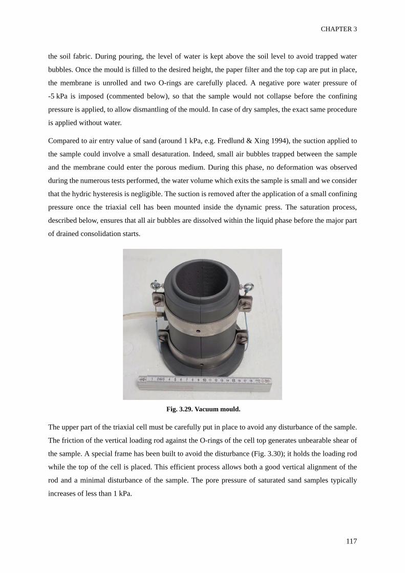
CHAPTER 3
117
the soil fabric. During pouring, the level of water is kept above the soil level to avoid trapped water
bubbles. Once the mould is filled to the desired height, the paper filter and the top cap are put in place,
the membrane is unrolled and two O-rings are carefully placed. A negative pore water pressure of
-5 kPa is imposed (commented below), so that the sample would not collapse before the confining
pressure is applied, to allow dismantling of the mould. In case of dry samples, the exact same procedure
is applied without water.
Compared to air entry value of sand (around 1 kPa, e.g. Fredlund & Xing 1994), the suction applied to
the sample could involve a small desaturation. Indeed, small air bubbles trapped between the sample
and the membrane could enter the porous medium. During this phase, no deformation was observed
during the numerous tests performed, the water volume which exits the sample is small and we consider
that the hydric hysteresis is negligible. The suction is removed after the application of a small confining
pressure once the triaxial cell has been mounted inside the dynamic press. The saturation process,
described below, ensures that all air bubbles are dissolved within the liquid phase before the major part
of drained consolidation starts.
Fig. 3.29. Vacuum mould.
The upper part of the triaxial cell must be carefully put in place to avoid any disturbance of the sample.
The friction of the vertical loading rod against the O-rings of the cell top generates unbearable shear of
the sample. A special frame has been built to avoid the disturbance (Fig. 3.30); it holds the loading rod
while the top of the cell is placed. This efficient process allows both a good vertical alignment of the
rod and a minimal disturbance of the sample. The pore pressure of saturated sand samples typically
increases of less than 1 kPa.
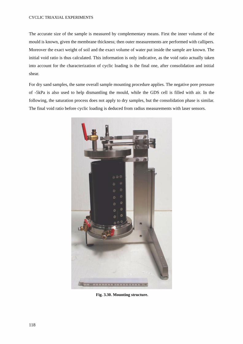
CYCLIC TRIAXIAL EXPERIMENTS
118
The accurate size of the sample is measured by complementary means. First the inner volume of the
mould is known, given the membrane thickness; then outer measurements are performed with callipers.
Moreover the exact weight of soil and the exact volume of water put inside the sample are known. The
initial void ratio is thus calculated. This information is only indicative, as the void ratio actually taken
into account for the characterization of cyclic loading is the final one, after consolidation and initial
shear.
For dry sand samples, the same overall sample mounting procedure applies. The negative pore pressure
of -5kPa is also used to help dismantling the mould, while the GDS cell is filled with air. In the
following, the saturation process does not apply to dry samples, but the consolidation phase is similar.
The final void ratio before cyclic loading is deduced from radius measurements with laser sensors.
Fig. 3.30. Mounting structure.
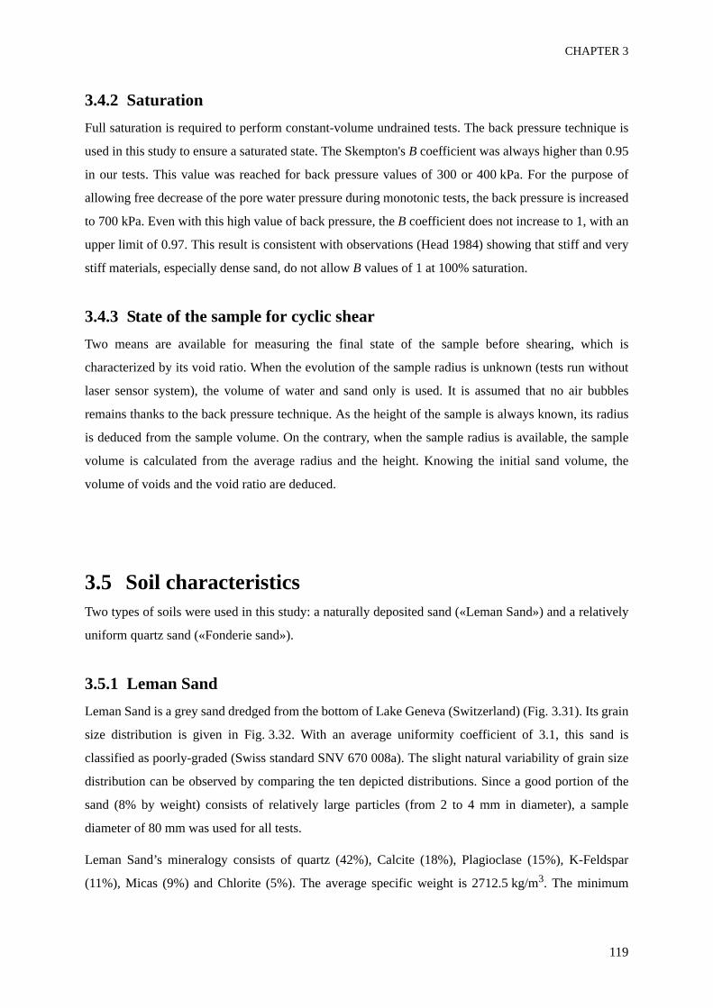
CHAPTER 3
119
3.4.2 SaturationFull saturation is required to perform constant-volume undrained tests. The back pressure technique is
used in this study to ensure a saturated state. The Skempton's B coefficient was always higher than 0.95
in our tests. This value was reached for back pressure values of 300 or 400 kPa. For the purpose of
allowing free decrease of the pore water pressure during monotonic tests, the back pressure is increased
to 700 kPa. Even with this high value of back pressure, the B coefficient does not increase to 1, with an
upper limit of 0.97. This result is consistent with observations (Head 1984) showing that stiff and very
stiff materials, especially dense sand, do not allow B values of 1 at 100% saturation.
3.4.3 State of the sample for cyclic shearTwo means are available for measuring the final state of the sample before shearing, which is
characterized by its void ratio. When the evolution of the sample radius is unknown (tests run without
laser sensor system), the volume of water and sand only is used. It is assumed that no air bubbles
remains thanks to the back pressure technique. As the height of the sample is always known, its radius
is deduced from the sample volume. On the contrary, when the sample radius is available, the sample
volume is calculated from the average radius and the height. Knowing the initial sand volume, the
volume of voids and the void ratio are deduced.
3.5 Soil characteristicsTwo types of soils were used in this study: a naturally deposited sand («Leman Sand») and a relatively
uniform quartz sand («Fonderie sand»).
3.5.1 Leman SandLeman Sand is a grey sand dredged from the bottom of Lake Geneva (Switzerland) (Fig. 3.31). Its grain
size distribution is given in Fig. 3.32. With an average uniformity coefficient of 3.1, this sand is
classified as poorly-graded (Swiss standard SNV 670 008a). The slight natural variability of grain size
distribution can be observed by comparing the ten depicted distributions. Since a good portion of the
sand (8% by weight) consists of relatively large particles (from 2 to 4 mm in diameter), a sample
diameter of 80 mm was used for all tests.
Leman Sand’s mineralogy consists of quartz (42%), Calcite (18%), Plagioclase (15%), K-Feldspar
(11%), Micas (9%) and Chlorite (5%). The average specific weight is 2712.5 kg/m3. The minimum
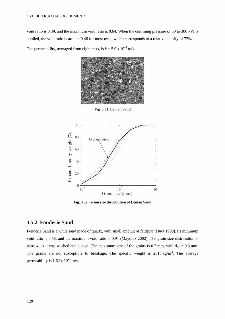
CYCLIC TRIAXIAL EXPERIMENTS
120
void ratio is 0.39, and the maximum void ratio is 0.64. When the confining pressure of 50 to 300 kPa is
applied, the void ratio is around 0.46 for most tests, which corresponds to a relative density of 72%.
The permeability, averaged from eight tests, is k = 5.9 x 10⁻⁴ m/s.
Fig. 3.31. Leman Sand.
Fig. 3.32. Grain size distribution of Leman Sand.
3.5.2 Fonderie SandFonderie Sand is a white sand made of quartz, with small amount of feldspar (Huot 1999). Its minimum
void ratio is 0.53, and the maximum void ratio is 0.91 (Mayoraz 2002). The grain size distribution is
narrow, as it was washed and sieved. The maximum size of the grains is 0.7 mm, with d60 = 0.3 mm.
The grains are not susceptible to breakage. The specific weight is 2618 kg/m3. The average
permeability is 1.62 x 10⁻⁴ m/s.
10 100
101
0
20
40
60
80
100
Per
cent
finer
by w
eight
[%]
Grain size [mm]
Average curve
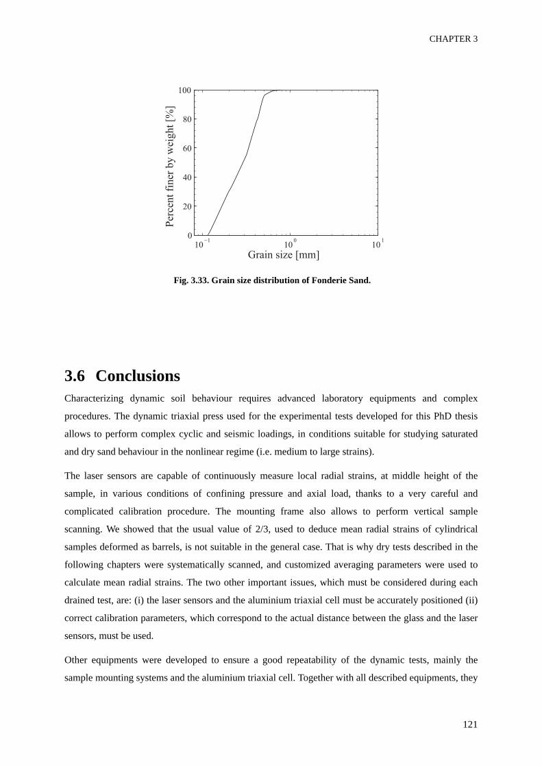
CHAPTER 3
121
Fig. 3.33. Grain size distribution of Fonderie Sand.
3.6 ConclusionsCharacterizing dynamic soil behaviour requires advanced laboratory equipments and complex
procedures. The dynamic triaxial press used for the experimental tests developed for this PhD thesis
allows to perform complex cyclic and seismic loadings, in conditions suitable for studying saturated
and dry sand behaviour in the nonlinear regime (i.e. medium to large strains).
The laser sensors are capable of continuously measure local radial strains, at middle height of the
sample, in various conditions of confining pressure and axial load, thanks to a very careful and
complicated calibration procedure. The mounting frame also allows to perform vertical sample
scanning. We showed that the usual value of 2/3, used to deduce mean radial strains of cylindrical
samples deformed as barrels, is not suitable in the general case. That is why dry tests described in the
following chapters were systematically scanned, and customized averaging parameters were used to
calculate mean radial strains. The two other important issues, which must be considered during each
drained test, are: (i) the laser sensors and the aluminium triaxial cell must be accurately positioned (ii)
correct calibration parameters, which correspond to the actual distance between the glass and the laser
sensors, must be used.
Other equipments were developed to ensure a good repeatability of the dynamic tests, mainly the
sample mounting systems and the aluminium triaxial cell. Together with all described equipments, they
10 100
101
0
20
40
60
80
100
Per
cent
finer
by w
eight
[%]
Grain size [mm]

CYCLIC TRIAXIAL EXPERIMENTS
122
allowed to perform reliable triaxial tests in drained and undrained conditions. Moreover, it should be
noticed that the use of all these devices is very complicated, requires full attention and precise gestures,
and complete training of the user is necessary to understand the processes and implement the dynamic
triaxial press.
CHAPTER 4
CHARACTERIZATION OF
NONLINEAR SAND BEHAVIOUR
WITH MONOTONIC AND CYCLIC
TRIAXIAL TESTS
CHARACTERIZATION OF NONLINEAR SAND BEHAVIOUR
124
4.1 IntroductionUndrained saturated and dry monotonic and cyclic tests were performed with Leman and Fonderie
Sand. In undrained tests, the dilative and contractive behaviour of the porous material appears as the
evolution (increase or decrease) of the pore water pressure. The saturated undrained boundary condition
leads to the assumption of a zero volumetric strain increment, thus relating the radial strain to the
measured axial strain. In dry tests, the sample volume changes, and radial strains must be continuously
measured by the laser system.
Cyclic loadings are stress-controlled with a constant cyclic deviatoric stress amplitude (Δq) applied to
the sample. The total mean stress (p) is necessarily a positive value, but the deviatoric value (q) can be
negative (triaxial extension) in the case of stress reversal loading paths.
Although non-conventional loading paths were studied using the dynamic press (see Chapter 6), only
cyclic Conventional Triaxial Compression (CTC) and alternate cyclic Conventional Triaxial
Compression and Reduced Triaxial Extension (CTC-RTE) test results are presented in this chapter. The
Tab. 4.1 summarizes the characteristics of the monotonic tests, and Tab. 4.3, Tab. 4.4, Tab. 4.7 and
Tab. 4.10 those of the cyclic tests.
After monotonic undrained tests on Leman Sand (section 4.2), preliminary cyclic tests (section 4.3) and
undrained saturated cyclic tests (section 4.4) on Leman Sand are described. Then these results are
compared with undrained tests on Fonderie Sand (section 4.5). Before presenting in details dry test
results on Leman Sand (section 4.7), the validity of radial strain measurement with the lasers device is
analysed with an undrained test (section 4.6): the soil response is computed with either laser-based
measurement of ε3 or with the assumption of no volumetric strain, and both results are compared. An
analysis of the formation of the shear band at large strain amplitude (section 4.8) is finally presented, to
evaluate the validity range of the test results.
For the sake of brevity, every test performed with the dynamic triaxial press is not described in detail
within the thesis. Instead, examples illustrating their common features are presented, as well as figures
which summarize several test results. Beyond the stress-strain relation and the stress path, the nonlinear
cyclic behaviour of Leman and Fonderie Sand is summarized by (i) the development of excess pore
pressure or volumetric strain, (ii) the secant shear modulus, (iii) the damping ratio. The material
parameters of the two constitutive models (description in Chapter 2) are determined, from the tests
presented here, in Chapter 7.
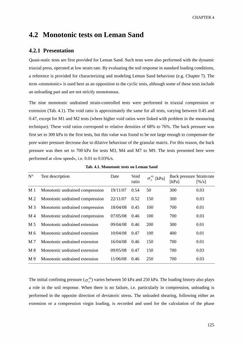
CHAPTER 4
125
4.2 Monotonic tests on Leman Sand
4.2.1 PresentationQuasi-static tests are first provided for Leman Sand. Such tests were also performed with the dynamic
triaxial press, operated at low strain rate. By evaluating the soil response in standard loading conditions,
a reference is provided for characterizing and modeling Leman Sand behaviour (e.g. Chapter 7). The
term «monotonic» is used here as an opposition to the cyclic tests, although some of these tests include
an unloading part and are not strictly monotonous.
The nine monotonic undrained strain-controlled tests were performed in triaxial compression or
extension (Tab. 4.1). The void ratio is approximately the same for all tests, varying between 0.45 and
0.47, except for M1 and M2 tests (where higher void ratios were linked with problem in the measuring
technique). These void ratios correspond to relative densities of 68% to 76%. The back pressure was
first set to 300 kPa in the first tests, but this value was found to be not large enough to compensate the
pore water pressure decrease due to dilative behaviour of the granular matrix. For this reason, the back
pressure was then set to 700 kPa for tests M3, M4 and M7 to M9. The tests presented here were
performed at «low speed», i.e. 0.01 to 0.03%/s.
Tab. 4.1. Monotonic tests on Leman Sand
The initial confining pressure ( ) varies between 50 kPa and 250 kPa. The loading history also plays
a role in the soil response. When there is no failure, i.e. particularly in compression, unloading is
performed in the opposite direction of deviatoric stress. The unloaded shearing, following either an
extension or a compression virgin loading, is recorded and used for the calculation of the phase
N° Test description Date Void ratio
[kPa] Back pressure [kPa]
Strain rate [%/s]
M 1 Monotonic undrained compression 19/11/07 0.54 50 300 0.03
M 2 Monotonic undrained compression 22/11/07 0.52 150 300 0.03
M 3 Monotonic undrained compression 18/04/08 0.45 100 700 0.01
M 4 Monotonic undrained compression 07/05/08 0.46 100 700 0.03
M 5 Monotonic undrained extension 09/04/08 0.46 200 300 0.01
M 6 Monotonic undrained extension 10/04/08 0.47 100 400 0.01
M 7 Monotonic undrained extension 16/04/08 0.46 150 700 0.01
M 8 Monotonic undrained extension 09/05/08 0.47 150 700 0.03
M 9 Monotonic undrained extension 11/06/08 0.46 250 700 0.03
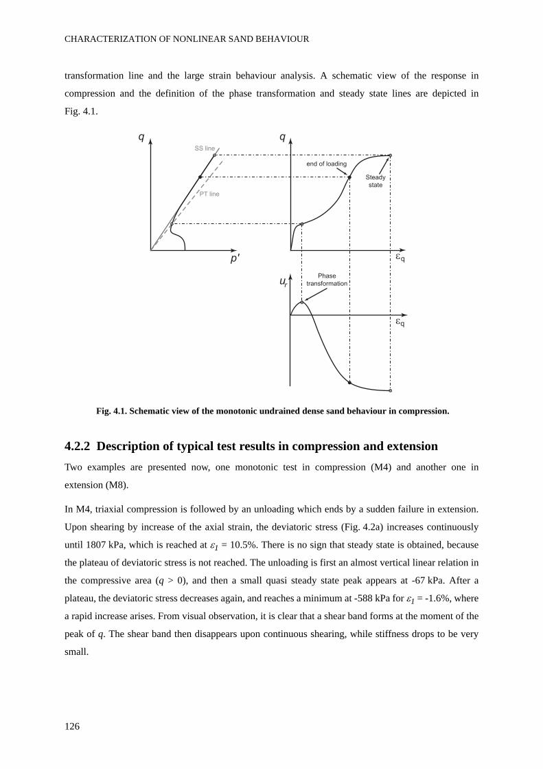
CHARACTERIZATION OF NONLINEAR SAND BEHAVIOUR
126
transformation line and the large strain behaviour analysis. A schematic view of the response in
compression and the definition of the phase transformation and steady state lines are depicted in
Fig. 4.1.
Fig. 4.1. Schematic view of the monotonic undrained dense sand behaviour in compression.
4.2.2 Description of typical test results in compression and extensionTwo examples are presented now, one monotonic test in compression (M4) and another one in
extension (M8).
In M4, triaxial compression is followed by an unloading which ends by a sudden failure in extension.
Upon shearing by increase of the axial strain, the deviatoric stress (Fig. 4.2a) increases continuously
until 1807 kPa, which is reached at ε1 = 10.5%. There is no sign that steady state is obtained, because
the plateau of deviatoric stress is not reached. The unloading is first an almost vertical linear relation in
the compressive area (q > 0), and then a small quasi steady state peak appears at -67 kPa. After a
plateau, the deviatoric stress decreases again, and reaches a minimum at -588 kPa for ε1 = -1.6%, where
a rapid increase arises. From visual observation, it is clear that a shear band forms at the moment of the
peak of q. The shear band then disappears upon continuous shearing, while stiffness drops to be very
small.
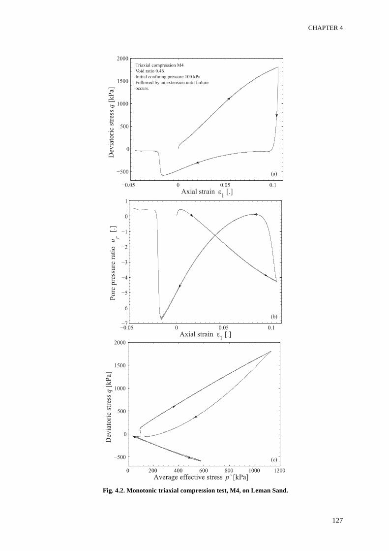
CHAPTER 4
127
Fig. 4.2. Monotonic triaxial compression test, M4, on Leman Sand.
Dev
iato
ric
stre
ss q
[kP
a]
Axial strain
Pore
pre
ssure
rat
io
ur
Axial strain
Dev
iato
ric
stre
ss q
[kP
a]
Average effective stress p’ [kPa]
Followed by an extension until failure
(a)
(b)
(c)
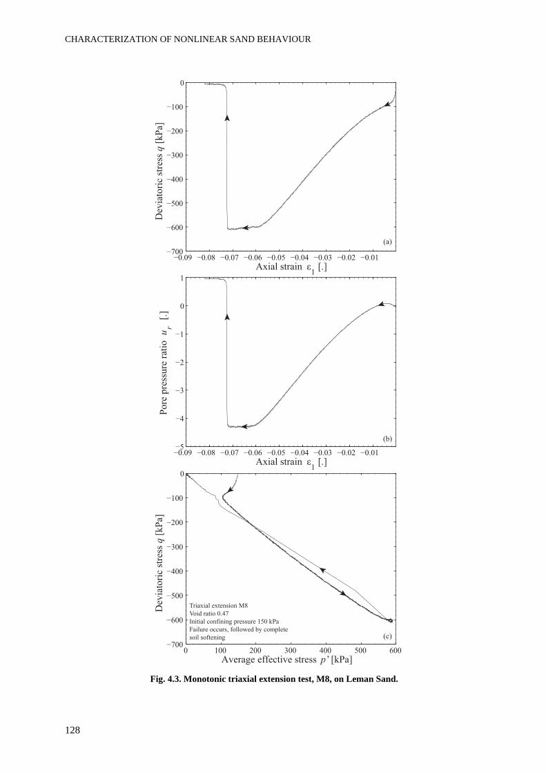
CHARACTERIZATION OF NONLINEAR SAND BEHAVIOUR
128
Fig. 4.3. Monotonic triaxial extension test, M8, on Leman Sand.
0 100 200 300 400 500 600
0
Dev
iato
ric
stre
ss q
[kP
a]
Average effective stress p’ [kPa]
0
1
Po
re p
ress
ure
rat
io
ur
Axial strain 1
0
Dev
iato
ric
stre
ss q
[k
Pa]
Axial strain 1
Initial confining pressure 150 kPa
Failure occurs, followed by complete
soil softening
(a)
(b)
(c)
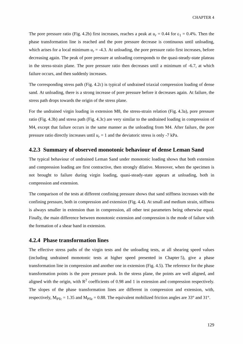
CHAPTER 4
129
The pore pressure ratio (Fig. 4.2b) first increases, reaches a peak at ur = 0.44 for ε1 = 0.4%. Then the
phase transformation line is reached and the pore pressure decrease is continuous until unloading,
which arises for a local minimum ur = -4.3. At unloading, the pore pressure ratio first increases, before
decreasing again. The peak of pore pressure at unloading corresponds to the quasi-steady-state plateau
in the stress-strain plane. The pore pressure ratio then decreases until a minimum of -6.7, at which
failure occurs, and then suddenly increases.
The corresponding stress path (Fig. 4.2c) is typical of undrained triaxial compression loading of dense
sand. At unloading, there is a strong increase of pore pressure before it decreases again. At failure, the
stress path drops towards the origin of the stress plane.
For the undrained virgin loading in extension M8, the stress-strain relation (Fig. 4.3a), pore pressure
ratio (Fig. 4.3b) and stress path (Fig. 4.3c) are very similar to the undrained loading in compression of
M4, except that failure occurs in the same manner as the unloading from M4. After failure, the pore
pressure ratio directly increases until ur = 1 and the deviatoric stress is only -7 kPa.
4.2.3 Summary of observed monotonic behaviour of dense Leman SandThe typical behaviour of undrained Leman Sand under monotonic loading shows that both extension
and compression loading are first contractive, then strongly dilative. Moreover, when the specimen is
not brought to failure during virgin loading, quasi-steady-state appears at unloading, both in
compression and extension.
The comparison of the tests at different confining pressure shows that sand stiffness increases with the
confining pressure, both in compression and extension (Fig. 4.4). At small and medium strain, stiffness
is always smaller in extension than in compression, all other test parameters being otherwise equal.
Finally, the main difference between monotonic extension and compression is the mode of failure with
the formation of a shear band in extension.
4.2.4 Phase transformation linesThe effective stress paths of the virgin tests and the unloading tests, at all shearing speed values
(including undrained monotonic tests at higher speed presented in Chapter 5), give a phase
transformation line in compression and another one in extension (Fig. 4.5). The reference for the phase
transformation points is the pore pressure peak. In the stress plane, the points are well aligned, and
aligned with the origin, with R2 coefficients of 0.98 and 1 in extension and compression respectively.
The slopes of the phase transformation lines are different in compression and extension, with,
respectively, MPTc = 1.35 and MPTe = 0.88. The equivalent mobilized friction angles are 33° and 31°.
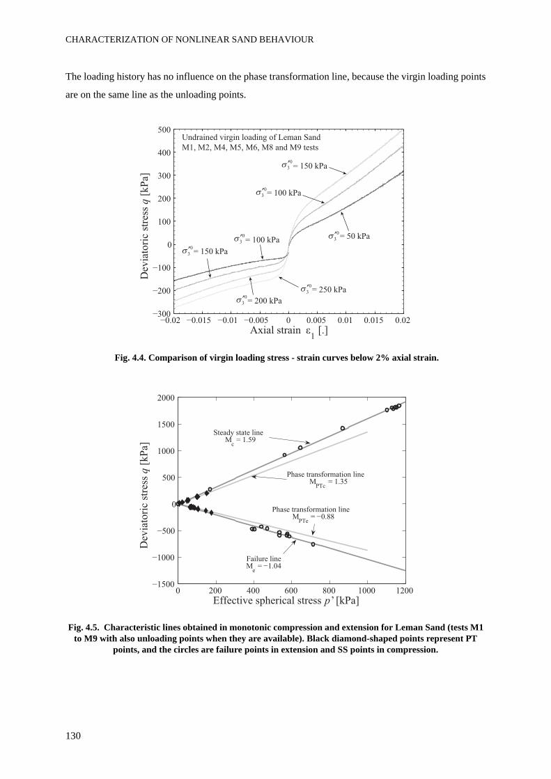
CHARACTERIZATION OF NONLINEAR SAND BEHAVIOUR
130
The loading history has no influence on the phase transformation line, because the virgin loading points
are on the same line as the unloading points.
Fig. 4.4. Comparison of virgin loading stress - strain curves below 2% axial strain.
Fig. 4.5. Characteristic lines obtained in monotonic compression and extension for Leman Sand (tests M1 to M9 with also unloading points when they are available). Black diamond-shaped points represent PT
points, and the circles are failure points in extension and SS points in compression.
Axial strain
Dev
iato
ric
stre
ss q
Undrained virgin loading of Leman Sand
0 200 400 600 800 1000 1200
0
1000
2000
Dev
iato
ric
stre
ss q
[kP
a]
Effective spherical stress p’ [kPa]
Steady state lineM
c
Phase transformation lineM
PTc
Failure lineM
e = 1.04
Phase transformation lineM
PTe = 0.88
CHAPTER 4
131
4.2.5 Behaviour at large strainThe behaviour at large strain can be characterized by the peak of the stress-strain relation, or by the
residual strength, which is also the stress at steady state or critical state. The steady state is not reached
during the tests, because (i) in compression, the stiffness of the sample is so strong that the loading
capacity is surpassed and (ii) in extension, shear bands appear thus creating heterogeneity in the
sample. In compression, it is assumed that the stress-path envelop is on the steady state line, thanks to
the behaviour depicted in Fig. 4.1. In extension, only the failure line can be obtained, which is not an
intrinsic soil property.
In extension, the failure mechanism is clearly identified. The deviator stress peak occurs just before the
pore pressure peak, and a shear band appears. When the axial strain is sufficiently large, the deviatoric
stress tends to almost zero and the pore pressure ratio becomes equal to 1 after the peak. This complete
softening is similar to liquefaction, although the stress path is not contractive. The shear band is no
longer visible. In the p’- q plane, the loci of the extension peaks form a line passing through the origin,
with a slope Me = 1.04, a mobilized friction angle of 39° and a R2 value of 0.98.
In compression, the maximum stress permitted by the equipment was reached at strains around 10%.
The expected steady state plateau is not reached yet in the ε1 - q plane. However in the p’ - q plane, all
the lines follow exactly the same stress path at large strain, which is assumed to be the steady state line
of slope Mc (cf. Fig. 4.1). The points ending each compressional loading form a straight line passing
through the origin, with a slope Mc = 1.59, a mobilized friction angle of 39° and R2 value of 1.
These two slopes, in compression and extension, characterizing large strains in the p’ - q plane, are
independent from loading history and initial confining pressure; they are limited to void ratio values of
0.45 to 0.47. The mobilized friction angles are the same in compression and extension, at SS and failure
respectively.
4.2.6 Comments and conclusions on the monotonic resultsWhile the tested material is a natural sand, and the content of the samples can slightly vary, the phase
transformation line and the stress path at large strains, obtained by linear regression, fit all the tests,
regardless of test loading history or initial confining pressure. The mobilized friction angle at steady
state is 39° in compression. The failure line in extension also corresponds to a peak friction angle of
39°.
The phase transformation lines in compression and extension are 33.3° and 31° respectively. Vaid et al.
(1990) and Ibsen (1994) mention that PT lines and SS lines are the same in compression and extension,
and for all loading history, even for anisotropic samples. However, De Gennaro et al. (2004) find two
CHARACTERIZATION OF NONLINEAR SAND BEHAVIOUR
132
different values, with Hostun sand, in compression (30°) and in extension (23°). The soil anisotropy
caused by the deposition method is claimed to be responsible for the difference between compression
and extension loadings. Also because of anisotropy, Hostun sand is stiffer in the vertical direction than
in the horizontal direction. For the Leman Sand as well, the stiffness is higher in compression than in
extension.
The characteristic PT and SS angles determined for Leman Sand are summarized in Tab. 4.2. They are
used in Chapter 7, as material parameters for the Hujeux elastoplastic model.
Tab. 4.2. PT and SS characteristics of Leman Sand
* The value given for the steady state in extension is rather a failure angle than a steady state angle.
4.3 Preliminary undrained cyclic triaxial tests
4.3.1 IntroductionThe effect of confining pressure, strain or stress amplitude and average deviatoric stress are compared
using four tests in stress-controlled mode and one test in strain-controlled conditions. The void ratio is
in the same range as all other tests with Leman Sand (between 0.45 and 0.48). The frequency of all tests
is 0.8 Hz.
These tests allowed to get an overview on the stress-strain response and pore pressure increase of
saturated undrained Leman Sand. It should however be noticed that, because of an imperfect sample
mounting procedure, full saturation is not reached, with a B coefficient varying between 0.6 and 0.9.
The results can be biased by the different saturation index, they are thus only indicative of cyclic sand
behaviour.
MPT [.] MSS [.] φPT [°] φSS [°]
Compression 1.35 1.59 33.3 39
Extension 0.88 (1.04)* 31 (39)*
CHAPTER 4
133
Tab. 4.3. Preliminary cyclic tests on Leman Sand
4.3.2 Typical stress-controlled test resultsEach test is performed at three amplitudes only, even if failure does not occur. Actually cyclic
liquefaction arises only during PC1 and PC5, at the last amplitude level. The other tests exhibit a stable
behaviour with accommodation process.
The test PC3 is described in details now (Fig. 4.6). Undrained sinusoidal cycles on Leman Sand are
performed with constant deviatoric stress amplitudes (Fig. 4.6a). The cyclic deviatoric stress amplitude
starts at Δq = 100 kPa for 25 cycles. Then the pore-water pressure is released, and 25 more cycles are
performed at 200 kPa stress amplitude. This process is repeated in a third step, with a final amplitude of
300 kPa. The cyclic stress ratio (CSR, defined in Eq. 2.20) of each step is indicated in Fig. 4.6a for test
PC3.
The mechanical response of the sample is primarily a cyclic deviatoric strain in phase with the stress
loading (Fig. 4.6b). The deviatoric strain amplitude clearly increases when Δq increases at each step.
Moreover, the strain cycles are not symmetric towards the axis εq = 0 and they regularly shift towards
larger strains. In the same way, the pore pressure ratio amplitude regularly increases with the number of
cycles (Fig. 4.6c).
N° Test description Date Void ratio
[kPa] qav [kPa] Amplitude B coefficient
PC 1 Cyclic undrained stress-controlled CTC and CTC-RTE
30/05/07 0.48 209 185 100 kPa200 kPa300 kPa
0.63
PC 2 Cyclic undrained stress-controlled CTC
31/05/07 0.47 207 390 100 kPa200 kPa300 kPa
0.75
PC 3 Cyclic undrained stress-controlled CTC and CTC-RTE
23/05/07 0.48 407 175 100 kPa200 kPa300 kPa
0.84
PC 4 Cyclic undrained stress-controlled CTC
24/05/07 0.47 406 380 100 kPa200 kPa300 kPa
0.86
PC 5 Cyclic undrained strain-controlled CTC and CTC-RTE
02/05/07 0.45 207 0 0.01%0.1%1%
0.77
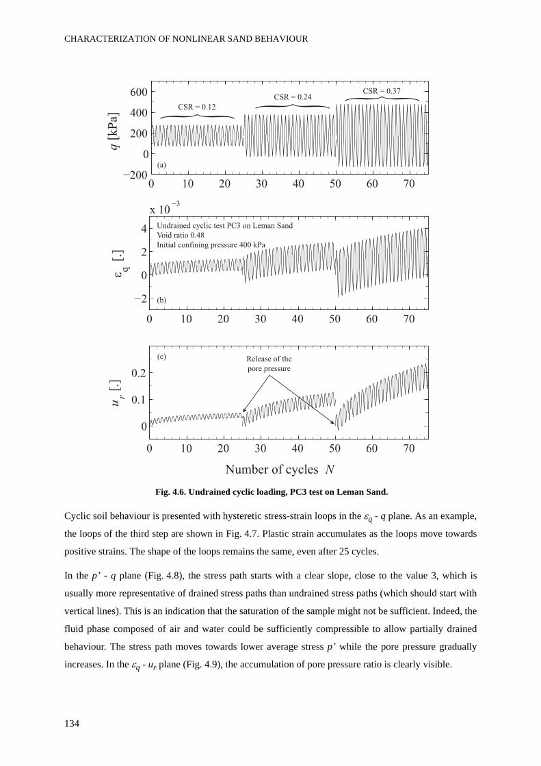
CHARACTERIZATION OF NONLINEAR SAND BEHAVIOUR
134
Fig. 4.6. Undrained cyclic loading, PC3 test on Leman Sand.
Cyclic soil behaviour is presented with hysteretic stress-strain loops in the εq - q plane. As an example,
the loops of the third step are shown in Fig. 4.7. Plastic strain accumulates as the loops move towards
positive strains. The shape of the loops remains the same, even after 25 cycles.
In the p’ - q plane (Fig. 4.8), the stress path starts with a clear slope, close to the value 3, which is
usually more representative of drained stress paths than undrained stress paths (which should start with
vertical lines). This is an indication that the saturation of the sample might not be sufficient. Indeed, the
fluid phase composed of air and water could be sufficiently compressible to allow partially drained
behaviour. The stress path moves towards lower average stress p’ while the pore pressure gradually
increases. In the εq - ur plane (Fig. 4.9), the accumulation of pore pressure ratio is clearly visible.
0 10 20 30 40 50 60 70
0
200
400
600
q [
kP
a]
0 10 20 30 40 50 60 70
2
0
2
4
x 103
q [
.]
0 10 20 30 40 50 60 70
0
0.1
0.2
ur [
.]
Number of cycles N
CSR = 0.12
CSR = 0.24CSR = 0.37
Undrained cyclic test PC3 on Leman Sand
Void ratio 0.48
Initial confining pressure 400 kPa
Release of the
pore pressure
(a)
(b)
(c)
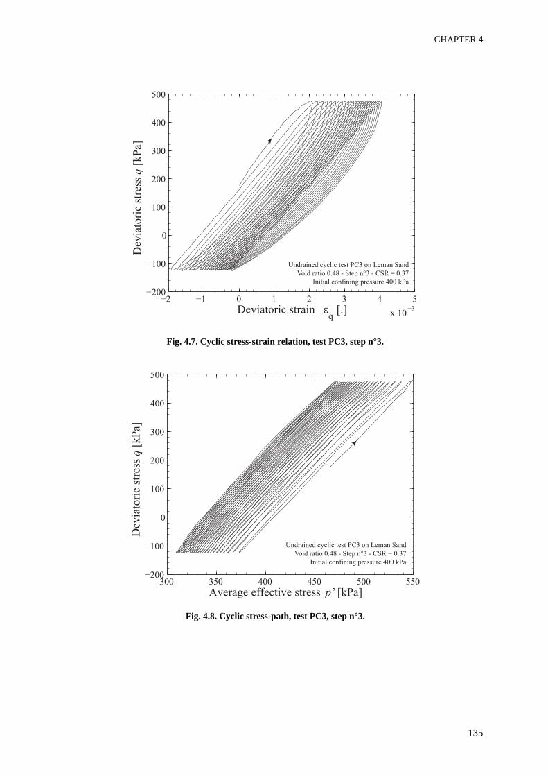
CHAPTER 4
135
Fig. 4.7. Cyclic stress-strain relation, test PC3, step n°3.
Fig. 4.8. Cyclic stress-path, test PC3, step n°3.
0 3 4 53
0
300
400
500
Dev
iato
ric
stre
ss q
[kP
a]
Deviatoric strain q [.]
Undrained cyclic test PC3 on Leman Sand
Void ratio 0.48 - Step n°3 - CSR = 0.37
Initial confining pressure 400 kPa
300 350 400 450 500 550
0
300
400
500
Dev
iato
ric
stre
ss q
[kP
a]
Average effective stress p’ [kPa]
Undrained cyclic test PC3 on Leman Sand
Void ratio 0.48 - Step n°3 - CSR = 0.37
Initial confining pressure 400 kPa
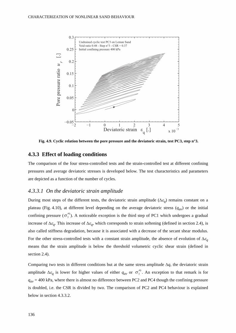
CHARACTERIZATION OF NONLINEAR SAND BEHAVIOUR
136
Fig. 4.9. Cyclic relation between the pore pressure and the deviatoric strain, test PC3, step n°3.
4.3.3 Effect of loading conditionsThe comparison of the four stress-controlled tests and the strain-controlled test at different confining
pressures and average deviatoric stresses is developed below. The test characteristics and parameters
are depicted as a function of the number of cycles.
4.3.3.1 On the deviatoric strain amplitudeDuring most steps of the different tests, the deviatoric strain amplitude (Δεq) remains constant on a
plateau (Fig. 4.10), at different level depending on the average deviatoric stress (qav) or the initial
confining pressure ( ). A noticeable exception is the third step of PC1 which undergoes a gradual
increase of Δεq. This increase of Δεq, which corresponds to strain softening (defined in section 2.4), is
also called stiffness degradation, because it is associated with a decrease of the secant shear modulus.
For the other stress-controlled tests with a constant strain amplitude, the absence of evolution of Δεq
means that the strain amplitude is below the threshold volumetric cyclic shear strain (defined in
section 2.4).
Comparing two tests in different conditions but at the same stress amplitude Δq, the deviatoric strain
amplitude Δεq is lower for higher values of either qav or . An exception to that remark is for
qav = 400 kPa, where there is almost no difference between PC2 and PC4 though the confining pressure
is doubled, i.e. the CSR is divided by two. The comparison of PC2 and PC4 behaviour is explained
below in section 4.3.3.2.
0 3 4 53
0.05
0
0.05
0.3
Pore
pre
ssure
rat
io
ur
[.]
Deviatoric strain q [.]
Undrained cyclic test PC3 on Leman Sand
Void ratio 0.48 - Step n°3 - CSR = 0.37
Initial confining pressure 400 kPa
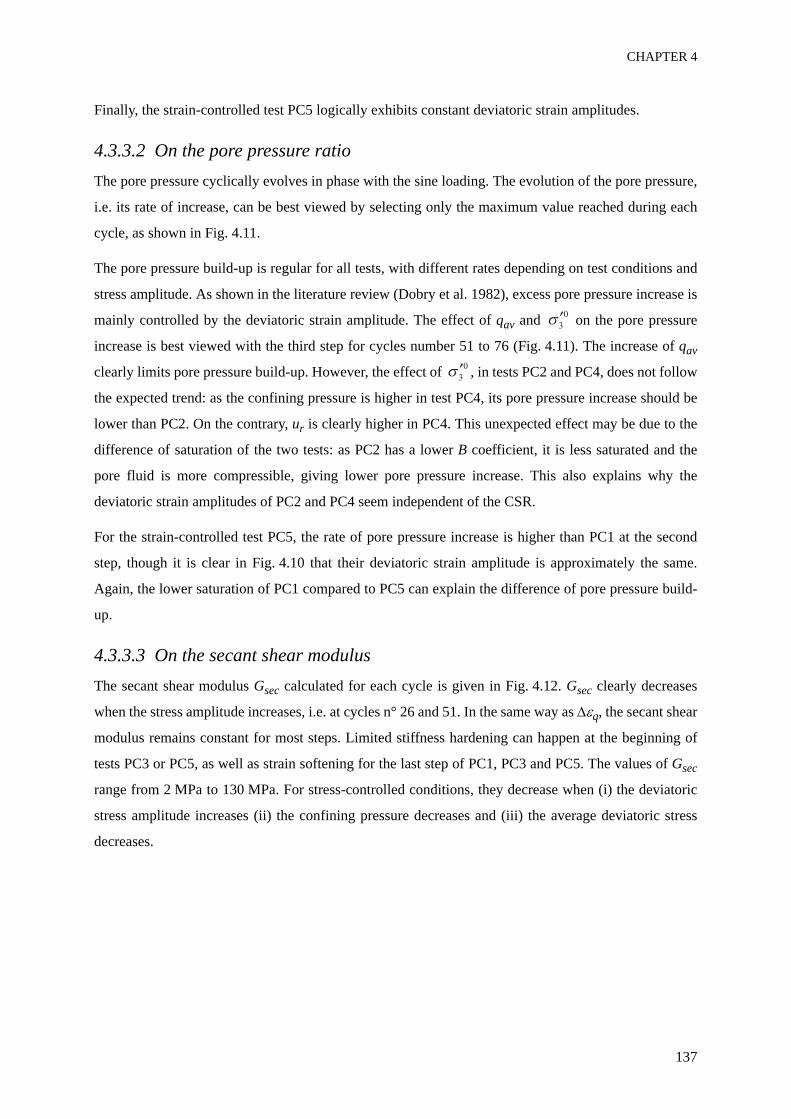
CHAPTER 4
137
Finally, the strain-controlled test PC5 logically exhibits constant deviatoric strain amplitudes.
4.3.3.2 On the pore pressure ratioThe pore pressure cyclically evolves in phase with the sine loading. The evolution of the pore pressure,
i.e. its rate of increase, can be best viewed by selecting only the maximum value reached during each
cycle, as shown in Fig. 4.11.
The pore pressure build-up is regular for all tests, with different rates depending on test conditions and
stress amplitude. As shown in the literature review (Dobry et al. 1982), excess pore pressure increase is
mainly controlled by the deviatoric strain amplitude. The effect of qav and on the pore pressure
increase is best viewed with the third step for cycles number 51 to 76 (Fig. 4.11). The increase of qav
clearly limits pore pressure build-up. However, the effect of , in tests PC2 and PC4, does not follow
the expected trend: as the confining pressure is higher in test PC4, its pore pressure increase should be
lower than PC2. On the contrary, ur is clearly higher in PC4. This unexpected effect may be due to the
difference of saturation of the two tests: as PC2 has a lower B coefficient, it is less saturated and the
pore fluid is more compressible, giving lower pore pressure increase. This also explains why the
deviatoric strain amplitudes of PC2 and PC4 seem independent of the CSR.
For the strain-controlled test PC5, the rate of pore pressure increase is higher than PC1 at the second
step, though it is clear in Fig. 4.10 that their deviatoric strain amplitude is approximately the same.
Again, the lower saturation of PC1 compared to PC5 can explain the difference of pore pressure build-
up.
4.3.3.3 On the secant shear modulusThe secant shear modulus Gsec calculated for each cycle is given in Fig. 4.12. Gsec clearly decreases
when the stress amplitude increases, i.e. at cycles n° 26 and 51. In the same way as Δεq, the secant shear
modulus remains constant for most steps. Limited stiffness hardening can happen at the beginning of
tests PC3 or PC5, as well as strain softening for the last step of PC1, PC3 and PC5. The values of Gsec
range from 2 MPa to 130 MPa. For stress-controlled conditions, they decrease when (i) the deviatoric
stress amplitude increases (ii) the confining pressure decreases and (iii) the average deviatoric stress
decreases.
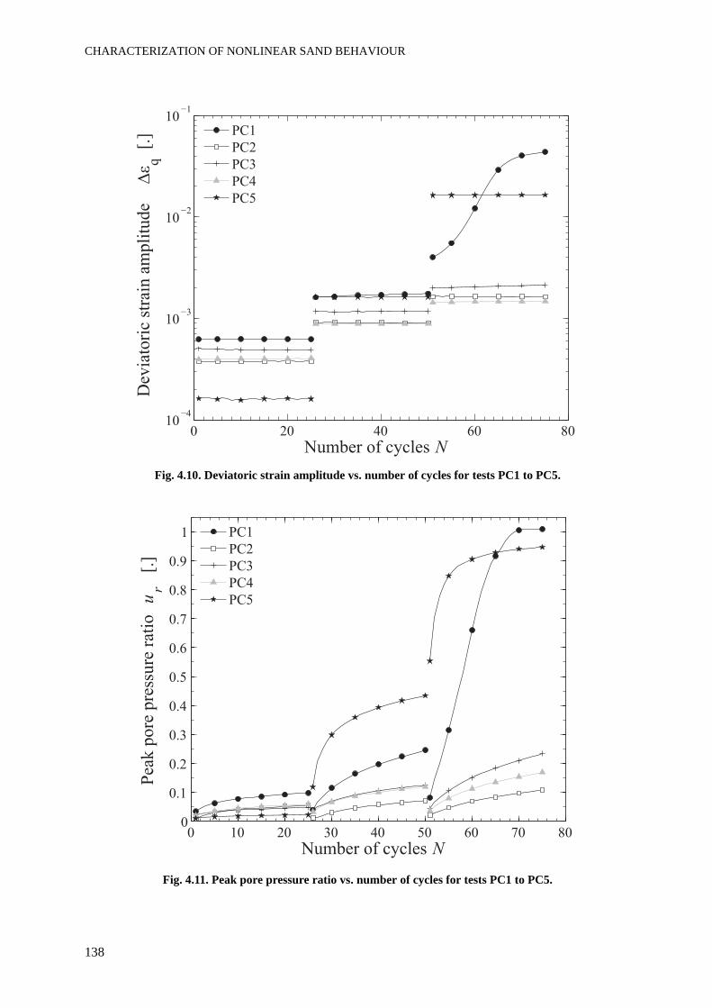
CHARACTERIZATION OF NONLINEAR SAND BEHAVIOUR
138
Fig. 4.10. Deviatoric strain amplitude vs. number of cycles for tests PC1 to PC5.
Fig. 4.11. Peak pore pressure ratio vs. number of cycles for tests PC1 to PC5.
0 20 40 60 8010
103
102
101
Dev
iato
ric
stra
in a
mp
litu
de
q [
.]
Number of cycles N
PC1
PC2
PC3
PC4
PC5
0 10 20 30 40 50 60 70 800
0.1
0.2
0.3
0.4
0.5
0.6
0.7
0.8
0.9
1
Pea
k p
ore
pre
ssu
re r
atio
u
r [
.]
Number of cycles N
PC1
PC2
PC3
PC4
PC5
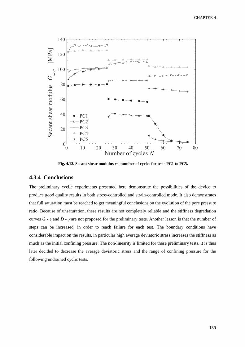
CHAPTER 4
139
Fig. 4.12. Secant shear modulus vs. number of cycles for tests PC1 to PC5.
4.3.4 ConclusionsThe preliminary cyclic experiments presented here demonstrate the possibilities of the device to
produce good quality results in both stress-controlled and strain-controlled mode. It also demonstrates
that full saturation must be reached to get meaningful conclusions on the evolution of the pore pressure
ratio. Because of unsaturation, these results are not completely reliable and the stiffness degradation
curves G - γ and D - γ are not proposed for the preliminary tests. Another lesson is that the number of
steps can be increased, in order to reach failure for each test. The boundary conditions have
considerable impact on the results, in particular high average deviatoric stress increases the stiffness as
much as the initial confining pressure. The non-linearity is limited for these preliminary tests, it is thus
later decided to decrease the average deviatoric stress and the range of confining pressure for the
following undrained cyclic tests.
0 10 20 30 40 50 60 70 800
20
40
60
80
100
120
140
Sec
ant
shea
r m
od
ulu
s G
sec
[M
Pa]
Number of cycles N
PC1
PC2
PC3
PC4
PC5
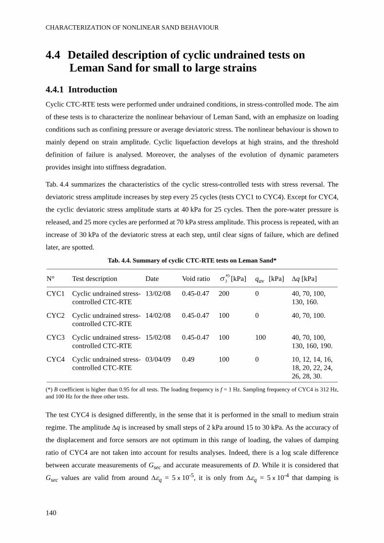
CHARACTERIZATION OF NONLINEAR SAND BEHAVIOUR
140
4.4 Detailed description of cyclic undrained tests on Leman Sand for small to large strains
4.4.1 IntroductionCyclic CTC-RTE tests were performed under undrained conditions, in stress-controlled mode. The aim
of these tests is to characterize the nonlinear behaviour of Leman Sand, with an emphasize on loading
conditions such as confining pressure or average deviatoric stress. The nonlinear behaviour is shown to
mainly depend on strain amplitude. Cyclic liquefaction develops at high strains, and the threshold
definition of failure is analysed. Moreover, the analyses of the evolution of dynamic parameters
provides insight into stiffness degradation.
Tab. 4.4 summarizes the characteristics of the cyclic stress-controlled tests with stress reversal. The
deviatoric stress amplitude increases by step every 25 cycles (tests CYC1 to CYC4). Except for CYC4,
the cyclic deviatoric stress amplitude starts at 40 kPa for 25 cycles. Then the pore-water pressure is
released, and 25 more cycles are performed at 70 kPa stress amplitude. This process is repeated, with an
increase of 30 kPa of the deviatoric stress at each step, until clear signs of failure, which are defined
later, are spotted.
Tab. 4.4. Summary of cyclic CTC-RTE tests on Leman Sand*
(*) B coefficient is higher than 0.95 for all tests. The loading frequency is f = 1 Hz. Sampling frequency of CYC4 is 312 Hz,and 100 Hz for the three other tests.
The test CYC4 is designed differently, in the sense that it is performed in the small to medium strain
regime. The amplitude Δq is increased by small steps of 2 kPa around 15 to 30 kPa. As the accuracy of
the displacement and force sensors are not optimum in this range of loading, the values of damping
ratio of CYC4 are not taken into account for results analyses. Indeed, there is a log scale difference
between accurate measurements of Gsec and accurate measurements of D. While it is considered that
Gsec values are valid from around Δεq = 5 x 10⁻⁵, it is only from Δεq = 5 x 10⁻⁴ that damping is
N° Test description Date Void ratio [kPa] qav [kPa] Δq [kPa]
CYC1 Cyclic undrained stress-controlled CTC-RTE
13/02/08 0.45-0.47 200 0 40, 70, 100, 130, 160.
CYC2 Cyclic undrained stress-controlled CTC-RTE
14/02/08 0.45-0.47 100 0 40, 70, 100.
CYC3 Cyclic undrained stress-controlled CTC-RTE
15/02/08 0.45-0.47 100 100 40, 70, 100, 130, 160, 190.
CYC4 Cyclic undrained stress-controlled CTC-RTE
03/04/09 0.49 100 0 10, 12, 14, 16, 18, 20, 22, 24, 26, 28, 30.
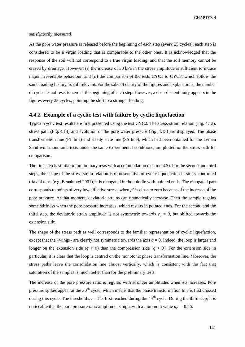
CHAPTER 4
141
satisfactorily measured.
As the pore water pressure is released before the beginning of each step (every 25 cycles), each step is
considered to be a virgin loading that is comparable to the other ones. It is acknowledged that the
response of the soil will not correspond to a true virgin loading, and that the soil memory cannot be
erased by drainage. However, (i) the increase of 30 kPa in the stress amplitude is sufficient to induce
major irreversible behaviour, and (ii) the comparison of the tests CYC1 to CYC3, which follow the
same loading history, is still relevant. For the sake of clarity of the figures and explanations, the number
of cycles is not reset to zero at the beginning of each step. However, a clear discontinuity appears in the
figures every 25 cycles, pointing the shift to a stronger loading.
4.4.2 Example of a cyclic test with failure by cyclic liquefactionTypical cyclic test results are first presented using the test CYC2. The stress-strain relation (Fig. 4.13),
stress path (Fig. 4.14) and evolution of the pore water pressure (Fig. 4.15) are displayed. The phase
transformation line (PT line) and steady state line (SS line), which had been obtained for the Leman
Sand with monotonic tests under the same experimental conditions, are plotted on the stress path for
comparison.
The first step is similar to preliminary tests with accommodation (section 4.3). For the second and third
steps, the shape of the stress-strain relation is representative of cyclic liquefaction in stress-controlled
triaxial tests (e.g. Benahmed 2001), it is elongated in the middle with pointed ends. The elongated part
corresponds to points of very low effective stress, when p’ is close to zero because of the increase of the
pore pressure. At that moment, deviatoric strains can dramatically increase. Then the sample regains
some stiffness when the pore pressure increases, which results in pointed ends. For the second and the
third step, the deviatoric strain amplitude is not symmetric towards εq = 0, but shifted towards the
extension side.
The shape of the stress path as well corresponds to the familiar representation of cyclic liquefaction,
except that the «wings» are clearly not symmetric towards the axis q = 0. Indeed, the loop is larger and
longer on the extension side (q < 0) than the compression side (q > 0). For the extension side in
particular, it is clear that the loop is centred on the monotonic phase transformation line. Moreover, the
stress paths leave the consolidation line almost vertically, which is consistent with the fact that
saturation of the samples is much better than for the preliminary tests.
The increase of the pore pressure ratio is regular, with stronger amplitudes when Δq increases. Pore
pressure spikes appear at the 30th cycle, which means that the phase transformation line is first crossed
during this cycle. The threshold ur = 1 is first reached during the 44th cycle. During the third step, it is
noticeable that the pore pressure ratio amplitude is high, with a minimum value ur = -0.26.
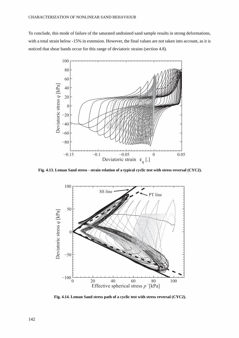
CHARACTERIZATION OF NONLINEAR SAND BEHAVIOUR
142
To conclude, this mode of failure of the saturated undrained sand sample results in strong deformations,
with a total strain below -15% in extension. However, the final values are not taken into account, as it is
noticed that shear bands occur for this range of deviatoric strains (section 4.8).
Fig. 4.13. Leman Sand stress - strain relation of a typical cyclic test with stress reversal (CYC2).
Fig. 4.14. Leman Sand stress path of a cyclic test with stress reversal (CYC2).
Deviatoric strain q
Dev
iato
ric
stre
ss q
0 20 40 60 80 100
0
100
Dev
iato
ric
stre
ss q
[kP
a]
Effective spherical stress p’ [kPa]
PT lineSS line
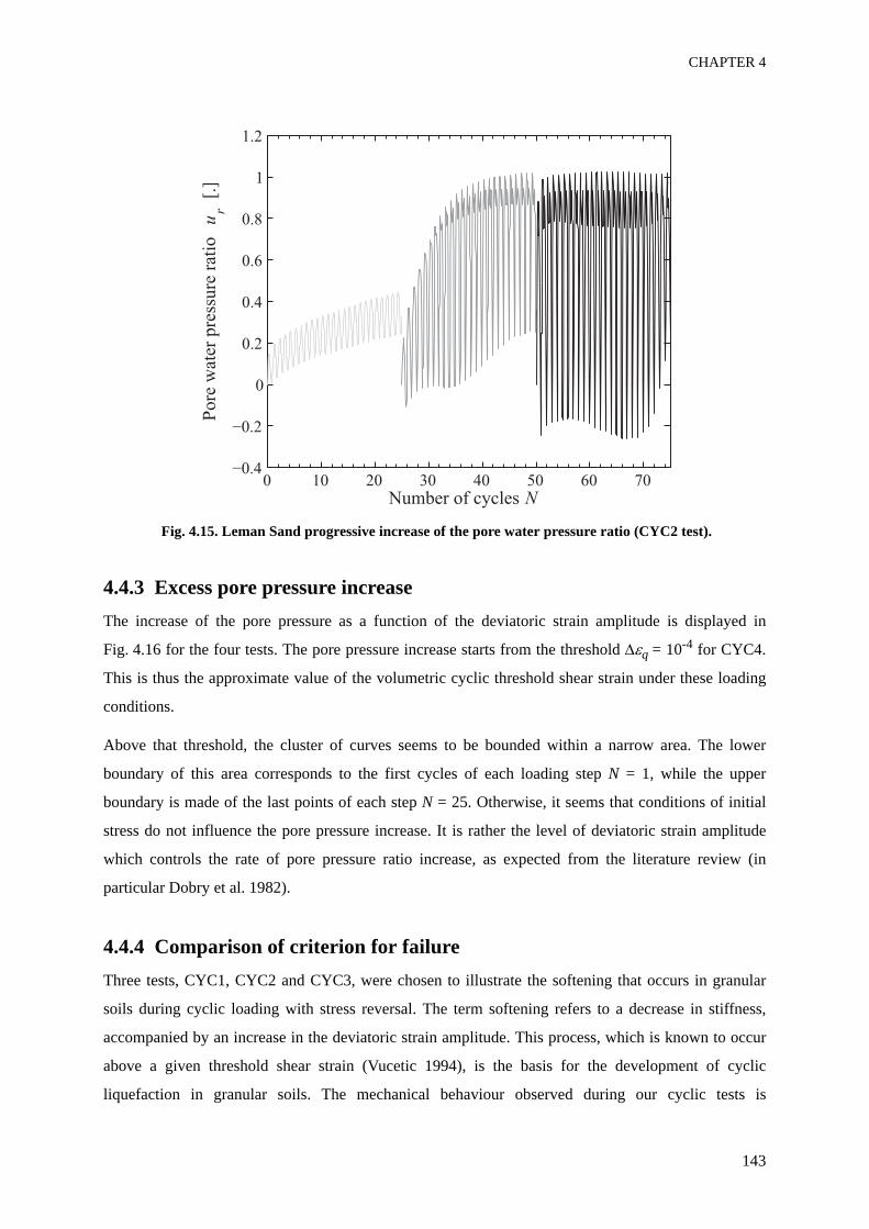
CHAPTER 4
143
Fig. 4.15. Leman Sand progressive increase of the pore water pressure ratio (CYC2 test).
4.4.3 Excess pore pressure increaseThe increase of the pore pressure as a function of the deviatoric strain amplitude is displayed in
Fig. 4.16 for the four tests. The pore pressure increase starts from the threshold Δεq = 10-4 for CYC4.
This is thus the approximate value of the volumetric cyclic threshold shear strain under these loading
conditions.
Above that threshold, the cluster of curves seems to be bounded within a narrow area. The lower
boundary of this area corresponds to the first cycles of each loading step N = 1, while the upper
boundary is made of the last points of each step N = 25. Otherwise, it seems that conditions of initial
stress do not influence the pore pressure increase. It is rather the level of deviatoric strain amplitude
which controls the rate of pore pressure ratio increase, as expected from the literature review (in
particular Dobry et al. 1982).
4.4.4 Comparison of criterion for failureThree tests, CYC1, CYC2 and CYC3, were chosen to illustrate the softening that occurs in granular
soils during cyclic loading with stress reversal. The term softening refers to a decrease in stiffness,
accompanied by an increase in the deviatoric strain amplitude. This process, which is known to occur
above a given threshold shear strain (Vucetic 1994), is the basis for the development of cyclic
liquefaction in granular soils. The mechanical behaviour observed during our cyclic tests is
0 10 20 30 40 50 60 70
0
1
Number of cycles N
Pore
wat
er p
ress
ure
rat
io
ur
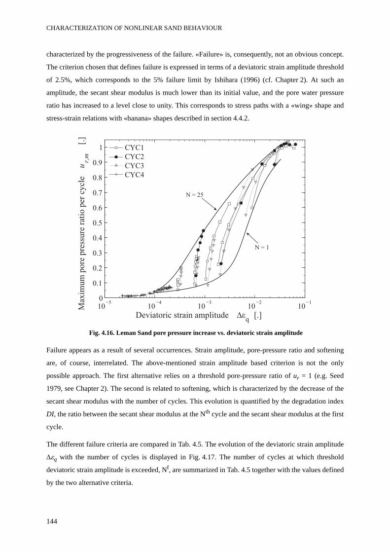
CHARACTERIZATION OF NONLINEAR SAND BEHAVIOUR
144
characterized by the progressiveness of the failure. «Failure» is, consequently, not an obvious concept.
The criterion chosen that defines failure is expressed in terms of a deviatoric strain amplitude threshold
of 2.5%, which corresponds to the 5% failure limit by Ishihara (1996) (cf. Chapter 2). At such an
amplitude, the secant shear modulus is much lower than its initial value, and the pore water pressure
ratio has increased to a level close to unity. This corresponds to stress paths with a «wing» shape and
stress-strain relations with «banana» shapes described in section 4.4.2.
Fig. 4.16. Leman Sand pore pressure increase vs. deviatoric strain amplitude
Failure appears as a result of several occurrences. Strain amplitude, pore-pressure ratio and softening
are, of course, interrelated. The above-mentioned strain amplitude based criterion is not the only
possible approach. The first alternative relies on a threshold pore-pressure ratio of ur = 1 (e.g. Seed
1979, see Chapter 2). The second is related to softening, which is characterized by the decrease of the
secant shear modulus with the number of cycles. This evolution is quantified by the degradation index
DI, the ratio between the secant shear modulus at the Nth cycle and the secant shear modulus at the first
cycle.
The different failure criteria are compared in Tab. 4.5. The evolution of the deviatoric strain amplitude
Δεq with the number of cycles is displayed in Fig. 4.17. The number of cycles at which threshold
deviatoric strain amplitude is exceeded, Nf, are summarized in Tab. 4.5 together with the values defined
by the two alternative criteria.
10 104
103
102
101
0
0.1
0.2
0.3
0.4
0.6
0.7
0.8
0.9
1
Max
imum
pore
pre
ssure
rat
io p
er c
ycl
e u
r,m
[.]
Deviatoric strain amplitude q
[.]
CYC1
CYC2
CYC3
CYC4
N = 1
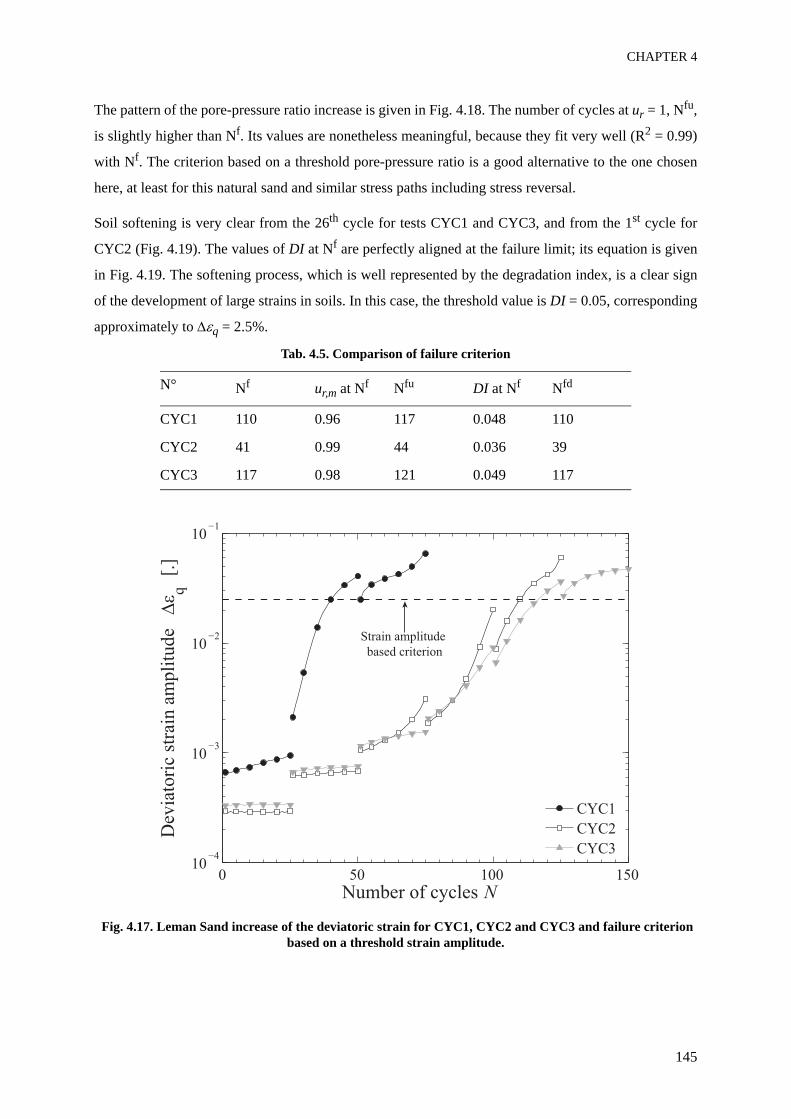
CHAPTER 4
145
The pattern of the pore-pressure ratio increase is given in Fig. 4.18. The number of cycles at ur = 1, Nfu,
is slightly higher than Nf. Its values are nonetheless meaningful, because they fit very well (R2 = 0.99)
with Nf. The criterion based on a threshold pore-pressure ratio is a good alternative to the one chosen
here, at least for this natural sand and similar stress paths including stress reversal.
Soil softening is very clear from the 26th cycle for tests CYC1 and CYC3, and from the 1st cycle for
CYC2 (Fig. 4.19). The values of DI at Nf are perfectly aligned at the failure limit; its equation is given
in Fig. 4.19. The softening process, which is well represented by the degradation index, is a clear sign
of the development of large strains in soils. In this case, the threshold value is DI = 0.05, corresponding
approximately to Δεq = 2.5%.
Tab. 4.5. Comparison of failure criterion
Fig. 4.17. Leman Sand increase of the deviatoric strain for CYC1, CYC2 and CYC3 and failure criterion based on a threshold strain amplitude.
N° Nf ur,m at Nf Nfu DI at Nf Nfd
CYC1 110 0.96 117 0.048 110
CYC2 41 0.99 44 0.036 39
CYC3 117 0.98 121 0.049 117
0 50 100 15010
103
102
101
Dev
iato
ric
stra
in a
mp
litu
de
q [
.]
Number of cycles N
CYC1
CYC2
CYC3
Strain amplitude
based criterion
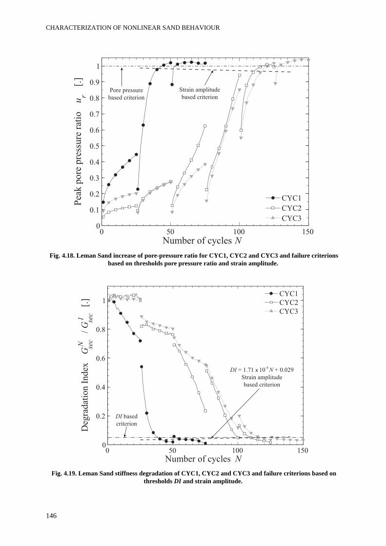
CHARACTERIZATION OF NONLINEAR SAND BEHAVIOUR
146
Fig. 4.18. Leman Sand increase of pore-pressure ratio for CYC1, CYC2 and CYC3 and failure criterions based on thresholds pore pressure ratio and strain amplitude.
Fig. 4.19. Leman Sand stiffness degradation of CYC1, CYC2 and CYC3 and failure criterions based on thresholds DI and strain amplitude.
0 50 100 1500
0.1
0.2
0.3
0.4
0.5
0.6
0.7
0.8
0.9
1
Pea
k p
ore
pre
ssu
re r
atio
u
r [
.]
Number of cycles N
CYC1
CYC2
CYC3
Pore pressure
based criterion
Strain amplitude
based criterion
0 50 100 1500
0.2
0.4
0.6
0.8
1
Deg
radat
ion I
ndex
G
N sec
/ G
1 sec
[.]
Number of cycles N
CYC1
CYC2
CYC3
DI = 1.71 x 10⁻⁴
N + 0.029
Strain amplitude
based criterion
DI based
criterion
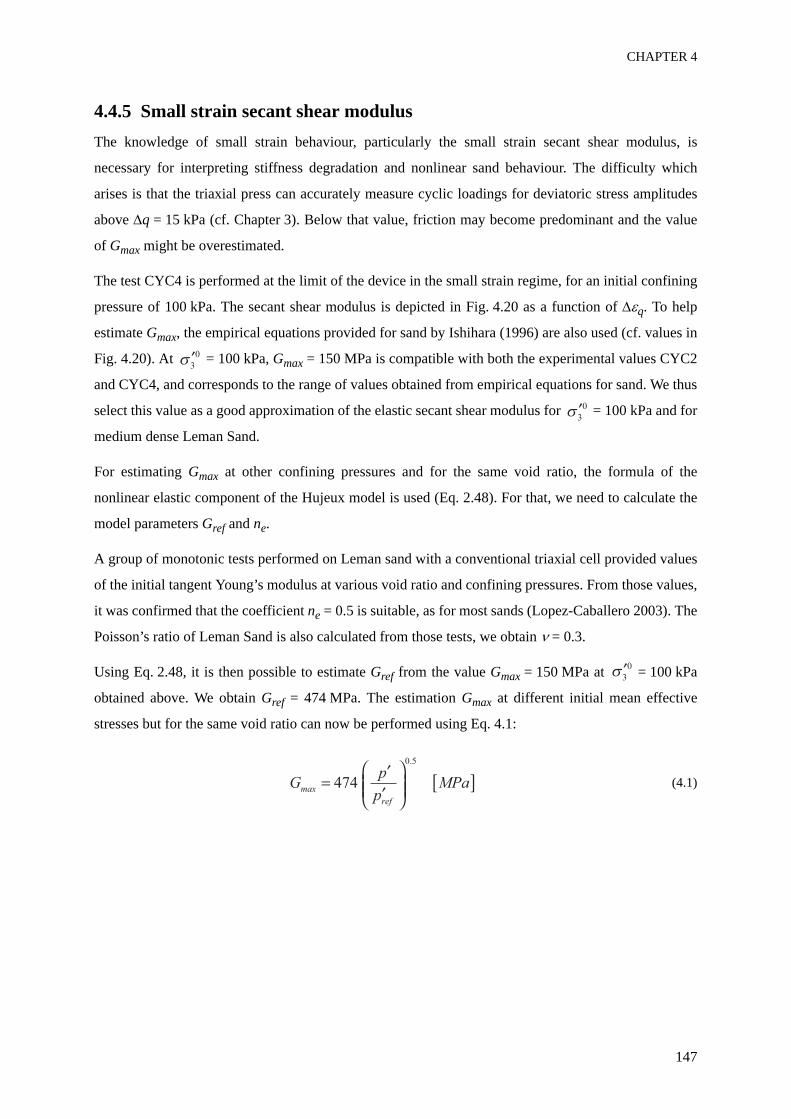
CHAPTER 4
147
4.4.5 Small strain secant shear modulusThe knowledge of small strain behaviour, particularly the small strain secant shear modulus, is
necessary for interpreting stiffness degradation and nonlinear sand behaviour. The difficulty which
arises is that the triaxial press can accurately measure cyclic loadings for deviatoric stress amplitudes
above Δq = 15 kPa (cf. Chapter 3). Below that value, friction may become predominant and the value
of Gmax might be overestimated.
The test CYC4 is performed at the limit of the device in the small strain regime, for an initial confining
pressure of 100 kPa. The secant shear modulus is depicted in Fig. 4.20 as a function of Δεq. To help
estimate Gmax, the empirical equations provided for sand by Ishihara (1996) are also used (cf. values in
Fig. 4.20). At = 100 kPa, Gmax = 150 MPa is compatible with both the experimental values CYC2
and CYC4, and corresponds to the range of values obtained from empirical equations for sand. We thus
select this value as a good approximation of the elastic secant shear modulus for = 100 kPa and for
medium dense Leman Sand.
For estimating Gmax at other confining pressures and for the same void ratio, the formula of the
nonlinear elastic component of the Hujeux model is used (Eq. 2.48). For that, we need to calculate the
model parameters Gref and ne.
A group of monotonic tests performed on Leman sand with a conventional triaxial cell provided values
of the initial tangent Young’s modulus at various void ratio and confining pressures. From those values,
it was confirmed that the coefficient ne = 0.5 is suitable, as for most sands (Lopez-Caballero 2003). The
Poisson’s ratio of Leman Sand is also calculated from those tests, we obtain ν = 0.3.
Using Eq. 2.48, it is then possible to estimate Gref from the value Gmax = 150 MPa at = 100 kPa
obtained above. We obtain Gref = 474 MPa. The estimation Gmax at different initial mean effective
stresses but for the same void ratio can now be performed using Eq. 4.1:
(4.1)Gp
pMPamax
ref
474
0 5.
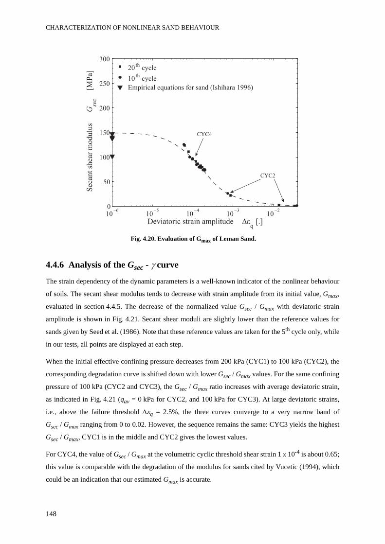
CHARACTERIZATION OF NONLINEAR SAND BEHAVIOUR
148
Fig. 4.20. Evaluation of Gmax of Leman Sand.
4.4.6 Analysis of the Gsec - γ curve
The strain dependency of the dynamic parameters is a well-known indicator of the nonlinear behaviour
of soils. The secant shear modulus tends to decrease with strain amplitude from its initial value, Gmax,
evaluated in section 4.4.5. The decrease of the normalized value Gsec / Gmax with deviatoric strain
amplitude is shown in Fig. 4.21. Secant shear moduli are slightly lower than the reference values for
sands given by Seed et al. (1986). Note that these reference values are taken for the 5th cycle only, while
in our tests, all points are displayed at each step.
When the initial effective confining pressure decreases from 200 kPa (CYC1) to 100 kPa (CYC2), the
corresponding degradation curve is shifted down with lower Gsec / Gmax values. For the same confining
pressure of 100 kPa (CYC2 and CYC3), the Gsec / Gmax ratio increases with average deviatoric strain,
as indicated in Fig. 4.21 (qav = 0 kPa for CYC2, and 100 kPa for CYC3). At large deviatoric strains,
i.e., above the failure threshold Δεq = 2.5%, the three curves converge to a very narrow band of
Gsec / Gmax ranging from 0 to 0.02. However, the sequence remains the same: CYC3 yields the highest
Gsec / Gmax, CYC1 is in the middle and CYC2 gives the lowest values.
For CYC4, the value of Gsec / Gmax at the volumetric cyclic threshold shear strain 1 x 10⁻⁴ is about 0.65;
this value is comparable with the degradation of the modulus for sands cited by Vucetic (1994), which
could be an indication that our estimated Gmax is accurate.
10 105
104
103
102
0
50
100
150
200
250
300
Deviatoric strain amplitude q [.]
Sec
ant
shea
r m
odulu
s G
sec
[M
Pa]
20th
cycle
10th
cycle
CYC2
CYC4
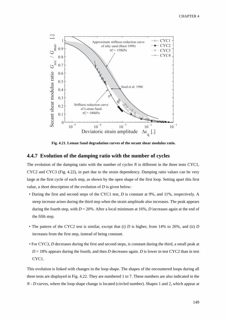
CHAPTER 4
149
Fig. 4.21. Leman Sand degradation curves of the secant shear modulus ratio.
4.4.7 Evolution of the damping ratio with the number of cyclesThe evolution of the damping ratio with the number of cycles N is different in the three tests CYC1,
CYC2 and CYC3 (Fig. 4.22), in part due to the strain dependency. Damping ratio values can be very
large at the first cycle of each step, as shown by the open shape of the first loop. Setting apart this first
value, a short description of the evolution of D is given below:
• During the first and second steps of the CYC1 test, D is constant at 9%, and 11%, respectively. A
steep increase arises during the third step when the strain amplitude also increases. The peak appears
during the fourth step, with D = 20%. After a local minimum at 16%, D increases again at the end of
the fifth step.
• The pattern of the CYC2 test is similar, except that (i) D is higher, from 14% to 26%, and (ii) D
increases from the first step, instead of being constant.
• For CYC3, D decreases during the first and second steps, is constant during the third, a small peak at
D = 18% appears during the fourth, and then D decreases again. D is lower in test CYC2 than in test
CYC1.
This evolution is linked with changes in the loop shape. The shapes of the encountered loops during all
three tests are displayed in Fig. 4.22. They are numbered 1 to 7. These numbers are also indicated in the
N - D curves, where the loop shape change is located (circled number). Shapes 1 and 2, which appear at
10 104
103
102
101
0
0.1
0.2
0.3
0.4
0.6
0.7
0.8
0.9
1
Sec
ant
shea
r m
odulu
s ra
tio
Gse
c /
Gm
ax
[.]
Deviatoric strain amplitude q [.]
CYC1
CYC2
CYC3
CYC4
Seed et al. 1986
Stiffness reduction curve
of Leman Sand
3 = 100kPa'0
Approximate stiffness reduction curve
of silty sand (Huot 1999)
3'0
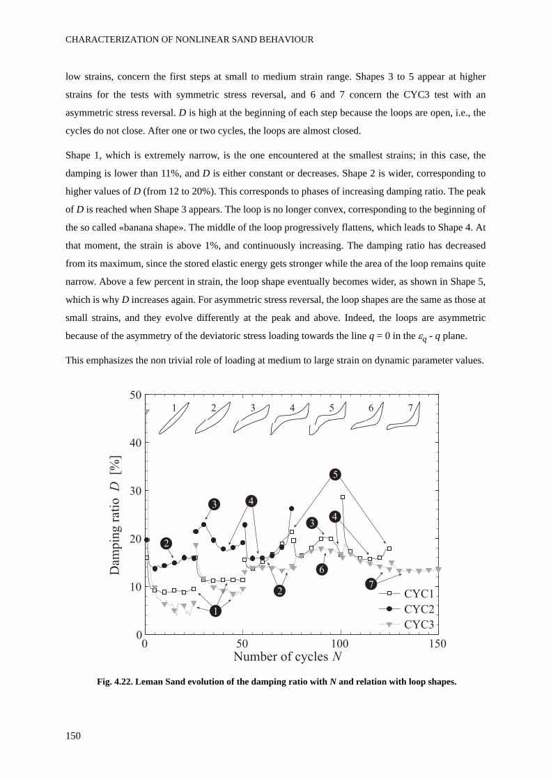
CHARACTERIZATION OF NONLINEAR SAND BEHAVIOUR
150
low strains, concern the first steps at small to medium strain range. Shapes 3 to 5 appear at higher
strains for the tests with symmetric stress reversal, and 6 and 7 concern the CYC3 test with an
asymmetric stress reversal. D is high at the beginning of each step because the loops are open, i.e., the
cycles do not close. After one or two cycles, the loops are almost closed.
Shape 1, which is extremely narrow, is the one encountered at the smallest strains; in this case, the
damping is lower than 11%, and D is either constant or decreases. Shape 2 is wider, corresponding to
higher values of D (from 12 to 20%). This corresponds to phases of increasing damping ratio. The peak
of D is reached when Shape 3 appears. The loop is no longer convex, corresponding to the beginning of
the so called «banana shape». The middle of the loop progressively flattens, which leads to Shape 4. At
that moment, the strain is above 1%, and continuously increasing. The damping ratio has decreased
from its maximum, since the stored elastic energy gets stronger while the area of the loop remains quite
narrow. Above a few percent in strain, the loop shape eventually becomes wider, as shown in Shape 5,
which is why D increases again. For asymmetric stress reversal, the loop shapes are the same as those at
small strains, and they evolve differently at the peak and above. Indeed, the loops are asymmetric
because of the asymmetry of the deviatoric stress loading towards the line q = 0 in the εq - q plane.
This emphasizes the non trivial role of loading at medium to large strain on dynamic parameter values.
Fig. 4.22. Leman Sand evolution of the damping ratio with N and relation with loop shapes.
0 50 100 1500
10
20
30
40
50
Dam
pin
g r
atio
D[%
]
Number of cycles N
CYC1
CYC2
CYC3
1 2 3 4 5 6 7
1
2
3 4
2
34
5
6
7
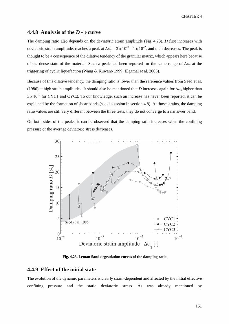
CHAPTER 4
151
4.4.8 Analysis of the D - γ curveThe damping ratio also depends on the deviatoric strain amplitude (Fig. 4.23). D first increases with
deviatoric strain amplitude, reaches a peak at Δεq = 3 x 10⁻³ - 1 x 10⁻², and then decreases. The peak is
thought to be a consequence of the dilative tendency of the granular matrix, which appears here because
of the dense state of the material. Such a peak had been reported for the same range of Δεq at the
triggering of cyclic liquefaction (Wang & Kuwano 1999; Elgamal et al. 2005).
Because of this dilative tendency, the damping ratio is lower than the reference values from Seed et al.
(1986) at high strain amplitudes. It should also be mentioned that D increases again for Δεq higher than
3 x 10⁻² for CYC1 and CYC2. To our knowledge, such an increase has never been reported; it can be
explained by the formation of shear bands (see discussion in section 4.8). At those strains, the damping
ratio values are still very different between the three tests; they do not converge to a narrower band.
On both sides of the peaks, it can be observed that the damping ratio increases when the confining
pressure or the average deviatoric stress decreases.
Fig. 4.23. Leman Sand degradation curves of the damping ratio.
4.4.9 Effect of the initial stateThe evolution of the dynamic parameters is clearly strain-dependent and affected by the initial effective
confining pressure and the static deviatoric stress. As was already mentioned by
10 103
102
101
0
5
10
15
20
25
30
Dam
pin
g r
atio
D [
%]
Deviatoric strain amplitude q [.]
CYC1
CYC2
CYC3
Seed et al. 1986
CHARACTERIZATION OF NONLINEAR SAND BEHAVIOUR
152
Hardin & Drnevich (1972a), the effective mean principal stress influences the degradation curves of the
sand. The observed effect of the confining pressure corresponds to the results obtained by Kokusho
(1980) with Toyoura sand: Gsec / Gmax increases and D decreases, i.e., they are shifted to the right on
the degradation curves, when increases. The effect of the initial shear stress on cyclic sand
behaviour is mentioned by Ishihara (1996); the cyclic strength is known to increase with the static shear
stress for dense sand (while it decreases for loose sands). This observation is confirmed in our cyclic
tests. Compared to symmetric loading with qav = 0, the number of cycles to reach 2.5% axial strain is
almost threefold when the static deviatoric stress is equal to 100 kPa. Moreover the secant shear
modulus ratio is higher: at N = 10, Gsec / Gmax more than doubles between the CYC2 and CYC3 tests,
from 0.18 to 0.41. The damping ratio is clearly lower with, for example, a peak value circa 23% for
CYC2 and only 17% for CYC3. The whole Δεq - D curve is shifted down with a positive static
deviatoric stress.
4.4.10 DiscussionThis detailed analysis of four cyclic saturated undrained tests with stress reversal provides insight into
stiffness degradation and the development of failure modes in Leman Sand. The increase of pore
pressure above the volumetric cyclic threshold shear strain appears for the four tests at medium to large
strain. Apparently, the curve ur vs. Δεq depends on the number of cycles only, and not on the confining
pressure or average deviatoric stress, as observed by Dobry et al. (1982).
Among the salient features, the asymmetry of the mechanical response between extension and
compression is noticeable, as well as for monotonic loading. Indeed, the asymmetry of stiffness and PT
lines in monotonic loading are reflected in the response to cyclic loading as well. This asymmetry
influences the stress-strain relation and the stress path.
Low void ratios are easily reached at the tested confining pressure. As a consequence, negative excess
pore pressure develops, which stabilizes the sand. The mechanism that leads to the development of
large strains and cyclic liquefaction actually starts when the stress path crosses a phase transformation
line. Above the phase transformation line, excess pore pressure first decreases. Then, a strong increase
of the pore-pressure ratio towards unity, accompanied by a gradual increase of the deviatoric strain,
appears during the unloading parts of the cycle. At reloading, the sand strength increases again because
of the decrease of excess pore pressure. As a consequence, the «banana shape», or «S shape» loop
appears. The apparition of a peak of D in the Δεq - D curve is explained by the evolution of the shape of
the stress-strain loop.
The phase-transformation line is considered to be the same in monotonic and cyclic loading (De
CHAPTER 4
153
Gennaro et al. 2004; Georgiannou et al. 2008; Shibuya et al. 2003). In addition, for the Leman Sand, the
two wings in extension and compression seem centred on the monotonic phase transformation line in
the p' - q plane (Fig. 4.14). Benahmed (2001) showed that the onset of instability usually appears on the
extension side for two-way symmetrical loadings with stress reversal. It is also the case in the CYC1
test (at N = 91) and in the CYC2 test (at N = 29). Indeed, the slope of the phase transformation line is
lower in extension. Larger strains in extension than in compression develop as well. The loops are not
symmetric in the εq - q plane with regard to the vertical axis, and the negative deviatoric strains in
extension are larger than the positive strains when the S-shape develops.
The effect of the number of cycles on Gsec and D has been studied for drained loading with a large
number of cycles (Li & Yang 1998; Wichtmann et al. 2005) and for undrained tests with stiffness
degradation (Vucetic 1994). Our experimental data show that, even at small and medium strains, D can
significantly evolve with the number of cycles N. The analysis of the shape of the cycles shows that this
evolution is recognizable from the loop shape, independent of the secant shear modulus.
Thanks to the estimation of the elastic shear modulus, the stiffness reduction curves Gsec / Gmax can be
plotted and compared to other results on sand (Fig. 4.21). Shear modulus ratio obtained for Leman Sand
are slightly lower than the area of reference defined by Seed et al. (1986). However, the value of
stiffness degradation of CYC4 at the volumetric cyclic threshold shear strain is in good agreement with
Vucetic (1994) and Huot (1999), which confirms the values obtained for Gmax.
As explained previously, the evolution of damping ratio vs. Δεq has an unexpected shape. The increase
of D with Δεq is within the range of the reference from Seed et al. (1986), but a first peak appears
because of dilatant mechanism at strain amplitude around 5 x 10⁻³. The final increase of D at large
strains (Δεq > 3 x 10⁻²), after this first peak, is seen as a consequence of the shear band which is visible
at the end of CYC1 and CYC2 tests. With such localization, the measured stress and strain are doubtful.
It is still interesting to see that the apparition of the shear band leads to a change in the shape of the
stress-strain loop (Shape 5), which is a type of distorted S shape.
4.4.11 ConclusionsA laboratory study was performed on saturated Leman Sand samples in undrained conditions with an
advanced triaxial apparatus, focusing on the cyclic behaviour at medium to large strains with an
emphasis on (i) excess pore pressure increase (ii) sample failure definition (iii) the evolution of
dynamic parameters (iv) the effect of initial and boundary conditions. The observations can be
summarized as follows:
CHARACTERIZATION OF NONLINEAR SAND BEHAVIOUR
154
• Excess pore pressure increases from the threshold Δεq = 10-4 and depends mainly on the strain
amplitude. The number of loading cycles N also influences the pore pressure increase, in the sense
that several curves Δεq - ur are obtained for the different values of N.
• Cyclic stiffness degradation arises by cyclic liquefaction. The material softens, and its degradation
index reaches very low values. The failure criterion can be based on a threshold deviatoric strain
Δεq = 2.5%. It matches the level of the degradation index well, which can thus be used as an
alternative criterion for failure. Another candidate can be the pore water pressure ratio.
• Stiffness degradation curves of the dynamic parameters as a function of the deviatoric strain
amplitude are calculated for saturated Leman Sand. The small strain secant shear modulus is
evaluated by cross-checking empirical equations for sands and cyclic test results at small to medium
strain. The Δεq - Gsec / Gmax curves are thus obtained in the medium to large strain domain.
• Furthermore, the damping ratio strongly evolves between the 1st and the 25th cycle. This evolution is
explained by the loop shape, which depends on the stress path. A peak of the damping ratio in the
degradation curve arises at strains of 0.3 to 1%.
4.5 Nonlinear Fonderie Sand behaviour in undrained saturated conditions
4.5.1 IntroductionMonotonic and cyclic saturated undrained triaxial tests were also performed with Fonderie Sand (see
soil characteristics in section 3.5.2). As it is a relatively uniform sand, it is possible to use pluviation
technique to obtain samples at several relative densities. This sand is thus used to study the nonlinear
soil behaviour at various relative densities, from medium to dense sand. The comparison with Leman
Sand nonlinear behaviour also gives interesting perspectives in terms of effect of the soil fabric.
The monotonic tests are briefly summarized, before nonlinear stiffness degradation at medium to large
cyclic strain is described. Failure appears thanks to pore pressure increase coupled with the plastic
strain accumulation. The dynamic parameters are provided. Stiffness degradation curves are compared
to reference values for sand and to the results obtained with Leman Sand.
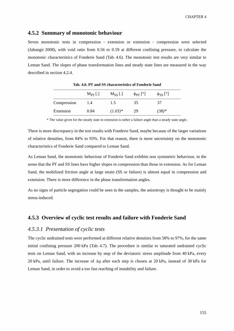
CHAPTER 4
155
4.5.2 Summary of monotonic behaviourSeven monotonic tests in compression - extension or extension - compression were selected
(Jahangir 2008), with void ratio from 0.56 to 0.59 at different confining pressure, to calculate the
monotonic characteristics of Fonderie Sand (Tab. 4.6). The monotonic test results are very similar to
Leman Sand. The slopes of phase transformation lines and steady state lines are measured in the way
described in section 4.2.4.
Tab. 4.6. PT and SS characteristics of Fonderie Sand
* The value given for the steady state in extension is rather a failure angle than a steady state angle.
There is more discrepancy in the test results with Fonderie Sand, maybe because of the larger variations
of relative densities, from 84% to 93%. For that reason, there is more uncertainty on the monotonic
characteristics of Fonderie Sand compared to Leman Sand.
As Leman Sand, the monotonic behaviour of Fonderie Sand exhibits non symmetric behaviour, in the
sense that the PT and SS lines have higher slopes in compression than those in extension. As for Leman
Sand, the mobilized friction angle at large strain (SS or failure) is almost equal in compression and
extension. There is more difference in the phase transformation angles.
As no signs of particle segregation could be seen in the samples, the anisotropy is thought to be mainly
stress-induced.
4.5.3 Overview of cyclic test results and failure with Fonderie Sand
4.5.3.1 Presentation of cyclic testsThe cyclic undrained tests were performed at different relative densities from 58% to 97%, for the same
initial confining pressure 200 kPa (Tab. 4.7). The procedure is similar to saturated undrained cyclic
tests on Leman Sand, with an increase by step of the deviatoric stress amplitude from 40 kPa, every
20 kPa, until failure. The increase of Δq after each step is chosen at 20 kPa, instead of 30 kPa for
Leman Sand, in order to avoid a too fast reaching of instability and failure.
MPT [.] MSS [.] φPT [°] φSS [°]
Compression 1.4 1.5 35 37
Extension 0.84 (1.03)* 29 (38)*
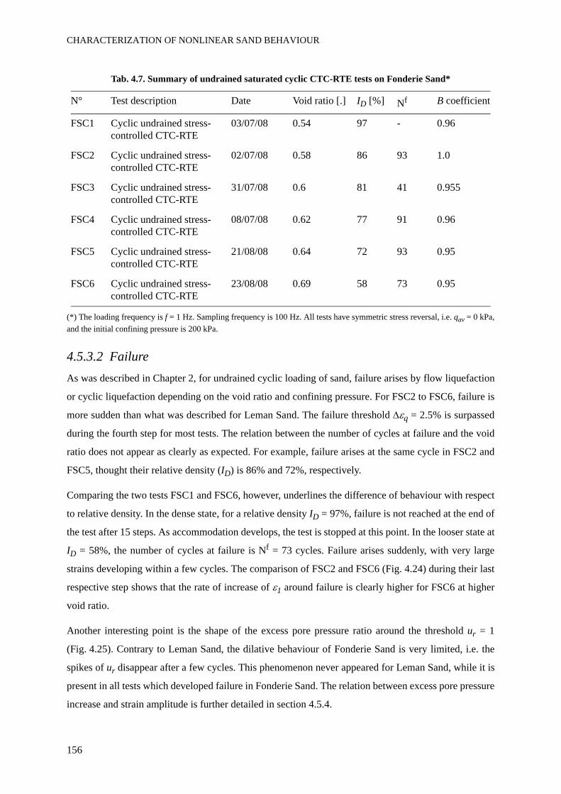
CHARACTERIZATION OF NONLINEAR SAND BEHAVIOUR
156
Tab. 4.7. Summary of undrained saturated cyclic CTC-RTE tests on Fonderie Sand*
(*) The loading frequency is f = 1 Hz. Sampling frequency is 100 Hz. All tests have symmetric stress reversal, i.e. qav = 0 kPa,and the initial confining pressure is 200 kPa.
4.5.3.2 FailureAs was described in Chapter 2, for undrained cyclic loading of sand, failure arises by flow liquefaction
or cyclic liquefaction depending on the void ratio and confining pressure. For FSC2 to FSC6, failure is
more sudden than what was described for Leman Sand. The failure threshold Δεq = 2.5% is surpassed
during the fourth step for most tests. The relation between the number of cycles at failure and the void
ratio does not appear as clearly as expected. For example, failure arises at the same cycle in FSC2 and
FSC5, thought their relative density (ID) is 86% and 72%, respectively.
Comparing the two tests FSC1 and FSC6, however, underlines the difference of behaviour with respect
to relative density. In the dense state, for a relative density ID = 97%, failure is not reached at the end of
the test after 15 steps. As accommodation develops, the test is stopped at this point. In the looser state at
ID = 58%, the number of cycles at failure is Nf = 73 cycles. Failure arises suddenly, with very large
strains developing within a few cycles. The comparison of FSC2 and FSC6 (Fig. 4.24) during their last
respective step shows that the rate of increase of ε1 around failure is clearly higher for FSC6 at higher
void ratio.
Another interesting point is the shape of the excess pore pressure ratio around the threshold ur = 1
(Fig. 4.25). Contrary to Leman Sand, the dilative behaviour of Fonderie Sand is very limited, i.e. the
spikes of ur disappear after a few cycles. This phenomenon never appeared for Leman Sand, while it is
present in all tests which developed failure in Fonderie Sand. The relation between excess pore pressure
increase and strain amplitude is further detailed in section 4.5.4.
N° Test description Date Void ratio [.] ID [%] Nf B coefficient
FSC1 Cyclic undrained stress-controlled CTC-RTE
03/07/08 0.54 97 - 0.96
FSC2 Cyclic undrained stress-controlled CTC-RTE
02/07/08 0.58 86 93 1.0
FSC3 Cyclic undrained stress-controlled CTC-RTE
31/07/08 0.6 81 41 0.955
FSC4 Cyclic undrained stress-controlled CTC-RTE
08/07/08 0.62 77 91 0.96
FSC5 Cyclic undrained stress-controlled CTC-RTE
21/08/08 0.64 72 93 0.95
FSC6 Cyclic undrained stress-controlled CTC-RTE
23/08/08 0.69 58 73 0.95
CHAPTER 4
157
We consider the rate of increase of the deviatoric strain close to failure as the best criterion to determine
whether failure arises by cyclic liquefaction or flow liquefaction. As an analogy to the response of
Hostun Sand in terms of both deviatoric strain and pore pressure, as they are described above (cf.
Benahmed 2001), failure resembles more flow liquefaction in the test FSC6, while for FSC2, the
response is assimilated to cyclic liquefaction. To verify this affirmation, and to determine the failure
mechanism for tests of intermediate relative densities, Fig. 4.26 provides the strain amplitudes at failure
of all tests concerned for Fonderie Sand. Apart from FSC2 for which the rate of increase of the
deviatoric strain amplitude is slightly smaller, all tests exhibit a rapid failure as shown for the test
FSC6.
4.5.3.3 Comparison with Leman SandCompared to Leman Sand in test CYC1, which is in the same initial condition as test FSC5 in terms of
relative density and initial confining pressure, stiffness degradation of Fonderie Sand is sudden
(Fig. 4.26). Strain amplitude is higher for Leman Sand of approximately one log-scale at the beginning
of the tests, and regularly increases. On the contrary, the strain amplitude of Fonderie Sand is low and
stable at the beginning of the tests, but it increases suddenly and reaches the level of the failure
threshold within a few cycles.
As the behaviours of Leman Sand and Fonderie Sand seem quite different, the comparison of stress-
strain relation and stress paths of CYC1 and FSC5 (similar relative density) at failure is given in
Fig. 4.27 and Fig. 4.28. The cyclic stress ratio (CSR) at failure is smaller for Fonderie Sand; it thus
seems that cyclic strength of Fonderie Sand is lower than cyclic strength of Leman Sand, thought this
notion can not be ascertain by only these two tests.
The stress-strain relation presents a banana shape for both sands (Fig. 4.27). The shape of the stress-
strain relation of Fonderie Sand decays because the stress amplitude decreases. This is due to the fact
that the sand stiffness decreases so suddenly that the regulation system cannot impose the prescribed
force. The increase of deviatoric strain arises predominantly in the side of extension for both sands. As
seen before, the rate of increase of the deviatoric strain is faster in Fonderie Sand than in Leman Sand.
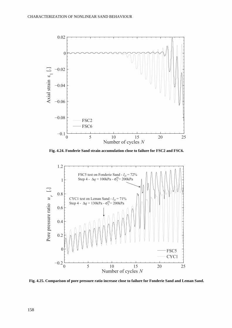
CHARACTERIZATION OF NONLINEAR SAND BEHAVIOUR
158
Fig. 4.24. Fonderie Sand strain accumulation close to failure for FSC2 and FSC6.
Fig. 4.25. Comparison of pore pressure ratio increase close to failure for Fonderie Sand and Leman Sand.
0 5 10 15 20 25
0
Number of cycles N
Axia
l st
rain
1
FSC2
0 5 10 15 20 25
0
1
Pore
pre
ssure
rat
io
ur
Number of cycles N
FSC5
CYC1
FSC5 test on Fonderie Sand - ID = 72%
q = 100kPa - 3 = 200kPa
CYC1 test on Leman Sand - ID = 71%
q = 130kPa - 3 = 200kPa ‘0
‘0
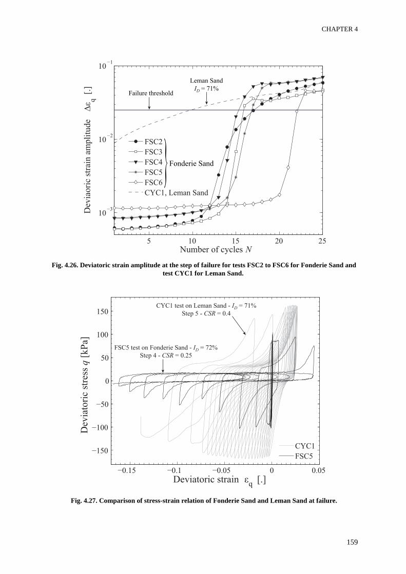
CHAPTER 4
159
Fig. 4.26. Deviatoric strain amplitude at the step of failure for tests FSC2 to FSC6 for Fonderie Sand and test CYC1 for Leman Sand.
Fig. 4.27. Comparison of stress-strain relation of Fonderie Sand and Leman Sand at failure.
5 10 15 20 25
10
102
101
Dev
iaori
c st
rain
am
pli
tude
q [
.]
Number of cycles N
FSC2
FSC4
FSC5
FSC6
CYC1, Leman Sand
Failure threshold
Leman Sand
ID = 71%
Fonderie Sand}
Dev
iato
ric
stre
ss q
[k
Pa]
Deviatoric strain q
ID = 72%
CSR
ID
CSR
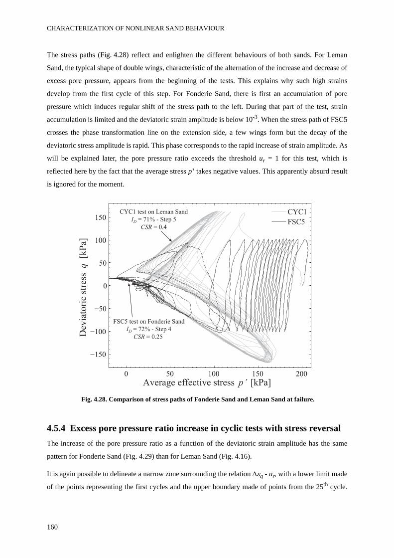
CHARACTERIZATION OF NONLINEAR SAND BEHAVIOUR
160
The stress paths (Fig. 4.28) reflect and enlighten the different behaviours of both sands. For Leman
Sand, the typical shape of double wings, characteristic of the alternation of the increase and decrease of
excess pore pressure, appears from the beginning of the tests. This explains why such high strains
develop from the first cycle of this step. For Fonderie Sand, there is first an accumulation of pore
pressure which induces regular shift of the stress path to the left. During that part of the test, strain
accumulation is limited and the deviatoric strain amplitude is below 10-3. When the stress path of FSC5
crosses the phase transformation line on the extension side, a few wings form but the decay of the
deviatoric stress amplitude is rapid. This phase corresponds to the rapid increase of strain amplitude. As
will be explained later, the pore pressure ratio exceeds the threshold ur = 1 for this test, which is
reflected here by the fact that the average stress p’ takes negative values. This apparently absurd result
is ignored for the moment.
Fig. 4.28. Comparison of stress paths of Fonderie Sand and Leman Sand at failure.
4.5.4 Excess pore pressure ratio increase in cyclic tests with stress reversalThe increase of the pore pressure ratio as a function of the deviatoric strain amplitude has the same
pattern for Fonderie Sand (Fig. 4.29) than for Leman Sand (Fig. 4.16).
It is again possible to delineate a narrow zone surrounding the relation Δεq - ur, with a lower limit made
of the points representing the first cycles and the upper boundary made of points from the 25th cycle.
0 50 100 150 200
0
50
100
150
Dev
iato
ric
stre
ssq
[k
Pa]
Average effective stress p’ [kPa]
CYC1
FSC5
FSC5 test on Fonderie Sand
ID = 72% - Step 4
CSR = 0.25
CYC1 test on Leman Sand
ID = 71% - Step 5
CSR = 0.4
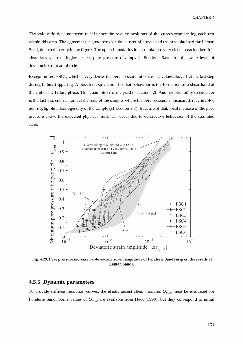
CHAPTER 4
161
The void ratio does not seem to influence the relative positions of the curves representing each test
within this area. The agreement is good between the cluster of curves and the area obtained for Leman
Sand, depicted in gray in the figure. The upper boundaries in particular are very close to each other. It is
clear however that higher excess pore pressure develops in Fonderie Sand, for the same level of
deviatoric strain amplitude.
Except for test FSC1, which is very dense, the pore pressure ratio reaches values above 1 at the last step
during failure triggering. A possible explanation for that behaviour is the formation of a shear band at
the end of the failure phase. This assumption is analysed in section 4.8. Another possibility to consider
is the fact that end-restraint at the base of the sample, where the pore pressure is measured, may involve
non-negligible inhomogeneity of the sample (cf. section 3.3). Because of that, local increase of the pore
pressure above the expected physical limits can occur due to contractive behaviour of the saturated
sand.
Fig. 4.29. Pore pressure increase vs. deviatoric strain amplitude of Fonderie Sand (in grey, the results of Leman Sand).
4.5.5 Dynamic parametersTo provide stiffness reduction curves, the elastic secant shear modulus Gmax must be evaluated for
Fonderie Sand. Some values of Gmax are available from Huot (1999), but they correspond to initial
10 103
102
101
0
0.1
0.2
0.3
0.5
0.6
0.7
0.8
0.9
1
Max
imum
pore
pre
ssure
rat
io p
er c
ycl
e u
r,m
[.]
Deviatoric strain amplitude q
[.]
FSC1
FSC2
FSC3
FSC5
FSC6N = 1
N = 25
Overshooting of ur for FSC2 to FSC6,
assumed to be caused by the formation of
a shear band
Leman Sand
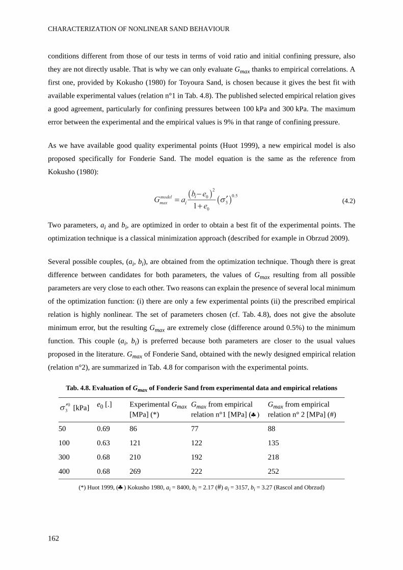
CHARACTERIZATION OF NONLINEAR SAND BEHAVIOUR
162
conditions different from those of our tests in terms of void ratio and initial confining pressure, also
they are not directly usable. That is why we can only evaluate Gmax thanks to empirical correlations. A
first one, provided by Kokusho (1980) for Toyoura Sand, is chosen because it gives the best fit with
available experimental values (relation n°1 in Tab. 4.8). The published selected empirical relation gives
a good agreement, particularly for confining pressures between 100 kPa and 300 kPa. The maximum
error between the experimental and the empirical values is 9% in that range of confining pressure.
As we have available good quality experimental points (Huot 1999), a new empirical model is also
proposed specifically for Fonderie Sand. The model equation is the same as the reference from
Kokusho (1980):
(4.2)
Two parameters, ai and bi, are optimized in order to obtain a best fit of the experimental points. The
optimization technique is a classical minimization approach (described for example in Obrzud 2009).
Several possible couples, (ai, bi), are obtained from the optimization technique. Though there is great
difference between candidates for both parameters, the values of Gmax resulting from all possible
parameters are very close to each other. Two reasons can explain the presence of several local minimum
of the optimization function: (i) there are only a few experimental points (ii) the prescribed empirical
relation is highly nonlinear. The set of parameters chosen (cf. Tab. 4.8), does not give the absolute
minimum error, but the resulting Gmax are extremely close (difference around 0.5%) to the minimum
function. This couple (ai, bi) is preferred because both parameters are closer to the usual values
proposed in the literature. Gmax of Fonderie Sand, obtained with the newly designed empirical relation
(relation n°2), are summarized in Tab. 4.8 for comparison with the experimental points.
Tab. 4.8. Evaluation of Gmax of Fonderie Sand from experimental data and empirical relations
(*) Huot 1999, (♣) Kokusho 1980, ai = 8400, bi = 2.17 (#) ai = 3157, bi = 3.27 (Rascol and Obrzud)
[kPa] e0 [.] Experimental Gmax [MPa] (*)
Gmax from empirical relation n°1 [MPa] (♣)
Gmax from empirical relation n° 2 [MPa] (#)
50 0.69 86 77 88
100 0.63 121 122 135
300 0.68 210 192 218
400 0.68 269 222 252
G ab e
emax
model 0
2
0
3
0 5
1
.
i
i
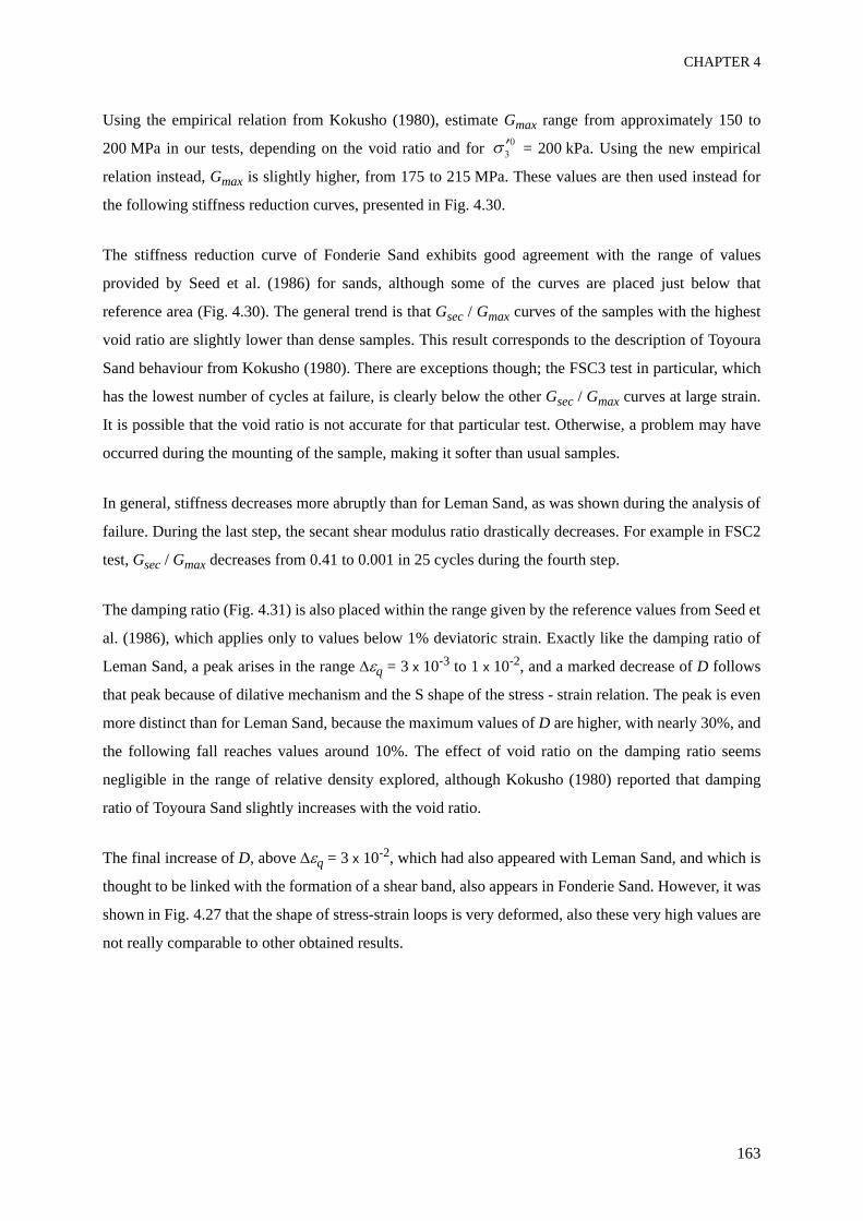
CHAPTER 4
163
Using the empirical relation from Kokusho (1980), estimate Gmax range from approximately 150 to
200 MPa in our tests, depending on the void ratio and for = 200 kPa. Using the new empirical
relation instead, Gmax is slightly higher, from 175 to 215 MPa. These values are then used instead for
the following stiffness reduction curves, presented in Fig. 4.30.
The stiffness reduction curve of Fonderie Sand exhibits good agreement with the range of values
provided by Seed et al. (1986) for sands, although some of the curves are placed just below that
reference area (Fig. 4.30). The general trend is that Gsec / Gmax curves of the samples with the highest
void ratio are slightly lower than dense samples. This result corresponds to the description of Toyoura
Sand behaviour from Kokusho (1980). There are exceptions though; the FSC3 test in particular, which
has the lowest number of cycles at failure, is clearly below the other Gsec / Gmax curves at large strain.
It is possible that the void ratio is not accurate for that particular test. Otherwise, a problem may have
occurred during the mounting of the sample, making it softer than usual samples.
In general, stiffness decreases more abruptly than for Leman Sand, as was shown during the analysis of
failure. During the last step, the secant shear modulus ratio drastically decreases. For example in FSC2
test, Gsec / Gmax decreases from 0.41 to 0.001 in 25 cycles during the fourth step.
The damping ratio (Fig. 4.31) is also placed within the range given by the reference values from Seed et
al. (1986), which applies only to values below 1% deviatoric strain. Exactly like the damping ratio of
Leman Sand, a peak arises in the range Δεq = 3 x 10⁻³ to 1 x 10⁻², and a marked decrease of D follows
that peak because of dilative mechanism and the S shape of the stress - strain relation. The peak is even
more distinct than for Leman Sand, because the maximum values of D are higher, with nearly 30%, and
the following fall reaches values around 10%. The effect of void ratio on the damping ratio seems
negligible in the range of relative density explored, although Kokusho (1980) reported that damping
ratio of Toyoura Sand slightly increases with the void ratio.
The final increase of D, above Δεq = 3 x 10⁻², which had also appeared with Leman Sand, and which is
thought to be linked with the formation of a shear band, also appears in Fonderie Sand. However, it was
shown in Fig. 4.27 that the shape of stress-strain loops is very deformed, also these very high values are
not really comparable to other obtained results.
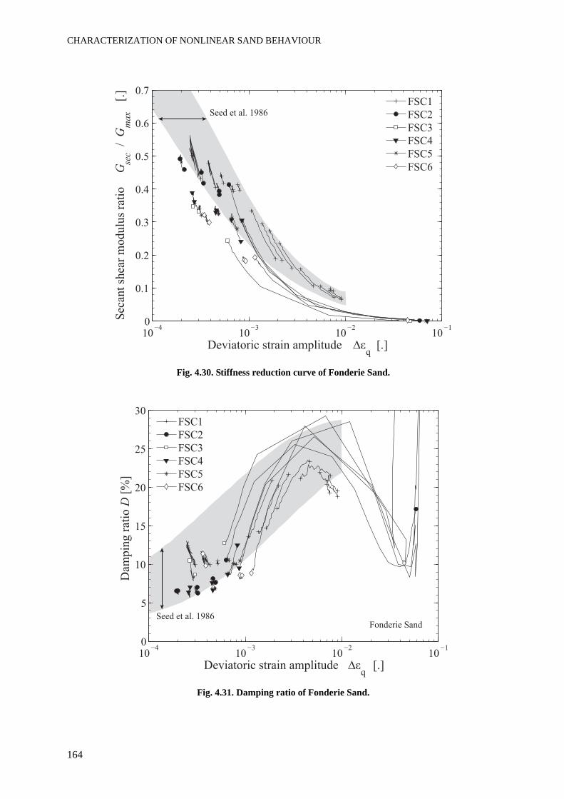
CHARACTERIZATION OF NONLINEAR SAND BEHAVIOUR
164
Fig. 4.30. Stiffness reduction curve of Fonderie Sand.
Fig. 4.31. Damping ratio of Fonderie Sand.
Seed et al. 1986
10 103
102
101
0
0.1
0.2
0.3
0.5
0.6
0.7
Sec
ant
shea
r m
odulu
s ra
tio
Gse
c /
G
ma
x [
.]
Deviatoric strain amplitude q
[.]
FSC1
FSC2
FSC3
FSC5
FSC6
10 103
102
101
0
5
10
15
20
25
30
Dam
pin
g r
atio
D[%
]
Deviatoric strain amplitude q
[.]
FSC1
FSC2
FSC3
FSC5
FSC6
Seed et al. 1986Fonderie Sand
CHAPTER 4
165
4.5.6 DiscussionIn the first place, we did not obtain a simple quantitative relation between the relative density ID of
Fonderie Sand, in the medium to dense state, and the number of cycles to failure. It is however possible
to distinguish three types of response: a dense behaviour with accommodation (FSC1), a dense
behaviour with failure similar to cyclic liquefaction (FSC2) and a medium behaviour with sudden
failure assimilated to flow liquefaction (FSC3 to FSC6). This classification of the failure mode as flow
liquefaction relies on the comparison with test results of Benahmed (2001) with Hostun Sand. This
interpretation may then depend on subjectivity.
The comparison with Leman Sand, for tests with the same initial confining pressure and relative
density, provides perspective into the nonlinear behaviour of both sands. The mechanism of stiffness
degradation is rather continuous and progressive in Leman Sand, while it is a sudden and rapid
phenomenon in Fonderie Sand. The striking difference can be explained by a different liquefaction
susceptibility. Kramer (1996) mentions that grain size distribution and the shape of the grains influence
liquefaction susceptibility (see section 2.4.13): narrow graded sands are more susceptible to
liquefaction than well graded sands, and rounded grains are more susceptible to liquefaction than
angular grains. Fonderie Sand grains are rounder, and the particle size distribution is really narrow,
compared to Leman Sand. Both aspects can thus explain the two different nonlinear behaviours. It also
reflects the different values of phase transformation and steady state angles of the two sands.
On the other hand, the relations Δεq - ur, Δεq - Gsec / Gmax, and Δεq - D are quite similar for Fonderie
and Leman Sand. Particularly, the peak in the Δεq - D curve, which was previously linked to the
apparition of the dilative behaviour, occurs for both sands. As the banana shape of the stress-strain
relation develop as well, it seems appropriate to obtain the same kind of stiffness degradation curves.
There is anyway a small difference in the relation Δεq - ur between Fonderie and Leman Sand, which
may be ascribed to the different particle size distribution and grain shape.
4.5.7 SummaryThe steady state and phase transformation lines are drawn for Fonderie Sand from several monotonic
tests performed in a dense state, at a relative density around 88% and for different confining pressures.
Cyclic tests on Fonderie Sand were performed in undrained conditions. Three different behaviours are
obtained with regard to failure: the denser material exhibits accommodation, the following dense
sample exhibits cyclic liquefaction while the rest of the medium-dense samples exhibit failure which
resembles flow liquefaction. Near failure, the excess pore pressure ratio unexpectedly increases
above 1. This phenomenon may be a symptom of soil inhomogeneity, either due to strain localization or
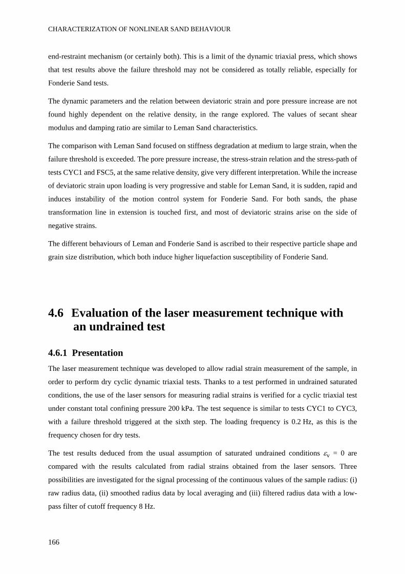
CHARACTERIZATION OF NONLINEAR SAND BEHAVIOUR
166
end-restraint mechanism (or certainly both). This is a limit of the dynamic triaxial press, which shows
that test results above the failure threshold may not be considered as totally reliable, especially for
Fonderie Sand tests.
The dynamic parameters and the relation between deviatoric strain and pore pressure increase are not
found highly dependent on the relative density, in the range explored. The values of secant shear
modulus and damping ratio are similar to Leman Sand characteristics.
The comparison with Leman Sand focused on stiffness degradation at medium to large strain, when the
failure threshold is exceeded. The pore pressure increase, the stress-strain relation and the stress-path of
tests CYC1 and FSC5, at the same relative density, give very different interpretation. While the increase
of deviatoric strain upon loading is very progressive and stable for Leman Sand, it is sudden, rapid and
induces instability of the motion control system for Fonderie Sand. For both sands, the phase
transformation line in extension is touched first, and most of deviatoric strains arise on the side of
negative strains.
The different behaviours of Leman and Fonderie Sand is ascribed to their respective particle shape and
grain size distribution, which both induce higher liquefaction susceptibility of Fonderie Sand.
4.6 Evaluation of the laser measurement technique with an undrained test
4.6.1 PresentationThe laser measurement technique was developed to allow radial strain measurement of the sample, in
order to perform dry cyclic dynamic triaxial tests. Thanks to a test performed in undrained saturated
conditions, the use of the laser sensors for measuring radial strains is verified for a cyclic triaxial test
under constant total confining pressure 200 kPa. The test sequence is similar to tests CYC1 to CYC3,
with a failure threshold triggered at the sixth step. The loading frequency is 0.2 Hz, as this is the
frequency chosen for dry tests.
The test results deduced from the usual assumption of saturated undrained conditions εv = 0 are
compared with the results calculated from radial strains obtained from the laser sensors. Three
possibilities are investigated for the signal processing of the continuous values of the sample radius: (i)
raw radius data, (ii) smoothed radius data by local averaging and (iii) filtered radius data with a low-
pass filter of cutoff frequency 8 Hz.
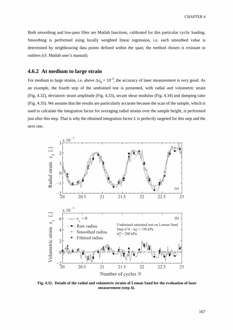
CHAPTER 4
167
Both smoothing and low-pass filter are Matlab functions, calibrated for this particular cyclic loading.
Smoothing is performed using locally weighted linear regression, i.e. each smoothed value is
determined by neighbouring data points defined within the span; the method chosen is resistant to
outliers (cf. Matlab user’s manual).
4.6.2 At medium to large strainFor medium to large strains, i.e. above Δεq = 10-3, the accuracy of laser measurement is very good. As
an example, the fourth step of the undrained test is presented, with radial and volumetric strain
(Fig. 4.32), deviatoric strain amplitude (Fig. 4.33), secant shear modulus (Fig. 4.34) and damping ratio
(Fig. 4.35). We assume that the results are particularly accurate because the scan of the sample, which is
used to calculate the integration factor for averaging radial strains over the sample height, is performed
just after this step. That is why the obtained integration factor L is perfectly targeted for this step and the
next one.
Fig. 4.32. Details of the radial and volumetric strains of Leman Sand for the evaluation of laser measurement (step 4).
20 20.5 21 21.5 22 22.5 23
0
1
2
3x 10
3
Rad
ial
stra
in
3 [
.]
20 20.5 21 21.5 22 22.5 232
0
2
4
6
x 103
Volu
met
ric
stra
in
v [
.]
Number of cycles N
v = 0
Raw radius
Smoothed radius
Filtered radius
(a)
(b)
Undrained saturated test on Leman Sand
Step n°4 - q = 130 kPa
3 = 200 kPa‘0
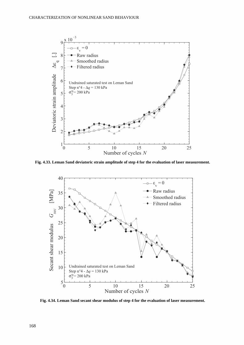
CHARACTERIZATION OF NONLINEAR SAND BEHAVIOUR
168
Fig. 4.33. Leman Sand deviatoric strain amplitude of step 4 for the evaluation of laser measurement.
Fig. 4.34. Leman Sand secant shear modulus of step 4 for the evaluation of laser measurement.
0 5 10 15 20 251
2
3
4
5
6
7
8
9x 10
Dev
iato
ric
stra
in a
mpli
tude
q [
.]
Number of cycles N
v = 0
Raw radius
Smoothed radius
Filtered radius
Undrained saturated test on Leman Sand
Step n°4 - q = 130 kPa
3 = 200 kPa‘0
0 5 10 15 20 255
10
15
20
25
30
35
40
Sec
ant
shea
r m
odulu
s G
sec
[M
Pa]
Number of cycles N
v = 0
Raw radius
Smoothed radius
Filtered radius
Undrained saturated test on Leman Sand
Step n°4 - q = 130 kPa
3 = 200 kPa‘0
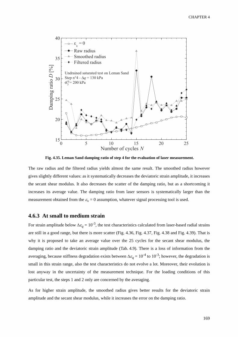
CHAPTER 4
169
Fig. 4.35. Leman Sand damping ratio of step 4 for the evaluation of laser measurement.
The raw radius and the filtered radius yields almost the same result. The smoothed radius however
gives slightly different values: as it systematically decreases the deviatoric strain amplitude, it increases
the secant shear modulus. It also decreases the scatter of the damping ratio, but as a shortcoming it
increases its average value. The damping ratio from laser sensors is systematically larger than the
measurement obtained from the εv = 0 assumption, whatever signal processing tool is used.
4.6.3 At small to medium strainFor strain amplitude below Δεq = 10-3, the test characteristics calculated from laser-based radial strains
are still in a good range, but there is more scatter (Fig. 4.36, Fig. 4.37, Fig. 4.38 and Fig. 4.39). That is
why it is proposed to take an average value over the 25 cycles for the secant shear modulus, the
damping ratio and the deviatoric strain amplitude (Tab. 4.9). There is a loss of information from the
averaging, because stiffness degradation exists between Δεq = 10-4 to 10-3; however, the degradation is
small in this strain range, also the test characteristics do not evolve a lot. Moreover, their evolution is
lost anyway in the uncertainty of the measurement technique. For the loading conditions of this
particular test, the steps 1 and 2 only are concerned by the averaging.
As for higher strain amplitude, the smoothed radius gives better results for the deviatoric strain
amplitude and the secant shear modulus, while it increases the error on the damping ratio.
0 5 10 15 20 2515
20
25
30
35
40
Dam
pin
g r
atio
D [
%]
Number of cycles N
v = 0
Raw radius
Smoothed radius
Filtered radius
Undrained saturated test on Leman Sand
Step n°4 - q = 130 kPa
3 = 200 kPa‘0
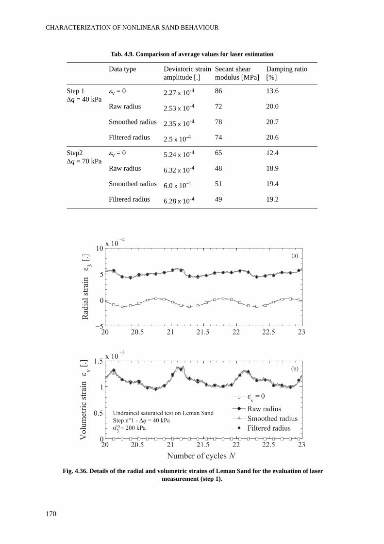
CHARACTERIZATION OF NONLINEAR SAND BEHAVIOUR
170
Tab. 4.9. Comparison of average values for laser estimation
Fig. 4.36. Details of the radial and volumetric strains of Leman Sand for the evaluation of laser measurement (step 1).
Data type Deviatoric strain amplitude [.]
Secant shear modulus [MPa]
Damping ratio [%]
Step 1Δq = 40 kPa
εv = 0 2.27 x 10⁻⁴ 86 13.6
Raw radius 2.53 x 10⁻⁴ 72 20.0
Smoothed radius 2.35 x 10⁻⁴ 78 20.7
Filtered radius 2.5 x 10⁻⁴ 74 20.6
Step2Δq = 70 kPa
εv = 0 5.24 x 10⁻⁴ 65 12.4
Raw radius 6.32 x 10⁻⁴ 48 18.9
Smoothed radius 6.0 x 10⁻⁴ 51 19.4
Filtered radius 6.28 x 10⁻⁴ 49 19.2
20 20.5 21 21.5 22 22.5 23
0
5
10x 10
4
Rad
ial
stra
in
3 [
.]
20 20.5 21 21.5 22 22.5 230
0.5
1
1.5x 10
3
Volu
met
ric
stra
in
v [
.]
Number of cycles N
v = 0
Raw radius
Smoothed radius
Filtered radius
Undrained saturated test on Leman Sand
Step n°1 - q = 40 kPa
3 = 200 kPa‘0
(a)
(b)

CHAPTER 4
171
Fig. 4.37. Leman Sand deviatoric strain amplitude of step 1 for the evaluation of laser measurement.
Fig. 4.38. Leman Sand secant shear modulus of step 1 for the evaluation of laser measurement.
0 5 10 15 20 251.8
2
2.2
2.4
2.6
2.8
3
3.2
3.4x 10
Dev
iato
ric
stra
in a
mpli
tude
q [
.]
Number of cycles N
v = 0
Raw radius
Smoothed radius
Filtered radius
Undrained saturated test on Leman Sand
Step n°1 - q = 40 kPa
3 = 200 kPa‘0
0 5 10 15 20 2550
60
70
80
90
100
110
Sec
ant
shea
r m
odulu
s G
sec
[M
Pa]
Number of cycles N
v = 0
Raw radius
Smoothed radius
Filtered radius
Undrained saturated test on Leman Sand
Step n°1 - q = 40 kPa
3 = 200 kPa‘0
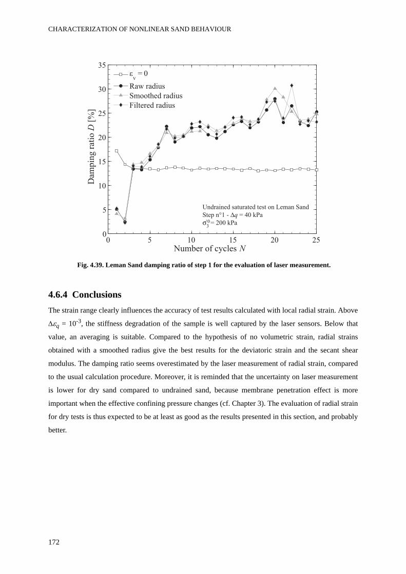
CHARACTERIZATION OF NONLINEAR SAND BEHAVIOUR
172
Fig. 4.39. Leman Sand damping ratio of step 1 for the evaluation of laser measurement.
4.6.4 ConclusionsThe strain range clearly influences the accuracy of test results calculated with local radial strain. Above
Δεq = 10-3, the stiffness degradation of the sample is well captured by the laser sensors. Below that
value, an averaging is suitable. Compared to the hypothesis of no volumetric strain, radial strains
obtained with a smoothed radius give the best results for the deviatoric strain and the secant shear
modulus. The damping ratio seems overestimated by the laser measurement of radial strain, compared
to the usual calculation procedure. Moreover, it is reminded that the uncertainty on laser measurement
is lower for dry sand compared to undrained sand, because membrane penetration effect is more
important when the effective confining pressure changes (cf. Chapter 3). The evaluation of radial strain
for dry tests is thus expected to be at least as good as the results presented in this section, and probably
better.
0 5 10 15 20 250
5
10
15
20
25
30
35
Dam
pin
g r
atio
D [
%]
Number of cycles N
v = 0
Raw radius
Smoothed radius
Filtered radius
Undrained saturated test on Leman Sand
Step n°1 - q = 40 kPa
3 = 200 kPa‘0
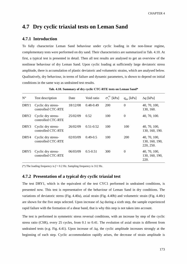
CHAPTER 4
173
4.7 Dry cyclic triaxial tests on Leman Sand
4.7.1 IntroductionTo fully characterize Leman Sand behaviour under cyclic loading in the non-linear regime,
complementary tests were performed on dry sand. Their characteristics are summarized in Tab. 4.10. At
first, a typical test is presented in detail. Then all test results are analysed to get an overview of the
nonlinear behaviour of dry Leman Sand. Upon cyclic loading at sufficiently large deviatoric stress
amplitude, there is accumulation of plastic deviatoric and volumetric strains, which are analysed below.
Qualitatively, dry behaviour, in terms of failure and dynamic parameters, is shown to depend on initial
conditions in the same way as undrained test results.
Tab. 4.10. Summary of dry cyclic CTC-RTE tests on Leman Sand*
(*) The loading frequency is f = 0.2 Hz. Sampling frequency is 312 Hz.
4.7.2 Presentation of a typical dry cyclic triaxial testThe test DRY1, which is the equivalent of the test CYC1 performed in undrained conditions, is
presented now. This test is representative of the behaviour of Leman Sand in dry conditions. The
variations of deviatoric stress (Fig. 4.40a), axial strain (Fig. 4.40b) and volumetric strain (Fig. 4.40c)
are shown for the five steps selected. Upon increase of Δq during a sixth step, the sample experienced
rapid failure with the formation of a shear band, that is why this step is not taken into account.
The test is performed in symmetric stress reversal conditions, with an increase by step of the cyclic
stress ratio (CSR), every 25 cycles, from 0.1 to 0.41. The evolution of axial strain is different from
undrained tests (e.g. Fig. 4.41). Upon increase of Δq, the cyclic amplitude increases strongly at the
beginning of each step. Cyclic accommodation rapidly arises, the decrease of strain amplitude is
N° Test description Date Void ratio [kPa] qav [kPa] Δq [kPa]
DRY1 Cyclic dry stress-controlled CTC-RTE
18/12/08 0.48-0.49 200 0 40, 70, 100, 130, 160.
DRY2 Cyclic dry stress-controlled CTC-RTE
25/02/09 0.52 100 0 40, 70, 100.
DRY3 Cyclic dry stress-controlled CTC-RTE
26/02/09 0.51-0.52 100 100 40, 70, 100, 130, 160, 190.
DRY4 Cyclic dry stress-controlled CTC-RTE
02/03/09 0.49-0.5 100 200 40, 70, 100, 130, 160, 190, 220, 250.
DRY5 Cyclic dry stress-controlled CTC-RTE
06/03/09 0.5-0.51 300 0 40, 70, 100, 130, 160, 190, 220.
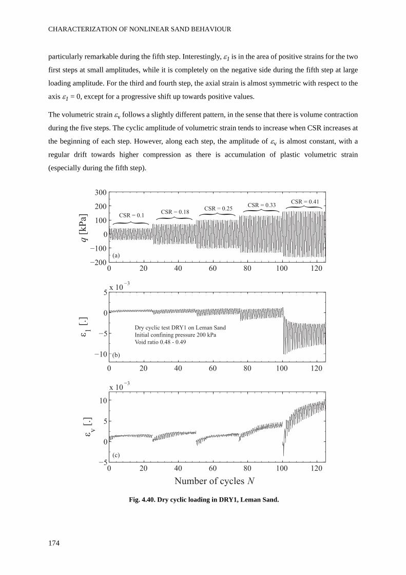
CHARACTERIZATION OF NONLINEAR SAND BEHAVIOUR
174
particularly remarkable during the fifth step. Interestingly, ε1 is in the area of positive strains for the two
first steps at small amplitudes, while it is completely on the negative side during the fifth step at large
loading amplitude. For the third and fourth step, the axial strain is almost symmetric with respect to the
axis ε1 = 0, except for a progressive shift up towards positive values.
The volumetric strain εv follows a slightly different pattern, in the sense that there is volume contraction
during the five steps. The cyclic amplitude of volumetric strain tends to increase when CSR increases at
the beginning of each step. However, along each step, the amplitude of εv is almost constant, with a
regular drift towards higher compression as there is accumulation of plastic volumetric strain
(especially during the fifth step).
Fig. 4.40. Dry cyclic loading in DRY1, Leman Sand.
0 20 40 60 80 100 120
0
100
200
300
q[k
Pa]
0 20 40 60 80 100 120
10
5
0
5x 10
3
1 [
.]
0 20 40 60 80 100 1205
0
5
10
x 103
Number of cycles N
v [
.]
CSR = 0.1CSR = 0.18
CSR = 0.25
Dry cyclic test DRY1 on Leman Sand
Initial confining pressure 200 kPa
Void ratio 0.48 - 0.49
CSR = 0.33CSR = 0.41
(a)
(b)
(c)
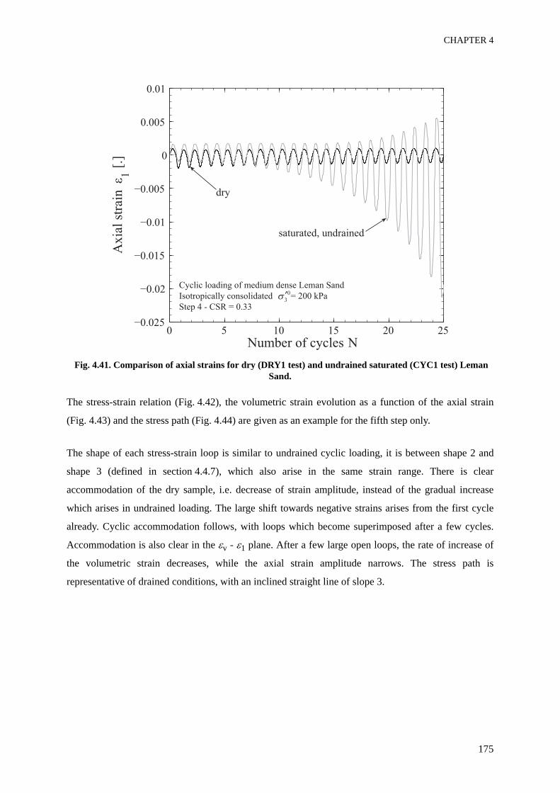
CHAPTER 4
175
Fig. 4.41. Comparison of axial strains for dry (DRY1 test) and undrained saturated (CYC1 test) Leman Sand.
The stress-strain relation (Fig. 4.42), the volumetric strain evolution as a function of the axial strain
(Fig. 4.43) and the stress path (Fig. 4.44) are given as an example for the fifth step only.
The shape of each stress-strain loop is similar to undrained cyclic loading, it is between shape 2 and
shape 3 (defined in section 4.4.7), which also arise in the same strain range. There is clear
accommodation of the dry sample, i.e. decrease of strain amplitude, instead of the gradual increase
which arises in undrained loading. The large shift towards negative strains arises from the first cycle
already. Cyclic accommodation follows, with loops which become superimposed after a few cycles.
Accommodation is also clear in the εv - ε1 plane. After a few large open loops, the rate of increase of
the volumetric strain decreases, while the axial strain amplitude narrows. The stress path is
representative of drained conditions, with an inclined straight line of slope 3.
0 5 10 15 20 25
0
Number of cycles N
Ax
ial
stra
in
1
Cyclic loading of medium dense Leman Sand
Isotropically consolidated = 200 kPa
dry
saturated, undrained
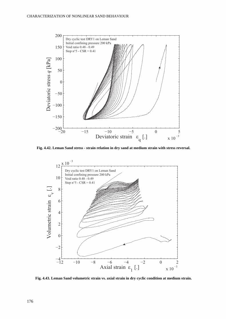
CHARACTERIZATION OF NONLINEAR SAND BEHAVIOUR
176
Fig. 4.42. Leman Sand stress - strain relation in dry sand at medium strain with stress reversal.
Fig. 4.43. Leman Sand volumetric strain vs. axial strain in dry cyclic condition at medium strain.
3
Dev
iato
ric
stre
ss q
[k
Pa]
Deviatoric strain q [.]
3
3
Vo
lum
etri
c st
rain
v [
.]
Axial strain [.]
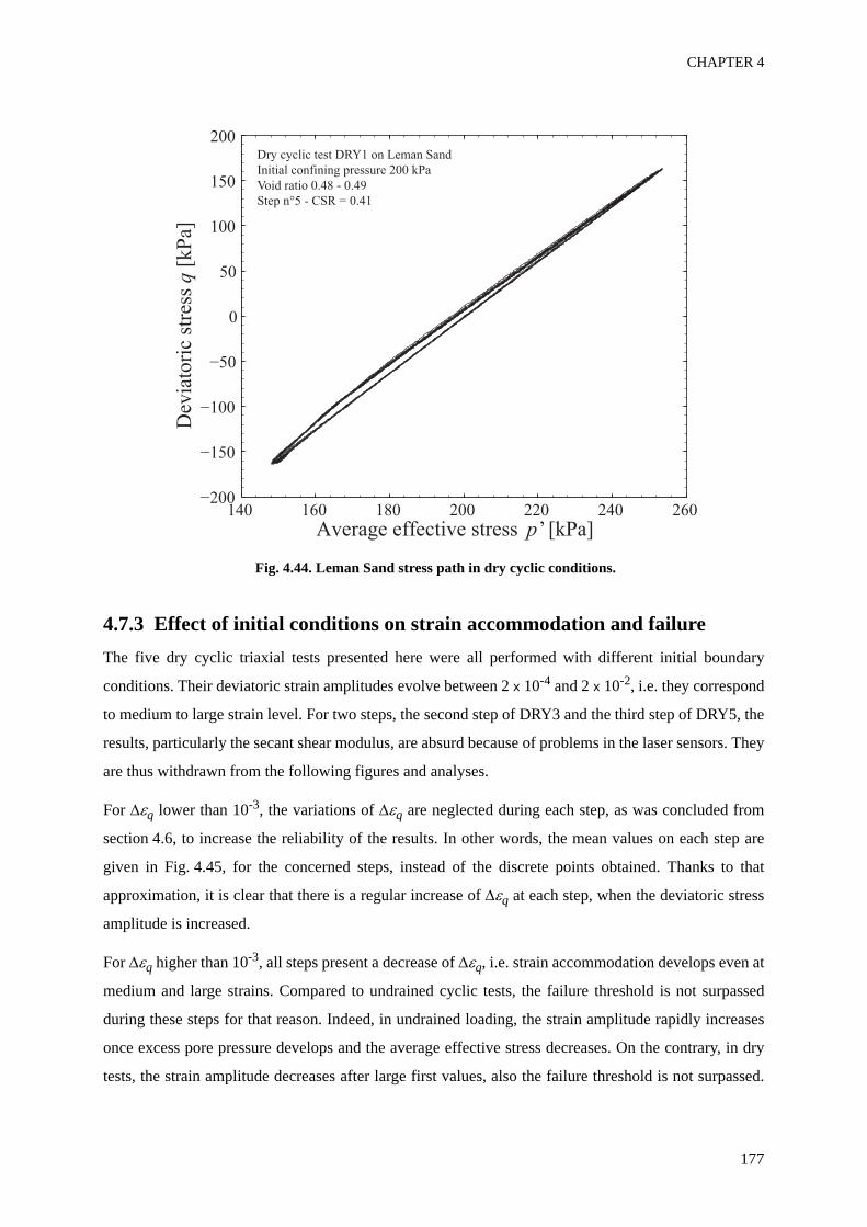
CHAPTER 4
177
Fig. 4.44. Leman Sand stress path in dry cyclic conditions.
4.7.3 Effect of initial conditions on strain accommodation and failureThe five dry cyclic triaxial tests presented here were all performed with different initial boundary
conditions. Their deviatoric strain amplitudes evolve between 2 x 10⁻⁴ and 2 x 10⁻², i.e. they correspond
to medium to large strain level. For two steps, the second step of DRY3 and the third step of DRY5, the
results, particularly the secant shear modulus, are absurd because of problems in the laser sensors. They
are thus withdrawn from the following figures and analyses.
For Δεq lower than 10-3, the variations of Δεq are neglected during each step, as was concluded from
section 4.6, to increase the reliability of the results. In other words, the mean values on each step are
given in Fig. 4.45, for the concerned steps, instead of the discrete points obtained. Thanks to that
approximation, it is clear that there is a regular increase of Δεq at each step, when the deviatoric stress
amplitude is increased.
For Δεq higher than 10-3, all steps present a decrease of Δεq, i.e. strain accommodation develops even at
medium and large strains. Compared to undrained cyclic tests, the failure threshold is not surpassed
during these steps for that reason. Indeed, in undrained loading, the strain amplitude rapidly increases
once excess pore pressure develops and the average effective stress decreases. On the contrary, in dry
tests, the strain amplitude decreases after large first values, also the failure threshold is not surpassed.
140 160 180 200 220 240 260
0
100
200
Dev
iato
ric
stre
ss q
[k
Pa]
Average effective stress p’ [kPa]
Dry cyclic test DRY1 on Leman Sand
Initial confining pressure 200 kPa
Void ratio 0.48 - 0.49
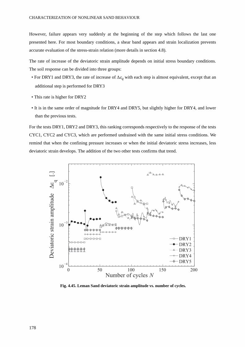
CHARACTERIZATION OF NONLINEAR SAND BEHAVIOUR
178
However, failure appears very suddenly at the beginning of the step which follows the last one
presented here. For most boundary conditions, a shear band appears and strain localization prevents
accurate evaluation of the stress-strain relation (more details in section 4.8).
The rate of increase of the deviatoric strain amplitude depends on initial stress boundary conditions.
The soil response can be divided into three groups:
• For DRY1 and DRY3, the rate of increase of Δεq with each step is almost equivalent, except that an
additional step is performed for DRY3
• This rate is higher for DRY2
• It is in the same order of magnitude for DRY4 and DRY5, but slightly higher for DRY4, and lower
than the previous tests.
For the tests DRY1, DRY2 and DRY3, this ranking corresponds respectively to the response of the tests
CYC1, CYC2 and CYC3, which are performed undrained with the same initial stress conditions. We
remind that when the confining pressure increases or when the initial deviatoric stress increases, less
deviatoric strain develops. The addition of the two other tests confirms that trend.
Fig. 4.45. Leman Sand deviatoric strain amplitude vs. number of cycles.
0 50 100 150 20010
103
102
Dev
iato
ric
stra
in a
mp
litu
de
q [
.]
Number of cycles N
DRY1
DRY2
DRY3
DRY5
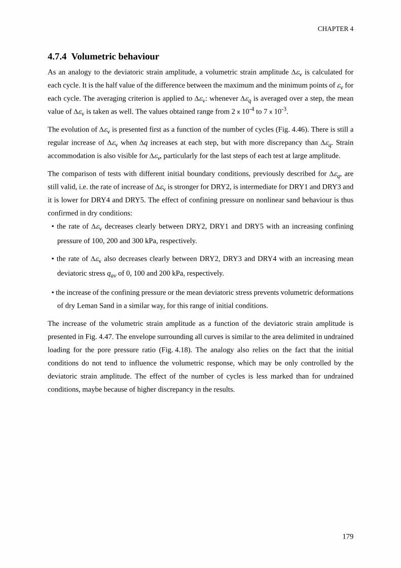
CHAPTER 4
179
4.7.4 Volumetric behaviourAs an analogy to the deviatoric strain amplitude, a volumetric strain amplitude Δεv is calculated for
each cycle. It is the half value of the difference between the maximum and the minimum points of εv for
each cycle. The averaging criterion is applied to Δεv: whenever Δεq is averaged over a step, the mean
value of Δεv is taken as well. The values obtained range from 2 x 10⁻⁴ to 7 x 10⁻³.
The evolution of Δεv is presented first as a function of the number of cycles (Fig. 4.46). There is still a
regular increase of Δεv when Δq increases at each step, but with more discrepancy than Δεq. Strain
accommodation is also visible for Δεv, particularly for the last steps of each test at large amplitude.
The comparison of tests with different initial boundary conditions, previously described for Δεq, are
still valid, i.e. the rate of increase of Δεv is stronger for DRY2, is intermediate for DRY1 and DRY3 and
it is lower for DRY4 and DRY5. The effect of confining pressure on nonlinear sand behaviour is thus
confirmed in dry conditions:
• the rate of Δεv decreases clearly between DRY2, DRY1 and DRY5 with an increasing confining
pressure of 100, 200 and 300 kPa, respectively.
• the rate of Δεv also decreases clearly between DRY2, DRY3 and DRY4 with an increasing mean
deviatoric stress qav of 0, 100 and 200 kPa, respectively.
• the increase of the confining pressure or the mean deviatoric stress prevents volumetric deformations
of dry Leman Sand in a similar way, for this range of initial conditions.
The increase of the volumetric strain amplitude as a function of the deviatoric strain amplitude is
presented in Fig. 4.47. The envelope surrounding all curves is similar to the area delimited in undrained
loading for the pore pressure ratio (Fig. 4.18). The analogy also relies on the fact that the initial
conditions do not tend to influence the volumetric response, which may be only controlled by the
deviatoric strain amplitude. The effect of the number of cycles is less marked than for undrained
conditions, maybe because of higher discrepancy in the results.
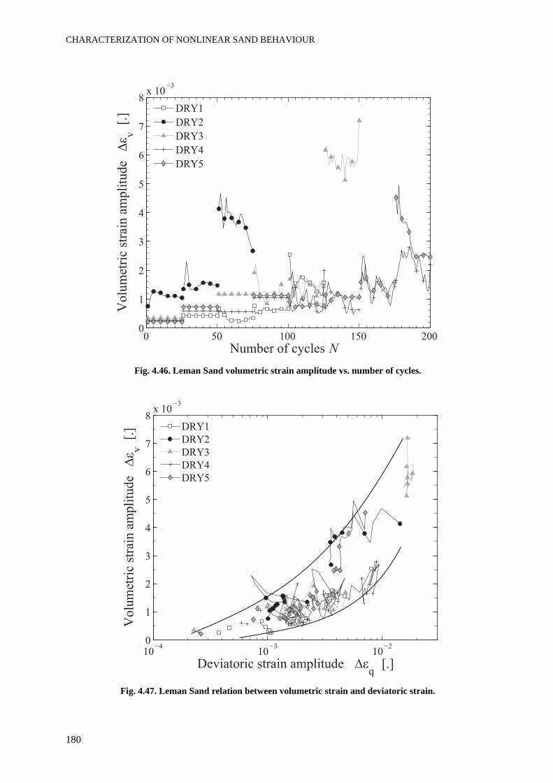
CHARACTERIZATION OF NONLINEAR SAND BEHAVIOUR
180
Fig. 4.46. Leman Sand volumetric strain amplitude vs. number of cycles.
Fig. 4.47. Leman Sand relation between volumetric strain and deviatoric strain.
0 50 100 150 2000
1
2
3
4
5
6
7
8x 10
Vo
lum
etri
c st
rain
am
pli
tud
e v
[.]
Number of cycles N
DRY1
DRY2
DRY3
DRY4
DRY5
10 103
102
0
1
2
3
5
6
7
8x 10
3
Vo
lum
etri
c st
rain
am
pli
tud
e v
[.]
Deviatoric strain amplitude q
[.]
DRY1
DRY2
DRY3
DRY5
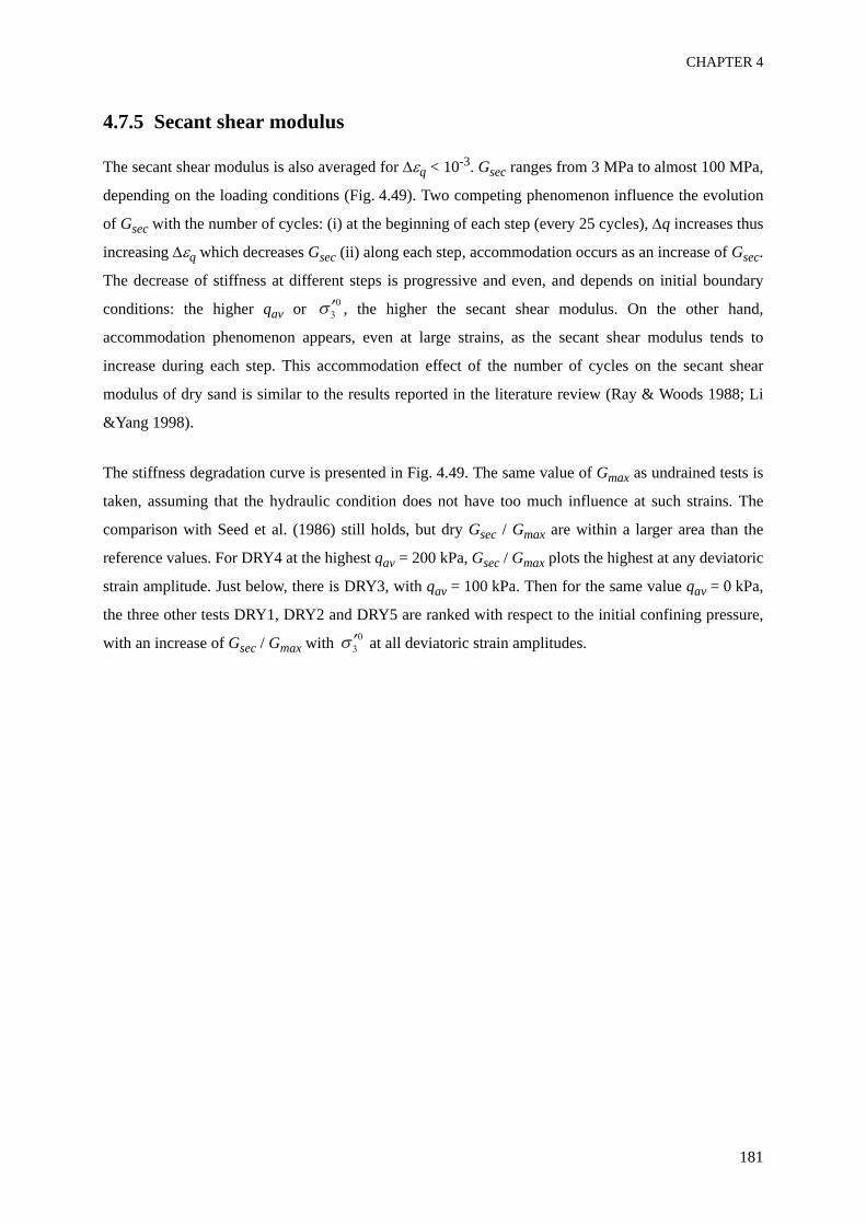
CHAPTER 4
181
4.7.5 Secant shear modulus
The secant shear modulus is also averaged for Δεq < 10-3. Gsec ranges from 3 MPa to almost 100 MPa,
depending on the loading conditions (Fig. 4.49). Two competing phenomenon influence the evolution
of Gsec with the number of cycles: (i) at the beginning of each step (every 25 cycles), Δq increases thus
increasing Δεq which decreases Gsec (ii) along each step, accommodation occurs as an increase of Gsec.
The decrease of stiffness at different steps is progressive and even, and depends on initial boundary
conditions: the higher qav or , the higher the secant shear modulus. On the other hand,
accommodation phenomenon appears, even at large strains, as the secant shear modulus tends to
increase during each step. This accommodation effect of the number of cycles on the secant shear
modulus of dry sand is similar to the results reported in the literature review (Ray & Woods 1988; Li
&Yang 1998).
The stiffness degradation curve is presented in Fig. 4.49. The same value of Gmax as undrained tests is
taken, assuming that the hydraulic condition does not have too much influence at such strains. The
comparison with Seed et al. (1986) still holds, but dry Gsec / Gmax are within a larger area than the
reference values. For DRY4 at the highest qav = 200 kPa, Gsec / Gmax plots the highest at any deviatoric
strain amplitude. Just below, there is DRY3, with qav = 100 kPa. Then for the same value qav = 0 kPa,
the three other tests DRY1, DRY2 and DRY5 are ranked with respect to the initial confining pressure,
with an increase of Gsec / Gmax with at all deviatoric strain amplitudes.
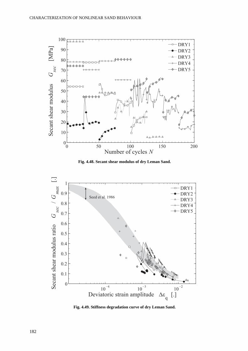
CHARACTERIZATION OF NONLINEAR SAND BEHAVIOUR
182
Fig. 4.48. Secant shear modulus of dry Leman Sand.
Fig. 4.49. Stiffness degradation curve of dry Leman Sand.
0 50 100 150 2000
10
20
30
40
50
60
70
80
90
100
Sec
ant
shea
r m
od
ulu
s G
sec
[M
Pa]
Number of cycles N
DRY1
DRY2
DRY3
DRY4
DRY5
10 103
102
0
0.1
0.2
0.3
0.5
0.6
0.7
0.8
0.9
1
Sec
ant
shea
r m
od
ulu
s ra
tio
G
sec
/ G
max
[.]
Deviatoric strain amplitude q
[.]
DRY1
DRY2
DRY3
DRY5
Seed et al. 1986
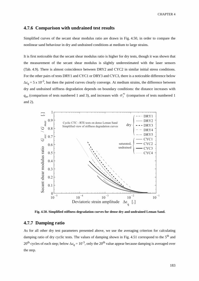
CHAPTER 4
183
4.7.6 Comparison with undrained test results
Simplified curves of the secant shear modulus ratio are drawn in Fig. 4.50, in order to compare the
nonlinear sand behaviour in dry and undrained conditions at medium to large strains.
It is first noticeable that the secant shear modulus ratio is higher for dry tests, though it was shown that
the measurement of the secant shear modulus is slightly underestimated with the laser sensors
(Tab. 4.9). There is almost coincidence between DRY2 and CYC2 in similar initial stress conditions.
For the other pairs of tests DRY1 and CYC1 or DRY3 and CYC3, there is a noticeable difference below
Δεq = 5 x 10⁻³, but then the paired curves clearly converge. At medium strains, the difference between
dry and undrained stiffness degradation depends on boundary conditions: the distance increases with
qav (comparison of tests numbered 1 and 3), and increases with (comparison of tests numbered 1
and 2).
Fig. 4.50. Simplified stiffness degradation curves for dense dry and undrained Leman Sand.
4.7.7 Damping ratioAs for all other dry test parameters presented above, we use the averaging criterion for calculating
damping ratio of dry cyclic tests. The values of damping shown in Fig. 4.51 correspond to the 5th and
20th cycles of each step; below Δεq = 10-3, only the 20th value appear because damping is averaged over
the step.
10 104
103
102
101
0
0.1
0.2
0.3
0.4
0.6
0.7
0.8
0.9
1
Sec
ant
shea
r m
odulu
s ra
tio
Gse
c /
Gm
ax
[.]
Deviatoric strain amplitude q
[.]
DRY1
DRY2
DRY3
DRY4
CYC1
CYC2
CYC3
CYC4
Cyclic CTC - RTE tests on dense Leman Sand
Simplified view of stiffness degradation curves dry
saturated,
undrained
{{
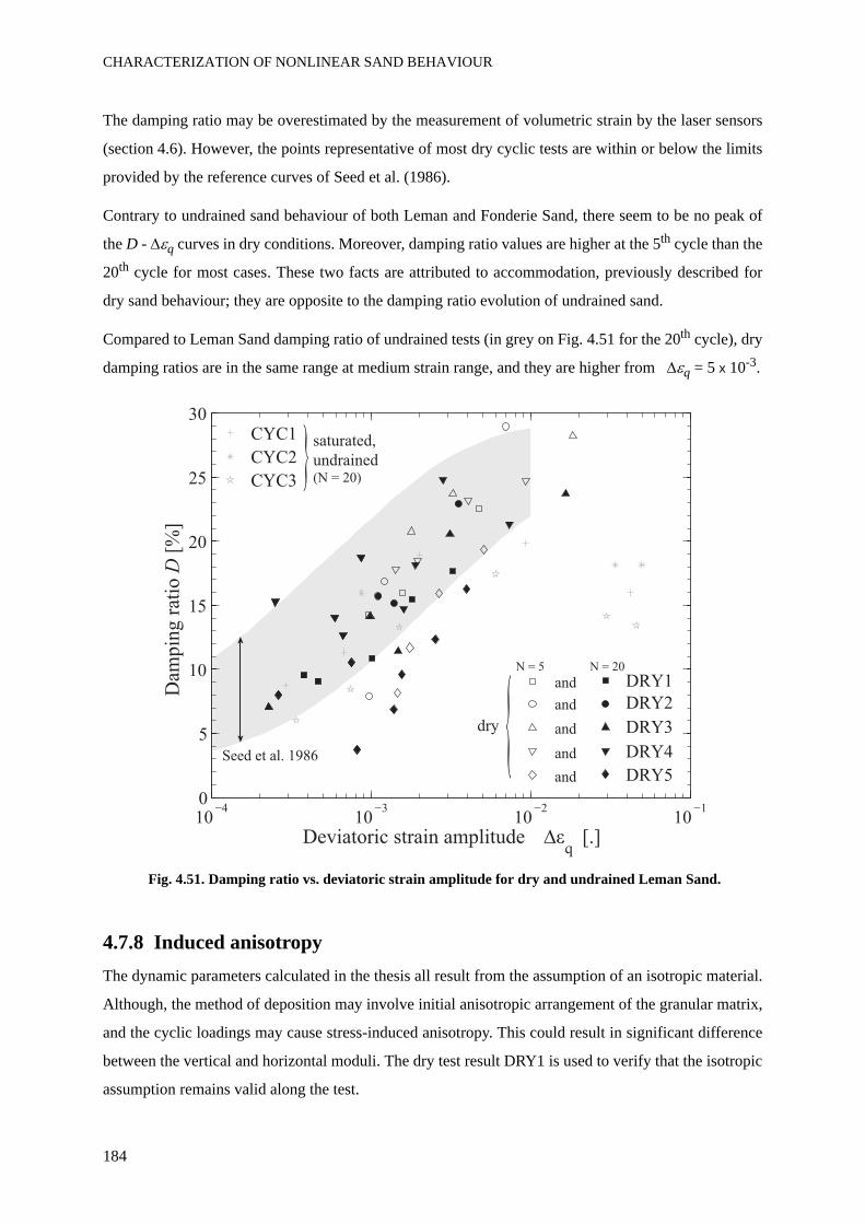
CHARACTERIZATION OF NONLINEAR SAND BEHAVIOUR
184
The damping ratio may be overestimated by the measurement of volumetric strain by the laser sensors
(section 4.6). However, the points representative of most dry cyclic tests are within or below the limits
provided by the reference curves of Seed et al. (1986).
Contrary to undrained sand behaviour of both Leman and Fonderie Sand, there seem to be no peak of
the D - Δεq curves in dry conditions. Moreover, damping ratio values are higher at the 5th cycle than the
20th cycle for most cases. These two facts are attributed to accommodation, previously described for
dry sand behaviour; they are opposite to the damping ratio evolution of undrained sand.
Compared to Leman Sand damping ratio of undrained tests (in grey on Fig. 4.51 for the 20th cycle), dry
damping ratios are in the same range at medium strain range, and they are higher from Δεq = 5 x 10⁻³.
Fig. 4.51. Damping ratio vs. deviatoric strain amplitude for dry and undrained Leman Sand.
4.7.8 Induced anisotropyThe dynamic parameters calculated in the thesis all result from the assumption of an isotropic material.
Although, the method of deposition may involve initial anisotropic arrangement of the granular matrix,
and the cyclic loadings may cause stress-induced anisotropy. This could result in significant difference
between the vertical and horizontal moduli. The dry test result DRY1 is used to verify that the isotropic
assumption remains valid along the test.
10 103
102
101
0
5
10
15
20
25
30
Dam
pin
g r
atio
D [
%]
Deviatoric strain amplitude q
[.]
DRY1
DRY2
DRY3
DRY5
CYC1
CYC2
CYC3
and
and
and
and
and
N = 5 N = 20
Seed et al. 1986
}
dry
saturated,
undrained(N = 20)
{
CHAPTER 4
185
Elastic transverse anisotropy can be characterized thanks to triaxial tests by three coefficients, E*
(which is equal to Ev, the vertical Young’s modulus), ν* and α*, with the relation Eh / Ev = (α*)2 (Muir
Wood 1990). Moreover, the anisotropic secant shear modulus can be deduced from these three
parameters. When α* = 1, the medium is isotropic. For example, an anisotropic clay can be
characterized by the coefficient α* = 0.2. When α* < 1, the soil is stiffer vertically.
The reloading part of the 24th cycle of the last step of DRY1 is used to calculate these parameters. We
find α* = 0.99, which means that anisotropy is very small. Moreover, there is only 1% difference
between the Young’s modulus calculated with the assumption of an isotropic material (61.2 MPa) and
the Young’s modulus calculated with the anisotropy assumption (Ev = 61.9 MPa). There is also 1% of
difference for the shear modulus. The ratio Eh / Ev is equal to 0.97.
The same procedure used for the four previous steps yields a higher value of α*, which tends to
decrease from 1.03 to 1.01 between the first and the fourth step. This is an indication of a slight effect of
stress-induced anisotropy during cyclic loading. These α*-values are sufficiently close to 1 so that
anisotropy can be considered as negligible.
4.7.9 ConclusionsMany comments arise from the analyses of the dry cyclic tests on Leman Sand, and by comparing the
dry tests with undrained cyclic test results from section 4.4:
• Comparing the response between the different steps, Δεq increases with Δq, which is the same
answer as undrained tests. Inside each step, Δεq decreases, which is the contrary of what happens in
undrained conditions.
• Though the loading is symmetric with respect to the stress origin in tests DRY1, DRY2, DRY5, the
volumetric and deviatoric strains are not symmetric with respect to their respective origin. The
volumetric strain is positive, which corresponds to plastic contraction. For deviatoric strains, the
answer is more complex: they are first positive at small CSR, but they gradually become negative
when CSR increases.
• Accommodation behaviour is visible during steps of constant stress amplitude (i) in εq - q loops, (ii)
in ε1 - εv loops, and for Δεq > 10-3, (iii) in Δεq, (iv) in Δεv, (v) in Gsec and (vi) in D.
• The effect of initial boundary conditions is the same as undrained loading. If qav or increases,
Δεq and Δεv are smaller, while Gsec and Gsec / Gmax are higher.
CHARACTERIZATION OF NONLINEAR SAND BEHAVIOUR
186
• An area limiting the relation Δεq - Δεv is drawn for medium to large strains. By comparison with the
relation between the pore pressure increase and the deviatoric strain in undrained test results, from
the literature (Dobry et al. 1982) and with the Leman Sand (section 4.4.3), this area seems
independent from the boundary conditions. The effect of the number of cycles is not discernible with
our equipment, contrary to undrained tests.
• Stiffness reduction curves Gsec / Gmax are similar to undrained conditions, and correspond to the
results from Seed et al. (1986), except that the cluster of curves lies within a slightly larger area.
• A schematic view of both dry and undrained curves Gsec / Gmax confirms the effect of qav and .
More important, it allows to compare tests with the same boundary conditions except for the
hydraulic condition. For tests with the same initial qav and , dry tests give higher Gsec / Gmax at
strain amplitude below 5 x 10⁻³, but dry and undrained curves converge above that threshold. The
distance between dry and undrained curves depends on initial boundary conditions.
• Damping ratios of dry Leman Sand are obtained for strain amplitudes between 2 x 10⁻⁴ and 2 x 10⁻².
The numerous experimental points clearly show the increase of D with strain amplitudes.
Accommodation can explain the difference with undrained saturated behaviour observed for Leman
and Fonderie Sand. In dry sand, even at large strain, D decreases with the number of cycles, but
without the formation of the peak of the D - Δεq curves.
• Induced anisotropy is evaluated for the test DRY1 and considered as negligible with only 1%
difference between the moduli calculated with the assumptions of isotropic or anisotropic elasticity.
4.8 Shear strain localization in cyclic tests at large strain amplitude
4.8.1 Tests concernedThe occurrence of a shear band at large strain amplitude is first estimated by direct visual observation.
Most cyclic tests with symmetric stress reversal exhibit strain localization when the axial strain
becomes very low on the extension side. Monotonic tests in extension also exhibit such failure
mechanism. Localization usually occurs as a clear narrowing of the diameter on a limited part of the
sample height (e.g. Fig. 4.52). When this failure is witnessed, the test is stopped and no other step is
added. It is noticeable that strain localization was never observed during compressive tests with no
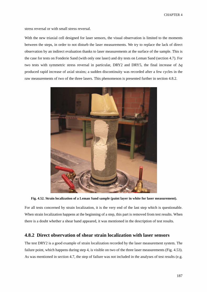
CHAPTER 4
187
stress reversal or with small stress reversal.
With the new triaxial cell designed for laser sensors, the visual observation is limited to the moments
between the steps, in order to not disturb the laser measurements. We try to replace the lack of direct
observation by an indirect evaluation thanks to laser measurements at the surface of the sample. This is
the case for tests on Fonderie Sand (with only one laser) and dry tests on Leman Sand (section 4.7). For
two tests with symmetric stress reversal in particular, DRY2 and DRY5, the final increase of Δq
produced rapid increase of axial strains; a sudden discontinuity was recorded after a few cycles in the
raw measurements of two of the three lasers. This phenomenon is presented further in section 4.8.2.
Fig. 4.52. Strain localization of a Leman Sand sample (paint layer in white for laser measurement).
For all tests concerned by strain localization, it is the very end of the last step which is questionable.
When strain localization happens at the beginning of a step, this part is removed from test results. When
there is a doubt whether a shear band appeared, it was mentioned in the description of test results.
4.8.2 Direct observation of shear strain localization with laser sensorsThe test DRY2 is a good example of strain localization recorded by the laser measurement system. The
failure point, which happens during step 4, is visible on two of the three laser measurements (Fig. 4.53).
As was mentioned in section 4.7, the step of failure was not included in the analyses of test results (e.g.
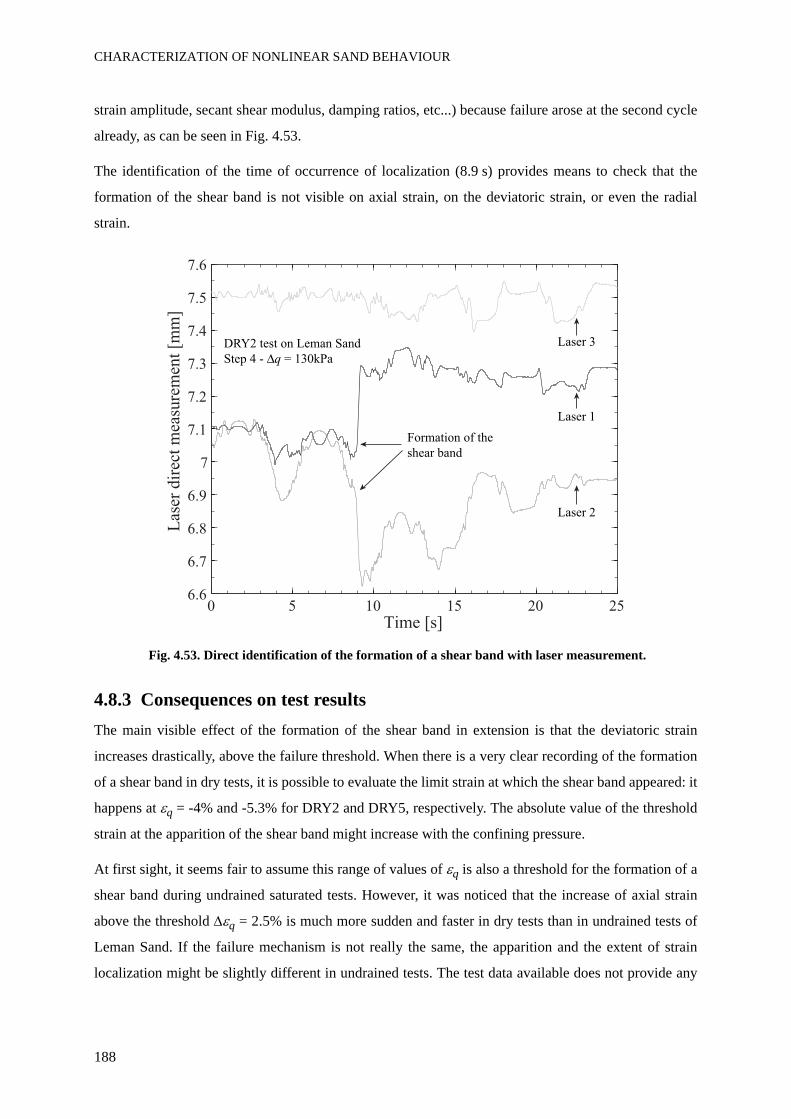
CHARACTERIZATION OF NONLINEAR SAND BEHAVIOUR
188
strain amplitude, secant shear modulus, damping ratios, etc...) because failure arose at the second cycle
already, as can be seen in Fig. 4.53.
The identification of the time of occurrence of localization (8.9 s) provides means to check that the
formation of the shear band is not visible on axial strain, on the deviatoric strain, or even the radial
strain.
Fig. 4.53. Direct identification of the formation of a shear band with laser measurement.
4.8.3 Consequences on test resultsThe main visible effect of the formation of the shear band in extension is that the deviatoric strain
increases drastically, above the failure threshold. When there is a very clear recording of the formation
of a shear band in dry tests, it is possible to evaluate the limit strain at which the shear band appeared: it
happens at εq = -4% and -5.3% for DRY2 and DRY5, respectively. The absolute value of the threshold
strain at the apparition of the shear band might increase with the confining pressure.
At first sight, it seems fair to assume this range of values of εq is also a threshold for the formation of a
shear band during undrained saturated tests. However, it was noticed that the increase of axial strain
above the threshold Δεq = 2.5% is much more sudden and faster in dry tests than in undrained tests of
Leman Sand. If the failure mechanism is not really the same, the apparition and the extent of strain
localization might be slightly different in undrained tests. The test data available does not provide any
0 5 10 15 20 256.6
6.7
6.8
6.9
7
7.1
7.2
7.3
7.4
7.5
7.6
Las
er d
irec
t m
easu
rem
ent
[mm
]
Time [s]
Laser 1
Laser 2
Laser 3
Formation of the
shear band
DRY2 test on Leman Sand
Step 4 - q = 130kPa
CHAPTER 4
189
recording, with the laser sensor, of the apparition of strain localization in undrained saturated tests of
sands.
The final increase of the damping ratio at very large strain could be linked with the development of a
shear band. For example, the final increase of the damping ratio arises for strains below εq = -5% in
extension for test CYC2. As seen for dry tests, this value is sufficient to induce such localization, which
may involve inhomogeneity in the stress and strain field.
The development of excess pore pressure ratio values above ur = 1 seems an absurd result. However the
pressure-meters were well calibrated, also these values were actually measured, at the bottom of the
sample, after failure of Fonderie Sand. For example, the first large exceeding of ur = 1 arises just after
the deviatoric strain reaches a minimum at εq = -3.4% in extension for test FSC5. If strain localization
appears at that moment, it may be associated with dilation bands (Muir Wood 2001), which would be
conveyed as inhomogeneity in the pore pressure field. Moreover, preferential paths of pore fluid
displacement may form within the sample. There are direct experimental evidences of local variations
of the density within sand samples sheared at large strains (Muir Wood 2007). Even if critical state has
not been reached, such inhomogeneity may also have appeared within cyclically sheared Leman Sand
samples.
4.8.4 ConclusionsShear strain localization, and the formation of inhomogeneity within the sample, is not suitable for a
correct evaluation of sand behaviour. The occurrence of such phenomenon is only related to
isotropically consolidated tests with symmetric stress reversal in the strain range and confining
pressures tested for our experimental studies. The observation of direct recordings from the three lasers
in dry tests shows that a clear discontinuity appeared on two of the three time histories, at the beginning
of the large increase of deviatoric strains. This discontinuity occurs above the threshold deviatoric
strain failure criterion, around εq = 4 to 5%. Strain localization may (i) depend on confining pressure,
(ii) depend on the hydraulic conditions, and (iii) be responsible for large increase of the damping ratio
and the excess pore pressure ratio.
CHARACTERIZATION OF NONLINEAR SAND BEHAVIOUR
190
4.9 SummaryMany monotonic and cyclic CTC-RTE tests on Leman Sand and Fonderie Sand were performed in the
nonlinear regime. Phase transformation lines and steady state lines, in extension and compression, were
obtained from the undrained monotonic tests. The different cyclic tests presented here provide deep
insight into stiffness degradation of both sands, until failure. At large strain, the occurrence of cyclic
liquefaction or flow liquefaction was observed, depending on the soil tested.
Preliminary cyclic tests demonstrated the importance of sample preparation, and in particular a special
care was then devoted to get fully saturated samples. These tests also showed the importance of initial
conditions and boundary conditions on the nonlinear soil response. These conclusions allowed to
perform undrained saturated tests on Leman and Fonderie Sand with stiffness degradation and failure.
Dry cyclic tests on Leman Sand were also performed and compared to the undrained response. The
conclusions of the cyclic tests are now summarized.
• Effect of initial and boundary conditions
The effect of boundary conditions, i.e. the average deviatoric stress and the initial confining pressure, is
the same in undrained saturated and dry loading of Leman Sand: if qav or increases, Δεq and Δεv
(dry test) or ur (undrained test) decrease, while Gsec and Gsec / Gmax increase and the damping ratio of
undrained Leman Sand decreases.
When the loading is symmetric with respect to the stress origin (isotropically consolidated sample) in
tests CYC1, CYC2, DRY1, DRY2, DRY5 on Leman Sand and for all tests on Fonderie Sand, the
deviatoric strains are not symmetric with respect to the origin. This different behaviour in compression
and extension is significant in the stress - strain relations and the stress paths. It reflects well the
difference of phase transformation angles in extension and compression for both sands.
• Volumetric behaviour of granular soils and pore pressure increase
Excess pore pressure of undrained saturated Leman Sand increases from the threshold Δεq = 10-4 and
depends mainly on the strain amplitude. The number of loading cycles N also influences the pore
pressure increase, in the sense that several curves Δεq - ur are obtained for the different values of N.
They form a narrow band, which is also similar for undrained Fonderie Sand, although slightly higher
pore pressures are obtained in the narrow-graded sand. A similar area surrounds the relation Δεq - Δεv
for medium to large strains in dry tests on Leman Sand.
• Stiffness degradation
Undrained saturated tests exhibit stiffness degradation during continuous cyclic stress-controlled
CHAPTER 4
191
loading. When the stress amplitude is large enough (the threshold depends on initial and boundary
conditions), the deviatoric strain amplitude increases, either regularly with Leman Sand, or more
suddenly with Fonderie Sand. The pore pressure ratio, which is coupled to the deviatoric strain via the
Δεq - ur curves, accordingly increases.
Stiffness degradation curves, i.e. the secant shear modulus and damping ratio as a function of the
deviatoric strain amplitude, were obtained for saturated Leman and Fonderie Sand. Their small strain
secant shear moduli were evaluated by cross-checking empirical equations for sands and cyclic test
results at small to medium strain. The Δεq - Gsec / Gmax curves are thus obtained in the medium to large
strain domain. The Δεq - D curves of both sands exhibit a peak at deviatoric strains from 0.3 to 1%,
which is linked with the occurrence of dilative behaviour and the banana shape of the stress-strain
loops. Furthermore, we showed that the damping ratio of Leman Sand evolves with the number of
cycles.
On the contrary, accommodation behaviour prevails in dry tests during steps of constant stress
amplitude Δq. Stiffness degradation then occurs thanks to the increase of Δq every 25 cycles. The
curves Gsec / Gmax vs. Δεq are similar in dry and undrained conditions, and correspond to the results
from Seed et al. (1986), except that the cluster of curves lies within a slightly larger area for dry tests.
Comparing tests with the same initial average deviatoric stress and confining pressure, dry conditions
induce higher Gsec / Gmax than undrained conditions at strain amplitude below 5 x 10⁻³; dry and
undrained curves converge above that threshold.
• Failure
Sample failure of medium dense saturated undrained Leman Sand arises by cyclic liquefaction. The
material softens, and its degradation index reaches very low values. The failure criterion can be based
on a threshold deviatoric strain Δεq = 2.5%. It matches the level of the degradation index well, which
can thus be used as an alternative criterion for failure. Another candidate can be the pore water pressure
ratio.
Three different behaviours are obtained with regard to failure in Fonderie Sand: the denser material
exhibits accommodation, the slightly less dense sample exhibits cyclic liquefaction while the rest of the
medium-dense samples exhibit failure which resembles flow liquefaction. At the same relative density,
the increase of deviatoric strain upon loading is very progressive and stable for Leman Sand, while it is
sudden, rapid and induces instability of the motion control system for Fonderie Sand. Fonderie Sand
samples exhibit inhomogeneity above failure, especially concerning excess pore pressure which
dramatically increases above 1 due to end-restraint and strain localization.
CHARACTERIZATION OF NONLINEAR SAND BEHAVIOUR
192
The different behaviours of Leman and Fonderie Sand is ascribed to their respective particle shape and
grain size distribution, which both induce higher liquefaction susceptibility of Fonderie Sand. For both
sands, the phase transformation line in extension is touched first, and most of deviatoric strains arise on
the side of negative strains.
Failure of dry tests on Leman Sand is not shown because it arises brutally at the beginning of a new
step, thanks to accommodation of dry samples. However, the behaviour of dry sand close to failure is
analysed through the comments developed around the formation of a shear band at very large strain.
Shear strain localization, and the formation of inhomogeneity within the sample, violate the assumption
of homogenous state of stress and strain in the sample. The occurrence of such phenomenon is only
related to isotropically consolidated tests with symmetric stress reversal in the strain range and
confining pressures tested for our experimental studies.
The observation of direct recordings from the three laser sensors in dry tests shows that a clear
discontinuity appeared on two of the three time histories, at the beginning of the large increase of
deviatoric strains. This discontinuity occurs above the threshold deviatoric strain failure criterion,
around εq = 4 to 5%. Strain localization seems to (i) depend on confining pressure, (ii) depend on the
hydraulic conditions, and (iii) be responsible for large increase of the damping ratio and the excess pore
pressure ratio.
• Validation of the sample radius measurement by laser sensors
The laser sensors used for measuring radial strains were calibrated and validated with various
techniques presented in Chapter 3. The final validation of the laser sensors, presented in section 4.6, is
based on the assumption of no volumetric strain during undrained loading of Leman Sand. Above
Δεq = 10-3, the stiffness degradation of the sample is well captured by the laser sensors. Below that
value, an averaging is suitable.
Compared to the assumption of no volumetric strain, radial strains obtained with a smoothed radius
give the best results for the deviatoric strain and the secant shear modulus. The damping ratio seems
overestimated by the laser measurement of radial strain. As the uncertainty on laser measurement is
lower for dry sand compared to undrained sand, the evaluation of radial strain for dry tests is expected
to be at least as good as the results obtained for undrained saturated sand.
CHAPTER 5
FREQUENCY EFFECTS IN
LEMAN SAND
FREQUENCY EFFECTS IN LEMAN SAND
194
5.1 IntroductionRate effect in granular materials may result from viscosity, dynamic effects, coupling between the soil
matrix and the pore fluid (section 2.7). In cyclic loading, sand was proved to exhibit frequency-
dependence, with or without the pore water saturating the granular matrix. Most experimental studies
reported in the literature showed that the damping ratio tends to increase with the frequency in the
earthquake frequency range. For the same frequencies (f), the results are less clear for the secant shear
modulus (Gsec), but it seems that Gsec slightly increases with f. Laboratory testing of undrained
frequency-dependence of sand at medium strain range is poorly referenced. However, numerical
approaches of this problem showed that the frequency-dependence can be important, in particular it
influences the results on site effect analysis.
To our knowledge, laboratory testing of frequency effect on cyclic sand behaviour at medium and large
strains and in the earthquake frequency range was never performed with a triaxial apparatus. The
challenge is to combine strong loadings together with the precise measurement of small variations in
the soil response.
We saw, in Chapter 4, that Leman Sand behaves in a very stable way at medium to large strains,
compared to Fonderie Sand. This particular behaviour allowed us to perform tests in this strain range
without inducing critical failure, and at different frequencies for the same sample. The effect of
frequency (also called rate effect, cf. section 2.7) on the pore pressure ratio, deviatoric strain amplitude,
dynamic parameters can thus be observed.
All tests presented in Chapter 5 were performed on medium dense Leman Sand. First, monotonic tests
at four different strain rate show that it is not possible to discern any strain rate effect in the range of
strain rates involved. Then cyclic undrained preliminary tests, of the same kind as preliminary tests of
Chapter 4, are presented for four different frequencies. The main results in saturated undrained cyclic
conditions are then presented in section 5.4, and an equivalent test in dry conditions is presented in
section 5.5.
5.2 Monotonic undrained conditions
5.2.1 Tests characteristicsFour monotonic undrained strain-controlled triaxial tests were performed at different strain rate
(Tab. 5.1). Compression, in CTC conditions, is followed by an unloading and triaxial extension RTE.
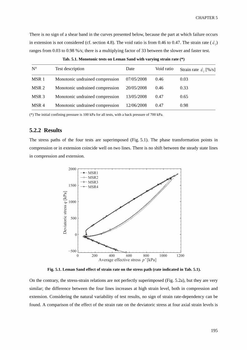
CHAPTER 5
195
There is no sign of a shear band in the curves presented below, because the part at which failure occurs
in extension is not considered (cf. section 4.8). The void ratio is from 0.46 to 0.47. The strain rate ( )
ranges from 0.03 to 0.98 %/s; there is a multiplying factor of 33 between the slower and faster test.
Tab. 5.1. Monotonic tests on Leman Sand with varying strain rate (*)
(*) The initial confining pressure is 100 kPa for all tests, with a back pressure of 700 kPa.
5.2.2 ResultsThe stress paths of the four tests are superimposed (Fig. 5.1). The phase transformation points in
compression or in extension coincide well on two lines. There is no shift between the steady state lines
in compression and extension.
Fig. 5.1. Leman Sand effect of strain rate on the stress path (rate indicated in Tab. 5.1).
On the contrary, the stress-strain relations are not perfectly superimposed (Fig. 5.2a), but they are very
similar; the difference between the four lines increases at high strain level, both in compression and
extension. Considering the natural variability of test results, no sign of strain rate-dependency can be
found. A comparison of the effect of the strain rate on the deviatoric stress at four axial strain levels is
N° Test description Date Void ratio Strain rate [%/s]
MSR 1 Monotonic undrained compression 07/05/2008 0.46 0.03
MSR 2 Monotonic undrained compression 20/05/2008 0.46 0.33
MSR 3 Monotonic undrained compression 13/05/2008 0.47 0.65
MSR 4 Monotonic undrained compression 12/06/2008 0.47 0.98
1
1
0 200 400 600 800 1000 1200
0
1000
2000
Dev
iato
ric
stre
ss q
[k
Pa]
Average effective stress p’ [kPa]
MSR1
MSR2
MSR3
MSR4
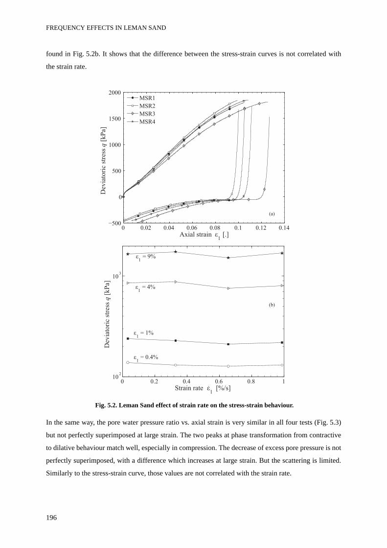
FREQUENCY EFFECTS IN LEMAN SAND
196
found in Fig. 5.2b. It shows that the difference between the stress-strain curves is not correlated with
the strain rate.
Fig. 5.2. Leman Sand effect of strain rate on the stress-strain behaviour.
In the same way, the pore water pressure ratio vs. axial strain is very similar in all four tests (Fig. 5.3)
but not perfectly superimposed at large strain. The two peaks at phase transformation from contractive
to dilative behaviour match well, especially in compression. The decrease of excess pore pressure is not
perfectly superimposed, with a difference which increases at large strain. But the scattering is limited.
Similarly to the stress-strain curve, those values are not correlated with the strain rate.
0 0.02 0.04 0.06 0.08 0.1 0.12 0.14
0
1000
2000
Dev
iato
ric
stre
ss q
[k
Pa]
Axial strain 1 [.]
MSR1
MSR2
MSR3
MSR4
0 0.2 0.4 0.6 0.8 110
2
103
Strain rate 1
[%/s]
Dev
iato
ric
stre
ss q
[k
Pa]
1 = 9%
1 = 4%
1 = 1%
1 = 0.4%
(a)
(b)
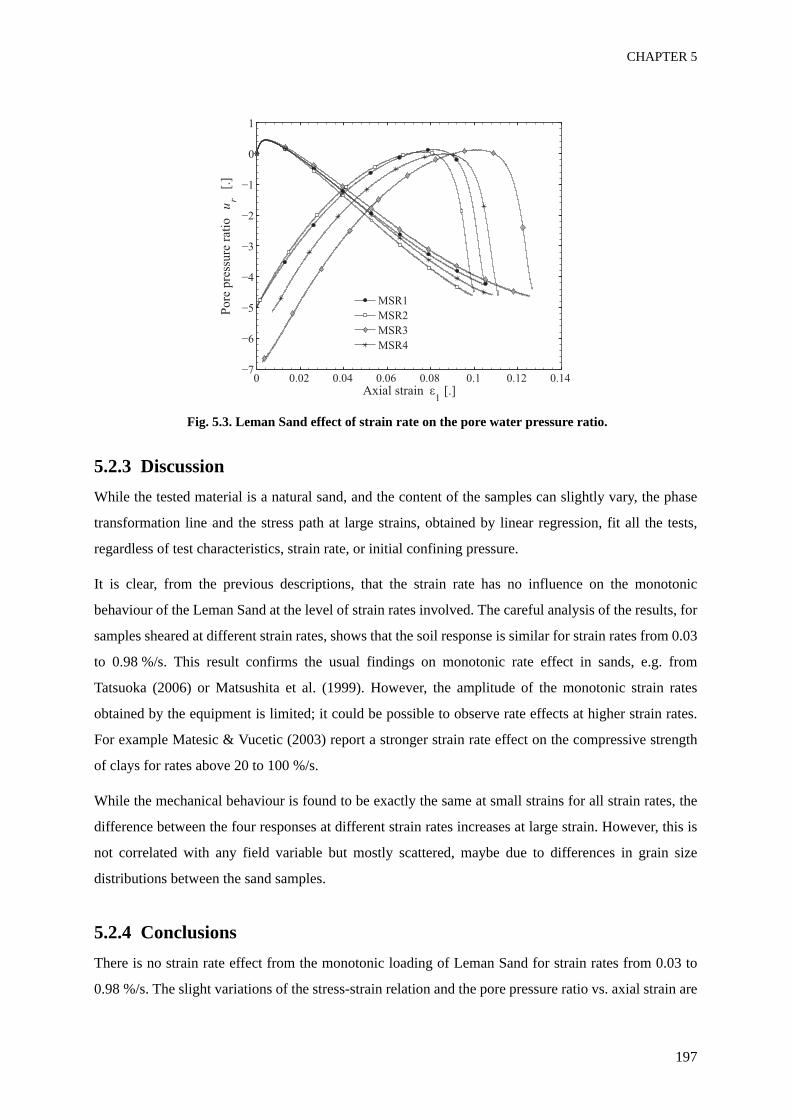
CHAPTER 5
197
Fig. 5.3. Leman Sand effect of strain rate on the pore water pressure ratio.
5.2.3 DiscussionWhile the tested material is a natural sand, and the content of the samples can slightly vary, the phase
transformation line and the stress path at large strains, obtained by linear regression, fit all the tests,
regardless of test characteristics, strain rate, or initial confining pressure.
It is clear, from the previous descriptions, that the strain rate has no influence on the monotonic
behaviour of the Leman Sand at the level of strain rates involved. The careful analysis of the results, for
samples sheared at different strain rates, shows that the soil response is similar for strain rates from 0.03
to 0.98 %/s. This result confirms the usual findings on monotonic rate effect in sands, e.g. from
Tatsuoka (2006) or Matsushita et al. (1999). However, the amplitude of the monotonic strain rates
obtained by the equipment is limited; it could be possible to observe rate effects at higher strain rates.
For example Matesic & Vucetic (2003) report a stronger strain rate effect on the compressive strength
of clays for rates above 20 to 100 %/s.
While the mechanical behaviour is found to be exactly the same at small strains for all strain rates, the
difference between the four responses at different strain rates increases at large strain. However, this is
not correlated with any field variable but mostly scattered, maybe due to differences in grain size
distributions between the sand samples.
5.2.4 ConclusionsThere is no strain rate effect from the monotonic loading of Leman Sand for strain rates from 0.03 to
0.98 %/s. The slight variations of the stress-strain relation and the pore pressure ratio vs. axial strain are
0 0.02 0.04 0.06 0.08 0.1 0.12 0.14
0
1
Po
re p
ress
ure
rat
io
ur
[.]
Axial strain 1 [.]
MSR1
MSR2
MSR4
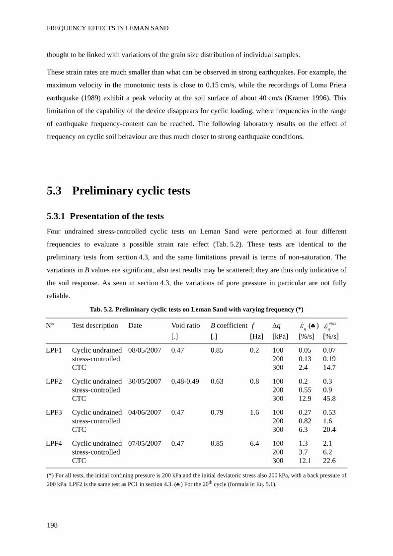
FREQUENCY EFFECTS IN LEMAN SAND
198
thought to be linked with variations of the grain size distribution of individual samples.
These strain rates are much smaller than what can be observed in strong earthquakes. For example, the
maximum velocity in the monotonic tests is close to 0.15 cm/s, while the recordings of Loma Prieta
earthquake (1989) exhibit a peak velocity at the soil surface of about 40 cm/s (Kramer 1996). This
limitation of the capability of the device disappears for cyclic loading, where frequencies in the range
of earthquake frequency-content can be reached. The following laboratory results on the effect of
frequency on cyclic soil behaviour are thus much closer to strong earthquake conditions.
5.3 Preliminary cyclic tests
5.3.1 Presentation of the testsFour undrained stress-controlled cyclic tests on Leman Sand were performed at four different
frequencies to evaluate a possible strain rate effect (Tab. 5.2). These tests are identical to the
preliminary tests from section 4.3, and the same limitations prevail is terms of non-saturation. The
variations in B values are significant, also test results may be scattered; they are thus only indicative of
the soil response. As seen in section 4.3, the variations of pore pressure in particular are not fully
reliable.
Tab. 5.2. Preliminary cyclic tests on Leman Sand with varying frequency (*)
(*) For all tests, the initial confining pressure is 200 kPa and the initial deviatoric stress also 200 kPa, with a back pressure of200 kPa. LPF2 is the same test as PC1 in section 4.3. (♣) For the 20th cycle (formula in Eq. 5.1).
N° Test description Date Void ratio[.]
B coefficient [.]
f [Hz]
Δq [kPa]
(♣)[%/s] [%/s]
LPF1 Cyclic undrained stress-controlled CTC
08/05/2007 0.47 0.85 0.2 100200300
0.050.132.4
0.070.1914.7
LPF2 Cyclic undrained stress-controlled CTC
30/05/2007 0.48-0.49 0.63 0.8 100200300
0.20.5512.9
0.30.945.8
LPF3 Cyclic undrained stress-controlled CTC
04/06/2007 0.47 0.79 1.6 100200300
0.270.826.3
0.531.620.4
LPF4 Cyclic undrained stress-controlled CTC
07/05/2007 0.47 0.85 6.4 100200300
1.33.712.1
2.16.222.6
q q
max
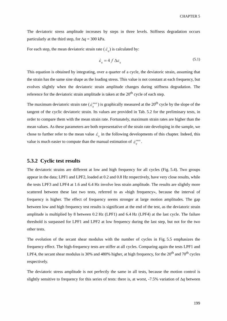
CHAPTER 5
199
The deviatoric stress amplitude increases by steps in three levels. Stiffness degradation occurs
particularly at the third step, for Δq = 300 kPa.
For each step, the mean deviatoric strain rate ( ) is calculated by:
(5.1)
This equation is obtained by integrating, over a quarter of a cycle, the deviatoric strain, assuming that
the strain has the same sine shape as the loading stress. This value is not constant at each frequency, but
evolves slightly when the deviatoric strain amplitude changes during stiffness degradation. The
reference for the deviatoric strain amplitude is taken at the 20th cycle of each step.
The maximum deviatoric strain rate ( ) is graphically measured at the 20th cycle by the slope of the
tangent of the cyclic deviatoric strain. Its values are provided in Tab. 5.2 for the preliminary tests, in
order to compare them with the mean strain rate. Fortunately, maximum strain rates are higher than the
mean values. As these parameters are both representative of the strain rate developing in the sample, we
chose to further refer to the mean value in the following developments of this chapter. Indeed, this
value is much easier to compute than the manual estimation of .
5.3.2 Cyclic test resultsThe deviatoric strains are different at low and high frequency for all cycles (Fig. 5.4). Two groups
appear in the data; LPF1 and LPF2, loaded at 0.2 and 0.8 Hz respectively, have very close results, while
the tests LPF3 and LPF4 at 1.6 and 6.4 Hz involve less strain amplitude. The results are slightly more
scattered between these last two tests, referred to as «high frequency», because the interval of
frequency is higher. The effect of frequency seems stronger at large motion amplitudes. The gap
between low and high frequency test results is significant at the end of the test, as the deviatoric strain
amplitude is multiplied by 8 between 0.2 Hz (LPF1) and 6.4 Hz (LPF4) at the last cycle. The failure
threshold is surpassed for LPF1 and LPF2 at low frequency during the last step, but not for the two
other tests.
The evolution of the secant shear modulus with the number of cycles in Fig. 5.5 emphasizes the
frequency effect. The high-frequency tests are stiffer at all cycles. Comparing again the tests LPF1 and
LPF4, the secant shear modulus is 30% and 480% higher, at high frequency, for the 20th and 70th cycles
respectively.
The deviatoric stress amplitude is not perfectly the same in all tests, because the motion control is
slightly sensitive to frequency for this series of tests: there is, at worst, -7.5% variation of Δq between
q
q qf4
q
max
q
q
max
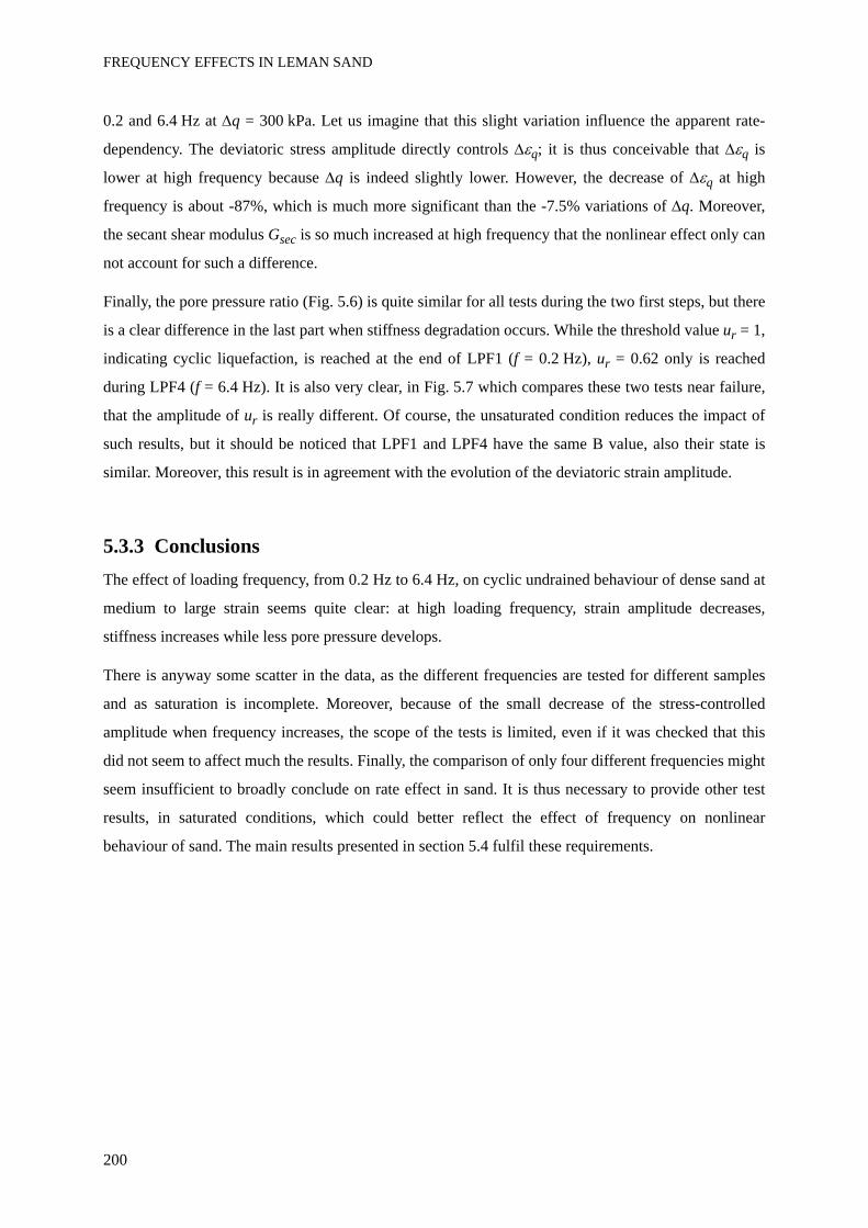
FREQUENCY EFFECTS IN LEMAN SAND
200
0.2 and 6.4 Hz at Δq = 300 kPa. Let us imagine that this slight variation influence the apparent rate-
dependency. The deviatoric stress amplitude directly controls Δεq; it is thus conceivable that Δεq is
lower at high frequency because Δq is indeed slightly lower. However, the decrease of Δεq at high
frequency is about -87%, which is much more significant than the -7.5% variations of Δq. Moreover,
the secant shear modulus Gsec is so much increased at high frequency that the nonlinear effect only can
not account for such a difference.
Finally, the pore pressure ratio (Fig. 5.6) is quite similar for all tests during the two first steps, but there
is a clear difference in the last part when stiffness degradation occurs. While the threshold value ur = 1,
indicating cyclic liquefaction, is reached at the end of LPF1 (f = 0.2 Hz), ur = 0.62 only is reached
during LPF4 (f = 6.4 Hz). It is also very clear, in Fig. 5.7 which compares these two tests near failure,
that the amplitude of ur is really different. Of course, the unsaturated condition reduces the impact of
such results, but it should be noticed that LPF1 and LPF4 have the same B value, also their state is
similar. Moreover, this result is in agreement with the evolution of the deviatoric strain amplitude.
5.3.3 ConclusionsThe effect of loading frequency, from 0.2 Hz to 6.4 Hz, on cyclic undrained behaviour of dense sand at
medium to large strain seems quite clear: at high loading frequency, strain amplitude decreases,
stiffness increases while less pore pressure develops.
There is anyway some scatter in the data, as the different frequencies are tested for different samples
and as saturation is incomplete. Moreover, because of the small decrease of the stress-controlled
amplitude when frequency increases, the scope of the tests is limited, even if it was checked that this
did not seem to affect much the results. Finally, the comparison of only four different frequencies might
seem insufficient to broadly conclude on rate effect in sand. It is thus necessary to provide other test
results, in saturated conditions, which could better reflect the effect of frequency on nonlinear
behaviour of sand. The main results presented in section 5.4 fulfil these requirements.
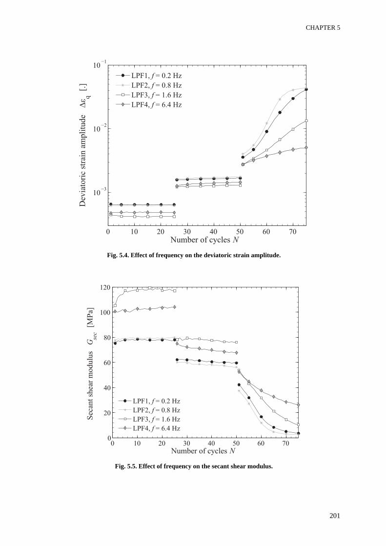
CHAPTER 5
201
Fig. 5.4. Effect of frequency on the deviatoric strain amplitude.
Fig. 5.5. Effect of frequency on the secant shear modulus.
0 10 20 30 40 50 60 70
10
102
101
Dev
iato
ric
stra
in a
mpli
tude
q [
.]
Number of cycles N
LPF1, f = 0.2 Hz
LPF2, f = 0.8 Hz
LPF3, f = 1.6 Hz
LPF4, f = 6.4 Hz
0 10 20 30 40 50 60 700
20
40
60
80
100
120
Sec
ant
shea
r m
odulu
s G
sec
[M
Pa]
Number of cycles N
LPF1, f = 0.2 Hz
LPF2, f = 0.8 Hz
LPF3, f = 1.6 Hz
LPF4, f = 6.4 Hz
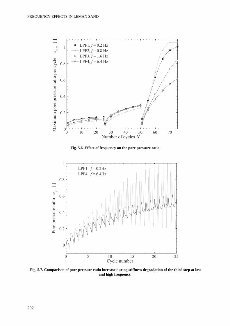
FREQUENCY EFFECTS IN LEMAN SAND
202
Fig. 5.6. Effect of frequency on the pore pressure ratio.
Fig. 5.7. Comparison of pore pressure ratio increase during stiffness degradation of the third step at low and high frequency.
0 10 20 30 40 50 60 700
0.2
0.4
0.6
0.8
1
Max
imum
pore
pre
ssure
rat
io p
er c
ycl
e u
r,m
[.]
Number of cycles N
LPF1, f = 0.2 Hz
LPF2, f = 0.8 Hz
LPF3, f = 1.6 Hz
LPF4, f = 6.4 Hz
0 5 10 15 20 25
0
0.2
0.4
0.6
0.8
1
Pore
pre
ssure
rat
io
ur
[.]
Cycle number
LPF1 f = 0.2Hz
LPF4 f = 6.4Hz
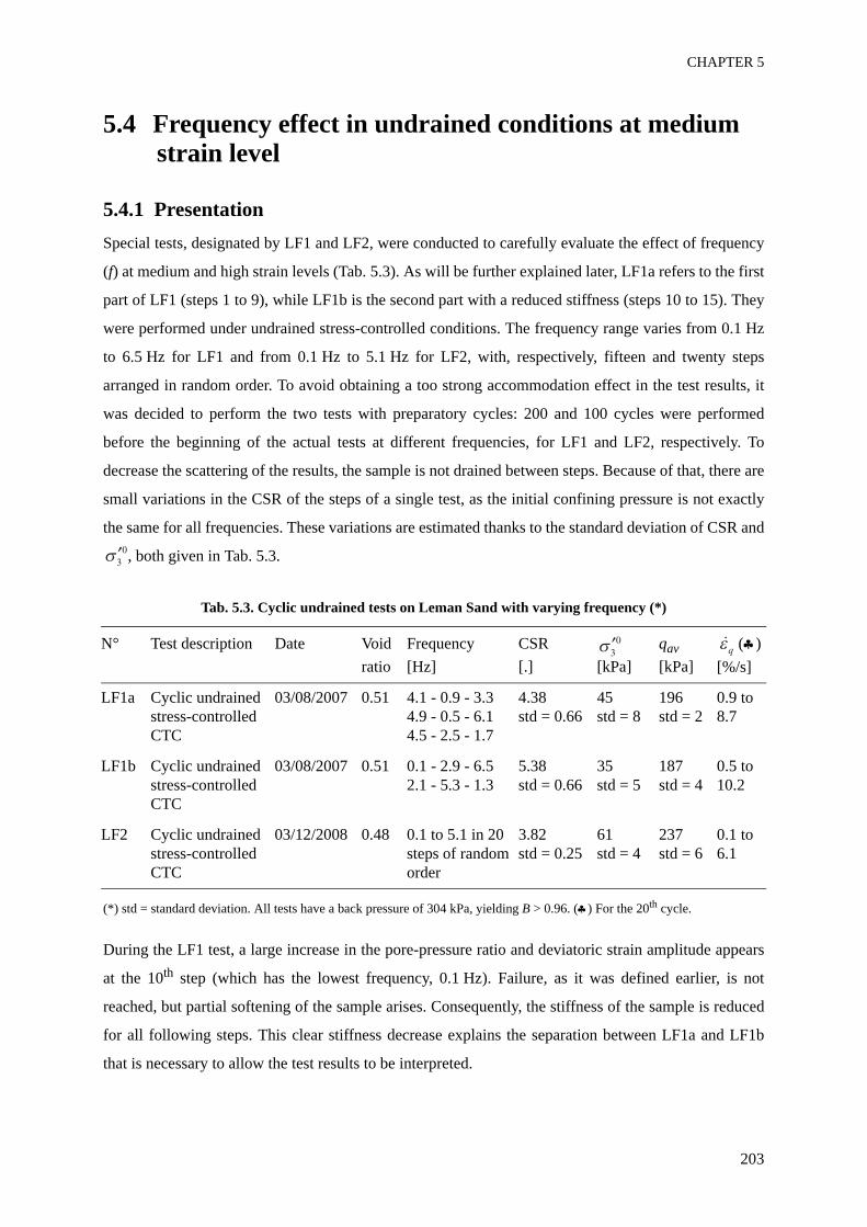
CHAPTER 5
203
5.4 Frequency effect in undrained conditions at medium strain level
5.4.1 PresentationSpecial tests, designated by LF1 and LF2, were conducted to carefully evaluate the effect of frequency
(f) at medium and high strain levels (Tab. 5.3). As will be further explained later, LF1a refers to the first
part of LF1 (steps 1 to 9), while LF1b is the second part with a reduced stiffness (steps 10 to 15). They
were performed under undrained stress-controlled conditions. The frequency range varies from 0.1 Hz
to 6.5 Hz for LF1 and from 0.1 Hz to 5.1 Hz for LF2, with, respectively, fifteen and twenty steps
arranged in random order. To avoid obtaining a too strong accommodation effect in the test results, it
was decided to perform the two tests with preparatory cycles: 200 and 100 cycles were performed
before the beginning of the actual tests at different frequencies, for LF1 and LF2, respectively. To
decrease the scattering of the results, the sample is not drained between steps. Because of that, there are
small variations in the CSR of the steps of a single test, as the initial confining pressure is not exactly
the same for all frequencies. These variations are estimated thanks to the standard deviation of CSR and
, both given in Tab. 5.3.
Tab. 5.3. Cyclic undrained tests on Leman Sand with varying frequency (*)
(*) std = standard deviation. All tests have a back pressure of 304 kPa, yielding B > 0.96. (♣) For the 20th cycle.
During the LF1 test, a large increase in the pore-pressure ratio and deviatoric strain amplitude appears
at the 10th step (which has the lowest frequency, 0.1 Hz). Failure, as it was defined earlier, is not
reached, but partial softening of the sample arises. Consequently, the stiffness of the sample is reduced
for all following steps. This clear stiffness decrease explains the separation between LF1a and LF1b
that is necessary to allow the test results to be interpreted.
N° Test description Date Void ratio
Frequency[Hz]
CSR[.] [kPa]
qav[kPa]
(♣)[%/s]
LF1a Cyclic undrained stress-controlled CTC
03/08/2007 0.51 4.1 - 0.9 - 3.34.9 - 0.5 - 6.14.5 - 2.5 - 1.7
4.38std = 0.66
45std = 8
196std = 2
0.9 to 8.7
LF1b Cyclic undrained stress-controlled CTC
03/08/2007 0.51 0.1 - 2.9 - 6.52.1 - 5.3 - 1.3
5.38std = 0.66
35std = 5
187std = 4
0.5 to 10.2
LF2 Cyclic undrained stress-controlled CTC
03/12/2008 0.48 0.1 to 5.1 in 20 steps of random order
3.82std = 0.25
61std = 4
237std = 6
0.1 to 6.1
q
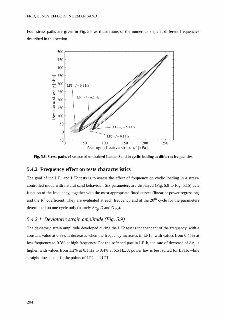
FREQUENCY EFFECTS IN LEMAN SAND
204
Four stress paths are given in Fig. 5.8 as illustrations of the numerous steps at different frequencies
described in this section.
Fig. 5.8. Stress paths of saturated undrained Leman Sand in cyclic loading at different frequencies.
5.4.2 Frequency effect on tests characteristicsThe goal of the LF1 and LF2 tests is to assess the effect of frequency on cyclic loading in a stress-
controlled mode with natural sand behaviour. Six parameters are displayed (Fig. 5.9 to Fig. 5.15) as a
function of the frequency, together with the most appropriate fitted curves (linear or power regression)
and the R2 coefficient. They are evaluated at each frequency and at the 20th cycle for the parameters
determined on one cycle only (namely Δεq, D and Gsec).
5.4.2.1 Deviatoric strain amplitude (Fig. 5.9)The deviatoric strain amplitude developed during the LF2 test is independent of the frequency, with a
constant value at 0.3%. It decreases when the frequency increases in LF1a, with values from 0.45% at
low frequency to 0.3% at high frequency. For the softened part in LF1b, the rate of decrease of Δεq is
higher, with values from 1.2% at 0.1 Hz to 0.4% at 6.5 Hz. A power law is best suited for LF1b, while
straight lines better fit the points of LF2 and LF1a.
0 50 100 150 200 250
0
50
100
150
200
250
300
350
400
450
500D
evia
tori
c st
ress
q [
kP
a]
Average effective stress p’ [kPa]
LF1 - f = 6.5 Hz
LF1 - f = 0.1 Hz
LF2 - f = 5.1 Hz
LF2 - f = 0.1 Hz
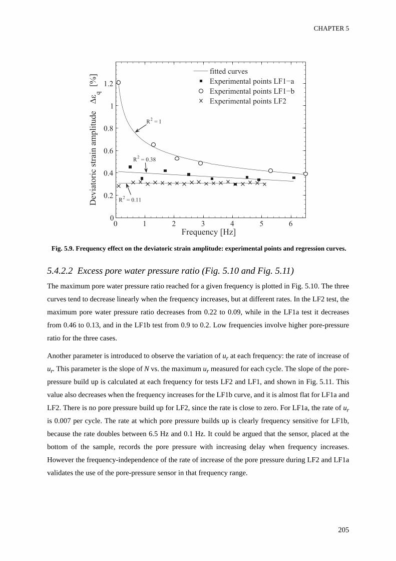
CHAPTER 5
205
Fig. 5.9. Frequency effect on the deviatoric strain amplitude: experimental points and regression curves.
5.4.2.2 Excess pore water pressure ratio (Fig. 5.10 and Fig. 5.11)The maximum pore water pressure ratio reached for a given frequency is plotted in Fig. 5.10. The three
curves tend to decrease linearly when the frequency increases, but at different rates. In the LF2 test, the
maximum pore water pressure ratio decreases from 0.22 to 0.09, while in the LF1a test it decreases
from 0.46 to 0.13, and in the LF1b test from 0.9 to 0.2. Low frequencies involve higher pore-pressure
ratio for the three cases.
Another parameter is introduced to observe the variation of ur at each frequency: the rate of increase of
ur. This parameter is the slope of N vs. the maximum ur measured for each cycle. The slope of the pore-
pressure build up is calculated at each frequency for tests LF2 and LF1, and shown in Fig. 5.11. This
value also decreases when the frequency increases for the LF1b curve, and it is almost flat for LF1a and
LF2. There is no pore pressure build up for LF2, since the rate is close to zero. For LF1a, the rate of ur
is 0.007 per cycle. The rate at which pore pressure builds up is clearly frequency sensitive for LF1b,
because the rate doubles between 6.5 Hz and 0.1 Hz. It could be argued that the sensor, placed at the
bottom of the sample, records the pore pressure with increasing delay when frequency increases.
However the frequency-independence of the rate of increase of the pore pressure during LF2 and LF1a
validates the use of the pore-pressure sensor in that frequency range.
0 1 2 3 4 5 60
0.2
0.4
0.6
0.8
1
1.2
Dev
iato
ric
stra
in a
mpli
tude
q [
%]
Frequency [Hz]
fitted curves
Experimental points LF2
R2 = 1
R2 = 0.38
R2 = 0.11
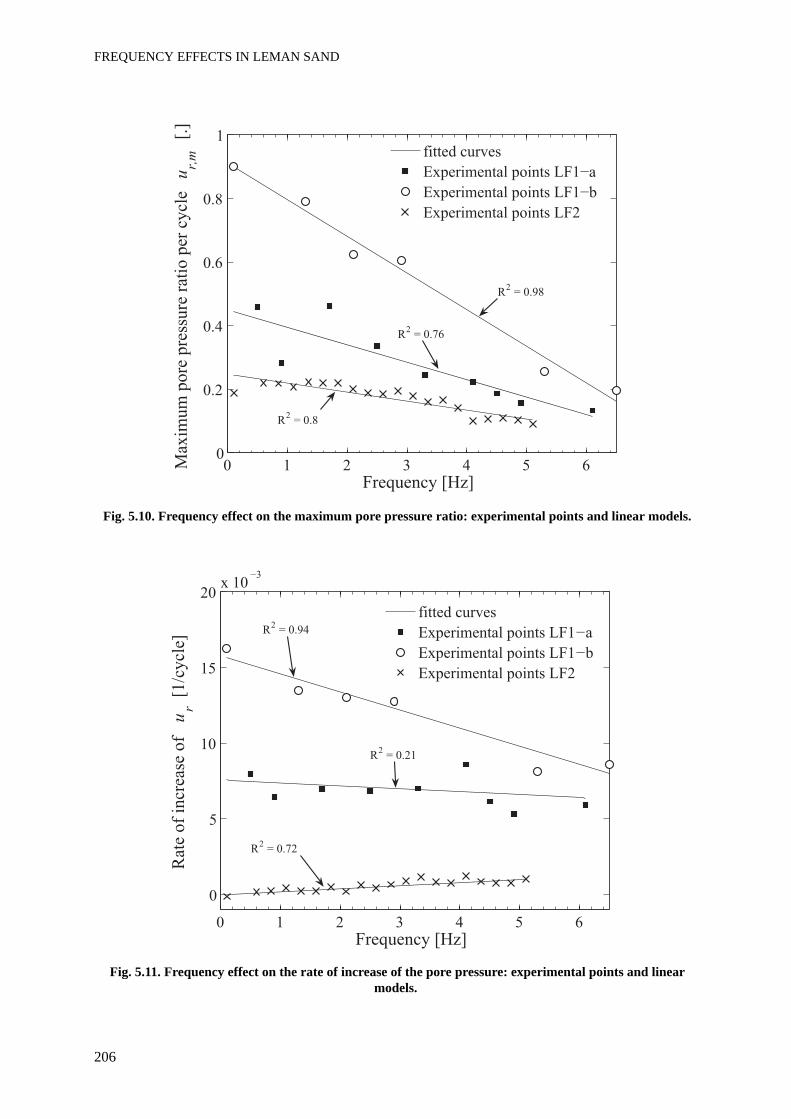
FREQUENCY EFFECTS IN LEMAN SAND
206
Fig. 5.10. Frequency effect on the maximum pore pressure ratio: experimental points and linear models.
Fig. 5.11. Frequency effect on the rate of increase of the pore pressure: experimental points and linear models.
0 1 2 3 4 5 60
0.2
0.4
0.6
0.8
1
Max
imum
pore
pre
ssure
rat
io p
er c
ycl
e u
r,m
[.]
Frequency [Hz]
fitted curves
Experimental points LF2
R2 = 0.98
R2 = 0.76
R2 = 0.8
0 1 2 3 4 5 6
0
5
10
15
20x 10
Rat
e of
incr
ease
of
ur
[1/c
ycl
e]
Frequency [Hz]
fitted curves
Experimental points LF1 a
Experimental points LF1 b
Experimental points LF2
R2 = 0.94
R2 = 0.21
R2 = 0.72

CHAPTER 5
207
5.4.2.3 Damping ratio D (Fig. 5.12)The LF1 test shows an increase of damping ratio with frequency (Fig. 5.12), with a different slope
before or after softening. In fact, the softening does not play such a great role at high frequency; on the
contrary, at low frequency, the damping ratio is lower for the LF1b test than for the LF1a. A power law
better fits this series of data. The damping ratio of LF2 is more scattered, and no conclusion can be
drawn concerning the frequency effect for this test.
Fig. 5.12. Frequency effect on the damping ratio: experimental points and regression curves.
5.4.2.4 Secant shear modulus Gsec (Fig. 5.13)
As we don’t have any data on the frequency effect on the elastic modulus Gmax in Leman Sand, it seems
inappropriate to study the ratio Gsec / Gmax. Only total values of the secant shear modulus Gsec are thus
studied now.
The frequency also influences the secant shear modulus, with large differences between tests
(Fig. 5.13). There is a clear separation of the Gsec level between the three curves. LF2 is stiffer than
LF1a, which is stiffer than LF1b. The secant shear modulus of LF2 is not frequency-dependent, with a
mean value of 37 kPa and a standard deviation of 1 kPa. In LF1a, Gsec slightly increases with
frequency, but the data scattering is relatively large. Finally in LF1b, Gsec clearly decreases at low
frequency, with a mean rate of 2.1 MPa per frequency unit.
0 1 2 3 4 5 69
10
11
12
13
14
15
Dam
pin
g r
atio
D [
%]
Frequency [Hz]
fitted curves
Experimental points LF2
R2 = 0.98
R2 = 0.98
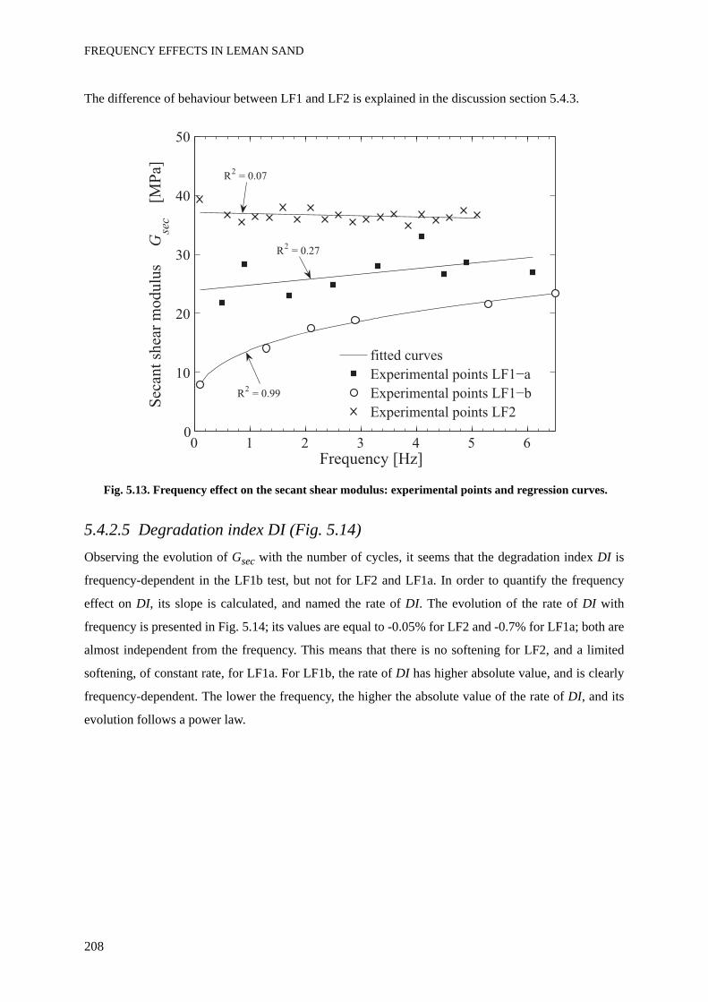
FREQUENCY EFFECTS IN LEMAN SAND
208
The difference of behaviour between LF1 and LF2 is explained in the discussion section 5.4.3.
Fig. 5.13. Frequency effect on the secant shear modulus: experimental points and regression curves.
5.4.2.5 Degradation index DI (Fig. 5.14)Observing the evolution of Gsec with the number of cycles, it seems that the degradation index DI is
frequency-dependent in the LF1b test, but not for LF2 and LF1a. In order to quantify the frequency
effect on DI, its slope is calculated, and named the rate of DI. The evolution of the rate of DI with
frequency is presented in Fig. 5.14; its values are equal to -0.05% for LF2 and -0.7% for LF1a; both are
almost independent from the frequency. This means that there is no softening for LF2, and a limited
softening, of constant rate, for LF1a. For LF1b, the rate of DI has higher absolute value, and is clearly
frequency-dependent. The lower the frequency, the higher the absolute value of the rate of DI, and its
evolution follows a power law.
0 1 2 3 4 5 60
10
20
30
40
50
Sec
ant
shea
r m
odulu
s G
sec
[M
Pa]
Frequency [Hz]
fitted curves
Experimental points LF2
R2 = 0.07
R2 = 0.27
R2 = 0.99
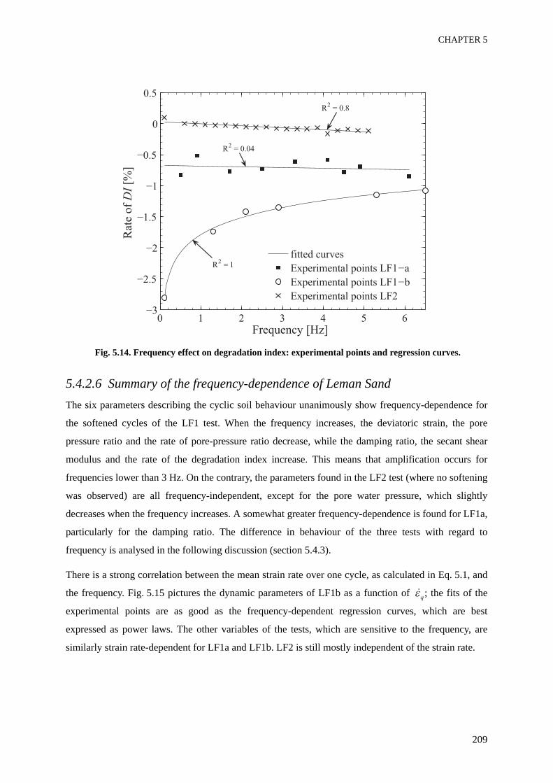
CHAPTER 5
209
Fig. 5.14. Frequency effect on degradation index: experimental points and regression curves.
5.4.2.6 Summary of the frequency-dependence of Leman SandThe six parameters describing the cyclic soil behaviour unanimously show frequency-dependence for
the softened cycles of the LF1 test. When the frequency increases, the deviatoric strain, the pore
pressure ratio and the rate of pore-pressure ratio decrease, while the damping ratio, the secant shear
modulus and the rate of the degradation index increase. This means that amplification occurs for
frequencies lower than 3 Hz. On the contrary, the parameters found in the LF2 test (where no softening
was observed) are all frequency-independent, except for the pore water pressure, which slightly
decreases when the frequency increases. A somewhat greater frequency-dependence is found for LF1a,
particularly for the damping ratio. The difference in behaviour of the three tests with regard to
frequency is analysed in the following discussion (section 5.4.3).
There is a strong correlation between the mean strain rate over one cycle, as calculated in Eq. 5.1, and
the frequency. Fig. 5.15 pictures the dynamic parameters of LF1b as a function of ; the fits of the
experimental points are as good as the frequency-dependent regression curves, which are best
expressed as power laws. The other variables of the tests, which are sensitive to the frequency, are
similarly strain rate-dependent for LF1a and LF1b. LF2 is still mostly independent of the strain rate.
0 1 2 3 4 5 6
0R
ate
of
DI
[%]
Frequency [Hz]
fitted curves
Experimental points LF1 a
Experimental points LF1 b
Experimental points LF2
R2 = 1
R2
R2
q
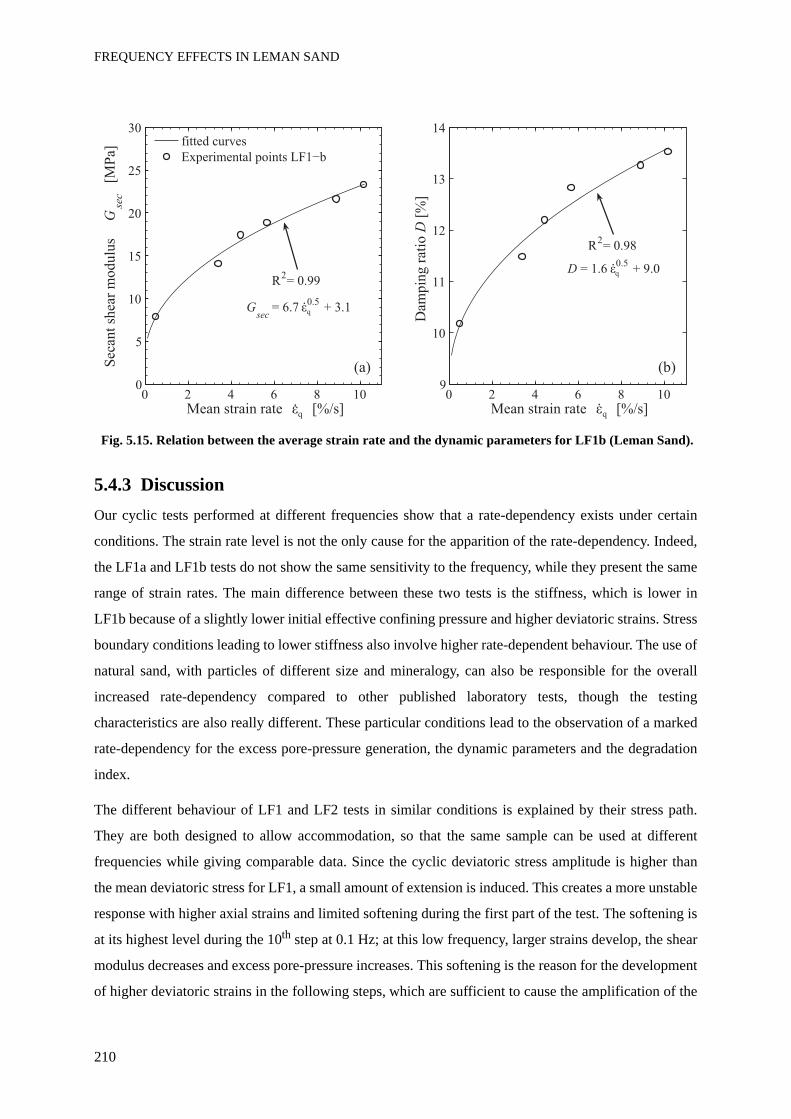
FREQUENCY EFFECTS IN LEMAN SAND
210
Fig. 5.15. Relation between the average strain rate and the dynamic parameters for LF1b (Leman Sand).
5.4.3 DiscussionOur cyclic tests performed at different frequencies show that a rate-dependency exists under certain
conditions. The strain rate level is not the only cause for the apparition of the rate-dependency. Indeed,
the LF1a and LF1b tests do not show the same sensitivity to the frequency, while they present the same
range of strain rates. The main difference between these two tests is the stiffness, which is lower in
LF1b because of a slightly lower initial effective confining pressure and higher deviatoric strains. Stress
boundary conditions leading to lower stiffness also involve higher rate-dependent behaviour. The use of
natural sand, with particles of different size and mineralogy, can also be responsible for the overall
increased rate-dependency compared to other published laboratory tests, though the testing
characteristics are also really different. These particular conditions lead to the observation of a marked
rate-dependency for the excess pore-pressure generation, the dynamic parameters and the degradation
index.
The different behaviour of LF1 and LF2 tests in similar conditions is explained by their stress path.
They are both designed to allow accommodation, so that the same sample can be used at different
frequencies while giving comparable data. Since the cyclic deviatoric stress amplitude is higher than
the mean deviatoric stress for LF1, a small amount of extension is induced. This creates a more unstable
response with higher axial strains and limited softening during the first part of the test. The softening is
at its highest level during the 10th step at 0.1 Hz; at this low frequency, larger strains develop, the shear
modulus decreases and excess pore-pressure increases. This softening is the reason for the development
of higher deviatoric strains in the following steps, which are sufficient to cause the amplification of the
0 2 4 6 8 109
10
11
12
13
14
Dam
pin
g r
atio
D [
%]
Mean strain rate [%/s]0 2 4 6 8 10
0
5
10
15
20
25
30
Sec
ant
shea
r m
odulu
s G
sec
[M
Pa]
Mean strain rate [%/s]
fitted curves
R2= 0.98
R2= 0.99
Gsec
= 6.70.5
+ 3.1
D = 1.60.5
+ 9.0
(a)
. .
.
.
q q
q
q
CHAPTER 5
211
frequency-dependent behaviour. While the quantitative parameters are in the same range before and
after softening at the high frequency level, there is a clear difference at low frequencies. In the LF1b
test between 6.5 Hz and 0.1 Hz, the deviatoric strain is multiplied by 3 and the pore-pressure ratio is
multiplied by 4.5, while the secant shear modulus is divided by 3 and the rate of the degradation index
by 2.5. Those parameters are not independent from each other; for example, the pore water pressure
build up is controlled by the deviatoric strain, and it is expected that its variation with frequency is
similar.
There is a regular progression in the level of rate-dependency for the three tests. While LF2 is mostly
rate-independent, LF1a is slightly rate-dependent, and the behaviour of LF1b is strongly frequency-
dependent. This evolution is correlated with the overall decrease of the stiffness along the three tests,
and also follows the increase of CSR (Tab. 5.3). Thus, a link between the stress boundary conditions
driving the sample stiffness and sensitivity to frequency is a possible explanation for the three different
behaviours.
Gosh & Madabushi (2003) showed, in the case of finite element modeling of a saturated sandy deposit
during real earthquake events at different frequencies, that the excess pore pressure is higher for lower
frequencies. An amplification phenomenon is found at 1 Hz, which is called the «natural frequency» of
the deposit. Not only the peak magnitude, but also the rate of increase of the excess pore pressure is
found to be rate-dependent. This prediction is confirmed by the LF1b test for the peak value and for the
rate of increase.
The practical consequences of the increase of ur,m with decreasing f might be crucial. It should thus be
taken into account for the modeling of liquefaction phenomenon, and for scaled models that are
performed at higher frequency. We also notice that it is rather positive to obtain an amplified low
frequency behaviour, considering that pseudo-static tests are usually performed in the range of 0.1 to
1 Hz. This range of frequency thus yields the highest strain amplitudes, also such tests are conservative.
The increase of the damping ratio of dry sand with frequency, for typical earthquake frequency range, is
observed by Lin et al. (1996) and Hoque & Tatsuoka (2004). The latter performed triaxial tests
indicating a stronger increase in the damping ratio at high strains. The former group showed a linear
relationship between D and the frequency using torsional tests on full cylindrical samples. The dynamic
parameters of their linear model mainly depend on the shear strain amplitude and the effective
confining pressure. All of these observations apply to our test results on Leman Sand in undrained
conditions; however, none of the previous studies have addressed the rate effect at medium to high
strains.
FREQUENCY EFFECTS IN LEMAN SAND
212
5.4.4 ConclusionsA clear frequency-dependence is found during cyclic loading under certain conditions, which are
probably linked with stress boundary conditions leading to low stiffness of the Leman Sand sample.
The deviatoric strain amplitude, the maximum excess pore water pressure ratio and the rate of increase
of the pore-pressure ratio decrease when the frequency increases. The secant shear modulus, the
damping ratio and the rate of the degradation index increase with frequency.
5.5 Frequency effect in cyclic dry conditions
5.5.1 Test presentation
One test, called LDF, was also performed at different frequencies on a sample of dry sand (Tab. 5.4).
The boundary conditions and applied load are slightly different from the undrained cyclic tests at
different frequencies, LF1 and LF2. The CSR is slightly lower than undrained saturated tests, because
the effective confining pressure is higher; indeed, to avoid accommodation, preparatory cycles were
performed for both kind of tests, but induced a decrease of the effective confining pressure only in
undrained conditions. The void ratio is also higher in the dry test. It varies cyclically during loading, but
the average value is very stable between all steps. There is no stress reversal and the point q = 0 is
touched once per cycle.
Similarly to the undrained LF1 test, there is a clear separation (especially in Gsec) between steps
performed before or after the step at which f = 0.1 Hz (step n°11 in LDF and step n°10 in LF1): for the
interpretation of sand characteristics as a function of the loading frequency, the test is separated into
two parts LDFa (steps 1 to 10) and LDFb (steps 11 to 22). Actually, the step n°11 is between the two
trends, it could also be set apart from LDFb, as will be seen later.
In the same way as previous results analyses, the test characteristics selected for the following figures
are all obtained at the 20th cycle for each frequency.
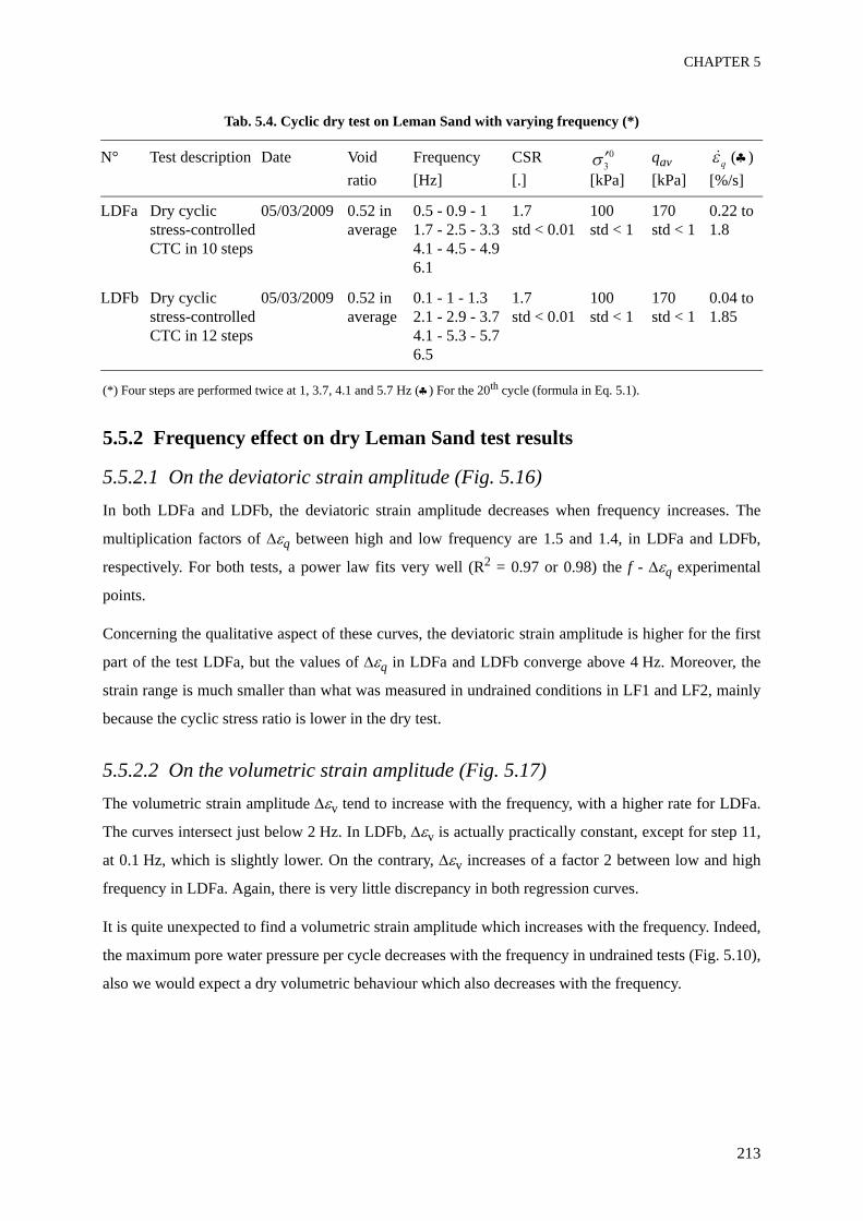
CHAPTER 5
213
Tab. 5.4. Cyclic dry test on Leman Sand with varying frequency (*)
(*) Four steps are performed twice at 1, 3.7, 4.1 and 5.7 Hz (♣) For the 20th cycle (formula in Eq. 5.1).
5.5.2 Frequency effect on dry Leman Sand test results
5.5.2.1 On the deviatoric strain amplitude (Fig. 5.16)In both LDFa and LDFb, the deviatoric strain amplitude decreases when frequency increases. The
multiplication factors of Δεq between high and low frequency are 1.5 and 1.4, in LDFa and LDFb,
respectively. For both tests, a power law fits very well (R2 = 0.97 or 0.98) the f - Δεq experimental
points.
Concerning the qualitative aspect of these curves, the deviatoric strain amplitude is higher for the first
part of the test LDFa, but the values of Δεq in LDFa and LDFb converge above 4 Hz. Moreover, the
strain range is much smaller than what was measured in undrained conditions in LF1 and LF2, mainly
because the cyclic stress ratio is lower in the dry test.
5.5.2.2 On the volumetric strain amplitude (Fig. 5.17)The volumetric strain amplitude Δεv tend to increase with the frequency, with a higher rate for LDFa.
The curves intersect just below 2 Hz. In LDFb, Δεv is actually practically constant, except for step 11,
at 0.1 Hz, which is slightly lower. On the contrary, Δεv increases of a factor 2 between low and high
frequency in LDFa. Again, there is very little discrepancy in both regression curves.
It is quite unexpected to find a volumetric strain amplitude which increases with the frequency. Indeed,
the maximum pore water pressure per cycle decreases with the frequency in undrained tests (Fig. 5.10),
also we would expect a dry volumetric behaviour which also decreases with the frequency.
N° Test description Date Void ratio
Frequency [Hz]
CSR [.] [kPa]
qav [kPa]
(♣)[%/s]
LDFa Dry cyclic stress-controlled CTC in 10 steps
05/03/2009 0.52 in average
0.5 - 0.9 - 1 1.7 - 2.5 - 3.3 4.1 - 4.5 - 4.9 6.1
1.7std < 0.01
100std < 1
170std < 1
0.22 to 1.8
LDFb Dry cyclic stress-controlled CTC in 12 steps
05/03/2009 0.52 in average
0.1 - 1 - 1.3 2.1 - 2.9 - 3.7 4.1 - 5.3 - 5.7 6.5
1.7std < 0.01
100std < 1
170std < 1
0.04 to 1.85
q
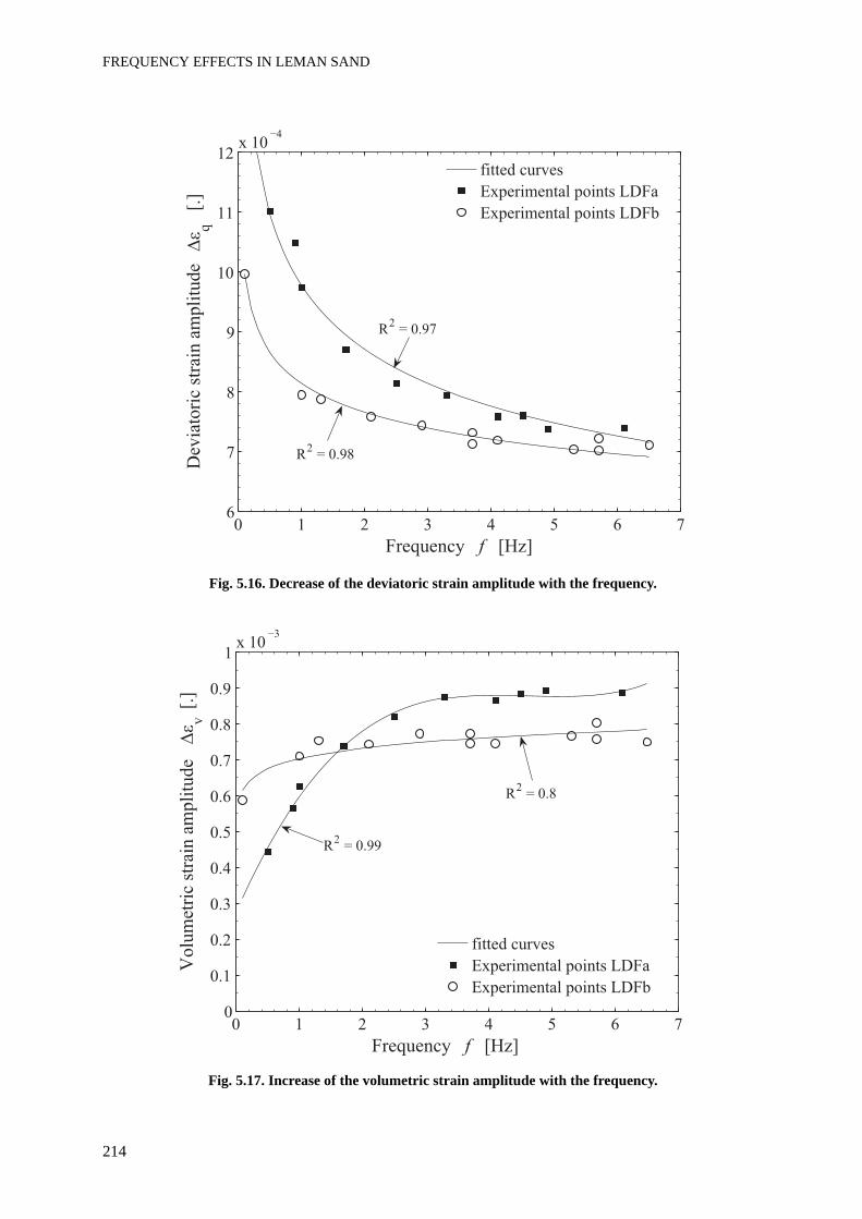
FREQUENCY EFFECTS IN LEMAN SAND
214
Fig. 5.16. Decrease of the deviatoric strain amplitude with the frequency.
Fig. 5.17. Increase of the volumetric strain amplitude with the frequency.
0 1 2 3 4 5 6 76
7
8
9
10
11
12x 10
Dev
iato
ric
stra
in a
mpli
tude
q [
.]
Frequency f [Hz]
fitted curves
Experimental points LDFa
Experimental points LDFb
R2 = 0.97
R2 = 0.98
0 1 2 3 4 5 6 70
0.1
0.2
0.3
0.4
0.5
0.6
0.7
0.8
0.9
1x 10
Volu
met
ric
stra
in a
mpli
tude
v [
.]
Frequency f [Hz]
fitted curves
Experimental points LDFa
Experimental points LDFb
R2 = 0.8
R2 = 0.99
CHAPTER 5
215
5.5.2.3 On the secant shear modulus (Fig. 5.18)Both parts of the dry cyclic test exhibit an increase of Gsec with the frequency (Fig. 5.18), as for
undrained loading (Fig. 5.13). There is very small scatter in the data; the best fits are a straight line and
a power law for LDFa and LDFb, respectively, with R2 = 0.97 for both parts. LDFb is stiffer than
LDFa, except at high frequency where the curves converge.
Contrary to undrained cyclic loading, the first part LDFa is softer than the second part LDFb, probably
because of accommodation. We saw in chapter 4 that the response of dry sand can be very different
from the undrained saturated response. Moreover, LDFa exhibits more rate-dependency: the ratio of the
maximum (at 6.5 Hz) to the minimum (at 0.1 Hz) Gsec, from the regression curves, is 1.65 and 1.45 for
LDFa and LDFb, respectively. This test is thus in agreement with the assumption that the intensity of
rate-dependency increases at stress boundary conditions leading to lower stiffness (undrained test result
in section 5.4.3).
Fig. 5.18. Increase of the secant shear modulus with the frequency.
5.5.2.4 On the damping ratio (Fig. 5.19)Damping ratios observed in LDFb test is independent from the frequency, with a mean value of 17%
and a standard deviation of 1.3%. This value seems too high compared to the evolution of damping with
the deviatoric strain amplitude in undrained conditions. Indeed, there is great limitations in the
0 1 2 3 4 5 6 770
80
90
100
110
120
130
Sec
ant
shea
r m
odulu
s G
sec
[M
Pa]
Frequency f [Hz]
fitted curves
Experimental points LDFa
Experimental points LDFb
R2 = 0.97
R2 = 0.97
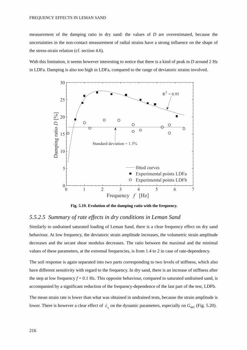
FREQUENCY EFFECTS IN LEMAN SAND
216
measurement of the damping ratio in dry sand: the values of D are overestimated, because the
uncertainties in the non-contact measurement of radial strains have a strong influence on the shape of
the stress-strain relation (cf. section 4.6).
With this limitation, it seems however interesting to notice that there is a kind of peak in D around 2 Hz
in LDFa. Damping is also too high in LDFa, compared to the range of deviatoric strains involved.
Fig. 5.19. Evolution of the damping ratio with the frequency.
5.5.2.5 Summary of rate effects in dry conditions in Leman SandSimilarly to undrained saturated loading of Leman Sand, there is a clear frequency effect on dry sand
behaviour. At low frequency, the deviatoric strain amplitude increases, the volumetric strain amplitude
decreases and the secant shear modulus decreases. The ratio between the maximal and the minimal
values of these parameters, at the extremal frequencies, is from 1.4 to 2 in case of rate-dependency.
The soil response is again separated into two parts corresponding to two levels of stiffness, which also
have different sensitivity with regard to the frequency. In dry sand, there is an increase of stiffness after
the step at low frequency f = 0.1 Hz. This opposite behaviour, compared to saturated undrained sand, is
accompanied by a significant reduction of the frequency-dependence of the last part of the test, LDFb.
The mean strain rate is lower than what was obtained in undrained tests, because the strain amplitude is
lower. There is however a clear effect of on the dynamic parameters, especially on Gsec (Fig. 5.20).
0 1 2 3 4 5 6 70
5
10
15
20
25
30
Dam
pin
g r
atio
D [
%]
Frequency f [Hz]
fitted curves
Experimental points LDFa
Experimental points LDFb
R2 = 0.95
Standard deviation = 1.3%
q
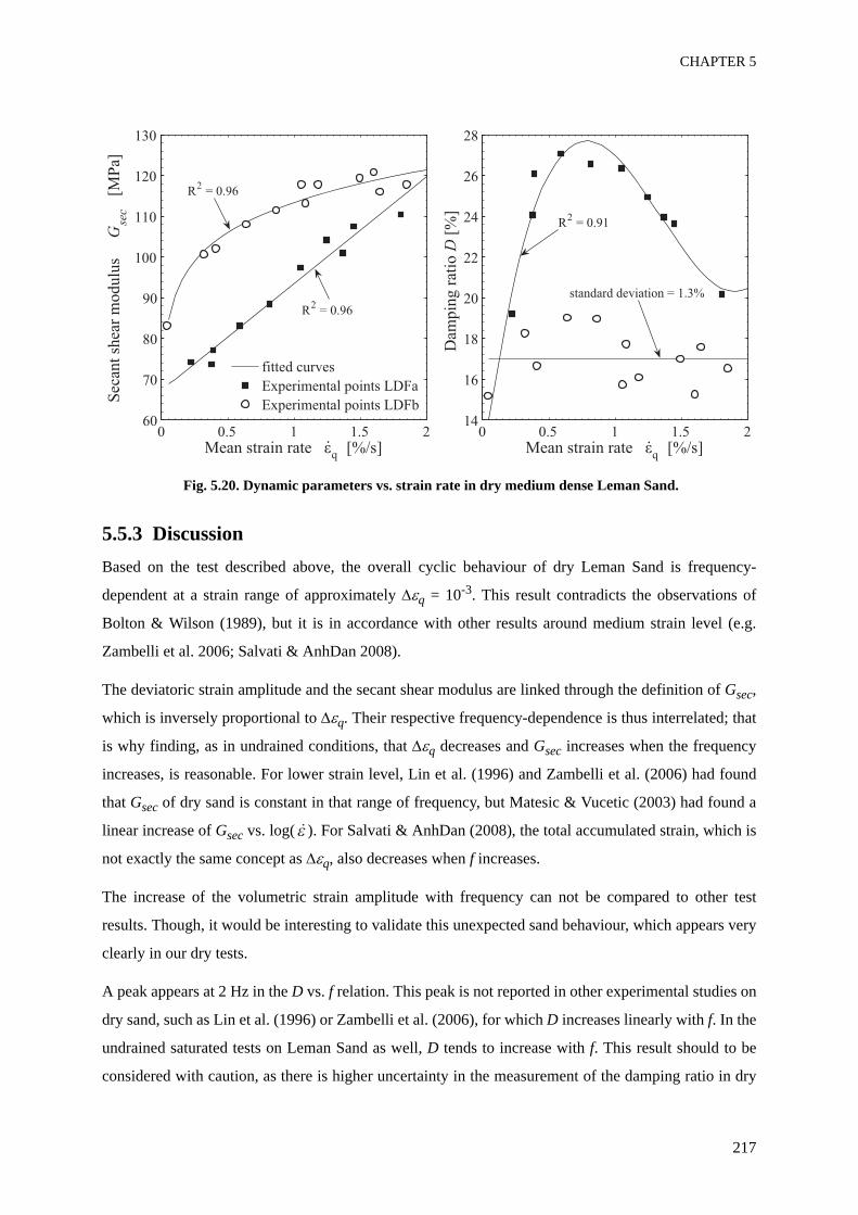
CHAPTER 5
217
Fig. 5.20. Dynamic parameters vs. strain rate in dry medium dense Leman Sand.
5.5.3 DiscussionBased on the test described above, the overall cyclic behaviour of dry Leman Sand is frequency-
dependent at a strain range of approximately Δεq = 10-3. This result contradicts the observations of
Bolton & Wilson (1989), but it is in accordance with other results around medium strain level (e.g.
Zambelli et al. 2006; Salvati & AnhDan 2008).
The deviatoric strain amplitude and the secant shear modulus are linked through the definition of Gsec,
which is inversely proportional to Δεq. Their respective frequency-dependence is thus interrelated; that
is why finding, as in undrained conditions, that Δεq decreases and Gsec increases when the frequency
increases, is reasonable. For lower strain level, Lin et al. (1996) and Zambelli et al. (2006) had found
that Gsec of dry sand is constant in that range of frequency, but Matesic & Vucetic (2003) had found a
linear increase of Gsec vs. log( ). For Salvati & AnhDan (2008), the total accumulated strain, which is
not exactly the same concept as Δεq, also decreases when f increases.
The increase of the volumetric strain amplitude with frequency can not be compared to other test
results. Though, it would be interesting to validate this unexpected sand behaviour, which appears very
clearly in our dry tests.
A peak appears at 2 Hz in the D vs. f relation. This peak is not reported in other experimental studies on
dry sand, such as Lin et al. (1996) or Zambelli et al. (2006), for which D increases linearly with f. In the
undrained saturated tests on Leman Sand as well, D tends to increase with f. This result should to be
considered with caution, as there is higher uncertainty in the measurement of the damping ratio in dry
0 0.5 1 1.5 214
16
18
20
22
24
26
28
Dam
pin
g r
atio
D [
%]
Mean strain rate q
[%/s]0 0.5 1 1.5 2
60
70
80
90
100
110
120
130
Sec
ant
shea
r m
odulu
s G
sec
[M
Pa]
Mean strain rate q
[%/s]
fitted curves
Experimental points LDFa
Experimental points LDFb
R2 = 0.96
R2 = 0.96
R2 = 0.91
standard deviation = 1.3%
..
FREQUENCY EFFECTS IN LEMAN SAND
218
triaxial tests.
As was shown previously in undrained saturated condition, dry Leman Sand is rate sensitive during
cyclic loading. The conditions of CSR and strain range of our dry and undrained tests are not exactly
similar, also it is not possible to deduce from this experimental study if dry and undrained saturated
conditions yields the same amount of rate effect. Thus, the importance of water in rate effect cannot be
evaluated with available experimental data. Nawir et al. (2003) showed that the effect of step changes
of strain rate in sands was similar in dry and saturated drained conditions. We now add that, in cyclic
loading, the change of frequency involves sizeable changes in both dry and saturated undrained sand
behaviour at medium strain level.
The dry cyclic test LDF clearly separates into two frequency-dependent parts, which exhibit different
levels of rate-dependency. The parallel between the undrained saturated response and the dry response
of sand is striking: while the first part of the test is stiffer and less rate-dependent in the undrained test
LF1a, the first part is less stiff and more frequency-dependent in LDFa. The difference of evolution of
the overall stiffness may be expected, in the sense that dry sand exhibits accommodation while
undrained sand involves stiffness degradation in the same conditions. The concordance of the
sensitivity to frequency and the relative stiffness level in both hydraulic conditions is an interesting
conclusion from the comparison of these cyclic tests. The stress boundary conditions leading to lower
stiffness thus induce a suitable environment for enhanced cyclic rate effects in dry and undrained
saturated sands.
Finally, for Salvati & AnhDan (2008), frequency-dependent behaviour of dry sand increases with low
confining pressure and for high CSR. This comment enlightens the difference between our dry and
undrained tests at different CSR. On one hand, higher frequency-dependence (i.e. more amplification at
low frequency) is obtained in the saturated test LF1 with a higher CSR than the dry test LDF. On the
other hand, the relation, found in our tests, between stiffness degradation and rate effect indirectly
confirms the result of Salvati & AnhDan (2008). Indeed, considering that lower confining pressure
reduces sand stiffness (cf. Chapter 4), the conditions of low stiffness and the effect of confining
pressure both yield the same response in terms of frequency-dependence of sand behaviour. The test
results presented here and the observations of Salvati & AnhDan (2008) are then compatible.
5.5.4 ConclusionsDry Leman Sand is clearly frequency-dependent at medium strain level. At low frequency, the
deviatoric strain amplitude increases, the volumetric strain amplitude decreases and the secant shear
modulus decreases. The ratio between the maximal and the minimal values of these parameters, at the
CHAPTER 5
219
extremal frequencies, is from 1.4 to 2 in case of rate-dependency (i.e. except for some parameters in
LDFb). The second part of the test LDF, which is stiffer (but with the same CSR) than the first ten steps
at ten frequencies (LDFa), seems also less frequency-dependent. Salvati & AnhDan (2008) had shown
that the frequency-dependent response of dry sand depends on the confining pressure. As a
complement, we show that stress boundary conditions leading to lower stiffness induce a suitable
environment for enhanced cyclic rate effects in sands. This idea is supported by the comparison
between dry and undrained saturated sand behaviour at different frequencies.
5.6 Discussions on rate effect in Leman sand
5.6.1 Experimental artefactsBefore concluding on the effect of frequency on Leman Sand behaviour, we must consider the
hypothesis that the observed rate-dependent Leman Sand behaviour could be an artificial effect of the
triaxial press or the measuring system. In other words, a small review of the different parts which could
wrongly increase the frequency effect is listed now.
The possible test and measuring artefacts that we could foresee are: (i) the numeric filters used in the
recording of sensor output (ii) the temporal resolution of the sensors (iii) the sensitivity of the motion
control to the frequency (iv) local physical measurement errors of the pore pressure and the laser
sensors. Their possible effect on the test results is analysed.
The numeric filters included in the Fast Track controlling system, which records sensor ouputs, are
triggered with a cut-off frequency at the same level as the sampling frequency, which is itself adapted to
the loading frequency. We checked that these values do not influence the output data. The test
equipment was designed to allow frequencies up to 100 Hz, also the temporal resolution of sensors is
not a problem either, as loading frequency remains below 10 Hz.
Motion regulation is performed via a closed loop system, which might be sensitive to loading
frequency. However, the stress amplitude is very stable in dry tests, with a standard deviation of both
the average and the amplitude values of q below 1%. Such stability is remarkable, and shows that
motion regulation is not an issue with these loading features.
A linear elastic model of the test showed that the time necessary to equilibrate pore pressures within the
sample is not a problem for loading frequency below the maximum used frequency f = 6.5 Hz
(section 3.2.1). For the measurement of radial strains with the laser technique in dry tests, we can
FREQUENCY EFFECTS IN LEMAN SAND
220
wonder whether this measurement is sensitive to the frequency. However, the maximum sampling
frequency with the lasers is 2.5 kHz; thus, the maximum admissible loading frequency should be one
tens, i.e. 250 Hz. The range of loading frequency of our tests is then very much smaller than this
maximum.
Finally, some test results were found frequency-independent in some conditions, or for some parts of
the tests. For example, the deviatoric strain amplitude and the rate of increase of the pore pressure ratio
is constant during the undrained test LF2. In the dry test LDFb, D and Δεv are also almost constant
values.
This small analysis enhanced our confidence in the test results on rate effect in Leman Sand presented
in this chapter.
5.6.2 Physical interpretation and general commentsA clear definition of viscous time effects is given by Di Benedetto (2006):
«By definition time effects exist if a change in the stress-strain curve(s) is observed when changing the
rate of loading».
Our cyclic tests on dry and undrained saturated Leman Sand demonstrate a clear time-dependent
behaviour, as the cyclic loops depend on the stress frequency (e.g. the parameters Δεq, Gsec, D are
shown to depend on frequency). Moreover, the stress frequency (or loading rate) and mean strain rate
(which also depends on strain amplitude) have similar effects on material parameters (e.g. Fig. 5.12,
Fig. 5.13 and Fig. 5.15).
It is not new that sand can exhibit time-dependent behaviour. The literature review provided examples
and possible explanations of rate effects in granular media. In particular, recent experimental studies
(e.g. Tatsuoka 2006; Duttine et al. 2008) demonstrated that granular materials are sensitive to changes
in strain rate rather than the absolute strain rate values in monotonic conditions. We showed that the
effect of frequency on the particular sand used, Leman Sand, which is an angular poorly-graded natural
sand, can be non negligible in the range of strain amplitude and frequency content of a strong
earthquake. Low frequency motions, i.e. between 0.1 and 1 Hz, are amplified by comparison with high
frequency motions between 4 and 6.5 Hz. The strain amplitude, the volumetric behaviour (pore
pressure in undrained condition and volumetric strain in dry condition), the dynamic parameters are all
influenced by the loading frequency in certain conditions.
The test procedure and the stability of Leman Sand behaviour both allowed to obtain such distinct
results. As the frequency-dependent behaviour of Leman Sand also appears in the preliminary tests, the
CHAPTER 5
221
rate effect here is not caused only by a change in strain rate, as was shown for monotonic loads
(Tatsuoka 2006; Duttine et al. 2008), but is necessarily linked with the value of frequency itself.
However, the new procedure in which frequency changes by steps every 25 cycles, which allows to
have exactly identical sample fabric, may also include this effect of change of strain rate during the first
loading cycles of each step.
Duttine et al. (2008) demonstrated that the angularity of the grains influence the viscous behaviour of
sand in case of direct shear monotonic tests; as Leman Sand is particularly angular, we assume that this
enhanced viscous behaviour obtained in Leman Sand may be due to the angular grain shape.
The physical interpretation of such complex phenomenon is hazardous. In particular, the limited
number of tests makes it difficult to get a perfect overview on the relative effects of density, confining
pressure, CSR, etc.... A more detailed parametric study would be needed to assess, in particular, the role
of the pore fluid in the frequency-dependence.
Anyway, as both dry and undrained tests exhibit frequency-dependent behaviour, the coupling of the
grains and the pore fluid only is not responsible for that rate-dependent behaviour. This result is
consistent with the description of rate-dependent dry sand behaviour presented by Pham Van Bang et al.
(2007) in pseudo-static conditions (i.e. for creep, relaxation, and step change of strain rate). Our
laboratory tests demonstrate that rate-dependent behaviour of dry sand can also be observed during
cyclic loading at medium strain amplitude, and for larger strain rates.
Given the wave length of the loading (cf. section 3.2.1), even at the highest frequency, a true dynamic
amplification due to wave propagation can be withdrawn from the possible meanings of the frequency-
dependence observed in Leman Sand.
Inherent viscosity at the particle contact between the grains is a popular assumption for time-dependent
sand behaviour. For example, Nawir et al. (2003) for triaxial compression tests of dry sand:
«The origin of such global viscous properties of sand [...] is time-dependent slipping at inter-particle
contacts caused by viscous deformation inside particles at and near the inter-particle contacts [...]. It
seems that, inside a sand specimen subjected to creep loading, such local viscous behaviour as
described above is active only in limited zones at every moment and these zones are continuously
moving while the overall viscous activities decay with time»
Such an explanation may be adapted and applied to the observed frequency-dependent cyclic behaviour
of Leman Sand, in both dry and undrained conditions. However, such interpretation of our test results at
the micro-scale level does not rely on tangible scientific proofs.
FREQUENCY EFFECTS IN LEMAN SAND
222
5.7 ConclusionsFour monotonic triaxial undrained compression tests performed at different strain rates, from 0.03 to
0.98 %/s, allowed to conclude that there is no monotonic strain rate effect in Leman Sand in this range
of strain rate. The slight differences in the stress-strain and the pore pressure ratio vs. axial strain
relations are thought to be linked with variations of the grain size distribution of individual samples.
In cyclic loading, the four preliminary tests at different frequencies, the two undrained saturated tests
and the dry test, all performed on dense Leman Sand, allow to conclude on a cyclic effect of the
frequency on sand behaviour. The overall rate-sensitivity of this granular material is thought to be
enhanced by the angularity of the grains.
Though they were performed at a limited number of frequency and in imperfect conditions, the
preliminary tests LPF1 to LPF4 show that, compared to low frequencies, high frequencies induce lower
strain amplitude, higher stiffness and less excess pore pressure at medium to large strain.
The same consequences on stiffness degradation behaviour are inferred, in certain conditions, from the
test LF1, where undrained saturated Leman Sand is cyclically sheared in various steps of different
frequencies. A strong frequency-dependence is found in part of the results: in LF1b, the deviatoric
strain amplitude decreases of a factor 3, the maximum pore pressure ratio decreases of a factor 4.5 and
the secant shear modulus increases of a factor 3 when the frequency increases from 0.1 to 6.5 Hz. The
rate of increase of the pore pressure ratio decreases with frequency, while the damping ratio and the rate
of the degradation index increase. Though, the other test at lower CSR, LF2, is practically frequency-
independent in approximately the same frequency range but with higher stiffness.
Dry Leman Sand is also frequency-dependent at medium strain level in certain conditions. As for
undrained sand, the deviatoric strain amplitude increases and the secant shear modulus decreases at low
frequency, while the volumetric strain amplitude decreases. The ratio between the maximal and the
minimal values of these parameters, at the extremal frequencies, is from 1.4 to 2 in the rate-dependent
part.
Both dry and undrained tests demonstrate an effect of stress boundary conditions on the sensitivity of
sand behaviour to cyclic rate effect. The stiffer parts of the tests are less frequency-dependent, whatever
other conditions, and especially independently of the cyclic stress ratio which remains constant in the
dry test. As a complement to Salvati & AnhDan (2008), we show that stress boundary conditions
leading to lower stiffness induce a suitable environment for enhanced cyclic rate effects in sands. This
idea is supported by the comparison between dry and undrained saturated sand behaviour at different
frequencies.
CHAPTER 6
EFFECT OF MULTIDIRECTIONAL
AND IRREGULAR STRONG
LOADINGS
EFFECT OF MULTIDIRECTIONAL AND IRREGULAR STRONG LOADINGS
224
6.1 IntroductionThe propagation of seismic waves in subsurface soil layers induces complex stress fields. Seismic
loadings are intrinsically irregular, in both amplitude and frequency content. They are known primarily
by recordings of acceleration time-history at the soil surface, or possibly at a certain depth when
seismographs were installed in boreholes. These measurements are performed in three perpendicular
directions, as the soil motion is inherently multidirectional. The recent analysis of case histories of
strong motions showed that, as well as the two horizontal motions, the vertical component can play an
important role in the soil instability (e.g. Lin et al. 2009). It is then established that the three directions
of motion are important, but there might as well be an interaction between them at the scale of a soil
element (e.g. sample), without even looking at multidimensional site effects (section 2.3.5) and the
influence of the geometrical characteristics of the substratum.
The laboratory tests presented in this chapter address the issue of bidirectional strong loadings, with
either sinusoidal or irregular seismic motion. There are two main scopes: (i) evaluation of the
assumption of the superposition of loadings in nonlinear soil motions and (ii) understanding the
coupled nature of the response of the pore fluid and the granular matrix in the sand behaviour. The test
results can not embrace totally these two broad fundamental questions, but they provide examples to
enhance the comprehension of dynamic soil behaviour.
Previous laboratory studies showed that the superposition of two shear loads on the system boundaries
affects soil behaviour (cf. Chapter 2). The multidirectional effect is mainly taken into account with a
correction factor included in unidirectional procedures. Some numerical studies show that using a
coupled dynamic formulation with an elastoplastic law is relevant for modelling multidirectional
loadings of the soil deposit (e.g. Bernardie et al. 2006). However, the transient behaviour of saturated
sand under earthquake loading with a triaxial device under cyclic bidirectional loading have no
available test data.
«Complex loadings», in the frame of this thesis, are bidirectional cyclic and irregular stress-controlled
loadings in triaxial conditions. They consist in the superposition of a deviatoric stress and a confining
pressure of varying amplitudes, and possibly frequency content. All tests were performed using Leman
Sand in undrained saturated conditions. In order to understand bidirectional effects in cyclic conditions,
sinusoidal stresses at the same frequency and with constant amplitudes were first used. The application
of cyclic test results to a seismic problem is then evaluated by conducting tests of varying amplitude
and frequency. The bidirectional test procedures are first described for cyclic conditions, and test results
are analysed (section 6.2). The description of irregular unidirectional and bidirectional loadings is
presented in section 6.3. A discussion follows on the effects of complex loading on nonlinear soil
CHAPTER 6
225
behaviour, with a tentative explanation for the observed phenomenon and some propositions to take the
experimental results into account at the level of soil modelling (section 6.4).
6.2 Multidirectional effects on cyclic behaviour
6.2.1 Tests characteristics and examplesThe tests LIP1 and OOP1 are unidirectional tests, while the other ones LIP2 to LIP4 and OOP2 to
OOP6 are bidirectional tests with a variation of the total confining pressure, σ3 (see Tab. 6.1 and
Tab. 6.2). These complex loadings are first described. In cyclic bidirectional loading (2D), the two
sinusoidal loads are defined by (cf. also section 3.2.2):
in [kPa] (6.1)
where t is the time, f the frequency, Δq and Δσ3 are the amplitudes of the two signals and the phase
angle ζ is in [°]. The in-phase bidirectional loadings are defined by ζ = 0°; out-of-phase loadings
correspond to . Unidirectional loadings are defined by Δσ3 = 0.
6.2.1.1 In-phase bidirectional loading pathsBidirectional loading paths are made of the superposition of a cyclic deviatoric stress with a cyclic
confining pressure. In all cyclic tests, the frequency is the same in both directions. For in-phase tests,
there is no time-lag between the two loadings (Tab. 6.1). The total stress path is a straight line of slope
different than the value 3, which is obtained for unidirectional (1D) cyclic triaxial tests as those
presented in Chapters 4 and 5. It is clear in Fig. 6.1 that, for the highest amplitude (CSR = 1.25), the
stress path is not a perfect slope but a rather deformed shape. Indeed, the servo control system is less
accurate close to failure, when large deformations occur in the sample.
The tests presented here were performed in three steps of 25 cycles each, with increasing deviatoric
stress amplitude Δq between each step and constant confining pressure amplitude (Δσ3). As a result, the
inclination of the stress path changes, i.e. its slope increases at each step (Fig. 6.1). Compared to a 1D
stress path, the slopes are lower in our in-phase tests. The pore water pressure is released between the
steps, as for the cyclic tests presented in Chapter 4.
q t q f t
t f t
sin
sin
2
2180
3 3
0
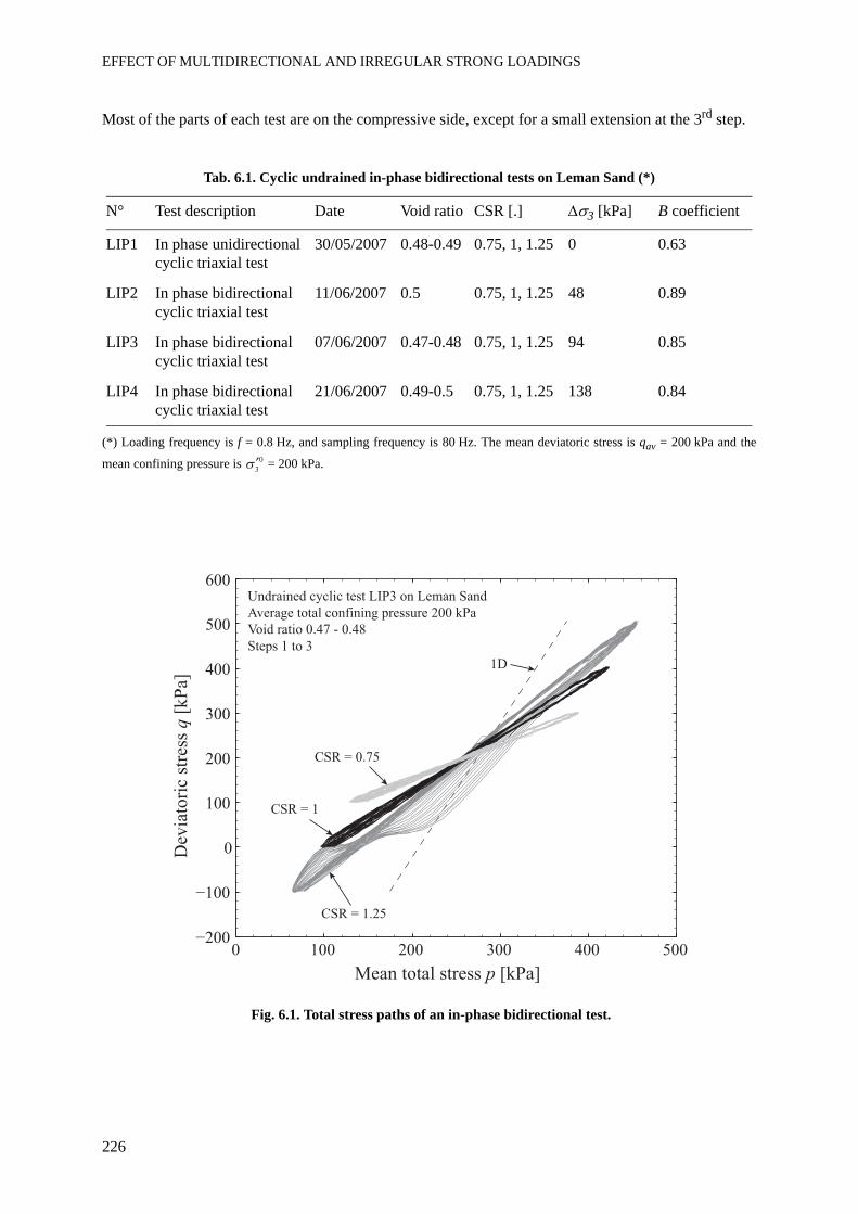
EFFECT OF MULTIDIRECTIONAL AND IRREGULAR STRONG LOADINGS
226
Most of the parts of each test are on the compressive side, except for a small extension at the 3rd step.
Tab. 6.1. Cyclic undrained in-phase bidirectional tests on Leman Sand (*)
(*) Loading frequency is f = 0.8 Hz, and sampling frequency is 80 Hz. The mean deviatoric stress is qav = 200 kPa and the
mean confining pressure is = 200 kPa.
Fig. 6.1. Total stress paths of an in-phase bidirectional test.
N° Test description Date Void ratio CSR [.] Δσ3 [kPa] B coefficient
LIP1 In phase unidirectional cyclic triaxial test
30/05/2007 0.48-0.49 0.75, 1, 1.25 0 0.63
LIP2 In phase bidirectional cyclic triaxial test
11/06/2007 0.5 0.75, 1, 1.25 48 0.89
LIP3 In phase bidirectional cyclic triaxial test
07/06/2007 0.47-0.48 0.75, 1, 1.25 94 0.85
LIP4 In phase bidirectional cyclic triaxial test
21/06/2007 0.49-0.5 0.75, 1, 1.25 138 0.84
0 100 200 300 400 500
0
100
200
300
400
500
600
Mean total stress p [kPa]
Dev
iato
ric
stre
ss q
[kP
a]
Undrained cyclic test LIP3 on Leman Sand
Average total confining pressure 200 kPa
Void ratio 0.47 - 0.48
Steps 1 to 3
CSR = 0.75
CSR = 1
CSR = 1.25
1D
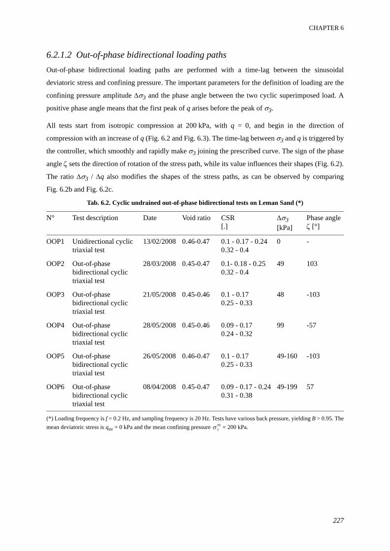
CHAPTER 6
227
6.2.1.2 Out-of-phase bidirectional loading pathsOut-of-phase bidirectional loading paths are performed with a time-lag between the sinusoidal
deviatoric stress and confining pressure. The important parameters for the definition of loading are the
confining pressure amplitude Δσ3 and the phase angle between the two cyclic superimposed load. A
positive phase angle means that the first peak of q arises before the peak of σ3.
All tests start from isotropic compression at 200 kPa, with q = 0, and begin in the direction of
compression with an increase of q (Fig. 6.2 and Fig. 6.3). The time-lag between σ3 and q is triggered by
the controller, which smoothly and rapidly make σ3 joining the prescribed curve. The sign of the phase
angle ζ sets the direction of rotation of the stress path, while its value influences their shapes (Fig. 6.2).
The ratio Δσ3 / Δq also modifies the shapes of the stress paths, as can be observed by comparing
Fig. 6.2b and Fig. 6.2c.
Tab. 6.2. Cyclic undrained out-of-phase bidirectional tests on Leman Sand (*)
(*) Loading frequency is f = 0.2 Hz, and sampling frequency is 20 Hz. Tests have various back pressure, yielding B > 0.95. Themean deviatoric stress is qav = 0 kPa and the mean confining pressure = 200 kPa.
N° Test description Date Void ratio CSR [.]
Δσ3 [kPa]
Phase angle ζ [°]
OOP1 Unidirectional cyclic triaxial test
13/02/2008 0.46-0.47 0.1 - 0.17 - 0.24 0.32 - 0.4
0 -
OOP2 Out-of-phase bidirectional cyclic triaxial test
28/03/2008 0.45-0.47 0.1- 0.18 - 0.25 0.32 - 0.4
49 103
OOP3 Out-of-phase bidirectional cyclic triaxial test
21/05/2008 0.45-0.46 0.1 - 0.170.25 - 0.33
48 -103
OOP4 Out-of-phase bidirectional cyclic triaxial test
28/05/2008 0.45-0.46 0.09 - 0.170.24 - 0.32
99 -57
OOP5 Out-of-phase bidirectional cyclic triaxial test
26/05/2008 0.46-0.47 0.1 - 0.170.25 - 0.33
49-160 -103
OOP6 Out-of-phase bidirectional cyclic triaxial test
08/04/2008 0.45-0.47 0.09 - 0.17 - 0.24 0.31 - 0.38
49-199 57
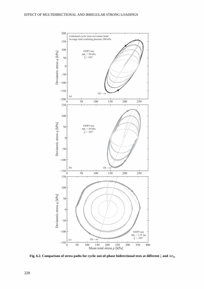
EFFECT OF MULTIDIRECTIONAL AND IRREGULAR STRONG LOADINGS
228
Fig. 6.2. Comparison of stress paths for cyclic out-of-phase bidirectional tests at different ζ and Δσ3.
0 50 100 150 200 250
0
50
100
150
Dev
iato
ric
stre
ss q
[k
Pa]
0 50 100 150 200 250 300 350 400
0
50
100
150
Mean total stress p [kPa]
Dev
iato
ric
stre
ss q
[k
Pa]
0 50 100 150 200 250
0
50
100
150
200
Dev
iato
ric
stre
ss q
[k
Pa] OOP2 test
3 = 50 kPa
= 103°
Undrained cyclic tests on Leman Sand
Average total confining pressure 200 kPa
1D
OOP3 test
3 = 50 kPa
= -103°
OOP5 test
3 = 1.25 q
= -103°(c)
(b)
(a)
1D
1D
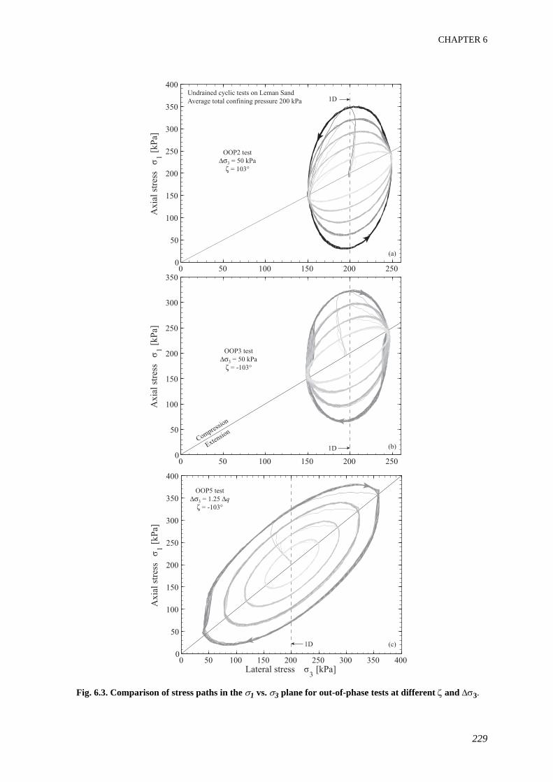
CHAPTER 6
229
Fig. 6.3. Comparison of stress paths in the σ1 vs. σ3 plane for out-of-phase tests at different ζ and Δσ3.
0 50 100 150 200 2500
50
100
150
200
250
300
350
Ax
ial
stre
ss
1 [
kP
a]
0 50 100 150 200 250 300 350 4000
50
100
150
200
250
300
350
400
Lateral stress 3 [kPa]
Ax
ial
stre
ss
1 [
kP
a]
0 50 100 150 200 2500
50
100
150
200
250
300
350
400
Ax
ial
stre
ss
1 [
kP
a]OOP2 test
3 = 50 kPa
= 103°
Undrained cyclic tests on Leman Sand
Average total confining pressure 200 kPa 1D
OOP3 test
3 = 50 kPa
= -103°
OOP5 test
3 = 1.25 q
= -103°
(c)
(b)
(a)
1D
1D
Compression
Extension
EFFECT OF MULTIDIRECTIONAL AND IRREGULAR STRONG LOADINGS
230
6.2.2 Introduction to test results
LIP1 to LIP4 tests were anisotropically consolidated, with a mean deviatoric stress of 200 kPa. Their
behaviour is quite different from the isotropically consolidated bidirectional out-of-phase tests.
However, deviatoric strain amplitudes are in the same range for all in-phase and out-of-phase tests, i.e.
from 0.03% to 3%.
The effect of the superimposed compression is described below. These observations are based on values
from the 10th and 15th cycle of each step, for anisotropic and isotropic tests respectively. As the cyclic
behaviour of sand has a strong strain dependency, it was decided to show the results as functions of
deviatoric strain amplitude.
6.2.3 Stress-strain relation
The stress-strain relation in unidirectional and bidirectional tests have similar patterns, whatever the
characteristics of the bidirectional loading. To illustrate this observation, the four first steps of tests
OOP1 and OOP5 are compared through their respective stress-strain relations (Fig. 6.4).
The following comments arise from the observation of these two tests:
• The shape of the stress-strain loops remains the same in unidirectional and bidirectional tests.
• For the four deviatoric stress amplitudes, there is more strain in extension in bidirectional tests.
• The development of cyclic liquefaction is faster in the bidirectional test.
• A fifth step is needed to reach failure in the unidirectional test.
6.2.4 Deviatoric strain amplitude
To compare the stress-strain relations in all multidimensional tests, the deviatoric stress amplitude vs.
deviatoric strain amplitude is presented in Fig. 6.5. There is no large effect of the bidirectional in-phase
loading (Fig. 6.5a), if we accept a small scattering due to soil variability. Out-of-phase bidirectional
tests are slightly different from OOP1 (Fig. 6.5b).
Compared to the strain induced by unidirectional cyclic loading, the induced deviatoric strain of the
bidirectional tests is first equivalent at 40 kPa, then lower at 70 and 100 kPa, then higher at 130 kPa and
again lower at larger Δq. Three different overall shapes can be distinguished in Fig. 6.5b. The stress-
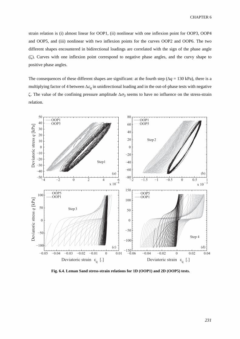
CHAPTER 6
231
strain relation is (i) almost linear for OOP1, (ii) nonlinear with one inflexion point for OOP3, OOP4
and OOP5, and (iii) nonlinear with two inflexion points for the curves OOP2 and OOP6. The two
different shapes encountered in bidirectional loadings are correlated with the sign of the phase angle
(ζ). Curves with one inflexion point correspond to negative phase angles, and the curvy shape to
positive phase angles.
The consequences of these different shapes are significant: at the fourth step (Δq = 130 kPa), there is a
multiplying factor of 4 between Δεq in unidirectional loading and in the out-of-phase tests with negative
ζ. The value of the confining pressure amplitude Δσ3 seems to have no influence on the stress-strain
relation.
Fig. 6.4. Leman Sand stress-strain relations for 1D (OOP1) and 2D (OOP5) tests.
0 6
x 10
50
30
10
0
10
30
50
Dev
iato
ric
stre
ss q
[kP
a]
OOP1OOP5
Step1
0 1
x 103
80
60
0
60
80OOP1OOP5
Step
0
0
50
100
Dev
iato
ric
stre
ss q
[kP
a]
Deviatoric strain q
OOP5OOP1
Step3
0
0
50
100
150
Deviatoric strain q
OOP5OOP1
Step
(a) (b)
(c) (d)
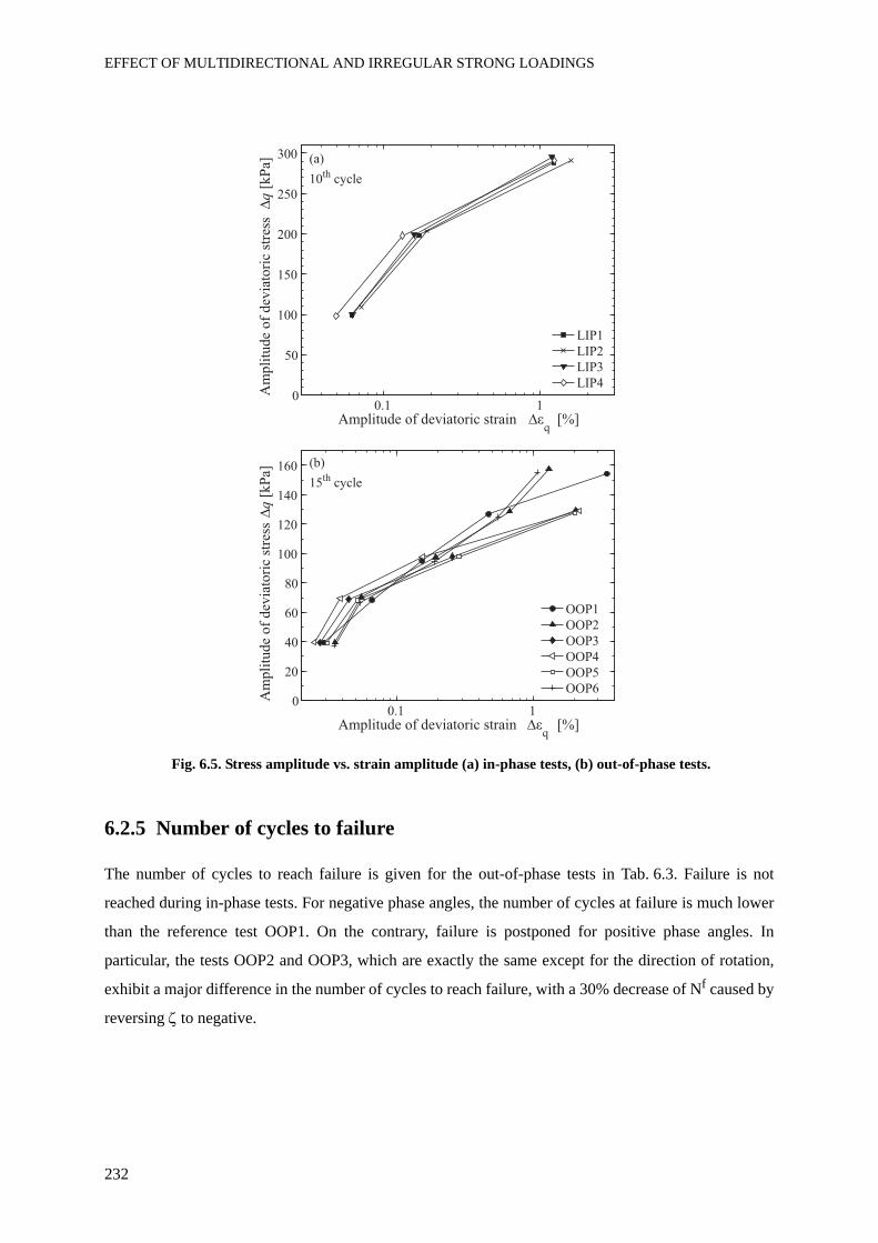
EFFECT OF MULTIDIRECTIONAL AND IRREGULAR STRONG LOADINGS
232
Fig. 6.5. Stress amplitude vs. strain amplitude (a) in-phase tests, (b) out-of-phase tests.
6.2.5 Number of cycles to failure
The number of cycles to reach failure is given for the out-of-phase tests in Tab. 6.3. Failure is not
reached during in-phase tests. For negative phase angles, the number of cycles at failure is much lower
than the reference test OOP1. On the contrary, failure is postponed for positive phase angles. In
particular, the tests OOP2 and OOP3, which are exactly the same except for the direction of rotation,
exhibit a major difference in the number of cycles to reach failure, with a 30% decrease of Nf caused by
reversing ζ to negative.
0.1 10
20
40
60
80
100
120
140
160
Amplitude of deviatoric strain q
[%]
Am
pli
tude
of
dev
iato
ric
stre
ss
q [
kP
a]
OOP1
OOP2
OOP3
OOP4
OOP5
OOP6
0.1 10
50
100
150
200
250
300
Amplitude of deviatoric strain q
[%]
Am
pli
tude
of
dev
iato
ric
stre
ss
q [
kP
a]
LIP1
LIP2
LIP3
LIP4
(a)
(b)
10th cycle
15th cycle
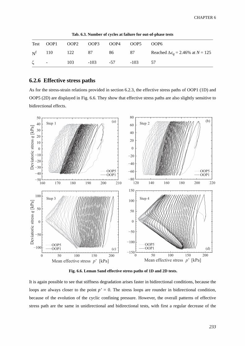
CHAPTER 6
233
Tab. 6.3. Number of cycles at failure for out-of-phase tests
6.2.6 Effective stress pathsAs for the stress-strain relations provided in section 6.2.3, the effective stress paths of OOP1 (1D) and
OOP5 (2D) are displayed in Fig. 6.6. They show that effective stress paths are also slightly sensitive to
bidirectional effects.
Fig. 6.6. Leman Sand effective stress paths of 1D and 2D tests.
It is again possible to see that stiffness degradation arises faster in bidirectional conditions, because the
loops are always closer to the point p’ = 0. The stress loops are rounder in bidirectional condition,
because of the evolution of the cyclic confining pressure. However, the overall patterns of effective
stress path are the same in unidirectional and bidirectional tests, with first a regular decrease of the
Test OOP1 OOP2 OOP3 OOP4 OOP5 OOP6
Nf 110 122 87 86 87 Reached Δεq = 2.46% at N = 125
ζ - 103 -103 -57 -103 57
0 50 100 150 200
0
50
100
150
Mean effective stress p’ [kPa]
OOP5OOP1
Step 4
160 170 180 190 200 210
0
10
20
40
50
Dev
iato
ric
stre
ss q
[kP
a]
OOP5OOP1
Step 1
120 140 160 180 200 220
0
20
40
60
80
OOP5OOP1
Step 2
0 50 100 150 200
0
50
100
Dev
iato
ric
stre
ss q
[kP
a]
Mean effective stress p’ [kPa]
OOP5OOP1
Step
(a) (b)
(c) (d)
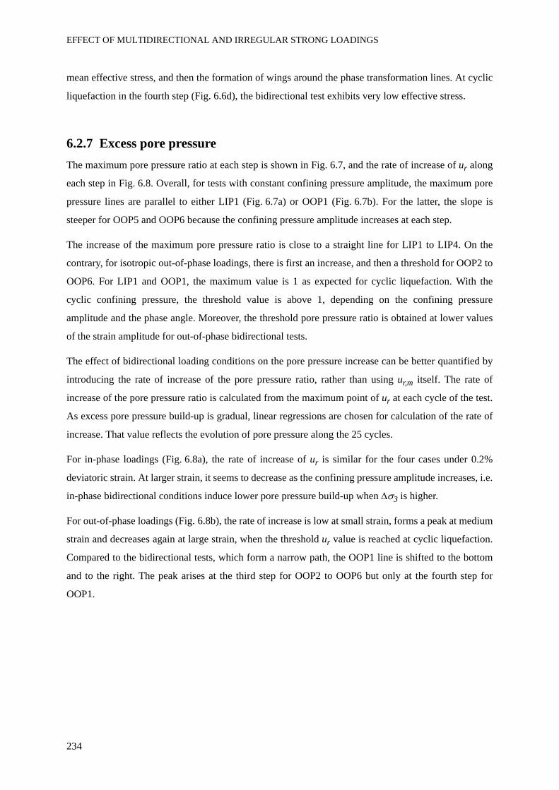
EFFECT OF MULTIDIRECTIONAL AND IRREGULAR STRONG LOADINGS
234
mean effective stress, and then the formation of wings around the phase transformation lines. At cyclic
liquefaction in the fourth step (Fig. 6.6d), the bidirectional test exhibits very low effective stress.
6.2.7 Excess pore pressureThe maximum pore pressure ratio at each step is shown in Fig. 6.7, and the rate of increase of ur along
each step in Fig. 6.8. Overall, for tests with constant confining pressure amplitude, the maximum pore
pressure lines are parallel to either LIP1 (Fig. 6.7a) or OOP1 (Fig. 6.7b). For the latter, the slope is
steeper for OOP5 and OOP6 because the confining pressure amplitude increases at each step.
The increase of the maximum pore pressure ratio is close to a straight line for LIP1 to LIP4. On the
contrary, for isotropic out-of-phase loadings, there is first an increase, and then a threshold for OOP2 to
OOP6. For LIP1 and OOP1, the maximum value is 1 as expected for cyclic liquefaction. With the
cyclic confining pressure, the threshold value is above 1, depending on the confining pressure
amplitude and the phase angle. Moreover, the threshold pore pressure ratio is obtained at lower values
of the strain amplitude for out-of-phase bidirectional tests.
The effect of bidirectional loading conditions on the pore pressure increase can be better quantified by
introducing the rate of increase of the pore pressure ratio, rather than using ur,m itself. The rate of
increase of the pore pressure ratio is calculated from the maximum point of ur at each cycle of the test.
As excess pore pressure build-up is gradual, linear regressions are chosen for calculation of the rate of
increase. That value reflects the evolution of pore pressure along the 25 cycles.
For in-phase loadings (Fig. 6.8a), the rate of increase of ur is similar for the four cases under 0.2%
deviatoric strain. At larger strain, it seems to decrease as the confining pressure amplitude increases, i.e.
in-phase bidirectional conditions induce lower pore pressure build-up when Δσ3 is higher.
For out-of-phase loadings (Fig. 6.8b), the rate of increase is low at small strain, forms a peak at medium
strain and decreases again at large strain, when the threshold ur value is reached at cyclic liquefaction.
Compared to the bidirectional tests, which form a narrow path, the OOP1 line is shifted to the bottom
and to the right. The peak arises at the third step for OOP2 to OOP6 but only at the fourth step for
OOP1.
CHAPTER 6
235
Fig. 6.7. Pore pressure ratio vs. deviatoric strain amplitude (a) in-phase tests, (b) out-of-phase tests.
This difference involves that the rate of pore pressure increase is stronger in bidirectional out-of-phase
conditions before the occurrence of cyclic liquefaction, which thus arises faster in 2D tests than in the
1D test. Moreover, the maximum pore pressure build-up is reached at lower strain amplitudes in
bidirectional conditions. This means that the coupling of strains and pore pressures may be influenced
by bidirectional loading conditions.
Among the out-of-phase bidirectional tests, the higher values of the rate of increase of ur are obtained
for negative phase angles. The amplitude of the confining pressure is also important. For example, at
the same phase angle ζ = -103°, the peak rate increases by 10% between OOP3 and OOP5, performed
at 50 kPa and 125 kPa confining pressure amplitude, respectively.
These analyses show that bidirectional effects on the pore pressure build-up depend on the phase angle
and the cyclic stress amplitudes, Δσ3 and Δq.
0.1 10
0.5
1
1.5
2
Max
imum
pore
pre
ssure
rat
io
u r,m
[.]
Amplitude of deviatoric strain q
[%]
OOP1
OOP2
OOP3
OOP4
OOP5
OOP6
0.1 10
0.5
1
1.5
Max
imum
pore
pre
ssure
rat
io
ur,
m [
.]
Amplitude of deviatoric strain q
[%]
LIP1
LIP2
LIP3
LIP4
(a)
(b)
10th cycle
15th cycle
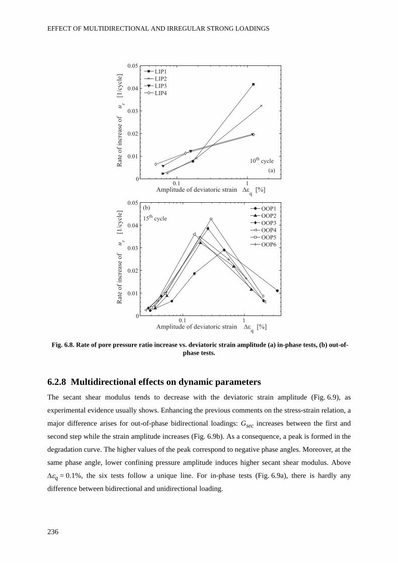
EFFECT OF MULTIDIRECTIONAL AND IRREGULAR STRONG LOADINGS
236
Fig. 6.8. Rate of pore pressure ratio increase vs. deviatoric strain amplitude (a) in-phase tests, (b) out-of-phase tests.
6.2.8 Multidirectional effects on dynamic parametersThe secant shear modulus tends to decrease with the deviatoric strain amplitude (Fig. 6.9), as
experimental evidence usually shows. Enhancing the previous comments on the stress-strain relation, a
major difference arises for out-of-phase bidirectional loadings: Gsec increases between the first and
second step while the strain amplitude increases (Fig. 6.9b). As a consequence, a peak is formed in the
degradation curve. The higher values of the peak correspond to negative phase angles. Moreover, at the
same phase angle, lower confining pressure amplitude induces higher secant shear modulus. Above
Δεq = 0.1%, the six tests follow a unique line. For in-phase tests (Fig. 6.9a), there is hardly any
difference between bidirectional and unidirectional loading.
0.1 10
0.01
0.02
0.03
0.04
0.05
Rat
e of
incr
ease
of
ur
[1/c
ycl
e]
Amplitude of deviatoric strain q
[%]
OOP1
OOP2
OOP3
OOP4
OOP5
OOP6
0.1 10
0.01
0.02
0.03
0.04
0.05
Rat
e of
incr
ease
of
ur
[1/c
ycl
e]
Amplitude of deviatoric strain q
[%]
LIP1
LIP2
LIP3
LIP4
(a)
(b)
10th cycle
15th cycle
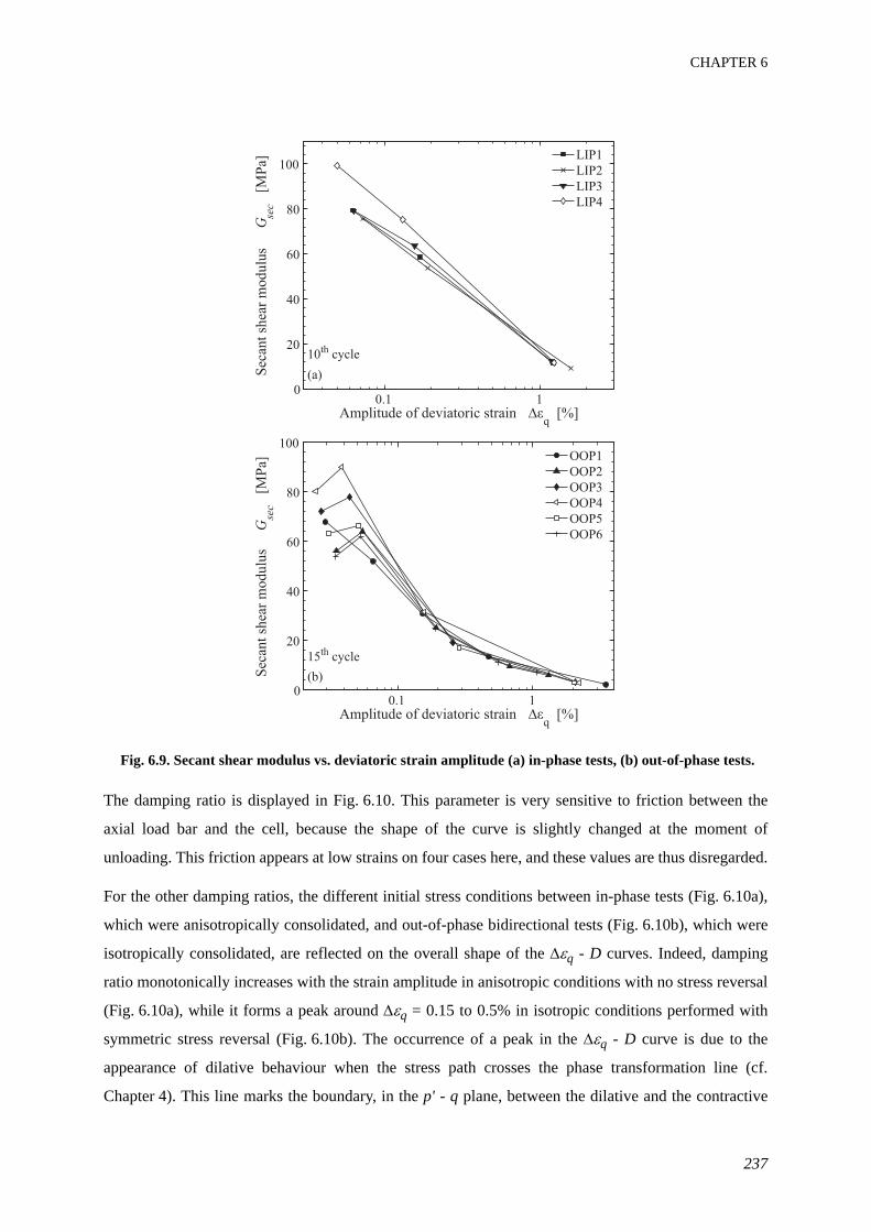
CHAPTER 6
237
Fig. 6.9. Secant shear modulus vs. deviatoric strain amplitude (a) in-phase tests, (b) out-of-phase tests.
The damping ratio is displayed in Fig. 6.10. This parameter is very sensitive to friction between the
axial load bar and the cell, because the shape of the curve is slightly changed at the moment of
unloading. This friction appears at low strains on four cases here, and these values are thus disregarded.
For the other damping ratios, the different initial stress conditions between in-phase tests (Fig. 6.10a),
which were anisotropically consolidated, and out-of-phase bidirectional tests (Fig. 6.10b), which were
isotropically consolidated, are reflected on the overall shape of the Δεq - D curves. Indeed, damping
ratio monotonically increases with the strain amplitude in anisotropic conditions with no stress reversal
(Fig. 6.10a), while it forms a peak around Δεq = 0.15 to 0.5% in isotropic conditions performed with
symmetric stress reversal (Fig. 6.10b). The occurrence of a peak in the Δεq - D curve is due to the
appearance of dilative behaviour when the stress path crosses the phase transformation line (cf.
Chapter 4). This line marks the boundary, in the p' - q plane, between the dilative and the contractive
0.1 10
20
40
60
80
100
Sec
ant
shea
r m
odulu
s G
sec
[M
Pa]
Amplitude of deviatoric strain q
[%]
OOP1
OOP2
OOP3
OOP4
OOP5
OOP6
0.1 10
20
40
60
80
100
Sec
ant
shea
r m
odulu
s G
sec
[M
Pa]
Amplitude of deviatoric strain q
[%]
LIP1
LIP2
LIP3
LIP4
(a)
(b)
10th cycle
15th cycle
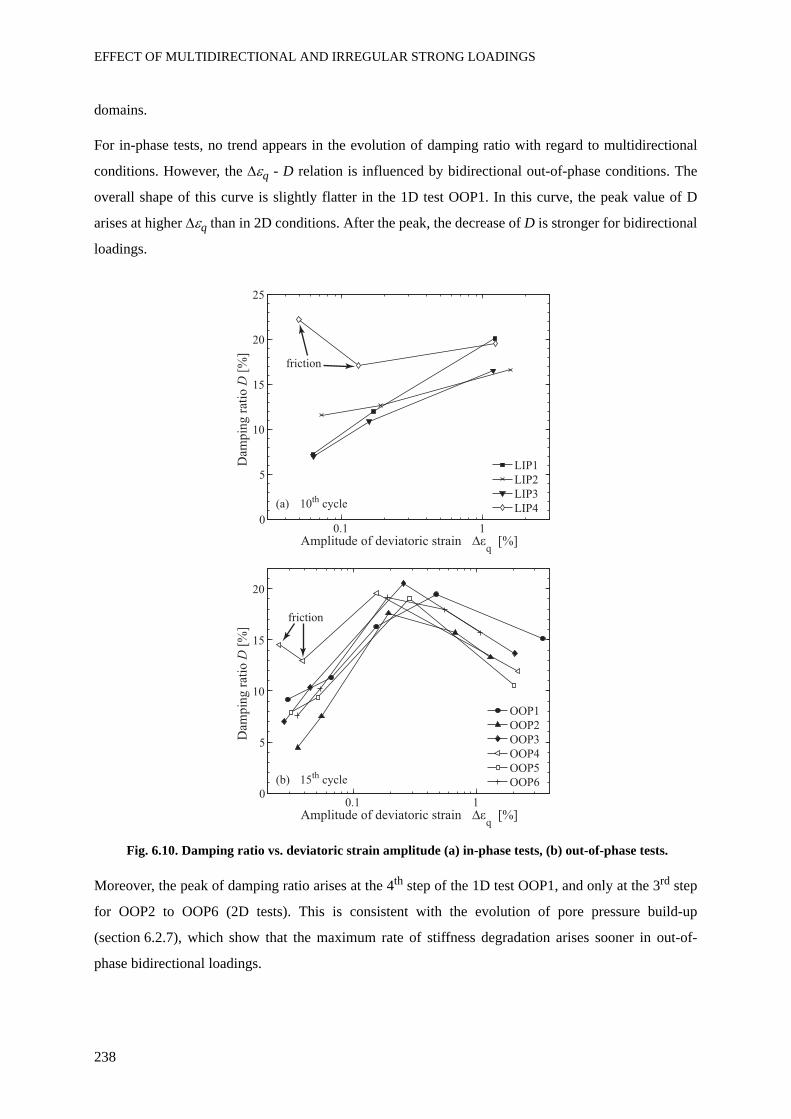
EFFECT OF MULTIDIRECTIONAL AND IRREGULAR STRONG LOADINGS
238
domains.
For in-phase tests, no trend appears in the evolution of damping ratio with regard to multidirectional
conditions. However, the Δεq - D relation is influenced by bidirectional out-of-phase conditions. The
overall shape of this curve is slightly flatter in the 1D test OOP1. In this curve, the peak value of D
arises at higher Δεq than in 2D conditions. After the peak, the decrease of D is stronger for bidirectional
loadings.
Fig. 6.10. Damping ratio vs. deviatoric strain amplitude (a) in-phase tests, (b) out-of-phase tests.
Moreover, the peak of damping ratio arises at the 4th step of the 1D test OOP1, and only at the 3rd step
for OOP2 to OOP6 (2D tests). This is consistent with the evolution of pore pressure build-up
(section 6.2.7), which show that the maximum rate of stiffness degradation arises sooner in out-of-
phase bidirectional loadings.
0.1 10
5
10
15
20
Dam
pin
g r
atio
D [
%]
Amplitude of deviatoric strain q
[%]
OOP1
OOP2
OOP3
OOP4
OOP5
OOP6
0.1 10
5
10
15
20
25
Dam
pin
g r
atio
D [
%]
Amplitude of deviatoric strain q
[%]
LIP1
LIP2
LIP3
LIP4(a)
(b)
10th cycle
15th cycle
friction
friction
CHAPTER 6
239
6.2.9 Analyses of multidirectional effectsThe comparison between unidirectional deviatoric cyclic tests and cyclic tests with superimposed
confining and deviatoric stresses proves that superposition of the two loadings has an influence on
undrained saturated sand behaviour.
6.2.9.1 Concerning pore pressuresFirst the theoretical evaluation of the effect of the cyclic confining stress alone is developed. In order to
account for the change in applied total confining pressure, the pore pressure ratio is decomposed into
two parts: .
We assume that the cyclic compression (sinusoidal variation of σ3, with a mean value ) of the
saturated granular medium results in a cyclic pore pressure centred on its initial value, which is zero in
our tests, with the same amplitude as the cyclic confining pressure. This gives a theoretical pore
pressure variation resulting from the cyclic confining pressure .
On the other hand, the B-Skempton coefficient, which is calculated for each test, reaches approximately
0.96. Indeed, this dense sand has a high stiffness, thus B = 1 cannot be reached (Head 1984). To account
for the compressibility of the pore fluid of each individual sample, which is usually neglected although
it might not be exactly the same in all cases, the correction factor B is introduced within the theoretical
pore pressure ratio resulting from the isotropic load, defined as:
(6.2)
In 1D tests, is always equal to zero. The pore pressure ratio ur thus reflects only the hydro-
mechanical coupling. For 2D tests, the part of the pore pressure ratio related to the cyclic confining
pressure, , is added to the true pore pressure variations resulting from the soil tendency to dilate
and contract, which we choose to call . The notion of total pore pressure (ur) is thus not equivalent in
1D and 2D tests, this is why ur can reach values higher than 1 in bidirectional tests. The parameter
is thus introduced for 2D tests, to allow the comparison of excess pore pressure components resulting
only from the deviatoric stress. The relation is explicitly:
(6.3)
Thanks to this decomposition of the pore pressure ratio into two parts which takes into account the
change of total applied stress path, the actual pore pressure increase due to cyclic loading, , can thus
be carefully analysed. Moreover, the pore fluid compressibility is also taken into account by including
the B-Skempton coefficient into the component of isotropic loading. We thus ensure that is
u u ur r
comp
r
q
3
0
u 3 3
0
uB
r
comp 3 3
0
3
0
ur
comp
ur
comp
ur
q
ur
q
u u ur
q
r r
comp
ur
q
ur
q
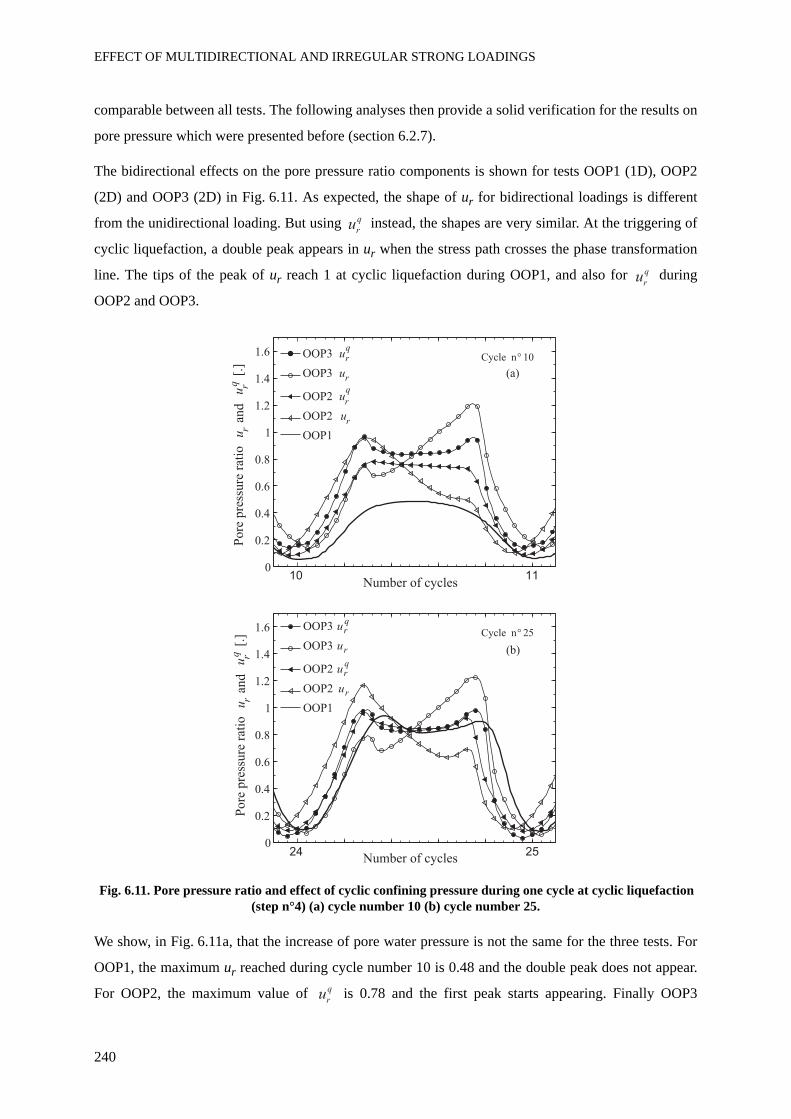
EFFECT OF MULTIDIRECTIONAL AND IRREGULAR STRONG LOADINGS
240
comparable between all tests. The following analyses then provide a solid verification for the results on
pore pressure which were presented before (section 6.2.7).
The bidirectional effects on the pore pressure ratio components is shown for tests OOP1 (1D), OOP2
(2D) and OOP3 (2D) in Fig. 6.11. As expected, the shape of ur for bidirectional loadings is different
from the unidirectional loading. But using instead, the shapes are very similar. At the triggering of
cyclic liquefaction, a double peak appears in ur when the stress path crosses the phase transformation
line. The tips of the peak of ur reach 1 at cyclic liquefaction during OOP1, and also for during
OOP2 and OOP3.
Fig. 6.11. Pore pressure ratio and effect of cyclic confining pressure during one cycle at cyclic liquefaction (step n°4) (a) cycle number 10 (b) cycle number 25.
We show, in Fig. 6.11a, that the increase of pore water pressure is not the same for the three tests. For
OOP1, the maximum ur reached during cycle number 10 is 0.48 and the double peak does not appear.
For OOP2, the maximum value of is 0.78 and the first peak starts appearing. Finally OOP3
ur
q
ur
q
0
0.2
0.4
0.6
0.8
1
1.2
1.4
1.6
Number of cycles
Cycle n° 25
0
0.2
0.4
0.6
0.8
1
1.2
1.4
1.6
Pore
pre
ssure
rat
io
u r [
.]
Number of cycles
OOP3 urq
OOP3 ur
OOP2 ur
OOP2 ur
OOP1
Cycle n° 10
(a)
(b)
10 11
24 25
OOP3 urq
OOP3 ur
OOP2 urq
OOP2 ur
OOP1
qu ran
dq
Pore
pre
ssure
rat
io
u r [
.]u r
and
q
ur
q
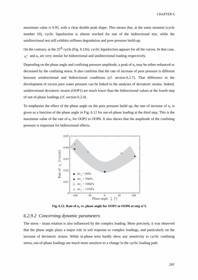
CHAPTER 6
241
maximum value is 0.95, with a clear double peak shape. This means that, at the same moment (cycle
number 10), cyclic liquefaction is almost reached for one of the bidirectional test, while the
unidirectional test still exhibits stiffness degradation and pore pressure build-up.
On the contrary, at the 25th cycle (Fig. 6.11b), cyclic liquefaction appears for all the curves. In that case,
and ur are very similar for bidirectional and unidirectional loading respectively.
Depending on the phase angle and confining pressure amplitude, a peak of ur may be either enhanced or
decreased by the confining stress. It also confirms that the rate of increase of pore pressure is different
between unidirectional and bidirectional conditions (cf. section 6.2.7). That difference in the
development of excess pore water pressure can be linked to the analyses of deviatoric strains. Indeed,
unidirectional deviatoric strains (OOP1) are much lower than the bidirectional values at the fourth step
of out-of-phase loadings (cf. section 6.2.4).
To emphasize the effect of the phase angle on the pore pressure build up, the rate of increase of ur is
given as a function of the phase angle in Fig. 6.12 for out-of-phase loading at the third step. This is the
maximum value of the rate of ur for OOP2 to OOP6. It also shows that the amplitude of the confining
pressure is important for bidirectional effects.
Fig. 6.12. Rate of ur vs. phase angle for OOP1 to OOP6 at step n°3.
6.2.9.2 Concerning dynamic parametersThe stress - strain relation is also influenced by the complex loading. More precisely, it was observed
that the phase angle plays a major role in soil response to complex loadings, and particularly on the
increase of deviatoric strains. While in-phase tests hardly show any sensitivity to cyclic confining
stress, out-of-phase loadings are much more sensitive to a change in the cyclic loading path.
ur
q
Rat
e of
u r
[°
EFFECT OF MULTIDIRECTIONAL AND IRREGULAR STRONG LOADINGS
242
This dependency arises at different strain levels. For the secant shear modulus, the main feature is a
peak, close to 0.03%, in the secant shear modulus degradation curve, which is also reflected in the
stress-strain relation. Out-of-phase bidirectional tests are stiffer at the second loading step. On the
contrary, at the fourth loading step, and at a strain range from 0.5% to 2%, the unidirectional loading is
stiffer than complex ones. At this strain level, however, the Δεq - Gsec curve shape is not influenced.
The Δεq - D relation, on the other hand, also depends on bidirectional effects. The main consequence of
the superposition of loadings is the occurrence of the peak in the evolution of the damping ratio, which
arises at smaller strains during out-of-phase bidirectional tests.
6.2.9.3 Interpretation of coupling effectsAs shown in the total stress paths (Fig. 6.3), all tests, whether unidirectional or bidirectional, start with
compression. The extension phase then arises, either on the left or on the right of the 1D line, depending
on the sign of the phase angle. The increase of the rate of stiffness degradation with negative phase
angles is thus due to the direction of rotation of the stress path.
As shown in Fig. 6.11a during the 10th cycle (step n°4), when the rate of pore pressure increase is at its
maximum, i.e. stiffness degradation also, ur has a strong negative pore pressure second peak in OOP3.
This is because the maximum value of σ3 arises at the moment of that second peak. We then assume
that the amplification of the soil response, during stiffness degradation and for negative phase angles, is
related to the timing of dilative and contractive volumetric parts of the motion with regard to the
evolution of the total confining pressure. If σ3 is high during phase transformation at unloading, as
shown for OOP3, the second spike of ur is emphasized.
This can be related to the amplification of deviatoric strain amplitude, at that step, for negative phase
angles (Fig. 6.5): Δεq = 0.5%, 0.7% and 2.1% for OOP1 (1D), OOP2 (ζ > 0) and OOP3 (ζ < 0)
respectively (15th cycle). The three other bidirectional tests also confirm this amplification of deviatoric
strains for negative phase angles. The coupling between the pore pressure and the deviatoric strain may
then play an important role in the amplification of stiffness degradation in certain conditions of
complex loading.
6.2.10 ConclusionsTo conclude, the coupling effect due to superposition of a cyclic deviatoric and confining stress is
complex, even if both are at the same frequency. The coupling mainly depends on the phase angle. The
stress path and strain level are also important for the extent of the effect. The most important conclusion
from the tests is that the triggering of cyclic liquefaction may happen earlier with the bidirectional
loading in certain conditions. The development of pore water pressure, of deviatoric strain and the
CHAPTER 6
243
degradation of the secant shear modulus are faster for OOP2 to OOP6. The peak in the damping ratio
arises sooner. Failure triggering is slower for bidirectional tests with a positive phase angle, i.e. the
development of large deviatoric strain amplitude is decreased in part of the bidirectional tests. On the
contrary, failure arises much sooner for all bidirectional tests with a negative phase angle.
6.3 Irregular seismic loading in multidirectional condition
6.3.1 Description of irregular loadings with a seismic signalReal earthquake acceleration recordings, obtained at the ground surface, are used to design the irregular
signals given as input loading of varying amplitude and frequency content. As for the previous 2D
experiments, two irregular loadings are superimposed on the principal directions σ1 and σ3. The
seismic recording was obtained at 82 km of the earthquake epicentre, for an earthquake of moment
magnitude of 6.5 (San Simeon earthquake, California, December 22nd 2003, acceleration recording
data provided by COSMOS Virtual Data Center http://db.cosmos-eq.org/scripts/default.plx). These
conditions do not correspond to in situ nonlinear behaviour. The seismic event was chosen anyway,
because the rather large peak ground acceleration (PGA) of the vertical recording, once treated, gave
interestingly large variations of the confining pressure.
Assuming initial stress isotropy, the imposed irregular functions q(t) and σ3(t) (Fig. 6.13) are calculated
from an elastic inverse analysis and a scaling of the original seismic recording, to obtain loadings in the
nonlinear regime. The process used to obtain the functions q(t) and σ3(t) is described in Appendix 2.
The aim of these tests is not to realistically reproduce the in situ response, but rather to evaluate the
effect of bidirectional loading on sand response for an irregular signal representative of a seismic
loading. The signal is representative of the bidirectional stress field at 10 m depth, in the middle of a
thick Leman Sand layer. Arbitrarily, the maximum deviatoric stress, equivalent to the peak ground
acceleration (PGA) at the surface, arises on the side of extension on the time-history of q.
The Fourier spectrum of both functions are also provided below (Fig. 6.14).
From the time-history of stresses at the desired depth (Fig. 6.13), three irregular tests were performed in
different conditions (Tab. 6.4). Two parameters are introduced to characterize the irregular motion.
CSREQ is the maximum amplitude of the cyclic stress ratio (defined in Eq. 2.20 for cyclic loading),
while is the maximum amplitude of confining pressure. They are both expressed as relative
values compared to the initial stress.3
EQ
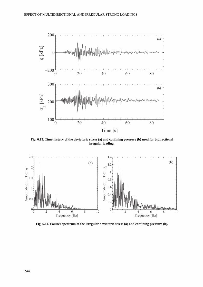
EFFECT OF MULTIDIRECTIONAL AND IRREGULAR STRONG LOADINGS
244
Fig. 6.13. Time-history of the deviatoric stress (a) and confining pressure (b) used for bidirectional irregular loading.
Fig. 6.14. Fourier spectrum of the irregular deviatoric stress (a) and confining pressure (b).
0 20 40 60 80
0
200
q [
kP
a]
0 20 40 60 80100
200
300
3 [
kP
a]
Time [s]
(a)
(b)
0 2 4 6 8 100
0.5
1
1.5
2
2.5
Am
pli
tud
e o
f F
FT
of
q
Frequency [Hz]
(a)
0 2 4 6 8 100
0.2
0.4
0.6
0.8
1
1.2
1.4
Am
pli
tud
e o
f F
FT
of
3
Frequency [Hz]
(b)
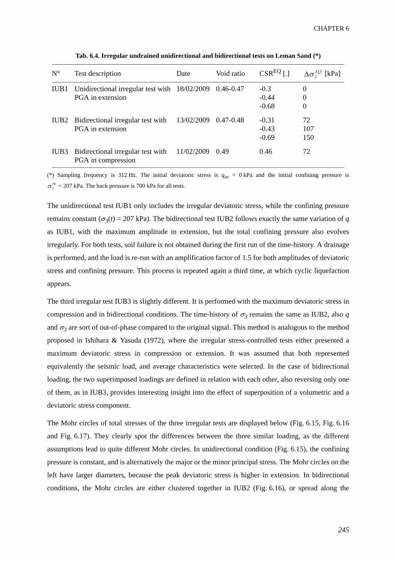
CHAPTER 6
245
Tab. 6.4. Irregular undrained unidirectional and bidirectional tests on Leman Sand (*)
(*) Sampling frequency is 312 Hz. The initial deviatoric stress is qav = 0 kPa and the initial confining pressure is
= 207 kPa. The back pressure is 700 kPa for all tests.
The unidirectional test IUB1 only includes the irregular deviatoric stress, while the confining pressure
remains constant (σ3(t) = 207 kPa). The bidirectional test IUB2 follows exactly the same variation of q
as IUB1, with the maximum amplitude in extension, but the total confining pressure also evolves
irregularly. For both tests, soil failure is not obtained during the first run of the time-history. A drainage
is performed, and the load is re-run with an amplification factor of 1.5 for both amplitudes of deviatoric
stress and confining pressure. This process is repeated again a third time, at which cyclic liquefaction
appears.
The third irregular test IUB3 is slightly different. It is performed with the maximum deviatoric stress in
compression and in bidirectional conditions. The time-history of σ3 remains the same as IUB2, also q
and σ3 are sort of out-of-phase compared to the original signal. This method is analogous to the method
proposed in Ishihara & Yasuda (1972), where the irregular stress-controlled tests either presented a
maximum deviatoric stress in compression or extension. It was assumed that both represented
equivalently the seismic load, and average characteristics were selected. In the case of bidirectional
loading, the two superimposed loadings are defined in relation with each other, also reversing only one
of them, as in IUB3, provides interesting insight into the effect of superposition of a volumetric and a
deviatoric stress component.
The Mohr circles of total stresses of the three irregular tests are displayed below (Fig. 6.15, Fig. 6.16
and Fig. 6.17). They clearly spot the differences between the three similar loading, as the different
assumptions lead to quite different Mohr circles. In unidirectional condition (Fig. 6.15), the confining
pressure is constant, and is alternatively the major or the minor principal stress. The Mohr circles on the
left have larger diameters, because the peak deviatoric stress is higher in extension. In bidirectional
conditions, the Mohr circles are either clustered together in IUB2 (Fig. 6.16), or spread along the
N° Test description Date Void ratio CSREQ [.] [kPa]
IUB1 Unidirectional irregular test with PGA in extension
18/02/2009 0.46-0.47 -0.3-0.44-0.68
000
IUB2 Bidirectional irregular test with PGA in extension
13/02/2009 0.47-0.48 -0.31-0.43-0.69
72107150
IUB3 Bidirectional irregular test with PGA in compression
11/02/2009 0.49 0.46 72
3
EQ
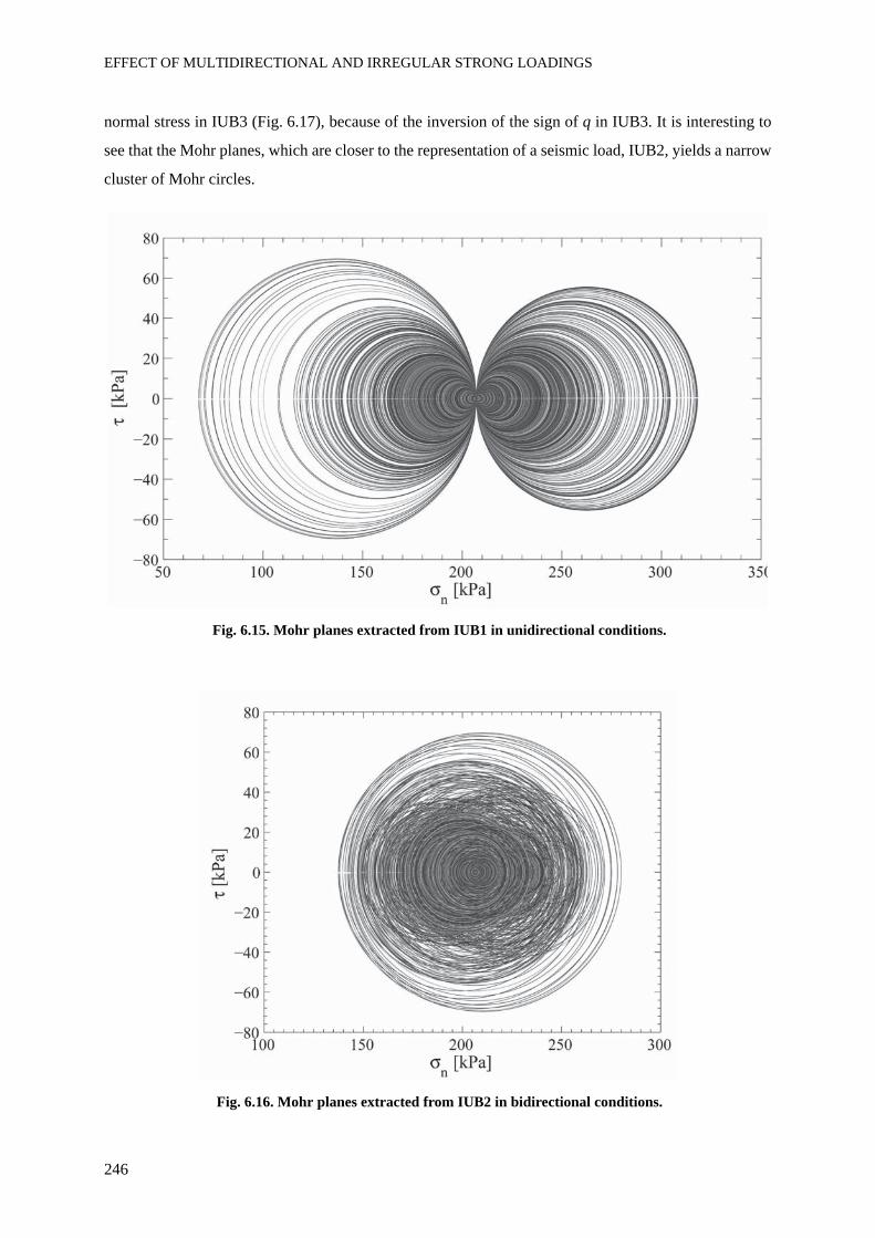
EFFECT OF MULTIDIRECTIONAL AND IRREGULAR STRONG LOADINGS
246
normal stress in IUB3 (Fig. 6.17), because of the inversion of the sign of q in IUB3. It is interesting to
see that the Mohr planes, which are closer to the representation of a seismic load, IUB2, yields a narrow
cluster of Mohr circles.
Fig. 6.15. Mohr planes extracted from IUB1 in unidirectional conditions.
Fig. 6.16. Mohr planes extracted from IUB2 in bidirectional conditions.
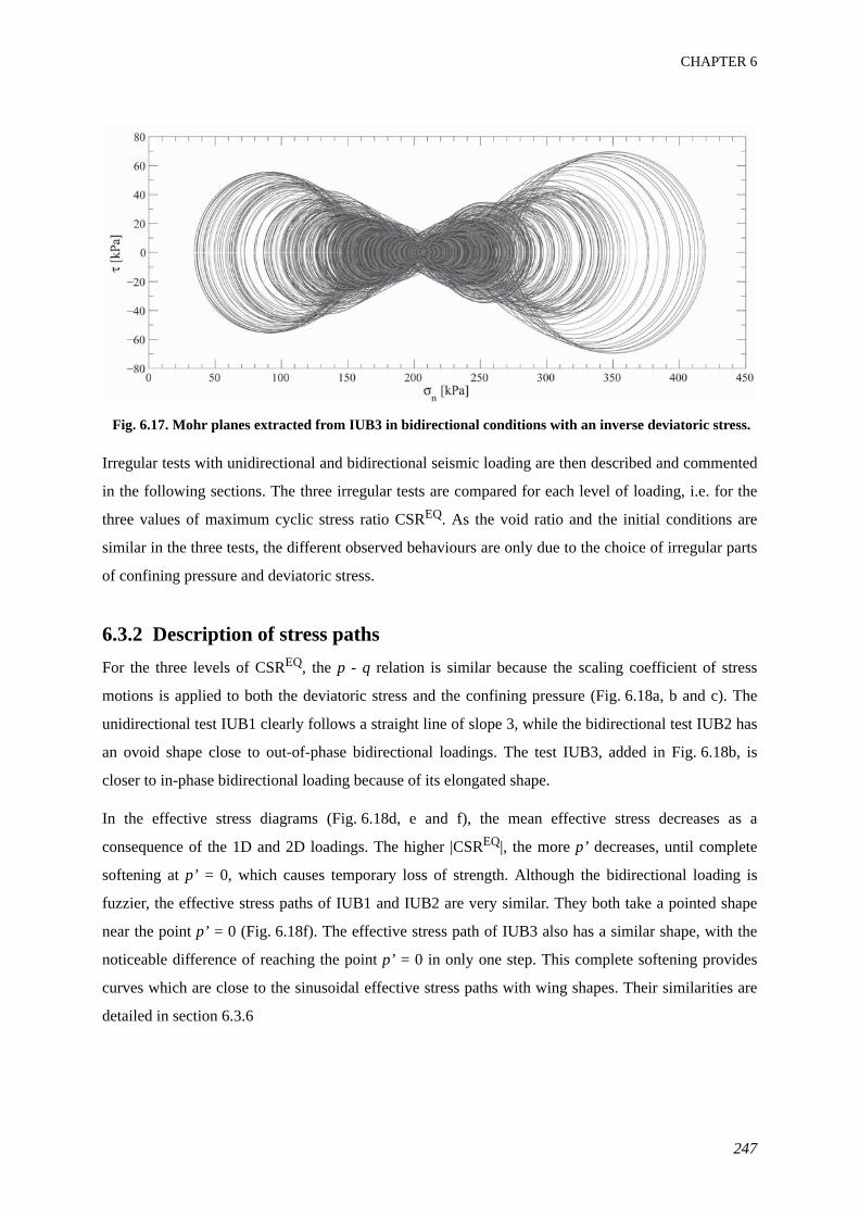
CHAPTER 6
247
Fig. 6.17. Mohr planes extracted from IUB3 in bidirectional conditions with an inverse deviatoric stress.
Irregular tests with unidirectional and bidirectional seismic loading are then described and commented
in the following sections. The three irregular tests are compared for each level of loading, i.e. for the
three values of maximum cyclic stress ratio CSREQ. As the void ratio and the initial conditions are
similar in the three tests, the different observed behaviours are only due to the choice of irregular parts
of confining pressure and deviatoric stress.
6.3.2 Description of stress pathsFor the three levels of CSREQ, the p - q relation is similar because the scaling coefficient of stress
motions is applied to both the deviatoric stress and the confining pressure (Fig. 6.18a, b and c). The
unidirectional test IUB1 clearly follows a straight line of slope 3, while the bidirectional test IUB2 has
an ovoid shape close to out-of-phase bidirectional loadings. The test IUB3, added in Fig. 6.18b, is
closer to in-phase bidirectional loading because of its elongated shape.
In the effective stress diagrams (Fig. 6.18d, e and f), the mean effective stress decreases as a
consequence of the 1D and 2D loadings. The higher |CSREQ|, the more p’ decreases, until complete
softening at p’ = 0, which causes temporary loss of strength. Although the bidirectional loading is
fuzzier, the effective stress paths of IUB1 and IUB2 are very similar. They both take a pointed shape
near the point p’ = 0 (Fig. 6.18f). The effective stress path of IUB3 also has a similar shape, with the
noticeable difference of reaching the point p’ = 0 in only one step. This complete softening provides
curves which are close to the sinusoidal effective stress paths with wing shapes. Their similarities are
detailed in section 6.3.6
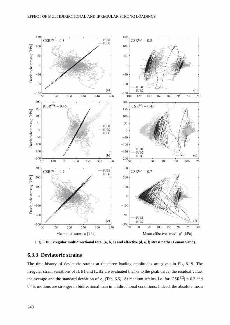
EFFECT OF MULTIDIRECTIONAL AND IRREGULAR STRONG LOADINGS
248
Fig. 6.18. Irregular multidirectional total (a, b, c) and effective (d, e, f) stress paths (Leman Sand).
6.3.3 Deviatoric strainsThe time-history of deviatoric strains at the three loading amplitudes are given in Fig. 6.19. The
irregular strain variations of IUB1 and IUB2 are evaluated thanks to the peak value, the residual value,
the average and the standard deviation of εq (Tab. 6.5). At medium strains, i.e. for |CSREQ| = 0.3 and
0.45, motions are stronger in bidirectional than in unidirectional conditions. Indeed, the absolute mean
50 100 150 200 250 300 350
0
50
100
150
200
Dev
iato
ric
stre
ss q
[k
Pa]
IUB1IUB2IUB3
160 180 200 220 240 260
0
50
100
150
Dev
iato
ric
stre
ss q
[k
Pa]
IUB1IUB2
100 150 200 250 300 350
0
100
200
300
Mean total stress p [kPa]
Dev
iato
ric
stre
ss q
[k
Pa]
IUB1IUB2
(a)
(b)
(c)
0 50 100 150 200 250
0
50
100
150
200
IUB1IUB2IUB3
0 50 100 150 200 250 300
0
100
200
300
Mean effective stress p’ [kPa]
IUB1
IUB2
100 120 140 160 180 200 220 240
0
50
100
150
IUB1IUB2 (d)
(e)
(f)
CSREQ = -0.3
CSREQ = -0.7
CSREQ = -0.3
CSREQ = -0.7
|CSREQ| = 0.45 |CSREQ| = 0.45
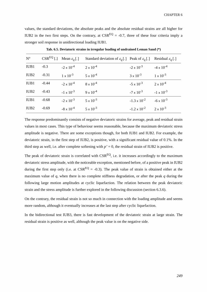
CHAPTER 6
249
values, the standard deviations, the absolute peaks and the absolute residual strains are all higher for
IUB2 in the two first steps. On the contrary, at CSREQ = -0.7, three of these four criteria imply a
stronger soil response in unidirectional loading IUB1.
Tab. 6.5. Deviatoric strains in irregular loading of undrained Leman Sand (*)
The response predominantly consists of negative deviatoric strains for average, peak and residual strain
values in most cases. This type of behaviour seems reasonable, because the maximum deviatoric stress
amplitude is negative. There are some exceptions though, for both IUB1 and IUB2. For example, the
deviatoric strain, in the first step of IUB2, is positive, with a significant residual value of 0.1%. In the
third step as well, i.e. after complete softening with p’ = 0, the residual strain of IUB2 is positive.
The peak of deviatoric strain is correlated with CSREQ, i.e. it increases accordingly to the maximum
deviatoric stress amplitude, with the noticeable exception, mentioned before, of a positive peak in IUB2
during the first step only (i.e. at CSREQ = -0.3). The peak value of strain is obtained either at the
maximum value of q, when there is no complete stiffness degradation, or after the peak q during the
following large motion amplitudes at cyclic liquefaction. The relation between the peak deviatoric
strain and the stress amplitude is further explored in the following discussion (section 6.3.6).
On the contrary, the residual strain is not so much in connection with the loading amplitude and seems
more random, although it eventually increases at the last step after cyclic liquefaction.
In the bidirectional test IUB3, there is fast development of the deviatoric strain at large strain. The
residual strain is positive as well, although the peak value is on the negative side.
N° CSREQ [.] Mean εq [.] Standard deviation of εq [.] Peak of εq [.] Residual εq [.]
IUB1 -0.3 -2 x 10⁻⁴ 2 x 10⁻⁴ -2 x 10⁻³ -4 x 10⁻⁴
IUB2 -0.31 1 x 10⁻³ 5 x 10⁻⁴ 3 x 10⁻³ 1 x 10⁻³
IUB1 -0.44 -2 x 10⁻⁴ 8 x 10⁻⁴ -5 x 10⁻³ 2 x 10⁻⁴
IUB2 -0.43 -1 x 10⁻³ 9 x 10⁻⁴ -7 x 10⁻³ -1 x 10⁻³
IUB1 -0.68 -2 x 10⁻³ 5 x 10⁻³ -1.3 x 10⁻² -6 x 10⁻³
IUB2 -0.69 -8 x 10⁻⁴ 5 x 10⁻³ -1.2 x 10⁻² 2 x 10⁻³
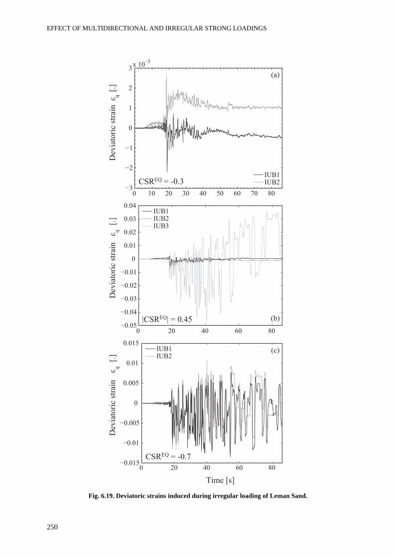
EFFECT OF MULTIDIRECTIONAL AND IRREGULAR STRONG LOADINGS
250
Fig. 6.19. Deviatoric strains induced during irregular loading of Leman Sand.
0 20 40 60 80
0
Dev
iato
ric
stra
in
q
IUB2
0 20 40 60 70 80
0
2
Dev
iato
ric
stra
in
q
IUB2
0 20 40 60 80
0
Dev
iato
ric
stra
in
q
IUB2
(a)
(b)
(c)
CSREQ
|CSREQ
CSREQ
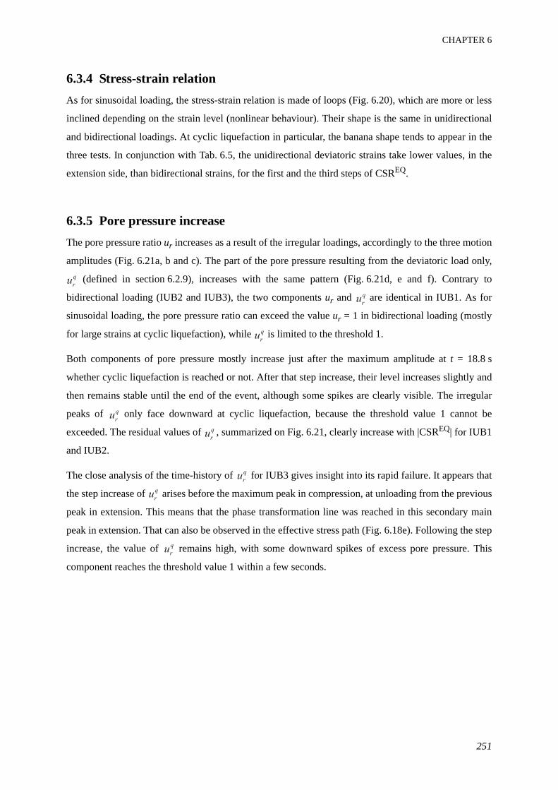
CHAPTER 6
251
6.3.4 Stress-strain relationAs for sinusoidal loading, the stress-strain relation is made of loops (Fig. 6.20), which are more or less
inclined depending on the strain level (nonlinear behaviour). Their shape is the same in unidirectional
and bidirectional loadings. At cyclic liquefaction in particular, the banana shape tends to appear in the
three tests. In conjunction with Tab. 6.5, the unidirectional deviatoric strains take lower values, in the
extension side, than bidirectional strains, for the first and the third steps of CSREQ.
6.3.5 Pore pressure increaseThe pore pressure ratio ur increases as a result of the irregular loadings, accordingly to the three motion
amplitudes (Fig. 6.21a, b and c). The part of the pore pressure resulting from the deviatoric load only,
(defined in section 6.2.9), increases with the same pattern (Fig. 6.21d, e and f). Contrary to
bidirectional loading (IUB2 and IUB3), the two components ur and are identical in IUB1. As for
sinusoidal loading, the pore pressure ratio can exceed the value ur = 1 in bidirectional loading (mostly
for large strains at cyclic liquefaction), while is limited to the threshold 1.
Both components of pore pressure mostly increase just after the maximum amplitude at t = 18.8 s
whether cyclic liquefaction is reached or not. After that step increase, their level increases slightly and
then remains stable until the end of the event, although some spikes are clearly visible. The irregular
peaks of only face downward at cyclic liquefaction, because the threshold value 1 cannot be
exceeded. The residual values of , summarized on Fig. 6.21, clearly increase with |CSREQ| for IUB1
and IUB2.
The close analysis of the time-history of for IUB3 gives insight into its rapid failure. It appears that
the step increase of arises before the maximum peak in compression, at unloading from the previous
peak in extension. This means that the phase transformation line was reached in this secondary main
peak in extension. That can also be observed in the effective stress path (Fig. 6.18e). Following the step
increase, the value of remains high, with some downward spikes of excess pore pressure. This
component reaches the threshold value 1 within a few seconds.
ur
q
ur
q
ur
q
ur
q
ur
q
ur
q
ur
q
ur
q
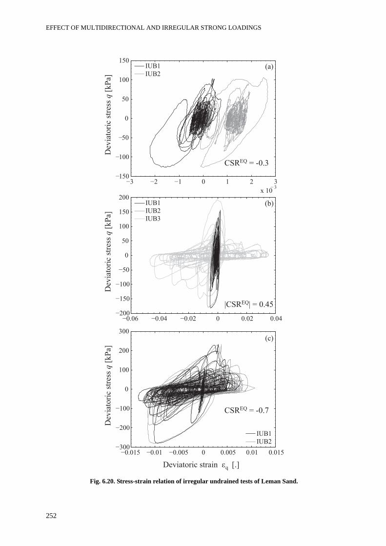
EFFECT OF MULTIDIRECTIONAL AND IRREGULAR STRONG LOADINGS
252
Fig. 6.20. Stress-strain relation of irregular undrained tests of Leman Sand.
Dev
iato
ric
stre
ss q
[k
Pa] IUB3
33
Dev
iato
ric
stre
ss q
[k
Pa]
Dev
iato
ric
stre
ss q
[k
Pa]
Deviatoric strain q
(a)
(b)
(c)
CSREQ
CSREQ
|CSREQ
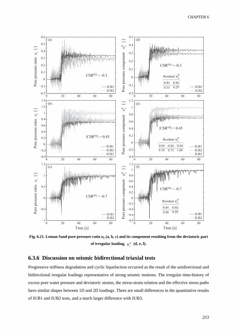
CHAPTER 6
253
Fig. 6.21. Leman Sand pore pressure ratio ur (a, b, c) and its component resulting from the deviatoric part
of irregular loading, (d, e, f).
6.3.6 Discussion on seismic bidirectional triaxial testsProgressive stiffness degradation and cyclic liquefaction occurred as the result of the unidirectional and
bidirectional irregular loadings representative of strong seismic motions. The irregular time-history of
excess pore water pressure and deviatoric strains, the stress-strain relation and the effective stress paths
have similar shapes between 1D and 2D loadings. There are small differences in the quantitative results
of IUB1 and IUB2 tests, and a much larger difference with IUB3.
0 20 40 60 80
0
1
Po
re p
ress
ure
rat
io
u r
IUB1
IUB2
IUB3
0 20 40 60 80
0
Po
re p
ress
ure
rat
io
u r
IUB1
IUB2
0 20 40 60 80
0
1
Po
re p
ress
ure
rat
io
ur
IUB1IUB2
(a)
(b)
(c)
0 20 40 60 80
0
1
IUB1
IUB2
IUB3
0 20 40 60 80
0
IUB1
IUB2
0 20 40 60 80
0
1
Po
re p
ress
ure
co
mp
on
ent
ur
IUB1
IUB2
qP
ore
pre
ssu
re c
om
po
nen
t u
rqP
ore
pre
ssu
re c
om
po
nen
t u
rq
(d)
(e)
(f)
CSREQ
CSREQ
CSREQ
CSREQ
|CSREQ
|CSREQ
ur
qResidual
IUB1 IUB2
ur
qResidual
IUB1 IUB2
ur
qResidual
IUB1 IUB2 IUB3
ur
q
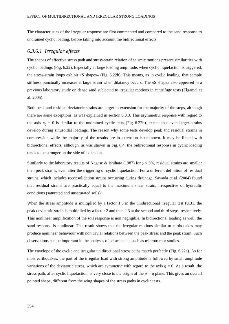
EFFECT OF MULTIDIRECTIONAL AND IRREGULAR STRONG LOADINGS
254
The characteristics of the irregular response are first commented and compared to the sand response to
undrained cyclic loading, before taking into account the bidirectional effects.
6.3.6.1 Irregular effectsThe shapes of effective stress path and stress-strain relation of seismic motions present similarities with
cyclic loadings (Fig. 6.22). Especially at large loading amplitude, when cyclic liquefaction is triggered,
the stress-strain loops exhibit «S shapes» (Fig. 6.22b). This means, as in cyclic loading, that sample
stiffness punctually increases at large strain when dilatancy occurs. The «S shape» also appeared in a
previous laboratory study on dense sand subjected to irregular motions in centrifuge tests (Elgamal et
al. 2005).
Both peak and residual deviatoric strains are larger in extension for the majority of the steps, although
there are some exceptions, as was explained in section 6.3.3. This asymmetric response with regard to
the axis εq = 0 is similar to the undrained cyclic tests (Fig. 6.22b), except that even larger strains
develop during sinusoidal loadings. The reason why some tests develop peak and residual strains in
compression while the majority of the results are in extension is unknown. It may be linked with
bidirectional effects, although, as was shown in Fig. 6.4, the bidirectional response in cyclic loading
tends to be stronger on the side of extension.
Similarly to the laboratory results of Nagase & Ishihara (1987) for γ < 3%, residual strains are smaller
than peak strains, even after the triggering of cyclic liquefaction. For a different definition of residual
strains, which includes reconsolidation strains occurring during drainage, Sawada et al. (2004) found
that residual strains are practically equal to the maximum shear strain, irrespective of hydraulic
conditions (saturated and unsaturated soils).
When the stress amplitude is multiplied by a factor 1.5 in the unidirectional irregular test IUB1, the
peak deviatoric strain is multiplied by a factor 2 and then 2.3 at the second and third steps, respectively.
This nonlinear amplification of the soil response is non negligible. In bidirectional loading as well, the
sand response is nonlinear. This result shows that the irregular motions similar to earthquakes may
produce nonlinear behaviour with non trivial relations between the peak stress and the peak strain. Such
observations can be important in the analyses of seismic data such as microtremor studies.
The envelope of the cyclic and irregular unidirectional stress paths match perfectly (Fig. 6.22a). As for
most earthquakes, the part of the irregular load with strong amplitude is followed by small amplitude
variations of the deviatoric stress, which are symmetric with regard to the axis q = 0. As a result, the
stress path, after cyclic liquefaction, is very close to the origin of the p’ - q plane. This gives an overall
pointed shape, different from the wing shapes of the stress paths in cyclic tests.
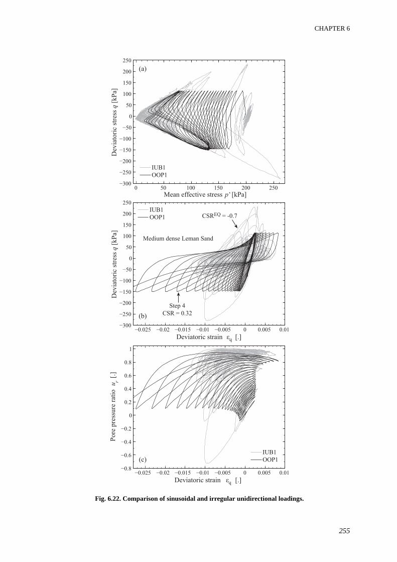
CHAPTER 6
255
Fig. 6.22. Comparison of sinusoidal and irregular unidirectional loadings.
Dev
iato
ric
stre
ss q
[kP
a]
Deviatoric strain q
Pore
pre
ssure
rat
io
u r
Deviatoric strain q
Mean effective stress p’ [kPa]
Dev
iato
ric
stre
ss q
[kP
a]
(a)
(b)
(c)
Medium dense Leman Sand
CSREQ
EFFECT OF MULTIDIRECTIONAL AND IRREGULAR STRONG LOADINGS
256
The excess pore pressure ratio increases in one step, following the peak deviatoric stress, whether
cyclic liquefaction is triggered or not (Fig. 6.21). This is true at all steps, for all tests, including the test
IUB3 with the maximum deviatoric stress in compression. This result is slightly different from the
triaxial test results from Ishihara & Yasuda (1972). They showed that ur also exhibits a fast increase in
EM tests, but gradually reaches the threshold 1 in CM tests. After the triggering of cyclic liquefaction,
the pore pressure presents negative spikes, particularly visible in Fig. 6.21f. These spikes all arise
exactly at the same time as local peaks of q, mostly in extension. They are the consequences of the
dilative tendency of the sand response to the higher peaks of the irregular loading.
The shape of the irregular pore pressure ratio vs. deviatoric strain is compared to the cyclic response in
Fig. 6.22c for unidirectional conditions. It is interesting to see that, although the deviatoric strains have
larger amplitudes, the pore pressure ratio is lower in cyclic tests. The overall shape of that relation is
however very similar in irregular and cyclic conditions.
6.3.6.2 Influence of bidirectional effect in irregular loadingsThe response of IUB3, the bidirectional test in compression, is clearly more unstable than the two other
tests: pore pressure increases and especially deviatoric strains are much larger than the response of
IUB1 and IUB2 at the same |CSREQ|. The time-history of deviatoric stress are opposite, it was then
expected to obtain a different response. We did not perform the unidirectional test with a peak in
compression, that is why there is no certainty on the results obtained in such case. However, all
previous unidirectional studies presented in Chapter 2 emphasize the fact that EM tests (peak stress in
extension) always induce lower cyclic strength than CM tests (peak stress in compression). The cyclic
tests presented in Chapter 4 also indicate that such a test, placed on the compression side of q, would
have yielded a higher strength than IUB1 (and IUB3).
The explanation for that unexpected behaviour is then related to the bidirectional loading. The Mohr
circles of IUB3 (Fig. 6.17) show that, at some points, the stress state of the soil is closer to the origin of
the Mohr plane, which could make it easier to cross the failure threshold. The interpretation of irregular
tests in the p’ - q plane is not simple. However, it is possible to see, in Fig. 6.18e, that the phase
transformation line is first crossed by IUB3 during an extension peak, though this is not the maximum
peak value. More precisely, the analysis of the time-history of showed that the triggering event for
cyclic liquefaction is a secondary peak in extension before the maximum peak in compression. This
secondary peak is the apex locus on the extension side, in the total stress path of IUB3 (Fig. 6.18b).
The inclination of the total stress path of IUB3 and the location of the low apex at the left of the 1D
stress path allow the effective stress path to cross the phase transformation line before the maximum
loading peak. As shown from the comparison with IUB1, failure at such a level of |CSREQ| would not
ur
q
CHAPTER 6
257
have been possible in a unidirectional loading having the same pattern of deviatoric stress.
We then demonstrated experimentally that the combination of irregular deviatoric stress and confining
pressure of IUB3 significantly reduces the |CSREQ| necessary to induce liquefaction, although the stress
path, in the p - q plane, seems really similar to IUB1 at first sight (Fig. 6.18b).
Comparing IUB1 and IUB2, bidirectional effects in irregular conditions can also be small; yet the
observed tendency, detailed below, shows a sensitivity to bidirectional conditions in good agreement
with out-of-phase cyclic test results. The results are anyway taken with caution, because of the low
number of irregular tests.
At medium strain, the bidirectional test exhibits a slightly amplified response: both peak and residual
strains are higher than unidirectional loading for the two lower values of |CSREQ|. On the contrary,
higher strains develop in unidirectional than bidirectional tests after cyclic liquefaction. The same
tendency appears in cyclic OOP tests, in particular for positive phase angles: the medium strain
response is amplified in bidirectional loading, but larger strains develop at cyclic liquefaction in
unidirectional loading.
The pore pressure increase is slightly higher in unidirectional test at the smallest |CSREQ|, but lower at
the medium strain level. At failure, at the third step, both responses are similar, although the threshold
ur = 1 is reached much earlier for the bidirectional (t1 = 26.6 s) than the unidirectional ur
(t2 = 54.5 s). The rate of increase of in 2D thus seems higher than the rate of increase of ur in 1D,
just previous to the triggering of cyclic liquefaction, as was obtained in OOP tests.
The state of the art provides reference of bidirectional irregular simple shear tests on undrained
saturated sand, for example Nagase & Ishihara (1988) showed that there is no effect of 2D loading on
settlements induced by liquefaction. However, the conclusions of these experiments do not really apply
to our study, because (i) the equipment and loadings are different and (ii) our results are less focused on
the quantitative comparison with cyclic loading, and more focused on the qualitative analyses and
description of the nonlinear soil behaviour.
6.3.7 ConclusionsThree irregular tests, with seismic patterns and performed in unidirectional and bidirectional
conditions, illustrate and emphasize the role of loading conditions on the nonlinear soil response. The
1D and 2D total stress paths, effective stress paths, stress-strain relations have the same shapes. They
also present similarities with cyclic behaviour, although the strains are more limited, at cyclic
liquefaction, in irregular loadings. It is for example interesting to see «S shape» stress-strain loops
appearing in irregular tests, as they are characteristic of the cyclic alternation of increasing and
ur
q
ur
q
EFFECT OF MULTIDIRECTIONAL AND IRREGULAR STRONG LOADINGS
258
decreasing excess pore pressure in medium and dense undrained sand (cf. Chapter 4).
Looking at the response induced by the irregular loading, we observed that the deviatoric strains are
mainly negative, i.e. on the extension side for most cases. Moreover, the peak values of εq are higher
than residual strains. The relation between the peak deviatoric strain and the peak deviatoric stress is
not trivial, i.e. it is nonlinear, even in unidirectional loading.
The pore pressures from bidirectional irregular tests are separated into two components, as was
previously done in cyclic bidirectional loading. The unidirectional pore pressure ur and the
bidirectional pore pressure component have similar shapes; their residual values are also close to
each other in IUB1 and IUB2 tests. They reach the threshold value 1 at cyclic liquefaction, by a step
increase which follows the maximum deviatoric stress. This sudden increase in one main step also
arises for motions with lower |CSREQ| which do not induce liquefaction.
Some bidirectional effects are observed, although they do not imply major differences in the soil
response by considering only the two tests IUB1 and IUB2. These effects are similar to what was
observed in out-of-phase cyclic tests: in bidirectional conditions, there are (i) stronger deviatoric strains
at medium strain (ii) faster reach of cyclic liquefaction (iii) lower strains at large motions. The very
unstable response of the test IUB3 is seen as a consequence of the bidirectional stress path; this shows
that bidirectional loading can also have strong impact on soil behaviour in irregular conditions, and can
significantly reduce the undrained strength.
6.4 Comments on bidirectional and irregular effects
6.4.1 Effect of complex loadings on nonlinear soil behaviourThe first scope of these experimental studies, cited in the introduction of the chapter, was to assess the
effect of the superposition of two loadings on the nonlinear behaviour of granular soils. It is clear now
that the superposition, in triaxial conditions, of a cyclic deviatoric stress and a cyclic confining pressure
has an effect on the nonlinear stiffness degradation and failure of saturated Leman Sand. The response
of the soil is not the simple superposition of a cyclic pore pressure, resulting from the variation of the
total confining pressure, and the cyclic shearing of the sample, which also induces cyclic variation and
gradual increase of the pore pressure. The consequences of bidirectional loading are complex, and the
short summary below reflects the main points observed:
ur
q
CHAPTER 6
259
• In cyclic conditions, dynamic parameters are slightly influenced by the superposition of loadings.
The secant shear modulus vs. deviatoric strain curve exhibits a peak at medium strains, but
otherwise is very similar to the unidirectional curve. The damping ratio vs. deviatoric strain also
exhibits a peak, arising from dilative effect and the formation of the «S shape» of the stress-strain
relation (Chapter 4). That peak also happens in unidirectional loading, but it arises for smaller
values of the deviatoric strain amplitude in bidirectional tests. That means that dilatancy occurs for
lower strains in bidirectional loadings.
• Cyclic strength is either enhanced or reduced by bidirectional loading. The phenomenon is more
obvious in cyclic loading, although the response of the test IUB3 in bidirectional irregular loading
shows that rapid failure may arise as a consequence of a complex loading. The number of cycles to
reach failure, Nf, which is the simpler tool to assess cyclic strength, is clearly influenced by
bidirectional loadings. The difference, with identical CSR, can reach 30% for out-of-phase tests with
opposite phase angles.
• Deviatoric strains were shown to exhibit nonlinear responses to unidirectional and bidirectional,
cyclic and irregular stress-controlled tests. εq is stronger at medium motion amplitude (more
generally before the triggering of cyclic liquefaction) for bidirectional irregular and cyclic
conditions. After failure, bidirectional loading may slightly prevent the formation of large deviatoric
strains, at least in certain conditions (e.g. positive phase angle).
• Pore pressures, in bidirectional loadings, are divided into two components to remove the cyclic effect
of the purely isotropic part and visualize only the component related to the shearing part, . In
parallel to the deviatoric strain, pore pressures increase faster in bidirectional loading before cyclic
liquefaction. After cyclic liquefaction, the level of is limited to the threshold value 1, also no
further evolution is expected. Negative spikes of excess pore pressure appear in all conditions.
6.4.2 Physical interpretationThe stress path only, and its distance to phase transformation and steady state lines, can not explain by
itself the bidirectional effects observed in cyclic and irregular loadings. Indeed, even stress paths with
the same shape but different direction of rotation, for example OOP2 and OOP3, exhibit completely
different cyclic strength and nonlinear response.
We assume that any dynamic amplification can be withdrawn, because the pseudo-dynamic regime
prevails in these studies, as for all tests previously presented.
The nonlinear superposition of two independent loading does not necessarily imply that the response
will be the sum of the two loadings, like for the usual assumption of linear elastic behaviour. Indeed, we
ur
q
ur
q
EFFECT OF MULTIDIRECTIONAL AND IRREGULAR STRONG LOADINGS
260
showed that some kind of coupling appears as an effect of the combination of two cyclic or irregular
loads. A possible explanation is that pore pressure itself influences the development of deviatoric
strains, while the contractive behaviour of the soil matrix also induces increase of the pore pressure.
This assumption is supported by the analyses, for OOP tests (section 6.2.9), of the effect of the phase
angle with respect to time-history of the pore pressure ratio: negative spikes of ur are enhanced for
particular values of the phase angle, which also correspond to the tests with the lowest cyclic strength
(i.e. lower Nf).
The bidirectional amplification of deviatoric strain amplitudes and of the rate of pore pressure increase,
before cyclic liquefaction, could then result from the coupling between the pore fluid and the granular
matrix. After the triggering of cyclic liquefaction, the pore pressure ratio stabilizes, also it seems
reasonable to admit that there is no more amplification of the response, and that the strains may develop
less strongly than in unidirectional conditions.
6.4.3 Consequences for modelling and design purposesTo fully take into account the bidirectional effects, in particular within the frame of geotechnical
earthquake engineering, an accessible solution would be to evaluate the effect of 2D and irregular
loading on the cyclic strength curves, CSR vs. number of cycles to reach failure. More tests would be
needed to get significant curves for various initial states. That would also allow to define multiplying
factors which take into account the superposition of stresses and irregular effect in triaxial conditions
(cf. Nagase & Ishihara 1987).
Another question concerns the constitutive law and numerical modelling of the bidirectional effects. It
is not really obvious now whether a constitutive law based on multi-mechanisms like the Hujeux model
could account for the bidirectional effects described above, because the reason for these observed
phenomenon are not fully understood yet. The following Chapter 7 addresses this question.
6.5 ConclusionsSignificant examples of complex triaxial tests in bidirectional undrained conditions were described
with a particular emphasis on the application to earthquake geotechnical engineering.
First, the cyclic tests demonstrated that the superposition of two stresses of different nature, one
deviatoric and one isotropic, induced coupling effects in the nonlinear soil response. The bidirectional
effects result in an amplification of motion before cyclic liquefaction, and a limitation of strains after
CHAPTER 6
261
cyclic liquefaction. The phase angle between deviatoric and confining stress has a particularly strong
influence on Leman Sand behaviour. Cyclic strength is significantly modified by complex loadings.
Three irregular seismic tests were also performed in unidirectional and bidirectional conditions to
illustrate the effect of superposition of loadings in conditions closer to in situ seismic motions.
Bidirectional irregular loadings can increase deviatoric strains and pore pressure build up compared to
unidirectional motions. The conditions of amplification of the response are similar to cyclic tests:
before cyclic liquefaction, the superposition of loading slightly accelerates stiffness degradation. In the
case of seismic loading, soil behaviour after cyclic liquefaction is practically equivalent in
unidirectional and bidirectional loading.
The parallel between cyclic and irregular loading was illustrated with (i) characteristic «S shape»
stress-strain relations, which are a consequence of dilative behaviour, (ii) total and effective stress
paths, (iii) the relation between pore pressure increase and deviatoric strains. In irregular tests, we also
showed that the relation between the maximum strain amplitude and the maximum stress amplitude is
not trivial, i.e. nonlinear, even in unidirectional loading.
In order to understand and compare the coupling between the two loadings, the pore pressure ratio of
bidirectional tests is separated into two components. The unidirectional pore pressure ratio ur and the
bidirectional component , which corresponds to the deviatoric part of the load, have similar shapes
in both irregular and cyclic motions. They both reach the threshold value 1 at cyclic liquefaction.
The interpretation of bidirectional effects is based on the coupling between the pressure in the pore
fluid and the deviatoric strains of the granular matrix. While the cyclic variation of the confining
pressure are assumed to be reported only on the pore pressure, the coupling between pore pressure and
deviatoric strains also amplifies the response to the variations of deviatoric stress. Stiffness reduction
and the occurrence of cyclic liquefaction is then accelerated in bidirectional conditions.
ur
q

EFFECT OF MULTIDIRECTIONAL AND IRREGULAR STRONG LOADINGS
262
CHAPTER 7
CONSTITUTIVE MODELLING OF
CYCLIC SAND BEHAVIOUR
CONSTITUTIVE MODELLING OF CYCLIC SAND BEHAVIOUR
264
7.1 IntroductionSome of the dynamic tests performed with the triaxial press (presented in Chapters 4, 5 and 6) are now
modelled to evaluate the capability of two quite different models to reproduce nonlinear sand
behaviour. The identification of model parameters for Leman Sand is also described.
The two existing constitutive laws assessed in this chapter are: (i) the simple linear equivalent method
and (ii) the complex Hujeux model for cyclic loading (both are described in section 2.7). The first
simple model is widely used in practice for geotechnical earthquake engineering applications. It
comprises 3 material parameters and two degradation curves (secant shear modulus decrease and
damping ratio increase as a function of the shear strain amplitude). The second model, which is more
research-oriented, is a multi-mechanism elastoplastic law designed to account for cyclic effects
(Hujeux 1985); it is based on coupled hydro-mechanical equations, with a total of 18 parameters. Both
models can be implemented in the commercial software CyberQuake, the elastoplastic law in a
simplified version with 15 parameters (CyberQuake user’s guide v.2.01). In the following study, the
elastoplastic law is implemented in its complete form in an independent module (LAWYER routine,
detailed later).
First, the linear equivalent method is used to model the beginning of a cyclic undrained test with
symmetric stress reversal, which induced cyclic liquefaction (CYC2). The soil parameters for this
model are directly calculated from the laboratory test results.
Then, the elastoplastic model is applied to several cyclic undrained tests and a monotonic test, in order
to calibrate some of the model parameters for Leman Sand by curve fitting. The other parameters were
obtained from different procedures, which are also described. The model is then applied to a cyclic dry
test (DRY1).
The possibility to model rate effects and multidirectional effects with the two models is also discussed.
The advantages and limitations of the two models are finally summarized in the discussions, with some
possible extensions which could take into account the effects of complex loading observed in the
laboratory tests.
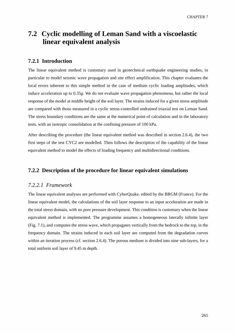
CHAPTER 7
265
7.2 Cyclic modelling of Leman Sand with a viscoelastic linear equivalent analysis
7.2.1 IntroductionThe linear equivalent method is customary used in geotechnical earthquake engineering studies, in
particular to model seismic wave propagation and site effect amplification. This chapter evaluates the
local errors inherent to this simple method in the case of medium cyclic loading amplitudes, which
induce acceleration up to 0.35g. We do not evaluate wave propagation phenomena, but rather the local
response of the model at middle height of the soil layer. The strains induced for a given stress amplitude
are compared with those measured in a cyclic stress-controlled undrained triaxial test on Leman Sand.
The stress boundary conditions are the same at the numerical point of calculation and in the laboratory
tests, with an isotropic consolidation at the confining pressure of 100 kPa.
After describing the procedure (the linear equivalent method was described in section 2.6.4), the two
first steps of the test CYC2 are modelled. Then follows the description of the capability of the linear
equivalent method to model the effects of loading frequency and multidirectional conditions.
7.2.2 Description of the procedure for linear equivalent simulations
7.2.2.1 FrameworkThe linear equivalent analyses are performed with CyberQuake, edited by the BRGM (France). For the
linear equivalent model, the calculations of the soil layer response to an input acceleration are made in
the total stress domain, with no pore pressure development. This condition is customary when the linear
equivalent method is implemented. The programme assumes a homogeneous laterally infinite layer
(Fig. 7.1), and computes the stress wave, which propagates vertically from the bedrock to the top, in the
frequency domain. The strains induced in each soil layer are computed from the degradation curves
within an iteration process (cf. section 2.6.4). The porous medium is divided into nine sub-layers, for a
total uniform soil layer of 9.45 m depth.
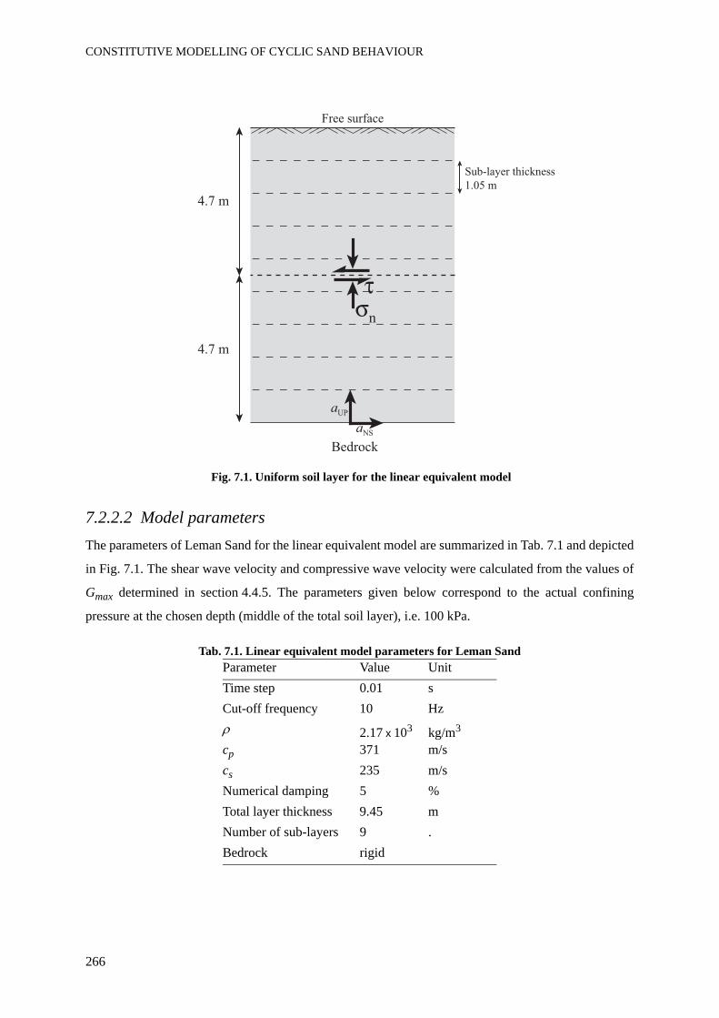
CONSTITUTIVE MODELLING OF CYCLIC SAND BEHAVIOUR
266
Fig. 7.1. Uniform soil layer for the linear equivalent model
7.2.2.2 Model parametersThe parameters of Leman Sand for the linear equivalent model are summarized in Tab. 7.1 and depicted
in Fig. 7.1. The shear wave velocity and compressive wave velocity were calculated from the values of
Gmax determined in section 4.4.5. The parameters given below correspond to the actual confining
pressure at the chosen depth (middle of the total soil layer), i.e. 100 kPa.
Tab. 7.1. Linear equivalent model parameters for Leman SandParameter Value UnitTime step 0.01 sCut-off frequency 10 Hzρ 2.17 x 10³ kg/m3
cp 371 m/scs 235 m/sNumerical damping 5 %Total layer thickness 9.45 mNumber of sub-layers 9 .Bedrock rigid
Bedrock
aUP
aNS
n
Free surface
4.7 m
4.7 m
Sub-layer thickness
1.05 m
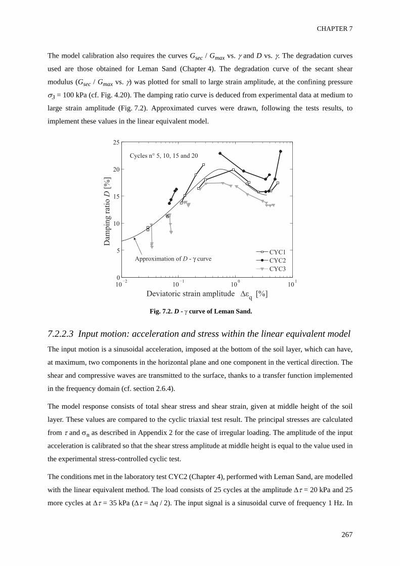
CHAPTER 7
267
The model calibration also requires the curves Gsec / Gmax vs. γ and D vs. γ. The degradation curves
used are those obtained for Leman Sand (Chapter 4). The degradation curve of the secant shear
modulus (Gsec / Gmax vs. γ) was plotted for small to large strain amplitude, at the confining pressure
σ3 = 100 kPa (cf. Fig. 4.20). The damping ratio curve is deduced from experimental data at medium to
large strain amplitude (Fig. 7.2). Approximated curves were drawn, following the tests results, to
implement these values in the linear equivalent model.
Fig. 7.2. D - γ curve of Leman Sand.
7.2.2.3 Input motion: acceleration and stress within the linear equivalent modelThe input motion is a sinusoidal acceleration, imposed at the bottom of the soil layer, which can have,
at maximum, two components in the horizontal plane and one component in the vertical direction. The
shear and compressive waves are transmitted to the surface, thanks to a transfer function implemented
in the frequency domain (cf. section 2.6.4).
The model response consists of total shear stress and shear strain, given at middle height of the soil
layer. These values are compared to the cyclic triaxial test result. The principal stresses are calculated
from τ and σn as described in Appendix 2 for the case of irregular loading. The amplitude of the input
acceleration is calibrated so that the shear stress amplitude at middle height is equal to the value used in
the experimental stress-controlled cyclic test.
The conditions met in the laboratory test CYC2 (Chapter 4), performed with Leman Sand, are modelled
with the linear equivalent method. The load consists of 25 cycles at the amplitude Δτ = 20 kPa and 25
more cycles at Δτ = 35 kPa (Δτ = Δq / 2). The input signal is a sinusoidal curve of frequency 1 Hz. In
10 101
100
101
0
5
10
15
Dam
pin
g r
atio
D [
%]
q [%]
CYC1
CYC3
Deviatoric strain amplitude
Approximation of D - curve
CONSTITUTIVE MODELLING OF CYCLIC SAND BEHAVIOUR
268
unidirectional condition, only one component of the acceleration varies cyclically in the horizontal
plane. At the depth 4.7 m, the medium is isotropically consolidated at the confining pressure
σ3 = 100 kPa, which corresponds to experimental conditions of the test CYC2. The relative density is
not explicitly taken into account, but stiffness degradation curves correspond to the desired void ratio.
7.2.3 Results
Fig. 7.3a and Fig. 7.3b show the deviatoric stress variations corresponding to Δq = 40 kPa and 70 kPa,
respectively obtained for cyclic acceleration amplitudes of 0.16g and 0.22g imposed to the bedrock.
Cyclic axial strains computed with the linear equivalent method are clearly lower than the experimental
results, at both loading amplitudes (Fig. 7.4). At the 20th cycle for example, the strain amplitude is 1.5
times higher for experimental results at medium strain level (Fig. 7.4a), and 13 times higher for the
larger strain level (Fig. 7.4b).
The large difference observed at large strain between the modelled values and the experimental results
is reflected on the stress-strain relation (Fig. 7.5b). It is clear, from the loop shapes, that the modelled
stiffness is too high and the damping ratio too low. The S shape, typical of the development of cyclic
liquefaction, does not appear in the linear equivalent model because dilative behaviour cannot be
modelled by this method. For medium strain level (Fig. 7.5a), the loop shape is well-reproduced;
however, the evolution of the stress - strain relation does not appear in this model.
Fig. 7.3. Deviatoric stress of the linear equivalent model at mid-depth of the soil layer compared to the steps 1 (a) and 2 (b) of the cyclic triaxial test CYC2.
0 5 10 15 20 25
0
20
Time [s]
0 5 10 15 20 25
0
10
20
50
Dev
iato
ric
stre
ss q
[kP
a]
Time [s]
Experimental curveLinear equivalent model
(a) (b)
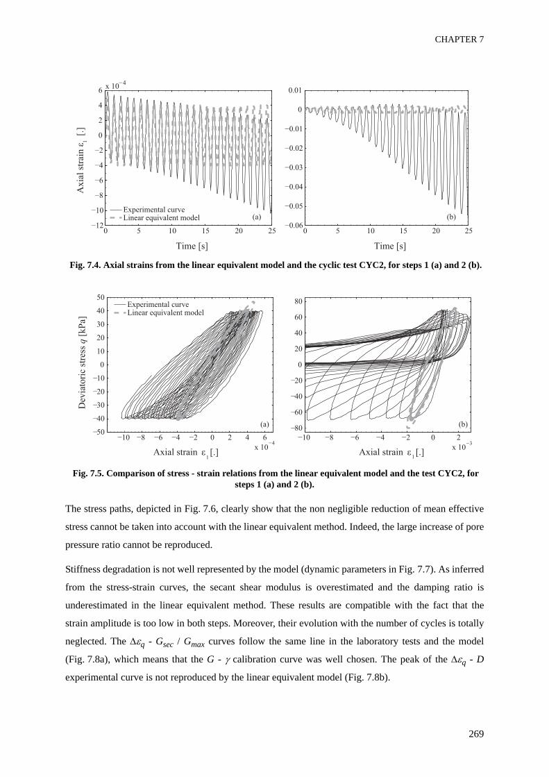
CHAPTER 7
269
Fig. 7.4. Axial strains from the linear equivalent model and the cyclic test CYC2, for steps 1 (a) and 2 (b).
Fig. 7.5. Comparison of stress - strain relations from the linear equivalent model and the test CYC2, for steps 1 (a) and 2 (b).
The stress paths, depicted in Fig. 7.6, clearly show that the non negligible reduction of mean effective
stress cannot be taken into account with the linear equivalent method. Indeed, the large increase of pore
pressure ratio cannot be reproduced.
Stiffness degradation is not well represented by the model (dynamic parameters in Fig. 7.7). As inferred
from the stress-strain curves, the secant shear modulus is overestimated and the damping ratio is
underestimated in the linear equivalent method. These results are compatible with the fact that the
strain amplitude is too low in both steps. Moreover, their evolution with the number of cycles is totally
neglected. The Δεq - Gsec / Gmax curves follow the same line in the laboratory tests and the model
(Fig. 7.8a), which means that the G - γ calibration curve was well chosen. The peak of the Δεq - D
experimental curve is not reproduced by the linear equivalent model (Fig. 7.8b).
(a) (b)
0 5 10 15 20 25
0
2
x 10A
xia
l st
rain
1 [
.]
Time [s]
Experimental curveLinear equivalent model
0 5 10 15 20 25
0
0.01
Time [s]
(a) (b)
Dev
iato
ric
stre
ss q
[kP
a]
Axial strain [.]
Experimental curveLinear equivalent model
Axial strain [.]3
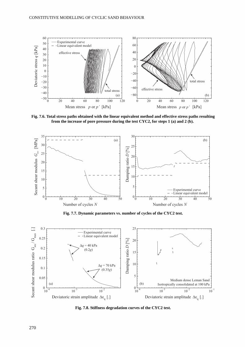
CONSTITUTIVE MODELLING OF CYCLIC SAND BEHAVIOUR
270
Fig. 7.6. Total stress paths obtained with the linear equivalent method and effective stress paths resulting from the increase of pore pressure during the test CYC2, for steps 1 (a) and 2 (b).
Fig. 7.7. Dynamic parameters vs. number of cycles of the CYC2 test.
Fig. 7.8. Stiffness degradation curves of the CYC2 test.
(a) (b)
0 20 40 60 80 100 120
0
10
20
40
60D
evia
tori
c st
ress
q [
kP
a]
Mean stress [kPa]
Experimental curveLinear equivalent model
0 20 40 60 80 100 120
0
20
40
60
80
Mean stress [kPa]p or p’ p or p’
effective stress
total stress effective stress
total stress
(a) (b)
0 10 20 30 40 500
5
10
15
20
25
30
35
Sec
ant
shea
r m
odulu
s G
sec [
MP
a]
Number of cycles N
0 10 20 30 40 500
5
10
15
20
25
30
Dam
pin
g r
atio
D [
%]
Number of cycles N
Experimental curveLinear equivalent model
(a) (b)
10 103
102
0
0.05
0.1
0.15
0.2
0.25
0.3
Sec
ant
shea
r m
odulu
s ra
tio
Gse
c / G
max
[.]
Deviatoric strain amplitude q [.]
Experimental curveLinear equivalent model
10 103
102
101
0
5
10
15
20
25
Dam
pin
g r
atio
D [
%]
q
(0.2g)
q
(0.35g)
Medium dense Leman Sand
Deviatoric strain amplitude q [.]
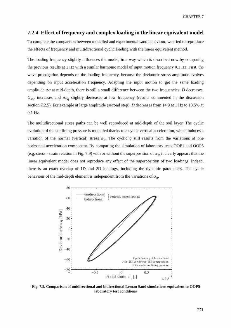
CHAPTER 7
271
7.2.4 Effect of frequency and complex loading in the linear equivalent modelTo complete the comparison between modelled and experimental sand behaviour, we tried to reproduce
the effects of frequency and multidirectional cyclic loading with the linear equivalent method.
The loading frequency slightly influences the model, in a way which is described now by comparing
the previous results at 1 Hz with a similar harmonic model of input motion frequency 0.1 Hz. First, the
wave propagation depends on the loading frequency, because the deviatoric stress amplitude evolves
depending on input acceleration frequency. Adapting the input motion to get the same loading
amplitude Δq at mid-depth, there is still a small difference between the two frequencies: D decreases,
Gsec increases and Δεq slightly decreases at low frequency (results commented in the discussion
section 7.2.5). For example at large amplitude (second step), D decreases from 14.9 at 1 Hz to 13.5% at
0.1 Hz.
The multidirectional stress paths can be well reproduced at mid-depth of the soil layer. The cyclic
evolution of the confining pressure is modelled thanks to a cyclic vertical acceleration, which induces a
variation of the normal (vertical) stress σn. The cyclic q still results from the variations of one
horizontal acceleration component. By comparing the simulation of laboratory tests OOP1 and OOP5
(e.g. stress - strain relation in Fig. 7.9) with or without the superposition of σn, it clearly appears that the
linear equivalent model does not reproduce any effect of the superposition of two loadings. Indeed,
there is an exact overlap of 1D and 2D loadings, including the dynamic parameters. The cyclic
behaviour of the mid-depth element is independent from the variations of σn.
Fig. 7.9. Comparison of unidirectional and bidirectional Leman Sand simulations equivalent to OOP5 laboratory test conditions
3Axial strain
Dev
iato
ric
stre
ss q
unidirectional
bidirectional }perfectly superimposed
Cyclic loading of Leman Sand
of the cyclic confining pressure
CONSTITUTIVE MODELLING OF CYCLIC SAND BEHAVIOUR
272
7.2.5 DiscussionNonlinear soil behaviour is supposed to happen for acceleration around 0.4g. In these simulations,
accelerations involved are below that level, but significant stiffness degradation and pore pressure
generation are observed in the laboratory. At the surface, the acceleration is 0.2g for step 1 and 0.35g
for step 2.
The model underestimates axial strains, which are below the expected level, especially for the second
step at the acceleration 0.35g. It reproduces well the degradation curve of the secant shear modulus, but
the peak of the damping ratio does not appear, maybe because the modelled strains are too small.
Stiffness degradation cannot be reproduced by the linear equivalent method, and the coupling with the
pore pressure is neglected because this model is implemented as a total stress analysis. This model
cannot discriminate between dry and saturated undrained conditions, although major differences were
experimentally observed in Chapter 4.
Frequency effects are not well captured by the linear equivalent method. The increase of Gsec and
decrease of Δεq at low frequency are opposite to what was observed in our laboratory tests. However,
the rate-dependency of damping is similar to the observed effect of frequency on undrained Leman
Sand. Multidirectional effects are not at all taken into account, which was expected from this simple
numerical tool.
7.2.6 SummaryAlthough it reproduces well the stiffness degradation curves, i.e. the relation between the dynamic
parameters and shear strains, the linear equivalent model is not able to model the strain increase
associated with undrained behaviour of dynamically loaded saturated sand at medium strain. The
modelling of failure is even less possible. Strain amplitudes are underestimated, the accumulation of
irrecoverable strain is not modelled, and neither is pore water pressure increase. The effects of
frequency and multidirectional loading observed in triaxial tests cannot be modelled either. These
observations apply to an acceleration at the top of the soil layer of maximum 0.35g, which is around the
threshold usually considered for nonlinear soil behaviour. However, this model gives acceptable stress -
strain relation at the lowest amplitude (which corresponds to an acceleration of 0.2g at the top of the
soil layer), although strain amplitudes are underestimated.
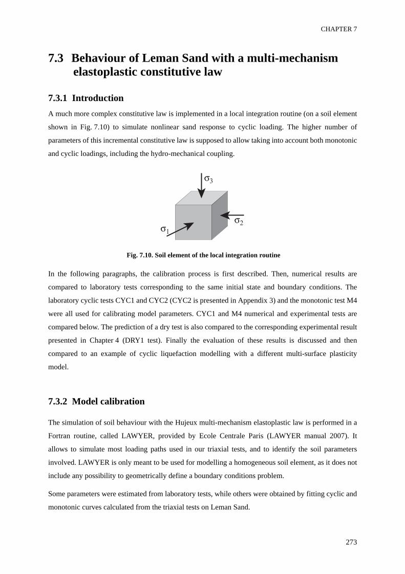
CHAPTER 7
273
7.3 Behaviour of Leman Sand with a multi-mechanism elastoplastic constitutive law
7.3.1 IntroductionA much more complex constitutive law is implemented in a local integration routine (on a soil element
shown in Fig. 7.10) to simulate nonlinear sand response to cyclic loading. The higher number of
parameters of this incremental constitutive law is supposed to allow taking into account both monotonic
and cyclic loadings, including the hydro-mechanical coupling.
Fig. 7.10. Soil element of the local integration routine
In the following paragraphs, the calibration process is first described. Then, numerical results are
compared to laboratory tests corresponding to the same initial state and boundary conditions. The
laboratory cyclic tests CYC1 and CYC2 (CYC2 is presented in Appendix 3) and the monotonic test M4
were all used for calibrating model parameters. CYC1 and M4 numerical and experimental tests are
compared below. The prediction of a dry test is also compared to the corresponding experimental result
presented in Chapter 4 (DRY1 test). Finally the evaluation of these results is discussed and then
compared to an example of cyclic liquefaction modelling with a different multi-surface plasticity
model.
7.3.2 Model calibration
The simulation of soil behaviour with the Hujeux multi-mechanism elastoplastic law is performed in a
Fortran routine, called LAWYER, provided by Ecole Centrale Paris (LAWYER manual 2007). It
allows to simulate most loading paths used in our triaxial tests, and to identify the soil parameters
involved. LAWYER is only meant to be used for modelling a homogeneous soil element, as it does not
include any possibility to geometrically define a boundary conditions problem.
Some parameters were estimated from laboratory tests, while others were obtained by fitting cyclic and
monotonic curves calculated from the triaxial tests on Leman Sand.
1
2
3
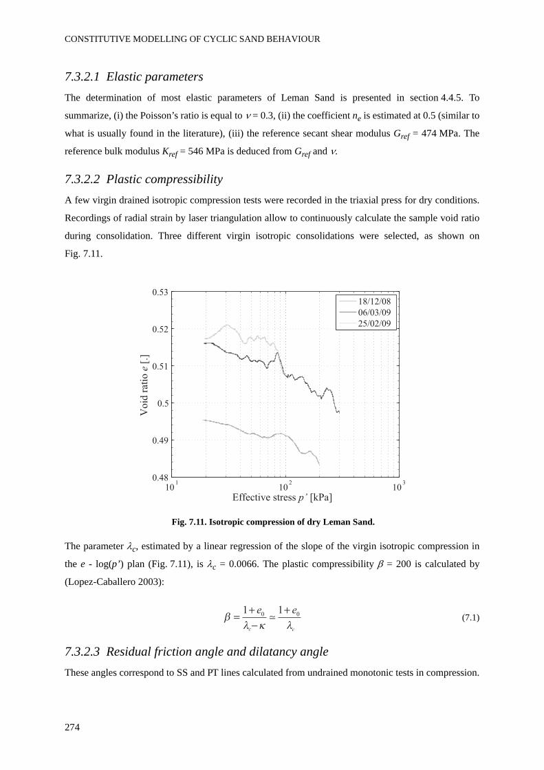
CONSTITUTIVE MODELLING OF CYCLIC SAND BEHAVIOUR
274
7.3.2.1 Elastic parametersThe determination of most elastic parameters of Leman Sand is presented in section 4.4.5. To
summarize, (i) the Poisson’s ratio is equal to ν = 0.3, (ii) the coefficient ne is estimated at 0.5 (similar to
what is usually found in the literature), (iii) the reference secant shear modulus Gref = 474 MPa. The
reference bulk modulus Kref = 546 MPa is deduced from Gref and ν.
7.3.2.2 Plastic compressibilityA few virgin drained isotropic compression tests were recorded in the triaxial press for dry conditions.
Recordings of radial strain by laser triangulation allow to continuously calculate the sample void ratio
during consolidation. Three different virgin isotropic consolidations were selected, as shown on
Fig. 7.11.
Fig. 7.11. Isotropic compression of dry Leman Sand.
The parameter λc, estimated by a linear regression of the slope of the virgin isotropic compression in
the e - log(p’) plan (Fig. 7.11), is λc = 0.0066. The plastic compressibility β = 200 is calculated by
(Lopez-Caballero 2003):
(7.1)
7.3.2.3 Residual friction angle and dilatancy angleThese angles correspond to SS and PT lines calculated from undrained monotonic tests in compression.
101
102
103
0.48
0.49
0.5
0.51
0.52
0.53
Vo
id r
atio
e [
.]
Effective stress p’ [kPa]
18/12/08
06/03/09
25/02/09
1 10 0e e
c c
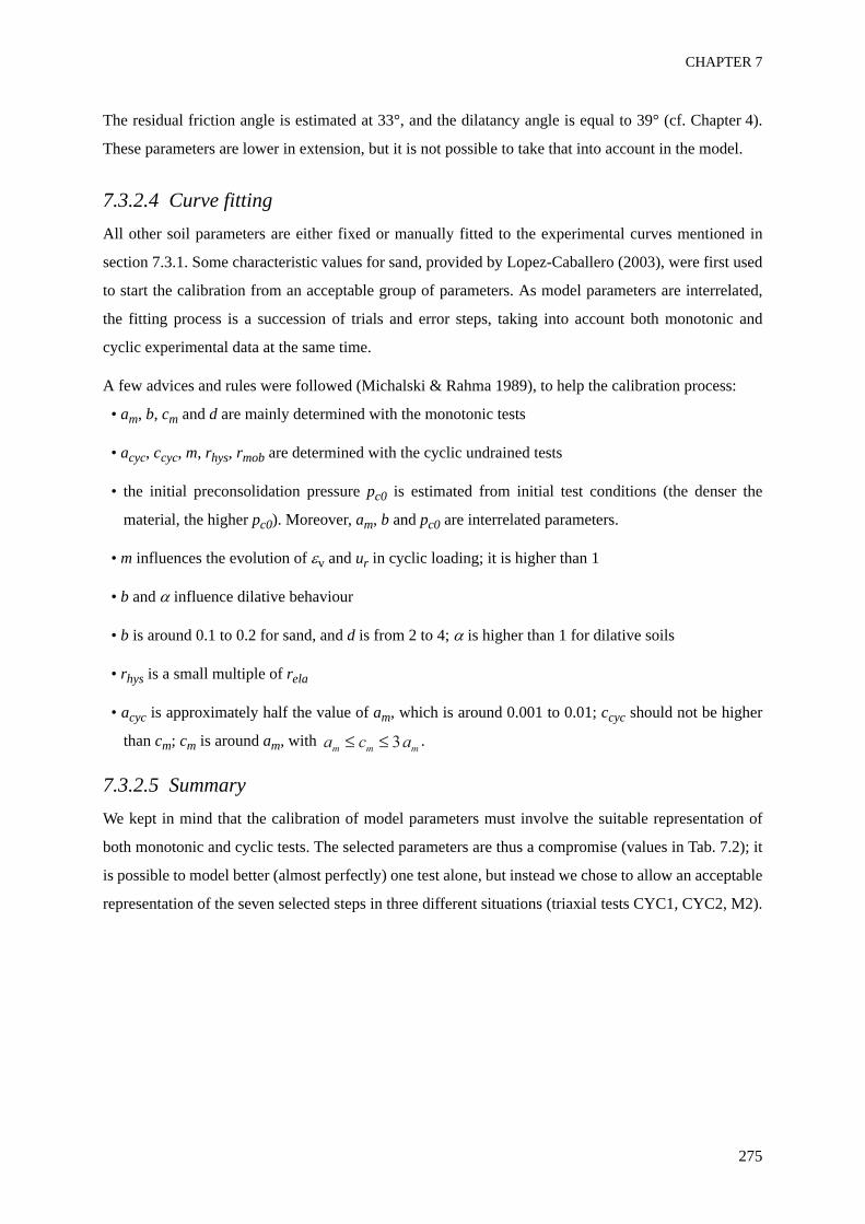
CHAPTER 7
275
The residual friction angle is estimated at 33°, and the dilatancy angle is equal to 39° (cf. Chapter 4).
These parameters are lower in extension, but it is not possible to take that into account in the model.
7.3.2.4 Curve fittingAll other soil parameters are either fixed or manually fitted to the experimental curves mentioned in
section 7.3.1. Some characteristic values for sand, provided by Lopez-Caballero (2003), were first used
to start the calibration from an acceptable group of parameters. As model parameters are interrelated,
the fitting process is a succession of trials and error steps, taking into account both monotonic and
cyclic experimental data at the same time.
A few advices and rules were followed (Michalski & Rahma 1989), to help the calibration process:
• am, b, cm and d are mainly determined with the monotonic tests
• acyc, ccyc, m, rhys, rmob are determined with the cyclic undrained tests
• the initial preconsolidation pressure pc0 is estimated from initial test conditions (the denser the
material, the higher pc0). Moreover, am, b and pc0 are interrelated parameters.
• m influences the evolution of εv and ur in cyclic loading; it is higher than 1
• b and α influence dilative behaviour
• b is around 0.1 to 0.2 for sand, and d is from 2 to 4; α is higher than 1 for dilative soils
• rhys is a small multiple of rela
• acyc is approximately half the value of am, which is around 0.001 to 0.01; ccyc should not be higher
than cm; cm is around am, with .
7.3.2.5 SummaryWe kept in mind that the calibration of model parameters must involve the suitable representation of
both monotonic and cyclic tests. The selected parameters are thus a compromise (values in Tab. 7.2); it
is possible to model better (almost perfectly) one test alone, but instead we chose to allow an acceptable
representation of the seven selected steps in three different situations (triaxial tests CYC1, CYC2, M2).
a c am m m3
CONSTITUTIVE MODELLING OF CYCLIC SAND BEHAVIOUR
276
Tab. 7.2. Hujeux model parameters for Leman Sand
7.3.3 Results
7.3.3.1 Cyclic undrained testThe four first steps of CYC1 (initial confining pressure = 200kPa, Δq = 40, 70, 100 and 130 kPa
in steps 1 to 4) were selected to be modelled with the elastoplastic law. The steps number 3 and 4 are
depicted in details (stress-strain relation, stress paths, etc...) in Fig. 7.12 to Fig. 7.16 (step 3 in part (a)
and step 4 in part (b)), followed by the evolution of the deviatoric strain amplitude (Fig. 7.17),
maximum pore pressure ratio (Fig. 7.18) and dynamic parameters (Fig. 7.19 to Fig. 7.21) for all steps.
Parameter Value UnitElastic parametersKref 546 MPaGref 474 MPane 0.5 .Dilatancy ruleϕ 33 °α 1.7 .Deviatoric yield surface and hardening parametersφ 39 °β 200 .b 0.2 .am 0.008 .acyc 0.0015 .Deviatoric domains
rela 0.001 .
rhys 0.004 .
rmob 0.8 .m 2.6 .Isotropic yield surface and hardening parametersd 2.5 .cm 0.03 .ccyc 0.03 .Initial state
pc0 at = 100kPa 1.5 MPa
pc0 at = 200kPa 2.5 MPa
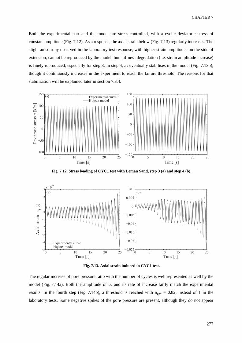
CHAPTER 7
277
Both the experimental part and the model are stress-controlled, with a cyclic deviatoric stress of
constant amplitude (Fig. 7.12). As a response, the axial strain below (Fig. 7.13) regularly increases. The
slight anisotropy observed in the laboratory test response, with higher strain amplitudes on the side of
extension, cannot be reproduced by the model, but stiffness degradation (i.e. strain amplitude increase)
is finely reproduced, especially for step 3. In step 4, ε1 eventually stabilises in the model (Fig. 7.13b),
though it continuously increases in the experiment to reach the failure threshold. The reasons for that
stabilization will be explained later in section 7.3.4.
Fig. 7.12. Stress loading of CYC1 test with Leman Sand, step 3 (a) and step 4 (b).
Fig. 7.13. Axial strain induced in CYC1 test.
The regular increase of pore pressure ratio with the number of cycles is well represented as well by the
model (Fig. 7.14a). Both the amplitude of ur and its rate of increase fairly match the experimental
results. In the fourth step (Fig. 7.14b), a threshold is reached with ur,m = 0.82, instead of 1 in the
laboratory tests. Some negative spikes of the pore pressure are present, although they do not appear
(a) (b)
0 5 10 15 20 25
0
50
100
150
Time [s]
0 5 10 15 20 25
0
50
100
150
Dev
iato
ric
stre
ss q
[kP
a]
Time [s]
Experimental curveHujeux model
(a) (b)
0 5 10 15 20 25
0
1
2
x 10
Axia
l st
rain
1 [
.]
Time [s]
Experimental curveHujeux model
0 5 10 15 20 25
0
0.005
0.01
Time [s]
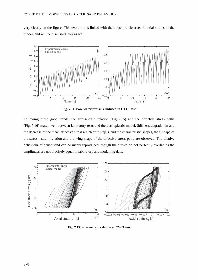
CONSTITUTIVE MODELLING OF CYCLIC SAND BEHAVIOUR
278
very clearly on the figure. This evolution is linked with the threshold observed in axial strains of the
model, and will be discussed later as well.
Fig. 7.14. Pore water pressure induced in CYC1 test.
Following these good trends, the stress-strain relation (Fig. 7.15) and the effective stress paths
(Fig. 7.16) match well between laboratory tests and the elastoplastic model. Stiffness degradation and
the decrease of the mean effective stress are clear in step 3, and the characteristic shapes, the S shape of
the stress - strain relation and the wing shape of the effective stress path, are observed. The dilative
behaviour of dense sand can be nicely reproduced, though the curves do not perfectly overlap as the
amplitudes are not precisely equal in laboratory and modelling data.
Fig. 7.15. Stress-strain relation of CYC1 test.
0 5 10 15 20 25
0
1
Time [s]0 5 10 15 20 25
0
Pore
pre
ssure
rat
io u
r
Time [s]
Experimental curveHujeux model
(a) (b)
(a) (b)
0
x 103
100
50
0
50
100
Dev
iato
ric
stre
ss q
[kP
a]
Axial strain 1 [.]
Experimental curveHujeux model
0 0.005 0.01
0
50
100
150
Axial strain 1 [.]
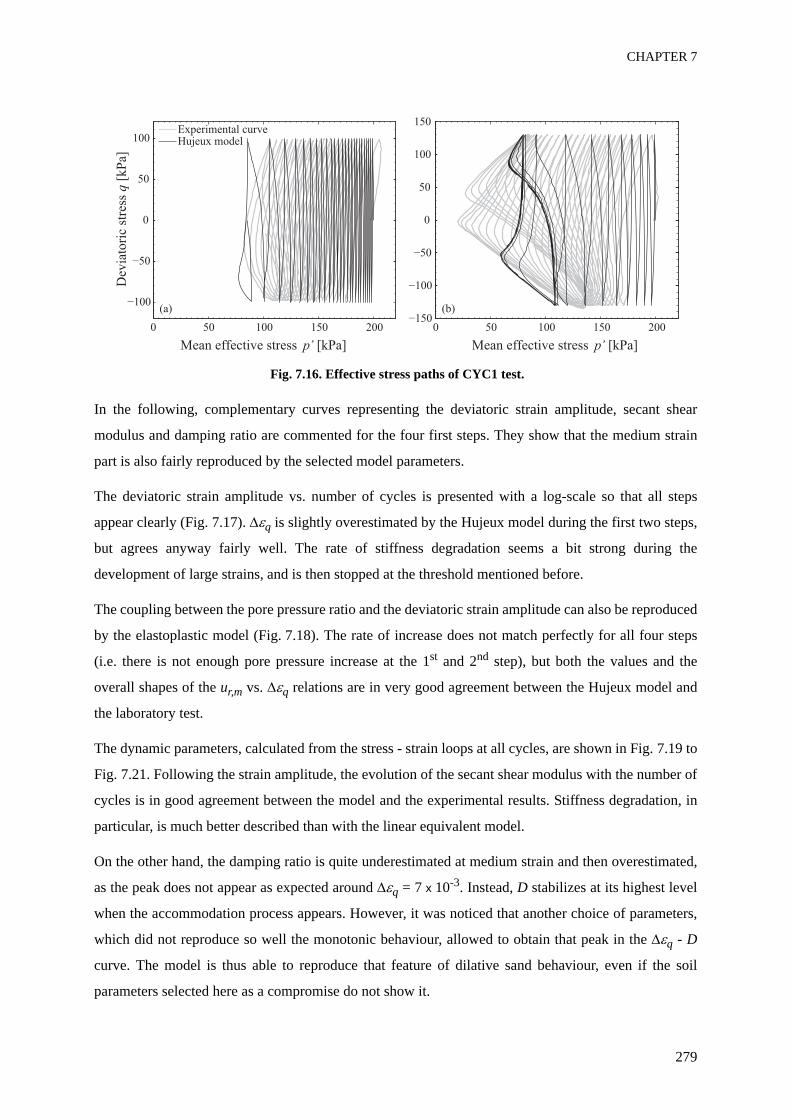
CHAPTER 7
279
Fig. 7.16. Effective stress paths of CYC1 test.
In the following, complementary curves representing the deviatoric strain amplitude, secant shear
modulus and damping ratio are commented for the four first steps. They show that the medium strain
part is also fairly reproduced by the selected model parameters.
The deviatoric strain amplitude vs. number of cycles is presented with a log-scale so that all steps
appear clearly (Fig. 7.17). Δεq is slightly overestimated by the Hujeux model during the first two steps,
but agrees anyway fairly well. The rate of stiffness degradation seems a bit strong during the
development of large strains, and is then stopped at the threshold mentioned before.
The coupling between the pore pressure ratio and the deviatoric strain amplitude can also be reproduced
by the elastoplastic model (Fig. 7.18). The rate of increase does not match perfectly for all four steps
(i.e. there is not enough pore pressure increase at the 1st and 2nd step), but both the values and the
overall shapes of the ur,m vs. Δεq relations are in very good agreement between the Hujeux model and
the laboratory test.
The dynamic parameters, calculated from the stress - strain loops at all cycles, are shown in Fig. 7.19 to
Fig. 7.21. Following the strain amplitude, the evolution of the secant shear modulus with the number of
cycles is in good agreement between the model and the experimental results. Stiffness degradation, in
particular, is much better described than with the linear equivalent model.
On the other hand, the damping ratio is quite underestimated at medium strain and then overestimated,
as the peak does not appear as expected around Δεq = 7 x 10⁻³. Instead, D stabilizes at its highest level
when the accommodation process appears. However, it was noticed that another choice of parameters,
which did not reproduce so well the monotonic behaviour, allowed to obtain that peak in the Δεq - D
curve. The model is thus able to reproduce that feature of dilative sand behaviour, even if the soil
parameters selected here as a compromise do not show it.
0 50 100 150 200
0
50
100
Dev
iato
ric
stre
ss q
[kP
a]
Mean effective stress p’ [kPa]
Experimental curveHujeux model
0 50 100 150 200
0
50
100
150
Mean effective stress p’ [kPa]
(a) (b)
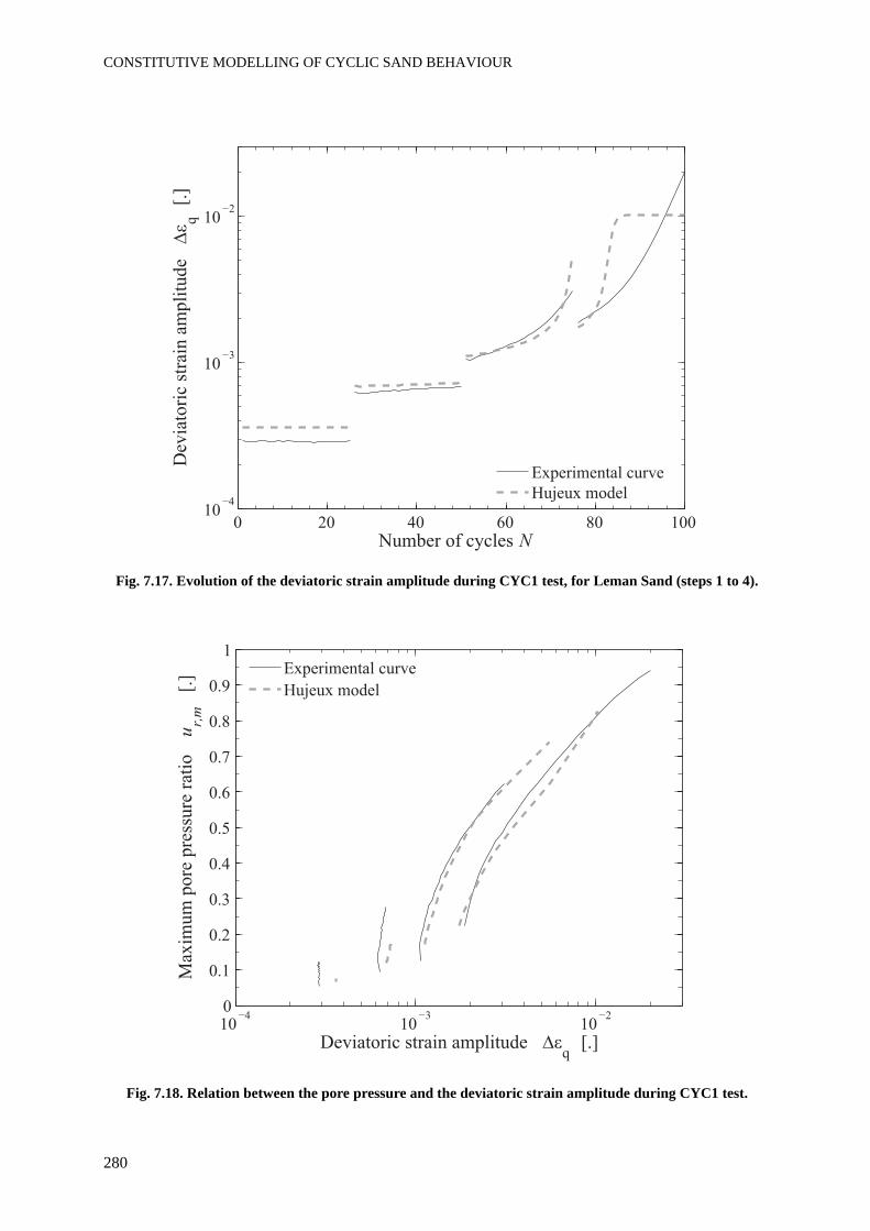
CONSTITUTIVE MODELLING OF CYCLIC SAND BEHAVIOUR
280
Fig. 7.17. Evolution of the deviatoric strain amplitude during CYC1 test, for Leman Sand (steps 1 to 4).
Fig. 7.18. Relation between the pore pressure and the deviatoric strain amplitude during CYC1 test.
0 20 40 60 80 10010
103
102
Dev
iato
ric
stra
in a
mpli
tude
q [
.]
Number of cycles N
Experimental curve
Hujeux model
10 103
102
0
0.1
0.2
0.3
0.5
0.6
0.7
0.8
0.9
1
Max
imum
pore
pre
ssure
rat
io
ur,
m [
.]
Deviatoric strain amplitude q
[.]
Experimental curve
Hujeux model
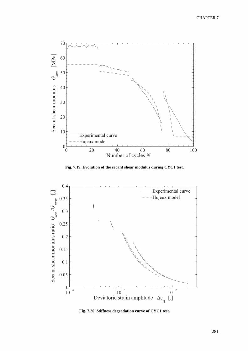
CHAPTER 7
281
Fig. 7.19. Evolution of the secant shear modulus during CYC1 test.
Fig. 7.20. Stiffness degradation curve of CYC1 test.
0 20 40 60 80 1000
10
20
30
40
50
60
70
Sec
ant
shea
r m
odulu
s G
sec
[M
Pa]
Number of cycles N
Experimental curve
Hujeux model
10 103
102
0
0.05
0.1
0.15
0.2
0.25
0.3
0.35
Sec
ant
shea
r m
odulu
s ra
tio
Gse
c/G
ma
x [
.]
Deviatoric strain amplitude q
[.]
Experimental curve
Hujeux model
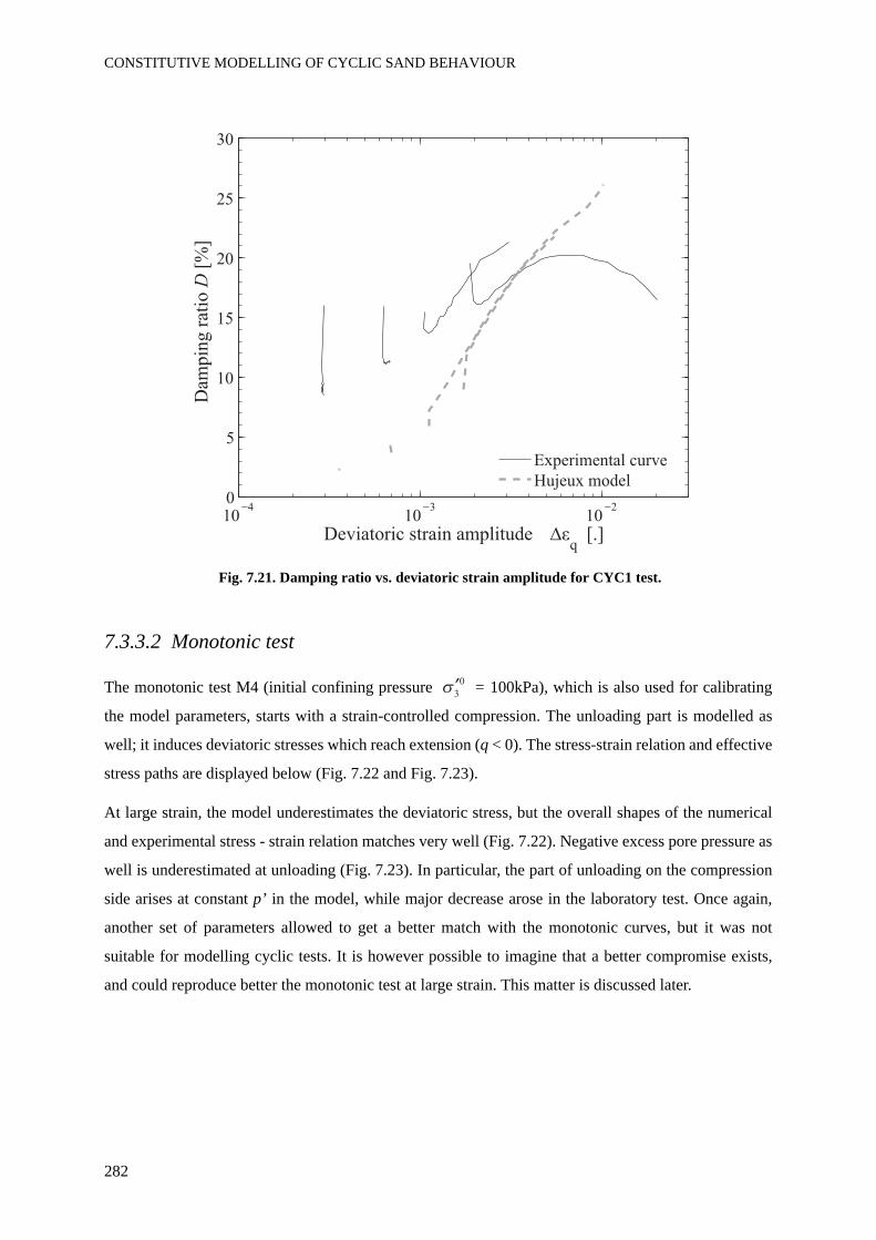
CONSTITUTIVE MODELLING OF CYCLIC SAND BEHAVIOUR
282
Fig. 7.21. Damping ratio vs. deviatoric strain amplitude for CYC1 test.
7.3.3.2 Monotonic test
The monotonic test M4 (initial confining pressure = 100kPa), which is also used for calibrating
the model parameters, starts with a strain-controlled compression. The unloading part is modelled as
well; it induces deviatoric stresses which reach extension (q < 0). The stress-strain relation and effective
stress paths are displayed below (Fig. 7.22 and Fig. 7.23).
At large strain, the model underestimates the deviatoric stress, but the overall shapes of the numerical
and experimental stress - strain relation matches very well (Fig. 7.22). Negative excess pore pressure as
well is underestimated at unloading (Fig. 7.23). In particular, the part of unloading on the compression
side arises at constant p’ in the model, while major decrease arose in the laboratory test. Once again,
another set of parameters allowed to get a better match with the monotonic curves, but it was not
suitable for modelling cyclic tests. It is however possible to imagine that a better compromise exists,
and could reproduce better the monotonic test at large strain. This matter is discussed later.
10 103
102
0
5
10
15
20
25
30
Dam
pin
g r
atio
D[%
]
Deviatoric strain amplitude q
[.]
Experimental curve
Hujeux model
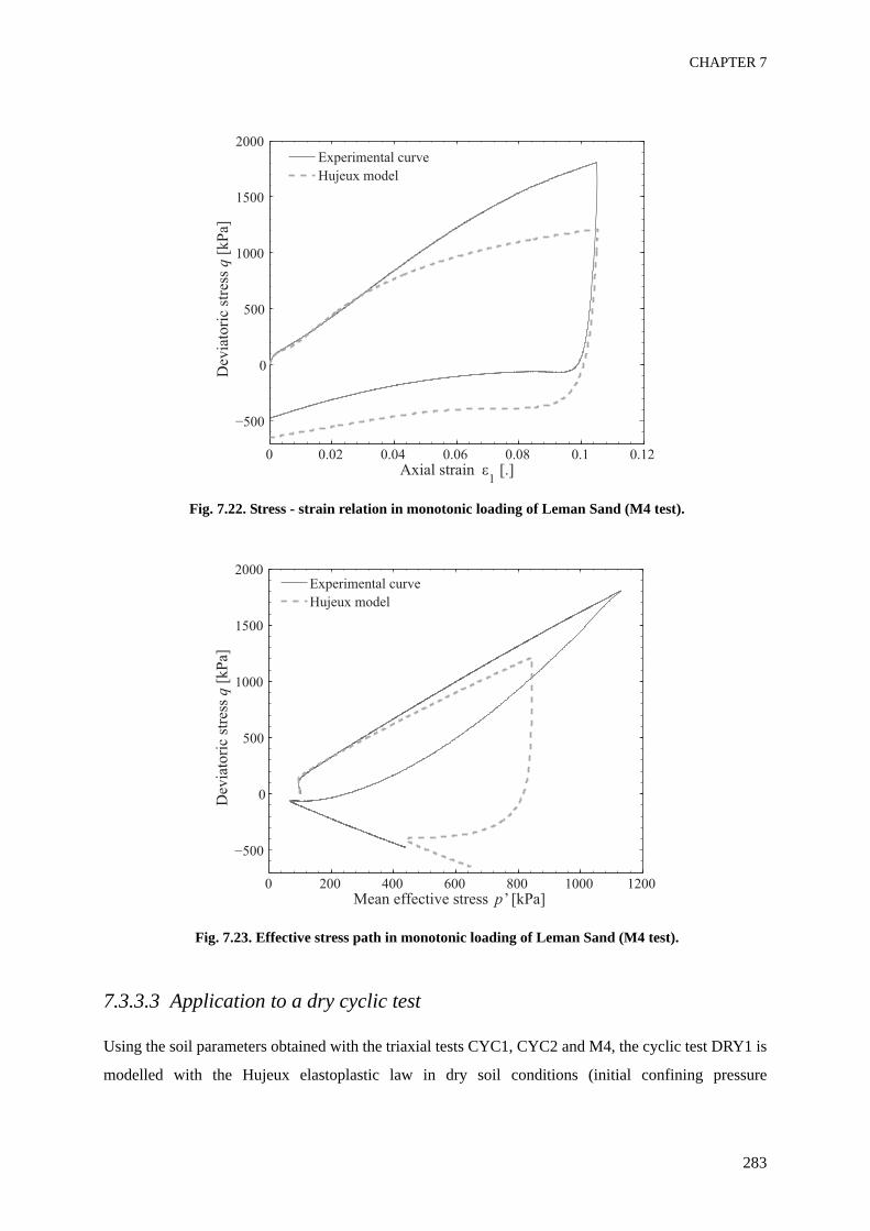
CHAPTER 7
283
Fig. 7.22. Stress - strain relation in monotonic loading of Leman Sand (M4 test).
Fig. 7.23. Effective stress path in monotonic loading of Leman Sand (M4 test).
7.3.3.3 Application to a dry cyclic test
Using the soil parameters obtained with the triaxial tests CYC1, CYC2 and M4, the cyclic test DRY1 is
modelled with the Hujeux elastoplastic law in dry soil conditions (initial confining pressure
0 0.02 0.04 0.06 0.08 0.1 0.12
0
1000
2000
Dev
iato
ric
stre
ss q
[k
Pa]
Axial strain 1 [.]
Experimental curve
Hujeux model
0 200 400 600 800 1000 1200
0
1000
2000
Dev
iato
ric
stre
ss q
[k
Pa]
Mean effective stress p’ [kPa]
Experimental curve
Hujeux model
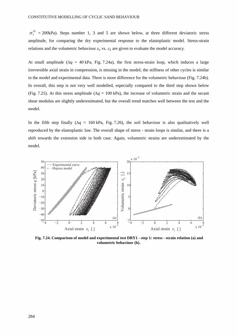
CONSTITUTIVE MODELLING OF CYCLIC SAND BEHAVIOUR
284
= 200kPa). Steps number 1, 3 and 5 are shown below, at three different deviatoric stress
amplitude, for comparing the dry experimental response to the elastoplastic model. Stress-strain
relations and the volumetric behaviour εv vs. ε1 are given to evaluate the model accuracy.
At small amplitude (Δq = 40 kPa, Fig. 7.24a), the first stress-strain loop, which induces a large
irreversible axial strain in compression, is missing in the model; the stiffness of other cycles is similar
in the model and experimental data. There is more difference for the volumetric behaviour (Fig. 7.24b).
In overall, this step is not very well modelled, especially compared to the third step shown below
(Fig. 7.25). At this stress amplitude (Δq = 100 kPa), the increase of volumetric strain and the secant
shear modulus are slightly underestimated, but the overall trend matches well between the test and the
model.
In the fifth step finally (Δq = 160 kPa, Fig. 7.26), the soil behaviour is also qualitatively well
reproduced by the elastoplastic law. The overall shape of stress - strain loops is similar, and there is a
shift towards the extension side in both case. Again, volumetric strains are underestimated by the
model.
Fig. 7.24. Comparison of model and experimental test DRY1 - step 1: stress - strain relation (a) and volumetric behaviour (b).
0 6 8
x 10
50
30
10
0
10
30
50
Axial strain 1 [.]
Dev
iato
ric
stre
ss q
[kP
a]
Experimental curveHujeux model
0 6 85
0
5
10
15
Volu
met
ric
stra
in
V [
.]
Axial strain 1 [.]
x 10
x 10
(a) (b)
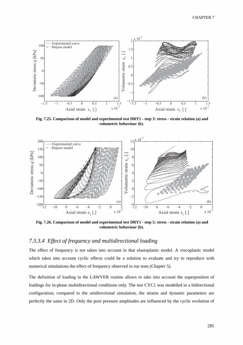
CHAPTER 7
285
Fig. 7.25. Comparison of model and experimental test DRY1 - step 3: stress - strain relation (a) and volumetric behaviour (b).
Fig. 7.26. Comparison of model and experimental test DRY1 - step 5: stress - strain relation (a) and volumetric behaviour (b).
7.3.3.4 Effect of frequency and multidirectional loadingThe effect of frequency is not taken into account in that elastoplastic model. A viscoplastic model
which takes into account cyclic effects could be a solution to evaluate and try to reproduce with
numerical simulations the effect of frequency observed in our tests (Chapter 5).
The definition of loading in the LAWYER routine allows to take into account the superposition of
loadings for in-phase multidirectional conditions only. The test CYC1 was modelled in a bidirectional
configuration; compared to the unidirectional simulation, the strains and dynamic parameters are
perfectly the same in 2D. Only the pore pressure amplitudes are influenced by the cyclic evolution of
3
Axial strain
Dev
iato
ric
stre
ss q
Experimental curveHujeux model
2
Volu
met
ric
stra
in
V
(a) (b)
Axial strain
3
3
3
Axial strain [.]
Dev
iato
ric
stre
ss q
[kP
a]
Experimental curveHujeux model
Volu
met
ric
stra
in
V [
.]
(a) (b)
Axial strain [.]
3
3
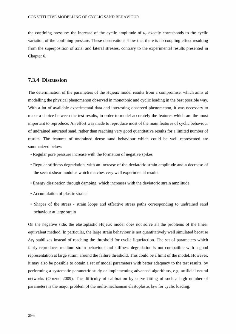
CONSTITUTIVE MODELLING OF CYCLIC SAND BEHAVIOUR
286
the confining pressure: the increase of the cyclic amplitude of ur exactly corresponds to the cyclic
variation of the confining pressure. These observations show that there is no coupling effect resulting
from the superposition of axial and lateral stresses, contrary to the experimental results presented in
Chapter 6.
7.3.4 Discussion
The determination of the parameters of the Hujeux model results from a compromise, which aims at
modelling the physical phenomenon observed in monotonic and cyclic loading in the best possible way.
With a lot of available experimental data and interesting observed phenomenon, it was necessary to
make a choice between the test results, in order to model accurately the features which are the most
important to reproduce. An effort was made to reproduce most of the main features of cyclic behaviour
of undrained saturated sand, rather than reaching very good quantitative results for a limited number of
results. The features of undrained dense sand behaviour which could be well represented are
summarized below:
• Regular pore pressure increase with the formation of negative spikes
• Regular stiffness degradation, with an increase of the deviatoric strain amplitude and a decrease of
the secant shear modulus which matches very well experimental results
• Energy dissipation through damping, which increases with the deviatoric strain amplitude
• Accumulation of plastic strains
• Shapes of the stress - strain loops and effective stress paths corresponding to undrained sand
behaviour at large strain
On the negative side, the elastoplastic Hujeux model does not solve all the problems of the linear
equivalent method. In particular, the large strain behaviour is not quantitatively well simulated because
Δε1 stabilizes instead of reaching the threshold for cyclic liquefaction. The set of parameters which
fairly reproduces medium strain behaviour and stiffness degradation is not compatible with a good
representation at large strain, around the failure threshold. This could be a limit of the model. However,
it may also be possible to obtain a set of model parameters with better adequacy to the test results, by
performing a systematic parametric study or implementing advanced algorithms, e.g. artificial neural
networks (Obrzud 2009). The difficulty of calibration by curve fitting of such a high number of
parameters is the major problem of the multi-mechanism elastoplastic law for cyclic loading.
CHAPTER 7
287
The stabilization occurring at the end of all cyclic undrained simulations, when the maximum pore
pressure ratio does not reach ur,m = 1.0, i.e. cyclic liquefaction does not fully develop, seems to
correspond to accommodation. This kind of sand response at large strain is not really understood, but
could be linked to the development of dilative behaviour. Different choices of model parameters can
support the formation of much larger strains above a few percent, developing as cyclic liquefaction or
flow liquefaction, also this is not an intrinsic limitation of the Hujeux model. Accommodation is rather
a result of the compromise made to reproduce the overall sand behaviour.
The full complexity of the model is not necessary to simulate conventional triaxial tests. However, the
multimechanisms are useful to try to capture the bidirectional effects observed in Chapter 6. Moreover,
they are necessary in view of the applications of this research project: it is foreseen to apply the
validated model parameters for multidirectional site effects analyses.
In the literature, a few advanced models based on incremental laws are able to reproduce, with good
accuracy, stiffness degradation and cyclic liquefaction of saturated undrained sand (references in
section 2.7.5). For example, the multi-surface plasticity model described by Elgamal et al. (2003) can
also reproduce the features of cyclic undrained dense sand behaviour summarized above, like pore
pressure increase and negative spikes of ur or accumulation of irreversible strains. The few curves
comparing experimental and numerical soil response give nice examples of very good match in terms
of strains induced and pore pressure increase; the dynamic parameters are not calculated in the study,
also there is no possible comparison for these test characteristics.
7.3.5 SummaryThe Hujeux model is able to reproduce most of the physical phenomenon observed in cyclic loading of
undrained sand, in conditions of unidirectional loading, at a given frequency, for symmetric CTC - RTE
tests. Even if the calibration is a difficult process, some typical values exist for various soils and can
facilitate the process. This study provides a new set of parameters for a natural poorly-graded sand.
Although the irreversible strains could not be accurately reproduced, the most prominent features of
cyclic soil behaviour at large strain, e.g. the S shape of the stress - strain loops and the increase of pore
pressure with negative spikes, were satisfactorily modelled.
The difficulty of calibration is also increased by the fact that many laboratory tests are available, also
the determination of the soil parameters is a compromise. Because of that, the robustness of the
calibration is increased even if the application of the model on a case by case basis seems less accurate.
CONSTITUTIVE MODELLING OF CYCLIC SAND BEHAVIOUR
288
The multidirectional and frequency effects can not be taken into account directly by this elastoplastic
constitutive law.
7.4 Comparison and evaluation of the models
An initial question raised in this work was to determine whether it is appropriate to use linear
equivalent models for site effect analyses, as what is used in practise, if the seismic motion is strong and
complex, and the soil response in the nonlinear regime. The answer is clearly negative; it can be further
developed, with the following comments:
• The linear equivalent method is relatively easy to implement and calibrate, if laboratory tests (or in
situ tests described in Appendix 1) provide P wave and S wave velocities as well as stiffness
degradation parameters for all soil layers.
• The limit for nonlinear sand behaviour is usually defined for accelerations around 0.4g. The results
of the experimental study and the comparison with the linear equivalent model show that, even
below this limit (e.g. 0.2g for the first step of CYC2), this method does not reproduce correctly (i)
stiffness degradation (ii) the strain amplitude (iii) the increase of irreversible strain (iv) the pore
pressure increase. This fact can be compared to the seismic hazard map of Switzerland, which
provides a PGA in Valais of 0.15g (section 2.3.2). The soil response to a strong event in this zone of
medium seismicity could thus be underestimated by such model.
• The linear equivalent model can accurately reproduce the secant shear modulus and damping ratio
from the degradation curves provided for calibration. With a known prescribed loading, it is thus
possible to derive the dynamic parameters from laboratory tests or empirical equations, and then
implement them in the linear equivalent model. However, the scopes of such applications seem
limited. Moreover, the evolution of the dynamic parameters with the number of cycles is totally
neglected.
• The multidirectional propagation of seismic waves of any kind and shape can be implemented
without difficulty within the linear equivalent model until medium strain level (as mentioned before,
the resulting strains are largely underestimated at medium strain level). However, the coupling
effects resulting from the superposition of axial and lateral stresses, which can decrease cyclic
strength (cf. Chapter 6), cannot be modelled.
On the other hand, the elastoplastic model used in this chapter provides much better results, though they
CHAPTER 7
289
are not perfect either. It has the great advantage of being able to reproduce the complex phenomenon
observed in undrained sand behaviour during cyclic loading, with alternate increase and decrease of the
pore pressure. Cyclic liquefaction is adequately modelled, which is a great achievement. The problem,
mentioned before, is that the calibration process is quite difficult, that is why obtaining the good set of
parameters requires some practise. Because of that, obtaining accurate accumulated strains is difficult,
even in the simple case of the modelling of a laboratory triaxial test. The extension to a real case of
seismic wave propagation within relatively heterogeneous materials, which was not implemented
within this research project, would be even more problematic.
Although both models allow to impose loading conditions similar to the complex loading presented in
this research, neither of them can accurately take into account the frequency effect and the effect of
superposition of loading observed in nonlinear cyclic sand behaviour. As described from the respective
laboratory studies (Chapters 5 and 6), these two features of cyclic loading have non negligible impact
on the triggering of failure in cyclic conditions, and also for irregular seismic loading (shown for
bidirectional effect only).
Taking into account these two phenomena in the linear equivalent model may not be useful, as failure is
anyway not adequately modelled. Refining such a tool, which provides broad approximations and is not
suitable for nonlinear applications, would not make a lot of sense.
On the contrary, it would be interesting to implement in detail these experimental observations in a
modified multi-mechanism elastoplastic model; this could allow to understand the physical
mechanisms responsible for such behaviour. The possible modifications could be to:
• implement a viscoplastic model in a multi-mechanism framework, to try to take into account the
effect of frequency
• re-evaluate the coupling of the isotropic and the deviatoric mechanisms, to give the possibility to
model bidirectional effects
• introduce new functions, which could take into account the strain rate and a parameter for
bidirectional effects, to enhance the volumetric response (pore pressure increase) and its coupling
with strains.
These possibilities could all be implemented at the level of the constitutive law. The hydro-mechanical
coupling is complex in such models, and also involves the balance equations. Even if we believe that
dynamic wave propagation is not involved in the phenomena observed with the triaxial press, it could
be interesting to evaluate the laboratory tests in a fully coupled finite element model.
CONSTITUTIVE MODELLING OF CYCLIC SAND BEHAVIOUR
290
7.5 ConclusionsTwo models, able to reproduce cyclic soil behaviour, are presented in this chapter, including their
calibration and the comparison with cyclic and monotonic triaxial tests.
We first showed that the linear equivalent model is not suitable for studying undrained sand behaviour
for medium to high strains. The hydro-mechanical coupling, in particular, is an essential feature of our
tests which is completely neglected in this model. Stiffness degradation is also underestimated. The
peak ground acceleration of central Valais (Switzerland), defined by the Swiss Seismological Service,
is very close to the acceleration needed to induce the nonlinear soil response characteristic of our tests.
It is often considered that such a tool is adequate for regions of relatively medium seismicity, but this
example demonstrates that the application of the linear equivalent model could imply non negligible
underestimation of predicted strains.
On the contrary, the Hujeux elastoplastic law can model most features of nonlinear soil behaviour. In
particular, the shape of stress - strain loops, observed in dense sand because of alternate increase and
decrease of the excess pore pressure, is greatly reproduced. The hydro-mechanical coupling as well is
finely obtained. By developing a systematic calibration procedure, it should be possible to facilitate the
access to this efficient model and even improve the quality of the modelling. The model could also be
developed to take into account the effect of frequency and the effect of multidirectional loading
described in the previous chapters of this study.

CHAPTER 8
CONCLUSIONS AND PERSPECTIVES

CONCLUSIONS AND PERSPECTIVES
292
8.1 Achievements
In order to evaluate the effect of complex loading (strong seismic motions) on the dynamic response of
granular soils, cyclic sand behaviour was extensively analysed by means of various triaxial tests. The
focus was put on several characteristics of seismic wave propagation:
• Loading amplitude, initial stress conditions, hydraulic conditions (Chapter 4)
• Effect of frequency, and evaluation of the parameters influencing the rate-dependency (Chapter 5)
• Effect of superposing axial and lateral stresses with cyclic loading (Chapter 6)
• Irregular seismic loading in unidirectional and bidirectional conditions (Chapter 6)
Besides the description of sand behaviour in strong and complex loading conditions, this study aims at
evaluating the importance of particular loading features, which are usually neglected. It also provides
good quality and innovative experimental results, helping to understand the physical processes involved
in soil dynamics.
Such an experimental work was possible thanks to the developments of advanced laboratory
equipments (described in Chapter 3). A short synthesis of the lessons learned from the technological
developments, calibration and validation is first presented below.
These important laboratory test results are finally used to evaluate two very different but well accepted
constitutive models (Chapter 7). In fact, reproducing cyclic soil behaviour at large strain comprises
many difficulties. It is our now documented impression that the numerical methods currently used in
practice may not be appropriate for modelling strong earthquake loading.
8.1.1 Developments of laboratory equipmentThe dynamic triaxial press was designed to perform complex cyclic and seismic loadings, in conditions
suitable for studying saturated and dry sand behaviour in the nonlinear regime (i.e. medium to large
strains). We performed developments, calibrations and validation of this complex device.
An innovative non-contact technique, based on laser sensors, was conceived, built and calibrated to
continuously measure local radial strains at middle height of the sample. The mounting frame also
allows to perform vertical sample scanning. Besides the complete calibration process and validation
with rubber and steel samples, we performed a validation of the laser sensors based on the assumption
of zero volumetric strain during undrained loading of Leman Sand. This validation defines the limits of
application of the laser sensors in terms of threshold strain amplitude; data analyses are improved
thanks to smoothing and averaging procedures. Local radial strain amplitudes from 4 x 10⁻⁴ to 4 x 10⁻¹
CHAPTER 8
293
can be monitored with loading frequency in the earthquake frequency range (0.1 to 10 Hz). An
interesting application of this device is that it allows to verify that induced anisotropy is negligible for
the cyclic triaxial tests performed on Leman Sand.
Other equipments were developed to ensure a good accuracy of the dynamic tests, mainly the sample
mounting system and the aluminium triaxial cell. Together with all described equipment, they allow to
perform reliable triaxial tests in drained and undrained conditions.
8.1.2 Cyclic dense sand behaviourSeveral monotonic and cyclic triaxial tests on Leman Sand and Fonderie Sand were performed in the
nonlinear regime. The different cyclic tests provide deep insight into stiffness degradation of both
sands, up to failure. At large strain in undrained conditions, the occurrence of cyclic liquefaction or
flow liquefaction is observed, depending on the soil tested. In dry conditions, sudden failure was
observed in dense sand.
Cyclic soil behaviour is described for different initial and boundary stress conditions. The effects of the
average deviatoric stress and the initial confining pressure on soil behaviour are the same in undrained
saturated and dry loading of Leman Sand: the overall soil behaviour is stiffer for higher mean deviatoric
stress (qav) or higher initial confining pressure ( ). Moreover, there are significant differences,
observed in the stress - strain relations and the stress paths, for compression and extension monotonic
and cyclic loading.
Undrained saturated tests exhibit stiffness degradation during continuous cyclic stress-controlled
loading. Depending on the soil type, initial and boundary conditions, the rate of increase of strain
amplitudes varies significantly. The conditions involving the highest rates of stiffness degradation are:
(i) uniform sand (Fonderie Sand), (ii) higher void ratio, (iii) lower initial confining pressure, (iv) lower
mean deviatoric stress. On the contrary, accommodation behaviour prevails in dry tests during steps of
constant stress amplitude.
Excess pore pressures of undrained saturated Leman Sand and Fonderie Sand increase as a function of
strain amplitudes. The curves Δεq - ur form a narrow band which mainly depends on the number of
cycles. Slightly higher pore pressures are obtained in the uniform sand. The increase of volumetric
strains with deviatoric strains in dry Leman Sand is represented by similar curves Δεq - Δεv. They also
seem to depend mainly on the number of cycles.
Dynamic material parameters, i.e. the secant shear modulus (Gsec) and damping ratio (D), are
calculated for cyclic loading of Leman and Fonderie Sand. Stiffness degradation curves
(Δεq - Gsec / Gmax) are obtained in the medium to large strain domain. They are similar in dry and
CONCLUSIONS AND PERSPECTIVES
294
undrained saturated conditions. On the contrary, hydraulic conditions influence the evolution of the
damping ratio. While D monotonically increases with the deviatoric strain amplitude in dry conditions,
it exhibits a peak, at medium strains, in undrained saturated dense sand. This peculiar evolution is due
to the evolution of excess pore pressure in negative spikes, during undrained cyclic loading, and it is
linked with the «S shape» of the stress - strain loops.
Sample failure of dense undrained saturated Leman Sand arises by cyclic liquefaction. The material
progressively softens, and its degradation index reaches very low values. The failure criterion can be
based on a threshold deviatoric strain Δεq = 2.5%. It matches the level of the degradation index well,
which can thus be used as an alternative criterion for failure. Another candidate can be the pore water
pressure ratio.
Three different behaviours are obtained with regard to failure in the rather uniform Fonderie Sand,
depending on the relative density: accommodation, cyclic liquefaction and flow liquefaction. At the
same relative density, the increase of deviatoric strain upon loading is very progressive and stable for
the natural Leman Sand, while it is sudden, rapid and induces instability of the motion control system
for Fonderie Sand. Fonderie Sand samples exhibit inhomogeneity above failure, especially concerning
excess pore pressure which dramatically increases above 1 due to end-restraint and strain localization.
The different behaviours of Leman and Fonderie Sand is ascribed to their respective particle shape and
grain size distribution, where round particles and uniform distribution induce higher liquefaction
susceptibility in the case of Fonderie Sand. For both sands, the phase transformation line in extension is
reached first, and most of deviatoric strains arise on the side of negative strains.
Shear strain localization was observed in particular loading conditions, and carefully analysed, thanks
to the observation of direct records from the three laser sensors in dry tests. The clear discontinuity
occurs above the threshold deviatoric strain failure criterion, around εq = 4 to 5%. Strain localization
was found to (i) depend on confining pressure, (ii) depend on the hydraulic conditions, and (iii) be
responsible for the large increase of damping ratio and excess pore pressure ratio.
8.1.3 Frequency-dependence of granular materialsCreep and relaxation tests reported in the literature provide examples of viscous behaviour of dry and
saturated granular materials. However, rate effects are neither well-known nor understood, especially
for conditions of strong seismic loading. This work provides laboratory tests showing the influence of
loading frequencies on soil behaviour, applicable under such strain amplitude and frequency range
conditions.
Monotonic triaxial undrained compression tests performed at different strain rates below 1 %/s show
CHAPTER 8
295
that there is no observable monotonic strain rate effect in Leman Sand in this range of strain rate. On the
contrary, the cyclic tests performed on dense Leman Sand show a frequency effect between 0.1 and
6.5 Hz in dry and undrained conditions.
Preliminary stress-controlled cyclic tests at four frequencies show that, compared to high frequencies,
low frequencies induce higher strain amplitudes, lower stiffness and higher excess pore pressure at
medium to large strain. The same consequences on stiffness degradation behaviour are inferred, in
certain conditions, from undrained saturated tests at 15 different frequencies. Dry Leman Sand also
exhibits frequency-dependent behaviour at medium strain level. As for undrained sand, deviatoric
strain amplitudes increase at low frequency.
A strong frequency-dependence is found in an undrained saturated test: the deviatoric strain amplitude
decreases by a factor of 3, the maximum pore pressure ratio decreases by a factor of 4.5 and the secant
shear modulus increases by a factor of 3 when the frequency increases from 0.1 to 6.5 Hz. Interestingly,
other test boundary conditions, inducing higher sample stiffness, lead to practically frequency-
independent soil behaviour in approximately the same frequency range. This observation is also
confirmed for a dry sample.
A dry cyclic test also exhibits frequency-dependent behaviour, therefore the coupled motion of the
granular matrix and the pore water is not the sole phenomenon behind frequency effects in sand. As for
creep described in the literature for dry and saturated sands, viscous behaviour of inter-particle contacts
may then play a role in frequency effects.
8.1.4 Effect of cyclic bidirectional conditions on undrained sand behaviourCyclic bidirectional tests were performed on Leman Sand in saturated undrained conditions. They
demonstrate that the superposition of axial and radial stresses induces coupling effects in the nonlinear
soil response. Bidirectional loadings produce an amplification of motions before cyclic liquefaction,
and a limitation of strains after cyclic liquefaction. The phase angle between axial and lateral stresses
has a particularly strong influence on Leman Sand behaviour. Cyclic strength is significantly modified
by complex loadings.
In order to understand and compare the coupling between the two loadings, the pore pressure ratio of
bidirectional tests is separated into two components which account for the change in total applied
stress. The unidirectional pore pressure ratio ur and the bidirectional component , which corresponds
to the deviatoric part of the load, have similar shapes. Moreover, both reach the threshold value 1 at
cyclic liquefaction. The component of pore pressure ratio which accounts for the cyclic isotropic load,
, includes water compressibility by including the sample B-Skempton coefficient.
ur
q
ur
comp
CONCLUSIONS AND PERSPECTIVES
296
A possible explanation for bidirectional effects is that the pore pressure itself influences the
development of deviatoric strains. At the same time, the contractive behaviour of the soil matrix
induces pore water pressure build-up. This double-way coupling, which is emphasized in our
bidirectional tests depending on the value of the phase angle, induces a reduction of stiffness, and the
occurrence of cyclic liquefaction is then accelerated.
8.1.5 Seismic unidirectional and bidirectional loadingThree irregular seismic tests were also performed in unidirectional and bidirectional conditions to
illustrate the effect of superposition of loading in conditions close to in situ seismic motions. For
irregular amplitudes and frequency content, bidirectional loadings can also increase deviatoric strains
and pore pressure build up compared to unidirectional motions. The conditions of amplification of the
response are similar to cyclic tests: before cyclic liquefaction, the superposition of loading slightly
accelerates stiffness degradation. In the case of seismic loading, soil behaviour after cyclic liquefaction
is practically equivalent in unidirectional and bidirectional loading.
The parallel between cyclic and irregular loading is illustrated with (i) characteristic «S shape» stress-
strain relations, as a consequence of the evolution of excess pore pressure, (ii) total and effective stress
paths, (iii) the relation between pore pressure increase and deviatoric strains. In irregular tests, we also
showed that the relation between the maximum strain amplitude and the maximum stress amplitude is
nonlinear, even in unidirectional loading.
8.1.6 Modelling the cyclic behaviour of dense sandTwo different models were applied, the linear equivalent model and the multi-mechanism elastoplastic
model of Hujeux. They both illustrate the difficulties of modelling the cyclic soil behaviour at medium
to large strain. Model calibrations are presented for Leman Sand, and the comparison with cyclic and
monotonic triaxial tests is analysed.
We first show that the linear equivalent model is not suitable for modelling undrained sand behaviour
for medium to high strains, in terms of qualitative description of the physical mechanisms. The
quantitative results as well are poorly adequate. The hydro-mechanical coupling, an essential feature of
our tests, is completely neglected in this model. Stiffness degradation is also underestimated, as well as
strain amplitude.
It is often considered that the linear equivalent model is adequate for regions of relatively medium
seismicity; however, the comparison of peak ground acceleration defined for Valais (Switzerland) and
the acceleration needed to induce the nonlinear soil response characteristic of our tests are very close.
CHAPTER 8
297
This shows that the application of the linear equivalent model in such areas, for example in
microzonation studies for evaluating site effects, could imply non negligible underestimation of
predicted strains.
The Hujeux constitutive law, which was adapted to cyclic loading, belongs to the category of Cam-clay
models in the sense that it is an elastoplastic model defined within the critical state framework. Strain
amplitudes of Leman Sand are well reproduced by the elastoplastic law, except at cyclic liquefaction,
for which they are underestimated. Moreover, most features of the nonlinear sand behaviour can be
modelled. In particular, the elastoplastic model provides accurate «S shapes» of the stress - strain loops,
which occur in dense sand because of alternate increase and decrease of the excess pore pressure. The
hydro-mechanical coupling is thus finely obtained. This model thus seems adequate for applications to
strong seismic motions.
8.2 Outlook
The results presented in this work should be taken into account when designing earthquake-resistant
structures. In particular, they may affect performance-based design (PBD) in geomechanics, which
relies on an accurate prediction of the behaviour of a soil deposit or structure subjected to various
loadings, including nonlinear effects. Moreover, the consequences of our study could be important for
the evaluation of site effects.
On laboratory test side, we demonstrate that some loading features which are usually neglected can
have a strong impact on the soil response. How to take these loading features into account within design
procedures and site effects analyses is an open question.
We propose relations of Leman Sand secant shear modulus and damping ratio as a function of the
average strain rate. The parameters of these power laws seem to depend on soil stiffness, as well as the
overall rate-dependent behaviour. In particular, pore pressure build-up was shown to increase at low
frequency, with a higher rate-dependency at small soil stiffness. Complementary tests on Leman Sand
at different confining pressures and void ratios could be useful to evaluate the range of variation of
these parameters, and to more precisely evaluate the limit between rate-dependent and rate-independent
sand behaviour. The effects of particle shape and hydraulic conditions on rate-sensitivity could be
explored in depth, to help understanding the mechanisms responsible for frequency-dependent
behaviour of granular materials.
CONCLUSIONS AND PERSPECTIVES
298
We also showed that bidirectional conditions have an impact on stiffness degradation and the triggering
of cyclic liquefaction. Bidirectional effects are strongly dependent on phase angle, i.e. coupling effects
are not trivial. In order to obtain significant curves for design purpose, more tests at other phase angles
and for different initial stress and void ratios would be needed in bidirectional conditions.
Moreover, it would be very interesting to introduce continuous rotations of principal stress directions
within the laboratory triaxial tests, in order to obtain a more realistic simulation of complex seismic
motions. Indeed, the dynamic triaxial press can also control cyclic and seismic axial rotations of the
axisymmetric sample, which can be superimposed to the bidirectional loadings used in this research.
This third independent component would allow to impose «tridirectional» stresses within the soil
sample. Introducing the rotation of principal stresses represents more than just adding a new test
parameter, it would allow to explore much more general stress states.
On the modelling side, we show that the linear equivalent model, usually used in practice for site effect
analyses, is not suitable for conditions corresponding to strong earthquakes (at least for acceleration
above 0.2g). We recommend to use more complete models, which can reproduce soil behaviour more
realistically, in particular for sensitive areas.
The Hujeux elastoplastic model is a possibility, but adequate training is necessary. By developing a
systematic calibration procedure, it should be possible to facilitate the access to this efficient model and
even improve the quality of the modelling.
It would be interesting to evaluate the effect of frequency observed in our tests within a viscoplastic
framework suitable for cyclic loading. This could allow to verify if the observed frequency-dependent
behaviour is linked with viscous phenomena. The Hujeux model could also be developed to take into
account the effects of multidirectional loading on cyclic soil behaviour.
Finally, these results could also have applications to other dynamic loading of strong amplitude,
especially the sand response to shock, explosion and blasting (mining applications, terrorism-related
risks, dynamic compaction, etc...).
299
References
Abrantes, A.E., and Yamamuro, J.A. 2002. Experimental and data analysis techniques used for highstrain rate tests on cohesionless soil. Geotechnical Testing Journal, 25(2): 128-141.
Aggour, M.S., and Zhang, J.X. 2006. Degradation of sands due to combined sinusoidal loading.Journal of Geotechnical and Geoenvironmental Engineering, 132(12): 1628-1632.
Altun, S., and Goktepe, A.B. 2006. Dependence of dynamic shear modulus of uniform sands on stresslevel and density. Civil Engineering and Environmental Systems, 23(2): 101-116.
Amini, F., and Qi, G.Z. 2000. Liquefaction Testing of Stratified Silty Sands. Journal of Geotechnicaland Geoenvironmental Engineering ASCE, 126(3): 208-218.
AnhDan, L.Q., Koseki, J., and Sato, T. 2006. Evaluation of quasi-elastic properties of gravel using alarge-scale true triaxial apparatus. Geotechnical Testing Journal, 29(5): 374-384.
Assimaki, D., and Kausel, E. 2002. An equivalent linear algorithm with frequency and pressure-dependent moduli and damping for the seismic analysis of deep sites. Soil Dynamics andEarthquake Engineering, 22(9-12): 959-965.
Assimaki, D., Kausel, E., and Whittle, A. 2000. Model for dynamic shear modulus and damping forgranular soils. Journal of Geotechnical and Geoenvironmental Engineering, 126(10): 859-869.
Augustesen, A., Liingaard, M., and Lade, P.V. 2004. Evaluation of time-dependent behavior of soils.International Journal of Geomechanics, 4(3): 137-156.
Baldi, G., Hight, D.W., and Thomas, G.E. 1988. A reevaluation of Conventional Triaxial Test Methods.In Advanced triaxial testing of soil and rock. Edited by R.C.C. Robert t. Donaghe, Marshall L.Silver. Louisville, United States. ASTM, pp. 219-263.
Bard, P.-Y., and Riepl, J. 2000. Wave propagation in complex geological structures and their effects onstrong ground motion. In Wave Motion in Earthquake Engineering. WIT Press, Southampton.pp. 37-95.
Benahmed, N. 2001. Comportement mécanique d'un sable sous cisaillement monotone et cyclique :application aux phénomènes de liquéfaction et de mobilité cyclique, Ecole Nationale des Pontset Chaussées, Paris, PhD thesis.
Bernardie, S., Foerster, E., and Modaressi, H. 2006. Non-linear site response simulations in Chang-Hwa region during the 1999 Chi-Chi earthquake, Taiwan. Soil Dynamics and EarthquakeEngineering, 26(11): 1038-1048.
REFERENCES
300
Biot, M.A. 1956. Theory of Propagation of Elastic Waves in a Fluid-Saturated Porous Solid. I. Low-Frequency Range. Journal of the Acoustical Society of America, 28(2): 168-178.
Bolton, M.D., and Wilson, J.M.R. 1989. An experimental and theoretical comparison between staticand dynamic torsional soil tests. Géotechnique, 39, No. 4: 584-599.
Bolton, M.D., and Wilson, J.M.R. 1990. Soil stiffness and damping. In European conference onstructural dynamics. Edited by K.e. al. Bochum, Germany. Balkema, Rotterdam, pp. 209-216.
Boukpeti, N., Mroz, Z., and Drescher, A. 2004. Modeling rate effects in undrained loading of sands.Canadian Geotechnical Journal, 41(2): 342-350.
Boulanger, R.W., and Seed, R.B. 1995. Liquefaction of Sand under Bidirectional Monotonic and CyclicLoading. Journal of Geotechnical Engineering, 121(12): 870-878.
Bray, J.D., and Sancio, R.B. 2006. Assessment of the liquefaction susceptibility of fine-grained soils.Journal of Geotechnical and Geoenvironmental Engineering, 132(9): 1165-1177.
Brennan, A.J., Thusyanthan, N.I., and Madabhushi, S.P.G. 2004. Evalution of Shear Modulus andDamping in Dynamic Centrifuge Tests. Technical report, Report CUED/D-SOILS/TR336,Cambridge University Engineering Department.
BRGM 2005. CyberQuake User's Guide Version 2.01. BRGM.
Bui, M.T., Clayton, C.R.I., and Priest, J.A. 2007. Effect of particle shape on small strain shear modulusof geomaterials. In 4th International Conference on Earthquake Geotechnical Engineering.Edited by K. Pitilakis. Thessaloniki, Greece, 8 pages.
Campanella, R.G., Robertson, P.K., and Gillespie, D. 1986. Seismic cone penetration test. In In Situ1986, ASCE Specialty Conference on Use of In Situ Tests in Geotechnical Engineering. Editedby S.P. Clemence. Blacksburg, VA, pp. 116-130.
Carvajal, J.C., Taboada-Urtuzuastegui, V.M., and Romo, M.P. 2002. Influence of earthquake frequencycontent on soil dynamic properties at CAO site. Soil Dynamics and Earthquake Engineering,22(4): 297-308.
Cascante, G., and Santamarina, J.C. 1996. Interparticle contact behavior and wave propagation. Journalof Geotechnical Engineering-ASCE, 122(10): 831-839.
Cekerevac, C. 2003. Thermal effects on the mechanical behaviour of saturated clays : an experimentaland constitutive study. EPFL, Lausanne, PhD. Thesis.
Chaudhary, S.K., Kuwano, J., Hashimoto, S., Hayano, Y., and Nakamura, Y. 2002. Effects of initialfabric and shearing direction on cyclic deformation characteristics of sand. Soils andFoundations, 42(1): 147-157.
Chazelas, J., Escoffier, S., Garnier, J., Thorel, L., and Rault, G. 2008. Original technologies for provenperformances for the new LCPC earthquake simulator. Bulletin of Earthquake Engineering,6(4): 723-728.
Choi, C., and Arduino, P. 2004. Behavioral characteristics of gravelly soils under general cyclic loadingconditions. In Cyclic Behaviour of Soils and Liquefaction Phenomena. Edited by T.Triantafyllidis. Bochum, Germany. Taylor and Francis Group, pp. 115-128.
Chu, J. 1995. An experimental examination of the critical state and other similar concepts for granularsoils. Canadian Geotechnical Journal, 32(6): 1065-1075.
REFERENCES
301
Cid, J., Susagna, T., Goula, X., Chavarria, L., Figueras, S., Fleta, J., Casas, A., and Roca, A. 2001.Seismic zonation of Barcelona based on numerical simulation of site effects. Pure and AppliedGeophysics, 158(12): 2559-2577.
Cox, B.R., Stokoe, K.H., and Rathje, E.M. 2009. An In Situ Test Method for Evaluating the CoupledPore Pressure Generation and Nonlinear Shear Modulus Behavior of Liquefiable Soils.Geotechnical Testing Journal, 32(1): 11-21.
De Gennaro, V., Canou, J., Dupla, J.C., and Benahmed, N. 2004. Influence of loading path on theundrained behaviour of a medium loose sand. Canadian Geotechnical Journal, 41(1): 166-180.
Delepine, N. 2007. Modélisation des effets de site sismiques dans les bassins sédimentaires et influencedes non-linéarités de comportement des sols, Ecole nationale des ponts et chaussées, Marne-la-Vallée, PhD thesis.
Demircioglu, M.B., Sesetyan, K., Durukal, E., and Erdik, M. 2007. Assessment of earthquake hazard inTurkey. In 4th International Conference on Earthquake Geotechnical Engineering. Edited by K.Pitilakis. Thessaloniki.
Di Benedetto, H. 2006. Small strain behaviour and viscous effects on sands and sand-clay mixtures. InSoil Stress-Stain Behavior: Measurement, Modeling and Analysis. Geotechnical Symposiumheld to celebrate the 60th Birthday of Fumio Tatsuko. Edited by H. Ling, L. Callisto, D.Leshchinsky, and J. Koseki. Rome, Italy. MAR 16-17, 2006. Springer, pp. 159-190.
Di Benedetto, H., and Tatsuoka, F. 1997. Small strain behavior of geomaterials: modelling of strain rateeffects. Soils and Foundations, 37(2): 127-138.
Di Benedetto, H., Tatsuoka, F., and Ishihara, M. 2002. Time-dependent shear deformationcharacteristics of sand and their constitutive modelling. Soils and Foundations, 42(2): 1-22.
Dobry, R.R., Ladd, S., Yokel, F.Y., Chung, R.M., and Powell, D. 1982. Prediction of pore waterpressure buildup and liquefaction of sands during earthquakes by the cyclic strain method.National Bureau of Standards, Washington, DC.
Drosos, V., Gerolymos, N., and Gazetas, G. 2007. Calibration and verification of nonlinear wavepropagation method. In 4th International Conference on Earthquake Geotechnical Engineering.Edited by K. Pitilakis. Thessaloniki.
Duttine, A., Tatsuoka, F., Kongkitkul, W., and Hirakawa, D. 2008. Viscous behaviour of unboundgranular materials in direct shear. Soils and Foundations, 48(3): 297-318.
Elgamal, A., Zeghal, M., Parra, E., Gunturi, R., Tang, H.T., and Stepp, J.C. 1996. Identification andmodeling of earthquake ground response. 1. Site amplification. Soil Dynamics and EarthquakeEngineering, 15(8): 499-522.
Elgamal, A., Yang, Z.H., and Parra, E. 2002. Computational modeling of cyclic mobility and post-liquefaction site response. Soil Dynamics and Earthquake Engineering, 22(4): 259-271.
Elgamal, A., Yang, Z., Parra, E., and Ragheb, A. 2003. Modeling of cyclic mobility in saturatedcohesionless soils. International Journal of Plasticity, 19(6): 883-905.
Elgamal, A., Yang, Z., Lai, T., Kutter, B.L., and Wilson, D.W. 2005. Dynamic response of saturateddense sand in laminated centrifuge container. Journal of Geotechnical and GeoenvironmentalEngineering, 131(5): 598-609.
Elgamal, A., Pitilakis, K., Dimitrios, R., Garnier, J., Madabhushi, S.P.G., Pinto, A., Steidl, J., Stewart,
REFERENCES
302
H.E., Stokoe, K.H., Taucer, F., Tokimatsu, K., and Wallace, J.W. 2007. A review of large-scaletesting facilities in geotechnical earthquake engineering. In 4th International Conference onEarthquake Geoechnical Engineering. Edited by K.D. Pitilakis. Thessaloniki, Greece. june2007. Springer, pp. 93-127.
Endo, O., and Komanobe, K. 1995. Single- and multi-directional shaking table tests of sandliquefaction. In First International Conference on Earthquake Geotechnical Engineering.Edited by K. Ishihara. Tokyo. 14-16 November 1995. A.A. Balkema, Vol.2, pp. 675-680.
Enomoto, T., Tatsuoka, F., Shishime, M., Kawabe, S., and Di Benedetto, H. 2006. Viscous property ofgranular material in drained triaxial compression. In Soil Stress-Strain Behavior: Measurement,Modeling and Analysis. Geotechnical Symposium held to celebrate the 60th Birthday of FumioTatsuko. Edited by H.I. Ling, L. Callisto, D. Leshchinsky, and J. Koseki. Rome, ITALY. Mar16-17. Springer, pp. 383-397.
Erten, D., and Maher, M.H. 1995. Cyclic undrained behavior of silty sand. Soil Dynamics andEarthquake Engineering, 14(2): 115-123.
Finge, Z., Doanh, T., and Dubujet, P. 2006. Undrained anisotropy of Hostun RIF loose sand: newexperimental investigations. Canadian Geotechnical Journal, 43(11): 1195-1212.
Finn, W.D.L., Pickering, D.J., and Bransby, P.L. 1971. Sand liquefaction in triaxial and simple sheartests. Journal of the soil mechanics and foundations division, 97(4): 20.
François, B. 2008. Thermo-plasticity of fine-grained soils at various saturation states: Application tonuclear waste disposal, EPFL, Lausanne, PhD thesis.
Fredlund, D.G., and Xing, A.Q. 1994. Equations for the Soil-Water Characteristic Curve (Vol 31, Pg521, 1994). Canadian Geotechnical Journal, 31(6): 1026-1026.
Gajo, A. 1995. Influence of Viscous Coupling in Propagation of Elastic Waves in Saturated Soil.Journal of Geotechnical Engineering, 121(9): 636-644.
Gajo, A. 1996. The effects of inertial coupling in the interpretation of dynamic soil tests. Geotechnique,46(2): 245-257.
Gallage, P.C.K., Towhata, I., and Nishimura, S. 2005. Laboratory investigation on rate-dependentproperties of sand undergoing low confining effective stress. Soils and Foundations, 45(4): 43-60.
Georgiannou, V.N., and Tsomokos, A. 2008. Comparison of two fine sands under torsional loading.Canadian Geotechnical Journal, 45(12): 1659-1672.
Georgiannou, V.N., Tsomokos, A., and Stavrou, K. 2008. Monotonic and cyclic behaviour of sandunder torsional loading. Geotechnique, 58(2): 113-124.
Gerolymos, N., and Gazetas, G. 2005. Constitutive model for 1-D cyclic soil behaviour applied toseismic analysis of layered deposits. Soils and Foundations, 45(3): 147-159.
Ghionna, V.N., and Porcino, D. 2006. Liquefaction resistance of undisturbed and reconstituted samplesof a natural coarse sand from undrained cyclic triaxial tests. Journal of Geotechnical andGeoenvironmental Engineering, 132(2): 194-202.
Ghosh, B., and Madabhushi, S.P.G. 2003. A numerical investigation into effects of single and multiplefrequency earthquake motions. Soil Dynamics and Earthquake Engineering, 23(8): 691-704.
Giardini, D., Wiemer, S., Fah, D., and Deichmann, N. 2004. Seismic hazard assessment of Switzerland,
REFERENCES
303
Swiss Seismological Service, Zurich.
Govindaraju, L., and Sitharam, T.G. 2007. Effect of loading frequency on cyclic behaviour of soils. In4th International Conference on Earthquake Geotechnical Engineering. Edited by K. Pitilakis.Thessaloniki, Greece, p. p. 13.
Habib, P., and Luong, M.P. 1985. Comportement du milieu pulvérulent. In Génie Parasismique. Pressesde l'Ecole Nationale des Ponts et Chausées, Paris. pp. 303-311.
Hardin, B.O., and Drnevich, V.P. 1972a. Shear modulus and damping in soils: measurement andparameters effects. Journal of the soil mechanics and foundations division, 98(SM 6): 603-624.
Hardin, B.O., and Drnevich, V.P. 1972b. Shear modulus and damping in soils: design equations andcurves. Journal of the soil mechanics and foundations division, 98(SM 7): 667-692.
Hardin, B.O., and Kalinski, M.E. 2005. Estimating the shear modulus of gravelly soils. Journal ofGeotechnical and Geoenvironmental Engineering, 131(7): 867-875.
Hartzell, S., Bonilla, L.F., and Williams, R.A. 2004. Prediction of Nonlinear Soil Effects. Bulletin ofthe Seismological Society of America, 94(5): 1609-1629.
Hatzor, Y.H., Gvirtzman, H., Wainshtein, I., and Orian, I. 2009. Induced liquefaction experiment inrelatively dense, clay-rich sand deposits. Journal of Geophysical Research-Solid Earth, 114: 22.
Head, K.H. 1984. Manual of soil laboratory testing. Volume 3: effective stress tests. Pentech Press,London.
Hecht, E. 1998. Physique. De Boek.
Hoque, E., and Tatsuoka, F. 2004. Triaxial testing system for measuring loading-rate effects duringcyclic tests of sand. Geotechnical Testing Journal, 27(5): 483-495.
Houlsby, G.T. 1998. Advanced interpretation of field tests. In 1st International Conference on SiteCharacterization (ISC 98). Edited by P.K. Robertson and P.W. Mayne. Atlanta, Ga. Apr 19-22.A.A. Balkema, pp. 99-112.
Hujeux, J.-C. 1985. Une loi de comportement pour le chargement cyclique des sols. In GénieParasismique, Paris. pp. 287-302.
Huot, F. 1999. Caractéristiques élastiques des sols - Du comportement pseudo-statique à la propagationdes ultrasons, Université de Lausanne, Lausanne, PhD thesis.
Huot, F., and Vulliet, L. 1998. Small strain elastic moduli of a saturated sand. In Biot Conference onPoromechanics. Louvain-La-Neuve, pp. 93-97.
Hyde, A.F.L., Higuchi, T., and Yasuhara, K. 2006. Liquefaction, cyclic mobility, and failure of silt.Journal of Geotechnical and Geoenvironmental Engineering, 132(6): 716-735.
Hyodo, M., Hyde, A.F.L., and Aramaki, N. 1998. Liquefaction of crushable soils. Geotechnique, 48(4):527-543.
Hyodo, M., Hyde, A.F.L., Aramaki, N., and Nakata, Y. 2002. Undrained monotonic and cyclic shearbehaviour of sand under low and high confining stresses. Soils and Foundations, 42(3): 63-76.
Iai, S., and Tobita, T. 2006. Soil non-linearity and effects on seismic site response. In 3rd InternationalSymposium on the effects of Surface Geology on Seismic Motion. Edited by P.-Y. Bard, E.Chaljub, C. Cornou, F. Cotton, and P. Gueguen. Grenoble. LCPC, Vol.1, pp. p 21-46.
REFERENCES
304
Ibraim, E., Di Benedetto, H., and Doanh, T. 2009. Time-Dependent Behaviour and Static LiquefactionPhenomenon of Sand. Geotechnical and Geological Engineering, 27(1): 181-191.
Ibsen, L.B. 1994. The Stable State in Cyclic Triaxial Testing on Sand. Soil Dynamics and EarthquakeEngineering, 13(1): 63-72.
Idriss, I.M., and Sun, J.I. 1992. User's manual for SHAKE91: a computer program for conductingequivalent linear seismic response analyses of horizontally layered soil deposits, Department ofCivil & Environmental Engineering, University of California, Davis, California.
Idriss, I.M., and Boulanger, R.W. 2007. SPT- and CPT-based relationships for the residual shearstrength of liquefied soils. In 4th International Conference on Earthquake GeotechnicalEngineering. Edited by K.D. Pitilakis. Thessaloniki, GREECE. Jun, pp. 1-22.
Ishihara, K. 1996. Soil behaviour in earthquake geotechnics. Oxford University Press Inc., New York.
Ishihara, K., and Yasuda, N. 1972. Sand Liquefaction Due to Irregular Excitation. Soils andfoundations, 12(4): 65.
Ishihara, K., and Yasuda, S. 1975. Sand liquefaction in hollow cylinder torsion under irregularexcitation. Soils and Foundations, 15(1): 45-59.
Ishihara, K., and Yamazaki, F. 1980. Cyclic Simple Shear Tests on Saturated Sand in Multi-directionalLoading. Soils and Foundations, 20(1): 45-59.
Ishihara, K., and Nagase, H. 1988. Multi-directional irregular loading tests on sand. Soil Dynamics andEarthquakes Engineering, 7(4): 201-212.
Ishihara, K., Tatsuoka, F., and Yasuda, S. 1975. Undrained deformation and liquefaction of sand undercyclic stresses. Soils and Foundations, 15(1): 29-44.
Iverson, R.M., and LaHusen, R.G. 1989. Dynamic Pore-Pressure Fluctuations in Rapidly ShearingGranular Materials. Science, 246(4931): 796-799.
Jaeger, H.M., and Nagel, S.R. 1992. Physics of the Granular State. Science, 255(5051): 1523-1531.
Jahangir, E. 2008. Caractérisation du sable de Fonderie sous chargement sismique. EPFL, LMS. Masterthesis.
Jeremic, B., Cheng, Z., Taiebat, M., and Dafalias, Y. 2008. Numerical simulation of fully saturatedporous materials. International Journal for Numerical and Analytical Methods inGeomechanics, 32(13): 1635-1660.
Ju, S.-H., and Ni, S.-H. 2007. Determining Rayleigh damping parameters of soils for finite elementanalysis, pp. 1239-1255.
Kalkan, E., and Gulkan, P. 2004. Site-Dependent Spectra Derived from Ground Motion Records inTurkey. Earthquake Spectra, 20(4): 1111-1138.
Kammerer, A.M., Pestana, J.M., and Seed, R.B. 2003. Behavior of Monterey 0/30 sand underMultidirectional Loading Conditions. In Geomechanics: Testing, Modeling, and Simulation(GSP 143). Edited by J.K.-E. Jerry A. Yamamuro. Boston. 2005. ASCE, Vol.143, pp. 154-173.
Kammerer, A.M., Seed, R.B., Wu, J., Riemer, M.F., and Pestana, J.M. 2004. Pore PressureDevelopment in Liquefiable Soils Under Bi-Directional Loading Conditions. Report.
Karg, C., and Haegeman, W. 2009. Elasto-plastic long-term behavior of granular soils: Experimental
REFERENCES
305
investigation. Soil Dynamics and Earthquake Engineering, 29(1): 155-172.
Khalili, N., Habte, M.A., and Valliappan, S. 2005. A bounding surface plasticity model for cyclicloading of granular soils. International Journal for Numerical Methods in engineering, 63:1939-1960.
Khan, Z.H., Cascante, G., El Naggar, M.H., and Lai, C.G. 2008. Measurement of frequency-dependentdynamic properties of soils using the resonant-column device. Journal of Geotechnical andGeoenvironmental Engineering, 134(9): 1319-1326.
Kim, S.I., Park, K.B., Park, S.Y., Hwang, S.J., Lee, J.H., and Choi, J.S. 2005. Effects of irregulardynamic loads on soil liquefaction. In 16th International Conference on Soil Mechanics andGeotechnical Engineering. Osaka, JAPAN. 2005. Millpress Science Publishers, pp. 2673-2676.
Kokusho, T. 1980. Cyclic triaxial test of dynamic soil properties for wide strain range. Soils andFoundations, 20(2): 45-60.
Kokusho, T., Hara, T., and Hiraoka, R. 2004. Undrained shear strength of granular soils with differentparticle gradations. Journal of Geotechnical and Geoenvironmental Engineering, 130(6): 621-629.
Koliji, A. 2008. Mechanical behaviour of unsaturated aggregated soils, EPFL, Lausanne, PhD thesis.
Kramer, S.L. 1996. Geotechnical Earthquake Engineering, Upper Saddle River, New Jersey.
Kuwano, R., and Jardine, R.J. 2002. On measuring creep behaviour in granular materials throughtriaxial testing. Canadian Geotechnical Journal, 39(5): 1061-1074.
Lacave, C., Bard, P.Y., Kham, M., and Koller, M.G. 2008. 2D equivalent linear site effect simulation:example applications to two deep valleys. Bulletin of Earthquake Engineering, 6(2): 197-211.
Laloui, L. 1992. Modélisation du comportement thermo-hydro-mécanique des milieux poreuxanélastiques, Ecole Centrale Paris, Chatenay Malabry, PhD thesis.
Leroueil, S., and Marques, M.S. 1996. Importance of strain rate and temperature effects in geotechnicalengineering. In Measuring and modelling time dependent soil behavior. Edited by T.C.S.a.V.N.Kaliakin. Washington, D.C. November, 10-14 1996 ASCE, pp. 1-60.
Li, X.S. 1990. Free field soil response under multidirectional earthquake loading, Univerity ofCalifornia, Davis. PhD thesis.
Li, X.S. 1997. Rotational shear effects on ground earthquake response. Soil Dynamics and EarthquakesEngineering, 16(1): 9-19.
Li, X.S., and Yang, W.L. 1998. Effects of vibration history on modulus and damping of dry sand.Journal of Geotechnical and Geoenvironmental Engineering, 124(11): 1071-1081.
Li, X.S., Shen, C.K., and Wang, Z.L. 1998. Fully coupled inelastic site response analysis for 1986Lotung earthquake. Journal of Geotechnical and Geoenvironmental Engineering, 124(7): 560-573.
Li, X.S., Dafalias, Y., and Wang, Z.L. 1999. State-dependant dilatancy in critical-state constitutivemodelling of sand. Canadian Geotechnical Journal, 36(4): 599-611.
Lin, M.L., Huang, T.H., and You, J.C. 1996. The effects of frequency on damping properties of sand.Soil Dynamics and Earthquake Engineering, 15(4): 269-278.
REFERENCES
306
Lin, M.L., Wang, K.L., and Chen, T.C. 2009. Tsaoling landslide in Taiwan during the 1999 Chi-Chiearthquake. In Earthquake Geotechnical Case Histories for Performance-Based Design. Taylor& Francis Group - Balkema, London. pp. 273-287.
Ling, H.I., and Liu, H.B. 2003. Pressure-level dependency and densification behavior of sand throughgeneralized plasticity model. Journal of Engineering Mechanics-ASCE, 129(8): 851-860.
LMSSMAT, Ecole Centrale Paris. 2007. LAWYER: Logiciel de simulation d'essais homogènes decomportement des sols.
Lopez-Caballero, F. 2003. Influence du comportement non linéaire du sol sur les mouvementssismiques induits dans des géo-structures, Ecole Centrale Paris, Chatenay Malabry, PhD thesis.
Lopez-Querol, S., and Blazquez, R. 2006. Liquefaction and cyclic mobility model for saturatedgranular media. International Journal for Numerical and analytical methods in geomechanics,30: 413-439.
Lopez-Querol, S., and Blazquez, R. 2007. Validation of a new endochronic liquefaction model forgranular soil by using centrifuge test data. Soil Dynamics and Earthquake Engineering, 27(10):920-937.
Lunne, T., Robertson, P.K., and Powell, J.J. 1997. Cone Penetration Testing in Geotechnical Practice.Blackie Academic & Professional, an imprint of Chapman & Hall, London.
Luong, M.P. 1980. Phénomènes cycliques dans les sols pulvérulents. Revue française de Géotechnique,10(1): 39-53.
Madabhushi, S.P.G. 2004. Modelling of earthquake damage using geotechnical centrifuges. CurrentScience, 87(10): 1405-1416.
Matesic, L., and Vucetic, M. 2003. Strain-rate effect on soil secant shear modulus at small cyclicstrains. Journal of Geotechnical and Geoenvironmental Engineering, 129(6): 536-549.
Matsushita, M., Tatsuoka, F., Koseki, J., Cazacliu, B., Di Benedetto, H., and Yasin, S.J.M. 1999. Timeeffect on the pre-peak deformation properties of sands. In Second International Conférence onPre-Failure Deformation Characteristics of Geomaterials. Edited by J.e. al. Torino. Balkema,Vol.1, pp. 681-689.
Mayoraz, F. 2002. Comportement mécanique des milieux granulaires sous sollicitations cycliques:Application aux fondations de chaussées, EPFL, Lausanne, PhD thesis.
Mellal, A. 1997. Analyse des effets du comportement non linéaire des sols sur le mouvement sismique,Ecole Centrale Paris, Châtenay Malabry, PhD thesis.
Meng, J. 2007. Earthquake ground motion simulation with frequency-dependent soil properties. SoilDynamics and Earthquake Engineering, 27(3): 234-241.
Messerklinger, S., and Springman, S.M. 2007. Local radial displacement measurements of soilspecimens in a triaxial test apparatus using laser transducers. Geotechnical Testing Journal,30(6): 454-465.
Michalski, E., and Rahma, A. 1989. Modélisation du comportement des sols en élastoplasticité:définition des paramètres des modèles Hujeux-Cyclade et recherche des valeurs des paramètrespour différents sols, BRGM - Service géologique national.
Micro-Epsilon Instruction Manual optoNCDT1700, Ortenburg.
REFERENCES
307
Mohajeri, M., and Towhata, I. 2003. Shake table tests on residual deformation of sandy slopes due tocyclic loading. Soils and Foundations, 43(6): 91-106.
Mohkam, M. 1983. Contribution à l'étude expérimentale et théorique du comportement des sables souschargements cycliques, Université Scientifique et médicale et Institut National Polytechniquede Grenoble, Grenoble, PhD thesis.
Mroz, Z., Norris, V.A., and Zienkiewicz, O.C. 1981. An Anisotropic, Critical State Model for SoilsSubject to Cyclic Loading. Geotechnique, 31(4): 451-469.
Muir Wood, D. 1990. Soil Behaviour and Critical State Soil Mechanics. Cambridge University Press
Muir Wood, D. 1998. Deformation properties of soils for dynamic analyses. In 6th SECED Conferenceon Seismic Design Practice into the Next Century. Edited by E. Booth. Oxford, England. Mar26-27, pp. 15-24.
Muir Wood, D. 2001. Some observations of volumetric instabilities in soils. In Symposium on MaterialInstabilities and the Effect of Microstructure. Austin, Texas. May 07-11. Pergamon-ElsevierScience Ltd, pp. 3429-3449.
Muir Wood, D. 2004. Geotechnical Modelling. Spon Press, London.
Muir Wood, D. 2007. The magic of sands - The 20th Bjerrum Lecture presented in Oslo, 25 November2005. Canadian Geotechnical Journal, 44(11): 1329-1350.
Muir Wood, D., Sadek, T., Dihoru, L., and Lings, M. 2006. Deviatoric stress response envelopes frommultiaxial tests on sand. In Soil Stress-Strain Behavior: Measurement, modeling and Analysis.Geotechnical Symposium held to celebrate the 60th Birthday of Fumio Tatsuko. Edited by H.I.Ling, C. L., L. D., and K. J. Rome, ITALY. Mar 16-17. Springer, pp. 253-262.
Muravskii, G.B. 2001. Application of experimental results on cyclic deforming of soils to seismicresponse analysis. Soil Dynamics and Earthquake Engineering, 21(8): 661-669.
Nagase, H., and Ishihara, K. 1987. Effects of load irregularity on the cyclic behaviour of sand. SoilDynamics and Earthquake Engineering, 6(4): 239-249.
Nagase, H., and Ishihara, K. 1988. Liquefaction-induced compaction and settlement of sand duringearthquakes. Soils and Foundations, 28(1): 65-76.
Nawir, H., Tatsuoka, F., and Kuwano, R. 2003. Experimental evaluation of the viscous properties ofsand in shear. Soils and Foundations, 43(6): 13-31.
Nowacki, W.K. 1978. Stress waves in non-elastic solids, Oxford.
Nuth, M. 2009. Constitutive modelling of unsaturated soils with hydro-geomechanical couplings,EPFL, Lausanne, PhD thesis.
O'Reilly, M.P., and Brown, S.F. 1991. Cyclic Loading of Soils: from theory to design. Blackie and SonLtd, Glasgow.
Obrzud, R.F. 2009. Numerical modeling and neural networks to identify constitutive parameters fromin situ tests, EPFL, Lausanne, PhD thesis.
Okamoto, S. 1973. Introduction to earthquake engineering. University of Tokyo Press.
Okur, D.V., and Ansal, A. 2007. Stiffness degradation of natural fine grained soils during cyclicloading. Soil Dynamics and Earthquake Engineering, 27(9): 843-854.
REFERENCES
308
Osinov, V.A. 2003. Cyclic shearing and liquefaction of soil under irregular loading: an incrementalmodel for the dynamic earthquake-induced deformation. Soil Dynamics and EarthquakeEngineering, 23(7): 535-548.
Pastor, M., Zienkiewicz, O.C., and Chan, A.H.C. 1990. Generalized Plasticity and the Modeling of SoilBehavior. International Journal for Numerical and Analytical Methods in Geomechanics,14(3): 151-190.
Pecker, A. 1984. Dynamique des sols. Presses de l'école nationale des ponts et chaussées, Paris.
Péron, H. 2008. Desiccation cracking of soils, EPFL, Lausanne, PhD thesis.
Pham Van Bang, D., Di Benedetto, H., Duttine, A., and Ezaoui, A. 2007. Viscous behaviour of drysand. International Journal for Numerical and Analytical Methods in Geomechanics, 31(15):1631-1658.
Popescu, R., Prevost, J.H., Deodatis, G., and Chakrabortty, P. 2006. Dynamics of nonlinear porousmedia with applications to soil liquefaction. Soil Dynamics and Earthquake Engineering, 26(6-7): 648-665.
Porcino, D., Caridi, G., and Ghionna, V.N. 2008. Undrained monotonic and cyclic simple shearbehaviour of carbonate sand. Geotechnique, 58(8): 635-644.
Poulos, S.J. 1981. The Steady-State of Deformation. Journal of the Geotechnical Engineering Division-ASCE, 107(5): 553-562.
Puzrin, A.M., and Shiran, A. 2000. Effects of the constitutive relationship on seismic response of soils.Part I. Constitutive modeling of cyclic behavior of soils. Soil Dynamics and EarthquakeEngineering, 19(5): 305-318.
Pyke 1973. Settlement and Liquefaction of Sands Under Multidirectional Loading, University ofCalifornia, Berkeley, PhD thesis.
Ray, R.P., and Woods, R.D. 1988. Modulus and Damping Due to Uniform and Variable Cyclic Loading.Journal of Geotechnical Engineering-ASCE, 114(8): 861-876.
Richardson, A.M., and Whitman, R.V. 1963. Effect of strain-rate upon undrained shear resistance of asaturated remoulded fat clay. Geotechnique, 13(4): 310-324.
Riemer, M.F., and Seed, R.B. 1997. Factors affecting apparent position of steady-state line. Journal ofGeotechnical and Geoenvironmental Engineering, 123(3): 281-288.
Robertson, P.K. 1994. Suggested terminology for liquefaction. In 47th Canadian GeotechnicalConference. Halifax, N.S., pp. 277-286.
Romero, E. 1999. Characterisation and thermo-mechanical behaviour of unsaturated Boon clay: Anexperimental study, UPC, Barcelona, PhD thesis.
Sadek, T., Lings, M., Dihoru, L., and Muir Wood, D. 2007. Wave transmission in Hostun sand:multiaxial experiments. Italian Geotechnical Journal, 41(2): 69-84.
Salvati, L.A., and Anhdan, L.Q. 2008. Rate-dependent response of dense sand in cyclic triaxial tests.Soils and Foundations, 48(3): 447-451.
Sanin, M.V., and Wijewickreme, D. 2006. Cyclic shear response of channel-fill Fraser River Delta silt.Soil Dynamics and Earthquake Engineering, 26(9): 854-869.
REFERENCES
309
Sassa, K., Wang, G.H., Fukuoka, H., and Vankov, D.A. 2005. Shear-displacement-amplitude dependentpore-pressure generation in undrained cyclic loading ring shear tests: An energy approach.Journal of Geotechnical and Geoenvironmental Engineering, 131(6): 750-761.
Sawada, S., Tsukamoto, Y., and Ishihara, K. 2004. Residual deformation characteristics of partiallysaturated sandy soils subjected to seismic excitation. In 11th International Conference on SoilDynamics and Earthquake Engineering/3rd International Conference on EarthquakeGeotechnical Engineering. Berkeley, CA. Jan 07-09, pp. 175-182.
Schofield, A., and Wroth, P. 1968. Critical State Soil Mechanics. McGraw-Hill, London.
Schrott, L., and Sass, O. 2008. Application of field geophysics in geomorphology: Advances andlimitations exemplified by case studies. Geomorphology, 93(1-2): 55-73.
Seed, H.B. 1979. Soil liquefaction and cyclic mobility evaluation for level ground during earthquakes.Journal of the Geotechnical Engineering Division, 105(2): 201-255.
Seed, H.B., and Idriss, I.M. 1971. Simplified Procedure for Evaluating Soil Liquefaction Potential.Journal of the Soil Mechanics and Foundations Division 97(9): 1249-1273.
Seed, H.B., Tokimatsu, K., Harder, L.F., and Chung, R.M. 1985. Influence of SPT procedures in soilliquefaction resistance evaluations. Journal of Geotechnical Engineering, 111(12): 1425-1445.
Seed, H.B., Wong, R.T., Idriss, I.M., and Tokimatsu, K. 1986. Moduli and damping factors for dynamicanalyses of cohesionless soils. Journal of Geotechnical Engineering, 112(7): 1016-1032.
Seed, R.B., Cetin, K.O., Moss, R.E.S., Kammerer, A., Wu, J., Pestana, J., and Riemer, M. 2001. Recentadvances in soil liquefaction engineering and seismic site response evaluation. In 4th
International Conference and Symposium on Recent Advances in Geotechnical EarthquakeEngineering and Soil Dynamics. University of Missouri, Rolla.
Semblat, J.F. 1994. Sols sous sollicitations dynamiques et transitoire: Réponse dynamique aux barresde Hopkinson, propagation d'ondes en milieu centrifugé, Ecole Polytechnique, Palaiseau, PhDthesis.
Semblat, J.F. 1997. Rheological interpretation of Rayleigh damping. Journal of Sound and Vibration,206(5): 741-744.
Semblat, J.F., and Luong, M.P. 1998. Wave propagation through soils in centrifuge testing. Journal ofEarthquake Engineering, 2(1): 147-171.
Semblat, J.-F., Luong, M.P., and Gary, G. 1999. 3D-Hopkinson bar: new experiments for dynamictesting on soils. Soils and Foundations, 39(1): 1-10.
Semblat, J.F., Kham, M., Bard, P.Y., Pitilakis, K., Makra, K., and Raptakis, D. 2005. Seismic waveamplification: Basin geometry vs soil layering. Soil Dynamics and Earthquake Engineering,25(7-10): 529-538.
Shahnazari, H., and Towhata, I. 2002. Torsion shear tests on cyclic stress-dilatancy relationship of sand.The Japanese Geotechnical Society, pp. 105-119.
Shibuya, S., Hight, D.W., and Jardine, R.J. 2003. Four-dimensional local boundary surfaces of anisotropically consolidated loose sand. Soils and Foundations, 43(2): 89-103.
Sitharam, T.G., GovindaRaju, L., and Murthy, B.R.S. 2004. Evaluation of liquefaction potential anddynamic properties of silty sand using cyclic triaxial testing. Geotechnical Testing Journal,27(5): 423-429.
REFERENCES
310
Sivathayalan, S., and Vaid, Y.P. 2002. Influence of generalized initial state and principal stress rotationon the undrained response of sands. Canadian Geotechnical Journal, 39(1): 63-76.
Studer, J.A., Koller, M.G., Loew, S., and Lateltin, O. 2004. Classification of soil profiles withcorresponding earthquake design spectra for specific conditions in switzerland. In 13th WorldConference on Earthquake Engineering. Vancouver, B.C., Canada.
Swiss standard SNV 670 008a. 1997. VSS.
Tatsuoka, F. 2006. Inelastic deformation characteristics of geomaterial. In Soil Stress-Stain Behavior:Measurement, Modeling and Analysis. Geotechnical Symposium held to celebrate the 60thBirthday of Fumio Tatsuko. Ling, HI; Callisto, L; Leshchinsky, D; Koseki, J, Rome, ITALY,pp. 1-108.
Tatsuoka, F., Yasuda, S., Iwasaki, T., and Tokida, K. 1980. Normalized dynamic undrained strength ofsands subjected to cyclic and random loading. Soils and Foundations, 20(3): 1-16.
Tatsuoka, F., Ishihara, M., Di Benedetto, H., and Kuwano, R. 2002. Time-dependent shear deformationcharacteristics of geomaterials and their simulation. Soils and Foundations, 42(2): 103-129.
Terzaghi, K. 1943. Theoretical Soil Mechanics. Chapman and Hall, London.
The MathWorks, I. 2009. Matlab Support http://www.mathworks.com/index.html?ref=logo&s_cid=docframe_homepage.
Towhata, I., and Ishihara, K. 1985. Undrained strength of sand undergoing cyclic rotation of principalstress axes. The Japanese Geotechnical Society, pp. 135-147.
Toyota, H., Nakamura, K., and Kazama, M. 2004. Shear and liquefaction characteristics of sandy soilsin triaxial tests. Soils and Foundations, 44(2): 117-126.
Tsukamoto, Y., Ishihara, K., and Sawada, S. 2004. Settlement of silty sand deposits followingliquefaction during earthquakes. Soils and Foundations, 44(5): 135-148.
Ueng, T.S., Wang, M.H., Chen, M.H., Chen, C.H., and Peng, L.H. 2006. A large biaxial shear box forshaking table test on saturated sand. Geotechnical Testing Journal, 29(1): 1-8.
Uthayakumar, M., and Vaid, Y.P. 1998. Static liquefaction of sands under multiaxial loading. CanadianGeotechnical Journal, 35(2): 273-283.
Vaid, Y.P., and Sivathayalan, S. 1996. Static and cyclic liquefaction potential of Fraser Delta sand insimple shear and triaxial tests. Canadian Geotechnical Journal, 33(2): 281-289.
Vaid, Y.P., Chung, E.K.F., and Kuerbis, R.H. 1989. Preshearing and undrained response of sand. Soilsand Foundations, 29(4): 49-61.
Vaid, Y.P., Chung, E.K.F., and Kuerbis, R.H. 1990. Stress Path and Steady-State. CanadianGeotechnical Journal, 27(1): 1-7.
Verdugo, R., and Ishihara, K. 1996. The steady state of sandy soils. Soils and Foundations, 36(2): 81-91.
Verruijt, A., and Cordova, C.C. 2001. Moving loads on an elastic half-plane with hysteretic damping.Journal of Applied Mechanics-Transactions of the Asme, 68(6): 915-922.
Vucetic, M. 1994. Cyclic threshold shear strains in soils. Journal of Geotechnical Engineering, 120(12):2208-2228.
REFERENCES
311
Vucetic, M. 2004. Emerging Trends in Dynamic Simple Shear Testing. In International workshop onUncertainties in Nonlinear Soil Properties and their Impact on Modeling Dynamic SoilReponse. Peer Headquarters, UC Berkeley. March 18-19 2004, p. 15.
Vucetic, M., and Dobry, R. 1991. Effect of soil plasticity on cyclic response. Journal of GeotechnicalEngineering, 117(1): 89-107.
Vucetic, M., and Tabata, K. 2003. Influence of soil type on the effect of strain rate on small-strain cyclicshear modulus. Soils and Foundations, 43(5): 161-173.
Vulliet, L., and Hutter, K. 1988. Viscous type sliding laws for landslides. Canadian GeotechnicalJournal, 25(3): 467-477.
Wang, G.X., and Kuwano, J. 1999. Modeling of strain dependency of shear modulus and damping ofclayey sand. Soil Dynamics and Earthquake Engineering, 18(6): 463-471.
Wang, Y.H., and Santamarina, J.C. 2007. Attenuation in sand: an exploratory study on the small-strainbehavior and the influence of moisture condensation. Granular Matter, 9(6): 365-376.
Wichtmann, T., and Triantafyllidis, T. 2004. Influence of a cyclic and dynamic loading history ondynamic properties of dry sand, part I: cyclic and dynamic torsional prestraining. SoilDynamics and Earthquake Engineering, 24(2): 127-147.
Wichtmann, T., Niemunis, A., and Triantafyllidis, T. 2005. Strain accumulation in sand due to cyclicloading: drained triaxial tests. Soil Dynamics and Earthquake Engineering, 25: 967-979.
Wichtmann, T., Niemunis, A., and Triantafyllidis, T. 2007a. Strain accumulation in sand due to cyclicloading: Drained cyclic tests with triaxial extension. Soil Dynamics and EarthquakeEngineering, 27(1): 42-48.
Wichtmann, T., Niemunis, A., and Triantafyllidis, T. 2007b. On the influence of the polarization and theshape of the strain loop on strain accumulation in sand under high-cyclic loading. SoilDynamics and Earthquake Engineering, 27(1): 14-28.
Wolf, J.P. 1994. Foundation Viration Analysis Using Simple Physical Models. Prentice-Hall,Englewood Cliffs.
Yamada, S., Hyodo, M., Orense, R.P., Dinesh, S.V., and Hyodo, T. 2008. Strain-dependent dynamicproperties of remolded sand-clay mixtures. Journal of Geotechnical and GeoenvironmentalEngineering, 134(7): 972-981.
Yamamuro, J.A., and Lade, P.V. 1993. Effects of strain rate on instability of granular soils. GeotechnicalTesting Journal, 16(3): 304-313.
Yasuda, N., Matsumoto, N., Yoshioka, R., and Takahashi, M. 1997. Undrained monotonic and cyclicstrength of compacted rockfill material from triaxial and torsional simple shear tests. CanadianGeotechnical Journal, 34(3): 357-367.
Yoshida, N., Kobayashi, S., Suetomi, I., and Miura, K. 2002. Equivalent linear method consideringfrequency dependent characteristics of stiffness and damping. Soil Dynamics and EarthquakeEngineering, 22(3): 205-222.
Zambelli, C., di Prisco, C., d'Onofrio, A., Visone, C., and de Magistris, F.S. 2006. Dependency of themechanical behaviour of granular soils on loading frequency: Experimental results andconstitutive modelling. In Soil Stress-Strain Behavior: Measurement, Modeling and Analysis.Geotechnical Symposium held to celebrate the 60th Birthday of Fumio Tatsuko. Edited by H.I.

REFERENCES
312
Ling, C. L., L. D., and K. J. Rome, ITALY. Mar 16-17. Springer, pp. 567-582.
Zhang, H.M., and Garga, V.K. 1997. Quasi-steady state: a real behaviour? Canadian GeotechnicalJournal, 34(5): 749-761.
Zhang, J.M., Shamoto, Y., and Tokimatsu, K. 1997. Moving critical and phase-transformation stressstate lines of saturated sand during undrained cyclic shear. Soils and Foundations, 37(2): 51-59.

APPENDIX 1
IN SITU TESTING FOR THE
EVALUATION OF DYNAMIC SOIL
BEHAVIOUR
IN SITU TESTING FOR THE EVALUATION OF DYNAMIC SOIL BEHAVIOUR
2
A1.1 Geophysical methods
IntroductionIn situ investigations of the subsoil is a good method to obtain soil characteristics of a given site.
Among common geophysical methods, the ones using seismic wave propagation are summarized here.
These techniques use elastic wave propagation models. They aim at determining layering, elastic
properties and inclusions. They are divided here between non-invasive and borehole methods.
Free surface measurementSeismic waves are generated by a sledge hammer hitting a metal plate placed on the ground. The elastic
wave signal is received by geophones strategically placed at known distance of the emission. The time
delay between emission and reception of the elastic waves is precisely measured. These methods can
provide celerity of the seismic waves, as well as the thickness of the soil layers and bedrock. It can also
indicate water table depth. Small strain elastic moduli can be calculated.
Seismic refraction is the most popular seismic free surface measurement technique among
geophysicists (Schrott & Sass 2008). It relies on the fact that soil layers become denser and wave
velocities increase with depth. When the emitted wave hits a surface discontinuity at the critical
refraction angle, the refracted wave follows the boundary (Fig. A1-1). Along its journey, the refracted
wave emits head waves which travel back to the soil surface and are recorded by receivers. The P
waves travel faster in deeper soil deposit, also the head waves are the first waves recorded by
geophones.
To illustrate the results obtained by seismic refraction, a seismogram (Fig. A1-2) shows the sounding of
a talus cone (Schrott & Sass 2008), with the distance between the source and geophones in abscissa.
Each vertical signal is an average of several shots recorded on the geophones. There are three lines
joining the first arrival of refracted waves. The slope of these lines is proportional to the velocity of the
P wave in each soil layer, which is written on the figure.
Typical investigated profile have a depth of 10 to 30 m. Deeper soil profiles can be obtained with
explosions, instead of sledge hammer. Problems related to seismic refraction are mainly (i) noise from
human activities or natural sources, such as strong wind, rainfall, close torrents (ii) inaccurate detection
of seismic wave onset (iii) hidden loose layers. Moreover P wave velocities are not uniquely related to
one soil or rock type, also complementary drillings are necessary for a precise identification. The great
advantage of seismic refraction is that it gives a continuous profile along the investigated zone,
including the inclination of boundaries thanks to back analyses. Seismic refraction is best adapted to
preliminary on site surveys. This method, as well as other geophysical methods, is a reliable source of
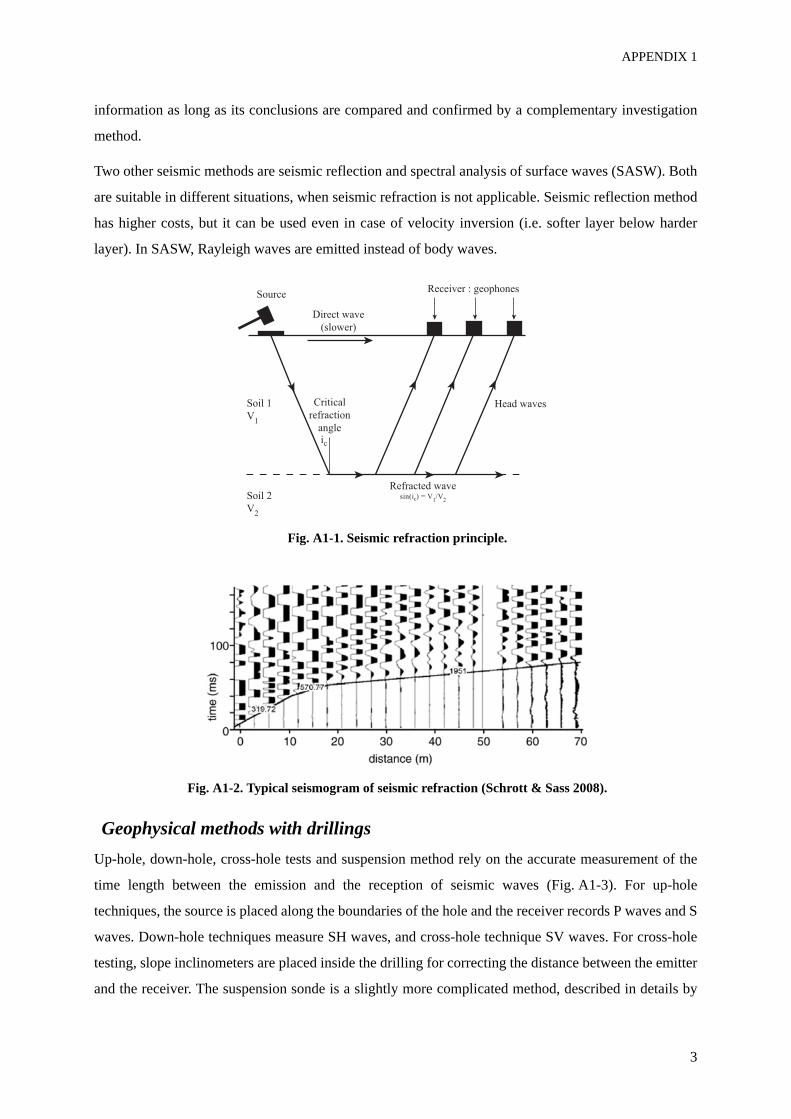
APPENDIX 1
3
information as long as its conclusions are compared and confirmed by a complementary investigation
method.
Two other seismic methods are seismic reflection and spectral analysis of surface waves (SASW). Both
are suitable in different situations, when seismic refraction is not applicable. Seismic reflection method
has higher costs, but it can be used even in case of velocity inversion (i.e. softer layer below harder
layer). In SASW, Rayleigh waves are emitted instead of body waves.
Fig. A1-1. Seismic refraction principle.
Fig. A1-2. Typical seismogram of seismic refraction (Schrott & Sass 2008).
Geophysical methods with drillingsUp-hole, down-hole, cross-hole tests and suspension method rely on the accurate measurement of the
time length between the emission and the reception of seismic waves (Fig. A1-3). For up-hole
techniques, the source is placed along the boundaries of the hole and the receiver records P waves and S
waves. Down-hole techniques measure SH waves, and cross-hole technique SV waves. For cross-hole
testing, slope inclinometers are placed inside the drilling for correcting the distance between the emitter
and the receiver. The suspension sonde is a slightly more complicated method, described in details by
Receiver : geophones
Soil 1
V1
Soil 2
V2
Direct wave
(slower)
ic
Critical
refraction
angle
Refracted wave
Head waves
Source
sin(ic) = V1/V
2

IN SITU TESTING FOR THE EVALUATION OF DYNAMIC SOIL BEHAVIOUR
4
Ishihara (1996). The single drilling is filled with water, in which the sonde is immersed. A compression
wave is emitted at the bottom, and induce, among others, a horizontally polarized shear wave travelling
vertically in the soil deposit. The arrival time of this shear wave is recorded to calculate the velocity of
wave propagation.
With these testing methods, the shear wave velocity can be measured also the maximum shear modulus
Gmax of soil layers is estimated.
Fig. A1-3. (a) up-hole, (b) down-hole (c) cross-hole tests and (d) suspension sonde.
A1.2 Geotechnical in situ testing
IntroductionThere are other possibilities for determining soil parameters in situ. Because so many techniques have
been developed in the last forty years, it is not within the scope of this chapter to assemble all existing
methods. Many empirical correlations can be found in the literature. Some of them, concerning soil
dynamics and earthquake geotechnical engineering, are mentioned below. The emphasis is also put on
methods which allow the direct evaluation of dynamic soil behaviour.
Measurement of Gmax
Instead of using geophysical tests, Campanella et al. (1986) proposed a new method, the seismic cone
penetration test, for determining the maximum shear modulus. Small geophones are incorporated to the
cone, and measure the shear wave velocity resulting from an impact at the soil surface. This method is
less expensive than down-hole tests (Lunne et al. 1997). Two penetrometers installed in parallel can
also perform tests equivalent to the cross-hole method. Small strain damping ratio can also be
calculated.
(a) (b) (c)
Receiver
Source
Source
Source
Receiver
Receiver
slope
inclinometers
Oscilloscope
t
Oscilloscope
t
Oscilloscope
t
(d)
Receivers
Source
Oscilloscope
t
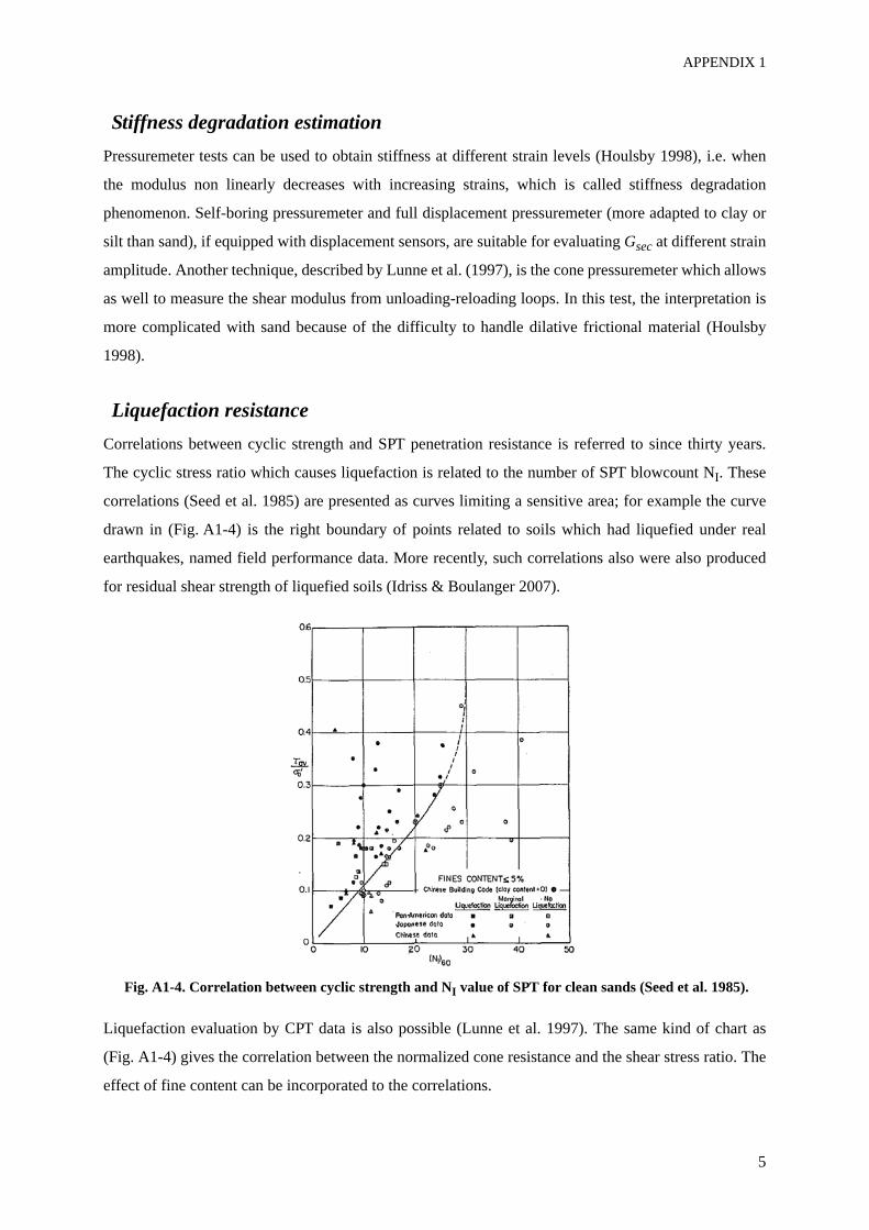
APPENDIX 1
5
Stiffness degradation estimationPressuremeter tests can be used to obtain stiffness at different strain levels (Houlsby 1998), i.e. when
the modulus non linearly decreases with increasing strains, which is called stiffness degradation
phenomenon. Self-boring pressuremeter and full displacement pressuremeter (more adapted to clay or
silt than sand), if equipped with displacement sensors, are suitable for evaluating Gsec at different strain
amplitude. Another technique, described by Lunne et al. (1997), is the cone pressuremeter which allows
as well to measure the shear modulus from unloading-reloading loops. In this test, the interpretation is
more complicated with sand because of the difficulty to handle dilative frictional material (Houlsby
1998).
Liquefaction resistanceCorrelations between cyclic strength and SPT penetration resistance is referred to since thirty years.
The cyclic stress ratio which causes liquefaction is related to the number of SPT blowcount NI. These
correlations (Seed et al. 1985) are presented as curves limiting a sensitive area; for example the curve
drawn in (Fig. A1-4) is the right boundary of points related to soils which had liquefied under real
earthquakes, named field performance data. More recently, such correlations also were also produced
for residual shear strength of liquefied soils (Idriss & Boulanger 2007).
Fig. A1-4. Correlation between cyclic strength and NI value of SPT for clean sands (Seed et al. 1985).
Liquefaction evaluation by CPT data is also possible (Lunne et al. 1997). The same kind of chart as
(Fig. A1-4) gives the correlation between the normalized cone resistance and the shear stress ratio. The
effect of fine content can be incorporated to the correlations.
IN SITU TESTING FOR THE EVALUATION OF DYNAMIC SOIL BEHAVIOUR
6
An in situ test, which induces and measures liquefaction, has recently been developed for research
purpose (Cox et al. 2009). A strong horizontal excitation is created at the soil surface by a specifically
equipped vehicle. It generates shear waves travelling downward into the soil. The response of the soil
layer is recorded by four «liquefaction sensors», which measure static and dynamic pore pressure,
acceleration and tilt. As a result, the liquefaction process of a sand layer can be analysed in situ.
Simpler methods, based on blasting performed in situ, can provide insight into liquefaction-induced
settlement (Hatzor et al. 2009).
The in situ state of sandy soil can be identified along the soil profile by a range of in situ tests. Ground
water conditions, density, grain size, fine content, shear wave velocity are parameters important for
liquefaction potential assessment which can be measured in situ. If these tests reveal that the area is
prone to liquefaction, and if the hazard level is high, sampling and laboratory tests on undisturbed soil
is mandatory.
A1.3 Sumary and remarksIn situ methods for determining soil parameters for dynamic soil behaviour, and in particular for
seismic applications, were briefly described. The investigation of a sensitive site for implementing
earthquake resistant design usually requires to use a combination of these techniques, and also to
perform complementary laboratory tests.
Geophysical methods gather various possibilities to investigate areas with different characteristics.
Most of them allow to determine elastic moduli, which are then very usefull to calibrate geotechnical
models. For example, the linear equivalent method, used in Chapter 7, requires both P wave and S wave
velocities.
Among the many existing in situ tests, it is possible to find applications to various parts of geotechnical
earthquake engineering. Besides the determination of elastic moduli, some methods focus on the
determination of soil parameters in the nonlinear regime, and others on the assessment of liquefaction
susceptibility. The dynamic laboratory tests presented in chapter 4 also provide this kind of
identification of mechanical soil properties.
APPENDIX 2
DETERMINATION OF DEVIATORIC
AND CONFINING STRESSES FROM
SEISMIC ACCELERATION
RECORDINGS
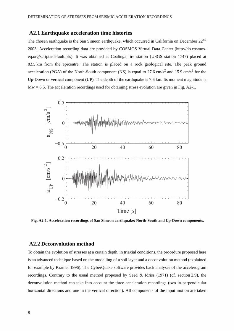
DETERMINATION OF STRESSES FROM SEISMIC ACCELERATION RECORDINGS
8
A2.1 Earthquake acceleration time historiesThe chosen earthquake is the San Simeon earthquake, which occurred in California on December 22nd
2003. Acceleration recording data are provided by COSMOS Virtual Data Center (http://db.cosmos-
eq.org/scripts/default.plx). It was obtained at Coalinga fire station (USGS station 1747) placed at
82.5 km from the epicentre. The station is placed on a rock geological site. The peak ground
acceleration (PGA) of the North-South component (NS) is equal to 27.6 cm/s2 and 15.9 cm/s2 for the
Up-Down or vertical component (UP). The depth of the earthquake is 7.6 km. Its moment magnitude is
Mw = 6.5. The acceleration recordings used for obtaining stress evolution are given in Fig. A2-1.
Fig. A2-1. Acceleration recordings of San Simeon earthquake: North-South and Up-Down components.
A2.2 Deconvolution methodTo obtain the evolution of stresses at a certain depth, in triaxial conditions, the procedure proposed here
is an advanced technique based on the modelling of a soil layer and a deconvolution method (explained
for example by Kramer 1996). The CyberQuake software provides back analyses of the accelerogram
recordings. Contrary to the usual method proposed by Seed & Idriss (1971) (cf. section 2.9), the
deconvolution method can take into account the three acceleration recordings (two in perpendicular
horizontal directions and one in the vertical direction). All components of the input motion are taken
0 20 40 60 80
0
aN
S [
cm/s
2]
0 20 40 60 80
0
aU
P [
cm/s
2]
Time [s]
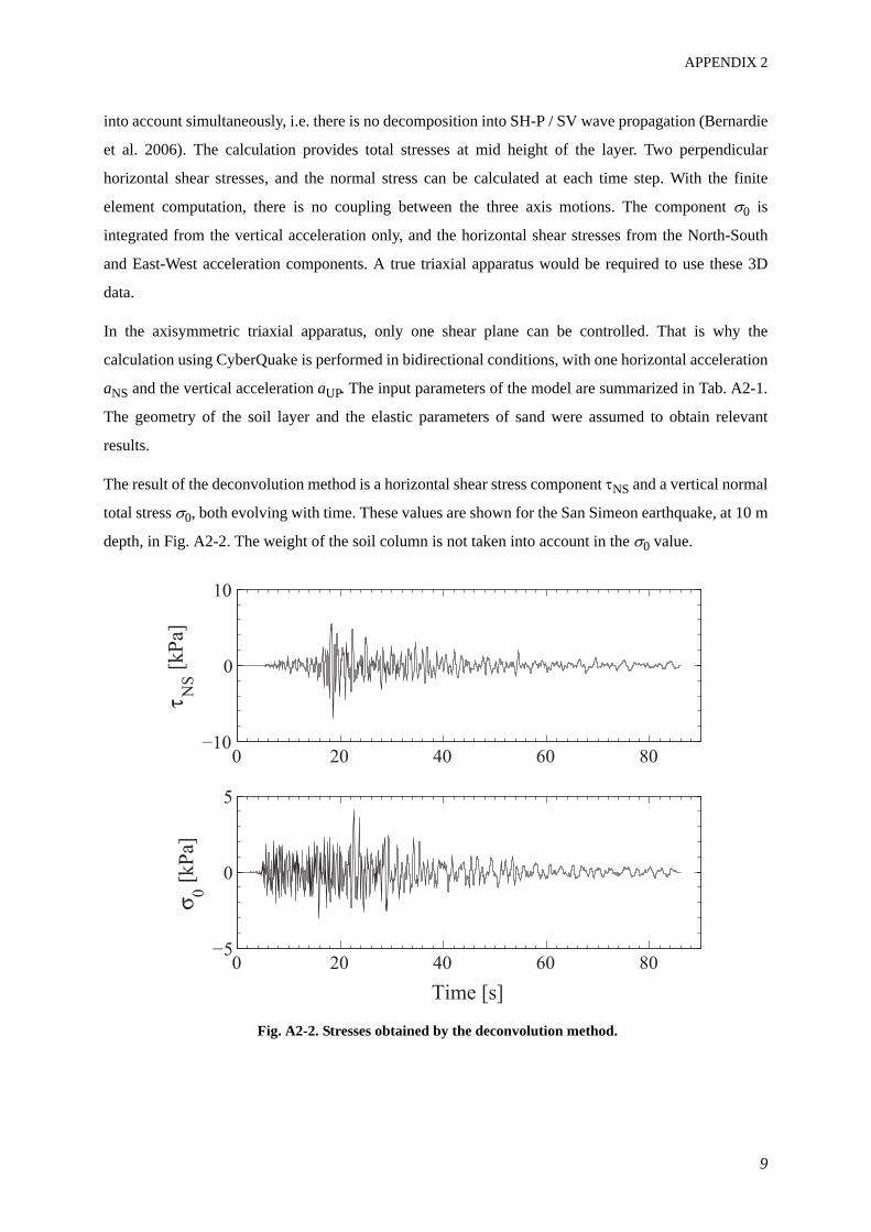
APPENDIX 2
9
into account simultaneously, i.e. there is no decomposition into SH-P / SV wave propagation (Bernardie
et al. 2006). The calculation provides total stresses at mid height of the layer. Two perpendicular
horizontal shear stresses, and the normal stress can be calculated at each time step. With the finite
element computation, there is no coupling between the three axis motions. The component σ0 is
integrated from the vertical acceleration only, and the horizontal shear stresses from the North-South
and East-West acceleration components. A true triaxial apparatus would be required to use these 3D
data.
In the axisymmetric triaxial apparatus, only one shear plane can be controlled. That is why the
calculation using CyberQuake is performed in bidirectional conditions, with one horizontal acceleration
aNS and the vertical acceleration aUP. The input parameters of the model are summarized in Tab. A2-1.
The geometry of the soil layer and the elastic parameters of sand were assumed to obtain relevant
results.
The result of the deconvolution method is a horizontal shear stress component τNS and a vertical normal
total stress σ0, both evolving with time. These values are shown for the San Simeon earthquake, at 10 m
depth, in Fig. A2-2. The weight of the soil column is not taken into account in the σ0 value.
Fig. A2-2. Stresses obtained by the deconvolution method.
0 20 40 60 80
0
NS [
kP
a]
0 20 40 60 805
0
5
0 [
kP
a]
Time [s]
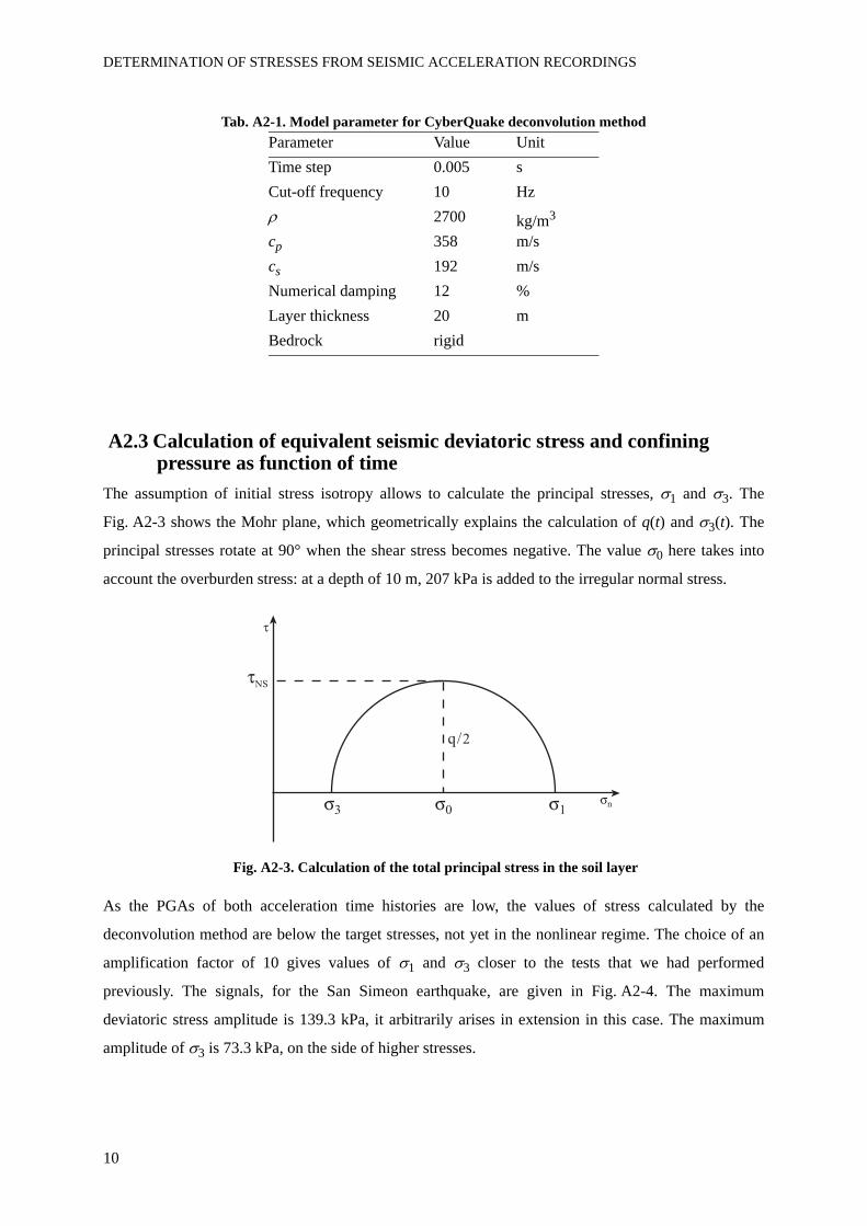
DETERMINATION OF STRESSES FROM SEISMIC ACCELERATION RECORDINGS
10
Tab. A2-1. Model parameter for CyberQuake deconvolution method
A2.3 Calculation of equivalent seismic deviatoric stress and confining pressure as function of time
The assumption of initial stress isotropy allows to calculate the principal stresses, σ1 and σ3. The
Fig. A2-3 shows the Mohr plane, which geometrically explains the calculation of q(t) and σ3(t). The
principal stresses rotate at 90° when the shear stress becomes negative. The value σ0 here takes into
account the overburden stress: at a depth of 10 m, 207 kPa is added to the irregular normal stress.
Fig. A2-3. Calculation of the total principal stress in the soil layer
As the PGAs of both acceleration time histories are low, the values of stress calculated by the
deconvolution method are below the target stresses, not yet in the nonlinear regime. The choice of an
amplification factor of 10 gives values of σ1 and σ3 closer to the tests that we had performed
previously. The signals, for the San Simeon earthquake, are given in Fig. A2-4. The maximum
deviatoric stress amplitude is 139.3 kPa, it arbitrarily arises in extension in this case. The maximum
amplitude of σ3 is 73.3 kPa, on the side of higher stresses.
Parameter Value UnitTime step 0.005 sCut-off frequency 10 Hzρ 2700 kg/m3
cp 358 m/scs 192 m/sNumerical damping 12 %Layer thickness 20 mBedrock rigid
n0
NS
13
q/2
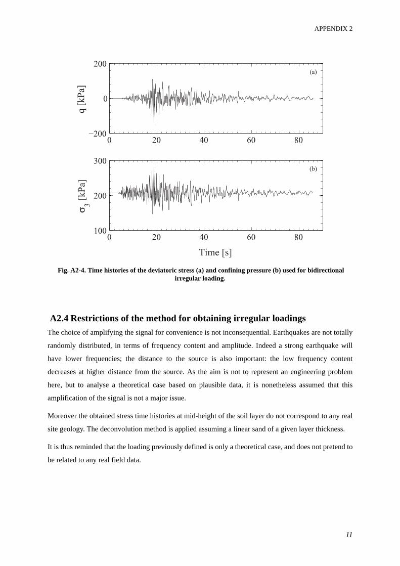
APPENDIX 2
11
Fig. A2-4. Time histories of the deviatoric stress (a) and confining pressure (b) used for bidirectional irregular loading.
A2.4 Restrictions of the method for obtaining irregular loadingsThe choice of amplifying the signal for convenience is not inconsequential. Earthquakes are not totally
randomly distributed, in terms of frequency content and amplitude. Indeed a strong earthquake will
have lower frequencies; the distance to the source is also important: the low frequency content
decreases at higher distance from the source. As the aim is not to represent an engineering problem
here, but to analyse a theoretical case based on plausible data, it is nonetheless assumed that this
amplification of the signal is not a major issue.
Moreover the obtained stress time histories at mid-height of the soil layer do not correspond to any real
site geology. The deconvolution method is applied assuming a linear sand of a given layer thickness.
It is thus reminded that the loading previously defined is only a theoretical case, and does not pretend to
be related to any real field data.
0 20 40 60 80
0
200
q [
kP
a]
0 20 40 60 80100
200
300
3 [
kP
a]
Time [s]
(a)
(b)

DETERMINATION OF STRESSES FROM SEISMIC ACCELERATION RECORDINGS
12
APPENDIX 3
ADDITIONAL RESULTS:
MODELLING OF AN UNDRAINED
CYCLIC TEST WITH THE
ELASTOPLASTIC MODEL
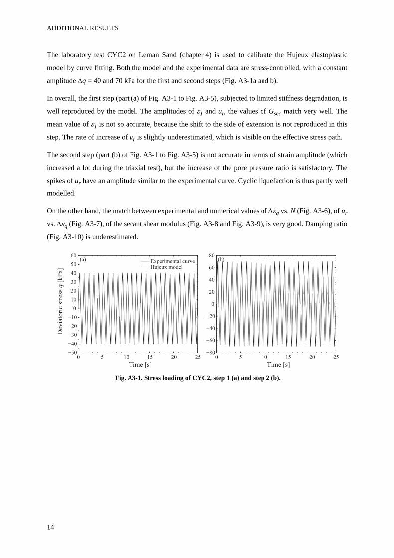
ADDITIONAL RESULTS
14
The laboratory test CYC2 on Leman Sand (chapter 4) is used to calibrate the Hujeux elastoplastic
model by curve fitting. Both the model and the experimental data are stress-controlled, with a constant
amplitude Δq = 40 and 70 kPa for the first and second steps (Fig. A3-1a and b).
In overall, the first step (part (a) of Fig. A3-1 to Fig. A3-5), subjected to limited stiffness degradation, is
well reproduced by the model. The amplitudes of ε1 and ur, the values of Gsec match very well. The
mean value of ε1 is not so accurate, because the shift to the side of extension is not reproduced in this
step. The rate of increase of ur is slightly underestimated, which is visible on the effective stress path.
The second step (part (b) of Fig. A3-1 to Fig. A3-5) is not accurate in terms of strain amplitude (which
increased a lot during the triaxial test), but the increase of the pore pressure ratio is satisfactory. The
spikes of ur have an amplitude similar to the experimental curve. Cyclic liquefaction is thus partly well
modelled.
On the other hand, the match between experimental and numerical values of Δεq vs. N (Fig. A3-6), of ur
vs. Δεq (Fig. A3-7), of the secant shear modulus (Fig. A3-8 and Fig. A3-9), is very good. Damping ratio
(Fig. A3-10) is underestimated.
Fig. A3-1. Stress loading of CYC2, step 1 (a) and step 2 (b).
(a) (b)
0 5 10 15 20 25
0
20
Time [s]
0 5 10 15 20 25
0
10
20
50
Dev
iato
ric
stre
ss q
[k
Pa]
Time [s]
Experimental curveHujeux model
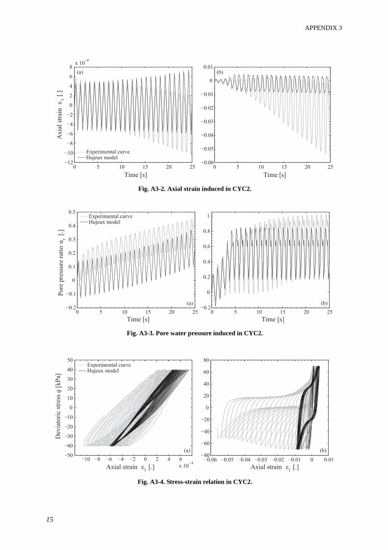
APPENDIX 3
15
Fig. A3-2. Axial strain induced in CYC2.
Fig. A3-3. Pore water pressure induced in CYC2.
Fig. A3-4. Stress-strain relation in CYC2.
(a) (b)
0 5 10 15 20 25
0
2
x 10A
xia
l st
rain
1 [
.]
Time [s]
Experimental curveHujeux model
0 5 10 15 20 25
0
0.01
Time [s]
Time [s]
Po
re p
ress
ure
rat
io u
r [
.]
Time [s]
(a) (b)
0 5 10 15 20 25
0
0.2
0.4
0.6
0.8
1
0 5 10 15 20 25
0
0.1
0.2
0.3
0.4
0.5Experimental curveHujeux model
(a) (b)
Dev
iato
ric
stre
ss q
[kP
a]
Axial strain
Experimental curveHujeux model
Axial strain
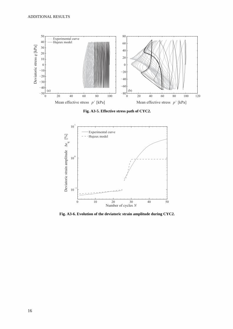
ADDITIONAL RESULTS
16
Fig. A3-5. Effective stress path of CYC2.
Fig. A3-6. Evolution of the deviatoric strain amplitude during CYC2.
(a) (b)
0 20 40 60 80 100 120
0
20
40
60
80
0 20 40 60 80 100
0
10
20
40
Dev
iato
ric
stre
ss q
[k
Pa]
Mean effective stress p’ [kPa]
Experimental curveHujeux model
Mean effective stress p’ [kPa]
0 10 20 30 40 50
10
100
101
Dev
iato
ric
stra
in a
mp
litu
de
q [
%]
Number of cycles N
Experimental curve
Hujeux model
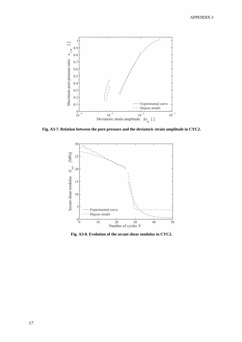
APPENDIX 3
17
Fig. A3-7. Relation between the pore pressure and the deviatoric strain amplitude in CYC2.
Fig. A3-8. Evolution of the secant shear modulus in CYC2.
10 103
102
101
0
0.1
0.2
0.3
0.5
0.6
0.7
0.8
0.9
1
Max
imu
m p
ore
pre
ssu
re r
atio
u
r,m
[.]
Deviatoric strain amplitude q
[.]
Experimental curve
Hujeux model
0 10 20 30 40 500
5
10
15
20
25
30
Sec
ant
shea
r m
od
ulu
s G
sec
[M
Pa]
Number of cycles N
Experimental curve
Hujeux model
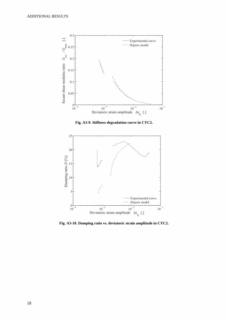
ADDITIONAL RESULTS
18
Fig. A3-9. Stiffness degradation curve in CYC2.
Fig. A3-10. Damping ratio vs. deviatoric strain amplitude in CYC2.
10 103
102
101
0
0.05
0.1
0.15
0.2
0.25
0.3
Sec
ant
shea
r m
od
ulu
s ra
tio
G
sec
/ G
max
[.]
Deviatoric strain amplitude q
[.]
Experimental curve
Hujeux model
10 103
102
101
0
5
10
15
20
25
Dam
pin
g r
atio
D [
%]
Deviatoric strain amplitude q
[.]
Experimental curve
Hujeux model

Décembre 2009
E M I L I E R A S C O L
R E S U M É D E S Q U A L I F I C A T I O N S : Doctorat EPFL en géotechnique. Ingénieure civil diplômée de l’Ecole Centrale Nantes. Mécanique et dynamique des sols, hydrologie, hydraulique : tests en laboratoire et modélisation numérique. Génie parasismique : propagation d’ondes sismiques, effets de sites, comportement dynamique des structures.
FORMATION
Doctorat - Ecole doctorale de Mécanique 2006 - 2009 Ecole Polytechnique Fédérale de Lausanne Laboratoire de Mécanique des Sols http://lms.epfl.ch/
Master Recherche 2004 - 2005 Ecole Centrale Nantes (ECN), France Mécanique appliquée pour le Génie Civil - Classée 1ère www.ec-nantes.fr
Ingénieure Génie Civil et Environnement 2002 - 2005 Ecole Centrale Nantes (ECN), France Master Professionnel www.ec-nantes.fr
Cours préparatoires pour le concours 2000 - 2002 Lycée Saint-Louis, Paris, France d’entrée aux grandes écoles françaises filière MP (Matières principales: Maths, Physiques, Chimie)
Baccalauréat scientifique option mathématiques 1997 - 2000 Lycée E. Branly, Nogent-sur-Marne, France Mention Bien
EXPERIENCE PROFESSIONELLE ET ACADEMIQUE
Laboratoire de Mécanique des Sols, EPFL, Lausanne Avril 2006 – Décembre 2009
Recherche de doctorat : Cyclic Properties of Sand: Dynamic Behaviour for Seismic Applications Directeur de thèse : Prof. Laurent Vulliet - BG Ingénieurs Conseils - Laboratoire de Mécanique des Sols, EPFL.
Définition et conduite de tests de laboratoire - tests triaxiaux dynamiques monotones, cycliques et chargements sismiques.
Développement d’un appareil de mesure sans contact, basé sur de la triangulation par laser, pour mesurer les déformations radiales en continu pendant un chargement triaxial cyclique.
Programmation d’un post-processeur Matlab pour traiter les résultats des tests, en incluant le module de cisaillement et le coefficient d’amortissement.
Simulation des résultats expérimentaux avec un modèle linéaire équivalent et un modèle élastoplastique adapté aux chargements cycliques et sismiques.
Encadrement d’un projet de Master.
Assistante responsable du cours de Mécanique des Sols, EPFL, Lausanne Avril 2006 – Avril 2009 Pour le Bachelor EPFL, section Génie Civil et le Master ELSTE (UNIL, section Géophysique). Définition et correction des exercices et des applications numériques, notation des examens écrits, logistique des documents du cours.
LCPC, Nantes (6 mois) et Karlsruhe Universität (1.5 mois) Avril 2005 – Novembre 2005
Travail de Master : Etude de l’infiltration de la nappe phréatique dans les réseaux d’assainissement Modélisation hydrologique d’un basin versant urbain à l’aide d’un système d’information géographique (MapInfo)-
Application à Nantes Modélisation hydraulique de l’infiltration de la nappe dans les canalisations des réseaux d’assainissement
Bouygues, DV Construction, Bordeaux Juin 2004 – Septembre 2004
Stage d’ingénieur au département des Méthodes sur le chantier “Laser Mégajoule” pour le Commissariat à l’Energie Atomique Détermination et dessin des processus de construction de la zone centrale d’expérimentation
N A T I O N A L I T E F R A N C A I S EN E E L E 3 J U I N 1 9 8 2
H T T P : / / P E R S O N N E S . E P F L . C H / E M I L I E . R A S C O L
A V E N U E W A R N E R Y 1 0 , 1 0 0 7 L A U S A N N E , S U I S S EE - M A I L : E M I L I E R A S C O L @ H O T M A I L . C O M T E L E P H O N E : 0 7 8 6 3 7 8 0 4 7

Décembre 2009
COMMUNICATION SCIENTIFIQUE
LANGUES
Français : Langue maternelle Anglais : Courant Allemand : Niveau moyen Espagnol: Connaissances de base
COMPETENCES IT
Outils scientifiques de modélisation numérique : Matlab, CESAR-LCPC, CyberQuake et Z-Soil (éléments finis), GEO-SLOPE (stabilité de pentes), Robot (structures), MapInfo (Systèmes d’Information Géographiques), Feflow (hydrogéologie), SolidWorks, AutoCAD.
Maîtrise l’environnement Office, ainsi que les logiciels d’édition et de design: Adobe FrameMaker, Illustrator et Photoshop.
ACTIVITES EXTRA-PROFESSIONNELLES
Aime les sports de montagne (escalade, snowboard, randonnée) et d’endurance (course à pied, natation). A participé, depuis l’enfance, à des compétitions dans de nombreux sports (par exemple judo et aviron). Apprécie la photographie, pratiquée surtout à l’occasion de voyages en Europe et en Asie (Japon, Inde, Indonésie). Intéressée par différents aspects des cultures européennes : cinéma, peinture, architecture, et littérature par-dessus tout.
Articles de journaux et de conférences E. Rascol, L. Vulliet, 2009. Frequency effects in natural sand under cyclic loading. Canadian Geotechnical Journal, en
révision. E. Rascol, L. Vulliet, 2009: Characterization of natural sand under complex dynamic loading. In: Performance-Based
Design in Earthquake Geotechnical Engineering, p. 1505-1513, CRC Press/Balkema, Taylor & Francis Group, London. S. Vecchiato, E. Rascol, W.-J. Zwanenburg, 2009: Earthquake protection for high-speed rail traffic: risky business? In:
Safety and Security Engineering III, p. 507-516, WIT Press, Southampton. doi: 10.2495/SAFE090471. En coopération avec le LITEP (Laboratoire d’Intermodalité des Transports et de Planification), EPFL.
Présentations à des conférences et séminaires E. Rascol, L. Vulliet: Characterization of natural sand under complex dynamic loading. In IS Tokyo, International
conference on Performance-Based Design in Geotechnical Earthquake Engineering, 15-18 Juin 2009, Tokyo, Japon. E. Rascol: Soil dynamics testing under seismic loading conditions. Seminar on Geomechanics, Underground
Construction and Environment, 8 - 10 Décembre 2008, EPFL, Lausanne. E. Rascol: Soil Dynamics. Geomechanics research discussions, 21 Février 2008, EPFL, Lausanne. E. Rascol, L. Vulliet: Frequency effect for the Leman Sand under complex stress paths. ALERT Geomaterials, 10
Octobre 2007, Aussois, France. E. Rascol: Comportement non linéaire des sols granulaires sous chargements cycliques complexes. ROSOL meeting,
20 Novembre 2007, EPFL, Lausanne.
Posters E. Rascol, L. Vulliet: Dynamic non-contact measurement of radial strain during triaxial cyclic loading. ALERT
Geomaterials, 6-8 Octobre 2008, Aussois, France. E. Rascol: Comportement dynamique du sable sous chargement sismique. Women of Sciences exhibition, 8 Avril 2008,
EPFL, Lausanne. E. Rascol, L. Vulliet: Complex dynamic stress paths response of Leman Sand. ALERT Geomaterials, 8-10 Octobre 2007,
Aussois, France. E. Rascol: Dynamic behaviour of granular soils under strong and fast earthquake loading. EPFL Research day, 16
Novembre 2006, Lausanne.

![Algebra cochains and cyclic cohomologyim0.p.lodz.pl/.../QuillenPMIHES_1988__68__139_0.pdf · tative geometry [Cl], In the other, cyclic homology appeared as a Lie analogue of algebraic](https://img.pdfslide.fr/doc/110x75/6015673b32b6a7243678943b/algebra-cochains-and-cyclic-cohomologyim0plodzplquillenpmihes1988681390pdf.jpg)