Estimation of an Empirical FAVAR Model andDSGE Model for Evaluation of Government

Expenditure E¤ects in Japan

Kohei FukawaCity University of New York, Graduate Center

February 19, 2012

Abstract

This paper studies the e¤ects of government spending on the economythrough estimation of an empirical Factor Augmented Vector Autoregres-sion (FAVAR) model and a theoretical DSGE model. We �rst conductedFAVAR using 107 time series of Japan, and found that an increase ingovernment investment and consumption leads to an increase in privateconsumption and real wages. We then setup a New Keynesian generalequilibrium model with real and nominal rigidities, including both Edge-worth complementarity/substitutability between private and governmentconsumption and productive public capital. Our model succeeds in privateconsumption and real wages increase in response to government expendi-ture shocks. We estimated key parameters of the model using Bayesianinference, and showed that private and government consumption are Edge-worth complements and that marginal productivity of public capital isproductive in Japan.

1 Introduction

How does government expenditure a¤ect the economy? This is a very old ques-tion. After the global �nancial crisis in the late 2000s, there has been renewedinterest in the size of government spending multipliers. Large-scale-discretionary�scal policies were undertaken, such as the America Recovery and ReinvestmentAct of 2009 by the U.S. government1 , and huge successive economic policy ac-tions in 2008 and early 2009 by the Japanese government. In Japan, a short-termmacro model created by ESRI (an Error Correction model) was widely used forgovernment multiplier arguments in Japan (Sakuma et al. (2011)). That model

1The act was comprised of approximately $500 billion in government spending and $290billion in tax cuts, which means a total of 5.5% of GDP in the United States.

1

(2011 version) declared a GDP multiplier of government investment equal to1:07 in the �rst year and 1:14 for the second year.To assess the e¤ects of government spending, we �rst conducted an empir-

ical study using a Factor Augmented Vector Autoregression (FAVAR) in thispaper. As for empirical studies on �scal policy e¤ects, there have been severalapproaches and debates over the e¤ects on private consumption and real wages.The �rst approach is the so-called "government spending innovation ap-

proach," which uses a SVAR model and identi�es a government spending shockusing timing restrictions, which means government spending is not a¤ected onimpact by other shocks (i.e. Blanchard and Perotti (2002), Fatas and Mihov(2001), Gali et al. (2007), among others2). This approach typically �nds that anincrease in public spending leads to a signi�cant increase in private consumptionand real wages.The second approach is the "dummy variables identi�cation approach," or

the "narrative approach" (i.e. Ramey and Shapiro (1998), Burnside et al.(2004), Ramey (2011), among others). This approach tried to avoid the identi�-cation problem inherent in structural VAR analysis and instead looked for �scalepisodes that can be seen as exogenous with respect to the state of the economy.Ramey (2011) has argued that the large increases in military spending associatedwith the onset of the Korean war, the Vietnam war, the Carter-Reagan militarybuildup, and 9/11 can be seen as such exogenous events. During the episodesof large, exogenous increase in defense spending, output increases but privateconsumption and real wages fall, thus this approach gives smaller governmentmultiplier.The third approach uses a large dimensional dynamic factor model (i.e. Forni

and Gambetti (2010)). Several criticisms of the VAR approach to policy shockidenti�cation focus on a small amount of information used by low dimensionalVARs. To conserve degrees of freedom, standard VARs rarely employ more than10 variables, even though this small number of variables is unlikely to span theinformation sets actually used by the government. Using low-dimensional VARsmeans that the measurement of policy innovation is likely to be contaminated.Forni and Gambetti (2010) studied the e¤ects of government spending by usinga structural dynamic factor model. They used principal components from morethan 100 series, and used sign restriction for shock identi�cation. They foundgovernment spending raises both consumption and investment with no evidenceof crowding out.This paper is of this third approach. We conducted FAVAR initiated by

Bernanke, Boivin and Elizas (2005) 3using 107 time series; to make these se-ries, I made reference to the Cabinet O¢ ce�s "Monthly Economic Reports" and"Memorandum of Recent Economic Trends," two publications that, I believe,

2Blanchard and Perotti (2002) assumed the government expenditure shock does not re-spond to the output residual within a quarter due to �scal policy lags, and they set outputelasticity to government spending equal to zero in their SVAR

3Forni, Gambetti (2010) is di¤erent from FAVAR in that they tried to give the factorsthemselves a structural interpretation; unobservable factors in FAVAR do not have exactmeanings.

2

the government actually uses for analysis of the Japanese economy. To identify agovernment spending shock, we considered the timing of shocks; a governmentspending shock is not a¤ected on impact by other shocks (we used Choleskidecomposition).We compared the results with preliminary VAR. We showed that the fac-

tors included are Granger cause variable to most other variables included. Theimpulse response of VAR and the FAVAR model showed both government in-vestment shock and government consumption shock trigger an increase in pri-vate consumption and output. Wages also increased after both shocks, althoughthere were sign changes in initial periods for the government consumption shock.As far as we know, this is the �rst paper that applied FAVAR to analyze �scalpolicy shocks in Japan. We found that an increase in government investmentand consumption leads to an increase in private consumption and real wages,which is in line with previous empirical studies.This empirical crowd-in e¤ect of private consumption and the increase in real

wages violate neoclassical macroeconomic theory, according to which govern-ment spending decreases consumption. As explained by Baxter and King (1993),the standard neoclassical model, one with in�nitely-lived, forward-looking agents,�exible prices, complete asset markets and a lump-sum taxation model, predictsthat increases in government spending create negative wealth e¤ects by lower-ing permanent household income. Although households typically increase laborsupply to prevent a large drop in consumption, this substitution e¤ect is typ-ically not strong enough to o¤set the wealth e¤ect. In addition, this increasein labor supply decreases real wages, but both of these results contradict withempirical evidence.E¤orts aimed at reconciling this empirical evidence with theoretical modeling

have several approaches. The �rst direction is to adopt a non-separable prefer-ence over consumption and leisure to strengthen the substitution e¤ects afterthe increase in real wages. Perotti and Monacelli (2008) employed the Green-wood, Hercowitz, and Hu¤man preference in an otherwise standard neoclassicalmodel, and their calibrated model �t SVAR impulse in that consumption andreal wages increase with government spending. This approach, however, seemsto be di¢ cult to verify empirically.Another direction is to embed the "deep habits" assumption of Ravn et al.

(2007) into imperfectly competitive product markets. This result is a model ofendogenous time-varying markups of price over marginal cost, and succeededin consumption and real wages increases in response to a government spendingshock, and there are some papers to estimate "deep habits" embedded modelsuch as Zubairy (2010).Another direction is to adopt a credit-constrained agent (i.e. Gali et al.

(2007), Lopez-Salido and Rabanal (2006), Iwata (2011) among others), in whicha fraction of consumers is not allowed to optimize over the life-cycle. But awidely recognized drawback of this approach is the excessive reliance on theexogenous fraction of the credit-constrained agent to obtain a non-negative con-sumption multiplier.We adopt here an alternative approach that focuses on the presence of �ow

3

of government consumption that is able to a¤ect private consumption throughmodi�cation of its marginal utility and productive government investment. Ourmotivation is based on the belief that government consumption and investmentnever deliver waste only; they enhance utility and production in the economy.There have been attempts to explicitly consider Edgeworth complementar-

ity / substitutability between private and government consumption into DSGEmodels, such as Bouakez and Rebei (2007), and Marattin and Marzo (2010).Bouakez and Rebei (2007) augmented a standard RBC model with complemen-tarity between public and private consumption and habit formation to explainthe crowd-in e¤ects of private consumption, and estimated the parameters us-ing U.S. data. They found a strong degree of complementarity between publicand private consumption, and their estimated model succeeded in replicatingthe crowd-in efect of consumption but failed in replicating the real wage in-crease. Marattin and Marzo (2010) employed a New Keynesian equilibriummodel with Edgeworth complementarity / substitutability between private con-sumption and government spending, capital adjustment cost, and distortional�scal policy rules, and calibration on the Euro area. Their calibrated modelwas able to deliver positive private consumption multipliers while they gave nofocus on the real wage movement.There have also been attempts to consider productive government investment

into general equilibrium models, such as Baxter and King (1993) and Leeper etal. (2009).In addition, in Japan, many previous studies have estimated the production

function with public capital, such as Mera (1973), Asako et al. (1994), Mitsuiand Inoue (1995), Kawaguchi et al. (2005). For example, Mitsui and Inoue(1995) estimated production function using a macroeconomic time series andfound the marginal product of public capital to be around 0:25. Kawaguchiet al. (2005) estimated the marginal product of public capital using exoge-nous variation in number of seats in the Diet by electoral reform in 1994 as aninstrument variable, and found the elasticity to be around 0:2.In this paper, we build on these contributions, and our key contributions

of model sections are as follows. First, we extend Bouakez and Rebei (2007)model in the three respects: Our model is a New Keynesian setup, adding realrigidity (variable capital utilization) and productive public capital in produc-tion function. The model explicitly distinguishes government consumption andinvestment, and considered both Edgeworth complementarity/substitutabilitybetween private and government consumption and productive public capital4 .

4There have been also attempts to consider both productive government investment andEdgeworth complementarity/substitutability between private and government consumptioninto general equilibrium models, such as Mazraani (2010) and Iwata (2012).Mazraani (2010) augmented a standard RBC model with a distinction to government con-

sumption and investment, using CES speci�cations over composite consumption and capital.She estimated the parameters using U.S. data, and found that both government consumptionand capital complement private consumption and capital, and this results in the crowd-in toprivate consumption and private investment in respnse to government expenditure, althoughthis model could not replicate the increase in real wages in initial periods.Iwata (2012) established a medium-scale small open economy DSGE model augmented

4

This model succeeds in private consumption and real wages increase in responseto government expenditure shock.Second, we estimated key parameters, i.e. elasticity of substitution between

private consumption and government consumption or productive public capi-tal share in production function, jointly with other structural parameters ina general equilibrium model using Japanese data. As for Edgeworth comple-mentarity/substitutability between private and government consumption, wefound that private and government consumption are Edgeworth complements,as Boaukez and Rebei (2007) found for U.S. data and Okubo (2003) found forJapanese data. As for marginal productivity of public capital in productionfunction, the parameter was 0:30, which is larger than the estimate of 0:25 byMitsui and Inoue (1995) and 0:20 by Kawaguchi et al. (2005). Also, from theestimated model, we showed the impact output multiplier to government con-sumption shock amounts to 1:81, while that to government investment shock is0:75. In addition, we compared the impulse response of government spendingshocks of estimated DSGE model with VAR and FAVAR models.Third, we showed in the appendix that our model of new Keynesian setup

with investment adjustment cost succeeds in more inertial movement in invest-ment. Also, We showed that variable capital utilization helps dampen the largesurge of rental rate of capital in response to government consumption or govern-ment investment shock, as pointed out by Christiano, Eichenbaum and Evans(2005).The remainder of this paper is organized as follows. Section 2 discusses the

empirical VAR and FAVAR models as a benchmark model. In Section 3, we setup the model. Section 4 shows the estimation result, and Section 5 concludes.

2 Empirical Evidence

The purpose of this section is to construct and estimate a benchmark VARand FAVAR to illustrate the macroeconomic e¤ects of a government spendingshock.5

2.1 FAVAR framework:

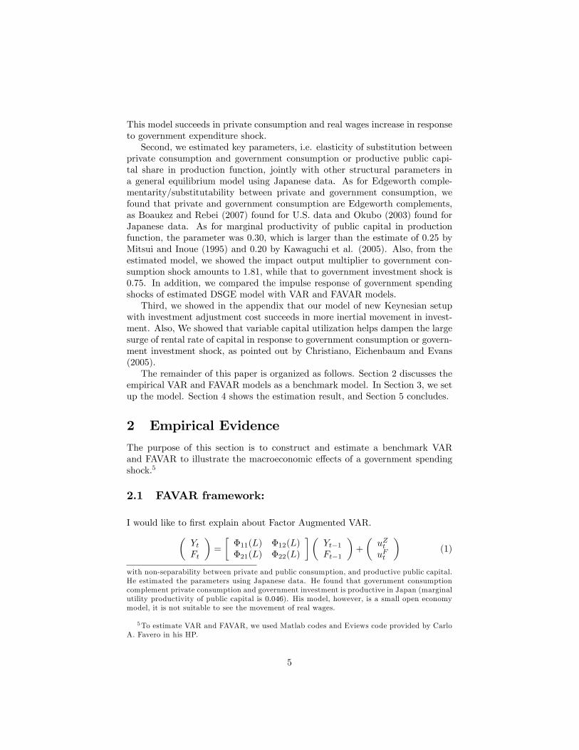
I would like to �rst explain about Factor Augmented VAR.�YtFt

�=

��11(L) �12(L)�21(L) �22(L)

��Yt�1Ft�1

�+

�uZtuFt

�(1)

with non-separability between private and public consumption, and productive public capital.He estimated the parameters using Japanese data. He found that government consumptioncomplement private consumption and government investment is productive in Japan (marginalutility productivity of public capital is 0:046). His model, however, is a small open economymodel, it is not suitable to see the movement of real wages.

5To estimate VAR and FAVAR, we used Matlab codes and Eviews code provided by CarloA. Favero in his HP.

5

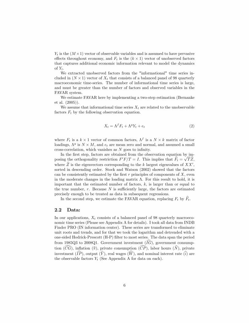
Yt is the (M�1) vector of observable variables and is assumed to have pervasivee¤ects throughout economy, and Ft is the (k � 1) vector of unobserved factorsthat captures additional economic information relevant to model the dynamicsof Yt.We extracted unobserved factors from the "informational" time series in-

cluded in (N � 1) vector of Xt that consists of a balanced panel of 98 quarterlymacroeconomic time-series. The number of informational time series is large,and must be greater than the number of factors and observed variables in theFAVAR system.We estimate FAVAR here by implementing a two-step estimation (Bernanke

et al. (2005)).We assume that informational time series Xt are related to the unobservable

factors Ft by the following observation equation.

Xt = �fFt + �

yYt + et (2)

where Ft is a k � 1 vector of common factors, �f is a N � k matrix of factorloadings, �y is N �M , and et are mean zero and normal, and assumed a smallcross-correlation, which vanishes as N goes to in�nity.In the �rst step, factors are obtained from the observation equation by im-

posing the orthogonality restriction F 0F=T = I. This implies that bFt = pT bZ,where bZ is the eigenvectors corresponding to the k largest eigenvalues of XX 0,sorted in descending order. Stock and Watson (2002) showed that the factorscan be consistently estimated by the �rst r principles of components of X, evenin the moderate changes in the loading matrix �. For this result to hold, it isimportant that the estimated number of factors, k, is larger than or equal tothe true number, r. Because N is su¢ ciently large, the factors are estimatedprecisely enough to be treated as data in subsequent regressions.In the second step, we estimate the FAVAR equation, replacing Ft by bFt.

2.2 Data:

In our applications, Xt consists of a balanced panel of 98 quarterly macroeco-nomic time series (Please see Appendix A for details). I took all data from INDBFinder PRO (IN information center). These series are transformed to eliminateunit roots and trends, and for that we took the logarithm and detrended with aone-sided Hodrick-Prescott (H-P) �lter to most series. The data span the periodfrom 1985Q3 to 2008Q1. Government investment (cIG), government consump-tion (dCG), in�ation (b�), private consumption (dCP ), labor hours ( bN), privateinvestment (cIP ), output (bY ), real wages (cW ), and nominal interest rate (bi) arethe observable factors Yt (See Appendix A for data on each).

6

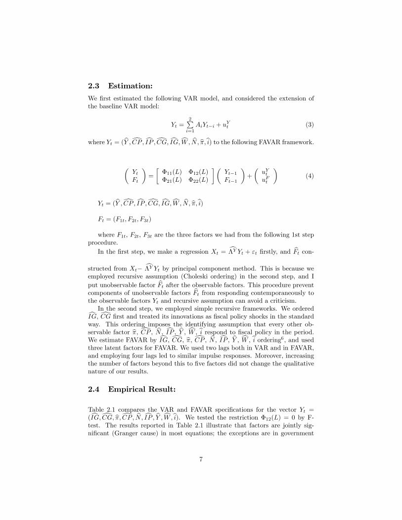
2.3 Estimation:

We �rst estimated the following VAR model, and considered the extension ofthe baseline VAR model:

Yt =2Pi=1

AiYt�i + uYt (3)

where Yt = (bY ;dCP; cIP ;dCG; cIG;cW; bN; b�;bi) to the following FAVAR framework.�YtFt

�=

��11(L) �12(L)�21(L) �22(L)

��Yt�1Ft�1

�+

�uYtuFt

�(4)

Yt = (bY ;dCP; cIP ;dCG; cIG;cW; bN; b�;bi)Ft = (F1t; F2t; F3t)

where F1t, F2t, F3t are the three factors we had from the following 1st stepprocedure.In the �rst step, we make a regression Xt = c�Y Yt + "t �rstly, and bFt con-

structed from Xt� c�Y Yt by principal component method. This is because weemployed recursive assumption (Choleski ordering) in the second step, and Iput unobservable factor bFt after the observable factors. This procedure preventcomponents of unobservable factors bFt from responding contemporaneously tothe observable factors Yt and recursive assumption can avoid a criticism.In the second step, we employed simple recursive frameworks. We orderedcIG, dCG �rst and treated its innovations as �scal policy shocks in the standard

way. This ordering imposes the identifying assumption that every other ob-servable factor b�, dCP , bN , cIP , bY , cW , bi respond to �scal policy in the period.We estimate FAVAR by cIG, dCG, b�, dCP , bN , cIP , bY , cW , bi ordering6 , and usedthree latent factors for FAVAR. We used two lags both in VAR and in FAVAR,and employing four lags led to similar impulse responses. Moreover, increasingthe number of factors beyond this to �ve factors did not change the qualitativenature of our results.

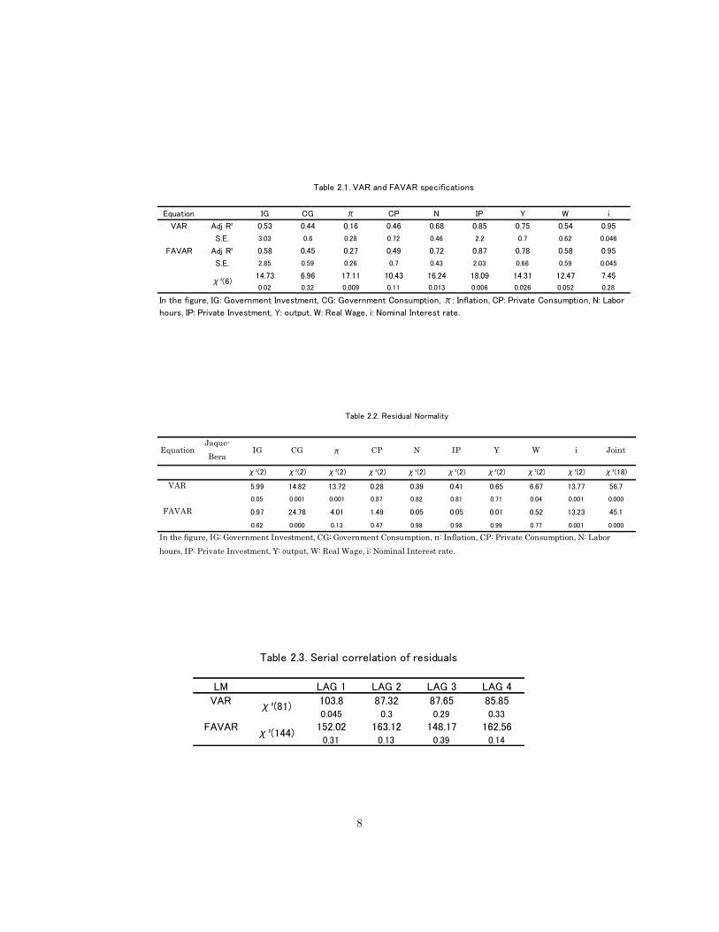
2.4 Empirical Result:

Table 2.1 compares the VAR and FAVAR speci�cations for the vector Yt =(cIG;dCG; b�;dCP; bN; cIP ; bY ;cW;bi). We tested the restriction �12(L) = 0 by F-test. The results reported in Table 2.1 illustrate that factors are jointly sig-ni�cant (Granger cause) in most equations; the exceptions are in government

7

Equation IG CG π CP N IP Y W i

Adj R² 0.53 0.44 0.16 0.46 0.68 0.85 0.75 0.54 0.95

S.E. 3.03 0.6 0.28 0.72 0.46 2.2 0.7 0.62 0.046

Adj R² 0.58 0.45 0.27 0.49 0.72 0.87 0.78 0.58 0.95

S.E. 2.85 0.59 0.26 0.7 0.43 2.03 0.66 0.59 0.045

14.73 6.96 17.11 10.43 16.24 18.09 14.31 12.47 7.45

0.02 0.32 0.009 0.11 0.013 0.006 0.026 0.052 0.28

VAR

FAVAR

χ²(6)

Table 2.1. VAR and FAVAR specifications

In the figure, IG: Government Investment, CG: Government Consumption, π: Inflation, CP: Private Consumption, N: Labor

hours, IP: Private Investment, Y: output, W: Real Wage, i: Nominal Interest rate.

EquationJaque­Bera

IG CG π CP N IP Y W i Joint

χ²(2) χ²(2) χ²(2) χ²(2) χ²(2) χ²(2) χ²(2) χ²(2) χ²(2) χ²(18)

5.99 14.82 13.72 0.28 0.39 0.41 0.65 6.67 13.77 56.7

0.05 0.001 0.001 0.87 0.82 0.81 0.71 0.04 0.001 0.000

0.97 24.78 4.01 1.49 0.05 0.05 0.01 0.52 13.23 45.1

0.62 0.000 0.13 0.47 0.98 0.98 0.99 0.77 0.001 0.000

VAR

FAVAR

Table 2.2. Residual Normality

In the figure, IG: Government Investment, CG: Government Consumption, π: Inflation, CP: Private Consumption, N: Laborhours, IP: Private Investment, Y: output, W: Real Wage, i: Nominal Interest rate.

LM LAG 1 LAG 2 LAG 3 LAG 4

103.8 87.32 87.65 85.850.045 0.3 0.29 0.33

152.02 163.12 148.17 162.560.31 0.13 0.39 0.14

VAR

FAVAR

χ²(81)

χ²(144)

Table 2.3. Serial correlation of residuals

8

consumption (dCG), private consumption (dCP ), wages ( bw), and interest rate (bi)equation.Tables 2.2 and 2.3 report the evidence on the residual analysis from the VAR

and FAVAR models. Table 2.2 contains the outcome of Jarque and Bera (1980)tests of null hypothesis of normality of residuals from each equation and for thejoint 9 equation model. The null of normality is rejected for both VAR andFAVAR in the joint 9 equation model; the main cause of this rejection is thenon-normality of residuals in dCG and bi equations.Table 2.3 reports the Breush-Godfrey Lagrange Multiplier tests of null hy-

pothesis of no serial correlation of residuals at all lags from one to four. Theresult showed in the �rst lag of VAR speci�cation points toward residual auto-correlations, while the null hypothesis of absence of residual correlation at anylags cannot be rejected in FAVAR speci�cations.

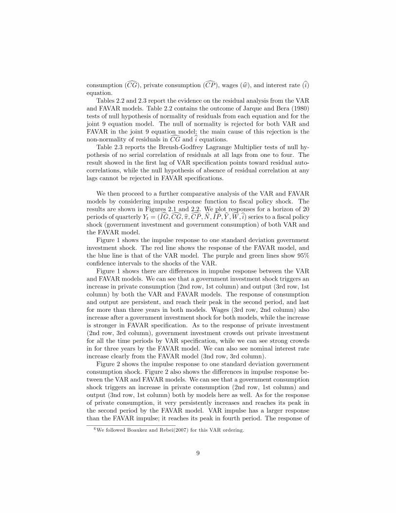
We then proceed to a further comparative analysis of the VAR and FAVARmodels by considering impulse response function to �scal policy shock. Theresults are shown in Figures 2.1 and 2.2. We plot responses for a horizon of 20periods of quarterly Yt = (cIG;dCG; b�;dCP; bN; cIP ; bY ;cW;bi) series to a �scal policyshock (government investment and government consumption) of both VAR andthe FAVAR model.Figure 1 shows the impulse response to one standard deviation government

investment shock. The red line shows the response of the FAVAR model, andthe blue line is that of the VAR model. The purple and green lines show 95%con�dence intervals to the shocks of the VAR.Figure 1 shows there are di¤erences in impulse response between the VAR

and FAVAR models. We can see that a government investment shock triggers anincrease in private consumption (2nd row, 1st column) and output (3rd row, 1stcolumn) by both the VAR and FAVAR models. The response of consumptionand output are persistent, and reach their peak in the second period, and lastfor more than three years in both models. Wages (3rd row, 2nd column) alsoincrease after a government investment shock for both models, while the increaseis stronger in FAVAR speci�cation. As to the response of private investment(2nd row, 3rd column), government investment crowds out private investmentfor all the time periods by VAR speci�cation, while we can see strong crowdsin for three years by the FAVAR model. We can also see nominal interest rateincrease clearly from the FAVAR model (3nd row, 3rd column).Figure 2 shows the impulse response to one standard deviation government

consumption shock. Figure 2 also shows the di¤erences in impulse response be-tween the VAR and FAVAR models. We can see that a government consumptionshock triggers an increase in private consumption (2nd row, 1st column) andoutput (3nd row, 1st column) both by models here as well. As for the responseof private consumption, it very persistently increases and reaches its peak inthe second period by the FAVAR model. VAR impulse has a larger responsethan the FAVAR impulse; it reaches its peak in fourth period. The response of

6We followed Boaukez and Rebei(2007) for this VAR ordering.

9

Figure 1: Impulse response to IG impact with VAR-FAVAR comparison【機密性 2情報】

Figure 1 shows impulse responses of 1std. government investment shock. In the figure, IG: Government Investment, CG: Government Consumption, Pi: Inflation,

CP: Private Consumption, N: Labor hours, IP: Private Investment, Y: output, W: Real Wage, i: Nominal Interest rate. FAVAR (Red solid line): Impulse response of

FAVAR, VAR (Blue solid line): Impulse response of VAR, LB, UB (Green and Purple dotted Lines): Lower and Upper 95% confidence intervals of VAR.

­1

­0.5

0

0.5

1

1.5

2

2.5

3

3.5

4

1 2 3 4 5 6 7 8 9 1011121314151617181920

IG

FAVAR

VAR

LB

UB

­0.15

­0.1

­0.05

0

0.05

0.1

0.15

0.2

0.25

1 2 3 4 5 6 7 8 9 1011121314151617181920

CG

FAVAR

VAR

LB

UB

­0.15

­0.1

­0.05

0

0.05

0.1

1 2 3 4 5 6 7 8 9 1011121314151617181920

Pi

FAVAR

VAR

LB

UB

­0.2

­0.1

0

0.1

0.2

0.3

0.4

1 2 3 4 5 6 7 8 9 1011121314151617181920

CP

FAVAR

VAR

LB

UB

­0.3

­0.25

­0.2

­0.15

­0.1

­0.05

0

0.05

0.1

0.15

0.2

1 2 3 4 5 6 7 8 9 1011121314151617181920

N

FAVAR

VAR

LB

UB

­1.5

­1

­0.5

0

0.5

1

1 2 3 4 5 6 7 8 9 1011121314151617181920

IP

FAVAR

VAR

LB

UB

­0.3

­0.2

­0.1

0

0.1

0.2

0.3

0.4

1 2 3 4 5 6 7 8 9 1011121314151617181920

Y

FAVAR

VAR

LB

UB

­0.25

­0.2

­0.15

­0.1

­0.05

0

0.05

0.1

0.15

0.2

0.25

1 2 3 4 5 6 7 8 9 1011121314151617181920

W

FAVAR

VAR

LB

UB

­0.04

­0.03

­0.02

­0.01

0

0.01

0.02

0.03

0.04

0.05

1 2 3 4 5 6 7 8 9 1011121314151617181920

i

FAVAR

VAR

LB

UB

10

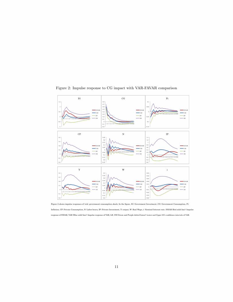
Figure 2: Impulse response to CG impact with VAR-FAVAR comparison【機密性 2情報】

Figure 2 shows impulse responses of 1std. government consumption shock. In the figure, IG: Government Investment, CG: Government Consumption, Pi:

Inflation, CP: Private Consumption, N: Labor hours, IP: Private Investment, Y: output, W: Real Wage, i: Nominal Interest rate. FAVAR (Red solid line): Impulse

response of FAVAR, VAR (Blue solid line): Impulse response of VAR, LB, UB (Green and Purple dotted Lines): Lower and Upper 95% confidence intervals of VAR.

­1

­0.5

0

0.5

1

1.5

1 2 3 4 5 6 7 8 9 1011121314151617181920

IG

FAVAR

VAR

LB

UB

­0.2

­0.1

0

0.1

0.2

0.3

0.4

0.5

0.6

0.7

0.8

1 2 3 4 5 6 7 8 9 1011121314151617181920

CG

FAVAR

VAR

LB

UB

­0.15

­0.1

­0.05

0

0.05

0.1

1 2 3 4 5 6 7 8 9 1011121314151617181920

Pi

FAVAR

VAR

LB

UB

­0.2

­0.1

0

0.1

0.2

0.3

0.4

1 2 3 4 5 6 7 8 9 1011121314151617181920

CP

FAVAR

VAR

LB

UB

­0.25

­0.2

­0.15

­0.1

­0.05

0

0.05

0.1

0.15

0.2

0.25

1 2 3 4 5 6 7 8 9 1011121314151617181920

N

FAVAR

VAR

LB

UB

­0.6

­0.4

­0.2

0

0.2

0.4

0.6

0.8

1

1.2

1.4

1 2 3 4 5 6 7 8 9 1011121314151617181920

IP

FAVAR

VAR

LB

UB

­0.2

­0.1

0

0.1

0.2

0.3

0.4

1 2 3 4 5 6 7 8 9 1011121314151617181920

Y

FAVAR

VAR

LB

UB

­0.2

­0.15

­0.1

­0.05

0

0.05

0.1

0.15

0.2

0.25

0.3

1 2 3 4 5 6 7 8 9 1011121314151617181920

W

FAVAR

VAR

LB

UB

­0.04

­0.03

­0.02

­0.01

0

0.01

0.02

0.03

0.04

0.05

1 2 3 4 5 6 7 8 9 1011121314151617181920

i

FAVAR

VAR

LB

UB

11

output has the same tendency. It reaches its peak in 3nd period and increasefor 2 years by FAVAR model. The response of wages (3rd row, 2nd column)also seems to increase after a government consumption shock, but changes signsthree times within the �rst four quarters for both models. As for the responseof private investment (2nd row, 3rd column), a government consumption shockcrowds out for the �rst 10 quarters by the FAVAR model, while we can seepersistent crowds in movement from the VAR model.

3 The Model

The model we setup extends Bouakez and Rebei (2007) model in three demen-sion. First, we setup a New Keynesian model. Second, we include intertempo-ral investment adjustment cost and variable capital utilization as real rigidities.Third, we consider both government consumption and government investmentand assumed government capital stocks enters the production function.

3.1 The Representative Household

The economy is populated by a single, in�nitely lived representative agent thatdrives utility from e¤ective consumption ( ~Ct) and leisure (1 � Nt). E¤ectiveconsumption is assumed to be the CES index of private consumption (Cp) andgovernment consumption (CG)7 .

u( ~Ct; ~Ct�1Nt) =1

1� " (~Ct

~Ct�1 )1�" + � ln(1�Nt) (5)

~Ct = [�Cp v�1

vt + (1� �)Cg

v�1v

t ]v

v�1 (6)

where " stands for the inverse of the long-run intertemporal elasticity of sub-stitution, and " and � are positive parameters. 2 (0; 1) measures the degreeof habit formation8 . v > 0 is the elasticity of substitution between privateconsumption and government consumption.The representative household supply labor and public capital to �rms, and

pays lump-sum tax to the government, Zt.

Cpt + Ipt + (Ut)Kpt +

BtPt

+ Zt � wtNt + rtUtKpt +

Bt�1Rt�1

Pt+�tPt

(7)

where Bt is government debt issued at t, which pays BtRt units of goods at t+1,�t is dividends from owning imperfect competitive intermediate goods �rm, Ut

7Earlier studies that assume consumer preferences to be CES index of private consumptionand government spending include Amano and Wirjanto (1997), Okubo (2003), Linnemann andSchabert (2003), Boualez and Rebei (2007), Marrattin and Marzo (2010), Mazraani (2010).

8We assumed habit formation for e¤ective consumption following Boualez and Rebei (2007).

12

is the capital utilization rate, and rtUtKpt represents household earnings from

supplying capital services9 . The steady state capital utilization rate is assumedto be U = 1. Increases from steady state utilization incurs a cost, (Ut)K

pt ,

and we assume functional form for the adjustment cost of capital utilization isgiven by

(Ut) = �U1+

�1

t � 11 + �1

where is the inverse of elasticity of the capital utilization with respect to therental rate of one e¤ective unit of private capital and > 0 . Note that (Ut)is an increasing, convex function ( 0(Ut) > 0,

00(Ut) > 0), and in steady states,cost is zero ( (1) = 0). UtK

pt represents the e¤ective units of private capital.

The rental rate of one e¤ective unit of private capital is rt and wage rate is wt .Private capital evolves according to

Kpt+1 = (1� �

p)Kpt + f1� S(

IptIpt�1

)gIpt (8)

where �p is the private capital depreciation rate, and S(�) stands for adjustmentcost for capital de�ned as a quadratic function as follows.

S(IptIpt�1

) =1

2�(IptIpt�1

� 1)2 (9)

where � implies inverse of the elasticity of investment on the price of capital. As

can be seen from the above speci�cation, the bigger the deviation of the currentphysical investment from the previous period, the higher the adjustment cost.Therefore, it will be in the interest of the household to install the capital assmoothly as possible to minimize the leakage. Also, it should be noted thatadjustment cost is zero in steady states, i.e. S(1) = S0(1) = 0.Given the budget constraint (7) and capital accumulation equation (8), the

dynamic optimizing problem of the household is

$ = E0

1Xt=0

[�tu( ~Ct; ~Ct�1Nt) (10)

��tfCpt + Ipt + (Ut)Kpt +

BtPt

+ Zt � wtNt � rtUtKpt �

Bt�1Rt�1

Pt� �

Ptg

��tfKpt+1 � (1� �

p)Kpt � (1�

1

2�(IptIpt�1

� 1)2)Ipt g]

where �t stands for the Lagrange multiplier attached to the budget constraint9We introduce variable capital utilization as in Christiano, Eichenbaum, and Evans (2005),

in which households are assumed to act as invester as well and make capital accumulationand utilization decisions. This assumption is made for convenience; at the cost of moreconvenience, they said, at the cost of more complicated notation, they could work with analternative decentralization scheme in which �rms make these decisions.

13

at point t and �t stands for the Lagrange multiplier attached to the capitalaccumulation equation.The �rst order conditions associated with each control variables, Bt, IPt , Nt,

CPt , KPt+1, Ut are

bond holdings:

�t = �Et[�t+1RtPtPt+1

] (11)

physical investment:

�t = �t[1�1

2�� 3

2�(IptIpt�1

)2 +2

�(IptIpt�1

)]� �Et�t+1[1

�(Ipt+1Ipt

)2(1�Ipt+1Ipt

)] (12)

labor supply:�t =

�

wt(1�Nt)(13)

consumption:

�t = �(~CtCpt

)1� f( 1

~Ct�1 )(

~Ct~Ct�1

)�" � � Et[(~Ct+1~Ct1+

)(~Ct+1~Ct

)�"]g (14)

capital holdings:

�t = �Et[�t+1frt+1Ut+1 � (Ut+1)g+ �t+1(1� �p)] (15)

capital utilization:rt = 0(Ut) (16)

As to the �rst order condition with the physical investment (12), the LHS canbe interpreted as the marginal cost of investment. By investing in one additionalconsumption good, the household forgo the same amount of consumption goodsfrom its budget. RHS of the equation (12) represents the marginal bene�t ofinvestment. By investing in one additional unit, the household can increase theamount of private capital stock to some extent, but the magnitude of increasein capital stock is reduced to the leakage in capital installment. In the �rstbracket in (12), this leakage of capital installment on the margin is represented.In addition, we set the adjustment cost function as (9), a marginal change of thecurrent investment will also a¤ect the next period�s adjustment cost, and thise¤ect is represented in the second bracket. Both these e¤ects multiplying with

14

the shadow price of capital will constitute the marginal bene�t from additionalinvestment.Moreover, as to the �rst order condition with private consumption (14),

the LHS is marginal cost of private consumption. The RHS of the equation

(14) represents the marginal utility of private consumption. �(~CtCpt)1� represents

additional e¤ective consumption by one unit of private consumption, and thesecond bracket represents marginal utility from one unit of e¤ective consump-tion. Notice that the second bracket reduces to ~C�"t only if current e¤ectiveconsumption matters ( = 0).Next, equation (15) represents the �rst order condition associated with the

capital holdings. LHS �t is the shadow price of capital and the marginal costof adding one unit of capital at time t. The RHS represents a marginal bene�tof adding one unit of capital. Households can expect to increase (1 � �p) unitof capital at time t+ 1, thus ��t+1(1� �p) represents a present value marginalbene�t of adding one unit of capital, and rt+1Ut+1 � (Ut+1) represents house-hold�s additional income via capital holding minus additional capital utilizationcost coming with the additional capital lending.Finally, as can be seen from (16), the optimality condition regarding capital

utilization requires households to equalize the marginal cost of capital utilizationto the rental rate. By increasing the capital utilization level marginally, thehousehold can increase its income by rtK

pt , which can be considered a marginal

bene�t to the household. However, an increase in capital utilization delivers acost. By increasing the capital utilization, the household need to give up 0(Ut)amount of consumption goods on its margin.

3.2 Firms

3.2.1 The �nal goods �rms

We assume that there is a continuum of intermediate �rms of unit mass indexed

by i 2 [0; 1] and each �rm produces an intermediate good that is di¤erent fromthat of other �rms. The continuum of intermediate goods in period t, Yi;t getsbundled by �nal goods �rms into �nal goods Yt. The �nal goods productiontechnology is

Yt = [

Z 1

0

Y��1�

i;t di]�

��1 (17)

where � is the elasticity of substitution in production and governing the �rm�smarkup over the marginal cost.A pro�t-maximizing �nal goods �rm chooses the amount of intermediate

goods to maximize pro�t given aggregate price Pt and intermediate goods pricePi;t. We could have a demand function of goods i as,

Yi;t = (Pi;tPt)��Yt (18)

15

Putting this demand for sector i�s output (3.14) into the bundler function

(3.13), we can have a �nal goods pricing rule of,

Pt = [

Z 1

0

P 1��i;t di]1

1�� (19)

3.2.2 The intermediate goods �rms

The production function for intermediate goods �rm i is

Yi;t = AtgKpi;t

�Ni;t

(1��)(KGt )

� (20)

where gKpi;t = Ui;tK

pi;t and all �rms are subject to the same technology shock, At.

KGt is the government capital stock. Notice that KG

t does not have subscripti, thus we assume KG

t as well has common productivity to each �rm. Thisproduction function is increasing return to scale as a whole but private sectorresource is a constant return to scale10 .Under a Calvo (1983)-type sticky price setting, for any given period t, each

�rm has a � probability that it will keep the price of the previous period, and 1��probability that it will be able to choose its price optimally. An intermediategoods �rm, i, which can choose price in period t, choose the price, P �i;t, tomaximize pro�t:

maxP�i;t

Et

1Xj=0

�j�j [P �i;tYt+j(Pt+jP �i;t

)� � Pt+jrt+jK̂pi;t+j � Pt+jwt+jNi;t+j ] (21)

s:t:Yt+j(Pt+jP �i;t

)� = AtgKpi;t

�Ni;t

1��(KGt )

� (22)

A �rm that is maximizing pro�t is simultaneously minimizing total cost.

The cost minimization problem for the �rm i can be expressed as follows.

cost function: mingKpi;t,Ni;t

rtgKpi;t+wtNi;t+mci;t(Yi;t�AtgKp

i;t

�Ni;t

1��(KGt )

�) (23)

where the Lagrange multiplier, mci;t, is the marginal cost of producing Yi;t.Solving the cost minimization, the �rst order condition is

wtrt=(1� �)�

gKpi;t

Ni;t(24)

10As for production function, Mitsui and Inoue (1995) showed that, in Japan, assuming aconstant return to scale for the private sector is better than assuming a constant return toscale as a whole (including productive public capital) from a production function estimationusing prefectural data.

16

solve (24) for gKpi;t and Ni;t, and substituting these factor demands into the cost

equations,

TCi;t = rtgKpi;t + wtNi;t =

Yi;tAt

(1� �)��1��

r�t w1��t

1

(KGt )

�(25)

so, the �rm i�s marginal cost is

mci;t =TCi;tYi;t

=1

At

(1� �)��1��

r�t w1��t

1

(KGt )

�(26)

Notice that the speci�cation of marginal cost (26) does not depend on sub-script i , and this implies the marginal cost is symmetric across �rms. Sincethe marginal cost is symmetric across �rms, we simply suppress subscript i onmarginal cost.Substituting total costs (25) to pro�t maximization problems (21) yields,

maxP�i;t

Et

1Xj=0

�j�j [P �i;tYt+j(Pt+jP �i;t

)� � Pt+jrt+jK̂pi;t+j � Pt+jwt+jNi;t+j ]

= Et

1Xj=0

(��)j [(P �i;t � Pt+jmct+j)Yi;t+j ] (27)

The �rst order condition for the pro�t maximization problem yields

Et

1Xj=0

(��)jYi;t+j [1� � + �Pt+jP �i;t

mct+j ] = 0

Rearranging further yields the following optimal pricing rule for �rm i.

P �i;t =�

� � 1

Et1Pj=0

(��)j(Pt+jYi;t+jmct+j)

Et1Pj=0

(��)jYi;t+j

(28)

Notice that � > 1, and the expression ���1 > 1 is the gross markup of the

intermediate goods �rm i�s price over the ratio of the discounted stream ofnominal total costs divided by the discounted stream of real output.Notice that all intermediate goods �rms that can �x their prices set the

same-markup over the same marginal cost, so in every period t, P �i;t is the samefor all 1�� �rms that adjust their prices, and all non-adjusting �rms keep theirprice as it was in the previous period. Combining with the �nal goods pricingrule (19), we have the aggregate goods pricing rule,

Pt1�� = �Pt�1

1�� + (1� �)P �t 1�� (29)

17

3.3 The Policy Side

3.3.1 Fiscal Authority

The �scal authority purchases �nal goods CGt , IGt , issues bonds Bt , and levies

lump-sum tax Zt. The �ow budget constraint for �scal authority is,

CGt + IGt +Rt�1Bt�1

Pt= Zt +

BtPt

(30)

Government spending CGt , IGt evolve according to a AR(1) stochastic process.

dCGt = �CG[CGt�1 + "

CGt (31)

dIGt = �IGdIGt�1 + "IGt (32)

government capital stock evolve according to

KGt+1 = IGt + (1� �G)KG

t (33)

where �G is the government capital depreciation rate.

3.3.2 Monetary Policy

The central bank sets the nominal interest rate according to a simple feedbackrule of the following rule11 .

cRt = �r[Rt�1 + (1� �r)�r� d�t�1 + (1� �r)�ry bYt (34)

where d�t�1 � log(Pt�1=Pt�2) denote in�ation rate.3.4 Market Clearing Condition

We impose the market-clearing condition for the �nal goods market. We requirethe supply of �nal goods to be equal to the demand of �nal goods for privateconsumption, private investment, capital utilization, government consumption,and government investment12 .

Yt = Cpt + Ipt + (Ut)K

pt + C

Gt + I

Gt (35)

11This type of Taylor rule with interest-rate inertia can be found in Rotemberg and Wood-ford (1999), Clarida, Gali, and Gertler (1999), and Christiano, Eichenbaum, and Evans (2005).12A Log-linearized version of the model could be found in Appendix B.

18

4 Model Estimation

4.1 Estimation Methodology

The purpose of this section is to use Japanese data to obtain values for themodel parameters. In particular, we are interested in measuring the extentof complementarity between government consumption and private consumptionand public capital share in the production function. We describe below ourestimation methodology brie�y following Boaukez and Rebei (2007) and Iiboshi,Nishiyama and Watanabe (2008).The model�s solution can be written in the following recursive equilibrium

low of motion:st = G(�)st�1 +H(�)"t (36)

where st is a 23 � 1 vector of endogenous variables: st = [ bYt, b�t, c~Ct, dCpt ,cIPt , b�t, b�t, cNt, cwt, brt, dmct , [KPt+1,

[KGt+1, cRt, cAt, cIGt , dCGt , Etd�t+1, Et[]Ct+1,

Etd�t+1, Etd�t+1, EtdIPt+1,Etdrt+1]0, and "t is a vector of endogenous shocks: "t =["At ; "

IGt ; "CGt ]0, and � is the vector of deep parameters to be estimated. From

equation (4.1), we set a state space model which consists of a transition equationand measurement equation as follows;

st = G(�)st�1 +H(�)"t (37)

yt = Jst (38)

where yt is the 9 � 1 vector of observable variables at time t and J is a 9 �23 matrix that links the observed yt vector and the unobserved st. For thisstate space model with Gaussian error terms, unobservable variables st and thelikelihood of the model are obtained using a Kalman �lter. The Kalman �lteris the algorithm that provides the mean and the covariance matrix of the statevector st (t = 1; :::; T ) conditional on the observations up to t, i.e., (Y1; :::; YT )in a linear Gaussian state space model.A crucial requirement of the Kalman �lter is that the number of observable

variables used in the estimation does not exceed the number of shocks in themodel; otherwise, the variance-covariance matrix of the residuals becomes sin-gular. In our case, we have only three structural shocks, so we can use as little asthree series. To circumvent this problem, we followed Boaukez and Rebei (2007)and add measurement errors to the variables in the measurement equation13 .This yields the following empirical model:

st = G(�)st�1 +H(�)"t (39)

yt = Jst + �t (40)

13The addition of measurement errors to get around the singularity problem has been doneby McGrattan, Rogerson and Wright (1997), Ireland (2004), and Boakez and Rebei (2007),Nishiyama et al (2011).

19

Parameter Meanings ValueStructual parameters

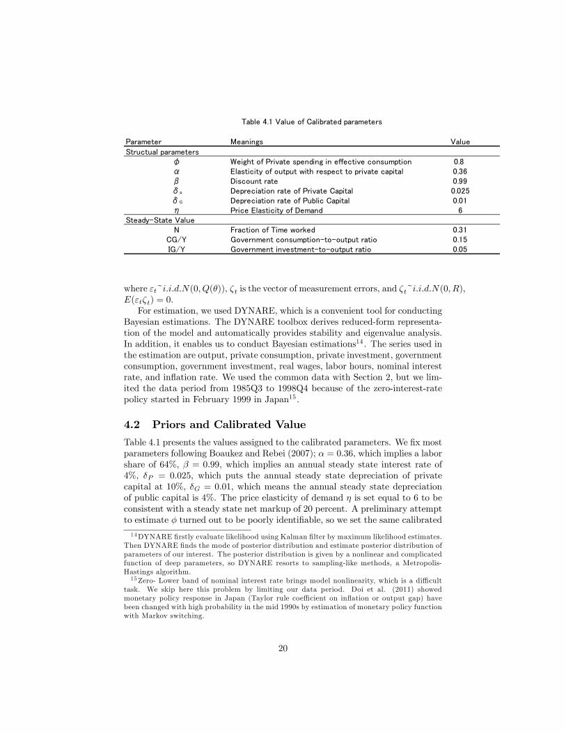
φ Weight of Private spending in effective consumption 0.8α Elasticity of output with respect to private capital 0.36β Discount rate 0.99δp Depreciation rate of Private Capital 0.025δG Depreciation rate of Public Capital 0.01η Price Elasticity of Demand 6

Steady­State ValueN Fraction of Time worked 0.31

CG/Y Government consumption­to­output ratio 0.15IG/Y Government investment­to­output ratio 0.05

Table 4.1 Value of Calibrated parameters

where "t~i:i:d:N(0; Q(�)), �t is the vector of measurement errors, and �t~i:i:d:N(0; R),E("t�t) = 0.For estimation, we used DYNARE, which is a convenient tool for conducting

Bayesian estimations. The DYNARE toolbox derives reduced-form representa-tion of the model and automatically provides stability and eigenvalue analysis.In addition, it enables us to conduct Bayesian estimations14 . The series used inthe estimation are output, private consumption, private investment, governmentconsumption, government investment, real wages, labor hours, nominal interestrate, and in�ation rate. We used the common data with Section 2, but we lim-ited the data period from 1985Q3 to 1998Q4 because of the zero-interest-ratepolicy started in February 1999 in Japan15 .

4.2 Priors and Calibrated Value

Table 4.1 presents the values assigned to the calibrated parameters. We �x mostparameters following Boaukez and Rebei (2007); � = 0:36, which implies a laborshare of 64%, � = 0:99, which implies an annual steady state interest rate of4%, �P = 0:025, which puts the annual steady state depreciation of privatecapital at 10%, �G = 0:01, which means the annual steady state depreciationof public capital is 4%. The price elasticity of demand � is set equal to 6 to beconsistent with a steady state net markup of 20 percent. A preliminary attemptto estimate � turned out to be poorly identi�able, so we set the same calibrated

14DYNARE �rstly evaluate likelihood using Kalman �lter by maximum likelihood estimates.Then DYNARE �nds the mode of posterior distribution and estimate posterior distribution ofparameters of our interest. The posterior distribution is given by a nonlinear and complicatedfunction of deep parameters, so DYNARE resorts to sampling-like methods, a Metropolis-Hastings algorithm.15Zero- Lower band of nominal interest rate brings model nonlinearity, which is a di¢ cult

task. We skip here this problem by limiting our data period. Doi et al. (2011) showedmonetary policy response in Japan (Taylor rule coe¢ cient on in�ation or output gap) havebeen changed with high probability in the mid 1990s by estimation of monetary policy functionwith Markov switching.

20

parameters meanings type mean s.e.

structual parameters

υ Elasticity of substitution normal 0.8 0.5

ε Curvature parameter normal 2 2

γ Habit­formation parameter beta 0.6 0.2

ξ Inverse of adjustment­cost parameter normal 0.25 0.75

Ψ Capital utilization cost normal 1 1

ρ Calvo price no­revise probabirity beta 0.7 0.2

μ Productivity of public capital beta 0.2 0.1

Policy parameters

ρr Interest rate smoothing coeff. beta 0.8 0.1

ρπ interest rate inflation coeff. normal 1.5 1

ρy interest rate output gap coeff. normal 0.125 0.075

Shock persistence

ρa persistence of productivity beta 0.85 0.1

ρcg persistence of government consumption beta 0.85 0.1

ρIG persistence of government investment beta 0.85 0.1

Standard Errors of shocks

ηa SE of productivity shock inv. Gamma 0.4 2

ηCG SE of government consumption shock inv. Gamma 0.2 2

ηIG SE of government investment shock inv. Gamma 0.3 2

ηY SE of mesurement err. for output gap inv. Gamma 0.2 2

ηCP SE of mesurement err. for private consumption inv. Gamma 0.2 2

ηIP SE of mesurement err. for private investment inv. Gamma 1 4

ηCG SE of mesurement err. for government consumption inv. Gamma 0.1 2

ηIG SE of mesurement err. for government investment inv. Gamma 0.5 4

ηN SE of mesurement err. for real wage inv. Gamma 0.1 2

ηW SE of mesurement err. for labor hour inv. Gamma 0.1 2

ηπ SE of mesurement err. for inflation inv. Gamma 0.1 2

ηi SE of mesurement err. for nominal interest rate inv. Gamma 0.05 1

Standard Errors for Mesurement Errors

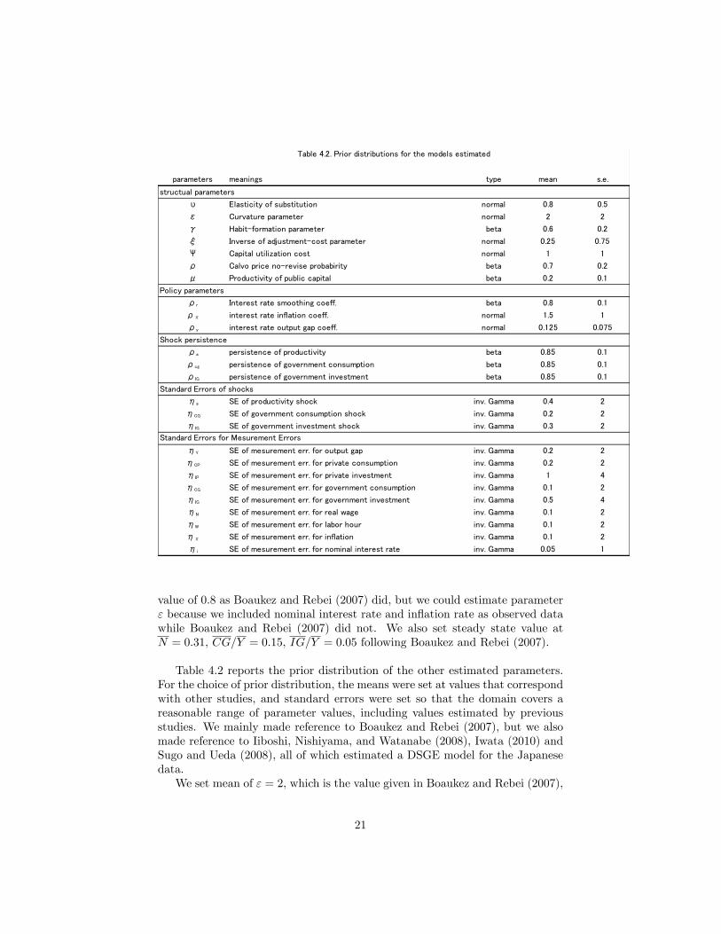
Table 4.2. Prior distributions for the models estimated

value of 0:8 as Boaukez and Rebei (2007) did, but we could estimate parameter" because we included nominal interest rate and in�ation rate as observed datawhile Boaukez and Rebei (2007) did not. We also set steady state value atN = 0:31, CG=Y = 0:15, IG=Y = 0:05 following Boaukez and Rebei (2007).

Table 4.2 reports the prior distribution of the other estimated parameters.For the choice of prior distribution, the means were set at values that correspondwith other studies, and standard errors were set so that the domain covers areasonable range of parameter values, including values estimated by previousstudies. We mainly made reference to Boaukez and Rebei (2007), but we alsomade reference to Iiboshi, Nishiyama, and Watanabe (2008), Iwata (2010) andSugo and Ueda (2008), all of which estimated a DSGE model for the Japanesedata.We set mean of " = 2, which is the value given in Boaukez and Rebei (2007),

21

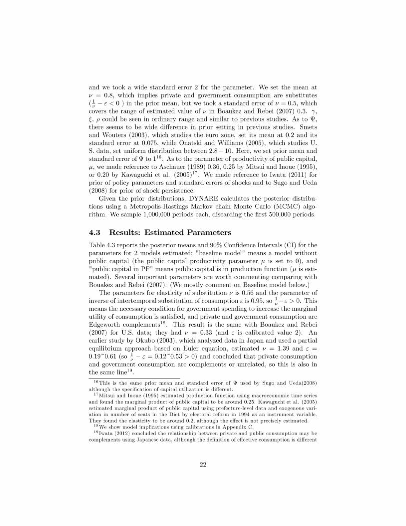
and we took a wide standard error 2 for the parameter. We set the mean at� = 0:8, which implies private and government consumption are substitutes( 1� � " < 0 ) in the prior mean, but we took a standard error of � = 0:5, whichcovers the range of estimated value of � in Boaukez and Rebei (2007) 0:3. ,�, � could be seen in ordinary range and similar to previous studies. As to ,there seems to be wide di¤erence in prior setting in previous studies. Smetsand Wouters (2003), which studies the euro zone, set its mean at 0:2 and itsstandard error at 0:075, while Onatski and Williams (2005), which studies U.S. data, set uniform distribution between 2:8� 10. Here, we set prior mean andstandard error of to 116 . As to the parameter of productivity of public capital,�, we made reference to Aschauer (1989) 0:36, 0:25 by Mitsui and Inoue (1995),or 0:20 by Kawaguchi et al. (2005)17 . We made reference to Iwata (2011) forprior of policy parameters and standard errors of shocks and to Sugo and Ueda(2008) for prior of shock persistence.Given the prior distributions, DYNARE calculates the posterior distribu-

tions using a Metropolis-Hastings Markov chain Monte Carlo (MCMC) algo-rithm. We sample 1,000,000 periods each, discarding the �rst 500,000 periods.

4.3 Results: Estimated Parameters

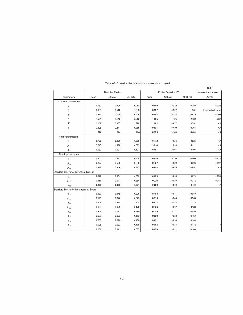
Table 4.3 reports the posterior means and 90% Con�dence Intervals (CI) for theparameters for 2 models estimated; "baseline model" means a model withoutpublic capital (the public capital productivity parameter � is set to 0), and"public capital in PF" means public capital is in production function (� is esti-mated). Several important parameters are worth commenting comparing withBouakez and Rebei (2007). (We mostly comment on Baseline model below.)The parameters for elasticity of substitution � is 0:56 and the parameter of

inverse of intertemporal substitution of consumption " is 0:95, so 1��" > 0. This

means the necessary condition for government spending to increase the marginalutility of consumption is satis�ed, and private and government consumption areEdgeworth complements18 . This result is the same with Boaukez and Rebei(2007) for U.S. data; they had � = 0:33 (and " is calibrated value 2). Anearlier study by Okubo (2003), which analyzed data in Japan and used a partialequilibrium approach based on Euler equation, estimated � = 1:39 and " =0:19~0:61 (so 1

� � " = 0:12~0:53 > 0) and concluded that private consumptionand government consumption are complements or unrelated, so this is also inthe same line19 .16This is the same prior mean and standard error of used by Sugo and Ueda(2008)

although the speci�cation of capital utilization is di¤erent.17Mitsui and Inoue (1995) estimated production function using macroeconomic time series

and found the marginal product of public capital to be around 0:25. Kawaguchi et al. (2005)estimated marginal product of public capital using prefecture-level data and exogenous vari-ation in number of seats in the Diet by electoral reform in 1994 as an instrument variable.They found the elasticity to be around 0:2, although the e¤ect is not precisely estimated.18We show model implications using calibrations in Appendix C.19 Iwata (2012) concluded the relationship between private and public consumption may be

complements using Japanese data, although the de�nition of e¤ective consumption is di¤erent

22

(Ref.)

Bouakez and Rebei

parameters mean CI(Low) CI(High) mean CI(Low) CI(High) (2007)

structual parameters

υ 0.557 0.380 0.714 0.589 0.372 0.782 0.332

ε 0.950 0.510 1.353 0.982 0.562 1.361 2(calibrated value)

γ 0.483 0.170 0.796 0.497 0.188 0.810 0.250

ξ 1.684 1.148 2.210 1.656 1.126 2.180 1.052

Ψ 2.109 0.867 3.328 2.062 0.827 3.291 N.A

ρ 0.605 0.441 0.765 0.601 0.440 0.765 N.A

μ N.A. N.A. N.A. 0.295 0.108 0.484 N.A

Policy parameters

ρr 0.772 0.625 0.923 0.772 0.624 0.924 N.A

ρπ 3.015 1.880 4.083 3.010 1.928 4.111 N.A

ρy 0.053 0.004 0.101 0.055 0.005 0.104 N.A

Shock persistence

ρa 0.820 0.743 0.898 0.820 0.740 0.900 0.873

ρcg 0.727 0.565 0.888 0.727 0.559 0.896 0.912

ρIG 0.891 0.846 0.937 0.903 0.855 0.951 N.A

Standard Errors for Structual Shocks

ηa 0.377 0.094 0.699 0.356 0.095 0.674 0.005

ηCG 0.181 0.047 0.334 0.220 0.045 0.372 0.013

ηIG 0.282 0.068 0.537 0.250 0.070 0.466 N.A

Standard Errors for Mesurement Errors

ηY 0.327 0.042 0.509 0.188 0.045 0.360 ­

ηCP 0.178 0.046 0.323 0.213 0.046 0.360 ­

ηIP 0.875 0.242 1.604 0.915 0.234 1.712 ­

ηCG 0.095 0.022 0.172 0.106 0.022 0.188 ­

ηIG 0.484 0.111 0.920 0.503 0.111 0.935 ­

ηN 0.088 0.023 0.163 0.090 0.023 0.169 ­

ηW 0.086 0.023 0.158 0.091 0.024 0.164 ­

ηπ 0.098 0.022 0.179 0.094 0.023 0.172 ­

ηi 0.051 0.011 0.097 0.056 0.011 0.103 ­

Baseline Model Public Capital in PF

Table 4.3. Posterior distributions for the models estimated

23

The parameter for consumption habit formation is about 0:48, which islarger than Bouakez and Rebei (2007) 0:25. The parameter for capital utilizationcost, , is 2:1 and this is similar to Onatski and Williams (2004) 2:8. Theparameter of inverse of investment adjustment costs, � is 1:7. This implies thatinvestment increases 1:7 percent in the long run following a 1 percent increase inTobin�s q. This estimated parameter is larger than that found in other studies,i.e. Levin et al. (2005) 0:55 or Smets and Wouters (2007) 0:1420 .Regarding in�ation dynamics, the Calvo price-setting parameter � is 0:61, so

the probability that a given price can be optimized in a quarterly period (1��)is 0:39. This implies an average contract duration of price setting is estimatedto be about 2:5 quarters.Regarding monetary policy parameters, the coe¢ cient on lagged interest

rates in the monetary policy rule �r is 0:82. This implies that monetary policyhas high inertia. The response of interest rate to in�ation �� is 3, which is muchgreater than one, indicates that the monetary authority in Japan reacts veryactively to in�ation. On the contrary, the response to output, �Y is small, at0:05.As for the results of "public capital in production function," our interest is

in the parameter of productivity of public capital in production function, and itis 0:30. This is smaller than Aschauer�s (1989) 0:36 but larger than the estimateof 0:25 by Mitsui and Inoue (1995), 0:2 by Kawaguchi et al. (2005), or 0:046 byIwata (2012). Other parameters estimated are similar to the baseline case, sowe omit an explanation of these results here.

4.4 Impulse Response

In this subsection, we would like to see the impulse responses of endogenousvariables to government investment and government consumption shocks for�ve years following each of the shocks. The horizontal axis represents time ona quarterly scale, and the vertical axis represents percentage deviation fromequilibrium.Figure 3 illustrates impulse responses to a government consumption shock.

This captures important channels that determine impact on a government con-sumption shock: crowding-out e¤ects, wealth e¤ects, and the e¤ects from privateand government consumption Edgeworth complementarity.First, higher government consumption absorbs existing resources so that

there are fewer goods available for the private sector to save (invest) or con-sume. As goods today become more valuable and not all intermediate goods�rm can adjust its price, the real marginal cost (rental cost of private capital andreal wages) increases, but the increase of capital utilization alleviate the surgeof the rental cost of private capital. Second, higher government consumption �-nanced by lump-sum tax generates a negative wealth e¤ect, encouraging agents

from us here (Iwata (2012) used a linear form, cCt = CPt + vCGt ).20Although Bouakez and Rebei (2007) estimated under capital adjustment cost setting, the

parameter for adjustment cost is 1:05, and is smaller than ours.

24

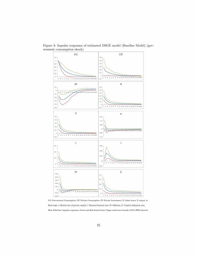
Figure 3: Impulse responses of estimated DSGE model (Baseline Model) (gov-ernment consumption shock)

【機密性 2情報】

CG: Government Consumption, CP: Private Consumption, IP: Private Investment, N: Labor hours, Y: output, w:

Real wage, r: Rental rate of private capital, i: Nominal Interest rate, Pi: Inflation, U: Capital utilization rate.

Blue Solid line: Impulse responses, Green and Red dotted Lines: Upper and Lower bounds of 90% HPD interval.

0

0.2

0.4

0.6

0.8

1

1.2

1 2 3 4 5 6 7 8 9 10 11 12 13 14 15 16 17 18 19 20

CG

­0.1

0

0.1

0.2

0.3

0.4

0.5

0.6

1 2 3 4 5 6 7 8 9 10 11 12 13 14 15 16 17 18 19 20

CP

­0.5

­0.4

­0.3

­0.2

­0.1

0

0.1

1 2 3 4 5 6 7 8 9 10 11 12 13 14 15 16 17 18 19 20

IP

­0.1

0

0.1

0.2

0.3

0.4

0.5

0.6

1 2 3 4 5 6 7 8 9 10 11 12 13 14 15 16 17 18 19 20

N

­0.1

0

0.1

0.2

0.3

0.4

0.5

1 2 3 4 5 6 7 8 9 10 11 12 13 14 15 16 17 18 19 20

Y

­0.1

­0.05

0

0.05

0.1

0.15

1 2 3 4 5 6 7 8 9 10 11 12 13 14 15 16 17 18 19 20

w

0

0.1

0.2

0.3

1 2 3 4 5 6 7 8 9 10 11 12 13 14 15 16 17 18 19 20

r

­0.01

0

0.01

0.02

0.03

1 2 3 4 5 6 7 8 9 10 11 12 13 14 15 16 17 18 19 20

i

­0.02

­0.01

0

0.01

0.02

0.03

0.04

0.05

1 2 3 4 5 6 7 8 9 10 11 12 13 14 15 16 17 18 19 20

Pi

0

0.1

0.2

0.3

0.4

1 2 3 4 5 6 7 8 9 10 11 12 13 14 15 16 17 18 19 20

U

25

Variable 1 quarter 4 quarters 8 quarters 12 quarters 20 quartersBaseline Model△Y/△CG 1.81 1.41 1.28 1.28 1.34△CP/△CG 1.04 0.91 0.88 0.85 0.80△IP/△CG ­0.22 ­0.49 ­0.60 ­0.58 ­0.46

△Y/△IG 0.75 0.71 0.72 0.70 0.86△CP/△IG ­0.17 ­0.19 ­0.21 ­0.24 ­0.29△IP/△IG ­0.07 ­0.16 ­0.21 ­0.23 ­0.22

Model with Productive Public Capital in Production Function△Y/△CG 1.67 1.33 1.21 1.21 1.27△CP/△CG 0.88 0.78 0.77 0.74 0.70△IP/△CG ­0.20 ­0.45 ­0.56 ­0.53 ­0.43

△Y/△IG 0.76 0.62 0.68 0.84 1.23△CP/△IG ­0.04 ­0.03 0.04 0.11 0.26△IP/△IG ­0.18 ­0.35 ­0.36 ­0.27 ­0.02

Table4.4   Impact Multiplier and Present Value Multiplier

to work harder, and this will increase output but reduce marginal productivityof labor on the other hand. Third, when private and government consumptionare Edgeworth complements, government consumption increases marginal util-ity of consumption, so people consume more in the current period. On the otherhand this leads to increase labor supply and real wages su¤er decreasing e¤ects.To see the impulse responses, as to private consumption, the e¤ect of Edge-

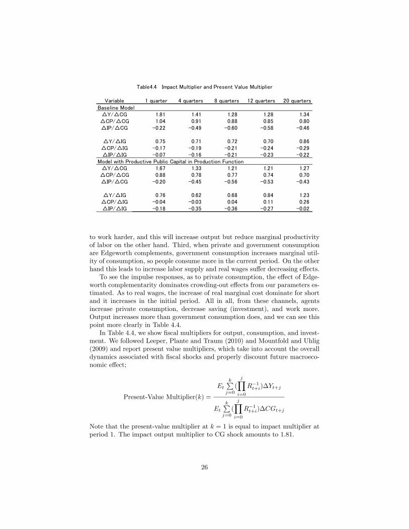
worth complementarity dominates crowding-out e¤ects from our parameters es-timated. As to real wages, the increase of real marginal cost dominate for shortand it increases in the initial period. All in all, from these channels, agentsincrease private consumption, decrease saving (investment), and work more.Output increases more than government consumption does, and we can see thispoint more clearly in Table 4.4.In Table 4.4, we show �scal multipliers for output, consumption, and invest-

ment. We followed Leeper, Plante and Traum (2010) and Mountfold and Uhlig(2009) and report present value multipliers, which take into account the overalldynamics associated with �scal shocks and properly discount future macroeco-nomic e¤ect;

Present-Value Multiplier(k) =

EtkPj=0

(

jYi=0

R�1t+i)�Yt+j

EtkPj=0

(

jYi=0

R�1t+i)�CGt+j

Note that the present-value multiplier at k = 1 is equal to impact multiplier atperiod 1. The impact output multiplier to CG shock amounts to 1:81.

26

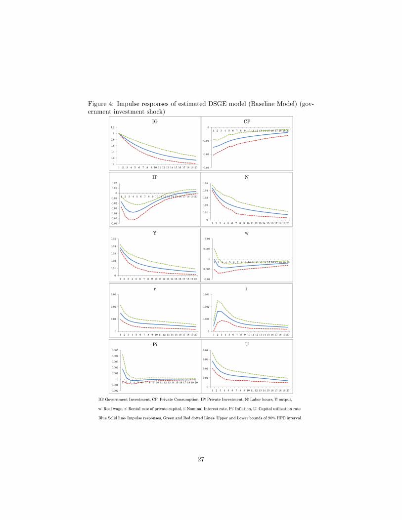
Figure 4: Impulse responses of estimated DSGE model (Baseline Model) (gov-ernment investment shock)

【機密性 2情報】

IG: Government Investment, CP: Private Consumption, IP: Private Investment, N: Labor hours, Y: output,

w: Real wage, r: Rental rate of private capital, i: Nominal Interest rate, Pi: Inflation, U: Capital utilization rate

Blue Solid line: Impulse responses, Green and Red dotted Lines: Upper and Lower bounds of 90% HPD interval.

0

0.2

0.4

0.6

0.8

1

1.2

1 2 3 4 5 6 7 8 9 10 11 12 13 14 15 16 17 18 19 20

IG

­0.03

­0.02

­0.01

01 2 3 4 5 6 7 8 9 10 11 12 13 14 15 16 17 18 19 20

CP

­0.06

­0.05

­0.04

­0.03

­0.02

­0.01

0

0.01

0.02

1 2 3 4 5 6 7 8 9 10 11 12 13 14 15 16 17 18 19 20

IP

0

0.01

0.02

0.03

0.04

0.05

1 2 3 4 5 6 7 8 9 10 11 12 13 14 15 16 17 18 19 20

N

0

0.01

0.02

0.03

0.04

0.05

1 2 3 4 5 6 7 8 9 10 11 12 13 14 15 16 17 18 19 20

Y

­0.01

­0.005

0

0.005

0.01

1 2 3 4 5 6 7 8 9 10 11 12 13 14 15 16 17 18 19 20

w

0

0.01

0.02

0.03

1 2 3 4 5 6 7 8 9 10 11 12 13 14 15 16 17 18 19 20

r

0

0.001

0.002

0.003

1 2 3 4 5 6 7 8 9 10 11 12 13 14 15 16 17 18 19 20

i

­0.002

­0.001

0

0.001

0.002

0.003

0.004

0.005

1 2 3 4 5 6 7 8 9 10 11 12 13 14 15 16 17 18 19 20

Pi

0

0.01

0.02

0.03

0.04

1 2 3 4 5 6 7 8 9 10 11 12 13 14 15 16 17 18 19 20

U

27

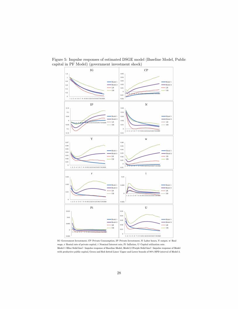
Figure 5: Impulse responses of estimated DSGE model (Baseline Model, Publiccapital in PF Model) (government investment shock)

【機密性 2情報】

IG: Government Investment, CP: Private Consumption, IP: Private Investment, N: Labor hours, Y: output, w: Realwage, r: Rental rate of private capital, i: Nominal Interest rate, Pi: Inflation, U: Capital utilization rate.Model 1 (Blue Solid line) : Impulse response of Baseline Model, Model 2 (Purple Solid line) : Impulse response of Modelwith productive public capital, Green and Red dotted Lines: Upper and Lower bounds of 90% HPD interval of Model 2.

0

0.2

0.4

0.6

0.8

1

1.2

1 2 3 4 5 6 7 8 9 1011121314151617181920

IG

Model 1Model 2

LBUB

­0.02

­0.01

0

0.01

0.02

0.03

0.04

0.05

1 2 3 4 5 6 7 8 9 1011121314151617181920

CP

Model 1Model 2

LBUB

­0.15

­0.1

­0.05

0

0.05

0.1

0.15

1 2 3 4 5 6 7 8 9 1011121314151617181920

IP

Model 1Model 2

LBUB

­0.01

0

0.01

0.02

0.03

0.04

0.05

1 2 3 4 5 6 7 8 9 1011121314151617181920

N

Model 1Model 2

LBUB

0

0.01

0.02

0.03

0.04

0.05

0.06

0.07

1 2 3 4 5 6 7 8 9 1011121314151617181920

Y

Model 1Model 2

LBUB

­0.01

0

0.01

0.02

0.03

0.04

0.05

0.06

1 2 3 4 5 6 7 8 9 1011121314151617181920

w

Model 1Model 2

LBUB

0

0.01

0.02

0.03

1 2 3 4 5 6 7 8 9 1011121314151617181920

r

Model 1Model 2

LBUB

­0.005

0

0.005

0.01

1 2 3 4 5 6 7 8 9 1011121314151617181920

i

Model 1Model 2

LBUB

­0.005

0

0.005

0.01

0.015

1 2 3 4 5 6 7 8 9 1011121314151617181920

Pi

Model 1Model 2

LBUB

0

0.01

0.02

0.03

0.04

0.05

1 2 3 4 5 6 7 8 9 1011121314151617181920

U

Model 1Model 2

LBUB

28

Figures 4 and 5 illustrates impulse responses to government investmentshock. Figure 4 illustrates impulse response of the Baseline model (model with-out public capital in production function), and Figure 5 compares the impulseresponse of Baseline model with that of the model with productive public cap-ital. These �gures capture important channels, crowding-out e¤ects, wealthe¤ects, and the e¤ects from productive public capital to change the marginalproductivity of private inputs.For Figures 4, the �rst two channels are working as in the CG shock: higher

government investment absorbs existing resources so that there are fewer goodsavailable for the private sector to save (invest) or consume. As goods todaybecome more valuable and not all intermediate goods �rm can adjust its price,the real marginal cost of intermediate goods �rms, rental cost of private capital,and real wages increases; higher government investment �nanced by lump-sumtax generates a negative wealth e¤ect, encouraging agents to work harder, sothis leads to increase in output but decrease marginal productivity of labor (realwages is a¤ected a decreasing e¤ect). So Figure 4 shows that agents decreaseconsumption, decrease saving (investment), and work more. As to real wages,the impulse response is in negative region because the �rst e¤ect of real marginalcost increase was not enough to dominate the second e¤ect of the decreasingmarginal productivity of labor, by our parameters estimated. Output increaseis less than government investment, and from Table 4.4, output multiplier to IGshock is 0:75 and does not exceed 1 in the initial period.For Figure 5, however, when government investment is productive, there

is another wealth e¤ect from the opposite direction and the productive publiccapital e¤ects to change the marginal productivity of private inputs. As forwealth e¤ects, a higher stock of productive public capital acts like a total factorproductivity increase to create the expectation that more goods will be avail-able in the future, and this discourages current savings and encourages currentconsumption. We can see from Figure 5 that private investment decreases moreand consumption decreases less in initial periods than in the baseline model.In addition, as for the model with productive public capital, the marginal

product of labor and private capital increases at longer horizons as a graduallyrising stock of public capital, which results in higher wages and a return toprivate capital. This brings incentives to work and invest, which induces higheroutput in later periods. As to real wages, among these three e¤ects, the thirde¤ect of increase in marginal productivity of labor by productive public capitaldominates even in the initial periods and impulse response of real wages come upto the positive region all the time. From Table 4.4, we can see output multiplierto an IG shock in the initial period is 0:76 -not much di¤erent from baselinecase- but after the re�ection of the later period until 20 quarters, an outputmultiplier of the model with productive public capital is as high as 1:23, whilethe output multiplier in the baseline model stays at 0:86.Finally, we would like to show the comparison of impulse responses of em-

pirical models and estimated DSGE models.In Figure 6, we showed the impulse response to government consumption

shocks of the estimated DSGE model (light blue solid line), the FAVAR model

29

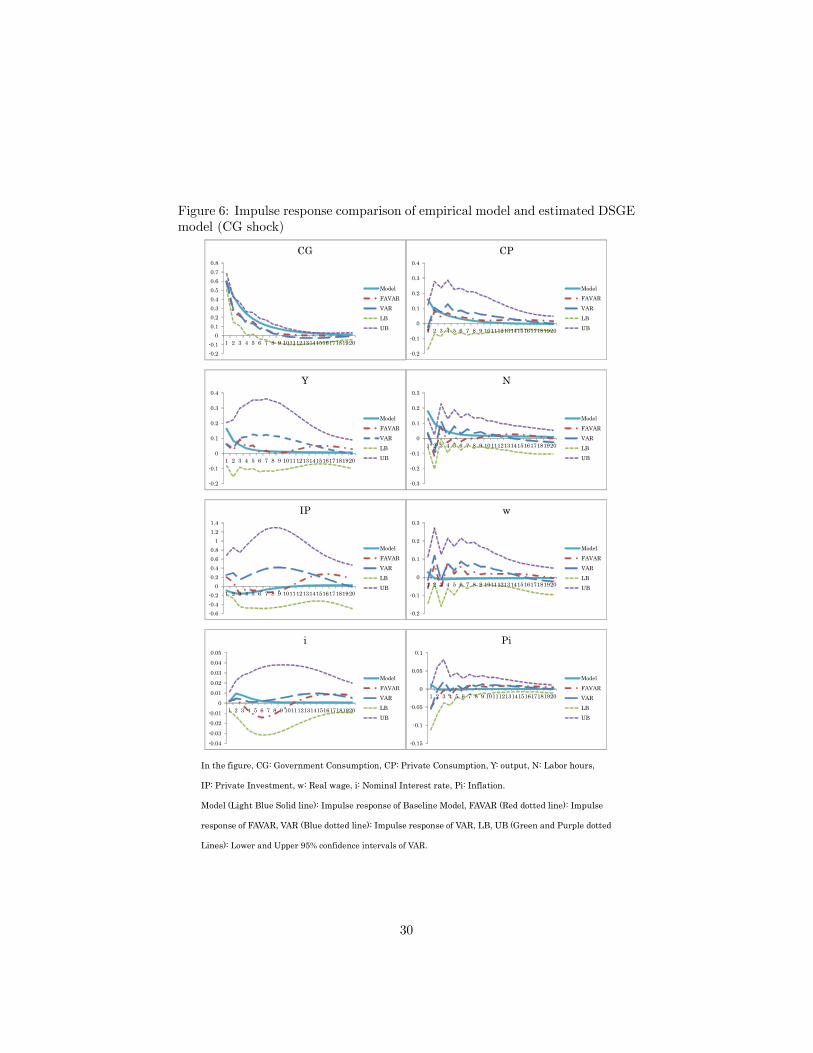
Figure 6: Impulse response comparison of empirical model and estimated DSGEmodel (CG shock)【機密性 2情報】

In the figure, CG: Government Consumption, CP: Private Consumption, Y: output, N: Labor hours,

IP: Private Investment, w: Real wage, i: Nominal Interest rate, Pi: Inflation.

Model (Light Blue Solid line): Impulse response of Baseline Model, FAVAR (Red dotted line): Impulse

response of FAVAR, VAR (Blue dotted line): Impulse response of VAR, LB, UB (Green and Purple dotted

Lines): Lower and Upper 95% confidence intervals of VAR.

­0.2­0.1

00.10.20.30.40.50.60.70.8

1 2 3 4 5 6 7 8 9 1011121314151617181920

CG

ModelFAVARVARLBUB

­0.2

­0.1

0

0.1

0.2

0.3

0.4

1 2 3 4 5 6 7 8 9 1011121314151617181920

CP

ModelFAVARVARLBUB

­0.2

­0.1

0

0.1

0.2

0.3

0.4

1 2 3 4 5 6 7 8 9 1011121314151617181920

Y

ModelFAVARVARLBUB

­0.3

­0.2

­0.1

0

0.1

0.2

0.3

1 2 3 4 5 6 7 8 9 1011121314151617181920

N

ModelFAVARVARLBUB

­0.6­0.4­0.2

00.20.40.60.8

11.21.4

1 2 3 4 5 6 7 8 9 1011121314151617181920

IP

ModelFAVARVARLBUB

­0.2

­0.1

0

0.1

0.2

0.3

1 2 3 4 5 6 7 8 9 1011121314151617181920

w

ModelFAVARVARLBUB

­0.04­0.03­0.02­0.01

00.010.020.030.040.05

1 2 3 4 5 6 7 8 9 1011121314151617181920

i

ModelFAVARVARLBUB

­0.15

­0.1

­0.05

0

0.05

0.1

1 2 3 4 5 6 7 8 9 1011121314151617181920

Pi

ModelFAVARVARLBUB

30

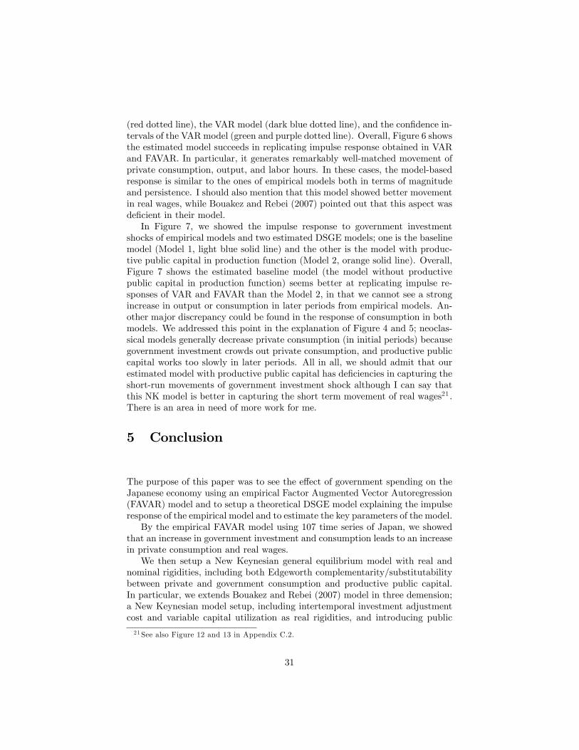
(red dotted line), the VAR model (dark blue dotted line), and the con�dence in-tervals of the VAR model (green and purple dotted line). Overall, Figure 6 showsthe estimated model succeeds in replicating impulse response obtained in VARand FAVAR. In particular, it generates remarkably well-matched movement ofprivate consumption, output, and labor hours. In these cases, the model-basedresponse is similar to the ones of empirical models both in terms of magnitudeand persistence. I should also mention that this model showed better movementin real wages, while Bouakez and Rebei (2007) pointed out that this aspect wasde�cient in their model.In Figure 7, we showed the impulse response to government investment

shocks of empirical models and two estimated DSGE models; one is the baselinemodel (Model 1, light blue solid line) and the other is the model with produc-tive public capital in production function (Model 2, orange solid line). Overall,Figure 7 shows the estimated baseline model (the model without productivepublic capital in production function) seems better at replicating impulse re-sponses of VAR and FAVAR than the Model 2, in that we cannot see a strongincrease in output or consumption in later periods from empirical models. An-other major discrepancy could be found in the response of consumption in bothmodels. We addressed this point in the explanation of Figure 4 and 5; neoclas-sical models generally decrease private consumption (in initial periods) becausegovernment investment crowds out private consumption, and productive publiccapital works too slowly in later periods. All in all, we should admit that ourestimated model with productive public capital has de�ciencies in capturing theshort-run movements of government investment shock although I can say thatthis NK model is better in capturing the short term movement of real wages21 .There is an area in need of more work for me.

5 Conclusion

The purpose of this paper was to see the e¤ect of government spending on theJapanese economy using an empirical Factor Augmented Vector Autoregression(FAVAR) model and to setup a theoretical DSGE model explaining the impulseresponse of the empirical model and to estimate the key parameters of the model.By the empirical FAVAR model using 107 time series of Japan, we showed

that an increase in government investment and consumption leads to an increasein private consumption and real wages.We then setup a New Keynesian general equilibrium model with real and

nominal rigidities, including both Edgeworth complementarity/substitutabilitybetween private and government consumption and productive public capital.In particular, we extends Bouakez and Rebei (2007) model in three demension;a New Keynesian model setup, including intertemporal investment adjustmentcost and variable capital utilization as real rigidities, and introducing public

21See also Figure 12 and 13 in Appendix C.2.

31

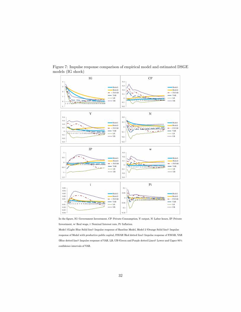
Figure 7: Impulse response comparison of empirical model and estimated DSGEmodels (IG shock)

【機密性 2情報】

In the figure, IG: Government Investment, CP: Private Consumption, Y: output, N: Labor hours, IP: Private

Investment, w: Real wage, i: Nominal Interest rate, Pi: Inflation.

Model 1(Light Blue Solid line): Impulse response of Baseline Model, Model 2 (Orange Solid line): Impulse

response of Model with productive public capital, FAVAR (Red dotted line): Impulse response of FAVAR, VAR

(Blue dotted line): Impulse response of VAR, LB, UB (Green and Purple dotted Lines): Lower and Upper 95%

confidence intervals of VAR.

­1

0

1

2

3

4

1 2 3 4 5 6 7 8 9 1011121314151617181920

IG

Model1Model2FAVARVARLBUB

­0.2

­0.1

0

0.1

0.2

0.3

0.4

1 2 3 4 5 6 7 8 9 1011121314151617181920

CP

Model1Model2FAVARVARLBUB

­0.3

­0.2

­0.1

0

0.1

0.2

0.3

0.4

1 2 3 4 5 6 7 8 9 1011121314151617181920

Y

Model1Model2FAVARVARLBUB

­0.3

­0.2

­0.1

0

0.1

0.2

1 2 3 4 5 6 7 8 9 1011121314151617181920

N

Model1Model2FAVARVARLBUB

­1.5

­1

­0.5

0

0.5

1

1 2 3 4 5 6 7 8 9 1011121314151617181920

IP

Model1Model2FAVARVARLBUB

­0.3

­0.2

­0.1

0

0.1

0.2

0.3

1 2 3 4 5 6 7 8 9 1011121314151617181920

w

Model1Model2FAVARVARLBUB

­0.04­0.03­0.02­0.01

00.010.020.030.040.05

1 2 3 4 5 6 7 8 9 1011121314151617181920

i

Model1Model2FAVARVARLBUB

­0.15

­0.1

­0.05

0

0.05

0.1

1 2 3 4 5 6 7 8 9 1011121314151617181920

Pi

Model1Model2FAVARVARLBUB

32

capital stocks as an externality to the production function of intermediate goods�rms. This model succeeds in private consumption and real wages increase inresponse to government expenditure shocks.Then, we estimated the key parameters of the model using Bayesian in-

ference, and showed that private and government consumption are Edgeworthcomplements as Boaukez and Rebei (2007) found for U.S. data and Okubo(2003) and Iwata (2012) for Japanese data, and that public capital is produc-tive in Japan. In addition, from the estimated model, we showed the impactoutput multiplier to government consumption shock amounts to 1:81, while thatto government investment shock is 0:75.Finally, I compared the impulse response of estimated DSGE model with

those obrtained by VAR and FAVAR model. Concerning government consump-tion shock, the estimated model succeeds in replicating impulse response byVAR and FAVAR model; it generates remarkably well matched movement ofprivate consumption, output, labor hours, and real wages. On the other hand,our estimated model with productive public capital showed deferences in cap-turing the short-run movements of government investment shock. This is myvery �rst step for model development and I will take up this issue in the futurework.

A Data

All series are taken from IN information Center /INDB Finder PRO Database.Data period is from1985Q3-2008Q1.Data included in the observable factors Yt are the following.1. Output: Real gross domestic product (billion yen) de�ated by Chain-type

price index (2000=100) : s.a (SNA),2. Private consumption: Real �nal consumption of household (billion yen)

de�ated by Chain-type price index (2000=100) : s.a (SNA),3. Private investment: Real gross capital formation of private sectors (billion

yen) de�ated by Chain-type price index (2000=100) : s.a (SNA),4. Government consumption: Real government �nal consumption expendi-

ture (billion yen) de�ated by Chain-type price index (2000=100) : s.a (SNA),5. Government investment: Real gross capital formation of public sectors

(billion yen) de�ated by Chain-type price index (2000=100) : s.a (SNA),6. Labor hours: Index of labor hour, total hours worked, all industries, 30

or more employees (2005=100): s.a.7. Real wages: Index of Real Wages, total amount of cash earnings in all

industries, 30 or more employees (2005=100), s.a.8. Nominal interest rate: Call rate (uncollateralized overnight, end of month),9. In�ation: GDP de�ator, implicit de�ator, s.a.All data except in�ation are transformed to logarithms and are one-sided

HP �ltered. As for in�ation, we use one-sided HP �ltered.

33

The other 98 variables can be seen in Table A.1. In the table, transformationcodes mean 1: one-sided HP �ltered, 2: logarithm and one-sided HP �ltered.The circle for seasonal adjustment means we made seasonal adjustment usingX12-ARIMA because seasonally adjusted series are not provided.

B Log linearized Model

For the sake of Bayesian estimation, which requires the model to be in thelinear state-space form, we log-linearize the model around the steady states. wesimply state the result here. The hat above a variable denotes log derivationfrom steady state: i.e. bx = lnx� lnxss where xss is steady state.B.0.1 Equilibrium Conditions from Housing Sector

(1)Consumption Euler equation:

b�t = Et[d�t+1 +cRt � d�t+1] (41)

where

b�t = � ("� 1)1� � Et

[~Ct+1�� ( ("� 1)� 1) + "� (1�� )

�

1� � c~Ct+ ("� 1)

1� � [~Ct�1�

1

�cCpt(42)

and

c~Ct = �(CP

~C)v�1v dCpt + (1� �)(C

G

~C)v�1v dCgt (43)

(2)Labor Supply equation:

N

1�NcNt = b�t +cwt (44)

(3) Investment Euler equation:

cIPt = �

1 + �EtdIPt+1 + 1

1 + �dIPt�1 + �

1 + �( b�t � b�t) (45)

(4) Asset Pricing Euler equation:

b�t � b�t = �(cRt � Etd�t+1) + (1� �P )Et(d�t+1 � d�t+1) + r(1 + )Etdrt+11� �P + r

(46)

(5) Private Capital Accumulation equation

[Kpt+1 = �p bIpt + (1� �p)dKP

t (47)

34

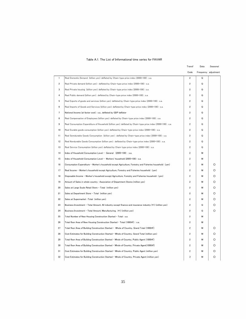
Table A.1. The List of Informational time series for FAVAR

Transf

Code

Data

Frequency

Seasonal

adjustment

1 Real Domestic Demand  (billion yen): deflated by Chain­type price index (2000=100) : s.a. 2 Q

2 Real Private demand (billion yen) : deflated by Chain­type price index (2000=100) : s.a. 2 Q

3 Real Private housing  (billion yen): deflated by Chain­type price index (2000=100) : s.a. 2 Q

4 Real Public demand (billion yen) : deflated by Chain­type price index (2000=100) : s.a. 2 Q

5 Real Exports of goods and services (billion yen): deflated by Chain­type price index (2000=100) : s.a. 2 Q

6 Real Imports of Goods and Services (billion yen): deflated by Chain­type price index (2000=100) : s.a. 2 Q

7 National Income (at factor cost) : s.a., deflated by GDP deflator 2 Q

8 Real Compensation of Employees (billion yen): deflated by Chain­type price index (2000=100) : s.a. 2 Q

9 Real Consumption Expenditure of Household (billion yen): deflated by Chain­type price index (2000=100) : s.a. 2 Q

10 Real Durable goods consumption (billion yen): deflated by Chain­type price index (2000=100) : s.a. 2 Q

11 Real Semidurable Goods Consumption  (billion yen) : deflated by Chain­type price index (2000=100) : s.a. 2 Q

12 Real Nondurable Goods Consumption (billion yen) : deflated by Chain­type price index (2000=100) : s.a. 2 Q

13 Real Service Consumption (billion yen): deflated by Chain­type price index (2000=100) : s.a. 2 Q

14 Index of Household Consumption Level ­  General   (2005=100)  : s.a. 2 M

15 Index of Household Consumption Level ­  Workers' household (2005=100) : s.a. 2 M

16 Consumption Expenditure ­ Worker's household except Agriculture, Forestry and Fisheries household : (yen) 2 M ○

17 Real Income ­ Worker's household except Agriculture, Forestry and Fisheries household : (yen) 2 M ○

18 Disposable Income ­ Worker's household except Agriculture, Forestry and Fisheries household : (yen) 2 M ○

19 Amount of Sales in whole country : Association of Department Stores (million yen) 2 M ○

20 Sales at Large Scale Retail Store ­ Total  (million yen) 2 M ○

21 Sales at Department Store ­ Total  (million yen) 2 M ○

22 Sales at Supermarket ­Total  (million yen) 2 M ○

23 Business Investment ­ Total Amount, All industry except finance and insurance industry (*1) (million yen) 2 Q ○

24 Business Investment ­ Total Amount, Manufacturing,  (*1) (million yen) 2 Q ○

25 Total Number of New Housing Construction Started ­ Total : s.a. 2 M

26 Total floor Area of New Housing Construction Started ­ Total (1000㎡） : s.a. 2 M

27 Total floor Area of Building Construction Started ­  Whole of Country, Grand Total (1000㎡） 2 M ○

28 Cost Estimates for Building Construction Started ­ Whole of Country, Grand Total (million yen) 2 M ○

29 Total floor Area of Building Construction Started ­ Whole of Country, Public Agent (1000㎡） 2 M ○

30 Total floor Area of Building Construction Started ­ Whole of Country, Private Agent(1000㎡） 2 M ○

31 Cost Estimates for Building Construction Started ­ Whole of Country, Public Agent (million yen) 2 M ○

32 Cost Estimates for Building Construction Started ­ Whole of Country, Private Agent (million yen) 2 M ○

35

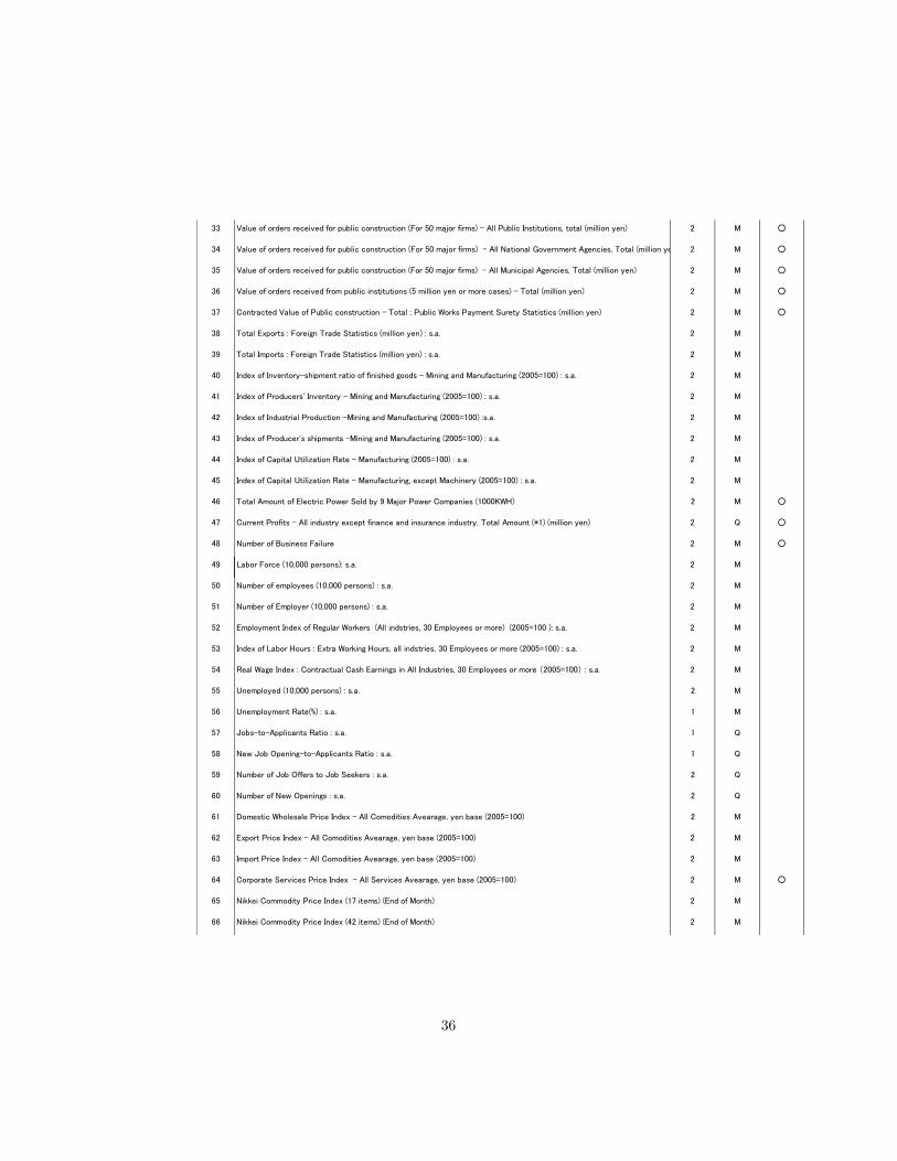
33 Value of orders received for public construction (For 50 major firms) ­ All Public Institutions, total (million yen) 2 M ○

34 Value of orders received for public construction (For 50 major firms)  ­ All National Government Agencies, Total (million yen) 2 M ○

35 Value of orders received for public construction (For 50 major firms)  ­ All Municipal Agencies, Total (million yen) 2 M ○

36 Value of orders received from public institutions (5 million yen or more cases) ­ Total (million yen) 2 M ○

37 Contracted Value of Public construction ­ Total : Public Works Payment Surety Statistics (million yen) 2 M ○

38 Total Exports : Foreign Trade Statistics (million yen) : s.a. 2 M

39 Total Imports : Foreign Trade Statistics (million yen) : s.a. 2 M

40 Index of Inventory­shipment ratio of finished goods ­ Mining and Manufacturing (2005=100) : s.a. 2 M

41 Index of Producers' Inventory ­ Mining and Manufacturing (2005=100) : s.a. 2 M

42 Index of Industrial Production ­Mining and Manufacturing (2005=100) :s.a. 2 M

43 Index of Producer's shipments ­Mining and Manufacturing (2005=100) : s.a. 2 M

44 Index of Capital Utilization Rate ­ Manufacturing (2005=100) : s.a. 2 M

45 Index of Capital Utilization Rate ­ Manufacturing, except Machinery (2005=100) : s.a. 2 M

46 Total Amount of Electric Power Sold by 9 Major Power Companies (1000KWH) 2 M ○

47 Current Profits ­ All industry except finance and insurance industry, Total Amount (*1) (million yen) 2 Q ○

48 Number of Business Failure 2 M ○

49 Labor Force (10,000 persons): s.a. 2 M

50 Number of employees (10,000 persons) : s.a. 2 M

51 Number of Employer (10,000 persons) : s.a. 2 M

52 Employment Index of Regular Workers  (All indstries, 30 Employees or more)  (2005=100 ): s.a. 2 M

53 Index of Labor Hours : Extra Working Hours, all indstries, 30 Employees or more (2005=100) : s.a. 2 M

54 Real Wage Index : Contractual Cash Earnings in All Industries, 30 Employees or more （2005=100） : s.a. 2 M

55 Unemployed (10,000 persons) : s.a. 2 M

56 Unemployment Rate(%) : s.a. 1 M

57 Jobs­to­Applicants Ratio : s.a. 1 Q

58 New Job Opening­to­Applicants Ratio : s.a. 1 Q

59 Number of Job Offers to Job Seekers : s.a. 2 Q

60 Number of New Openings : s.a. 2 Q

61 Domestic Wholesale Price Index ­ All Comodities Avearage, yen base (2005=100) 2 M

62 Export Price Index ­ All Comodities Avearage, yen base (2005=100) 2 M

63 Import Price Index ­ All Comodities Avearage, yen base (2005=100) 2 M

64 Corporate Services Price Index  ­ All Services Avearage, yen base (2005=100) 2 M ○

65 Nikkei Commodity Price Index (17 items) (End of Month) 2 M

66 Nikkei Commodity Price Index (42 items) (End of Month) 2 M

36

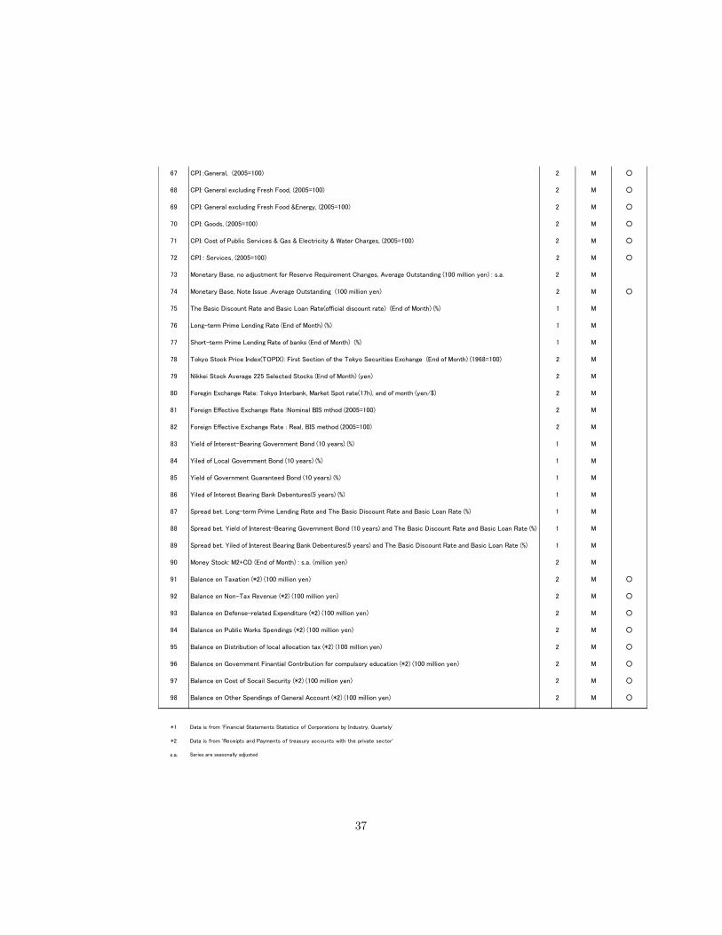
67 CPI :General,  (2005=100) 2 M ○

68 CPI: General excluding Fresh Food, (2005=100) 2 M ○

69 CPI: General excluding Fresh Food &Energy, (2005=100) 2 M ○

70 CPI: Goods, (2005=100) 2 M ○

71 CPI: Cost of Public Services & Gas & Electricity & Water Charges, (2005=100) 2 M ○

72 CPI : Services, (2005=100) 2 M ○

73 Monetary Base, no adjustment for Reserve Requirement Changes, Average Outstanding (100 million yen) : s.a. 2 M

74 Monetary Base, Note Issue ,Average Outstanding  (100 million yen) 2 M ○

75 The Basic Discount Rate and Basic Loan Rate(official discount rate)  (End of Month) (%) 1 M

76 Long­term Prime Lending Rate (End of Month) (%) 1 M

77 Short­term Prime Lending Rate of banks (End of Month)  (%) 1 M

78 Tokyo Stock Price Index(TOPIX): First Section of the Tokyo Securities Exchange  (End of Month) (1968=100) 2 M

79 Nikkei Stock Average 225 Selected Stocks (End of Month) (yen) 2 M

80 Foregin Exchange Rate: Tokyo Interbank, Market Spot rate(17h), end of month (yen/$) 2 M

81 Foreign Effective Exchange Rate :Nominal BIS mthod (2005=100) 2 M

82 Foreign Effective Exchange Rate : Real, BIS method (2005=100) 2 M

83 Yield of Interest­Bearing Government Bond (10 years) (%) 1 M

84 Yiled of Local Government Bond (10 years) (%) 1 M

85 Yield of Government Guaranteed Bond (10 years) (%) 1 M

86 Yiled of Interest Bearing Bank Debentures(5 years) (%) 1 M

87 Spread bet. Long­term Prime Lending Rate and The Basic Discount Rate and Basic Loan Rate (%) 1 M

88 Spread bet. Yield of Interest­Bearing Government Bond (10 years) and The Basic Discount Rate and Basic Loan Rate (%) 1 M

89 Spread bet. Yiled of Interest Bearing Bank Debentures(5 years) and The Basic Discount Rate and Basic Loan Rate (%) 1 M

90 Money Stock: M2+CD (End of Month) : s.a. (million yen) 2 M

91 Balance on Taxation (*2) (100 million yen) 2 M ○

92 Balance on Non­Tax Revenue (*2) (100 million yen) 2 M ○

93 Balance on Defense­related Expenditure (*2) (100 million yen) 2 M ○

94 Balance on Public Works Spendings (*2) (100 million yen) 2 M ○

95 Balance on Distribution of local allocation tax (*2) (100 million yen) 2 M ○

96 Balance on Government Finantial Contribution for compulsory education (*2) (100 million yen) 2 M ○

97 Balance on Cost of Socail Security (*2) (100 million yen) 2 M ○

98 Balance on Other Spendings of General Account (*2) (100 million yen) 2 M ○

*1 Data is from 'Financial Statements Statistics of Corporations by Industry, Quartely'

*2 Data is from 'Receipts and Payments of treasury accounts with the private sector'

s.a. Series are seasonally adjusted

37

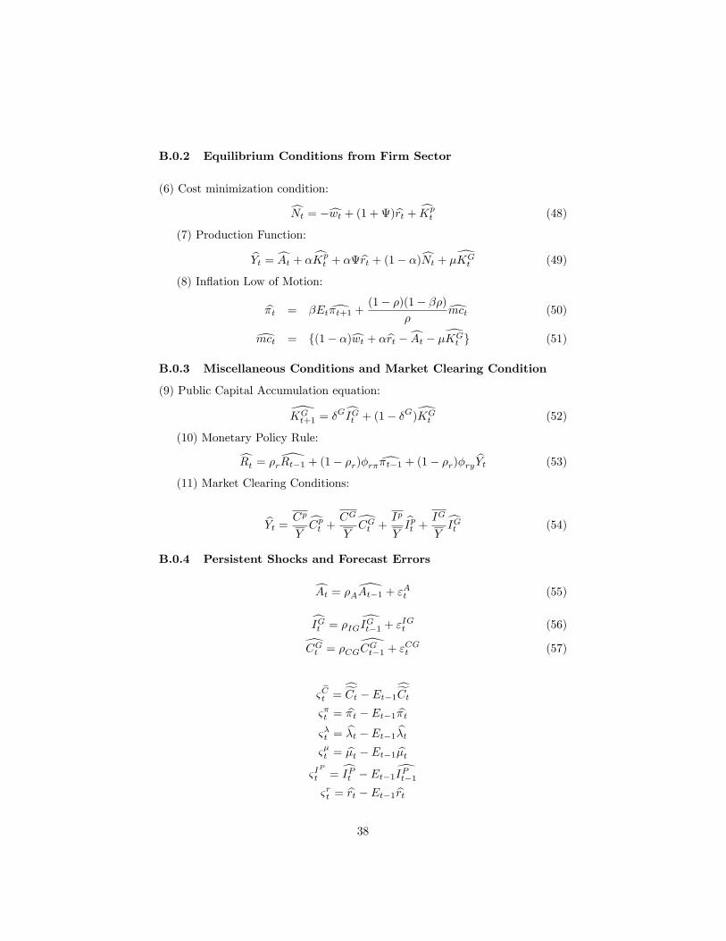
B.0.2 Equilibrium Conditions from Firm Sector

(6) Cost minimization condition:cNt = �cwt + (1 + )brt + cKpt (48)

(7) Production Function:bYt = cAt + �cKpt + �brt + (1� �)cNt + �dKG

t (49)

(8) In�ation Low of Motion:

b�t = �Etd�t+1 + (1� �)(1� ��)�

dmct (50)

dmct = f(1� �)cwt + �brt �cAt � �dKGt g (51)

B.0.3 Miscellaneous Conditions and Market Clearing Condition

(9) Public Capital Accumulation equation:

[KGt+1 = �GcIGt + (1� �G)dKG

t (52)

(10) Monetary Policy Rule:cRt = �r[Rt�1 + (1� �r)�r� d�t�1 + (1� �r)�ry bYt (53)

(11) Market Clearing Conditions:

bYt = Cp

YcCpt + CG

YdCGt + Ip

YbIpt + IG

YcIGt (54)

B.0.4 Persistent Shocks and Forecast Errors

cAt = �A[At�1 + "At (55)

cIGt = �IGdIGt�1 + "IGt (56)dCGt = �CG[CGt�1 + "

CGt (57)

&eCt =

cfCt � Et�1cfCt&�t = b�t � Et�1 b�t&�t =

b�t � Et�1 b�t&�t = b�t � Et�1 b�t

&IP

t = cIPt � Et�1dIPt�1&rt = brt � Et�1 brt

38

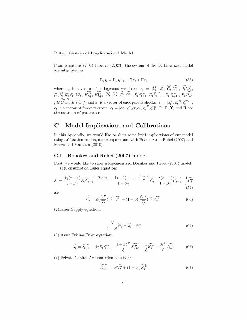
B.0.5 System of Log-linearized Model

From equations (2.01) through (2.023), the system of the log-linearized modelare integrated as

�0st = �1st�1 +�"t +�&t (58)

where st is a vector of endogenous variables: st = [ bYt, b�t, c~Ct,dCpt , cIPt , b�t,b�t,cNt,cwt,brt,dmct , [KPt+1,

[KGt+1, cRt, cAt, cIGt ,dCGt , Etd�t+1, Etd�t+1 , Etd�t+1 , EtdIPt+1

, Et[]Ct+1, Etdrt+1]0, and "t is a vector of endogenous shocks: "t = ["At , "IGt ,"CGt ]0.

&t is a vector of forecast errors: &t = [&eCt , &

�t ,&

�t ,&

�t , &

IP

t ,&rt ]0. �0,�1,�, and � are

the matrices of parameters.

C Model Implications and Calibrations

In this Appendix, we would like to show some brief implications of our modelusing calibration results, and compare ours with Boaukez and Rebei (2007) andMarzo and Marattin (2010).

C.1 Bouakez and Rebei (2007) model

First, we would like to show a log-linearized Boaukez and Rebei (2007) model.(1)Consumption Euler equation:

b�t = � ("� 1)1� � Et

[~Ct+1�� ( ("� 1)� 1) + "� (1�� )

�

1� � c~Ct+ ("� 1)

1� � [~Ct�1�

1

�cCpt(59)

and c~Ct = �(CP

~C)v�1v dCpt + (1� �)(C

G

~C)v�1v dCgt (60)

(2)Labor Supply equation:

N

1�NcNt = b�t +cwt (61)

(3) Asset Pricing Euler equation:

b�t = d�t+1 + �rEtdrt+1 � 1 + ��P�

[KPt+1 +

1

�dKPt +

��P

�dIPt+1 (62)

(4) Private Capital Accumulation equation:

[Kpt+1 = �p bIpt + (1� �p)dKP

t (63)

39

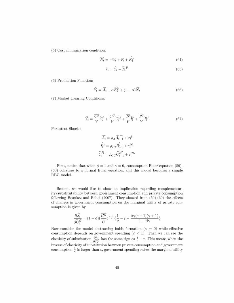
(5) Cost minimization condition:

cNt = �cwt + brt + cKpt (64)

brt = bYt �dKPt (65)

(6) Production Function:

bYt = cAt + �cKpt + (1� �)cNt (66)

(7) Market Clearing Conditions:

bYt = Cp

YcCpt + CG

YdCGt + Ip

YbIpt + IG

YcIGt (67)

Persistent Shocks:

cAt = �A[At�1 + "AtcIGt = �IGdIGt�1 + "IGtdCGt = �CG[CGt�1 + "

CGt

First, notice that when � = 1 and = 0, consumption Euler equation (59)-(60) collapses to a normal Euler equation, and this model becomes a simpleRBC model.

Second, we would like to show an implication regarding complementar-ity/substitutability between government consumption and private consumptionfollowing Boaukez and Rebei (2007). They showed from (59)-(60) the e¤ectsof changes in government consumption on the marginal utility of private con-sumption is given by

@ b�t@dCGt = (1� �)(C

G

~C)v�1v f1

�� "� � ("� 1)( + 1)

1� � g

Now consider the model abstracting habit formation ( = 0) while e¤ectiveconsumption depends on government spending (� < 1). Then we can see the

elasticity of substitution @c�t@dCG

t

has the same sign as 1� � ". This means when the

inverse of elasticity of substitution between private consumption and governmentconsumption 1

� is larger than ", government spending raises the marginal utility

40

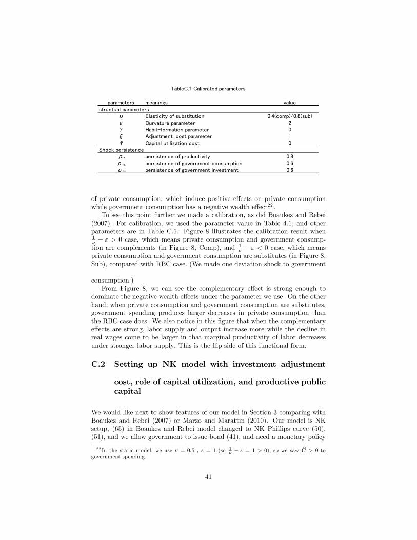
parameters meanings value

structual parametersυ Elasticity of substitution 0.4(comp)/0.8(sub)ε Curvature parameter 2γ Habit­formation parameter 0ξ Adjustment­cost parameter 1Ψ Capital utilization cost 0

Shock persistenceρa persistence of productivity 0.8ρcg persistence of government consumption 0.6ρIG persistence of government investment 0.6

TableC.1 Calibrated parameters

of private consumption, which induce positive e¤ects on private consumptionwhile government consumption has a negative wealth e¤ect22 .To see this point further we made a calibration, as did Boaukez and Rebei

(2007). For calibration, we used the parameter value in Table 4.1, and otherparameters are in Table C.1. Figure 8 illustrates the calibration result when1� � " > 0 case, which means private consumption and government consump-tion are complements (in Figure 8, Comp), and 1

� � " < 0 case, which meansprivate consumption and government consumption are substitutes (in Figure 8,Sub), compared with RBC case. (We made one deviation shock to government

consumption.)From Figure 8, we can see the complementary e¤ect is strong enough to

dominate the negative wealth e¤ects under the parameter we use. On the otherhand, when private consumption and government consumption are substitutes,government spending produces larger decreases in private consumption thanthe RBC case does. We also notice in this �gure that when the complementarye¤ects are strong, labor supply and output increase more while the decline inreal wages come to be larger in that marginal productivity of labor decreasesunder stronger labor supply. This is the �ip side of this functional form.

C.2 Setting up NK model with investment adjustment

cost, role of capital utilization, and productive publiccapital

We would like next to show features of our model in Section 3 comparing withBoaukez and Rebei (2007) or Marzo and Marattin (2010). Our model is NKsetup, (65) in Boaukez and Rebei model changed to NK Phillips curve (50),(51), and we allow government to issue bond (41), and need a monetary policy

22 In the static model, we use � = 0:5 , " = 1 (so 1�� " = 1 > 0), so we saw bC > 0 to

government spending.

41

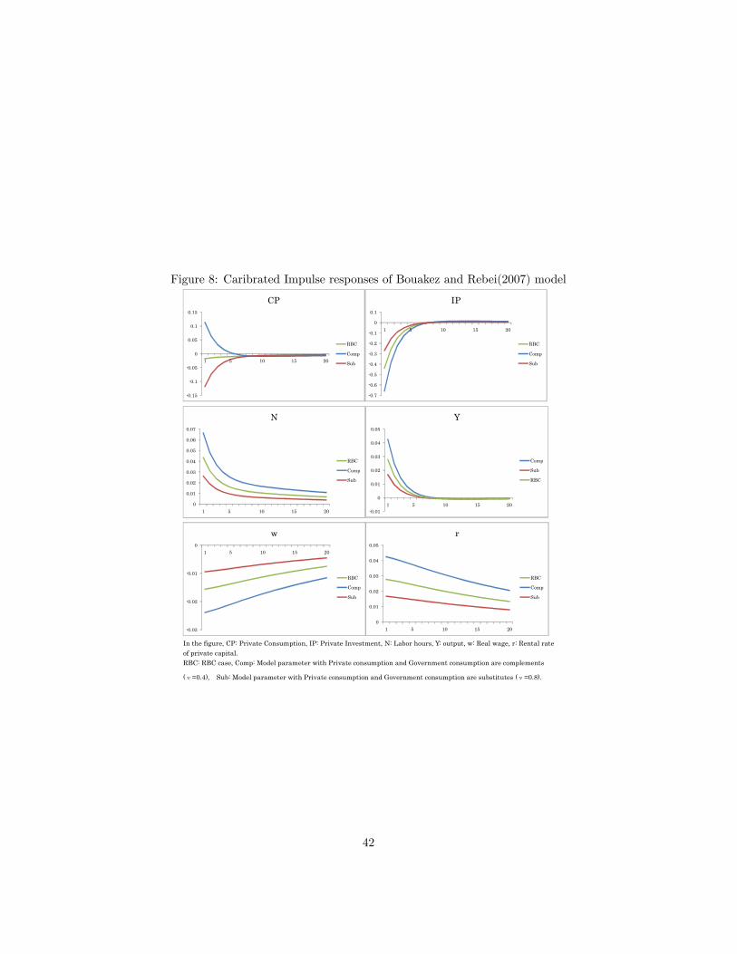
Figure 8: Caribrated Impulse responses of Bouakez and Rebei(2007) model【機密性 2情報】

In the figure, CP: Private Consumption, IP: Private Investment, N: Labor hours, Y: output, w: Real wage, r: Rental rateof private capital.RBC: RBC case, Comp: Model parameter with Private consumption and Government consumption are complements

(ν=0.4), Sub: Model parameter with Private consumption and Government consumption are substitutes (ν=0.8).

­0.15

­0.1

­0.05

0

0.05

0.1

0.15

1 5 10 15 20

CP

RBC

Comp

Sub

­0.7

­0.6

­0.5

­0.4

­0.3

­0.2

­0.1

0

0.1

1 5 10 15 20

IP

RBC

Comp

Sub

0

0.01

0.02

0.03

0.04

0.05

0.06

0.07

1 5 10 15 20

N

RBC

Comp

Sub

­0.01

0

0.01

0.02

0.03

0.04

0.05

1 5 10 15 20

Y

Comp

Sub

RBC

­0.03

­0.02

­0.01

01 5 10 15 20

w

RBC

Comp

Sub

0

0.01

0.02

0.03

0.04

0.05

1 5 10 15 20

r

RBC

Comp

Sub

42

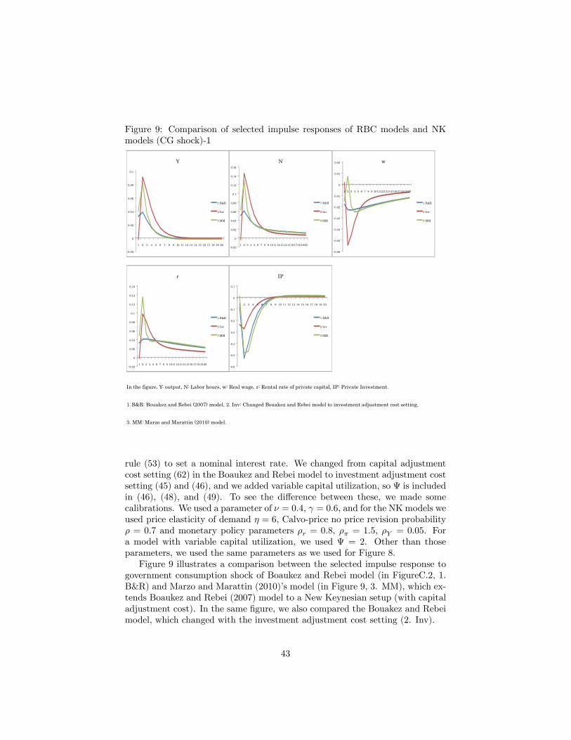
Figure 9: Comparison of selected impulse responses of RBC models and NKmodels (CG shock)-1【機密性 2情報】

In the figure, Y: output, N: Labor hours, w: Real wage, r: Rental rate of private capital, IP: Private Investment.

1. B&R: Bouakez and Rebei (2007) model, 2. Inv: Changed Bouakez and Rebei model to investment adjustment cost setting,

3. MM: Marzo and Marattin (2010) model.

­0.02

0

0.02

0.04

0.06

0.08

0.1

1 2 3 4 5 6 7 8 9 10 11 12 13 14 15 16 17 18 19 20

Y

1 B&R

2 Inv

3 MM

­0.02

0

0.02

0.04

0.06

0.08

0.1

0.12

0.14

0.16

1 2 3 4 5 6 7 8 9 1011121314151617181920

N

1 B&R

2 Inv

3 MM

­0.06

­0.05

­0.04

­0.03

­0.02

­0.01

0

0.01

0.02

1 2 3 4 5 6 7 8 9 1011121314151617181920

w

1 B&R

2 Inv

3 MM

­0.02

0

0.02

0.04

0.06

0.08

0.1

0.12

0.14

0.16

1 2 3 4 5 6 7 8 9 1011121314151617181920

r

1 B&R

2 Inv

3 MM

­0.6

­0.5

­0.4

­0.3

­0.2

­0.1

0

0.1

1 2 3 4 5 6 7 8 9 10 11 12 13 14 15 16 17 18 19 20

IP

1 B&R

2 Inv

3 MM

rule (53) to set a nominal interest rate. We changed from capital adjustmentcost setting (62) in the Boaukez and Rebei model to investment adjustment costsetting (45) and (46), and we added variable capital utilization, so is includedin (46), (48), and (49). To see the di¤erence between these, we made somecalibrations. We used a parameter of � = 0:4, = 0:6, and for the NK models weused price elasticity of demand � = 6, Calvo-price no price revision probability� = 0:7 and monetary policy parameters �r = 0:8, �� = 1:5, �Y = 0:05. Fora model with variable capital utilization, we used = 2. Other than thoseparameters, we used the same parameters as we used for Figure 8.Figure 9 illustrates a comparison between the selected impulse response to

government consumption shock of Boaukez and Rebei model (in FigureC.2, 1.B&R) and Marzo and Marattin (2010)�s model (in Figure 9, 3. MM), which ex-tends Boaukez and Rebei (2007) model to a New Keynesian setup (with capitaladjustment cost). In the same �gure, we also compared the Bouakez and Rebeimodel, which changed with the investment adjustment cost setting (2. Inv).

43

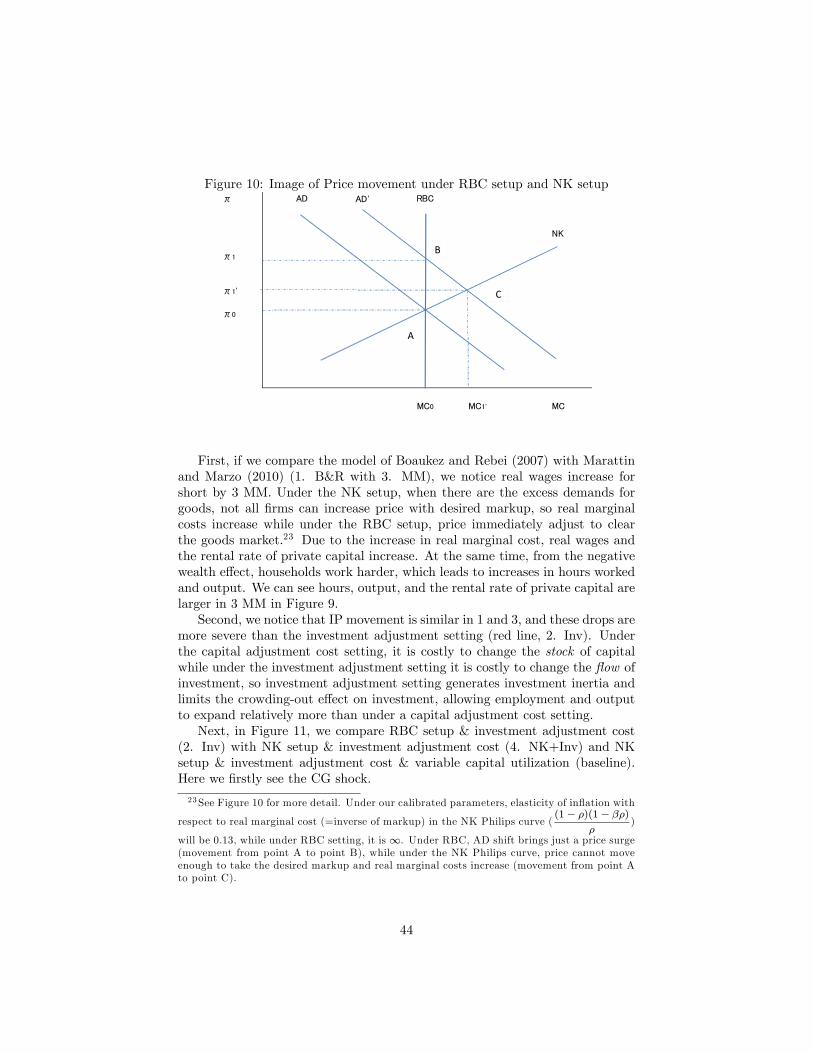
Figure 10: Image of Price movement under RBC setup and NK setupπ AD'

NK

π1

π1'

π0

MC1' MC

AD RBC

MC0

A

B

C

First, if we compare the model of Boaukez and Rebei (2007) with Marattinand Marzo (2010) (1. B&R with 3. MM), we notice real wages increase forshort by 3 MM. Under the NK setup, when there are the excess demands forgoods, not all �rms can increase price with desired markup, so real marginalcosts increase while under the RBC setup, price immediately adjust to clearthe goods market.23 Due to the increase in real marginal cost, real wages andthe rental rate of private capital increase. At the same time, from the negativewealth e¤ect, households work harder, which leads to increases in hours workedand output. We can see hours, output, and the rental rate of private capital arelarger in 3 MM in Figure 9.Second, we notice that IP movement is similar in 1 and 3, and these drops are

more severe than the investment adjustment setting (red line, 2. Inv). Underthe capital adjustment cost setting, it is costly to change the stock of capitalwhile under the investment adjustment setting it is costly to change the �ow ofinvestment, so investment adjustment setting generates investment inertia andlimits the crowding-out e¤ect on investment, allowing employment and outputto expand relatively more than under a capital adjustment cost setting.Next, in Figure 11, we compare RBC setup & investment adjustment cost

(2. Inv) with NK setup & investment adjustment cost (4. NK+Inv) and NKsetup & investment adjustment cost & variable capital utilization (baseline).Here we �rstly see the CG shock.

23See Figure 10 for more detail. Under our calibrated parameters, elasticity of in�ation with

respect to real marginal cost (=inverse of markup) in the NK Philips curve ((1� �)(1� ��)

�)

will be 0.13, while under RBC setting, it is 1. Under RBC, AD shift brings just a price surge(movement from point A to point B), while under the NK Philips curve, price cannot moveenough to take the desired markup and real marginal costs increase (movement from point Ato point C).

44

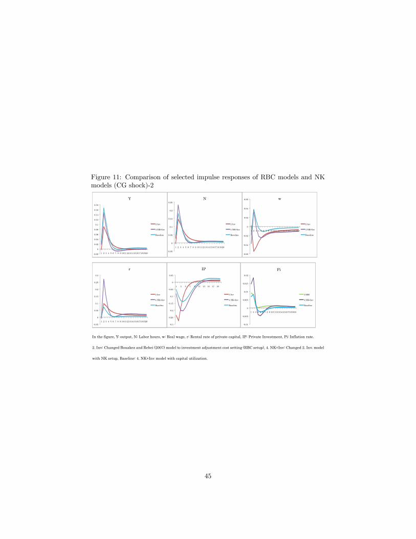
Figure 11: Comparison of selected impulse responses of RBC models and NKmodels (CG shock)-2【機密性 2情報】

In the figure, Y: output, N: Labor hours, w: Real wage, r: Rental rate of private capital, IP: Private Investment, Pi: Inflation rate.

2. Inv: Changed Bouakez and Rebei (2007) model to investment adjustment cost setting (RBC setup), 4. NK+Inv: Changed 2. Inv. model

with NK setup, Baseline: 4. NK+Inv model with capital utilization.

­0.02

0

0.02

0.04

0.06

0.08

0.1

0.12

0.14

0.16

0.18

1 2 3 4 5 6 7 8 9 1011121314151617181920

Y

2 Inv

4 NK+Inv

Baseline

­0.05

0

0.05

0.1

0.15

0.2

0.25

1 2 3 4 5 6 7 8 9 1011121314151617181920

N

2 Inv

4 NK+Inv

Baseline

­0.06

­0.04

­0.02

0

0.02

0.04

0.06

1 2 3 4 5 6 7 8 9 1011121314151617181920

w

2 Inv

4 NK+Inv

Baseline

­0.05

0

0.05

0.1

0.15

0.2

0.25

0.3

1 2 3 4 5 6 7 8 9 1011121314151617181920

r

2 Inv

4 NK+Inv

Baseline

­0.3

­0.25

­0.2

­0.15

­0.1

­0.05

0

0.05

1 3 5 7 9 11 13 15 17 19

IP

2 Inv

4 NK+Inv

Baseline

­0.01

­0.005

0

0.005

0.01

0.015

0.02

1 2 3 4 5 6 7 8 9 1011121314151617181920

Pi

3 MM

4 NK+Inv

Baseline

45

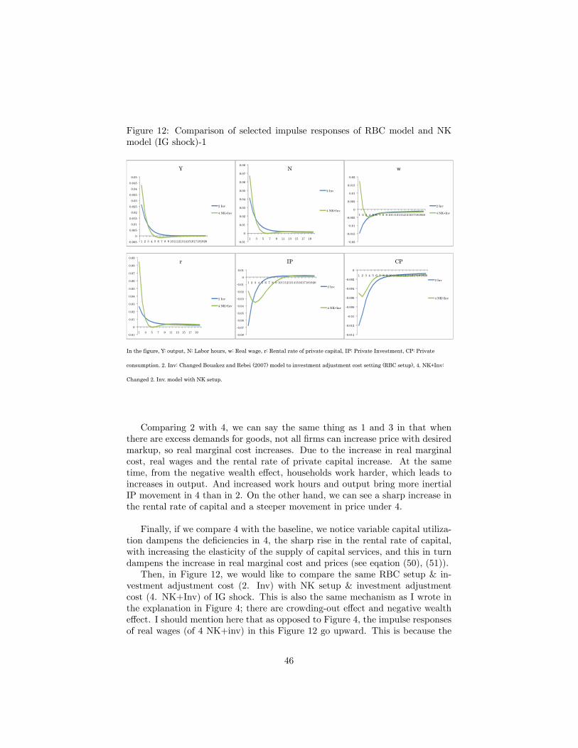
Figure 12: Comparison of selected impulse responses of RBC model and NKmodel (IG shock)-1【機密性 2情報】

In the figure, Y: output, N: Labor hours, w: Real wage, r: Rental rate of private capital, IP: Private Investment, CP: Private

consumption. 2. Inv: Changed Bouakez and Rebei (2007) model to investment adjustment cost setting (RBC setup), 4. NK+Inv:

Changed 2. Inv. model with NK setup.

­0.005

0

0.005

0.01

0.015

0.02

0.025

0.03

0.035

0.04

0.045

0.05

1 2 3 4 5 6 7 8 9 1011121314151617181920

Y

2 Inv

4 NK+Inv

­0.01

0

0.01

0.02

0.03

0.04

0.05

0.06

0.07

0.08

1 3 5 7 9 11 13 15 17 19

N

2 Inv

4 NK+Inv

­0.02

­0.015

­0.01

­0.005

0

0.005

0.01

0.015

0.02

1 2 3 4 5 6 7 8 9 1011121314151617181920

w

2 Inv

4 NK+Inv

­0.01

0

0.01

0.02

0.03

0.04

0.05

0.06

0.07

0.08

0.09

1 3 5 7 9 11 13 15 17 19

r

2 Inv

4 NK+Inv

­0.08

­0.07

­0.06

­0.05

­0.04

­0.03

­0.02

­0.01

0

0.01

1 2 3 4 5 6 7 8 9 1011121314151617181920

IP

2 Inv

4 NK+Inv

­0.014

­0.012

­0.01

­0.008

­0.006

­0.004

­0.002

01 2 3 4 5 6 7 8 9 1011121314151617181920

CP

2 Inv

4 NK+Inv

Comparing 2 with 4, we can say the same thing as 1 and 3 in that whenthere are excess demands for goods, not all �rms can increase price with desiredmarkup, so real marginal cost increases. Due to the increase in real marginalcost, real wages and the rental rate of private capital increase. At the sametime, from the negative wealth e¤ect, households work harder, which leads toincreases in output. And increased work hours and output bring more inertialIP movement in 4 than in 2. On the other hand, we can see a sharp increase inthe rental rate of capital and a steeper movement in price under 4.

Finally, if we compare 4 with the baseline, we notice variable capital utiliza-tion dampens the de�ciencies in 4, the sharp rise in the rental rate of capital,with increasing the elasticity of the supply of capital services, and this in turndampens the increase in real marginal cost and prices (see eqation (50), (51)).Then, in Figure 12, we would like to compare the same RBC setup & in-

vestment adjustment cost (2. Inv) with NK setup & investment adjustmentcost (4. NK+Inv) of IG shock. This is also the same mechanism as I wrote inthe explanation in Figure 4; there are crowding-out e¤ect and negative wealthe¤ect. I should mention here that as opposed to Figure 4, the impulse responsesof real wages (of 4 NK+inv) in this Figure 12 go upward. This is because the

46

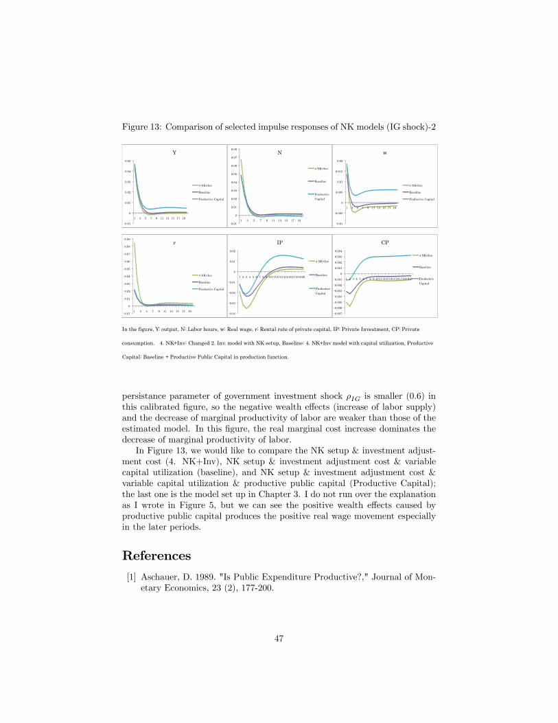
Figure 13: Comparison of selected impulse responses of NK models (IG shock)-2【機密性 2情報】

In the figure, Y: output, N: Labor hours, w: Real wage, r: Rental rate of private capital, IP: Private Investment, CP: Private

consumption. 4. NK+Inv: Changed 2. Inv. model with NK setup, Baseline: 4. NK+Inv model with capital utilization, Productive

Capital: Baseline + Productive Public Capital in production function.

­0.01

0

0.01

0.02

0.03

0.04

0.05

1 3 5 7 9 11 13 15 17 19

Y

4 NK+Inv

Baseline

Productive Capital

­0.01

0

0.01

0.02

0.03

0.04

0.05

0.06

0.07

0.08

1 3 5 7 9 11 13 15 17 19

N

4 NK+Inv

Baseline

ProductiveCapital

­0.01

­0.005

0

0.005

0.01

0.015

0.02

1 3 5 7 9 11 13 15 17 19

w

4 NK+Inv

Baseline

Productive Capital

­0.01

0

0.01

0.02

0.03

0.04

0.05

0.06

0.07

0.08

0.09

1 3 5 7 9 11 13 15 17 19

r

4 NK+Inv

Baseline

Productive Capital

­0.04

­0.03

­0.02

­0.01

0

0.01

0.02

1 2 3 4 5 6 7 8 9 1011121314151617181920

IP

4 NK+Inv

Baseline

ProductiveCapital

­0.007

­0.006

­0.005

­0.004

­0.003

­0.002

­0.001

0

0.001

0.002

0.003

0.004

1 2 3 4 5 6 7 8 9 1011121314151617181920

CP

4 NK+Inv

Baseline

ProductiveCapital

persistance parameter of government investment shock �IG is smaller (0:6) inthis calibrated �gure, so the negative wealth e¤ects (increase of labor supply)and the decrease of marginal productivity of labor are weaker than those of theestimated model. In this �gure, the real marginal cost increase dominates thedecrease of marginal productivity of labor.In Figure 13, we would like to compare the NK setup & investment adjust-

ment cost (4. NK+Inv), NK setup & investment adjustment cost & variablecapital utilization (baseline), and NK setup & investment adjustment cost &variable capital utilization & productive public capital (Productive Capital);the last one is the model set up in Chapter 3. I do not run over the explanationas I wrote in Figure 5, but we can see the positive wealth e¤ects caused byproductive public capital produces the positive real wage movement especiallyin the later periods.

References

[1] Aschauer, D. 1989. "Is Public Expenditure Productive?," Journal of Mon-etary Economics, 23 (2), 177-200.

47

[2] Amano, R. A., Wirjanto T. S. 1998. "Government Expenditures and thePermanent-Income Model," Review of Economic Dynamics, 1 (3), 719-730.

[3] Baxter, M., King, R. G. 1993. "Fiscal Policy in General Equilibrium,"American Economic Review 83 (3), 315-334.

[4] Bernanke, B. S., Boivin, J., Eliasz, P. 2005. �Measuring the E¤ects ofMonetary Policy: A Factor-Augmented Vector Autoregressive (FAVAR)Approach,�The Quarterly Journal of Economics, 120 (1), 387-422.

[5] Blanchard, O., Perotti R. 2002. "An Empirical Characterization Of TheDynamic E¤ects Of Changes In Government Spending And Taxes On Out-put," The Quarterly Journal of Economics, 117 (4), 1329-1368.

[6] Bouakez, H., Rebei, A. 2007. �Why Does Private Consumption Rise After aGovernment Spending Shock?,�Canadian Journal of Economics, CanadianEconomics Association, 40 (3), 954-979.

[7] Burnside, C., Eichenbaum, M., Fisher, J. 2003. "Fiscal Shocks and TheirConsequences," Journal of Economic Theory, 115 (1), 89-117.

[8] Calvo, G. A. 1983. "Staggered Prices in a Utility-maximizing Framework,"Journal of Monetary Economics, 12 (3), 383-398.

[9] Clarida, R., Gali, J., Gertler, M. 1999. "The Science of Monetary Policy: ANew Keynesian Perspective," Journal of Economic Literature, vol. 37(4),1661-1707.

[10] Consolo, A., Favero, C. A., Paccagnini, A. 2009. �On the Statistical Iden-ti�cation of DSGE Models,�Journal of Econometrics, 150 (1), 99-115.

[11] Doi, T., Hoshi, T., Okimoto, T. 2011. "Japanese Government Debt andSustainability of Fiscal Policy," NBER Working Paper No.17305.

[12] Fatas, A., Mihov, I. 2001. "The E¤ects of Fiscal Policy on Consumptionand Employment: Theory and Evidence," CEPR Discussion Papers No.2760.

[13] Forni, M., Gambetti, L. 2010. "Fiscal Foresight and the E¤ects of Govern-ment Spending," CEPR Discussion Papers No. 7840.

[14] Gali, J., Lopez-Salido, J. D., Valles, J. 2007. "Understanding the E¤ectsof Government Spending on Consumption," Journal of the European Eco-nomic Association, 5 (1), 227-270.

[15] Gri¤oli, T. M. "DYNARE User Guide".

[16] Iiboshi, H., Nishiyama, S.-I., Watanabe, T. 2008. "An Estimated Dy-namic Stochastic General Equilibrium Model of the Japanese Economy:A Bayesian Analysis," Mimeo.

48

[17] Ireland, P. 2004. "A Method for Taking Models to the Data," Journal ofEconomic Dynamics and Control, 28 (6), 1205-1226.

[18] Iwata, Y. 2011. "The Government Spending Multiplier and Fiscal Financ-ing: Insights from Japan," International Finance, 14 (2), 231�264.

[19] Iwata, Y. 2012. "Non-Wasteful Government Spending in an EstimatedOpen Economy DSGE Model: Two Fiscal Policy Puzzles Revisited,"Mimeo.

[20] Kawaguchi, D., Ohtake, F., Tamada, K. 2005. "The Productivity of Pub-lic Capital: Evidence from the 1994 Electoral Reform of Japan," ISERDiscussion Paper No. 627.

[21] Kühn, S., Muysken, J., Van Veen, T., 2010. "The Adverse E¤ect of Gov-ernment Spending on Private Consumption in New Keyensian Models,"Metroeconomica, 61(4), 621-639.

[22] Leeper, E. M., Plante, M., Traum, N. 2010. "Dynamics of Fiscal Financingin the United States," Journal of Econometrics, 156 (2), 304-321.

[23] Leeper, E. M., Walker, T. B, Yang S-C. S. 2009. �Government Investmentand Fiscal Stimulus in the Short and Long Runs,�NBER Working PaperNo.15153.

[24] Linnemann, L., Schabert, A. 2004. �Can Fiscal Spending Stimulate PrivateConsumption?�Economics Letters, 82 (2), 173-179.

[25] Marattin, L., Marzo, M. 2010. �The Multiplier-E¤ects of Non-WastefulGovernment Expenditure,� Working Papers 704, Dipartimento ScienzeEconomiche, Universita�di Bologna.

[26] Mazraani, M. S., 2010. �Public Expenditures in an RBC Model: A Likeli-hood Evaluation of Crowding-in and Crowding-out E¤ects,�Mimeo.

[27] McGrattan, E., Rogerson, R., Wright, R. 1997. "An Equilibrium Model ofthe Business Cycle with Household Production and Fiscal Policy," Inter-national Economic Review, 38 (2), 267-290.

[28] Mera, K. 1973. "II. Regional Production Functions and Social OverheadCapital: An Analysis of the Japanese Case," Regional and Urban Eco-nomics, 3(2), 157-185.

[29] Mitsui, K., Inoue, J. 1995. "Productivity E¤ects of Public Capital," (ShakaiShihon no Seisanryoku Kouka) Chapter 3 of Mitsui K., Ohta K. "Produc-tivity of Public capital and public �nance," (Shakai Shihon no Seisansei toKouteki Kinyu). Nihon Hyoronsya.

[30] Monacelli, T., Perotti, R. 2008. "Fiscal Policy, Wealth E¤ects, andMarkups," NBER Working Papers 14584, National Bureau of EconomicResearch.

49

[31] Mountford, A., Uhlig, H. 2009. "What are the E¤ects of Fiscal PolicyShocks?," Journal of Applied Econometrics, 24(6), 960-992.

[32] Nishiyama, S.-I., Iiboshi, H., Matsumae, T., Namba, R. 2011. "How BadWas the Lehman Shock?: Estimating a DSGE Model with Firm andBank Balance Sheets in a Data-Rich Environment," presented at ESRI-CEPREMAP joint workshop.

[33] Okubo, M. 2003. �Intratemporal Substitution Between Private and Gov-ernment Consumption: The Case of Japan,� Economics Letters, 79 (1),75-81.

[34] Ramey, V. A., Shapiro, M. D. 1998. "Costly Capital Reallocation and theE¤ects of Government Spending," Carnegie-Rochester Conference Serieson Public Policy, 48(1), 145-194.

[35] Ramey, V. A. 2011. "Identifying Government Spending Shocks: It�s Allin the Timing," The Quarterly Journal of Economics, Oxford UniversityPress, 126(1), 1-50.

[36] Ravn, M., Schmitt-Grohe, S., Uribe, M. 2006. "Deep Habits," Review ofEconomic Studies, 73(1), 195-218.

[37] Rotemberg, J., Woodford, M. 1999. "Interest Rate Rules in an EstimatedSticky Price Model," NBER Chapters in Monetary Policy Rules, 57-126.

[38] Sakuma, T., Masujima, M., Maeda, S., Fukawa, K., Iwamoto, K. 2011."The ESRI Short-term Macro-econometric Model of the Japanese Econ-omy: Version 2011," ESRI Discussion Paper No. 259, Economic and SocialResearch Institute, Cabinet O¢ ce.

[39] Shibamono, M. 2007. �An Analysis of Monetary Policy Shocks In Japan: AFactor Augmented Vector Autoregressive Approach,� Japanese EconomicReview, 58 (4), 484-503.

[40] Smets, F., Wouters, R. 2003. "An Estimated Dynamic Stochastic GeneralEquilibrium Model of the Euro Area," Journal of the European EconomicAssociation 1 (5), 1123-1175.

[41] Sugo, T., Ueda, K. 2008. "Estimating a Dynamic Stochastic GeneralEquilibrium Model for Japan," Journal of the Japanese and InternationalEconomies, 22 (4),476-502.

[42] Zubairy, S. 2010. "Deep Habits, Nominal Rigidities and Interest RateRules," MPRA Paper No. 26053, University Library of Munich.

50