Embed Size (px)
Citation preview
N◦ d’ordre : 449 N◦ attribué par la bibliothèque : 07ENSL0449
ÉCOLE NORMALE SUPÉRIEURE DE LYONLaboratoire de l’Informatique du Parallélisme
THÈSE
présentée et soutenue publiquement le 16 janvier 2008 par
Stéphane LE ROUX
pour l’obtention du grade de
Docteur de l’École Normale Supérieure de Lyon
spécialité : informatique
au titre de l’École doctorale de mathématiques et d’informatique fondamentale de Lyon
Generalisation and Formalisationin Game Theory
Directeurs de thèse : Pierre LESCANNE
Après avis de : Franck DELAPLACEJean-François MONIN
Devant la commission d’examen formée de :
Pierre CASTÉRAN MembreJean-Paul DELAHAYE MembreFranck DELAPLACE Membre/RapporteurPierre LESCANNE MembreJean-François MONIN Membre/RapporteurSylvain SORIN Membre

2
Contents
1 Introduction 111.1 Extended Abstract . . . . . . . . . . . . . . . . . . . . . . . . . . 111.2 Proof Theory . . . . . . . . . . . . . . . . . . . . . . . . . . . . . . 141.3 Game Theory . . . . . . . . . . . . . . . . . . . . . . . . . . . . . 16
1.3.1 General Game Theory . . . . . . . . . . . . . . . . . . . . 171.3.2 Strategic Game and Nash Equilibrium . . . . . . . . . . . 171.3.3 Nash’s Theorem . . . . . . . . . . . . . . . . . . . . . . . . 181.3.4 Sequential Game and Nash Equilibrium . . . . . . . . . . 181.3.5 Kuhn’s Theorem . . . . . . . . . . . . . . . . . . . . . . . 191.3.6 Ordering Payoffs . . . . . . . . . . . . . . . . . . . . . . . 191.3.7 Graphs and Games, Sequential and Simultaneous . . . . 20
1.4 Contributions . . . . . . . . . . . . . . . . . . . . . . . . . . . . . 211.4.1 Will Nash Equilibria Be Nash Equilibria? . . . . . . . . . 211.4.2 Abstracting over Payoff Functions . . . . . . . . . . . . . 221.4.3 Abstracting over Game Structure . . . . . . . . . . . . . . 221.4.4 Acyclic Preferences, Nash and Perfect Equilibria:
a Formal and Constructive Equivalence . . . . . . . . . . 231.4.5 Acyclic Preferences and Nash Equilibrium Existence:
Another Proof of the Equivalence . . . . . . . . . . . . . 241.4.6 Sequential Graph Games . . . . . . . . . . . . . . . . . . 241.4.7 Abstract Compromising Equilibria . . . . . . . . . . . . . 261.4.8 Discrete Non-Determinism and Nash Equilibria
for Strategy-Based Games . . . . . . . . . . . . . . . . . . 271.5 Convention . . . . . . . . . . . . . . . . . . . . . . . . . . . . . . 291.6 Reading Dependencies of Chapters . . . . . . . . . . . . . . . . . 291.7 Graphical Summary . . . . . . . . . . . . . . . . . . . . . . . . . 31
2 Abstract Nash Equilibria 332.1 Introduction . . . . . . . . . . . . . . . . . . . . . . . . . . . . . . 33
2.1.1 Contribution . . . . . . . . . . . . . . . . . . . . . . . . . 332.1.2 Contents . . . . . . . . . . . . . . . . . . . . . . . . . . . . 34
2.2 Strategic Game and Nash Equilibrium . . . . . . . . . . . . . . . 342.2.1 Strategic Game . . . . . . . . . . . . . . . . . . . . . . . . 342.2.2 Nash Equilibrium . . . . . . . . . . . . . . . . . . . . . . . 352.2.3 Strict Nash Equilibrium . . . . . . . . . . . . . . . . . . . 37
2.3 Convertibility Preference Game . . . . . . . . . . . . . . . . . . . 372.4 Best Response Game . . . . . . . . . . . . . . . . . . . . . . . . . 39
3
4 CONTENTS
3 Topological Sorting 433.1 Introduction . . . . . . . . . . . . . . . . . . . . . . . . . . . . . . 43
3.1.1 Decidability and Computability . . . . . . . . . . . . . . 433.1.2 Transitive Closure, Linear Extension, and
Topological Sorting . . . . . . . . . . . . . . . . . . . . . . 443.1.3 Contribution . . . . . . . . . . . . . . . . . . . . . . . . . 443.1.4 Contents . . . . . . . . . . . . . . . . . . . . . . . . . . . . 453.1.5 Convention . . . . . . . . . . . . . . . . . . . . . . . . . . 45
3.2 Preliminaries . . . . . . . . . . . . . . . . . . . . . . . . . . . . . . 463.2.1 Types and Relations . . . . . . . . . . . . . . . . . . . . . 463.2.2 Excluded Middle and Decidability . . . . . . . . . . . . . 46
3.3 On Lists . . . . . . . . . . . . . . . . . . . . . . . . . . . . . . . . . 473.3.1 Lists in the Coq Standard Library . . . . . . . . . . . . . . 473.3.2 Decomposition of a List . . . . . . . . . . . . . . . . . . . 483.3.3 Repeat-Free Lists . . . . . . . . . . . . . . . . . . . . . . . 49
3.4 On Relations . . . . . . . . . . . . . . . . . . . . . . . . . . . . . . 493.4.1 Transitive Closure in the Coq Standard Library . . . . . . 493.4.2 Irreflexivity . . . . . . . . . . . . . . . . . . . . . . . . . . 503.4.3 Restrictions . . . . . . . . . . . . . . . . . . . . . . . . . . 50
3.5 On Paths and Transitive Closure . . . . . . . . . . . . . . . . . . 513.5.1 Paths . . . . . . . . . . . . . . . . . . . . . . . . . . . . . . 513.5.2 Bounded Paths . . . . . . . . . . . . . . . . . . . . . . . . 523.5.3 Restriction, Decidability, and Transitive Closure . . . . . 523.5.4 Intermediate Results . . . . . . . . . . . . . . . . . . . . . 53
3.6 Linear Extension and Topological Sorting . . . . . . . . . . . . . 533.6.1 Total . . . . . . . . . . . . . . . . . . . . . . . . . . . . . . 543.6.2 Try Add Arc . . . . . . . . . . . . . . . . . . . . . . . . . . 543.6.3 Try Add Arc (One to Many) . . . . . . . . . . . . . . . . . 553.6.4 Try Add Arc (Many to Many) . . . . . . . . . . . . . . . . 553.6.5 Linear Extension/Topological Sort Function . . . . . . . 563.6.6 Linear Extension . . . . . . . . . . . . . . . . . . . . . . . 573.6.7 Topological Sorting . . . . . . . . . . . . . . . . . . . . . . 58
3.7 Conclusion . . . . . . . . . . . . . . . . . . . . . . . . . . . . . . . 60
4 Abstract Sequential Games 634.1 Introduction . . . . . . . . . . . . . . . . . . . . . . . . . . . . . . 64
4.1.1 Contribution . . . . . . . . . . . . . . . . . . . . . . . . . 644.1.2 Contents . . . . . . . . . . . . . . . . . . . . . . . . . . . . 65
4.2 Traditional Sequential Game Theory . . . . . . . . . . . . . . . . 654.3 Why Total Order? . . . . . . . . . . . . . . . . . . . . . . . . . . . 69
4.3.1 Selfishness Refinements . . . . . . . . . . . . . . . . . . . 694.3.2 Lack of Information . . . . . . . . . . . . . . . . . . . . . 70
4.4 Preliminaries . . . . . . . . . . . . . . . . . . . . . . . . . . . . . . 714.4.1 Extension of Predicates to Lists . . . . . . . . . . . . . . . 714.4.2 Extension of Functions to Lists . . . . . . . . . . . . . . . 724.4.3 Extension of Binary Relations to Lists . . . . . . . . . . . 724.4.4 No Successor . . . . . . . . . . . . . . . . . . . . . . . . . 74
4.5 Sequential Games . . . . . . . . . . . . . . . . . . . . . . . . . . . 754.5.1 Definition of Sequential Games . . . . . . . . . . . . . . . 754.5.2 Induction Principle for Sequential Games . . . . . . . . . 77
CONTENTS 5
4.5.3 Outcomes Used in a Sequential Game . . . . . . . . . . . 794.6 Strategy Profiles . . . . . . . . . . . . . . . . . . . . . . . . . . . . 81
4.6.1 Definition of Strategy Profiles . . . . . . . . . . . . . . . . 814.6.2 Induction Principle for Strategy Profiles . . . . . . . . . . 834.6.3 Underlying Game of a Strategy Profile . . . . . . . . . . . 844.6.4 Induced Outcome of a Strategy Profile . . . . . . . . . . . 86
4.7 Convertibility . . . . . . . . . . . . . . . . . . . . . . . . . . . . . 874.7.1 Definition of Convertibility . . . . . . . . . . . . . . . . . 874.7.2 Induction Principle for Convertibility . . . . . . . . . . . 90
4.8 Concepts of Equilibrium . . . . . . . . . . . . . . . . . . . . . . . 914.9 Existence of Equilibria . . . . . . . . . . . . . . . . . . . . . . . . 92
4.9.1 “Backward Induction” . . . . . . . . . . . . . . . . . . . . 924.9.2 The Total Order Case . . . . . . . . . . . . . . . . . . . . . 944.9.3 Limitation . . . . . . . . . . . . . . . . . . . . . . . . . . . 954.9.4 General Case . . . . . . . . . . . . . . . . . . . . . . . . . 964.9.5 Examples . . . . . . . . . . . . . . . . . . . . . . . . . . . 98
4.10 Conclusion . . . . . . . . . . . . . . . . . . . . . . . . . . . . . . . 99
5 Abstract Sequential Games Again 1015.1 Introduction . . . . . . . . . . . . . . . . . . . . . . . . . . . . . . 101
5.1.1 Contribution . . . . . . . . . . . . . . . . . . . . . . . . . 1015.1.2 Contents . . . . . . . . . . . . . . . . . . . . . . . . . . . . 102
5.2 Preliminaries . . . . . . . . . . . . . . . . . . . . . . . . . . . . . . 1025.3 The Proof . . . . . . . . . . . . . . . . . . . . . . . . . . . . . . . . 1045.4 Conclusion . . . . . . . . . . . . . . . . . . . . . . . . . . . . . . . 109
6 Graphs and Path Equilibria 1116.1 Introduction . . . . . . . . . . . . . . . . . . . . . . . . . . . . . . 111
6.1.1 Contribution . . . . . . . . . . . . . . . . . . . . . . . . . 1116.1.2 Contents . . . . . . . . . . . . . . . . . . . . . . . . . . . . 1136.1.3 Conventions . . . . . . . . . . . . . . . . . . . . . . . . . . 114
6.2 Dalographs and Equilibria . . . . . . . . . . . . . . . . . . . . . . 1146.2.1 Dalographs . . . . . . . . . . . . . . . . . . . . . . . . . . 1146.2.2 Walks and Paths . . . . . . . . . . . . . . . . . . . . . . . 1156.2.3 Equilibria . . . . . . . . . . . . . . . . . . . . . . . . . . . 118
6.3 Binary Relations . . . . . . . . . . . . . . . . . . . . . . . . . . . . 1206.3.1 General Binary Relations . . . . . . . . . . . . . . . . . . 1206.3.2 Binary Relations over Sequences . . . . . . . . . . . . . . 123
6.4 Equilibrium Existence . . . . . . . . . . . . . . . . . . . . . . . . 1256.4.1 The Proof . . . . . . . . . . . . . . . . . . . . . . . . . . . 1256.4.2 Examples . . . . . . . . . . . . . . . . . . . . . . . . . . . 1306.4.3 Application to Network Routing . . . . . . . . . . . . . . 135
6.5 Simple closures . . . . . . . . . . . . . . . . . . . . . . . . . . . . 1356.6 Preservation of Equilibrium Existence . . . . . . . . . . . . . . . 1396.7 Sufficient Condition and Necessary Condition . . . . . . . . . . 143
6.7.1 Synthesis . . . . . . . . . . . . . . . . . . . . . . . . . . . . 1446.7.2 Example . . . . . . . . . . . . . . . . . . . . . . . . . . . . 1466.7.3 Application to Network Routing . . . . . . . . . . . . . . 147
6.8 Conclusion . . . . . . . . . . . . . . . . . . . . . . . . . . . . . . . 147
6 CONTENTS
7 Sequential Graph Games 1497.1 Introduction . . . . . . . . . . . . . . . . . . . . . . . . . . . . . . 149
7.1.1 Graphs and Games . . . . . . . . . . . . . . . . . . . . . . 1507.1.2 Contribution . . . . . . . . . . . . . . . . . . . . . . . . . 1517.1.3 Contents . . . . . . . . . . . . . . . . . . . . . . . . . . . . 152
7.2 Sequential Graph Games and Equilibria . . . . . . . . . . . . . . 1527.2.1 Sequential Graph Games . . . . . . . . . . . . . . . . . . 1527.2.2 Plays . . . . . . . . . . . . . . . . . . . . . . . . . . . . . . 1547.2.3 Equilibria . . . . . . . . . . . . . . . . . . . . . . . . . . . 157
7.3 Sequential Game Equilibrium . . . . . . . . . . . . . . . . . . . . 1627.3.1 Sequential Tree Games are Sequential Graph Games . . . 1627.3.2 Subgame Perfect Equilibrium and Nash Equilibrium Co-
incide . . . . . . . . . . . . . . . . . . . . . . . . . . . . . . 1647.4 Global Equilibrium Existence . . . . . . . . . . . . . . . . . . . . 168
7.4.1 Preliminary Results . . . . . . . . . . . . . . . . . . . . . . 1687.4.2 Sufficient and Necessary Conditions . . . . . . . . . . . . 1727.4.3 Further Equilibrium (Non-) Existence . . . . . . . . . . . 175
7.5 Conclusion . . . . . . . . . . . . . . . . . . . . . . . . . . . . . . . 176
8 Abstract Compromised Equilibria 1798.1 Introduction . . . . . . . . . . . . . . . . . . . . . . . . . . . . . . 179
8.1.1 Nash’s Theorem . . . . . . . . . . . . . . . . . . . . . . . . 1798.1.2 Contribution . . . . . . . . . . . . . . . . . . . . . . . . . 1798.1.3 Contents . . . . . . . . . . . . . . . . . . . . . . . . . . . . 180
8.2 Probabilistic Nash Equilibrium . . . . . . . . . . . . . . . . . . . 1808.3 Continuous Abstract Nash Equilibria . . . . . . . . . . . . . . . . 182
8.3.1 Continuous BR Nash Equilibrium . . . . . . . . . . . . . 1838.3.2 Continuous CP Nash Equilibrium . . . . . . . . . . . . . 183
8.4 Discrete and Dynamic Equilibria . . . . . . . . . . . . . . . . . . 1848.4.1 Strongly Connected Component . . . . . . . . . . . . . . 1848.4.2 Discrete and Dynamic Equilibrium for CP Game . . . . . 1878.4.3 Discrete and Dynamic Strict Equilibrium for BR Game . 1888.4.4 Examples and Comparisons . . . . . . . . . . . . . . . . . 189
8.5 Conclusion . . . . . . . . . . . . . . . . . . . . . . . . . . . . . . . 191
9 Discrete Non Determinism 1939.1 Introduction . . . . . . . . . . . . . . . . . . . . . . . . . . . . . . 193
9.1.1 Contribution . . . . . . . . . . . . . . . . . . . . . . . . . 1949.1.2 Contents . . . . . . . . . . . . . . . . . . . . . . . . . . . . 195
9.2 Abstract Strategic Games . . . . . . . . . . . . . . . . . . . . . . . 1959.3 From Continuous to Discrete Non Determinism . . . . . . . . . 1979.4 A Simple Pre-Fixed Point Result . . . . . . . . . . . . . . . . . . 1989.5 Ndbr Multi Strategic Games . . . . . . . . . . . . . . . . . . . . . 2009.6 Equilibrium for Abstract Strategic Games . . . . . . . . . . . . . 202
9.6.1 Non Deterministic Equilibrium Existence . . . . . . . . . 2039.6.2 Example . . . . . . . . . . . . . . . . . . . . . . . . . . . . 2059.6.3 Comparisons . . . . . . . . . . . . . . . . . . . . . . . . . 207
9.7 Equilibrium for Multi Strategic Games . . . . . . . . . . . . . . . 2099.8 Conclusion . . . . . . . . . . . . . . . . . . . . . . . . . . . . . . . 214
CONTENTS 7
10 Conclusion 21510.1 Summary and Additional Remarks . . . . . . . . . . . . . . . . . 21510.2 Further Research . . . . . . . . . . . . . . . . . . . . . . . . . . . 219
8 CONTENTS
Résumé
Les jeux stratégiques sont une classe de jeux fondamentale en théorie des jeux :la notion d’équilibre de Nash fut d’abord définie pour cette classe. On peutse demander si tout jeu stratégique a un équilibre de Nash, mais ce n’est pasle cas. En outre, il semble qu’il n’existe pas de caractérisation simple des jeuxstratégiques qui ont un équilibre de Nash. Dans la littérature, on peut trouverau moins deux méthodes qui pallient ce problème : selon la premièreméthode,on définit les jeux séquentiels qui, à plongement près, sont une sous-classedes jeux stratégiques ; ensuite on définit les équilibres parfaits en sous-jeuxqui sont, pour les jeux séquentiels, un raffinement de la notion d’équilibre deNash ; enfin on prouve que tout jeu séquentiel a un équilibre parfait en sous-jeux. C’est ainsi que Kuhn montra que tout jeu séquentiel a un équilibre deNash. Selon la deuxième méthode, on affaiblit la notion d’équilibre de Nash,par exemple en utilisant les probabilités. C’est ainsi que Nash montra que toutjeu stratégique fini a un équilibre de Nash probabiliste.Les travaux susnommés furent effectués pour des jeux impliquant seule-
ment des gains qui sont des nombres réels; ceci après justification de cette re-striction par von Neumann et Morgenstern qui mentionnèrent également, sansen poursuivre l’étude, une notion de gain abstrait. En raison de son succès,la restriction aux nombres réels devint rapidement un principe pour la plu-part des théoriciens de jeux. Malheureusement, ce glissement d’une restrictionconsciente vers un dogme peut interdire l’émergence d’approches alternatives.Cependant, certaines de ces approches pourraient être non seulement intéres-santes pour elles-mêmes, mais aussi aider à mieux appréhender l’approchetraditionnelle.Cette thèse propose la suppression du dogme "tout est nombre réel" et
l’étude d’approches alternatives. Elle introduit des formalismes abstraits quigénéralisent les notions de jeu stratégique et d’équilibre de Nash. Bien en-tendu, certains jeux abstraits n’ont pas d’équilibre de Nash abstrait. Pour pal-lier ce problème d’existence, cette thèse exploite successivement les techniquesde Kuhn et de Nash. Selon Kuhn et ses précurseurs (e.g. Zermelo), cette thèseintroduit la notion de jeu séquentiel abstrait et généralise le résultat de Kuhn demanière substantielle, tout ceci étant intégralement formalisé dans l’assistantde preuve Coq. Ensuite on généralise les jeux séquentiels abstraits au moyendes graphes et on obtient des résultats encore plus généraux. Selon Nash etses précurseurs (e.g. Borel), cette thèse considère des manières d’affaiblir lanotion d’équilibre de Nash afin de garantir l’existence d’équilibre pour toutjeu. Cependant, l’approche probabiliste n’est plus pertinente dans les jeux ab-straits. Alors, en fonction de la classe de jeux abstraits considérée, on résout leproblème soit grâce à une notion de non-déterminisme discret, soit grâce à unenotion de puits pour composante fortement connexe dans un graphe orienté.
CONTENTS 9
Abstract
Strategic games are a fundamental class of games in game theory: the notion ofNash equilibrium was first defined for this class. One may wonder whether ornot every strategic game has a Nash equilibrium, but this is not the case. Fur-thermore, there seems to be no simple characterisation of the strategic gamesthat actually have a Nash equilibrium. At least two ways to cope with thisissue can be found in the literature: First, one defines a subclass (up to em-bedding) of strategic games, namely sequential games; then one defines thestronger notion of subgame perfect equilibrium as a refinement of Nash equi-librium for this subclass; finally, one proves that every sequential game has asubgame perfect equilibrium. That is how Kuhn proved that every sequen-tial game has a Nash equilibrium. Second, one weakens the notion of Nashequilibrium, for instance by using probabilities. That is how Nash proved thatevery finite strategic game has a probabilistic Nash equilibrium.All this work was done for games involving payoffs that are real numbers,
a few years after this restriction was consciously made and justified by vonNeumann and Morgenstern who also considered abstract payoffs without fur-ther studying them. Due to great success of the real-number restriction, it soonbecame a principle for most of the game theorists. Unfortunately, this shiftfrom a conscious restriction to a dogma may prevent alternative approachesfrom emerging. Some of these alternative approaches may be not only inter-esting for themselves, but they also may help understand better the traditionalapproach.This thesis proposes to suppress the "real-number-only dogma", and to con-
sider alternative approaches. It introduces very abstract formalisms that gen-eralise the notion of strategic games and the notion of Nash equilibrium. Sub-sequently, not all these abstract games have (abstract) Nash equilibria. Thisthesis exploits both Kuhn’s technique and Nash’s technique to cope with thisissue. Along Kuhn and his precursors (e.g. Zermelo), this thesis introducesthe notion of abstract sequential game and substantially generalises Kuhn’s re-sult, all of this being fully formalised using the proof assistant Coq. Then itgeneralises abstract sequential games in graphs and thus further generalisesKuhn’s result. Along Nash and his precursors (e.g. Borel), this thesis consid-ers ways of weakening the notion of Nash equilibrium to guarantee existencefor every game. The probabilistic approach is irrelevant in this new settings,but depending on the new setting, either a notion of discrete non-determinismor the notion of sink for strongly connected component in a digraph will helpsolve the problem.
10 CONTENTS
Acknowledgements
The topic of my PhD, generalisation and formalisation in game theory, wassuggested by Pierre Lescanne. This topic sustained my excitement for threewhole years, and I even enjoyed writing the dissertation. I also appreciateboth the great freedom of research that I was allowed and Pierre’s availability,especially for discussions that raised my interest in history of science.In the beginning of my PhD, René Vestergaard’s work on formal game the-
ory inspired part of my work; in the end of my PhD, Martin Ziegler introducedme to computable analysis. In the course of our research on computable analy-sis, I benefited from the knowledge of Emmanuel Jeandel and Vincent Nesmefrom the information science department in ENS Lyon, as well as Etienne Ghysand Bruno Sévennec from the mathematics department in ENS Lyon.During these three years, I held a teaching position in ENS Lyon. Victor
Poupet and Damien Pous’s explanations helped me a lot to fulfil my teachingduties. Generally speaking I also benefited from research courses taken at ENSLyon, UCBL or JAIST, and from various scientific discussions with PhilippeAudebaud, Florent Becker, Jean Duprat, Nick Galatos, Laurent Lyaudet, Guil-laume Melquiond, Sylvain Perifel, Jean-Baptiste Rouquier, Eric Thierry, Mat-thias Wiesmannn. Better memory and assessment ability would substantiallyincrease the length of this list. (I hereby tackle the main issue of the acknowl-edgment section.)Also, Jingdi Zeng’s proofreadingmade my dissertation more readable than
its early draft, and multiple rehearsals at ENS Lyon (in the team Plume) and atthe MSR-INRIA joint centre (at Assia Mahboubi’s suggestion) helped improvemy PhD defense quickly.Finally, most of the comments of the reviewers and jury members lead to
useful adjustments in the dissertation.
Chapter 1
Introduction
This introduction is composed of four parts. First, it presents the thesis in asynthetic manner. Second, it discusses a few facets of proof theory that areuseful to the thesis. Third, it presents the game theoretical context of the thesis.Fourth, it describes the contributions of the thesis.
1.1 Extended Abstract
This extended abstract presents the thesis in four points. First, it surveys brieflythe relevant context of the thesis. Second, it mentions the subject and presentsthe methodology. Third, it categorises the contributions into chapters. Fourth,it suggests possible research directions.
Context
The title of the thesis is composed of three phrases, namely "abstraction", "for-malisation", and "game theory". While these phrases may sound familiar tothe reader, a quick explanation may be required nevertheless. The followingtherefore explains the meaning of these words within the scope of this thesis.Abstraction is a classic mathematical operation, and more widely a scien-
tific tool. It consists in suppressing assumptions and definitions that are use-less with respect to a given theorem, while of course preserving the correctnessof the theorem. This process yields object with fewer properties, which thusbroadens the scope of the theorem. An abstraction is therefore a generalisa-tion.Formalisationwas already a dream of Leibniz. It consists in writing proofs
that can be verified automatically, i.e. with a computer. Actual projects intend-ing to develop tools for such dreams started several decades ago. Thanks to aseries of breakthroughs in the field of proof theory, proof formalisation is nowpossible. A few softwares share this niche market. Coq is one of them, and it isbeing developed by INRIA. Coq relies on the Curry-Howard correspondence(proposition=type and proof=programme). This allows for constructive proofsfrom which certified computer programs can be extracted "for free".Game theory became a research area on its own after the work of von Neu-
mann and Morgenstern in 1944. (Although a few game theoretic results were
11
12 CHAPTER 1. INTRODUCTION
stated earlier.) Game theory helps model situations in economics, politics, bi-ology, information science, etc. These situations usually involve two or moreagents, i.e. players. These agents have to take decisions when playing a gameby given rules. In the course a play, often in the end, the agents are rewardedwith payoffs. Despite its vague definition that allows for various usages, gametheory seems to be very seldom the target of abstraction effort. For instance,agents’ payoffs are most of the time assumed to be real numbers. As such, theyare compared through the usual and implicit total order over the real num-bers. Nevertheless, a fair amount of concrete situations would benefit frombeing modelled with alternative ordered structures.
Subject and Methodology
This thesis adopts an abstract and formal approach to game theory. It mostlydiscusses the concepts of game and Nash-like equilibrium in such a game. Themain steps and features of the approach are described in the following.First, basic concepts such as "game" or "Nash equilibrium" are abstracted
as much as possible in order to identify their essence (more precisely, one es-sential understanding). Second, the concepts are described in a simple for-malism, i.e. a formalism that invokes as little as possible mathematical back-ground and that requires as little as possible mathematical development. Thefirst two stages are often required before encoding the concepts and provingresults about them using the constructive proof assistant Coq. This encodingprovides an additional guarantee of proof correctness. Moreover, the processof formalisation, when done properly, requires extreme simplifications in termsof definitions, statements and proofs. This helps understand how the proofs ar-ticulate. In addition, constructive proofs give a better intuition on how thingswork, so they are preferred over non-constructive proofs. These proof clarifica-tions permit generalising current game theoretic results and introducing newrelevant concepts. Working at a high level of abstraction yields objects withfew properties. However in this thesis, when a choice is required, discrete ispreferred over continuous and finite over infinite, which seems to contradictthe current mainstream research directions in game theory (but not in infor-matics). For instance, probabilities are not used in the definitions, statements,and proofs that are proposed in this thesis. (Probabilities might be useful infurther research though.)Despite the philosophical claim above, not all the results of this thesis are
formalised using Coq. Actually, most of the results are not formalised, becauseit is not necessary (or even possible) to formalise everything. However, theexperience of proof formalisation helps keep things simple, as if they were tobe actually formalised.
Contributions
Below are listed contributions that mostly correspond to chapters of the thesis.These contributions sometimes relate to areas of (discrete) mathematics thatare beyond the scope of game theory. Indeed, formalising a theorem requiresto formalise lemmas on which the theorem relies, whereas these stand alonelemmas are not always connected directly to the area of the theorem.
1.1. EXTENDED ABSTRACT 13
Topological sorting
Topological sorting usually refers to linear extension of binary relations in afinite setting. Here, the setting is semi-finite. A topological sorting result is for-malised using Coq. This chapter presents the proofs in detail, and it is readableby a mathematician who is not familiar with Coq. These results are invoked inthe next chapter.
Generalisation of Kuhn’s theorem
Traditional sequential games are labelled rooted trees. This chapter abstractsthem together with their Nash equilibria and their subgame perfect equilibria.These abstractions enable a generalisation of Kuhn’s theorem (stating existenceof a Nash equilibrium for every sequential game). The proof of the generali-sation proceeds by structural induction on the definition of abstract sequentialgames. Moreover, this yields an equivalence property instead of a simple im-plication. These results are fully formalised using Coq, and they refer to theCoq proof of topological sorting. The chapter is designed to be readable by areader who is not interested in Coq, as well as a reader who demands detailsabout the Coq formalisation.
An alternative proof to the generalisation of Kuhn’s theorem
This chapter presents a second proof of the generalisation of Kuhn’s theorem.Its structure and proof techniques are different from the ones that are involvedin the previous chapter. Especially, the concept of subgame perfect equilib-rium is not required in this proof that proceeds by induction on the size of thegames rather than structural induction on the definition of games. In addition,the induction hypotheses are invoked at most twice, while they are invokedarbitrarily (although finitely) many times in the first proof.
Path optimisation in graphs
This chapter is a generic answer to the problem of path optimisation in graphs.For some notion of equilibrium, the chapter presents both a sufficient condi-tion and a necessary condition for equilibrium existence in every graph. Thesetwo conditions are equivalent when comparisons relate to a total order. As anexample, these results are applied to network routing.
Generalisation of Kuhn’s theorem in graphs
Invoking the previous chapter, a few concepts are generalised in graphs: ab-stract sequential game, Nash equilibrium, and subgame perfect equilibrium.This enables a second and stronger generalisation of Kuhn’s theorem. In pass-ing, the chapter also shows that subgame perfect equilibria could have beennamed Nash equilibria.
Discrete and dynamic compromising equilibrium
This contribution corresponds to two chapters that introduce two abstractionsof strategic game and (pure) Nash equilibrium. The first abstraction adopts
14 CHAPTER 1. INTRODUCTION
a "convertibility preference" approach; the second abstraction adopts a "bestresponse" approach. Like strategic games, both abstractions lack the guaran-tee of Nash equilibrium existence. To cope with this problem in the strategicgame setting, Nash introduced probabilities into the game. He weakened thedefinition of equilibrium, and thus guaranteed existence of a (weakened) equi-librium. However, probabilities do not seem to suit the above-mentioned twoabstractions of strategic games. This suggests to "think different". For both ab-stractions, a discrete and dynamic notion of equilibrium is defined in lieu ofthe continuous, i.e. probabilistic, and static notion that was defined by Nash.Equilibrium existence is also guaranteed in theses new settings, and computingthese equilibria has a polynomial (low) algorithmic complexity. Beyond theirtechnical contributions, these two chapters are also useful from a psychologicalperspective: now one knows that there are several relevant ways of weaken-ing the definition of (pure) Nash equilibrium in order to guarantee equilibriumexistence. One can thus "think different" from Nash without feeling guilty.
Discrete and static equilibrium
This chapter presents an approach that lies between Nash’s probabilistic ap-proach and the abstract approach above. Since mixing strategies with prob-abilities becomes irrelevant at an abstract level, a notion of discrete and nondeterministic Nash equilibrium is introduced. Existence of these equilibria isguaranteed. Then, multi strategic games are defined. They generalise bothstrategic games and sequential games in graphs. The discrete and non deter-ministic approach provides multi strategic games with non deterministic equi-libria that are guaranteed to exist.
Further exploration
The thesis suggests various research directions, such as:
• A few generalisations that are performed in the thesis are not optimalin the sense that they lead to implications that may not (yet) be equiva-lences.
• In strategic games, it may be possible to define a relevant notion of equi-librium that guarantees (pure) equilibrium existence.
• The notion of recommendation is still an open problem. It may be pos-sible to define a relevant notion of recommendation thanks to the notionof discrete non-determinism that is used in the thesis.
1.2 Proof Theory
This section adopts a technical and historical approach. It presents the mainingredients of the proof assistant Coq in four subsections, namely inductivemethods, constructivism, the Curry-De Bruijn-Howard correspondence, andconstructive proof assistant in general.
1.2. PROOF THEORY 15
A Historical View on Inductive Methods
Acerbi [2] identifies the following three stages in the history of proof by in-duction. First, an early intuition can be found in Plato’s Parmenides. Second,in 1575, Maurolico [34] showed by an inductive argument that the sum of thefirst n odd natural numbers equals n2. Third, Pascal seems to have performedfully conscious inductive proofs. Historically, definitions by induction camelong after proofs by induction. In 1889, even though the Peano’s axiomatiza-tion of the natural numbers [42] referred to the successor of a natural, it wasnot yet an inductive definitionbut merely a property that had to hold on pre-existing naturals. Early XXth century, axiomatic set theory enabled inductivedefinitions of the naturals, like von Neumann [54], starting from the empty setrepresenting zero. Beside the natural numbers, other objects also can be induc-tively/recursively defined. According to Gochet and Gribomont [16], primi-tive recursive functions were introduced by Dedekind and general recursivefunctions followed works of Herbrand and Gödel; since then, it has been alsopossible to define sets by induction, as subsets of known supersets. However,the inductive definition of objects from scratch, i.e., not as part of a greater col-lection, was mainly developed through recursive types (e.g., lists or trees).
Constructivism in Proof Theory
Traditional mathematical reasoning is ruled by classical logic. First attemptsto formalize this logic can be traced back to ancient Greeks like Aristotle [4]who discussed the principle of proof by contradiction among others: to prove aproposition by contradiction, one first derives an absurdity from the denial ofthe proposition, which means that the proposition can not not hold. From this,one eventually concludes that the proposition must hold. This principle is cor-rect with respect to classical logic and it yields elegant and economical proofarguments. For example, a proof by contradiction may show the existence ofobjects complying with a given predicate without exhibiting a constructed wit-ness: if such an object can not not exist then it must exist. At the beginning of theXXth century, many mathematicians started to think that providing an actualwitness was a stronger proof argument. Some of them, like Brouwer, wouldeven consider the proof by contradiction as a wrong principle. This mindsetled to intuitionistic logic and, more generally, to constructivist logics formalizedby Heyting, Gentzen, and Kleene among others. Instead of the principle ofproof by contradiction, intuitionists use a stricter version stating only that anabsurdity implies anything. Intuitionistic logic is smaller than classical logicin the sense that any intuitionistic theorem is also a classical theorem, but theconverse does not hold. In [52], a counter-example shows that the intermediatevalue theorem is only classical, which implies the same for the Brouwer fixedpoint theorem. The principle of excluded middle states that any propositionis either “true” or “false”. It is also controversial and it is actually equivalent,with respect to intuitionistic logic, to the principle of proof by contradiction.Adding any of those two principles to the intuitionistic logic yields the classi-cal logic. In this sense, each of those principles captures the difference betweenthe two logics.
16 CHAPTER 1. INTRODUCTION
The Curry-De Bruijn-Howard Correspondence
Nowadays, intuitionistic logic is also of interest due to practical reasons: theCurry-De Bruijn-Howard correspondence identifies intuitionistic proofswith func-tional computer programs and propositions with types. For example a pro-gram f of type A→ B is an object requiring an input of type A and returning anoutput of type B. By inhabiting the type A→ B, the function f is also a proof of“A implies B”. This vision results from many breakthroughs in proof and typetheories: type theory was first developed by Russell and Whitehead in [56] inorder to cope with paradoxes in naive set theory. People like Brouwer, Heyt-ing, and Kolmogorov had the intuition that a proof was a method (or an al-gorithm, or a function), but could not formally state it at that time. In 1958,Curry saw a connection between his combinators and Hilbert’s axioms. Later,Howard [47] made a connection between proofs and lambda terms. Eventually,De Bruijn [38] stated that the type of a proof was the proven proposition.
Constructive Proof Assistants
The Curry-De Bruijn-Howard Correspondence led to rather powerful proof as-sistants. Those pieces of software verify a proof by checking whether the pro-gram encoding the proof is well-typed. Accordingly, proving a given propo-sition amounts to providing a program of a given type. Some basic proof-writing steps are automated but users have to code the “interesting” parts ofthe proofs themselves. Each single step is verified, which gives an additionalguarantee of the correctness of a mathematical proof. Of course this guaran-tee is not absolute: technology problems (such as software or hardware bugs)may yield validation of a wrong proof and human interpretations may alsodistort a formal result. Beside level of guarantee, another advantage is that awell-structured formal proof can be translated into natural language by men-tioning all and only the key points fromwhich a full formal proof can be easilyretrieved. Such a reliable summary is usually different from the sketch of a“proof” that has not been actually written. An advantage of intuitionistic logicover classical logic is that intuitionistic proofs of existence correspond to searchalgorithms and some proof assistants, like Coq, are able to automatically extractan effective search program from an encoded proof, and the program is certi-fied for free. Details can be found on the Coq website [1] and in the book byBertot and Casteran [9].
1.3 Game Theory
This section first describes briefly game theory from an historical viewpoint.Second, it presents the notion of strategic game and Nash equilibrium. Third,it discusses Nash’s theorem. Fourth, it presents the notion of sequential gameand (sequential) Nash equilibrium. Fifth, it discusses Kuhn’s theorem. Sixth, itmentions and questions the payoffs being traditionally real numbers. Seventh,it discusses graph structure for games that may involve both sequential andsimultaneous decision making.
1.3. GAME THEORY 17
1.3.1 General Game Theory
Game theory embraces the theoretical study of processes involving (more orless conscious) possibly interdependent decision makers. Game theory origi-nates in economics, politics, law, and also games dedicated to entertainment.Instances of game theoretic issues may be traced back to Babylonian timeswhen the Talmud would prescribemarriage contracts that seem to be solutionsof some relevant games described in [20]. In 1713, a simple card game raisedquestions and solutions involving probabilities, as discussed in [6]. During theXVIIth and XVIIIth centuries, philosophers such as Hobbes [19] adopted anearly game theoretical approach to study political systems. In 1838, Cournot [14]introduced the notion of equilibrium for pricing in a duopoly, i.e. where twocompanies compete for the same market sector. Around 1920, Borel (e.g. [12])also contributed to the field but it is said that game theory became a disciplineon its own only in 1944, when von Neumann and Morgenstern [39] publisheda summary of prior works and a systematic study of a few classes of games.In 1950, the notion of equilibrium and the corresponding solution concept dis-cussed by Cournot were generalised by Nash [36] for a class of games calledstrategic games. In addition to economics, politics and law, modern game theoryis consciously involved in many other fields such as biology, computer science,and sociology.
1.3.2 Strategic Game and Nash Equilibrium
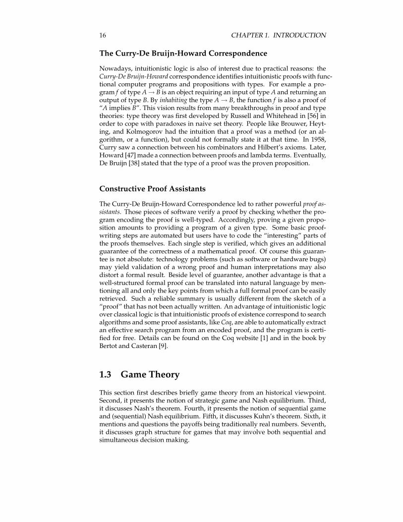
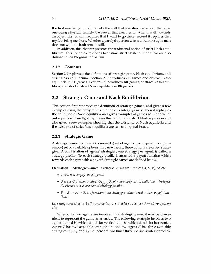
A strategic game involves a (non-empty) set of agents. Each agent has a (non-empty) set of available options. In game theory, these options are called strate-gies. A combination of agents’ strategies, one strategy per agent, is called astrategy profile. To each strategy profile is attached a payoff function whichrewards each agent with a payoff. The following example involves two agentsnamed V , which stands for vertical, andH , which stands for horizontal. AgentV has two available strategies: v1 and v2. Agent H has three available strate-gies: h1, h2, and h3. So there are two times three, i.e. six, strategy profiles.The top-left profile is (v1, h1). To this profile corresponds a payoff function thatrewards V with 0 andH with 1.
h1 h2 h3
v1 0 1 0 0 1 2v2 2 2 1 0 1 1
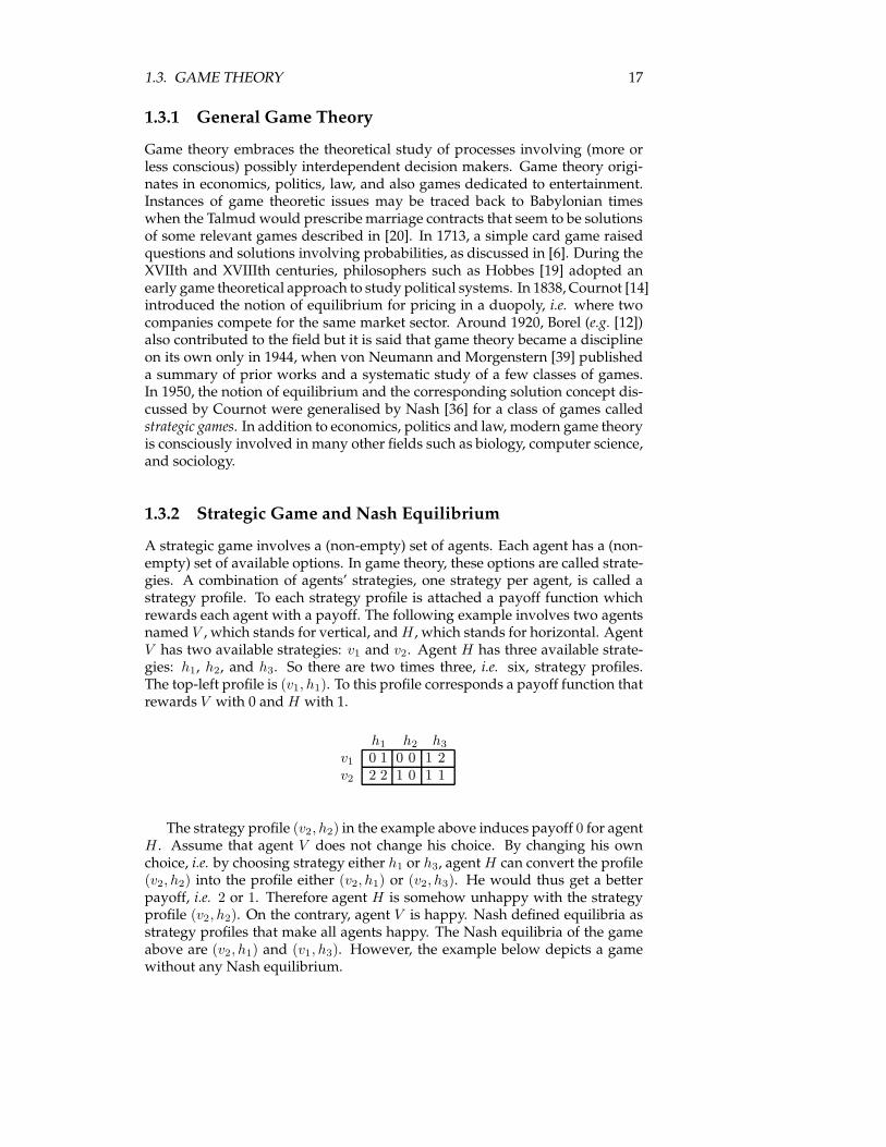
The strategy profile (v2, h2) in the example above induces payoff 0 for agentH . Assume that agent V does not change his choice. By changing his ownchoice, i.e. by choosing strategy either h1 or h3, agentH can convert the profile(v2, h2) into the profile either (v2, h1) or (v2, h3). He would thus get a betterpayoff, i.e. 2 or 1. Therefore agent H is somehow unhappy with the strategyprofile (v2, h2). On the contrary, agent V is happy. Nash defined equilibria asstrategy profiles that make all agents happy. The Nash equilibria of the gameabove are (v2, h1) and (v1, h3). However, the example below depicts a gamewithout any Nash equilibrium.
18 CHAPTER 1. INTRODUCTION
h1 h2
v1 1 0 0 1v2 0 1 1 0
1.3.3 Nash’s Theorem
As seen in the above subsection, not all finite strategic games have a Nashequilibrium. Since a guarantee of existence is a desirable property, Nash weak-ened his definition of equilibrium to assure the existence of a "compromising"equilibrium. More specifically, introducing probabilities into the game, he al-lowed agents to choose their individual strategies with a probability distribu-tion rather than choosing a single strategy deterministically. Subsequently, in-stead of a single strategy profile chosen deterministically, Nash’s probabilisticcompromise involves a probability distribution over strategy profiles. So, ex-pected payoff functions are involved instead of payoff functions. For instance,the sole probabilistic Nash equilibrium for the last game in the above subsec-tion is the probability assignment vi 7→
12 , hi 7→
12 , and the expected payoff is
12
for both agents. This compromise actually builds a new strategic game that iscontinuous. Nash proved that this new game always has a Nash equilibrium,which is called a probabilistic Nash equilibrium for the original game. A firstproof of this result [36] invokes Kakutani’s fixed point theorem [22], and a sec-ond proof [37] invokes (the proof-theoretically simpler) Brouwer’s fixed pointtheorem.
1.3.4 Sequential Game and Nash Equilibrium
Another class of games is that of sequential games, also called games in extensiveform. It traditionally refers to games where players play in turn till the playends and payoffs are granted. For instance, the game of chess is oftenmodelledby a sequential game where payoffs are “win”, “lose” and “draw”. Sequentialgames are often represented by finite rooted trees each of whose internal nodesis owned by a player, and each of whose external nodes, i.e. leaves, enclosesone payoff per player. In 1912, Zermelo [57] proved about the game of chessthat either white can win (whatever black may play), or black can win, or bothsides can force a draw. This is sometimes considered as the first non-trivialtheoretical results in game theory.The following graphical example involves the two agents a and b. At every
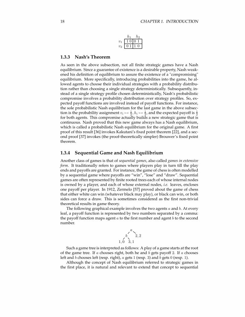
leaf, a payoff function is represented by two numbers separated by a comma:the payoff function maps agent a to the first number and agent b to the secondnumber.
a
b 2, 2
1, 0 3, 1
Such a game tree is interpreted as follows: A play of a game starts at the rootof the game tree. If a chooses right, both he and b gets payoff 2. If a choosesleft and b chooses left (resp. right), a gets 1 (resp. 3) and b gets 0 (resp. 1).Although the concept of Nash equilibrium referred to strategic games in
the first place, it is natural and relevant to extend that concept to sequential
1.3. GAME THEORY 19
games. The extension is made through an embedding of sequential gamesinto strategic games. This embedding applied to the above example yieldsthe following strategic game. The Nash equilibria of the strategic game image,namely (aright, bleft) and (aleft, bright), are also called the Nash equilibria ofthe original sequential game.
bleft bright
aleft 1 0 3 1aright 2 2 2 2
1.3.5 Kuhn’s Theorem
In 1953, Kuhn [25] showed the existence of Nash equilibrium for sequentialgames. For this, he built a specific Nash equilibrium through what is called“backward induction” in game theory. In 1965, Selten ([48] and [49]) intro-duced the concept of subgame perfect equilibrium in sequential games. Thisis a refinement of Nash equilibrium that seems to be even more meaningfulthan Nash equilibrium for sequential games. The two concepts of “backwardinduction” and subgame perfect equilibrium happen to coincide, so Kuhn’sresult also guarantees existence of subgame perfect equilibrium in sequentialgames.A subgame perfect equilibrium is a Nash equilibrium whose substrategy
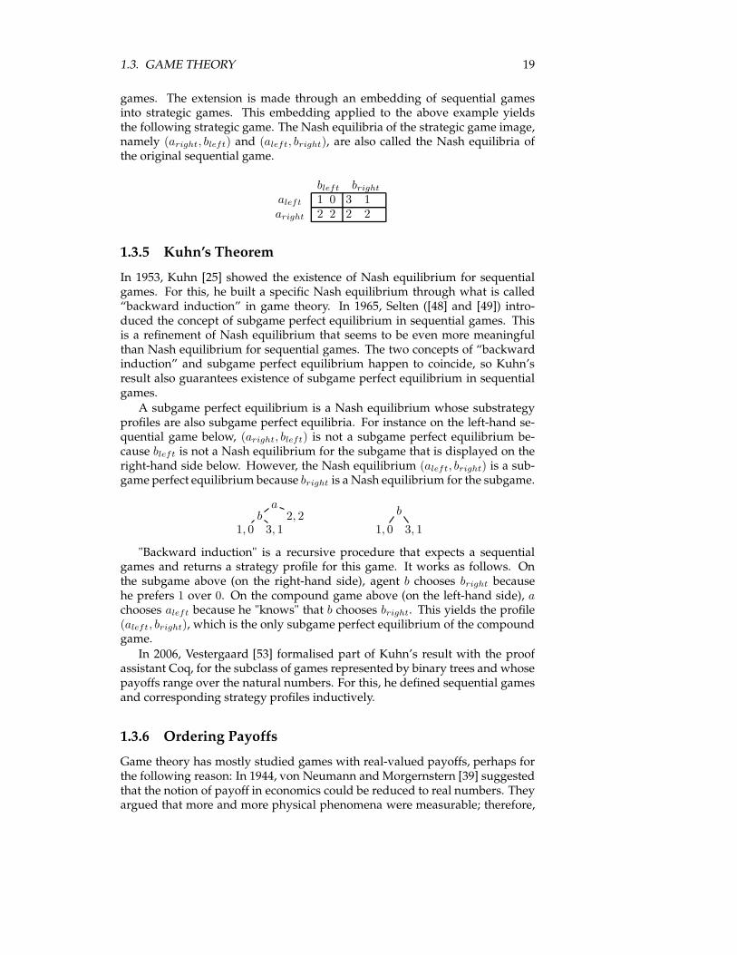
profiles are also subgame perfect equilibria. For instance on the left-hand se-quential game below, (aright, bleft) is not a subgame perfect equilibrium be-cause bleft is not a Nash equilibrium for the subgame that is displayed on theright-hand side below. However, the Nash equilibrium (aleft, bright) is a sub-game perfect equilibrium because bright is a Nash equilibrium for the subgame.
ab 2, 2
1, 0 3, 1
b
1, 0 3, 1
"Backward induction" is a recursive procedure that expects a sequentialgames and returns a strategy profile for this game. It works as follows. Onthe subgame above (on the right-hand side), agent b chooses bright becausehe prefers 1 over 0. On the compound game above (on the left-hand side), achooses aleft because he "knows" that b chooses bright. This yields the profile(aleft, bright), which is the only subgame perfect equilibrium of the compoundgame.In 2006, Vestergaard [53] formalised part of Kuhn’s result with the proof
assistant Coq, for the subclass of games represented by binary trees and whosepayoffs range over the natural numbers. For this, he defined sequential gamesand corresponding strategy profiles inductively.
1.3.6 Ordering Payoffs
Game theory has mostly studied games with real-valued payoffs, perhaps forthe following reason: In 1944, von Neumann and Morgernstern [39] suggestedthat the notion of payoff in economics could be reduced to real numbers. Theyargued that more and more physical phenomena were measurable; therefore,
20 CHAPTER 1. INTRODUCTION
one could reasonably expect that payoffs in economics, although not yet mea-surable, would become reducible to real numbers some day. However, gametheory became popular soon thereafter, and its scope grew larger. As a result,several scientists and philosophers questioned the reducibility of payoffs toreal numbers. In 1955, Simon [50] discussed games where agents are awarded(only partially ordered) vectors of real-valued payoffs instead of single real-valued payoffs. In 1956, Blackwell [10] proved a result involving vectors ofpayoffs. Those vectors model agents that take several non-commensurable di-mensions into consideration; such games are sometimes called multi criteriagames. More recent results about multi criteria games can be found in [44],for instance. In 1994, Osborne and Rubinstein [40] mentioned arbitrary prefer-ences for strategic games, but without any further results. In 2003, Krieger [24]noticed that “backward induction” on sequential multi criteria games may notyieldNash equilibria, and yet showed that sequential multi criteria games haveNash equilibria. The proof seems to invoke probabilities and Nash’s theoremfor strategic games.
1.3.7 Graphs and Games, Sequential and Simultaneous
Traditional game theory seems to work mainly with strategic games and se-quential games, i.e. games whose underlying structure is either an array or arooted tree. These game can involve many players. On the contrary, combina-torial game theory studies games with various structures, for instance gamesin graphs. It seems that most of these combinatorial games involve two playersonly. Moreover, the possible outcomes at the end of most of these games are"win-lose", "lose-win", and "draw" only. The book [7] presents many aspects ofcombinatorial game theory.Chess is usually thought as a sequential tree game. However, plays in chess
can be arbitrarily long (in terms of number of moves) even with the fifty movesrules which says that a player can claim a draw if no capture has been madeand no pawn has been moved in the last fifty consecutive moves. So, the gameof chess is actually defined through a directed graph rather than a tree, sincea play can enter a cycle. Every node of the graph is made of both the locationof the pieces on the chessboard and an information about who has to movenext. The arcs between the nodes correspond to the valid moves. So the gameof chess is a bipartite digraph (white and black play in turn) with two agents.This may sound like a detail since the game of chess is well approximated by atree. However, this is not a detail in games that may not end for intrinsic rea-sons instead of technical rules: for instance poker game or companies sharinga market. In both cases, the game can continue as long as there are at least twoplayers willing to play. In the process, a sequence of actions can lead to a situ-ation similar to a previous situation (in terms of poker chips or market share),hence a cycle.Internet, too, can be seen as a directed graphwhose nodes represent routers
and whose arcs represent links between routers. When receiving a packet, arouter has to decide where to forward it to: either to a related local networkor to another router. Each router chooses according to "it’s owner interest".Therefore Internet can be seen as a digraph with nodes labelled with ownersof routers. This digraph is usually symmetric since a link from router A torouter B can be easily transformed to a link between router b and router A.
1.4. CONTRIBUTIONS 21
Moreover, the interests of two different owners, i.e. Internet operators, may becontradictory since they are supposed to be competitors. Therefore the owners’trying to maximise their benefits can be considered a game. Local benefits (orcosts) of a routing choice may be displayed on the arcs of the graph.Many systems from the real world involve both sequential and simultane-
ous decision-making. For instance, a country with several political parties is acomplex system. Unlike chess, poker, and Internet, rules may not be definableby a digraph, but at least the system may be modelled by a graph-like struc-ture: The nodes represent the political situations of the country, i.e. which partyis in power at which level, etc. At each node, simultaneous decisions are takenby the parties, i.e. vote a law, start a campaign, design a secret plan, etc. Thecombination of the decisions of the parties yields a short-term outcome (goodfor some parties, bad for some others) and leads to another node where otherdecisions are to be taken. This process may enter a cycle when a sequence ofactions and elections leads to a political situation that is similar to a previoussituation, i.e. the same parties are in power at the same levels as before. Insuch complex a setting, some decision-making processes are sequential, someare simultaneous, and some involve both facets.
1.4 Contributions
This section accounts for the different contributions of the thesis. For presen-tation reasons, it does not follow exactly the structure of the dissertation. First,the section discusses extending the notion of Nash equilibrium from strate-gic games to sequential games. Second, it replaces real-valued payoff func-tion with abstract outcomes. Third, it replaces specific structures such as treeand array with loose structures that still allows a game-theoretic definition ofNash equilibrium. Fourth, it discusses a necessary and sufficient condition forNash equilibrium existence in abstract sequential tree games. Fifth, it men-tions a different proof of the above result. Sixth, it defines sequential games ongraphs. Seventh, it defines dynamic equilibria in the loose game structures asa compromise to guarantee existence of equilibrium. Eighth, it defines discretenon-determinism and uses it in a general setting.
1.4.1 Will Nash Equilibria Be Nash Equilibria?
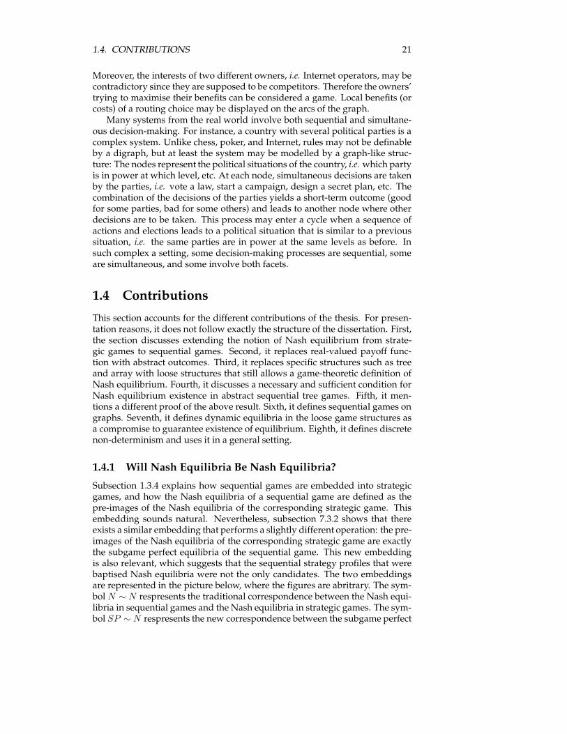
Subsection 1.3.4 explains how sequential games are embedded into strategicgames, and how the Nash equilibria of a sequential game are defined as thepre-images of the Nash equilibria of the corresponding strategic game. Thisembedding sounds natural. Nevertheless, subsection 7.3.2 shows that thereexists a similar embedding that performs a slightly different operation: the pre-images of the Nash equilibria of the corresponding strategic game are exactlythe subgame perfect equilibria of the sequential game. This new embeddingis also relevant, which suggests that the sequential strategy profiles that werebaptised Nash equilibria were not the only candidates. The two embeddingsare represented in the picture below, where the figures are abritrary. The sym-bol N ∼ N respresents the traditional correspondence between the Nash equi-libria in sequential games and the Nash equilibria in strategic games. The sym-bol SP ∼ N respresents the new correspondence between the subgame perfect
22 CHAPTER 1. INTRODUCTION
equilibria in sequential games and the Nash equilibria in strategic games.
a
b 2, 2
1, 0 3, 11 0 0 20 0 2 1
N ∼ N
SP ∼ N
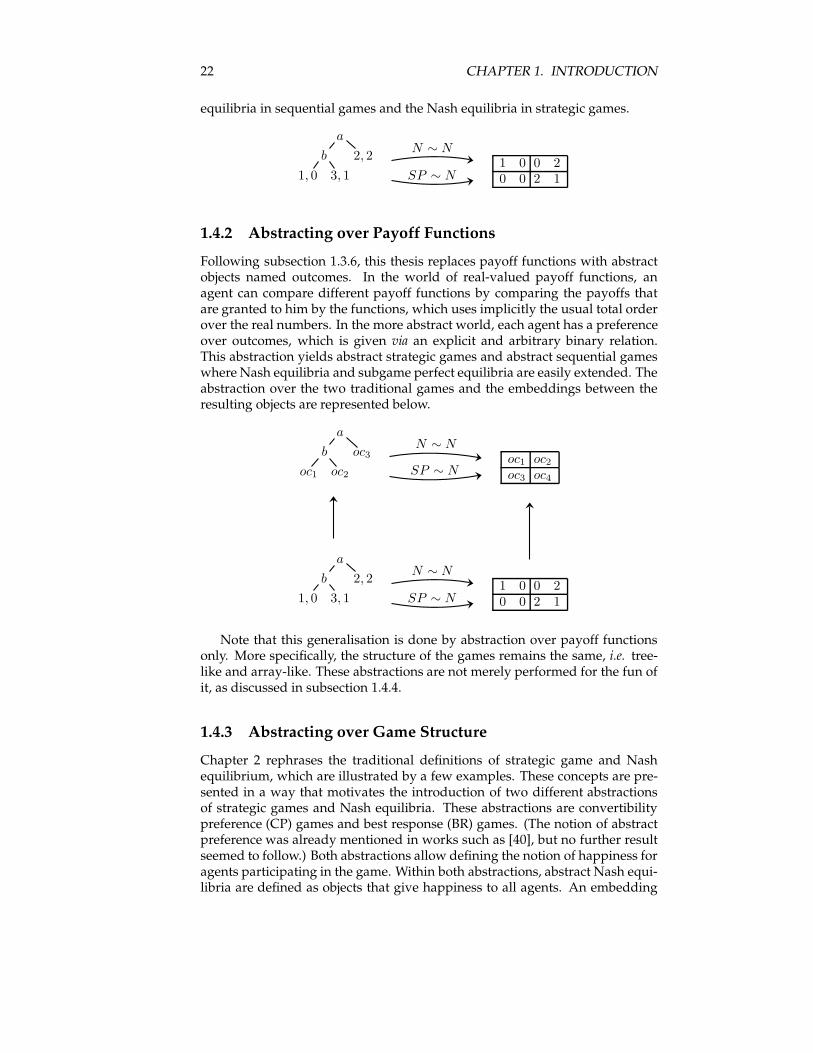
1.4.2 Abstracting over Payoff Functions
Following subsection 1.3.6, this thesis replaces payoff functions with abstractobjects named outcomes. In the world of real-valued payoff functions, anagent can compare different payoff functions by comparing the payoffs thatare granted to him by the functions, which uses implicitly the usual total orderover the real numbers. In the more abstract world, each agent has a preferenceover outcomes, which is given via an explicit and arbitrary binary relation.This abstraction yields abstract strategic games and abstract sequential gameswhere Nash equilibria and subgame perfect equilibria are easily extended. Theabstraction over the two traditional games and the embeddings between theresulting objects are represented below.
a
b oc3
oc1 oc2
oc1 oc2
oc3 oc4
a
b 2, 2
1, 0 3, 11 0 0 20 0 2 1
N ∼ N
SP ∼ N
N ∼ N
SP ∼ N
Note that this generalisation is done by abstraction over payoff functionsonly. More specifically, the structure of the games remains the same, i.e. tree-like and array-like. These abstractions are not merely performed for the fun ofit, as discussed in subsection 1.4.4.
1.4.3 Abstracting over Game Structure
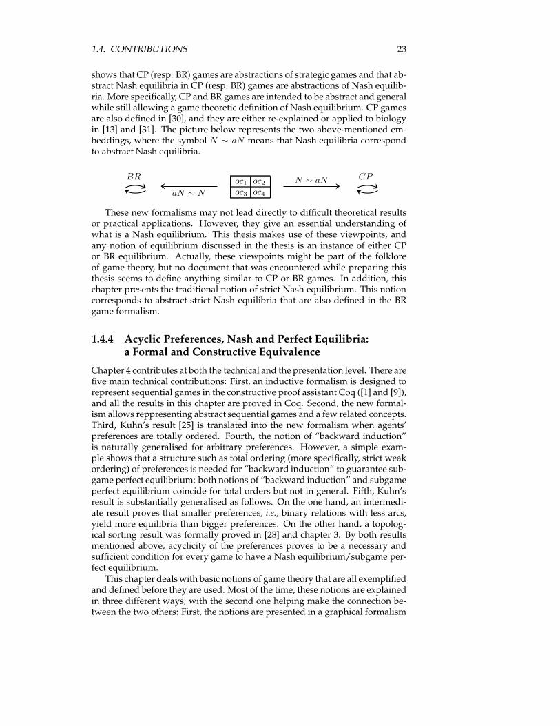
Chapter 2 rephrases the traditional definitions of strategic game and Nashequilibrium, which are illustrated by a few examples. These concepts are pre-sented in a way that motivates the introduction of two different abstractionsof strategic games and Nash equilibria. These abstractions are convertibilitypreference (CP) games and best response (BR) games. (The notion of abstractpreference was already mentioned in works such as [40], but no further resultseemed to follow.) Both abstractions allow defining the notion of happiness foragents participating in the game. Within both abstractions, abstract Nash equi-libria are defined as objects that give happiness to all agents. An embedding
1.4. CONTRIBUTIONS 23
shows that CP (resp. BR) games are abstractions of strategic games and that ab-stract Nash equilibria in CP (resp. BR) games are abstractions of Nash equilib-ria. More specifically, CP and BR games are intended to be abstract and generalwhile still allowing a game theoretic definition of Nash equilibrium. CP gamesare also defined in [30], and they are either re-explained or applied to biologyin [13] and [31]. The picture below represents the two above-mentioned em-beddings, where the symbol N ∼ aN means that Nash equilibria correspondto abstract Nash equilibria.
BR oc1 oc2
oc3 oc4
CPN ∼ aN
aN ∼ N
These new formalisms may not lead directly to difficult theoretical resultsor practical applications. However, they give an essential understanding ofwhat is a Nash equilibrium. This thesis makes use of these viewpoints, andany notion of equilibrium discussed in the thesis is an instance of either CPor BR equilibrium. Actually, these viewpoints might be part of the folkloreof game theory, but no document that was encountered while preparing thisthesis seems to define anything similar to CP or BR games. In addition, thischapter presents the traditional notion of strict Nash equilibrium. This notioncorresponds to abstract strict Nash equilibria that are also defined in the BRgame formalism.
1.4.4 Acyclic Preferences, Nash and Perfect Equilibria:a Formal and Constructive Equivalence
Chapter 4 contributes at both the technical and the presentation level. There arefive main technical contributions: First, an inductive formalism is designed torepresent sequential games in the constructive proof assistant Coq ([1] and [9]),and all the results in this chapter are proved in Coq. Second, the new formal-ism allows reppresenting abstract sequential games and a few related concepts.Third, Kuhn’s result [25] is translated into the new formalism when agents’preferences are totally ordered. Fourth, the notion of “backward induction”is naturally generalised for arbitrary preferences. However, a simple exam-ple shows that a structure such as total ordering (more specifically, strict weakordering) of preferences is needed for “backward induction” to guarantee sub-game perfect equilibrium: both notions of “backward induction” and subgameperfect equilibrium coincide for total orders but not in general. Fifth, Kuhn’sresult is substantially generalised as follows. On the one hand, an intermedi-ate result proves that smaller preferences, i.e., binary relations with less arcs,yield more equilibria than bigger preferences. On the other hand, a topolog-ical sorting result was formally proved in [28] and chapter 3. By both resultsmentioned above, acyclicity of the preferences proves to be a necessary andsufficient condition for every game to have a Nash equilibrium/subgame per-fect equilibrium.This chapter dealswith basic notions of game theory that are all exemplified
and defined before they are used. Most of the time, these notions are explainedin three different ways, with the second one helping make the connection be-tween the two others: First, the notions are presented in a graphical formalism
24 CHAPTER 1. INTRODUCTION
close to traditional game theory. Second, they are presented in a graphicalformalism suitable for induction. Third, they are presented in a light Coq for-malism close to traditional mathematics, so that only a basic understanding ofCoq is needed. (A quick look at the first ten pages of [28] or chapter 3 willintroduce the reader to the required notions.) The proofs are structured alongthe corresponding Coq proofs but are written in plain English.
1.4.5 Acyclic Preferences and Nash Equilibrium Existence:Another Proof of the Equivalence
Chapter 5 proves that, when dealing with abstract sequential games, the fol-lowing two propositions are equivalent: 1) Preferences over the outcomes areacyclic. 2) Every sequential game has a Nash equilibrium. This is a corollaryof the triple equivalence mentioned in subsection ??, however the new proofinvokes neither structural induction on games, nor “backward induction”, nortopological sorting. Therefore, this alternative argument is of proof theoreticalinterest. The proof of the implication 1) ⇒ 2) invokes three main arguments.First, if preferences are strict partial orders, then every game has a Nash equi-librium, by induction on the size of the game and a few cut-and paste tricks onsmaller games. Second, if a binary relation is acyclic, then its transitive closureis a strict partial order. Third, smaller preferences generate more equilibria, asseen in [29] and chapter 4. The converse 2)⇒ 1) is proved as in [29] and chap-ter 4. It is worth noting that in [29], the implication 1) ⇒ 2) follows 1) ⇒ 3)and 3) ⇒ 2). However, the proof of this chapter is direct: it does not involvesubgame perfect equilibria.
1.4.6 Sequential Graph Games
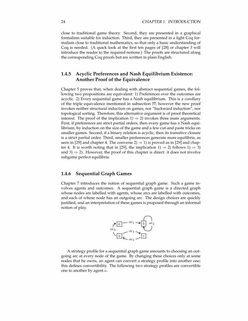
Chapter 7 introduces the notion of sequential graph game. Such a game in-volves agents and outcomes. A sequential graph game is a directed graphwhose nodes are labelled with agents, whose arcs are labelled with outcomes,and each of whose node has an outgoing arc. The design choices are quicklyjustified, and an interpretation of these games is proposed through an informalnotion of play.
a b
a c
oc1 oc2
oc3 oc4
oc2
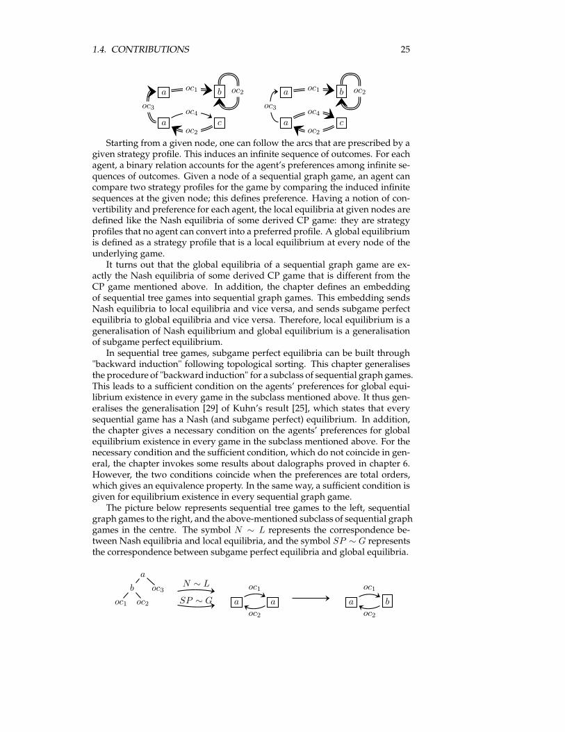
A strategy profile for a sequential graph game amounts to choosing an out-going arc at every node of the game. By changing these choices only at somenodes that he owns, an agent can convert a strategy profile into another one;this defines convertibility. The following two strategy profiles are convertibleone to another by agent a.
1.4. CONTRIBUTIONS 25
a b
a c
oc1 oc2
oc3 oc4
oc2
a b
a c
oc1 oc2
oc3 oc4
oc2
Starting from a given node, one can follow the arcs that are prescribed by agiven strategy profile. This induces an infinite sequence of outcomes. For eachagent, a binary relation accounts for the agent’s preferences among infinite se-quences of outcomes. Given a node of a sequential graph game, an agent cancompare two strategy profiles for the game by comparing the induced infinitesequences at the given node; this defines preference. Having a notion of con-vertibility and preference for each agent, the local equilibria at given nodes aredefined like the Nash equilibria of some derived CP game: they are strategyprofiles that no agent can convert into a preferred profile. A global equilibriumis defined as a strategy profile that is a local equilibrium at every node of theunderlying game.It turns out that the global equilibria of a sequential graph game are ex-
actly the Nash equilibria of some derived CP game that is different from theCP game mentioned above. In addition, the chapter defines an embeddingof sequential tree games into sequential graph games. This embedding sendsNash equilibria to local equilibria and vice versa, and sends subgame perfectequilibria to global equilibria and vice versa. Therefore, local equilibrium is ageneralisation of Nash equilibrium and global equilibrium is a generalisationof subgame perfect equilibrium.In sequential tree games, subgame perfect equilibria can be built through
"backward induction" following topological sorting. This chapter generalisesthe procedure of "backward induction" for a subclass of sequential graph games.This leads to a sufficient condition on the agents’ preferences for global equi-librium existence in every game in the subclass mentioned above. It thus gen-eralises the generalisation [29] of Kuhn’s result [25], which states that everysequential game has a Nash (and subgame perfect) equilibrium. In addition,the chapter gives a necessary condition on the agents’ preferences for globalequilibrium existence in every game in the subclass mentioned above. For thenecessary condition and the sufficient condition, which do not coincide in gen-eral, the chapter invokes some results about dalographs proved in chapter 6.However, the two conditions coincide when the preferences are total orders,which gives an equivalence property. In the same way, a sufficient condition isgiven for equilibrium existence in every sequential graph game.The picture below represents sequential tree games to the left, sequential
graph games to the right, and the above-mentioned subclass of sequential graphgames in the centre. The symbol N ∼ L represents the correspondence be-tween Nash equilibria and local equilibria, and the symbol SP ∼ G representsthe correspondence between subgame perfect equilibria and global equilibria.
a
b oc3
oc1 oc2 a a
oc1
oc2
a b
oc1
oc2
N ∼ L
SP ∼ G
26 CHAPTER 1. INTRODUCTION
1.4.7 Abstract Compromising Equilibria
First, chapter 8 explores possible generalisations of Nash’s result within the BRand CP formalisms. These generalisations invoke Kakutani’s fixed point the-orem, which is a generalisation of Brouwer’s. However, there is a differencebetween Nash’s theorem and its generalisations in the BR and CP formalisms:Nash’s probabilised strategic games correspond to finite strategic games sincethey are derived from them. However, it seems difficult to introduce probabil-ities within a given finite BR or CP game, since BR and CP games do not haveany Cartesian product structure. Therefore, one considers a class of already-continuous BR or CP games. Kakutani’s fixed point theorem, which is muchmore appropriate than Brouwer’s in this specific case, helps guarantee the exis-tence of an abstract Nash equilibrium. However, these already-continuous BRor CP games do not necessarily correspond to relevant finite BR or CP games,so practical applications might be difficult to find.
Second, this chapter explores compromises that are completely differentfromNash’s probabilistic compromise. Two conceptually very simple compro-mises are presented in this section, one for BR games and one for CP games.The one for BR games is named or-best response strict equilibrium, and the onefor CP games is named change-of-mind equilibrium, as in [30]. Both compro-mising equilibria are natural generalisations of Nash equilibria for CP gamesand strict Nash equilibria for BR games. It turns out that both generalisationsare (almost) the same: they both define compromising equilibria as the sinkstrongly connected components of a relevant digraph. Informally, if nodesrepresent the microscopic level and strongly connected components the macro-scopic level, then the compromising equilibria are the macroscopic equilibriaof a microscopic world.
Since BR and CP games are generalisations of strategic games, the new com-promising equilibria are relevant in strategic games too. This helps see thatNash’s compromise and the new compromises are different in many respects.Nash’s probabilistic compromise transforms finite strategic games into contin-uous strategic games. Probabilistic Nash equilibria for the original game aredefined as the (pure) Nash equilibria for the continuous derived game. Thismakes the probabilistic setting much more complex than the "pure" setting. Onthe contrary, the new compromises are discrete in the sense that the compro-mising equilibria are finitely many among finitely many strongly connectedcomponents. While probabilistic Nash equilibria are static, the new compro-mising equilibria are dynamic. While Nash equilibria are fixed points obtainedby Kakutani’s (or Brouwer’s) fixed point theorem, the new equilibria are fixedpoints obtained by a simple combinatorial argument (or Tarski’s fixed pointtheorem if one wishes to stress the parallel between Nash’s construction andthis one). While probabilistic Nash equilibria are non-computable in general,the new compromising equilibria are computable with low algorithmic com-plexity. Finally, while probabilistic Nash equilibria are Nash equilibria of aderived continuous game, the new compromising equilibria seem not to be theNash equilibria of any relevant derived game.
1.4. CONTRIBUTIONS 27
1.4.8 Discrete Non-Determinism and Nash Equilibriafor Strategy-Based Games
Chapter ?? tries to do what Nash did for traditional strategic games: to intro-duce probabilities into abstract strategic games to guarantee the existence ofa weakened kind of equilibrium. However, it is mostly a failure because theredoes not seem to exist any extension of a poset to its barycentres that is relevantto the purpose. So, instead of saying that "an agent chooses a given strategywith some probability", this chapter proposes to say that "the agentmay choosethe strategy", without further specification.The discrete non-determinism proposed above is implemented in the no-
tion of non deterministic best response (ndbr ) multi strategic game. As hintedby the terminology, the best response approach is preferred over the convert-ibility preference approach for this specific purpose. (Note that discrete non-determinism for abstract strategic games can be implemented in a formalismthat is more specific and simpler than ndbr multi strategic games, but this gen-eral formalism will serve further purposes.) This chapter defines the notionof ndbr equilibrium in these games, and a pre-fixed point result helps prove asufficient condition for every ndbr multi strategic game to have an ndbr equi-librium.This chapter also defines the notion of multi strategic game that is very
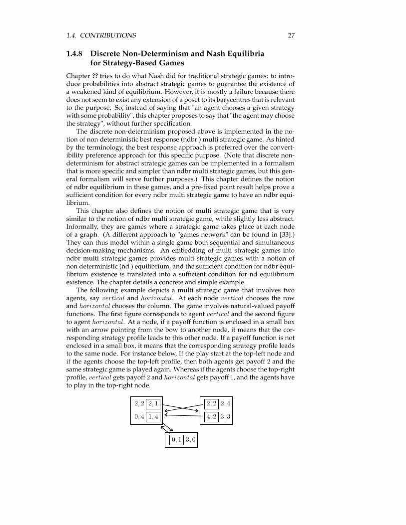
similar to the notion of ndbr multi strategic game, while slightly less abstract.Informally, they are games where a strategic game takes place at each nodeof a graph. (A different approach to "games network" can be found in [33].)They can thus model within a single game both sequential and simultaneousdecision-making mechanisms. An embedding of multi strategic games intondbr multi strategic games provides multi strategic games with a notion ofnon deterministic (nd ) equilibrium, and the sufficient condition for ndbr equi-librium existence is translated into a sufficient condition for nd equilibriumexistence. The chapter details a concrete and simple example.The following example depicts a multi strategic game that involves two
agents, say vertical and horizontal. At each node vertical chooses the rowand horizontal chooses the column. The game involves natural-valued payofffunctions. The first figure corresponds to agent vertical and the second figureto agent horizontal. At a node, if a payoff function is enclosed in a small boxwith an arrow pointing from the bow to another node, it means that the cor-responding strategy profile leads to this other node. If a payoff function is notenclosed in a small box, it means that the corresponding strategy profile leadsto the same node. For instance below, If the play start at the top-left node andif the agents choose the top-left profile, then both agents get payoff 2 and thesame strategic game is played again. Whereas if the agents choose the top-rightprofile, vertical gets payoff 2 and horizontal gets payoff 1, and the agents haveto play in the top-right node.
2, 2 2, 1
0, 4 1, 4
2, 2 2, 4
4, 2 3, 3
0, 1 3, 0
28 CHAPTER 1. INTRODUCTION
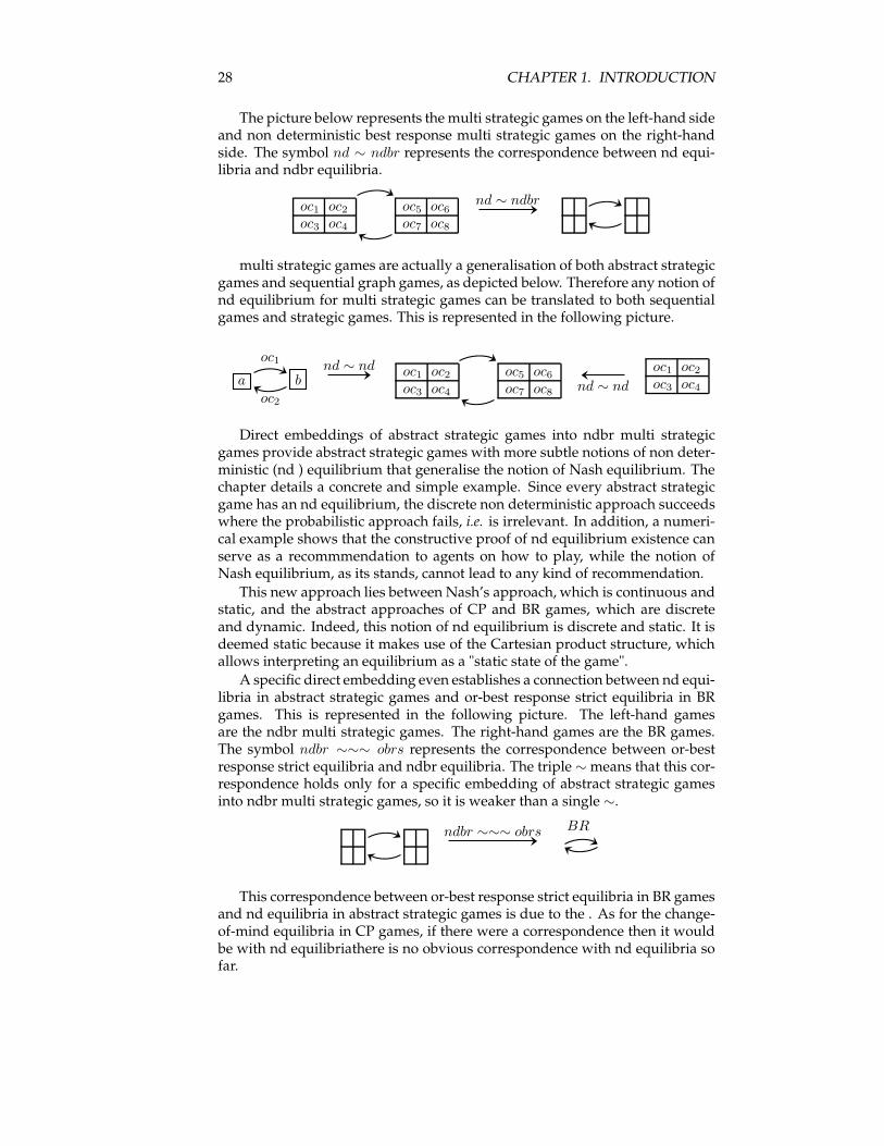
The picture below represents the multi strategic games on the left-hand sideand non deterministic best response multi strategic games on the right-handside. The symbol nd ∼ ndbr represents the correspondence between nd equi-libria and ndbr equilibria.
oc1 oc2
oc3 oc4
oc5 oc6
oc7 oc8
nd ∼ ndbr
multi strategic games are actually a generalisation of both abstract strategicgames and sequential graph games, as depicted below. Therefore any notion ofnd equilibrium for multi strategic games can be translated to both sequentialgames and strategic games. This is represented in the following picture.
a b
oc1
oc2
oc1 oc2
oc3 oc4
oc5 oc6
oc7 oc8
oc1 oc2
oc3 oc4
nd ∼ nd
nd ∼ nd
Direct embeddings of abstract strategic games into ndbr multi strategicgames provide abstract strategic games with more subtle notions of non deter-ministic (nd ) equilibrium that generalise the notion of Nash equilibrium. Thechapter details a concrete and simple example. Since every abstract strategicgame has an nd equilibrium, the discrete non deterministic approach succeedswhere the probabilistic approach fails, i.e. is irrelevant. In addition, a numeri-cal example shows that the constructive proof of nd equilibrium existence canserve as a recommmendation to agents on how to play, while the notion ofNash equilibrium, as its stands, cannot lead to any kind of recommendation.This new approach lies between Nash’s approach, which is continuous and
static, and the abstract approaches of CP and BR games, which are discreteand dynamic. Indeed, this notion of nd equilibrium is discrete and static. It isdeemed static because it makes use of the Cartesian product structure, whichallows interpreting an equilibrium as a "static state of the game".A specific direct embedding even establishes a connection between nd equi-
libria in abstract strategic games and or-best response strict equilibria in BRgames. This is represented in the following picture. The left-hand gamesare the ndbr multi strategic games. The right-hand games are the BR games.The symbol ndbr ∼∼∼ obrs represents the correspondence between or-bestresponse strict equilibria and ndbr equilibria. The triple ∼means that this cor-respondence holds only for a specific embedding of abstract strategic gamesinto ndbr multi strategic games, so it is weaker than a single ∼.
BRndbr ∼∼∼ obrs
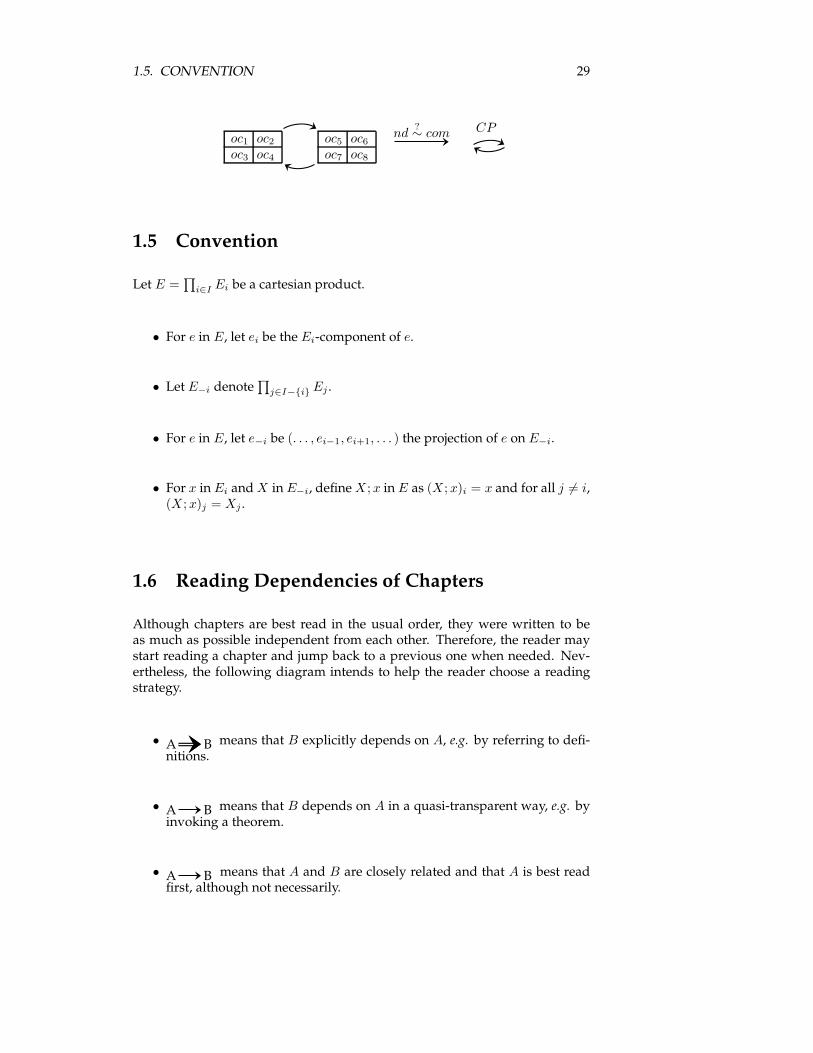
This correspondence between or-best response strict equilibria in BR gamesand nd equilibria in abstract strategic games is due to the . As for the change-of-mind equilibria in CP games, if there were a correspondence then it wouldbe with nd equilibriathere is no obvious correspondence with nd equilibria sofar.
1.5. CONVENTION 29
oc1 oc2
oc3 oc4
oc5 oc6
oc7 oc8
CPnd?∼ com
1.5 Convention
Let E =∏
i∈I Ei be a cartesian product.
• For e in E, let ei be the Ei-component of e.
• Let E−i denote∏
j∈I−{i} Ej .
• For e in E, let e−i be (. . . , ei−1, ei+1, . . . ) the projection of e on E−i.
• For x in Ei andX in E−i, defineX ; x in E as (X ; x)i = x and for all j 6= i,(X ; x)j = Xj .
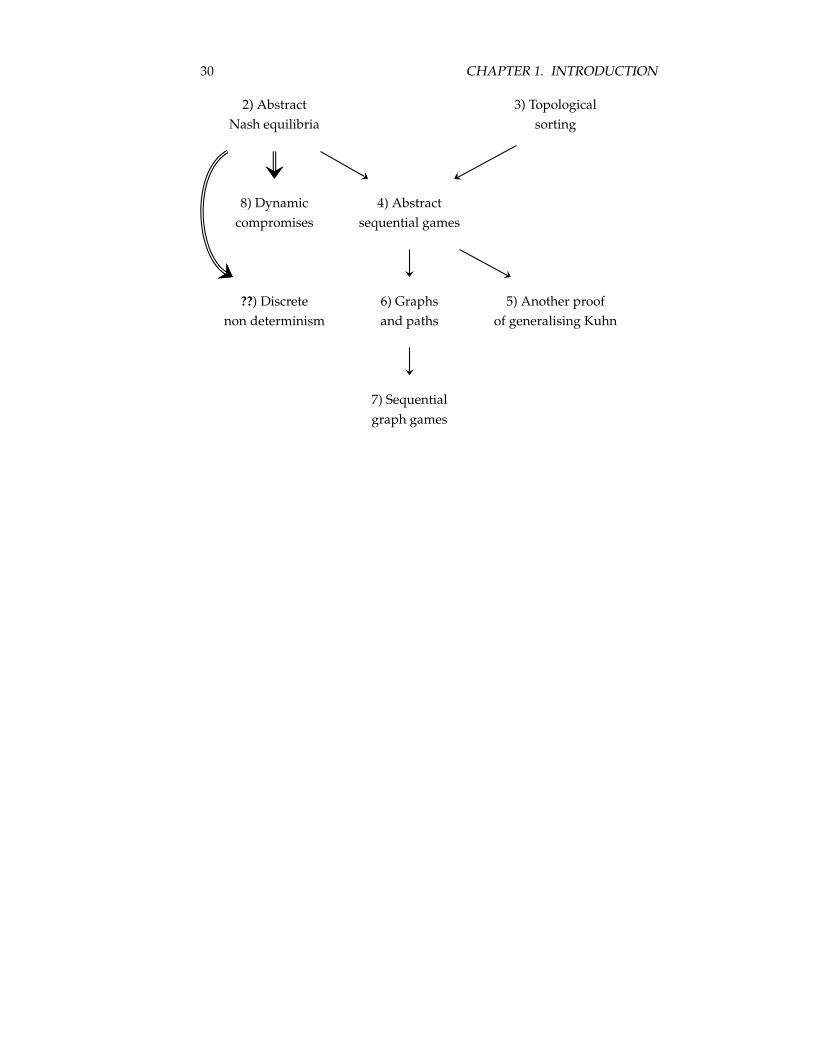
1.6 Reading Dependencies of Chapters
Although chapters are best read in the usual order, they were written to beas much as possible independent from each other. Therefore, the reader maystart reading a chapter and jump back to a previous one when needed. Nev-ertheless, the following diagram intends to help the reader choose a readingstrategy.
• A B means that B explicitly depends on A, e.g. by referring to defi-nitions.
• A B means that B depends on A in a quasi-transparent way, e.g. byinvoking a theorem.
• A B means that A and B are closely related and that A is best readfirst, although not necessarily.
30 CHAPTER 1. INTRODUCTION
2) Abstract 3) TopologicalNash equilibria sorting
8) Dynamic 4) Abstractcompromises sequential games
??) Discrete 6) Graphs 5) Another proofnon determinism and paths of generalising Kuhn
7) Sequential
graph games
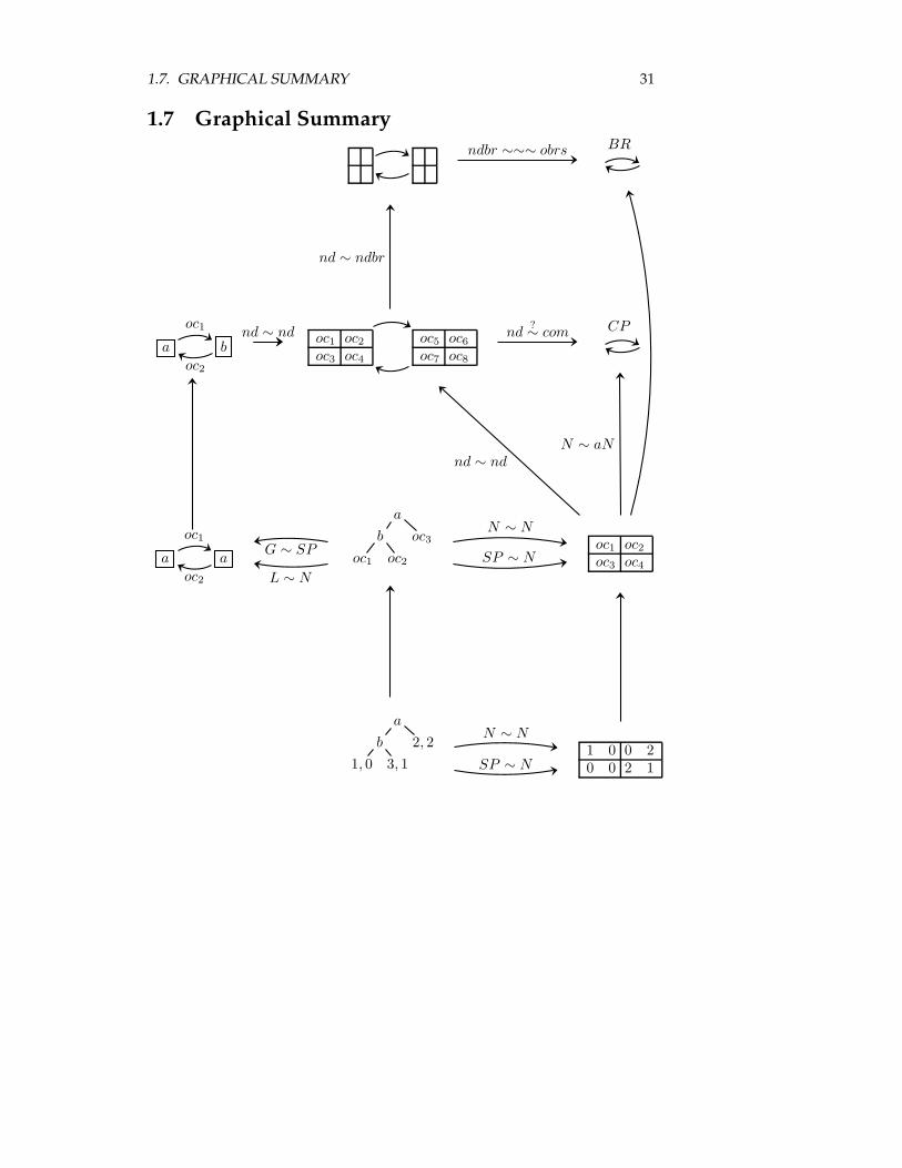
1.7. GRAPHICAL SUMMARY 31
1.7 Graphical SummaryBR
a b
oc1
oc2
oc1 oc2
oc3 oc4
oc5 oc6
oc7 oc8
CP
a a
oc1
oc2
a
b oc3
oc1 oc2
oc1 oc2
oc3 oc4
a
b 2, 2
1, 0 3, 11 0 0 20 0 2 1
nd ∼ ndbr
ndbr ∼∼∼ obrs
nd?∼ comnd ∼ nd
N ∼ aNnd ∼ nd
L ∼ N
G ∼ SP
N ∼ N
SP ∼ N
N ∼ N
SP ∼ N
32 CHAPTER 1. INTRODUCTION
Chapter 2
Abstract Nash Equilibria
2.1 Introduction
Nash introduced the concept of non-cooperative equilibrium, i.e. Nash equilib-rium, for strategic games. This chapter shows that Nash equilibria are relevantbeyond the scope of strategic games.
2.1.1 Contribution
This chapter rephrases the traditional definitions of strategic game and Nashequilibrium, which are illustrated by a few examples. These concepts are pre-sented in a way that motivates the introduction of two different abstractionsof strategic games and Nash equilibria. These abstractions are convertibilitypreference (CP) games (also defined in [30]) and best response (BR) games.Note that the notion of abstract preference was already mentioned in workssuch as [40] and that the terminology of best response already exists in gametheory. Both abstractions allow defining the notion of happiness for agents par-ticipating in the game. Within both abstractions, abstract Nash equilibria aredefined as objects that give happiness to all agents. An embedding shows thatCP (resp. BR) games are abstractions of strategic games and that abstract Nashequilibria in CP (resp. BR) games are abstractions of Nash equilibria. Morespecifically, CP and BR games are intended to be abstract and general whilestill allowing a game theoretic definition of Nash equilibrium. These new for-malisms may not lead directly to difficult theoretical results or practical appli-cations, but they give an essential understanding of what a Nash equilibriumis. This thesis makes use of these viewpoints. Although no document that wasencountered while preparing this thesis defines anything similar to CP or BRgames, the informal version of the convertibility/preference viewpoint may beconsidered as part of the folklore. Indeed for instance, Rousseau [46] wrote:"Toute action libre a deux causes qui concourent à la produire, l’une morale,savoir la volonté qui détermine l’acte, l’autre physique, savoir la puissance quil’exécute. Quand je marche vers un objet, il faut premièrement que j’y veuillealler ; en second lieu, que mes pieds m’y portent. Qu’un paralytique veuillecourir, qu’un homme agile ne le veuille pas, tous deux resteront en place."Roughly, this may be translated as follows: Any free action has two causes,
33
34 CHAPTER 2. ABSTRACT NASH EQUILIBRIA
the first one being moral, namely the will that specifies the action, the otherone being physical, namely the power that executes it. When I walk towardsan object, first of all it requires that I want to go there; second it requires thatmy feet bring me there. Whether a paralytic person wants to run or a agile mandoes not want to, both remain still.In addition, this chapter presents the traditional notion of strict Nash equi-
librium. This notion corresponds to abstract strict Nash equilibria that are alsodefined in the BR game formalism.
2.1.2 Contents
Section 2.2 rephrases the definitions of strategic game, Nash equilibrium, andstrict Nash equilibrium. Section 2.3 introduces CP games and abstract Nashequilibria in CP games. Section 2.4 introduces BR games, abstract Nash equi-libria, and strict abstract Nash equilibria in BR games.
2.2 Strategic Game and Nash Equilibrium
This section first rephrases the definition of strategic games, and gives a fewexamples using the array representation of strategic games. Then it rephrasesthe definition of Nash equilibria and gives examples of games with and with-out equilibria. Finally, it rephrases the definition of strict Nash equilibria andalso gives a few examples showing that the existence of Nash equilibria andthe existence of strict Nash equilibria are two orthogonal issues.
2.2.1 Strategic Game
A strategic game involves a (non-empty) set of agents. Each agent has a (non-empty) set of available options. In game theory, these options are called strate-gies. A combination of agents’ strategies, one strategy per agent, is called astrategy profile. To each strategy profile is attached a payoff function whichrewards each agent with a payoff. Strategic games are defined below.
Definition 1 (Strategic Games) Strategic Games are 3-tuples 〈A,S , P〉, where:
• A is a non-empty set of agents.
• S is the Cartesian product⊗
a∈A Sa of non-empty sets of individual strategiesS . Elements of S are named strategy profiles.
• P : S → A → R is a function from strategy profiles to real-valued payoff func-tion.
Let s range over S , let sa be the a-projection of s, and let s−a be the (A−{a})-projectionof s.
When only two agents are involved in a strategic game, it may be conve-nient to represent the game as an array. The following example involves twoagents named V , which stands for vertical, andH , which stands for horizontal.Agent V has two available strategies: v1 and v2. Agent H has three availablestrategies: h1, h2, and h3. So there are two times three, i.e. six, strategy profiles.
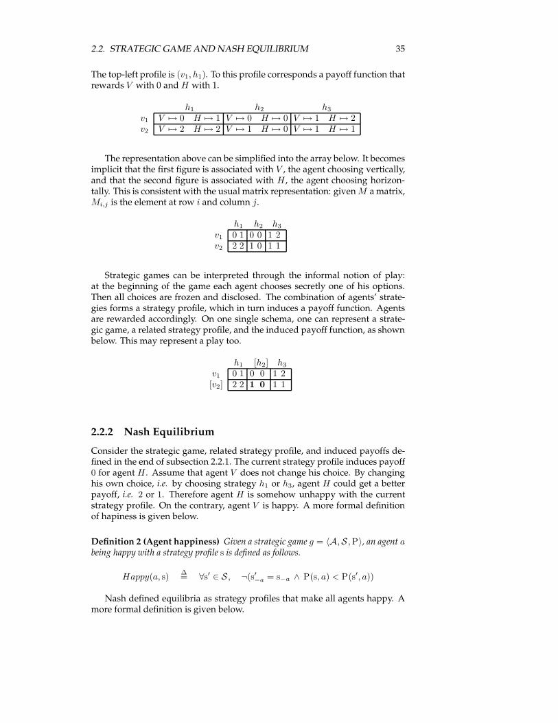
2.2. STRATEGIC GAME AND NASH EQUILIBRIUM 35
The top-left profile is (v1, h1). To this profile corresponds a payoff function thatrewards V with 0 andH with 1.
h1 h2 h3
v1 V 7→ 0 H 7→ 1 V 7→ 0 H 7→ 0 V 7→ 1 H 7→ 2v2 V 7→ 2 H 7→ 2 V 7→ 1 H 7→ 0 V 7→ 1 H 7→ 1
The representation above can be simplified into the array below. It becomesimplicit that the first figure is associated with V , the agent choosing vertically,and that the second figure is associated with H , the agent choosing horizon-tally. This is consistent with the usual matrix representation: givenM a matrix,Mi,j is the element at row i and column j.
h1 h2 h3
v1 0 1 0 0 1 2v2 2 2 1 0 1 1
Strategic games can be interpreted through the informal notion of play:at the beginning of the game each agent chooses secretly one of his options.Then all choices are frozen and disclosed. The combination of agents’ strate-gies forms a strategy profile, which in turn induces a payoff function. Agentsare rewarded accordingly. On one single schema, one can represent a strate-gic game, a related strategy profile, and the induced payoff function, as shownbelow. This may represent a play too.
h1 [h2] h3
v1 0 1 0 0 1 2[v2] 2 2 1 0 1 1
2.2.2 Nash Equilibrium
Consider the strategic game, related strategy profile, and induced payoffs de-fined in the end of subsection 2.2.1. The current strategy profile induces payoff0 for agent H . Assume that agent V does not change his choice. By changinghis own choice, i.e. by choosing strategy h1 or h3, agent H could get a betterpayoff, i.e. 2 or 1. Therefore agent H is somehow unhappy with the currentstrategy profile. On the contrary, agent V is happy. A more formal definitionof hapiness is given below.
Definition 2 (Agent happiness) Given a strategic game g = 〈A,S , P〉, an agent abeing happy with a strategy profile s is defined as follows.
Happy(a, s)∆= ∀s′ ∈ S , ¬(s′−a = s−a ∧ P(s, a) < P(s′, a))
Nash defined equilibria as strategy profiles that make all agents happy. Amore formal definition is given below.
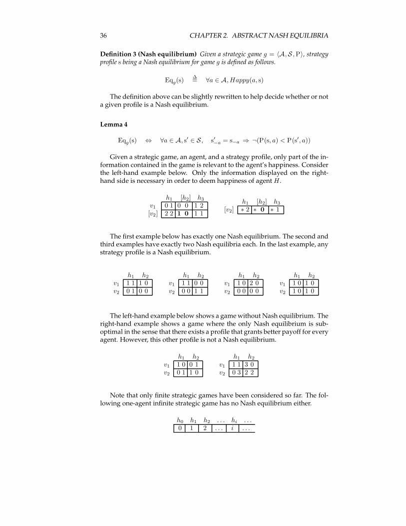
36 CHAPTER 2. ABSTRACT NASH EQUILIBRIA
Definition 3 (Nash equilibrium) Given a strategic game g = 〈A,S , P〉, strategyprofile s being a Nash equilibrium for game g is defined as follows.
Eqg(s)∆= ∀a ∈ A, Happy(a, s)
The definition above can be slightly rewritten to help decide whether or nota given profile is a Nash equilibrium.
Lemma 4
Eqg(s) ⇔ ∀a ∈ A, s′ ∈ S , s′−a = s−a ⇒ ¬(P(s, a) < P(s′, a))
Given a strategic game, an agent, and a strategy profile, only part of the in-formation contained in the game is relevant to the agent’s happiness. Considerthe left-hand example below. Only the information displayed on the right-hand side is necessary in order to deem happiness of agentH .
h1 [h2] h3
v1 0 1 0 0 1 2[v2] 2 2 1 0 1 1
h1 [h2] h3
[v2] ∗ 2 ∗ 0 ∗ 1
The first example below has exactly one Nash equilibrium. The second andthird examples have exactly two Nash equilibria each. In the last example, anystrategy profile is a Nash equilibrium.
h1 h2
v1 1 1 1 0v2 0 1 0 0
h1 h2
v1 1 1 0 0v2 0 0 1 1
h1 h2
v1 1 0 2 0v2 0 0 0 0
h1 h2
v1 1 0 1 0v2 1 0 1 0
The left-hand example below shows a gamewithout Nash equilibrium. Theright-hand example shows a game where the only Nash equilibrium is sub-optimal in the sense that there exists a profile that grants better payoff for everyagent. However, this other profile is not a Nash equilibrium.
h1 h2
v1 1 0 0 1v2 0 1 1 0
h1 h2
v1 1 1 3 0v2 0 3 2 2
Note that only finite strategic games have been considered so far. The fol-lowing one-agent infinite strategic game has no Nash equilibrium either.
h0 h1 h2 . . . hi . . .0 1 2 . . . i . . .
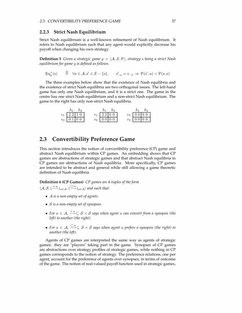
2.3. CONVERTIBILITY PREFERENCE GAME 37
2.2.3 Strict Nash Equilibrium
Strict Nash equilibrium is a well-known refinement of Nash equilibrium. Itrefers to Nash equilibrium such that any agent would explicitly decrease hispayoff when changing his own strategy.
Definition 5 Given a strategic game g = 〈A,S , P〉, strategy s being a strict Nashequilibrium for game g is defined as follows.
Eq+g (s)
∆= ∀a ∈ A, s′ ∈ S − {s}, s′−a = s−a ⇒ P(s′, a) < P(s, a)
The three examples below show that the existence of Nash equilibria andthe existence of strict Nash equilibria are two orthogonal issues. The left-handgame has only one Nash equilibrium, and it is a strict one. The game in thecentre has one strict Nash equilibrium and a non-strict Nash equilibrium. Thegame to the right has only non-strict Nash equilibria.
h1 h2
v1 2 2 1 0v2 0 1 0 0
h1 h2
v1 2 2 0 0v2 0 0 0 0
h1 h2
v1 0 0 0 0v2 0 0 0 0
2.3 Convertibility Preference Game
This section introduces the notion of convertibility preference (CP) game andabstract Nash equilibrium within CP games. An embedding shows that CPgames are abstractions of strategic games and that abstract Nash equilibria inCP games are abstractions of Nash equilibria. More specifically, CP gamesare intended to be abstract and general while still allowing a game theoreticdefinition of Nash equilibria.
Definition 6 (CP Games) CP games are 4-tuples of the form
〈A,S, (+ a−→)a∈A, (
© a−→)a∈A〉 and such that:
• A is a non-empty set of agents.
• S is a non-empty set of synopses.
• For a ∈ A,+ a−→⊆ S × S says when agent a can convert from a synopsis (the
left) to another (the right).
• For a ∈ A,©a−→⊆ S × S says when agent a prefers a synopsis (the right) to
another (the left).
Agents of CP games are interpreted the same way as agents of strategicgames: they are "players" taking part in the game. Synopses of CP gamesare abstractions over strategy profiles of strategic games, while nothing in CPgames corresponds to the notion of strategy. The preference relations, one peragent, account for the preference of agents over synopses, in terms of outcomeof the game. The notion of real-valued payoff function used in strategic games,
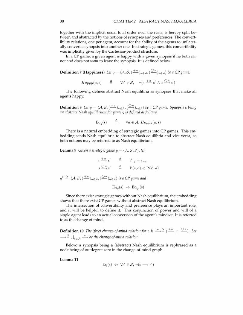
38 CHAPTER 2. ABSTRACT NASH EQUILIBRIA
together with the implicit usual total order over the reals, is hereby split be-tween and abstracted by the notions of synopses and preferences. The convert-ibility relations, one per agent, account for the ability of the agents to unilater-ally convert a synopsis into another one. In strategic games, this convertibilitywas implicitly given by the Cartesian-product structure.In a CP game, a given agent is happy with a given synopsis if he both can
not and does not want to leave the synopsis. It is defined below.
Definition 7 (Happiness) Let g = 〈A,S, (+ a−→)a∈A, (
© a−→)a∈A〉 be a CP game.
Happy(a, s)∆= ∀s′ ∈ S, ¬(s
+ a−→ s′ ∧ s
© a−→ s′)
The following defines abstract Nash equilibria as synopses that make allagents happy.
Definition 8 Let g = 〈A,S, (+ a−→)a∈A, (
© a−→)a∈A〉 be a CP game. Synopsis s being
an abstract Nash equilibrium for game g is defined as follows.
Eqg(s)∆= ∀a ∈ A, Happy(a, s)
There is a natural embedding of strategic games into CP games. This em-bedding sends Nash equilibria to abstract Nash equilibria and vice versa, soboth notions may be referred to as Nash equilibrium.
Lemma 9 Given a strategic game g = 〈A,S , P〉, let
s+ a−→ s′
∆= s′−a = s−a
s©a−→ s′
∆= P(s, a) < P(s′, a)
g′∆= 〈A,S , (
+ a−→)a∈A, (
© a−→)a∈A〉 is a CP game and
Eqg(s) ⇔ Eqg′(s)
Since there exist strategic games without Nash equilibrium, the embeddingshows that there exist CP games without abstract Nash equilibrium.The intersection of convertibility and preference plays an important role,
and it will be helpful to define it. This conjunction of power and will of asingle agent leads to an actual conversion of the agent’s mindset. It is referredto as the change of mind.
Definition 10 The (free) change-of-mind relation for a isa−→
∆= (
+ a−→ ∩
© a−→). Let
−→∆=
⋃a∈A
a−→ be the change-of-mind relation.
Below, a synopsis being a (abstract) Nash equilibrium is rephrased as anode being of outdegree zero in the change-of-mind graph.
Lemma 11Eq(s) ⇔ ∀s′ ∈ S, ¬(s −→ s′)
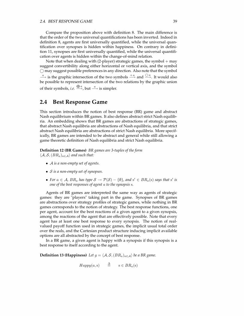
2.4. BEST RESPONSE GAME 39
Compare the proposition above with definition 8. The main difference isthat the order of the two universal quantifications has been inverted. Indeed indefinition 8, agents are first universally quantified, while the universal quan-tification over synopses is hidden within happiness. On contrary in defini-tion 11, synopses are first universally quantified, while the universal quantifi-cation over agents is hidden within the change-of-mind relation.Note that when dealing with (2-player) strategic games, the symbol +may
suggest convertibility along either horizontal or vertical axis, and the symbol©may suggest possible preferences in any direction. Also note that the symbol
a−→ is the graphic intersection of the two symbols + a
−→ and© a−→. It would also
be possible to represent intersection of the two relations by the graphic union
of their symbols, i.e.L
a−→, but a
−→ is simpler.
2.4 Best Response Game
This section introduces the notion of best response (BR) game and abstractNash equilibrium within BR games. It also defines abstract strict Nash equilib-ria. An embedding shows that BR games are abstractions of strategic games,that abstract Nash equilibria are abstractions of Nash equilibria, and that strictabstract Nash equilibria are abstractions of strict Nash equilibria. More specif-ically, BR games are intended to be abstract and general while still allowing agame theoretic definition of Nash equilibria and strict Nash equilibria.
Definition 12 (BR Games) BR games are 3-tuples of the form〈A,S, (BRa)a∈A〉 and such that:
• A is a non-empty set of agents.
• S is a non-empty set of synopses.
• For a ∈ A, BRa has type S → P(S) − {∅}, and s′ ∈ BRa(s) says that s′ isone of the best responses of agent a to the synopsis s.
Agents of BR games are interpreted the same way as agents of strategicgames: they are "players" taking part in the game. Synopses of BR gamesare abstractions over strategy profiles of strategic games, while nothing in BRgames corresponds to the notion of strategy. The best response functions, oneper agent, account for the best reactions of a given agent to a given synopsis,among the reactions of the agent that are effectively possible. Note that everyagent has at least one best response to every synopsis. The notion of real-valued payoff function used in strategic games, the implicit usual total orderover the reals, and the Cartesian product structure inducing implicit availableoptions are all abstracted by the concept of best response.In a BR game, a given agent is happy with a synopsis if this synopsis is a
best response to itself according to the agent.
Definition 13 (Happiness) Let g = 〈A,S, (BRa)a∈A〉 be a BR game.
Happy(a, s)∆= s ∈ BRa(s)
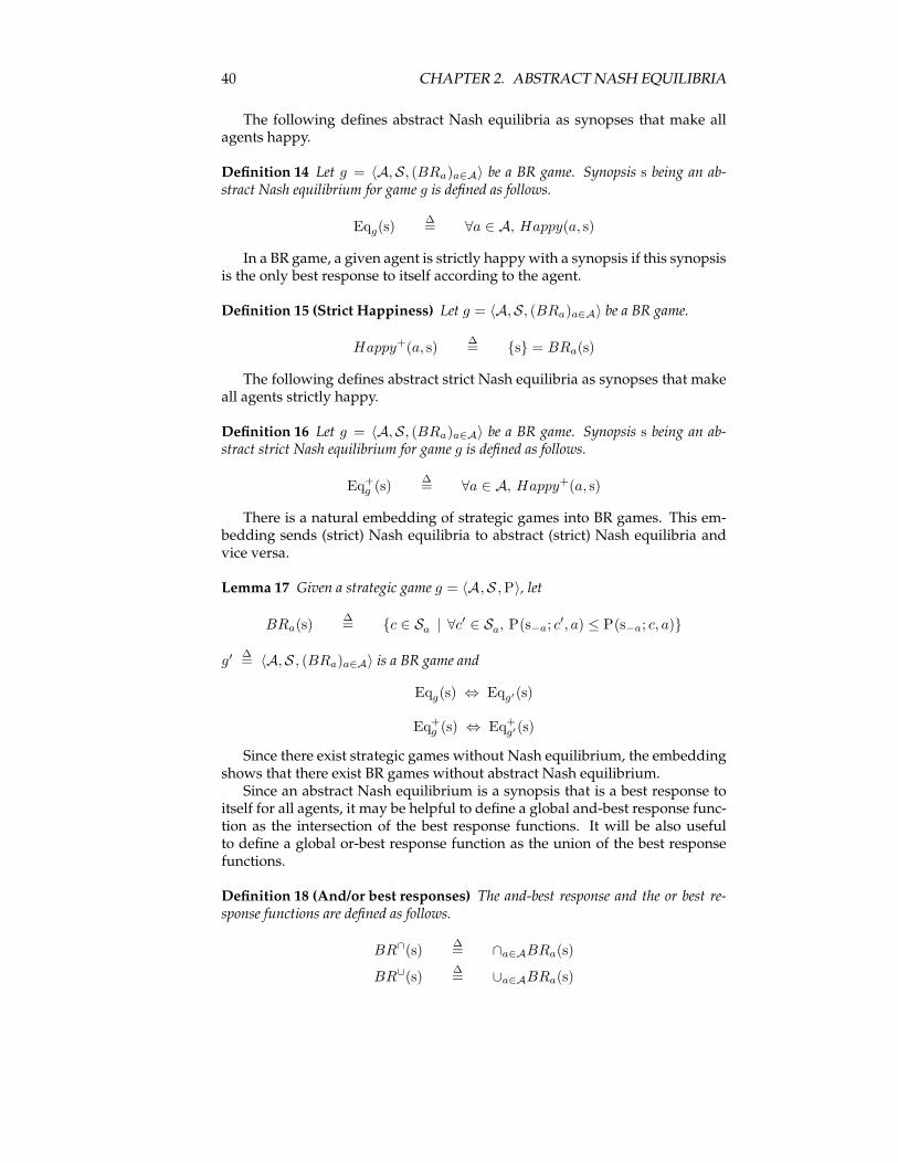
40 CHAPTER 2. ABSTRACT NASH EQUILIBRIA
The following defines abstract Nash equilibria as synopses that make allagents happy.
Definition 14 Let g = 〈A,S, (BRa)a∈A〉 be a BR game. Synopsis s being an ab-stract Nash equilibrium for game g is defined as follows.
Eqg(s)∆= ∀a ∈ A, Happy(a, s)
In a BR game, a given agent is strictly happywith a synopsis if this synopsisis the only best response to itself according to the agent.
Definition 15 (Strict Happiness) Let g = 〈A,S, (BRa)a∈A〉 be a BR game.
Happy+(a, s)∆= {s} = BRa(s)
The following defines abstract strict Nash equilibria as synopses that makeall agents strictly happy.
Definition 16 Let g = 〈A,S, (BRa)a∈A〉 be a BR game. Synopsis s being an ab-stract strict Nash equilibrium for game g is defined as follows.
Eq+g (s)
∆= ∀a ∈ A, Happy+(a, s)
There is a natural embedding of strategic games into BR games. This em-bedding sends (strict) Nash equilibria to abstract (strict) Nash equilibria andvice versa.
Lemma 17 Given a strategic game g = 〈A,S , P〉, let
BRa(s)∆= {c ∈ Sa | ∀c
′ ∈ Sa, P(s−a; c′, a) ≤ P(s−a; c, a)}
g′∆= 〈A,S , (BRa)a∈A〉 is a BR game and
Eqg(s) ⇔ Eqg′(s)
Eq+g (s) ⇔ Eq+
g′(s)
Since there exist strategic games without Nash equilibrium, the embeddingshows that there exist BR games without abstract Nash equilibrium.Since an abstract Nash equilibrium is a synopsis that is a best response to
itself for all agents, it may be helpful to define a global and-best response func-tion as the intersection of the best response functions. It will be also usefulto define a global or-best response function as the union of the best responsefunctions.
Definition 18 (And/or best responses) The and-best response and the or best re-sponse functions are defined as follows.
BR∩(s)∆= ∩a∈ABRa(s)
BR∪(s)∆= ∪a∈ABRa(s)
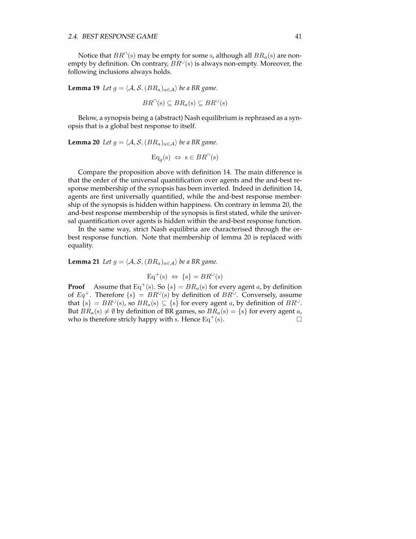
2.4. BEST RESPONSE GAME 41
Notice that BR∩(s)may be empty for some s, although all BRa(s) are non-empty by definition. On contrary, BR∪(s) is always non-empty. Moreover, thefollowing inclusions always holds.
Lemma 19 Let g = 〈A,S, (BRa)a∈A〉 be a BR game.
BR∩(s) ⊆ BRa(s) ⊆ BR∪(s)
Below, a synopsis being a (abstract) Nash equilibrium is rephrased as a syn-opsis that is a global best response to itself.
Lemma 20 Let g = 〈A,S, (BRa)a∈A〉 be a BR game.
Eqg(s) ⇔ s ∈ BR∩(s)
Compare the proposition above with definition 14. The main difference isthat the order of the universal quantification over agents and the and-best re-sponse membership of the synopsis has been inverted. Indeed in definition 14,agents are first universally quantified, while the and-best response member-ship of the synopsis is hidden within happiness. On contrary in lemma 20, theand-best response membership of the synopsis is first stated, while the univer-sal quantification over agents is hidden within the and-best response function.In the same way, strict Nash equilibria are characterised through the or-
best response function. Note that membership of lemma 20 is replaced withequality.
Lemma 21 Let g = 〈A,S, (BRa)a∈A〉 be a BR game.
Eq+(s) ⇔ {s} = BR∪(s)
Proof Assume that Eq+(s). So {s} = BRa(s) for every agent a, by definitionof Eq+. Therefore {s} = BR∪(s) by definition of BR∪. Conversely, assumethat {s} = BR∪(s), so BRa(s) ⊆ {s} for every agent a, by definition of BR∪.But BRa(s) 6= ∅ by definition of BR games, so BRa(s) = {s} for every agent a,who is therefore stricly happy with s. Hence Eq+(s). �

42 CHAPTER 2. ABSTRACT NASH EQUILIBRIA
Chapter 3
Acyclicity and Finite LinearExtendability:a Formal and ConstructiveEquivalence
Linear extension of partial orders emerged in the late 1920’s. Its computer-oriented version, i.e., topological sorting of finite partial orders, arose in the late1950’s. However, those issues have not yet been considered from a viewpointthat is both formal and constructive; this chapter discusses a few related claimsformally proved with the constructive proof assistant Coq. For instance, itstates that a given decidable binary relation is acyclic and equality is decidableon its domain iff an irreflexive linear extension can be computed uniformly forany of its finite restriction. A detailed introduction and proofs written in plainEnglish shall help readers who are not familiar with constructive issues or Coqformalism.
3.1 Introduction
This section adopts an approach technical and historical. It presents the twonotions of computability and linear extension, both involved in the resultsproved in Coq and discussed in this chapter. It also describes the main resultsand the contents of the chapter.
3.1.1 Decidability and Computability
In the middle of the 1930’s, Church introduced the lambda calculus, and Tur-ing and Post independently designed their very similar machines. Those threenotions are by somemeans equivalent models for computer programs. A ques-tion is said to be decidable if there exists a computer program (equivalentlylambda term or Post-Turing machine) requiring the parameters of the ques-tions as input, returning (within finite time) “yes” or “no” as output, and thus
43
44 CHAPTER 3. TOPOLOGICAL SORTING
correctly answering the question. In this way, a binary relation over a set issaid to be decidable if there exists a program expecting two elements in thatset and returning “yes” if they are related or “no” if they are not. A sister no-tion is that of computable (or recursive) function, i.e., mathematical functionthe images of which are computable within finite time by the same computerprogram although the domain and the codomain of the function may be infi-nite. Note that computability with two-element-codomain functions amountsto decidability. If several computable functions can be all computed by thesame program, then these functions are said to be uniformly computable.
3.1.2 Transitive Closure, Linear Extension, andTopological Sorting
The calculus of binary relations was developed by De Morgan around 1860.The notion of transitive closure of a binary relation (smallest transitive binaryrelation including a given binary relation) was defined in different manners bydifferent people about 1890. See Pratt [45] for a historical account. In 1930,Szpilrajn [51] proved that, assuming the axiom of choice, any partial order hasa linear extension, i.e., is included in some total order. The proof invokes anotion close to transitive closure. Szpilrajn acknowledged that Banach, Kura-towsky, and Tarski had found unpublished proofs of the same result. In the late1950’s, The US Navy [3] designed PERT (Program Evaluation Research Task orProject Evaluation Review Techniques) for management and scheduling pur-poses. This tool partly consists in splitting a big project into small jobs on achart and expressing with arrows when one job has to be done before anotherone can start up. In order to study the resulting directed graph, Jarnagin [35]introduced a finite and algorithmic version of Szpilrajn’s result. This gave birthto the widely studied topological sorting issue, which spread to the industryin the early 1960’s (see [26] and [21]). Some technical details and computer-oriented examples can be found in Knuth’s book [23].
3.1.3 Contribution
This chapter revisits a few folklore results involving transitive closure, ex-cluded middle, computability, linear extension, and topological sorting. Mostof the properties are logical equivalences instead of one-way implications, whichsuggests maximal generality. Claims have been fully formalized (and proved)in Coq and then slightly modified in order to fit in and be part of the Coq-related CoLoR library [11]. This chapter follows the structure of the underlyingCoq development but some straightforward results are omitted. Argumentsare constructive (therefore also classical) and usually simple. This chapter ismeant to be read by a mathematician who is not familiar with constructivism.Concepts specific to Coq are introduced before they are used. Formal defini-tions and results are stated in a light Coq formalism that is very close to tradi-tional mathematics and slightly different from the actual Coq code in order toease the reading. Proofs are mostly written in plain English. The main resultin this chapter relies on an intermediate one, and is itself invoked in a gametheoretic proof (in Coq) not published yet.In this chapter, a binary relation over an arbitrary set is said to be middle-
3.1. INTRODUCTION 45
excluding if for any two elements in the set, either they are related or theyare not. The intermediate result of this chapter implies that in an arbitrary setwith decidable (resp. middle-excluding) equality, a binary relation is decidable(resp. middle-excluding) iff the transitive closures of its finite restrictions areuniformly decidable (resp. middle-excluding). The main result splits into twoparts, one on excluded middle and one on computability: First, consider amiddle-excluding relation. It is acyclic and equality on its domain is middle-excluding iff its restriction to any finite set has a middle-excluding irreflexivelinear extension. Second, consider R a decidable binary relation over A. Thefollowing three propositions are equivalent. Note that computability of linearextensions is non-uniform in the second proposition but uniform in the thirdone.
• Equality on A is decidable and R is acyclic.
• Equality onA is decidable and every finite restriction of R has a decidablelinear extension.
• There exists a computable function that expects finite restrictions of Rand returns (decidable) linear extensions of them.
3.1.4 Contents
Section 3.2 gives a quick look at the Coq versions of types, binary relations,excluded middle, and computability. Through the example of lists, section 3.3explains the principle of definition by induction in Coq, as well as the associ-ated inductive proof principle and definition by recursion. In particular, sub-section 3.3.2 details a simple proof by induction on list. Subsection 3.4.1 ex-plains the inductive notion of transitive closure and the associated inductiveproof principle. Subsections 3.4.2 and 3.4.3 discuss irreflexivity, representationof “finite sets” by lists, define finite restrictions of a binary relation, and detail asimple proof by induction on transitive closure. Section 3.5 defines paths withrespect to a binary relation and proves their correspondence with transitiveclosure. It also defines bounded paths that are proved to preserve decidabil-ity and middle-exclusion properties of the original relation. Since boundedpaths and paths are by some means equivalent on finite sets, subsection 3.5.4states the intermediate result. Subsection 3.6.1 defines relation totality over fi-nite sets. Subsections 3.6.2 to 3.6.5 define an acyclicity-preserving conditionalsingle-arc addition (to a relation), and an acyclicity-preserving multi-stage arcaddition over finite sets, which consists in repeating in turn single-arc additionand transitive closure. This procedure helps state linear extension equivalencein 3.6.6 and topological sorting equivalence in 3.6.7.
3.1.5 Convention
LetA be a Set. Throughout this chapter x, y, z, and t implicitly refer to objects oftype A. In the same way R, R’, and R” refer to binary relations over A; l, l’, andl” to lists over A, and n to natural numbers. For the sake of readability, typeswill sometimes be omitted according to the above convention, even in formalstatements where Coq could not infer them. The notation ¬P stands for P →False, x 6=y for x=y→ False, and 6 ∃x, P for (∃x, P)→ False.
46 CHAPTER 3. TOPOLOGICAL SORTING
3.2 Preliminaries
3.2.1 Types and Relations
Any Coq object has a type, which informs of the usage of the object and its pos-sible interactions with other Coq objects. The Coq syntax Obj : T means thatObj has type T. For example, f : A→ Bmeans that f requires an argument in thedomain A and returns an output in the codomain B. If x has type A then f andx can be combined and yield (f x), also written f (x) or f x, of type B. A type isalso a Coq object so it has a type too. The only types of types mentioned in thischapter are Prop and Set. The two propositions True and False are in Prop but ina constructive setting there are propositions, i.e., objects in Prop, neither equiv-alent to True nor to False. Both the collection of all natural numbers and thecollection of the two booleans true and false have type Set. Intuitively, provingpropositions in Prop amounts to traditional (and intuitionistic) mathematicalreasoning as proving objects in Set is computationally stronger since effectiveprograms can be extracted from theorems in Set. Now consider g : A→ (B→ C)where the parentheses are usually omitted by convention. The function g ex-pects an argument in A and returns a function expecting an argument in B andreturning an output in C. Therefore g can be seen as a function requiring a firstargument in A, a second one in B, and returning an object in C. Binary relationsover A can be represented by functions typed in A→ A→ Prop, i.e. requiringtwo arguments in A and returning a proposition (that may be interpreted as“the two arguments are related”). The returned proposition may be True, False,or something else that may or may not be equivalent to either True or False. Forexample if it returns always something absurd, i.e., implying False, then it is“the” empty relation over A. The object Identity relation, defined below in thelight Coq formalism using this chapter’s convention, can be interpreted as theidentity relation over A. Indeed, it requires two arguments in A and returns aproposition asserting that those arguments are equal.
Definition Identity relation x y : Prop := x=y.
The actual Coq code would need to make it clear that x and y are in A.
Definition Identity relation (x y : A) : Prop := x=y.
3.2.2 Excluded Middle and Decidability
The following two objects define middle-excluding equality on A and middle-excluding binary relations over A, respectively.
Definition eq midex := ∀ x y, x=y ∨ x 6=y.
Definition rel midex R := ∀ x y, R x y ∨ ¬R x y.
Note that in general the proposition eq midex is only a definition but not atheorem in Coq, i.e., there is no proof of which the conclusion is the proposition∀ x y, x=y ∨ x 6=y. Same remark for rel midex.This chapter widely uses the syntax ∀ v, {B}+{C} which is a ∀ v, B ∨ C with
a computational content. It means that for all v either B holds or C holds, andthat, in addition, there exists a computable function expecting a v and pointingto one that holds. The next two definitions respectively say that equality on Ais decidable and that a given binary relation over A is decidable.
3.3. ON LISTS 47
Definition eq dec := ∀ x y, {x=y}+{x 6=y}.
Definition rel dec R := ∀ x y, {R x y}+{¬R x y}.
The remainder of this subsection 3.2.2 justifies further the syntax ∀ v, {B}+{C}as correct representation for decidability. Roughly speaking, {Obj : T | P} meansthe existence, with computational content, of an object of type T satisfying thepredicate P, whereas ∃Obj : T, P does the samewithout computational content.As shown by the two lemmas below, rel dec R is equivalent to “computable”existence of a function requiring two arguments inA and returning the booleantrue if the two arguments are related or false if they are not, which amounts todecidability as discussed in subsection 3.1.1.
Lemma rel dec bool : ∀ R,rel dec R→ {f : A→ A→ bool | ∀ x y : A, if f x y then R x y else ¬R x y}.
Lemma bool rel dec : ∀ R,{f : A→ A→ bool | ∀ x y : A, if f x y then R x y else ¬R x y}→ rel dec R.
Therefore the syntax {P}+{¬P} is usually a convenient way to represent de-cidability in Coq. In terms of usage: while proving a proposition, both x=y ∨x 6=y and {x=y}+{x 6=y} allow case splitting (first case x=y and second case x 6=y).When building a function, however, only {x=y}+{x 6=y} allows case splitting,e.g., to perform a traditional “if-then-else”. It means that the computationalcontent of {x=y}+{x 6=y} is stronger, as suggested below. The same kind of resultis available for binary relations.
Lemma eq dec midex : eq dec→ eq midex.
Lemma rel dec midex : rel dec→ rel midex.
3.3 On Lists
3.3.1 Lists in the Coq Standard Library
All the underlying Coq code of this subsection can be found in the Coq Stan-dard Library [1]. Semi-formally, lists are defined by induction as follows. Let Bbe any set. Consider all L complying with the following two conditions:
• nil is in L and is called the empty list over B.
• If x is in B and l is in L then (cons x l) is in L.
The lists over B are defined as the (unique) least such an L. Formally inCoq, lists over A can be defined as follows:
Inductive list : Set :=| nil : list| cons : A→ list→ list.
The first line defines lists over A by induction and considers the collectionof all lists over A as a Set. The next line says that nil is a list over A and thelast line says that giving an element of A and list over A as arguments to theconstructor cons yields a new list over A. The notation x::l stands for cons x l.Call x the head of x::l and l its tail.
48 CHAPTER 3. TOPOLOGICAL SORTING
Example 22 If x and y are in A then cons x (cons y nil) is a list over A represented byx::y::nil.
In Coq, any definition by induction comes with an inductive proof prin-ciple, aka induction principle. For lists, it states that if a predicate holds forthe empty list and is preserved by list construction, then it holds for all lists.Formally:
∀ (P : list→ Prop), P nil→ (∀ a l, P l→ P (a :: l))→ ∀ l, P l.
There is a way to define functions over inductively defined objects, justalong the inductive definition of those objects. This is called a definition byrecursion. For example, appending two lists l and l’ is defined by recursion onthe first list argument l.
Fixpoint app l l’ {struct l} : list :=match l with| nil⇒ l’| x :: l”⇒ x :: app l” l’end.
The function app requires two lists over A and returns a list over A. Thecommand Fixpoint means that app is defined by recursion and {struct l} meansthat the recursion involves l, the first list argument. As lists are built usingtwo constructors, the body of the function case splits on the structure of thelist argument. If it is nil then the appending function returns the second listargument. If not then the appending function returns a list involving the sameappending function with a strictly smaller first list argument, which ensuresprocess termination. The notation l++l’ stands for app l l’.
Example 23 Let x, y, z, and t be in A. Computation steps are shown below.(x::y::nil)++(z::t::nil) x::((y::nil)++(z::t::nil)) x::y::(nil++(z::t::nil)) x::y::z::t::nil.
The function length of a list is defined by recursion, as well as the predicateIn saying that a given element occurs in a given list. The predicate incl says thatall the elements of a first list occur in a second list. It is defined by recursion onthe first list, using In.
3.3.2 Decomposition of a List
If equality is middle-excluding on A and if an element occurs in a list built overA, then the list can be decomposed into three parts: a list, one occurrence of theelement, and a second list where the element does not occur.
Lemma In elim right : eq midex→ ∀ x l,In x l→ ∃ l’, ∃ l”, l=l’++(x::l”) ∧ ¬In x l”.
Proof Assume that equality is middle-excluding on A and let x be in A. Next,prove by induction on l the proposition ∀ l, In x l→ ∃ l’, ∃ l”, l=l’++(x::l”) ∧ ¬Inx l”. The base case, l=nil, is straightforward since x cannot occur in the emptylist. For the inductive case, l=y::l1, the induction hypothesis is In x l1 → ∃ l’,∃ l”, l1=l’++(x::l”) ∧ ¬In x l”. Assume that x occurs in l and prove ∃ l’, ∃ l”,y::l1=l’++(x::l”) ∧ ¬In x l” as follows: case split on x occurring in l1. If x occurs
3.4. ON RELATIONS 49
in l1 then get l’ and l” from the induction hypothesis, and show that y::l’ andl” are witnesses. If x does not occur in l1 then x equals y, so nil and l1 arewitnesses. �
3.3.3 Repeat-Free Lists
The predicate repeat free says that no element occurs more than once in a givenlist. It is defined by recursion on its sole argument.
Fixpoint repeat free l : Prop :=match l with| nil⇒ True| x::l’⇒ ¬In x l’ ∧ repeat free l’end.
If equality is middle-excluding on A then a repeat free list included in an-other list is not longer than the other list. This is proved by induction on therepeat free list. For the inductive step, invoke In elim right to decompose theother list along the head of the repeat free list.
Lemma repeat free incl length : eq midex→ ∀ l l’,repeat free l→ incl l l’→ length l≤length l’.
3.4 On Relations
3.4.1 Transitive Closure in the Coq Standard Library
Traditionally, the transitive closure of a binary relation is the smallest transitivebinary relation including the original relation. The notion of transitive closurecan be formally defined by induction, in the Coq Standard Library. The fol-lowing function clos trans expects a relation over A and yields its transitiveclosure, which is also a relation over A.
Inductive clos trans R : A→ A→ Prop :=| t step : ∀ x y, R x y→ clos trans R x y| t trans :∀ x y z, clos trans R x y→ clos trans R y z→ clos trans R x z.
Informally, the t step constructor guarantees that clos trans R contains Rand the t trans constructor adds all “arcs” the absence of which would contra-dict transitivity.Intuitively, two elements are related by the transitive closure of a binary re-
lation if one can start at the first element and reach the second one in finitelymany steps of the original relation. Therefore replacing clos trans R x y →clos trans R y z → clos trans R x z by R x y → clos trans R y z → clos trans Rx z or clos trans R x y→ R y z→ clos trans R x z in the definition of clos transwould yield two relations coinciding with clos trans. Those three relations areyet different in intension: only clos trans captures the meaning of the terminol-ogy “transitive closure”.The Coq Standard Library also defines what a transitive relation is. In addi-
tion, this chapter needs the notion of subrelation.
50 CHAPTER 3. TOPOLOGICAL SORTING
Definition sub rel R R’ : Prop := ∀ x y, R x y→ R’ x y.
The notion of subrelation helps express the induction principle for clos trans.It states that if a relation contains R and satisfies the following “weak transitiv-ity” property then it also contains clos trans R.
∀ R’, sub rel R R’→(∀ x y z, clos trans R x y→ R’ x y→ clos trans R y z→R’ y z→ R’ x z)→ sub rel(clos trans R) R’
The next lemma asserts that a transitive relation contains its own transitiveclosure (they actually coincide).
Lemma transitive sub rel clos trans : ∀ R,transitive R→ sub rel (clos trans R) R.
Proof Let R be a transitive relation over A. Prove the subrelation property bythe induction principle of clos trans. The base case is trivial and the inductivecase is derived from the transitivity of R. �
3.4.2 Irreflexivity
A relation is irreflexive if no element is related to itself. Therefore irreflexivityof a relation implies irreflexivity of any subrelation.
Definition irreflexive R : Prop := ∀ x, ¬R x x.
Lemma irreflexive preserved : ∀ R R’,sub rel R R’→ irreflexive R’→ irreflexive R.
3.4.3 Restrictions
Throughout this chapter, finite “subsets” of A are represented by lists over A.For that specific use of lists, the number and the order of occurrences of ele-ments in a list are irrelevant. Let R be a binary relation over A and l be a listover A. The binary relation restriction R l relates elements that are both occur-ring in l and related by R. The predicate is restricted says that “the support ofthe given binary relation R is included in the list l”. And the next lemma showsthat transitive closure preserves restriction to a given finite set.
Definition restriction R l x y : Prop := In x l ∧ In y l ∧ R x y.
Definition is restricted R l : Prop := ∀ x y, R x y→ In x l ∧ In y l.
Lemma restricted clos trans : ∀ R l,is restricted R l→ is restricted (clos trans R) l.
Proof Assume that R is restricted to l. Let x and y in A be such that clos transR x y, and prove by induction on that last hypothesis that x and y are in l. Thebase case, where “clos trans R x y comes from R x y”, follows by definition ofrestriction. For the inductive case, where “clos trans R x y comes from clos transR x z and clos trans R z y for some z in A”, induction hypotheses are In x l ∧ Inz l and In z l ∧ In y l, which allows concluding. �
3.5. ON PATHS AND TRANSITIVE CLOSURE 51
If the support of a relation involves only two (possibly equal) elements,and if those two elements are related by the transitive closure, then they arealso related by the original relation. By the induction principle for clos transand lemma restricted clos trans.
Lemma clos trans restricted pair : ∀ R x y,is restricted R (x::y::nil)→ clos trans R x y→ R x y.
3.5 On Paths and Transitive Closure
3.5.1 Paths
The notion of path relates to one interpretation of transitive closure. Informally,a path is a list recording consecutive steps of a given relation. The followingpredicate says that a given list is a path between two given elements with re-spect to a given relation.
Fixpoint is path R x y l {struct l} : Prop :=match l with| nil⇒ R x y| z::l’⇒ R x z ∧ is path R z y l’end.
The following two lemmas show the correspondence between paths andtransitive closure. The first is proved by the induction principle of clos transand an appending property on paths proved by induction on lists. For thesecond, let y be in A and prove ∀ l x, is path R x y l → clos trans R x y byinduction on l. Now consider the variable appearance order ∀ y l x in thislemma. Changing the order would yield a correct lemma as well, but the proofwould be less workable. Indeed y can be fixed once for all but x needs to beuniversally quantified in the induction hypothesis, so xmust appear after l onwhich the induction is performed. Also note that the two lemmas imply ∀ x y,clos trans R x y↔ ∃ l, is path R x y l.
Lemma clos trans path : ∀ x y, clos trans R x y→ ∃ l, is path R x y l.
Lemma path clos trans : ∀ y l x, is path R x y l→ clos trans R x y.
Assume that equality is middle-excluding on A and consider a path be-tween two points. Between those two points there is a repeat free path avoidingthem and (point-wise) included in the first path. The inclusion is also arc-wiseby construction, but it is not needed in this chapter.
Lemma path repeat free length : eq midex→ ∀ y l x,is path R x y l→∃ l’, ¬In x l’ ∧ ¬In y l’ ∧ repeat free l’ ∧length l’≤ length l ∧ incl l’ l ∧ is path R x y l’.
Proof Assume that equality is middle-excluding on A, let y be in A, and per-form an induction on l. For the inductive step, call a the head of l. If a equalsy then the empty list is a witness for the existential quantifier. Now assumethat a and y are distinct. Use the induction hypothesis with a and get a list l’.Case split on x occurring in l’. If x occurs in l’ then invoke lemma In elim right
52 CHAPTER 3. TOPOLOGICAL SORTING
and decompose l’ along x, and get two lists. In order to prove that the secondlist, where x does not occur, is a witness for the existential quantifier, noticethat splitting a path yields two paths (a priori between different elements) andthat appending reflects the repeat free predicate (if the appending of two lists isrepeat free then the original lists also are). Next, assume that x does not occurin l’. If x equals a then l’ is a witness for the existential quantifier. If x and a aredistinct then a::l’ is a witness. �
3.5.2 Bounded Paths
Given a relation and a natural number, the function bounded path returns a re-lation saying that there exists a path of length atmost the given natural numberbetween two given elements.
Inductive bounded path R n : A→ A→ Prop :=| bp intro : ∀ x y l, length l≤ n→ is path R x y l→ bounded path R n x y.
Below, two lemmas relate bounded path and clos trans. The first lemma isderived from path clos trans and the second one is derived from clos trans path,path repeat free length, repeat free incl length, and a path of a restricted relationbeing included in the support of the relation. Especially, the second lemmasays that in order to know whether two elements are related by the transitiveclosure of a restricted relation, it suffices to check whether there is, betweenthose two elements, a path of length at most the “cardinal” of the support ofthe relation.
Lemma bounded path clos trans : ∀ R n,sub rel (bounded path R n) (clos trans R).
Lemma clos trans bounded path : eq midex→ ∀ R l,is restricted R l→ sub rel (clos trans R) (bounded path R (length l)) .
3.5.3 Restriction, Decidability, and Transitive Closure
The following lemma says that it is decidablewhether or not one step of a givendecidable relation from a given starting point to some point z in a given finiteset and one step of another given decidable relation from the same point z canlead to another given ending point. Moreover such an intermediate point z iscomputable when it exists, hence the syntax {z : A | . . . }.
Lemma dec lem : ∀ R’ R” x y l, rel dec R’→ rel dec R”→{z : A | In z l ∧ R’ x z ∧ R” z y}+{ 6 ∃ z : A, In z l ∧ R’ x z ∧ R” z y}.
The following lemma is themiddle-excluding version of the previous lemma.
Lemma midex lem : ∀ R’ R” x y l, rel midex R’→ rel midex R”→(∃ z : A, In z l ∧ R’ x z ∧ R” z y) ∨ ( 6 ∃ z : A, In z l ∧ R’ x z ∧ R” z y).
Proof By induction on l. For the inductive step, call a the head of l. Then casesplit on the induction hypothesis. In the case of existence, any witness for theinduction hypothesis is also a witness for the wanted property. In the case ofnon-existence, case split on R’ x a and R” a y. �
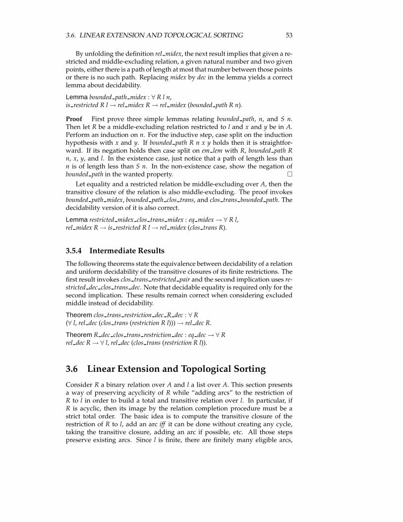
3.6. LINEAR EXTENSION AND TOPOLOGICAL SORTING 53
By unfolding the definition rel midex, the next result implies that given a re-stricted and middle-excluding relation, a given natural number and two givenpoints, either there is a path of length atmost that number between those pointsor there is no such path. Replacing midex by dec in the lemma yields a correctlemma about decidability.
Lemma bounded path midex : ∀ R l n,is restricted R l→ rel midex R→ rel midex (bounded path R n).
Proof First prove three simple lemmas relating bounded path, n, and S n.Then let R be a middle-excluding relation restricted to l and x and y be in A.Perform an induction on n. For the inductive step, case split on the inductionhypothesis with x and y. If bounded path R n x y holds then it is straightfor-ward. If its negation holds then case split on em lem with R, bounded path Rn, x, y, and l. In the existence case, just notice that a path of length less thann is of length less than S n. In the non-existence case, show the negation ofbounded path in the wanted property. �
Let equality and a restricted relation be middle-excluding over A, then thetransitive closure of the relation is also middle-excluding. The proof invokesbounded path midex, bounded path clos trans, and clos trans bounded path. Thedecidability version of it is also correct.
Lemma restricted midex clos trans midex : eq midex→ ∀ R l,rel midex R→ is restricted R l→ rel midex (clos trans R).
3.5.4 Intermediate Results
The following theorems state the equivalence between decidability of a relationand uniform decidability of the transitive closures of its finite restrictions. Thefirst result invokes clos trans restricted pair and the second implication uses re-stricted dec clos trans dec. Note that decidable equality is required only for thesecond implication. These results remain correct when considering excludedmiddle instead of decidability.
Theorem clos trans restriction dec R dec : ∀ R(∀ l, rel dec (clos trans (restriction R l)))→ rel dec R.
Theorem R dec clos trans restriction dec : eq dec→ ∀ Rrel dec R→ ∀ l, rel dec (clos trans (restriction R l)).
3.6 Linear Extension and Topological Sorting
Consider R a binary relation over A and l a list over A. This section presentsa way of preserving acyclicity of R while “adding arcs” to the restriction ofR to l in order to build a total and transitive relation over l. In particular, ifR is acyclic, then its image by the relation completion procedure must be astrict total order. The basic idea is to compute the transitive closure of therestriction of R to l, add an arc iff it can be done without creating any cycle,taking the transitive closure, adding an arc if possible, etc. All those stepspreserve existing arcs. Since l is finite, there are finitely many eligible arcs,
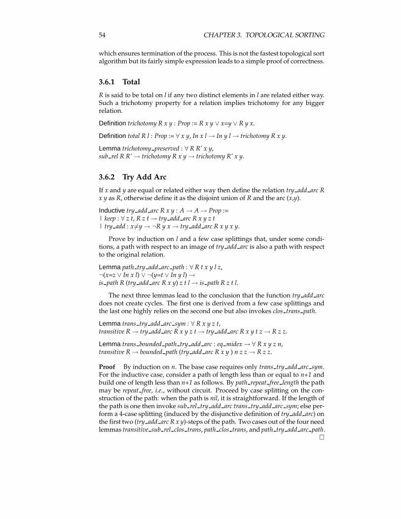
54 CHAPTER 3. TOPOLOGICAL SORTING
which ensures termination of the process. This is not the fastest topological sortalgorithm but its fairly simple expression leads to a simple proof of correctness.
3.6.1 Total
R is said to be total on l if any two distinct elements in l are related either way.Such a trichotomy property for a relation implies trichotomy for any biggerrelation.
Definition trichotomy R x y : Prop := R x y ∨ x=y ∨ R y x.
Definition total R l : Prop := ∀ x y, In x l→ In y l→ trichotomy R x y.
Lemma trichotomy preserved : ∀ R R’ x y,sub rel R R’→ trichotomy R x y→ trichotomy R’ x y.
3.6.2 Try Add Arc
If x and y are equal or related either way then define the relation try add arc Rx y as R, otherwise define it as the disjoint union of R and the arc (x,y).
Inductive try add arc R x y : A→ A→ Prop :=| keep : ∀ z t, R z t→ try add arc R x y z t| try add : x 6=y→ ¬R y x→ try add arc R x y x y.
Prove by induction on l and a few case splittings that, under some condi-tions, a path with respect to an image of try add arc is also a path with respectto the original relation.
Lemma path try add arc path : ∀ R t x y l z,¬(x=z ∨ In x l) ∨ ¬(y=t ∨ In y l)→is path R (try add arc R x y) z t l→ is path R z t l.
The next three lemmas lead to the conclusion that the function try add arcdoes not create cycles. The first one is derived from a few case splittings andthe last one highly relies on the second one but also invokes clos trans path.
Lemma trans try add arc sym : ∀ R x y z t,transitive R→ try add arc R x y z t→ try add arc R x y t z→ R z z.
Lemma trans bounded path try add arc : eq midex→ ∀ R x y z n,transitive R→ bounded path (try add arc R x y ) n z z→ R z z.
Proof By induction on n. The base case requires only trans try add arc sym.For the inductive case, consider a path of length less than or equal to n+1 andbuild one of length less than n+1 as follows. By path repeat free length the pathmay be repeat free, i.e., without circuit. Proceed by case splitting on the con-struction of the path: when the path is nil, it is straightforward. If the length ofthe path is one then invoke sub rel try add arc trans try add arc sym; else per-form a 4-case splitting (induced by the disjunctive definition of try add arc) onthe first two (try add arc R x y)-steps of the path. Two cases out of the four needlemmas transitive sub rel clos trans, path clos trans, and path try add arc path.
�
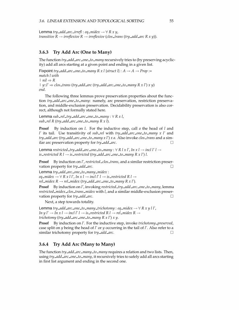
3.6. LINEAR EXTENSION AND TOPOLOGICAL SORTING 55
Lemma try add arc irrefl : eq midex→ ∀ R x y,transitive R→ irreflexive R→ irreflexive (clos trans (try add arc R x y)).
3.6.3 Try Add Arc (One to Many)
The function try add arc one to many recursively tries to (by preserving acyclic-ity) add all arcs starting at a given point and ending in a given list.
Fixpoint try add arc one to many R x l {struct l} : A→ A→ Prop :=match l with| nil⇒ R| y::l’⇒ clos trans (try add arc (try add arc one to many R x l’) x y)end.
The following three lemmas prove preservation properties about the func-tion try add arc one to many: namely, arc preservation, restriction preserva-tion, and middle-exclusion preservation. Decidability preservation is also cor-rect, although not formally stated here.
Lemma sub rel try add arc one to many : ∀ R x l,sub rel R (try add arc one to many R x l).
Proof By induction on l. For the inductive step, call a the head of l andl’ its tail. Use transitivity of sub rel with try add arc one to many x l’ andtry add arc (try add arc one to many x l’) x a. Also invoke clos trans and a sim-ilar arc preservation property for try add arc. �
Lemma restricted try add arc one to many : ∀ R l x l’, In x l→ incl l’ l→is restricted R l→ is restricted (try add arc one to many R x l’) l.
Proof By induction on l’, restricted clos trans, and a similar restriction preser-vation property for try add arc. �
Lemma try add arc one to many midex :eq midex→ ∀ R x l l’, In x l→ incl l’ l→ is restricted R l→rel midex R→ rel midex (try add arc one to many R x l’).Proof By induction on l’, invoking restricted try add arc one to many, lemmarestricted midex clos trans midexwith l, and a similar middle-exclusion preser-vation property for try add arc. �
Next, a step towards totality.
Lemma try add arc one to many trichotomy : eq midex→ ∀ R x y l l’,In y l’→ In x l→ incl l’ l→ is restricted R l→ rel midex R→trichotomy (try add arc one to many R x l’) x y.Proof By induction on l’. For the inductive step, invoke trichotomy preserved,case split on y being the head of l’ or y occurring in the tail of l’. Also refer to asimilar trichotomy property for try add arc. �
3.6.4 Try Add Arc (Many to Many)
The function try add arc many to many requires a relation and two lists. Then,using try add arc one to many, it recursively tries to safely add all arcs startingin first list argument and ending in the second one.
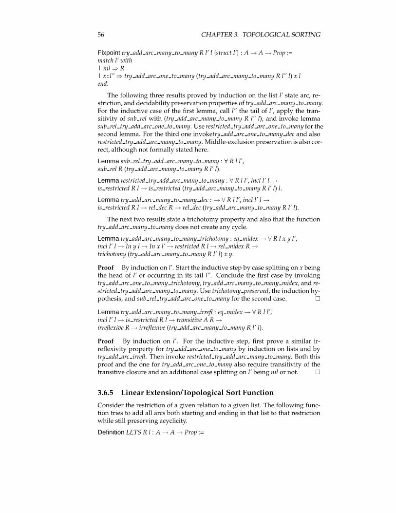
56 CHAPTER 3. TOPOLOGICAL SORTING
Fixpoint try add arc many to many R l’ l {struct l’} : A→ A→ Prop :=match l’ with| nil⇒ R| x::l”⇒ try add arc one to many (try add arc many to many R l” l) x lend.
The following three results proved by induction on the list l’ state arc, re-striction, and decidability preservation properties of try add arc many to many.For the inductive case of the first lemma, call l” the tail of l’, apply the tran-sitivity of sub rel with (try add arc many to many R l” l), and invoke lemmasub rel try add arc one to many. Use restricted try add arc one to many for thesecond lemma. For the third one invoketry add arc one to many dec and alsorestricted try add arc many to many. Middle-exclusion preservation is also cor-rect, although not formally stated here.
Lemma sub rel try add arc many to many : ∀ R l l’,sub rel R (try add arc many to many R l’ l).
Lemma restricted try add arc many to many : ∀ R l l’, incl l’ l→is restricted R l→ is restricted (try add arc many to many R l’ l) l.
Lemma try add arc many to many dec : → ∀ R l l’, incl l’ l→is restricted R l→ rel dec R→ rel dec (try add arc many to many R l’ l).
The next two results state a trichotomy property and also that the functiontry add arc many to many does not create any cycle.
Lemma try add arc many to many trichotomy : eq midex→ ∀ R l x y l’,incl l’ l→ In y l→ In x l’→ restricted R l→ rel midex R→trichotomy (try add arc many to many R l’ l) x y.
Proof By induction on l’. Start the inductive step by case splitting on x beingthe head of l’ or occurring in its tail l”. Conclude the first case by invokingtry add arc one to many trichotomy, try add arc many to many midex, and re-stricted try add arc many to many. Use trichotomy preserved, the induction hy-pothesis, and sub rel try add arc one to many for the second case. �
Lemma try add arc many to many irrefl : eq midex→ ∀ R l l’,incl l’ l→ is restricted R l→ transitive A R→irreflexive R→ irreflexive (try add arc many to many R l’ l).
Proof By induction on l’. For the inductive step, first prove a similar ir-reflexivity property for try add arc one to many by induction on lists and bytry add arc irrefl. Then invoke restricted try add arc many to many. Both thisproof and the one for try add arc one to many also require transitivity of thetransitive closure and an additional case splitting on l’ being nil or not. �
3.6.5 Linear Extension/Topological Sort Function
Consider the restriction of a given relation to a given list. The following func-tion tries to add all arcs both starting and ending in that list to that restrictionwhile still preserving acyclicity.
Definition LETS R l : A→ A→ Prop :=
3.6. LINEAR EXTENSION AND TOPOLOGICAL SORTING 57
try add arc many to many (clos trans (restriction R l)) l l.
The next three lemmas are proved by sub rel try add arc many to many,transitive clos trans, and restricted try add arc many to many respectively.
Lemma LETS sub rel : ∀ R l,sub rel (clos trans (restriction R l)) (LETS R l).
Lemma LETS transitive : ∀ R l, transitive (LETS R l).
Lemma LETS restricted : ∀ R l, is restricted (LETS R l) l.
Under middle-excluding equality, the finite restriction of R to l has no cycleiff LETSR l is irreflexive. Prove left to right by try add arc many to many irrefl,and right to left by irreflexive preserved and LETS sub rel.
Lemma LETS irrefl : eq midex→ ∀ R l,(irreflexive (clos trans (restriction R l))↔ irreflexive (LETS R l)).
If R and equality on A are middle-excluding then LETS R l is total on l.This is proved by lemmas R midex clos trans restriction midex (in 3.5.4 ) andtry add arc many to many trichotomy.
Lemma LETS total : eq midex→ ∀ R l, rel midex R→ total (LETS R l) l.
The next two lemmas show that ifR and equality onA aremiddle-excluding(resp. decidable) then so is LETS R l: by try add arc many to many midex(resp. try add arc many to many dec) andR midex clos trans restriction midex(resp. R dec clos trans restriction dec).
Lemma LETS midex : eq midex→ ∀ R l,rel midex R→ rel midex (LETS R l).
Lemma LETS dec : eq dec→ ∀ R, rel dec R→ ∀ l, rel dec (LETS R l).
3.6.6 Linear Extension
Traditionally, a linear extension of a partial order is a total order including thepartial order. Below, a linear extension (over a list) of a binary relation is a stricttotal order (over the list) that is bigger than the original relation (restricted tothe list).
Definition linear extension R l R’ := is restricted R’ l ∧sub rel (restriction R l) R’ ∧ transitive A R’ ∧ irreflexive R’ ∧ total R’ l.
The next two lemmas say that a relation “locally” contained in some acyclicrelation is “globally” acyclic and that if for any list over A there is a middle-excluding total order over that list, then equality is middle-excluding on A.
Lemma local global acyclic : ∀ R,(∀ l, ∃ R’, sub rel (restriction R l) R’ ∧ transitive R’ ∧ irreflexive R’)→irreflexive (clos trans R).
Proof Let R be a relation over A. Assume that any finite restriction of R isincluded in some strict partial order. Let x be in A such that clos trans R x x.Then derive False as follows. Invoke clos trans path and get a path. It is still apath for the restriction of R to the path itself (the path is a list seen as a subset ofA). Use path clos trans, then the main assumption, transitive sub rel clos trans,and the monotonicity of clos transwith respect to sub rel. �
58 CHAPTER 3. TOPOLOGICAL SORTING
Lemma total order eq midex :(∀ l, ∃ R, transitive R ∧ irreflexive R ∧ total R l ∧ rel midex R)→ eq midex.
Proof Assume the left conjunct, let x and y be in A, use the assumption withx::y::nil, get a relation, and double case split on x and y being related eitherway. �
Consider a middle-excluding relation on A. It is acyclic and equality ismiddle-excluding on A iff for any list over A there exists, on the given list,a decidable strict total order containing the original relation.
Theorem linearly extendable : ∀ R, rel midex R→(eq midex ∧ irreflexive (clos trans R)↔∀ l, ∃ R’, linear extension R l R’ ∧ rel midex R’).
Proof Left to right: by the relevant lemmas of subsection 3.6.5, (LETS R l) isa witness for the existential quantifier. Right to left by local global acyclic andtotal order eq midex. �
3.6.7 Topological Sorting
In this subsection, excluded-middle results of subsection 3.6.6 are translatedinto decidability results and augmented: as there is only one concept of lin-ear extension in subsection 3.6.6, this section presents three slightly differ-ent concepts of topological sort. Instead of the equivalence of theorem lin-early extendable, those three definitions yield a quadruple equivalence.From now on a decidable relation may be represented by a function to
booleans instead of a function to Prop satisfying the definition rel dec. How-ever, those two representations are “equivalent” thanks to lemmas rel dec booland bool rel dec in subsection 3.2.2.In this chapter, a given relation over A is said to be non-uniformly (topolog-
ically) sortable if the restriction of the relation to any list has a decidable linearextension.
Definition non uni topo sortable R :=∀ l, ∃ R’ : A→ A→ bool, linear extension R l (fun x y⇒ R’ x y=true).
In the definition above, R’ represents a decidable binary relation that in-tends to be a linear extension of R over the list l. But R’ has type A → A →bool so it cannot be used with the predicate linear extension R l that expects anobject of type A → A → Prop, which is the usual type for representing binaryrelations in Coq. The function fun x y⇒ (R’ x y)=true above is the translationof R’ in the suitable type/representation. It expects two elements x and y in Aand returns the proposition R’ x y=true, in Prop.In this chapter, a given relation over A is said to be uniformly sortable if
there exists a computable function expecting a list over A and producing, overthe list argument, a (decidable) linear extension of the original relation.
Definition uni topo sortable R := {F : list A→ A→ A→ bool |∀ l, linear extension R l (fun x y⇒ (F l x y)=true )}.
The third definition of topological sort uses the concept of asymmetry, whichis now informally introduced; from an algorithmic viewpoint: given a way of
3.6. LINEAR EXTENSION AND TOPOLOGICAL SORTING 59
representing binary relations, different objects may represent the same binaryrelation; from a logical viewpoint: two binary relations different in intension,i.e. their definitions intend different things, may still coincide, i.e. may be logi-cally equivalent. In an arbitrary topological sort algorithm, the returned linearextension may depend on which object has been chosen to represent the origi-nal binary relation. For example, applying the empty relation on a given two-element set to a topological sort algorithmmay produce the two possible linearextensions depending on the order in which the two elements constituting theset are given. This remark leads to the definition below. It is not clear what thisnotion of asymmetry would be useful for, but a result follow.
Definition asym R G := ∀ x y : A,x 6=y→ ¬R x y→¬R y x→ ¬(G (x::y::nil) x y ∧ G (y::x::nil) x y).
Next comes the definition of asymmetry for a topological sort of a binaryrelation. The syntax let variable:= formula in formula’ avoids writing formula sev-eral times in formula’.
Definition asym topo sortable R := {F : list A→ A→ A→ bool |let G:= (fun l x y⇒ F l x y=true) inasym R G ∧ ∀ l, linear extension R l (G l)}.
Given a binary relation R over A, the remainder of this subsection provesthat the four following assertions are equivalent:
1. Equality on A is decidable, and R is decidable and acyclic.
2. R is middle-excluding and asymmetrically sortable.
3. R is decidable and uniformly sortable.
4. Equality onA is decidable, andR is decidable and non-uniformly sortable.
The following lemma says that if there exists a computable function ex-pecting a list over A and producing a (decidable) strict total order over A, thenequality onA is decidable. The proof is similar to the one for total order eq midex.
Lemma total order eq dec :{F : list A→ A→ A→ bool | ∀ l, let G := fun x y⇒ F l x y=true intransitive A G ∧ irreflexive G ∧ total G l}→ eq dec A.
Next lemma shows that LETS yields asymmetric topological sort.
Lemma LETS asym : ∀ R, asym R (LETS R).
Proof Assume all possible premises, especially let x and y be in A. As a pre-liminary: the hypotheses involve one relation image of restriction and four re-lations images of try add arc. Prove that all of them are restricted to x::y::nil.Then perform a few cases splittings and apply clos trans restricted pair seventimes. �
60 CHAPTER 3. TOPOLOGICAL SORTING
The quadruple equivalence claimed above is derived from rel dec midexand the six theorems below. The proofs are rather similar to themiddle-excludingcase in subsection 3.6.6. The first theorem proves 1 → 2 by the relevant lem-mas of subsection 3.6.5 and LETS producing a witness for the computationalexistence. The second (straightforward) and the third show 2→ 3. The fourth(straightforward) and the fifth, proved by total order eq dec, yield 3→ 4. Thelast shows 4→ 1 by invoking local global acyclic.
Theorem possible asym topo sorting : ∀ R,eq dec A→ rel dec R→ irreflexive (clos trans A R)→ asym topo sortable R.
Theorem asym topo sortable uni topo sortable : ∀ R,asym topo sortable R→ uni topo sortable R.
Theorem asym topo sortable rel dec : ∀ R,rel midex R→ asym topo sortable R→ rel dec R.
Proof First notice that R is acyclic by local global acyclic and that equality onA is decidable by total order eq dec. Then let x and y be in A. By decidableequality, case split on x and y being equal. If they are equal then they arenot related by acyclicity. Now consider that they are distinct. Thanks to theassumption, get TS an asymmetric topological sort of R. Case split on x andy being related by TS (x::y::nil). If they are not then they cannot be related byR by subrelation property. If they are related then case split again on x and ybeing related by TS (y::x::nil). If they are not then they cannot be related by Rby subrelation property. If they are then they also are by R by the asymmetryproperty. �
Theorem uni topo sortable non uni topo sortable : ∀ R,uni topo sortable R→ non uni topo sortable R.
Theorem rel dec uni topo sortable eq dec : ∀ R,rel dec R→ uni topo sortable R→ eq dec A.
Theorem rel dec non uni topo sortable acyclic : ∀ R,rel dec R→ non uni topo sortable R→ irreflexive (clos trans A R).
3.7 Conclusion
This chapter has given a detailed account on a few facts related to linear ex-tensions of acyclic binary relations. The discussion is based on a formal proofdevelopedwith the proof assistant Coq. Since arguments are constructive, theyare also correct with respect to traditional mathematical reasoning. The chap-ter aimes to be understandable to mathematicians new to Coq or more gener-ally by readers unfamiliar with constructive issues. The three main results arestated again below. First, a binary relation over a set with decidable/middle-excluding equality is decidable/middle-excluding iff transitive closures of itsfinite restrictions are also decidable/middle-excluding. This theorem is in-volved in the proof of the second and third main results. Second, consider amiddle-excluding relation over an arbitrary domain. It is acyclic and equality

3.7. CONCLUSION 61
on its domain is middle-excluding iff any of its finite restriction has a middle-excluding linear extension. Third, consider R a decidable binary relation overA. The following three propositions are equivalent:
• Equality on A is decidable and R is acyclic.
• Equality on A is decidable and R is non-uniformly sortable.
• R is uniformly sortable.
The proofs of the last two main results rely on the constructive functionLETS that is actually (similar to) a basic topological sort algorithm. An effectiveprogram could therefore be extracted from the Coq development (related tocomputability). The original proof would in turn serve as a formal proof ofcorrectness for the program.
62 CHAPTER 3. TOPOLOGICAL SORTING
Chapter 4
Acyclicity of Preferences,Nash Equilibria, andSubgame Perfect Equilibria:a Formal and ConstructiveEquivalence
Sequential game and Nash equilibrium are basic key concepts in game theory.In 1953, Kuhn showed that every sequential game has a Nash equilibrium. Thetwo main steps of the proof are as follows: First, a procedure expecting a se-quential game as an input is defined as “backward induction” in game theory.Second, it is proved that the procedure yields a Nash equilibrium. “Backwardinduction” actually yieldsNash equilibria that define a proper subclass of Nashequilibria. In 1965, Selten named this proper subclass subgame perfect equilib-ria. In game theory, payoffs are rewards usually granted at the end of a game.Although traditional game theory mainly focuses on real-valued payoffs thatare implicitly ordered by the usual total order over the reals, there is a demandfor results dealing with non totally ordered payoffs. In the mid 1950’s, worksof Simon or Blackwell already involved partially ordered payoffs. This chap-ter further explores the matter: it generalises the notion of sequential gameby replacing real-valued payoff functions with abstract atomic objects, calledoutcomes, and by replacing the usual total order over the reals with arbitrarybinary relations over outcomes, called preferences. This introduces a generalabstract formalismwhere Nash equilibrium, subgame perfect equilibrium, and“backward induction” can still be defined. Using a lemma on topological sort-ing, this chapter proves that the following three propositions are equivalent: 1)Preferences over the outcomes are acyclic. 2) Every sequential game has a Nashequilibrium. 3) Every sequential game has a subgame perfect equilibrium. Theresult is fully computer-certified using the (highly reliable) constructive proofassistant called Coq. Beside the additional guarantee of correctness providedby the proof in Coq, the activity of formalisation also helps clearly identify theuseful definitions and the main articulations of the proof.
63
64 CHAPTER 4. ABSTRACT SEQUENTIAL GAMES
4.1 Introduction
4.1.1 Contribution
This chapter contributes at both the technical and the presentation level. Thereare five main technical contributions:
• An inductive formalism is designed to represent sequential games in the con-structive proof assistant Coq ([1] and [9]), and all the results in this chap-ter are proved in Coq.
• The new formalism allows the chapter to introduce an abstraction of tra-ditional sequential games and of a few related concepts. The abstractionpreserves the tree structure of the game but replaces the real-valued pay-off functions, enclosed in the leaves of the trees, by arbitrary outcomes.Each agent has a preference over outcomes, which is given via an explicitand arbitrary binary relation. This preference replaces the implicit andtraditional “usual total order” over the real numbers. Nash equilibriaand subgame perfect equilibria are defined accordingly.
• Kuhn’s result [25] is translated into the new formalismwhen agents’ pref-erences are totally ordered.
• The notion of “backward induction” is naturally generalised for arbitrarypreferences. However, a simple example shows that total ordering ofpreferences is needed for “backward induction” to guarantee subgameperfect equilibrium: both notions of “backward induction” and subgameperfect equilibrium coincide for total orders but not in general.
• Kuhn’s result is substantially generalised as follows. On the one hand, anintermediate result proves that smaller preferences, i.e., binary relationswith less arcs, yield more equilibria than bigger preferences. On the otherhand, a topological sorting result was formally proved in [28] and chap-ter 3. By both results mentioned above, acyclicity of the preferences provesto be a necessary and sufficient condition for every game to have a Nash equilib-rium/subgame perfect equilibrium.
This chapter deals with basic notions of game theory that are all exemplifiedand defined before they are used. Most of the time, these notions are explainedin three different ways, with the second one helping make the connection be-tween the two others:
• The notions are presented in a graphical formalism close to traditionalgame theory.
• They are presented in a graphical formalism suitable for induction.
• They are presented in a light Coq formalism close to traditional mathe-matics, so that only a basic understanding of Coq is needed. (A quicklook at the first ten pages of [28] or chapter 3 will introduce the reader tothe required notions.)
Moreover, the proofs are structured along the corresponding Coq proofs butare written in plain English.
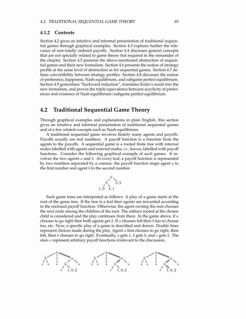
4.2. TRADITIONAL SEQUENTIAL GAME THEORY 65
4.1.2 Contents
Section 4.2 gives an intuitive and informal presentation of traditional sequen-tial games through graphical examples. Section 4.3 explores further the rele-vance of non-totally ordered payoffs. Section 4.4 discusses general conceptsthat are not specially related to game theory but required in the remainder ofthe chapter. Section 4.5 presents the above-mentioned abstraction of sequen-tial games and their new formalism. Section 4.6 presents the notion of strategyprofile at the same level of abstraction as for sequential games. Section 4.7 de-fines convertibility between strategy profiles. Section 4.8 discusses the notionof preference, happiness, Nash equilibrium, and subgame perfect equilibrium.Section 4.9 generalises “backward induction”, translates Kuhn’s result into thenew formalism, and proves the triple equivalence between acyclicity of prefer-ences and existence of Nash equilibrium/subgame perfect equilibrium.
4.2 Traditional Sequential Game Theory
Through graphical examples and explanations in plain English, this sectiongives an intuitive and informal presentation of traditional sequential gamesand of a few related concepts such as Nash equilibrium.A traditional sequential game involves finitely many agents and payoffs.
Payoffs usually are real numbers. A payoff function is a function from theagents to the payoffs. A sequential game is a rooted finite tree with internalnodes labelled with agents and external nodes, i.e., leaves, labelled with payofffunctions. Consider the following graphical example of such games. It in-volves the two agents a and b. At every leaf, a payoff function is representedby two numbers separated by a comma: the payoff function maps agent a tothe first number and agent b to the second number.
a
b 2, 2
1, 0 3, 1
Such game trees are interpreted as follows: A play of a game starts at theroot of the game tree. If the tree is a leaf then agents are rewarded accordingto the enclosed payoff function. Otherwise, the agent owning the root choosesthe next node among the children of the root. The subtree rooted at the chosenchild is considered and the play continues from there. In the game above, if achooses to go right then both agents get 2. If a chooses left then b has to choosetoo, etc. Now, a specific play of a game is described and drawn. Double linesrepresent choices made during the play. Agent a first chooses to go right, thenleft, then b chooses to go right. Eventually, a gets 1, b gets 0, and c gets 2. Thestars ∗ represent arbitrary payoff functions irrelevant to the discussion.
a a a
b c a b c a b c a
∗ ∗ ∗ b ∗ ∗ ∗ ∗ b ∗ ∗ ∗ ∗ b ∗
∗ 1, 0, 2 ∗ 1, 0, 2 ∗ 1, 0, 2
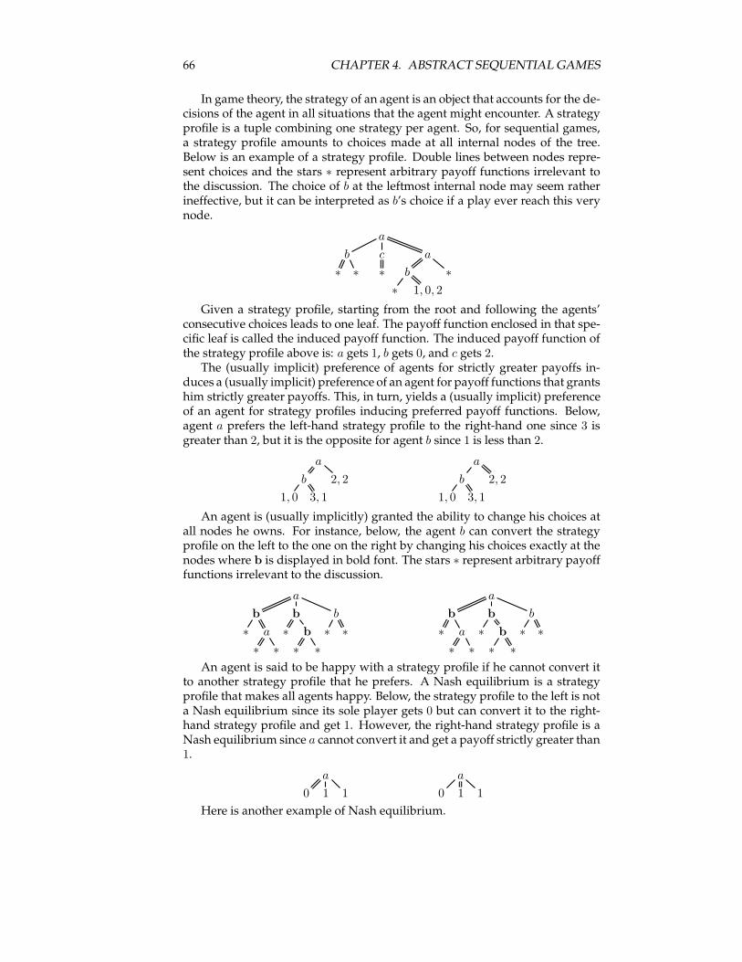
66 CHAPTER 4. ABSTRACT SEQUENTIAL GAMES
In game theory, the strategy of an agent is an object that accounts for the de-cisions of the agent in all situations that the agent might encounter. A strategyprofile is a tuple combining one strategy per agent. So, for sequential games,a strategy profile amounts to choices made at all internal nodes of the tree.Below is an example of a strategy profile. Double lines between nodes repre-sent choices and the stars ∗ represent arbitrary payoff functions irrelevant tothe discussion. The choice of b at the leftmost internal node may seem ratherineffective, but it can be interpreted as b’s choice if a play ever reach this verynode.
a
b c a
∗ ∗ ∗ b ∗
∗ 1, 0, 2
Given a strategy profile, starting from the root and following the agents’consecutive choices leads to one leaf. The payoff function enclosed in that spe-cific leaf is called the induced payoff function. The induced payoff function ofthe strategy profile above is: a gets 1, b gets 0, and c gets 2.The (usually implicit) preference of agents for strictly greater payoffs in-
duces a (usually implicit) preference of an agent for payoff functions that grantshim strictly greater payoffs. This, in turn, yields a (usually implicit) preferenceof an agent for strategy profiles inducing preferred payoff functions. Below,agent a prefers the left-hand strategy profile to the right-hand one since 3 isgreater than 2, but it is the opposite for agent b since 1 is less than 2.
a a
b 2, 2 b 2, 2
1, 0 3, 1 1, 0 3, 1
An agent is (usually implicitly) granted the ability to change his choices atall nodes he owns. For instance, below, the agent b can convert the strategyprofile on the left to the one on the right by changing his choices exactly at thenodes where b is displayed in bold font. The stars ∗ represent arbitrary payofffunctions irrelevant to the discussion.
a a
b b b b b b
∗ a ∗ b ∗ ∗ ∗ a ∗ b ∗ ∗
∗ ∗ ∗ ∗ ∗ ∗ ∗ ∗
An agent is said to be happy with a strategy profile if he cannot convert itto another strategy profile that he prefers. A Nash equilibrium is a strategyprofile that makes all agents happy. Below, the strategy profile to the left is nota Nash equilibrium since its sole player gets 0 but can convert it to the right-hand strategy profile and get 1. However, the right-hand strategy profile is aNash equilibrium since a cannot convert it and get a payoff strictly greater than1.
a a
0 1 1 0 1 1
Here is another example of Nash equilibrium.
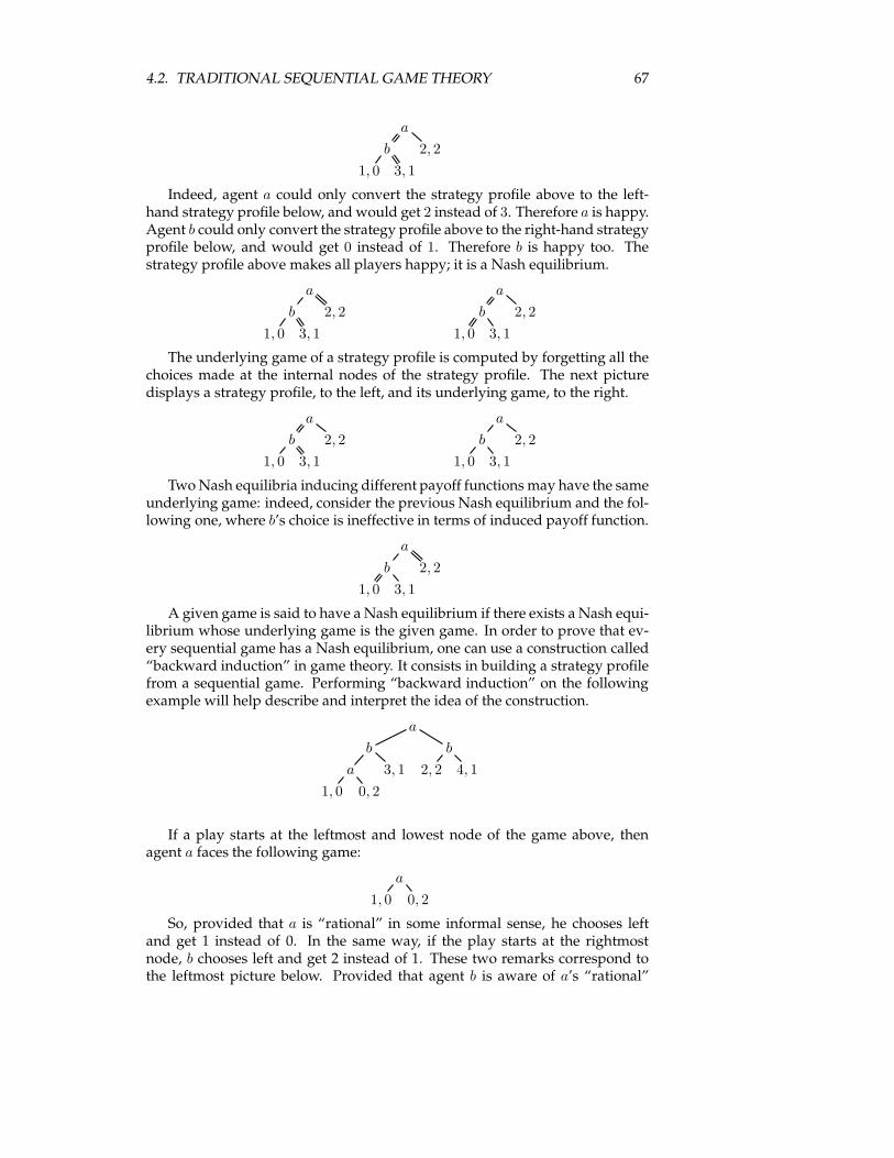
4.2. TRADITIONAL SEQUENTIAL GAME THEORY 67
a
b 2, 2
1, 0 3, 1
Indeed, agent a could only convert the strategy profile above to the left-hand strategy profile below, and would get 2 instead of 3. Therefore a is happy.Agent b could only convert the strategy profile above to the right-hand strategyprofile below, and would get 0 instead of 1. Therefore b is happy too. Thestrategy profile above makes all players happy; it is a Nash equilibrium.
a a
b 2, 2 b 2, 2
1, 0 3, 1 1, 0 3, 1
The underlying game of a strategy profile is computed by forgetting all thechoices made at the internal nodes of the strategy profile. The next picturedisplays a strategy profile, to the left, and its underlying game, to the right.
a a
b 2, 2 b 2, 2
1, 0 3, 1 1, 0 3, 1
TwoNash equilibria inducing different payoff functions may have the sameunderlying game: indeed, consider the previous Nash equilibrium and the fol-lowing one, where b’s choice is ineffective in terms of induced payoff function.
a
b 2, 2
1, 0 3, 1
A given game is said to have a Nash equilibrium if there exists a Nash equi-librium whose underlying game is the given game. In order to prove that ev-ery sequential game has a Nash equilibrium, one can use a construction called“backward induction” in game theory. It consists in building a strategy profilefrom a sequential game. Performing “backward induction” on the followingexample will help describe and interpret the idea of the construction.
a
b b
a 3, 1 2, 2 4, 1
1, 0 0, 2
If a play starts at the leftmost and lowest node of the game above, thenagent a faces the following game:
a
1, 0 0, 2
So, provided that a is “rational” in some informal sense, he chooses leftand get 1 instead of 0. In the same way, if the play starts at the rightmostnode, b chooses left and get 2 instead of 1. These two remarks correspond tothe leftmost picture below. Provided that agent b is aware of a’s “rational”
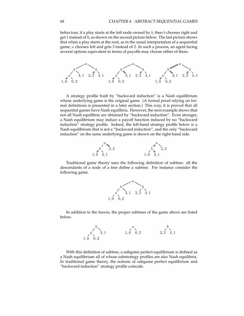
68 CHAPTER 4. ABSTRACT SEQUENTIAL GAMES
behaviour, if a play starts at the left node owned by b, then b chooses right andget 1 instead of 0, as shown on the second picture below. The last picture showsthat when a play starts at the root, as in the usual interpretation of a sequentialgame, a chooses left and gets 3 instead of 2. In such a process, an agent facingseveral options equivalent in terms of payoffs may choose either of them.
a a a
b b b b b b
a 3, 1 2, 2 4, 1 a 3, 1 2, 2 4, 1 a 3, 1 2, 2 4, 1
1, 0 0, 2 1, 0 0, 2 1, 0 0, 2
A strategy profile built by “backward induction” is a Nash equilibriumwhose underlying game is the original game. (A formal proof relying on for-mal definitions is presented in a later section.) This way, it is proved that allsequential games have Nash equilibria. However, the next example shows thatnot all Nash equilibria are obtained by “backward induction”. Even stronger,a Nash equilibrium may induce a payoff function induced by no “backwardinduction” strategy profile. Indeed, the left-hand strategy profile below is aNash equilibrium that is not a “backward induction”, and the only “backwardinduction” on the same underlying game is shown on the right-hand side.
a a
b 2, 2 b 2, 2
1, 0 3, 1 1, 0 3, 1
Traditional game theory uses the following definition of subtree: all thedescendants of a node of a tree define a subtree. For instance consider thefollowing game.
a
b b
a 3, 1 2, 2 4, 1
1, 0 0, 2
In addition to the leaves, the proper subtrees of the game above are listedbelow.
b a b
a 3, 1 1, 0 0, 2 2, 2 4, 1
1, 0 0, 2
With this definition of subtree, a subgame perfect equilibrium is defined asa Nash equilibrium all of whose substrategy profiles are also Nash equilibria.In traditional game theory, the notions of subgame perfect equilibrium and“backward induction” strategy profile coincide.
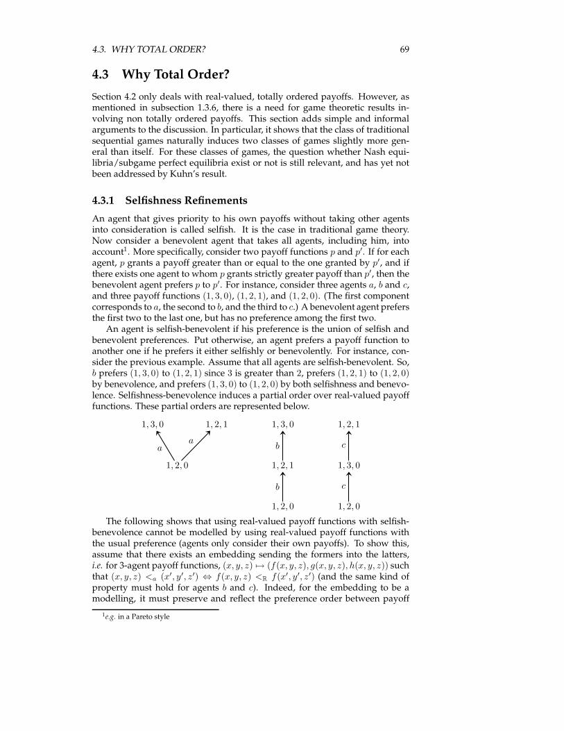
4.3. WHY TOTAL ORDER? 69
4.3 Why Total Order?
Section 4.2 only deals with real-valued, totally ordered payoffs. However, asmentioned in subsection 1.3.6, there is a need for game theoretic results in-volving non totally ordered payoffs. This section adds simple and informalarguments to the discussion. In particular, it shows that the class of traditionalsequential games naturally induces two classes of games slightly more gen-eral than itself. For these classes of games, the question whether Nash equi-libria/subgame perfect equilibria exist or not is still relevant, and has yet notbeen addressed by Kuhn’s result.
4.3.1 Selfishness Refinements
An agent that gives priority to his own payoffs without taking other agentsinto consideration is called selfish. It is the case in traditional game theory.Now consider a benevolent agent that takes all agents, including him, intoaccount1. More specifically, consider two payoff functions p and p′. If for eachagent, p grants a payoff greater than or equal to the one granted by p′, and ifthere exists one agent to whom p grants strictly greater payoff than p′, then thebenevolent agent prefers p to p′. For instance, consider three agents a, b and c,and three payoff functions (1, 3, 0), (1, 2, 1), and (1, 2, 0). (The first componentcorresponds to a, the second to b, and the third to c.) A benevolent agent prefersthe first two to the last one, but has no preference among the first two.An agent is selfish-benevolent if his preference is the union of selfish and
benevolent preferences. Put otherwise, an agent prefers a payoff function toanother one if he prefers it either selfishly or benevolently. For instance, con-sider the previous example. Assume that all agents are selfish-benevolent. So,b prefers (1, 3, 0) to (1, 2, 1) since 3 is greater than 2, prefers (1, 2, 1) to (1, 2, 0)by benevolence, and prefers (1, 3, 0) to (1, 2, 0) by both selfishness and benevo-lence. Selfishness-benevolence induces a partial order over real-valued payofffunctions. These partial orders are represented below.
1, 3, 0 1, 2, 1 1, 3, 0 1, 2, 1
1, 2, 0 1, 2, 1 1, 3, 0
1, 2, 0 1, 2, 0
aa
b
b
c
c
The following shows that using real-valued payoff functions with selfish-benevolence cannot be modelled by using real-valued payoff functions withthe usual preference (agents only consider their own payoffs). To show this,assume that there exists an embedding sending the formers into the latters,i.e. for 3-agent payoff functions, (x, y, z) 7→ (f(x, y, z), g(x, y, z), h(x, y, z)) suchthat (x, y, z) <a (x′, y′, z′) ⇔ f(x, y, z) <R f(x′, y′, z′) (and the same kind ofproperty must hold for agents b and c). Indeed, for the embedding to be amodelling, it must preserve and reflect the preference order between payoff
1e.g. in a Pareto style
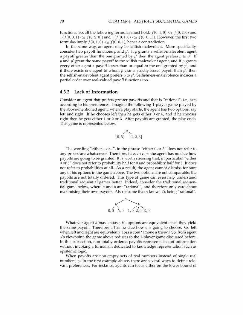
70 CHAPTER 4. ABSTRACT SEQUENTIAL GAMES
functions. So, all the following formulas must hold: f(0, 1, 0) <R f(0, 2, 0) and¬(f(0, 0, 1) <R f(0, 2, 0)) and ¬(f(0, 1, 0) <R f(0, 0, 1)). However, the first twoformulas imply f(0, 1, 0) <R f(0, 0, 1), hence a contradiction.In the same way, an agent may be selfish-malevolent. More specifically,
consider two payoff functions p and p′. If p grants a selfish-malevolent agenta payoff greater than the one granted by p′ then the agent prefers p to p′. Ifp and p′ grant the same payoff to the selfish-malevolent agent, and if p grantsevery other agent a payoff lesser than or equal to the one granted by p′, andif there exists one agent to whom p grants strictly lesser payoff than p′, thenthe selfish-malevolent agent prefers p to p′. Selfishness-malevolence induces apartial order over real-valued payoff functions too.
4.3.2 Lack of Information
Consider an agent that prefers greater payoffs and that is “rational”, i.e., actsaccording to his preferences. Imagine the following 1-player game played bythe above-mentioned agent: when a play starts, the agent has two options, sayleft and right. If he chooses left then he gets either 0 or 5, and if he choosesright then he gets either 1 or 2 or 3. After payoffs are granted, the play ends.This game is represented below.
a
{0, 5} {1, 2, 3}
The wording “either... or...”, in the phrase “either 0 or 5” does not refer toany procedure whatsoever. Therefore, in each case the agent has no clue howpayoffs are going to be granted. It is worth stressing that, in particular, “either0 or 5” does not refer to probability half for 0 and probability half for 5. It doesnot refer to probabilities at all. As a result, the agent cannot dismiss for sureany of his options in the game above. The two options are not comparable; thepayoffs are not totally ordered. This type of game can even help understandtraditional sequential games better. Indeed, consider the traditional sequen-tial game below, where a and b are “rational”, and therefore only care aboutmaximising their own payoffs. Also assume that a knows b’s being “rational”.
a
b b
0, 0 5, 0 1, 0 2, 0 3, 0
Whatever agent a may choose, b’s options are equivalent since they yieldthe same payoff. Therefore a has no clue how b is going to choose: Go leftwhen left and right are equivalent? Toss a coin? Phone a friend? So, from agenta’s viewpoint, the game above reduces to the 1-player game discussed before.In this subsection, non totally ordered payoffs represents lack of informationwithout invoking a formalism dedicated to knowledge representation such asepistemic logic.When payoffs are non-empty sets of real numbers instead of single real
numbers, as in the first example above, there are several ways to define rele-vant preferences. For instance, agents can focus either on the lower bound of
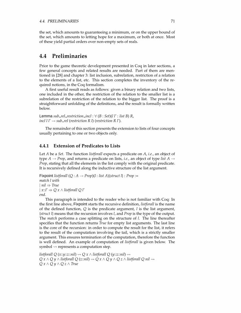
4.4. PRELIMINARIES 71
the set, which amounts to guaranteeing a minimum, or on the upper bound ofthe set, which amounts to letting hope for a maximum, or both at once. Mostof these yield partial orders over non-empty sets of reals.
4.4 Preliminaries
Prior to the game theoretic development presented in Coq in later sections, afew general concepts and related results are needed. Part of them are men-tioned in [28] and chapter 3: list inclusion, subrelation, restriction of a relationto the elements of a list, etc. This section completes the inventory of the re-quired notions, in the Coq formalism.A first useful result reads as follows: given a binary relation and two lists,
one included in the other, the restriction of the relation to the smaller list is asubrelation of the restriction of the relation to the bigger list. The proof is astraightforward unfolding of the definitions, and the result is formally writtenbelow.
Lemma sub rel restriction incl : ∀ (B : Set)(l l’ : list B) R,incl l l’→ sub rel (restriction R l) (restriction R l’).
The remainder of this section presents the extension to lists of four conceptsusually pertaining to one or two objects only.
4.4.1 Extension of Predicates to Lists
Let A be a Set. The function listforall expects a predicate on A, i.e., an object oftype A → Prop, and returns a predicate on lists, i.e., an object of type list A →Prop, stating that all the elements in the list comply with the original predicate.It is recursively defined along the inductive structure of the list argument.
Fixpoint listforall (Q : A→ Prop)(l : list A){struct l} : Prop :=match l with| nil⇒ True| x::l’⇒ Q x ∧ listforall Q l’end.This paragraph is intended to the reader who is not familiar with Coq: In
the first line above, Fixpoint starts the recursive definition, listforall is the nameof the defined function, Q is the predicate argument, l is the list argument,{struct l} means that the recursion involves l, and Prop is the type of the output.The match performs a case splitting on the structure of l. The line thereafterspecifies that the function returns True for empty list arguments. The last lineis the core of the recursion: in order to compute the result for the list, it refersto the result of the computation involving the tail, which is a strictly smallerargument. This ensures termination of the computation, therefore the functionis well defined. An example of computation of listforall is given below. Thesymbol represents a computation step.
listforall Q (x::y::z::nil) Q x ∧ listforall Q (y::z::nil) Q x ∧ Q y ∧ listforall Q (z::nil) Q x ∧ Q y ∧ Q z ∧ listforall Q nil Q x ∧ Q y ∧ Q z ∧ True
72 CHAPTER 4. ABSTRACT SEQUENTIAL GAMES
Note that Q x ∧ Q y ∧ Q z ∧ True is equivalent to Q x ∧ Q y ∧ Q z, which iswhat the function listforall is meant for.The following four lemmas involve the notion of appending (++), also called
concatenation, of two lists. It is defined in the Coq Standard Library. The fourlemmas express basic properties of the listforall function. They are all provedby induction on the list l.
Lemma listforall app : ∀ Q l’ l,listforall Q l→ listforall Q l’→ listforall Q (l++l’).
Lemma listforall appl : ∀ Q l’ l, listforall Q (l++l’)→ listforall Q l.
Lemma listforall appr : ∀ Q l’ l, listforall Q (l++l’)→ listforall Q l’.
Lemma listforall In : ∀ Q x l, In x l→ listforall Q l→ Q x.
4.4.2 Extension of Functions to Lists
The Coq Standard Library provides a functionmap that, given a list and a func-tion f, returns a list with the images by f of the elements of the original list. Itis defined by recursion.
Fixpoint map (A B : Set)(f : A→ B)(l : list A) : list B :=match l with| nil⇒ nil| a::t⇒ (f a)::(map A B f t)end.
Consider the simplified computation example below, where domains andcodomains of f are omitted for better readability.
map f (x::y::z::nil) · · · (f x)::(f y)::(f z)::nil
The next two lemmas state map’s preserving two functions being inverseand commutativity between map and appending. Both lemmas are provedby induction on the list l. The second one comes from the Coq Standard Li-brary [1].
Lemma map inverse : ∀ (A B : Set)(f : A→ B) g,(∀ x, g (f x)=x)→ ∀ l, map g (map f l)=l.
Lemma map app : ∀ (A B : Set)l l’ (f : A→ B), map f (l++l’) = (map f l)++(map fl’).
4.4.3 Extension of Binary Relations to Lists
Let A be a Set. Given a binary relation P : A→ A→ Prop, the function rel vectorexpects two lists over A and states that they are component-wise related by P.Note that if they are component-wise related then their lengths are the same.
Fixpoint rel vector (P : A→ A→ Prop)(l l’ : list A) {struct l}: Prop :=match l with| nil⇒ l’=nil| x::l2⇒ match l’ with
4.4. PRELIMINARIES 73
| nil⇒ False| x’::l2’⇒ P x x’ ∧ rel vector P l2 l2’end
end.
The following examples describe three typical computations of the rel vectorpredicate.
rel vector P (x::y::nil) (x’::y’::nil) P x x’ ∧ rel vector P (y::nil) (y’::nil) P x x’ ∧P y y’ ∧ rel vector P (nil) (nil) P x x’ ∧ P y y’ ∧ nil=nil
Note that P x x’ ∧ P y y’ ∧ nil=nil is equivalent to P x x’ ∧ P y y’.
rel vector P (x::y::nil) (x’::nil) P x x’ ∧ rel vector P (y::nil) (nil) P x x’ ∧ False
Note that P x x’ ∧ False is equivalent to False.
rel vector P (x::nil) (x’::y’nil) P x x’ ∧ rel vector P (nil) (y’::nil) P x x’ ∧ y’::nil=nil
Note that P x x’ ∧ y’::nil=nil is equivalent to False since y’::nil=nil is equiva-lent to False.The following lemma states that if two lists are component-wise related,
then two elements occurring at the same place in each list are also related.
Lemma rel vector app cons same length : ∀ P a a’ m m’ l l’,rel vector P (l++a::m) (l’++a’::m’)→ length l=length l’→ P a a’.
Proof Let P be a binary relation over A, let a and a’ be in A, and let m and m’be lists over A. Prove ∀ l l’, rel vector P (l++a::m) (l’++a’::m’)→ length l=length l’→ P a a’ by induction on l. For the inductive case, implying that l’ is non-empty,apply the induction hypothesis with the tail of l’. �
The next result shows that if two lists are component-wise related, thengiven one element in the second list, one can compute an element of the firstlist such that both elements are related.
Lemma rel vector app cons exists : ∀ P a q l m,rel vector P l (m++a::q)→ {x : A | In x l ∧ P x a}.
Proof By induction on l and case splitting on m being empty. For the induc-tive case, if m is empty then the head of l is a witness, if m is not empty thenuse the induction hypothesis with the tail of m; the computable element is awitness. �
The following lemma says that if two lists are component-wise related, thengiven one element in the first list and one in the second list, but at differentplaces, there is another element in the first list, either before or after the elementmentioned first, that is related to the element of the second list.
Lemma rel vector app cons different length : ∀ P l a m l’ a’ m’,rel vector P (l++a::m) (l’++a’::m’)→ length l6=length l’→ {x : A | (In x l ∨ In x m)∧ P x a’}.
Proof By induction on l. For the base case, l is empty, if l’ is empty then itis straightforward, if l’ is not empty then applying rel vector app cons existsgives a witness. For the inductive case, l is not empty, case split on l’ beingempty and use the induction hypothesis when l’ is not empty. �
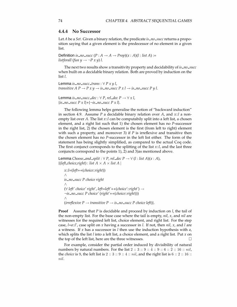
74 CHAPTER 4. ABSTRACT SEQUENTIAL GAMES
4.4.4 No Successor
LetA be a Set. Given a binary relation, the predicate is no succ returns a propo-sition saying that a given element is the predecessor of no element in a givenlist.
Definition is no succ (P : A→ A→ Prop)(x : A)(l : list A) :=listforall (fun y→ ¬P x y) l.
The next two results show a transitivity property and decidability of is no succwhen built on a decidable binary relation. Both are proved by induction on thelist l.
Lemma is no succ trans : ∀ P x y l,transitive A P→ P x y→ is no succ P x l→ is no succ P y l.
Lemma is no succ dec : ∀ P, rel dec P→ ∀ x l,{is no succ P x l}+{¬is no succ P x l}.
The following lemma helps generalise the notion of “backward induction”in section 4.9. Assume P a decidable binary relation over A, and x::l a non-empty list over A. The list x::l can be computabily split into a left list, a chosenelement, and a right list such that 1) the chosen element has no P-successorin the right list, 2) the chosen element is the first (from left to right) elementwith such a property, and moreover 3) if P is irreflexive and transitive thenthe chosen element has no P-successor in the left list either. The form of thestatement has being slightly simplified, as compared to the actual Coq code.The first conjunct corresponds to the splitting of the list x::l, and the last threeconjuncts correspond to the points 1), 2) and 3)as mentioned above.
Lemma Choose and split : ∀ P, rel dec P→ ∀ (l : list A)(x : A),{(left,choice,right) : list A × A × list A |
x::l=(left++(choice::right))∧is no succ P choice right∧(∀ left’ choice’ right’, left=left’++(choice’::right’)→¬is no succ P choice’ (right’++(choice::right)))∧(irreflexive P→ transitive P→ is no succ P choice left)}.
Proof Assume that P is decidable and proceed by induction on l, the tail ofthe non-empty list. For the base case where the tail is empty, nil, x, and nil arewitnesses for the required left list, choice element, and right list. For the stepcase, l=a::l’, case split on x having a successor in l. If not, then nil, x, and l area witness. If x has a successor in l then use the induction hypothesis with a,which splits the list l into a left list, a choice element, and a right list. Put x onthe top of the left list, here are the three witnesses. �
For example, consider the partial order induced by divisibility of naturalnumbers by natural numbers. For the list 2 :: 3 :: 9 :: 4 :: 9 :: 6 :: 2 :: 16 :: nil,the choice is 9, the left list is 2 :: 3 :: 9 :: 4 :: nil, and the right list is 6 :: 2 :: 16 ::nil.
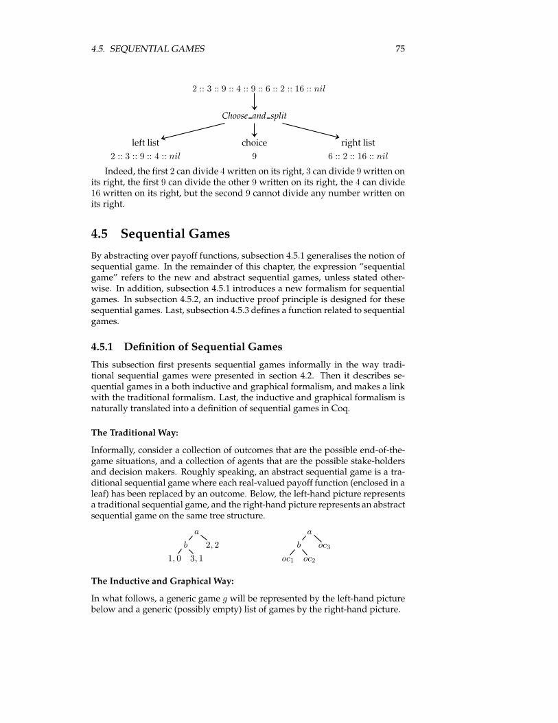
4.5. SEQUENTIAL GAMES 75
2 :: 3 :: 9 :: 4 :: 9 :: 6 :: 2 :: 16 :: nil
Choose and split
left list choice right list2 :: 3 :: 9 :: 4 :: nil 9 6 :: 2 :: 16 :: nil
Indeed, the first 2 can divide 4written on its right, 3 can divide 9written onits right, the first 9 can divide the other 9 written on its right, the 4 can divide16 written on its right, but the second 9 cannot divide any number written onits right.
4.5 Sequential Games
By abstracting over payoff functions, subsection 4.5.1 generalises the notion ofsequential game. In the remainder of this chapter, the expression “sequentialgame” refers to the new and abstract sequential games, unless stated other-wise. In addition, subsection 4.5.1 introduces a new formalism for sequentialgames. In subsection 4.5.2, an inductive proof principle is designed for thesesequential games. Last, subsection 4.5.3 defines a function related to sequentialgames.
4.5.1 Definition of Sequential Games
This subsection first presents sequential games informally in the way tradi-tional sequential games were presented in section 4.2. Then it describes se-quential games in a both inductive and graphical formalism, and makes a linkwith the traditional formalism. Last, the inductive and graphical formalism isnaturally translated into a definition of sequential games in Coq.
The Traditional Way:
Informally, consider a collection of outcomes that are the possible end-of-the-game situations, and a collection of agents that are the possible stake-holdersand decision makers. Roughly speaking, an abstract sequential game is a tra-ditional sequential game where each real-valued payoff function (enclosed in aleaf) has been replaced by an outcome. Below, the left-hand picture representsa traditional sequential game, and the right-hand picture represents an abstractsequential game on the same tree structure.
a a
b 2, 2 b oc3
1, 0 3, 1 oc1 oc2
The Inductive and Graphical Way:
In what follows, a generic game g will be represented by the left-hand picturebelow and a generic (possibly empty) list of games by the right-hand picture.
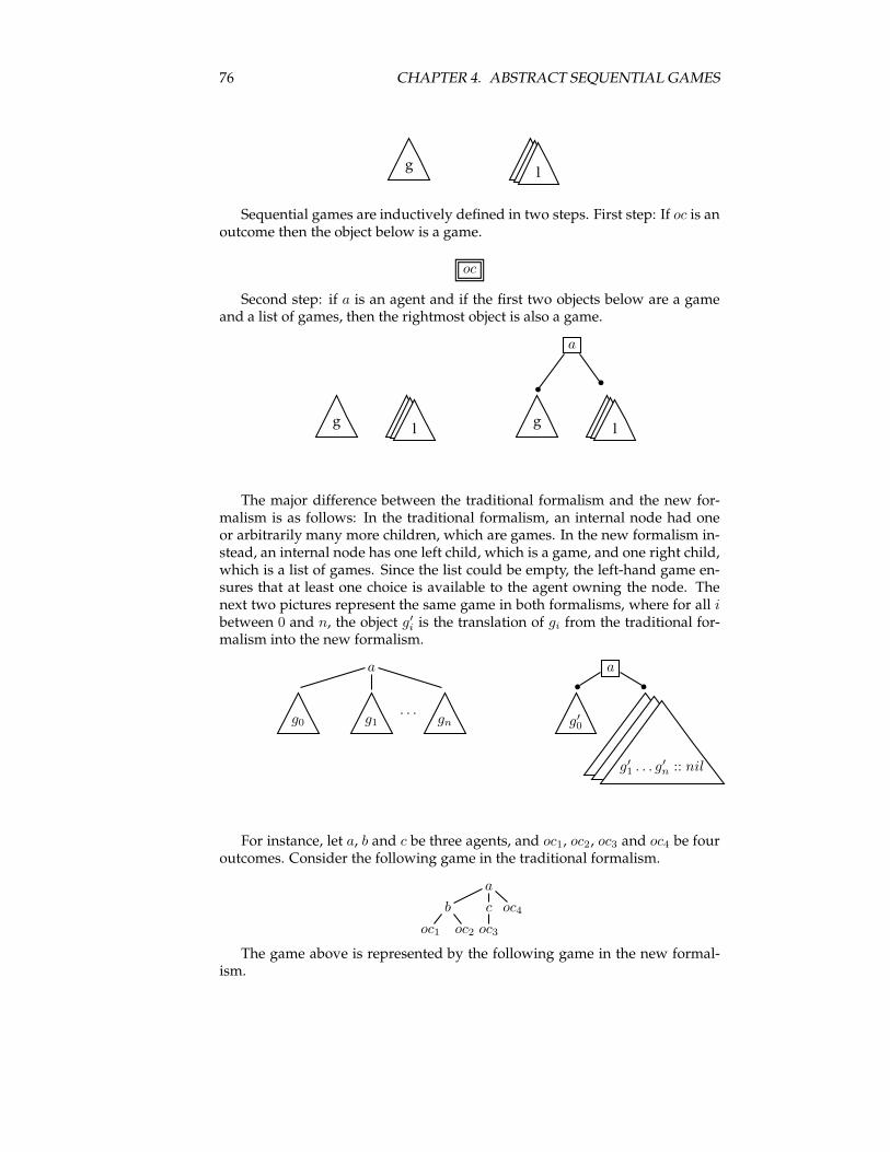
76 CHAPTER 4. ABSTRACT SEQUENTIAL GAMES
g l
Sequential games are inductively defined in two steps. First step: If oc is anoutcome then the object below is a game.
oc
Second step: if a is an agent and if the first two objects below are a gameand a list of games, then the rightmost object is also a game.
a
g l g l
The major difference between the traditional formalism and the new for-malism is as follows: In the traditional formalism, an internal node had oneor arbitrarily many more children, which are games. In the new formalism in-stead, an internal node has one left child, which is a game, and one right child,which is a list of games. Since the list could be empty, the left-hand game en-sures that at least one choice is available to the agent owning the node. Thenext two pictures represent the same game in both formalisms, where for all ibetween 0 and n, the object g′i is the translation of gi from the traditional for-malism into the new formalism.
a a
g0 g1. . .
gn g′0
g′1 . . . g′n :: nil
For instance, let a, b and c be three agents, and oc1, oc2, oc3 and oc4 be fouroutcomes. Consider the following game in the traditional formalism.
a
b c oc4
oc1 oc2 oc3
The game above is represented by the following game in the new formal-ism.
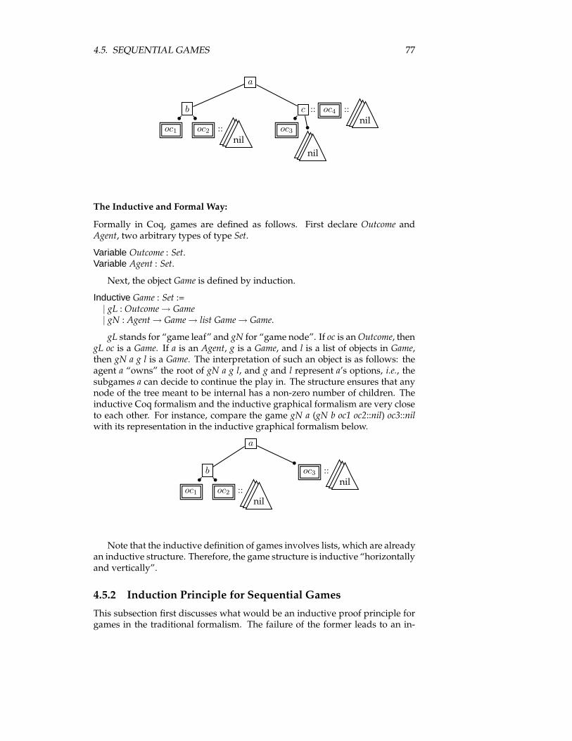
4.5. SEQUENTIAL GAMES 77
a
b c :: oc4 ::nil
oc1 oc2 ::nil
oc3
nil
The Inductive and Formal Way:
Formally in Coq, games are defined as follows. First declare Outcome andAgent, two arbitrary types of type Set.
Variable Outcome : Set.Variable Agent : Set.
Next, the object Game is defined by induction.
Inductive Game : Set :=| gL : Outcome→ Game| gN : Agent→ Game→ list Game→ Game.
gL stands for “game leaf” and gN for “game node”. If oc is anOutcome, thengL oc is a Game. If a is an Agent, g is a Game, and l is a list of objects in Game,then gN a g l is a Game. The interpretation of such an object is as follows: theagent a “owns” the root of gN a g l, and g and l represent a’s options, i.e., thesubgames a can decide to continue the play in. The structure ensures that anynode of the tree meant to be internal has a non-zero number of children. Theinductive Coq formalism and the inductive graphical formalism are very closeto each other. For instance, compare the game gN a (gN b oc1 oc2::nil) oc3::nilwith its representation in the inductive graphical formalism below.
a
b oc3 ::nil
oc1 oc2 ::nil
Note that the inductive definition of games involves lists, which are alreadyan inductive structure. Therefore, the game structure is inductive “horizontallyand vertically”.
4.5.2 Induction Principle for Sequential Games
This subsection first discusses what would be an inductive proof principle forgames in the traditional formalism. The failure of the former leads to an in-
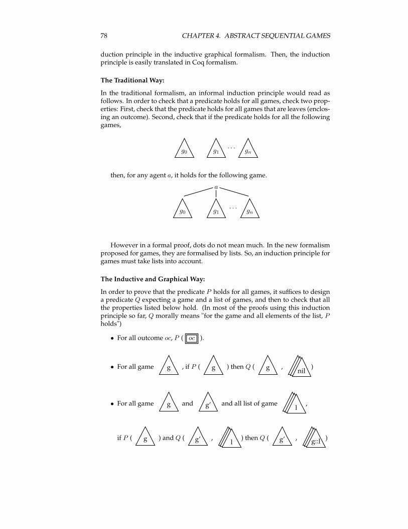
78 CHAPTER 4. ABSTRACT SEQUENTIAL GAMES
duction principle in the inductive graphical formalism. Then, the inductionprinciple is easily translated in Coq formalism.
The Traditional Way:
In the traditional formalism, an informal induction principle would read asfollows. In order to check that a predicate holds for all games, check two prop-erties: First, check that the predicate holds for all games that are leaves (enclos-ing an outcome). Second, check that if the predicate holds for all the followinggames,
g0 g1. . .
gn
then, for any agent a, it holds for the following game.
a
g0 g1. . .
gn
However in a formal proof, dots do not mean much. In the new formalismproposed for games, they are formalised by lists. So, an induction principle forgames must take lists into account.
The Inductive and Graphical Way:
In order to prove that the predicate P holds for all games, it suffices to designa predicate Q expecting a game and a list of games, and then to check that allthe properties listed below hold. (In most of the proofs using this inductionprinciple so far, Q morally means "for the game and all elements of the list, Pholds")
• For all outcome oc, P ( oc ).
• For all game g , if P ( g ) then Q ( g ,nil
)
• For all game g and g’ and all list of gamel,
if P ( g ) and Q ( g’ ,l) then Q ( g’ , g::l )
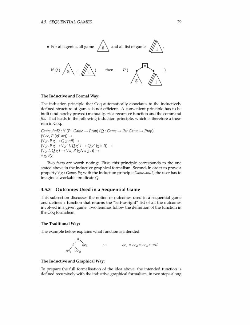
4.5. SEQUENTIAL GAMES 79
• For all agent a, all game g and all list of gamel,
if Q ( g ,l) then P (
a
g l
)
The Inductive and Formal Way:
The induction principle that Coq automatically associates to the inductivelydefined structure of games is not efficient. A convenient principle has to bebuilt (and hereby proved) manually, via a recursive function and the commandfix. That leads to the following induction principle, which is therefore a theo-rem in Coq.
Game ind2 : ∀ (P : Game→ Prop) (Q : Game→ list Game→ Prop),(∀ oc, P (gL oc))→(∀ g, P g→ Q g nil)→(∀ g, P g→ ∀ g’ l, Q g’ l→ Q g’ (g :: l))→(∀ g l, Q g l→ ∀ a, P (gN a g l))→∀ g, Pg
Two facts are worth noting: First, this principle corresponds to the onestated above in the inductive graphical formalism. Second, in order to prove aproperty ∀ g : Game, Pgwith the induction principle Game ind2, the user has toimagine a workable predicateQ.
4.5.3 Outcomes Used in a Sequential Game
This subsection discusses the notion of outcomes used in a sequential gameand defines a function that returns the “left-to-right” list of all the outcomesinvolved in a given game. Two lemmas follow the definition of the function inthe Coq formalism.
The Traditional Way:
The example below explains what function is intended.
a
b oc3 oc1 :: oc2 :: oc3 :: nil
oc1 oc2
The Inductive and Graphical Way:
To prepare the full formalisation of the idea above, the intended function isdefined recursively with the inductive graphical formalism, in two steps along
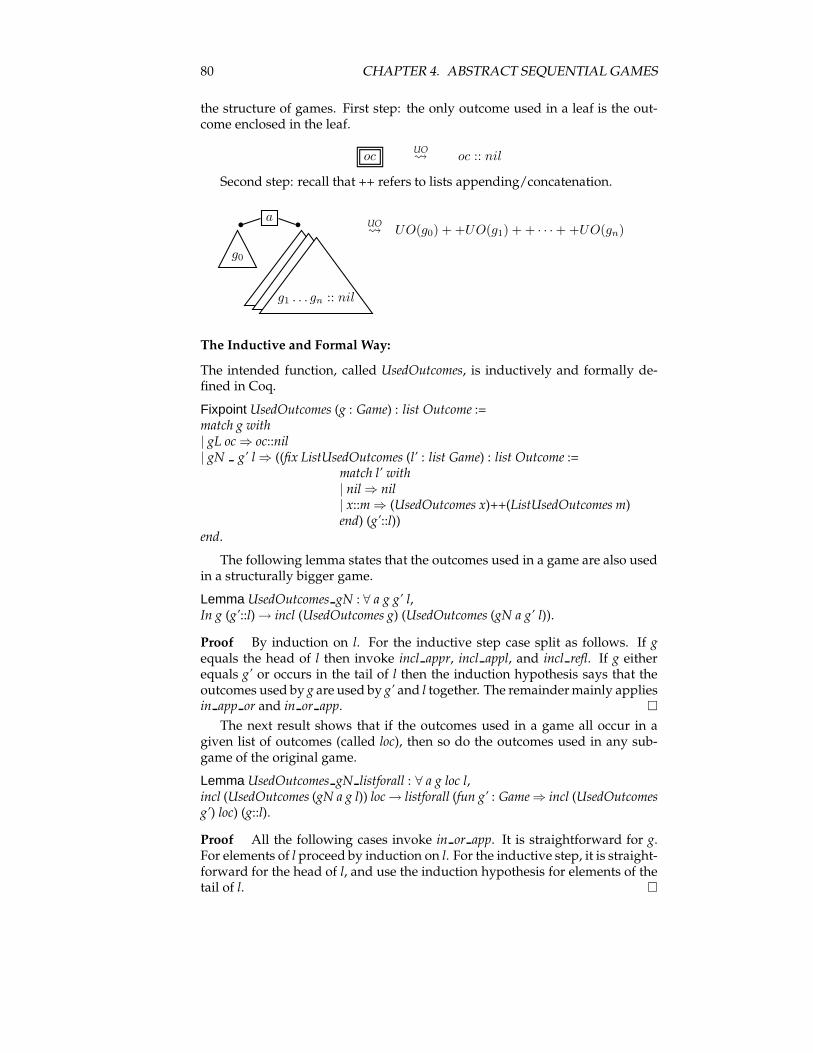
80 CHAPTER 4. ABSTRACT SEQUENTIAL GAMES
the structure of games. First step: the only outcome used in a leaf is the out-come enclosed in the leaf.
ocUO oc :: nil
Second step: recall that ++ refers to lists appending/concatenation.
a
g0
g1 . . . gn :: nil
UO UO(g0) + +UO(g1) + + · · ·+ +UO(gn)
The Inductive and Formal Way:
The intended function, called UsedOutcomes, is inductively and formally de-fined in Coq.
Fixpoint UsedOutcomes (g : Game) : list Outcome :=match g with| gL oc⇒ oc::nil| gN g’ l⇒ ((fix ListUsedOutcomes (l’ : list Game) : list Outcome :=
match l’ with| nil⇒ nil| x::m⇒ (UsedOutcomes x)++(ListUsedOutcomes m)end) (g’::l))
end.
The following lemma states that the outcomes used in a game are also usedin a structurally bigger game.
Lemma UsedOutcomes gN : ∀ a g g’ l,In g (g’::l)→ incl (UsedOutcomes g) (UsedOutcomes (gN a g’ l)).
Proof By induction on l. For the inductive step case split as follows. If gequals the head of l then invoke incl appr, incl appl, and incl refl. If g eitherequals g’ or occurs in the tail of l then the induction hypothesis says that theoutcomes used by g are used by g’ and l together. The remaindermainly appliesin app or and in or app. �
The next result shows that if the outcomes used in a game all occur in agiven list of outcomes (called loc), then so do the outcomes used in any sub-game of the original game.
Lemma UsedOutcomes gN listforall : ∀ a g loc l,incl (UsedOutcomes (gN a g l)) loc→ listforall (fun g’ : Game⇒ incl (UsedOutcomesg’) loc) (g::l).
Proof All the following cases invoke in or app. It is straightforward for g.For elements of l proceed by induction on l. For the inductive step, it is straight-forward for the head of l, and use the induction hypothesis for elements of thetail of l. �
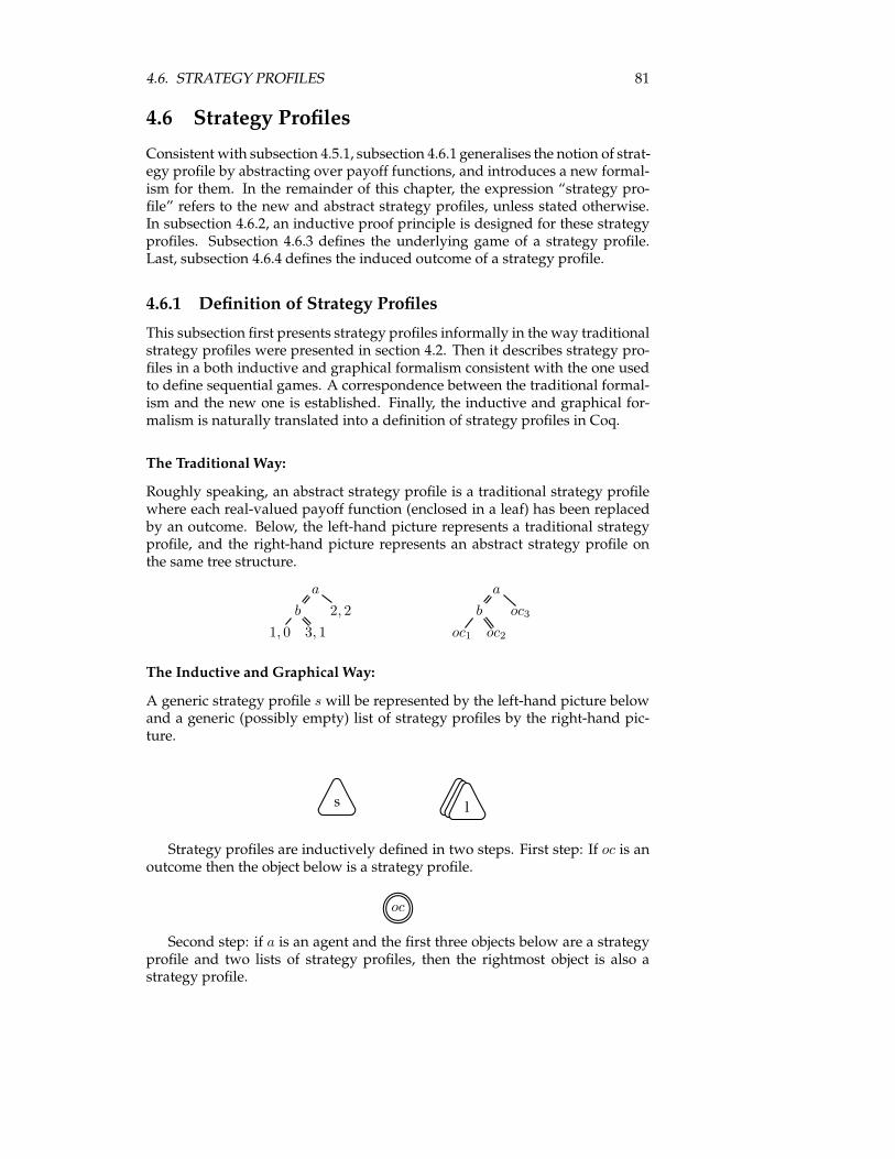
4.6. STRATEGY PROFILES 81
4.6 Strategy Profiles
Consistent with subsection 4.5.1, subsection 4.6.1 generalises the notion of strat-egy profile by abstracting over payoff functions, and introduces a new formal-ism for them. In the remainder of this chapter, the expression “strategy pro-file” refers to the new and abstract strategy profiles, unless stated otherwise.In subsection 4.6.2, an inductive proof principle is designed for these strategyprofiles. Subsection 4.6.3 defines the underlying game of a strategy profile.Last, subsection 4.6.4 defines the induced outcome of a strategy profile.
4.6.1 Definition of Strategy Profiles
This subsection first presents strategy profiles informally in the way traditionalstrategy profiles were presented in section 4.2. Then it describes strategy pro-files in a both inductive and graphical formalism consistent with the one usedto define sequential games. A correspondence between the traditional formal-ism and the new one is established. Finally, the inductive and graphical for-malism is naturally translated into a definition of strategy profiles in Coq.
The Traditional Way:
Roughly speaking, an abstract strategy profile is a traditional strategy profilewhere each real-valued payoff function (enclosed in a leaf) has been replacedby an outcome. Below, the left-hand picture represents a traditional strategyprofile, and the right-hand picture represents an abstract strategy profile onthe same tree structure.
a a
b 2, 2 b oc3
1, 0 3, 1 oc1 oc2
The Inductive and Graphical Way:
A generic strategy profile s will be represented by the left-hand picture belowand a generic (possibly empty) list of strategy profiles by the right-hand pic-ture.
s l
Strategy profiles are inductively defined in two steps. First step: If oc is anoutcome then the object below is a strategy profile.
oc
Second step: if a is an agent and the first three objects below are a strategyprofile and two lists of strategy profiles, then the rightmost object is also astrategy profile.
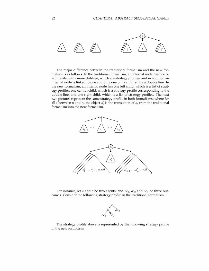
82 CHAPTER 4. ABSTRACT SEQUENTIAL GAMES
a
s l l’ l s l’
The major difference between the traditional formalism and the new for-malism is as follows: In the traditional formalism, an internal node has one orarbitrarily many more children, which are strategy profiles, and in addition aninternal node is linked to one and only one of its children by a double line. Inthe new formalism, an internal node has one left child, which is a list of strat-egy profiles, one central child, which is a strategy profile corresponding to thedouble line, and one right child, which is a list of strategy profiles. The nexttwo pictures represent the same strategy profile in both formalisms, where forall i between 0 and n, the object s′i is the translation of si from the traditionalformalism into the new formalism.
a
s0. . .
si. . .
sn
a
s′0 . . . s′i−1 :: nil
s′i
s′i+1 . . . s′n :: nil
For instance, let a and b be two agents, and oc1, oc2 and oc3 be three out-comes. Consider the following strategy profile in the traditional formalism.
a
b oc3
oc1 oc2
The strategy profile above is represented by the following strategy profilein the new formalism.
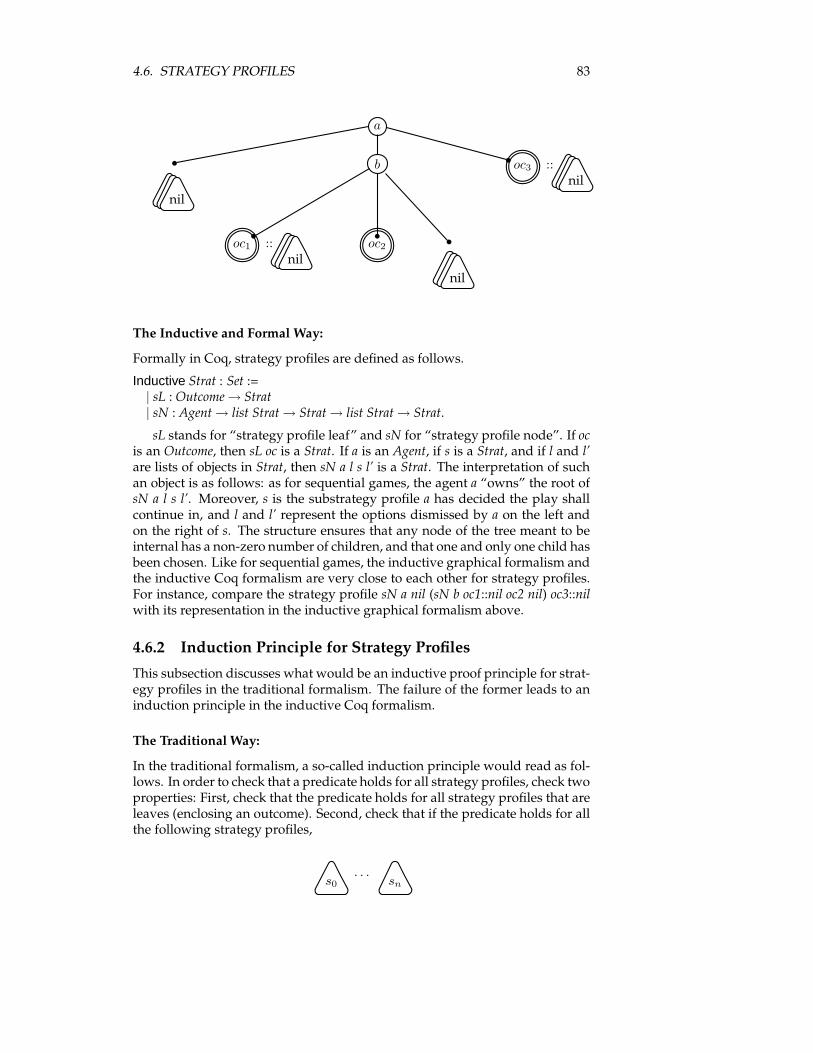
4.6. STRATEGY PROFILES 83
a
nil
b oc3 ::nil
oc1 ::nil
oc2
nil
The Inductive and Formal Way:
Formally in Coq, strategy profiles are defined as follows.
Inductive Strat : Set :=| sL : Outcome→ Strat| sN : Agent→ list Strat→ Strat→ list Strat→ Strat.
sL stands for “strategy profile leaf” and sN for “strategy profile node”. If ocis an Outcome, then sL oc is a Strat. If a is an Agent, if s is a Strat, and if l and l’are lists of objects in Strat, then sN a l s l’ is a Strat. The interpretation of suchan object is as follows: as for sequential games, the agent a “owns” the root ofsN a l s l’. Moreover, s is the substrategy profile a has decided the play shallcontinue in, and l and l’ represent the options dismissed by a on the left andon the right of s. The structure ensures that any node of the tree meant to beinternal has a non-zero number of children, and that one and only one child hasbeen chosen. Like for sequential games, the inductive graphical formalism andthe inductive Coq formalism are very close to each other for strategy profiles.For instance, compare the strategy profile sN a nil (sN b oc1::nil oc2 nil) oc3::nilwith its representation in the inductive graphical formalism above.
4.6.2 Induction Principle for Strategy Profiles
This subsection discusses what would be an inductive proof principle for strat-egy profiles in the traditional formalism. The failure of the former leads to aninduction principle in the inductive Coq formalism.
The Traditional Way:
In the traditional formalism, a so-called induction principle would read as fol-lows. In order to check that a predicate holds for all strategy profiles, check twoproperties: First, check that the predicate holds for all strategy profiles that areleaves (enclosing an outcome). Second, check that if the predicate holds for allthe following strategy profiles,
s0. . .
sn
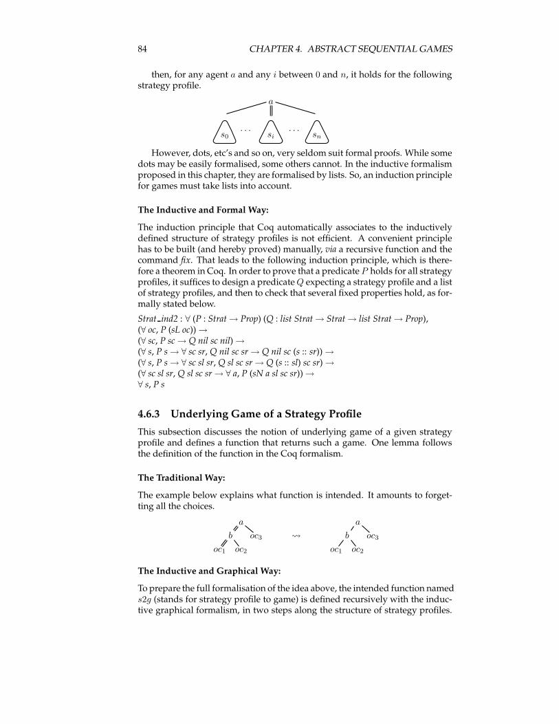
84 CHAPTER 4. ABSTRACT SEQUENTIAL GAMES
then, for any agent a and any i between 0 and n, it holds for the followingstrategy profile.
a
s0. . .
si
. . .sn
However, dots, etc’s and so on, very seldom suit formal proofs. While somedots may be easily formalised, some others cannot. In the inductive formalismproposed in this chapter, they are formalised by lists. So, an induction principlefor games must take lists into account.
The Inductive and Formal Way:
The induction principle that Coq automatically associates to the inductivelydefined structure of strategy profiles is not efficient. A convenient principlehas to be built (and hereby proved) manually, via a recursive function and thecommand fix. That leads to the following induction principle, which is there-fore a theorem in Coq. In order to prove that a predicate P holds for all strategyprofiles, it suffices to design a predicateQ expecting a strategy profile and a listof strategy profiles, and then to check that several fixed properties hold, as for-mally stated below.
Strat ind2 : ∀ (P : Strat→ Prop) (Q : list Strat→ Strat→ list Strat→ Prop),(∀ oc, P (sL oc))→(∀ sc, P sc→ Q nil sc nil)→(∀ s, P s→ ∀ sc sr, Q nil sc sr→ Q nil sc (s :: sr))→(∀ s, P s→ ∀ sc sl sr, Q sl sc sr→ Q (s :: sl) sc sr)→(∀ sc sl sr, Q sl sc sr→ ∀ a, P (sN a sl sc sr))→∀ s, P s
4.6.3 Underlying Game of a Strategy Profile
This subsection discusses the notion of underlying game of a given strategyprofile and defines a function that returns such a game. One lemma followsthe definition of the function in the Coq formalism.
The Traditional Way:
The example below explains what function is intended. It amounts to forget-ting all the choices.
a a
b oc3 b oc3
oc1 oc2 oc1 oc2
The Inductive and Graphical Way:
To prepare the full formalisation of the idea above, the intended function nameds2g (stands for strategy profile to game) is defined recursively with the induc-tive graphical formalism, in two steps along the structure of strategy profiles.
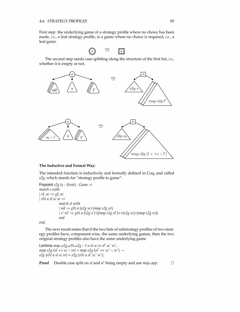
4.6. STRATEGY PROFILES 85
First step: the underlying game of a strategy profile where no choice has beenmade, i.e., a leaf strategy profile, is a game where no choice is required, i.e., aleaf game.
as2g a
The second step needs case splitting along the structure of the first list, i.e.,whether it is empty or not.
a a
nil s l’
s2g
s2g s
map s2g l′
a a
s0 :: l s l’
s2g
s2g s0
map s2g (l + +s :: l′)
The Inductive and Formal Way:
The intended function is inductively and formally defined in Coq, and calleds2g, which stands for “strategy profile to game”.
Fixpoint s2g (s : Strat) : Game :=match s with| sL oc⇒ gL oc| sN a sl sc sr⇒
match sl with| nil⇒ gN a (s2g sc) (map s2g sr)| s’::sl’⇒ gN a (s2g s’) ((map s2g sl’)++(s2g sc)::(map s2g sr))end
end.
The next result states that if the two lists of substrategy profiles of two strat-egy profiles have, component-wise, the same underlying games, then the twooriginal strategy profiles also have the same underlying game.
Lemma map s2g sN s2g : ∀ a sl sc sr sl’ sc’ sr’,map s2g (sl ++ sc :: sr) = map s2g (sl’ ++ sc’ :: sr’)→s2g (sN a sl sc sr) = s2g (sN a sl’ sc’ sr’).
Proof Double case split on sl and sl’ being empty and use map app. �
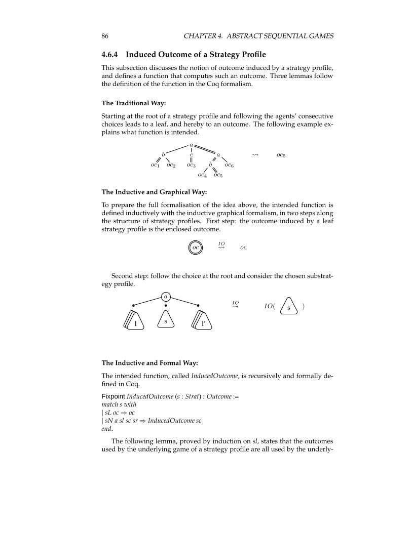
86 CHAPTER 4. ABSTRACT SEQUENTIAL GAMES
4.6.4 Induced Outcome of a Strategy Profile
This subsection discusses the notion of outcome induced by a strategy profile,and defines a function that computes such an outcome. Three lemmas followthe definition of the function in the Coq formalism.
The Traditional Way:
Starting at the root of a strategy profile and following the agents’ consecutivechoices leads to a leaf, and hereby to an outcome. The following example ex-plains what function is intended.
a
b c a oc5
oc1 oc2 oc3 b oc6
oc4 oc5
The Inductive and Graphical Way:
To prepare the full formalisation of the idea above, the intended function isdefined inductively with the inductive graphical formalism, in two steps alongthe structure of strategy profiles. First step: the outcome induced by a leafstrategy profile is the enclosed outcome.
ocIO oc
Second step: follow the choice at the root and consider the chosen substrat-egy profile.
a
l s l’
IO IO( s )
The Inductive and Formal Way:
The intended function, called InducedOutcome, is recursively and formally de-fined in Coq.
Fixpoint InducedOutcome (s : Strat) : Outcome :=match s with| sL oc⇒ oc| sN a sl sc sr⇒ InducedOutcome scend.
The following lemma, proved by induction on sl, states that the outcomesused by the underlying game of a strategy profile are all used by the underly-

4.7. CONVERTIBILITY 87
ing game of a bigger strategy profile whose chosen substrategy profile is theoriginal strategy profile.
Lemma UsedOutcomes sN incl : ∀ a sl sc sr,incl (UsedOutcomes (s2g sc)) (UsedOutcomes (s2g (sN a sl sc sr))).
The next result says that the outcome induced by a strategy profile is alsoan outcome used in the underlying game.
Lemma Used Induced Outcomes : ∀ s : Strat,In (InducedOutcome s) (UsedOutcomes (s2g s)).
Proof Write the claim as a predicate on s and apply the induction principleStrat ind2whereQ l s l’ is In (InducedOutcome s) (UsedOutcomes (s2g s)). For thelast induction case invoke UsedOutcomes sN incl. �
Note that if the underlying game of a strategy profile is a leaf game enclos-ing a given outcome, then the strategy profile is a leaf strategy profile enclosingthe same outcome, so that the outcome induced by the strategy profile is alsothe same outcome: if s2g s=gL oc then InducedOutcome s=oc. The followinglemma is the list version of the remark above. It is prove by induction on ls.
Lemma map s2g gL InducedOutcome : ∀ ls loc,map s2g ls =map (fun y⇒ gL y) loc→ map InducedOutcome ls = loc.
4.7 Convertibility
The first subsection defines convertibility, whichwill be used to formally definethe notion of Nash equilibrium in section 4.8. The second subsection designsan inductive proof principle for convertibility.
4.7.1 Definition of Convertibility
This subsection discusses the notion of convertibility, which is the ability of anagent to convert a strategy profile into another strategy profile, and defines apredicate accounting for it. Four lemmas follow its definition in Coq.
The Traditional Way:
An agent is (usually implicitly) granted the ability to simultaneously changehis choices at all nodes that he owns. The following example shows one pos-sible such change: agent b changes his choices exactly at the nodes where b isdisplayed in bold font.
a a
b b bConv b←→ b b b
oc1 a oc4 b oc7 oc8 oc1 a oc4 b oc7 oc8
oc2 oc3 oc5 oc6 oc2 oc3 oc5 oc6
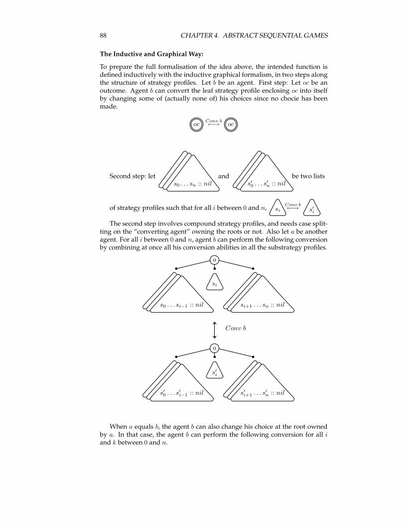
88 CHAPTER 4. ABSTRACT SEQUENTIAL GAMES
The Inductive and Graphical Way:
To prepare the full formalisation of the idea above, the intended function isdefined inductively with the inductive graphical formalism, in two steps alongthe structure of strategy profiles. Let b be an agent. First step: Let oc be anoutcome. Agent b can convert the leaf strategy profile enclosing oc into itselfby changing some of (actually none of) his choices since no chocie has beenmade.
ocConv b←→ oc
Second step: lets0 . . . sn :: nil
ands′0 . . . s′n :: nil
be two lists
of strategy profiles such that for all i between 0 and n, si
Conv b←→ s′i
The second step involves compound strategy profiles, and needs case split-ting on the “converting agent” owning the roots or not. Also let a be anotheragent. For all i between 0 and n, agent b can perform the following conversionby combining at once all his conversion abilities in all the substrategy profiles.
a
s0 . . . si−1 :: nil
si
si+1 . . . sn :: nil
Conv b
a
s′0 . . . s′i−1 :: nil
s′i
s′i+1 . . . s′n :: nil
When a equals b, the agent b can also change his choice at the root ownedby a. In that case, the agent b can perform the following conversion for all iand k between 0 and n.
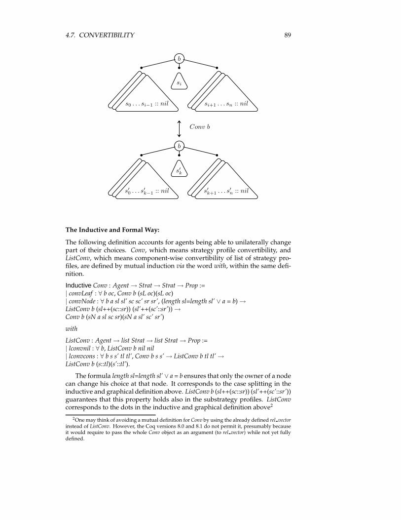
4.7. CONVERTIBILITY 89
b
s0 . . . si−1 :: nil
si
si+1 . . . sn :: nil
Conv b
b
s′0 . . . s′k−1 :: nil
s′k
s′k+1 . . . s′n :: nil
The Inductive and Formal Way:
The following definition accounts for agents being able to unilaterally changepart of their choices. Conv, which means strategy profile convertibility, andListConv, which means component-wise convertibility of list of strategy pro-files, are defined by mutual induction via the word with, within the same defi-nition.
Inductive Conv : Agent→ Strat→ Strat→ Prop :=| convLeaf : ∀ b oc, Conv b (sL oc)(sL oc)| convNode : ∀ b a sl sl’ sc sc’ sr sr’, (length sl=length sl’ ∨ a = b)→ListConv b (sl++(sc::sr)) (sl’++(sc’::sr’))→Conv b (sN a sl sc sr)(sN a sl’ sc’ sr’)
with
ListConv : Agent→ list Strat→ list Strat→ Prop :=| lconvnil : ∀ b, ListConv b nil nil| lconvcons : ∀ b s s’ tl tl’, Conv b s s’→ ListConv b tl tl’→ListConv b (s::tl)(s’::tl’).
The formula length sl=length sl’ ∨ a = b ensures that only the owner of a nodecan change his choice at that node. It corresponds to the case splitting in theinductive and graphical definition above. ListConv b (sl++(sc::sr)) (sl’++(sc’::sr’))guarantees that this property holds also in the substrategy profiles. ListConvcorresponds to the dots in the inductive and graphical definition above2
2Onemay think of avoiding a mutual definition for Conv by using the already defined rel vectorinstead of ListConv. However, the Coq versions 8.0 and 8.1 do not permit it, presumably becauseit would require to pass the whole Conv object as an argument (to rel vector) while not yet fullydefined.
90 CHAPTER 4. ABSTRACT SEQUENTIAL GAMES
The following two lemmas establish the equivalence between ListConv onthe one hand and rel vector and Conv on the other hand. They are both provedby induction on the list l and by a case splitting on l’.
Lemma ListConv rel vector : ∀ a l l’,ListConv a l l’→ rel vector (Conv a) l l’.
Lemma rel vector ListConv : ∀ a l l’,rel vector (Conv a) l l’→ ListConv a l l’ .
The next two results state reflexivity property of Conv and ListConv.
Lemma Conv refl : ∀ a s , Conv a s s.
Proof Let a be an agent and s a strategy profile. It suffices to prove that P swhere P s’ is Conv a s’ s’ by definition. Apply the induction principle Strat ind2where Q sl sc sr is ListConv a (sl++sc::sr) (sl++sc::sr) by definition. Checking allcases is straightforward. �
Lemma ListConv refl : ∀ a l, ListConv a l l.
Proof By rel vector ListConv, induction on the list l, and Conv refl. �
4.7.2 Induction Principle for Convertibility
The Inductive and Formal Way:
A suitable induction principle for convertibility is automatically generated inCoq with the command Scheme, and hereby is a theorem in Coq. The principlestates that under four conditions, Conv a is a subrelation of the binary relationP a for all agents a. Note that in order to prove such a property, the user has toimagine a workable predicate P0.
conv lconv ind : ∀ (P : Agent→ Strat→ Strat→ Prop)(P0 : Agent→ list Strat→ list Strat→ Prop),
(∀ b oc, P b (sL oc) (sL oc))→
(∀ b a sl sl’ sc sc’ sr sr’, length sl = length sl’ ∨ a = b→ ListConv b (sl ++ sc :: sr) (sl’++ sc’ :: sr’)→ P0 b (sl ++ sc :: sr) (sl’ ++ sc’ :: sr’)→ P b (sN a sl sc sr) (sN a sl’ sc’sr’))→
(∀ b, P0 b nil nil)→
(∀ b s s’ tl tl’, Conv b s s’→ P b s s’→ ListConv b tl tl’→ P0 b tl tl’→ P0 b (s :: tl)(s’ :: tl’))→
∀ a s s0, Conv a s s0→ P a s s0
This induction principle is used below to prove that two convertible strat-egy profiles have the same underlying game.
Lemma Conv s2g : ∀ (a : Agent)(s s’ : Strat), Conv a s s’→ s2g s = s2g s’.
Proof Assume s and s’ convertible by a. Write s2g s = s2g s’ as P a s s’ forsome P and proceed by the induction principle conv lconv ind where P0 b l l’is (ListConv b l l’→ map s2g l=map s2g l’) by definition. The remainder invokesmap s2g sN s2g. �
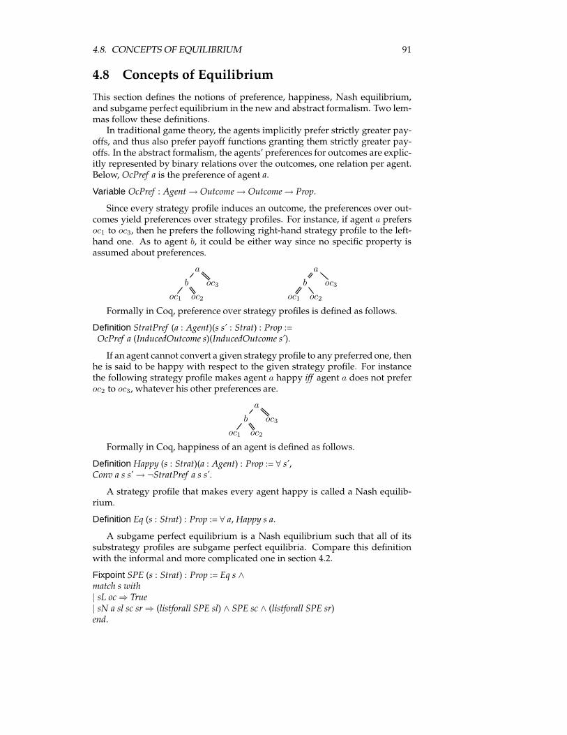
4.8. CONCEPTS OF EQUILIBRIUM 91
4.8 Concepts of Equilibrium
This section defines the notions of preference, happiness, Nash equilibrium,and subgame perfect equilibrium in the new and abstract formalism. Two lem-mas follow these definitions.In traditional game theory, the agents implicitly prefer strictly greater pay-
offs, and thus also prefer payoff functions granting them strictly greater pay-offs. In the abstract formalism, the agents’ preferences for outcomes are explic-itly represented by binary relations over the outcomes, one relation per agent.Below, OcPref a is the preference of agent a.
Variable OcPref : Agent→ Outcome→ Outcome→ Prop.
Since every strategy profile induces an outcome, the preferences over out-comes yield preferences over strategy profiles. For instance, if agent a prefersoc1 to oc3, then he prefers the following right-hand strategy profile to the left-hand one. As to agent b, it could be either way since no specific property isassumed about preferences.
a a
b oc3 b oc3
oc1 oc2 oc1 oc2
Formally in Coq, preference over strategy profiles is defined as follows.
Definition StratPref (a : Agent)(s s’ : Strat) : Prop :=OcPref a (InducedOutcome s)(InducedOutcome s’).
If an agent cannot convert a given strategy profile to any preferred one, thenhe is said to be happy with respect to the given strategy profile. For instancethe following strategy profile makes agent a happy iff agent a does not preferoc2 to oc3, whatever his other preferences are.
a
b oc3
oc1 oc2
Formally in Coq, happiness of an agent is defined as follows.
Definition Happy (s : Strat)(a : Agent) : Prop := ∀ s’,Conv a s s’→ ¬StratPref a s s’.
A strategy profile that makes every agent happy is called a Nash equilib-rium.
Definition Eq (s : Strat) : Prop := ∀ a, Happy s a.
A subgame perfect equilibrium is a Nash equilibrium such that all of itssubstrategy profiles are subgame perfect equilibria. Compare this definitionwith the informal and more complicated one in section 4.2.
Fixpoint SPE (s : Strat) : Prop := Eq s ∧match s with| sL oc⇒ True| sN a sl sc sr⇒ (listforall SPE sl) ∧ SPE sc ∧ (listforall SPE sr)end.
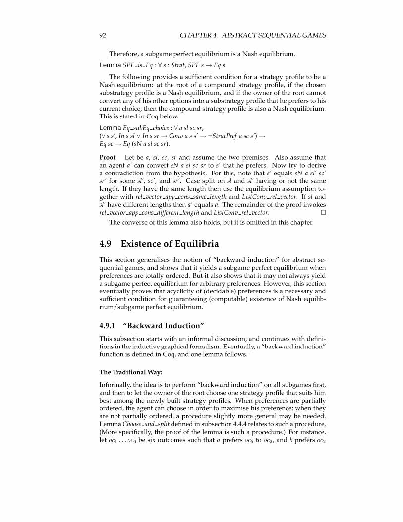
92 CHAPTER 4. ABSTRACT SEQUENTIAL GAMES
Therefore, a subgame perfect equilibrium is a Nash equilibrium.
Lemma SPE is Eq : ∀ s : Strat, SPE s→ Eq s.
The following provides a sufficient condition for a strategy profile to be aNash equilibrium: at the root of a compound strategy profile, if the chosensubstrategy profile is a Nash equilibrium, and if the owner of the root cannotconvert any of his other options into a substrategy profile that he prefers to hiscurrent choice, then the compound strategy profile is also a Nash equilibrium.This is stated in Coq below.
Lemma Eq subEq choice : ∀ a sl sc sr,(∀ s s’, In s sl ∨ In s sr→ Conv a s s’→ ¬StratPref a sc s’)→Eq sc→ Eq (sN a sl sc sr).
Proof Let be a, sl, sc, sr and assume the two premises. Also assume thatan agent a’ can convert sN a sl sc sr to s’ that he prefers. Now try to derivea contradiction from the hypothesis. For this, note that s’ equals sN a sl’ sc’sr’ for some sl’, sc’, and sr’. Case split on sl and sl’ having or not the samelength. If they have the same length then use the equilibrium assumption to-gether with rel vector app cons same length and ListConv rel vector. If sl andsl’ have different lengths then a’ equals a. The remainder of the proof invokesrel vector app cons different length and ListConv rel vector. �
The converse of this lemma also holds, but it is omitted in this chapter.
4.9 Existence of Equilibria
This section generalises the notion of “backward induction” for abstract se-quential games, and shows that it yields a subgame perfect equilibrium whenpreferences are totally ordered. But it also shows that it may not always yielda subgame perfect equilibrium for arbitrary preferences. However, this sectioneventually proves that acyclicity of (decidable) preferences is a necessary andsufficient condition for guaranteeing (computable) existence of Nash equilib-rium/subgame perfect equilibrium.
4.9.1 “Backward Induction”
This subsection starts with an informal discussion, and continues with defini-tions in the inductive graphical formalism. Eventually, a “backward induction”function is defined in Coq, and one lemma follows.
The Traditional Way:
Informally, the idea is to perform “backward induction” on all subgames first,and then to let the owner of the root choose one strategy profile that suits himbest among the newly built strategy profiles. When preferences are partiallyordered, the agent can choose in order to maximise his preference; when theyare not partially ordered, a procedure slightly more general may be needed.LemmaChoose and split defined in subsection 4.4.4 relates to such a procedure.(More specifically, the proof of the lemma is such a procedure.) For instance,let oc1 . . . oc6 be six outcomes such that a prefers oc5 to oc2, and b prefers oc2
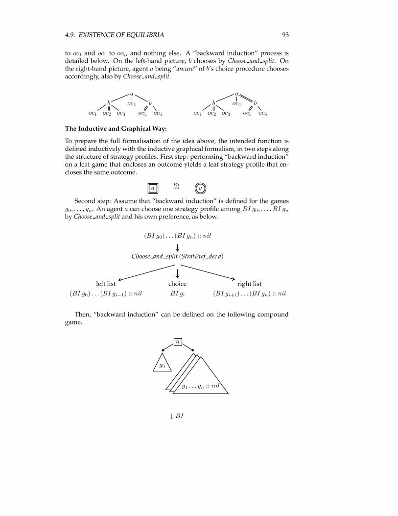
4.9. EXISTENCE OF EQUILIBRIA 93
to oc1 and oc1 to oc2, and nothing else. A “backward induction” process isdetailed below. On the left-hand picture, b chooses by Choose and split. Onthe right-hand picture, agent a being “aware” of b’s choice procedure choosesaccordingly, also by Choose and split.
a a
b oc4 b b oc4 b
oc1 oc2 oc3 oc5 oc6 oc1 oc2 oc3 oc5 oc6
The Inductive and Graphical Way:
To prepare the full formalisation of the idea above, the intended function isdefined inductively with the inductive graphical formalism, in two steps alongthe structure of strategy profiles. First step: performing “backward induction”on a leaf game that encloses an outcome yields a leaf strategy profile that en-closes the same outcome.
aBI a
Second step: Assume that “backward induction” is defined for the gamesg0, . . . , gn. An agent a can choose one strategy profile among BI g0, . . . , BI gn
by Choose and split and his own preference, as below.
(BI g0) . . . (BI gn) :: nil
Choose and split (StratPref dec a)
left list choice right list(BI g0) . . . (BI gi−1) :: nil BI gi (BI gi+1) . . . (BI gn) :: nil
Then, “backward induction” can be defined on the following compoundgame.
a
g0
g1 . . . gn :: nil
↓ BI
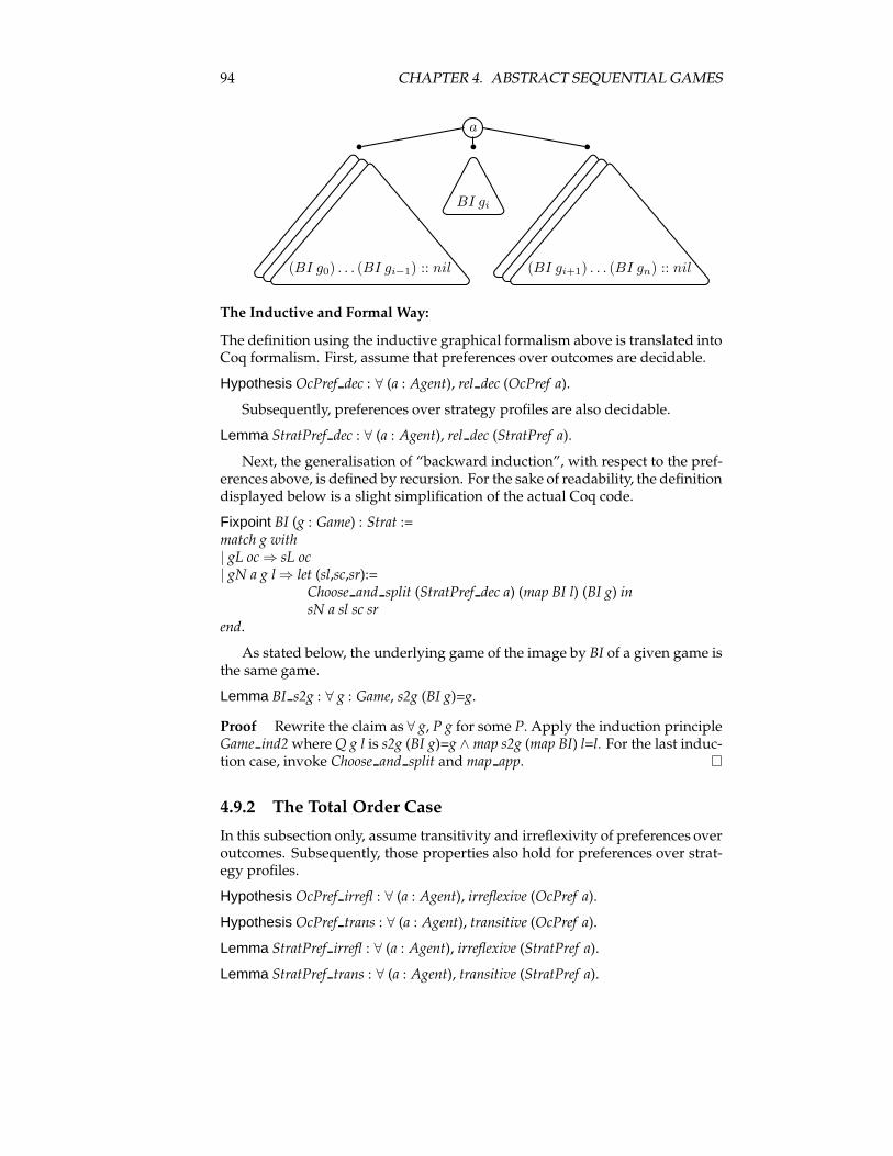
94 CHAPTER 4. ABSTRACT SEQUENTIAL GAMES
a
(BI g0) . . . (BI gi−1) :: nil
BI gi
(BI gi+1) . . . (BI gn) :: nil
The Inductive and Formal Way:
The definition using the inductive graphical formalism above is translated intoCoq formalism. First, assume that preferences over outcomes are decidable.
Hypothesis OcPref dec : ∀ (a : Agent), rel dec (OcPref a).
Subsequently, preferences over strategy profiles are also decidable.
Lemma StratPref dec : ∀ (a : Agent), rel dec (StratPref a).
Next, the generalisation of “backward induction”, with respect to the pref-erences above, is defined by recursion. For the sake of readability, the definitiondisplayed below is a slight simplification of the actual Coq code.
Fixpoint BI (g : Game) : Strat :=match g with| gL oc⇒ sL oc| gN a g l⇒ let (sl,sc,sr):=
Choose and split (StratPref dec a) (map BI l) (BI g) insN a sl sc sr
end.
As stated below, the underlying game of the image by BI of a given game isthe same game.
Lemma BI s2g : ∀ g : Game, s2g (BI g)=g.
Proof Rewrite the claim as ∀ g, P g for some P. Apply the induction principleGame ind2whereQ g l is s2g (BI g)=g ∧ map s2g (map BI) l=l. For the last induc-tion case, invoke Choose and split and map app. �
4.9.2 The Total Order Case
In this subsection only, assume transitivity and irreflexivity of preferences overoutcomes. Subsequently, those properties also hold for preferences over strat-egy profiles.
Hypothesis OcPref irrefl : ∀ (a : Agent), irreflexive (OcPref a).
Hypothesis OcPref trans : ∀ (a : Agent), transitive (OcPref a).
Lemma StratPref irrefl : ∀ (a : Agent), irreflexive (StratPref a).
Lemma StratPref trans : ∀ (a : Agent), transitive (StratPref a).
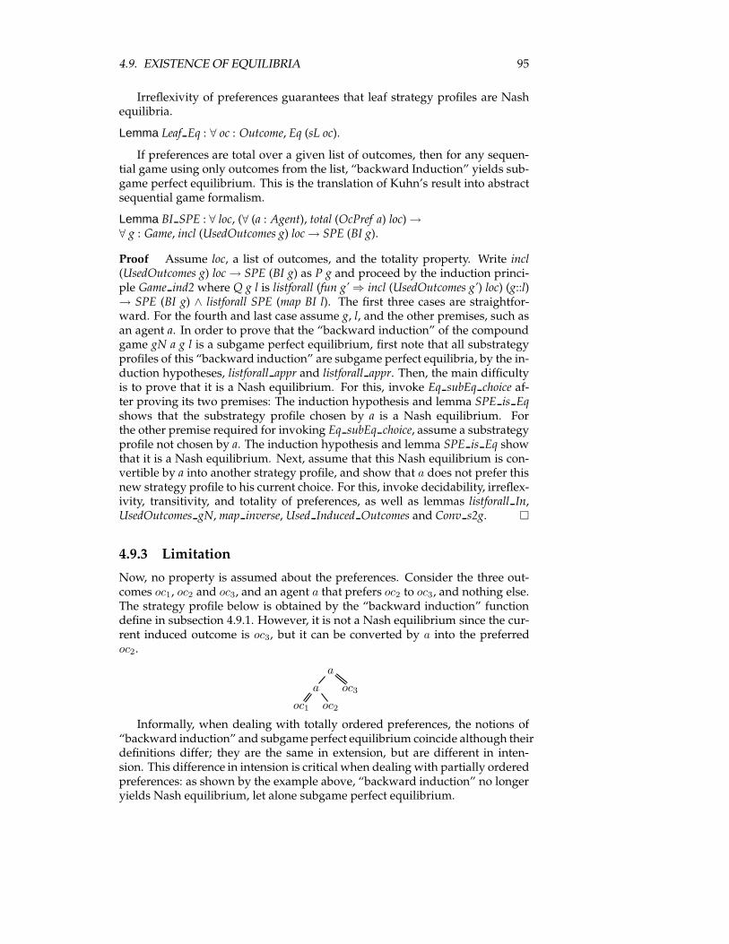
4.9. EXISTENCE OF EQUILIBRIA 95
Irreflexivity of preferences guarantees that leaf strategy profiles are Nashequilibria.
Lemma Leaf Eq : ∀ oc : Outcome, Eq (sL oc).
If preferences are total over a given list of outcomes, then for any sequen-tial game using only outcomes from the list, “backward Induction” yields sub-game perfect equilibrium. This is the translation of Kuhn’s result into abstractsequential game formalism.
Lemma BI SPE : ∀ loc, (∀ (a : Agent), total (OcPref a) loc)→∀ g : Game, incl (UsedOutcomes g) loc→ SPE (BI g).
Proof Assume loc, a list of outcomes, and the totality property. Write incl(UsedOutcomes g) loc→ SPE (BI g) as P g and proceed by the induction princi-ple Game ind2 where Q g l is listforall (fun g’⇒ incl (UsedOutcomes g’) loc) (g::l)→ SPE (BI g) ∧ listforall SPE (map BI l). The first three cases are straightfor-ward. For the fourth and last case assume g, l, and the other premises, such asan agent a. In order to prove that the “backward induction” of the compoundgame gN a g l is a subgame perfect equilibrium, first note that all substrategyprofiles of this “backward induction” are subgame perfect equilibria, by the in-duction hypotheses, listforall appr and listforall appr. Then, the main difficultyis to prove that it is a Nash equilibrium. For this, invoke Eq subEq choice af-ter proving its two premises: The induction hypothesis and lemma SPE is Eqshows that the substrategy profile chosen by a is a Nash equilibrium. Forthe other premise required for invoking Eq subEq choice, assume a substrategyprofile not chosen by a. The induction hypothesis and lemma SPE is Eq showthat it is a Nash equilibrium. Next, assume that this Nash equilibrium is con-vertible by a into another strategy profile, and show that a does not prefer thisnew strategy profile to his current choice. For this, invoke decidability, irreflex-ivity, transitivity, and totality of preferences, as well as lemmas listforall In,UsedOutcomes gN,map inverse, Used Induced Outcomes and Conv s2g. �
4.9.3 Limitation
Now, no property is assumed about the preferences. Consider the three out-comes oc1, oc2 and oc3, and an agent a that prefers oc2 to oc3, and nothing else.The strategy profile below is obtained by the “backward induction” functiondefine in subsection 4.9.1. However, it is not a Nash equilibrium since the cur-rent induced outcome is oc3, but it can be converted by a into the preferredoc2.
a
a oc3
oc1 oc2
Informally, when dealing with totally ordered preferences, the notions of“backward induction” and subgame perfect equilibrium coincide although theirdefinitions differ; they are the same in extension, but are different in inten-sion. This difference in intension is critical when dealing with partially orderedpreferences: as shown by the example above, “backward induction” no longeryields Nash equilibrium, let alone subgame perfect equilibrium.
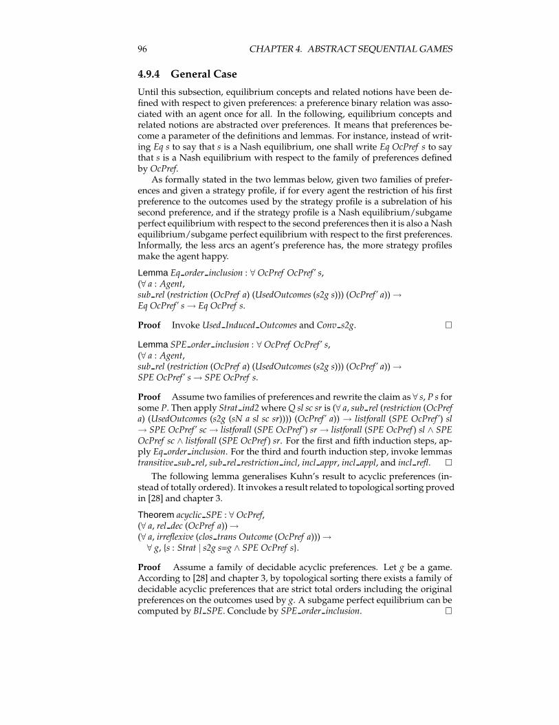
96 CHAPTER 4. ABSTRACT SEQUENTIAL GAMES
4.9.4 General Case
Until this subsection, equilibrium concepts and related notions have been de-fined with respect to given preferences: a preference binary relation was asso-ciated with an agent once for all. In the following, equilibrium concepts andrelated notions are abstracted over preferences. It means that preferences be-come a parameter of the definitions and lemmas. For instance, instead of writ-ing Eq s to say that s is a Nash equilibrium, one shall write Eq OcPref s to saythat s is a Nash equilibrium with respect to the family of preferences definedby OcPref.As formally stated in the two lemmas below, given two families of prefer-
ences and given a strategy profile, if for every agent the restriction of his firstpreference to the outcomes used by the strategy profile is a subrelation of hissecond preference, and if the strategy profile is a Nash equilibrium/subgameperfect equilibriumwith respect to the second preferences then it is also a Nashequilibrium/subgame perfect equilibrium with respect to the first preferences.Informally, the less arcs an agent’s preference has, the more strategy profilesmake the agent happy.
Lemma Eq order inclusion : ∀ OcPref OcPref’ s,(∀ a : Agent,sub rel (restriction (OcPref a) (UsedOutcomes (s2g s))) (OcPref’ a))→Eq OcPref’ s→ Eq OcPref s.
Proof Invoke Used Induced Outcomes and Conv s2g. �
Lemma SPE order inclusion : ∀ OcPref OcPref’ s,(∀ a : Agent,sub rel (restriction (OcPref a) (UsedOutcomes (s2g s))) (OcPref’ a))→SPE OcPref’ s→ SPE OcPref s.
Proof Assume two families of preferences and rewrite the claim as ∀ s, P s forsome P. Then apply Strat ind2whereQ sl sc sr is (∀ a, sub rel (restriction (OcPrefa) (UsedOutcomes (s2g (sN a sl sc sr)))) (OcPref’ a)) → listforall (SPE OcPref’) sl→ SPE OcPref’ sc→ listforall (SPE OcPref’) sr→ listforall (SPE OcPref ) sl ∧ SPEOcPref sc ∧ listforall (SPE OcPref ) sr. For the first and fifth induction steps, ap-ply Eq order inclusion. For the third and fourth induction step, invoke lemmastransitive sub rel, sub rel restriction incl, incl appr, incl appl, and incl refl. �
The following lemma generalises Kuhn’s result to acyclic preferences (in-stead of totally ordered). It invokes a result related to topological sorting provedin [28] and chapter 3.
Theorem acyclic SPE : ∀ OcPref,(∀ a, rel dec (OcPref a))→(∀ a, irreflexive (clos trans Outcome (OcPref a)))→∀ g, {s : Strat | s2g s=g ∧ SPE OcPref s}.
Proof Assume a family of decidable acyclic preferences. Let g be a game.According to [28] and chapter 3, by topological sorting there exists a family ofdecidable acyclic preferences that are strict total orders including the originalpreferences on the outcomes used by g. A subgame perfect equilibrium can becomputed by BI SPE. Conclude by SPE order inclusion. �
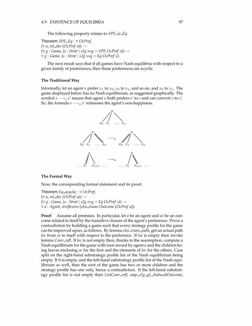
4.9. EXISTENCE OF EQUILIBRIA 97
The following property relates to SPE is Eq.
Theorem SPE Eq : ∀ OcPref,(∀ a, rel dec (OcPref a))→(∀ g : Game, {s : Strat | s2g s=g ∧ SPE OcPref s})→∀ g : Game, {s : Strat | s2g s=g ∧ Eq OcPref s}.
The next result says that if all games have Nash equilibria with respect to agiven family of preferences, then these preferences are acyclic.
The Traditional Way
Informally, let an agent a prefer x1 to x0, x2 to x1, and so on, and x0 to xn. Thegame displayed below has no Nash equilibrium, as suggested graphically. Thesymbol s −→a s’means that agent a both prefers s’ to s and can convert s to s’.So, the formula s −→a s’ witnesses the agent’s non-happiness.
a
x0 x1 . . . xn
a a
−→a
x0 x1 . . . xn x0 x1 . . . xn
a a
−→a
. . . xi xi+1 . . . . . . xi xi+1 . . .
The Formal Way
Now, the corresponding formal statement and its proof.
Theorem Eq acyclic : ∀ OcPref,(∀ a, rel dec (OcPref a))→(∀ g : Game, {s : Strat | s2g s=g ∧ Eq OcPref s})→∀ a : Agent, irreflexive (clos trans Outcome (OcPref a)).
Proof Assume all premises. In particular, let a be an agent and oc be an out-come related to itself by the transitive closure of the agent’s preference. Prove acontradiction by building a game such that every strategy profile for the gamecan be improved upon, as follows. By lemma clos trans path, get an actual pathloc from oc to itself with respect to the preference. If loc is empty then invokelemma Conv refl. If loc is not empty then, thanks to the assumption, compute aNash equilibrium for the gamewith root owned by agent a and the children be-ing leaves enclosing oc for the first and the elements of loc for the others. Casesplit on the right-hand substrategy profile list of the Nash equilibrium beingempty. If it is empty, and the left-hand substrategy profile list of the Nash equi-librium as well, then the root of the game has two or more children and thestrategy profile has one only, hence a contradiction. If the left-hand substrat-egy profile list is not empty then ListConv refl, map s2g gL InducedOutcome,
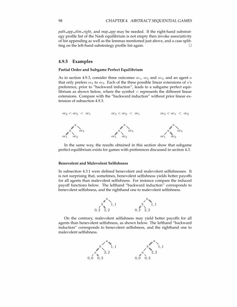
98 CHAPTER 4. ABSTRACT SEQUENTIAL GAMES
path app elim right, and map app may be needed. If the right-hand substrat-egy profile list of the Nash equilibrium is not empty then invoke associativityof list appending as well as the lemmas mentioned just above, and a case split-ting on the left-hand substrategy profile list again. �
4.9.5 Examples
Partial Order and Subgame Perfect Equilibrium
As in section 4.9.3, consider three outcomes oc1, oc2 and oc3, and an agent athat only prefers oc2 to oc3. Each of the three possible linear extensions of a’spreference, prior to “backward induction”, leads to a subgame perfect equi-librium as shown below, where the symbol < represents the different linearextensions. Compare with the “backward induction” without prior linear ex-tension of subsection 4.9.3.
oc2 < oc3 < oc1 oc3 < oc2 < oc1 oc3 < oc1 < oc2
a a a
a oc3 a oc3 a oc3
oc1 oc2 oc1 oc2 oc1 oc2
In the same way, the results obtained in this section show that subgameperfect equilibrium exists for games with preferences discussed in section 4.3.
Benevolent andMalevolent Selfishness
In subsection 4.3.1 were defined benevolent and malevolent selfishnesses. Itis not surprising that, sometimes, benevolent selfishness yields better payoffsfor all agents than malevolent selfishness. For instance compare the inducedpayoff functions below. The lefthand “backward induction” corresponds tobenevolent selfishness, and the righthand one to malevolent selfishness.
a a
b 1, 1 b 1, 1
0, 2 2, 2 0, 2 2, 2
On the contrary, malevolent selfishness may yield better payoffs for allagents than benevolent selfishness, as shown below. The lefthand “backwardinduction” corresponds to benevolent selfishness, and the righthand one tomalevolent selfishness.
a a
b 1, 1 b 1, 1
a 2, 2 a 2, 2
0, 0 0, 3 0, 0 0, 3
4.10. CONCLUSION 99
4.10 Conclusion
This chapter introduces a new inductive formalism for sequential games. italso replaces real-valued payoff functions with atomic objects called outcomes,and the usual total order over the reals with arbitrary preferences. This way,it also defines an abstract version of sequential games, with similar tree struc-ture and notion of convertibility as for traditional sequential games. The no-tions of Nash equilibrium, subgame perfect equilibrium, and “backward in-duction” are translated into the new formalism. When preferences are totallyordered, “backward induction”guarantees existence of subgame perfect equi-librium for all sequential games, thus translating Kuhn’s result in the new for-malism. However, an example shows that “backward induction” fails to pro-vide equilibrium for non-totally ordered preferences, e.g., partial orders. Butwhen preferences are acyclic, it is still possible to perform “backward induc-tion” on a game whose preferences have been linearly extended. This yieldsa subgame perfect equilibrium of the game with respect to the acyclic prefer-ences, because removing arcs from a preference relation amounts to removingreasons for being unhappy. So, given a collection of outcomes, the followingthree propositions are equivalent:
• The agents’ preferences over the given outcomes are acyclic.
• Every game built over the given outcomes has a Nash equilibrium.
• Every game built over the given outcomes has a subgame perfect equi-librium.
The formalism introduced in this chapter is suitable for proofs in Coq, whichis a (highly reliable) constructive proof assistant. This way, the above-mentionedequivalence is fully computer-certified using Coq. Beside the additional guar-antee of correctness provided by the Coq proof, the activity of formalisationalso provides the opportunity to clearly identify the useful definitions and themain articulations of the proof.Informally, a result due to Aumann states that, when dealing with tradi-
tional sequential games, “common knowledge of rationality among agents” isequivalent to “backward induction” (where “rationality” means playing in or-der to maximise one’s payoff). This is arguable in abstract sequential gamesif one expects “common knowledge of rationality among agents” to implyNash equilibrium. Indeed, “backward induction” may not imply Nash equilib-rium, as seen in this chapter. Therefore, “backward induction” may not imply“common knowledge of rationality among agents”. Instead, one may won-der whether “common knowledge of rationality among agents” is equivalentto subgame perfect equilibrium, whatever it may mean, when preferences areacyclic, i.e. rational in some sense. In this case, the difference between “back-ward induction” and subgame perfect equilibrium seems critical again.
100 CHAPTER 4. ABSTRACT SEQUENTIAL GAMES
Chapter 5
Acyclic Preferences and NashEquilibrium Existence:Another Proof of theEquivalence
Abstract sequential games are a class of games that generalises traditional se-quential games. Basically, abstract atomic objects, called outcomes, replace thetraditional real-valued payoff functions, and arbitrary binary relations overoutcomes, called preferences, replace the usual total order over the reals. In1953, Kuhn proved that every traditional sequential game has a Nash equilib-rium. In 1965, Selten introduced refined Nash equilibria named subgame per-fect equilibria. Lately, Le Roux proved (using the proof assistant Coq) that thefollowing three propositions are equivalent: 1) Preferences over the outcomesare acyclic. 2) Every abstract sequential game has a Nash equilibrium. 3) Ev-ery abstract sequential game has a subgame perfect equilibrium. Part of theproof is akin to Kuhn’s proof. This chapter proves that propositions 1) and 2)are equivalent, which is a corollary of the above-mentioned result. However,the proof presented in this chapter adopts a significantly different techniquecompared to the previous ones.
5.1 Introduction
5.1.1 Contribution
This chapter proves that, when dealing with abstract sequential games, the fol-lowing two propositions are equivalent: 1) Preferences over the outcomes areacyclic. 2) Every sequential game has a Nash equilibrium. This is a corollaryof the triple equivalence proved in [29] and chapter 4, however the new proofinvokes neither structural induction on games, nor “backward induction”, nortopological sorting. Therefore, this alternative argument is of proof theoreticalinterest. The proof of the implication 1) ⇒ 2) invokes three main arguments.First, if preferences are strict partial orders, then every game has a Nash equi-
101
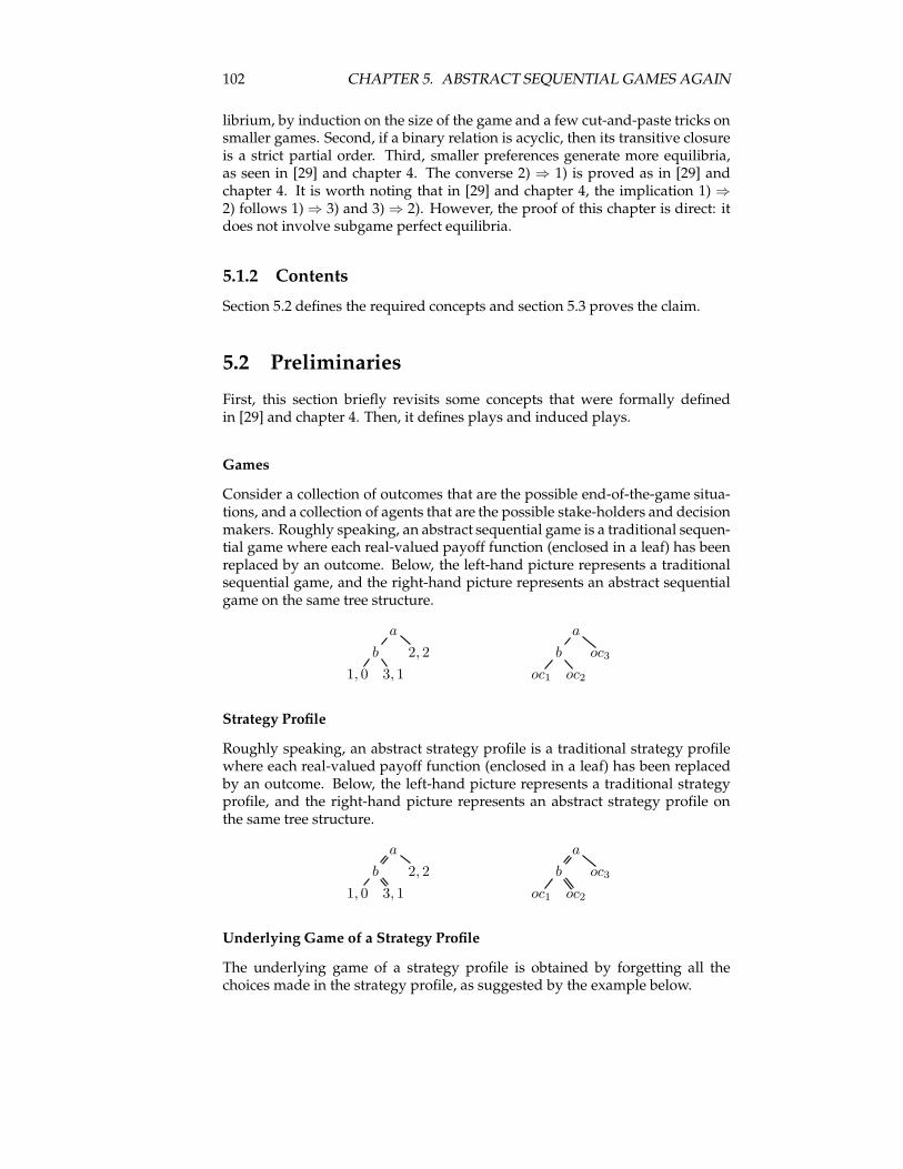
102 CHAPTER 5. ABSTRACT SEQUENTIAL GAMES AGAIN
librium, by induction on the size of the game and a few cut-and-paste tricks onsmaller games. Second, if a binary relation is acyclic, then its transitive closureis a strict partial order. Third, smaller preferences generate more equilibria,as seen in [29] and chapter 4. The converse 2) ⇒ 1) is proved as in [29] andchapter 4. It is worth noting that in [29] and chapter 4, the implication 1) ⇒2) follows 1)⇒ 3) and 3)⇒ 2). However, the proof of this chapter is direct: itdoes not involve subgame perfect equilibria.
5.1.2 Contents
Section 5.2 defines the required concepts and section 5.3 proves the claim.
5.2 Preliminaries
First, this section briefly revisits some concepts that were formally definedin [29] and chapter 4. Then, it defines plays and induced plays.
Games
Consider a collection of outcomes that are the possible end-of-the-game situa-tions, and a collection of agents that are the possible stake-holders and decisionmakers. Roughly speaking, an abstract sequential game is a traditional sequen-tial game where each real-valued payoff function (enclosed in a leaf) has beenreplaced by an outcome. Below, the left-hand picture represents a traditionalsequential game, and the right-hand picture represents an abstract sequentialgame on the same tree structure.
a a
b 2, 2 b oc3
1, 0 3, 1 oc1 oc2
Strategy Profile
Roughly speaking, an abstract strategy profile is a traditional strategy profilewhere each real-valued payoff function (enclosed in a leaf) has been replacedby an outcome. Below, the left-hand picture represents a traditional strategyprofile, and the right-hand picture represents an abstract strategy profile onthe same tree structure.
a a
b 2, 2 b oc3
1, 0 3, 1 oc1 oc2
Underlying Game of a Strategy Profile
The underlying game of a strategy profile is obtained by forgetting all thechoices made in the strategy profile, as suggested by the example below.
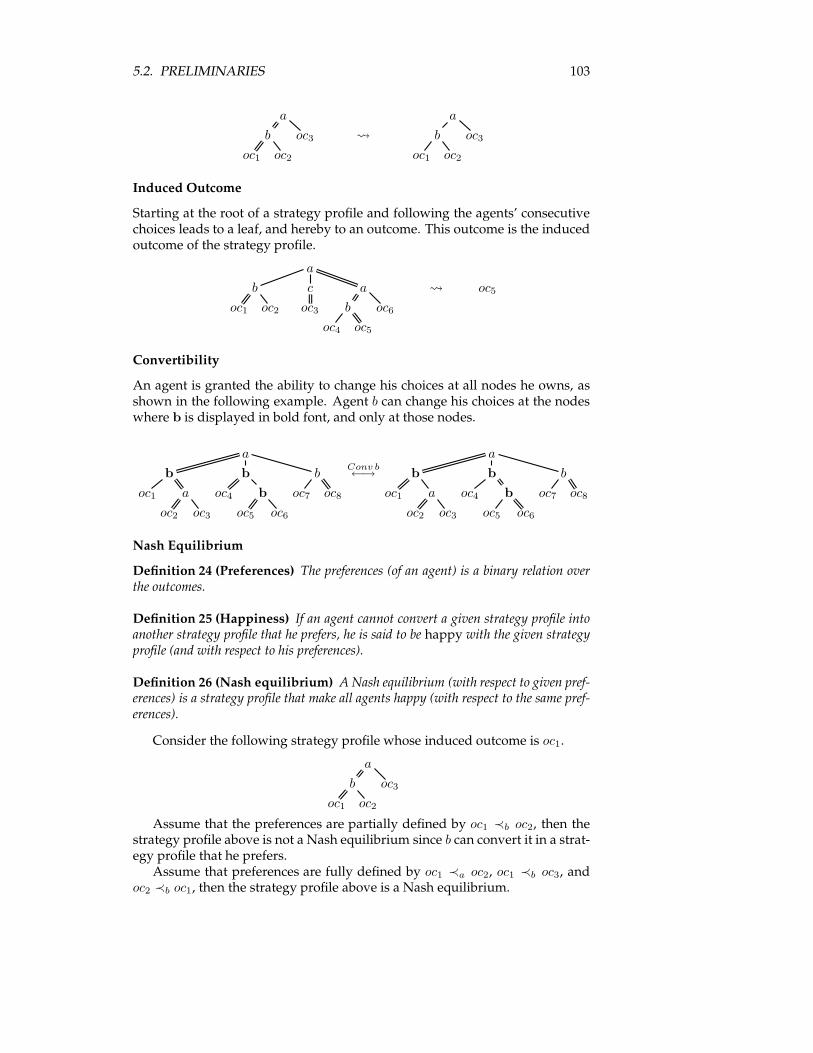
5.2. PRELIMINARIES 103
a a
b oc3 b oc3
oc1 oc2 oc1 oc2
Induced Outcome
Starting at the root of a strategy profile and following the agents’ consecutivechoices leads to a leaf, and hereby to an outcome. This outcome is the inducedoutcome of the strategy profile.
a
b c a oc5
oc1 oc2 oc3 b oc6
oc4 oc5
Convertibility
An agent is granted the ability to change his choices at all nodes he owns, asshown in the following example. Agent b can change his choices at the nodeswhere b is displayed in bold font, and only at those nodes.
a a
b b bConv b←→ b b b
oc1 a oc4 b oc7 oc8 oc1 a oc4 b oc7 oc8
oc2 oc3 oc5 oc6 oc2 oc3 oc5 oc6
Nash Equilibrium
Definition 24 (Preferences) The preferences (of an agent) is a binary relation overthe outcomes.
Definition 25 (Happiness) If an agent cannot convert a given strategy profile intoanother strategy profile that he prefers, he is said to be happy with the given strategyprofile (and with respect to his preferences).
Definition 26 (Nash equilibrium) ANash equilibrium (with respect to given pref-erences) is a strategy profile that make all agents happy (with respect to the same pref-erences).
Consider the following strategy profile whose induced outcome is oc1.
a
b oc3
oc1 oc2
Assume that the preferences are partially defined by oc1 ≺b oc2, then thestrategy profile above is not a Nash equilibrium since b can convert it in a strat-egy profile that he prefers.Assume that preferences are fully defined by oc1 ≺a oc2, oc1 ≺b oc3, and
oc2 ≺b oc1, then the strategy profile above is a Nash equilibrium.
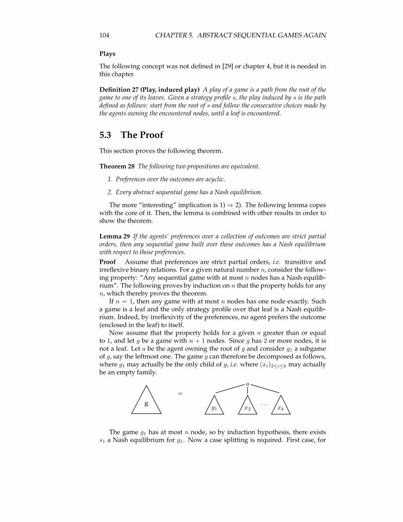
104 CHAPTER 5. ABSTRACT SEQUENTIAL GAMES AGAIN
Plays
The following concept was not defined in [29] or chapter 4, but it is needed inthis chapter.
Definition 27 (Play, induced play) A play of a game is a path from the root of thegame to one of its leaves. Given a strategy profile s, the play induced by s is the pathdefined as follows: start from the root of s and follow the consecutive choices made bythe agents owning the encountered nodes, until a leaf is encountered.
5.3 The Proof
This section proves the following theorem.
Theorem 28 The following two propositions are equivalent.
1. Preferences over the outcomes are acyclic.
2. Every abstract sequential game has a Nash equilibrium.
The more “interesting” implication is 1)⇒ 2). The following lemma copeswith the core of it. Then, the lemma is combined with other results in order toshow the theorem.
Lemma 29 If the agents’ preferences over a collection of outcomes are strict partialorders, then any sequential game built over these outcomes has a Nash equilibriumwith respect to those preferences.
Proof Assume that preferences are strict partial orders, i.e. transitive andirreflexive binary relations. For a given natural number n, consider the follow-ing property: “Any sequential game with at most n nodes has a Nash equilib-rium”. The following proves by induction on n that the property holds for anyn, which thereby proves the theorem.If n = 1, then any game with at most n nodes has one node exactly. Such
a game is a leaf and the only strategy profile over that leaf is a Nash equilib-rium. Indeed, by irreflexivity of the preferences, no agent prefers the outcome(enclosed in the leaf) to itself.Now assume that the property holds for a given n greater than or equal
to 1, and let g be a game with n + 1 nodes. Since g has 2 or more nodes, it isnot a leaf. Let a be the agent owning the root of g and consider g1 a subgameof g, say the leftmost one. The game g can therefore be decomposed as follows,where g1 may actually be the only child of g, i.e. where (xi)2≤i≤k may actuallybe an empty family.
g
a
=
g1 x2. . .
xk
The game g1 has at most n node, so by induction hypothesis, there existss1 a Nash equilibrium for g1. Now a case splitting is required. First case, for
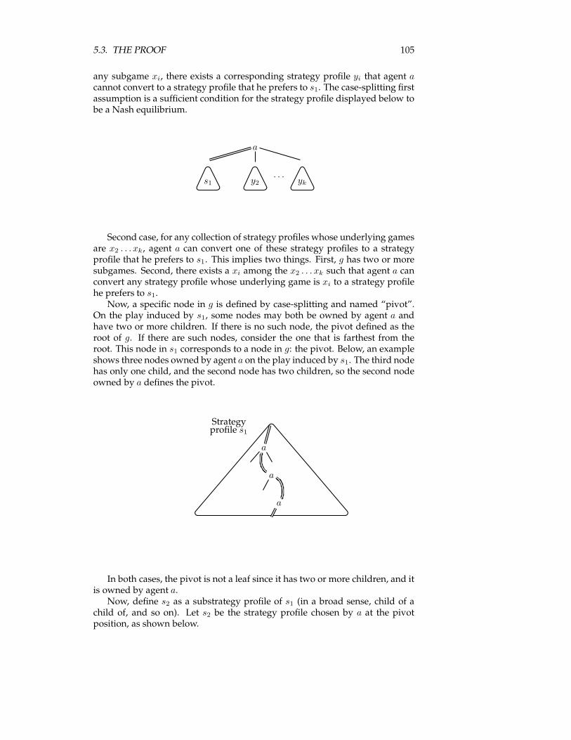
5.3. THE PROOF 105
any subgame xi, there exists a corresponding strategy profile yi that agent acannot convert to a strategy profile that he prefers to s1. The case-splitting firstassumption is a sufficient condition for the strategy profile displayed below tobe a Nash equilibrium.
a
s1 y2. . .
yk
Second case, for any collection of strategy profiles whose underlying gamesare x2 . . . xk , agent a can convert one of these strategy profiles to a strategyprofile that he prefers to s1. This implies two things. First, g has two or moresubgames. Second, there exists a xi among the x2 . . . xk such that agent a canconvert any strategy profile whose underlying game is xi to a strategy profilehe prefers to s1.Now, a specific node in g is defined by case-splitting and named “pivot”.
On the play induced by s1, some nodes may both be owned by agent a andhave two or more children. If there is no such node, the pivot defined as theroot of g. If there are such nodes, consider the one that is farthest from theroot. This node in s1 corresponds to a node in g: the pivot. Below, an exampleshows three nodes owned by agent a on the play induced by s1. The third nodehas only one child, and the second node has two children, so the second nodeowned by a defines the pivot.
Strategyprofile s1
a
a
a
In both cases, the pivot is not a leaf since it has two or more children, and itis owned by agent a.Now, define s2 as a substrategy profile of s1 (in a broad sense, child of a
child of, and so on). Let s2 be the strategy profile chosen by a at the pivotposition, as shown below.
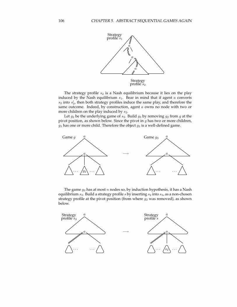
106 CHAPTER 5. ABSTRACT SEQUENTIAL GAMES AGAIN
Strategyprofile s1
a
a
a
Strategyprofile s2
The strategy profile s2 is a Nash equilibrium because it lies on the playinduced by the Nash equilibrium s1. Bear in mind that if agent a convertss2 into s′2, then both strategy profiles induce the same play, and therefore thesame outcome. Indeed, by construction, agent a owns no node with two ormore children on the play induced by s2.Let g2 be the underlying game of s2. Build g3 by removing g2 from g at the
pivot position, as shown below. Since the pivot in g has two or more children,g3 has one or more child. Therefore the object g3 is a well-defined game.
Game g a Game g3a
a −→ a
. . . g2 . . . . . . . . .
The game g3 has at most n nodes so, by induction hypothesis, it has a Nashequilibrium s3. Build a strategy profile s by inserting s2 into s3, as a non-chosenstrategy profile at the pivot position (from where g2 was removed), as shownbelow.
Strategyprofile s3
a Strategyprofile s
a
a −→ a
. . . . . . . . . s2 . . .
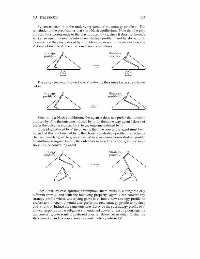
5.3. THE PROOF 107
By construction, g is the underlying game of the strategy profile s. Theremainder of the proof shows that s is a Nash equilibrium. Note that the playinduced by s corresponds to the play induced by s3, since it does not involves2. Let an agent b convert s into a new strategy profile s′, and hereby s2 to s′2.Case split on the play induced by s′ involving s′2 or not. If the play induced bys′ does not involve s′2, then the conversion is as follows.
Strategyprofile s
a Strategyprofile s′
a
s2
Conv b−→
s′2
The same agent b can convert s3 to s′3 inducing the same play as s′, as shown
below.
Strategyprofile s3
a Strategyprofile s3′
a
Conv b−→
Since s3 is a Nash equilibrium, the agent b does not prefer the outcomeinduced by s′3 to the outcome induced by s3. In the same way, agent b does notprefer the outcome induced by s′ to the outcome induced by s.If the play induced by s′ involves s′2, then the converting agent must be a.
Indeed, at the pivot owned by a, the chosen substrategy profile must actuallychange towards s′2, while s2 was inserted in s3 as a non-chosen strategy profile.In addition, as argued before, the outcomes induced by s′2 and s2 are the samesince a is the converting agent.
Strategyprofile s
a Strategyprofile s′
a
s2
Conv a−→
s′2
Recall that, by case splitting assumption, there exists xi a subgame of gdifferent from g1 and with the following property: agent a can convert anystrategy profile whose underlying game is xi into a new strategy profile heprefers to s1. Agent a would also prefer the new strategy profile to s′2 sinceboth s1 and s′2 induce the same outcome. Let yi be the substrategy profile of s′
that corresponds to the subgame xi mentioned above. By assumption, agent acan convert yi into some y′
i preferred over s′2. Below, let us detail further thestructure of s′ and its conversion by agent a into a preferred s′′.
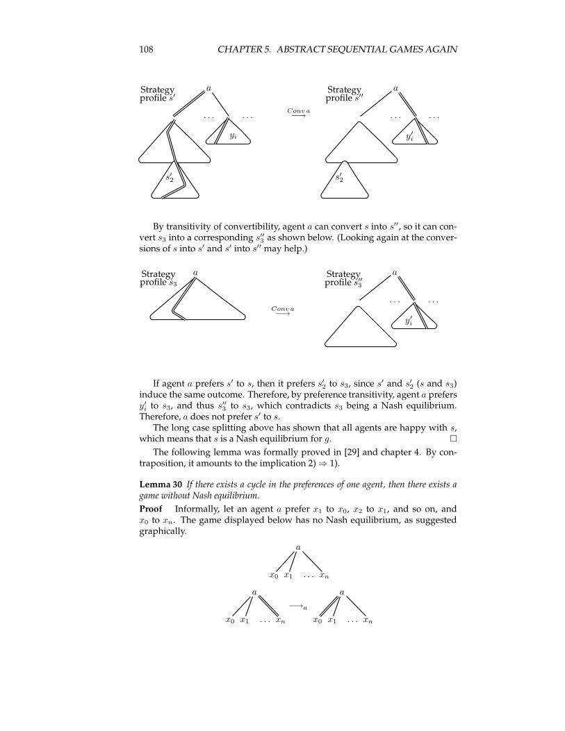
108 CHAPTER 5. ABSTRACT SEQUENTIAL GAMES AGAIN
Strategyprofile s′
a Strategyprofile s′′
a
. . .
yi
. . .Conv a−→ . . .
y′i
. . .
s′2 s′2
By transitivity of convertibility, agent a can convert s into s′′, so it can con-vert s3 into a corresponding s′′3 as shown below. (Looking again at the conver-sions of s into s′ and s′ into s′′ may help.)
Strategyprofile s3
a Strategyprofile s′′3
a
. . .
y′i
. . .Conv a−→
If agent a prefers s′ to s, then it prefers s′2 to s3, since s′ and s′2 (s and s3)induce the same outcome. Therefore, by preference transitivity, agent a prefersy′
i to s3, and thus s′′3 to s3, which contradicts s3 being a Nash equilibrium.Therefore, a does not prefer s′ to s.The long case splitting above has shown that all agents are happy with s,
which means that s is a Nash equilibrium for g. �
The following lemma was formally proved in [29] and chapter 4. By con-traposition, it amounts to the implication 2)⇒ 1).
Lemma 30 If there exists a cycle in the preferences of one agent, then there exists agame without Nash equilibrium.
Proof Informally, let an agent a prefer x1 to x0, x2 to x1, and so on, andx0 to xn. The game displayed below has no Nash equilibrium, as suggestedgraphically.
a
x0 x1 . . . xn
a a
−→a
x0 x1 . . . xn x0 x1 . . . xn
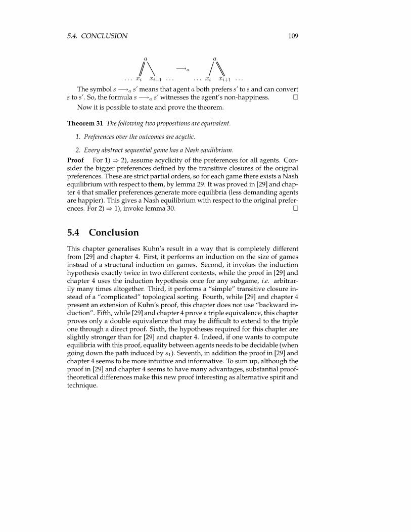
5.4. CONCLUSION 109
a a
−→a
. . . xi xi+1 . . . . . . xi xi+1 . . .
The symbol s −→a s’means that agent a both prefers s’ to s and can converts to s’. So, the formula s −→a s’ witnesses the agent’s non-happiness. �
Now it is possible to state and prove the theorem.
Theorem 31 The following two propositions are equivalent.
1. Preferences over the outcomes are acyclic.
2. Every abstract sequential game has a Nash equilibrium.
Proof For 1) ⇒ 2), assume acyclicity of the preferences for all agents. Con-sider the bigger preferences defined by the transitive closures of the originalpreferences. These are strict partial orders, so for each game there exists a Nashequilibriumwith respect to them, by lemma 29. It was proved in [29] and chap-ter 4 that smaller preferences generate more equilibria (less demanding agentsare happier). This gives a Nash equilibrium with respect to the original prefer-ences. For 2)⇒ 1), invoke lemma 30. �
5.4 Conclusion
This chapter generalises Kuhn’s result in a way that is completely differentfrom [29] and chapter 4. First, it performs an induction on the size of gamesinstead of a structural induction on games. Second, it invokes the inductionhypothesis exactly twice in two different contexts, while the proof in [29] andchapter 4 uses the induction hypothesis once for any subgame, i.e. arbitrar-ily many times altogether. Third, it performs a “simple” transitive closure in-stead of a “complicated” topological sorting. Fourth, while [29] and chapter 4present an extension of Kuhn’s proof, this chapter does not use “backward in-duction”. Fifth, while [29] and chapter 4 prove a triple equivalence, this chapterproves only a double equivalence that may be difficult to extend to the tripleone through a direct proof. Sixth, the hypotheses required for this chapter areslightly stronger than for [29] and chapter 4. Indeed, if one wants to computeequilibria with this proof, equality between agents needs to be decidable (whengoing down the path induced by s1). Seventh, in addition the proof in [29] andchapter 4 seems to be more intuitive and informative. To sum up, although theproof in [29] and chapter 4 seems to have many advantages, substantial proof-theoretical differences make this new proof interesting as alternative spirit andtechnique.
110 CHAPTER 5. ABSTRACT SEQUENTIAL GAMES AGAIN
Chapter 6
Graphs and Path Equilibria
The quest for optimal/stable paths in graphs has gained attention in a fewpractical or theoretical areas. To take part in this quest this chapter adoptsan equilibrium-oriented approach that is abstract and general: it works with(quasi-arbitrary) arc-labelled digraphs, and it assumes very little about thestructure of the sought paths and the definition of equilibrium, i.e. optimal-ity/stability. In this setting, this chapter presents a sufficient condition forequilibrium existence for every graph; it also presents a necessary conditionfor equilibrium existence for every graph. The necessary condition does notimply the sufficient condition a priori. However, the chapter pinpoints theirlogical difference and thus identifies what work remains to be done. More-over, the necessary and the sufficient conditions coincide when the definitionof optimality relates to a total order, which provides a full-equivalence prop-erty. These results are applied to network routing.
6.1 Introduction
This chapter provides an abstract formalism that enables generic proofs, yetaccurate results, about path equilibria in graphs. Beyond this, the purpose ofthis chapter is to provide a tool for a generalisation of sequential (tree-) gameswithin graphs. However, these game-theoretic facets are not discussed in thischapter. In addition to the game-theoretic application, the results presentedin this chapter may help solve problems of optimisation/stability of paths ingraphs: a short example is presented for the problem of network routing .
6.1.1 Contribution
This chapter introduces the terminology of dalographs which refers to finite,arc-labelled, directed graphs with non-zero outdegree, i.e. each of whose nodehas an outgoing arc. An embedding of arc-labelled digraphs into dalographsshows that the non-zero-outdegree constraint may not yield a serious loss ofgenerality. The paths that are considered in this chapter are infinite. Indeed, fi-nite paths and infinite paths are of slightly different "types". Considering bothmay hinder an algebraic approach of the system. However, another embed-ding allows representing finite paths in a dalograph as infinite paths in another
111
112 CHAPTER 6. GRAPHS AND PATH EQUILIBRIA
dalograph. This shows that the infiniteness constraint may not yield a seriousloss of generality either. Note that the non-zero-outdegree constraint ensuresexistence of infinite paths, starting from any node. This uniformity facilitatesan algebraic approach of the system. The paths considered in this chapter arenon-self-crossing, which somehow suggests consistency. This sounds desirablein many areas, but it may be an actual restriction in some others.In this formalism, a path induces an ultimately periodic sequence of labels
(of arcs that are involved in the path). An arbitrary binary relation over ul-timately periodic sequences of labels is assumed and named preference. Thisinduces a binary relation over paths, which is also named preference. It isdefined as follows. Given two paths starting from the same node, one is pre-ferred over the other if the sequence of labels that is induced by the former ispreferred over the sequence of labels that is induced by the latter. Maximalityof a given path in a graph means that no path is preferred over the given path.A strategy is an object built over a dalograph. It amounts to every node choos-ing an outgoing arc. This way, a strategy induces paths starting from any givennode. An equilibrium is a strategy inducing optimal paths for any node.The proof of equilibrium existence is structured as follows. First, a seeking-
forward function is defined so that given a node it returns a path. Given a node,the function chooses a path that is maximal (according to the definition of theprevious paragraph), and the function "follows" the path until the remainingpath is not maximal (among the paths starting from the current node). In thiscase, the function chooses a maximal path starting from the current node andproceeds as before. All of this is done under the constraint that a path is non-self-crossing. Under some conditions, this procedure yields a path that is max-imal not only at its starting node, but also at all nodes along the path. Sucha path is called a hereditary maximal path. Equipped with this lemma, the exis-tence of an equilibrium for every dalograph is proved as follows by inductionon the number of arcs in the dalograph.
• Compute a hereditary maximal path in the dalograph.
• Remove the arcs of the dalograph that the path ignored while visitingadjacent nodes and get a smaller dalograph.
• Compute an equilibrium on this smaller dalograph and add the ignoredarcs back. This yields an equilibrium for the original dalograph.
The sufficient condition for equilibrium existence involves a notion lyingbetween strict partial order and strict total order, namely strict weak order. Thischapter requires a few preliminary results about strict weak orders. Moreover,the definition of the seeking-forward function requires the design of a recursionprinciple that is also used as a proof principle in this chapter. To show theusefulness of this sufficient condition, this chapter provides a few examples ofnon-trivial relations that meet the requirements of this condition: lexicographicextension of a strict weak order, Pareto-like order, and two limit-set-orientedorders. Then, as an application to network routing, one derives a sufficientcondition for a routing policy to guarantee existence of stable routing solutions.The proof of the necessary condition for equilibrium existence involves var-
ious closures of binary relations. Most of the closures defined here are re-lated to properties that are part of the sufficient condition. For instance, the
6.1. INTRODUCTION 113
sufficient condition involves transitivity of some preference (binary relation),and the necessary condition involves the transitive closure of the preference.Each of those various closures is proved to preserve existence of equilibrium.More specifically, if a preference ensures existence of equilibrium for everydalograph, then the closure of the preference also ensures existence of equi-librium for every dalograph. A new closure is defined subsequently as thecombination of all the above-mentioned closures. Thanks to a preliminary de-velopment introducing the notion of simple closure, this combination closurealso preserves existence of equilibrium. Since the combination closure has afew properties, this gives a non-trivial necessary condition for equilibrium ex-istence. All the closures mentioned above are defined inductively through in-ference rules, which allows using rule induction as a proof principle. To showthe usefulness of this necessary condition, this chapter provides an example ofa non-trivial relation that does not meet the requirements of this condition.However, not all the properties that are part of the sufficient condition can
be easily turned into a simple closure preserving equilibrium existence (andhereby be part of the necessary condition). Therefore, the necessary conditionand sufficient condition do not look exactly the same. Some examples showthat the necessary condition is too weak. Some more work, i.e. the designof more general simple closures, is likely to take care of those examples, andhereby provide a stronger necessary condition. However, there is also likelyto be more complex examples that would require the design of more complexsimple closures. As to the sufficient condition, it is still unclear whether or notit is too strong.In the case where the preference is a total order, the sufficient and neces-
sary conditions coincide. This gives a necessary and sufficient condition (ona total order preference) for existence of equilibrium in every dalograph. Thisleads to a necessary and sufficient condition (on a total order preference) forequilibrium existence in the network routing application mentioned above.
6.1.2 Contents
Section 6.2 defines a graph-like structure named dalograph and the notion ofequilibrium in dalographs. Section 6.3 defines a refinement of partial orderthat is named strict weak order in the literature. This section also connects thenotion of strict weak order to other properties of binary relations. Section 6.4proves a sufficient condition that guarantees existence of equilibrium for alldalographs. It also gives a few examples of non-trivial relations meeting therequirements of the sufficient condition. Finally, it gives an application in net-work routing. Section 6.5 defines the notion of simple closure and proves aproperty about the union of simple closures. Section 6.6 discusses preservationof equilibrium existence by closures, and thus provides a necessary conditionfor existence of equilibrium for all dalographs. Section 6.7 compares the suf-ficient condition and the necessary condition, and shows that they coincide inthe total order case but not in general. It also describes a relation that does notmeet the requirements of the necessary condition. Finally, it gives a necessaryand sufficient condition, in the total order case, for equilibrium existence in thenetwork routing application mentioned above.
114 CHAPTER 6. GRAPHS AND PATH EQUILIBRIA
6.1.3 Conventions
Unless otherwise stated, universal quantifiers are usually omitted in front of(semi-) formal statements. For instance, a claim of the form P (x, y) should beread ∀x, y, P (x, y).Usually, when proving a claim of type τ0 ⇒ · · · ⇒ τn−1 ⇒ τn ⇒ τ , the
beginning of the proof implicitly assumes τ0,..., τn−1 , and τn, and then startsproving τ .Given u a non-empty finite sequence, uf (resp. ul) represents the first (resp.
last) element of u.The notation P (x)
∆= Q(x)means that P is defined as coinciding with Q.
The negation of a relation ≺ is written as follows.
α 6≺ β∆= ¬(α ≺ β)
The corresponding incomparability relation is defined below.
α♯β∆= α 6≺ β ∧ β 6≺ α
The inverse of a relation ≺ is defined as follows.
α ≻ β∆= β ≺ α
Restrictions of binary relations are written as follows.
α ≺|S β∆= α ≺ β ∧ (α, β) ∈ S2
Function composition is defined as (almost) usual. For any functions f1 oftype A → B and f2 of type B → C, the composition of f1 and f2 is writtenf2 ◦ f1. It is of type A→ C and it is defined as follows.
f2 ◦ f1(x)∆= f2(f1(x))
In this chapter, f1 ◦ f2 may be written f1f2, in the same order.
6.2 Dalographs and Equilibria
Subsection 6.2.1 defines a class of arc-labelled digraphs, subsection 6.2.2 de-fines a class of paths in such arc-labelled digraphs, and subsection 7.2.3 derivesa notion of equilibrium from a notion of maximality for paths. The more gen-eral will be those graphs and paths, the more general will be the derived notionof equilibrium.
6.2.1 Dalographs
This subsection gives a name to the class of arc-labelled directed graphs eachof whose node has at least one outgoing arc. Then it briefly justifies why arc la-belling is "more general" than node labelling, and why the non-zero-outdegreeconstraint may not yield a serious loss of generality.
Definition 32 (Dalograph) Let L be a collection of labels. A dalograph is a finitedirected graph whose arcs are labelled with elements of L, and such that every node hasa non-zero outdegree.
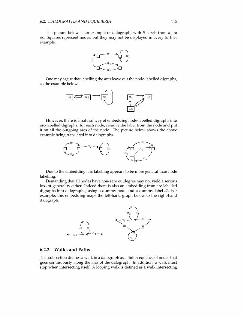
6.2. DALOGRAPHS AND EQUILIBRIA 115
The picture below is an example of dalograph, with 5 labels from a1 toa5. Squares represent nodes, but they may not be displayed in every furtherexample.
a1 a2
a3a4
a5
One may argue that labelling the arcs leave out the node-labelled digraphs,as the example below.
a1 a2 a3 a4 a5
x6
However, there is a natural way of embedding node-labelled digraphs intoarc-labelled digraphs: for each node, remove the label from the node and putit on all the outgoing arcs of the node. The picture below shows the aboveexample being translated into dalographs.
b
a1
a2
a2 a3
a4
a5
a6a6
Due to the embedding, arc labelling appears to be more general than nodelabelling.Demanding that all nodes have non-zero outdegree may not yield a serious
loss of generality either. Indeed there is also an embedding from arc-labelleddigraphs into dalographs, using a dummy node and a dummy label dl. Forexample, this embedding maps the left-hand graph below to the right-handdalograph.
a1a2
a3a4
a1a2
a3a4
dl dl
dl
6.2.2 Walks and Paths
This subsection defines a walk in a dalograph as a finite sequence of nodes thatgoes continuously along the arcs of the dalograph. In addition, a walk muststop when intersecting itself. A looping walk is defined as a walk intersecting
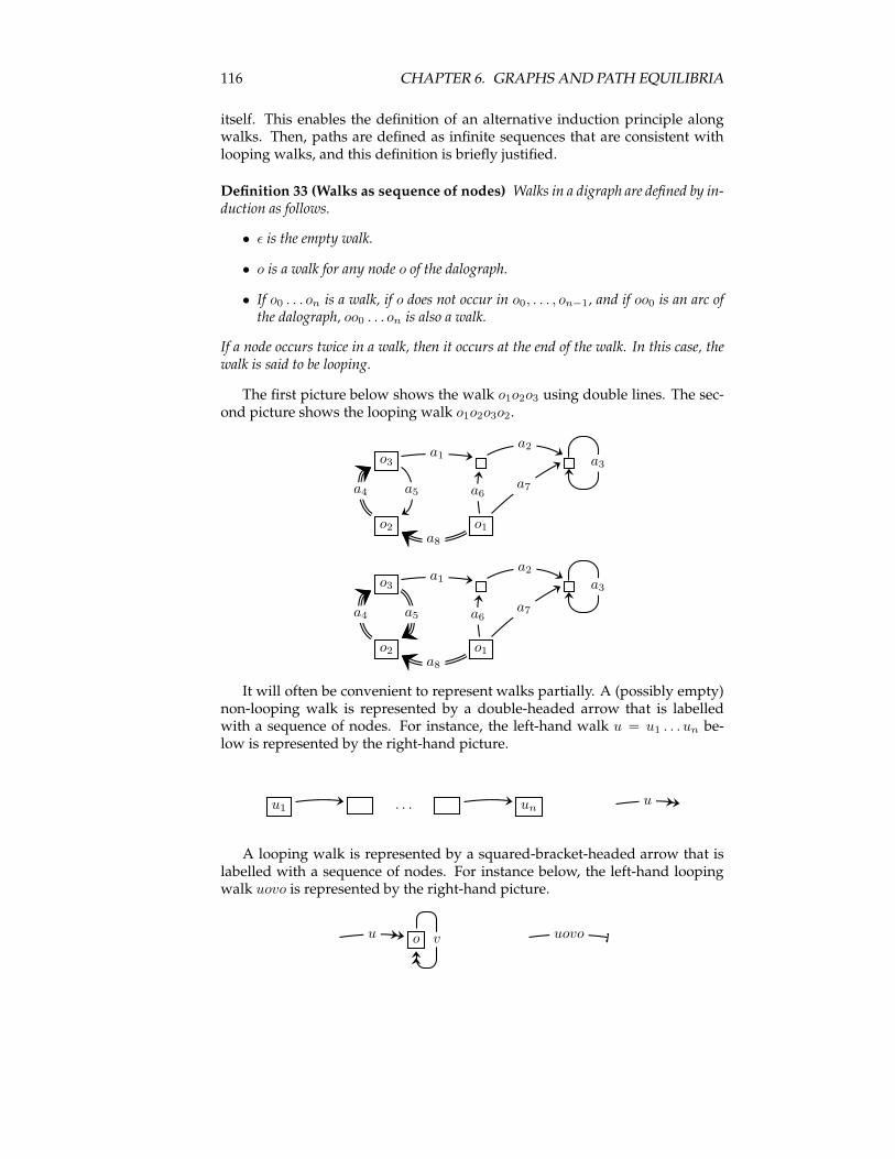
116 CHAPTER 6. GRAPHS AND PATH EQUILIBRIA
itself. This enables the definition of an alternative induction principle alongwalks. Then, paths are defined as infinite sequences that are consistent withlooping walks, and this definition is briefly justified.
Definition 33 (Walks as sequence of nodes) Walks in a digraph are defined by in-duction as follows.
• ǫ is the empty walk.
• o is a walk for any node o of the dalograph.
• If o0 . . . on is a walk, if o does not occur in o0, . . . , on−1, and if oo0 is an arc ofthe dalograph, oo0 . . . on is also a walk.
If a node occurs twice in a walk, then it occurs at the end of the walk. In this case, thewalk is said to be looping.
The first picture below shows the walk o1o2o3 using double lines. The sec-ond picture shows the looping walk o1o2o3o2.
o3
o2 o1
a1a2
a5a4
a8
a6a7
a3
o3
o2 o1
a1a2
a5a4
a8
a6a7
a3
It will often be convenient to represent walks partially. A (possibly empty)non-looping walk is represented by a double-headed arrow that is labelledwith a sequence of nodes. For instance, the left-hand walk u = u1 . . . un be-low is represented by the right-hand picture.
u1 . . . unu
A looping walk is represented by a squared-bracket-headed arrow that islabelled with a sequence of nodes. For instance below, the left-hand loopingwalk uovo is represented by the right-hand picture.
o uovou v
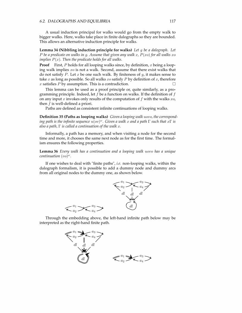
6.2. DALOGRAPHS AND EQUILIBRIA 117
A usual induction principal for walks would go from the empty walk tobigger walks. Here, walks take place in finite dalographs so they are bounded.This allows an alternative induction principle for walks.
Lemma 34 (Nibbling induction principle for walks) Let g be a dalograph. LetP be a predicate on walks in g. Assume that given any walk x, P (xo) for all walks xoimplies P (x). Then the predicate holds for all walks.
Proof First, P holds for all looping walks since, by definition, x being a loop-ing walk implies xo is not a walk. Second, assume that there exist walks thatdo not satisfy P . Let x be one such walk. By finiteness of g, it makes sense totake x as long as possible. So all walks xo satisfy P by definition of x, thereforex satisfies P by assumption. This is a contradiction. �
This lemma can be used as a proof principle or, quite similarly, as a pro-gramming principle. Indeed, let f be a function on walks. If the definition of fon any input x invokes only results of the computation of f with the walks xo,then f is well-defined a priori.Paths are defined as consistent infinite continuations of looping walks.
Definition 35 (Paths as looping walks) Given a looping walk uovo, the correspond-ing path is the infinite sequence u(ov)ω . Given a walk x and a path Γ such that xΓ isalso a path, Γ is called a continuation of the walk x.
Informally, a path has a memory, and when visiting a node for the secondtime and more, it chooses the same next node as for the first time. The formal-ism ensures the following properties.
Lemma 36 Every walk has a continuation and a looping walk uovo has a uniquecontinuation (vo)ω .
If one wishes to deal with "finite paths", i.e. non-looping walks, within thedalograph formalism, it is possible to add a dummy node and dummy arcsfrom all original nodes to the dummy one, as shown below.
a1
a2
a3
a4
a1
a2
a3
a4
dl dl dl
dl
Through the embedding above, the left-hand infinite path below may beinterpreted as the right-hand finite path.
a1
a2
a3
a4
dl dl dl
dla1
a2
a3
a4
118 CHAPTER 6. GRAPHS AND PATH EQUILIBRIA
6.2.3 Equilibria
This subsection compares paths by comparing infinite sequences of labels. Itdefines strategies as dalographs having chosen an outgoing arc for each of theirnodes, and it defines equilibria as strategies inducing maximal paths every-where.Below, finite sequences of labels induced by walks are defined by induc-
tion (the usual induction principle, not the nibbling one). Subsequently, pathsinduce infinite sequences of labels.
Definition 37 (Induced sequence) Induced sequences are inductively defined as fol-lows.
• A walk o induces the empty sequence.
• A walk o1o2x induces the sequence a.seq(o2x) where a is the label on the arco1o2.
A path corresponding to a looping walk uovo induces a sequence seq(uo)seq(ovo)ω .A sequence that is induced by a path starting from a given node is said eligible at thisnode.
The ultimately periodic sequences over labels are comparable through anarbitrary binary relation.
Definition 38 (Preference) A relation over the ultimately periodic sequences overlabels is called a preference. Preferences are written ≺ in this chapter.
Comparing the induced sequences of two paths starting from the samenode is a natural way of comparing paths.
Definition 39 (Paths comparison) If paths Γ1 and Γ2 start from the same node andinduce sequences γ1 and γ2 with γ1 ≺ γ2 (resp. γ1 6≺ γ2), one writes Γ1 ≺ Γ2 (resp.Γ1 6≺ Γ2) by abuse of notation.
The following definition captures the notion of maximality (with respect toa preference) of a path among the continuations of a given walk.
Definition 40 (Maximal continuation) The notationmg,≺(xo, Γ) accounts for theproperty: xoΓ is a path in g and oΓ 6≺ oΓ′ for all paths xoΓ′ of the dalograph g.
One may writem(xo, Γ) instead ofmg,≺(xo, Γ)when there is no ambiguity.In addition to a path being maximal from the point of view of its starting node,this chapter needs to discuss paths all of whose subpaths are maximal fromtheir starting points. The notion of hereditary maximality captures this ideabelow.
Definition 41 (Hereditary maximal path) Let Γ be a path. If mg,≺(o, Γ′) for anydecomposition Γ = xoΓ′ where xo is a non-looping walk, one writes hmg,≺(Γ).
A strategy is an object built on a dalograph by choosing an outgoing arc ateach node.
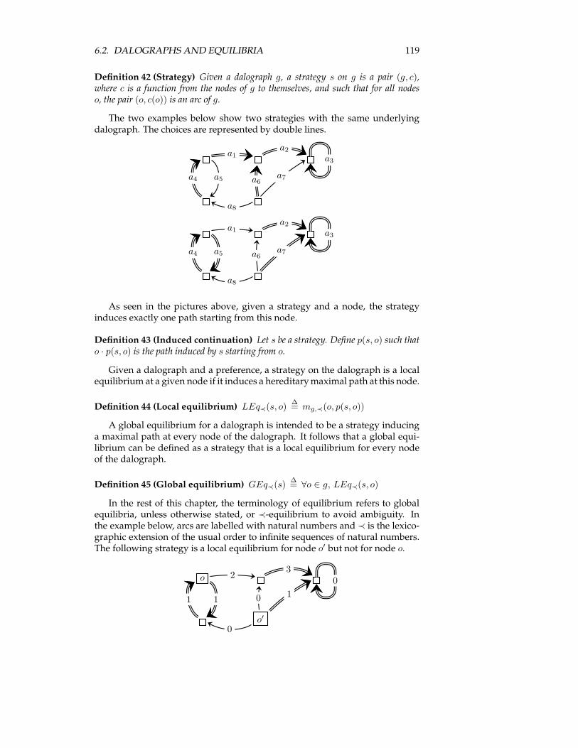
6.2. DALOGRAPHS AND EQUILIBRIA 119
Definition 42 (Strategy) Given a dalograph g, a strategy s on g is a pair (g, c),where c is a function from the nodes of g to themselves, and such that for all nodeso, the pair (o, c(o)) is an arc of g.
The two examples below show two strategies with the same underlyingdalograph. The choices are represented by double lines.
a1a2
a5a4
a8
a6a7
a3
a1a2
a5a4
a8
a6a7
a3
As seen in the pictures above, given a strategy and a node, the strategyinduces exactly one path starting from this node.
Definition 43 (Induced continuation) Let s be a strategy. Define p(s, o) such thato · p(s, o) is the path induced by s starting from o.
Given a dalograph and a preference, a strategy on the dalograph is a localequilibrium at a given node if it induces a hereditarymaximal path at this node.
Definition 44 (Local equilibrium) LEq≺(s, o)∆= mg,≺(o, p(s, o))
A global equilibrium for a dalograph is intended to be a strategy inducinga maximal path at every node of the dalograph. It follows that a global equi-librium can be defined as a strategy that is a local equilibrium for every nodeof the dalograph.
Definition 45 (Global equilibrium) GEq≺(s)∆= ∀o ∈ g, LEq≺(s, o)
In the rest of this chapter, the terminology of equilibrium refers to globalequilibria, unless otherwise stated, or ≺-equilibrium to avoid ambiguity. Inthe example below, arcs are labelled with natural numbers and ≺ is the lexico-graphic extension of the usual order to infinite sequences of natural numbers.The following strategy is a local equilibrium for node o′ but not for node o.
o
o′
23
11
0
0 1
0
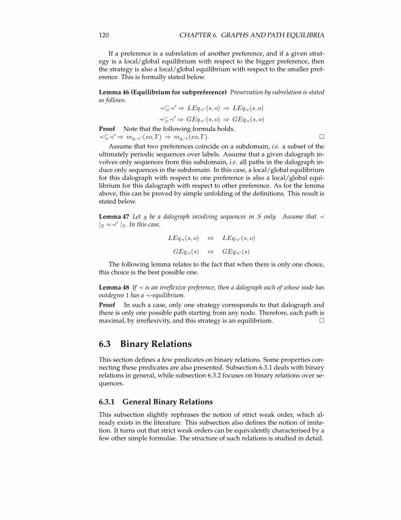
120 CHAPTER 6. GRAPHS AND PATH EQUILIBRIA
If a preference is a subrelation of another preference, and if a given strat-egy is a local/global equilibrium with respect to the bigger preference, thenthe strategy is also a local/global equilibrium with respect to the smaller pref-erence. This is formally stated below.
Lemma 46 (Equilibrium for subpreference) Preservation by subrelation is statedas follows.
≺⊆≺′⇒ LEq≺′(s, o) ⇒ LEq≺(s, o)
≺⊆≺′⇒ GEq≺′(s, o) ⇒ GEq≺(s, o)
Proof Note that the following formula holds.≺⊆≺′⇒ mg,≺′(xo, Γ) ⇒ mg,≺(xo, Γ). �
Assume that two preferences coincide on a subdomain, i.e. a subset of theultimately periodic sequences over labels. Assume that a given dalograph in-volves only sequences from this subdomain, i.e. all paths in the dalograph in-duce only sequences in the subdomain. In this case, a local/global equilibriumfor this dalograph with respect to one preference is also a local/global equi-librium for this dalograph with respect to other preference. As for the lemmaabove, this can be proved by simple unfolding of the definitions. This result isstated below.
Lemma 47 Let g be a dalograph involving sequences in S only. Assume that ≺|S =≺′ |S . In this case,
LEq≺(s, o) ⇔ LEq≺′(s, o)
GEq≺(s) ⇔ GEq≺′(s)
The following lemma relates to the fact that when there is only one choice,this choice is the best possible one.
Lemma 48 If ≺ is an irreflexive preference, then a dalograph each of whose node hasoutdegree 1 has a ≺-equilibrium.
Proof In such a case, only one strategy corresponds to that dalograph andthere is only one possible path starting from any node. Therefore, each path ismaximal, by irreflexivity, and this strategy is an equilibrium. �
6.3 Binary Relations
This section defines a few predicates on binary relations. Some properties con-necting these predicates are also presented. Subsection 6.3.1 deals with binaryrelations in general, while subsection 6.3.2 focuses on binary relations over se-quences.
6.3.1 General Binary Relations
This subsection slightly rephrases the notion of strict weak order, which al-ready exists in the literature. This subsection also defines the notion of imita-tion. It turns out that strict weak orders can be equivalently characterised by afew other simple formulae. The structure of such relations is studied in detail.
6.3. BINARY RELATIONS 121
The notions of transitive, asymmetric, and irreflexive binary relation thatare used in this chapter are the usual ones.
Definition 49 (Transitivity, asymmetry and irreflexivity) A binary relation ≺ istransitive if it complies with the first formula below. Asymmetry amounts to the secondformula, and irreflexivity to the third one.
α ≺ β ⇒ β ≺ γ ⇒ α ≺ γ transitivityα ≺ β ⇒ β 6≺ α asymmetry
α 6≺ α irreflexivity
Asymmetry implies irreflexivity, as being formally stated below.
Lemma 50 (∀α, β, α ≺ β ⇒ β 6≺ α) ⇒ ∀α, α 6≺ α
Proof Instantiate β with α. �
Transitivity of the negation of a relation does not imply transitivity of therelation. For instance, letα 6= β and define≺ on {α, β} byα ≺ β and β ≺ α, andnothing more. Due to the symmetry, ≺ is not transitive, while 6≺ is transitive.The next definition and two lemmas shows that transitivity of the negationalmost implies transitivity.
Definition 51 (Strict weak order) A strict weak order is an asymmetric relationwhose negation is transitive.
Equivalent definitions of strict weak order can be found in the literature.The rest of this subsection explains some properties of strict weak orders andit gives an intuition of the underlying structure. The following lemma showsthat transitivity of a relation can be derived from asymmetry of the relationand transitivity of its negation.
Lemma 52 A strict weak order is transitive.
Proof Let α, β and γ be such that α ≺ β and β ≺ γ. Therefore β 6≺ α andγ 6≺ β by asymmetry, and γ 6≺ α by transitivity of the negation . If α 6≺ γ thenβ 6≺ α and transitivity of the negation yields β 6≺ γ, which is absurd. Thereforeα ≺ γ. �
Strict weak orders have a second property that makes non-comparabilityan equivalence relation.
Lemma 53 If ≺ is a strict weak order, then ♯ is an equivalence relation.
Proof If ¬(α♯α) then α ≺ α, which contradicts asymmetry by lemma 50.So ♯ is reflexive. If α♯β then β♯α by definition, so ♯ is symmetric. If α♯β andβ♯γ, then β 6≺ α and γ 6≺ β by definition. So γ 6≺ α by transitivity of thenegation. In the same way, α 6≺ γ also holds, so α♯γ. Therefore ♯ is transitive.The incomparability relation ♯ is symmetric by definition, so ♯ is an equivalencerelation. �
122 CHAPTER 6. GRAPHS AND PATH EQUILIBRIA
Abinary relation is lower (resp. upper) imitating if any two non-comparableelements have the same predecessors (resp. successors).
Definition 54 (Lower/upper imitation) A binary relation ≺ complying with thefollowing formula is called a lower-imitating relation.
(α♯β ∧ γ ≺ α)⇒ γ ≺ β
A binary relation ≺ complying with the following formula is called a upper-imitatingrelation.
(α♯β ∧ α ≺ γ)⇒ β ≺ γ
A relation that is both lower and upper imitating is called an imitating relation.
Lower and upper imitations do not only look "symmetric" definitions, theyalso are.
Lemma 55 If a relation is lower (resp. upper) imitating, then its inverse is upper(resp. lower) imitating.
Proof Let ≺ be a binary relation. Assume that ≺ is lower imitating and as-sume that α♯−1β and β ≻ γ. So α♯β and γ ≺ β, which implies γ ≺ α, andtherefore α ≻ γ. �
Guaranteeing asymmetry makes the predicates of lower and upper imita-tions coincide.
Lemma 56 Let ≺ be an asymmetric relation. In this case, ≺ is upper-imitating iff ≺is lower-imitating.
Proof left-to-right. Assume α♯β and γ ≺ β. If α ≺ γ then β ≺ γ by upper-imitation, which contradicts asymmetry. If α♯γ then α ≺ β by upper-imitation,which is absurd. So γ ≺ α. The converse follows lemma 55, knowing that theinverse of an asymmetric relation is asymmetric. �
Because of the lemma above, only the concept of imitation will be referredto when dealing with asymmetric relations. The next lemma connects the no-tion of imitation to the notion of transitivity.
Lemma 57 If≺ is transitive and ♯ is an equivalence relation, then≺ is irreflexive andimitating.
Proof If α ≺ α then ♯ is not reflexive, which contradicts the assumption. So≺is irreflexive. Assume that α♯β and β ≺ γ. If γ ≺ α then α ≺ β by transitivity,which is absurd. If γ♯α, then β♯γ by transitivity of ♯, which is absurd. Thereforeα ≺ γ. �
Imitation implies transitivity provided that "small" cycles are forbidden.
Lemma 58 Let ≺ be without any cycle involving 2 or 3 elements. If ≺ is imitatingthen ≺ is transitive.
Proof Assume α ≺ β and β ≺ γ. If γ ≺ α then there is a cycle involving 3elements, which is absurd. Now assume that γ♯α. If ≺ is imitating then β ≺ α,which contradicts asymmetry. So α ≺ γ. �
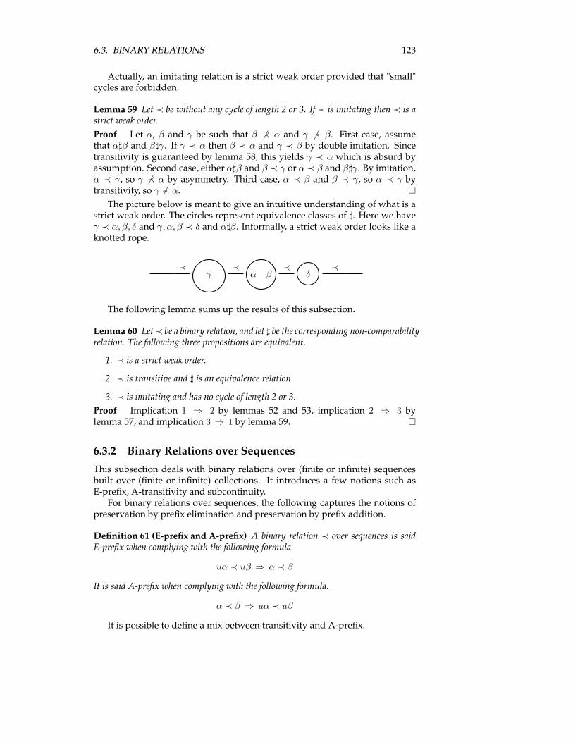
6.3. BINARY RELATIONS 123
Actually, an imitating relation is a strict weak order provided that "small"cycles are forbidden.
Lemma 59 Let ≺ be without any cycle of length 2 or 3. If ≺ is imitating then ≺ is astrict weak order.
Proof Let α, β and γ be such that β 6≺ α and γ 6≺ β. First case, assumethat α♯β and β♯γ. If γ ≺ α then β ≺ α and γ ≺ β by double imitation. Sincetransitivity is guaranteed by lemma 58, this yields γ ≺ α which is absurd byassumption. Second case, either α♯β and β ≺ γ or α ≺ β and β♯γ. By imitation,α ≺ γ, so γ 6≺ α by asymmetry. Third case, α ≺ β and β ≺ γ, so α ≺ γ bytransitivity, so γ 6≺ α. �
The picture below is meant to give an intuitive understanding of what is astrict weak order. The circles represent equivalence classes of ♯. Here we haveγ ≺ α, β, δ and γ, α, β ≺ δ and α♯β. Informally, a strict weak order looks like aknotted rope.
γ α β δ≺ ≺ ≺ ≺
The following lemma sums up the results of this subsection.
Lemma 60 Let≺ be a binary relation, and let ♯ be the corresponding non-comparabilityrelation. The following three propositions are equivalent.
1. ≺ is a strict weak order.
2. ≺ is transitive and ♯ is an equivalence relation.
3. ≺ is imitating and has no cycle of length 2 or 3.
Proof Implication 1 ⇒ 2 by lemmas 52 and 53, implication 2 ⇒ 3 bylemma 57, and implication 3 ⇒ 1 by lemma 59. �
6.3.2 Binary Relations over Sequences
This subsection deals with binary relations over (finite or infinite) sequencesbuilt over (finite or infinite) collections. It introduces a few notions such asE-prefix, A-transitivity and subcontinuity.For binary relations over sequences, the following captures the notions of
preservation by prefix elimination and preservation by prefix addition.
Definition 61 (E-prefix and A-prefix) A binary relation ≺ over sequences is saidE-prefix when complying with the following formula.
uα ≺ uβ ⇒ α ≺ β
It is said A-prefix when complying with the following formula.
α ≺ β ⇒ uα ≺ uβ
It is possible to define a mix between transitivity and A-prefix.
124 CHAPTER 6. GRAPHS AND PATH EQUILIBRIA
Definition 62 (A-transitivity) A relation over sequences is said A-transitive whencomplying with the following formula.
α ≺ β ⇒ uβ ≺ γ ⇒ uα ≺ γ
The following lemma shows the connections between transitivity, A-prefix,and A-transitivity. Note that the converse implications do not hold a priori.
Lemma 63 Transitivity plus A-prefix imply A-transitivity, and A-transitivity im-plies transitivity.
Proof Consider the formula defining A-transitivity. For the first claim, uα ≺uβ by A-prefix, and conclude by transitivity. For the second claim, instantiateuwith the empty sequence. �
The following lemma shows that a strict weak order that is preserved byprefix elimination is A-transitive.
Lemma 64 An E-prefix strict weak order is A-transitive.
Proof Assume that α ≺ β and uβ ≺ γ. Therefore β 6≺ α by asymmetry, souβ 6≺ uα by contraposition of E-prefix. If uα 6≺ γ then uβ 6≺ γ by transitivity ofthe negation, which contradicts the assumption. Therefore uα ≺ γ. �
The A-prefix predicate seems to be a bit too restrictive for what is intendedin this chapter, but a somewhat related notion will be useful. Informally, con-sider a relation ≺ that is A-prefix and transitive. If α ≺ uα then uα ≺ u2α andwe have an infinite ascending chain α ≺ uα ≺ · · · ≺ unα ≺ . . . . In this case, anatural thought might be to topologically close the chain with uω as an upperbound, i.e. α ≺ uα ≺ · · · ≺ unα ≺ · · · ≺ uω. The following definition capturesthis informal thought.
Definition 65 (Subcontinuity) A relation over sequences is said subcontinuous whencomplying with the following formula, where u is any non-empty finite sequence.
α ≺ uα ⇒ uω 6≺ α
The next definition proceeds in the vein of the previous one and gives analternative, slightly more complex definition of subcontinuity.
Definition 66 (Alt-subcontinuity) A relation over sequences is alt-subcontinuouswhen complying with the following formula, where v and t are any non-empty finitesequences.
α ≺ tβ ⇒ (vα ≺ β ∨ α ≺ (tv)ω)
The next lemma shows that alt-subcontinuity is "stronger" than subconti-nuity.
Lemma 67 An alt-subcontinuous asymmetric relation is subcontinuous.
Proof Let ≺ be an alt-subcontinuous asymmetric relation. Assume that α ≺uα for some u and α. By alt-subcontinuity, uα ≺ α ∨ α ≺ uω. By asymmetry,uα 6≺ α, so α ≺ uω. Therefore uω 6≺ α by asymmetry. �
6.4. EQUILIBRIUM EXISTENCE 125
The following lemma states that, under some demanding conditions, sub-continuity implies alt-subcontinuity.
Lemma 68 A E-prefix subcontinuous strict weak order is alt-subcontinuous.
Proof Assume that vα 6≺ β, α 6≺ (tv)ω , and α ≺ tβ. If (tv)ω 6≺ tβ then α 6≺ tβby transitivity of 6≺, which is a contradiction, so (tv)ω ≺ tβ. So (vt)ω ≺ β byE-prefix. If (vt)ω 6≺ vα then (vt)ω 6≺ β by transitivity of 6≺, which is a contra-diction, so (vt)ω ≺ vα, and (tv)ω ≺ α. By subcontinuity, this implies α 6≺ tvα.By assumption, vα 6≺ β, so tvα 6≺ tβ by contraposition of E-prefix. Thereforeα 6≺ tβ by transitivity of the negation, which contradicts the assumption, soα 6≺ tβ. �
The following two definitions generalise the notion of E-prefix.
Definition 69 LetW be a non-empty finite set of finite sequences such that the emptysequence is not inW and such that at most one sequence of length 1 is inW . If for allwalks u inW there exists a walk v inW such that uα ≺ vβ, one writesWα ≺Wβ.
Definition 70 (Gen-E-prefix) A relation over sequences is said gen-E-prefix whencomplying with the following formula.
Wα ≺Wβ ⇒ α ≺ β
6.4 Equilibrium Existence
Subsection 6.4.1 proves a sufficient condition that guarantees existence of equi-librium in any dalograph; subsection 6.4.2 gives a few examples of non-trivialrelations meeting the requirements of the sufficient condition; subsection 6.4.3applies the result to network routing.
6.4.1 The Proof
The two main stages of the proof are, first, building hereditary maximal paths,which are the only paths involved in equilibria, and second, proceeding byinduction on the number of arcs in the dalograph.Hereditary maximal paths seem difficult to be built a priori. A weaker no-
tion is that of semi-hereditary maximal path. On the one hand, a subpath ofa hereditary maximal path is a maximal continuation of the preceding nodealong the hereditary maximal path. On the other hand, a subpath of a semi-hereditary maximal path is a maximal continuation of the beginning of thesemi-hereditary maximal path, as defined below.
Definition 71 (Semi-hereditarymaximal path) Let x be a non-empty walk of con-tinuation Γ. Ifm(xy, Γ′) for all decompositionsΓ = yΓ′ where xy is a walk, one writesshm(x, Γ).
Unsurprisingly, semi-hereditary maximality implies maximality.
Lemma 72 shm(x, Γ) ⇒ m(x, Γ)
Proof Instantiate y with the empty walk in the definition of shm. �
126 CHAPTER 6. GRAPHS AND PATH EQUILIBRIA
The next result states that semi-hereditary maximality is implied by maxi-mality plus semi-hereditary maximality of the subpath starting one node fur-ther along the path.
Lemma 73 m(x, oΓ) ⇒ shm(xo, Γ) ⇒ shm(x, oΓ)
Proof Consider a decomposition oΓ = yΓ′ where xy is a walk. If y is emptythen Γ′ = oΓ so m(xy, Γ′) by assumption. If y is not empty then y = oz. SinceΓ = zΓ′ and shm(xo, Γ), it follows thatm(xoz, Γ′). Hence shm(x, oΓ). �
The notion of semi-hereditarymaximality can also be defined along anotherinduction principle for walks. In such a case, the definition would look likelemma 73.As to the nibbling induction principle for walks in subsection 6.2.2, it will
be exploited as a recursive programming principle instead. It is used below todefine a function that expects a non-empty walk and returns a path. It startsfrom one given node, finds a direction that promises maximality, follows thedirection until there is a better direction to be followed, and so on, but withoutever going back. It stops when the walk is looping because a looping walkdefines a path. It is called the seeking-forward function.
Definition 74 (Seeking-forward function) Let ≺ be an acyclic preference and letg be a dalograph. Define a function that expects a non-empty walk in g and a continu-ation of this walk. More specifically, F (x, Γ) is recursively defined along the nibblinginduction principle for walks.
• If x is a looping walk of continuation Γ, let F (x, Γ)∆= Γ.
• If x is not a looping walk then case split as follows.
1. Ifm(x, Γ) then F (x, Γ)∆= oF (xo, Γ′), where Γ = oΓ′.
2. If ¬m(x, Γ) then F (x, Γ)∆= oF (xo, Γ′) for some oΓ′ such thatm(x, oΓ′)
and xlΓ ≺ xloΓ′.
The following lemma states that whatever the point of view, a path pro-cessed by the seeking-forward function is somehow not worse than the originalpath. Before reading the lemma recall that given u a non-empty finite sequence,uf (resp. ul) represents the first (resp. last) element of u.
Lemma 75 Let ≺ be an irreflexive and A-transitive preference. Let u be a non-emptysuffix of x. The following formula holds.
uF (x, Γ) ≺ uf∆ ⇒ uΓ ≺ uf∆
Proof By nibbling induction on walks. Base step, x is a looping walk ofunique continuation Γ. By definition of F we have F (x, Γ) = Γ, so the claimholds. Inductive step, case split on Γ being or not a maximal continuation ofx. First case, m(x, Γ), so F (x, Γ) = oF (xo, Γ′) with Γ = oΓ′. Assume thatuF (x, Γ) ≺ uf∆, so oF (xo, Γ′) ≺ uf∆. By induction hypothesis, uoΓ′ ≺ uf∆,so uΓ ≺ uf∆. Second case, ¬m(x, Γ), so F (x, Γ) = oF (xo, Γ′) and xlΓ ≺ xloΓ′
for some oΓ′ maximal continuation of x. Assume that uF (x, Γ) ≺ uf∆, souoF (xo, Γ′) ≺ uf∆. By induction hypothesis, uoΓ′ ≺ uf∆. Since u is a non-empty suffix of x, we have ul = xl. It follows that ulΓ ≺ uloΓ′. By A-transitivity, uΓ ≺ uf∆. �
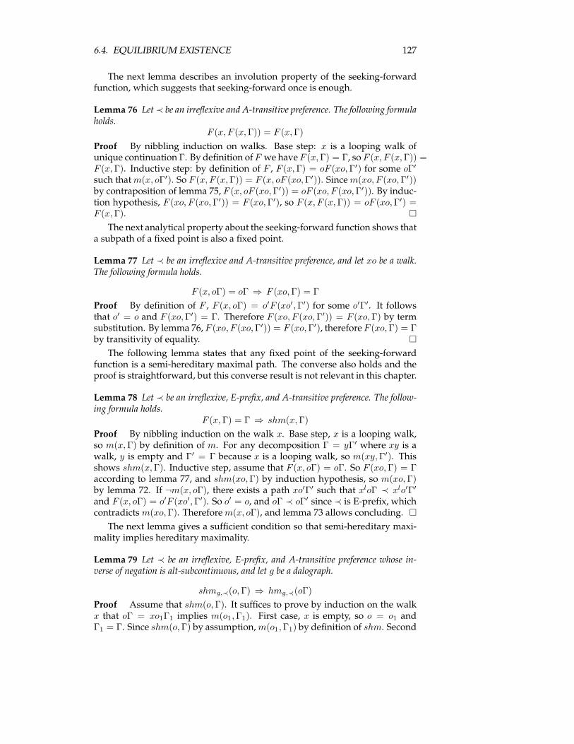
6.4. EQUILIBRIUM EXISTENCE 127
The next lemma describes an involution property of the seeking-forwardfunction, which suggests that seeking-forward once is enough.
Lemma 76 Let≺ be an irreflexive and A-transitive preference. The following formulaholds.
F (x, F (x, Γ)) = F (x, Γ)
Proof By nibbling induction on walks. Base step: x is a looping walk ofunique continuation Γ. By definition ofF we haveF (x, Γ) = Γ, soF (x, F (x, Γ)) =F (x, Γ). Inductive step: by definition of F , F (x, Γ) = oF (xo, Γ′) for some oΓ′
such thatm(x, oΓ′). So F (x, F (x, Γ)) = F (x, oF (xo, Γ′)). Sincem(xo, F (xo, Γ′))by contraposition of lemma 75, F (x, oF (xo, Γ′)) = oF (xo, F (xo, Γ′)). By induc-tion hypothesis, F (xo, F (xo, Γ′)) = F (xo, Γ′), so F (x, F (x, Γ)) = oF (xo, Γ′) =F (x, Γ). �
The next analytical property about the seeking-forward function shows thata subpath of a fixed point is also a fixed point.
Lemma 77 Let ≺ be an irreflexive and A-transitive preference, and let xo be a walk.The following formula holds.
F (x, oΓ) = oΓ ⇒ F (xo, Γ) = Γ
Proof By definition of F , F (x, oΓ) = o′F (xo′, Γ′) for some o′Γ′. It followsthat o′ = o and F (xo, Γ′) = Γ. Therefore F (xo, F (xo, Γ′)) = F (xo, Γ) by termsubstitution. By lemma 76, F (xo, F (xo, Γ′)) = F (xo, Γ′), thereforeF (xo, Γ) = Γby transitivity of equality. �
The following lemma states that any fixed point of the seeking-forwardfunction is a semi-hereditary maximal path. The converse also holds and theproof is straightforward, but this converse result is not relevant in this chapter.
Lemma 78 Let ≺ be an irreflexive, E-prefix, and A-transitive preference. The follow-ing formula holds.
F (x, Γ) = Γ ⇒ shm(x, Γ)
Proof By nibbling induction on the walk x. Base step, x is a looping walk,so m(x, Γ) by definition of m. For any decomposition Γ = yΓ′ where xy is awalk, y is empty and Γ′ = Γ because x is a looping walk, so m(xy, Γ′). Thisshows shm(x, Γ). Inductive step, assume that F (x, oΓ) = oΓ. So F (xo, Γ) = Γaccording to lemma 77, and shm(xo, Γ) by induction hypothesis, so m(xo, Γ)by lemma 72. If ¬m(x, oΓ), there exists a path xo′Γ′ such that xloΓ ≺ xlo′Γ′
and F (x, oΓ) = o′F (xo′, Γ′). So o′ = o, and oΓ ≺ oΓ′ since ≺ is E-prefix, whichcontradictsm(xo, Γ). Thereforem(x, oΓ), and lemma 73 allows concluding. �The next lemma gives a sufficient condition so that semi-hereditary maxi-
mality implies hereditary maximality.
Lemma 79 Let ≺ be an irreflexive, E-prefix, and A-transitive preference whose in-verse of negation is alt-subcontinuous, and let g be a dalograph.
shmg,≺(o, Γ) ⇒ hmg,≺(oΓ)
Proof Assume that shm(o, Γ). It suffices to prove by induction on the walkx that oΓ = xo1Γ1 implies m(o1, Γ1). First case, x is empty, so o = o1 andΓ1 = Γ. Since shm(o, Γ) by assumption,m(o1, Γ1) by definition of shm. Second
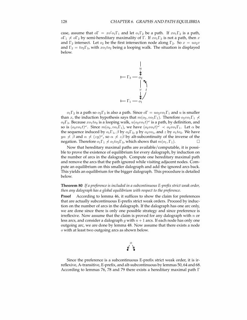
128 CHAPTER 6. GRAPHS AND PATH EQUILIBRIA
case, assume that oΓ = xo′o1Γ1 and let o1Γ2 be a path. If xo1Γ2 is a path,oΓ1 6≺ oΓ2 by semi-hereditary maximality of Γ. If xo1Γ2 is not a path, then xand Γ2 intersect. Let o2 be the first intersection node along Γ2. So x = uo2vand Γ2 = to2Γ3, with xo1to2 being a looping walk. The situation is displayedbelow.
o2
o1
u
Γ3
v
Γ1
t
o1Γ2 is a path so o2Γ3 is also a path. Since oΓ = uo2vo1Γ1 and u is smallerthan x, the induction hypothesis says that m(o2, vo1Γ1). Therefore o2vo1Γ1 6≺o2Γ3. Because xo1to2 is a looping walk, u(o2vo1t)
ω is a path, by definition, andso is (o2vo1t)
ω. Since m(o2, vo1Γ1), we have (o2vo1t)ω ≺ o2vo1Γ1. Let α be
the sequence induced by o1Γ1, β by o2Γ3, y by o2vo1, and z by o1to2. We haveyα 6≺ β and α 6≺ (zy)ω, so α 6≺ zβ by alt-subcontinuity of the inverse of thenegation. Therefore o1Γ1 6≺ o1to2Γ3, which shows thatm(o1, Γ1). �
Now that hereditary maximal paths are available/computable, it is possi-ble to prove the existence of equilibrium for every dalograph, by induction onthe number of arcs in the dalograph. Compute one hereditary maximal pathand remove the arcs that the path ignored while visiting adjacent nodes. Com-pute an equilibrium on this smaller dalograph and add the ignored arcs back.This yields an equilibrium for the bigger dalograph. This procedure is detailedbelow.
Theorem 80 If a preference is included in a subcontinuous E-prefix strict weak order,then any dalograph has a global equilibrium with respect to the preference.
Proof According to lemma 46, it suffices to show the claim for preferencesthat are actually subcontinuous E-prefix strict weak orders. Proceed by induc-tion on the number of arcs in the dalograph. If the dalograph has one arc only,we are done since there is only one possible strategy and since preference isirreflexive. Now assume that the claim is proved for any dalograph with n orless arcs, and consider a dalograph g with n + 1 arcs. If each node has only oneoutgoing arc, we are done by lemma 48. Now assume that there exists a nodeowith at least two outgoing arcs as shown below.
o
Since the preference is a subcontinuous E-prefix strict weak order, it is ir-reflexive, A-transitive, E-prefix, and alt-subcontinuous by lemmas 50, 64 and 68.According to lemmas 76, 78 and 79 there exists a hereditary maximal path Γ
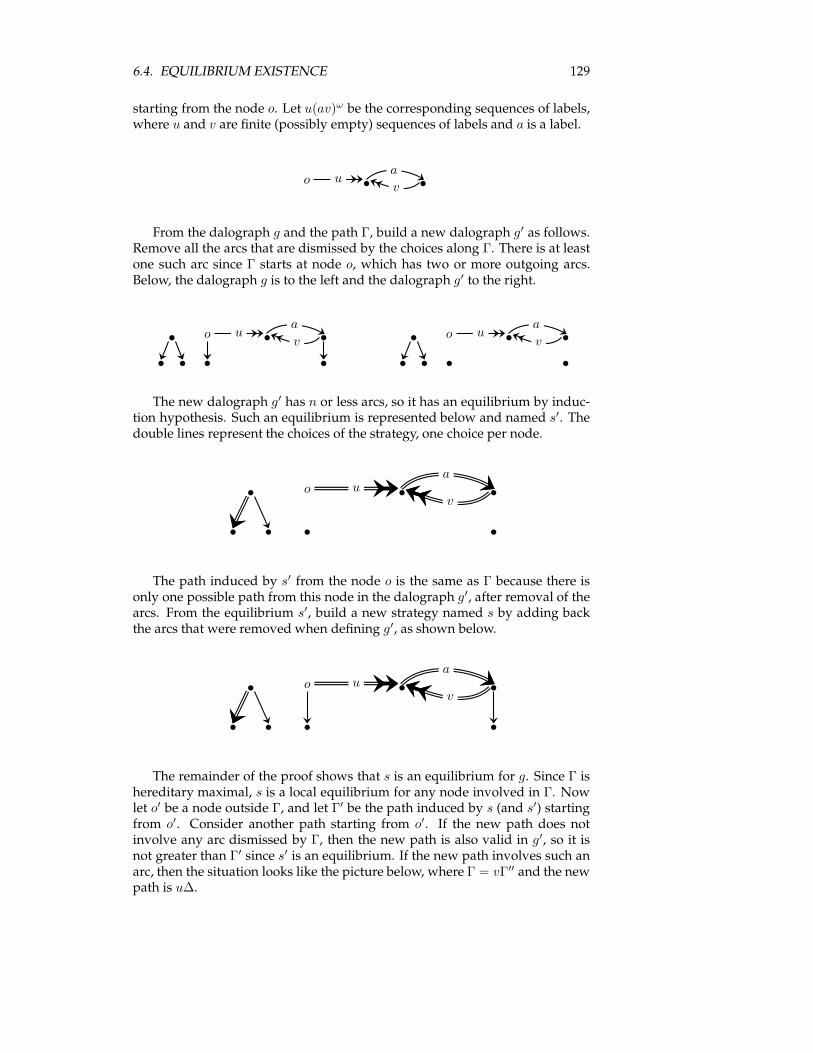
6.4. EQUILIBRIUM EXISTENCE 129
starting from the node o. Let u(av)ω be the corresponding sequences of labels,where u and v are finite (possibly empty) sequences of labels and a is a label.
o ua
v
From the dalograph g and the path Γ, build a new dalograph g′ as follows.Remove all the arcs that are dismissed by the choices along Γ. There is at leastone such arc since Γ starts at node o, which has two or more outgoing arcs.Below, the dalograph g is to the left and the dalograph g′ to the right.
o ua
vo u
a
v
The new dalograph g′ has n or less arcs, so it has an equilibrium by induc-tion hypothesis. Such an equilibrium is represented below and named s′. Thedouble lines represent the choices of the strategy, one choice per node.
o ua
v
The path induced by s′ from the node o is the same as Γ because there isonly one possible path from this node in the dalograph g′, after removal of thearcs. From the equilibrium s′, build a new strategy named s by adding backthe arcs that were removed when defining g′, as shown below.
o ua
v
The remainder of the proof shows that s is an equilibrium for g. Since Γ ishereditary maximal, s is a local equilibrium for any node involved in Γ. Nowlet o′ be a node outside Γ, and let Γ′ be the path induced by s (and s′) startingfrom o′. Consider another path starting from o′. If the new path does notinvolve any arc dismissed by Γ, then the new path is also valid in g′, so it isnot greater than Γ′ since s′ is an equilibrium. If the new path involves such anarc, then the situation looks like the picture below, where Γ = vΓ′′ and the newpath is u∆.
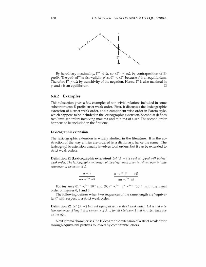
130 CHAPTER 6. GRAPHS AND PATH EQUILIBRIA
o′ o
Γ′ u v
∆Γ′′
By hereditary maximality, Γ′′ 6≺ ∆, so uΓ′′ 6≺ u∆ by contraposition of E-prefix. The path uΓ′′ is also valid in g′, so Γ′ 6≺ uΓ′′ because s′ is an equilibrium.Therefore Γ′ 6≺ u∆ by transitivity of the negation. Hence, Γ′ is also maximal ing, and s is an equilibrium. �
6.4.2 Examples
This subsection gives a few examples of non-trivial relations included in somesubcontinuous E-prefix strict weak order. First, it discusses the lexicographicextension of a strict weak order, and a component-wise order in Pareto style,which happens to be included in the lexicographic extension. Second, it definestwo limit-set orders involving maxima and minima of a set. The second orderhappens to be included in the first one.
Lexicographic extension
The lexicographic extension is widely studied in the literature. It is the ab-straction of the way entries are ordered in a dictionary, hence the name. Thelexicographic extension usually involves total orders, but it can be extended tostrict weak orders.
Definition 81 (Lexicographic extension) Let (A,≺) be a set equipped with a strictweak order. The lexicographic extension of the strict weak order is defined over infinitesequences of elements of A.
a ≺ b
aα ≺lex bβ
α ≺lex β a♯b
aα ≺lex bβ
For instance 01ω ≺lex 10ω and (03)ω ≺lex 1ω ≺lex (30)ω, with the usualorder on figures 0, 1 and 3.The following defines when two sequences of the same length are "equiva-
lent" with respect to a strict weak order.
Definition 82 Let (A,≺) be a set equipped with a strict weak order. Let u and v betwo sequences of length n of elements of A. If for all i between 1 and n, ui♯vi, then onewrites u♯v.
Next lemma characterises the lexicographic extension of a strict weak orderthrough equivalent prefixes followed by comparable letters.
6.4. EQUILIBRIUM EXISTENCE 131
Lemma 83 Let (A,≺) be a set equipped with a strict weak order, and let ≺lex be itslexicographic extension.
α ≺lex βm
∃u, v ∈ A∗, ∃a, b ∈ A, ∃α′, β′ ∈ Aω , α = uaα′ ∧ β = vbβ′ ∧ u♯v ∧ a ≺ b
Proof left-to-right: by rule induction. First rule, α ≺lex β comes from a ≺ b,so α = aα′ and β = bβ′ for some α′ and β′. Second rule, α ≺lex β comes fromα′ ≺lex β′ and a♯b. The induction hypothesis provides some u, v; au and bv arewitnesses of for the claim. Right-to-left. By induction on the length of u. If u isempty then the claim corresponds to the first inference rule. For the inductivestep, invoke the second inference rule. �
The following lemma states the transitivity of the lexicographic extensionof a strict weak order.
Lemma 84 Let (A,≺) be a set equipped with a strict weak order. Then ≺lex is tran-sitive.
Proof Assume that α ≺lex β and β ≺lex γ. By lemma 83, this gives onedecomposition α = uaα′ and β = ubβ′ with a ≺ b, and one decompositionβ = vb′β′′ and γ = vcγ′ with b′ ≺ c. Therefore β = ubβ′ = vb′β′′. Case splitalong the following three mutually exlusive cases: first u = v, second u is aproper prefix of v, and third v is a proper prefix of u. If u = v then b = b′ soa ≺ c by transitivity of ≺, so α ≺lex γ by lemma 83. If u is a proper prefix of vthen u = vb′v′, so α = vb′v′α′ and γ = vcγ′ with b′ ≺ c, therefore α ≺lex γ bylemma 83. If v is a proper prefix of u then v = ubu′, so α = uaα′ and γ = ubu′γ′
with a ≺ b, therefore α ≺lex γ by lemma 83. �
By contraposition, lemma 83 yields the following characterisation of 6≺lex,the negation of ≺lex.
Lemma 85 Let (A,≺) be a set equipped with a strict weak order, and let ≺lex be itslexicographic extension.
α 6≺lex βm
∀u, v ∈ A∗, ∀a, b ∈ A, ∀α′, β′ ∈ Aω, α = uaα′ ∧ β = vbβ′ ∧ u♯v ⇒ a 6≺ b
The construction of the lexicographic extension preserves strict weak order-ing, as stated below.
Lemma 86 Let (A,≺) be a set equipped with a strict weak order. The derived ≺lex isalso a strict weak order.
Proof Since ≺lex is transitive by lemma 84, it suffices to show that ♯lex isan equivalence relation, by lemma 60. The relation ≺lex is irreflexive, whichcan be proved by rule induction on its definition. So ♯lex is reflexive. It isalso symmetric by definition. By lemma 85, α♯lexβ is equivalent to u♯v for alldecompositions α = uα′ and β = vβ′ with u and v of the same length. Thisproperty is transitive since ♯ is transitive by lemma 60. �
132 CHAPTER 6. GRAPHS AND PATH EQUILIBRIA
The lexicographic extension of a strict weak order is E-prefix.
Lemma 87 Let (A,≺) be a set equipped with a strict weak order. The derived ≺lex isE-prefix.
Proof Prove by induction on u that uα ≺lex uβ implies α ≺lex β. If u isempty, that is trivial. If u = au′, then au′α ≺lex au′β must come from thesecond inference rule of the definition of ≺lex, which means that u′α ≺lex u′β.Therefore α ≺lex β by induction hypothesis. �
The lexicographic extension of a strict weak order is also subcontinuous.
Lemma 88 Let (A,≺) be a set equipped with a strict weak order. The derived ≺lex issubcontinuous.
Proof Assume that uω ≺lex α, so unu′♯v, u = u′au′′, α = vbα′, and a ≺ bfor some n, u′, u′′, a, b and α′. Therefore un+1u′♯uv, which can be writtenunu′au′′u′♯uv. Decompose uv = v′cv′′ with v′′ and u′′u′ of the same length.So unu′♯v′ and a♯c. So c ≺ b by strict weak ordering and v♯v′ since ♯ is anequivalence relation. Since uα = v′c(v′′bα′) and α = vbα′, uα ≺lex α. Therefore≺lex is subcontinuous. �
Theorem 80 together with lemmas 86, 87, and 88 allows stating the follow-ing.
Theorem 89 A dalograph labelled with elements of a strict weak order has a globalequilibrium with respect to the lexicographic extension of the strict weak order.
Pareto Extension
A Pareto extension allows comparing vectors with comparable components.A first vector is "greater" than a second one if it is not smaller component-wise and if it is greater for some component. This can be extended to infinitesequences.
Definition 90 (Pareto extension) Let (A,≺) be a set equipped with a strict weakorder. The Pareto extension of the strict weak order is defined over infinite sequencesof elements of A.
α ≺P β∆= ∀n ∈ N, β(n) 6≺ α(n) ∧ ∃n ∈ N, α(n) ≺ β(n)
For instance 01ω 6≺P 10ω but (01)ω ≺P 1ω ≺P (13)ω with the usual order onfigures 0, 1 and 3.The following lemma states that a Pareto extension of a strict weak order is
included in the lexicographic extension of the same strict weak order.
Lemma 91 Let (A,≺) be a set equipped with a strict weak order.
α ≺P β ⇒ α ≺lex β
Proof Assume that α ≺P β, so by definition β(n) 6≺ α(n) for all naturals n,and α(n) ≺ β(n) for some natural n. Let n0 be the smallest natural n such thatα(n) ≺ β(n). So α = uaα′ and β = vbα for some u and v of length n0 anda ≺ b. For i between 0 and n0 − 1, v(i) 6≺ u(i) by assumption, and u(i) 6≺ v(i)by definition of n0. Therefore u♯v, so α ≺lex β by lemma 60. �
6.4. EQUILIBRIUM EXISTENCE 133
Pareto extension also guarantees existence of equilibrium in dalographs.
Theorem 92 A dalograph labelled with elements of a strict weak order has a globalequilibrium with respect to the derived Pareto extension.
Proof Invoke lemmas 91 and 46, and theorem 89. �
Max-Min Limit-Set Order
As discussed in subsection 6.3.1, two non-comparable elements of a strict weakorder compare the same way against any third element. Therefore, compari-son of two elements amounts to comparison of their non-comparability equiv-alence classes.
Definition 93 Let (E,≺) be a set equipped with a strict weak order. This induces atotal order defined as follows on the ♯-equivalence classes A♯ and B♯.
A♯ ≺ B♯ ∆= ∃x ∈ A♯, ∃y ∈ B♯, x ≺ y
Through total ordering, it is easy to define a notion of extrema of finite sets.
Definition 94 (Class maximum and minimum) Let (E,≺) be a set equipped witha strict weak order. The maximum (resp. minimum) of a finite subset A of E is themaximal (resp. minimal) ♯-class intersecting A.
An order over sets is defined below. It involves extrema of sets.
Definition 95 (Max-min order over sets) Let (E,≺) be a set equipped with a strictweak order. The max-min order is defined on finite subsets of E.
A ≺Mm B∆= max(A) ≺ max(B)∨ (max(A) = max(B)∧min(A) ≺ min(B))
For instance {1, 2, 3} ≺Mm {0, 4} and {0, 2, 3} ≺Mm {1, 3} with the usualtotal order over the naturals.The negation of the above order is characterised below.
Lemma 96 Let (E,≺) be a set equipped with a strict weak order.
A 6≺Mm B ⇔ max(A) 6≺ max(B)∧ (max(A) = max(B) ⇒ min(A) 6≺ min(B))
The max-min construction preserves strict weak ordering, as stated below.
Lemma 97 Let (E,≺) be a set equipped with a strict weak order. The Max-min orderon E is also a strict weak order.
Proof First, prove transitivity of its negation. Assume that A 6≺Mm B andB 6≺Mm C. By assumption, max(A) 6≺ max(B) and max(B) 6≺ max(C), somax(A) 6≺ max(C) since≺ is a total order for ♯-classes. Assume thatmax(A) =max(C), so max(A) = max(C) = max(B). Therefore min(A) 6≺ min(B) andmin(B) 6≺ min(C) follows from the assumptions, and min(A) 6≺ min(C) bytotal ordering. This shows that A 6≺Mm C. Second, prove that ♯Mm is an equiv-alence relation: just note that A♯MmB is equivalent to max(A) = max(B) andmin(A) = min(B). �
134 CHAPTER 6. GRAPHS AND PATH EQUILIBRIA
The elements that appear infinitely many times in an infinite sequence con-stitute the limit set of the sequence. Sequences with non-empty limit sets canbe compared through max-min comparisons of their limit sets.
Definition 98 (Max-min limit-set order) Let (E,≺) be a set equipped with a strictweak order. For α infinite sequence over E, let Lα be its limit set, i.e. the set of theelements that occur infinitely often in α. Two infinite sequences whose limit sets arenon-empty are compared as follows.
α ≺Mmls β∆= Lα ≺
Mmβ
For instance 3n4ω ≺Mmls 0p(50q)ω because 4 ≺ 5 according to the usualorder over the naturals.Next lemma states preservation of strict weak ordering by the max-min
construction.
Lemma 99 Let (E,≺) be a set equipped with a strict weak order. The max-min limit-set order is a strict weak order over the sequences with non-empty limit set.
Since the limit set of a sequence is preserved by prefix elimination and ad-dition, the following holds.
Lemma 100 Let (E,≺) be a set equipped with a strict weak order. The max-minlimit-set order is E-prefix and subcontinuous over the sequences of non-empty limitset.
Theorem 80 together with lemmas 99 and 100 allows stating the following.
Theorem 101 A dalograph labelled with elements of a strict weak order has a globalequilibrium with respect to the derived max-min limit-set order.
Max-Min-Light Limit-Set Order
Roughly speaking, the max-min-light order relates sets such that the elementsof one are bigger than the elements of the other.
Definition 102 (Max-min-light order) Let (E,≺) be a set equipped with a strictweak order. The max-min-light order is defined on finite subsets of E.
A ≺Mml B∆= ∀x ∈ A, ∀y ∈ B, y 6≺ x ∧ ∃x ∈ A, ∃y ∈ B, x ≺ y
For instance {1, 2} 6≺Mml {0, 3} but {0, 1} ≺Mml {1} ≺Mml {1, 2}
Definition 103 (Max-min-light limit-set order) Let (E,≺) be a set equipped witha strict weak order. For α infinite sequence over E, let Lα be its limit set, i.e. the setof the elements that occur infinitely often in α. Two infinite sequences whose limit setsare non-empty are compared as follows.
α ≺Mmlls β∆= Lα ≺
Mmlβ
The following theorem states that the max-min-light limit-set order guar-antees equilibrium existence.
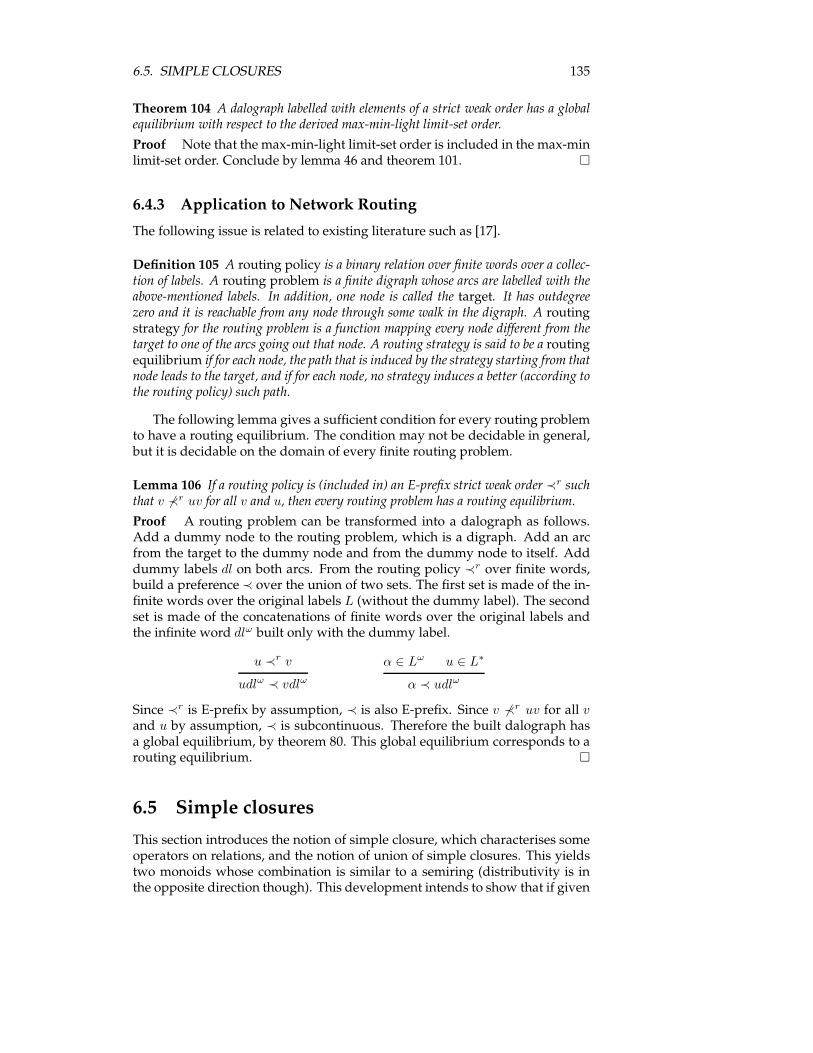
6.5. SIMPLE CLOSURES 135
Theorem 104 A dalograph labelled with elements of a strict weak order has a globalequilibrium with respect to the derived max-min-light limit-set order.
Proof Note that the max-min-light limit-set order is included in the max-minlimit-set order. Conclude by lemma 46 and theorem 101. �
6.4.3 Application to Network Routing
The following issue is related to existing literature such as [17].
Definition 105 A routing policy is a binary relation over finite words over a collec-tion of labels. A routing problem is a finite digraph whose arcs are labelled with theabove-mentioned labels. In addition, one node is called the target. It has outdegreezero and it is reachable from any node through some walk in the digraph. A routingstrategy for the routing problem is a function mapping every node different from thetarget to one of the arcs going out that node. A routing strategy is said to be a routingequilibrium if for each node, the path that is induced by the strategy starting from thatnode leads to the target, and if for each node, no strategy induces a better (according tothe routing policy) such path.
The following lemma gives a sufficient condition for every routing problemto have a routing equilibrium. The condition may not be decidable in general,but it is decidable on the domain of every finite routing problem.
Lemma 106 If a routing policy is (included in) an E-prefix strict weak order ≺r suchthat v 6≺r uv for all v and u, then every routing problem has a routing equilibrium.
Proof A routing problem can be transformed into a dalograph as follows.Add a dummy node to the routing problem, which is a digraph. Add an arcfrom the target to the dummy node and from the dummy node to itself. Adddummy labels dl on both arcs. From the routing policy ≺r over finite words,build a preference≺ over the union of two sets. The first set is made of the in-finite words over the original labels L (without the dummy label). The secondset is made of the concatenations of finite words over the original labels andthe infinite word dlω built only with the dummy label.
u ≺r v
udlω ≺ vdlω
α ∈ Lω u ∈ L∗
α ≺ udlω
Since ≺r is E-prefix by assumption, ≺ is also E-prefix. Since v 6≺r uv for all vand u by assumption, ≺ is subcontinuous. Therefore the built dalograph hasa global equilibrium, by theorem 80. This global equilibrium corresponds to arouting equilibrium. �
6.5 Simple closures
This section introduces the notion of simple closure, which characterises someoperators on relations, and the notion of union of simple closures. This yieldstwo monoids whose combination is similar to a semiring (distributivity is inthe opposite direction though). This development intends to show that if given
136 CHAPTER 6. GRAPHS AND PATH EQUILIBRIA
simple closures preserve a predicate, then any finite restriction of their unionalso preserves this predicate. This result will be usefull in section 6.6.The section starts with the following general lemma. It states that if a pred-
icate is preserved by given functions, then it is preserved by any compositionof these functions.
Lemma 107 Let f0 to fn be functions of type A → A. Let Q be a predicate on A.Assume that each fk preserves Q. Then for all x in A and all w words on the fk thefollowing formula holds.
Q(x) ⇒ Q(w(x))
Proof By induction on w. First case, w is the empty word, i.e. the identityfunction. So x equals w(x), and Q(x) implies Q(w(x)). Second case, w equalsfkw′ and the claim holds for w′. Assume Q(x), so Q(w′(x)) by induction hy-pothesis, and Q(fk ◦ w′(x)) since fk preservesQ. �
In the remainder of this section, the function domain A that is mentionedin lemma 107 above will be a set of relations. More specifically, A will be therelations of arity r, for an arbitrary r that is fixed throughout the section. Inaddition, the symbol X represents a vector (X1, . . . , Xr) of dimension r.Usually in mathematics, the closure of an object is the smallest bigger (or
equal) object of same type that complies with some given predicates. What fol-lows describes a certain kind of closures for relations of arity r, namely simpleclosures. Simple closures are operators (on relations of araity r) inductivelydefined through inference rules. The first rule ensures that the simple closuresare bigger or equal than the original relation. The other rules pertain to theintended properties of the simple closure.
Definition 108 Let f be an operator on relations of arity r. The operator f is said tobe a simple closure if it is inductively defined with the first inference rule below andsome rules having the same form as the second inference rule below.
R(X)
f(R)(X)
K(X, {X i}i∈C) ∧i∈C f(R)(X i)
f(R)(X)
The next lemma states a few basic properties involving simple closures andinclusion.
Lemma 109 Let f be a simple closure. The following formulae hold.
• R ⊆ f(R)
• R ⊆ R′ ⇒ f(R) ⊆ f(R′)
• f ◦ f(R) ⊆ f(R)
Proof The first claim follows the first rule R(X) ⇒ f(R)(X). The secondclaim is proved by rule induction on the definition of f . First case, f(R)(X)comes from R(X). By inclusion, R′(X), so f(R′)(X). Second case f(R)(X)
6.5. SIMPLE CLOSURES 137
comes from ∧i∈Cf(R)(X i). By induction hypothesis, ∧i∈Cf(R′)(X i), there-fore f(R′)(X). The third claim is also proved by rule induction on the defi-nition of f . First case, f ◦ f(R)(X) comes from f(R)(X) we are done. Sec-ond case f ◦ f(R)(X) comes from ∧i∈Cf ◦ f(R)(X i). By induction hypothesis,∧i∈Cf(R)(X i), so f(R)(X). �
The following lemma generalises the first property of lemma 109.
Lemma 110 Let f0 to fn be simple closures on relations of arity r, and Let w, u, andv be words on the fk. For all R relation of arity r and for all X vector of dimension r,the following formula holds.
w(R)(X) ⇒ uwv(R)(X)
Proof First, prove the claim for empty v by induction on u. If u is emptythen it is trivial. If u = fiu
′ then u′w(R)(X) by induction hypothesis, sofiu
′w(R)(X) by the first part of lemma 109. Second, prove the claim for emptyu by induction on v. If v is empty then it is trivial. If v = v′fi thenwv′(R)(X) byinduction hypothesis. Since R ⊆ fi(R) by the first part of lemma 109, we alsohave wv′fi(R)(X) by the second part of lemma 109. Third, assume w(R)(X).So uw(R)(X) by the first part of this proof, and uwv(R)(X) by the second partof this proof. �
Definition 111 (Rule union) Let f and g be two simple closure on relations of arityr. Assume that f is defined by the induction rules F1 to Fn, and that g is defined bythe induction rules G1 toGm. Then, the operator f + g defined by the induction rulesF1 to Fn and G1 to Gm is also a simple closure on relations of arity r.
The law + defines an abelian monoid on simple closures on relation of thesame arity, the neutral element being the identity operator. Moreover the law+ is distributive over the law ◦, but it should be the opposite for (A→ A, +, ◦)to be a semiring.The union of two simple closures yields bigger relations than simple clo-
sures alone, as stated below. It is provable by rule induction on the definitionof f .
Lemma 112 Let R be a relation and let f and g be simple closures. The followingformula holds.
f(R) ⊆ (f + g)(R)
The following lemma generalises the previous result. It shows that compo-sition is somehow "bounded" by union.
Lemma 113 Let f0 to fn be simple closures on relations of arity r, and let f equalΣ0≤k≤nfk. Let w be a word on the fk. For all R relation of arity r, we have w(R) ⊆f(R).
Proof By induction on w. If w is empty then w(R) = R and the first part oflemma 109 allows concluding. If w = fiw
′ then w′(R) ⊆ f(R) by inductionhypothesis. So fiw
′(R) ⊆ f ◦ f(R) by lemma 112, and fiw′(R) ⊆ f(R) by the
third part of lemma 109. �
138 CHAPTER 6. GRAPHS AND PATH EQUILIBRIA
Although composition is "bounded" by union, union is approximable bycomposition, as developed in the next two lemmas. For any relation R of arityr, the union of given simple closures (applied toR) can be simulated at a givenpoint X by some composition of the same simple closures (applied to R), asstated below.
Lemma 114 Let f0 to fn be simple closures on relations of arity r, and let f equalΣ0≤k≤nfk. Let R be a relation of arity r. If f(R)(X) then w(R)(X) for some word won the fk.
Proof By rule induction on the definition of f . First case, assume that f(R)(X)comes from the following rule.
R(X)
f(R)(X)
Since R(X) holds, id(R)(X) also holds, so the empty word is a witness for theclaim. Second case, assume that f(R)(X) is induced by the following rule.
K(X, {X i}i∈C) ∧i∈C f(R)(X i)
f(R)(X)
By induction hypothesis, for all i in C, f(R)(X i) implies that wi(R)(X i) forsome word wi. Let w be a concatenation of the wi. By lemma 110, we havew(R)(X i) for all i. Assume that the inference rule above comes from fk. Bylemma 110, fk+1 . . . fnw(R)(X i) holds for all i. So, fkfk+1 . . . fnw(R)(X) byapplying the inference rule. So f0 . . . fnw(R)(X) by lemma 110 again. There-fore the word f0 . . . fnw is a witness, whatever fk the inference rule may comefrom. �
For any relation R of subdomain S, the union of given simple closures (ap-plied to R) can be approximated on S by a composition of the same simpleclosures (applied to R), as stated below.
Lemma 115 Let f0 to fn be simple closures on relations of arity r, and let f equalΣkfk. Let R be a relation of arity r, and let S be a finite subdomain of R. There existsa word w on the fk such that f(R) |S is included in w(R).
Proof Since S is finite, there exist finitely many X in S such that f(R)(X).For each such X there exists a word u such that u(R)(X), by lemma 114. Letw be a concatenation of all these u. By lemma 110, w(R)(X) for each such X .Therefore f(R) |S is included in w(R). �
The following lemma shows that if given simple closures preserve a predi-cate that is also preserved by subrelation, then any finite restriction of the unionof the closures also preserves the predicate.
Lemma 116 Let Q be a predicate on relations that is preserved by the simple closuresf0 to fn and subrelation, i.e. R ⊂ R′ ⇒ Q(R′) ⇒ Q(R). Then for all relations R offinite subdomain S, Q(R) implies Q(Σkfk(R) |S).
Proof Lemma 115 provides a w such that f(R) |S is included in w(R). Thenlemma 107 shows that Q(w(R)), and preservation by subrelation allows con-cluding. �
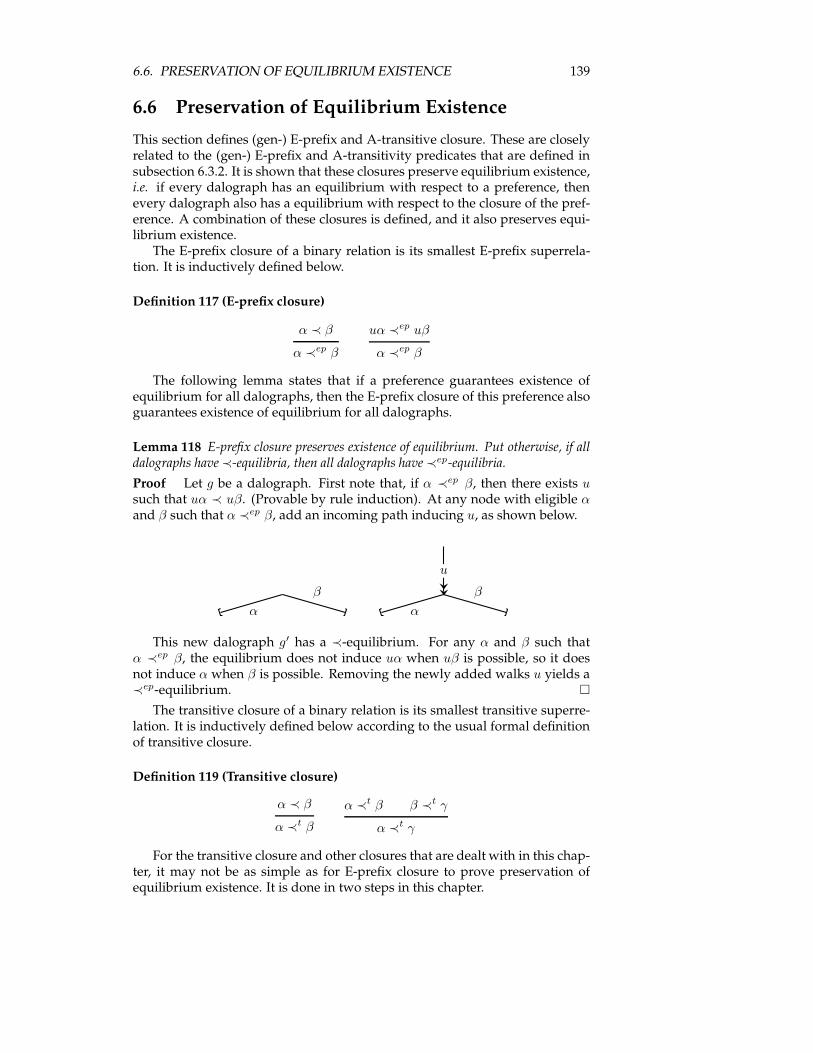
6.6. PRESERVATION OF EQUILIBRIUM EXISTENCE 139
6.6 Preservation of Equilibrium Existence
This section defines (gen-) E-prefix and A-transitive closure. These are closelyrelated to the (gen-) E-prefix and A-transitivity predicates that are defined insubsection 6.3.2. It is shown that these closures preserve equilibrium existence,i.e. if every dalograph has an equilibrium with respect to a preference, thenevery dalograph also has a equilibrium with respect to the closure of the pref-erence. A combination of these closures is defined, and it also preserves equi-librium existence.The E-prefix closure of a binary relation is its smallest E-prefix superrela-
tion. It is inductively defined below.
Definition 117 (E-prefix closure)
α ≺ β
α ≺ep β
uα ≺ep uβ
α ≺ep β
The following lemma states that if a preference guarantees existence ofequilibrium for all dalographs, then the E-prefix closure of this preference alsoguarantees existence of equilibrium for all dalographs.
Lemma 118 E-prefix closure preserves existence of equilibrium. Put otherwise, if alldalographs have≺-equilibria, then all dalographs have ≺ep-equilibria.
Proof Let g be a dalograph. First note that, if α ≺ep β, then there exists usuch that uα ≺ uβ. (Provable by rule induction). At any node with eligible αand β such that α ≺ep β, add an incoming path inducing u, as shown below.
α
β
u
α
β
This new dalograph g′ has a ≺-equilibrium. For any α and β such thatα ≺ep β, the equilibrium does not induce uα when uβ is possible, so it doesnot induce α when β is possible. Removing the newly added walks u yields a≺ep-equilibrium. �
The transitive closure of a binary relation is its smallest transitive superre-lation. It is inductively defined below according to the usual formal definitionof transitive closure.
Definition 119 (Transitive closure)
α ≺ β
α ≺t β
α ≺t β β ≺t γ
α ≺t γ
For the transitive closure and other closures that are dealt with in this chap-ter, it may not be as simple as for E-prefix closure to prove preservation ofequilibrium existence. It is done in two steps in this chapter.
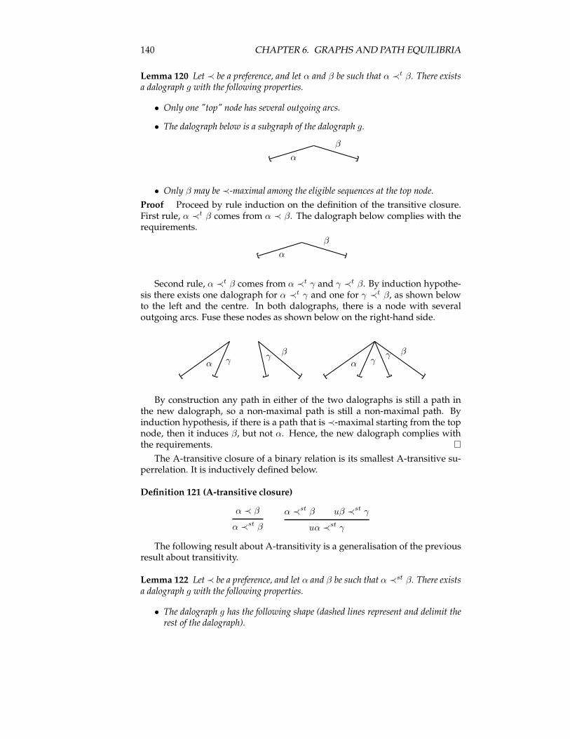
140 CHAPTER 6. GRAPHS AND PATH EQUILIBRIA
Lemma 120 Let ≺ be a preference, and let α and β be such that α ≺t β. There existsa dalograph g with the following properties.
• Only one "top" node has several outgoing arcs.
• The dalograph below is a subgraph of the dalograph g.
α
β
• Only β may be ≺-maximal among the eligible sequences at the top node.
Proof Proceed by rule induction on the definition of the transitive closure.First rule, α ≺t β comes from α ≺ β. The dalograph below complies with therequirements.
α
β
Second rule, α ≺t β comes from α ≺t γ and γ ≺t β. By induction hypothe-sis there exists one dalograph for α ≺t γ and one for γ ≺t β, as shown belowto the left and the centre. In both dalographs, there is a node with severaloutgoing arcs. Fuse these nodes as shown below on the right-hand side.
α γ γ β
α γγ β
By construction any path in either of the two dalographs is still a path inthe new dalograph, so a non-maximal path is still a non-maximal path. Byinduction hypothesis, if there is a path that is ≺-maximal starting from the topnode, then it induces β, but not α. Hence, the new dalograph complies withthe requirements. �
The A-transitive closure of a binary relation is its smallest A-transitive su-perrelation. It is inductively defined below.
Definition 121 (A-transitive closure)
α ≺ β
α ≺st β
α ≺st β uβ ≺st γ
uα ≺st γ
The following result about A-transitivity is a generalisation of the previousresult about transitivity.
Lemma 122 Let≺ be a preference, and let α and β be such that α ≺st β. There existsa dalograph g with the following properties.
• The dalograph g has the following shape (dashed lines represent and delimit therest of the dalograph).

6.6. PRESERVATION OF EQUILIBRIUM EXISTENCE 141
αβ
• The path inducing β is not branching after the top node.
• Any equilibrium for g involves the path inducing β.
Proof Proceed by rule induction on the definition of the A-transitive closure.First rule, the subproof is straightforward. Second rule, uα ≺st γ comes fromuβ ≺st γ and α ≺st β. By induction hypothesis there exist a dalograph g1 foruβ ≺st γ and a dalograph g2 for α ≺st β. Cut the path inducing β away fromg2 (but the top node), and fuse two nodes as shown below.
u
β
γ
αβ
u
β
γ
α
By induction hypothesis, the node inducing γ is not branching in g1, so itit still not branching in the new dalograph g. In an equilibrium, the node justbelow umust choose β, by induction hypothesis. So the top node must involvethe path inducing γ, also by induction hypothesis. �
The gen-E-prefix closure is a generalisation of the E-prefix closure.
Definition 123 (gen-E-prefix closure)
α ≺ β
α ≺sep β
Wα ≺sep Wβ
α ≺sep β
The following lemma is a step towards a generalisation of lemma 118 aboutE-prefix closure.
Lemma 124 Let ≺ be a preference. For any α ≺sep β there exists a dalograph g withthe following properties.
• The dalograph below is a subgraph of the dalograph g.
α
β
• Aside from the top node, the paths inducing α and β are not branching.
• Any equilibrium for g involves the path inducing β.
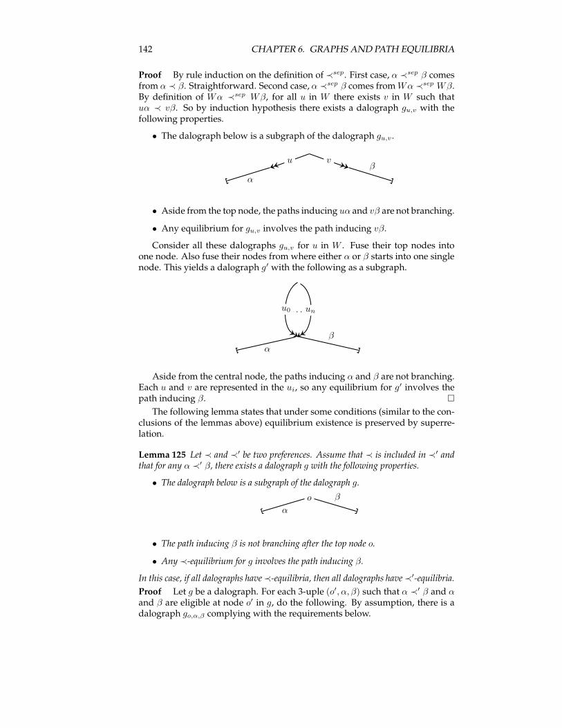
142 CHAPTER 6. GRAPHS AND PATH EQUILIBRIA
Proof By rule induction on the definition of ≺sep. First case, α ≺sep β comesfrom α ≺ β. Straightforward. Second case, α ≺sep β comes fromWα ≺sep Wβ.By definition of Wα ≺sep Wβ, for all u in W there exists v in W such thatuα ≺ vβ. So by induction hypothesis there exists a dalograph gu,v with thefollowing properties.
• The dalograph below is a subgraph of the dalograph gu,v.
u v
α
β
• Aside from the top node, the paths inducing uα and vβ are not branching.
• Any equilibrium for gu,v involves the path inducing vβ.
Consider all these dalographs gu,v for u in W . Fuse their top nodes intoone node. Also fuse their nodes from where either α or β starts into one singlenode. This yields a dalograph g′ with the following as a subgraph.
. . .u0 un
α
β
Aside from the central node, the paths inducing α and β are not branching.Each u and v are represented in the ui, so any equilibrium for g′ involves thepath inducing β. �
The following lemma states that under some conditions (similar to the con-clusions of the lemmas above) equilibrium existence is preserved by superre-lation.
Lemma 125 Let ≺ and ≺′ be two preferences. Assume that ≺ is included in ≺′ andthat for any α ≺′ β, there exists a dalograph g with the following properties.
• The dalograph below is a subgraph of the dalograph g.
o
α
β
• The path inducing β is not branching after the top node o.
• Any ≺-equilibrium for g involves the path inducing β.
In this case, if all dalographs have≺-equilibria, then all dalographs have≺′-equilibria.
Proof Let g be a dalograph. For each 3-uple (o′, α, β) such that α ≺′ β and αand β are eligible at node o′ in g, do the following. By assumption, there is adalograph go,α,β complying with the requirements below.
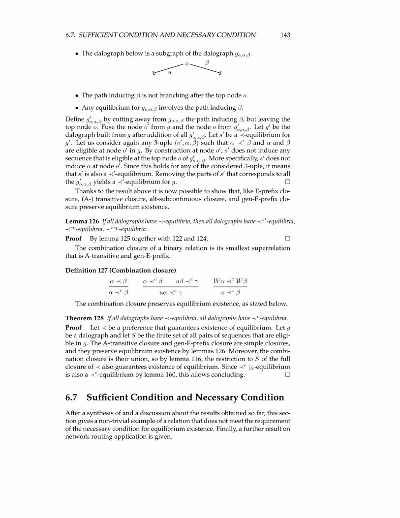
6.7. SUFFICIENT CONDITION AND NECESSARY CONDITION 143
• The dalograph below is a subgraph of the dalograph go,α,β .
o
α
β
• The path inducing β is not branching after the top node o.
• Any equilibrium for go,α,β involves the path inducing β.
Define g′o,α,β by cutting away from go,α,β the path inducing β, but leaving thetop node o. Fuse the node o′ from g and the node o from g′o,α,β. Let g
′ be thedalograph built from g after addition of all g′o,α,β. Let s
′ be a ≺-equilibrium forg′. Let us consider again any 3-uple (o′, α, β) such that α ≺′ β and α and βare eligible at node o′ in g. By construction at node o′, s′ does not induce anysequence that is eligible at the top node o of g′o,α,β. More specifically, s
′ does notinduce α at node o′. Since this holds for any of the considered 3-uple, it meansthat s′ is also a≺′-equilibrium. Removing the parts of s′ that corresponds to allthe g′o,α,β yields a ≺
′-equilibrium for g. �
Thanks to the result above it is now possible to show that, like E-prefix clo-sure, (A-) transitive closure, alt-subcontinuous closure, and gen-E-prefix clo-sure preserve equilibrium existence.
Lemma 126 If all dalographs have≺-equilibria, then all dalographs have≺st-equilibria,≺sc-equilibria, ≺sep-equilibria.
Proof By lemma 125 together with 122 and 124. �
The combination closure of a binary relation is its smallest superrelationthat is A-transitive and gen-E-prefix.
Definition 127 (Combination closure)
α ≺ β
α ≺c β
α ≺c β uβ ≺c γ
uα ≺c γ
Wα ≺c Wβ
α ≺c β
The combination closure preserves equilibrium existence, as stated below.
Theorem 128 If all dalographs have ≺-equilibria, all dalographs have ≺c-equilibria.
Proof Let ≺ be a preference that guarantees existence of equilibrium. Let gbe a dalograph and let S be the finite set of all pairs of sequences that are eligi-ble in g. The A-transitive closure and gen-E-prefix closure are simple closures,and they preserve equilibrium existence by lemmas 126. Moreover, the combi-nation closure is their union, so by lemma 116, the restriction to S of the fullclosure of ≺ also guarantees existence of equilibrium. Since ≺c |S-equilibriumis also a ≺c-equilibrium by lemma 160, this allows concluding. �
6.7 Sufficient Condition and Necessary Condition
After a synthesis of and a discussion about the results obtained so far, this sec-tion gives a non-trivial example of a relation that does not meet the requirementof the necessary condition for equilibrium existence. Finally, a further result onnetwork routing application is given.
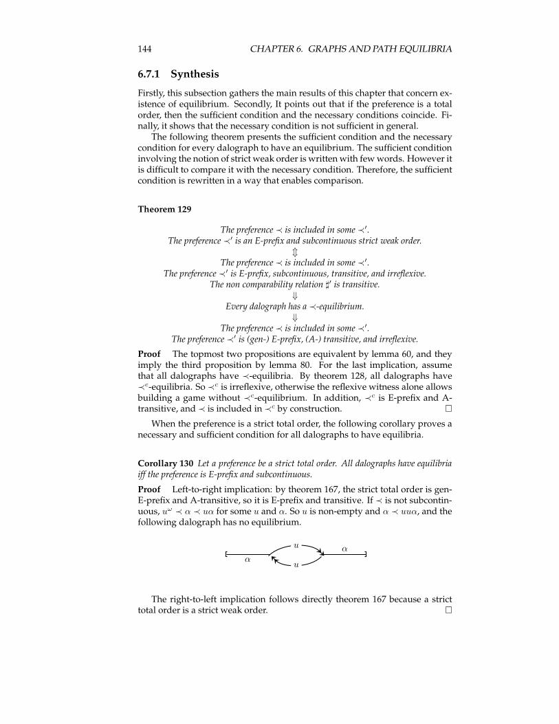
144 CHAPTER 6. GRAPHS AND PATH EQUILIBRIA
6.7.1 Synthesis
Firstly, this subsection gathers the main results of this chapter that concern ex-istence of equilibrium. Secondly, It points out that if the preference is a totalorder, then the sufficient condition and the necessary conditions coincide. Fi-nally, it shows that the necessary condition is not sufficient in general.The following theorem presents the sufficient condition and the necessary
condition for every dalograph to have an equilibrium. The sufficient conditioninvolving the notion of strict weak order is written with fewwords. However itis difficult to compare it with the necessary condition. Therefore, the sufficientcondition is rewritten in a way that enables comparison.
Theorem 129
The preference ≺ is included in some ≺′.The preference ≺′ is an E-prefix and subcontinuous strict weak order.
mThe preference ≺ is included in some ≺′.
The preference ≺′ is E-prefix, subcontinuous, transitive, and irreflexive.The non comparability relation ♯′ is transitive.
⇓Every dalograph has a ≺-equilibrium.
⇓The preference ≺ is included in some ≺′.
The preference ≺′ is (gen-) E-prefix, (A-) transitive, and irreflexive.
Proof The topmost two propositions are equivalent by lemma 60, and theyimply the third proposition by lemma 80. For the last implication, assumethat all dalographs have ≺-equilibria. By theorem 128, all dalographs have≺c-equilibria. So ≺c is irreflexive, otherwise the reflexive witness alone allowsbuilding a game without ≺c-equilibrium. In addition, ≺c is E-prefix and A-transitive, and ≺ is included in ≺c by construction. �
When the preference is a strict total order, the following corollary proves anecessary and sufficient condition for all dalographs to have equilibria.
Corollary 130 Let a preference be a strict total order. All dalographs have equilibriaiff the preference is E-prefix and subcontinuous.
Proof Left-to-right implication: by theorem 167, the strict total order is gen-E-prefix and A-transitive, so it is E-prefix and transitive. If ≺ is not subcontin-uous, uω ≺ α ≺ uα for some u and α. So u is non-empty and α ≺ uuα, and thefollowing dalograph has no equilibrium.
α
u
u
α
The right-to-left implication follows directly theorem 167 because a stricttotal order is a strict weak order. �
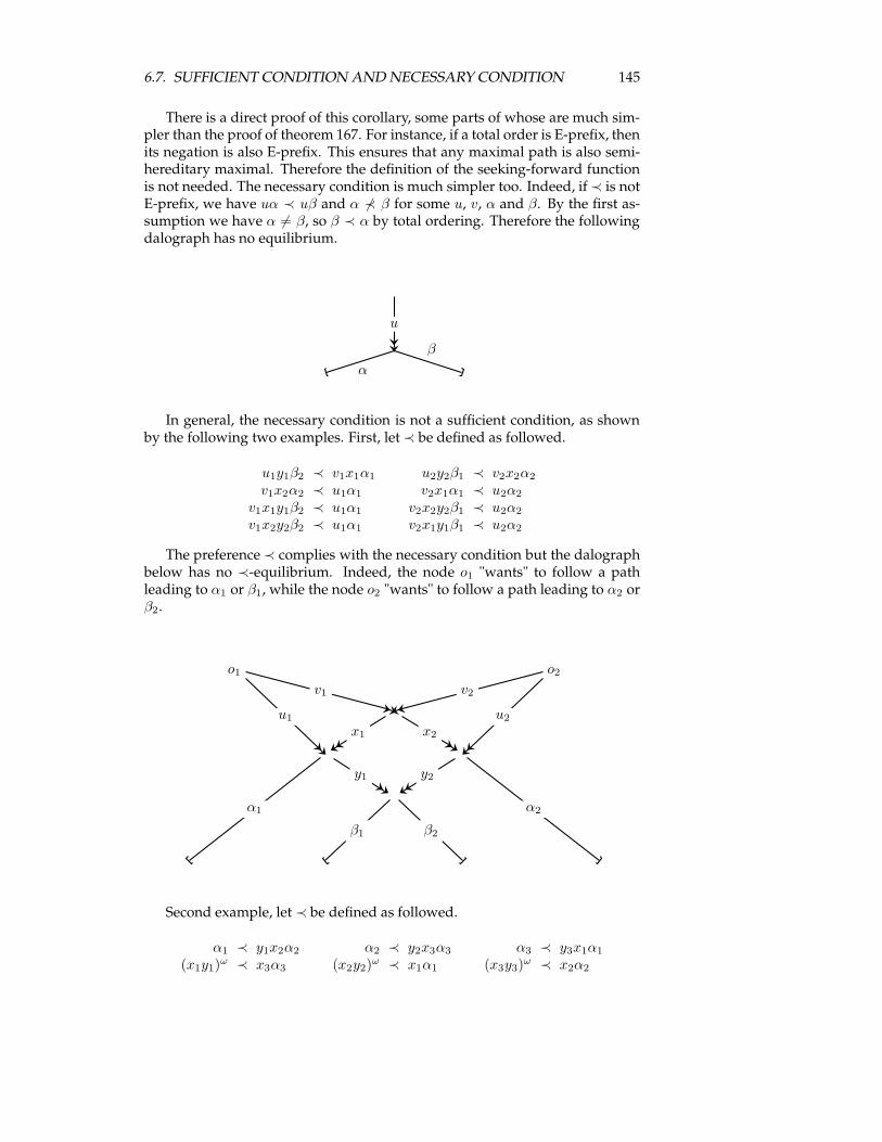
6.7. SUFFICIENT CONDITION AND NECESSARY CONDITION 145
There is a direct proof of this corollary, some parts of whose are much sim-pler than the proof of theorem 167. For instance, if a total order is E-prefix, thenits negation is also E-prefix. This ensures that any maximal path is also semi-hereditary maximal. Therefore the definition of the seeking-forward functionis not needed. The necessary condition is much simpler too. Indeed, if≺ is notE-prefix, we have uα ≺ uβ and α 6≺ β for some u, v, α and β. By the first as-sumption we have α 6= β, so β ≺ α by total ordering. Therefore the followingdalograph has no equilibrium.
u
α
β
In general, the necessary condition is not a sufficient condition, as shownby the following two examples. First, let ≺ be defined as followed.
u1y1β2 ≺ v1x1α1 u2y2β1 ≺ v2x2α2
v1x2α2 ≺ u1α1 v2x1α1 ≺ u2α2
v1x1y1β2 ≺ u1α1 v2x2y2β1 ≺ u2α2
v1x2y2β2 ≺ u1α1 v2x1y1β1 ≺ u2α2
The preference≺ complies with the necessary condition but the dalographbelow has no ≺-equilibrium. Indeed, the node o1 "wants" to follow a pathleading to α1 or β1, while the node o2 "wants" to follow a path leading to α2 orβ2.
o1 o2
v1
u1
v2
u2
x1 x2
y1 y2
α1
β1 β2
α2
Second example, let ≺ be defined as followed.
α1 ≺ y1x2α2 α2 ≺ y2x3α3 α3 ≺ y3x1α1
(x1y1)ω ≺ x3α3 (x2y2)
ω ≺ x1α1 (x3y3)ω ≺ x2α2
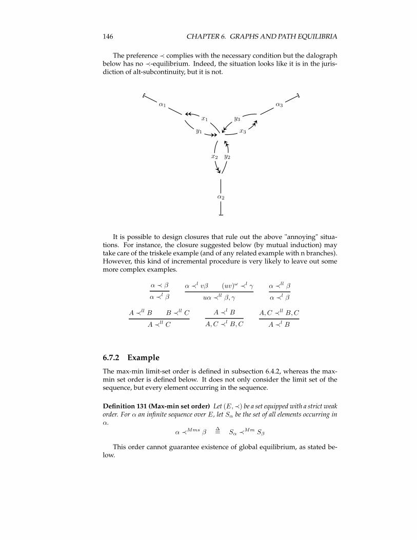
146 CHAPTER 6. GRAPHS AND PATH EQUILIBRIA
The preference≺ complies with the necessary condition but the dalographbelow has no ≺-equilibrium. Indeed, the situation looks like it is in the juris-diction of alt-subcontinuity, but it is not.
α1 α3
α2
x1
x3
x2
y1
y3
y2
It is possible to design closures that rule out the above "annoying" situa-tions. For instance, the closure suggested below (by mutual induction) maytake care of the triskele example (and of any related example with n branches).However, this kind of incremental procedure is very likely to leave out somemore complex examples.
α ≺ β
α ≺l β
α ≺l vβ (uv)ω ≺l γ
uα ≺ll β, γ
α ≺ll β
α ≺l β
A ≺ll B B ≺ll C
A ≺ll C
A ≺l B
A, C ≺l B, C
A, C ≺ll B, C
A ≺l B
6.7.2 Example
The max-min limit-set order is defined in subsection 6.4.2, whereas the max-min set order is defined below. It does not only consider the limit set of thesequence, but every element occurring in the sequence.
Definition 131 (Max-min set order) Let (E,≺) be a set equipped with a strict weakorder. For α an infinite sequence over E, let Sα be the set of all elements occurring inα.
α ≺Mms β∆= Sα ≺
Mm Sβ
This order cannot guarantee existence of global equilibrium, as stated be-low.
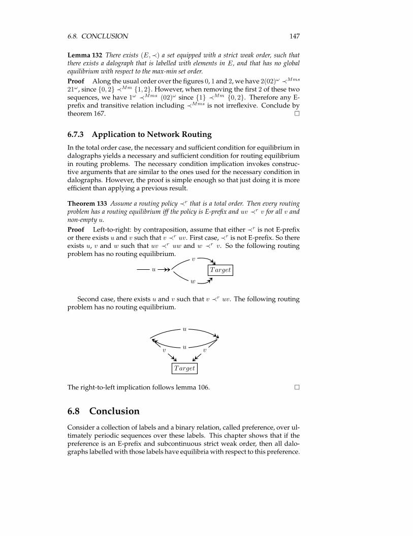
6.8. CONCLUSION 147
Lemma 132 There exists (E,≺) a set equipped with a strict weak order, such thatthere exists a dalograph that is labelled with elements in E, and that has no globalequilibrium with respect to the max-min set order.
Proof Along the usual order over the figures 0, 1 and 2, we have 2(02)ω ≺Mms
21ω, since {0, 2} ≺Mm {1, 2}. However, when removing the first 2 of these twosequences, we have 1ω ≺Mms (02)ω since {1} ≺Mm {0, 2}. Therefore any E-prefix and transitive relation including ≺Mms is not irreflexive. Conclude bytheorem 167. �
6.7.3 Application to Network Routing
In the total order case, the necessary and sufficient condition for equilibrium indalographs yields a necessary and sufficient condition for routing equilibriumin routing problems. The necessary condition implication invokes construc-tive arguments that are similar to the ones used for the necessary condition indalographs. However, the proof is simple enough so that just doing it is moreefficient than applying a previous result.
Theorem 133 Assume a routing policy ≺r that is a total order. Then every routingproblem has a routing equilibrium iff the policy is E-prefix and uv ≺r v for all v andnon-empty u.
Proof Left-to-right: by contraposition, assume that either ≺r is not E-prefixor there exists u and v such that v ≺r uv. First case,≺r is not E-prefix. So thereexists u, v and w such that uv ≺r uw and w ≺r v. So the following routingproblem has no routing equilibrium.
Targetu
v
w
Second case, there exists u and v such that v ≺r uv. The following routingproblem has no routing equilibrium.
Target
u
uv v
The right-to-left implication follows lemma 106. �
6.8 Conclusion
Consider a collection of labels and a binary relation, called preference, over ul-timately periodic sequences over these labels. This chapter shows that if thepreference is an E-prefix and subcontinuous strict weak order, then all dalo-graphs labelledwith those labels have equilibria with respect to this preference.
148 CHAPTER 6. GRAPHS AND PATH EQUILIBRIA
This sufficient condition is proved by a recursively-defined seeking-forwardfunction followed by a proof by induction on the number of arcs in a dalo-graph. A necessary condition is also proved thanks to the notion of simpleclosure and the design of some simple closures, the union of which preservesequilibrium existence. Some examples show that the necessary condition isnot sufficient in general. However, a few examples show the usefulness ofboth the sufficient and the necessary conditions. A detailed study shows thatthe neccessary condition plus the subcontinuity plus the transitivity of the in-comparability relation implies the sufficient condition. Because of this, the twoconditions coincide when the preference is a strict total order, which could alsobe found by a direct proof. However for now, there is no obvious hint sayingwhether or not the sufficient condition is also necessary.This chapter applies its theoretical results to a network routing problem:
first, the above-mentioned sufficient condition yields a sufficient condition onrouting policy for routing equilibrium existence in a simple routing problem.Second, the above-mentioned necessary and sufficient condition of the total or-der case also yields a necessary and sufficient condition on a total order routingpolicy for routing equilibrium existence in a simple routing problem.This chapter is also useful to one other respect: many systems that are dif-
ferent from dalographs also require a notion of preference. In a few of thesesystems, preferences may be thought as total orders without a serious loss ofgenerality: in these systems, any preference that guarantees equilibrium exis-tence is included in some total order also guaranteeing equilibrium existence,and equilibrium existence is preserved by subrelation. In such a setting, con-sidering only total orders somehow accounts for all binary relations. Howeverin the case of dalographs, there might exist a preference guaranteeing equi-librium existence, such that any linear extension of the preference does notguarantee equilibrium existence. In this case, assuming total ordering of thepreference would yield a (non-recoverable) loss of generality. The followingexample is a candidate for such a preference. Consider the ultimately periodicsequences over {a, b, c, d}. An A-transitive preference ≺ over these sequencesis defined below.
aω ≺ cbω ≺ daω
dbω ≺ caω ≺ bω
The preference ≺ defined above is (A-) transitive and (gen-) E-prefix. Inaddition, it is not included in any transitive and E-prefix total order. Indeed,let < be such a total order. If aω < bω then daω < dbω by E-prefix and totalordering, so cbω < caω by transitivity, so bω < aω by E-prefix, contradiction. Ifbω < aω then caω < cbω by transitivity, so aω < bω by E-prefix, contradiction.So, the key question is whether or not the preference≺ guarantees equilibriumexistence for all dalographs (this is not proved in this chapter).
Chapter 7
Sequential Graph Games
Abstract sequential tree games generalise traditional sequential tree games, byabstraction over the real-valued payoff functions, while keeping the tree struc-ture. This permits generalising Kuhn’s result, which states that every tradi-tional sequential game has a Nash equilibrium. This generalisation also usesthe concept of "backward induction" already used by Kuhn. The main pur-pose of this chapter is to define games whose structures are more general thantrees, but where "backward induction" still allows building an equilibrium. Forthis, the chapter generalises further the concept of abstract sequential game byusing a graph structure. In such a setting, local and global equilibria are de-fined. They generalise Nash and subgame perfect equilibria respectively. Fora subclass of sequential graph games, the chapter presents both a necessarycondition and a sufficient condition for global equilibrium existence. Theseconditions relate to the necessary condition and sufficient condition for equi-librium existence in dalographs. Moreover, the sufficient condition adapts anduses "backward induction", which is the aim of this chapter. In addition, theconcept of global equilibrium makes clear that subgame perfect equilibria of asequential tree game are the Nash equilibria of some derived abstract game.More concretely, an embedding identifies the subgame perfect equilibria ofa traditional sequential game with the Nash equilibria of a derived strategicgame.
7.1 Introduction
In the first place, the notion of Nash equilibrium relates to strategic games withreal-valued payoff functions. However, there exists a natural embedding ofsequential games with real-valued payoff functions into strategic games withreal-valued payoff functions. A strategy profile (of a sequential game) whoseimage by the embedding is a Nash equilibrium is also called a Nash equilib-rium. Kuhn [25] proved in 1953 that every traditional sequential game hasa Nash equilibrium. For this he used a procedure named "backward induc-tion". Lately in [29], the notion of sequential game was generalised by replac-ing real-valued payoff functions with abstract atomic objects, called outcomes,and by replacing the usual total order over the reals with arbitrary binary re-lations over outcomes, called preferences. This introduces a general abstract
149
150 CHAPTER 7. SEQUENTIAL GRAPH GAMES
formalism where Nash equilibrium, subgame perfect equilibrium, and “back-ward induction” can still be defined. Using a lemma on topological sorting,the above-mentioned paper proves that the following three propositions areequivalent: 1) Preferences over the outcomes are acyclic. 2) Every sequentialgame has a Nash equilibrium. 3) Every sequential game has a subgame perfectequilibrium. The result was fully computer-certified using Coq.
7.1.1 Graphs and Games
Traditional game theory seems to work mainly with strategic games and se-quential games, i.e. games whose underlying structure is either an array or arooted tree. These game can involve many players. On the contrary, combina-torial game theory studies games with various structures, for instance gamesin graphs. It seems that most of these combinatorial games involve two playersonly. Moreover, the possible outcomes at the end of most of these games are"win-lose", "lose-win", and "draw" only. The book [7] presents many aspects ofcombinatorial game theory.Chess is usually thought as a sequential tree game. However, plays in chess
can be arbitrarily long (in terms of number of moves) even with the fifty movesrules which says that a player can claim a draw if no capture has been madeand no pawn has been moved in the last fifty consecutive moves. So, the gameof chess is actually defined through a directed graph rather than a tree, sincea play can enter a cycle. Every node of the graph is made of both the locationof the pieces on the chessboard and an information about who has to movenext. The arcs between the nodes correspond to the valid moves. So the gameof chess is a bipartite digraph (white and black play in turn) with two agents.This may sound like a detail since the game of chess is well approximated by atree. However, this is not a detail in games that may not end for intrinsic rea-sons instead of technical rules: for instance poker game or companies sharinga market. In both cases, the game can continue as long as there are at least twoplayers willing to play. In the process, a sequence of actions can lead to a situ-ation similar to a previous situation (in terms of poker chips or market share),hence a cycle.A country with several political parties is a complex system. Unlike chess
and poker, rules may not be definable by a digraph, but at least the systemmay be modelled by a digraph: The nodes represent the political situations ofthe country, i.e. which party is in power at which level, etc. Each node is alsolabelled with the party that has to take the next decision, i.e. vote a law, starta campaign, etc. The possible decision are represented by arcs from the nodeto other nodes where other parties have to take other decisions. The arcs arelabelled with the short-term outcomes of the decision. This process may entera cycle when a sequence of actions and elections leads to a political situationthat is similar to a previous situation, i.e. the same parties are in power at thesame levels as before.Internet can be seen as a directed graph whose nodes represent routers and
whose arcs represent links between routers. When receiving a packet, a routerhas to decide where to forward it to: either to a related local network or to an-other router. Each router chooses according to "it’s owner interest". ThereforeInternet can be seen as a digraph with nodes labelled with owners of routers.This digraph is usually symmetric since a link from router A to router B can
7.1. INTRODUCTION 151
be easily transformed to a link between router b and router A. Moreover, theinterests of two different owners, i.e. Internet operators, may be contradictorysince they are supposed to be competitors. Therefore the owners’ trying tomaximise their benefits can be considered a game. Local benefits (or costs) of arouting choice may be displayed on the arcs of the graph.
7.1.2 Contribution
This chapter introduces the notion of sequential graph game. Such a gameinvolves agents and outcomes. A sequential graph game is a directed graphwhose nodes are labelled with agents, whose arcs are labelled with outcomes,and each of whose node has an outgoing arc. The design choices are quicklyjustified, and an interpretation of these games is proposed through an infor-mal notion of play. A strategy profile for a sequential graph game amounts tochoosing an outgoing arc at every node of the game. By changing these choicesonly at some nodes that he owns, an agent can convert a strategy profile intoanother one; this defines convertibility. Starting from a given node, one canfollow the arcs that are prescribed by a given strategy profile. This induces aninfinite sequence of outcomes. For each agent, a binary relation accounts forthe agent’s preferences among infinite sequences of outcomes. Given a nodeof a sequential graph game, an agent can compare two strategy profiles forthe game by comparing the induced infinite sequences at the given node; thisdefines preference. Having a notion of convertibility and preference for eachagent, the local equilibria at given nodes are defined like the Nash equilibria ofsome derived C/P game: they are strategy profiles that no agent can convertinto a preferred profile. A global equilibrium is defined as a strategy profilethat is a local equilibrium at every node of the underlying game.It turns out that the global equilibria of a sequential graph game are ex-
actly the Nash equilibria of some derived C/P game that is different from theC/P game mentioned above. In addition, the chapter defines an embeddingof sequential tree games into sequential graph games. This embedding sendsNash equilibria to local equilibria and vice versa, and sends subgame perfectequilibria to global equilibria and vice versa. Therefore, local equilibrium is ageneralisation of Nash equilibrium and global equilibrium is a generalisationof subgame perfect equilibrium.In sequential tree games, subgame perfect equilibria can be built through
"backward induction" following topological sorting. This chapter generalisesthe procedure of "backward induction" for a subclass of sequential graph games.This leads to a sufficient condition on the agents’ preferences for global equi-librium existence in every game in the subclass mentioned above. It thus gen-eralises the generalisation [29] of Kuhn’s result [25], which states that everysequential game has a Nash (and subgame perfect) equilibrium. In addition,the chapter gives a necessary condition on the agents’ preferences for globalequilibrium existence in every game in the subclass mentioned above. For thenecessary condition and the sufficient condition, which do not coincide in gen-eral, the chapter invokes some results about dalographs proved in chapter 6.However, the two conditions coincide when the preferences are total orders,which gives an equivalence property. In the same way, a sufficient condition isgiven for equilibrium existence in every sequential graph game.Asmentioned above, the subgame perfect equilibria of a game are the global
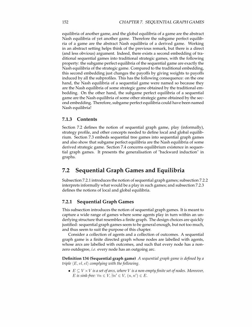
152 CHAPTER 7. SEQUENTIAL GRAPH GAMES
equilibria of another game, and the global equilibria of a game are the abstractNash equilibria of yet another game. Therefore the subgame perfect equilib-ria of a game are the abstract Nash equilibria of a derived game. Workingin an abstract setting helps think of the previous remark, but there is a direct(and less obvious) argument. Indeed, there exists a second embedding of tra-ditional sequential games into traditional strategic games, with the followingproperty: the subgame perfect equilibria of the sequential game are exactly theNash equilibria of the strategic game. Compared to the traditional embedding,this second embedding just changes the payoffs by giving weights to payoffsinduced by all the subprofiles. This has the following consequence: on the onehand, the Nash equilibria of a sequential game were named so because theyare the Nash equilibria of some strategic game obtained by the traditional em-bedding. On the other hand, the subgame perfect equilibria of a sequentialgame are the Nash equilibria of some other strategic game obtained by the sec-ond embedding. Therefore, subgame perfect equilibria could have been namedNash equilibria!
7.1.3 Contents
Section 7.2 defines the notion of sequential graph game, play (informally),strategy profile, and other concepts needed to define local and global equilib-rium. Section 7.3 embeds sequential tree games into sequential graph gamesand also show that subgame perfect equilibria are the Nash equilibria of somederived strategic game. Section 7.4 concerns equilibrium existence in sequen-tial graph games. It presents the generalisation of "backward induction" ingraphs.
7.2 Sequential Graph Games and Equilibria
Subsection 7.2.1 introduces the notion of sequential graph games; subsection 7.2.2interprets informally what would be a play in such games; and subsection 7.2.3defines the notions of local and global equilibria.
7.2.1 Sequential Graph Games
This subsection introduces the notion of sequential graph games. It is meant tocapture a wide range of games where some agents play in turn within an un-derlying structure that resembles a finite graph. The design choices are quicklyjustified: sequential graph games seem to be general enough, but not too much,and thus seem to suit the purpose of this chapter.Consider a collection of agents and a collection of outcomes. A sequential
graph game is a finite directed graph whose nodes are labelled with agents,whose arcs are labelled with outcomes, and such that every node has a non-zero outdegree, i.e. every node has an outgoing arc.
Definition 134 (Sequential graph game) A sequential graph game is defined by atriple 〈E, vl, el〉 complying with the following.
• E ⊆ V ×V is a set of arcs, where V is a non-empty finite set of nodes. Moreover,E is sink-free: ∀n ∈ V, ∃n′ ∈ V, (n, n′) ∈ E.
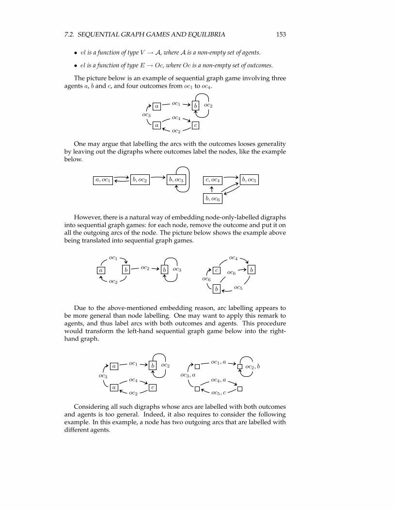
7.2. SEQUENTIAL GRAPH GAMES AND EQUILIBRIA 153
• vl is a function of type V → A, where A is a non-empty set of agents.
• el is a function of type E → Oc, where Oc is a non-empty set of outcomes.
The picture below is an example of sequential graph game involving threeagents a, b and c, and four outcomes from oc1 to oc4.
a b
a c
oc1 oc2
oc3 oc4
oc2
One may argue that labelling the arcs with the outcomes looses generalityby leaving out the digraphs where outcomes label the nodes, like the examplebelow.
a, oc1 b, oc2 b, oc3 c, oc4 b, oc5
b, oc6
However, there is a natural way of embedding node-only-labelled digraphsinto sequential graph games: for each node, remove the outcome and put it onall the outgoing arcs of the node. The picture below shows the example abovebeing translated into sequential graph games.
a b b c b
b
oc1
oc2
oc2 oc3
oc4
oc5
oc6oc6
Due to the above-mentioned embedding reason, arc labelling appears tobe more general than node labelling. One may want to apply this remark toagents, and thus label arcs with both outcomes and agents. This procedurewould transform the left-hand sequential graph game below into the right-hand graph.
a b
a c
oc1 oc2
oc3 oc4
oc2
oc1, aoc2, b
oc3, aoc4, a
oc5, c
Considering all such digraphs whose arcs are labelled with both outcomesand agents is too general. Indeed, it also requires to consider the followingexample. In this example, a node has two outgoing arcs that are labelled withdifferent agents.
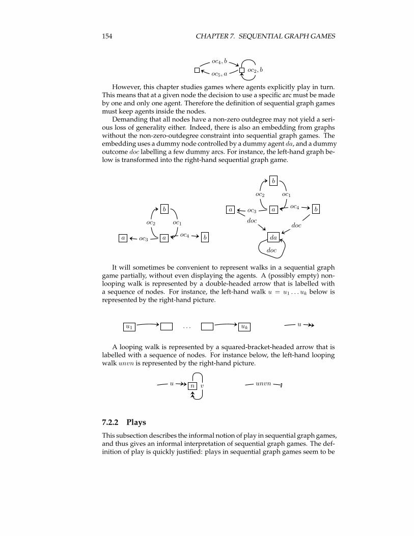
154 CHAPTER 7. SEQUENTIAL GRAPH GAMES
oc2, b
oc4, b
oc5, a
However, this chapter studies games where agents explicitly play in turn.This means that at a given node the decision to use a specific arc must be madeby one and only one agent. Therefore the definition of sequential graph gamesmust keep agents inside the nodes.Demanding that all nodes have a non-zero outdegree may not yield a seri-
ous loss of generality either. Indeed, there is also an embedding from graphswithout the non-zero-outdegree constraint into sequential graph games. Theembedding uses a dummy node controlled by a dummy agent da, and a dummyoutcome doc labelling a few dummy arcs. For instance, the left-hand graph be-low is transformed into the right-hand sequential graph game.
b
a a b
oc1oc2
oc3oc4
b
a a b
da
oc1oc2
oc3oc4
docdoc
doc
It will sometimes be convenient to represent walks in a sequential graphgame partially, without even displaying the agents. A (possibly empty) non-looping walk is represented by a double-headed arrow that is labelled witha sequence of nodes. For instance, the left-hand walk u = u1 . . . uk below isrepresented by the right-hand picture.
u1 . . . uku
A looping walk is represented by a squared-bracket-headed arrow that islabelled with a sequence of nodes. For instance below, the left-hand loopingwalk unvn is represented by the right-hand picture.
n unvnu v
7.2.2 Plays
This subsection describes the informal notion of play in sequential graph games,and thus gives an informal interpretation of sequential graph games. The def-inition of play is quickly justified: plays in sequential graph games seem to be
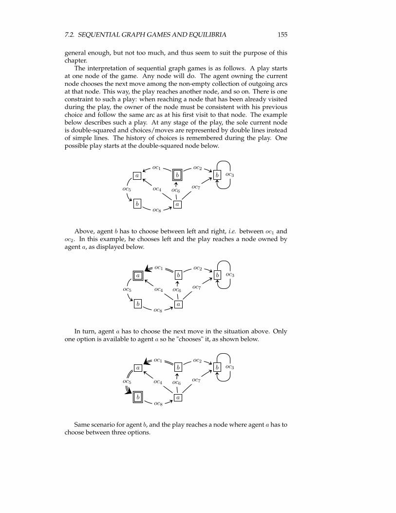
7.2. SEQUENTIAL GRAPH GAMES AND EQUILIBRIA 155
general enough, but not too much, and thus seem to suit the purpose of thischapter.The interpretation of sequential graph games is as follows. A play starts
at one node of the game. Any node will do. The agent owning the currentnode chooses the next move among the non-empty collection of outgoing arcsat that node. This way, the play reaches another node, and so on. There is oneconstraint to such a play: when reaching a node that has been already visitedduring the play, the owner of the node must be consistent with his previouschoice and follow the same arc as at his first visit to that node. The examplebelow describes such a play. At any stage of the play, the sole current nodeis double-squared and choices/moves are represented by double lines insteadof simple lines. The history of choices is remembered during the play. Onepossible play starts at the double-squared node below.
a b b
b a
oc1 oc2
oc5 oc4
oc8
oc6oc7
oc3
Above, agent b has to choose between left and right, i.e. between oc1 andoc2. In this example, he chooses left and the play reaches a node owned byagent a, as displayed below.
a b b
b a
oc1 oc2
oc5 oc4
oc8
oc6oc7
oc3
In turn, agent a has to choose the next move in the situation above. Onlyone option is available to agent a so he "chooses" it, as shown below.
a b b
b a
oc1 oc2
oc5 oc4
oc8
oc6oc7
oc3
Same scenario for agent b, and the play reaches a node where agent a has tochoose between three options.
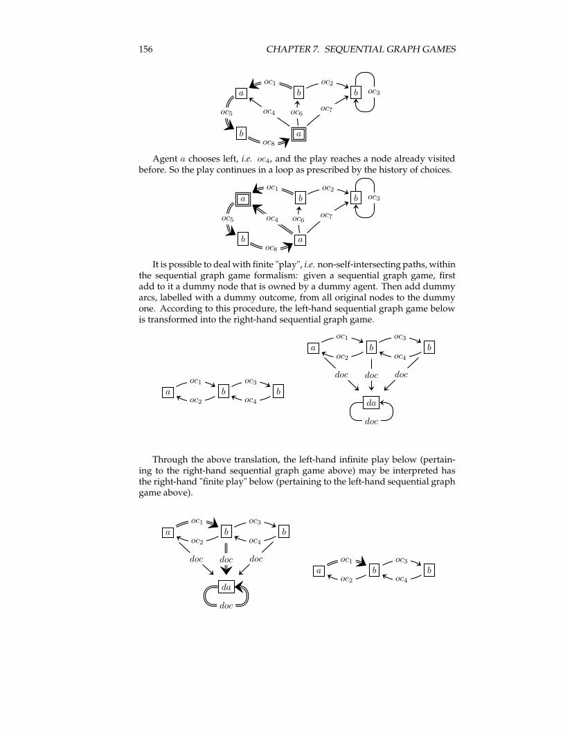
156 CHAPTER 7. SEQUENTIAL GRAPH GAMES
a b b
b a
oc1 oc2
oc5 oc4
oc8
oc6oc7
oc3
Agent a chooses left, i.e. oc4, and the play reaches a node already visitedbefore. So the play continues in a loop as prescribed by the history of choices.
a b b
b a
oc1 oc2
oc5 oc4
oc8
oc6oc7
oc3
It is possible to dealwith finite "play", i.e. non-self-intersecting paths, withinthe sequential graph game formalism: given a sequential graph game, firstadd to it a dummy node that is owned by a dummy agent. Then add dummyarcs, labelled with a dummy outcome, from all original nodes to the dummyone. According to this procedure, the left-hand sequential graph game belowis transformed into the right-hand sequential graph game.
a b boc1
oc2
oc3
oc4
a b b
da
oc1
oc2
oc3
oc4
doc doc doc
doc
Through the above translation, the left-hand infinite play below (pertain-ing to the right-hand sequential graph game above) may be interpreted hasthe right-hand "finite play" below (pertaining to the left-hand sequential graphgame above).
a b b
da
oc1
oc2
oc3
oc4
doc doc doc
doc
a b boc1
oc2
oc3
oc4
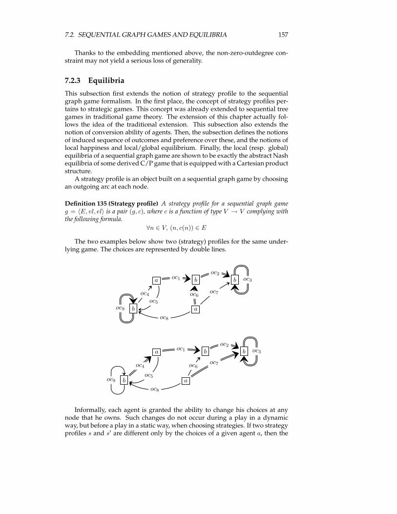
7.2. SEQUENTIAL GRAPH GAMES AND EQUILIBRIA 157
Thanks to the embedding mentioned above, the non-zero-outdegree con-straint may not yield a serious loss of generality.
7.2.3 Equilibria
This subsection first extends the notion of strategy profile to the sequentialgraph game formalism. In the first place, the concept of strategy profiles per-tains to strategic games. This concept was already extended to sequential treegames in traditional game theory. The extension of this chapter actually fol-lows the idea of the traditional extension. This subsection also extends thenotion of conversion ability of agents. Then, the subsection defines the notionsof induced sequence of outcomes and preference over these, and the notions oflocal happiness and local/global equilibrium. Finally, the local (resp. global)equilibria of a sequential graph game are shown to be exactly the abstract Nashequilibria of some derivedC/P game that is equippedwith a Cartesian productstructure.A strategy profile is an object built on a sequential graph game by choosing
an outgoing arc at each node.
Definition 135 (Strategy profile) A strategy profile for a sequential graph gameg = 〈E, vl, el〉 is a pair (g, c), where c is a function of type V → V complying withthe following formula.
∀n ∈ V, (n, c(n)) ∈ E
The two examples below show two (strategy) profiles for the same under-lying game. The choices are represented by double lines.
a b b
b a
oc1
oc2
oc5
oc4
oc8
oc6oc7
oc3
oc9
a b b
b a
oc1oc2
oc5
oc4
oc8
oc6oc7
oc3
oc9
Informally, each agent is granted the ability to change his choices at anynode that he owns. Such changes do not occur during a play in a dynamicway, but before a play in a static way, when choosing strategies. If two strategyprofiles s and s′ are different only by the choices of a given agent a, then the
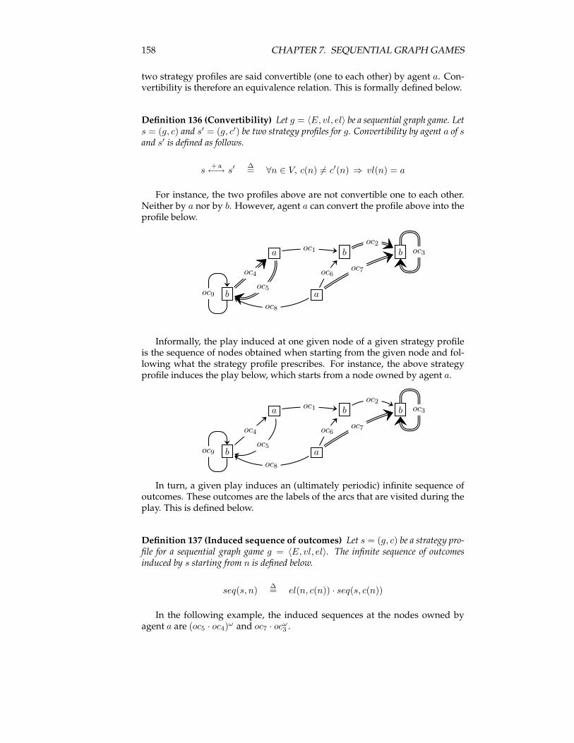
158 CHAPTER 7. SEQUENTIAL GRAPH GAMES
two strategy profiles are said convertible (one to each other) by agent a. Con-vertibility is therefore an equivalence relation. This is formally defined below.
Definition 136 (Convertibility) Let g = 〈E, vl, el〉 be a sequential graph game. Lets = (g, c) and s′ = (g, c′) be two strategy profiles for g. Convertibility by agent a of sand s′ is defined as follows.
s+a←→ s′
∆= ∀n ∈ V, c(n) 6= c′(n) ⇒ vl(n) = a
For instance, the two profiles above are not convertible one to each other.Neither by a nor by b. However, agent a can convert the profile above into theprofile below.
a b b
b a
oc1oc2
oc5
oc4
oc8
oc6oc7
oc3
oc9
Informally, the play induced at one given node of a given strategy profileis the sequence of nodes obtained when starting from the given node and fol-lowing what the strategy profile prescribes. For instance, the above strategyprofile induces the play below, which starts from a node owned by agent a.
a b b
b a
oc1oc2
oc5
oc4
oc8
oc6oc7
oc3
oc9
In turn, a given play induces an (ultimately periodic) infinite sequence ofoutcomes. These outcomes are the labels of the arcs that are visited during theplay. This is defined below.
Definition 137 (Induced sequence of outcomes) Let s = (g, c) be a strategy pro-file for a sequential graph game g = 〈E, vl, el〉. The infinite sequence of outcomesinduced by s starting from n is defined below.
seq(s, n)∆= el(n, c(n)) · seq(s, c(n))
In the following example, the induced sequences at the nodes owned byagent a are (oc5 · oc4)
ω and oc7 · ocω3 .
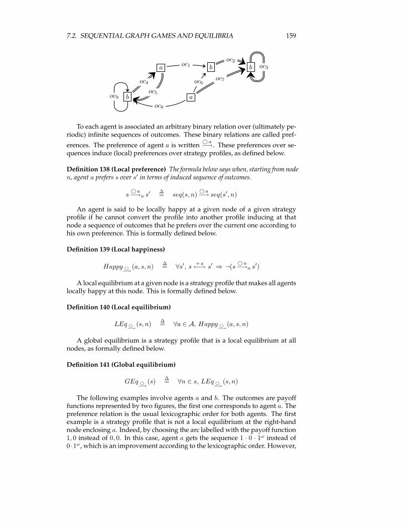
7.2. SEQUENTIAL GRAPH GAMES AND EQUILIBRIA 159
a b b
b a
oc1oc2
oc5
oc4
oc8
oc6oc7
oc3
oc9
To each agent is associated an arbitrary binary relation over (ultimately pe-riodic) infinite sequences of outcomes. These binary relations are called pref-
erences. The preference of agent a is written© a−→. These preferences over se-
quences induce (local) preferences over strategy profiles, as defined below.
Definition 138 (Local preference) The formula below says when, starting from noden, agent a prefers s over s′ in terms of induced sequence of outcomes.
s© a−→n s′
∆= seq(s, n)
© a−→ seq(s′, n)
An agent is said to be locally happy at a given node of a given strategyprofile if he cannot convert the profile into another profile inducing at thatnode a sequence of outcomes that he prefers over the current one according tohis own preference. This is formally defined below.
Definition 139 (Local happiness)
Happy ©−→
(a, s, n)∆= ∀s′, s
+a←→ s′ ⇒ ¬(s
© a−→n s′)
A local equilibrium at a given node is a strategy profile thatmakes all agentslocally happy at this node. This is formally defined below.
Definition 140 (Local equilibrium)
LEq ©−→
(s, n)∆= ∀a ∈ A, Happy ©
−→(a, s, n)
A global equilibrium is a strategy profile that is a local equilibrium at allnodes, as formally defined below.
Definition 141 (Global equilibrium)
GEq ©−→
(s)∆= ∀n ∈ s, LEq ©
−→(s, n)
The following examples involve agents a and b. The outcomes are payofffunctions represented by two figures, the first one corresponds to agent a. Thepreference relation is the usual lexicographic order for both agents. The firstexample is a strategy profile that is not a local equilibrium at the right-handnode enclosing a. Indeed, by choosing the arc labelled with the payoff function1, 0 instead of 0, 0. In this case, agent a gets the sequence 1 · 0 · 1ω instead of0 ·1ω, which is an improvement according to the lexicographic order. However,
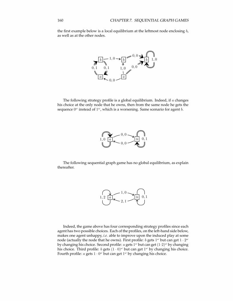
160 CHAPTER 7. SEQUENTIAL GRAPH GAMES
the first example below is a local equilibrium at the leftmost node enclosing b,as well as at the other nodes.
b b b
a a
1, 00, 0
0, 10, 1
0, 0
1, 0 0, 0
1, 0
The following strategy profile is a global equilibrium. Indeed, if a changeshis choice at the only node that he owns, then from the same node he gets thesequence 0ω instead of 1ω, which is a worsening. Same scenario for agent b.
a b1, 0 0, 10, 0
0, 0
The following sequential graph game has no global equilibrium, as explainthereafter.
a b1, 2 0, 11, 0
2, 1
Indeed, the game above has four corresponding strategy profiles since eachagent has two possible choices. Each of the profiles, on the left-hand side below,makes one agent unhappy, i.e. able to improve upon the induced play at somenode (actually the node that he owns). First profile: b gets 1ω but can get 1 · 2ω
by changing his choice. Second profile: a gets 1ω but can get (1·2)ω by changinghis choice. Third profile: b gets (1 · 0)ω but can get 1ω by changing his choice.Fourth profile: a gets 1 · 0ω but can get 1ω by changing his choice.
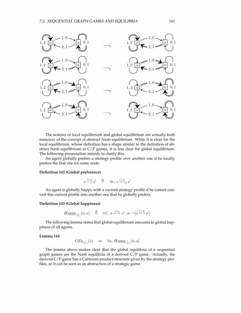
7.2. SEQUENTIAL GRAPH GAMES AND EQUILIBRIA 161
a b1, 2 0, 11, 0
2, 1 −→ba b1, 2 0, 1
1, 0
2, 1
a b1, 2 0, 11, 0
2, 1 −→aa b1, 2 0, 1
1, 0
2, 1
a b1, 2 0, 11, 0
2, 1 −→ba b1, 2 0, 1
1, 0
2, 1
a b1, 2 0, 11, 0
2, 1 −→aa b1, 2 0, 1
1, 0
2, 1
The notions of local equilibrium and global equilibrium are actually bothinstances of the concept of abstract Nash equilibrium. While it is clear for thelocal equilibrium, whose definition has a shape similar to the definition of ab-stract Nash equilibrium in C/P games, it is less clear for global equilibrium.The following presentation intends to clarify this.An agent globally prefers a strategy profile over another one if he locally
prefers the first one for some node.
Definition 142 (Global preference)
s© a−→ s′
∆= ∃n, s
© a−→n s′
An agent is globally happy with a current strategy profile if he cannot con-vert this current profile into another one that he globally prefers.
Definition 143 (Global happiness)
Happy ©−→
(a, s)∆= ∀s′, s
+a←→ s′ ⇒ ¬(s
© a−→ s′)
The following lemma states that global equilibrium amounts to global hap-piness of all agents.
Lemma 144GEq ©
−→(s) ⇔ ∀a, Happy ©
−→(a, s)
The lemma above makes clear that the global equilibria of a sequentialgraph games are the Nash equilibria of a derived C/P game. Actually, thederived C/P game has a Cartesian product structure given by the strategy pro-files, so it can be seen as an abstraction of a strategic game.
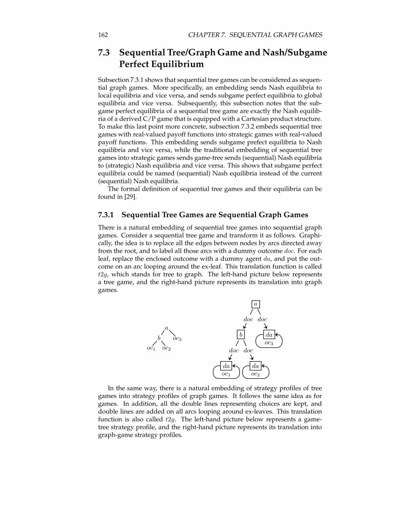
162 CHAPTER 7. SEQUENTIAL GRAPH GAMES
7.3 Sequential Tree/GraphGame andNash/SubgamePerfect Equilibrium
Subsection 7.3.1 shows that sequential tree games can be considered as sequen-tial graph games. More specifically, an embedding sends Nash equilibria tolocal equilibria and vice versa, and sends subgame perfect equilibria to globalequilibria and vice versa. Subsequently, this subsection notes that the sub-game perfect equilibria of a sequential tree game are exactly the Nash equilib-ria of a derived C/P game that is equipped with a Cartesian product structure.To make this last point more concrete, subsection 7.3.2 embeds sequential treegames with real-valued payoff functions into strategic games with real-valuedpayoff functions. This embedding sends subgame prefect equilibria to Nashequilibria and vice versa, while the traditional embedding of sequential treegames into strategic games sends game-tree sends (sequential) Nash equilibriato (strategic) Nash equilibria and vice versa. This shows that subgame perfectequilibria could be named (sequential) Nash equilibria instead of the current(sequential) Nash equilibria.The formal definition of sequential tree games and their equilibria can be
found in [29].
7.3.1 Sequential Tree Games are Sequential Graph Games
There is a natural embedding of sequential tree games into sequential graphgames. Consider a sequential tree game and transform it as follows. Graphi-cally, the idea is to replace all the edges between nodes by arcs directed awayfrom the root, and to label all those arcs with a dummy outcome doc. For eachleaf, replace the enclosed outcome with a dummy agent da, and put the out-come on an arc looping around the ex-leaf. This translation function is calledt2g, which stands for tree to graph. The left-hand picture below representsa tree game, and the right-hand picture represents its translation into graphgames.
a
b oc3
oc1 oc2
a
b da
da da
doc doc
doc doc
oc3
oc1 oc2
In the same way, there is a natural embedding of strategy profiles of treegames into strategy profiles of graph games. It follows the same idea as forgames. In addition, all the double lines representing choices are kept, anddouble lines are added on all arcs looping around ex-leaves. This translationfunction is also called t2g. The left-hand picture below represents a game-tree strategy profile, and the right-hand picture represents its translation intograph-game strategy profiles.
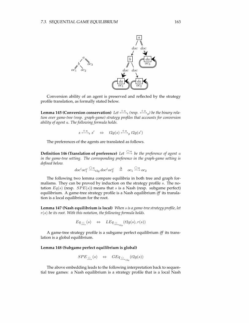
7.3. SEQUENTIAL GAME EQUILIBRIUM 163
a
b oc3
oc1 oc2
a
b da
da da
doc doc
doc doc
oc3
oc1 oc2
Conversion ability of an agent is preserved and reflected by the strategyprofile translation, as formally stated below.
Lemma 145 (Conversion conservation) Let + a←→t (resp.
+ a←→g) be the binary rela-
tion over game-tree (resp. graph-game) strategy profiles that accounts for conversionability of agent a. The following formula holds.
s+ a←→t s′ ⇔ t2g(s)
+ a←→g t2g(s′)
The preferences of the agents are translated as follows.
Definition 146 (Translation of preference) Let©a−→ be the preference of agent a
in the game-tree setting. The corresponding preference in the graph-game setting isdefined below.
dociocω1
© a−→t2g docjocω
2∆= oc1
© a−→ oc2
The following two lemma compare equilibria in both tree and graph for-malisms. They can be proved by induction on the strategy profile s. The no-tation Eq(s) (resp. SPE(s)) means that s is a Nash (resp. subgame perfect)equilibrium. A game-tree strategy profile is a Nash equilibrium iff its transla-tion is a local equilibrium for the root.
Lemma 147 (Nash equilibrium is local) When s is a game-tree strategy profile, letr(s) be its root. With this notation, the following formula holds.
Eq ©−→
(s) ⇔ LEq ©−→t2g
(t2g(s), r(s))
A game-tree strategy profile is a subgame perfect equilibrium iff its trans-lation is a global equilibrium.
Lemma 148 (Subgame perfect equilibrium is global)
SPE ©−→
(s) ⇔ GEq ©−→t2g
(t2g(s))
The above embedding leads to the following interpretation back to sequen-tial tree games: a Nash equilibrium is a strategy profile that is a local Nash
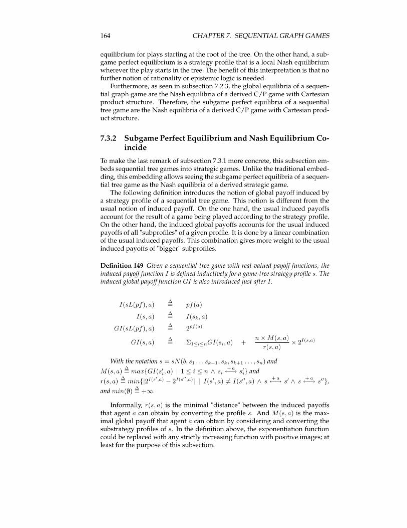
164 CHAPTER 7. SEQUENTIAL GRAPH GAMES
equilibrium for plays starting at the root of the tree. On the other hand, a sub-game perfect equilibrium is a strategy profile that is a local Nash equilibriumwherever the play starts in the tree. The benefit of this interpretation is that nofurther notion of rationality or epistemic logic is needed.Furthermore, as seen in subsection 7.2.3, the global equilibria of a sequen-
tial graph game are the Nash equilibria of a derived C/P game with Cartesianproduct structure. Therefore, the subgame perfect equilibria of a sequentialtree game are the Nash equilibria of a derived C/P game with Cartesian prod-uct structure.
7.3.2 Subgame Perfect Equilibrium andNash Equilibrium Co-incide
To make the last remark of subsection 7.3.1 more concrete, this subsection em-beds sequential tree games into strategic games. Unlike the traditional embed-ding, this embedding allows seeing the subgame perfect equilibria of a sequen-tial tree game as the Nash equilibria of a derived strategic game.The following definition introduces the notion of global payoff induced by
a strategy profile of a sequential tree game. This notion is different from theusual notion of induced payoff. On the one hand, the usual induced payoffsaccount for the result of a game being played according to the strategy profile.On the other hand, the induced global payoffs accounts for the usual inducedpayoffs of all "subprofiles" of a given profile. It is done by a linear combinationof the usual induced payoffs. This combination gives more weight to the usualinduced payoffs of "bigger" subprofiles.
Definition 149 Given a sequential tree game with real-valued payoff functions, theinduced payoff function I is defined inductively for a game-tree strategy profile s. Theinduced global payoff function GI is also introduced just after I .
I(sL(pf), a)∆= pf(a)
I(s, a)∆= I(sk, a)
GI(sL(pf), a)∆= 2pf(a)
GI(s, a)∆= Σ1≤i≤nGI(si, a) +
n×M(s, a)
r(s, a)× 2I(s,a)
With the notation s = sN(b, s1 . . . sk−1, sk, sk+1 . . . , sn) and
M(s, a)∆= max{GI(s′i, a) | 1 ≤ i ≤ n ∧ si
+ a←→ s′i} and
r(s, a)∆= min{|2I(s′,a) − 2I(s′′,a)| | I(s′, a) 6= I(s′′, a) ∧ s
+ a←→ s′ ∧ s
+ a←→ s′′},
andmin(∅)∆= +∞.
Informally, r(s, a) is the minimal "distance" between the induced payoffsthat agent a can obtain by converting the profile s. And M(s, a) is the max-imal global payoff that agent a can obtain by considering and converting thesubstrategy profiles of s. In the definition above, the exponentiation functioncould be replacedwith any strictly increasing function with positive images; atleast for the purpose of this subsection.
7.3. SEQUENTIAL GAME EQUILIBRIUM 165
The following lemma states that the functions M and r are invariant byprofile convertibility.
Lemma 150
s′+ a←→ s ⇒ M(s′, a) = M(s, a) ∧ r(s′, a) = r(s, a)
Next lemma says that GI is positive, which can be proved by induction onthe strategy profile argument.
Lemma 151 0 < GI(s, a).
Now consider two convertible profiles. If one of them induces greater pay-off than the other, then it also induces greater global payoff, as shown below.
Lemma 152
s′+ a←→ s ⇒ I(s′, a) < I(s, a) ⇒ GI(s′, a) < GI(s, a)
Proof Case split on s being or not a compound profile. First case, assumethat s has only one node. So s = s′ = sL pf for some payoff function pf , soI(s′, a) = I(s, a). Second case, let s = sN(b, s1 . . . sk−1, sk, sk+1 . . . , sn) be acompound profile and let s′ = sN(b, s′1 . . . s′k′−1, s
′k′ , s′k′+1 . . . , s′n) be such that
s′+ a←→ s. Assume that I(s′, a) < I(s, a). Since 2I(s′,a) < 2I(s,a), we also have1
r(s′,a) × 2I(s′,a) + 1 ≤ 1r(s,a) × 2I(s,a) by definition of r and lemma 150. For
all i between 1 and n, we have s′i+ a←→ si, so GI(s′i, a) ≤ M(s, a). Therefore
Σ1≤i≤nGI(s′i, a) ≤ n × M(s, a). So GI(s′, a) ≤ n × M(s, a) × (1 + 1r(s′,a) ×
2I(s′,a)) ≤ n × M(s, a) × 1r(s,a) × 2I(s,a). But GI(s, a) = Σ1≤i≤nGI(si, a) +
n×M(s,a)r(s,a) × 2I(s,a) with 0 < Σ1≤i≤nGI(si, a) by lemma 151. Hence GI(s′, a) <
GI(s, a). �
The following defines an embedding of real-valuedpayoff function sequen-tial tree game into real-valued payoff function strategic game.
Definition 153 Let g be a sequential tree game. Define Gsg(g) the global strategicgame of g as follows. The agents are the same in g andGsg(g), the strategy profiles arethe same, the convertibility relations are the same, and the payoff functions of Gsg(g)are the induced global payoff functions GI of the sequential tree game.
Note that the only difference between the traditional embedding and theembedding above is that the former uses the induced payoff functions I andthe latter the global induced payoff functions GI .Next lemma proves that the above embedding sends subgame perfect equi-
libria to Nash equilibria (of some strategic games).
Lemma 154 A subgame perfect equilibrium for a sequential tree game g is a Nashequilibrium for Gsg(g).
Proof By structural induction on s, a subgame perfect equilibrium for g. Notethat the claim holds for leaf games. Now let s = sN(b, s1 . . . sk−1, sk, sk+1 . . . , sn)be a compound profile and assume that the claim holds for subprofiles of s. Bydefinition of subgame perfect equilibrium, si is a subgame perfect equilibrium
166 CHAPTER 7. SEQUENTIAL GRAPH GAMES
for all i. So by induction hypothesis, si+ a←→ s′i implies GI(s′i, a) ≤ GI(si, a) for
all i. Assume that s + a←→ s′ for some s′ = sN(b, s′1 . . . s′k′−1, s
′k′ , s′k′+1 . . . , s′n). So
si+ a←→ s′i for all i, andGI(s′i, a) ≤ GI(si, a). As a subgame perfect equilibrium,
s is also a Nash equilibrium, so I(s′, a) ≤ I(s, a). ThereforeGI(s′, a) ≤ GI(s, a)by definition of GI and by invoking lemma 150. So s is a Nash equilibrium forGsg(g). �
Nash equilibria are preserved by the embedding, as stated below.
Lemma 155 Let g be a sequential tree game. A Nash equilibrium for Gsg(g) is aNash equilibrium for g.
Proof Let s be a profile for g. Assume that s is a Nash equilibrium forGsg(g).So by definition, s + a
←→ s′ implies GI(s′, a) ≤ GI(s′, a) for all profiles s′. There-fore, s + a
←→ s′ implies I(s′, a) ≤ I(s′, a) by lemma 152. So s is also a Nashequilibrium for g. �
Consider a strategy profile s for a sequential tree game g. If s is a Nashequilibrium for Gsg(g), then the substrategy profiles of s are Nash equilibriafor the images by the embedding of the corresponding subgames of g.
Lemma 156 Let s = sN(b, s1 . . . sk−1, sk, sk+1 . . . , sn) be a strategy profile for asequential tree game g = gN(b, g1, . . . , gn).
EqGsg(g)(s) ⇒ ∀i, EqGsg(gi)(si)
Proof Assume si+ a←→ s′i. Built s
′ from s by replacing si with s′i. So s+ a←→ s′,
and GI(s′, a) ≤ GI(s, a) follows. If i 6= k then 0 ≤ GI(s, a) − GI(s′, a) =GI(si, a) − GI(s′i, a). If i = k then 0 ≤ GI(s, a) − GI(s′, a) = GI(sk, a) −GI(s′k, a) + c × (I(sk, a) − I(s′k, a)) for some 0 ≤ c. If c = 0 then GI(s′k, a) ≤GI(sk, a) follows. Now assume that 0 < c. If GI(sk, a) < GI(s′k, a) then wehave I(sk, a) ≤ I(s′k, a) by lemma 152, which leads to 0 < 0. So GI(s′k, a) ≤GI(sk, a). �
The following lemma shows that, for g a sequential tree game, a Nash equi-librium for Gsg(g) is a subgame perfect equilibrium for g.
Lemma 157 Let s be a strategy profile for the sequential game g.
EqGsg(g)(s) ⇒ SPE(s)
Proof By induction on s the Nash equilibrium forGsg(g). Note that the claimholds for leaf profiles. Now let s = sN(b, s1 . . . sk−1, sk, sk+1 . . . , sn) be a com-pound profile for the game g = gN(b, g1, . . . , gn). Assume that the claim holdsfor subprofiles of s. By lemma 156, every si is a Nash equilibrium for Gsg(gi).By induction hypothesis, si is a subgame perfect equilibrium. Moreover, s is aNash equilibrium by lemma 155, so s is a subgame perfect equilibrium. �
The theorem below states that the subgame perfect equilibria of a sequentialtree game g are exactly the Nash equilibria of the strategic game Gsg(g). Theresult follows lemmas 154 and 157.
Theorem 158 Let s be a strategy profile for the sequential game g.
EqGsg(g)(s) ⇔ SPE(s)
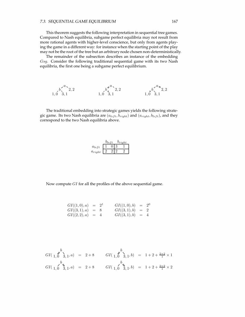
7.3. SEQUENTIAL GAME EQUILIBRIUM 167
This theorem suggests the following interpretation in sequential tree games.Compared to Nash equilibria, subgame perfect equilibria may not result frommore rational agents with higher-level conscience, but only from agents play-ing the game in a different way: for instance when the starting point of the playmay not be the root of the tree but an arbitrary node chosen non-deterministically.The remainder of the subsection describes an instance of the embedding
Gsg. Consider the following traditional sequential game with its two Nashequilibria, the first one being a subgame perfect equilibrium.
ab 2, 2
1, 0 3, 1
ab 2, 2
1, 0 3, 1
ab 2, 2
1, 0 3, 1
The traditional embedding into strategic games yields the following strate-gic game. Its two Nash equilibria are (aleft, bright) and (aright, bleft), and theycorrespond to the two Nash equilibria above.
bleft bright
aleft 1 0 3 1aright 2 2 2 2
Now compute GI for all the profiles of the above sequential game.
GI((1, 0), a) = 21 GI((1, 0), b) = 20
GI((3, 1), a) = 8 GI((3, 1), b) = 2GI((2, 2), a) = 4 GI((3, 1), b) = 4
GI(b
1, 0 3, 1, a) = 2 + 8 GI(b
1, 0 3, 1, b) = 1 + 2 + 2×21 × 1
GI(b
1, 0 3, 1, a) = 2 + 8 GI(b
1, 0 3, 1, b) = 1 + 2 + 2×21 × 2
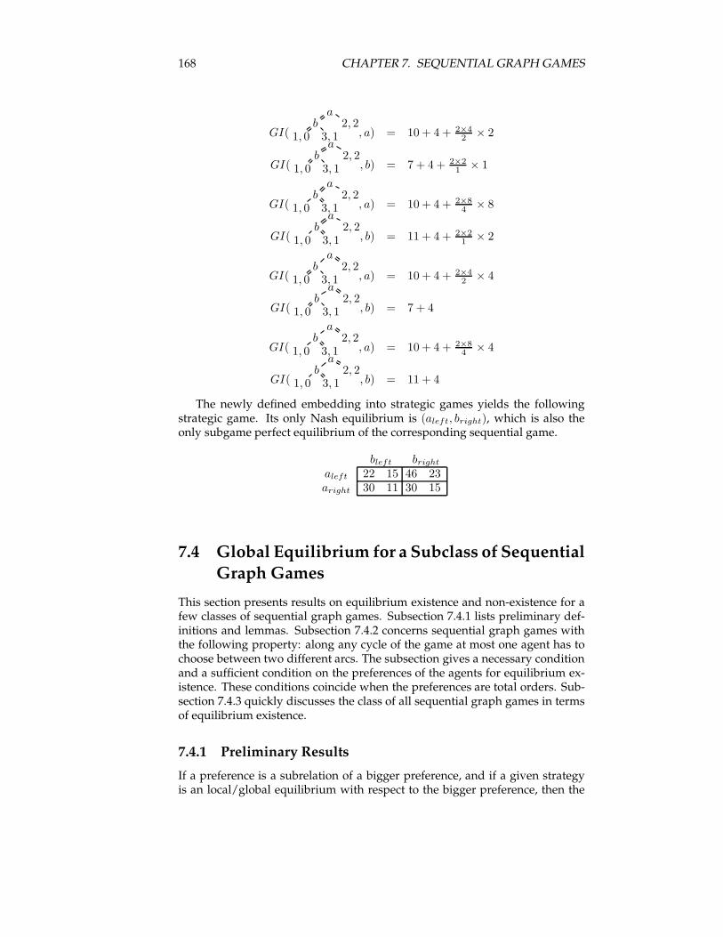
168 CHAPTER 7. SEQUENTIAL GRAPH GAMES
GI(
ab 2, 2
1, 0 3, 1 , a) = 10 + 4 + 2×42 × 2
GI(
ab 2, 2
1, 0 3, 1 , b) = 7 + 4 + 2×21 × 1
GI(
ab 2, 2
1, 0 3, 1 , a) = 10 + 4 + 2×84 × 8
GI(
ab 2, 2
1, 0 3, 1 , b) = 11 + 4 + 2×21 × 2
GI(
ab 2, 2
1, 0 3, 1 , a) = 10 + 4 + 2×42 × 4
GI(
ab 2, 2
1, 0 3, 1 , b) = 7 + 4
GI(
ab 2, 2
1, 0 3, 1 , a) = 10 + 4 + 2×84 × 4
GI(
ab 2, 2
1, 0 3, 1 , b) = 11 + 4
The newly defined embedding into strategic games yields the followingstrategic game. Its only Nash equilibrium is (aleft, bright), which is also theonly subgame perfect equilibrium of the corresponding sequential game.
bleft bright
aleft 22 15 46 23aright 30 11 30 15
7.4 Global Equilibrium for a Subclass of SequentialGraph Games
This section presents results on equilibrium existence and non-existence for afew classes of sequential graph games. Subsection 7.4.1 lists preliminary def-initions and lemmas. Subsection 7.4.2 concerns sequential graph games withthe following property: along any cycle of the game at most one agent has tochoose between two different arcs. The subsection gives a necessary conditionand a sufficient condition on the preferences of the agents for equilibrium ex-istence. These conditions coincide when the preferences are total orders. Sub-section 7.4.3 quickly discusses the class of all sequential graph games in termsof equilibrium existence.
7.4.1 Preliminary Results
If a preference is a subrelation of a bigger preference, and if a given strategyis an local/global equilibrium with respect to the bigger preference, then the
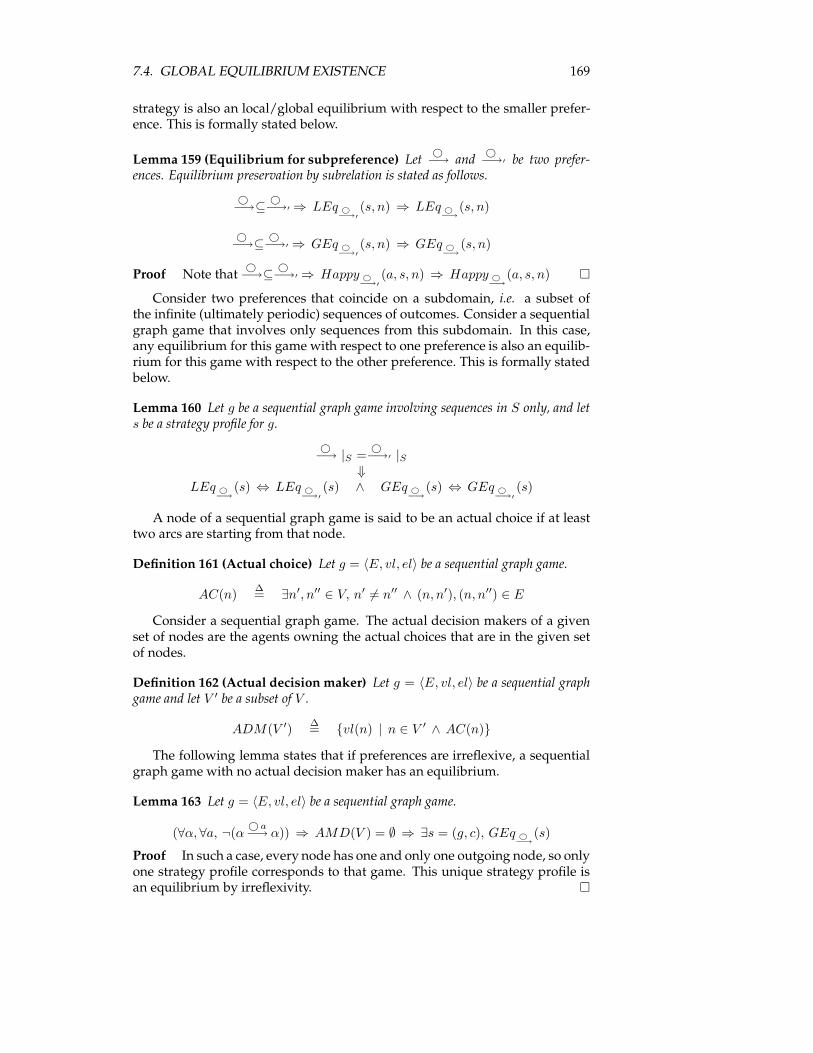
7.4. GLOBAL EQUILIBRIUM EXISTENCE 169
strategy is also an local/global equilibrium with respect to the smaller prefer-ence. This is formally stated below.
Lemma 159 (Equilibrium for subpreference) Let©−→ and
©−→′ be two prefer-
ences. Equilibrium preservation by subrelation is stated as follows.
©−→⊆
©−→′⇒ LEq ©
−→′
(s, n) ⇒ LEq ©−→
(s, n)
©−→⊆
©−→′⇒ GEq ©
−→′
(s, n) ⇒ GEq ©−→
(s, n)
Proof Note that©−→⊆
©−→′⇒ Happy ©
−→′
(a, s, n) ⇒ Happy ©−→
(a, s, n) �
Consider two preferences that coincide on a subdomain, i.e. a subset ofthe infinite (ultimately periodic) sequences of outcomes. Consider a sequentialgraph game that involves only sequences from this subdomain. In this case,any equilibrium for this game with respect to one preference is also an equilib-rium for this game with respect to the other preference. This is formally statedbelow.
Lemma 160 Let g be a sequential graph game involving sequences in S only, and lets be a strategy profile for g.
©−→ |S =
©−→′ |S⇓
LEq ©−→
(s) ⇔ LEq ©−→′
(s) ∧ GEq ©−→
(s) ⇔ GEq ©−→′
(s)
A node of a sequential graph game is said to be an actual choice if at leasttwo arcs are starting from that node.
Definition 161 (Actual choice) Let g = 〈E, vl, el〉 be a sequential graph game.
AC(n)∆= ∃n′, n′′ ∈ V, n′ 6= n′′ ∧ (n, n′), (n, n′′) ∈ E
Consider a sequential graph game. The actual decision makers of a givenset of nodes are the agents owning the actual choices that are in the given setof nodes.
Definition 162 (Actual decision maker) Let g = 〈E, vl, el〉 be a sequential graphgame and let V ′ be a subset of V .
ADM(V ′)∆= {vl(n) | n ∈ V ′ ∧ AC(n)}
The following lemma states that if preferences are irreflexive, a sequentialgraph game with no actual decision maker has an equilibrium.
Lemma 163 Let g = 〈E, vl, el〉 be a sequential graph game.
(∀α, ∀a, ¬(α© a−→ α)) ⇒ AMD(V ) = ∅ ⇒ ∃s = (g, c), GEq ©
−→(s)
Proof In such a case, every node has one and only one outgoing node, so onlyone strategy profile corresponds to that game. This unique strategy profile isan equilibrium by irreflexivity. �
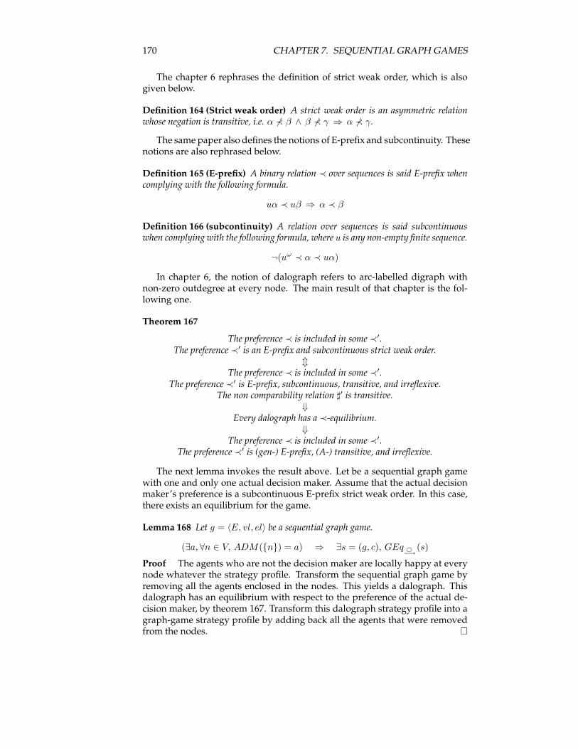
170 CHAPTER 7. SEQUENTIAL GRAPH GAMES
The chapter 6 rephrases the definition of strict weak order, which is alsogiven below.
Definition 164 (Strict weak order) A strict weak order is an asymmetric relationwhose negation is transitive, i.e. α 6≺ β ∧ β 6≺ γ ⇒ α 6≺ γ.
The same paper also defines the notions of E-prefix and subcontinuity. Thesenotions are also rephrased below.
Definition 165 (E-prefix) A binary relation ≺ over sequences is said E-prefix whencomplying with the following formula.
uα ≺ uβ ⇒ α ≺ β
Definition 166 (subcontinuity) A relation over sequences is said subcontinuouswhen complying with the following formula, where u is any non-empty finite sequence.
¬(uω ≺ α ≺ uα)
In chapter 6, the notion of dalograph refers to arc-labelled digraph withnon-zero outdegree at every node. The main result of that chapter is the fol-lowing one.
Theorem 167
The preference ≺ is included in some ≺′.The preference ≺′ is an E-prefix and subcontinuous strict weak order.
mThe preference ≺ is included in some ≺′.
The preference ≺′ is E-prefix, subcontinuous, transitive, and irreflexive.The non comparability relation ♯′ is transitive.
⇓Every dalograph has a ≺-equilibrium.
⇓The preference ≺ is included in some ≺′.
The preference ≺′ is (gen-) E-prefix, (A-) transitive, and irreflexive.
The next lemma invokes the result above. Let be a sequential graph gamewith one and only one actual decision maker. Assume that the actual decisionmaker’s preference is a subcontinuous E-prefix strict weak order. In this case,there exists an equilibrium for the game.
Lemma 168 Let g = 〈E, vl, el〉 be a sequential graph game.
(∃a, ∀n ∈ V, ADM({n}) = a) ⇒ ∃s = (g, c), GEq ©−→
(s)
Proof The agents who are not the decision maker are locally happy at everynode whatever the strategy profile. Transform the sequential graph game byremoving all the agents enclosed in the nodes. This yields a dalograph. Thisdalograph has an equilibrium with respect to the preference of the actual de-cision maker, by theorem 167. Transform this dalograph strategy profile into agraph-game strategy profile by adding back all the agents that were removedfrom the nodes. �
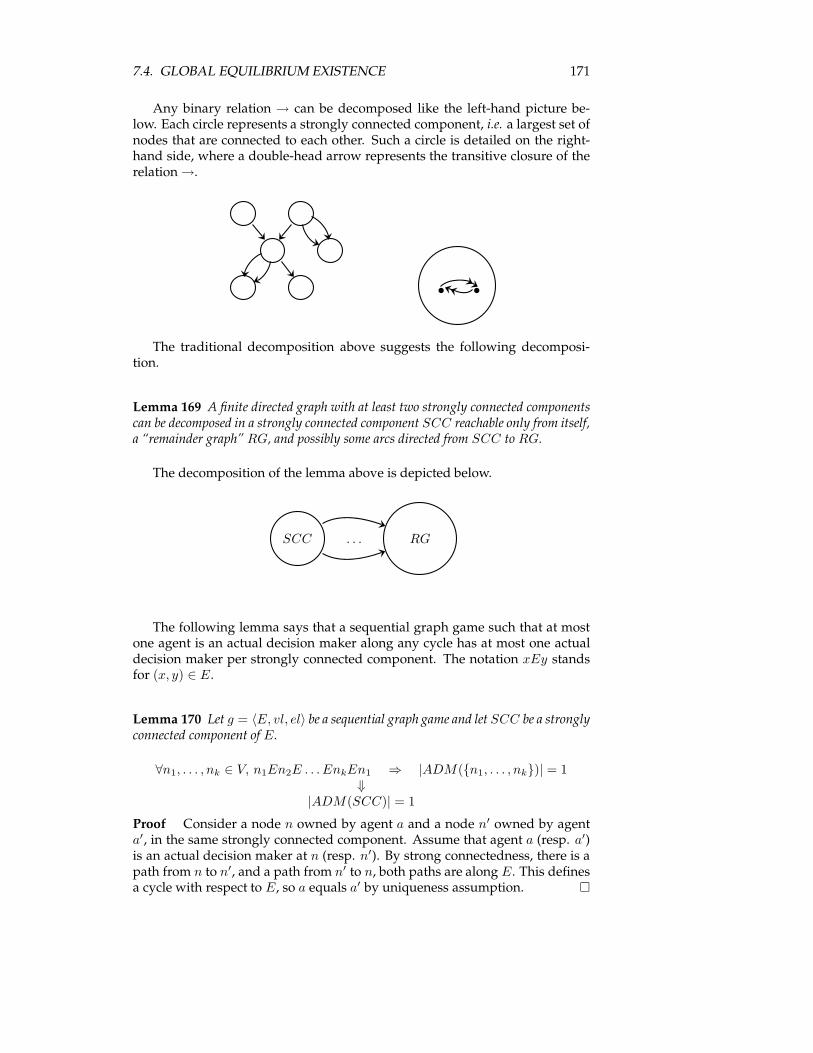
7.4. GLOBAL EQUILIBRIUM EXISTENCE 171
Any binary relation → can be decomposed like the left-hand picture be-low. Each circle represents a strongly connected component, i.e. a largest set ofnodes that are connected to each other. Such a circle is detailed on the right-hand side, where a double-head arrow represents the transitive closure of therelation→.
The traditional decomposition above suggests the following decomposi-tion.
Lemma 169 A finite directed graph with at least two strongly connected componentscan be decomposed in a strongly connected component SCC reachable only from itself,a “remainder graph” RG, and possibly some arcs directed from SCC to RG.
The decomposition of the lemma above is depicted below.
SCC . . . RG
The following lemma says that a sequential graph game such that at mostone agent is an actual decision maker along any cycle has at most one actualdecision maker per strongly connected component. The notation xEy standsfor (x, y) ∈ E.
Lemma 170 Let g = 〈E, vl, el〉 be a sequential graph game and let SCC be a stronglyconnected component of E.
∀n1, . . . , nk ∈ V, n1En2E . . . EnkEn1 ⇒ |ADM({n1, . . . , nk})| = 1⇓
|ADM(SCC)| = 1
Proof Consider a node n owned by agent a and a node n′ owned by agenta′, in the same strongly connected component. Assume that agent a (resp. a′)is an actual decision maker at n (resp. n′). By strong connectedness, there is apath from n to n′, and a path from n′ to n, both paths are along E. This definesa cycle with respect to E, so a equals a′ by uniqueness assumption. �
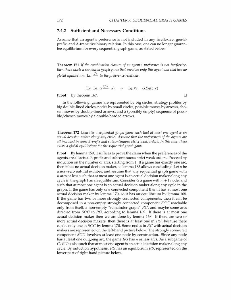
172 CHAPTER 7. SEQUENTIAL GRAPH GAMES
7.4.2 Sufficient and Necessary Conditions
Assume that an agent’s preference is not included in any irreflexive, gen-E-prefix, and A-transitive binary relation. In this case, one can no longer guaran-tee equilibrium for every sequential graph game, as stated below.
Theorem 171 If the combination closure of an agent’s preference is not irreflexive,then there exists a sequential graph game that involves only this agent and that has no
global equilibrium. Let©−→ be the preference relations.
(∃α, ∃a, α©a−→c α) ⇒ ∃g, ∀c, ¬GEq(g, c)
Proof By theorem 167. �
In the following, games are represented by big circles, strategy profiles bybig double-lined circles, nodes by small circles, possible moves by arrows, cho-sen moves by double-lined arrows, and a (possibly empty) sequence of possi-ble/chosen moves by a double-headed arrows.
Theorem 172 Consider a sequential graph game such that at most one agent is anactual decision maker along any cycle. Assume that the preferences of the agents areall included in some E-prefix and subcontinuous strict weak orders. In this case, thereexists a global equilibrium for the sequential graph game.
Proof By lemma 159, it suffices to prove the claimwhen the preferences of theagents are all actual E-prefix and subcontinuous strict weak orders. Proceed byinduction on the number of arcs, starting from 1. If a game has exactly one arc,then it has no actual decision maker, so lemma 163 allows concluding. Let n bea non-zero natural number, and assume that any sequential graph game withn arcs or less such that at most one agent is an actual decision maker along anycycle in the graph has an equilibrium. ConsiderG a game with n+1 node, andsuch that at most one agent is an actual decision maker along any cycle in thegraph. If the game has only one connected component then it has at most oneactual decision maker by lemma 170, so it has an equilibrium by lemma 168.If the game has two or more strongly connected components, then it can bedecomposed in a non-empty strongly connected component SCC reachableonly from itself, a non-empty “remainder graph” RG, and maybe some arcsdirected from SCC to RG, according to lemma 169. If there is at most oneactual decision maker then we are done by lemma 168. If there are two ormore actual decision makers, then there is at least one in RG, because therecan be only one in SCC by lemma 170. Some nodes inRGwith actual decisionmakers are represented on the left-hand picture below. The strongly connectedcomponent SCC involves at least one node by construction. Since any nodehas at least one outgoing arc, the game RG has n or less arcs. As a subgame ofG, RG is also such that at most one agent is an actual decision maker along anycycle. By induction hypothesis, RG has an equilibrium RS, represented on thelower part of right-hand picture below.
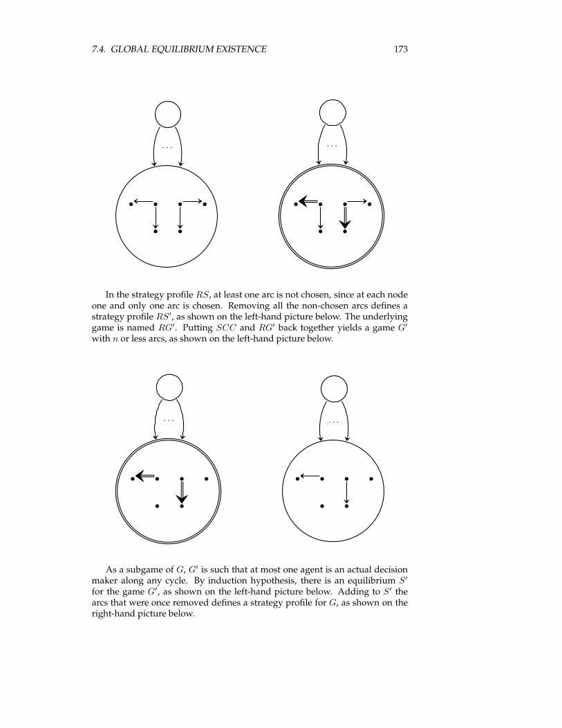
7.4. GLOBAL EQUILIBRIUM EXISTENCE 173
. . . . . .
In the strategy profile RS, at least one arc is not chosen, since at each nodeone and only one arc is chosen. Removing all the non-chosen arcs defines astrategy profile RS′, as shown on the left-hand picture below. The underlyinggame is named RG′. Putting SCC and RG′ back together yields a game G′
with n or less arcs, as shown on the left-hand picture below.
. . . . . .
As a subgame of G, G′ is such that at most one agent is an actual decisionmaker along any cycle. By induction hypothesis, there is an equilibrium S′
for the game G′, as shown on the left-hand picture below. Adding to S′ thearcs that were once removed defines a strategy profile for G, as shown on theright-hand picture below.
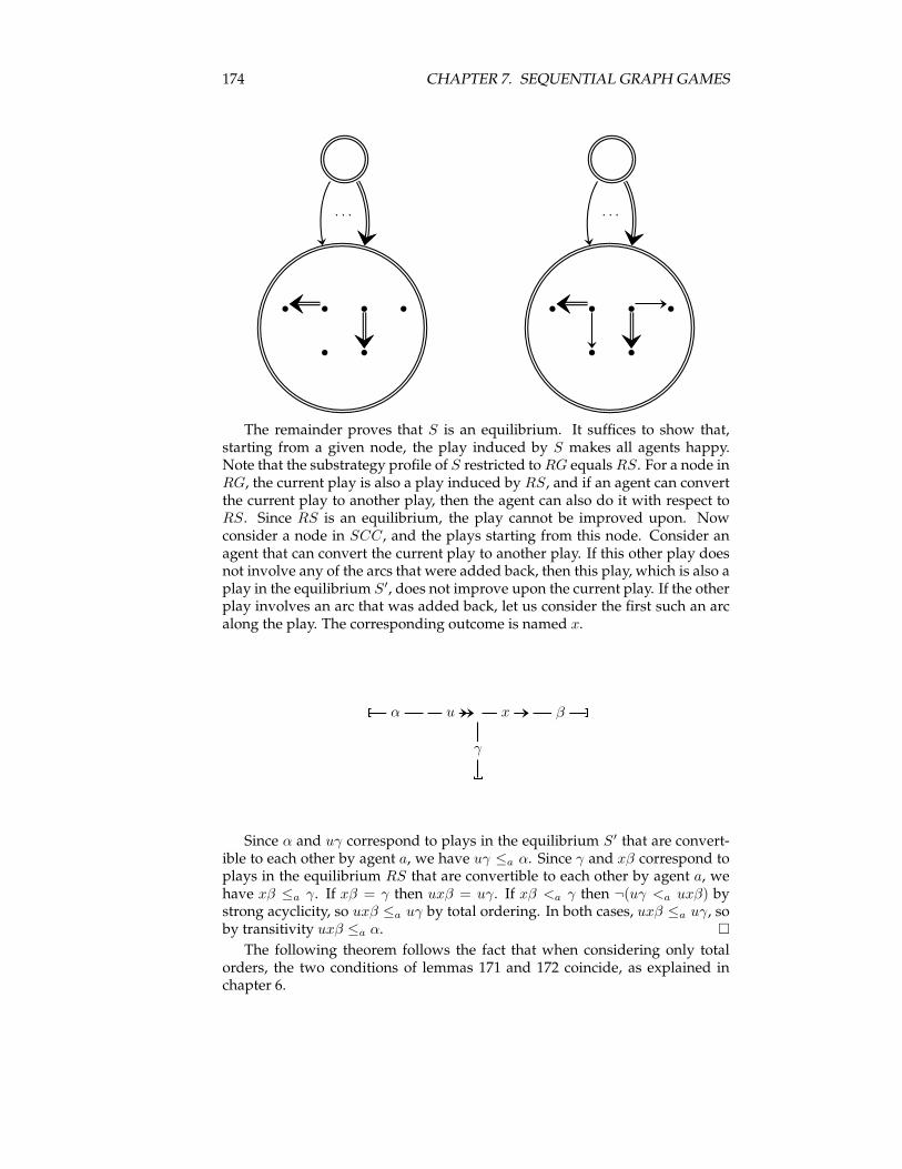
174 CHAPTER 7. SEQUENTIAL GRAPH GAMES
. . . . . .
The remainder proves that S is an equilibrium. It suffices to show that,starting from a given node, the play induced by S makes all agents happy.Note that the substrategy profile of S restricted toRG equalsRS. For a node inRG, the current play is also a play induced by RS, and if an agent can convertthe current play to another play, then the agent can also do it with respect toRS. Since RS is an equilibrium, the play cannot be improved upon. Nowconsider a node in SCC, and the plays starting from this node. Consider anagent that can convert the current play to another play. If this other play doesnot involve any of the arcs that were added back, then this play, which is also aplay in the equilibrium S′, does not improve upon the current play. If the otherplay involves an arc that was added back, let us consider the first such an arcalong the play. The corresponding outcome is named x.
α u x β
γ
Since α and uγ correspond to plays in the equilibrium S′ that are convert-ible to each other by agent a, we have uγ ≤a α. Since γ and xβ correspond toplays in the equilibrium RS that are convertible to each other by agent a, wehave xβ ≤a γ. If xβ = γ then uxβ = uγ. If xβ <a γ then ¬(uγ <a uxβ) bystrong acyclicity, so uxβ ≤a uγ by total ordering. In both cases, uxβ ≤a uγ, soby transitivity uxβ ≤a α. �
The following theorem follows the fact that when considering only totalorders, the two conditions of lemmas 171 and 172 coincide, as explained inchapter 6.
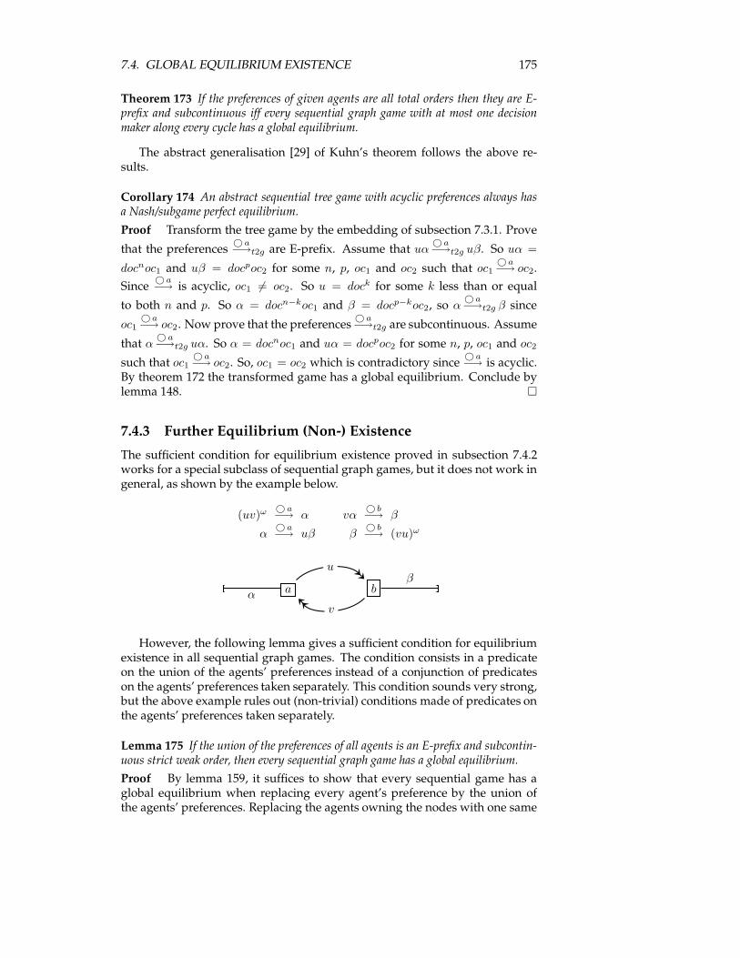
7.4. GLOBAL EQUILIBRIUM EXISTENCE 175
Theorem 173 If the preferences of given agents are all total orders then they are E-prefix and subcontinuous iff every sequential graph game with at most one decisionmaker along every cycle has a global equilibrium.
The abstract generalisation [29] of Kuhn’s theorem follows the above re-sults.
Corollary 174 An abstract sequential tree game with acyclic preferences always hasa Nash/subgame perfect equilibrium.
Proof Transform the tree game by the embedding of subsection 7.3.1. Prove
that the preferences© a−→t2g are E-prefix. Assume that uα
©a−→t2g uβ. So uα =
docnoc1 and uβ = docpoc2 for some n, p, oc1 and oc2 such that oc1©a−→ oc2.
Since©a−→ is acyclic, oc1 6= oc2. So u = dock for some k less than or equal
to both n and p. So α = docn−koc1 and β = docp−koc2, so α©a−→t2g β since
oc1©a−→ oc2. Now prove that the preferences
© a−→t2g are subcontinuous. Assume
that α© a−→t2g uα. So α = docnoc1 and uα = docpoc2 for some n, p, oc1 and oc2
such that oc1©a−→ oc2. So, oc1 = oc2 which is contradictory since
©a−→ is acyclic.
By theorem 172 the transformed game has a global equilibrium. Conclude bylemma 148. �
7.4.3 Further Equilibrium (Non-) Existence
The sufficient condition for equilibrium existence proved in subsection 7.4.2works for a special subclass of sequential graph games, but it does not work ingeneral, as shown by the example below.
(uv)ω © a−→ α vα
© b−→ β
α© a−→ uβ β
© b−→ (vu)ω
a bα
u
v
β
However, the following lemma gives a sufficient condition for equilibriumexistence in all sequential graph games. The condition consists in a predicateon the union of the agents’ preferences instead of a conjunction of predicateson the agents’ preferences taken separately. This condition sounds very strong,but the above example rules out (non-trivial) conditions made of predicates onthe agents’ preferences taken separately.
Lemma 175 If the union of the preferences of all agents is an E-prefix and subcontin-uous strict weak order, then every sequential graph game has a global equilibrium.
Proof By lemma 159, it suffices to show that every sequential game has aglobal equilibrium when replacing every agent’s preference by the union ofthe agents’ preferences. Replacing the agents owning the nodes with one same
176 CHAPTER 7. SEQUENTIAL GRAPH GAMES
agent for all nodes yields a convertibility binary relation that includes the orig-inal convertibility relation of each agent. Therefore an equilibrium for this newgame is also an equilibrium for the original game. By lemma 168, this newgame has a global equilibrium, which is also an global equilibrium for the orig-inal game. �
7.5 Conclusion
This chapter defines sequential graph games, and the related notions of strat-egy profile, convertibility, and local/global preference. Based on this, it definesthe notions of local and global equilibrium. They correspond to the notions ofNash and subgame perfect equilibrium respectively, as shown by an embed-ding. They also both correspond to the abstractNash equilibria of two differentderived C/P games.Putting the two previous remarks together suggests that the subgame per-
fect equilibria of a sequential game are the Nash equilibria of a derived C/Pgame. Working in an abstract setting helps think of this idea, but the notions ofsequential graph games and C/P games are not actually needed to express thisidea. Indeed, this chapter defines an embedding from sequential games withreal-valued payoff functions into strategic games with real-valued payoff func-tions. The images by the embedding of the subgame perfect equilibria (of thesequential game) are exactly the Nash equilibria (of the strategic game). Thisresult shows that, in some sense, subgame perfect equilibria could be calledNash equilibria of sequential games in lieu of their current Nash equilibria.The main goal of this chapter is achieved as follows: the chapter considers a
subclass of sequential graph games and proves a sufficient condition and a nec-essary condition for equilibrium existence in this subclass. It does it by invok-ing results on equilibrium existence in dalographs. The proof of the sufficientcondition uses a construction similar to "backward induction". This way, it triesto fully exploit the conceptual power of "backward induction" and seeks for avery general setting where "backward induction" still helps build equilibria.The necessary condition and the sufficient condition coincide when the agents’preferences are total orders, which gives an equivalence property. These re-sults supersede the first generalisation [29] of Kuhn’s theorem. This chapteralso gives a sufficient condition on the union of the agents’ preferences forequilibrium existence in all sequential graph games. However, this conditionis strong and it is likely not to hold in many interesting examples and appli-cations. In the same line of work, it may be interesting to study the subclassof sequential graph games where each agent occurs at most once, i.e. owns atmost one node.This chapter also leads to the following thoughts. In abstract sequential
games, every game involving only one agent has a Nash/subgame perfectequilibrium iff every game has a Nash/subgame perfect equilibrium, as shownin [29]. (This does not hold in strategic games, as shown by some basic exam-ples.) This chapter gives a sufficient condition for equilibrium existence for ev-ery sequential graph game involving only one agent. It also gives a sufficientcondition for equilibrium existence for every game of a subclass of sequentialgraph games. Actually, this subclass includes games involving only one agentand these two sufficient conditions are the same (in this chapter). However, it

7.5. CONCLUSION 177
is not obvious whether or not equilibrium existence in games involving onlyone agent implies equilibrium existence in the subclass mentioned above. So, itmay be interesting to seek a "most general" subclass of sequential graph gameswhere the following holds: "If every game involving only one agent has anequilibrium, then every game has an equilibrium". It may be interesting es-pecially because the property "every game involving only one agent has anequilibrium" could be a low-level definition of rationality, i.e. not involvingfurther theories such as epistemic logic.
178 CHAPTER 7. SEQUENTIAL GRAPH GAMES
Chapter 8
Abstract CompromisedEquilibria
8.1 Introduction
8.1.1 Nash’s Theorem
As seen before, not all finite strategic games have a (pure) Nash equilibrium,even though a guarantee of existence is a desirable property. Therefore, Nashweakened the definition of (pure Nash) equilibrium to assure the existenceof a "compromising" equilibrium. More specifically, introducing probabilitiesinto the game, he allowed agents to choose their individual strategies witha probability distribution rather than choosing a single strategy deterministi-cally. Subsequently, instead of a single strategy profile chosen deterministi-cally, Nash’s probabilistic compromise involves a probability distribution overstrategy profiles. So, expected payoff functions are involved instead of payofffunctions. This compromise actually builds a new strategic game that is con-tinuous. Nash [36] proved that this new game always has a Nash equilibrium,which is called a probabilistic Nash equilibrium for the original game. A firstproof of this result invokes Kakutani’s fixed point theorem, and a second proofinvokes (the proof-theoretically simpler) Brouwer’s fixed point theorem.
8.1.2 Contribution
First, this chapter explores possible generalisations of Nash’s result within theBR and CP formalisms. These generalisations invoke Kakutani’s fixed pointtheorem, which is a generalisation of Brouwer’s. However, there is a differencebetween Nash’s theorem and its generalisations in the BR and CP formalisms:Nash’s probabilised strategic games correspond to finite strategic games sincethey are derived from them. However, it seems difficult to introduce probabil-ities within a given finite BR or CP game, since BR and CP games do not haveany Cartesian product structure. Therefore, one considers a class of already-continuous BR or CP games. Kakutani’s fixed point theorem, which is muchmore appropriate than Brouwer’s in this specific case, helps guarantee the exis-tence of an abstract Nash equilibrium. However, these already-continuous BR
179
180 CHAPTER 8. ABSTRACT COMPROMISED EQUILIBRIA
or CP games do not necessarily correspond to relevant finite BR or CP games,so practical applications might be difficult to find.Second, this chapter explores compromises that are completely different
fromNash’s probabilistic compromise. Two conceptually very simple compro-mises are presented in this section, one for BR games and one for CP games.The one for BR games is named or-best response strict equilibrium, and the onefor CP games is named change-of-mind equilibrium, as in [30]. Both compro-mising equilibria are natural generalisations of Nash equilibria for CP gamesand strict Nash equilibria for BR games. It turns out that both generalisationsare (almost) the same: they both define compromising equilibria as the sinkstrongly connected components of a relevant digraph. Informally, if nodesrepresent the microscopic level and strongly connected components the macro-scopic level, then the compromising equilibria are the macroscopic equilibriaof a microscopic world.Since BR and CP games are generalisations of strategic games, the new com-
promising equilibria are relevant in strategic games too. This helps see thatNash’s compromise and the new compromises are different in many respects.Nash’s probabilistic compromise transforms finite strategic games into contin-uous strategic games. Probabilistic Nash equilibria for the original game aredefined as the (pure) Nash equilibria for the continuous derived game. Thismakes the probabilistic setting much more complex than the "pure" setting. Onthe contrary, the new compromises are discrete in the sense that the compro-mising equilibria are finitely many among finitely many strongly connectedcomponents. While probabilistic Nash equilibria are static, the new compro-mising equilibria are dynamic. While Nash equilibria are fixed points obtainedby Kakutani’s (or Brouwer’s) fixed point theorem, the new equilibria are fixedpoints obtained by a simple combinatorial argument (or Tarski’s fixed pointtheorem if one wishes to stress the parallel between Nash’s construction andthis one). While probabilistic Nash equilibria are non-computable in general,the new compromising equilibria are computable with low algorithmic com-plexity. Finally, while probabilistic Nash equilibria are Nash equilibria of aderived continuous game, the new compromising equilibria seem not to be theNash equilibria of any relevant derived game.
8.1.3 Contents
Section 8.2 defines probabilistic Nash equilibria and states the related Nash’stheorem; section 8.3 tries to generalise Nash’s result within the BR or CP for-malisms; section 8.4 introduces discrete and dynamic new compromising equi-libria and proves a few related results.
8.2 Probabilistic Nash Equilibrium
As noted before, not all strategic games have (pure) Nash equilibria. The left-hand example is finite and involves two agents. The right-hand example isinfinite and involves only one agent. None of them has a Nash equilibrium.
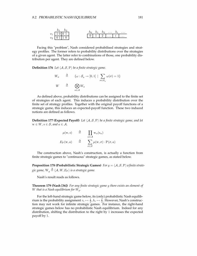
8.2. PROBABILISTIC NASH EQUILIBRIUM 181
h1 h2
v1 1 0 0 1v2 0 1 1 0
h0 h1 h2 . . . hi . . .0 1 2 . . . i . . .
Facing this "problem", Nash considered probabilised strategies and strat-egy profiles. The former refers to probability distributions over the strategiesof a given agent. The latter refer to combinations of those, one probability dis-tribution per agent. They are defined below.
Definition 176 Let 〈A,S , P〉 be a finite strategic game.
Wa∆= {ω : Sa → [0, 1] |
∑
σ∈Sa
ω(σ) = 1}
W∆=
⊗
a∈A
Wa
As defined above, probability distributions can be assigned to the finite setof strategies of each agent. This induces a probability distribution over thefinite set of strategy profiles. Together with the original payoff functions of astrategic game, this induces an expected-payoff function. These two inducednotions are defined as follows.
Definition 177 (Expected Payoff) Let 〈A,S , P〉 be a finite strategic game, and letw ∈W , s ∈ S , and a ∈ A.
µ(w, s)∆=
∏
α∈A
wα(sα)
EP(w, a)∆=
∑
σ∈S
µ(w, σ) · P(σ, a)
The construction above, Nash’s construction, is actually a function fromfinite strategic games to "continuous" strategic games, as stated below.
Proposition 178 (Probabilistic Strategic Games) For g = 〈A,S , P〉 a finite strate-
gic game,Wg∆= 〈A, W, EP〉 is a strategic game.
Nash’s result reads as follows.
Theorem 179 (Nash [36]) For any finite strategic game g there exists an element ofW that is a Nash equilibrium forWg .
For the left-hand strategic game below, its (only) probabilistic Nash equilib-rium is the probability assignment vi 7→
12 , hi 7→
12 . However, Nash’s construc-
tion may not work for infinite strategic games. For instance, the right-handstrategic games below has no probabilistic Nash equilibrium. Indeed for anydistribution, shifting the distribution to the right by 1 increases the expectedpayoff by 1.
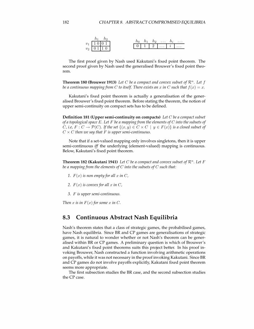
182 CHAPTER 8. ABSTRACT COMPROMISED EQUILIBRIA
h1 h2
v1 1 0 0 1v2 0 1 1 0
h0 h1 h2 . . . hi . . .0 1 2 . . . i . . .
The first proof given by Nash used Kakutani’s fixed point theorem. Thesecond proof given by Nash used the generalised Brouwer’s fixed point theo-rem.
Theorem 180 (Brouwer 1913) Let C be a compact and convex subset of Rn. Let fbe a continuous mapping from C to itself. There exists an x in C such that f(x) = x.
Kakutani’s fixed point theorem is actually a generalisation of the gener-alised Brouwer’s fixed point theorem. Before stating the theorem, the notion ofupper semi-continuity on compact sets has to be defined.
Definition 181 (Upper semi-continuity on compacts) Let C be a compact subsetof a topological space E. Let F be a mapping from the elements of C into the subsets ofC, i.e, F : C → P(C). If the set {(x, y) ∈ C × C | y ∈ F (x)} is a closed subset ofC × C then we say that F is upper semi-continuous.
Note that if a set-valued mapping only involves singletons, then it is uppersemi-continuous iff the underlying (element-valued) mapping is continuous.Below, Kakutani’s fixed point theorem.
Theorem 182 (Kakutani 1941) Let C be a compact and convex subset ofRn. Let Fbe a mapping from the elements of C into the subsets of C such that:
1. F (x) is non empty for all x in C,
2. F (x) is convex for all x in C,
3. F is upper semi-continuous.
Then x is in F (x) for some x in C.
8.3 Continuous Abstract Nash Equilibria
Nash’s theorem states that a class of strategic games, the probabilised games,have Nash equilibria. Since BR and CP games are generalisations of strategicgames, it is natural to wonder whether or not Nash’s theorem can be gener-alised within BR or CP games. A preliminary question is which of Brouwer’sand Kakutani’s fixed point theorems suits this project better. In his proof in-voking Brouwer, Nash constructed a function involving arithmetic operationson payoffs, while it was not necessary in the proof invoking Kakutani. Since BRand CP games do not involve payoffs explicitly, Kakutani fixed point theoremseems more appropriate.The first subsection studies the BR case, and the second subsection studies
the CP case.
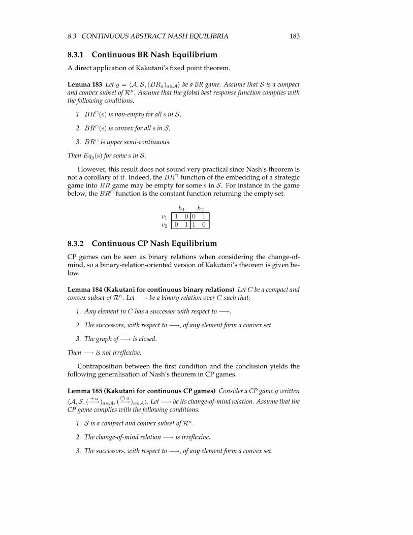
8.3. CONTINUOUS ABSTRACT NASH EQUILIBRIA 183
8.3.1 Continuous BR Nash Equilibrium
A direct application of Kakutani’s fixed point theorem.
Lemma 183 Let g = 〈A,S, (BRa)a∈A〉 be a BR game. Assume that S is a compactand convex subset ofRn. Assume that the global best response function complies withthe following conditions.
1. BR∩(s) is non-empty for all s in S,
2. BR∩(s) is convex for all s in S,
3. BR∩ is upper semi-continuous.
Then Eqg(s) for some s in S.
However, this result does not sound very practical since Nash’s theorem isnot a corollary of it. Indeed, the BR∩ function of the embedding of a strategicgame into BR game may be empty for some s in S. For instance in the gamebelow, the BR∩ function is the constant function returning the empty set.
h1 h2
v1 1 0 0 1v2 0 1 1 0
8.3.2 Continuous CP Nash Equilibrium
CP games can be seen as binary relations when considering the change-of-mind, so a binary-relation-oriented version of Kakutani’s theorem is given be-low.
Lemma 184 (Kakutani for continuous binary relations) LetC be a compact andconvex subset ofRn. Let −→ be a binary relation over C such that:
1. Any element in C has a successor with respect to −→.
2. The successors, with respect to −→, of any element form a convex set.
3. The graph of −→ is closed.
Then −→ is not irreflexive.
Contraposition between the first condition and the conclusion yields thefollowing generalisation of Nash’s theorem in CP games.
Lemma 185 (Kakutani for continuous CP games) Consider a CP game g written
〈A,S, (+ a−→)a∈A, (
© a−→)a∈A〉. Let−→ be its change-of-mind relation. Assume that the
CP game complies with the following conditions.
1. S is a compact and convex subset ofRn.
2. The change-of-mind relation −→ is irreflexive.
3. The successors, with respect to −→, of any element form a convex set.
184 CHAPTER 8. ABSTRACT COMPROMISED EQUILIBRIA
4. The graph of −→ is closed.
Then Eqg(s) for some s in S.
It is unclear how practical this generalisation is. Indeed, while probabilisedstrategic games correspond to finite strategic games, it may be difficult to seewhat kind of discrete CP games those continuous CP games correspond to.
8.4 Discrete and Dynamic Equilibria
This section first defines the strongly connected components (SCC) of a di-graph, and a few related properties. Second, it defines change-of-mind equi-librium as an SCC-sink of a relevant digraph. Third, it defines or-best responsestrict equilibrium as an SCC-sink of a relevant digraph. Fourth, it gives a fewexamples and compares briefly the three compromising equilibria (probabilis-tic, change-of-mind, or-best response strict) in the strategic game setting.
8.4.1 Strongly Connected Component
This subsection defines the transitive and reflexive closure of a binary relation,using the usual inductive definition. It gives some properties of this closure,which it uses to define the strongly connected components of a digraph, andthe notion of (SCC-) sink. Then, it gives a few equivalent characterisations forSCC-sinks, in general as well as for finite digraphs without sink. This subsec-tion also shows in two different manners the existence of SCC-sinks for finitedigraphs. Most of the results discussed in this subsection must already belongto the folklore of graph theory.
Preliminary
Formally, the transitive and reflexive closure of a binary relation is defined asfollows.
Definition 186 (Transitive and reflexive closure)
s→∗ s
s→ s′
s→∗ s′
s→∗ s′ s′ →∗ s′′
s→∗ s′′
The following lemma says that if several steps (from a given starting point)allow to escape from a set, then one step (from a well chosen starting point)also does.
Lemma 187 Let→ be a digraph and let C be a subset of its nodes. If s→∗ s′ for somes in C and s′ not in C, then s→∗ s1 → s′1 →
∗ s′ for some s1 in C and s′1 not in C.
Proof By rule induction on the definition of the transitive and reflexive clo-sure (of→). �
The next lemma says that if several steps (from a given starting point) leadto an end point, then one step (from a well chosen starting point) also does.
Lemma 188 Let → be a digraph and let s and s′ be two different nodes such thats→∗ s′. There exists s′′ such that s→∗ s′′ → s′.
Proof Apply lemma 187 with C defined as the nodes different from s′. �
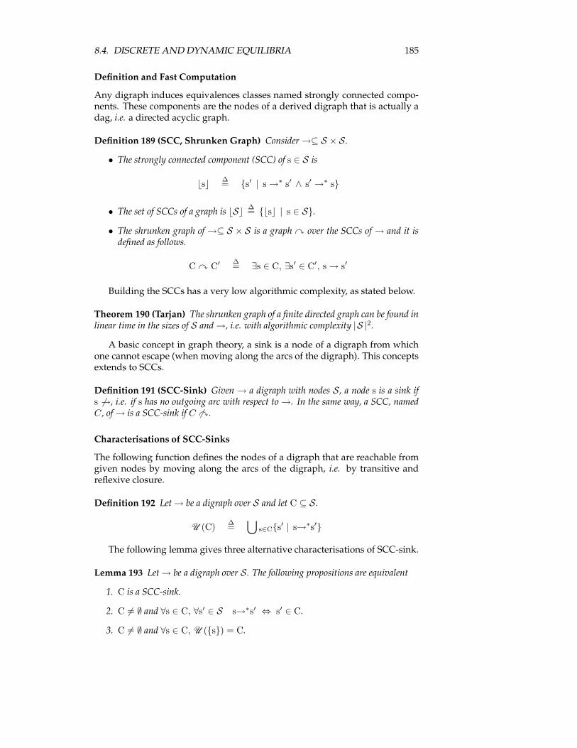
8.4. DISCRETE AND DYNAMIC EQUILIBRIA 185
Definition and Fast Computation
Any digraph induces equivalences classes named strongly connected compo-nents. These components are the nodes of a derived digraph that is actually adag, i.e. a directed acyclic graph.
Definition 189 (SCC, Shrunken Graph) Consider→⊆ S × S.
• The strongly connected component (SCC) of s ∈ S is
⌊s⌋∆= {s′ | s→∗ s′ ∧ s′ →∗ s}
• The set of SCCs of a graph is ⌊S⌋∆= {⌊s⌋ | s ∈ S}.
• The shrunken graph of →⊆ S × S is a graphy over the SCCs of → and it isdefined as follows.
C y C′ ∆= ∃s ∈ C, ∃s′ ∈ C′, s→ s′
Building the SCCs has a very low algorithmic complexity, as stated below.
Theorem 190 (Tarjan) The shrunken graph of a finite directed graph can be found inlinear time in the sizes of S and→, i.e. with algorithmic complexity |S |2.
A basic concept in graph theory, a sink is a node of a digraph from whichone cannot escape (when moving along the arcs of the digraph). This conceptsextends to SCCs.
Definition 191 (SCC-Sink) Given → a digraph with nodes S, a node s is a sink ifs 6→, i.e. if s has no outgoing arc with respect to→. In the same way, a SCC, namedC, of→ is a SCC-sink if C 6y.
Characterisations of SCC-Sinks
The following function defines the nodes of a digraph that are reachable fromgiven nodes by moving along the arcs of the digraph, i.e. by transitive andreflexive closure.
Definition 192 Let→ be a digraph over S and let C ⊆ S.
U (C)∆=
⋃s∈C{s
′ | s→∗s′}
The following lemma gives three alternative characterisations of SCC-sink.
Lemma 193 Let→ be a digraph over S. The following propositions are equivalent
1. C is a SCC-sink.
2. C 6= ∅ and ∀s ∈ C, ∀s′ ∈ S s→∗s′ ⇔ s′ ∈ C.
3. C 6= ∅ and ∀s ∈ C, U ({s}) = C.

186 CHAPTER 8. ABSTRACT COMPROMISED EQUILIBRIA
4. C is a least (for set inclusion) non-empty fixed-point of U .
Proof 1) ⇒ 2): C is non-empty since it an SCC. Let s be in C and s′ be in S.If s′ is in C then s→∗s′ by definition of SCC. Conversely, assume s→∗s′. If s′ isnot in C then there exist s1 in C and s′1 not in C such that s1 → s′1, accordingto lemma 187. So C y ⌊s′1⌋ by definition of y, which contradicts C being aSCC-sink. Therefore s′ is in C.
2) ⇒ 3): by assumption and by definition of U .3) ⇒ 4): C is non-empty by assumption. It is a fixed point by assumption
and by definition of U . By definition of U and by assumption, ∅ 6= C′ ( Cimplies U (C′) = C. This shows that C is a least non-empty fixed point for U .
4) ⇒ 1): first show that C is an SCC. Let s be in C. By definition of U ,U ({s}) ⊆ U (C). Also, U (U ({s})) = U ({s}). Therefore U ({s}) = U (C),otherwise it would contradict minimality of the fixed point U (C) = C. Sos→∗ s′ for all s and s′ in C; C is an SCC. Now show that C is an SCC-sink. Lets be in C and s′ be in S such that s→ s′. By definition of U , s′ is in U (C) sinces is in C. But U (C) = C by assumption, so s′ is in C. Therefore by definition ofy, there exists no SCC C′ such that C y C′; C is an SCC-sink. �
Since SCC-sinks are sinks of a derived dag, this suggests that they are in-evitable. The left-to-right implication of the second characterisation of lemma 193suggests that one cannot escape from them. The fourth characterisation sug-gests atomicity of SCC-sinks.
Existence of SCC-Sinks
There are at least two ways of guaranteeing existence of SCC-sink for finitedigraph. First way, every finite dag has a sink. Second way, invoke the thirdcharacterisation of lemma 193 together with Tarski’s fixed point theorem, asshown below.
Lemma 194 Given a digraph,U has a least non-empty fixed point.Proof Let to be a digraph over finite S. First show that U has a completelattice of fixed points. The empty set ∅ and the full set S are fixed points of U .Note that U is order-preserving (C1 ⊆ C2 ⇒ U (C1) ⊆ U (C2)) by construc-tion, and that it is defined on P(S), which is a complete lattice when orderedby set inclusion. Tarski’s Fixed Point Theorem allows to state the intermediateclaim. Since S is finite and fixed point for U , there exists a least non-emptyfixed point for U . �
SCC-Sinks For Non-Zero Outdegrees
The following function expresses all the nodes that are exactly one step awayfrom given nodes.
Definition 195succ(C)
∆= ∪s∈C{s
′ | s→ s′}
Fixed points of succ are fixed points of U . (The converse is false.)
Lemma 196succ(C) = C ⇒ U (C) = C
8.4. DISCRETE AND DYNAMIC EQUILIBRIA 187
Proof Prove by induction on the definition of the transitive and reflexiveclosure (of→) that s ∈ C and s→∗ s′ implies s′ ∈ C. �
For finite digraphs without sink, least non-empty fixed points are the samefor succ and U .
Lemma 197 If a finite digraph→ has no sink then the following two propositions areequivalent.
1. C is a least (for set inclusion) non-empty fixed-point of U .
2. C is a least (for set inclusion) non-empty fixed-point of succ.
Proof 1) ⇒ 2): succ(C) ⊆ U (C) by definitions of succ,U , and the transitiveand reflexive closure. So succ(C) ⊆ C since U (C) = C by assumption. Con-versely, let s be in C. Since the digraph has no sink, there exists s′ in S suchthat s → s′. If s′ = s then s ∈ succ({s}) ⊆ succ(C). Now assume that s′ 6= s.Since s′ is in succ(C), it is also in C, as just proved. Therefore U ({s′}) = C bythe third characterisation of lemma 193. More specifically, s′ →∗ s. Since s′ 6= s,there exists s′′ such that s′ →∗ s′′ → s, according to lemma 188. Since s′′ is inU (C) = C, the node s is in succ(C).
2) ⇒ 1): U (C) = C by lemma 196. Let C′ be a least non-empty fixedpoint ofU included in C (it exists by finiteness assumption of the digraph). Asproved in 1) ⇒ 2), the set C′ is also a least non-empty fixed point of succ. SoC′ = C, not to contradict the assumption. �
8.4.2 Discrete and Dynamic Equilibrium for CP Game
In CP games, (abstract) Nash equilibria are sinks of the change-of-mind rela-tion; change-of-mind equilibria are defined below as SCC-sinks of the change-of-mind relation.
Definition 198 Let g be a CP game with synopses S and change-of-mind relation−→.
Eqg(⌊s⌋)∆= ∀s′ ∈ S, ⌊s⌋ 6y ⌊s′⌋
The above definition is a natural extension of (abstract) Nash equilibria inCP games for two reasons: first, both viewpoints are similar since they defineequilibria as sinks. Second, an (abstract) Nash equilibrium in a CP game is alsoa change-of-mind equilibrium of the same CP game since a sink is an SCC-sink.Since a finite digraph has an SCC-sink, the next result follows directly the
above definition.
Lemma 199 A finite CP game has a change-of-mind equilibrium.
Informally, change-of-mind equilibria can be interpreted as the "generalisedcycles", one of which a CP game will enter and remain in if the play complieswith the following two conditions. First, agents plays in turn, i.e. in a se-quential manner. Second, an agent may go for anything better than his currentsituation, irrespectively to any long-term planning.
188 CHAPTER 8. ABSTRACT COMPROMISED EQUILIBRIA
8.4.3 Discrete and Dynamic Strict Equilibrium for BR Game
This subsection extends the or-best response function that pertains to BR games.Using this, it extends the notion of strict Nash equilibrium. It turns out that thisgeneralised notion coincides with SCC-sinks of some well-chosen digraph.The or-best response function, which expects a synopsis, is generalised so
that it expects a set of synopses.
Definition 200 (Generalised or-best response) Let g = 〈A,S, (BRa)a∈A〉 be aBR game.
BR∪(C)∆= ∪s∈CBR∪(s)
Note that unfolding the definition of BR∪(s) shows that BR∪(C) equals∪s∈C,a∈ABRa(s).According to lemma 21, s is a strict Nash equilibrium in a BR game, written
Eq+g (s), iff {s} = BR∪(s). The following definition extends to sets of syn-
opses the concept of strict Nash equilibrium that is defined only for synopsesin the first place. More specifically, the generalised equilibria, named or-bestresponse strict equilibria, are the least (with respect to set inclusion) non-emptyfixed points of the generalised or-best response function.
Definition 201 (or-best response strict equilibrium) Consider a BR game g =〈A,S, (BRa)a∈A〉.
Eq+g (C)
∆= C = BR∪(C)
∧ C 6= ∅ ∧ ∀C′, ∅ 6= C′ ( C ⇒ C′ 6= BR∪(C′)
The above definition is a natural extension of (abstract) strict Nash equilib-ria in BR games for two reasons: first, both viewpoints are similar since theydefine strict equilibria as fixed points of a or-best response function. Second,an (abstract) strict Nash equilibrium in a BR game is also an or-best responsestrict equilibrium of the same BR game, by definition of BR∪.The following lemma states that the or-best response strict equilibria of a
BR game are the SCC-sinks of a derived digraph.
Lemma 202 Let g = 〈A,S, (BRa)a∈A〉 be a BR game. Define→ as follows.
∀s, s′ ∈ S, s→ s′∆= s′ ∈ BR∪(s)
The or-best response strict equilibria of g are the SCC-sinks of→.
Proof Note that BR∪(C) equals succ(C). �
Equipped with the above lemma, it is possible to state existence of or-bestresponse strict equilibria.
Lemma 203 Any finite BR game has an or-best response strict equilibrium.
Proof By definition of BR games, the digraph → has no sink, therefore theresult follows lemmas 193 , 202, and 197. �
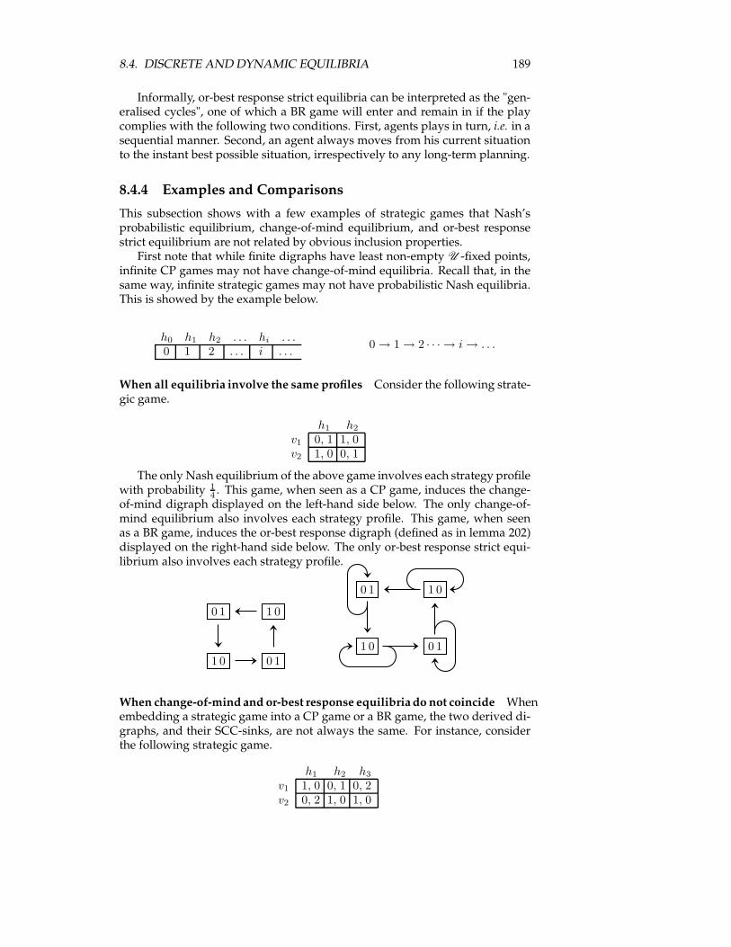
8.4. DISCRETE AND DYNAMIC EQUILIBRIA 189
Informally, or-best response strict equilibria can be interpreted as the "gen-eralised cycles", one of which a BR game will enter and remain in if the playcomplies with the following two conditions. First, agents plays in turn, i.e. in asequential manner. Second, an agent always moves from his current situationto the instant best possible situation, irrespectively to any long-term planning.
8.4.4 Examples and Comparisons
This subsection shows with a few examples of strategic games that Nash’sprobabilistic equilibrium, change-of-mind equilibrium, and or-best responsestrict equilibrium are not related by obvious inclusion properties.First note that while finite digraphs have least non-empty U -fixed points,
infinite CP games may not have change-of-mind equilibria. Recall that, in thesame way, infinite strategic games may not have probabilistic Nash equilibria.This is showed by the example below.
h0 h1 h2 . . . hi . . .0 1 2 . . . i . . .
0→ 1→ 2 · · · → i→ . . .
When all equilibria involve the same profiles Consider the following strate-gic game.
h1 h2
v1 0, 1 1, 0v2 1, 0 0, 1
The only Nash equilibrium of the above game involves each strategy profilewith probability 1
4 . This game, when seen as a CP game, induces the change-of-mind digraph displayed on the left-hand side below. The only change-of-mind equilibrium also involves each strategy profile. This game, when seenas a BR game, induces the or-best response digraph (defined as in lemma 202)displayed on the right-hand side below. The only or-best response strict equi-librium also involves each strategy profile.
0 1 1 0
1 0 0 1
0 1 1 0
1 0 0 1
When change-of-mindand or-best response equilibria do not coincide Whenembedding a strategic game into a CP game or a BR game, the two derived di-graphs, and their SCC-sinks, are not always the same. For instance, considerthe following strategic game.
h1 h2 h3
v1 1, 0 0, 1 0, 2v2 0, 2 1, 0 1, 0
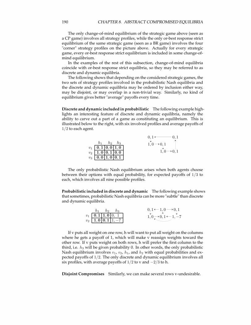
190 CHAPTER 8. ABSTRACT COMPROMISED EQUILIBRIA
The only change-of-mind equilibrium of the strategic game above (seen asa CP game) involves all strategy profiles, while the only or-best response strictequilibrium of the same strategic game (seen as a BR game) involves the four"corner" strategy profiles on the picture above. Actually for every strategicgame, every or-best response strict equilibrium is included in some change-of-mind equilibrium.In the examples of the rest of this subsection, change-of-mind equilibria
coincide with or-best response strict equilibria, so they may be referred to asdiscrete and dynamic equilibria.The following shows that depending on the considered strategic games, the
two sets of strategy profiles involved in the probabilistic Nash equilibria andthe discrete and dynamic equilibria may be ordered by inclusion either way,may be disjoint, or may overlap in a non-trivial way. Similarly, no kind ofequilibrium gives better "average" payoffs every time.
Discrete and dynamic included in probabilistic The following example high-lights an interesting feature of discrete and dynamic equilibria, namely theability to carve out a part of a game as constituting an equilibrium. This isillustrated below to the right, with six involved profiles and average payoffs of1/2 to each agent.
h1 h2 h3
v1 0,1 0,0 1,0v2 1,0 0,1 0,0v3 0,0 1,0 0,1
0, 1 0, 1
1, 0 0, 1
1, 0 0, 1
The only probabilistic Nash equilibrium arises when both agents choosebetween their options with equal probability, for expected payoffs of 1/3 toeach, which involves all nine possible profiles.
Probabilistic included in discrete and dynamic The following example showsthat sometimes, probabilistic Nash equilibria can bemore "subtle" than discreteand dynamic equilibria.
h1 h2 h3
v1 0,1 1,0 0, 1v2 1,0 0,1 1,−7
0, 1 1, 0 0, 1
1, 0 0, 1 1,−7
If v puts all weight on one row, h will want to put all weight on the columnswhere he gets a payoff of 1, which will make v reassign weights toward theother row. If v puts weight on both rows, h will prefer the first column to thethird, i.e. h3 will be given probability 0. In other words, the only probabilisticNash equilibrium involves v1, v2, h1, and h2 with equal probabilities and ex-pected payoffs of 1/2. The only discrete and dynamic equilibrium involves allsix profiles, with average payoffs of 1/2 to v and −2/3 to h.
Disjoint Compromises Similarly, we can make several rows v-undesirable.
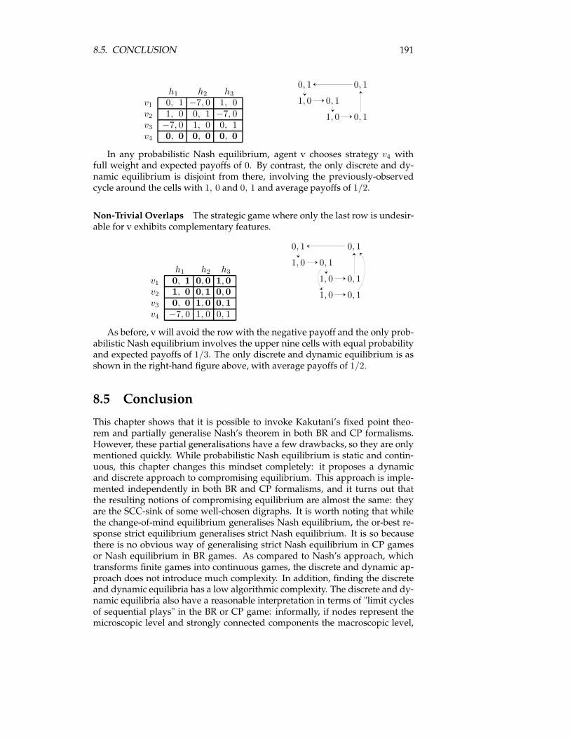
8.5. CONCLUSION 191
h1 h2 h3
v1 0, 1 −7, 0 1, 0v2 1, 0 0, 1 −7, 0v3 −7, 0 1, 0 0, 1v4 0, 0 0, 0 0, 0
0, 1 0, 1
1, 0 0, 1
1, 0 0, 1
In any probabilistic Nash equilibrium, agent v chooses strategy v4 withfull weight and expected payoffs of 0. By contrast, the only discrete and dy-namic equilibrium is disjoint from there, involving the previously-observedcycle around the cells with 1, 0 and 0, 1 and average payoffs of 1/2.
Non-Trivial Overlaps The strategic game where only the last row is undesir-able for v exhibits complementary features.
h1 h2 h3
v1 0, 1 0,0 1,0v2 1, 0 0,1 0,0v3 0, 0 1,0 0,1v4 −7, 0 1, 0 0, 1
0, 1 0, 1
1, 0 0, 1
1, 0 0, 1
1, 0 0, 1
As before, v will avoid the row with the negative payoff and the only prob-abilistic Nash equilibrium involves the upper nine cells with equal probabilityand expected payoffs of 1/3. The only discrete and dynamic equilibrium is asshown in the right-hand figure above, with average payoffs of 1/2.
8.5 Conclusion
This chapter shows that it is possible to invoke Kakutani’s fixed point theo-rem and partially generalise Nash’s theorem in both BR and CP formalisms.However, these partial generalisations have a few drawbacks, so they are onlymentioned quickly. While probabilistic Nash equilibrium is static and contin-uous, this chapter changes this mindset completely: it proposes a dynamicand discrete approach to compromising equilibrium. This approach is imple-mented independently in both BR and CP formalisms, and it turns out thatthe resulting notions of compromising equilibrium are almost the same: theyare the SCC-sink of some well-chosen digraphs. It is worth noting that whilethe change-of-mind equilibrium generalises Nash equilibrium, the or-best re-sponse strict equilibrium generalises strict Nash equilibrium. It is so becausethere is no obvious way of generalising strict Nash equilibrium in CP gamesor Nash equilibrium in BR games. As compared to Nash’s approach, whichtransforms finite games into continuous games, the discrete and dynamic ap-proach does not introduce much complexity. In addition, finding the discreteand dynamic equilibria has a low algorithmic complexity. The discrete and dy-namic equilibria also have a reasonable interpretation in terms of "limit cyclesof sequential plays" in the BR or CP game: informally, if nodes represent themicroscopic level and strongly connected components the macroscopic level,
192 CHAPTER 8. ABSTRACT COMPROMISED EQUILIBRIA
then the compromising equilibria are the macroscopic equilibria of a micro-scopic world. Even though this discrete and dynamic view might not have asmany practical applications as Nash’s theorem does, they are useful in at leastone respect: it shows that probabilities are not the only possible way of weak-ening the definition of Nash equilibrium and thus guaranteeing existence ofweakened equilibrium.
Chapter 9
Discrete Non Determinismand Nash Equilibria forStrategy-Based Games
Several notions of game enjoy a Nash-like notion of equilibrium without guar-antee of existence. There are different ways of weakening a definition of Nash-like equilibrium in order to guarantee the existence of a weakened equilibrium.Nash’s approach to the problem for strategic games is probabilistic, i.e. contin-uous, and static. CP and BR approaches for CP and BR games are discreteand dynamic. This chapter proposes an approach that lies between those twodifferent approaches: a discrete and static approach. Multi strategic gamesare introduced as a formalism that is able to express both sequential and si-multaneous decision-making, which promises a good modelling power. Multistrategic games are a generalisation of strategic games and sequential graphgames that still enjoys a Cartesian product structure, i.e. where agent actuallychoose their strategies. A pre-fixed point result allows guaranteeing existenceof discrete and non deterministic equilibria. On the one hand, these equilibriacan be computed with polynomial (low) complexity. On the other hand, theyare effective in terms of recommendation, as shown by a numerical example.
9.1 Introduction
Not all strategic games have a (pure) Nash equilibrium. On the one hand,Nash’s probabilistic approach copes with this existence problem with an adhoc solution: Nash’s solution is dedicated to a setting with real-valued payofffunctions. On the other hand, CP and BR games propose an abstract and gen-eral approach that is applicable tomany types of game. Both approaches gener-alise the notion of Nash equilibrium and guarantee the existence of a weakenedNash equilibrium. There are twomain differences between the two approachesthough. First, Nash’s approach considers finite objects and yields continuousobjects, whereas the CP and BR approach preserves finiteness. Second, Nash’sapproach is static, whereas the CP and BR approach is dynamic: Nash’s ap-proach is static because a probabilistic Nash equilibrium can be interpreted
193
194 CHAPTER 9. DISCRETE NON DETERMINISM
as a probabilistic status quo that is (pure) Nash equilibrium of a probabilisedgame. The Cartesian product structure enables a static approach. CP and BRapproach is dynamic because a CP or BR equilibrium can be interpreted as alimit set of states that are tied together by explicit forces. It may be interestingtomix features from both approaches, and to present for instance a discrete andstatic notion of equilibrium. Actually, such an approach was already adoptedin [27], whose purpose was to provide sequential tree games with a notion ofdiscrete non deterministic equilibrium. This approach assumed partially or-dered payoffs, and simple "backward induction" guarantees existence of nondeterministic subgame perfect equilibrium. This result is superseded by [29]which adopts a completely different approach, but the discrete non determin-ism spirit can be further exploited.
9.1.1 Contribution
This chapter introduces the concept of abstract strategic games, which corre-sponds to traditional strategic games where real-valued payoff functions havebeen replacedwith abstract objects called outcomes. In addition, the usual totalorder over the reals has been replacedwith binary relations, one per agent, thataccount for agent’s preferences over the outcomes. Abstract strategic gamesthus generalise strategic games like abstract sequential tree games generalisesequential tree games. A notion of Nash equilibrium is defined, but not allabstract strategic games have a Nash equilibrium since traditional strategicgames already lack this property.Like Nash did for traditional strategic games, an attempt is made to in-
troduce probabilities into these new games. However, it is mostly a failurebecause there does not seem to exist any extension of a poset to its barycentresthat is relevant to the purpose. So, instead of saying that "an agent chooses agiven strategy with some probability", this chapter proposes to say that "theagent may choose the strategy", without further specification.The discrete non determinism proposed above is implemented in the no-
tion of non deterministic best response (ndbr ) multi strategic game. As hintedby the terminology, the best response approach is preferred over the convert-ibility preference approach for this specific purpose. (Note that discrete nondeterminism for abstract strategic games can be implemented in a formalismthat is more specific and simpler than ndbr multi strategic games, but this gen-eral formalism will serve further purposes.) This chapter defines the notionof ndbr equilibrium in these games, and a pre-fixed point result helps prove asufficient condition for every ndbr multi strategic game to have an ndbr equi-librium. An embedding of abstract strategic games into ndbr multi strategicgames provides abstract strategic games with a notion of non deterministic(nd ) equilibrium that generalises the notion of Nash equilibrium. Since ev-ery abstract strategic game has an nd equilibrium (under some condition), thediscrete non deterministic approach succeeds where the probabilistic approachfails, i.e. is irrelevant. This new approach lies between Nash’s approach, whichis continuous and static, and the abstract approaches of CP and BR games,which are discrete and dynamic. Indeed, this notion of nd equilibrium is dis-crete and static. It is deemed static because it makes use of the Cartesian prod-uct structure, which allows interpreting an equilibrium as a "static state of thegame".
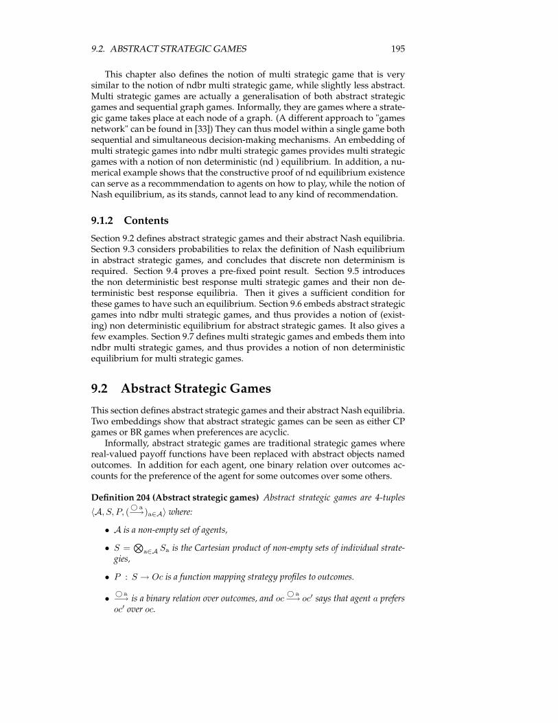
9.2. ABSTRACT STRATEGIC GAMES 195
This chapter also defines the notion of multi strategic game that is verysimilar to the notion of ndbr multi strategic game, while slightly less abstract.Multi strategic games are actually a generalisation of both abstract strategicgames and sequential graph games. Informally, they are games where a strate-gic game takes place at each node of a graph. (A different approach to "gamesnetwork" can be found in [33]) They can thus model within a single game bothsequential and simultaneous decision-making mechanisms. An embedding ofmulti strategic games into ndbr multi strategic games provides multi strategicgames with a notion of non deterministic (nd ) equilibrium. In addition, a nu-merical example shows that the constructive proof of nd equilibrium existencecan serve as a recommmendation to agents on how to play, while the notion ofNash equilibrium, as its stands, cannot lead to any kind of recommendation.
9.1.2 Contents
Section 9.2 defines abstract strategic games and their abstract Nash equilibria.Section 9.3 considers probabilities to relax the definition of Nash equilibriumin abstract strategic games, and concludes that discrete non determinism isrequired. Section 9.4 proves a pre-fixed point result. Section 9.5 introducesthe non deterministic best response multi strategic games and their non de-terministic best response equilibria. Then it gives a sufficient condition forthese games to have such an equilibrium. Section 9.6 embeds abstract strategicgames into ndbr multi strategic games, and thus provides a notion of (exist-ing) non deterministic equilibrium for abstract strategic games. It also gives afew examples. Section 9.7 defines multi strategic games and embeds them intondbr multi strategic games, and thus provides a notion of non deterministicequilibrium for multi strategic games.
9.2 Abstract Strategic Games
This section defines abstract strategic games and their abstract Nash equilibria.Two embeddings show that abstract strategic games can be seen as either CPgames or BR games when preferences are acyclic.Informally, abstract strategic games are traditional strategic games where
real-valued payoff functions have been replaced with abstract objects namedoutcomes. In addition for each agent, one binary relation over outcomes ac-counts for the preference of the agent for some outcomes over some others.
Definition 204 (Abstract strategic games) Abstract strategic games are 4-tuples
〈A, S, P, (© a−→)a∈A〉 where:
• A is a non-empty set of agents,
• S =⊗
a∈A Sa is the Cartesian product of non-empty sets of individual strate-gies,
• P : S → Oc is a function mapping strategy profiles to outcomes.
•© a−→ is a binary relation over outcomes, and oc
© a−→ oc′ says that agent a prefers
oc′ over oc.
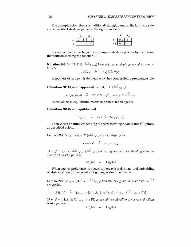
196 CHAPTER 9. DISCRETE NON DETERMINISM
The example below shows a traditional strategic game on the left-hand side,and an abstract strategic game on the right-hand side.
h1 h2
v1 0 2 1 1v2 0 1 2 0
h1 h2
v1 oc1 oc2
v2 oc3 oc4
For a given game, each agent can compare strategy profiles by comparingtheir outcomes using the function P .
Notation 205 Let 〈A, S, P, (© a−→)a∈A〉 be an abstract strategic game and let s and s′
be in S.
s©a−→ s′
∆= P (s)
© a−→ P (s′)
Happiness of an agent is defined below, in a convertibility preference style.
Definition 206 (Agent happiness) Let 〈A, S, P, (© a−→)a∈A〉
Happy(a, s)∆= ∀s′ ∈ S, ¬(s′−a = s−a ∧ s
©a−→ s′)
As usual, Nash equilibrium means happiness for all agents.
Definition 207 (Nash Equilibrium)
Eqg(s)∆= ∀a ∈ A, Happy(a, s)
There exists a natural embedding of abstract strategic games into CP games,as described below.
Lemma 208 Let g = 〈A, S, P, (© a−→)a∈A〉 be a strategic game.
s+ a←→ s′
∆= s−a = s′−a,
Then g′ = 〈A, S, (+a←→)a∈A, (
© a−→)a∈A〉 is a CP game and the embedding preserves
and reflects Nash equilibria.
Eqg(s) ⇔ Eqg′(s)
When agents’ preferences are acyclic, there exists also a natural embeddingof abstract strategic games into BR games, as described below.
Lemma 209 Let g = 〈A, S, P, (© a−→)a∈A〉 be a strategic game. Assume that the
© a−→
are acyclic.
BRa(s)∆= {s−a} × {s
′ ∈ Sa | ∀s′′ ∈ Sa, ¬(s−a; s′
© a−→ s−a; s′′)}
Then g′ = 〈A, S, (BRa)a∈A〉 is a BR game and the embedding preserves and reflectsNash equilibria.
Eqg(s) ⇔ Eqg′(s)
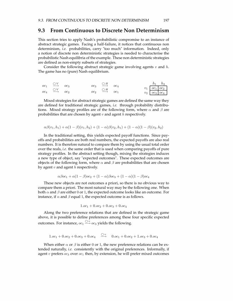
9.3. FROM CONTINUOUS TO DISCRETE NON DETERMINISM 197
9.3 From Continuous to Discrete Non Determinism
This section tries to apply Nash’s probabilistic compromise to an instance ofabstract strategic games. Facing a half-failure, it notices that continuous nondeterminism, i.e. probabilities, carry "too much" information. Indeed, onlya notion of discrete non deterministic strategies is needed to characterise theprobabilistic Nash equilibria of the example. These non deterministic strategiesare defined as non-empty subsets of strategies.Consider the following abstract strategic game involving agents v and h.
The game has no (pure) Nash equilibrium.
oc1©V−→ oc3 oc3
©H−→ oc4
oc4©V−→ oc2 oc2
©H−→ oc1
h1 h2
v1 oc1 oc2
v2 oc3 oc4
Mixed strategies for abstract strategic games are defined the same way theyare defined for traditional strategic games, i.e. through probability distribu-tions. Mixed strategy profiles are of the following form, where α and β areprobabilities that are chosen by agent v and agent h respectively.
αβ(v1, h1) + α(1 − β)(v1, h2) + (1− α)β(v2, h1) + (1− α)(1 − β)(v2, h2)
In the traditional setting, this yields expected payoff functions. Since pay-offs and probabilities are both real numbers, the expected payoffs are also realnumbers. It is therefore natural to compare them by using the usual total orderover the reals, i.e. the same order that is used when comparing payoffs of purestrategy profiles. In the abstract setting though, mixing the strategies inducesa new type of object, say "expected outcomes". These expected outcomes areobjects of the following form, where α and β are probabilities that are chosenby agent v and agent h respectively.
αβoc1 + α(1− β)oc2 + (1− α)βoc3 + (1− α)(1 − β)oc4
These new objects are not outcomes a priori, so there is no obvious way tocompare them a priori. The most natural way may be the following one. Whenboth α and β are either 0 or 1, the expected outcome looks like an outcome. Forinstance, if α and β equal 1, the expected outcome is as follows.
1.oc1 + 0.oc2 + 0.oc3 + 0.oc4
Along the two preference relations that are defined in the strategic gameabove, it is possible to define preferences among these four specific expected
outcomes. For instance, oc1© v−→ oc3 yields the following.
1.oc1 + 0.oc2 + 0.oc3 + 0.oc4© v−→ 0.oc1 + 0.oc2 + 1.oc3 + 0.oc4
When either α or β is either 0 or 1, the new preference relations can be ex-tended naturally, i.e. consistently with the original preferences. Informally, ifagent v prefers oc3 over oc1 then, by extension, he will prefer mixed outcomes
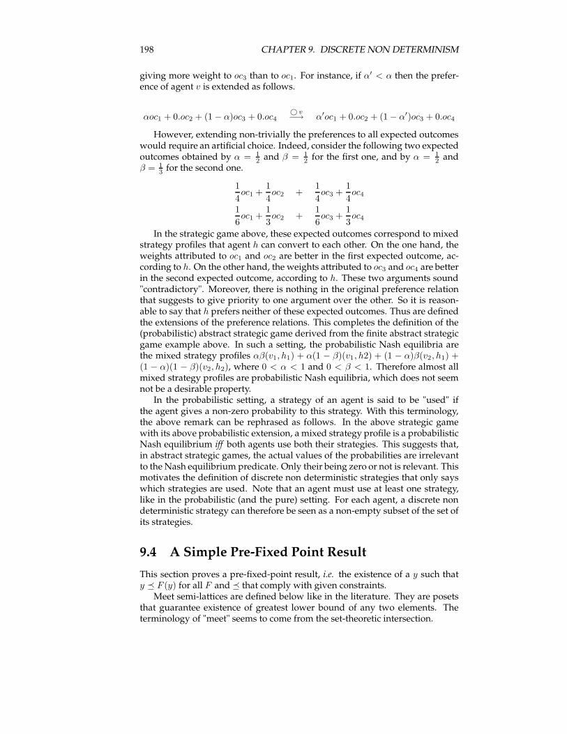
198 CHAPTER 9. DISCRETE NON DETERMINISM
giving more weight to oc3 than to oc1. For instance, if α′ < α then the prefer-ence of agent v is extended as follows.
αoc1 + 0.oc2 + (1− α)oc3 + 0.oc4© v−→ α′oc1 + 0.oc2 + (1− α′)oc3 + 0.oc4
However, extending non-trivially the preferences to all expected outcomeswould require an artificial choice. Indeed, consider the following two expectedoutcomes obtained by α = 1
2 and β = 12 for the first one, and by α = 1
2 andβ = 1
3 for the second one.
1
4oc1 +
1
4oc2 +
1
4oc3 +
1
4oc4
1
6oc1 +
1
3oc2 +
1
6oc3 +
1
3oc4
In the strategic game above, these expected outcomes correspond to mixedstrategy profiles that agent h can convert to each other. On the one hand, theweights attributed to oc1 and oc2 are better in the first expected outcome, ac-cording to h. On the other hand, the weights attributed to oc3 and oc4 are betterin the second expected outcome, according to h. These two arguments sound"contradictory". Moreover, there is nothing in the original preference relationthat suggests to give priority to one argument over the other. So it is reason-able to say that h prefers neither of these expected outcomes. Thus are definedthe extensions of the preference relations. This completes the definition of the(probabilistic) abstract strategic game derived from the finite abstract strategicgame example above. In such a setting, the probabilistic Nash equilibria arethe mixed strategy profiles αβ(v1, h1) + α(1 − β)(v1, h2) + (1 − α)β(v2, h1) +(1 − α)(1 − β)(v2, h2), where 0 < α < 1 and 0 < β < 1. Therefore almost allmixed strategy profiles are probabilistic Nash equilibria, which does not seemnot be a desirable property.In the probabilistic setting, a strategy of an agent is said to be "used" if
the agent gives a non-zero probability to this strategy. With this terminology,the above remark can be rephrased as follows. In the above strategic gamewith its above probabilistic extension, a mixed strategy profile is a probabilisticNash equilibrium iff both agents use both their strategies. This suggests that,in abstract strategic games, the actual values of the probabilities are irrelevantto the Nash equilibrium predicate. Only their being zero or not is relevant. Thismotivates the definition of discrete non deterministic strategies that only sayswhich strategies are used. Note that an agent must use at least one strategy,like in the probabilistic (and the pure) setting. For each agent, a discrete nondeterministic strategy can therefore be seen as a non-empty subset of the set ofits strategies.
9.4 A Simple Pre-Fixed Point Result
This section proves a pre-fixed-point result, i.e. the existence of a y such thaty � F (y) for all F and � that comply with given constraints.Meet semi-lattices are defined below like in the literature. They are posets
that guarantee existence of greatest lower bound of any two elements. Theterminology of "meet" seems to come from the set-theoretic intersection.
9.4. A SIMPLE PRE-FIXED POINT RESULT 199
Definition 210 (Meet semi-lattice) A meet semi-lattice is a partially ordered set(S,�), i.e. the binary relation � is reflexive and transitive, such that any sets withtwo elements has a greatest lower bound.
Defined as a specific type of posets, meet semi-lattices have algebraic prop-erties. (Actually, meet semi-lattices are sometimes defined as algebraic struc-tures from where an ordering is derived.)
Definition 211 In a partially ordered set, a greatest lower bound of two elements isunique, which induces the binary operator "greatest lower bound". This operator iscommutative and associative, which enables the definition of the greatest lower boundof any non-empty finite subset of S. Let us call inf this greatest lower bound function.
Given a function from a meet semi-lattice to itself, a meeting point is anelement of the lattice such that every decreasing sequence that starts with themeeting point is not too much "scattered" by the function. This is accuratelydescribed below.
Definition 212 Let (S,�) be a meet semi-lattice with least elementm, and let inf bethe infimum function corresponding to �. Let F be a function from S to itself and letx be in S. Assume that for all x1 . . . xn such thatm 6= x1 � · · · � xn � x, we haveinf(F (x1), . . . , F (xn), x) 6= m. If x 6= m then x is said to be a F -meeting point, andone writesMF (x).
The F -meeting point predicate is preserved by the greatest lower boundoperator used with the image of the point by F , as stated below.
Lemma 213 Let (S,�) be a meet semi-lattice with least element m; let inf be theinfimum function corresponding to �; and let F be a function from S to itself. Thefollowing formula holds.
MF (x) ⇒ MF ◦ inf(x, F (x))
Proof Assume MF (x), so x and m are different. By reflexivity x � x, soinf(x, F (x)) 6= m by definition of meeting point. Assume m 6= x1 � · · · �xn � inf(x, F (x)), so m 6= x1 � · · · � xn � x � x since inf(x, F (x)) � x bydefinition of inf . So inf(F (x1), . . . , F (xn), F (x), x) 6= m since x is a F -meetingpoint. Therefore inf(F (x1), . . . , F (xn), inf(F (x), x)) 6= m, by associativity ofthe greatest lower bound operator underlying the infimum function inf . Soinf(x, F (x)) is a F -meeting point. �
The F -meeting point predicate preservation can be combined with the as-sumption that there exists no infinite strictly decreasing sequence. In this case,iteration of lemma 213 yields a non-trivial pre fixed point of F .
Lemma 214 Let (S,�) be a meet semi-lattice with least element m, and assume that� is well-founded. Let F be a function from S to itself. If there exists a F -meetingpoint, then there exists a F pre fixed point different from m, i.e. there exists y 6= msuch that y � F (y).
Proof Assume MF (x0). An infinite sequence of elements of S is built asfollows. It starts with x0, and it is gradually defined by induction. Assumexn, . . . , x0 such that MF (xn), and xk+1 = inf(xk, F (xk)) for all 0 ≤ k < n.
200 CHAPTER 9. DISCRETE NON DETERMINISM
Let xn+1 = inf(xn, F (xn)). By Lemma 213,MF (xn+1). By well-foundness as-sumption, there exists n such that xn+1 = xn, whichmeans that xn = inf(xn, F (xn)),so xn � F (xn). Moreover,MF (xn) by construction of the sequence, so xn 6= m.
�
9.5 Non Deterministic Best Response Multi Strate-gic Games
Using the concept of discrete non deterministic strategy, this section definesnon deterministic best response multi strategic games and their non determin-istic Nash equilibria. This section also proves a sufficient condition for nondeterministic Nash equilibrium existence in every non deterministic best re-sponse multi strategic game. These results will be used to guarantee existenceof non deterministic equilibrium for abstract strategic games and non deter-ministic multi strategic game.Informally, non deterministic best response multi strategic games involve
agents who play on several (abstractions of) strategic games at the same time.Agents’ strategies are non deterministic, i.e. on each game each agent has tochoose one or more (pure) strategies among his available strategies. When allthe opponents of an agent have chosen their non deterministic strategies on allgames, a function tells agent a what his non deterministic best responses are.These games are formally defined below.
Definition 215 (Non deterministic best response multi strategic games)An ndbr multi strategic game is a pair 〈(Si
a)i∈Ia∈A, (BRa)a∈A〉 complying with the
following.
• I is a non-empty set of indices and A is a non-empty set of agents.
• For all a in A, BRa is a function from Σ−a to Σa,whereΣ =
⊗a∈A Σa andΣa =
⊗i∈I P(Si
a)−{∅} andΣ−a =⊗
a′∈A−{a} Σa′ .
Elements of Σa are called nd strategies for a, and elements of Σ are called nd strategyprofiles.
Informally, an agent is happy with an nd strategy profile if its own nd strat-egy is included in its best responses against other agents’ nd strategies. Agents’happiness is formally defined as follows.
Definition 216 (Happiness) Let g = 〈(Sia)i∈I
a∈A, (BRa)a∈A〉 be an ndbr multi strate-gic game, and let σ be in Σ.
Happy(σ, a)∆= σa ⊆ BRa(σ−a)
As usual, (non deterministic) Nash equilibrium amounts to happiness forall agents.
Definition 217 (Non deterministic Nash equilibrium) Let g be an ndbr multistrategic game, g = 〈(Si
a)i∈Ia∈A, (BRa)a∈A〉.
Eqg(σ)∆= ∀a ∈ A, Happy(σ, a)
9.5. NDBR MULTI STRATEGIC GAMES 201
The individual best response functions can be combined into a collectivebest response function from the non deterministic profiles into themselves.
Definition 218 (Combined best response) Given an ndbr multi strategic gamewith (BRa)a∈A a family of agent best responses. The combined best response is afunction from Σ to itself defined as follows.
BR(σ)∆=
⊗
a∈A
BRa(σ−a)
Through the combined best response function, the non deterministic Nashequilibria are characterised below as nd profiles included in their images bythe combined best response.
Lemma 219 An ndbr equilibrium for g = 〈(Sia)i∈I
a∈A, (BRa)a∈A〉 is characterised asfollows.
Eqg(σ) ⇔ σ ⊆ BR(σ)
Like in BR games, it is easy to define agents’ strict happiness.
Definition 220 (Strict happiness) Let g = 〈(Sia)i∈I
a∈A, (BRa)a∈A〉 be an ndbr multistrategic game, and let σ be in Σ.
Happy+(σ, a)∆= σa = BRa(σ−a)
Then, (non deterministic) strict Nash equilibrium is defined as strict happi-ness for all agents.
Definition 221 (Non deterministic strict Nash equilibrium) Let g be an ndbr multistrategic game, g = 〈(Si
a)i∈Ia∈A, (BRa)a∈A〉, and let σ be in Σ.
Eq+g (σ)
∆= ∀a ∈ A, Happy+(σ, a)
The following embedding of non deterministic best responsemulti strategicgames into BR games preserves an reflects equilibria.
Lemma 222 Let g = 〈(Sia)i∈I
a∈A, (BRa)a∈A〉 be an ndbr multi strategic game. DefineBR′
a with a Cartesian product below, for σ ∈ Σ.
BR′a(σ)
∆= {σ−a} ×
⊗
i∈I
P(BRia(σ−a))− {∅}
Where BRia(σ−a) is the i-projection of BRa(σ−a). Then the object g′ defined by
g′ = 〈A, Σ, (BR′a)a∈A〉 is a BR game and Nash equilibria correspond as follows.
Eqg′(σ) ⇔ Eqg(σ)
Proof Let σ be in Σ =⊗
a∈A
⊗i∈I(P(Si
a) − {∅}). The following chain ofequivalences proves the claim. Eqg′(σ) ⇔ ∀a, σ ∈ BR′
a(σ) ⇔ ∀a, σ ∈ {σ−a}×⊗i∈I P(BRi
a(σ−a)) − {∅} ⇔ ∀a, σa ∈⊗
i∈I P(BRia(σ−a)) − {∅} ⇔ ∀a, σa ⊆
BRa(σ−a) ⇔ Eqg(σ) �
202 CHAPTER 9. DISCRETE NON DETERMINISM
The remainder of the section invokes the fixed-point results of section 9.4,but prior to that, a meet lattice needs to be identified.
Lemma 223 Given an ndbr multi strategic game 〈(Sia)i∈I
a∈A, (BRa)a∈A〉, the poset(Σ ∪ {∅},⊆) is a meet semi-lattice with least element ∅.
A first equilibrium existence result is given below.
Lemma 224 Given an ndbr multi strategic game 〈(Sia)i∈I
a∈A, (BRa)a∈A〉, if there ex-ists a BR-meeting point, then there exists a non deterministic Nash equilibrium.
Proof By lemma 214, if there exists a BR-meeting point, then there exists anon-empty pre fixed point σ forBR, i.e. there exists σ 6= ∅ such that σ ⊆ BR(σ).It is an ndbr equilibrium by definition. �
The main equilibrium existence result is stated below.
Lemma 225 Consider an ndbr multi strategic game 〈(Sia)i∈I
a∈A, (BRa)a∈A〉. Let σ bein Σ. Assume that for all agents a, for all γ1 . . . γn in Σ−a, if γn ⊆ · · · ⊆ γ1 ⊆ σ−a
then ∩1≤k≤nBRa(γk) ∩ σa 6= ∅. In this case, the game has an ndbr equilibrium.
Proof By lemma 224, it suffices to show that there exists aBR-meeting point.Let us prove that σ is such a meeting point. First of all, σ is non-empty since itbelongs to Σ. Second, assume σ1 . . . σn in Σ such that σ1 ⊆ · · · ⊆ σn ⊆ σ. So forall agents a, σ1
−a ⊆ · · · ⊆ σn−a ⊆ σ−a. By assumption, ∩1≤k≤nBRa(σk
−a) ∩ σa 6=∅, which amounts to (∩1≤k≤nBR(σk) ∩ σ)a 6= ∅. Since this holds for all a, wehave ∩1≤k≤nBR(σk) ∩ σ 6= ∅. Therefore σ is a BR-meeting point. �
Equilibria are preserved when "increasing" the best response functions, asstated below.
Lemma 226 Let g = 〈(Sia)i∈I
a∈A, (BRa)a∈A〉 and g′ = 〈(Sia)i∈I
a∈A, (BR′a)a∈A〉 be two
ndbr multi strategic games such that for all a in A, for all γ in Σ−a, BRa(γ) ⊆BR′
a(γ). In this case, the following implication holds.
Eqg(σ) ⇒ Eqg′(σ)
Proof Since for all a in A, for all γ in Σ−a, BRa(γ) ⊆ BR′a(γ), it follows that
for all σ in Σ, BR(σ) ⊆ BR′(σ). So, σ ⊆ BR(σ) implies σ ⊆ BR′(σ). �
9.6 Discrete and Static Compromising Equilibriumfor Abstract Strategic Games
Subsection 9.6.1 embeds abstract strategic games into ndbrmulti strategic games,and thus provides a notion of non deterministic Nash equilibrium for abstractstrategic games. Finally it proves equilibrium existence for all abstract strate-gic games. Subsection 9.6.2 gives an example of such non deterministic Nashequilibrium on a strategic game with real-valued payoff functions. The build-ing of the equilibrium is described step by step. Subsection 9.6.3 suggests by anumerical example that the constructive proof of existence of such an equilib-rium yields a notion of recommendation that is better on average than playingrandomly.
9.6. EQUILIBRIUM FOR ABSTRACT STRATEGIC GAMES 203
9.6.1 Non Deterministic Equilibrium Existence
The following definition extends orders over functions’ codomains to ordersover (restrictions of) functions.
Definition 227 Let f and f ′ be functions of type A→ B, and let A′ be a subset of A.Let ≺ be an irreflexive binary relation over B, and let � be its reflexive closure.
f �A′
f ′ ∆= ∀x ∈ A′, f(x) � f ′(x)
f ≺A′
f ′ ∆= f �A′
f ′ ∧ ∃x ∈ A′, f(x) ≺ f ′(x)
One simply writes f ≺ f ′ instead of f ≺A f ′.
For example if the two functions are represented by vectors of naturals withthe usual total order, then (1, 1) < (1, 2), (0, 2) < (1, 2) and (0, 1) < (1, 2).The extension above preserves strict partial orders, as stated below.
Lemma 228 If ≺ is a strict partial order over B, then the derived ≺A over functionsof type A→ B is also a strict partial order.
Given finitely many functions of the same type, given an order on the co-domain, given finitely many subsets of the domain that are totally ordered byinclusion, one of these functions is maximal for the extension order with re-spect to each of the subsets. This is proved by the following.
Lemma 229 Let E be a finite set of functions of type A→ B. Let ≺ be an irreflexiveand transitive binary relation over B, and let � be its reflexive closure. For any ∅ 6=A0 ⊆ · · · ⊆ An ⊆ A there exists an f in E that is maximal with respect to all theextended orders from ≺A0 to ≺An .
Proof By induction on n. First case, n = 0. There exists an f in E that ismaximal, i.e. have no successor, with respect to≺A0 since≺A0 is a partial order.Second case, assume that the claim holds for n and let ∅ 6= A0 ⊆ · · · ⊆ An+1 besubsets of A. Let f in E be maximal with respect to all the ≺A0 · · · ≺An . Let f ′
be maximal with respect to ≺An+1 among the functions in E that coincide withf on An. Since ∅ 6= A0 ⊆ · · · ⊆ An, the function f ′ is maximal in E with respectto all the ≺A0 · · · ≺An . Let f ′′ in E be such that f ′ �An+1 f ′′. So f ′ �An f ′′
since An ⊆ An+1. Therefore f ′ and f ′′ coincide on An by maximality of f ′ withrespect to ≺An . Since f and f ′ coincide on An, the functions f and f ′′ alsocoincide on An. Therefore ¬(f ′ ≺An+1 f ′′) by definition of f ′, which showsthat f ′ is also maximal with respect to ≺An+1 . �
Below, an ndbr multi strategic game is built from an abstract strategic game.This ndbr multi strategic game always has an ndbr equilibrium. In the notation
s© a−→γ s′ below, the strategies s and s′ are seen as functions from Sa to theoutcomes.
Lemma 230 Let g = 〈A, S, P, (© a−→)a∈A〉 be an abstract strategic game. Assume that
the© a−→ are strict partial orders, i.e. irreflexive and transitive. For each agent a and
204 CHAPTER 9. DISCRETE NON DETERMINISM
each γ in Σ−a, the following defines a subset of Sa.
BRa(γ)∆= {s ∈ Sa | ∀s′ ∈ Sa, ¬(s
©a−→S−a
s′) ∧
∀s′ ∈ Sa, ¬(s©a−→γ s′) ∧
∃c ∈ γ, ∀s′ ∈ Sa, ¬(s©a−→{c} s′) }
The object 〈(Sa)a∈A, (BRa)a∈A〉 is an ndbr multi strategic game, and it has an ndbrequilibrium.
Proof Let a be an agent. First note that, through the function P , every strat-egy s in Sa can be seen as a function from S−a to the outcomes Oc. Let γ1 ⊆· · · ⊆ γn be in Σ−a and let c be in γ1. According to lemma 229, there exists an s
in Sa that is maximal with respect to©a−→{c},
© a−→γ1
, . . . ,©a−→γn
,© a−→S−a
. By defi-nition ofBRa (third conjunct), this strategy s is in all theBRa(γ1), . . . , BRa(γn).First, this shows that BRa returns non-empty sets, so 〈(Sa)a∈A, (BRa)a∈A〉 isindeed an ndbr multi strategic game. Second, this game has an ndbr equilib-rium by lemma 225. �
The ndbr equilibrium for the derived ndbr multi strategic game is called anon deterministic equilibrium for the original abstract strategic game. Othersimilar definitions are possible for non deterministic equilibrium. Especiallydefinitions more generous than the one in lemma 230, which guarantee theexistence of a non deterministic equilibrium, according to lemma 226. Thisyields the following lemma.
Lemma 231 Let g = 〈A, S, P, (© a−→)a∈A〉 be a strategic game. Assume that the
© a−→
are strict partial orders, i.e. irreflexive and transitive. For each agent a and each γ inΣ−a, the following defines three subsets of Sa.
BR1a(γ)
∆= {s ∈ Sa | ∀s
′ ∈ Sa, ¬(s©a−→S−a
s′)}
BR2a(γ)
∆= {s ∈ Sa | ∀s
′ ∈ Sa, ¬(s©a−→γ s′)}
BR3a(γ)
∆= {s ∈ Sa | ∃c ∈ γ, ∀s′ ∈ Sa, ¬(s
©a−→{c} s′)}
BR4a(γ)
∆= {s ∈ Sa | ∀s
′ ∈ Sa, ∃c ∈ γ, ¬(s©a−→{c} s′)}
The object 〈A, S, (BRia)a∈A〉, for i between 1 and 4, is an ndbr multi strategic game,
and it has an ndbr equilibrium.
The first three BRia above correspond tho the three conjuncts of the BRa of
lemma 230, andBR4a is evenmore generous thanBR2
a. Note thatBR2 andBR4
somewhat relate to the notions of dominated strategy, studied in [15] and [32],and rationalizability, studied in [8] and [43]. These notions are more recentlydiscussed in [18], for instance. (These notions are also related to "backwardinduction", but this thesis does not further explore the matter.)The rest of the subsection discusses a few properties of these equilibria.
Definition 232 (Cartesian union) Let⊗
i∈ I Ai be a cartesian product. The Carte-sian union is defined as follows within
⊗i∈ I Ai.
pi(D)∆= {xi | x ∈ D}
9.6. EQUILIBRIUM FOR ABSTRACT STRATEGIC GAMES 205
B ∪× C∆=
⊗
i∈ I
pi(B) ∪ pi(C)
Where pi is the projection on Ai.
The equilibria related to BR1 define a simple structure, as stated below.
Lemma 233 The ndbr equilibria related toBR1 are the elements ofΣ that are included
in⊗
a∈A{s ∈ Sa | ∀s′ ∈ Sa, ¬(s©a−→S−a
s′)}.
Proof For all σ in Σ, BR1(σ) =⊗
a∈A{s ∈ Sa | ∀s′ ∈ Sa, ¬(s©a−→S−a
s′)}. �
The following lemma states that the ndbr equilibria related toBR3 define aCartesian union lattice.
Lemma 234 Let g = 〈A, S, P, (© a−→)a∈A〉 be a strategic game. Assume that the
© a−→
are strict partial orders, i.e. irreflexive and transitive. If equilibrium is defined throughBR3 then the following holds.
Eqg(σ) ∧ Eqg(σ′) ⇒ Eqg(σ ∪
× σ′)
Proof It suffices to prove that σ ∪× σ′ ⊆ BR3(σ ∪× σ′). Let s be in σ ∪× σ′.If s is in σ then it is also in BR3(σ) by equilibrium assumption. So for everyagent a, there exists c in σ−a (so c is also in σ−a ∪× σ′
−a) such that for all s′ in
Sa, neg(s©a−→{c} s′). Therefore s is in BR3(σ ∪× σ′). Same scenario if s is in σ′.
So σ ∪× σ′ ⊆ BR3(σ ∪× σ′). �
The following lemma states that the ndbr equilibria related toBR4 define aCartesian union lattice.
Lemma 235 Let g = 〈A, S, P, (© a−→)a∈A〉 be a strategic game. Assume that the
© a−→
are strict partial orders, i.e. irreflexive and transitive. If equilibrium is defined throughBR4 then the following holds.
Eqg(σ) ∧ Eqg(σ′) ⇒ Eqg(σ ∪
× σ′)
Proof It suffices to prove that σ ∪× σ′ ⊆ BR4(σ ∪× σ′). Let s be in σ ∪× σ′. Ifs is in σ then it is also in BR4(σ) by equilibrium assumption. So for all s′ in Sa,
there exists c in σ−a such that ¬(s©a−→{c} s′), and each of these c also belongs
to σ−a ∪× σ′−a. Therefore s is in BR4(σ ∪× σ′). Same scenario if s is in σ′. So
σ ∪× σ′ ⊆ BR4(σ ∪× σ′). �
9.6.2 Example
The proof of existence of an ndbr equilibrium is constructive, so it provides forfree an algorithm that computes such an equilibrium. The time complexity ofthe algorithm is polynomial with respect to the number of strategy profiles |S|(when each agent has at least two available strategies). Indeed informally, eachcall to BR dismisses at least one strategy of one agent, so it dismisses at leastone profile. Therefore BR is called at most |S| times. Each use of BR invokesall the BRa, which needs (at most) to consider each agent strategy and decidewhether or not this strategy is a best response. So there are at most |S| such
decisions. Such a decision requires at most 3 × |S| calls to a© a−→. Therefore
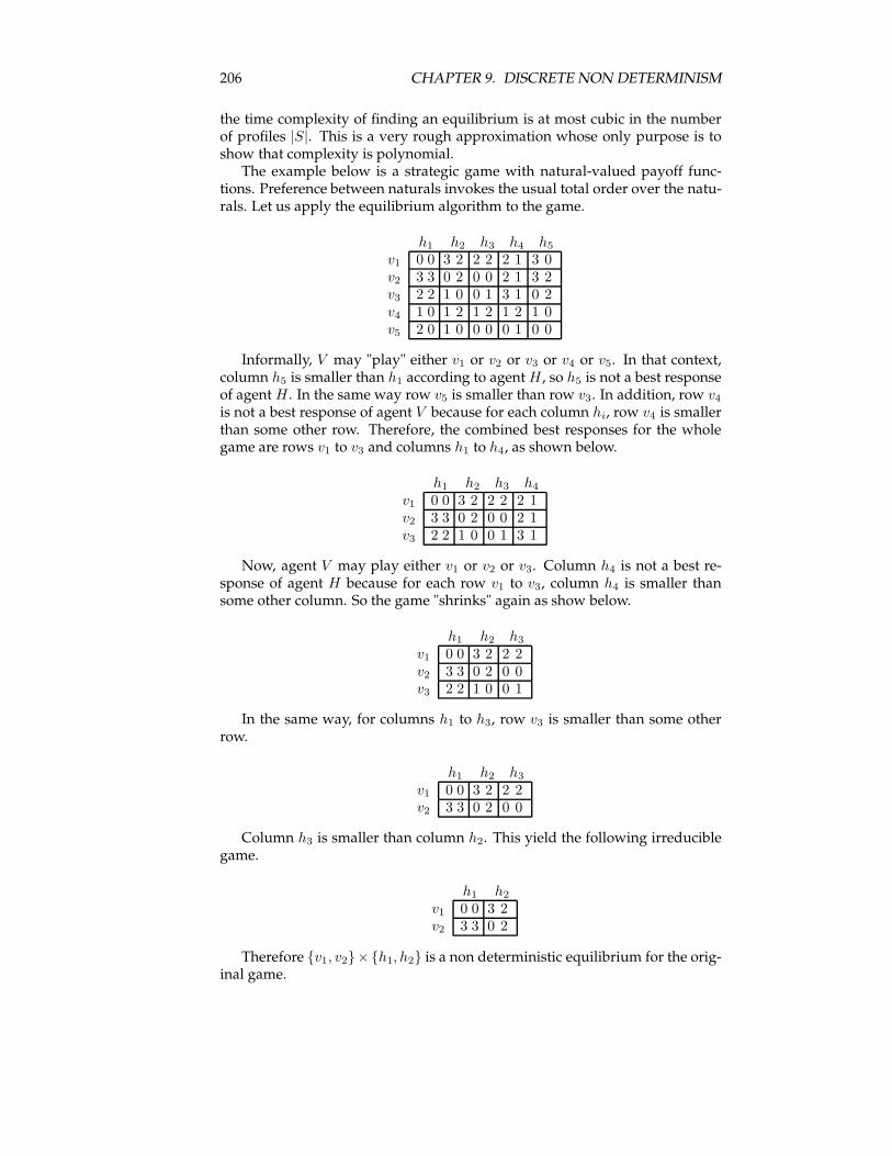
206 CHAPTER 9. DISCRETE NON DETERMINISM
the time complexity of finding an equilibrium is at most cubic in the numberof profiles |S|. This is a very rough approximation whose only purpose is toshow that complexity is polynomial.The example below is a strategic game with natural-valued payoff func-
tions. Preference between naturals invokes the usual total order over the natu-rals. Let us apply the equilibrium algorithm to the game.
h1 h2 h3 h4 h5
v1 0 0 3 2 2 2 2 1 3 0v2 3 3 0 2 0 0 2 1 3 2v3 2 2 1 0 0 1 3 1 0 2v4 1 0 1 2 1 2 1 2 1 0v5 2 0 1 0 0 0 0 1 0 0
Informally, V may "play" either v1 or v2 or v3 or v4 or v5. In that context,column h5 is smaller than h1 according to agentH , so h5 is not a best responseof agent H . In the same way row v5 is smaller than row v3. In addition, row v4
is not a best response of agent V because for each column hi, row v4 is smallerthan some other row. Therefore, the combined best responses for the wholegame are rows v1 to v3 and columns h1 to h4, as shown below.
h1 h2 h3 h4
v1 0 0 3 2 2 2 2 1v2 3 3 0 2 0 0 2 1v3 2 2 1 0 0 1 3 1
Now, agent V may play either v1 or v2 or v3. Column h4 is not a best re-sponse of agent H because for each row v1 to v3, column h4 is smaller thansome other column. So the game "shrinks" again as show below.
h1 h2 h3
v1 0 0 3 2 2 2v2 3 3 0 2 0 0v3 2 2 1 0 0 1
In the same way, for columns h1 to h3, row v3 is smaller than some otherrow.
h1 h2 h3
v1 0 0 3 2 2 2v2 3 3 0 2 0 0
Column h3 is smaller than column h2. This yield the following irreduciblegame.
h1 h2
v1 0 0 3 2v2 3 3 0 2
Therefore {v1, v2}×{h1, h2} is a non deterministic equilibrium for the orig-inal game.
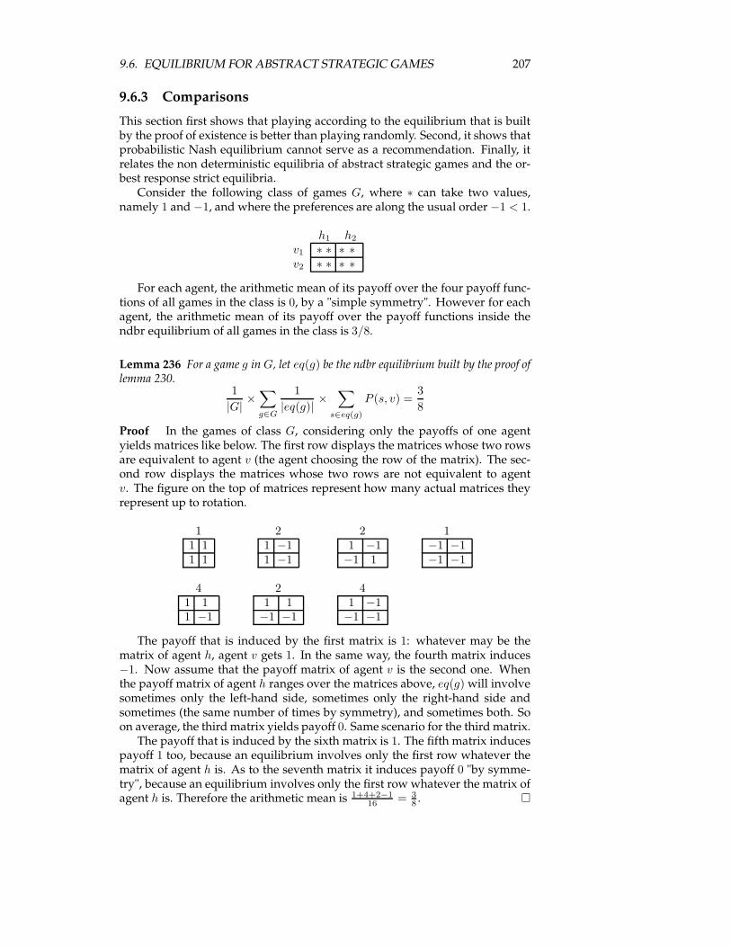
9.6. EQUILIBRIUM FOR ABSTRACT STRATEGIC GAMES 207
9.6.3 Comparisons
This section first shows that playing according to the equilibrium that is builtby the proof of existence is better than playing randomly. Second, it shows thatprobabilistic Nash equilibrium cannot serve as a recommendation. Finally, itrelates the non deterministic equilibria of abstract strategic games and the or-best response strict equilibria.Consider the following class of games G, where ∗ can take two values,
namely 1 and −1, and where the preferences are along the usual order −1 < 1.
h1 h2
v1 ∗ ∗ ∗ ∗v2 ∗ ∗ ∗ ∗
For each agent, the arithmetic mean of its payoff over the four payoff func-tions of all games in the class is 0, by a "simple symmetry". However for eachagent, the arithmetic mean of its payoff over the payoff functions inside thendbr equilibrium of all games in the class is 3/8.
Lemma 236 For a game g inG, let eq(g) be the ndbr equilibrium built by the proof oflemma 230.
1
|G|×
∑
g∈G
1
|eq(g)|×
∑
s∈eq(g)
P (s, v) =3
8
Proof In the games of class G, considering only the payoffs of one agentyields matrices like below. The first row displays the matrices whose two rowsare equivalent to agent v (the agent choosing the row of the matrix). The sec-ond row displays the matrices whose two rows are not equivalent to agentv. The figure on the top of matrices represent how many actual matrices theyrepresent up to rotation.
1 2 2 11 11 1
1 −11 −1
1 −1−1 1
−1 −1−1 −1
4 2 41 11 −1
1 1−1 −1
1 −1−1 −1
The payoff that is induced by the first matrix is 1: whatever may be thematrix of agent h, agent v gets 1. In the same way, the fourth matrix induces−1. Now assume that the payoff matrix of agent v is the second one. Whenthe payoff matrix of agent h ranges over the matrices above, eq(g)will involvesometimes only the left-hand side, sometimes only the right-hand side andsometimes (the same number of times by symmetry), and sometimes both. Soon average, the third matrix yields payoff 0. Same scenario for the third matrix.The payoff that is induced by the sixth matrix is 1. The fifth matrix induces
payoff 1 too, because an equilibrium involves only the first row whatever thematrix of agent h is. As to the seventh matrix it induces payoff 0 "by symme-try", because an equilibrium involves only the first row whatever the matrix ofagent h is. Therefore the arithmetic mean is 1+4+2−1
16 = 38 . �
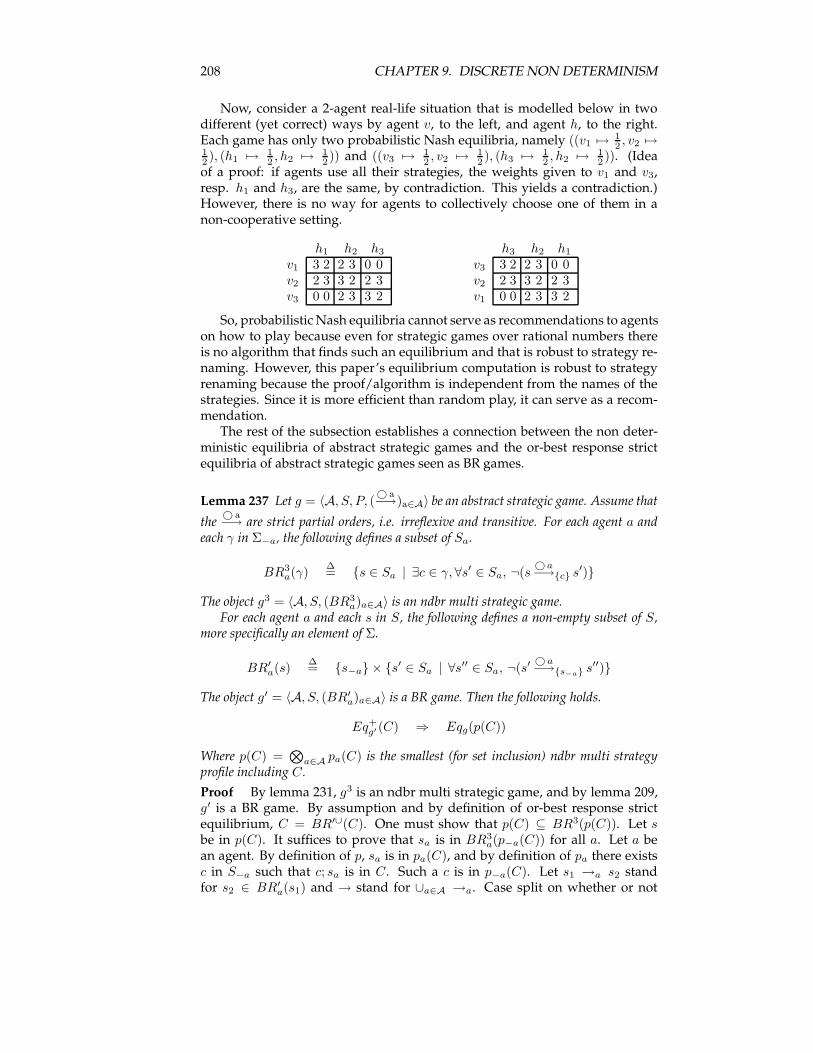
208 CHAPTER 9. DISCRETE NON DETERMINISM
Now, consider a 2-agent real-life situation that is modelled below in twodifferent (yet correct) ways by agent v, to the left, and agent h, to the right.Each game has only two probabilistic Nash equilibria, namely ((v1 7→
12 , v2 7→
12 ), (h1 7→
12 , h2 7→
12 )) and ((v3 7→
12 , v2 7→
12 ), (h3 7→
12 , h2 7→
12 )). (Idea
of a proof: if agents use all their strategies, the weights given to v1 and v3,resp. h1 and h3, are the same, by contradiction. This yields a contradiction.)However, there is no way for agents to collectively choose one of them in anon-cooperative setting.
h1 h2 h3
v1 3 2 2 3 0 0v2 2 3 3 2 2 3v3 0 0 2 3 3 2
h3 h2 h1
v3 3 2 2 3 0 0v2 2 3 3 2 2 3v1 0 0 2 3 3 2
So, probabilistic Nash equilibria cannot serve as recommendations to agentson how to play because even for strategic games over rational numbers thereis no algorithm that finds such an equilibrium and that is robust to strategy re-naming. However, this paper’s equilibrium computation is robust to strategyrenaming because the proof/algorithm is independent from the names of thestrategies. Since it is more efficient than random play, it can serve as a recom-mendation.The rest of the subsection establishes a connection between the non deter-
ministic equilibria of abstract strategic games and the or-best response strictequilibria of abstract strategic games seen as BR games.
Lemma 237 Let g = 〈A, S, P, (© a−→)a∈A〉 be an abstract strategic game. Assume that
the© a−→ are strict partial orders, i.e. irreflexive and transitive. For each agent a and
each γ in Σ−a, the following defines a subset of Sa.
BR3a(γ)
∆= {s ∈ Sa | ∃c ∈ γ, ∀s′ ∈ Sa, ¬(s
©a−→{c} s′)}
The object g3 = 〈A, S, (BR3a)a∈A〉 is an ndbr multi strategic game.
For each agent a and each s in S, the following defines a non-empty subset of S,more specifically an element of Σ.
BR′a(s)
∆= {s−a} × {s
′ ∈ Sa | ∀s′′ ∈ Sa, ¬(s′
© a−→{s−a} s′′)}
The object g′ = 〈A, S, (BR′a)a∈A〉 is a BR game. Then the following holds.
Eq+g′ (C) ⇒ Eqg(p(C))
Where p(C) =⊗
a∈A pa(C) is the smallest (for set inclusion) ndbr multi strategyprofile including C.
Proof By lemma 231, g3 is an ndbr multi strategic game, and by lemma 209,g′ is a BR game. By assumption and by definition of or-best response strictequilibrium, C = BR′∪(C). One must show that p(C) ⊆ BR3(p(C)). Let sbe in p(C). It suffices to prove that sa is in BR3
a(p−a(C)) for all a. Let a bean agent. By definition of p, sa is in pa(C), and by definition of pa there existsc in S−a such that c; sa is in C. Such a c is in p−a(C). Let s1 →a s2 standfor s2 ∈ BR′
a(s1) and → stand for ∪a∈A →a. Case split on whether or not
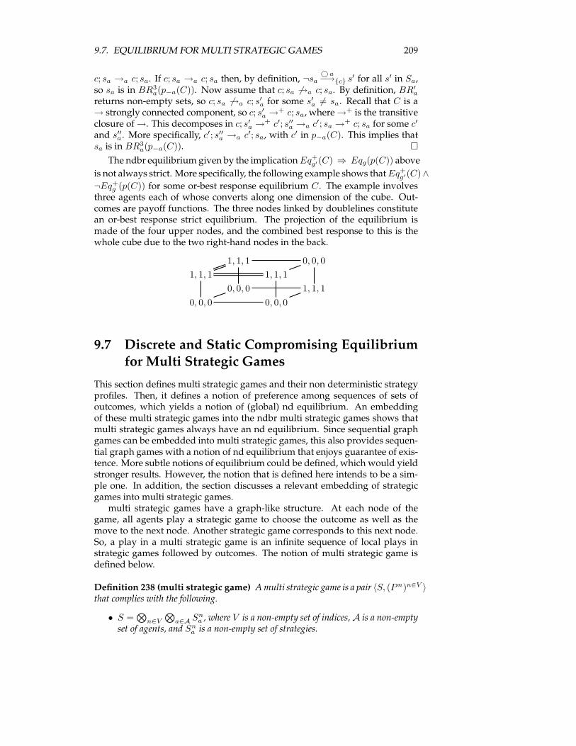
9.7. EQUILIBRIUM FOR MULTI STRATEGIC GAMES 209
c; sa →a c; sa. If c; sa →a c; sa then, by definition, ¬sa© a−→{c} s′ for all s′ in Sa,
so sa is in BR3a(p−a(C)). Now assume that c; sa 6→a c; sa. By definition, BR′
a
returns non-empty sets, so c; sa 6→a c; s′a for some s′a 6= sa. Recall that C is a→ strongly connected component, so c; s′a →
+ c; sa, where→+ is the transitiveclosure of→. This decomposes in c; s′a →
+ c′; s′′a →a c′; sa →+ c; sa for some c′
and s′′a . More specifically, c′; s′′a →a c′; sa, with c′ in p−a(C). This implies that
sa is in BR3a(p−a(C)). �
The ndbr equilibrium given by the implicationEq+g′(C) ⇒ Eqg(p(C)) above
is not always strict. More specifically, the following example shows thatEq+g′(C)∧
¬Eq+g (p(C)) for some or-best response equilibrium C. The example involves
three agents each of whose converts along one dimension of the cube. Out-comes are payoff functions. The three nodes linked by doublelines constitutean or-best response strict equilibrium. The projection of the equilibrium ismade of the four upper nodes, and the combined best response to this is thewhole cube due to the two right-hand nodes in the back.
1, 1, 1 0, 0, 0
1, 1, 1 1, 1, 1
0, 0, 0 1, 1, 1
0, 0, 0 0, 0, 0
9.7 Discrete and Static Compromising Equilibriumfor Multi Strategic Games
This section defines multi strategic games and their non deterministic strategyprofiles. Then, it defines a notion of preference among sequences of sets ofoutcomes, which yields a notion of (global) nd equilibrium. An embeddingof these multi strategic games into the ndbr multi strategic games shows thatmulti strategic games always have an nd equilibrium. Since sequential graphgames can be embedded into multi strategic games, this also provides sequen-tial graph games with a notion of nd equilibrium that enjoys guarantee of exis-tence. More subtle notions of equilibrium could be defined, which would yieldstronger results. However, the notion that is defined here intends to be a sim-ple one. In addition, the section discusses a relevant embedding of strategicgames into multi strategic games.multi strategic games have a graph-like structure. At each node of the
game, all agents play a strategic game to choose the outcome as well as themove to the next node. Another strategic game corresponds to this next node.So, a play in a multi strategic game is an infinite sequence of local plays instrategic games followed by outcomes. The notion of multi strategic game isdefined below.
Definition 238 (multi strategic game) Amulti strategic game is a pair 〈S, (Pn)n∈V 〉that complies with the following.
• S =⊗
n∈V
⊗a∈A Sn
a , where V is a non-empty set of indices,A is a non-emptyset of agents, and Sn
a is a non-empty set of strategies.
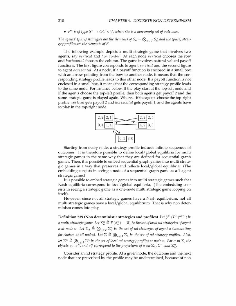
210 CHAPTER 9. DISCRETE NON DETERMINISM
• Pn is of type Sn → OC × V , where Oc is a non-empty set of outcomes.
The agents’ (pure) strategies are the elements of Sa =⊗
n∈V Sna and the (pure) strat-
egy profiles are the elements of S.
The following example depicts a multi strategic game that involves twoagents, say vertical and horizontal. At each node vertical chooses the rowand horizontal chooses the column. The game involves natural-valued payofffunctions. The first figure corresponds to agent vertical and the second figureto agent horizontal. At a node, if a payoff function is enclosed in a small boxwith an arrow pointing from the bow to another node, it means that the cor-responding strategy profile leads to this other node. If a payoff function is notenclosed in a small box, it means that the corresponding strategy profile leadsto the same node. For instance below, If the play start at the top-left node andif the agents choose the top-left profile, then both agents get payoff 2 and thesame strategic game is played again. Whereas if the agents choose the top-rightprofile, vertical gets payoff 2 and horizontal gets payoff 1, and the agents haveto play in the top-right node.
2, 2 2, 1
0, 4 1, 4
2, 2 2, 4
4, 2 3, 3
0, 1 3, 0
Starting from every node, a strategy profile induces infinite sequences ofoutcomes. It is therefore possible to define local/global equilibria for multistrategic games in the same way that they are defined for sequential graphgames. Then, it is possible to embed sequential graph games into multi strate-gic games in a way that preserves and reflects local/global equilibria. (Theembedding consists in seeing a node of a sequential graph game as a 1-agentstrategic game.)It is possible to embed strategic games into multi strategic games such that
Nash equilibria correspond to local/global equilibria. (The embedding con-sists in seeing a strategic game as a one-node multi strategic game looping onitself).However, since not all strategic games have a Nash equilibrium, not all
multi strategic games have a local/global equilibrium. That is why non deter-minism comes into play.
Definition 239 (Non deterministic strategies and profiles) Let 〈S, (Pn)n∈V 〉 be
a multi strategic game. Let Σna
∆= P(Sn
a )−{∅} be the set of local nd strategies of agent
a at node n. Let Σa∆=
⊗n∈V Σn
a be the set of nd strategies of agent a (accounting
for choices at all nodes). Let Σ∆=
⊗a∈A Σa be the set of nd strategy profiles. Also,
let Σn ∆=
⊗a∈A Σn
a be the set of local nd strategy profiles at node n. For σ in Σ, theobjects σa, σ
n, and σna correspond to the projections of σ on Σa, Σ
n, and Σna .
Consider an nd strategy profile. At a given node, the outcome and the nextnode that are prescribed by the profile may be undetermined, because of non
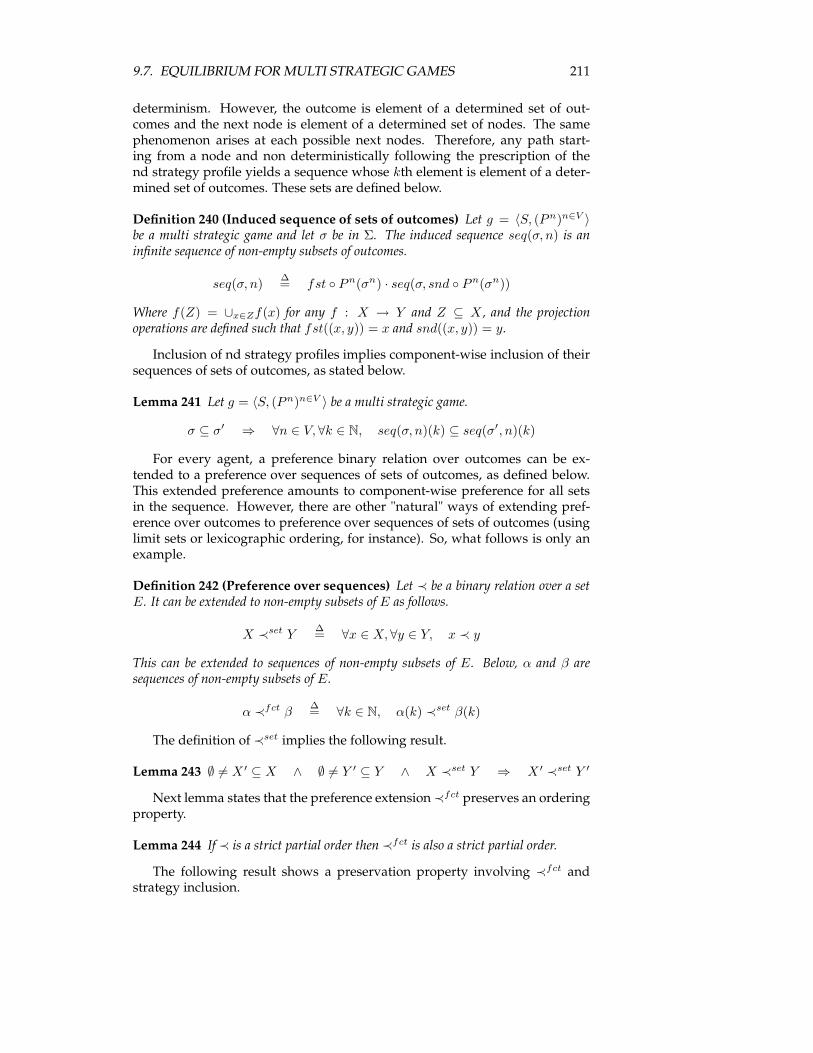
9.7. EQUILIBRIUM FOR MULTI STRATEGIC GAMES 211
determinism. However, the outcome is element of a determined set of out-comes and the next node is element of a determined set of nodes. The samephenomenon arises at each possible next nodes. Therefore, any path start-ing from a node and non deterministically following the prescription of thend strategy profile yields a sequence whose kth element is element of a deter-mined set of outcomes. These sets are defined below.
Definition 240 (Induced sequence of sets of outcomes) Let g = 〈S, (Pn)n∈V 〉be a multi strategic game and let σ be in Σ. The induced sequence seq(σ, n) is aninfinite sequence of non-empty subsets of outcomes.
seq(σ, n)∆= fst ◦ Pn(σn) · seq(σ, snd ◦ Pn(σn))
Where f(Z) = ∪x∈Zf(x) for any f : X → Y and Z ⊆ X , and the projectionoperations are defined such that fst((x, y)) = x and snd((x, y)) = y.
Inclusion of nd strategy profiles implies component-wise inclusion of theirsequences of sets of outcomes, as stated below.
Lemma 241 Let g = 〈S, (Pn)n∈V 〉 be a multi strategic game.
σ ⊆ σ′ ⇒ ∀n ∈ V, ∀k ∈ N, seq(σ, n)(k) ⊆ seq(σ′, n)(k)
For every agent, a preference binary relation over outcomes can be ex-tended to a preference over sequences of sets of outcomes, as defined below.This extended preference amounts to component-wise preference for all setsin the sequence. However, there are other "natural" ways of extending pref-erence over outcomes to preference over sequences of sets of outcomes (usinglimit sets or lexicographic ordering, for instance). So, what follows is only anexample.
Definition 242 (Preference over sequences) Let ≺ be a binary relation over a setE. It can be extended to non-empty subsets of E as follows.
X ≺set Y∆= ∀x ∈ X, ∀y ∈ Y, x ≺ y
This can be extended to sequences of non-empty subsets of E. Below, α and β aresequences of non-empty subsets of E.
α ≺fct β∆= ∀k ∈ N, α(k) ≺set β(k)
The definition of ≺set implies the following result.
Lemma 243 ∅ 6= X ′ ⊆ X ∧ ∅ 6= Y ′ ⊆ Y ∧ X ≺set Y ⇒ X ′ ≺set Y ′
Next lemma states that the preference extension≺fct preserves an orderingproperty.
Lemma 244 If ≺ is a strict partial order then ≺fct is also a strict partial order.
The following result shows a preservation property involving ≺fct andstrategy inclusion.
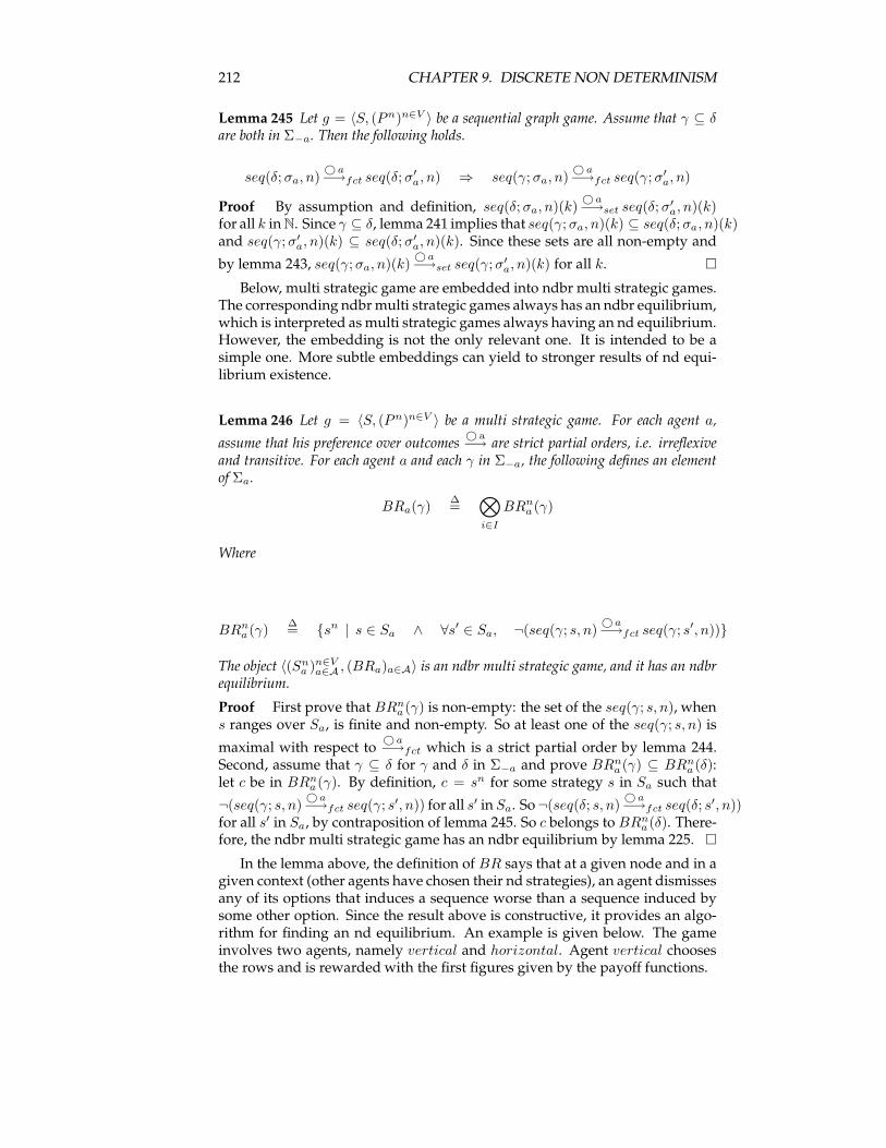
212 CHAPTER 9. DISCRETE NON DETERMINISM
Lemma 245 Let g = 〈S, (Pn)n∈V 〉 be a sequential graph game. Assume that γ ⊆ δare both in Σ−a. Then the following holds.
seq(δ; σa, n)© a−→fct seq(δ; σ′
a, n) ⇒ seq(γ; σa, n)© a−→fct seq(γ; σ′
a, n)
Proof By assumption and definition, seq(δ; σa, n)(k)©a−→set seq(δ; σ′
a, n)(k)for all k inN. Since γ ⊆ δ, lemma 241 implies that seq(γ; σa, n)(k) ⊆ seq(δ; σa, n)(k)and seq(γ; σ′
a, n)(k) ⊆ seq(δ; σ′a, n)(k). Since these sets are all non-empty and
by lemma 243, seq(γ; σa, n)(k)©a−→set seq(γ; σ′
a, n)(k) for all k. �
Below, multi strategic game are embedded into ndbr multi strategic games.The corresponding ndbrmulti strategic games always has an ndbr equilibrium,which is interpreted asmulti strategic games always having an nd equilibrium.However, the embedding is not the only relevant one. It is intended to be asimple one. More subtle embeddings can yield to stronger results of nd equi-librium existence.
Lemma 246 Let g = 〈S, (Pn)n∈V 〉 be a multi strategic game. For each agent a,
assume that his preference over outcomes© a−→ are strict partial orders, i.e. irreflexive
and transitive. For each agent a and each γ in Σ−a, the following defines an elementof Σa.
BRa(γ)∆=
⊗
i∈I
BRna (γ)
Where
BRna (γ)
∆= {sn | s ∈ Sa ∧ ∀s′ ∈ Sa, ¬(seq(γ; s, n)
©a−→fct seq(γ; s′, n))}
The object 〈(Sna )n∈V
a∈A , (BRa)a∈A〉 is an ndbr multi strategic game, and it has an ndbrequilibrium.
Proof First prove that BRna (γ) is non-empty: the set of the seq(γ; s, n), when
s ranges over Sa, is finite and non-empty. So at least one of the seq(γ; s, n) is
maximal with respect to©a−→fct which is a strict partial order by lemma 244.
Second, assume that γ ⊆ δ for γ and δ in Σ−a and prove BRna (γ) ⊆ BRn
a (δ):let c be in BRn
a (γ). By definition, c = sn for some strategy s in Sa such that
¬(seq(γ; s, n)©a−→fct seq(γ; s′, n)) for all s′ in Sa. So¬(seq(δ; s, n)
© a−→fct seq(δ; s′, n))
for all s′ in Sa, by contraposition of lemma 245. So c belongs to BRna (δ). There-
fore, the ndbr multi strategic game has an ndbr equilibrium by lemma 225. �
In the lemma above, the definition of BR says that at a given node and in agiven context (other agents have chosen their nd strategies), an agent dismissesany of its options that induces a sequence worse than a sequence induced bysome other option. Since the result above is constructive, it provides an algo-rithm for finding an nd equilibrium. An example is given below. The gameinvolves two agents, namely vertical and horizontal. Agent vertical choosesthe rows and is rewarded with the first figures given by the payoff functions.
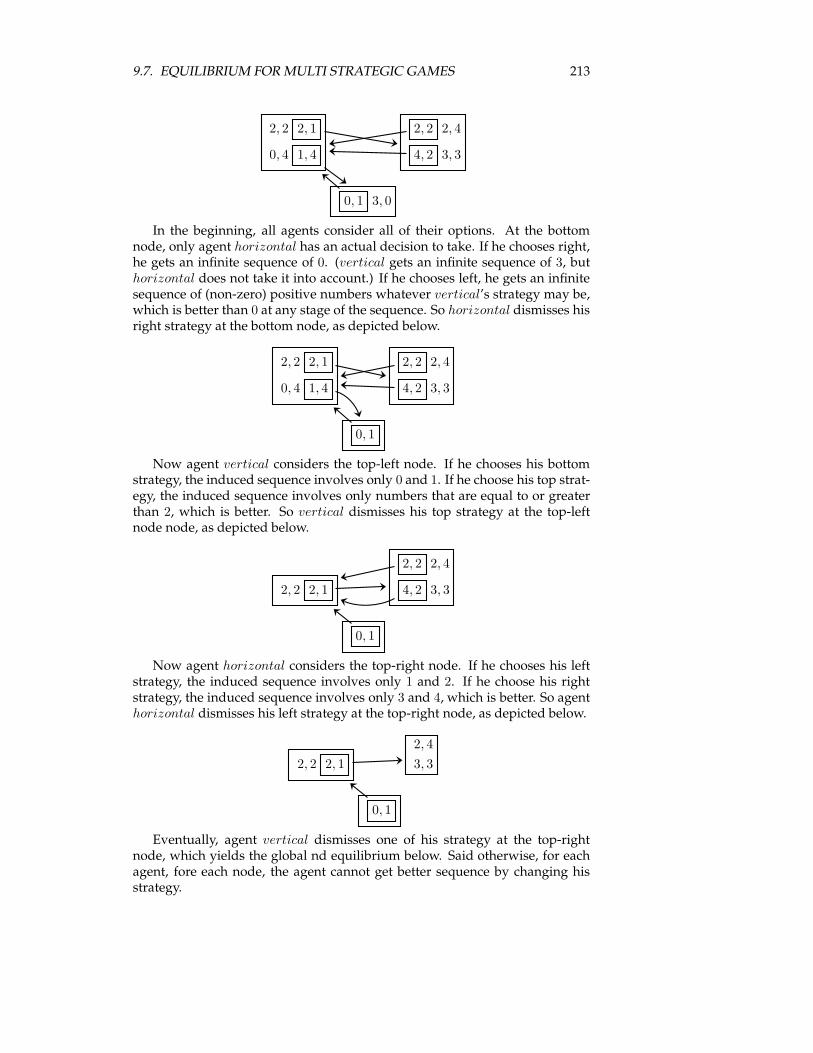
9.7. EQUILIBRIUM FOR MULTI STRATEGIC GAMES 213
2, 2 2, 1
0, 4 1, 4
2, 2 2, 4
4, 2 3, 3
0, 1 3, 0
In the beginning, all agents consider all of their options. At the bottomnode, only agent horizontal has an actual decision to take. If he chooses right,he gets an infinite sequence of 0. (vertical gets an infinite sequence of 3, buthorizontal does not take it into account.) If he chooses left, he gets an infinitesequence of (non-zero) positive numbers whatever vertical’s strategy may be,which is better than 0 at any stage of the sequence. So horizontal dismisses hisright strategy at the bottom node, as depicted below.
2, 2 2, 1
0, 4 1, 4
2, 2 2, 4
4, 2 3, 3
0, 1
Now agent vertical considers the top-left node. If he chooses his bottomstrategy, the induced sequence involves only 0 and 1. If he choose his top strat-egy, the induced sequence involves only numbers that are equal to or greaterthan 2, which is better. So vertical dismisses his top strategy at the top-leftnode node, as depicted below.
2, 2 2, 1
2, 2 2, 4
4, 2 3, 3
0, 1
Now agent horizontal considers the top-right node. If he chooses his leftstrategy, the induced sequence involves only 1 and 2. If he choose his rightstrategy, the induced sequence involves only 3 and 4, which is better. So agenthorizontal dismisses his left strategy at the top-right node, as depicted below.
2, 2 2, 1
2, 4
3, 3
0, 1
Eventually, agent vertical dismisses one of his strategy at the top-rightnode, which yields the global nd equilibrium below. Said otherwise, for eachagent, fore each node, the agent cannot get better sequence by changing hisstrategy.
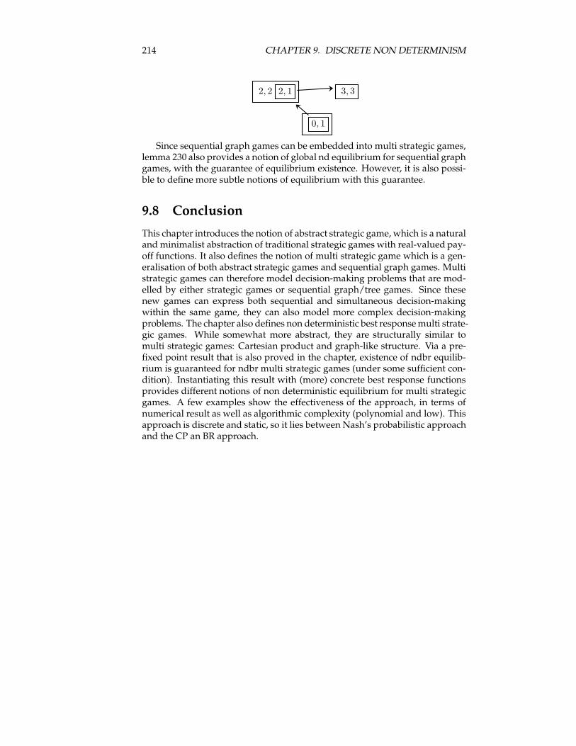
214 CHAPTER 9. DISCRETE NON DETERMINISM
2, 2 2, 1 3, 3
0, 1
Since sequential graph games can be embedded into multi strategic games,lemma 230 also provides a notion of global nd equilibrium for sequential graphgames, with the guarantee of equilibrium existence. However, it is also possi-ble to define more subtle notions of equilibrium with this guarantee.
9.8 Conclusion
This chapter introduces the notion of abstract strategic game, which is a naturaland minimalist abstraction of traditional strategic games with real-valued pay-off functions. It also defines the notion of multi strategic game which is a gen-eralisation of both abstract strategic games and sequential graph games. Multistrategic games can therefore model decision-making problems that are mod-elled by either strategic games or sequential graph/tree games. Since thesenew games can express both sequential and simultaneous decision-makingwithin the same game, they can also model more complex decision-makingproblems. The chapter also defines non deterministic best responsemulti strate-gic games. While somewhat more abstract, they are structurally similar tomulti strategic games: Cartesian product and graph-like structure. Via a pre-fixed point result that is also proved in the chapter, existence of ndbr equilib-rium is guaranteed for ndbr multi strategic games (under some sufficient con-dition). Instantiating this result with (more) concrete best response functionsprovides different notions of non deterministic equilibrium for multi strategicgames. A few examples show the effectiveness of the approach, in terms ofnumerical result as well as algorithmic complexity (polynomial and low). Thisapproach is discrete and static, so it lies between Nash’s probabilistic approachand the CP an BR approach.
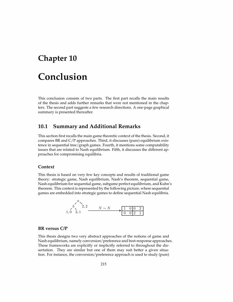
Chapter 10
Conclusion
This conclusion consists of two parts. The first part recalls the main resultsof the thesis and adds further remarks that were not mentioned in the chap-ters. The second part suggests a few research directions. A one-page graphicalsummary is presented thereafter.
10.1 Summary and Additional Remarks
This section first recalls the main game theoretic context of the thesis. Second, itcompares BR and C/P approaches. Third, it discusses (pure) equilibrium exis-tence in sequential tree/graph games. Fourth, it mentions some computabilityissues that are related to Nash equilibrium. Fifth, it discusses the different ap-proaches for compromising equilibria.
Context
This thesis is based on very few key concepts and results of traditional gametheory: strategic game, Nash equilibrium, Nash’s theorem, sequential game,Nash equilibrium for sequential game, subgame perfect equilibrium, andKuhn’stheorem. This context is represented by the following picture, where sequentialgames are embedded into strategic games to define sequential Nash equilibria.
a
b 2, 2
1, 0 3, 11 0 0 20 0 2 1
N ∼ N
BR versus C/P
This thesis designs two very abstract approaches of the notions of game andNash equilibrium, namely conversion/preference and best-response approaches.These frameworks are explicitly or implicitly referred to throughout the dis-sertation. They are similar but one of them may suit better a given situa-tion. For instance, the conversion/preference approach is used to study (pure)
215
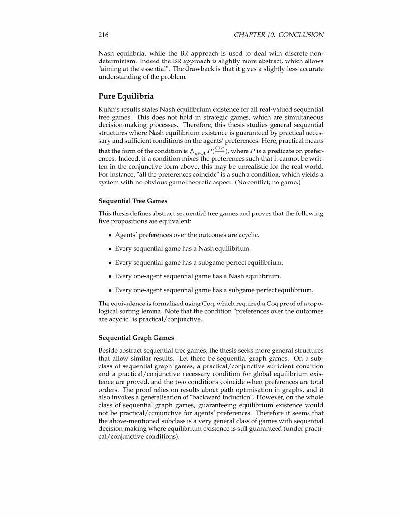
216 CHAPTER 10. CONCLUSION
Nash equilibria, while the BR approach is used to deal with discrete non-determinism. Indeed the BR approach is slightly more abstract, which allows"aiming at the essential". The drawback is that it gives a slightly less accurateunderstanding of the problem.
Pure Equilibria
Kuhn’s results states Nash equilibrium existence for all real-valued sequentialtree games. This does not hold in strategic games, which are simultaneousdecision-making processes. Therefore, this thesis studies general sequentialstructures where Nash equilibrium existence is guaranteed by practical neces-sary and sufficient conditions on the agents’ preferences. Here, practical means
that the form of the condition is∧
a∈A P (© a−→), where P is a predicate on prefer-
ences. Indeed, if a condition mixes the preferences such that it cannot be writ-ten in the conjunctive form above, this may be unrealistic for the real world.For instance, "all the preferences coincide" is a such a condition, which yields asystem with no obvious game theoretic aspect. (No conflict; no game.)
Sequential Tree Games
This thesis defines abstract sequential tree games and proves that the followingfive propositions are equivalent:
• Agents’ preferences over the outcomes are acyclic.
• Every sequential game has a Nash equilibrium.
• Every sequential game has a subgame perfect equilibrium.
• Every one-agent sequential game has a Nash equilibrium.
• Every one-agent sequential game has a subgame perfect equilibrium.
The equivalence is formalised using Coq, which required a Coq proof of a topo-logical sorting lemma. Note that the condition "preferences over the outcomesare acyclic" is practical/conjunctive.
Sequential Graph Games
Beside abstract sequential tree games, the thesis seeks more general structuresthat allow similar results. Let there be sequential graph games. On a sub-class of sequential graph games, a practical/conjunctive sufficient conditionand a practical/conjunctive necessary condition for global equilibrium exis-tence are proved, and the two conditions coincide when preferences are totalorders. The proof relies on results about path optimisation in graphs, and italso invokes a generalisation of "backward induction". However, on the wholeclass of sequential graph games, guaranteeing equilibrium existence wouldnot be practical/conjunctive for agents’ preferences. Therefore it seems thatthe above-mentioned subclass is a very general class of games with sequentialdecision-making where equilibrium existence is still guaranteed (under practi-cal/conjunctive conditions).
10.1. SUMMARY AND ADDITIONAL REMARKS 217
Computability of Probabilistic Nash Equilibria
Consider the following class of 1-agent, 2-strategy games g(x) with x in R. Ifthe agent chooses strategy h1, he gets payoff 0, and if he chooses strategy h2,he gets payoff x.
h1 h2
0 x
If Nash equilibria were computable in general, they would be computablefor the above-mentioned subclass of games; said otherwise, there would exista computable function f from R to R such that (h1 7→ f(x), h2 7→ 1 − f(x))is a Nash equilibrium for g(x) for all x. However, a computable function iscontinuous, as explained in Weihrauch’s book [55]. Moreover, if x is negativethen the only Nash equilibrium is (h1 7→ 1, h2 7→ 0), whereas if x is positivethen the only Nash equilibrium is (h1 7→ 0, h2 7→ 1), which shows that such anf is discontinuous, hence a contradiction.Nevertheless, the following sketches the proof of non-uniform existence
of a computable Nash equilibrium. By the Tarski-Seidenberg principle (men-tioned e.g. in [5]), every non-empty semi-algebraic set on a real closed fieldhas an element whose components are all in the real closed field. The set ofNash equilibria of a given strategic game is semi-algebraic. The computablereals form a real closed field. Therefore, every strategic game with computablepayoffs has a computable Nash equilibrium. Note that the above-mentionedcontinuity argument says that these computable Nash equilibria are not uni-formly computable. Said otherwise, for each such strategic game, there ex-ists a program that "converges" towards a Nash equilibrium, but there existsno program expecting such a strategic game and converging towards a Nashequilibrium.However, if the payoff functions are restricted to rational numbers (with
decidable equality), then there are uniform computability (and complexity) re-sults in the literature about these specific Nash equilibria. Some of these re-sults [41] are due to Papadimitriou.
Compromising Equilibria
Beside specific sequential graph games (including sequential tree games), thegames defined in the thesis offer no guarantee of (pure) equilibrium existence,unless under non-practical conditions. This thesis shows that applying Nash’sprobabilistic approach for these abstract games is irrelevant. So it finds othermeans of weakening the definition of equilibrium in order to guarantee theirexistence, while following the features of Nash’s approach to some extent.
Discrete Non-Deterministic Equilibria
The notion of discrete non-deterministic strategy is introduced: instead of say-ing that "an agent chooses a strategy with some probability", one says that "theagent may choose the strategy". The notion of multi-strategic games is also in-troduced. Such a game amounts to playing an abstract strategic game at eachnode of a sequential graph game. At a given node/abstract strategic game,the next move is no longer chosen by a single agent. Instead, the short-term
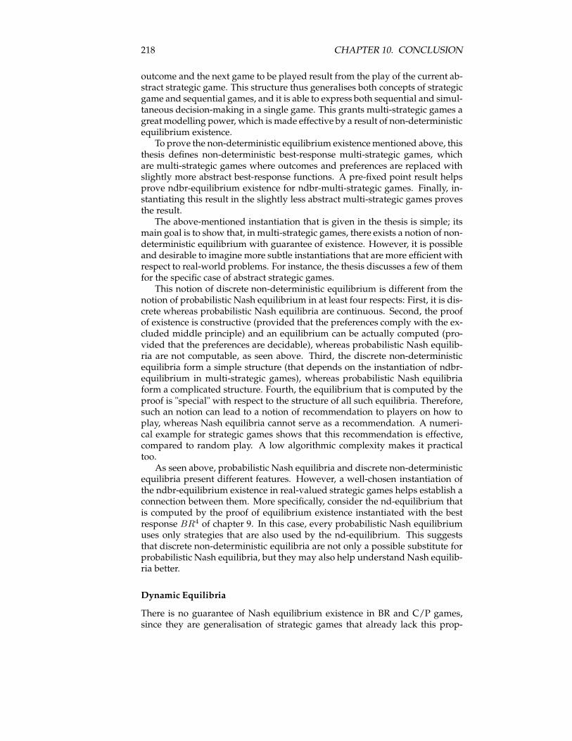
218 CHAPTER 10. CONCLUSION
outcome and the next game to be played result from the play of the current ab-stract strategic game. This structure thus generalises both concepts of strategicgame and sequential games, and it is able to express both sequential and simul-taneous decision-making in a single game. This grants multi-strategic games agreatmodelling power, which is made effective by a result of non-deterministicequilibrium existence.To prove the non-deterministic equilibrium existencementioned above, this
thesis defines non-deterministic best-response multi-strategic games, whichare multi-strategic games where outcomes and preferences are replaced withslightly more abstract best-response functions. A pre-fixed point result helpsprove ndbr-equilibrium existence for ndbr-multi-strategic games. Finally, in-stantiating this result in the slightly less abstract multi-strategic games provesthe result.The above-mentioned instantiation that is given in the thesis is simple; its
main goal is to show that, in multi-strategic games, there exists a notion of non-deterministic equilibrium with guarantee of existence. However, it is possibleand desirable to imagine more subtle instantiations that are more efficient withrespect to real-world problems. For instance, the thesis discusses a few of themfor the specific case of abstract strategic games.This notion of discrete non-deterministic equilibrium is different from the
notion of probabilistic Nash equilibrium in at least four respects: First, it is dis-crete whereas probabilistic Nash equilibria are continuous. Second, the proofof existence is constructive (provided that the preferences comply with the ex-cluded middle principle) and an equilibrium can be actually computed (pro-vided that the preferences are decidable), whereas probabilistic Nash equilib-ria are not computable, as seen above. Third, the discrete non-deterministicequilibria form a simple structure (that depends on the instantiation of ndbr-equilibrium in multi-strategic games), whereas probabilistic Nash equilibriaform a complicated structure. Fourth, the equilibrium that is computed by theproof is "special" with respect to the structure of all such equilibria. Therefore,such an notion can lead to a notion of recommendation to players on how toplay, whereas Nash equilibria cannot serve as a recommendation. A numeri-cal example for strategic games shows that this recommendation is effective,compared to random play. A low algorithmic complexity makes it practicaltoo.As seen above, probabilistic Nash equilibria and discrete non-deterministic
equilibria present different features. However, a well-chosen instantiation ofthe ndbr-equilibrium existence in real-valued strategic games helps establish aconnection between them. More specifically, consider the nd-equilibrium thatis computed by the proof of equilibrium existence instantiated with the bestresponse BR4 of chapter 9. In this case, every probabilistic Nash equilibriumuses only strategies that are also used by the nd-equilibrium. This suggeststhat discrete non-deterministic equilibria are not only a possible substitute forprobabilistic Nash equilibria, but they may also help understand Nash equilib-ria better.
Dynamic Equilibria
There is no guarantee of Nash equilibrium existence in BR and C/P games,since they are generalisation of strategic games that already lack this prop-
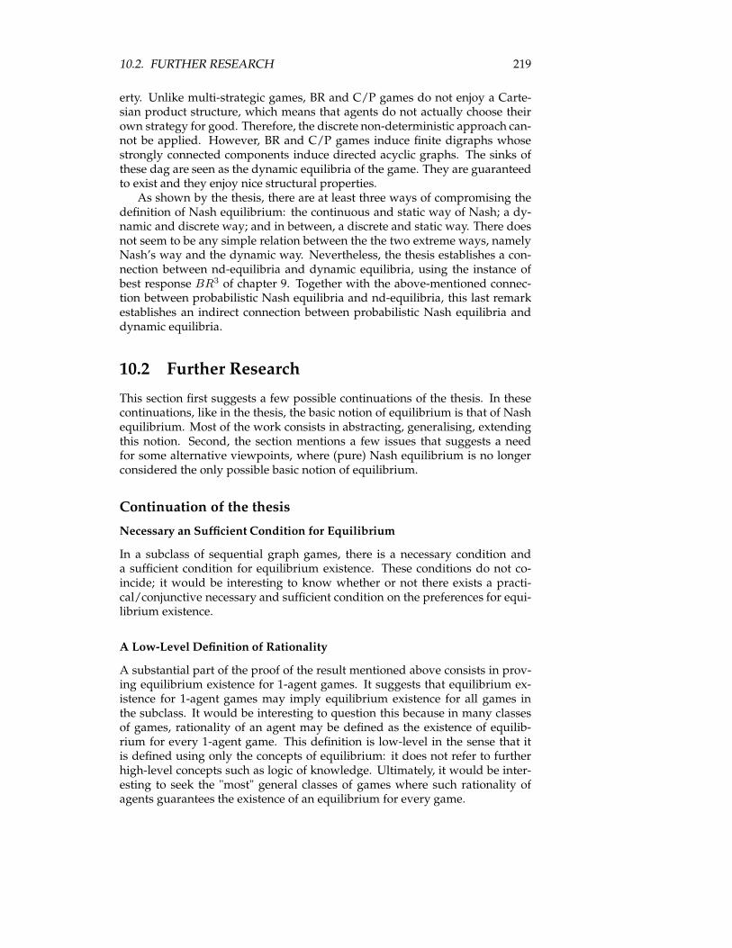
10.2. FURTHER RESEARCH 219
erty. Unlike multi-strategic games, BR and C/P games do not enjoy a Carte-sian product structure, which means that agents do not actually choose theirown strategy for good. Therefore, the discrete non-deterministic approach can-not be applied. However, BR and C/P games induce finite digraphs whosestrongly connected components induce directed acyclic graphs. The sinks ofthese dag are seen as the dynamic equilibria of the game. They are guaranteedto exist and they enjoy nice structural properties.As shown by the thesis, there are at least three ways of compromising the
definition of Nash equilibrium: the continuous and static way of Nash; a dy-namic and discrete way; and in between, a discrete and static way. There doesnot seem to be any simple relation between the the two extreme ways, namelyNash’s way and the dynamic way. Nevertheless, the thesis establishes a con-nection between nd-equilibria and dynamic equilibria, using the instance ofbest response BR3 of chapter 9. Together with the above-mentioned connec-tion between probabilistic Nash equilibria and nd-equilibria, this last remarkestablishes an indirect connection between probabilistic Nash equilibria anddynamic equilibria.
10.2 Further Research
This section first suggests a few possible continuations of the thesis. In thesecontinuations, like in the thesis, the basic notion of equilibrium is that of Nashequilibrium. Most of the work consists in abstracting, generalising, extendingthis notion. Second, the section mentions a few issues that suggests a needfor some alternative viewpoints, where (pure) Nash equilibrium is no longerconsidered the only possible basic notion of equilibrium.
Continuation of the thesis
Necessary an Sufficient Condition for Equilibrium
In a subclass of sequential graph games, there is a necessary condition anda sufficient condition for equilibrium existence. These conditions do not co-incide; it would be interesting to know whether or not there exists a practi-cal/conjunctive necessary and sufficient condition on the preferences for equi-librium existence.
A Low-Level Definition of Rationality
A substantial part of the proof of the result mentioned above consists in prov-ing equilibrium existence for 1-agent games. It suggests that equilibrium ex-istence for 1-agent games may imply equilibrium existence for all games inthe subclass. It would be interesting to question this because in many classesof games, rationality of an agent may be defined as the existence of equilib-rium for every 1-agent game. This definition is low-level in the sense that itis defined using only the concepts of equilibrium: it does not refer to furtherhigh-level concepts such as logic of knowledge. Ultimately, it would be inter-esting to seek the "most" general classes of games where such rationality ofagents guarantees the existence of an equilibrium for every game.
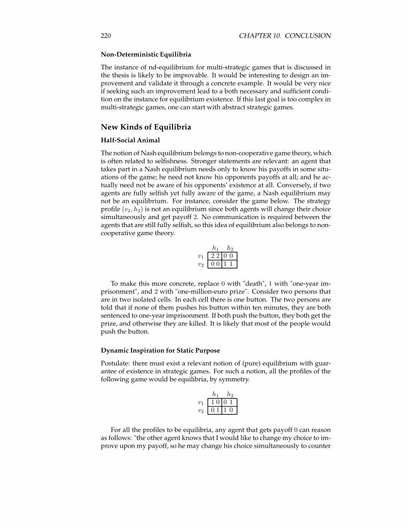
220 CHAPTER 10. CONCLUSION
Non-Deterministic Equilibria
The instance of nd-equilibrium for multi-strategic games that is discussed inthe thesis is likely to be improvable. It would be interesting to design an im-provement and validate it through a concrete example. It would be very niceif seeking such an improvement lead to a both necessary and sufficient condi-tion on the instance for equilibrium existence. If this last goal is too complex inmulti-strategic games, one can start with abstract strategic games.
New Kinds of Equilibria
Half-Social Animal
The notion of Nash equilibrium belongs to non-cooperative game theory, whichis often related to selfishness. Stronger statements are relevant: an agent thattakes part in a Nash equilibrium needs only to know his payoffs in some situ-ations of the game; he need not know his opponents payoffs at all; and he ac-tually need not be aware of his opponents’ existence at all. Conversely, if twoagents are fully selfish yet fully aware of the game, a Nash equilibrium maynot be an equilibrium. For instance, consider the game below. The strategyprofile (v2, h2) is not an equilibrium since both agents will change their choicesimultaneously and get payoff 2. No communication is required between theagents that are still fully selfish, so this idea of equilibrium also belongs to non-cooperative game theory.
h1 h2
v1 2 2 0 0v2 0 0 1 1
To make this more concrete, replace 0 with "death", 1 with "one-year im-prisonment", and 2 with "one-million-euro prize". Consider two persons thatare in two isolated cells. In each cell there is one button. The two persons aretold that if none of them pushes his button within ten minutes, they are bothsentenced to one-year imprisonment. If both push the button, they both get theprize, and otherwise they are killed. It is likely that most of the people wouldpush the button.
Dynamic Inspiration for Static Purpose
Postulate: there must exist a relevant notion of (pure) equilibrium with guar-antee of existence in strategic games. For such a notion, all the profiles of thefollowing game would be equilibria, by symmetry.
h1 h2
v1 1 0 0 1v2 0 1 1 0
For all the profiles to be equilibria, any agent that gets payoff 0 can reasonas follows: "the other agent knows that I would like to change my choice to im-prove upon my payoff, so he may change his choice simultaneously to counter
10.2. FURTHER RESEARCH 221
me". Continuing this reasoning may produce concepts that are very closed tothe notions of dynamic compromising equilibria that are discussed in this the-sis. So, the dynamic approach for "short-sighted" agents may be useful to astatic approach with agents that are aware of their opponents.
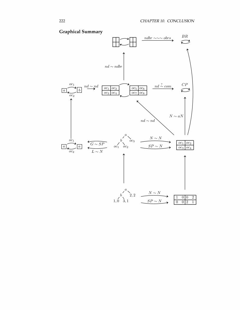
222 CHAPTER 10. CONCLUSION
Graphical SummaryBR
a b
oc1
oc2
oc1 oc2
oc3 oc4
oc5 oc6
oc7 oc8
CP
a a
oc1
oc2
a
b oc3
oc1 oc2
oc1 oc2
oc3 oc4
a
b 2, 2
1, 0 3, 11 0 0 20 0 2 1
nd ∼ ndbr
ndbr ∼∼∼ obrs
nd?∼ comnd ∼ nd
N ∼ aNnd ∼ nd
L ∼ N
G ∼ SP
N ∼ N
SP ∼ N
N ∼ N
SP ∼ N
Bibliography
[1] The Coq proof assistant, version 8.1, http://coq.inria.fr/.
[2] Fabio Acerbi. Plato: Parmenides 149a7-c3. a proof by complete induction?Archive for History of Exact Sciences, 55(1):57–76, 2000.
[3] Anonymous. Program evaluation research task. Summary report Phase 1and 2, U.S. Government Printing Office, Washington, D.C., 1958.
[4] Aristotle. Organon, Prior Analytics, 350 BC.
[5] Saugata Basu, Richard Pollack, and Marie-Francoise Roy. Algorithms inReal Algebraic Geometry. Springer, 2003.
[6] W. J. Baumol and S. M. Goldfeld. Precursors in Mathematical Economics: AnAnthology, pages 3–9. London School of Economics and Political Science,1968. Kuhn, H. W., Preface to Waldegrave’s Comments: Excerpt fromMontmort’s Letter to Nicholas Bernoulli.
[7] Elwyn R. Berlekamp, John Horton Conway, and Richard K. Guy. WinningWays for Your Mathematical Plays. A K Peters, Ltd., 2003.
[8] B. Douglas Bernheim. Rationalizable strategic behavior. Econometrica,52:1007–1028, 1984.
[9] Yves Berthot and Pierre Castéran. Interactive Theorem Proving and Pro-gramDevelopment Coq’Art: The Calculus of Inductive Constructions. Springer,2004.
[10] David Blackwell. An analog of the minimax theorem for vector payoffs.Pacific Journal of Mathematics, 6:1–8, 1956.
[11] F. Blanqui, S. Coupet-Grimal, W. Delobel, S. Hinderer, and A. Koprowski.CoLoR, a Coq Library on rewriting and termination. In Workshop on Ter-mination, 2006. http://color.loria.fr/.
[12] Emile Borel. La théorie du jeu et les equations intégrales à noyausymétrique. Comptes Rendus Hebdomadaires des séances de l’académie des Sci-ences, 173:1304–1308, 1921.
[13] Chafika Chettaoui, Franck Delaplace, Pierre Lescanne, Mun’delanjiVestergaard, and René Vestergaard. Rewriting game theory as a founda-tion for state-based models of gene regulation. In Computational Methodsin Systems Biology, International Conference, CMSB 2006, 2006.
223
224 BIBLIOGRAPHY
[14] Augustin A. Cournot. Recherches sur les Principes Mathematiques de la The-orie des Richesses. Hachette, Paris, 1838.
[15] David Gale. A theory of n-person games games with perfect information.Proceedings of the National Academy of Sciences of the United States of America,39:496–501, 1953.
[16] Paul Gochet and Pascal Gribomont. Logique, méthode pour l’informatiquefondamentale. Hermes, 1991.
[17] Timothy G. Griffin and Joäo Luís Sobrinho. Metarouting. In SIGCOMM’05: Proceedings of the 2005 conference on Applications, technologies, architec-tures, and protocols for computer communications, pages 1–12, New York, NY,USA, 2005. ACM Press.
[18] John Hillas and Elon Kohlberg. Foundations of strategic equilibrium. InR.J. Aumann and S. Hart, editors, Handbook of Game Theory with EconomicApplications. 2002.
[19] Thomas Hobbes. Leviathan, or The Matter, Forme and Power of a CommonWealth Ecclesiasticall and Civil. Andrew Crooke, London, 1651.
[20] Aumann R. J. and M. Maschler. Game theoretic analysis of a bankruptcyproblem from the Talmud. Journal of Economic Theory, 36:195–213, 1985.
[21] A. B. Kahn. Topological sorting of large networks. Commun. ACM,5(11):558–562, 1962.
[22] Shizuo Kakutani. A generalization of Brouwer’s fixed point theorem.Duke Math. J., 8:457–459, 1941.
[23] Donald E. Knuth. The Art of Computer Programming, volume 1, secondedition. Addison Wesley, 1973.
[24] Thomas Krieger. On pareto equilibria in vector-valued extensive formgames. Mathematical Methods of Operations Research, 58:449–458, 2003.
[25] Harold W. Kuhn. Extensive games and the problem of information. Con-tributions to the Theory of Games II, 1953.
[26] Daniel J. Lasser. Topological ordering of a list of randomly-numberedelements of a network. Commun. ACM, 4(4):167–168, 1961.
[27] Stéphane Le Roux. Non-determinism and Nash equilibria forsequential game over partial order. In Proceedings Computa-tional Logic and Applications, CLA ’05. DMTCS Proceedings, 2006.http://www.dmtcs.org/pdfpapers/dmAF0106.pdf.
[28] Stéphane Le Roux. Acyclicity and finite linear extendability: a formal andconstructive equivalence. Research report RR2007-14, LIP, École normalesupérieure de Lyon, 2007. http://www.ens-lyon.fr/LIP/Pub/rr2007.php.
[29] Stéphane Le Roux. Acyclicity of preferences, Nash equilibria, and sub-game perfect equilibria: a formal and constructive equivalence. Researchreport RR2007-18, LIP, École normale supérieure de Lyon, 2007.
BIBLIOGRAPHY 225
[30] Stéphane Le Roux, Pierre Lescanne, and René Vestergaard. A discreteNash theorem with quadratic complexity and dynamic equilibria. Re-search report IS-RR-2006-006, JAIST, 2006.
[31] Pierre Lescanne. Cp games: a tutorial. Technical report, LIP, 2006.
[32] Robert Duncan Luce and Howard Raiffa. Games and Decisions. John Wileyand Sons, New York, 1957.
[33] M. Manceny. Réseaux de jeux. Une extension de la théorie des jeux pour la mod-élisation des interactions locales. Applications aux réseaux de régulation géné-tique. PhD thesis, Université d’Évry-Val d’Essonne, 2006.
[34] Francesco Maurolico. Arithmeticorum libri duo, 1575.
[35] M.P.Jarnagin. Automatic machine methods of testing pert networks forconsistency. Technical Memorandum K-24/60, U. S. Naval Weapons Lab-oratory, Dahlgren, Va, 1960.
[36] John Nash. Equilibrium points in n-person games. Proceedings of the Na-tional Academy of Sciences, 36:48–49, 1950.
[37] John Nash. Non-cooperative games. Annals of Mathematics, 54, 1951.
[38] R.P. Nederpelt, J.H. Geuvers, and R.C. de Vrijer, editors. Selected Papers onAutomath, volume 133 of Studies in Logic and the Foundations of Mathematics.North-Holland, Amsterdam, 1994.
[39] John von Neumann andOskar Morgenstern. Theory of Games and EconomicBehavior. Princeton Univ. Press, Princeton, 1944.
[40] Martin J. Osborne and Ariel Rubinstein. A Course in Game Theory. TheMIT Press, 1994.
[41] Christos H. Papadimitriou. On the complexity of the parity argumentand other inefficient proofs of existence. Journal of Computer and SystemSciences, 48(3):498–532, 1994.
[42] Giuseppe Peano. Arithmetices principia, nova methodo exposita. 1889.
[43] DG Pearce. Rationalizable strategic behavior and the problem of perfec-tion. Econometrica, 52:1029–1050, 1984.
[44] FO vanMegen PO Borm and SO Tijs. A perfectness concept for multicrite-ria games. Mathematical Methods of Operations Research (ZOR), 49:401–412,1999.
[45] Vaughan Pratt. Origins of the calculus of binary relations. In Logic inComputer Science, 1992.
[46] Jean Jacques Rousseau. Du Contrat Social ou Principes du Droit Politique.Marc-Michel Rey, Amsterdam, 1762.
[47] J.P. Seldin and J.R. Hindley, editors. To H.B. Curry: Essays on CombinatoryLogic, Lambda Calculus and Formalism. Academic Press, London, 1980.
226 BIBLIOGRAPHY
[48] Reinhard Selten. Spieltheoretische Behandlung eines Oligopolmodells mitNachfrageträgheit. Zeitschrift für die desamte Staatswissenschaft, 121, 1965.
[49] Reinhard Selten. Reexamination of the perfectness concept for equilib-rium points in extensive games. International Journal of Game Theory, 4,1975.
[50] Herbert A. Simon. A behavioral model of rational choice. The QuarterlyJournal of Economics, 69(1):99–118, 1955.
[51] Edward Szpilrajn. Sur l’extension de l’ordre partiel. Fund. Math, 1930.
[52] A.S. Troelstra and D. Van Dalen. Constructivism in mathematics. An intro-duction., volume 1, chapter 6, section 1.2. North-Holland, 1988.
[53] René Vestergaard. A constructive approach to sequential Nash equilibria.Information Processing Letter, 97:46–51, 2006.
[54] John von Neumann. Zur Einfürung der transfiniten Zahlen. Acta Lit-terarum ac Scientiarum Regiae Universitatis Hungaricae Franscisco-JosephinaeSection Scientiarum Mathematicarum, 1:199–208, 1923.
[55] Klaus Weihrauch. Computable analysis: an introduction. Springer-VerlagNew York, Inc., Secaucus, NJ, USA, 2000.
[56] Alfred North Whitehead and Bertrand Russell. Principia Mathematica.Cambridge Mathematical Library, 1910.
[57] Ernst Zermelo. Über eine Anwendung der Mengenlehre auf die Theoriedes Schachspiels. Proceedings of the Fifth International Congress of Mathe-maticians, 2, 1912.