Massimo Caccia

Réplication optimale pour des options basées sur des modèlesautorégressifs à changement de régimes

Mémoire

présentéà HEC Montréalpour l'obtention

du grade de maître ès sciences de gestion (M.Se.) en ingénierie financière

HEC MONTREAL

©Massimo Caccia, 2017

Déclaration de l'étudiante, Registrariat 3000, chemin de la Côte-Sainte-Cathenne XJiC^ M/^klTDCAlde l'étudiant Montréal (Québec), Canada H3T 2A7 11111^^ I ixTlÀM-Éthique en rechercheauprès des êtres humains

Recherche ne nécessitant pas l'approbation du CER

Ce formulaire est requis pour les thèses, mémoires ou projets supervisés correspondant àune des deux situations suivantes :

1) un cas pédagogique;2) une recherche menée auprès d'employés d'une organisation spécifique et qui servira

exclusivement à des fins d'évaluation, de gestion ou d'amélioration de cette organisation.

Ou, la thèse, le mémoire ou le projet supervisé n'implique aucune des trois situations suivantes :1) une collecte de données impliquant des sujets humains (par entrevue, groupe de discussion,

questionnaire, observation ou toute autre méthode de collecte);

2) l'utilisation de données déjà collectées impliquant de l'information sur des sujets humains quin'est pas accessible au public;

3) le couplage de plusieurs des données impliquant de l'information sur des sujets humains,que celle-ci soit publique ou non (le couplage est un recoupement de deux ensembles dedonnées distincts qui permet de lier des données particulières entre elles).

Titr© d© Isrecherche f^éplication optimale pour des options basées sur des modèles

autorégressifs à changement de régimes

Nom de l'étudiant : Massimo Caccia

Signature : tDate : 8 juin 2017

Nom du directeur : Bruno Rémillard

Signature :

Date: 8 juin 2017

Veuillez remettre ce formulaire dûment complété et signé lors de votre dépôt initial

Pour toute question, veuillez vous adresser à cer@hec.ca

imprimer

2016-03-10

Résumé

Dans cet article, nous résolvons le problème de réplication optimale en temps discret lorsque les rendements d'actifs suivent un modèle autorégressif multivarié àchangement de régimes. La volatilité dépendante du temps et la dépendance ensérie sont des propriétés bien établies des séries chronologiques financières et notremodèle couvre les deux. Pour illustrer la pertinence de notre méthodologie, nouscomparons d'abord le modèle proposé avec le modèle de Markov caché bien connugrâce à des tests de taux de vraisemblance et un nouveau test d'ajustement sur lesrendements journaliers du S&P 500. Deuxièmement, nous présentons des résultatsde couverture hors échantillon sur les options vanille S&P 500 ainsi qu'une stratégiede négociation basée sur les prix théoriques, que nous comparons à des modèlesplus simples, y compris l'approche classique de couverture du delta Black-Scholes.

Abstract

In this paper we solve the discrète time mean-variance hedging problem when assetreturns follow a multivariate autoregressive hidden Markov model. Time dépendentvolatility and sériai dependence are well established properties of financial timesériés and our model covers both. To illustrate the relevance of our proposedmethodology, we first compare the proposed model with the well-known hiddenMarkov model via likelihood ratio tests and a novel goodness-of-fit test on theS&P 500 daily returns. Secondly, we présent out-of-sample hedging results on S&P500 vanilla options as well as a trading strategy based on theoretical prices, whichwe compare to simpler models including the classical Black-Scholes delta-hedgingapproach.

m

Table des matières

Résumé i

Abstract iii

Remerciements vii

INTRODUCTION 1

1 Option Pricing and Hedging 7

Abstract 71.1 Introduction 71.2 Regime-Switching Autoregressive models 10

1.2.1 Régime prédiction 101.2.2 Estimation of parameters 131.2.3 Goodness-of-fit test and sélection of the number of régimes . 141.2.4 Application to S&P 500 daily returns 14

1.3 Optimal Discrète Time Hedging 221.3.1 Implementation issues 251.3.2 Global hedging 271.3.3 Simulated hedging errors 27

1.4 Out-of-sample vanilla pricing and hedging 271.4.1 Methodology 271.4.2 Empirical results 31

1.5 Gonclusion 37

l.A Extension of Baum-Welch Algorithm 37l.B Proof of Proposition 1 38l.G Estimation of regime-switching models 39

l.C.l Proof of the EM algorithm for the estimation 40l.D Goodness-of-fit Test for Autoregressive Hidden Markov Model . . . 43

l.D.l Gonditional distribution functions and the Rosenblatt's trans-form 43

1.D.2 Test statistic 441.D.3 Parametric bootstrap algorithm 45

l.E Optimal Hedging 45l.E.l Proof of Theorem 2 45l.E.2 Optimal hedging algorithm 47l.E.3 Semi-exact calculations 48l.E.4 Bi-linear interpolation 51l.E.5 Simulation of Gaussian ARHMM(l) 52

Bibliography 52

CONCLUSION 57

Remerciements

Mes plus grands remerciements vont à mon directeur de recherche, Bruno Rémillard,pour sa patience, sa disponibilité et surtout ses judicieux conseils. Inutile de direque sans ses efforts et ses connaissances sans frontières, ce travail n'aurait pas étépossible.

J'aimerais également remercier mes parents, Nicole et Paul, pour leur soutienet leurs encouragements continus.

Finalement, j'aimerais remercier les professeurs Geneviève Gauthier de HECMontréal et Frédéric Godin de Concordia University pour l'évaluation de ce mémoire.

vu

Introduction

La recherche du modèle d'évaluation d'options parfait est clairement un sujet important dans la littérature sur les finances mathématiques. Cox and Ross (1976) ontfourni l'observation suivante: si un actif contingent est évalué par arbitrage dansun monde avec un actif et une obligation, sa valeur peut être trouvée en adaptantd'abord le modèle afin que l'actif gagne le taux sans risque, puis en calculant lavaleur attendue de la réclamation. L'idée de trouver une stratégie d'investissementoptimale autofinancée qui réplique le paiement terminal de la créance est maintenant connue sous le nom de couverture dynamique.

On peut modéliser les retombées de l'actif sous-jacent avec le mouvement Brow-nian géométrique et récupérer une méthode de tarification et de réplication intuitiveet résoluble. C'est précisément ce que Black and Cox (1976) ont proposé. Malheureusement, les marchés financiers sont trop complexes pour un modèle aussisimple que celui-ci et ce protocole de couverture peut entraîner de grandes erreursde couverture, comme cela sera montré plus loin dans cet article. Le principal inconvénient de cette méthodologie est l'hypothèse de volatilité constante. En effet,la volatilité semble varier avec le temps (Schwert, 1989, Hamilton and Lin, 1996),principalement pour des raisons macroéconomiques. En outre, ce modèle supposeune indépendance en série pour les rendements, ce qui est également une hypothèsequi est violée en général.

Une couverture optimale a ensuite été introduite, ce qui consiste à minimiserl'erreur de réplication quadratique. Les solutions ont été dérivées en temps continuSchweizer (1992) et plus tard en temps discret Schweizer (1995). Cette méthodologiepeut être appliquée au mouvement brownien géométrique, ou avec des modèles plusintéressant comme ceux à volatilité stochastique.

Les modèles de Markov cachés Hamilton (1989), Hamilton (1990) ont été extrêmement utiles pour la modélisation des séries chronologiques économiques etfinancières. Ils sont robustes à la volatilité variable dans le temps, la corrélationen série et les moments d'ordre supérieur, qui sont tous des faits stylisés bienétablis des rendement d'actifs. Le principe de ces modèles est que des événementsidentifiables peuvent rapidement modifier les caractéristiques des rendements d'unactif. Cela doit être pris en compte lors de la tarification d'un produit dérivé. Cesévénements pourraient être sur un long horizon - changements fondamentaux dans

1

les politiques monétaires, fiscales ou de revenu - ou sur un horizon plus court - lesnouvelles liées au sous-jacent ou les changements dans la bande cible pour le tauxdes fonds fédéraux. Cependant, la mise en oeuvre classique d'un HMM ne peutpas tenir compte de plusieurs horizons.

Les travaux d'Elliot sur l'énergie et la modélisation des taux d'intérêt, où leretour vers la moyenne (mean reversion), une caractéristique largement acceptée,répond à ce problème. Wu and Elliott (2005) ont introduit un modèle de régressionvers la moyenne à changement de régimes avec sauts. Ils ont trouvé que la calibra-tion du modèle était difficile en raison des petites quantités de sauts dans les sérieschronologiques exposées. Elliott et al. (2011) ont ensuite introduit un modèle similaire sans sauts, et où c'est la volatilité qui est sujette aux changement de régimeset régression vers la moyenne. Il s'est basé sur le fait que la volatilité, entraînéepar les forces macroéconomiques, ne devait pas être modélisée par les mouvementsde prix. D'où la nécessité de la modéliser par une chaîne de Markov cachée. Enfin,Elliott et al. (2013) étudie l'évaluation des options européennes et américaines selonun autre modèle où la volatilité est sujette aux changements de régime, mais cettefois, la chaîne de Markov est observable. Le papier suggère qu'il serait intéressantde développer certaines méthodes et leurs critères correspondants pour déterminerle nombre optimal d'états pour la chaîne de Markov cachée dans leur contexte.C'est précisément une des contributions de notre article.

À la lumière de tout ce qui précède, nous avons décidé de généraliser le travail deRémillard et al. (2017): nous combinons le modèle de changement de régimes avecun paramètre autorégressif pour tenir compte des tendances et des régressions versla moyenne Fama and French (1988) sans avoir à changer de régime. Les modèlesautorégressifs à changement de régimes (ARHMM) ont été appliqués à l'ingénieriefinancière et ont montré des résultats prometteurs Shi and Weigend (1997). Pourtant, ces modèles n'ont jamais été utilisés en conjonction avec une couverture optimale. Nous dérivons la solution de la stratégie de couverture et obtenons lesprix des produits dérivés pour cette classe de modèles. Il est également à noter quenous utiliserons des techniques semi-exactes pour calculer les espérances nécessairesà la couverture optimale, au lieu des techniques Monte Carlo, qui accélérerontconsidérablement les calculs. Pour la paramétrisation, nous mettrons en oeuvrel'algorithme EM Dempster et al. (1977) sur l'ARHMM. Cette méthode est largement utilisée dans l'apprentissage automatique non supervise afin de trouver desstructures cachées, dans notre cas, des régimes. Afin de choisir le nombre optimalde régimes et d'évaluer la pertinence du modèle, nous proposons un nouveau testd'ajustement basé sur le travail de Genest et al. (2006) et Rémillard (2011). Letest est basé sur la transformation de Rosenblatt et sur le bootstrap paramétrique.Par rapport au travail d'Elliot, notre modèle peut modéliser des régression vers lamoyenne, mais ne se limite pas à cela. Il pourrait donc être plus approprié pour lamodélisation d'une plus grande variété d'actifs financiers.

Dans sa célèbre étude Fama (1965), Fama a présenté des preuves fortes et volumineuses en faveur de l'hypothèse de marche aléatoire. Par contre, il suggèreque d'autres tests - stratégies statistiques ou génératrices de profits - pourraientconfirmer ou contredire ses résultats. Dans cet article, nous explorerons les deuxavenues. Nous montrerons statistiquement que l'ARHMM est un modèle adéquatpour la modélisation financière en utilisant le test d'ajustement que nous avonsdéveloppé et les tests de taux de vraisemblance, et nous montrerons qu'il est possible de générer de l'argent en achetant/vendant des options et en les répliquantjusqu'à leur échéance. Pour soutenir notre approche, nous comparons les rendements de la stratégie de négociation avec différentes méthodologies: couverture deBlack-Scholes et couverture optimale lorsque les actifs suivent une marche aléatoiregéométrique. Nous comparons également les résultats de couverture avec la couverture du delta en utilisant la volatilité implicite des marchés.

Tout d'abord, nous présentons les résultats du test du rapport de vraisemblanceconfirmant que l'ARHMM est un meilleur ajustement que le HMM classique sur lesrendements quotidiens S&P, en particulier parce que notre modèle a la capacité derégression vers la moyenne. Deuxièmement, les prix empiriques et les résultats decouverture suggèrent que notre méthodologie est supérieure à ses homologues en atteignant la meilleure erreur de carré moyen dans quatre des huit cas, et constituantla stratégie la plus rentable.

Le reste du document est organisé comme suit. La section 2 décrit le modèleet met en oeuvre l'algorithme EM pour l'estimation des paramètres. En outre,nous allons présenter les tests statistiques et évaluer sa pertinence sur les marchésfinanciers. Ensuite, dans la section 3, nous introduirons le modèle de couverture dynamique à temps discret optimal lorsque les actifs suivent un ARHMM.Les résultats de la mise en oeuvre des stratégies de couverture dynamique serontprésentés à la section 4. La section 5 conclut.

Références

F. Black and J.C. Cox. Valuing corporate securities: some efïects of bonds indentureprovisions. Journal of Finance, 31:351-367, 1976.

J. Cox and S. Ross. The valuation of options for alternative stochastic processes.Journal of Financial Economies, 3:145-166, 1976.

A. P. Dempster, N. M. Laird, and D. B. Rabin. Maximum likelihood from incomplète data via the EM algorithm. J. Roy. Statist. Soc. Ser. B, 39:1-38, 1977.

R. J. Elliott, H. Miao, and Z. Wu. An asset pricing model with mean reversionand régime switching stochastic volatility. In The Oxford handbook of nonlinearfiltering, pages 960-989. Oxford Univ. Press, Oxford, 2011.

R. J. Elliott, L. Chan, and T. K. Siu. Option valuation under a regime-switchingconstant elasticity of variance process. Appl. Math. Comput., 219(9):4434-4443,2013.

E. F. Fama. The behavior of stock-market prices. Journal of Business, 38(1):34-105, 1965.

E. F. Fama and K. R. French. Dividend yields and expected stock returns. Journalof Financial Economies, pages 3-25, 1988.

C. Genest, J.-F. Quessy, and B. Rémillard. Goodness-of-fit procédures for copulamodels based on the intégral probability transformation. Scand. J. Statist., 33:337-366, 2006.

J. D. Hamilton. Analysis of time sériés subject to changes in régime. J. Economet-rics, 45(1-2) :39-70, 1990.

James D. Hamilton. A new approach to the économie analysis of nonstationarytime sériés and the business cyle. Eonometrica, pages 357-384, 1989.

James D. Hamilton and Gang Lin. Stock market volatility and business cycle.Journal of Applied Econometrics, pages 573-593, 1996.

6

B. Rémillard. Validity of the parametric bootstrap for goodness-of-fit testing indynamic models. Technical report, SSRN Working Paper Sériés No. 1966476,2011.

B. Rémillard, A. Hocquard, H. Lamarre, and N. A. Papageorgiou. Option pricingand hedging for discrète time regime-switching model. Modem Economy, 2017.

M. Schweizer. Mean-variance hedging for général daims. Ann. Appl. Probab., 2(1):171-179,1992.

M. Schweizer. Variance-optimal hedging in discrète time. Math. Oper. Res., 20(1):1-32, 1995.

G. W. Schwert. Why does stock market volatility change over time? Journal ofFinance, 44:1115-1153, 1989.

S. Shi and A. S Weigend. Taking time seriously: hidden Markov experts appliedto financial engineering. Computational Intelligence for Financial Engineering(CIFFr), pages 244-252, 1997.

P. Wu and R. J. Elliott. Parameter estimation for a regime-switching mean-reverting model with jumps. Int. J. Theor. Appl. Finance, 8(6):791-806, 2005.

Chapitre 1

Option Pricing and Hedging forDiscrète Time AutoregressiveHidden Markov Model

Massimo Caccia/ Bruno Rémillard ^

Abstract

In this paper we solve the discrète time mean-variance hedging problem whenasset returns follow a multivariate autoregressive hidden Markov model. Time dépendent volatility and sériai dependence are well established properties of financialtime sériés and our model covers both. To illustrate the relevance of our proposedmethodology, we first compare the proposed model with the well-known hiddenMarkov model via likelihood ratio tests and a novel goodness-of-fit test on theS&P 500 daily returns. Secondly, we présent out-of-sample hedging results on S&P500 vanilla options as well as a trading strategy based on theoretical prices, whichwe compare to simpler models including the classical Black-Scholes delta-hedgingapproach.

Keywords: Option Pricing, Auto-Régressive, Dynamic Hedging, Regime-Switching,Goodness-of-fit, Hidden Markov Models.

1.1 Introduction

The quest for the perfect option pricing model is clearly an important topic inthe mathematical finance literature. Cox and Ross (1976) provided the following

^Massimo Caccia is a M.Se. student at HEC Montréal.^Bruno Rémillard is a Professer at HEC Montréal in the Department of Décision Sciences,

and member of the CRM and GERAD.

observation: if a daim is priced by arbitrage in a world with one asset and onebond, then its value can be found by first adapting the model so that the asset earnsthe risk-free rate, and then Computing the expected value of the daim. The ideaof finding a self-financing optimal investment strategy that replicates the terminalpayoff of the daim is now known as dynamic hedging.

One can model the underlying asset's returns with the géométrie Brownianmotion and retrieve a tractable and intuitive way of pricing and replicating options. This is precisely what Black and Scholes (1973) proposed. Unfortunately,financial markets are far too complex for a model as simple as this one and thishedging protocol can lead to large hedging errors, as it will be shown later in thispaper. The main drawback of this framework is the constant volatility's assump-tion. Indeed, volatility seems to vary over time (Schwert, 1989), (Hamilton andLin, 1996), mainly for macroeconomics reason. Furthermore, this model assumessériai independence for the returns, which is also an hypothesis that is violated ingénéral.

Optimal hedging was later introduced, which consists in minimizing the quadraticerror of replication. The solutions were derived in continuons time (Schweizer,1992) and later in discrète time (Schweizer, 1995). This methodology can be ap-plied to géométrie Brownian motion, or more interestingly to stochastic volatilitymodels.

Hidden Markov models Hamilton (1989), Hamilton (1990) were proven to beextremely useful for modeling économie and financial time sériés. They are robustto time-varying volatility, sériai corrélation and higher-order moments, which areail well-established stylized facts of asset returns. The premise for these models isthat identifiable events can quickly change the characteristics of an asset's returns.This should be taken into account when pricing a derivative. These events couldbe on a long horizon - fundamental changes in monetary, fiscal or income policies- or on a shorter horizon - news related to the underlying stock or changes in thetarget band for the Fédéral funds rate. However, the classical implementation ofan HMM can't account for multiple horizons.

Elliot's work on energy finance and interest rate modeling, where mean-reversionis a widely accepted feature, addresses this problem. Wu and Elliott (2005) introduced a way to parameterize a regime-switching mean-reverting model withjumps. They found the calibration of the model to be difficult because of the smallamounts of jumps in the time sériés exhibited. Elliott et al. (2011) later introduced a similar model with no jumps, and where it is the volatility that is subjectto mean-reverting regime-switches. His basis was that volatility, being driven bymacroeconomic forces, was not to be modeled by price movements. Hence the needto model it by a hidden Markov chain. Finally, Elliott et al. (2013) investigates

the valuation of European and American options under another model where thevolatility is subject to regime-switches, but this time the Markov chain being observable. The paper suggest that it would be interesting to develop some methodsand their corresponding criteria to déterminé the optimal number of states for thehidden Markov chain in their setting. This is precisely one of the contributions ofour paper.

In light of ail the above, we decided to generalize the work of Rémillard et al.(2017): we combine the regime-switching model with an autoregressive parame-ter to account for trends and mean-reversions (Fama and French, 1988) withouthaving to change régime. Autoregressive hidden Markov models (ARHMM) havebeen applied to hnancial engineering and have shown promising results (Shi andWeigend, 1997). Still, this model has never been used in conjunction with optimalhedging. We dérivé the solution of the hedging strategy and obtain derivativesprices under this class of models. It is also noteworthy to add that we will usesemi-exact techniques to compute expectations necessary for the optimal hedging,instead of Monte Carlo techniques, which will greatly speed up computations. Forparameterization, we will implement the FM algorithm (Dempster et al., 1977)to the ARHMM. This method is widely used in unsupervised machine learningin order to find hidden structures, in our case, régimes. In order to choose theoptimal number of régimes and to assess the suitability of the model, we proposea new goodness-of-fit test based on the work of Genest et al. (2006) and Rémillard(2011b). It is based on the Rosenblatt transform and on parametric bootstrap.Compared to Flliot's work, our model can exhibit mean-reversion, but is not re-stricted to it. It could thus be more adéquate for the modeling of a wider varietyof financial assets.

In his famous study Fama (1965), Fama presented strong and voluminous évidence in favor of the random walk hypothesis. He although suggests that othertests - statistical or profit generating stratégies - could either confirm or contradicthis findings. In this paper, we will explore both avenues. We will statistically showthat the ARHMM is an adéquate model for financial modelling using the goodness-of-fit test as well as likelihood ratio tests, and we will show that it is possible togenerate money by buying/selling options and replicating them until maturity. Tosupport our approach, we will compare the trading strategy's returns with différent méthodologies: Black-Scholes delta-hedging and optimal hedging when assetsfollow a géométrie random walk. We will also compare the hedging results withthe delta-hedging using the market's implicit volatility.

First, we présent likelihood ratio test results confirming the ARHMM is a betterfit than the classical HMM on S&P daily returns, in particular, because our model

10

has the capacity for mean-reversion. Secondly, empirical pricing and hedging resultssuggest that our methodology is superior to its counterparts by achieving the bestmean-squared errer in six eut of eight cases, as well as being the most profitablestrategy.

The rest of the paper is organized as follows. Section 2 describes the modeland implements the EM algorithm for parameter estimation. In addition, we willintroduce the goodness-of-fit test and study its snitability in the financial markets.Then, in Section 3, we will state the optimal dynamic discrète time hedging modelwhen assets follow a ARHMM. The results of the implementation of the dynamichedging stratégies will be presented in Section 4. Section 5 concludes.

1.2 Regime-Switching Autoregressive modelsThe proposed models are quite intuitive. The régime process r is a homogeneousMarkov chain on {1, . . . , Z}, with transition matrix Q. At period t — l, if rt_i =i, and the return Yt-i has value yt-i, then at time t, Tt = j with probabilityQij, and the return Yt has conditional distribution fj{yt',yt-i)', here lower caseletters yi, . . . ,yn are used to dénoté a realization of Fi, . . . , It follows from thisconstruction that {Yt,Tt) is a Markov process.

For example, for j G {1,. .. , /}, one could take a Gaussian AR(1) model meaningthat given Yt-i = yt-i and Tt = j, Yt = yj + ̂ j{yt-i - y-j) + £t, with et ~ A^(0, A^);more precisely, the conditional density of Yt at yt G is

fj{yt\yt-i) = (27r)'^/2|Aj|i/2 'where yj G M'', ïs a d x d matrix such that $" —>• 0 as n —)• oo^, and Aj is adxd non degenerate covariance matrix. The matrices <I>i, . . . , $; are mean-reversionparameters. Let Bd be the set oi d x d matrices B such R" —>■ 0 as n -> oo and let

be the set of symmetric positive definite dxd matrices. Note that Bd is the seto{ dxd matrices with spectral radius smaller than 1, meaning that the eigenvaluesare ail in the unit complex bail of radius 1; in particular, I — B is invertible for anyB G Bd- Note that the the so-called Hidden Markov Model is obtained by setting

= ... = $, = 0.

1.2.1 Régime prédiction

Since the régimes are not observable, we have to find a way to predict them. Thiswill be of utmost importance for pricing and hedging derivatives.

^This condition ensures that for any j € {1, ..., l}, the matrix Bj = ^jAj is welldefined and satisfies Bj = -|- Aj.

11

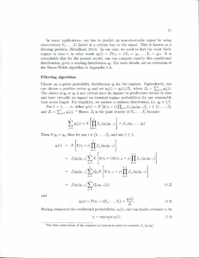
In many applications, one has to predict an non-observable signal by usingobservations Yi, . . . ,Yt linked in a certain way to the signal. This is known as afiltering problem (Rémillard, 2013). In our case, we need to find the most likelyrégime at time t, in other words r]t{i) = P{rt = i\Yi = yi, . . . ,Yt = yt). It isremarkable that for the présent model, one can compute exactly this conditionaldistribution, given a starting distribution rjo. For more détails, see an extension ofthe Baum-Welch algorithm in Appendix l.A.

Filtering algorithm

Choose an a priori probability distribution r]o for the régimes. Equivalently, onecan choose a positive vector go and set ?7o(i) = qo{i)/Zo, where Zq =The choice of go or t/q is not critical since its impact on prédictions decays in timeand have virtually no impact on terminal régime probabilities for any reasonabletime sériés length. For simplicity, we assume a uniform distribution, i.e. go = l/l.

For t = 1, . . . ,n, define qt{i) = E [l(Tt = i) HLi frkiVklyk-i)], i e {1,. . .,/},and Zt = qt{j)- Hence, Zt is the joint density of Ti,. . . , Yj because

5]]gt(j) = E1=1

Ylfri^iVklyk-l).k=l

= fi:t{yi,- - -,yt)

Then if go = rjo, then for any i E {1,... ,1}, and any t > 1,

qt{i) = E Hn = i)Ylfrk{yk\yk-i)k=l

= fiiytlyt-i)"^ E1=1

I

i{Tt = = j)'[lfr,{yk\y,fc-ijfc=i

= fiiyt\yt-i)^QjiE1=1

I

t-i

= j)YlfTk{yk\yk-i)k=l

and

= fi{yt\yt-i)'^Qjiqt-i{j)-1=1

Vt{i) = P{Tt = i\Y,,... ,Yt) = qt{i)

(1.2)

(1.3)

Having computed the conditional probabilities, ?7t(i), one can finally estimate Tf by

Tt = argmaxr/t(i), (1.4)

''The first observation of the sequence is burn-in in order to compute friivilyo)

12

i.e. as the most probable régime.In view of applications, it is préférable to rewrite (1.3) only in terms of 77, i.e.,

1,{i) = (1.5)

where7 I I

j=i i=i

As a resuit, Zt\t-i is the conditional density of Yt given F — 1,... , Yj-i, evaluatedat yi,

Conditional distribution

From the results of the previous section, the joint density fi-,t of Fi, . . . , Yj is Zt.Also, for any t > 2, the conditional density ft\t-i = Zt\t-i of Yt given Fi, . . . ,Ff_i,can be expressed as a mixture, viz.

i i i

ît\t-i{yt\yu ■ ■ • ,yt-i) = ̂ /i(yt|yt-i) = ̂ fi{yt\yt-\)Wt-\{i)i=l j=l i=l

(1.6)where

i

Wt-id) = i e {1,... (1.7)1=1

Note that for ail t > 1, Wt-i{i) = P{Tt = ̂ iVÎ-i = yt-i, • • • ,Fi = yi). As a resuit,it follows that

i

P{Tt+k = i\Yt = y^, . . . ,Fi = yi) = i € {1,..., (1.8)j=i

so the conditional law of Ft+i given Fi, . .. , Yj has densityi

ft+i\t{yt+i\yi, ■ ■ ■ ,yt) ^^fi{yt+i\yt)Wt{i). (1.9)i=l

Next, it is easy to check that the conditional law of Y^+i, ..., Y^+m given Fi, . . . , Y^has density

i i i

/t+m|t(yt+i) ■ • • ) yt+Tn|yi) ■ ■ • yt) ~io = lîl=l ÎTn = l

Qik-likfik {yt+k\yt+k-l)-X

fc=l

13

Stationary distribution in the Gaussian case

Suppose that the model specified by (1.1) holds, ergo the innovations are Gaussian.If Yn converges in law to a stationary distribution, for any given starting point yo)then this distribution must be Gaussian, with mean y and covariance matrix A.Suppose the Markov chain is ergodic with stationary distribution v. Then withprobability i G {1,.. . , /}, Yi = {I — + ̂ >iTo + e,, where e ~ iV(0, Ai) isindependent of Yo ~ ^)- It then follows that

Similarly, A must satisfies A = T{A), where

i

T{A) = B + (1-11)i=l

with B = + [(-^ ~ + ̂ il^V + A] ■ From theconditions on $i,. . . , there is a norm || • || on the space of matrices such that||$i|| < 1 for every i G {1, . .. , The operator T is then a contraction since forany two matrices ^0,^1, ||F(Ai)-T(^o)|| < ll^i-^oll ZlLi ^ cHyli-^doU,with c = maxi<j</ ||$i|p < 1. Also, since T{A) is a covariance matrix wheneverA is one, and B is positive definite, it follows that there is a unique fixed point Aof T, meaning that A = T{A), and this unique fixed point A is a positive definitecovariance matrix. If fact, A is the limit of any sequence An = r(A„_i), with Aqa non-negative definite covariance matrix. For example, one could take even takeAq = 0. This provides a way to approximate the limiting covariance A by settingA ^ An for n large enough.

1.2.2 Estimation of parameters

The EM algorithm (Dempster et ah, 1977) is a quite efficient estimation procédurefor incomplète datasets. Under hidden Markov models, observations are partialsince r is unobservable. The algorithm proceeds iteratively to converge to themaximum likelihood estimation of parameters (Dempster et ah, 1977). We derivedits implementation for ARHMM and the détails are in Appendix l.G. It seems thatstarting the parameter's estimation of the ARHMM with the HMM parameters'estimate (obtained by setting = • • ■ = = 0) was slightly more stable. Theoptimal number of régimes must be known a priori, an issue we will discuss next.

®Recall that all norms are équivalent.

14

Table 1.1: P-values (in percentage) for the nonparametric change point test usingthe Kolmogorov-Smirnov statistic with N=10000 bootstrap samples.

Period P-value

2000's recovery2008-2009 Financial Crisis2010's recovery

39.8

0.4

9.7

1.2.3 Goodness-of-fit test and sélection of the number ofrégimes

To Select the optimal number or régimes, one must test the adequacy of fittedmodels with différent number of régimes. This is generally done by using a testbased on likelihoods. However, goodness-of-fit tests based on likelihoods are notrecommended for regime-switching models (Cappé et al., 2005). We opt for asimpler approach based on a parametric bootstrapping. It was shown to work ona large number of dynamic models, including hidden Markov models. The testwas built on the work of Genest and Rémillard (2008) and its implementation is inAppendix l.D.

Selecting the number of régimes

Choosing the optimal number of régimes. The goodness-of-fit test methodologydescribed in Appendix B produces P-value from Cramér-von Mises type statistics,for a given number of régimes L As suggested in Papageorgiou et al. (2008), itmake sense to choose the optimal number of régimes, £*, as the first £ for which theP-value is larger than 5%. An illustration of the proposed methodology is given inSection 2.4.

1.2.4 Application to S&P 500 daily returns

To assess the relevance of our model on real data, we estimated the parameters onthe close-to-close log-returns of the daily price sériés of the S&P 500 Total Return.To find stationary estimation Windows, we used a nonparametric changepoint testfor a univariate sériés using a Kolmogorov-Smirnov type statistic (Rémillard, 2013).We focused on recent data, i.e. from early 2000 to today. We found two stationary estimation window: from 05/01/2004 to 02/01/2008 and from 05/01/2010 to20/01/2017. We can refer to the former as the 2000's recovery and 2010's recoveryfor the latter. Results of the tests are presented is Table 1.1. We will also studythe interesting period in between, the 2008-2009 Financial Crisis, even though thenull hypothesis of stationarity has a P-value of 0.4%.

Next, we perform the goodness-of-fit test (GoF for short) described in Appendix

15

l.D for the ARHMM (AR(1)) as well as for the HMM (AR(0)), as a mean ofcomparison. The results are presented in Tables 1.2, 1.4 and 1.6. According to thesélection methods described in Section 1.2.3, we optimally select a three-regimemodel for the 2000's recovery, since 3 is the smallest number of régimes for whichthe P-valne is larger than 5%. This is also true for the HMM model. Likewise, wechoose a three-regime model for the 2008-2009 Financial Crisis, and a four-regimemodel for the 2010's recovery. Note that in the case of the 2010's Bull markets, afour régime model for the HMM was not enough to get a P-value > 5%.

Furthermore, to measure the significance of ARHMM over HMM, we performa likelihood ratio test. This is possible because the HMM is a spécial case of theARHMM corresponding to $i = • • • = = 0. The corresponding statistic iscomputed as follow:

D = -21og('lÀfâU-21ogP'»'^'L{9i\x)/ \fl-.n{yu- - - ,yn\9l)

where 6q are the model's parameters estimated under the null hypothesis, i.e.$1 = ■ • • = $£ = 0, so the returns follow a Gaussian hidden Markov model, and9i are the model's parameters estimated under the alternative, i.e. returns followan autoregressive hidden Markov model. Under the null hypothesis, this statisticis distributed as a chi-square distribution with the number of degrees of freedomequal to the number of extra parameters in the alternative model. In our case, wehave one extra parameter per régime, i.e. so the number of degrees of freedomis i. Hence, under the null hypothesis, D ~ The log-likelihoods of bothmodels, the statistical test D and the )~â critical value at a significance level of 5%are also presented in Tables 1.2, 1.4 and 1.6. We clearly reject the null hypothesisfor ail models, proving we should favor ARHMM over HMM for each dataset.

The estimated parameters for the three periods are presented in Tables 1.3,1.5, and 1.7, where the mean and standard déviation of each AR(1) and AR(0)Gaussian régime density /, are respectively denoted by /Xj and a,, and are presentedas annualized percentages values. The tables further contains the long-term, i.e.stationary, régime probabilities v, together with the estimated transition matrix,Q.

Régimes are ordered by increasing volatility cTj, and incidentally by decreasingmean which is in line with what we typically observe on the markets.

In the case of the 2000's recovery. Régime 1 is associated to bull markets,which are characterized by strong positive premium and low risk (pi = 35.89 and(Ti = 3.34). It seems that this state is intermittent in the sense that the Markovchain does not stay or has a very small probability of staying in régime 1 sinceQi\ ~ 0. However, this state is not due to outliers since the percentage of time theMarkov chain is in this state is 11% for the HMM and 19% for the ARHMM.

16

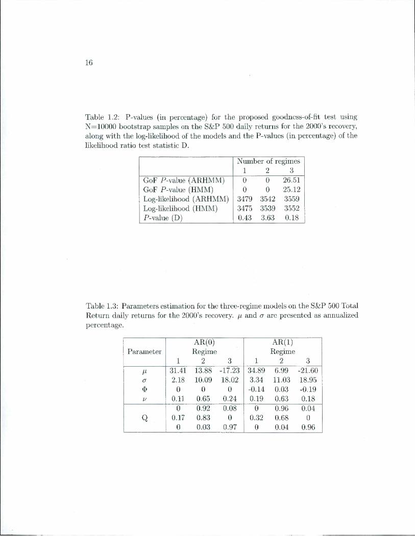
Table 1.2: P-values (in percentage) for the proposed goodness-of-fit test usingN=10000 bootstrap samples on the S&P 500 daily returns for the 2000's recovery,along with the log-likelihood of the models and the P-values (in percentage) of thelikelihood ratio test statistic D.

Number of régimes1 2 3

GoF P-value (ARHMM)GoF P-value (HMM)Log-likelihood (ARHMM)Log-likelihood (HMM)P-value (D)

0 0 26.510 0 25.12

3479 3542 3559

3475 3539 3552

0.43 3.63 0.18

Table 1.3: Parameters estimation for the three-regime models on the S&P 500 TotalReturn daily returns for the 2000's recovery. /r and a are presented as annualizedpercentage.

AR(0) AR(1)Parameter Régime Régime

1 2 3 1 2 3

31.41 13.88 -17.23 34.89 6.99 -21.60

a 2.18 10.09 18.02 3.34 11.03 18.95

$ 0 0 0 -0.14 0.03 -0.19

V 0.11 0.65 0.24 0.19 0.63 0.18

G 0.92 0.08 0 0.96 0.04

Q 0.17 0.83 0 0.32 0.68 0

0 0.03 0.97 0 0.04 0.96

17

1.4

1.3

ou

gÉ1.1

siO.ç

-'V-i /

2006

Year

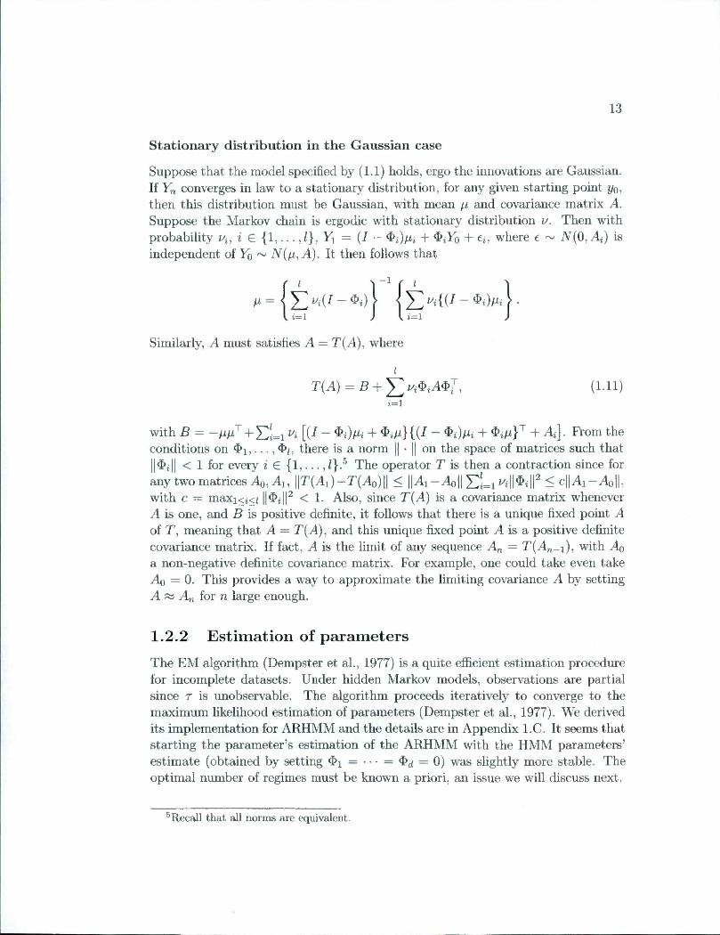
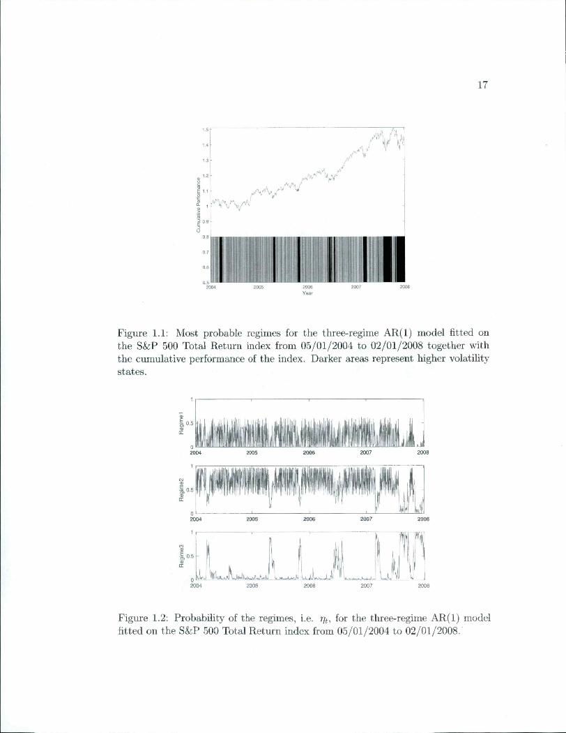
Figure 1.1: Most probable régimes for the three-regime AR(1) model fitted onthe S&P 500 Total Return index from 05/01/2004 to 02/01/2008 together withthe cumulative performance of the index. Darker areas represent higher volatilitystates.

2007 20082004 2005 2006

iJll2007

2005

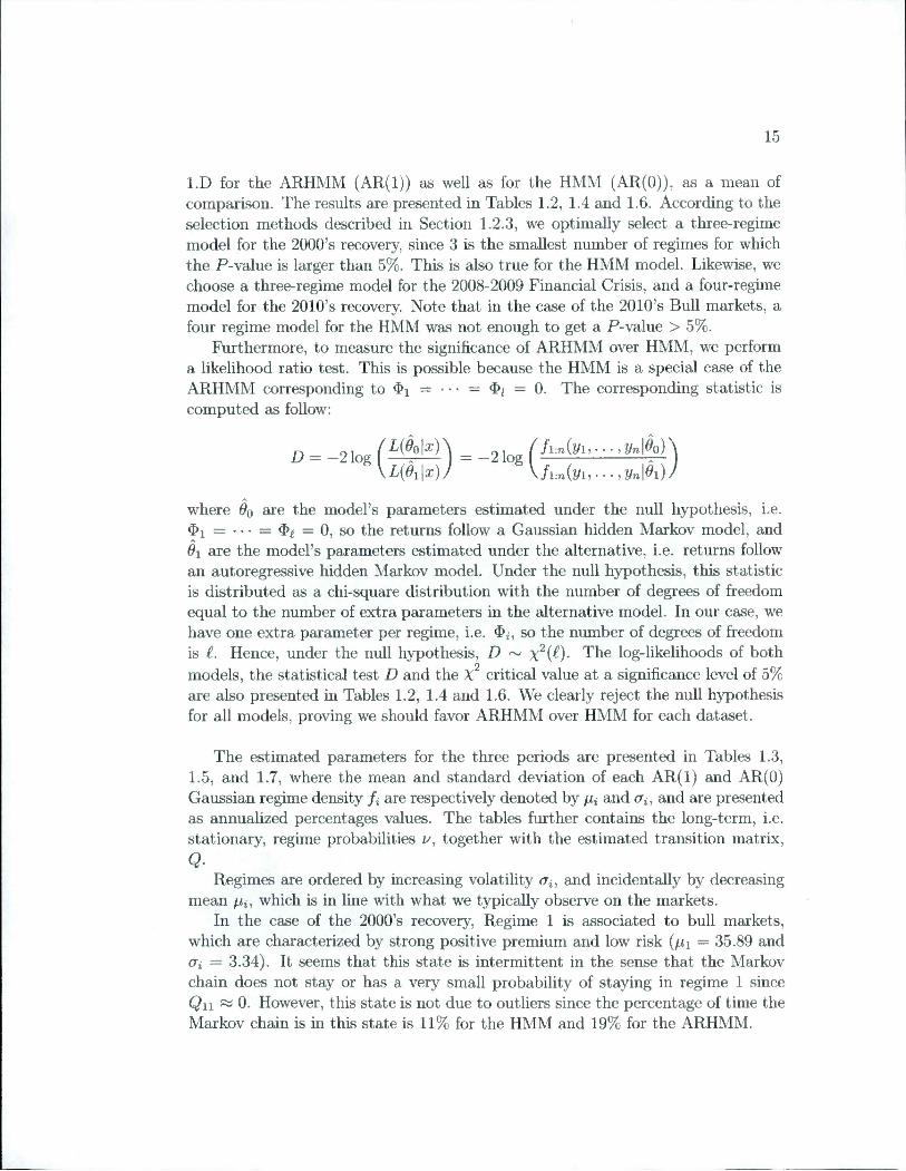
Figure 1.2: Probability of the régimes, i.e. r/f, for the three-regime AR(1) modelfitted on the S&P 500 Total Return index from 05/01/2004 to 02/01/2008.

18

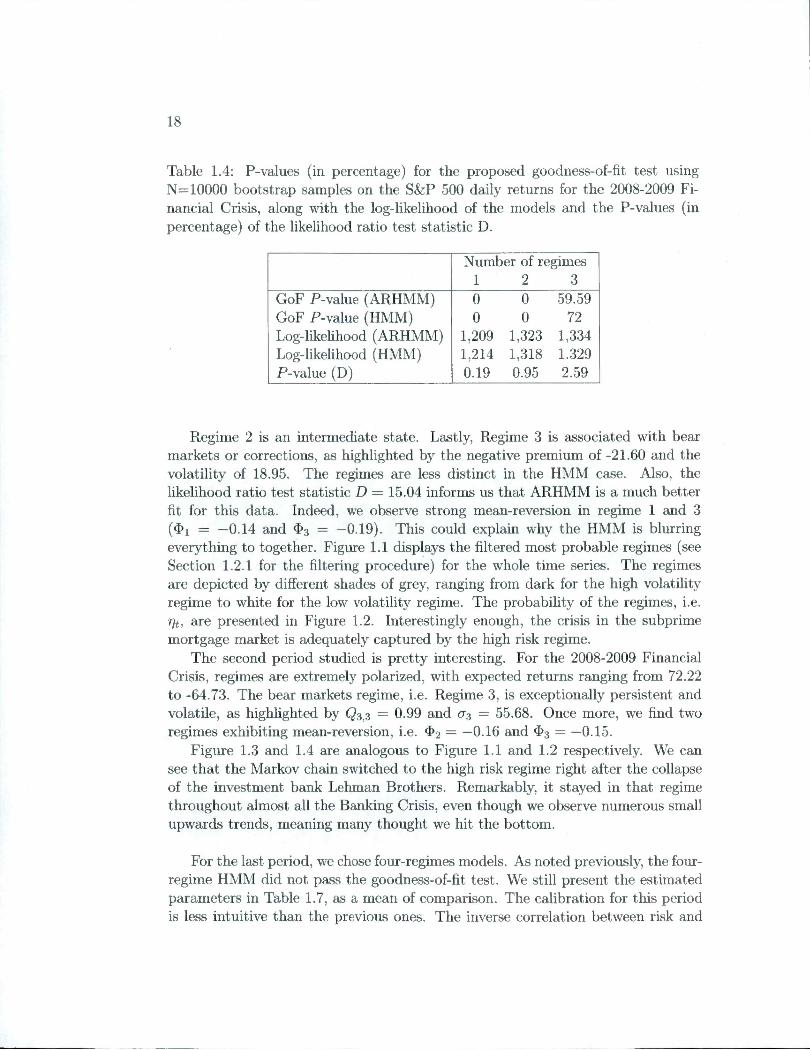
Table 1.4: P-values (in percentage) for the proposed goodness-of-fit test usingN=10000 bootstrap samples on the S&P 500 daily returns for the 2008-2009 Fi-nancial Crisis, along with the log-likelihood of the models and the P-values (inpercentage) of the likelihood ratio test statistic D.

Number of régimes1 2 3

GoF P-value (ARHMM)GoF P-value (HMM)Log-likelihood (ARHMM)Log-likelihood (HMM)P-value (D)

0 0 59.590 0 72

1,209 1,323 1,3341,214 1,318 1.3290.19 0.95 2.59

Régime 2 is an intermediate state. Lastly, Régime 3 is associated with bearmarkets or corrections, as highlighted by the négative premium of -21.60 and thevolatility of 18.95. The régimes are less distinct in the HMM case. Also, thelikelihood ratio test statistic D = 15.04 informs us that ARHMM is a much betterfît for this data. Indeed, we observe strong mean-reversion in régime 1 and 3($1 = —0.14 and $3 = —0.19). This could explain why the HMM is blurringeverything to together. Figure 1.1 displays the filtered most probable régimes (seeSection 1.2.1 for the filtering procédure) for the whole time sériés. The régimesare depicted by différent shades of grey, ranging from dark for the high volatilityrégime to white for the low volatility régime. The probability of the régimes, i.e.rjt, are presented in Figure 1.2. Interestingly enough, the crisis in the subprimemortgage market is adequately captured by the high risk régime.

The second period studied is pretty interesting. For the 2008-2009 FinancialCrisis, régimes are extremely polarized, with expected returns ranging from 72.22to -64.73. The bear markets régime, i.e. Régime 3, is exceptionally persistent andvolatile, as highlighted by = 0.99 and = 55.68. Once more, we find tworégimes exhibiting mean-reversion, i.e. $2 = —0.16 and $3 = —0.15.

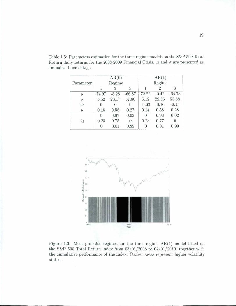
Figure 1.3 and 1.4 are analogous to Figure 1.1 and 1.2 respectively. We cansee that the Markov chain switched to the high risk régime right after the collapseof the investment bank Lehman Brothers. Remarkably, it stayed in that régimethroughout almost ail the Banking Crisis, even though we observe numerous smallupwards trends, meaning many thought we hit the bottom.

For the last period, we chose four-regimes models. As noted previously, the four-regime HMM did not pass the goodness-of-fit test. We still présent the estimatedparameters in Table 1.7, as a mean of comparison. The calibration for this periodis less intuitive than the previous ones. The inverse corrélation between risk and

19

Table 1.5: Parameters estimation for the three-regime models on the S&P 500 TotalReturn daily returns for the 2008-2009 Financial Crisis. // and a are presented asannualized percentage.

AR(0) AR(1)Parameter Régime Régime

1 2 3 1 2 3

74.97 -5.28 -66.87 72.22 -0.42 -64.73

a 5.52 23.17 57.80 5.12 22.56 55.68

$ 0 0 0 -0.03 -0.16 -0.15

V 0.15 0.58 0.27 0.14 0.58 0.28

0 0.97 0.03 0 0.98 0.02

Q 0.25 0.75 0 0.23 0.77 0

0 0.01 0.99 0 0.01 0.99

!>I 0.6

Û- 0.5

SI 0.4

Vh/^\

rv'

Figure 1.3: Most probable régimes for the three-regime AR(1) model fitted onthe S&P 500 Total Return index from 03/01/2008 to 04/01/2010, together withthe cumulative performance of the index. Darker areas represent higher volatilitystates.

20

^ 0.5

2009

.,1.. . il I

ï V

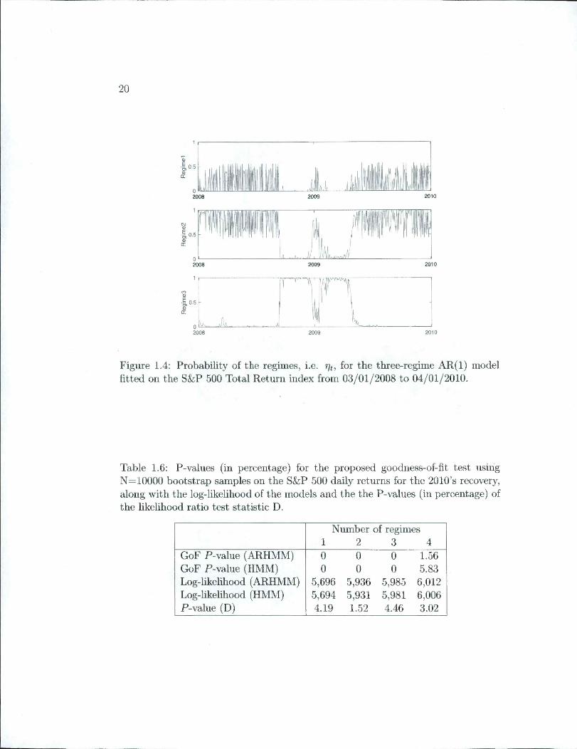
1 lFigure 1.4: Probability of the régimes, i.e. for the three-regime AR(1) modelfitted on the S&P 500 Total Return index from 03/01/2008 to 04/01/2010.

Table 1.6: P-values (in percentage) for the proposed goodness-of-fit test usirigN=10000 bootstrap samples on the S&P 500 daily returns for the 2010's recovery,along with the log-likelihood of the models and the the P-values (in percentage) ofthe likelihood ratio test statistic D.

Number of régimes1 2 3 4

GoF P-value (ARHMM)GoF P-value (HMM)Log-likelihood (ARHMM)Log-likelihood (HMM)P-value (D)

0 0 0 1.56

0 0 0 5.835,696 5,936 5,985 6,0125,694 5,931 5,981 6,0064.19 1.52 4.46 3.02

21

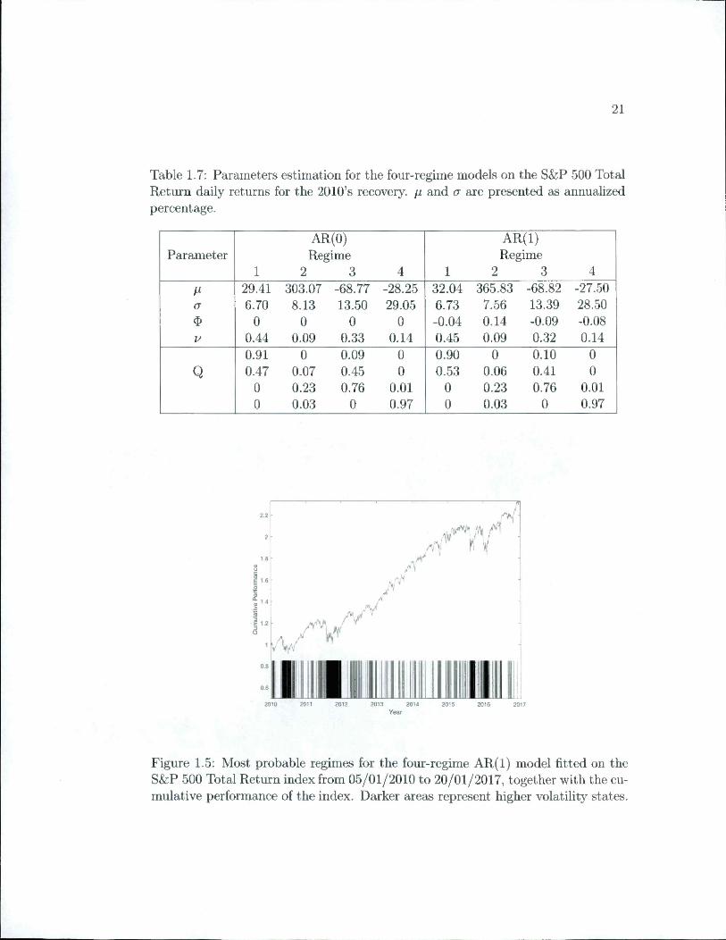
Table 1.7: Parameters estimation for the four-régime models on the S&P 500 TotalReturn daily returns for the 2010's recovery. ji and cr are presented as annualizedpercentage.

AR(0) AR(1)Parameter Régime Régime

1 2 3 4 1 2 3 4

29.41 303.07 -68.77 -28.25 32.04 365.83 -68.82 -27.50

a 6.70 8.13 13.50 29.05 6.73 7.56 13.39 28.50

$ 0 0 0 0 -0.04 0.14 -0.09 -0.08

u 0.44 0.09 0.33 0.14 0.45 0.09 0.32 0.14

0.91 0 0.09 0 0.90 0 0.10 0

Q 0.47 0.07 0.45 0 0.53 0.06 0.41 0

0 0.23 0.76 0.01 0 0.23 0.76 0.01

0 0.03 0 0.97 0 0.03 0 0.97

,1»

A '

A/

IYear

Figure 1.5: Most probable régimes for the four-regime AR(1) model fitted on theS&P 500 Total Return index from 05/01/2010 to 20/01/2017, together with the cumulative performance of the index. Darker areas represent higher volatility states.

22

2010 2011 2012 2013 2014 2015 2016 2017

2015 20 62010 20 20 2 2013 2014

^ 0.5

11#2010 2011 2012 2013 2014 2015 2016

0.5

2017

2010 2011

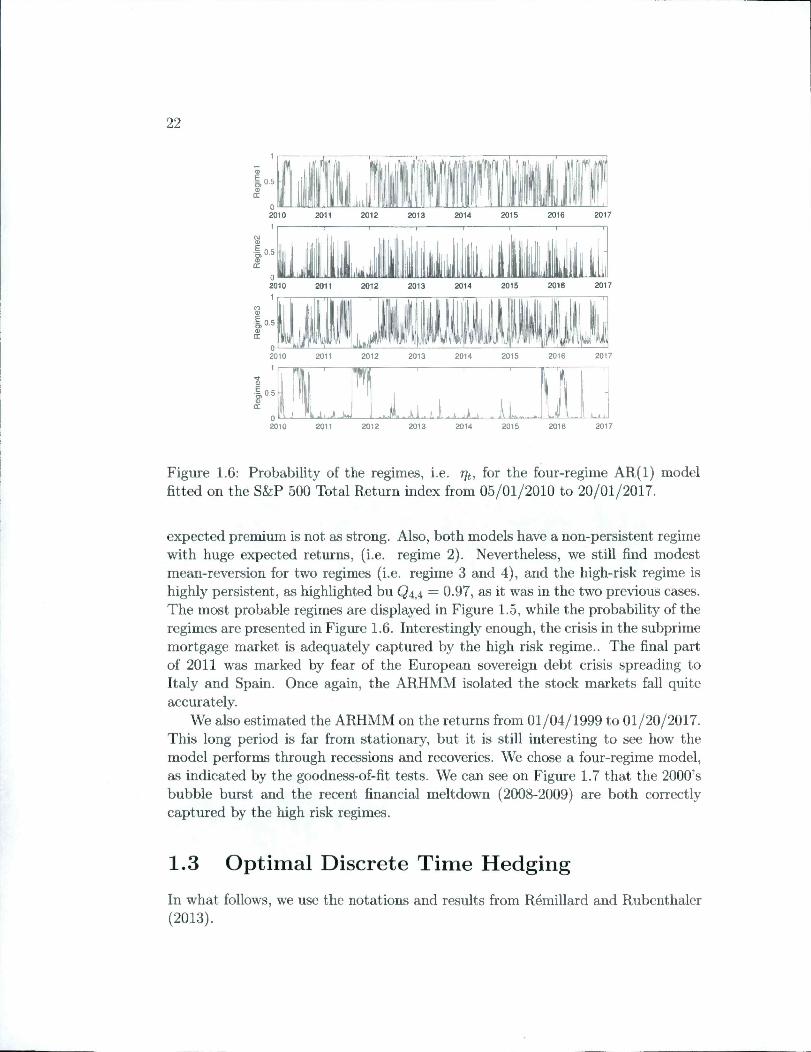
Figure 1.6: Probability of the régimes, i.e. rjt, for the four-regime AR(1) modelfitted on the S&P 500 Total Return index from 05/01/2010 to 20/01/2017.

expected premium is not as strong. Also, both models have a non-persistent régimewith huge expected returns, (i.e. régime 2). Nevertheless, we still find modestmean-reversion for two régimes (i.e. régime 3 and 4), and the high-risk régime ishighly persistent, as highlighted bu Q4,4 = 0.97, as it was in the two previous cases.The most probable régimes are displayed in Figure 1.5, while the probability of therégimes are presented in Figure 1.6. Interestingly enough, the crisis in the subprimemortgage market is adequatcly captured by the high risk régime.. The final partof 2011 was marked by fear of the European sovereign debt crisis spreading toItaly and Spain. Once again, the ARHMM isolated the stock markets fall quiteaccurately.

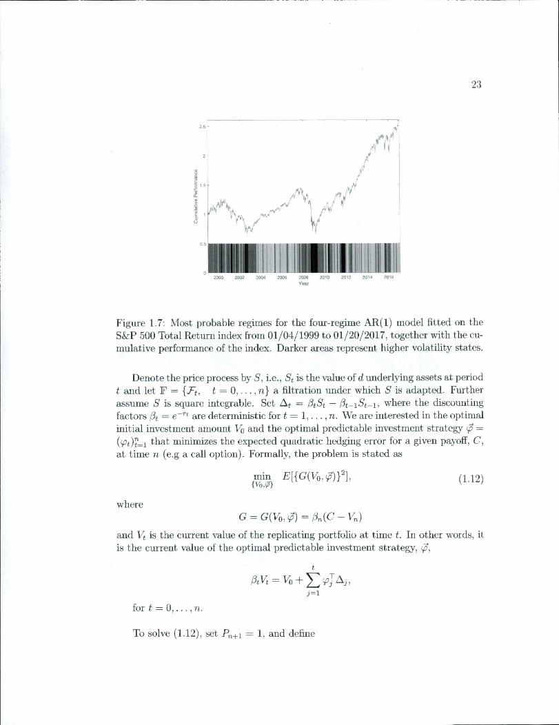
We also estimated the ARHMM on the returns from 01/04/1999 to 01/20/2017.This long period is far from stationary, but it is still interesting to see how themodel performs through recessions and recoveries. We chose a four-regime model,as indicated by the goodness-of-fit tests. We can see on Figure 1.7 that the 2000'sbubble burst and the recent financial meltdown (2008-2009) are both correctlycaptured by the high risk régimes.

1.3 Optimal Discrète Time Hedging

In what follows, we use the notations and results from Rémillard and Rubenthaler(2013).

23

!sI 1.5

/M

/

//"V /'iw S a/ r.A-,-"» 1 /'I»/^r \

<Sv'f \ /

"V ¥

Diiini2000 2002 2004 2006 2008 2010 2012 2014 2016

Year

Figure 1.7: Most probable régimes for the four-regime AR(1) model fitted on theS&P 500 Total Return index from 01/04/1999 to 01/20/2017, together with the cumulative performance of the index. Darker areas represent higher volatility states.

Dénoté the price process by S, i.e., St is the value of d underlying assets at periodt and let F = {J"(, t = 0, . . . ,n} a filtration under which S is adapted. Furtherassume S is square integrable. Set Af = PtSt — A-i-St-i; where the discountingfactors Pt = e"'"' are deterministic for t = 1, . . . , n. We are interested in the optimalinitial investment amount Vq and the optimal predictable investment strategy 0 =('7't)"=i fhat minimizes the expected quadratic hedging error for a given payofî, C,at time n (e.g a call option). Formally, the problem is stated as

min E[{G{Vq,0)Y{Vom

(1.12)

where

G = G{Vo,0)=Pn{C-Vn)

and Vt is the current value of the replicating portfolio at time t. In other words, itis the current value of the optimal predictable investment strategy, 0,

PtVt^Vo + '^^jAj,j=i

for t = 0, . . . ,n.

To solve (1.12), set P„+i = 1, and define

24

7t+i — E{PtJ^i\jFj),Ot = E{AtAj Pt+i\J^s-i) = E{AtAj ̂ t+i\Et-i),bt = E{AtPt+i\Et-i) = E{Aat+x\Et-i),Pt = a;^bt,

n

j=t

ioT k = n,. . . ,1.

We can now state Theorem 1 of Rémillard and Rubenthaler (2013), which is amultivariate extension of Schweizer (1995).

Theorem 1. Suppose that E{Pt\Et-i) 7^ 0 P-a.s., for This condition isalways respected for régime-switching models. Then, the solution {Vo,0) of theminimization problem (1.12) fs Vq = E{l3nCPi)/E{Pi), and

ipt = Oit-Vt-iPu k = l,. .. ,n. (1.13)

where

a, = af'E[^nCAtPt+i\Tt-,). (1.14)

and S and V are the présent values of S and V.

Remark 1. Vq chosen such that the expected hedging error, G, is zéro. Rémillardand Rubenthaler (2013) also showed that Ct{St,Tt) given by

a (-y E{(3nCPt+l\Et) , .

is the optimal investment at period t so that the value of the portfolio at period n isas close as possible to C in term of mean square error G, in particular, 140 = ̂ 0.

Ct can be interpreted as the option price at period t. By increasing the numberof hedging periods, Ct should tend to a price under a risk-neutral measure; see, e.g.,Rémillard and Rubenthaler (2016). For example, when there is only one régime,the density is Gaussian and 4>i fixed at 0, Ct tends to the usual Black-Scholes price.The detailed optimal hedging implementation for ARHMM is described in AppendixLE. R then follows that

Ct-i = = ̂ {(1 - pjAt)Ct\Et-t) (1.16)

«t = af'E{CtAt\Et-i). (1.17)

25

To dérivé the optimal hedging algorithm, we also need the following resuit, validfor a général ARHMM.

First, Write St = D{St-i)^\ where is the vector with componentsaiid D{s) is the diagonal matrix with diagonal elements {s)j, j G {1,.. . , d}.

The proof of the following theorem is given in Appendix l.E.l.

Theorem 2. For any t G dt = D{St-i)at{Yt-i,Tt-i)D{St-i), bt =pt = D-'^{St-i)ht{Yt-i,Tt-i), and-ft = 9t{Yt-i,Tt-i), with

ht = a^^bt, where at, bt, and Çt are deterministic functions given respectively by

at{y,i) = E{CtCjgt+i{Yt,Tt)\Yt-i = y,Tt-i = i}, (1.18)bt{y,i) = E{Ctgt+i{Yt,Tt)\Yt-i=y,Tt^i=i}, (1.19)gt{y,i) = E {gt+i{Yt,Tt)\Yt-i = y,Tt-i = i} (1.20)

-bJ{Yt^r,Tt^,)ht{Yt^,,rt-x),

with Ct = — 1, and gn+i = 1. If in addition j3nC = ^'„(5„), then Ct ='^t{St,Yt,Tt), where

^t_i(s,7/,z) = E [^t {D{s)e^*~''',Yt,rt} {l - ht{y,iyCt}\Yt-i = y,Tt-i = i] ,(1.21)

and

at = D-\St-x)a;\Yt^i,rt^i)At{St-x,Yt^x,Tt-x), (1.22)where

At{s,y,i) = E [l>t{D{s)e''^-'\Yt,Tt}Ct\Yt-i=y,rt-x=i] . (1.23)

For example, for a call option with strike K, ̂ '„(s) = max(0, s — jdnK).

1.3.1 Implementation issues

There are two main problems related to the implementation of the hedging strat-egy: Of, bt, gt, ^*4 and At defined in expressions (1.18)-(1.23) must be approximatedand régimes must be predicted.

We discretize at, bt gt functions of the underlying values y with a grid G. In asimilar manner, we discretize ^*4 and A4 functions of the underlying values s and y.To solve the recursion given by (1.21)-(1.23), Rémillard et al. (2017) interpolate andextrapolate linearly the simulated outcomes on G, using a stratified Monte Carlosampling procédure. Because the simulations are computationally expensive andintroduce variability, we propose a novel technique to approximate these intégraisusing semi-exact calculations, inspired by Rémillard (2013) Chapter 3. The détailsfor the semi-exact calculations are presented in Appendix l.E.3.

26

We also included the Monte Carlo sampling procédure as a mean of compari-son. Interestingly, we found that by simply rescaling the Monte Carlo samples tothe desired mean and volatility, we achieved results as accurate as the semi-exactcalculations, as pointed ont in Section 1.3.3.

As for defining the points on the grid, previous literature suggest choosing 10^equidistant points marginally covering at least 3 standard déviations under the respective highest volatility régimes. Importantly, we found that strategically choosing the points with respect to the percentiles of simulated processes significantlyreduces the number of points needed while keeping the accuracy at a reasonablelevel.

Next, we need to predict Ti based on {Ri, Rq and tq) and so on. The predictedrégime is f is the one having the largest probability given the information onprices up to time t, i.e. the most probable régime given by (1.4). Note thatthis methodology introduces a bias. We also studied the less biased approach ofweighting the régimes proportionally to rp, but since the results were comparableand did not lead to any significant improvement, they are omitted from the analysis.For more détails on régime prédictions, see section 1.2.1.

Then, according to (1.13) and (1.22), the optimal hedging weights ipt for period[f — 1, f) are approximated by

ift = t = 1, ■ ■ • , n. (1.24)

Vo is approximated by Co{So, tq, 0) while the reniaining monies, Vq — (p^So, areinvested in the riskless asset. Next, as is observed, one firsts computes the actualportfolio value Vi, then predicts the current régime Ti and finally approximates theoptimal weights ip2- This process is iterated until expiration of the option.

Using régime prédictions

Here, we obtain option prices and stratégies that dépend on the unobservablerégimes r, since {St, Tt) is a Markov chain. However, François et al. (2014) proposeda very interesting approach: they showed that {St, rjt) is Markov, so one can obtainprices and hedging stratégies depending on {St,T]t) instead. This makes sense finan-cially. However, this new Markov chain lives in a /-|-d—1-dimensional space, becausethe values of pt belong to the simplex Si = {xj, . . . , x/; > 0, x—1 + - • ■+Xci = 1}.François et al. (2014) considered only 2 régimes and one asset, so the real dimensionis 2. When l > 2, this becomes numerically intractable.

27

1.3.2 Global hedging

In practice, an expected hedging error characterized by Vt — Ct will emerge. In otherwords, the replicating portfolio at period t will not be worth the optimal investmentCt- Under the Black-Scholes setting, such error is unaccounted for since derivativescan be replicated perfectly (in continuons time). In contrast, under the proposedoptimal hedging protocol, the exposures (pt dépend on the replicating portfolio,Vt-i (see équation 1.13), which in turn dépends on the past strategy path.Under extreme scénarios, the replication of a call option might lead to optimalexposures ip greater than one share. Intuitively, this feature is optimal with respectto closing the gap between V and C.

1.3.3 Simulated hedging errors

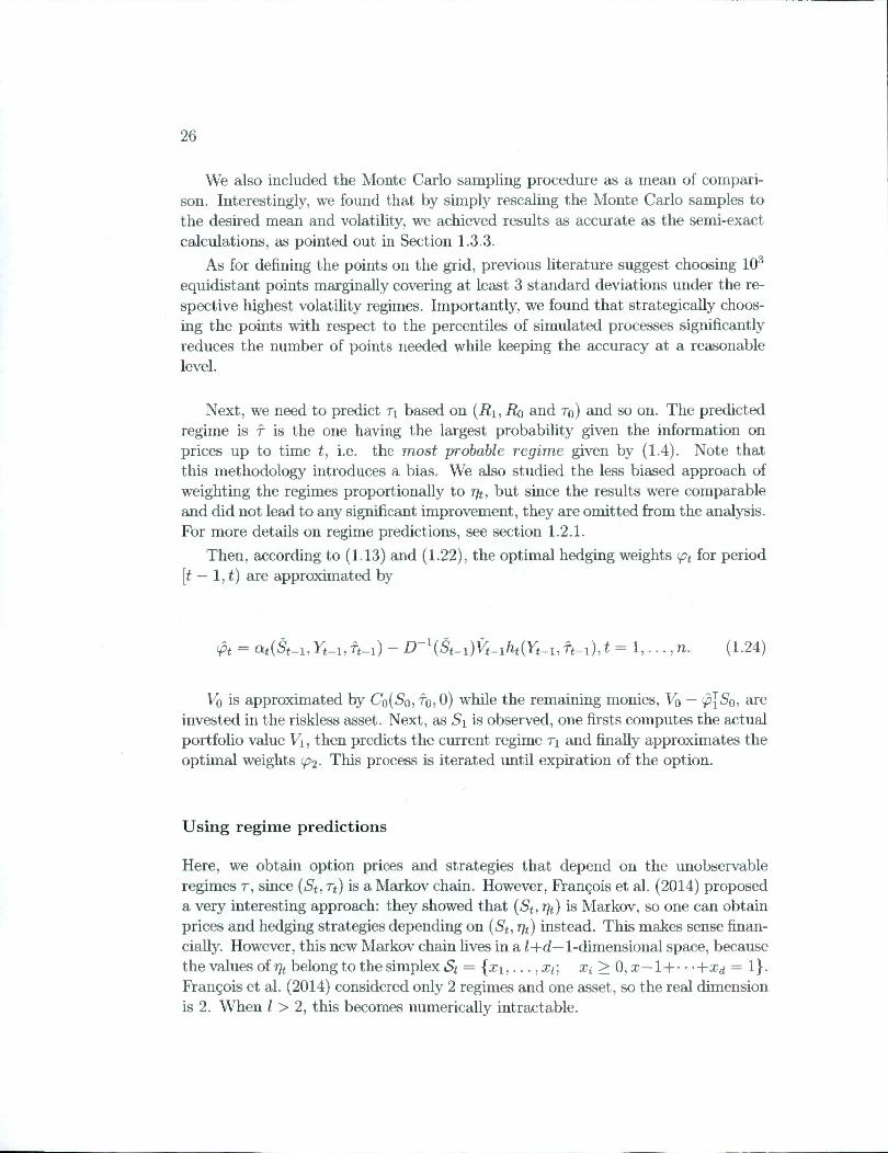
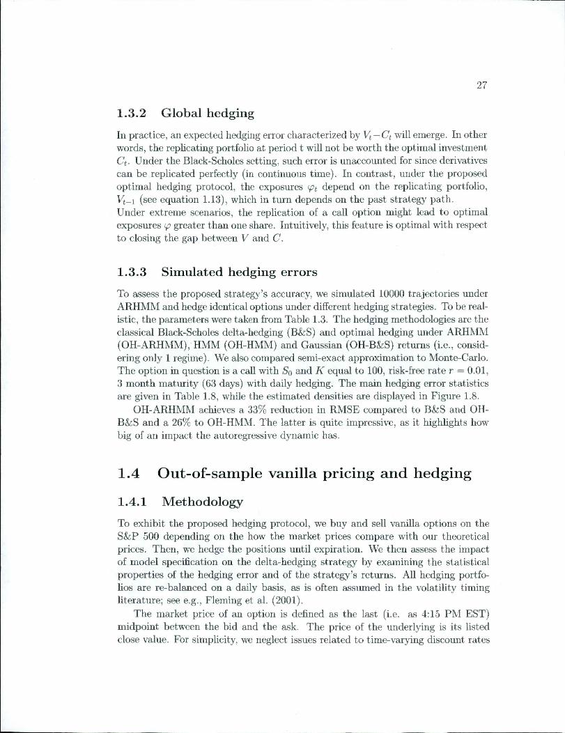
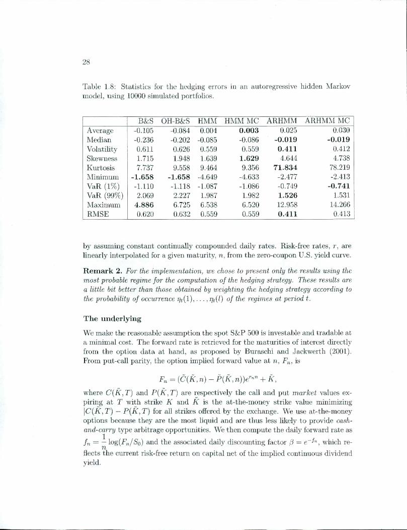
To assess the proposed strategy's accuracy, we simulated 10000 trajectories underARHMM and hedge identical options under différent hedging stratégies. To be real-istic, the parameters were taken from Table 1.3. The hedging méthodologies are theclassical Black-Scholes delta-hedging (B&S) and optimal hedging under ARHMM(OH-ARHMM), HMM (OH-HMM) and Gaussian (OH-B&S) returns (i.e., consid-ering only 1 régime). We also compared semi-exact approximation to Monte-Carlo.The option in question is a call with Sq and K equal to 100, risk-free rate r = 0.01,3 month maturity (63 days) with daily hedging. The main hedging error statisticsare given in Table 1.8, while the estimated densities are displayed in Figure 1.8.

OH-ARHMM achieves a 33% réduction in RMSE compared to B&S and OH-B&S and a 26% to OH-HMM. The latter is quite impressive, as it highlights howbig of an impact the autoregressive dynamic has.

1.4 Out-of-sample vanilla pricing and hedging

1.4.1 Methodology

To exhibit the proposed hedging protocol, we buy and sell vanilla options on theS&P 500 depending on the how the market prices compare with our theoreticalprices. Then, we hedge the positions until expiration. We then assess the impactof model spécification on the delta-hedging strategy by examining the statisticalproperties of the hedging error and of the strategy's returns. Ail hedging portfolios are re-balanced on a daily basis, as is often assumed in the volatility timingliterature; see e.g., Fleming et al. (2001).

The market price of an option is defined as the last (i.e. as 4:15 FM EST)midpoint between the bid and the ask. The price of the underlying is its listedclose value. For simplicity, we neglect issues related to time-varying discount rates

28

Table 1.8: Statistics for the hedging errors in an autoregressive hidden Markovmodel, using 10000 simulated portfolios.

B&S OH-B&S HMM HMM MC ARHMM ARHMM MC

Average -0.105 -0.084 0.004 0.003 0.025 0.030

Médian -0.236 -0.202 -0.085 -0.086 -0.019 -0.019

Volatility 0.611 0.626 0.559 0.559 0.411 0.412

Skewness 1.715 1.948 1.639 1.629 4.644 4.738

Kurtosis 7.737 9.558 9.464 9.356 71.834 78.219

Minimum -1.658 -1.658 -4.649 -4.633 -2.477 -2.413

VaR (1%) -1.110 -1.118 -1.087 -1.086 -0.749 -0.741

VaR (99%) 2.069 2.227 1.987 1.982 1.526 1.531

Maximum 4.886 6.725 6.538 6.520 12.958 14.266

RMSE 0.620 0.632 0.559 0.559 0.411 0.413

by assuming constant continually compounded daily rates. Risk-free rates, r, arelinearly interpolated for a given maturity, n, from the zero-coupon U.S. yield curve.

Remark 2. For the implementation, we chose to présent only the results using themost probable régime for the computation of the hedging strategy. These results area little bit better than those obtained by weighting the hedging strategy according tothe probability of occurrence T/t(l), . . . , T]t{l) of the régimes at period t.

The underlying

We make the reasonable assumption the spot S&P 500 is investable and tradable ata minimal cost. The forward rate is retrieved for the maturities of interest directlyfrom the option data at hand, as proposed by Buraschi and Jackwerth (2001).From put-call parity, the option implied forward value at n, is

= {C{k, n) - p{k, n))e'-"" + K,where C{K,T) and P{K,T) are respectively the call and put market values ex-piring at T with strike K and K is the at-the-money strike value minimizing\C{K^T) — P{K,T) for ail strikes offered by the exchange. We use at-the-moneyoptions because they are the most liquid and are thus less likely to provide cash-and-carry type arbitrage opportunities. We then compute the daily forward rate as

fn — — log(F„/So) and the associated daily discounting factor (3 = e~^", which re-n

fiects the current risk-free return on capital net of the implied continuons dividendyield.

29

-1 r~

2,5

B&SOH-B&SOH-HMMOH-ARHMM

2 -

1.5

.5 -2 -0.5 0.5 1.5

Figure 1.8: Estimated densities for the hedging errors in an autoregressive hiddenMarkov model, using 50000 portfolios. Only the semi-exact densities are shown, asthey were indiscernible from the Monte Carlo ones.

Option dataset

Exchange-traded options on the S&P 500 are European, heavily traded and havea high number of strikes and maturities.To assess the accuracy of our model, we will analyze two periods with very différent characteristics: the 2008 Financial Crisis, and a chunk of the recent recovery.Dates range from 09/24/2007 to 09/20/2009 and from 09/23/2013 to 07/08/2015,respectively. This will help us discern the impact on hedging and pricing when adramatic régime change occurs, in the former, and when it does not, in the latter.In order to minimize the efîect of varying maturities, we will build the dataset ofoptions having a maturity of about 1 year, more precisely from 231 to 273 trading days till expiration. Also, because in-the-money and out-of-the-money are lessliquid, we will only include options where moneyness (strike value divided by theunderlying value), is between 0.9 and 1.1. This leaves us with a total of 180 optionsfor the first period, and 478 for the second. Note that at a given date, more thanone option can meet these criteria.

30

Backtesting

We apply the AR(1) regime-switching optimal hedging methodology with 3 régimes(ARHMM). We chose 3 régimes because it is the number of régimes that seemed thebest given the time Windows studied, which we will describe in the next paragraph.We will compare it to the case with 1 régime and $ fixed at 0, corresponding tothe optimal hedging under the Black-Scholes model (OH-B&S).

For each option in the dataset, we estimate the ARHMM parameters on the S&P500 log-returns with a 500 and 2000 day trailing window. We choose to backtestusing 2 estimation Windows in order to have a more in depth understanding ofmodel spécification on pricing and hedging. The 2000 day trailing window willalways include the previous financial meltdown, i.e., dot-com bubble for our firstanalysis, and the 2008 financial crisis for the second one. The 500 day trailingwindow won't. Similarly, we applied this methodology to ail the hedging protocolsincluded in the analysis, which will be introduced below.

From Merton (1973), for a given moneyness, the value of an option is homoge-neous of degree one with respect to the underlying value. Thus, for each inceptiondate, we normalize the option prices, the strike values and the underlying path atan initial S&P 500 value of 100. Results can thus be aggregated through time andinterpreted as a percentage of S&P 500. Note that for each inception date, thehedging protocols are applied out-of-sample until maturity.

To ensure comparability, OH-B&S assumes the stationary distribution of theARHMM when the autoregressive parameter d> = 0. The OH-B&S optimal hedgingexposure is derived from an algorithm similar to the one presented in Section1.3. Optimal hedging under unconditional distributions is presented in Rémillard(2013). Both stratégies minimize the expected quadratic hedging error under theirrespective null hypothesis, namely that the returns follow an autoregressive regime-switching model (ARHMM), and a Gaussian model (OH-B&S).

OH-B&S methodology is not to be confused with the classical Black-Scholesdelta hedging protocol. Indeed, the terminology only refiects the fact that we hedgeand price under the Black-Scholes framework hypothesis, namely that Eissets followgéométrie Brownian motions. Even though the OH-B&S prices converge to theusual Black-Scholes prices as the number of hedging periods tends to infinity, thediscrète time hedging stratégies will not necessarily be the same. For this reason,the classical Black-Scholes delta-hedging methodology (B&S) is also considered.Similarly to OH-B&S, the B&S volatility is calibrated to the stationary volatilityof ARHMM.

We will add a final benchmark to our analysis, one that refiects how well themarket would have hedged the same options, namely the delta-hedging methodology where the volatility is calibrated to the implied volatility at each hedgingperiod (B&S-M). It will inform us how well the models compare to market's intuition. The effect of using the implied volatility was discussed in Carr (2002).

31

However, his theoretical analysis cannot be performed here.

To recap, we will buy and sell options depending on their market value comparedto the theoretical priées, and hedge the positions until maturity. We will analysethe P&L of the différent méthodologies, as well as the hedging errors. Two periodswill be studied: the 2008 Financial Crisis and a chunk of the following recoveryspanning from mid-2013 to mid-2015.

1.4.2 Empirical results

We define the hedging error as the présent value of the liability f5nC minus theprésent value of terminal portfolio PnVn- The options' maturity being set toone year, the annualized root-mean-squared hedging error can be computed by

\JÊ{/3nVn — f^nCy. This reulized risk is the empirical counterpart of the quantitywe minimized and as such, is the most relevant metric for comparing the différentmodels. Keep in mind that there is a lot of overlap in our dataset, so the hedgingerror values are not independent, nor identically distributed since the moneynessor other parameters are not constant. Despite these inconveniences, the hedgingerrors are still useful to compare the models.

Concerning the trading strategy, if the market is overvalued with respect to themodel, we sell the option and hedge our position. Thus, the présent value of thereturn is (Cq — Vq) — (/3n,C„ — If the market is undervalued, we buy theoption and hedge our position. The return will be the négative of the former.

2008-2009 financial crisis

In this section, we will focus on options with inception dates from September2007 to September 20^'' 2009. This period is really interesting. In the first part,the market experienced a huge increase in volatility and decrease in returns. In thesecond, the opposite.

We will first turn our attention to the 500 trailing estimation window case.Table 1.9 and Figure 1.9 présent the hedging error's statistics and density approximation. Figure 1.10 présents the results of the trading strategy, i.e., the cumulativevalue of a portfolio that traded the 90 options. The x axis is the cumulative numberof options traded in chronological order. In this case, ARHMM is by far the su-perior methodology. It achieved the best hedging error considering ail the metricsfor both calls and puts. Further, it was the best trading strategy for both type ofoptions, even though the hedging errors are almost entirely négative in the callscase. Note that the statistic "Bias" refers to the différence between the market

price and the theoretical price. Therefore, it is always 0 for the BS-M, since theimplied volatility is used.

32

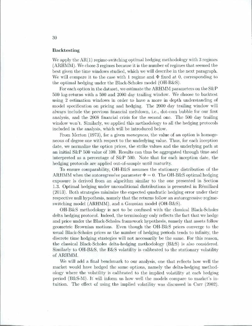
When volatility increases and returns turn négative, the puts' value increaseand one needs to be hedge accordingly. B&S and B&S-M failed to do so, resultingin huge hedging errors and great losses portfolio wise.

Table 1.9: Hedging error statistics for the 90 calls and the 90 puts traded in the2008-2009 Financial Crisis with 500 days trailing estimation window.

B&S-M B&SCallsOH-B&S ARHMM B&S-M B&S

Puts

OH-B&S ARHMM

RMSE 3.87 5.27 4.53 0.61 39.95 42.52 4.53 0.98

Bias 0 -4.52 -4.37 -5.35 0 -1.05 -0.91 -1.87

VaR 1% -7.64 -12.02 -12.47 -3.17 -28.39 -33.24 -12.47 -3.18

Médian 2.9 3.82 2.68 -1.65e-04 30.78 29.77 2.68 0.01

VaR 99% 9.16 8.61 7.57 -1.97e-09 72.9 77.22 7.57 4.75

(a)

USM

USOH^

(b)

Figure 1.9: Hedging error density approximation for the 90 calls (a) and 90 puts (b)traded in the 2008-2009 Financial Crisis with 500 days trailing estimation window.

Similar results are presented in Table 1.10 and Figures 1.11 and 1.12, althoughthe trailing estimation window, previously set to 500 days, is now 2000 days. Thisestimation window includes another financial crisis, the Dot-com Bubble. The saineconclusion as the previous experience can be drawn.

2013-2015 Bull markets

Our second and last analysis focuses on a part of the recent recovery spanning fromSeptember 23*'' 2013 to August 7"' 2015. This period is quite the opposite of afinancial crash. It is characterized by steady returns and low volatility.

33

•a 200 -

I

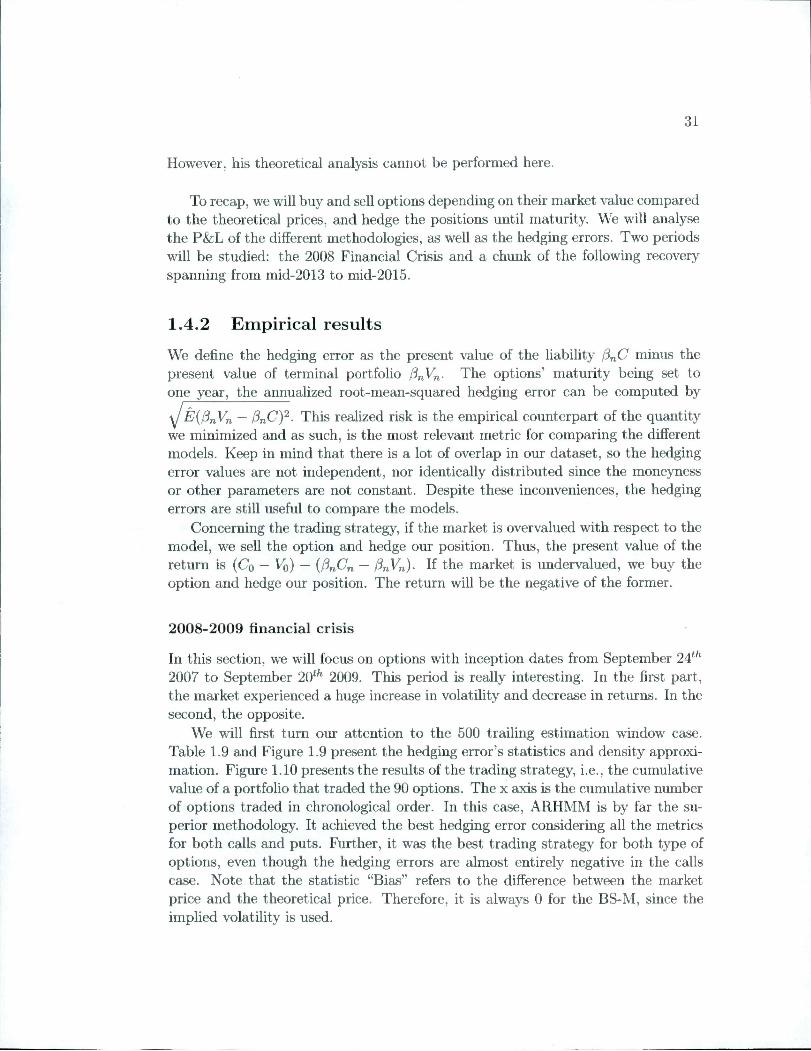
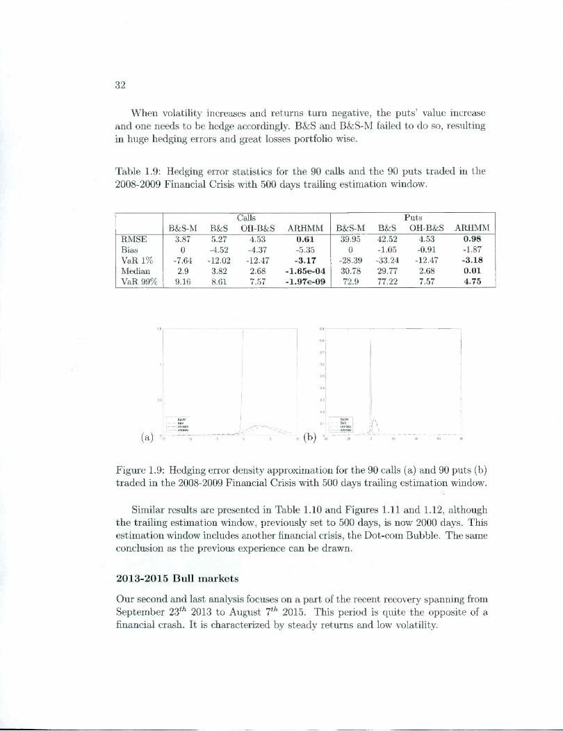
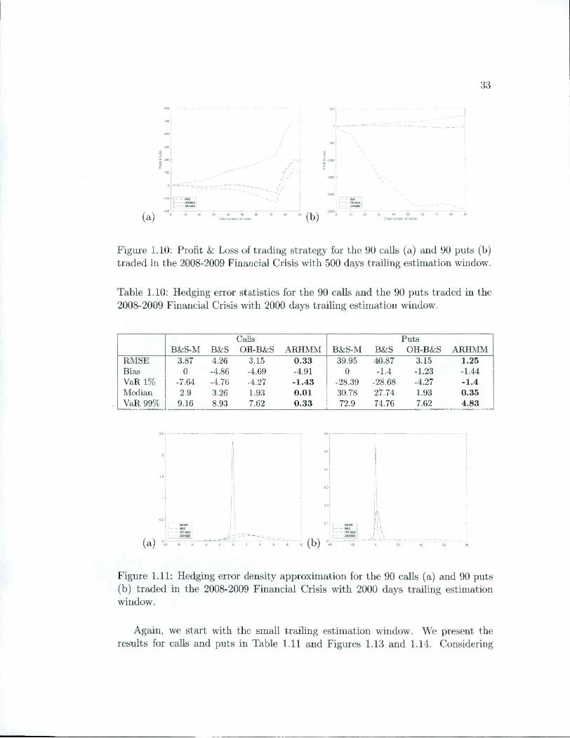
(a) Total lURibor ol fades (b)

Figure 1.10: Profit k. Loss of trading strategy for the 90 calls (a) and 90 puts (b)traded in the 2008-2009 Financial Crisis with 500 days trailing estimation window.

Table 1.10: Hedging error statistics for the 90 calls and the 90 puts traded in the2008-2009 Financial Crisis with 2000 days trailing estimation window.

B&S-M B&SCallsOH-B&S ARHMM B&S-M B&S

PutsOH-B&S ARHMM

RMSE 3.87 4.26 3.15 0.33 39.95 40.87 3.15 1.25

Bias 0 -4.86 -4.69 -4.91 0 -1.4 -1.23 -1.44

VaR 1% -7.64 -4.76 -4.27 -1.43 -28.39 -28.68 -4.27 -1.4

Médian 2.9 3.26 1.93 0.01 30.78 27.74 1.93 0.35

VaR 99% 9.16 8.93 7.62 0.33 72.9 74.76 7.62 4.83

(a) •10 -8 -S

Figure 1.11: Hedging error density approximation for the 90 calls (a) and 90 puts(b) traded in the 2008-2009 Financial Crisis with 2000 days trailing estimationwindow.

Again, we start with the small trailing estimation window. We présent theresults for calls and puts in Table 1.11 and Figures 1.13 and 1.14. Considering

34

(a) " - " (b)

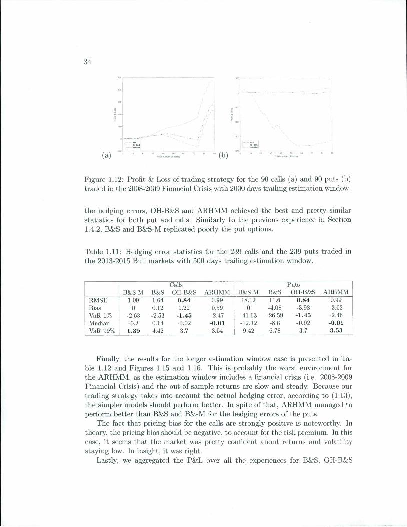
Figure 1.12: Profit & Loss of trading strategy for the 90 calls (a) and 90 puts (b)traded in the 2008-2009 Financial Crisis with 2000 days trailing estimation window.

the hedging errors, OH-B&S and ARHMM achieved the best and pretty similarstatistics for both put and calls. Similarly to the previous experience in Section1.4.2, B&S and B&S-M replicated poorly the put options.

Table 1.11: Hedging error statistics for the 239 calls and the 239 puts traded inthe 2013-2015 Bull markets with 500 days trailing estimation window.

Calls Puts

B&S-M B&S OH-B&S ARHMM B&S-M B&S OH-B&S ARHMM

RMSE 1.09 1.64 0.84 0.99 18.12 11.6 0.84 0.99

Bias G 0.12 0.22 0.59 0 -4.08 -3.98 -3.62

VaR 1% -2.63 -2.53 -1.45 -2.47 -41.63 -26.59 -1.45 -2.46

Médian -0.2 0.14 -0.02 -0.01 -12.12 -8.6 -0.02 -0.01

VaR 99% 1.39 4.42 3.7 3.54 9.42 6.78 3.7 3.53

Finally, the results for the longer estimation window case is presented in Table 1.12 and Figures 1.15 and 1.16. This is probably the worst environment forthe ARHMM, as the estimation window includes a financial crisis (i.e. 2008-2009Financial Crisis) and the out-of-sample returns are slow and steady. Because ourtrading strategy takes into account the actual hedging error, according to (1.13),the simpler models should perform better. In spite of that, ARHMM managed toperform better than B&S and B&:-M for the hedging errors of the puts.

The fact that pricing bias for the calls are strongly positive is noteworthy. Intheory, the pricing bias should be négative, to account for the risk premium. In thiscase, it seems that the market was pretty confident about returns and volatilitystaying low. In insight, it was right.

Lastly, we aggregated the P&L over ail the expériences for B&S, OH-B&S

35

(a)

USMBtS 1OH-BtSi-

„..r'/ / V--

0 1 2 3 (b) ».

I USM I; us I! 0H4«8 I

10 0 10

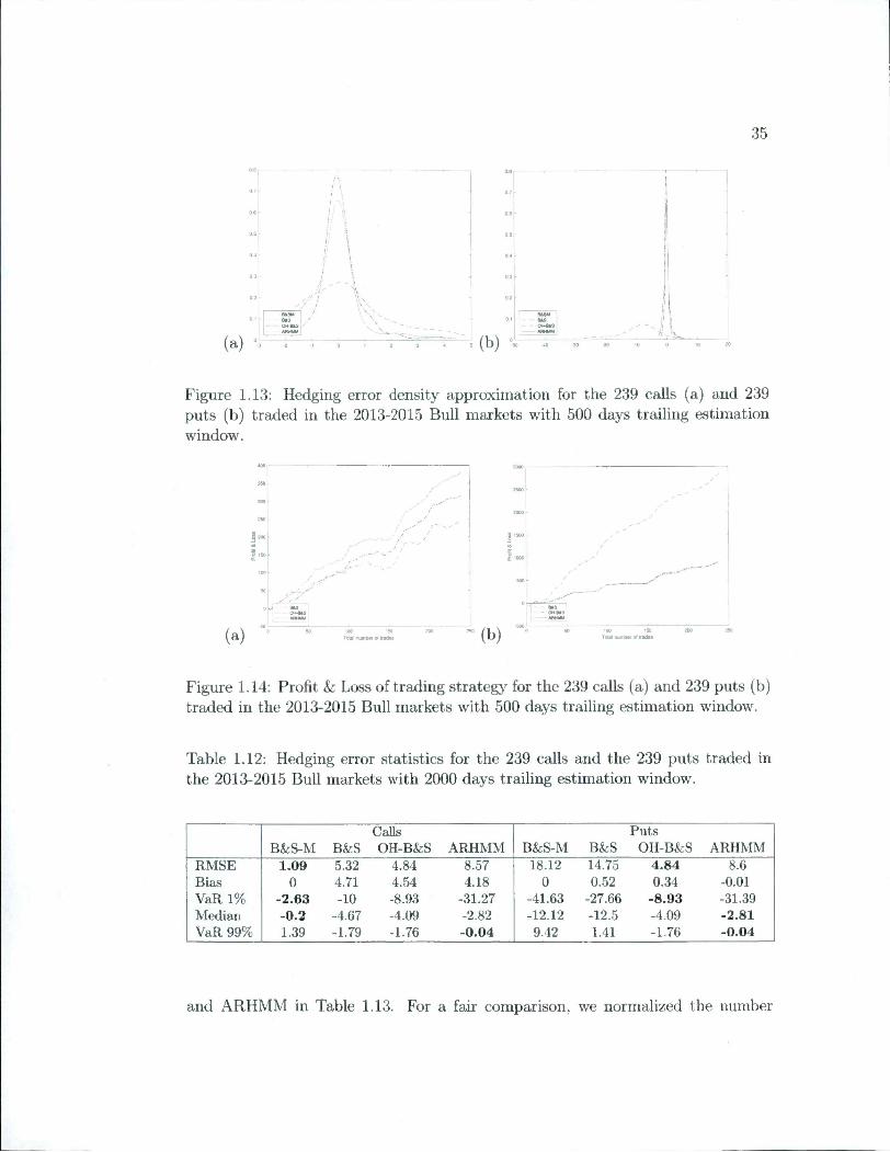
Figure 1.13: Hedging error density approximation for the 239 calls (a) and 239puts (b) traded in the 2013-2015 Bull markets with 500 days trailing estimationwindow.

(a) (b)

Figure 1.14: Profit & Loss of trading strategy for the 239 calls (a) and 239 puts (b)traded in the 2013-2015 Bull markets with 500 days trailing estimation window.

Table 1.12: Hedging error statistics for the 239 calls and the 239 puts traded inthe 2013-2015 Bull markets with 2000 days trailing estimation window.

B&S-M B&SCallsOH-B&S ARHMM B&S-M B&S

PutsOH-B&S ARHMM

RMSE 1.09 5.32 4.84 8.57 18.12 14.75 4.84 8.6

Bias 0 4.71 4.54 4.18 0 0.52 0.34 -0.01

VaR 1% -2.63 -10 -8.93 -31.27 -41.63 -27.66 -8.93 -31.39

Médian -0.2 -4.67 -4.09 -2.82 -12.12 -12.5 -4.09 -2.81

VaR 99% 1.39 -1.79 -1.76 -0.04 9.42 1.41 -1.76 -0.04

and ARHMM in Table 1.13. For a fair comparison, we normalized the number

36

(a)

! \

//

// /

20 -15

( Ii i

'' N ! !' \ I /

/ y /

OH-US

(b) °» ï'

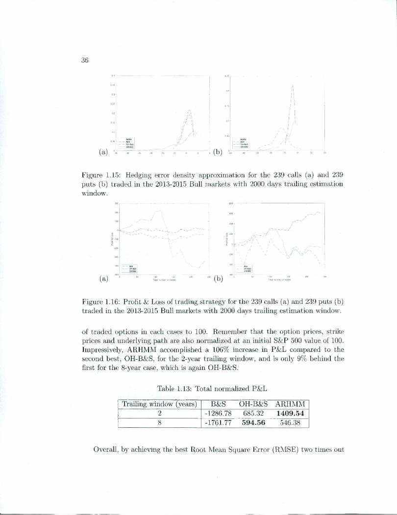
Figure 1.15: Hedging error density approximation for the 239 calls (a) and 239puts (b) traded in the 2013-2015 Bull markets with 2000 days trailing estimationwindow.

(a) Total numMr Of Inde* (b)OH-M8

•A.,

Total number oirato*

Figure 1.16: Profit k Loss of trading strategy for the 239 calls (a) and 239 puts (b)traded in the 2013-2015 Bull markets with 2000 days trailing estimation window.

of traded options in each cases to 100. Remember that the option prices, strikeprices and underlying path are also normalized at an initial S&P 500 value of 100.Impressively, ARHMM accomplished a 106% increase in P&L compared to thesecond best, OH-B&S, for the 2-year trailing window, and is only 9% behind thefirst for the 8-year case, which is again OH-B&S.

Table 1.13: Total normalized P&L

Trailing window (years) B&S OH-B&S ARHMM2 -1286.78 685.32 1409.54

8 -1761.77 594.56 546.38

Overall, by achieving the best Root Mean Square Error (RMSE) two times out

37

of four for both the 2-year and 8-year window, and by being the most profitablestrategy three times out of four for the 2-year window and two times ont of fourfor the 8-year window, the ARHMM is the superior hedging protocol.

However, the practitioners should keep in mind that if the ARHMM is estimatedon a window including a financial crisis, they should expect higher hedging errorsthan the simpler models if returns stay slow and steady. From our results, westrongly suggest to use a 2-year trailing window as it consistently achieved anRMSE lower than 1, i.e., the ARHMM can accurately hedge options in a financialcrisis without ever seeing one.

1.5 Conclusion

In this paper, we propose an antoregressive hidden Markov model to fit financial data, and we show how to implement an optimal hedging strategy when theunderlying asset returns follow an antoregressive regime-switching random walk.

First, we présent estimation and filtering procédures for the ARHMM. In orderto détermine the optimal number of régimes, we propose a novel goodness-of-fittest for univariate and multivariate ARHMM based on the work of Bai (2003),Genest and Rémillard (2008) and Rémillard et al. (2017).

To illustrate the proposed strategy, we model three daily return sériés of theS&P 500. Using likelihood test, we show that the ARHMM is a much better fitthan the classical HMM, particularly because it bas the capacity to model mean-reversion.

Morcover, we présent the implementation of the discrete-time optimal hedgingalgorithm minimizing the mean-squared hedging error. Becanse it further performspricing, we implemented a trading strategy consisting of selling overpriced andbuying underpriced options and hedging the position till maturity. Out of eightcases and compared to three other hedging protocols, our strategy achieves the bestroot-mean-squared hedging error four times and is the most profitable strategy fivetimes. Furthermore, it realized the best total P&L.

Because of its ability to model régime switches as well as mean-reversion, itwould be interesting to see this model applied to multivariate time sériés. Thehedging algorithm can also be applied to multivariate or American options.

l.A Extension of Baum-Welch Algorithm

For f G {1, ... , Z} and 1 <t < n, define

Xt{i) = P{rt = i\Yu.. . ,Yn).

38

Also, for i,j G {1, , /} and 1 < t < n — 1, define

= P{Tt = i,Tt+i =j\Yi,. . . ,Yn),

and let fit{i) be the conditional density of (Y^+i,. . . , Y^), given Yt and Tf = i.Further set = 1- Note that An{i,j) = Xn{i)Qij: for any ï, j G {1,. . . , /}.

The proof of the following proposition is given in Appendix l.B.

Vt+iW = —I— , t = 0,.. .,n-l, (1.25)

Proposition 1. For ail i,j G {1,...,/},

ELi EÏj=i faiYt+i\Yt)rit{p)Q0c. 'i

t = 0, . ..,n-l, (1.26)/3=1

X /-X ,_n n 07^, , ) t —0, . . . ,n, (1-27)

At{i,j) = t = 0, ...,n-l. (1.28)rit {i)Qijfjt+i {j)fj {Yt+i\Yt)HL=ir]t{a)fjt{a)

In particular,i

^At(z,d)-At(i), t = 0, ...,n. (1.29)3=1

l.B Proof of Proposition 1

Let ^ G {1,. . . , /} and t G (1,. . . , n} be given. Set X = (Yi,... , Y"t-i), C = Yt andW = (Yi+i, . .. , Yn). Let / dénotés the density of X. If follows from the définitionof conditional expectations that for any bounded measurable functions F, G, andH,

E{F{X)G{Or,,(i)) = iî{FmG(Ç)l(r, = !)}

= J P('^)aU)Vt-lW)f(x)fi{z\x)dzdx.As a by-product, one gets

E{F(X)G{Oru(i)] = Ql3a f F{x)G{z)r]t{i)r]t-i{a)f{x)fc,{z\x)dzdx.a=l 13=1 •'

Since the last équation holds for any F and G, it follows that (1.25) holds true.

3=1

l l

39

Next,

E{G{OH{W)\Yt = y,n_i=i} = J G{z)H{w)fjt{t)dzdw= ^Qiy f fi3{z\y)fjt+i{l3)G{z)H{w)dzdw,

13=1

proving that (1.26) holds.Next, let /(x, z) be the density of {X, Q = (Fi,.. . , Y^). Then

£;{F(X)G(C)//(VY)At(i)} = E{F{X)G{OH{W)l{n = 0}

= J F{x)G{z)H{w)r)t-i{i)Qijfjt{j)f{x, z)dwdzdx.As a by-product,

E{E{X)G{C)H{W)Xt{i)} = 53 / F{x)G{z)H{w)\t{i)'nt{a)fjt{a)f{x,z)dwdzdx,a=l

proving (1.27). It is easy to extend the last argument to the case t = 0.Finally,

E{E{X)G{C)H{W)At_r{i,j)} = E{E{X)GiOH{W)l{n-,=i,n=j)}

= Qij J E{x)G{z)H{w)r]t(i)fit{j)X f {x) fi{z\x)dwdzdx.

As a by-product, the latter can also be written as

i i

EE/ E{x)G{z)H{w)At-i{i,j)Qai3m{<^)VtW)f{x)f0{z\x)dwdzdx,a=l 13=1

proving (1.28). It is easy to extend the last argument to the case t = 0. Thiscomplétés the proof. ■

l.C Estimation of regime-switching models

To describe the EM algorithm for the estimation, suppose that at step fc > 0, onehas the parameters Q, /ij, Ai, i G {1,.. . , /}.

Let wt{i) = Xt{i) j Y2=i and set y, = Ylt=i and y. = Y11=i Wt{i)yt-i,i G {1, . . . ,/}, where Xt and At are given in Proposition 1.

40

Then, at step fc + 1, for z, j G {1, . . . , /}, one has

^(fc+l) _ X^t=l -^<-1(^1 j) _ St=l j) /l OQ\" " Er^.v,(z) ' ^ - ^U

(fc+1) (/_$f+0)-^(y._$('=+i)^^)^ (1.31)(fc+i) ^ (yt-i-yj (yt-i-y.) | (1-32)

X ~ (^«-1 ~ y») I '(1-33)

t=i

where eji = yt-yi- (yt-i - y^, t = l,. . . ,n.The proof is given in the next section.

l.C.l Proof of the EM algorithm for the estimation

The EM algorithm for estimating parameters consists of two steps, expectation andmaximization:

E-Step: Compute the conditional probabilities.

At(z) = P{Tt = i\Yi, . .. ,y„) and Kt{i,j) = P(rt = i,Tt+i = i|Yi,... ,y„),

for ail 1 < f < rz and i,j G{1, ...,/}.

M-Step:Let Q be the set oil x l transition matrices with positive entries. Suppose that

Q E Q-, and 0 G 0. Then the log-likelihood is

n n

L(yi,. . . .y„,ri,. . . ,r„,(3,6') = ̂ iogQn-i,n + J^^®s/n(yt|yt-lA)•t=l t=i

It then follows that

C{Q,è-,Q,e) EQ,e|L(^yi, . .. ,y„,ri,. . . ,r„,(5,(9) |yi =yi,...,y„ = y„|n l l n i

= EEE At-i(bi)logQp' + EE Af(z)log/i(yt|yt-i,À-t=l i=l j=l t=l i=l

41

If Q,9 are the parameters at step k, then the parameters at stepA: + 1 are

(Q(fc+i)^^(fc+i)) ^arg max C{QÀQ,9).QeQ.èee

It is easy to check that

n l lQ(fc + 1) _ ^]-g EEE

satisfies

t=i i=i j=i

r.{k+i) _ . . r. j.

E/3=EkiEr.iA.-.(',« Er..A.-i(i)proving (1.30). Also,

n ly

eeet

0{k+i) _ gj,g EE=l i=l

Estimation for Gaussian AR(1) regime-switching models (M-Step)

For the estimation procédure, we assume the densities /i, . . . , // are given by (1.1),so 9 = {fiu. . . , Al) ee = W^'xBfxSf.

In this case, the function L{9) = — X]"=i J2[=i log fi{yt\yt-i, 9) to minimizeis given by

n lT

{y'^ ~ ~ ~ {vt - k'i - - k-i)}t=l i=l

nd 1 ir—\ —X . / .X , I T I+— log 27r + - 2_] 2^t=l i=l

Let Wt{ï) = Xt{i) j 5Zfc=i If then follows that for any z G {1, . . . , Z},

^ w^t(0 [yt - (yt-i - } = o, (i.34)t=l

è ~ (^<-1 ~ } (î/t-i - /^f = 0. (1-35)

= ̂ wt{i)ztizl, (1.36)t=i

and

(=1

42

where Zu = yt - /uf (vt-i - ,t = l,. . . ,n, since

t=\ i=l

where ^tii)/n, and for any non singular d x d matrix B,TriB)-\og\B\ > d.

The latter is true because f{x) = x — log(x) > /(l) = 1 for any x > 0.Next, set = Y^^=iWt{i)yt and y. = 5Z"=i Then it follows from

(1.34) that

^f+') = (/ - $(>+'>)"' - •î.f"'!/,) , ! 6 {1,.. . ,1},proving (1.31). Now, for f G {1,..., /},

(yt ~ {yt-i - = Y1 ^yt ~ y») (y*-^ ~ y()t=i t=i

+ - Vi) - y^T

Il ^

^ {yt - Vi) (yt-i - y.)i=l

+4r'(Mr''-a)(4'""-ï,)'.using (1.31), and

è {yt-^ ~ yf {vt-i - è tvtii) [yt-i - y^ (yt-i - y.)t=i t=i

+(/'r"-E.) ("r'-ï.)'-As a resuit, for i G {1,..., l},

-1I . T I

;,(fc+l){n r n^ wtii) (yt-i - y.) (yt-i - y.) | «^((0 (yt - Vi) (vt-i - y^

proving (1.32)It also follows from (1.31) that (1.36) can be written as

n

2G{1,.. . ,Z}, (1.37)t=i

where

eu = yt-yi- (yt-i - y^) , f e {l,. ..,/}, t = i,. .. ,n.

43

l.D Goodness-of-fit Test for Autoregressive Hid-den Markov Model

In this appendix, we state the goodness-of-fit test, which can be performed toasses the snitability of a Gaussian AR(1) regime-switching models as well as toSelect the optimal number of régimes, l*. The proposed test, based on the workof Diebold et al. (1998), Genest and Rémillard (2008) and Rémillard (2011a), usesthe Rosenblatt's transform. For conciseness, we détail the implementation for twodiniensional Gaussian AR(1) regime-switching models, but the approach can beeasily generalized.

l.D.l Conditional distribution functions and the Rosen

blatt's transform.

Let i G {1, . . . ,/} be fixed an Ri be a random vector with density fi. For anyç G {1,.. . , d}, dénoté by fi^i-g the density of (R-^\ . . . , Ri^^), and by ft^q the densityof rY' given {Rf\.. . ,R^f~^'*). Further dénoté by Fi^q the distribution functionassociated with density fi^q. By convention, i dénotés the unconditional densityof Then, the Rosenblatt's transform

X i-> Ti{x) = (Fj,i(x^^^), .. . , Fi,d(z^^\ ... ,is such that Ti{Ri) is uniformly distributed in [0,1]'^.

For example, if fi is the density of a bivariate Gaussian distribution with mean Ujand covariance matrix

F"',,(1) ...A,(1).,(2)s, =

(1) (2) (2)F 'v) v]

fi^2 is the density of a Gaussian distribution with mean -|- — /xp^) andvariance vf'\\ — pf), with (5i = Pi\Jvf'^/v^i^\ These results can easily be extendedto the Gaussian AR(1) distribution.However, for regime-switching random walks models, past returns must also beincluded in the conditioning information set. For any . . . ,x(''' G M, the (d-dimensional) Rosenblatt's transform corresponding to the density (1.6) conditional on Xi, . . . , X(_i G M'' is given by

i

= ̂ 'i^^(a:i, ... ,xt_i,x|^^) = ̂ IRj_i(z)Fi,i(xp^)i=l

44

and(xf ̂ , . . . , (xi,. . ., Xt_i, ... , )

^ = l'Wt-i(i)/i,i:g-i(xp\... ,x|''""^^)Fi,g(x[^^)E!=1 W^t-l(0/^,l:q-l(4^^ • • ■

for q e {2, . .. ,d}.Suppose Ri,. . . ,Rn is a size n sample of d-dimensional vectors drawn from a joint(continuons) distribution P. Also, let V be the parametric family of GaussianAR(1) regime-switching models with l régimes. Formally, the hypothesis to betested is

no:Pev = {Pe-,eee} vs Hi -. p^vUnder the null, it follows that {U\ = 4'i(iîi, 0), t/2 = ^2(-Ri, -^2) • • ■ > =^{Ri,. .. , Rn,0)) are independent and uniformly distributed over [0,1]'^, where

are the Rosenblatt's transforms conditional on the set of pa-rameters 0 G 0.Since 0 is unknown, it must be estimated by some Then, the pseudo-observations,(Ûi = 4'i(Ri, . . . ,Un — 4'n(Ri, ■ - ■ , Rn-, ̂ n)) are approximately uniformly distributed over [0,1]"^ and approximately independent. We next propose a test statis-tic based on these pseudo observations.

1.D.2 Test statistic

The test statistic builds from the following empirical process:

n d

Dn{u) = - n ^ ^ • • • ' ^ [0' 1]'-" t=l g=l

To test I-Lq against Ri we propose a Cramér-von Mises type statistic;

= Bn{ûi, . . .,Ûn)=n [ Il ,=1 J

- Ti n d x ^ n d

= E E n {1 - ^ E 11(1 - +t=l fe=l 9=1 ) t=l 9=1

n

¥

Since Ûi is almost uniformly distributed on [0,1]'' under the null hypothesis, largevalues of 5„ should lead to rejection of the null hypothesis. Unfortunately, thelimiting distribution of the test statistic will dépend on the unknown parameterset, 9. Since it is impossible to construct tables, we use a différent methodology,namely parametric bootstrap, to compute P-values. The validity of the parametric bootstrap approach has been shown for a wide range of assumptions in Genest

45

and Rémillard (2008). These results were recently extended to dynamic models(Rémillard, 2011b), including regime-switching random walks. In this paper, wegeneralized the procédure to AR(1) Gaussian regime-switching model by condi-tioning the Rosenblatt's transform on the previous return.

1.D.3 Parametric bootstrap algorithm

a) For a given nuniber of régimes, estimate parameters with 6^ computed from theEM algorithm applied to {Ri,..., Rn)

b) Compute the test statistic,

Sn^Bn{Û,... ,Ûn),

from the estimated pseudo observations, Ui = . . . ,Ri, On), for î G {1,... , n}.

c) For some large integer N (say 1000), repeat the following steps for every k G

i) Generate a random sample {Rj,. . . , 0^} from distributionii) Compute 6^ by applying the EM algorithm to the simulated sample, Rj, . . . , R^.iii) Let Ùi = ̂ «(Rj,. . . , R^, 0^) for i G 1, . .. , n, and finally compute

Then, the approximate R-value for the test based on the Gramér von Misesstatistic Sn is given by

k=l

l.E Optimal Hedging

l.E.l Proof of Theorem 2

Proof. First, we show this is true for the off-line random sequences a, b,7,p andP. The resuit is clearly true for R„+i = 1. Now,

a„ = E{AnAl\Pn-l)= R(S„_i)R|(e^"-^" - 1) - l)^ D(S„_i)= D{Sn-l)an{Yn-l,Tr,-l)D{Sn-l),

46

since ("K, r) is a Markov process. For the same reason,

bn = E{An\Tn-l)

-^(*^71—1 1 î 1 )•

As a resuit, = F>-^(5„_i)a-^(y„_i,r„_i)fe„((F„_i,r„_i), so

- l) .

Therefore, 7„ = 5n(^n-i, Ai-i)- The rest of the proof is doue by induction. Assumethis is true for t + 1, then we have to prove this is true for t. Now

at = E (AtAj-ft+i\Et-i)= D{St.^)E - 1) - l)^ gt+,iYt,Tt)\Et-i}

since {Y, r) is a Markov process. Similarly,

bt = E {At^t+i\Et-i)= D{St-,)E - 1) gt+,{YuTt)\Et-,}

Hence, pt = D-'^{St-i)a^'^{Yt-i,Tt-i)ht{Yt-urt-i), so

pjAt = ht{{Yt-i,Tt-if a~^{Yt-i,Tt-i) - l) .

Therefore,

7t = E {{I - p1 At)-it+\\^t-i]= E{gt+r{Y,n)\Et-x}

= gt{Yt-i,Tt-i).

This proves that (1.18)-(1.20) hold true for any t G {1, . . . , n}.Suppose now that /3„C„ = 4'„(5„). Using induction together with (1.16), one

gets

= = E[{1 - pjAt)Ct\Et-i]= E[{1 - ht{Yt_,,n-iV - l)}^t{SuYt,rt)\Et.,]

47

Finally, it follows from (1.14) and (1.16) that

= a;'E{l3nCAtPt+i\Ft-i) = a;'E{PtCtAat+i\J't-i) = a;'E{CtAt\Tt-i).

As a resuit, using (1.18)-(1.21), one gets

where

At{s,y,i) = E [4*4 {D{s)e^'~''\Yt,Tt} (e^'"'"' - l) \Yt-i = y,rj_i = i] .m

1.E.2 Optimal hedging algorithm

We now need to evaluate the (1.18)-(1.23). First,

at{y,i) = £;|(e^'~''' - l) - l)^ gt+i{Yt,Tt)\Yt-i = y,Tt-i = ï|' r= '^Qij / - 1) 9t+i{z,j)fj{z\y)dz,

j=i

bt{y,i) = F; {(e^'"'"' - l) gt+i{Yt,Tt)\Yt-i = y,Tt-i = i}

= ^Qij j -i)gt+i{z,j)fj{z\y)dz,j=i

gt{y,i) = E{gt+i(Yt,Tt)\Yt-i = y,Tt-i = i}-bJ{y,i)ht{y,i)

= ^Qij / 9t+i{z,j)fj{z\y)dz-bJ{y,i)ht{y,i),j=i

'ift-i{s,y,i) = E [4^4 {D{s)e^'~''\Yt,Tt] {l - ht{y,iy - l)} |Fi-i = y,rt_i = i]

= ^Qij j '^t{D{s)e^-''\z,j] {l-ht{y,iy -1)] fj[z\y)dzj=i ''

At{s,y,i) = E {'i!t{D{s)e^'~''',Yt,Tt} -l) \Yt-i = y,Tt-i=i}

= ^Qij j '^t{D{s)e^~''',z,j]{e^-'''-1) fj{z\y)dz.j=i

Since these variables are weighted expectations they can be approximated byusing Monte Carlo simulations, coupled with interpolations. This method was pro-posed in Papageorgiou et al. (2008). Because the simulations are computationallyexpensive and introduce variance, we propose a novel technique to approximatethese expectations using semi-exact calculations, based on Rémillard (2013).

48

1.E.3 Semi-exact calculations.

By defining a grid, i.e. xq < Xi < ... < Xm < x^+i, one can approximate a functionF by the continuous piecewise linear function

m

f{x) = ̂ l{xq <x < Xq+i) {A^iq) + xB^{q)}), (1.38)9=0

where

Bf{q) = (1.39)Xq-^\

A^{q) = fiXq)-XqBf{q). (1.40)New, for simplicity, take d = 1. Using (1.38)-(1.40), we can approximate gt the

following wayk

9t{y,i) = X^i(y^ <y < yv+i){A!{v,i)+ yB^{v,i))v=0

where

^ 9tiyv+iÀ) -9t{yv,i)Uv+l Vv

At{vA) = gt{yv,i) - yvBt{v,i)-Remember that Çn+i = 1. The formula for gt is shown later.

Now, let J\f{x) be the cumulative distribution function of the standard normal_z2/2distribution and let M'{z) = ^^ be the associated density. Also, M"{z) =

—zM'{z). If A" ~ N{ii, a^), and if a < 6 are given, then for any û G R, one has

M(0) = E [e^^l{a < X < 6)] = WMb)} - AA{/t(a)}],

M'{e) = E[Xe^^l{a<X <b)]= {fi + ea^)M{e) - W{<b)} - Ar'{K(a)}],

and

M"{e) = E [X^e^^l{a < X < b)]= a^M{e) + {fi + 9a^)M'{e)

^efi+o'^(T^/2+ae"^^" " '^|(r[A/'"{/t(6)} - A^"{K(a)}](/i + 0(7^) [A/''{k(6)} - A/''{K(a)}] l,

49

X

where for any x G R,

k{x) =a

In particular,

M'(0) = E[Xl{a<X<h)]

— Oa'^ — /X

=— O

This way, we can approximate a, b and g as follows.

For any n G {1, . .. , A;} and any i G {1. . . , i}, set

à,{V..i) = E<?«E / F"" - 1) - 1)J=1 t,=0

x(^f+i(î^. j) + zB^+i{v,j))fj{z\yu)dz_! /•»«+! (

= \ - 2e"^'eMf+i(î;,j)j = l ,;=0 dyv t

j) + j) + Bf^i{v, j)^fj{z\yu)dz,

btiyuJ)^ fUv+l

= Qij Y / ~ + zBf^^{v,j))fj{z\yu)dzj=l v=0 •'V"J_ Je ry^+i r

j=i t,=o dyv t

+e-''*ze'B^t^-^{v,j)^fj{z\yu)dz.and

^ *• ^ ryv+i9t{yu,i) = Y^'^Y / {^t{v,j) + zBf{v,j)}fj{z\yu)dz-bt{yu,iyht{yn,i),

j=i v=o dyv

where ht{yu,i) = àï^{yu,i)bt{yu,i)- For values of y not on the grid, we can alsointerpolate â, b, and g using (1.38)-(1.40).

To approximate ^ and a, we need to define a second grid, defined by 0 = sq <Si < ... < Sjn < «m+i = oc. 'ï't cau be also be approximated by a produet ofcontinuons piecewise linear functions viz.

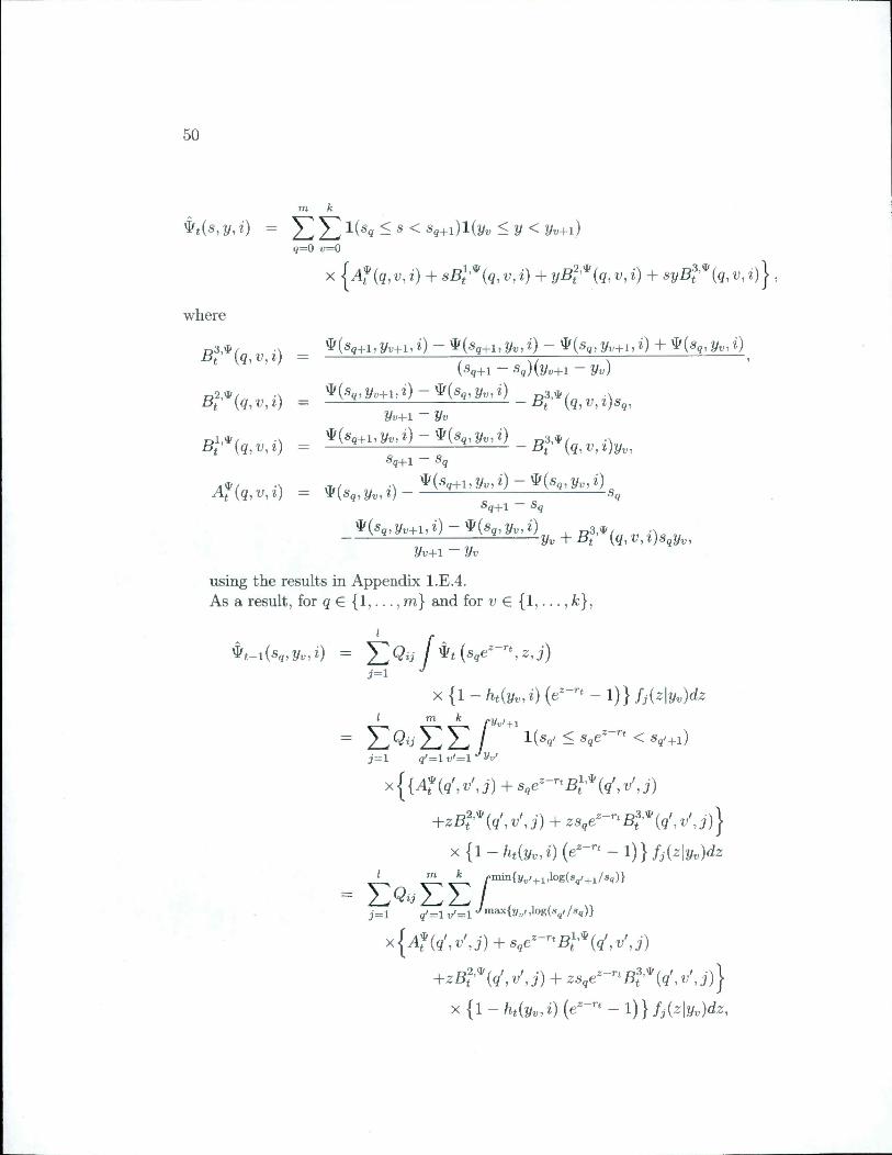
50

m A.

#t(s,2/,î) = < s < Sç+i)l(t/„ < y < y^+i)

X |ylf(ç,î;,z) + sBt'*(g,v,2) + y5t'*(g,v,z) + syBf'*(y,v,i)|,g=0 t;=0

where

^(^g+l i ?/^+l ' ̂ ) ^('^(?+l ) ) ^) yii+l) 0 "^~ yt)) 0(■^q+1 ■5ij)(yt>+i ytj)

2/i;+l Vv

Bl^''{q,v,i) =•^ç+l ^q

■^{Sg+i,yy,i) - ̂ (gq,yt„0■^q+l — Sn

Î/d+I Uv

using the results in Appendix l.E.4.As a resuit, for y G {1, . . . , m} and for n G {1,.. . , k},

'^t-l{Sq,yv,i) = ^Qij f '^t{Sqe^'''',Z,j)j=i

X {l - ht{yv,i) - l)}/j(2ly„)dzJ' ™ ^ rVv'+i

= < V+l)J = 1 q' = l v' = l ̂v'

x{{AÎ{<l': '"'J) + Sqe'~^'Bl''^{q',v',j)+zBt''^{q',v',j) + zsqe'^"'''5f'*(y', 't;',j)|

X {l - ht{yv,i) - l)} fj{z\yy)dz

~ ^2 /q/=l„'=l>'niax{y„,,log(s^//s,)}

X {a* i) + i)+z5t^'*(y',n',y) + zSqe^~'''A'*(9'>^'> j)}

X {l - ht{yy,i) - l)} fj{z\yy)dz,

51

with the convention that the intégral is 0 if

max{?/„/,log(sq//s,)} > min{y„/+i, log(sg/+i/sg)}.

There is a similar expression for At{Sq,yy,i), namely

Ât{sg,yy,i) = '^Qij -l) fj{z\yy)dz.7=1

' JIL ^ ry-'+i= < v+i)

j=l q' = l v' = l

X {q\ v', j) + Sqe'-'''B]''^{q', v', j)

+zBt''^{q',v',j) + j)|X - l) fj{z\y^)dz

= ^ Qij 2_^ 2-^ /j=l g' = l v' = l •'™a^{l/t;'.log(s,//s,)}

X {^f W, w', J) + Sqe'''''Bl''^(q', v', j)+zBt''^(q',v',j) + zSqe'~'''Bi'*(q',v\j)j

X - l) fj(zlyy)dz.

Note that ^t-i(0,yA) = '^n(0,y,i) and At(0,y,i) = /it(y,z)^„(0,y,i) for ailt = l,. . . ,n. For example, 5'f(0,y,z) = 0 for ail t, while for a put option withstrike K, ̂ 14(0, y, i) = PnK, for alH G {0, . . . , n}.

1.E.4 Bi-linear interpolation

One wants to interpolate / hy / over [aïoiici] x [yo^yi]- Set fij = f{xi,yj), i,j G{0,1}.

Then f{x,y) = + ̂ oo, where

Bqo = /oo).^10 = /lO ~ /oO)Bqi — foi — /oo,Bii = /il — /lo — foi + /oo-

52

1.E.5 Simulation of Gaussian ARHMM(l)If {Yt,Tt) = then with Tt+i = j with probability Qij and then Yt+i = yj -\-

— Hj) + BjE, where BjBj = Yj and e ~ N{0,1).AIso, when d = 1, a random sample of size N from fj{-\y) is given by Zij =

Pi + — fij) + ajCi, with ~ A"(0,1). So the sequence of innovations e areindependent of j.

In this case, every intégrai Ij{h) = f h(z)fj(zly)dz is approximated by

In particular, this means that for any ji, £ {1; ■ ■ • > 0'

1 ^ ^ I ̂~ JY ^ ^ •^^2(^2) — Jy y ^1=1 i=l

References

J. Bai. Testing parametric conditional distributions of dynamic models. The Reviewof Economies and Statistics, 85(3):531-549, 2003.

F. Black and M. Scholes. The pricing of options and corporate liabilities. Journalof Political Economy, 81:637-654, 1973.

A. Buraschi and J. Jackwerth. The price of a smile: hedging and spanning in optionmarkets. The Review of Financial Studies, 14(2):495-527, 2001.

O. Cappé, E. Moulines, and T. Rydén. Inference in Hidden Markov Models.Springer Sériés in Statistics. Springer, New York, 2005.

P. Carr. FAQ's in option pricing theory. Technical report, NYU, 2002.

J. Cox and S. Ross. The valuation of options for alternative stochastic processes.Journal of Financial Economies, 3:145-166, 1976.

A. P. Dempster, N. M. Laird, and D. B. Rubin. Maximum likelihood from incomplète data via the EM algorithm. J. Roy. Statist. Soc. Ser. B, 39:1-38, 1977.

F. X. Diebold, T. A. Gunther, and A. S. Tay. Evaluating density forecasts withapplications to financial risk management. International Economie Review, 39(4):863-883, 1998.

R. J. Elliott, H. Miao, and Z. Wu. An asset pricing model with mean reversionand régime switching stochastic volatility. In The Oxford handbook of nonlinearfiltering, pages 960-989. Oxford Univ. Press, Oxford, 2011.

R. J. Elliott, L. Chan, and T. K. Siu. Option valuation under a regime-switchingconstant elasticity of variance process. Appl. Math. Compwt., 219(9):4434-4443,2013.

E. F. Fama. The behavior of stock-market prices. Journal of Business, 38(1):34-105, 1965.

53

54

E. F. Fama and K. R. French. Dividend yields and expected stock returns. Journalof Financial Economies, pages 3-25, 1988.

J. Fleming, C. Kirby, and B. Ostdiek. The économie value of volatility timing. TheJournal of Finance, 56(l):329-352, 2001.

P. François, G. Gauthier, and F. Godin. Optimal hedging when the underlying assetfollows a regime-switching Markov process. European Journal of OperationalResearch, 237(l):312-322, 2014.

G. Genest and B. Rémillard. Validity of the parametric bootstrap for goodness-of-fit testing in semiparametric models. Ann. Inst. H. Poincaré Sect. B, 44;1096-1127, 2008.

C. Genest, J.-F. Quessy, and B. Rémillard. Goodness-of-fit procédures for copulamodels based on the intégral probability transformation. Scand. J. Statist., 33:337-366, 2006.

J. D. Hamilton. Analysis of time sériés subject to changes in régime. J. Economet-rics, 45(l-2):39-70, 1990.

James D. Hamilton. A new approach to the économie analysis of nonstationarytime sériés and the business cyle. Eonometrica, pages 357-384, 1989.

James D. Hamilton and Gang Lin. Stock market volatility and business cycle.Journal of Applied Econometrics, pages 573-593, 1996.

R. G. Merton. Theory of rational option pricing. The Bell Journal of Economiesand Management Science, 4(1):141-183, 1973.

N. Papageorgiou, B. Rémillard, and A. Hocquard. Replicating the properties ofhedge fund returns. Journal of Alternative Invesments, 11:8-38, 2008.

B. Rémillard. Tests of independence. In Miodrag Lovric, editor. InternationalEncyclopedia of Statistical Science, pages 1598-1601. Springer Berlin Heidelberg,2011a. ISBN 978-3-642-04898-2.

B. Rémillard. Validity of the parametric bootstrap for goodness-of-fit testing indynamic models. Technical report, SSRN Working Paper Sériés No. 1966476,2011b.

B. Rémillard. Statistical Methods for Einancial Engineering. Chapman andHall/GRG Financial Mathematics Sériés. Taylor & Francis, 2013.

B. Rémillard and S. Rubenthaler. Optimal hedging in discrète time. QuantitativeFinance, 13(6):819-825, 2013.

55

B. Rémillard and S. Rubenthaler. Option pricing and hedging for regime-switchingéométrie Brownian motion models. Working paper sériés, SSRN Working PaperSériés No. 2599064, 2016.

B. Rémillard, A. Hocquard, H. Lamarre, and N. A. Papageorgiou. Option pricingand hedging for discrète time regime-switching model. Modem Economy, 2017.

M. Schweizer. Mean-variance hedging for général daims. Ann. Appl. Probab., 2(1):171-179, 1992.

M. Schweizer. Variance-optimal hedging in discrète time. Math. Oper. Res., 20(1):1 32, 1995.

G. W. Schwert. Why does stock market volatility change over time? Journal ofFinance, 44:1115-1153, 1989.

S. Shi and A. S Weigend. Taking time seriously: hidden Markov experts appliedto financial engineering. Computational Intelligence for Financial Fngineering(CIFFr), pages 244-252, 1997.

P. Wu and R. J. Elliott. Parameter estimation for a regime-switching mean-reverting model with jumps. Int. J. Theor. Appl. Finance, 8(6):791-806, 2005.

Conclusion

Dans ce document, nous proposons un modèle de Markov caché autorégressif pours'ajuster aux données financières, et nous montrons comment mettre en oeuvreune stratégie de couverture optimale lorsque les rendements des actifs sous-jacentssuivent une marche aléatoire autoregressive à changement de régimes.

Tout d'abord, nous présentons les procédures d'estimation des paramètres etde filtrage pour l'ARHMM. Afin de déterminer le nombre optimal de régimes, nousproposons un nouveau test d'ajustement de l'ARHMM univarié ou multivarié basésur le travail de Bai (2003), Genest and Rémillard (2008) et Rémillard et al. (2017).

Pour illustrer la stratégie proposée, nous proposons trois séries de rendementsquotidiens du S&P 500. A l'aide du test de vraisemblance, nous montrons quel'ARHMM est bien meilleur que le HMM classique, en particulier parce qu'il a lacapacité de modéliser la régression vers la moyenne.

En outre, nous présentons la mise en oeuvre de l'algorithme de couvertureoptimale à temps discret minimisant l'erreur de couverture quadratique. Parce quela méthodologie effectue aussi la tarification, nous avons mis en place une stratégiede négociation consistant à vendre lorsque les prix des options sont trop élevés et àacheter lorsqu'ils sont trop bas, et couvrir la position jusqu'à l'échéance. Sur huitcas et par rapport à trois autres protocoles de couverture, notre stratégie atteintquatre fois la meilleure erreur de couverture quadratique moyenne et est la stratégiela plus rentable cinq fois. En outre, elle a réalisé le meilleur P&L total.

En raison de sa capacité à modéliser les changements de régimes ainsi que larégression vers la moyenne, il serait intéressant de voir ces modèles appliqués à desséries chronologiques multivariées. L'algorithme de couverture pourrait égalementêtre appliqué à des options multivariées ou américaines.

57

CERTIFICATIONDéclaration de transfert de support par numérisation

En conformité avec l'article 2842 du Code civil du Québec, je, soussignée, France Morin, affectéeau transfert de support des documents par procédé de numérisation, déclare ce qui suit :

1. J'atteste que j'ai été désignée à titre de personne responsable de la conservation des documentspar le Directeur du Service de la gestion des documents et des archives conformément à ladélégation de pouvoir du Conseil d'administration de HEC Montréal adoptée par unerésolution datée du 8 octobre 2009;

2. J'ai procédé à la numérisation de «Mémoire - A089W90959»2.1 Format d'origine : Papier2.2 Délai de conservation ; 0308 Thèse et mémoire - Gestion de l'évaluation de l'étudiant2.3 Procédé de transfert : Numérisation

Numériseur : Paper Stream IP fi-6770 djFormat de fichier : PDF/ARésolution de l'image : 300 pppMode colorimétrique : couleur

3. J'ai effectué cette opération à HFC Montréal, 5255, avenue Decelles, Montréal, Québec,le 5 janvier 2018;

4. Je certifie que lesdits documents ont été fidèlement numérisés et que les copies présentent lamême information que les documents originaux;

5. En conformité avec l'article 17 de la Loi concernant le cadre juridique des technologies del'information, l'intégrité des copies des documents reproduits est assurée par les garantiessuivantes :

5.1 le format PDF/A constitue un support non altérable et pérenne;5.2 les procédures de gestion des documents et archives adoptées par le Service de la gestion des

documents et des archives de HFC Montréal et soutenant les activités de transfert de supportrespectent toutes les exigences du cadre législatif et réglementaire en vigueur au Québec;

5.3 les conditions de conservation répondent aux normes archivistiques et de sécurité.

En foi de quoi, j'ai signé à Montréal

-rance MorinDate : 5 janvier 2018

+HCC MONT«€ALService

de la gestion des documentset des archives