C. R. Acad. Sci. Paris, t. 325, S&ie II b, p. 323-330, 1997 Mkanique des fluides/F/uid mechanics

Particule allong6e en bcoulement de Stokes : une rbolution asymptotique par 6quation integrale de front&e Antoine SELLIER

Ladhyx? kcole Polytechnique, 91128 Palaiseau cedex, Franw.

E-mail . . sellier@ladhyx.polytt:chuique.fr

RCsumt!. On construit, en fonction du petit parametre d’elancement de la particule, une approxi- mation de la repartition surfacique de forces exercees par un Ccoulement de Stokes arbitraire sur celle-ci. L’ id& consiste a inverser asymptotiquement l’equation integrale de Fredholm de premiere espece regissant cette densitt de forces. La methode proposee permet de traiter le cas rarernent envisage d’une particule non axisymetrique.

Mots ~115s : Ccoulement de Stokes / developpement asymptotique

Stokes flow past a slender particle

Abstract. A systematic and slender-body theory i.~ proposed for a slender particle not necessarily of circular cross-section and embedded in an arbitrary Stokes jfow. The approach consists in asymptotically e.rpanding and inverting the well-posed Fredholm integral equation of the jirst kind, which governs the unknown surface force the particle experiments.

Keywords: Stokes flow / asymptotic expansion

A bridged English Version

Consider a slender particle z&” but not necessarily of revolution (see jig. I), whose smooth boundary a&’ admits rounded ends 0’ and Et. If L = O’E’ and e denotes the main radius of &’ the slenderness ratio E = e/L is small and a slender-body theory is built for ~9” embedded in a general Stokes flow (am, pm). This is achieved by asymptotically expanding and inverting with respect to E a boundary integral equation fulfilled by the surface stress applied on the particle.

Throughout this Note the integers i or k belong to { 1,2, 3) whereas j or I belong to { 1, 2) with the notation aj bi = al b, + a2 b2 + us b, q : al bl + a3 b,. Any point M of a&” is located either by its cylindrical co-ordinates ( ef( 8, x3 ), 8, IX, ) of axis Ed = O’E’IL or its dimensionless Cartesian coordinates (x,, x2, x3 ) such that OM = exl el + DC, e3 (see jg. I), n(M) denotes the unit and

Note prCsentCe par Paul GERMAIN.

1251.8069/97/03250323 0 Acaddmie des SciencesiElsevier, Paris 323

A. Sellier

normal vector outwarding &’ at M and C(X, ) = {P E a& ‘; ,-& = x3} is the cross-section of a&’ to which M( 8, x3) belongs. The positive body shape function f is smooth with #if:= d’flavi if v E (0, x3},f2 offering near x3 = 0 or x3 = 1 the behavior (2.1) with 0 < Cj- r( 0) = O( 1 ). The ambient flow ( uW , pm) satisfies the Stokes equations (2.2) in R3 and can be written urn (M) = Uv,“(M) ei , if U designates the typical velocity magnitude, with (3.1) holding near d’, The total flow (urn + u,p” +p) induces the unknown surface stress f on a&‘. The perturbation flow (u, p) fulfills (2.2) this time in W= R3 \ ( &” u a&‘) and the boundary conditions (2.3). Consequently [see Kim and Karrila (1991) and Pozrikidis (1992)] one obtains for (u, p) and in terms of the unknown density f the basic integral representations (2.4)-(2.5) in 9’. Accordingly, the no-slip condition on a&’ yields for f the boundary inl.egral

equation (2.6). Since ss

uW .n dS> = 0, such a Fredholm integral equation of the first kind is ad

indeed well-posed and its solution writes f, + In for i constant and f, a particular solution. Here we impose the pressure pw to be linear in zc- and select the solution f as a linear function of the data (zP , pm). Thanks to our cylindrical coordinates the equation (2.6) takes the form (3.4) wlhere the new unknown density d, the linear operator A!;: and function H( Q,, 4, 0, x3 ), respectively, obey the definitions (3.3), (3.6) and (3.7). By setting E = 0 one obtains for A@[v] a singular integral and the application of the matched asymptotic procedure to build the asymptotic behavior of A:;:[ v] with respect to E leads to tedious algebra. An alternative and systematic method (Sellier, 1996) has thus been derived in order to avoid such troubles and leads, if v, = MUX,,,, , ,I v 1, to the behavior (3.8) and definitions (3.9)-(3.11) where pf indicates an integration in the finite part sense of Hadamard (Schwartz, 1966). By only requiring the function v in the cross-section C(X,) the terms Z;1, [v] and it; ‘;“[ v] are two-dimensional, whereas ty 3 [ v] , I$?[ v] and Zz 3[ v] are tlhree- dimensional quantities. The solution of the asymptotic system (3.12)-(3.13) is sought under the form (4.1) and the reader may check that the occurring functions tin,, ob’ey for n E { 0, 1 }, m 2 0 and & 0 := 0 the pyramidal set of equations (4.4) and integral equations of the first kind (4.5)-(4.6), respectively, related to the integral formulation of two-dimensional Dirichlet problems for the Laplace and the Stokes equations, where the K”’ L0.X’ SOS X3 = Sfb3

0:perators e, and Vx3( a) are defined by (4.2) (4.3) and (4.7) with dl, =fs,, do, in

any cross-section C( x3). By resorting to some algebra one finds that the data (b:,, ; b: ,) satisfies $C(Xj)bk, m r$” dl, = 0 if nzd = n;” e, denotes the unit vector outwarding C( x,), i.e. that each integral equation (4.5) is indeed well-posed. The first-order solution $, m is given by (4.12)-(4.13) if the particular functions uO, t1 = (4 ; t’,) or operators A,, B, such that (Vl(X3)i v2(x3)) =A, (a,(r); a2(t)) and (wl(x3) ;w2(x3)) =K,. (al(t) ; 4t))l obey equations (4.8)-(4.11). As regards the solution ti,, one introduces the operator L$x3 ,and the functions ul, vI, wI, 7j = ( T; ; m 2 0 and if rF= bf, o=

t;) and P = (r;“; 6) by (4.14)-(4.17). Thus r{,,n tdkes for Kx3[ 4, 0] = 0 the form (4.18) with the definitions (4.19) and the

inductive relations (4.20)-(4.23). As soon as (&‘( t ) ) = (0) ( consider for example, a pure shear flow for (urn, p”)) then &, m = 0 and the solutions t:, m give the leading terms.

The present theory has been applied to the body of ellipsoidal cross-section [see eq. (5.1)] with q constant and h a smooth function such that h( 0) = h( 1 ) = 0. In such a case one actually pos#sibly obtains ti m in a closed form. The results both agree with Geer (1976) for r = 1 (circular cross-section) and the asymptotic behavior of the exact solution one may build for a slender ellipsoid [choose h2( x3) = 4 x3( 1 - x3 )] embedded in the Stokes flow described by e:quation (5.2) [see Jeffery (1922) and Lamb (1932)].

324

Particule allongPe en 6coulement de Stokes

1. Introduction

Les proprietes macroscopiques d’une solution colloi’dale (Happel et Brenner, 1973 ; Kim et Karrila, 1991) dependent de l’ecoulement de Stokes baignant chaque constituant suppose isole. Souvent ce dernier est une particule allongee, ce qui autorise un traitement asymptotique et, except6 Batchelor (1970) restreint au premier ordre d’approximation, la particule est axisymetrique, la resoltnion s’appuyant sur la Methode des developpements asymptotiques raccordes (Keller et Rubinow, 1976) ou sur l’inversion d’une equation indgrale Ctablie pour une densite de singularites disposees sur une partie de l’axe du corps (Geer, 1976). Cette note propose de construire une solution aux ordres tleves, pour une forme Clan&e et un Ccoulement amont de Stokes arbitraires, en inversant l’equation integrale qui rtgit cette fois la densitt surfacique des efforts exercts par l’ecoulement sur la particule.

2. Hypothbes et prCsentation intCgrale du problkme

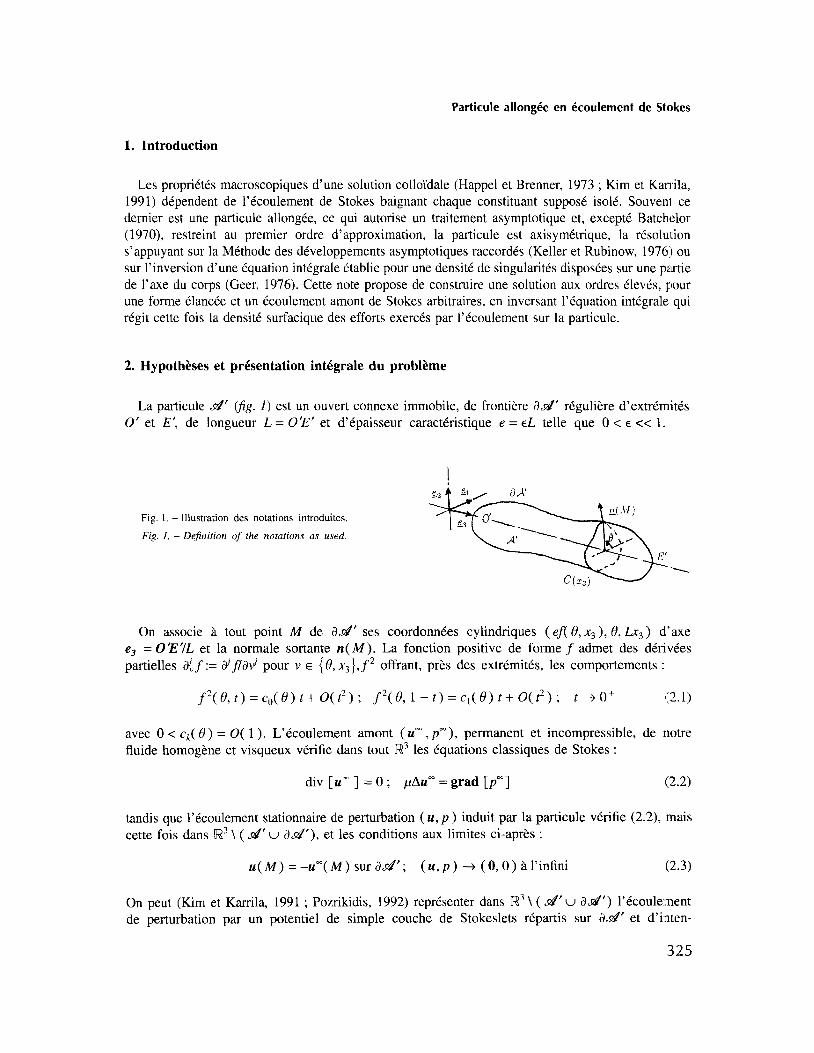
La particule &’ (fig. 1) est un ouvert connexe immobile, de front&e ad’ reguliere d’extremites 0’ et E’, de longueur L = O’E’ et d’epaisseur caracteristique e = EL telle que 0 < E <:< 1.

Fig. 1. - Illustration des notations introduites.

Fig. I. - Definition of the notations as used.

On associe a tout point A4 de ad’ ses coordonnees cylindriques ( ef( 8, x3), 8, Zxs) d’axe = O’E’IL et la normale sortante n(M). La fonction positive de forme f admet des derivees

2 offrant, p&s des extremitts, les comportements :

f2(f?,t)=C~(o)t+O(ry f2(&1-t)=c,(e)t+O(t2); t-o+ 112.1)

avec 0 < ck( /3) = 0( 1 ). L’ecoulement amont (urn , pm ), permanent et incompressible, de notre fluide homogene et visqueux verifie dans tout lw3 les equations classiques de Stokes :

div [u”] =O; pAu”=grad [p”] ((2.2)

tandis que l’ecoulement stationnaire de perturbation (u, p) induit par la particule verifie (2.2), mais cette fois dans [w3 \ (&’ u ad’), et les conditions aux limites ci-apres :

u(M) =-u-(M) surJ&‘; (24,~) + (0,O) Bl’infini (2.3)

On peut (Kim et Karrila, 1991 ; Pozrikidis, 1992) rep&enter dans Iw3 \ ( d’u a&‘) 1’Ccoule:ment de perturbation par un potentiel de simple couche de Stokeslets repartis sur a&” et d’i-nten-

325

A. Sellier

site f=g.n si CT designe le tenseur des contraintes associt a I’ecoulement total (u” + u,p- +p). En usant du repere orthonorme ( O’, e, , e2 , es) il vient, pour ME R3\(d’uad’):

8qm(M).ei =- ss

(a,If’M+ [PM.e;] [PM.e,]/PM3}f,(P) dSL ad’ (2.4)

47c~(M) =- ss

PM. f( P)lPM3 dS; dd’

(2.3

Cet ecoulement (u. p ) est evanescent a l’infini tandis que (2.4) reste valable par continuite sur ad’, ce qui procure, via (2.3), l’equation integrale de Fredholm de premiere espece d’inconnuef

8quu”(M) .ei = ss

{S,IPM+ [PM.ei] [PM.~,]/PM’}~,(P)~S~;ME f&l’ (2.6) a.!&

Comme ss ’

Urn . n dS6 = 0 l’equation (2.6) admet des solutions (Dautray et Lions, 1!988) de

forme gtn&%e f, + Rn, oti f, est une solution particulihe et 1 une co&ante arbitraire. Par linearite nous retenons la solution f lineaire de (urn, pm), sous reserve d’imposer Cgalement pour pm une expression lineaire en urn , ce qui definit la pression totale pm + p modulo une constante.

3. kcriture asymptotique de l’bquation intkgrale de frontiitre

Desormais i ou k parcourent { 1, 2, 3) et j ou 1 decrivent { 1, 2). Pour M( x1, x2, x3 ) voisin de d’ avec O’MIL = exj ej +x3 e3 on suppose que l’ecoulement amont a pour vitesse caracteristi- que U et s’ecrit Urn (M) = CJvl( M) ei = UuT( ExI, exz, x3) ei avec l’approximation suivante :

~~(M)=ff~~(x~)+~~a~~~(x~)~,+a~‘(~~)x~]+0(~~); ~‘(~~)=O(l)sij+I~l (3.1)

L’hypothese div [urn ] = 0 impose : ui,” + u$ ’ + at &” = 0. L’usage de nos coordormees cylindriques permet de reecrire en fonction de E le second membre de (2.6). A ce titre il vient :

h(P)G=GAJkl (&,~jdQ&$; s,(0,x3)=(l +(f’f~~)‘+(~~~.~)~)~‘* (3.2)

Introduisons la nouvelle inconnue d = di ei telle que :

87wW P > = elfSEfl ( P > = 43,fl ( b, 6 1 (3.3)

En rep&ant chaque point M de a&’ par le couple (8, xg ), l’equation integrale (2.6) devient :

vi( 0, x3) = s

t” {A;;“[dJ + E2-6c3-d~3A$~[hik( 8,, 4, 8, x3) d, ]} do, (3.4)

si les nouvelles fonctions hik et l’operateur lineaire A:;: obeissent pour n entier non nul, 1’ une fonction regulibe et M( 8, x3 ) = M( x1, x2, x3 ) a :

hik(UP,~,~,X3)=(~-xXi)(~---Xk) (3.5)

Af$[v] := s 44Y G 0 [(~-X3)2+E2HZ(ep,~,B,Xj)]n’*= -1) s I -.x3 u( u + x3 ) du [U2+E2h2(U)y2 (3.6)

326

Particule allong~e en ecoulement de Stokes

tandis que Ia fonction h( U) vCrifie h( u ) = H( S,, u + xs, 8, xj ) avec la definition ci-ap& :

H( OPT 43 03 x3 > := {f2( 474 > +f2( 0, x3 > - 2 cos ( 0, - S)f( o,, x(yf( 8, x3))“2 (3.7)

Si BP f B alors H > 0, ce qui permet de choisir pour presque tout le domaine de l’integrale (3.4) des inttgrales A;z[v] ‘g 1” re u meres des que E > 0. Mais A:;?[ v] devient hypersinguliere pour E = 0 et l’etablissement de son comportement asymptotique pour E petit s’avere t&s ardu lorsqu’on utilise la technique des Developpements asymptotiques raccordes (Van Dyke, 1975). Une autre methode systematique (Sellier, 1996) s’applique ici et m&e, pour v,~ = Max,a, ,I Iv/, B :

s 2x

A$z[v] dO, =&s Zt:[ ]/ v o E2+z;~.[v]logE+z~;‘[v] +o(v,E*logE); FZE {1,3} (:3X)

avec, si pf designe la par-tie finie au sens d’Hadamard (Schwartz, 1966), les operateurs suivants :

z-y; 1 [ v ] -=-

2 s *n v( Op, x3 ) dZ3, ;

Z$Y[v] 0

+-- = s 2n v( 0,, x3 ) dBP

H2( B,, x3,8, x3 > (3.9)

o

s

V,J~ldt+~ s

2n Zf;,[v] log 2 +pf

log W 6, x3, 8, x3 > -

+x31 0 v-Y 6% x3 ) de,

0 (3.10)

Z@[v] = -pf s

’ I;J[V] dt d2

0 2]t-x,13 -2 1 + log

H( 6, t, 6 x3 )

2 v( 6, t ) de, I f = xg

(3.11)

Comme I;; 1 [v] et I@[ v] n’impliquent que la trace de v sur la section C( xs ) = {P E a& ; -$ = x3} passant par M( Q, x3 ) ce sont des contributions bidimensionnelles. Le terme Z;i3[v] est faiblement tridimensionnel mais ~2-y [v] et Z2 ;‘[ v] concernant v sur tout a&’ sont fortement tridimensionnels. Pour Di = Maxdd, Idi( l’alliance de (3.4) et (3.8) procure :

V~(~tX3)=I;tl[dj] lOgE+I$;‘[dj] +Ity{($‘-s~i) [($-~,)dl +($-~2)d2]}

+E[z~;3+z;~310gc] [(~‘Xj)(~-Xx,)d3]+O(D1,D2,ED3)E210gE; jE {1,2} (3.12)

vy(&x3)={l;;,[d31 +~;~3[(~---3:~2d31}logE+z~~[d3] +z@[(4-x3>2d3]

+E[Z2;‘+Z;;slogE] [d,(&x,)+d*($-xx,)] +O(ED,,ED2,D3)E210gE (3.13)

Pour Ctablir ce resultat, nous avons aussi exploite 1’CgalitC I@[ w( $ - x3 ) ] = 0, valable [Cq. (3.9)] pour toute fonction w( $ ) regulitre au voisinage du point x3.

4. Approximation asymptotique de la den&C surfacique de forces

A la lueur du systeme (3.12)-(3.13) et de (3.1) cherchons alors chaque solution di sous la forme :

di( 8, X3) = ~ ~ cfs 0 .,,,I (~,x,)~“[log~]-“+o(~210g~); d&:=fiotnTm (4.1) t” n=om=lLn

327

A. Sellier

Sur toute section C( x3 ) notons que dlP =fs,, d0, et definjssons pour M( 8, xX) E C( x3) un operateur K”’ et deux equations integrales de premiere espbce, de donnees b et (b, ; b, >, par :

Kx3[u] = &,,, u(P) dip ; L”.“‘[u] = -$c(sgI log [PM] u(P) dl, = b(M) (4.2)

syy u, ; U2)=&-r3){4~llog [PM] + [PM.ej] [PM.e,]IPM2}ul(P)dZ,=bj(Mj (4.3)

Les equations (4.2) ou (4.3), aussi not&e @X3( u1 ; ~1~) = SF-X3( U, ; u2) ej = [b, ; b,], correspon- dent aux formulations integrales de type potentiel de simple couche de problemes de Djrj,&]et bidimensionnels respectivement pour l’operateur de Laplace et les equations de Stokes. A ]‘inst.ar de (2.6), l’equation integrale (4.3) n’admet une solution g&&ale, cette fois definie module le vecteur rP, normale sortante a C(nj), que si $ (3.12)-(3.13) mene pour &

ccX,) bl el . nzd dl, = 0. L’injection de (4. I.) dans := 0, IZ E (0, 1 } et m 2 0 aux jeux suivants de relations r&urentes :

K”“[&J =-ay(x,)/2’+d~3; K”‘[t;,,] =o (4.4)

sj%jl,m, t,,> = Kytjn,m+l 1 - V~~(0){K’[tj,,,l}+6,,/2(S,,[a~““(X3)X, +~,o*1(x,)~21 -I~~l(~-Xj)(~---Xg)d~,,+Il +(6,0-1)z~~[(~“-xj)(~-X3)d~,,J) :zb’,xml:@.‘X3)

(4.5) L8q$J = K*qjn,m+l l-~*~~~~~~I~‘C~‘,,,l}+~,o~4~~,,,C~:~o~~~~~,+~30~‘~~~~~;!1

-Td(&xd C&-J &,t+, } + Cd,,- l>Z~t?{i+x3) [+x1] d;.,}) :=b:,,(8,.r3)

(4.6)

ou pour a reel et une fonction reguliere a, I’operateur lineaire Vx,( a) {a(t)} obeit ?t :

s

l o(t)dt V,,(a){@)}= k%2-a14~3)+PS y-q-4 (4.7)

0

Les liens (4.5)-(4.6) constituent un systbme pyramidal bien pose (l’auteur a v&if% pour chaque Cb A, m ; bz, ,] la condition anterieure de compatibilitt) permettant de construire en cascade sons les conditions (4.4) et en ne retenant pour (4.5) que la solution linkire en [ 6:. m ; bi, ,] les qwmtit& K”‘[$,,] et &,,. Definissons pour toute section C(X,) les solutions particulieres uo, t’ = (4 ; r$), les reels non nuls c0(n3 ), A(x3) et les operateurs AX3 et Bx3 par :

si (vd-d; %(-x3)) =A3 h(t) 0.k =O

i%(f)) et (wI(x~);w~x~))=B,, (a,(t);aZ(t)). Si *3 x3 OOz3-’ pour k>l et Oz3[a(t)] =a(+) il vient, pour ~7~2 1:

“-‘{&“(t)}uO; t~,m=b;,,tjl+b;,,$ (4.12)

328

Particule aHong6e en Ccoulement de Stokes

2(K”‘[&J ;K”~[~,~])=-B~-‘(a~“(t);a~~o(t));

(h!,,,; bi,,wJ =A, W'~&nl ; ~'P?i,,l 1 (4.13)

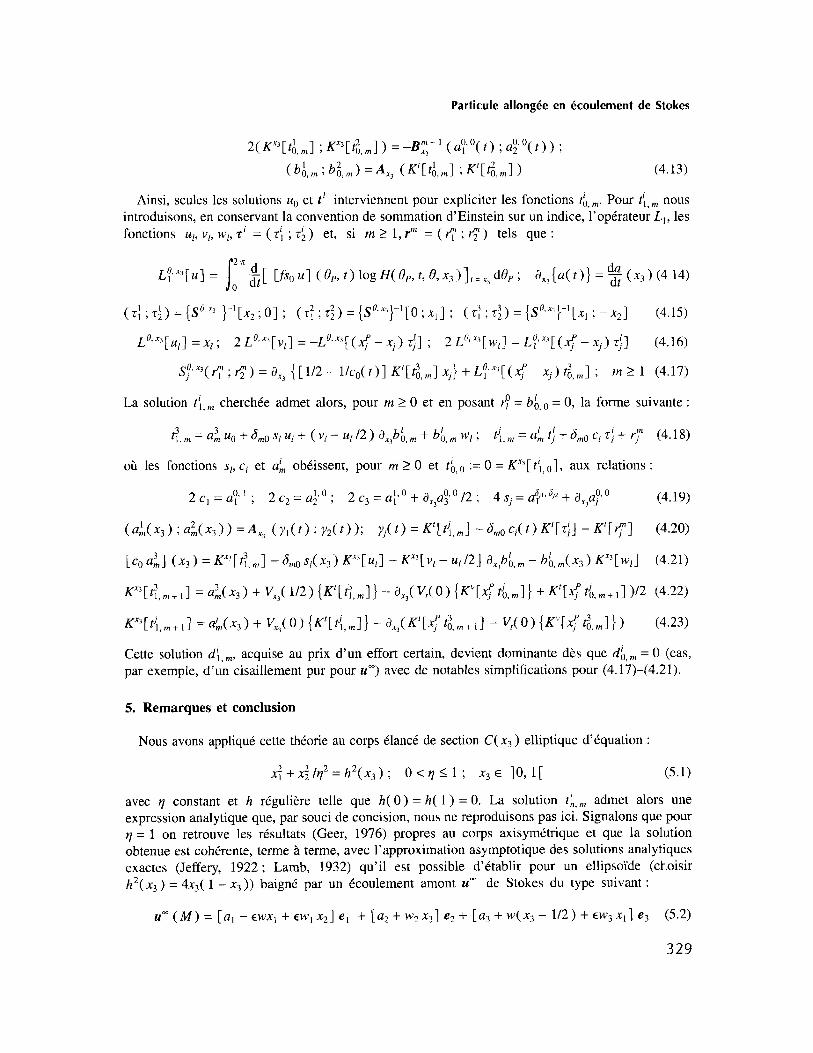
Ainsi, seules les solutions u. et t’ interviennent pour expliciter les fonctions &,,. Pour ti,, nous introduisons, en conservant la convention de sommation d’Einstein sur un indice, l’optrateur L,, les fonctions ul, vI, We, 7i = ( zi ; zk) et, si mll,P =(q’;$) tels que:

s

2n

pqu] = o $[ v‘sou] (8,,t)logH(8,,t,8,x,)],=,dB,; aXT{a(r)}=%(xj)(414)

(71 ; T:) = {SUJJ }-‘[x2 ; O] ; (T: ; z;) = {s”~*‘}-~‘[o ; x,] ; (zi’ ; T;) = {s”‘“}-‘[x, ; -x2] (4.15)

LUJ3[uJ =x,; 2L0’“3[V,] = -LUJq(xp -x;) $1 ; 2P”[y] = LyJ’[($ -xj) T,!] (4.16)

sJ@yfl ; $ j = ax3 {[i/2 - ik,(tj] ~‘[t;,,] xj} + ~:y(xp -xj) f;,,] ; M 2 I (4.17)

La solution t;,, cherchCe admet alors. pour m 2 0 et en posant $ = bb,, = 0, la forme suivante :

~,m=a~uo+6,0s,ui+(v,-~~l/2)~x,b~,,+b~,,w,; tj,,=nl,r~+~~o~j~j+r,~ (4.18)

oti les fonctions sI, ci et ub obCissent, pour m 2 0 et t&o := 0 = ZP[r;, o], aux relations :

2 Cl = uy ’ ; 2 c2 = L22 O ; 2 c3 = u) O + ax3uy O I2 ; 4 sj = Up~J? + a&~ O (4.19)

(dn(~d;d,(x,j)=A,~ (y,tf);dtjj; ;;.(t>=K’[tj,,] -&,&)K’[z;] -K’[y] (4.20)

[cod1 (~3) =~Y$nl -~,o~I(x~)~~~[~II -WV,- 4/21 ax~bb,m-bb,,(x3)KX’[W11 (4.21)

fW-?,,+ I I =~~(~3>+v,~(1~2~{~‘~~~.,l}-~,(vf~o~{~~C~~j,,,l}+~~~X;P~jO,m+ll~~2 (4.22)

~x3Pl,m+l 1 =a’,(X3)+VX3(0){Ktrf~,ml}-a,(K’[~’,,+,l -ww”bpiLIl}) (4.23)

Cette solution d’,, m, acquise au prix d’un effort certain, devient dominante d?s que df, m = 0 ((cas, par exemple, d’un cisaillement pur pour u”) avec de notables simplifications pour (4.17)-(4.21).

5. Remarques et conclusion

Nous avons appliquC cette thkorie au corps Clan& de section C( xj ) elliptique d’Cquation :

$+~//r2=h2(xg); O<Pjll; XjE ]O,l[ ((5.1)

avec q constant et h rCguliitre telle que h( 0) = h( 1) = 0. La solution th,,, admet alors une expression analytique que, par souci de concision, nous ne reproduisons pas ici. Signalons que pour q = 1 on retrouve les resultats (Geer, 1976) propres au corps axisymCtrique et que la solution obtenue est cohCrente, terme ti terme, avec l’approximation asymptotique des solutions analytiques exactes (Jeffery, 1922 ; Lamb, 1932) qu’il est possible d’Ctablir pour un ellipso’ide (choisir h2( x3) = 4x3( 1 - x3)) baignC par un Ccoulement amont urn de Stokes du type suivant :

uoo (M) = [al - EWX, + EW,X~] el + [a2 + w2x3] e2 + [a3 + w(x3 - l/2) + EW~X,] e3 (5.2)

329

A. Sellier

La densite auxiliaire d presente un developpement (4.1) uniforme pour x3 E IO, 1 [ qui permet d’obtenir le comportement de quantites integrees d’interet pratique : force ou moments riisultants d’ordre quelconque exerces sur la particule, approximation uniforme dans R3 \ ( .&’ ’ u &d ‘) de l’tcoulement (u, p) induit par la presence de celle-ci en exploitant (2.4)-(2.5).

Enfin la methode d&rite possede l’avantage de s’appliquer au cas utile, mais rarement trait& du corps non axisymetrique et de permettre l’acds, grace a la formule systematique de developpement d’une integrale en fonction d’un petit parametre (Sellier, 1996), aux ordres ClevCs d’approximation en Cvitant les delicates regles de raccord de la methode des Developpements asymptotiques raccordes.

Remerciements. L’auteur remercie le Professeur J. P. Guiraud pour I’intCr&t qu’il a port6 B ce travail.

Note remise le 7 avril 1997, acceptee aprbs hision le 11 juin 1997.

.RCf&ences bibliographiques

Batchelor G. K., 1970. Slender-body theory for particles of arbitrary cross-section in Stokes Row, J. Fluid. Mech., 44, 419-440. Dautray R., Lions J. I,., 1988. An&se mathkmmatique et cakul nume’rique, 6, Masson. Geer J., 1976. Stokes flow past a slender body of revolution, .I. FLuid. Mech., 78, 577.600. Happel J., Brenner H., 1973. Low Reyno[d.r number hydrodynamics, Martinus Nijhoff. Jeffery G. B., 1922. The motion of ellipsoidal particles immersed in a viscous fluid. Proc. Roy Sot. London Sez A, 102,

161-179. Keller J. B., Rubinow S. I., 1976. Slender-body theory for slow viscous flow, J. Fluid. Mech., 77, 705-714. Kim S., Karrila S. J., 1991. Microhydrodynamics: Principles and Selected Applications, Butterworth, Boston. Lamb H., 1932. Hydrodynamics, 6th edition, Cambridge University Press. Pozrikidis C., 1992. Boundary integral and singularity methods for linearized viscous J&xv, Cambridge University Press. Schwartz L., 1966. ThPorie des distributions, Hermann: Paris. Sellier A., 1996. Asymptotic expansion of a general integral, PI-oc. Roy. Sot. London Ser A, 452, 2655-2690. Van Dyke M., 1975. Perturbation Methods in Fluid Mechanics, Parabolic Press, New York.

330