TTHHÈÈSSEE

En vue de l'obtention du

DDOOCCTTOORRAATT DDEE LL’’UUNNIIVVEERRSSIITTÉÉ DDEE TTOOUULLOOUUSSEE

Délivré par : l’Université Toulouse III-Paul Sabatier Discipline ou spécialité : Génie Civil

Présentée et soutenue par Muazzam Ghous SOHAIL Le 14/05/2013

Corrosion of Steel in Concrete: Development of an Accelerated Test

by Carbonation and Galvanic Coupling

JURY

Dr. HDR Valérie L’HOSTIS Rapporteur CEA Saclay

Prof. Karim AIT-MOKHTAR Rapporteur Université de la Rochelle

Prof. Abdelhafid KHELIDJ Examinateur Université de Nantes

Prof. Jean-Paul BALAYSSAC Examinateur Université de Toulouse

Dr. Stéphane LAURENS Examinateur Université de Toulouse

Dr. Fabrice DEBY Examinateur Université de Toulouse

Ecole doctorale : Mécanique, Energétique, Génie civil et Procédés (MEGeP)

Unité de recherche : Laboratoire Matériaux et Durabilité des Constructions (LMDC) Directeur de Thèse: Jean-Paul BALAYSSAC Co-directeur: Stéphane LAURENS Co-directeur: Fabrice DEBY

I

Acknowledgement If I am writing an acknowledgement of my Ph.D. thesis, it is only by the grace of mother

and my father, who have worked so hard to make me what I am today. I dedicate this

thesis to my parents and all those parents who introduce their children to the wisdom of

knowledge. Then I thank to my sisters Farah and Uzma and my brother Ali for their love

and care, you all are my proud.

I am very thankful to my supervisors, Prof. Dr. Jean-Paul Balayssac, Dr. Stéphane

Laurens and Dr. Fabrice Deby for their utmost support during these three years of my

Ph.D. work. During all those lengthy scientific discussions, I have learnt a lot, not just

about my subject but also about the attitude towards research. I feel honored to be

working with a team full of knowledge and passion to advance in research.

I am also thankful to director of Laboratoire Matériaux et Durabilité des Constructions

(LMDC) Mr. Gilles Escadeillas for receiving me in the institute and providing me all the

facilities and equipment required to carry out this research work. I would like to thank all

the technical staff of LMDC who has helped during my work, specially Mr. Attard,

Sylvain and Carole. I pray for the prosperity of this prestigious laboratory.

I am thankful to Higher Education Commission of Pakistan (HEC) for awarding me a

scholarship and providing me this opportunity to study in France. I would also like to

thank SFERE for taking care of all the administrative matters during my stay in France.

I am also thankful to all my friends in Toulouse, specially Dr. Rashid, Dr. Rizwan, Dr.

Majid, Dr. Toufeer, Dr. Ilyas and Dr. Shahid. Then I would like to thank, Abid, Ayesha,

Inam and Tameez, their presence made my stay more pleasant. I am thankful to all my

collegues of office, Angel, Minh, Rackel, Hugo, Marie, Rémy and Raphaëlle, and a very

special thanks to Antoine, who helped me a lot during my Ph.D.

Above all I thank to God, the most Merciful and Generous, who gave me the strength and

knowledge to achieve this milestone of my life.

II

Abstract

This work presents the results of an experimental and numerical study of an accelerated

corrosion test, performed in laboratory. The acceleration of corrosion in reinforced concrete is

due to the elimination of initiation phase by an artificial environment technique. The initiation

phase takes years to undergo, if it is accelerated, the studies can be focused on the kinetics of

steel corrosion in concrete. For acceleration of initiation phase the concrete samples were kept

in a carbonation chamber set at 50% CO2 and 65% RH. The geometry used in this test is

comprised of two concrete cylinders. The inner concrete cylinder is carbonated and has a steel

bar in the center, the bar is depassivated and acts as anode (A). The outer cylinder comprised

of non-carbonated concrete, casted around the inner carbonated cylinder. Four steel bars are

embedded around centered bar at given distance in non-carbonated concrete; these bars are in

passive state and act as cathodes (C). The presence of these passive bars will allow changing

the cathode surface and hence C/A ratio, by connecting different number of bars to active bar.

The geometry for the test is defined by numerical simulations using COMSOL Multiphysics®

software, and its sensitivity in particular the effect of C/A ratio, is defined by numerical

experiments. In order to provide reliable inputs for the model the corrosion parameters are

measured. Once the geometry of the samples is defined an extensive experimental program

involving 15 samples is carried out. Despite the higher resistivity of carbonated concrete

layer, the measurements of macrocell current revealed high levels of galvanic corrosion rate

even in case of low C/A ratio. With the increase in C/A ratio the higher macrocell current

levels are achieved in propagation phase. The importance of galvanic coupling in carbonation-

induced corrosion is therefore also experimentally demonstrated.

The accordance between numerical and experimental results is demonstrated regarding both

potential field and C/A influence on macrocell current. This coherence highlights the

relevance of the numerical modeling.

Key words: Concrete corrosion, carbonation, accelerated corrosion test, macrocell corrosion

system, numerical modeling.

III

Resume

L’objectif principal de ce travail est de développer un essai accéléré de corrosion dans le

béton armé capable de bien représenter les conditions de développement de la corrosion en

environnement réel. Le test reproduit les phases d’initiation et de propagation. La phase

d’initiation correspond à la période durant laquelle les agents agressifs (le CO2 ou les ions

chlorure) pénètrent à travers le béton d’enrobage jusqu’à atteindre l’armature. La phase de

propagation se produit une fois que le béton entourant les armatures est totalement pollué par

les agents agressifs et les conditions nécessaires étant réunies, la corrosion de l’acier démarre.

Dans cette étude la phase d’initiation est accélérée en exposant le béton dans une enceinte

avec un taux de CO2 de 50% et une humidité relative de 65%. Dans la phase de propagation la

corrosion de type galvanique est accélérée en augmentant le rapport de surface entre cathode

et anode.

Les échantillons utilisés sont composés de deux cylindres de béton imbriqués. Le cylindre

interne contient une seule armature et le béton d’enrobage est entièrement carbonaté. Autour

de cette éprouvette un cylindre externe de béton est alors coulé avec quatre armatures

régulièrement réparties sur sa périphérie. Le béton du cylindre externe est préservé de la

carbonatation. Les barres externes sont donc dans un état passif et la barre interne dans un état

actif. La distance entre chaque barre du cylindre externe et la barre du cylindre interne est

identique. La connexion entre une ou plusieurs barres passives et la barre active génère un

courant galvanique qui va entraîner la corrosion de la barre active. En jouant sur le nombre de

barres passives connectées on peut donc faire varier l’intensité du courant galvanique et donc

accéléré ou ralentir la corrosion.

Pour éviter de réaliser un trop grand nombre d’essais en laboratoire, la conception de l’essai et

la définition de sa sensibilité sont effectuées par le biais de simulations numériques à l’aide du

logiciel commercial COMSOL Multiphysics® qui utilise les éléments finis. La vitesse de

corrosion de l'acier dans le béton est déduite de la densité de courant à la surface de l'acier,

qui est elle-même reliée au potentiel. La modélisation numérique de la corrosion dans le béton

implique la résolution de deux équations simultanément, l'équation du transfert de charge et la

loi d'Ohm, avec des conditions aux limites appropriées. Le comportement du système

électrochimique est décrit par l'équation de Butler-Volmer pour les aciers actifs et passifs. Les

paramètres nécessaires à l’implémentation des équations de Butler-Volmer (constantes de

IV

Tafel, potentiel et courant de corrosion) sont mesurés par le biais d’une campagne

expérimentale sur un nombre significatif d’échantillons carbonatés ou non carbonatés. Il est

ainsi possible de disposer de données réellement représentatives des conditions de l’essai

accéléré. L’essai est ensuite réalisé en conditions de laboratoire et les résultats sont analysés et

comparés aux calculs du modèle numérique.

Le premier chapitre de la thèse est dédié à une revue bibliographique sur les phénomènes liés

à la corrosion dans le béton armé. L'électrochimie qui exprime le phénomène de corrosion et

la cinétique de Butler-Volmer de corrosion de l'acier (métal) sont présentées. Ensuite, les

méthodes de caractérisation de la corrosion de l'acier dans le béton sont discutées. Les

modèles numériques disponibles dans la littérature jusqu'à présent sont détaillés, en focalisant

sur ceux qui prédisent la densité de courant de corrosion d'une barre d’acier en utilisant la

cinétique de Butler-Volmer. A la fin, les tests accélérés utilisés par les différents chercheurs

sont présentés et analysés.

Le deuxième chapitre est consacré à la mesure des paramètres nécessaires pour modéliser la

corrosion dans le béton armé. Les paramètres tels que le potentiel de corrosion, la densité de

courant de corrosion, les coefficients de Tafel anodique et cathodique sont obtenus à partir des

courbes de polarisation. Pour obtenir ces courbes de polarisation des expériences de Tafel

sont effectuées sur des échantillons cylindriques de béton carbonaté et non carbonaté.

L’influence de la vitesse de balayage a été en particulier étudiée. Dans certaines conditions,

les résultats obtenus montrent une variabilité relativement importante des paramètres de Tafel.

Dans le troisième chapitre, la conception du test de corrosion accélérée proposé est présentée.

La géométrie numérique et expérimentale de l'échantillon utilisée pour ces tests est élaborée.

Dans les expériences numériques, la variation de la surface polarisée sur l’acier actif en

fonction du nombre d’aciers passifs connectés est particulièrement bien démontrée. A l'aide

des simulations numériques, une étude paramétrique a été réalisée et l’incidence des différents

paramètres de corrosion sur le courant galvanique est observée. L’influence de la résistivité

du béton sur l’intensité du courant galvanique d’une part et sur la polarisation de barres

d'acier actif et passif d’autre part est également soulignée.

Le quatrième chapitre présente les résultats expérimentaux obtenus durant la phase de

différents essais mettant en œuvre 15 éprouvettes. L'accélération de corrosion à la propagation

a été réalisée en augmentant le nombre de barres passives connectées suivant deux

V

configurations. Un dispositif expérimental original a permis de suivre l’évolution du courant

galvanique au cours de la durée de l’essai. Les résultats confirment bien les prévisions du

modèle, en particulier l’influence du nombre de barres passives connectées sur la polarisation

de la barre active. Les courants galvaniques obtenus sont ensuite comparés aux résultats du

modèle et les tendances sont également confirmées. Des autopsies pratiquées sur certaines

éprouvettes ont permis de comparer la masse de produits de corrosion formés à la masse

calculée à partir de la loi de Faraday en faisant intervenir le courant galvanique et le temps

d’exposition.

VI

TABLEOFCONTENTS

INTRODUCTION …………………………………………..1

1 STATEOFTHEART…………………………………….4

1.1 Electrochemistry involved in corrosion ................................................................................................... 4 1.1.1 Thermodynamics ..................................................................................................................................4 1.1.2 Nernst Equation ....................................................................................................................................5 1.1.3 Pourbaix Diagram ..................................................................................................................................6

1.2 Kinetics Involved in Corrosion Process .................................................................................................... 9 1.2.1 Butler-Volmer kinetics ..........................................................................................................................9 1.2.2 Polarization Behavior ..........................................................................................................................11 1.2.3 Tafel Slope Constants ..........................................................................................................................11 1.2.4 Faradays Law .......................................................................................................................................13

1.3 Corrosion of steel in Concrete ............................................................................................................... 14 1.3.1 Causes of Corrosion in Concrete .........................................................................................................16

1.3.1.1 Carbonation of Concrete .......................................................................................................... 16 1.3.1.2 Chloride ingress in concrete ..................................................................................................... 17

1.3.2 Uniform Corrosion ..............................................................................................................................17 1.3.3 Localized corrosion .............................................................................................................................18

1.4 Corrosion measurement Techniques ..................................................................................................... 19 1.4.1 Half-cell Potential ................................................................................................................................19 1.4.2 Linear Polarization Resistance Technique (LPR) .................................................................................22

1.4.2.1 Basic Theory ............................................................................................................................. 22 1.4.2.2 Equipment required for Rp measurements .............................................................................. 23

1.4.3 Tafel Extrapolation Technique ............................................................................................................25 1.4.4 Electrochemical Impedance Spectroscopy ........................................................................................25

1.5 Simulation of Reinforced concrete corrosion ........................................................................................ 28 1.5.1 Empirical Models ................................................................................................................................29 1.5.2 Numerical Models ...............................................................................................................................30

1.5.2.1 Equivalent Resistor model ........................................................................................................ 30 1.5.2.2 Models based on Butler-Volmer Equation ............................................................................... 31 1.5.2.3 Modified Butler-Volmer Equation ............................................................................................ 32 1.5.2.4 Limiting Current ........................................................................................................................ 33

1.6 Accelerated Corrosion Testing ............................................................................................................... 35 1.6.1 Artificial Climate Technique ................................................................................................................36 1.6.2 Impressed current technique/ Galvanostatic method ........................................................................37

2 CHARACTERIZATIONOFCORROSION

PARAMETERS ……………………………………………….42

2.1 Introduction .......................................................................................................................................... 42

VII

2.2 Experimental Procedure ........................................................................................................................ 43 2.2.1 Material characteristics ......................................................................................................................43 2.2.2 Sample preparation ............................................................................................................................45 2.2.3 Sample conditioning ...........................................................................................................................46

2.3 Measurement set up ............................................................................................................................. 49 2.3.1 Three electrode set up ........................................................................................................................49 2.3.2 Experimental Program ........................................................................................................................50 2.3.3 IR Compensation .................................................................................................................................54 2.3.4 Polarization Curves and Extrapolation: ...............................................................................................57

2.4 Experimental Results ............................................................................................................................ 62 2.4.1 Corrosion Potential Distribution .........................................................................................................62 2.4.2 Corrosion Current density ...................................................................................................................64 2.4.3 Anodic Tafel slope in carbonated and Non-carbonated sample .........................................................67 2.4.4 Cathodic Tafel slope in carbonated and Non-carbonated samples ....................................................68

2.5 Conclusions ........................................................................................................................................... 69

3 DESIGNOFACCELERATIONCORROSION

TEST …………………………………………………………..70

3.1 Introduction .......................................................................................................................................... 70

3.2 Details of the test .................................................................................................................................. 71 3.2.1 Geometry of Sample ...........................................................................................................................71 3.2.2 Sample preparation and conditioning ................................................................................................72

3.3 Corrosion measurements ...................................................................................................................... 74

3.4 Microcell and Macrocell Corrosion Systems .......................................................................................... 75 3.4.1 Microcell/Uniform corrosion system ..................................................................................................75 3.4.2 Macrocell/Galvanic corrosion system .................................................................................................78

3.5 Numerical Model details ....................................................................................................................... 80 3.5.1 Geometrical model .............................................................................................................................80 3.5.2 Electrokinetics equations ....................................................................................................................80 3.5.3 Boundary Conditions...........................................................................................................................81 3.5.4 Simulation parameters........................................................................................................................81

3.6 Numerical results .................................................................................................................................. 82 3.6.1 Face to face polarization .....................................................................................................................82 3.6.2 Potential distribution ..........................................................................................................................84 3.6.3 Galvanic current in corrosion specimens ............................................................................................85

3.7 Parametric study ................................................................................................................................... 86 3.7.1 Effects of Corrosion current densities of Active (jacorr) and Passive (jpcorr) steel ............................87 3.7.2 Effects of corrosion potential of active and passive steel ...................................................................89 3.7.3 Effects of anodic and cathodic Tafel slope coefficients for active steel .............................................90 3.7.4 Effects of anodic and cathodic Tafel slope coefficients for passive steel ...........................................91 3.7.5 Effects of concrete resistivity ..............................................................................................................93

3.8 Conclusions ........................................................................................................................................... 96

VIII

4 EXPERIMENTALANDNUMERICAL

VALIDATIONOFACCELERATEDCORROSION

TEST …………………………………………………………97

4.1 Introduction .......................................................................................................................................... 97

4.2 Experimental program .......................................................................................................................... 97 4.2.1 Configuration A ...................................................................................................................................98 4.2.2 Configuration B ................................................................................................................................ 101

4.3 Comparison of numerical and experimental results ............................................................................ 101 4.3.1 Potential range of active and passive bars ...................................................................................... 101 4.3.2 Potential mapping on experimental sample and potential field with numerical simulations ......... 103 4.3.3 Accelerated Macrocell current in corrosion specimens................................................................... 106

4.3.3.1 Numerical calculations of macrocell current .......................................................................... 106 4.3.3.2 Experimental measurements of macrocell current ................................................................ 108

4.3.3.2.1 Results of configuration A .................................................................................................. 108 4.3.3.2.2 Weight Loss measurements ............................................................................................... 116 4.3.3.2.3 Results of configuration B .................................................................................................. 119

4.4 Conclusion .......................................................................................................................................... 122

5 CONCLUSIONSANDPROSPECTS ……….123

6 REFERENCES ………………………………………127

IX

LISTOFFIGURES

Figure 1-1 Activation Complex, showing transfer of ions into solution (Cefracor, n.d.) .......................... 4

Figure 1-2 Pourbaix diagram for Iron ...................................................................................................... 7

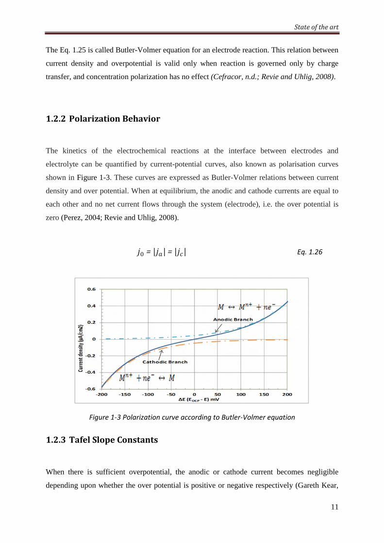
Figure 1-3 Polarization curve according to Butler-Volmer equation ..................................................... 11

Figure 1-4 Plot of log || against or Tafel plot showing the exchange current density can be

obtained with the intercept ................................................................................................................... 12

Figure 1-5 Schematic diagram of corrosion process in concrete ........................................................... 14

Figure 1-6 Schematic of rust production at steel-concrete interface .................................................... 15

Figure 1-7 Schematic of uniform corrosion in concrete (Hansson et al., 2007) ..................................... 18

Figure 1-8 Schematic of localized corrosion in concrete (Hansson et al., 2007) ................................... 18

Figure 1-9 Schematic showing basics of the half-cell potential measurement technique .................... 19

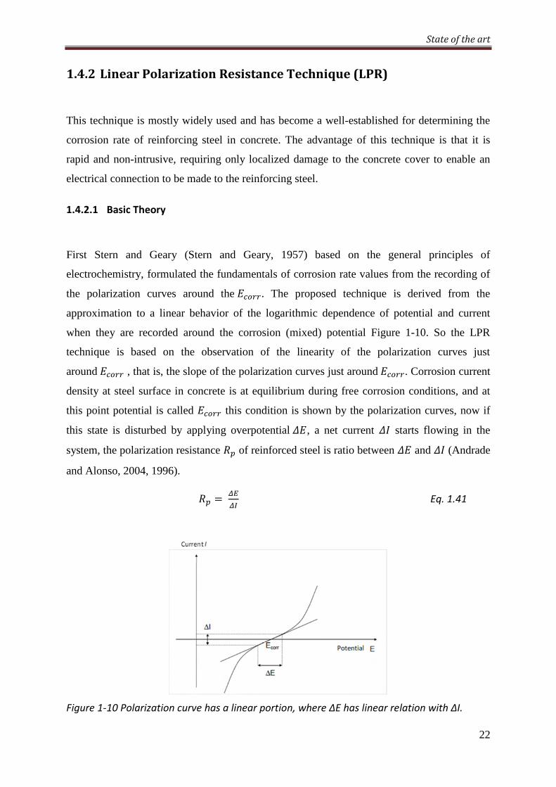
Figure 1-10 Polarization curve has a linear portion, where ∆E has linear relation with ∆I. .................. 22

Figure 1-11 Equipment and measurement set up for LPR technique .................................................... 24

Figure 1-12 Linear polarization resistance measurements with confining guard rings (Ha-Won Song,

2007) ...................................................................................................................................................... 24

Figure 1-13 Polarization curve to measure Tafel slope coefficients and corrosion current density

(McCafferty, 2005). ............................................................................................................................... 25

Figure 1-14 Equivalent circuit for concrete sample ............................................................................... 27

Figure 1-15 Nyquist plot for a simple corroding system. ....................................................................... 28

Figure 1-16 Simplified model of reinforced corrosion ........................................................................... 30

Figure 1-17 Concentration profile of reactants near electrode surface (Tanner’s Chemistry, n.d.) ...... 33

Figure 1-18 Polarization curve showing Limiting current due to diffusion of reactant. ........................ 34

Figure 1-19 Tuutti corrosion model ....................................................................................................... 36

Figure 1-20 Schematic of Galvanostatic technique to induce corrosion (Yingshu Y, 2007)................... 37

Figure 1-21 Accelerated corrosion test setup used by (El Maaddawy and Soudki, 2003) ..................... 38

Figure 1-22 Arrangement of Accelerated corrosion test by (Ahn, 2001). .............................................. 39

Figure 1-23 Set up used by (Ahmad, 2009)............................................................................................ 40

Figure 1-24 Sample geometry for Galvanic corrosion test b) sample is merged into water during the

experiments (Fortuné, 2009). ................................................................................................................ 40

Figure 1-25 Galvanic samples with active and passive bars (Fortuné, 2009) ........................................ 41

Figure 2-1 Cylindrical mould with spacer .............................................................................................. 44

Figure 2-2 a) Steel bar before treatment, oxide layer is covering the steel surface b) Steel bar after

mechanical treatment of brushing ........................................................................................................ 44

Figure 2-3 Sample preparation before pouring of concrete .................................................................. 45

Figure 2-4 Final shape and size of lollypop samples .............................................................................. 46

Figure 2-5 Samples in controlled environment ...................................................................................... 46

Figure 2-6 Carbonated sample, corrosion products are visible at steel surface and nearby concrete .. 48

Figure 2-7 Non- carbonated sample; phenolphthalein test gives a pink color due to higher pH values.

Steel bar has a shining surface and no corrosion products. .................................................................. 48

Figure 2-8 Schematic of Three electrode arrangement measurements, b) Experiments underway ..... 49

Figure 2-9 Tafel experiment underway ................................................................................................. 50

Figure 2-10 Randle’s equivalent circuit model for steel in concrete ...................................................... 54

Figure 2-11Response of a carbonated sample to a galvanic pulse of 50µA .......................................... 55

Figure 2-12 Response of a non-carbonated sample to a galvanic pulse of 50µA ................................. 55

Figure 2-13 Polarization curve of a carbonated sample with and without IR compensation ............... 56

Figure 2-14 Polarization curve of a non-carbonated sample with and without IR compensation ........ 56

Figure 2-15 Polarization curve for a steel bar in carbonated sample.................................................... 58

Figure 2-16 Polarization curve for a passive bar in non-carbonated concrete ...................................... 58

Figure 2-17 Curve fit for a steel bar in carbonated concrete ................................................................. 59

X

Figure 2-18 Curve fit for a steel bar in non-carbonated concrete ......................................................... 59

Figure 2-19 Anodic polarization for steel bars in carbonated samples ................................................. 60

Figure 2-20 Cathodic polarization for steel bars in carbonated samples .............................................. 60

Figure 2-21 Anodic polarization of steel bar in non-carbonated samples ............................................. 61

Figure 2-22 Cathodic polarization of steel bar in non-carbonated sample ........................................... 61

Figure 2-23 Corrosion potential monitoring before Tafel experiments ................................................. 63

Figure 2-24 Corrosion potential distribution of steel bars in carbonated concrete samples ................ 63

Figure 2-25 Corrosion potential distribution of steel bars in non-carbonated concrete samples ......... 63

Figure 2-26 Schematic representation of the corrosion conditions of passive steel in concrete, under

different conditions of moisture content (Bertolini et al., 2004). .......................................................... 64

Figure 2-27 Corrosion current density at steel surface in carbonated samples .................................... 65

Figure 2-28 Corrosion current density at steel surface in Non-carbonated samples ............................ 65

Figure 2-29 Corrosion current density Vs Corrosion potential in carbonated samples ......................... 66

Figure 2-30 Corrosion current density Vs Corrosion potential in Non-carbonated samples ................. 67

Figure 2-31 Anodic Tafel slope coefficient βa for Active and Passive steel bars .................................... 68

Figure 2-32 Cathodic Tafel slope coefficient βc for Active and Passive steel bars ................................. 69

Figure 3-1 The preparation of specimen for accelerated corrosion tests, used mould with all the

dimensions. (Dimensions are in cm). ..................................................................................................... 71

Figure 3-2 Fixation of carbonated inner cylinder and passive steel bars into the base plate and then in

the mould. ............................................................................................................................................. 72

Figure 3-3 Accelerated corrosion test sample ....................................................................................... 73

Figure 3-4 Cross-sectional view, dimensions of galvanic corrosion specimens and experiment principle

............................................................................................................................................................... 73

Figure 3-5 Yokogawa MW100® acquisition machine ............................................................................ 75

Figure 3-6 Qualitative electrochemical behavior of active and passive systems (no electrical

connection) ............................................................................................................................................ 77

Figure 3-7 Macrocell current due to the connection of steel bars in concrete ...................................... 78

Figure 3-8 Qualitative description of the equilibrium of a 1D galvanic corrosion system (electrical

coupling between active and passive steel bars) .................................................................................. 79

Figure 3-9 Geometrical model and meshing ......................................................................................... 80

Figure 3-10 Face-to-face polarization effect (only one passive bar connected) .................................... 83

Figure 3-11 Potential field (top view) – a) One passive bar connected - b) Two passive bars connected -

c) Three passive bars connected - d) Four passive bars connected ....................................................... 85

Figure 3-12 Macrocell current density streamlines (top view of the specimens): a) one passive bar

connected, b) three passive bars connected ......................................................................................... 86

Figure 3-13 Active and passive steel bars with points Pa and Pc respectively, at these points potential

values were observed for comparison purposes. .................................................................................. 87

Figure 3-14 Effects of corrosion current density of active bar on macrocell corrosion system ............. 88

Figure 3-15 Effects of corrosion current density of passive bar on macrocell corrosion system ........... 88

Figure 3-16 Effects of change in corrosion potential of active bar (Ecorr) on macrocell corrosion system

............................................................................................................................................................... 89

Figure 3-17 Effects of change in corrosion potential of passive bar (Epcorr) on macrocell corrosion

system .................................................................................................................................................... 89

Figure 3-18 Effects of Anodic Tafel slope coefficients of active steel on macrocell corrosion system .. 90

Figure 3-19 Effects of Cathodic Tafel slope coefficients of active steel on macrocell corrosion system 91

Figure 3-20 Effects of Anodic Tafel slope coefficients of passive steel on macrocell corrosion system 92

Figure 3-21 Effects of Cathodic Tafel slope coefficients of passive steel on macrocell corrosion system

............................................................................................................................................................... 93

Figure 3-22 Effect of concrete resistivity on galvanic system variables: uniform resistivity ................. 94

Figure 3-23 Local ohmic resistance versus electrical resistivity of concrete .......................................... 95

XI

Figure 4-1 Configuration A1, : one passive bar connected with central active bar. The bar connected is

shown by a line, connecting it to central active bar. In parenthesis are the designated names of bars,

the open circuit potential of the bars is given in mV/SCE...................................................................... 99

Figure 4-2 Configuration A2: two passive bars connected with central active bar. .............................. 99

Figure 4-3 Configuration A3: three passive bars connected with central active bar. ......................... 100

Figure 4-4 Configuration A4: four passive bars connected with central active bar. ........................... 100

Figure 4-5 Statistical distribution of free potential values achieved, a) on passive steel bars, b) on

active steel bars ................................................................................................................................... 102

Figure 4-6 Schematic of experimental sample: a, b, c are points where experimental and numerical

potential values were compared ......................................................................................................... 104

Figure 4-7 Potential field collected on lateral surface of two galvanic corrosion specimens: specimen

with one passive bar connected (red) and specimen with 4 passive bars connected (blue) ............... 104

Figure 4-8 Effect of cathode-to-anode ratio on the macrocell current in simulated galvanic systems107

Figure 4-9 Experimental sample with one passive bar connected to central active bar via 1Ω resistance

of Yokogawa MW 100 ® ...................................................................................................................... 108

Figure 4-10 Macrocell current on samples with one passive bar connected to active one ................. 109

Figure 4-11 Macrocell current on samples with two passive bars connected to active one ............... 109

Figure 4-12 Macrocell current on samples with three passive bars connected to active one ............. 110

Figure 4-13 Macrocell current on samples with four passive bars connected to active one ............... 111

Figure 4-14 Effect of increase in No. of passive bars on macrocell current in configuration A. .......... 111

Figure 4-15 Quantitave illustration of two passive systems with different corrosion parameters ..... 114

Figure 4-16 Influence of Cathodic Tafel slopes coefficient on macrocell corrosion system ................ 114

Figure 4-17 Sample 4C-31 after autopsy, on the active bar corrosion products are clearly visible

travelled into concrete volume ............................................................................................................ 115

Figure 4-18 Sample 4C-30 after autopsy, on the active bar corrosion products are only formed at steel

concrete interface ................................................................................................................................ 115

Figure 4-19 Active steel bars of sample 4C-31 and 4C-30, just after taken out from concrete ........... 116

Figure 4-20 Steel bars after passing through Clark’s solution and Ultrasonic bath. ........................... 116

Figure 4-21 Weight loss in two samples with same number of passive bars but different current

density ................................................................................................................................................. 117

Figure 4-22 Comparison between weight loss measured gravimetrically and the weight loss calculated

by Faraday’s law. ................................................................................................................................. 118

Figure 4-23 Comparison between experimental and numerical results of Cathode/Anode ratio effect,

in case of configuration A. ................................................................................................................... 119

Figure 4-24 Macrocell current reduced gradually with the increase in the time of electrical connection

............................................................................................................................................................. 121

Figure 4-25 Macrocell current on different samples when passive bars were progressively increased

from 1 to 4 ........................................................................................................................................... 121

Figure 4-26 Experimental average values of macrocell current in case of configuration B vs cathode-

to-anode surface ratio – Comparison with numerical simulations ..................................................... 122

XII

LISTOFTABLES

Table 1-1 Selected half-cell electrodes used in practice, their potentials, given versus the Standard

Hydrogen Electrode (SHE) at 25 C and temperature coefficients (Nygaard, 2009). ........................... 20

Table 1-2 Corrosion condition related with half-cell potential (HCP) measurement............................. 21

Table 1-3-Corrosion condition according to the current calculated with Linear Polarization Resistance

............................................................................................................................................................... 24

Table 2-1- Chemical composition of steel bars (% by weight) ............................................................... 44

Table 2-2- Formulation of Concrete ....................................................................................................... 45

Table 2-3-Porosity of concrete samples (in water) ................................................................................ 47

Table 2-4 Carbonated sample with scan rate and type of applied polarization ................................... 52

Table 2-5 Non-carbonated samples with the scan rate and type of polarization applied to them ....... 53

Table 3-1 – Corrosion parameters used for simulations........................................................................ 82

Table 4-1 Free potential of both active and passive bars for all the samples (the values in bold case

are the potential of bar connected as shown in Figure 4-1 to 4-4). .................................................... 101

Table 4-2 Open circuit potential of passive and active steel bars in 4C-31 before connection and just

after disconnecting. ............................................................................................................................. 113

Table 4-3 Open circuit potential of passive and active steel bars in 4C-30 before connection and just

after disconnecting. ............................................................................................................................. 113

1

INTRODUCTION

Corrosion of reinforced concrete (RC) is a major cause of structural degradation. Maintenance

and rehabilitation of RC structures has become as important and costly as new construction.

The economic loss and damage caused by the corrosion of steel in concrete makes it the

largest infrastructure problem faced by industrialized countries in recent times. The cost of

repair to damage caused by corrosion could be around 3.5% GDP in developed countries.

Corrosion in concrete is due to the ingress of chloride ions till the steel surface or carbonation

of concrete cover. The pH of concrete pores solution is normally above 12, in such alkaline

environment an oxide film is formed at steel surface, which protects steel from corroding. The

carbonation reduces the pH of concrete below 9, which causes the breakdown of oxide

passive layer, and steel becomes depassivated and corrosion process starts.

The concrete volume provides excellent protection for steel reinforcement thanks to the high

alkalinity of concrete pore solutions. The quality of concrete cover also provides good

physical protection to steel from aggressive environment, and it takes years for aggressive

agents like CO2 and chloride ions Cl- to reach steel surface. This makes the study of corrosion

behavior, in different environments of concrete, a time taking project even in the laboratory

experiments. That is why accelerated tests are designed. They help to study the corrosion

behavior and to predict the remaining structure life for engineering purposes. According to

Tuutti’s corrosion model, corrosion process can be divided in two phases, initiation phase,

where aggressive agents penetrate through the concrete cover and reach the steel surface, and

propagation phase, where corrosion process of steel reinforcement starts and develops.

The main objective of this work was to develop an accelerated corrosion test (ACT), which

could simulate the naturally occurring corrosion in concrete structures, in laboratory

environment. The accelerated corrosion test presented in this work consists of two stages; the

first is to accelerate the corrosion process in initiation phase, which was achieved by

accelerated carbonation. While in propagation phase corrosion process was accelerated by

increasing Cathode/Anode surface ratio. The increase in cathode surface was achieved by

increasing the number of passive bars embedded in concrete.

In addition, to avoid time consuming laboratory experiments, the design of the accelerated

corrosion test was at first carried out by means of numerical simulations. The simulations

Introduction

2

were performed by using commercially available software COMSOL Multiphysics® which is

based on FEM. The corrosion rate of steel in concrete could be deduced from current density

at steel surface, which is related with potential at the steel surface. Numerical modeling of

corrosion in concrete involves the solution of two equations simultaneously; the equation of

charge transfer and the second is Ohm’s law, for appropriate boundary conditions. The

polarization behavior of electrochemical systems is described by the Butler–Volmer equation

for both active and passive steel bars. Parameters involved in equations were calculated from

polarization curves obtained from Tafel experiments on carbonated and non-carbonated

concrete samples.

The first chapter presents the state of the art in the field of corrosion in reinforced concrete.

The electrochemistry involved in corrosion phenomenon is explained. The Butler-Volmer

kinetics of steel corrosion is presented afterwards. Then, the methods of assessing the

corrosion state of steel and the methods of measurements of corrosion currents in concrete are

discussed. The numerical models available in the literature up to now are elaborated; the

models which predict the corrosion current density of a corroding bar by using Butler-Volmer

kinetics are also discussed. At the end, the accelerated tests used by researcher till present are

discussed and their techniques are described.

The second chapter is dedicated to the parameters required to model the corrosion

phenomenon in reinforced concrete. The parameters like corrosion potential, corrosion current

density, anodic Tafel slope coefficient and cathodic Tafel slope coefficients were calculated

from polarization curves. These polarization curves were obtained from Tafel experiments

performed on the cylindrical carbonated and non-carbonated concrete samples.

In third chapter, the design of proposed accelerated corrosion test (ACT) is presented. The

numerical and experimental geometry of the sample used for these tests is elaborated. The

basic theory of microcell and macrocell corrosion phenomenon is explained with the help of

polarization curves of the active and passive systems. By numerical experiments, the face-to-

face polarization effects and the effect of increase in Cathode/Anode ratio on polarization

behviour of both active and passive bars were observed. With help of these numerical

simulations a parametric study was performed on a galvanic corrosion system, hence the

effects of change in all corrosion parameters were observed. The effects of concrete resistivity

on macrocell current and on the polarization behviour of active and passive steel bars were

also observed.

Introduction

3

The chapter four presents the results of accelerated corrosion test. The acceleration in

propagation was achieved by increasing the number of passive bars in a macrocell corrosion

system. At first the effects of Cathode/Anode ratio on macrocell corrosion current found by

numerical simulations are presented. Then the results of laboratory experiments which study

the effect of Cathode/Anode ratio are discussed. A comparison between numerical and

experimental results is done to validate the corrosion model. The conclusions and perspectives

are discussed at the end.

4

CHAPTER#1

1 Stateoftheart

1.1 Electrochemistryinvolvedincorrosion

1.1.1 Thermodynamics

The iron is found in the form of oxides in natural environment. When thermal or mechanical

treatments are applied to convert iron into pure steel, it becomes thermodynamically unstable,

and always tends to revert back to its original form which is at a lower level of energy, i.e. in

the form of oxides. Hence, the steel always tends to corrode to form oxides in an environment

where humidity and oxygen are present. To understand the corrosion mechanism in concrete

it is important to discuss the thermodynamics and kinetics of an electrochemical reaction.

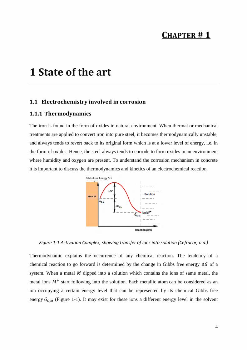
Figure 1-1 Activation Complex, showing transfer of ions into solution (Cefracor, n.d.)

Thermodynamic explains the occurrence of any chemical reaction. The tendency of a

chemical reaction to go forward is determined by the change in Gibbs free energy ∆ of a

system. When a metal dipped into a solution which contains the ions of same metal, the

metal ions start following into the solution. Each metallic atom can be considered as an

ion occupying a certain energy level that can be represented by its chemical Gibbs free

energy, (Figure 1-1). It may exist for these ions a different energy level in the solvent

State of the art

5

represented by chemical Gibbs free energy , as shown in the (Cefracor, n.d.; Revie and

Uhlig, 2008).

Due to thermal agitation, metal ions tend to jump into solution by crossing the energy barrier

that is the breakage of their electronic bonds. In Figure 1-1, the difference between

highest energy level and G,represents the energy of activation∆∗(), which is required

for the transition of metal into the solution (Perez, 2004; Revie and Uhlig, 2008).

The Eq.1.1 and Eq.1.2 are examples of iron dissolution and conversion of ferric ions into

ferrous ions. As more negative value of Gibbs free energy indicates more rapid forward

reaction, so in Eq.1.2 the reaction will go forward, but in first reaction it would not proceed

forward naturally.

+2 → ° =– .440, ° = +.880 Eq. 1.1

" + → ° = +.771, ° =– .771 Eq. 1.2

1.1.2 NernstEquation

Based on thermodynamic principle, Nernst established an equation to calculate the cell

potential or potential of an electrochemical reaction, which depends upon the activities of

reactant and products (Perez, 2004; Revie and Uhlig, 2008). When a metal is dipped into a

solution, metal ions starts moving into solution due to potential difference, however, the

presence of positive ions near the metal-water interface and excess of electrons at the metal

surface create a potential barrier and halts the further dissolution of metal ions. This creates a

dynamic equilibrium (Perez, 2004).

↔& + ' Eq. 1.3

This equilibrium corresponds to a potential, which represents potential between the metal

and the solution containing ions&. is called reversible electrode potential ()*. When

this equilibrium is formed, there is equality between the change in Gibbs free energy ∆,( of

State of the art

6

the dissolution reaction and electrical energy +,needs to cross the potential barrier Figure

1-1. For an electrochemical reaction electrical energy is written in absolute terms of Eq.1.4.

+, = ' Eq. 1.4

Where, is the Faraday number (charge of one mole of electrons: 96,500 Coulomb/mole).

The thermodynamic relation between standard Gibbs free ° and Gibbs free energy at

any instant is given by.

= ° + -./'0 Eq. 1.5

Where: - gas constant, 8.314 J/ mol. k, .temperature,0 is rate of reaction.

Since,

° =– '° Eq. 1.6

° is standard electrode potential and ' is number of electrons taking part in a reaction. The

general equation can be written as,

=– '

–' =– '° + -.1'0

= ° − 34&5 /'0 Eq. 1.7

Eq. 1.7 is Nernst equation which gives the instantaneous potential of an electrochemical cell

in terms of reaction rate0, which in turn related to the activities of products and reactants

(Perez, 2004; Redaelli et al., 2006; Revie and Uhlig, 2008).

1.1.3 PourbaixDiagram

M. Pourbaix (Pourbaix, 1974) devised a compact summary of thermodynamic data in the

form of potential-67 diagram, which relates to the electrochemical and corrosion behaviour

of the any metal in water. These diagrams have the advantage of showing at glance the

specific conditions of potential and 67 under which the metal either does not react or reacts

to form specific oxides or complex ions, i.e. the Pourbaix diagrams indicate the potential and

67domains in which a metal is stable (Cefracor, n.d.; Redaelli et al., 2006; Revie and Uhlig,

2008).

State of the art

7

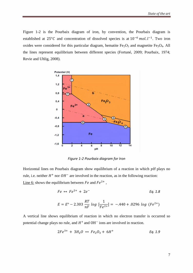
Figure 1-2 is the Pourbaix diagram of iron, by convention, the Pourbaix diagram is

established at 25°9 and concentration of dissolved species is at10:;<1. 1=. Two iron

oxides were considered for this particular diagram, hematite Fe2O3 and magnetite Fe3O4. All

the lines represent equilibrium between different species (Fortuné, 2009; Pourbaix, 1974;

Revie and Uhlig, 2008).

Figure 1-2 Pourbaix diagram for Iron

Horizontal lines on Pourbaix diagram show equilibrium of a reaction in which 67plays no

rule, i.e. neither 7 nor >7 are involved in the reaction, as in the following reaction:

Line 6: shows the equilibrium between and ,

↔ +2 Eq. 1.8

= ° − 2.303 -.' 1<@ A1

B = −.440 + .0296 1<@ (E

A vertical line shows equilibrium of reaction in which no electron transfer is occurred so

potential change plays no rule, and 7 and OHions are involved in reaction.

2" + 37> ↔ >" +67 Eq. 1.9

State of the art

8

0 = (7+E6

(3+E2 = 1<@H = 61<@ I7+J−21<@ I3+J =−667−21<@(3+E

1<@("E = −.72 − 367 , taking " = 10-6 ;<1. 1, we have 67 = 1.76.

Other lines on Pourbaix diagram give the equilibrium as shown in following equations.

Line 2: 2 + 37> ↔ >" + 67 + 2 Eq. 1.10

(E = 0.728– 0.177367– 0.059 1<@AB (E = 1.082 − .177367

Line 3: 3 + 47> ↔ ">K + 87 +2 Eq. 1.11

(E = 0.980– 0.236467– 0.0886 1<@AB (E = 1.512– 0.236467

Line 4: 2">K + 7> ↔ 3>" + 27 + 2 Eq. 1.12

(E = 0.221– 0.05967

Line 5: 3 + 47> ↔ ">K +87 + 8 Eq. 1.13

(E = 0.085– 0.05967

Line 6: ) ↔ +2 Eq. 1.14

(E = −0.440 + 0.0295 logAB (E = −0.617

Line 7: ↔ +,(E = −0.771 Eq. 1.15

Two inclined dotted lines O & P shown in Figure 1-2, these lines distinguish the three

important regions,

I. All metals having ionic concentration 10-6 ;<1. 1=, whose equilibrium potential is

located below the line O, are attacked by water with evolution of hydrogen.

+ Q7> ↔ + Q>7 + R7

State of the art

9

II. All metals having ionic concentration 10-6 ;<1. 1=, whose equilibrium potential is

located between the lines O and P are attacked in presence of oxygen in the reaction:

+ RK> +

R7> ↔ R + Q>7

III. All metals having ionic concentration 10-6 ;<1. 1=, whose equilibrium potential is

located above the lineP, are thermodynamically stable.

The oxides formed during the attack at a metal may protect the metal from further

corrosion, so metal remains in passive state, and this rust is called passive layer of oxides. In

the case of an attack at a metal by water at25°9, Pourbaix diagrams can define theoretical

areas of immunity, passivation and corrosion of the metal. The Pourbaix diagram gives no

account on the rate of an electrochemical reaction, it only gives the thermodynamic

considerations (Cefracor, n.d.; Perez, 2004; Revie and Uhlig, 2008).

1.2 KineticsInvolvedinCorrosionProcess

1.2.1 Butler-Volmerkinetics

Thermodynamics explains the concept of corrosion tendency, but it does not give any idea on

rate of corrosion, which is measured by kinetics principles. In practice we are interested in the

rate at which the corrosion reaction is taking place. The rate of a chemical reaction can be

defined as the number of moles of atoms reacting per unit time and per unit surface of an

electrode. In the case of an electrochemical reaction, which involves charge transfer, the rate

of reaction (corrosion) is calculated in terms of equivalent current or charge transfer rate,

which can presented by Eq. 1.16 (Cefracor, n.d.; Redaelli et al., 2006; Warkus and Raupach,

2006)

= 'S Eq. 1.16

Where;

: Current density of charge-transfer (T.;)

' : number of mole of electron

: Faraday constant (965009<1.;<1=) S: rate of reaction (;<1. U=.;) Applying this formula to the oxidation-reduction reaction representative of the corrosion of

any metal at equilibrium.

-V ↔ >W + ' Eq. 1.17

State of the art

10

When this equilibrium is disturbed by either anodic or cathodic polarization, the reaction rates

are given by Arrhenius law.

Anodic reaction rate: H()X9()XY6(− O∗E/-. Eq. 1.18

Cathodic reaction rate: H[\9[\Y6(− ]∗E/-. Eq. 1.19

O∗ = O^_ − `' Eq. 1.20

]∗ = ]^_ + (1 − `E' Eq. 1.21

WhereH()X and Ha\ are reduction and oxidation reaction rate constants respectively, 9()X

and 9[\ are concentrations of reacting species, O∗ and ]∗are activation energies of

anodic and cathodic reactions respectively, - is the gas constant and . is the temperature in

Kelvin (0). The electrochemical Gibbs energy of activation can be decomposed into the

Gibbs chemical activation energy ^_ (which does not depend on the potential) and

electrical energy of charge transfer. The represents the change in potential at the metal-

electrolyte interface (∆ = − ()*E, and is the coefficient of charge transfer(0 < ` <1E, which reflects the ratio of charge transfer between the two partial reactions, anodic and

cathodic. The reaction rates can be expressed by the anodic and cathodic current densities,

given below,

= Q0()X9()X Y6c−defghij k Y6 Il&534 J Eq. 1.22

= Q0[\9[\ Y6c−degghij k Y6 I− (=lE&5

34 J Eq. 1.23

For a reversible electrode at equilibrium, the current density becomes the exchange current

density, that is

a = Q0()X9()X Y6c−defghij k = Q0[\9[\ Y6c−deggh

ij k Eq. 1.24

= − = m nY6 Il&534 ( − ()*EJ − Y6 I− (=lE&534 ( − ()*EJo Eq. 1.25

State of the art

11

The Eq. 1.25 is called Butler-Volmer equation for an electrode reaction. This relation between

current density and overpotential is valid only when reaction is governed only by charge

transfer, and concentration polarization has no effect (Cefracor, n.d.; Revie and Uhlig, 2008).

1.2.2 PolarizationBehavior

The kinetics of the electrochemical reactions at the interface between electrodes and

electrolyte can be quantified by current-potential curves, also known as polarisation curves

shown in Figure 1-3. These curves are expressed as Butler-Volmer relations between current

density and over potential. When at equilibrium, the anodic and cathode currents are equal to

each other and no net current flows through the system (electrode), i.e. the over potential is

zero (Perez, 2004; Revie and Uhlig, 2008).

m = || = | | Eq. 1.26

Figure 1-3 Polarization curve according to Butler-Volmer equation

1.2.3 TafelSlopeConstants

When there is sufficient overpotential, the anodic or cathode current becomes negligible

depending upon whether the over potential is positive or negative respectively (Gareth Kear,

State of the art

12

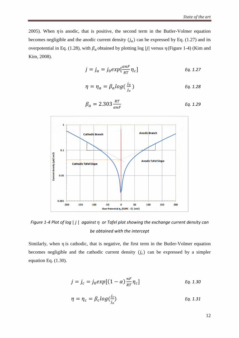
2005). When is anodic, that is positive, the second term in the Butler-Volmer equation

becomes negligible and the anodic current density (E can be expressed by Eq. (1.27) and its

overpotential in Eq. (1.28), with p obtained by plotting log || versus η (Figure 1-4) (Kim and

Kim, 2008).

= = mY6Al&534 ^B Eq. 1.27

= = p1<@(qfqrE Eq. 1.28

p = 2.303 34l&5 Eq. 1.29

Figure 1-4 Plot of log || against or Tafel plot showing the exchange current density can

be obtained with the intercept

Similarly, when η is cathodic, that is negative, the first term in the Butler-Volmer equation

becomes negligible and the cathodic current density ( E can be expressed by a simpler

equation Eq. (1.30).

= = mY6A(1 − `E &534 ^B Eq. 1.30

= ^ = p^1<@(qgqrE Eq. 1.31

State of the art

13

p^ is the cathodic Tafel slope coefficient described in Eq. 1.32. It can be obtained from the

slope of a plot of log || against ,as shown in Figure 1-4. The intercept between the two

straight lines yields the value for m (Kear and Walsh, 2005).

p^ = −2.303 34(=lE&5 Eq. 1.32

1.2.4 FaradaysLaw

Faradays law is used to quantify the mass loss due to corrosion. To determine the life of a

structure it is necessary to evaluate the mass loss as a function of time.

; = s.tgruu.v&5 Eq. 1.33

T: Atomic mass of metal (@E w a((: Intensity of corrosion current (T;6)

x: Time (sec)

': Number electrons

: Faradays constant 96500 9<y1./;<1

Mass loss is proportional to the corrosion current, mass is measured in mm/year (Ha-Won

Song, 2007; Nasser, 2010).

State of the art

14

1.3 CorrosionofsteelinConcrete Corrosion in concrete is due to ingress of chloride ions to the steel surface or carbonation of

concrete cover. The 67of concrete pore solution is normally above 12. In such an alkaline

environment, an oxide film is formed on steel surface, which protects steel from corroding. It

is referred to as steel passivation. Both carbonation and chloride ingress cause this oxide film

to breakdown (Broomfield, 2007; Elsener et al., 2003), steel is then depassivated and

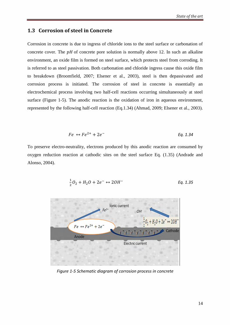
corrosion process is initiated. The corrosion of steel in concrete is essentially an

electrochemical process involving two half-cell reactions occurring simultaneously at steel

surface (Figure 1-5). The anodic reaction is the oxidation of iron in aqueous environment,

represented by the following half-cell reaction (Eq.1.34) (Ahmad, 2009; Elsener et al., 2003).

↔ + 2 Eq. 1.34

To preserve electro-neutrality, electrons produced by this anodic reaction are consumed by

oxygen reduction reaction at cathodic sites on the steel surface Eq. (1.35) (Andrade and

Alonso, 2004).

=> + 7> + 2 ↔ 2>7 Eq. 1.35

Figure 1-5 Schematic diagram of corrosion process in concrete

State of the art

15

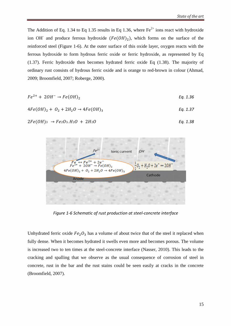
The Addition of Eq. 1.34 to Eq 1.35 results in Eq 1.36, where Fe2+ ions react with hydroxide

ion OH- and produce ferrous hydroxide ((>7EE, which forms on the surface of the

reinforced steel (Figure 1-6). At the outer surface of this oxide layer, oxygen reacts with the

ferrous hydroxide to form hydrous ferric oxide or ferric hydroxide, as represented by Eq

(1.37). Ferric hydroxide then becomes hydrated ferric oxide Eq (1.38). The majority of

ordinary rust consists of hydrous ferric oxide and is orange to red-brown in colour (Ahmad,

2009; Broomfield, 2007; Roberge, 2000).

+2>7 → (>7E Eq. 1.36

4(>7E +> + 27> → 4(>7E" Eq. 1.37

2(>7E3 → 2>3. 72> + 272> Eq. 1.38

Figure 1-6 Schematic of rust production at steel-concrete interface

Unhydrated ferric oxide >" has a volume of about twice that of the steel it replaced when

fully dense. When it becomes hydrated it swells even more and becomes porous. The volume

is increased two to ten times at the steel-concrete interface (Nasser, 2010). This leads to the

cracking and spalling that we observe as the usual consequence of corrosion of steel in

concrete, rust in the bar and the rust stains could be seen easily at cracks in the concrete

(Broomfield, 2007).

State of the art

16

1.3.1 CausesofCorrosioninConcrete

1.3.1.1 Carbonation of Concrete

Carbonation is the result of the interaction of carbon dioxide gas in the atmosphere with the

alkaline hydroxides in the concrete. Like many other gases carbon dioxide dissolved in water

to form an acid. Unlike most other acids the carbonic acid does not attack the cement paste,

but just neutralizes the alkalis in the pore water, mainly forming calcium carbonate that lies in

the pores (Fortuné, 2009; Haselbach, 2009).

9>2+ 9O(>7E2 → 9O9>3+ 72> Eq. 1.39

Normally there is a lot of calcium hydroxide in the concrete pores than can be dissolved in the

pore water. This helps maintain the 67 at its usual level of around 12or 13 as the carbonation

reaction occurs. However, eventually all the locally available calcium hydroxide (9O(>7E) reacts, precipitating the calcium carbonate and allowing the67 to fall to a level where steel

will corrode (Broomfield, 2007). The carbonation can occur even when the concrete cover

depth to the reinforcing steel is high. This may be due to a very open pore structure where

pores are well connected together and allow rapid CO2 ingress. It may also happen when

alkaline reserves in content, high water cement ratio and poor curing of the concrete.

Carbonation depth is the average distance, from the surface of concrete or mortar where the

carbon dioxide has reduced the alkalinity of the hydrated cement (Poursaee, 2007). A

carbonation front proceeds into the concrete following the laws of diffusion (Broomfield,

2007). The carbonation depth is considered to be dependent on square root of time, and a

coefficient which takes account of the concrete conditions.

Y = 0√x Eq. 1.40

Where:

x carbonation depth, t is time and K is the diffusion coefficient.

K depends upon the concrete quality, temperature, RH% and the CO2 concentration around

concrete. Depending on the concrete quality and curing condition, the carbonation depth is

different (Balayssac et al., 1995). The depth of carbonation can be determined by different

State of the art

17

techniques. As carbonation reduces the 67, therefore determination 67 of concrete by

applying 67 indicators such as phenolphthalein to a freshly fractured or freshly cut surface of

concrete can be used to estimate the depth of carbonation. Upon application of

phenolphthalein, noncarbonated areas turn red or purple while carbonated areas remain

colorless. Maximum color change to deep purplish red occurs at 67 of 9.8 or higher. Below

9.8 the colour may be pink and at 67of8 colorless (Verbeck, 1958).

1.3.1.2 Chloride ingress in concrete

Chloride ions can be present in the concrete due to the use of chloride contaminated

components or the use of 9O91 as an accelerator when mixing the concrete, or by diffusion

into the concrete from the outside environment (Broomfield, 2007). A localized breakdown of

the passive layer occurs when sufficient amount of chlorides reach reinforcing bars, and the

corrosion process is then initiated. Chlorides in concrete can be either dissolved in the pore

solution (free chlorides) or chemically and physically bound to the cement hydrates and their

surfaces (bound chlorides). Only the free chlorides dissolved in the pore solution are

responsible for initiating the process of corrosion.

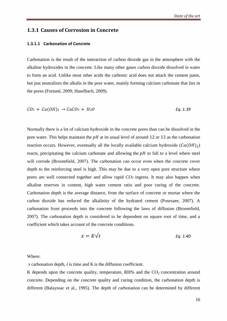
1.3.2 UniformCorrosion

When anode and cathode sites are microscopically small and spatially indistinguishable, i.e

oxidation of iron and reduction of oxygen are happening simultaneously at same place, the

corrosion is said to be uniform corrosion (Marques and Costa, 2010). Anodically and

cathodically acting surface location is not fixed and randomly changed with the time (Figure

1-7). This case is often encountered when corrosion is initiated by carbonation of concrete

(Nasser et al., 2010; Warkus et al., 2006). Whole surface of affected steel is corroded

homogenously.

State of the art

18

Figure 1-7 Schematic of uniform corrosion in concrete (Hansson et al., 2007)

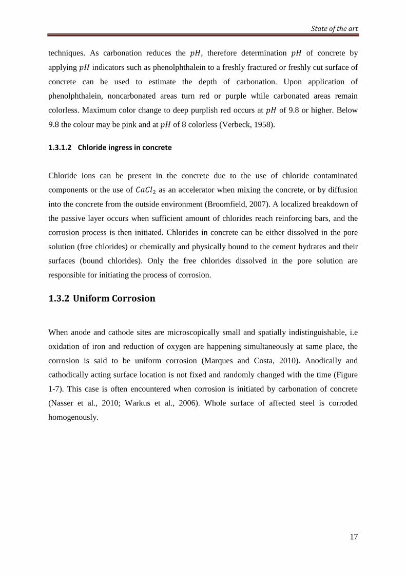
1.3.3 Localizedcorrosion

Other form of corrosion observed on steel surface in concrete is localized or pitting corrosion.

Where corrosion is concentrated on a particular area and loss in cross section of steel is much

higher than that in uniform corrosion. Anode and cathode sites are spatially distinguishable i.e

they are easily identified by electrochemical potential measurements. This form is normally

observed in chloride induced corrosion. Figure 1-8 shows the schematic of uniform and

localized corrosion phenomena (Elsener et al., 2003).

Figure 1-8 Schematic of localized corrosion in concrete (Hansson et al., 2007)

State of the art

19

1.4 CorrosionmeasurementTechniques

For measurement of the corrosion rate of reinforcing steel in concrete many electrochemical

and non-destructive techniques are available, which help to monitor the corrosion of steel in

concrete structures. Following are some common techniques used to assess the reinforced

corrosion:

1. Half Cell Potential Measurement Technique

2. Linear Polarization Resistance Technique (LPR)

3. Tafel Extrapolation

4. Electrochemical Impedance Technique

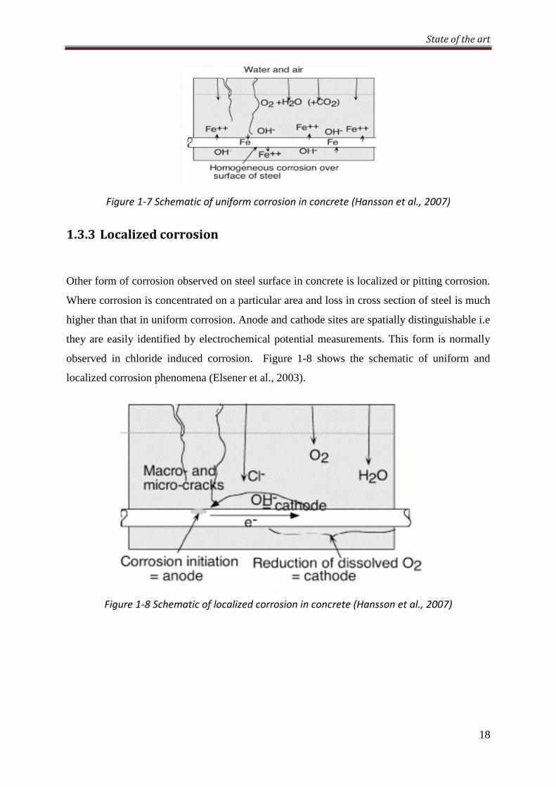
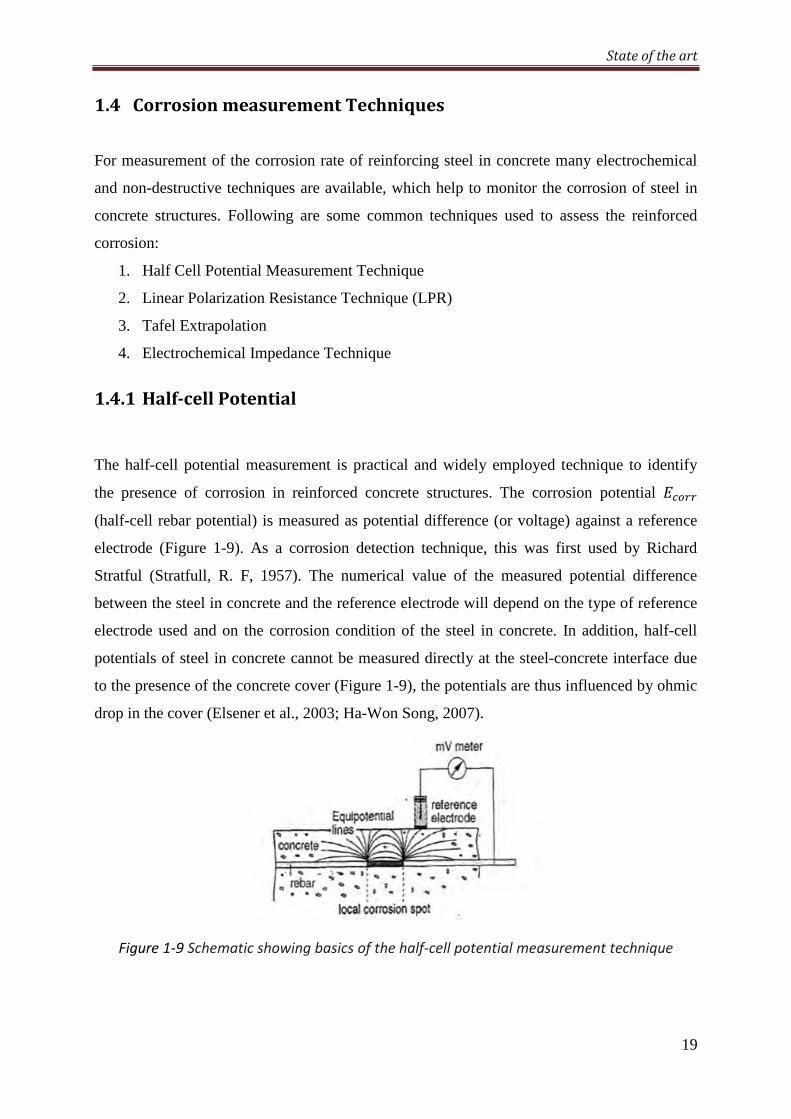
1.4.1 Half-cellPotential

The half-cell potential measurement is practical and widely employed technique to identify

the presence of corrosion in reinforced concrete structures. The corrosion potential ^a(( (half-cell rebar potential) is measured as potential difference (or voltage) against a reference

electrode (Figure 1-9). As a corrosion detection technique, this was first used by Richard

Stratful (Stratfull, R. F, 1957). The numerical value of the measured potential difference

between the steel in concrete and the reference electrode will depend on the type of reference

electrode used and on the corrosion condition of the steel in concrete. In addition, half-cell

potentials of steel in concrete cannot be measured directly at the steel-concrete interface due

to the presence of the concrete cover (Figure 1-9), the potentials are thus influenced by ohmic

drop in the cover (Elsener et al., 2003; Ha-Won Song, 2007).

Figure 1-9 Schematic showing basics of the half-cell potential measurement technique

State of the art

20

To measure half-cell potential a connection has to be made with the steel bar as shown in

Figure 1-9. The reinforcing steel bar is connected to the positive terminal of a high impedance

voltmeter, and the reference electrode is connected to the negative terminal. In this

arrangement half-cell potential readings generally will be negative. The occurrence of positive

potentials is possible on a passive rebar in dry concrete.

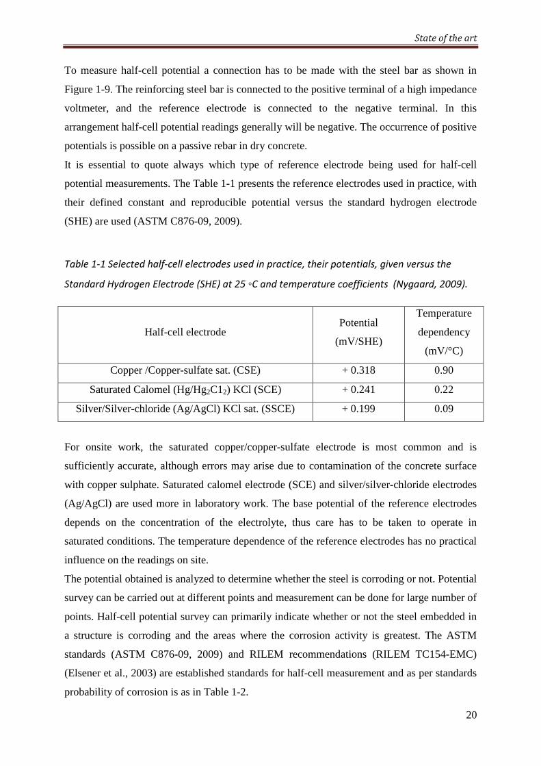
It is essential to quote always which type of reference electrode being used for half-cell

potential measurements. The Table 1-1 presents the reference electrodes used in practice, with

their defined constant and reproducible potential versus the standard hydrogen electrode

(SHE) are used (ASTM C876-09, 2009).

Table 1-1 Selected half-cell electrodes used in practice, their potentials, given versus the

Standard Hydrogen Electrode (SHE) at 25 C and temperature coefficients (Nygaard, 2009).

For onsite work, the saturated copper/copper-sulfate electrode is most common and is

sufficiently accurate, although errors may arise due to contamination of the concrete surface

with copper sulphate. Saturated calomel electrode (SCE) and silver/silver-chloride electrodes

(Ag/AgCl) are used more in laboratory work. The base potential of the reference electrodes

depends on the concentration of the electrolyte, thus care has to be taken to operate in

saturated conditions. The temperature dependence of the reference electrodes has no practical

influence on the readings on site.

The potential obtained is analyzed to determine whether the steel is corroding or not. Potential

survey can be carried out at different points and measurement can be done for large number of

points. Half-cell potential survey can primarily indicate whether or not the steel embedded in

a structure is corroding and the areas where the corrosion activity is greatest. The ASTM

standards (ASTM C876-09, 2009) and RILEM recommendations (RILEM TC154-EMC)

(Elsener et al., 2003) are established standards for half-cell measurement and as per standards

probability of corrosion is as in Table 1-2.

Half-cell electrode Potential

(mV/SHE)

Temperature

dependency

(mV/°C)

Copper /Copper-sulfate sat. (CSE) + 0.318 0.90

Saturated Calomel (Hg/Hg2C12) KCl (SCE) + 0.241 0.22

Silver/Silver-chloride (Ag/AgCl) KCl sat. (SSCE) + 0.199 0.09

State of the art

21

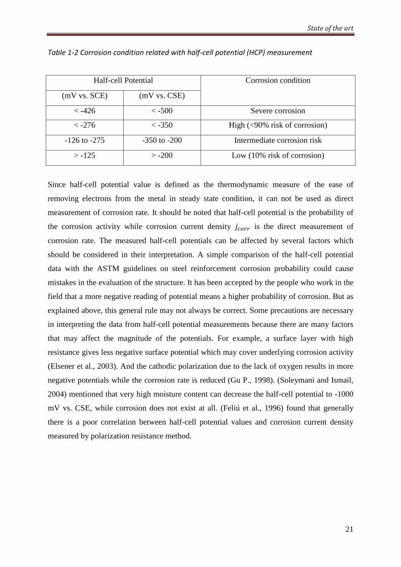
Table 1-2 Corrosion condition related with half-cell potential (HCP) measurement

Since half-cell potential value is defined as the thermodynamic measure of the ease of

removing electrons from the metal in steady state condition, it can not be used as direct

measurement of corrosion rate. It should be noted that half-cell potential is the probability of

the corrosion activity while corrosion current density a(( is the direct measurement of

corrosion rate. The measured half-cell potentials can be affected by several factors which

should be considered in their interpretation. A simple comparison of the half-cell potential

data with the ASTM guidelines on steel reinforcement corrosion probability could cause

mistakes in the evaluation of the structure. It has been accepted by the people who work in the

field that a more negative reading of potential means a higher probability of corrosion. But as

explained above, this general rule may not always be correct. Some precautions are necessary

in interpreting the data from half-cell potential measurements because there are many factors

that may affect the magnitude of the potentials. For example, a surface layer with high

resistance gives less negative surface potential which may cover underlying corrosion activity

(Elsener et al., 2003). And the cathodic polarization due to the lack of oxygen results in more

negative potentials while the corrosion rate is reduced (Gu P., 1998). (Soleymani and Ismail,

2004) mentioned that very high moisture content can decrease the half-cell potential to -1000

mV vs. CSE, while corrosion does not exist at all. (Feliú et al., 1996) found that generally

there is a poor correlation between half-cell potential values and corrosion current density

measured by polarization resistance method.

Half-cell Potential Corrosion condition

(mV vs. SCE) (mV vs. CSE)

< -426 < -500 Severe corrosion

< -276 < -350 High (<90% risk of corrosion)

-126 to -275 -350 to -200 Intermediate corrosion risk

> -125 > -200 Low (10% risk of corrosion)

State of the art

22

1.4.2 LinearPolarizationResistanceTechnique(LPR)

This technique is mostly widely used and has become a well-established for determining the

corrosion rate of reinforcing steel in concrete. The advantage of this technique is that it is

rapid and non-intrusive, requiring only localized damage to the concrete cover to enable an

electrical connection to be made to the reinforcing steel.

1.4.2.1 Basic Theory

First Stern and Geary (Stern and Geary, 1957) based on the general principles of

electrochemistry, formulated the fundamentals of corrosion rate values from the recording of

the polarization curves around the^a((. The proposed technique is derived from the

approximation to a linear behavior of the logarithmic dependence of potential and current

when they are recorded around the corrosion (mixed) potential Figure 1-10. So the LPR

technique is based on the observation of the linearity of the polarization curves just

around^a(( , that is, the slope of the polarization curves just around^a((. Corrosion current

density at steel surface in concrete is at equilibrium during free corrosion conditions, and at

this point potential is called ^a(( this condition is shown by the polarization curves, now if

this state is disturbed by applying overpotential , a net current starts flowing in the

system, the polarization resistance -| of reinforced steel is ratio between and (Andrade

and Alonso, 2004, 1996).

-| = ,~ Eq. 1.41

Figure 1-10 Polarization curve has a linear portion, where ∆E has linear relation with ∆I.

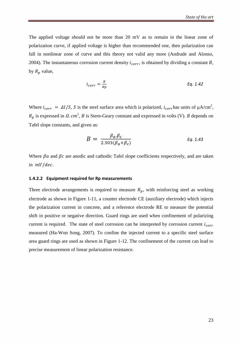
State of the art

23

The applied voltage should not be more than 20 mV as to remain in the linear zone of

polarization curve, if applied voltage is higher than recommended one, then polarization can

fall in nonlinear zone of curve and this theory not valid any more (Andrade and Alonso,

2004). The instantaneous corrosion current density^a((, is obtained by dividing a constant,

by -| value,

^a(( = 3| Eq. 1.42

Where^a(( = /, is the steel surface area which is polarized, ^a((has units of µA/cm2,

-| is expressed in . ];2, is Stern-Geary constant and expressed in volts (V). depends on

Tafel slope constants, and given as:

= f.g."m"(fgE Eq. 1.43

Where pO and p] are anodic and cathodic Tafel slope coefficients respectively, and are taken

in ;/V].

1.4.2.2 Equipment required for Rp measurements

Three electrode arrangements is required to measure -|, with reinforcing steel as working

electrode as shown in Figure 1-11, a counter electrode CE (auxiliary electrode) which injects

the polarization current in concrete, and a reference electrode RE to measure the potential

shift in positive or negative direction. Guard rings are used when confinement of polarizing

current is required. The state of steel corrosion can be interpreted by corrosion current ^a((

measured (Ha-Won Song, 2007). To confine the injected current to a specific steel surface

area guard rings are used as shown in Figure 1-12. The confinement of the current can lead to

precise measurement of linear polarization resistance.

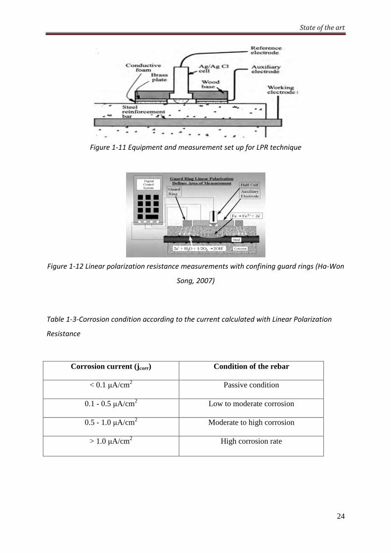
State of the art

24

Figure 1-11 Equipment and measurement set up for LPR technique

Figure 1-12 Linear polarization resistance measurements with confining guard rings (Ha-Won

Song, 2007)

Table 1-3-Corrosion condition according to the current calculated with Linear Polarization

Resistance

Corrosion current (jcorr) Condition of the rebar

< 0.1 µA/cm2 Passive condition

0.1 - 0.5 µA/cm2 Low to moderate corrosion

0.5 - 1.0 µA/cm2 Moderate to high corrosion

> 1.0 µA/cm2 High corrosion rate

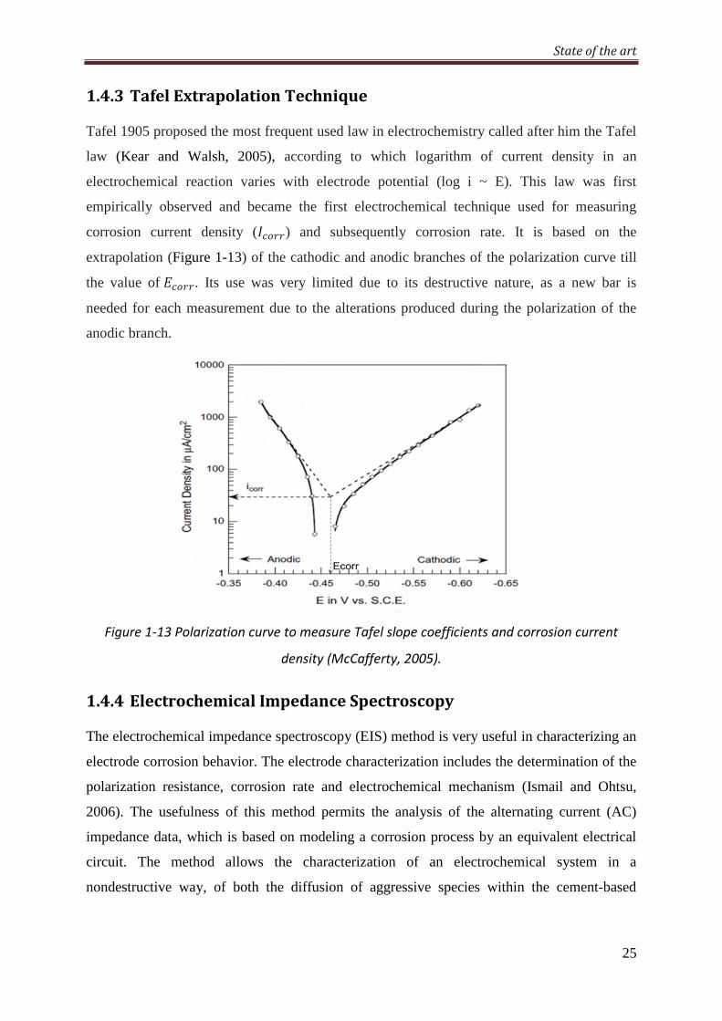
State of the art

25

1.4.3 TafelExtrapolationTechnique

Tafel 1905 proposed the most frequent used law in electrochemistry called after him the Tafel

law (Kear and Walsh, 2005), according to which logarithm of current density in an

electrochemical reaction varies with electrode potential (log i ~ E). This law was first

empirically observed and became the first electrochemical technique used for measuring

corrosion current density ( a(() and subsequently corrosion rate. It is based on the

extrapolation (Figure 1-13) of the cathodic and anodic branches of the polarization curve till

the value of^a((. Its use was very limited due to its destructive nature, as a new bar is

needed for each measurement due to the alterations produced during the polarization of the

anodic branch.

Figure 1-13 Polarization curve to measure Tafel slope coefficients and corrosion current

density (McCafferty, 2005).

1.4.4 ElectrochemicalImpedanceSpectroscopy

The electrochemical impedance spectroscopy (EIS) method is very useful in characterizing an

electrode corrosion behavior. The electrode characterization includes the determination of the

polarization resistance, corrosion rate and electrochemical mechanism (Ismail and Ohtsu,

2006). The usefulness of this method permits the analysis of the alternating current (AC)

impedance data, which is based on modeling a corrosion process by an equivalent electrical

circuit. The method allows the characterization of an electrochemical system in a

nondestructive way, of both the diffusion of aggressive species within the cement-based

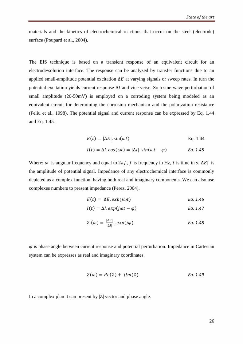
State of the art

26

materials and the kinetics of electrochemical reactions that occur on the steel (electrode)

surface (Poupard et al., 2004).

The EIS technique is based on a transient response of an equivalent circuit for an

electrode/solution interface. The response can be analyzed by transfer functions due to an

applied small-amplitude potential excitation ∆ at varying signals or sweep rates. In turn the

potential excitation yields current response ∆ and vice verse. So a sine-wave perturbation of

small amplitude (20-50mV) is employed on a corroding system being modeled as an

equivalent circuit for determining the corrosion mechanism and the polarization resistance

(Feliu et al., 1998). The potential signal and current response can be expressed by Eq. 1.44

and Eq. 1.45.

(xE = |∆|. sin(xE Eq. 1.44

(xE = ∆. ]<U(xE = |∆|. U'(x − E Eq. 1.45

Where: is angular frequency and equal to2, is frequency in Hz, x is time inU.|∆| is

the amplitude of potential signal. Impedance of any electrochemical interface is commonly

depicted as a complex function, having both real and imaginary components. We can also use

complexes numbers to present impedance (Perez, 2004).

(xE = ∆. Y6(xE Eq. 1.46

(xE = ∆. Y6(x − E Eq. 1.47

(E = |∆,||∆~| . Y6(E Eq. 1.48

is phase angle between current response and potential perturbation. Impedance in Cartesian

system can be expresses as real and imaginary coordinates.

(E = -(E + ;(E Eq. 1.49

In a complex plan it can present by |Z| vector and phase angle.

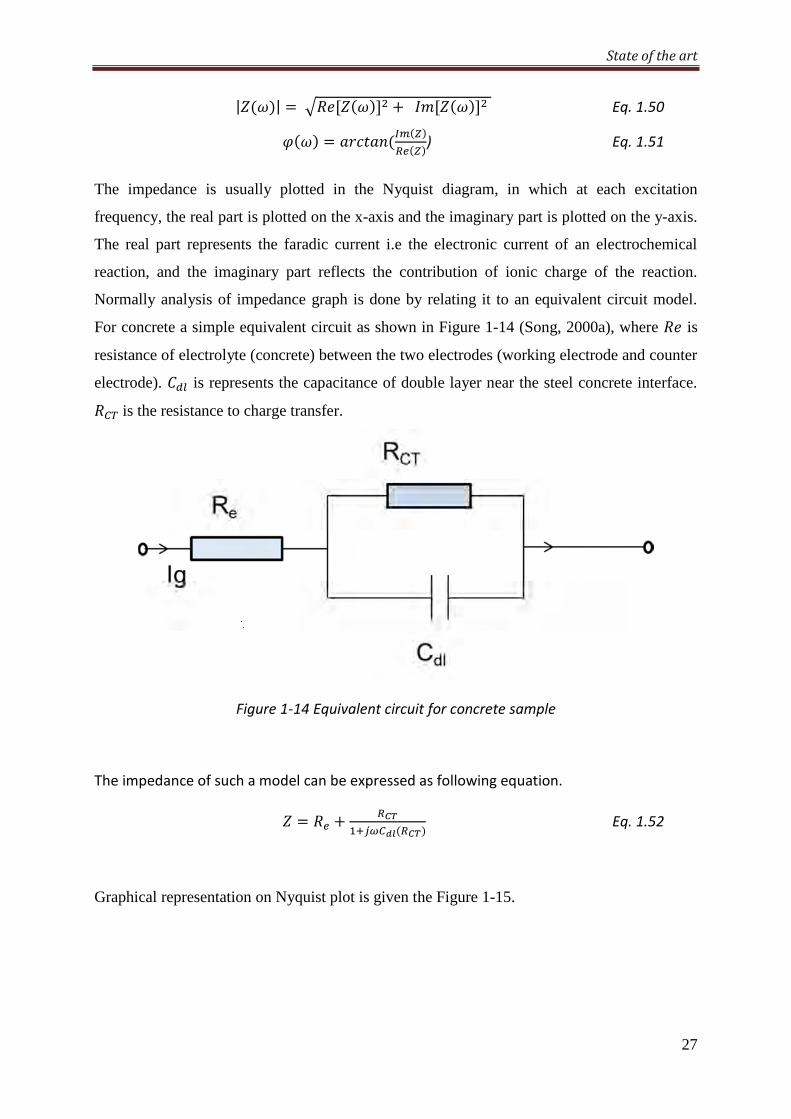
State of the art

27

|(E| = -A(EB + ;A(EB Eq. 1.50

(E = O]xO'(~(E3)(E) Eq. 1.51

The impedance is usually plotted in the Nyquist diagram, in which at each excitation

frequency, the real part is plotted on the x-axis and the imaginary part is plotted on the y-axis.

The real part represents the faradic current i.e the electronic current of an electrochemical

reaction, and the imaginary part reflects the contribution of ionic charge of the reaction.

Normally analysis of impedance graph is done by relating it to an equivalent circuit model.

For concrete a simple equivalent circuit as shown in Figure 1-14 (Song, 2000a), where - is

resistance of electrolyte (concrete) between the two electrodes (working electrode and counter

electrode). 9X is represents the capacitance of double layer near the steel concrete interface.

-4is the resistance to charge transfer.

Figure 1-14 Equivalent circuit for concrete sample

The impedance of such a model can be expressed as following equation.

= -) + 3j=q(3jE Eq. 1.52

Graphical representation on Nyquist plot is given the Figure 1-15.

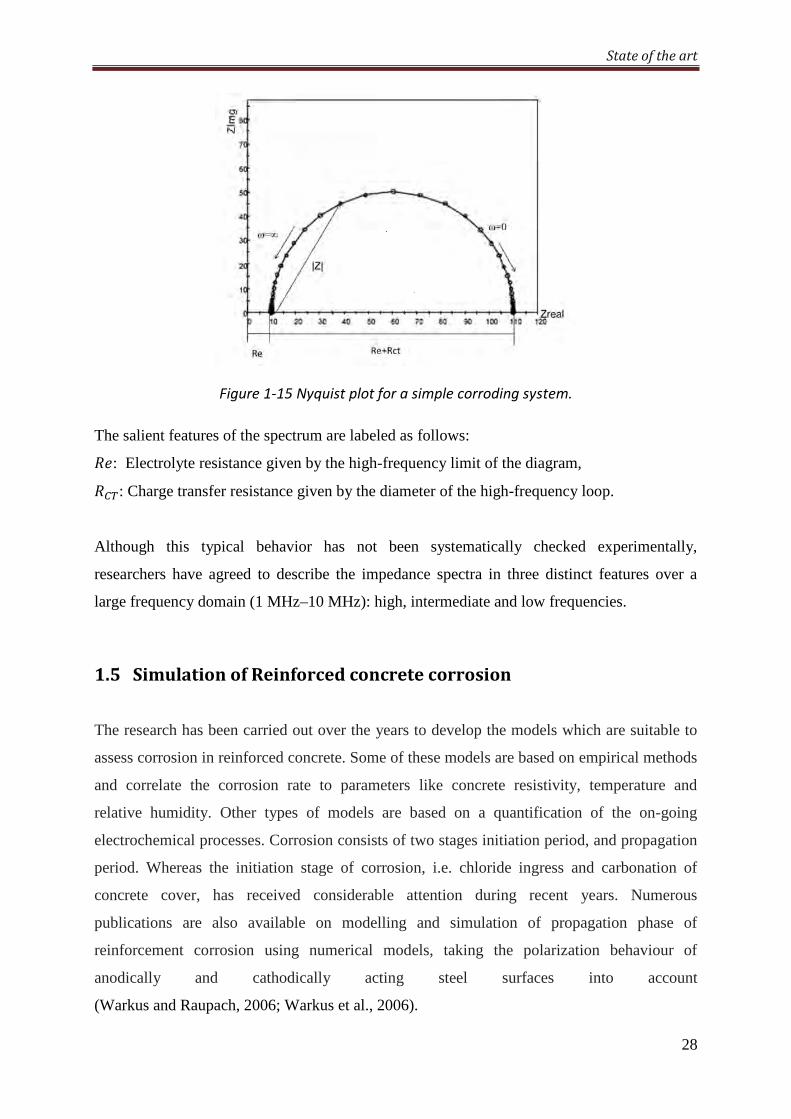
State of the art

28

Figure 1-15 Nyquist plot for a simple corroding system.

The salient features of the spectrum are labeled as follows:

-: Electrolyte resistance given by the high-frequency limit of the diagram,

-4: Charge transfer resistance given by the diameter of the high-frequency loop.

Although this typical behavior has not been systematically checked experimentally,

researchers have agreed to describe the impedance spectra in three distinct features over a

large frequency domain (1 MHz–10 MHz): high, intermediate and low frequencies.

1.5 SimulationofReinforcedconcretecorrosion

The research has been carried out over the years to develop the models which are suitable to

assess corrosion in reinforced concrete. Some of these models are based on empirical methods

and correlate the corrosion rate to parameters like concrete resistivity, temperature and

relative humidity. Other types of models are based on a quantification of the on-going

electrochemical processes. Corrosion consists of two stages initiation period, and propagation

period. Whereas the initiation stage of corrosion, i.e. chloride ingress and carbonation of

concrete cover, has received considerable attention during recent years. Numerous

publications are also available on modelling and simulation of propagation phase of

reinforcement corrosion using numerical models, taking the polarization behaviour of

anodically and cathodically acting steel surfaces into account

(Warkus and Raupach, 2006; Warkus et al., 2006).

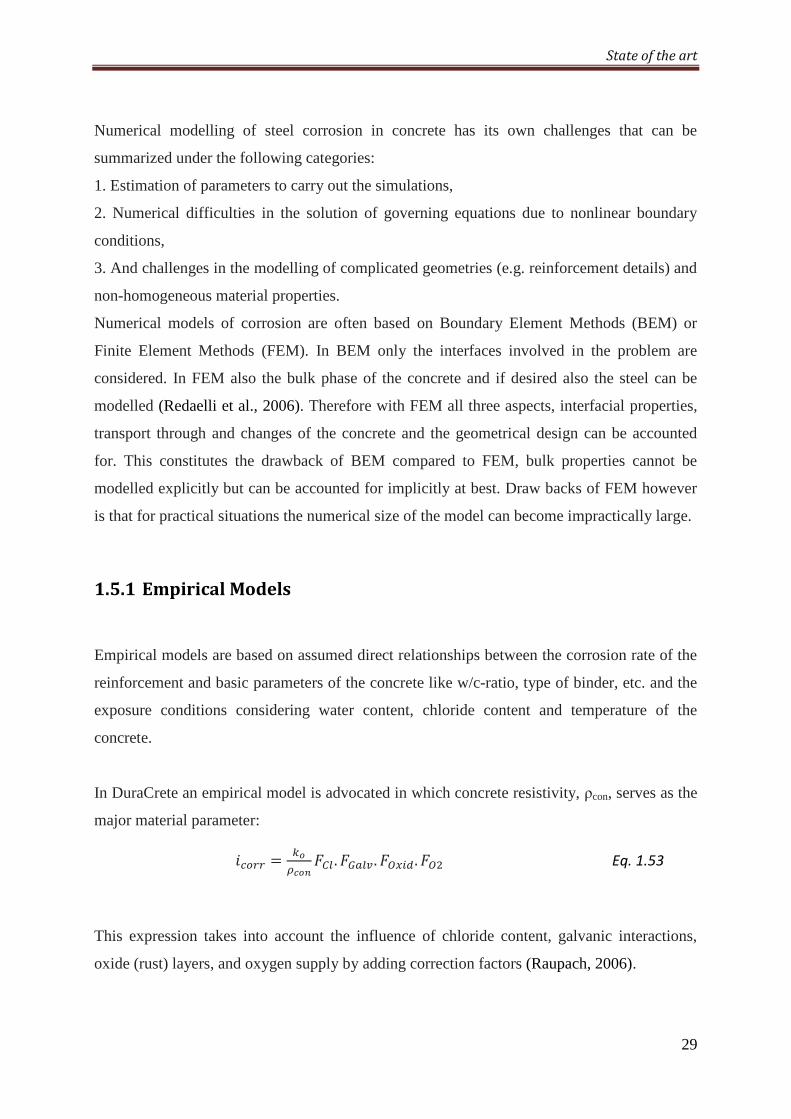
State of the art

29

Numerical modelling of steel corrosion in concrete has its own challenges that can be

summarized under the following categories:

1. Estimation of parameters to carry out the simulations,

2. Numerical difficulties in the solution of governing equations due to nonlinear boundary

conditions,

3. And challenges in the modelling of complicated geometries (e.g. reinforcement details) and

non-homogeneous material properties.

Numerical models of corrosion are often based on Boundary Element Methods (BEM) or

Finite Element Methods (FEM). In BEM only the interfaces involved in the problem are

considered. In FEM also the bulk phase of the concrete and if desired also the steel can be

modelled (Redaelli et al., 2006). Therefore with FEM all three aspects, interfacial properties,

transport through and changes of the concrete and the geometrical design can be accounted

for. This constitutes the drawback of BEM compared to FEM, bulk properties cannot be

modelled explicitly but can be accounted for implicitly at best. Draw backs of FEM however

is that for practical situations the numerical size of the model can become impractically large.

1.5.1 EmpiricalModels

Empirical models are based on assumed direct relationships between the corrosion rate of the

reinforcement and basic parameters of the concrete like w/c-ratio, type of binder, etc. and the

exposure conditions considering water content, chloride content and temperature of the

concrete.

In DuraCrete an empirical model is advocated in which concrete resistivity, ρcon, serves as the

major material parameter:

^a(( = rgr . * . [\X. [ Eq. 1.53

This expression takes into account the influence of chloride content, galvanic interactions,

oxide (rust) layers, and oxygen supply by adding correction factors (Raupach, 2006).

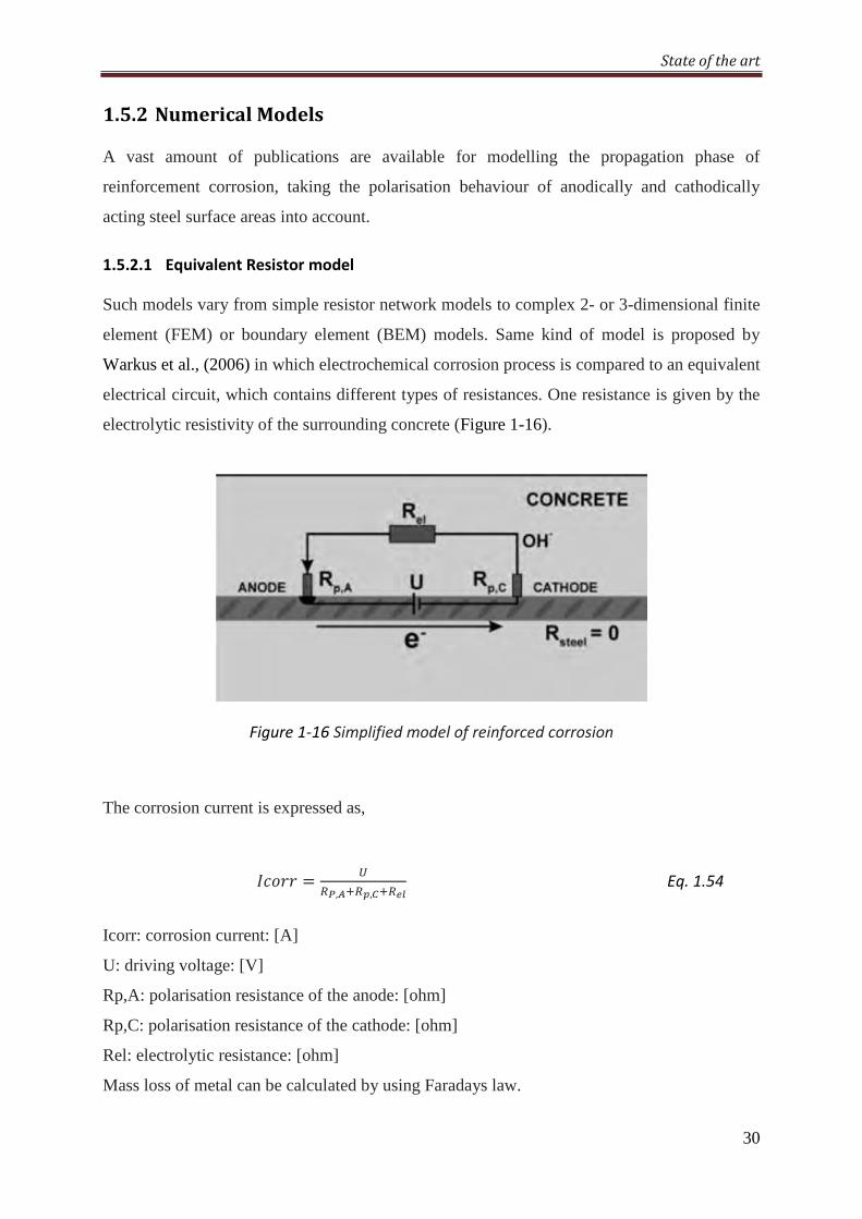
State of the art

30

1.5.2 NumericalModels

A vast amount of publications are available for modelling the propagation phase of

reinforcement corrosion, taking the polarisation behaviour of anodically and cathodically

acting steel surface areas into account.

1.5.2.1 Equivalent Resistor model

Such models vary from simple resistor network models to complex 2- or 3-dimensional finite

element (FEM) or boundary element (BEM) models. Same kind of model is proposed by

Warkus et al., (2006) in which electrochemical corrosion process is compared to an equivalent

electrical circuit, which contains different types of resistances. One resistance is given by the

electrolytic resistivity of the surrounding concrete (Figure 1-16).

Figure 1-16 Simplified model of reinforced corrosion

The corrosion current is expressed as,

]< = 3,3,3 Eq. 1.54

Icorr: corrosion current: [A]

U: driving voltage: [V]

Rp,A: polarisation resistance of the anode: [ohm]

Rp,C: polarisation resistance of the cathode: [ohm]

Rel: electrolytic resistance: [ohm]

Mass loss of metal can be calculated by using Faradays law.

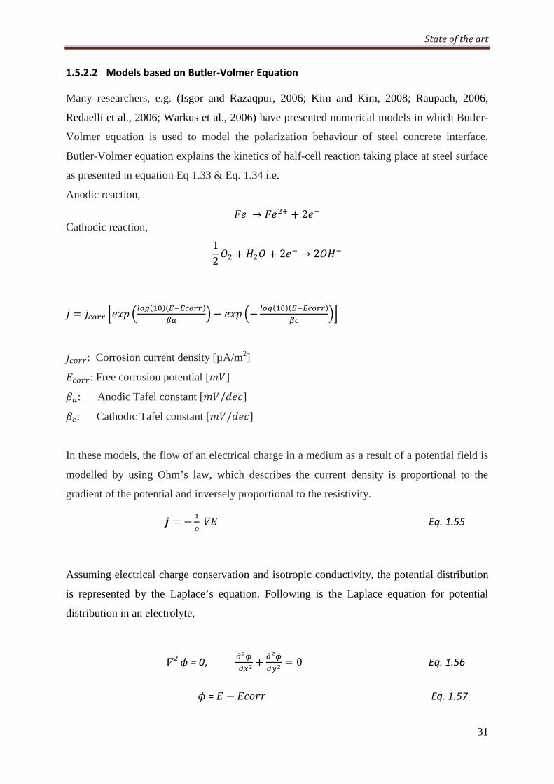
State of the art

31

1.5.2.2 Models based on Butler-Volmer Equation

Many researchers, e.g. (Isgor and Razaqpur, 2006; Kim and Kim, 2008; Raupach, 2006;

Redaelli et al., 2006; Warkus et al., 2006) have presented numerical models in which Butler-

Volmer equation is used to model the polarization behaviour of steel concrete interface.

Butler-Volmer equation explains the kinetics of half-cell reaction taking place at steel surface

as presented in equation Eq 1.33 & Eq. 1.34 i.e.

Anodic reaction,

→ + 2 Cathodic reaction,

12> + 7> + 2 → 2>7

= a(( nY6 Ia (=mE(,,^a((E J − Y6 I− a (=mE(,,^a((E^ Jo

a((: Corrosion current density [µA/m2]

^a((: Free corrosion potential [;]

p: Anodic Tafel constant [;/V]] p^: Cathodic Tafel constant [;/V]]

In these models, the flow of an electrical charge in a medium as a result of a potential field is

modelled by using Ohm’s law, which describes the current density is proportional to the

gradient of the potential and inversely proportional to the resistivity.

¡ = − = ¢ Eq. 1.55

Assuming electrical charge conservation and isotropic conductivity, the potential distribution

is represented by the Laplace’s equation. Following is the Laplace equation for potential

distribution in an electrolyte,

∇2 ¤ = 0, ¥¦§¥\¦ +

¥¦§¥¨¦ = 0 Eq. 1.56

¤ = − ]< Eq. 1.57

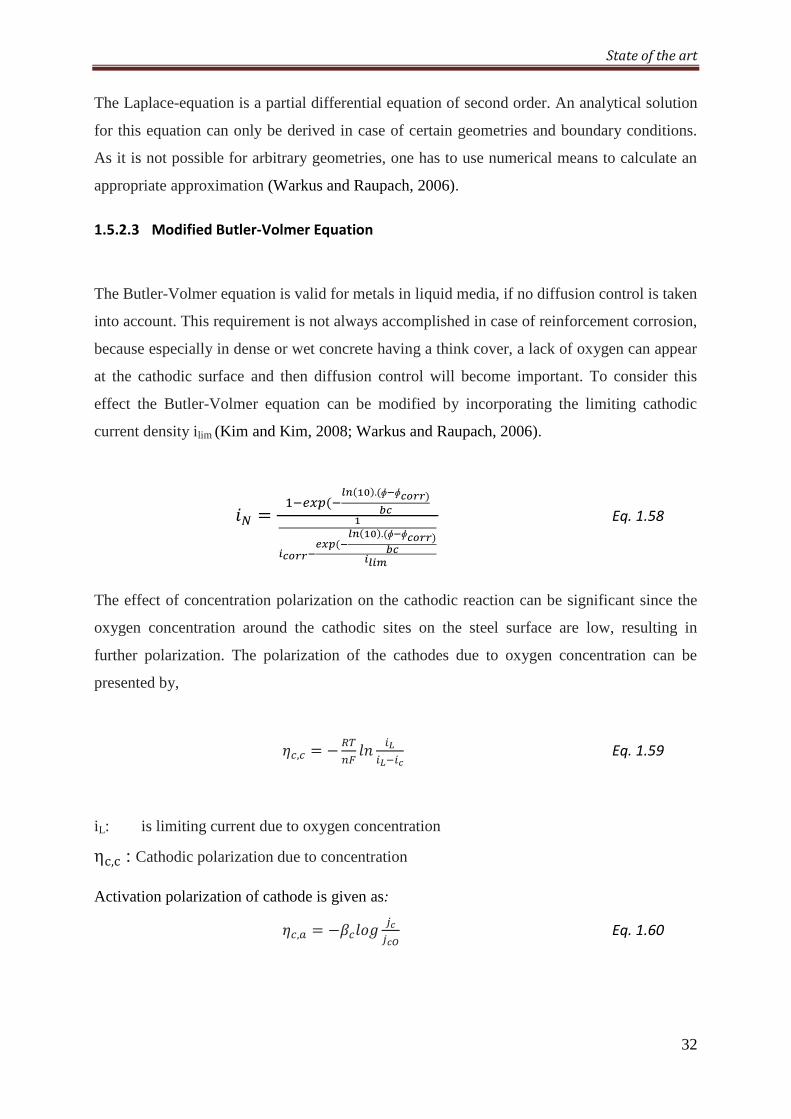
State of the art

32

The Laplace-equation is a partial differential equation of second order. An analytical solution

for this equation can only be derived in case of certain geometries and boundary conditions.

As it is not possible for arbitrary geometries, one has to use numerical means to calculate an

appropriate approximation (Warkus and Raupach, 2006).

1.5.2.3 Modified Butler-Volmer Equation

The Butler-Volmer equation is valid for metals in liquid media, if no diffusion control is taken

into account. This requirement is not always accomplished in case of reinforcement corrosion,

because especially in dense or wet concrete having a think cover, a lack of oxygen can appear

at the cathodic surface and then diffusion control will become important. To consider this

effect the Butler-Volmer equation can be modified by incorporating the limiting cathodic

current density ilim (Kim and Kim, 2008; Warkus and Raupach, 2006).

© = =)\|((ª«E.(ɸ¬ɸgruuE­gª

®gruu¬¯(¬

(ª«E.(ɸ¬ɸgruuE­g®®°

Eq. 1.58

The effect of concentration polarization on the cathodic reaction can be significant since the

oxygen concentration around the cathodic sites on the steel surface are low, resulting in

further polarization. The polarization of the cathodes due to oxygen concentration can be

presented by,

^,^ = − 34&5 1'

±±g Eq. 1.59

iL: is limiting current due to oxygen concentration

η³,³ : Cathodic polarization due to concentration

Activation polarization of cathode is given as:

^, = −p^1<@ qgqg´ Eq. 1.60

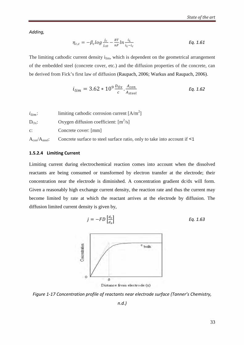
State of the art

33

Adding,

^,^ = −p^1<@ qgqg´ −

34&5 1'

±±g Eq. 1.61

The limiting cathodic current density ilim, which is dependent on the geometrical arrangement

of the embedded steel (concrete cover, etc.) and the diffusion properties of the concrete, can

be derived from Fick’s first law of diffusion (Raupach, 2006; Warkus and Raupach, 2006).

= 3.62 ∗ 10µ ¶´¯^ .sgrs·v Eq. 1.62

: limiting cathodic corrosion current [A/m2]

DOx: Oxygen diffusion coefficient: [m2/s]

c: Concrete cover: [mm]

Acon/Asteel: Concrete surface to steel surface ratio, only to take into account if ˂1

1.5.2.4 Limiting Current

Limiting current during electrochemical reaction comes into account when the dissolved

reactants are being consumed or transformed by electron transfer at the electrode; their

concentration near the electrode is diminished. A concentration gradient dc/dx will form.

Given a reasonably high exchange current density, the reaction rate and thus the current may

become limited by rate at which the reactant arrives at the electrode by diffusion. The

diffusion limited current density is given by,

= −¸ nXgX¯o Eq. 1.63

Figure 1-17 Concentration profile of reactants near electrode surface (Tanner’s Chemistry,

n.d.)

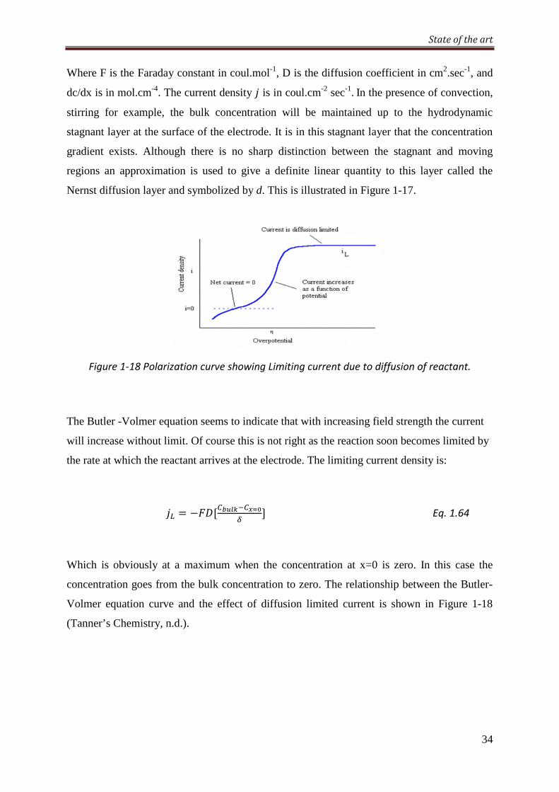
State of the art

34

Where F is the Faraday constant in coul.mol-1, D is the diffusion coefficient in cm2.sec-1, and

dc/dx is in mol.cm-4. The current density is in coul.cm-2 sec-1. In the presence of convection,

stirring for example, the bulk concentration will be maintained up to the hydrodynamic

stagnant layer at the surface of the electrode. It is in this stagnant layer that the concentration

gradient exists. Although there is no sharp distinction between the stagnant and moving

regions an approximation is used to give a definite linear quantity to this layer called the

Nernst diffusion layer and symbolized by d. This is illustrated in Figure 1-17.

Figure 1-18 Polarization curve showing Limiting current due to diffusion of reactant.

The Butler -Volmer equation seems to indicate that with increasing field strength the current

will increase without limit. Of course this is not right as the reaction soon becomes limited by

the rate at which the reactant arrives at the electrode. The limiting current density is:

¹ = −¸A­º»¯¼«½ B Eq. 1.64

Which is obviously at a maximum when the concentration at x=0 is zero. In this case the

concentration goes from the bulk concentration to zero. The relationship between the Butler-

Volmer equation curve and the effect of diffusion limited current is shown in Figure 1-18

(Tanner’s Chemistry, n.d.).

State of the art

35

1.6 AcceleratedCorrosionTesting

Normally concrete provides a good resistance to corrosion due it’s another important

characteristic i.e. the high alkalinity of the pore solution, which is comprised of mainly

sodium and potassium hydroxides, with a 67 ranging from 12.6 to 13.8. At this 67 level a

protective (or passive) film is spontaneously formed during the early stages of cement

hydration. This passive film may grow to a thickness of the order of 10-3 to 10-1 µm and

contains hydrated iron oxides (Ramachandran et al., 2001). The theory of the existence of this

passive layer is based on indirect evidence of anodic polarization measurement. There is still

much to be learned concerning this passive film, such as the conditions of its formation, and

its chemical and mineralogical composition. It is possible that this passivation film consists of

several phases (Smith, 2007). The concrete cover also provides good physical protection to

steel from chloride ions and prevents carbonation. So it takes a long time for steel to

depassivate and allow corrosion process to start. That makes it very difficult to replicate,

study and to understand the corrosion phenomena in laboratories. To overcome this problem

Accelerated Corrosion Tests are developed, by using them we can induce corrosion in

reinforced concrete samples in laboratory in short period of time (Ahn, 2001; Yingshu et al.,

2007).

Tuutti (Tuutti, K, 1982) proposed a corrosion model; according to which the corrosion

process can be divided in two distinct time phases: initiation phase and propagation phase

Figure 1-19. The initiation phase corresponds to the progressive ingress of the aggressive

agents like carbon dioxide 9> and chloride ions 91 through the concrete cover. As

previously discussed, concrete provides excellent protection for steel reinforcement thanks to

the high alkalinity of concrete pore solution. The quality of the concrete cover is also involved

in the physical protection of steel from environment, because concrete transport properties

control the ingress kinetics of aggressive agents. During this phase, no corrosion occurs and it

usually takes many years for aggressive agents to reach steel surface and depassivate steel

(Yingshu et al., 2007).

State of the art

36

Figure 1-19 Tuutti corrosion model

The laboratory acceleration of corrosion is primarily consists on the acceleration of the

initiation phase so that the depassivation of steel is quickly achieved.

1.6.1 ArtificialClimateTechnique

In this technique corrosion process is accelerated by way of high temperature, high humidity,

and repeated wetting-and drying cycles. Artificial environment techniques, in which the

samples are kept in controlled environment, are often used to accelerate initiation period. The

artificial climate conditions given by (Yingshu et al., 2007) are temperature . =40°9(104°E, relative humidity (-7E = 80%, and salt water (5%¿O91 solution)

spraying (1 hour) and infrared light shining (7 hours) for the wetting-and-drying cycle. The

most commonly used techniques are:

- Carbonation chamber with 50% CO2 and 65% RH,

- Samples contaminated by 3-5% NaCl solution (permanent immersion or wetting-

drying cycles).

The corrosion process and corrosion characteristics of the steel bar under artificial

environments are similar to that of corrosion under natural environment. Artificial climate

environment as an accelerated laboratory test method is more representative than the

galvanostatic method.

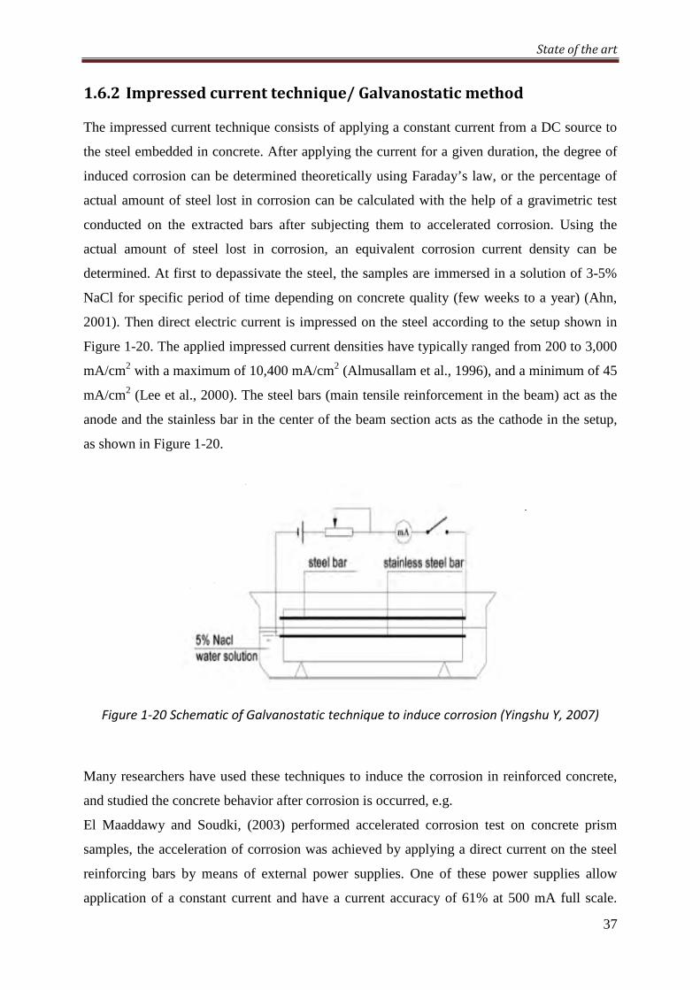
State of the art

37

1.6.2 Impressedcurrenttechnique/Galvanostaticmethod

The impressed current technique consists of applying a constant current from a DC source to

the steel embedded in concrete. After applying the current for a given duration, the degree of

induced corrosion can be determined theoretically using Faraday’s law, or the percentage of

actual amount of steel lost in corrosion can be calculated with the help of a gravimetric test

conducted on the extracted bars after subjecting them to accelerated corrosion. Using the

actual amount of steel lost in corrosion, an equivalent corrosion current density can be

determined. At first to depassivate the steel, the samples are immersed in a solution of 3-5%

NaCl for specific period of time depending on concrete quality (few weeks to a year) (Ahn,

2001). Then direct electric current is impressed on the steel according to the setup shown in

Figure 1-20. The applied impressed current densities have typically ranged from 200 to 3,000

mA/cm2 with a maximum of 10,400 mA/cm2 (Almusallam et al., 1996), and a minimum of 45

mA/cm2 (Lee et al., 2000). The steel bars (main tensile reinforcement in the beam) act as the

anode and the stainless bar in the center of the beam section acts as the cathode in the setup,

as shown in Figure 1-20.

Figure 1-20 Schematic of Galvanostatic technique to induce corrosion (Yingshu Y, 2007)

Many researchers have used these techniques to induce the corrosion in reinforced concrete,

and studied the concrete behavior after corrosion is occurred, e.g.

El Maaddawy and Soudki, (2003) performed accelerated corrosion test on concrete prism

samples, the acceleration of corrosion was achieved by applying a direct current on the steel

reinforcing bars by means of external power supplies. One of these power supplies allow

application of a constant current and have a current accuracy of 61% at 500 mA full scale.

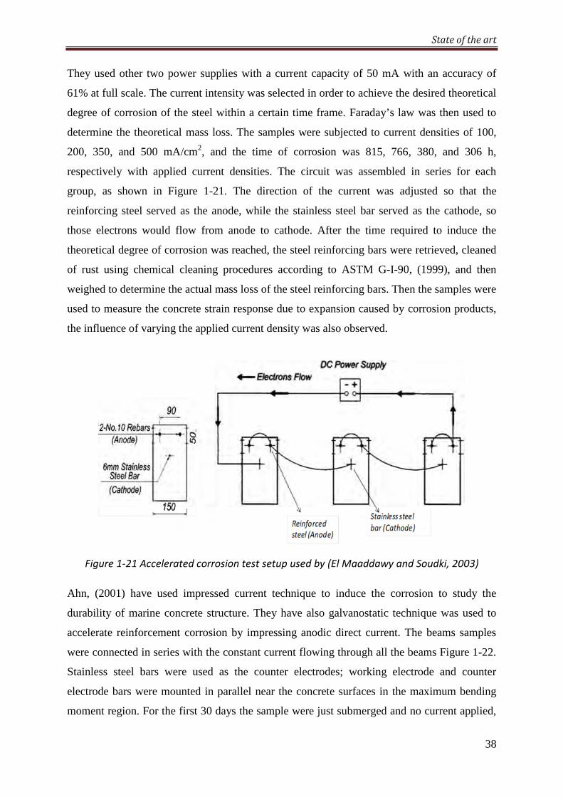
State of the art

38

They used other two power supplies with a current capacity of 50 mA with an accuracy of

61% at full scale. The current intensity was selected in order to achieve the desired theoretical

degree of corrosion of the steel within a certain time frame. Faraday’s law was then used to

determine the theoretical mass loss. The samples were subjected to current densities of 100,

200, 350, and 500 mA/cm2, and the time of corrosion was 815, 766, 380, and 306 h,

respectively with applied current densities. The circuit was assembled in series for each

group, as shown in Figure 1-21. The direction of the current was adjusted so that the

reinforcing steel served as the anode, while the stainless steel bar served as the cathode, so

those electrons would flow from anode to cathode. After the time required to induce the

theoretical degree of corrosion was reached, the steel reinforcing bars were retrieved, cleaned

of rust using chemical cleaning procedures according to ASTM G-I-90, (1999), and then

weighed to determine the actual mass loss of the steel reinforcing bars. Then the samples were

used to measure the concrete strain response due to expansion caused by corrosion products,

the influence of varying the applied current density was also observed.

Figure 1-21 Accelerated corrosion test setup used by (El Maaddawy and Soudki, 2003)

Ahn, (2001) have used impressed current technique to induce the corrosion to study the

durability of marine concrete structure. They have also galvanostatic technique was used to

accelerate reinforcement corrosion by impressing anodic direct current. The beams samples

were connected in series with the constant current flowing through all the beams Figure 1-22.

Stainless steel bars were used as the counter electrodes; working electrode and counter

electrode bars were mounted in parallel near the concrete surfaces in the maximum bending

moment region. For the first 30 days the sample were just submerged and no current applied,

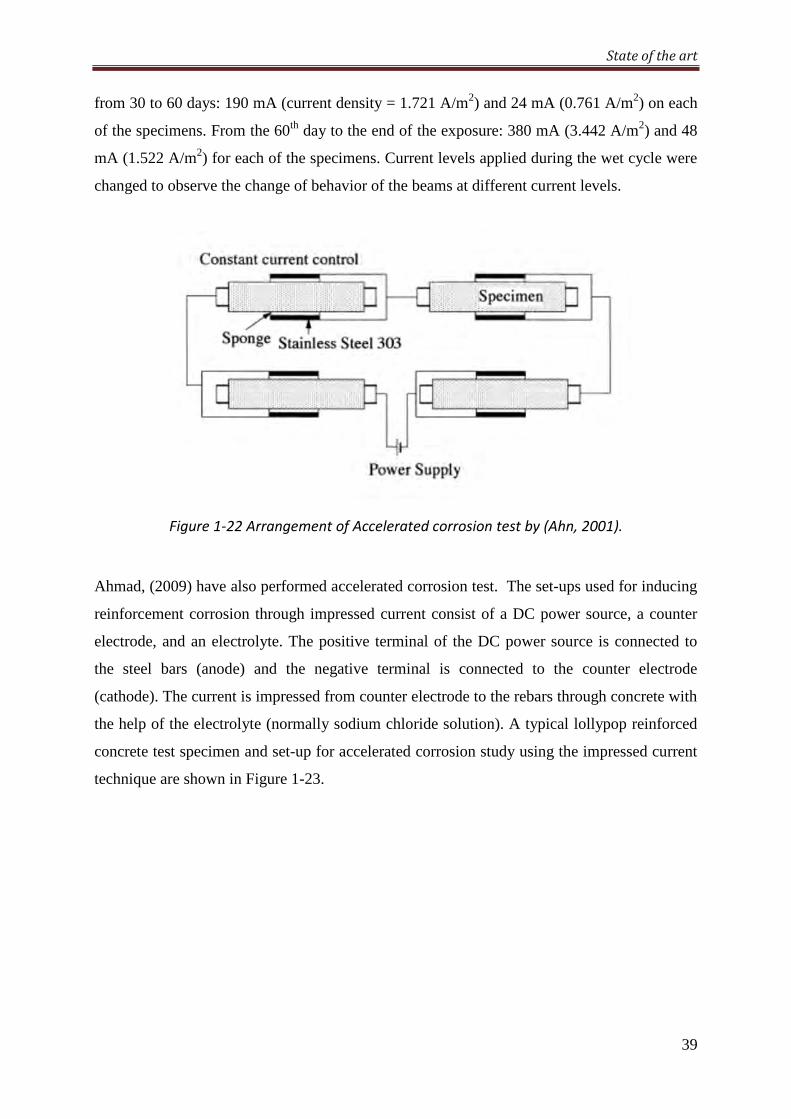
State of the art

39

from 30 to 60 days: 190 mA (current density = 1.721 A/m2) and 24 mA (0.761 A/m2) on each

of the specimens. From the 60th day to the end of the exposure: 380 mA (3.442 A/m2) and 48

mA (1.522 A/m2) for each of the specimens. Current levels applied during the wet cycle were

changed to observe the change of behavior of the beams at different current levels.

Figure 1-22 Arrangement of Accelerated corrosion test by (Ahn, 2001).

Ahmad, (2009) have also performed accelerated corrosion test. The set-ups used for inducing

reinforcement corrosion through impressed current consist of a DC power source, a counter

electrode, and an electrolyte. The positive terminal of the DC power source is connected to

the steel bars (anode) and the negative terminal is connected to the counter electrode

(cathode). The current is impressed from counter electrode to the rebars through concrete with

the help of the electrolyte (normally sodium chloride solution). A typical lollypop reinforced

concrete test specimen and set-up for accelerated corrosion study using the impressed current

technique are shown in Figure 1-23.

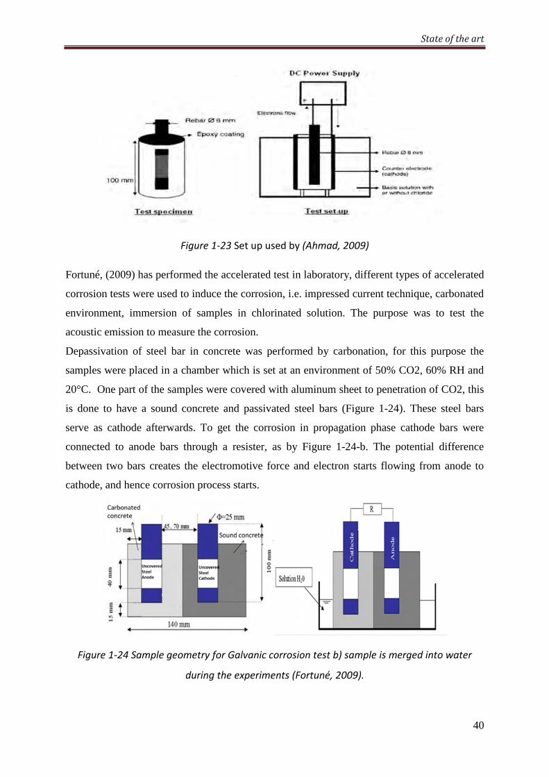
State of the art

40

Figure 1-23 Set up used by (Ahmad, 2009)

Fortuné, (2009) has performed the accelerated test in laboratory, different types of accelerated

corrosion tests were used to induce the corrosion, i.e. impressed current technique, carbonated

environment, immersion of samples in chlorinated solution. The purpose was to test the

acoustic emission to measure the corrosion.

Depassivation of steel bar in concrete was performed by carbonation, for this purpose the

samples were placed in a chamber which is set at an environment of 50% CO2, 60% RH and

20°C. One part of the samples were covered with aluminum sheet to penetration of CO2, this

is done to have a sound concrete and passivated steel bars (Figure 1-24). These steel bars

serve as cathode afterwards. To get the corrosion in propagation phase cathode bars were

connected to anode bars through a resister, as by Figure 1-24-b. The potential difference

between two bars creates the electromotive force and electron starts flowing from anode to

cathode, and hence corrosion process starts.

Figure 1-24 Sample geometry for Galvanic corrosion test b) sample is merged into water

during the experiments (Fortuné, 2009).

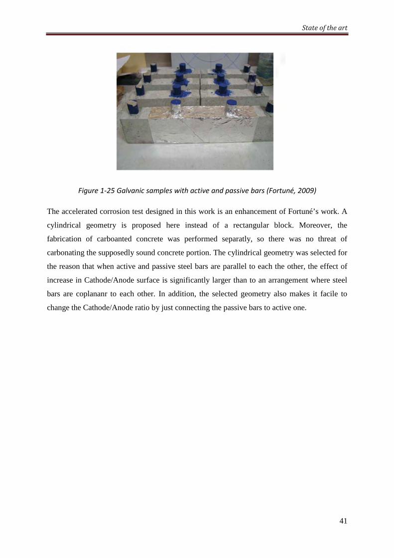
State of the art

41

Figure 1-25 Galvanic samples with active and passive bars (Fortuné, 2009)

The accelerated corrosion test designed in this work is an enhancement of Fortuné’s work. A

cylindrical geometry is proposed here instead of a rectangular block. Moreover, the

fabrication of carboanted concrete was performed separatly, so there was no threat of

carbonating the supposedly sound concrete portion. The cylindrical geometry was selected for

the reason that when active and passive steel bars are parallel to each the other, the effect of

increase in Cathode/Anode surface is significantly larger than to an arrangement where steel

bars are coplananr to each other. In addition, the selected geometry also makes it facile to

change the Cathode/Anode ratio by just connecting the passive bars to active one.

42

CHAPTER#2

2 Characterizationofcorrosion

parameters

2.1 IntroductionThis chapter characterizes all the corrosion parameters with respect to the condition of

concrete and steel in it, i.e whether concrete is carbonated or sound, or if reinforcement steel

is depassivated or in passive state. Moreover the chapter also explains the properties of

materials used, the conditioning of concrete samples and the protocol of experiments

performed to get the corrosion parameters in carbonated and non-carbonated concrete.

The corrosion parameters like corrosion potential^a((, corrosion current density a((, anodic tafel slope βa and cathodic tafel slope βc are sensitive to different factors like

temperature, relative humidity, 67 and carbonate contents in the pore solution (Elsener, 2005;

Garcés et al., 2005). The researchers who have modeled corrosion in reinforced concrete have

used a wide range of the values of βa & βc. The variety of values used by different authors,

shows the uncertainty exists in selecting these parameters.

For the measurement of linear polarization resistance (LPR) also supposes the values of Stern-

Geary constant between 26 and 52 for active and passive steel respectively. Constant

depends on Tafel slope coefficients and can be calculated with the help of Eq. 1.43. The value

of B is 26 when βa and βc are 120;/V], and is 52 for βa infinity and βc 120;/V]. But in many of cases, these theoretical values of βa and βc could be much different, i.e. anodic

Tafel slope of active steel could be much higher than 120;/V]. With different concrete

conditions (RH%, Temperature, oxygen availability, carbonation, chloride contents) the

constant B could be from 8 to ∞, so using as 26;and52; can be erroneous (Chang et

al., 2008; Song, 2000b). Little literature is available on Tafel slopes (βa, βc) for different

concrete conditions, especially in case of carbonated concrete.

In addition, to simulate numerically the electrochemical corrosion phenomena in concrete, the

corrosion parameters have to be identified for different conditions encountered in real life

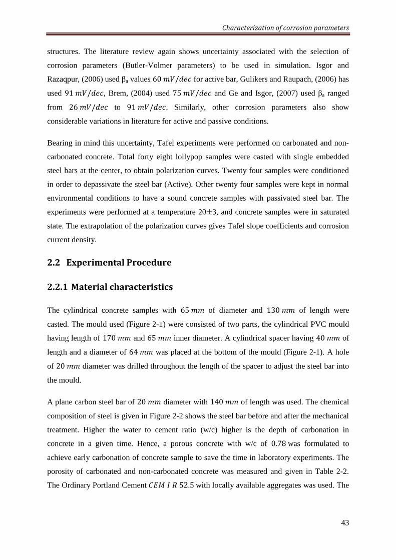
Characterization of corrosion parameters

43

structures. The literature review again shows uncertainty associated with the selection of

corrosion parameters (Butler-Volmer parameters) to be used in simulation. Isgor and

Razaqpur, (2006) used βa values 60;/V] for active bar, Gulikers and Raupach, (2006) has

used 91;/V], Brem, (2004) used 75;/V] and Ge and Isgor, (2007) used βa ranged

from 26;/V] to 91;/V]. Similarly, other corrosion parameters also show

considerable variations in literature for active and passive conditions.

Bearing in mind this uncertainty, Tafel experiments were performed on carbonated and non-

carbonated concrete. Total forty eight lollypop samples were casted with single embedded

steel bars at the center, to obtain polarization curves. Twenty four samples were conditioned

in order to depassivate the steel bar (Active). Other twenty four samples were kept in normal

environmental conditions to have a sound concrete samples with passivated steel bar. The

experiments were performed at a temperature 20±3, and concrete samples were in saturated

state. The extrapolation of the polarization curves gives Tafel slope coefficients and corrosion

current density.

2.2 ExperimentalProcedure

2.2.1 Materialcharacteristics

The cylindrical concrete samples with 65;; of diameter and 130;; of length were

casted. The mould used (Figure 2-1) were consisted of two parts, the cylindrical PVC mould

having length of 170;; and 65;; inner diameter. A cylindrical spacer having 40;; of

length and a diameter of 64;; was placed at the bottom of the mould (Figure 2-1). A hole

of 20;; diameter was drilled throughout the length of the spacer to adjust the steel bar into

the mould.

A plane carbon steel bar of 20;; diameter with 140;; of length was used. The chemical

composition of steel is given in Figure 2-2 shows the steel bar before and after the mechanical

treatment. Higher the water to cement ratio (w/c) higher is the depth of carbonation in

concrete in a given time. Hence, a porous concrete with w/c of 0.78was formulated to

achieve early carbonation of concrete sample to save the time in laboratory experiments. The

porosity of carbonated and non-carbonated concrete was measured and given in Table 2-2.

The Ordinary Portland Cement9-52.5with locally available aggregates was used. The

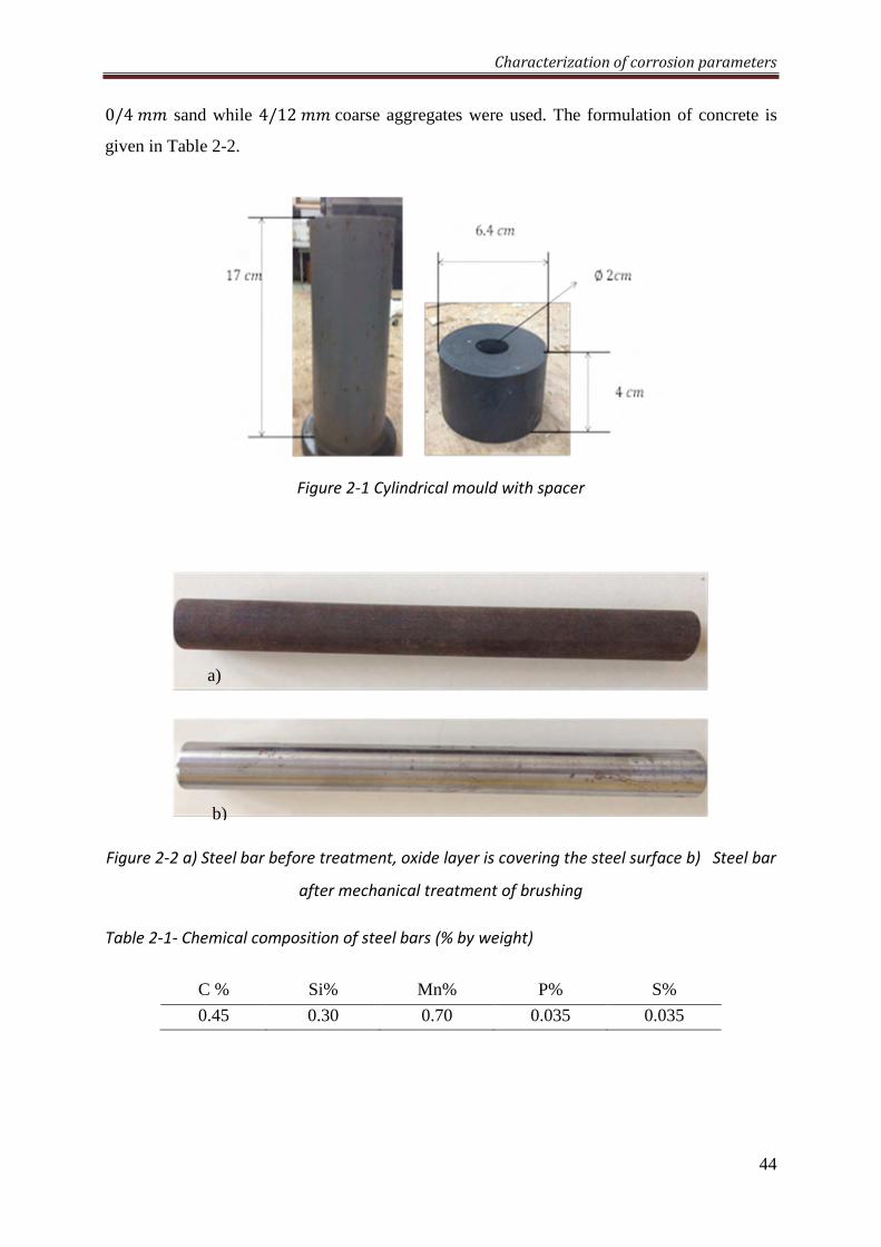
Characterization of corrosion parameters

44

0/4;; sand while 4/12;;coarse aggregates were used. The formulation of concrete is

given in Table 2-2.

Figure 2-1 Cylindrical mould with spacer

Figure 2-2 a) Steel bar before treatment, oxide layer is covering the steel surface b) Steel bar

after mechanical treatment of brushing

Table 2-1- Chemical composition of steel bars (% by weight)

C % Si% Mn% P% S%

0.45 0.30 0.70 0.035 0.035

a)

b)

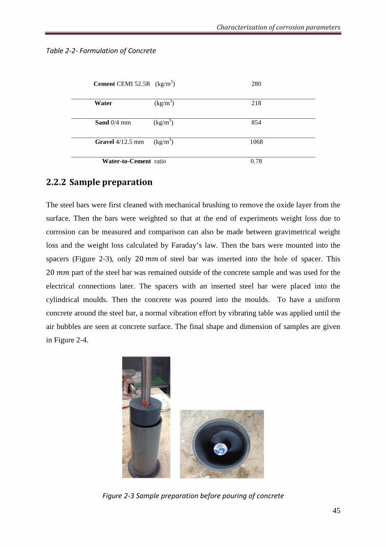
Characterization of corrosion parameters

45

Table 2-2- Formulation of Concrete

2.2.2 Samplepreparation

The steel bars were first cleaned with mechanical brushing to remove the oxide layer from the

surface. Then the bars were weighted so that at the end of experiments weight loss due to

corrosion can be measured and comparison can also be made between gravimetrical weight

loss and the weight loss calculated by Faraday’s law. Then the bars were mounted into the

spacers (Figure 2-3), only 20;;of steel bar was inserted into the hole of spacer. This

20;; part of the steel bar was remained outside of the concrete sample and was used for the

electrical connections later. The spacers with an inserted steel bar were placed into the

cylindrical moulds. Then the concrete was poured into the moulds. To have a uniform

concrete around the steel bar, a normal vibration effort by vibrating table was applied until the

air bubbles are seen at concrete surface. The final shape and dimension of samples are given

in Figure 2-4.

Figure 2-3 Sample preparation before pouring of concrete

Cement CEMI 52.5R (kg/m3) 280

Water (kg/m3) 218

Sand 0/4 mm (kg/m3) 854

Gravel 4/12.5 mm (kg/m3) 1068

Water-to-Cement ratio 0.78

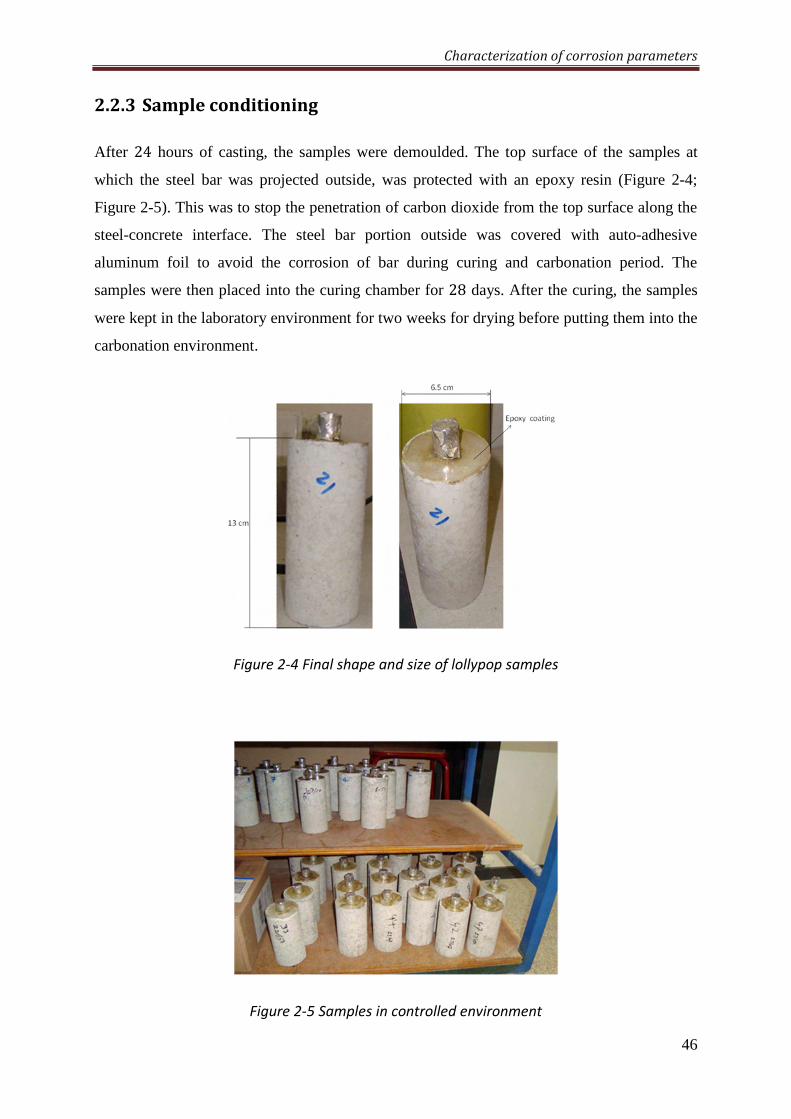
Characterization of corrosion parameters

46

2.2.3 Sampleconditioning

After 24 hours of casting, the samples were demoulded. The top surface of the samples at

which the steel bar was projected outside, was protected with an epoxy resin (Figure 2-4;

Figure 2-5). This was to stop the penetration of carbon dioxide from the top surface along the

steel-concrete interface. The steel bar portion outside was covered with auto-adhesive

aluminum foil to avoid the corrosion of bar during curing and carbonation period. The

samples were then placed into the curing chamber for 28 days. After the curing, the samples

were kept in the laboratory environment for two weeks for drying before putting them into the

carbonation environment.

Figure 2-4 Final shape and size of lollypop samples

Figure 2-5 Samples in controlled environment

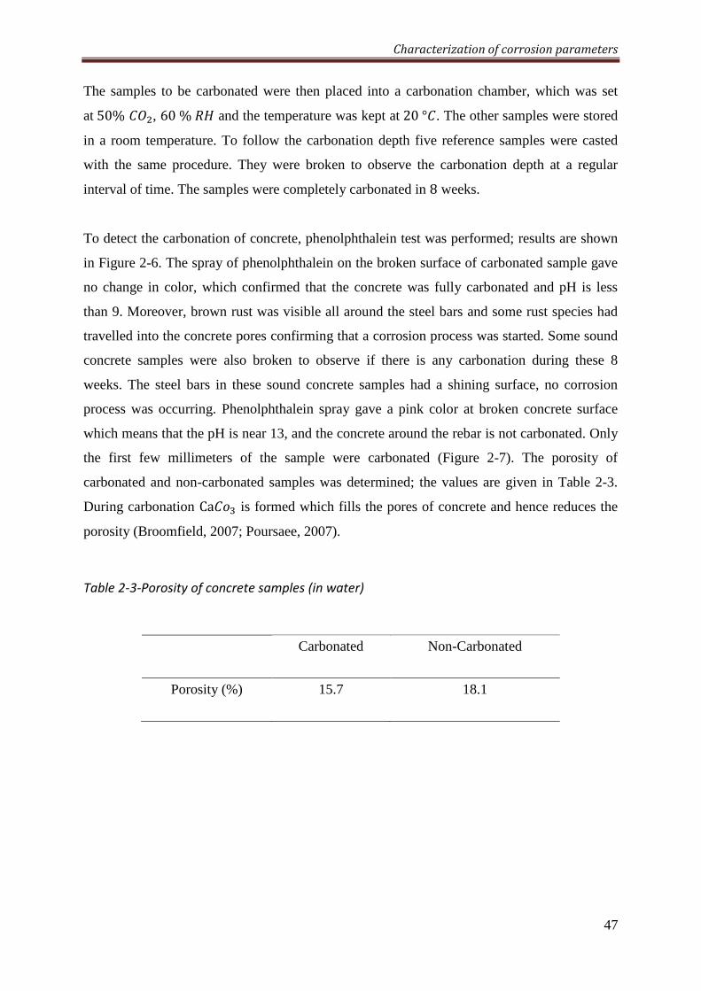
Characterization of corrosion parameters

47

The samples to be carbonated were then placed into a carbonation chamber, which was set

at50% 9>, 60%-7 and the temperature was kept at20°9. The other samples were stored

in a room temperature. To follow the carbonation depth five reference samples were casted

with the same procedure. They were broken to observe the carbonation depth at a regular

interval of time. The samples were completely carbonated in 8 weeks.

To detect the carbonation of concrete, phenolphthalein test was performed; results are shown

in Figure 2-6. The spray of phenolphthalein on the broken surface of carbonated sample gave

no change in color, which confirmed that the concrete was fully carbonated and pH is less

than 9. Moreover, brown rust was visible all around the steel bars and some rust species had

travelled into the concrete pores confirming that a corrosion process was started. Some sound

concrete samples were also broken to observe if there is any carbonation during these 8

weeks. The steel bars in these sound concrete samples had a shining surface, no corrosion

process was occurring. Phenolphthalein spray gave a pink color at broken concrete surface

which means that the pH is near 13, and the concrete around the rebar is not carbonated. Only

the first few millimeters of the sample were carbonated (Figure 2-7). The porosity of

carbonated and non-carbonated samples was determined; the values are given in Table 2-3.

During carbonation Ca9<" is formed which fills the pores of concrete and hence reduces the

porosity (Broomfield, 2007; Poursaee, 2007).

Table 2-3-Porosity of concrete samples (in water)

Carbonated Non-Carbonated

Porosity (%) 15.7 18.1

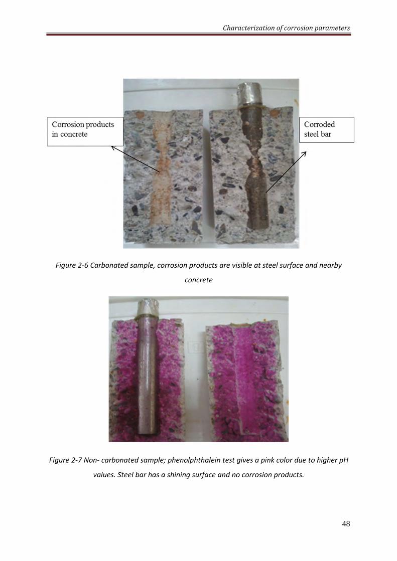
Characterization of corrosion parameters

48

Figure 2-6 Carbonated sample, corrosion products are visible at steel surface and nearby

concrete

Figure 2-7 Non- carbonated sample; phenolphthalein test gives a pink color due to higher pH

values. Steel bar has a shining surface and no corrosion products.

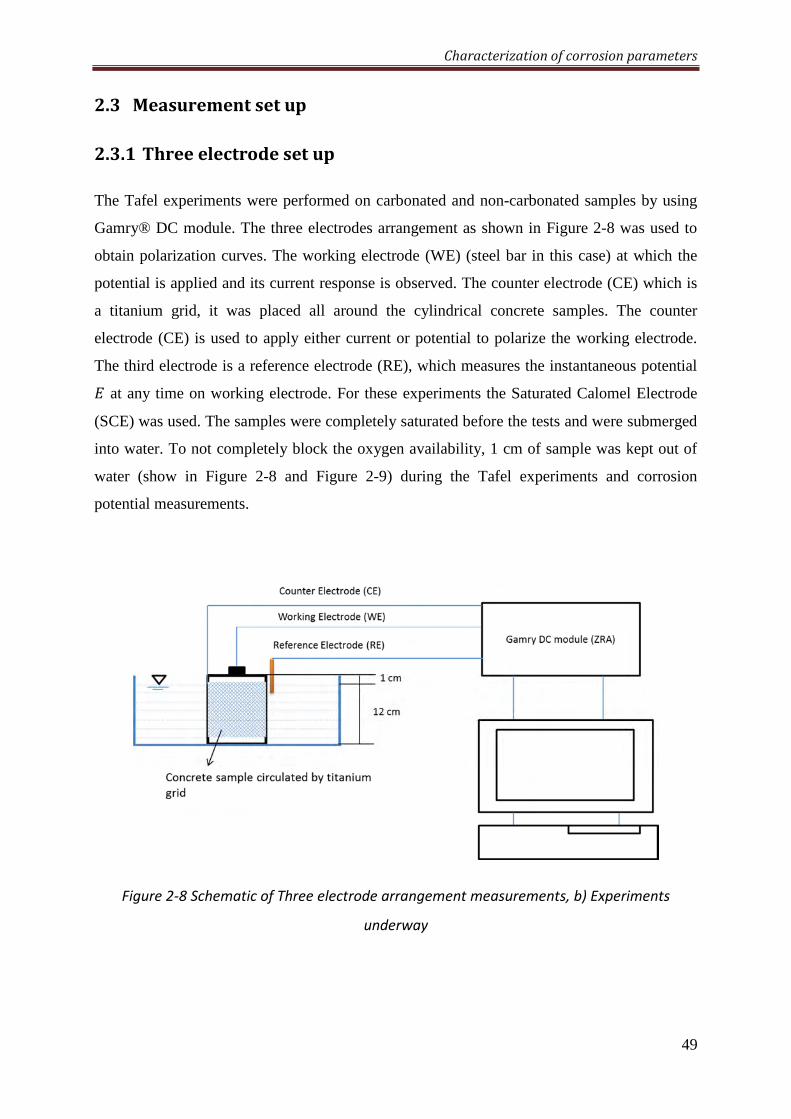
Characterization of corrosion parameters

49

2.3 Measurementsetup

2.3.1 Threeelectrodesetup

The Tafel experiments were performed on carbonated and non-carbonated samples by using

Gamry® DC module. The three electrodes arrangement as shown in Figure 2-8 was used to

obtain polarization curves. The working electrode (WE) (steel bar in this case) at which the

potential is applied and its current response is observed. The counter electrode (CE) which is

a titanium grid, it was placed all around the cylindrical concrete samples. The counter

electrode (CE) is used to apply either current or potential to polarize the working electrode.

The third electrode is a reference electrode (RE), which measures the instantaneous potential

at any time on working electrode. For these experiments the Saturated Calomel Electrode

(SCE) was used. The samples were completely saturated before the tests and were submerged

into water. To not completely block the oxygen availability, 1 cm of sample was kept out of

water (show in Figure 2-8 and Figure 2-9) during the Tafel experiments and corrosion

potential measurements.

Figure 2-8 Schematic of Three electrode arrangement measurements, b) Experiments

underway

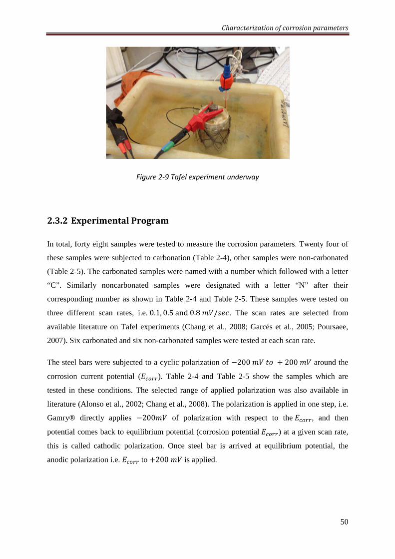
Characterization of corrosion parameters

50

Figure 2-9 Tafel experiment underway

2.3.2 ExperimentalProgram

In total, forty eight samples were tested to measure the corrosion parameters. Twenty four of

these samples were subjected to carbonation (Table 2-4), other samples were non-carbonated

(Table 2-5). The carbonated samples were named with a number which followed with a letter

“C”. Similarly noncarbonated samples were designated with a letter “N” after their

corresponding number as shown in Table 2-4 and Table 2-5. These samples were tested on

three different scan rates, i.e.0.1, 0.5and0.8;/U]. The scan rates are selected from

available literature on Tafel experiments (Chang et al., 2008; Garcés et al., 2005; Poursaee,

2007). Six carbonated and six non-carbonated samples were tested at each scan rate.

The steel bars were subjected to a cyclic polarization of −200;x< + 200; around the

corrosion current potential (^a((). Table 2-4 and Table 2-5 show the samples which are

tested in these conditions. The selected range of applied polarization was also available in

literature (Alonso et al., 2002; Chang et al., 2008). The polarization is applied in one step, i.e.

Gamry® directly applies −200; of polarization with respect to the^a((, and then

potential comes back to equilibrium potential (corrosion potential^a(() at a given scan rate,

this is called cathodic polarization. Once steel bar is arrived at equilibrium potential, the

anodic polarization i.e. a(( to +200; is applied.

Characterization of corrosion parameters

51

The drawback of one step polarization is that the potential of steel bar often does not come

back exactly at ^a(( before starting anodic polarization. Which means the equilibrium could

be disturbed with strong cathodic polarization.

In addition some samples were tested under a partial polarization. In these experiments the

applied polarization was only in one direction on a sample, i.e. either anodic (]< +200;) or cathodic (]< − 200;) polarization was applied. Three carbonated and three

non-carbonated samples were tested for each type of partial polarization. The scan rate was

kept at 0.5;/U for all these applied polarizations. These tests were performed to observe the

effect of the polarization procedure (continuous/cyclic) on the polarization curve.

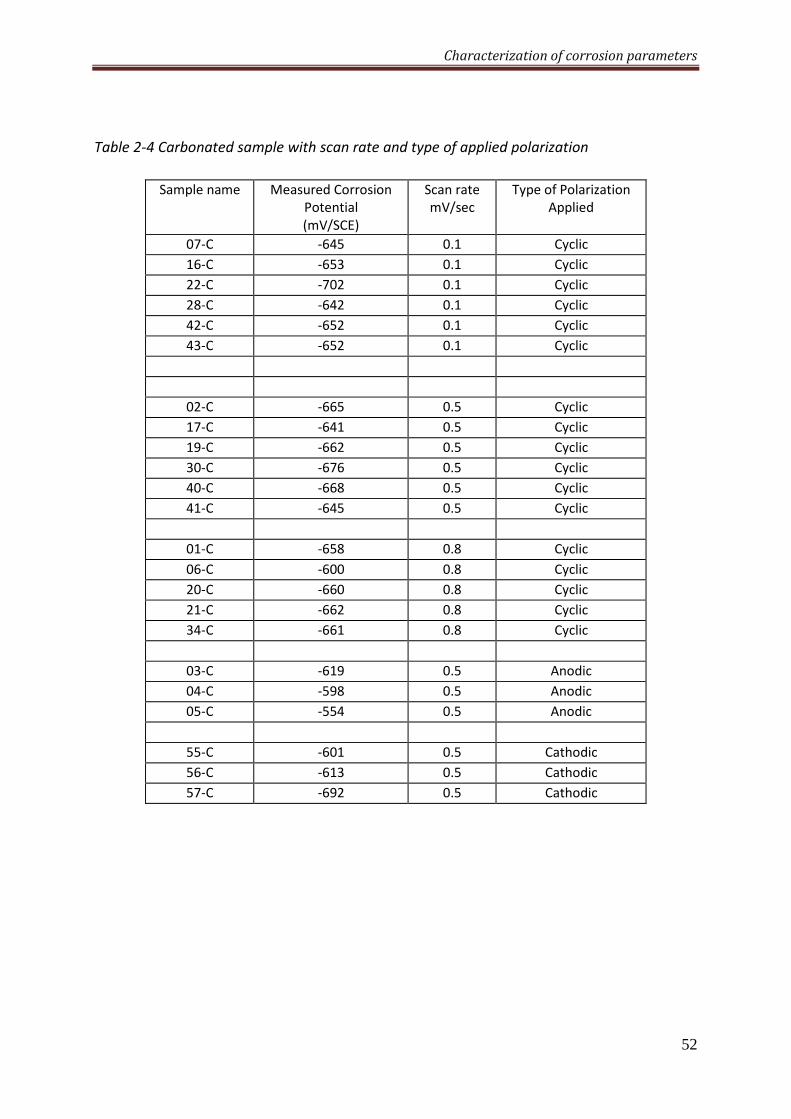
Characterization of corrosion parameters

52

Table 2-4 Carbonated sample with scan rate and type of applied polarization

Sample name Measured Corrosion

Potential

(mV/SCE)

Scan rate mV/sec

Type of Polarization

Applied

07-C -645 0.1 Cyclic

16-C -653 0.1 Cyclic

22-C -702 0.1 Cyclic

28-C -642 0.1 Cyclic

42-C -652 0.1 Cyclic

43-C -652 0.1 Cyclic

02-C -665 0.5 Cyclic

17-C -641 0.5 Cyclic

19-C -662 0.5 Cyclic

30-C -676 0.5 Cyclic

40-C -668 0.5 Cyclic

41-C -645 0.5 Cyclic

01-C -658 0.8 Cyclic

06-C -600 0.8 Cyclic

20-C -660 0.8 Cyclic

21-C -662 0.8 Cyclic

34-C -661 0.8 Cyclic

03-C -619 0.5 Anodic

04-C -598 0.5 Anodic

05-C -554 0.5 Anodic

55-C -601 0.5 Cathodic

56-C -613 0.5 Cathodic

57-C -692 0.5 Cathodic

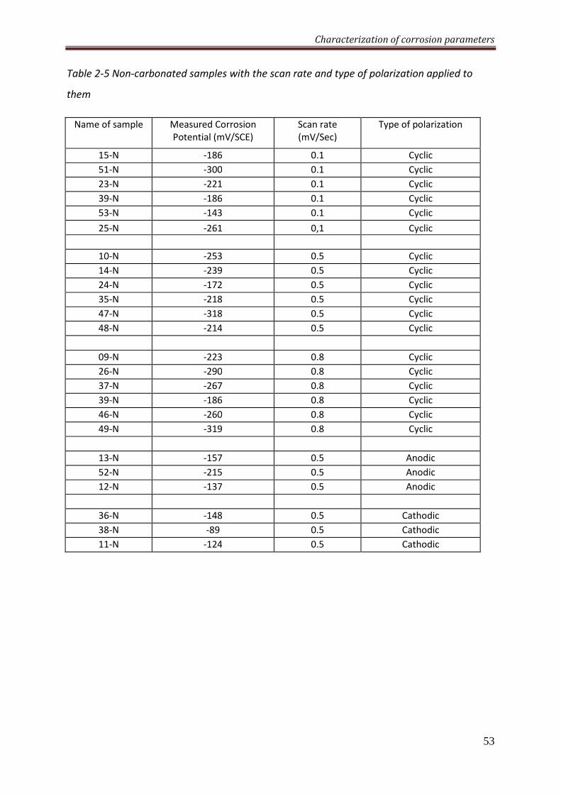
Characterization of corrosion parameters

53

Table 2-5 Non-carbonated samples with the scan rate and type of polarization applied to

them

Name of sample Measured Corrosion

Potential (mV/SCE)

Scan rate

(mV/Sec)

Type of polarization

15-N -186 0.1 Cyclic

51-N -300 0.1 Cyclic

23-N -221 0.1 Cyclic

39-N -186 0.1 Cyclic

53-N -143 0.1 Cyclic

25-N -261 0,1 Cyclic

10-N -253 0.5 Cyclic

14-N -239 0.5 Cyclic

24-N -172 0.5 Cyclic

35-N -218 0.5 Cyclic

47-N -318 0.5 Cyclic

48-N -214 0.5 Cyclic

09-N -223 0.8 Cyclic

26-N -290 0.8 Cyclic

37-N -267 0.8 Cyclic

39-N -186 0.8 Cyclic

46-N -260 0.8 Cyclic

49-N -319 0.8 Cyclic

13-N -157 0.5 Anodic

52-N -215 0.5 Anodic

12-N -137 0.5 Anodic

36-N -148 0.5 Cathodic

38-N -89 0.5 Cathodic

11-N -124 0.5 Cathodic

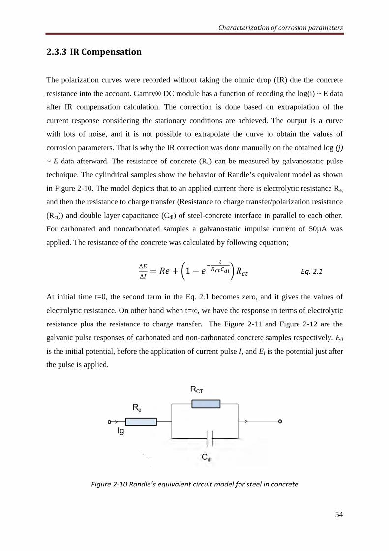
Characterization of corrosion parameters

54

2.3.3 IRCompensation

The polarization curves were recorded without taking the ohmic drop (IR) due the concrete

resistance into the account. Gamry® DC module has a function of recoding the log(i) ~ E data

after IR compensation calculation. The correction is done based on extrapolation of the

current response considering the stationary conditions are achieved. The output is a curve

with lots of noise, and it is not possible to extrapolate the curve to obtain the values of

corrosion parameters. That is why the IR correction was done manually on the obtained log (j)

~ E data afterward. The resistance of concrete (Re) can be measured by galvanostatic pulse

technique. The cylindrical samples show the behavior of Randle’s equivalent model as shown

in Figure 2-10. The model depicts that to an applied current there is electrolytic resistance Re,

and then the resistance to charge transfer (Resistance to charge transfer/polarization resistance

(Rct)) and double layer capacitance (Cdl) of steel-concrete interface in parallel to each other.

For carbonated and noncarbonated samples a galvanostatic impulse current of 50µA was

applied. The resistance of the concrete was calculated by following equation;

∆,∆~ = - + Ä1 −

vigvÅ-^Æ Eq. 2.1

At initial time t=0, the second term in the Eq. 2.1 becomes zero, and it gives the values of

electrolytic resistance. On other hand when t=∞, we have the response in terms of electrolytic

resistance plus the resistance to charge transfer. The Figure 2-11 and Figure 2-12 are the

galvanic pulse responses of carbonated and non-carbonated concrete samples respectively. E0

is the initial potential, before the application of current pulse I, and Ei is the potential just after

the pulse is applied.

Figure 2-10 Randle’s equivalent circuit model for steel in concrete

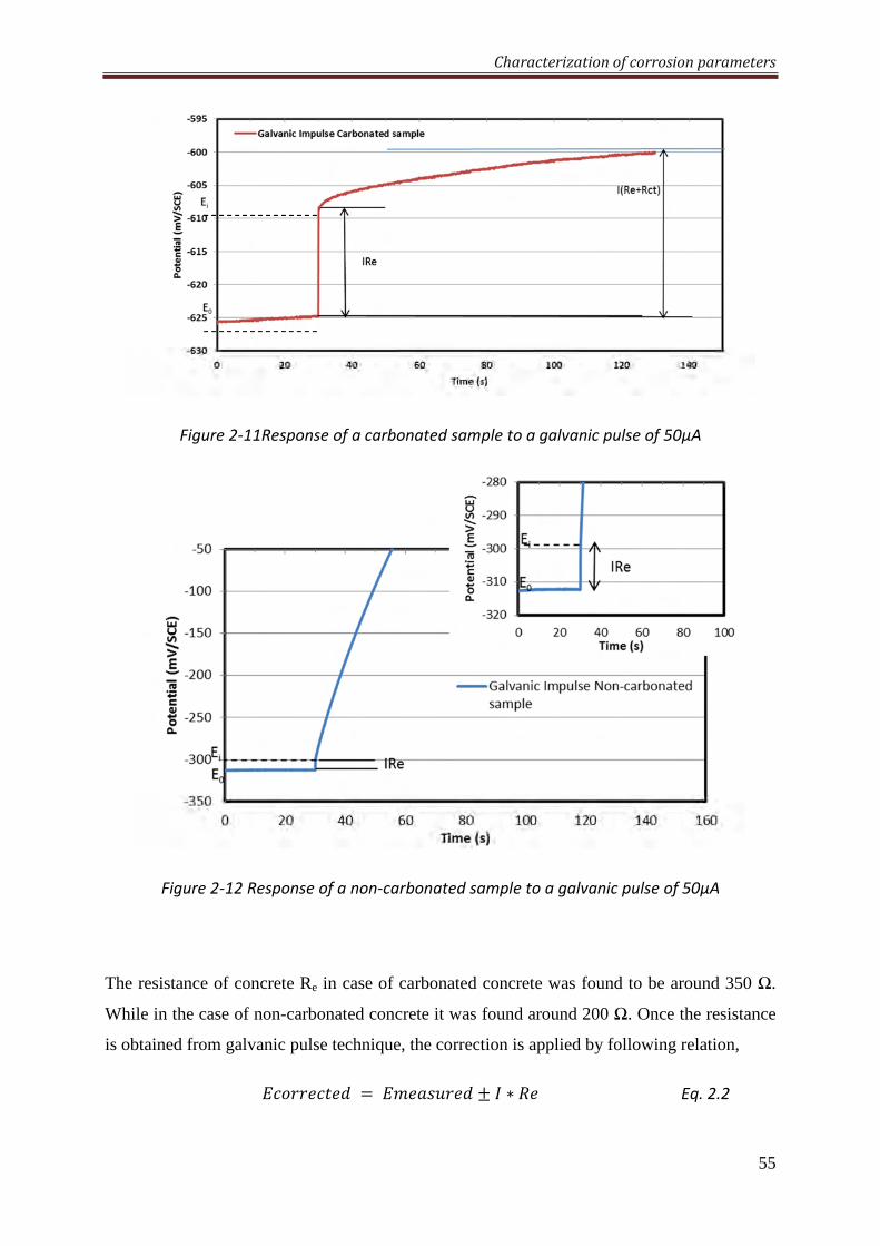
Characterization of corrosion parameters

55

Figure 2-11Response of a carbonated sample to a galvanic pulse of 50µA

Figure 2-12 Response of a non-carbonated sample to a galvanic pulse of 50µA

The resistance of concrete Re in case of carbonated concrete was found to be around 350 Ω.

While in the case of non-carbonated concrete it was found around 200 Ω. Once the resistance

is obtained from galvanic pulse technique, the correction is applied by following relation,

]<]xV = ;OUyV ± ∗ - Eq. 2.2

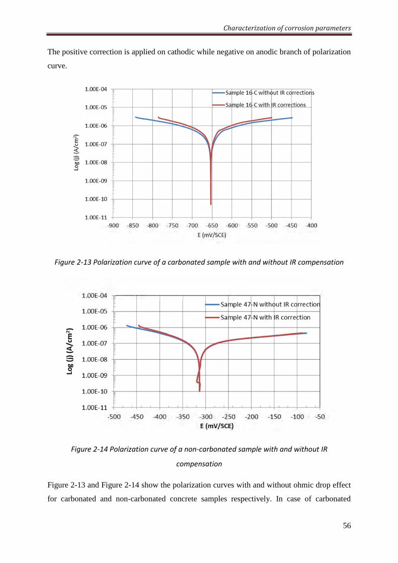
Characterization of corrosion parameters

56

The positive correction is applied on cathodic while negative on anodic branch of polarization

curve.

Figure 2-13 Polarization curve of a carbonated sample with and without IR compensation

Figure 2-14 Polarization curve of a non-carbonated sample with and without IR

compensation

Figure 2-13 and Figure 2-14 show the polarization curves with and without ohmic drop effect

for carbonated and non-carbonated concrete samples respectively. In case of carbonated

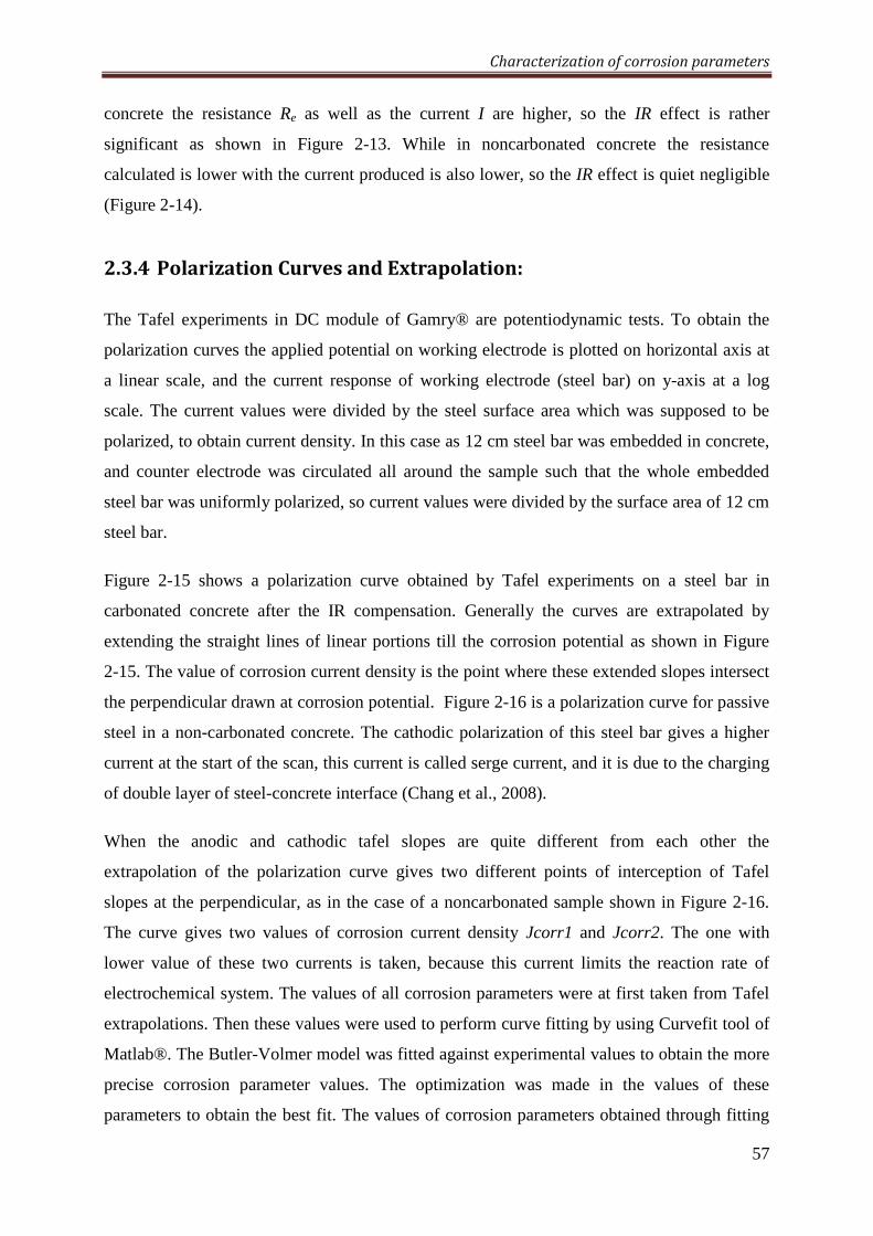
Characterization of corrosion parameters

57

concrete the resistance Re as well as the current I are higher, so the IR effect is rather

significant as shown in Figure 2-13. While in noncarbonated concrete the resistance

calculated is lower with the current produced is also lower, so the IR effect is quiet negligible

(Figure 2-14).

2.3.4 PolarizationCurvesandExtrapolation:

The Tafel experiments in DC module of Gamry® are potentiodynamic tests. To obtain the

polarization curves the applied potential on working electrode is plotted on horizontal axis at

a linear scale, and the current response of working electrode (steel bar) on y-axis at a log

scale. The current values were divided by the steel surface area which was supposed to be

polarized, to obtain current density. In this case as 12 cm steel bar was embedded in concrete,

and counter electrode was circulated all around the sample such that the whole embedded

steel bar was uniformly polarized, so current values were divided by the surface area of 12 cm

steel bar.

Figure 2-15 shows a polarization curve obtained by Tafel experiments on a steel bar in

carbonated concrete after the IR compensation. Generally the curves are extrapolated by

extending the straight lines of linear portions till the corrosion potential as shown in Figure

2-15. The value of corrosion current density is the point where these extended slopes intersect

the perpendicular drawn at corrosion potential. Figure 2-16 is a polarization curve for passive

steel in a non-carbonated concrete. The cathodic polarization of this steel bar gives a higher

current at the start of the scan, this current is called serge current, and it is due to the charging

of double layer of steel-concrete interface (Chang et al., 2008).

When the anodic and cathodic tafel slopes are quite different from each other the

extrapolation of the polarization curve gives two different points of interception of Tafel

slopes at the perpendicular, as in the case of a noncarbonated sample shown in Figure 2-16.

The curve gives two values of corrosion current density Jcorr1 and Jcorr2. The one with

lower value of these two currents is taken, because this current limits the reaction rate of

electrochemical system. The values of all corrosion parameters were at first taken from Tafel

extrapolations. Then these values were used to perform curve fitting by using Curvefit tool of

Matlab®. The Butler-Volmer model was fitted against experimental values to obtain the more

precise corrosion parameter values. The optimization was made in the values of these

parameters to obtain the best fit. The values of corrosion parameters obtained through fitting

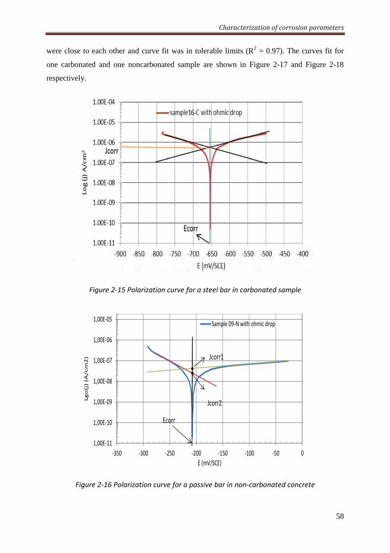
Characterization of corrosion parameters

58

were close to each other and curve fit was in tolerable limits (R2 = 0.97). The curves fit for

one carbonated and one noncarbonated sample are shown in Figure 2-17 and Figure 2-18

respectively.

Figure 2-15 Polarization curve for a steel bar in carbonated sample

Figure 2-16 Polarization curve for a passive bar in non-carbonated concrete

1,00E-11

1,00E-10

1,00E-09

1,00E-08

1,00E-07

1,00E-06

1,00E-05

-350 -300 -250 -200 -150 -100 -50 0

Lg

o(j)

(A

/cm

2)

E (mV/SCE)

Sample 09-N with ohmic drop

Jcorr1

Ecorr

Jcorr2

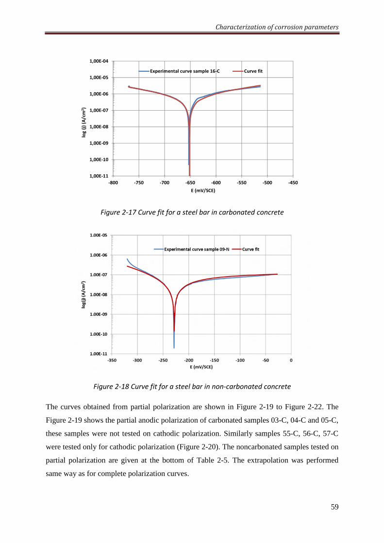
Characterization of corrosion parameters

59

Figure 2-17 Curve fit for a steel bar in carbonated concrete

Figure 2-18 Curve fit for a steel bar in non-carbonated concrete

The curves obtained from partial polarization are shown in Figure 2-19 to Figure 2-22. The

Figure 2-19 shows the partial anodic polarization of carbonated samples 03-C, 04-C and 05-C,

these samples were not tested on cathodic polarization. Similarly samples 55-C, 56-C, 57-C

were tested only for cathodic polarization (Figure 2-20). The noncarbonated samples tested on

partial polarization are given at the bottom of Table 2-5. The extrapolation was performed

same way as for complete polarization curves.

1,00E-11

1,00E-10

1,00E-09

1,00E-08

1,00E-07

1,00E-06

1,00E-05

1,00E-04

-800 -750 -700 -650 -600 -550 -500 -450

log

(j)

(A

/cm

2)

E (mV/SCE)

Experimental curve sample 16-C Curve fit

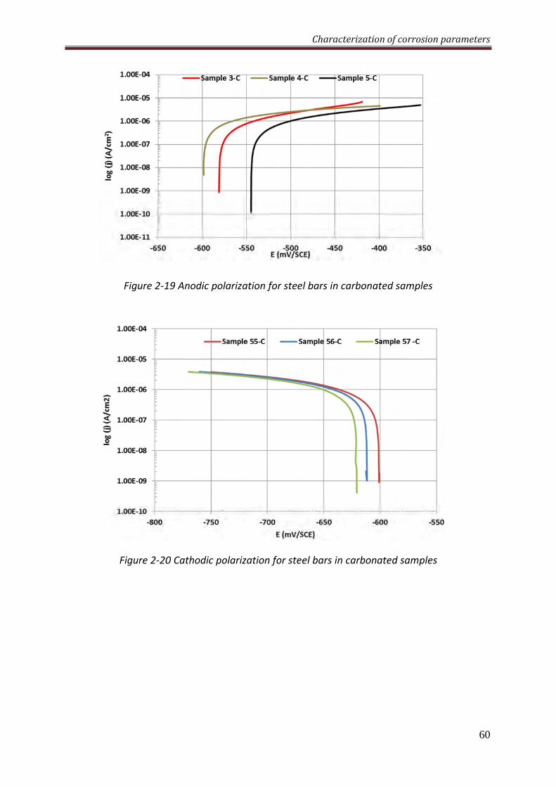
Characterization of corrosion parameters

60

Figure 2-19 Anodic polarization for steel bars in carbonated samples

Figure 2-20 Cathodic polarization for steel bars in carbonated samples

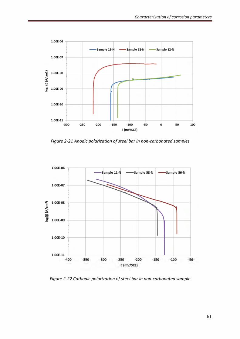
Characterization of corrosion parameters

61

Figure 2-21 Anodic polarization of steel bar in non-carbonated samples

Figure 2-22 Cathodic polarization of steel bar in non-carbonated sample

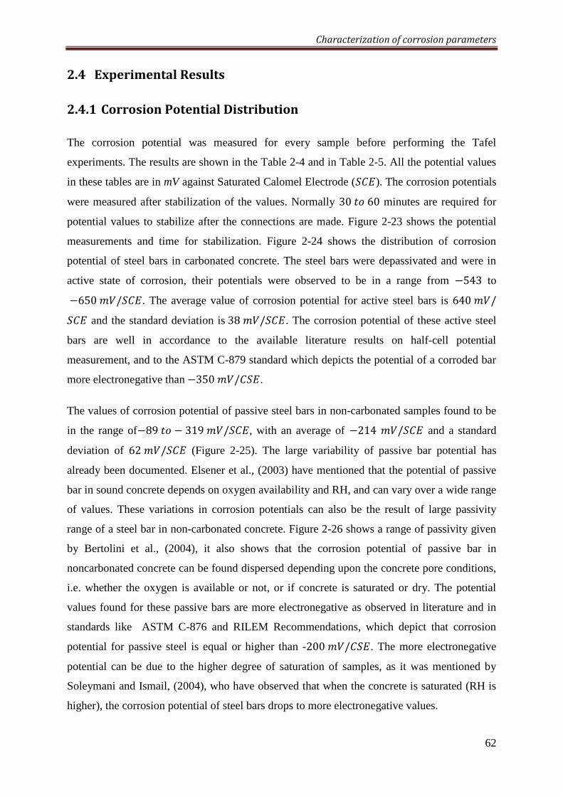
Characterization of corrosion parameters

62

2.4 ExperimentalResults

2.4.1 CorrosionPotentialDistribution

The corrosion potential was measured for every sample before performing the Tafel

experiments. The results are shown in the Table 2-4 and in Table 2-5. All the potential values

in these tables are in mV against Saturated Calomel Electrode (9). The corrosion potentials

were measured after stabilization of the values. Normally 30x<60 minutes are required for

potential values to stabilize after the connections are made. Figure 2-23 shows the potential

measurements and time for stabilization. Figure 2-24 shows the distribution of corrosion

potential of steel bars in carbonated concrete. The steel bars were depassivated and were in

active state of corrosion, their potentials were observed to be in a range from −543 to

−650;/9. The average value of corrosion potential for active steel bars is 640;/9 and the standard deviation is38;/9. The corrosion potential of these active steel

bars are well in accordance to the available literature results on half-cell potential

measurement, and to the ASTM C-879 standard which depicts the potential of a corroded bar

more electronegative than−350;/9.

The values of corrosion potential of passive steel bars in non-carbonated samples found to be

in the range of−89x< − 319;/9, with an average of −214 ;/9 and a standard

deviation of 62;/9 (Figure 2-25). The large variability of passive bar potential has

already been documented. Elsener et al., (2003) have mentioned that the potential of passive

bar in sound concrete depends on oxygen availability and RH, and can vary over a wide range

of values. These variations in corrosion potentials can also be the result of large passivity

range of a steel bar in non-carbonated concrete. Figure 2-26 shows a range of passivity given

by Bertolini et al., (2004), it also shows that the corrosion potential of passive bar in

noncarbonated concrete can be found dispersed depending upon the concrete pore conditions,

i.e. whether the oxygen is available or not, or if concrete is saturated or dry. The potential

values found for these passive bars are more electronegative as observed in literature and in

standards like ASTM C-876 and RILEM Recommendations, which depict that corrosion

potential for passive steel is equal or higher than -200;/9. The more electronegative

potential can be due to the higher degree of saturation of samples, as it was mentioned by

Soleymani and Ismail, (2004), who have observed that when the concrete is saturated (RH is

higher), the corrosion potential of steel bars drops to more electronegative values.

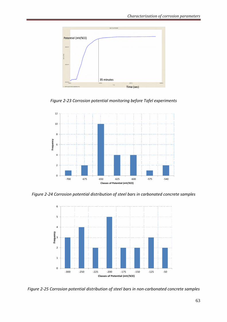
Characterization of corrosion parameters

63

Figure 2-23 Corrosion potential monitoring before Tafel experiments

Figure 2-24 Corrosion potential distribution of steel bars in carbonated concrete samples

Figure 2-25 Corrosion potential distribution of steel bars in non-carbonated concrete samples

0

2

4

6

8

10

12

-700 -675 -650 -625 -600 -575 -540

Fre

qu

en

cy

Classes of Potential (mV/SCE)

0

1

2

3

4

5

6

-300 -250 -225 -200 -175 -150 -125 -50

Fre

qu

en

cy

Classes of Potential (mV/SCE)

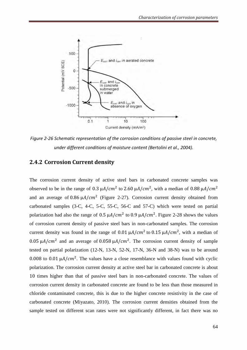
Characterization of corrosion parameters

64

Figure 2-26 Schematic representation of the corrosion conditions of passive steel in concrete,

under different conditions of moisture content (Bertolini et al., 2004).

2.4.2 CorrosionCurrentdensity

The corrosion current density of active steel bars in carbonated concrete samples was

observed to be in the range of 0.3μT/]; to2.60μT/];, with a median of 0.88μT/];

and an average of0.86μT/]; (Figure 2-27). Corrosion current density obtained from

carbonated samples (3-C, 4-C, 5-C, 55-C, 56-C and 57-C) which were tested on partial

polarization had also the range of 0.5μT/]; to0.9μT/];. Figure 2-28 shows the values

of corrosion current density of passive steel bars in non-carbonated samples. The corrosion

current density was found in the range of 0.01μT/];to0.15μT/];, with a median of

0.05μT/]; and an average of0.058μT/];. The corrosion current density of sample

tested on partial polarization (12-N, 13-N, 52-N, 17-N, 36-N and 38-N) was to be around

0.008 to 0.01μT/];. The values have a close resemblance with values found with cyclic

polarization. The corrosion current density at active steel bar in carbonated concrete is about

10 times higher than that of passive steel bars in non-carbonated concrete. The values of

corrosion current density in carbonated concrete are found to be less than those measured in

chloride contaminated concrete, this is due to the higher concrete resistivity in the case of

carbonated concrete (Miyazato, 2010). The corrosion current densities obtained from the

sample tested on different scan rates were not significantly different, in fact there was no

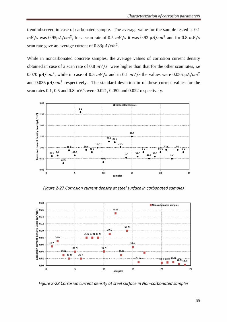
Characterization of corrosion parameters

65

trend observed in case of carbonated sample. The average value for the sample tested at 0.1

;/U was 0.95μT/];, for a scan rate of 0.5 ;/U it was 0.92 μT/]; and for 0.8 ;/U scan rate gave an average current of 0.83μT/];.

While in noncarbonated concrete samples, the average values of corrosion current density

obtained in case of a scan rate of 0.8 ;/U were higher than that for the other scan rates, i.e

0.070 μT/];, while in case of 0.5 ;/U and in 0.1 ;/Uthe values were 0.055 μT/];

and 0.035μT/]; respectively. The standard deviation in of these current values for the

scan rates 0.1, 0.5 and 0.8 mV/s were 0.021, 0.052 and 0.022 respectively.

Figure 2-27 Corrosion current density at steel surface in carbonated samples

Figure 2-28 Corrosion current density at steel surface in Non-carbonated samples

16-C 7-C

22-C

28-C

43-C

2-C

19-C41-C

17-C

40-C

30-C 20-C

21-C

1-C

34-C

33-C

6-C

42-C55-C

56-C57-C

3-C

4-C5-C

0,00

0,50

1,00

1,50

2,00

2,50

3,00

0 5 10 15 20 25

Co

rro

sio

n c

urr

en

t d

en

sity

Jco

rr (

µA

/cm

2)

samples

Carbonated samples

10-N

14-N

15-N

23-N

24-N

26-N

35-N 37-N 39-N

46-N

47-N

48-N

49-N

50-N

53-N

51-N 38-N 11-N 13-N52-N 12-N

0,00

0,02

0,04

0,06

0,08

0,10

0,12

0,14

0,16

0,18

0 5 10 15 20 25

Co

rro

sio

n c

urr

en

t d

en

sity

Jc

orr

(µ

A/cm

2)

samples

Non-carbonated samples

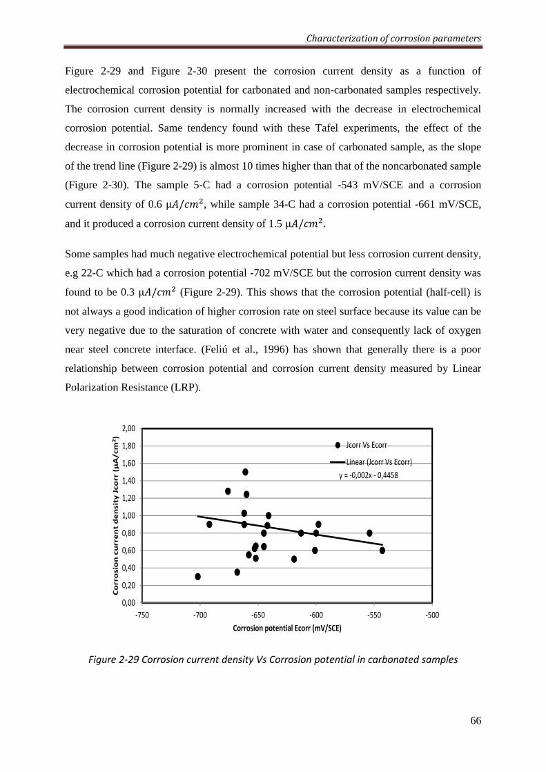
Characterization of corrosion parameters

66

Figure 2-29 and Figure 2-30 present the corrosion current density as a function of

electrochemical corrosion potential for carbonated and non-carbonated samples respectively.

The corrosion current density is normally increased with the decrease in electrochemical

corrosion potential. Same tendency found with these Tafel experiments, the effect of the

decrease in corrosion potential is more prominent in case of carbonated sample, as the slope

of the trend line (Figure 2-29) is almost 10 times higher than that of the noncarbonated sample

(Figure 2-30). The sample 5-C had a corrosion potential -543 mV/SCE and a corrosion

current density of 0.6 μT/];, while sample 34-C had a corrosion potential -661 mV/SCE,

and it produced a corrosion current density of 1.5 μT/];.

Some samples had much negative electrochemical potential but less corrosion current density,

e.g 22-C which had a corrosion potential -702 mV/SCE but the corrosion current density was

found to be 0.3 μT/]; (Figure 2-29). This shows that the corrosion potential (half-cell) is

not always a good indication of higher corrosion rate on steel surface because its value can be

very negative due to the saturation of concrete with water and consequently lack of oxygen

near steel concrete interface. (Feliú et al., 1996) has shown that generally there is a poor

relationship between corrosion potential and corrosion current density measured by Linear

Polarization Resistance (LRP).

Figure 2-29 Corrosion current density Vs Corrosion potential in carbonated samples

y = -0,002x - 0,4458

0,00

0,20

0,40

0,60

0,80

1,00

1,20

1,40

1,60

1,80

2,00

-750 -700 -650 -600 -550 -500

Co

rro

sio

n c

urre

nt

de

nsit

y J

co

rr

(µA

/cm

2)

Corrosion potential Ecorr (mV/SCE)

Jcorr Vs Ecorr

Linear (Jcorr Vs Ecorr)

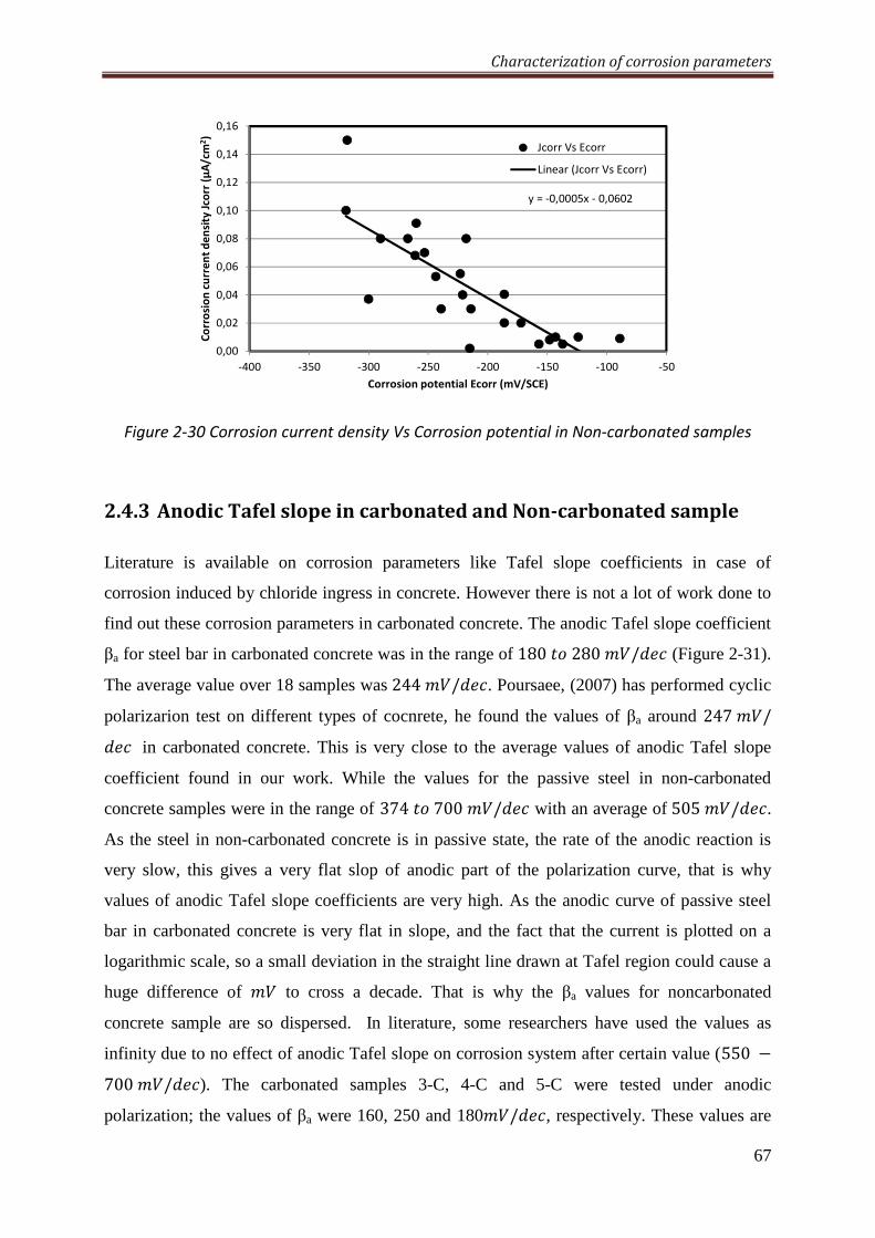
Characterization of corrosion parameters

67

Figure 2-30 Corrosion current density Vs Corrosion potential in Non-carbonated samples

2.4.3 AnodicTafelslopeincarbonatedandNon-carbonatedsample

Literature is available on corrosion parameters like Tafel slope coefficients in case of

corrosion induced by chloride ingress in concrete. However there is not a lot of work done to

find out these corrosion parameters in carbonated concrete. The anodic Tafel slope coefficient

βa for steel bar in carbonated concrete was in the range of180x<280;/V] (Figure 2-31).

The average value over 18 samples was244;/V]. Poursaee, (2007) has performed cyclic

polarizarion test on different types of cocnrete, he found the values of βa around 247;/V] in carbonated concrete. This is very close to the average values of anodic Tafel slope

coefficient found in our work. While the values for the passive steel in non-carbonated

concrete samples were in the range of 374x<700;/V] with an average of505;/V]. As the steel in non-carbonated concrete is in passive state, the rate of the anodic reaction is

very slow, this gives a very flat slop of anodic part of the polarization curve, that is why

values of anodic Tafel slope coefficients are very high. As the anodic curve of passive steel

bar in carbonated concrete is very flat in slope, and the fact that the current is plotted on a

logarithmic scale, so a small deviation in the straight line drawn at Tafel region could cause a

huge difference of ; to cross a decade. That is why the βa values for noncarbonated

concrete sample are so dispersed. In literature, some researchers have used the values as

infinity due to no effect of anodic Tafel slope on corrosion system after certain value (550 −700;/V]). The carbonated samples 3-C, 4-C and 5-C were tested under anodic

polarization; the values of βa were 160, 250 and 180;/V], respectively. These values are

y = -0,0005x - 0,0602

0,00

0,02

0,04

0,06

0,08

0,10

0,12

0,14

0,16

-400 -350 -300 -250 -200 -150 -100 -50

Co

rro

sio

n c

urr

en

t d

en

sity

Jco

rr (

µA

/cm

2)

Corrosion potential Ecorr (mV/SCE)

Jcorr Vs Ecorr

Linear (Jcorr Vs Ecorr)

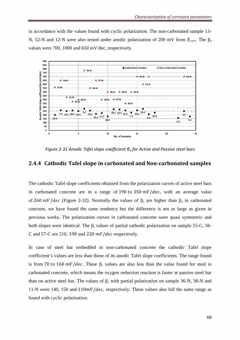
Characterization of corrosion parameters

68

in accordance with the values found with cyclic polarization. The non-carbonated sample 13-

N, 52-N and 12-N were also tested under anodic polarization of 200 mV from Ecorr. The βa

values were 700, 1000 and 650 mV/dec, respectively.

Figure 2-31 Anodic Tafel slope coefficient βa for Active and Passive steel bars

2.4.4 CathodicTafelslopeincarbonatedandNon-carbonatedsamples

The cathodic Tafel slope coefficients obtained from the polarization curves of active steel bars

in carbonated concrete are in a range of190x<350;/V], with an average value

of260;/V] (Figure 2-32). Normally the values of βc are higher than βa in carbonated

concrete, we have found the same tendency but the difference is not as large as given in

previous works. The polarization curves in carbonated concrete were quasi symmetric and

both slopes were identical. The βc values of partial cathodic polarization on sample 55-C, 56-

C and 57-C are 210, 190 and 220;/V]respectively.

In case of steel bar embedded in non-carbonated concrete the cathodic Tafel slope

coefficient‘s values are less than those of its anodic Tafel slope coefficients. The range found

is from70x<160;/V]. These βc values are also less than the value found for steel in

carbonated concrete, which means the oxygen reduction reaction is faster at passive steel bar

than on active steel bar. The values of βc with partial polarization on sample 36-N, 38-N and

11-N were 140, 150 and110;/V], respectively. These values also fall the same range as

found with cyclic polarization.

16-C

7-C 22-C 28-C 43-C2-C

19-C

41-C 17-C

40-C

30-C 20-C 21-C1-C

34-C33-C

6-C42-C

3-C

4-C

5-C

10-N

14-N

15-N

23-N24-N

26-N

35-N

37-N

39-N

46-N

47-N

48-N

49-N

50-N

53-N

51-N

52-N

0

50

100

150

200

250

300

350

400

450

500

550

600

650

700

750

800

850

900

0 5 10 15 20 25

An

od

ic T

afe

l sl

op

e c

off

icie

nt

βa

(m

V/d

ec)

No. of samples

Carbonated samples Non-carbonated samples

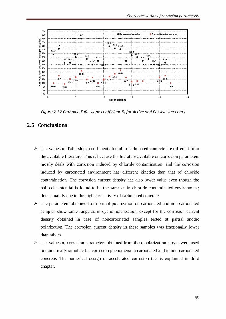
Characterization of corrosion parameters

69

Figure 2-32 Cathodic Tafel slope coefficient βc for Active and Passive steel bars

2.5 Conclusions

The values of Tafel slope coefficients found in carbonated concrete are different from

the available literature. This is because the literature available on corrosion parameters

mostly deals with corrosion induced by chloride contamination, and the corrosion

induced by carbonated environment has different kinetics than that of chloride

contamination. The corrosion current density has also lower value even though the

half-cell potential is found to be the same as in chloride contaminated environment;

this is mainly due to the higher resistivity of carbonated concrete.

The parameters obtained from partial polarization on carbonated and non-carbonated

samples show same range as in cyclic polarization, except for the corrosion current

density obtained in case of noncarbonated samples tested at partial anodic

polarization. The corrosion current density in these samples was fractionally lower

than others.

The values of corrosion parameters obtained from these polarization curves were used

to numerically simulate the corrosion phenomena in carbonated and in non-carbonated

concrete. The numerical design of accelerated corrosion test is explained in third

chapter.

16-C

7-C

22-C 28-C

43-C

2-C

19-C

41-C

17-C

40-C

30-C20-C

21-C

1-C

34-C33-C

6-C42-C

55-C

56-C

57-C

10-N

14-N

15-N

23-N24-N

26-N

35-N37-N

39-N

46-N

47-N48-N

49-N

50-N

53-N 51-N

38-N11-N

13-N

50

70

90

110

130

150

170

190

210

230

250

270

290

310

330

350

370

390

0 5 10 15 20 25

Ca

tho

dic

Ta

fel

slo

pe

co

ffic

ien

t β

a (

mV

/de

c)

No. of samples

Carbonated samples Non-carbonated samples

70

CHAPTER#3

3 DesignofAccelerationCorrosion

test

3.1 Introduction This chapter explains the experimental and numerical design of the accelerated corrosion test

proposed in this thesis. The long time periods involved in replicating reinforcement corrosion

within laboratories has resulted in a number of accelerated test methods being developed. We

first proposed to accelerate the corrosion in the initiation phase by carbonation, and to achieve

the higher corrosion current density in propagation phase, we propose to increase the

Cathode/Anode (C/A) ratio. To easily increase and decrease cathode/anode ratio in laboratory

experiments, we decided to have a cylindrical concrete sample with different number of steel

bars embedded in the concrete. The central cylindrical concrete was carbonated to have a

depassivated steel bar. Then another concrete ring was casted around the inner cylinder,

having four different steel bars embedded at a constant distance from center and also from

each other.

As laboratory experiments are often time consuming and laborious, that is why at first the

accelerated corrosion test was designed by means of numerical simulations. The simulations

were performed by using the commercially available software COMSOL Multiphysics which

is based on FEM. A same geometry with one interior concrete cylinder and one exterior

cylinder was used to simulate corrosion. It was supposed that interior cylinder was carbonated

and steel embedded in it was in active state, while steel bars in sound concrete were in passive

state.

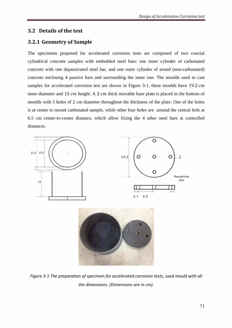
Design of Acceleration Corrosion test

71

3.2 Detailsofthetest

3.2.1 GeometryofSample

The specimens proposed for accelerated corrosion tests are composed of two coaxial

cylindrical concrete samples with embedded steel bars: one inner cylinder of carbonated

concrete with one depassivated steel bar, and one outer cylinder of sound (non-carbonated)

concrete enclosing 4 passive bars and surrounding the inner one. The moulds used to cast

samples for accelerated corrosion test are shown in Figure 3-1, these moulds have 19.2];

inner diameter and 15]; height. A 2]; thick movable base plate is placed in the bottom of

moulds with 5 holes of 2 cm diameter throughout the thickness of the plate. One of the holes

is at center to mount carbonated sample, while other four holes are around the central hole at

6.5 cm center-to-center distance, which allow fixing the 4 other steel bars at controlled

distances.

Figure 3-1 The preparation of specimen for accelerated corrosion tests, used mould with all

the dimensions. (Dimensions are in cm).

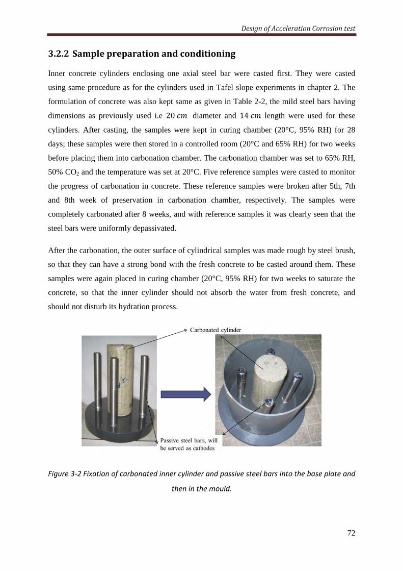
Design of Acceleration Corrosion test

72

3.2.2 Samplepreparationandconditioning

Inner concrete cylinders enclosing one axial steel bar were casted first. They were casted

using same procedure as for the cylinders used in Tafel slope experiments in chapter 2. The

formulation of concrete was also kept same as given in Table 2-2, the mild steel bars having

dimensions as previously used i.e 20]; diameter and 14]; length were used for these

cylinders. After casting, the samples were kept in curing chamber (20°C, 95% RH) for 28

days; these samples were then stored in a controlled room (20°C and 65% RH) for two weeks

before placing them into carbonation chamber. The carbonation chamber was set to 65% RH,

50% CO2 and the temperature was set at 20°C. Five reference samples were casted to monitor

the progress of carbonation in concrete. These reference samples were broken after 5th, 7th

and 8th week of preservation in carbonation chamber, respectively. The samples were

completely carbonated after 8 weeks, and with reference samples it was clearly seen that the

steel bars were uniformly depassivated.

After the carbonation, the outer surface of cylindrical samples was made rough by steel brush,

so that they can have a strong bond with the fresh concrete to be casted around them. These

samples were again placed in curing chamber (20°C, 95% RH) for two weeks to saturate the

concrete, so that the inner cylinder should not absorb the water from fresh concrete, and

should not disturb its hydration process.

Figure 3-2 Fixation of carbonated inner cylinder and passive steel bars into the base plate and

then in the mould.

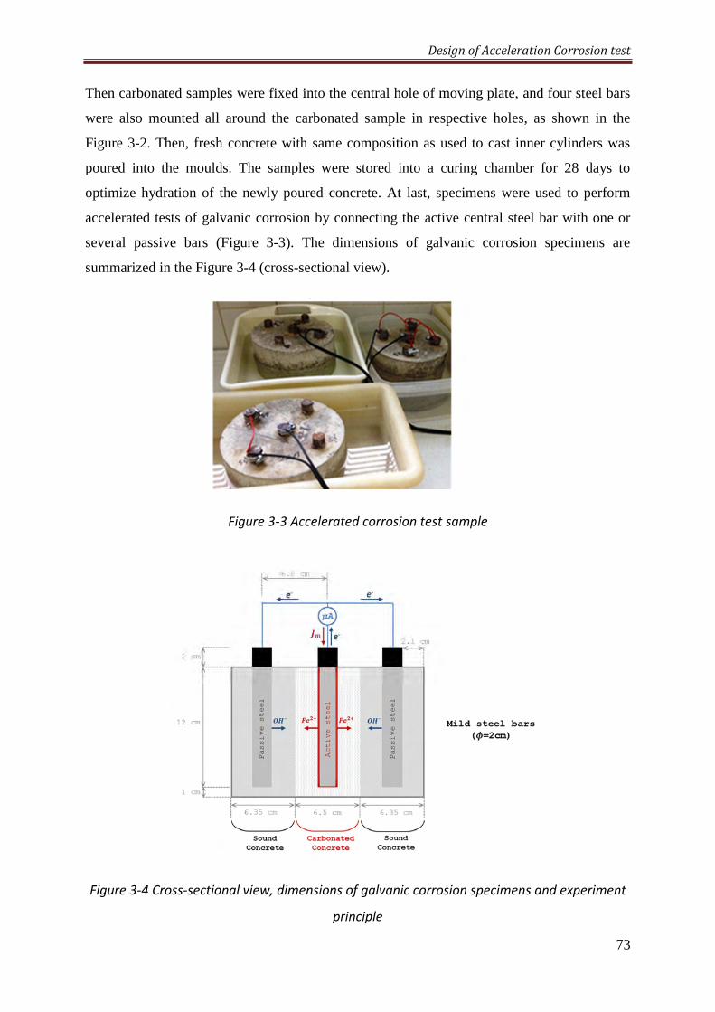
Design of Acceleration Corrosion test

73

Then carbonated samples were fixed into the central hole of moving plate, and four steel bars

were also mounted all around the carbonated sample in respective holes, as shown in the

Figure 3-2. Then, fresh concrete with same composition as used to cast inner cylinders was

poured into the moulds. The samples were stored into a curing chamber for 28 days to

optimize hydration of the newly poured concrete. At last, specimens were used to perform

accelerated tests of galvanic corrosion by connecting the active central steel bar with one or

several passive bars (Figure 3-3). The dimensions of galvanic corrosion specimens are

summarized in the Figure 3-4 (cross-sectional view).

Figure 3-3 Accelerated corrosion test sample

Figure 3-4 Cross-sectional view, dimensions of galvanic corrosion specimens and experiment

principle

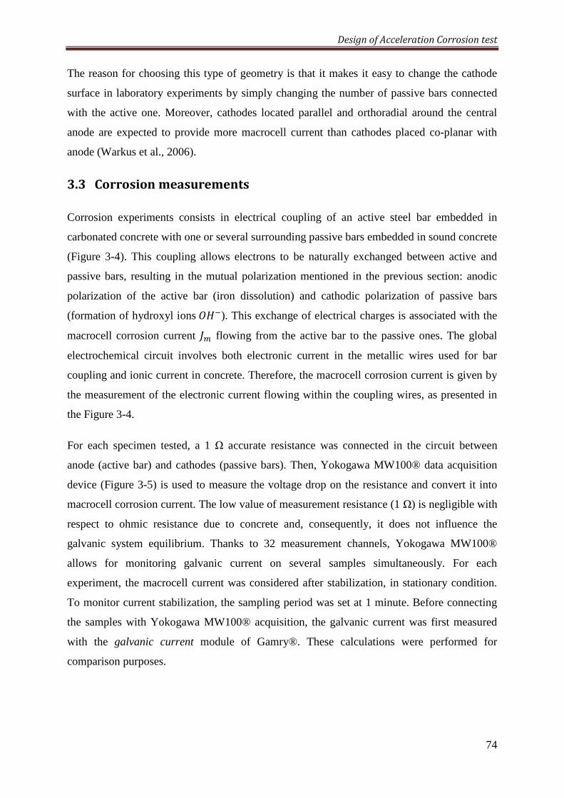
Design of Acceleration Corrosion test

74

The reason for choosing this type of geometry is that it makes it easy to change the cathode

surface in laboratory experiments by simply changing the number of passive bars connected

with the active one. Moreover, cathodes located parallel and orthoradial around the central

anode are expected to provide more macrocell current than cathodes placed co-planar with

anode (Warkus et al., 2006).

3.3 Corrosionmeasurements

Corrosion experiments consists in electrical coupling of an active steel bar embedded in

carbonated concrete with one or several surrounding passive bars embedded in sound concrete

(Figure 3-4). This coupling allows electrons to be naturally exchanged between active and

passive bars, resulting in the mutual polarization mentioned in the previous section: anodic

polarization of the active bar (iron dissolution) and cathodic polarization of passive bars

(formation of hydroxyl ions>7). This exchange of electrical charges is associated with the

macrocell corrosion current w flowing from the active bar to the passive ones. The global

electrochemical circuit involves both electronic current in the metallic wires used for bar

coupling and ionic current in concrete. Therefore, the macrocell corrosion current is given by

the measurement of the electronic current flowing within the coupling wires, as presented in

the Figure 3-4.

For each specimen tested, a 1 Ω accurate resistance was connected in the circuit between

anode (active bar) and cathodes (passive bars). Then, Yokogawa MW100® data acquisition

device (Figure 3-5) is used to measure the voltage drop on the resistance and convert it into

macrocell corrosion current. The low value of measurement resistance (1 Ω) is negligible with

respect to ohmic resistance due to concrete and, consequently, it does not influence the

galvanic system equilibrium. Thanks to 32 measurement channels, Yokogawa MW100®

allows for monitoring galvanic current on several samples simultaneously. For each

experiment, the macrocell current was considered after stabilization, in stationary condition.

To monitor current stabilization, the sampling period was set at 1 minute. Before connecting

the samples with Yokogawa MW100® acquisition, the galvanic current was first measured

with the galvanic current module of Gamry®. These calculations were performed for

comparison purposes.

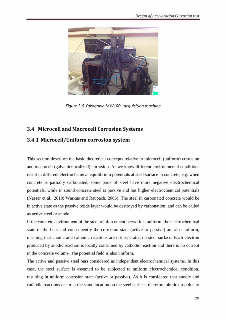
Design of Acceleration Corrosion test

75

Figure 3-5 Yokogawa MW100® acquisition machine

3.4 MicrocellandMacrocellCorrosionSystems

3.4.1 Microcell/Uniformcorrosionsystem

This section describes the basic theoretical concepts relative to microcell (uniform) corrosion

and macrocell (galvanic/localized) corrosion. As we know different environmental conditions

result in different electrochemical equilibrium potentials at steel surface in concrete, e.g. when

concrete is partially carbonated, some parts of steel have more negative electrochemical

potentials, while in sound concrete steel is passive and has higher electrochemical potentials

(Nasser et al., 2010; Warkus and Raupach, 2006). The steel in carbonated concrete would be

in active state as the passive oxide layer would be destroyed by carbonation, and can be called

as active steel or anode.

If the concrete environment of the steel reinforcement network is uniform, the electrochemical

state of the bars and consequently the corrosion state (active or passive) are also uniform,

meaning that anodic and cathodic reactions are not separated on steel surface. Each electron

produced by anodic reaction is locally consumed by cathodic reaction and there is no current

in the concrete volume. The potential field is also uniform.

The active and passive steel bars considered as independent electrochemical systems. In this

case, the steel surface is assumed to be subjected to uniform electrochemical condition,

resulting in uniform corrosion state (active or passive). As it is considered that anodic and

cathodic reactions occur at the same location on the steel surface, therefore ohmic drop due to

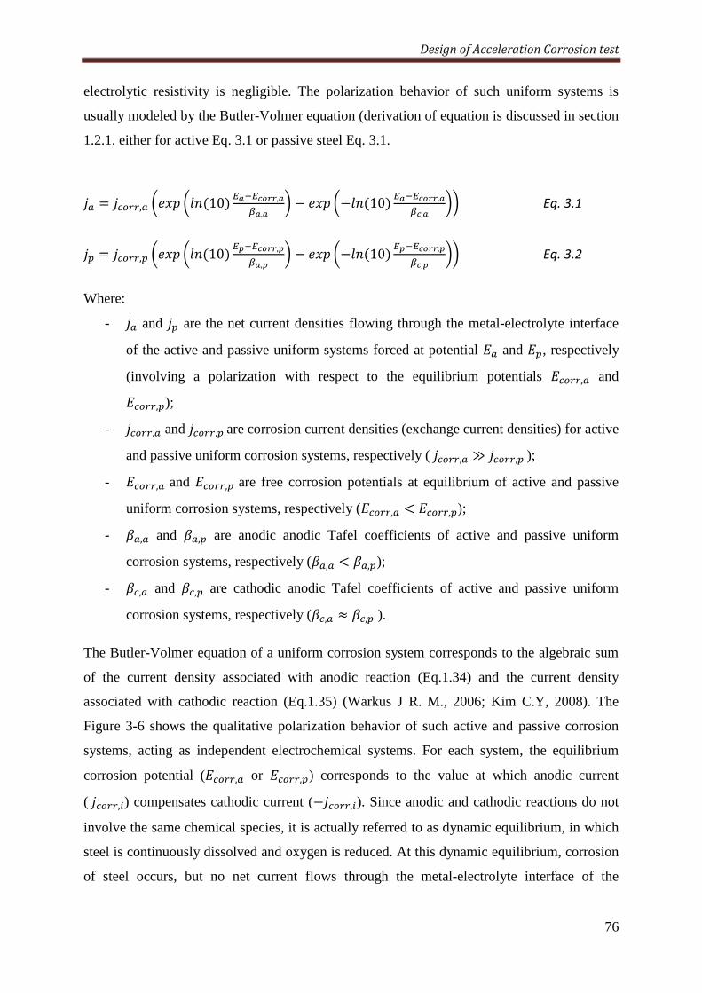
Design of Acceleration Corrosion test

76

electrolytic resistivity is negligible. The polarization behavior of such uniform systems is

usually modeled by the Butler-Volmer equation (derivation of equation is discussed in section

1.2.1, either for active Eq. 3.1 or passive steel Eq. 3.1.

= a((, ÄY6 Ä1'(10E ,f,gruu,ff,f Å − Y6 Ä−1'(10E ,f,gruu,fg,f ÅÅ Eq. 3.1

| = a((,| ÄY6 Ä1'(10E ,,gruu,f, Å − Y6 Ä−1'(10E ,,gruu,g, ÅÅ Eq. 3.2

Where:

- and | are the net current densities flowing through the metal-electrolyte interface

of the active and passive uniform systems forced at potential and |, respectively

(involving a polarization with respect to the equilibrium potentials ^a((, and

^a((,|);

- a((, and a((,| are corrosion current densities (exchange current densities) for active

and passive uniform corrosion systems, respectively ( a((, ≫ a((,| );

- ^a((, and ^a((,| are free corrosion potentials at equilibrium of active and passive

uniform corrosion systems, respectively (^a((, < ^a((,|);

- p, and p,| are anodic anodic Tafel coefficients of active and passive uniform

corrosion systems, respectively (p, < p,|);

- p^, and p^,| are cathodic anodic Tafel coefficients of active and passive uniform

corrosion systems, respectively (p^, ≈ p^,| ).

The Butler-Volmer equation of a uniform corrosion system corresponds to the algebraic sum

of the current density associated with anodic reaction (Eq.1.34) and the current density

associated with cathodic reaction (Eq.1.35) (Warkus J R. M., 2006; Kim C.Y, 2008). The

Figure 3-6 shows the qualitative polarization behavior of such active and passive corrosion

systems, acting as independent electrochemical systems. For each system, the equilibrium

corrosion potential (^a((, or ^a((,|) corresponds to the value at which anodic current

(^a((,) compensates cathodic current (−^a((,). Since anodic and cathodic reactions do not

involve the same chemical species, it is actually referred to as dynamic equilibrium, in which

steel is continuously dissolved and oxygen is reduced. At this dynamic equilibrium, corrosion

of steel occurs, but no net current flows through the metal-electrolyte interface of the

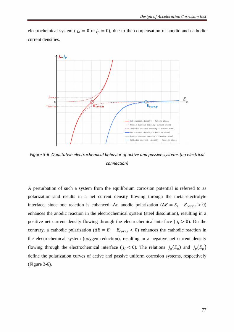
Design of Acceleration Corrosion test

77

electrochemical system ( = 0 or| = 0), due to the compensation of anodic and cathodic

current densities.

Figure 3-6 Qualitative electrochemical behavior of active and passive systems (no electrical

connection)

A perturbation of such a system from the equilibrium corrosion potential is referred to as

polarization and results in a net current density flowing through the metal-electrolyte

interface, since one reaction is enhanced. An anodic polarization (∆ = − ^a((, Ê 0)

enhances the anodic reaction in the electrochemical system (steel dissolution), resulting in a

positive net current density flowing through the electrochemical interface ( Ê 0). On the

contrary, a cathodic polarization (∆ = − ^a((, < 0) enhances the cathodic reaction in

the electrochemical system (oxygen reduction), resulting in a negative net current density

flowing through the electrochemical interface ( < 0). The relations (E and |c|k define the polarization curves of active and passive uniform corrosion systems, respectively

(Figure 3-6).

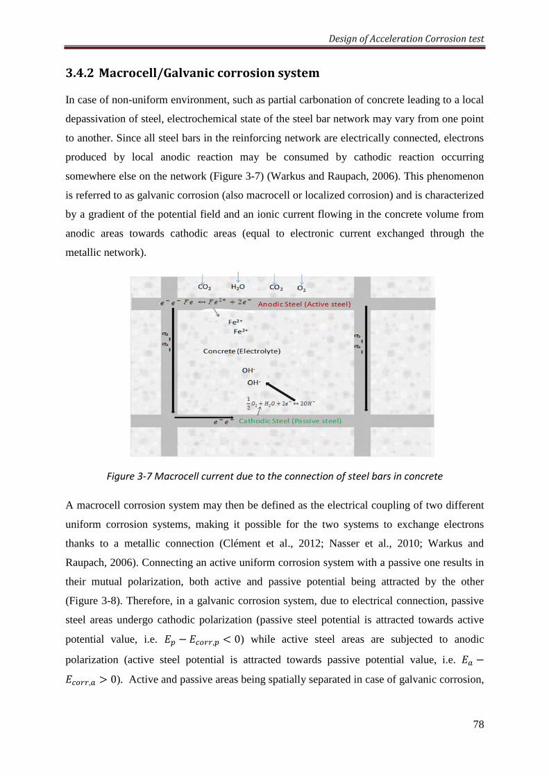
Design of Acceleration Corrosion test

78

3.4.2 Macrocell/Galvaniccorrosionsystem

In case of non-uniform environment, such as partial carbonation of concrete leading to a local

depassivation of steel, electrochemical state of the steel bar network may vary from one point

to another. Since all steel bars in the reinforcing network are electrically connected, electrons

produced by local anodic reaction may be consumed by cathodic reaction occurring

somewhere else on the network (Figure 3-7) (Warkus and Raupach, 2006). This phenomenon

is referred to as galvanic corrosion (also macrocell or localized corrosion) and is characterized

by a gradient of the potential field and an ionic current flowing in the concrete volume from

anodic areas towards cathodic areas (equal to electronic current exchanged through the

metallic network).

Figure 3-7 Macrocell current due to the connection of steel bars in concrete

A macrocell corrosion system may then be defined as the electrical coupling of two different

uniform corrosion systems, making it possible for the two systems to exchange electrons

thanks to a metallic connection (Clément et al., 2012; Nasser et al., 2010; Warkus and

Raupach, 2006). Connecting an active uniform corrosion system with a passive one results in

their mutual polarization, both active and passive potential being attracted by the other

(Figure 3-8). Therefore, in a galvanic corrosion system, due to electrical connection, passive

steel areas undergo cathodic polarization (passive steel potential is attracted towards active

potential value, i.e. | − ^a((,| < 0) while active steel areas are subjected to anodic

polarization (active steel potential is attracted towards passive potential value, i.e. −^a((, Ê 0). Active and passive areas being spatially separated in case of galvanic corrosion,

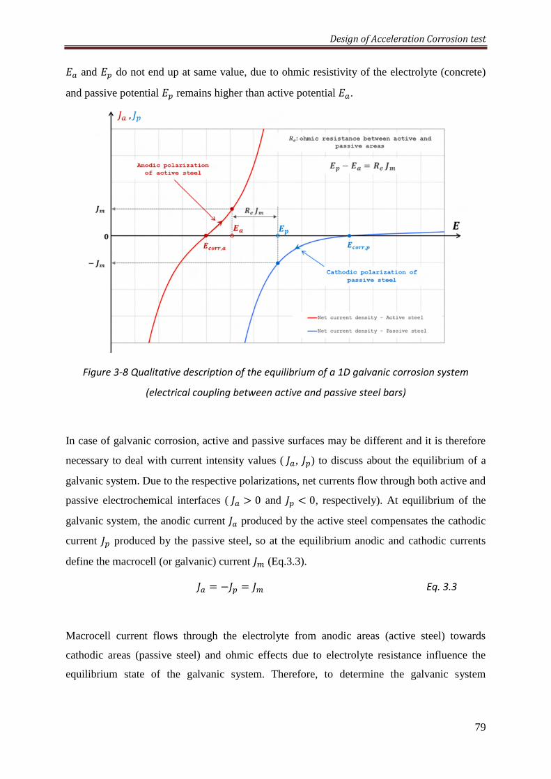
Design of Acceleration Corrosion test

79

and | do not end up at same value, due to ohmic resistivity of the electrolyte (concrete)

and passive potential | remains higher than active potential .

Figure 3-8 Qualitative description of the equilibrium of a 1D galvanic corrosion system

(electrical coupling between active and passive steel bars)

In case of galvanic corrosion, active and passive surfaces may be different and it is therefore

necessary to deal with current intensity values (w, w|) to discuss about the equilibrium of a

galvanic system. Due to the respective polarizations, net currents flow through both active and

passive electrochemical interfaces (w Ê 0 and w| < 0, respectively). At equilibrium of the

galvanic system, the anodic current w produced by the active steel compensates the cathodic

current w| produced by the passive steel, so at the equilibrium anodic and cathodic currents

define the macrocell (or galvanic) current w (Eq.3.3).

w = −w| = w Eq. 3.3

Macrocell current flows through the electrolyte from anodic areas (active steel) towards

cathodic areas (passive steel) and ohmic effects due to electrolyte resistance influence the

equilibrium state of the galvanic system. Therefore, to determine the galvanic system

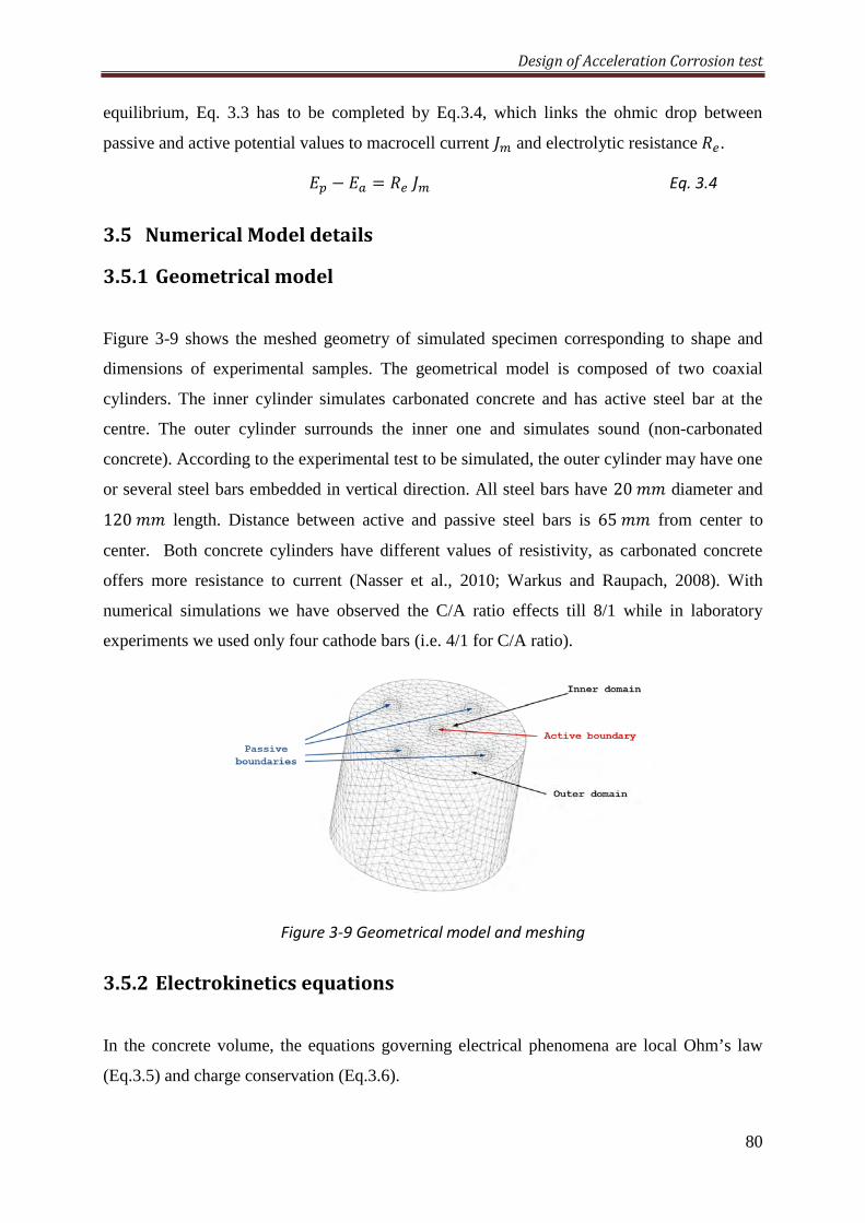
Design of Acceleration Corrosion test

80

equilibrium, Eq. 3.3 has to be completed by Eq.3.4, which links the ohmic drop between

passive and active potential values to macrocell current w and electrolytic resistance-). | − = -)w Eq. 3.4

3.5 NumericalModeldetails

3.5.1 Geometricalmodel

Figure 3-9 shows the meshed geometry of simulated specimen corresponding to shape and

dimensions of experimental samples. The geometrical model is composed of two coaxial

cylinders. The inner cylinder simulates carbonated concrete and has active steel bar at the

centre. The outer cylinder surrounds the inner one and simulates sound (non-carbonated

concrete). According to the experimental test to be simulated, the outer cylinder may have one

or several steel bars embedded in vertical direction. All steel bars have 20;; diameter and

120;; length. Distance between active and passive steel bars is 65;; from center to

center. Both concrete cylinders have different values of resistivity, as carbonated concrete

offers more resistance to current (Nasser et al., 2010; Warkus and Raupach, 2008). With

numerical simulations we have observed the C/A ratio effects till 8/1 while in laboratory

experiments we used only four cathode bars (i.e. 4/1 for C/A ratio).

Figure 3-9 Geometrical model and meshing

3.5.2 Electrokineticsequations

In the concrete volume, the equations governing electrical phenomena are local Ohm’s law

(Eq.3.5) and charge conservation (Eq.3.6).

Design of Acceleration Corrosion test

81

¡ = − = ¢ Eq. 3.5

¢. ¡ = 0 Eq. 3.6

Where j is the local current density, ρ is the electrical resistivity of concrete and is the

local value of the potential field (Clément et al., 2012; Nasser et al., 2010).

3.5.3 BoundaryConditions

The steel-concrete boundaries were modeled according to Butler-Volmer equation for both

active and passive bars (Eq.3.1 and Eq.3.2, respectively) with specific parameter values. All

other interfaces are modeled as electrical insulation, except for the internal boundary between

inner and outer domains where a continuity condition is applied. The potential and the current

density fields in concrete volume are computed by solving Eq.3.5 and Eq.3.6, subjected to the

different prescribed boundary conditions (Ge and Isgor, 2007; Isgor and Razaqpur, 2006).

3.5.4 Simulationparameters

The corrosion parameters show considerable variations in literature for active and passive

conditions as already discussed in Chapter 2. Bearing in mind the uncertainty, Tafel

experiments were performed on carbonated and non-carbonated concrete samples with

embedded steel bars to obtain polarization curves. Concrete samples were saturated and

experiments were performed at room temperature (20°C). Majority of these parameters

matched well with those given in the literature, e.g corrosion potential, corrosion current

density of active and passive steel bar, anodic and cathodic Tafel slope coefficients of passive

steel bar, cathodic Tafel slop coefficient of active steel bar. Only the anodic Tafel slope

coefficients value of active steel was found to quite high than those given in literature. The

simulations were first performed by using the corrosion parameters given in Table 3-1, and

then a detailed parametric study was performed to observe their effects on macrocell

corrosion system. The geometry of sample was such that the use of Wenner probe to

measure the resistivity was not possible. With Gamry® Get Ru module, the values obtained

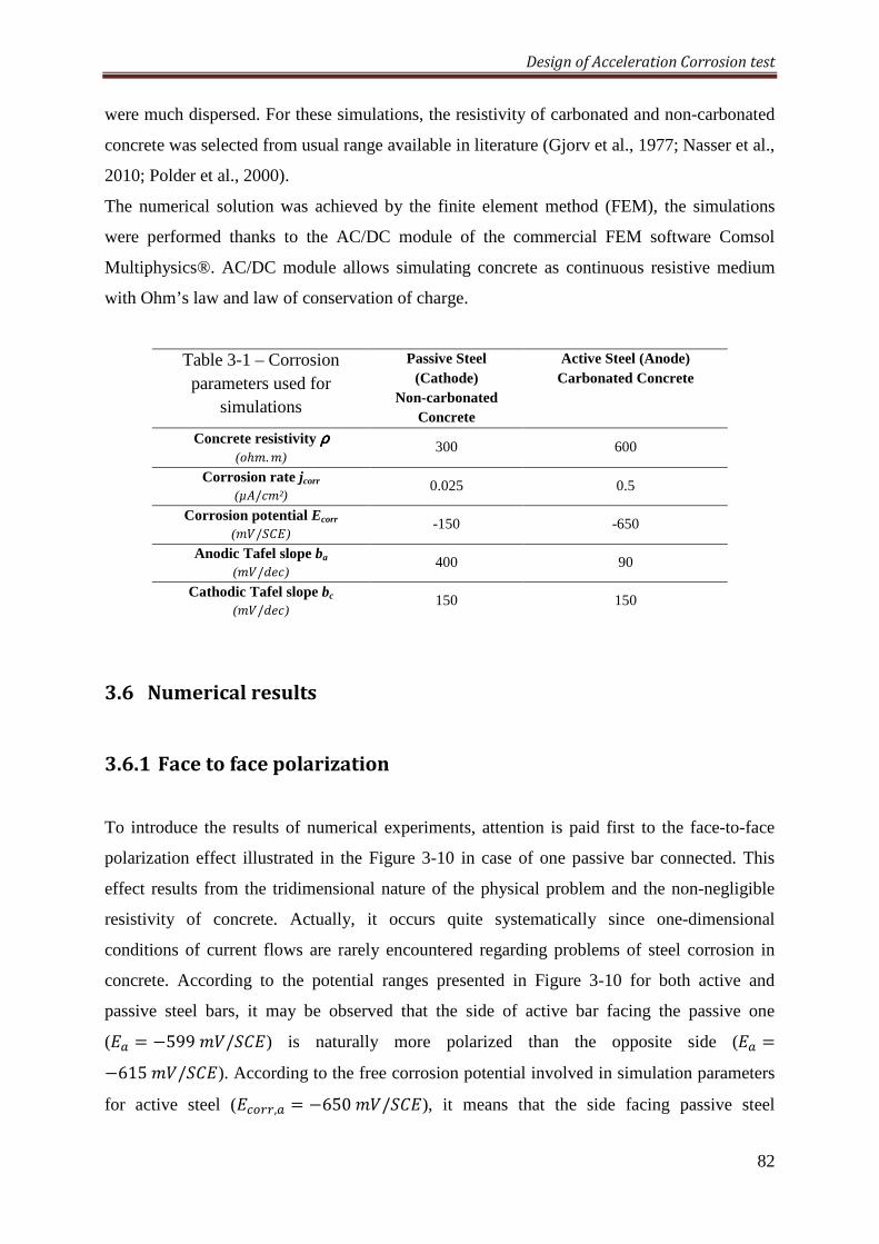
Design of Acceleration Corrosion test

82

were much dispersed. For these simulations, the resistivity of carbonated and non-carbonated

concrete was selected from usual range available in literature (Gjorv et al., 1977; Nasser et al.,

2010; Polder et al., 2000).

The numerical solution was achieved by the finite element method (FEM), the simulations

were performed thanks to the AC/DC module of the commercial FEM software Comsol

Multiphysics®. AC/DC module allows simulating concrete as continuous resistive medium

with Ohm’s law and law of conservation of charge.

Table 3-1 – Corrosion parameters used for

simulations

Passive Steel (Cathode)

Non-carbonated Concrete

Active Steel (Anode) Carbonated Concrete

Concrete resistivity ρρρρ (<ℎ;.;)

300 600

Corrosion rate jcorr (µT/];²)

0.025 0.5

Corrosion potential Ecorr (;/9)

-150 -650

Anodic Tafel slope ba (;/V]) 400 90

Cathodic Tafel slope bc (;/V]) 150 150

3.6 Numericalresults

3.6.1 Facetofacepolarization

To introduce the results of numerical experiments, attention is paid first to the face-to-face

polarization effect illustrated in the Figure 3-10 in case of one passive bar connected. This

effect results from the tridimensional nature of the physical problem and the non-negligible

resistivity of concrete. Actually, it occurs quite systematically since one-dimensional

conditions of current flows are rarely encountered regarding problems of steel corrosion in

concrete. According to the potential ranges presented in Figure 3-10 for both active and

passive steel bars, it may be observed that the side of active bar facing the passive one

( = −599;/9) is naturally more polarized than the opposite side ( =−615;/9). According to the free corrosion potential involved in simulation parameters

for active steel (^a((, = −650;/9), it means that the side facing passive steel

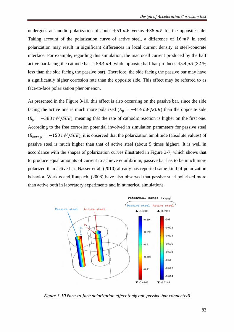
Design of Acceleration Corrosion test

83

undergoes an anodic polarization of about +51; versus +35; for the opposite side.

Taking account of the polarization curve of active steel, a difference of 16; in steel

polarization may result in significant differences in local current density at steel-concrete

interface. For example, regarding this simulation, the macrocell current produced by the half

active bar facing the cathode bar is 58.4ÌT, while opposite half-bar produces 45.4ÌT (22%

less than the side facing the passive bar). Therefore, the side facing the passive bar may have

a significantly higher corrosion rate than the opposite side. This effect may be referred to as

face-to-face polarization phenomenon.

As presented in the Figure 3-10, this effect is also occurring on the passive bar, since the side

facing the active one is much more polarized (| = −414;/9) than the opposite side

(| = −388;/9), meaning that the rate of cathodic reaction is higher on the first one.

According to the free corrosion potential involved in simulation parameters for passive steel

(^a((,| = −150;/9), it is observed that the polarization amplitude (absolute values) of

passive steel is much higher than that of active steel (about 5 times higher). It is well in

accordance with the shapes of polarization curves illustrated in Figure 3-7, which shows that

to produce equal amounts of current to achieve equilibrium, passive bar has to be much more

polarized than active bar. Nasser et al. (2010) already has reported same kind of polarization

behavior. Warkus and Raupach, (2008) have also observed that passive steel polarized more

than active both in laboratory experiments and in numerical simulations.

Figure 3-10 Face-to-face polarization effect (only one passive bar connected)

Design of Acceleration Corrosion test

84

3.6.2 Potentialdistribution

The Figure 3-11 shows the potential gradients achieved in the concrete volume with different

numbers of passive bars connected to the active one. As expected, regarding galvanic

equilibrium condition, for each simulation case, active steel undergoes anodic polarization

(with respect to^a((, = −650;/9) while passive steel bars are subjected to cathodic

polarization (with respect to^a((,| = −150;/9).

As expected according to galvanic corrosion theory, it is observed that increasing the number

of connected passive bars results in higher anodic polarization of active steel, which is

accompanied by an increase in anodic reaction rate. This galvanic coupling effect is well

known and the numerical simulation allows here for taking into account of system geometry

in equilibrium determination. When only one passive bar is available, active steel undergoes

+51; maximum polarization, from −650 to −599; (values collected at point Pa

defined in Figure 3-10, for which the polarization is maximum due to face-to-face effect),

while with four passive bars connected, it undergoes +62; uniform polarization. On the

contrary, increasing the number of passive bars results in a decrease of the global polarization

range of passive steel, because larger area is available to produce the cathodic current

necessary to achieve equilibrium.

Regarding the geometry of the specimens studied here, since passive bars are located in the

circumferential direction and at equal distances from the active bar, the simulation case

involving 4 passive bars connected produces a radial potential field (Figure 3-11-d). In this

case, the active steel bar is quite uniformly polarized, while passive bars still undergo face-to-

face polarization effect. The surface potential field on the outer circumferential boundary is

quite uniform in this case. Regarding other simulation cases (1, 2 and 3 connected passive

bars), surface potential fields on circumferential outer boundaries are non-uniform.

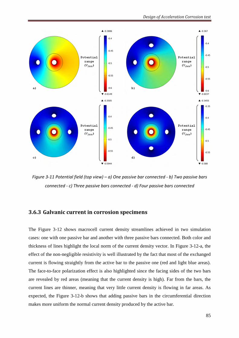
Design of Acceleration Corrosion test

85

Figure 3-11 Potential field (top view) – a) One passive bar connected - b) Two passive bars

connected - c) Three passive bars connected - d) Four passive bars connected

3.6.3 Galvaniccurrentincorrosionspecimens

The Figure 3-12 shows macrocell current density streamlines achieved in two simulation

cases: one with one passive bar and another with three passive bars connected. Both color and

thickness of lines highlight the local norm of the current density vector. In Figure 3-12-a, the

effect of the non-negligible resistivity is well illustrated by the fact that most of the exchanged

current is flowing straightly from the active bar to the passive one (red and light blue areas).

The face-to-face polarization effect is also highlighted since the facing sides of the two bars

are revealed by red areas (meaning that the current density is high). Far from the bars, the

current lines are thinner, meaning that very little current density is flowing in far areas. As

expected, the Figure 3-12-b shows that adding passive bars in the circumferential direction

makes more uniform the normal current density produced by the active bar.

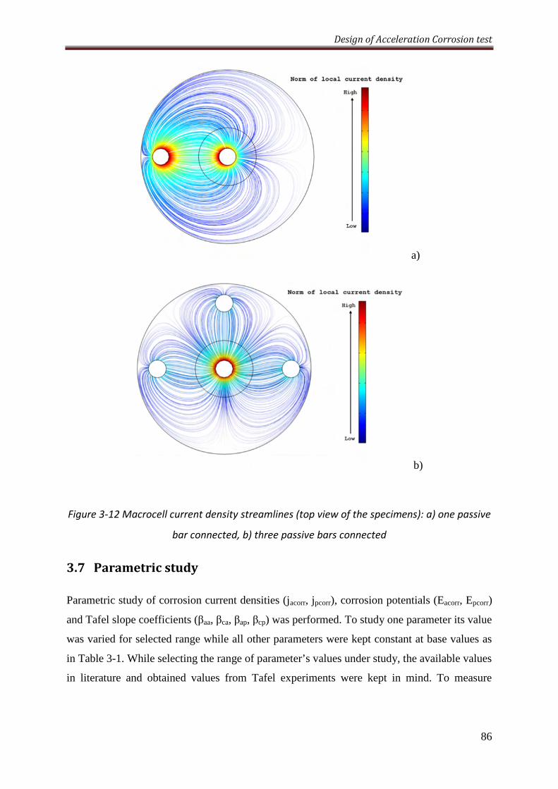
Design of Acceleration Corrosion test

86

a)

b)

Figure 3-12 Macrocell current density streamlines (top view of the specimens): a) one passive

bar connected, b) three passive bars connected

3.7 Parametricstudy

Parametric study of corrosion current densities (jacorr, jpcorr), corrosion potentials (Eacorr, Epcorr)

and Tafel slope coefficients (βaa, βca, βap, βcp) was performed. To study one parameter its value

was varied for selected range while all other parameters were kept constant at base values as

in Table 3-1. While selecting the range of parameter’s values under study, the available values

in literature and obtained values from Tafel experiments were kept in mind. To measure

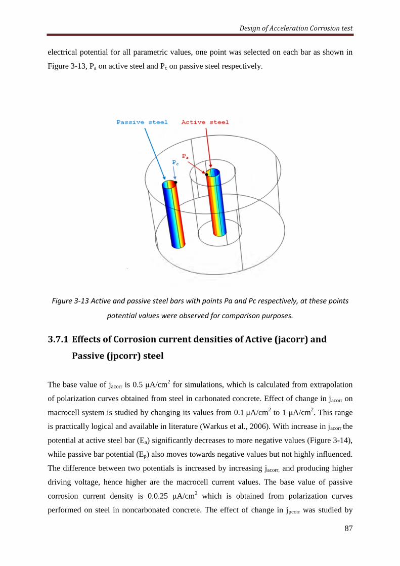
Design of Acceleration Corrosion test

87

electrical potential for all parametric values, one point was selected on each bar as shown in

Figure 3-13, Pa on active steel and Pc on passive steel respectively.

Figure 3-13 Active and passive steel bars with points Pa and Pc respectively, at these points

potential values were observed for comparison purposes.

3.7.1 EffectsofCorrosioncurrentdensitiesofActive(jacorr)and

Passive(jpcorr)steel

The base value of jacorr is 0.5 µA/cm2 for simulations, which is calculated from extrapolation

of polarization curves obtained from steel in carbonated concrete. Effect of change in jacorr on

macrocell system is studied by changing its values from 0.1 µA/cm2 to 1 µA/cm2. This range

is practically logical and available in literature (Warkus et al., 2006). With increase in jacorr the

potential at active steel bar (Ea) significantly decreases to more negative values (Figure 3-14),

while passive bar potential (Ep) also moves towards negative values but not highly influenced.

The difference between two potentials is increased by increasing jacorr, and producing higher

driving voltage, hence higher are the macrocell current values. The base value of passive

corrosion current density is 0.0.25 µA/cm2 which is obtained from polarization curves

performed on steel in noncarbonated concrete. The effect of change in jpcorr was studied by

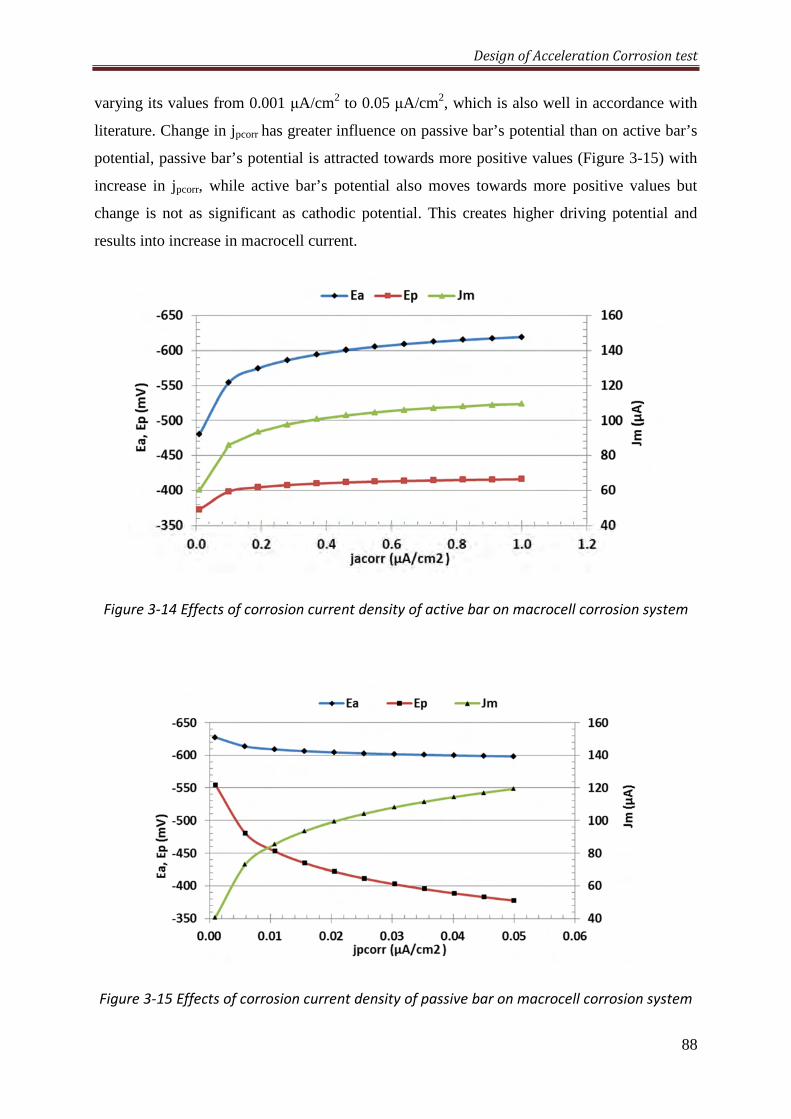
Design of Acceleration Corrosion test

88

varying its values from 0.001 µA/cm2 to 0.05 µA/cm2, which is also well in accordance with

literature. Change in jpcorr has greater influence on passive bar’s potential than on active bar’s

potential, passive bar’s potential is attracted towards more positive values (Figure 3-15) with

increase in jpcorr, while active bar’s potential also moves towards more positive values but

change is not as significant as cathodic potential. This creates higher driving potential and

results into increase in macrocell current.

Figure 3-14 Effects of corrosion current density of active bar on macrocell corrosion system

Figure 3-15 Effects of corrosion current density of passive bar on macrocell corrosion system

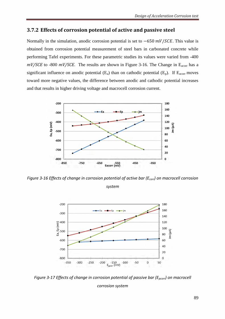
Design of Acceleration Corrosion test

89

3.7.2 Effectsofcorrosionpotentialofactiveandpassivesteel

Normally in the simulation, anodic corrosion potential is set to −650;/9. This value is

obtained from corrosion potential measurement of steel bars in carbonated concrete while

performing Tafel experiments. For these parametric studies its values were varied from -400

mV/SCE to -800 mV/SCE. The results are shown in Figure 3-16. The Change in Eacorr has a

significant influence on anodic potential (Ea) than on cathodic potential (Ep). If Eacorr moves

toward more negative values, the difference between anodic and cathodic potential increases

and that results in higher driving voltage and macrocell corrosion current.

Figure 3-16 Effects of change in corrosion potential of active bar (Ecorr) on macrocell corrosion

system

Figure 3-17 Effects of change in corrosion potential of passive bar (Epcorr) on macrocell

corrosion system

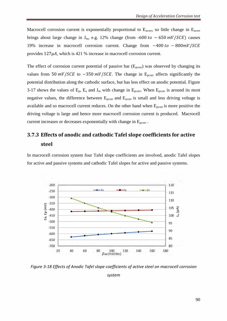
Design of Acceleration Corrosion test

90

Macrocell corrosion current is exponentially proportional to Eacorr, so little change in Eacorr

brings about large change in Jm, e.g. 12% change (from -600x< − 650;/9E causes

19% increase in macrocell corrosion current. Change from −400x< − 800;/9

provides127ÌT, which is 421 % increase in macrocell corrosion current.

The effect of corrosion current potential of passive bar (Epcorr) was observed by changing its

values from 50;/9 to −350;/9. The change in Epcorr affects significantly the

potential distribution along the cathodic surface, but has less effect on anodic potential. Figure

3-17 shows the values of Ep, Ea and Jm with change in Epcorr. When Epcorr is around its most

negative values, the difference between Epcorr and Eacorr is small and less driving voltage is

available and so macrocell current reduces. On the other hand when Epcorr is more positive the

driving voltage is large and hence more macrocell corrosion current is produced. Macrocell

current increases or decreases exponentially with change in Epcorr .

3.7.3 EffectsofanodicandcathodicTafelslopecoefficientsforactive

steel

In macrocell corrosion system four Tafel slope coefficients are involved, anodic Tafel slopes

for active and passive systems and cathodic Tafel slopes for active and passive systems.

Figure 3-18 Effects of Anodic Tafel slope coefficients of active steel on macrocell corrosion

system

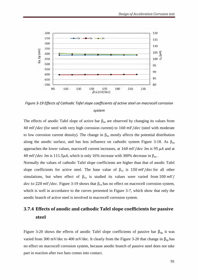
Design of Acceleration Corrosion test

91

Figure 3-19 Effects of Cathodic Tafel slope coefficients of active steel on macrocell corrosion

system

The effects of anodic Tafel slope of active bar βaa are observed by changing its values from

40;/V](for steel with very high corrosion current) to 160;/V] (steel with moderate

to low corrosion current density). The change in βaa mostly affects the potential distribution

along the anodic surface, and has less influence on cathodic system Figure 3-18. As βaa

approaches the lower values, macrocell current increases, at 160;/V] Jm is 95ÌT and at

40;/V] Jm is 111.5ÌT, which is only 16% increase with 300% decrease in βaa .

Normally the values of cathodic Tafel slope coefficients are higher than that of anodic Tafel

slope coefficients for active steel. The base value of βca is 150;/V]for all other

simulations, but when effect of βca is studied its values were varied from100;/V]x<220;/V]. Figure 3-19 shows that βca has no effect on macrocell corrosion system,

which is well in accordance to the curves presented in Figure 3-7, which show that only the

anodic branch of active steel is involved in macrocell corrosion system.

3.7.4 EffectsofanodicandcathodicTafelslopecoefficientsforpassive

steel

Figure 3-20 shows the effects of anodic Tafel slope coefficients of passive bar βap, it was

varied from 300 mV/dec to 400 mV/dec. It clearly from the Figure 3-20 that change in βap has

no effect on macrocell corrosion system, because anodic branch of passive steel does not take

part in reaction after two bars comes into contact.

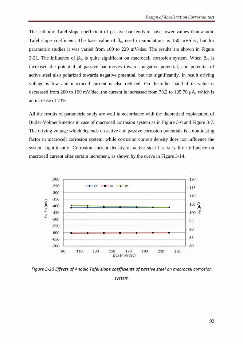
Design of Acceleration Corrosion test

92

The cathodic Tafel slope coefficient of passive bar tends to have lower values than anodic

Tafel slope coefficient. The base value of βcp used in simulations is 150 mV/dec, but for

parametric studies it was varied from 100 to 220 mV/dec. The results are shown in Figure

3-21. The influence of βcp is quite significant on macrocell corrosion system. When βcp is

increased the potential of passive bar moves towards negative potential, and potential of

active steel also polarized towards negative potential, but not significantly. In result driving

voltage is low and macrocell current is also reduced. On the other hand if its value is

decreased from 200 to 100 mV/dec, the current is increased from 78.2 to 135.78 µA, which is

an increase of 73%.

All the results of parametric study are well in accordance with the theoretical explanation of

Butler-Volmer kinetics in case of macrocell corrosion system as in Figure 3-6 and Figure 3-7.

The driving voltage which depends on active and passive corrosion potentials is a dominating

factor in macrocell corrosion system, while corrosion current density does not influence the

system significantly. Corrosion current density of active steel has very little influence on

macrocell current after certain increment, as shown by the curve in Figure 3-14.

Figure 3-20 Effects of Anodic Tafel slope coefficients of passive steel on macrocell corrosion

system

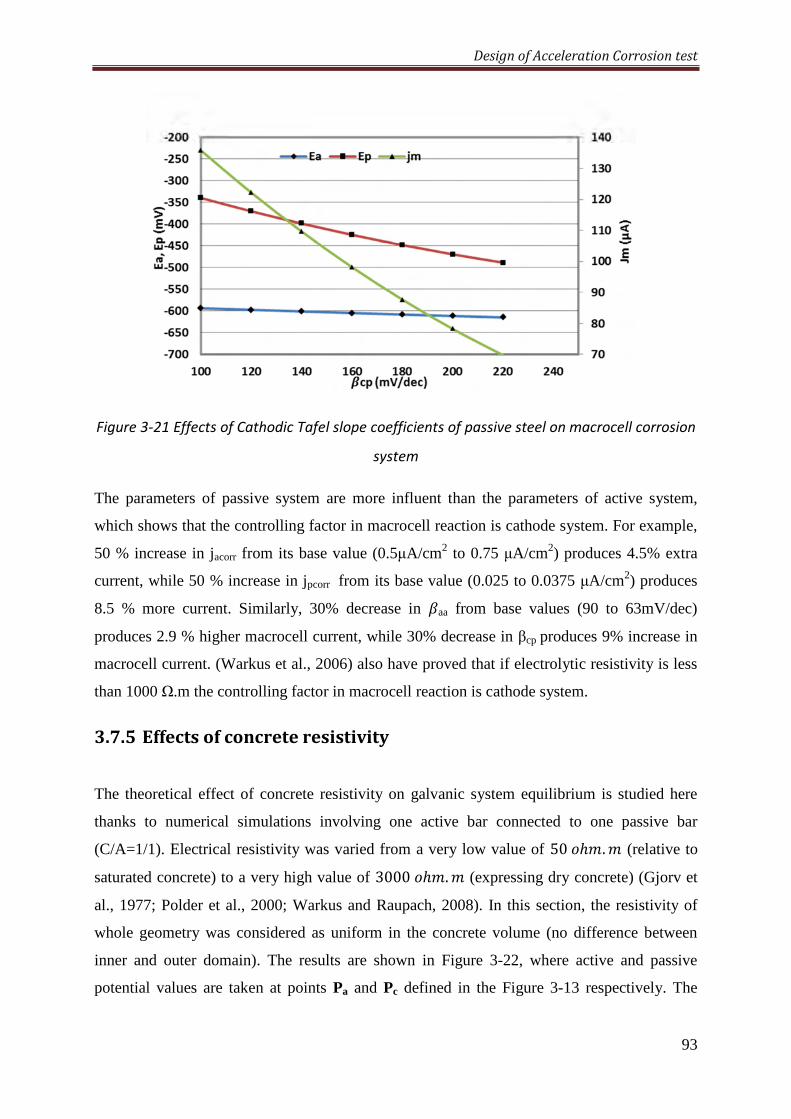
Design of Acceleration Corrosion test

93

Figure 3-21 Effects of Cathodic Tafel slope coefficients of passive steel on macrocell corrosion

system

The parameters of passive system are more influent than the parameters of active system,

which shows that the controlling factor in macrocell reaction is cathode system. For example,

50 % increase in jacorr from its base value (0.5µA/cm2 to 0.75 µA/cm2) produces 4.5% extra

current, while 50 % increase in jpcorr from its base value (0.025 to 0.0375 µA/cm2) produces

8.5 % more current. Similarly, 30% decrease in paa from base values (90 to 63mV/dec)

produces 2.9 % higher macrocell current, while 30% decrease in βcp produces 9% increase in

macrocell current. (Warkus et al., 2006) also have proved that if electrolytic resistivity is less

than 1000 Ω.m the controlling factor in macrocell reaction is cathode system.

3.7.5 Effectsofconcreteresistivity

The theoretical effect of concrete resistivity on galvanic system equilibrium is studied here

thanks to numerical simulations involving one active bar connected to one passive bar

(C/A=1/1). Electrical resistivity was varied from a very low value of 50<ℎ;.; (relative to

saturated concrete) to a very high value of 3000<ℎ;.; (expressing dry concrete) (Gjorv et

al., 1977; Polder et al., 2000; Warkus and Raupach, 2008). In this section, the resistivity of

whole geometry was considered as uniform in the concrete volume (no difference between

inner and outer domain). The results are shown in Figure 3-22, where active and passive

potential values are taken at points Pa and Pc defined in the Figure 3-13 respectively. The

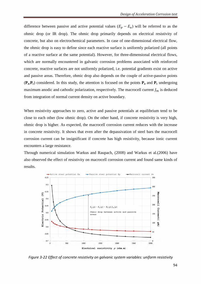
Design of Acceleration Corrosion test

94

difference between passive and active potential values (| − ) will be referred to as the

ohmic drop (or IR drop). The ohmic drop primarily depends on electrical resistivity of

concrete, but also on electrochemical parameters. In case of one-dimensional electrical flow,

the ohmic drop is easy to define since each reactive surface is uniformly polarized (all points

of a reactive surface at the same potential). However, for three-dimensional electrical flows,

which are normally encountered in galvanic corrosion problems associated with reinforced

concrete, reactive surfaces are not uniformly polarized, i.e. potential gradients exist on active

and passive areas. Therefore, ohmic drop also depends on the couple of active-passive points

(Pa,Pc) considered. In this study, the attention is focused on the points Pa and Pc undergoing

maximum anodic and cathodic polarization, respectively. The macrocell current w is deduced

from integration of normal current density on active boundary.

When resistivity approaches to zero, active and passive potentials at equilibrium tend to be

close to each other (low ohmic drop). On the other hand, if concrete resistivity is very high,

ohmic drop is higher. As expected, the macrocell corrosion current reduces with the increase

in concrete resistivity. It shows that even after the depassivation of steel bars the macrocell

corrosion current can be insignificant if concrete has high resistivity, because ionic current

encounters a large resistance.

Through numerical simulation Warkus and Raupach, (2008) and Warkus et al.(2006) have

also observed the effect of resistivity on macrocell corrosion current and found same kinds of

results.

Figure 3-22 Effect of concrete resistivity on galvanic system variables: uniform resistivity

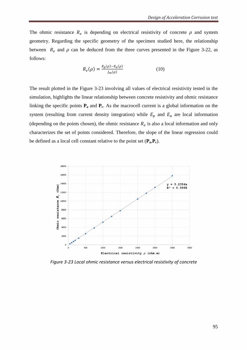
Design of Acceleration Corrosion test

95

The ohmic resistance -) is depending on electrical resistivity of concrete Í and system

geometry. Regarding the specific geometry of the specimen studied here, the relationship

between -) and Í can be deduced from the three curves presented in the Figure 3-22, as

follows:

-)(ÍE = ,(E,f(Et°(E (10)

The result plotted in the Figure 3-23 involving all values of electrical resistivity tested in the

simulation, highlights the linear relationship between concrete resistivity and ohmic resistance

linking the specific points Pa and Pc. As the macrocell current is a global information on the

system (resulting from current density integration) while | and are local information

(depending on the points chosen), the ohmic resistance -) is also a local information and only

characterizes the set of points considered. Therefore, the slope of the linear regression could

be defined as a local cell constant relative to the point set (Pa,Pc).

Figure 3-23 Local ohmic resistance versus electrical resistivity of concrete

Design of Acceleration Corrosion test

96

3.8 Conclusions Comsol Multiphysics® a powerful tool to simulate the physical phenomena, the convergence

to a unique solution was achieved easily. The model of corrosion in reinforced concrete,

where current flow in concrete volume is governed by the ohm’s law, the law of charge

conservation is applied and the steel-concrete interface is model by Butler-Volmer equation,

such model show exactly the same behaviour as elaborated by the theoretical polarization

curves of a galvanic/macrocell corrosion system.

The parametric study shows that in a macrocell corrosion system where is resistivity of

concrete is not very high, the passive (cathodic) system is a governing factor.

97

CHAPTER#4

4 Experimental and Numerical

Validation of the Accelerated

CorrosionTest

4.1 Introduction In the previous chapters the acceleration of initiation phase of corrosion process was

discussed. This chapter elaborates the experimental and numerical results to validate that the

corrosion can also be accelerated in propagation phase by galvanic coupling of one or several

passive steel bars with an active steel bar. The results of experiments and numerical

simulations are also compared in this chapter. By changing Cathode/Anode ratio two main

parameters of macrocell corrosion system were studied numerically as well as experimentally.

Those two parameters are potential distribution during the course of experiment and

macrocell corrosion current.

4.2 Experimentalprogram

Fifteen cylindrical concrete samples were casted for accelerated galvanic corrosion tests. With

the geometry of samples used (as discussed in chapter 3) it was possible to connect up till four

cathodically acting passive steel bars with the anodically acting active bar. To observe the

effect of increase in cathodic surface area on corrosion current density and on the polarization

behavior of active and passive corrosion systems, two configurations of laboratory

experiments were used.

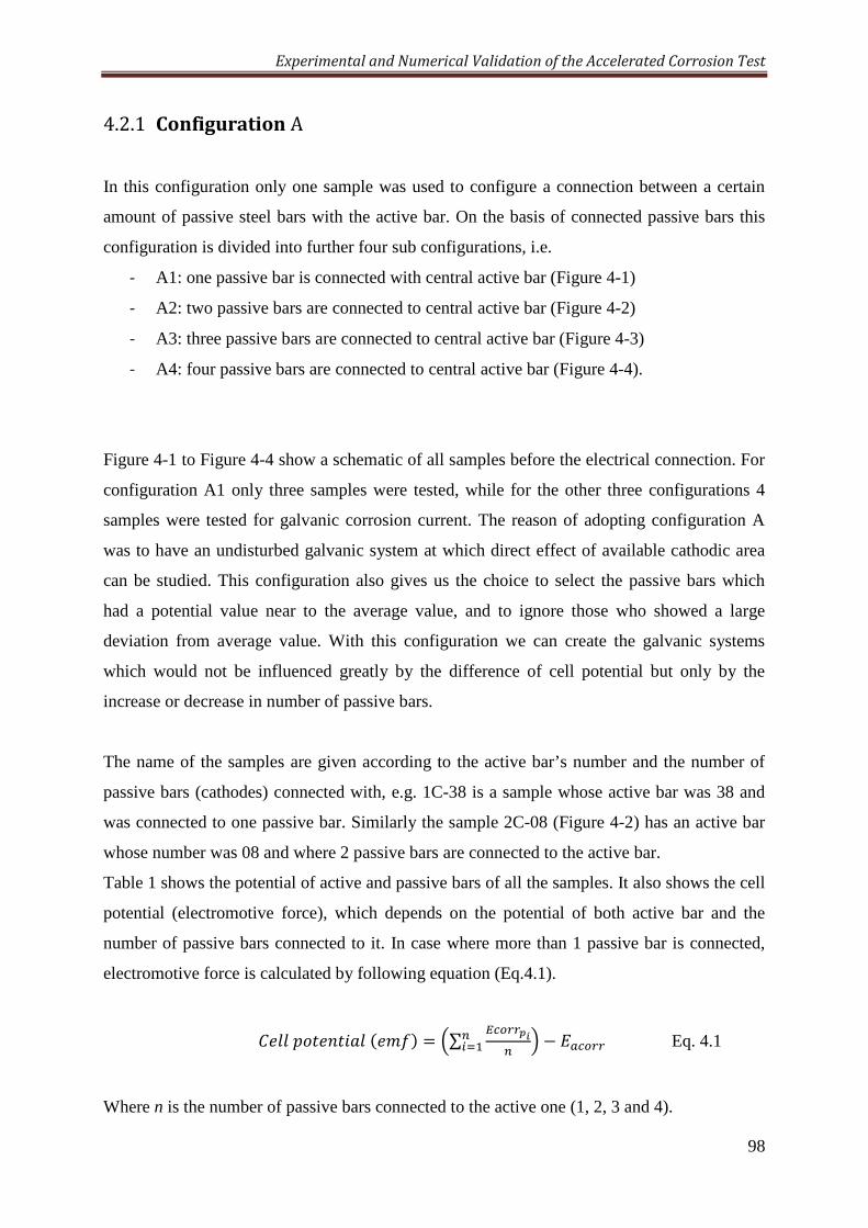
Experimental and Numerical Validation of the Accelerated Corrosion Test

98

4.2.1 Configuration A

In this configuration only one sample was used to configure a connection between a certain

amount of passive steel bars with the active bar. On the basis of connected passive bars this

configuration is divided into further four sub configurations, i.e.

- A1: one passive bar is connected with central active bar (Figure 4-1)

- A2: two passive bars are connected to central active bar (Figure 4-2)

- A3: three passive bars are connected to central active bar (Figure 4-3)

- A4: four passive bars are connected to central active bar (Figure 4-4).

Figure 4-1 to Figure 4-4 show a schematic of all samples before the electrical connection. For

configuration A1 only three samples were tested, while for the other three configurations 4

samples were tested for galvanic corrosion current. The reason of adopting configuration A

was to have an undisturbed galvanic system at which direct effect of available cathodic area

can be studied. This configuration also gives us the choice to select the passive bars which

had a potential value near to the average value, and to ignore those who showed a large

deviation from average value. With this configuration we can create the galvanic systems

which would not be influenced greatly by the difference of cell potential but only by the

increase or decrease in number of passive bars.

The name of the samples are given according to the active bar’s number and the number of

passive bars (cathodes) connected with, e.g. 1C-38 is a sample whose active bar was 38 and

was connected to one passive bar. Similarly the sample 2C-08 (Figure 4-2) has an active bar

whose number was 08 and where 2 passive bars are connected to the active bar.

Table 1 shows the potential of active and passive bars of all the samples. It also shows the cell

potential (electromotive force), which depends on the potential of both active bar and the

number of passive bars connected to it. In case where more than 1 passive bar is connected,

electromotive force is calculated by following equation (Eq.4.1).

9116<x'xO1(;E = I∑ ,^a((®&

&Ï= J − ^a(( Eq. 4.1

Where n is the number of passive bars connected to the active one (1, 2, 3 and 4).

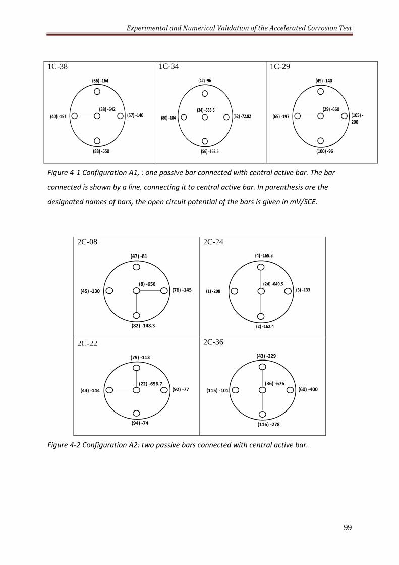
Experimental and Numerical Validation of the Accelerated Corrosion Test

99

1C-38

1C-34

1C-29

Figure 4-1 Configuration A1, : one passive bar connected with central active bar. The bar

connected is shown by a line, connecting it to central active bar. In parenthesis are the

designated names of bars, the open circuit potential of the bars is given in mV/SCE.

2C-08

2C-24

2C-22

2C-36

Figure 4-2 Configuration A2: two passive bars connected with central active bar.

(38) -642(57) -140

(66) -164

(88) -550

(40) -151

(34) -653.5(52) -72.82

(42) -96

(56) -162.5

(80) -184

(29) -660(105) -

200

(49) -140

(100) -96

(65) -197

(8) -656(76) -145

(47) -81

(82) -148.3

(45) -130

(24) -649.5

(3) -133

(4) -169.3

(2) -162.4

(1) -208

(22) -656.7(92) -77

(79) -113

(94) -74

(44) -144

(36) -676(60) -400

(43) -229

(116) -278

(115) -101

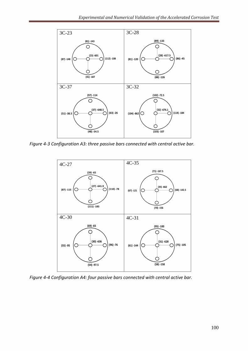
Experimental and Numerical Validation of the Accelerated Corrosion Test

100

3C-23

3C-28

3C-37

3C-32

Figure 4-3 Configuration A3: three passive bars connected with central active bar.

4C-27

4C-35

4C-30

4C-31

Figure 4-4 Configuration A4: four passive bars connected with central active bar.

(23) -601(112) -108

(81) -143

(41) -187

(87) -148

(28) -617.5(86) -45

(89) -133

(88) -126

(81) -120

(37) -648.5(63) -26

(97) -114

(48) -54.5

(51) -38.5

(32) -676.1(114) -184

(102) -72.5

(103) -107

(104) -862

(27) -641.9(110) -78

(39) -65

(111) -183

(87) -115(35) -662

(68) -142.5

(70) -156

(67) -121

(71) -167.5

(30) -636(96) -76

(69) -65

(54) -97.5

(55) -95

(31) -628(75) -105

(95) -100

(58) -158

(61) -144

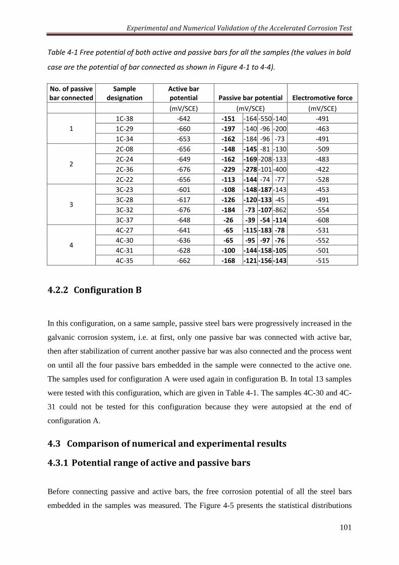
Experimental and Numerical Validation of the Accelerated Corrosion Test

101

Table 4-1 Free potential of both active and passive bars for all the samples (the values in bold

case are the potential of bar connected as shown in Figure 4-1 to 4-4).

No. of passive

bar connected Sample

designation Active bar

potential Passive bar potential Electromotive force

(mV/SCE) (mV/SCE) (mV/SCE)

1

1C-38 -642 -151 -164 -550 -140 -491

1C-29 -660 -197 -140 -96 -200 -463

1C-34 -653 -162 -184 -96 -73 -491

2

2C-08 -656 -148 -145 -81 -130 -509

2C-24 -649 -162 -169 -208 -133 -483

2C-36 -676 -229 -278 -101 -400 -422

2C-22 -656 -113 -144 -74 -77 -528

3

3C-23 -601 -108 -148 -187 -143 -453

3C-28 -617 -126 -120 -133 -45 -491

3C-32 -676 -184 -73 -107 -862 -554

3C-37 -648 -26 -39 -54 -114 -608

4

4C-27 -641 -65 -115 -183 -78 -531

4C-30 -636 -65 -95 -97 -76 -552

4C-31 -628 -100 -144 -158 -105 -501

4C-35 -662 -168 -121 -156 -143 -515

4.2.2 ConfigurationB

In this configuration, on a same sample, passive steel bars were progressively increased in the

galvanic corrosion system, i.e. at first, only one passive bar was connected with active bar,

then after stabilization of current another passive bar was also connected and the process went

on until all the four passive bars embedded in the sample were connected to the active one.

The samples used for configuration A were used again in configuration B. In total 13 samples

were tested with this configuration, which are given in Table 4-1. The samples 4C-30 and 4C-

31 could not be tested for this configuration because they were autopsied at the end of

configuration A.

4.3 Comparisonofnumericalandexperimentalresults

4.3.1 Potentialrangeofactiveandpassivebars

Before connecting passive and active bars, the free corrosion potential of all the steel bars

embedded in the samples was measured. The Figure 4-5 presents the statistical distributions

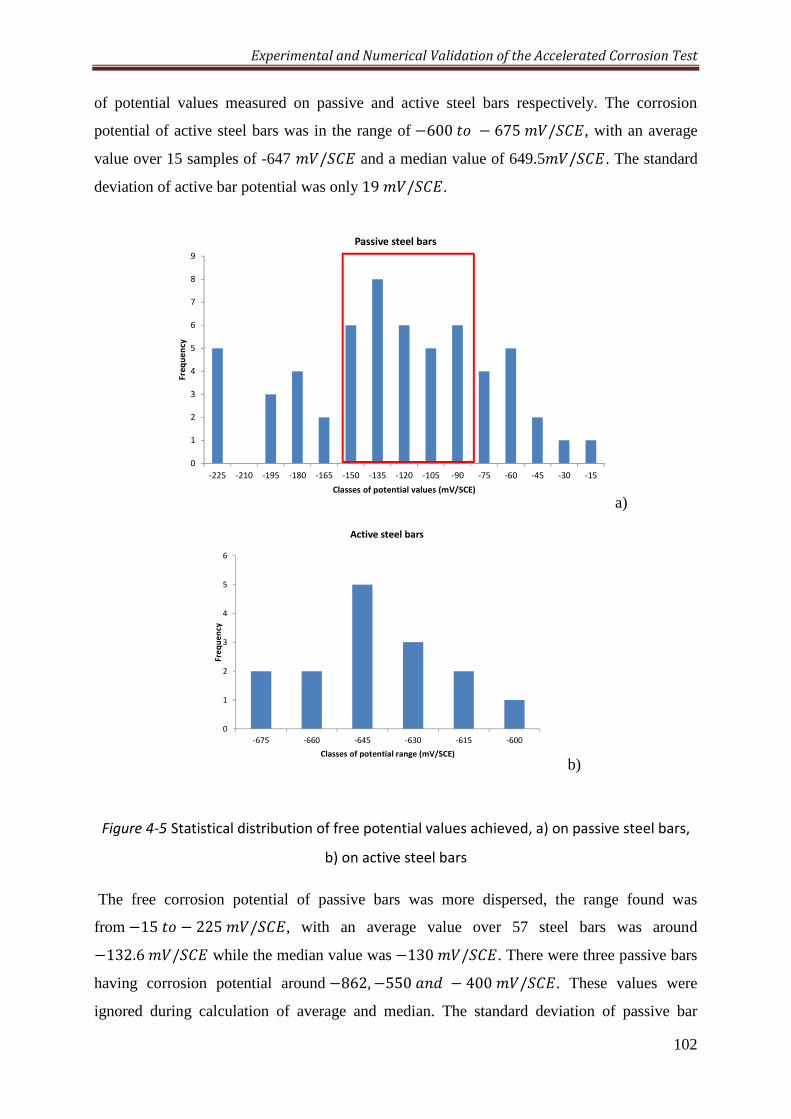
Experimental and Numerical Validation of the Accelerated Corrosion Test

102

of potential values measured on passive and active steel bars respectively. The corrosion

potential of active steel bars was in the range of−600x< − 675;/9, with an average

value over 15 samples of -647 ;/9 and a median value of 649.5;/9. The standard

deviation of active bar potential was only19;/9.

a)

b)

Figure 4-5 Statistical distribution of free potential values achieved, a) on passive steel bars,

b) on active steel bars

The free corrosion potential of passive bars was more dispersed, the range found was

from−15x< − 225;/9, with an average value over 57 steel bars was around

−132.6;/9 while the median value was−130;/9. There were three passive bars

having corrosion potential around−862,−550O'V − 400;/9. These values were

ignored during calculation of average and median. The standard deviation of passive bar

0

1

2

3

4

5

6

7

8

9

-225 -210 -195 -180 -165 -150 -135 -120 -105 -90 -75 -60 -45 -30 -15

Fre

qu

en

cy

Classes of potential values (mV/SCE)

Passive steel bars

0

1

2

3

4

5

6

-675 -660 -645 -630 -615 -600

Fre

qu

en

cy

Classes of potential range (mV/SCE)

Active steel bars

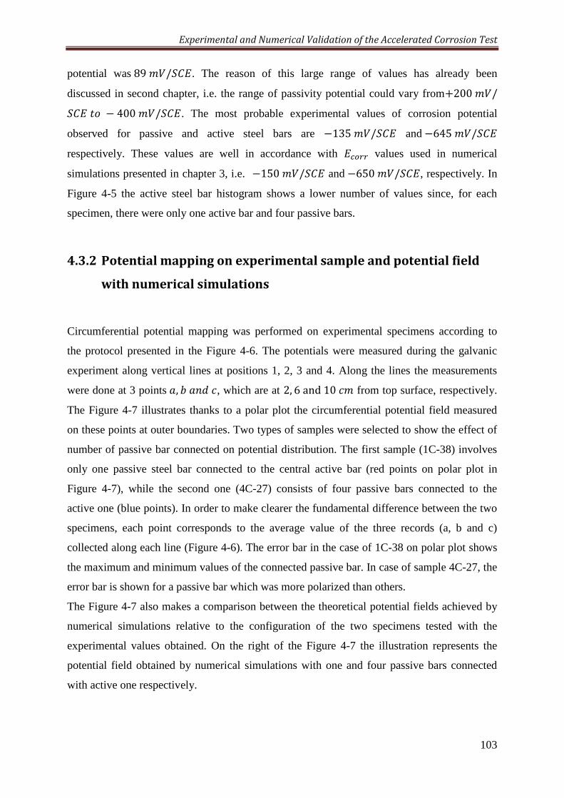
Experimental and Numerical Validation of the Accelerated Corrosion Test

103

potential was89;/9. The reason of this large range of values has already been

discussed in second chapter, i.e. the range of passivity potential could vary from+200;/9x< − 400;/9. The most probable experimental values of corrosion potential

observed for passive and active steel bars are −135;/9 and−645;/9 respectively. These values are well in accordance with ^a(( values used in numerical

simulations presented in chapter 3, i.e. −150;/9 and−650;/9, respectively. In

Figure 4-5 the active steel bar histogram shows a lower number of values since, for each

specimen, there were only one active bar and four passive bars.

4.3.2 Potentialmappingonexperimentalsampleandpotentialfield

withnumericalsimulations

Circumferential potential mapping was performed on experimental specimens according to

the protocol presented in the Figure 4-6. The potentials were measured during the galvanic

experiment along vertical lines at positions 1, 2, 3 and 4. Along the lines the measurements

were done at 3 pointsO, PO'V], which are at 2, 6and10]; from top surface, respectively.

The Figure 4-7 illustrates thanks to a polar plot the circumferential potential field measured

on these points at outer boundaries. Two types of samples were selected to show the effect of

number of passive bar connected on potential distribution. The first sample (1C-38) involves

only one passive steel bar connected to the central active bar (red points on polar plot in

Figure 4-7), while the second one (4C-27) consists of four passive bars connected to the

active one (blue points). In order to make clearer the fundamental difference between the two

specimens, each point corresponds to the average value of the three records (a, b and c)

collected along each line (Figure 4-6). The error bar in the case of 1C-38 on polar plot shows

the maximum and minimum values of the connected passive bar. In case of sample 4C-27, the

error bar is shown for a passive bar which was more polarized than others.

The Figure 4-7 also makes a comparison between the theoretical potential fields achieved by

numerical simulations relative to the configuration of the two specimens tested with the

experimental values obtained. On the right of the Figure 4-7 the illustration represents the

potential field obtained by numerical simulations with one and four passive bars connected

with active one respectively.

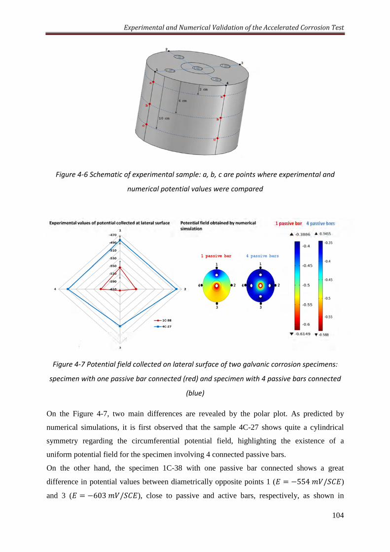
Experimental and Numerical Validation of the Accelerated Corrosion Test

104

Figure 4-6 Schematic of experimental sample: a, b, c are points where experimental and

numerical potential values were compared

Figure 4-7 Potential field collected on lateral surface of two galvanic corrosion specimens:

specimen with one passive bar connected (red) and specimen with 4 passive bars connected

(blue)

On the Figure 4-7, two main differences are revealed by the polar plot. As predicted by

numerical simulations, it is first observed that the sample 4C-27 shows quite a cylindrical

symmetry regarding the circumferential potential field, highlighting the existence of a

uniform potential field for the specimen involving 4 connected passive bars.

On the other hand, the specimen 1C-38 with one passive bar connected shows a great

difference in potential values between diametrically opposite points 1 ( = −554;/9)

and 3 ( = −603;/9), close to passive and active bars, respectively, as shown in

Experimental and Numerical Validation of the Accelerated Corrosion Test

105

Figure 4-7. Moreover, the records collected at points 2 and 4 show that the potential value

changes progressively on the circumference from a maximum (at position 1) to minimum (at

position 3). The potential gradient appears clearly in this case.

The qualitative behavior of experimental samples and simulations are quite similarly, i.e. the

potential near the connected passive bar in the case where only one passive bar is connected

(1C-38), is less electronegative, which means it is more polarized, same behavior is shown by

simulations when only one passive bar is connected. But the difference in potential values is

significant in both cases, in experimental sample the potential is around−554;/9,

while in case of simulations it was around −450;/9 as can be seen in the scale of

simulation results (blue area; 1 passive bar scale). The same remark can be done with sample

4C-27, where all four passive bars were connected. The circumferential potential near the

passive steel bars was around -475;/9, while the values in case of numerical

simulation were found to be around −350;/9 (blue area of scale with 4 passive bars).

A difference of about 100x<125;/9 is found between experimental and numerical

values in both case of 1 or 4 passive bars connected to active one. This difference can be

explained by the fact that the corrosion conditions supposed in numerical simulations are

different from the conditions in real samples. For example, with numerical simulations it has

been seen that if the concrete resistivity is higher, the difference between active and passive

bar potential is also higher at equilibrium in galvanic system. Moreover the cathodic tafel

slope of passive system βcp values in simulation were supposed as150;/V], and with

sensitivity analysis it has been observed that if βcp is increased, the potential of passive steel

bar reduced to very negative values at galvanic equilibrium, which makes cell potential also

more negative. This could clearly explain the more electronegative potential in case of

experimental sample, which could have a polarization curve with higher Tafel slope (βc) and

concrete has less resistivity.

Another major difference is highlighted by the global potential levels related to the two

experimental specimens. Globally, the specimen with one passive bar connected has potential

values lower than those of the specimen with 4 passive bars connected, even close to the

connected passive bar (position 1). This observation is in accordance with the theoretical

effect of the increase in the cathode-to-anode surface ratio discussed in potential distribution

section in the third chapter. Increasing the number of passive bars results in higher anodic

polarization of active steel and lower cathodic polarization of passive steel. Regarding outer

potential measurement of galvanic systems, a system involving a high cathode-to-anode ratio

may globally have higher potential values than a system with low cathode-to-anode ratio. This

Experimental and Numerical Validation of the Accelerated Corrosion Test

106

result confirms that half–cell potential measurements are not sufficient to deduce information

on corrosion state in reinforced concrete, since high corrosion rate systems (due to high C/A

ratio) may appear with higher potential levels than low corrosion rate systems.

4.3.3 AcceleratedMacrocellcurrentincorrosionspecimens

In this section, the numerical results of the effects of Cathode/Anode ratio on macrocell

current density are firstly presented. Then the results of laboratory experiments are explained.

As macrocell corrosion current depends on potential at steel surface, it is essential here to

mention that the numerical results of potential distribution during galvanic connection are

already been presented in section 3.6.2 and 4.3.2.

4.3.3.1 Numerical calculations of macrocell current

The global macrocell corrosion current w may be simply deduced from numerical

simulations by the integration of normal current density & on the active boundary surface

(Eq.4.2).

w = ∬ &f d Eq. 4.2

Several simulations were carried out to study the effect of cathode-to-anode ratio (C/A) on the

macrocell currentw. Anode surface area was kept constant while cathodic surface was

changed by increasing the number of passive steel bars in the system. These simulations

involved 1 to 8 passive bars connected to a central active bar, corresponding here to C/A

ratios from 1/1 up to8/1. The results of the numerical experiments are presented in the

Figure 4-8. As it may be seen in the Figure 4-8, the macrocell current density is increased

with the cathode surface, which means that more corrosion is occurring with large available

cathode area in concrete. When C/A ratio is1/1, 103ÌT current is produced, while it is

154ÌT when C/A is2/1. It gradually increases with increase in C/A ratio, and reaches to

254ÌT when C/A is8/1. Nevertheless, the rate of increase in macrocell current is decreased

with C/A. For instance, 45% additional current is produced when changing from one to two

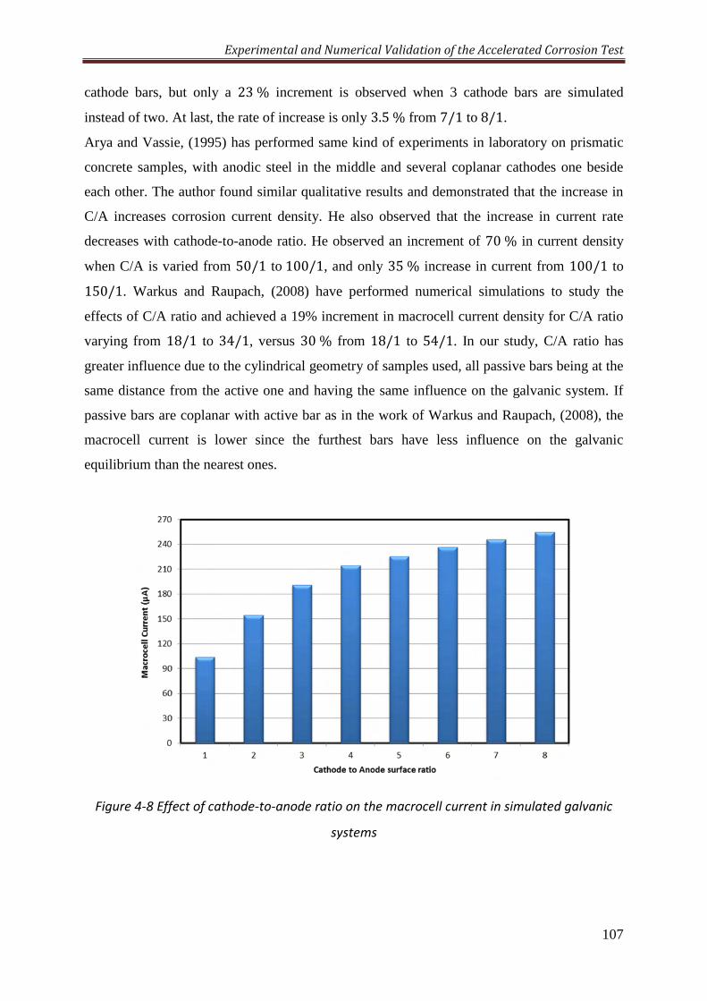
Experimental and Numerical Validation of the Accelerated Corrosion Test

107

cathode bars, but only a 23% increment is observed when 3 cathode bars are simulated

instead of two. At last, the rate of increase is only 3.5% from 7/1 to8/1. Arya and Vassie, (1995) has performed same kind of experiments in laboratory on prismatic

concrete samples, with anodic steel in the middle and several coplanar cathodes one beside

each other. The author found similar qualitative results and demonstrated that the increase in

C/A increases corrosion current density. He also observed that the increase in current rate

decreases with cathode-to-anode ratio. He observed an increment of 70% in current density

when C/A is varied from 50/1 to100/1, and only 35% increase in current from 100/1 to

150/1. Warkus and Raupach, (2008) have performed numerical simulations to study the

effects of C/A ratio and achieved a 19% increment in macrocell current density for C/A ratio

varying from 18/1 to 34/1, versus 30% from 18/1 to 54/1. In our study, C/A ratio has

greater influence due to the cylindrical geometry of samples used, all passive bars being at the

same distance from the active one and having the same influence on the galvanic system. If

passive bars are coplanar with active bar as in the work of Warkus and Raupach, (2008), the

macrocell current is lower since the furthest bars have less influence on the galvanic

equilibrium than the nearest ones.

Figure 4-8 Effect of cathode-to-anode ratio on the macrocell current in simulated galvanic

systems

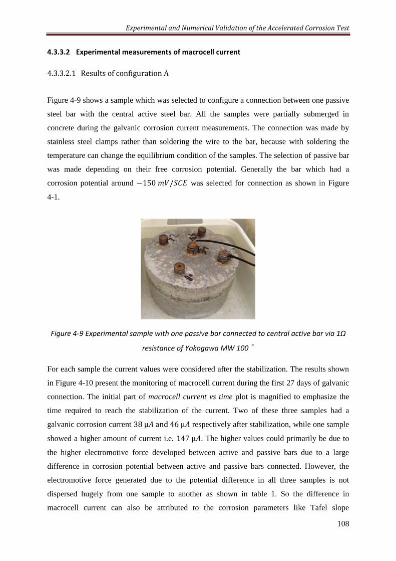
Experimental and Numerical Validation of the Accelerated Corrosion Test

108

4.3.3.2 Experimental measurements of macrocell current

4.3.3.2.1 Results of configuration A

Figure 4-9 shows a sample which was selected to configure a connection between one passive

steel bar with the central active steel bar. All the samples were partially submerged in

concrete during the galvanic corrosion current measurements. The connection was made by

stainless steel clamps rather than soldering the wire to the bar, because with soldering the

temperature can change the equilibrium condition of the samples. The selection of passive bar

was made depending on their free corrosion potential. Generally the bar which had a

corrosion potential around −150;/9 was selected for connection as shown in Figure

4-1.

Figure 4-9 Experimental sample with one passive bar connected to central active bar via 1Ω

resistance of Yokogawa MW 100 ®

For each sample the current values were considered after the stabilization. The results shown

in Figure 4-10 present the monitoring of macrocell current during the first 27 days of galvanic

connection. The initial part of macrocell current vs time plot is magnified to emphasize the

time required to reach the stabilization of the current. Two of these three samples had a

galvanic corrosion current 38μTand46μT respectively after stabilization, while one sample

showed a higher amount of current i.e. 147μT. The higher values could primarily be due to

the higher electromotive force developed between active and passive bars due to a large

difference in corrosion potential between active and passive bars connected. However, the

electromotive force generated due to the potential difference in all three samples is not

dispersed hugely from one sample to another as shown in table 1. So the difference in

macrocell current can also be attributed to the corrosion parameters like Tafel slope

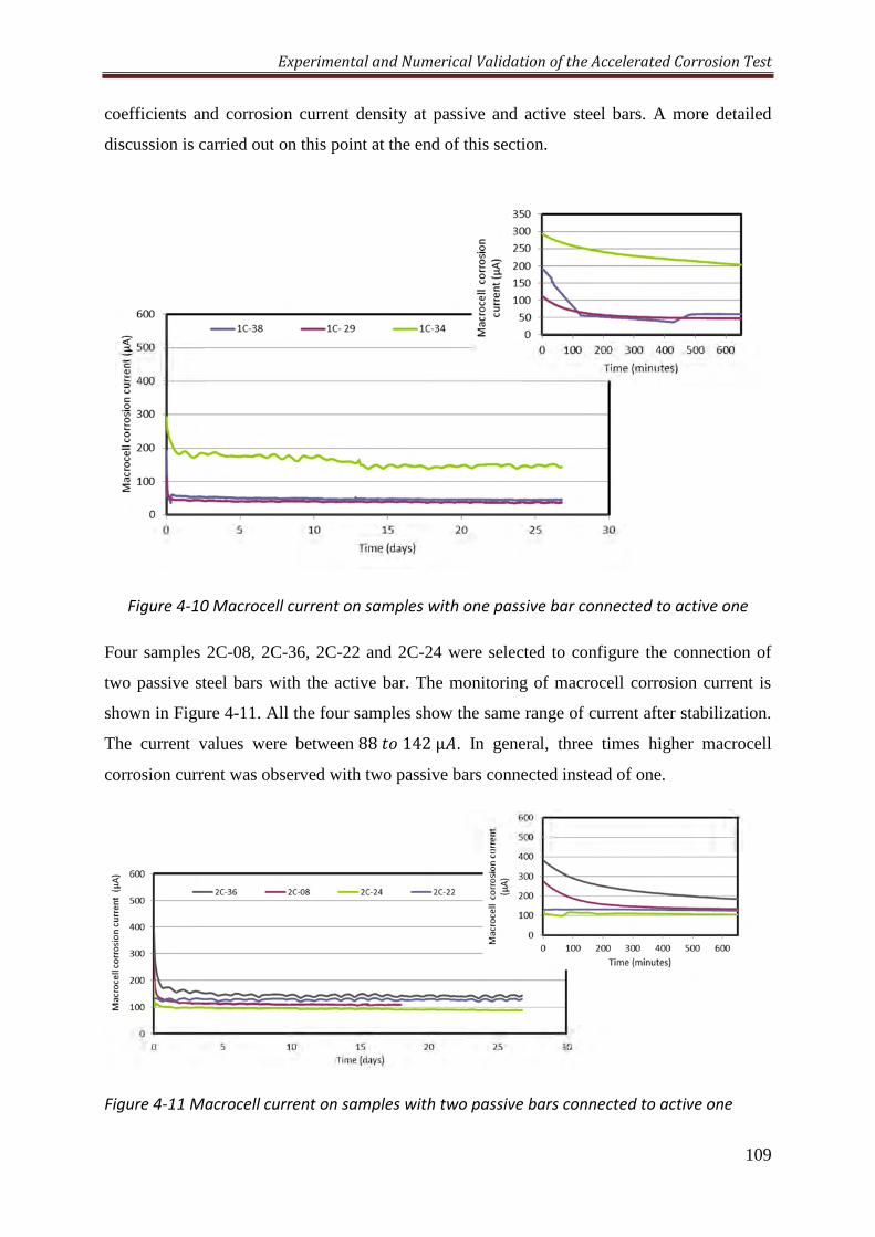
Experimental and Numerical Validation of the Accelerated Corrosion Test

109

coefficients and corrosion current density at passive and active steel bars. A more detailed

discussion is carried out on this point at the end of this section.

Figure 4-10 Macrocell current on samples with one passive bar connected to active one

Four samples 2C-08, 2C-36, 2C-22 and 2C-24 were selected to configure the connection of

two passive steel bars with the active bar. The monitoring of macrocell corrosion current is

shown in Figure 4-11. All the four samples show the same range of current after stabilization.

The current values were between88x<142μT. In general, three times higher macrocell

corrosion current was observed with two passive bars connected instead of one.

Figure 4-11 Macrocell current on samples with two passive bars connected to active one

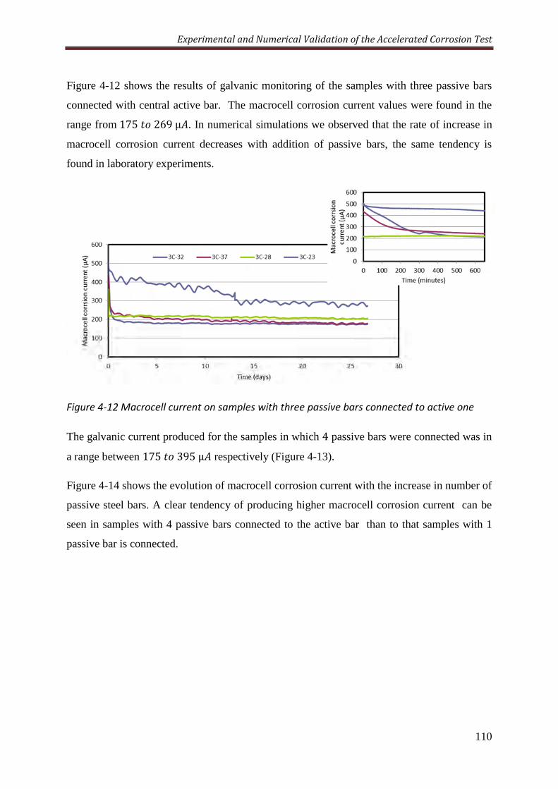
Experimental and Numerical Validation of the Accelerated Corrosion Test

110

Figure 4-12 shows the results of galvanic monitoring of the samples with three passive bars

connected with central active bar. The macrocell corrosion current values were found in the

range from175x<269μT. In numerical simulations we observed that the rate of increase in

macrocell corrosion current decreases with addition of passive bars, the same tendency is

found in laboratory experiments.

Figure 4-12 Macrocell current on samples with three passive bars connected to active one

The galvanic current produced for the samples in which 4 passive bars were connected was in

a range between 175x<395μT respectively (Figure 4-13).

Figure 4-14 shows the evolution of macrocell corrosion current with the increase in number of

passive steel bars. A clear tendency of producing higher macrocell corrosion current can be

seen in samples with 4 passive bars connected to the active bar than to that samples with 1

passive bar is connected.

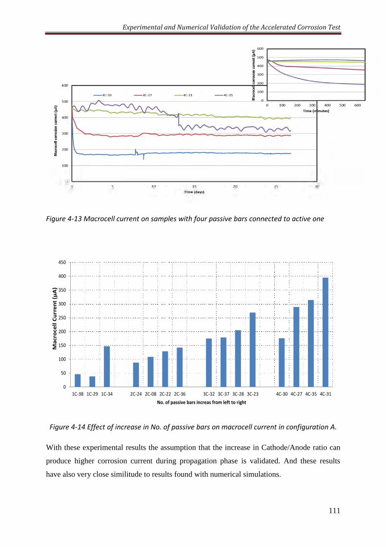
Experimental and Numerical Validation of the Accelerated Corrosion Test

111

Figure 4-13 Macrocell current on samples with four passive bars connected to active one

Figure 4-14 Effect of increase in No. of passive bars on macrocell current in configuration A.

With these experimental results the assumption that the increase in Cathode/Anode ratio can

produce higher corrosion current during propagation phase is validated. And these results

have also very close similitude to results found with numerical simulations.

0

50

100

150

200

250

300

350

400

450

1C-38 1C-29 1C-34 2C-24 2C-08 2C-22 2C-36 3C-32 3C-37 3C-28 3C-23 4C-30 4C-27 4C-35 4C-31

Ma

cro

ce

ll C

urr

en

t (µ

A)

No. of passive bars increas from left to right

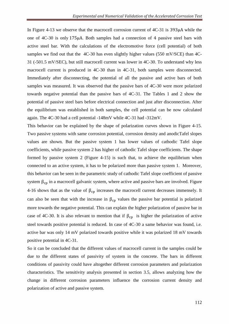
Experimental and Numerical Validation of the Accelerated Corrosion Test

112

In Figure 4-13 we observe that the macrocell corrosion current of 4C-31 is 393μA while the

one of 4C-30 is only175μA. Both samples had a connection of 4 passive steel bars with

active steel bar. With the calculations of the electromotive force (cell potential) of both

samples we find out that the 4C-30 has even slightly higher values (550 mV/SCE) than 4C-

31 (-501.5 mV/SEC), but still macrocell current was lower in 4C-30. To understand why less

macrocell current is produced in 4C-30 than in 4C-31, both samples were disconnected.

Immediately after disconnecting, the potential of all the passive and active bars of both

samples was measured. It was observed that the passive bars of 4C-30 were more polarized

towards negative potential than the passive bars of 4C-31. The Tables 1 and 2 show the

potential of passive steel bars before electrical connection and just after disconnection. After

the equilibrium was established in both samples, the cell potential can be now calculated

again. The 4C-30 had a cell potential -148mV while 4C-31 had -312mV.

This behavior can be explained by the shape of polarization curves shown in Figure 4-15.

Two passive systems with same corrosion potential, corrosion density and anodicTafel slopes

values are shown. But the passive system 1 has lower values of cathodic Tafel slope

coefficients, while passive system 2 has higher of cathodic Tafel slope coefficients. The shape

formed by passive system 2 (Figure 4-15) is such that, to achieve the equilibrium when

connected to an active system, it has to be polarized more than passive system 1. Moreover,

this behavior can be seen in the parametric study of cathodic Tafel slope coefficient of passive

system β³Ó in a macrocell galvanic system, where active and passive bars are involved. Figure

4-16 shows that as the value of β³Ó increases the macrocell current decreases immensely. It

can also be seen that with the increase in β³Ó values the passive bar potential is polarized

more towards the negative potential. This can explain the higher polarization of passive bar in

case of 4C-30. It is also relevant to mention that if β³Ó is higher the polarization of active

steel towards positive potential is reduced. In case of 4C-30 a same behavior was found, i.e.

active bar was only 14 mV polarized towards positive while it was polarized 18 mV towards

positive potential in 4C-31.

So it can be concluded that the different values of macrocell current in the samples could be

due to the different states of passivity of system in the concrete. The bars in different

conditions of passivity could have altogether different corrosion parameters and polarization

characteristics. The sensitivity analysis presented in section 3.5, allows analyzing how the

change in different corrosion parameters influence the corrosion current density and

polarization of active and passive system.

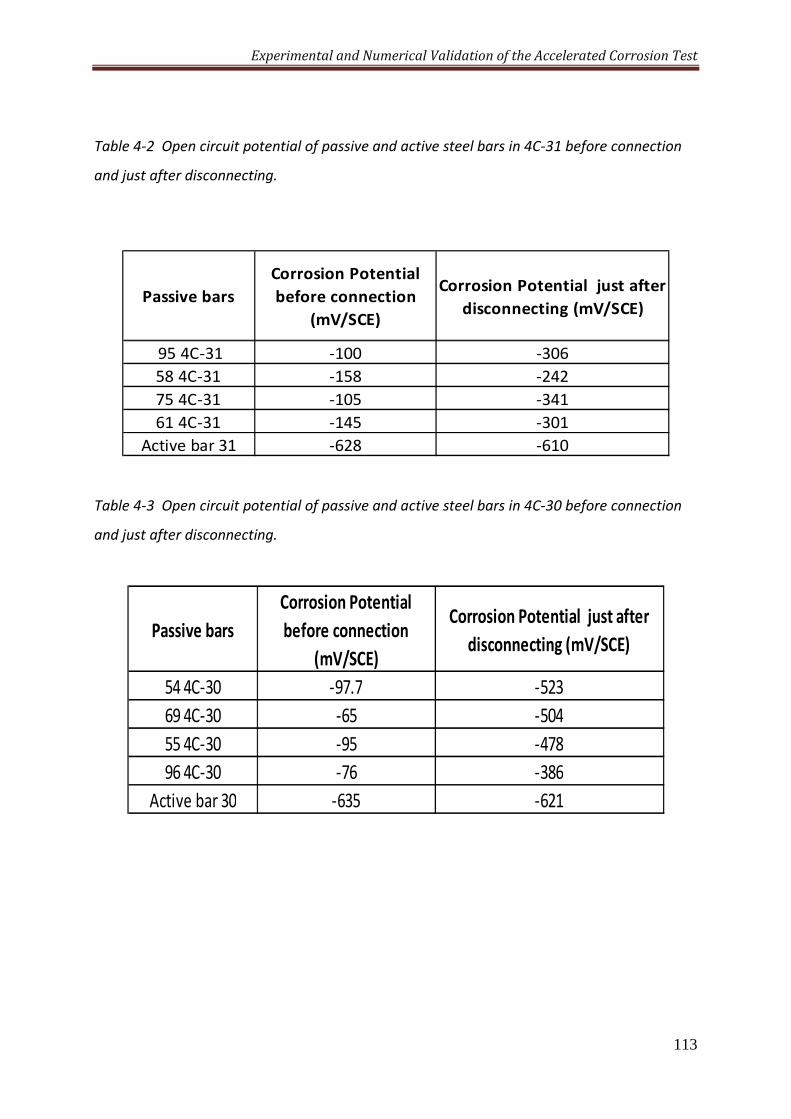
Experimental and Numerical Validation of the Accelerated Corrosion Test

113

Table 4-2 Open circuit potential of passive and active steel bars in 4C-31 before connection

and just after disconnecting.

Table 4-3 Open circuit potential of passive and active steel bars in 4C-30 before connection

and just after disconnecting.

Passive bars

Corrosion Potential

before connection

(mV/SCE)

Corrosion Potential just after

disconnecting (mV/SCE)

95 4C-31 -100 -306

58 4C-31 -158 -242

75 4C-31 -105 -341

61 4C-31 -145 -301

Active bar 31 -628 -610

Passive bars

Corrosion Potential

before connection

(mV/SCE)

Corrosion Potential just after

disconnecting (mV/SCE)

54 4C-30 -97.7 -523

69 4C-30 -65 -504

55 4C-30 -95 -478

96 4C-30 -76 -386

Active bar 30 -635 -621

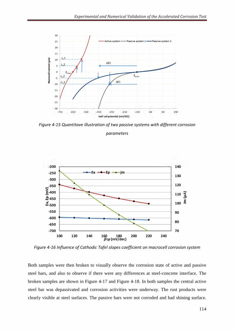
Experimental and Numerical Validation of the Accelerated Corrosion Test

114

Figure 4-15 Quantitave illustration of two passive systems with different corrosion

parameters

Figure 4-16 Influence of Cathodic Tafel slopes coefficient on macrocell corrosion system

Both samples were then broken to visually observe the corrosion state of active and passive

steel bars, and also to observe if there were any differences at steel-concrete interface. The

broken samples are shown in Figure 4-17 and Figure 4-18. In both samples the central active

steel bar was depassivated and corrosion activities were underway. The rust products were

clearly visible at steel surfaces. The passive bars were not corroded and had shining surface.

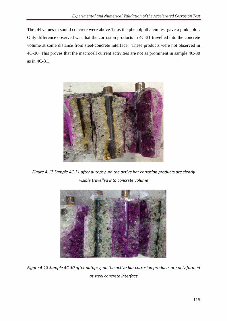
Experimental and Numerical Validation of the Accelerated Corrosion Test

115

The pH values in sound concrete were above 12 as the phenolphthalein test gave a pink color.

Only difference observed was that the corrosion products in 4C-31 travelled into the concrete

volume at some distance from steel-concrete interface. These products were not observed in

4C-30. This proves that the macrocell current activities are not as prominent in sample 4C-30

as in 4C-31.

Figure 4-17 Sample 4C-31 after autopsy, on the active bar corrosion products are clearly

visible travelled into concrete volume

Figure 4-18 Sample 4C-30 after autopsy, on the active bar corrosion products are only formed

at steel concrete interface

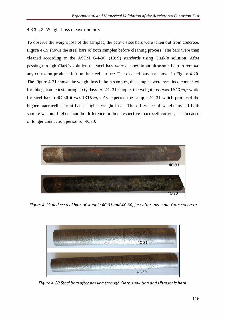
Experimental and Numerical Validation of the Accelerated Corrosion Test

116

4.3.3.2.2 Weight Loss measurements

To observe the weight loss of the samples, the active steel bars were taken out from concrete.

Figure 4-19 shows the steel bars of both samples before cleaning process. The bars were then

cleaned according to the ASTM G-I-90, (1999) standards using Clark’s solution. After

passing through Clark’s solution the steel bars were cleaned in an ultrasonic bath to remove

any corrosion products left on the steel surface. The cleaned bars are shown in Figure 4-20.

The Figure 4-21 shows the weight loss in both samples, the samples were remained connected

for this galvanic test during sixty days. At 4C-31 sample, the weight loss was 1643;@ while

for steel bar in 4C-30 it was1315;@. As expected the sample 4C-31 which produced the

higher macrocell current had a higher weight loss. The difference of weight loss of both

sample was not higher than the difference in their respective macrocell current, it is because

of longer connection period for 4C30.

Figure 4-19 Active steel bars of sample 4C-31 and 4C-30, just after taken out from concrete

Figure 4-20 Steel bars after passing through Clark’s solution and Ultrasonic bath.

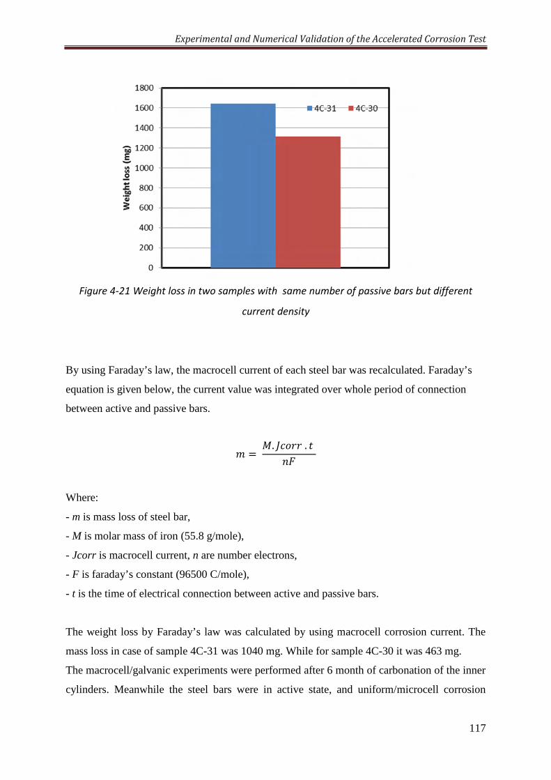
Experimental and Numerical Validation of the Accelerated Corrosion Test

117

Figure 4-21 Weight loss in two samples with same number of passive bars but different

current density

By using Faraday’s law, the macrocell current of each steel bar was recalculated. Faraday’s

equation is given below, the current value was integrated over whole period of connection

between active and passive bars.

; =. w]<. x'

Where:

- m is mass loss of steel bar,

- M is molar mass of iron (55.8 g/mole),

- Jcorr is macrocell current, n are number electrons,

- F is faraday’s constant (96500 C/mole),

- t is the time of electrical connection between active and passive bars.

The weight loss by Faraday’s law was calculated by using macrocell corrosion current. The

mass loss in case of sample 4C-31 was 1040 mg. While for sample 4C-30 it was 463 mg.

The macrocell/galvanic experiments were performed after 6 month of carbonation of the inner

cylinders. Meanwhile the steel bars were in active state, and uniform/microcell corrosion

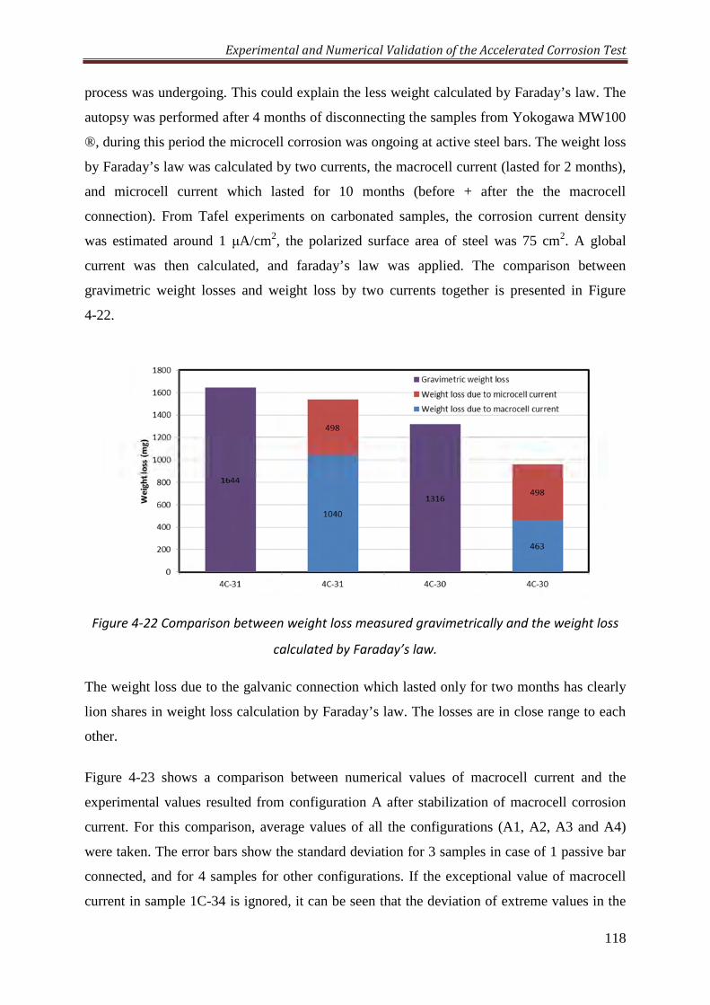
Experimental and Numerical Validation of the Accelerated Corrosion Test

118

process was undergoing. This could explain the less weight calculated by Faraday’s law. The

autopsy was performed after 4 months of disconnecting the samples from Yokogawa MW100

®, during this period the microcell corrosion was ongoing at active steel bars. The weight loss

by Faraday’s law was calculated by two currents, the macrocell current (lasted for 2 months),

and microcell current which lasted for 10 months (before + after the the macrocell

connection). From Tafel experiments on carbonated samples, the corrosion current density

was estimated around 1 µA/cm2, the polarized surface area of steel was 75 cm2. A global

current was then calculated, and faraday’s law was applied. The comparison between

gravimetric weight losses and weight loss by two currents together is presented in Figure

4-22.

Figure 4-22 Comparison between weight loss measured gravimetrically and the weight loss

calculated by Faraday’s law.

The weight loss due to the galvanic connection which lasted only for two months has clearly

lion shares in weight loss calculation by Faraday’s law. The losses are in close range to each

other.

Figure 4-23 shows a comparison between numerical values of macrocell current and the

experimental values resulted from configuration A after stabilization of macrocell corrosion

current. For this comparison, average values of all the configurations (A1, A2, A3 and A4)

were taken. The error bars show the standard deviation for 3 samples in case of 1 passive bar

connected, and for 4 samples for other configurations. If the exceptional value of macrocell

current in sample 1C-34 is ignored, it can be seen that the deviation of extreme values in the

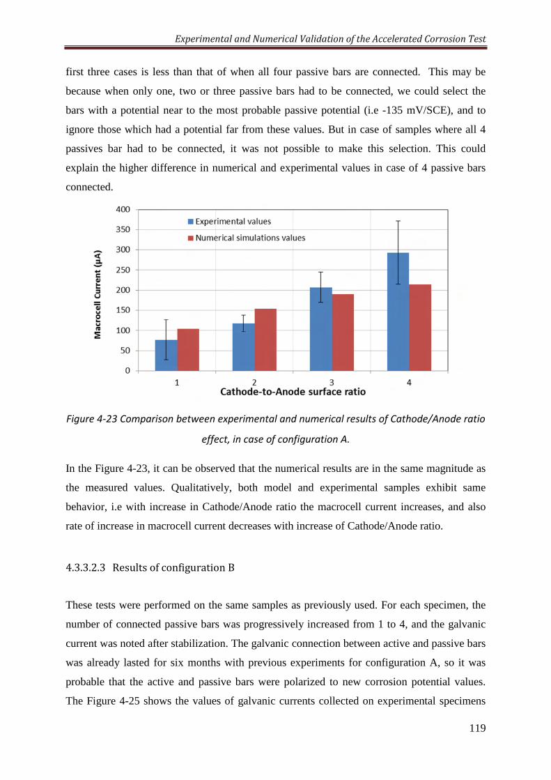
Experimental and Numerical Validation of the Accelerated Corrosion Test

119

first three cases is less than that of when all four passive bars are connected. This may be

because when only one, two or three passive bars had to be connected, we could select the

bars with a potential near to the most probable passive potential (i.e -135 mV/SCE), and to

ignore those which had a potential far from these values. But in case of samples where all 4

passives bar had to be connected, it was not possible to make this selection. This could

explain the higher difference in numerical and experimental values in case of 4 passive bars

connected.

Figure 4-23 Comparison between experimental and numerical results of Cathode/Anode ratio

effect, in case of configuration A.

In the Figure 4-23, it can be observed that the numerical results are in the same magnitude as

the measured values. Qualitatively, both model and experimental samples exhibit same

behavior, i.e with increase in Cathode/Anode ratio the macrocell current increases, and also

rate of increase in macrocell current decreases with increase of Cathode/Anode ratio.

4.3.3.2.3 Results of configuration B

These tests were performed on the same samples as previously used. For each specimen, the

number of connected passive bars was progressively increased from 1 to 4, and the galvanic

current was noted after stabilization. The galvanic connection between active and passive bars

was already lasted for six months with previous experiments for configuration A, so it was

probable that the active and passive bars were polarized to new corrosion potential values.

The Figure 4-25 shows the values of galvanic currents collected on experimental specimens

Experimental and Numerical Validation of the Accelerated Corrosion Test

120

thanks to Yokogawa MW100® device. Despite identical geometries and conditions, some

differences are observed in experimental macrocell current levels between the specimens for

each C/A ratio, as shown in Figure 4-25. For example 1C-29 produced 88 µA, while 4C-35

produced 267 µA macrocell current even if both samples had 4 passive bars connected to

active one. Again these differences arise from the variability observed in free corrosion

potential, and also from probable natural variability of the electrochemical parameters.

Nevertheless, for each specimen, the experimental relation between C/A ratio and macrocell

current is well in accordance with the theoretical prediction achieved from numerical

simulations presented in the Figure 4-8. Regarding the geometry of the specimens studied

here, the macrocell current is increased by 2 to 8 times when changing the C/A ratio from 1 to

4. In Figure 4-25, the samples are organized according to the macrocell current values when

all 4 passive bars were connected. The first sample 2C-08 gives minimum macrocell current

when all four passive bars were connected, so it was presented at extreme left side, while

sample 4C-35 gave a maximum value so it was at extreme right. All samples exhibit an

increment in macrocell current when Cathode/Anode ratio is increased by adding passive

bars.

The values of macrocell corrosion current obtained from configuration B are generally lower

than those shown in case of configuration A. The values shown in configuration A are after 27

days, but the macrocell connection lasted for a period of six months, and over this period the

macrocell current values were gradually reduced. The sample 4C-35 shows a current of 314

µA after 27 days. However, these values were decreased to 265 µA just before disconnection

of configuration A and start of configuration B (Figure 4-24). Similarly sample 4C-27 in

Figure 4-24 had a macrocell current value 289 µA after 27 days, and after 6 months the values

were reduced to 235µA. The macrocell current values found in sample 4C-27 when 4 passive

bars were connected during configuration B were 199 µA. So the lower values in case of

configuration B could be explained by the time elapse between two experiments, during

which the concrete-steel surface interface condition were significantly changed by the

corrosion products.

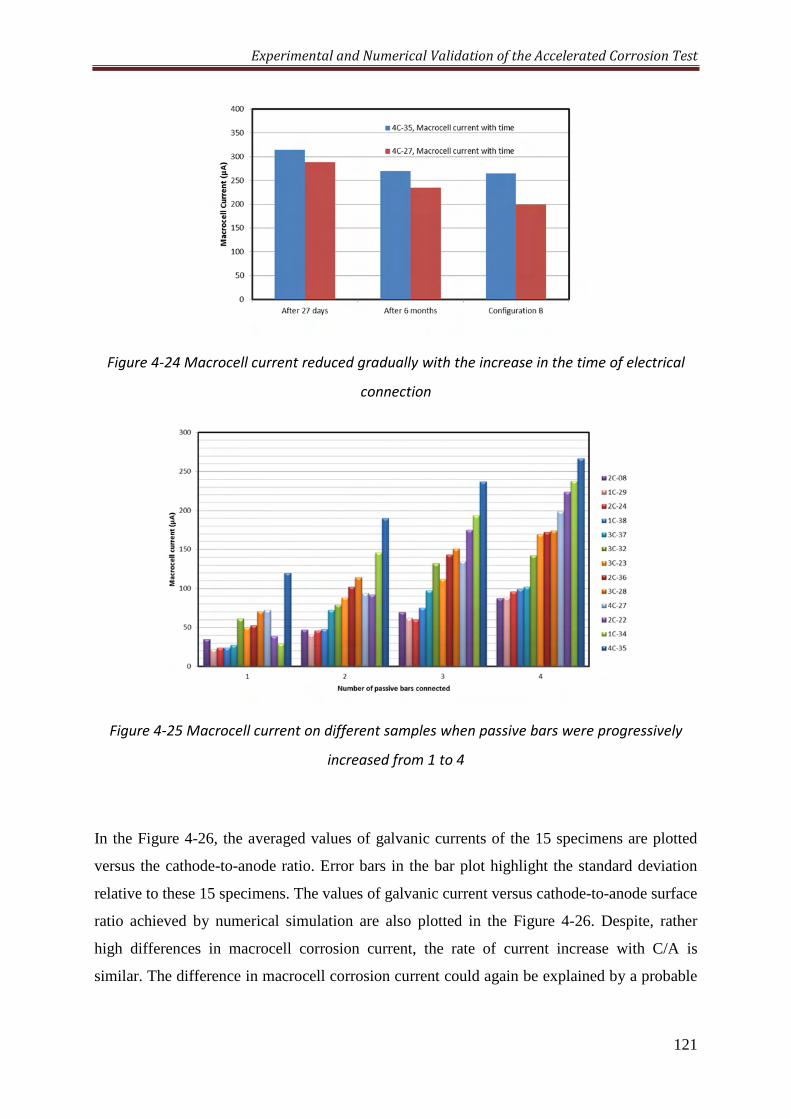
Experimental and Numerical Validation of the Accelerated Corrosion Test

121

Figure 4-24 Macrocell current reduced gradually with the increase in the time of electrical

connection

Figure 4-25 Macrocell current on different samples when passive bars were progressively

increased from 1 to 4

In the Figure 4-26, the averaged values of galvanic currents of the 15 specimens are plotted

versus the cathode-to-anode ratio. Error bars in the bar plot highlight the standard deviation

relative to these 15 specimens. The values of galvanic current versus cathode-to-anode surface

ratio achieved by numerical simulation are also plotted in the Figure 4-26. Despite, rather

high differences in macrocell corrosion current, the rate of current increase with C/A is

similar. The difference in macrocell corrosion current could again be explained by a probable

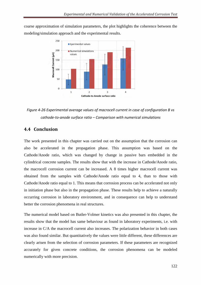
Experimental and Numerical Validation of the Accelerated Corrosion Test

122

coarse approximation of simulation parameters, the plot highlights the coherence between the

modeling/simulation approach and the experimental results.

Figure 4-26 Experimental average values of macrocell current in case of configuration B vs

cathode-to-anode surface ratio – Comparison with numerical simulations

4.4 Conclusion The work presented in this chapter was carried out on the assumption that the corrosion can

also be accelerated in the propagation phase. This assumption was based on the

Cathode/Anode ratio, which was changed by change in passive bars embedded in the

cylindrical concrete samples. The results show that with the increase in Cathode/Anode ratio,

the macrocell corrosion current can be increased. A 8 times higher macrocell current was

obtained from the samples with Cathode/Anode ratio equal to 4, than to those with

Cathode/Anode ratio equal to 1. This means that corrosion process can be accelerated not only

in initiation phase but also in the propagation phase. These results help to achieve a naturally

occurring corrosion in laboratory environment, and in consequence can help to understand

better the corrosion phenomena in real structures.

The numerical model based on Butler-Volmer kinetics was also presented in this chapter, the

results show that the model has same behaviour as found in laboratory experiments, i.e. with

increase in C/A the macrocell current also increases. The polarization behavior in both cases

was also found similar. But quantitatively the values were little different, these differences are

clearly arisen from the selection of corrosion parameters. If these parameters are recognized

accurately for given concrete conditions, the corrosion phenomena can be modeled

numerically with more precision.

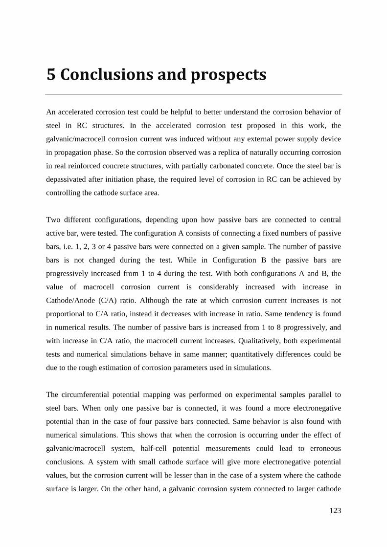
123

5 Conclusionsandprospects

An accelerated corrosion test could be helpful to better understand the corrosion behavior of

steel in RC structures. In the accelerated corrosion test proposed in this work, the

galvanic/macrocell corrosion current was induced without any external power supply device

in propagation phase. So the corrosion observed was a replica of naturally occurring corrosion

in real reinforced concrete structures, with partially carbonated concrete. Once the steel bar is

depassivated after initiation phase, the required level of corrosion in RC can be achieved by

controlling the cathode surface area.

Two different configurations, depending upon how passive bars are connected to central

active bar, were tested. The configuration A consists of connecting a fixed numbers of passive

bars, i.e. 1, 2, 3 or 4 passive bars were connected on a given sample. The number of passive

bars is not changed during the test. While in Configuration B the passive bars are

progressively increased from 1 to 4 during the test. With both configurations A and B, the

value of macrocell corrosion current is considerably increased with increase in

Cathode/Anode (C/A) ratio. Although the rate at which corrosion current increases is not

proportional to C/A ratio, instead it decreases with increase in ratio. Same tendency is found

in numerical results. The number of passive bars is increased from 1 to 8 progressively, and

with increase in C/A ratio, the macrocell current increases. Qualitatively, both experimental

tests and numerical simulations behave in same manner; quantitatively differences could be

due to the rough estimation of corrosion parameters used in simulations.

The circumferential potential mapping was performed on experimental samples parallel to

steel bars. When only one passive bar is connected, it was found a more electronegative

potential than in the case of four passive bars connected. Same behavior is also found with

numerical simulations. This shows that when the corrosion is occurring under the effect of

galvanic/macrocell system, half-cell potential measurements could lead to erroneous

conclusions. A system with small cathode surface will give more electronegative potential

values, but the corrosion current will be lesser than in the case of a system where the cathode

surface is larger. On the other hand, a galvanic corrosion system connected to larger cathode

Conclusions and prospects

124

surface area can give less electronegative values of half-cell potential while the rate of

corrosion can be very high.

To simulate corrosion phenomenon numerically, it is essential to estimate the corrosion

parameters (corrosion potential, corrosion current density and anodic and cathodic Tafel

slope) accurately according to the conditions of concrete and steel in it. A comprehensive

experimental study is presented on corrosion parameters in carbonated concrete as well as in

non-carbonated concrete. The average value of corrosion potential of active bars in

carbonated concrete was found to -645 mV/SCE, and deviation from average values was

small. While in case of steel in non-carbonated concrete the range of corrosion potential value

was quite large, from -15mV/SCE to -214mV/SEC. This range could be explained by large

range of passive zone (potential values) of a steel bar which is under the oxide layer (passive

layer). The equilibrium could be formed at different values of potential, depending upon the

steel passivity and also to the degree of saturation of concrete. So it is very important to

consider the state of concrete to access the corrosion parameters for modeling.

The average corrosion current density of active steel bar was 0.86µA/cm2. The average of

corrosion current density for passive steel bars was 0.05µA/cm2, these values are well in

accordance with the values found in literature. The values of anodic and cathodic Tafel slope

for active steel bars were 244mV/dec and 260mv/dec respectively. These values are

considerably higher than those used by other researchers who simulated the corrosion in

reinforced concrete. The scan rates from 0.1, 0.5 and 0.8 mV/s were used to perform Tafel

experiments, the polarization curves obtained under different scan rates had same shape, and

hence, the parameters found under different scan rates were in same range. Since there is not a

lot of work performed on corrosion parameters in carbonated concrete, these results could

provide an initial step towards defining the corrosion parameters values in carbonated

concrete.

As the corrosion parameters found in literature and also in this work are somewhat scattered,

a sensitivity analysis was carried out to observe the effects on macrocell corrosion system

with the change in these corrosion parameters. Some parameters e.g. equilibrium corrosion

potential (Eacorr, Epcorr) are found to be highly influential on macrocell corrosion. Corrosion

parameters of passive system are more influential on macrocell current than the parameters of

active system. As illustrated by polarization curves of a macrocell corrosion system, the

anodic Tafel slope coefficient of active system and cathodic Tafel slope of passive system

Conclusions and prospects

125

were more influential on macrocell corrosion system. Moreover, change in cathodic Tafel

slope of passive system had more effect on macrocell system than to anodic slope coefficient

of active system.

With numerical simulations, the face to face polarization phenomenon was observed. The face

of active steel which faces the passive steel bar was more polarized than to its opposite side.

Similarly, the side of passive bar which was facing the active bar was more polarized than the

opposite side. Concrete resistivity has a huge role in development of a macrocell/galvanic

corrosion system in concrete structures. With higher values of resistivity, ohmic drop is quite

significant and macrocell corrosion current is very small and vice-versa.

Main perspectives:

The results have shown the reliability of this accelerated corrosion test clearly. This test could

be used to observe the corrosion sensitivity of various systems involving different types of

reinforcing steels or concretes at different environmental conditions. For example, different

types of cements can be used to cast the concrete, and their effects on corrosion could be

studied. The corrosion behavior can be studied when different additions like, fly ash,

metakaolin and silica fume are used in concrete. Their effects on polarization curves could be

observed. Moreover, the efficiency of corrosion inhibitors could be checked on the

development of macrocell corrosion. The test could also be easily performed in different

environmental conditions by varying temperature and/or hygrometry.

The numerical model could also be improved. In particular, the numerical simulations were

performed on the assumption that the polarization is only due to the activation; charge is

transferred only by electron flow. The Butler-Volmer equations can be modified to simulate

the effect of oxygen diffusion and limiting current density parameter can also be taken into

account. Further research should also be carried out to build a dynamic model in transitory

state of corrosion, by taking account of capacitance of concrete-steel interface. In order to

achieve a better quantitative correlation between numerical and experimental results, inverse

modeling could be carried out to optimize electrochemical parameters involved in the

simulations.

The test could also be used for a better quantification of the effects of galvanic corrosion in

carbonated concrete. Indeed, usually, concrete carbonation is assumed to induce uniform

corrosion of reinforcing steel by uniform depassivation. In electrochemistry, the assumption

Conclusions and prospects

126

of uniform corrosion means that anodic and cathodic reactions occur quite at the same

locations on the steel-concrete interface. Since most of the time concrete is only partially

carbonated, so already active reinforcement bars are connected to the till passive bars in sound

concrete through stirrups or by longitudinal bars. That is why, in most of the cases in

reinforced concrete, the corrosion phenomena are macrocell rather than microcell. Or at least

the macrocell current is much more significant than the microcell current. But in contrast,

most of the corrosion measuring instruments are based on the theory of microcell/uniform

corrosion. That is why further research must be carried out to develop the corrosion

measurement methods in concrete structures where macrocell/galvanic corrosion is underway.

127

6 References

Ahmad, S., 2009. Techniques for inducing accelerated corrosion of steel in concrete. The Arabian Journal for Science and Engineering 95–104.

Ahn, W., 2001. Galvanostatic testing for the durability of marine concrete under fatigue loading. Cement and Concrete Research 31, 343–349.

Almusallam, A.A., Al-Gahtani, A.S., Aziz, A.R., Rasheeduzzafar, 1996. Effect of reinforcement corrosion on bond strength. Construction and Building Materials 10, 123–129.

Alonso, C., Castellote, M., Andrade, C., 2002. Chloride threshold dependence of pitting potential of reinforcements. Electrochimica Acta 47, 3469–3481.

Andrade, C., Alonso, C., 1996. Corrosion rate monitoring in the laboratory and on-site. Construction and Building Materials 10, 315–328.

Andrade, C., Alonso, C., 2004. Test methods for on-site corrosion rate measurement of steel reinforcement in concrete by means of the polarization resistance method. Mat. Struct. 37, 623–643.

Arya, C., Vassie, P.R.., 1995. Influence of cathode-to-anode area ratio and separation distance on galvanic corrosion currents of steel in concrete containing chlorides. Cement and Concrete Research 25, 989–998.

ASTM C876-09, 2009. Test Method for Corrosion Potentials of Uncoated Reinforcing Steel in Concrete. G01 Committee, ASTM International.

ASTM G-I-90, 1999. Practice for Preparing, Cleaning, and Evaluating Corrosion Test Specimens. G01 Committee ASTM International.

Balayssac, J.P., Détriché, C.H., Grandet, J., 1995. Effects of curing upon carbonation of concrete. Construction and Building Materials 9, 91–95.

Bertolini, L., Elsener, B., Pedeferri, P., Polder, R.B., 2004. Corrosion of Steel in Concrete. John Wiley & Sons.

Brem, 2004. Numerische Modellierung der Korrosion in Stahlbetonbauten. Dissertation. Edgennoissche Technische Hochschule Zurich.

Broomfield, J.P., 2007. Corrosion of Steel in Concrete: Understanding, Investigation and Repair. Taylor & Francis.

Cefracor, n.d. Notions fondamentales, Aspects électrochimiques de la corrosion. Chang, Z.-T., Cherry, B., Marosszeky, M., 2008. Polarisation behaviour of steel bar samples

in concrete in seawater. Part 1: Experimental measurement of polarisation curves of steel in concrete. Corrosion Science 50, 357–364.

Clément, A., Laurens, S., Arliguie, G., Deby, F., 2012. Numerical study of the linear polarisation resistance technique applied to reinforced concrete for corrosion assessment. European Journal of Environmental and Civil Engineering 16, 491–504.

El Maaddawy, T.A., Soudki, K.A., 2003. Effectiveness of Impressed Current Technique to Simulate Corrosion of Steel Reinforcement in Concrete. Journal of Materials in Civil Engineering 15, 41–47.

Elsener, B., 2005. Corrosion rate of steel in concrete—Measurements beyond the Tafel law. Corrosion Science 47, 3019–3033.

Elsener, B., Andrade, C., Gulikers, J., Polder, R., Raupach, M., 2003. Hall-cell potential measurements—Potential mapping on reinforced concrete structures. Mat. Struct. 36, 461–471.

Feliú, S., González, J., Andrade, C., 1996. Electrochemical Methods for On-Site Determinations of Corrosion Rates of Rebars, in: Berke, N., Escalante, E., Nmai, C.,

References

128

Whiting, D. (Eds.), Techniques to Assess the Corrosion Activity of Steel Reinforced Concrete Structures. ASTM International, 100 Barr Harbor Drive, PO Box C700, West Conshohocken, PA 19428-2959, pp. 107–107–12.

Feliu, V., González, J.A., Adrade, C., Feliú, S., 1998. Equivalent circuit for modelling the steel-concrete interface. II. Complications in applying the stern-geary equation to corrosion rate determinations. Corrosion Science 40, 995–1006.

Fortuné, I.V., 2009. Sensibilité de la technique d’émission acoustique à la corrosion des armatures dans le béton [WWW Document]. URL http://thesesups.ups-tlse.fr/666/ (accessed 2.20.13).

Garcés, P., Andrade, M.C., Saez, A., Alonso, M.C., 2005. Corrosion of reinforcing steel in neutral and acid solutions simulating the electrolytic environments in the micropores of concrete in the propagation period. Corrosion Science 47, 289–306.

Ge, J., Isgor, O. b., 2007. Effects of Tafel slope, exchange current density and electrode potential on the corrosion of steel in concrete. Materials and Corrosion 58, 573–582.

Gjorv, O., Vennesland, Ø., El-Busaidy, A., 1977. Electrical Resistivity Of Concrete In The Oceans. The Offshore Technology Conference.

Gu P., 1998. Obtaining Effective Half-Cell Potential Measurements in Reinforced Concrete Structures. National Research Council of Canada.

Gulikers, J., Raupach, M., 2006. Modelling of reinforcement corrosion in concrete. Materials and Corrosion 57, 603–604.

Hansson, Jaffer, S. J.,, Poursea, A, 2007. Corrosion of Reinforcing Bars in Concrete. Portland Cement Association, Skokie, Illinois, USA:

Haselbach, L., 2009. Potential for Carbon Dioxide Absorption in Concrete. Journal of Environmental Engineering 135, 465–472.

Ha-Won Song, 2007. Corrosion Monitoring of Reinforced Concrete Structures – A Review. International Journal of Electrochem Science 2, 1– 28.

Isgor, O.B., Razaqpur, A.G., 2006. Modelling steel corrosion in concrete structures. Mater Struct 39, 291–302.

Ismail, M., Ohtsu, M., 2006. Corrosion rate of ordinary and high-performance concrete subjected to chloride attack by AC impedance spectroscopy. Construction and Building Materials 20, 458–469.

Kear, G., Walsh, F.C., 2005. The characteristics of a true Tafel slope [WWW Document]. Corrosion and Materials. URL http://eprints.soton.ac.uk/49025/ (accessed 2.20.13).

Kim, C.-Y., Kim, J.-K., 2008. Numerical analysis of localized steel corrosion in concrete. Construction and Building Materials 22, 1129–1136.

Lee, C., Bonacci, J.F., Thomas, M.D., Maalej, M., Khajehpour, S., Hearn, N., Pantazopoulou, S., Sheikh, S., 2000. Accelerated corrosion and repair of reinforced concrete columns using carbon fibre reinforced polymer sheets. Canadian Journal of Civil Engineering 27, 941–948.

Marques, P.F., Costa, A., 2010. Service life of RC structures: Carbonation induced corrosion. Prescriptive vs. performance-based methodologies. Construction and Building Materials 24, 258–265.

McCafferty, E., 2005. Validation of corrosion rates measured by the Tafel extrapolation method. Corrosion Science 47, 3202–3215.

Miyazato, S., 2010. Steel Corrosion Induced by Chloride or Carbonation in Mortar with Bending Cracks or Joints. Journal of Advanced Concrete Technology 8, 135–144.

Nasser, A., 2010. La corrosion des aciers dans le béton à l’état passif et par carbonatation : prise en compte des courants galvaniques et des défauts d’interface acier-béton [WWW Document]. URL http://thesesups.ups-tlse.fr/1091/ (accessed 2.20.13).

References

129

Nasser, A., Clément, A., Laurens, S., Castel, A., 2010. Influence of steel–concrete interface condition on galvanic corrosion currents in carbonated concrete. Corrosion Science 52, 2878–2890.

Nygaard, P.V., 2009. Non-destructive electrochemical monitoring of reinforcement corrosion. DTU Civil Engineering-Report R-202 (UK).

Perez, N., 2004. Electrochemistry and Corrosion Science. Polder, R., Andrade, C., Elsener, B., Vennesland, Ø., Gulikers, J., Weidert, R., Raupach, M.,

2000. Test methods for on site measurement of resistivity of concrete. Mat. Struct. 33, 603–611.

Poupard, O., Aı t-Mokhtar, A., Dumargue, P., 2004. Corrosion by chlorides in reinforced concrete: Determination of chloride concentration threshold by impedance spectroscopy. Cement and Concrete Research 34, 991–1000.

Pourbaix, M., 1974. Applications of electrochemistry in corrosion science and in practice. Corrosion Science 14, 25–82.

Poursaee, A.E., 2007. An Analysis of the Factors Influencing Electrochemical Measurements of the Condition of Reinforcing Steel in Concrete Structures. University of Waterloo, Waterloo Ontario, Canada.

Ramachandran, S. Campbell,, M. W Ward, 2001. The Interactions and Properties of Corrosion Inhibitors with Byproduct Layers. CORROSION 57.

Raupach, M., 2006. Models for the propagation phase of reinforcement corrosion – an overview. Materials and Corrosion 57, 605–613.

Redaelli, E., Bertolini, L., Peelen, W., Polder, R., 2006. FEM-models for the propagation period of chloride induced reinforcement corrosion. Materials and Corrosion 57, 628–635.

Revie, R.W., Uhlig, H.H., 2008. Corrosion and Corrosion Control: An Introduction to Corrosion Science and Engineering, Fourth Edition.

Roberge, P.R., 2000. Handbook of Corrosion Engineering. MCGraw Hill., New York. Smith, R., 2007. The effects of corrosion on the performance of reinforced concrete beams.

Theses and dissertations. Soleymani, H.R., Ismail, M.E., 2004. Comparing corrosion measurement methods to assess

the corrosion activity of laboratory OPC and HPC concrete specimens. Cement and Concrete Research 34, 2037–2044.

Song, G., 2000a. Equivalent circuit model for AC electrochemical impedance spectroscopy of concrete. Cement and Concrete Research 30, 1723–1730.

Song, G., 2000b. Theoretical analysis of the measurement of polarisation resistance in reinforced concrete. Cement and Concrete Composites 22, 407–415.

Stern, M., Geary, A.L., 1957. Electrochemical Polarization I . A Theoretical Analysis of the Shape of Polarization Curves. J. Electrochem. Soc. 104, 56–63.

Stratfull, R. F, 1957. The corrosion of steel in a reinforced concrete bridge. Corrosion 13, 173–178.

Tanner’s Chemistry, n.d. Tanner’s General Chemistry - Molar Conductivity [WWW Document]. URL http://www.tannerm.com/molar_cond.htm (accessed 2.20.13).

Tuutti, K, 1982. Corrosion of steel in concrete (Research Report FO 4). Swedish Cement and Concrete Research Institute,, Stockholm.

Verbeck, G.J., 1958. Carbonation of hydrated Portland cement. Portland Cement Association, Chicago.

Warkus, J., Brem, M., Raupach, M., 2006. BEM-models for the propagation period of chloride induced reinforcement corrosion. Materials and Corrosion 57, 636–641.

Warkus, J., Raupach, M., 2006. Modelling of reinforcement corrosion – Corrosion with extensive cathodes. Materials and Corrosion 57, 920–925.

References

130

Warkus, J., Raupach, M., 2008. Numerical modelling of macrocells occurring during corrosion of steel in concrete. Materials and Corrosion 59, 122–130.

Yingshu, Y., Yongsheng Ji, Surendra P. Shah, 2007. Comparison of Two Accelerated Corrosion Techniques for Concrete Structures. ACI Structural Journal 104, 344–347.