Embed Size (px)
Citation preview
Ministère de L’enseignement Supérieur et de la Recherche Scientifique وزارة التعلڍم العالي و البحت العلمي
Université Badji Mokhtar- Annaba
عنابة-جامعة باجي مختار
Faculté des Sciences
Département de Mathématiques
Thèse
en vue de l'obtention du Diplôme de Doctorat
Option: Mathématiques Appliquées
présentée par
Ahmed Berkane
Titre de la thèse
On the Asymptotic Behaviour and Oscillation of the
Solutions of Certain Differential Equations and Systems
with Delay
soutenue publiquement en Janvier 2010
Directeur de thèse: Prof. Mokhtar Kirane
Devant le jury composé de
Président REBBANI Faouzia Prof. Univ de Annaba
Directeur de thèse Mokhtar Kirane Prof. Univ de Larochelle
Examinateur MAZOUZI Said Prof. Univ de Annaba
Examinateur NISSE Lamine M.C. Univ de Annaba
Examinateur NOUAR Ahmed M. C. Univ de Skikda
Examinateur BADRAOUI Salah M. C. Univ de Guelma


Je dédie ce travail à mes parents, ma femme, mes enfants et mes frères.
iii

Remerciements
Je tiens á exprimer toute ma reconnaissance et mes remerciements au Professeur Mokhtar
KIRANE qui m'a fait l'honneur de deriger ce travail. Je le remercie pour ces conseils, ses
encouragements et sa disponibilté. Qu'il trouve l'aboutissement de ce travail le témoignage
de ma plus profonde gratitude.
Le Professeur F. REBBANI me fait l'honneur de présider mon jury de thèse. Je tiens à
elle exprimer ma profonde gratitude et la remercie vivement.
Je tiens aussi à remercier vivement le Professeur S. MAZOUZI de bien vouloir accepter
l'expertise de ce travail et de prendre part au jury.
Je tiens aussi à remercier les Professeurs L. NISSE, A. NOUAR, et S. BADRAOUI qui
ont bien voulu examiner ce travail.
Mes remerciements vont aussi à mes amis et mes collegues qui m'ont soutenu et encouragé
tout au long de ce travail.
v

Abstract
The abstract of this thesis, which concerns with the oscillatory behavior of the solutions of
dierential equations of second order and of partial equations , is as follows:
The rst contribution, subject of chapter two, is concerned with a simple generalization of
Parhi and Kirane [28]. Our essential contribution in this part of thesis is to consider the
coecients and the delays as functions.
The second contribution, subject of chapter three, is to consider the following equation
without forcing term
[r(t)ψ(x(t))x′(t)
]′+ p(t)x′(t) + q(t)f(x(t)) = 0, t ≥ t0 ≥ 0, (1)
where t0 ≥ 0, r(t) ∈ C1([t0,∞); (0,∞)), p(t) ∈ C([t0,∞)); R), q(t) ∈ C([t0,∞)); R), p(t) and
q(t) are not identical to zero on [t?,∞[ for some t? ≥ t0, f(x), ψ(x) ∈ C(R,R) and ψ(x) > 0
for x 6= 0.
We do not only prove the oscillation of equation (1), but we also localize its zeros thanks to
an idea of Nasr [27].
Our result is obtained under the following conditions:
• (C1) For some positive constant K, f(x)/x ≥ K > 0 for all x 6= 0.
• (C2) For some two positive constants C1, 0 < C ≤ ψ(x) ≤ C1
• (C3) Suppose further there exists a continuous function u(t) such that u(a) = u(b) = 0,
u(t) is dierentiable on the open set (a, b), a, b ≥ t?, and∫ b
a
[(Kq(t)− p2(t)
2Cr(t)
)u2(t)− 2C1r(t)(u
′)2(t)]dt ≥ 0 . (2)
The condition (C3) ensures that any solution of (1) admits a zero in [a, b].
This last result is an extension of the result of Kirane and Rogovchenko [21] where the
localization of the zeros is not treated.
On the other hand, our method to obtain previous result is very simple in the sense that we
use a simple Ricatti's transformation:
v(t) = −x′(t)
x(t), t ∈ [a, b], (3)
vii
with respect to the work of Kirane and Rogovchenko [21] where the following Ricatti's
transformation is used:
v(t) = ρr(t)ψ(x(t))x′(t)
x(t). (4)
Therefore, with the Ricatti's transformation (3), the computations could be done easily.
We should mention that, for a given second order equation, there is neither a general rule
to choose the Ricatti's transformation nor a Darboux transformation:
v(t) =A(t)x(t) +B(t)x′(t)
c(t)x(t) +D(t)x′(t). (5)
The technique used to study the oscillation of (1) is extended to study the oscillation of the
equation with forcing term
[r(t)ψ(x(t))x′(t)
]′+ p(t)x′(t) + q(t)f(x(t)) = g(t), t ≥ t0 ≥ 0, (6)
with the same conditions cited above for r, ψ, p, and q.
The forcing term g is assumed to satisfy the condition:
(C4): There exists an interval [a, b], where a, b ≥ t?, such that g(t) ≥ 0 and there exists
c ∈ (a, b) such that g(t) has dierent signs on [a, c] and [c, b].
We assume in addition that
(C1)? : f(x)x|x| ≥ K,
for some positive constant K and for all x 6= 0.
Furthermore, we assume that there exists a continuous function u(t) such that u(a) = u(b) =
u(c) = 0, u(t) is dierentiable on the open set (a, c) ∪ (c, b), and satises the inequalities∫ c
a
[(√Kq(t)g|(t)| − p2(t)
2Cr(t)
)u2 − 2C1r(t)(u
′)2(t)]d(t) ≥ 0, (7)∫ b
c
[(√Kq(t)g|(t)| − p2(t)
2Cr(t)
)u2 − 2C1r(t)(u
′)2(t)]d(t) ≥ 0 . (8)
Then every solution of equation (1) has a zero in [a, b].
The third contribution, subject of chapter four, in our thesis is a generalization of our work
of Magister [3].
We are concerned with the oscillation of the following hyperbolic equation:
utt (x, t) + αut(x, t)− [∆u(x, t) +k∑i=1
bi(t)∆u(x, σi(t))]
+ C(x, t, u(x, t), u(x, τ1(t)), u(x, τ2(t)), . . . , u(x, τm(t))) = f(x, t), (9)
where (x, t) ∈ Q = Ω× (0,∞) and Ω is a bounded domain of Rn with a suciently regular
boundary Γ and ∆ is the Laplacian in Rn.
Under some suitable conditions on σi(t), τi(t), the coecients bi(t), as well as some condition
on the nonlinearity C, we prove that all the solution of (9) are oscillatory. In addition, we
provide a localization for the zeros of such oscillatory solution.
Key words: Dierential equation of second order, Hyperbolic partial dierential equa-
tion with delays, Oscillation
AMS Classication: 34C10, 34K11, 92B05

Sommaire
1 Introduction 1
1.1 Some examples of oscillatory solutions . . . . . . . . . . . . . . . . . . . . . 3
1.1.1 The case of ordinary dierential equations . . . . . . . . . . . . . . . 3
1.1.2 Oscillation of the solution of some time dependent equations in higher
dimensions . . . . . . . . . . . . . . . . . . . . . . . . . . . . . . . . . 4
1.2 Oscillation of some nonlinear second order equations . . . . . . . . . . . . . 12
2 Oscillation of a coupled problem 21
2.1 Introduction . . . . . . . . . . . . . . . . . . . . . . . . . . . . . . . . . . . . 21
2.2 The coupled hyperbolic problem . . . . . . . . . . . . . . . . . . . . . . . . . 26
2.2.1 Existence theorem of oscillations . . . . . . . . . . . . . . . . . . . . 26
2.2.2 Examples . . . . . . . . . . . . . . . . . . . . . . . . . . . . . . . . . 38
3 Oscillation of a second order equation 42
3.1 Introduction . . . . . . . . . . . . . . . . . . . . . . . . . . . . . . . . . . . . 42
3.2 Solution of nonlinear secondorder dierential equation . . . . . . . . . . . . 44
3.2.1 Dierential equation without a forcing term . . . . . . . . . . . . . . 44
3.2.2 Dierential equation with a forcing term . . . . . . . . . . . . . . . . 47
4 Localization of the zero of the solutions 50
4.1 Introduction . . . . . . . . . . . . . . . . . . . . . . . . . . . . . . . . . . . . 50
4.2 Oscillation of the problem (4.1) . . . . . . . . . . . . . . . . . . . . . . . . . 52
4.2.1 Oscillation of the problem (4.1) with Dirichlet boundary condition . . 52
4.2.2 Oscillation of the problem (4.1) with Robin boundary condition . . . 53
4.3 Example . . . . . . . . . . . . . . . . . . . . . . . . . . . . . . . . . . . . . . 54
Perspectives 55
xi

xii Sommaire
Bibliography 57
Chapter 1
Introduction
While studying the heat conduction, C. Sturm, in 1936, posed the problem of oscillations of
linear dierential equations of the form
x′′(t) + a(t)x(t) = 0. (1.1)
Since the work of Sturm, several works have been devoted for the oscillation theory.
The works of Sturm and Liouville, e.g. Sturm separation and comparison theorems, could
be found in the standard books of dierential equations..
Swanson [38] summarized the classical results of the oscillation theory. We also nd a nice
review of such theory in Kreith Oscillation theory" Springer, 1973.
The oscillation theory of non linear dierential equations of second order has also attracted
an attention, see for instance the books of Bogolyubov and Mitropolski Méthodes asympto-
tiques en théorie des oscillations non linéaires", 1962, of Roseau Vibrations non linéaires",
1966, and of Coddington and Levinson Theory of ODEs", 1955. We do not know exactly
the rst work on the oscillation theory of non linear dierential equations of second order.
It seems that a rst attempt to study the oscillation theory of dierential equation with
delays was done by Fite in 1921.
Fite considered the following dierential equation of order n with a delayed argument :
y(n)(t) + p(t)y(r(t)) = 0, t ∈ R, (1.2)
where n ≥ 1, p ∈ C(R), r(t) = k − t, t ∈ R, and k is a positive constant.
We should mention that for dierential equations of rst order, not considered here, there is
1
2 Chapter 1. Introduction
a drastic between an equation of type:
y′(t) + p(t)y(t) = 0, p ∈ C(R+), (1.3)
and an equation with a delay of type
y′(t) + y(t− π
2) = 0, (1.4)
for example. The solutions of (1.3) have constant signs, whereas the equation (1.4) admits
an oscillatory solution y(t) = sin(t). This last oscillatory behaviour is caused by the delayπ2which appears in the argument of the second term on the left hand side of (1.4).
This remark shows that the study of equations with delays, even those simple, require a
particular attention.
It seems that the study of the oscillatory solutions of ordinary dierential equations, with or
without delays, or of partial dierential equations is important in practice, e.g. in biology,
mechanics, electronics, physics of elementary particles,....
Our rst contribution in this thesis is concerned with an ordinary non linear dierential
equation of second order with a forcing term in the general case, whereas the second contri-
bution is concerned with a non linear hyperbolic equation with delays and a forcing term.
The rst contribution, the subject of the third chapter and the article [2], is an extension
of Kirane and Rogovchenko [20]. In [20], the authors show only that the solutions are oscil-
latory, whereas in our work we provide with a criterion allowing us to localize the zeros of
such oscillatory solutions. These results are important in practice.
In [2], we suggest a simple Ricatti's transformation, in contrast of [20], to study the oscillation
of the equation under consideration. This simple transformation makes our computations
easy.
We should mention that, for a given second order equation, there is neither a general rule
to choose the Ricatti's transformation nor a Darboux transformation:
v(t) =A(t)x(t) +B(t)x′(t)
c(t)x(t) +D(t)x′(t).
The second contribution, the subject of the fourth chapter, does not only provide us with
some criterion for the oscillation behaviour of the solutions of an hyperbolic partial dieren-
tial equation, but also allows us to localize the zeros of such oscillatory solutions.
In the end of thesis, we suggest some problems which could be good paths of research to be
followed in the future.
1.1. Some examples of oscillatory solutions 3
1.1 Some examples of oscillatory solutions
1.1.1 The case of ordinary dierential equations
Consider the following dierential equation:
x′′(t) + q(t)x(t) = 0, t ∈ [t0,+∞), (1.5)
where the function q is locally integrable.
The following criterion is due to Wintner [39]: if the following condition
limt→+∞
1
t
∫ t
t0
dr
∫ r
t0
q(s)ds = +∞ (1.6)
is fullled, then the solutions of equation (1.5) are oscillatory. Hartman [17] showed that
the condition (1.6) could be replaced by an upper limit.
Theorem 1.1.1. (cf. Kamenev [23])
Let the function t1−nAn(t), where An is the nth primitive of the function q, be not
bounded above for some n > 2 (not necessarily integral). Then the solutions of (1.5) are
oscillatory.
Proof We can remark that
An =1
Γ(n)
∫ t
t0
(t− s)n−1q(s)ds, (1.7)
so one could write the condition of Theorem 1.1.1 as
lim supt→+∞
t1−n∫ t
t0
(t− s)n−1q(s)ds = +∞. (1.8)
If we set
w =x′
x, (1.9)
Then equation (1.5) is transformed into
w′+ w2 + q = 0, (1.10)
which implies that
4 Chapter 1. Introduction
∫ t
t0
(t− s)n−1w′(s)ds+
∫ t
t0
(t− s)n−1w2(s)ds = −∫ t
t0
(t− s)n−1q(s)ds. (1.11)
Thanks to an integration by parts, we have
∫ t
t0
(t− s)n−1w′(s)ds = (n− 1)
∫ t
t0
(t− s)n−2w(s)ds− w(t0)(t− t0)n−1. (1.12)
Inserting this in (1.11) and multiplying by t1−n, we get
t1−n∫ t
t0
(t− s)n−1q(s)ds = −t1−n∫ t
t0
((n− 1)(t− s)n−2w(s) + (t− s)n−1w2(s)
)ds
+ w(t0)(t− t0t
)n−1
= −t1−n∫ t
t0
(t− s)n−1
2 w(s) +n− 1
2(t− s)
n−32 2
+(n− 1)2(t− t0)n−2
4(n− 2)tn−1
+ w(t0)(t− t0t
)n−1
≤ (n− 1)2(t− t0)n−2
4(n− 2)tn−1+ w(t0)(
t− t0t
)n−1
≤ C1, (1.13)
for all t ≥ t0, which contradicts assumption (1.8).
Remark 1.1.1. It is useful to mention that assumption (1.6) implies assumption (1.8) for
n = 3. Therefore the Wintner's criterion for the oscillation of equation (1.5) could be a
particular application of Theorem 1.1.1.
1.1.2 Oscillation of the solution of some time dependent equations
in higher dimensions
In the previous subsection, we quoted some criteria for the oscillation of some one dimensional
dierential equations. These criteria are given in [23] and [39].
In this subsection, we quote some criteria for the oscillation of some dierential equations in
higher dimensions. The models and the criteria we will quote in this subsection are given in
Parhi and Kirane [28]. These models are important from the point of view that they appear
Oscillation of the solution of some time dependent equations in higher dimensions 5
in biology.
We will focus our attention on the following delay " equations:
utt(x, t) + βutt(x, t− ρ) + γut(x, t− θ)− ∆u(x, t) + α∆u(x, t− τ)
+ c(x, t, u(x, t), u(x, t− σ)) = f(x, t), (x, t) ∈ Q = Ω× (0,∞), (1.14)
where Ω is a bounded domain in Rd, with regular boundary Γ = ∂Ω.
Of course, to get the wellposedness of (1.14), we need additional conditions. Some of these
conditions are concerned with the boundary conditions like
u(x, t) = ψ(x, t), (x, t) ∈ Γ× (0,∞), Dirichlet boundary conditions. (1.15)
∇u(x, t) · n(x) = ψ(x, t), (x, t) ∈ Γ× (0,∞), Neumann boundary conditions. (1.16)
∇u(x, t) · n(x) + µu(x, t) = 0, (x, t) ∈ Γ× (0,∞), , Robin boundary conditions. (1.17)
(Where we have denoted, as usual, n(x), x ∈ Γ, the unit vector normal to the boundary Γ
on the point x, outward to Ω.)
Here
∆u(x) =d∑i=1
∂2u
∂x2i
, x = (x1, x2, x3, . . . , xd). (1.18)
The functions ψ, ψ in (1.15)(1.16) are given functions, and µ in (1.17) is positive.
The constants α, β, γ, θ, τ, σ which appear in (1.14) are positive. In addition to this, we
assume that
f ∈ C(Q). (1.19)
We need the following assumption on the function c which appears (1.14):
Assumption 1. We assume that the function c satises
6 Chapter 1. Introduction
H1 : c(x, t, ξ, η) is a real valued continuous function on Q× R× R.
H2 : c(x, t, ξ, η) ≥ 0 for all (x, t, ξ, η) ∈ Q× R+ × R+.
H3 : c(x, t,−ξ,−η) = −c(x, t, ξ, η) is a real valued continuous function on Q× R+ × R+.
To analyze the oscillation of the time dependent equations (1.14), we need to use an
eigenfunction for Laplace operator; it is known that the rst eigenvalue λ1 of the following
spectral problem,
−∆ω(x) = λω(x), x ∈ Ω, (1.20)
with homogenous Dirichlet boundary condition
ω(x) = 0, x ∈ Γ, (1.21)
is positive and the corresponding eigenfunction is either positive or negative. One could
remark that if ω is an eigenfunction corresponding to an eigenvalue λ, than −ω is also an
eigenfunction corresponding to an eigenvalue λ, one could choose the eigenfunction, denoted
by ϕ, corresponding to the rst value λ1 such that ϕ(x) > 0, for all x ∈ Ω .
We also use the following notations, for all u ∈ C2(Q) ∩ C1(Q):
U(t) =
∫Ω
u(x, t)ϕ(x)dx, (1.22)
U(t) =
∫Ω
u(x, t)dx, (1.23)
F (t) =
∫Ω
f(x, t)ϕ(x)dx, (1.24)
F (t) =
∫Ω
f(x, t)dx, (1.25)
Ψ(t) =
∫Γ
ψ(x, t)∇ϕ(x) · n(x)dx, (1.26)
Ψ(t) =
∫Γ
ψ(x, t)dx. (1.27)

Oscillation of the solution of some time dependent equations in higher dimensions 7
The following Theorems, see [3], give sucient conditions for the oscillation of equation
(1.14) with dierent boundary conditions.
Theorem 1.1.2. (Oscillation of (1.14) with Dirichlet boundary condition) Assume that
Assumption 1 and the following conditions are fullled:
1.
lim inft→∞
∫ t
t0
(1− s
t
)(F (s)−Ψ(s)− αΨ(s− τ)) ds = −∞, (1.28)
2.
lim supt→∞
∫ t
t0
(1− s
t
)(F (s)−Ψ(s)− αΨ(s− τ)) ds = +∞, (1.29)
for a suciently large t0, then each solution of (1.14)(1.15) is oscillatory on Q.
Theorem 1.1.3. (Oscillation of (1.14) with Neumann boundary conditions) Assume that
Assumption 1 and the following conditions are fullled:
3.
lim inft→∞
∫ t
t0
(1− s
t
)(F (s) + Ψ(s) + αΨ(s− τ)
)ds = −∞, (1.30)
4.
lim supt→∞
∫ t
t0
(1− s
t
)(F (s) + Ψ(s) + αΨ(s− τ)
)ds = +∞, (1.31)
for a suciently large t0, then each solution of (1.14) with (1.16) is oscillatory on Q.
Theorem 1.1.4. (Oscillation of (1.14) with Robin boundary conditions) Assume that As-
sumption 1 and the following conditions are fullled:
5.
lim inft→∞
∫ t
t0
(1− s
t
)F (s)ds = −∞, (1.32)
6.
lim supt→∞
∫ t
t0
(1− s
t
)F (s)ds = +∞, (1.33)
for a suciently large t0, then each solution of (1.14) with (1.17) is oscillatory on Q.
8 Chapter 1. Introduction
The Proofs of Theorems 1.1.21.1.4 are similar, we only present the Proof of Theorem
1.1.2.
Proof of Theorem 1.1.2:
Assume that the solution u is not oscillatory, then there exists a > 0 such that u is either
positive or negative on Qa (recall that Qa = Ω× (a,∞)).
We assume that
u(x, t) > 0, ∀(x, t) ∈ Qa. (1.34)
Multiplying (1.14) by ϕ (Recall that ϕ is the positive eigenfunction corresponding to the
rst positive eigenvalue λ1 of (1.20).) and integrating the result over x ∈ Ω, we get
Utt(t) + βUtt(t− ρ) + γUt(t− θ) = F (t)
+
∫Ω
∆u(x, t)ϕ(x)dx+ α
∫Ω
∆u(x, t− τ)ϕ(x)dx
−∫
Ω
c(x, t, u(x, t), u(x, t− σ))ϕ(x)dx, ∀t ∈ (0,∞). (1.35)
We rst remark that, thanks to Assumption 1, and the fact that u and ϕ are positive
−∫
Ω
c(x, t, u(x, t), u(x, t− σ))ϕ(x) ≤ 0, ∀t ∈ (a+ σ,∞). (1.36)
On the other hand, thanks to an integration by parts, we get∫Ω
∆u(x, t)ϕ(x)dx = −∫
Γ
u(x, t)∇ϕ(x) · n(x)dx+
∫Ω
∆ϕ(x)u(x, t)dx
= −∫
Γ
ψ(x, t)∇ϕ(x) · n(x)dx− λ1
∫Ω
ϕ(x)u(x, t)dx
≤ −Ψ(t), (1.37)
and by the same way, we have
∫Ω
∆u(x, t− τ)ϕ(x)dx ≤ −Ψ(t− τ), ∀t ∈ (a+ τ,∞). (1.38)
From (1.35)(1.38), we deduce that, for any t ∈ (a+ max(τ, σ),∞)
Utt(t) + βUtt(t− ρ) + γUt(t− θ) ≤ F (t)−Ψ(t)− αΨ(t− τ). (1.39)
Oscillation of the solution of some time dependent equations in higher dimensions 9
To simplify the notation, we set
g(t) = F (t)−Ψ(t)− αΨ(t− τ), ∀t ∈ (T0,∞) , (1.40)
where, for the sake of simplicity of the notations
T0 = a+ max(τ, σ). (1.41)
Thanks to (1.39) and denition (1.40) of g, we have
Utt(t) + βUtt(t− ρ) + γUt(t− θ) ≤ g(t), ∀t ∈ (T0,∞) . (1.42)
Integrating inequality (1.42) over (T0,∞), we get
Ut(t) + βUt(t− ρ) + γU(t− θ) ≤∫ t
T0
g(s)ds+ d1, ∀t ∈ (T0,∞) , (1.43)
where d1 ∈ R.Integrating again (1.43) over (T1,∞), where T1 = a + max(τ, σ, θ, σ, ρ), we get since U and
γ are positive
U(t) + βU(t− ρ) ≤∫ t
T1
∫ r
T0
g(s)dsdr + d1(t− T1)− γ∫ t
T1
U(r − θ)dr + d2
≤∫ t
T1
∫ r
T0
g(s)dsdr + d1(t− T1) + d2, (1.44)
where d2 ∈ R.
One could remark that
∫ t
T1
∫ r
T0
g(s)dsdr =
∫ t
T1
(t− s)g(s)ds + ζ(t− T1) for some ζ ∈ R, one
could deduce from the previous inequality that
U(t) + βU(t− ρ) ≤∫ t
T1
(t− s)g(s)ds+ d1(t− T1) + d2, (1.45)
for some d1 ∈ R.Since U is positive on (T1,∞) (recall that T1 = a+ max(τ, σ, θ, σ, ρ)), we have
lim inft→∞
1
t− T1
∫ t
T1
U(s) + βU(s− ρ)ds ≥ 0, (1.46)
which implies, using (1.45), that
10 Chapter 1. Introduction
lim inft→∞
1
t− T1
∫ t
T1
(t− s)g(s)ds ≥ 0. (1.47)
On the other hand, thanks to assumption (1.28) of Theorem 1.1.2, we have
lim inft→∞
1
t− T1
∫ t
T1
(t− s)g(s)ds = lim inft→∞
t
t− T1
∫ t
T1
(1− s
t)g(s)ds
= lim inft→∞
∫ t
T1
(1− s
t)g(s)ds
= −∞, (1.48)
which is a contradiction with (1.47).
So far, we proved, under the assumptions of Theorem 1.1.2, that on any interval (a,∞) u
can not be only positive, i.e., for each a > 0, there exists some t ∈ (a,∞) such that u(t) ≤ 0.
To conclude now the Proof of Theorem 1.1.2, we should prove that on any interval (a,∞) u
can not be only negative, i.e., for each a > 0, there exists some t ∈ (a,∞) such that u(t) ≥ 0.
This will allow us to conrm that for each interval (a,∞), there exists some t1 ∈ (a,∞) such
that u(t1) = 0.
Assume then that there exists a > 0 such that
u(x, t) < 0, ∀(x, t) ∈ Qa. (1.49)
Set
v(x, t) = −u(x, t), ∀(x, t) ∈ Qa, (1.50)
which implies, using (1.49)
v(x, t) > 0, ∀(x, t) ∈ Qa. (1.51)
Multiplying (1.35) by −1, we get
Vtt(t) + βVtt(t− ρ) + γVt(t− θ) = −F (t) +
∫Ω
∆v(x, t)ϕ(x)dx+ α
∫Ω
∆v(x, t− τ)ϕ(x)dx
+
∫Ω
c(x, t,−v(x, t),−v(x, t− σ))ϕ(x)dx, ∀t ∈ (0,∞), (1.52)
where
V (t) = −U(t), ∀t > 0. (1.53)
Oscillation of the solution of some time dependent equations in higher dimensions 11
Using now hypothesis H3 of Assumption 1, equation (1.52) with (1.51) leads to
Vtt(t)+βVtt(t−ρ)+γVt(t−θ) ≤ −F (t)+
∫Ω
∆v(x, t)ϕ(x)dx+α
∫Ω
∆v(x, t−τ)ϕ(x)dx, (1.54)
for any t ∈ (0,∞).
On the other hand, thanks to an integration by parts, we get∫Ω
∆v(x, t)ϕ(x)dx = −∫
Γ
v(x, t)∇ϕ(x) · n(x)dx+
∫Ω
∆ϕ(x)v(x, t)dx
=
∫Γ
ψ(x, t)∇ϕ(x) · n(x)dx− λ1
∫Ω
ϕ(x)v(x, t)dx
≤ Ψ(t), (1.55)
and by the same way, we have∫Ω
∆u(x, t− τ)ϕ(x)dx ≤ Ψ(t− τ), ∀t ∈ (a+ τ,∞). (1.56)
From (1.54)(1.56), we deduce that
Vtt(t) + βVtt(t− ρ) + γVt(t− θ) ≤ h(t), ∀t ∈ (a+ max(τ, σ),∞) , (1.57)
where h is dened by
h(t) = −F (t) + Ψ(t) + αΨ(t− τ). (1.58)
On the other hand, thanks to assumption (1.29) of Theorem 1.1.2, for a suciently large T1
lim inft→∞
1
t− T1
∫ t
T1
(t− s)h(s)ds = lim inft→∞
t
t− T1
∫ t
T1
(1− s
t)h(s)ds
= lim inft→∞
∫ t
T1
(1− s
t)h(s)ds
= −∞. (1.59)
This allows us to apply the same techniques used in (1.42)(1.48), and consequently we get
a contradiction, which completes the proof.
12 Chapter 1. Introduction
1.2 Oscillation of some nonlinear second order equations
Among the results related to our principal contribution given in chapter three, are those of
the article [20].
The article [20] presents new oscillation creteria for a nonlinear second order dierential
equation with a damping term. An essential result in [20] is the nondecreasing property of
the nonlinearity.
Kirane and Rogovchenko [20] studied the oscillatory solutions of the equation
[r(t)ψ(x(t))x′(t)
]′+ p(t)x′(t) + q(t)f(x(t)) = 0, t ≥ t0, (1.60)
where t0 ≥ 0, r(t) ∈ C1([t0,∞); (0,∞)), p(t) ∈ C([t0,∞); R), q(t) ∈ C([t0,∞);
(0,∞)), q(t) is not identical to zero on [t∗,∞) for some t∗ ≥ t0, f(x), ψ(x) ∈ C(R,R) and
ψ(x) > 0 for x 6= 0.
As usual, a function x : [t0, t1) → (−∞,∞) with t1 > t0 is called a solution of equation
(1.60) if x(t) satises Equation (1.60) for all t ∈ [t0, t1) . The authors consider only proper
solutions x(t) of (1.60) in the sense that x(t) is non-constant solutions which exist for all
t ≥ t0 and
sup x(t);∀t ≥ t0 > 0. (1.61)
A proper solution x(t) of (1.60) is called oscillatory if it has arbitrarily large zeroes; oth-
erwise it is called nonoscillatory. Finally, an equation (1.60) is said to be oscillatory if all its
proper solutions are oscillatory.
Oscillatory and nonoscillatory behavior of solutions for dierent classes of linear and
nonlinear second order dierential equations has been studied by many authors (see, for
example, [126] and the references quoted therein). Some papers [12, 13, 15, 16, 21, 23] are
concerned with particular cases of equation (1.60) such as linear equations:
x′′(t) + q(t)x(t) = 0, (1.62)
(r(t)x′(t))′+ q(t)x(t) = 0, (1.63)
and the nonlinear equation
1.2. Oscillation of some nonlinear second order equations 13
(r(t)x′(t))′+ q(t)f(x(t)) = 0. (1.64)
The main idea to deal with Equations (1.62)(1.64) uses the average behavior of the
integral of q(t) and originates from the techniques used in Wintner [39], Hartman [17] and
Kamenev [23]. For more details, we refer to Yan [42], Philos [29], and Li [24] , where one
can follow the renement of the ideas and methods cited above, see also corrections to the
later paper in Rogovchenko [31].
The purpose of [20] is to derive new oscillation criteria for equation (1.60) which com-
plements and extends those in [9], [11], [31], [40],[42].
More precisely, the techniques used [20] are similar to that used in Grace [11], Kirane
and Rogovchenko [21], Philos [29], Rogovchenko [32], [33], and Yan [42]. Their results are as
follows
Theorem 1.2.1. Assume that for some constants K,C,C1 and for all x 6= 0, f(x)/x ≥K > 0 and 0 < C ≤ ψ(x) ≤ C1. Let h, H ∈ C(D,R), where D = (t, s) : t ≥ s ≥ t0, besuch that
(i) H(t, t) = 0 for t ≥ t0, H(t, s) > 0 in D0 = (t, s) : t > s ≥ t0
(ii) H has a continuous and non-positive partial derivative in D0 with respect to the second
variable, and
−∂H∂s
= h(t, s)√H(t, s) (1.65)
for all (t, s) ∈ D0.
If there exists a function ρ ∈ C1([t0,∞); (0,∞)) such that
lim supt→+∞
1
H(t, t0)
∫ t
t0
[H(t, s)Θ(s)− C1
4ρ(s)r(s)Q2(t, s)]ds =∞ , (1.66)
where
Θ(t) = ρ(t)(Kq(t)−
( 1
C− 1
C1
)p2(t)
4r(t)
),
Q(t, s) = h(t, s) +[ p(s)
C1r(s)− ρ′(s)
ρ(s)
]√H(t, s),
then (1.60) is oscillatory.
14 Chapter 1. Introduction
Proof Assume that a solution x(t) for (1.60) is not oscillatory, therefore there exists a
T0 ≥ t0 such that x(t) 6= 0 for all t ∈ (T0,+∞).
Let us consider the function v(t) dened by
v(t) = ρ(t)r(t)ψ(x(t))x
′(t)
x(t),∀t ∈ (T0,+∞). (1.67)
Since x(t) 6= 0 for all t ∈ (T0,+∞), then v(t) is well dened.
Dierentiating (1.67) and using (1.60), we get
v′(t) = ρ
′(t)r(t)ψ(x(t))x
′(t)
x(t)
+ ρ(t)[r(t)ψ(x(t))x
′(t)]
′x(t)− r(t)ψ(x(t))[x
′(t)]2
x2(t)
= ρ′(t)r(t)ψ(x(t))x
′(t)
x(t)
− ρ(t)p(t)x′(t)
x(t)− ρ(t)
q(t)f(x(t))
x(t)
− ρ(t)r(t)ψ(x(t))[x
′(t)]2
x2(t)
= −ρ(t)q(t)f(x(t))
x(t)
+ρ′(t)r(t)ψ(x(t))− ρ(t)p(t)
x′(t)x(t)
− ρ(t)r(t)ψ(x(t))[x′(t)
x(t)]2 (1.68)
On the other hand, thanks to (1.67), we get
x′(t)
x(t)=
v(t)
ρ(t)r(t)ψ(x(t)). (1.69)
1.2. Oscillation of some nonlinear second order equations 15
Inserting this in (1.68), we get
v′(t) = −ρ(t)
q(t)f(x(t))
x(t)
+ρ′(t)r(t)ψ(x(t))− ρ(t)p(t)
v(t)
ρ(t)r(t)ψ(x(t))− ρ(t)r(t)ψ(x(t))[
v(t)
ρ(t)r(t)ψ(x(t))]2
= −ρ(t)q(t)f(x(t))
x(t)+ρ′(t)
ρ(t)v(t)
− 1
r(t)ψ(x(t))
p(t)v(t) +
1
ρ(t)v2(t)
= −ρ(t)
q(t)f(x(t))
x(t)+ρ′(t)
ρ(t)v(t) +
p2(t)ρ(t)
4r(t)ψ(x(t))
− 1
r(t)ψ(x(t))
p(t)
√ρ(t)
2+
1√ρ(t)
v(t)
2
. (1.70)
Thanks to the hypothesis f(x)/x ≥ K > 0 of Theorem 1.2.1 , for x 6= 0, and since x(t) 6= 0,
for all t ∈ (T0,+∞), ρ and q are positive, we have the following estimate for the rst term
on the righthand side of the previous inequality
−ρ(t)q(t)f(x(t))
x(t)≤ −Kρ(t)q(t), ∀t ∈ (T0,+∞). (1.71)
Thanks to the hypothesis C1 ≥ ψ(x) ≥ C > 0 of Theorem 1.2.1, and since x(t) 6= 0, for all
t ∈ (T0,+∞), and ρ is positive, we have the following estimate for the third term on the
righthand side of inequality (1.70)
p2(t)ρ(t)
4r(t)ψ(x(t))≤ p2(t)ρ(t)
4Cr(t), ∀t ∈ (T0,+∞). (1.72)
and the following estimate for the fourth term on on the righthand side of inequality (1.70)
− 1
r(t)ψ(x(t))
p(t)
√ρ(t)
2+
1√ρ(t)
v(t)
2
≤ − 1
C1r(t)
p(t)
√ρ(t)
2+
1√ρ(t)
v(t)
2
= − 1
C1r(t)
p(t)v(t) +
1
ρ(t)v2(t)
− p2(t)ρ(t)
4C1r(t), (1.73)
for any t ∈ (T0,+∞).
16 Chapter 1. Introduction
Combining now (1.72) and (1.73) with (1.71), we get
v′(t) ≤ −Kρ(t)q(t) +
ρ′(t)
ρ(t)v(t) +
1
4p2(t)ρ(t)r(t)(
1
C− 1
C1
)
− 1
C1r(t)
p(t)v(t) +
1
ρ(t)v2(t)
= −Θ(t)−
(p(t)
C1r(t)− ρ
′(t)
ρ(t)
)v(t)− 1
C1r(t)ρ(t)v2(t), (1.74)
for any t ∈ (T0,+∞).
where Θ(t) is dened in Theorem 1.2.1.
Multiplying both sides of (1.74) by H(t, s), integrating the result over (T, t), where t ≥ T ≥T0, by an integration by parts, using the fact that H(t, t) = 0 and (1.65), we get∫ t
T
H(t, s)Θ(s)ds ≤ −∫ t
T
H(t, s)v′(s)ds−
∫ t
T
H(t, s)
(p(s)
C1r(s)− ρ
′(s)
ρ(s)
)v(s)ds
−∫ t
T
H(t, s)1
C1r(s)ρ(s)v2(s)ds
= −∫ t
T
H(t, s)v′(s)ds−
∫ t
T
H(t, s)
(p(s)
C1r(s)− ρ
′(s)
ρ(s)
)v(s)ds
−∫ t
T
H(t, s)
C1r(s)ρ(s)v2(s)ds
= −∫ t
T
H(t, s)v′(s)ds−
∫ t
T
Q(t, s)√H(t, s)v(s)ds−
∫ t
T
∂H
∂s(t, s)v(s)ds
−∫ t
T
H(t, s)
C1r(s)ρ(s)v2(s)ds
= H(t, T )v(T )−∫ t
T
Q(t, s)√H(t, s)v(s)ds−
∫ t
T
H(t, s)
C1r(s)ρ(s)v2(s)ds
= H(t, T )v(T )
−∫ t
T
√H(t, s)
C1r(s)ρ(s)v(s) +
1
2
√C1r(s)ρ(s)Q(t, s)
2
ds
+C1
4
∫ t
T
r(s)ρ(s)Q2(t, s)ds, (1.75)
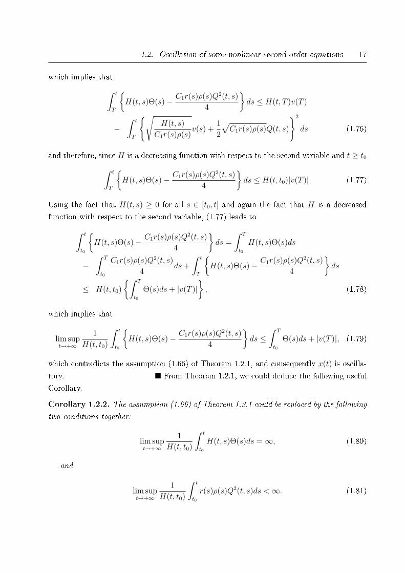
1.2. Oscillation of some nonlinear second order equations 17
which implies that∫ t
T
H(t, s)Θ(s)− C1r(s)ρ(s)Q2(t, s)
4
ds ≤ H(t, T )v(T )
−∫ t
T
√H(t, s)
C1r(s)ρ(s)v(s) +
1
2
√C1r(s)ρ(s)Q(t, s)
2
ds (1.76)
and therefore, since H is a decreasing function with respect to the second variable and t ≥ t0∫ t
T
H(t, s)Θ(s)− C1r(s)ρ(s)Q2(t, s)
4
ds ≤ H(t, t0)|v(T )|. (1.77)
Using the fact that H(t, s) ≥ 0 for all s ∈ [t0, t] and again the fact that H is a decreased
function with respect to the second variable, (1.77) leads to∫ t
t0
H(t, s)Θ(s)− C1r(s)ρ(s)Q2(t, s)
4
ds =
∫ T
t0
H(t, s)Θ(s)ds
−∫ T
t0
C1r(s)ρ(s)Q2(t, s)
4ds+
∫ t
T
H(t, s)Θ(s)− C1r(s)ρ(s)Q2(t, s)
4
ds
≤ H(t, t0)
∫ T
t0
Θ(s)ds+ |v(T )|, (1.78)
which implies that
lim supt→+∞
1
H(t, t0)
∫ t
t0
H(t, s)Θ(s)− C1r(s)ρ(s)Q2(t, s)
4
ds ≤
∫ T
t0
Θ(s)ds+ |v(T )|, (1.79)
which contradicts the assumption (1.66) of Theorem 1.2.1, and consequently x(t) is oscilla-
tory. From Theorem 1.2.1, we could deduce the following useful
Corollary.
Corollary 1.2.2. The assumption (1.66) of Theorem 1.2.1 could be replaced by the following
two conditions together:
lim supt→+∞
1
H(t, t0)
∫ t
t0
H(t, s)Θ(s)ds =∞, (1.80)
and
lim supt→+∞
1
H(t, t0)
∫ t
t0
r(s)ρ(s)Q2(t, s)ds <∞. (1.81)
18 Chapter 1. Introduction
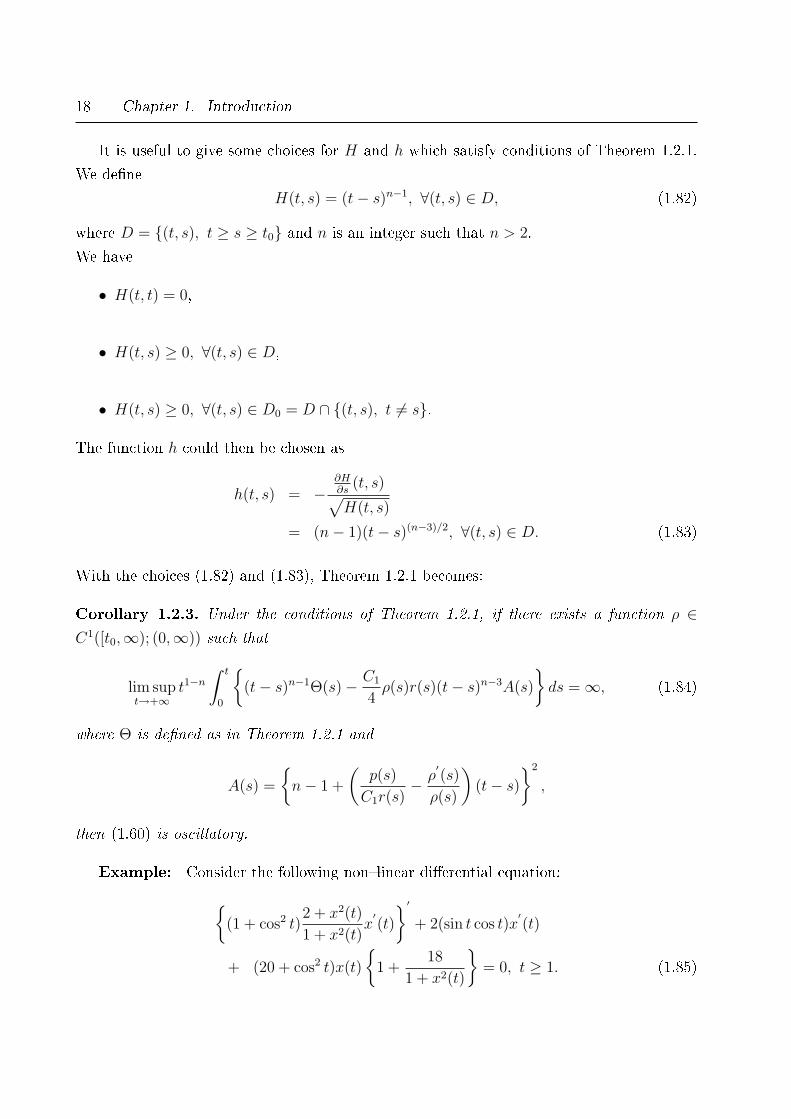
It is useful to give some choices for H and h which satisfy conditions of Theorem 1.2.1.
We dene
H(t, s) = (t− s)n−1, ∀(t, s) ∈ D, (1.82)
where D = (t, s), t ≥ s ≥ t0 and n is an integer such that n > 2.
We have
• H(t, t) = 0,
• H(t, s) ≥ 0, ∀(t, s) ∈ D,
• H(t, s) ≥ 0, ∀(t, s) ∈ D0 = D ∩ (t, s), t 6= s.
The function h could then be chosen as
h(t, s) = −∂H∂s
(t, s)√H(t, s)
= (n− 1)(t− s)(n−3)/2, ∀(t, s) ∈ D. (1.83)
With the choices (1.82) and (1.83), Theorem 1.2.1 becomes:
Corollary 1.2.3. Under the conditions of Theorem 1.2.1, if there exists a function ρ ∈C1([t0,∞); (0,∞)) such that
lim supt→+∞
t1−n∫ t
0
(t− s)n−1Θ(s)− C1
4ρ(s)r(s)(t− s)n−3A(s)
ds =∞, (1.84)
where Θ is dened as in Theorem 1.2.1 and
A(s) =
n− 1 +
(p(s)
C1r(s)− ρ
′(s)
ρ(s)
)(t− s)
2
,
then (1.60) is oscillatory.
Example: Consider the following nonlinear dierential equation:(1 + cos2 t)
2 + x2(t)
1 + x2(t)x′(t)
′+ 2(sin t cos t)x
′(t)
+ (20 + cos2 t)x(t)
1 +
18
1 + x2(t)
= 0, t ≥ 1. (1.85)
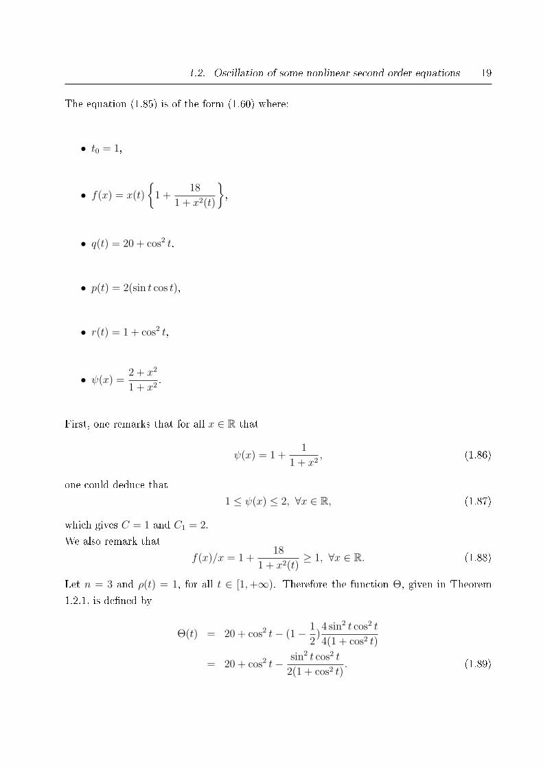
1.2. Oscillation of some nonlinear second order equations 19
The equation (1.85) is of the form (1.60) where:
• t0 = 1,
• f(x) = x(t)
1 +
18
1 + x2(t)
,
• q(t) = 20 + cos2 t,
• p(t) = 2(sin t cos t),
• r(t) = 1 + cos2 t,
• ψ(x) =2 + x2
1 + x2.
First, one remarks that for all x ∈ R that
ψ(x) = 1 +1
1 + x2, (1.86)
one could deduce that
1 ≤ ψ(x) ≤ 2, ∀x ∈ R, (1.87)
which gives C = 1 and C1 = 2.
We also remark that
f(x)/x = 1 +18
1 + x2(t)≥ 1, ∀x ∈ R. (1.88)
Let n = 3 and ρ(t) = 1, for all t ∈ [1,+∞). Therefore the function Θ, given in Theorem
1.2.1, is dened by
Θ(t) = 20 + cos2 t− (1− 1
2)4 sin2 t cos2 t
4(1 + cos2 t)
= 20 + cos2 t− sin2 t cos2 t
2(1 + cos2 t). (1.89)
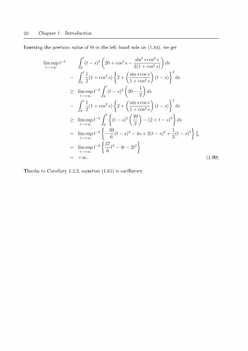
20 Chapter 1. Introduction
Inserting the previous value of Θ in the lefthand side on (1.84), we get
lim supt→+∞
t−2
∫ t
0
(t− s)2
(20 + cos2 s− sin2 s cos2 s
2(1 + cos2 s)
)ds
−∫ t
0
1
2(1 + cos2 s)
2 +
(sin s cos s
1 + cos2 s
)(t− s)
2
ds
≥ lim supt→+∞
t−2
∫ t
0
(t− s)2
(20− 1
2
)ds
−∫ t
0
1
2(1 + cos2 s)
2 +
(sin s cos s
1 + cos2 s
)(t− s)
2
ds
≥ lim supt→+∞
t−2
∫ t
0
(t− s)2
(39
2
)− (2 + t− s)2
ds
= lim supt→+∞
t−2
−39
6(t− s)3 − 4s+ 2(t− s)2 +
1
3(t− s)3
|t0
= lim supt→+∞
t−2
37
6t3 − 4t− 2t2
= +∞. (1.90)
Thanks to Corollary 1.2.3, equation (1.85) is oscillatory.
Chapter 2
On the zeros of the solutions of certain
coupled hyperbolic problems with delays
2.1 Introduction
The study of the oscillatory behavior of the solutions of hyperbolic dierential equations of
neutral type had an increasing interest these last years.
It seems that the rst attempt in this direction was made by Mishev and Bainov [25]. In
[25], they have obtained sucient conditions for the oscillation of all solutions of a class of
neutral hyperbolic equations with conditions at the boundary of the Neumann type. Yosida
[7] had obtained sucient conditions which garantee the existence of bounded domains in
which each solution of a neutral hyperbolic equation with boundary conditions of the Dirich-
let, Neumann ou Robin type has a zero.
The oscillatory behavior of the solutions of dierential equations of neutral type are
studied recently by many authors (see for instance [28], [26], [45], and [46], and the references
quoted therein.).
Let us cite for example the attempt of Parhi and Kirane [28] who studied the oscillatory
behavior of equations of type
utt (x, t) + βutt (x, t− ρ) + γut (x, t− θ)− [δ4µ (x, t) + α4u (x, t− z)]
+ c (x, t, u (x, t, u (x, t) , u (x, t− σ))) = f(x, t) (2.1)
and other generalizations on the coecients and on the delays, as well as the work of Parhi
21
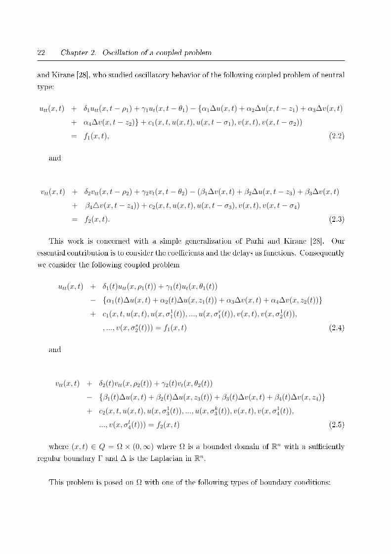
22 Chapter 2. Oscillation of a coupled problem
and Kirane [28], who studied oscillatory behavior of the following coupled problem of neutral
type:
utt(x, t) + δ1utt(x, t− ρ1) + γ1ut(x, t− θ1)− α1∆u(x, t) + α2∆u(x, t− z1) + α3∆v(x, t)
+ α4∆v(x, t− z2)+ c1(x, t, u(x, t), u(x, t− σ1), v(x, t), v(x, t− σ2))
= f1(x, t), (2.2)
and
vtt(x, t) + δ2vtt(x, t− ρ2) + γ2vt(x, t− θ2)− (β1∆v(x, t) + β2∆u(x, t− z3) + β3∆v(x, t)
+ β44v(x, t− z4)) + c2(x, t, u(x, t), u(x, t− σ3), v(x, t), v(x, t− σ4)
= f2(x, t). (2.3)
This work is concerned with a simple generalization of Parhi and Kirane [28]. Our
essential contribution is to consider the coecients and the delays as functions. Consequently
we consider the following coupled problem
utt(x, t) + δ1(t)utt(x, ρ1(t)) + γ1(t)ut(x, θ1(t))
− α1(t)∆u(x, t) + α2(t)∆u(x, z1(t)) + α3∆v(x, t) + α4∆v(x, z2(t))
+ c1(x, t, u(x, t), u(x, σ11(t)), ..., u(x, σr1(t)), v(x, t), v(x, σ1
2(t)),
, ..., v(x, σs2(t))) = f1(x, t) (2.4)
and
vtt(x, t) + δ2(t)vtt(x, ρ2(t)) + γ2(t)vt(x, θ2(t))
− β1(t)∆u(x, t) + β2(t)∆u(x, z3(t)) + β3(t)∆v(x, t) + β4(t)∆v(x, z4)
+ c2(x, t, u(x, t), u(x, σ13(t)), ..., u(x, σk3(t)), v(x, t), v(x, σ1
4(t)),
..., v(x, σl4(t))) = f2(x, t) (2.5)
where (x, t) ∈ Q = Ω × (0,∞) where Ω is a bounded domain of Rn with a suciently
regular boundary Γ and ∆ is the Laplacian in Rn.
This problem is posed on Ω with one of the following types of boundary conditions:
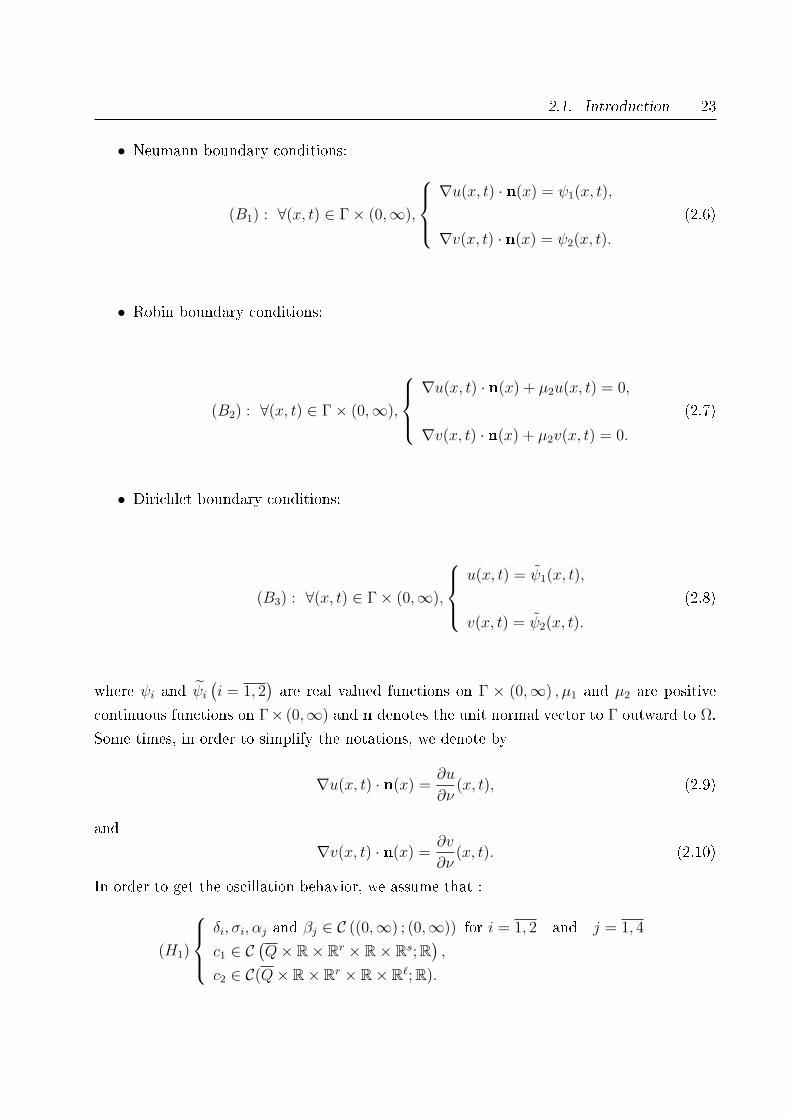
2.1. Introduction 23
• Neumann boundary conditions:
(B1) : ∀(x, t) ∈ Γ× (0,∞),
∇u(x, t) · n(x) = ψ1(x, t),
∇v(x, t) · n(x) = ψ2(x, t).
(2.6)
• Robin boundary conditions:
(B2) : ∀(x, t) ∈ Γ× (0,∞),
∇u(x, t) · n(x) + µ2u(x, t) = 0,
∇v(x, t) · n(x) + µ2v(x, t) = 0.
(2.7)
• Dirichlet boundary conditions:
(B3) : ∀(x, t) ∈ Γ× (0,∞),
u(x, t) = ψ1(x, t),
v(x, t) = ψ2(x, t).
(2.8)
where ψi and ψi(i = 1, 2
)are real valued functions on Γ × (0,∞) , µ1 and µ2 are positive
continuous functions on Γ× (0,∞) and n denotes the unit normal vector to Γ outward to Ω.
Some times, in order to simplify the notations, we denote by
∇u(x, t) · n(x) =∂u
∂ν(x, t), (2.9)
and
∇v(x, t) · n(x) =∂v
∂ν(x, t). (2.10)
In order to get the oscillation behavior, we assume that :
(H1)
δi, σi, αj and βj ∈ C ((0,∞) ; (0,∞)) for i = 1, 2 and j = 1, 4
c1 ∈ C(Q× R× Rr × R× Rs; R
),
c2 ∈ C(Q× R× Rr × R× R`; R).
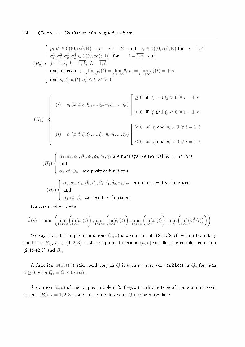
24 Chapter 2. Oscillation of a coupled problem
(H2)
ρi, θi ∈ C((0,∞); R) for i = 1, 2 and zi ∈ C((0,∞); R) for i = 1, 4
σ1i , σ
2j , σ
3k, σ
4L ∈ C((0,∞); R) for i = 1, r and
j = 1, s, k = 1, k, L = 1, `,
and for each j : limt→+∞
ρi(t) = limt→+∞
θi(t) = limt→+∞
σji (t) = +∞
and ρi(t), θi(t), σji ≤ t,∀t > 0
(H3)
(i) c1 (x, t, ξ, ξ1, ..., ξr, η, η1, ..., ηs)
≥ 0 if ξ and ξi > 0,∀ i = 1, r
≤ 0 if ξ and ξi < 0,∀ i = 1, r
(ii) c2 (x, t, ξ, ξ1, ..., ξk, η, η1, ..., η`)
≥ 0 si η and ηi > 0,∀ i = 1, `
≤ 0 si η and ηi < 0,∀ i = 1, `
(H4)
α2, α3, α4, β4, δ1, δ2, γ1, γ2 are nonnegative real valued unctions
and
α1 et β3 are positive functions.
(H5)
α2, α3, α4, β1, β2, β4, δ1, δ2, γ1, γ2 are nonnegative functions
and
α1 et β3 are positive functions.
For our need we dene:
t (s) = min
(min
1≤i≤2
(inft≥sρi (t)
), min
1≤i≤z
(inft≥sθi (t)
), min
1≤i≤4
(inft≥tzi (t)
); mini,∂J
(inft≥s
(σJi (t)
)))We say that the couple of functions (u, v) is a solution of ((2.4),(2.5)) with a boundary
condition Bi0 , i0 ∈ 1, 2, 3 if the couple of functions (u, v) satises the coupled equation
(2.4)(2.5) and Bi0 .
A function w(x, t) is said oscillatory in Q if w has a zero (or vanishes) in Qa for each
a ≥ 0, with Qa = Ω× (a,∞).
A solution (u, v) of the coupled problem (2.4)(2.5) with one type of the boundary con-
ditions (Bi) , i = 1, 2, 3 is said to be oscillatory in Q if u or v oscillates.
2.1. Introduction 25
A solution (u, v) of (2.4)(2.5), with one type of the boundary conditions (Bi) , i = 1, 2, 3
is said to be strongly oscillatory in Q if u, v oscillates at the some time.
We assume that:
(i) (α1 + β3)2 ≥ 4 (α1 β3 − α3 β1) .
(ii) α1 β3 > β1 α3
which ensures the total hyperbolicity of equations (2.4)(2.5) (see [6]).
The following notations will be used in what follows.
For each
u, v ∈ C2 (Q)⋂C2(Q),
We write:
U (t) =
∫Ω
u (x, t) dx, V (t) =
∫Ω
v (x, t) dx,
U (t) =
∫Ω
ϕ (x) u (x, t) dx, V (t) =
∫Ω
ϕ (x) v (x, t) dx.
In addition, for all i ∈ 1, 2, we denote by
Ψi (t) =
∫Γ
ψi (x, t) dγ(x),
Ψi (t) =
∫Γ
Ψi (x, t)∂ϕ
∂vdγ(x)
Fi (t) =
∫Ω
fi (x, t) dx
Fi (t) =
∫Ω
ϕ (x) fi (x, t) dx,
where dγ denotes the integration symbol for (n− 1)dimensional Lebesgue measure on the
considered hyperplane.
26 Chapter 2. Oscillation of a coupled problem
2.2 The coupled hyperbolic problem
2.2.1 Existence theorem of oscillations
The main results of our paper are the following Theorems:
Theorem 2.2.1. We assume that the conditions (H1) , (H2) , (H3) , (H5) hold. If in addition
(A1)
lim inft→∞
1t−t0
∫ tt0
(t− s) [F1 (s) + α1Ψ1 (s) + α2Ψ1 (s− z1 (s)) +
+ α3Ψ2 (s) + α4Ψ2 (s− z2 (s))] ds = −∞,
and
(A2)
lim supt→∞
1t−t0
∫ tt0
(t− s) [F1 (s) + α1Ψ1 (s) + α2Ψ1 (s− z1 (s)) +
+α3Ψ2 (s) + α4Ψ2 (s− z2 (s))] ds =∞,
or if
(A3)
lim inft→∞
1t−t0
∫t0
t(t− s) [F2 (s) + β1Ψ1 (s) + β2Ψ1 (s− z3(s)) +
+ β3Ψ2 (s) + β4Ψ2 (s− z4 (s))] ds = −∞
and
(A4)
lim supt→∞
1t−t0
∫t0
t(t− s) [F2 (s) + β1Ψ1 (s) + β2Ψ1 (s− z3(s)) +
+ β3Ψ2 (s) + β4Ψ2 (s− z4(s))] ds =∞
for any t0 ≥ 0 , then each solution (u, v) of the coupled problem ((2.4),(2.5)) with (B1)
oscillates in Q.
Theorem 2.2.2. We assume that the conditions (H1) , (H2) , (H5) , (A1)− (A4) hold. Then
each solution of problem ((2.4),(2.5)) , (B1) oscillates in Q.
Theorem 2.2.3. Assume that the conditions (H1) , (H2) , (H4) are satised and (A1)−(A4)
hold, then each solution of problem ((2.4),(2.5)) , (B2) oscillates in Q.
Theorem 2.2.4. We assume that the conditions (H1) , (H2) , (H5) are satised. If
Existence theorem of oscillations 27
lim inft→∞
1
t− t0
∫t0
t
(t− s) [F1 (s)− α1Ψ1 (s)− α2Ψ1 (s− z1(s))−
− α3Ψ2 (s)− α4Ψ2 (s− z2 (s))] ds = −∞,
lim inft→∞
1
t− t0
∫t0
t
(t− s) [F1 (s)− β3Ψ1 (s)− β2Ψ1 (s− z3(s))−
− β3Ψ2 (s)− β4Ψ2 (s− z4 (s))] ds = −∞,
lim supt→∞
1
t− t0
∫t0
t
(t− s) [F1 (s)− α1Ψ1 (s)− α2Ψ1 (s− z1 (s))−
− α3Ψ2 (s)− α4Ψ2 (s− z2 (s))] ds =∞,
and
lim supt→∞
1
t− t0
∫t0
t
(t− s) [F2 (s)− β3Ψ1 (s)− β2Ψ1 (s− z3(s))−
− β4Ψ2 (s− z4 (s))] ds =∞,
for each t0 ≥ 0, then each solution of problem (2.4)(2.5), (B3) oscillates in Q.
In order to prove Theorems 2.2.22.2.4, we need to use the following technical Lemmata:
Lemma 2.2.1. We assume that the conditions (H1) , (H2), (H3) (i) , (H5) are satised. If
(u, v) is a solution of problem ((2.4),(2.5)), (B1) and u (x, t) > 0 in Qt0 . Then the function
U satises the following dierential inequality of neutral type:
y′′ (t) + δ1 y′′ (ρ1 (t)) + γ1 y
′ (θ1 (t)) ≤ F1 (t) +
+ α1Ψ1 + α2Ψ1 (z1 (t)) + α3Ψ2 (t) + α4Ψ2 (z2 (t))
(2.11)
for a suciently large t.
Proof Integrating equation (2.4) over the domain Ω, we get:
U ′′ + δ1 (t)U ′′ (ρ1 (t)) + γ1 (t)U ′ (θ1 (t))−
28 Chapter 2. Oscillation of a coupled problem
[α1(t)
∫Ω
4 u(x, t) dx+ α2(t)
∫Ω
4 u (x, z1(t)) dx+
+α3(t)
∫Ω
4 v(x, t) dx+ α4(t)
∫Ω
4 v(x, z2(t)) dx]+
+
∫Ω
c1(x, t, u(x, t), u(x, σ11(t)), ..., u(x, σr1(t)), v(x, t), v(x, σ1
2(t)), ..., v(x, σs2(t)))dx = F1 (t)
An integration by parts yields:
∫Ω
4 u (x, t) dx =
∫Γ
∂u
∂ν(x, t) dγ(x)
=
∫Γ
ψ1 (x, t) dγ(x)
= Ψ1 (t) (2.12)
and
∫Ω
4 u (x, z1 (t)) dx = Ψ1 (z1 (t)) .
Assumption (H2) implies that limt→+∞
σ11 (t) = +∞, and then there exists some A > 0 such
that for all t > A, we have
σ11(t) > t0. (2.13)
This together with the hypothesis u(x, t) > 0 yields that
u(x, σ11(t)) > 0, (2.14)
for a suciently large t.
By the same manner, we justify that
u(x, σi1(t)) > 0, ∀i = 1, r, (2.15)
for a suciently large t.
Existence theorem of oscillations 29
Inequality (2.15) together with hypothesis (H3)(i) implies that
c1(x, t, u(x, t), u(x, σ11(t)), ..., u(x, σr1(t)), v(x, t), v(x, σ1
2(t)), ..., v(x, σs2(t))) > 0, (2.16)
for a suciently large t.
Which implies
U ′′ (t) + δ1 (t)U ′′ (ρ1 (t)) + δ1 (t)U ′ (θ1 (t))− α1(t)Ψ1(t)− α2(t)Ψ1 (z1(t))−
α3(t)Ψ2(t)− α4(t)Ψ2 (z2(t)) ≤ F1 (t) ,
and therefore
U ′′ (t) + δ1 (t)U ′′ (ρ1 (t)) + γ1 (t)U ′ (θ1 (t)) ≤
F1 (t) + α1Ψ1(t) + α2Ψ1 (z1(t)) + α3Ψ2(t) + α4Ψ2 (z2(t)) .
Lemma 2.2.2. We assume that the conditions (H1) , (H2), (H3) (ii) , (H5) are satised, if
(u, v) is a solution of ((2.4),(2.5)),(B1) such that v (x, t) > 0 on Qt0, then the solution V (t)
satises the following neutral ordinary dierential inequality:
y′′ (t) + δ2 (t) y′′ (ρ2 (t)) + γ2 y′ (θ2(t)) ≤ F2 (t) + β1Ψ1 (t) +
β2Ψ1 (z3 (t)) + β3 (t) Ψ2 (t) + β4 (t) Ψ2 (z4 (t)) (2.17)
for a suciently large t.
The proof of this Lemma is similar to the one of Lemma 2.2.1, so we omit it.
Lemma 2.2.3. Let us suppose that the conditions (H1) , (H2), (H3) (i) , (H4) are satised,
and (u, v) is a solution of the coupled problem ((2.4),(2.5)), (B2) such that u (x, t) >
0 and v (x, t) > 0 on Qt0 for some t0 > 0.
Then the solution U satises inequality (2.11) for a suciently large t.
If u < 0 and v < 0 on Qt0, then the function −U satises the following neutral ordinary
dierential inequality:
y′′ (t) + δ1 (t) y′′ (ρ1 (t)) + γ1 y′ (θ1) ≤
30 Chapter 2. Oscillation of a coupled problem
− [−F1 (t) + α1 (t) Ψ1 (t) + α2 (t) Ψ1 (z1 (t)) + α3 (t) Ψ2 (t) + α4 (t) Ψ2 (z2 (t))] (2.18)
for a suciently large t.
Lemma 2.2.4. Assume that the conditions (H1) , (H2), (H3) (ii) , (H4) are satised, if (u, v)
is a solution of problems ((2.4),(2.5)),(B2).
If u < 0 and v > 0 on a Qt0, then V (t) satises the ordinary dierential inequality (2.17)
for a suciently large t.
If u > 0 and v < 0 on Qt0 , then −V (t) satises inequality:
y′′ (t) + δ2 (t) y′′ (ρ2 (t)) + γ2 y′ (θ2 (t)) ≤
− [−F2 (t) + β1 (t) Ψ1 (t) + β2 (t) Ψ1 (z3 (t)) + β3 (t) Ψ2 (t) + β4 (t) Ψ2 (z4 (t))] (2.19)
for suciently large t.
The proofs of Lemmata 2.2.3 and 2.2.4 are similar to that of Lemma 2.2.1, so we omit
them.
Lemma 2.2.5. Let us suppose that the conditions (H1) , (H3) (i) , (H4) are satised, if (u, v)
is a solution of problem ((2.4),(2.5)),(B3) . If u (x, t) > 0 and v (x, t) > 0 on a Qt0 , then
the function U (t) veries the following dierential inequality of neutral type:
y′′ (t) + δ1 (t) y′′ (ρ1 (t)) + γ1 y′ (θ1 (t)) ≤
F1 (t)− α1 (t) Ψ1 (t)− α2 (t) Ψ1 (z1 (t))− α3 (t) Ψ2 (t) + α4 (t) Ψ2 (z2 (t)) (2.20)
for a suciently large t. If u (x, t) > 0 and v (x, t) < 0 on a Qt0 , then the function
−U (t) satises the following inequality:
y′′ (t) + δ1 (t) y′′ (ρ1 (t)) + δ1 y′ (θ1 (t))
≤ −F1 (t)− α1 (t) Ψ1 (t)− α2 (t) Ψ1 (z1 (t))− α3 (t) Ψ2 (t) + α4 (t) Ψ2 (z2 (t)) (2.21)
Proof Multiplying both sides of equation (2.4) by the function ϕ (x), integrating the
result over Ω, using (H2) and (H3)(ii), to obtain:
Existence theorem of oscillations 31
U ′′ (t) + δ1 (t)U ′′ (ρ1 (t)) + γ1 (t) U ′ (θ1 (t))
≤ F1 (t) + α1 (t)
∫Ω
ϕ(x)4 u (x, t) dx+ α2 (t)
∫Ω
ϕ(x)4 u (x, z1 (t)) dx+
+α3 (t)
∫Ω
ϕ(x)4 v (x, t) dx+ α4 (t)
∫Ω
ϕ(x)4 v (x, z2 (t)) dx,
for a suciently large t.
An application of the Green's formula yields, since ϕ = 0 in Γ and ∆ϕ = −λ1ϕ:
∫Ω
ϕ(x)4 u (x, t) dx =
∫Γ
ϕ(x)∇u(x)·n(x)dγ(x)−∫Γ
u(x)∇ϕ(x)·n(x)dγ(x)+
∫Ω
u(x)∆ϕ(x)dx
= −∫Γ
u(x)∇ϕ(x) · n(x)dγ(x)− λ1
∫Ω
u(x)ϕ(x)dx
= −Ψ1 (t)− λ1U(t)
and then, thanks to (H1), u > 0, ϕ > 0, and λ1 > 0:
U ′′ (t) + δ1 (t)U ′′ (ρ1 (t)) + γ1 (t) U ′ (θ1 (t))
≤ F1 (t)− α1 (t) Ψ1 (t)− α2 (t) Ψ1 (z1 (t))− α3 (t) Ψ2 (t) + α4 (t) Ψ2 (z2 (t)) .
Hence the rst part of the Lemma is proved. The second part of the Lemma can handled
as above.
Lemma 2.2.6. Assume that the conditions (H1) , (H3) (ii) , (H4) are satised, if (u, v) is a
solution of problem ((2.4),(2.5)),(B3) . If u (x, t) < 0 and v (x, t) > 0 on some Qt0, then
V (t) veries the following dierential inequality of neutral type:
y′′ + δ2 (t) y′′ (ρ2 (t)) + δ2 y′ (θ2(t))
32 Chapter 2. Oscillation of a coupled problem
≤ F2 (t)− β1 (t) Ψ1 (t)− β2 (t) Ψ1 (z3 (t))− β3 (t) Ψ2 (t)− β4 (t) Ψ2 (z4 (t)) (2.22)
for suciently large t.
If u(x, t) > 0 and v(x, t) < 0 on some Qt0 , then the function −V (t) satises the following
inequality:
y′′ (t) + δ2 (t) y′′ (ρ2 (t)) + δ2 y′ (θ2 (t)) ≤
−[F2 (t)− β1 (t) Ψ1 (t)− β2 (t) Ψ1 (z3 (t))− β3 (t) Ψ2 (t)− β4 (t) Ψ2 (z4 (t))
]for a suciently large t.
The proof of this Lemma is similar to that one of Lemma 2.2.5, so we omit it.
Theorem 2.2.5. Assume that the conditions (H1) − (H5) are fullled. If the dierential
inequatities (2.11) and (2.18) or the dierential inequalities (2.17) and (2.19) do not admit
positive solutions for a suciently large t, then all solutions of problem ((2.4),(2.5)),(B1)
oscillate in Q.
Proof Let (u, v) be a solution of problem ((2.4),(2.5)),(B1) which does not oscillates in
Q. Then, there exists t0 such that
u (x, t) 6= 0 and v (x, t) 6= 0 in Qt0 .
Assume that (2.11) and (2.18) do not admit positive solutions for a sucently large t.
Since u (x, t) 6= 0 in Qt0 , one has u(x, t) > 0 or u(x, t) < 0 in Qt0 .
If u(x, t) > 0 in Qt0 , then thanks to Lemma 2.2.1, U is a positive solution of (2.11) for a
sucently large t, which is a contradiction.
If u(x, t) < 0 on Qt0 , we set u(x, t) = −u(x, t) on Q, and then (u, v) is a solution of the
following problem:
utt (x, t) + δ1 (t) utt (x, ρ1 (t)) + γ1(t)ut (x, θ1 (t))−
[α1 (t)4 u (x, t) + α2 (t)4 u (x, z1 (t))− α3 (t)4 v (x, t)− α4 (t)4 v (x, z2 (t))]
− c1
(x, t,−u (x, t) ,− u
(x, σ1
1 (t))), ...,−u (x, σr1 (t)) , v (x, t) ,
Existence theorem of oscillations 33
v(x, σ1
2 (t)), ..., v (x, σs2 (t)) = −f1 (x, t)
vtt (x, t) + δ2 (t) vtt (x, ρ2 (t)) + γ2 vt (x, θ2 (t))−
[β14 u (x, t) + β2 (t)4 u (x, z3 (t))− β34 v (x, t)− β4 (t) ∆ v (x, z4 (t))]
− c2
(x, t,− u (x, t) ,− u
(x, σ1
2 (t))), ...,− u (x, σr3 (t)) , v (x, t) ,
v(x, σ1
4 (t)), ..., v (x, σs4 (t)) = f2(x, t),
and
∂u
∂ν= −ψ1 and
∂v
∂ν= ψ2 on Γ× (0,∞) .
Proceeding as in the proof of Lemma 2.2.1 one may prove that U is a positive solution of
(2.18), where
U =
∫Ω
u(x, t)dx.
we get a contradiction.
If the dierential inequalities (2.17) and (2.19) do not admit positive solutions for large
t, then we proceed as above considering v(x, t) 6= 0 in some Qt0 to arrive at necessary
contradictions. This completes the proof of the Theorem.
Theorem 2.2.6. Assume that conditions (H1) − (H5) are satised. Suppose that none of
the dierential inequalities (2.11), (2.17), (2.18) and (2.19) admit a positive solution for
large t. Then all solutions of problem ((2.4),(2.5)), (B1) oscillates strongly in Q.
ProofAssume the contrary, so there exists a solution (u(x, t), v(x, t)) of problem ((2.4),(2.5))
(B1) which does not oscillate strongly in Q. This means that u or v does not oscillate.
If u does not oscillate on Q, then there exists some t0 such that u(x, t) > 0 or u(x, t) < 0 in
Qt0 . If u(x, t) > 0 in Qt0 , then thanks to Lemma 2.2.1 it follows that U(t) =∫
Ωu(x, t)dx is
a positive solution of inequality (2.11), a contradiction.
If u(x, t) < 0 in Qt0 , then by setting u(x, t) = −u(x, t) and proceeding as in Lemma 2.2.1 it
34 Chapter 2. Oscillation of a coupled problem
may be proven that U =∫Ω
u (x, t) dx is a positive solution of (2.18), contradiction. Similar
contradictions may be obtained thanks to 2.2.2 if v(x, t) does not osciallate in Q. The proof
of the Theorem is complete.
Theorem 2.2.7. Let us suppose that (H1)−(H4) are satised, if inequalities (2.11), (2.17),
(2.18) and (2.19) do not admit positive solutions for suciently large t, then each solution
of problem ((2.4),(2.5)), (B2) oscillates in Q.
The proof of this Theorem is similar to that of the previous Theorem.
Similarly we prove:
Theorem 2.2.8. Assume that (H1)− (H4) are satised. If the inequalities (2.11), (2.17),
(2.18) and (2.19) do not admit positive solutions for suciently large t, then each solution
of problem ((2.4),(2.5)), (B3) oscillates in Q.
In the previous section, we remarked that the oscillation of problem ((2.4),(2.5)) with
one of the boundary conditions (Bi), where i ∈ 1, 2, 3, depends on the fact if (2.23), given
below, admit or not positive solutions.
For this reason, we will devote the following sections to give some sucient conditions, see
Lemma 2.2.7 given below, in order that inequality (2.23) does not admit positive solution
for large t.
Let
y′′(t) + λ1 (t) y′′ (ρ (t)) + λ2 (t) y′ (θ (t)) ≤ g (t) (2.23)
where
• ρ is a positive increasing function
• ρ has an inverse ξ such that ξ′ is an increasing function
• limt→+∞ ρ(t) = +∞
• the same properties satised by ρ should be satised by θ. The inverse of θ will be
denoted by χ.
In addition, λ1 and λ2 are decreasing positive functions and there derivatives are increasing
functions.
Existence theorem of oscillations 35
Lemma 2.2.7. If the following limit holds
limt→+∞
1
t− t0
∫t0
t
(t− s) g (s) ds = −∞ (2.24)
for each t0 > 0, then inequality (2.23) does not admit positive solution for large t.
Proof Assume the contrary, which means that there exists a positive solution y (t) for
(2.23) for some t > t0 > 0 .
Let us condsider t > t1 > t0 such that ρ (t1) > t0 and θ (t1) > t0 (this is possible since
limt→+∞ ρ(t) = +∞ and limt→+∞ θ(t) = +∞).
Integrating (2.23) over (t1, t) to get∫t1
t
y′′ (s) ds+
∫t1
t
λ1 (s) y′′ (ρ (s)) ds+
∫t1
t
λ2 (s) y′′ (θ (s)) ds ≤∫t1
t
g (s) ds. (2.25)
Integrations by parts, the previous inequality yields that
y′ (t) +M (ρ (t)) y′ (ρ (t))−M ′ (ρ (t)) y (ρ (t)) +
∫ ρ(t)
ρ(t1)
M ′′ (s) y (s) ds+
+ m (θ (t)) y′ (θ (t))−m′ (θ (t)) y (θ (t)) +
∫ θ(t)
θ(t1)
m′′ (s) y (s) ds+ c1 ≤∫t1
t
g (s) ds
with c1 ∈ R, M(s) = λ1(ξ(s))ξ′(s) and m(s) = λ2(χ(s))χ′(s).
A second integration from t to t1, yields:
y (t) +
∫t1
t
M (ρ (α)) y′ (ρ (α)) dα−∫t1
t
M ′ (ρ (α)) y (ρ (α)) dα+
∫t1
t(∫ ρ(α)
ρ(t1)
M ′′ (s) y (s) ds
)dα+
∫t1
t
m (θ (α)) y′ (θ (α)) dα−∫t1
t
m′ (θ (α)) y′ (θ (α)) dα+
+
(∫ θ(α)
θ(t1)
m” (s) y (s) ds
)dα + c1 (t− t1) ≤
∫t1
t
(t− s) g (s) ds,
36 Chapter 2. Oscillation of a coupled problem
which yields
y (t) +H (ρ (t)) y (ρ (t)) + c−∫ ρ(t)
ρ(t1)
H ′ (x) y (x) dx−∫t1
t
M ′ (ρ (α)) y (ρ (α)) dα+
+
∫t1
t(∫ ρ(α)
ρ(t1)
M” (s) y (s) ds
)dα + h (θ (t)) y (θ (t))−
∫ θ(t)
θ(t1)
h′ (x) y (x) dx−
−∫t1
t
m′ (θ (α)) y (θ (α)) dα + c1 (t− t1) ≤∫t1
t
(t− s) g (s) ds
with M (x) = λ1 (ρ−1 (x)) ,
m (x) = λ2 (θ−1 (x)) ,
and
H (x) = M (x)(ρ−1 (x)′
),
h (x) = m (x)((θ−1 (x))
′).
We have
H (ρ (t)) ≥ 0
and
h (θ (t)) ≥ 0
and
H decreases⇒ H ′ ≤ 0
h decreases⇒ h′ ≤ 0
Now:
M ′ (x) =(ρ−1 (x)
)′λ′1(ρ−1 (x)
).
and then
M ′′ (x) =(ρ−1 (x)
)′′λ′1(ρ−1 (x)
)+[(ρ−1 (x)′
)]2λ”
1
(ρ−1 (x)
)≤ 0
By the same way, we justify that
m′′ ≤ 0. (2.26)
Therefore
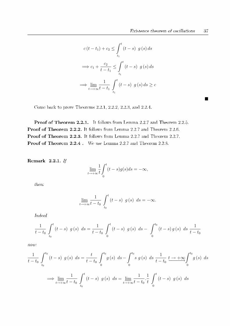
Existence theorem of oscillations 37
c (t− t1) + c2 ≤∫t1
t
(t− s) g (s) ds
=⇒ c1 +c2
t− t1≤∫t1
t
(t− s) g (s) ds
=⇒ limt→+∞
1
t− t1
∫t1
t
(t− s) g (s) ds ≥ c
Come back to prove Theorems 2.2.1, 2.2.2, 2.2.3, and 2.2.4.
Proof of Theorem 2.2.1. It follows from Lemma 2.2.7 and Theorem 2.2.5.
Proof of Theorem 2.2.2. It follows from Lemma 2.2.7 and Theorem 2.2.6.
Proof of Theorem 2.2.3. It follows from Lemma 2.2.7 and Theorem 2.2.7.
Proof of Theorem 2.2.4 . We use Lemma 2.2.7 and Theorem 2.2.8.
Remark 2.2.1. If
limt→+∞
1
t
∫0
t
(t− s)g(s)ds = −∞,
then:
limt→+∞
1
t− t0
∫t0
t
(t− s) g (s) ds = −∞.
Indeed
1
t− t0
∫t0
t
(t− s) g (s) ds =1
t− t0
∫0
t
(t− s) g (s) ds−∫0
t0
(t− s) g (s) ds1
t− t0
now:
1
t− t0
∫t0
t0
(t− s) g (s) ds =t
t− t0
∫0
t0
g (s) ds−∫0
t0
s g (s) ds1
t− t0t→ +∞−−−−−→
∫0
t0
g (s) ds
=⇒ limt→+∞
1
t− t0
∫t0
t
(t− s) g (s) ds = limt→+∞
1
t− t0.1
t
∫0
t
(t− s) g (s) ds
38 Chapter 2. Oscillation of a coupled problem
= limt→+∞
1
t
∫0
t
(t− s) g (s) ds = −∞.
The following examples, even not describing phenomena of physics, of elasticity or other
sciences, though illustrate our results .
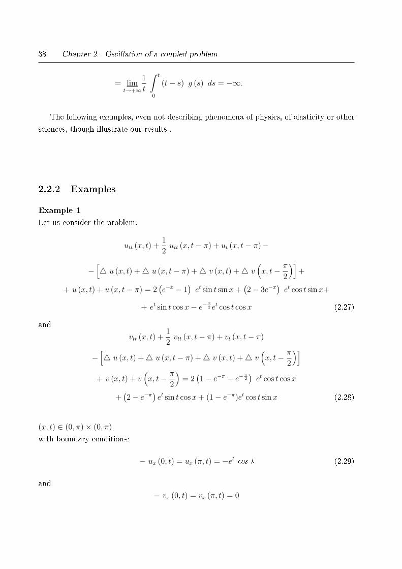
2.2.2 Examples
Example 1
Let us consider the problem:
utt (x, t) +1
2utt (x, t− π) + ut (x, t− π)−
−[4 u (x, t) +4 u (x, t− π) +4 v (x, t) +4 v
(x, t− π
2
)]+
+ u (x, t) + u (x, t− π) = 2(e−x − 1
)et sin t sinx+
(2− 3e−x
)et cos t sinx+
+ et sin t cosx− e−x2 et cos t cosx (2.27)
and
vtt (x, t) +1
2vtt (x, t− π) + vt (x, t− π)
−[4 u (x, t) +4 u (x, t− π) +4 v (x, t) +4 v
(x, t− π
2
)]+ v (x, t) + v
(x, t− π
2
)= 2
(1− e−π − e−
π2
)et cos t cosx
+(2− e−π
)et sin t cosx+ (1− e−π)et cos t sinx (2.28)
(x, t) ∈ (0, π)× (0, π),
with boundary conditions:
− ux (0, t) = ux (π, t) = −et cos t (2.29)
and
− vx (0, t) = vx (π, t) = 0
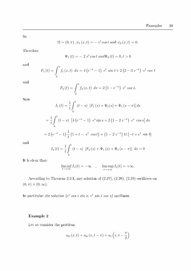
Examples 39
So
Ω = (0, π) , ψ1 (x, t) = − et cos t and ψ2 (x, t) = 0.
Therefore
Ψ1 (t) = − 2 et cos t andΨ2 (t) = 0, t > 0
and
F1 (t) =
∫0
π
f1 (x, t) dx = 4(e−π − 1
)et sin t + 2
(2− 3 e−π
)et cos t
and
F2 (t) =
∫0
π
f2 (x, t) dx = 2(1− e−π
)et cos t.
Now
I1 (t) =1
t
∫0
t
(t− s) [F1 (s) + Ψ1(s) + Ψ1 (s− π)] ds
=1
t
∫0
t
(t− s)[4(e−π − 1
)es sin s+ 2
(1− 2 e−π
)es cos s
]ds
= 2(e−π − 1
) 1
t
(1 + t− et cos t
)+(1− 2 e−π
)1t(−t+ et sin t
)and
I2 (t) =1
t
∫0
t
(t− s) [F2 (s) + Ψ1 (s) + Ψ1 (s− π)] ds = 0
It is clear that:
lim inft→+∞
I1(t) = −∞ , lim supt→+∞
I1(t) = +∞.
According to Theorem 2.2.1, any solution of (2.27), (2.28), (2.29) oscillates on
(0, π)× (0,∞).
In particular the solution (et cos t sin x, et sin t cos x) oscillates.
Example 2
Let us consider the problem:
utt (x, t) + utt (x, t− π) + ut
(x, t− π
2
)
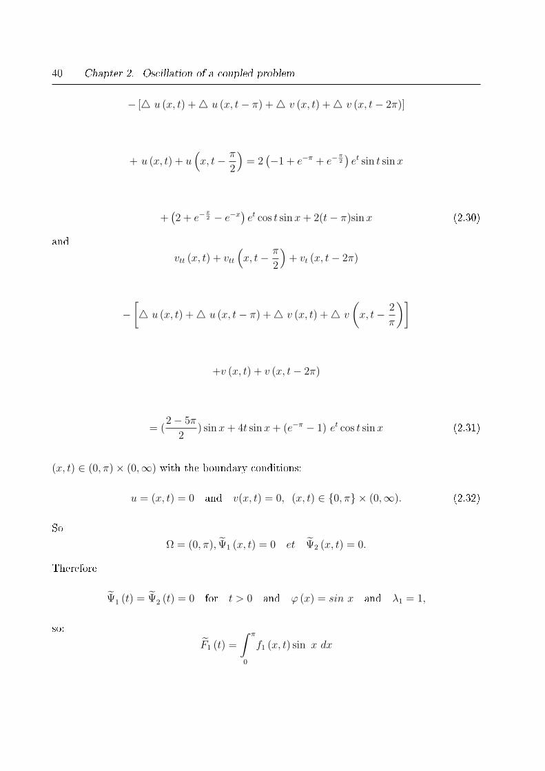
40 Chapter 2. Oscillation of a coupled problem
− [4 u (x, t) +4 u (x, t− π) +4 v (x, t) +4 v (x, t− 2π)]
+ u (x, t) + u(x, t− π
2
)= 2
(−1 + e−π + e−
π2
)et sin t sinx
+(2 + e−
x2 − e−x
)et cos t sinx+ 2(t− π)sinx (2.30)
and
vtt (x, t) + vtt
(x, t− π
2
)+ vt (x, t− 2π)
−[4 u (x, t) +4 u (x, t− π) +4 v (x, t) +4 v
(x, t− 2
π
)]
+v (x, t) + v (x, t− 2π)
= (2− 5π
2) sinx+ 4t sinx+ (e−π − 1) et cos t sinx (2.31)
(x, t) ∈ (0, π)× (0,∞) with the boundary conditions:
u = (x, t) = 0 and v(x, t) = 0, (x, t) ∈ 0, π × (0,∞). (2.32)
So
Ω = (0, π), Ψ1 (x, t) = 0 et Ψ2 (x, t) = 0.
Therefore
Ψ1 (t) = Ψ2 (t) = 0 for t > 0 and ϕ (x) = sin x and λ1 = 1,
so:
F1 (t) =
∫0
π
f1 (x, t) sin x dx
Examples 41
= a1et sin t+ a2 e
t cos t + πt− π2
with:
a1 = π(−1 + e−π + e−
π2
), a2 =
π
2
(2 + e−
π2 − e−π
)and:
F2 (t) =
∫0
π
f2 (x, t) sin x dx
= (2− 5π)π
4+ 2xt+
π
2
(e−π − 1
)et cos t.
and:
I1 (t) =1
t
∫0
t
(t− s) F1 (s) ds
=et
2t
[a1
(e−t + t e−t + cos t
)+ a2
(−t e−t + sin t
)+π
3
(t3e−t − π2t2e−t
)]and:
I2 (t) =et
t
[π3t3e−t + (2− 5π)
x
8t2 e−t +
(e−π − 1
) π4
(−t e−t + sin t
)]it is clear that:
lim inft→+∞
I1(t) = −∞ and lim supt→+∞
I1(t) =∞,
lim inft→+∞
I2(t) = −∞ and lim supt→+∞
I2(t) =∞
According to Theorem 2.2.4 any solution of problem (2.30), (2.31), (2.32) oscillates on (0, π)×(0,∞). In particular (et cos t sin x, t sin x) oscillates.
Chapter 3
Sucient conditions for the oscillation of
solutions to nonlinear second-order
dierential equations
3.1 Introduction
Kirane and Rogovchenko [20] studied the oscillatory solutions of the equation
[r(t)ψ(x(t))x′(t)
]′+ p(t)x′(t) + q(t)f(x(t)) = g(t), t ≥ t0, (3.1)
where t0 ≥ 0, r(t) ∈ C1([t0,∞); (0,∞)), p(t) ∈ C([t0,∞); R), q(t) ∈ C([t0,∞);
(0,∞)), q(t) is not identical zero on [t∗,∞) for some t∗ ≥ t0, f(x), ψ(x) ∈ C(R,R) and
ψ(x) > 0 for x 6= 0. Their results read as follows
Theorem 3.1.1. Case g(t) ≡ 0: Assume that for some constants K,C,C1 and for all
x 6= 0, f(x)/x ≥ K > 0 and 0 < C ≤ Ψ(x) ≤ C1. Let h, H ∈ C(D,R), where D = (t, s) :
t ≥ s ≥ t0, be such that
(i) H(t, t) = 0 for t ≥ t0, H(t, s) > 0 in D0 = (t, s) : t > s ≥ t0
(ii) H has a continuous and non-positive partial derivative in D0 with respect to the second
variable, and
−∂H∂s
= h(t, s)√H(t, s)
for all (t, s) ∈ D0.
42
3.1. Introduction 43
If there exists a function ρ ∈ C1([t0,∞); (0,∞)) such that
lim supt→+∞
1
H(t, t0)
∫ t
t0
[H(t, s)Θ(s)− C1
4ρ(s)r(s)Q2(t, s)]ds =∞ ,
where
Θ(t) = ρ(t)(Kq(t)−
( 1
C− 1
C1
)p2(t)
4r(t)
),
Q(t, s) = h(t, s) +[ p(s)
C1r(s)− ρ′(s)
ρ(s)
]√H(t, s),
then (3.1) is oscillatory.
Theorem 3.1.2. Case g(t) 6= 0: Let the assumptions of Theorem 3.1.1 be satised and
suppose that the function g(t) ∈ C([t0,∞); R) satises∫ ∞ρ(s)|g(s)|ds = N <∞ .
Then any proper solution x(t) of (3.1); i.e, a non-constant solution which exists for all t ≥ t0
and satises supt≥t0 |x(t)| > 0, satises
lim inft→∞
|x(t)| = 0.
Note that localization of the zeros is not given in the work by Kirane and Rogovchenko
[20]. Here we intend to give conditions that allow us to localize the zeros of solutions to
(3.1). Observe that in contrast to [20] where a Ricatti type transform,
v(t) = ρr(t)ψ(x(t))x′(t)
x(t),
is used, here we simply use a usual Ricatti transform.
44 Chapter 3. Oscillation of a second order equation
3.2 Solution of nonlinear secondorder dierential equa-
tion
3.2.1 Dierential equation without a forcing term
Consider the second-order dierential equation
[r(t)ψ(x(t))x′(t)
]′+ p(t)x′(t) + q(t)f(x(t)) = 0, t ≥ t0 (3.2)
where t0 ≥ 0, r(t) ∈ C1([t0,∞); (0,∞)), p(t) ∈ C([t0,∞)); R), q(t) ∈ C([t0,∞)); R), p(t) and
q(t) are not identical zero on [t?,∞) for some t? ≥ t0, f(x), ψ(x) ∈ C(R,R) and ψ(x) > 0 for
x 6= 0. The next theorem follows the ideas in Nasr [27].
Theorem 3.2.1. Assume that for some constants K,C,C1 and for all x 6= 0,
f(x)
x≥ K ≥ 0, (3.3)
0 < C ≤ ψ(x) ≤ C1 . (3.4)
Suppose further there exists a continuous function u(t) such that u(a) = u(b) = 0, u(t) is
dierentiable on the open set (a, b), a, b ≥ t?, and∫ b
a
[(Kq(t)− p2(t)
2Cr(t)
)u2(t)− 2C1r(t)(u
′)2(t)]dt ≥ 0 . (3.5)
Then every solution of (3.2) has a zero in [a, b].
Proof Let x(t) be a solution of (3.2) that has no zero on [a, b]. We may assume that
x(t) > 0 for all t ∈ [a, b] since the case when x(t) < 0 can be treated analogously. Let
v(t) = −x′(t)
x(t), t ∈ [a, b]. (3.6)
Dierential equation without a forcing term 45
Multiplying this equality by r(t)ψ(x(t)) and dierentiate the result. Using (3.2) we obtain
(r(t)ψ(x(t))v(t))′ = −(r(t)ψ(x(t))x′(t))′
x(t)+ r(t)ψ(x(t))v2(t)
= −p(t)v(t) + q(t)f(x(t))
x(t)+ r(t)ψ(x(t))v2(t)
=(r(t)ψ(x(t))
2v2(t) +
r(t)ψ(x(t))
2
(v2(t)− 2
p(t)
r(t)ψ(x(t))v(t)
)+ q(t)
f(x(t))
x(t)
=(r(t)ψ(x(t))
2v2(t) +
r(t)ψ(x(t))
2
(v(t)− p(t)
(r(t)ψ(x(t))
)2
− p2(t)
2r(t)ψ(x(t))+ q(t)
f(x(t))
x(t).
Using (3.3)-(3.4) and the fact that
(r(t)ψ(x(t))
2
(v(t)− p(t)
r(t)ψ(x(t))
)2 ≥ 0,
we have
(r(t)ψ(x(t))v(t))′ ≥ (r(t)ψ(x(t))
2v2(t)− p2(t)
2Cr(t)+Kq(t) (3.7)
46 Chapter 3. Oscillation of a second order equation
Multiplying both sides of this inequality by u2(t) and integrating on [a, b]. Using integration
by parts on the left side, the condition u(a) = u(b) = 0 and (3.4), we obtain
0 ≥∫ b
a
r(t)ψ(x(t))
2v2(t)u2(t)dt+ 2
∫ b
a
r(t)ψ(x(t))v(t)u(t)u′(t)dt
+
∫ b
a
Kq(t)u2(t)dt−∫ b
a
p2(t)
2Cr(t)u2(t)dt
≥∫ b
a
r(t)ψ(x(t))
2(v2(t)u2(t) + 4v(t)u(t)u′(t))dt
+
∫ b
a
Kq(t)u2(t)dt−∫ b
a
p2(t)u2(t)
2Cr(t)dt
≥∫ b
a
r(t)ψ(x(t))
2[v(t)u(t) + 2u′(t)]2dt− 2
∫ b
a
r(t)ψ(x(t))u′2(t)dt
+
∫ b
a
Kq(t)u2(t)dt−∫ b
a
p2(t)
2Cr(t)u2(t)dt
≥∫ b
a
[(Kq(t)− p2(t)
2Cr(t)
)u2(t)− 2r(t)ψ(x(t))u′2(t)
]dt
+
∫ b
a
r(t)ψ(x(t))
2[v(t)u(t) + 2u′(t)]2dt .
Now, from (3.4) we have
0 ≥∫ b
a
[(Kq(t)− p2(t)
2Cr(t)
)u2(t)− 2r(t)C1u
′2(t)]dt
+
∫ b
a
r(t)ψ(x(t))
2[v(t)u(t) + 2u′(t)]2dt.
If the rst integral on the right-hand side of the inequality is greater than zero, then we have
directly a contradiction. If the rst integral is zero and the second is also zero then x(t) has
the same zeros as u(t) at the points a and b; (x(t) = ku2(t)), which is again a contradiction
with our assumption.
Corollary 3.2.2. Assume that there exist a sequence of disjoint intervals [an, bn], and a
sequence of functions un(t) dened and continuous an [an, bn], dierentiable on (an, bn) with
un(an) = un(bn) = 0, and satisfying assumption (3.5). Let the conditions of Theorem 3.2.1.
hold. Then (3.2) is oscillatory.
Dierential equation with a forcing term 47
3.2.2 Dierential equation with a forcing term
Consider the dierential equation
[r(t)ψ(x(t))x′(t)
]′+ p(t)x′(t) + q(t)f(x(t)) = g(t), t ≥ t0 (3.8)
where t0 ≥ 0, g(t) ∈ C([t0,∞); R) r(t) ∈ C1([t0,∞); (0,∞)), p(t) ∈ C([t0,∞)); R), q(t) ∈C([t0,∞)); R), p(t) and q(t) are not identical zero on [t?,∞[ for some t? ≥ t0, f(x), ψ(x) ∈C(R,R) and ψ(x) > 0 for x 6= 0. Assume that there exists an interval [a, b], where a, b ≥ t?,
such that g(t) ≥ 0 and there exists c ∈ (a, b) such that g(t) has dierent signs on [a, c] and
[c, b]. Without loss of generality, let g(t) ≤ 0 on [a, c] and g(t) ≥ 0 on [c, b].
Theorem 3.2.3. Let (3.4) hold and assume that
f(x)
x|x|≥ K, (3.9)
for a positive constant K and for all x 6= 0. Furthermore assume that there exists a con-
tinuous function u(t) such that u(a) = u(b) = u(c) = 0, u(t) dierentiable on the open set
(a, c) ∪ (c, b), and satises the inequalities∫ c
a
[(√Kq(t)g|(t)| − p2(t)
2Cr(t)
)u2 − 2C1r(t)(u
′)2(t)]d(t) ≥ 0, (3.10)∫ b
c
[(√Kq(t)g|(t)| − p2(t)
2Cr(t)
)u2 − 2C1r(t)(u
′)2(t)]d(t) ≥ 0 . (3.11)
Then every solution of equation (3.8) has a zero in [a, b].
48 Chapter 3. Oscillation of a second order equation
Proof Assume to the contrary that x(t), a solution of (3.8), has no zero in [a, b]. Let
x(t) < 0 for example. Using the same computations as in the rst part, we obtain:
(r(t)ψ(x(t))v(t))′ = −(r(t)ψ(x(t))x′(t))′
x(t)+ r(t)ψ(x(t))v2(t)− g(t)
x(t)
= −p(t)v(t) + q(t)f(x(t))
x(t)+ r(t)ψ(x(t))v2(t)− g(t)
x(t)
=(r(t)ψ(x(t))
2v2(t) +
r(t)ψ(x(t))
2
(v2(t)− 2
p(t)v(t)
r(t)ψ(x(t))
)+ q(t)
f(x(t))
x(t)− g(t)
x(t)
=(r(t)ψ(x(t))
2v2(t) +
r(t)ψ(x(t))
2
(v(t)− p(t)
r(t)ψ(x(t))v(t)
)2
− p2(t)
2r(t)ψ(x(t))+ q(t)
f(x(t))
x(t)− g(t)
x(t)
For t ∈ [c, b] we have
(r(t)ψ(x(t))v(t))′ =r(t)ψ(x(t))
2v2(t) +
r(t)ψ(x(t))
2
(v(t)− p(t)
r(t)ψ(x(t))
)2
− p2(t)
2r(t)ψ(x(t))+ q(t)
f(x(t))
x(t)|x(t)||x(t)|+ |g(t)|
|x(t)|
From (3.9), and using the fact that
r(t)ψ(x(t))
2
(v(t)− p(t)
r(t)ψ(x(t))
)2 ≥ 0
we deduce
(r(t)ψ(x(t))v(t))′ ≥ (r(t)ψ(x(t))
2v2(t)− p2(t)
2r(t)ψ(x(t))+Kq(t)|x(t)|+ |g(t)|
|x(t)|. (3.12)
Using the Hölder inequality in (3.12) we obtain
(r(t)ψ(x(t))v(t))′ ≥ (r(t)ψ(x(t))
2v2(t) +
√Kq(t)|g(t)| − p2(t)
2r(t)ψ(x(t)). (3.13)
Dierential equation with a forcing term 49
Multiplying both sides of this inequality by u2(t) and integrating on [c, b], we obtain after
using integration by parts on the left-hand side and the condition u(c) = u(b) = 0,
0 ≥∫ b
c
r(t)ψ(x(t))
2v2(t)u2(t)dt+
∫ b
c
√Kq(t)|g(t)|u2(t)dt
−∫ b
c
p2(t)u2(t)
2r(t)ψ(x(t))dt+ 2
∫ b
c
r(t)ψ(x(t))v(t)u(t)u′(t)dt
≥∫ b
c
r(t)ψ(x(t))
2[v(t)u(t)− 2u′(t)]2dt− 2
∫ b
c
r(t)ψ(x(t))u′2(t)dt
+
∫ b
c
√Kq(t)|g(t)|u2(t)dt−
∫ b
c
p2(t)u2(t)
2r(t)ψ(x(t))dt.
Assumption (3.4) allows us to write
0 ≥∫ b
c
r(t)ψ(x(t))
2[v(t)u(t) + 2u′(t)]2dt− 2
∫ b
c
C1r(t)(u′)2(t)dt
+
∫ b
c
√Kq(t)|g(t)|u2(t)dt−
∫ b
c
p2(t)u2(t)
2Cr(t)dt
≥∫ b
c
r(t)ψ(x(t))
2[v(t)u(t) + 2u′(t)]2dt
+
∫ b
c
[(√Kq(t)g|(t)| − p2(t)
2Cr(t)
)u2(t)− 2C1r(t)(u
′)2(t)]dt.
This leads to a contradiction as in Theorem 3.2.1; the proof is complete.
Corollary 3.2.4. Assume that there exist a sequence of disjoint intervals [an, bn] a sequences
of points cn ∈ (an, bn), and a sequence of functions un(t) dened and continuous on [an, bn],
dierentiable on (an, cn)∪ (cn, bn)with un(an) = un(bn) = un(cn) = 0, and satisfying assump-
tions (3.10)-(3.11). Let the conditions of Theorem 3.2.3 hold. Then (3.8) is oscillatory.
Chapter 4
Some results concerning the oscillations
of solutions of a hyperbolic equation
with delays
4.1 Introduction
In this chapter, we extend the results of [3] to the equation
utt (x, t) + αut(x, t)− [∆u(x, t) +k∑i=1
bi(t)∆u(x, σi(t))]
+ C(x, t, u(x, t), u(x, τ1(t)), u(x, τ2(t)), . . . , u(x, τm(t))) = f(x, t), (4.1)
where (x, t) ∈ Q = Ω× (0,∞) and Ω is a bounded domain of Rn with a suciently regular
boundary Γ and ∆ is the Laplacian in Rn.
This problem is posed on Ω with one of the following types of boundary conditions:
• Dirichlet boundary conditions:
(DBC) : u(x, t) = ψ(x, t), Γ× (0,+∞) (4.2)
• Robin boundary conditions:
(RBC) : ∇u(x, t) · n(x) + µu(x, t) = ψ, Γ× (0,+∞) (4.3)
50
4.1. Introduction 51
where ψ, ψ, µ ∈ C(Γ× (0,∞)) and µ ≥ 0 on Γ× (0,∞).
We assume that
(H1) bi ∈ C([0,∞); [0,∞)), i = 1, . . . , k, f(x, t) ∈ C(Q; R), and α is constant
(H2) σi ∈ C([0,∞); R), i = 1, . . . , k, τi ∈ C([0,∞; R), i = 1, . . . ,m.
limt→∞
σi(t) =∞, σi(t) ≤ t, ∀t ∈ [0,∞), i = 1, . . . , k (4.4)
limt→∞
τi(t) =∞, τi(t) ≤ t, ∀t ∈ [0,∞), i = 1, . . . ,m (4.5)
(H3) C(x, t, ξ, η1, . . . , ηm) ∈ C(Q× R× Rm; R),
C(x, t, ξ, η1, . . . , ηm) ≥ K20ξ, ∀(x, t) ∈ Q, ξ ≥ 0, ηi ≥ 0, (4.6)
C(x, t, ξ, η1, . . . , ηm) ≤ K20ξ, ∀(x, t) ∈ Q, ξ ≤ 0, ηi ≤ 0, (4.7)
where K0 is some positive constant.
We dene the following denitions:
t?(s) = min1≤i≤k
inft≥s
σi(t), (4.8)
t??(s) = min1≤i≤m
inft≥s
τi(t), (4.9)
T ? = mint?(s), t??(s). (4.10)
It is useful to mention that the generalization of this section does not only consider the delay
as function but also the number of delays is increased. It is also useful to mention that, in
contrast of the previous section, the ((RBC) is not homogeneous.The notion of a solution is
given in the following denition:
Definition 1. A function u ∈ C2(Ω×(t?(0),∞); R)∩C(Ω×(t??(0),∞); R) satisfying (4.1),
with (4.3) (resp. (4.2)) is said to be a solution of (4.1) with (4.3) (resp. (4.2)).
52 Chapter 4. Localization of the zero of the solutions
4.2 Oscillation of the problem (4.1)
4.2.1 Oscillation of the problem (4.1) with Dirichlet boundary con-
dition
Theorem 4.2.1. Assume that α2−4(λ1+K20) < 0, and let ω1 = α
2and ω2 = 1
2
√4(λ1 +K2
0)− α2.
If there exists a number s such that T ?(s) ≥ 0 and
H(s) =
∫ s+ πω2
s
R(t)eω1(t−s) sin(ω2(t− s))dt = 0, (4.11)
where
R(s) = F (s)−Ψ(s)−k∑i=1
bi(s)Ψ(σi(s)), (4.12)
where Ψ is given by (1.26).
Then any solution u of problem (4.1) with (4.2) has a zero in Ω× (T ?, s+ πω2
).
Proof Assume the contrary. So there exists a solution u with no zero in Ω× (T ?, s+ πω2
).
Assume then that u > 0 on Ω× (T ?, s+ πω2
).
Multiplying both sides of (4.1) by ϕ and integrating over Ω, we get for t > 0
Utt(t) + αUt(t)−∫
Ω
[∆(x, t) +k∑i=1
bi(t)∆U(x, σi(t))]ϕ(x)dx
+
∫Ω
C(x, t, u(x, t), u(x, τ1(t)), u(x, τ2(t)), . . . , u(x, τm(t)))ϕ(x)dx = F (t), (4.13)
where F (t) is given by (1.24).
Using the fact that∫Ω
C(x, t, u(x, t), u(x, τ1(t)), . . . , u(x, τm(t)))ϕ(x)dx ≥ K20U(t), (4.14)
for all t ∈ [s, s+ πω2
).
Combining (4.14) with (4.13), we get
Utt(t) + αUt(t)(λ1 +K20)U(t) + λ1
k∑i=1
bi(t)U(σi(t)) ≤ F (t), (4.15)
for t ∈ [s, s+ πω2
).
Oscillation of the problem (4.1) with Robin boundary condition 53
Since u > 0 on (T ?, s + πω2
), then U(σi(t)) ≥ 0, for i ∈ 1, . . . , k, on [s, s + πω2
) thanks to
the denition of T ?(s).
Therefore U(t) is a positive solution of the following dierential inequation
Utt(t) + αUt(t)(λ1 +K20)U(t) ≤ R(t), t ∈ [s, s+
π
ω2
), (4.16)
where R(t) is given by (4.12).
which is equivalent to
Utt(t) + 2ω1Ut(t)(ω21 + ω2
2)U(t) ≤ R(t), t ∈ [s, s+π
ω2
). (4.17)
Multiplying both sides of the previous inequality by eω1(t−s) sin(ω2(t − s)) and integrating
both sides of the resulting inequation over (s, s+ πω2
), we get
0 < U(s+π
ω2
)eω1ω2π
+ U(s) ≤ 1
ω2
∫ s+ πω2
s
R(t)eω1(t−s) sin(ω2(t− s))dt (4.18)
Using the denition of H(s) given by (4.11), we get
0 < U(s+π
ω2
)eω1ω2π
+ U(s) ≤ 1
ω2
H(s). (4.19)
This with (4.11) leads to a contradiction.
If u < 0, we set v = −u and obtain, for V (t) = −∫
Ωu(x, t)ϕ(x)dx, the following inequation
Vtt(t) + 2ω1Vt(t)(ω21 + ω2
2)V (t) ≤ −R(t), t ∈ [s, s+π
ω2
). (4.20)
We can obtain a contradition by following the steps of the previous proof.
4.2.2 Oscillation of the problem (4.1) with Robin boundary condi-
tion
The following theorem gives a sucient condition for the oscillation of (4.1) with (4.3).
Theorem 4.2.2. Let K0 > 0 and assume that α2 − 4K20 < 0, and let ω3 = 1
2
√4K2
0 − α2).
If there exists a number s such that T ?(s) ≥ 0 and
H?(s) =
∫ s+ πω2
s
R(t)eω1(t−s) sin(ω3(t− s))dt = 0, (4.21)
54 Chapter 4. Localization of the zero of the solutions
where
R(s) = F (s) + Ψ(s)−k∑i=1
bi(s)Ψ(σi(s)). (4.22)
Then any solution u of problem (4.1) with (4.3) has a zero in Ω× (T ?, s+ πω3
).
Proof The proof of this Theorem is similar to that of Theorem 4.2.1
4.3 Example
Let us consider the following one dimensional problem
utt(x, t)+2ut(x, t)−[uxx(x, t)+2uxx(x, t−π)]+u(x, t) = 4 sinx cos 2t, (x, t) ∈ (0, π)×(0,∞),
(4.23)
with the Dirichlet boundary condition
u(0, t) = u(π, t) = 0, t > 0. (4.24)
Here n = 1, Ω = (0, π), α = 2, k = 1, b1(t) = 2, σ1(t) = t − π, K0 = 1, ψ = 0, and
f(x, t) = 4 sinx cos 2t.
It is easily seen that ω1 = ω2 = 1, T ?(s) = inft≥s(t−s) = s−π and F (x, t) =∫ π
04 sinx cos 2tdx =
2π cos 2t.
On the other hand, since ψ(t) = 0, we have R(t) = F (t).
Some computation gives us
H(s) =
∫ s+ πω2
s
4 cos 2tet−s sin(t− s)dt
=1√5
(eπ + 1) sin(2s− θ0), (4.25)
where θ0 = tg−1(12) (0 < θ0 <
π2).
Therefore H(s) = 0 for s = sn = θ02
+ nπ2(n = 2, 3, . . .).
Theorem 4.2.1 implies that any solution of (4.23)(4.24) has a zero on Ω× (sn − π, sn + π).
Such solution is u(x, t) = sinx ˙sin2t.
Perspectives
Although a huge number of articles has been devoted to the oscillation theory of dierential
equations, some interesting problems have not attracted the attention it merits yet.
Let us quote some of these problems:
1. Find conditions for non existence of oscillatory solutions of functional dierential equa-
tions (FDEs).
It is well known that there is a considrable number of articles devoted to nd the
sucient conditions such that all the solutions of the following second order ordinary
dierential equation are not oscillatory:
y′′ + p(t)f(y) = 0, (1)
whereas there is lack of such results concerning the second order FDE:
y′′(t) + p(t)f(y(r(t))) = 0. (2)
The technique used to look for the sucient conditions in order that all the solutions
of (1) are oscillatory is based in general on the constuction of the energy function and
on the use of the uniqueness of the zero solution.
It is well known that all the solutions of
y′(t) + q(t)y(t) + p(t)y([t]) = 0, (3)
are nonoscillatory, if p(t) ≤ 0 or p(t) ≥ 0 and lim supn→+∞
∫ n+1
n
p(t)exp
(∫ t
n
q(s)ds
)dt < 1
where [t] denotes the integer part function.
There is no such result even for
y′(t) + q(t)y(t) + p(t)y(τ(t)) = 0, (4)
55
56 Perspectives
where τ(t) ≤ t (τ(t) 6≡ t) and limt→∞ τ(t) =∞.
2. Find conditions for the existence of oscillatory solutions of FDE.
3. Study oscillation and non oscillation problems for delay systems.
4. Find conditions for the non oscillation caused by delays.
It is easy to see that every solution (x(t), y(t)) ofx′(t) = 2x(t)− y(t)
y′(t) = x(t) + y(t)(5)
is oscillatory. If we consider the corresponding delay system of the formx′(t) = 2x(t)− y
(t− 1
3log 4
)y′(t) = x
(t− 1
3log 4
)+ y(t),
(6)
then it is easy to nd that (6) has a non oscillatory solution x(t) = exp(32t), y(t) =
exp(32t).
This non oscillation is caused by the delay.
But there is no further result concerning this problem till now.
5. Find further relation between the oscillation theory of second order FDE and the
corresponding boundary value problems.
6. Study the distribution of zeros, the variations of amplitude and the asymptotic behavior
of oscillatory solutions.
7. Study some special FDE, which are posed by practical applications. For example,
consider the oscillation problems for the equations with delays, which depends on the
states, such as
y(n)(t) + p(t)y (t− r(t)) = 0. (7)
Even the case n = 1 is interesting to be considered.
There are also other paths to be followed like partial dierential equations and systems
of equations with delays depending on the states.
Bibliography
[1] J. W. Baker, Oscillation theorems for a second order damped nonlinear dierential
equation. SIAM J . Math. Anal. 25 (1973), 3740.
[2] A. Berkane, Sucient conditions for the oscillation of solutions to nonlinear second-
order dierential equations. Vol.03, (2008), 16.
[3] A. Berkane, Sur les Zéros des Solutions de Certaines Equations Hyperbolic à Retards.
Thesis of Magister" at Annaba's University, 1996.
[4] L. E. Bobisud, Oscillation of solutions of damped nonlinear dierential equations. SIAM
J . Math. Anal. 18 (1970), 601 606.
[5] G. J. Butler, The oscillatory behavior of a second order nonlinear dierential equation
with damping. J . Math. Anal. Appl. 57 (1977), 273289.
[6] R. Courant and D. Hilbert, Methods of mathematical physics. John Wiley and sons,
New York, I, 1989.
[7] E. M. Elabbasy, T.S. Hassan, S. H. Saker Oscillation of second-order nonlinear dieren-
tial equations with a damping term. Electronic Journal of Dierential Equations, Vol.
No. 76, (2005) pp. 1-13.
[8] M. A. El-Sayed, An oscillation criterion for forced second order linear dierential equa-
tion, Proc. Amer. Math. Soc. 33 (1972), 613-817.
[9] S. R. Grace, Oscillation theorems for second order nonlinear dierential equations with
damping. Math. Nachr. 141 (1989), 117127.
[10] S. R. Grace, Oscillation criteria for second order nonlinear dierential equations with
damping. J . Austral. Math. Soc. Ser . A 49 (1990), 43 54.
[11] S. R. Grace, Oscillation theorems for nonlinear dierential equations of second order. J
. Math. Anal. Appl. 171 (1992), 220 241.
57
58 Bibliography
[12] S. R. Grace and B. S. Lalli, Oscillation theorems for certain second order perturbed
nonlinear dierential equations. J . Math. Anal. Appl. 77 (1980), 205214.
[13] S. R. Grace and B. S. Lalli, Integral averaging technique for the oscillation of second
order nonlinear dierential equations. J . Math. Anal. Appl. 149 (1990), 277 311.
[14] S. R. Grace and B. S. Lalli, Oscillation theorems for second order superlinear dierential
equations with damping. J . Austral. Math. Soc. Ser . A 53 (1992), 156165.
[15] S. R. Grace and B. S. Lalli, and C. C. Yeh, Oscillation theorems for nonlinear second
order dierential equations with a nonlinear damping term. SIAM J . Math. Anal. 15
(1984), 1082 1093.
[16] S. R. Grace, B. S. Lalli, and C. C. Yeh, Addendum :Oscillation theorems for nonlinear
second order dierential equations with a nonlinear damping term. SIAM J . Math.
Anal. 19 (1988), 12521253.
[17] P. Hartman, On nonoscillatory linear dierential equations of second order. Amer. J .
Math. 74 (1952), 389400.
[18] A. G. Kartsatos, On the maintenance of oscillation of n-th order equation under the
eect of a small forcing terms, J. Di. Equations 10 (1971), 355-363.
[19] A. G. Kartsatos, On the maintenance of oscillation of a periodic forcing term, Proc.
Amer. Math. Soc. 33 (1972), 377-382.
[20] M. Kirane and Y. Rogovchenko, Oscillations results for the second order damped dier-
ential equation with non-monotonous nonlinearity, J. Math. Anal. Appl. 250, 118-138
(2000).
[21] M. Kirane and Yu. V. Rogovchenko, On oscillation of nonlinear second order dieren-
tial equation with damping term. Appl. Math. Comput., to appear.
[22] V. Komkov, On boundedness and oscillation of the dierential equation x′′−A(t)g(x) =
f(t) in Rn, SIAM J. Appl. Math. 22 (1972), 561-568.
[23] I. V. Kamenev, An integral criterion for oscillation of linear dierential equations. Mat.
Zametki 23 (1978), 249251.
59
[24] H. J. Li, Oscillation criteria for second order linear dierential equations. J. Math. Anal.
Appl., 194 (1995), 217234.
[25] D.P. Mishev and D.D. Bainov, Oscillation properties of the solutions of hyperbolic
equations of neutral type, Procedings of the colloquim on qualitative theory of dierential
equation (eds. B.S. Nagy and L. Hatvani, 771780, 1984.
[26] D.P. Mishev and D.D. Bainov, Oscillation properties of the solutions of a class of
hyperbolic equations of neutral type, Funks. Ekvac, 29, 213218, 1986.
[27] A. H. Nasr, Sucient conditions for the oscillation of forced super-linear second order
dierential equations with oscillatory potential, Proc. Amer. Math. Soc. 126, 1, (1998)
123-125.
[28] N. Parhi and M. Kirane, Oscillatory behaviour of solutions of coupled hyperbolic dier-
ential equations, Analysis, 14, 4356 (1994).
[29] Ch. G. Philos, Oscillation theorems for linear dierential equations of second order.
Arch. Math., 53 (1989), 483492.
[30] S. M. Rankin, Oscillation theorems for second order nonhomogeneous linear dierential
equations, J. Math. Anal. 53 (1976), 550-556.
[31] Yu. V. Rogovchenko, Note on Oscillation criteria for second order linear dierential
equations". J. Math. Anal. Appl., 203 (1996), 560563.
[32] Yu. V. Rogovchenko, Oscillation criteria for second order nonlinear perturbed dieren-
tial equations. J. Math. Anal. Appl., 215 (1997), 334357.
[33] Yu. V. Rogovchenko, Oscillation theorems for second order equations with damping.
Nonlinear Anal., 41 (2000), 10051028.
[34] Yu. V. Rogovchenko, Oscillation criteria for certain nonlinear dierential equations. J.
Math. Anal. Appl., 229 (1999), 399416.
[35] Svitlana P. Rogovechenko and Yuri. V. Rogovechenko, Oscillation of second-order Dif-
ferential equations with damping. Mathematical Analysis 10 (2003), 447461.
[36] S. H. Saker, P. Y. H. Pang and Ravi P. Agarwal, Oscillation theorems for second order
nonlinear functional dierential equations with damping. Dynamic Systems and Appli-
cations 12 (2003), 307322.
60 Bibliography
[37] Y. G. Sun, New Kamenev-type oscillation criteria for second-order nonlinear dierential
equations with damping. J. Math. Anal. Appl. 291 (2004), 341351
[38] C. A. Swanson, Comparison and Oscillation Theory of Linear Dierential Equations.
Academic Press, New York, 1968.
[39] A. Wintner, A criterion of oscillatory stability. Quart. Appl. Math. 7 (1949), 115117.
[40] J. S. W. Wong, A second order nonlinear oscillation. Funkcial. Ekvac. 11 (1968), 207
234.
[41] J. S. W. Wong, On Kamenev-type oscillation theorems for second order dierential
equations with damping. J. Math. Anal. Appl. 258 (2001), 244-257.
[42] J. Yan, A note on an oscillation criterion for an equation with damped term. Proc.
Amer. Math. Soc. 90 (1984), 277280.
[43] J. Yan, Oscillation theorems for second order linear dierential equations with damping
. Proc. Amer. Math. Soc. 98 (1986), 276282.
[44] C. C. Yeh, Oscillation theorems for nonlinear second order dierential equations with
damping term. Proc. Amer. Math. Soc. 84 (1982), 397402.
[45] N. Yoshida, On the zeros of solutions to non linear hyperbolic equations, Proc. R.
Soc. Edinb., Sect. A 106, 121129, 1987.
[46] N. Yoshida, On the zeros of solutions of hyperbolic equations of neutral type, Di.
Integ. Eqns., 3, 155160, 1990.
[47] J. S. W. Wong, Second order nonlinear forced oscillations, SIAM J. Math. Anal. 19, 3
(1998).