Embed Size (px)
Citation preview

complement scientifique Ecole Doctorale MATISSE
IRISA et INRIA, salle Markov
jeudi 19 janvier 2012
Introduction au Filtrage Particulaire
Exemples en Navigation, Localisation et Poursuite
Francois Le Gland
INRIA Rennes et IRMAR
http://www.irisa.fr/aspi/legland/ed-matisse/
directeur de recherche INRIA, responsable de l’equipe
ASPI : Applications Statistiques des Systemes de Particules en Interaction
http://www.irisa.fr/aspi/
themes
• filtrage particulaire, et applications en
– localisation, navigation et poursuite
– assimilation de donnees sequentielle
• inference statistique des modeles de Markov caches
• simulation d’evenements rares, et extensions en
– simulation moleculaire
– optimisation globale
• analyse mathematique des methodes particulaires

contrats industriels
• avec France Telecom R&D, sur la localisation de terminaux mobiles
• avec Thales, sur la navigation par correlation de terrain
• avec DGA /Techniques Navales, sur l’optimisation du positionnement et de
l’activation de capteurs
collaboration reguliere avec l’ONERA (office nationale de recherche et d’etudes
aerospatiales) : encadrement de doctorants
projets ANR
• FIL, sur la fusion de donnees pour la localisation
• PREVASSEMBLE, sur les methodes d’ensemble pour l’assimilation de
donnees et la prevision
projets europeens
• HYBRIDGE et iFLY, sur les methodes de Monte Carlo conditionnelles pour
l’evaluation de risque en trafic aerien
Introduction to filtering
• Bayesian approach
• usefulness of a prior model
• some models
• Bayesian estimation (static case)
• exemple : Gaussian model (static case)
1 (Bayesian approach : 1)
Bayesian approach
objective is to estimate, in a recursive manner as much as possible, the unknown
state Xn of a system (typically, position and velocity of a mobile) in view of noisy
observations Y0:n = (Y0 · · ·Yn) related to the hidden state by a relation such as
Yk = hk(Xk) + Vk
many applications in localization, navigation and tracking of a mobile
in such cases, objective is to estimate position and velocity of a mobile, using :
(i) measurements provided by sensors
(ii) possibly a reference database, available for instance as a digital map
often needed to take into account
(iii) a prior model (not necessarily accurate) for the mobile displacement or
evolution, usually a Markov model
2 (Bayesian approach : 2)
Bayesian approach, aka information fusion
prior information (state model)
+ likelihood (sensor model, consistency between state and measurement)
⇒ posteriori information
general principle : using Bayes rule
pX,Y (x, y) = pX|Y=y(x) pY (y) = pY |X=x(y) pX(x)
conditional distribution of X0:n given Y0:n (from which conditional distribution of
Xn given Y0:n is easily obtained, by marginalization) can be expressed in terms of
• conditional distribution of Y0:n given X0:n, often easy to evaluate for instance
in the additive model
Yk = hk(Xk) + Vk
• distribution of X0:n
recursive implementation possible thanks to Markov property
3 (Bayesian approach : 3)
however, conditional distribution of Xn given Y0:n does not have an explicit
expression, except in a few special situations
• Markov chain with finite state space (forward Baum equation)
• Gaussian linear systems (Kalman filter)
in more general situations, growing interest (since beginning of 90’s) for
simulation–based methods of Monte Carlo type
particle filtering provides an implementation of Bayesian approach that is
• intuitive, easy to understand and implement
• flexible, many algorithmic variants available
• numerically efficient
• easy to analyze mathematically
questions
• why a prior model should be needed ? how to take it into account ?
• why (and how) should conditional distributions be computed ?
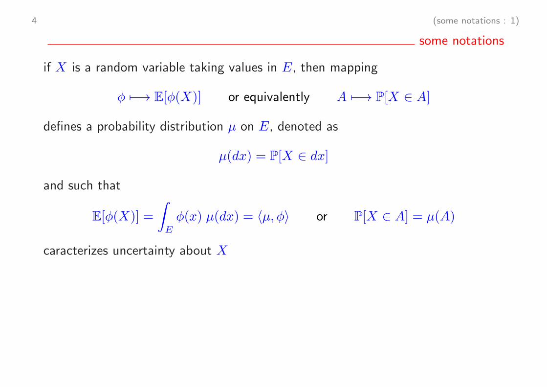
4 (some notations : 1)
some notations
if X is a random variable taking values in E, then mapping
φ 7−→ E[φ(X)] or equivalently A 7−→ P[X ∈ A]
defines a probability distribution µ on E, denoted as
µ(dx) = P[X ∈ dx]
and such that
E[φ(X)] =
∫
E
φ(x) µ(dx) = 〈µ, φ〉 or P[X ∈ A] = µ(A)
caracterizes uncertainty about X
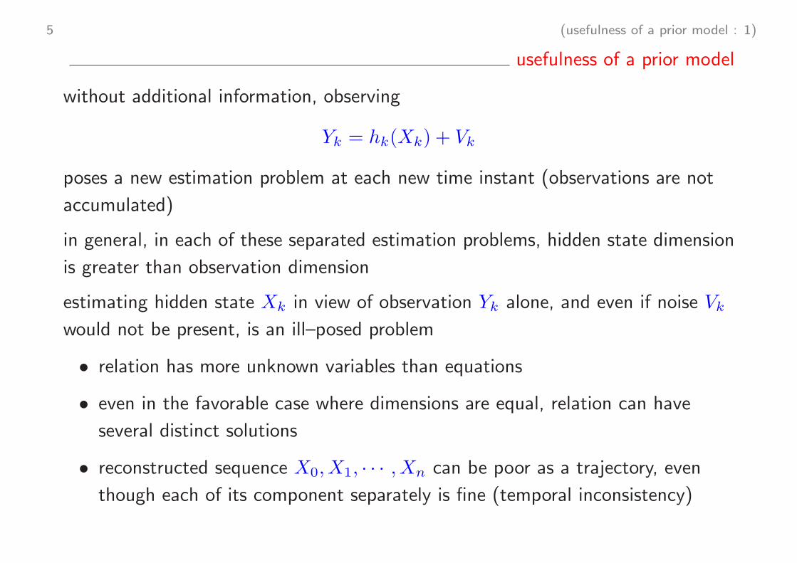
5 (usefulness of a prior model : 1)
usefulness of a prior model
without additional information, observing
Yk = hk(Xk) + Vk
poses a new estimation problem at each new time instant (observations are not
accumulated)
in general, in each of these separated estimation problems, hidden state dimension
is greater than observation dimension
estimating hidden state Xk in view of observation Yk alone, and even if noise Vkwould not be present, is an ill–posed problem
• relation has more unknown variables than equations
• even in the favorable case where dimensions are equal, relation can have
several distinct solutions
• reconstructed sequence X0, X1, · · · , Xn can be poor as a trajectory, even
though each of its component separately is fine (temporal inconsistency)
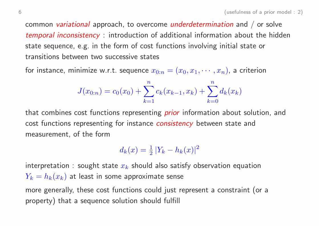
6 (usefulness of a prior model : 2)
common variational approach, to overcome underdetermination and / or solve
temporal inconsistency : introduction of additional information about the hidden
state sequence, e.g. in the form of cost functions involving initial state or
transitions between two successive states
for instance, minimize w.r.t. sequence x0:n = (x0, x1, · · · , xn), a criterion
J(x0:n) = c0(x0) +
n∑
k=1
ck(xk−1, xk) +
n∑
k=0
dk(xk)
that combines cost functions representing prior information about solution, and
cost functions representing for instance consistency between state and
measurement, of the form
dk(x) =12 |Yk − hk(x)|
2
interpretation : sought state xk should also satisfy observation equation
Yk = hk(xk) at least in some approximate sense
more generally, these cost functions could just represent a constraint (or a
property) that a sequence solution should fulfill
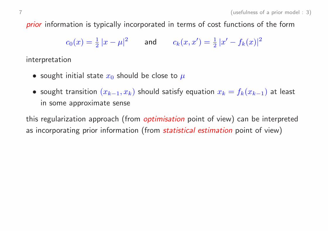
7 (usefulness of a prior model : 3)
prior information is typically incorporated in terms of cost functions of the form
c0(x) =12 |x− µ|2 and ck(x, x
′) = 12 |x
′ − fk(x)|2
interpretation
• sought initial state x0 should be close to µ
• sought transition (xk−1, xk) should satisfy equation xk = fk(xk−1) at least
in some approximate sense
this regularization approach (from optimisation point of view) can be interpreted
as incorporating prior information (from statistical estimation point of view)
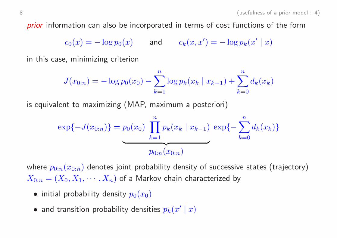
8 (usefulness of a prior model : 4)
prior information can also be incorporated in terms of cost functions of the form
c0(x) = − log p0(x) and ck(x, x′) = − log pk(x
′ | x)
in this case, minimizing criterion
J(x0:n) = − log p0(x0)−
n∑
k=1
log pk(xk | xk−1) +
n∑
k=0
dk(xk)
is equivalent to maximizing (MAP, maximum a posteriori)
exp{−J(x0:n)} = p0(x0)
n∏
k=1
pk(xk | xk−1)
︸ ︷︷ ︸p0:n(x0:n)
exp{−
n∑
k=0
dk(xk)}
where p0:n(x0:n) denotes joint probability density of successive states (trajectory)
X0:n = (X0, X1, · · · , Xn) of a Markov chain characterized by
• initial probability density p0(x0)
• and transition probability densities pk(x′ | x)
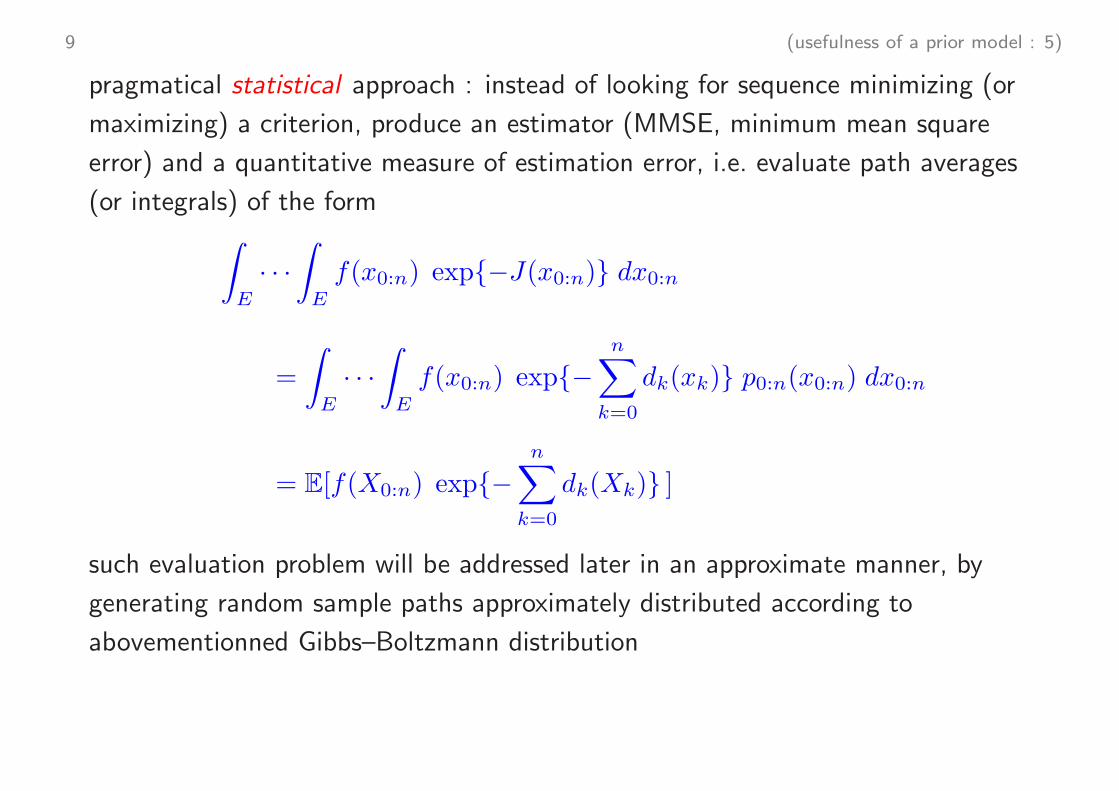
9 (usefulness of a prior model : 5)
pragmatical statistical approach : instead of looking for sequence minimizing (or
maximizing) a criterion, produce an estimator (MMSE, minimum mean square
error) and a quantitative measure of estimation error, i.e. evaluate path averages
(or integrals) of the form∫
E
· · ·
∫
E
f(x0:n) exp{−J(x0:n)} dx0:n
=
∫
E
· · ·
∫
E
f(x0:n) exp{−
n∑
k=0
dk(xk)} p0:n(x0:n) dx0:n
= E[f(X0:n) exp{−n∑
k=0
dk(Xk)} ]
such evaluation problem will be addressed later in an approximate manner, by
generating random sample paths approximately distributed according to
abovementionned Gibbs–Boltzmann distribution
10 (usefulness of a prior model : 6)
Summary usefulness of a prior model
• to complement information coming from observations
• to connect observations received at different time instants (needed, just
because a mobile . . . usually moves between these time instants 6= fixed
parameter)
this can be a rough not necessarily accurate model, and it is usually a noisy model
(to acknowledge that a model is necessarily wrong, and in an attempt to quantify
modelling error, in a statistical manner)
11 (some models : 1)
some models
modeles (simplest to most general)
state space model (continuous state space, usually Rm)
• linear, Gaussian noise
• non–linear, Gaussian noise
• general state space model : non–linear, non Gaussian noise
hidden Markov model (HMM), and extensions
• hidden Markov model (hidden state sequence Markov, observations mutually
independant / Markov conditionally w.r.t. hidden states)
• partially observed Markov chains (hidden state and observation sequence
jointly Markov)
12 (some models : 2)
general state space
• discrete : finite, countable
• continuous : Euclidian space Rm, differentiable manifold
• hybrid continuous / discrete
• constrained
• graphical (collection de connected edges)
13 (Bayesian estimation (static case) : 1)
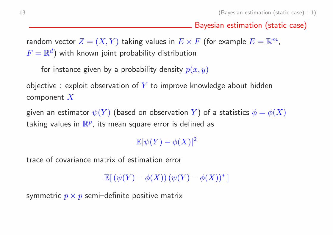
Bayesian estimation (static case)
random vector Z = (X,Y ) taking values in E × F (for example E = Rm,
F = Rd) with known joint probability distribution
for instance given by a probability density p(x, y)
objective : exploit observation of Y to improve knowledge about hidden
component X
given an estimator ψ(Y ) (based on observation Y ) of a statistics φ = φ(X)
taking values in Rp, its mean square error is defined as
E|ψ(Y )− φ(X)|2
trace of covariance matrix of estimation error
E[ (ψ(Y )− φ(X)) (ψ(Y )− φ(X))∗ ]
symmetric p× p semi–definite positive matrix
14 (Bayesian estimation (static case) : 2)
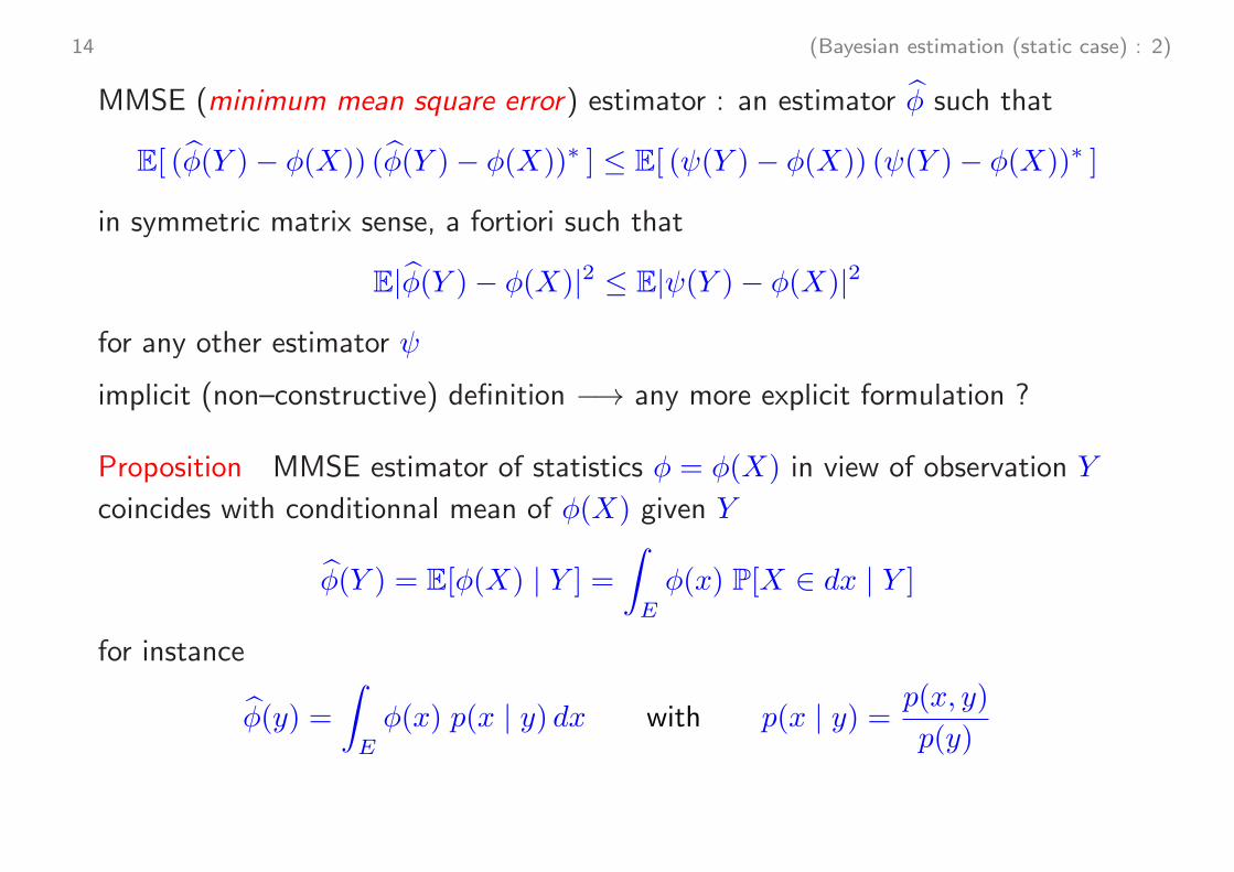
MMSE (minimum mean square error) estimator : an estimator φ such that
E[ (φ(Y )− φ(X)) (φ(Y )− φ(X))∗ ] ≤ E[ (ψ(Y )− φ(X)) (ψ(Y )− φ(X))∗ ]
in symmetric matrix sense, a fortiori such that
E|φ(Y )− φ(X)|2 ≤ E|ψ(Y )− φ(X)|2
for any other estimator ψ
implicit (non–constructive) definition −→ any more explicit formulation ?
Proposition MMSE estimator of statistics φ = φ(X) in view of observation Y
coincides with conditionnal mean of φ(X) given Y
φ(Y ) = E[φ(X) | Y ] =
∫
E
φ(x) P[X ∈ dx | Y ]
for instance
φ(y) =
∫
E
φ(x) p(x | y) dx with p(x | y) =p(x, y)
p(y)
15 (exemple : Gaussian model (static case) : 1)
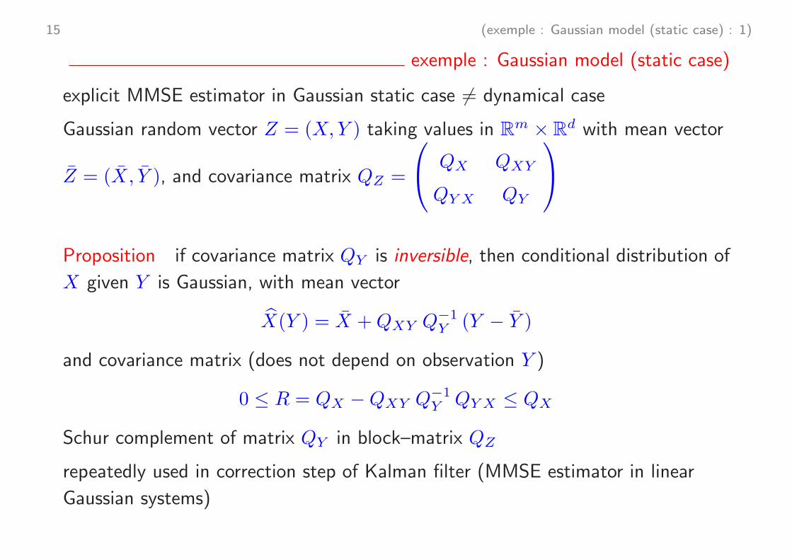
exemple : Gaussian model (static case)
explicit MMSE estimator in Gaussian static case 6= dynamical case
Gaussian random vector Z = (X,Y ) taking values in Rm × R
d with mean vector
Z = (X, Y ), and covariance matrix QZ =
QX QXY
QY X QY
Proposition if covariance matrix QY is inversible, then conditional distribution of
X given Y is Gaussian, with mean vector
X(Y ) = X +QXY Q−1Y (Y − Y )
and covariance matrix (does not depend on observation Y )
0 ≤ R = QX −QXY Q−1Y QY X ≤ QX
Schur complement of matrix QY in block–matrix QZ
repeatedly used in correction step of Kalman filter (MMSE estimator in linear
Gaussian systems)
16 (linear Gaussian systems : Kalman filter : 1)
linear Gaussian systems : Kalman filter
hidden state sequence {Xk} taking values in Rm, such that
Xk = FkXk−1 + fk +Wk
and observation sequence {Yk} taking values in Rd, such that
Yk = HkXk + hk + Vk
assumptions :
• initial state X0 Gaussian vector with mean X0 and covariance matrix QX0
• state noise {Wk} Gaussian white noise with covariance matrix QWk
• observation noise {Vk} Gaussian white noise with covariance matrix QVk
• noise sequences {Wk} and {Vk} and initial state X0 mutually independant
17 (linear Gaussian systems : Kalman filter : 2)
interpretation of prior model
Xk = FkXk−1 + fk +Wk
in terms of uncertainty propagation
• even if state Xk−1 = x would be known exactly at time instant (k − 1), state
Xk at time instant k is uncertain, distributed as a Gaussian vector with mean
Fk x+ fk and covariance matrix QWk
• if state Xk−1 is uncertain at time instant (k − 1), distributed as a Gaussian
vector with mean Xk−1 and covariance matrix QXk−1, then this uncertainty is
propagated to time instant k : even if model noise would not be present,
state Xk at time instant k is uncertain, distributed as a Gaussian vector with
mean Fk Xk−1 + fk and covariance matrix FkQXk−1 F
∗k
18 (linear Gaussian systems : Kalman filter : 3)
Theorem [Kalman filter] if covariance matrix QVk is invertible
then conditional distribution of hidden state Xk given observation sequence Y0:kis Gaussian, with mean Xk and covariance matrix Pk, that satisfy following
recurrent equations
X−k = Fk Xk−1 + fk
P−k = Fk Pk−1 F
∗k +QW
k
and
Xk = X−k +Kk [Yk − (Hk X
−k + hk)]
Pk = [I −KkHk] P−k
where matrix
Kk = P−k H∗
k [Hk P−k H∗
k +QVk ]
−1
is called Kalman gain, and with initialization
X−0 = X0 = E[X0] and P−
0 = QX0 = cov(X0)
Non–linear and non Gaussian systems, with examples
• non–linear and non Gaussian systems
• hybridized inertial navigation (TAN, terrain aided navigation)
• visual tracking with color histogramme
• tracking a dim target (TBD, track–before–detect)
• indoor navigation
19 (non–linear and non Gaussian systems : 1)
non–linear and non Gaussian systems
◮ evolution of hidden state
Xk = fk(Xk−1,Wk) with Wk ∼ pk(dw)
interpretation as a model for propagating estimators and attached uncertainties
only requirement : easy to simulate model uncertainties
X0 ∼ µ0(dx) and Wk ∼ pk(dw)
more generally, for any x ∈ E
P[Xk ∈ dx′ | Xk−1 = x] = Qk(x, dx′)
only requirement : easy to simulate uncertain transitions
Xk ∼ Qk(x, dx′)
20 (non–linear and non Gaussian systems : 2)
◮ relation between observation and hidden state
Yk = hk(Xk) + Vk with Vk ∼ qk(v) dv
only requirement : easy to evaluate likelihood function
gk(x) = qk(Yk − hk(x))
consistency between a possible state and true observation, e.g.
gk(x) ∝ exp{− 12 |Yk − hk(x)|
2}
more generally, for any x ∈ E
P[Yk ∈ dy | Xk = x] = gk(x, y)λk(dy)
only requirement : easy to evaluate likelihood function (with abuse of notation)
gk(x) = gk(x, Yk)
21 (non–linear and non Gaussian systems : 3)
objective : recursively estimate hidden state Xk
in view of observations Y0:k = (Y0 · · ·Yk)
for instance, numerically approximate Bayesian filter
µk(dx) = P[Xk ∈ dx | Y0:k]
22 (non–linear and non Gaussian systems : 4)
non–linear / non Gaussian systems : particle filtering
numerical approximation of Bayesian filter by weighted empirical probability
distribution
µNk =
N∑
i=1
wik δξik
with
N∑
i=1
wik = 1
associated with a system of N particles, caracterised by
• their positions (ξ1k · · · ξNk )
• and positive (nonnegative) normalized weights (w1k · · ·w
Nk )
system of interacting particles, that
• explore independently the state space, by following prior model
• and interact under a selection mechanism, related with how each particle is
consistent with current observation, by evaluating a likelihood function
23 (non–linear and non Gaussian systems : 5)
SIS (sequential importance sampling) algorithm
• prediction : independently for any i = 1 · · ·N
ξik = fk(ξik−1,W
ik) with W i
k ∼ pk(dw)
• correction : for any i = 1 · · ·N
wik =
wik−1 qk(Yk − hk(ξ
ik))
N∑
j=1
wjk−1 qk(Yk − hk(ξ
jk))
24 (non–linear and non Gaussian systems : 6)
alternatively (and preferably), weights can be used for re–sampling
SIR (sampling with importance resampling) algorithm : basic (bootstrap) version
• resampling (selection) : independently for any i = 1 · · ·N
within current population (ξ1k−1, · · · , ξNk−1), pick an individual ξ i
k−1
in a manner that is related with weights (w1k−1, · · · , w
Nk−1)
• prediction (mutation) : independently for any i = 1 · · ·N
ξik = fk(ξik−1,W
ik) with W i
k ∼ pk(dw)
• correction (weighting) : for any i = 1 · · ·N
wik =
qk(Yk − hk(ξik))
N∑
j=1
qk(Yk − hk(ξjk))
25 (demos : 1)
some examples
twofold purpose
• modeling with non–linear and non (necessarily) Gaussian systems
• behaviour (more than actual performance) of basic bootstrap SIR algorithm
four examples
• non–linear and non Gaussian systems
• hybridized inertial navigation (TAN, terrain aided navigation)
• visual tracking with color histogramme
• tracking a dim target (TBD, track–before–detect)
• indoor navigation
26 (demos : 2)
1st example : hybridized inertial navigation (TAN)
funding : DGA, programme d’etude amont NCT (nouveaux concepts pour la
navigation par correlation de terrain), coordination Thales Communications
• inertial measurements
– linear acceleration and angular velocity of an aircraft (INS, inertial
navigation system)
→ double integration yields inertial estimation of aircraft position and velocity
• prior model for evolution of inertial estimation error
• noisy altimeter measurements of
– height of aircraft above sea level (baro–altimeter)
– height of aircraft above terrain (radio–altimeter)
→ noisy measurement of height of terrain below aircraft above sea level
• correlation with a digital map (DTED, digital terrain elevation data)
providing height of terrain for any position in horizontal plane
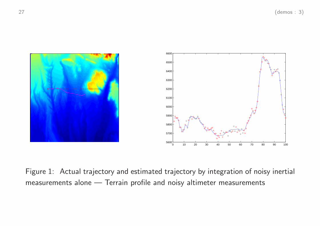
27 (demos : 3)
0 10 20 30 40 50 60 70 80 90 1005600
5700
5800
5900
6000
6100
6200
6300
6400
6500
6600
Figure 1: Actual trajectory and estimated trajectory by integration of noisy inertial
measurements alone — Terrain profile and noisy altimeter measurements
28 (demos : 4)
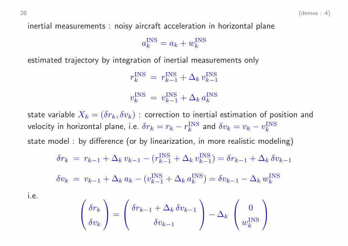
inertial measurements : noisy aircraft acceleration in horizontal plane
aINSk = ak + wINS
k
estimated trajectory by integration of inertial measurements only
rINSk = rINS
k−1 +∆k vINSk−1
vINSk = vINS
k−1 +∆k aINSk
state variable Xk = (δrk, δvk) : correction to inertial estimation of position and
velocity in horizontal plane, i.e. δrk = rk − rINSk and δvk = vk − vINS
k
state model : by difference (or by linearization, in more realistic modeling)
δrk = rk−1 +∆k vk−1 − (rINSk−1 +∆k v
INSk−1) = δrk−1 +∆k δvk−1
δvk = vk−1 +∆k ak − (vINSk−1 +∆k a
INSk ) = δvk−1 −∆k w
INSk
i.e. δrk
δvk
=
δrk−1 +∆k δvk−1
δvk−1
−∆k
0
wINSk
29 (demos : 5)
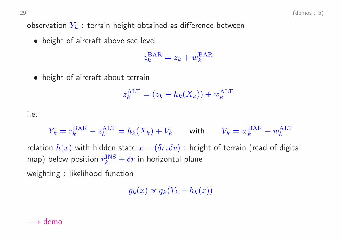
observation Yk : terrain height obtained as difference between
• height of aircraft above see level
zBARk = zk + wBAR
k
• height of aircraft about terrain
zALTk = (zk − hk(Xk)) + wALT
k
i.e.
Yk = zBARk − zALT
k = hk(Xk) + Vk with Vk = wBARk − wALT
k
relation h(x) with hidden state x = (δr, δv) : height of terrain (read of digital
map) below position rINSk + δr in horizontal plane
weighting : likelihood function
gk(x) ∝ qk(Yk − hk(x))
−→ demo
31 (demos : 7)
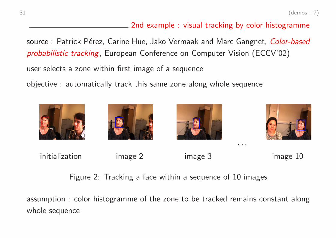
2nd example : visual tracking by color histogramme
source : Patrick Perez, Carine Hue, Jako Vermaak and Marc Gangnet, Color-based
probabilistic tracking , European Conference on Computer Vision (ECCV’02)
user selects a zone within first image of a sequence
objective : automatically track this same zone along whole sequence
. . .
initialization image 2 image 3 image 10
Figure 2: Tracking a face within a sequence of 10 images
assumption : color histogramme of the zone to be tracked remains constant along
whole sequence
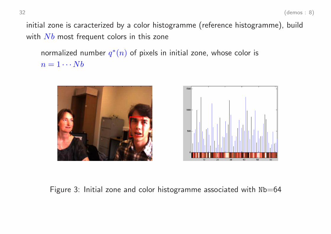
32 (demos : 8)
initial zone is caracterized by a color histogramme (reference histogramme), build
with Nb most frequent colors in this zone
normalized number q∗(n) of pixels in initial zone, whose color is
n = 1 · · ·Nb
Figure 3: Initial zone and color histogramme associated with Nb=64
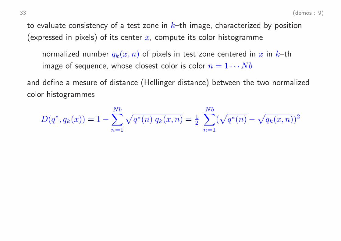
33 (demos : 9)
to evaluate consistency of a test zone in k–th image, characterized by position
(expressed in pixels) of its center x, compute its color histogramme
normalized number qk(x, n) of pixels in test zone centered in x in k–th
image of sequence, whose closest color is color n = 1 · · ·Nb
and define a mesure of distance (Hellinger distance) between the two normalized
color histogrammes
D(q∗, qk(x)) = 1−Nb∑
n=1
√q∗(n) qk(x, n) =
12
Nb∑
n=1
(√q∗(n)−
√qk(x, n))
2
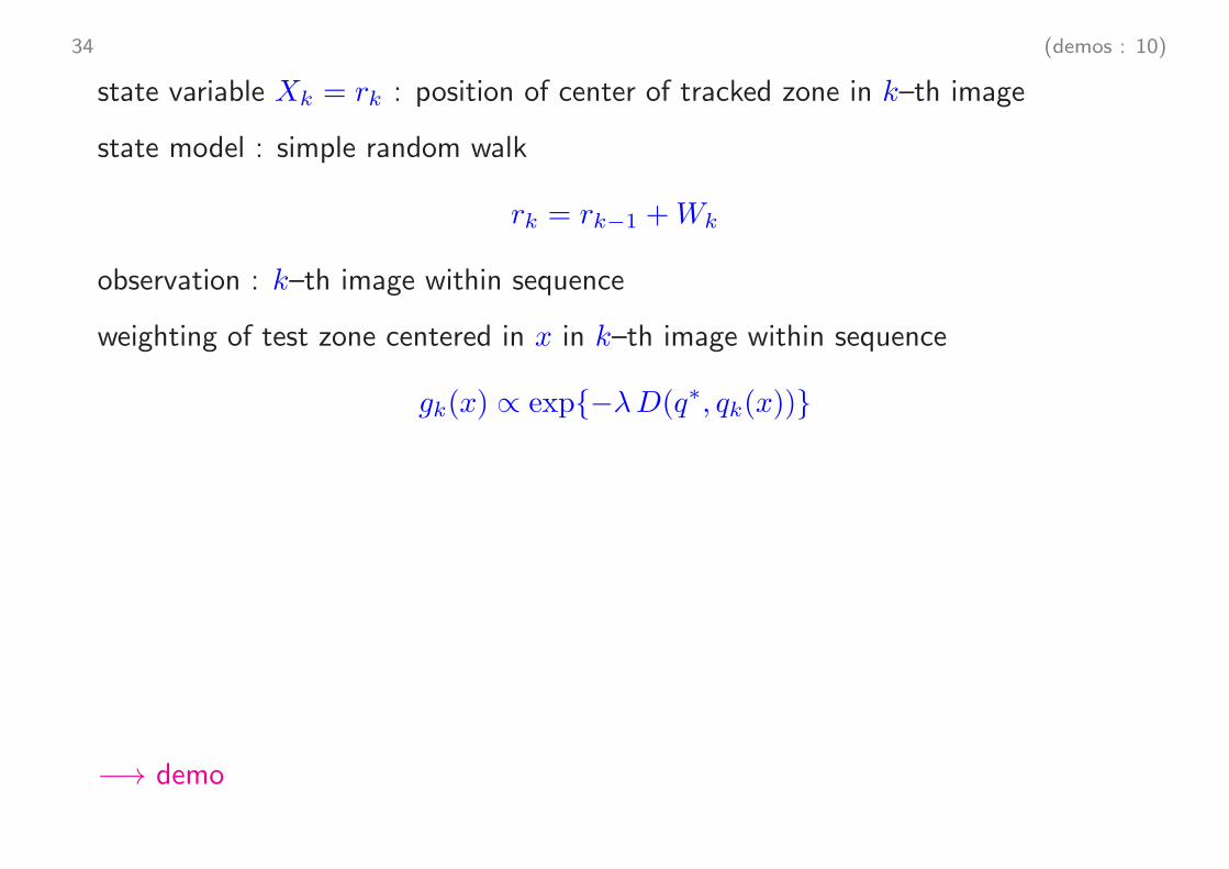
34 (demos : 10)
state variable Xk = rk : position of center of tracked zone in k–th image
state model : simple random walk
rk = rk−1 +Wk
observation : k–th image within sequence
weighting of test zone centered in x in k–th image within sequence
gk(x) ∝ exp{−λD(q∗, qk(x))}
−→ demo
39 (demos : 15)
3rd example : tracking a dim target (TBD)
source : David J. Salmond and H. Birch, A particle filter for track-before-detect,
American Control Conference (ACC’01)
radar image : rectangular pixel array, where echo intensity received in a pixel is
coded in terms of grey level, ranging from darkest (echo with low intensity) to
brighter (echo with high intensity)
in principle, if a target is present in physical space, it will appear in image plane in
the form of a pixel brighter than other pixels
to detect (and localize) target, it is therefore sufficient to search for brightest
pixel, i.e. with highest intensity, or simply to use thresholding
repeating this procedure on each radar image successively, it is therefore possible
first to detect, then to track, target in image sequence
high SNR : threshold detection on each image separately, then tracking
vs. low SNR : tracking before (or even without) detection
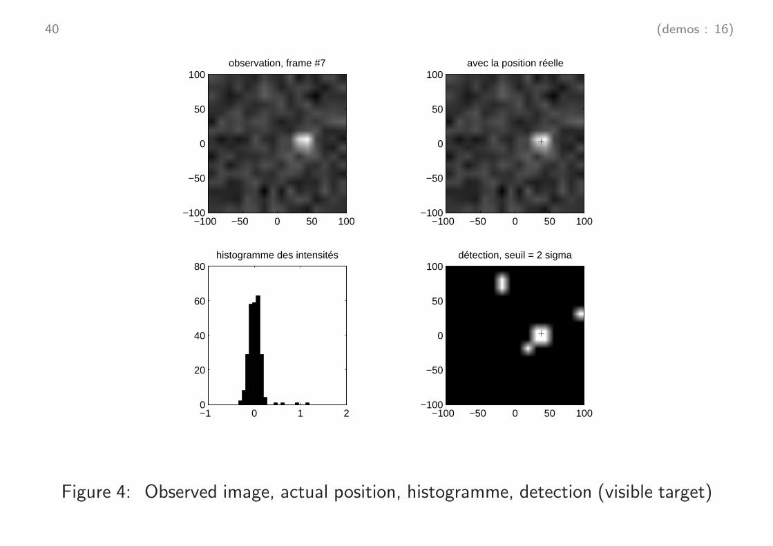
40 (demos : 16)
observation, frame #7
−100 −50 0 50 100−100
−50
0
50
100avec la position réelle
−100 −50 0 50 100−100
−50
0
50
100
détection, seuil = 2 sigma
−100 −50 0 50 100−100
−50
0
50
100
−1 0 1 20
20
40
60
80histogramme des intensités
Figure 4: Observed image, actual position, histogramme, detection (visible target)
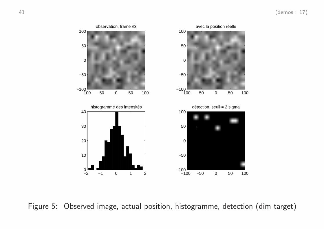
41 (demos : 17)
observation, frame #3
−100 −50 0 50 100−100
−50
0
50
100avec la position réelle
−100 −50 0 50 100−100
−50
0
50
100
détection, seuil = 2 sigma
−100 −50 0 50 100−100
−50
0
50
100
−2 −1 0 1 20
10
20
30
40histogramme des intensités
Figure 5: Observed image, actual position, histogramme, detection (dim target)
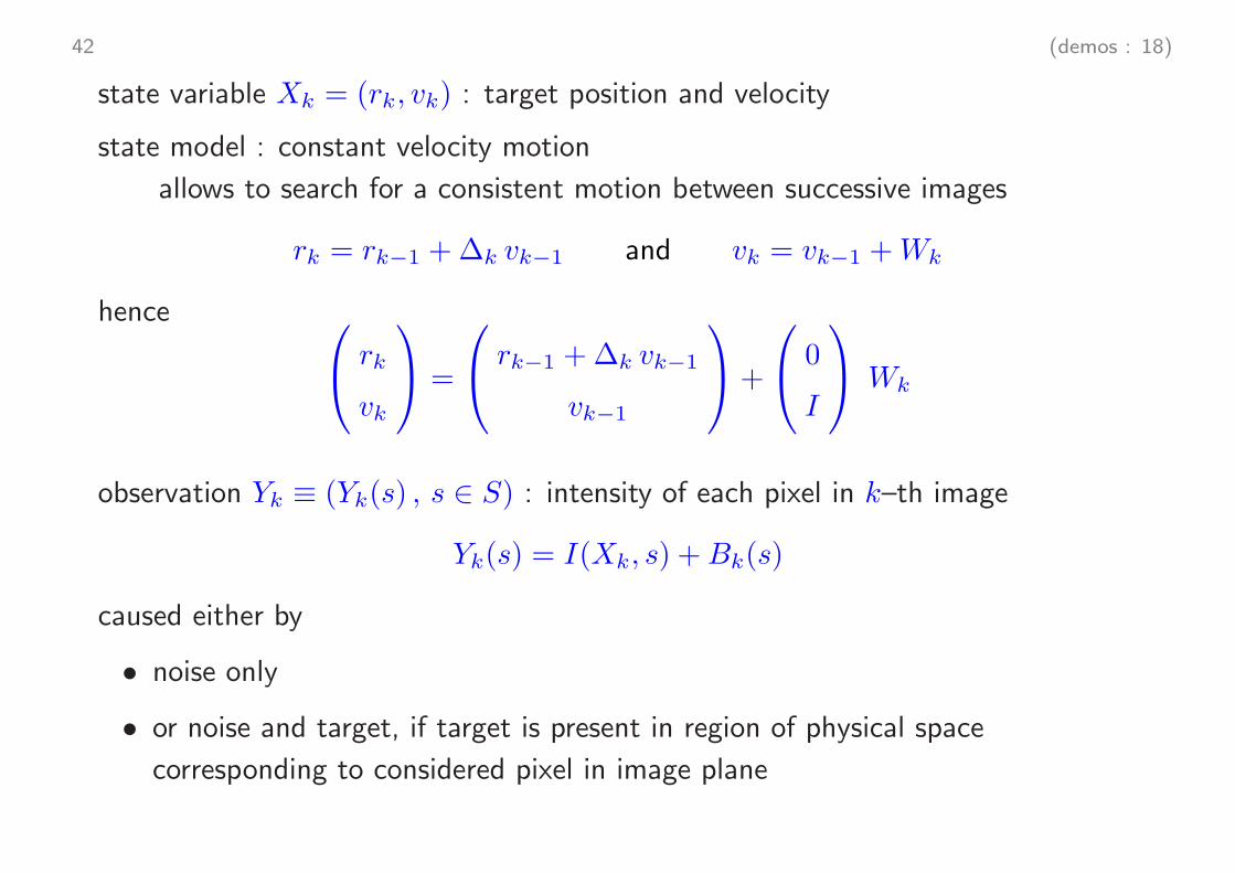
42 (demos : 18)
state variable Xk = (rk, vk) : target position and velocity
state model : constant velocity motion
allows to search for a consistent motion between successive images
rk = rk−1 +∆k vk−1 and vk = vk−1 +Wk
hence rk
vk
=
rk−1 +∆k vk−1
vk−1
+
0
I
Wk
observation Yk ≡ (Yk(s) , s ∈ S) : intensity of each pixel in k–th image
Yk(s) = I(Xk, s) +Bk(s)
caused either by
• noise only
• or noise and target, if target is present in region of physical space
corresponding to considered pixel in image plane
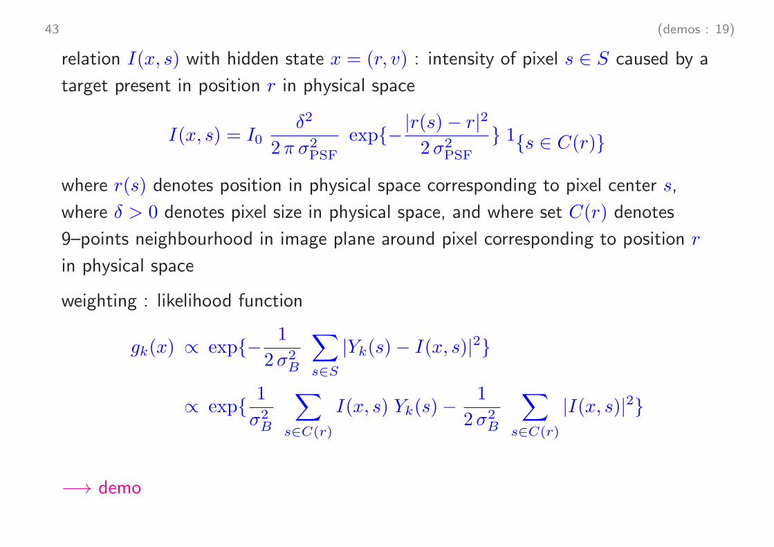
43 (demos : 19)
relation I(x, s) with hidden state x = (r, v) : intensity of pixel s ∈ S caused by a
target present in position r in physical space
I(x, s) = I0δ2
2π σ2PSF
exp{−|r(s)− r|2
2σ2PSF
} 1{s ∈ C(r)}
where r(s) denotes position in physical space corresponding to pixel center s,
where δ > 0 denotes pixel size in physical space, and where set C(r) denotes
9–points neighbourhood in image plane around pixel corresponding to position r
in physical space
weighting : likelihood function
gk(x) ∝ exp{−1
2σ2B
∑
s∈S
|Yk(s)− I(x, s)|2}
∝ exp{1
σ2B
∑
s∈C(r)
I(x, s) Yk(s)−1
2σ2B
∑
s∈C(r)
|I(x, s)|2}
−→ demo
47 (demos : 23)
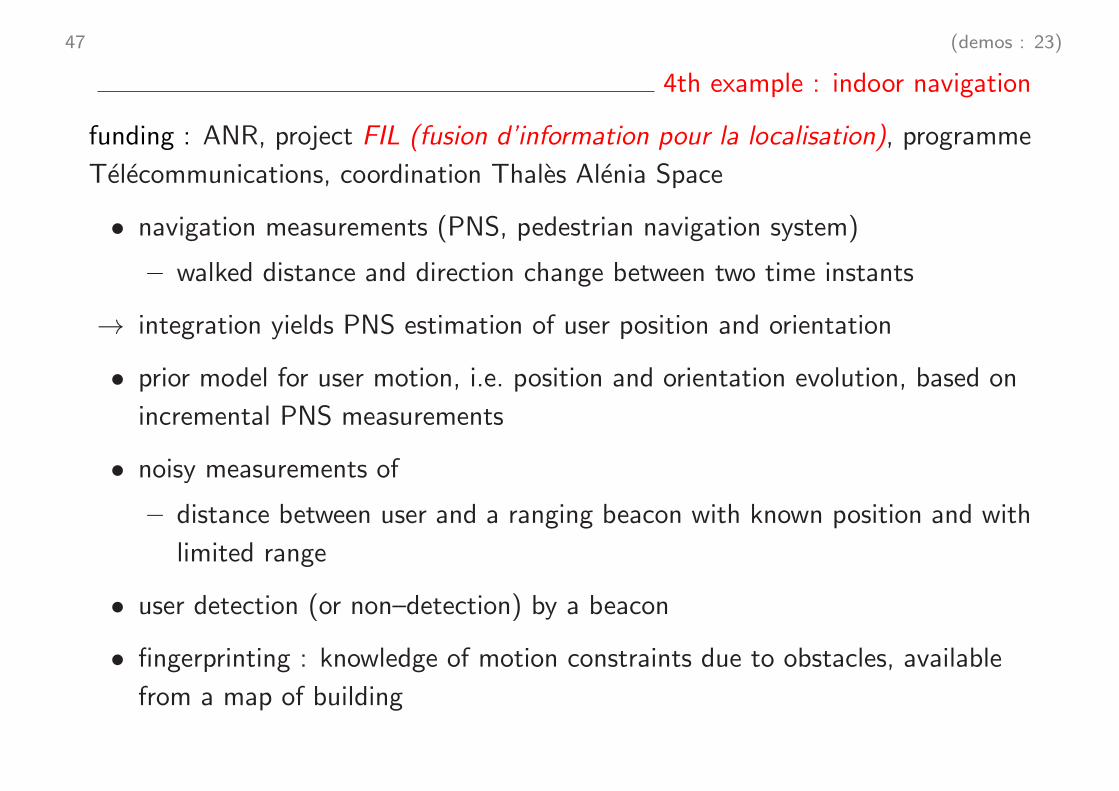
4th example : indoor navigation
funding : ANR, project FIL (fusion d’information pour la localisation), programme
Telecommunications, coordination Thales Alenia Space
• navigation measurements (PNS, pedestrian navigation system)
– walked distance and direction change between two time instants
→ integration yields PNS estimation of user position and orientation
• prior model for user motion, i.e. position and orientation evolution, based on
incremental PNS measurements
• noisy measurements of
– distance between user and a ranging beacon with known position and with
limited range
• user detection (or non–detection) by a beacon
• fingerprinting : knowledge of motion constraints due to obstacles, available
from a map of building
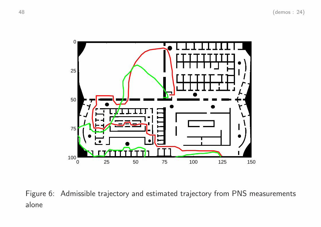
48 (demos : 24)
0 25 50 75 100 125 150
0
25
50
75
100
Figure 6: Admissible trajectory and estimated trajectory from PNS measurements
alone
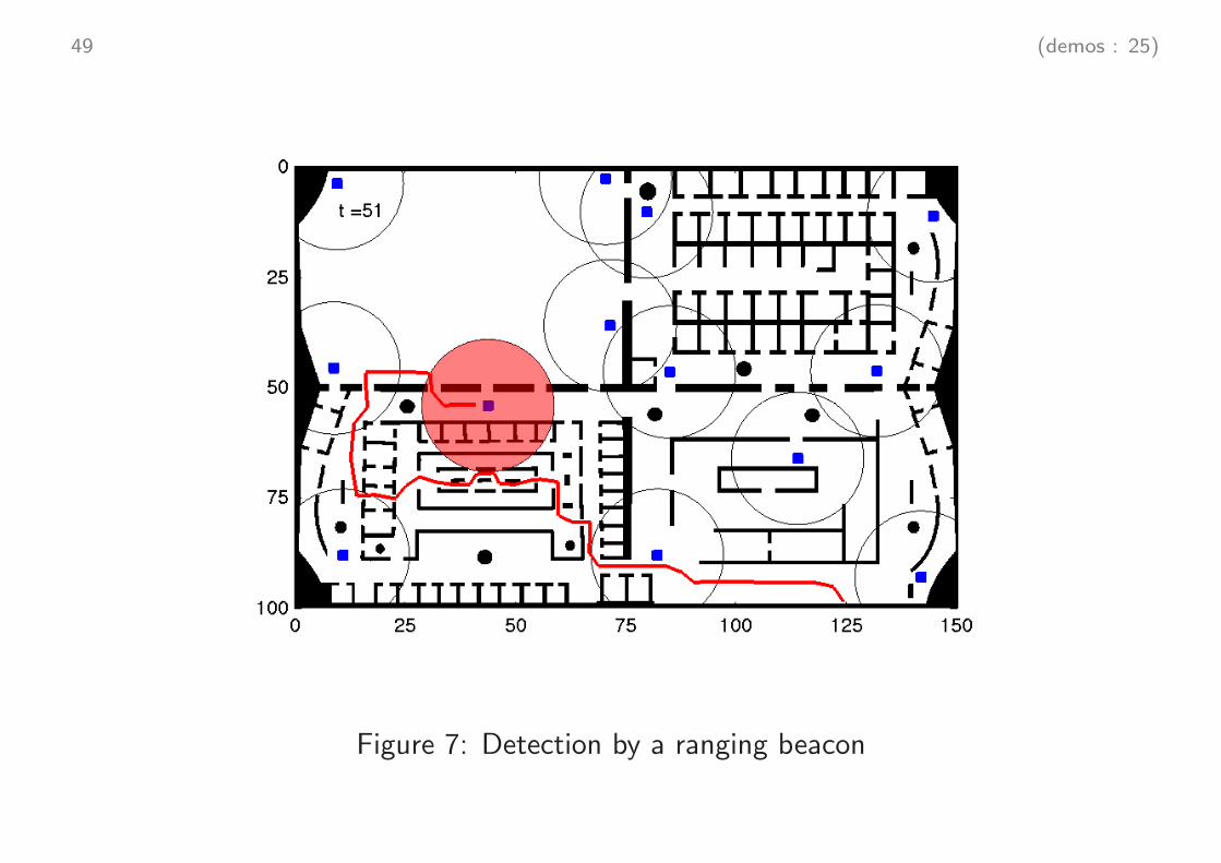
49 (demos : 25)
Figure 7: Detection by a ranging beacon
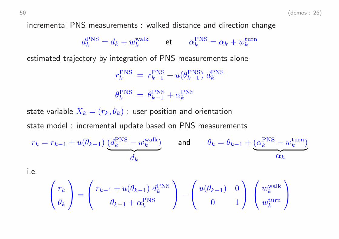
50 (demos : 26)
incremental PNS measurements : walked distance and direction change
dPNSk = dk + wwalk
k et αPNSk = αk + wturn
k
estimated trajectory by integration of PNS measurements alone
rPNSk = rPNS
k−1 + u(θPNSk−1 ) d
PNSk
θPNSk = θPNS
k−1 + αPNSk
state variable Xk = (rk, θk) : user position and orientation
state model : incremental update based on PNS measurements
rk = rk−1 + u(θk−1) (dPNSk − wwalk
k )︸ ︷︷ ︸dk
and θk = θk−1 + (αPNSk − wturn
k )︸ ︷︷ ︸αk
i.e. rk
θk
=
rk−1 + u(θk−1) d
PNSk
θk−1 + αPNSk
−
u(θk−1) 0
0 1
wwalk
k
wturnk
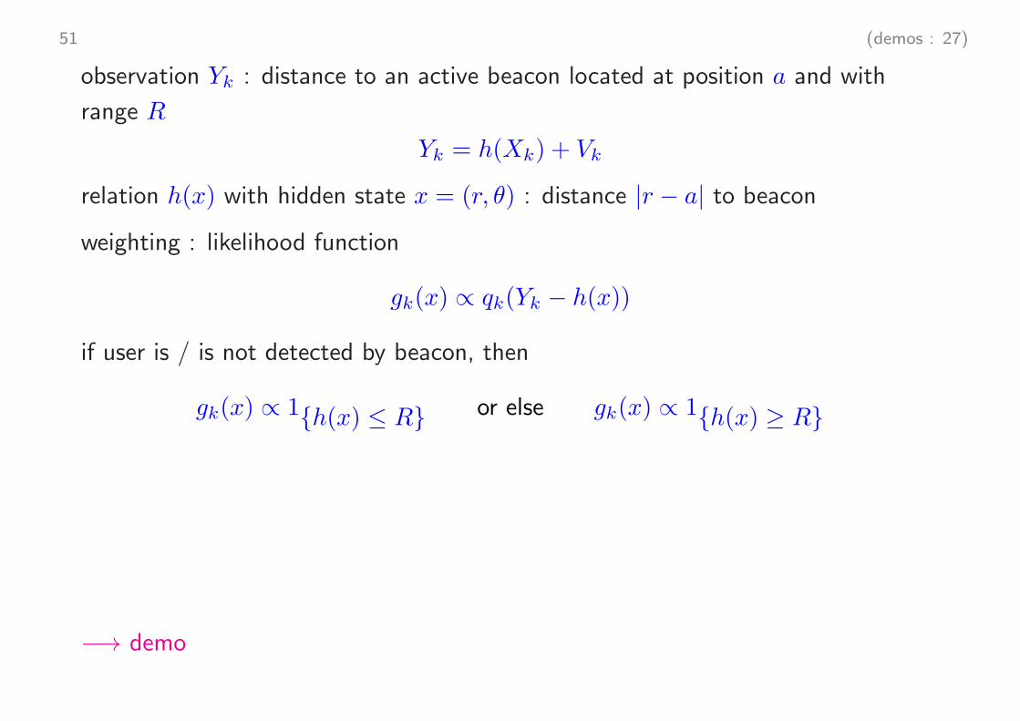
51 (demos : 27)
observation Yk : distance to an active beacon located at position a and with
range R
Yk = h(Xk) + Vk
relation h(x) with hidden state x = (r, θ) : distance |r − a| to beacon
weighting : likelihood function
gk(x) ∝ qk(Yk − h(x))
if user is / is not detected by beacon, then
gk(x) ∝ 1{h(x) ≤ R} or else gk(x) ∝ 1{h(x) ≥ R}
−→ demo
54 (conclusion : 1)
to be continued next time . . .
#1 more general models, from non–linear and non Gaussian systems to hidden
Markov models and partially observed Markov chains, so as to handle e.g.
• regime / mode switching
• correlation between state noise and observation noise
#2 for each of these models (or just for most general model), representation of
P[X0:n ∈ dx0:n | Y0:n]
as a Gibbs–Boltzmann distribution, with recursive formulation, and idem for
P[Xn ∈ dxn | Y0:n]
#3 particle approximation (SIS and SIR algorithms) from either representations
#4 asymptotic behaviour as sample size goes to infinity
#5 numerous algorithmic variants

complement scientifique Ecole Doctorale MATISSE
IRISA et INRIA, salle Markov
jeudi 26 janvier 2012
Variantes Algorithmiques et Justifications Theoriques
Francois Le Gland
INRIA Rennes et IRMAR
http://www.irisa.fr/aspi/legland/ed-matisse/
Modeles generaux
au–dela des systemes lineaires gaussiens
• systemes non–lineaires / non–gaussiens
• modeles de Markov caches
1 (some notations : 1)
some notations (continued)
if X is a random variable taking values in E, then mapping
φ 7−→ E[φ(X)] or equivalently A 7−→ P[X ∈ A]
defines a probability distribution µ on E, denoted as
µ(dx) = P[X ∈ dx]
and such that
E[φ(X)] =
∫
E
φ(x) µ(dx) = 〈µ, φ〉 or P[X ∈ A] = µ(A)
caracterizes uncertainty about X
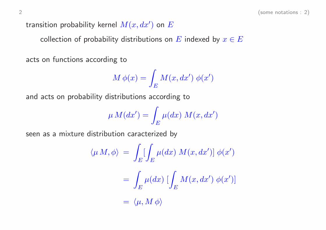
2 (some notations : 2)
transition probability kernel M(x, dx′) on E
collection of probability distributions on E indexed by x ∈ E
acts on functions according to
M φ(x) =
∫
E
M(x, dx′) φ(x′)
and acts on probability distributions according to
µM(dx′) =
∫
E
µ(dx)M(x, dx′)
seen as a mixture distribution caracterized by
〈µM,φ〉 =
∫
E
[
∫
E
µ(dx)M(x, dx′)] φ(x′)
=
∫
E
µ(dx) [
∫
E
M(x, dx′) φ(x′)]
= 〈µ,M φ〉
3 (some notations : 3)
product of two transition probability kernels
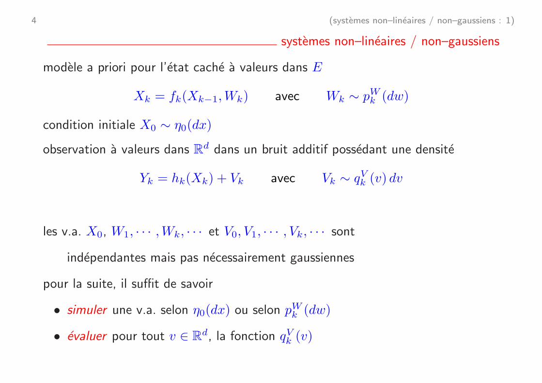
4 (systemes non–lineaires / non–gaussiens : 1)
systemes non–lineaires / non–gaussiens
modele a priori pour l’etat cache a valeurs dans E
Xk = fk(Xk−1,Wk) avec Wk ∼ pWk (dw)
condition initiale X0 ∼ η0(dx)
observation a valeurs dans Rd dans un bruit additif possedant une densite
Yk = hk(Xk) + Vk avec Vk ∼ qVk (v) dv
les v.a. X0, W1, · · · ,Wk, · · · et V0, V1, · · · , Vk, · · · sont
independantes mais pas necessairement gaussiennes
pour la suite, il suffit de savoir
• simuler une v.a. selon η0(dx) ou selon pWk (dw)
• evaluer pour tout v ∈ Rd, la fonction qVk (v)
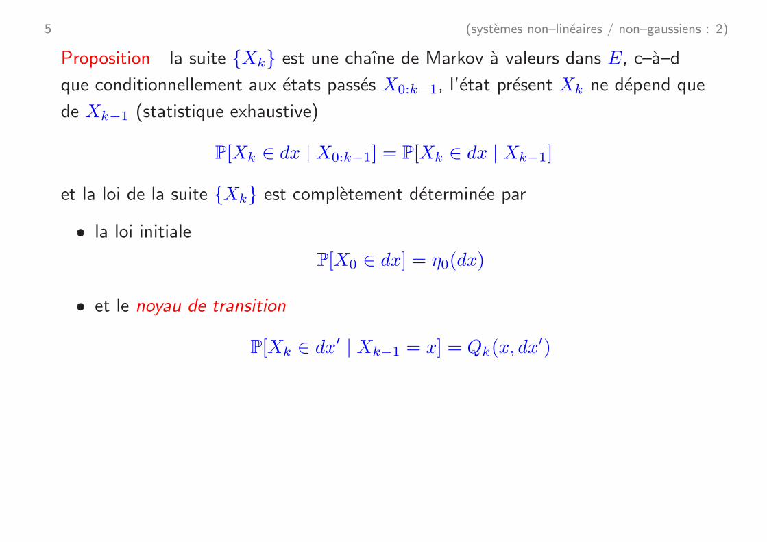
5 (systemes non–lineaires / non–gaussiens : 2)
Proposition la suite {Xk} est une chaıne de Markov a valeurs dans E, c–a–d
que conditionnellement aux etats passes X0:k−1, l’etat present Xk ne depend que
de Xk−1 (statistique exhaustive)
P[Xk ∈ dx | X0:k−1] = P[Xk ∈ dx | Xk−1]
et la loi de la suite {Xk} est completement determinee par
• la loi initiale
P[X0 ∈ dx] = η0(dx)
• et le noyau de transition
P[Xk ∈ dx′ | Xk−1 = x] = Qk(x, dx′)
6 (systemes non–lineaires / non–gaussiens : 3)
Preuve compte tenu que X0:k−1 et Wk sont independants
E[φ(Xk) | X0:k−1] = E[φ(fk(Xk−1,Wk)) | X0:k−1]
=
∫
Rp
φ(fk(Xk−1, w)) pWk (dw)
ne depend que de Xk−1, c–a–d que
E[φ(Xk) | X0:k−1] = E[φ(Xk) | Xk−1]
d’ou la propriete de Markov , et∫
E
Qk(x, dx′) φ(x′) = E[φ(Xk) | Xk−1 = x] =
∫
Rp
φ(fk(x,w)) pWk (dw)
ce qui definit implicitement le noyau de transition 2
7 (systemes non–lineaires / non–gaussiens : 4)
Remarque si fk(x,w) = bk(x) +w et si la distribution de probabilite pWk (dw) de
la v.a. Wk admet une densite encore notee pWk (w), c’est–a–dire si
Xk = bk(Xk−1) +Wk avec Wk ∼ pWk (w) dw
alors
Qk(x, dx′) = pWk (x′ − bk(x)) dx
′
c’est–a–dire que le noyau Qk(x, dx′) admet une densite
en effet, le changement de variable x′ = bk(x) + w donne immediatement
Qk φ(x) =
∫
Rm
φ(bk(x) + w) pWk (w) dw =
∫
Rm
φ(x′) pWk (x′ − bk(x)) dx′
8 (systemes non–lineaires / non–gaussiens : 5)
Remarque en general, le noyau Qk(x, dx′) n’admet pas de densite
en effet, conditionnellement a Xk−1 = x, le v.a. Xk appartient necessairement au
sous–ensemble
M(x) = {x′ ∈ Rm : il existe w ∈ R
p tel que x′ = fk(x,w)}
et dans le cas ou p < m ce sous ensemble M(x) est generalement, sous certaines
hypotheses de regularite, une sous–variete differentielle de dimension p dans
l’espace Rm
il ne peut donc pas y avoir de densite par rapport a la mesure de Lebesgue de Rm
pour la distribution de probabilite Qk(x, dx′) du v.a. Xk
9 (systemes non–lineaires / non–gaussiens : 6)
Proposition la suite {Yk} verifie l’hypothese de canal sans memoire, c–a–d que
pour tout instant n
• conditionnellement aux etats caches X0:n les observations Y0:n sont
mutuellement independantes, ce qui se traduit par
P[Y0:n ∈ dy0:n | X0:n] =
n∏
k=0
P[Yk ∈ dyk | X0:n]
• pour tout k = 0 · · ·n, la loi conditionnelle de Yk sachant X0:n ne depend que
de Xk, ce qui se traduit par
P[Yk ∈ dyk | X0:n] = P[Yk ∈ dyk | Xk]
avec la densite d’emission
P[Yk ∈ dy | Xk = x] = qVk (y − hk(x)) dy
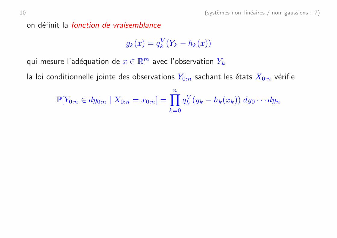
10 (systemes non–lineaires / non–gaussiens : 7)
on definit la fonction de vraisemblance
gk(x) = qVk (Yk − hk(x))
qui mesure l’adequation de x ∈ Rm avec l’observation Yk
la loi conditionnelle jointe des observations Y0:n sachant les etats X0:n verifie
P[Y0:n ∈ dy0:n | X0:n = x0:n] =
n∏
k=0
qVk (yk − hk(xk)) dy0 · · · dyn
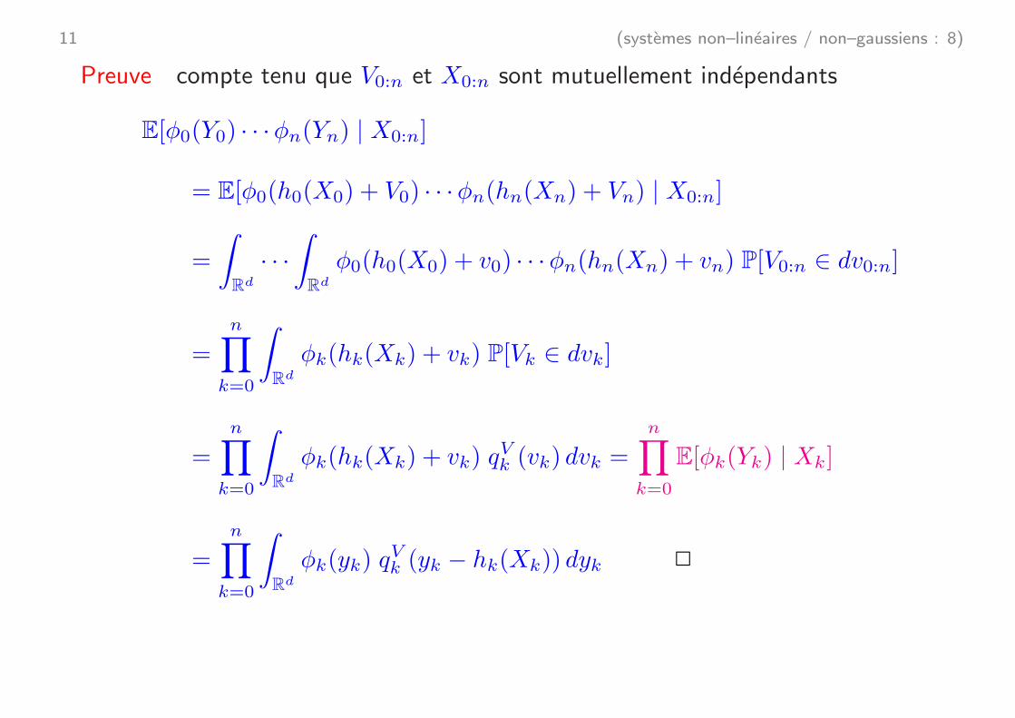
11 (systemes non–lineaires / non–gaussiens : 8)
Preuve compte tenu que V0:n et X0:n sont mutuellement independants
E[φ0(Y0) · · ·φn(Yn) | X0:n]
= E[φ0(h0(X0) + V0) · · ·φn(hn(Xn) + Vn) | X0:n]
=
∫
Rd
· · ·
∫
Rd
φ0(h0(X0) + v0) · · ·φn(hn(Xn) + vn) P[V0:n ∈ dv0:n]
=
n∏
k=0
∫
Rd
φk(hk(Xk) + vk) P[Vk ∈ dvk]
=
n∏
k=0
∫
Rd
φk(hk(Xk) + vk) qVk (vk) dvk =
n∏
k=0
E[φk(Yk) | Xk]
=n∏
k=0
∫
Rd
φk(yk) qVk (yk − hk(Xk)) dyk 2
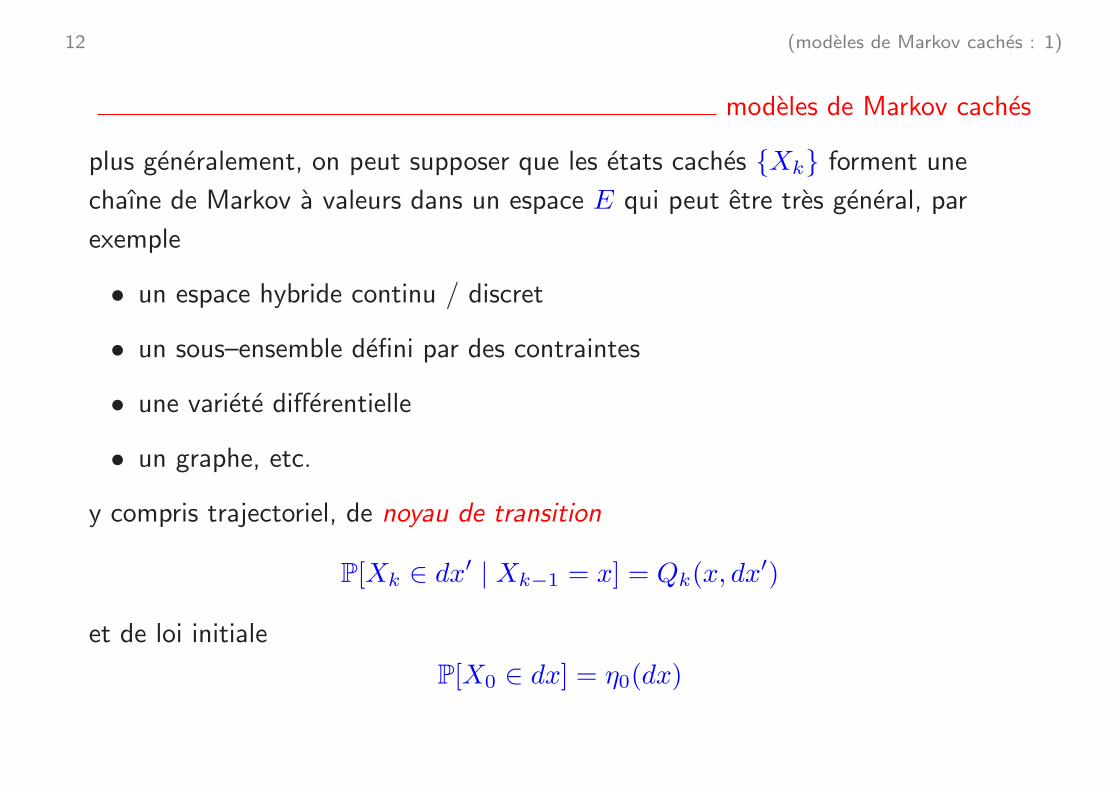
12 (modeles de Markov caches : 1)
modeles de Markov caches
plus generalement, on peut supposer que les etats caches {Xk} forment une
chaıne de Markov a valeurs dans un espace E qui peut etre tres general, par
exemple
• un espace hybride continu / discret
• un sous–ensemble defini par des contraintes
• une variete differentielle
• un graphe, etc.
y compris trajectoriel, de noyau de transition
P[Xk ∈ dx′ | Xk−1 = x] = Qk(x, dx′)
et de loi initiale
P[X0 ∈ dx] = η0(dx)
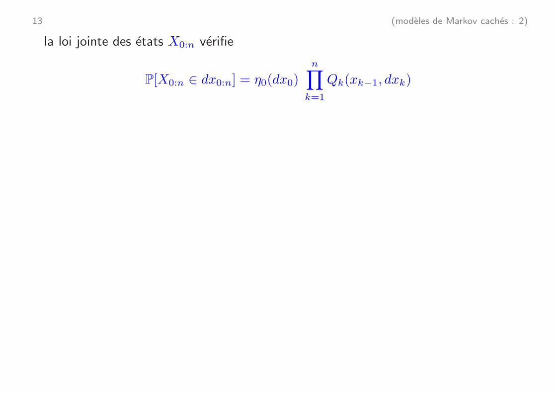
13 (modeles de Markov caches : 2)
la loi jointe des etats X0:n verifie
P[X0:n ∈ dx0:n] = η0(dx0)
n∏
k=1
Qk(xk−1, dxk)
14 (modeles de Markov caches : 3)
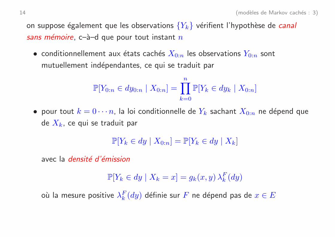
on suppose egalement que les observations {Yk} verifient l’hypothese de canal
sans memoire, c–a–d que pour tout instant n
• conditionnellement aux etats caches X0:n les observations Y0:n sont
mutuellement independantes, ce qui se traduit par
P[Y0:n ∈ dy0:n | X0:n] =
n∏
k=0
P[Yk ∈ dyk | X0:n]
• pour tout k = 0 · · ·n, la loi conditionnelle de Yk sachant X0:n ne depend que
de Xk, ce qui se traduit par
P[Yk ∈ dy | X0:n] = P[Yk ∈ dy | Xk]
avec la densite d’emission
P[Yk ∈ dy | Xk = x] = gk(x, y)λFk (dy)
ou la mesure positive λFk (dy) definie sur F ne depend pas de x ∈ E
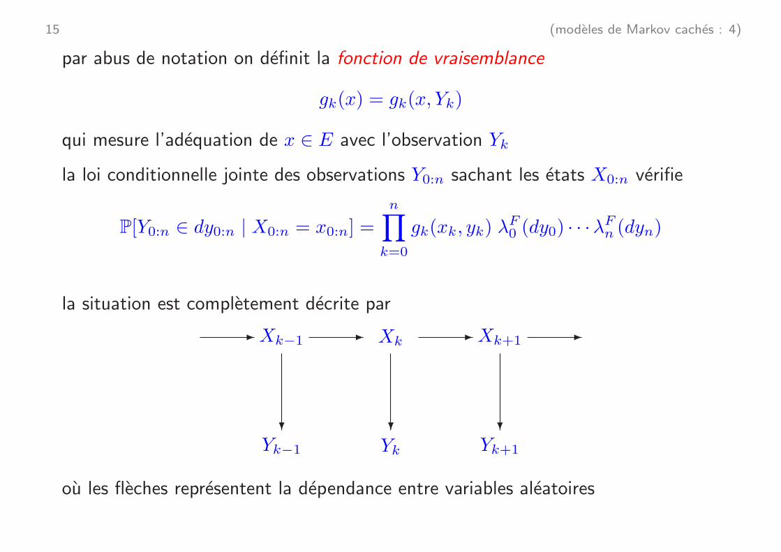
15 (modeles de Markov caches : 4)
par abus de notation on definit la fonction de vraisemblance
gk(x) = gk(x, Yk)
qui mesure l’adequation de x ∈ E avec l’observation Yk
la loi conditionnelle jointe des observations Y0:n sachant les etats X0:n verifie
P[Y0:n ∈ dy0:n | X0:n = x0:n] =n∏
k=0
gk(xk, yk) λF0 (dy0) · · ·λ
Fn (dyn)
la situation est completement decrite par
- - - -Xk−1 Xk Xk+1
? ? ?
Yk−1 Yk Yk+1
ou les fleches representent la dependance entre variables aleatoires
16 (modeles de Markov caches : 5)
pour la suite il suffit de savoir
• simuler pour tout x ∈ E, une v.a. selon le noyau de transition Qk(x, dx′)
• evaluer pour tout x′ ∈ E, la fonction de vraisemblance gk(x′)
pour tout instant k = 1 · · ·n
Filtre bayesien pour les modeles de Markov caches
• representation probabiliste
• equation recurrente
17 (filtre bayesien : modeles de Markov caches : representation probabiliste : 1)
modeles de Markov caches : representation probabiliste
Theorem le filtre bayesien µn defini par
〈µn, φ〉 = E[φ(Xn) | Y0:n]
admet la representation probabiliste
〈µn, φ〉 =〈γn, φ〉
〈γn, 1〉avec 〈γn, φ〉 = E[φ(Xn)
n∏
k=0
gk(Xk) ]
Remarque l’esperance porte seulement sur les etats caches successifs X0:n : les
fonctions de vraisemblance gk(x) sont definies par abus de notation comme
gk(x) = gk(x, Yk)
pour tout k = 0, 1 · · ·n, et dependent implicitement des observations Y0:n, mais
celles–ci sont considerees comme fixees
18 (filtre bayesien : modeles de Markov caches : representation probabiliste : 2)
Preuve d’apres la formule de Bayes, et d’apres la propriete de canal sans
memoire, la loi jointe des etats caches X0:n et des observations Y0:n verifie
P[X0:n ∈ dx0:n, Y0:n ∈ dy0:n] = P[Y0:n ∈ dy0:n | X0:n = x0:n] P[X0:n ∈ dx0:n]
= P[X0:n ∈ dx0:n]
n∏
k=0
gk(xk, yk)λF0 (dy0) · · ·λ
Fn (dyn)
en integrant par rapport aux variables x0:n, on obtient la loi jointe des
observations Y0:n, c–a–d
P[Y0:n ∈ dy0:n] =
∫
E
· · ·
∫
E
n∏
k=0
gk(xk, yk) P[X0:n ∈ dx0:n]λF0 (dy0) · · ·λ
Fn (dyn)
= E[
n∏
k=0
gk(Xk, yk) ] λF0 (dy0) · · ·λ
Fn (dyn)
19 (filtre bayesien : modeles de Markov caches : representation probabiliste : 3)
d’apres la formule de Bayes, il vient
P[X0:n ∈ dx0:n, Y0:n ∈ dy0:n]
= P[X0:n ∈ dx0:n]
n∏
k=0
gk(xk, yk) λF0 (dy0) · · ·λ
Fn (dyn)
= P[X0:n ∈ dx0:n | Y0:n = y0:n] P[Y0:n ∈ dy0:n]
= P[X0:n ∈ dx0:n | Y0:n = y0:n] E[
n∏
k=0
gk(Xk, yk) ] λF0 (dy0) · · ·λ
Fn (dyn)
et on obtient
P[X0:n ∈ dx0:n | Y0:n = y0:n] =
n∏
k=0
gk(xk, yk) P[X0:n ∈ dx0:n]
E[n∏
k=0
gk(Xk, yk) ]
pour toute suite y0:n d’observations
20 (filtre bayesien : modeles de Markov caches : representation probabiliste : 4)
pour toute fonction φ definie sur E
E[φ(Xn) | Y0:n = y0:n] =
∫
E
· · ·
∫
E
φ(xn)
n∏
k=0
gk(xk, yk) P[X0:n ∈ dx0:n]
E[
n∏
k=0
gk(Xk, yk) ]
=
E[φ(Xn)
n∏
k=0
gk(Xk, yk) ]
E[
n∏
k=0
gk(Xk, yk) ]
comme cette identite est verifiee pour toute suite y0:n d’observations
〈µn, φ〉 = E[φ(Xn) | Y0:n] =
E[φ(Xn)
n∏
k=0
gk(Xk) ]
E[
n∏
k=0
gk(Xk) ]
=〈γn, φ〉
〈γn, 1〉2
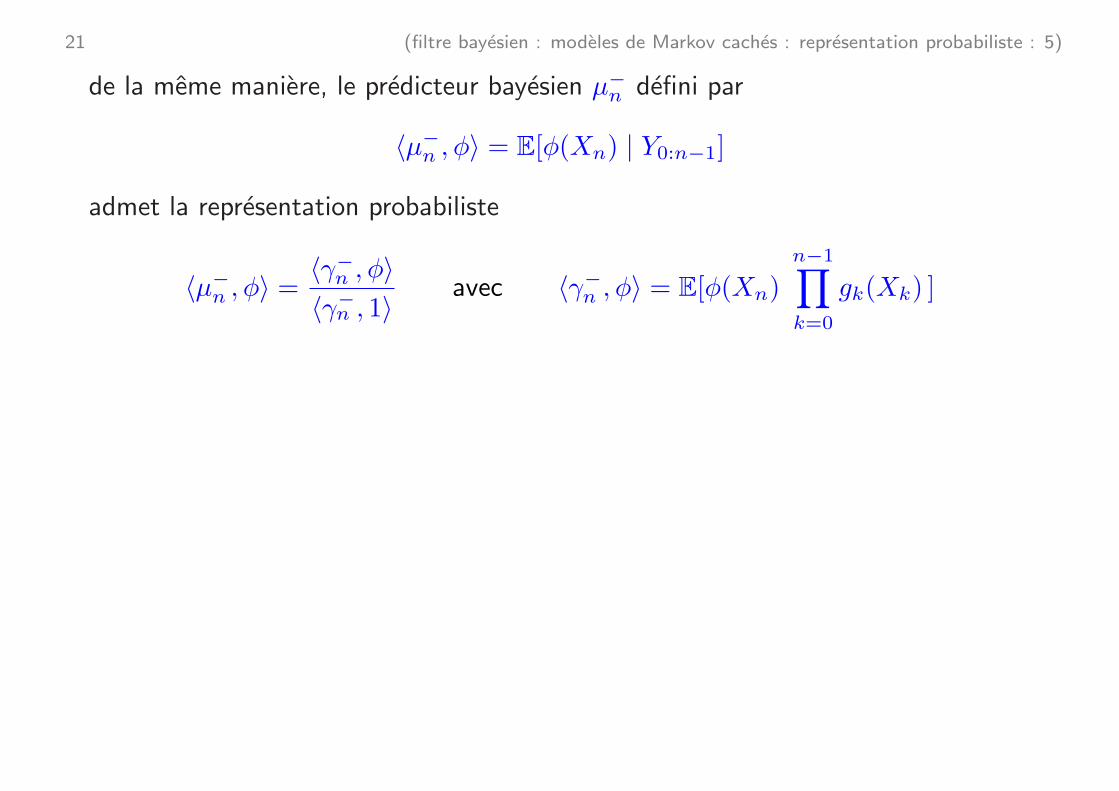
21 (filtre bayesien : modeles de Markov caches : representation probabiliste : 5)
de la meme maniere, le predicteur bayesien µ−n defini par
〈µ−n , φ〉 = E[φ(Xn) | Y0:n−1]
admet la representation probabiliste
〈µ−n , φ〉 =
〈γ−n , φ〉
〈γ−n , 1〉avec 〈γ−n , φ〉 = E[φ(Xn)
n−1∏
k=0
gk(Xk) ]
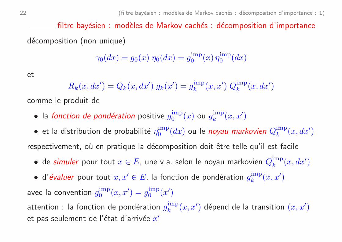
22 (filtre bayesien : modeles de Markov caches : decomposition d’importance : 1)
filtre bayesien : modeles de Markov caches : decomposition d’importance
decomposition (non unique)
γ0(dx) = g0(x) η0(dx) = gimp0 (x) ηimp
0 (dx)
et
Rk(x, dx′) = Qk(x, dx
′) gk(x′) = g
impk (x, x′) Qimp
k (x, dx′)
comme le produit de
• la fonction de ponderation positive gimp0 (x) ou gimp
k (x, x′)
• et la distribution de probabilite ηimp0 (dx) ou le noyau markovien Qimp
k (x, dx′)
respectivement, ou en pratique la decomposition doit etre telle qu’il est facile
• de simuler pour tout x ∈ E, une v.a. selon le noyau markovien Qimpk (x, dx′)
• d’evaluer pour tout x, x′ ∈ E, la fonction de ponderation gimpk (x, x′)
avec la convention gimp0 (x, x′) = g
imp0 (x′)
attention : la fonction de ponderation gimpk (x, x′) depend de la transition (x, x′)
et pas seulement de l’etat d’arrivee x′
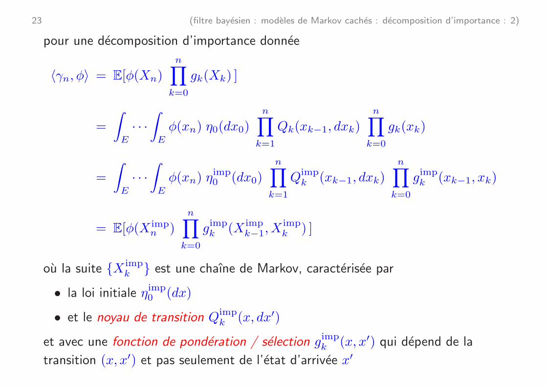
23 (filtre bayesien : modeles de Markov caches : decomposition d’importance : 2)
pour une decomposition d’importance donnee
〈γn, φ〉 = E[φ(Xn)
n∏
k=0
gk(Xk) ]
=
∫
E
· · ·
∫
E
φ(xn) η0(dx0)n∏
k=1
Qk(xk−1, dxk)n∏
k=0
gk(xk)
=
∫
E
· · ·
∫
E
φ(xn) ηimp0 (dx0)
n∏
k=1
Qimpk (xk−1, dxk)
n∏
k=0
gimpk (xk−1, xk)
= E[φ(X impn )
n∏
k=0
gimpk (X imp
k−1, Ximpk ) ]
ou la suite {X impk } est une chaıne de Markov, caracterisee par
• la loi initiale ηimp0 (dx)
• et le noyau de transition Qimpk (x, dx′)
et avec une fonction de ponderation / selection gimpk (x, x′) qui depend de la
transition (x, x′) et pas seulement de l’etat d’arrivee x′
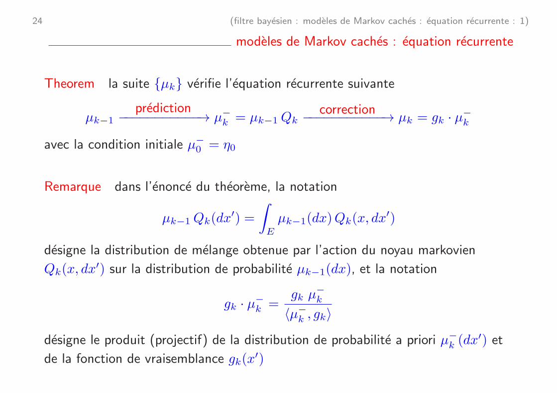
24 (filtre bayesien : modeles de Markov caches : equation recurrente : 1)
modeles de Markov caches : equation recurrente
Theorem la suite {µk} verifie l’equation recurrente suivante
µk−1prediction
−−−−−−−−−−−→ µ−k = µk−1Qk
correction−−−−−−−−−−−→ µk = gk · µ−
k
avec la condition initiale µ−0 = η0
Remarque dans l’enonce du theoreme, la notation
µk−1Qk(dx′) =
∫
E
µk−1(dx)Qk(x, dx′)
designe la distribution de melange obtenue par l’action du noyau markovien
Qk(x, dx′) sur la distribution de probabilite µk−1(dx), et la notation
gk · µ−k =
gk µ−k
〈µ−k , gk〉
designe le produit (projectif) de la distribution de probabilite a priori µ−k (dx
′) et
de la fonction de vraisemblance gk(x′)
25 (filtre bayesien : modeles de Markov caches : equation recurrente : 2)
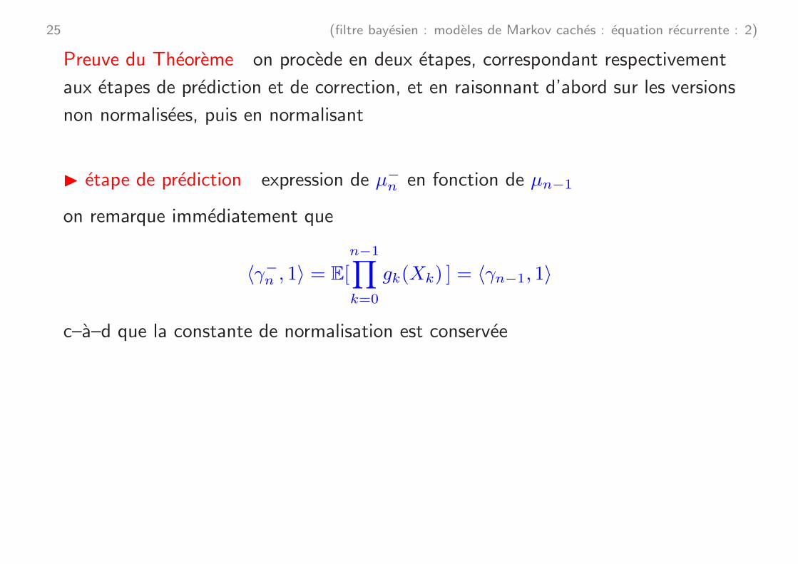
Preuve du Theoreme on procede en deux etapes, correspondant respectivement
aux etapes de prediction et de correction, et en raisonnant d’abord sur les versions
non normalisees, puis en normalisant
◮ etape de prediction expression de µ−n en fonction de µn−1
on remarque immediatement que
〈γ−n , 1〉 = E[
n−1∏
k=0
gk(Xk) ] = 〈γn−1, 1〉
c–a–d que la constante de normalisation est conservee
26 (filtre bayesien : modeles de Markov caches : equation recurrente : 3)
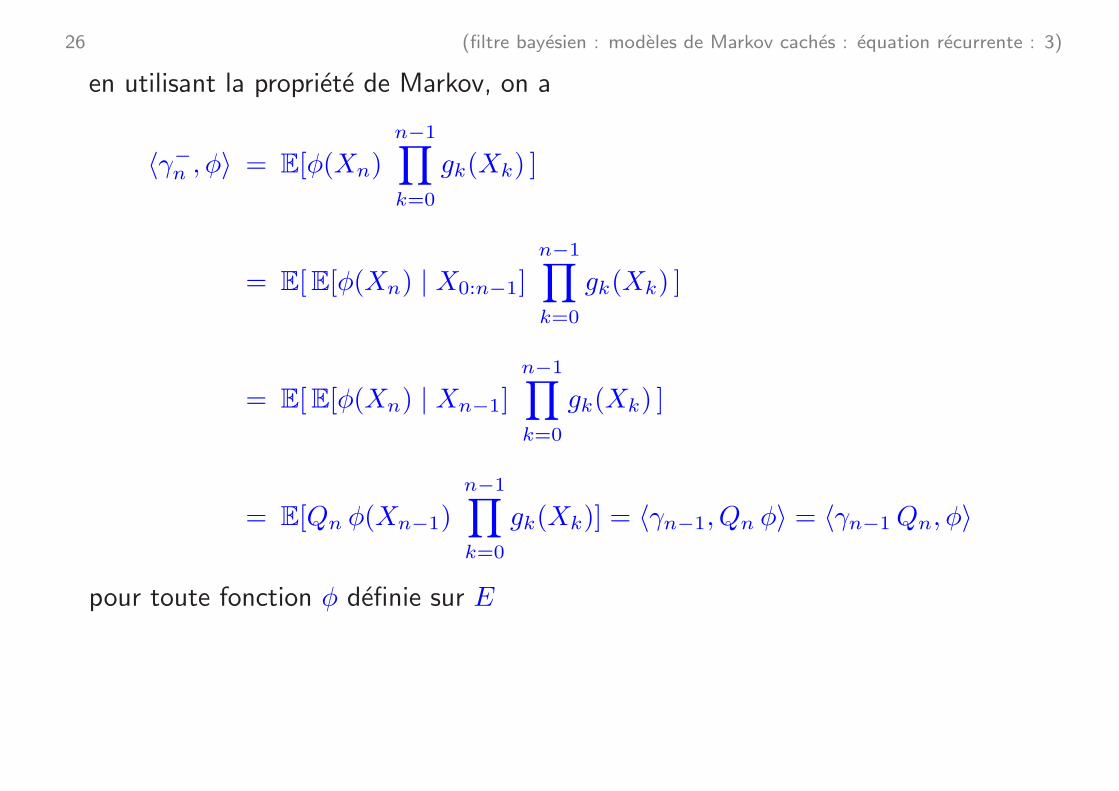
en utilisant la propriete de Markov, on a
〈γ−n , φ〉 = E[φ(Xn)
n−1∏
k=0
gk(Xk) ]
= E[E[φ(Xn) | X0:n−1]n−1∏
k=0
gk(Xk) ]
= E[E[φ(Xn) | Xn−1]
n−1∏
k=0
gk(Xk) ]
= E[Qn φ(Xn−1)
n−1∏
k=0
gk(Xk)] = 〈γn−1, Qn φ〉 = 〈γn−1Qn, φ〉
pour toute fonction φ definie sur E
27 (filtre bayesien : modeles de Markov caches : equation recurrente : 4)
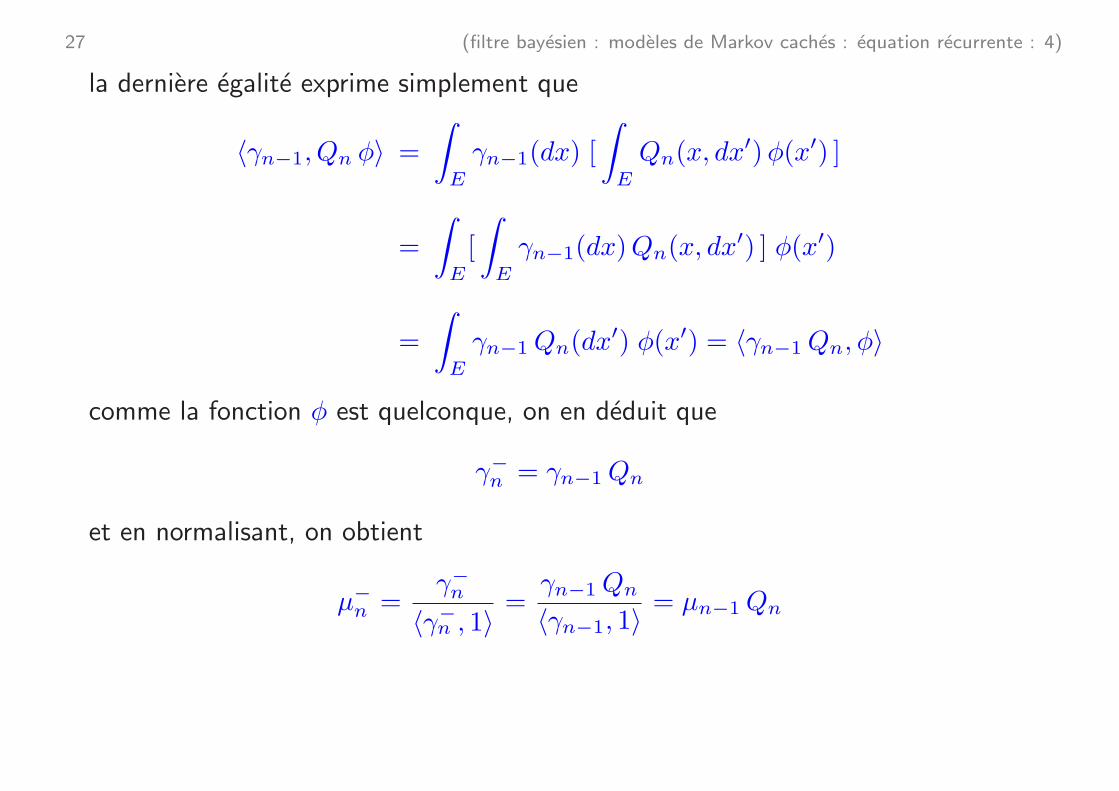
la derniere egalite exprime simplement que
〈γn−1, Qn φ〉 =
∫
E
γn−1(dx) [
∫
E
Qn(x, dx′)φ(x′) ]
=
∫
E
[
∫
E
γn−1(dx)Qn(x, dx′) ] φ(x′)
=
∫
E
γn−1Qn(dx′) φ(x′) = 〈γn−1Qn, φ〉
comme la fonction φ est quelconque, on en deduit que
γ−n = γn−1Qn
et en normalisant, on obtient
µ−n =
γ−n
〈γ−n , 1〉=γn−1Qn
〈γn−1, 1〉= µn−1Qn
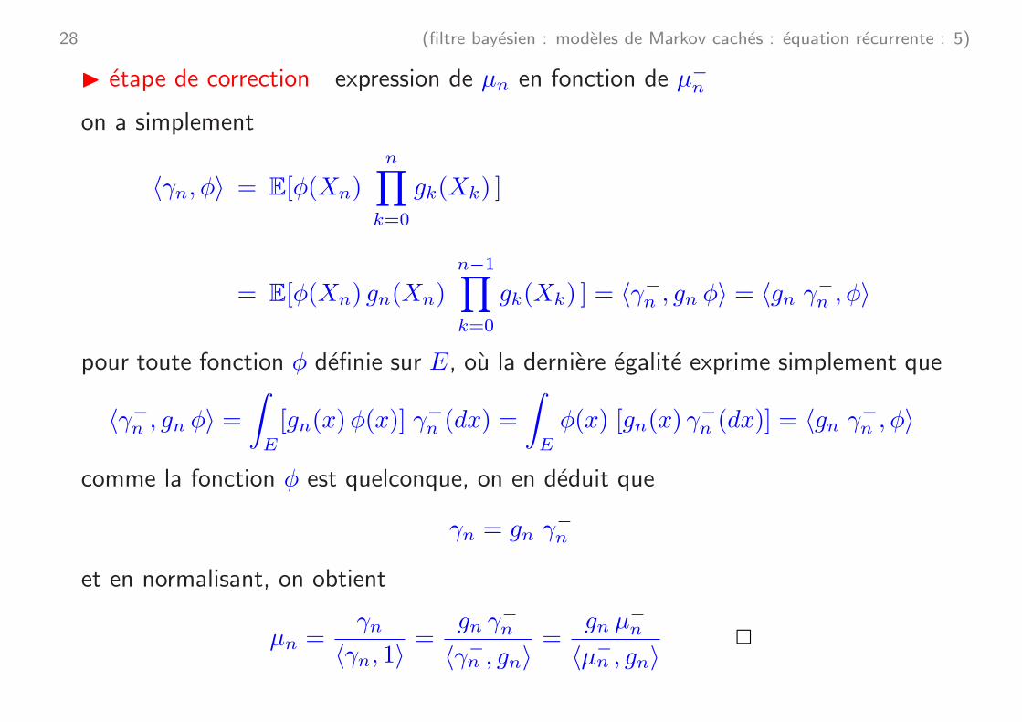
28 (filtre bayesien : modeles de Markov caches : equation recurrente : 5)
◮ etape de correction expression de µn en fonction de µ−n
on a simplement
〈γn, φ〉 = E[φ(Xn)
n∏
k=0
gk(Xk) ]
= E[φ(Xn) gn(Xn)n−1∏
k=0
gk(Xk) ] = 〈γ−n , gn φ〉 = 〈gn γ−n , φ〉
pour toute fonction φ definie sur E, ou la derniere egalite exprime simplement que
〈γ−n , gn φ〉 =
∫
E
[gn(x)φ(x)] γ−n (dx) =
∫
E
φ(x) [gn(x) γ−n (dx)] = 〈gn γ
−n , φ〉
comme la fonction φ est quelconque, on en deduit que
γn = gn γ−n
et en normalisant, on obtient
µn =γn
〈γn, 1〉=
gn γ−n
〈γ−n , gn〉=
gn µ−n
〈µ−n , gn〉
2
29 (a suivre : 1)
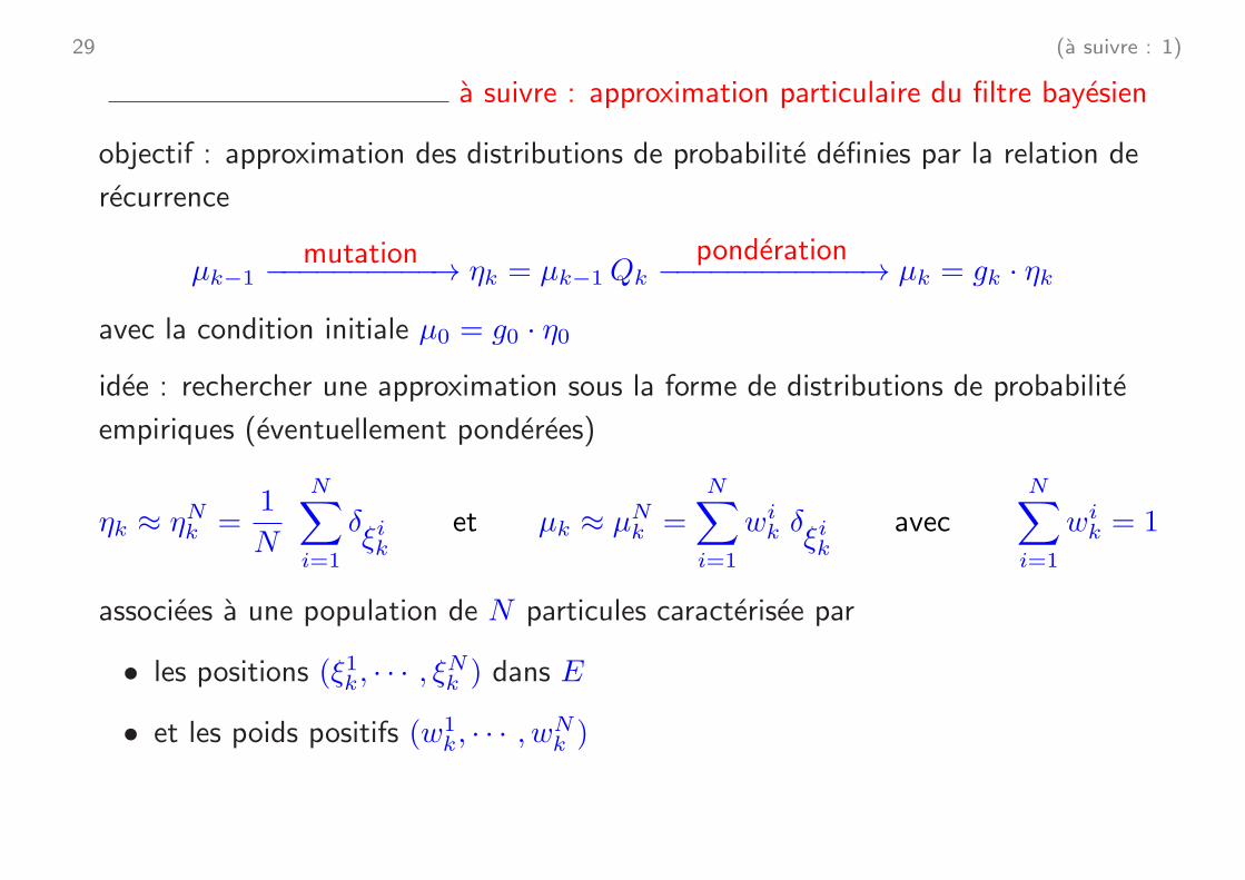
a suivre : approximation particulaire du filtre bayesien
objectif : approximation des distributions de probabilite definies par la relation de
recurrence
µk−1mutation
−−−−−−−−−−→ ηk = µk−1Qk
ponderation−−−−−−−−−−−−→ µk = gk · ηk
avec la condition initiale µ0 = g0 · η0
idee : rechercher une approximation sous la forme de distributions de probabilite
empiriques (eventuellement ponderees)
ηk ≈ ηNk =1
N
N∑
i=1
δξik
et µk ≈ µNk =
N∑
i=1
wik δξik
avec
N∑
i=1
wik = 1
associees a une population de N particules caracterisee par
• les positions (ξ1k, · · · , ξNk ) dans E
• et les poids positifs (w1k, · · · , w
Nk )
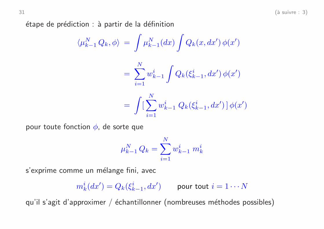
31 (a suivre : 3)
etape de prediction : a partir de la definition
〈µNk−1Qk, φ〉 =
∫µNk−1(dx)
∫Qk(x, dx
′)φ(x′)
=
N∑
i=1
wik−1
∫Qk(ξ
ik−1, dx
′)φ(x′)
=
∫[
N∑
i=1
wik−1 Qk(ξ
ik−1, dx
′) ]φ(x′)
pour toute fonction φ, de sorte que
µNk−1Qk =
N∑
i=1
wik−1 m
ik
s’exprime comme un melange fini, avec
mik(dx
′) = Qk(ξik−1, dx
′) pour tout i = 1 · · ·N
qu’il s’agit d’approximer / echantillonner (nombreuses methodes possibles)