Solitons in the Korteweg-de Vries Equation (KdV Equation)

� Introduction

The Korteweg-de Vries Equation (KdV equation) describes the theory of water waves inshallow channels, such as a canal. It is a non-linear equation which exhibits specialsolutions, known as solitons, which are stable and do not disperse with time. Further-more there as solutions with more than one soliton which can move towards each other,interact and then emerge at the same speed with no change in shape (but with a time"lag" or "speed up").

The KdV equation is

�������¶u

¶t= 6 u �������

¶u

¶x- ���������

¶3u

¶x3

Because of the u ¶ u/¶ x term the equation is non-linear (this term increases fourtimes if u is doubled).

� One soliton solution

The simplest soliton solution is

u Hx, tL = -2 sech2 Hx - 4 tL,

which is a trough of depth 2 traveling to the right with speed 4 and not changing itsshape.

Let us verify that it does satisfy the equation:

In[4]:= uexact@x_, t_D = -2 Sech@x - 4 tD^2

Out[4]= -2 Sech@4 t - xD2

In[5]:= D@uexact@x, tD, tD � 6 uexact@x, tD D@uexact@x, tD, xD - D@uexact@x, tD, 8x, 3<D �� Simplify

Out[5]= True

Mathematica returns True, indicating that equation is satisfied.

Mathematica function NDSolve can solve partial differential equations in two (but notmore than two) variables, such as x and t. However, it tends to be very slow andrequire a lot of memory. Nonetheless, if we put in the soliton at the initial time,it correctly propagates the soliton in time:

In[6]:= xmin = -8; xmax = 8;sol = NDSolve@ 8D@u@x, tD, tD � 6 u@x, tD D@u@x, tD, xD - D@u@x, tD, 8x, 3<D,

u@x, 0D � -2 Sech@xD^2, u@xmin, tD � u@xmax, tD <, u, 8x, xmin, xmax<, 8t, -1, 1< D

NDSolve::mxsst :

Using maximum number of grid points 10000 allowed by the MaxPoints or MinStepSizeoptions for independent variable x. �

Out[6]= 88u ® InterpolatingFunction@88-8., 8.<, 8-1., 1.<<, <>D<<

Plotting the solution shows the trough propagating to the right.

In[7]:= Plot3D@u@x, tD �. Flatten@solD, 8x, -7, 7<, 8t, -1, 1<,PlotPoints ® 50, PlotRange ® All, AxesLabel ® 8"x", "t", "u"<D

Out[7]=

-5

0

5x

-1.0

-0.5

0.0

0.5

1.0

t-2.0-1.5-1.0-0.5

0.0

u

A contour plot can also be useful:

In[8]:= ContourPlot@u@x, tD �. Flatten@solD, 8t, -1, 1<, 8x, -7, 7<,ColorFunction ® HHue@0.7‘ ð1D &L, PlotPoints ® 50, PlotRange ® All, FrameLabel ® 8"t", "x"<D

Out[8]=

-1.0 -0.5 0.0 0.5 1.0

-6

-4

-2

0

2

4

6

t

x

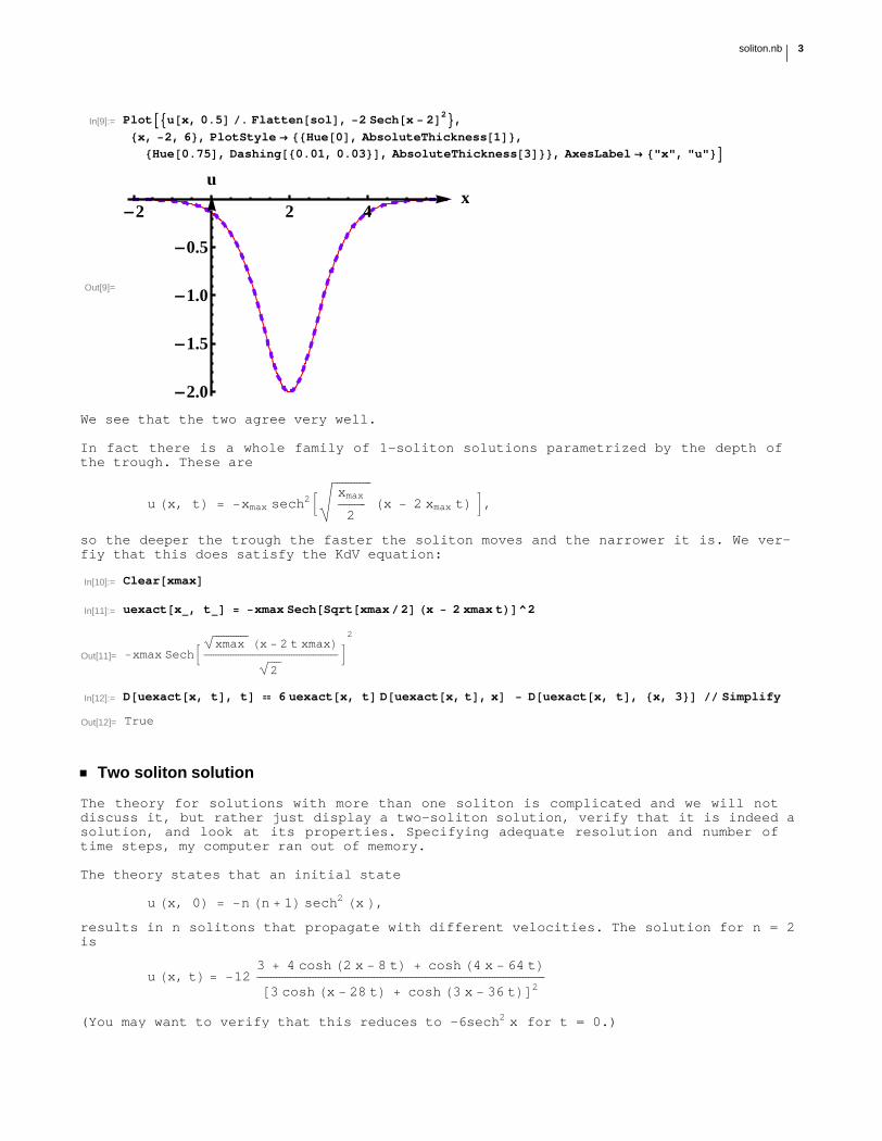
To verify that the numerical solution is the soliton, we plot both for a particularvalue of t (t = 0.5 here):

2 soliton.nb

In[9]:= PlotA9u@x, 0.5D �. Flatten@solD, -2 Sech@x - 2D2=,

8x, -2, 6<, PlotStyle ® 88Hue@0D, AbsoluteThickness@1D<,

8Hue@0.75D, Dashing@80.01, 0.03<D, AbsoluteThickness@3D<<, AxesLabel ® 8"x", "u"<E

Out[9]=

-2 2 4x

-2.0

-1.5

-1.0

-0.5

u

We see that the two agree very well.

In fact there is a whole family of 1-soliton solutions parametrized by the depth ofthe trough. These are

u Hx, tL = -xmax sech2B$%%%%%%%%%%%%%����������

xmax

2 Hx - 2 xmax tL F,

so the deeper the trough the faster the soliton moves and the narrower it is. We ver-fiy that this does satisfy the KdV equation:

In[10]:= Clear@xmaxD

In[11]:= uexact@x_, t_D = -xmax Sech@Sqrt@xmax�2D Hx - 2 xmax tLD^2

Out[11]= -xmax SechB �������������������������������������������������������

�!!!!!!!!!!!!!!xmax Hx - 2 t xmaxL

�!!!!!2

F

2

In[12]:= D@uexact@x, tD, tD � 6 uexact@x, tD D@uexact@x, tD, xD - D@uexact@x, tD, 8x, 3<D �� Simplify

Out[12]= True

� Two soliton solution

The theory for solutions with more than one soliton is complicated and we will notdiscuss it, but rather just display a two-soliton solution, verify that it is indeed asolution, and look at its properties. Specifying adequate resolution and number oftime steps, my computer ran out of memory.

The theory states that an initial state

u Hx, 0L = -n Hn + 1L sech2 Hx L,

results in n solitons that propagate with different velocities. The solution for n = 2is

u Hx, tL = -12 �������������������������������������������������������������������������������������������������������3 + 4 cosh H2 x - 8 tL + cosh H4 x - 64 tL

@3 cosh Hx - 28 tL + cosh H3 x - 36 tLD2

(You may want to verify that this reduces to -6sech2 x for t = 0.)It is not immediately evident that the above expression for u(x, t) satisfies the KdVequation, but Mathematica confirms that it does:

soliton.nb 3

(You may want to verify that this reduces to -6sech2 x for t = 0.)It is not immediately evident that the above expression for u(x, t) satisfies the KdVequation, but Mathematica confirms that it does:

In[13]:= uexact@x_, t_D = -12 H3 + 4 Cosh@2 x - 8 tD + Cosh@4 x - 64 tDL � H3 Cosh@x - 28 tD + Cosh@3 x - 36 tDL^2

Out[13]= - ���������������������������������������������������������������������������������������������������������������12 H3 + Cosh@64 t - 4 xD + 4 Cosh@8 t - 2 xDL

HCosh@36 t - 3 xD + 3 Cosh@28 t - xDL2

In[14]:= D@uexact@x, tD, tD � 6 uexact@x, tD D@uexact@x, tD, xD - D@uexact@x, tD, 8x, 3<D �� Simplify

Out[14]= True

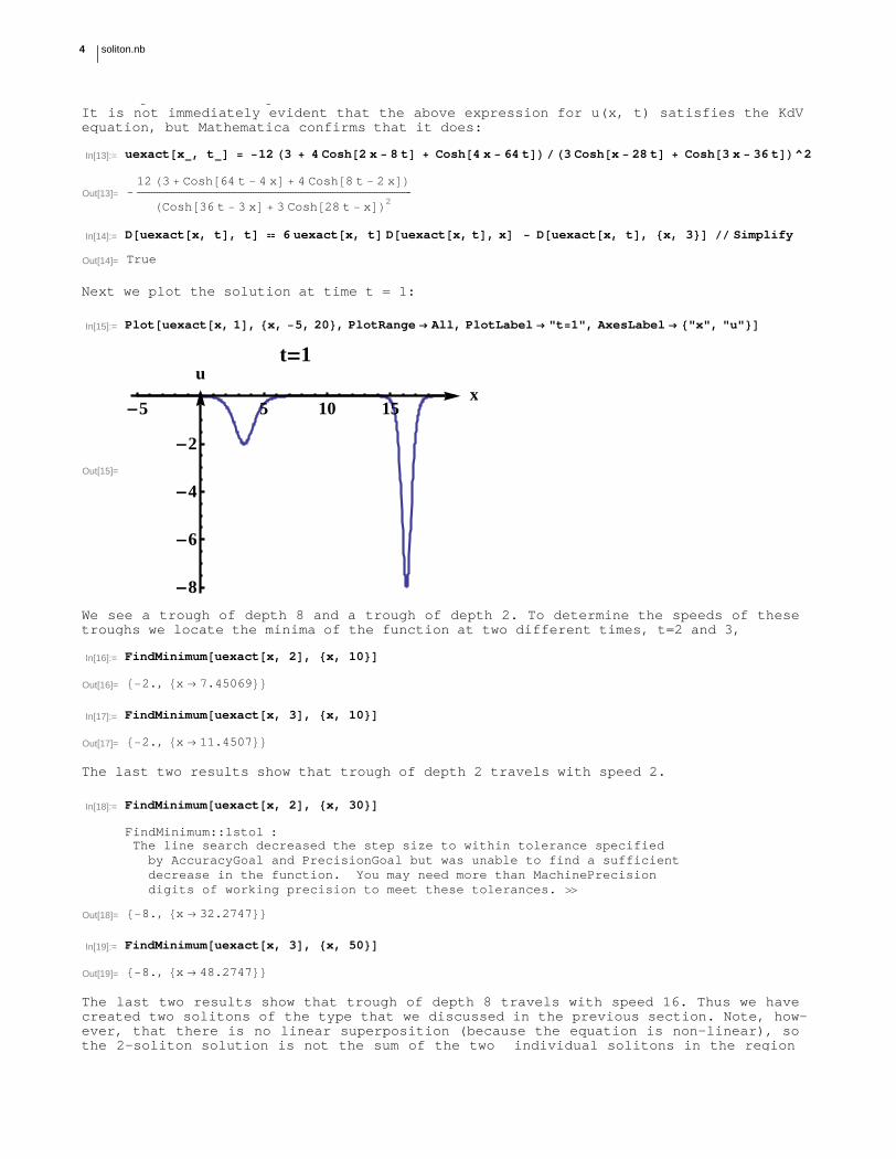
Next we plot the solution at time t = 1:

In[15]:= Plot@uexact@x, 1D, 8x, -5, 20<, PlotRange ® All, PlotLabel ® "t=1", AxesLabel ® 8"x", "u"<D

Out[15]=

-5 5 10 15x

-8

-6

-4

-2

ut=1

We see a trough of depth 8 and a trough of depth 2. To determine the speeds of thesetroughs we locate the minima of the function at two different times, t=2 and 3,

In[16]:= FindMinimum@uexact@x, 2D, 8x, 10<D

Out[16]= 8-2., 8x ® 7.45069<<

In[17]:= FindMinimum@uexact@x, 3D, 8x, 10<D

Out[17]= 8-2., 8x ® 11.4507<<

The last two results show that trough of depth 2 travels with speed 2.

In[18]:= FindMinimum@uexact@x, 2D, 8x, 30<D

FindMinimum::lstol :

The line search decreased the step size to within tolerance specifiedby AccuracyGoal and PrecisionGoal but was unable to find a sufficientdecrease in the function. You may need more than MachinePrecisiondigits of working precision to meet these tolerances. �

Out[18]= 8-8., 8x ® 32.2747<<

In[19]:= FindMinimum@uexact@x, 3D, 8x, 50<D

Out[19]= 8-8., 8x ® 48.2747<<

The last two results show that trough of depth 8 travels with speed 16. Thus we havecreated two solitons of the type that we discussed in the previous section. Note, how-ever, that there is no linear superposition (because the equation is non-linear), sothe 2-soliton solution is not the sum of the two individual solitons in the regionwhere they overlap, as one can see from the explicit solutions.

Let’s now see these two solitons interact in the vicninity of t = 0. We do a 3D plot,

4 soliton.nb

The last two results show that trough of depth 8 travels with speed 16. Thus we havecreated two solitons of the type that we discussed in the previous section. Note, how-ever, that there is no linear superposition (because the equation is non-linear), sothe 2-soliton solution is not the sum of the two individual solitons in the regionwhere they overlap, as one can see from the explicit solutions.

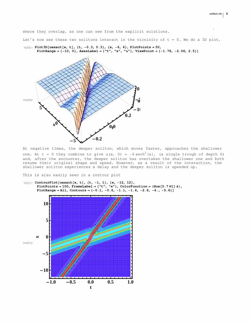
Let’s now see these two solitons interact in the vicninity of t = 0. We do a 3D plot,

In[20]:= Plot3D@uexact@x, tD, 8t, -0.3, 0.3<, 8x, -6, 6<, PlotPoints ® 50,PlotRange ® 8-10, 0<, AxesLabel ® 8"t", "x", "u"<, ViewPoint ® 8-1.78, -2.06, 2.5<D

Out[20]=

-0.2

0.0

0.2

t

-5

0

5

x

-10

-5

0

u

At negative times, the deeper soliton, which moves faster, approaches the shallower

one. At t = 0 they combine to give u(x, 0) = -6 sech2HxL, (a single trough of depth 6)and, after the encounter, the deeper soliton has overtaken the shallower one and bothresume their original shape and speed. However, as a result of the interaction, theshallower soliton experiences a delay and the deeper soliton is speeded up.

This is also easily seen in a contour plot

In[21]:= ContourPlot@uexact@x, tD, 8t, -1, 1<, 8x, -12, 12<,PlotPoints ® 100, FrameLabel ® 8"t", "x"<, ColorFunction ® HHue@0.7 ð1D &L,PlotRange ® All, Contours ® 8-0.1, -0.6, -1.1, -1.6, -2.6, -4., -5.6<D

Out[21]=

-1.0 -0.5 0.0 0.5 1.0

-10

-5

0

5

10

t

x

Finally we show an animation of the two solitons crossing each other.

soliton.nb 5

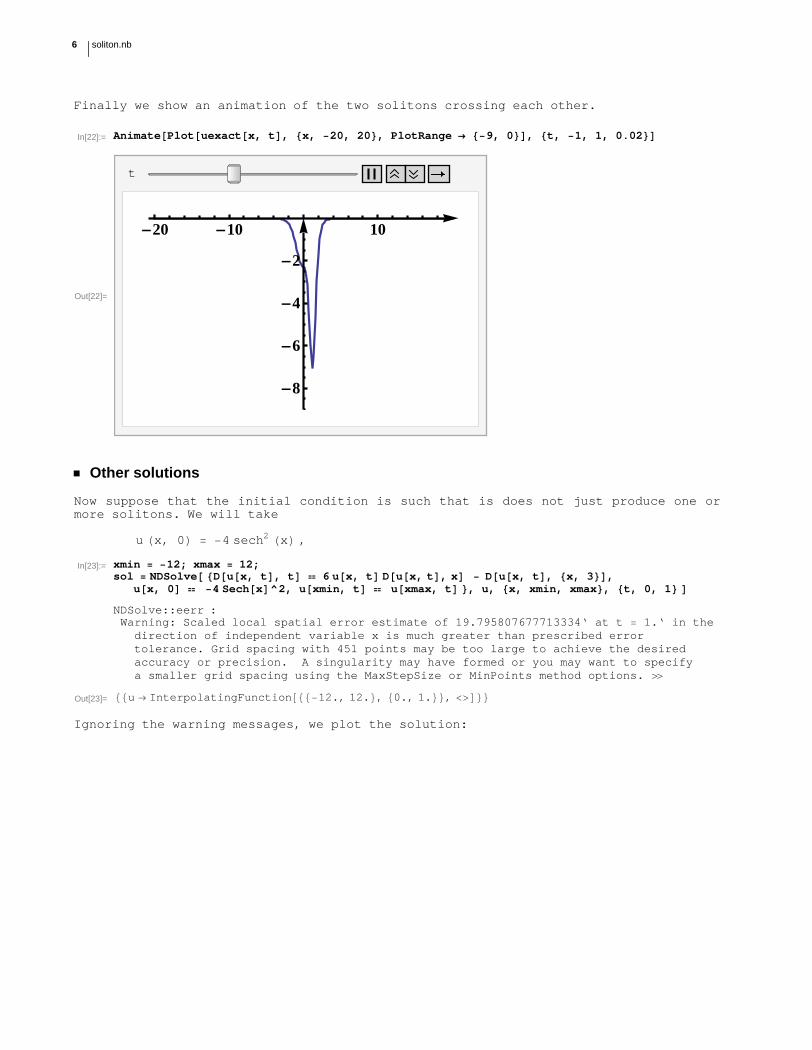
Finally we show an animation of the two solitons crossing each other.

In[22]:= Animate@Plot@uexact@x, tD, 8x, -20, 20<, PlotRange ® 8-9, 0<D, 8t, -1, 1, 0.02<D

Out[22]=

t

-20 -10 10

-8

-6

-4

-2

� Other solutions

Now suppose that the initial condition is such that is does not just produce one ormore solitons. We will take

u Hx, 0L = -4 sech2 HxL ,

In[23]:= xmin = -12; xmax = 12;sol = NDSolve@ 8D@u@x, tD, tD � 6 u@x, tD D@u@x, tD, xD - D@u@x, tD, 8x, 3<D,

u@x, 0D � -4 Sech@xD^2, u@xmin, tD � u@xmax, tD <, u, 8x, xmin, xmax<, 8t, 0, 1< D

NDSolve::eerr :

Warning: Scaled local spatial error estimate of 19.795807677713334‘ at t = 1.‘ in thedirection of independent variable x is much greater than prescribed errortolerance. Grid spacing with 451 points may be too large to achieve the desiredaccuracy or precision. A singularity may have formed or you may want to specifya smaller grid spacing using the MaxStepSize or MinPoints method options. �

Out[23]= 88u ® InterpolatingFunction@88-12., 12.<, 80., 1.<<, <>D<<

Ignoring the warning messages, we plot the solution:

6 soliton.nb

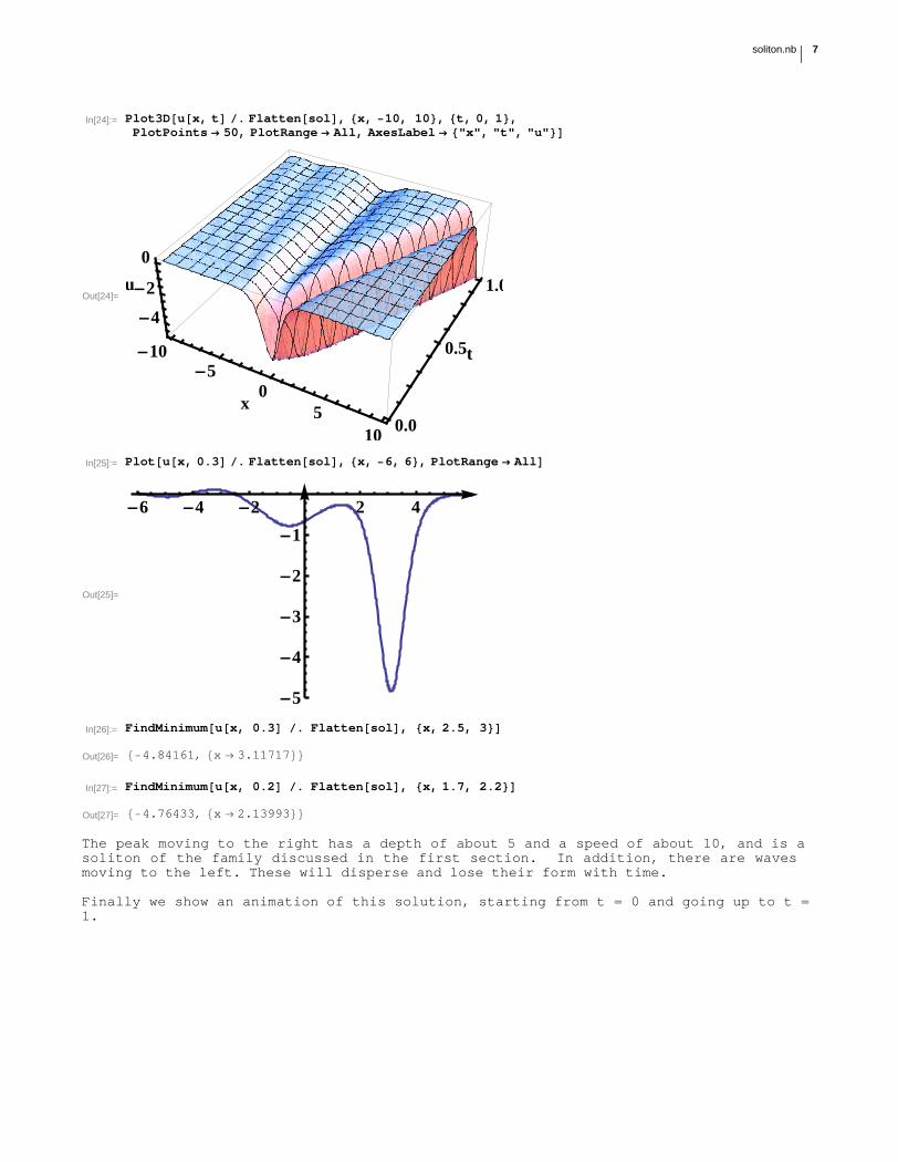
In[24]:= Plot3D@u@x, tD �. Flatten@solD, 8x, -10, 10<, 8t, 0, 1<,PlotPoints ® 50, PlotRange ® All, AxesLabel ® 8"x", "t", "u"<D

Out[24]=

-10-5

05

10

x0.0

0.5

1.0

t

-4

-2

0

u

In[25]:= Plot@u@x, 0.3D �. Flatten@solD, 8x, -6, 6<, PlotRange ® AllD

Out[25]=

-6 -4 -2 2 4

-5

-4

-3

-2

-1

In[26]:= FindMinimum@u@x, 0.3D �. Flatten@solD, 8x, 2.5, 3<D

Out[26]= 8-4.84161, 8x ® 3.11717<<

In[27]:= FindMinimum@u@x, 0.2D �. Flatten@solD, 8x, 1.7, 2.2<D

Out[27]= 8-4.76433, 8x ® 2.13993<<

The peak moving to the right has a depth of about 5 and a speed of about 10, and is asoliton of the family discussed in the first section. In addition, there are wavesmoving to the left. These will disperse and lose their form with time.

Finally we show an animation of this solution, starting from t = 0 and going up to t =1.

soliton.nb 7

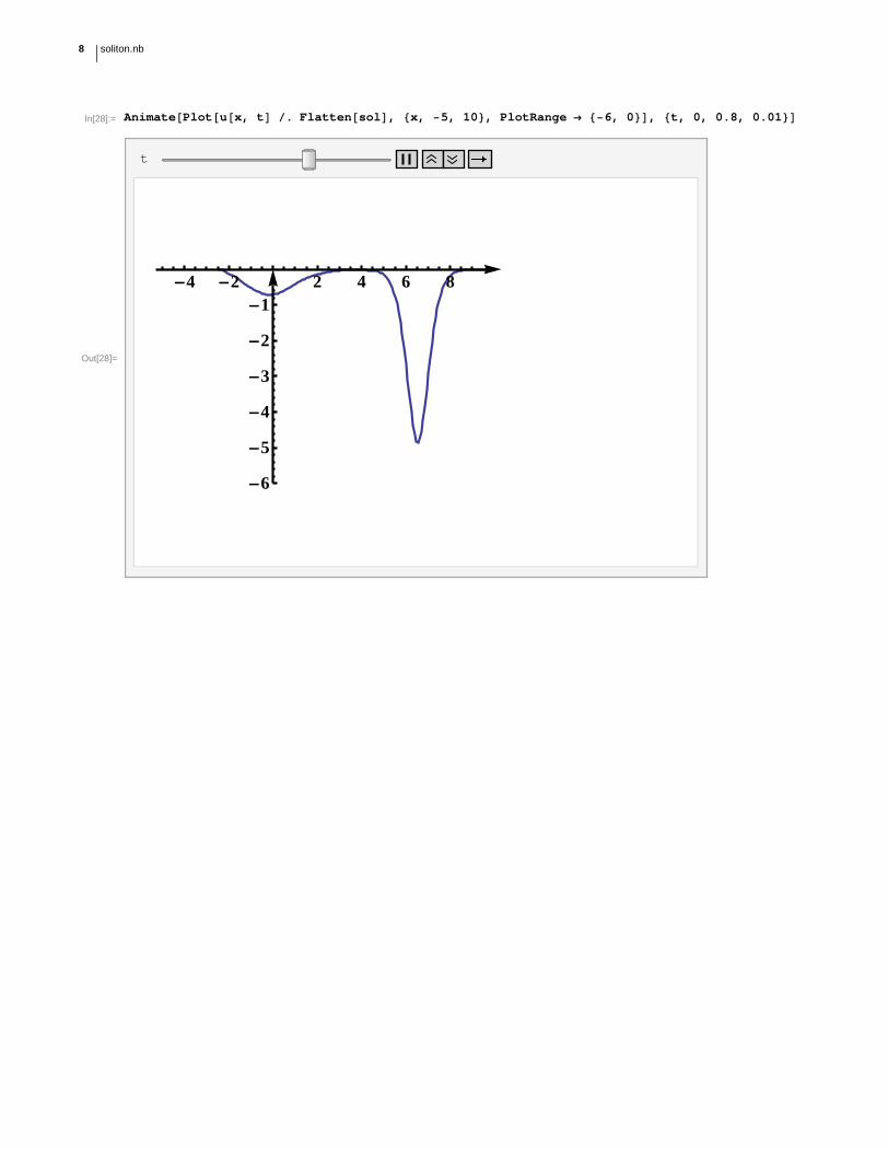
In[28]:= Animate@Plot@u@x, tD �. Flatten@solD, 8x, -5, 10<, PlotRange ® 8-6, 0<D, 8t, 0, 0.8, 0.01<D

Out[28]=

t

-4 -2 2 4 6 8

-6

-5

-4

-3

-2

-1

8 soliton.nb